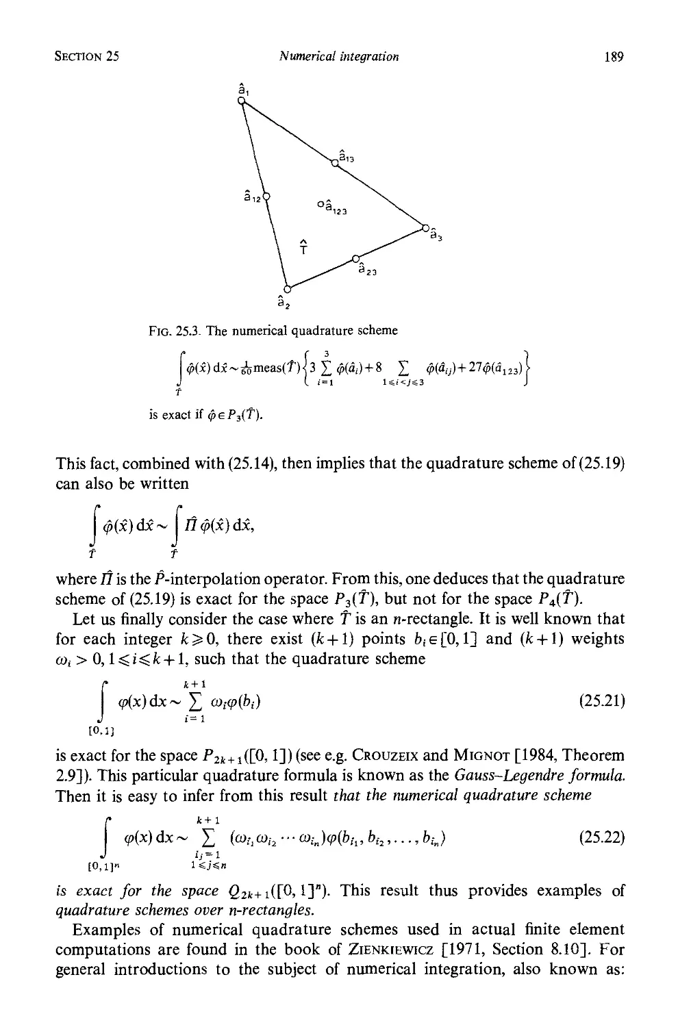
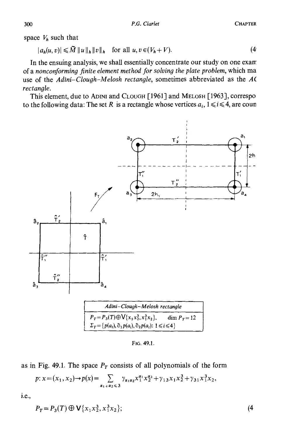
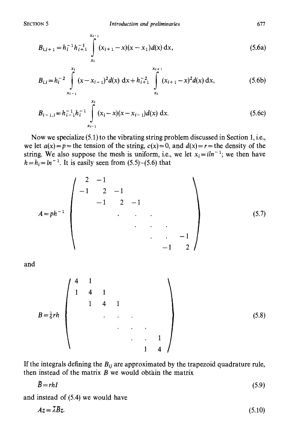
/


Author: Ciarlet P.G. Lions J.L.
Tags: mathematics mathematical analysis numerical analysis
ISBN: 0-444-70365-9
Year: 1991
Similar


Text
Finite Elements: An Introduction
J. Tinsley Oden
Finite elements; perhaps no other family of approximation methods has had
a greater impact on the theory and practice of numerical methods during the
twentieth century. Finite element methods have now been used in virtually every
conceivable area of engineering that can make use of models of nature characterized
by partial differential equations. There are dozens of textbooks, monographs,
handbooks, memoirs, and journals devoted to its further study; numerous
conferences, symposia, and workshops on various aspects of finite element
methodology are held regularly throughout the world. There exist easily over one
hundred thousand references on finite elements today, and this number is growing
exponentially with further revelations of the power and versatility of the method.
Today, finite element methodology is making significant inroads into fields in which
many thought were outside its realm; for example, computational fluid dynamics. In
time, finite element methods may assume a position in this area of comparable or
greater importance than classical difference schemes which have long dominated the
subject.
Why finite elements?
A natural question that one may ask is: why have finite element methods been so
popular in both the engineering and mathematical community? There is also the
question, do finite element methods possess properties that will continue to make
them attractive choices of methods to solve difficult problems in physics and
engineering?
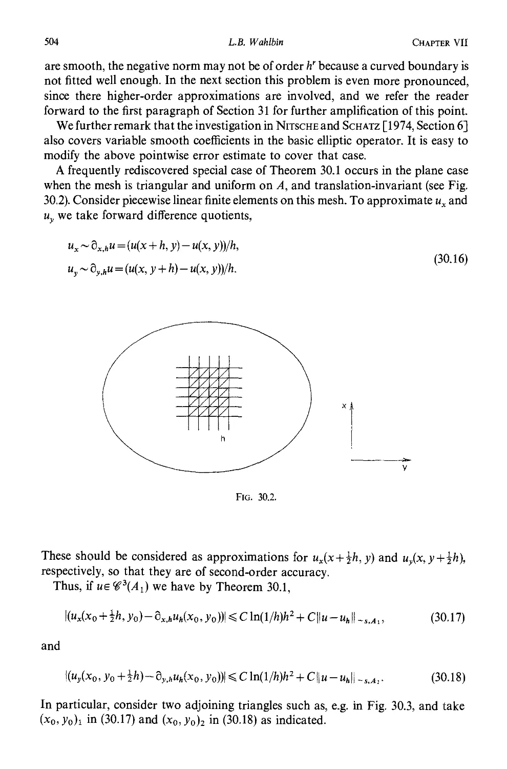
In answering these questions, one must first point to the fact that finite element
methods are based on the weak, variational, formulation of boundary and initial
value problems. This is a critical property, not only because it provides a proper
setting for the existence of very irregular solutions to differential equations (e.g.
distributions), but also because the solution appears in the integral of a quantity over
HANDBOOK OF NUMERICAL ANALYSIS, VOL. II
Finite Element Methods (Part 1)
Edited by P.G. Ciarlet and J.L. Lions
© 1991. Elsevier Science Publishers B.V. (North-Holland)
3
4
J. T. Oden
a domain. The simple fact that the integral of a measurable function over an
arbitrary domain can be broken up into the sum of integrals over an arbitrary
collection of almost disjoint subdomains whose union is the original domain, is
a vital observation in finite element theory. Because of it, the analysis of a problem
can literally be made locally, over a typical subdomain, and by making the
subdomain sufficiently small one can argue that polynomial functions of various
degrees are adequate for representing the local behavior of the solution. This
summability of integrals is exploited in every finite element program. It allows the
analysts to focus their attention on a typical finite element domain and to develop an
approximation independent of the ultimate location of that element in the final
mesh.
The simple integral property also has important implications in physics and in
most problems in continuum mechanics. Indeed, the classical balance laws of
mechanics are global, in the sense that they are integral laws applying to a given
mass of material, a fluid or solid. From the onset, only regularity of the primitive
variables sufficient for these global conservation laws to make sense is needed.
Moreover, since these laws are supposed to be fundamental axioms of physics, they
must hold over every finite portion of the material: every finite element of the
continuum. Thus once again, one is encouraged to think of approximate methods
defined by integral formulations over typical pieces of a continuum to be studied.
These rather primitive properties of finite elements lead to some of its most
important features:
A) Arbitrary geometries. The method is essentially geometry-free. In principle,
finite element methods can be applied to domains of arbitrary shape and with quite
arbitrary boundary conditions.
B) Unstructured meshes. While there is still much prejudice in the numerical
analysis literature toward the use of coordinate-dependent algorithms and mesh
generators, there is nothing intrinsic in finite element methodology that requires
such devices. Indeed, finite element methods by their nature lead to unstructured
meshes. This means, in principle, analysts can place finite elements anywhere they
please. They may thus model the most complex types of geometries in nature and
physics, ranging from the complex cross-sections of biological tissues to the exterior
of aircraft to internal flows in turbo machinery, without strong use of a global fixed
coordinate frame.
C) Robustness. It is well known that in finite element methods the contributions
of local approximations over individual elements are assembled together in
a systematic way to arrive at a global approximation of a solution to a partial
differential equation. Generally, this leads to schemes which are stable in appropriate
norms, and, moreover, insensitive to singularities or distortions of the mesh, in sharp
contrast to classical difference methods. There are notable exceptions to this, of
course, and these exceptions have been the subject of some of the most important
works in finite element theory. But, by and large, the direct use of Galerkin or
Petrov-Galerkin methods to derive finite element methods leads to conservative
and stable algorithms, for most classes of problems in mechanics and mathematical
physics.
Introduction
5
D) Mathematical foundation. Because of the extensive work on the mathematical
foundations done during the seventies and eighties, finite elements now enjoy a rich
and solid mathematical basis. The availability of methods to determine a priori and
a posteriori estimates provides a vital part of the theory of finite elements, and makes
it possible to lift the analysis of important engineering and physical problems above
the traditional empiricism prevalent in many numerical and experimental studies.
These properties are intrinsic to finite element methods and continue to make
these methods among the most attractive for solving complex problems.
They represent the most desirable properties of any numerical scheme designed to
handle real-world problems. Moreover, the basic features of finite element
methodology provide an ideal setting for innovative use of modern supercomputing
architectures, particularly parallel processing. For these reasons, it is certain that
finite element concepts will continue to occupy an important role in applications
and in research on the numerical solution of partial differential equations.
The early history
When did finite elements begin? It is difficult to trace the origins of finite element
methods because of a basic problem in defining precisely what constitutes a "finite
element method". To most mathematicians, it is a method of piecewise polynomial
approximation and, therefore, its origins are frequently traced to the appendix of
a paper by Courant [1943] in which piecewise linear approximations of the
Dirichlet problem over a network of triangles is discussed. Also, the "interpretation
of finite differences" by Poly a [1952] is regarded as embodying piecewise
polynomial approximation aspects of finite elements.
On the other hand, the approximation of variational problems on a mesh of
triangles goes back much further: 92 years. In 1851, Schellbach [1851] proposed
a finite-element-like solution to Plateau's problem of determining the surface S of
minimum area enclosed by a given closed curve. Schellbach used an approximation
Sk of S by a mesh of triangles over which the surface was represented by piecewise
linear functions, and he then obtained an approximation to the solution to Plateau's
problem by minimizing Sh with respect to the coordinates of hexagons formed by six
elements (see Williamson [1980]). Not quite the conventional finite element
approach, but certainly as much a finite element technique as that of Courant.
Some say that there is even an earlier work that uses some of the ideas underlying
finite element methods: Gottfried Leibniz himself employed a piecewise linear
approximation of the Brachistochrone problem proposed by Johann Bernoulli in
1696 (see the historical volume, Leibniz [1962]). With the help of his newly
developed calculus tools, Leibniz derived the governing differential equation for the
problem, the solution of which is a cycloid. However, most would agree that to credit
this work as a finite element approximation is somewhat stretching the point.
Leibniz had no intention of approximating a differential equation; rather, his
purpose was to derive one. Two and a half centuries later it was realized that useful
approximations of differential equations could be determined by not necessarily
6
J.T. Oden
taking infinitesimal elements as in the calculus, but by keeping the elements finite in
size. This idea is, in fact, the basis of the term "finite element".
There is also some difference in the process of laying a mesh of triangles over
a domain on the one hand and generating the domain of approximation by piecing
together triangles on the other. While these processes may look the same in some
cases, they may differ dramatically in how the boundary conditions are imposed.
Thus, neither Schellbach nor Courant, nor for that matter Synge who used
triangular meshes many years later, were particularly careful as to how boundary
conditions were to be imposed or as to how the boundary of the domain was to be
modeled by elements, issues that are now recognized as an important feature of finite
element methodologies. If a finite element method is one in which a global
approximation of a partial differential equation is built up from a sequence of local
approximations over subdomains, then credit must go back to the early papers of
Hrennikoff [1941], and perhaps beyond, who chose to solve plane elasticity
problems by breaking up the domain of the displacements into little finite pieces,
over which the stiffnesses were approximated using bars, beams, and spring
elements. A similar "lattice analogy" was used by McHenry [1943]. While these
works are draped in the most primitive physical terms, it is nevertheless clear that
the methods involve some sort of crude piecewise linear or piecewise cubic
approximation over rectangular cells. Miraculously, the methods also seem to be
convergent.
To the average practitioner who uses them, finite elements are much more than
a method of piecewise polynomial approximation. The whole process of partitioning
of domains, assembling elements, applying loads and boundary conditions, and, of
course, along with it, local polynomial approximation, are all components of the
finite element method.
If this is so, then one must acknowledge the early papers of Gabriel Kron who
developed his "tensor analysis of networks" in 1939 and applied his "method of
tearing" and "network analysis" to the generation of global systems from large
numbers of individual components in the 1940s and 1950s (Kron [1939]; see also
Kron [1953]). Of course, Kron never necessarily regarded his method as one of
approximating partial differential equations; rather, the properties of each component
were regarded as exactly specified, and the issue was an algebraic one of connecting
them all appropriately together.
In the early 1950s, Argyris [1954] began to put these ideas together into what
some call a primitive finite element method: he extended and generalized the
combinatoric methods of Kron and other ideas that were being developed in the
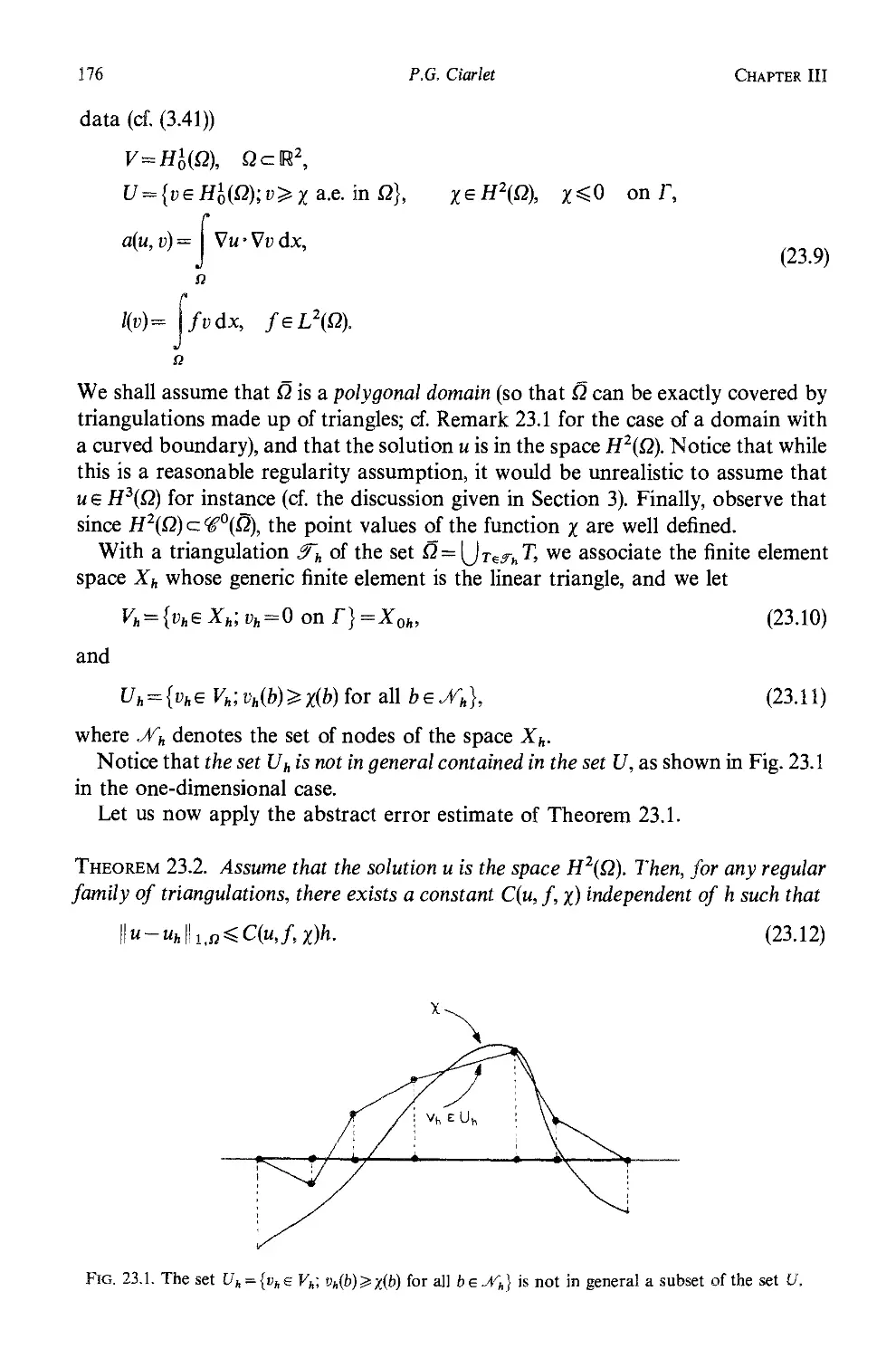
literature on system theory at the time, and added to it variational methods of
approximation, a fundamental step toward true finite element methodology.
Around the same time, Synge [1957] described his "method of the hypercircle" in
which he also spoke of piecewise linear approximations on triangular meshes, but
not in a rich variational setting and not in a way in which approximations were built
by either partitioning a domain into triangles or assembling triangles to approximate
a domain (indeed Synge's treatment of boundary conditions was clearly not in the
spirit of finite elements, even though he was keenly aware of the importance of
Introduction
7
convergence criteria and of the "angle condition" for triangles, later studied in some
depth by others).
It must be noted that during the mid-1950s there were a number of independent
studies underway which made use of "matrix methods" for the analysis of aircraft
structures. A principal contributor to this methodology was Levy [1953] who
introduced the "direct stiffness method" wherein he approximated the structural
behavior of aircraft wings using assemblies of box beams, torsion boxes, rods and
shear panels. These assuredly represent some sort of crude local polynomial
approximation in the same spirit as the Hrennikoff and McHenry approaches. The
direct stiffness method of Levy had a great impact on the structural analysis of
aircraft, and aircraft companies throughout the United States began to adopt and
apply some variant of this method or of the methods of Argyris to complex aircraft
structural analyses. During this same period, similar structural analysis methods
were being developed and used in Europe, particularly in England, and one must
mention in this regard the work of Taig [1961] in which shear lag in aircraft wing
panels was approximated using basically a bilinear finite element method of
approximation. Similar element-like approximations were used in many aircraft
industries as components in various matrix methods of structural analyses. Thus the
precedent was established for piecewise approximations of some kind by the
mid-1950s.
To a large segment of the engineering community, the work representing the
beginning of finite elements was that contained in the pioneering paper of Turner,
Clough, Martin and Topp [1956] in which a genuine attempt was made at both
a local approximation (of the partial differential equations of linear elasticity) and
the use of assembly strategies essential to finite element methodology. It is
interesting that in this paper local element properties were derived without the use of
variational principles. It was not until 1960 that Clough [1960] actually dubbed
these techniques as "finite element methods" in a landmark paper on the analysis of
linear plane elasticity problems.
The 1960s were the formative years of finite element methods. Once it was
perceived by the engineering community that useful finite element methods could be
derived from variational principles, variational^ based methods significantly
dominated all the literature for almost a decade. If an operator was unsymmetric, it
was thought that the solution of the associated problem was beyond the scope of
finite elements, since it did not lend itself to a traditional extremum variational
approximation in the spirit of Rayleigh and Ritz.
From 1960 to 1965, a variety of finite element methods were proposed. Many were
primitive and unorthodox; some were innovative and successful. During this time,
a variety of attempts at solving the biharmonic equation for plate bending problems
were proposed which employed piecewise polynomial approximations, but did not
provide the essentials for convergence. This led to the concern of some as to whether
the method was indeed applicable to such problems. On the other hand, it was clear
that classical Fourier series solutions of plate problems were, under appropriate
conditions, convergent and could be fit together in an assemblage of rectangular
components (Oden [1962]) and, thus, a form of "spectral finite element methods"
8
J.T. Oden
was introduced early in the study of such problems. However, such high-order
schemes never received serious attention in this period, as it was felt that piecewise
polynomial approximations could be developed which did give satisfactory results.
It was not until the mid- to late 1960s that papers on bicubic spline approximations
by Bogner, Fox, and Schmit [1966] and Birkhoff, Schultz, and Varga [1968]
provided successful polynomial finite element approximations for these classes of
problems.
Many workers in the field feel that the famous Dayton conferences on finite
elements (at the Air Force Flight Dynamics Laboratory in Dayton, Ohio, USA)
represented landmarks in the development of the field (see Przemienieckj et al.
[1966]). Held in 1965, 1968, 1970, these meetings brought specialists from all over
the world to discuss their latest triumphs and failures, and the pages of the
proceedings, particularly the earlier volumes, were filled with remarkable and
innovative accomplishments from a technical community just beginning to learn the
richness and power of this new collection of ideas. In these volumes one can find
many of the premier papers of now well-known methods. In the first volume alone
one can find mixed finite element methods (Herrmann [1966]), Hermite
approximations (Pestel [1966]), C^-bicubic approximations (Bogner, Fox and Schmit
[1966]), hybrid methods (Pian [1966]) and other contributions. In later volumes,
further assaults on nonlinear problems and special element formulations can be
found.
Near the end of the sixties and early seventies there finally emerged the realization
that the method could be applied to unsymmetric operators without difficulty and
thus problems in fluid mechanics were brought within the realm of application of
finite element methods; in particular, finite element models of the full Navier-Stokes
equations were first presented during this period (Oden [1969], Oden and Somogyi
[1968], Oden [1970]).
The early textbook by Zienkiewicz and Cheung [1967] did much to popularize
the method with the practicing engineering community. However, the most
important factor leading to the rise in popularity during the late 1960s and early
1970s was not purely the publication of special formulations and algorithms, but the
fact that the method was being very successfully used to solve difficult engineering
problems. Much of the technology used during this period was due to Bruce Irons,
who with his colleagues and students developed a multitude of techniques for the
successful implementation of finite elements. These included the frontal solution
technique (Irons [1970]), the patch test (Irons and Razzaque [1972]), isoparametric
elements (Ergatoudis, Irons and Zienkiewicz [1966]), and numerical integration
schemes (Irons [1966]) and many more. The scope of finite element applications in
the 1970s would have been significantly diminished without these contributions.
The mathematical theory
The mathematical theory of finite elements was slow to emerge from this caldron of
activity. The beginning works on the mathematical theory of finite elements were
Introduction
9
understandably concerned with one-dimensional elliptic problems and used many
of the tools and jargon of Ritz methods, interpolation, and variational differences.
An early work in this line was the paper of Varga [1966] which dealt with "Hermite
interpolation-type Ritz methods" for two-point boundary value problems. We also
mention in this regard the paper of Birkhoff, de Boor, Schwartz and Wendroff
[1966] on "Rayleigh-Ritz approximation by piecewise cubic polynomials". This is
certainly one of the first papers to deal with the issue of convergence of finite element
methods, although some papers on variational differences yielded similar results but
did not focus on the piecewise polynomial features of finite elements. The work of
Kang Feng [1965], published in Chinese (a copy of which I have not been able to
acquire for review) may fall into this category and is sometimes noted as relevant to
the convergence of finite element methods.
The mathematical theory of finite elements for two-dimensional and higher-
dimensional problems began in 1968 and several papers were published that year on
the subject. One of the first papers in this period to address the problem of
convergence of a finite method in a rigorous way and in which a priori error
estimates for bilinear approximations of a problem in plane elasticity are obtained,
is the often overlooked paper of Johnson and McLa^ [1968], which appeared in the
Journal of Applied Mechanics. This paper correctly developed error estimates in
energy norms, and even attempted to characterize the deterioration of convergence
rates due to corner singularities. In the same year there appeared the first of two
important papers by Ogenesjan and Ruchovec [1968,1969] in the Russian
literature, in which "variational difference schemes" were proposed for linear
second-order elliptic problems in two-dimensional domains. These works dealt with
the estimates of the rate of convergence of variational difference schemes.
Also in 1968 there appeared the important mathematical paper of Zlamal [1968]
in which a detailed analysis of interpolation properties of a class of triangular
elements and their application to second-order and fourth-order linear elliptic
boundary value problems is discussed. This paper attracted the interest of a large
segment of the numerical analysis community and several very good mathematicians
began to work on finite element methodologies. The paper by Zlamal also stands
apart from other multidimensional finite element papers of this era since it
represented a departure of studies of tensor products of polynomials on rectangular
domains and provided an approach toward approximations in general
polygonal domains. In the same year, Ciarlet [1968] published a rigorous proof of
convergence of piecewise linear finite element approximation of a class of linear
two-point boundary value problems and proved V° estimates using a discrete
maximum principle. We also mention the work of Oliveira [1968] on convergence
of finite element methods which established correct rates of convergence for certain
problems in appropriate energy norms.
A year later, Schultz [1969] presented error estimates for "Rayleigh-Ritz-
Galerkin methods" for multidimensional problems. Two years later, Schultz
[1971] published L2 error bounds for these types of methods.
By 1972, finite element methods had emerged as an important new area of
numerical analysis in applied mathematics. Mathematical conferences were held on
10
J.T. Oden
the subject on a regular basis, and there began to appear a rich volume of literature
on mathematical aspects of the method applied to elliptic problems, eigenvalue
problems, and parabolic problems. A conference of special significance in this period
was held at the University of Maryland in 1972 and featured a penetrating series of
lectures by Ivo BabuSka (see Babuska and Aziz [1972]) and several important
mathematical papers by leading specialists in the mathematics of finite elements, all
collected in the volume edited by Aziz [1972].
One unfamiliar with aspects of the history of finite elements may be led to the
erroneous conclusion that the method of finite elements emerged from the growing
wealth of information on partial differential equations, weak solutions of boundary
value problems, Sobolev spaces, and the associated approximation theory for
elliptic variational boundary value problems. This is a natural mistake, because the
seeds for the modern theory of partial differential equations were sown about the
same time as those for the development of modern finite element methods, but in an
entirely different garden.
In the late 1940s, Laurent Schwartz was putting together his theory of
distributions around a decade after the notion of generalized functions and their use in partial
differential equations appeared in the pioneering work of S.L. Sobolev. A long
list of other names could be added to the list of contributors to the modern theory of
partial differential equations, but that is not our purpose here. Rather, we must only
note that the rich mathematical theory of partial differential equations which began
in the 1940s and 1950s, blossomed in the 1960s, and is now an integral part of the
foundations of not only partial differential equations but also approximation
theory, grew independently and parallel to the development of finite element
methods for almost two decades. There was important work during this period on
the foundations of variational methods of approximation, typified by the early work
of Lions [1955] and by the French school in the early 1960s; but, while this work did
concern itself with the systematic development of mathematical results that would
ultimately prove to be vital to the development of finite element methods, it did not
focus on the specific aspects of existing and already successful finite element
concepts. It was, perhaps, an unavoidable occurrence, that in the late 1960s these
two independent subjects, finite element methodology and the theory of
approximation of partial differential equations via functional analysis methods, united in an
inseparable way, so much so that it is difficult to appreciate the fact that they were
ever separate.
The 1970s must mark the decade of the mathematics of finite elements. During
this period, great strides were made in determining a priori error estimates for
a variety of finite element methods, for linear elliptic boundary value problems, for
eigenvalue problems, and certain classes of linear and nonlinear parabolic problems;
also, some preliminary work on finite element applications to hyperbolic equations
was done. It is both inappropriate and perhaps impossible to provide an adequate
survey of this large volume of literature, but it is possible to present an albeit biased
reference to some of the major works along the way.
An important component in the theory of finite elements is an interpolation
theory: how well can a given finite element method approximate functions of a given
Introduction
11
class locally over a typical finite element? A great deal was known about this subject
from the literature on approximation theory and spline analysis, but its particular-
ization to finite elements involves technical difficulties. One can find results on finite
element interpolation in a number of early papers, including those of ZlAmal
[1968], Birkhoff [1969], Schultz [1969], Bramble and ZlAmal [1970], BabuSka
[1970,1971], and BabuSka and Aziz [1972]. But the elegant work on Lagrange and
Hermite interpolations of finite elements by Ciarlet and Raviart [1972a] must
stand as a very important contribution to this vital aspect of finite element theory.
A landmark work on the mathematics of finite elements appeared in 1972 in the
remarkably comprehensive and penetrating memoir of BabuSka and Aziz [1972] on
the mathematical foundations of finite element methods. Here one can find
interwoven with the theory of Sobolev spaces and elliptic problems, general results
on approximation theory that have direct bearing on finite element methods. It was
known that Cea's lemma (Cea [1964]) established that the approximation error in
a Galerkin approximation of a variational boundary value problem is bounded by
the so-called interpolation error; that is, the distance in an appropriate energy norm
from the solution of the problem to the subspace of approximations. Indeed, it was
this fact that made the results on interpolation theory using piecewise polynomials
of particular interest in finite element methods. In the work of BabuSka [1971] and
BabuSka and Aziz [1972], this framework was dramatically enlarged by BabuSka's
introduction of the so-called "INF-SUP" condition. This condition is encountered
in the characterization of coerciveness of bilinear forms occuring in elliptic
boundary value problems. The characterization of this "INF-SUP" condition for
the discrete finite element approximation embodies in it the essential elements for
studying the stability in convergence of finite element methods. Brezzi [1974]
developed an equivalent condition for studying constrained elliptic problems and
these conditions provide for a unified approach to the study of qualitative
properties, including rates of convergence, of broad classes of finite element
methods.
The fundamental work of Nitsche [1970] on L°° estimates for general classes of
linear elliptic problems must stand out as one of the most important contributions of
the seventies. Strang [1972], in an important communication, pointed out
"variational crimes", inherent in many finite element methods, such as improper
numerical quadrature, the use of nonconforming elements, improper satisfaction of
boundary conditions, etc., all common practices in applications, but all frequently
leading to exceptable numerical schemes.
In the same year, Ciarlet and Raviart [1972b, c] also contributed penetrating
studies of these issues. Many of the advances of the 1970s drew upon earlier results
on variational methods of approximation based on the Ritz method and finite
differences; for example the fundamental Aubin-Nitsche method for lifting the order
of convergence to lower Sobolev norms (see Aubin [1967] and Nitsche [1963]; see
also Ogenesjan and Ruchovec [1969]) used such results. In 1974, the important
paper of Brezzi [1974] mentioned earlier, used such earlier results on saddle point
problems and laid the groundwork for a multitude of papers on problems with
constraints and on the stability of various finite element procedures. While
12
J. T. Oden
convergence of special types of finite element strategies such as mixed methods and
hybrid methods had been attempted in the early 1970s (e.g. Oden [1972]), the Brezzi
results, and the methods of BabuSka for constrained problems, provided a general
framework for studying virtually all mixed and hybrid finite elements (e.g. Raviart
[1975], Raviart and Thomas [1977], BabuSka, Oden and Lee [1977]).
The first textbook on mathematical properties of finite element methods was the
popular book of Strang and Fix [1973]. A book on an introduction to the
mathematical theory of finite elements was published soon after by Oden and
Reddy [1976] and the well-known treatise on the finite element method for elliptic
problems by Ciarlet [1978] appeared two years later.
The penetrating work of Nitsche and Schatz [1974] on interior estimates and
Schatz and Wahlbin [1978] on L°° estimates and singular problems represented
notable contributions to the growing mathematical theory of finite elements. The
important work of Douglas and Dupont (e.g. [1970, 1973]; Dupont [1973]) on
finite element methods for parabolic problems and hyperbolic problems must be
mentioned along with the idea of elliptic projections of Wheeler [1973] which
provided a useful technique for deriving error bounds for time-dependent problems.
The 1970s also represented a decade in which the generality of finite element
methods began to be appreciated over a large portion of the mathematics and
scientific community, and it was during this period that significant applications to
highly nonlinear problems were made. The fact that very general nonlinear
phenomena in continuum mechanics, including problems of finite deformation of
solids and of flow of viscous fluids could be modeled by finite elements and solved on
existing computers was demonstrated in the early seventies (e.g. Oden [1972]), and,
by the end of that decade, several "general purpose" finite element programs were in
use by engineers to treat broad classes of nonlinear problems in solid mechanics and
heat transfer. The mathematical theory for nonlinear problems also was advanced
in this period, and the important work of Falk [1974] on finite element
approximations of variational inequalities should be mentioned.
It is not too inaccurate to say that by 1980, a solid foundation for the
mathematical theory of finite elements for linear problems had been established and
that significant advances in both theory and application into nonlinear problems
existed. The open questions that remain are difficult ones and their solution will
require a good understanding of the mathematical properties of the method. The
works collected in this volume should not only provide a summary of important
results and approaches to mathematical issues related to finite elements, but also
they should provide a useful starting point for further research.
References
Argyris, J.H. A954), Energy theorems and structural analysis, Aircraft Engrg. 26,347-356; 383-387; 394.
Argyris, J.H. A955), Energy theorems and structural analysis, Aircraft Engrg. 27,42-58; 80-94; 125-134;
145-158.
Argyris, J.H. A966), Continua and discontinua, in: Proceedings Conference on Matrix Methods in
Structural Mechanics, Wright-Patterson AFB, Dayton, OH, 11-190.
Aubin, J.P. A967), Behavior of the error of the approximate solutions of boundary-value problems for
linear elliptic operators by Galerkin's method and finite differences, Ann. Scuola Norm. Pisa C) 21,
599-637.
Aziz, A.K., ed. A972), The Mathematical Foundations of the Finite Element Method with Applications to
Partial Differential Equations (Academic Press, New York).
Babuska, I. A970), Finite element methods for domains with corners, Computing 6, 264-273.
Babuska, I. A971), Error bounds for the finite element method, Numer. Math. 16, 322-333.
Babuska, I. and A.K. Aziz A972), Survey lectures on the mathematical foundation of the finite element
method, in: A.K. Aziz, ed. The Mathematical Foundations of the Finite Element Method with
Applications to Partial Differential Equations (Academic Press, New York) 5-359.
Babuska, I., J.T. Oden and J.K. Lee A977), Mixed-hybrid finite element approximations of second-order
elliptic boundary-value problems, Comput. Methods Appl. Mech. Engrg. 11, 175-206.
Birkhoff, G. A969), Piecewise bicubic interpolation and approximation in polygons, in: IJ. Schoenberg,
ed., Approximations with Special Emphasis on Spline Functions (Academic Press, New York) 85-121.
Birkhoff, G., C. de Boor, M.H. Schultz and В. Wendroff A966), Rayleigh-Ritz approximation by
piecewise cubic polynomials, SI AM J. Numer. Anal. 3, 188-203.
Birkhoff, G., M.H. Schultz and R.S. Varga A968), Piecewise Hermite interpolation in one and two
variables with applications to partial differential equations, Numer. Math. 11, 232-256.
Bogner, F.K., R.L. Fox and L.A. Schmit Jr A966), The generation of interelement, compatible stiffness
and mass matrices by the use of interpolation formulas, in: Proceedings Conference on Matrix
Methods in Structural Mechanics, Wright-Patterson AFB, Dayton, OH, 397-444.
Bramble, J.H. and M. Zlamal A970), Triangular element in the finite element method, Math. Сотр. 24
A12), 809-820.
Brezzi, F. A974), On the existence, uniqueness, and approximation of saddle-point problems arising
from Lagrange multipliers, Rev. Francaise d'Automat. Inform. Reck Oper. 8-R2, 129-151.
Cea, J. A964), Approximation variationnelle des problems aux limites, Ann. Inst. Fourier (Grenoble) 14,
345^44.
Ciarlet, P.G. A968), An 0(h2) method for a non-smooth boundary-value problem, Aequationes Math. 2,
39-49.
Ciarlet, P.G. A978), The Finite Element Method for Elliptic Problems (North-Holland, Amsterdam).
Ciarlet, P.G. and P.A. Raviart A972a), General Lagrange and Hermite interpolation in R" with
applications to the finite elment method, Arch. Rational Mech. Anal. 46, 177-199.
Ciarlet, P.G. and P.A. Raviart A972b), Interpolation theory over curved elements with applications to
finite element methods, Comput. Methods Appl. Mech. Engrg. 1, 217-249.
Ciarlet, P.G. and P.A. Raviart A972c), The combined effect of curved boundaries and numerical
integration in isoparametric finite element methods, in: A.K. Aziz, ed., The Mathematical Foundations
of the Finite Element Method with Applications to Partial Differential Equations (Academic Press, New
York) 409-^74.
13
14
J.T. Oden
Clough, R.W. A960), The finite element method in plane stress analysis, in: Proceedings 2nd ASCE
Conference on Electronic Computation, Pittsburgh, PA.
Courant, R. A943), Variational methods for the solution of problems of equilibrium and vibration, Bull.
Amer, Math. Soc. 49, 1-23.
Douglas, J. and T. Dupont A970), Galerkin methods for parabolic problems, SI AM J. Numer. Anal. 1,
575-626.
Douglas, J. and T. Dupont A973), Superconvergence for Galerkin methods for the two-point boundary
problem via local projections, Numer. Math. 21, 220-228.
Dupont, T. A973), L2 -estimates for Galerkin methods for second-order hyperbolic equations, SI AM J.
Numer. Anal. 10, 880-889.
Ergatoudis, I., B.M. Irons and O.C. Zienkiewicz A966), Curved isoparametric quadrilateral finite
elements, Internat. J, Solids Structures 4, 31-42.
Falk, S.R. A974), Error estimates for the approximation of a class of variational inequalities, Math.
Сотр. 28, 963-971.
Herrmann, L.R. A966), A bending analysis for plates, in: Proceedings Conference on Matrix Methods in
Structural Mechanics, Wright-Patterson AFB, Dayton, OH, 577.
Hrennikoff, H. A941), Solutions of problems in elasticity by the framework method, J. Appl. Mech.,
A169-175.
Irons, B. A966), Engineering applications of numerical integration in stiffness methods, AIAA J. 4,
2035-3037
Irons, B. A970), A frontal solution program for finite element analysis, Internat, J. Numer. Methods
Engrg. 2, 5-32.
Irons, B. and A. Razzaque A972), Experience with the patch test for convergence of finite elements, in:
A.K. Aziz, Ed., The Mathematical Foundations of the Finite Element Method with Applications to
Partial Differential Equations (Academic Press, New York) 557-587.
Johnson Jr, M.W. and R.W. McLay A968), Convergence of the finite element method in the theory of
elasticity, J. Appl. Mech. E, 35, 274-278.
Rang, Feng A965), A difference formulation based on the variational principle, Appl. Math. Comput.
Math. 2, 238-162 (in Chinese).
Kron, G. A939), Tensor Analysis of Networks (Wiley, New York).
Kron, G. A953), A set of principles to interconnect the solutions of physical systems, J. Appl. Phys. 24,
965-980.
Leibniz, G. A962), G.W. Leibniz Mathematische Schriften, С Gerhardt, ed. (G. Olms Verlagsbuchhand-
lung) 290-293.
Levy, S. A953), Structural analysis and influence coefficients for delta wings, J. Aeronaut. Set 20.
Lions, J. A955), Problemes aux limites en theorie des distributions, Acta Math. 94, 13-153.
McHenry, D. A943), A lattice analogy for the solution of plane stress problems, J. Inst. Civ. Engrg. 21,
59-82.
Nitsche, J.A. A963), Ein Kriterium fur die Quasi-Optimalitat des Ritzschen Verfahrens, Numer. Math. 2,
346-348.
Nitsche, J.A. A970), Lineare Spline-Funktionen und die Methoden von Ritz fur elliptische Randwert-
probleme, Arch. Rational Mech. Anal. 36, 348-355.
Nitsche, J.A. and A.H. Schatz A974), Interior estimates for Ritz-Galerkin methods, Math. Сотр. 28,
937-958.
Oden, J.T. A962), Plate beam structures, Dissertation, Oklahoma State University, Stillwater, OK.
Oden, J.T. A969), A general theory of finite elements, II: Applications, Internat. J. Numer. Methods
Engrg. 1, 247-259.
Oden, J.T. A970), A finite element analogue of the Navier-Stokes equations, J. Engrg. Mech. Div. ASCE
96 (EM 4).
Oden, J.T. A972), Finite Elements of Nonlinear Continua (McGraw-Hill, New York).
Oden, J.T. and J.N. Reddy A976), An Introduction to the Mathematical Theory of Finite Elements
(Wiley-Interscience, New York).
Oden, J.T. and D. Somogyi A968), Finite element applications in fluid dynamics, J. Engrg. Mech. Div.
ASCE 95 (EM 4), 821-826.
References
15
Ogenesjan, L.A. and L.A. Ruchovec A968), Variational-difference schemes for linear second-order
elliptic equations in a two-dimensional region with piecewise smooth boundary, U.S.S.R. Comput.
Math, and Math. Phys. 8 A), 129-152.
Ogenesjan, L.A. and L.A. Ruchovec A969), Study of the rate of convergence of variational difference
schemes for second-order elliptic equations in a two-dimensional field with a smooth boundary,
U.S.S.R. Comput. Math, and Math. Phys. 9 E), 158-183.
Oliveira, E.R. de Arantes e. A968), Theoretical foundation of the finite element method, Internat. J.
Solids Structures 4, 926-952.
Pestel, E. A966), Dynamic stiffness matrix formulation by means of Hermitian polynomials, in:
Proceedings Conference on Matrix Methods in Structural Mechanics, Wright-Patterson AFB, Dayton,
OH, 479-502.
PiAN, T.H.H. A966), Element stiffness matrices for boundary compatibility and for prescribed stresses, in:
Proceedings Conference on Matrix Methods in Structural Mechanics, Wright-Patterson AFB, Dayton,
OH, 455-478.
Polya, G. A952), Sur une interpretation de la methode des differences finies qui peut fournir des bornes
superieures ou inferieures, C.R. Acad. Sci. Paris 235, 995-997.
Przemieniecki, J.S., R.M. Bader, W.F. Bozich, J.R. Johnson and W.J. Mykytow, eds. A966),
Proceedings Conference on Matrix Methods in Structural Mechanics, Wright-Patterson AFB, Dayton,
OH.
Raviart, P.A. A975), Hybrid methods for solving 2nd-order elliptic problems, in: J.H.H. Miller, ed.,
Topics in Numerical Analysis (Academic Press, New York) 141-155.
Raviart, P.A. and J.M. Thomas A977), A mixed finite element method for 2nd-order elliptic problems,
in: Proceedings Symposium on the Mathematical Aspects of the Finite Element Methods, Rome.
Schatz, A.H. and L.B. Wahlbin A977), Interior maximum norm estimates for finite element methods,
Math. Сотр. 31, 414-442.
Schatz, A.H. and L.B. Wahlbin A978), Maximum norm estimates in the finite element method on
polygonal domains, Part I, Math. Сотр. 32, 73-109.
Schellbach, K. A851), Probleme der Variationsrechnung, J. Reine Angew. Math. 41, 293-363.
Schultz, M.H. A969a), L"-multivariate approximation theory, SIAM J. Numer. Anal. 6, 161-183.
Schultz, M.H. A969b), Rayleigh-Ritz-Galerkin methods for multi-dimensional problems, SIAM J.
Numer. Anal. 6, 523-538.
Schultz, M.H. A971), L2 error bounds for the Rayleigh-Ritz-Galerkin method, SIAM J. Numer. Anal.
8, 737-748.
Strang, G. A972), Variational crimes in the finite element method, in: A.K. Aziz, ed., The Mathematical
Foundations of the Finite Element Method with Applications to Partial Differential Equations (Academic
Press, New York).
Strang, G. and G. Fix A973), An Analysis of the Finite Element Method (Prentice-Hall, Englewood Cliffs,
NJ).
Synge, J.L. A957), The Hypercircle Method in Mathematical Physics (Cambridge University Press,
Cambridge).
Taig, I.C. A961), Structural analysis by the matrix displacement method, English Electrial Aviation Ltd.
Report, S-O-17.
Turner, M.J., R.W. Clough, H.C. Martin and L.J. Topp A956), Stiffness and deflection analysis of
complex structures, J. Aero. Sci. 23, 805-823.
Varga, R.S. A966), Hermite interpolation-type Ritz methods for two-point boundary value problems,
J.H. Bramble, ed., Numerical Solution of Partial Differential Equations (Academic Press, New York).
Wheeler, M.F. A973), A-priori L2-error estimates for Galerkin approximations to parabolic partial
differential equations, SIAM J. Numer. Anal. 11, 723-759.
Williamson, F. A980), A historical note on the finite element method, Internat. J. Numer. Methods
Engrg. 15, 930-934.
Zienkiewicz, O.C. and Y.K. Cheung A967), The Finite Element Method in Structural and Continuum
Mechanics (McGraw-Hill, New York).
Zlamal, M. A968), On the finite element method, Numer. Math. 12, 394-409.
Basic Error Estimates
for Elliptic Problems
P.G. Ciarlet
Analyse Numerique, Tour 55-65
Universite Pierre et Marie Curie
4, Place Jussieu
75005 Paris, France
HANDBOOK OF NUMERICAL ANALYSIS, VOL. II
Finite Element Methods (Part 1)
Edited by P.G. Ciarlet and J.L. Lions
© 1991. Elsevier Science Publishers B.V. (North-Holland)
Contents
Preface 21
Chapter I. Elliptic Boundary Value Problems 23
Introduction 23
1. Abstract minimization problems, variational inequalities and the Lax-Milgram lemma 24
2. The Sobolev spaces Hm(Q) and Green's formulae 30
3. Examples of second-order boundary value problems: The membrane problem, the
boundary value problem of linearized elasticity and the obstacle problem 35
4. Examples of fourth-order boundary value problems: The biharmonic problem and the
plate problems 53
Chapter II. Introduction to the Finite Element Method 59
Introduction 59
5. The three basic aspects of the finite element method 60
6. Examples of simplicial finite elements and their associated finite element spaces 65
7. Examples of rectangular finite elements and their associated finite element spaces 75
8. Examples of finite elements with derivatives as degrees of freedom and their associated
finite element spaces 83
9. Examples of finite elements for fourth-order problems and their associated finite element
spaces 87
10. Finite elements as triples (T, P, S) and their associated /Vinterpolation operators Пт 93
11. Affine families of finite elements 97
12. General properties of finite element spaces 102
13. General considerations on the convergence of finite element methods and Cea's lemma 112
Chapter III. Finite Element Methods for Second-Order Problems: The Basic Error Estimates 115
Introduction 115
14. The Sobolev spaces Wm-P(Q) and the quotient space Wk+1-p(Q)/Pk(Q) 118
15. Estimate of the seminorms \v — IITv\mT for polynomial-preserving operators Пт 121
16. Estimate of the interpolation errors \v — IlTv\m T for an affine family of finite elements 126
17. Interpolation and approximation properties of finite element spaces 131
18. Estimate of the error ||« —u»|| t D when the solution и is smooth and sufficient conditions
for limt_0 ||«-u»||liD=0 when ue H\Q) 137
19. Estimate of the error \u — uh\0 n when и is smooth and the Aubin-Nitsche lemma, first
estimate of the error \u — uh\0 ш D 140
20. Discrete maximum principle in finite element spaces 144
21. Estimates of the error \u — uh\0 ш n when ue W1,r(D), n<p, or when ue W2-P(Q), n<2p,
when the discrete maximum principle holds 150
22. Estimates of the errors \u — uh\0 M_n and \u — uj, fl when ue W2,a>(Q) and Nitsche's
method of weighted norms 155
23. Estimate of the error ||и —uh||j n for the obstacle problem and Falk's method 173
24. Additional references 180
19
20
P.G. Ciarlet
Chapter IV. The Effect of Numerical Integration for Second-Order Problems 183
Introduction 183
25. The effect of numerical integration and examples of numerical quadrature schemes 184
26. Abstract error estimate and the first Strang lemma 192
27. Uniform JVellipticity of the approximate bilinear forms 193
28. Consistency error estimates and the Bramble-Hilbert lemma 196
29. Estimate of the error || и — Mj, || j fi 204
Chapter V. Nonconforming Finite Element Methods for Second-Order Problems 209
Introduction 209
30. Nonconforming methods 210
31. Abstract error estimate and the second Strang lemma 212
32. An example of a nonconforming finite element: Wilson's brick 214
33. Consistency error estimate and the bilinear lemma 219
34. Estimate of the error {£twJm--"<iIi,t}1/2 for Wilson's brick and the patch test 221
Chapter VI. Finite Element Methods for Second-Order Problems Posed over Curved
Domains 227
Introduction 227
35. Isoparametric families of finite elements 228
36. Examples of isoparametric finite elements 232
37. Estimates of the interpolation errors || v—Пт v \\ m T for an isoparametric family of finite
elements 237
38. Approximation of a domain with a curved boundary with isoparametric finite elements 250
39. Isoparametric numerical integration 254
40. Abstract error estimate 256
41. Uniform Kft-ellipticity of the approximate bilinear forms 258
42. Interpolation and consistency error estimates 260
43. Estimate of the error flu—ujj n 265
Chapter VII. Finite Element Methods for Fourth-Order Problems 273
Introduction 273
44. Conforming methods for fourth-order problems: Almost-affine families of finite elements 274
45. Examples of polynomial finite elements of class Ч1 276
46. Examples of composite finite elements of class #! 279
47. Examples of singular finite elements of class 'i1 288
48. Estimates of the error ||u —uj|2 n for finite elements of class cel 295
49. A nonconforming finite element for the plate problem: The Adini-Clough-Melosh
rectangle 298
50. Estimate of the error {£ТеГ\и — uh\22 T}1/2 for the Adini-Clough-Melosh rectangle 302
References 313
Glossary of Symbols 335
Subject Index
343
Preface
The objectives of this article are to give a thorough mathematical description of the
finite element method applied to linear elliptic problems of the second and fourth
order that typically arise in linearized elasticity (including the "almost linear"
problems modeled by variational inequalities) and to establish the corresponding
"global" error estimates; the "interior" error estimates are established in the next
article by Wahlbin.
The prerequisites consist essentially in a good knowledge of analysis, functional
analysis, and a certain familiarity with Sobolev spaces and linear elliptic partial
differential equations. Apart from these, the article is essentially self-contained.
The main topics covered are the following (more detailed informations are
provided in the introductions to each chapter):
- Description and mathematical analysis of various problems of linearized
elasticity, such as the membrane and plate problems, the boundary value
problem of three-dimensional elasticity, the obstacle problem (Chapter I).
- Description of the conforming finite elements currently used for approximating
second- and fourth-order problems, including composite and singular elements
in the latter case (Chapters II and VII).
- Derivation of the fundamental error estimates in the ff ^norm, L2-norm, and
L°°-norm, for conforming finite element methods applied to second-order
problems, including detailed analyses of the discrete maximum principle, and of
the method of weighted norms of Nitsche (Chapter III).
- Derivation of the error estimates in the Ях-погт for the obstacle problem
(Chapter III).
- Description of finite element methods with numerical integration for second-
order problems, and derivation of the corresponding error estimates in the
Я^погт (Chapter IV).
- Description of nonconforming finite element methods for second- and fourth-
order problems, and derivation of the corresponding error estimates in the
discrete Я1- and Я2-погт (Chapters V and VII).
- Description of the combined use of isoparametric finite elements and of
isoparametric numerical integration for second-order problems posed over
domains with curved boundaries, and derivation of the corresponding error
estimates in the Я^погт (Chapter VI).
- Derivation of the error estimates in the Я2-погт for the polynomial, composite,
and singular, finite elements used for solving fourth-order problems (Chapter
VII).
21
22
P.G. Ciariet
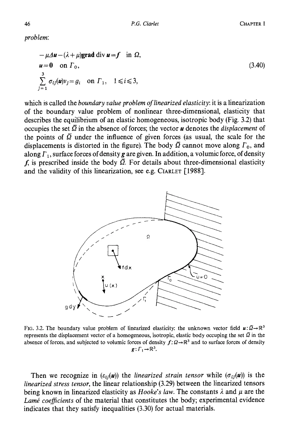
In addition, various relevant extensions, refinements, etc., of these estimates have
been mentioned, with appropriate references to the existing literature.
This article is a revised, updated, and enlarged edition of those parts of my book,
The Finite Element Methodfor Elliptic Problems (North-Holland, Amsterdam, 1978)
that are relevant here. Although I have added more than 230 items to the 316
references that I have kept from this book, I have made no attempt to compile an
exhaustive bibliography. I however hope that the present bibliography is
"reasonably complete".
The various finite elements described in this article have been named according to
the most common usages in the engineering literature. As a result, the terminology
adopted in this article often departs strikingly from that used in my book of 1978.
For instance, what I then called a "triangle of type A)" or a "rectangle of type B)" are
now called a "linear triangle" or a "biquadratic rectangle". Since the readers of this
article are perfectly aware that a triangle may be isoceles, but certainly not genuinely
"linear", or that a rectangle may be square, but certainly not genuinely
"biquadratic", I have blithely committed these serious abus de langage, which clearly
convey more information than the names that I had originally chosen.
Chapter I
Elliptic Boundary Value Problems
Introduction
Many problems in linearized elasticity are modeled by a minimization problem of
the following form: The unknown u, which is the displacement of a mechanical
system, satisfies
и e U and J(u) = inf J(v),
veU
where the set U of admissible displacements is a closed convex subset of a Hilbert
space V, and the energy J of the system takes the form
J(v) = ^a(v,v)-l(v),
where a{',-) is a symmetric bilinear form and I a linear form, both defined and
continuous over the space V. In Section 1, we first prove a general existence result
(Theorem 1.1) for such minimization problems, the main assumptions being the
completeness of the space V and the V-ellipticity of the bilinear form. We also
describe other formulations of the same problem (Theorem 1.2), which are its
variational formulations. When the bilinear form is not symmetric, these
formulations make up variational problems on their own. For such problems, we give an
existence theorem when U=V (Theorem 1.3), which is the celebrated Lax-Milgram
lemma.
All these problems are called abstract problems inasmuch as they represent an
"abstract" formulation which is common to many examples, such as those examined
in this chapter.
The analysis made in Section 1 shows that a candidate for the space V must have
the following properties: It must be complete on the one hand, and it must be such
that the expression J(v) is well defined for all functions ve V on the other hand (V is
a "space of finite energy"). The Sobolev spaces fulfill these requirements. After briefly
mentioning in Section 2 some of their basic properties (other properties will be
introduced in later sections as needed), we examine in Sections 3 and 4 specific
examples that fit in the abstract setting of Section 1, such as the membrane problem,
the obstacle problem, the clamped plate problem, and the boundary value problem of
linearized elasticity, which is by far the most important example. Indeed, even
though throughout this article we will often find it convenient to work with the
23
24
P.G. Ciarlet
Chapter I
simpler looking problems described at the beginning of Section 3, it must not be
forgotten that these are essentially convenient model problems for the boundary
value problem of linearized elasticity.
For each of the examples, we establish in particular the V-ellipticity of the
associated bilinear form, and, using various Green's formulae in Sobolev spaces, we
show that when solving these problems, one solves, at least formally, elliptic
boundary value problems of the second and fourth order.
1. Abstract minimization problems, variational inequalities and
the Lax-Milgram lemma
All functions and vector spaces considered in this article are real.
Let there be given a normed vector space V with norm || • ||, a continuous bilinear
form a(','):Vx V-+M, a continuous linear form /: V-+U and a nonempty subset U
of the space V. With these data we associate an abstract minimization problem:
Find an element и such that
ueU, J{u) = inf J(v), A.1)
veV
where the functional J: V-*U is defined by
J:veV^J{v)=^a(v,v)-l(v). A.2)
As regards existence and uniqueness properties of the solution of this problem,
the following result is essential.
Theorem 1.1. Assume in addition that (i) the space V is complete, (ii) U is a closed
convex subset of V, (iii) the bilinear form a( •, •) zs symmetric and (iv) the bilinear form
is V-elliptic, in the sense that there exists a constant a such that
a>\ (i.3)
a || и || ^ a(v, v) for all veV.
Then the abstract minimization problem A.1) has one and only one solution.
Proof. The bilinear form a( •, •) is an inner product over the space V, and the
associated norm is equivalent to the given norm || • ||. Thus the space V is a Hilbert
space when it is equipped with this inner product. By the Riesz representation
theorem, there exists an element ale V such that
l(v) = a(al,v) for all veV,
so that, taking again into account the symmetry of the bilinear form, we may
rewrite the functional as
J(v) = %a{v, v) — a(al, v) = ja(v — ol,v — al) — \a{al, ol).
Hence solving the abstract minimization problem amounts to minimizing the
Section 1 Elliptic boundary value problems 25
distance between the element al and the set U, with respect to the norm ч/й( •, •).
Consequently, the solution is simply the projection of the element al onto the set U,
with respect to the inner product a(v)- By tne projection theorem, such a
projection exists and is unique, since U is a closed convex subset of the space V. □
Next, we give equivalent formulations of this problem.
Theorem 1.2. An element и is the solution of the abstract minimization problem A.1)
if and only if it satisfies the relations
ueU,
A.4)
a(u,v — u)^l(v—u) for all veil,
in the general case, or
ueU,
e(«, »)>/(») for alive U, A.5)
a(u, u) = l{u),
if U is a closed convex cone with vertex 0, or
ueU, (L6)
a(u, v) = l(v) for all veU,
if U is a closed subspace.
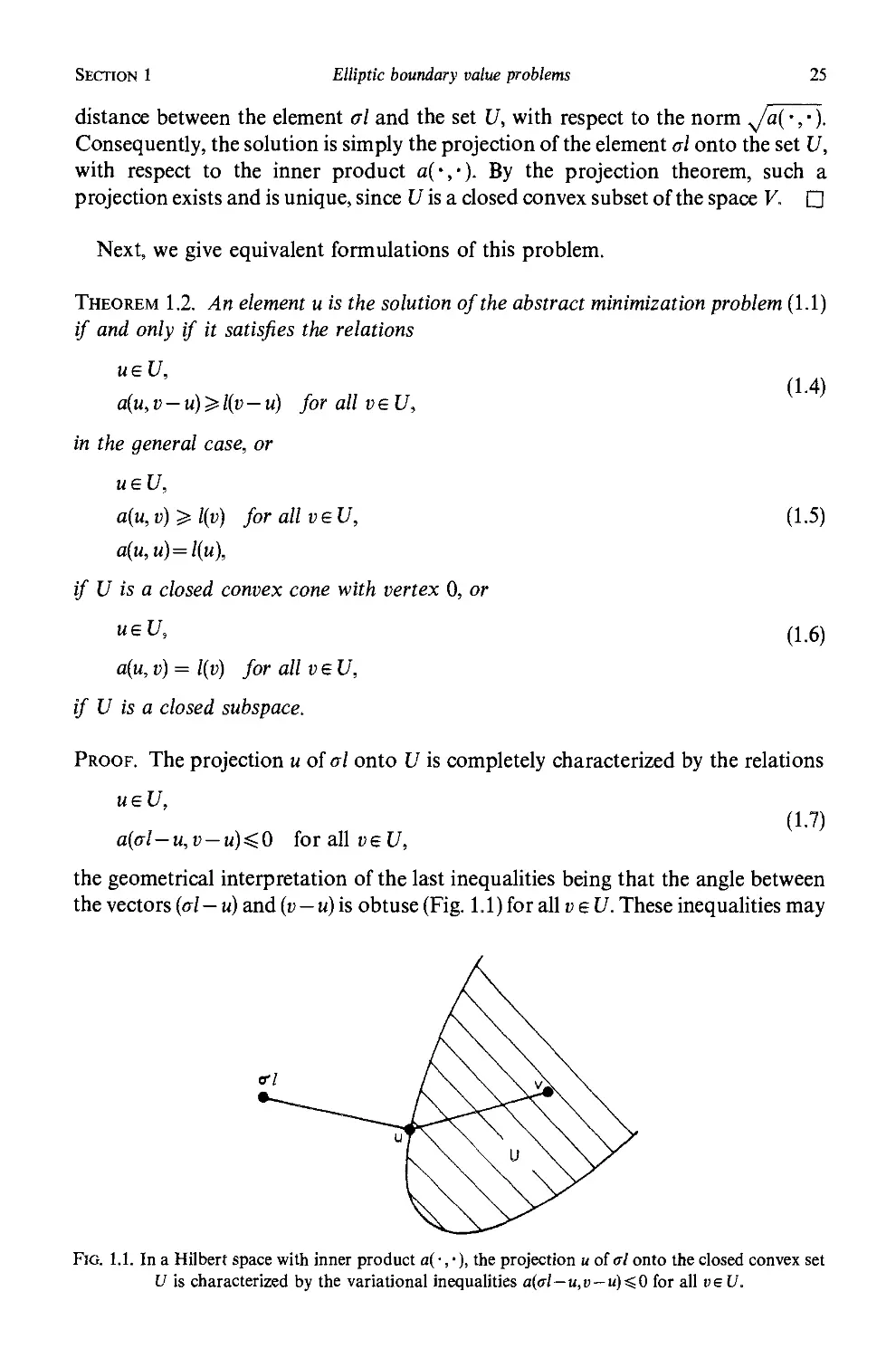
Proof. The projection и of al onto U is completely characterized by the relations
ueU,
A.7)
a{al—u,v — u)^0 for all veU,
the geometrical interpretation of the last inequalities being that the angle between
the vectors (al — u) and (t> — u) is obtuse (Fig. 1.1) for all v e U. These inequalities may
Fig. 1.1. In a Hilbert space with inner product a( •, •), the projection и of al onto the closed convex set
U is characterized by the variational inequalities a(rsl — u,v — u)<0 for all veU.
26
P.G. Ciarlet
Chapter I
be written as
a(u, v—u)^-a(ai, v — u) = l(v — u) for all veU,
which proves relations A.4).
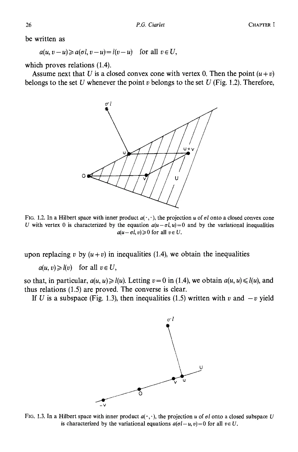
Assume next that U is a closed convex cone with vertex 0. Then the point (u + v)
belongs to the set U whenever the point v belongs to the set U (Fig. 1.2). Therefore,
Fig. 1.2. In a Hilbert space with inner product a{ •, •), the projection и of al onto a closed convex cone
U with vertex 0 is characterized by the equation a(u — al, u)=0 and by the variational inequalities
a(u — al,!>)>0 for all veU.
upon replacing v by (u + v) in inequalities A.4), we obtain the inequalities
a(u,v)^l(v) for all veU,
so that, in particular, a(u, u)^l{u). Letting v = 0 in A.4), we obtain a{u, u)^l(u), and
thus relations A.5) are proved. The converse is clear.
If U is a subspace (Fig. 1.3), then inequalities A.5) written with v and —v yield
Fig. 1.3. In a Hilbert space with inner product a(-,-), the projection и of <r( onto a closed subspace U
is characterized by the variational equations a(al—u, d) = 0 for all vs U.
Section 1
Elliptic boundary value problems
27
a(u, v) ^ l(v) and a{u, v) =$ l(v) for all veU, from which relations A.6) follow. Again the
converse is clear. □
Remark 1.1. Since the projection mapping is linear if and only if the subset U is
a subspace, it follows that problems associated with variational inequalities are
generally nonlinear, the linearity or nonlinearity being that of the mapping
le V'-me V, where V is the dual space of V, all other data being fixed. One should
not forget, however, that if the resulting problem is linear when one minimizes over
a subspace, this is also because the functional is quadratic, i.e., it is of the form
A.2). The minimization of more general functionals over a subspace would
correspond to nonlinear problems.
The various equivalent formulations of the minimization problem A.1) given in
Theorems 1.1 and 1.2 may be also interpreted from the point of view of differential
calculus, as follows. We first observe that the functional J is differentiable at every
point ueV, the action of its Frechet derivative J'(u) e V on an arbitrary element
v e V being given by
J'(ify = a(u,v)-l(v). A.8)
Let then и be the solution of the minimization problem A.1) and let v = u + w be
any point of the convex set U. Since the points (u + 6w) belong to the set U for all
6e [0,1] (Fig. 1.4), we have, by definition of the derivative J(u),
0^J(u + 6w)-J(u) = ej'(u)w + 6\\w\\s(e)
Fig. 1.4. If и belongs to a convex set U and if J(u)=infytsUJ{v), then for each v = {u + w)el),
J(u + 0w)-J(uK=O for all Os£0s: 1.
for all 0e[0,1], with Итв^0е(в) = 0. As a consequence, we necessarily have
J'(u)w>0, A.9)
since otherwise the difference J(u + 6w)—J(u) would be <0 for в small enough.
Using A.8), we may rewrite inequality A.9) as
J'(u)w — J'(u)(v — u) = a(u, v — u) — l(v—u)^ 0,
28
P.G. Ciariet
Chapter I
which is precisely A.4). Conversely, assume that we have found an element ueU
such that
J'(u)(v-u)^Q for all ve U. A.10)
The second derivative 5"{и)&У?2(У\ Щ of the functional J is independent of
ueV and its action on arbitrary elements veV and we V is given by
J"(u)(v,w) = a(v,w). A.11)
Thus, for any point v = u + w belonging to the set U, an application of Taylor's
formula yields
J(u + w) - J{u) = J'(«)(w) + ie(w,w)^ia || w ]|2, A.12)
which shows that и is a solution of problem A.1). We have J(v) — J(u)>0 unless
v = u so that we see once again that the solution is unique.
Arguing as in the proof of Theorem 1.2, we then easily verify that inequalities
A.10) are equivalent to the relations
J'(u)v^Q, J'(u)u=0 for all veU, A.13)
when U is a convex cone with vertex 0, and that they reduce to
J'(u)v = 0 for all uel/, A.14)
when U is a subspace. Notice that relations A.13) coincide with relations A.5), and
that relations A.14) coincide with relations A.6).
When U=V, relations A.14) reduce to the familiar condition that the first
variation of the functional J, i.e., the first-order term J'(u)w in the Taylor expansion
A.12), vanishes for all w e V when the point и is a minimum of the function /: V-*M,
this condition being also sufficient if the function J is convex, as is the case here. By
means of the equivalent relations A.10), A.13), and A.14), relations A.4), A.5), and
A.6) thus appear as generalizations of the previous condition, the expression
a{u, v—u)—f{v-u)~ J'(u)(v — u) playing in the present situation the role of the first
variation of the functional J relative to the convex set U. It is in this sense that the
formulations of Theorem 1.2 are called variational.
More precisely, the characterizations A.4), A.5), and A.6) are called variational
formulations of the original minimization problem, the equations A.6) are called
variational equations, and the inequalities of A.4) and A.5) are called variational
inequalities.
Without making explicit reference to the functional J, we can also define various
abstract variational problems: Find an element и such that
U€U> A.15)
a(u, v — u)^l(v — u) for all ve U,
Section 1
Elliptic boundary value problems
29
in the general case, or, find an element и such that
ueU,
a(u,v)>l(v) for all eel/, A.16)
a(u, u) = l(u),
if U is a cone with vertex 0, or, finally, find an element и such that
ueU, (U7)
a(u, v) = l(v) for all veV,
if U is a subspace. By Theorem 1.1, each of these problems has one and only one
solution if the space V is complete, if the subset U of V is closed and convex, and if
the bilinear form is F-elliptic, continuous, and symmetric. // the assumption of
symmetry of the bilinear form is dropped, the above variational problems still have
one and only one solution if the space V is a Hilbert space, but there is no longer an
associated minimization problem. Here we shall confine ourselves to the case where
U=V.
Theorem 1.3. (Lax-Milgram lemma). Let Vbea Hilbert space, leta(- ,-):Vx V~* Ш.
be a continuous V-elliptic bilinear form, and let l:V-*U be a continuous linear form.
Then the abstract variational problem: Find an element и such that
ueV> A.18)
a(u,v)=l(v) for all veV,
has one and only one solution.
Proof. Let M be a constant such that
|а(и,о)|<М||и|||И forallu,ueF. A.19)
For each ueV, the linear form ve V-*a(u, v) is continuous and thus there exists
a unique element AueV (V is the dual space of V) such that
a(u, v) = Au(v) for all v e V. A.20)
Denoting by || • ||' the norm in the space V', we have
Mu|r = sup!^f^M||u|!.
veV И
Consequently, the linear mapping A: V-+V is continuous, with
MII*(K;K',<M. A.21)
Let t.V'->V denote the Riesz mapping which is such that, by definition,
l(v)=((zl,»)) for all /e V and all ve V, A.22)
where ((•,•)) denotes the inner- product in the space V. Then solving the variational
problem A.18) is equivalent to solving the equation xAu = xl. We will show that this
30 P.G. Ciariet Chapter I
equation has one and only one solution by showing that, for appropriate values of
a parameter p > 0, the affine mapping
veV-*v-p{xAv-xl)eV A.23)
is a contraction. To see this, we observe that
\\v- pxAv\\2 = \\v\\2 -2p{(xAv,v))+p2\\xAv\\2
^{\-2pa + p2M2)\\v\\2,
since, by inequalities A.3) and A.21),
{(tAv, v)) = Av(v) = a(v, v) > a || v \\2,
||ту1«|| = ||А»||'<||Х||||о||<М||»||.
Therefore the mapping defined in A.23) is a contraction whenever the number
p belongs to the interval ]0,2a/M2[ and the proof is complete. □
Remark 1.2. It follows from the previous proof that the mapping A: V-+V is
onto. Since
0£||и||2<в(и,и) = /(и)<||/|Г||и||,
the mapping A has a continuous inverse A'1, with
Therefore the variational problem A.18) is well-posed in the sense that its solution
exists, is unique, and depends continuously on the data f (all other data being equal).
More generally, one can show that, if Wj and u2 are solutions of problem A.15)
corresponding to linear forms lx and l2, then
ll«i-«2K-l|fi-M'.
a
The original reference of the Lax-Milgram lemma is Lax and Milgram [1954].
Our proof follows the method of Lions and Stampacchia [1967], where it is applied
to the general variational problem A.15), and where the case of semipositive-
definite bilinear forms is also considered; Stampacchia [1964] had the original
proof in this case. For constructive existence proofs and additional references, see
also Glowinski, Lions and Tremolieres [1976a]. We also mention that BabuSka
(Babuska and Aziz [1972, Theorem 5.2.1]) has extended the Lax-Milgram lemma
to the case of bilinear forms defined on a product of two distinct Hilbert spaces.
2. The Sobolev spaces Hm(Q) and Green's formulae
For treatments of differential calculus with Frechet derivatives, the reader may
consult Avez [1983], Cartan [1967], Dieudonne [1967], Schwartz [1967]. For
the theory of distributions and its applications to partial differential equations, see
Section 2
Elliptic boundary value problems
31
Schwartz [1966]. Other references are Treves [1967], Shilov [1968], Vo-Khac
Khoan [1972a, 1972b], Choquet-Bruhat [1973], Hormander [1983]. The
Hilbertian Sobolev spaces Hm(Q) are studied in Lions and Magenes [1968,
Chapter 1], Dautray and Lions [1984, Chapter 4] (references on the more general
Sobolev spaces Wm,p(Q) are given in Section 14).
Let us first briefly recall some results from differential calculus. Let there be given
two normed vector spaces X and 7 and a function v: A^ Y, where A is a subset of X.
If the function is к times differentiable at a point as A, we shall denote by Dkv(a), or
simply by Dv(a) if к = 1, its kih Frechet derivative. Note that we also use the alternate
notations Dv(a) = v'(a) and D2v(a) = v"(a). The fcth derivative Dkv(a) is a symmetric
element of the space Л?к(Х; Y), and its norm is given by
\\Dkv(a)\\= sup \\Dkv{a)(huh2,...,hk)l
lUisik
In the special case where X = R" and Y= R, let eh l^i^n, denote the canonical
basis vectors of №. Then the usual partial derivatives are given by
biV(a) = Dv{a)ei,
dijv(a) = D2v(a)(ehej),
dijkv(a) = D3v(a)(et, eh ek), etc.,
and occasionally, we use the notation Vu(a), or Sv{a), to denote the gradient of the
function v at the point a, i.e., the vector in R" whose components are the partial
derivatives 8,i?(a), 1 ^ i ^ n.
We also use the multi-index notation for denoting the partial derivatives: Given
a multi-index a=(a!,a2,.. .,a„)eN", we let |а| = Е"=1аг. Then the partial derivative
d*v(a) is the result of the application of the |a|th derivative £)|а|и(а) to any |a|-vector
of (R"I"' where each vector et occurs at times, 1 <i<n. For instance, if n — 3, we have
Э1»(в) = ЭA,0-0)ф), 6123ф) = 8A'1'1)ф), d111v(a) = di3'°-0)v(a),... Clearly, there
exist constants C(m, n) such that for any partial derivative d"v(a) with |a| = m and
any function v,
\dxv(a)\^ ||Dmv(a)|| <C(m,n) max \dxv(a)\
(unless otherwise specified, it is understood that the space W is equipped with the
Euclidean norm).
As a rule, we represent by symbols such as Dkv,v",Qtv,dxv,..., the functions
associated with any derivative or partial derivative.
When h1 = h2 = --- = hk = h, we simply write
Dkv(a)(h1,h2,...,hk)=Dkv(a)hk.
Thus, given a real-valued function v, Taylors formula of order к is written as
* 1 1
v(a + h) = v(a)+ X -Dlv(a)hl + -—-Dk+1v(a + 6h)hk+1,
for some 0e]0,1[ (whenever such a formula applies).
32
P.G. Ciarlet
Chapter I
Given a bounded open subset Q in W, the space &>(Q) consists of all indefinitely
differentiable functions v:Q-*U with compact support.
For each integer m ^ 0, the Sobolev space Hm{Q) consists of those functions
v e L2(Q) for which the partial derivatives d*v in the distributional sense with |a| ^ m,
belong to the space L2(Q) for all |a| 5%m, i.e., for each multi-index a with |a| ^m, there
exists a function dav e L2{Q) that satisfies
dVdx = (~l)|a| Ue^dx iord\\<t>e9(Q). B.1)
n a
Equipped with the norm
MML.n=( I [|6ar]2dxI/2,
\|«|<m J /
the space Hm(Q) is a Hilbert space. We shall also make frequent use of the semi-norm
\|a[=m J /
П
We define the Sobolev space
the closure being understood in the sense of the norm || • ||тЯ. When the set Q is
bounded, the Poincare-Friedrichs inequality holds: there exists a constant C(Q) such
that
No.n<C(fi)Hli0 foraU»eflJ(Q). B.2)
Therefore, w/геи t/ге set Q is bounded, the seminorm | • |m,n is a norm over the space
Hq(Q), equivalent to the norm || • ||mifi (see also Theorem 3.1).
Following NeCas [1967], we say that an open set Q has a Lipschitz-continuous
boundary Г if the following conditions are fulfilled: There exist constants a>0
and /?>0, and a finite number of local coordinate systems and local maps
ar, 1 ^r<K, that are Lipschitz-continuous on their respective domains of
definitions {xreRn;|x,'|sS<x}, such that (Fig. 2.1):
R
T=U {{x\,xr);x\=ar(xr),\xr\<a},
r=l
{{x\,xr);ar{xr)<x\<aT{xr) + P, |xr|<a}c:£2, 1<г^Д,
{(xr1,xr);ar(xr)-li<xr1<ar(xr),\xr\<a}c:W-Q, l^r^R,
where xr = (x;>,.. .,xr„), and |xr|<a stands for |xf|<a,l^i^n.
Occasionally, we shall also need the following definitions: A boundary is of class
S£ if the functions a/. \xr\ <<x~>R are of class Ж (such as <€m or свт'% and a boundary
Section 2
Elliptic boundary value problems
33
Fig. 2.1. A domain in U2 is an open, bounded, connected subset with a Lipschitz-continuous boundary.
is said to be sufficiently smooth if it is of class <€m, or ^""'a, for sufficiently high values
of m, or m and a.
A domain in W is an open, bounded, connected subset with a Lipschitz-
continuous boundary. This definition is particularly well suited for our subsequent
purposes, in that it allows the consideration of domains with "corners" or "edges",
such as polyhedra.
In the remaining part of this section, it will be always understood that Q is a
domain in R". In particular then, a superficial measure, which we shall denote dy,
can be defined along the boundary, so that it makes sense to consider the spaces
Ь2(Г), whose norm shall be denoted || • ||£,2(r).
Then it can be proved that there exists a constant C(O) such that
NL*(r)*£C(G)N|1(o for all ve^iQ). B.3)
Since {^"(fl)} ~ =H1(Q) if О is a domain, the closure being taken with respect to the
norm I| • [|lrn, there exists a continuous linear mapping tr:veHx(Q)-*tr veL2(r),
which is called the trace operator. Note however that, when no confusion should
arise, we shall simply write trt; = y. The following characterization of the space
34 P.O. Ciarlet Chapter I
Hh{Q) holds:
Hh(Q)={veH Щ; v=0 on Г}.
Since the unit outer normal vector v = (v1(..., v„) (Fig, 2.1) exists almost
everywhere along Г, the (outer) normal derivative operator,
n
is defined almost everywhere along Г for smooth functions. Extending its definition
to 8V = S"=! V; tr 8; for functions in the space H2(Q), we obtain the following
characterization of the space Яо(£2):
Hg(fl) = {ueH2(fi);u = 8vt;=0 on Г}.
Given two functions u, veH1(Q), the fundamental Green formula
udtv dx = —
btu v dx + \u vvt dy
B.4)
holds for any ie [1, n]. From this formula, other Green's formulae are easily deduced.
For example, replacing и by 8,u and summing from 1 to n, we get
Y, 8;tt3;t)dx=— Auvdx+ 8vui;dy B.5)
n г
for all ueH2(Q), veH\Q). As a consequence, we obtain by subtraction:
(uAv — Auv)dx =
n
{ubvv — dvuv)dy
B.6)
for all u, veH2(Q). Replacing и by Au in formula B.6), we obtain
Mu/li>dx = A2uvdx— \dvAuvdy+ AudYvdy B.7)
J -J J л
q а г г
for all ueH\Q), veH2{Q). As another application of formula B.4), let us prove the
relation
\Mo.a = \v\2,a &>га11»еЯ§@), B.8)
which implies that, over the space Hq(Q), the seminorm v-*\Av\0i{} is a norm,
equivalent to the norm || • ||2,д: We have, by definition,
\v\l,n =
Z@i;vJ+Y@ijvJ\^
i iitj J
Section 3 Elliptic boundary value problems 35
Clearly, it suffices to prove relations B.8) for all functions v e 3>{Q). But for such
functions, we have
(8yi?J dx =
divQijjV dx -
dijvdjjv dx,
as two applications of Green's formula B.4) show, and thus B.8) is proved.
For n = 2, let т = (тх, т2) denote the unit tangential vector along the boundary Г,
oriented in the usual way. In addition to the normal derivative operator 3V, we
introduce the differential operators 8t, Svr, 6„ defined by
2
dzv{a)=Dv{a)x= ]T тД-i^a),
i=i
2
8vti;(a)=D2t;(a)(v,T)= £ v^Syufa),
2
3„ф) = /Jф)(т,т) = ^ т(т;8ур(а).
u=i
Note that 8zzv does not coincide in general with the second derivative of the
function v considered as a function of the curvilinear abscissa along the boundary. Then
one can show that another Green's formula, viz.,
{2d12ud12V-dilud22V-d22ud11v}dx'= {-dztudvv + dvtudrv} dy, B.9)
r
holds for all functions ueH\Q), veH2{Q).
3. Examples of second-order boundary value problems: The membrane problem,
the boundary value problem of linearized elasticity and the obstacle problem
We next proceed to examine several examples of minimization problems that fall in
the abstract setting of Section 1. According to the analysis made in this section, we
thus need to specify for each example the space V, a subset U of the space V,
a bilinear form a(-,-):Vx F->R, and a linear form /: V-*R. In all the examples,
the set Q is a domain in W.
Example 3.1. The first example corresponds to the following data:
V=U = Hh(Q),
a(u,v)= I Y, SjuSji) + buv I dx, C.1)
я
/(d) = \fvdx,
Q
36 P.G. Ciarlet Chapter I
and the following assumptions are made on the functions b and /:
beU°{Q), b^O a.e. опй, feL2(Q). C.2)
To begin with, it is clear that the symmetric bilinear form a( •, •) is continuous
since for all u,veHl(Q),
n
\a(u,V)\^ £ |6;М|о,я|9;1>|0,й+|Ь|о,а,,йМо,яМо,Я
i=l
<max{l,]b|0,oo.o}Nli,oNli,fl.
where j • \0if, and | • |0o0 fi denote the norms of the space L\Q) and L°°(fi) respectively.
Further, it is Ho(£2)-elliptic since, for all veH1(Q),
a(v, v) >
Q
Y @ivJ dx = \v\la
(by the Poincare-Friedrichs inequality B.2), the seminorm | • 11>fi is a norm over the
space Ho(Q), equivalent to the norm || • || li0). Next, the linear form I is continuous
since for all veH1(Q),
\m\<\f\o,o\v\0.o^\f\ o.nlMli.n-
Therefore, by Theorem 1.1, there exists a unique function неЯо(Й) that
minimizes the functional
J:»-»J(») = i
£ (diVJ + bv2]dx-
fv dx C.3)
Q
over the space Ho(Q), or equivalently, by Theorem 1.2, that satisfies the variational
equations
1 Г
£ Э,иЭ,1> + buv Ydx = fv dx for all v e Hh(Q). C.4)
;=i J J
q n
Using these equations, we now show that we are also solving a partial differential
equation in the distributional sense. More specifically, let @)'(Q) denote the space of
distributions over the set Q, i.e., the dual space of the space @{Q\ equipped with the
Schwartz topology, and let <•,•> denote the duality pairing between the spaces
2'{Щ and 3>{Q). As usual we identify a function g that is locally integrable over Q
with the distribution g: феЩ£2)-+§Рдфйх.
Since the inclusion
9{Q)aV-=Hl(Q)
holds, the variational equations C.4) are satisfied for all functions ce§(fl).
Therefore, by definition of the differentiation of distributions, we may write
n
a(u,ф) = £ <S/",б,Ф> + <Ъи,ф} = (-Аи + Ьи,фУ for all фе®{Q).
;=i
Section 3
Elliptic boundary value problems
37
Since 1(ф) = {/, ф) for all ^e^(fl), it follows from the above relations that и is
a solution of the partial differential equation — Au + bu=fin <%'(Q).
To sum up, the solution и of the minimization (or variational) problem associated
with the data C.1) is also a solution of the problem: Find a distribution ue@)'{Q)
such that
ueHh№ C.5)
-Au + bu=f in 9>\Q),
and conversely, if a distribution и satisfies C.5), it is a solution of the original
problem. To see this, we observe that the equalities
a(u,ф) = (-Аи + Ьи,ф} = (/,ф) = 1ф) for all фе2{Q)
hold in fact for all functions ф е Hq@) since 3>(Q) is a dense subspace of the space
Hh@).
Remembering that the functions in the space Hq(Q) have a vanishing trace
along Г, we shall say that we have formally solved the associated boundary value
problem
— Au + bu=f in Q, u = 0 on Г. C.6)
The terminology "boundary value problem" refers to the fact that the values of the
unknown function и (as in this example) or of some differential operator acting on
the unknown function и (as in some of the subsequent examples) are specified along
the boundary of the set Q.
Problem C.6) is called a homogeneous Dirichlet problem for the operator
u-* — Au-\-bu, since it is formally posed exactly as in the classical sense where,
typically, one would seek a solution in the space #°(£2)п#2(£2). Actually, when the
data are sufficiently smooth, it can be proved (but this is not easy) that the solution of
C.4) is also a solution of C.6) in the classical sense. Nevertheless, one should keep in
mind that, in general, nothing guarantees that the partial differential equation
— Au + bu =f in Q can be given a sense otherwise than in the space 3i'(Q). Likewise
the boundary condition и=0 on Г cannot be understood in general otherwise than
in the sense of a vanishing trace, or even in no sense at all if the set Q were "only"
supposed to be bounded.
A modification of the linear form of C.1) will lead us to the second example.
Example 3.2. Let the space V and the bilinear form be as in C.1), and let the linear
form be defined by
l(v) = \fvdx-a{u0,v), C.7)
n
where the functions / and b satisfy assumptions C.2) and u0 is a given function in
the space H1(Q). Proceeding as before, we could likewise show that these data
correspond to the formal solution of the nonhomogeneous Dirichlet problem for the
38
P.G. Ciariet
Chapter I
operator u-+ —Au + bu, viz.,
— Au + bu~f in Q, u = u0 on Г.
C.8)
When b=0 and n — 2, this problem is called the membrane problem: It arises in
linearized elasticity when one considers the problem of finding the equilibrium
position of an elastic membrane, with tension т, under the action of a vertical force of
density F = xf, and whose vertical displacement и is equal to a known function u0
along the boundary Г (cf. Fig. 3.1).
Fdx
Fig, 3.1. The membrane problem: the unknown function u: Q <= U2 ->R represents the vertical
displacement of a membrane subjected to a vertical force of density F per unit area.
Example 3.3. The third example corresponds to the following data:
a{u, v) =
£ diudiv + buv )dx,
l(v) = fvdx+ \gv dy,
о г
and the following assumptions are made on the functions a, f and g:
beL^iQ), b^bo>0 a.e. on Q,
feL2(Q), gsL2(D
C.9)
C.30)
Section 3
Elliptic boundary value problems
39
for some constant b0. Hence both the space V and the linear form / differ from those
of Example 3.1.
The bilinear form is Hl{Q)-e\liptic since a(v, v) ^ min{l,b0} ||«||ii0 for all
veHl(Q). The linear form veH1(Q) -* $rgvdy is continuous since by inequality
B.3),
gvdy
<Ыьнг)Ытп =* C(Q)\\g\\LHn\\v\\uo.
Therefore there exists a unique function ue H1(Q) that minimizes the functional
J:»-»J(») = i
Z(d,vJ + bv2\dx
fvdx —
gvdy,
over the space H\Q) or, equivalently, such that
Y, diUdiV + buv>dx
fv dx + gv dy for all v e H1 (Q).
C.11)
Because @{Q) is a subspace of the space Hi{Q), an argument similar to the one
used in Example 3.1 shows that и is also a solution of the partial differential
equation — Au + bu = f in 3i'(Q). Hence we have
(—Au + bu)vdx = a(u, v)~ \gvdy for all veHi(Q).
To sum up, the solution u of the minimization (or variational) problem associated
with the data C.9) is also a solution of the problem: Find a distribution и е !3'{Q) such
that
ueH\Q), -Au + bu = f in ЩП),
Г C-12)
( — Au + bu)vdx = a(u,v)— gvdy for all vsH1(Q),
and, conversely, if a distribution и is a solution of problem C.12), it is clearly
a solution of the variational equations C.11).
If we assume additional smoothness on the solution, the second relations in C.12)
shows that the solution satisfies a boundary condition: If the solution и is in the space
H2{Q), for example, an application of Green's formula B.5) shows that, for all
veH'iQ),
a(u, v) =
(—Au + bu)vdx +
dvuvdy
fvdx +
gvdy.
C.13)
40 P.G. Ciarlet Chapter I
Therefore the conjunction of relations C.12) and C.13) implies that
9vMt>dy= \gvdy for all veH1(Q), C.14)
г г
and from these, one deduces that dyu=g on Г.
Consequently, we shall say that we have formally solved the associated boundary
value problem:
— Au + bu = f in Q, dvu = g on Г, C.15)
which is called a nonhomogeneous Neumann problem if g ф 0, or a homogeneous
Neumann problem if g = 0, for the operator и ~* ~-Au + bu.
Remark 3.1. Without using differentiation of distributions, we may use Green's
formula B.5) to obtain the partial differential equation since
а{и,ф)= ( — Аи + аи)фйх — < — Ли + аи, ф) for all ф е 3)(Q).
о
This is not a coincidence: The definition of differentiation for distributions is
precisely based upon the fundamental Green formula B.4).
If b = 0, the bilinear form a(- ,•) of'C.9) is no longer Hl(Q)-elliptic. We can however
circumvent this difficulty by using the following result (which is a special case of
a result proved later; cf. Theorem 14.1): Let P0{Q) denote the space of all constant
functions over Q. Then the seminorm I'li.o is a norm over the quotient space
H1(Q)/P0(Q), equivalent to the quotient norm. This observation leads us to our fourth
example,
Example 3.4. Let we Hl(£2)/P0(Q) denote the equivalence class of an arbitrary
element wsH1{Q), and let:
5/=[/ = Я1@)/Ро(А),
а(й, v) =
Y, 9,u9;t)dx, C.16)
/(«5) =
fv dx + gv dy.
г
The bilinear form a( •, •) is well defined and continuous over the quotient space
V=H1(Q)/P0(Q), and further, it is now V-elliptic by the aforesaid result. If (and only
if)
fdx+ \gdy = 0, C.17)
Section 3 Elliptic boundary value problems 41
the linear form I is also well defined and continuous over the quotient space.
Arguing as before, we find that the variational problem associated with the data
C.16) corresponds to the formal solution of the associated boundary value problem
— Ли-f in Q, dvu=g on Г, C.18)
which is another nonhomogeneous Neumann problem for the operator —A.
Remark 3.2. The necessity of the relation C.17) also follows a posteriori from
C.18) and from the formula \qAu Ax = \Tbyu dy, obtained by letting v = 1 in Green's
formula B.5).
Example 3.5. In the fifth example, we extend in two directions the previous
examples: First the associated partial differential equation will have nonconstant
coefficients and secondly, the bilinear form will not be necessarily symmetric so that
the Lax-Milgram lemma (Theorem 1.3) will be needed for proving the existence of
a solution. The data are the following:
У=и = {оеНЩ-^ = 0 on Г0},
a(u, v)-
< £ aifiiudjV + buvfdx, C.19)
l(v)= \fvdx + gvdy,
a ri
where Г0 = Г—Г t is a dy-measurable subset of the boundary Г whose dy-measure is
>0, and the functions a,7, b and / satisfy the following assumptions:
flyeL^Q), KiJ^n,
beL°°(fl), b>0 a.e. on O, C.20)
feL2(Q), geLHTil
and there exists a constant ft such that
л n
j3>0, £ ayZtZj^fi £ & for all &, Ui^ a.e. on Q. C.21)
The F-ellipticity of the bilinear form of C.19) will be a consequence of the
following result.
Theorem 3.1. Let Qbea domain in Ш". Then the space V defined in C.19) is a closed
subspace of Hl(Q). If the dy-measure of Г0 is >0, the seminorm |*ti,n iS a norm over
the space V, equivalent to the norm || * lli.n-
Proof. Let (vk) be a sequence of functions in the space V that converges to an
element ve H1(Q). Since the sequence (trut) converges to try in the space Ь2(Г)
(cf. inequalities B.3)), it contains a subsequence that converges almost everywhere
42
P.G. Ciarlet
Chapter I
to tr v and thus tr v = 0 a.e. on Г0, This implies that the function v belongs to the
space V.
Next, let us show that | • |1>fl is a norm over the space V. Let v be a function in the
space V that satisfies |t>|1>n=0. Then it is a constant function by virtue of the
connectedness of the set Q; thus its trace is a constant function that takes the same
value, and this value is zero since the trace vanishes on the set F0, whose dy-measure
is >0.
Finally, assume that the two norms | • |ljC and || • |i 1,0 are not equivalent over the
space V. Then there exists a sequence (vk) of functions vke V such that
llf*IIi,o=l for all k, lim Ы1>п = 0.
fc->oo
By Rellich's theorem, any bounded sequence in the space H1(Q) contains a
subsequence that converges in L2(Q), so that there exists a sequence (t>() of functions d, e V
that converges in the space L2{Q). Since Нт^иМ^я = 0, on the other hand, the
sequence {vt) is a Cauchy sequence in the complete space V, and therefore it
converges with respect to the norm || ■ ||1>я to an element veV.
Since |y| 1>fi = limi_ ao\vi\i,n — 0>we deduce that v = 0, which is in contradiction with
the equalities ||t^||1;fi=l for all k. □
From this theorem, we infer that the bilinear form of C.19) is F-elliptic since we
have a(v,v)^P\v\ln for all veHl{Q) by inequalities C.20) and C.21).
By the Lax-Milgram lemma (Theorem 1.3), there exists a unique function ueV
that satisfies the variational equations
1 I] uijdiudjV + buvfdx —
fvdx +
gv dy for all v e V. C.22)
Referring once again to formula B.4), we obtain another Green's formula:
n Г п Г п
Y, aijdiudjvdx= — ]T 5j(aij6iu)vdx+ ^ a^dtuvjdy, C.23)
ij= 1 J Uj= 1 J Uj= 1
a n г
valid for all functions ue H\Q),ve H1(Q), provided the functions atJ are smooth
enough, e.g., in the space <^'1(Q), so that the functions ауЭ(н belong to the space
Hl(Q). Using C.23) we conclude that we have formally solved the associated
boundary value problem
n
~ Yj dj(aijdiu) + bu=f in Q,
u=i
и = 0 on Г0, C.24)
n
£ aijyfiiU = g on Гъ
Section 3 Elliptic boundary value problems 43
which is called a homogeneous mixed problem ifg=Q, or a nonhomogeneous mixed
problem if g=£0, for the operator
n
"-"- E Э;(ауЭ,и) + Ьм. C.25)
Notice that condition C.21) is the classical ellipticity condition for an operator
such as that of C.25), which is accordingly called an elliptic operator when this
condition is fulfilled. The boundary operator
и
u-> £ atjVjdiU
u=i
is called the conormal derivative operator associated with the operator of C.25).
If Г=Г0, or if Г=Г!, we have formally solved a homogeneous Dirichlet problem, or
a homogeneous or a nonhomogeneous Neumann problem respectively, for the operator
of C.25) (in the second case, we would require an inequality such as b > b0 > 0 a.e. on
Q to get existence).
We now come to the sixth example, which is by far the most important.
Example 3.6. Let Q be a domain in U3. We define the space
V=U={v = (Vl,v2,v3)e(H\Q)K; »,=0 on Г0, Ui<3}, C.26)
where Г0 is a dy-measurable subset of Г, whose dy-measure is >0. The space V,
which is a closed subspace of (Hl(Q)K, is equipped with the product norm
/ 3 N1/2
r = (»i,»2,»3)-IMIi,o = ( E ЫЫ C-27)
For any у=(г1,у2,из)е(Я1(А)K, let
Ф) = tyW = i(9y», + 3,-оД 1 ^ i,j ^ 3, C.28)
and
ffyW==^W = -l( I ^(")Vy + 2/iey(v), l^UO, C.29)
where Ey is the Kronecker's symbol, and A and /^ are two constants that satisfy
A>0, ц>0. C.30)
We then define the symmetric bilinear form
a(u,v) =
з
£ ffy(»)£y(v)d*
i,j=l
j A div и div v + 2ц £ ey(»Ny(v) i dx, C.31)
44
P.O. Ciarlet
Chapter I
and the linear form
l(v)= \f-vdx +
g-vdy
з
= £ f,vtdx+ \ Y,9iVidy, C.32)
where/=(/1J2J3N(L2(fi)K andg = igug2,g3)e(L2{r1)K, with Г^Г~Г0.
It is clear that these bilinear and linear forms are continuous over the space V.
To prove the P-ellipticity of the bilinear form (Theorem 3.2), one needs Korn's
inequality: There exists a constant C(Q) such that, for all v = (v1,v2, v3)e{H1(Q)K,
Ыип^СЩ £ |ey(r)|§>0+ £ ЫЬУ'2. C.33)
\«,j=i ;=i /
This inequality is difficult to establish; its proof may be found in Duvaut and
Lions [1972, Chapter 3, Section 3.3], or in Fichera [1972a, Section 12].
Theorem 3.2. Let Q be a domain in R3, and let Г0 denote a dy-measurable subset
of Г, whose dy-measure is >0. Then the mapping
С 3 -11/2
v=(i>i,t>2,i>3)-{Z М")|Ц C-34)
is a norm over the space V of C.26), equivalent to the product norm C.27).
Proof. The proof is similar to that of Theorem 3.1, and for this reason will be
only sketched (for details, see e.g. Duvaut and Lions [1972] or Ciarlet [1988,
Section 6.3]). One first shows that a function ve (H1{Q)K that satisfies ey(v)=0 in
Q, 1 ^i,j<3, is of the form v: x-+v(x) = a+bx Ox, for some constant vectors aeU3
and be U3. Using Korn's inequality C.33), one then shows that the norm defined in
C.34) is equivalent to the product norm. □
The F-ellipticity of the bilinear form C.31) is therefore a consequence of
inequalities C.30), since by C.31):
з
a(v,v)^2fi X |£y(v)|giQ.
ij=l
We thus conclude that there exists a unique function us V that minimizes the
functional
J{v) = i \ JA(div(v)J + 2/i £ (£;>)J1 dx-
f-vdx +
g-vdy) C.35)
Section 3 Elliptic boundary value problems
over the space V or, equivalently, that satisfies
45
Г 3
£ ffv(ii)ey(»)dx =
f-vdx +
g-vdy for all ve V.
C.36)
Since relations C.36) are satisfied by all functions v e {ЩО)K, they could yield the
associated partial differential equations. However, as was pointed out in Remark
3.1, it is equivalent to use Green's formulae, which in addition have the advantage
of simultaneously yielding the associated boundary conditions (cf. C.40)).
Using Green's formula B.4), we obtain, for all ue {H2(Q)f and all ve (НЩK:
<rij(ufijVidx = - \(QJaij(H))vidx + ои{и)ь^йу,
so that, using definitions C.28) and C.29) we have proved that the following Green's
formula holds:
* з
n
= [ £ (- £ W)W+ f £ ( £ ffu(Wkdy> C-37)
J i=l \ j=l / J i=l \j=l /
A Г
for all functions us{H2{Q)f and vs{H\Q)f.
Arguing as in the previous examples, we find that we are formally solving the
equations
These equations are sometimes written in vector form as
— \xAu—{k+^)grad div и =/ in Q,
C.38)
C.39)
which is obtained from C.38) simply by using relations C.29).
Taking equations C.38) into account, we find that the variational equations C.36)
reduce to
•3/3 \ /* 3
E £ ffij(u)vJ\vidy= Y,9tVidy forallveF,
J t=l \j=l / J i=l
since v = 0 on Г0 = Г — Г%.
To sum up, we have formally solved the following associated boundary value
46
P.G. Ciarlet
Chapter I
problem:
—цЛи—(Х + /x)grad div и =f in Q,
u = 0 on Г0, C.40)
з
X Oij(u)Vj=gt on Л, f ^ i s$ 3,
;=i
which is called the boundary value problem of linearized elasticity, it is a linearization
of the boundary value problem of nonlinear three-dimensional, elasticity that
describes the equilibrium of an elastic homogeneous, isotropic body (Fig. 3.2) that
occupies the set Q in the absence of forces; the vector и denotes the displacement of
the points of Q under the influence of given forces (as usual, the scale for the
displacements is distorted in the figure). The body Q cannot move along Г0, and
along Г и surface forces of density g are given. In addition, a volumic force, of density
/ is prescribed inside the body Q. For details about three-dimensional elasticity
and the validity of this linearization, see e.g. Ciarlet [1988].
Fig. 3.2. The boundary value problem of linearized elasticity: the unknown vector field u:Q->R3
represents the displacement vector of a homogeneous, isotropic, elastic body occuping the set U in the
absence of forces, and subjected to volumic forces of density /: Q-+R3 and to surface forces of density
Then we recognize in (еу(и)) the linearized strain tensor while (<Ху(и)) is the
linearized stress tensor, the linear relationship C.29) between the linearized tensors
being known in linearized elasticity as Hooke's law. The constants X and fi are the
Lame coefficients of the material that constitutes the body; experimental evidence
indicates that they satisfy inequalities C.30) for actual materials.
Section 3
Elliptic boundary value problems
47
Remark 3.3. It can be shown that the bilinear form of C.31) remains elliptic under
the weaker assumptions 3A + 2//>0, /i>0.
The variational equations C.36) represent in linearized elasticity the principle of
virtual work, valid for all kinematically admissible displacements v, i.e., that satisfy
the boundary condition v=0 on Г0.
Remark 3.4. It is interesting to notice that the strict positiveness of the dy-measure
of Г0 has a physical interpretation: It is intuitively clear that if the dy-measure of Г0
were zero, the body would be "free" and therefore there could not exist an
equilibrium position in general.
The functional J of C.35) represents in linearized elasticity the total energy of
the body. It is the sum of the strain energy:
ijb(divvJ + 2^ i(£ij(v)J\ux,
and of the potential energy of the exterior forces:
(J
f-vdx +
g-vdy
Example 3.6 is the most crucial one, not only because it has obviously many
applications, but also because its variational formulation, described here, is basically
responsible for the invention of the finite element method by engineers.
We conclude this section by studying various problems posed in terms of
variational inequalities, i.e., where the set U is not a vector space. To begin this second
series of examples, we describe an interesting variant of the membrane problem.
Example 3.7. The obstacle problem consists in finding the equilibrium position of an
elastic membrane, with tension z, which, as before (cf. Fig. 3.1), passes through the
boundary Г of an open set Q of the horizontal plane and is subjected to the action of
a vertical force of density F = zf but which, in addition, must lie over an "obstacle"
which is represented by a function %: П-*М, as illustrated in Fig. 3.3. This seventh
example is thus naturally associated with the following data:
V=Hh(Q\ О с U2,
U = {veHl0{Q);v^x a.e. in Q}, C.41)
a{u, v) =
Vu-Vrdx, Kv) =
fvdx.
For definiteness, we shall make the following assumptions on the functions % and
/:
XeH2(Q), x^O onf, feL2(Q). C.42)
P.G. Ciarlet
Chapter I
Unknown
contact zone
Fig. 3.3. The obstacle problem: the membrane must lie over an "obstacle", which is represented by a
function x- U-*R.
The set U, which is not empty by virtue of the second assumption of C.42), is
easily seen to be convex. To show that it is closed, it suffices to observe that every
convergent sequence in the space L2(Q) contains an a.e. pointwise convergent
subsequence.
Thus we may apply Theorem 1.1: There exists a unique function ueU that
minimizes the membrane energy
J:v-*J(v)=$
||Vi;|l2dx-
fvdx
C.43)
over the set U, and it is also the unique solution of the variational inequalities
Vu • V(t> — u) dx > f(v — u) dx for all veU,
C.44)
by Theorem 1.2.
By contrast with the solution of the membrane problem, the solution of the
obstacle problem is not smooth in general, even if the data are very smooth. To be
convinced of this phenomenon, consider the one-dimensional analog with f = 0, as
shown in Fig. 3.4. In this case, the solution is affine in the region where it does not
touch the obstacle and consequently, whatever the smoothness of the function x, the
second derivatives will have discontinuities at points such as £ and n. Therefore the
solution и is "only" in the space H2(I).
These results carry over to the two-dimensional case, but they are of course much
less easy to prove. For example, it is known that if the function x satisfies the
assumptions of C.42),/ = 0, and Q is a convex polygon, the solution и belongs to the
space Hq(Q) n H2(Q). If the set Q is convex with a boundary of class tf2 and
Section 3
Elliptic boundary value problems
49
Fig. 3.4. The one-dimensional analog of the obstacle problem, with /=0.
assumptions C.42) hold then we have again и е Ho(Q) n H2(Q). In both cases, the
norm ||и||2,о can be estimated in terms of the norms Hxll2.fi and \f\0,n of the data.
These results are proved in Brezis and Stampacchia [1968] and Lewy and
Stampacchia [1969].
In order to interpret the variational inequalities C.44) as a boundary value
problem, assume that the solution и is in the space H2(Q). Hence the function (u—%)
is in the space 4>°{Q), since #еЯ2@) by the first assumption of C.42), and
H2{Q)c(e0(Q) when n = 2. Let xe Q be such that u(x)>x(x). Then there exist <5>0
and r>0 such that
Br(x)={yeU2;\\y-x\\^r}cQ,
Ф)>Х(у) + & for all yeBr(x).
Consequently, if q>e 3)(Q) is such that supp cpczBr(x), there exists eo(<p)>0 such
that
v£ — (u + вер) 6 U for all |е|^е0(<р).
Using the functions vE, |e| ^e0{(p), in the variational inequalities C.44), we find that
Vw • Vq> dx —
f(p dx > ^0 for all |s| <£0{(p)-
n
Therefore,
Vu • V<p dx — \ fcp dx = 0
for all <p e 2> (Q) such that supp q> с Br(x).
From Green's formula B.5), we thus infer that — Au = f'm the open ball
(ye R2; \\y — x\\ <r). Hence — Au — f in the open set Q+ = {xe Q; м(х)>/(х)}.
Using the same Green formula and the relation — Au = f in Q+,v/e next find that
50
P.G. Ciarlet
Chapter I
the variational inequalities C.44) reduce to
{-Au-f)(v-x)dx^0 for all «e f/,
and thus — Au^f on the set {xeQ;u(x) = x(x)}-
To sum up, we have formally solved the associated boundary value problem:
— Au—f in Q+= {xeQ;u(x)>x{x)},
-Au^f mQ° = {xeQ;u{x) = x{x)}, C.45)
и > x in Д и = 0 on Г.
As was already observed (cf. Remark 1.1), this is a nonlinear problem, since the set
U of C.41) is not a vector space. In the same vein, notice that the region where the
membrane touches the obstacle, i.e., the set Q°, is not known in advance.
We may also view the boundary value problem C.45) as &free boundary problem,
where the free boundary Г* = Ш+r\bQ° is one of the unknowns. In such a
formulation, it is customary to adjoin to C.45) two transmission conditions:
^frl^t , J on Г*, C.46)
trav(uifi*) = tr6v(u|0o)j
which simply reflect here the assumption that и e H2(Q). Observe, however, that
these transmission conditions make sense only if Г* is smooth enough.
Example 3.8. This example, which is closely related to Example 3.7, corresponds
to the following data:
V=H\Q\
!/={1)€Я'(й);^0 dy-a.e. on Г},
a{u, v) =
r
100=
fi
< Y, 9;u6jP + bui?>dx,
;dx,
C.47)
where the functions b and / satisfy the same assumptions as in C.10). Arguing as
before, we easily see that the corresponding variational problem amounts to
formally solving the associated boundary value problem:
— Au + bu = f in Q,
u^O on Г, C.48)
3vu>0 on Г, u9vu=0 on Г.
This problem falls in the class of Signorinfs problems, named after Signorini [1933],
i.e., problems where some boundary conditions take the form of inequalities, such as
Section 3
Elliptic boundary value problems
51
those appearing in C.48). For extensive discussions of such problems, see
Duvaut and Lions [1972b], Fichera [1972], Necas [1975], Glowinski, Lions and
Tremolieres [1976a, 1976b], Necas and Hlavacek [1981], Glowinski [1984].
Example 3.9. Another problem modeled by variational inequalities is the elastic-
plastic torsion problem, which arises in the following situation: Consider a cylindrical
thin rod with a simply connected cross section ficl2, subjected to a torsion around
the axis supporting the vector e3. The torsion angle т per unit length is assumed to be
constant throughout the length of the rod (cf. Fig. 3.5, where the vertical scale should
be considerably increased).
^=^
Fig. 3.5. The elastic-plastic torsion problem: A cylindrical rod is subjected to a constant torsion angle
т per unit length along the vertical direction.
Let us first assume that this problem is modeled by linearized elasticity. Then
certain simplifying assumptions (the weight of the rod is neglected among other
things) imply that the components <т1Ь <т12, o21 and <x33 of the stress tensor vanish
everywhere in the rod, while the components al3 and а2Ъ, which are functions of x ±
and x2 only, are such that
ег13 = 2/га32м, cr23= — 2jUt6xM,
52
P.O. Ciarlet
Chapter I
where ц is the second Lame coefficient of the constitutive material of the rod, and
the stress function и satisfies
~Au—\ in Q, u — Q on Г.
Therefore the function и minimizes the functional
J: v-*J{v)-
Wvfdx-
fvdx, with /=1,
over the space Hq(Q).
If the plasticity of the material is also taken into account, the stresses cannot take
arbitrary large values. A particular mathematical model of this restriction is the
von Mises criterion, which reduces in this case to the condition that the quantity
(к1з12 + к2з12I/2> and consequently the norm ||Vu||, cannot exceed a certain
constant. Notice, however, that by contrast with linearized elasticity, it is no longer
straightforward to relate the displacement field to the stress field, as shown for
instance by the discussion in Duvaut and Lions [1972, Chapter 5, Section 6].
This problem thus corresponds to the following data (for definiteness, the upper
bound on ||Vm|| has been set equal to one):
V=Hh@), n = 2,
U^{veHi{Q); ||Vi?||<1 a.e. in Q),
a(u,v) = Vu-Vvdx. C.49)
/(i?)= fvdx, feL2(Q),
n
with / = 1 in this case. Since U is again a nonempty closed convex subset of the
space V, the variational problem associated with the data C.49) has a unique
solution u, which can be shown to be in the space W2'"(Q)r\Ho(Q) for 1 <p< go if
feLp(Q) and the boundary Г is smooth enough; cf. Brezis and Stampacchia
[1968]. Using Green's formula B.5), we then infer that we have formally solved the
associated boundary value problem:
-Au=f inG* = {xefi;||V«(x)||<l},
||V«|| = 1 in £2-0*, C.50)
и = 0 on Г.
As in the case of the obstacle problem, we may view C.50) as a free boundary
value problem and accordingly, adjoin to C.50) appropriate transmission conditions
at the interface between the sets Q* and (Q — Q*). More details about the elastic-
plastic torsion problem are found in Lanchon [1972], Glowinski and Lanchon
[1973]. In Necas and Hlavacek [1981], more general elastic-plastic problems are
also considered.
Thorough treatments of the variational formulations of linear elliptic boundary
Section 4
Elliptic boundary value problems
53
value problems are given in Lions [1962], Agmon [1965], NeCas [1967], Lions and
Magenes [1968], Vo-Khac Khoan [1972b]. Shorter accounts are given in Aubin
[1972], Babuska and Aziz [1972], Oden and Reddy [1976a]. More specialized
treatments, particularly for general nonlinear problems, are LadyZenskaja and
Ural'CEva [1968], Lions [1969], Ekeland and Темам [1974]. For regularity
results, see Grisvard [1976,1985,1987], Kondratev [1967], Blum and Rannacher
[1980]. For more classically oriented treatments, see for example Bers, John and
Schechter [1964], Courant and Hilbert [1953, 1962], Gilbarg and Trudinger
[1983], Miranda [1970], Stakgold [1968].
As introductions to classical linearized elasticity, see Landau and Lifchitz
[1967], Germain [1972], Fraeijs de Veubeke [1979], Valid [1977], Bamberger
[1981], Germain [1986a, 1986b]. Mathematical treatments of problems of
linearized elasticity, including their variational formulations, are given in Knops
and Payne [1971], Gurtin [1972], Fichera [1972a, 1972b], Duvaut and Lions
[1972], Villagio [1972], Oden and Reddy [1976b], Necas and HlavAcek [1981].
The derivation of linearized elasticity from "genuine", nonlinear, elasticity, is
described in Ciarlet [1987, Section 6.2].
For detailed expositions of variational inequalities, and their applications to
linearized elasticity, see in particular Duvaut and Lions [1972], Fichera [1972b],
Glowinski, Lions and Tremolieres [1976], Baiocchi and Capelo [1978],
Kinderlehrer and Stampacchia [1980], Necas and HlavAcek [1981], Glowinski
[1984], Panagiotopoulos [1985], Rodrigues [1987].
4. Examples of fourth-order boundary value problems:
The biharmonic problem and the plate problems
Whereas in the preceding examples the spaces V were subspaces of the Sobolev space
H1(il), we consider in the last examples Sobolev spaces that involve second-order
derivatives. To begin with, we consider the minimization problem that corresponds
to the following data (Q is again a domain in W):
V=V = H$(Q),
a(u, v) =
AuAvdx, D.1)
/(e) = \fvdx, feL2(Q).
Since the mapping v -»• \Av\0,n is a norm over the space Hl{Q), as we showed in B.8),
the bilinear form is Ho(£?)-elliptic. Thus there exists a unique function ueHl(Q) that
minimizes the functional
J: v^J{v)=- U\Av\2dx- \fvdx D.2)
54
P.G. Ciarlet
Chapter I
over the space Hl(Q) or, equivalently, that satisfies the variational equations
AuAvdx = fvdx for all veHl(Q). D.3)
j
a
Using Green's formula B.7):
AuAvdx = A2uvdx
dvAuvdy + ]Audvvdy,
we find that we have formally solved the following homogeneous Dirichlet problem
for the biharmonic operator A2:
A2u = f in Q, m = 8vu = 0 on Г. D.4)
This problem is, in particular, a mathematical model for a specific class of
problems in fluid mechanics: It can be shown (see e.g. Ciarlet [1978, p. 280ff.]) that
the solution of the Stokes problem for an incompressible viscous fluid in a simply
connected domain QcU2 may be reduced to the solution of D.4), where the
unknown и is an appropriate stream function.
Finally, we let, for n = 2,
V=U=HUO),
a(u,v)= | {AuAv + (l—v)Bd12ud12v — d11ud22v — d22ud11v)}dx
D.5)
{vAuAv + A — v)(Si 1ud11v + 822 ud2i v + 2d12ud12v)} dx,
a
l{v)=\fvdx, feL2(Q).
These data correspond to the variational formulation of the clamped plate problem
in linearized elasticity: The unknown и represents the vertical displacement of a
plate of constant thickness e under the action of a transverse force, of density
F = T^£e3//(l-cr2) per unit area. The constants E = /iCA + 2/i)/(A + fi) and v = i*/
(A + fi) are respectively the Young modulus and the Poisson coefficient of the elastic
material constituting the plate, X and \i being the Lame coefficients of the same
material. When /=0, the plate lies in the plane of coordinates (xl7x2) (cf. Fig. 4.1).
The condition u = 8„u=0 contained in the definition of the space U\{Q) take into
account the fact that the plate is clamped.
It is worth noticing that the expressions found in the variational formulation
D.5) of the clamped plate problem can be obtained by applying a "limit" analysis
(when the thickness of the plate approaches zero) to the variational formulation of
the boundary value problem of three-dimensional elasticity (cf. C.31) and C.32)).
Section 4
Elliptic boundary value problems
55
fc
Fdx
/
/
1-i—
7/x
г
Fig. 4.1. The clamped plate problem: the unknown «:fJc=R2->R represents the vertical displacement
of a clamped plate occupying the set Q in the absence of applied forces, and subjected to a vertical force
of density F per unit area.
This process results in a simpler problem, in that there are now only two
independent variables. However, this advantage is compensated by the fact that second
partial derivatives are now present in the bilinear form. This will yield a fourth-
order partial differential equation; see D.8).
The Poisson coefficient v satisfies the inequalities 0<v<2; hence the bilinear
form is Ho(£2)-elliptic, since we have
a(o,p) = vM»|§,0 + (l-v)|»|i,0 for all veH2(Q).
Thus, there exists a unique function ueHl(Q) that minimizes the total energy
of the plate:
J(»)=i
\Av\2+2(l-v)((dl2vJ-d11vd22v)}dx-
fvdx,
D.6)
over the space #o(fi) or, equivalently, that solves the variational equations
{jMZlt>-l-(l—v)B512w812i> —З^мб^и—322«9iitf)}dx= \fvdx
n
forall»eiJg(fl).
Using Green's formulae B.7) and B.9):
D.7)
AuAvdx= A2uvdx-
bvAuvdy +
Audvvdy,
{2312u812d — d11uc>22V — 322M611t;}dx =
{— 8„u8Tt> + d„uQzv} dy,
56
P.G. Ciarlet
Chapter I
we find that we have again formally solved the homogeneous Dirichlet problem for
the biharmonic operator A2:
A2u = f in 0, w = c\,w=0 onf. D.8)
Therefore, in spite of a different bilinear form, we eventually find the same problem
as in the previous example. This is so because, in view of the second Green formula
which we used, the contribution of the integral
A — v){2812w812t; — 611u622f--S22iii;}dx
я
is zero when the functions v are in the space Щ0), and consequently in its closure
Hl(Q). Thus, the partial differential equation is still A2u — fin Q. However different
boundary conditions would result from another choice for the space V.
To distinguish the two problems, we shall refer to a fourth-order problem
corresponding to the functional of D.2) as a biharmonic problem, while we shall refer to
a fourth-order problem corresponding to the functional of D.6) as a plate problem.
Other plate problems are also of interest. For instance, if we let
V={veH2(Q);v = dvv = 0 on Г0, v = Oonr1} D.9)
where Г0 and Tj are two disjoint dy-measurable subsets of Г, with dy-meas Г0 >0,
and the bilinear and linear form are as in D.5), we find that the plate is subjected to
a boundary condition of simple support along f\, and to a boundary condition of
free edge along Г — {Гои/^}. For details about such boundary conditions, which
are quite commonly encountered in practical situations, see, e.g., Germain [1986b,
p. 86], Ciarlet [1990].
Remark 4.1. The membrane problem, which we have already described (cf. Fig. 3.1),
and the plate problems, which we just described, can be derived from the boundary
value problem of three-dimensional linearized elasticity described in Section 3
through a systematic "limit" process, which has recently received considerable
attention; see in particular Ciarlet and Destuynder [1979], Ciarlet and Kesavan
[1980], Ciarlet and Rabier [1980], Destuynder [1981, 1986], Raoult [1985],
and the book by Ciarlet [1990]. In particular, the problem is reduced by this process
to a problem in two variables with only one unknown function (the "vertical"
displacement).
To sum up, we have examined in Sections 3 and 4 various minimization or
variational problems whose associated bilinear form is F-elliptic on an appropriate
Hilbert space V. For this reason these minimization or variational problems, as
well as their associated boundary value problems, are called elliptic boundary value
problems. In the same spirit such problems are said to be second-order problems, or
fourth-order problems, when the associated partial differential equation is of order
two or four, respectively.
Finally, one should recall that even though the association between the two
Section 4
Elliptic boundary value problems
57
formulations may be formal, it is possible to prove, under appropriate smoothness
assumptions on the data, that a solution of any of the variational problems
considered here is also a solution in the classical sense of the associated boundary
value problem.
Remark 4.2. In this article, one could conceivably omit all reference to the
associated boundary value problems, inasmuch as the finite element method is based
only on the variational formulations. Note that, by contrast, finite difference
methods are most often derived from the boundary value problems themselves.
Chapter II
Introduction to the
Finite Element Method
Introduction
This chapter is an introduction to the finite element method, which is a very powerful
means of approximating the solutions of second-order or fourth-order problems
posed in variational form over a space V. A well-known approach for approximating
such problems is Galerkirfs method, which consists in defining similar problems,
called discrete problems, over finite-dimensional subspaces Vh of the space V. Then
a conforming finite element method, i.e., a finite element method in its simplest form, is
a Galerkin method characterized by three basic aspects in the construction of the
space Vh: First, a triangulation 3~h is established over the set Q, i.e., the set О is written
as a finite union of polyhedra Te$~h. Secondly, the functions vhe Vh are piecewise
polynomials, in the sense that for each Те ZTh, the spaces PT = {vh\T; vh e Vh} consist
of polynomials. Thirdly, there should exist a basis in the space Vh whose functions
have small supports. These three basic aspects are discussed in Section 5, where we
also give simple criteria that insure the validity of inclusions such as VkcH1(Q), or
VhcH2{Q) (Theorems 5.1 and 5.2). We also briefly indicate how these three basic
aspects still pervade the more general finite element methods that will be
subsequently described.
In Sections 6-9 we describe various examples of finite elements, which are either
n-simplices (simplicial finite elements) or n-rectangles (rectangular finite elements), in
which either all degrees of freedom are point values (Lagrange finite elements), or
some degrees of freedom are directional derivatives (Hermite finite elements). These
finite elements yield either the inclusion Vh <=Hl(Q) (finite elements of class её°) or the
inclusion Vh с H2(Q) (finite elements of class 4>x) when they are assembled in a finite
element space Xh.
In Sections 10-12j\\ve give general definitions pertaining to finite elements and
finite element spaces, and we discuss their various properties. Of particular
importance are the notion of an affine family (T, PT,LT) of finite elements (Section
11), where all the finite elements in the family can be obtained as images through
affine mappings of a single reference finite element, and the notion of PT-interpolation
operators; in particular, a basic relationship between these two notions is proved in
Theorem 11.1. The Pr-interpolation operator and its global counterpart, the
X^-interpolation operator, both play a fundamental role in the interpolation theory
in Sobolev spaces that will be developed in the next chapter. We also show how to
59
60
P.G. Ciarlet
Chapter II
impose boundary conditions on functions in finite element spaces. In Section 12, we
also briefly indicate why a particular finite element should be preferred to another
one in practical computations.
Finally, in Section 13, we define the convergence and the order of convergence for
a family of discrete problems. In this respect, Ceds lemma (Theorem 13.1) is crucial:
The error \\u—uh \\, i.e., the distance (measured in the norm of the space V) between
the solution и of the original problem and the solution uh of the discrete problem,
is, up to a constant independent of the space Vk, bounded above by the distance
1пСй6г„ II" — vh || between the function и and the subspace Vh. This is a
particularly important result, since all subsequent convergence results will be essentially
variations on this theme!
The finite element method was first conceived in a paper by Courant [1943], but
the importance of this contribution was ignored at that time. Then the engineers
independently re-invented the method in the early fifties: The earliest references
generally quoted in the engineering literature are those of Argyris [1954-1955],
Turner, Clough, Martin and Topp [1956]. The name of the method was proposed
by Clough [1960]. Historical accounts on the development of the method from the
engineering point of view are given in Oden [1972], and Zienkiewicz [1973], and in
the introductory article of J.T. Oden.
Many books have been written on the manifold aspects of the numerical
implementation of the finite element method. We mention in particular the
successive editions of the celebrated book by Zienkiewicz [1971], the pioneering
book of Oden [1972] (whose value was probably not fully recognized when it
appeared), and the other successful books of Norrie and de Vries [1973],
Gallagher [1975], Irons and Ahmad [1979], Zienkiewicz and Morgan [1983],
Bathe [1982], Dhatt and Touzot [1984], Kardestuncer and Norrie [1987],
Argyris and Mlejnek [1986-1988].
Nice blends of computational and mathematical aspects are found in the
pioneering books of Strang and Fix [1973] and in the later books of Oden and
Carey [1981-1984], Axelsson and Barker [1984], Wait and Mitchell [1985], and
Hughes [1987].
Mathematical aspects are the main themes in Oden and Reddy [1976a], Raviart
and Thomas [1983], Johnson [1987], and, at a more advanced level, in Babuska
and Aziz [1972] and Ciarlet [1978].
Among the many more specialized books on this method, we mention in
particular George [1986] for the fascinating topic of automatic generation of tri-
angulations, Bernadou and Boisserie [1982] for shell problems, Thomasset [1981],
Темам [1984] and Girault and Raviart [1986] for the Navier-Stokes equations,
and Glowinski [1984] for nonlinear variational problems.
5. The three basic aspects of the finite element method
Consider the linear abstract variational problem: Find ueV such that
a(u,v) = l(v) for all ve V, E.1)
Section 5
Introduction to the finite element method
61
where the space V, the bilinear form a(v), and the linear form / are assumed to
satisfy the assumptions of the Lax-Milgram lemma (Theorem 1.3). Then the
Galerkin method for approximating the solution of such a problem consists in
defining similar problems in finite-dimensional subspaces of the space V. More
specifically, with any finite-dimensional subspace Vh of V, we associate the discrete
problem: Find uh e Vh such that
a{uh,vh) = l(vh) for all vheVh. E.2)
Applying the Lax-Milgram lemma, we infer that such a problem has one and only
one solution uh, which we shall call a discrete solution. If the bilinear form is
symmetric, the discrete solution is also characterized by the property (Theorem 1.2):
J(uh)= inf J(vh), E.3)
where the functional J is given by J(v)=$a(v,v)—f(v). This alternate definition of
the discrete solution is known as the Ritz method.
Let us henceforth assume that the abstract variational problem E.1) corresponds to
a second-order or to a fourth-order elliptic boundary value problem posed over an open
subset Q of W, with a Lipschitz-continuous boundary Г. Typical examples of such
problems have been studied in Sections 3 and 4.
In order to apply the Galerkin, or the Ritz, method, we face, by definition, the
problem of constructing finite-dimensional subspaces Vh of spaces V such as
H})(Q),H1{Q),Hq(Q}, The finite element method in its simplest form к a specific
process of constructing subspaces Vh, which are then called finite element spaces:
This construction is characterized by three basic aspects, which for convenience
shall be recorded as (FEM1), (FEM2) and (FEM3), respectively, and which shall be
described in this section.
(FEM1) The first basic aspect, and certainly the most characteristic, is that a
triangulation 2Th is established over the set Q, i.e., the set U is subdivided into a finite
number of subsets T, in such a way that the following properties are satisfied:
BTh 1) For each Те 3~h, the set T is closed and its interior T is nonempty and
connected.
E~л2) For each Te^h, the boundary б Г is Lipschitz-continuous.
(fk3) G=\)TefbT.
(<rh4) For each distinct TuT2e&~h, one has f1nf2=0.
Remark 5.1. A fifth condition (^,5), relating "adjacent" sets Г, will be later
introduced.
Once a triangulation 3Th is established over the set Q, one defines a finite element
space Xh through a specific process, which will be illustrated by many examples in
this chapter. All we need to know for the moment is that Xh is a finite-dimensional
space of functions defined over the set Q. Hence we ignore at this stage instances of
finite element spaces whose "functions" may have two definitions across "adjacent"
sets T (see Section 12).
62
P.G. Ciarlet
Chapter II
Given a finite element space Xh, we define the finite-dimensional spaces
PT = {vh\T;vheXh},
spanned by the restrictions vh\T of the functions vh e Xh to the sets Те 2Th. Since our
aim is to approximate the solutions of problems posed in spaces such as H1(Q) or
H2(Q), our first task consists in obtaining sufficient conditions that guarantee that
the inclusion XhczH1(Q), or the inclusion XhcH2(Q), holds (converses of these
results hold, as we shall show in Theorems 30.1 and 49.1).
Remark 5.2. Here and subsequently, we shall systematically use the improper
notation Hm(T) in lieu of Hm(f), for the sake of notational brevity.
Theorem 5.1. Assume that the inclusions PTc:Hl(T)for all Те3~hand Xhc^iQ)
hold. Then the inclusions
XhczH\Q),
X0h = {vHeXh; vh = 0 on Г}сHh(Q),
hold.
Proof. Let a function v e Xh be given. Since Xk <=<g0(Q), v is in the space L2(Q).
Therefore, by definition of the space H1(Q), it remains to find functions vte L2(Q)
such that
v;4>ux--
vd^dx forall</>e^(fi).
Q П
For each i, a natural candidate is the function whose restriction to each finite
element Г is the function 9,(i;|r). Since by assumption each set T has a Lipschitz-
continuous boundary dT, we may apply Green's formula B.4): For each Te$~h,
д:(ю\т)фйх--
v\Td;4>dx +
i>|r<Krdv,
where viS is the rth component of the unit outer normal vector along ЭГ. By
summing over all finite elements, we obtain
tv
>dx =
юд(фйх+ £
»\тфч1.тйу,
Te^h J
8Г
and the proof follows since the sum
I
TeSTh
ь\тфуитйу
vanishes: Either a portion of 9 T is a portion of the boundary Г of Q in which case
ф = 0 along this portion, or the contribution of adjacent elements is zero.
Section 5
Introduction to the finite element method
63
The boundary Г being Lipschitz-continuous by assumption, the second inclusion
follows from the characterization (cf. Section 2)
Hh(O) = {veH1(Q);v = 0oar}. □
If a space Xh fulfills the assumptions of Theorem 5.1, we shall use the finite element
space Vh — X0h if we are solving a second-order homogeneous Dirichlet problem, or
the space Vh — Xh if we are solving a second-order homogeneous or non-
homogeneous Neumann problem.
The proof of the next theorem is similar to that of Theorem 5.1 and, for this
reason, is omitted.
Theorem 5.2. Assume that the inclusions Рт сH2(T) for all Ге 3~h, and Xhc'i^1 (Q),
hold. Then the inclusions
1»сЯ2(Й),
XOh = {vheXk;vh = 0 on Г}сH2(Q)nHl0(Q),
Xooh = {vh eXh;vh = dvvh = 0 on Г} с Hl(Q),
hold.
Thus if we are to solve a simply supported plate problem, or a clamped plate
problem, we shall use the finite element space Vh = X0h, or the finite element space
Vk = X00h, respectively, as given in the previous theorem.
Let us return to the description of the finite element method.
(FEM2) The second basic aspect of the finite element method is that the spaces
Рт, Те 3~h, contain polynomials, or, at least, contain functions that are "close to"
polynomials.
At this stage, we cannot be too specific about the underlying reasons for this
aspect of the method but at least, we can say that (i) it is the key to all convergence
results as we shall see and (ii) it yields simple computations of the coefficients of the
resulting linear system E.4).
Let us now briefly examine how the discrete problem E.2) is solved in practice. Let
(wfc)f=i be a basis in the space Vh. Then the solution uh = Y$=llkwk of problem E.2)
is such that the vector (d, £2,..., См) is solution of the linear system
м
£ a(wk,wJC = l(wm), l<ms£M, E.4)
k = l
whose matrix is always invertible, since the bilinear form, being assumed to be
F-elliptic, is a fortiori Vh -elliptic. By reference to the data associated with the
boundary value problem of linearized elasticity (Section 3), the matrix (a(wk, wm))
and the vector (l{wm)) are often called the stiffness matrix and the load vector,
respectively.
In the choice of the basis (wt)£i i, it is of paramount importance, from a numerical
standpoint, that the resulting matrix possess as many zeros as possible,
64
P.G. Ciarlet
Chapter II
For all the examples that were considered in Section 3 the coefficients a(wk, wm) are
integrals of a specific form: For instance, in the case of Example 3.1, one has
a(wk,wm)= ( £ diwkdiwm + bwkwm)dx,
n
so that a coefficient a(wk, wm) vanishes whenever the dx-measure of the intersection
of the supports of the basis functions wk and wm is zero. As a consequence, we next
state:
(FEM3) The third basic aspect of the finite element method is that there exists at
least one "canonical" basis in the space Vh whose corresponding basis functions have
supports that are as "small" as possible, it being implicitly understood that these basis
functions can be easily described.
Note that when the bilinear form is symmetric, the matrix {a(wk, wm)) is symmetric
and positive-definite, a fact of considerable practical importance for the numerical
solution of the linear system E.4). By contrast, this is not usually the case for
standard finite difference methods, except for domains with special geometries, such
as rectangular domains.
Since another noticeable practical feature of the matrix (a(wk, wm)) is its sparsity,
one could conceivably, assuming again the symmetry of the bilinear form, start out
with any given basis, and, using the Gram-Schmidt orthonormalization procedure,
construct a new basis (w? )£L x that is orthonormal with respect to the inner product
a{ •, •). This is indeed an efficient way of getting a sparse matrix since the
corresponding matrix a{wf,wf) is the identity matrix! However, this process is not
recommended from a practical standpoint: For comparable computing times, it
yields worse results than the solution by standard methods of the linear system
corresponding to the "canonical" basis.
It was mentioned at the beginning of this section that the three basic aspects were
characteristic of the finite element method in its simplest form. Indeed, there are more
general finite element methods:
(i) One may start out with more general variational problems, such as variational
inequalities (see Section 3) or different variational formulations such as mixed, or
hybrid, formulations (see the article by Roberts and Thomas in this volume), or
boundary formulations (see the article by Nedelec in a later volume), etc.
(ii) The space Vh, in which one seeks the discrete solution, may no longer be
a subspace of the space V. This may happen when the boundary of the set Q is
curved, for instance. Then it cannot be exactly triangulated in general by standard
finite elements and thus it is replaced by an approximate set Qh (see Section 38). This
also happens when the functions in the space Vh lack the proper continuity across
adjacent finite elements (see the "nonconforming" methods described in Section 30
and Section 49).
(iii) Finally, the bilinear form and the linear form may be approximated. This is
the case for instance when numerical integration is used for computing the
coefficients of the linear system E.4) (see Sections 25 and 39).
Section 6
Introduction to the finite element method
65
Nevertheless, it is characteristic of all these more general finite element methods
that the three basic aspects, possibly in some more elaborate form, constitute their
underlying principles. In order to establish a distinction with these more general
methods, we shall reserve the terminology conforming finite element methods for the
finite element methods described at the beginning of this section, i.e., for which the
space Vh is a subspace of the space V, and the bilinear form and the linear forms of the
discrete problem are identical to the original ones.
Let us therefore assume, as in the rest of this chapter, that we are using
a conforming finite element method for solving a second-order or a fourth-order
boundary value problem. We first summarize the various requirements that a finite
element space Xh must satisfy, according to the considerations that we have made so
far:
(i) Such a space is associated with a triangulation 2Th of the set Q, i.e., Q =
Ureirh T (FEM1), and for each Те $~h, the space
PT = {vh\T;vheXh} E.5)
should consist of functions that are polynomials or "nearly polynomials" (FEM2).
(ii) By Theorems 5.1 and 5.2, inclusions such as Xh <= "W°(Q) or Xh <= Я?1 (Q) should
hold, depending upon whether we are solving a second-order or a fourth-order
problem. For the time being, we shall ignore boundary conditions, which we shall
take into account in Section 12.
(iii) Finally, we must check that there exists one canonical basis in the space Xk,
whose functions have "small" supports, and which are easy to describe (FEM3).
In this chapter we shall describe various finite elements that are all polyedra in IR",
and which are for this reason sometimes called straight finite elements. By virtue of
the relation & = {]тег„Т, we shall therefore restrict ourselves in this chapter to
problems that are posed over a set Q that is itself a polyhedron, in which case we
shall say that the set Q is polygonal.
6. Examples of simplicial finite elements and their associated finite element spaces
We begin, in Sections 6-8, by examining examples of finite element spaces Xh that
satisfy the inclusion Xk <= <£°(Q), and which are the most commonly used by engineers
for solving second-order problems arising in linearized elasticity with conforming
finite element methods. As shown in Sections 3 and 4 such problems are posed in
open subsets of either IR2 or R3. Hence the value to be assigned in practice to the
dimension и in the forthcoming examples is either 2 or 3.
We equip the space W with its canonical basis (e;)"=i- For each integer fc^O, we
denote by Pt the space of all polynomials of degree </c in the variables x1,x2,.-., xn,
i.e., a polynomial pe Pk is of the form
p:x = (x1,x2,...,x„)eW-+p(x) = £ Уг1«2-х„х?х?---х?г,
for appropriate coefficients уЯ1а2...Хп, or equivalently, if the multi-index notation is
66
P.G. Ciarlet
Chapter II
used,
p;xeU"->p(x) = £ yax*.
The dimension of the space Pk is given by
к
dim Pk -
F.1)
If Ф is a space of functions defined over W, and if A is any subset of U", we denote
by Ф (A) the space formed by the restrictions to the set A of the functions in the space
Ф. Thus, for instance, we let
Pk(A) = {p\A;pePk}. F.2)
Notice that the dimension of the space Pk(A) is the same as that of the space Pk =
Pjt(R") if the interior of the set A is nonempty.
An n-simplex in 0?" is the convex hull Г of (n +1) points a, = (ау)"= i 6 W, which are
called the vertices of the n-simplex, and which, by definition, are such that the matrix
flll fl12 '" al,n+l \
д., 1 a^-i '°° a~) „ i
A =
a,
\1
nl "n2
1
a,
F.3)
n,n + 1
1 /
is invertible (equivalently, the {n+1) points a,- are not contained in a hyperplane).
Thus, one has
F.4)
T=lx= Y, V,;0<A^ 1,1 <./<»+1, Z ^ = 1
t j'=i j=i
Notice that a 2-simplex is a triangle and that a 3-simplex is a tetrahedron.
Remark 6.1. If the matrix A of F.3) is singular, the set T defined by F.4) is still the
convex hull of the points ap 1 ^;'<n+1, but it is not necessarily an m-simplex for
some m < n.
For any integer m with 0 ^ m ^ n, an m-face of the n-simplex T is any m-simplex
whose (m+1) vertices are also vertices of Г. In particular, any (n — l)-face is simply
called a face, any 1-face is called an edge, or a side.
The barycentric coordinates А. = ЛДх), 1<;"<п+1, of any point x = (x;)"= x e R"
with respect to the (n+1) vertices o7- are the (unique) solutions of the linear system
n+1 n+1
Z аиЛ=х.' ^'^ Z^=1>
j=i ;=i
F.5)
whose matrix is precisely the matrix A of F.3). By inspecting the linear system F.5),
Section 6
Introduction to the finite element method
67
one sees that the bar у centric coordinates of a point xeU" are affine functions of the
coordinates xl,x2,...,x„ of x (i.e., they belong to the space Pj):
n
A<= EMj + ^i. U»<n + 1, F.6)
j=i
where the matrix B=(b,7) is the inverse of the matrix A.
Remark 6.2. In the engineering literature, the barycentric coordinates are often
called area coordinates if n = 2, or volume coordinates if и = 3.
The barycenter, or center of gravity, of an n-simplex T is the point of T whose all
barycentric coordinates are equal (to l/(n +1)).
To describe our first finite element, we need to prove that a polynomial
p: х-^Е^-лУаХ0 of degree 1 is uniquely determined by its values at the (n +1) vertices
aj of any n-simplex in №. To see this, it suffices to show that the linear system
£ ya(aif = ni, К^и+1,
1*1 <i
has one and only one solution (j„, |<x| < 1) for all right-hand sides pp 1 <j'^n+1.
Since
dimPx = card I (J {a,-} 1 =и + 1,
the matrix of this linear system is square, and therefore it suffices to prove either
uniqueness or existence. In this case, the existence is clear: The barycentric
coordinates verify Аг(а^) = 5у, l^i,j^n + l, and thus the polynomial
; = i
has the desired interpolation property. As a consequence, we have proved the
identity
P= 1р(«Д' for all pe Px. F.7)
i=l
Although we shall not repeat this kind of argument in the sequel, it will be often
implicitly used.
Having thus completely determined a polynomial pe Pt by its values р(а,), К i<
n +1, we can now define the simplest "paradigm of all finite elements", which we
shall call linear n-simplex: The set T is an n-simplex with vertices at, 1 < i'^n +1, the
space PT is the space P^T), and the degrees of freedom of the finite element, i.e., those
parameters that uniquely define a function in the space Pr, consist of the values at
the vertices. Denoting by ST the corresponding set of degrees of freedom, we shall
write symbolically
ZT = {p(ai):l^i^n + l}.
68 P.O. Ciarlet Chapter II
linear triangle, or
CouranVs triangle,
dimPr = 3
linear n-simplex
PT=Pl(T), dimPT=(n + l)
ST = {p{aiy.l^i^n + l}
Fig. 6.1
In Fig. 6.1, we have recorded the main characteristics of this finite element for
arbitrary n, along with the figures in the special cases n = 2 and 3. Note that the linear
triangle (и = 2) is also known as Courant's triangle, after Courant [1943].
Let us call ay = i(a,- + a,-), l<i</<n + l, the midpoints of the edges of the n-
simplex Г. Observing that 1к{аи) = %Fki + 5kj), 1 < i < ; < n + 1,1 ^ ^ ^ " + 1» and
that
dimP2(r) = card((j{e,})u( \J {atJ}
we obtain the identity (here and subsequently, indices i, j,k,..., are always assumed
to take all possible values in the set {1,2,..., n) whenever this fact is not specified):
р = £да*-Мвг)+14МР(«ц) forallpeP2. F.8)
This identity allows us to define a finite element, called the quadratic n-simplex: the
space PT is P2(T), and the set ST consists of the values at the vertices and at the
midpoints of the edges (Fig. 6.2).
Let auj=iBaf + a,) for i Ф], and am = $[at + a}+ak) for i <j < k. From the identity
/>=£HCA;- 1)CA( -2)р(ад+ E !WA,- l)p(e<u) + I 27Я1-ЯД,р(аик)
i 1Фз i<j<k
forallpeP3, F-9)
we deduce the definition of the cubic n-simplex (Fig. 6.3).
linear tetrahedron
dimP7.=4
Section 6
Introduction to the finite element method
69
quadratic triangle
dimPT=6
quadratic tetrahedron
dimPT = 10
quadratic n-simplex
Pj. = p2(D, dimPT=|(n + l)(n + 2)
ZV = {p(a,):l<Kn+l;p(ey):l«i<./«n + l}
Fig. 6.2.
зэ a331 з113 a.
cubic triangle
dimPT = 10
cubic tetrahedron
dimPT = 20
cubic n-simplex
Pr=P3(T), dimPr=£(n+l)(n+2)(n + 3)
2'7. = {р(о,-):1<1<и+1;р(ощ):1<и<п + 1,Мл
р(а,д): l<!<;'<fe<n+l}
Fig. 6.3.
70 P.G. Ciarlet Chapter II
One may define analogous finite elements with polynomials of higher degree, but
they are not often used. In this respect, we leave to the reader the proof of the
following theorem (for a proof, see e.g. Nicolaides [1972]), from which the definition
of the n-simplex of degree к can be derived for any integer k^l.
Theorem 6.1. Let T be an n-simplex with vertices aj, 1 ^_/<n+1. Then for a given
integer fe> 1, any polynomial pePk is uniquely determined by its values on the set
f n+1 "+1 { 1 k— 1 ") 1
Lk{T) = \x = £ Xja/, £ A, = l,A7ejO,-,...,—,lkl<Kn + a F.10)
Remark 6.3. The set Lk(T) is called the principal lattice of order к of the n-simplex T.
Let us now examine how the degrees of freedom p(aijk) can be eliminated in the
definition of the cubic n-simplex. This elimination yields a new finite element, which
is often preferred by engineers in actual computations, and whose definition is based
on the following result:
Theorem 6.2. For each triple (i,j, k) with i<j<k, let
<Mp) = 12p(ay*) + 2 X Р(аг)-3 £ р{ацт). F.11)
l = i,j,k l,m = itj,k
1Фт
Then any polynomial in the space
P'3 = {peP3;<t>ijk(P) = 0,l^i<j<k^n + l} F.12)
is uniquely determined by its values at the vertices ab 1 ^i^n+1, and at the points
aujb l^i,j^n+ l,i¥=j- In addition, the inclusion
Рг^Р'ъ F.13)
holds.
Proof. The ("t1) degrees of freedom фт are linearly independent (since фцк{р) =
I2p(aijk)+ •••) and thus, the dimension of the space P'3 is
dimF3=dimP3-r^J = (n+lJ,
i.e., precisely the number of degrees of freedom. Using identity F.9), we thus obtain
the identity
P = I (Wa, - 1)CA, - 2) - # £ W* W
+ E(fWA(-l) + ¥ £ X,kjh)pfoy) forallpeP's, F.14)
and the first part of the theorem is proved.
Section 6 Introduction to the finite element method 71
To prove that the inclusion F.13) holds, let p be a polynomial of degree ^2 and
let Л£^2(К"; Щ be its second derivative (which is constant). From the expansions
p(al) = piaijk) + Dp(aijk)(ai -aijk) + jA(a, -aiJkJ, lei,
valid for any triple I = {i,j,k] with i<j<k, we deduce
£ Piai) = Мацк) + 2 £ A(ai~aijkJ,
lei Ш
since П;е/(аг— aijk) = 0. Likewise, from the expansions
P(fliim)=Piflijk) + Dp(aiJk)(allm - aijk) + jA(allm - aijkf,
l,meJ, 1фт,
we deduce
£ Р(ацт) = 6р{ацк)+ 2 £ A(allm-aijkJ,
l,mel l,mel
taking into account that
а.'д = 2 (««у + fl*«) = г(%* + fli.k) = 2 iflm + %;)•
Because Л is a bilinear mapping, and because
aum ~ aijk = iB(a, - aiJk)+(am - ayt)),
we can write
E -4(a( - aijkf -§E л(а"т - aijkf = - f Л( £ (а, - агд)) = О,
ie/ i.me/ Vis/ /
1фт
and the proof is complete. □
From Theorem 6.1, we deduce the definition of the reduced cubic n-simplex
(Fig. 6.4).
We next describe the construction of the finite element spaces associated with
anyone of the finite elements that have been described so far. Since an n-simplex has
a nonempty interior and a Lipschitz-continuous boundary, conditions (^~hl) and
E^,2) of Section 5 are automatically satisfied. In order that a triangulation 3~h made
up of n-simplices Те 3~h also satisfy conditions (^*3) and (^~j,4), we shall assemble
them in such a way that Q= (JTe^hT and that distinct n-simplices have piecewise
disjoint interiors. Then the first basic aspect (FEM1) of Section 5 is satisfied. In view
of satisfying inclusions such as It c1°(fi) and 1лс^'(й), we shall however
impose a fifth condition on a triangulation made up of n-simplices, viz. (cf. Theorems
5.1 and 5.2, and Theorem 6.3 below)
(•^*5) Any face of any n-simplex Тг in the triangulation is either a subset of the
boundary Г, or a face of another n-simplex T2 in the triangulation.
72 P.O. Ciarlet Chapter II
reduced cubic reduced cubic
triangle tetrahedron
dimPT = 9 dimPr = 16
reduced cubic n-simplex
PT = P'3(T) (cf. F.12)), dimPT =(n+1J
Хт = {р(а,): 1 «i«n +1;р[аи1): Uy^n+1,!#j)
Fig. 6.4.
In the second case, the n-simplices Т\ and T2 are said to be adjacent. An example
of a triangulation for n = 2 is given in Fig. 6.5 while Fig. 6.6 shows an example of
a triangulation that violates condition E"fc5), since the intersection of 7\ and T2
is not an edge of T2.
We then associate with any triangulation S~h that satisfies conditions (&~hl) to
(^"л5) and with each type of finite element, a finite element space Xh, whose
functions vh:Q-*U are constructed as follows:
With linear n-simplices, a function vh e Xh is (i) such that each restriction vh\T is in
the space PT =Pi(T) for each Те ^ and (ii) completely determined by its values at
all the vertices of the triangulation. Likewise, with quadratic n-simplices, a function
of Xh is (i) in the space PT = P2(T) for each Те 3Th and (ii) completely determined by
its values at all the vertices and all the mid-points of the edges of the triangulation.
Similar constructions hold for cubic, or reduced cubic, n-simplices.
In all cases, a function vh in the space Xh is thus determined by degrees of
freedom b-+vh(b), which make up a set of the form
Zh = {vh(b):beNh}, F.15)
where Nh is a finite subset of Q. The set Zh is the set of degrees of freedom of the
finite element space Xh.
Section 6
Introduction to the finite element method
73
Fig. 6.5. An example of a triangulation of a polygonal set in R2.
Fig. 6.6. An example of a situation that violates condition (^,5).
One should observe that if there is no ambiguity in the definition of the degrees of
freedom across adjacent finite elements, it is precisely because we have required that
triangulations satisfy condition {3~hb\ This requirement also plays a crucial role in
the proof of the following result.
Theorem 6.3. Let Xh be a finite element space associated with n-simplices of degree
к for some integer к ^ 1 or with reduced cubic n-simplices. Then the inclusion
Xhcz^°(Q)nHx{Q)
holds.
Proof. We shall give the proof in the case n = 2 and for quadratic triangles; the
other cases are similarly treated. Given a function vh in the space Xh, consider the
74
P.O. Ciarlet
Chapter II
two functions vh\Tl and vh\Tl along the common side T = [Ь,-,Ь,] of two adjacent
triangles Тг and T2 (Fig. 6.7). Let t denote an abscissa along the axis containing
the segment T. Considered as functions of t, the two functions vh\Tl and i;fc|T2 are
quadratic polynomials along T", whose values coincide at the three points
bhbj,bij =%(bi + bj). Therefore these polynomials are identical, and the inclusion
Fig. 6.7. Quadratic triangles assembled in a triangulation.
Xhczcg0(Q) holds. Hence the inclusion XhcH1(Q) is a consequence of Theorem
5.1. □
Since requirement (FEM2) is clearly satisfied (in each case, the spaces Рт, Те 2Th,
consist of polynomials), it remains to verify requirement (FEM3), i.e., that each one of
these finite element spaces Xh possesses a "canonical" basis whose functions have small
supports. In each case, the set Zh of degrees of freedom of the spaces is of the form (cf.
F.15)):
Ih = {v(bk):l^k^M]. F.16)
If we define functions wk, 1 ^ к ^ М, by the conditions
wkeXh, wk(bt) = dk„ l^k,l^M, F.17)
it is seen that (i) such functions form a basis of the space Xh and that (ii) they have
"small" supports. In Fig. 6.8, we have represented the three types of supports that are
encountered when cubic triangles are employed, for instance.
Section 7
Supp(w;)
Supptw;)
Supp (wk)
Fig. 6.8. Supports of the basis functions associated with cubic triangles.
7. Examples of rectangular finite elements and their
associated finite element spaces
Before we turn to a second category of finite elements, we need a few definitions.
For each integer к > 0, we denote by Qk the space of all polynomials that are of
degree <fc with respect to each one of the n variables x i, X2,. •., xn, i.e., a
polynomial p e Qk is of the form
р:х=(хьх2,...,х„)£К"->-р(л;)= £ yXia2-inxVx¥---Xn",
for appropriate coefficients уагаг...ап. The dimension of the space Qk is given by
dimQt = (fc+l)", G.1)
and the inclusions
Pk^&cPa G.2)
hold. Notice that the dimension of the space Qk(A) is the same as that of the space
Q,k = Qk(№") as long as the interior of the set А с R" is not empty.
Theorem 7.1. A polynomial peQk is uniquely determined by its values on the set
Mk = \x = r^,lj,.../AeUn;ije{0,l,...,k},l<j^n\. G.3)
76 P.G. Ciarlet Chapter II
Proof. It suffices to use the identity
- - i - ;'—/' I \ к к к
Oiij^k 7=1 \ i} = 0 h h I \ "- K K
p= I П П Щ^Ы'Ьт^т) {1A)
oaij^k 7=1 \ i}=o
1 «7<n \ij*h
forallpegit. П
Remark 7.1. To prove Theorem 7.1, one could also show that if a polynomial of Qk
vanishes on the set Mk, it is identically zero.
In W, an n-rectangle, or simply a rectangle if n = 2, is a set of the form
в
Т=П iahbi] = {x = (xl,X2,...,xn); a,-<Xi<bj, l<i<n}, G-5)
!=1
with — oo < a; < fc,- < + oo for each г, i.e., it is a product of compact intervals with
nonempty interiors; in particular, the unit hypercube [0,1]" is an n-rectangle.
A face of an n-rectangle T is any one of the sets
n л
Ы x П [««. M or {bj} x П [a«,b,], 1 </■<«,
;=i t=i
while an edge of T, also called a side, is any one of the sets
n
i=l
■#7
with Cj = a( or bi; 1 < i< n, г =£/', 1 <j^ n. A uertex of T is any point x=(xt, x2, ■ ■ ■, x„)
of T with X; = a; or bh 1 ^ i ^ n.
Given an n-rectangle Г, there exists a (nonuniquely determined) diagonal affine
mapping, i.e., of the form FT(x) = BTx + bT, where BT is an n x n diagonal matrix
and for is a vector in R", such that
T=FT(w,m
Observing that the set Mk of G.3) is a subset of the unit hypercube [0,1]", we then
infer from Theorem 7.1 that a polonomial pe Qk is also uniquely determined by its
values on the subset
Mk(T) = FT(Mk) G.6)
of the n-rectangle T; from this observation, we deduce the definition of finite
elements called n-rectangles of degree k.
Just as in the case of n-simplices, the values k= 1,2 or 3 are the most commonly
encountered. In Figs. 7.1, 7.2 and 7.3, the corresponding elements are represented
for n = 2 and 3, their most common names are indicated, and the numbering of the
nodes, i.e., of the points occurring in the sets of degrees of freedom, is indicated for
Section 7
Introduction to the finite element method
77
ut т
a* *a
/
bilinear, or A-node,
rectangle
dimPT=4
3-rectangle
of degree 2
dimPT = 8
n-rectangle of degree 2
PT = Ql(T), dimFr = 2B
'Sr^ipiay.asMdT)}^. G.6))
Fig. 7.1.
. a7 a
T—т—T
<>- -f-? 41
О • 1
a,,.
e,
biquadratic, or
9-node, rectangle
dimPr = 9
^^
i-rectangle
of degree 3
dimPr=27
n-rectangle of degree 3
Pt = Qi(T), dimPr = 3"
IT = {p(a):asM2(T)} (cf. G.6))
Fig. 7.2.
78
P.G. Ciarlet
Chapter II
bicubic rectangle 3-rectangle
dim P T = 16 of degree A
dim PT = 64
n-rectangle of degree 4
Pt = Q3(T), dimP = 4"
Г7. = {р(Я):а£М3(Г)}(сГ.G.6))
Fig. 7.3.
и = 2, according to the following rule: Assuming, without loss of generality, that the
set Г is the unit square [0, l]2, we number four points consecutively if they are
the vertices of a square centered at the point (£, j). This rule allows for particularly
simple expressions of the four corresponding functions pt appearing in identities
of the form
Р = 1>(я.')Р.- for all peQ»,
i
which are special cases (for k= 1,2, 3 and n-2) of the identity G.4): we first notice
that the coordinates of a given point with respect to the four vertices at, 10'^4, of
the unit square are
(x1,x2), (x2,l-Xl), (l-x1;l-x2), {l-x2,x1),
respectively. Then, if we introduce the variables
x3 = l—xb x4=l— x2, G.7)
it can be easily checked that the four functions p, corresponding to such four
consecutively numbered points at are obtained through circular permutations of the
variables x1,x2,x3,x4 (such permutations correspond to rotations of + jn around
the point (j, i)). Let us illustrate this fact by means of examples:
Section 7 79
If we consider the biline^. L0,1]2), we have the
identity
4
V= Z P(ai)Pi for all peSi,
with
p1=(l-x1)(l-x2), p2 = x1{l-x2),
p3 = x1x2, P4 = (l-x1)x2.
We may thus condense these expressions as
Pi=x3x4, ... G.8)
Likewise, if we consider the biquadratic unit square, we have the identity
9
Р=£рО;)Р; for all ре<?2,
with
Pi = x3Bx3 - l)x4Bx4 -1),
p5 = -4x3(x3-l)x4Bx4-l), ... G.9)
Pg == 10X5X2X3X4.,
using the above rule. Finally, if we consider the bicubic unit square, we have
Pi = ЬсзCхз - l)Cx3 - 2)x4Cx4 - l)Cx4 - 2), ...
Р5=-4Хз(Зх3-1)(хз-1)х4(Зх4-1)(Зх4-2), ••■ ,7щ
p9 = |x3Cx3 - 2)(x3 - l)x4Cx4 - l)Cx4 - 2),
P13 = ¥^зCх3 - l)(x3 - l)x4Cx4-l)(x4 -1),
Remark 7.2. The inconsistency for the notations ah 5^i^9, between the
biquadratic and bicubic rectangles avoids the introduction of a new letter.
We now define finite elements similar to the biquadratic or bicubic rectangles, but
in which the values at the interior nodes are no longer degrees of freedom (for
simplicity, we restrict ourselves to the^ case и = 2). The existence of these finite
elements is a consequence of the following two theorems.
Theorem 7.2. Let the points ah l^i^9,beas in Fig. 7.2. Then any polynomial in the
space
Q'2 = \peQ2; 4p(a9)+ £ p(a;)-2 £ p(a;) = ol G.11)
(. 1=1 1=5 J
80 P.G. Ciarlet Chapter II
is uniquely determined by its value at the points ah 1 < i ^ 8. In addition, the inclusion
Pz^Q'i G.12)
holds.
Proof. The first part of the proof is similar to the first part of the proof of Theorem
6.2. In particular we have the identity
8
P = E P(a'}P' for allpeQ'2,
i = l
with
Pi=x3x4Bx3+ 2x4-3), ...
р5 = -4хзХ4(хз-1),
To prove the inclusion G.12), let p be a polynomial of degree 2, and let A denote its
(constant) second derivative. From the expansions
P(ad=P(a9) + Dp{a9)(ai—a9)Jr\A{al—a9I, KK8,
we deduce
4 4
E p(a;)=4p(a9) + | X A(ai-agJ,
i=l 1=1
8 8
E p(fli) = 4p(a9)+ i £ A(at-a9J,
;=5 i = 5
since
4 8
£ (fl»-fl9)= E (a~a9) = 0.
i=l i=5
Because the mapping A is bilinear, and because a5 = г(а1 + Яг)> • • • > we obtain
8 4
E Л(а;-а9J=4 E Mfl{-a9f.
i = 5 J=l
Combining the previous relations, we deduce that
4 8
4p(a9)+ E Р^гЬ2 E P(«.') = 0,
1=1 i=5
and the proof is complete. □
Theorem 7.3. Let the points ah 1 ^ i < 16, be as in Figf. 7.3. Define the space
Q'3 = {peQ3; MP) = 0,1^<4}, G.14)
Section 7
where
Introduction to the finite element method
81
ф1(р)=9р{а13) + 4р{а1)+2р(а2) + р{а3)+2р{а4)
~6p(as)-3p(a6)-3p(a11)-6p{ai2), G.15)
and ф2{р), Фг(р), and ФЛр) are derived by circular permutations in the sets
U(a;}, (JW. U W, 0D
1=1 i = 5 i = 9 «=13
Then any polynomial in the space Q'3 is uniquely determined by its values at the points
ah 1 ^z'^ 12. In addition, the inclusion
Ps^Q's
G.16)
holds.
Proof. The proof is similar to that of Theorem 7.2 and for this reason, is omitted.
We shall only record here the identity
P = Z P(ai)Pi fOT a11 PE б'з>
with
p1=x3x4(l + ^x3(x3-l) + ^xi(x4.-l)),
Ps=-jx3(x3-l){3x3-l)x^, •••
р9=|хз(х3-1)Cх3-2)х4,
G.17)
From these two theorems we derive the definition of the reduced, or S-node,
biquadratic rectangle (Fig. 7.4) and of the reduced, or Yl-node, bicubic rectangle (Fig.
7.5); they are also called the biquadratic, and bicubic, rectangles of the Serendipity
family, as a reminder of the ingenuity that their discovery indeed required! Other
a8(»
e,,L
a?
-•-
A3
i>a6
reduced, or 8-node, biquadratic rectangle
PT = Q'2(T)(ci.G.U)), dimPT--
Fig. 7.4.
82
P.G, Ciarlet
Chapter II
e,"
a4
аЧ>
a,,«»
Эц
a?
I
<»
a9
reduced, or Yl-node, bicubic rectangle
PT = Q'3(T)(d.(l.U)),
Гг={р(аг): 1$К12}
dimPT=12
Fig. 7.5.
examples of Serendipity finite elements are found in Zienkiewicz [1971, pp. 108,
121, 126], in particular for n = 3. Their basis functions (and those of other
rectangular finite elements) are found in El-Zafrany and Cookson [1986]. See also
ZlAmal [1973c] for an interesting approach to such finite elements.
If it happens that the set Qc W is rectangular, i.e., it is either an n-rectangle or
a finite union of n-rectangles, it can be conveniently "triangulated" by finite elements
which are themselves n-rectangles: The fifth condition ($~h5) imposed on such a
triangulation now reads:
(#"й5) Any face of any n-rectangle Ty in the triangulation is either a subset of the
boundary Г, or a face of another n-rectangle T2 in the triangulation.
In the second case, the n-rectangles 7\ and T2 are said to be adjacent. An example
of a triangulation made up of rectangles is given in Fig. 7.6.
With such a triangulation, we may associate in a natural way a finite element
space Xh with each type of the rectangular finite elements that we just described.
Since the discussion is almost identical to the one concerning n-simplices, we shall
be very brief. In particular, one can prove the following analog of Theorem 6.3.
Theorem 7.4. Let Xh be a finite element space associated with n-rectangles of degree
к for some integer k^l,or with reduced biquadratic, or reduced bicubic, rectangles.
Then the inclusion
XiC^fljnH'P
G.18)
holds.
Section 8
Introduction to the finite element method
83
Fig. 7.6. A triangulation made up with rectangles.
Finally, as in the case of simplicial finite elements (Section 6), it is easily seen that
such finite element spaces possess bases whose functions have "small" supports.
8. Examples of finite elements with derivatives as degrees of freedom and their
associated finite element spaces
So far, the degrees of freedom of each finite element have been "point values", i.e., of
the form p{a), for some points aeT. We now introduce finite elements in which some
degrees of freedom are partial derivatives, or, more generally directional derivatives,
i.e., expressions such as Dp{a)b, D2p(a)(b, c),..., where b, с are vectors in R".
The first example of this type of finite element is based on the following theorem.
Theorem 8.1. Let T be an n-simplex with vertices at, l^i^n+l,andletaiJk=^(ai +
aj + ak\ Kkj'<fc<n+1. Then any polynomial in the space P3 is uniquely
determined by its values at the vertices ab 1 ^ i ^ n +1, by the values of its n first partial
derivatives at the vertices ah l^i<n+l, and by its values at the points aiik,
l^i<j<k^n+l.
Proof. The argument relies as usual on an identity:
P=T,(-2X.! + 3X?-7b £ XjXk\p(ai) + 27 £ Mjbpiatjb)
1 \ }<k ] i<j<k
+ £ Я,Я,BЯ, + Я>- 1)Ор(а,)(ъ-а1) for all peP3. (8.1)
To prove this identity, one needs in particular an expression for the derivatives
of the barycentric coordinates, in order to show that Dp(at) = Dpia,), l<z'<n + l,
where p denotes the right-hand side of (8.1). By differentiating the polynomial p, we
84
P.G. Ciarlet
Chapter II
obtain
Hence, to show that the above expression is equal to Dp(at), it is equivalent to show
that
Dp{ai){ak—ai) = Dp{ai){ak — ai), l^k^n + l, кфй
These last relations are in turn consequences of the relations
Dlj(ak~ai) = 5jk—A/(a;), l^k^n+l, кф1,
which clearly hold, since each function A,- is affine. П
From this theorem, we deduce the definition of a finite element, which is called the
cubic Hermite n-simplex (Fig. 8.1), where the directional derivatives Ор(щ)(ал—а{)
are degrees of freedom. Of course, the knowledge of these n directional derivatives
at a vertex at is equivalent to the knowledge of the first derivative Dp(at). Such
a knowledge is indicated graphically by one small circle, or sphere, centered at the
point at. Since the first derivative Dp(at) is equally well determind by the partial
derivatives Qjp(at), 1 ^j ^ n, another possible set of degrees of freedom for this
element is the set FT indicated in Fig. 8.1.
cubic cubic
Hermite triangle Hermite tetrahedron
dim?r=10 dim?T = 20
PT--
IT-
rT-
=ЫТ)
= {p(a,Y-
Dpia,
= {p(e.)=
djp(a
cubic Hermite n-simplex
dimPr = £(n + l)(n + 2)(n + 3)
lsSisSn+1; p(aijk): Ki<j<k^n
Щ-а,): l^Uj^n + lJ^i}
): Kisjn + l, K;'<n}
+ 1;
+ 1;
Fig. 8.1
Section 8
Introduction to the finite element method
85
By the same method that led us to the reduced cubic п-simplex, we can eliminate
the degrees of freedom p(aiJk), i<j<k. This "reduction" relies on the following
theorem, whose proof is similar to that of Theorem 6.2:
Theorem 8.2. For each triple (i,j, k) with i<j<k, let
^;д(Р) = 6Р(Яи*)-2 £ p(al)+ £ Dpia^a, - aijk).
l = i,j,k l = i,j,k
Then any polynomial in the space
P'i = {peP3; фик(р) = 0, Ui</<k<n + l}
(8.2)
(8.3)
is uniquely determined by its values and the values of its n first partial derivatives at the
vertices ah l<i<n + l. In addition, the inclusion
holds.
From this theorem, we deduce the definition of the reduced cubic Hermite
n-simplex which, for и = 2, is also called the Zienkiewicz triangle (Fig. 8.2), after
Bazeley, Cheung, Irons and Zienkiewicz [1965].
Given a triangulation &~h made up of n-simplices, we associate in a natural way
a finite element space Xh with either type of finite elements. For instance assume we
Zienkiewicz triangle, or
reduced cubic Hermite triangle
dimPT = 9
reduced cubic
Hermite tetrahedron
dimPT=16
PT=
ZT =
I'T--
reduced cubic Hermite
= P(T)(cf. (8.3)), dimPr = (
•{рЫ-
= {Pfa):
l^i^n+l;Dp(a,)(aj-
l«i«n + l; dtp(aty.l^
n-simplex
n+lf
e,):l<i
Kn+1,
j<n+l,
l^j<n}
■*}},
Fig. 8.2
86
P.G. Ciarlet
Chapter II
are using cubic Hermite n-simplices, the case of reduced cubic Hermite n-simplices
being similar. Then a function vh is in the space Xh if (i) each restriction vh\T is in the
space PT = P3(T) for each Те &~h, and (ii) it is defined by its values at all the vertices
of the triangulation, by its values at the centers of gravity of all triangles found as
2-faces of the n-simplices Те 3~п, and by the values of its n first partial derivatives
at all the vertices of the triangulation. The corresponding set of degrees of freedom
of the space Xh is thus of the form
Sh ={vh(b):beNvuNc, djvh(b), beNy, l<j<n}, (8.4)
where Ny denotes the set of all the vertices of the n-simplices of the triangulation and
Nc denotes the set of all centers of gravity of all 2-faces of the n-simplices found in the
triangulation. Note that requirement ($~h5) (cf. Section 6) again insures that the
degrees of freedom are unambiguously defined across adjacent finite elements; this
requirement is also the basis for the following theorem.
Theorem 8.3. Let Xh be the finite element space associated with cubic, or reduced
cubic, Hermite n-simplices. Then the inclusion
Xhc<g°(u)r\H\0) (8.5)
holds.
Proof. As in Theorem 6.3, it suffices to prove the inclusion Xhcz<g°(Q). Assume
n = 2, then along any side common to two adjacent triangles, there is a unique
polynomial of degree 3 in one variable that takes on prescribed values and
prescribed first derivatives at the end points of the side.
This argument easily extends to the n-dimensional case. □
To verify that the third basic aspect (FEM 3) (cf. Section 5) is satisfied, let us
assume, to fix ideas, that we are considering cubic Hermite triangles, so that the
associated set of degrees of freedom of the space is of the form
Zh={v(bk), dlV(h), 82t;(bt): 1^/c^J; фк): J+l^k^L}. (8.6)
Then if we define functions wk, wk,wke Xh by the conditions
w*(bi) = <5iu, l^kJ^L,
d1wk(b,) = 82wk(bl) = 0, l^k^L, l^l^J,
wk1(fei) = 0, l^k^J, 1</<L,
diwl(b,) = 5kh d2w1k(bl) = 0, l^kJ^J,
wfcbl) = 0, l<k<J, 1^/<L,
ЗХ(Ь,)=0, d2wi(bl)=ekl, l^k,KJ,
it is easily seen that these functions form a basis of the space Xh and that they have
"small" supports.
Section 9
Introduction to the finite element method
87
9. Examples of finite elements for fourth-order problems and their
associated finite element spaces
Finally, we examine some examples of finite elements whose associated finite
element spaces satisfy the inclusion Xh c^iQ), and which may therefore be used
for solving fourth-order problems if the inclusions PT<=H2(T), Те STh, also hold;
cf. Theorem 5.2. It is legitimate to restrict ourselves to the case where n = 2, in view
of the examples given in Section 4. Our first example is based on the following result.
Theorem 9.1. Let T be a triangle with vertices a;,l^i<3, and let ау=|(а; + а^),
l<i</<3, denote the midpoints of the sides. Then any polynomial p of degree 5 is
uniquely determined by the following set of 21 degrees of freedom:
Гг = {6*р(а,.):|а|^2,1<^3; 8vpfflu): l<i<./<3}, (9.1)
where 9„ denote the normal derivative operator along the boundary of T.
Proof. Given a set of degrees of freedom, finding the corresponding polynomial of
degree 5 amounts to solving a linear system with a square matrix, for which existence
and uniqueness for all right-hand sides are equivalent properties, as we already
observed. We shall prove the latter property, i.e., that any polynomial peP5 such
that
6ар(а,) = 0, |а|<2, Ui<3,
8vp(fly) = 0, Ui</<3,
is identically zero.
Let t denote an abscissa along the axis that contains the side T = [a1,a2']. Then
the restriction p\r, considered as a function q of t, is a polynomial of degree 5, and
q satisfies
q(a1) = q'(a1) = q"(a1) = q(a2) = q'(a2) = q"(a2) = 0,
since, if т is a unit vector on the axis containing the side T, we have
9'(fli) = 9tP(fliX q"(a1) = dz%p(a1), ...;
hence q=0.
Likewise, considered as a function r of t, the normal derivative 3vp along T is
a polynomial of degree 4, and r satisfies
г(а1)=/-'(а1)=ф12) = г(а2) = г'(а2)=0,
since
r(a1) = dvp(a1), r'(a1) = 8vtp(a1), r(a12) = 6vp(a12), ...;
hence r = 0.
Since we have 8rp = 0 along T'(p = 0 along T), we have proved that p and its
first derivative Dp vanish identically along T. We now show that this implies that
88 P.G, Ciarlet Chapter II
the polynomial X\ is a factor of p: After using an appropriate affine mapping if
necessary, we may assume without loss of generality that i3(x1,x2) = x1. We can
write
5
p(xi,x2)= £4p.-(*2)
! = 0
where рь0^^5, are polynomials of degree E —£) in the variable x2. Therefore
p@,x2)=p0(x2)=0 forallx2eR,
51p@,x2)=Pi(x2)=0 forallx2eR,
which proves our assertion.
Similar arguments hold for the other sides, and we find that the polynomial
(A? X\X\) is a factor of p. Since the A,- are polynomials of degree 1 that do not reduce to
constants, it necessarily follows that p=0. □
With Theorem 9.1 we can define a finite element, the ^-quintic triangle, also
called the 21-degree of freedom triangle, or the Argyris triangle (Fig. 9.1), after
Argyris, Fried and Scharpf [1968]. Its basis functions may be found in Bernadou
Argyris triangle, or ^-quintic triangle, or 21-degree of freedom triangle
PT = P5(T), dimPr = 21
^T = {p(ai),9ip(a,),82p(e,),Sup(Oi),812p(a,))e22P(Oi): KK3;
Э,р(ау):1$1<;<3}
r; = {p(ai): l^i^DpiaMaj-a,): Ui,j<3,;Vi;
D2p(a,)(aj — ahak— a,): 1 < i, j, к г£ 3, )ф i, к ф i;
SvPK): Ki<;<3}
I? = {p(fl,.),Dp(fl|.)(<i1..1 -af),Dp(a,)(a,.+ 1 -a,): l«i«£3;
£>2p(a,)K'+1 - a;J: 1 < ', i < 3; Dp(ati)vt: {i, j, k} = {1,2,3}, i < j}.
Fig. 9.1
Section 9
Introduction to the finite element method
89
and Boisserie [1982, p. 71]. We also note that Theorem 3 of ZlAmal [1968] yields
an alternate proof to Theorem 9.1.
Figure 9.1 is self-explanatory as regards the graphical symbols used for
representing the various degrees of freedom. We observe that at each vertex ab the
first and second derivatives Dp(at) and D2p[at) are known. With this observation in
mind, we see that other possible definitions for the set of degrees of freedom are the
sets E'T and 1"T indicated in Fig. 9.1. In the expression of the set I"T, the indices are
numbered modulo 3, and each vector vb 1 < i < 3, is the height originating at the
point at.
It may be desirable to dispose of the degrees of freedom Э„р(ау), 1<г'<;<3.
This reduction will be a consequence of the following result.
Theorem 9.2. Any polynomial in the space
P'5(T) = {pe P5(T); 8vpe Р3(Г) for each side Г of T} (9.2)
is uniquely determined by the following set of IS degrees of freedom:
ZT = {&'p(ai):\a\^2,l^i^3}. (9.3)
The space P'5(T) satisfies the inclusion
P4(T)c=F5(T). (9.4)
Proof. By writing dvpeP3(T) in definition (9.2), it is of course meant that,
considered as a function of an abscissa along an axis containing the side T", the
normal derivative dvp is a polynomial of degree 3. The inclusion (9.4) being obvious,
it remains to prove the first part of the theorem.
To begin with, we prove a preliminary result: Let T = [ah af] be a segment in W,
with midpoint a^, and let v be a function such that v\T,e P4(T'). Then we have
v\T.eP3(T') if and only if £y(p)=0, where
Zy(») = Щщ) + viaj)) - Щаи) + Dv(ai)(aj -at) + Ща^ - а,.). (9.5)
To see this, let, for any xe T',aA = D4v(x)t4, where т is a unit vector along T, so
that a4 is a constant. Then we have
Ф,) = Фу) + Щац){а{ - ау)+\D2 фу)(а,- - ауJ
+ iD3v{aij)(ai -ауK + £а41| a^a^ ||4,
v(aj) = фу) + Dv(au)(aj - ay) + \D2 v[au){aj - ayJ
+iD3v(aij)(aj-aijK + £а41| а3-аи ||4,
from which we deduce (al—aij= — (a; — ay)):
ф;) + v(aj) = 2фу) + \{D2 фу)(а, - ayJ + D2 фу)(а; - ayJ}
+ 2S^{\\ai-aij\\4 + \\aJ-aij\\4}.
90
P.G. Ciarlet
Chapter II
Likewise,
Dv(ai)(ai - au) = D2v(aij)(ai - аиJ + jD3 «(ау)(а,- - ayK + £a4 Ц a( - ay |[4,
Dviaj){aj - otj) = £>2 фу)(а^ - ayJ + i£>3 фу)(й/ - ayK + ia41| as - ay ||4,
and therefore,
£>2фу)(а,- - auJ +D2 ю(ац){а} - auJ
= Dv(ai)(ai-aij) + Dv(aj)(aj-aij)-&4{\\ai-aij\\4+\\aj-aijf}.
Combining our previous relations, we get
2v(au) = v(fli) + v{a})+i {Dvia^aj - а,-)+£>ф;)(а; - a_,-)} + <fea41| a; - a^ ||4,
and the assertion is proved.
As a consequence of this preliminary result, the space P'S(T) may be also defined as
Р'5(Г) = {pe PS(T); Zy(SvP) = 0» Ui<7<3}. (9-6)
i.e., we have characterized the space PH^) by the property that each normal
derivative Svp(a;j) is expressed as a linear combination of the parameters 9°tp(aI),
dxp(aj), | a [ = 1,2. Then the proof is completed by combining the usual argument with
the result of Theorem 9.1. Q
From Theorem 9.2, we deduce the definition of a finite element, called the reduced
^-quintic triangle, or the 18-degree of freedom triangle, or the Bell triangle, after
Bell [1969]; see Fig. 9.2, where we have indicated three possible sets of degrees of
freedom that parallel those of the Argyris triangle.
Remark 9.1. The Argyris and Bell triangles should be also attributed to Felippa
[1966], who described them for the first time.
Given a triangulation made up of triangles, we associate a finite element space Xh
with either type of finite elements. We leave it to the reader to derive the associated
set of degrees of freedom of the space Xh and to check that the canonical basis is
again composed of functions with "small" support. We shall only prove the
following result.
Theorem 9.3. Let Xh be the finite element space associated with Argyris triangles or
Bell triangles. Then the inclusion
Xhc<el(U)r\H2(Q) (9.7)
holds.
Proof. By Theorem 5.2, it suffices to show that the inclusion 1,с^'(й) holds.
Let Ti and T2 be two adjacent triangles with a common side 7" = \bh bf\ (Fig. 9.3)
and let vh be a function in the space Xh constructed with Argyris triangles.
Considered as functions of an abscissa t along an axis containing the side T, the
Section 9
Introduction to the finite element method
91
Bell triangle, or reduced ^-quintic triangle, or li-degree of freedom triangle
PT = F}(T) (cf. (9.2)), dimPT = 18
Zt = {Pfe), Sip(e,), Э2р(а;), St iPiai), Э12р(а,), 622р(а,): 1 =S К 3}
£'r = Wa.-): 1<1<3;Вр(а,-)(а;-в|): l<i,j<3,jiH;
1Jр(а,-Ж—fli,eic-ai):Ui,7',fc«3,j#i>fe9ti}
J'f = {р(а,)(Вр(в()(а1-_1 -a1-),Dp(fli)(aI+1 -a,): 1 *£i<3;
D2p(a,.)(aJ+1-a/:Ui,^3}
Fig. 9.2.
Fig. 9.3. Two adjacent Argyris triangles.
functions vh\Ti and гл|Гг are along V polynomials of degree 5 in the variable t. Call
these polynomials </, and q2. Since, by definition of the space Xh, we have
q(bi} = q'(bi) = l"(bi) = q(bj) = q'(bJ) = q"(bj) = 0,
with q = qx—q2, it follows that q=0 and hence the inclusion Vhcz<g°(Q) holds.
92
P.G. Ciariet
Chapter II
Likewise, call r1 and r2, the restrictions to the side T" of the functions dvvh\Ti and
—bvvh\Tl. Then both rt and r2 are polynomials of degree 4 in the variable t and,
again by definition of the space Xh, we have
Kb,) = r'(^)=КЬу) = Ф}) = r'(hj)=0,
with r~r1—r2, so that r=0. We have thus proved the continuity of the normal
derivative which, combined with the continuity of the tangential derivative (q=0
along T implies q' = 0 along T"), shows that the first derivatives are also continuous
on Q.
If the space Xh is constructed with Bell triangles, the argument is identical for the
difference q = qi~q2- The difference r — rl—r2 vanishes because it is a polynomial of
degree 3 in the variable t which is such that
г(Ь() = г'(Ь£) = г(^.) = г'(^) = 0. □
To conclude, we give one instance of a rectangular finite element which may be
used for solving fourth-order problems posed over rectangular domains. Its
existence depends upon the following theorem, whose proof offers no difficulties.
Theorem 9.4. Let T denote a rectangle with vertices at, 1 ^ i < 4. Then a polynomial
peQ3 is uniquely determined by the following set of degrees of freedom:
ST = {p(ai),d1p(aild2p(ai),d12p(ai):l^i^4}.
(9.8)
The resulting finite element is the Bogner-Fox-Schmit rectangle named after
Bogner, Fox and Schmit [1965]; it is also called the У?1-bicubic rectangle; see
Fig. 9.4, which is again self-explanatory for the graphical symbols.
е„и
Bogner-Fox-Schmit rectangle
or W1 -bicubic rectangle
PT = Qi, dimfV=16
IT = {p(ai), dlP(o,), e2p(fli), е12р(а,): 1 $ К 4}
Fig. 9.4.
Section 10 Introduction to the finite element method 93
The proof of the next result is similar to that of Theorem 9.3.
Theorem 9.5. Let Xh be the finite element space associated with Bogner-Fox-Schmit
rectangles. Then the inclusion
Xhc=Vl(Q)nH2{Q) (9.9)
holds.
Finally, one easily checks, using the standard construction, that a finite element
space constructed with any one of the last three finite elements indeed possesses
canonical bases whose functions have "small" supports.
Remark 9.2. Other examples of finite elements yielding the inclusion Xh c<g'1@)n
H2(Q) will be given in Sections 45-47.
Whereas it is fairly easy to conceive finite element spaces contained in %>°(Q), the
construction of finite element spaces contained in <^1(fl) is less obvious, as shown by
the three examples described in this section (and by the even more intricate examples
that will be given in Chapter VII; see also the discussion in Zienkiewicz [1971,
Section 10.3]). This observation has been justified by the beautiful result of ZeniSek
[1973,1974], who has proved the following: Let n = 2, let Xh be a finite element space
where all the sets Tare triangles, and where the spaces PT are spaces of polynomials,
i.e., there exists some integer / such that the inclusions Рт с Pt(T) hold for all Те 2Th
(therefore finite elements of class Ш1 using "singular functions", or of "composite"
type, as described in Chapter VII are excluded from the present analysis). Then, for
any integer m>0, the inclusion ХксЯ?т(П) implies that, at each vertex b of the
triangulation, the linear forms vh->d"vh(b) are degrees of freedom of the space Xh
for all | а К 2m. As a corollary, the inequality / ^ 4m +1 holds (the proof of the
corollary is simple, but the proof of the first result is by no means trivial).
Thus for instance the particular choice m = 1 shows that the Bell triangle is
optimal for fourth-order problems, since the dimension A8) of the space P'S(T) of
(9.2) is the smallest possible for conforming finite element methods using piecewise
polynomial spaces and triangles. Note that 2eniSek [1972] has also extended his
results to the case of higher dimensions. See also Le Mehaute [1984] for further
extensions.
Finite element spaces whose functions are piecewise polynomials, and which are
contained in ^""(£2), have also been studied by Barnhill and Gregory [1975b],
Deleze and Goel [1976], Morgan and Scott [1975], Scott [1974], Strang [1973,
1974].
10. Finite elements as triples (T,P,Z) and their associated Pr-interpolation
operators ПТ
Motivated by the previous examples, we are now in a position to give a general
definition, first proposed by Ciarlet [1975, p. 61]: A finite element in № is a triple
94
P.G. Ciarlet
Chapter II
(£?,£) where:
(i) Г is a closed subset of W with a nonempty interior and a Lipschitz-
continuous boundary;
(ii) P is a finite-dimensional space of real-valued functions defined over the set T;
we let iV=dimP;
(iii) Z is a set of N linear forms фи К i < N, defined over the space P and, by
definition, it is assumed that the set Z is P-unisolvent, in the following sense: given any
real scalars x^l^i^N, there exists a unique function peP that satisfies
ф1(р) = а1, l^i^N. A0.1)
Of course, this implies that the N linear forms ф^ are linearly independent.
In particular, there exist N functions p,e P, 1 sSi^iV, that satisfy
Ф}{рд = Ьф l^j^N, A0.2)
and the following identity holds:
Р=1Ф,(Р)Р1 for all peP. A0.3)
The linear forms 0,, 1 ^ i ^ N, are called the degrees of freedom of the finite element,
and the functions pt,l^i^N, are called the basis functions of the finite element.
Whenever we find it convenient, we shall use the notations PT, ZT, ф1Т and pt, in
lieu of Р,Е,ф( and pt.
Remark 10.1. The basis functions are also called the shape functions in the
engineering literature.
Remark 10.2. We shall see later that, in practice, the linear forms ф1 are in fact
defined over spaces that are larger than P, but we ignore this fact for the time being.
Remark 10.3. The set T itself is often called a finite element; this is clearly an abus
de langagel
Remark 10.4. The P-unisolvence of the set Z is equivalent to the fact that the N
linear forms ф{ form a basis in the dual space of P. One may then view the bases
{<tpi)?= i and (Pi$= i as being dual bases, in the algebraic sense (cf. in particular identity
A0.3)).
In the light of the definition of a finite element, let us briefly review the examples
given in the previous sections.
We have seen examples for which the set Г is either an n-simplex, in which case the
finite element is said to be simplicial, or triangular iin — 2, or tetrahedral if n = 3, or an
n-rectangle in W, in which case the finite element is said to be rectangular. As we
already mentioned, these are all special cases of straight finite elements, i.e., for which
the set T is a polyhedron in W. Other polygonal shapes are found in practice, such
Section 10
Introduction to the finite element method
95
as quadrilaterals (see Sections 36 and 46) or "prismatic" finite elements (cf. Fig. 12.1).
We shall also describe (Section 36) "curved" finite elements, i.e., whose boundaries
are composed of "curved" faces.
The main characteristic of the various spaces P encountered in the examples is
that they all contain a "full" polynomial space Pk(T) for some integer fc^l, a
property that will be shown in the subsequent chapters to be crucial as far as
convergence properties are concerned.
In all the previously described examples, the degrees of freedom were of some
of the following forms:
p-*p(af),
p->Dp(amk, (Ю.4)
p->D2p(amik,ti),
where the points a',r=0,1,2, belong to the finite element, and the nonzero vectors
£», £?ь £?i are either "attached to the geometry" of the finite element (as in
Dp(ai)(aj — aj), 6vp(ai;),...) or are fixed vectors of R" (as in 9,р(аД 80р(ак)). The
points a\,r=0,1,2, are called the nodes of the finite element.
Whereas only directional derivatives of order 1 or 2 occurred in the examples, one
could conceivably consider degrees of freedom that would be partial derivatives of
arbitrarily high order, but these are seldom used in practice. As we shall see later
(cf. Sections 32 and 50) there are however practical instances of degrees of freedom
that are not attached to nodes: They are instead averages (over the finite element or
over one of its faces) of some partial derivative.
When all the degrees of freedom of a finite element are of the form р-+р(аг), we say
that the associated finite element is a Lagrange finite element, while if at least one
directional derivative occurs as a degree of freedom, the associated finite element is
said to be a Hermite finite element.
As the examples in the previous sections have shown, there are essentially two
methods for proving that a given set I of degrees of freedom is P-unisolvent: After
it has been checked that dim P = card(X), one either exhibits the basis functions, or
one shows that if all the degrees of freedom are set equal to zero, then the only
corresponding function in the space P is identically zero. Note that we have used the
first method for all the examples, except for the Argyris triangle.
Given a finite element (T,P,E) and a function v: T-*U sufficiently smooth, so
that the degrees of freedom 4>i(v), 1 =$ i < N, are well defined, we let
m= £ ФШ (Ю.5)
denote the P-interpolant of the function v; the P-interpolant is also denoted nTv
if necessary. Since the set I is P-unisolvent, the P-interpolant is also the unique
function that satisfies
UveP, ф;(т) = ф&), l^i^N. A0.6)
Whenever the degrees of freedom are of the form A0.4), let s denote the maximal
96
P.O. Ciariet
Chapter II
order of derivatives occurring in the definition of the set 1. Since, for all the finite
elements described so far, the inclusion Pcz<£s(T) holds, we shall consider that the
domain dom П of the P-interpolation operator П is the space
dom П = ЩТ). A0.7)
This being the case, it follows that the F'-interpolation operator reduces to the
identity over the space P с dom П, i.e.,
Пр=р for all pe P. A0.8)
In order that the P-interpolation operator be unambiguously defined, it is
therefore necessary that the forms фь which are a priori only defined on the space P,
be also defined on the space ^S(T). To see this, assume again that the space P is
contained in the space <ё'(Т). Then if a degree of freedom were only defined over the
space P, it would have infinitely many extensions to the space ^(T). Let us give one
simple example of such a phenomenon: Let T be an n-simplex with barycenter a.
Then the linear form
pe^TD——^ lpdx
meas(T) j
т
is one possible extension of the form pe P1(T)->'p(a).
Of course, these considerations are usually omitted: when a degree of freedom
such as dipiuj) is considered for instance, it is implicitly understood that this linear
form is the usual one, i.e., it is defined over the space ^(T), but it is not any one of
its other possible extensions from the space P to the space <^1(T). For another
illustration of this circumstance, see the description of Wilson's brick in Section 32.
Whereas for a Lagrange finite element, the set of degrees of freedom is
unambiguously defined (indeed, it can be conveniently identified with the set of
nodes), there are always several possible definitions for the degrees of freedom of
a Hermite finite element which correspond to the "same" finite element. More
precisely, we shall say that two finite elements (T, P, I) and (S, Q, E) are equal if we
have
T=S, P = Q, ПТ = П8. A0.9)
To illustrate this point, consider the reduced cubic Hermite n-simplex. Two
possible sets of degrees of freedom for this element are (cf. Fig. 8.2):
Z = {p{al): 1^г'<п + 1;£)р(а,.)(а7.~а;): l^i,j^n+ U#;'},
E' = {p{ai): l^!'sSn + l;c\p(a;): ls£i^n+l,l*£fcs£n}.
Let us denote by П and П' the corresponding P3(T)-interpolation operators.
Then, for any function ve сё1 (Г) = dom Я = dom П', we have, with self-explanatory
Section 11
Introduction to the finite element method
97
notations,
IIv = £ via^Pi + £0ф,)(ау - aL)pip
Я'» = £ viajp't + ^кФдРш,
i i,k
and
n
i=l
for appropriate coefficients fiijk for each pair (i,j). To conclude that П = П', it
suffices to observe that for each polynomial ре Р'з(Т), one also has Dp(ai)(aj — ai) =
4t=i /4>AP(a>) with the same coefficients цт.
11. Affine families of finite elements
We now come to an essential idea, which we shall first illustrate by means of an
example. Suppose that we are given a family of quadratic triangles (T,PT,ET), and
that we want to describe such a family as simply as possible.
Let f be a triangle with vertices d;, and midpoints of the sides aij = j(ai + aJ),
1 < i<J< 3, and ЫЕ ={p(ai): l^i^3;p{du): 1<i'<j'<3}, so that the triple (T,P,E)
with P=P2(f) is also a quadratic triangle. Then for each finite element (T, PT, ET) in
the family (Fig. 11.1), there exists a unique invertible affine mapping
FT: xe U2->FT(x) — BTx + bT,
Fig. 11.1. Two quadratic triangles are affine-equivalent.
98 P-G. Ciarlet Chapter II
where BT is an invertible 2x2 matrix and bT is a vector of U2, such that
Рг(а,.) = а,-, l^i<3.
Then it automatically follows that
*V(«y) = ey> l^i<;<3,
since the property for a point to be the midpoint of a segment is preserved by an
affine mapping (likewise, the points that we called a{iJ or aijk keep their geometrical
property through an affine mapping).
Once we have established a bijection xe T-+x = FT(x)e T between the points of
the sets f and T, it is natural to associate the space
QT = {p:T->U;p=poFT1,peP}
with the space P. Then it automatically follows that
Qt = Pi(T) = Pt,
because the mapping FT is affine.
In other words, rather than prescribing such a family by the data T, PT and ZT, it
suffices to give one referencefinite element (f, 1, P) and to specify the affine mappings
FT. Then the generic finite element (T,PT,ZT) in the family is such that
T=FT(f),
PT = {p--T-+R;p=poF-1,peP},
ZT = {p(FTto)): U»'<3;p(fг(йц)): Ui</<3}.
With this example in mind, we are in a position to give the general definition: Two
finite elements (f, P, 2) and (T, P, Z), with degrees of freedom of the form A0.4) are
said to be affine-equivalent if there exists an invertible affine mapping:
F:x€U"-*F(x) = Bx + beU", A1.1)
such that the following relations hold:
T=F(T), A1.2)
P = {p:T^R;p=p°F-\peP}, A1.3)
a\ = F{a'd, r = 0,l,2, A1.4)
&=B&, a = B&k, Й = ВЙ, A1.5)
whenever the nodes а,, respectively c-, and vectors £», £JL £jj, respectively <fa» I*. &h
occur in the definition of the set Z, respectively Z.
Remark 11.1. The justification of the relations A1.5) will be found in the proof of
Theorem 11.1.
Remark 11.2. Let (Г, Р, Z) be a finite element with degrees of freedom of the form
A0.4), let F: R"-»Rn be an invertible affine mapping and let Г, Р and Z be defined
Section 11
Introduction to the finite element method
99
through relations A1.2)-A1-5). Then it is easily seen that the triple (T, P, I) is a finite
element. This observation thus provides a systematic means of constructing finite
elements. For instance, let {t,P,£) be an n-rectangle of degree k. Then finite
elements whose associated sets Г are parallelograms for и = 2, parallelepipeds for
n = 3,..., can be constructed in this fashion (such finite elements are seldom used in
practice however). The real merit of this observation lies in that mappings F more
general than affine mappings may be allowed: This is the basis for defining an
important class of "curved" finite elements (cf. Section 35).
With this definition of affine-equivalent finite elements in mind, let us review the
examples given so far (the reader should check the details of the various assertions
that follow). To begin with, it is clear that two n-simplices of the same degree к ^ 1 are
affine equivalent, and that this is also the case for reduced cubic и-simplices, in view
of the definition F.12) of the associated space PT. Likewise, two п-rectangles of
the same degree к ^ 1, or two reduced biquadratic, or bicubic rectangles are affine
equivalent through diagonal affine mappings. In other words, two Lagrange finite
elements of any one of the types considered so far are affine-equivalent.
As regards Hermite finite elements, the situation is less simple. Consider for
example two cubic Hermite n-simplices with sets of degrees of freedom of the form
ET (Fig- 8.1). Then it is clear that they are affine-equivalent because the relations
a^-a;=JF(aJ.)-F(ai) = B(aJ.-d;), ls%ij's£n + l, j^i,
hold among other things. However, had we chosen sets of degrees of freedom in the
form Z'T, it would not have been clear to decide whether the two finite elements were
affine-equivalent, and yet these two sets of degrees of freedom correspond to the
same finite element, as we already pointed out.
The same analysis and conclusion apply to the reduced cubic Hermite n-simplex,
or to the Bogner-Fox-Schmit rectangle. In the latter case, it suffices to observe that
this rectangular finite element can also be defined by the following set of degrees of
freedom (the index i being counted modulo 4)
X'T = {p(ai),Dp(ai){ai-1 -ai),Dp{ai){ai+1 -at),
D2p{ai)(ai-1-ai,ai+1-aiy. l<i<4}, A1.6)
whose degrees of freedom satisfy relations A1.4) and A1.5).
There are counter-examples. For instance, consider a finite element in R2 where
some degrees of freedom are normal derivatives at some boundary nodes. Then two
such finite elements are not in general affine equivalent: The property for a vector to
be normal to a side is not in general preserved through an affine mapping. Thus two
Argyris triangles are not affine-equivalent in general, except (for instance) if they
happen to be both equilateral triangles. In the same vein, it can be shown that two
Bell triangles are not affine-equivalent in general, because condition A1.3) is violated.
Whenever two finite elements are affine-equivalent, we shall systematically use the
correspondences
100 P.G. Ciarlet Chapter II
xef-*x = F{x)eT, A1.7)
peP-tp^poF-teP, A1.8)
between the points x e t and xeT, and the functions peP and peP. Notice that
these correspondences imply that
p(x)=p{x) for all J?ef, peP. A1.9)
We next prove a crucial relationship between the P-interpolation operator П and
the P-interpolation operator П associated with two affine-equivaient finite elements
(T, P, f) and (T, P, E). This relationship is a consequence of the fact that the basis
functions are also in the correspondence A1.8), as we now show:
Theorem 11.1. Let (T,P,E) and (T,P,E) be two affine-equivaient finite elements
with degrees of freedom of the form A0.4), and let ph l^i^JV, denote the basis
functions of the finite element (T,P,E). Then the functions Pi=pi°F~1, Ki<N,
are the basis functions of the finite element (T, P, E).
In addition, the associated P-interpolation operator П and the P-interpolation
operator П satisfy
{nvf = m, A1.10)
for all functions yedom П and uedorn П associated in the correspondence
u6domi7-*u = tJoF-1Gdomn. A1.11)
Proof. The P-interpolation operator П is of the following form (the notations
are self-explanatory):
IIv = liv(a?)p? + ll{Dv(ai)Zhl}phc+ £ {DMafML ti)}ph.
i i,k itk,l
Using the chain rule, we obtain
Dv(al)a=Dv(F(a} ))B& = Dv{F{a\ ))DF{a\ )&
=D(vF){u})& = m&NL
and
D2v(af)(a, ti) = D2v(F(d?)№?k, BU) = D2v(F(al))(DF(a?)£fk, DF{af)&)
=D2(vF)(aMfk, U) = D2v(afMfk, 8),
since D2F = 0. Thus we also have
n»=£«(a?)p?+IP»(#)&}pi+ I {D2v(af)(ifk,U)}pii
i Uk i,k,l
from which we deduce, using the correspondence A1.8),
{nvT=Ylvia?)p?+Z{msl)ik}pk+1 {D2wmL&)}*&«■
Section 11
Introduction to the finite element method
101
Using functions v e P in this relation, we infer that the functions pf, pfk, pfk are the
basis functions of the finite element (f,P,I), by virtue of identity A0.8). Using this
result, we conclude that the function {Ilv}" is equal to the function Ш, by definition
of the P-interpolation operator П. □
Remark 11.3. The basis functions of each simplicial finite element (T,P,E) described
in Sections 6 and 8 are polynomial functions of the barycentric coordinates attached
to the n-simplex T. The invariance of the barycentric coordinates by the affine
mapping F shows directly in this case that the basis functions are in the
correspondence A1.8).
It is easy to verify that the conclusions of Theorem 11.1 hold in the more general
situation where the sets of degrees of freedom are given as £ = {<f>t: l^i^N} and
1={фг. 1 <i^N}, provided the degrees of freedom satisfy
^,@)=M»), ККЛГ, foralluedomn, A1.12)
and, in essence, the proof of Theorem 11.1 consisted in showing that these relations
are satisfied when the degrees of freedom are of the form A0.4).
Remark 11.4. In Section 32, we shall encounter an instance of a degree of freedom,
which is not of the form A0.4) but which satisfies relations A1.12).
A family of finite elements is called an affine family if all its finite elements are
affine-equivalent to a single finite element (T, P, I), which is called the reference finite
element of the family (the finite element (t, Р, t) need not belong itself to the family).
If an affine family consists of simplicial finite elements, a customary choice for the
set t is the unit n-simplex, whose vertices are
fii=(l,0,...,0),
d2=@,l,0,..,,0),
d„=@,...,0,l),
a„+1=@,0,...,0).
In this case, the barycentric coordinates take the simple form
n
li = xi, Ui^n, Ля+1=1-£x(.
If an affine family consists of rectangular finite elements, customary choices for
the set t are the unit hypercube [0,1]", or the hypercube [— 1,1]".
The concept of an affine family of finite elements is of crucial importance, for
the following reasons:
(i) In practical computations, most of the work involved in the computation of
the coefficients of the linear system E.4) is performed on a reference finite element,
102
P.G. Ciarlet
Chapter II
not on a generic finite element. This point will be further illustrated in Sections 25
and 39.
(ii) For such affine families, a fairly elegant interpolation theory can be developed
(Section 16), which is in turn the basis of convergence theorems.
(iii) Even when a family of finite elements of a given type is not an affine family, it
is generally associated in a natural way with an affine family whose "intermediate"
role is essential. For example, when we shall study in Section 45 the interpolation
properties of the Argyris triangle, an important step will consist in introducing
a slightly different finite element, the ^"-quintic Hermite triangle, which can be
imbedded in an affine family. In the same fashion, we shall consider in Section 37 the
"isoparametric" families of curved finite elements essentially as perturbations of
affine families.
12. General properties of finite element spaces
Our next task is to give a precise description of the construction of a finite element
space with finite elements (T,PT,IT), Те &~h. For the sake of simplicity, we shall
restrict ourselves to the case where the finite elements are all polygonal, so that the set
& = U Te^ii T *s necessarily polygonal, and to the case where the finite elements are all
of Lagrange type. These restrictions will allow us to avoid technical difficulties, such
as appropriately defining a "face" of a nonpolygonal finite element, or explicitly
stating the compatibility conditions that degrees of freedom of adjacent Hermite
finite elements should satisfy.
There are indeed polygonal finite elements that are used in actual computations,
and which are neither n-simplices nor и-rectangles. Of course, such finite elements
are not just arbitrary polygonal domains. Rather they are adapted to special
circumstances: Thus, if the domain Q is a cylindrical domain in M3, it might be
appropriate to use prismatic finite elements, an example of which is given in Fig. 12.1:
Fig. 12.1. An example of a prismatic finite element.
Section 12 Introduction to the finite element method 103
The space P is the tensor product of affine polynomials in x1, x2 by the space of affine
polynomials in x3, i.e., a function p in the space P is of the form
p(x1,x2,x3) = y1+y2x1+y3x2+ytlx3+y5x1x3+y6x2x3.
Returning to the general case, we shall assume that each polygonal set T has
a nonempty interior, and that the interiors of distincts sets Те 2Th are pairwise
disjoint, so that requirements {&~h\)-{!Fh4) of Section 5 are satisfied (a polygonal
domain has a Lipschitz-continuous boundary). A portion T of the boundary of T is
a face if it is a connected subset of an affine hyperplane of R" with a nonempty
interior relatively to this hyperplane.
In order to unambiguously define the functions of the finite element space, we ask
that the finite elements satisfy the following requirement, which generalizes
condition (^"/,5) already required for п-simplices and п-rectangles (Section 6 and 7):
(■^"/,5) Any face of a finite element I1! is either a face of another finite element T2,
in which case the finite elements 7\ and T2 are said to be adjacent, or it is a portion
of the boundary of the set Q.
Finally, we ask that the sets of degrees of freedom of adjacent finite elements shall
be related as follows: Whenever (Tl,Pl,Zl), with 2;' = {p(a|): 1 ^i^N1}, 1=1,2, are
two adjacent finite elements, then
(Й{а!-})пТ2=(У{а,?})пГ2- A2Л)
We define the set
Nh= (J NT A2.2)
TePh
where NT denotes the set of nodes of the finite element (T,PT, IT). For each b e Nh,
we let T(X), Ae Л{Ь), denote all those finite elements for which b is a node. Then the
associated finite element space Xh is defined by
Xh = lv=(vT)Teyhe J] рт\
(- Te3Th
VTw(b) = vT(ll)(b) for all be Nh and all l,fie A{b)
and a function in the space Xh, is uniquely determined by the set
Zh = {v(b):beNh}, A2.3)
which is called the set of degrees of freedom of the finite element space.
Since Xh is a priori defined as a subspace of the product space ITr6^rhPr, it is thus
104
P.G. Ciarlet
Chapter II
realized that an element veXhis not in general a function defined over the set Д
since it need not have a unique definition along faces common to adjacent finite
elements. It is nevertheless customary to say that the elements of the space Xh are
"functions" over П, which, by virtue of assumption A2.1) are at least continuous at
all nodes common to adjacent finite elements (the inclusions Ртасё0{Т), Те 3~h,
usually hold in practice). It is also a usual practice to consider the functions
vT, Те 3~h, as being the restrictions to the finite elements Г of the function ye Xh, just
as if v were an "ordinary" function defined over the set U. This is why we shall use the
alternate notation v\T = vT.
If it happens, however, that for each function ve Xh, the restrictions v\Tl and v\T2
coincide along the face common to any pair of adjacent finite elements 7\ and T2,
then the function v can indeed be identified with a function defined over the set U.
Although this last property is satisfied by all the finite element spaces that we
have constructed so far, it is by no means necessary. Following Crouzeix and
Raviart [1973], let us consider for example the finite element space constructed with
the following finite element (T,P,S): The set T is an n-simplex with vertices
Qj, 1 «$ j < n +1, the space P is the space P x (Г) and the set of degrees of freedom is the
set IT = (p(Cj): 1 ^ i ^ n +1}, where for each i the point c; is the barycenter of the face
that does not contain the point a;,i.e.,
Cj= - £ dj, ligi<n+l.
Fig. 12.2. The nonconforming Crouzeix-Raviart linear triangle and tetrahedron.
The resulting finite element is called the nonconforming Crouzeix-Raviart linear
n-simplex; cf. Fig. 12.2 for the special cases n — 2 and 3.
To show that the set ET is P^TJ-unisolvent, it suffices to observe that the points
сi = (Cj-i)"= i, К i < и +1, are also the vertices of an n-simplex: If we Jet С denote the
Section 12
Introduction to the finite element method
105
(n +1) x (n +1) matrix defined by
C =
u
'12
-21 ^22
■■"nl
Ы2
-l,n+l \
un,n +1
1
v i ■ 1 /
it is easily verified that det C=( — l/n)"det Л, where A is the matrix of F.3) and thus
detC#0. One may also notice that the functions
Pi = l — nXu l^i^n+1,
are the associated basis functions. Then it is clear that the functions of the
corresponding finite element space generally have two definitions along faces common
to adjacent finite elements, except at the centroids of these faces.
Remark 12.1. This triangular finite element has no "rectangular counterpart"!
For let T be the unit square and let the points a,-, 5 < i < 8, be as in Fig. 7.2. Then the
set {p{cii): 5^is*8} is not 6i(T)-unisolvent (consider the polynomial p(x1,x2) =
(xi-i)(x2-i)).
In the same vein, let T be a triangle with vertices flj,l<i<3, and let aUi =
£Ba,-+ a,-). Then the set {р(ащ): l^i,j^3,i=£j} is not P2(T)-unisolvent.
All the previous considerations can be extended so as to include the case of finite
element spaces constructed with Hermite finite elements: The only difficulties are
technical; for instance, extending the compatibility conditions A2.1) to general
Hermite finite elements is easy in its principle, yet it involves cumbersome notational
devices. We shall simply point out that it is usually necessary to choose between
various possible sets of degrees of freedom corresponding to the same finite element,
so as to unambiguously define a set Ih of degrees of freedom of the corresponding
finite element space. These considerations have been illustrated at various places in
Sections 8 and 9.
When the degrees of freedom of all the finite elements encountered in a finite
element space are of the forms A0.4), the degrees of freedom of the finite element
space are of the following forms:
v->v(b%
v->Dv{b})rj}k,
v-^D2tib]){ri]k,nll
A2.4)
where the points Ц,г — 0,1,2, are called the nodes of the finite element space. If we
write the set Ih as
^ = {^:1<J'<M}, A2.5)
then the basis functions wp l^j^M, of the finite element space are defined by the
106
P.G. Ciarlet
Chapter II
relations
It is easy to verify on each example that the basis functions of the finite element
space are constructed by appropriately assembling the basis functions of the finite
elements. More specifically, let фн е Eh be a degree of freedom of one of the forms
A2.4), let b be the associated node, and let Tx , A e A(b), denote all the finite elements
of ^~h that contain b as a node (see Fig. 12.3, where bilinear rectangles are
considered). For each Ae A(b), let pk denote the basis function of the finite element Тл
Fig. 12.3. Construction of a basis function of the finite element space associated with bilinear
rectangles.
associated with the restriction of фн to Тд. Then the function we Xh defined by
fpA over Тх,ЛеЛ(Ь),
0 elsewhere,
w =
A2.7)
is the basis function of the space Xn associated with the degree of freedom фи.
As a practical consequence, requirement (FEM3) (existence of a basis of Xh whose
functions have "small supports") is always satisfied by the examples. The reader
should refer to Fig. 6.8 where it was shown on an example that the basis functions
constructed in this fashion have indeed "small" supports. The "worst" case concerns
a basis function attached to a vertex, say b, of the triangulation. In this case, the
corresponding support is the union of those finite elements that have b as a vertex. In
most commonly encountered triangulations in the plane, the number of such finite
elements is very low (six or seven, for example).
Let there be given a finite element space Xh with a set of degrees of freedom of
the form A2.5). With any function v:U-+U, sufficiently smooth in order that the
degrees of freedom <£j,A(t>), l^j'^M, be well defined, we associate the function
nhV= £ ФзА^},
A2.8)
j=i
Section 12
Introduction to the finite element method
107
where the functions Wj are the basis functions defined in A2.6). The function IIkv,
which is called the Xk-interpolant of the function v, is equivalently characterized
by the conditions
A2.9)
nhve Xk,
If s denotes the maximal order of directional derivatives found in the finite
elements {T,PT,IT), e3~k, we shall consider, in accordance with A0.7), that the
domain dom Лл of the X^-interpolation operator Пк is the space
dom nh = T(Q). A2.10)
It might be helpful to keep in mind the following tableau (Fig. 12.4), where we
have listed the main "global" (i.e., on Q) versus "local" (i.e., on a generic finite
element (T,P,I)) notations, definitions and correspondences.
"Global" definitions
S3
Boundary of the set Q: Г
Triangulation of the set U: 0~ъ
Finite element space: Xh
Generic function of Xh: v or vh
Set of degrees of freedom of Xh ■ £ь
Degrees of freedom of Xh:
Фн or <t>Jih,l*:j^M
Basis functions of Xh: v/s,l^j^M
Nodes of X/,: bj
^-interpolation operator: TIh
"Local" definitions
(T,P,I): finite element
ST: boundary of T; T: side, or face, of T
P ot PT = {v\T;veXh]
p or pT: generic function of PT
Г or IT: set of degrees of freedom of (T, P, Г)
ф, or фит, l^i^JV:
degrees of freedom of (T, P, Г)
Pt or piT, 1 ^i^N:basis functions of (T,P, 1)
а,,аф.'..:nodes of(T,P,S)
П or Пт: PT-interpolation operator
Fig. 12.4. "Global" definitions, pertaining to a finite element space Xh, and "local" definitions,
pertaining to a finite element (T, P, £).
We next state a relationship of paramount importance between the "global"
interpolation operator nh and the "local" interpolation operators Пт.
Theorem 12.1. Let v be any function in the space domIlh. Then the restrictions v\T
belong to the spaces dom Пт, and we have
{nhv)\T = nT(v\T) for all Те Гк.
A2.11)
Proof. These relations are direct consequences of the way in which the set Ik is
derived from the sets IT, Те !Fk. □
It has always been assumed thus far that all the finite elements (T, PT, ST), Те $~к,
used in the definition of a finite element space are all of the same type. By this, we
mean that, for instance, the finite elements are all quadratic n-simplices, or that the
108
P.O. Ciarlet
Chapter II
finite elements are all Argyris triangles, etc. If this is the case, we shall say that any
finite element (T,PT,ET), Те 3~h, is the generic finite element of the finite element
space. The next two definitions are of particular importance, in view of Theorems
5.1 and 5.2.
We say that a finite element (T, PT, ET) is of class #° if (i) the inclusion Рт с <g°(T)
holds and (ii) whenever it is the generic finite element of a triangulation and Tt and
T2 are two adjacent finite elements, the restrictions vh\Tl and vh\Tj coincide along the
face common to Tx and T2 for any function vh in the corresponding finite element
space. Hence the inclusion Xhc<^°(Q) holds in this case.
Likewise, we say that a finite element (T,PT,IT) of a given type is of class ^l if
(i) the inclusion PT cg^CT) holds and (ii) whenever it is the generic finite element
of a triangulation and T: and T2 are two adjacent finite elements, for any function vh
in the corresponding finite element space the restrictions vh\Tl and vh\Tl coincide
along the face T common to Tt and T2 and the outer normal derivatives satisfy
3v^!r, +5v^lr2=0 along T". Hence the inclusion Xh<=.<$x(U) holds in this case.
Thus all the finite elements seen in Sections 6-8 are of class <&°, the Argyris and
Bell triangles and the Bogner-Fox-Schmit rectangle (Section 9) are of class (ё1.
There are also finite elements that are not of class сё°, such as the nonconforming
Crouzeix-Raviart linear n-simplex (cf. Fig. 12.2).
One may also combine finite elements of different types, provided some
compatibility conditions are satisfied along faces that are common to adjacent finite
elements, in such a way that a function in the resulting finite element space Xh is still
unambigously defined on the one hand, and an inclusion such as Xhcz<&°(Q) (for
example) holds on the other hand: For instance, one may combine n-simplices of
degree к with n-rectangles of degree k; another example is considered in Fig. 12.5.
•— •—
reduced
о biquadratic
rectangle
i •
Fig. 12.5. Combining finite elements of different types in a finite element space.
The last topic we wish to examine in this section is: How are boundary conditions
taken into account in a finite element space? Again, we shall essentially concentrate
on examples.
Let Xh be a finite element space whose generic finite element is one of the
following: и-simplex of degree k,k^l, reduced cubic n-simplex, «-rectangle of
degree k,k^\, reduced biquadratic or bicubic rectangle. Then the inclusion Xh с
<£°{йIлН1{П) holds (Theorems 6.3 and 7.4) and thus the inclusion
XOh = {vkeXh;vh\r = 0}^Hh(Q) A2.12)
holds. In each case, it is easily verified that a sufficient (and clearly necessary)
Section 12
Introduction to the finite element method
109
condition for a function vh e Xh to vanish along Г is that it vanishes at all the
boundary nodes, i.e., those nodes of the space Xh that are on the boundary Г. In other
words, if we let Nh denote the set of nodes of the space Xh, the finite element space
X0k of A2.12) is simply given by
X0h = {vhe X„;vh(b)=0 for all be Ы„пГ}. A2.13)
When Hermite finite elements are used, the situation is less simple. Let us
consider for example cubic, or reduced cubic, Hermite и-simplices. For each boundary
node be Nhr\r, we let ry(b),ye Г(Ь), denote a maximal set of linearly independent
vectors in W with the property that the points (b + ty{b)),ye Г(Ь), belong to the
boundary Г. Then the space X0h of A2.12) is given in this case by
X0h = {vhe X„; i>„(b)=0 for all be Ы„пГ,
Dvh(b)ty{b) = 0 for all be Ы„пГ and all ye Г(Ь)}. A2.14)
Fig. 12.6. When cubic, or reduced cubic, Hermite triangles are used, the values vk(b), vh(b*), and the
directional derivatives Dvh{b)z1,Dvh{b*)xl, Dvh(b*)x2 must vanish in order that vk=0 on Г.
As an illustration, we have indicated in Fig. 12.6 the directional derivatives that
must be set equal to zero along a specific portion of the boundary of a polygonal set
in U2, when cubic or reduced cubic, Hermite triangles are used. In particular, one
should observe that at a corner, such as b*, the directional derivatives Dvh(b*)fi3
and Dvh(b*)iiA must necessarily vanish.
If we next assume that the inclusion Xh c<^,1(iQ)nH2(Q) holds, it follows that we
have the inclusions
X0k = {vheXh; vh\r=0}czH2(G)nHtiQ), A2.15)
XOOh = {vheXh;vh\r=dvvh\r = 0}cHtiQ), A2.16)
so that we are facing the problem of constructing such spaces X0k and X00k. Again
they are obtained by canceling appropriate values and directional derivatives at
boundary nodes. As an example, we have indicated in Fig. 12.7 all the directional
derivatives that must be set equal to zero when Argyris triangles are used and the
second inclusion A2.16) is needed. It should be realized that at a boundary node such
110
P.G. Ciarlet
Chapter II
у(Ьг) = Э,у(Ьг)=Э^(Ьг> =
a„v(b,8) = o
v(b,) = a,v(b,) = avv(b1)-
~f~fk j = aI1v(b,) = a„v(b1)=a^v(b,)=o
b, V. x
Fig. 12.7. Directional derivatives that must vanish in order that t> = 5vi>=0 on Г when Argyris triangles
are used.
as b2, the only "free" degree of freedom is Qvvvh(b2) while all degrees of freedom
are zero at a corner such as bt.
We shall also record for subsequent uses the following crucial properties:
(i) All finite elements of class <^° and of class <^1 described in Sections 6-9 are
such that
vedomIIh and v\r = 0 => IIhveX0h, A2.17)
where the finite element space X0h is defined as in A2.12), or A2.15) if finite elements
of classЧ?1 are employed.
(ii) All finite elements of class её1 described in Sections 6-9 have the property
that
veuom.TIh and v\r = 5vv\r = 0 => IIhveX00k, A2.18)
where the finite element space X00h is defined as in A2.16).
Notice that it is clearly possible to extend the previous considerations so as to
include the case where boundary conditions are imposed only over a portion Г0 of
the boundary Г, provided such a portion Г0 is exactly the union of some faces of
the finite elements found in the triangulation.
Remark 12.2. Let us briefly show how some "global" properties, i.e., of a finite
element space, may be in fact derived from a "local" property, i.e., of a generic finite
element. For simplicity, we restrict ourselves to Lagrange finite elements, leaving
the case of Hermite finite elements to the reader.
Let (T, P, I) be a Lagrange finite element, with ЛГ as its set of nodes; hence the set of
degrees of freedom is of the form E = {p{a): ae N}.lfT is any face of the set T, we let
2|r = {p(a):aeWn7"},
РG") = {р|г;Г->Ш:рбР}.
Section 12
Introduction to the finite element method
111
Then all the Lagrange finite elements heretofore described, except the
nonconforming Crouzeix-Raviart linear triangle, have the property that for each one
of their faces T, the set E\r is P(T')-unisolvent. This crucial "local" property has
the following easily established consequences:
(i) The Pr-interpolant of a function v e dom Пт which vanishes along a face T
also vanishes along T. As a consequence, the "global'' property A2.17) holds.
(ii) Let ф: ре P-*p{a) be one of the degrees of freedom of the finite element and
let p be the associated basis function. Then the basis function p vanishes along any
face that does not contain the node a. The wa_y in which the basis functions of the
space Xh are constructed from the basis functions of each finite element (cf. A2.7))
then implies the "global" property that the basis functions of the space Xh have
indeed small supports (FEM3).
(iii) Assume in addition that, for each pair {Т^^г) of adjacent finite elements
found in a triangulation, one has PTl \T = РТг\т along the common face T", and that
the inclusions Рт с %°(Т), Те Ph, hold. Then the "global" inclusion Xh c<e°{Q)
holds.
The choice of a finite element for solving a given problem usually relies on the
following considerations:
(i) The finite element must be well adapted to the geometry of the problem, and
yet be easy to assemble. For example, assembling tetrahedra is not an easy task and
thus prismatic finite elements (see Fig. 12.1 for an example) are usually preferred
whenever possible. In this respect, see the discussion in Zienkiewicz [1971, Chapter
6]. Geometrical considerations may also justify the choice of curved finite elements
(cf. Chapter VI) instead of straight finite elements for some "particularly curved"
domains.
(ii) The finite element must satisfy appropriate continuity requirements: They
must be of class <ё°, or of class Ш1, if we are to solve a second-order, or a fourth-order,
problem by a conforming method.
(iii) We shall see that a mathematical proof of convergence requires (among
other things) the inclusions Pt{T)<=.PT> Те УА, for second-order problems, and
the inclusions P2(T)^PT,Te$~h, for fourth-order problems. Incidentally, the
engineers were well aware of these conditions, which they discovered empirically,
long before the mathematicians undertook the numerical analysis of the finite
element method!
(iv) The coefficients of the resulting linear system E.4) should be easy to compute
on the one hand, and the linear system should be as easy as possible to solve on the
other hand. We shall very briefly discuss here these fundamental practical aspects of
the finite element method, by simply recording two simple guidelines that tend to
reduce certain computational difficulties:
A first guideline is that, if possible, the sets of degrees of freedom associated with
a given node in the triangulation be all alike, so as to avoid different instructions
depending on which node is considered. This explains for instance why reduced
cubic Hermite n-simplices may be preferred to cubic Hermite n-simplices, or why
Bell triangles may be preferred to Argyris triangles, even though there is in both
112
P.G. Ciarlet
Chapter II
cases a decrease of one in the order of convergence, as we shall see; in addition, such
choices slightly reduce the dimension of the resulting linear system.
A second guideline is that each node of the finite element space should be common
to the greatest possible number of finite elements. For example, it is easily realized
that, for a given triangulation, cubic Hermite triangles lead to a smaller linear system
than cubic triangles; yet the asymptotic rates of convergence are the same, as we
shall see.
(v) In addition, miscellaneous aspects may be considered. For instance, one may
argue that cubic Hermite triangles introduce artificial "constraints" (the continuity
of the first derivatives at the vertices) on the one hand, but on the other hand, this is
an advantage when solving the boundary value problem of linearized elasticity, if
one needs to compute the stresses (cf. C.29)) at the vertices. Likewise, one may argue
that the use of Argyris triangles for solving a plate problem introduces artificial
"constraints" (the continuity of the second derivatives at the vertices and "extra"
boundary conditions as shown in Fig. 12.7) on the one hand, but on the other hand,
this is an advantage if one needs to compute the "bending moments" at the vertices
(the bending moments are linear expressions involving the second partial derivatives
of the solution), etc.
For more details, the reader is referred to the books listed in the Introduction of
this chapter.
13. General considerations on the convergence of
finite element methods and Cea's lemma
Whereas up to now, our discussion has been concerned with one discrete problem,
we shall now consider families of discrete problems. More specifically, assume that
we are approximating the solution и of the variational equations
a(u,v) = l{v) for all ve V, A3.1)
where the space V, the bilinear form a(v), and the linear form /, satisfy the
assumptions of the Lax-Milgram lemma (Theorem 1.3). Confining ourselves to the
case of conforming finite element methods, we consider a family (Vh) of subspaces of
the space V, where it is understood that h is the defining parameter of the family
and that h approaches zero (the parameter h will be given a specific meaning in
Section 17).
With each finite element space Vh is associated the discrete solution uh, which
satisfies
a{uh,vh) = l(vh) for all u,,e K„. A3.2)
Then we shall say that the associated family of discrete problems is convergent or,
equivalently, that convergence holds, if, for any problem of the form A3.1) posed in
the space V, we have
lim||u-Mj|=0, A3.3)
ft-0
where || • || denotes the norm in the space V.
Section 13
Introduction to the finite element method
113
We are therefore interested in giving sufficient conditions for convergence and, as
a first result in this direction, we have the following basic abstract error estimate.
Theorem 13.1 (Cea's lemma). There exists a constant С independent of the sub-
space Vh such that
\\u-uh\\^C inf \\u-vj. A3.4)
VheVh
Consequently, a sufficient condition for convergence is that there exists a family (Vh)
of subspaces of the space V such that, for each ueV,
lim inf || и-и,, ||=0. A3.5)
k-0 vheVh
Proof. Let wh be an arbitrary element in Vh. It follows from A3.1) and A3.2) that
a{u-uh,wh)=0. Using the same constants a,M as in A.3) and A.19), we have, for
any vh e Vh,
oc\\u-uh\\2 ^a{u-uk,u-uh)
= a(u-u„,u-vh)^M\\u-uh\\ \\v-vh\\,
and the conclusion follows with C = M/ot. □
Cea's lemma is named after Сёа [1964, Proposition 3.1], who proved it in the
symmetric case. It was independently rediscovered by Varga [1966a], and extended
to the nonsymmetric case by Birkhoff, Schultz and Varga [1968, Theorem 13].
Note that, when the bilinear form is symmetric, there is a remarkable
interpretation of the discrete solution. Since a(u—uh,wh) = 0 for all whe Vh, it follows that
uh is the projection over Vh of the exact solution u, with respect to the inner product
a(v)- Therefore, we have in this case:
a(u — uh,u — uh)= inf a(u — vh,u — vh).
Using the K-ellipticity and the continuity of the bilinear form, we deduce
||и-мЛ<У(М/а) inf ||u-i>J|.
Thus we have obtained a "better" constant than in the proof of Theorem 13.1, since
we necessarily have M^tx.
The simple, yet crucial, inequality A3.4) shows that the problem of estimating
the error \\u — uh|| is reduced to a problem in approximation theory, i.e., to evaluate
the distance d(u, Vh)= inf„,,eKh \\u — vh || between a function ue V and a subspace
Vh с V. This explains why this problem will be a central theme of the next chapter,
where we shall essentially prove results of the following type: Assuming
appropriate smoothness on the function u, we shall show that the distance d(u, Vh) is itself
bounded by a constant (which usually involves norms of higher order derivatives
of the function u) times he, for some exponent /? > 0. We shall therefore obtain the
114
P.G. Ciarlet
Chapter II
additional information that, for a smooth enough solution u, there exists a constant
C(u) independent of h such that
||и-илКС(и)Л'. A3.6)
If this is the case, we shall say that the order of convergence is /?, or equivalently,
that we have an 0(hp) convergence, and we shall simply write
||u-«J| = 0(h'). A3.7)
Using more elaborated techniques, we shall also evaluate the difference {u — uh) in
other norms than the norm of the space V (which is either the || • || li0 or the || • ||2>fi
norm), such as the |-|0iO or |*|o,oo,n norms (cf. Sections 19 and 21 respectively), and
we shall also call errors the corresponding norms \u — М),|о,д or |и—ujJo,x,a-
Whereas a mathematician is generally satisfied with a sufficient condition for
convergence such as that of Theorem 13.1, this condition rightly appears as a
philosophical matter to many an engineer, who is much more concerned in getting even a
rough estimate of the error for a given space Vh: For practical problems, one chooses
often one, sometimes two, seldom more, subspaces Vk, but certainly not an infinite
family. In other words, the parameter h never approaches zero in practice]
Chapter III
Finite Element Methods for
Second-Order Problems:
The Basic Error Estimates
Introduction
In this chapter, we estimate various norms of the difference («—uh), where и е V is
the solution of a second-order boundary value problem and uh e Vh is the discrete
solution obtained in a subspace Vh of V.
The first error estimate is based on Cea's lemma (Theorem 13.1): it consists in
estimating the distance inf„heKl> \\u — vh || 1>n by means of the ZA-interpolant Пни of the
solution u. This gives the error estimate
ll«-W)illi,o<C||u-nA«||lin.
Since we shall assume in this chapter that the set U is polygonal, it can be written
as a union Q= (Jre^h T of polygonal sets T and straight finite elements (T, PT, XV),
Te$~h, can thus be used for constructing subspaces Vh с V, as indicated in
Chapter II. Hence the corresponding finite element method is conforming.
Taking into account that we are using the norm || • ||li0 and that (ПИи)\т = Пти
for all Te$~h (Theorem 12.1), we can write
ll«-n*H||ll0 = | Z 1|и-Лги|||,г
Therefore, the problem of finding an estimate of the error ||м—h4||1iD is reduced
to the problem of estimating the "local" interpolation errors ||и —Яги||11Г. The
solution of such "local" interpolation problems is the object of Sections 15 and 16,
where in view of other future needs, we shall also estimate more general norms or
seminorms of the difference (и—Пти).
A typical, and crucial, result in this direction is that, for a finite element (Г, PT, IT)
that can be imbedded in an affine family and whose PT-interpolation operator leaves
invariant all polynomials of degree^k (equivalently, the inclusions Pk(T) с Рт
hold), there exists a constant С independent of T such that
hk+1
l»-tfr0|«.r<C-ZJrM* + i.r> O^m^k+l for alive Hk+i(T),
Рт
1/2
115
116
P.G. Ciarlet
Chapter III
where
hT— diameter of T,
pT = supremum of the diameters of the spheres inscribed in Г,
Such a result is proved (in a more general form) in Theorem 16.1.
One key idea for obtaining such an estimate consists in first obtaining it over a
reference finite element and then to convert it into an estimate valid for any affine-
equivalent finite element.
Another key idea is to use a basic result about Sobolev spaces, due to Deny and
Lions, which pervades the mathematical analysis of the finite element method: Over the
quotient space Hk+i(Q)/Pk(Q), the seminorm |*|t+i,n is a norm equivalent to the
quotient norm. This result is proved in Theorem 14.1, for the more general Sobolev
spaces Wm-P(Q).
In practice, one often considers a regular family of finite elements, in the sense that
the diameters hT approach zero, and that there exists a constant a independent of
Г such that hT^apT. For such a regular family, the interpolation error estimate
becomes (Theorem 16.2)
\v-nTv\m>T = 0(hkT+1-m), O^m^k + 1, ifveHk+1{T).
Hence, using Cea's lemma, we obtain in this fashion the error estimate (Theorem
18.1)
\\u~uh\\un^C\\u~nhu\\ua = 0(hk),
with h=maxTrfh h,ifueHk + 1 (Q).
We also mention in passing the inverse inequalities (Theorem 17.2), a "technical"
property of finite element spaces that is often useful in the process of getting error
estimates.
The range of applicability of the above error estimate is however limited since it
requires that the solution и be smooth enough in order that its Xft-interpolant be
well defined and that it be in the space Hk+1(Q). Fortunately, we show in Theorem
18.2 that, under the minimal assumptions that the solution и is in the space H1(Q)
and that the spaces PT contain the space Pi(T), T e &~h) convergence still holds, i.e.,
one has limfc-0l|w —w*lli,n=0.
Next, using a method due to Aubin and Nitsche (cf. the Aubin-Nitsche lemma
(Theorem 19.1)), we show that there is in most cases an improvement in the estimate
of the error \u—Н/,|о,п, in the sense that (Theorem 19.2)
1«-и„|0,п = О(йк+1).
We then turn to various ways of estimating the error \u—«л1о,а>,я- After a first
estimate, based on the estimate of the error \u — uh\0,n combined with an inverse
inequality (cf. Theorem 19.3), we consider in Section 20 the situation where the
discrete problem satisfies a discrete maximum principle, in the sense that
/^0 => maxuA(x)^max{0, maxu^x)},
Introduction
Basic error estimates
117
where / denotes the function appearing in the right-hand side of the partial
differential equation of the associated boundary value problem.
In the case of the operator (—А и + au) with a > 0 and n=2, it is shown (Theorem
20.1) that the discrete maximum principle holds for h small enough if there exists
e>0 such that all the angles of all the triangles found in all the triangulations are
^(гтс — е); if fl = 0, it suffices that the angles of the triangles be ^j% (Theorem 20.2).
Returning to the general case, we show that when the discrete problems satisfy a
maximum principle, one has (Theorem 21.5):
lim\u—uh\0 0,0 = 0, if ue W1'P(Q) with p>n,
й->0
1"-"а1о,оо,я = 0(й), if и е W2-P{Q) with 2p>n.
We then follow in Section 22 the penetrating method of weighted norms ofNitsche,
who has shown that, if и e Wk+Ux(Q),
|и-"/.1о,со,«- \глгик + 1
0{h2'e) for any e>0, if fc=l,
0(hk+1), if k>2,
_@(h1~E) for any £>0, if k=l,
\\u~~uh 1, oo,fi~ \r\/ik\ -с i^i
@(hk), if k^2,
where Но.со.я and || • \\li00yp represent the norms of the spaces L°°(f2) and IF1'00 (£2),
respectively. These error estimates are established in Theorem 22.7 for fc= 1.
It is worth pointing out that all the error estimates found in this chapter are optimal
in the sense that, with the same regularity assumptions on the function u, one gets the
same asymptotic estimates (or "almost" the same for the norms [•|0oo-ftand || • || i,oo,«
when /c= 1) when the discrete solution щ е Vh is replaced by the ZA-interpolant
Пьи £ Vh.
In Section 23, we consider the finite element approximation of problems posed
as variational inequalities, and in particular, we consider the approximation of the
obstacle problem: Following an ingenious method due to Falk, we show in this case
that the discrete solutions obtained with linear triangles satisfy (Theorem 23.2)
\\u-uh\\ua=0{h).
This result is itself a consequence of an abstract error estimate (Theorem 23.1), valid
for general variational inequalities.
Finally, we give in Section 24 a review of various extensions of the basic error
estimates established in this chapter.
It is only in the sixties that mathematicians, notably Mikhlin [1964,1971],
showed real interest in the analysis of the Galerkin and Ritz methods. Although they
were not aware of the engineers' contributions, it is interesting to notice that the
approximate methods that they studied resembled more and more the finite element
method, as exemplified by the basic contributions of Сёа [1964], Varga [1966b] (for
the one-dimensional case), Birkhoff, Schultz and Varga [1968] (for the
multidimensional, but still tensor product, case), Friedrichs and Keller [1966], where
a finite difference method was analyzed as a finite element method on special
118
P.G. Ciarlet
Chapter III
triangulations. Then the outbreak came with the paper of Zlamal [1968], which is
generally regarded as the first mathematical error analysis of the "general" finite
element method as we know it today. Other "historical" references on the numerical
analysis of the method are found in the introductory article of Oden.
14. The Sobolev spaces W"*@) and the quotient space Wk+1'p(Q)/Pk(Q)
For general references on Sobolev spaces, see Adams [1975], Lions [1962], NeCas
[1967]. An excellent introduction is given in Brezis [1983, Chapter 9].
Throughout this section, Q denotes a domain in U", i.e., a bounded open connected
subset of W with a Lipschitz-continuous boundary. For any integer m^O, and any
number p satisfying 1 ^p^ oo, the Sobolev space Wm,p{Q) consists of those functions
ve LP(Q) for which all partial derivatives d*v (in the distribution sense) with |a| =%m
belong to the space LP(Q). Equipped with the norm
\S*v\pdx\ , if l<p<oo,
INL.,.0=«r' о A4.1)
max < ess sup |5si;(x)j >, if p = со,
the space Wm,p(Q) is a Banach space. We shall also use the seminorms
I
|a =m J
Up
v\pdx> , if ls£p<co,
«>1».р.о = < я A4.2)
max < ess sup \d*v{x)\ >, if p = oo.
,М=» (. «я j
The Sobolev space W$-P(Q) is the closure of the space 3>(Q) in the space Wm,p(Q).
Given a subset A of W and given a function ие^%4), the notations IHL,,»,^
and \v\m<aDiA also denote the norm max|a|<m sup^^S'i^x)! and the seminorm
rnax|a|=m supxe^|9aD(x)|, respectively. Notice that
Wm'2{Q) = Hm{Q), \У%л{П) = Щ@),
II ' llm,2,G= II ' \\m,D> \'\m,2,Q=\'\m,Q-
We now record some basic properties of the Sobolev spaces that will often be used.
In what follows, the notation Xo,Y indicates that the normed linear space X is
contained in the normed linear space Y with a continuous injection, and the
notation X с Y indicates that this injection is compact. Finally, for any integer m ^ 0
and any number a e ]0,1], <^m-'\Q) denotes the space of all functions in <<gm(Q) whose
mth derivatives satisfy a Holder's condition with exponent a. Equipped with the
Section 14
norm
Basic error estimates
119
N*™.«=l|tf|L,«,,6+ max sup
|0| -m x,yeQ
хфу
\&Щх)-&х(у)\
\\х-У\\
where || • || denotes the Euclidean norm in R", the space Cm,"(U) is a Banach space.
By the Sobolev imbedding theorems, the following inclusions hold, for all integers
m^O and for all numbers p with l<p^ oo,
f LP\Q) with
1 1 m
p* p n
L"(Q) forallge[l,oo[,
^•"(Q) forallO<a<l,
if m < - ,
P
., и
it m = - ,
P
if- <m< - + 1,
P P
if m=- + l,
P
if - +1 < m.
P
A4.3)
By the Kondrasov theorems, the compact injections
Г 11m
L«(Q) for all l^q<p* with — = ---,
P* P n
if m<-
if m= -,
P
., и
if-<m,
^•'(fijc^ L«(fl) for all 9e[l, oo[, ifw=^ A4.4)
hold for all l^p^oo. The compact injection
which holds for any n by the Kondrasov theorems, is known as RellicKs theorem.
Notice that analogous inclusions can be derived by "translating" the orders of
derivations. Thus for instance, one has Wm+r,p(Q)c+ W'P*(Q) if m<(n/p), etc.
We also note that, for l^p<oo, one has the important density property:
{^x(Q)}' = Wm-p(Q).
Remark 14.1. The assumption that Q is a domain in № is not necessarily needed for
proving some of the above properties. For example, one can derive the compact
inclusion W1,p{Q)<gLq(Q) for all l^q<p*, or the above density property, under
weaker assumptions.
120 P-G. Ciarlet Chapter III
Since an open set Q with a Lipschitz-continuous boundary is bounded, the space
Pk(Q) is contained in the space Wk+i,p{Q), and thus it makes sense to consider the
quotient space Wk+1'p(Q)/Pk(Q). This space is a Banach space when it is equipped
with the quotient norm
veWk+1'p(Q)/Pk(Q)-+\\v\\k+Up,n = inf ||»+p||t+1.,l0, A4.5)
where
v = {weWk+Up{Q);(w-v)ePk(Q)} A4.6)
denotes the equivalence class of the element ve Wk+1,P(Q).
Then the mapping
ve Wk+1-p(Q)/Pk(Q)^\v\k+Up,a = \v\k+Up>a A4.7)
is a priori only a seminorm on the quotient space Wk + 1,p(Q)/Pk(Q), which satisfies
the inequality
l4+i,„.fl^Nn.i.p.o fotd\veWk+1-p(Q)/Pk(Q). A4.8)
To see this, observe that, for any polynomial pe Pk{Q),
\\v + p\\k+Up,Q = {\v\k+l,p,Q+\\v + p\\iP,!2}ilP>\v\k+l,p,Q,
with the standard modification for p = oo. It is a fundamental result that the mapping
defined in A4.7) is in fact a norm over the quotient space, equivalent to the quotient
norm A4.5). This result was first proved by Deny and Lions [1953-1954].
Theorem 14.1. Let k^O be an integer, and let pe [1, oo]. There exists a constant
C(Q) such that
inf ||o + p||lk + 1.^<C(Q)|»|t+liP.fl forallveWk+l'"(Q) A4.9)
pePk(fi)
and consequently, such that
ll»llt+i.*o<C(G)l4+i.,.n forallveWk + 1'p(Q)/Pk(Q). A4.10)
Proof. Let N = dim Pk{Q) and let f, 1 < i < N, be a basis of the dual space of Pk{Q).
Thus, by the Hahn-Banach extension theorem, there exist continuous linear forms
over the space Wk+ Up(Q), again denoted fhl^i^N, such that /,-(p) = 0, Ki^JV,
implies p = 0 if pe Pk(Q). We will show that there exists a constant C(Q) such that
\\v\\k+l,P,B^C(Q)(\v\k + Up,n+ Y\m\) foral\veWk + 1-p(Q). A4.11)
Inequality A4.9) will then be a consequence of inequality A4.11): Given any
function се Wk+Up{Q), let qePk{Q) be such that fi{v + q) = Q, lsgisSAT. Then by
A4.11),
inf \\v + p\\k + ltPiQ^\\v + q\\k + UPin^C(Q)\v\k+Up>i2,
psPk(fi)
Section 15
Basic error estimates
121
which proves A4.9). If inequality A4.11) is false, there exists a sequence (t?,) of
functions t?,e Wk+i-p{Q), such that
NI* + i.,.o = l for all/>1,
, N 1 A4.12)
ИтЫк+ир,п+ Zl/»(o,)lHa
Since the sequence (t?,) is bounded in W11+1,p@), there exists a subsequence, again
denoted (t?,) for notational convenience, that converges in the space Wk,p{Q) (this
follows from the Kondrasov or Rellich theorems for 1 ^p< со and from Ascoli's
theorem for p = со). Since
lim|t?,|t + 1,p,fi = 0,
/-♦oo
by A4.12), and since the space Wk+1,P{Q) is complete, the sequence (t?,) converges in
the space Wk+Up{G).
The limit t? of this sequence is such that
|S°4o>p,g = lim |8"t?,|ofp,o = 0 for all a with |a| = к +1,
(-►CO
and thus 6at? = 0 for all multi-indices a with |a| = k+1. Since a domain is connected,
by assumption, it follows from distribution theory (see Schwartz [1966, p. 60] that
the function v is a polynomial of degree ^k. Using A4.12), we have
/,(»)= lim/,(»,)=0;
i->co
hence we conclude that v=0 since vePk(£2). But this contradicts the equality
IMI* + i,p,n = l for all/. □
15. Estimate of the seminorms ||v—nTv\m^T for polynomial-preserving operators Пт
One of our main objectives in this chapter is to estimate the interpolation errors
\v — nTv\m<4iT and ||t?—nrt»||m>eiT, where Пт is the PT-interpolation operator
associated with a finite element (T, PT, ZT). At other places, however, we shall need
similar estimates, but in situations where Пт is a more general polynomial-
preserving operator, i.e., Пт is not necessarily an interpolation operator. This is why
we shall develop an error theory valid also for such general operators; we follow here
Ciarlet and Raviart [1972a].
To begin with, we need a definition: We say that two open subsets Q and U of W
are affine-equivalent if there exists an invertible affine mapping
F:xeU"^F(x) = Bx + beU" A5.1)
such that
Q = F{U).
A5.2)
122 P.G. Ciariet Chapter III
As in the case of affine-equivalent finite elements (compare with A1.1) and A1.3)),
the correspondences
xeti-*x = F(x)eQ, A5.3)
(v:fi-+U)^(v = v°F-1:Q->U), A5.4)
hold between the points xeU and xefi, and between functions defined over the set
U and the set Q. Notice that we have
v(x) = v(x) A5.5)
for all points x and x in the correspondence A5.3) and all functions v, v in the
correspondence A5.4).
Remark 15.1. If the functions v and v are defined only almost everywhere (as in the
next theorem for instance), it is understood that relation A5.5) needs to hold for
almost all points x e U, and thus for almost all points xeQ.
We first show that, if Q and U are affine-equivalent, any Sobolev seminorm | ■ |mj)>0
(cf. A4.2)) is bounded above and below by the corresponding seminorm |*|т,р,й,
times factors that depend on the matrix В of A5.1), and on the numbers m and p.
Here and subsequently, || • || stands for both the Euclidean norm in W and for the
associated matrix norm.
Theorem 15.1. Let Q and U be two affine-equivalent open domains in W. If a function
v belongs to the space Wm'p(Q)for some integer m ^ 0 and some number p e [1, oo], the
function v = vF belongs to the space Wm'p(Q); in addition, there exists a constant
С = С(т, n) such that
\v\m,„,a^C\\B\\m\uttBr^\v\n^ forallveWm-p(Q), A5.6)
where В is the matrix o/A5.1). Analogously, one has
Ыт.г*^С\\В-1\Г\де1В\1»Щя,р.а forallveWm-"(Q). A5.7)
Proof, (i) Let us first assume that the function v belongs to the space ^""(O), so that
the function v belongs to the space ^тф).
Since, for any multi-index a. with |a| = m, one has
d*v(x) = Dmv{x)(eXi,eX2,,..,eJ
where the vectors eai, 1 ^ i^ m, are some of the basis vectors of R", we deduce that
|8«i5(x)|<||D"iS(Jc)||= sup \Dmv(x){^^2,,..,U\.
Consequently, we obtain
|«|=FB
Up
Up
Dmv{x)\\pdx} , A5.8)
я
Section 15 Basic error estimates 123
where the constant Ci{m,n) may be chosen as
C1(m,n) = sup(card{ae Nm: \u\ = m}I/p.
1*SP
Using the chain rule, we note that, for any vectors &e R", 1 <i<m,
ОтЩШг, {2,..., U = Dmv(x№u B£2,..., B£J,
so that
\\Dmv{x)\\^\\Dmv(x)\\\\B\r,
and, therefore,
' \\Dmv\
Dmv(x)\\pdx^\\B\\mp \\Dmv(F(x))\\" dx. A5.9)
a
Using the formula of change of variables in multiple integrals, we get
||/)mi;(F(x))||pdJc = |det£-1| \\Dmv(x)\\p dx, A5.10)
й й
and since there exists a constant C2(m, n) such that
|[£>mi;(x)|| < C2(m, n) max |6афс)|,
|«|=m
we obtain
\Dmv{x)\\p dx}'\c2{m,n)\v\m,pM. A5.11)
Inequality A5.6) is then a consequence of inequalities A5.8)—A5.11).
(ii) To complete the proof when p Ф со, it remains to use the continuity of the
linear operator г: ve^m(Q)-^^e Wm-p(U) with respect to the norms || • \\т,р,а and
II' II m.p.tf, the denseness of the space ^m(Q) in the space Wm-"(Q), and the definition of
the (unique) extension of the mapping i to the space Wm'p(Q).
(iii) Let us finally consider the case p= со. A function ve Wm,co(Q) belongs to the
spaces Wm'p{Q) for all p < со (recall that a domain is bounded). Therefore, by (ii), the
function v belongs to the spaces Wm'p{U) for all p< со, and there exists a constant
C(m, n) such that
|ЗЖр,й^1%1,р,й
^C(m, n)||B||W sup Met £Г1/р1Ит,р,я
up
for all p> 1 and for all multi-indices aeNm such that |a| <m. Since this upper bound
on the seminorm |8ау|0,р,й is independent of the number p, it follows that, for each
|a|<m, the function d"v is in the space L°°(i5) for each |a|<m. Consequently, the
function v belongs to the space И"",С0(Й). То conclude, it suffices to use inequality
124 P.G. Ciarlet CHAPTER III
A5.7), which holds for all p^l, in conjunction with the property that, for any
function weL°°(£7},
w
o.oo.n = Hm Mo,p,fi.
p-* 00
(iv) Inequality A5.7) is proved in a similar fashion. □
In order to apply Theorem 15.1 it is desirable to evaluate the norms \\B\\ and
|| B~x || in terms of simple geometric quantities attached to the sets Q and U. This is
the object of the next theorem, where we use the following notations:
fc = diam(G). £=diam(d), A5.12)
p = sup{diam(S); S is a ball contained in Q}, ..
/5 = sup{diam(£); § is a ball contained in $}.
Theorem 15.2. Let F:xe W-+F(x) = Bx + beU"bean affine mapping, and let U and
Q = F(U) be two affine-equivalent bounded open subsets ofW. Then the upper bounds
\\B\\^h/p, WB-'W^H/p A5.14)
hold.
Proof. We may write
||B||=4 sup ||B£||.
P 11411=?
Given a vector £ satisfying ||£|| =p, there exist two points y,ze{U)~~ such that
у - z = £, by definition of p (Fig. 15.1). Since Bf = F( j>) - F{z) with F{y) e Q, F{z) e Q,
we deduce that \\B£\\^h, and thus the first inequality of A5.14) is proved. The other
inequality is proved in a similar fashion. □
We are now in a position to prove an important property of polynomial-preserving
operators, i.e., that leave invariant some space Pk(U) (cf. A5.16)).
Theorem 15.3. Assume that, for some integers k^O and m^O and some numbers
p,qe [1, oo], Wk+1'P{Q) and Wm,\U) are two Sobolev spaces that satisfy
Wk + 1*{U)<^Wm«{u), A5.15)
and let ne^C(Wk + hp{U); Wm<\U)) be a mapping that satisfies
Пр=р for allpePk{U). A5.16)
For any open set Q that is affine-equivalent to the set U, let the mapping TlQ be
defined by
{navf = ne, A5.17)
Section 15
Basic error estimates
125
Fig. 15.1. Examples of affine-equivalent open subsets in R2. Two open subsets U and Q are affine-
equivalent if there exists an affine mapping F:xe W->(Bx + b)eU"'S\xcb that Q = F(U).
for all functions ve Wk+1,P(G) and ve Wk+1'"(Q) in the correspondence A5.4). Then
there exists a constant С(П, Q) such that, for all affine-equivalent sets Q,
\v-nQv\m,q^C{n,Q){m^{Q)Ylq~llp ~\v\k+1,P,n, A5.18)
for alive Wk+1-'(Q\
where h and p are defined as in A5.12) and A5.13).
Proof. Using the polynomial invariance A5.16), we obtain the identity
v-fiv = (I-fi){v+p) ior&\\veWk+Up(U), pePk{U),
where / denotes the identity mapping from Wk+1-"{U) into Wm,q(U), which is
continuous by A5.15). From this identity we deduce that
1^-Ли|т>д,й^||/-Я||^(^+1,Р(й);^».,«(й)) inf ||t5+p|U+i,p,fl
<С(П,й)Щк+ир#, A5.19)
by Theorem 14.1. It follows from relation A5.17) that v — Uv ={v—IJnv}~, and
therefore an application of Theorem 15.1 yields
Iv-n^L^^CWB-'ridetBl^lv-nvU^. A5.20)
126 P.G. Ciarlet Chapter III
By the same theorem,
l%+i.p.ft<C||B||* + 1|detBr1"|»|i+i.,l0, A5.21)
and thus, to obtain inequality A5.18), it suffices to combine inequalities A5.19),
A5.20) and A5.21), the upper bounds \\B\\^h/p and ||В_1|| ^h~/p (Theorem 15.2),
and, finally, to observe that
|det B\ = meas@)/meas(O). □
Remark 15.2. A similar result can be established for polynomial-preserving
operators that leave invariant the space Qk(Q) instead of the space Pk(Q). In this case,
the seminorm \v\k+UPiD appearing in the right-hand side of inequality A5.18) can be
replaced by the seminorm
p ")i/p
dx> .
84'
This result follows from an abstract generalization of Theorem 14.1, which is due to
Luc Tartar, and which may be found in Brezzi and Marini [1975], or in Ciarlet
[1978, Exercise 3.1.1].
16. Estimate of the interpolation errors |v—nTv\mqT for an affine family
of finite elements
In Theorem 15.3, let us now choose as a particular polynomial-preserving operator
Пт the PT-interpolation operator associated with a finite element (Г, PT, ET) that is
affine-equivalent to a finite element (f, P, Z). We obtain in this fashion the following
result, which is essentially Theorem 6 of Ciarlet and Raviart [1972a].
Theorem 16.1. Let (t,P,t) be a finite element, and let s denotes the greatest
order of the partial derivatives occurring in the definition oft. Assume that for some
integers m^O and /c:>0 and for some numbers p,qe [1, со], the following inclusions
hold:
Wk+1'"(f)^^s(f), A6.1)
Wk+1'"(f)c+ Wm'q{t), A6.2)
Pk(T) с Р <= Wm'q(t). A6.3)
Then there exists a constant C(T, P, t) such that, for all affine-equivalent finite
elements (T, P, £), and all functions v e Wk + 1'P(T),
Iv-nTvL^r^CifJ^^meas^y^-^^-M^^r, A6.4)
Section 16 Basic error estimates 127
where TITv denotes the PT-interpolant of the function v, and
mesLs(T) = dx-measure of T,
hT = dmm(T), A6.5)
/9T = sup{diam(S); S is a ball contained in T}.
Proof. The inclusion Pk(t) с Р in conjunction with the fact that the P-interpolation
operator П reduces to the identity over the space P (cf. A0.8)) implies that
Пр = р tora\\pePk{T). A6.6)
Let v be a function in the space Wk+1,P(T). Then v belongs to the space
dom77 = ^s(f) (cf. A0.7)) since the inclusion Wk+1-P(f) a <<?s(f) holds. For
definiteness, let us assume that s = 2 (recall that in practice, s = 0,1 or 2) so that the
P-interpolant of the function v takes the form
nv = Y^f)P? + I{Dv(^)Uk}pk+ Z {D2v(af)(HU)}pfkl. A6.7)
i i,k i,kj
We now show that the linear mapping П: Wk+Up(T)->Wm'q{f) denned in this
fashion (recall that fiv s P and that P с Wm-q{t) by A6.3)) is continuous. To see
4his, we observe that, by A6.7),
ii^»iL.,.f<ii^?iiip?iimf„f+2:i{D^/)a}iiiPiL.,.f
i i,k
+ ^\{D,v{aMl,m\\\PlAm,q,T
<С(||р?||и,в,г, \\Ш\ \\Pk\\m,g,t, \\Ш \\Ш \\Ph\Ut.TWh.*>.t,
and thus, by A6.1)
\\fi4m*.f<C(t,P,£)\\v\\k+itP,t.
Since the PT- and P-interpolation operators are related through the
correspondence
{nTv}~ = Ш for all v e dom IJT
(cf. A1.10)), we may apply Theorem 15.3. Hence inequality A6.4) is just inequality
A5.18) adapted to the present situation. □
Remark 16.1. The factor {meas(T)}1/?"/p found in A6.4) may also be expressed in
terms of the parameters hT and pT by means of the inequalities
{nTv} = Ш for all v £ dom Пт
where /?„ denotes the dx-measure of the unit ball in R".
Theorem 16.1 thus gives us an estimate of the interpolation error \v — IITv\m^T,
which is valid for all finite elements that are affine-equivalent to the same finite
128
P.G. Giarlet
Chapter III
element (T, P, t). In other words, the estimate of Theorem 16.1 is valid for all finite
elements of an affine family, according to the definition given in Section 11.
We now show that it is possible to dispose of the parameter pT in the estimate
A6.4) provided we restrict ourselves to finite elements that do not become "fiat".
More specifically, we shall say that a family of finite elements (T, PT, ET) is regular if
the following two conditions are satisfied (for notational brevity, Г is viewed here as
the parameter that defines the family):
A) there exists a constant a such that
—<<r for all T; A6.8)
Pt
B) the family (hT) is bounded and 0 is its unique accumulation point; by an abus
criant de notation, we shall record the latter properties as
/гг-0. A6.9)
When an affine family is regular, the interpolation error estimate of Theorem 16.1
can be immediately converted into simple estimates of the norms \\v — nTv\\m<qtT,
Theorem 16.2. Let there be given a regular affine family of finite elements (T, PT, ET)
whose reference finite element (T, P, t) satisfies assumptions A6.1), A6.2) and A6.3).
Then there exists a constant C(t, P, I) such that, for all finite elements (T, PT, IT) in
the family and all functions v e Wk+l'p(T),
\\v-nTv\Uq,T<C(f,Pj){m™s(T)}ll'l-UphkT+1-m\v\k+Up,T. A6.10)
Remark 16.2. Only the boundedness of the diameters hT is used here, in conjunction
with inequality A6.8).
For a family of triangular finite elements, condition A6.8) is equivalent to Zlamal's
condition (Zlamal [1968]) that there exists a constant 60 such that
вт^во>0 for all Г, A6.11)
where for each triangle T, 6T denotes the smallest angle of T.
In order to get a more concrete understanding of the estimates of Theorem 16.2 we
have recorded in Fig. 16.1 estimates of the interpolation error \\v — nTv\\m:T
(p = q = 2) tor various finite elements that can be imbedded in regular affine families.
Note that, if the function v lacks the "optimal" regularity assumed in Fig. 16.1
("optimal", in the sense that it yields the highest possible exponent of hT in the
interpolation error estimate), weaker estimates may still hold, provided the
PT-interpolant is still defined. Assume for instance that we are considering cubic
triangles, or cubic tetrahedra, and that the function v is only in the space H2(T).
Since H2(T) c+ <£°(T) for n^3, Theorems 16.1 and 16.2 can still be applied with
/c=l; this yields ||u — nTv\\m)T =0{hr~m) for 0<ms?2. If we were considering
Hermite cubic triangles, or Hermite cubic tetrahedra, however, these theorems
could not be applied, since the space H2(T) is not contained in the space <5?1(Г)
(except for n=l).
Section 16
Basic error estimates
129
!lv-llTvilm/r
0<m<2
(k = 1)
0(h^-m)
0«m«3
(k = 2)
0(h^--m)
0<m «4
(k = 3)
Regularity of
the function v
H2(T)
hj(T)
H"m
Upper bound on
the dimension n,
to insure that
Hk+1(T)CtS(TI
n «3
(s = 0)
n« 5
(s = 0)
n<3
<s= 1)
n « 7
(s = 0)
n< 5
(s= II
h<3
(s = 2)
Simplicial
finite elements
Rectangular
finite elements
Ш
I'M
I_! ' "
Fig. 16.1. Examples of interpolation error estimates ||» — nTv\\mT for finite elements that are imbedded in
regular affine families.
It is worth mentioning at this point that a different, and more constructive,
approach to interpolation theory for affine-equivalent finite elements can be also
developed, along the following lines: Let (T, P, E) be a Lagrange finite element such
that the inclusion
Pk(T) с Р с 4f*(T) A6.12)
holds for some integer fc>0, and let there be given a function v е <gk+1(T). If a and
x are two points in the set T (assumed here to be convex), Taylor's formula with
integral remainder gives us:
v(a) = v(x) + Dv(x)(a-x)+ ■■■ +—D"v(x)(a-xf+ Rk(v;a,x),
A6.13)
130 P.G. Ciarlei Chapter III
where
Rk(v;a,x) = -
(l-tfDK+1v{ta+(\-t)x)(a-x)k+1dt. A6.14)
Let Г = {р(а(): l^i^N}, and let p(, l^i^N, denote the associated basis
functions. It can then be shown (cf. Ciarlet and Raviart [1972a]) that the
associated P-interpolation operator satisfies
JV
Dm(nv-v)(x}= ^Rk(v;ai,x)Dmpi(x), O^m^k, for all xeT. A6.15)
i = l
Note that, for m=0, relation A6.15) reduces to a multipoint Taylor formula
N N
v(x)= £ o(e()p,(x)- X Rk{%ai,x)pi{x),
i=i i=i
that Ciarlet and Wagschal [1971] already used for estimating the interpolation
errors associated with certain types of finite elements. In the same spirit, Coatmelec
[1966] had earlier made an in-depth study of polynomial approximation of Taylor
fields, viewed as constructive solutions of Whitney's extension theorem.
From A6.14) and A6.15), it then follows that
sup||D"(nu-»Xx)||
xeT
^_!_SUp||D* + 1o(x)|| sup{£ k-xir^supHZTpiMli- A6.16)
(fe+1)! xeT *eT [i=1 J xeT
We also note that there exists a constant C(m, n), which can be estimated, such that
l<a>,r^up]|£mt<x)KC(m,n)Mm)tc,T for all i;e<r(T), A6.17)
xeT
and that, if (f, P, 1) denotes an affme-equivalent finite element, we have
\\Dmpi(x)\\^\\Dmpi(x)\\\\B-1\r A6.18)
(cf. the proof of Theorem 15.1). Hence A6.16H16.18) yield a sharp estimate of the
constant C{T, P, I) that appears in the inequality
\v-nv\m^,T < C{f, P, t)(hkT+ l/pT) \v\k+ 1>00,r, A6.19)
which is nothing but the special case p = q = ao of inequality A6.4). As shown in
Ciarlet and Raviart [1972a], this analysis can be also extended to affine-equivalent
Hermite finite elements of the type considered in Theorem 16.1.
Using estimates of the norms \Rk{v; а, ')\0,р,т, Arcangeli and Gout [1976] and
Gout [1977] have likewise obtained sharp estimates of the constant C(T, P, I) that
appears in the inequality A6.4) when p = q. For instance, they have obtained the
following estimates: For linear triangles,
1«-Лг»Цг^З(Л?./р50М2.г for m=0,1;
Section 17
Basic error estimates
131
for quadratic triangles,
\v-nTv\o,T^2hT\v\3iT,
\v-nTv\UT^6(h\lpT)\v\XT,
\v-nTv\2,T <9(hl/p$)\v\3,T.
17. Interpolation and approximation properties of finite element spaces
We are given a polygonal domain BcW, a family (&~h) of triangulations Q =
[jreshT and an associated family (Xh) of finite element spaces made up of finite
elements (Г, Рт, £т)те!гь- We shall consistently make three basic assumptions about
the triangulations and the finite elements, according to the following definitions:
(HI) A family of triangulations $~h is regular if there exists a constant a such that
— <<r for all Ге (J*^i, A7.1)
Рт
and if the quantity
h = maxhT A7.2)
TsSi,
approaches zero.
In other words, the family formed by the finite elements (T, PT, ET), Te{Jh$~h, is
a regular family of finite elements, in the sense understood in Section 16.
Remark 17.1. There is of course an abus de notation about h, which was first
considered as a defining parameter of both families (J~h) and {Xh), and which is now
specifically defined in A7.2).
(H2) All the finite elements (T, Рт, Ет), Те {Jh&~h, ore affine-equivalent to a single
reference finite element (T, P, I). In other words, the family (T, Рт, Ет), Те \Ji,&~h, is
an affine family of finite elements, in the sense understood in Section 11.
(H3) All the finite elements (T,PT,ZT), Te(J;,,^"k, are of class <ti>°, in the sense
understood in Section 12.
We first prove an approximation property of the associated family of finite
element spaces Vh (Theorem 17.1), from which we will later derive an estimate for the
error || и — ил|| 1,д (Theorem 18.1). Whenever no confusion should arise, we use in the
sequel the same letter С to denote various constants which are not necessarily the
same at their various occurrences. It is an easy exercise, which is left to the reader, to
derive more general interpolation error estimates, obtained by replacing A7.3)—
A7.4) by the more general assumptions A6.1)—A6.3).
132 P.G. Ciarlet Chapter III
Theorem 17.1. In addition to (HI), (H2) and (H3), assume that there exist integers
к and I with 0^1 <fc, such that the following inclusions are satisfied:
Pk(T)^PczHl(T), A7.3)
Hk+\T)c><$s(T), A7.4)
where s is the maximal order of partial derivatives occurring in the definition of the set 2.
Then there exists a constant С independent of h such that, for all functions
veHk+\Q)nV,
\\v-nkv\\mM^Chk + 1-m\v\k+US2, 0</nsSmin{U}, A7-5)
")l/2
E \\v-nhv\\i,T\ ^Chk+1~m\v\k+un, 2<m<min{k+U}, A7.6)
where nhve Vh is the Xh-interpolant of the function v.
Proof. Applying Theorem 16.2 with p = <j = 2, we obtain
\\v-nTv\\m,T^ChkT+1-m\v\k+UT, 0<m^min{fc+U}.
Using the relations (IIhv)\T = nT{v\T), Те $~h (cf. A2.11)) and the inequalities hT^h,
Te9~h{d. A7.2)), we get
I 1/2 Г 1 1>2
{ X ||с-Л»<г}1/2<СЙ* + 1-"{ £ \v\2k + 1,T
= Chk+1-m\v\k+USi, (Kms£min{fc+U}.
Thus inequalities A7.6) are proved, and inequalities A7.5) likewise follow, since
")l/2
E \\v-nkv\\i,A = И»-ВД„.о,
~ТеГ„ J
for m = 0 and for m = l (when f^l), and since the inclusions Рсй'(Г) and
Xfcc^°@) imply ХнсЯНО) (Theorem 5.1). □
Remark 17.2. Analogous interpolation error estimates hold if the function v is only
in the spaces <es(Q)rJlTe^hHk+1(T)nV. It suffices to replace the seminorm |i4+i,a
by the seminorm {Хгея, Mi?+1 г}1/2 m the right-hand sides of inequalities A7.5) and
A7.6).
While the approximation properties of finite element spaces obtained in Theorem
17.1 rely on the interpolation theory developed in Section 16, a different,
"interpolation-free", approximation theory is also possible. Let us describe such an
approach, due to Clement [1975], and further generalized by Bernardi [1986]: The
objective is to construct an operator rh:ve Hl(Q)-*rhve Xh, whose approximation
properties are similar to those of the .^-interpolation operator Пн, even when the
X,,-interpolant TIhv is not defined (for example, when /=0).
To fix ideas, consider a finite element space XH made up of linear triangles (the
Section 17 Basic error estimates 133
analysis can be extended to triangles of degree k). With each vertex bt, 1< i<M, of
the triangulation, we associate as usual the basis function wt e Xh defined by the
relations wi(bJ) = 5ij, 1 <j^M, and we let
S; = suppw,-. A7.7)
Given a function veL2(Q), let Ptv denote the L2(S;)-projection of v on the
subspace Pi(S,), l^i^M, i.e., Ptv satisfies
РреРШ
A7.8)
(v-Ptv)pdx = 0 for all pgPi№),
S,-
and let the operator rh be defined by
м
rh:veL2(Q)^rhv = £ Рф^е Xh. A7.9)
Then the operators rh: L2(Q)-+Xh associated with a regular family of triangulations
satisfy the following approximation properties (as usual, С denotes various
constants independent of h): For all functions v e L2(Q),
lim\v-rhv\0ji = 0, \v-rhv\o,a**Qv\0,al A7.10)
A->0
for all functions veH1(Q),
lim|»-r4»|lfl=0, Ic-rjrUo^Cft1-"!»!^, m = 0,l; A7.11)
for all functions v e H2{Q),
\v-rHv\m,n^Ch2-m\v\2,Q, m=0,l, { £ |i;-r^|ifij1/2^C|t;|2,fl. A7.12)
(гея, J
There are other ways of defining an "interpolation-free" approximation theory for
finite element spaces; see Hilbert [1973], Pini [1974], and, in particular, Strang
[1972a], who cleverly adapts to finite element spaces the regularization by
convolution procedure. See also the interesting "иои/оса/" finite element proposed by
Scott [1976c].
There has been a considerable interest in interpolation theory and approximation
theory in several variables during the past decades, one reason behind this interest
being the need of such theories for studying the convergence of finite element
methods. Special mention must be made of the pioneering works of Polya [1952]
and Synge [1957], who considered what we call here bilinear rectangles and linear
triangles, respectively.
The "classical" approach consists in obtaining error estimates in ^-norms. In
this direction, see the contributions of Barnhill and Gregory [1976b], Barnhill
and Whiteman [1973], Birkhoff [1971, 1972], Birkhoff, Schultz and Varga
[1968], Carlson and Hall [1973], Ciarlet and Raviart [1972a], Ciarlet and
134
P.G. Ciarlet
Chapter III
Wagschal [1971], Coatmelec [1966], Leaf and Kaper [1974], Nicolaides [1972,
1973], Nielson [1973], Schultz [1969, 1973], Strang [1971, 1972a], ZenJsek
[1970, 1972, 1973], ZlAmal [1968, 1970].
Although in most cases a special role is played by the canonical Cartesian
coordinates, a more powerful coordinate-free approach, using Frechet derivatives,
can be developed, as in Coatmelec [1966], Ciarlet and Wagschal [1971], Ciarlet
and Raviart [1972a], where, as noted earlier in Section 16, the interpolation error
estimates are obtained as corollaries of multipoint Taylor formulae. See also le
Mehaute [1981, 1984], Apprato, Arcangeli and Manzanilla [1987], for further
extensions, Another frequently used tool is the kernel theorem of Sard [1963].
Some authors have obtained realistic estimates of the constants that appear in the
interpolation error estimates. See Arcangeli and Gout [1976], Atteia [1977],
Barnhill and Whiteman [1973], Gout [1977], Meinguet [1975,1977,1978,1979,
1981, 1984], Meinguet and Descloux [1977], Sanchez and Arcangeli [1984].
The approach in Sobolev spaces that we have followed here has been given much
attention. In this respect, we quote the pioneering contributions of Bramble and
Hilbert [1970, 1971] and Bramble and ZlAmal [1970]. Other relevant references
are Aubin [1967a, 1967b, 1968a, 1968b], Babuska [1970b, 1972b], Birkhoff,
Schultz and Varga [1968], Bramble [1970], Ciarlet and Raviart [1972a], Fix
and Strang [1969], di Guglielmo [1970], Hedstrom and Varga [1971], Koukal
[1973], Nitsche [1969, 1970], Schultz [1969], Varga [1971].
Interesting connections between interpolation theory and spline theory can be
found in Atteia [1975], Mansfield [1972b], Nielson [1973], Sablonniere [1987],
Boattin [1988] and, especially, Duchon [1976, 1977].
The dependence of the interpolation error estimates upon the geometry of the
element (through the parameters hT and pT) generalized Zlamal's condition, as given
in ZlAmal [1968,1970], and the "uniformity condition" of Strang [1972a]. Jamet
[1976a] has also shown that, for some finite elements at least, the regularity
condition given in A6.8) can be replaced by a less stringent one; the same condition
has been simultaneously and independently found in a special case by Babuska and
Aziz [1976]. If triangles are considered, this condition states that no angle of the
triangle should approach % in the limit while by the present analysis no angle should
approach 0 in the limit. Incidentally, this was already observed by Synge [1957].
The classical Jackson-Bernstein-Zygmund theory for trigonometric
approximation has been extended to finite element approximations by Widlund [1977], who
has shown that approximation error estimates of a certain order with respect to
h imply conversely that the approximated function has some specific smoothness.
Another constructive approach to approximation theory, based on appropriately
averaged Taylor expansions, has been used by Dupont and Scott [1978,1980], who
notably obtained error estimates in fractional order Sobolev spaces; see also Sanchez
and Arcangeli [1984].
The Banach space interpolation method of Lions and Peetre [1964] has been used
by Bramble and Scott [1978] and Scott [1979], who have shown that
approximation estimates in the different norms of a same "Banach scale" may be all derived
from the estimates expressed in the "highest-order" norm.
Section 17 Basic error estimates 135
To conclude this section, we record another basic assumption on triangulations,
which was not needed thus far, but which is crucial for establishing some refined
error estimates (see in particular Theorem 19.3 and Section 22):
(H4) A family of triangulations 2Th satisfies an inverse assumption if there exists
a constant v such that
-^-<v for all Te\J3Th. A7.13)
nT h
A regular family of triangulations that satisfies an inverse assumption (i.e., (HI)
and (H4) are satisfied) is called quasi-uniform. For such families, we are able to
estimate the equivalence constants between Sobolev seminorms (we recall that a is
the constant that appears in the regularity assumption; cf. A7.1)).
Theorem 17.2. Let there be given a family of triangulations that satisfies hypotheses
(HI), (H2) and (H4), and let there be given two pairs (I, r) and (m, q) with l,m^0 and
{r,q)€ [1, oo] such that
l^m and P<=Wl'r(f)nWm'q(T). A7.14)
Then there exists a constant С — C(a, v, /, r, m, q) such that
]i/e £ ( yir
I Ыт,в,Г j < (fcB)m,{0,l/r-l/«}ft»-i 1 E Nk.r j M M Vh £ *h,
A7.15)
ifp,q<oo, with
max^L^r in lieu of \ £ \vh\qm,q,T} , if <? = <»,
max Ы,оо,г in lieu of < £ М^Л , if r = со.
1/r
Te2Th
Proof. Given a function vh e Xh and a finite element Г e ^, we have by assumption
(H2) and by Theorem 15.1,
l»rl/.,.f <C||Br||l|detBr|-1/'|f*li.r,7-,
I^L^r^CIIBr^ridetBrl^lPrL.,.^ l '
where the function vT is in the standard correspondence with the function vh\T.
Define the space
N = {peP:\p\lrt = 0}J{V> , if' = °'
xy imr,r ' 1РпР,_,(Г), if/^1.
136 P-G. Ciarlet Chapter HI
Since l^m by assumption, the implication
peN => \р\ял,т = 0
holds, and therefore the mapping
ре?/Я^\\Р\\тЛ.т=ШР-5\тл,т
seN
is a norm over the quotient space Pj$. Since this quotient space is finite-
dimensional, this norm is equivalent to the quotient norm IMkr.r and therefore
there exists a constant С = C(l, r, m, q) such that
\PL,q,T = \\nm,q,T^C\\p\\i,r,T = C\P\i,r,i forallpeP. A7.17)
Taking into account assumptions (HI) and (H4), we obtain from inequalities
A7.16), A7.17), and from Theorem 15.2,
/•LnU/e-l/r
|f»L.,.T<C(ff, v) ~^r- кЬ,г,т. A7.18)
Assume first that q = со, so that there exists T0e$~h such that
(й")~1/г (hnyllr
™мК|м,со,г = |ра|И|Я,,Го<С-^гт-|р>|,,г>Го<С fem_; |i>t|,„
by A7.18). Assume next that <j<co. We deduce from inequality A7.18) that
)l/4 (WU/e-l/r С )l/q
Then we distinguish three cases:
(i) r^q, so that
) 1/8 f ") 1/r
TeSTh J (.Ts^h J
by Jensen's inequality;
(ii) q<r< oo, so that
I Ы?,„г ^l"-1" I k|I,,r[
with
JTfc = cardjr^C((j,v)//in,
by Holder's inequality;
(iii) r= со, in which case
"j i/e
Z KliU.il ^Jr^'maxlonlj^.r,
and inequality A7.15) is proved in all cases. □
Section 18
Basic error estimates
137
Inequalities of the form A7.15) may be immediately converted into inequalities
involving the seminorms |*|m>e>n or \-\i,r>n if it so happens that the inclusions
Xh с Wm'q(Q) or Xh с Wlr(Q) hold. For example, let us assume that assumption (H3)
is also satisfied and that the inclusion P<^Hv{t) holds, so that the inclusion
XhcV°{Q)r\H\Q) holds. Then we have
С
Klo,«,,a<^7iklo,G for all «„б**, A7.19)
С
Ni,fi*S ^|»*1ол for all v„eXh, etc. A7.20)
If hypothesis (H3) is satisfied and if the inclusion PcWlcc(T) holds, then we get
similarly
С
Ni.oo,c*$^No.c0,fl forall^eA"*, etc. A7.21)
Clearly, similar inequalities between norms can be also derived from these
inequalities. For instance, we deduce from A7.20) that
Ыкя^Ыся ioT&llvk€Xh. A7.22)
Inequalities such as A7.19)—A7.22), and the more general inequality A7.15), bear
the generic name of inverse inequalities (whence the terminology "inverse
assumption" in (H4)). Inverse inequalities can be likewise established which involve other
seminorms or norms: For instance, let there be given a family of triangulations that
satisfies (H2) and (H4), and assume that Рс<ё°{Т). Then for each pe [1, со], there
exists a constant C(p) such that
HLp(n^-j^jf\vh\o,P,i2, etc. A7.23)
Inverse inequalities have appeared at many places; see notably Descloux [1973].
Remark 17.3. Usually, inverse inequalities have no "continuous" counterpart
(consider e.g. inequalities A7.19)—A7.23)), as reflected by a factor in the right-hand
sides that tends to infinity as h tends to zero.
18. Estimate of the error ||и—«*|Imj when the solution и is smooth and
sufficient conditions for limA^01| и—иА [[ 1>ft=0 when ueH1(ii)
Let there be given a second-order boundary value problem, posed over a space
V that satisfies the usual inclusions Ho(Q)c V = V сЯ'(й). A basic assumption
throughout the remainder of this chapter will be that the set Q is polygonal,
essentially because such an assumption allows us to exactly cover the set Q with
polygonal finite elements. Then with any such finite element and with any
triangulation &~h of Q, we associate a finite element space Xh, and we define an
138
P.G. Ciarlet
Chapter III
appropriate subspace Vh of Xh which takes into account the boundary conditions
contained in the definition of the space V (cf. Section 12). Since Vh is then included in
the space V, we are using a conforming finite element method.
Another basic assumption will be that the space Vh contains the X h-interpolant of
the solution и of the boundary value problem; in this respect, see Section 12, where
the special cases Vh=Xk^V = H1(Q) and Vh — Xoh^V=Hi{Q) have been
thoroughly discussed. If the space V is of the form
F={D€H1(fl);c = Oonf0},
and if the subset Г0 of Г can be exactly covered by a union of faces of finite elements,
it is easily seen that the space
Vh = {vheXh;vh = 0 on Г0}
still contains the XA-interpolant of u. By contrast, this is not true if we are
approximating a nonhomogeneous Dirichlet problem; such a problem requires
specific approximations, which will be briefly described in Section 24.
We now prove our first convergence result; we recall that assumptions (HI), (H2),
(H3) have been defined in Section 17.
Theorem 18.1. In addition to (HI), (H2) and (H3), assume that there exists an integer
к > 1 such that the following inclusions are satisfied:
Pk{T)dPc:Hl{T), A8.1)
Як+1(Г)с^(Г), A8.2)
where s is the maximal order of partial derivatives occurring in the definition of the
set t.
Then if the solution ueV of the variational problem is also in the space Hk+ 1(Q),
there exists a constant С independent of h such that
\\u-uh\\1<n^Chk\u\k+UQ, A8.3)
where uhe Vh is the discrete solution.
Proof. It suffices to use inequality A7.5) with v = u and m= 1, in conjunction with
Cea's lemma (Theorem 13.1); this yields
ll«-«*lli,n^C inf \\u-vh\\UQ^C\\u-nhu\\un. □
The error estimate || и — uh ||: Q < Chk\u\k +1 n of Theorem 18.1 has been established
under the assumptions that the solution и is sufficiently smooth (ue Hk+ 1(Q) for some
/c^l) and that the Xh-interpolant TIhu exists (cf. the inclusion Hk+l(T)c+<tf\T),
which is satisfied if к > \n — 1 + s). If these hypotheses are not valid, it is still possible
to prove the convergence of the method if the solution и "only" belongs to the space
H1(Q) and if the "minimal" inclusions A8.4) below hold. One should notice that
neither the inclusions A8.4) nor the assumption s^l in the next theorem are
restrictive in practice for second-order problems.
Section 18 Basic error estimates 139
Theorem 18.2. In addition to (HI), (H2) and (H3), assume that the inclusions
PiCftcPcH^t) A8.4)
are satisfied, and that there are no directional derivatives of order ^ 2 in the set t. Then
lim||u-»A[|ljfi=0. A8.5)
/i-»0
Proof. Define the space
Г =W2'x{Q)r\V. A8.6)
Since the inclusions A8.1) and
W2'">(K)c+<g%g), s=0orl, W2'<°(K)c+H\K),
hold, we may apply Theorem 16.2 with fc = l, p = oo, m = \, q—2: There exists
a constant С such that
\\v-IlTv\\UT^C{meas(T)}ll2hT\v\2,x,T for all сетГ.
Therefore,
\\v-nhv\\un = \ Y Iv-nMlX'^ChimeasiQ)}1'2^^,
and thus we have proved that
lim||!>-n»i>||liO = 0. A8.7)
fi-0
For all h and all nef", we can write
1|и-ад1>0 < ll«-»||i,o+ \\v-nhv\\uii. A8.8)
Given the solution ueV and any number e>0, there exists a function p£ef that
satisfies the inequality ||и—vell i,n^ie» smce tne space 'V is dense in the space V.
Then by A8.7) there exists an /i0(e) such that \\ve — nhve\\li(i^js for all h^h0(e).
Hence ||m—nhvE\\1<n^s by A8.8), and thus
lim inf ||u — vh\\=0.
Л-0 vheVh
Then the conclusion again follows from Cea's lemma (Theorem 13.1). □
Remark 18.1. An inspection of the above proof shows that the choice A8.6) for the
space "У is the result of the following requirements: On the one hand -f" must to be
dense in the space V; on the other hand the value к = 1 is needed in order to apply
Theorem 16.2 so as to obtain property A8.7) with the assumption Р1(Г)<=Р.
Therefore the space У must contain derivatives of order 2 (this condition limits in
turn the admissible values of s to 0 and 1) and consequently one is naturally led to the
choice A8.6). In fact, any space of the form У = W2 'P(Q) n V with p sufficiently large,
would have also been acceptable, as one may verify.
140
P.G. Ciarlet
Chapter III
Remark 18.2. While we have used here a "density argument", based on the
interpolation theory of Section 16, an "interpolation-free" approach is also possible, ■
since the estimates of A7.11), used in conjunction with Cea's lemma, provide another
proof of Theorem 18.2.
Remark 18.3. (i) Using a priori estimates in various norms on the solution (cf. e.g.
NeCas [1967] and Kondratev [1967]), it is possible to get error estimates that
depend solely on the data of the problem. See Bramble and Zlamal [1970], Nitsche
[1970], Oganesjan and Rukhovets [1969].
(ii) In the case of the equation - Ли = f over a rectangle, Barnhill and Gregory
[1976a] obtain theoretical values for the constants that appear in the error estimate,
and these values are realistic, as shown in Barnhill, Brown, McQueen and
Mitchell [1976].
(iii) Error estimates expressed in mesh-dependent norms have been obtained by
Babuska and Osborn [1980].
(iv) Using the theory of n-widths, BabuSka and Aziz [1972, Section 6.4] have
discussed whether the estimate of the error \\u — uA||lifi is indeed the best possible.
19. Estimate of the error \u—«Aj0,n when и is smooth and the Aubin-Nitsche
lemma, first estimate of the ИТОГ I" н*1о,оо,Я
In Theorem 18.1 we have given assumptions that insure that ^u — uh\\ua = 0(hk);
hence the error | и — щ 10;fl is at least of the same order. We now show that, under mild
additional assumptions, one has in fact \u — uh\Q<il = 0{hk +1). To this end, we begin by
defining an abstract setting adapted to this type of improved error estimates:
Let there be given a normed vector space V, with norm |j • ||, and a Hilbert space
with norm | • | and inner product (•, •), such that
Р=Я and Vc+H
(in the applications we have in mind, we shall have typically Hq(Q)c VczH1(Q) and
H = L2(Q)). Our first observation is that, if the space H is identified with its dual space,
the space H may then be identified with a subspace of the dual space V of V. To see this,
let / e Я be given. Since Vc H with a continuous injection г, we have
l(/,»KI/IM<IMII/INI for alb e К
and thus the mapping v e V-+(fi v) defines an element Je V. The mapping
fe H-tJe V is an injection for if (/, v) = 0 for all veV, then (/, i>) = 0 for all v e H
since V is dense in Я, and thus / = 0. We may therefore identify / and /, i.e., we shall
write
(/») = /(») for all fe H, veV. A9.1)
Remark 19.1. Some care should be exercised when making such identifications, in
this respect see the discussion given by Brezis [1983, p. 81].
\u-uh\^M\\u-uh\\[ sap {— inf; ||q>e-q>h\\ \), A9.5)
Section 19 Basic error estimates 141
We next prove an abstract error estimate. Making the same assumptions as in the
Lax-Milgram lemma (Theorem 1.3), we let as usual ueV and uhe Vh denote the
solutions of the variational problems
a(u, v) = l{v) for all veV, A9.2)
a(uh, »»)= l(vh) forall^e^. A9.3)
respectively. We recall that M denotes an upper bound for the norm of the bilinear
form a(v)(cf. A.19)).
Theorem 19.1 (Aubin-Nitsche lemma). Let the assumptions and notations be as in
the Lax-Milgram lemma. In addition let Я be a Hilbert space, with norm | • | and inner
product (% •), such that
V=H and Vc*H. A9.4)
Then one has
'_1_
ygeH l\g\ <PheVh '
where, for any ge H, cpge V is the unique solution of the variational problem:
a(v,q>g) = (g,v) forallveV. A9.6)
Proof. To estimate \u — uh\, we shall use the characterization
\u - uh\ = sup \{g, и - uh)\/\g\. A9.7)
Using the identification A9.1) we can solve problem A9.6) for all ge H (the proof is
exactly the same as that of the Lax-Milgram lemma). Since (u — uh) is an element of
the space V, we have in particular
Ф~Щ,(рд) = {д, u-uh)
on the one hand, and we have
a(u — uh, (ph)=0 for all q>he Vh
on the other. Combining these relations, we obtain
(g,u-uh) = a(u-uh,cpg-(ph) for all cphв Vh,
and therefore,
|@,и-и»)|<М||и-и*|| inf \\<pt-<ph\\. A9.8)
PheVh
Inequality A9.5) is thus a consequence of the characterization A9.7) and of
inequality A9.8) □
An inspection of the above proof shows that cpg has to be the solution of A9.6), i.e.,
of a problem where the arguments are interchanged in the bilinear form. Problem
142
P.G. Ciarlet
Chapter III
A9.6) is a special case of the following variational problem: Given any element g e V,
find an element cpeV such that
a(v, cp)=g(v) for all veV. A9.9)
Such a problem is called the adjoint problem of problem A9.2). When solving the
variational problem A9.2) amounts to solving, at least formally, a second-order
boundary value problem (i.e., when V с Hl(Q)), it is easily verified that solving its
adjoint problem A9.9) also amounts to solving a second-order boundary value
problem, which is in general different, however (unless of course the bilinear form is
symmetric).
As we shall see, the abstract error estimate of Theorem 19.1 will yield an
improvement of the order of the estimate of the error |w —uh\0,Q, but only for
a restricted class of second-order problems, which we now define: A second-order
boundary value problem whose variational formulation is A9.2), or A9.9), is said to
be regular if, for any f e LZ(Q), or for any g e L2(Q), the corresponding solution uf, or
ug, is in the space H2(Q)r\V,
It then follows from the closed graph theorem (for a proof, see e.g. Brezis [1983,
p. 20]) that there exists a constant С such that
ll«/ll2.o<C|/|0jO forall/eL2@), A9.10)
l<Pgh,Q^C\g\0M forallgreL2^). A9.11)
Remark 19.2. Consider problem A9.2) for instance. Without the assumption of
regularity, we simply know that (use Remark 1.2 and the identification A9.1)):
«IIM^^H/r-sup^supi^l^l/lo,
veV || f|| i,o veV |И i,fi
for all feL2(Q).
; For problems with smooth data, the assumption of regularity is essentially
ш restriction on the possibility of "mixing" different boundary conditions. For instance,
while the Dirichlet (Г0 = Г) and Neumann (Го = 0) problems associated with the
idata of C.19) are regular if Q is convex and if the functions a^ and a are sufficiently
ismooth, the mixed problem associated with these data is not regular in general.
We are now in a position to estimate the error |w — uh\0,a-
Theorem 19.2. In addition to (HI), (H2) and (H3) (cf. Section 17), assume that s = 0,
that the dimension nis <3, and that there exists an integer k^l such that the solution
и is in the space Hk+l(Q) and such that the inclusions
PAT)cPcH\T) A9.12)
hold.
Then if the adjoint problem is regular, there exists a constant С independent of
Section 19
Basic error estimates
143
h such that
\u~uh\0M^Chk+1\u\k+ua. A9.13)
Proof. Since n^3, the inclusion Я2(Т)<^<^°(Г) holds (if s = l, the inclusion
H2(T) с» ^(Г) holds only if n = 1; this is why we have restricted ourselves to the case
s = 0). Applying Theorem 17.1 and inequality A9.11) we obtain, for each
geH=L\Q),
inf \\<Pg-9h\\i,n^\\q>g-nh<pg\\ltQ^Ch\<pg\lwQ^Ch\g\0tQ.
Combining this inequality with inequality A9.5) then gives
\u-uh\o,Q^Ch\\u-uh\\l,a,
and it remains to use inequality A8.3) of Theorem 18.1. □
The results of Theorems 19.1 and 19.2 were established independently by Aubin
[1967b] and Nitsche [1968], and also by Oganesjan and Rukhovets [1969]. See
also Kikuchi [1975c] for a generalization.
The asymptotic error estimates obtained in Theorems 18.1 and 19.2 are optimal,
in the sense that the orders of convergence are the same as if the discrete solution uh
were replaced by the XA-interpolant of the function и: Compare A8.3) and A9.13)
with A7.5) for m= 1 and m=0.
Consequently, Fig. 16.1 is also useful for getting a practical appraisal of the upper
bounds of Theorems 18.1 and 19.2. For instance, one gets \\u—uh\\m# = 0(h2~m),
w = 0,l, with linear и-simplices or with bilinear rectangles, ||u-—M/j||m,fi =
m = 0,l, with quadratic, or reduced cubic, n-simplices or with biquadratic, or
reduced biquadratic, rectangles, etc. Nevertheless, the higher the order of
convergence, the higher the assumed regularity of the solution, and this observation
limits considerably the practical value of such estimates. For example, let us assume
that we are using cubic и-simplices but that the solution is "only" in the space H2(Q):
Then the application of Theorems 18.1 and 19.2 with fe = l only implies that
ll"-"Jlm,« = 0(fo2-m), т=0Д.
If the solution is not very smooth, special techniques may be applied that yield
"local" error estimates which may nevertheless be of a high order. This fascinating
aspect of the error analysis for finite element methods is treated in depth in the next
article by Wahlbin.
We finally show that, if the family of triangulations satisfies an inverse
assumption, the estimate of the error |и — и»|0,я established in Theorem 19.2 may
be in turn used to derive a first estimate of the error |« —M/,j0,cc,g (other estimates
of the same error will be given in Sections 21 and 22).
Theorem 19.3. In addition to (HI), (H2), (H3), and (H4) (cf. Section 17), assume that
s = 0, that the dimension n is =%3, and that there exists an integer k^l such that the
144 P.G, Ciarlet Chapter III
solution и is in the space Hk+1(Q) and such that the inclusions
P^fjcPc^'ff) A9.14)
hold.
Then if the adjoint problem is regular, there exists a constant С independent of
h such that
\u-uh\0iCC,n^Chk+i-^\u\k + i,n- A9.15)
Proof. Write
1"-«А|о1о0>п^|и/,-^м[0,а),о + |м-Ялм|о,0о,о. A9.16)
We first infer from Theorem 16.2 that (by assumption (H3), we also have P с LQ0(f)):
\u-nhu\0^T^ChkT+1~nl2\u\k+UT for all Te\J!Th;
h
hence
|и-Я»н|0100>а<СЛ*+1-"/2М1+11О. A9.17)
We then infer from the inverse inequality A7.15) with l = m = 0, q=x>,r = 2, from
the error estimate A9.13), and from Theorem 16.2, that
\uh-nhu\0^M^Ch~m\uh-nhu\Q,n
^Ch-"'2{\u-uh\0,a + \u-nhu\0,Q} A9.18)
^C/zt+1-"/2|u|k+1,n,
and the error estimate A9.15) follows by combining inequalities A9.16), A9.17), and
A9.18). П
20. Discrete maximum principle in finite element spaces
Let Q be a polyhedral domain in IR", with boundary Г, and consider the model
problem
~Au + bu = f in Q, u = u0 on Г, B0.1)
where b, f and u0 are given functions, which are assumed to be sufficiently smooth
for the time being (specific smoothness assumptions will be given later on). We also
assume that
b^O in Г2. B0.2)
If we approximate the solution и of B0.1) by using finite element spaces made up of
linear n-simplices, it follows from Theorem 1У.З that
jO(fc) if us H\Q), и = 2, ,_
\u-uh\0^tD = < ,_ B0.3)
lO(y/h) ifueH2(Q), n = 3,
Section 20
Basic error estimates
145
if the adjoint problem is regular and if the associated family of triangulations is
quasi-uniform. Our next objective is to show that, for a general class of second-order
Dirichlet problems (cf. B0.16)), which include B0.1) as a special case, one can
improve the estimates B0.3) if the finite element spaces satisfy a discrete maximum
principle as introduced by Ciarlet [1970a, 1971]; it is the discrete analog of the
well-known "continuous" maximum principle (cf. Protter and Weinberger [1967],
Sperb [1981]). More specifically, we shall show in Section 21 that, if this is the case,
lim\u-uh\o^n=0 if u€W^(Q), n<p, B0.4)
A-»0
|и-и*1о.».о = 0(Л) ifueW2-p(Q), n<2p. B0.5)
The discrete maximum principle has been extensively used for proving
convergence and error estimates for classical finite difference schemes (cf. for example
Varga [1966a], Bramble, Hubbard and Thomee [1969], Ciarlet [1970b], and the
references therein). In this case the solution of a problem such as that of B0.1) is
supposed to be classical, in the sense that it has continuous derivatives of sufficiently
high order.
If the continuous problem is now approached from a variational viewpoint, then
a maximum principle for the continuous problem can be derived, as in Aronszajn
and Smith [1957], and a parallel approach can also be taken up for the finite element
method (cf. Ciarlet [1970a]).
We use here the discrete analog of another approach, due to Stampacchia [1965],
where the essential step consists in obtaining a priori bounds in L°°(£2) for the
solution of the discrete problem (cf. Theorem 21.4). A similar approach has been
used in Lebaud [1969], and Lebaud and Raviart [1969] for finite difference schemes
of variational type. We also mention that Nitsche [1970] has also obtained, by
a different approach, an estimate of the form B0.5) when Q is convex and n = p = 2.
Therefore, it is somehow a satisfactory situation to realize that for three
well-known approximation schemes for solving second-order Dirichlet problems
(classical finite differences, variational finite differences, finite element methods), the
existence of a maximum principle for the discrete problem implies the possibility of
obtaining uniform convergence of the approximate solutions to the exact solution.
We now describe the variational problem that we will be approximating: Let
Q denote as before a polyhedral domain in U" with Г = dQ. We are given functions
akleLm(Q), l<fc,/^n,
a^L^Q), К/с^и, B0.6)
beLx(Q),
we let
V=HlQ{Q) B0.7)
and we consider the bilinear form
146
P.G. Ciarlet
Chapter III
a(u,v) =
' ( « « ")
< Y, akAudkV+ Y, aAu v + buv>dx, B0.8)
u,i=i t=i J
By B0.6), this bilinear form is continuous over the space V xV. Furthermore, we
shall assume that the bilinear form is ^elliptic, i.e., that there exists a constant a > 0
such that
a{v,v)^a\\v\\lQ for all» e К B0.9)
For instance, this is the case if the functions akl satisfy the condition C.21), if
ak = 0 andifb^O.
Let V' = H~1(Q) denote the dual space of the space V. Given any function
u0eH1{Q) and any element leV, there exists, by the Lax-Milgram lemma
(Theorem 1.3), one and only one function us H1(Q) such that
a(u,v) = l{v) for all v eV, B0.10)
u-~u0eV, B0.11)
Suppose that we are given functions
fkeLp{Q), O^k^n, B0.12)
u0eW^{Q), B0.13)
with
2^n<p, B0.14)
so that the inclusion Wl'p(Q)c+<g°(Q) holds, in particular. Then the linear form
I defined by
UveV-+W= |/0i> + £/t_ldx B0.15)
Q
belongs to the space V since condition B0.14) implies that fkeL2(Q), O^k^n.
Moreover, the function u0 belongs to the space #°@) so that its restriction to Г (still
denoted u0) is well defined as a function in the space ^°(Г).
Using Green's formula, we find that solving the variational problem B0.10)-
B0.11) amounts to formally solving the boundary value problem
- £ 2*КАЦ+ Е аДм + 6и=/0- £ЭкЛ in Д
M=l k=\ Jc=l
U = U0 ОП Г,
B0.16)
which is a nonhomogeneous Dirichlet problem for the operator
n n
L:u-*Lu=— £ Qk(akldiu)+ £ akdku + bu. B0.17)
Section 20 Basic error estimates 147
With all the above assumptions, it can then be proved (cf. Stampacchia [1965,
Theorems 4.1 and 4.2]) that the solution u of B0.10)-B0.11) lies in the space
НЩпЬ°°@), and that
No.oo,a<ll"ollt»(o + Cj E I/*Io,p,oK B0.18)
for some constant С independent of the particular functions u0 e WX'P(Q), fk e LP{Q),
Osjfc^n.
Remark 20.1. It would be simpler to let fk=0, Kfe<n, but we shall need later on
(cf. the proof of Theorem 21.5) the possibility of having nonzero functions fk.
With a triangulation 3~h of the set Д made up of и-simplices Те £~h, we associate
as usual the finite element spaces
Xh = {vheV°(Q); i^eP^r) for all Те<Г„},
I/ / Y П Г\ B0Л9)
Vh = {vhe Xh;vh = 0 on П.
We let bt, l^i^N, and bh N+l^i^N + M, denote the vertices of the
triangulation &~h that belong to Q, and to Г, respectively, and we let wt,
l^i^N + M, denote the functions of Xh that satisfy
Wi(bj) = 5U, l^i,j^N + M, B0.20)
i.e., the functions wt, 1 ^ i < N, or wb 1 ^ i<N + M, form a basis of Vh, or of Xh. Given
the function u0 of B0.13), we let
N + M
"o* = Z uo{bi)wh B0.21)
i = N+l
so that u0h e Хл; then the discrete problem consists of finding a function uh e Xft such
that
a(uh,vh) = l(vh) for all^eF,, B0.22)
uh-u0heVh. B0.23)
Clearly, this problem has a unique solution. If we look for a solution uh of
B0.22M20.23) in the form
N
"а = "о* + £ <J,w, with {, = м4(ЬД ККЛГ, B0.24)
i=l
condition B0.22) is automatically satisfied, and the vector £=(<J1; £2,..., £w) is the
solution of the linear system
A£ = p, B0.25)
with
148 P.G. Ciarlet Chapter III
/4=(ay), atj^aiwpWi), t^i^N, l^j^N+M, B0.26)
n + M
P=(PlP2,.--Jn), Pt = №)- I Mbj)au l^i<N, B0.27)
J = JV+1
We then say that the discrete problem B0.22)-B0.23) is of nonnegative type if the
matrix A of B0.26) is irreducibly diagonally dominant (Varga [1962, p. 23]), and
the coefficients аи defined in B0.26) satisfy
ey<0 tor 1Ф), Ki^JV, l^j^N + M, B0.28)
N + M
£ ву>0, l^i^N. B0.29)
j=i
Note that these conditions are reminiscent of similar conditions for discrete
operators associated with finite difference schemes for solving B0.16). To be
more specific assume that f0^0 and fk=0, l<fc<n, in B0.15) so that l(wt) =
jn/oWidx^O, l^i<N, since each basis function wt is^O. Then we have (cf.
Ciarlet [1970b, Theorem 3]):
max{&;l<is$AT}<max{0, тах{и0(Ь,); N + l^j^N + M}}, B0.30)
an inequality that can be equivalently written as
тахиАг*тах{0, тах{м0л}}. B0.31)
Following Ciarlet [1970a], we shall then say that the discrete problem
B0.22)-B0.23) satisfies a discrete maximum principle, in the sense that inequality
B0.31) holds when /(w;)<0, l^i^N; note that this inequality is nothing but the
discrete analog of the maximum principle for the continuous problem (cf.
Stampacchia [1965, Theorem 3.6]).
Following Ciarlet [1971], we next give an example of a discrete problem that
satisfies the discrete maximum principle. Let
a(u,v)= < £ 5kudkv + buv>dx, B0.32)
a
with
beL°°(Q), b>0 infi, B0.33)
so that the operator L of B0.17) reduces to that of B0.1), viz.,
Lu=-Au + bu. B0.34)
Given an n-simplex T of the triangulation S~h, let ar, Kr^n+1, denote its
vertices and let Ar, 1<г<и+1, denote the barycentric coordinates of a point xeT
with respect to the points ar. With each n-simplex Г, we associate the parameter
a T = max {cos(DAP, DXsj}, B0.35)
Section 20 Basic error estimates 149
with
ШГ = (81ЯГ,82ЯГ,...,ЭЯХ l^r^n+l,
and
where • and || • || respectively denote the Euclidean scalar product and Euclidean
norm in W, Finally, with each triangulation 2Th, we associate the parameter
ah=maxaT. B0.36)
TePh
Theorem 20.1. Let the bilinear form be as in B0.32)-B0.33) with b^O, and consider
the finite element approximation B0.22)-B0.33) of the corresponding variational
problem B0.10)-B0.11). Given a sequence of triangulations 3~h for which
h = maxhT
TeFh
approaches 0, the discrete problem satisfies the discrete maximum principle for h small
enough if there exists a constant <т0 =<70(Ь) independent ofh such that
<7л<(То<0 for all h. B0.37)
If b=0, it suffices that
<тл<0 for all h. B0.38)
Proof. Consider an п-simplex T&3~h and a basis function w;. Then either
Гс supp wh which implies that the point bt is one of the vertices, say ar, of Г, so that
Wi\T =ЯГ; or T^supp W;, in which case w;|r = 0. Therefore, for j=£i, the coefficient
ai} = a(wj, wt) reduces to a finite sum of integrals of the form
fc=i
г
:=1 J
and the indices r and s are always different when they occur in the sum. Since the
functions Xt are affine and satisfy 0<lr^l, l^r^n, we have
a,^(W,"Ws + |fo|0,oc,fl)meas(r)< fe + |b|0.eJ, jmeas(T),
since l/h^\\DXr\\,l^r^n+l. Thus, we have
ars<0 for all r^s,
for h small enough if condition B0.37) is satisfied, or for all h if fe = 0; this shows that
conditions B0.28) are satisfied.
From the definition of the basis functions, it follows that T,^=^wj = 1 over Д and
therefore
150
P.G. Ciarlet
Chapter III
iv+м г
Y atj= I Kdx^O, l^i^N,
n
since b ^ 0 by B0.33). Hence conditions B0.29) are also satisfied. Since the matrix
(oy) is irreducibly diagonally dominant, the proof is complete. □
As observed by Ciarlet [1971], there is a simple geometrical intepretation of
condition B0.37) when n = 2:
Theorem 20.2. Let the assumptions be as in Theorem 20.1. When n — 2, the discrete
problem satisfies the discrete maximum principle for h small enough if there exists e > 0
such that for all h, all the angles of the triangles of 2Th are ^|я —e; if b = 0, it suffices
that all the angles of the triangles of $~h be <2Я-
Further information on the discrete maximum principle in finite element spaces
are found in Lorenz [1977], Hohn and Mittelmann [1981], Ruas Santos [1982].
21. Estimates of the error \u—н*1о,со,й when «e Wl'p(Q),n<p,
or when и e W1,r(Q), n < 2p, when the discrete maximum principle holds
We follow here Ciarlet and Raviart [1973]. To begin with, we prove various
technical results (Theorems 21.1, 21.2, 21.3).
Theorem 21.1 Let T be an n-simplex in W, with vertices ar,l^r^n + l, and let
a function ve Pi(T) be >0 on T. Then for any p with p> 1, there exists a constant
С i >0, independent of T and v, such that
d meas(T) £ {v{ar)Y^\v|gtP>r. B1.1)
r=l
Proof. Let A,(x) denote the barycentric coordinates of a point xeT with respect
to the points ar, 1<г^и + 1; observe that Яг^0 over T. Since the function
v = 1?tl v{ar)Xr is ^0 on T, we have, by Jensen's inequality,
Iv \po,P,t = I {"l v(ar)K(x)V dx >"% {v(ar)Y
T T
{K(x)}p dx.
Now let f be a fixed n-simplex of W with vertices йг, 1 ^r<n +1. Then there
exists an invertible matrix В of order n and a vector beW such that the set T is the
image of the set t through the mapping F: x->F(x) = Bx + b, and this mapping can
be so chosen that F(dr) = ar, 1 ^ r < n +1. Therefore, denoting by Xr, 1 «S r < n +1, the
barycentric coordinates of a point x e t with respect to the points ar, we obtain
Section 21 Basic error estimates 151
{Ar(x)}"dx = |{Ar(Bx+fe)}p|detDF(x)|dJc=^^2 j {£(*)}'dx,
J meas(T) J
т f t
since the barycentric coordinates are invariant through the affine mapping F. Thus,
inequality B1.1) holds, with
C1 = {meas(f)}"min
Ar(x)pdx;l<r<n+1>. □
Theorem 21.2. Let there be given a discrete problem of nonnegative type (cf
B0.28)~B0.29)). Let £,-, К i < N + M, be given real numbers and letaeU be given such
that
тах{0,тах{^; N+l^i ^ N+M}} ^oc. B1.2)
Then if we let
(IrminKa, l^i^N + M, B1.3)
we have
N N + M
E E a^-nMj^- B1.4)
Proof. Let / = {ls$KiV; £;>a} and J = {l^i<iV + M; &^а}. From B1.2), it
follows that /uJ= {1,2,..., iV+M}. Next, it is easily verified that
JV N + M N + M
E E ^rii)ij=a[Kr«) E au+E E %(£••-a)(£/-a)>
and thus this quantity is ^ 0: the first term is $s 0 since a ^ 0 by B1.2), (£; — a) > 0 for
г e 7 and Z^M ay > 0 by B0.29), and the second term is also ^ 0 since for i e / and
je J, we have ay<0 by B0.28) (Jn J= 0), (^-a)>0 for ieI and (£;-a)sS0 for
jeJ- D
Theorem 21.3. Let there be given a discrete problem of nonnegative type. Given any
function uh e Xh and any real number a, let uhA denote the function ofXh that satisfies
uhJbi) = min{<x,uh(bi)}, l^i^N + M. B1.5)
Then, if
max{0,max{ufc(fe,);iV+l^i^iV + M}}<a, B1.6)
the function
vh,* = 4-4,« B1-7)
belongs to Vh, and
Фи,*, vhJ^a(uhya, vh<a). B1.8)
152 P.G. Ciarlet Chapter III
Proof. We have uh(bl) = uhJlDi) for N +1 ^i^N + M by B1.6); hence vhtX belongs
to Vh. Next, we may write
Фй, f*,a) = Фи,*, Ча) + Ф*,«> Uh ~ %,J,
and thus, we have to prove that
Ф*,«ц-«*,»)>о.
If we let £( = ил(Ьг) and »/, = им(Ь;), 1 ^ i^ N + M, the last expression can be rewritten
as
N N + M
and this quantity is ^0 by Theorem 21.2, □
Following Ciarlet and Raviart [1973, Theorem 1], we now prove that the norms
|w*lo,a>,o are bounded independently of h. This crucial step towards estimating the
error JM — Mftlo, oo,n is nere nothing but the discrete analog of the a priori estimate
B0.18) for the continuous problem. A similar estimate has been established by
Schatz [1980].
Theorem 21.4. Let the assumptions on the continuous problem be as in Section 20.
Then there exists a constant C, which is the same for all the discrete problems of
nonnegative type, such that
n
oo.fi < II «ок»(П+С £ \fk
B1.9)
where uh e Xh is the solution of the discrete problem B0.22)-B0.23).
Proof. Let
a0h-max{0,maxuoh} = max{0,тах{ий(Ь;); N+l^i^N + M}},
and let a be any real number with
By Theorem 21.3, the function vKa—uh — uh^ belongs to Vh, and moreover
Фм> vhJ sS a(uh, vhJ = (/, vhJ. B1.10)
Since n^e^cfl1 (Q), the functions vht0L and dk v hA, 1 < к < n, belong to If' (£2) with
p' denned by l/p + 1/p' = 1 ip' < 2 by B0.14)); thus, by Holder's inequality, we obtain
П
Kvh,«X\fo\o.p,i}\Vh,*\o,p,,n+ £ \fk\o,P,n\dkVh,o:\o,p;s2- B1.11)
Let
E(u) = {xeQ;vhA(x)>0}. B1.12)
Section 21 Basic error estimates 153
Then vhyX = Qkvhwe = 0,1 < к ^ n, in Q — £(a), since £(a) is a union of n-simplices of 9~h
(Vh,« ^ 0 over Q); hence using again Holder's inequality, we obtain
I vh,x \o,p;a = I t>*,« |o,P',£(a) < \vh,a |0,£(a) {meas(£(a))}A/2)"
(i/p)
From this inequality, similar inequalities for bkvhA, l^k^n, and inequality B1.11),
we get
K.)<("+1){ £ |Л1о.р>01 II ofc.e ||1.в{шеа8(£(а))}<1^-<1/'>; B1.13)
from inequalities B0.9), B1.8), B1.10), and B1.13), we obtain
«KJIi.o^(« + l){£ |/t|o,P,«j{meas(£(a))}A/2>-A«. B1.14)
From the Sobolev imbedding theorem A4.3), we infer that
,"l/2*=i-l/n, if n>2,
НЧОЬьХЩ with■.„,,, , , .,
B*= any real number >1, if и = 2;
hence inequality B1.14) implies that there exists a constant C2 independent of h such
that
K«lo.2.,D <C2|£ |/,|0.n„|{meas(£(a))}<1/2>-<1^. B1.15)
Next, let /? be any real number that satisfies
/?>a,
and let £(/?) be defined as in B1.12). Using Theorem 21.1, we obtain
ГеВД J
Г
^Ci E {^,a(bi)}2*meas(suppw;) B1.16)
Ь(е£(я)
JsCiQS — aJ* £ meas(suppwI) = C1(^—aJ*meas(£(/J)).
Inequalities B1.15) and B1.16) imply that the function
ф:а^а.он -»■#*)=meas(£(a))
is >0 and nondecreasing on the interval [a0ft, + oo [, and that, for any f5>a^a0h,
with
2*
С3=СГ1<|С2 £ |Л|0.,4 , v = 2*(d/2)-(l/p)).
* = o
154 P.G. Ciarlet Chapter III
Therefore, applying a result of Stampacchia [1965, Lemma 4.1], we obtain
#Хо^2»«'-1>С3(#*о*)Г1}1/2*)=0,
which means that, for all xeQ,
П
^max{0,maxM0} + C Y \fa\a,p,a, B1.17)
r k = 0
with
C = СГ1/2* C22v/2*(v- 4(meas(fi)J*<v-J
(since the piecewise affine function uoh interpolates the function u0 on Г, we have
aQh «S max{0, тахги0 })• The conclusion of the theorem follows by observing that we
can similarly prove an inequality opposite to that of B1.17). □
We are now in a position to prove the main result of this section, due to Ciarlet
and Raviart [1973, Theorem 2].
Theorem 21.5. Let the assumptions on the continuous problem be as in Section 20, and
consider a family of discrete problems of nonnegative type, associated with a regular
family of triangulations. Then
lim|M-uh|o,oo,fi=0, if ue Wl-'{Q\ n<p, B1.18)
h->0
|и-и*1о.о0.о<СЛ|и|2>р.0, if ueW^iQ), n<2p. B1.19)
Proof. For each h, let Пни denote the Xft-interpolant of the solution u, i.e., the
unique function in Xh that satisfies Ялм(Ь;) = м(Ь;), l^i^N + M. Since the function
(щ ~Пни) belongs to the space Vh, we infer from B0.10) and B0.22) that
а(ин — Пии, vh) = a(u—nhu, vh) for all vh e Vh.
Hence we may write
a{u„-nhu,vh)=- I f0vh+ Y fAvh} dx for all vhe V„,
Q
with
n
f0 = b(u-nhu)+ Y акдк{и-П„и),
fk= Y ак1д,{и-П„и), l^k^n.
1=1
The assumptions B0.6) and the fact that ueWUp(Q) imply that fkeW(Q),
O^k^n. Hence we may apply Theorem 21.4; this shows that there exists a constant
Section 22 Basic error estimates 155
С independent of h and и such that
\uh -nhu|0>Oo,Q <C|| u-HhM || liP,fi,
and thus
1"-"а1о,оо,й^A + С)||м-Лам||11Р,й. B1.20)
If ue W2,p(fl) with n<2p, then
1|и-Л»н||,,Р@<СА|и|2>л0 B1.21)
by Theorem 16.2, and inequality B1.19) is proved when n<2p. Assume next that
n<p. By Theorem 16.2 again, there exists a constant С independent of h such that
11»-Яко||1.Р1й^С|р|1.л0 for all ve W^iQ), n<p,
and thus
№«;|li.,.D^(l+C)Nli.„.a for all re W^{Q), n<p. B1.22)
Let e>0 be given. Since the space W2,P(Q) is dense in the space Wi,p(Q) and since
inequality B1.22) holds, there exist uee W2'P{Q) such that
ll«-Mi.p.o<ie, ||n*(M-«,)lli.,l0<k B1.23)
Next, by B1.21), there exists /i0(e) such that
II ««-#*«« II i.i».o<ie ГогаНй<Мв). B1.24)
Hence B1.23) and B1.24) combined imply that
l|M-tfhu||1>p,fl^£ for all h^h0(e), B1.25)
and B1.18) follows from B1.20) and B1.25). □
22. Estimates of the errors \u—н*|о,<»,п and |н—«*|iH0,a when ue W^iQ) and
Nitsche's method of weighted norms
Our objective in this section is again to study the uniform convergence of the finite
element method when linear n-simplices are used. We shall however use a technique
quite different from that of the previous section, which relied on a discrete maximum
principle. We follow instead the particularly penetrating method of weighted norms of
Nitsche, which yields optimal orders of convergence if the solution is sufficiently
smooth, i.e., if we W2,co{Q) in the present case.
For ease of exposition, we shall simply consider the homogeneous Dirichlet
problem for the operator —AinQ, whose variational formulation corresponds to
the following data:
V=Hh(Q),
Г Г B2.1)
a(u, v)= VvVvdx, l(v) = \fv dx, fe L2 (O).
n a
156
P.G. Ciarlet
Chapter III
Assuming that Q is a convex polygonal subset of IR2, we shall restrict ourselves to
finite element spaces Xh which are made up of linear triangles; hence the
corresponding discrete problems are posed in the spaces Vk ~{vh e Xh; vh = 0 on Г}.
Extensions to triangles of higher degree and to higher dimensions are indicated at
the end of this section.
We shall assume once and for all that we are given a regular family of
triangulations of the set Q that also satisfies an inverse assumption, i.e., that there
exist two constants a and v such that
hT/pT^(x, ,222-
h/hT^v for all Гe (J 5;.
h
The main tool that Nitsche used in his study of the errors \u-uh\0ta0!„ and
l« —и* 11,00,я is the consideration of appropriate weighted norms and seminorms.
Accordingly, the first part of this section will be devoted to the study of those
properties of such seminorms that are of interest for our subsequent analysis; these
properties are the object of Theorems 22.1-22.4.
Given a weight function ф, i.e., a function that satisfies
феЬ<°@), ф^О а.е. on Q, B2.3)
we define, for each integer m^O, the weighted seminorms
veHm(Q)^\vU;m,Q = \ \ф £ \d»v\2dx\ . B2.4)
Я
To begin with, we observe that, if the function ф '1 exists and is also in the space
П°{0), an application of Cauchy-Schwarz inequality gives
а(и^)^\и\ф..иа\ь\ф-и.1>0 for all u^eH^Q), oteR. B2.5)
Departing from the general case, we shall in fact concentrate our subsequent study
on weighted seminorms of the particular type | • |^«;m>fi, ae U, where the function ф is
of the form B2.7) below. Our first task is to extend to such weighted seminorms the
property that there exists a constant clt solely dependent upon the set Q, such that
Mlo^c^AvIoj, for all ve HtiQ)r>H2(Q). B2.6)
We recall that such an inequality follows from the H2(£2)-regularity of the solution
и of problem B2.1) when feL2(Q) and Q is convex.
Theorem 22.1. There exists a constant Cx = Cx (Q) such that, for all functions ф of the
form
1
ф: хе и-*ф(х) —
,x-x||2 + 02' B2.7)
>0, x = (x!,Jc2NlR2,
Section 22
Basic error estimates
157
we have
M^2,fi^C1(M^-1;o,fl+Mb) forallveHl{Q)nH2{Q). B2.8)
Proof. Let v be an arbitrary function in the space Hl{Q)nH2(Q). Then the function
W = (Xi— Xi)v
also belongs to the space Hj(fl)nH2(fl), and
(x1—x1)d11v = d11w — 2d1v,
(xl-x1)d12V = d12W-d2v,
(x1-x1)822u = 822w,
Aw=(x1 — x1)Av + 2d1v.
Using these relations and inequality B2.6), we find that there exists a constant c2
such that
(x.-x,J X №dx
Q
<2cfHw|gpfl + 8|p|fi0
^c2j (x,-x1J(J»Jdx+|c|f,0l.
Since we have likewise
f
fi
(x2-x2J £ ISVdx^c,
1^1 = 2
(х2-х2J(Лг;)Мх + И1^,
we eventually obtain
Нф->;2,П:
((x1-x1J + (x2-x2J + 02) X |9<42dx
101 = 2
<max{2c2,c?}(Ht;||-i;o,0 + |i;|f,n),
and the proof is complete. □
As exemplified by the above computations, we shall depart in this section from
our usual practice of letting the same letter С denote various constants, not
necessarily the same in their various occurrences. This is due not only to the
unusually large number of such constants which we shall come across, but also, and
essentially, to their sometimes intricate interdependence. Therefore, constants will
be numbered and, in addition, their dependence on other quantities will be made
explicit when necessary. However the possible dependence on the set Q and on the
constants a and v of B2.2) will be systematically omitted. While we shall use capital
158
P.G. Ciarlet
Chapter III
letters Q, ijs 1, for constants occurring in important inequalities, lower-case letters
C{,i^l, will rather be reserved for intermediate computations.
In the next two theorems, we examine the relationships between the weighted
seminorms |#Ц«;т,п (when the function ф is as in B2.7)) and the standard seminorms
hlm.oo.o- Such relationships will play a crucial role in the derivation of the eventual
error estimates.
Theorem 22.2. For each number a> 1 and each integer m^Q, there exists a constant
C2{a., m) such that, for all functions ф of the form
ф: xe 0-*ф(х) =
9>0, xeQ,
1
i|x-xl|2 + 02'
B2.9)
we have
Nr;m,^C2(a, m) -rrloL.,,,0 for all ve Wm^{Q).
B2.10)
For each number ft e ]0,1[, and each integer m^O, there exists a constant C3(P, m)
such that, for all functions ф of the form B2.9), we have
МФ;т,^С3(р,т)\\пв\1'Мт,о>,п forallveW^iQ), в^р. B2.11)
Proof. Clearly, one has
Иф';т,П^С3{т)
"|l/2
фяйх\ \v\miXi£i.
Let next 5 = diam Q, so that
ф"йх^
Q B(x;5)
If a>l, we write
idr
ф"dx = 2k
zdx
r2 i Д2«
tdt
(т2 + в2)'
(t2 + 92f J (r2 + B2f 2(u-l)B2i'-1)'
and inequality B2.10) is proved with C2(a, m) = c3 (m) n/(a —1I/2. If a = 1, we have for
tdt
т2 + в2-\\пв\ + ^п(в2 + д2)
\1пв\ + ^ЫA + 52)^с^Р)\Ы9\,
Section 22
Basic error estimates
159
with
and inequality B2.11) is proved with C3{ji,m) = сг{т)BпсА{Р))г12. □
We next obtain inequalities in the opposite direction. In order that they be useful
for our subsequent purposes, however, we shall establish these inequalities only for
functions in the finite element space Xh, and further, we shall restrict ourselves to
weight functions of the form ф or ф2, with ф as in B2.9) for which (i) the parameter
в cannot approach zero too rapidly when h approaches zero (cf. B2.13)), and for
which (ii) the points x depend upon the particular function vh e Xh under
consideration (cf. B2.14) and B2.16)).
Theorem 22.3. Assume that for each h, we are given a function фн of the form
фк:хвй-^фн{х)=- 2 2, xheQ, B2.12)
|| x—хй || +uh
and that there exists a number у such that
7>0, 0h^yh for all h. B2.13)
Then there exist constants C4(y) and C5 (y) with the following properties: Let vh e Xh
be given. If the point xheQ in B2.12) is chosen in such a way that
M^)l = |o*lo.a,,o, B2.14)
then
Ыо,^^С4(у)(в2/И)К\ф1;0,п. B2.15)
If the point xheQ in B2.12) is chosen in such a way that
тах{\д^„(хк)\, \d2Vk{xh)\} = \Vh\i,«>,Q, B2.16)
then
IVkLco^CsiyrnhMw B2.17)
Proof, (i) Let vh be an arbitrary function in the space Xh, and let the point xh be
chosen as in B2.14). Then there exists a constant c5 such that
Ыо.оо.п- |f*(x)| = \vh(xh)\ - \v„(x)\ ^ \vh(xh)-vh(x)\
^VZKli.ao.siWx-XbW^ics/hyVb^acsiWx-Xhl
for all xeQ (in the last inequality we have used the fact that the family of
triangulations satisfies an inverse assumption; cf. Theorem 17.2). In other words,
К(хIИ1-(с5/й)||х-хА||)|р,,|о,0о,о for a11 xeQ,
160 P.O. Ciarlet Chapter III
and consequently (B(a;r) — {xe R2; ||x — a\\ ^r}),
finBixh;h/2c5)
The set Q being polygonal, there exists a constant c6 such that
f_ / й M / Л
2
meas<finBl xA; ~— I >^c6.
and we also have
с / h
l-~\\x-xh\\^j for all xeB\xh; —
h \ 2c5
and
1 1 1 , „ / h
by assumption B2.13). Combining the previous inequalities, we obtain an inequality
of the form B2.15), with
(ii) Let vh be an arbitrary function in the space Xh, let the point xh be chosen as in
B2.16), and let The Z!~h denote a triangle that contains the point xh. Since the
gradient Vvh is constant over the set Th, we deduce
2 2 f dx
j ||X — Xj,|| +4>h
Th
Combining this inequality and the inequalities
meas(Th)>c7(G, v)h2,
1 1
we obtain an inequality of the form B2.17) with
c5(y)=v/(T+T/y)/C7. □
To conclude this analysis of weighted seminorms, we examine in the next theorem
the interpolation error estimates expressed with the seminorms |*|ф«;т,д, where, for
each h, the function фк is of the form B2.12). The conclusion (cf. B2.20)) is that the
error estimates are exactly the same as in the case of the usual seminorms | • |m>n,
Section 22 Basic error estimates 161
provided the parameter 6h does not approach zero too rapidly with h (cf. B2.19)).
Notice, however, that if the behavior of the function 6h can be "at best" linear as in
the previous theorem, the constant that appears in inequality B2.19) is not arbitrary,
by contrast with the constant у which appeared in inequality B2.13). Finally,
observe that no restriction is imposed upon the points xh.
Theorem 22.4. Assume that for each h, we are given a function фк of the form
<f>h:xen-+<ph(x)=- 2 2, xheQ. B2.18)
Then there exists a constant C6, and for each aeR — {0}, there exist constants
C7(a)>0 and C8(a) such that, if
04>C7(«)A for all h, B2.19)
the following estimates hold:
\ь-ПАф^т,^С6п2'тЦФ1,2<о, m=0,l, for all ve H2(Q), B2.20)
and
\Ф&и-Л„(ф&к)\фГл.я
<C8(#A)(|f(,l«tl;o,B + |!'Jfti,fl) M all vheXh.
B2.21)
Proof, (i) There exists a constant c8 such that
\v-nTv\m,T^c8hz-m\v\2iT, m=0,l,
foralbe#2(G), TeSr„.
Next, we have
\ь-ПТр\Ф1,т,Т^{ф1{хТ)I12\ь-П^\тЛ,
Ы2,т<№(хт)Г1!2Ыфы,т,
if, for each Те 2ГН, the points xTe T and xTeT are chosen in such a way that
0 < ф1(хТ) = inf ф1(хт), ф1(хт) = sup фЦх).
Since
9;(<ffl(*) (*.—*ы) ._
фЦх) М\\х-хн\\2 + вГ ' l'A
we obtain
|6^)(x)| J|J(#)(*)IL„, \\x-xh\\ >|
xeQ Фь(х) хеП 4>h(x) xeO Wx~xh II + &и Vh
and therefore
Ф1{хт)^Ф'н(хт) + \Ф/вкЖ(хт).
162 P.O. Ciarlet Chapter III
Consequently, if we let
C7(a) = 2|«|,
so that
0h^C7(a)h
implies
ФЦхтУФЪхт)<2 for all Те STh,
the conjunction of the above inequalities yields inequality B2.20) with C6 = -Jlcs.
(ii) Since the function ф&ь is in the space ^°{П) = dom TIh and since the
restrictions ф%ьь\т belong to the space H2(T) for all TeJ~h, the same argument as in
(i) shows that
,1/2
I TeSrh
We have (recall that vh\TePX{T) for all Те 3Th)
ЫФн^)НЬцФ1^нН^Фн)Ь^ + {^Фь)^н in any Te^„,
and
9y(^*)(x) , , , п(*<-хм)(х;-хц) <50-
^j(x) v '(l|x-x*ll2+02J \\x-Xhf+ei
for all xefi.
Hence, using the inequalities
llx-xj2 ^,фА1/2(х) 1 ^Ф112(х)
Aх-хл||2 + 02J^ 2в, ' ||x-xJ2 + 02 ^ dh
we deduce that
\ди(ф1)(х)\^B/в„)(\а2 + а\ + \а\Ж+ ш(х) for all xeQ.
Using the above inequalities and the inequality (cf. (i))
|ЬШ)(х)\ ^(\а\/в„Шх) for all xeQ,
we conclude that there exists a constant cg(a) such that, in any Te3Th,
«S ^r (<^+ Нх)М*I2 + 0!(x) I |в|«*(хI2) for all x e T,
Section 22 Basic error estimates 163
and thus,
Z \ФЫк';2,Т
TeSTh
I [фГ I |8^№^)(х)|Чх<^(|^г>;0,я+Ы,2«;1,о).
T
Therefore we have proved inequality B2.21), with
С8(а) = С7УМ4 □
After the above preliminaries, we now come to the central object of this section,
i.e., the estimate of the errors | u — uh \ 0, ж >fi and \u — uh \ 1 y w ;fi via the method of weighted
norms ofNitsche. The analysis will comprise three stages. In the first stage (cf. the
next theorem), we consider for each h the projection operator
Ph: v 6 Hh@)-+Phv e Vh B2.22)
associated with the inner product a( •, •) of B2.1), which is therefore defined for each
v e Ho(Q) by the relations
PhveVh>
a{v-Phv,wh) = 0 for all whe Vk. B2.23)
Thus we have in particular uh = Phu, where uh is the discrete solution found in the
space Vh and и is the solution of the problem defined in B2.1). We shall then show
that for an appropriate choice of the parameters 6h in the functions фк (cf. B2.25) and
B2.26) below), the mappings Ph are bounded independently of h when both spaces
Hq(Q) and Vh are equipped with the weighted norm
»-»(l»IJj,-o.D + l»l«I1;i.oI/2. B2.24)
Theorem 22.5. Assume that for each h, we are given a function фк of the form
ф„:хей^фк(х)= „г.аг' xheQ- B2-25)
Then there exist three constants h0 e ]0,1[, C9 >0, and C10, such that, if
eh = Cgh\lnh\1/2 for all h, B2.26)
the following inequalities hold for all h^h0:
\Pk^ifijt +\Р0\Ф^# ^С10(\и\ф2,ом +|»|^;1>0) for allveHHQ). B2.27)
Proof. For convenience, the proof will be divided in four steps.
164 P.G. Ciarlet Chapter III
(i) There exist two constants Cu and C12 such that, if
вн>Сцк for all h, B2.28)
then
1Л,<;1,о ^ С12(\Р„и\2ф2,0М + \v\2K,un) for all v e Hh{Q). B2.29)
For brevity, let
vh=Phv.
Since
\щ\ф„-л.п =Фи,Фь^ь) + 2 Ыфь^ьйх
and
Аф„(х) = 4f,l|X~X*„ll2 ~f}*»W^4#M for a0 * 6 й>
llx-Xfcir+e^
we deduce that
N^,;i,fi <Ф*><Ь.ил) + 2Ы^;о,п- B2.30)
Using relations B2.23) we can write
a{vh,(t>hvh) = a(vh-v,<j)hvh-nh((t)hvh)) + a{v,<t>hvh), B2.31)
and an application of inequality B2.5) with a = 1 shows that
|a(wfc —и,0луь —iTfc(^fcUh))|<(|r|^h;lin + ji?h|^h;1,n)|0hy* —Г7л@ьил)|0-1.1>я.
We next infer from Theorem 22.4 that, if
Bh > c10h with c10 = C7(l) for all ft, B2.32)
then (cf. inequality B2.21) with a= 1)
l<M* - П11(фк1к)\ф-киа^с11(^в11){\и11\ф1.0^ + ^11\ф11.и{2}
with cn = C8(l).
Combining the previous inequalities, we find that, for eh^c10h,
\a(vh-v^hvh-IIh№hvh))\
+ ЫФнл,п). B2.33)
By another application of inequality B2.5) with a— 1, we obtain
ф, «MfcKM^i.nl^f.lfcr'ji.fl- B2.34)
Section 22 Basic error estimates 165
Since
£ \di(f>h(x)\2^m(x) forallxefl,
we find that there exists a constant c12 such that
l^*f*k-1;l.n<Cl2(|u*|^;0,n + |l'*k;l,n)- B2-35)
Combining relations B2.30)-B2.35), we find that, for Qh^cl0h,
l»*lJhil.O^2|»»|J>.0>o + C12|0|^;i.o(|»ji|^;0fo + l»*l*b;l,o)
+ с1ЛЩ8к)(Ыфн;1,п + \1>и\фь;1,п)(ЫФЪо,п + \»ь\филЛ
i.e., we have found an inequality of the form
A2^2C2 + c12B(A + C) + c11(h/eh)(A + B)(A + C).
Assuming that
eh>2clxh for all h, B2.36)
we get
A2^4C2+(l + 2c12)BC + A((l+2c12)B+Q
^4C2 + (i+c12)(B2 + C2)+i42 + (l + 2c12J£2 + C2,
and therefore step (i) is proved with (cf. B2.32) and B2.36))
Ci^maxfoo^cn) B2.37)
in relation B2.28), and
C12=max{ll+2c12, (l+2c12)C+4c12)} B2.38)
in relation B2.29).
(ii) Assume that в^СцИ, where the constant CX1 has been determined in step (i).
Then there exists a constant C13 such that
^
CMk;o,v+Ml,i,n + h2№h\l^;2,Q) forallveHh(Q), B2.39)
where, for each h, фн = ф/,(и) is the solution of the variational problem:
ФнеНКО),
Vi/vVwdx= \(j>l{Phv)w&x forallwsHl{Q). B2.40)
Notice that, because the set Q is assumed to be convex, the function фъ is in the space
H2(Q), and therefore it is legitimate to consider the seminorm \'\ф-'-2,я m inequality
B2.39).
166 P.G. Ciarlet Chapter III
Using the definition of the function \j/h, and letting again vh = Phv, we can write
Ыф>;о,а = Фн-и,Фь-Щ\1/н)+ \<f>fahvdx. B2.41)
n
By applying inequality B2.5) with a = 1 and inequality B2.20) with a = — 1 (this is
possible because we assume О^СцП and Cu ^c10 = C7(—1); cf. B2.32) and
B2.37)), we obtain
\Фь-^^н-Пнфн)\^С1Ы.Мфы1га + ^\фи;иоМь\ф-1-,2,а- B2.42)
Next we have
^»»od*^|ffcUio.ol,'k:04i<i(l»*lfe;o,o+l»l*i;;o.o). B2.43)
li
so that, by combining relations B2.41), B2.42), and B2.43), we obtain the inequality
l»J5^o,o^C7A(|»»|^;1,n + |cUIi;i.o#*|#-'i2,o + i(|i'iil5j;o,o + l»lfe;o.oX
which in turn implies the inequality
l»*l*^o.o<^l»»lLi.o+lwl*;:o,o + l»lLi.o + A + 1/5)C?fc2|^|J-l;2@
forany<5>0. B2.44)
Let then 8 = 1/CC12) in inequality B2.44), where C12 is the constant appearing in
inequality B2.29). Then inequality B2.44) added to inequality B2.29) times the factor
2/CC12) yields
iWb.fl+(i/CC12)Mwl>0
^Mfeio.0 + fK;i.o + (l + 3C12)C?fc2|^|J-i:2iD,
i.e., an inequality of the form B2.39).
(iii) Given any number в0е]0,1[, t/iere exists a constant Ci4@o) such tnai
Ш2Ф; ';2,о < C14@O) ^ \PHv\Jlo,n for all в„ e ]0,0O]. B2.45)
Since —A\\ih — ^\vh (recall that гл = Рй1)), we have
И</'*1^-1;о>о = 1"л1^;о.п.
and consequently, by Theorem 22.1,
l^l*h-l;2.n<C1(N23.0>n + |^|f.o). B2.46)
Since фк(х)^1/в% for all xe Д we first find that
Mko.n^pMfoo.o- B2-47)
Section 22
Basic error estimates
167
To take care of the other term that appears in the right-hand side of inequality
B2.46), we shall prove that, for each number 60 e ]0,1 [, there exists a constant с13(в0)
such that, for all functions ф of the form
ф:хе 0->ф(х) =
1
||x-x||2 + 02'
xeQ, O<0<0O,
we have
\Ф\\^с1Ъ(в0)Щ^\Аф\2-
;0,Si
for all ф е HKQ) n H2(Q);
B2.48)
B2.49)
the proof given here of inequality B2.49) is due to Rannacher [1977].
Taking into account that
\ДФи\ф;2;о,а=\»ь\ф1;о,а>
and applying inequalities B2.49) with ф = фь and ф = фи, B2.46), and B2.47), we then
find an inequality of the form B2.45), with
Ci4.(#o) = Ci
1
|ln<90
+ c13@o)
B2.50)
It therefore remains to prove relation B2.49) (another method for proving the
same relation is given in Nitsche [1977]). Given an arbitrary function ф е Яо(£2) n
H2(Q), we have
mu=-
^|ln0|. ./|2
фЛф Лх^\Лф\ф^.оа\ф\ф1.оп
в2
;0,Si
+
2|in e\
\Ф\ф2;0,П-
B2.51)
Let then G denote the Green function associated with the operator — Л in Q and the
boundary condition v=0 on Г, so that
\Ф\р-,о,а = Ф2Ы
Si
О(х,0Лф@^
dx
^\ф-2^)\Аф@\2Пф2(х)О(х,0
Si Si
ф2{п)С{х,ц)йп
W
dl
B2.52)
There exists a constant c14 such that (cf. for example Stakgold [1968, p. 143])
(KG(x,j;)s$c14(l-|-|ln||x-j;||| for all x,уеО, хфу. B2.53)
Using this inequality, we proceed to show that for arbitrary points x,xeQ and for
168 P.O. Ciarlet Chapter III
any number в with 0<в^в0<1, there exists a constant c15@o) such that
4>2(rj)G(x,rj)dri =
G(x, rj) ,„ ч |1п в\
(h-xp+e2J
B2.54)
a
To see this, write
m\\x — rj\\
(||»/-x||2 + 02)
d^= x
|ln||x-f?||
(||4-x||402)
d?y,
n
where
Ял
Q1 = fl1(x,0) = {^6f2;||^-xK0},
О2 = 02(х,0) = {чеС;в<||»/-хК1},
Оз=Оз(х) = {^бО;1<||^-х||}.
We then obtain the following inequalities (observe that the last two inequalities
make sense only if the sets Q2 and Q3 are not empty, and that we have diam £2 ^ 1 if
the set Q3 is not empty):
Mlx-glll H
^ 04
1
\n\\rj-x\\dri=-Q4
In II£II d£
г(£-1п0Хя 1 +
В@;в)
1 \ |1П 0|
2|ln0o|/ в2 '
ln\\x-t]\\
2 , o2\2
J (||,,-x||402)
«2
<|ln0|
drj
dr\
2 , Д2\2
П2
<|ln0|
(ll»?-x||2+02)
d?7
|ln0|
d£
(||т7-х||Ч02J 02 J A + ||^||2J
ln||x — rj
= 71-
|ln0|
Нч-хцче2J"^
«з
< ln(diam £2)
drj
(||77-x|!2 + 0
2 , Д2ч2
<ln(diam Q)
drj
(||4-jc||2 + fl2>
2 , Д2\2
Qi
= —^ ln(diam О) ^
Ttlnfdiamfl)^ |ln 0|
|lnflol
Section 22 Basic error estimates 169
Consequently, inequality B2.54) is proved, with
f 3 1 „ l + 21n(diamO)
Cl5@o) = rcC14<-—— + ... 2 + 2+
yin&ol 2|ln0ol 2|ln в01
Using this inequality, it is easy to verify that there exists a constant c15F0) such that
02(i7)G(x,ff)di7<cls@o)^.
Then inequalities B2.51)-B2.54) together imply inequality B2.49) with
C13@o)=4(l+C?5@o))-
(iv) It remains to combine the results of steps (ii) and (iii): We have determined
constants C11,C13 and C14@O) for each 0oe]O, 1[ such that (cf. inequalities B2.39)
and B2.45))
Cnh^eh^90<l
<C13(Nfco.0 + l<ii,D) + C13C14(eo) ^^ liVlfco*. B2-55)
Let for example 0O = i and let
0„ = C9/i|lnft|1/2 withC9 = 2(C13C14(i)I/2. B2.56)
Then there exists a number h0e ]0,1[ such that
Л<йо ^ |С11Л<в4<Ьво,
^ ° l|lnfl4|^2|lnfc|. l ;
This being the case, we have found an inequality of type B2.27) with
C10 = 2V/C^7. □ B2.58)
We next develop the second stage of this analysis. Using the inequalities (cf.
Theorems 22.2 and 22.3) relating the seminorms |'L,co,n> m = 0,l, and the weighted
seminorms that appear in inequality B2.27) we show in the next theorem that the
projection operators Ph of B2.22), considered as acting from the subspace H0(Q)n
W1,m(Q) of the space Hq(£2) onto the space Vh, are bounded independently ofh when
the space Ho(Q)nWl'°°(Q) is equipped with the norm
+ fc|lnfc||»|lf00(O B2.59)
and the space Vh is equipped with the norm
»-»|1пЛГ1/2Мо.<0,0 + ЛМ1.(в,0. B2.60)
Remark 22.1, Such norms may be viewed as "weighted W1,00(Q)-like" norms.
170 P.G, Ciarlet Chapter III
Theorem 22.6. Let the constant h0>0 be as in Theorem 22.5. Then there exists
a constant C15 such that, for all h^h0,
|lnftr1/2|PAi;|o,a),fi + /j!F^|1,o0,fi<C15(|t;[o,QO,n+fe|ln/j||D|1,00,n)
for all »ей}@)п№"'ю@). B2.61)
Proof. Let there be given a function v in the space Яо@)пИ/1'С10(й). For each
h^h0, we define the function
1
фоь:Х€П~*ф0„(х)= vOi|2.fl2' B162)
||X —Xfc|| + vh
with
\PHv(x°h)\ = \Phv\o,^a, eh = C9h\lnh\112, B2.63)
where /i0>0 and C9 are the constants found in Theorem 22.5. Since eh^-Cxxh for
h ^ h0 (cf. B2.57)), we may apply inequality B2.15): We find in this fashion that there
exists a constant
ci6 = Q(Cn) B2.64)
such that
in*>koo,^c16@»^U,,;o,«. B2.65)
By inequality B2.27),
and by inequalities B2.10) and B2.11), there exists a constant {в,,^e0-^iorh^h0;
cf. B2.57))
c17 = max{C2B,0), C3(i,l)} B2.67)
such that
N«J,.:o.o + l»l#„l>;i.n<c17^-|i;|o.„,o + |ln0»|1'2|»|1,oo,oj. B2.68)
Combining inequalities B2.65) to B2.68), we find that
ip i <r (в>ч i , №g»l1/2, i
]•» ftyl0,co,n^:<--10Cl6c17l T" Mo,оо,Я Н 7 It'll,oo.fi
Using the relations 0„ = C9h\ln h\112 (cf. B2.26)) and the inequality |ln в„\**2|ln h\
(cf. B2.57)), we eventually find that, for all h^h0,
|lnh|-1/2|Pfci;|o,a>.o<c18(|i;|o,e,l0 + fc|lnfc||»|1,00.0), B2.69)
with
Ci8 = C10c16c17max{C9!V/2Ci}. B2.70)
Section 22 Basic error estimates 171
Likewise, for each h^h0, define the function
ф1„:хеа-,ф,к(х)={{х_х^2 + щ, B2.71)
with
max{|81PJk«(xjl)|,|82Fikc(xi|)|} = |»*li.x,o, eh = C9h\lnh\1/2. B2.72)
Then inequality B2.17) shows that there exists a constant
Ci9 = C5(C11) B2.73)
such that
\PkV\u«,.0<c19(eh/h)\PkvUlllilfi; B2.74)
moreover, by inequality B2.27),
l^»UIfc:i^<C1o(N^io.fl + Klb:i.0)- B2-75)
Then, arguing as before, we find that for all h^h0,
Л|Р*»|1..л<с20(|р|о,».п + Л|1пЛ||»|1><0,0) B2.76)
with
C2o = C10Ci7C19max{l,x//2C9}. B2.77)
The conjunction of inequalities B2.69) and B2.76) implies that inequality B2.61)
holds, with
Cl5=C18+C20' □
Remark 22.2. In Theorem 22.5, the behavior of 6h as a function of h is bounded
below by a constant times Gi|ln h\112). The key to the success of the present argument
is that such a function of h tends nevertheless sufficiently rapidly vers zero with h so
as to produce the right factors (as functions of h) in inequalities B2.69) and B2.76).
In the third, and final, stage of this study, we show that the uniform boundedness of
the projection mappings Ph (which we just established) yields in turn the desired
error estimates (recall that the discrete solution uh is nothing but the projection Phu
of the solution u).
Theorem 22.7. Assume that the solution ueHo(Q) of the boundary value problem
associated with the data B2.1) is also in the space W2,X(Q). Then there exists
a constant С independent ofh such that
|и-и*1о...о<СЙ2|1пй|3/2|и|2>в>.0> B2.78)
<СЛ|1пА|М2.00.о. B2.79)
Proof. The norm of the identity mapping acting from the space Hq{Q)c\ Wl'x(Q)
172
P.G. Ciarlet
Chapter HI
equipped with the norm of B2.59) into the same space, but equipped with the norm
of B2.60), is bounded above by [In h0| ~1/2 for all h ^ h'0 = min{h0,1/e}. We next have
the identity
u — uh = u — Phu = {I~Ph)(u — vh) for all vhe Vh,
so that we infer from Theorem 22.6 that, for all h^h'0,
|ln/ir1/2|M~MA!o,oo,J3 + %~W»,ll,oc.fi
sc(|ln/i0r1/2 + C15) inf (\u-vh\0t<xl,Q + h\lnh\\u-vh\ltao,Q).
vt,eVh
Since there exists a constant c2i such that
inf (\u-vh\0,x,n + h\lnh\\u-vh\lra0,a)^c2lhz\\nh\\u\2iO:)tl},
VheVh
inequalities B2.78) and B2.79) follow with
C = c21(|ln/j0r1/2 + c15). D
In fact, the error estimate of B2.78) is not optimal: Nitsche [1977] has obtained
the improved error bound
l«-M»loI„,n<Ch2|lnft|M2iX>0, B2.80)
at the expense of a technical refinement in the argument, special to linear triangles.
Observe, however, that the discrepancy between the error estimates B2.78) and
B2.80) is in a sense insignificant: Both estimates yield an 0(hz~e) convergence for
any e>0.
To conclude, it is worth pointing out that all the essential features of Nitsche's
method of weighted norms have been presented: Indeed, the extension to more
general cases proceeds along the same lines. In particular, the use of higher-order
polynomial spaces (i.e., PT = Pk(T) for some к > 2, n arbitrary) yields a simplification
in that the "|ln h\" term present for к — 1 disappears in the norms then considered.
Thus inequality B2.61) is replaced by an inequality of the simpler form (cf. Nitsche
[1975])
+ h\Phv\l,x,a^C(\v\0,*,o + h\v\Ux,i2). B2.81)
Such inequalities are obtained after inequalities reminiscent of that of B2.27) have
been established for appropriate weighted norms of the form i*|^+1;o,fi + N^;i,fi>
jn<a<jn + l, with functions фн again defined as in B2.25).
The "|ln h\ factor" in the estimate of the error \u — U/,|ol0o,fi for linear triangles has
been the subject of various conjectures as to whether it should appear or not,
although Claes Johnson (cf. Scott [1976a, p. 684]), Jesperssen [1978], Fried [1980]
had pointed out that it is unavoidable, the reason being that piecewise linear
polynomials cannot approximate sufficiently well a Green's function. The
controversy was settled by Haverkamp [1984], who showed by means of an example that
the estimate no longer holds if (In h\ is replaced by o(|ln h\).
The subject of uniform convergence of finite element methods has a long story. In
Section 23
Basic error estimates
173
one dimension, an 0(h2) uniform convergence for piecewise linear approximations
was first obtained by Ciarlet [1968]. Further results were then established by
Nitsche [1969], Ciarlet and Varga [1970], Douglas and Dupont [1973,1976b],
Douglas, Dupont and Wahlbin [1975b], Natterer [1977]. For special types of
triangulations in higher dimensions, see Bramble, Nitsche and Schatz [1975],
Bramble and Schatz [1976], Bramble and Тномёе [1974], Douglas, Dupont and
Wheeler [1974b], Natterer [1975b].
The first contribution to the general case is that of Nitsche [1970]. Then Ciarlet
and Raviart [1973] improved the analysis of Nitsche by using a discrete maximum
principle, as shown in Sections 20 and 21, where various references on this approach
are found.
Then Natterer [1975a], Nitsche [1975, 1976b, 1977] and Scott [1976a]
obtained simultaneously optimal (or nearly optimal) orders of convergence. The
greatest generality is achieved by the method of weighted norms of Nitsche [1975]
(which we have followed in this section; see also Nitsche [1977,1981b]), and in the
work of Scott [1976a]. While weighted Sobolev norms are also introduced by
Natterer, Scott's main tool is a careful analysis of the approximation of the Green's
function. Nitsche's method has been combined with a duality argument using
a regularized Green's function, by Frehse and Rannacher [1976, 1978], and
Rannacher and Scott [1982]. Nitsche's method has also been extended to more
general second-order boundary value problems, by Rannacher [1976b]; to the
obstacle problem (cf. the next section); to higher-order triangles, by Raugel [1978b];
to Orlicz normes, by DurAn [1987]; to plate problems, by Rannacher [1976a].
The uniform boundedness in appropriate norms of particular Hilbertian
projections, on which Nitsche's argument is essentially based, was also noticed by
Douglas, Dupont and Wahlbin [1975a], who have established through a different
approach the boundedness in the norms |"|0,4,й, К<7< °o, of the L2(£2)-projections
onto certain finite element spaces; see also Crouzeix and Thomee [1987]. The
boundedness in L°°(Q) of the Hl(&)-projections have been established by Schatz
[1980], Schatz and Wahlbin [1982], Suzuki and Fuiita [1986]; and in Wl'p(Q), by
Rannacher and Scott [1982], who then obtained, by an interpolation argument,
estimates of the error |н—мй|0,р,я, 2<p<oo, and \u — uft|1)P,0, 1 < p ^ oo.
23. Estimate of the error ||н—h*||i,0 for the obstacle problem
and Falk's method
To conclude this chapter, we consider the finite element approximation of problems
posed as variational inequalities. Following an analysis due to Falk [1974], we shall
first prove an abstract error estimate (Theorem 23.1), which is valid for a general
class of approximation schemes for variational inequalities of the form B3.1) below,
and then we shall apply this result to the finite element approximation of the obstacle
problem (Theorem 23.2).
The abstract setting is the following: Let V be a Hilbert space, with norm |[ • \\, let
a(% •): Vx V-+U be a continuous, symmetric and F-elliptic bilinear form (with the
174
P.G. Ciarlet
Chapter HI
usual F-ellipticity and continuity constants a and M), let /: V-+U be a continuous
linear form, and let U be a nonempty closed convex subset of V. Then there is
a unique element и that satisfies (cf. Theorem 1.2)
ue U,
B3.1)
a(u, v — u)^l(v — u) for all veU.
Let Vh be a finite-dimensional subspace of the space V and let Uh be a nonempty
closed convex subset of Vh. Observe that, in general, the set Uh is not a subset of
U. Then, quite naturally, the discrete problem consists in finding an element щ such
that
uhe Uk,
B3 2)
a{uh,vh-uh)^l{vh-uh) for all vheUh,
and, again by Theorem 1.2, this problem has a unique solution uh.
In the proof of the next theorem, we shall use the mapping A e У(¥; К') defined by
the relations
Av(w) = a(v, w) for all v,weV, B3.3)
and which was already used in the proof of Theorem 1.3. Notice that in the present
situation we do not have Au = I in general, as in the case of the linear problem
(Lr=l/). Also, we shall consider a Hubert space H, with the norm |-| and inner
product (•, •), such that
V=H and V^H. B3.4)
The space H will be identified with its dual, so that it may be in turn identified with
a subspace of the dual space of V, as we showed in Section 19.
We now estimate the error \\u — uh\\,
Theorem 23.1. Assume that l(v) = (f,v) for some fsH and that
AueH. B3.5)
Then there exists a constant С independent of the subspace Vh and of the set Uh such
that
||и-и»КС{ inf {\\u-vh\\2 + \Au-f\\u-vh\} + \Au-f\M\uh-v\}112.
B3.6)
Proof. We have
a || и — uh ||2 ^ a(u — uh, и — uh) = a(u, u) + a(uh ,uh)~ a(u, uh) — a(uh, u),
Section 23
Basic error estimates
175
and thus, by B3.1) and B3.2),
a(u, u) ^ a(u, v) + f(u - v) for all v e 17,
a(uh, uh)^a(uh, vh) + f(uh-vh) for all vke Uh.
Therefore we deduce that, for all ve U and all vheUh,
cc\\u-uh\\2^a(u,v-uh) + a(uh,vh-u) + f(u-v)+f(uh-vh)
= a{u, v—uh)—f(v — uh)+a(u, vh — u)—f(vh — u) + a{uh — u,vh — u)
=(f—Au,u — vh)+(f —Au, uh — v) + a(u — uh,u — vh).
We thus have, for all ve U and all vheUh,
ct\\u-uh\\2^\f-Au\{\u-vh\ + \uh-v\} + M\\u-uh\\ ||u-»»||.
Since
1 fa M )
I|w-mJ| \\u-vh\\^-<—\\u-uh\\2 + ~\\u-vh\\2\,
we obtain, upon combining the two previous inequalities,
U\\u~uh\\2^\f-Au\{\u-vh\ + \uh-v\}+UM2M\\u-vh\\2, B3.7)
from which inequality B3.6) follows. □
Several comments are in order about this theorem:
(i) The proof has been given in such a way that it includes the case where the
bilinear form is not symmetric.
(ii) If 17 = V then Au—f=0, so that, with the natural choice Uh=Vh, the error
estimate of B3.6) reduces to the familiar error estimate of Cea's lemma (Theorem
13.1).
(iii) If the inclusion UhcU holds, then the term mfveV\uh — v\ (which can be
expected to be the harder to evaluate) vanishes in the error estimate. This is not the
case, however, of the finite element approximation of the obstacle problem which we
shall describe.
(iv) Had we not introduced the space H in our argument, we would have found,
instead of inequality B3.7), the inequality
fr\\u-uH\\2^\\Au-l\\'{\\u-vh\\ + \\uh-v\\} + №2M\\u-vh\\\ B3.8)
where || • ||' denotes as usual the norm of the dual space of V. However inequality
B3.8) is likely to yield a poorer order of convergence, since the term mivltSVyi\u — vh\
can be reasonably anticipated to be of a higher order than the term infPFi6£;b \\u — vh ||.
This observation will be confirmed in the proof of Theorem 23.2.
We next apply the abstract error estimate of Theorem 23.1 to the finite element
approximation of the obstacle problem; this problem corresponds to the following
176
P.G, Ciarlet
Chapter III
data (cf. C.41))
V=Hl{Q), QcU2,
U~{ve Ho(Qy,V^x a.e. in Q},
Vu-Vvdx,
fvdx, feL2(Q).
XeH2(Q\ *s£0 onf,
a(u, v) -■
n
Г
l(v) =
ft
B3.9)
We shall assume that О is a polygonal domain (so that Q can be exactly covered by
triangulations made up of triangles; cf. Remark 23.1 for the case of a domain with
a curved boundary), and that the solution и is in the space H2(Q). Notice that while
this is a reasonable regularity assumption, it would be unrealistic to assume that
и е H3(Q) for instance (cf. the discussion given in Section 3). Finally, observe that
since H2(Q)с%>°(П), the point values of the function x are well defined.
With a triangulation 2Th of the set Q— {Jth^T, we associate the finite element
space Xh whose generic finite element is the linear triangle, and we let
Vh = {vheXh;vh = Oonr}=X
Oft>
and
Uh = {vhe Vh;vh(b)>x(b)foT all ЬеЛ]
B3.10)
B3.11)
where Jfh denotes the set of nodes of the space Xh.
Notice that the set Uh is not in general contained in the set U, as shown in Fig. 23.1
in the one-dimensional case.
Let us now apply the abstract error estimate of Theorem 23.1.
Theorem 23.2. Assume that the solution и is the space H2(Q). Then, for any regular
family of triangulations, there exists a constant C{u, f, x) independent of h such that
\u-Uh\\i,a<C(u,f,x)h.
B3.12)
Fig. 23.1. The set Uh = {vh e Vk; vk(b)^x{b) for all be Л\) is not in general a subset of the set 17.
Section 23
Basic error estimates
111
Proof. We apply Theorem 23.1 with
H = L2(Q),
so that we need to verify that AueL2(Q) (feL2(Q) by assumption). Since the
solution и is assumed to be in the space H2(Q), we have
Au(v) = Vm • Vv dx = — Auvdx for all v eV,
ft Q
and thus
\Au(v)\^\Au\0,Q\v\0<a foralluEF.
Hence Au is indeed an element of the space H.
Let FIhu denote as usual the AVinterpolant of the function u, which is in the
space Vh. Since
nhu(b) = u(b) 7z x(b) for all beJfh,
it is also an element of the set Uh. Thus,
inf {||M-t)fc||f,n+|^u-/|0,n|u-t)j|o.n}
^||и-Лли|||,я + {Ми|о,о+|/|о.о}|м-и*|о,о
^C(\u\l,n+{\Au\Q,n + \f\0,n})u\2,n)h2. B3.13)
In order to estimate the term mtveV\uh — v\0<n, it is convenient to introduce the
function (Fig. 23.2)
ut = raax{uh,x}. B3.14)
Both functions uh and % being in the space HX{Q), their maximum uf is also in
H1{Q) (this is a nontnvial fact, whose proof may be found in Lewy and Stampacchia
[1969, p. 169]), and the assumption x<0 on Г further implies that и$еНЦО).
Finally, uf^xxaQ (by construction; cf. B3.14)) and thus ufieU. Let
Ah = {xeQ;uh<x},
Fig. 23.2. The discrete solution uh, the obstacle x, and the function u* = max{uh,x}-
178
P.G. Ciarlet
Chapter III
so that
I"a-«*Io,o= \uh-%\2dx,
Ah
since uh-ut = 0 on Q-Ah. Since the Xrinterpolant П\x of the function x satisfies
uk(b)>X(b)~nhX(b) for all be Jfh,
it follows that
uh-nhx^0 infl,
since we are using piecewise affine functions. Consequently
0<\(х-и„){х)Ых-щ)(хН(х-Па)(х)=--\(х-Пьх)(х)\ for all хеЛ„,
and thus
г
i
Х-Пих\26х^\х-Пнх\1я.
!и*-"*1о,п= \uk-x\2dx^
Ah Ah
Therefore,
inf \uh-v\0tQ^\uh-u^\OM^\x--nhx\o,a^C\x\2,Qh2, B3.15)
and the conclusion follows from inequalities B3.13) and B3.15). □
Remark 23.1. As shown by Falk [1975], the error estimate B3.12) of Theorem
23.2 holds unchanged in the following situation: The set Q is convex with a
sufficiently smooth boundary (so that и e H2(Q)). Let Qh — \JTeS-h T denote a triangu-
lation made up of triangles, in such a way that all the vertices of 3Th that are on
the boundary of the set Qh are also on Г.
Let then Xh denote the associated finite element space, whose generic element is
the linear triangle, and let X0h denote the subspace of Xh whose functions vanish on
the boundary of the set Qh. The space Vh then consists of the functions in the space
X0h extended by zero on the set Q — Qh. In this fashion, the functions in the space Vh
are defined over the set 0.
The proof then relies on an inequality analog to B3.15), adapted to the present
situation, and on the inequalities
!Ит,п-^С/12-т||ц||2,„, т = 0,1,
$ueH2{Q)r^Hl(Q).
The abstract error estimate of Theorem 23.1 has been independently rediscovered
by Roux [1976] in the study of the numerical approximation of a two-dimensional
compressible flow problem which can be reduced to variational inequalities by the
method of Brezis and Stampacchia [1973]. Incidentally, the functional setting for
Section 23
Basic error estimates
П9
this problem is interesting in itself in that the corresponding space К is a weighted
Sobolev space, and the domain of definition of its functions is unbounded. The
same problem is similarly studied via variational inequalities by Ciavaldini and
Tournemine [1977], who have extended the abstract error estimate of Theorem 23.1
so as to include the case where the bilinear and linear forms are approximated,
through the process of numerical integration. The related problem of a linearly
elastic body resting on a support has been thoroughly studied by Fremond [1971,
1972].
The error estimate of Theorem 23.2 has also been established by Mosco and
Strang [1974]; see also Mosco and Scarpini [1975]. Brezzi, Hager and Raviart
[1976] have given another proof of Theorem 23.2. They have also shown that
\\u~uh\\i,B-O(h3l2~e),E>0 arbitrarily small, when quadratic triangles are used.
Natterer [1975a] has studied the error in the norm | - lo,o> using an argument
based on the Aubin-Nitsche lemma. For another approach, see Berger [1976].
Nitsche [1977] has been able to apply his method of weighted norms to this
problem. In this fashion, he obtains an estimate of the form
l«-«tk».o<Ch2|lnfc|(||H||2>0OiO+||^||2,e).o).
However, the corresponding discrete solution uf is found in the subset Ujf =
UnX0h, instead of the present subset Uh. Then various estimates of the error
I" — и*1о,со,я have been obtained, by Baiocchi [1977], Finzi-Vita [1982], Cortey-
Dumont [1983].
The elastic-plastic torsion problem, which we described in Section 3, is another
instance of a problem modeled by variational inequalities: The space V, the bilinear
form a{-,•), and the linear form I, are as in B3.9), while the set U is of the form
U={veHh(Q); \\Wv\\ <1 a.e. in Q}. B3.16)
Assuming again that U is a polygonal domain, we let
Uh = {vheVh; ||Vi>»Kl a.e. in Q}, B3.17)
the space Vh being defined as in B3.10). Hence the inclusion
UhcU B3.18)
is satisfied in this case. This simplification is compensated, however, by the fact that
the Xh-interpolant of a function of the set U п#°(й) is not necessarily contained in the
set Uh. It can be shown, however, that if ue W2,P(Q) for some p>2, there exist
numbers e(/i)>0 such that
Шпб(й)-0, {\+г{К))-'П„иеи„.
/i->0
This property implies in turn that (cf. Glowinski [1984, p. 52]):
IlK-^lk^O^2-1").
The elastic-plastic torsion problem has been extensively studied in Lanchon
[1972]. Using techniques from duality theory, Falk and Mercier [1977] have
180
P.G. Ciarlet
Chapter III
constructed a finite element method that directly yields an approximation of the
stresses cr13 and с2з with an 0{h) convergence in the norm |#|о,д, a particularly
appropriate estimate for this problem, where a direct knowledge of the stresses is
more important than a knowledge of the stress function. For related results, see
Mercier [1975a, 1975b], Gabay and Mercier [1976], and Brezzi, Johnson and
Mercier [1977], where elasto-plastic plates are considered.
A third type of problem that reduces to variational inequalities occurs with
sets U of the form
U = {veH\Q); v^ij/ a.e. on Г}.
Such problems with unilateral constraints occur in particular in elasticity; they are
then called Signorini problems (cf. C.47)-C.48)). A finite element approximation of
such problems is studied in Scarpini and Vivaldi [1977].
An extension of the present setting consists in looking for the solution и of
variational inequalities of the form (see Duvaut and Lions [1972]):
a(u,v — u) +j{v) —j(u)>/(t; — u) for all veU,
where j: V->M is a nondifferentiable functional. Such problems are found in
particular in the study of Bingham flows, with _/(u) = Jn || Vi? || dx. Their finite
element approximations have been analyzed in Bristeau [1975, chapter 2],
Fortin [1972], Glowinski [1975].
Extensive treatments of variational inequalities and of their approximations are
found in Glowinski, Lions and Tremolieres [1976a, 1976b] and in Glowinski
[1984].
24. Additional references
There is an enormous literature on the numerical analysis and implementation of
the finite element method; our purpose in this section is simply to list some relevant
references in various domains that shall not be discussed in this article.
We first mention that error analyses have often been performed on variants of
the finite element method that are interesting by themselves. In this direction, see
notably Aubin [1967b, 1972], Babuska [1970b, 1971a, 1971b, 1972b, 1974a], Fix
and Strang [1969], di Guglielmo [1971], Strang [1971], Strang and Fix [1971],
Rose [1975], Mock [1976]. More specifically, "nonuniform" error estimates have
been obtained by Babuska and Kellogg [1975] and Helfrich [1976]; indefinite
bilinear forms are considered by Clement [1974], Schatz [1974]; Hoppe [1973] has
suggested using piecewise harmonic polynomials, and his idea has been justified by
Rabier [1977]. We also mention the very challenging and promising field of study
opened by Werschulz [1982], who has analyzed the finite element method from the
viewpoint of computational optimality.
There are various ways of treating nonhomogeneous Dirichlet boundary conditions.
The most straightforward method consists in interpolating the boundary condition
at the boundary nodes: See Aubin [1972], Strang and Fix [1973, Section 4.4],
Section 24
Basic error estimates
181
Тномёе [1973а]. Lagrange multipliers may also be used, as in Babuska [1973a],
PitkAranta [1979], Bramble [1981], as well as penalty techniques, as in Babuska
[1973b], Utku and Carey [1982], Shi [1984f]. Neumann problems are considered
by Molchanov and Galba [1985], while truly mixed problems are treated by Снои
and Wang [1979], ZenIsek [1987].
The computation of gradients of solutions is often of great importance, for example
in the stress analysis of elastic structures. For this aspect, and the related question of
superconvergence, see Douglas and Dupont [1973, 1974], Douglas, Dupont and
Wheeler [1974a, 1974b], Bramble and Schatz [1976, 1977], Тномёе [1977],
ZlAmal [1977, 1978], Lesaint and ZlAmal [1979], Louis [1979], Krizek and
NeittaanmAki [1984], Babuska and Miller [1984a, 1984b], Barker [1984],
Ciavaldini and Crouzeix [1985], Levine [1985], Wheeler and Whiteman [1987],
and the article of Wahlbin.
Superconvergence may be also obtained by applying the Richardson
extrapolation procedure to an appropriate asymptotic expansion of the finite element solution.
After the pioneering work of Lin, Lu and Shen [1983], such asymptotic expansions
have been studied by Lin and Lu [1984a, 1984b], Lin and Zhu [1984,1985,1986],
Blum, Lin and Rannacher [1986], Nakao [1987].
Since the solution of realistic boundary value problems usually presents
singularities at some portions of the domain Q, "interior" or "local" error estimates
have proved to be an invaluable tool for handling such situations, where the "global"
error estimates obtained in this chapter are of no avail. In this respect, see the
pioneering contributions of Nitsche [1972a], Nitsche and Schatz [1974], Bramble
and Тномёе [1974], Bramble, Nitsche and Schatz [1975], Descloux [1975,
1977], Descloux and Nassif [1977], Douglas and Dupont [1976], Schatz and
Wahlbin [1977, 1978, 1979, 1981], and the article of Wahlbin.
More generally, for problems where the solutions present singularities due to
corners, to changes in boundary conditions, to singular right-hand sides (such as the
Dirac distribution), or to coefficients that present singularities, see Fix [1969],
Ciarlet, Natterer and Varga [1970], Wait and Mitchell [1971], Babuska
[1970a, 1972a, 1974b, 1976], Dailey and Pierce [1972], Babuska and Rosenzweig
[1972], Fried and Yang [1972], Veidinger [1972], Barnhill and Whiteman
[1973, 1975], Crouzeix and Thomas [1973], Fix, Gulati and Wakoff [1973],
Strang and Fix [1973, Chapter 8], Scott [1973b], Nitsche [1976a], Schatz and
Wahlbin [1976], Thatcher [1976], Jesperssen [1978], Raugel [1978a, 1978b],
Schreiber [1980], Whiteman and Akin [1980], Bendalli [1981], Mercier and
Raugel [1982], Whiteman [1982], Blum and Dobrowolski [1983], Eriksson and
Тномёе [1984], Wahlbin [1984], Eriksson [1985], Casas [1985a, 1985b, 1985c],
Babuska and Osborn [1986], Li [1986], French [1987], Li, Mathon and Sermer
[1987], and the article of Wahlbin.
Chapter IV
The Effect of Numerical
Integration for Second-Order
Problems
Introduction
Up to now, we have considered finite elements methods that are conforming, in the
sense that the space Vh is a subspace of the space V, and the bilinear form and the
linear form used in the definition of the discrete problem are identical to those of the
original problem. In this and the next two chapters, we study various violations of
this "conformity", which are constantly used in everyday computations. To begin
with, we examine in this chapter the effect of numerical integration.
Assuming as before that the domain Q is polygonal and that the inclusion VhaV
still holds, we use in addition a quadrature scheme for computing the coefficients of
the resulting linear system. Each such coefficient being of the form
£ L(x)dx,
TeFh J
T
the integrals \Tcp{x)dx, Te^~h, are approximated by finite sums of the form
^=1Со1>гф(Ь1>7-), whose weights ft)ijT and nodes bltTe T are derived from a single
quadrature formula defined over a reference finite element. Examples of useful
quadrature formulae are given in Section 25. This approximation thus yields an
approximate bilinear form ah(', •) and an approximate linear form /,,(•), which are
defined over the space Vh, but not over the space V.
Our study of this kind of approximation follows a general pattern that is also
common to the two other methods described in Chapters V and VI. First, we prove
an abstract error estimate, the first Strang lemma (cf. Theorem 26.1), which relies on
the crucial assumption that the approximate bilinear forms are uniformly Vh-elliptic,
in the sense that there exists a constant <x>0 independent of h such that
a-h(vh,vh)^S\\vh\\2 for all vheVh. This is why we next examine (Theorem 27.1) under
which assumptions on the quadrature scheme over the reference finite element this
property is true.
The abstract error estimate of Theorem 26.1 generalizes Cea's lemma: In the
right-hand side of the inequality, there appear two additional consistency errors,
183
184
P.G. Ciarlet
Chapter IV
which measure the quality of the approximation of the bilinear form and of the linear
form, respectively.
We are then in a position to study the convergence of such methods. More
precisely, we shall essentially concentrate on the following problem: Find sufficient
conditions that insure that the order of convergence in the absence of numerical
integration is unaltered by the effect of numerical integration. Restricting ourselves for
simplicity to the case where PT = Pk(T) for all Te$~h, our main result in this
direction (Theorem 29.1) is that one still has
Ци-и*111.о = 0(й*),
provided the quadrature formula is exact for all polynomials of degree Bk — 2). The
proof of this result depends in particular on the Bramble-Hilbert lemma (Theorem
28.1), which is a useful tool for handling linear functional that vanish on polynomial
subspaces. In the present case, it is repeatedly used in the derivation of the
consistency error estimates (Theorems 28.2 and 28.3).
25. The effect of numerical integration and examples of numerical
quadrature schemes
Throughout this chapter, we shall assume that we are solving the second-order
boundary value problem that corresponds to the following data:
V=Hh(Q),
a(u, v) =
]T uijdiudjvdx, B5.1)
u=i
l(v)
fvdx,
where Q is a polygonal domain in W, and the functions ay e L°°(£2) and / e L2(Q) are
assumed to be everywhere defined over Q. We shall also assume that the ellipticity
condition is satisfied i.e., that there exists fi such that
/?>0,
B5.2)
П П
X aijMtiZjT*P £ Z? for all xeQ and all ^Ui^n.
U=i i = i
Hence the bilinear form of B5.1) is Ho@)-elliptic.
Solving this problem amounts to formally solving (cf. C.24)) the homogeneous
Dirichlet problem for the operator u~*— E"J=19,-(ajy9;M), viz.,
л
м = 0 on Г.
Section 25
Numerical integration
185
Indications for handling more general operators, such as м-+ — Z"J=i ЭДа^м) + bu,
are given in Section 29.
We are given a family of finite element spaces Xh made up of finite elements
(T, Рт, Ет) Те $~h, where 3~h are triangulations of the set Q (because the set Q is
assumed to be polygonal, it can be exactly covered by triangulations), and we define
as usual the spaces Vh = {vhe Xh; vh=0 on Г}.
The assumptions made throughout this chapter about the triangulations and the
finite elements are the same as in Section 17. Let us briefly record these assumptions
for convenience:
(HI) The associated family of triangulations is regular.
(H2) All the finite elements (T, PT,IT), Te{Jh$~h, are affine-equivalent to
a single reference finite element (f, P, t).
(H3) All the finite elements (T, PT, ZT), Те \)h3Th, are of class <$°.
As a consequence, the inclusions XkcH1(Q) and VhcHo(Q) hold, as long as the
inclusion PcH\T) holds.
Given a finite element space Vh, solving the corresponding discrete problem
amounts to finding the coefficients £k, 1 ^ к ^ M, of the expansion uh = ££i t Ck wfc of
the discrete solution uh over the basis functions wk, 1 ^k^M, of the space Vh. These
coefficients are solutions of the linear system (cf. E.4))
м
£ a(wk,wm)(k = l(wm), l^m^M, B5.4)
where, according to B5.1),
fl(wbwm)= £
£ dijdiWbdjWndx, B5.5)
TeFh
fwm dx. B5.6)
In practice, even if the functions a{j, f have simple analytical expressions, the
integrals Jr--dx that appear in B5.5) and B5.6) are seldom computed exactly.
Instead, they are approximated through the process of numerical integration, which
we now describe:
Let jY^*) dx denote any one of the integrals appearing in B5.5) or B5.6), and let
FT:xe T->FT(x) = BTx + bTbe the invertible affine mapping that maps f onto T.
Assuming, without loss of generality, that the (constant) Jacobian of the mapping
FT is > 0, we have
cp(x) dx = (det BT)
(p(x)dx, B5.7)
T T
where the functions ц> and ф are in the usual correspondence, i.e., <p(x) = ф(х) for all
186
P.G. Ciarlet
Chapter IV
x = FT(x), xef. Therefore, computing the integral\T<P(X) dx amounts to computing
the integral \тф(х)йх.
Then a numerical quadrature scheme over the set T consists in approximating the
integral $тф{х) dx by a finite sum of the form Ef= i c&i<p(ftj), an approximation that
we shall symbolically record as
U(x)di~ £>(ф(£,). B5.8)
J (=1
t
The numbers <S; are called the weights, and the points Si are called the nodes, of the
quadrature formula 2fi 1 й,ф(£(). For simplicity, we shall only consider in the sequel
examples for which the nodes belong to the set t and the weights are >0. Nodes
outside the set Г and negative weights are not excluded in principle, but, as expected,
they generally result in quadrature schemes that behave poorly in actual
computations. Hence these situations will not be considered here.
From B5.7) and B5.8), we infer that the quadrature scheme over the set
f automatically induces a quadrature scheme over the set T, namely,
L
<p(x)dx~ X <»1,тФ1,т), B5.9)
where the weights coliT and nodes bliT are defined by
coljT=(detBr)dib bhT = FT(Bl), 1^ЫЬ. B5.10)
Accordingly, we introduce the quadrature error functionals
ET(<p)= \(p{x)dx- £ аI<тфит), B5.11)
j (=i
т
Ё(ф)=Ш)йх~^оЬ1ф(£1), B5.12)
f
which are related by
Ет(ср) = (й(ЛВт)Ё(ф). B5.13)
Let us now give a few examples of often used quadrature formulae, which, by
B5.10), need only be defined over the reference set T. Notice that each scheme
preserves some space of polynomials; this polynomial invariance will subsequently
play a crucial role in the error estimates.
More precisely, given a space Ф of functions ф defined over the set f, we shall say
that the quadrature scheme is exact for the space Ф, or exact for the functions феФ,И
£(<p) = 0for all феФ.
Before we turn to the examples, let us mention a useful relation: Let T be an
n-simplex, and let A;(x), 1 ^i^n +1, denote the barycentric coordinates of a point
x with respect to the vertices of the п-simplex. Then for any integers a;>0,
Section 25 Numerical integration 187
1 =*;'</* +1, one has
XV(x)Xf(x)-X^i(x)dx= "l!g'!-l"+l!W' -,meas(D. B5.14)
т
Let 74 be an n-simplex with vertices ah 1 <;'^n +1, and barycenter
Г
Fig. 25.1. The numerical quadrature scheme Jfip(x)dx~meas(T)(p(d) is exact if феР^Т).
(Fig. 25.1). Then the quadrature scheme
<p(x)dx~meas{T)(p(a) B5.15)
is exact for polynomials of degree <1, i.e.,
<p(x)djc-meas(f)<p(d)=0 for all феР^Т). B5.16)
To see this, let <p= S-^/^d,)^- be any polynomial of degree <1. Using the
relations
(n+1)
%i (x) Ax = meas( f), К i s£ n +1
(cf. B5.14)), we obtain
meastf) n+1
<p(x)di = —— £ <p(d;) = meas(f)<p(d).
n + i 1 = 1
f
Let n = 2 and let Г be a triangle with midpoints of the sides dy, 1 <z^_/<3 (Fig.
188
P.G. Ciarlet
Chapter IV
Fig. 25.2. The numerical quadrature scheme jV<p(x)dx~£meas(f) Llei<jS3<p(a,j)is exact if феР2(Т).
25.2). Then the quadrature scheme
<p(x)dx~4meas(f) £ Ф(&ц) B5.17)
f
is exact for polynomials of degree =%2, i.e.,
U(x)dx-imeas(f) £ Ф{аи) = 0 for all феР2(Т). B5.18)
J 1«;<./чз
f
To see this, let П denote the P2(T)-interpolation operator associated with the set
t = {p[di): Ю'<3; р(аи): Kkj'^3}. Then using B5.14), one can show that
imeas(f) £ 0(atj) =
Пф(х) dx,
and the assertion is proved.
Finally, let n = 2 and let f be a triangle with vertices ah 1 < i < 3, with midpoints of
the sides au, Ki'</<3, and with barycenter d123 (Fig. 25.3). Then the quadrature
scheme
U(S)d£~&meas(f){3£.p(a() + 8 £ <p(ay) + 270(a123)l B5.19)
f
is exact /or polynomials of degree < 3, i.e.,
(p(x)dx-^meas(f) <3 £ <p(d,) + 8 £ ф(ау) + 27ф(а123)> = 0
t i=l l5i<j«:3 J
f
ГогаИфеРз(Т'). B5.20)
To see this, one first observes that the set
£ = {p(a,): Ui^3;^u): 1<*<7<3; £(d123)}
is P-unisolvent, where
i3=p2(f)©V{21l233}.
Section 25 Numerical integration 189
a,
Fig. 25.3. The numerical quadrature scheme
<p«)dx~6omeas(f)]3 £ф(а;) + 8 £ ф{йи) + 27ф(й123)
I i=l l«i<j«3
f
is exact if феР3(Т).
This fact, combined with B5.14), then implies that the quadrature scheme of B5.19)
can also be written
<p(x) dx ~ Я <p(x) dx,
where П is the P-interpolation operator. From this, one deduces that the quadrature
scheme of B5.19) is exact for the space P3{T), but not for the space P^{t).
Let us finally consider the case where f is an n-rectangle. It is well known that
for each integer /c^O, there exist (k+1) points bte[0,1] and (fc + 1) weights
a>i > 0, l<j^/c +1, such that the quadrature scheme
k + l
<p(x)dx~ £ o)i(p(bi) B5.21)
;= l
[0.1 J
is exact for the space P2k+1([0,1]) (see e.g. Crouzeix and Mignot [1984, Theorem
2.9]). This particular quadrature formula is known as the Gauss-Legendre formula.
Then it is easy to infer from this result that the numerical quadrature scheme
t + i
<p(x)dx~ £ (coitcoh ■■•coin)<p(bil,bh,...,bin) B5.22)
[0,1]" Kj"<ii
is exact for the space £>2k+i([0> 1]"). This result thus provides examples of
quadrature schemes over n-rectangles.
Examples of numerical quadrature schemes used in actual finite element
computations are found in the book of Zienkiewicz [1971, Section 8.10]. For
general introductions to the subject of numerical integration, also known as:
190
P.G. Ciariet
Chapter IV
numerical quadrature, approximate integration, approximate quadrature, see the
survey of Haber [1970], and the books of Davis and Rabinowitz [1975], Stroud
[1971].
Existing quadrature schemes over triangles are reviewed in Dunavant [1985];
over tetrahedra, in Keast [1986]; over the unit cube, in Dunavant [1986].
Quadrature schemes over arbitrary compact subsets T of U" that are exact for spaces
intermediate between the spaces Pk{T) and Qk(T) are studied in Guessab [1986].
The problem of finding quadrature schemes with a minimum number of nodes that
are exact for the space Pk(t) is studied in Schmid [1978], and, for the space Qk(T), in
Gout and Guessab [1986a, 1986b]. See also Guessab [1987] for further extensions.
Let us return to the description of the discrete problem. Instead of solving the
linear system B5.4) with the coefficients B5.5) and B5.6), all integrals JT • ■ ■ dx will be
computed using a quadrature scheme given on the set f. In other words, we are
solving the modified linear system
м
I ah(wk,wm)Ck = h(wm), l^m^M, B5.23)
k=l
where (compare with B5.5) and B5.6) respectively)
L n
ah{wk,wm)= Z £ Щ.Т Z (aiAwkdjWm)(bUT), B5.24)
TeSTh (=1 i,j=l
L
'»(*.)= Z Z Щ.тФ«№1.т). B5.25)
ТеУу, (=1
Remark 25.1. Conceivably, different quadrature formulae could be used for
approximating the coefficients a(wk, wm) on the one hand, and the coefficients l(wm)
on the other hand. However, our final result (Theorem 29.1) will show that this is
not necessary.
For our subsequent analysis, it will be more convenient to consider the following
equivalent formulation of the discrete problem, represented by the linear system
B5.23). We seek a discrete solution uh e Vh that satisfies
dh (Щ, vh) = lh {vh) for all vh e Vh, B5.26)
where, for all functions uh,vheVh, the bilinear form ah and the linear form fh are
respectively given by
L n
ah{uh,%)= £ £ o),,T £ {aijdiUkdjVh)(blfT), B5.27)
L
h(v„)= Z Z а>,.т№Жт). B5.28)
TeiTh 1=1
Note that the expressions B5.27) and B5.28) show why the functions au andf need
Section 25
Numerical integration
191
to be defined everywhere over the set Q, since the nodes bh T may be arbitrarily located
in Q.
Also, in order that definition B5.27) make sense, it is necessary that, over each set
T, the first partial derivatives of the functions in the space Xh should have
unambiguously defined extensions to the boundary of T, should some node blT be
situated on the boundary of T. If this node coincides with a node bUT* belonging to
an adjacent set T*, it should be clear that the values to be assigned to the derivatives
^iVh(bi,T> and 8jDft(bijT») are thus generally different.
Since the definition of the discrete problem requires the knowledge of the values of
the functions ay and /only at a finite number of points of Q, the discrete problem is
in this sense quite reminiscent of a discrete problem obtained by a finite difference
method. In fact, this is even true to the extent that most classical finite difference
schemes can be exactly interpreted as finite element methods with specific finite element
spaces and specific quadrature schemes.
To be more specific, let Q = [0, /p] x [0, Jp~\ where / and J_are integers and p is
a strictly positive number, let STh be a triangulation of the set Q made up of bilinear
rectangles, with sets Г of the form
[V,(' + 1)P]XUP,0'+1)P]. 0<K/-1, O^J^J-l,
and let Uij denote the unknown, so far denoted £*, corresponding to the fcth node
(ihjh), l<i^/-l, 1^_/<J—1. We further assume that the bilinear form is of the
form
a(u,v)= £ dtudivdx,
n
i.e., that the corresponding partial differential equation is the Poisson equation
— Au =f in Q, and we only consider nodes (ipjp) that are at least two squares away
from the boundary of the set Q, i.e., for which 2<г'</ —2, 2^j^J — 2.
Then, in the absence of numerical integration, the expression Hf=la(wk,wm)l,k
corresponding to the mth node (ipjp) is, up to a constant factor, given by the
expression
Wij—(Ui+lij+Ui+1j+i + Uij+1 + Ui-ij+l + Ui-1j
Assume next that we are using the following numerical quadrature scheme over
the reference square f =[0, l]2:
ф(х)йх~Цф@,0) + ФФ, 1) + ФA, D+0A,0)),
ЮЛ]2
which is exact for the space Qi{T). Then the equality £ttia/,(wt, wm)Ct = ^(wm)
becomes
4Uij-(Ui+lJ+ UiJ+1 + U^1J+UiJ^)^p2f(ip,jp),
192
P.O. Ciarlet
Chapter IV
i.e., it is exactly the standard five-point difference approximation to Poisson's
equation. It is interesting to notice that it is generally impossible to derive this
scheme from a finite element method without numerical integration (Birkhoff and
Gulati [1974]).
More general comparisons between finite element methods, with or without
numerical integration, and finite difference methods, are found in Birkhoff and
Gulati [1974], Tomlin [1972], Walsh [1971].
26. Abstract error estimate and the first Strang lemma
To sum up, we started out with a standard variational problem: Find ueV such that,
for all veV, a(u, v) - l(v), where the space V, the forms a{ •, •) and l( •) satisfy the
assumptions of the Lax-Milgram lemma. Then given a finite-dimensional subspace
Vh of the space V, the discrete problem consists in finding uh e Vh such that, for all
vh,eVh, ak{uh,vh) = lh(vh), where ah{- ,•) is a bilinear form defined over the space Vh
and /й( •) is a linear form defined over the space Vh.
Notice that, in the present case, the forms ah( *, •) and lh( •) are not defined on the
space V, since the point values are not defined in general for functions in the space
H\Q).
Our first task is to prove an abstract error estimate adapted to the above abstract
setting, but first we need some definitions: We shall refer to ah( •, •) as an approximate
bilinear form and to lh( •) as an approximate linear form. Denoting by || • || the norm of
the space V, we shall say that approximate bilinear forms ah(-,-):Vhx Vh->M,
associated with a family of subspaces Vh of the space V, are uniformly Vh-elliptic if
there exists a such that
S>\ B6.1)
a || vh |j2 < ah(vh, vh) for all vh e Vh and all h.
In particular then, the constant 5. is independent of the subspace Vh. Notice that
such an assumption implies in particular the existence of the discrete solutions.
The following error estimate is due to Strang [1972b].
Theorem 26.1 (First Strang lemma). Consider a family of discrete problems whose
associated approximate bilinear forms are uniformly Vh-elliptic.
Then there exists a constant С independent of the space Vh such that
и и^Л ■ f Iii и , \a(Vh,Wh)-ah(vh,wh)\
llu-M^C inf <\\u-vh\\+ sup —
\1Ы~1н(щ)\\
+ sup - ,;_ "v "" 1. B6.2)
Proof. Let vh be an arbitrary element in the space Vh. Using the assumption of
Section 27 Numerical integration 193
uniform ^-ellipticity, we may write:
a II uh - vh ||2 ^ ah(uh -vh,uh-vh)
= a(u-vh,uh-vh)+{a(vh,uh-vh)-ah(vh,uh-vk)}
+ {lk(uh-v„)-l(uh-vh)},
and thus, by the continuity of the bilinear form a{ •, •),
ll^,.jl ,, , \a{Vh,uh-vh)-ah{vh,uh-vh)\ \lh(uh-vh)-l(u„-vh)\
a uh~vh ^M u-vh\\+ +- ———
II «A — f A fl \)Uh-Vh\\
^,, \a(Vh,wh)-ah(vh,wh)\ !Wwfc) —/(wA)|
^M u-vk + sup — + sup — .
wheVh IIWAII WhzV„ 11**11
Combining the above inequality with the triangular inequality
\\u-u„\\^\\u-vh\\ + \\uh-vh\\
and taking the infimum with respect to vheVh, we find inequality B6.2). □
Note that the abstract error estimate B6.2) generalizes the abstract error estimate
established in Cea's lemma (Theorem 13.1) for conforming finite element methods,
since, in the absence of numerical integration, we would have ah( •, •) = a( •, •) and
'*(•) = '(■)■
Remark 26.1. One can similarly obtain an abstract error estimate that generalizes
the Aubin-Nitsche lemma (Theorem 19.1) in the present setting. Let Я be a Hilbert
space such that V=H with Vc+H. Then one can show that
|u-u,,|s:sup— inf {M\\u-uh\\\\(pe-<Ph\\
geH \9\ 9heVh
+ 1Ф*. <Ph)-ah(Uh, <Ph)\ + \K(Ph)-lk(<Ph)\},
where | • | denotes the norm in the space H, and for each geH, the function q>ge Vis
the unique solution of the variational problem
a(v, <pg) = (g, v) for all veV,
where (•,•) denotes the inner product in H.
27. Uniform Fj-ellipticity of the approximate bilinear forms
We now give sufficient conditions on a quadrature scheme that insure that the
approximate bilinear forms are uniformly Ffc-elliptic: Notice in particular that in the
next theorem assumptions B7.2) and B7.3) exhibit the relationship that should exist
between the reference finite element (t, P, t) and the quadrature scheme defined on T.
The next proof is based on, and generalizes, an idea of Strang (cf. Strang and Fix
[1973, Section 4-3]).
( = 1
or
194 P.G. Ciarlet Chapter IV
Theorem 27.1. Let there be given a quadrature scheme
L
0(x)dx~ £ <S|<p(£j), ш,>0, l^l^L,
f
over the reference finite element (t, P, 1), and assume that there exists an integer
k"^l such that:
P^PAT) B7.1)
on the one hand, and either
L
\J {61} contains a Pr_x(T)-unisolvent set, B7.2)
= i
|<K*)di=£<M(£«) forall<p<sP2k^2(f), B7.3)
f
or both B7.2) and B7.3) hold, on the other hand.
Then there exists a constant a. > 0 independent of h such that, for all approximate
bilinear forms of the form B5.27) and all spaces Vh,
&\Vk\i.s2<ah(Vh,vh) forallvheVh. B7.4)
Proof, (i) Let us first assume that the union (Jf=1{£j contains a Pf-^Tyum-
solvent subset. Using the positivity of the weights, we find that
L n
peP and £югХ(Э;р(£г)J=0
1=1 !=1
=> dip(bi)=0, Ki^n, l^I^L.
For each ie[l,и], the function S;p is in the space Pk^x{t) by assumption B7.1)
and thus it is identically zero since it vanishes on a P^-iCfj-unisolvent subset,
by assumption B7.2). As a consequence, the mapping
( L n -jl/2
p- Z^L is^)!2
U=l i=l J
defines a norm over the quotient space P/P0(t). Since the mapping p -* \p\imf is
also a norm over this space and since this space is finite-dimensional, there exists
a constant С > 0 such that
C\p\b^ £ <Si£ \QtP(€,)\2 for all p€F. B7.5)
i=l !=1
If we instead assume that the quadrature scheme is exact for the space Ргк-гС?),
inequality B7.5) becomes an equality with С = 1, since the function E"=1|S,p|2
belongs to the space Piv-iiT) for all peP and since Ef=1c&,£"=1F(р(?,)J is
Section 27 Numerical integration 195
precisely the quadrature formula that corresponds to the integral
fiiwdjc-ipif.f.
r
(ii) Let us next consider the approximation of one of the integrals
и
£ aijQiVhdjVhdx.
T
Let vh\T = pT, and let preP be the function associated with pT through the usual
correspondence xet-yFT(x) = BTx + bT=xeT. Using the ellipticity condition
B5.2) and the positivity of the weights, we can write
L n
£ ф1.т Z (aiAvhdjVh)(bliT)
1 = 1 i,j~l
L n
= Z <°i,t Z (ъАРт^РтККт) B7.6)
1=1 i,j=l
1=1 i=l
Observe that E"= j |S,pr(b,,r)|2 is the square of the Euclidean norm || • || of the vector
DpT(bLT). Since \DpT(b,)\\^\\BT\\\\DpT(bitT)\\ (for all ^R", we have Dp(b,)£ =
Dp{bitT){BT£)), we can write, using relations B5.10) and B7.5) and Theorem 15.1,
L и
Z ^'.r Z |9;Рг(Ьг,
= i >=i
>||5Г1Г22>,
i=i
=(detBr)|| 5r ||-
^C(detBT)\\BT\
t)\2
t z \шь)\2
1=1
2 £ й, i №
;=i (=i
-2|pr|?,f^C{
r$)l2
Вг IIII Bf
Ml}-
2|Prlf,r
B7.7)
Since the family of triangulations is regular by assumption, there exists a constant
С independent of T eS~h and h such that
llfirllllBF1!!^—<C. B7.8)
P Pt
Combining inequalities B7.6), B7.7) and B7.8), we find that there exists a constant
a > 0 independent ofT^3Th and h such that
L n
Z <°i,t £ (aiAvi$jVh){bi,T)>5.\vb\2UT for a\lvheVh. B7.9)
1=1 U=i
196 P.G. Ciarlet Chapter IV
(iii) It is then easy to conclude: Using inequalities B7.9) for all Те 3~h, we obtain
L n
Te^h l-l i,j=l
>& Z b*li,r = «|fi,li,c for all vheVh. Q
Те Л
Remark 27.1. The expressions £f=1 £5(Е"=1|9;рг(£,)|2 are precisely the
approximations we get when we apply the quadrature scheme to the integrals |prli,f>
which in turn correspond to the model problem — Ли =f in Q, и — 0 on Г. This
observation is the basis for assumptions B7.2) or B7.3), which in essence insure
that the mapping
Г L я "I 1/2
P- I Щ I |8,-р(йI2
u=i ;=i J
is a norm over the quotient space P/P0(T).
Let us apply this theorem to the examples of quadrature schemes given in
Section 25:
- If (T, P, Г) is a linear n-simplex (P = Pi(T) and thus k' = 1), we may use the
quadrature scheme of B5.15) since {a} is a P0(T)-unisolvent set.
- If (f , P, t) is a quadratic triangle (i3 = P2{T) and thus fc' = 2), we may use the
quadrature scheme of B5.17) since U;<j{dy} is a P^T)-unisolvent set.
Notice that in both cases, both assumptions B7.2) and B7.3) are satisfied.
- If (t, P, S) is a cubic or reduced cubic triangle (P с Р3(Г) and thus k' = 3), we
may use the quadrature scheme of B5.19) since the set of numerical integration
nodes (strictly) contains the PjCTJ-unisolvent subset (и,-{я;})и(уг<;-{ац}). Note
however that the quadrature scheme is not exact for the space P^(T); hence
assumption B7.3) is not satisfied in this case.
28. Consistency error estimates and the Bramble-HHbert lemma
Now that the question of uniform Fh-ellipticity has been taken care of, we can turn to
the problem of estimating the various terms appearing in the right-hand side of
inequality B6.2). For the sake of clarity, we shall essentially concentrate on one
special case (which nevertheless displays all the characteristic properties of the
general case), namely the case where
P = Pk(T) B8.1)
for some integer fc> 1. Indications for handling the cases where Рк(Т)сРс:Рк(Т)
or where Pk(t)czPdQk{t) are given at the end of Section 29.
If the solution и belongs to the space Hk+1{Q) and if its JsVinterpolant is well
Section 28 Numerical integration 197
defined, we infer from B8.1) that (cf. Theorem 17.1)
inf ||и-»»||1.о<||и-Л»«||1.0<Сй*|и|»+1,я- B8.2)
Thus we have an 0(hk) convergence in the absence of numerical integration.
Our basic objective is to give sufficient conditions on the quadrature scheme that
insure that the effect of numerical integration does not decrease this order of
convergence.
Remark 28.1. This criterion for appraising the required quality of the quadrature
scheme is to some extent arbitrary, but at least it is unambiguously defined.
Surprisingly, the results that shall be obtained in this fashion are nevertheless quite
similar to the conclusions that the engineers had empirically drawn from their
numerical experience.
Let us assume that the approximate bilinear forms are uniformly FA-elliptic, so
that we may apply the abstract error estimate of Theorem 26.1. In view of B6.2) and
B8.2), our aim is to obtain consistency error estimates of the form
\а(Пки, wfc) - ah(nhu, wfc)| k
:z —шг0—^С{аи'ф * B8J)
sup i*(y-M»»)i<cW B84)
wheVh II Wh 111, О
Notice that, in the usual terminology of numerical analysis, the uniform ellipticity
condition appears as a stability condition, while the conditions (implied by the
above error estimates)
\а(Пьи, wh) ~ ah(nhu, wh)\
hm sup — = 0,
ИО »heKh II WA lll.fi
hm sup —-— = 0,
h-+0 wheVh IIWhHl.fi
appear as consistency conditions. This is why we call consistency errors the two terms
of the form supWh€l/h{ • • •} appearing in the left-hand sides of inequalities B8.3) and
B8.4). By definition of the quadrature error functionals ET(-) of B5.11), we have,
for all wheVk,
a(Ilhu,wh)-ah{nhu,wh)= £ Ет{ Ё Яу0*№«)8/И>Д B8.5)
/(**)-/»(*»)= S ET(fwh). B8.6)
TeSTh
It turns out that we shall obtain (Theorems 28.2 and 28.3) "local" quadrature
198
P.G. Ciarlet
Chapter IV
error estimates of the form
|£г(в,у8;р'Э;рI <c(flylr;S<P')fcrl9yPlo.r for all p',pePT, B8.7)
|£r(/p)l*Wlr)A*r||p||1>T for all pePT, B8.8)
from which the "global" consistency error estimates B8.3) and B8.4) are deduced by
an application of the Cauchy-Schwarz inequality; this is possible only because
the constants C(a0-|r;S;p') and C(f\T) appearing in the above inequalities are of
an appropriate form.
To begin with, we prove a preliminary result, due to Bramble and Hilbert
[1970]. It is a very useful tool for getting error estimates, not only in numerical
integration, but also in interpolation theory, where it provides an alternate
approach to that based (as here) on Theorem 15.3.
Theorem 28.1 (Bramble-ffilbert lemma). Let Q be a domain in W; let k^O be an
integer, let pbea number satisfying 1 ^p< oo, and let I be a continuous linear form on
the space Wk+1,P(Q) with the property that
J(p) = 0 forallpePk(Q). B8.9)
Then there exists a constant C(Q) such that
\l(v)\^C(Q)\\l\\'k+i,P.a\v\k + 1,p,a forallveWk+l-"{Q), B8.10)
where \\ • ||i + i,p,n is the norm in the dual space of Wk+1'P(Q).
Proof. Let v be any function in the space Wk + l'p(Q). Since by assumption,
l(v) = l(v + p) for all pePk{Q), we may write
|/(»)| = |/(»+p)|^||/||i+i.pl0||c + p||in.i,p,o forallpePfc@),
and thus
№)!<ll'IIUi,P,n inf ||» + p||it+i.p.o.
pePk(Q)
The conclusion follows by Theorem 14.1. □
In the sequel, we shall often use the following result: Let the functions q> e Wm'q{Q),
and we (f",B(fl) be given. Then the function <pw belongs to the space Wm'4(Q), and
m
B8.11)
j = o
for some constant С solely dependent upon the integers m and n; thus С is in particular
independent of the set Q. To prove this, we use the formula
m
dx{q>w) = £ £ d^wd^'q) for all a with |a| = m,
J"=0 |/J|=7
0 + 0'=<x
Section 28 Numerical integration 199
in conjunction with inequalities of the form
л л
0,q,O-
1=1 0,?,fi Л=1
From now on in this chapter, we essentially follow Raviart [1972] and Ciarlet
and Raviart [1972c].
Theorem 28.2. Assume that, for some integer /c> 1,
P = Pk(f),
Ё(ф) = 0 /ога11феР2к-2(Т).
Then there exists a constant С independent of Te3~h and h such that
\ET(adip'djp)\*;ChkT\\a\\Ko0:T\\dip'\\k-UT\djp\0!T
^CbrNkoo.rllp'Ikrbkr
for all aeWk^{T),pePk{T),p'ePk(T).
B8.12)
B8.13)
B8.14)
Proof. We shall get an error estimate for the expression ET(avw) with a e Wk- °°(Г),
vePb-^T), wePk-!(T). From B5.13), we infer that
ET(avw) = {detBT)E{avw), B8.15)
with aeW^it), vePk-i{T), w£Pt_i(f). For any wePbl(f) and any фе
W^CT), we have (\Ук'х(Т)^^0{Т) since k&l)
\Ё{фЩ =
<pvv dx — Y, <*>i{<pw)(f>i)
/=i
where, here and subsequently, the letter С represents various constants solely
dependent upon the reference finite element. Since |<p|o,a>,f < II <P II *,»,?. and since
all norms are equivalent on the finite-dimensional space Pk-i(T), we deduce that
\Ё{фЩ^С\\ф\\К(Х1,тЩо,т-
Thus, for a given wePk-i(T), the linear form
фе\¥к'х(Т)->Ё(ф\Ь)
is continuous with norm <C|w|0,f on the one hand, and it vanishes over the
space Pk-X{t) on the other hand, by assumption B8.13). Therefore, using the
Bramble-Hilbert lemma (Theorem 28.1), there exists a constant С such that
\ЩЩ^С\ф\к,п,тЩоЛ for all фе Wk^{t), wePk.x{t).
Next, let ф = а€ with aeWk-x{t), uePt_i(f). Using B8.11) and taking into
200 P.G. Ciarlet Chapter IV
account that |гЗ|к,ю.г = 0, we get
\4>\k,o0,T = \av\k,x,,T
k-1 k~l
in the last inequality, we have again used the equivalence of norms over the
finite-dimensional space P^-iCf). Therefore, we obtain
\Ё(аЩ\^С< £ \a\k-laD,f\v\jA\w\0,T
w-° } B8.16)
forallde^^f), veP^^T), weP^^f).
Then it suffices to use the inequalities (cf. Theorems 15.1 and 15.2)
\u\k-j.n,t^ChkT-J\a\k.Jie)<T, 0^j^k-l,
\v\j,t^ChJT{det Вт)-1'2^^, (Kj^fc-1,
|wlo,r<C(detBr)-1/2|w|0,T,
in conjunction with relations B8.15) and B8.16). We obtain in this fashion:
\ET(avw)\^ChU £ N)c-j;co,rNj,rHw|o,r
^ChkT\\a\\k,XiT\\v\\k-UT\w\0iT,
for all ae W-^T), veP^^T), wePk-x(T),
and we conclude the proof by replacing v by btp' and w by djp in the last
inequality. Q
Remark 28.2. Let us indicate why a direct application of the Bramble-Hilbert
lemma to the quadrature error functionals ET( •) does not yield the proper estimate.
Let us assume that, for some integer /^0,
£(ф) = 0 for all феРг(Т),
and let r e [1, oo] be such that the inclusion W'+Ut(f )<+<g°(T) holds; hence we have
\Ё(Ф)\^С\ф\0^т^С\\ф\\1+иг,т forall<peW"+14f),
and thus assumption B8.13), together with the Bramble-Hilbert lemma, implies that
\Ё{ф)\^С\ф\1+1>ГшТ forall(p6W!+1'r(f).
Let us then replace ф by the product avw, with a sufficiently smooth function
a, vePk-1(T),wePk-1(t). Using inequalities of the form B8.11) and the
equivalence of norms over the space Р^-хСТ), we automatically get all the seminorms
\w\j,t> 0^/'<min{/ +1, k— 1}, in the right-hand side of the final inequality, whereas
only the seminorm |w|o,r should appear.
Section 28 Numerical integration 201
The reader should notice that the ideas involved in the proof of the previous
theorem are quite reminiscent of those involved in the proof of Theorem 15.3. In
both cases, the central idea is to apply the fundamental result of Theorem 14.1
(in the disguised form of the Bramble-Hilbert lemma in the present case) over the
reference finite element and then to use the standard inequalities to go from T to T,
and back. The same analogies also hold for our next result.
Theorem 28.3. Assume that, for some integer /c> 1,
P=Pk(t), B8.17)
Ё(ф) = 0 forallcpeP2k-2(T), B8.18)
and let qe{\, со] be a number that satisfies the inequality
k~(n/q)>0. B8.19)
Then there exists a constant С independent of Te^l and h such that
\ЕтШ^Ыкт{ты5(Т)У'2-^М\\к^т\\р\\ит
for all feWk-\T), pePk(T).
B8.20)
Proof. For any /e WKq(T) and any pePk(T), we have
ET(fp) = (dctBT)E(fp), B8.21)
with feWk'q{T),pePk(f). Let us write
E(fp) = £(fnp) + £(f(p~np)), B8.22)
where 77 is the orthogonal projection in the space L2(T) onto the subspace Pi{T).
(i) Let us first estimate Ё(/Йр). For all ^e^'ff), we have
l^)l«Wlo.».r<Wl|t.,.r,
since inequality B8.19) implies that the inclusion Wk'q{T)z+<$°(T) holds, and, in
addition, Ё(ф)=0 for all феРъ-^Т), by virtue of assumption B8.18) (therefore, this
assumption is not fully used at this stage, unless /c= 1). Using the Bramble-Hilbert
lemma, we obtain
\Ё(Ф)\^С\ф\к,9,т forall06H*<(f).
In particular, let \ji=ffip with /e Wk-q{f),pePk(T). Using inequality B8.11), we
find:
\fUp\t,,,T<C{\f\k,qMfip\o,«.T+\f\k-i.,,t\Up\i.«>.t},
since all seminorms |i?p|/,a,,t vanish for 1^2 (fipeP^f)). Using the equivalence
of norms over the finite-dimensional space Py(t), we get
\fnp\k,q,T<c{\f\ktq,r\np\o,T+\f\k-uq,T\iip\uT}-
202
P.G. Ciarlet
Chapter IV
Further we have
\fip\o.T^\P\o,T>
since Я is a projection operator, and
\fip\i,t^\P-fip\i,T + \P\i,T-
Since the mapping Я leaves the space P0{t) invariant, there exists (cf. Theorem 15.3)
a constant С such that
\P~np\ut^c\p\liT.
Thus, upon combining all our previous inequalities, we have found a constant
С such that
\E(fnp)\^C{\f\Kq,t\p\o,T + \f\k-i,qMP\uT}
for all jWk-«(f), pePt(T). { '
(ii) Let us next estimate E(f(p — np)). We observe that if k~l, the difference
(p —Яр) vanishes and therefore, we may henceforth assume that /c^2. This being
the case, there exists a number pe [1, + oo] such that the inclusions
Wk«(t)c>Wk-'i"'>(t)i*<g%t)
hold.
To see this, consider first the case where 1 < q < n, and define a number p by
letting 1/p-l/q — l/n, so that the inclusion Wl'q{T)<^,lS{T) (and consequently the
inclusion Wk-q(T)<+ Wk-Up{t)) holds. Then the inclusion Wk'u"{t)c»<Jf0(f) also
holds because k-l-(n/p) = k-(n/q)>Q by B8.19).
Consider next the case where n^q. Then either n<q and the inclusion
Wl,q(T)<^Lp(T) holds for all pe[l, oo], or n=q and the same inclusion holds for
all (finite) p 3s 1, so that in both cases the inclusion Wk-\tК Wk~ Up{T) holds for all
p ^ 1. Since in this part (ii) we assume к ^ 2, it suffices to choose p large enough so
that k-l-(n/p)>0 and then the inclusion W*-1-p(f)c>«,0(f) holds.
Using now familiar arguments, we eventually find that
|£(/(p-^P))l<C|/(p-^)lo.».t<^l/lo.».t|p-rfplo.«,,r
^C||/!l*-i,,,flp-tfplo,oo,f for all /еГ-'Щ pePk(t),
Thus for a given pePk(T), the linear form
/6W*-i.*(f )->£(/(£-#>))
is continuous, with norm ^С\р—Пр\0<ао^, and it vanishes over the space Pk-2(f)
(notice that, by contrast with step (i), the "full" assumption B8.18) is used here).
Another application of the Bramble-Hilbert lemma shows that
\E{f{p-rtp))\^C\f\k-Up,T\p-np\0,T toTaHfeWk-1-"{t), pePk(T).
Section 28
Numerical integration
203
Since the operator Я leaves the space P0(T) invariant, we have, again by Theorem
15.3,
|p-tfp|o,f<£|Pkt-
We also have
\g\o,P,t^C{\g\0,q,f + \g\Uq,t} for all ge Wl-\t),
since the inclusion WUq(T)c+IJ{T) holds, and thus,
l/k-i.„.r<£{lA-1.,,r + l/k,.r} for all /e Wk-'(t).
Combining all our previous inequalities, we obtain:
\E(f{p-np))\^C{\f\^Uq,T+\flktq,T}\p\ut
for all /e иг*'«(?), pePk(T). ( ' '
(iii) The proof is completed by combining inequalities B8.21), B8.22), B8.23),
B8.24), and
\f\k-j.,.T<ChkT-1{<tetBTr1"\f\k-u.T, J=0,1,
\p\j,T<Chir(detBT)-ll2\p\j,T, ; = 0,1. П
Remark 28.3. Several comments are in order about this proof.
(i) There always exists a number q that satisfies inequality B8.19). In particular,
the choice q = oo is possible in all cases.
(ii) As in Theorem 28.2, a direct application of the Bramble-Hilbert lemma
yields unwanted norms in the right-hand side of the final inequality, which should
be of the form \ET(fp)\ ^ ••• ||p]| lyT (cf. Remark 28.2).
(iii) Why did we have to introduce the projection Я? Arguing otherwise as in
part (ii) of the proof, we would find either \E(fp)\ <C|/[k_ ltPtf |pj0i t, or \E(fp)\ <
^l/U- i,p,f IIPII i,f: In both cases, there would be a loss of one in the exponent of hT.
(iv) Since in both steps (i) and (ii) of the proof, only the invariance of the space
P0(f) through the projection operator is used, why is it not enough to consider the
orthogonal projection Я0 from the space L2(T) onto the subspace P0(fO It is true
that, if к > 2, the whole argument holds with Я0 instead of Я. If fc= 1 however, part
(i) of the proof yields the inequality \Ё[/П0р)\ =*£!/|*,4,? 1р!о,г, which is perfectly
admissible; but then part (ii) of the proof is needed, since it is necessary to estimate
the quantity Ё(/{р—П0р)) for peP^t). It is however impossible to find a space
W°-P{T) = LP(T) that would be contained in the space <ё°{Т). Thus it is simply to
avoid two distinct proofs (one with Я if k= 1, another one with Я0 if к >2) that we
have used the single mapping Я.
(v) Why is it necessary to introduce the intermediate space Wk~1,p(T)l For all
p e Pk(T), the function (p—lip) is also a polynomial of degree < k. Since, on the other
hand, the quadrature scheme is exact for polynomials of degree <Bfc —2), the
application of the Bramble-Hilbert lemma to the linear form f-*E{f{p — Up))
necessitates that the function / be taken in a Sobolev space that involves
derivatives up to and including the order (& — 1), and no more.
204
P.G. Ciarlet
Chapter IV
For studies of numerical integration along the lines developed here, see also
Mansfield [1971,1972a]). In Arcangeli and Gout [1976] and Meinguet [1975],
the constants appearing in the quadrature error estimates are evaluated.
29. Estimate of the error ||« — и^Ц^д
Combining the previous theorems, we obtain the main result of this chapter, which
is due to Raviart [1972] and Ciarlet and Raviart [1972c].
Theorem 29.1. In addition to (HI), (H2) and (H3), assume that there exists an
integer /c>l such that the following relations are satisfied:
P = Pk{T), B9.1)
Ык+\Т)с>ЩТ), B9.2)
where s is the maximal order of partial derivatives occurring in the definition of the
set 1, that the weights of the quadrature schemes are > 0, and that
Ё(ф) = 0 forall(j>6P2k~2(T). B9.3)
If the solution ueHo{Q) of the variational problem corresponding to the data
B5.1) belongs to the space Hk + Щ, if atj e Wk~ °°(й), 1 s$ i, j ^ n, and if fe WKq{Q) for
some number q^2 with к > n/q, there exists a constant С independent of h such that
ll«-uJ|li0<CA*||u|it, + liD+ £ Цвц1к».о11и|1*+1.п+11Я1м.п[- B9.4)
Proof. The assumptions B9.1) and B9.2) imply that (Theorem 17.1)
\\u-nhu\\un^Chk\u\k+un,
where, here and subsequently, С stands for a constant independent of h.
Using B8.5), Theorem 28.2, and the Cauchy-Schwarz inequality, we obtain, for
any wheVh,
\a(Ilhu,wh)-ah(nhu,wh)\
< I t !ЕгК-9г(П,,и|г)9>,,|г))|
n
^C £ h\ £ ||ayИ*,„.гII^a"Ht.rfWfcl 1>r
^chk( £ ikii^oV z \\nhu\\iTVl2\wh\1M.
Section 29 Numerical integration 205
By Theorem 17.1 we have
S ЦЯлМ||,2,г}1/2^11и,я + { £ \\и~Лни\Цт}112
<1|и|и,о + С/1|м|А + 1,я<С||н|и+1,05
and thus,
\a{Vk,wh)-ah(vk,wh)\]
inf <||«-t;J|1>n+ sup
i>heFh I w„eVh II wfc lll.fi
.,, „ ,, , |a(nfc«,wA)-a/l(n»«,vi'i)|
< и-Ялм lin+ sup —
WheVh II W Jl.fi
<СЙЧ|м|л + 1,л+ Ё Hflylkco.nlMlft + l,fl
I i,j=l
Combining likewise B8.6) and Theorem 28.3, we obtain
|/(wk)-«w»)|< I |£r(M)|
<C £ ^{measCD^-^H/IU.e.rllWfclli.r
^ Chk{meas{Q)}1/2 /? || /1| M,„ || w„ || lifl.
In the last inequality, we have used the inequality
r -ji/» г -ji/^r -)i/y
ЦвгМгК ZW ]ЦЬгГ {Ikrl4 ,
г (.г J (. r J (. t J
valid for any numbers a^l, /?^ 1, y> 1 that satisfy
111
a jS 7
Here, l/a=i—1/я, /? = <?, у = 2 (this is why the assumption <j>2 was needed).
Consequently, we obtain
sup ■|/G)"ft(w>)l<Cfc*{mea.@)}^-^||/lk<,o.
WheKh II wj|i,fi
To complete the proof, it remains to use the abstract error estimate of Theorem
26.1; we may indeed apply this result since, by virtue of assumptions B9.1) and
B9.3), the approximate bilinear forms are uniformly ^-elliptic, by Theorem
27.1. □
Remark 29.1. When P = Pk(t), the condition that the quadrature scheme be exact
for the space P2k-2(T) has a simple interpretation: It means that all integrals
\TaifiiUhftjVh&x are exactly computed when all the functions a^ are constant. To
206
P.G. Ciarkt
Chapter IV
see this, notice that
diP'djpdx = (det Вт){Ъ,р'У{д}р}" dx for all p',pe PT,
T f
with
det BT = constant, {Э,р'}"еР*-1(?'). {djpyeP^dt).
Let us now illustrate the error estimate of Theorem 29.1 by some applications:
- If we use linear n-simplices, we still get \\u — uh\\ltQ = 0(h) provided we use
a quadrature scheme exact for constant functions, such as that of B5.15).
- If we use quadratic triangles, we still get ||u—uh\\ i,n = 0(h2) provided we use
a quadrature scheme exact for polynomials of degree <2, such as that of B5.18).
- If we use cubic triangles, it is necessary to use a quadrature scheme exact for
polynomials of degree ^4, in order to preserve the error estimate \\u—uj|i Q =
0(h3), etc.
Let us next briefly mention various possible extensions of Theorem 29.1. For
example, one might wish to analyze the effect of numerical integration for the
homogeneous Neumann problem corresponding to the following data:
V=H1(Q),
a(u, v) =
j
Q
< Yj dijdiudjv + buvydx, B9.5)
/(») =
fvdx,
where the functions а^еЬ°°@) and fel!{Q) satisfy the same assumptions as in
B5.1), the function b is defined everywhere over the set Q and there exists b0 such
that
b0>Q,
b(x)^bo>0 for ailxeQ.
Thus the discrete problem corresponds to the approximate bilinear form
l n
M"i,,vh)= X £ (u,,r £ (ау8,-и*Э;РЛ)(Ь,>г)
Tefh 1=1 i,j=i
+ 1 I о»«.г(Ьи»»»КЬ«.т). B9-7)
ТеГн 1=1
With the same assumptions as in Theorem 27.1, one can then show that there
exists a constant a>0 such that
a II vh || i,Q<a„(vh, vh) for all vhe Vh and all h,
Section 29
Numerical integration
207
i.e., that the approximate bilinear forms are uniformly ^-elliptic. Assume next that,
for some integer k^ 1,
Ё(ф)=0 ior all феР2к-2(Т).
Then, the same arguments as in the proof of Theorem 28.2 imply that there exists
a constant С independent of TeiFh and of h such that
\Ет(ар'р)\^Сккт\\а\\к,ао,т\\р'\\к,тЫит
forallaeH^r), реРк(Т), р'еРк(Т).
From these results the analogue of Theorem 29.1 then easily follows.
A second extension due to Ciarlet and Raviart (unpublished) consists in studying
the case where the space P satisfies the inclusions
Pk(T)czPcpkiT). B9.8)
instead of the equality P = Pk(T) assumed thus far. We first observe that the question
of uniform Fft-ellipticity is already settled by Theorem 27.1. Theorems 28.2 and 28.3
can then be extended to this case if the quadrature scheme is exact for the space
Pk+k'-2(T); these results then imply that the analogue of Theorem 29.1 holds if all
the weights are >0, the union {Jf=i{Et} containsaPt_1(f)-unisolvent subset and
the quadrature scheme is exact for the space Pk+k'-z(T)- This shows in particular
that reduced cubic triangles may be used in conjunction with the quadrature scheme
of B5.19).
Finally, consider the case where the space P satisfies the inclusions
Pk(T)czPciQk(f), B9.9)
as is the case for rectangular finite elements.
Assuming again the positivity of the weights, one can show that the approximate
bilinear forms are uniformly K^-elliptic if the union (Jf=1{£j contains a Qk(T)n
P„fc_1('f)-unisolvent subset; the analogues of Theorem 28.2 and 28.3 likewise hold
if the quadrature scheme is exact for the space Qzk-iiT). These results then imply
that the analogue of Theorem 29.1 holds if all the weights are >0, if the union
U^=i(^'} contains a Qk{T)r\Pnk_ jCfj-unisolvent subset, and if the quadrature
scheme is exact for the space Q2k-i{T) (an example of such a scheme has been
given in B5.22)).
As a consequence, and contrary to the case where P = Pk(t) (cf. Remark 29.1), it
is no longer necessary to exactly compute the integrals §TaijdiUhdjVkdx when the
coefficients atj are constant functions.
This last extension is again due to Ciarlet and Raviart. Using the abstract error
estimate mentioned in Remark 26.1, Ciarlet and Raviart have also established that,
if the assumptions of Theorems 19.2 and 29.1 simultaneously hold, then
|M-w„|o,fi = 0(/i'c+1)
208
P.G. Ciarlet
Chapter IV
if the quadrature scheme is exact for the space Р2к-г{Т) if fc>2, or if the quadrature
scheme is exact for the space Р1(Г) if fc= 1.
An interesting extension of Theorem 29.1, based on appropriate discrete
Poincare-Friedrichs inequalities (cf. ZeniSek [1981a]), has been given by ZenISek
[1987], who has established convergence under the "minimal" assumption that
the solution и is in the space H1(Q).
Quadrature schemes of order lower than those indicated by the theory are often
employed in practice, in order to reduce computational costs: This procedure of
under integration sometimes leads to various numerical instabilities; in particular,
hourglass instabilities often develop, in that "spurious oscillations" are superposed
on an otherwise smooth solution. This interesting phenomenon is described and
studied in Belytschko and Ong [1984], Jacquotte and Oden [1984], Jacquotte
[1985], Jacquotte, Oden and Becker [1986], Кон and Kikuchi [1987], Wissmann,
Becker and Moller [1987].
For other references concerning the effect of numerical integration, see BabuSka
and Aziz [1972, Chapter 9], Fix [1972a, 1972b], Herbold [1968] where this
problem was studied for the first time, Herbold, Schultz and Varga [1969],
Herbold and Varga [1972], Oden and Reddy [1976a, Section 8.8], Schultz
[1972], Strang and Fix [1973, Section 4.3].
Chapter V
Nonconforming Finite Element
Methods for Second-Order Problems
Introduction
We study in this chapter a first instance of finite element methods for which the
spaces Vh are not contained in the space V. This violation of the inclusion VhcV
results of the use of finite elements that are not of class <^°, i.e., that are not
continuous across adjacent finite elements, so that the inclusion Vh с Hl(Q) is not
satisfied (Theorem 30.1). The terminology "nonconforming finite element method" is
specifically reserved for this type of "nonconformity" (likewise, nonconforming
methods for fourth-order problems use finite elements that are not of class У?1; cf.
Section 49).
For definiteness, we assume throughout this chapter that we are solving
a homogeneous Dirichlet problem posed over a polygonal domain Q. Then
the discrete problem consists in finding a function uh e Vh such that, for all
vhe Vk,ah(uh,vh) — l(vh), where the approximate bilinear form aA(v) is defined by
a*(v)= £ {•••}dx,
ТеГъ .
T
the integrand {• • •} being the same as in the bilinear form that is used in the definition
of the original problem. The linear form /(•) need not be approximated since the
inclusion Vh с L2(Q) holds.
Assuming that the mapping
is a norm over the space Vh, we prove an abstract error estimate, the second Strang
lemma (Theorem 31.1), where a consistency error term is added to the expected term
infVheVh\\u — vh \\h. Just as in the case of numerical integration (cf. Section 26), this
result holds under the assumption that the approximate bilinear forms are uniformly
Vh-elliptic, in the sense that there exists a constant a > 0 independent of h such that
ah(vh>vh)>u\\vh Ил for all vheVh.
We then proceed to describe in Section 32 a three-dimensional "nonconforming"
209
210
P.G. Ciarlet
Chapter V
finite element, known as Wilson's brick, which has gained some popularity among
engineers for solving the boundary value problem of linearized elasticity. Apart from
being nonconforming, this finite element presents the added theoretical interest that
some of its degrees of freedom are of a form not yet encountered. This is why we need
to adapt to this finite element the standard interpolation error analysis (Theorem
32.1).
Next, using a "bilinear lemma" which extends the Bramble-Hilbert lemma to
bilinear forms (Theorem 33.1), we analyze the consistency error (Theorem 34.1); we
show in this fashion that
ll"-«**ll* = J E l«-«**li.rf =0(h),
I TeSTh )
if the solution и is in the space H2(Q). We also establish the connection between the
convergence of such nonconforming finite element methods and the patch test of
Irons.
30. Nonconforming methods
Assume, as in Chapter IV, that we are solving the second-order boundary value
problem that corresponds to the following data:
V = Hh(Q),
Г "
a(u,v)= Yj ciifiiUdjVdx, C0.1)
a
l(v) - fa dx.
Q
At this descriptive stage, the only assumptions that we need to record are that
ay e I," (G), l^ij^n, feL2(Q), C0.2)
and that the set Q is a polygonal subset of W. As in the preceding chapter, this last
assumption insures that the set Q can be exactly covered with triangulations.
Assume next that, with any triangulation Q = []тегъТ of the set Q, we associate
a finite element space Xh whose generic finite element is not of class Я>°. Then the
space Xh will not be contained in the space H1(Q), as we now show (note that the
next theorem is the converse of Theorem 5.1).
Theorem 30.1. Assume that the inclusions Рт с <^°(Т) for all Te^~h and Xh a Hi(Q)
hold. Then the inclusion
holds.
Section 30
Nonconforming finite element methods
211
Proof. Assume that the conclusion is false. Then there exists a function veXh, there
exist two adjacent finite elements T(l) and TB), and there exists a nonempty open
set О с ГA)и ГB) such that (for instance)
(»lr(l) - »ll42)) > ° а1оПё Г'П0> C0-3)
where T is the face common to T{\) and TB). Let q>e£#(Q), <p > 0 with supp <p с 0.
Using Green's formula B.4), we obtain:
6itxpdx= X divcpdx
J A=l,2 .
q та)
= - E vd,<pdx+ £
A=l,2 J Л=1,:
"Irw'pVi.T.^dy
,2
ГЦ) 8Г(А)
(f|r(i)-^
vdi(pdx+ (f|r(i)-^lrB))<pvi,r(i)dy,
я т
and thus we reach a contradiction since the integral along T should be >0 by
C0.3). □
More specifically, let us assume that the inclusions
Рт с я1 (Г) for all Te^h, C0.4)
hold; hence at least the inclusion
Xh с L2(Q) C0.5)
holds. We then define a subspace X0h of Xh that takes as well as possible into
account the boundary condition v = 0 along the boundary Г of Q. For example, if
the generic finite element is a Lagrange element, all degrees of freedom are set equal
to zero at the boundary nodes. But, again because the finite element is not of class Я>°
(cf. Remark 12.2), the functions in the space X0h will in general vanish only at the
boundary nodes.
In order to define a discrete problem over the space Vh = X0h, we observe that, if
the linear form / is still defined over the space Vh by virtue of the inclusion C0.5), this
is not the case of the bilinear form a( •, •). To obviate this difficulty, we define, in view
of C0.1) and C0.4), the approximate bilinear form
ah(Uh,vh)= £
£ aifiiUhb}vh dx, C0.6)
and the discrete problem consists in finding a function uh e Vh such that
ak(uh,vh) = l(vh) for all vheVh. C0.7)
We shall call any such finite element approximation of a second-order boundary
212
P.G. Ciarlet
Chapter V
value problem a nonconforming finite element method. By extension, we shall call any
generic finite element used in such a method a nonconforming finite element.
31. Abstract error estimate and the second Strang lemma
To begin with, we must equip the space Vh with a norm. Since | • |liG is a norm over
the space V— Hl0{Q), a natural candidate is the mapping
^->K!L = { S klf.rV'2 Ci.i)
which is a priori only a seminorm over the space Vh. Thus, given a specific
nonconforming finite element, our first task is to check that the mapping of C1.1) is
indeed a norm on the space Vh.
After this, we shall be interested in finding sufficient conditions that guarantee
that the approximate bilinear forms of C0.6) are uniformly Vh-elliptic, in the sense
that there exists a constant a such that
a>0> C1.2)
«IIvh\\h ^ah(vh,vh) for all vheVh and all h.
This condition, which clearly implies the existence and uniqueness of the solution of
the discrete problem, is also a crucial assumption for obtaining the abstract error
estimate (Theorem 31.1).
It follows from the definition C1.1) of the norm || • \\h that the approximate bilinear
forms C0.6) are uniformly Vh-elliptic if the functions a^ satisfy the usual ellipticity
condition, i.e., if there exists a constant /? such that
j3>0,
£ay(x)^/?£tf C1.3)
for all (£j,£2,..., £n)eM" and for almost all xeQ.
From now on, we shall consider that the domain of definition of both the
approximate bilinear form of C0.7) and the seminorm of C1.1) is the space (Vh + V).
This being the case, notice that
ak(v, v) = a(v, v), \\v\\h = \v\un forallueK C1.4)
Also, the first assumptions C0.2) imply that there exists a constant M independent of
the space Vh such that
\ah(u,v)\^M\\u\\h\\v\\h for all u,ve(Vh + V). C1.5)
The next result is due to Strang [1972b].
Theorem 31.1 (Second Strang lemma). Consider a family of discrete problems whose
associated approximate bilinear forms are uniformly V^-elliptic.
Section 31 Nonconforming finite element methods 213
Then there exists a constant С independent of the subspace Vh such that
\\u-uh\\h<c( inf Uu-vhh+ sup ^>-^>l\ Cl.6)
\vheVh whsVh \\wh\\h /
Proof. Let vh be an arbitrary element in the space Vh. Using the uniform
JVellipticity and the continuity of the bilinear forms ah (cf. C1.2) and C1.5)) and the
definition C0.7) of the discrete problem, we may write
a IK - vh\\l < ah(uh - vh,uh - vh)
= ah(u - vh, uh - vh) + {l(uh - vh) - ah{u, uh - vh)},
from which we deduce
«\\uh-vk\\h<M\\u-vJh + — -—
Wuh-Vh\\h
\l(wh)-ah(u,wh)\
KM\\u-vh\\h+ sup jr—■т ■
WheVh II "'ft lift
Inequality C1.6) then follows from this inequality and the triangular inequality
II и - «»||k < II и - vj„ + || uh - v„ \\h. П
Note that the error estimate C1.6) indeed generalizes the error estimate
established in Cea's lemma (Theorem 13.1) for conforming methods, since the
difference {/(wA) — ah(u, wh)} vanishes for all wh e Vh when the space Vh is contained in
the space V.
Remark 31.1. An abstract error estimate can also be established that eventually
yields an estimate of the error \u — uh\0_n: Let Я be a Hilbert space such that V=H,
Vz+H and VhczH for all h, and let, for all u,ve(Vh+V),
Dh(u,v) = ah(u,v)- f{v).
Finally, assume that the bilinear form is symmetric. Then the abstract error estimate
of the Aubin-Nitsche lemma (Theorem 19.1) is replaced in the present situation by
the following inequality:
|u-MA|^sup— inf {M||w-hJ| \\q>g-<Ph\\ + \Dh(u,(pg-(ph)\ + \Dh(cpg,u-uk)\},
geH \g\ VheVh
where |• | denotes the norm in H, and for each geH, q>ge V denotes the unique
solution of the variational problem
a(v, q>g) = (g, v) for all veV,
where (%•) denotes the inner product in H.
This abstract error estimate is found in Nitsche [1974] and Lascaux and Lesaint
[1975].
214 P.O. Ciarlet Chapter V
32. An example of a nonconforming finite element: Wilson's brick
We now describe an example of a nonconforming finite element, named Wilson's
brick after Wilson, Taylor, Doherty and Ghabussi [1973]. It is used for
approximating the solution of linearized elasticity problems posed over three-
dimensional rectangular domains.
Remark 32.1. A two-dimensional analog of this finite element, known as Wilson's
rectangle, is used for approximating problems in "plane elasticity". This finite
element is studied in Lesaint [1976].
Wilson's brick is an example of a rectangular finite element in !R3: The set Г is
a 3-rectangle, whose vertices will be denoted at, l^i<8 (Fig. 32.1).
Wilson's brick, n = 3
Pt=Qi(T)® V{xj;l^j<l}, dim(Pr)=ll
Ir = ip(<ii): 1«(<8; L— е„рс!х:14У«£3>
Г *,Мз J " 3
т
Fig. 32.1.
The space PT is the space P2(T) to which are added linear combinations of the
function (x1x2x3); equivalently, the space PT is the space Qi(T) to which have been
added linear combinations of the three functions x), l<_/<3. We shall therefore
record this definition by writing
Fr = P2(r)©V{x1x2x3} = e1(r)©V{x?;l<j<3}. C2.1)
Notice that the inclusions
F2(T)c:Fr, Q1(T)czPT
C2.2)
Section 32
Nonconforming finite element methods
215
hold and that
dim(Pr)=ll. C2.3)
We next show that the values р[а{), К i< 8, at the vertices, together with the values
of the (constant) second derivatives дпр, 1 <j < 3,form a Pj-unisolvent set. To see this,
it suffices to check the validity of the following identity: For all functions pePf, with
f=[_l, +l]3, one has
p=Ul +x1)(l+x1){(l+x3)p(a1)+{l -x3)p(a5)}
+ Ы1-х1)A + х2){A+х3)р(а2) + A-х3)Р{&б)}
+ i(l-x1)(l-x2){(l+x3)p(a3)+(l-x3)p(fl7)} C2.4)
+ Ш+х1)A-х2){A+х3)р(а^) + A-хъ)р(а8)}
+ i(x?-l)S11p+i(xi-l)822p+i(x§-l)a33p.
Therefore if we denote by с = £Xf= j at the center of the finite element T, we are
naturally tempted to define the following set of degrees of freedom:
ST = {p(a;): Ui<8; Ъир(с): 1 ^3}, C2.5)
whose degrees of freedom are all in a familiar form. Of course, nothing obliges us to
attach the last three degrees of freedom to the particular point с (except perhaps an
aesthetical reason of symmetry), since the second derivatives djjp, 1 ^y < 3, are
constant for any function pe PT.
Keeping this last property in mind, we may also choose for degrees of freedom the
averages §тдпрйх, 1г%у'<3, and we shall indeed show that this choice is more
appropriate for our subsequent purposes. For the time being, we observe that such
degrees of freedom are of a new type, although they are still linear forms over the space
#2(T) as indeed they should be, to comply with the general definition of a degree of
freedom given in Section 10.
Notice that since any function pePT satisfies
«c)=8dbJ8^dx' lw' C16)
т
where 2hj, 1 <j < 3, denote the lengths of the sides as indicated in Fig. 32.1, the two
types of degrees of freedom are interchangeable over the space PT. However,
relations C2.6) do not hold in general for arbitrary functions in the space ^2(T); in
other words we obtain in this fashion two different finite elements (cf. Remark 32.2
below; also, this is an instance of a phenomenon that was mentioned in Section 10).
Let us then equip Wilson's brick with degrees of freedom of the form C2.6). Our
next objective is to extend the definition of affine-equivalence so that Wilson's bricks
can be imbedded in an affine family, the reference finite element being in this case the
hypercube f = [-1, +1]3. To do this, it suffices, according to equations A1.12), to
write the degrees of freedom in such a way that if we have the identity
8 3
P= TP(ui)Pi+ S Ф)Ш} forallpePf, C2.7)
■=i j=i
216 P.G. Ciarlet Chapter V
then we also have the identity
8 3
P= I PiadPi+1 ФАР)Ъ for all? 6 Рг, C2.8)
where the basis functions p,- and p(, respectively 4; and qjt are in the usual
correspondence A1.9), and ^and <f>j, l</<3, denote the degrees of freedom of the
form JT6^pdx, attached to the sets f and Г, respectively. Using C2.4), we easily
deduce that any function p in the space PT satisfies the following identity, where c,-,
1 ^ i < 3, denote the coordinates of the point c:
T
After inspecting C2.8) and C2.9), we find that the proper choices for <j>j and q} are:
2
1 / !x, — с
2
8,,pdx, q^^-Jj-l} _i), K;<3. C2.10)
These choices insure that the following relations hold:
Pi(flt) = <5at, l<i,fc<8,
fc(a,) = 0, Ui^8, l</<3, C2.11)
^(Pi) = 0, Ui<8, 1^3,
ФА<1}) = &ф Kj,/<3.
Consequently, we shall henceforth consider that t/ie set of degrees of freedom of
Wilson's brick is
1г = |р(аг): Ui^e;^-^- Ujpdx: 1^3 j. C2.12)
г
Notice that we could drop the multiplicative factors hj/(hlh2h3)m the last degrees of
freedom without changing the definition of the finite element.
According to definition A0.6), the associated PT-interpolation operator Пт is such
that, for any sufficiently smooth function v : T-»R, the function nTv belongs to the
space PT and is uniquely determined by the conditions
IITv(ai) = v{ai), ls£i<8,
C2.13)
ф;{Пть) = ф&), U;^3.
Section 32
Nonconforming finite element methods
217
Notice that the last three conditions can also be written as
дл(Птр) dx = дп v dx, 1 <K 3. C2.14)
T T
By construction, the Pr-interpolation operator satisfies
{nTv}~=nfv C2.15)
for functions v and v in the usual correspondence t>-»r = £ • F- \ Also, by virtue of the
first inclusion C2.2), we have
Птр=р for all peP2(f). C2.16)
Remark 32.2. According to definition A0.9), the finite elements {T,PT,ST) and
(T, PT, IT) (cf. C2.5) and C2.12)) are not identical since the associated interpolation
operators do not coincide over the space ^2(T) (we momentarily ignore that the
domain of the interpolation operator corresponding to the set IT is wider; see
below).
We are now in a position to explain the definite advantage of choosing the forms
ф} as degrees of freedom, rather than the point values дпр(с). On the one hand, the
basic properties C2.15) and C2.16) of the interpolation operator are unaltered, but
on the other hand, the interpolation operator Пт has a wider domain: Whereas in the
first case, one is led to assume that the function v : T-* U is twice differentiable over T
in order to define its Pr-interpolant, in the second case the Pr-interpolant is well
defined for functions "only" in the space H2(T) (which is contained in the space
<^°(T) for и = 3). This property will later avoid unnecessary restrictions on the
smoothness of the solution и of our original problem (cf. Theorem 34.1).
Although the larger Sobolev space over which the Pr-interpolant is defined is the
space W2'P(T) for p>§, we shall consider for simplicity that
dom ПТ = Н2(Т). C2.17)
In the next theorem, we estimate the interpolation errors |u — UTv\m<T. The
notations hT and pT represent the usual geometrical parameters (cf. A6.5)).
Theorem 32.1. There exists a constant С such thatjor all Wilson's bricks (Г, PT, ZT\
|»-tfr»L.r<C-4>|,.r> (Kms$/, / = 2,3, for all veH\T). C2.18)
Рт
Proof. By an argument similar to that used in the proof of Theorem 16.1, it can be
checked that the mapping
Пт: H\T) сH2(T) = dom Пт-+Нт{Т)
is continuous for O^m^l, 1=2 or 3. It then suffices to combine this fact with
relations C2.15) and C2.16), and to apply Theorem 15.3. □
218
P.G. Ciarlet
Chapter V
Let Q be a rectangular domain in R3, so that it may be covered by triangulations
&~h composed of 3-rectangles. We then let Xh denote the finite element space whose
functions vk have the following properties:
(i) For each Te$~h, the restrictions vk\T belong to the space PT defined in C2.1).
(ii) Each function vk e Xh is defined by its values at all the vertices and by the
averages
bnvh\Tdx, U/^3, Te$-h.
Since the basis functions qs given in C2.10) do not vanish on the boundary of
Wilson's brick, this element is not of class Я>°; hence the space Xh is not contained in the
space H1(Q), by Theorem 30.1. Continuity is however guaranteed at the vertices of
the triangulations, since the functions qj vanish at all nodes of Wilson's brick (cf.
C2.11)).
Finally, we let Vh = X0h, where X0h denotes the space of all functions vh e Xh that
vanish at the boundary nodes. For the same reasons as before, the functions in the
space X0h do not vanish along the boundary Г, but they vanish at the boundary
nodes.
According to the discussion made in Section 31, we need first to verify that the
mapping || • \\h defined in C1.1) is indeed a norm over the space Vk.
Theorem 32.2. The mapping
f*->ll»»IU = { I Ы1т\Ш C2.19)
is a norm over the finite element space Vk constructed with Wilson's bricks,
Proof. Let vk be a function in the space Vh that satisfies
hl=\ I Krilr}1/2=o.
Then each polynomial vk\T is a constant function. Hence djj(vh\T) = 0, l^y'^3, in
each Те 9~к, on the one hand. On the other, the function ък.й^>Ш must be equal to
the same constant over all Te3~k, since it is continuous at all the vertices and thus,
it is identically zero since it vanishes at the boundary nodes. □
In order to simpify the exposition, we shall henceforth assume that the bilinear
form of C0.1) is
a{u,v)— Y, 8juS(i;dx, C2.20)
J ; = i
n
i.e., the corresponding boundary value problem is a homogeneous Dirichlet
problem for the operator —A. The extension of the subsequent analysis to more
Section 33
Nonconforming finite element methods
219
general bilinear forms, such as
a(u, v) — \< Y, aijdiUdjV+buv>dx,
«
offers no particular difficulties (other than technical). With the choice C2.20), the
uniform Vh-ellipticity of the approximate bilinear forms is a consequence of the
identity
\\Vh\\h=ah(vh,vh) for all vhe V„. C2.21)
This being the case, we may apply the abstract error estimate of Theorem 31.1. The
first term, MVheVJ\u — vh\\h, is easily taken care of: Assuming that we consider
a family of discrete problems associated with a regular family of triangulations, and
assuming that the solution и is in the space H2(Q), we deduce from Theorem 32.1 that
inf ||H-ty»<J £ |и-Лги|?,г1 <СЛ|и|2>0. C2.22)
vheVh (TeXh J
Notice that the derivation of this interpolation error estimate makes a crucial use of
the familiar implication (cf. A2.17))
ve dom Пк — H2(Q) and v\r = 0 => ПниеХ0Н,
where Пн is the Xh -interpolation operator.
Remark 32.3. Of course, we could assume that ueH3{Q), thus getting an 0(h2)
estimate instead of C2.22). However the eventual gain is nil because the other term in
the right-hand side of inequality C1.6) is of order h, whatever the additional
smoothness of the solution may be. Besides, we recall that the weaker assumption
и € H2(Q) is more realistic: One does not have a smoother solution in general on
convex polygonal domains.
33. Consistency error estimate and the bilinear lemma
The other term,
Ыи,щ)-1(щ)\
SUP и—л ,
wheVh \\Wh\\h
which appears in inequality C1.6), is a consistency error term due to the
"nonconformity" of the method. Consequently, a sufficient condition for
convergence is the consistency condition:
lim sup l^b^Lo,
Our next objective is thus to estimate this consistency error term, through a careful
220 P.C. Ciarlet Chapter V
analysis of the difference
Dh{u,wh) = ah{u,wh)-l(wh), w„eVh C3.1)
Since — Au = f, we can write for any function wheVh,
Г з
Dh(u,wh)= £ X SiuSjWfcdx
Te^i,
i=l
fw„ dx.
T
— X ) Z SiMSiWfcdx + zJuWfcj-dx, C3.2)
TePhJ U=l J
Г
i.e., we have obtained one decomposition of the form
Dh(u,wh)= £ &тЫт,Щ\А C3.3)
TeSTh
where, for each Те 2Th, the mapping DT(%') is a bilinear form defined over the space
H2{T) x Pr. Ignoring for the time being that such a decomposition is not unique (we
shall return to this crucial point later), let us assume that, for one decomposition of
the form C3.3), we can show that there exists a constant С independent of T e STh and
h such that
\DT(v,p)\^ChT\v\2<T\p\lwT for all ve H2{T), pePT. C3.4)
Then an application of Cauchy-Schwarz inequality yields
\Dh(u,wh)\^Ch\u\2,n\\wh\\h> C3.5)
and therefore we obtain
\ah{u,wh)-l(wh)\
sup — ^Ch\u\2,Q, C3.6)
wheVh \\wh\\h
i.e., an estimate of the same order as that of C2.22).
For proving estimates such as those of C3.4), the following result turns out to be
useful. It plays with respect to bilinear forms the role played by the Bramble-Hilbert
lemma (Theorem 28.1) with respect to linear forms. For this reason, we shall refer to
this result, due to Ciarlet [1974a], as the "bilinear lemma".
Theorem 33.1. Let Q be a domain in W, letk^OJ^Obe integers,letp,qe [1, +oo],
let W be a space that satisfies the inclusions
P,(fl)cIfcH"+1(fi), C3.7)
and finally, let bbea continuous bilinear form over the space Wk+1'P(Q) x W(the space
W is equipped with the norm ||*|li+i,«,o) that satisfies
b(p,w) = 0 for allpePk(Q), weW, C3.8)
b(v,q) = 0 for alive Wk+1'p{Q), qe P,{Q). C3.9)
Section 34 Nonconforming finite element methods 221
Then there exists a constant C{Q) such that
|b(»,w)|^C(C)||b||Ni+1.Pl0K+ll,f0 forallveWk+1-*(Q), weW, C3.10)
where \\b\\ denotes the norm of the bilinear form b in the space ^£2{WkJel'p{Q) x W; U).
Proof. For each function we W, the linear form b(% w):ve Wk+1'p(Q)-*b(v, w) is
continuous and it vanishes over the space Pk(Q), by C3.8). Thus, by the
Bramble-Hilbert lemma, there exists a constant C^O) such that
\b{v,w)\^C1(Q)\\b(;w)\\'k + i.p.a\v\k+l.P,a for all veWk + 1-"(Q). C3.11)
Using C3.9),we may write b(v, w) = b(v, w+q) for all qeP^Q), and thus
\Hv,w)\ = \b(v,w + q)\^\\b\\\\v\\k + 1,Pia\\w + q\\l + UqM.
Therefore, by Theorem 14.1,
\b(v,w)\^\\b\\\\v\\k+Up,n inf ||w + 9lli+i.,.o
<C2(Q)\M ||»||*+llP>0|w|,+1>,^ for all ve Wk+1'"(Q), we W,
Consequently,
l|b(%w)lli+i.,.o= sup 'У'^1 ^Сг@)\\Ц\М,+1Лл, C3.12)
veWk+l.P{B) llplllt + l,p,0
and inequality C3.10) follows from inequalities C3.11) and C3.12). □
34. Estimate of the error {£r6*-J«—»*li,r}1/2 for Wilson's brick and the patch test
We now prove the main result of this chapter.
Theorem 34.1. Assume that the solution и is in the space H2(Q). Then, for any regular
family of triangulations, there exists a constant С independent of h such that
ll«-u*ll» = { I \u-uh\\X'\ch\u\2,Q. C4.1)
Proof. The central idea of the proof is to apply the bilinear lemma to each term
DT(u, wh) occurring in a decomposition of the expression Dh(u, wh) of the form C3.3).
Some care has to be exercised, however: From C3.2), an obvious choice for the
bilinear forms DT is
(v,p)eH2(T)xPT-+\ -JX divdip + Avp\dx =
т е
ire 9Vi T denotes the normal derivative operator г
set T. It is quickly realized, however, that there are not "enough" polynomial
dv.rvpdy,
т er
where 9v_r denotes the normal derivative operator along the boundary 9 Г of the
222 P.G. Ciarlet Chapter V
invariances at our disposal in such bilinear forms DT in order to eventually obtain
estimates of the form C3.4). Fortunately, there is another possible decomposition of
the form C3.3) which will yield the right estimates. The key idea is to obtain the
desired additional "local" polynomial invariances from a "global" polynomial
invariance, as we now show.
Let Yh denote the finite element space whose generic finite element is the bilinear
rectangle. In other words, for each Te$~h, the restrictions vh\T span the space Qi (T),
and each function vhe Yh is defined by its values at all the vertices of the
triangulation. Next, let Wh = Y0h denote the space of all functions vh e Yh that vanish
at all the boundary nodes, so that the inclusion
Whc<e0{Q)nHh{Q)
holds. Notice also that the second inclusion of C2.2) implies that the inclusions
YhcXk, Yoh = W„cX0h = Vh C4.2)
hold. Finally, let Dh\H2(Q)xXh-*U denote from now on the function defined
according to the second expression found in C3.2), viz.,
Dh(v,wh)=Y [iJ^QivdtWk + AvwXdx. C4.3)
Ts.Th J U=l J
T
Then
Dh(v,wh)=Q foi all veH2(Q), whe Wh. C4.4)
For any function whe Xh, let Ahwh denote the unique function in the space Yh that
takes the same values as wh at all the vertices of the triangulation. Then, for each
Te$~h, Ahwh\T—AT(wh\T), where Лт denotes the corresponding <2i(T)-interpola-
tion operator, and the function Ahwh belongs to the space Wh = Y0h if the function wh
belongs to the space Vh-X0h. Using the definition C4.3), we deduce that
Dh(v,wh) = Dh{v,wh-Ahwh) for all veH2{Q), whe Vh, C4.5)
so that another possible decomposition of the difference Dh(',-) of C4.3) consists in
writing
Dh(v,wh)= X DT(v,wh) for all veH2(Q), wheVh, C4.6)
ТеГн
where the bilinear forms DT(-, •) are now given by (compare with C3.2)):
DT{v,p)= \dVtTv(p-ATp)dy for all ve H2(T), pePT. C4.7)
We observe that, by definition of the operator AT, we have
DT{v,p) = 0 for alive H\T), peQ^T), C4.8)
and thus we get a first polynomial invariance.
To obtain a polynomial invariance with respect to the first argument v, assume
Section 34 Nonconforming finite element methods 223
that the function v belongs to the space Px (T). Then the expression DT(v, p) is a sum
of three terms, each of which is, up to a constant multiplicative factor, the difference
between integrals of the expression (p - Л тр) over opposite faces. Consider one such
term, say (with the notation of Fig. 32.1):
<5i= \(Р~Лтр)йх2йх3- Up-ATp)dx2dx3. C4.9)
r,
reusing the properties of the interpolation operator Лт, the identity C2.9), and the
equations 8л(Ллр) = 0, К;'<3, we deduce that
г
Since the function ({(xi—Cx)/^}2 —1) vanishes along the faces T\ and Tj,and
since the functions {{(x}—Cj)/hj}2 — 1), j=2,3, take on the same values at the points
P i and P i (cf. Fig. 32.1), we conclude that dt =0. The other analogous terms vanish
for the same reasons. Consequently, we obtain a second polynomial invariance:
DT(v,p) = 0 for allveP^T), pePT- C4.10)
Each expression DT(v, p) found in C4.6) is of the form
з
DT(v,p)= £ AlT(v,p), C4.11)
where
^i,r(u.p)= Sit;(p-/lrp)dx2dx3- 81u(p-/lrp)dx2 dx3, C4.12)
and the expressions A2T{v,p) and A3T(v,p) are analogously defined. Using the
standard correspondences v-*v between the functions v: T-+M and v: T->R, we
note that
^.r(»,P) = (*2M«iMi.r(M). etc. C4.13)
Since each function Ahf, je {1,2,3}, satisfies the following polynomial in-
variances:
Aj,T(v,P)=0 foraUveH2(T), peP0(T),
Ajs(v,p) = 0 for all veP^f), pePT,
we deduce from the bilinear lemma (Theorem 33.1) that there exists a constant
С such that
\Alt(v,p)\^C\v\2tT\p\ltT for all veH2(T), pePT. C4.15)
Using Theorem 15.1 and the regularity of the family of triangulations, we find that
224
P.G. Ciarlet
Chapter V
there exist constants С such that
|j5|2,f^C||Br||2|detBrr1/2|t;|2,r^C^^2|t;|2,r, C4.16)
Ipli.r^CHBrllldetBrr^lpli.r^Cfcf^lpli.r, C4.17)
so that, upon combining C4.11), C4.13), C4.15), C4.16), and C4.17), we eventually
find that there exists a constant С such that
\DT(v,p)\^ChT\v\2tT\p\UT for all Те [Jhrh, veH2(T).
This last inequality is of the desired form C3.4) and therefore the proof is
complete. □
Remark 34.1. Loosely speaking, one may think of the space Wh introduced in the
proof as representing the "conforming" part of the otherwise "nonconforming"
space Vh (cf. C4.4)).
In analyzing the consistency error, we have followed the method described in
Ciarlet [1974a] for studying nonconforming methods: The main idea consists in
obtaining two polynomial invariances in the functions DT(-, •), in such a way that an
application of the bilinear lemma yields the desired consistency error estimates. For
the specific application of this method to Wilson's brick, we have extended to the
three-dimensional case the analysis that Lesaint [1976] has made for Wilson's
rectangle. As already mentioned (cf. Remark 32.1), Lesaint has considered the use of
this element for approximating problems of "plane elasticity", for which he was able
to show the uniform ellipticity of the corresponding approximate bilinear forms. In
this fashion, Lesaint obtains an 0(h) convergence in the norm || • ||й. Also, the idea of
introducing the degrees of freedom jr8^pdx is due to Lesaint. More recently, Shi
[1988] has established that the 0(h) convergence is optimal.
Using the abstract error estimate mentioned in Remark 31,1, Lesaint [1976] has
also shown that, if the solution и is in the space H2(Q),
\u-uh\0,Q^Ch2\u\2,o- C4.18)
It is worth pointing out that, by contrast with C4.14), the "full" available polynomial
invariances are used in the derivation of the error estimate C4.18).
The second polynomial invariance C4.10) is related to the patch test, a famous
milestone in the history of the finite element method. It follows from C4.6) and
C4.10) that
Dh{p,w„) = 0 for all pe P^), whsVh.
Hence if the function wh is a basis function w( e V, whose support is thus a patch 3PU
i.e., a union of finite elements TeSTh, it follows that
A,(p,w;) = 0 for all pe PX (<?*,■) C4.19)
This is an instance of the celebrated Irons patch test, which Irons (cf. Bazekey,
Cheung, Irons and Zienkiewicz [1965], Irons and Razzaque [1972a]) was the first
Section 34
Nonconforming finite element methods
225
to empirically recognize as a condition for getting convergence of a nonconforming
finite element method. The theoretical importace of the patch test was immediately
recognized in the pioneering work of Gilbert Strang on the mathematical analysis of
nonconforming methods (cf. Strang [1972b], and Strang and Fix [1973, Section
4.2]).
The patch test and, more generally, the assessment of nonconforming methods
have received considerable attention in the engineering literature, as illustrated by
the contributions of Wilson, Taylor, Doherty and Ghabussi [1973], Fraeijs de
Veubeke [1974], Carey [1976], Taylor, Bersford and Wilson [1976], Oliveira
[1977], Sander and Beckers [1977], Samuelsson [1979].
Stummel [1979, 1980a] has shown that the following generalized patch test is
a necessary and sufficient condition for the convergence to 0 of the consistency error
term arising in the approximation of a 2mth-order elliptic problem over Q с W by
a nonconforming method:
vheVhmd ||»Ь||<М for all Л => Km £ \ <pd'vhvUTdy = 0 C4.20)
6Г
for any M>0, for all |«|^m—1, for all <pe${W), and for all i = l,2,...,rc, where
V; x denotes as usual the rth component of the unit outer normal vector along ST.
This generalized patch test is thus independent of the particular operator
considered (in particular, nonconstant coefficients are allowed), it holds for
operators of arbitrary orders, and, finally, it yields convergence (without orders,
however).
At the same time, Stummel [1980b] has questioned the validity of the
"traditional" patch test, and since then, a controversy has developed about which
patch test should be preferred! In this direction, see Robinson [1982], Irons and
Loikkanen [1983], Shi [1984c, 1984d, 1987a, 1989], Razzaque [1986], Taylor,
Simo, Zienkiewicz and Chan [1986].
Among the other studies of nonconforming methods, we mention Rachford and
Wheeler [1974], Nitsche [1974], Cea [1976], Kang [1979], Shi [1985]. The
nonconforming Crouzeix-Raviart linear triangle (cf. Fig. 12.2), proposed and
analyzed by Crouzeix and Raviart [1973], has proved to be very useful for studying
two-dimensional incompressible flows; this has prompted Fortin and Soulie
[1983] and Fortin [1985] to propose related nonconforming quadratic triangles
and tetrahedra. Estimates of the error |w —uAj0i00>i5 have been obtained by Gastaldi
and Nochetto [1987].
A "quadrilateral version" of Wilson's brick, called the quadrilateral Wilson's
element, has been proposed by Taylor, Bersford and Wilson [1976], and its
convergence has been studied by Lesaint and ZlAmal [1980] and Shi [1984a].
Another nonconforming quadrilateral element, introduced by Sander and Beckers
[1977], has been studied by Shi [1984b].
Finally, we mention that nonconforming finite elements may be also viewed as
special cases of "primal-hybrid" finite elements. See Section 19 of the article by
Roberts and Thomas.
Chapter VI
Finite Element Methods for
Second-Order Problems Posed over
Curved Domains
Introduction
We studied in Chapter V a first violation of the inclusion Vh с V. Another violation
of the inclusion Vh с V occurs in the approximation of a boundary value problem
posed over a domain Q with a curved boundary Г (i.e., the set Q is no longer assumed
to be polygonal). In this case, the set Q is usually approximated by two types of
finite elements: The finite elements of the first type are straight, i.e., they have
plane faces, and they are typically used "inside" Q. The finite elements of the
second type have at least one "curved" face, and they are typically used so as to
approximate "as well as possible" the boundary Г.
In Sections 35 and 36, we describe one way of generating finite elements of the
second type, the isoparametric finite elements, which are quite commonly used in
actual computations. The key idea underlying their conception is the generalization
of the notion of affine-equivalence: Let there be given a Lagrange finite element
(T, P, {р(а{): 1 ^ i s£ JV}) in W and let F: x e T-*F(x) = (F*(x))"= x e W be a mapping
such that FteP,l^i^n. Then the triple
(T = F(t),P = {p=poF-';peP}, {р(а^(а;)): l^i^N})
is also a Lagrange finite element (Theorem 35.1), and two cases can be distinguished:
(i) The mapping F is affine, i.e., FieP^t), 1 <i^n; therefore the finite elements
(Г, P, 27) and (f, P, 27) are affine-equivalent.
(ii) Otherwise, the finite element (Г, Р, 27) is said to be isoparametric, and
isoparametrically equivalent to the finite element (t, P, £). If (T, P, t) is a standard
straight finite element, it is easily seen in the second case that the boundary of the
set T is curved in general. This fact is illustrated by several examples.
We then develop an interpolation theory adapted to this type of finite element.
In our analysis, however, we shall restrict ourselves to the isoparametric quadratic
n-simplex: it is one of the simplest isoparametric finite element, yet it retains all the
characteristic features of more general such elements. For an isoparametric family
{T,PT,ZT) of quadratic n-simplices, we show (Theorem 37.3) that the nr-inter-
227
228
P.G. Ciarlet
Chapter VI
polant of a function v satisfies inequalities of the form
\v-nTv\m,T^Ch3T-m\\v\\3,T, 0O»<3,
where hT — diam(T). This estimate, which is of the same form as in the case of affine
families (cf. Section 16) is established under the crucial assumption that the
''isoparametric" mappings FT do not deviate too much from affine mappings; in
addition, the family is also assumed to be regular, in a sense that generalizes the
regularity of affine families.
Even if we use isoparametric finite elements Te^to "triangulate" a set Q, the
boundary of the set Qh = \Jtbsth T is usually not identical to the boundary F, even
though it may be much closer to Г than if we used straight finite elements. Since the
domain of definition of the functions in the resulting finite element space Vh is the set
Qh, the space Vh is thus not contained in the space V; therefore both the bilinear
form and the linear form need to be approximated.
In order to be in as realistic a situation as possible, we then study in Section 39 the
simultaneous effects of such an approximation of the domain Q and of isoparametric
numerical integration. As in Chapter IV, this last approximation amounts to use
a quadrature formula over a reference finite element T for computing all the
integrals |гф(х) dx appearing in the linear system, via the isoparametric mappings
FT: t-* T,Te$~h. Restricting ourselves again to isoparametric quadratic w-simplices
for simplicity, we show (Theorem 43.1) that, if the quadrature formula over the set
f is exact for polynomials of degree 2, we have
]|S-Mi,nh = 0(/i2),
where й is an extension of the solution of the given boundary value problem to the
set Qh (in general йьфй), and /i=maxrg^h/jr. This error estimate is obtained
through the familiar process: We first prove an abstract error estimate (Theorem
40.1), valid under a uniform Vh-ellipticity assumption of the approximate bilinear
forms. Then we use the interpolation theory developed in Section 37 for evaluating
the term ||й—Пьй\\ 1>0h (Theorem 42.1) and finally, we estimate the two consistency
errors (Theorems 42.2 and 42.3; these results largely depend on related results of
Chapter IV). It is precisely in these last estimates that a remarkable conclusion
arises: In order to retain the 0(h2) convergence, it is not necessary to use more
sophisticated quadrature schemes for approximating the integrals when isoparametric,
instead of straight, finite elements are used.
35. Isoparametric families of finite elements
Our first task consists in extending the notions of affine-equivalence and affine
families that we discussed in Section 11. There, we saw how to generate finite
elements through affine maps, a construction that will now be generalized in
Theorem 35.1 for more general mappings F. We begin by considering Lagrange
finite elements.
Section 35
Second-order problems posed over curved domains
229
Theorem 35.1 Let (T, P, E) be a Lagrange finite element in W with t = {p(di): 1 =%
i<;N}, let there be given a one-to-one mapping F:xe Г-*-(РДх))]= t e R" that
satisfies
FjeP, l</<n, C5.1)
and let
T=F{T),
P = {p:T-+U;p=p°F-1,peP}, C5.2)
Z = {p(F(U,)):l^i^N}.
Then the set I is P-unisolvent. Consequently, if T is a closed subset of W with
a nonempty interior, the triple (T, P, I) is a Lagrange finite element.
Proof. Let us establish the natural correspondences
xeT-+x = F(x)eT,
peP-*p=p^F~1eP,
between the points in the sets T and T, and between the functions in the spaces P
and P. If pi, 1 < i^ N, denote the basis functions of the finite element (t, P, £), we
have for all p e P and all x e T,
N N
p(x) = p(x)= Y P{al)pi(x)= £ p(ai)pi(x),
i.e.,
N
P= E P(ai)Pi for all peP.
;=i
The functions pt, l^i^N, are linearly independent since Е^=1/1;Р;=0 implies
£f=i A;p; = 0 and thus kt=0,l^i^N.ln other words, we have shown that the set
Г is P-unisolvent, which completes the proof. □
Remark 35.1. If the mapping F is in addition assumed to be continuous, the set
T=F(T) has a nonempty interior: Since Thas a nonempty interior (by definition of
a finite element; cf. Section 10), this follows from the invariance of domain theorem
(cf. Dieudonne [1982, Theorem 24.8.7]).
We shall henceforth use the following notation: To indicate that a mapping
F:xef-»F(x) = (Fj(x))?=1eRn satisfies relations C5.1), we write:
Fe(P)" *> FjeP, l<j'<n.
Notice that the construction of Theorem 35.1 is indeed a generalization of the
construction that led to affine-equivalent finite elements, because the inclusion
Pi{T)cP is satisfied by all the finite elements hitherto considered.
230
P.G. Ciarlet
Chapter VI
With Theorem 35.1 in mind, we now give several definitions: First, any finite
element (T,P, Z) constructed from another finite element (t,P,Z) through the
process described in this theorem is called an isoparametric finite element, and the
finite element (Г, P, Z) is said to be isoparametrically equivalent to the finite
element (t, P, t). Observe, however, that the finite elements (t, P, f) and (Г, P, Z)
cannot in general be interchanged in this definition, by contrast with the definition
of affme-equivalence.
Next, we say that a family of finite elements (T, PT, ZT) is an isoparametric family
if all its elements are isoparametrically equivalent to a single finite element (T, P, t),
called the reference finite element of the family. In other words, for each T, there
exists an isoparametric mapping FT: T-+W, i.e., that satisfies
FTe{P)" and FT is one-to-one, C5.3)
such that
T=FT(T),
PT = {p:T^U;p = p°FT1,peP}, C5.4)
ZT = {p(FT(ai)):l^i^N}.
As exemplified by the special case of affine-equivalent finite elements, one may
consider a family of isoparametric finite elements whose associated mappings FT all
belong to the same space (Q)", where б is a strict subspace of the space P. Such finite
elements are called subparametric finite elements. Examples are given in Fig. 36.4.
Remark 35.2. The prefix "iso" in the adjective "isoparametric" refers to the fact
that the same space P is used for defining both the finite element (f, P, Z) and
the isoparametric mapping FTe(P)".
It is worth pointing out that, by contrast with the space PT corresponding to an
affine-equivalent finite element, the space PT defined in C5.4) generally contains
functions that are not polynomials, even when the space P consists of polynomials.
However this complication is ignored in practical computation, inasmuch as all the
computations are performed on the set t, not on the set T. All that is needed is
the knowledge of the mapping FT, as we shall notably see in Section 39.
In practice, the isoparametric finite element found in Theorem 35.1 is not
determined by a mapping F but, rather, by N distinct points at,l^i^N, which in
turn uniquely determine a mapping F satisfying
Fe(P)m, F(ui) = ah l^i^N. C5.5)
Such a mapping is given by
N
F:xebF(x)=^pi(i)ai, C5.6)
as it is readily verified, and it is uniquely defined since the set Z is P-unisolvent and
Section 35
Second-order problems posed over curved domains
231
since, for each je {1,2,..., n}, we must have
FjeP, FjiaJ^aj,, l^i^N,
where we have let a; = (%)"=i- However, in the absence of additional assumptions,
nothing garantees that the mapping F: T-+F(T) is invertible, and indeed this
property will require a verification in each instance. Finally, notice that the points
at are precisely the nodes of the finite element (T, Р, I).
The main interest of isoparametric finite elements lies in the freedom in the choice of
the points ah which in turn yields more general geometric shapes of sets T than the
polygonal shapes considered up to now. As we shall show in Section 38, this property
is crucial for getting a good approximation of a curved boundary.
Isoparametric Hermite finite elements can be likewise defined. Their construction
relies on the following theorem whose proof, quite similar to that of Theorem 35.1,
is omitted.
Theorem 35.2. Let (T, P, 1) be a Hermite finite element in R", and assume that the
order of directional derivatives occurring in the set £ is one, i.e.,
£ = {cpf:l^i^N0;(pfk:l^k^di,l^i^N1}, C5.7)
and the degrees of freedom are of the following form:
ф?:р^р(а?), <plk:p->Dp(al)a. C5.8)
Let there be given a differentiable one-to-one mapping F: T-+IR" that satisfies
FeP", C5.9)
and let
T = F(f), P = {p:T->R;p=p°F-1,peP},
Z={q>?:l^i^N0;<pjk:lz:k^di,l^i^N1}, C5.10)
(p?:p-*p(af), q>\k:p-*Dp{a})^k,
where
a? = F(df), UKW0,
al = F(d}), l^i^Nu C5.11)
& = DF(a})&, Ufc^4, l&^Ni.
Then the set I is P-unisolvent. Consequently, if T is a closed subset of № with
a nonempty interior, the triple (T, P, Z) is a Hermite finite element.
The finite element (T, P, Z), which is called an isoparametric Hermite finite
element, shares the same properties as the isoparametric Lagrange finite element
constructed in Theorem 35.1: In particular, it generalizes the notion of affine-
equivalent Hermite finite element; as in C5.6), the mapping F can be easily expressed
in terms of the basis functions of the finite element (T, P, £); the finite element
(T, P, I) is completely determined once the finite element (Г, Р, £), the points df,
232
P.G. Ciarlet
Chapter VI
and the vectors £,}k are known (note that the points a} cannot be arbitrarily chosen,
however). For more details, cf. Ciarlet and Raviart Г1972Ь].
36. Examples of isoparametric finite elements
Let us now describe several instances of commonly used isoparametric finite
elements. For brevity, we shall give a detailed discussion only for our first example,
the isoparametric quadratic n-simplex, for which the finite element (f, P, t) is the
quadratic п-simplex. Such an isoparametric finite element is uniquely determined
once we are given (n+1) points denoted a£, 1 ^i^n+1, and |n(n+1) points denoted
atJ, Ki</^nH-l, since there exists a unique mapping F such that (cf. Theorem
35.1)
Fe(P2(T))",
F{ai)-al, KisSw+l,
Р(аи) = а^, Ukj^n+1,
This mapping is given by (cf. F.8) and C5.6)):
F: xe f-»F(x) = ]T A,(x)BA,(x)- l)at+ £ Щх)Цх)аи. C6.1)
Observe that, if it so happens that the points atj are exactly the midpoints
Kfli + Oj), then (by virtue of the uniqueness of the mapping F) the mapping F is
"degenerate" and becomes afline. This consideration is illustrated in Fig. 36.1 for
n = 2, i.e., in the case of the isoparametric quadratic triangle.
(Affine case)
a (Isoparametric case)
Fig. 36.1. Isoparametric quadratic triangle.
It is only later (Theorem 37.2) that we shall give sufficient conditions that
guarantee the invertibility of the mapping F of C6.1), but at least we can already
indicate that these conditions proceed from a natural idea: When n—2 (cf. Fig. 36.1),
let us assume that the three vertices a{, 1 <i<3, are the vertices of a nondegenerate
triangle T. Then the mapping F: f->T is invertible if the points ay are not "too far"
Section 36
Second-order problems posed over curved domains
233
from the actual midpoints i(a;+a,) of the triangle T (for a counterexample, see
Remark 36.1).
The boundary of the set T=F{f) is composed of faces, which are the images F(T')
of the faces t' of the n-simplex f. Since each basis function ф of the quadratic
и-simplex (f, P2(t), t) vanishes along any face of f that does not contain the node
associated with ф (cf. Remark 12.2), we conclude that each face of the isoparametric
quadratic n-simplex is solely determined by the nodes through which it passes. This
property, which is common to all the isoparametric finite elements considered in this
chapter (as the reader may check) allows the construction of triangulations made up
of isoparametric finite elements (cf. Section 38).
Remark 36.1. When n = 2, these considerations can be made more specific: Let a,-
and uj, i ф], be two "vertices" of an isoparametric quadratic triangle. Then the
curved "side" joining these two points is an arc of parabola uniquely determined by
the following conditions: It passes through the points ah aj, atJ and its asymptotic
direction is parallel to the vector ay—^(a,- + a,-).
With this result, it is easy to construct examples where the mapping F is not
one-to-one. For instance, the mapping F corresponding to the following nodes is
not invertible:
fl!=@,0),
fll2=(l,0),
e2 = B,0),
fll3=(U),
a3=@,2),
«23 =@,1).
Remark 36.2. Let us verify that our description indeed coincides with the one used
by the engineers; consider for instance the quadratic isoparametric triangle as
described by Felippa and Clough [1970, p. 224]: Given six points ai = (au,a2i),
Ki<6, in the plane (the points a4, a5 and a6 play momentarily the role of the
points that we usually call a12, a23 and a13, respectively), a "natural" coordinate
system is defined, whereby the following relation (written in matrix form) should
hold between the Cartesian coordinates xt and x2 describing the finite element
and the "new" coordinates Ab X2 and A3:
/Ai^-lA
fxA /au a12 fli3 a14. a15 a16\
x2 = a21 a22 a23 a24. a25 a26
l/ V i i i i i i
Mi^-l)
A2Bi2-1)
ЯзBА3-1)
AX^2
4/l2A3
. 4A3Ai
Then we observe that the first two lines of this matrix equation precisely represent
relation C6.1), with F{x) = (F1(x), F2(x)) now denoted (x1,x2). The last line implies
either At + X2 + A3 = 1 or Ax + A2 + A3 = —^, hence the solution At + X2 + A3 = 1 is the
only one that is acceptable if we impose the restriction that A,->0, l</<3.
Therefore, the "natural" coordinates Xy, X2 and X3 are nothing but the barycentric
234
P.G. Ciariet
Chapter VI
coordinates with respect to a fixed triangle T, and the isoparametric finite element
associated with the points ab 1 ^i<6, is in this formulation the set of those points
(x1,x2) given by the first two lines of the above matrix equation when the "natural"
coordinates Xb also known as "curvilinear" coordinates, satisfy the inequalities
0 s£ Xt «S1, 1 =$ i *S 3, and the equality Sf= x kt -1.
A general description of isoparametric finite elements along these lines is found
in ZffiNKJEWicz [1971, Chapter 8]. The first references where such finite elements
were found in the engineering literature are Argyris and Fried [1968] and
Ergatoudis, Irons and Zienkiewicz [1968].
(Affine case)
(Isoparametric case)
Fig. 36.2. Isoparametric cubic triangle.
We next consider the isoparametric cubic n-simplex (cf. Fig. 36.2 for n = 2), whose
associated mapping F is given by (cf. F.9)):
F:JC6f'-+F(x) = j;iAi(x)<3A1E)-l)CA,(jc)-2)(ai)
+ 1!Я,(х)А^)(ЗА,(х)-1)(а,у)+ £ 2П£хЩх)Хк(х)ат.
i*j i<j<k
C6.2)
Observe that, if the points aiJk play no role in the definition of the boundary of the
set T, the space PT depend on their positions.
We could similarly define the isoparametric reduced cubic n-simplex and, more
generally, the isoparametric n-simplex of degree к for any integer fe^l. All these
isoparametric finite elements are instances of isoparametric simplicial, or triangular
if и = 2, or tetrahedral if n = 3, finite elements in the sense that they are isopara-
metrically equivalent to a finite element for which the set T is an n-simplex.
Section 36
Second-order problems posed over curved domains
235
As an instance of isoparametric Hermite triangular element, we finally mention the
isoparametric cubic Hermite triangle which, according to Theorem 35.2, is defined by
three "vertices" ah 1 ^ i ^ 3, two directions <*,-, nt at each point ah 1 < i < 3, and a point
a123 (cf. Fig. 36.3).
Fig. 36.3. Isoparametric cubic Hermite triangle.
We next describe some examples of isoparametric rectangular finite elements, in
the sense that they are isoparametrically equivalent to a finite element for which the
set t is an n-rectangle, for example the unit hypercube Г=[0,1]". In this fashion
we obtain the isoparametric bilinear n-rectangle, also known for n = 2 as the
isoparametric 4-node rectangle, or as the 4-node quadrilateral (cf. Fig. 36.4).
Fig. 36.4. The isoparametric bilinear rectangle, also called the isoparametric 4-node rectangle, or the
4-node quadrilateral.
For и = 2, this is an example of a true isoparametric finite element whose sides
are not curved! This is so because the functions in the space Qi([0, l]2) are affine
in the direction of each coordinate axis. However, this is special to dimension 2. If
n = 3 for instance, the faces of the set T are portions of hyperbolic paraboloids and
are therefore generally curved.
Another instance of isoparametric rectangular finite element is the isoparametric
n-rectangle of degree 2, also known as the isoparametric biquadratic rectangle when
n = 2. This last element is represented in Fig. 36.5, where various subparametric
cases of interest are also indicated, notably the biquadratic quadrilateral, which
236
P.G. Ciarlet
Chapter VI
Isoparametric case
Fig. 36.5. The isoparametric biquadratic rectangle, also called the biquadratic quadrilateral if
Fe(QAT)Y,
corresponds to FeFi(r)J. If we replace, again when n = 2, the reference finite
element by the reduced biquadratic, or 8-node rectangle (cf. Fig. 7.4), we likewise
obtain the isoparametric %-node rectangle, and the 8-node quadrilateral when
Fe(QAT)J.
The biquadratic quadrilateral and the 8-node quadrilateral provide instances
of quadrilateral finite elements, that is, finite elements for which the set T is a
quadrilateral.
When a finite element (T, P, I) is isoparametrically equivalent to a finite element
(f, P, t) through a mapping F, we shall systematically use the correspondences
xet->x = F(x)eT,
peP->p = poF~1 eP,
C6.3)
C6.4)
between the points in the sets t and Г, and between the functions in the spaces P
and P, respectively. We shall extend the correspondence C6.4) to more general
Section 37
Second-order problems posed over curved domains
237
functions defined over the sets f and T by letting
(v: f-*U)-*{v=voF~1:T^R). C6.5)
Then the associated /-interpolation and /"-interpolation operators П and П
are such that
{ту = т foralb"€domi7=^0(f), C6.6)
provided vsAomtl=>v = v°F_1 edomП — Я>°{Т)\ hence this condition excludes
situations where the mapping F~l would not be continuous.
37. Estimates of the interpolation errors \\v—nTv\\m^T for
an isoparametric family of finite elements
This section, which is based on Ciarlet and Raviart [1972b], is devoted to the
derivation of an interpolation theory for isoparametric finite elements, i.e., we
shall estimate the interpolation errors \\v—ПTv||m>4iT for finite elements (T,P,E)
that are isoparametrically equivalent to a reference finite element (f, P, £). This
analysis is carried out in three stages, which parallel those used for affine-equivalent
finite elements:
(i) Assuming the P-interpolation operator П leaves the space Pk(t) invariant,
we obtain by an argument similar to that used in Theorem 15.3 inequalities of the
form
\v~nvUq,T^C{T,P,£)\v\k + 1^f, C7.1)
Thus this step is the same as before.
(ii) We then examine how the seminorms occurring in C7.1) can be bounded
above by analogous seminorms defined on T, and vice versa. Recall that for affine
families, we found inequalities of the form (cf. Theorem 15.1)
|BL.,,r<C||B|r|detB-1|1"'|«L,P.r, C7.2)
l«U,T^CHB-1ndetB!1/"|t5UP,f, C7.3)
with F:xe f->F(x) = Bx + b. In the present case, we shall find (Theorem 37.1) that
the seminorms \v\m:PtT are bounded above not only in terms of the seminorm
\v\m,p,T, but instead in terms of all the seminorms \v\itP,t, 1 <i<m.
(iii) As in the affine case, where the quantities ||B||, |detB_1|, ||B-11|, |detB|,
which appear in C7.2) and C7.3), were eventually estimated in terms of the
geometrical parameters meas(T), hT and pT (cf. Theorem 15.2), we shall also estimate
(Theorem 37.2) analogous quantities appearing in the more general inequalities
found in step (ii) in terms of simple geometrical parameters attached to the finite
element (T, P, ZT).
Thus there are essentially two new steps ((ii) and (iii)) to develop. For ease of
exposition, we shall detail these new steps about one example only, the isoparametric
quadratic n-simplex. Indications for handling more general isoparametric elements
will be also given.
238 P.G. Ciarlet Chapter VI
We shall use the following notations:
J(F)(x) = detCjF;(x)) = Jacobian of F at jc,
j(F-i)(x) = {j(F-1)(x)}_1=Jacobian of F at x, C7'4)
|F|,,co,r = sup||i),F(x)||^(R«;Rn),
*«!■ C7.5)
|F-1h,».rsssup||D'F-1(x)||iP,(R";R"),
whenever F: f cz№-*T=F{T)ciW is a sufficiently smooth mapping with a
sufficiently smooth inverse F_1: Т-^Т. Notice that when the mapping F is of the
form F:x-*F(x) = Bx + b, then
J(F) = detB, J(F~1) = detB-1,
|i4i,».f=IIB||, |F"Mi,».t = IIB-1II-
Since we are considering isoparametric quadratic n-simplices, we shall apply
inequality C7.1) with the values m = 0,1,2,3 and к +1 = 3 only; thus we shall restrict
ourselves to the seminorms | • ]i,P,o with 0 =% / s$ 3 in the next theorem. Notice that the
following result is valid for general mappings F, i.e., it is irrelevant here that the
mapping F be in the space (i3)", with P attached to some finite element (T,P,t).
Theorem 37.1. Let Q and Q be two bounded open subsets of W such that Q = F(U),
where F is a sufficiently smooth one-to-one mapping with a sufficiently smooth inverse
F~l:Q^U,
Then if a function v:Q-+U belongs to the space Wi,p(Q) for some integer 1^0
and some number pe[l, со], the function v = v°F~1;Q->U belongs to the space
Wl'v(Q) and, in addition, there exist constants С such that
\v\o.P.o<\J(F)\h%,a\v\o.p,u forallvsU{Q), C7.6)
l«li.p.o<C|J(F)|i('e)ifi|F-1|i.a,.nl»li.p.fl forallveW^(U), C7.7)
l»l2.p.fl<C|J(F)|^e)>u{|F-1|f...0|i5|2.P.fl+|F-1|2.«,.Dl»li.p./>}
for alive W2'p{£2), C7.8)
|о|з.,,0^Си(Л1^.й{1^_1|!.».о1»1з.р.й
+ \F~l\Uaa,n\F-1\2^S2\v\2,P,a+\F~1\3,*,a\v\i,P,u}
for alive W3-P(Q). C7.9)
Proof. Let 1 =*p< oo. As in Theorem 15.1, it suffices to prove inequalities C7.6)-
C7.9) for smooth functions. Using the formula for change of variables in multiple
integrals, we obtain
\v\o,p,n-
\v(x)\pdx~-
v(F-1(x))\pdx= \J(F)(x)\\v(x)\pdx.
Section 37
Second-order problems posed over curved domains
239
from which we deduce inequality C7.6).
Since v = v°F~1, we next infer that
Dv(x) = Dv(x)oDF"'M for all x = F(x),
and thus,
||JMx)K|F-1|i.«,flllW(x))ll forallxefl.
Consequently,
\Dv(x)\\pdx^\F-1\p1,OD,n
=\F-up
1,oo.fi
|J(F)(x)|||jDt;(x)||pdx
^\F |1,«,,о|^(^)|о,оо,й
\Dv(x)\\pdx,
and inequality C7.7) follows from this inequality and the equivalence between the
seminorms (cf. A5.8) and A5.11))
«->M».,.n and c-< \\Dmv(x)Vdx
Vp
We likewise have for all x 6 Q, ^ e W, £2 e R",
i>2»(x)«i.f2) = ^(x)(D2F-1(x)K1,f2)) + D2»(Jc)(DF-1(x)f1,2)F-1(*)«2);
hence we obtain, for all x = F(x)ef2,
||Z>2r(x)|| = sup \D2v(x)(^^2)\^\F-1\2^Q\\Dv(m + iF'1\lx,i2\\D2vm
lift К1
г=1,2
Therefore,
| D2i;(x) || "dx^ ^IF
i/p
ID^F-^^rdx
i/p
+ l^1|2,oo,fi
\D2v{F~ ^W^dx
Up
240
Since
P.G. Ciarlet
Chapter VI
Dlv{F-\x))\\pAx
i/p
\j{F)(m\D%m^ Ax\'\\j{F)\y^J\{\\Div{xw uxl\tP
for any integer /, inequality C7.8) is proved.
Inequality C7.9) is proved analogously by using the following inequality:
||D3»WKIi7l3...flllD»(J£)ll+3|F-1li,».D|F-1l2.e,.0l|B2^)ll
+ \F-1\U,Q\\D3v(x)\\
which holds for all x = F(x) eQ. □
To apply the previous theorem, we must next obtain estimates of the following
quantities:
|J(F)lo...J-, l-W'^lo.-.r,
\F\l,ao,T> 1=1,2,3,
\F-
1=1,2,
for an isoparametric quadratic н-simplex. To this end, the key idea is the following:
Since the affine case is a special case of the isoparametric case, we may expect
the same type of error bounds as in the affine case, provided the mapping F is not
"too far" from the unique affine mapping F that satisfies
F(di) = ai, Ki'^n + 1.
Therefore we are naturally led to introduce the n-simplex
T=F(T)
and the points (cf. Fig. 37.1 for n — 2)
aij = F(aij), ls£i<Kn+l.
C7.10)
C7.11)
C7.12)
Fig. 37.1. The quadratic triangle (f, P, Ё) associated with an isoparametric quadratic triangle: Г has the
same vertices as T; P = P2{T), and f = {p(a,): Ui«3; p{ai}): l^i<j<3}.
Section 37 Second-order problems posed over curved domains 241
An inspection of Fig. 37.1 suggests that the vectors (ay —5y) serve as a good
measure of the discrepancy between the mappings F and F: To see that this is
indeed the case, let p0- denote the basis functions attached to the node a;j- in the
quadratic п-simplex (f, P2(T), Ё), where
Then we can write
F=¥+Y,PiA*t}-uiS), C7.13)
since the mapping
satisfies the relations
Ge(P2(T)r,
G(di)=ah l^z'<n + l,
G(fly)=ay, l<i</s£n + l,
which precisely characterize the unique isoparametric mapping F.
Let there be given an isoparametric family of quadratic n-simplices (T, PT, IT),
each of which is determined by the data of vertices aiiT, 1<г<и+ 1, and points
aij, r, 1 <' </^ w +1. As in C7.10) and C7.11), we let FT denote for each T the unique
affine mapping that satisfies ГГ(а;) = а;.Г, 1 ^i^n+1, and we define the n-simplex
T=FT(T). Finally, we let, for each (f),
nr = diam(T), C7.14)
pT — diameter of the sphere inscribed in T. C7.15)
We shall then say that such an isoparametric family of quadratic n-simplices is
regular if the following three conditions are simultaneously satisfied:
(i) There exists a constant a such that
hT/pT^a for all T. C7.16)
(ii) The quantities hT approach zero,
(iii) We have
К,7-А-.г11=0(й£), ki<y<«+l, C7.17)
where, for each T, aijt T — Рт(йи).
Remark 37.1. If the family is affine, condition C7.17) is automatically satisfied
since aiUT = aiUT. In this case, the above definition thus reduces to that of a regular
affine family as given in Section 16.
Although it is clear that condition C7.17) does insure that the mappings FT and FT
do not differ too much (cf. C7.13)), the condition that the vectors {aijtT—aijtT) have
242
P.G. Ciarlet
Chapter VI
to be precisely of order 0(hT) may seem arbitrary at this stage. As we shall show
later (cf. Theorem 37.3), the basic justification of this assumption is that it yields
the same interpolation error estimates as in the affine case.
To begin with, we show that this assumption allows us to obtain upper bounds
of the various quantities found in the inequalities of Theorem 37.1 and that it also
implies that the mappings FT are invertible for hT small enough (recall that the
invertibility of the mapping FT is part of the definition of an isoparametric family).
Theorem 37.2. Let there be given a regular isoparametric family of quadratic
n-simplices. Then, provided hT is small enough, the mappings FT:T~*T=FT(T)
are one-to-one, their Jacobians J(FT) do not vanish, and there exist constants С
such that
\FT\Uoo,f^ChT, \FT\2ta0tT^ChT, \FT\3,^f=0, C7.18)
|ff1li,».T^C/fcr, l^kc.r^C/ftr, C7.19)
|J(Fr)|o,cc,f<Cmeas(T), |J(Ff ^о^г^С/тамСТ). C7.20)
Proof. For notational convenience, we shall drop the index T throughout the
proof. Using the decomposition C7.13) of the mapping F, we deduce that, for all
xet,
DF{x)=DF{x) + E(x)=B + E(x) with £(x)= £ (ay-аи)Ори(х). C7.21)
Since assumption C7.17) holds and since the basis functions ри are independent
of T, we thus find that
sup|!£(x)KC7!2 C7.22)
xet
(as usual the same letter С stands for various constants). Therefore
|F|i.c0.r = sup||DF(x)K||B||+sup||£(x)KCA,
xeT xsT
since i| В || ^Ch (cf. Theorem 15.2); likewise,
D2F{x)=DE(x),
since D2F = 0; hence arguing as before, we find that
snp \\DE{x)\\^Ch2,
xet
and thus
m2,oo,? = sup||D2F(x)KC/i2.
xeT
Hence all relations C7.18) are proved (the last one is clear, since Fe(P2(f))n).
Considered as a function of its column vectors djF(x), 1 ^j^n, the determinant
J(F)(x) = det(DF(x)) is a continuous multilinear mapping; therefore there exists
Section 37 Second-order problems posed over curved domains 243
a constant C=C(n) such that
л
J(F)(x) < С £ II djF(x) || for all xeT.
j=i
Since the inequality | F | lf ю>j- < Cft proved earlier implies that sup*,,? || djF(x) || < C7i,
1 <7<и, it follows that
|J(^')lo.«,.r = sup|J(F)(Jc)|<Cfc"<Cmeas(T'),
xeT
and the first inequality of C7.20) is proved.
Because of assumption C7.16), the matrices В are all invertible; hence C7.21)
may be rewritten as
DF(x)=B(I + B-1E(x)).
Using the inequality ||B_1 \\^C/h (cf. Theorem 15.2 and assumptions C7.16)) and
inequality C7.22), we conclude that s\ipst£?\\B~1E(x)\\ ^Ch, Let then у be a fixed
number in the interval ]0,1[. There exists /i0>0 such that
sup||B_1£(x)||<y for all А^й0;
xeT
hence for h^h0, the operator (I + B~1E(x)) is invertible for each xeT, and
sxxpHI + B-'Eix))-1!^-^—. ' C7.23)
xeT 1~У
This shows that the derivative DF(x) is invertible for all xeT, with
(DF{x)) ~J = (/ + В ~J E(x)) -1В ~x. C7.24)
We next prove that the mapping F: T-+T is invertible. By the implicit function
theorem, we can only deduce that the mapping F is locally invertible, i.e., in a
sufficiently small neighborhood of each point of f; this is why the global invertibility
requires an additional analysis. Let then x, yet be such that F{x) = F(y). Since
the set t is convex, Taylor formula yields
F(y) = F(x) + DF(x)(y-x)+iA(y-xJ,
where A eiS^R"^") is the constant second derivative of the mapping F; hence
DF(x)(y-x)= -U(y~xJ= -U(x-yJ = DF(y)(x-y),
and consequently,
(DF(x) + DF(My-*) = 0.
Since each component Ft of the mapping F is in the space P2(T), and since
(Ux + y))et,
djF^PAt) => bjF№+djFt($)=2djFt(№+p)), i<»,;<«,
244 P.G. Ciarlet Chapter VI
i.e.,
0 - (DF(x)+DF(y))(y -x) = 2 DF&x + у))(У -*)■
Since the derivative DF(j(x+y)) is an invertible mapping in i?(R"), we conclude
that x = y.
We can now turn to the proof of inequalities C7.19) and C7.20). To begin with,
we have
{DF{x)}~l^DF~\x) for each xef
and thus, by inequalities C7.23) and C7.24),
IF-Mi.oo.r-suplflV-'MKC/A,
xsT
which proves the first inequality of C7.19).
Next, let there be given smooth enough functions F: R"-+Rn and G: R"-»-R";
then the function H = G°F: W^W is such that
D2H(x)^1,^2) = JDG(x)(ZJF(x)(^,^)) + ^2G(x)(DF(xK1,DF(x)^)
foralUbkeR".
If we apply this formula with G = F'\ in which case Я = /, we obtain
D2F-\x){DF{x)^, DF(x)£2) = -Df \x){D2F{x){^, £2))
forallx = F(x)ef.
Since the mapping DF(x): W-*W is invertible for each x = F(x)e Г, we infer that
D2F-1W(f?1,J72)=-DF-1(x)(ZJF(x)(DF-1(x)Ol,i)F~1W'72))
for all tjur}ze№,
and thus,
||D2F-1(x)H= sup IID^-^K^b^lKll^f^ini^F-1^)!!3-
llmKl
1=1,2
Hence, using the second inequality of C7.18) and the first inequality C7.19), we
conclude that
ii7|2.cc,r = sup||D2F-1(x)K|F|2,00,f!F-1|lOo,r^C//I,
xeT
and the second inequality of C7.19) is proved.
Using C7.24), we can write
B = DF(x){I + B~1E(x))-1 for all xef,
and thus, by C7.23),
\detB\ = \J(F%x)\\dst(I + B-xE(x))-1\^}J* for all xef.
Section 37
Second-order problems posed over curved domains
245
Therefore, we deduce that
1 1
r=inf J(f)(x)
^A — y)"|detB\^C meas(f),
and the second inequality of C7.20) is proved. □
The elegant proof of the invertibility of the mapping FTeP2(f) given here is
due to Annie Raoult. In more general cases, it can often be derived from the
following result, due to Meisters and Olech [1963]: Let tbea compact subset of R"
with a connected boundary df, and let there be given a mapping F: tс R"->R" that
satisfies the following assumptions:
(i) The mapping F can be extended to an open subset Q containing T in such a
way that its extension (still denoted) F is in the space (e1(U; W).
(ii) J{F){x)>0 for all xef.
(iii) The restriction of F to df is one-to-one.
Then the mapping F: f—>W is one-to-one.
Since it is usually straightforward to prove that the Jacobians J(F){x) > 0 for all
xef, checking that the mapping F is one-to-one on T thus amounts to checking
that it is one-to-one on df; when и = 2 for instance, this is particularly easy since
the boundary 9 Г is a union of arcs of simple algebraic curves (cf. Remark 36.1).
Other sufficient conditions of injectivity for such mappings F are given in Ciarlet
[1987, Section 5.5].
Let us now return to our discussion of the isoparametric quadratic triangle.
Combining Theorems 37.1 and 37.2, we are in a position to prove an important
result (compare with Theorem 16.2).
Theorem 37.3. Let there be given a regular isoparametric family of quadratic
n-simplices (T,PT,ST), and let there be given an integer m^O and two numbers
p, <je[l, oo] such that the following inclusions hold:
W3-P(f)c>%0{f), C7.25)
W3-p(f)c+Wm-%f), C7.26)
where (f, P, I) is the reference quadratic n-simplex of the family.
Then, if the diameters hT are small enough, there exists a constant С such that,
for all finite elements in the family, and all functions ve W3,P(T),
\\v-nTv\\m,q,T^C{meas(T)yi«-1'ph3T-m{\v\2,p,T + \v\Xp,T}, C7.27)
where, for each T, T denotes the n-simplex that has the same vertices as T.
Proof. The inclusion C7.25) guarantees the existence of the P- and Pr-inter-
polation operators Й and Пт, which satisfy relation C6.6). Combining the
246 P.G. Ciarlet Chapter VI
inequalities established in Theorems 37.1 and 37.2, we obtain
\v-nTv\0,t,T^\J{FT)\h%,T\e-Uv\o.<.t
<C{meas(T)}1'«|0-.tfp|o.e.i-,
\v-nTv\1,q,T^C\J(FT)\h{\a,T\Fj1\1,a),T№-Uv\i.<.T
^С{теа.&(Т)}114^\е-Пю\ичЛ,
|о-Яг|;|2.,.г^Си(^г)|^в,.1-{|^11?...г1<5-Ле|2,,,г
+ |ff1|2,oo,rl«-i?«5|l,«,t}
Г ] 1
^с{те^(Т)}^1-^\д-пе\2>йгт+—\е~т[ичЛ
The relation P = P2(T) and the inclusions C7.25) and C7.26) next imply, by
Theorem 15.3, that there exists a constant С depending only on the set f such that,
for all ve W3'P(T),
l«5-^lu,r<C|u|3>p,f, l^m,
and thus, after combining the above inequalities, we obtain
\v-nTvUg,T^C{mcas(f)}^--\v\3^t.
Another application of Theorems 37.1 and 37.2 then yields:
|pi3,p,^C|J(Ff1)|^,r{|Fr|f.00,f|t;|3,P,r +
+ l*Yll,<o,f \Ft\i,«>,t\v\2,p,T + |frkoo,?Ml,p,T}
^C{msas(T)}'^h3T{\v\2,p,T+\v\3,PtT},
and thus inequality C7.27) is proved for the values m — 0,1,2. The proof for m — 3
proceeds along the same lines and, for this reason, is omitted. □
It is interesting to compare the estimate of the above theorem with the analogous
estimates obtained for a regular affine family of quadratic n-simplices (cf. Theorem
16.2; in this case, Г=Г):
li» - ВД«.«.г < C{meas(T)}^- ШЬ3Т~"\v\3tPtT.
We conclude that the two estimates coincide except for the additional seminorm
Иг.р.г (which appears when one differentiates a function composed with other than
an affine function; cf. the end of the proof of Theorem 37.1). Also, the present
estimates have been established under the additional assumption that the diameter
hT are sufficiently small, basically to insure the invertibility of the derivatives
DFT(x), xet (cf. the proof of Theorem 37.2).
Remark 37.2. As in the case of affine families (cf. Remark 16.1), the parameter
Section 37
Second-order problems posed over curved domains
247
meas(f) can be replaced by h\ in inequality C7.27), since it satisfies (cf. C7.16)) the
inequalities
P„a~"hnT ^ meas(f) < PJTT,
where /?„ denotes the dx-measure of the unit ball in R".
Similar analyses can be carried out for other isoparametric finite elements.
Consider for instance the isoparametric cubic n-simplex (cf. Fig. 36.2 for n = 2).
If we introduce as in C7.10) the unique affine mapping FT that satisfies
FT(a;) = at, 1 ^ i: ^ n + 1, we can obtain by an argument similar to that of Theorem
37.3 interpolation error estimates similar to those of the affine theory, viz.,
H»-nr«;|L.f.r^C{meas(f)}1"-1'^-"ll»ll4.p.r» 0^m<4, C7.28)
provided we consider a regular isoparametric family of isoparametric cubic
и-simplices, in the following sense (compare with C7.17)):
\\aiij,T-aiihT\\=0{hl), l^i,j^n+l, гФ}, C7.29)
l|e№r-fly».rll = 0(ArX Ui<j<k«+1, C7.30)
where aiijiT = FT(aUJ) and aiJk<T = FT{dijk).
It is clear however that if the points aiij<T are taken from an actual boundary (as
they would be in practice), condition C7.29) cannot be satisfied since in this situation
one has at best ||агу>г — aUj,T || = 0(/г|). There is nevertheless one case where this
difficulty can be circumvented: Assume that n — 2 and that (cf. Fig. 37.2, where the
Fig. 37.2. The nodes an2 and a221 of the isoparametric cubic triangle may be chosen in such a way that
II «ii2 — ^i i2 II = 0(/i2), ||a22i — «22i II = 0(A2); yet if veH*(T), the interpolation error estimate is still
II v- Tlv||m,r = 0(/!*-m), 0 s= m < 4.
248 P-G. Ciarlet Chapter VI
indices Г have been dropped for convenience)
а331,Г=5з31,Г> flUJ,T = fl113J>
fl332,T =Й332,Г> а223,Г = «223,Tj C7.31)
I|ail2,r-flll2,rll =0(fcr), || «221,7- ~ 5221,7-11 = 0(/#),
II(йц2,г - flii2,r) - (fl22i,r ~ 522i,r) II = 0(h\), C7.32)
И(а123,г ~ Й123,г) - (ЯЦ2,Г - «ИМ) - (Я221.Г - Й221,г) II = O(fcj-).
Note that assumptions C7.32) are now realistic, in the sense that the points
fli 12,r and 022iir can be actually chosen along a smooth boundary so as to fulfill the
above conditions. Then it can be shown that the interpolation error estimates of
C7.28) still hold if the assumptions C7.29)-C7.30) are replaced by C7.31)-C7.32). For
details, see Ciarlet and Raviart [1972b], where the isoparametric cubic Hermite
triangle (Fig. 36.3) is also considered.
If we turn to isoparametric rectangular finite elements, the situation is less simple.
Of course, we could again consider this case as a perturbation of the affine case. But,
as exemplified by Fig. 36.5, this would reduce the possible shapes to "nearly
parallelograms". Hopefully, a new approach can be developed whereby the
admissible shapes correspond to mappings FT that are perturbations of mappings FT
in the space (Qi(f)f, instead of the space (P^f))", Accordingly, a new theory, valid
in particular for the 4-node quadrilateral, has to be developed, along the following
lines:
(i) Let Q be a domain in W. Then for any integer fcjs 1 and any pe [1, <x>], the
seminorm
v-+[v]
k,p,Q:
i = l
Up
£ \Dkv{x)(eiff dx\ C7.33)
is a norm over the quotient space Wk + 1'p(Q)/Qk(Q), equivalent to the quotient norm
(this fact was already noted in Remark 15.2). Hence, let there be given two Sobolev
spaces Wk+1-'(Q)aad W"*(fi)with Wk+1'P{Q)^ Wm>p{Q) and let Пе £(Wk+Up{Q);
Wm'q{Q)) be a mapping that satisfies
Tlq = q foralUe&@). . C7.34)
Then (compare with Theorem 15.3) there exist a constant C{Q, П) such that
\v-nv\llhqJ1^C{Q,n)[v]k + i,p,0 foi alive Wk+l"(Q). C7.35)
(ii) Let F: Q с К"-» R" be a sufficiently smooth mapping. For any integer l^ 1, we
let
га,=о,я= max sup||Z?'F(Jc)(e()'||. C7.36)
lsSi4n xetl
Then, if the same assumptions as in Theorem 37.1 hold, there exist constants
С such that
Section 37 Second-order problems posed over curved domains 249
for all ve W2*{Q),
M3,P,ft^C|J(F-1)|i^,«{[F]f,00,6|t;|3,P,n+[F31,to,6[F]2,00,d^2,P.fi
+ [^3.c0.fil»li,r.O} for all г6 W^{U), C7'38)
(iii) Consider an isoparametric family of 4-node quadrilaterals (cf. Fig. 36.4); and
for each Г, let
hT = dmm(T),
h'T=smallest length of the sides of T, C7.39)
yj-^maxllcosKaj+i-aJ^aj-i-aj)}!, l<i<4(mod4)}.
Such a family is said to be regular if all the sets T are convex, if there exist constants a'
and у such that
hT/h'T^a', yr<y<l for all T. C7.40)
and if the quantity hT approaches zero. Note that condition C7.40) implies that the
ratios hT/pT are bounded but that the converse is clearly false.
Then given a regular family, the mappings FT: T =[0,1]2-*T are one-to-one,
and the following estimates hold (compare with Theorem 37.2)
LFrli.cf^ChT, [FT]2.».T<Cftf, C7.41)
[Frll^,t^C/hT, C7.42)
\J(FT)\o.oo,T<Ch2T, \J(FT%,x,T^C/h2T. C7.43)
(iv) All the above results combined then imply that the following interpolation
error estimate holds: Assume that W2-p(f)o,<g0(T) and that W2'p(f) c» Wm-q(t).
Then there exists a constant С such that, for all ve W2,P(T),
\\v-nTv\\m«,T*ZC{hl}1i'-1"h$-m\\v\\2,p,T, m = 0,l. C7.44)
(v) Consider next an isoparametric family of biquadratic quadrilaterals (cf. Fig.
36.5). For each T = F(t), the mapping FT e (Q2 (t)J is uniquely determined by nine
points aitT, l^i^9.
Let then FT denote the mapping uniquely determined by the conditions
Рт£ШП\ FAd^a^, UK 4. C7.45)
Then we say that the family is regular if the family of quadrilaterals T—Fr(T) is
regular, if conditions C7.40) hold, and if (compare with C7.17)):
Нг-3,,г11=0(й& 5<К9, C7.46)
where aUT = FT(dt), 5j$z'<9.
If the family is regular, the mappings FT: f=[0,1]2-*T are one-to-one for hT
small enough, and the following estimates hold (compare again with Theorem 37.2):
[Fr]i.-.J-<Cfcr, [Fr]2,co,T<C#, [Fr]3jOO,f = 0, C7.47)
250
P.G. Ciarlet
Chapter VI
IffMi.co.r^C/Ar, Iff'kco.r^C/Ar, C7.48)
\JiFTb.*.t**Ch2T, lAF^h.^T^C/hl, C7.49)
and, finally, the following interpolation error estimates hold: Assume that W3,p(t)c+
^°(T) and that W3-P(TК PFm'«(f). Then, there exists a constant С such that, for all
teff3''(r),
\\v-nMm«.T^C{h2}ll*-l*h3T-m\\vh,P,T, « = 0,1,2. C7.50)
A general interpolation theory for isoparametric rectangular finite elements,
which comprises the above results as special cases, is given in Ciarlet and Raviart
[1972b]. Significant improvements have then been obtained by Jamet [1976b], who
obtained interpolation errors for quadrilateral elements degenerating into triangles.
Curved finite elements of other than isoparametric type have also been considered,
notably by ZlAmal [1970, 1973a, 1973b, 1974] and Scott [1973a]. Both authors
begin by constructing a curved face T" by approximating a smooth surface through
an (и— i)-dimensional interpolation process. This interpolation serves to define
a mapping FT which in turn allows to define a finite element with T" as a curved face.
Then the corresponding interpolation theory follows basically the same pattern as
here. In particular, Scott constructs in this fashion a curved finite element that
resembles the isoparametric cubic triangle and for which an interpolation theory
can be developed which requires weaker assumptions than those indicated here. See
also Bernardi [1988].
Wachspress [1971, 1973, 1975] has devised a clever class of rational finite
elements, where the sets T are quadrilaterals, or more generally, polygons, and where
"the spaces PT consist of rational functions. These finite elements of a new type have
then been studied along the lines developed here by Apprato and Arcangeli [1979],
Apprato, Arcangeli and Gout [1979a, 1979b], Gout [1979a, 1979b], Laydi and
Lesaint [1985].
Curved finite elements based on blending function interpolation have been
advocated by Gordon and Hall [1973]; in this direction, see also Cavendish,
Gordon and Hall [1976], Barnhill [1975a, 1975b], Zacharias and Subba Rao
[1982]. Other relevant references are McLeod and Mitchell [1972, 1975], Lukas
[1974], Mitchell [1976], Mitchell and Marshall [1975], Arcangeli and Gout
[1976], Leaf, Kaper and Lindeman [1976].
38. Approximation of a domain with a curved boundary with
isoparametric finite elements
As in Chapters IV and V, we consider the homogeneous second-order Dirichlet
problem that corresponds to the following data:
V=Hh(Q)
a(u,v)= 1 Yj a^diudjudx, Hp)= \fvdx, C8.1)
a a
Section 38
Second-order problems posed over curved domains
251
where Q is a bounded open subset of W with a curved boundary Г (the main novelty),
and the functions ai} e ЬЮ(А) and / e L2(Q) are everywhere defined over the set Q. We
shall assume that the ellipticity condition holds, i.e., that there exists a constant
/? such that
P>0,
» я C8 2)
£ OijixfaZj^p X tf for all xeQ, fo)e R".
In this section, we describe in detail how to construct a triangulation of the set
Q with isoparametric finite elements, a process that will lead us to the definition of
a discrete problem without numerical integration; the definition of a discrete
problem with numerical integration will be given in Section 39.
Our objective is to assemble isoparametric finite elements (T, PT> ZT), Te$~h, in
such a way that the union Qh = {JTs&-hT is a "good" approximation of the set U. We
assume that these elements form an isoparametric family, i.e., that they are all
constructed from a single reference finite element (T, P, t) through isoparametric
mappings FT e (P)" (cf. Section 35). Since we shall assume for ease of exposition that
(f, P, t) is a Lagrange element, each mapping FT is thus uniquely determined once
the nodes of the finite element (T,PT,ET) are specified. These nodes, which will
always be assumed to belong to the set Q, must thus be chosen in such a way that 3~h
is a triangulation of the set Qh, in the sense that conditions (^1)-(^"л4) set up in
Section 5 hold, and that the boundary of the set Q~h "approximates at best" the
boundary of Q.
Finally, we shall restrict ourselves to finite elements that possess the following
property:
Each basis function ф of the reference finite element (T, P, t) vanishes
along any face of the set f that does not contain the node associated
with ф. C8.3)
As shown by the examples given in Section 36, this is not a restrictive
assumption.
Of course, we shall take advantage of the isoparametric mappings FT for getting
a good approximation of the boundary Г: By an appropriate choice of nodes along
Г, we construct finite elements with (at least) one curved face which should be "close"
to Г, at any rate closer than a straight face would be. Let us assume for definiteness
that we are using simplicial finite elements. We then distinguish two cases: either the
mapping FT is affine, i.e., FT e (P: (f))", or the mapping FT is "truly" isoparametric,
i.e., FTe (P)" but FT$(P1(t))n. The latter case applies in particular to "boundary"
finite elements, while the former rather applies to "interior" finite elements. These
considerations are illustrated in Fig. 38.1, where we consider quadratic triangles.
For computational simplicity, it is desirable to keep to a minimum the number of
curved faces, and this is why, in general, only the "boundary" finite elements will
have one curved face. However, all the subsequent analysis applies equally well to all
252
P.G. Ciarlet
Chapter VI
Fig. 38.1 "Affine" and "truly isoparametric" quadratic triangles.
possible cases, including those in which all the finite elements (Г, Рт, Ет), Те 2Th, are
"truly" isoparametric.
Hence we must check in particular that the intersection of "adjacent" finite
elements is indeed a face for both of them. In other words, there should be no holes and
no overlaps. This is true because, by C5.6), the finite elements that satisfy C8.3) are
such that any one of their faces is solely determined by the nodes that are on it (of
course, the nodes that define a common face are assumed to be the same for two
adjacent finite elements). As an illustration, we have represented in Fig. 38.2 three
Section 38
Second-order problems posed over curved domains
253
isoparametric quadratic tetrahedra "just before assembly": The face T is completely
determined by the nodes au a2,a3, a12, a23, an, and the arc s/ is completely defined
by the nodes aua2 and a12.
Returning to the general case, we shall assume that all the nodes that are used in the
definition of the faces that approximate the boundary Г are on Г and that there are no
other nodes on Г.
Because each face V of an isoparametric finite element is necessarily of the form
T = FT(f') with FT e (J3)" and f' a face of t, it is clear that the boundary Гн of the set
Qh=\Jres-h T does not coincide in general with the boundary Г of the set Q.
Nevertheless, we shall call ^i, a triangulation of the set Q, even though it should more
appropriately be called a triangulation of the set Qh.
We then let Xh denote the finite element space whose functions vh:Qh->-U are
defined as follows:
(i) For each Te$~h, the restrictions vh\T span the space
Рт = {р:Т->П;р=р°Рт\реР}.
(ii) Over each Те 3~h, the restrictions vh\T are defined by their values at the nodes
of the finite element (T, PT, IT).
If the functions of the space P are smooth enough, such a space Xh is contained in
the space ^°(Qh) (by C8.3), a function in the space P is solely determined along a face
T of Tby its values at the nodes that lie on T'\ and consequently the inclusion
ХксН1{Оь) holds by Theorem 5.1, where Qh denotes the interior of the set Qh.
We let X0h denote the subspace ofXh whose functions vanish at the boundary nodes,
i.e., those nodes that are on the boundary Г. We recall that, by construction, these
nodes are precisely those that are on the boundary Гк. Therefore another
application of property C8.3) shows that the functions in the space Xoh vanish along
the boundary ГА, and thus the inclusion
Vh = X0h^Hh(Qh) C8.4)
holds.
Since we expect that the boundaries Fh and Г are closer and closer as /i->0, we
shall henceforth assume that there exists a bounded open set Q such that
QcQ and QhcQ C8.5)
for all the triangulations 2Th that we shall consider.
Then the most natural definition of a discrete problem associated with the space Vh
consists in finding a function Uh e Vh such that
Г " Г
£ aijdiHhdjvhdx= Jvhdx for all vhe Vh, C8.6)
J " ,j = l
я», ah
where the functions atj and / are some extensions of the functions ay and / to
the set Q.
254
P.G. Ciarlet
Chapter VI
39. Isoparametric numerical integration
In spite of the simplicity and of the natural character of definition C8.6), several
questions immediately arise: How should one choose between all possible
extensions? How should one construct such extensions in practice? What is the
dependence of the discrete solution uh upon these extensions? Surprisingly, it turns
out that these ambiguities will be circumvented by taking into account the effect of
isoparametric numerical integration:
As in Section 25, we assume that we have at our disposal a quadrature scheme
over the set T:
L
<p(x)dx~ X (Ь1ф{В1), ш,еН, dtet, 1*=/<L. C9.1)
i = i
т
Given two functions ф: T->Umd(p : T=FT(T)->U in the usual correspondence
ф-*(р = фор~1^ we have
<p(x) dx =
(p(x)J(Fr)(x) dx,
where the Jacobian J{FT) of the mapping FT may be assumed without loss of
generality to be >0 over the set f. Therefore, the quadrature scheme C9.1) over the
reference element t automatically induces a quadrature scheme over the finite element
T (compare with B5.9) and B5.10)), viz.,
L
<p(x)dx~ £ ojliT(p{bl<T), C9.2)
with weights coiiT and nodes blT defined by
oi,,T = cbiJ(FT)(Si), bKT = FT(Sl), 1</<L. C9.3)
Accordingly, we define the quadrature error junctionals
ET{(p) =
(р(х)йх-^(°итФ1Л C9.4)
£(ф)Лф(х)йх-^ mftPil C9.5)
J i=i
т
which are related through the equation
ET(<p)=E(<pJ(FT)). C9.6)
Let us examine how isoparametric numerical integration affects the definition of
the discrete problem C8.6). Assuming that the extensions ay and J are defined
everywhere over the set {Q}~, we now seek a discrete solution uhe Vh that satisfies
Section 39
Second-order problems posed over curved domains
255
(compare with B5.27) and B5.28)):
L n L
S Z т1.т Z (uiAuhdjVh)(bl<T)= £ £ ®1,тG"*)(^,т)
for allufteKh. C9.7)
We then show that the extensions atJ and J are not needed in the definition of the
discrete problem C9.7) if all the quadrature nodes blT, 1 ^/<L, Te3~h, belong to
the set Q. To show that this is indeed a common circumstance, let us consider one
typical example. Let и = 2 and assume that we are using'isoparametric quadratic
triangles and that each node of the quadrature scheme over the set t either coincides
with a node of the quadratic triangle T, or is in the interior int f of the set T; as
shown by the examples given in Section 25 (cf. Figs. 25.1, 25.2 and 25.3), this is
a realistic situation.
To prove our assertion, it suffices to consider only a "boundary" finite element
and, at this point, it becomes necessary to indicate how the boundary nodes are
actually chosen. With the notations of Fig. 39.1, the point allyT is chosen at the
Fig. 39.1. The boundary node a12 T of an isoparametric quadratic triangle is chosen as the intersection of
the boundary Г with the perpendicular bissector of the segment [al T, a2 r].
intersection between the boundary Г and the line perpendicular to the segment
[fli,r>02,r] passing through its midpoint ai2,T = i(fli,r + fl2,r)- This choice has three
important consequences:
First, if the boundary Г is smooth enough, we automatically have
I|fli2,r-a12,rll=0(^), C9.8)
where hT is the diameter of the triangle with vertices aUT, 1< i < 3. This estimate will
insure that a family made up of such isoparametric quadratic triangles is regular in
the sense understood in Section 37; we shall use this property in Theorem 42.1.
Secondly, the image bT — F-j(S) of any point Se int T belongs to the set fin T
provided hT is small enough.
Thirdly, it is clear that there exists a bounded open set Q such that the inclusions
C8.5) hold.
256
P.G. Ciarlet
Chapter VI
Remark 39.1. This construction can be easily extended to an open set with
a piecewise smooth boundary, i.e., a Lipschitz-continuous boundary composed of
a finite number of smooth arcs, provided each intersection of adjacent arcs is
a "vertex" of at least one isoparametric quadratic triangle.
Remark 39.2. When n = 3, a node such as a12 (cf. Fig. 38.2) may be chosen in such
a way that the distance between the points a12 and a12 is equal to the distance
between the point a12 and the boundary F.
Returning to the general case, we are therefore justified in assuming from now on
that the relations
bUT = FTFl)eQ, U^L, for all Tef„, C9.9)
hold for all the triangulations S~h to be considered. This being the case, the discrete
problem C9.7) consists in finding a discrete solution uhe Vh such that
ah{uh,vh) = lh{vh) foralbfc6Kk, C9.10)
where, for all functions uh,vhe Vh, the approximate bilinear form ah(-,-) and the
approximate linear form lh(-) are given by
L n
ah(uh,vh)= £ £ (oUT X {aifiiUi$jVh){KT), C9.11)
Te$-h 1 = 1 U=l
lh(v„) = £ £ ^Afv^b.r). C9.12)
ГеЛ, ( = 1
In other words, thanks to the effect of numerical integration, the discrete problem
can be defined without any reference to possible extensions of the functions atj and f,
and this observation is of course of great practical value (by contrast, extensions
explicitly appear in the final error estimate; cf. Theorem 43.1).
Conceivably, several quadrature schemes over the reference finite element could
be used, which vary according to which finite element is considered in the
triangulation. In particular, one would naturally expect that more sophisticated
schemes are needed for dealing with the "truly" isoparametric finite elements. Since
our final result (Theorem 43.1) shows however that this is not necessary, we shall
deliberately ignore this possibility (which, at this stage, would simply require
notational modifications in C9.11) and C9.12)).
40. Abstract error estimate
The remainder of this chapter is based on Ciarlet and Raviart [1972c].
Given a family of discrete problems of the form C9.10), we shall say that the
approximate bilinear forms ah{-,-) of C9.11) are uniformly Vh-elliptic if there exists
a constant a such that
*>0'2 D0.1)
&\\v>,\\i,nh^ah{vh,"и) for all vhe Vh and all h.
Section 40
Second-order problems posed over curved domains
257
As usual, we first prove an abstract error estimate. The arbitrariness of the
functions 5y and й appearing in the next theorem is temporary: When this error
estimate is actually applied, these functions will be extensions of the functions atJ
and и (cf. Theorem 43.1).
Theorem 40.1. Given an open set £2 that contains all the sets Qh, and given functions
aueL°°(&), let
ah(v,w)= £ uijdivdjwdx for all v,we Hl(Qh), D0.2)
J u=i
On
and consider a family of discrete problems of the form C9.10), whose associated
approximate bilinear forms are uniformly Vh-elliptic.
Then there exists a constant С independent of the space Vh such that
\\u-uhL^c( inf \\\u-vh]\uah+ sup l*<*.**>-*<*.".)
+ sup hy] » hK *"- , D0.3)
vv/iere u is any function in the space Я^Й), аш/ нй denotes for each h the solution of the
discrete problem C9.10).
Proof. The assumption of uniform ^-ellipticity insures in particular that each
discrete problem has a unique solution uh. Also, there exists a constant M
independent of h such that
\ah(v,w)\^M\\v\\US2Jw\\UQh for all v,weH\Qh). D0.4)
Let then vh denote an arbitrary element in the space Vh. We have
&\\Uh-vh\\2Uah**ah(uh-vh,uh-vh)
= ah(u-vh,uh-vh)+{ah(vh,uh-vh)-ah{vh,uh-vh)}
+ {lh(uh-vh)- ah(u, uh -vh)},
so that, using D0.4),
&\\Uh-vh\\i,ah
.,-,,. „ ,\ah(vh,uh-vh)-ah(vh,uh-vh)\
+
\\uk-vh\lUOh
\ah(u,u„-vh)-lh(uh-vh)\
\\uh-vh\\1A
..->„- „ , \ah(vh,Wh)-ak(vh,wh)\ \ah{u,wh)-lh(wh)\
^M\\u-vh\\UQh+ sup — + sup
WhsKh l|W(,||lf0h WheVh \\Wh\\l„
iih
258
P.G. Ciarlet
Chapter VI
Combining the above inequality with the triangular inequality
\\u-uh\\i,By,**\\u-vh\\liBh+\\uh-vh\\iiBh,
and taking the infimum with respect to vke Vh, we obtain inequality D0.3). □
The remainder of this chapter will thus be devoted to giving sufficient conditions
that imply the uniform FA-ellipticity of the approximate bilinear forms (Theorem
41.1) and to estimating the various terms that appear in the right-hand side of
inequality D0.3). To keep the development within reasonable limits, we shall
however restrict ourselves to finite element spaces made up of isoparametric
quadratic n-simplices.
In Section 37, we have defined a regular family of isoparametric quadratic
n-simplices (cf. C7.16) and C7.17)). Since this regularity will be a pervading
assumption in the remainder of this chapter, it is crucial to notice that condition
C7.17) is perfectly compatible with the construction of boundary elements (cf. C9.8)
and Remark 39.2).
41. Uniform Frellipticity of the approximate bilinear forms
It is remarkable that the following sufficient conditions for the uniform F^-ellipticity
are the same as for straight quadratic n-simplices (cf. Theorem 27.1 with fc' = 2).
Theorem 41.1. Let (Vh) be a family of finite element spaces made up of isoparametric
quadratic n-simplices forming a regular family, and let there be given a quadrature
scheme
L
cp(x)dx~ Yj <*>i<P{b~i)> ю(>0, 1</<L,
J ;=i
f
such that either the union (Jf=1{^} contains a P\(t)-unisolvent subset, or the
quadrature scheme is exact for the space Pz{f), or both these assumptions hold.
Then the associated approximate bilinear forms are uniformly Vh-elliptic, i.e., there
exists a constant a such that
a>0,
D1.1)
a||f*lli,fib<a*A'*. vh) far all vhe Vh and all h.
Proof, (i) Arguing as in part (i) of the proof of Theorem 27.1 we find that there
exists a constant C>0 such that
C|pli.r<X>« t !S«M)I2 forallp6P = P2(f). D1.2)
1=1 1=1
(ii) Given a finite element (T,PT,ZT), Те &~h, and a function vhe Vh, let p = vh\T.
Section 41 Second-order problems posed over curved domains 259
Using the ellipticity condition C8.2), we obtain
£ щ,т t (ауЗ^Э^ХМ^ I e>/.r t 1М2>,,гI2, D1.3)
1 = 1 i,j=l i = l i=l
and we recognize in the expression £"= j |5,p(b,,r)|2 the square of the Euclidean norm
|| • || of the vector Dp{bUT).
Since FT is invertible for h small enough by Theorem 37.2, we have Dp(x) =
DP{x)DFt1{x) for all x = FT(x), xet; here Dp(x) and Dp(x) are identified with the
row vectors (9j p{x),..., 9„p(x)) and F\ p(x),..,, d„p(x)) respectively, and DFj1 (x) is
identified with the Jacobian matrix of the mapping Ff * at x. Using the inequality
^AAr£,T^- \\A~1\\ ~2££T valid for any invertible matrix A and any row vector £ (the
superscript T denotes transposition), we obtain
|, ^~В^°^ЩШ> ,!>'** D1.4)
for allx = Fr(x)eT.
Since ю|>г = Ш|/(^г)(Я,) (cf. C9.3)) and since the weights d), are positive, we deduce
from D1.2) and D1.4) that:
Z щ,т £ №iP(bi,T)\2
(=1 i=l
1Л2
^ , * 2 Iplb, D1.5)
ККГ )kco,TKrll,os,r
where, here and subsequently, we use the notations introduced in C7.5). By Theorem
37.1, there exists a constant С such that
IPli.r^C 12 |p|li7. forallp = />oFf\ peP. D1.6)
ккгЛо;«,гкг и,»,г
Hence, combining inequalities D1.3), D1.5) and D1.6), we obtain
L n
Z mi,T Z (aiAvhQjVh){bi,T)
1 = 1 U=l
>BCC2 MlLr ш j)
"^ Wff^lo.oo.rl^rJIo.oc.rdFrlLoo.flfr-Ml.ocr}2' У''
If we next make use of the estimates established in Theorem 37.2, which we may
apply since the isoparametric family is assumed to be regular, we find that the
denominators appearing in the right-hand side of inequality D1.7) are uniformly
bounded for all Те STh, all vhe Vh and all h. Therefore we have shown that there
260 P.G. Ciarlet Chapter VI
exists a' such that
oc'>0,
L n
Z ш1,т Z (aiAVhdjVk)(bi,T)>a'\Vh\i,T
1=1 u-i D1.8)
for all Te^~h, all vheVh, and all ft.
(iii) Using inequality D1.8), we obtain
L n
Teirh 1 = 1 i,j=l
>«' Z Ni,r = a'kli,oh for all d,6 Randall ft. D1.9)
Since all the sets Qh are contained in a single bounded open set Q (cf. C8.5)), there
exists a constant С independent of ft such that
IMIia^CIpIlc foralbe#i(fl*). D1.10)
To see this, it suffices to apply the Poincare-Friedrichs inequality over the set Q to
the function ve Hl{Q) that equals an arbitrary function ve Hi(Q) on Qh and that
otherwise vanishes on Q—Qh.
Inequality D1.1) is then a consequence of inequalities D1.9) and D1.10). □
42. Interpolation and consistency error estimates
With the finite element space Xh constructed in Section 38, we associate the
X^-interpolation operator Tlh, whose definition is the natural extension of the
definition given in Section 12 in the case of straight finite elements: The
Xh-interpolant FIhv of a function vedomnh = ^0(Qh) is the unique function that
satisfies
nhveXh,
Ялр(а;,г) = ф,-,г), UiO + 1, for all ТеГк, D2.1)
Пн v(aUi T) = v(aih T), 1 s$ i < j s$ n +1, for all T e Fh.
In this fashion, it is clear that the relations
nhv\T = nTv for all Те Fh D2.2)
again hold.
We now estimate various norms of the difference {v — JJhv). In particular, these
estimates will subsequently allow us to obtain, for a specific choice of function й, an
estimate of the first term in the right-hand side of the error estimate D0.3) when we
choose vh = nhu. As usual, the same letter С stands for various constants
independent of ft and of the various functions involved.
Section 42 Second-order problems posed over curved domains 261
Theorem 42.1. Let (Xh) be a family of finite element spaces made up of isoparametric
quadratic n-simplices forming a regular family and assume that rc<5.
Then there exists a constant С independent of h such that
ll»-nht>|L,0h<C*3-»||»||3>ai, m = 0,l, for all veH\Q), D2.3)
E 11«-Пг»||*>гГ/%СЛ3-"||»||з.011, m = 2,3, for all veH\U),
where
h = max hT, D2.5)
TePh
and Q is any open set such that the inclusions C8.5) hold. We also have the implication
veH3(Q)andv = 0onr => TIhveX0h. D2.6)
Proof. Since n ^ 5, the inclusion H3(T)of'£0(T) holds and thus we may apply
Theorem 37.3: For all functions vbH3(T),
\\v-nTv\\m,T <CPT-m{\v\2,T + \v\3,T} ^Chrm\\v\\3,T, 0<m^3,
and inequalities D2.3) and D2.4) follow from these inequalities and property D2.2).
If a function vanishes on Г, its AVinterpolant vanishes at all the nodes situated
on Гк by construction; therefore it vanishes on the boundary Th of the set
@h= {Jrerh T, and implication D2.6) is thus proved. □
As in Chapter IV, the consistency errors
\ah{Vh,wh) - a„(vh,wh)\ \ah(u,w„) - l„(wh)\
sup — withrA6Kh, sup
WhtVt,
I W*||i,с WheV„ !|Wfc|ll,flh
which appeared in the abstract error estimate D0.3), will be estimated after similar,
but "local", terms have been themselves estimated. Such "local" estimates are the
object of the next two theorems (compare with Theorems 28.2 and 28.3). The
quadrature error functionals ET(-) and £(•) have been defined in C9.4) and C9.5).
Theorem 42.2. Let there be given a regular isoparametric family of quadratic
n-simplices (T, PT, IT), and let the quadrature scheme over the reference finite element
be exact for the space P2(T), i.e.,
Ё{ф) = 0 for all феР2(Т). D2.7)
Then there exists a constant С independent of T such that
|£т(аЭ(Р'8;р)|<СА?-||а||2>ао,г||р'||2.г1р11.г ,42 8)
for all aeW2<x{T), pePT, p'ePT.
Proof. For notational convenience, the indices T are dropped throughout the
proof.
262 P.G. Ciarlet Chapter VI
(i) To begin with, we record some consequences of Theorem 37.2: Inequalities
C7.18) imply that
ia«FJo,.,r<Cfc, l<i,fc*Sn, D2.9)
|3yf*lo.»,r ^Ch2, l^i,j,k^n, D2.10)
and inequalities C7.20) imply that
\W\o,*,,T^Ch", |J(F-1)|0,ao,T = |J(F)-1|o.=o,T^C//j''. D2.11)
Next, we show that
IMfJkoo.rsSC^1, l<i<n, D2.12)
|SyJ(f)lo.»,r<C/i" + 2, KU^n.
Let us denote by 3(F(x) and 3(j.F(x) the column vectors with components
6,^к(х), 1 ^ к < n, and 3;j-Ffe(x), 1 ^ /с ^ n, respectively. To prove the first inequalities
of D2.12), we observe that, for any xeT, we have
n
Э, J(F)(x) = X detC1 F(x),..., Qj.! F(x), 8yJF(x), 87+1 F(x),..., 6„F(x)),
j=i
and we use inequalities D2.9) and D2.10). The second inequalities of D2.12) are
proved in a similar fashion (since Fe(P2(t)f, the partial derivatives dijkF vanish
identically),
(ii) The expression to be estimated can be written as
£г(аЭ,р'ЭД = £(а{Э,р'Н8;рр(Л). D2.13)
Then it is clear that, by contrast with the affine case, the functions C;p'}л and {Qjp} A
no longer belong to the space Pi{f) in general. This is why our first task is to
determine the nature of these functions: Denoting by e, the jth basis vector of R", we
have
{bjPY(x) = djp(x) = Dp(x)ej=Dp(x)DF-1(x)ej=Dp{x)(DF(i))-1ej.
Noting that the vector fj = (DF(jt))~1ej is the solution of the linear system
DF(x)fj - ej, we find that
{SJ.p}"(x)={J(F)(x)}-1
x £ 3^)detC1F(x),...,8t-1F(x),eJ-,3t+1F(x),...,3nF(x)).
fc= l
D2.14)
Consequently, the expression {Э;р}~(х) J(F)(x) is a finite sum of terms of the form
±dkP{x)Y[dlFjm(x),
and likewise the expression {Эгр'}~(х) is a finite sum of terms of the form
±{ЛЛ(х)}-1ал'(*)Пал.>(*)-
Section 42 Second-order problems posed over curved domains 263
Using D2.13), we thus find that
ET(adiP'djP)= Y ±E({J(F)}-1alldsFMnd,Fmdrp\p), D2.15)
к,Щ),1фк \ s*r 1Фк /
r,j(s),s^r
where the symbol £' simply reminds that the indices ./G) and j(s) do not take all
possible values 1,2,..., n.
(iii) We now take crucial advantage of the fact that the functions {8;p'}~ and
{djp}~ can be expressed in terms of the functions dkp, 1 </c<n, which do belong to
the space Pi(t): Any one of the terms occurring in the sum D2.15) can be written as
E {J(F)} -'аИ Wm П WkiAP'\p ) = ЁFЩ,
\ sitr Хфк
D2.16)
D2.17)
with
s^r l^k
v = drp'eP1(T), w = dkpeP1(T),
and consequently, inequality B8.16) with fc = 2 yields
\E{Svw)\ «S C{|^|2,«„rl«5|o,J- + l^li,a,,f \v\i,t}\w\o,t
It thus remains to express the various seminorms found in this inequality in terms
of appropriate norms defined over the set T. Using Theorems 37.1 and 37.2, we
obtain:
D2.18)
|р|,.г<СА-"'2Л'|р|/.г, I = 0,1,
\p'\ut^Ch-"'2hl\\p'\\UT, /=1,2.
Next, we have (cf. B8.11))
|£|l,co,r
{J(F)}-iaUasFmYld,Fm
s*r l^k
1,00,?
D2.19)
^(•/(FrMo.co.rlaL.oo.r
П dsFm П diFjw
s#r l^k
0,co,r
+\т-1\о,оо,т\й\о,*,т
S5*r 1фк
№
l.OO.T
+ \m-1w.*>.t\&\o.*>.t
Пэ,^,Пэ^«)
s^r 1Фк
0,аэ,Т
D2.20)
and we likewise have an analogous inequality for the seminorm \S\2,ao,t- Using
264 P.G. Ciarlet Chapter VI
inequalities D2.9) and D2.10), we obtain
nasF,(s)ns,F„
jw 11 ui' m
1Фк
^Ch2"-2 + \ 1 = 0,1,2, D2.21)
X,a>,T
and, using inequalities D2.11) and D2.12), we obtain
\J(F)~l\b*,.t<CV-', м = 0,1,2. D2.22)
Therefore, combining inequalities D2.20), D2.21), D2.22) with the inequalities (cf.
Theorems 37.1 and 37.2)
l<2|v.e,.r<Cfcv||a||¥,0O,r> v = 0,1,2, D2.23)
we eventually find that
Ifli.x.r^C/f-Mlfllli.co.r- D2.24)
By a similar analysis, we would find that
\6\2,oo,T^Ch"\\a\\M. D2.25)
Then the inequalities D2.18), D2.19), D2.24), D2.25) together with D2.16) imply
that
<Cfc2||fl||2,0O.r||p'|l2.rlpli.7- D2-26)
Ё {/(F)} "МП bsFm П ^Fmdrp'dkp
\ s#r 1Фк
Adding up inequalities D2.26), we find that the expression £г(аЭ(р'б,р) (cf. D2.15))
satisfies an inequality similar to that of D2.26), and the proof is complete. □
Rem ark 42.1. With the same assumptions as in Theorem 42.2, one can show that the
estimates
\ET{adip'djp)\^ChT\\a\\2,a:,iT\\p'\\1,T\p\UT
hold. From these, another proof of the uniform Ffc-ellipticity of the approximate
bilinear forms can be deduced (this type of argument was used notably by Zlamal
[1974]).
Theorem 42.3. Let there be given a regular isoparametric family of quadratic
n-simplices (T,PT,IT), let the quadrature scheme over the reference finite element be
such that
Ё(ф) = 0 forall<peP2{t), D2.27)
and finally, let qe\_l, oo] be any number that satisfies the inequality
2-n/q> 0. D2.28)
Then there exists a constant С independent of T such that
|£r(/p)l<CfcHmeasE!')}1/2-1/« Ц/112.,,г||р||1>г
for all fW2'*(r), pePT, D2.29)
Section 43 Second-order problems posed over curved domains 265
where T denotes for each T the n-simplex with the same vertices as those of T.
Proof. For all feW2'"(T) and all pePT, we have
ET(fp) = E(fpJ(F)), D2.30)
and it follows from the proof of Theorem 28.3 (cf. B8.23) and B8.24)) that there
exists a constant С such that
\Щр)\ ^ С{{\0\1л,т + \9\2,q,t}\P\ut + l^l2*r|plo.r)
for al\ geW2«(T), peP2(T). D2.31)
Letting
g=fJ(F) D2.32)
in inequality D2.31) and making use of inequalities D2.11), D2.12), and
|/|M,r *c C{meas(?)}"l'W|| / ||м>г, ц = 0,1,2
(cf. Theorems 37.1 and 37.2), we obtain
^CimeasCfy-vw+'WfW^T, 1=1,2.
These last inequalities, combined with relations D2.30), D2.31), D2.32) and the
first inequalities of D2.19) with / = 0,1, yield inequality D2.29). □
43. Estimate of the еГГОГ ] | Й — H/, 11 m
We are now in a position to prove the main result of this chapter, which should be
compared with Theorem 29.1. We recall that и is the solution of the variational
problem corresponding to the data C8.1). For references concerning the existence of
extensions such as u and a;j below, see Lions [1965, Chapter 2], NeCas [1967,
Chapter 2].
Theorem 43.1. Let n ^ 5, let (Vh) be a family of finite element spaces made up of
isoparametric quadratic n-simplices forming a regular family, and let there be given
a quadrature scheme on the reference finite element that satisfies
Ё(ф) = 0 for all феР2(Т). D3.1)
Let Q be an open set such that the inclusions
Q<=Q, Qhc:Q for all h D3.2)
hold, and such that the functions и and aijt 1 < i,j ^ n, possess extensions й and
266 P.G. Ciariel Chapter VI
5y, 1 ^i,j^n, that satisfy
ueH3(Q), uijeW^iQ), l^i,j^n, D3.3)
7= E S;(aye,-u)eW2'«(G) for some q>2>n/q. D3.4)
u= i
T/jen t/геге exists a constant С independent of h such that
l|fi-«»lliA^ СЛ2|||и||э.й+ _t ||ау||2,да1й||й||з,а + ||7|12*й|, D3.5)
w/iere ft = max 7-^ toT.
Proof. By Theorem 41.1, the approximate bilinear forms are uniformly Vh -elliptic
and therefore, we can use the abstract error estimate D0.3) of Theorem 40.1.
(i) Since n «S 5, the inclusion H3{Q) c, <g°({U}') holds, and by Theorem 42.1, the
function Пкй belongs to the space X0h since и = и = 0 on the boundary Г. We may
thus let vh = Пнй in the term vaiVheVh{...} that appears in the abstract error
estimate. In this fashion, we obtain
l|w-Wfcili,fi1,^C^II""i7/1ulli,fih+ sup
(. wheKh II Wh II l.Ch,
+ sup ■' fcV *' hK нИ\, D3.6)
and, by Theorem 42.1, we know that
I! й - nhu || lifti < Ch21! Й j| 3,fih ^ С/г21| Й || з,й. D3.7)
(ii) To estimate the two consistency errors, a specific choice must be made of the
functions йц that appear in the bilinear form ah( •, •): We shall choose precisely the
functions given in D3.3). Notice that, since the inclusion W2-'X'{U) c*. <<f *({$} ~) holds,
the functions au are in particular defined everywhere on the set U Then we have, for
all wheVh,
ah{nhu,wh)-ah{nhu,wh)
Г" n L n
E йи9A"8;wftdx - E E шг.г Е (ЯгА-Л^^/Жг).
and, since all the quadrature nodes b,,r belong to the set Q, we have аи(Ъит) =
йиФит)- Consequently, we can rewrite the above expression as
ah(nhu,wh)-ah(nhu,wh)= £ £ £г(й,78(Ялй8^л).
Section 43 Second-order problems posed over curved domains 267
Using the estimates of Theorem 42.2 and Cauchy-Schwarz inequality, we obtain
\ah{nhu,wh)-ah{nhu,wh)\
tl
<C £ h2T Y, \\aij\\2,ao,AnTU\\2,T\WhW,T
^Ch2\ £ llSyll^flj j X \\Птй\\1т\\щ\иок-
Another application of Theorem 42.1 yields
11/2 Г ■} i/2
Z \\Птй\\1т\ ^\\й\\2Л, + 1 Z || м — ГГги || i.y }>
<11«1|2.011 + СЛ||й||з,01><С||й||з1Д,
and thus, we have shown that
\ah(Ilhu,wh) - ah(Ilhu,wh
sup
WheKh
, „ <Ch2 £ ||fly||2.«,,fll|fi||3.fl.
lWAlll,fih i,j=l
D3.8)
(iii) Let us next estimate the numerator of the second consistency error. First it is
easily verified that assumptions D3.3) imply in particular that the functions (ауб.й)
belong to the space ЯХ(Й). Therefore Green's formula yields
ah(u, wh) ■■
Oh
Z aijdiuejwb dx
Z 9j(ay8,fi)w» dx =
u=i
fwhdx for all wheVhcz Hi{Qh).
Oh
lib
Since
- Z 3/aiA") = - Z 8/ау8гм)=/ on Д
U=l i,j=l
the function f given in D3.4) is an extension of the function f. Besides, using once again
the fact that all integration nodes bt-T belong to the set Q, we infer that
f(bl:T) =/(b;,r); consequently, we can write
ah(u,wh)-lh(wh) =
fwh dx - Z Z wi,r(M)(b,,r)
Te$-h 1=1
Oh
= Z ETGwh),
268
P.G. Ciarlet
Chapter VI
and the estimates of Theorem 42.3 imply
\ah(u,wh)-lh(wh)\^C £ h2T{m^{t)}^-^\\J\\2^T\\wh\\uT
TeSTh
( ")I/2-l/e
^Ch4 £ meas(f» li/lk^J! wJ|1A.
t TeFh J
By construction, the interiors of the n-simplices do not overlap. Hence the
quantity
£ meas(r) = meas| [J Г]
TeSTh
is bounded independently of h. Thus, we have shown that
sup ^^-^Uch^n^ D3.9)
and inequality D3.5) follows from inequalities D3.6), D3.7), D3.8) and D3.9). □
We have therefore reached a remarkable conclusion: In order to retain the same
order of convergence as in the case of a polygonal domain {when only straight finite
elements are used), the same quadrature scheme should be used, whether it be for
straight or for isoparametric finite elements. Thus, if n = 2 for instance, we can use the
quadrature scheme of B5.18), which is exact for polynomials of degree ^2.
Remark 43.1. As expected, the order of convergence in the absence of numerical
integration is the same, i.e., one has \\u — uh\\iMh = 0{h2), where uh is now the
solution of the discrete problem C8.6). The corresponding error analysis, which
relies again on the abstract error estimate of Theorem 40.1, was carried out in Scott
[1973a].
To complete this study, it remains to show that for a given domain with a curved
boundary (irrespectively of whether or not numerical integration is used),
isoparametric quadratic n-simplices do yield better estimates than their straight
counterparts!
More specifically, assume that the set О is a bounded convex domain in U2 (Fig.
43.1). Given a triangulation 3~h made up only of "straight" triangles as indicated in
Fig. 43.1(a), let Xh denote the finite element space whose generic finite element is the
quadratic triangle, and let Vh = {vheXh; vh = 0 on rh}, where Fh is the boundary of
the set [JTer.T.
Then one can show (cf. Strang and Berger [1971], Тномёе [1973b]; see also
Strang and Fix [1973, chapter 4]) that
\\u-uhU,ah=0(h3/2),
Section 43 Second-order problems posed over curved domains 269
(a) (fa)
Fig. 43.1. Approximation of a domain in R3 with straight (a) or isoparametric (b) quadratic triangles.
where uh e Vh now satisfies
E aiAuhQjvhdx = fa* dx for all vhe Vh
3=1 J
i,j=l
(} Q
(note that in this case, the X^-interpolant of the solution и does not belong to the
space Vh). This shows that finite element spaces constructed with isoparametric
quadratic triangles, as in Fig. 43.1(b), yields better error estimates.
Remark 43.2. By contrast with the case of straight finite elements (cf. Remark 29.1)
the integrals f,ray3,-ufc8jt>4 dx are no longer computed exactly when the coefficients atJ
are constant functions. To see this, let (T,PT,IT) be an isoparametric quadratic
n-simplex; then we have
diP'djpdx--
J(F){Qip'Y{Qjpy d* for a11 Р',РеРт,
and (cf. D2.14)),
J(F)(x){diP'Y(x)= £ dkp'(x)det(9,F(x),...,Э*_^(jc),et, dk+1F(x),....8„F(x))
k=l
= {polynomial of degree ^n in x},
{djpY(x)={J(F)(x)}~1 x {polynomial of degree ^n in x}.
Since
J(F)(x) = det(81F(x),...,S„F(x)) = { polynomial of degree ^n in x},
it eventually follows that
{polynomial of degree ^ 2n in x}
6ip'5]pdx =
{polynomial of degree < n in x}
dx.
The exact computation of such integrals would thus require a quadrature scheme
exact for rational functions of the form N/D with NeP2„{T), DePn(T), and such
270
P.G. Ciarlet
Chapter VI
schemes are not known, except for the 4-node quadrilateral (cf. Babu and Finder
[1984], Mizukami [1986]).
Remark 43.3. Approximate quadrature used in conjunction with the 4-node
quadrilateral often leads to hourglass instabilities (cf. Liu and BelyTschko [1984]),
already noted at the end of Section 29 about the general phenomenon of
underintegration. In this direction, see also Girault [1976], who has nevertheless
shown that 4-node quadrilaterals may be used in conjunction with a one-node
quadrature scheme, even though the uniform FA-ellipticity no longer holds.
As already mentioned, the error analysis developed in this chapter follows the
general approach set up in Ciarlet and Raviart [1972c] (however it was thought at
that time that more accurate schemes were needed for isoparametric elements),
where an estimate of the error in the norm | • |g ^ was also obtained. See also Nedoma
[1979] and Lenoir [1986], for further results in the same spirit, and, especially,
Wahlbin [1978], who establishes the uniform convergence.
An analogous study was made by Zlamal [1974], who showed that, for
two-dimensional curved elements for which P = Pk{t), к even, it is sufficient to use
quadrature schemes exact for polynomials of degree ^ 2k — 2, in order to retain the
0(hk) convergence in the norm || • || 1>flh. Zlamal [1973b] has also evaluated the error
in the absence of numerical integration; for complementary results, see Veidinger
[1975]. Likewise, Scott [1973a] has shown that quadrature schemes of higher order
of accuracy are not needed when curved finite elements are used. However, the finite
elements considered by Zlamal and Scott are not of the isoparametric type as
understood here. For such elements, a general theory is yet to be developed, in
particular for quadrilateral finite elements.
Zlamal's method has been further improved by ZenISek [1981a, 1981b, 1987],
who was able in particular to handle various types of nonhomogeneous boundary
conditions, then by Lenoir [1986], who extended it to an arbitrary space dimension,
and finally by Bernardi [1986, Chapter 6], who was in addition able to handle
nonconforming curved elements. See also Cermak [1983a, 1983b] for related ideas.
Alternate ways of handling Dirichlet problems posed over domains with curved
boundaries have been proposed, which rely on various alterations of the bilinear
form of the given problem. In this direction, we notably mention:
(i) penalty methods, as advocated by Aubin [1969] and Babuska [1973b], and
later improved by King [1976];
(ii) methods where the boundary condition is considered as a constraint and as
such is treated via techniques from duality theory, as in Babuska [1973a];
(iii) least square methods as proposed and studied in Bramble and Schatz [1970,
1971], Bramble and Nitsche [1973], Baker [1973];
(iv) methods where the domain is approximated by a polygonal domain, as in
Bramble, Dupont and Thomee [1972];
(v) various methods proposed by Nitsche [1971, 1976c].
Finite element approximations of Neumann problems posed over domains with
curved boundaries have been studied by Barrett and Elliott [1984, 1987],
Section 43
Second-order problems posed over curved domains
271
Molchanov and Galba [1985]. References about nonconforming isoparametric
quadrilateral elements have been given at the end of Section 34. For additional
references for the finite element approximation of boundary value problems posed
over domains with curved boundaries, see Babuska [1971b], Berger [1973],
Berger, Scott and Strang [1972], Blair [1976], Bramble [1975], Nitsche
[1972b], Scott [1975], Shah [1970], Strang and Berger [1971], Strang and Fix
[1973, Chapter 4], Тномёе [1973а, 1973b].
We finally mention that, following the terminology of Strang [1972b], we have
perpetrated in the last three chapters three variational crimes, by using numerical
integration, nonconforming finite elements, and approximate boundaries.
Chapter VII
Finite Element Methods for
Fourth-Order Problems
Introduction
In this chapter, we study two commonly used finite element approximations of the
plate problem on polygonal domains.
To begin with, we consider various conforming methods, which thus require
straight finite elements of class c€l. Although such finite elements cannot be
imbedded in affine families in general, we show that, under very reasonable
assumptions, they form almost-ajfine families (Section 44), in the sense that if the
associated .P^interpolation operator Пт leaves invariant the space Pk(T), there
exists a constant С independent of T such that
\v-nTv\m,T^ChkT+1-m\v\k+1,T for all veHk+l(T),
for all integers m^k+1 for which PTcHm(T). This property is shared not only by
the finite elements of class W1 introduced in Section 9, such as the Argyris triangle
(Section 45), but also by composite finite elements, such as the Hsieh-Clough-Tocher
triangle (Section 46), and by singular finite elements, such as the singular Zienkiewicz
triangle (Section 47).
For finite element spaces made up of such almost-affine families, we obtain
(Theorem 48.1) error estimates of the form
\\u-uhh,n^C\\u-nhu\\2tn = 0(hk~1), h = maxhT,
by an application of Cea's lemma. We also show (Theorem 48.2) that the minimal
assumptions "ueH2(fi)" and "P2{T)<=:PT, Те Jt" insure convergence, i.e.,
Iimfc-,0|l"-«*ll2.n = 0.
The actual implementation of conforming methods offers serious computational
difficulties: Either the dimension of the "local" spaces PT is fairly large (at least 18 for
triangular polynomial elements) or the structure of the space PT is complicated (cf.
the Hsieh-Clough-Tocher triangle or the singular Zienkiewicz triangle for
example). The basic source of these difficulties is of course the required continuity of
the first-order partial derivatives across adjacent finite elements.
It is therefore tempting to relax this continuity requirement, and this results in
273
274
P.G. Ciarlet
Chapter VII
nonconforming methods: One looks for a discrete solution in a finite element space Vh
that is no longer contained in the space H2(Q), or not even in the space H1(Q) in some
cases. The discrete solution then satisfies ah{uh,vh)-=l(vh) for all vhe Vh, where
Tefh J
T
the integrand {■•■} being the same as in the bilinear form of the original problem.
The analysis of such nonconforming methods follows exactly the same pattern as
that of nonconforming methods for second order problems (cf. Chapter V). We
concentrate our study here on one example, where the generic finite element is the
Adini-Clough-Melosh rectangle, in which case we show that (Theorem 50.1)
I \u-uh\lTV'2 = 0(h),
if the solution и is in the space H3(Q).
The very important mixed and hybrid finite element methods for approximating
plate problems, or other fourth-order problems, are treated in depth in the article by
Roberts and Thomas.
There are numerous publications in the engineering literature about the various
finite elements that can be employed for solving plate problems. Rather than giving
a necessarily incomplete list, we refer the reader to the two "review" papers of Batoz,
Bathe and Ho [1980] and Hrabok and Hrudey [1984].
44. Conforming methods for fourth-order problems: Almost-affine
families of finite elements
To begin with, we study several types of conforming finite element methods commonly
used for approximating the solution of plate problems. For definiteness, we consider
the clamped plate problem, which corresponds to the following data (cf. Section 4):
V^H20{Q), QczU2,
a(u, v) =
{AuAv + {l — v)BQ12ud12v—d11ud22v — ^22ud11v)}dx, D4.1)
l(v)
fvdx, /eL2@),
where the constant v (the Poisson coefficient of the material constituting the plate)
lies in the interval ]0, ^[.
The conforming methods that we shall describe apply equally well to any fourth-
order boundary value problem posed over a space V such as Hl(Q), H2(Q)r\Hi{Q),
H2(Q), whose data a(-, •) and /(■) satisfy the assumptions of the Lax-Milgram lemma.
Section 44
Fourth-order problems
275
For instance, we could likewise consider the simply supported plate or the
biharmonic problem. By contrast, the nonconforming methods studied at the end of
this chapter are specifically adapted to plate problems (cf. Remark 49.1).
We assume that the set Q is polygonal, so that it may be covered by triangulations
composed of polygonal sets. In order to develop a conforming method, we face the
problem of constructing subspaces of the space H2{Q). Since the functions found in
standard finite element spaces are "locally regular" (PTc=H2(T) for all Те $~h), this
construction amounts in practice to finding finite element spaces Xh that satisfy the
inclusion Xhczc^1(Q) (cf. Theorem 5.2), i.e., whose finite elements are of class c€1.
Remark 44.1. A thorough discussion about the use of finite elements of class 4>l
from the engineering viewpoint is given in Zienkiewicz [1971, Chapter 10]. There,
finite elements of class Я>1 are called compatible, while finite elements that are not of
class Я>1 are called incompatible.
We have already described three finite elements that are of class (€1, the Argyris
triangle (cf. Fig. 9.1), the Bell triangle (cf. Fig. 9.2), and the Bogner-Fox-Schmit
rectangle (cf. Fig. 9.4).
As we pointed out in Section 11, Argyris triangles or Bell triangles cannot be
imbedded in affine families in general, because normal derivatives at some nodes are
used either as degrees of freedom (for the Argyris triangle) or in the definition of the
space PT (for the Bell triangle). This is in general the rule for finite elements of class
W1, but there are exceptions. For instance, the Bogner-Fox-Schmit rectangle is
a rectangular finite element of class <^1 that can be imbedded in an affine family.
Nevertheless, if most finite elements of class W1 do not form affine families, we
shall show that their interpolation properties are quite similar to those of affine
families, and it is this similarity that motivates the following definition (compare
with Theorem 16.1).
Definition 44.1. Consider a family of finite elements (T, PT, IT) of a given type, and
let s denote the greatest order of partial derivatives occurring in the definition of the
set Xr. Then such a family is said to be almost-affine if, for any integers к, т ^ 0 and
any numbers p,qe[l, oo] compatible with the following inclusions:
Wk+1-P{T)o><#"(T), D4.2)
Wk+l>p{T)c+Wm'q{T), D4.3)
Pk{T)cPTc:Wm'q(T), D4.4)
there exists a constant С independent of T such that
\\v~nTv\\m,gtT^C{mcas(T)}1"'-inkT+l-'"\v\k + liPiT
foralli;eW'* + 1>,'(r),
where Пт denotes as usual the associated PT-interpolation operator, and hT =
diam(T).
276
P.G. Ciarlet
Chapter VII
In order to simplify the exposition, we shall consider in the subsequent examples
only the highest possible value of the integer к for which the inclusions Wk + 1,p(T)t+
<g%T) and Pk(T)cPT are satisfied, but it is implicitly understood that any lower
value of к compatible with these two inclusions is also admissible.
By definition, a regular affine family is almost-affine. In particular then, a regular
family of Bogner-Fox-Schmit rectangles (T, PT, ZT) (cf. Fig. 9.4) is almost-affine.
We recall that the set Г is a rectangle with vertices ah 1 <i«t4, Рт=0,ъ{Т), and
IT = {p(ai), dip(a;), д2р(а{), 812p(a;): 1 s£i<4}.
Hence, for all pe]l,oo] (the inequality p>\ implies the inclusion WA'p{T)o>
<^2(T) = domПт) and all pairs (m, q) with mS=0 and qe[1, со] compatible with the
inclusion
W*-t{T)^Wm-\T), D4.6)
there exists a constant С independent of T such that
\\v-~nTv\\miq,T^C{mQas{T)}llq-lll'h^-m\v\^T for all veW*"(T). D4.7)
Remark 44.2. The Bogner-Fox-Schmit rectangle is not the only rectangular finite
element of class (el that may be used in practice. See for instance Gopalacharyulu
[1973].
45. Examples of polynomial finite elements of class <el
Let us next examine the Argyris triangle (cf. Fig. 9.1). We recall that this finite
element is a triple (T, PT, ET) where the set T is a triangle with vertices ah 1 <i<3,
and midpoints а0=у(а; + яу), l^i</'^3, of the sides, the space PT is the space
P5(T), and the set IT (whose P5(T)-unisolvence has been proved in Theorem 9.1)
can be chosen in the form
2г = {Э«р(а.-): 1<»<3,|«1<2; 8vp(ay): l<i<^3}.
The basis functions of the Argyris triangle are explicitly computed in Bernadou
and Boisserie [1982, pp. 69ff].
The first interpolation error estimates for the Argyris triangle are due to Zlamal
[1968], who obtained estimates of the norms |ji>—Яу^Ц^т-); the results and
methods of Zlamal were later extended by ZeniSek [1970] to finite element spaces
that satisfy the inclusion XhCWm(Q). Bramble and ZlAmal [1970] then obtained
estimates in Sobolev norms, which are contained in the next estimates. The method
of proof that we follow here is due to Ciarlet [1976].
Theorem 45.1. A regular family of Argyris triangles is almost-affine: For all
ре£1, со] and all pairs (m, q) with m^O and <?e[l, со] compatible with the inclusion
W6-P{T)<+ W""-«(T),
D5.1)
Section 45
Fourth-order problems
277
there exists a constant С independent of T such that
!к-ЯгИ|т.9,т^С{теа5(Г)}1/«-1^6г-т1^1б,р.г for all veW6-"(T), D5.2)
where Пт denotes the associated P5(T)-interpolation operator.
Proof. The key idea is to introduce a finite element similar to the Argyris triangle,
but which can be imbedded in an affine family, and which will play a crucial
intermediary role in obtaining the interpolation error estimate. Since the degrees of
freedom 8vp(a,7), l<i<;<3, are those that prevent the property of affine
equivalence, we naturally introduce the (tf0-quintic Hermite triangle, as described in
Fig. 45.1. For notational convenience, we shall henceforth denote by b( the midpoint
of the side that does not contain the vertex ah 1 ^г'^3. Arguments similar to those
used in the proof of Theorem 9.1 then show that the set ET is P5(T)-unisolvent and
that this is a finite element of class W0, but not of class её1.
t?°-quintic Hermite triangle
PT = P5(T), dimPj- = 21
ET = {d"p(at):l*ZiiZ3,\a\!Z2;Dp(bi)(ai-bi):l^i^3}
Fig. 45.1.
In addition, it is clear that two arbitrary ^°-quintic Hermite triangles are affine-
equivalent. Therefore, if AT denotes the associated P5(T)-interpolation operator,
for all pe[l, oo] and all pairs (m,q) with О^га^б and qe[\, oo] such that
W/6,p(T)c> Wm-q(T), there exists a constant С independent of T such that
^-^г^1т,9,к<С{теа8(Г)}1/«-1/рйГт1Иб,Р,г for all veW6'"(T). D5.3)
It thus remains to estimate the seminorms \HTv —Arv\m^r, where v is any
function in W6'P{T). The difference
Л =nTv — ATv
D5.4)
278 P.G. Ciarlet Chapter VII
is a polynomial of degree < 5 that satisfies
ЭМ(аг)=0, |а|<2, l<i<3, D5.5)
since d*nTv{ai) = d'xATv(ai) = dxv(ai),|a|s$2, l<i^3, and
ev4(ft,) = Sv(»->lr»)(bj), l^i<3, D5.6)
since bvnTv(bi) = dvv(bi), l^i<3.
For 1 ^i<3, let Vf and т,- be the unit outer normal and tangential vectors along
the side opposite to the vertex at. Denoting by • the Euclidean inner product in U2,
we can write, for 1 ^ i < 3,
DJ(bi)(ai-bI-) = 8v4(fei){(fl{-b£)-vi}, D5.7)
since on the one hand D A{bi)vi = bvA(bi), and since on the other DA(bi)ti = 0 as
a consequence of relations D5.5), which imply that the difference A vanishes along
each side of the triangle. Combining relations D5.6) and D5.7), we obtain
Dzl(bi)(ai-b!-) = 8v(t;-^Tu)(bi){(a,--b1)-vi}, l^i<3. D5.8)
Let qt denote the basis functions of the <^°-quintic Hermite triangle that are
associated with the degrees of freedom Орф{){а,—bt), 1 ^i^3. Then using relations
D5.5) and D5.8), we can write
з
A=nTv-ATv= £ {DA№at-b,)}qi
( = i
= £ Э,(»-Лт1>ХЬ,){(аг-Ь,)-*}<й. D5.9)
Applying Theorem 16.1 with m=l, q = co and fc = 5, we obtain
|а¥(ю-Лг1>)(Ь,)| ^s/2\v-ATv\Ua>tT
^ClmeastT)}-1"'^^!^^, l<i<3. D5.10)
Pt
Next, it is clear that
|(a,-bf)-Vil<hr, Ki<3. D5.11)
Finally, let qL be the basis functions of a reference ^°-quintic Hermite triangle,
associated in the usual correspondence with the basis functions qt. From Theorems
15.1 and 15.2, we infer that
k«U«.r<ci^5?P^|4lL.t.t. D5.12)
Pt
Relations D5.9)-D5.12) then imply that
\nTv-ATv\m^T^C{mws{T)yi«-^
-^TTl46,p,r
Pt
^C{mt^{T)Ytq-llph6T-n\v\6iPiT, D5.13)
Section 46
Fourth-order problems
279
since we are considering a regular family, and inequality D5.2) follows from
inequalities D5.3) and D5.13). □
By a similar method, we could likewise show that a regular family of Bell triangles
(cf. Fig. 9.2) is almost-affine, with the value k = 4 in the corresponding inequality
D4.5). The basis functions of the Bell triangle are explicitly computed in Mitchell
[1973], Barnhill and Farin [1981].
46. Examples of composite finite elements of class <4!x
For the first time in this article, we leave the realm of "purely polynomial" finite
elements.
As we already pointed out in Section 9, Bell's triangle is optimal among triangular
polynomial finite elements of class (€l, since dim PT^ 18 for such finite elements, as
a consequence of ZeniSek's result. Therefore, a smaller dimension of the space PT for
triangular finite elements of class сё1 requires that functions other than polynomials
be used.
For example, one can use piecewise polynomials inside the set T, a process that is
the basis for constructing composite finite elements, also named macro-elements. Or
one can add some judiciously selected rational functions to a space of polynomials,
a process that is the basis for constructing singular finite elements (singular in the
sense that some functions in the space PT or some of their derivatives become
infinite, or are not defined at some points of T). We shall describe and study in detail
one example of each type, and then briefly mention other examples of composite and
singular finite elements.
The Hsieh-Clough-Tocher triangle, sometimes abbreviated as the HCTtriangle,
is defined as follows: The set Г is a triangle subdivided into three triangles Tt with
vertices a, ai+i, ai + 2, 1«*;<3 (Fig. 46.1), where a is an arbitrary point in the
interior of the set T (here and subsequently, the indices are counted modulo 3 when
necessary). The space PT and the set ET are indicated in Fig. 46.1. For convenience,
we again denote by bh 1 ^i^3, the midpoint of the side that does not contain the
vertex a,. The Hsieh-Clough-Tocher triangle appeared in Clough and Tocher
[1965]. It is also named after Hsieh who was the first to conceive in 1962 the idea
of matching three polynomials in order to get a finite element of class сё1.
Our first task is as usual to prove the Pr-unisolvence of the set ZT. Since
dim P3(Ti) = 10, it is necessary to find 30 equations to define the three polynomials
p\Ti, 1 ^r<3. First, it is easily seen that the degrees of freedom of the set ZT provide
21 equations. To see that the condition "ре^^Г)" yields 9 additional equations,
it suffices to express that the functions p, 8xp and d2p are continuous at the point a
F equations) and that the normal derivatives are continuous across the midpoints
of the sides [a, a,] C equations). It therefore remains to show that the 30 x 30 matrix
of the corresponding linear system is invertible, and this is the object of the next
theorem.
The first proof of unisolvence that did not use the basis functions was given by
P.G. Ciarlet
Chapter VII
Hsieh-Clough-Tocher triangle
PT = {pe<e\T);p\TleP3(Td, UK3}, dimPT=12
rr = {p(ai),elP(ai),82p(fl(),avp(bi):Ui«3}
Fig. 46.1.
Ciarlet [1974c]. The proof given here is due to Percell [1976]; see also Douglas,
Dupont, Percell and Scott [1979]. Another proof consists in explicitly computing
its basis functions, as in Mitchell [1973], Bernadou and Hassan [1981], Bernadou
and Boisserie [1982, pp. 75ff].
Theorem 46.1. Let the triple {T,PT,ST) be as in Fig. 46.1. Then the set IT is
PT-unisolvent. The resulting Hsieh-Clough-Tocher triangle is a finite element of
class <ё1.
Proof. It suffices to show that a function p in the space PT vanishes if
р(а;)-51Р(а;) = 82р(а;) = 8,р(Ь;)-0, Ui*$3. D6.1)
For 1 =% / =$ 3, let Hi denote the unique function that satisfies
HiSP^Ti), jUj(a)=l, iii{ai+1) = ni(ai + 2) = 0.
Hence the function jx: T-+M defined by
is continuous. Since the function p | T. is a polynomial of degree < 3 over each triangle
T;, assumptions D6.1) imply that there exist functions v,- such that
vieP^T), p\Tt = yifif, Ui<3.
Since the functions p: T-+R and ц: Т-+М are continuous, the function v: Т-+Ш
Section 46
Fourth-order problems
281
defined by
is also continuous (the function ц does not vanish in the interior T of T).
On each segment [a, ai+2], the gradient Vp, which is unambiguously defined since
the function p is continuously differentiable, is given by either expression
[a,a,+2] [Bv,.+l№+1Vjui+1 + /u,?+iVvj+1)|[a>ei.+2],
and thus
2vV(Ju, + 1-/i;) + ^V(vi+1-vI-) = 0 along [a,aI + 2],
since ^0 in f. Since /i(ai+2) = 0 and V{ni+1—fii)¥:0 (otherwise the lines /i,= 0
and /ii + 1 = 0 would be parallel), we conclude that v(ai+2) = v;(a,+2) = 0. A similar
argument shows that V;(ai+1) = 0. Consequently, each function vieF1(ri) is of the
form
Vi = CiHi, Ci = constant,
and the continuity of the function v then implies that
v{a) = vi(a) = Ci, U/O.
Denoting by С the common values of the constant C;, we conclude that
v|r,=V; = C,"b 1^!<3,
and therefore that
P\n = Cnf,
whence
Wp\Tt = 3CfifVfih Ui<3.
Then the constant С is necessarily zero for otherwise the function p would not be
continuously differentiable along the segment [_a,ai+2] since VjUj^Vju,-+1.
That the Hsieh-Clough-Tocher triangle is of class #* follows by an argument
analogous to the proof of Theorem 9.3. Q
Remark 46.1. The normal derivatives at the midpoint of the sides can be eliminated
by requiring that the normal derivative vary linearly along the sides. This
elimination results in a finite element of class <^1 with dimPr = 9, which will be
described at the end of this section.
Remark 46.2. Triangular finite elements of class <€1 analogous to the Hsieh-
Clough-Tocher triangle, but which use polynomials of higher degree, may be also
defined: For instance, let T= |Jf=1 Tt denote a similar subdivision of the triangle T,
282
P.G. Ciarlet
Chapter VII
and let
P7. = {petf1(K);Plr(eP4(r,),U»'<3},
^r = {p(ai),S1p(ai),82p(a£): l<i<3;p(a0): l^i</<3;
8vp(a,y):l^iJ<3, i^j; р(а),Э1р(а),Э2р(а)},
where al7=4(a, + a,), а(и =4Ba; + a,-). Then the set ZT is PT-unisolvent (cf. Percell
[1976]).
Two reasons prevent the Hsieh-Clough-Tocher triangle from being imbedded in
an affine family: As for the Argyris triangle, one reason is the occurrence of the
normal derivatives 9vp(b;) as degrees of freedom; the other reason is that the point
a may be allowed to vary inside the set T. This is why we must adapt to this element
the notion of a regular family:
We shall say that a family of Hsieh-Clough-Tocher triangles (T, PT, IT) is regular
if the following three conditions are simultaneously satisfied:
(i) There exists a constant a such that hT/pT =$ a for all T.
(ii) The quantities hT approach zero.
(iii) Let t be a fixed triangle with vertices at, 1 < i < 3. For each triangle T with
vertices aUT, 1 ^ i ^ 3, let FT denote the unique affine mapping that satisfies
FT(&i) = aUT, 1 ^ i ^ 3. Then (Fig. 46.2) all the points aT = Ff 1(aT) must belong to
a fixed compact subset В of the interior of the triangle f (the compact subset В may
vary from one regular family to another).
Fig. 46.2. In a regular family of Hsieh-Clough-Tocher triangles, all the points uT = FT1(aT) belong to
a fixed compact subset В of int T,
Remark 46.3. Conditions (i) and (ii) are those that define a regular family of finite
elements (cf. Section 16). Condition (iii) expresses precisely in which sense the points
aT may vary inside the triangle T, so as to guarantee that the family under
consideration is almost-affine (cf. the next theorem).
Section 46
Fourth-order problems
283
The next interpolation error estimates are due to Ciarlet [1974c].
Theorem 46.2. A regular family of Hsieh-Clough-Tocher triangles is almost-affine:
For all pe[l,oo] and all pairs (m,q) with m^O and qe[l,oo] such that
W^(T)o>Wm«(T), D6.2)
Рт с Wm'q(T),
there exists a constant С independent of T such that
\\v-nTv\\^T < С{т^{Т)У^^пАт-тЩ^т for all veW*'"(T). D6.3)
Proof. We first observe that the inclusion W4'"(T) c> q1 (T) = dom Пт holds for all
p > 1. The proof of the theorem comprises three steps.
A) As in the proof of Theorem 45.1, we shall introduce an "intermediary" finite
element which is similar to the Hsieh-Clough-Tocher triangle, but which can be
imbedded in an affine family. To this end, we replace in the set ET the normal
derivatives by appropriate directional derivatives, and we restrict the position of the
points aT, as follows: With each Hsieh-Clough-Tocher triangle (T,PT,ST), we
associate the finite element (Т,РТ,БТ), where
ET = {р{ад, Dpiai)(ai+1 - ad, Dp(a,)(c,_i - аД Dp(bt)(a - b,): 1 < i < 3}D64)
(the proof of the Pr-unisolvence of the set ET is similar to that of the Pr-unisolvence
of the set IT as given in Theorem 46.1). We denote by AT the PT-interpolation
operator associated with each finite element (T,PT,ST).
For each point aeB, let 3~{a) denote the (possibly empty) subfamily of
Hsieh-Clough-Tocher triangles for which aT = FT{a). Then, for each deE, the
subfamily (T,PT, Ет), Те3~{a\ is affine. Consequently, for all pairs {m, q) compatible
with the inclusions D6.2), the inclusion
P3(T)czPT D6.5)
implies that there exists a constant C{a, t) such that
I» - Лть\тл,т ^ C(d, f){meaS(T)}llq-llpK-m\v\4,p,T
for all ve W*-P(T) and all Te^(d). D6'6)
B) We next show that, when the points a vary in the compact set Ё, the constants
C(d, f) appearing in the last inequality are bounded. To prove this, we recall that in
the proof of Theorem 15.3, we found that these constants are of the form (cf.
inequality A5.19)):
C(a, t) = C(t) || I - A\a) Www'.ptfy.wn.nT)), D6.7)
where, for each deB, A(d) denotes the Pj-interpolation operator associated with the
corresponding reference finite element (T,P(a),E(a)).
The P j-interpolant A(a)v of a function ve W4'P{T) is given by (the notation should
284 P.G. Ciarlet Chapter VII
be self-explanatory):
з з
A(d)v = X ЩШ&,')+ E {ОЩЩ - &i)}q^a,•)
+ £{Л^)(в-&«)}ЭДИ, D6.8)
i= 1
and there exist constants C(T) independent of a such that
№;)l *S |tJ|o,=o,r ^ C(f)||t5||4,p,t,
!Я-"ад}^*п<^--'<оЛ-'-
D6.9)
Let us then consider the norm || • \\m,qjT of any one of the basis functions р((а,-),
qi}{&, •) and r;(d, •). On each one of the triangles t;(d), 1 ^ i ^ 3, that subdivide the
triangle t, the restriction of any one of these basis functions is a polynomial of degree
^3, whose coefficients are obtained through the solution of a linear system with an
invertible matrix (the set 2(d) is ^(d)-unisolvent as long as the point a belongs to the
interior of the set t). This matrix depends continuously on the point a since
its coefficients are polynomial functions of the coordinates of the point a.
Consequently, each basis function is in turn a continuous function of the point a and
there exists a constant С such that
sup{||ft(£-)L,«.r, \\qi}(a,-)\\m,q,t, Hr,-D-)L.,.t} < C, D6.10)
aeB
since the set В is compact. Hence it follows from relations D6.7) to D6.10) that
supC(d,f) = C(B,f)<oo.
Лей
Combining this result with inequality D6.6), we obtain
\v-ATv\m,q,T ^ C(B,T){meas(T)yi*-llPhrm\v\4,P,T
for ail ve W4-P{T) and all Т. D6Л1)
C) By an argument similar to that used in the proof of Theorem 45.1 (cf. D5.9)),
we find that
nTv-ATv = £ Qy{v-ATv){bi){(a-biyvi}ri, D6.12)
where the functions rt, 1 ^ j < 3, are the basis functions associated with the degrees of
freedom {Dp(bt)(a — bf)} in the finite element (T,PT,ET). Applying Theorem 16.1
with m = 1, q = oo and к = 3, we find that
|8,(» - Лго)(Ь,)| < y/2\v- 'Mi.co.r ^ C{meas(r)}-1/p—|»|4.p.r. D6.13)
Pr
Section 46
Fourth-order problems
285
We next have
\{(a-bt)-vt}\^hT,
\rtL«.T<C
{meas(T)}1/e
Рт
D6.14)
D6.15)
and we deduce from relations D6.12) to D6.15) that
kr
n/q-l/p ,lT
h5
r---r-im,e,^C{meas(T)}1/"-1/',--^T|,|4>p>T
\Ilrv — ATv\,
v.
Pt
< C{meas(T)}ll9-llpki.-m\vU,Ptr.
D6.16)
Then the proof is completed by combining this inequality with inequality
D6.11). □
When q = 2, it is easily seen that the highest admissible value for the integer
m compatible with the inclusion Рт а Hm(T) is m = 2 (that the integer m is at least
2 follows from an application of Theorem 5.2 to the partitioned triangle
T=\Jf=i, Ti, that the integer m cannot exceed 2 can be seen by an argument that will
be used later; cf. Theorem 49.1). Hence this is the first instance of a restriction on the
possible inclusions Рт а Wm'q(T) (the other finite elements described in this and the
next sections provide further instances of this restriction). Fortunately, the inclusion
Рт с H2(T) is precisely that which is needed to insure convergence for fourth-order
problems (cf. Section 48).
Let us now describe the "reduced" finite element that was announced in Remark
46.1. The reduced Hsieh-Clough-Tocher triangle is a triangular finite element whose
corresponding space PT and set IT are indicated in Fig. 46.3. Combining the
reduced Hsieh-Clough-Tocher triangle
PT = {ps<g\T);p\r.eP3(T,\ 1<г<3,ЭуреР,(Г) for each side T of T}
dimPr=9
ZT = {p(a,), 51p(ai), Ь2р(щ): 1 <i<3}
Fig. 46.3.
286
P.G. Ciarlet
Chapter VII
methods found in the proofs of Theorems 9.2,46.1, and 46.2, we could then show that
the set LT is Pr-unisolvent, and that a regular family of reduced Hsieh-Clough-
Tocher triangles is almost-affine, with the value fe = 2 in the corresponding
interpolation error estimates D4.5); the definition of a regular family is verbatim that
of Hsieh-Clough-Tocher triangles.
The basis functions of the reduced Hsieh-Clough-Tocher triangle are explicitly
computed in Kikuchi [1975c], Bernadou and Hassan [1981], Bernadou and
Boisserie [1982, pp. 77ff].
The Hsieh-Clough-Tocher triangle, the reduced one, or more general composite
triangular finite elements, also play a crucial role for constructing smooth surface
interpolants with specified degrees of freedoms at arbitrary scattered points in the
plane; in this direction, see notably Powell and Sabin [1977], Sablonniere [1980,
1984, 1985], Barnhill and Farin [1981]. A three-dimensional Hsieh-Clough-
Tocher tetrahedron has been proposed by Alfeld [1984].
Composite finite elements are not necessarily triangular. Consider for instance the
Fraeijs de Veubeke-Sander quadrilateral (T, PT, ET): The set Г is a convex non-
degenerate quadrilateral, and the space PT and ZT are as in Fig. 46.4, where T\
Fraeijs de Veubeke-Sander quadrilateral
РТ = Л1(Г) + Л2(Г)
Ri(T)={pe<gl(T);p\TieP3(Ti),p\r^r,eP,(T-Tl)}, i = l,2
dimPr=16
IT = {р(а;), 6,p(q,.), 82р(а,.),avp(b,): UK4}
Fig. 46.4.
denotes the subtriangle with vertices al,a2,a4r,T1 denotes the subtriangle with
vertices au a2, a3, and bt denotes the midpoint of [a,-, ai+1]. The Pr-unisolvence of
the set ZT has been established by Ciavaldini and Nedelec [1974].
We shall say that a family of Fraeijs de Veubeke-Sander quadrilaterals is regular
if it is a regular family of finite elements in the usual sense and if, in addition, the
Section 46
Fourth-order problems
287
following condition is satisfied: For each quadrilateral T in the family, let FT denote
the unique affine mapping that satisfies FT@) = aT, FT(d1) = a1:T and FT(d2) = a2T,
where aT is the intersection of the two diagonals of the quadrilateral T, and where
d1=(l,0), d2 = @, l)(cf. Fig. 46.5). Then there must exist compact intervals/3 and/4
contained in the half-axes
{(x1,x2)e R2;x!<0, x2 = 0} and {{x1,x2)e U2; xt=0, x2<0}
respectively, such that all the points dJj = Ff1{aj,T) belong to the intervals Ij, for
j=3 and 4. In other words, the quadrilaterals Ft 1 (T) must lie "in between" the two
"extremal" quadrilaterals t0 and Ti indicated in Fig. 46.5.
Ciavaldini and Nedelec [1974] have shown that a regular family of Fraeijs de
Fig. 46.5. In a regular family of Fraeijs de Veubeke-Sander quadrilaterals, all the quadrilaterals Ff '(T)
must lie "in between" two fixed quadrilaterals T0 and Tt, where FT denotes the unique affine mapping
that satisfies F7@) = aT,FJ-(a|.) = ei,T, i'=l, 2.
288
P.G. Ciariet
Chapter VII
Veubeke-Sander quadrilaterals is almost qffine, with the value fe=3 in the
corresponding interpolation error estimates D4.5).
A similar analysis (unisolvence, interpolation error estimates) can be carried out
for the reduced Fraeijs de Veubeke-Sander quadrilateral, whose characteristics are
indicated in Fig. 46.6 (the spaces Ri(T) and R2(T) are denned in Fig. 46.4).
reduced Fraeijs de Veubeke-Sander quadrilateral
PT={peR1(T) + R2(T); d,.pe Р^Г) along each side Г of T]
dimPT=12
I7. = {p(e,-).S1p(fli))82p(fli):UK4}
Fra. 46.6.
47. Examples of singular finite elements of class #'
We next describe an example of a triangular finite element of class (£l, where the
<^1-continuity is obtained by adding appropriate rational functions to a familiar
space of polynomials. This element is found in Section 10.10 of Zienkiewicz [1971],
where other "singular" finite elements are also described.
The singular Zienkiewicz triangle is defined as follows (Fig. 47.1): The set T is
a triangle with vertices ah l^i^3, the space PT is the space P{T) of the
Zienkiewicz triangle (cf. Fig. 8.2) to which are added linear combinations of the three
functions q(: T->R, Ui^3, called singular shape functions by Zienkiewicz [1971],
and defined by
4Ai/.;+1A;+2
forO«£Af<l, <КЛ,+ 1,Л1+2<1,
D7.1)
(A; + li + i) (A; + Л; + 2 )
qi{ai+i) = qi(ai + 2) = 0,
where the functions Xh KK3, are the barycentric coordinates with respect to the
vertices at of the triangle T. Notice that the function given in the first line of definition
Section 47
Fourth-order problems
289
singular Zienkiewicz triangle
рг=Гз(Г)е v
dimPT = 12
^r = {p(e,-)»SiP(a
f 4Я(Я?+1А?+2 ^
[(А,-+Я,+1)(Я,-+А/+2)]
i),S2p(ai),Svp(bi):l^
• (cf. (8.3) and D7.1))
^3}
Fig. 47.1.
D7.1) is not defined for A,- + Ai+1=0 or for А; + Аг+2 = 0, i.e., for 2I+2 = l or Ai+1 = l;
this is why values must be assigned to the function qt at the vertices ai+1 and a, + 2.
Finally, the set IT is the same as the set IT of the Hsieh-Clough-Tocher triangle.
As usual, we begin by examining the question of unisolvence. Observe that this
finite element is an instance where the validity of the inclusion Ргс<^1(Г), which is
part of the definition of a finite element of class сё1, and of the inclusion Рт с Н2(Т)
requires a proof.
Theorem 47.1. Let the triple (T,PT,ET) be as in Fig. 47.1. Then the set ZT is
PT-unisolvent. The resulting singular Zienkiewicz triangle is a finite element of class
(€x, and the inclusion PTcH2(T) holds.
Proof. A) To begin with, we verify that the inclusions РТ<=^^Т) and PT <^H2{T)
hold. Since such inclusions are invariant through affine transformations, we may
consider the case where the set Tis the unit triangle with vertices dt =A,0), a2 = @,1),
and d3 = @,0). Then it suffices to study the behavior of the function qy: T-+U in
a neighborhood of the origin in T. We have
<fiM =
2
X^X2
(x1+x2)
fix) forx#0,
D7.2)
4i@) = 0,
where the function fix) = 4il—x1 — x2J/il—x2) and its derivatives have no
singularity at the origin. Since limXbX2^0+^1^2/(^1 +^г) = 0, we deduce that
290 P.G. Ciarlet Chapter VII
МтХиХг-,0+ij1(x)=0. Therefore the function qt is continuous at the origin. For
x1,x2^0 and x#0, we have:
3 2
8i4i(x)= ~r~72 №+ -^~ a1/(x),
D7.3)
x1x2Bx1+x2) хгх2
-=— Дх) H
(Xi+X2f Xj+X2
а2 ^! (х) = -^—-г^-^— Д*) + тгттг s2 /(*)>
and thus we conclude that
lim 3^j(x) = 0 = 6,-4!@), j = 1,2, D7.4)
which proves that the function qx is continuously differentiable at the origin.
Arguing analogously with the vertex a2, and next with the functions q2 and q3, we
conclude that the inclusion
Ргс<Г(Т)
holds. This inclusion implies the inclusion PT<=:Hl{T) and thus, in order to obtain
the inclusion PT<=H2(T), it remains to show that the second partial derivatives of
the function q± are square integrable around the origin. For x^O, we can write
2x3
{xi+x2Y
xlCxi+x2)
(xx+x2K
S1^1(x)= Г ГГэ /M + 0i2«, D7.5)
2x3
9224j.(x)= -—■ /(x) + 022(x),
pC!+X2J
where the functions gu,gi2 and #22 are continuous around the origin. Since the
three functions factoring the function f(x) are bounded on the set f, the inclusion
РтсЯ2(Г)
thus follows.
B) The inclusion PT с <й'1(Т) proved in A) guarantees that the degrees of freedom
of the set ET are well-defined for the functions in the space PT. The Pr-unisolvence
of the set IT will be a straightforward consequence of the PT-unisolvence of the set
ST = {р(ад,Dpiadidj-ai), Орфд^-Ъй U»J<3, \j-i\ = 1}, D7.6)
which we first establish.
Let ph l^i^3, and pu, l^i,j^3, \j—i\ = l, denote the basis functions of the
space Р'з(Г) as given in (8.3). By definition, they satisfy
Pi(at) = <5flb Dpi(ak)(a,-ak) = 0, D7.7)
Section 47 Fourth-order problems 291
for l«Si,fc,/s$3, |fc-/| = l, and
Ру(а*) = 0, Dpij(ak)(al-ak) = 5ikdjh D7.8)
for l<ij",fc,/^3, |j'-j| = |fc-/| = 1. We shall show that they also satisfy
DPi(bk)(ak-bk) = -i+iub 1^M3, D7.9)
^A)fe-^)=-Ht<5ft+l<5#, Ki,M<3, |j-i| = l. D7.10)
To this end, we first compute the directional derivatives Dp(fe,-)(fli — fe,-) of a
function p: T-*U expressed in terms of barycentric coordinates. Let р(х1,х2) =
q(Xu Я2, Я3) be such a function. Denoting by В — (fr^) the inverse matrix of the matrix
A of F.3) for n-2, we find that
з з
k=l k=l
Let us compute for example the quantity
2 3
Dp(b1)(a1-b1)= X I bkjdkq@AA)(ah-Haj2 + aJ3)),
where а,;, у = 1,2, denote the coordinates of the vertex at. By definition of the
matrices В and A,
2
^ h]aji = 5ki-bk3, l«Sfc,i<3,
and thus
Bp(b1)(fl,-b1) = 9ie@,i,i)-i{S29@,i,i) + 83e@,i,i)}. D7.11)
Then relations D7.9) and D7.10) follow from this relation and analogous relations
for Dp(bi)(ai — bi), i = 2,3, combined with the following expressions of the basis
functions Pi and ptj, which are easily derived from relations (8.1) and (8.2):
pt=-21? + 3ti+ 21^2*3, D7.12)
Рг;=иЯ,(Я,-Я;+1). D7.13)
On the other hand, the functions qt as defined in D7.1) satisfy
qi{ak) = 0, l^i,fc<3,
^«,-(я*)(в£-в») = 0, l**i,k,l^3, \k-l\ = l, D7.14)
D(li{bk){ak-bk) = 5ik, l<i,fc^3.
The second relations follow from D7.4); the last ones follow from another
application of relation D7.11) and similar ones.
292
P.O. Ciarlet
Chapter VII
Then relations D7.7)-D7.14) imply together that the functions (which all belong
to the space PT):
(Pij-U9i + 4-21i}l 1«ЗД^З, {У,/} = {1,2,3}, D7.15)
qh Ki<3,
form a basis of the space PT that corresponds to the degrees of freedom of the set ST
of D7.6). Hence ST is Pr-unisolvent.
It remains to establish that the set ET is also PT-unisolvent. To prove this, we
make the following observation: Along each side T" of the triangle T, the restrictions
p\r,pe PT, are polynomials of degree ^3 in one variable, while the restrictions
Dp(')^\T-,pePT, of any directional derivatives are polynomials of degree ^2 in one
variable. This is clearly true for the functions in the space РЦТ), and it is
a straightforward consequence of the definition for the functions q{. Notice that this
property implies in particular that this finite element is of class c€l.
Let then p e PT be a function that satisfies
p(ai) = d1p{ai) = d2p(ai) = dvp(bi) = 0, l s*i<3.
The conjunction of these relations and of the above property implies that the normal
derivative and the tangential derivative vanish along any side of the triangle T.
Consequently, the directional derivatives Dp(bi)(at~bi)t 1<i'<3, vanish, and
therefore the function p is identically zero since the set ET is Pr-unisolvent, □
Remark 47.1. The second partial derivatives of the basis function 4i as given in
D7.5) are not defined at the origin. More specifically, an easy computation shows
that, for each slope t > 0,
0*3
Sim dllq1(x) =
This phenomenon is also noted by Zienkiewicz [1971, p. 199], who observes that
"second-order derivatives have non-unique values at nodes."
While this observation does not prevent the function q± from being in the space
(i1(T)r\H2(T), it may nevertheless cause computational difficulties; in particular,
very accurate quadrature schemes should be used in conjunction with this element.
Irons and Razzaque [1972b] and Razzaque [1973] obviate this difficulty by
"smoothing" the second derivatives.
We next establish the interpolation error estimates.
Theorem 47.2. A regular family of singular Zienkiewicz triangles is almost-affine: For
Section 47
Fourth-order problems
293
all pe]1, oo] and all pairs (m,q) with m>0 and qe [1, oo] such that
W^{T)^W*<«{T), D7.16)
PTcWm-q(T),
there exists a constant С independent of T such that
\\v-nTv\Uq,T^C{meas(T)y">'^h3T-m\v\3,p,T for all ve W3'?(T). D7.17)
Proof. We simply give some indications. The inequalities D7.17) are first
established for the "intermediary" finite element (T, PT, ST) with ST as in D7.6), which can be
imbedded in an affine family, and which satisfies
P2(T)<=PT
(the inequality p > 1 guarantees that the inclusion W3-P{T) q. ^1{T) = dom Пт holds).
These estimates are then extended to the Zienkiewicz triangle by the same device as
in the proofs of Theorems 45.1 or 46.2. □
The normal derivatives at the midpoints of the sides can be again eliminated from
the set of degrees of freedom, by requiring that the normal derivative vary linearly
along each side. We obtain in this fashion the reduced singular Zienkiewicz triangle,
whose corresponding space PT and set ET are indicated in Fig. 47.2.
Arguing as in Theorems 47.1 and 47.2, we could then show that the set IT is
/V-unisolvent and that a regular family of reduced singular Zienkiewicz triangles
is almost-affine, with the value /c = 2 in the corresponding interpolation error
estimates D4.5).
We next describe yet another way of adding rational functions to a polynomial
space so as to obtain a singular finite element of class 4>l.
reduced singular Zienkiewicz triangle
PT={pe P'i(T)® V {gj;6vpe Pt(Г) for each side T of T} (cf. (8.3) and D7.1))
dimPr = 9
ZT = {p(a,), dtpiui), e2p(a,): 1«: i < 3}
Fig. 47.2.
294
P,G. Ciarlet
Chapter VII
Let T be a triangle, and let R3{T) denote the space of tricubic polynomials, i.e.,
polynomials whose restrictions along each parallel to any side of Г are polynomials
of degree О in one variable. One can then show that the space R3(T) coincides
with the space Р3(Г) to which are added linear combinations of the three
functions Af Я2Я3, kx к\къ and kx k2k\ (which are not linearly independent, however) and
that dimR3(T)=12. This space was introduced by Birkhoff [1971].
Following Birkhoff and Mansfield [1974], we then define the Birkhoff-
Mansfield triangle as indicated in Fig. 47.3 (as usual, 8vrp(fe;) = D2p(b,)(v, т) where r
is the unit tangential vector at the point bt). The following properties can then be
established:
Birkhoff-Mansfield triangle
Рг = К3(ТH V fi^iii-}, dimPr = 15
Zt = {p(fl,Q, Sip(a,), 82р(а;), 6vp(bj),Svtp(bi): 1 <i$3}
Fig. 47.3.
The functions in the space PT are polynomials of degree ^ 3 in one variable along
each side of the triangle T, and any directional derivative Dp(-)^, where £ is any fixed
vector in U2, is also a polynomial of degree ^ 3 in one variable along each side of
the triangle T; the set IT is Pr-unisolvent; the resulting Birkhoff-Mansfield triangle
is of class e#1, and the inclusion PTczH2{T) holds. Finally, a regular family of
Birkhoff-Mansfield triangles is almost-affine, with the value к = Ъ in the
corresponding interpolation error estimates D4.5).
A similar analysis (unisolvence and interpolation error estimate) can be carried
out for the reduced Birkhoff-Mansfield triangle, whose characteristics are indicated
in Fig. 47.4. Other ways of adding rational functions are mentioned in Mansfield
[1974, 1978], Dupuis and Goel [1970]. Boolean sum interpolation theory can also
be used to derive blending polynomial interpolants, which interpolate a function
v e ^""(T) and all its derivatives of order ^ m on the (possibly curved) boundary of
Section 48 Fourth-order problems 295
reduced Birkhoff-Mansfield triangle
PT = {PeR3(T)@ V I-—1-} Dp(-)ZeP2(K')
i~1 IM + M+i)
for each side T of T and all feR2}
dimPr = 12
Zr = {p(ai\ SiPfe), SzPfa), d.Pfe): 1 <K3}
Fig. 47.4.
a triangle T. In this direction, see Barnhill [1975a, 1975b], Barnhill, Birkhoff
and Gordon [1973], Barnhill and Gregory [1975a, 1975b].
48. Estimates of the error || и—»* II 2,0 for finite elements of class <ёх
Let us now return to the finite element approximation of a fourth-order problem,
such as the clamped plate problem D4.1), to fix ideas. We consider a family of finite
element spaces Xk, made up with finite elements (Г, PT, ET) of a given type, which
satisfy the following assumptions:
(H2') The family (T,PT,ZT), Те (J Fh, is almost-affine.
h
(H3') All finite elements (Г, PT, IT), Те (J &~h, are of class <el.
h
Note that (H2') and (H3') parallel the assumptions (H2) and (H3) made in Section
17.
If we assume, as in the subsequent theorems, that the inclusions Рт с Н2{Т) hold,
the inclusion Xh<^H2(Q) then follows from hypothesis (H3'). This being the case, let
Vh = X00h = {vheXh;vh = dyvh = 0 on Г}. D8.1)
Note further that the ^-interpolation operator associated with any one of the finite
elements of class &1 that we have so far considered satisfy the implication
vedomIIh, v = dvv = 0 on Г => IlhveX00k, D8.2)
296
P.G. Ciarlet
Chapter VII
which will accordingly be an implicit assumption in the remainder of this section.
To begin with, we obtain an estimate of the error \\u~uh\\2,n- As usual, the same
letter С represents various constants which may not be the same in their various
occurrences. We also recall that assumption (HI) means (cf. Section 17) that the
spaces Vh are associated with a regular family of triangulations.
Theorem 48.1. In addition to (HI), (H2'), (H3'), assume that there exists an integer
fc^2 such that the following inclusions are satisfied:
Pk(T)^PTcH2(T), D8.3)
Нк+1(Т)о,ЩТ), D8.4)
where s is the maximal order of partial derivatives occuring in the definition of the set
ET, and let uhe Vh denote the discrete solutions.
Then if the solution и е Ho{Q) of the clamped plate problem is also in the space
Hk+1(Q), there exists a constant С independent ofh such that
\\u~uh\\2,n^Chk-l\u\k+un- D8.5)
Proof. Using Cea's lemma (Theorem 13.1), inequality D4.5), and relation D8.2), we
obtain
f V2
VhsVh
<C||«-/T*«||2.0 = C-j X \\u-nTu\\iT
I TeFh J
From this theorem, the least assumptions that insure an 0(/i) convergence of the
error ||u — uj2,n are the inclusions P2(T)<=.PT on the one hand, and the H3{Q)-
regularity of the solution и of the plate problem on the other hand. Notice that
it is remarkable that this regularity result holds precisely if the right-hand side / is in
the space L2{Q), and if О is a convex polygon, an assumption often satisfied by
plates. Therefore, since one cannot expect better regularity in general, the choice
PT — P2(T) seems optimal from the point of view of convergence. However, by
ZeniSek's result (Section 9), this choice is not compatible with the inclusion Xh a
^l(U) for triangular "polynomial" finite elements, and thus either higher-degree
polynomials must be used, or one should use "nonpolynomial" finite elements such
as singular or composite elements in order to decrease the dimension of the space
PT. These considerations are illustrated in the following tableau (Fig. 48.1), where
we have summarized the application of Theorem 48.1 to various finite elements of
class <€l.
One should notice that, if the reduced Hsieh-Clough-Tocher triangle and the
reduced singular Zienkiewicz triangle are optimal in that the dimension of the
corresponding spaces PT is the smallest, this reduction in the dimension of the spaces
Section 48 Fourth-order problems 297
Finite element
Argyris triangle
Bell triangle
Bogner-Fox-Schmit
rectangle
Hsieh-Clough-Tocher
triangle
Reduced Hsieh-Clough-
Tocher triangle
Singular Zienkiewicz
triangle
Reduced singular
Zienkiewicz triangle
dim PT
21
18
16
12
9
12
9
Рк(Т)сЯг
Ps(T) = PT
PAT)^PT
P3(T)<zPT
P3(T)<=PT
P2(T)czPT
P2(T)czPT
P2(T)cPT
Ци-Mftlko
0(A«)
0(Л3)
Oih2)
0(h2)
0(h)
0(h)
0№)
Assumed regularity
of the solution
ueH6(Q)
И£й5(й)
ueH*(Q)
ueH*(Q)
ueH\Q)
ueH\Q)
ueH3(Q)
Fig. 48.1. Orders of convergence obtained with various finite elements of class #'.
PT is obtained at the expense of an increased complexity in the structure of the
functions psPT.
Notice that in order to get an 0(hk+1) estimate of the error \u — W/,|о,й based on
the Aubin-Nitsche lemma (Theorem 19.1), it would be necessary to assume that,
for any g e L2(Q), the corresponding solution (pg of the plate problem belongs to the
space H\Q)c\Hl(Q) and that there exists a constant С such that || (pg\\4.,n^C\g\0<n
for all gsL2(Q). However, this regularity no longer holds on convex polygonal
domains in general; cf. Kondratev [1967], Grisvard [1985]. It is true only if the
boundary Г is sufficiently smooth: For example, this is the case if the boundary Г
is of class сёА. But then this regularity of the boundary becomes incompatible with
our assumption that Q be a polygonal set!
We next give minimal assumptions (cf. D8.6)) that guarantee convergence.
Theorem 48.2. In addition to (HI), (H2'), and (H3')> assume that the inclusions
P2(T)cPTc:H2(T) D8.6)
are satisfied, and that the maximal order я of partial derivatives found in the set XT
is <2. Then
lim||«-K»||2.fl = 0. D8.7)
A->0
Proof. The argument is the same as in the proof of Theorem 18.2 and, for this
reason, will be only sketched. Using inequality D4.5) with к=2, p=oo, m-2 and
q = 2, one first shows that the space
Г = W3^(Q)nHl(Q)
298 P.G. Ciariet Chapter VII
is dense in the space Hl{Q), and this result is used in conjunction with the inequality
inf ||u-uh||2ifl^||u-i;i|2,o+||t)-nii;||2i„
Vh E Vh
which holds for any function ve'f. □
There are further aspects of the finite element approximation of the plate problem
or of more general fourth-order problems that will not be covered here. Let us
simply mention some relevant references: Rannacher [1976a] has obtained estimates
of the error \u — и»1о,а>,д- The effect of numerical integration is analyzed in
Bernadou and Ducatel [1978]. The approximation of fourth-order problems
on domains with curved boundaries is considered by Mansfield [1978], who handles
in addition the effect of numerical integration. Her approach parallels that given in
Ciarlet and Raviart [1972c] for second-order problems (cf. Chapter VI). Curved
isoparametric finite elements of a new type are suggested by Robinson [1973]. In
the case of the simply supported plate problem, we mention the BabuSka paradox
(cf. BabuSka [1963]; see also Birkhoff [1969]): Contrary to second-order problems,
no convergent approximation may be found if the curved boundary is replaced by
a polygonal domain. For, assume Q is a circular domain; then the exact solutions
on a sequence of polygonal domains approaching the circle do not converge to the
solution on the circle!
Additional references concerning curved boundaries, or different boundary
conditions for the plate problems, are Nitsche [1971, 1972b], Chernuka, Cowper,
Lindberg and Olson [1972], and the survey of Scott [1976b].
Finite element approximation of variational inequalities of order four are
considered by Glowinski [1975,1984], Glowinski, Marini and Vidrascu [1984]. See
also Glowinski, Lions and Tremolieres [1976b, Chapter 4].
49. A nonconforming finite element for the plate problem:
The Adini-Clough-Melosh rectangle
The general approach followed in this section is that of Ciarlet [1974a, 1974b].
In Lascaux and Lesaint [1975], a thorough study is made not only of the Adini-
Clough-Melosh rectangle, but of other nonconforming finite elements for the
plate problem, such as the Zienkiewicz triangle, Morley's triangle, and various
instances of Fraeijs de Veubeke triangles (these last finite elements are briefly
described at the end of this section); the convergence of the Adini-Clough-
Melosh rectangle has also been studied by Kikuchi [1975b, 1976] and Mivoshi
[1972].
Curved nonconforming elements have been considered by Barnhill and Brown
[1975]. Nonconforming elements for the plate problem are extensively discussed
from an engineering viewpoint in Zienkiewicz [1971, Chapter 10]. Although the
references given in Chapter V were more specifically concerned with second-order
Section 49
Fourth-order problems
299
problems, some of them are also relevant in the present situation, notably Сёа
[1976], Nitsche [1974], Oliveira [1977].
We first give the general definition of a nonconforming method for solving the
clamped plate problem, which corresponds to the data D4.1). Assuming that the set
Q is polygonal, so that it may be exactly covered with triangulations, we construct
a finite element space Xk whose generic finite element (T, PTt ET) is not of class <€1.
Using the same arguments as in Theorem 30.1, one can then prove the following
result, which shows that in this case, the space Xh cannot be a subspace of H2(Q)
(note that this theorem is the converse of Theorem 5.2).
Theorem 49.1 Assume that the inclusions РтсЯ>1{Т) for all T' e2Th and XhaH2(Q)
hold. Then the inclusion
holds.
Let us henceforth assume that we are using finite elements (T, PT, IT) that satisfy
PTcH2{T) for all Te^;. D9.1)
Then we have in particular
XhcL2(Q). D9.2)
After defining an appropriate subspace Xook of Xh, which takes the boundary
conditions f=Svt>=0 along Г into account as well as possible (this will be illustrated
on one example), we define the approximate bilinear form:
ah{uh,vh)= Y, {AuhAvh-\-{l-v){2d12uhd12Vh-'diiUhb22vh-'d22uhdllvh)}&x
Te<rh J
= Y. {v^M»* + (l-v)(911Mj811i;A + 822MA922^ + 2812MA9i2l'A)}dx.
TeSrh J
D9.3)
Observe that this definition is justified by the inclusions D9.1). Then the discrete
problem consists in finding a function uheVh = X00ll such that
a*(«*, Vh) = 1Ы for all vh e Vh D9.4)
(the linear form need not be approximated in view of the inclusion D9.2)). Since
\'\z,a is a norm over the space V=Hl(Q), we are naturally led to introduce the
seminorm
»*-KII* = { I I»*||.t}1/2 D9.5)
over the space Vh. We also extend the domains of definition of the mappings ah( •, •)
and || • ||л to the space {Vh + V). Thus there exists a constant M independent of the
300
P.G. Ciarlet
Chapter
space Vh such that
| a„(u, v)\^ M || и || h || vh fotauu,ve{Vh+V).
D
In the ensuing analysis, we shall essentially concentrate our study on one exarr
of a nonconforming finite element method for solving the plate problem, which ma
use of the Adini-Clough-Melosh rectangle, sometimes abbreviated as the AC
rectangle.
This element, due to Adini and Clough [1961] and Melosh [1963], correspo
to the following data: The set R is a rectangle whose vertices a„ 1 ^ i'^4, are coun
Ф-
аг
a3
т"
Ft
t
3l
f;
a4
r:
©
2h,
Adini-Clough-Melosh rectangle
/,T = i>3(T)®V{x1xLx?x2}, dimPr=12
2;T = {p(el),81p(e,}.8,p(e,):l<i<4}
a,
T,
e
2h
Fig. 49.1.
as in Fig. 49.1. The space PT consists of all polynomials of the form
/>:x = (xbx2)-»p(x)= X Уа,»;,*!1*:!2+ 713*1*2+Уз1*1*2>
i.e.,
Рт^Ръ{Т)®У{х1х1,х\х2};
D
Section 49
Fourth-order problems
301
hence the inclusion
P3(T)CPT D9.8)
holds, and
dimPr=12. D9.9)
Finally, the set Гг is given by
1т^{р(ад,д1Р(ад,д2Р(ад- 1^К4}. D9.10)
Let us assume without loss of generality that the set T is the square t=
[— 1, +1]2, in which case it is easily verified that
P=YP{ai)Pi+ I D№№j-&dPtj iorallpePf, D9.11)
i=l |j'-<| = l(mod4)
with
PiM=4(i +*iXi +*2)(i+Mxi +x2)-Uxl+xD),
Рг2(х) = Ш+х1)A+х2JA-х2), D9.12)
Pi4W = 8(l + ^2)(l+^iJ(l--^i), etc.
Therefore this identity implies that the set IT is PT-unisolvent.
Let us assume that the set Q is rectangular, so that it may be covered by
triangulations made up of rectangles. With such a triangulation 3^, we associate
a finite element space Xh whose functions vh are defined as follows: (i) for each
rectangle Te^l, the restrictions vh\T span the space PT of D9.7); (ii) each function
vh e Xh is defined by its values and the values of its first derivatives at all the vertices
of the triangulation.
Along each side 7" of a rectangle Г, the restrictions p\T',pePT are polynomials
of degree ^ 3 in one variable. Since such polynomials are uniquely determined by
their values and the values of their first derivative at the end-points of T", we
conclude that the Adini-Clough-Melosh rectangle is a finite element of class <€a. It
is not of class c£1, however: Along the side T\ = [a4, ax] (for instance; cf. Fig. 49.1),
the normal derivative is a polynomial of degree < 3 in the variable x2 on the one
hand, and on the other the only degrees of freedom that are available for specifying
the normal derivative along the side T\ are its values at the two end-points.
We then let Vh = X0oh, where X00h denotes the space of all functions vheXh that
satisfy vh{b)=biVh{b)—b2vh{b) = Q at all the boundary nodes b. Then the functions
vh e Vh vanish along the boundary Г; their derivatives dvvh vanish at all the boundary
nodes, but not along the entire boundary Г, in general. To sum up, we have
constructed a finite element space Vh whose functions vh satisfy:
vheHh(Q)nC°(Q),vh\TeH2(T) for all Te^,
^ „v л , , , . D9.13)
cvvh{b)=0 at the boundary nodes.
Observe that the associated ^-interpolation operator Uh is such that
v<EHl{Q)n&omTlh => nhveX00h=Vh. D9.14)
302
P.G. Ciarlet
Chapter VII
Hence this implication holds in particular for functions in the space Ho(Q)r\H3(Q),
since H3(Q)c^\Q) = domnh.
Prior to the error analysis, we must examine whether the mapping || ■ ||A of D9.5)
is indeed a norm.
Theorem 49.2. The mapping
Vh-+\\vh\\h = \ £ \ьь\\Л
is a norm over the space Vh.
Proof. Let vh be a function in the space Vh such that || vh || h — 0. Then the functions
8j(«ii I r)> J=U 2, are constant over each rectangle Te^j,. Since they are continuous
at the vertices, the functions djvh, j= 1,2, are therefore constant over the set Q, and
since they vanish at the boundary nodes, they are identically zero. Thus the function
vheVh is identically zero, as a consequence of the inclusion К),сЯо@)п^0@). □
Notice that the approximate bilinear forms ah(-,') are uniformly Vh-elliptic, since
(l~v)\\vh\\2h^ah(vh,vh) for аЛ о»б И», D9.15)
by D9.3), and the Poisson coefficient v lies in the interval ]0, i[.
Remark 49.1. Had we tried to use nonconforming finite element methods for the
biharmonic problem, in which case the approximate bilinear form reduces to
^re^fr^A^dx, the uniform FA-ellipticity is no longer automatic, and this is
essentially why we restrict ourselves to plate problems. By contrast, the conforming
methods described in the previous section apply equally well to any fourth-order
elliptic boundary value problem.
50. Estimate of the error {T.Te^\u-uh\l T}1'2 for the Adini-Clough-Melosh rectangle
We shall assume in what follows that the spaces Vh are associated with a regular
family of triangulations, and that the solution и is in the space Н3(Ц|пЯо@); this is
и ti ^Л ■ r n ii , |a*(",Wft)-fK)l\ ,,Л1,
Ци-ил||л<С mf l\u-vjh+ sup — . E0.1)
V^hsKh WheVh \\Wh\\h J
We shall assume in what follows that the spaces Vk are associated with a regular
family of triangulations, and that the solution и is in the space H3(Q)r~\Ho(Q); this is
a reasonable regularity assumption, which holds in particular if /e L2(Q) and Q is
a convex polygon, i.e., a rectangle in the present case. Since any family of
Section 50 Fourth-order problems
Adini-Clough-Melosh rectangles is affine, we obtain
inf \\u-vh\\h^\ £ \и-Пти\22Л <C/i|«|3jfl,
303
E0.2)
and this estimate takes care of the first term in the right-hand side of inequality E0.1).
The estimate of the second term, i.e., the consistency error estimate, rests on a careful
decomposition of the difference
Dh{u,wh) = ah{u,wh)-f{wh), wheVh, E0.3)
Let us first show that the term l(wh) = \Q fwhdx can be rewritten as
l(wh) =
V(Au)-Vwhdx for all whe Vh
E0.4)
(this equality clearly holds if и e H\Q)r\Hl{Q), in which case l(wh)= \nA2u wh dx,
but we only assume here that и е H*{Q)nHl(Q)). To see this, let wh e Vh be given, and
let (w\) be a sequence of functions wkh e ЩО) such that limt^ „, || wkh — wh\\ 1>fi = 0 (recall
that whe VhcHi{Q)). By making use of Green's formulae B.5) and B.9), we obtain
for all integers k,
AuAwkhdx =
V(Au)-Vwkhdx,
{2812«912.wJ-811M822wX-822«anwJ}dx = 0>
since 8„wJ = 8twj; = 0 along Г, and thus, by definition of the abstract problem (cf.
D4.1)),
fwkhdx=-\ V(Au)-Vwkhdx.
n a
Therefore,
fwh dx = lim
fw\ dx = lim I AuAwl dx
k-> oo
= lim <(- | V(Au)-Vwkhdx}=-
k~* oo
V(Au)-Vwhdx,
and equality E0.4) is proved.
304 P.G. Ciarlet Chapter VII
Using the same Green formulae as above, we obtain with the same notation as in
B.9),
{JuJwfc + (l-v)B812u812Wft-3uu822H'fc-822u911w^}dx
V(Au)-4whdx + Audv,Twhdy
dT
+ (l-v) {-dZZtTudv,Twh + dVTrTudZtTwh}dy
for all Te$~h and all whe V„.
When these expressions are added as in the approximate bilinear form of D9.3), we
find that
Y i - VDu) • Vw„ dx i = - V(Au)• Vwh dx = J(w„),
г n
using the inclusion Vhc:H\Q) and relation E0.4). Let us next show that
£ Svt,r"St,r(wft|r)dy=0-
7e55, J
er
To this end, consider separately the situation where T a 8 Г is a side common to two
adjacent rectangles Tx and T2, and the situation where T сЭГ is a portion of the
boundary Г. In the first case the two corresponding integrals cancel because
и e H3(Q) and wh € C°(Q), and in the second case the integral vanishes because wh = 0
along Г.
To sum up, we have found that
Dk(u,wh) = ah{u,wh)-l(wh)
= X I (Л«-A - v)8„,r«)8TfT(wfc,r) dy for all whe V„, E0.5)
ar
i.e., we have obtained one decomposition of the expression Dh(u, wh) as
Dk(u,wh)= Y DT(u\T,wh\T),
Te$-h
where each mapping DT(-, •) is a bilinear form over the space H3(T) x PT. As in the
proof of Theorem 34.1, the key idea consists in obtaining another decomposition of
the form E0.5) (cf. E0.8)), which takes into account the "conforming" part of the
first-order partial derivatives of the functions in the space Vh (for a related idea, cf.
Remark 34.1). This will in turn allow us to obtain appropriate estimates of the
difference Dh{u, wh), as we now show.
Section 50 Fourth-order problems 305
Theorem 50.1. Assume that the solution и of the plate problem is in the space
Ho@)r\H3(Q). Then,for any regular family of triangulations, there exists a constant
С independent ofh such that
\\u-uh\\h = < X \и-иИ\22Л ^Ch\u\3yD, E0.6)
ITe&h J
where uh denotes the discrete solution found with Adini-Clough-Melosh rectangles.
Proof. After inspecting the decomposition E0.5), we are naturally led to study the
bilinear form
Dh{-,-):{v,wh)eH\Q)xVh
-+Dh(v,wh)= £ {Av~(l-v)dt%Tv)dVtT{wyT)dy
Teffi, J
dT
=D1h(v,d1wh)+D2h(v,d2wh), E0.7)
with
Dl(v,djwh)= £
Tesrh
T'j
{Av-(l-v)dxl,Tv)dj(whlT)dy
{Av-{l-v)druTv)dj(whlT)dy\, j = l,2,
Tj
where, for each Те ^rh, the sides T} and T'j,j=l, 2, are defined as in Fig. 49.1.
For each triangulation &~h, let Yh denote the finite element space whose generic
finite element is the bilinear rectangle, and let Zh = Y0h denote the space of all
functions wh e Yh that vanish at the boundary nodes. Clearly, the inclusion
Z„ <= V°(i!)nHh(Q)
implies that
D{(v,zh) = 0, 7 = 1,2, forallreH3(fi), zheZ„,
where
Di(v,zh)= £ j
TeSTh
T'j
(Av-(l-v)dtliTv)zhdy
(Av-{l-v)dzuTv)zhdy\, 7=1,2.
Tj
Consequently, if AT denotes for each Te^h the g^THnterpolation operator
306 P.G. Ciarlet
associated with the bilinear rectangle, we can also write
Ai(u,Wi)= £ DT(v,wh) foiall(v,wh)eH3(Q)xVh,
TeSTh
where, for each Те 3~h, the bilinear form DT(', •) is given by
DT(v,p)^AUT(v,diP) + A2iT(v,d2p) for all (v,p)e H3(T)xPT,
with
Chapter VII
<4j,rMjP):
(Av-(l- v)drZtTv)(djp - ATdjp) dy
Tj
E0.8)
E0.9)
(Av - A - v)8„,To)(ajP - ЛгЭ,.р)ё7, j = 1,2. E0.10)
Using the definition of the operator Лт, we find a Jirsr polynomial invariance:
AlT(v,q) = 0, j=l,2, for all г;еЯ3(Г), geQ^T), E0.11)
with
Aj,t(v> l) =
(Av-(l~ vN„iTv)(q - ATq) dy
(Ли - A - vMZZiTv){q - ATq) dy, j = 1,2.
We next establish the second polynomial invariance:
AlT(v,q) = 0, j = 1,2, for all veP2(T), qedjPT,
where the spaces
ejPT = {djp;pePT}, j= 1,2,
both contain the space Qi(T). To see this, it suffices to show that
E0.12)
E0.13)
(q-ATq)dy = \{q-ATq)dy, ./=1,2 for all qedjPT. E0.14)
Tj Tj
Let us prove this equality for,/ = 1, for instance. Each function qedj^Pj is of the form
q = y0(*i) + ri(*i)*2 + y2*i + Уз*1
wherey0 andyj are polynomials of degree ^ 2 in the variable xt. Given any function
Section 50 Fourth-order problems 307
r defined on a side T, let XT{r) denote the linear function along T" that assumes the
same values as the function r at the end points of T. Then we have
(q - ATq)\Ti{x2) = y2x\ + уъх\ - kT\{y2x\ + y3x2),
and therefore,
(q-ATq)\ri(x2) = (q-ATq)\r;(x2),
which proves E0.14). Consequently, the polynomial invariance of E0.12) holds.
To estimate the quantities AjiT(v, djp) of E0.10), it suffices to estimate the similar
expressions
hA<P,<l)= \9(q-ATq)dy- \q>(q-ATq)dy E0.15)
Tj Г]
for cpeH1(T),qed)PT,) = \,2. Using the standard correspondences between the
functions v: T-> R and v: Г-> Ш, we obtain
<5i,r(<7>,4) = Mi,f(<M), <52,r(<P,«) = M2,7-(<M); E0.16)
we shall also take into account the fact that a function q belongs to the space QjPt
when the function q belongs to the space 5jPT-
Corresponding to the polynomial in variances E0.11) and E0.12), we now have:
«5,,H<M) = 0 for all феН\Т), qeP0(t),
<5;,r(<M) = 0 for all феР0(Т), qedjPt.
Hence if we equip the spaces djPT with the norm |j • ||1>r, we obtain
\ht@>4)\^^\\0\\LHbt)M\\LHst)<^^\\i.TH\\i.t
for all феН\Т), qedjPT,
and thus each bilinear form fy, j- (•, •) is continuous over the space H1 (t) x djPf. The
bilinear lemma (Theorem 33.1) then implies that there exists another constant
С such that
\31Т(ф,ф\^С\ф\иТ\4\иТ for all феН^Т), qed}PT. E0.18)
By Theorem 15.1 and the regularity assumption, there exists a constant С such
that
\Ф\1,т^С\ср\ит, \qh,T^C\q\UT. E0.19)
Combining relations E0.16), E0.18) and E0.19), we conclude that
\Sj,T(<P><l)\<Ch\(p\liT\q\UT
foiallcpeH'iT), qedjPT, ./=1,2. E0'20)
Let then veH3(T) and pePT be two given functions; hence the functions
cp = Av — A — v)b22vm&q = 6\p belong to the spaces H1^) and SjPy, respectively.
308
P.G. Ciariet
Chapter VII
Then we have
\Al,T(V,p)\=\e1,T(Av-(l--v)d22V,d1p)\^ChT\v\3tT\p\2iT.
Thus, after analogously estimating the term \A2tT(v,p)\, we obtain
\DT(v,p)\^ £ \AJtT(v,d}p)\^ChT\v\3<T\p\2,T
;=i
for all veHb{T), pePT.
In this fashion we are able to estimate the second term in the abstract error
estimate E0.1): We find that, for all wheVk,
\ah{u,w„)-l{wh)\^ £ \DT(u,wh)\^Ch\u\3^\\wh\\h,
TeFh
and the proof is complete. □
Using the abstract error estimate mentioned in Remark 31.1, Lascaux and
Lesaint [1975] have shown that the error estimate expressed with the norm || • || 1>n is
II и - u„ \\ua <С/г2|и|3,„,
i.e., it is of a higher order, as expected. The same authors have also shown that the
error estimate E0.6) can be improved when all the rectangles Te$~H are equal, in the
sense that in this case,
\\u-uh\\h^Chz\u\^Q,
if the solution и is in the space HA(Q).
Another popular nonconforming finite element for solving the plate problem is
the Zienkiewicz triangle (cf. Bazeley, Cheung, Irons and Zienkiewicz [1965]) which
was described in Section 8 (cf. Fig. 8.2). Through a refinement of the argument used
in the proof of Theorem 50.1, Lascaux and Lesaint [1975] have shown that the
needed polynomial invariances hold if and only if all sides of all the triangles found in
the triangulation are parallel to three directions only, in which case one gets
\\u-uh ||ft ^ Ch\u\3tC), \\u~uh ||1>0 < Ch2\u\xn,
if the solution и is the space H3(Q). This is therefore an answer to the Union Jack
problem: As pointed out in Zienkiewicz [1971, pp. 188-189], the engineers had
empirically discovered that the configuration of Fig. 50.1(a) systematically yields
poorer results than the configuration of Fig. 50.1(b).
The reason why the degree of freedom p[a123) (which is normally found in the
cubic Hermite triangle) should be eliminated is that the presence of the associated
basis function AiA2A3 (cf. (8.1)) destroys the required polynomial invariances. See
also Shi [1984e, 1987b] for a study of the Zienkiewicz triangle from the viewpoint of
Stummel's generalized patch test.
A modified Zienkiewicz triangle has also been proposed by Hanssen, Syvertsen
and Bergan [1978], and further developed by Argyris, Haase and Mlejnek [1980,
Section 50
Fourth-order problems
309
Я
(a)
Fig. 50.1. The Union Jack problem: If the nonconforming Zienkiewicz triangles are arranged as in (a),
the method does not converge; if the triangles are arranged as in (b), the method converges.
1982]. Then Shi [1987] has shown that the associated nonconforming finite element
method is convergent, without any geometrical restriction imposed on the
triangulations.
Whereas the Adini-Clough-Melosh rectangle and the Zienkiewicz triangle yield
finite element spaces that satisfy the inclusion Vhc<e°(Q)r\Ho(Q), there exist
convergent nonconforming finite elements for the plate problem that are not even of
class <ё°. Here we shall simply describe two such elements and mention their
convergence properties, referring the reader to Lascaux and Lesaint [1975] for
complete proofs. See also Ruas [1988] for extensions to biharmonic equations in R",
n>3.
The first element is named Morley triangle, after Morley [1968]; its
characteristics are indicated in Fig. 50.2. Details about its implementation are found in
Peisker and Braess [1987].
The second element, named Fraeijs de Veubeke triangle after Fraeijs de Veubeke
[1974]), is an example of a finite element where some degrees of freedom are averages
Morley triangle
PT = PZ{T), dim PT = 6
IT = {р(а,у. 1 =S i < 3; Svp(alV): 1 < i <j s: 3}
Fig. 50.2.
310 P.G. Ciarlet Chapter VII
Fraeijs de Veubeke triangle
Рт = {реР3(Т);ф(р)^0}, dimPr = 9
M0 = 27p(a1M)- l p(fl,)-8 I pK')+3 ^ -L IDpi-)(a12i-ai)dy
ST = \ pfa): 1 $ is* 3; p(ay): 1 =S i < J =S 3; —- 6vp dy: 1 sj i ^ 31.
Fig. 50.3,
(another similar instance is Wilson's brick; cf. Section 32). Its characteristics are
indicated in Fig. 50.3 where for each i, | T\ | denotes the length of the side T\.
One can then prove that each set IT is Pr-unisolvent, and that, for regular families
and for any veH3(T) с dom Пт,
\v~nTv\miT^Ch3~m\v\3,T, 0^m^3,
i.e., regular families of Morley triangles or Fraeijs de Veubeke triangles are
almost-affine (the space PT corresponding to the Fraeijs de Veubeke triangle
contains the space P2(T)).
Let next Xh denote the associated finite element space, and let Vh = X00h, where
X00h is composed of the functions in Xh whose degrees of freedom vanish along the
boundary Г. Although neither element is of class <ё°, the averages of the first-order
partial derivatives are the same across any side common to two adjacent finite
elements, and the same averages vanish along a side included in Г in both cases;
these last facts play a critical role in the error analysis.
It can then be established that, in each case, the seminorm || ■ \\h of D9.5) is a norm
over the space Vh, and that, if the solution и belongs to the space H4(Q), the error
estimate
It и — "л Ik ^ C(fc|u|3>n + /г2|иЦ,о)
holds. Note that, contrary to the Zienkiewicz triangle, no restriction need to be
imposed here on the geometry of the triangulations in order to get convergence.
Section 50
Fourth-order problems
311
The decomposition E0.5) is here replaced by
Dh(u,wh) = ah(u,wh)
ttu-(l~v)dzt,TU)dv,T(WlllT}dy
= z
TeSTH
ЭГ
- Z {{КтМЫт) + A - v)8vtjr«8t,r(wft|r)} dy
ТеЛ J
dT
for all WheVh,
and the key idea is again to subtract off appropriate "conforming" parts in the above
expression. Then it is possible to apply the bilinear lemma, one side at a time rather
than one element at a time, as in the case of Wilson's brick or the Adini-Clough-
Melosh rectangle.
There are alternate ways of defining nonconforming methods for plate problems.
For example, let us assume that we are given a finite element space Vh that satisfies
only the inclusion Vh с Я?°(й)г\Н1{0). If we assume as usual that the functions in
the spaces PT are smooth, the conformity would require the additional conditions
that 8v(t>j,|rA)) + 8v(ty|rB))=0 along any side T" common to two adjacent finite
elements T(l) and TB), and that dvvh = 0 along Г. If these conditions cannot be
exactly fulfilled, they may be considered as constraints, and accordingly, they may be
dealt with either by a penalty method or by duality techniques (for a general
introduction to these techniques, see e.g. Ciarlet [1983]).
In the first approach, one minimizes a functional of the form
J*(Vh) = iahivh, vh) - l(vh) + — 0(vh),
where
ФЮ= Z f {8vNr,i,) + 6vNr<2,)}2dy+ f(8v.J2dr,
ГA)#ГB) ГA)оГB) Г
and e( •) is a function of h that approaches zero as h -»0, e.g., e(/i) = Ch", С > 0, where
the exponent a > 0 is chosen so as to maximize the order of convergence. A method
of this type has been studied by Babuska and Zlamal [1973], who showed that cubic
Hermite triangles used in this fashion yield the error estimates
1|и-"Л*<Сч/й||м||з,й, ||M-MjJi,fl^Cfe||M||3,0,
if ueH3{Q) and s(h) = Ch2, and
II" - "* II* <Ch\\u||4in, ||и - uh ||lifl ^ Ch\\и ||4>й,
if ueHA(Q) and s{h) = Ch3. These authors have applied this penalty method to the
312
P.G. Ciarlet
Chapter VII
biharmonic problem instead of the plate problem. Such techniques are actually used
in practice: see Zienkiewicz [1974].
The second approach consists in introducing an appropriate Lagrangian. This is
advocated for example by Harvey and Kelsey [1971], who also use the cubic
Hermite triangle, but for solving the plate problem.
The uniform convergence of nonconforming finite element methods for plate
problems is studied in Rannacher [1977].
References
Adams, R.A. A975), Sobolev Spaces (Academic Press, New York).
Adini, A. and R.W. Clough A961), Analysis of plate bending by the finite element method, NSF Rept.
G.7337.
Agmon, S. A965), Lectures on Elliptic Boundary Value Problems (Van Nostrand, Princeton, NJ).
Alfeld, P. A984), A trivariate Clough-Tocher scheme for tetrahedral data, Comput. Aided Geom. Design
1, 169-181.
Apprato, D. and R. Arcangeli A979), Approximation d'un probleme aux limites elliptique d'ordre deux
par elements finis rationnels de Wachspress avec integration numerique, RAIRO Anal. Numer. 13,
3-20.
Apprato, D., R. Arcangeli and J.L. Gout A979a), Sur les elements finis rationnels de Wachspress,
Numer. Math. 32, 247-270.
Apprato, D., R. Arcangeli and J.L. Gout A979b), Rational interpolation of Wachspress error
estimates, Comput. Math. Appl. 5, 329-336.
Apprato, D., R. Arcangeli and R. Manzanilla A987), Sur la construction de surfaces de class
C* a partir d'un grand nombre de donnees de Lagrange, Modelisation Math. Anal. Numer. 21,
529-555.
Arcangeli, R. and J.L. Gout A976), Sur revaluation de l'erreur d'interpolation de Lagrange dans un
ouvert de R", Rev. Francaise Automat. Informal. Recherche Operationnelle Ser. Rouge Anal. Numer. 10,
5-27.
Argyris, J.H. A954-1955), Energy theorems and structural analysis, Part I: General theory, Aircraft
Engrg. 26, 347-356, 383-387, 394; 27,42-58, 80-94, 125-134 (also published as a book, Butterworths
Scientific Publications, London, 1960).
Argyris, J.H. and I. Fried A968), The LUMINA element for the matrix displacement method
(Lagrangian interpolation), Aero. J. Roy. Aero. Soc. 72, 514-517.
Argyris, J.H., I. Fried and D.W. Scharpf A968), The TUBA family of plate elements for the matrix
displacement method, Aero. J. Roy. Aero. Soc. 72, 701-709.
Argyris, J.H., M. Haase and H.P. Mlejnek A982), On an unconventional but natural formation of
a stiffness matrix, Comput. Methods Appl. Mech. Engrg. 22, 1-22.
Argyris, J.H., M. Haase and H.P. Mlejnek A980), Some considerations on the natural approach,
Comput. Methods Appl. Mech. Engrg. 30, 335-346.
Argyris, J.H. and H.P. Mlejnek A986-1988), Die Methode der Finiten Elemente, Band 1: Verschiebungs-
methode in der Statik; Band 2: Kraft und gemischte Methoden, Nicht-linearitaten; Band 3: Einfiihrung in
die Dynamite (Vieweg, Braunschweig) (English translation in preparation; North-Holland, Amsterdam).
Aronszajn, N. and K.T. Smith A957), Characterization of positive reproducing kernels; Application to
Green's/unctions, Amer. J. Math. 79, 611-622.
Atteia, M. A975), Fonctions "spline" et methode d'elements finis, Rev. Francaise Automat. Informat.
Recherche Operationnelle Ser. Rouge Anal. Numer. R-2, 13-40.
Atteia, M. A977), Evaluation de l'erreur dans la methode des elements finis, Numer. Math. 28, 295-306.
Aubin, J.P. A967a), Approximation des espaces de distributions et des operateurs differentiels, Memoire
12, Bull. Soc. Math. France.
Aubin, J.P. A967b), Behavior of the error of the approximate solutions of boundary value problems for
linear elliptic operators by Galerkin's and finite difference methods, Ann. Scuola Norm. Sup. Pisa 21,
599-637.
313
314
P.O. Ciarlel
Aubin, J.P. A968a), Evaluation des erreurs de troncature des approximations des espaces de Sobolev, J.
Math. Anal. Appl. 21, 356-368.
Aubin, J.P. A968b), Interpolation et approximations optimales et "spline functions", J. Math. Anal. Appl.
24, 1-24.
Aubin, J.P. A969), Approximation des problemes aux limites non homogenes et regularite de la
convergence, Calcolo 6, 117-139.
Aubin, J.P. A972), Approximation of Elliptic Boundary-Value Problems (Wiley-Interscience, New York).
Avez, A. A983), Calcul Differentiel (Masson, Paris).
Axelsson, O. and V.A. Barker A984), Finite Element Solution of Boundary Value Problems: Theory and
Compulation (Academic Press, New York).
Babu, D.K. and G.F. Pinder A984), Analytical integration formulae for linear isoparametric finite
elements, Internal. J. Numer. Methods Engrg. 20, 1153-1166.
BabuSka, I. A963), The theory of small changes in the domain of existence in the theory of partial
differential equations and its applications, in: Differential Equations and Their Applications (Academic
Press, New York) 13-26.
BabuSka, I, A970a), Finite element methods for domains with corners, Computing 6, 264-273.
BabuSka, I. A970b), Approximation by hill functions, Comment. Math. Univ. Carolin. 11, 787-811.
BabuSka, I. A971a), The rate of convergence for the finite element method, SI AM J. Numer. Anal. 8,
304-315.
BabuSka, I. A971b), Error bounds for the finite element method, Numer. Math. 16, 322-333.
BabuSka, I. A972a), A finite element scheme for domains with corners, Numer. Math. 20, 1-21.
BabuSka, I. A972b), Approximation by hill functions II, Comment. Math. Univ. Carolin. 13, 1-22.
BabuSka, I. A973a), The finite element method with Lagrangian multipliers, Numer. Math. 20, 179—
192.
BabuSka, I. A973b), The finite element method with penalty, Math. Сотр. 27, 221-228.
BabuSka, I. A974a), Method of weak elements, Technical Note BN-809, University of Maryland, College
Park, MD.
BabuSka, I. A974b), Solution of problems with interfaces and singularities, in: С de Boor, ed.,
Mathematical Aspects of Finite Elements in Partial Differential Equations, (Academic Press, New York)
213-277.
BabuSka, I. A976), Singularities problem in the finite element method, in: K.-J. Bathe, J.T. Oden and
W. Wunderlich, eds., Formulation and Computational Algorithms in Finite Element Analysis (MIT
Press, Cambridge, MA) 748-792.
BabuSka, I. and A.K. Aziz A972), Survey lectures on the mathematical foundations of the finite element
method, in: A.K. Aziz, ed., The Mathematical Foundations of the Finite Element Method with
Applications to Partial Differential Equations (Academic Press, New York) 3-359.
BabuSka, I. and A.K. Aziz A976), On the angle condition in the finite element method, SI AM J. Numer.
Anal. 13, 214-226.
BabuSka, I. and R.B. Kellogg A975), Nonuniform error estimates for the finite element method, SI AM
J. Numer. Anal. 12, 868-875.
BabuSka, I. and A. Miller A984a), The post-processing approach in the finite element method, Part 1:
Calculation of displacements, stresses and other higher derivatives of the displacements, Internal. J.
Numer. Methods Engrg. 20, 1085-1109.
BabuSka, I. and A. Miller A984b), The post-processing approach in the finite element method, Part 2:
The calculation of stress intensity factors, Internat. J. Numer. Methods Engrg. 20, 1111-1129.
BabuSka, I. and J. Osborn A980), Analysis of finite element methods for second order boundary value
problems using mesh dependent norms, Numer. Math. 34, 41-62.
BabuSka, I. and J. Osborn A986), Finite element methods for the solution of problems with rough input
data, in: P. Grisvard, W. Wendland and J.R. Whiteman, eds., Singularities and Constructive
Methods for Their Treatment, Lecture Notes in Mathematics 1121 (Springer, Berlin) 1-18.
BabuSka, I. and М.В. Rosenzweig A972), A finite element scheme for domains with corners, Numer.
Math. 20, 1-21.
BabuSka, I. and M. Zlamal A973), Nonconforming elements in the finite element method with penalty,
SI AM J. Numer. Anal. 10, 863-875.
References
315
Baiocchi, С. A977), Estimations d'erreur dans L°° pour les inequations a obstacle, in: I. Gallioani and
E. Magenes, eds., Mathematical Aspects of Finite Element Methods, Lecture Notes in Mathematics 606
(Springer, Berlin) 27-34.
Baiocchi, С and A. Capelo A978), Disequazioni Variazionali e Quasi Variazionali: Applicazioni
a Problemi di Frontiera Libera B Vols.) (Pitagora, Bologna). English translation: Variational and
Quasivariational Inequalities: Applications to Free Boundary Problems (Wiley-Interscience, New York,
1984).
Baker, G.A. A973), Simplified proofs of error estimates for the least squares method for Dirichlet's
problem, Math, Сотр. 27, 229-235.
Bakker, M. A984), One-dimensional Galerkin methods and superconvergence at interior nodal points,
SI AM J. Numer. Anal. 21, 101-110.
Bamberger, Y. A981), Mdcanique de I'Ingenieur II: Milieux Diformables (Hermann, Paris).
Barnhill, R.E. A975a), Blending function finite elements for curved boundaries, in: J.R. Whiteman, ed.,
Proceedings Conference on the Mathematics of Finite Elements and Applications (Academic Press,
London) 59-66.
Barnhill, R.E. A975b), Blending function interpolation: A survey and some new results, in: Numerische
Methoden der Approximationstheorie, Band 3 (Oberwolfach) 43-89.
Barnhill, R.E., G. Birkhoff and W.J. Gordon A973), Smooth interpolation in triangles, J.
Approximation Theory 8, 114-128.
Barnhill, R.E. and J.H. Brown A975), Curved nonconforming elements for plate problems, Rep. No. 8,
University of Dundee.
Barnhill, R.E., J.H. Brown, N. McQueen and A.R. Mitchell A976), Computable finite element error
bounds for Poisson's equation, lnternat. J. Numer. Methods Engrg. 11, 593-597.
Barnhill, R.E. and G. Farin A981), C1 quintic interpolation over triangles: Two explicit
representations, lnternat. J. Numer. Methods Engrg. 17, 1763-1778.
Barnhill, R.E. and J.A. Gregory A975a), Compatible smooth interpolation in triangles, J.
Approximation Theory 15, 214-225.
Barnhill, R.E. and J.A. Gregory A975b), Polynomial interpolation to boundary data on triangles,
Math. Сотр. 29, 726-735.
Barnhill, R.E. and J.A. Gregory A976a), Sard kernel theorems on triangular domains with application
to finite element error bounds, Numer. Math. 25, 215-229.
Barnhill, R.E. and J.A. Gregory A976b), Interpolation remainder theory from Taylor expansions on
triangles, Numer. Math. 25, 401^*08.
Barnhill, R.E. and J.R. Whiteman A973), Error analysis of finite element methods with triangles for
elliptic boundary value problems, in: J.R. Whiteman, ed., The Mathematics of Finite Elements and
Applications (Academic Press, London) 83-112.
Barnhill, R.E. and J.R. Whiteman A975), Error analysis of Galerkin methods for Dirichlet problems
containing boundary singularities, J. Inst. Math. Appl. 15, 121-125.
Barrett, J.W. and CM. Elliott A984), A finite element method for solving elliptic equations with
Neumann data on a curved boundary using unfitted meshes, IMA J. Numer. Anal. 4, 309-325.
Barrett, J.W. and CM. Elliott A987), A practical finite element approximation of a semi-definite
Neumann problem on a curved domain, Numer. Math. 51, 23-36.
Bathe, K.-J. A982), Finite Element Procedures in Engineering Analysis (Prentice-Hall, Englewood Cliffs,
NJ).
Batoz, J.-L., K.-J. Bathe and L-W. Ho A980), A study of three-node triangular plate bending elements,
lnternat. J. Numer. Methods Engrg. 15, 1771-1812.
Bazeley, G.P., Y.K. Cheung, В.М. Irons and O.C. Zienkiewicz A965), Triangular elements in bending:
Conforming and nonconforming solutions, in: Proceedings Conference on Matrix Methods in
Structural Mechanics, Wright Patterson A.F.B., Dayton, OH, 547-576.
Bell, K. A969), A refined triangular plate bending element, lnternat. J. Numer. Methods Engrg. 1,
101-122.
Belytschko, T. and J.S.-J. Ong A984), A consistent control of spurious singular modes in the 9-node
Lagrange element for the Laplace and Mindlin plate equations, Comput. Methods Appl. Mech. Engrg.
44, 269-295.
316
P.G. Ciarlet
Bendalli, A. A981), Approximation of a degenerate boundary value problem by a finite element method,
RAIRO Anal. Numer. 15, 87-99.
Berger, A.E. A973), L2-error estimates for finite elements with interpolated boundary conditions,
Numer. Math. 21, 345-349.
Berger, A.E. A976), The truncation method for the solution of a class of variational inequalities, Rev.
Francaise Automat. Informal. Recherche Operationnelle Sir. Rouge Anal. Numer. 10, 29-42.
Berger, A.E., R. Scott and G. Strang A972), Approximate boundary conditions in the finite element
method, in: Symposia Mathematica 10 (Academic Press, New York) 295-313.
Bernadou, M. and J.M. Boisserie A982), The Finite Element Method in Thin Shell Theory: Application
to Arch Dam Simulation (Birkhaiiser, Boston, MA).
Bernadou, M. and У. Ducatel A978), Methodes d'elements finis avec integration numerique pour des
problemes elliptiques du quatrieme ordre, RAIRO Anal. Numer. 12, 3-26,
Bernadou, M. and K. Hassan A981), Basis functions for general Hsieh-Clough-Tocher triangles,
complete or reduced, Internal. J. Numer. Methods Engrg. 17, 784-789,
Bernardi, С A986), Contributions а ГAnalyse Numerique de Problemes Non Lineaires, Doctoral
Dissertation, Universite Pierre et Marie Curie, Paris, France.
Bernardi, C. A988), Optimal finite element interpolation on curved domains, Technical Rept. R88008,
Laboratoire d'Analyse Numerique, Universite Pierre et Marie Curie, Paris, France.
Bers, L., F. John and M. Schechter A964), Partial Differential Equations (Wiley, New York).
Birkhoff, G. A969), Piecewise bicubic interpolation and approximation in polygons, in: I.J.
SCHOENBERG, ed., Approximation with Special Emphasis on Spline Functions (Academic Press, New
York) 185-221.
Birkhoff, G. A971), Tricubic polynomial interpolation, Proc. Nat. Acad. Sci. U.S.A. 68, 1162-1164.
Birkhoff, G, A972), Piecewise analytic interpolation and approximation in triangulated polygons, in:
A.K. Aziz, ed., The Mathematical Foundations of the Finite Element Method with Applications to Partial
Differential Equations (Academic Press, New York) 363-385.
Birkhoff, G. and S. Gulati A974), Optimal few-point discretizations of linear source problems, SI AM
J. Numer. Anal. 11, 700-728.
Birkhoff, G. and L. Mansfield A974), Compatible triangular finite elements, J. Math. Anal. Appl. 47,
531-553.
Birkhoff, G, M.H. Schultz and R.S. Varga A968), Piecewise Hermite interpolation in one and two
variables with applications to partial differential equations, Numer. Math. 11, 232-256.
Blair, J.J. A976), Higher order approximations to the boundary conditions for the finite element method,
Math. Сотр. 30, 250-262.
Blum, H. and М. Dobrowolski A983), On finite element methods for elliptic equations on domains with
corners, Computing 28, 53-63,
Blum, H, Q. Lin and R. Rannacher A986), Asymptotic error expansion and Richardson extrapolation
for linear finite elements, Numer. Math. 49, 11-37.
Blum, H. and R. Rannacher A980), On the boundary value problem of the biharmonic operator on
domains with angular corners, Math. Methods Appl. Sci. 2, 556-581.
Boattin, М. A988), Approximation en coordonnees barycentriques generalisees, These, Universite Paul
Sabatier, Toulouse, France.
Bogner, F.K., R.L. Fox and LA. Schmit A965), The generation of interelement compatible stiffness and
mass matrices by the use of interpolation formulas, in: Proceedings Conference on Matrix Methods in
Structural Mechanics, Wright Patterson A.F.B., Dayton, OH, 397-444.
Bramble, J.H. A970), Variational Methods for the Numerical Solution of Elliptic Problems (Chalmers
Institute of Technology, Goteborg).
Bramble, J.H. A975), A survey of some finite element methods proposed for treating the Dirichlet
problem, Adv. Math. 16, 187-196.
Bramble, J.H. A981), The Lagrange multiplier method for Dirichlet's problem, Math. Сотр. 37, 1-12.
Bramble, J.H., T. Dupont and V. Thomee A972), Projection methods for Dirichlet's problem in
approximating polygonal domains with boundary-value corrections, Math. Сотр. 26, 869-879.
Bramble, J.H. and S.R. Hilbert A970), Estimation of linear functional on Sobolev spaces with
application to Fourier transforms and spline interpolation, SI AM J. Numer. Anal. 7, 113-124.
References
317
Bramble, J.H. and S.R. Hilbert A971), Bounds for a class of linear functional with applications to
Hermite interpolation, Numer. Math. 16, 362-369.
Bramble, J.H., B.E. Hubbard and V. Thomee A969), Convergence estimates for essentially positive type
discrete problems, Math. Сотр. 23, 695-710.
Bramble, J.H. and J.A. Nitsche A973), A generalized Ritz-least-squares method for Dirichlet problems,
S1AM J. Numer. Anal. 10, 81-93.
Bramble, J.H., J.A. Nitsche and A.H. Schatz A975), Maximum-norm interior estimates for
Ritz-Galerkin methods, Math. Сотр. 29, 677-688.
Bramble, J.H. and A.H. Schatz A970), Rayleigh-Ritz-Galerkin methods for Dirichlet's problem using
subspaces without boundary conditions, Comm. Pure Appl. Math. 23, 653-675.
Bramble, J.H. and A.H. Schatz A971), Least squares methods for 2mth order elliptic boundary-value
problems, Math. Сотр. 25, 1-32.
Bramble, J.H. and A.H. Schatz A976), Estimates for spline projections, Rev. Francaise Automat.
Informal. Recherche Operationneile Sir. Rouge Anal. Numer. 10, 5-37.
Bramble, J.H. and A.H. Schatz A977), Higher order local accuracy by averaging in the finite element
method, in: C. de Boor, ed., Mathematical Aspects of Finite Elements in Partial Differential Equations
(Academic Press, New York), 1-14.
Bramble, J.H. and R. Scott A978), Simultaneous approximation in scales of Banach spaces, Math.
Сотр. 32, 947-954.
Bramble, J.H. and V. Thomee A974), Interior maximum norm estimates for some simple finite element
methods, Rev. Frangaise Automat. Informat. Recherche Operationneile Ser. Rouge Anal. Numer. R-2,
5-18.
Bramble, J.H. and M. Zlamal A970), Triangular elements in the finite element method, Math. Сотр. 24,
809-820.
Brezis, H. A983), Analyse Fonctionnelle (Masson, Paris).
Brezis, H. and G. Stampacchia A968), Sur la regularite de la solution d'inequations elliptiques, Bull. Soc.
Math. France 96, 153-180.
Brezis, H. and G. Stampacchia A973), Une nouvelle methode pour l'etude d'ecoulements stationnaires,
C.R. Acad. Sci. Paris Ser A 276, 129-132.
Brezzi, F., W.W. Hager and P.-A. Raviart A977), Error estimates for the finite element solution of
variational inequalities, Part 1: Primal theory, Numer. Math. 28, 431—443.
Brezzi, F., С Johnson and В. Mercier A977), Analysis of a mixed finite element method for
elasto-plastic plates, Math. Сотр. 31, 809-817.
Brezzi, F. and L.D. Marini A975), On the numerical solution of plate bending problems by hybrid
methods, Rev. Francaise Automat. Informat. Recherche Operationneile Ser. Rouge Anal. Numer. R-3,
5-50.
Brezzi, F. and P.-A. Raviart A976), Mixed finite element methods for 4th order elliptic equations,
Rapport interne No. 9, Centre de Mathematiques Appliquees, Ecole Polytechnique, Palaiseau.
Bristeau, M.-O. A975), Application de la methode des elements finis a la resolution numerique
d'inequations variationnelles d'evolution de type Bingham, Doctoral Thesis (Зыпе Cycle), Universite
Pierre et Marie Curie, Paris, France.
Carey, G.F. A976), An analysis of finite element equations and mesh subdivisions, Comput. Methods
Appl. Mech. Engrg. 9, 165-179.
Carlson, R.E. and C.A. Hall A973), Error bounds for bicubic spline interpolation, J. Approximation
Theory 4, 41-47.
Cartan, Н. A967), Calcul Differentiel (Hermann, Paris).
Casas, E. A985), L2 estimates for the finite element method for the Dirichlet problem with singular data,
Numer. Math. 47, 627-632.
Cavendish, J.C., W.J. Gordon and C.A. Hall A976), Ritz-Galerkin approximations in blending
function spaces, Numer. Math. 26, 155-178.
СЁА, J. A964), Approximation variationnelle des problemes aux limites, Ann. Inst. Fourier (Grenoble) 14,
345^44.
Cea, J. A976), Approximation variationnelle; convergence des elements finis; un test, in: Journies
Elements Finis (Universite de Rennes, Rennes).
318
KG. Ciaflel
CermAk., L. A983a), The finite element solution of second order elliptic problems with the Newton
boundary condition, Apl. Mat. 28, 430-456.
CermAk, L. A983b), A note on a discrete form of Friedrichs' inequality, Apl. Mat. 28, 457-466.
Chernuka, M.W., G.R. Cowper, G.M. Lindberg and M.D. Olson A972), Finite element analysis of
plates with curved edges, Internat. J. Numer, Methods Engrg. 4, 49-65.
Choquet-Bruhat, Y. A973), Distributions, Theorie et Problemes (Masson, Paris).
Chou, S.-I. and С.-С. Wang A979), Error estimates of finite element approximations for problems in
linear elasticity, Part 1: Problems in elastostatics, Arch. Rational Mech. Anal. 72, 41-60.
Ciarlet, P.G. A968), An 0(h2) method for a non-smooth boundary value problem, Aequationes Math. 2,
39-49.
Ciarlet, P.G. A970a), Discrete variational Green's function, I: Aequationes Math. 4, 74-82.
Ciarlet, P.G. A970b), Discrete maximum principle for finite-difference operators, Aequationes Math. 4,
338-352.
Ciarlet, P.G. A971), Fonctions de Green discretes et principe du maximum discret, Doctoral
Dissertation, Universite de Paris VI, Paris, France.
Ciarlet, P.G. A974a), Conforming and nonconforming finite element methods for solving the plate
problem, in: G.A. Watson, ed., Conference on the Numerical Solution of Differential Equations, Lecture
Notes in Mathematics 363 (Springer, Berlin) 21-31.
Ciarlet, P.G. A974b), Quelques methodes d'elements finis pour le probleme d'une plaque encastree, in:
R. Glowinski and J.L. Lions, eds., Computing Methods in Applied Sciences and Engineering, Lecture
Notes in Computer Science 10 (Springer, Berlin) 156-176.
Ciarlet, P.G. A974c), Sur I'element de Clough et Tocher, Rev. Francaise Automat. Informal. Recherche
Op'erationnelle Ser. Rouge Anal. Numer. R-2, 19-27.
Ciarlet, P.G. A975), Lectures on the finite element method, Tata Institute of Fundamental Research,
Bombay.
Ciarlet, P.G. A976), Numerical Analysis of the Finite Element Method, Seminaire de Mathematiques
Superieures (Presses de fUniversite de Montreal, Montreal, Que.).
Ciarlet, P.G. A978), The Finite Element Method for Elliptic Problems (North-Holland,
Amsterdam).
Ciarlet, P.G. A983), Introduction a TAnalyse Numerique Matricielle et a I'Optimisation (Masson, Paris);
English translation: Introduction to Numerical Linear Algebra and Optimization (Cambridge University
Press, Cambridge 1989).
Ciarlet, P.G. A988), Mathematical Elasticity I: Three-Dimensional Elasticity (North-Holland,
Amsterdam).
Ciarlet, P.G. A990), Mathematical Elasticity II: Lower-Dimensional Theories of Plctes and Rods
(North-Holland, Amsterdam).
Ciarlet, P.G. and P. Destuynder A979), A justification of the two-dimensional line?' - .te model, J.
Mecanique 18, 315-344.
Ciarlet, P.G. and S. Kesavan A980), Two-dimensional approximation of three-dimei..,onal eigenvalue
problems in plate theory, Comput. Methods Appl. Mech. Engrg. 26, 149-172.
Ciarlet, P.G., F. Natterer and R.S. Varga A970), Numerical methods of high-order accuracy for
singular nonlinear boundary value problems, Numer. Math. 15, 87-99.
Ciarlet, P.G. and P. Rabier A980), Les Equations de von Karman, Lecture Notes in Mathematics 826
(Springer, Berlin).
Ciarlet, P.G. and P.-A. Raviart A972a), General Lagrange and Hermite interpolation in R" with
applications to finite element methods, Arch. Rational Mech. Anal. 46, 177-199.
Ciarlet, P.G. and P.-A. Raviart A972b), Interpolation theory over curved elements, with applications
to finite element methods, Comput. Methods Appl. Mech. Engrg. 1, 217-249.
Ciarlet, P.G. and P.-A. Raviart A972c), The combined effect of curved boundaries and numerical
integration in isoparametric finite element methods, in: A.K. Aziz, ed., The Mathematical Foundations
of the Finite Element Method with Applications to Partial Differential Equations (Academic Press, New
York) 409-474.
Ciarlet, P.G. and P.-A. Raviart A973), Maximum principle and uniform convergence for the finite
element method, Comput. Methods Appl. Mech. Engrg. 2, 17-31.
References 319
Ciarlet, P.G. and R.S. Varga A970), Discrete variational Green's function, II: One dimensional
problem, Numer. Math. 16, 115-128.
Ciarlet, P.G. and С Wagschal A971), Multipoint Taylor formulas and applications to the finite
element method, Numer. Math. 17, 84-100.
Ciavaldini, J.F. and M. Crouzeix A985), A finite element method scheme for one dimensional elliptic
equations with high super convergence at the nodes, Numer. Math. 46, 417-427.
Ciavaldini, J.F. and J.C. Nedelec A974), Sur l'element de Fraeijs de Veubeke et Sander, Rev. Francaise
Automat. Informed. Recherche Operationnelle Sir. Rouge Anal. Numer. R-2, 29-45.
Ciavaldini, J.F. and G. Tournemine A977), A finite element method to compute stationary steady state
flows in the hodograph plane, J. Indian Math. Soc. 41, 69-89.
Clement, P. A974), Methode des elements finis appliquee a des problemes variationnels de type indefini.
Doctoral Thesis, Ecole Polytechnique Federale de Lausanne, Lausanne, Switzerland.
Clement, P. A975), Approximation by finite element functions using local regularization, Rev. Francaise
Automat. Informal. Recherche Operationnelle Ser. Rouge Anal. Numer. R-2, 77-84.
Clough, R.W. A960), The finite element method in plane stress analysis, in: Proceedings Second ASCE
Conference on Electronic Computation, Pittsburgh, PA.
Clough, R.W. and J.L. Tocher A965), Finite element stiffness matrices for analysis of plates in bending,
in: Proceedings Conference on Matrix Methods in Structural Mechanics, Wright Patterson A.F.B.,
Dayton, OH, 515-545.
Coatmelec, С A966), Approximation et interpolation des fonctions differentiables de plusieurs
variables, Ann. Sci. Ecole Norm. Sup. 83, 271-341.
Cortey-Dumont, P. A983), Contribution a I'approximation des inequations variationelles en norme
L", C.R. Acad. Sci. Paris Ser. I. Math. 296, 753-756.
Courant, R. A943), Variational methods for the solution of problems of equilibrium and vibrations, Bull.
Amer. Math. Soc. 49, 1-23.
Courant, R. and D. Hilbert A953), Methods of Mathematical Physics, I (Interscience, New York).
Courant, R. and D. Hilbert A962), Methods of Mathematical Physics, II (Interscience, New York).
Crouzeix, M. and A. Mignot A984), Analyse Numerique des Equations Dijferentielles (Masson,
Paris).
Crouzeix, M. and P.-A. Raviart A973), Conforming and nonconforming finite element methods for
solving the stationary Stokes equations I, Rev. Francaise Automat. Informal. Recherche Operationnelle
Ser. Rouge Anal. Numer. R-3, 33-76.
Crouzeix, M. and J.M. Thomas A973), Elements finis et problemes elliptiques degeneres, Rev. Francaise
Automat. Informat. Recherche Operationnelle Ser. Rouge Anal. Numer. R-3, 77-104.
Crouzeix, M. and V. Тномёе A987), The stability in Lp and Wlp of the L2 projection onto finite element
function spaces, Math. Сотр. 48, 521-532.
Dailey, J.W. and J.G. Pierce A972), Error bounds for the Galerkin method applied to singular and
nonsingular boundary value problems, Numer. Math. 19, 266-282.
Dautray, R. and J.-L. Lions A984), Analyse Mathematique et Calcul Numerique pour les Sciences et les
Techniques, Collection du Commissariat a l'Energie Atomique (Masson, Paris).
Davis, P.J. and P. Rabinowitz A975), Methods of Numerical Integration (Academic Press, New York).
Deleze, M. and J.-J. Goel A976), Tetraedre comme element fmi de classe C1, a seize parametres,
contenant les polynomes de degre deux, Report, Institut de Mathematiques, Universite de Fribourg,
Fribourg, France.
Deny, J. and J.L. Lions A953-1954), Les espaces du type de Beppo Levi, Ann. Inst. Fourier (Grenoble) 5,
305-370.
Descloux, J. A973), Two basic properties of finite elements, Report, Departement de Mathematiques,
Ecole Polytechnique Federale de Lausanne, Switzerland.
Descloux, J. A975), Interior regularity and local convergence of Galerkin finite element approximations
for elliptic equations, in: J.J.H. Miller, ed., Topics in Numerical Analysis II (Academic Press, New
York) 27-41.
Descloux, J. A977), Interior L" estimates for Galerkin approximations of elliptic equations, in:
Proceedings Symposium on the Mathematical Aspects of the Finite Element Methods, Rome, Italy.
Descloux, J. and N. Nassif A977), Interior Lm estimates for finite element approximations of solutions
320
P.G. Ciarlet
of elliptic equations, in: I. Galligani and E. Magenes, eds., Mathematical Aspects of Finite Element
Methods, Lecture Notes in Mathematics 606 (Springer, Berlin) 56-63.
Destuynder, P. A981), Comparaison entre les modeles tridimensionnels et bidimensionnels de plaques
en elasticite, RAIRO Anal. Numer. 15, 331-369.
Destuynder, P. A986), Une Thiorie Asymptotique des Plaques Minces en Elasticite Lineaire (Masson,
Paris).
Dhatt, G. and G. Touzot A984), The Finite Element Method Displayed (Wiley, New York).
Dieudonne, J. A967), Fondements de ('Analyse Moderne (Gauthier-Villars, Paris).
Dieudonne, J. A982), Elements d'Analyse 9 (Gauthier-Villars, Paris).
di Guglielmo, F. A971), Resolution approchee de problemes aux limites elliptiques par des schemas
aux elements finis a plusieurs fonctions arbitraires, Calcolo 8, 185-213.
Di Guglielmo, F. A971), Resolution approchee de problemes aux limites elliptiques par des schemas aux
elements finis a plusieurs fonctions arbitraires, Calcolo 8, 185-213.
Douglas Jr, J. and T. Dupont A973), Superconvergence for Galerkin Methods for the two point
boundary problem via local projections, Numer. Math. 21, 270-278.
Douglas, Jr, J. and T. Dupont A974), Galerkin approximations for the two point boundary problem
using continuous, piecewise polynomial spaces, Numer. Math. 22, 99-109.
Douglas Jr, J. and T. Dupont A976), Interior penalty procedures for elliptic and parabolic Galerkin
methods, in: R. Glowinski and J.L. Lions, ed., Computing Methods in Applied Sciences, Lecture
Notes in Physics 58 (Springer, Berlin) 207-216.
Douglas Jr, J., T. Dupont, P. Percell and R. Scott A979), A family of C1 finite elements with optimal
approximation properties for various Galerkin methods for 2nd and 4th order problems, Rev.
Francaise Automat. Informal. Recherche Operationelle Sir. Rouge Anal. Numer. R-13, 227-255.
Douglas Jr, J., T. Dupont and L. Wahlbin A975a), The stability in L" of the L2 -projection into finite
element function spaces, Numer. Math. 23, 193-197.
Douglas Jr, J., T. Dupont and L. Wahlbin A975b), Optimal La error estimates for Galerkin
approximations to solutions of two point boundary value problems, Math. Сотр. 29, 475-483.
Douglas Jr, J., T. Dupont and M.F. Wheeler A974a), A Galerkin procedure for approximating the flux
on the boundary for elliptic and parabolic boundary value problems, Rev. Francaise Automat.
Informat. Recherche Opirationnelle Sir. Rouge Anal. Numer. R-2, 47-59.
Douglas Jr, J., T. Dupont and M.F. Wheeler A974b), An L°° estimate and a super-convergence result
for a Galerkin method for elliptic equations based on tensor products of piecewise polynomials, Rev.
Francaise Automat. Informat. Recherche Opirationnelle Sir. Rouge Anal. Numer. R-2, 61-66.
Duchon, J. A976), Interpolation des fonctions de deux variables suivant le principe de la flexion des
plaques minces, Rev. Francaise Automat. Informat. Recherche Opirationnelle Sir. Rough Anal. Numer.
10 A2), 5-12.
Duchon, J. A977), Splines minimizing rotation: invariant semi-norms in Sobolev spaces in: Constructive
Theory of Functions of Several Variables, Lecture Notes in Mathematics 571 (Springer, Berlin) 85-100.
Dunavant, D.A. A985), High degree efficient symmetrical Gaussian quadrature rules for the triangle,
Internat. J. Numer. Meth. Engrg. 21, 1129-1148.
Dunavant, D.A. A986), Efficient symmetrical cubature rules for complete polynomials of high degree
over the unit cube, Internat. J. Numer. Meth. Engrg. 23, 397-407.
Dupont, T. and R. Scott A978), Constructive polynomial approximation in Sobolov spaces, in: C. de
Boor and G. Golub, eds., Recent Advances in Numerical Analysis (Academic Press, New York) 31^44.
Dupont, T. and R. Scott A980), Polynomial approximation of functions in Sobolov spaces, Math.
Сотр. 34, 441-463.
Dupuis, G. and J.-J. Goel A970), Finite elements with a high degree of regularity, Internat. J. Numer.
Methods Engrg. 2, 563-577.
DurAn, R.G. A987), Quasi-optimal estimates for finite element approximations using Orlicz norms,
Math. Сотр. 49, 17-23.
DUVAUT, G. and J.L. Lions A972), Les Iniquations en Mecanique et en Physique (Dunod, Paris).
EKELAND, 1. and R. Темам A974), Analyse Convexe et Problemes Variationals (Dunod, Paris).
El-Zafrany, A. and R.A. Cookson A986), Derivation of Lagrangian and Hermitian shape functions for
quadrilateral finite elements, Internat. J. Numer. Meth. Engrg. 23, 1939-1958.
References
321
Ergatoudis, I., B.M. Irons and O.C. Zienkiewicz A968), Curved, isoparametric, "quadrilateral"
elements for finite element analysis, Internat. J. Solids and Structures 4, 31-42.
Eriksson, K. A985a), Improved accuracy by adapted mesh-refinements in the finite element method,
Math. Сотр. 44, 321-343.
Eriksson, K. A985b), Finite element methods of optimal order for problems with singular data, Math.
Сотр. 44, 345-360.
Eriksson, K. A985c), Higher order local rate of convergence by mesh refinement in the finite element
method, Math. Сотр. 45, 109-142.
Eriksson, K. and V. Тномёе A984), Galerkin methods for singular boundary value problems in one
space dimension, Math. Сотр. 42, 345-367.
Falk, R.S. A974), Error estimates for the approximation of a class of variational inequalities, Math.
Сотр. 28, 963-971.
Falk, R.S. A975), Approximation of an elliptic boundary value problem with unilateral constraints, Rev.
Francaise Automat. Informal. Recherche Operationnelle Ser. Rouge Anal. Numer. R-2, 5-12.
Falk, R.S. and B. Mercier A977), Error estimates for elasto-plastic problems, Rev. Francaise Automat.
Informal. Recherche Operationnelle Sir. Rouge Anal. Numer. 11, 135-144.
Felippa, C.A. A966), Refined finite element analysis of linear and nonlinear two-dimensional structures,
Doctoral Thesis, University of California, Berkeley, CA.
Felippa, C.A. and R.W. Clough A970), The finite element method in solid mechanics, in: G. Birkhoff
and R.S. VARGA, eds., Numerical Solution of Field Problems in Continuum Mechanics (American
Mathematical Society, Providence, RI) 210-252.
Fichera, G. A972a), Existence theorems in elasticity, Handbuch der Physik VIa/2 (Springer, Berlin)
347-389.
Fichera, G. A972b), Boundary value problems of elasticity with unilateral constraints, Handbuch der
Physik VIa/2 (Springer, Berlin) 391-424.
Finzi-Vita, S. A982), L50-error estimates for variational inequalities with Holder continuous obstacle,
RA1RO Anal. Numer. 16, 27-37.
Fix, G J. A969), Higher-order Rayleigh-Ritz approximations, J. Math. Mech. 18, 645-658.
Fix, G.J. A972a), On the effects of quadrature in the finite element method, in: J.T. Oden, R.W. Clough
and Y. Yamamoto, eds., Advances in Computational Methods in Structural Mechanics and Design (The
University of Alabama Press, Huntsville, AL) 55-68.
Fix, G.J. A972b), Effects of quadrature errors in finite element approximation of steady state, eigenvalue
and parabolic problems, in: A.K. Aziz, ed., The Mathematical Foundations of the Finite Element
Method with Applications to Partial Differential Equations (Academic Press, New York) 525-556.
Fix, G.J., S. Gulati and G.I. Wakoff A973), On the use of singular functions with finite element
approximations, J. Comput. Phys. 13, 209-228.
Fix, G.J. and G. Strang A969), Fourier analysis of the finite element method in Ritz-Galerkin theory,
Stud. Appl. Math. 48, 265-273.
Fortin, M. A972), Calcul numerique des ecoulements des fluides de Bingham et des fluides Newtoniens
incompressibles par des methodes d'elements finis, Doctoral Thesis, Universite de Paris VI, France.
Fortin, M. A985), A three-dimensional quadratic nonconforming element, Numer. Math. 46, 269-279.
Fortin, M. and M. Soulie A983), A non-conforming piecewise quadratic finite element on triangles,
Internat. J. Numer. Methods Engrg. 19, 505-520.
Fraeus de Veubeke, B. A979), A Course in Elasticity (Springer, New York).
Fraeus de Veubeke, B. A984), Variational principles and the patch test, Internat. J. Numer. Methods
Engrg. 8, 783-801.
Frehse, J. and R. Rannacher A976), Eine L'-Fehlerabschatzung fur diskrete Grundlosungen in der
Methode der finite elemente, Bonner Math. Schriften 89, 92-114.
Frehse, J. and R. Rannacher, A978), Asymptotic L°°-error estimates for linear finite element
approximations of quasilinear boundary value problems, SI AM J. Numer. Anal 15, 418—431.
Fremond, M. A971), Etude de structures visco-elastiques stratifees soumises a des charges harmoniques,
et de solides elastiques reposant sur ces structures, Doctoral Thesis, Universite Pierre et Marie Curie
(Paris VI), Paris, France.
Fremond, M. A972), Utilisation de la dualite en elasticite. Complements sur les energies de Reissner.
322
P.G. Ciariet
Equilibre d'une dalle elastique reposant sur une structure stratifiee, Annaies de Flnstitut Technique du
Batiment et des Travaux Publics, Supplement au No. 294, 54-66.
French, D.A. A987), The finite element method for a degenerate elliptic equation, SI AM J. Numer. Anal.
24, 788-815.
Fried, I. A980), On the optimality of pointwise accuracy of the finite element solution, Internat. J. Numer.
Methods Engrg. 15, 451-456.
Fried, I., Yang, S.K. A972), Best finite elements distribution around a singularity, AIAA J. 10,
1244-1246.
Friedrichs, K.O. and H.B. Keller A966), A finite difference scheme for generalized Neumann
problems, in: J.H. Bramble, ed., Numerical Solution of Partial Differential Equations (Academic Press,
New York) 1-19.
Gabay, D. and B. Mercier A976), A dual algorithm for the solution of nonlinear variational problems
via finite element approximation, Comput. Math. Appl. 2, 17—40.
Gallagher, H. A975), Finite Element Analysis: Fundamentals, (Prentice-Hall, Englewood Cliffs, NJ).
Gastaldi, L. and R. Nochetto A987), Optimal L°°-error estimates for nonconforming and mixed finite
element methods of lowest order, Numer. Math. 50, 587-611.
George, P.L. A986), MODULEF: Generation automatique de maillages, Collection Didactique,
INRIA, Rocquencourt, France.
Germain, P. A972), Mecanique des Milieux Continus I (Masson, Paris).
Germain, P. A986a), Mecanique I, Ecole Polytechnique, Palaiseau, and Ellipses, Paris, France.
Germain, P. A986b), Mecanique II, Ecole Polytechnique, Palaiseau, and Ellipses, Paris, France.
Gilbarg, D. and N.S. Trudinger A983), Elliptic Partial Differential Equations of Second Order (Springer,
New York, 2nd ed.).
Girault, V. A976), Nonelliptic approximation of a class of partial differential equations with Neumann
boundary conditions, Math. Сотр. 30, 68-91.
Girault, V. and P.-A. Raviart A986), Finite Element Methods for Navier-Stokes Equations (Springer,
Berlin).
Glowinski, R. A984), Numerical Methods for Nonlinear Variational Problems (Springer, New York).
Glowinski, R. and H. Lanchon A973), Torsion elasto-plastique d'une barre cylindrique de section
multi-connexe, J. Mecanique 12, 151-171.
Glowinski, R., J.-L. Lions and R. Tremolieres A976a), Analyse Numerique des Inequations
Variationnelles 1: Theorie Generate, Premieres Applications (Dunod, Paris).
Glowinski, R., J.-L. Lions and R. Tremolieres A976b), Analyse Numerique des Inequations
Variationnelles 2: Applications aux Phenomenes Stationnaires et d'Evolution (Dunod, Paris).
Glowinski, R., L.D. Marini and M. Vidrascu A984), Finite-element approximations and iterative
solutions of a fourth-order elliptic variational inequality, IMA J. Numer. Anal. 4, 127-167.
Gopalacharyulu, S. A973), A higher order conforming, rectangular plate element, Internat. J. Numer.
Methods Engrg. 6, 305-309.
Gordon, W.J. and C.A. Hall A973), Transfinite element methods: Blending-function interpolation over
arbitrary curved element domains, Numer. Math. 21, 109-129.
GOUT, J.L. A977), Estimation de l'erreur d'interpolation d'Hermite dans R". Numer. Math. 28,407-429.
Gout, J.L. A979a), Interpolation error estimates on Hermite rational "Wachspress type" 3rd-degree
finite element, Comput. Math. Appl. 5, 249-257.
Gout, J.L. A979b), Construction of an Hermite rational interpolation Wachspress type finite element,
Comput. Math. Appl. 5, 337-347.
Gout, J.L. and A. Guessab A986a), Sur les formules de quadrature numerique a nombre minimal de
noeuds d'integration, Numer. Math. 49, 439-^55.
Gout, J.L. and A. Guessab A986b), Exemples de formules de quadrature numerique a nombre minimal
de noeuds sur des domaines a double symetrie axiale, Modelisation Math. Anal. Numer. 20, 287-
314.
Grisvard, P. A976), Behavior of the solutions of an elliptic boundary value problem in a polygonal or
polyhedral domain, in: B. Hubbard, ed., Numerical Solution of Partial Differential Equations, III
(SYNSPADE 1975) (Academic Press, New York) 207-274.
Grisvard, P. A985), Elliptic Problems in Nonsmooth Domains (Pitman, Boston, MA).
References
323
Grisvard, P. A987), Singularities in elasticity theory, in: P.G. Ciarlet and M. Roseau, eds., Applications
of Multiple Scaling in Mechanics (Masson, Paris).
Guessab, A. A986), Cubature formulae which are exact on spaces P intermediate between Pk and Qk,
Numer. Math. 49, 561-576.
Guessab, A. A987), Sur les formules de quadrature numerique dans R" avec certains noeuds ayant une
composante connue, Appl. Anal. 26, 129-144.
Gurtin, M.E. A972), The linear theory of elasticity, in: S. FlOgge and C. Truesdell, eds., Handbuch der
Physik VIa/2 (Springer, Berlin) 1-295.
Haber, S. A970), Numerical evaluation of multiple integrals, SI AM Rev. 12, 481-526.
Hanssen, L., T.G. Syvertsen and P.G. Bergan A978), Stiffness derivation based on element
convergence requirements, in: J.R. Whiteman, ed., The Mathematics of Finite Elements and
Applications (Academic Press, London) 83-96.
Harvey, J.W. and S. Kelsey A971), Triangular plate bending elements with enforced compatibility,
AIAA J. 9, 1023-1026.
Haverkamp, R. A984), Eine Aussage zur L^-Stabilitat und zur genauen Konvergenzordnung der
Hj-Projektionen, Numer. Math. 44, 393-405.
Hedstrom, G.W. and R.S. Varga A971), Application of Besov spaces to spline approximation, J.
Approximation Theory 4, 295-327.
Helfrich, H.-P. A976), Charakterisierung des K-Funktionales zwischen Hilbertfaumen und nicht-
uniforme Fehlerschranken, Bonner Math. Schriften 89, 31-41.
Herbold, R.J. A968), Consistent quadrature schemes for the numerical solution of boundary value
problems by variational techniques, Doctoral Thesis, Case Western Reserve University, Cleveland,
OH.
Herbold, R.J., M.H. Schultz and R.S. Varga A969), The effect of quadrature errors in the numerical
solution of boundary value problems by variational techniques, Aequationes Math. 3, 247-270.
Herbold, R.J. and R.S. Varga A972), The effect of quadrature errors in the numerical solution of
two-dimensional boundary value problems by variational techniques, Aequationes Math. 7, 36-58.
Hilbert, S. A973), A mollifier useful for approximations in Sobolev spaces and some applications to
approximating solutions of differential equations, Math. Сотр. 27, 81-89.
Hohn, W. and H.D. Mittelmann A981), Some remarks on the discrete maximum principle for finite
elements of higher order, Computing 27, 145-154.
Hoppe, V. A973), Finite elements with harmonic interpolation functions, in: J.R. Whiteman, ed., The
Mathematics of Finite Elements and Applications (Academic Press, London) 131-142.
HOrmander, L. A983), The Analysis of Partial Differential Equations I, Grundlehren der Mathematischen
Wissenschaften 256 (Springer, Berlin).
Hrabok, M.M. and T.M. Hrudey A984), A review and catalogue of plate bending finite elements,
Comput. & Structures 19, 479-495.
Hughes, T.J.R. A987), The Finite Element Method: Linear Static and Dynamic Finite Element Analysis
(Prentice-Hall, Englewood Cliffs, NJ).
Irons, B. and S. Ahmad A979), Techniques of Finite Elements (Ellis Horwood, Chichester).
Irons, B.M. and M.J. Loikkanen A983), An engineers' defence of the patch test, Internat. J. Numer.
Methods Engrg. 19, 1391-1401.
Irons, B.M. and A. Razzaque A972a), Experience with the patch test for convergence of finite elements,
in: A.K. Aziz, ed., The Mathematical Foundations of the Finite Element Method with Applications to
Partial Differential Equations (Academic Press, New York) 557-587.
Irons, B.M. and A. Razzaque A972b), Shape function formulations for elements other than
displacement models, presented at the International Conference on Variational Methods in
Engineering, Southampton, UK.
Jacquotte, O.-P. A985), Stability, accuracy, and efficiency of some underintegrated methods in finite
element computations, Comput. Methods Appl. Meek Engrg. 50, 275-293.
Jacquotte, O.-P. and J.T. Oden A984), Analysis of hourglass instabilities and control in underintegrated
finite element methods, Comput. Methods Appl. Mech. Engrg. 44, 339-363.
Jacquotte, O.-P., J.T. Oden and E.B. Becker A986), Numerical control of the hourglass instability,
Internat. J. Numer. Methods Engrg. 22, 219-228.
324
P.G. Ciarlet
Jamet, P. A976a), Estimation d'erreur pour des elements finis droits presque degeneres, Rev. Francaise
Automat, Informal. Recherche Operationnelle Ser. Rouge Anal. Numer. 10, 43-61,
Jamet, P. A976b), Estimation de l'erreur d'interpolation dans un domaine variable et application aux
elements finis quadrilateraux degeneres, in: Methodes Numeriques en Mathematiques Appliquees
(Presses de l'Universite de Montreal, Montreal, Que.) 55-100.
Jesperssen, D. A978), Ritz-Galerkin methods for singular boundary value problems, SIAM J. Numer.
Anal 15, 813-834.
Johnson, C. A987), Numerical Solutions of Partial Differential Equations by the Finite Element Method
(Cambridge University Press, Cambridge).
Kang, F. A979), On the theory of discontinuous finite elements, Math. Numer. Sinica 1, 378-385.
Kardestuncer, H. and D.H. Norrie, eds. A987), Finite Element Handbook (McGraw-Hill, New York).
Keast, P. A986), Moderate-degree tetrahedal quadrature formulas, Comput. Methods Appl. Mech. Engrg.
55, 339-348.
Khoan, V.-K. A972a), Distributions, Analyse de Fourier, Opirateurs aux Derivees Partielles 1 (Vuibert,
Paris).
Khoan, V.-K. A972b): Distributions, Analyse de Fourier, Operateurs aux Derivees Partielles 2 (Vuibert,
Paris).
KlKUCHI, F. A975a), Approximation in finite element models, Rept. No. 531, Institute of Space and
Aeronautical Science, University of Tokyo.
Kikucki, F. A975b), Convergence of the ACM finite element scheme for plate bending problems, Publ.
Res. Inst. Math. So'., Kyoto Univ. 11, 247-265.
Kikuchi, F. A975c), On a finite element scheme based on the discrete Kirchoff assumption, Numer. Math.
24, 211-231.
Kikucki, F. A976), Theory and examples of partial approximation in the finite element method, Internal.
J. Numer. Methods Engrg. 10, 115-122.
Kinderlehrer, D. and G. Stampacchia A980), An Introduction to Variational Inequalities and Their
Applications (Academic Press, New York).
King, J.T. A976), New error bounds for the penalty method and extrapolation, Numer. Math. 23,
153-165.
Knops, R.J. and L.E. Payne A971), Uniqueness Theorems in Linear Elasticity, Springer Tracts in Natural
Philosophy 19 (Springer, Berlin).
Кон, B.C. and N. Kikuchi A987), New improved hourglass control for bilinear and trilinear elements in
anisotropic linear elasticity, Comput. Methods Appl. Mech. Engrg. 65, 1-46.
Kondratev, V.A. A967), Boundary value problems for elliptic equations in domains with conical or
angular points, Trudy Moskov. Mat. Obshch. 16, 209-292.
Koukal, S. A973), Piecewise polynomial interpolations in the finite element method, Apt. Math. 18,
146-160.
KrIZEK, M. and P. NeittaanmAki A984), Superconvergence phenomenon in the finite element method
arising from averaging gradients, Numer. Math. 45, 105-116.
LadyZenskaja, O.A. and N.N. Urauceva A968), Linear and Quasilinear Elliptic Equations (Academic
Press, New York).
Lanchon, H. A972), Torsion elastoplastique d'un arbre cylindrique de section simplement ou
multiplement connexe, Doctoral Thesis, Universite Pierre et Marie Curie (Paris VI), France.
Landau, L. and E. Lifchitz A967), Theorie de lElasticite (Mir, Moscow).
Lascaux, P. and P. Lesaint A975), Some nonconforming finite elements for the plate bending problem,
Rev. Francaise Automat. Informat. Recherche Operationnelle Ser. Rouge Anal. Numer R-l, 9-53.
Lax, P.D. and A.N. Milgram A954), Parabolic equations, in: Annals of Mathematics Studies 33
(Princeton University Press, Princeton, NJ) 167-190.
Laydi, M. and P Lesaint A985), Sur les elements finis rationnels de Serendip de degre quelconque,
Numer. Math. 46, 175-187.
Leaf, G.K. and H.G. Kaper A974), L°°-error bounds for multivariate Lagrange approximation, SIAM
J. Numer. Anal. 11, 363-381.
Leaf, G'K., H.G. Kaper and A.J. Lindeman A976), Interpolation and approximation properties of
rational coordinates over quadrilaterals, J. Approximation Theory 16, 1-15.
References
325
Lebaud, G. A969), Sur I'approximation de l'equation Au= -2,Ui Di(\Diu\p~2Diu)= T, Rend. Mat. 2,
443-471.
Lebaud, G. and P.-A. Raviart A969), Sur I'approximation du probleme de Dirichlet pour les operateurs
elliptiques d'ordre 2, Rend. Mat. 2, 507-562.
le Mehaute, A. A981), Taylor interpolation of order n at the vertices of a triangle. Applications to
Hermite interpolation and finite elements, in: Approximation Theory and Applications (Academic
Press, New York) 171-185.
le Mehaute, A. A984), Interpolation et approximation par des fonctions polynomials par morceaux dans
R", Doctoral Dissertation, Universite de Rennes, France.
Lenoir, M. A986), Optimal isoparametric finite elements and error estimates for domains involving
curved boundaries, SIAM J. Numer. Anal. 23, 562-580.
Lesaint, P. A976), On the convergence of Wilson's nonconforming element for solving the elastic
problem, Comput. Methods Appl. Mech. Engrg. 7, 1-16.
Lesaint, P. and M. Zlamal A979), Superconvergence of the gradient of finite element solutions, RAIRO
Anal. Numer. 13, 139-166.
Lesaint, P. and M. Zlamal A980), Convergence of the nonconforming Wilson element for arbitrary
quadrilateral meshes, Numer. Math. 36, 33-52.
Levine, N. A985), Superconvergent recovery of the gradient from piecewise linear finite element
approximations, IMA J. Numer. Anal. 5, 407-427.
Lewy, H. and G. Stampacchia A969), On the regularity of the solution of a variational inequality, Comm.
Pure Appl. Math. 22, A969) 153-188.
Li, Z.-C. A986), A nonconforming combined method for solving Laplace's boundary value problems with
singularities, Numer. Math. 49, 475-497.
Li, Z.-C, R. Mathon and P. Sermer A987), Boundary methods for solving elliptic problems with
singularities and interfaces, SIAM J. Numer. Anal. 24, 487-498.
Lin, Q. and T. Lu A984a), Asymptotic expansions for finite element approximation of elliptic problems
on polygonal domains, in: R. Glowinski and J.L. Lions, eds., Computing Methods in Applied Sciences
and Engineering VI (North-Holland, Amsterdam) 317-321.
Lin, Q. and T. Lu A984b), Asymptotic expansions for finite element eigenvalues and finite element
solutions, Bonner Math. Schriften 158, 1-10.
Lin, Q., T. Lu and S. Shen A983), Asymptotic expansion for finite element approximations, Research
Rept. IMS-11, Chengdu Branch of Academia Sinica.
Lin, Q. and Q. Zhu A984), Asymptotic expansion for the derivative of finite elements, J. Comput. Math 2,
361-363.
Lin, Q. and Q. Zhu A985), Linear finite elements with high accuracy, J. Comput. Math. 3, 115-133.
Lin, Q. and Q. Zhu A986), Local asymptotic expansion and extrapolation for finite elements, J. Comput.
Math. 4, 263-265.
Lions, J.L. A962), Problemes aux Limiles dans les Equations aux Derivees Partielles (Presses de
I'Universite de Montreal, Montreal, Que.).
Lions, J.L. A965), Problemes aux Limites dans les Equations aux Derivees Partielles (Presses de
I'Universite de Montreal, Montreal, Que.).
Lions, J.L. A969), Quelques Methodes de Resolution des Problemes aux Limites Non Lineaires (Dunod,
Paris).
Lions, J.L. and E. Magenes A968), Problemes aux Limites non Homogenes et Applications, 1 (Dunod,
Paris).
Lions, J.L. and J. Peetre A964), Sur une classe d'espaces d'interpolation, Publ. Math. Inst. Hautes Etudes
Set 19, 5-68.
Lions, J.L. and G. Stampacchia A967), Variational inequalities, Comm. Pure Appl. Math. 20,493-519.
Liu, W.K. and T. Belytschko A984), Efficient linear and nonlinear heat conduction with a quadrilateral
element, Internat. J. Numer. Methods Engrg. 20, 931-948.
Lorenz, J. A977), Zur Inversmonotonie diskreter Probleme, Numer. Math. 27, 227-238.
Louis, A. A979), Acceleration of convergence for finite element solutions of the Poisson equation, Numer.
Math. 33, 43-53.
LukAs, I.L. A974), Curved boundary elements: General forms of polynomial mappings, in: J.T. Oden et
326
P.G. Ciarlet
al., eds., Computational Methods in Nonlinear Mechanics (Texas Institute for Computational
Mechanics, Austin, TX) 37-46.
Mansfield, L.E. A971), On the optimal approximation of linear functional in spaces of bivariate
functions, SI AM J. Numer. Anal. 8, 115-126.
Mansfield, L.E. A972a), Optimal approximation and error bounds in spaces of bivariate functions, /.
Approximation Theory 5, 77-96.
Mansfield, L.E. A972b), On the variational characterization and convergence of bivariate splines,
Numer. Math. 20, 99-114.
Mansfield, L.E. A974), Higher order compatible triangular finite elements, Numer. Math. 22, 89-97.
Mansfield, L.E. A978), Approximation of the boundary in the finite element solution of fourth order
problems, Si AM J. Numer. Anal. 15, 568-579.
McLeod, R. and A.R. Mitchell A972), The construction of basis functions for curved elements in the
finite element method, J. Inst. Math. Appl. 10, 382-393.
McLeod, R. and A.R. Mitchell A975), The use of parabolic arcs in matching curved boundaries in the
finite element method, J. Inst. Math. Appl. 16, 239-246.
Meinguet, J. A975), Realistic estimates for generic constants in multivariate pointwise approximation,
in: J J.H. Miller, ed., Topics in Numerical Analysis II (Academic Press, New York) 89-107.
Meinguet, J. A977), Structure et estimations de coefficients d'erreur, RAIRO Anal. Numer. 11,355-368.
Meinguet, J. A978), A practical method for estimating approximation errors in Sobolev spaces, in: D.C.
Handscomb, ed., Multivariate Approximation (Academic Press, London) 169-187.
Meinguet, J. A979), A convolution approach to multivariate representation formulas, in: W. Schempp
and K. Zeller, eds. Multivariate Approximation Theory (Birkhauser, Basel) 198-210.
Meinguet, J. A981), From Dirac distribution to multivariate representation formulas, in: Z. Ziegler,
ed. Approximation Theory and Applications (Academic Press, New York) 225-248.
Meinguet, J. A982), Sharp "a priori" error bounds for polynomial approximation in Sobolev spaces, in:
W. Schempp and K. Zeller, eds. Multivariate Approximation Theory II (Birkhauser, Basel) 255-274.
Meinguet, J. A984), A practical method for obtaining a priori error bounds in point-wise and
mean-square approximation problems, in: Approximation Theory, Spline Functions, and Applications
(Reidel, Dordrecht, Netherlands) 97-125.
Meinguet, J. and J. Descloux A977), An operator-theoretical approach to error estimation, Numer.
Math. 27, 307-326.
Meisters, G.H. and C. Olech A963), Locally one-to-one mappings and a classical theorem on Schlicht
functions, Duke Math. J. 30, 63-80.
Melosh, R.J. A963), Basis of derivation of matrices for the direct stiffness method, AIAA J. 1,1631-1637.
Mercier, B. A975a), Approximation par elements finis et resolution, par un algorithme de penalisation-
dualite, d'un probleme d'elasto-plasticite, C.R. Acad. Sci. Paris, Sir. A 280, 287-290.
Mercier, B. A975b), Une methode de resolution du probleme des charges Hmites utilisant les fiuides de
Bingham, C.R. Acad. Sci. Paris, Ser. A 281, 525-527.
Merqer, B. and G, Raugel A982), Solution of a boundary value problem in an axisymmetric domain by
finite elements in r, z and Fourier series in в, RAIRO Anal. Numer. 16, 405-461.
Mikhlin, S.G. A964), Variational Methods in Mathematical Physics (Pergamon, Oxford) (original
Russian edition: 1957).
Mikhlin, S.G. A971), The Numerical Performance of Variational Methods (Wolters-Noordhoff,
Groningen, Netherlands).
Miranda, С A970), Partial Differential Equations of Elliptic Type (Springer, New York).
Mitchell, A.R. A973), An introduction to the mathematics of the finite element method, in: J.R.
Whiteman, ed. The Mathematics of Finite Elements and Applications (Academic Press, London)
37-58.
Mitchell, A.R. A976), Basis functions for curved elements in the mathematical theory of finite elements
in: J.R. Whiteman, ed. The Mathematics of Finite Elements and Applications II (Academic Press,
London) 43-58.
Mitchell, A.R. and J.A. Marshall A975), Matching of essential boundary conditions in the finite
element method, in: J.J.H. Miller, ed. Topics in Numerical Analysis II (Academic Press, New York)
109-120.
References
327
Miyoshi, Т. A972), Convergence of finite elements solutions represented by a non-conforming basis,
Kumamoto J. Sci. {Math.) 9, 11-20.
Mizukami, A. A986), Some integration formulas for a four-node isoparametric element, Computer
Methods Appl. Meek Engrg. 59, 111-121.
Mock, M.S. A976), Projection methods with different trial and test spaces, Math. Сотр. 30, 400-416.
Molchanov, I.N. and E.F. Galba A985), On finite element methods for the Neumann problem, Numer.
Math. 46, 587-598.
Molchanov, I.N. and E.F. Galba A985), On finite element methods for the Neumann problem, Numer.
Math. 46, 587-598.
Morgan, J. and R. Scott A975), A nodal basis for C1 piecewise polynomials of degree и > 5, Math. Сотр.
29, 736-740.
Morley, L.S.D. A968), The triangular equilibrium element in the solution of plate bending problems,
Aero. Quart. 19, 149-169.
Mosco, U. and F. Scarpini A975), Complementarity systems and approximations of variational
inequalities, Rev. Francaise Automat. Informal. Recherche Operationnelle Sir. Rouge Anal. Numer. R-l,
5-8.
Mosco, U. and G. Strang A974), One-sided approximation and variational inequalities, Bull. Amer.
Math. Soc. 80 A974), 308-312.
Nakao, M.T. A987), Superconvergence of the gradient of Galerkin approximations for elliptic problems,
Modelisation Math. Anal. Numer. 21, 679-695.
Natterer, F. A975a), Uber die punktweise Konvergenz finiter Elemente, Numer. Math. 25, 67-77.
Natterer, F. A975b), Berechenbare Fehlerschranken fur die Methode der Finiten Elemente, in:
International Series of Numerical Mathematics 28 (Birkhauser, Basel) 109-121.
Natterer, F. A977), Uniform convergence of Galerkin's method for splines on highly nonuniform
meshes, Math. Сотр. 31, 457-468.
Necas, J. A967), Les Methodes Directes en Theorie des Equations Elliptiques (Masson, Paris).
NeCas, J. A975), On regularity of solutions to non-linear variational inequalities for second order elliptic
systems, Rend. Mat. 8, 481-498.
Necas, J. and I. HlavAcek A981), Mathematical Theory of Elastic and Elasto-Plastic Bodies: An
Introduction (Elsevier, Amsterdam).
Nedoma, J. A979), The finite element solution of elliptic and parabolic equations using simplicial
isoparametric elements, RAIRO Anal. Numer. 13, 257-289.
Nicolaides, R.A. A972), On a class of finite elements generated by Lagrange interpolation, SI AM J.
Numer. Anal. 9, 435-445.
Nicolaides, R.A. A973), On a class of finite elements generated by Lagrange interpolation II, SI AM J.
Numer. Anal. 10, 182-189.
Nielson, G.M. A973), Bivariate spline functions and the approximation of linear functionals, Numer.
Math. 21, 138-160.
Nitsche, J.A. A968), Ein Kriterium fur die Quasi-Optimalitat des Ritzchen Verfahrens, Numer. Math. 11,
346-348.
Nitsche, J.A. A969), Orthogonalreihenentwicklung nach linearen Spline-Funktionen, J. Approximation
Theory 2, 66-78.
Nitsche, J.A. A970), Linear Spline-Funktionen und die Methoden von Ritz fur elliptische Randwert-
probleme, Arch. Rational Mech. Anal. 36, 348-355.
Nitsche, J.A. A971), Uber ein Variationsprinzip zur Losung von Dirichlet-Problemen bei Verwendung
von Teilraumen, die keinen Randbedingungen unterworfen sind, Abh. Math. Sem. Univ. Hamburg 36,
9-15.
Nitsche, J.A. A972a), Interior error estimates of projection methods, in: Proceedings EquaDiff 3,
Purkyne University, Brno, 235-239.
Nitsche, J.A. A972b), On Dirichlet problems using subspaces with nearly zero boundary conditions, in:
A.K. Aziz, ed., The Mathematical Foundations of the Finite Element Method with Applications to Partial
Differential Equations (Academic Press, New York) 603-628.
Nitsche, J.A. A974), Convergence of nonconforming methods, in: С de Boor, ed., Mathematical Aspects
of Finite Elements in Partial Differential Equations (Academic Press, New York) 15-53.
328
P.G. Cianei
Nitsche, J.A. A975), L„ -convergence of finite element approximation, in: Proceedings Second Conference
on Finite Elements, Rennes, France.
Nitsche, J.A. A976a), Der Einfiuss von Randsingularitaten beim Ritzschen Verfahren, Numer. Math. 25,
263-278.
Nitsche, J.A. A976b), Ober L^-Abschatzungen von Projektionen auf finite Elemente, Bonner Math.
Schriften 89, 13-30.
Nitsche, J.A. A977), Lw -convergence of finite element approximations, in: I. Galugani and E.
Magenes, eds., Mathematical Aspects of Finite Element Methods, Lecture Notes in Mathematics 606
(Springer, Berlin) 261-274.
Nitsche, J.A. A981a), On Korn's second inequality, RAIRO Anal. Numer. 15, 237-248.
Nitsche, J.A. A981b), Schauder estimates for finite element approximations of second order elliptic
boundary value problems, in: Proceedings, Special Year on Numerical Analysis, College Park, MD,
290-343.
Nitsche, J.A. and A.H. Schatz A974), Interior estimates for Ritz-Galerkin methods, Math. Сотр. 28,
937-958.
Norrie, D.H. and G. de Vries A973), The Finite Element Method: Fundamentals and Applications
(Academic Press, New York).
Oden, J.T. A972), Finite Elements of Nonlinear Continua (McGraw-Hill, New York).
Oden, J.T. and G.F. Carey A981-1984), Finite Elements I: An Introduction (with E.B. Becker); II:
A Second Course; III: Computational Aspects; IV: Mathematical Aspects; V: Special Problems in Solid
Mechanics (Prentice-Hal!, Englewood Cliffs, NJ).
Oden, J.T. and J.N. Reddy A976a), An Introduction to the Mathematical Theory of Finite Elements
(Wiley-Interscience, New York),
Oden, J.T. and J.N. Reddy A976b), Variational Methods in Theoretical Mechanics (Springer, Heidelberg).
Oganbsjan, L.A. and P.A. Rukhovets A969), Investigation of the convergence rate of variational-
difference schemes for elliptic second order equations in a two-dimensional domain with a smooth
boundary, Zh. Vychisl. Mat. i Mat. Fiz. 9, 1102-1120 (in Russian).
Oliveira, E.R. de Arantes e A977), The patch test and the general convergence criteria of the finite
element method, Internal. J. Solids Structures 13, 159-178.
Panagiotopoulos, P.D. A985), Inequality Problems in Mechanics and Applications (Birkhauser, Boston,
MA).
Peisker, P. and D. Braess A987), A conjugate gradient method and a multigrid algorithm for Morley's
finite element approximation of the biharmonic equation, Numer. Math. 50, 567-586.
Percell, P. A976), On cubic and quartic Clough-Tocher finite elements, SIAM J. Numer. Anal. 13,
100-103.
Pini, F. A974), Approximation by finite element functions using global regularization, Report,
Departement de Mathematiques, Ecole Polytechnique Federate de Lausanne, Switzerland.
PitkAranta, J. A979), Boundary subpaces for the finite element method with Lagrange multipliers,
Numer. Math. 33, 273-289.
Poly a, G. A952), Sur une interpretation de la methode des differences finies qui peut fournir des bornes
superieures ou inferieures, C.R. Acad. Sci. Paris 235, 995-997.
Powell, M.J.D. and M.A. Sabin A977), Piecewise quadratic approximations on triangles, ACM Trans.
Math. Software 3, 316-325.
Protter, M. and H. Weinberger A967), Maximum Principles in Differential Equations, (Prentice-Hall,
Englewood Cliffs, NJ), also (Springer, Berlin, 1984).
Rabier, P. A977), Interpolation harmonique, Rev. Francaise Automat. Informal. Recherche Opera-
tionnelle Ser. Rouge Anal. Numer. 11, 159-180.
Rachford Jr, H.H. and M.F. Wheeler A974), An Я "' -Galerkin procedure for the two-point boundary
value problem, in: C. de Boor, ed., Mathematical Aspects of Finite Elements in Partial Differential
Equations (Academic Press, New York) 353-382.
Rannacher, R. A976a), Zur punktweisen Konvergenz der Methode der finiten Elemente beim
Plattenproblem, Manuscripta Math. 19, 401-416.
Rannacher, R. A976b), Zur Lm -Konvergenz linearer finiter Elemente beim Dirichlet problem, Math. Z.
149, 69-77.
References
329
Rannacher, R. A977), Lm-Fehlerabschatzung fur ein nicht konforme Finite-Elemente-Methode beim
Plattenproblern, Z. Angew. Math. Mech. 57, 247-249.
Rannacher, R. and R. Scott A982), Some optimal error estimates for piecewise linear finite element
approximations, Math. Сотр. 38, 437-445
Raoult, A. A985), Construction d'un modele devolution de plaques avec terme d'inertie de rotation,
Ann. Mat. Рига Appl. 139, 361-400.
Raugel, G. A978a), Resolution numerique de problemes elliptiques dans des domaines avec coins, C.R.
Acad. Sci. Paris Sir. A-B 286, 791-794.
Raugel, G. A978b), Resolution numerique de problemes elliptiques dans des domaines avec coins,
Doctoral Dissertation, Universite de Rennes, France.
Raviart, P.-A. A972), Mithodes des Elements Finis, Lecture Notes, Laboratoire d'Analyse Numerique,
Universite Pierre et Marie Curie, Paris, France.
Raviart, P.-A. and J.M. Thomas A983), Introduction а Г Analyse Numerique des Equations aux Dirivees
Partielles (Masson, Paris).
Razzaque, A. A973), Program for triangular bending elements with derivatives smoothing, Internal. J.
Numer. Methods Engrg. 6, 333-343.
Razzaque, A. A986), The patch test for elements, Internat. J. Numer. Methods Engrg. 22, 63-71.
Robinson, J. A973), Basis for isoparametric stress elements, Comput. Methods Appl. Mech. Engrg. 2,
43-63.
Robinson, J. A982), The patch test: Is it or isn't it?, Finite Element News 1, 30-34.
Rodrigues, J.F. A987), Obstacle Problems in Mathematical Physics (North-Holland, Amsterdam).
Rose, M.E. A975), Weak-element approximations to elliptic differential equations, Numer. Math. 24,
185-204.
Roux, J. A976), Resolution numerique d'un probleme d'ecoulement subsonique de fluides compressibles,
Rev. Francaise Automat. Informat. Recherche Opirationnelle Sir. Rouge Anal. Numer. 10, A2), 31-
50.
Ruas, V. A988), A quadratic finite element method for solving biharmonic problems in R", Numer. Math.
52, 33-43.
Ruas Santos, V. A982), On the strong maximum principle for some piecewise linear finite element
approximate problems of non-positive type, J. Fac. Sci. Univ. Tokyo, Sec. IA 29, 473-491.
Sablonniere, P. A980), Interpolation d'Hermite par des surfaces de classe C1 quadratiques par
morceaux, in: Actes du Deuxieme Congr'es International sur les Methodes Numeriques de Vlngenieur
(Dunod, Paris) 175-185.
Sablonniere, P. A984), Composite finite elements of class C\ J. Comput. Appl. Math. 12-13, 541-550.
Sablonniere, P. A987), Error bounds for Hermite interpolation by quadratic splines on an
a-triangulation, IMA J. Numer. Anal. 7, 495-508.
Samuelsson, A. A979), The global constant strain condition and the patch test, in: R. Glowinski, E.Y.
Rodin and O.C. Zienkiewicz, eds., Energy Methods in Finite Element Analysis (Wiley, Chichester)
49-68.
Sanchez, A.M. and R. Arcangeli A984), Estimations des erreurs de meilleure approximation
polynomiale et d'interpolation de Lagrange dans les espaces de Sobolev d'ordre non entier, Numer.
Math. 45, 301-321.
Sander, G. and P. Beckers A977), The influence of the choice of connectors in the finite element method,
Internat. J. Numer. Methods Engrg. 11, 1491-1505.
Sard, A. A963), Linear Approximation, Mathematical Surveys 9 (American Mathematical Society,
Providence, RI).
Scarpini, F. and Vivaldi, M.A. A977), Error estimates for the approximation of some unilateral
problems, Rev. Francaise Automat. Informat. Recherche Opirationnelle Sir. Rouge Anal. Numer. 11,
197-208.
Schatz, A.H. A974), An observation concerning Ritz-Galerkin methods with indefinite bilinear forms,
Math. Сотр. 28, 959-962.
Schatz, A.H. A980), A weak discrete maximum principle and stability of the finite element method in L"
on plane polygonal domains, Math. Сотр. 34, 77-91.
Schatz, A.H. and L.B. Wahlbin A976), Maximum norm error estimates in the finite element method for
330
P.G. Ciarlet
Poisson equation on plane domains with corners, in: C.K. Chui, G.G. Lorentz and L.L. Schumaker,
eds., Approximation Theory II (Academic Press, New York) 541-547.
Schatz, A.H. and L.B. Wahlbin A977), Interior maximum norm estimates for finite element methods,
Math. Сотр. 31, 414-442.
Schatz, A.H. and L.B. Wahlbin A978), Maximum norm estimates in the finite element method on plane
polygonal domains, Part 1, Math. Сотр. 32, 73-109.
Schatz, A.H. and L.B. Wahlbin A979), Maximum norm estimates in the finite element method on plane
polygonal domains, Part 2: Refinements, Math. Comp, 33, 465-492.
Schatz, A.H. and L.B. Wahlbin A981), On a local asymptotic error estimate in finite elements and its
use: numerical examples, in: R. Vichnevetsky and R.S. Stepleman, eds., Advances in Computer
Methods for Partial Differential Equations IV (IMACS, New Brunswick, NJ) 14-17.
Schatz, A.H. and L.B. Wahlbin A982), On the quasi-optimality in !„ of the H1 projection into finite
element spaces, Math. Сотр. 38, 1-22.
Schmid, H.J. A978), Cubature formulas with a minimal number of knots, Numer. Math. 31, 281-297.
Schreiber, R. A980), Finite element methods of high-order accuracy for singular two-point boundary
value problems with nonsmooth solutions, SIAM J. Numer. Anal. 17, 547-566.
Schultz, M.H. A969), L™ -multivariate approximation theory, SIAM J. Numer. Anal. 6, 161-183.
Schultz, M.H. A972), Quadrature-Galerkin approximations to solutions of elliptic differential
equations, Proc. Amer. Math. Soc. 33, 511-515.
Schultz, M.H. A973), Error bounds for a bivariate interpolation scheme, J. Approximation Theory 8,
189-194.
Schwartz, L. A966), Theorie des Distributions (Hermann, Paris).
Schwartz, L. A967), Cours d'Analyse (Hermann, Paris).
Scott, R. A973a), Finite element techniques for curved boundaries, Doctoral Thesis, MIT, Cambridge,
MA.
Scott, R. A973b), Finite element convergence for singular data, Numer. Math. 21, 317-327.
Scott, R. A974), C1 continuity via constraints for 4th order problems, in: С de Boor, ed., Mathematical
Aspects of Finite Elements in Partial Differential Equations (Academic Press, New York) 171-193.
Scott, R. A975), Interpolated boundary conditions in the finite element method, SIAM J. Numer. Anal.
12, 404-427.
Scott, R. A976a), Optimal L" estimates for the finite'element method on irregular meshes, Math. Сотр.
30, 681-697.
Scott, R. A976b), A survey of displacement methods for the plate bending problem, in: K.-J. Bathe, J.T.
Oden and W. Wunderlich, eds., Proceedings V'.S.-Germany Symposium on Formulations and
Computational Algorithms in Finite Element Analysis (MIT Press, Cambridge, MA) 855-876.
Scott, R. A976c), A hexagonal finite element with one degree-of-freedom per hexagon, Internat. J.
Numer. Methods Engrg. 10, 958-959.
Scott, R. A979), Applications of Banach space interpolation to finite element theory, in: M.Z. Nashed,
ed., Functional Analysis Methods in Numerical Analysis, Lecture Notes in Mathematics 701 (Springer,
Berlin) 298-318.
Shah, J.M. A970), Two-dimensional polynomial splines, Numer. Math. 15, 1-14.
Shi, Z. A984a), A convergence condition for the quadrilateral Wilson element, Numer. Math. 44,349-361.
Shi, Z. A984b), On the convergence properties of the quadrilateral elements of Sander and Beckers, Math.
Сотр. 42, 493-504.
Shi, Z. A984c), An explicit analysis of Stummel's patch test examples, Internat. J. Numer. Methods Engrg.
20, 1233-1246.
Shi, Z. A984d), Difficulties with Irons' patch test, Z. Angew. Math. Mech. 64, T314-T315.
Shi, Z. A984e), The generalized patch test for Zienkiewicz's triangles, J. Comput. Math. 2, 279-286.
Shi, Z. A984f), On the convergence rate of the boundary penalty method, Internat. J. Numer. Methods
Engrg. 20, 2027-2032.
Shi, Z. A985), Convergence properties of two nonconforming finite elements, Comput. Methods Appl.
Mech. Engrg. 48, 123-137.
Shi, Z. A986), The optimal order of convergence of Wilson's nonconforming element, Math. Numer.
Sinica 8, 159-163.
References
331
Shi, Z. A987a), The F-E-M-test for convergence of nonconforming finite elements, Math. Сотр. 49,
391-405.
Shi, Z. A987b), Convergence of the TRUNC plate element, Comput. Methods Appl. Meek Engrg. 62,
71-88.
Shi, Z. A989), On Stummel's examples to the patch test, Comput. Meek 5, 81-87.
Shilov, G.E. A968), Generalized Functions and Partial Differential Equations (Gordon and Breach, New
York).
Signorini, A. A933), Sopra alcune questioni di elastostatica, Atti Soc. Ital. Prog. Sci.
Sperb, R. A981), Maximum Principles and Their Applications (Academic Press, New York).
Stakgold, I. A968), Boundary Value Problems of Mathematical Physics II (MacMillan, New York).
Stampacchia, G. A964), Formes bilineaires coercitives sur les ensembles convexes, C.R. Acad. Sci. Paris
Ser. A. 258, 4413-4416.
Stampacchia, G. A965), Le probleme de Dirichlet pour les equations elliptiques du second ordre
a coefficients discontinus, Ann. Inst. Fourier {Grenoble) 15, 189-258.
Strang, G. A971), The finite element method and approximation theory, in: B.E. Hubbard, ed.,
Numerical Solutions of Partial Differential Equations II (Academic Press, New York) 547-583.
Strang, G. A972a), Approximation in the finite element method, Numer. Math. 19, 81-98.
Strang, G. A972b), Variational crimes in the finite element method, in: A.K. Aziz, ed., The Mathematical
Foundations of the Finite Element Method with Applications to Partial Differential Equations (Academic
Press, New York) 689-710.
Strang, G. A973), Piecewise polynomials and the finite-element method, Bull. Amer. Math. Soc. 79,
1128-1137.
Strang, G. A974), The dimension of piecewise polynomials, and one-sided approximation, in: G.A.
Watson, ed., Conference on the Numerical Solution of Differential Equations, Lecture Notes in
Mathematics 363 (Springer, New York) 144-152.
Strang, G. and A. Berger A971), The change in solution due to change in domain, in: Proceedings AMS
Symposium on Partial Differential Equations, Berkeley, CA, 199-205.
Strang, G. and G.J. Fix A971), A Fourier analysis of the finite element method, in: Proceedings CIME
Summer School, Cremonese, Rome.
Strang, G. and G.J. Fix A973), An Analysis of the Finite Element Method (Prentice-Hall, Englewood
Cliffs, NJ).
Stroud, A.H. A971), Approximate Calculation of Multiple Integrals (Prentice-Hall, Englewood Cliffs,
NJ).
Stummel, F. A979), The generalized patch test, SIAM J. Numer. Anal. 16, 449^171.
Stummel, F. A980a), Basic compactness properties of nonconforming and hybrid finite element spaces,
RAIRO Anal. Numer. 4, 81-115.
Stummel, F. A980b), The limitations of the patch test, Internat. J. Numer. Methods Engrg. 15, 177-188.
Suzuki, T. and H. Fujita A986), A remark on the L" bounds of the Ritz operator associated with a finite
element approximation, Numer. Math. 49, 529-544.
Synge, J.L. A957), The Hypercircle in Mathematical Physics (Cambridge University Press, Cambridge).
Taylor, R.L., P.J. Bersford and E.L. Wilson A976), A non-conforming element for stress analysis,
Internat. J. Numer. Methods Engrg. 10, 1211-1220.
Taylor, R.L., J.C. Simo, O.C. Zienkiewicz and A.C.H. Chan A986), The patch test: A condition for
assessing FEM convergence, Internat. J. Numer. Methods Engrg. 22, 39-62.
Темам, R. A984), Navier-Stokes Equations: Theory and Numerical Analysis (North-Holland,
Amsterdam, 3rd rev. ed.).
Thatcher, R.W. A976), The use of infinite grid refinements at singularities in the solution of Laplace's
equation, Numer. Math. 25, 163-178.
Thomasset, F. A981), Implementation of Finite Element Methods for Navier-Stokes Equations (Springer,
Heidelberg).
ТномЁЕ, V. A973a), Approximate solution of Dirichlet's problem using approximating polygonal
domain, in: J.J.H. Miller, ed., Topics in Numerical Analysis (Academic Press, New York) 311-328.
ТномЁЕ, V. A973 b), Polygonal domain approximation in Dirichlet's problem, J. Inst. Math. Appl. 11,
33^14.
332
P.G. Ciarlei
Тномёе, V. A977), High-order local approximations to derivatives in the finite element method, Math.
Сотр. 31, 652-660.
Tomlin, G.R. A972), An optimal successive overrelaxation technique for solving second order finite
difference equations for triangular meshes, Internat. J. Numer. Methods Engrg. 5, 25-39.
Treves, F. A967), Topological Vector Spaces, Distributions and Kernels (Academic Press, New York).
Turner, M.J., R.W. Clough, H.C. Martin and L.J. Topp A956), Stiffness and deflection analysis of
complex structures, J. Aero. Sci. 23, 805-823.
Utku, М. and G.F. Carey A982), Boundary penalty techniques, Comput. Methods Appl. Meek. Engrg.
30, 103-118.
Valid, R. A977), La Mecanique des Milieux Continus et le Calcul des Structures (Eyralles, Paris).
English translation: Mechanics of Continuous Media and Analysis of Structures (North-Holland,
Amsterdam, 1981).
Varga, R.S. A962), Matrix Iterative Analysis (Prentice-Hall, Englewood Cliffs, NJ).
Varga, R.S A966a), On a discrete maximum principle, SIAM J. Numer. Anal. 3, 355-359.
Varga, R.S. A966b), Hermite interpolation-type Ritz methods for two-point boundary value problems,
in: J.H. Bramble, ed., Numerical Solution of Partial Differential Equations (Academic Press, New
York) 365-373.
Varga, R.S. A971), Functional Analysis and Approximation Theory in Numerical Analysis, Regional
Conference Series in Applied Mathematics (SIAM, Philadelphia, PA).
Veidinger, L. A972), On the order of convergence of the Rayleigh-Ritz method with piecewise linear trial
functions, Acta Math. Acad. Sci. Hungar. 23, 507-517.
Veidinger, L. A975), On the order of convergence of a finite element method in regions with curved
boundaries, Acta Math. Acad. Sci. Hungar. 26, 419-431.
Villagio, P. A972), Energetic bounds in finite elasticity, Arch. Rational Mech. Anal. 45, 282-293.
Wachspress, E.L. A971), A rational basis for function approximation, J. Inst. Math. Appl. 8, 57-
68.
Wachspress, E.L. A973), A rational basis for function approximation, II: Curved sides, J. Inst. Math.
Appl. 11, 83-104.
Wachspress, E.L. A975), A Rational Finite Element Basis (Academic Press, New York).
Wahlbin, L.B. A978), Maximum norm error estimates in the finite element method with isoparametric
quadratic elements and numerical integration, RAIRO Anal. Numer. 12, 173-202.
Wahlbin, L.B. A984), On the sharpness of certain local estimates for Я1 projections into finite element
spaces: influence of a reentrant corner, Math. Сотр. 42, 1-8.
Wait, R. and A.R. Mitchell A971), Corner singularities in elliptic problems by finite element methods,
J. Comput. Phys. 8, 45-52.
Wait, R. and A.R. Mitchell A985), Finite Element Analysis and Applications (Wiley, New York); rev. ed.
of The Finite Element Method in Partial Differential Equations (Wiley, New York 1977).
Walsh, J. A971), Finite-difference and finite-element methods of approximation, Proc. Roy. Soc.
London Ser. A 323, 155-165.
Werschulz, A.G. A982), Optimal error properties of finite element methods for second order elliptic
Dirichlet problems, Math. Сотр. 158, 401-413.
Wheeler, M.F. and J.R. Whiteman A987), Superconvergent recovery of gradients on subdomains from
piecewise linear finite-element approximations, Numer. Methods Partial Differential Equations 3,
65-82.
Whiteman, J.R. A982), Finite elements for singularities in two- and three-dimensions, in: J.R.
Whiteman, ed., The Mathematics of Finite Elements and Applications IV (Academic Press, London)
35-51.
Whiteman, J.R. and J.E. Akin A980), Finite elements, singularities, and fracture, in: J.R. Whiteman, ed.,
The Mathematics of Finite Elements and Applications III (Academic Press, London) 35-51.
WlDLUND, O. A977), On best error bounds for approximation by piecewise polynomial functions, Numer.
Math. 27, 327-338.
Wilson, E.L., R.L. Taylor, W,P. Doherty and J. Ghabussi A973), Incompatible displacement models,
in: S.T. FENVES et al, eds., Numerical and Computational Methods in Structural Mechanics (Academic
Press, New York) 43-57.
References
333
Wissmann, J.W., Т. Becker and H. MOller A987), Stabilization of the zero-energy modes of
under-integrated isoparametric finite elements, Comput. Mech. 2, 289-306.
Zacharias, С and V. Subba Rao A982), Curved elements with polynomials of varying degree, J. Math.
Phys. Sci. 16, 223-230.
ZenISek, A. A970), Interpolation polynomials on the triangle, Numer. Math. 15, 283-296.
ZenISek, A. A972), Hermite interpolation on simplexes in the finite element method, in Proceedings
EquaDiff3, Purkyne University, Brno, 271-277.
ZenISek, A. A973), Polynomial approximation on tetrahedrons in the finite element method, J.
Approximation Theory 7, 334-351.
Zeni'Sek, A. A974), A general theorem on triangular finite C'^-elements, Rev. Francaise Automat.
Informal. Recherche Operationnelle Ser. Rouge Anal. Numer. R-2, 119-127.
ZenISek, A. A981a), Discrete form of Friedrichs' inequalities in the finite element method, RAIRO Anal.
Numer. 15, 265-286.
ZenISek, A. A981b), Nonhomogeneous boundary conditions and curved triangular finite elements, Apt
Mat. 26, 121-141.
ZenISek, A. A987), How to avoid the use of Green's theorem in the Ciarlet-Raviart theory of variational
crimes, Modelisation Math. Anal. Numer. 21, 171-191.
Zienkiewicz, O.C. A971), The Finite Element Method in Engineering Science (McGraw-Hill, London).
Zienkiewicz, O.C. A973), Finite elements: The background story, in: J.R. Whiteman, ed., The
Mathematics of Finite Elements and Applications (Academic Press, London) 1-35.
Zienkiewicz, O.C. A974), Constrained variational principles and penalty function methods in finite
element analysis, in: G.A. Watson, ed., Conference on the Numerical Solution of Differential Equations,
Lecture Notes in Mathematics 363 (Springer, New York) 207-214.
Zienkiewicz, O.C. and K. Morgan A983), Finite Elements and Approximation (Wiley, New York).
Zlamal, M. A968), On the finite element method, Numer. Math. 12, 394-409.
Zlamal, M. A970), A finite element procedure of the second order of accuracy, Numer. Math. 16,
39<M02.
ZlAmal, M. A973a), The finite element method in domains with curved boundaries, Internat. J. Numer.
Methods Engrg. 5, 367-373.
Zlamal, M. A973b), Curved elements in the finite element method, I. SI AM J. Numer. Anal. 10,229-240.
Zlamal, M. A973c), A remark on the "Serendipity family", Internat. J. Numer. Methods Engrg. 7,98-100.
Zlamal, M. A974), Curved elements in the finite element method, II, SI AM J. Numer. Anal. 11,347-362.
Zlamal, M. A77), Some superconvergence results in the finite element method, in: I. Galligani and E.
Magenes, eds., Mathematical Aspects of Finite Element Methods, Lecture Notes in Mathematics 606
(Springer, Berlin) 353-362.
Zlamal, M. A978), Superconvergence and reduced integration in the finite element method, Math. Сотр.
32, 663-685.
Glossary of Symbols
General notation
{xeA;R(x)}: general notation for a set.
?;(•), v( •,*),...: function v of one variable, two variables,
v(',b): partial mapping x-+v{x,b).
supp v = с1{хеЛГ; фс) # 0}: support of a function v.
osc(v;A)= sup \v{x) — v(y)\.
X,J!€A
vA or v\A: restriction of a function v to the set A.
P(A) = {p\A; peP}, where P is any space of functions defined
over a domain that contains the set A.
tr v or simply v. trace of a function v.
C(a), C(a, b),...: any "constant" that depends solely on a, a and b,....
c\A or A: closure of a set A.
intv4 or A: interior of a set A.
dA: boundary of a set A.
card(/l): number of elements of a set A.
diam(j4): diameter of a set A.
X — A: complement set of the subset A of the set X.
=>: implies.
Derivatives and differential calculus
Dv(a) or v'(a): first (Frechet) derivative of a function v at a point a.
£>2y(a) or t/'(fl): second (Frechet) derivative of a function v at a point a.
D^a) or t/fc,(a): fcth (Frechet) derivative of a function г; at a point a.
Dkv{a)hk = Z)*^)^!,й2>..., /ij if hx = h2 = ■■■ = hk = A.
diV(a) = Dv(a)ei ~)
8yi^fl) = £Jг;(а)(е;,е^) > also used for vector-valued functions.
bijkv{a) = Div{a){ei,ej,ek) J
335
336 P.G. Ciarkt
J(F)(x) = det(8/,.(x)):
Jacobian of a mapping F:xer-»F(x) = (fi(*))?=ieR''at x.
n
div v = Yi ^iv-
4v(a) = (8(p)f = i, also denoted Vp(a) or grad v(a).
n
!=1
|ot| = £ a;, for a multi-index a = (al5... ,a„)el4l".
aj times a2 times a„ times
9"г;(с) = Z)wt;(a)(e;,.. .,e1,e2,...,e2>. ,,,e„,...,e„).
v = (vl5 v2,..., v„): unit outer normal vector.
9V = £ VjSji (outer) normal derivative operator.
i=l
т = (t15t2): unit tangential vector along the boundary of a plane domain.
2
9Tu(a) = Dv{a)x = £ тД.у(а).
i=i
2
6vtu(o) = D2D(a)(v>T)= £ у.-тД.ф).
U=l
2
8„г;(а) = £2г;(а)(т,т)= J] т£тДс(а).
Genera! notation for vector spaces
II' II or || • \\x- norm (in the space X).
|-|: seminorm.
Br(a) = {xeX; \\x-a\\ O).
Br = ВД0).
S£(X\ Y): space of continuous linear mappings from X into Y.
Glossary of symbols 337
J?k(X; Y): space of continuous /c-linear mappings from Xk into Y.
X': dual of a space X.
|| • ||': norm in the space X'.
<•,•>: duality pairing between a space and its dual.
x+Y={x+y;ysY}.
X+Y={x + y;xeX,yeY}.
X®Y={x + y,xeX, yeY} whenXn7={0}.
X/Y: quotient space of X by Y.
У{еА,ХеЛ}: vector space spanned by the vectors ел,ЯеЛ.
I: identity mapping.
e*: inclusion with continuous injection.
€: inclusion with compact injection.
dim X: dimension of the space X.
KerA = {xeX;Ax = 0}.
ImA = {AxeY;xeX].
Notation for specific vector spaces
(u, v) =
(«,v) =
uvdx: inner product in L2(Q).
wvdx: inner product in (L2 (Q))n.
^m{A): space of real-valued, m times continuously differentiable functions on
a subset A of №.
V«>(A)= f) V*(A).
<€m*{A) = \ve<$m{Q); for each $ with fi = m, sup |8У 8У' < + oo >>.
I x,yeA \\X — y\\
хфу
IMI*~-M) = II"L.»m + max SUP ' F^ FT^-
\l>\=™ x,yeA \\X-y\\
хфу
ЩО) = {ve4>x(Q); suppt; is a compact subset of Q}.
@'(Q); space of distributions over Q.
338 P.C. Ciarlet
Hm{Q) = {veL2(Q); b*veL2{Q) for all a with |a| «S ra}.
Щ@): closure of 3>{Q) in Hm(Q).
. |z|€m
1 1/2
|3ay|2dxf ,
. |a|=m j
Й
1/2
" IL.o = i I II0/ lllo \ for functions f = (Vi)U г т (HQ)f,
1/2
j v ко H .|>( l-.fi \ for functions v = (Vi)U i in (Я^))'1.
W™-p@) = {veLP{Q); d"v€Lp(Q) for all a with |a| ^ m}.
WZ'P(Q): closure of 0(G) in Wm-"(Q),
v\\m.P.a = l I |Э"«|'<ЬсУ , U?<
i/p
oo.
If IL,ao,n = max ^esssup|Sat;(x)|>.
IIf ll'm,p,fi: norm in the dual space of Wm,p(Q).
f Г 1 1/p
I»L.p.oH I |8«»|'dx[ , Up<co.
Mm,co,o = max ^esssup|3*u(x)
v = {weWk+1-!'(Qy,(w-v)ePk(Q)}
\\v\\k+i,p,n = inf \\v + p\\k+Up,a, vei
реРк<Я)
|i5|t+i,p,n = |fk+i,p,n, ^e*5
1/2
notation in the quotient space
Wk+1-p(Q)/Pk(Q).
v\cp;m,Q=) \<P Z |9^u|2dx> : weighted seminoma
\v\m,*>.T = sup \\Dmv{x)\\Xm{U„,R) for v.Ti
Glossary of symbols 339
I F |M>0O.r = sup \\DmF(x)\\<?miStn;Kn) for F:fc K"^K".
Ит,оо,т = max sup ||Z)mF(x)(e,.)m || for F: fa W -►R".
Ят(Т),И""-"(Г), ||-L,p,r,...:
alternate notation for Hm(f), W""'p(f), || • j|m,Pj/,..., where T is a subset of U"
with interior t.
Elasticity
X, ц: Lame's coefficients of a material.
£ = : Young s modulus.
Я
Poisson's coefficient.
2{k + iiY
Eo(H)= 2$jui + diuj)'- components of the linearized strain tensor.
Gу(и): components of the stress tensor.
Spaces of polynomials
Pk: space of all polynomials in xlt..., x„ of degree </c.
Qk: space of all polynomials in xx,..,, x„, of degree =$/c with respect to
each variable xt, 1 < г^ n.
Notation special to U"
eh 1 < i ^ n: canonical basis of №.
( n ] i/2
IIv II = ) Z I ui I f : Euclidean norm of the vector v = («,.)"= t.
Wl
IIВ || = sup - : norm of the matrix B, induced by the Euclidean
veK" II II vector norm.
a • b: Euclidean scalar product in W of the vectors a and b.
ax b: vector product of the vectors a and b.
det B: determinant of a square matrix B.
meas(yl) = dx: dx-measure of a set A <= W.
A
340 P.G. Ciarlet
dy: superficial measure along a Lipschitz-continuous boundary of an open
subset of R".
Xj = kj(x): barycentric coordinates of a point xeIR", l^j^n+1.
dij^Hai + aj), i<j.
= iBa; + aj), i Ф).
= i(af 4- a• + ak), 1Ф), )Фк, кФи
Finite elements (most common notation)
(T, P, Z) or (T, PT, ZT): finite element.
P = jPt: space of functions p or pT: T-* U.
Z = ZT: set of degrees of freedom of a finite element.
4>i — 9i,T, 1 < i < AT: degrees of freedom of a finite element.
Pi = Put, 1 < i < N: basis functions of a finite element.
r\T: set of nodes of a finite element.
s = sT: maximal order of directional derivatives found in the set Z.
Uv = nTv: P- or FT-interpolant of a function v.
dom П = <Р{Т).
/iT = diam(T).
pr = sup{diam(S): S is a ball contained in Г}.
xebx=F(x)sT:
corresponding points of f and T= F{T) (F: bijection).
(v: f-+№)^(v = v-F-1: T-R):
corresponding functions defined over f and T = F{T) (F: bijection).
FeiPfoFteP, l^i^n
T = F(T), where Рб(Р1{Т)У>,
F(di) = ai, l^t<rt+l
v for isoparametric
' simplicial elements.
hT = diam(f)
pT: diameter of the sphere inscribed in f j
L
q>(x)ux~ Y, °W(&i): quadrature formula with weights a>l and nodes bt.
т
Г . L
Е(ф)= ф(х)йх~ Y щфкРгУ- quadrature error functional on T.
J 1 = 1
f
Glossary of symbols 341
£r(<?)= U>(x)dx- Ёй!.гАг>:
T
quadrature error functional on T = FT(T), where
a)i,T=tt>iJ(FT)(h), bhT = FT(b,).
Finite element spaces (most common notation)
STh: triangulation of a set Q.
Xh: finite element space without boundary conditions.
X0h = {v„eXk; vh =0 on Г}.
Xooh = {vheXh; vh = dvvh = 0 on Г).
Vh: finite element space with boundary conditions,
Ih: set of degrees of freedom of a finite element space Xh.
cph or (pkh, 1 < к ^ M: degrees of freedom of a finite element space Xh.
{wk)ff=1: basis in a finite element space Xh or Vh.
t]h: set of nodes of a finite element space Xh.
nhv: Xfc-interpolant of a function v.
dom ПА = ^"(Q), s = max sT.
Various sets of hypotheses concerning the finite element method
(FEM1) The set Q is triangulated.
(FEM2) The spaces PT, T&2Th, contain polynomials or "nearly polynomials".
(FEM3) There exists a basis in the finite element space Vh whose functions have
"small" supports.
{$~h 1) Each set T is closed, t Ф 0, and f is connected.
(^~h2) Each boundary 6T is Lipschitz-continuous.
{3rh2)Q={JTe^T.
(Fh4) Т,ФТ2 => ftnf2=0.
{3~ьЬ) Condition on adjacent finite elements.
342 P.G. Ciarkl
(HI) Regularity of a family of triangulations.
(H2) All finite elements (T,PT,ET), Ts\Jh$~h, are affine-equivalent to a single
reference finite element.
(H3) All finite elements (T,PT,ZT), Te\JhFh, are of class %°.
(H4) The family of triangulations satisfies an inverse assumption.
(H2') The family (Г, PT, IT), Те {jh^h, is almost-affine,
(H3') All finite elements (T,PT,IT), Te{Jh2Th, are of class <%K
Subject Index
An asterisk in the left margin indicates a specific finite element
Abstract error estimate, 113, 117, 141, 183, 192,
193, 213, 228, 257, 302
Abstract minimization problem, 23, 24
Abstract variational problem, 23, 28, 29
*ACM rectangle, 300
*Adini-Clough-Melosh rectangle, 274,298,300,
302
Adjacent finite elements, 73, 86, 103
Adjacent isoparametric finite elements, 252
Adjacent n-rectangles, 82
Adjacent n-simplices, 72, 73
Adjoint problem, 142
Admissible displacement, 23, 47
Affine-equivalent finite elements, 97,98,100,215,
227, 229, 277
Affine-equivalent open subsets of R", 99,121,125
Affine family of finite elements, 59, 97,101,115,
129, 276
Affine mapping, 76, 97, 98, 121, 125, 227
Almost-affine family of finite elements, 273,275,
' 276, 277, 283, 286, 288, 292, 293, 294
Approximate bilinear form, 183, 192, 206, 209,
211,219,224,256,299
Approximate integration, 190
Approximate linear form, 183, 192, 256
Approximate quadrature, 190
Approximation without interpolation, 132,133,
140
Area coordinate, 67
*Argyris triangle, 88, 90, 91, 99, 108, 109, 111,
112,273,275,276,297
Basis functions of the —, 88, 89, 276
Asymptotic expansion of the discrete solution,
181
Aubin-Nitsche lemma, 116, 141, 179, 193
Automatic generation of triangulations, 60
Averages, as degrees of freedom, 93, 215, 216
224, 309
BabuSka's paradox, 298
Banach space interpolation method, 134
Barycenter of an «-simplex, 67
Barycentric coordinate, 66
Basic aspects of the finite element method, 59,61,
63, 64, 65
Basis function of a finite element 94, 100, 106,
107
Basis function of a finite element space, 63,64,74,
86, 105, 106
*Bell triangle, 90, 91, 99, 108, 275, 279, 297
Basis functions of the —, 90, 91, 279
•Bicubic rectangle, 78, 79
♦<Г—, 92
•Reduced —, 81, 82, 99
Biharmonic operator, 54, 56
Biharmonic problem, 56, 275, 302, 309, 312
Bilinear form, 23
Indefinite —, 180
F-elliptic —, 23, 24
Bilinear lemma, 210, 219, 220, 221, 224, 307
♦Bilinear rectangle, 77, 222
♦Isoparametric —, 235, 236, 249
♦Biquadratic rectangle, 77, 79
♦Isoparametric —, 235, 236
♦Reduced —, 81, 82, 99
♦Birkhoff-Mansfield triangle, 294
♦Reduced —, 294, 295
Blending function interpolation, 250, 294
♦Bogner-Fox-Schmit rectangle, 92,99,108,275,
297
Boundary,
— node, 109, 253, 255
— of class X, 32
Curved —, 250, 251, 268, 270, 271, 298
Free —, 50
Lipschitz-continuous —, 32
Piecewise smooth —, 256
Sufficiently smooth —, 33
Boundary condition, 39
— in a finite element space, 60, 108, 209, 218,
301
343
344
P.G. Ciarlet
Boundary value problem, 37, 56
— formally associated with a variational
problem, 37, 40, 42, 45
—of linearized elasticity, 23,46,56,63,65,210,
214
Elliptic —, 24, 56
Fourth-order —, 56, 65, 273
Nonlinear —, 46, 47, 48, 50, 52, 53
Regular second-order —, 142
Regularity of the solution of a —, 53, 142,297
Second-order —, 56
Bramble-Hilbert lemma, 184, 198, 220, 221
Cea's lemma, 60, 113, 193
Center of gravity of an n-simplex, 67
Choice of a finite element, 111
Clamped plate problem, 23, 54, 55, 56, 63, 274,
295, 296, 298, 299
Compatible finite elements, 275
Composite finite element, 279, 286
Conforming finite element method, 59, 65, 115,
138
— for fourth-order problems, 274
— for plate problems, 274
— for second-order problems, 65, 115, 138
Conormal derivative operator, 43
Consistency condition, 197, 219
Consistency error, 183, 197, 209, 219, 261
— estimate, 197, 199, 201, 221, 261, 26ч
303
Convergence, 60, 112, 114
Convergent family of discrete problems, 112
Coordinate,
Area —, 67
Barycentric —, 66
Curvilinear —, 234
Volume —, 67
Corner singularity, 181
♦Courant's triangle, 68
*Crouzeix-Raviart linear n-simplex, 104
*Crouzeix-Raviart linear tetrahedron, 104
*Crouzeix-Raviart linear triangle, 104, 105,
225
*Cubic Hermite n-simplex, 85, 86
♦Reduced —, 85, 86
*Cubic Hermite tetrahedron, 84
♦Reduced —, 72, 85
"Cubic Hermite triangle, 84
♦Isoparametric —, 235, 248
♦Reduced —, 85
♦Cubic n-simplex, 68, 69
♦Isoparametric —, 234, 247
♦Isoparametric reduced —, 234
♦Reduced —, 71, 72
♦Cubic triangle, 69, 74, 196
♦Isoparametric —, 234
♦Cubic tetrahedron, 69
♦Reduced —, 72, 85
Curved boundary, curved domain, 227,250,251,
268, 270, 271, 298
Curved finite element, 95, 250, 298
Nonconforming —, 274, 298
Curved nonconforming finite element, 270,
298
Curvilinear coordinate, 234
Definition of a finite element, 93
Degrees of freedom,
— of adjacent finite elements, 73, 86, 103,
105
— of a finite element, 59, 67, 83, 94, 95, 216,
309
— of a finite element space, 59, 72, 105
— which are averages, 95, 215, 216, 224, 309
Set of— of a finite element, 67,94,95,96,103,
105
Set of— of a finite element space, 72, 86,103,
105
Derivative, 31
Diagonal affine mapping, 76
Differential calculus, 27, 30, 31
Directional derivative, 59, 83, 84
Dirichlet problem,
Homogeneous — 37, 43, 54, 56, 63, 184, 185,
209, 218, 250
Nonhomogeneous —, 37, 146, 180
Discrete maximum principle, 116, 145, 148,150,
173
Discrete Poincare-Friedrichs inequality, 208
Discrete problem, 59,61,112,147,185, 206,209,
211,253,255,256,299
— of nonnegative type, 148, 151
Discrete solution, 61, 116, 190, 254, 256
Asymptotic expansion of the —,181
Displacement, 23, 46
Distribution, 30, 36
Domain in R", 33, 118
Domain with corners, 33, 53
Duality techniques, duality theory, 179, 270,
311
Edge of an n-rectangle, 76
Edge of an и-simplex, 66
♦8-node rectangle, 81
Subject Index
345
*18-degree of freedom triangle, 90, 91
Elasticity,
Linearized —, 23,46,51,53,56,63,65,210,214
Nonlinear —, 46, 53
Elasto-plastic torsion problem, 51, 52, 179
Elliptic boundary value problem, 24, 56
Ellipticity condition, 43, 184
Energy, 23
— of a plate, 55
potential — of the exterior forces, 47
Strain —, 47
Total —, 47
Equality of two finite elements, 96, 215
Error, 60, 113, 114
Error estimate,
Abstract —, 113, 117, 141, 183, 192,193, 213,
228, 257, 302
— in mesh-dependent norms, 140
— in the norm |-|0 „, 143, 179, 207, 224, 270,
297
— inthenomi||ilo,or(Zr^J-|Jr)"M38,
176, 204, 221, 266, 270, 308, 311
— in the norm || • |i2 D, or BT«^N| Tf'\ 273,
274, 296, 297, 302, 305, 308, 311
— in the norm |-|0oo„, 144,154,171,179, 298
— in the norm INIlf00>o, 171
— in the norm No.p.o' 2<p<oo, 173
— in the norm ll'llliPin, l<p<oo, 173
Interior —,181
Local —, 143, 181
Nonuniform —, 180
Estimate of the constant,
— in the error estimate, 113, 140
— in the interpolation error estimate, 134
— in the quadrature error estimate, 204
Extension operator, 257
Extrapolation procedure,
Richardson's —,181
Face,
— of an isoparametric finite element, 252
— of an isoparametric quadratic и-simplex,
232, 233
— of an и-rectangle, 76
— of an n-simplex, 66
Finite difference method, 57, 64, 191, 192
Finite element,
Adjacent —s, 73, 86, 103
Adjacent isoparametric —s, 252
Affine-equivalent —s, 97, 98, 100, 215, 227,
229, 277
Affine family of —s, 59, 97, 101, 115, 129,
276
Almost-affine family of —s, 273,275,276,277,
283, 286, 288, 292, 293, 294
Basis function of a —, 94, 100, 106, 107
Choice of a —, 111
Compatible —s, 275
Composite —, 279, 286
Curved —, 95, 250, 298
Curved nonconforming —, 270, 298
Definition of a —, 93
Degree of freedom of a —, 59, 67, 83, 94, 95,
216, 309
Degrees of freedom of adjacent —s, 73,86,103,
105
Equality of two —s, 96, 215
Face of an isoparametric —, 252
— not of class «*>, 210, 218, 309
— of a given type, 107, 108
— of class «*>, 59, 93, 108,110
— of class че1, 59, 93,108,110, 275, 276, 279,
280, 281, 288, 289, 292, 293, 296
—s of different types, 108
Generic — of a finite element space, 102,105,
106
Hermite —, 59, 95, 96
Incompatible —, 275
Isoparametric family of —s, 230
Isoparametric —, 227, 230, 234, 270, 271
Isoparametric Hermite —, 231
Isoparametric Lagrange —, 229, 230
Isoparametrically equivalent —s, 227, 230
Lagrange —, 59, 95, 96, 99, 227, 228
Node of a—, 76, 95, 231
Nonconforming —,212
Nonconforming — for second-order
problems, 214
Nonconforming—for the plate problem, 274,
298,299,300,308,311
Nonlocal —, 133
Parallelepiped —, 99
Parallelogram —, 99
Prismatic —, 95, 102
Quadrilateral —, 95, 235, 236, 250, 271
Rational —, 250
Rectangular —, 59, 75, 82, 94, 101, 214
Reference — of a family, 98, 101, 230
Regular family of —s, 116, 128, 131, 134
Serendipity —, 82
Set of degrees of freedom of a —, 67,94,95,96,
103, 105
Set of nodes of a —, 95
Simplicial —, 59, 65, 94, 101
Simplicial isoparametric —, 234
Singular —, 273, 279, 288, 293
Straight —, 65, 94, 227, 273
346
P.G. Ciarlet
Subparametric —, 230
Tetrahedral —, 94
Tetrahedral isoparametric —, 234
Triangular —, 94, 128
Triangular isoparametric —, 234
Finite element method, 47, 57, 59, 60, 61, 64
Basic aspects of the —, 59, 61, 63, 64, 65
Computational optimality of the —, 180
Conforming —, 59, 65, 115, 138
Conforming—for fourth-order problems, 274
Conforming — for plate problems, 274
Conforming — for second-order problems, 65,
115, 138
Hybrid —, 225, 274
Linear system found in the —, 63,101,185,190
Mixed —, 274
Nonconforming —, 209, 210, 212, 270, 271,
274, 275
Nonconforming — for plate problems, 274
Nonconforming — for second-order
problems, 210, 214
Numerical implementation of the —, 60, 111,
180
Variants of the —, 180
Finite element space,
Basis function of a —, 63, 64, 74, 86, 105, 106
Boundary condition in a —-, 60, 108, 209, 218,
301
Degrees of freedom of a —, 59, 67, 83, 94, 95,
216, 309
— made up of isoparametric finite elements,
253
Generic finite element of a —, 102, 105, 108
Node of a —, 105
Requirements for a —, 65
Set of degrees of freedom of a — 72, 86, 103,
105
Set of nodes of a —, 105
Support of a basis function in a —, 59, 64, 74,
106
First Strang lemma, 183, 192
Flow problem, 178, 180
Formal solution of a boundary value problem.
37, 40, 42, 45
*4-node quadrilateral, 235, 249, 270
*4-node rectangle, 77
Fourth-order boundary value problem, 56, 65,
273
*Fraeijs de Veubeke-Sander quadrilateral,
286
* Reduced —, 288
*Fraeijs de Veubeke triangle, 298, 309
Fractional order Sobolev space, 138
Frechet derivative, 27, 30, 31
Free boundary, 50
— problem, 50, 52
Free edge of a plate, 56
Galerkin's method, 59, 61
Gauss-Legendre formula, 189
Generalized patch test, 225, 308
Generic finite element of a finite element space,
102, 105, 106
Gradient,
Finite element approximations of—, 181
Green's formula, 24, 34, 35, 42, 62
Green's function,
Finite element approximation of —, 172,
173
Harmonic polynomial, 180
*HCT triangle, 279
Hermite finite element, 59, 95, 96, 99
Homogeneous Dirichlet problem, 37, 43, 54, 56,
63, 184, 185, 209, 218, 250
Homogeneous mixed problem, 43
Homogeneous Neumann problem, 40, 43, 63,
206
Hooke's law, 46
Hourglass instability, 208, 270
*Hsieh-Clough-Tocher tetrahedron, 286
*Hsieh-Clough-Tocher triangle, 273, 279, 280,
281, 282, 283, 286, 296, 297
Basis functions of the —, 280
♦Reduced —, 285, 286, 297
Hybrid finite element method, 225, 274
Incompatible finite element, 275
Indefinite bilinear form, 180
Instability,
Hourglass —, 208, 270
Interior error estimate, 181
Interpolation error, interpolation error estimate,
115, 121, 126, 129, 161, 245, 246, 259, 261
Interpolation-free approximation theory, 132,
133, 140
Interpolation method,
Banach space —, 134
Inverse assumption, 135, 156
Inverse inequality, 116, 137
Irons patch test, 210, 224
"Isoparametric bilinear rectangle, 235
"Isoparametric biquadratic rectangle, 235, 236
Isoparametric cubic Hermite triangle, 235,
248
Subject Index
347
♦Isoparametric cubic n-simplex, 234, 241
•Isoparametric cubic triangle, 234
Isoparametric family of finite elements, 102,
230
Isoparametric finite element, 227,230,270,271
Adjacent —s, 64, 252
Face of an —, 252
Finite element space made up of —s, 253
Nonconforming —, 271
Quadrilateral —, 236, 271
Simplicial —, 234
Tetrahedral —, 234
Triangular —, 234
Triangulation made up of—s, 233, 251, 253
'Isoparametric 4-node quadrilateral, 235
Isoparametric Hermite finite element, 231
Isoparametric Lagrange finite element, 229,
230
Isoparametric mapping, 228, 230
"Isoparametric n-rectangle of degree 2, 235
♦Isoparametric n-simplex of degree k, 234
Isoparametric numerical integration, 228, 254
♦Isoparametric quadratic n-simplex, 227, 232,
241, 246, 258
♦Isoparametric quadratic triangle, 232, 252,
255
♦Isoparametric reduced cubic n-simplex, 234
♦Isoparametrically equivalent finite elements,
227, 230
Kinematically admissible displacement, 47
Kondrasov theorem, 119
Korn's inequality, 44
Lagrange finite element, 59, 95, 96, 99, 227, 228
Lagrange multiplier, 181
Lame's coefficient, 46
Lax-Milgram lemma, 23, 29
Least square method, 270
♦Linear n-simplex, 67, 68, 196
Linear system found in the finite element
method, 63, 101, 185, 190
♦Linear tetrahedron, 68
♦Linear triangle, 68, 156
Linearized elasticity, 23,46,51,53,56,63,65,210,
214
Lipschitz-continuous boundary, 32
Load vector, 63
Local error estimate, 143, 181
Macroelement, 278
Maximum principle, 145
Discrete — 116, 145, 148, 150, 173
Membrane problem, 23, 38, 47, 56
Mesh-dependent norms,
Error estimate in —, 140
Method of weighted norms of Nitsche, 117,155,
163, 172, 179
m-face of an n-simplex, 66
Minimization problem, 23, 24, 27, 35, 56
Abstract —, 23, 24
Variational formulation of a —, 23, 28
Mixed finite element method, 274
Mixed problem, 43, 181
♦Morley triangle, 298, 309
Multi-index notation, 31
Multi-point Taylor formula, 130, 134
Navier-Stokes equations, 60
Neumann problem,
Homogeneous —, 40, 43, 63, 206
Nonhomogeneous —, 40, 41, 43, 63
♦9-node rectangle, 77
Nitsche's method of weighted norms, 117, 155,
163, 172, 179
Node of a finite element, 76, 95, 231
Node of a finite element space, 105
Node of a quadrature formula, 183, 186, 254
Nonconforming finite element, 212
— for curved domains, 270, 298
— for second-order problems, 210, 214
— for the plate problem, 274, 298, 299, 300,
308, 311, 312
— of isoparametric type, 271
Nonconforming finite element method, 209,212,
274
— for second-order problems, 210, 214
— for the plate problem, 274, 298, 299, 300,
308, 311, 312
Nonhomogeneous Dirichlet problem, 37, 146,
180
Nonhomogeneous mixed problem, 43
Nonhomogeneous Neumann problem, 40, 41,
43,63
Nonlinear elasticity, 46, 53
Nonlinear problem, 27, 46, 47, 48, 50, 52, 53,
60
Nonnegative type,
Discrete problem of—, 148, 151
Nonuniform error estimate, 180
Normal derivative operator, 128
n-rectangle, 59, 76, 82
Adjacent —s, 82
♦n-rectangle of degree к, 76, 77, 78, 82, 99
348
P.G. Ciarlet
n-simplex, 59, 66
Adjacent n-simplices, 72, 73
*Crouzeix-Raviart linear —, 104
♦Cubic Hermite —, 84, 86
•Cubic —, 68, 69
* Linear —, 67, 68, 200
*— of degree k, 70, 99
♦Quadratic —, 68, 69, 245
Reduced cubic Hermite —, 85, 86
Reduced cubic —, 71, 72, 99
Numerical implementation of the finite element
method, 60, 111, 180
Numerical integration, 64, 183, 185, 192, 204,
208, 254, 298
Isoparametric —, 254
Numerical Quadrature, 186, 190
n-width, 140
0(/г") convergence, 114
Obstacle problem, 23, 47, 48, 173, 175
Optimality of the finite element method,
Computational —, 180
Order of convergence, 60, 114
Parallelepiped finite element, 99
Parallelogram finite element, 99
Patch test,
Generalized — of Stummel, 225, 308
Irons —, 210, 224
Penalty method, 181, 270, 311
Piecewise harmonic polynomial, 180
Piecewise smooth boundary, 256
P-interpolant, 95
P-interpolation operator, 59, 96, 100, 107, 216,
237
Plasticity, 52
Plate,
Clamped —, 23, 54, 55, 274, 295, 296, 298
Energy of a —,55
Free edge of a —, 56
Simply supported —, 56, 63, 275, 298
Plate problem,
Clamped —, 23, 54, 55, 56, 63, 274, 296, 298,
299
Conforming finite element method for the —,
274
Nonconforming finite element method for the
—, 274, 298, 299, 300, 308, 311, 312
Simply supported —, 56, 63, 275, 298
Poincare-Friedrichs inequality, 32
Discrete —, 208
Poisson's coefficient, 54
Polygonal subset of R", 65, 137
Polynomial preserving operator, 121, 124
Potential energy of the exterior forces, 47
Principal lattice of order k, 70
Principle of virtual work, 47
Prismatic finite element, 95, 102
Problem,
Abstract minimization —, 23, 24
Abstract variational —, 23, 28, 29
Adjoint —, 142
Biharmonic —, 56, 275, 302, 309, 312
Boundary value —, 37, 56
Clamped plate —, 23, 54, 55, 56, 63, 274, 295,
296, 298, 299
Elasticity —, 23, 46, 56, 63, 65, 210, 214
Elasto-plastic torsion —, 51, 52, 179
Elliptic boundary value —, 24, 56
Fourth-order boundary value —, 56, 65, 273
Free boundary —, 50, 52
Homogeneous Dirichlet ■—, 37, 43, 54, 56, 63,
184, 185, 209, 218, 250
Homogeneous mixed —, 43
Homogeneous Neumann —, 40, 43, 63, 206
Membrane —, 23, 38, 47, 56
Minimization —, 23, 24, 27, 35, 56
Mixed —, 42, 181
Navier-Stokes —, 60
Nonhomogeneous Dirichlet —, 37, 146, 180
Nonhomogeneous mixed —, 43
Nonhomogeneous Neumann —, 40,41,43,63
Nonlinear — 27, 46, 47, 48, 50, 52, 53, 60
Obstacle —, 23, 47, 48, 173, 175
Plate —, 23, 54, 55, 56, 63, 274, 275, 296, 298,
299
Second-order boundary value —, 56
Shell —, 60
Signorini —, 50, 180
Simply supported plate —, 56, 63, 275, 298
Stokes —, 54
Union Jack —, 308, 309
Variational —, 23
Well-posed —, 30
Quadratic functional, 27
♦Quadratic n-simplex, 68, 69
♦Isoparametric —, 227
♦Quadratic tetrahedron, 69
♦Quadratic triangle, 69, 74, 87, 196, 225
♦Isoparametric —, 232
Quadrature error estimate, 198, 261
Quadrature error functional, 186, 254, 261
Quadrature formula, 183, 186
Example of a—, 187, 188, 189
Node of a—, 183, 186,254
Subject Index
349
— exact for a given function space, 186
Weight of a — 183, 186, 254
Quadrilateral,
♦Biquadratic —, 235, 236, 249
*4-node —, 235, 249, 270
*Fraeijs de Veubeke-Sander —, 286
♦Reduced Fraeijs de Veubeke-Sander —,
288
♦Wilson's — 225
Quadrilateral finite element, 95, 235, 236, 250,
271
♦Quintic Hermite triangle,
«*- —, 102, 277
Quintic triangle,
♦<Г- —, 88
♦Reduced <Г- —, 90, 91
Rational finite element, 250
Rational function, 250, 269, 288, 294
Rectangle,
♦ACM —, 300
♦Adini-Clough-Melosh —, 274, 298, 300,
302
♦Bicubic —, 78, 79
♦Bilinear —, 77, 222
♦Biquadratic —, 77, 79
♦Bogner-Fox-Schmit —, 92, 99, 108, 275,
297
♦«"-bicubic — 92
♦8-node —, 81
♦4-node —, 77
♦Isoparametric biquadratic —, 236
♦9-node — 77
*n— of degree 1, 77
*n— of degree 2, 77
*n-— of degree 3, 78
♦Reduced bicubic —, 81, 82, 99
♦Reduced biquadratic —, 81, 82, 99
♦12-node —, 81, 82
♦Wilson's —, 214, 224
Rectangular subset of R", 82
Rectangular finite element, 59, 75, 82, 94, 101,
214
♦Reduced biquadric rectangle, 81, 82, 99
♦Reduced Birkhoff-Mansfield triangle, 294,
295
♦Reduced cubic tetrahedron, 72, 85
♦Reduced Fraeijs de Veubeke-Sander
quadrilateral, 288
♦Reduced Hsieh-Clough-Tocher triangle, 285,
297
Basis function of the —, 286
♦Reduced singular Zienkiewicz triangle, 293,
297
Reference finite element of an affine family, 59,
98, 101
Reference finite element of an isoparametric
family, 230
Regular family
— of biquadratic quadrilaterals, 249
— of finite elements, 116, 128, 131, 134
— of 4-node quadrilaterals, 249
— of Fraeijs de Veubeke-Sander
quadrilaterals, 286
— of Hsieh-Clough-Tocher triangles, 282
— of isoparametric quadratic n-simplices, 241,
246, 258
— of isoparametric cubic n-simplices, 241
— of triangulations, 131
— of triangulations made up of quadratic
n-simplices, 241, 258
Regularization by convolution, 133
Regular second-order boundary value problem,
142
Regularity of the solution of a boundary value
problem, 53, 142, 297
Rellich's theorem, 42, 119
Richardson's extrapolation procedure, 181
Ritz method, 61
Second-order boundary value problem, 56
Second Strang lemma, 209, 212, 213
Serendipity finite elements, 82
Set of degrees of freedom of a finite element, 67,
94, 95, 96, 103, 105
Set of degrees of freedom of a finite element
space, 59, 72, 105
Set of nodes of a finite element, 95
Set of nodes of a finite element space, 105
Shell problem, 60
Side of an n-rectangle, 76
Side of an n-simplex, 66
Signorini problem, 50, 180
Simplicial finite element, 59, 65, 94, 101
Simplicial isoparametric finite element, 234
Simply supported plate, 56, 63, 275, 298
♦Singular Zienkiewicz triangle, 273, 288, 289,
297
♦Reduced —, 293, 297
Singular finite element, 273, 279, 288, 293
Singular right-hand side, 181
Singularities in the solution of a boundary value
problem, 181
Singularity,
Corner —,181
Sobolev imbedding theorem, 119
Sobolev space, 23, 31, 32, 116, 118
350
P.G. Ciarlet
Fractional order —, 134
Spline theory, 134
Stability condition, 197
Stiffness matrix, 63
Stokes problem, 54
Straight finite element, 65, 94, 227, 273
Strain energy, 47
Strain tensor, 46
Stress function, 54
Stress tensor, 46
Stammers generalized patch test, 225, 308
Subparametric finite element, 230
Sufficiently smooth boundary, 33
Superconvergence, 181
Support of a basis function of a finite element
space, 59, 64, 74, 106
Taylor formula, 31
Multipoint —, 130, 134
Tetrahedral finite element, 94
Tetrahedral isoparametric finite element, 234
Tetrahedron,
♦Crouzeix-Raviart linear —, 104
*Cubic Hermite —, 84
♦Cubic —, 69
♦Hsieh-Clough-Tocher —, 286
"Linear —, 68
♦Quadratic —, 69, 225
♦Reduced cubic —, 72, 85
*3-rectangle of degree 1, 77
*3-rectangle of degree 2, 77
*3-rectangle of degree 3, 79
Total potential energy, 47
Trace operator, 33
Transmission conditions, 50, 52
Triangle,
♦Argyris —, 88, 90, 91, 99, 108, 109, 111, 112,
273, 275, 276, 297
•Bell —, 90, 91, 99, 108, 275, 279, 297
♦Birkhoff-Mansfield —, 294
*Courant's —, 68
♦•if-quintic Hermite — 102, 277
♦^-quintic—, 88
♦Crouzeix-Raviart linear —, 104, 105, 225
♦Cubic Hermite —, 84
♦Cubic —, 69, 74, 196
♦Fraeijs de Veubeke —, 298, 309, 310
♦HCT —, 279
♦Hsieh-Clough-Tocher —, 273,279,280,281,
282, 283, 286, 296, 297
♦Linear —, 68, 156
♦Morley — 298, 309
♦Quadratic —, 69, 74, 97, 196, 225
♦Reduced Birkhoff-Mansfield —, 298, 299
♦Reduced «''-quintic, 90, 91
♦Reduced cubic Hermite —, 85
♦Reduced cubic —, 72, 196
♦Reduced singular Zienkiewicz —, 293, 297
♦Singular Zienkiewicz —, 273, 288, 289,
297
♦21-degree of freedom —, 88
♦Zienkiewicz —, 85, 298, 308
Triangular finite element, 94, 128
Triangular isoparametric finite element, 234
Triangulation, 59, 61, 65, 73, 74, 82, 83, 251,
253
Automatic generation of —s, 60
Quasi-uniform family of—s, 135
Regular family of—s, 131
Regular family of —s made up of quadratic
n-simplices, 241, 258
Tricubic polynomial, 294
Trigonometric approximation, 134
♦12-node rectangle, 81, 82
♦21-degree of freedom triangle, 88
Underintegration, 208, 270
Uniform convergence, 144, 154, 155, 171, 179,
270, 298, 312
Uniform Kj-ellipticity of approximate bilinear
forms, 183,192,209,212,219,224, 228,256,
258, 264, 302
Unilateral constraint, 180
Union Jack problem, 308, 309
Unisolvence of a set of degrees of freedom, 94,95
Unit hypercube in R", 76
Unit n-simplex, 101
Unit square, 78
Variational crime, 271
Variational equations, 28
Variational formulation of a minimization
problem, 23, 28
Variational inequalities, 24, 27, 28, 64, 117,173,
180
— of order four, 298
Variational problem,
Abstract —, 23, 28, 29
Nonlinear —, 60
Well-posed —, 30
K-elliptic bilinear form, 23, 24
Vertex of an isoparametric quadratic n-simplex,
232
Vertex of an n-rectangle, 76
Vertex of an n-simplex, 66
Volume coordinate, 67
Subject Index
351
Von Mises criterion, 52
*Wachspress rational finite elements, 250
Weight function, 156
Weight of a quadrature formula, 183, 186
Weighted norm, 156, 163
Weighted seminorm, 156
Well-posed problem, 30
♦Wilson's brick, 210, 214, 216
•Wilson's quadrilateral, 225
*Wilson's rectangle, 214, 224
AVinterpolant, 107, 260
.^-interpolation operator, 59, 107, 260
Young's modulus, 54
Zenisek's result, 93, 279, 296
"Zienkiewicz triangle, 85, 298, 308
♦Modified —, 308
•Singular —, 273, 288, 289, 297
ZlamaFs condition, 128, 134
Local Behavior in
Finite Element
Methods
Lars B. Wahlbin
Department of Mathematics
and Center for Applied Mathematics
White Hall
Cornell University
Ithaca, NY 14853, USA
Supported by the National Science Foundation, U.S.A. and by the Army
Research Office through the Mathematical Sciences Institute at Cornell.
HANDBOOK OF NUMERICAL ANALYSIS, VOL. II
Finite Element Methods (Part 1)
Edited by P.G. Ciarlet and J.L. Lions
© 1991. Elsevier Science Publishers B.V. (North-Holland)
Contents
Chapter I. Introduction 357
1. Foreword 357
2. Perspective: Local behavior in Fourier series 359
3. Prologue: Local behavior in one-dimensional spline-L2 projections. Exponential decay 365
4. Prologue continued: Local behavior in one-dimensional elliptic projections. Negative
norms 372
5. Prologue concluded: Superconvergence and local averaging in one-dimensional elliptic
projections 381
6. Overview: Capsule summaries of each section 389
Chapter II. Local Behavior in Finite Element L2 Projections 395
7. Locally quasi-uniform meshes 395
8. Less regular meshes in two-dimensional Lagrangian elements 399
Chapter III. Local Estimates in the Finite Element Method for Second-Order Elliptic Problems,
with Applications 403
9. Local estimates in energy and L2 norms 403
10. Local pointwise error estimates 409
11. Problems with a rough right-hand side 416
12. A model problem on a plane polygonal domain with a reentrant corner: Unrefined
meshes 421
13. Sharpness of the results of Section 12: Pollution 425
14. A priori and adaptive mesh refinements 428
15. Stress intensity factors, and better a posteriori approximations via the Trigonometric
Fitting Method 436
16. Local behavior when singular functions are added 442
17. Local behavior in problems with rough coefficients: Pollution 446
18. An example of global pollution with numerical integration 449
Chapter IV. A Singularly Perturbed Elliptic to Elliptic Model Problem 451
19. The model problem 451
20. The finite element method and its local behavior in energy 452
21. Local pointwise error estimates 457
22. Some concrete estimates using Theorem 21.2 463
Chapter V. A Singularly Perturbed Convection-Dominated Model Problem 467
23. The model problem 467
24. The streamline diffusion finite element method 471
25. Numerical crosswind and downwind spread 476
26. The numerical crosswind spread: An alternative proof 480
27. Pointwise local error estimates 483
355
356
LB. Wahlbin
Chapter VI. Time-Localized Behavior in Second-Order Parabolic Problems 491
28. A linear model problem: Full advantage of the smoothing effect 491
29. A nonlinear model problem: Restricted advantage of the smoothing effect 496
Chapter VII. Superconvergence 501
30. Difference quotients on translation-invariant meshes for approximating derivatives 501
31. Higher-order local accuracy by averaging: The K-operator 506
32. Miscellaneous results 508
References 513
Subject Index 521
Note added in proof
This article reflects my knowledge as of December 1986. Only minor corrections have been made during
proof-reading.
Chapter I
Introduction
1. Foreword
The purpose of this article is to survey what is mathematically known about local
behavior in finite element projection methods. The purpose of this introductory
chapter is to display some relevant questions, sidelights, and techniques, in very
simple one-dimensional cases.
When facing various types of singularities one is often forced to consider the local
behavior of an approximation method. This situation is eloquently summed up in
the last section of Oliger [1978, Section 5, pp. 105-106], in his article from an AMS
short course in numerical analysis (italics mine):
In closing, I want to point out an area of research activity which involves
detailed mathematical analysis of the solutions of approximate methods.
In our discussions up to this point we have only considered
approximations of smooth solutions. However, many problems of interest do not
have smooth solutions—they have contact discontinuities, shocks, etc. It
is necessary to know how our methods behave in the neighborhood of such
discontinuities and whether or not the resulting effects are local or global.
That is, if something "funny" happens near a discontinuity, will this pollute
our answers everywhere, or not? Most of the studies regarding these
questions are carried out on simple model equations This is an area of
research activity where the tools of classical and modern analysis are
providing significant results, where questions are abundant and answers
are rare.
An archetypical question is the following: The problem at hand contains isolated
singularities and we know, a priori, that our approximation method cannot resolve
these singularities (to resolve them may be too costly, we do not know where the
singularities are, or even what is) their nature. Assuming then that we have given
up on resolving the singular behaviors, can we at last assert how good our
approximation is in regions of smooth behavior? Can we precisely account for the
spread of errors emanating at the singularities into smooth regions? And, can the
analysis indicate an efficient way of resolving the singularities, e.g. by mesh
refinement, inclusion of special functions mimicking a singularity, tracking of its
unknown location, or by a posteriori processing? Regrettably, "... questions are
abundant and answers are rare."
357
358
L.B. Wahlbin
Chapter I
The term "pollution" may be given the following meaning: On a subdomain A of
the basic domain, the function sought is smooth and, in principle, approximable to
some optimal order 0{hr). However, the projection method under consideration
gives a lower rate of convergence on A.
Some theory is known. As an example the reader may ponder the following: Why
is it that finite element solutions with unrefined meshes of a two-dimensional
cracked torsion problem lead only to first order accuracy in function values away
from the crack, regardless of the order of the finite elements used, whereas when
approximating the Green's function in an uncracked problem (with a smooth
boundary), while still not refining the meshes, we have essentially the best possible
order of accuracy that the finite elements allow away from the point of singularity.
After all, the Green's function singularity is worse than the crack singularity! This is
a question that present theory can elucidate.
Furthermore, present theory can tell how to do an economical mesh refinement,
e.g. in the cracked torsion problem, either a priori or adaptively a posteriori. The
refinement suggested by theory often looks "dramatic" and therefore many an
eyeball refinement ends up being not daring enough and, in the end, uneconomical.
(Cf., e.g., Figs. 14.2 and 14.3 below.)
Another, rather distinct, question about local behavior is that of "supercon-
vergence": Are there identifiable points where the rate of convergence can be proven
to be better than in general? Or, is there some simple a posteriori processing that
gives better rate of convergence at selected points? Again, answers are rare.
I now remind the reader that "most of the studies regarding these questions are
carried out on simple model equations". Amplifying this point, I quote from Kreiss
and Oliger [1973, Introduction]:
We have developed many concepts and carried out many analyses by
studying model equations. We find that most computational difficulties
are linear effects and can be studied in simple situations where a detailed
analysis is possible. We stress the importance of this technique. An
adequate, rigorous analysis is usually practically impossible for the large
nonlinear models; computational difficulties are apt to be wrongly
ascribed. This can easily lead to a large and incorrect folklore which can
steer future research in the wrong direction. There are certainly many
examples of this in the past. This is not to say that there are no pitfalls
inherent in this technique. Great care must be used in selecting model
equations and in extrapolating conclusions to more complicated
phenomena. However, this is an invaluable tool to isolate and analyze phenomena.
The impracticality of a complete, rigorous analysis in complicated situations is
easily understood: You have to combine, say, four model situations (sharp front not
resolved, numerical integration, approximate treatment of boundary conditions and
approximate, fast, solution of matrix equations, e.g.). Each of the basic papers in
model situations cover, say, 30 pages. A fully combined proof will end up being
excessive in length.
Section 2
Introduction
359
When wishing to apply a typical result to a specific situation, then, the First Law
of Applied Mathematics is in effect: Nothing Fits. The treatment of boundary
conditions at curved boundaries is different, numerical integration is not taken into
account, the result is proven for triangular elements but not for quadrilaterals, for
strictly polynomial shape functions but not for isoparametric ones, the result is
proven only for strictly interior subdomains but not for subdomains contiguous to
the boundary of the basic domain, for Runge-Kutta time stepping methods but not
for linear multistep methods, etc. (Sometimes results are given in a model situation
which contains generically conflicting hypotheses, "for simplicity". A common case
is that of a basic polygonal domain where the solution is as smooth as required,
affectionately known as the "smooth polygonal" case. Another common pitfall is
that of assuming
min \\u-x\\i.2.Q^Chr~1\\u]\r,2,o
for general r, general curved boundaries and imposed essential boundary
conditions.)
It is important to understand the basic techniques of proofs concerning local
behavior. Once the underlying ideas are comprehended, one may extend the known
results to a model situation which contains the salient features of interest. It is
therefore my intention to elucidate the techniques of proof in this survey.
The rest of this Introduction will be devoted to a brief overview of results and
techniques for Fourier series and spline projections with respect to L2 and Я1 norms
in one-space dimension. The aim is to contrast the three cases in order to appreciate
the local nature of the spline projections, and also to give an introduction to
important techniques for proving local results about finite element projections. We
end with a section on identifiable superconvergence points in one dimension, and
also an overview of the article.
I will, no doubt, commit errors of omission of relevant results, errors of
misattributing credit, as well as factual errors in giving results and proofs. I would
appreciate having such errors brought to my attention so that I can correct them in
future editions of the Handbook.
2. Perspective: Local behavior in Fourier series
The finite element methods we shall consider are of Petrov-Galerkin, most often
Galerkin, type. Thus, in simple cases, they are methods of projection with respect to
some norm. To put the present survey in perspective, we shall briefly consider the
local convergence in Fourier series; in Section 3 we shall contrast the results with
those for spline-L2 projections and, in Section 4, with Ht projections.
The well-known controversy in the eighteenth century as to whether a plucked
string may be represented by its Fourier series is, perhaps, the first example of
a typical local problem in projection methods. For our present purposes it is
appropriate to pose three questions:
360
L.B. Wahlbin
Chapter I
Can the plucked string be represented by any trigonometric series? B.1)
How does the Fourier series behave near the singularity? B.2)
How does the Fourier series behave in smooth regions? B.3)
In the finite element context the analogue of question B.1) is frequently easy to
settle. Various interpolants or quasi-interpolants are of a highly local nature which
can or cannot be fitted to a particular singularity and, if they can, the question is
answered in the positive. If the interpolant cannot fit the singularity, it is often easy
enough to show that no function from the finite element space employed can. (Of
course the word "fit" above implies questions of asymptotic convergence.)
The analogues of questions B.2) and B.3) are often much harder in the finite
element context.
In the Fourier series context a high point in elucidating the local behavior came
with Riemann's Habilitationsschrift, Riemann [1854], also known by his charming
prelude that, although he knew that the Fourier coefficients were given by integrals,
he did not quite know what an integral was, and hence desired to discuss that point.
His localization principle asserts that, provided the function is globally in L1 (in
modern terms), convergence at a point is determined only by the behavior of the
function approximated in any open (periodic) neighborhood of that point.
The questions B.1) - B.3) are not asked with sufficient precision for modern
purposes. It is necessary to specify what error measure is used and, at least, what is
then the asymptotic rate of convergence. Otherwise, the results would give little
practical guidance to a computer user. (Some researchers impose more rigorous
standards of precision, in particular, they take issue with the very concept of
asymptotic rate of convergence. As an example I quote from Fichera [1978, p. 10] in
his critique of the investigations of Bramble and Osborn [1973]:
Bramble and Osborn can only claim to have "ultimately" estimated the
rate of convergence of /4B) towards ц. But the concept of an ultimate
estimate (i.e. valid starting from some unspecified n0) is, indeed,
meaningless in numerical analysis!
In order not to end this article prematurely, asymptotic estimates with constants
that are impossible to realistically secure, except by numerical experimentation, are
admitted in this article. Such asymptotic estimates constitute an invaluable
debugging tool, for example.)
We shall next consider the selection of an error measure in the context of local
error behavior near a singularity. We shall do so in the situation of a simple example
of a stepfunction. Let thus u(x) denote the 27t-periodic function defined by
JO for -^7С<Х<^71,
uix) — < „ , , , B.4)
[1 for —я<х<—£я; or jn<x^n.
The Fourier series is
1 2
(cos x—-jcos Зх+ycos 5x—•■•) B.5)
2 n
Section 2
Introduction
361
and we let u„(x) stand for the nth truncated Fourier series. Let further V„ denote the
trigonometric polynomials of degree n.
Let now A denote any open interval of Q=(—п, к) containing the two rough
points, x = + £n. Assuming that we desire to measure the error as the maximum over
A, i.e., as \\u—un\\XfA, it is clear that we do not have convergence, since even
inf \\u-v„\\0,<»,A>l B.6)
v„eV„
We try instead an error measure more forgiving to approximating discontinuous
functions by continuous ones, let us say the Hausdorff graph measure. For the
convenience of the reader I will recall its definition. First, for the discontinuous
function such as u(x) of B.4), we define its augmented plane graph AGu by vertically
filling in the jump discontinuities.
~>x (AGu)
-i^t о iit
For a continuous function, the augmented graph is the ordinary one. For points
P = (xP,yP), Q=(xQ, yQ) in the plane, set dist(P,Q)=meLx(\xP-XQ\,\yP-yQ\). The
Hausdorff graph measure of the distance between и and v over the interval A is then
H{u,v;A):=max.( max min dist(P, Q), max min dist(P, Q)) B.7)
\ Pel/ QeV QeV PeU J
where U denotes the portion of AGu over the x-interval A, and similarly for V. From
Sendov [1969] it is known that there exists vneV„ such that
H(u,vn;Q)=o(^\. B.8)
However, for the Fourier series u„ the classical Gibbs phenomenon tells us that for
any open interval A containing — j% or %n,
H (u,un; A) = 0A) B.9)
and not better. Thus, approximation of this step function is in principle possible in
the Hausdorff measure to order (In n)/n but the Fourier series does not converge
in Hausdorff measure near ±iir.
Various error measures in which the Fourier series for the step function и does
converge near the singular points include any U measure for p < oo, any negative
norm
We are now advised that results concerning local behavior in regions including
singularities may dramatically differ according to the error measure chosen.
In our finite element situation a more typical problem, at present, is to consider
the error in smooth regions, away from singularities. In the Fourier series context,
Riemann's localization principle tells us that we have pointwise convergence in such
smooth regions (provided the function approximated is globally in L1). However,
consider the step function u(x) of B.4) and its Fourier series given in B.5). The
362
LB. Wahibin
Chapter I
interval A>=[—i,i] is certainly an interval of smoothness for u; «=0 there! But, as
is easily seen from B.5),
1|м-"л|1о,^ = 0(п-1) B.10)
and not better. In fact, it is easy to construct examples for which, in regions where the
approximating function vanishes identically, its Fourier series converges arbitrarily
slow, see Wahlbin [1985, Example 6.1].
It is now a challenge to determine the underlying principles of how the global
deportment of a function approximated determines the rate of convergence of its
Fourier series in smooth regions. We shall first give an almost trivial result, cast in
a form that can be readily compared with the corresponding result for spline-L2 and
Я1 projections (to be given in Sections 3 and 4).
To fix notation, let u{x) denote a 2n:-periodic function to be approximated and let
u„(x) denote its nth degree Fourier series. Let Xn £ Vn denote an arbitrary
trigonometric polynomial of degree at most n. Further, introduce the Dirichlet kernel
Dn(r)=~sin((n + iW/sini£. B.11)
Then, fixing a point x0 of interest,
(u - un)(x0) = (u-x„){x0) + (Xn - un)(x0). B.12)
Since the nth Fourier approximation of x„ e V„ is itself, we have as is well known,
iln - wB)(x0) = Яп(*о ~ t)(Xn ~ u)(t) dt. B.13)
At this point another question of precision enters: we wish to explain the rate of
convergence of the Fourier series for u, at x0, in terms of the local behavior of
и around x0, and the global (periodic) behavior of u. (Certainly, as argued above,
both these factors need to be taken into account.) To make those two factors precise,
introduce a parameter d, where (always interpreted in the periodic sense),
Ad = [x0-d,x0 + d] B.14)
will be the interval around xQ where local behavior of и will be taken into account.
Assume for the moment that
d^n'1. B.15)
Then from B.13) (again in the periodic sense),
\(Xn~u„){x0)\
\D„(x0-t)(In-u)(t)\dt
^ \Dn{x0-t)(xn-u)(t)\dt +
+ J \D„(x0-t)(x„-u)(t)\dt. B.16)
Section 2
Introduction
363
From B.11) it is easy to estimate the Dirichlet kernel in the various regions involved
in B.16). In the first integral, |DB(x0 —f)|<C«, for the second,
d
~dx^Cln{nd).
x
\D„(x0-t)\dt^C
л~'«|хо-(|«<1 л
Finally, in the third integral of B.16), we use the estimate
\D„(t-x0)\^C/d
in that region. Thus, using the L00 norm for %„-u in the first two integrals in B.16)
and the L1 norm in the third, and combining with B.12), and letting fi = [—я, я]
denote the global interval,
l("-"n)(*o)l
^ + C\in(nd)\)\\U-Xn\\o,cc,Ad+(C/d)\\u-x„\\o,un, any XneVn. B.17)
(It is trivial to extend this result to the case d^n-1.)
For future reference we state B.17) in precise form.
Theorem 2.1. Let и be a In-periodic function and let un be its nth-order Fourier
approximation. There exists a constant C, independent of n, such that if Ad =
[x0 — d,x0 + d~\ {in the periodic sense), and Q = [—%b%],for any %„ a trigonometric,
polynomial of degree at most n,
|(«-M,)(xo)l<(l + C|ln(nd)|)||«-Zll||o.e).^ + (C/d)||ii-Zl,||o.1jj. B.17')
We have here a trivial result which gives the rate of convergence for the Fourier
series at a point x0 in terms of how the basic function can be approximated by any
trigonometric polynomial of degree n, viz., %n. We point out that the estimate B.17)
involves the local approximability of и on the neighboring domain Ad in a more
severe error measure (viz., the maximum norm) than that which measures the global
influence (viz., the global L1 deviance).
Another, most important, feature of B.17) is the following. If we try to be more
lenient about taking the local behavior of н into account, that is, we decrease d, the
more prominently the global L1 term enters due to the factor Cd'1. This balance
between local and global influences to convergence is typical also of the finite
element situation.
To use B.17') in order to predict the rate of convergence at x0 in any specific
situation, one must select a suitable trigonometric polynomial %„■ In order to give
a simple result, introduce the pth modulus of continuity in a Banach space В with
step t,
cop(u, t;B) = sup || J?u\\B B.18)
where ^f is the pth undivided difference,
A?u(x) = {Tx-iyu(x), 7>(х)=ф + т). B.19)
364
L.B. Wahtbin
Chapter I
Theorem 2.2. Given natural numbers p and q, there exist a constant С such that the
following holds: There exists %„ e Vn such that
Wu~Xn\\o,a,,Ad
<Cffl'U^^;L»(^+c(ta.w-)) + C«"f(ll«llo.a,.^+ll«|lo.i4») С2-20)
and
\u-Xnh,i,Q^CcoPl u,^^-;L1{Q) ) + Cn-«||M||0.i.n-
B.21)
Sketch of Proof. The proof follows traditional lines. We shall use a very localized
trigonometric kernel k„(t) due to Noble [1954], cf. Bary [1964, Lemma, p. 270]. The
kernel has the following properties: With a uniform constant С = C(q),
\k„(t)\^Cn/\nn, all t,
|fc„(r)| s=Cn~« tor C{\nn)/n^\t\^Ti,
B.22)
B.23)
fe„(£)df = l,
B.24)
\k„(t)\dt^C.
Define then for any p,
B.25)
Xn(x)--
kn(t)Y Ljuix + ltjdt
B.26)
which is a trigonometric polynomial of degree n, cf. Lorentz [1966, p. 58]. Then
Я
Л
u(x)-x„(x)= kH(t)A?u(x)dt. B.27)
~K
For xeAd,
\(u-Xn)(x)\< \kn(t)Ufu{x)\dt+ \kn(t)\\^u{x)\dt
|г|5=СAпп)/и |f|JsC(Inn)/n
which by use of B.22) and B.23), B.25) gives B.20).
Section 3 Introduction 365
For B.21),
Iw-xJi.fi^
\k„(t)Afu{x)\dxdt
■•• +
|l|«C(lnn)/n |t|>C(lnn)/n
which gives B.21) by use of B.22), and B.23). □
Combining Theorems 2.1 and 2.2, we see that in order to guarantee a rate of
convergence of almost order p ((In ri)p+ 1n~p to be exact) for the Fourier series at Xq,
it is necessary that u has essentially p derivatives in the L°° sense on an interval
around x0, but also that и has essentially p derivatives globally in the L1 sense.
The reader may readily apply the two theorems to the stepfunction of B.4), taking
x0 =0 for instance. The prediction is, with p = 1, q = 2, that the convergence is as
0((ln ri)jn) which is sharp apart from the logarithmic factor.
3. Prologue: Local behavior in one-dimensional spline-L2 projections.
Exponential decay
Theorem 2.1 gives a result on how the local behavior in Fourier series is influenced
by the mixture of local and global effects in a "best possible" approximation by
trigonometric series. Our goal in this section is to give two "analogues" of Theorem
2.1. One, Theorem 3.1, is a rather straight analogue, but does display that spline-L2
approximation is appreciably more local than Fourier series approximation is.
Then, Theorem 3.3 gives a further localization, of considerable interest for our future
purposes. (The "analogue" of Theorem 2.2, referring to straight approximation
theory, is well known in the spline case and stated as Theorem 3.2 below merely for
completeness; again, though, it is considerably more local than its Fourier
counterpart.) To amplify this point, in every comparison spline-L2 projection will
turn out to be much more local than Fourier series, i.e., L2 projection into
trigonometric polynomials.
We shall use the fundamental techniques of Nitsche and Schatz [1972] and since
some essential ideas will recur throughout this article we shall give a fair amount of
detail. Our aim is not, however, to give the best possible results; this would swell the
exposition to unmanageable bounds.
We first need to establish some notation. Let Q = [ — 1,1], say, and let Th denote
a family of interval subdivisions of O,
U= U Tlt Т, = [х„х,+ 1],
i = 0,..., N, with x0= —1, xN+1 — l. The parameter h can be thought of as
366
L.B. Wahlbin
Chapter I
(proportional to) N \ Let Vh denote spline spaces on Th. With integers ц and r,
-U/*<r-2, C.1)
we define
Vh = {veWiH): v is a polynomial of degree r— 1 on each interval 7}}. C.2)
Given a function м on Q we let uh=Phue Vh denote its L2 projection into Vh so that
(u-Phu,v) = 0 (oweVh, C.3)
where (f,g)= $ofg.
As a first indication that convergence may be more locally determined than in the
case of Fourier series, consider the case //= — 1 so that Vh consists of unconnected
piecewise polynomials. Clearly then Phu is completely determined on each
subinterval Tt by the behavior of и only on that T{. At present we do not wish to
consider local properties on a scale smaller than that of a mesh interval. The
properties of L2 projection into full polynomials on an interval, that is, Legendre
series, have been extensively studied; a facile investigation of their local properties
from the present points of view is contained in Wahlbin [1985]; in the case of
discontinuous splines this amounts to a "microlocal" analysis. (We shall return to
such microlocal, or subscale, analysis only in connection with superconvergence
points.)
For piecewise polynomials that are at least continuously connected across mesh
points xh i.e., fi^O, Pku suffers some influence from и from outside intervals. To
simplify our analysis of the situation (cf. references at the end of this section) we
assume that our family of triangulations Yh is quasi-uniform, i.e., that there exist
positive constants с and С independent of h such that
c/i^measTj^C/i, i = 0,...,N. C.4)
The assumption C.4) implies the following inverse property. Its proof is well known
and can be found in any basic text on finite element methods.
Lemma 3.1 (Inverse property). There exists a constant С independent ofh such that for
any mesh interval Th
l|o|L.,.r(^Cfc---<1/«-1/rt||»||oAri forveV„, l^q^p^n. C.5)
The next result represents the basic technical tool introduced by Nitsche and
Schatz [1972]. It is often referred to as "superapproximation" and is still the most
important general tool. To describe it we need some notation. For intervals
AqSA^Q set
8<(^0M1) = distF^0\6f2,6^1\3fi) C.6)
i.e., the minimum distance between endpoints of A0 and Ax, not counting endpoints
Section 3 Introduction 367
coinciding with dQ. Let further
«,?(I) = {t)e^co(l):a<(suppz;,/l)>0} C.7)
and
V^(A)^{veVh:d<(snpvv,A)>0}. C.8)
Lemma 3.2 ("Superapproximation"). There exist constants с and С such that the
following holds.
Let A0^AX ЕЙ be intervals with d = d<(A0,A1)^ch. Let о>е<^5(Л0) with
Nlltco.Ao^^"'» 1 = 0,..., Г. C.9)
Then for any xeVh there exists феУ^А^ such that
\\ыХ-Ф\\о,2,а1^СЛ№)\\х\\о,2,а0- C.10)
Proof. We first consider the case of %?° splines, i.e., ц — 0 in C.2). We may then for any
function ve^iTi) construct its {r — l)st-degree polynomial interpolant TIhv on T,
using r equispaced interpolation points, including both endpoints of Тг. By the
Bramble-Hilbert lemma, Bramble and Hilbert [1970, 1971],
11»-Я4»||§>2>Г|^СЛ2г||рм||§.2,г,. C.11)
For юеЩА0) the combination of those local interpolants result in a function in
Vh(^i) provided с is large enough; we denote it still by TIhv. Further with
1Н1*,Ло=( I ИГ2.2.Т,У/2 C.12)
denoting the piecewise Hr(A0) norm, C.11) gives
W^nhvU,2,Ai^Ch2lv\\2h;r,Ao. C.13)
To prove C.10) we take \jj — IIh{oix); it remains to calculate h2r\\oix\\l;r,A0- By
Leibnitz' lemma and since Dr%=0 on each Tt, this can be estimated by a sum of terms
of the form
/22l(Da<a)(Z>^)|lb,rj, a + /J = r, /J<r-1.
By C.9) and the inverse property of Lemma 3.1 each such term is estimated by
CA2d-2W-t>)\\X\\l2,Ti
and for h/d^l, this quantity is bounded by
CA2(h/dJ1| x II Ь,2.тг
Summing over all Tt involved gives C.10) in the case ц = 0.
The case of general ц is similar. An analogue of C.13) is needed and to construct it
we first recall the quasi-interpolation operator of de Boor and Fix [1973]: Set
Li — LXmax@,i-r+l), ^min(W+l,i + r)] • C.14)
368
LB. Wahlbin
Chapter I
There exists a constant С and a family of operators IIh:W-*Vh such that
\\v-nhv\\l2<Ti^Ch2'\\v^\\l2,ft. C.15)
Taking v = a>x we would need to convert the norm on the right of C.15) into
a piecewise norm. This is done by the following trick from Douglas, Dupont
and Wahlbin [1975a]: With each interior mesh point xt associate the functions
Vik(x)—(x — xtf+, к = ц + 1,..., r— 1. Starting at left we determine a linear
combination w of the vik so that a>x + wee&r~1r\Hr. Set then \ji=nh(o)x + w) — w which is
clearly in Vh. By C.15),
\\Q>X-^\\i2,Ti=\\(oiX + w)-nh((ox + w)\\lZrT(
< Ch2'\\ (ox + хГ Ilk- = Ch2'\\ ((охГ Who
and we have obtained a proper estimate involving only the piecewise r derivatives.
The proof is concluded as before. □
We now wish to consider the error (u—Phu)(x0). Stressing the analogy with the
Fourier case we proceed as follows: For any #ле Vh,
(u-Phu){x0) = (u-Xh)(xo) + Ph{Xh-u)(x0). C.16)
Assume that x0e %. Let 6° be a polynomial of degree r— 1 on Tt such that
vd° dx = t^x0) for any v a polynomial of degree r— 1. C.17)
Tt
Regard 5° as extended by zero to Q. It is clear from simple considerations involving
mapping Ti to a unit interval that
|5°(x)I^Cfc_1 forxei;. C.18)
Consider now the second term on the right of C.16). We have
Рн{Хн-и)Ы = {Рь{Хь-и),60) = (Хи-и,Рьд% C.19)
Thus, dl-=Ph8°eVh here takes the role of the Dirichlet kernel in the Fourier case.
We shall next give an estimate for 3% ■ For future purposes we state a preliminary
result in greater generality.
Lemma 3.3. There exist positive constants c0, c1 and С such that the following holds.
Let A^AdsQ with d = d<(A,A<i)'5::Coh. Assume that vheVh is such that
(»*,Z*)=0 forallXheVZ{Ad). C.20)
Then
IMo^^Ce-'^IIMo^,. C-21)
Proof. With the constant с from Lemma 3.2, let ch-3; let A£A6s.A2S with
8 = d<(A,Ai)=d<(Ai,A2g). Let a>e'e<(As) be a nonnegative function with
||<»||,i00<^-', 1 = 0,..., r, C.22)
Section 3 Introduction 369
and with
cos 1 on A. C.23)
Then
\\vh\\2o,2,A^(vh,covh). C.24)
Assuming now A2d GAd, we have (vh, ф)-0 for any %e V^(A2g) and thus
\\vh\\o,2,A^(vh,o)vh-x)- C.25)
Using Lemma 3.2,
\\vh\\2o,2,A<C(h/S)\\vh\\l2,A26. C.26)
The argument can clearly be repeated with domains A2g £ A3S £ А4E £ • ■ • £ Л 2JW as
long as they are inside Д,, i.e., since <5 = ch,
N = 0(d/h). C.27)
Assuming, as we may, that Ch/5 < 1, C.26) leads to the result C.21). □
Remark 3.1. The quasi-uniform condition C.4) is demanded in Lemma 3.3 only for
those Г( that meet Ad.
Applying C.21) to vh = db, using that, by the inverse property of Lemma 3.1,
15A°(x) | <C/T1/21| <5л° || о,2,г,, xeTj C.28)
and that by the stability in L2 and C.18),
11^0|1о,2,й<11<5°||о,2,й = СЙ-1/2, C.29)
we have
Lemma 3.4. Assume that C.4) holds. Then there exist constants с and С such that
\5°h(x)\^Ce-c^'xoVhh-1, C.30)
or, after a change of constants,
.С/Г1, \x-x0\^h,
№)l=< с . lft {331)
-e-el*-«l/*, |х-х0|^й.
\x-x0\
Thus the kernel in spline-L2 projection is considerably more localized than the
Dirichlet kernel in Fourier series, for which the estimate corresponding to C.31) is
(Cn , |x-x0|=$n_1,
|£„ (х-х0)|<{ С i i^-i
|x — x0|
We note incidentally the following consequence of Lemma 3.4.
370 L.B. Wahlbin Chapter I
Lemma 3.5. Assume that C.4) holds. Then the L2 projection is stable in any If norm,
Proof. From C.30) it follows that || <5° ||o, i,n *S С with С independent of x0. Thus,
|P*«(xo)| = IM?)|< || и ||0l„.oC,
and Ph is stable in L°°. By duality
\\PhU\\Un= sup (Phu,v)
and since (Phu,v) = (Phu,Phv) = (u,Phv), the already established result gives
CP*M,i>K||u||0,i>nC
so that Ph is also stable in L1. By Riesz-Thorin's interpolation lemma it is then stable
in any LP space. □
We return now to C.19) and use Lemma 3.4. Let Ad = \_x0 — d,x0+d]nQ; we
obtain for d ^ h,
\Ръ(Хь-и)(х0)\^1>\х„-и\\50н\+ \ \xh-u\\d°h\
Ad fi\-4d
<C||M-Z*||0i00,Ail+(C/d)e-a'/*||«-z*||o.i,o-
Combining this with C.16) we have the following analogue of Theorem 2.1.
Theorem 3.1 (Exponential decay in spline-L2 projection). Assume that the family of
subdivisions of Q is quasi-uniform, C.4), and let Vh be given as in C.2). There exist
positive constants с and С such that the following holds. If Ad = [x0 — d, x0 + d~\r\Q
and uh denotes the spline-L? projection of a function u, then for ih arbitrary in Vh,
|(«-u*)(x0)|^C||H-ZJ|0,..^ + (C/d)e-'**||tt-ZA||o,il0. C.32)
Thus, in spline-L2 projection the global influence is weighted down by an
additional factor e~cdlh compared to the global influence in Fourier series.
The analogue of Theorem 2.2 is well known for splines. The result of de Boor and
Fix quoted in C.15) holds in greater generality with respect to norms and rates of
convergence less than r, and one may derive the following by use of well-known
smoothing techniques, cf. Strang [1972] and Hilbert [1973].
Theorem 3.2. Given a natural number p^r there exists a constant С such that the
following holds.
There exists XheVh such that
11«-Х»11о.«,.^<СА'||ы^||0>00^га, C.33)
ll«-X*llo.i.o<C||u||0.li0. C.34)
Section 3 Introduction 371
We next give a result which "completely" localizes Theorem 3.1 to a subdomain. It
assumes the quasi-uniformity condition C.4) only for elements T; in that subdomain;
often this criterion is enough to meet practical situations involving systematic mesh
refinements towards a known singularity. Although the technique is by no means
the best possible in many situations for one-dimensional spline-L2 projections (cf.
the references at the end of this section) it is the way in which we shall proceed in
multidimensional Galerkin methods for partial differential equations and so we take
this opportunity to illustrate the technique in a situation where all the technical
work is already done.
Assume thus that x0 is given, Ad = [x0 — d,x0 + d}r\Q with d^cyh (cx
conveniently large) and assume that the family of subdivisions is quasi-uniform on Ad,
i.e., corresponding to C.4),
di^meas Ti^Ch for those Tt that intersect Ad. C.35)
Assume also that
(u~uh,X) = 0 forzePJW C36)
Theorem 3.3 (Further localization of exponential decay in spline-L2 projection).
Assuming C.35) and C.36) there exist constants c, cx and С such that the following
holds for any %heVh: If d~z-cxh, then
|(Ii-uft)(x0)|<C||u-xA||o,0o,^ + Cd-1/2e-c<i/A||u-u)lt|0,2,^. C.37)
Thus when applying this result the quantity ||м — щ\\ол,ла has to be estimated.
This is frequently easy to do to one's satisfaction, by standard techniques.
Proof. Let Ph denote the L2 projection into V^(Ad). We have already seen,
combining Remark 3.1 and Lemma 3.5, that Ph is stable in L00. Thus,
(u - uh){x0) = (u(x0) ~ РнФо)) + (РиФо) ~ РнФо))- C.38)
Here,
\u(x0)-Phu(xo)\^C\\u\\0,KtAil C.39)
while Phu—Phu satisfies C.20) and hence by Lemma 3.3, cf. again Remark 3.1, after
combining with the inverse estimate,
\Phu(x0)-Phu(xu)\^Ch-1i2e-cd'h\\Phu-Phu\\0t2Md
<Cd-v2e-«"hilPhu-Phulk2,A< C-40)
(after a change of constants).
Next,
\\Phu-Phu\\0<2<A<1
<[lFA«-u|!o,2,^+il^«-"llo,2,xd
< Н»11о,2,А,+ 11Л."-М11о,2,Л„^1/2||"Но,оо,Л„+ \\PhU~u\\o,2,Ad-
372
L.B. Wahlbin
Chapter I
Combining this with C.38)-C.40),
|(M-M(l)(xo)|^C||u||0.ooM(, + Cd-1/2e-^',||u-«/1||0,2,/4<i.
Since PhXk = Xh f°r апУ lhtVh we may add and subtract Xh to arrive at C.37). □
Our treatment above has followed the fundamental paper of Nitsche and Schatz
[1972]. In particular, Lemma 3.2 is basic. In the one-dimensional spline situation
one may proceed via a careful analysis of the inverse of a banded matrix, cf. Demko
[1977], to obtain similar results.
The decay estimates given above are frequently implicit in investigations
concerning the Lp stability of the L2 projection, also under relaxed mesh conditions
as compared to quasi-uniformity. As examples we mention Descloux [1972],
Douglas, Dupont and Wahlbin [1975a], and Demko's paper. We shall give
Descloux's argument, as adapted by Crouzeix and Тномёе [1987а], in Section 8.
For a survey of Lp stability of the L2 projection under relaxed mesh conditions, see
de Boor [1979] where references to original contributions in this regard are given.
4. Prologue continued: Local behavior in one-dimensional elliptic projections.
Negative norms
Our goal in this section is not to prove the best possible results for one-dimensional
elliptic spline projections but rather to introduce, in a simple setting, techniques and
results that generalize to problems in more dimensions. Nevertheless, the results are
often sharp also in one dimension, cf. Section 17.
(To prove "better", i.e., more localized, results in one dimension, the reader may
contemplate integrating the results for the L2 projection in Section 3, or, in the case
of continuous splines, ^ = 0, skip forward to Theorems 5.1 and 5.3 to "deduce" that
the elliptic projection lies within 0(ftr+1) of a completely local interpolant on each
mesh interval where the solution is smooth. Care is advised in carrying through such
a program, to account for outside singularities, in particular for roughness
emanating from unsmooth coefficients, cf. again Section 17.)
We shall first give an analogue of Theorem 3.3 (Theorem 4.1 below) and contrast
the two. We then proceed to weaken the global influence, in Theorem 4.2.
The reader not familiar with negative norms is urged to contemplate Theorem 4.2,
Lemma 4.4 and their interplay.
Let x0e£2 = [—1,1] be a point of interest and let Ad = [x0— d,x0 + d]. For
simplicity assume Ad s Int Q. Let Vh be a spline space as in C.1), C.2) with ц ^ 0 and
let for A<qQ,
Vh(A) = {ve Vh: dist(supp v, A)>0}, D.1)
corresponding to C.8) (for notational simplicity we do not consider the case when A,
or Ad, may abut on the boundary of Q).
Let now u(x) be a function and uh e Vh be such that
(u'-u'h,x') = 0 for all х*К(АЛ D.2)
Section 4
Introduction
373
We first observe that D.2) makes sense also if и is merely continuous. For, integrating
by parts over each element Ti intersecting Ad,
(m'-M;,x')= I - ("-
Tic\Ad¥4 L J
uh)x"dx + (u-uh)x'\sTl
D.3)
Thus we may, perhaps, expect to obtain a result valid if и is merely continuous on Ad.
Let now Ph denote a local elliptic projection into Vh, i.e., PhueVh with
(u'-(P„u)',x') = 0 forallxeVV
Let further с«е<^(Л,/2) with
co(x) = l on AdjA..
Then
(u-uh)(x0)={cou-Ph(ou)(x0)+{Pha>u-uh)(x0).
D.4)
D.5)
D.6)
We first argue that Ph is stable in L°° for functions with support in Ad/2, d^ch.
Assume for this that the family of triangulations is quasi-uniform on Ad, i.e., that
C.35) holds.
Lemma 4.1. There exists a constant С such that for v with s\nppv^Ad/2,
II Phv Wo,oo,Adi2 ^C\\v Цо.оо.Ллг-
Proof. We have
llA.f|lo,oo„4d/2= SUp (P„V,w).
ws^oi.Ada)
l|w|ll.^d/2=l
For each such w, let W be the solution of
-W" = w mAd, W=0 ondAd.
Further, set Wh = PhW. Then
(Phv,w)=((Phvy,W')=((Phv)',W'k)
= (v',W'h) = (v',(Wh-W)') + (v,w)
D.7)
D.8)
D.9)
*I
v(Wh- W)" dx + v(Wk- W)' \dTi } + (v, w).
D.10)
Ti
A simple trace inequality establishes that (since the mesh is quasi-uniform on Ad),
for xeT,.,
\mHc\\r\\0,UTi+ch-i\\f\\0>UT, D.ii)
(Use a cutoff function that isolates Г; and then the Fundamental Theorem of
374 L.B. Wahlbin Chapter I
Calculus.) Thus from D.10), using D.11) m\hf=(Wh-W)',
l(A», w)|
<CMo,*.Art{MWh-WrUil,A„ + h-4(Wh-W)'\\o.1,At/2 +1} D-12)
where the subscript h in the norm for the second derivatives of Wh — W denotes that
we are operating piece wise on each element intersecting Aij2,
Letting TIhW be, say, the piece wise linear interpolant of W, we have since then
{nhW)" = 0 piecewise,
Wh~Wy\;UAd/^\\W^UAd+\l(Wk~nhW)l\kiUAd/2. D.13)
Note that
\\W"\\0,UAd^L D.14)
By inverse properties, assuming as we may here that AAI1 is a mesh domain for
notational simplicity,
\\(Wh-nhW)"\\h;UAd/2
^ch-4iwh-nhw)'\\0A<Am
^Ch-4{Wh-W)'\\^UAd^ + Ch--'\\{W-nhW)'\\0A<Adn, D.15)
and since, as is well known, cf. Theorem 3.2,
\W-nhwy\\0A ^Ch\\W"\\o,i,Ad/2^Ch,
we have from D.13)—D.15),
\\(Wh-Wy\\h;UAa/2*:C + Ch-l\\(Wh~Wy\\0,UAdl2. D.16)
Thus, combining with D.12),
\(Phv,w)\<C\\v\\0taiAm{l+h-4(Wh-W\\0iltAJ. D.17)
Under the circumstances, since (W'h — W, 1)=0, W'h is the L2 projection of W
into a spline space with ц and r lowered by one. Thus by Lemma 3.5 (easily localized),
for i in that lower spline space,
\\W'h-W'\\0^Ad/2^Cmm \\W'-x\\o,uAdll D-18)
x
and using again a variation of Theorem 3.2 for approximation,
min W-%\\oA,Ad^Ch\\W"\\0A,Ad^Ch. D.19)
i
By D.17)-D.19) then,
l(At>,w)i<ciMi0i00iAV2,
which in light of D.8) proves D.7). □
Section 4 Introduction 375
Returning now to D.6) we have, using Lemma 4.1 with v = a>u,
\(u-uh)(xo)\^C\\u\\0^Ad/2 + C\(Phcau-uh)(x0)\. D.20)
We next come to a crucial part of our argument. Let
Wh:=Ph0)U-Uk. D.21)
Then wheVh and satisfies
K,x') = 0 forallZe^04-/4), D.22)
since o)= 1 on Ad/4.. Following Nitsche and Schatz [1974] we may call wh "discrete
harmonic" in AdjA.
Letting now & with d>(x0)= 1 be a suitable cutoff function isolating Adji, hence
HcS'lloo^Crf-1, we have by Cauchy-Schwarz' inequality,
KCx0)| =
{&wh)'^Cd-^2\\whU^Adl^Cd^\\Wh\\o,2,A^ D.23)
The following is a fundamental result from Nitsche and Schatz [1974]. Again
"superapproximation", cf. Lemma 3.2, will figure in its proof but we shall merely
note so at the relevant place.
Lemma 4.2. Assuming that the family of meshes is quasi-uniform on Ad, that d > ch, and
that wheVh satisfies D.22), we have
llwillo.a.^.^ci-'HwJIo.a.^. D.24)
Proof. For simplicity in writing we set |d = E, id=25. Let here й)е<^о>(Лзв/2) be
such that
<y = l on As, D.25)
«о^Ио.со^г-', 1=0,...,r. D.26)
We have
II < || l,2,A6 < || (OW'„ || Ъа,Лм13 = (W'h, CO2 W'h)
={Wh,{<o2wh)')-2{(oWh,(o'wh). D.27)
Here,
@)Wi, CO'W„) ^ С5 ~ 1 || 0)Wi || 0,2,^3,5,2 II Wh II 0,2,Лз,/2
^\\coK\\l2,A^ + CS-2\\wh\\l2,A}6l2. D.28)
Further, by D.22),
(W'h,(co2whY) = {w'h,(co2wh-xy) iov any XeVh(A2d). D.29)
An easy modification (left to the reader) of the superapproximation result of
376 L.B. Wahlbin Chapter I
Lemma 3.2 gives that there is a % in th{AiSI2) (slightly enlarged) such that
ll(«2wh-x)'||o,2.^,/2<C(^)(||w;||0,2,^/2 + r4|wfc||o,2.^/2). D-30)
Thus, from D.29),
IK, (u>2w„)')| ^ C(h/3)(\\ w'„ ||g,2,^/2+^-1 II w'h Цо.2^3^ || wh \\0,2,Aim
<C(h/3)\\ Wh\\la,Aiil2 + C3-21| Wk \\i2,Aw. D.31)
Combining D.27) with D.28) and D.31),
II wi \\2o,2,A6 ^ C(h/3)\\ w'„ || 20a,Aim + C3 - 21| щ || la,A3il2
and repeating the argument once more with §<5 and 23 taking the role of 3 and
f 3, respectively,
II Wfc \Ц2,Аб < C(fc2/<52)|| w'h \\l2,A26 + C3~21| wh \\l2iAu. D.32)
Assuming as we may (modulo shrinking 23 somewhat) that A2d is a mesh domain
we have by the inverse property Lemma 3.1 applied locally,
h2\\w'h\\l2>A2i^C\\wh\\l2M„.
Inserting this into D.32) we obtain the desired result D.24). □
We now use Lemma 4.2 in equation D.23). Thus,
|wfc(x0)|^Cd-1/2||wft||o,2,^. D.33)
Next use this with wh = Pha>u — uh in D.20) so that
|«-M»(x0)I^C||M||o,<0.^I + Cd-1/2||J,»fl)M-M*llo.2.^4- D-34)
To further elaborate the last term of D.34), since cos 1 on Ал/Л,
\\PhCOU-Uh\\o,2,AdM^\lPh(OU-0}u\\0i2:Adli + \\u-Uh\\0,2,Aal4- D-35)
By Cauchy-Schwarz' inequality and Lemma 3.1,
||Phoiu-ani||o.2,^/4<Cd1121|Phcou-coul\0,wA,IA ^Cd1'21| и\\0,w,Adl2. D.36)
We next combine D.34)-D.36), add and subtract a general xeK, and have
then proven the following result (changing the constant slightly). Recall that
Ad = \_x0-d,x0+d'].
Theorem 4.1. Assume that the family of triangulations is quasi-uniform on Ad, cf
C.35). There exist constants с and С such that the following holds. Let d^ch and
uhe Vh be such that ((u — uh)', ty') = 0for all фе V^Aj). Then for any xe Vh,
\(u-uh)(x0)\^C\\u-X\\o,oo,Ad + Cd-ll2\\u-uh\\oa,Ad. D.37)
Comparing Theorem 4.1 with Theorem 3.3 one immediately notices the absence
of the factor e~cdlh in C.37). The form \\u — uh\\2iAi contains the global influences
Section 4 Introduction 377
affecting the error at x0; in light of the quasi-interpolant of de Boor and Fix
[1973], cf. C.15), the first term on the right of D.37) is a very adequate
representation of local influences to the error at x0.
It is then clearly desirable to weaken the global term. This can be done by
replacing the L2 norm by a still weaker norm, viz., a negative norm in H~s(Ad), the
dual of Й*{АЛ) over the pivot space L2. Any s may be taken. We follow here the
development of Nitsche and Schatz [1974].
Thus define
IMI~s>2,^= sup (v,w). D.38)
we«SoMd)
l|w|U,2,^|<1=l
If a function is appreciably smaller in a negative norm than in, say, the L2 norm, this
is frequently due to oscillations. As an example the reader may contemplate the
functions vn(x) = sin(nx), n= 1,2,... on [0, ri]. Here,
IKII-^ClT'.
We need to extend the inverse estimates of Lemma 3.1 somewhat to negative
norms.
Lemma 4.3. There exists a constant С such that for A any mesh domain and vs Vh,
\\v\\o,2,A^Ch-s\\v\\-s,2,A. D.39)
Proof. Let A = (J Tb T; mesh intervals. Then
i
A standard scaling argument establishes that
IMIo.T.^Cr^lMI-^j,.
The proof is then concluded by noting that for the negative norms we are
considering,
W\2-S,2,T^\M2-s,2,A. П
i
Remark 4.1. We do not claim the extended estimate
IMI-,,2„4<C7rs+t|M|_s,2w4, O^t^s,
with С independent of A. Actually this is true in one dimension but we know of no
proof in many dimensions except by the theory of interpolation spaces in which case
С will depend on A.
To weaken the global term in D.37) proceed as follows:
Break into the proof of Theorem 4.1 at the point D.34) and consider the term
\\PhOM-uh\\0i2iAdlA.
378 L.B. Wahlbin Chapter I
Now wh = Phtou — uh is a function in Vh which is discrete harmonic, i.e., satisfies
(п'к,ф')=0{отфеУ„(А2а) D.40)
(we change domain notation slightly at this point for simplicity).
Lemma 4.4. For wheVh satisfying D.40),
!|w*||o.2.x^Cd-s||wA||_s,2,^. D.41)
Proof. Consider first the case of d of unit size. Set
A0 = Ad, Al = A3dl2, A2 = A2d.
Let coe^oiAzdii) with со = 1 on Ad. Then, for any nonnegative integer /,
\\Wh\\-i.2.A0^\\oiv/h\\-i,2.Al= SUP (<»Wk,v). D.42)
ve4t$(Ai)
II f II 1.2=1
For any such v, let V solve
-V" = ° on A,, D.43)
F = 0 on ЪАу.
Then
\\V\\! + 2,2,a^M,,2,Ai. D-44)
Now
(coWh,v) = ((cowhY, V') = (to'wh, V') + (cow'h, V)
= (co'Wh,V') + (w'h,(coV)'-co'V)
= ((o'w„, V')-{co'W'h, V) + (w'h,(toV)')
= {wh,2w'V' + a>HV) + (w'i.,(a>V)'-ili'h)
for any \j/h e V(A0). Thus, by approximation theory,
{coWh,vHC\\Wh\\^^,Al\\V\\l+2,Ai + \\wh\\i,A2Ch>\\V\\l+2,Al
where у = min(/+1, r— 1), or, in light of D.44) and D.42),
l|w/,||-Wo<C||Wfc||-/_ljXl + CF||wft||1^2.
Now recalling Lemma 4.2 we obtain (changing notation for the domains),
II w* II _ M„ < С || wh || _, _, ,A2 + Ch> || щ || 0,Al ■ D.45)
For /=0, using Lemma 4.3, we have since у = 1 then (assuming A2 a mesh domain
for notational simplicity),
НЩ|о,Ло<С|К11-1,л2-
The argument now proceeds by induction.
In the case of general d, transform the situation to unit size d. The mesh parameter
Section 4
Introduction
379
for the spline space will then be replaced by h/d, and the factor d s in D.41) results
from this transformation. □
We now return to D.34) and apply the above lemma, D.41), to obtain (again
changing notation)
\(u-uh)(x0)\^C\\u\\0ja>jAdl2 + Cd~ll2-s\\Ph(ou-uh\\-s,Adl4
^С||и|[0,хЛт + Cd"ll2-S]|Phcou-cou|| _s,Ad/4
+ Cd-ll2-s\\u-uh\\-SrAdl4. D.46)
By Friedrich's inequality, \\v\\0<Ad/4^Cds\\v\\s,Adl4 for ve^^A^ and hence by
duality,
d~s~1/2\\Ph(ou-a)u\\-.SiAdlA
^Cd-lt2\\Ph(ou-wu\\0tAdl4
^C\\Pha)u-a>u\\0^Ad/4^C\\u\\0^Adl2. D.47)
We thus obtain the following further elaboration of Theorem 4.1.
Theorem 4.2. Under the general hypotheses of Theorem 4.1, for any s^O, for any
|(и-«»)(х0)|<С||«-х11о,..^ + С«/-1/2-*||и-и»||_м, D.48)
(where С now depends also on s).
Theorem 4.2 holds if the elliptic projection is taken with respect to an equation
with variable coefficients, i.e.,
(a(x)(u-uh)', ф') + (Ь(х)(и-щ)', ф) + {с(х)(и-и„),ф) = 0
for ikeV„(Ad),
provided the coefficients are sufficiently smooth; we shall not give the arguments but
refer to Thomee and Wahlbin [1983, Lemma 3.4] for the counterpart of Lemma 4.1,
i.e., Ьх stability of the elliptic projection. (Although given there in a global setting it
is not hard to localize the arguments.)
Theorem 4.2 is a one-dimensional version of a multidimensional result of Schatz
and Wahlbin [1977] which will be given later in this article. Some essential points of
proof will recur, e.g. the L00 stability of a localized projection (very simple in the
one-dimension situation) and the use of the energy-norm-based techniques of
Nitsche and Schatz [1974].
In the one-dimensional spline-L2 projection there was room for improvement of
the results with respect to constraints on the triangulations, mainly to reduce the
quasi-uniformity constraint. Such is also the situation for one-dimensional elliptic
projections. We refer to Natterer [1977] and GOsman [1981] for results which are
very much related to Theorem 4.1.
Finally we remark on the use of Theorem 4.2. Pose the following question: What
380 L.B. Wahlbin Chapter I
does it take in order to guarantee optimal rate of convergence, 0(hr), at a point x0l
For the first term on the right of D.48) it takes e.g. that ue^At). We then ask for
\\u-uh\\-SiAd^Chr, somes. D.49)
(We disregard the factor d~s~112 here.)
A simple answer is as follows; we assume for simplicity that the meshes are
globally quasi-uniform although this is by no means necessary.
Lemma 4.5. For l<s<r,
||«-«fc||-(r-2,.0<Cfc,-1min||ii-Z||1.2.0<Cfc'+f-2||«||I,2j,. D.50)
Proof. We have
||«-И*||-(г-2),П= S"P (U-Uh,v).
re«J(G)
Wr-2,D=1
For each such v, let
-w" = v in Q, w(-l) = w(l) = 0.
Then with wh the projection of w,
(u-uh,v) = ((u-uh)',w') = ((u-uhy,(w-why)
= (("-x)',(w-wJ')<||M-zl!i,2,«C^-1||w||r,2.fl
which leads to the desired result. □
Hence D.49) and local optimal order follows if ueH2(Q).
The result of this lemma can often be, and needs to be, improved. E.g., let u = G1,
the Green's function centered at Xj for our two-point boundary value problem and
consider x0 ф x^. Then G1 is not in H2(Q) so that our theory does not predict optimal
order at x0. If Xj is a mesh point and ^=0 this is disturbing since, in our simple case,
then G1 — Gl =0. A slightly different result is as follows.
Lemma 4.6.
ll"-"JI-(r-i),fi<C/ir-1min||u-zll1,lif3. D.51)
Proof. As in the proof of the previous lemma we have with || v ||r_ 1>2>fi = 1 now,
(u-uh,v) = ((u-xy,(w-why)^\\u~x\\uuii\\w-wh\\Ux>Si.
We know (for quasi-uniform meshes) that the elliptic projection is stable in L°°;
Lemma 4.1 is simple to adapt to the case of the whole of Q. Using then inverse
estimates and approximation theory it is easy to see that the projection is stable in
Section 5 Introduction 381
WUco. Hence
l|w-wJlie)>0<Cmin llw-x||li00iO<C/i,~1|N|rie)iO
x
<C^-1||w||r+1>1>fi = C/i-1.
The desired result D.51) is thus proven. Q
Going back to the Green's function G1 above, it is easily derived that
ram\\Gl-x\\ulM*kCh
X^h
and thus Gl approximates to optimal order hr at x0 фхх. (Since we cannot expect
better for variable smooth coefficients and we have a proof that clearly generalizes to
that case, we stop.)
Negative norm estimates play important roles in finite element theory. As we have
seen above they help explain how local roughness spreads into regions of smooth
behavior. They are essential for results about convergence in finite element
approximations for eigenvalues, see Bramble and Osborn [1973]. In the next
section they will play a prominent role in connection with averaging to obtain higher
rate of convergence. (In our multidimensional investigations later they will also be
an important tool, but, alas, the counterparts of Lemmas 4.4 and 4.5 are seldom
perfectly valid in practice, either because the domain or coefficients do not admit
perfect duality estimates or, in smooth situations, because of slight "imperfections"
in approximating curved boundaries.)
5. Prologue concluded: Superconvergence and local averaging in
one-dimensional elliptic projections
In a smooth problem the best general pointwise approximation of function values is
0(hr), with r as in C.1), C.2). In this section we consider two problems: (i) Can we find
a priori identifiable points with higher order of accuracy, and (ii) can we obtain
higher order of accuracy via (simple) postprocessing? For problem (i), that of super-
convergent points, we first consider the case of continuous splines in two-point
boundary value problems (^ = 0 in C.1), C.2)). Here identifiable superconvergence
points for function values are found; the mesh points themselves are 0(Jt2r~2) and
some r—2 specified interior points on each mesh interval are of order 0{hr+1). This
result also holds for nonuniform meshes.
A second result about superconvergent points concerns Hermite cubics (/г = 1,
r = 4) for two-point boundary value problems. Here there are two identifiable
superconvergent points on each mesh interval of 0(/i5) accuracy, but only on strictly
interior subintervals and only for completely uniform meshes. As we look on mesh
intervals Tt approaching the boundary, or we consider nonuniform meshes, we can
still assert that §Tj error = 0 (in a very simple situation, see E.18)) so that we know
that the error vanishes at least at one point; however, no such point has ever been
382
L.B. Wahlbin
Chapter I
identified. This may illustrate that the problem of finding superconvergent points is
challenging.
In each case mentioned above we first find superconvergent points for the
derivatives and then the result is integrated. Since the derivative of the elliptic
projection is the L2 projection into a lower-order spline space we actually give
results for L2 projections too. (These latter results are classical for the case \x — 0, that
is, for L1 projections into full polynomial spaces.)
For problem (ii) above, that of a posteriori processing, we describe the salient
points about the "X-operator" of Bramble and Schatz [1977]. This easily
implemented method gives 0(h2r~2) accuracy at points where the solution is
smooth and the mesh is completely uniform in a neighborhood (provided the
solution is somewhat smooth globally). We shall later return to the iC-operator in
several dimensions; it is the one practical method of some generality.
Let now 12 = [ — 1,1] be a basic domain, let Vh denote a spline space with
vh(—1) = 0 for all vheVh and consider the problem of finding и s.t.
~(a(x)u')'=f(x) infl, ы(-1) = н'A) = 0. E.1)
We assume a(x) ^ a0 > 0 and that a(x) and / are as smooth as required. (The form of
E.1) considered is for simplicity only.)
The projection (Galerkin approximation) uhevh to E.1) is given by
Ж"-"/,,*) s (Ф)(и-"/,)', Z') = 0 ioxxeK E.2)
Consider first the case of continuous splines, д = 0 in C.1), C.2). Since E.1) has
a unique solution for every/(x), it has a Green's function G°(x) = G(x,x0) centered
at x0 such that
A(v,G°) = v(x0) E.3)
for each veH1 with t>(—1) = 0. In particular,
(u-uh)(x0)~A(u-uh,G°). E.4)
Letting G°heVh be the projection of G°, by E.2) and E.4),
{u-uh){x0) = A{u-uh,G°~G°h). E.5)
Thus,
\{u~uh)(x0)\^C\\u-uh\\ul^\\G0~G0h\\U2<Q, E.6)
Since и is smooth we have, as is well known,
\\и-Ч\\иг,0^Ск'-К E.7)
Further, as is a nice observation from Douglas and Dupont [1974], since G° has
a break in its first derivative at x0 but is smooth on both sides if x0 is a mesh point,
the continuous splines can mimic that break so that
l|G°-G?||i,2.D<C inf ||G°-z||1,2>e<CA'-1, E.8)
Section 5 Introduction 383
as is easily seen. Combining this with E.6) and E.7), we have the following result of
Douglas and Dupont.
Theorem 5.1 (Mesh point superconvergence in "if0 splines). Assume the problem E.1)
is smooth and that ц=0 in C.1), C.2). Then for xt a mesh point,
|(и-м»)(х,)|<СЙ2г-2. E.9)
We continue with the case of continuous splines and search for surperconvergent
point(s) inside each element 7V (The simple argument appears to be first published
in Chen [1979], cf. also Barker [1982, 1984].)
Let e(x) = (u — uh)(x) denote the error. Let p(x) denote any function in Pr_ 2(T;), the
polynomials of degree r—2 on Г( = [хг,х1+1]. Set with p(x) = 0 outside Th
p jp(t)dt, x*xt+1, EШ)
-1
^"\xi+lh X>Xi + 1.
Then P(x)e Vh. By E.2),
i
a(x)e'{x)P'(x) = 0,
-l
or
ae'p=0 foranypePr_2G;.). E.11)
We next Taylor expand ae' on Tt around the midpoint xi+lj2. Writing the Taylor
expansion in terms of Legendre polynomials L;(x) we have
ae' = c0L0{x) + c1L1(x)+--- + cr~1Lr-1{x) + O(hr),
and, by E.11), c0 = c1 = --- = cr_2=0 so that
ae'(x) = cr_1Lr_1(x) + 0(hr). E.12)
Since a(x) ^ a0 > 0 we have the following superconvergence result for derivatives,
one order better than the global result.
Theorem 5.2 (Interior superconvergence for derivatives in ^° splines). Assume that
the problem E.1) is smooth and that \i = 0 in C.1), C.2). Then for x a zero of the (r — l)th
Legendre polynomial on T(,
(M-u„)'(Jc) = 0(/ir). E.13)
384
L.B. Wahlbin
Chapter I
Finally, integrating from xt,
ae =
{ae)' -
a!e — ae(x) — ae(xt) —
a e
or by E.9) and E.12), assuming
\e{x)\^Chr E.14)'
(as is known in many cases), and that r 3=3 so that 2r —2^r+l,
ae(x) = Q(hr + 1) + cr_1
Lr-i(t)to.
Using Legendre's differential equation one sees that the inside zeros of the integral
on the right coincides with the inside zeros of Ь'г-г.
Thus we have the following superconvergence result for the function values, again
one order better than globally.
Theorem 5.3 (Interior superconvergence in 4>° splines). Assume that the problem
E.1) is smooth, and that ц = 0 in C.1), C.2). Further assume E.14) and that r ^ 3. Then
for x a zero of the derivative of the (r-l)th Legendre polynomial on Th
(u-uh)(x) = 0(hr+1). E.15)
Hence, in the case of merely continuous splines, we have identifiable super-
convergence points on all mesh intervals, also for nonuniform meshes.
Without attempting to be systematic we next consider the example of Hermite
cubics as an illustration. Further, the arguments will only be sketched. Assume for
simplicity that a = \ in E.1). With e{x)=(u — uh)(x), we shall first investigate e'(x).
Then u'h is the L2 projection P°u' of u' into <^° quadratics, essentially. Set, for
notational simplicity, v=u', vh =P°v. At a point x0, let further vh be a function in the
^° quadratics that interpolates v at x0. Assume also a uniform mesh. Then with 5°
an approximate Dirac delta for quadratics centered at x0, and with <5? its L2
projection into the continuous quadratics,
{v-vh)(x0) = (vh-vh)(xo) = (vh-vh,6%) = (Vh-v,&h)- E.16)
Lemma 3.4 gives us very fine control over the behavior of <5°. In particular, if x0 is
interior to Q the exponential decay suggests that, provided the mesh is completely
uniform, 5% is (almost) symmetric if x0 is either a mesh point or halfway between two
mesh points. If then vh —1> = const • (x — x0K 4—, the third-order term will be
cancelled out in E.16) so that
(v-vh)(x0) = O(h%
x0 interior mesh point or midpoint, uniform mesh. E.17)
This is a superconvergence result for derivatives in Hermite cubic approximations
Section 5 Introduction 385
to two-point boundary value problems. The approximation is one order better
than globally at the above-mentioned points.
To translate E.17) into a superconvergence result for function values, note first
that
e= ex = 0. E.18)
T, Tt
For, if
— w" = l|r. or x|Ti, 0 outside Th
vv(-l) = w'(l) = 0,
then we Vh in the Hermite cubic case.
Thus,
i
e=~\ ew"=(e',w') = 0.
T, -1
(We have assumed a== 1 for simplicity.) This shows E.18).
Writing now for Tj = [x—\h, хЛ-\\х\ with x the midpoint,
e(x)=A+B(x-x) + C(x~xJ+D(x-xK+E(x-xL + 0(h5) E.19)
we know that В = 0(h4) since e'(x) = 0(fc4). Further, E.18) leads to, when integrating
E.19) against x-x, that D = 0(h2). Thus,
e(x) = A + C{x - xJ + E(x - JcL + 0(hs). E.20)
Integrating this against 1, E.18) gives
M + fC(i>iK+f£(i/iM = 0(/i6). E.21)
Further e'(x)=0(h*) at endpoints gives
2C-i/i + 4£(i/03 = O(h4),
or,
C^-$Eh2+0(h3). E.22)
Reporting E.22) in E.21),
A-%Eh2\h2+lEijh* = 0(h5)
so that
386
L.B. Wahtbin
Chapter I
Thus, inserting this and E.22) in E.20),
e(x) -= Eh4-?— - \Eh2{x ~- xJ + E(x - xL + Q(h5)
15* 16
= £(йоЛ4-Мх-хJ+(х-хL) + 0(й5).
We see from this that the superconvergent points for function values are given at
the inside roots of the polynomial multiplying E, i.e., at
(x-x)/7i = ±(i- 1/V30I/2 = ±0.2596648112.... E.23)
We summarize the above investigation of superconvergence in Hermite cubics.
The result extends to variable coefficients but, as numerical experimentation shows,
the restriction to interior intervals and completely uniform meshes is essential. (This is
in spite of the fact that, by E.18), the error e(x) changes sign on each Tt also for
nonuniform meshes and Tt near ends. The point(s) where this happens in general
have never been identified.) Thus we are dealing with a fairly fickle phenomenon
here.
Theorem 5.4 (Superconvergence in Hermite cubics). Assume that the problem E.1)
is smooth and that ц = 1, r=4 in C.1), C.2). Further assume that the mesh is uniform,
i.e., measG])=h, all i. Let AuQbea fixed subinterval of Q. Then for any Tt inside A,
(и-мА)'(х) = 0(й4), x = x1-,x,+1/2,xj+i, E.24)
and
(m-u„)(x) = 0(A5), x = xi+1/2±/1(i-l/v/30I/2. E.25)
The argument given extends to other ^l splines, since essentially only the
symmetry (almost) of <5£ and E.18) were used.
In the remainder of this section we describe, in a simple case, the so-called
K-operator of Bramble and Schatz [1977]. This method extends to several
dimensional problems. It applies to a very general class of locally uniform meshes
and sometimes furnishes a pointwise accuracy of 0(h2r~2) by use of a local
averaging operator which is a priori computed and depends only on the finite
elements being used, not on h or on the variable coefficients of the second-order
elliptic problem considered.
A point to note is that sometimes somewhere (in a smooth problem) an order of
accuracy 0(h2r~2) is lurking, viz., if one measures the error in a negative norm
Я~(г~2), see Lemma 4.5.
Higher-order accuracy in a negative norm suggests oscillatory behavior of the
error. Bramble and Schatz found a local, simple and systematic way of averaging
out those oscillations to obtain 0(h2'~2) convergence in smooth problems.
Consider, for simplicity in one part of the argument, the problem
-u"=f in[-l, 1] = 0, m(-1) = u'A) = 0. E.26)
Assume that the mesh is uniform (throughout the domain, for simplicity at present),
Section 5
Introduction
387
i.e., that
meas(Ti)==/t.
E.27)
For each of the finite element spaces Vh considered, we have for interior points,
xeAuQ, for h sufficiently small, a local basis: There exist functions <Pi,..., <p„
independent of h which are piecewise polynomials with compact support such that
any %{x)e Vh is of the form
j=l heZ
E.28)
A particular case is that of smoothest splines, fi = r — 2, in which we have the
"classical" В splines. Since the construction of the X-operator is based on those, we
describe them in more detail:
For t real, define
m=
and for / an integer,
\l/i(t)=ift*ij/*---*il/, convolution I times.
E.29)
E.30)
Then ij/i is the В spline basis function, a piecewise polynomial of degree I. In this case,
/i=r—2 = 1— 1, any %eVh is of the form
X(x)= ^apil/iix/h-P).
fisZ
E.31)
Consider now a kernel Kh defined in terms of the above В spline basis function as
0—2)
Kh{x)= X h-lWT-2(xlh-fi.
P=-(r-2)
E.32)
The coefficients kfi are solutions of a certain system of linear equations and tables
are given in Bramble and Schatz [1977]. The choice of kfi can be summed up in
Kh being an approximate identity of order 2r—2. Here we shall merely point out
certain properties of Kh at the points of our development where they are used.
The idea is then to replace uh, the Galerkin approximation, by
Kh*uh(x)-=h
= b-i
K„(x-y)u(y)dy.
If, cf. E.28), щ = T,j IiXaiq>j(x/h — a), if x = hy is a mesh point in А С Q (so that
resulting integrals never abut on the boundary on Q), then
{Kh*uh){hy)= x Eai
Y,h Wr-2(y-P-x-y)<Pj(y)&y
388 L.B. Wahlbin Chapter I
where
di=l,kfLr-2E-p-y)<pj(y)dy.
Thus the values of Kh*uh at mesh points are given via a finite linear combination
of the coefficients a{ for uh in the basis (pj. The finitely many nonzero d{ may be
computed a priori; they are independent of h, of the particular mesh point
considered and depend only on the particular finite element function space used.
We proceed to give the salient points about why
u(x0)-K„*uh(x0) = O(h2r-2), x0eA, E.33)
in smooth situations. Write
и-Кк*ик=(и-К„*и) + Кк*(и-и„). E.34)
The choice of coefficients kfi in Kh has been made so that it is an approximate identity
(with a highly localized kernel). Then, for x0elnt A0<qA,
\(u-Kh*u)(x0)\^Ch2'-2\\u\}2r-Mo. E.35)
It remains to consider Kh*(u — uh) in E.34). For a general v, one has for Aq^A^,
see Bramble and Schatz [1977, Lemma 4.2],
IMIo.*„<C £ l|£J't>ll-,r-2),2M,- E.36)
0«j<r-2
A first crucial fact is that
&(Kh*v)(x) = R\»*biv(x) E.37)
where d{ is the y'th centered divided difference. Here
RV>(x)=h~l *£ k»ii,,-2-j(x/h-p).
/>=-<r-2)
as is easily seen. It follows that
||Я^*^-<г-2>,2.л1<С||8И-<г-2),2,,42 for A,€A2.
Based on the above ideas and after some minor further technicalities involving
Sobolev's inequality, Bramble and Schatz show in their Lemma 6.1 that
r-l r-2
|(X»*i;)(Xo)|^C £ ||6(t;||-(r_2),2Mo + ^-2 £ Ш„,Ао. E.38)
j=0 J=0
It remains to apply this with v = e = и — uk. A second crucial aspect can now be
appreciated. Namely, that on uniform meshes, difference quotients of e satisfies "the
same" approximate equation as e does. In the present simple situation, i.e.,
(e',X') = 0 (orXePh(A0)
one has
Section 6 Introduction 389
(Не',х')=(е'Л(Х'))=(е',Ш')=0
since (if v40€ff), dlxeVh, cf. E.28). (For variable coefficients there are some further
technicalities.)
Returning to E.38) and taking v=e, we have then for the two terms on the right,
for AquAx,
l|8ie II -(,- 2),2.л0 < Ch2(\\ и \\r+l2,Ai + || и ||r.2i0) E.39)
(after localization of Lemma 4.4) and, using the local result of Theorem 4.2,
1|8|е||о,оо^^С||9|и~х11оо.л1/2 + С||^е||_(г_2),2,Л1
^Ch'(\\u\\r+j,K,Al + \\ula,n). E.40)
Inserting E.39) and E.40) into E.38), and combining with E.35) and then E.34), we
have the following theorem.
Theorem 5.5. Assume that x0eInt/lcQ, and that the mesh is uniform on A. There
exists a constant С such that with r as in C.1), C.2),
\(u-Kh*uJ(x0)\^Ch2r-2qu\\2r-i.2.A + Mr.2.a)- E-41)
We may summarize the most important points in the above derivation via the
following mnemonic notation.
e(x0) = Local approximability +1| e || _(r_2)>2>й (Theorem 4.2),
D\Kh*e)=^*dle,
дЦик) = FJ,u)h for locally translation-invariant finite element spaces,
|[e || ~(r-2),2,n = 0(/г2г_2) in smooth problems (Lemma 4.5).
Note that, as a consequence of E.40), difference quotients are better
approximations to derivatives than the differentiated approximate solution itself. We shall
return to this point in several dimensions in Section 30.
6. Overview: Capsule summaries of each section
In this section we give a capsule summary of each section of this article, except the
Foreword and this section itself.
Chapter L Introduction
2. Perspective: Local behavior in Fourier series
Local behavior in Fourier series is determined by local approximability and global
influences. The global influences may be measured by best global L1 approximation
and are, in comparison to the finite element situation, quite severe.
390
LB. Wahlbin
Chapter I
3. Prologue: Local behavior in one-dimensional spline-L2 projections. Exponential
decay
Local behavior in spline-L2 projections is determined by local approximability and
exponentially decaying outside influences.
4. Prologue continued: Local behavior in one-dimensional elliptic projections. Negative
norms
Local behavior in approximating second-order two-point boundary value problems
is determined by local approximability and global influences. The global influences
may be measured by the error in any negative norm, a "weak" measure.
5. Prologue concluded: Superconvergence and local averaging in one-dimensional
elliptic projections
Superconvergence without postprocessing is a fickle phenomenon. Only the case of
continuous splines is reasonably understood. With Hermite cubics, as an example,
superconvergence occurs on uniform meshes but only away from the boundary. On
uniform meshes the K-operator averages out oscillations and recovers the best
error, hidden in negative norms.
Chapter II. Local behavior in finite element L2 projections
7. Locally quasi-uniform meshes
As in the one-dimensional situation, local behavior is determined by local
approximability and exponentially decaying outside influences.
8. Less regular meshes in two-dimensional Lagrangian elements
A more precise accounting of the outside influences is given.
Chapter III. Local estimates in the finite element method for second-order elliptic
problems, with applications
9. Local estimates in energy and L2 norms
Basic estimates for the local error in the above-mentioned norms are given. They
depend on local approximability and global influences; the latter are measured in
negative norms.
10. Local pointwise error estimates
The estimates again depend on local approximability and global influences, the
latter measured in negative norms. The theory is not mature when estimating the
pointwise error close to the boundary. The rest of this chapter consists of
applications of the basic estimates of this section.
11. Problems with a rough right-hand side
The theory of Section 10 is applied away from rough spots. Careful duality estimates
for the global influences show that, in smooth domains, the error in the finite element
Section 6
Introduction
391
solution conforms to what one would expect from elementary approximation
theory,
12. A model problem on a plane polygonal domain with a reentrant corner: Unrefined
meshes
The basic theory of Section 10 is applied. On interior domains, suboptimal order
estimates result, due to a failure of the duality argument in this case. This is in
contrast to the results of Section 11.
13. Sharpness of the results of Section 12: Pollution
The results of Section 12 are shown to be sharp.
14. A priori and adaptive mesh refinements
The basic theory of Section 10 is applied to the case of a model problem on a
polygonal domain with a reentrant corner. It is shown that mesh refinements guided
by elementary approximation theory give optimal results. Thereafter the results of
Eriksson and Johnson [1988] for an adaptive algorithm are described.
15. Stress intensity factors, and better a posteriori approximations via the
Trigonometric Fitting Method
In the case of a model problem on a polygonal domain, the basic theory of Section 10
gives guidelines as how to recover the parameters in the singular expansion around
a corner.
16. Local behavior when singular functions are added
Still in the model problem on a polygonal domain, it is shown how the local
behavior when singular functions are added may be reduced to the "same" question
without singular functions, already solved in Section 10.
17. Local behavior in problems with rough coefficients: Pollution
One-dimensional examples are given and, following the inverse technique of Section
13, severe pollution effects are exhibited.
18. An example of global pollution with numerical integration
Systematic integration errors lead to severe global pollution.
Chapter IV. A singularly perturbed elliptic to elliptic model problem
19. The model problem
Salient features of the singularities entering are described.
20. The finite element method and its local behavior in energy
A preliminary investigation, to be used in earnest in the next section.
392
L.B. Wahlbin
Chapter I
21. Local pointwise error estimates
The pollution effects are not severe in this problem; influences of the singularities are
locally confined.
22. Some concrete estimates using Theorem 21.2
The estimates of Section 21 are further elucidated in the neighborhood of typical
singularities.
Chapter V. A singularly perturbed convection-dominated model problem
23. The model problem
The singularly features are elucidated, via proofs that will later be used in the finite
element situation.
24. The streamline diffusion finite element method
The ordinary Galerkin method is worthless. Instead, the streamline diffusion
method is introduced. It is modified with artificial crosswind diffusion.
25. Numerical crosswind and downwind spread
While downwind spread is always restricted to Chln(l/h), numerical crosswind
spread is harder to analyze. We give an analysis and choose crosswind diffusion as to
minimize crosswind spread according to these results. (According to numerical
experiments these results are not sharp.)
26. The numerical crosswind spread: An alternative proof
We explain in more transparent detail how our minimizing crosswind result of
Section 25 was arrived at. Also, we further localize the result.
27. Pointwise local error estimates
The tight control of numerical crosswind spread gained in Sections 25 and 26 allows
decent pointwise error estimates. (They are, however, probably not sharp in
practice.)
Chapter VI. Time-localized behavior in second-order parabolic problems
28. A linear model problem: Full advantage of the smoothing effect
Solving a second order parabolic problem with rough or incompatible initial data,
but otherwise smooth data, the solution is smooth for positive time. Using the L2
projection into Vh to approximate initial data, the semidiscrete time continuous
Galerkin approximation is of optimal order for positive time in a linear problem,
provided integrations in evaluating the L2 projection are faithfully carried out.
Systematic errors in evaluating L2 projections or time-discretization in the presence
of variable coefficients may drastically alter these optimal order results.
Section 6
Introduction
393
29. A nonlinear model problem: Restricted advantage of the smoothing effect
Still the solution is smooth for positive time but, due to nonlinear aliazing, the
Galerkin solution does not take "full" advantage of this. The restricted result is
shown to be sharp.
Chapter VII. Superconvergence
30. Difference quotients on translation-invariant meshes for approximating
derivatives
On domains where the solution is smooth, difference quotients of the finite element
solution provide an optimal 0{hr) order approximation to derivatives of the
continuous solution. (This is in contrast to what the derivatives of the finite element
solution provide.) The result is subject to sufficient-order approximation globally
in negative norms, which may be hampered by singularities in right-hand sides,
coefficients, reentrant corners, or, more subtly, deficient approximation of smooth
boundaries.
31. Higher-order local accuracy by averaging: The K-operator
On locally translation invariant meshes, a simple postprocessing of the finite
element solution provides a superapproximating approximation (up to order
h2r~2), subject again to global influences measured in negative norms (which may
again be subtly obstructed).
32. Miscellaneous results
Various identifiable superconvergence points for functions or gradients are
described, in special situations. Various postprocessing methods, local and global,
are also given. Again the results are subject to subtle obstructions, in particular from
approximations of smooth boundaries.
Chapter II
Local Behavior in Finite Element
L2 Projections
7. Locally quasi-uniform meshes
When seeking finite element solutions of partial differential equations the L2
projection frequently appears. E.g., in Lagrangian formulations the mesh moves and
may, after some time, deteriorate so that it is necessary to rectify it. Then, how does
one transfer data from the old mesh to the new? One possibility is to use the L2
projection, cf. Chavez [1983]. Another example occurs in the solution of parabolic
problems where it has been found that taking the approximate initial data as the
L2 projection of the given data into a finite element space has some interesting
properties, cf. Section 28, when initial data is not smooth, or incompatible. Also,
a right-hand side of an equation is, in many finite element methods, replaced by its
L2 projection.
In this section we shall give the multidimensional counterpart of Theorem 3.3.
Again our development follows Nitsche and Schatz [1972] with some ideas from
Schatz and Wahlbin [1983] thrown in to show exponential decay.
In the one-dimensional case our spline spaces were characterized by two
parameters, ц and r in C.1) and C.2). (Clearly, we could have let these parameters
vary across, respectively on, each mesh interval.) In several dimensions there is
a plethora of possible finite element spaces and the only practical way is to nail down
a priori assumptions, letting the user of a particular finite element space worry about
verifying these assumptions.
For the reader not familiar with applying (or deriving) local results, we point out
that deciding on what these a priori assumptions should be is not easy: one may err
on the side of giving too specific hypotheses which, say, only apply to Lagrange
elements, or one may err in giving very general hypotheses which are almost
impossible to verify for a nonexpert.
In the present section we shall formalize the superapproximation Lemma 3.2, as
translated to the multidimensional case, as our basic assumption. (Various
comments about this will be given later.) We now need to introduce notation.
Let Q be a basic compact domain in UN and for A0sAx zQ set
8<(^o,^i) = dist(e/40\8fl,6/41\6f2). G.1)
Thus for instance d<(A0fA1)=d in the following situation
395
396
LB. Wahlbin
Chapter II
Fig. 7.1.
Further, let <$™(A)^{ve%x(A):d<(supvv,A)>0} and
V£(A) = {veVh:d<(suppv,A)>0} G.2)
where Vh is some basic family of finite element spaces on Q.
Assumption 7.1 (Superapproximation). There exist constants с and С and a number
L such that the following holds: Let Aq^A^^Q with rf = 3<(/i0,/i1)^c/i. Let
further we#5(A)) with
M\i*,A0^Ad~l, ! = 0,.,.,L. G.3)
Then for any %eVh there exists феУ^А^) such that
\\cox-i>\\o,2,A^CAh/d\\X\\o,2,Ao- G-4)
We have seen the basic ingredients necessary for verifying Assumption 7.1 in
Lemma 3.2: It takes a local approximation operator with error governed by the
local || ||r>2 norm, it takes that Drx=0 for xzVh (e.g., for isoparametric elements,
D'x is not exactly zero), and it takes a locally quasi-uniform mesh. In the case of
tensor products, e.g., one needs to have a more precise error functional, cf. Bramble
and Hilbert [1970,1971]. It is my experience that it is quite easy to verify Assumption
7.1 in any situation with a locally quasi-uniform mesh family.
The next result corresponds to Lemma 3.3. The proof is virtually the same but
repeated here to bring out essential features.
Lemma 7.1. Assume that Assumption 7.1 holds. There exist positive constants c0,c1
and С such that the following holds. Let А0^Аг with d = d<(A0,A1)^c0h. Assume
further that vh e Vh is such that
(vh,x„) = 0, all taeVfiAt). G.5)
Then
\\vh\\0,2,A0^C^d/h\\vh\\0,2,Al. G.6)
Proof. Let 5 = ch, with с as in Assumption 7.1. Let further A0^AS^A2S with
Section 7 Finite element L2 projections 397
d = d<(A0,Ai)=d<(Ait2i)- Let ше^?(Лй) be a nonnegative function with
Mkoo^AS'1, /=0,...,L, G.7)
and with
(o = l onA0. G.8)
Then
\MlAo^(VH,COVh). G.9)
Assuming that A2»^Ai, we have from G.5),
.II»*IIomo<(»*.«b»*-z)» GЛ0)
for #e Vh(A2s). Thus, via Assumption 7.1,
11»*11§.ло<С(Ь/5)||»4||§Ми.
Repeat the argument with domains A2s£ •■• ZA2NS as long as they remain inside
Л1; i.e., since <5=ch, for N = 0(d/h). Since Ch/3<1 may be assumed, we obtain the
result upon setting Ch/S = e "cons!. П
Now consider (и — uh)(x0) for x0e£2. Assume that
(u-u„,x) = 0 forZeK», G.11)
i.e., that щ is the L2 projection of и into Vk.
We next make an assumption that is trivial to verify in most situations.
Assumption 7.2. There exists a constant С such that for any x0 e Q, there exists a
function 5° with supp(<5°)eBch(x0) and for Kp^oo,
insert1*-™,
and such that
(vh,e°) = vh(x0) forvheVh. G.12)
Now, for any xeVh,
(u - uh)(x0) = (" - x)(x0) + (x~ uh)(x0). G.13)
Here,
(Z-«*)(xo) = (z-«*,50)d-(Z-m*.^0)o G-14)
where <5° denotes the L2(Q) projection of E° into Vh.
We continue to parallel the development in Section 3. We are aiming for local
results expressed in a pointwise fashion. Since the L2 projection is inherently based
on the L2 inner product, cf. Lemma 7.1, it becomes necessary to have means of going
between various "LP norms. We, therefore, formalize the inverse property of Lemma
3.1 in the multidimensional situation.
Assumption 7.3 (Inverse assumption). There exists a constant С independent of h
398 L.B. Wahlbin Chapter II
such that for any element. Th
Ыо.р,тЛСЪ~т*~шЫол.т, fi>rveVh, K^p^oo. G.15)
We can now give the counterpart of Lemma 3.4.
Lemma 7.2. Assume Assumptions 7.1, 7.2, and 7.3. Then there exist positive constants
с and С such that
\6°h(x)\^Ce~cix'xol/h/hN. G.16)
Proof. By Assumption 7.3,
№I<СЙ-*/2||й2||о>7., G.17)
where xe 7}. For \x — xQ\^Ch we have from Lemma 7.1 that
ll^llcr^Ce-^-^H^IIoj, G-18)
and then by Assumption 7.2 and the obvious stability in L2 of the L2 projection,
ll#||o.0^ll*0||o,0<Ch-"'2. G-19)
The desired result G.16) obtains. □
As in Lemma 3.5 we have the LP stability of the L2 projection. The proof is exactly
the same.
Lemma 7.3. Let Assumptions 7.1, 7.2, and 7.3 hold. Then the L2 projection is stable
in any LP norm, 1 ^p^oo.
The counterpart of Theorem 3.1 is now the following. Again the proof is the
same.
Theorem 7.1 (Exponential decay in finite element L2 projections). Let Assumptions
7.1, 7.2, and 7.3 hold. There exist positive constants с and С such that the following
holds. IfAd — B(x0, d)nQ and ukeVhis the L2 projection into Vh, then for %h arbitrary
in Vh,
\(u~uh)(x0)\
<C\\u-Xh\\o,o0,Ad + Cd-Nc-c',lh\\u-xh\\o,i,n- G-20)
To utilize this result one has to make assumptions about local approximability,
cf. Theorem 3.2. Since this is well known in standard finite element analysis, we leave
it to the reader.
Finally in this section we will further localize Theorem 7.1 as in Theorem 3.3.
Again let Ad = B(x0, d)r\Q and let Assumptions 7.1, 7.2, and 7.3 hold whenever we
are on Ald. Assume also that
{u-u„,x) = 0 forxeV?(Ad). G.21)
Section 8 Finite element L2 projections 399
Theorem 7.2 (Further localization of exponential decay in finite element L2
projection). There exists a constant ct such that if d^c1h and Assumptions 7.1, 7.2, and
7.3 hold on A2i, and G.21) holds, then with positive с and С independent of h, for
any xheVh,
\(u-uh)(x0)\^C\\u~XH\\o,a,,Ad + Cd-N'2e-c<"h\\u-uh\\o,A<,- G-22)
Sketch of proof. The proof is so close to that of Theorem 3.3 that we shall merely
sketch it. Let Ph denote the L2 projection into Vh and Ph the L2 projection into
Vb{Ad). Then
(u-uh)(x0) = {u(xo)-Phu(x0))+(Phu(x0)-Phu(x0)). G.23)
By an obvious localization of Lemma 7.3,
\u(x0)-Phu(x0)\^C\\u\\0 G.24)
The quantity {Ph — Ph)u satisfies G.5) and hence from Lemma 7.1 (localized),
combined with the inverse assumption,
KPk-PkHxo)l<Ch-«>2e-cd/k\\(Pk-Pl,)ul\0.A<
<Cd-^2e-c"/A||(PA-PA)u||o,^, G.25)
after a change of constants. Then use the triangle inequality, and Cauchy-Schwarz'
inequality, and again Lemma 7.3 (localized), obtaining
\\Phu-Phu\\0,Ad^{\u-Phul0,Ad+\\u-Phu{{0,Ad
<CdN'2\\u-Phu\\0^Ad+\\u-Phu\\0rAd
<,CdNI2\\u\\0^,Ad+\\u-PhuU,Ad. G-26)
The combination of G.23)-G.26) leads to G.22) for #/, = 0. Since PhXh = Xh f°r
Xh e Vh we may add and subtract %h to arrive at G.22). □
8. Less regular meshes in two-dimensional Lagrangian elements
In Section 7 we gave Theorem 7.2, a result pertaining to the case when the family of
meshes is quasi-uniform on the subregion of the full region Q considered.
Considering its proof, or the proofs of LP stability of the L2 projection as in Descloux
[1972], Douglas, Dupont and Wahlbin [1975b], or the one-dimensional cases
surveyed in de Boor [1979], one is led to consider relaxing the assumption of local
quasi-uniformity of the meshes; exponential decay as d/h should be replaced by
decay according to the number of elements which are removed from the basic point.
Here we shall review the careful investigation of Crouzeix and Тномёе [1987а,
Section 2] which is based on Descloux's technique.
We consider a bounded polygonal domain Q in the plane. The family of
triangulations ^ is into disjoint triangles Tt such that no vertex of any triangle lies
400
L.B. Wahlbin
Chapter II
on the interior of a side of another triangle. (This technically rules out many
situations of a posteriori, or adaptive, mesh refinement.) The finite element spaces Vh
will be of Lagrangian, i.e., <<?0, type:
Vh = {ve<e°(Q):v\T. is a polynomial of degree r — 1}. (8.1)
We introduce the relevant, notation of Crouzeix and Thomee. Let T0 be a fixed
triangle. Let Rj{T0) be the set of triangles which are; triangles away from T0, defined
recursively as R(T0)= T0 and, for j> 1, Rj(T0) is the union of closed triangles in 3~h
which are not in [JkjRi but which have at least one vertex in K,-_j. For TeRj(T0)
we set the generalized distance between T and T0 as
ЩТ0, T):=j, (8.2)
Thus, for T ф T0,S>{T0,T) is the least integer; such that there exists a sequence of
vertices vhi=l,...J, with vx a vertex of T0, Vj a vertex of Г, and u,- and vi + 1 are
vertices of the same triangle for 1 <is£;. It follows that 2{T, Т0) = ^(Г0, Т).
Let further
ar = area of triangle T. (8.3)
The following is the basic result of Descloux, as further amended by Crouzeix and
Thomee.
Theorem 8.1. Let 1 ^p^ со. There exist positive constants с and C, depending only
on r {the polynomial degree), and r and p, respectively, such that if supptHST0, if
DJ=[)Rl{T0)= U T (8-4)
l>j ЩТо, T)>j
and if Phv0 is the L2 projection into Vh, then
II P*v0 II 0.2.D, < Genial2 ~ *» \\ v01| „,,. (8.5)
Proof. We shall show that for some к> 0,
\\РЫ\Ъл^к\\Рм\\ЬшЯ, for;>l. (8.6)
Assuming this for the moment, since Rj^Dj^^Dj, we have
Qj^Wj-i-Qj), (8.7)
where
Qj=\\Phv0\\lDj. (8.8)
Thus
G^(K/(l+K))Gj-i<(K/(K+l)yeo<e-e«||P4i;ollS, (8.9)
Section 8 Finite element 1} projections 401
where е~с=(к/A + к)I/2. Since supp %eT0,
||PA,0||o = max^|Zo
x*v* Hz Ho
^ mH ITU^ II y0 II 0,p, Го maX ^7~Ц
qellr-iiTo) JJ9tlO.ro яеПг-i И\\о,Т0
where p' is the conjugate index to p.
By a standard transformation to a reference triangle (as used in proving most
inverse assumptions), with С depending only on r,
Ml O^To^f-1'2 II? |1о,Го
whence
|| Phv01| о < Catf-vr || v01! 0.Р.ГО- (8-Ю)
Using this in (8.9), and taking square roots,
ИЛ»о11о,1)^е-еЧо2/,,11''о11о.лго,
which would show (8.5).
It remains to prove (8.6). We have
(P*vo,X) = 0 for x in Ц, (8.П)
with support in Dj-i—DjURj,}^ 1. Let w=PAu0 and define, for any we J^, a new
function Wj in Ул by setting
Wj=w on £>,,
w, = 0 on Q\Dj-x-
(8.12)
To define w,- on the triangles Г in Rj = Dj\DJ-1, introduce for such a triangle Г
the Lagrangian nodes, with barycentric coordinates (i'i/(r— 1), i2/(r — l), i3/(r — l))
for i\,ii,h nonnegative numbers.
Now set w;-=w on all nodes that are interior to Rj (i.e., wj is cut down to zero on
nodes on or inside the closure of \Ji<jRi(T0)). Then setting # = w,- in (8.11) we have
with w = Phv0,
(w, wj) = || w || §л + (w, w^.=0, (8.13)
so that
1Иб>,.= --(и',^)кг (8.14)
In order to estimate the quantity on the right of (8.14), consider again a triangle T
in Rj. Note that T has either only one vertex or one whole edge on Rj-x- For
qeIIr-x(T) we let qTenr-x(T) be the polynomial that vanishes at the Lagrangian
nodal points of T in Rj-1 and that agrees with q at other Lagrangian nodal points.
Then
~(w, Wj)T~ — (w, wT)T. (8.15)
We now have a localized problem: What happens on one triangle if we cut down
402
L.B. Wahlbin
Chapter II
a polynomial w to vanish on one vertex or one edge? Transformation to a reference
triangle is then possible, Jacobian determinants cancel, etc. and we easily find that
|(w,wT)rl^K||w||o,T, (8-16)
where к only depends on r, the polynomial degree. Thus from (8.14), (8.15), (8.16),
after summation,
iMiiUj^KiMiiW
This proves (8.6) and thus, as we have noted, completes the proof of the
theorem. □
It should now be clear that we can select v0 = S° as a polynomial of degree r — 1
on T0 э x0 such that
(%,<50)г0 = х(хо), МхеПг-ЛТо). (8.17)
Further,
11<5011од,г„<С (8.18)
so that, cf. Assumption 7.2,
ll^llo.^CaV?-1', (8.19)
as follows by transforming the situation to a reference triangle.
Then as before, for uh the L2 projection into Vh of u, for x0 e T0, %h e Vh,
(w - uh)(x0) = {u- Xh)(x0) + (Xh ~ Щ){х0) (8.20)
where
(Xh - uh){x0) = (Хь ~ uh, <5°) = (Xh ~ м, <5л )д (8.21)
with ё® the L2 projection of «5°. By use of (8.19) and Theorem 8.1 results about the
local behavior of u — uh can then be obtained. Clearly the precise expression of such
results will depend (if phrased in norms other than L2) on assumptions concerning
the mesh family, e.g., triangle size on Rj{T) as compared to T etc. We refrain from
writing them up; the reader should have no problem in a situation where the mesh
is, say, orderly refined. In Crouzeix and Тномёе [1987а] conditions are given that
assure that the L2 projection is stable in LP(Q) or W1,P(Q), thus opening the
possibility for further localization, cf. Theorem 7.2.
The conditions given there will give the reader sufficient clues as how to proceed
in a specific case.
Chapter III
Local Estimates in the Finite Element
Method for Second-Order Elliptic
Problems, with Applications
9. Local estimates in energy and L2 norms
In this section we shall give local error estimates in energy and L2 norms. We follow,
by and large, the treatment in Nitsche and Schatz [1974], cf. also Nitsche [1972a]
and Descloux [1976]. Modifications are introduced as in Schatz and Wahlbin
[1977, 1982]. In particular, our statements follow these two later papers.
The results are not only models for later pointwise local error estimates but also
provide basic technical tools in deriving these. Indeed, the local estimates in energy
based norms give a fundamental tool in proving any U or W1,p error estimate
as witnessed by the proofs in the following papers devoted to global estimates:
Natterer [1975], Nitsche [1975, 1977], Frehse and Rannacher [1976], Scott
[1976], Rannacher and Scott [1982], and Schatz and Wahlbin [1982].
The investigation in Nitsche and Schatz [1974] is quite general in that it treats
variable coefficient problems and a general set of finite element spaces, given via
assuming suitable hypotheses. We wish to keep the present exposition in a less
general setting as not to overburden it. The interested reader is referred to the
original paper for the general case. On the other hand, the results of Nitsche and
Schatz are not given for subdomains abutting on the boundary of the basic domain.
We shall include this case, very important in practice, in our simplified setting.
To fix thoughts, let Q € UN be a basic domain and consider as a basic problem that
of finding и such that
— Au~f on Q
и=0 on dQ.
(9.1)
To approximate (9.1), let тА = (J Г,- be a family of triangulations of Qh into simplicial
elements, possibly modified in the isoparametric fashion near the boundary.
Although somewhat questionable in practice, we assume for simplicity that
Qh^Q. (9.2)
On these triangulations let Vh denote Lagrangian elements of order r—1 which
vanish on 5Qh.
403
404 L.B. Wahlbin Chapter III
Let next
B<=QhsQ (9.3)
be a basic domain inside of which almost all our considerations will take place.
Most often, В can be thought of as a disc intersected with Qh. Further, with notation
as in G.1) with Q now replaced by Qh,
V^(B) = {vsVh:8<(^PPV,B)>0}, (9.4)
and similarly for <^5(B). Consider then any function uhe Vh such that
Щи - uh, x) s V(« - uh)Vx = 0 for xe V£(B). (9.5)
ft.
In particular, щ could be the finite element solution to (9.1).
Furthermore, we asume that the family of triangulations is quasi-uniform on B,
i.e., that there exist positive constants с and С such that
cfc<pT<diam(T)^Ch for ТглВФф, (9.6)
where pT denotes the radius of the largest inscribed ball of Г.
In this setting and seeing to it that the possible isoparametric modifications at the
boundary are well behaved, cf. Ciarlet [1978,4.3], it is frequently easy to verify the
following two properties which will be basic in our development. Since we do not
wish to go into details about the isoparametric modifications the properties are
stated as assumptions. (The properties are the analogues of Assumptions 7.1 and
7.3, but we restate them here since there are some minor changes.)
Assumption 9.1 (Superapproximation). Let A0zAl^B with d = d<(A0,Ai)'^ch.
Let (oe^^iAo). Then for any xeVh there exists \j/eV^(Ai) with
\\<ox-*!>\\i,2,A,^Ch\\xh,2,A0 (9.7)
where C = C(co).
Assumption 9.2 (Inverse assumption). There exists a constant С independent of h
such that for any element Tt meeting B,
WkP,T^Ch~^^-m^^\\v\\m,q,T, (9.8)
for veVh, l^q^p^co, l^m. Further let
\\v\\-s,a= sup (v,w).
we<e™(A)
М.,л = 1
Then for veVh and A a mesh domain
\Ho,A<Ch-s\H-s,A
where С does not depend on A or v.
Section 9 Local estimates 405
For this, cf. Lemma 4.3; the proof there easily extends to the case when A abuts
on the boundary.
The following is our basic local energy estimate. Many ideas in its proof were
sketched in a simple situation in Section 4.
Theorem 9.1. Let Assumptions 9.1 and 9.2 hold on B^Qh and let e=u — uh satisfy
(9.5). Let A^B with d<(A,B)>0. Then {for h sufficiently small),
||Ve||0M<Cmin \\u-x\\i,B + C\\e\\0iB (9.9)
where С depends on ЬК(А, В) and the constants of the assumptions.
The proof will rely on the following lemma.
Lemma 9.1. Let wheVh be such that
D(wh,X) = 0 forxeV^A,). (9.10)
ThenforAcAuQ<(A,A1)>0,
\\Wh\\i.A^C\\w„\\0,Al. (9.11)
The proof of this lemma is postponed for the moment.
Proof of Theorem 9.1. Let AzA1cA2^B with 3<(/l,y41), d<(A1,A2)>0. Let
(ое<ё^(А2) with cosl on Au and let Px denote the H^Q) projection into Vh.
Then on A,
u-uh = lcou~P1(cou)'] + lP1(cou)-uh]. (9.12)
Here, as is well known,
||V(©«-/'1(fl)H))||0li<C||(B«||1.Oli<C||H||ltB. (9.13)
Set next wh = P1(cou) — uh. Then wh satisfies (9.10) and so by Lemma 3.1,
\Ы\1,л<С\\щ\\А1^\\<т-Р1{аш)\\А1 + \\е\\Л1. (9.14)
By Poincare's inequality (note that сои can be assumed to vanish on a major
portion of 5\4i even if cou^O on dQh), and using (9.13),
||ow-P1((Bii)L1^||V(aw-P1((BH))||0li<C||M||1,J,. (9.15)
Combining (9.12)—(9.15) proves (9.9) with x = 0. Now add and subtract a /e Vh. □
It remains to verify the lemma.
Proof of Lemma 9.1. We first consider ||VwA||o,^- Let соe<€<(Ax) with co= 1 on A.
Then, by (9.10),
l|VwJ|gM<(Vwfc) coVwh) = (Vwh, V(cowh)) + (Vwh, (Vco)wh)
= (VwA, V(cowh-x)) + ?(wh, (Aco)wh).
406
LB. Wahlbin
Chapter III
Thus, by the superapproximation hypothesis,
UVwJg.^CfcllwJf.^ + illwJg,^
and so
\\y>k\\l.A^Chll2\\wh\\liAi+C\\Wh\\0,Ar
The argument may be repeated for ||wJliAl on the right to yield with AzA2^B,
\\wh\\UA^Ch\\Wh\\ltAj + C\\w„\\0tA2. (9.16)
In light of the inverse hypothesis this proves (9.11) after a change of notation. D
It is easy to trace through the proof how the constant in Theorem 9.1 varies if
d = 5<(A, B) becomes small. Another way of seeing the same thing is to consider
domains of size comparable to S<(/4, B), scale such up to unit size and then note (or,
in general, make an assumption) that after scaling, the previous assumptions hold
with h replaced by h/d. In the case of variable coefficients one would then have to be
careful about how constants associated with them enter into the proof, cf. Schatz
and Wahlbin [1977, Lemma 3.1].
Corollary 9.1. With d = d<{A, B)^const-h, (9.9) is replaced by
||Ve||0ii4^Cmin(||V(«-Z)||0il, + d-1||«-zllo,B) + Cd-1l|e|lo.B- (9-17)
XtVh
We next want to replace the L2 norm on the right-hand side of (9.9) by a weaker,
negative, norm,
||е||-,,в= sup (e,v). (9.18)
ds«?(B)
М«.в=1
For this we shall need three additional assumptions. The first one amounts in
practice to a very weak regularity condition on the boundary of Q and is not needed
if we consider only completely interior subdomains. It is needed for a duality
argument.
Assumption 9.3. The families of mesh boundaries SQh are uniformly Lipschitz so
that there exists a universal extension operator E (cf., e.g. Stein [1970]).
Assumption 9.4 (Locally smooth boundary). Let Л3 еВ, Э<(ЛЬ B)>0. There exists
iiEfl such that 9<(Л1пВ, В)>0 and such that if
— AV=v in Ay.
n я I (9Л9)
u = 0 on oAu
then
W\\1 + 2,a^CMlm> l = 0,...,s-l. (9.20)
Section 9
Local estimates
407
In order to verify Assumption 9.4 one would adjoin a surface smoothly to 60,
taking care that it goes between Ax and В in C2h.
We shall also need a very weak approximation hypothesis.
Assumption 9.5 (Weak approximation). There exists a constant С and a positive
number у such that the following holds. With At as in Assumption 9.4, for V
vanishing on dA~i,
min W-xWiM^^Ch^lVW^.
XeV<(AinQh)
In practice this is clear with y=i.
We can then proceed essentially as in Section 4.
Theorem 9.2. With assumptions as in Theorem 9.1 and with Assumptions 9.3, 9.4,
and 9.5,
HVelk^Cmin \\и-Х\\ив+С\\е\\-й,в (9.21)
xeVh
From the proof of Theorem 9.1 it is clear that Theorem 9.2 would follow from
the following result which extends Lemma 9.1.
Lemma 9.2. Let wheVh satisfy (9.10). Then
KI|^C||w»||_1>i4l. (9.22)
Proof. Let A^A0sA1 and let coe^<{A0) with w = l on A. Then
KII-m= sup (wh,v). (9.23)
For each fixed such v, let V solve (9.19) on a domain A0, where v is replaced by Ev
via the universal extension operator. Then
(щ, v) = {cowh, v) = D(awh, V)
= whBVa>VV-(Aco)V)+ \VwhV(coV-x)
for arbitrary %eV^(А0глОн). Consequently by Assumption 9.5,
|(w»,»)I^C(||w4||-/_1,i4o+||wik||1,>(ofc'')||^||I + 2Mo
so that by Assumptions 9.3 and 9.4,
\\Wb\\-i,A^C\\wh\\-i-uA0 + Cby\\»dLA0. (9.24)
By Lemma 9.1 then, taking 1=0, and changing notation for domains,
l|w*||oM^C||w»||_lii4o + CA'||w»||0.^.
408
L.B. Wahlbin
Chapter III
The argument may now be repeated until the inverse assumption can be applied to
the last term on the right. This would prove (9.22) for s=l. The argument then
proceeds via induction in (9.24). □
Again the mapping as described for Corollary 9.1 gives:
Corollary 9.2. With d = d<(A,B)^const-h, (9.21) is replaced by
l|Ve||0fi4<Cmm(||V(M-Z)||0iB + d-1||u-Z||0tB) + ОГ1-' ||e||_, B. (9.25)
XeVh
We now turn to local error estimates in the L2 norm. We cannot expect a
"straight" analogue of Theorem 9.1 (or Theorem 9.2) since the Я1 projection is not
in itself stable in L2 for merely continuous elements, see Babuska and Osborn
[1980, p. 58]. The traditional path to L2 error estimates is via a duality argument
and we shall follow this path. Note that in our previous duality arguments in this
section, namely in the proof of Lemma 9.2, we worked opposite a function in Vh and
thus the "skin layer" Q\Qh never entered our considerations. In particular, all our
results were stated in terms of domains which are subdomains of Qh. Since the H1
projection into Vh does not see и in the skin layer this is correct.
In the argument to follow shortly the behavior of и in the local skin layer will
enter through a boundary integral term.
We shall make the following modification of Assumption 9.5.
Assumption 9.6. There exists a constant С such that the following holds: With
Ax as in Assumption 9.4, with V vanishing on dQr\A1, and with A0zAt where
Э<(Ло,Л1)>0,
min \\V-x\\UAo^Ch\\V\\2rAi. (9.26)
In practice, this is clear provided dist(Sfl, 5Qh)^Ch2 locally.
Theorem 9.3. Let Assumptions 9.1-9.6 hold onB^Qh and let e = u-uh satisfy (9.5).
Let A^B with d<(A,B)>0. Then (for h sufficiently small)
\\e\\o,A^Chmin ||м —xIIi,b +^lul-i/2,BnBQ),
+ Q\e\\_SfB. (9.27)
XSVh
Proof. Let A be as in Assumption 9.4 and AS:A0^Ar\Qh with their 6< distances
positive (as can always be arranged). Let а»б^5(/40) with a> = 1 onl We have
||е||-1М= sup (coe,v). (9.28)
\\vh.A=i-
For each fixed v, let
-AV = Ev on A, F = 0 опйЛ. (9.29)
Section 10
Local estimates
409
Then, as in the proof of Lemma 9.2, and since uh-0 on dQh, for any tsVh,
(coe,v)annh)=- (oeAV =
V(coe)VV+
cou(dV/dn)
AnQh Anf)h ЪЯг\д£)н
VeV(a)V-x) +
(ou(dV/dn).
eBVcoVV-(Ao})V) +
Antih AnQ„ ЪАпдПь
Thus by our Assumptions 9.3 and 9.5 and by a trace inequality,
IklN^CIIell-j.^ + CAIIVelloMo + M- 1/2,ал0пЭпй-
The desired result now follows in the obvious fashion by use of Theorem 9.1 and
induction.
It is left to the reader to formulate the obvious analogue of Corollary 9.1.
Remark 9.1. As the reader has undoubtedly noticed, we have gone through some
contortions in order to keep the domains entering in our statements inside Qh. Apart
from the intellectual honesty of this (since only и as seen on Qh enters in the elliptic
projection) it is of some practical importance.
A well-known example is that of quadratics in the plane where the triangulation
is straight-edged with no isoparametric modifications at the boundary. Then for
smooth functions vanishing on 80 on a domain В abutting on a smooth boundary
bQ, the error in Я^В) is typically 0(/i) at best whereas the error in H1(Bn£2ll) is
0(/i3/2), see Strang and Fix [1973, p. 195]. Likewise, for isoparametric
modifications of polynomial order r — 1, the H1{B) error is typically of order 0(hrl2) whereas
the error in H1{BnQh) is of order 0(hr~x). (In certain cases it does happen that the
error in H1(B) is of order 0(hr~1); the reader may, as an elementary but interesting
calculus exercise, verify that this happens if quadratic plane isoparametrics are used
on Q the unit ball in U2; further, in this case Qh s Q when the usual halfpoint
interpolation procedure is used. These two facts are connected: if Qh я Q should occur,
then dist(£2, Qh) = 0(/i4) while if the boundaries of Qh and Q interweave, then
dist(Q,Qh) = 0(h3) in general. In the latter case, however, the undershoot and
overshoot areas cancel to order 0(ft4).)
The case of natural (Neumann) boundary conditions is considerably easier to
treat. We leave it to the reader and shall later freely use the relevant anologues of
the results above.
For local error estimates in mixed methods, see Douglas and Milner [1985].
10. Local point wise error estimates
We shall first consider interior estimates, following Schatz and Wahlbin [1977].
In order not to overburden the exposition we shall be somewhat cavalier in giving
410
LB. Wahlbin
Chapter III
hypotheses and refer to the paper mentioned for exactness. (By now the reader
should have appreciated the role of superapproximation.)
Let x0 be a point in Q, and let B€ Q be a ball of radius d around x0. With A{u, v)
the bilinear form associated with a uniformly elliptic second-order operator with
smooth coefficients, assume that uheVh(B) satisfies
Л(«-и*,х)=0, fOTXeVh(B), A0.1)
where Vh(B) denotes the functions in Vh restricted to B, and
Vh(B) = {xeVh(B):snppX^B}. A0.2)
Note that in this setting the boundary conditions on dQ do not enter.
Assume further that the family of meshes is quasi-uniform on В and that the
highest possible (the optimal) approximation order in IF is 0(hr), r^-2.
Theorem 10.1. Under the above hypotheses, there are constants с and С such that
for d^ch, for s^O,
|(tt-u,)(xo)I^C(ln^rmin|!U-x!|o,oo.B + C^-iV/2-sl!u-u/J||_s,B, A0.3)
where
A for r = 2.
For the necessity of the logarithmic factor, see Haverkamp [1984].
The result of Theorem 10.1 was known earlier than 1977 in various cases of
perfectly regular interior meshes (uniform, translation invariant). We refer to
Bramble and Thomee [1974], Bramble, Nitsche and Schatz [1975] and Bramble
and Schatz [1976] for such results, often based on local Fourier analysis.
We proceed to describe the salient features in the proof. We consider only the
case d = 1; the case of d< 1 follows by mapping В to a unit ball and replacing h by
h/d. In a sense one relies on global L^ stability results for elliptic projections in a
localized boundary value problem. For simplicity assume that the form A is coercive
on B, cf. Schatz and Wahlbin [1977, Appendix 1]. We then take the Neumann
problem over В as our basic localized problem: Find veH1(B) such that
A(v,q>)={fcp) for <peH\B). A0.5)
Let then Pt denote the elliptic projection into Vh(B). We note that
||»-PiP||I.B<Cfc»-'||»||liB A0.6)
for 1 = 0,1, 2=%s<r. This follows by extending v over dB and using ordinary
approximation theory and duality arguments.
Let next coe^gQB) with co(x)=l on \B. Then
(u-uh)(x0) = {cou-Pl{a)u)){x0) + {P1(a)u)-u„){x0). A0.7)
Section 10 Local estimates 411
The two essential steps are the following:
flow-ЛМПо. „.я/4 <C(ln l/hf \\(ou\\0^B A0.8)
and for the function w„ = P1(cou)—uheVh which is "discrete harmonic" on \B,
K(*o)l<CK||1(Jve. A0.9)
One then uses Lemmas 9.1 and 9.2 to obtain
K(Xo)I*SCIKI!-s,b/4
^C\\¥Am)-ym\_l%m + C\u-uh\_^. A0.10)
Here, by A0.8),
||«^-Р1(ви*)||_лВ/4<С||а)и-Р1(й)м)||01вI1,/4<СAп1/йУ||и||0>00|Я. A0.11)
Combining the above would give A0.3) for %=0; then write u — uh=(u~x) + ix—«*)
to complete the proof.
The two basic building blocks are thus A0.8) and A0.9).
The stability result A0.8) is reminiscent of global stability results such as those
referred to in the second paragraph of Section 9. We shall follow the ideas of
Frehse and Rannacher [1976] and Scott [1976], in particular.
A nice thing now happens: The results on the error in Li-based norms for
smoothed Green's functions that are basic in the global investigations just
mentioned also give a way of proving A0.9). Let us state this fundamental result:
Lemma 10.1. Let TciB be an element. Let (pe%?o(T) and let v and vhe Vh(B) satisfy
А(ф,и) = (ф,ср) foril/eH^B), A0.12)
A(x,v-v„) = 0 forXeVh(B). A0.13)
Then
lk-^lli,i,B<C^2+1(lnl//iri|(?||o,r, A0.14)
and for Bt CB,
II о-ИлН^гл.в, ^Cftw/2(ln 1/Л)'|| ф ||o.r- (Ю.15)
Here wh'2'l'h is the piecewise W2'1 norm.
Before indicating the proof of Lemma 10.1 in a simple case, let us show how A0.8)
and A0.9) would follow.
For A0.8), let Xj be a point in ^B and denote й=сои. If xteTx we have by the
inverse property,
\Plu(x1)\^Ch-N'2\\Plu\\0,Ti
«ЭДо.оо.г, +С/Г»'2||й-Р1й||0,г1. A0.16)
412 L.B. Wahlbin Chapter III
Here
ll«-.Pifi|lo.T1= sup (й-Р^ср). A0.17)
For each such q>, let и and vh satisfy A0.12), A0.13). Then
{u — P1u,(p) = A(u — P1u,v) = A(u — P1u,v — vh) = A{u,v — vh). A0.18)
With L* the adjoint elliptic operator associated with A, and with 9/5n denoting the
conormal derivative,
A(u,v-vk)=Z |fiL*(«-p»)+I J u^fv-vh). A0.19)
T, ЭГ;
The summation here is only over elements meeting supp й and thus they are quasi-
uniform. A simple trace inequality gives that
I/Il.cbt,, < C(|| V/||ll(r|) + h~ > \\f\\LliTl)). A0.20)
Thus, using Lemma 10.1,
A{u,v-vh)^C\\u\\0tO0{\\v-vl,\\h.2tUB^+h\\v-vh\\1AyB/A)
^СAп1/Л)'Л№/2||й||0,оо. (Ю.21)
Combining the above A0.8) obtains.
For A0.9), let t]he Vh be such that wh^r]h on jgB while supp r\h<^\B and ||r\h|| t <
C||Wfc||1>B/8. Such a cut-down is easily constructed, see Schatz and Wahlbin [1977,
Proposition 2.2]. Then if xoeT0,
\Мхо)\ = Ых0)\^Ск~^2\Ш\0гТо = Ск-т sup (r,h,cp). A0.22)
№1о,т0=1
Again, for each such q> let у and uft satisfy A0.12), A0.13). Then
{rjh,(p) = A(r]h,v) = A(rjh,vh). A0.23)
Let now хь = v>, on ^B and supported in fB, while || u,, - ih || i,W8)\(B/ie) <
C|]yJI i,(b/8)\(b/i6)- Then since /y/, = wA on r^B and wfc is discrete harmonic,
(r\h, cp) = A(rih, vh~Xh)^C\\ wh\\ ив/а || vh || 1i(b/8)\(b/i6)- A0.24)
The important point here is that we now only need to estimate vh on an annulus
A — ^B\-^B away from the "singular" point x0. Then vh is "discrete harmonic" on
this annulus and thus by (an easy extension of) Lemmas 9.1 and 9.2,
KIIi,^CIKIIi,i,b- A0.25)
Section 10
Local estimates
413
Here, by Lemma 10.1,
iMii,i,B^iif-^iii,i,B+iMii,i,ij
<CAw'2 + 1(ln W+Nli,i,B. A0.26)
It is easily seen, cf. Schatz and Wahlbin [1977, Lemma 4.2], that
II и II I.!.» <C|| cp ||0ЛрВ <C^'21| <p ||0,B = ChN'2.
Collecting the above, the estimate A0.9) follows.
To complete this informal description of the proof of Theorem 2.1, one should
indicate the proof of Lemma 10.1. First note that A0.15) follows from A0.14) by
introducing a suitable interpolant to v, by using inverse properties, and by using
well-known results about the continuous problem. (The use of inverse properties
accounts for the restriction to Bt <g# since elements at дБ may be very irregular.)
The result A0.14) is, for TV = 2, contained in e.g. Scott [1976]. While being
essentially a global result and thus outside the scope of this article, the proof is a
very nice application of the local Я1 estimates of Section 9 and thus we shall take
this opportunity to give a very brief sketch in the case of TV = 2 and piecewise
linear elements (r = 2).
Sketch of Proof of Lemma 10.1, A0.14), in a simple case. Let the element Г contain
the center of the unit circle B, taken as the origin for notational simplicity. Let Aj
denote the annuli
and let J be the largest integer such that 2~j^h. Set dj = 2~i,Ah = B\\Jj=0Aj so
that TcAh, and let
A^Aj-iUAjuAj+i.
Setting e = v—vh we have
IHIi,i,b= t \\*h.i.Aj + \Hh.i.Ah. (Ю.27)
By Cauchy-Schwarz' inequality and A0.6),
\\eh,i.A,^Ch\\e\\ltAb^Ch2\\v\\2,B^Ch2\\(p\\Q,T. A0.28)
Further, again using Cauchy-Schwarz, by the local H1 estimates and
approximation theory,
\\e\\i.i.Aj<Cdj\\e\\UAj^Cdj{hM2.A-J+dr1\\e\\o.Aj}- (Ю-29)
From well-known properties of the continuous problem, since v satisfies a
homogeneous equation away from T,
Wvh.Aj^Cd^Wvh.s^CdJ-ihMo.T.
414
L.B. Wahlbin
Chapter III
Hence,
1И1,1>^СЛ2||<рЦо.г + С|М|0,4
so that combining with A0.28), and using again A0.6),
1И1.1,*<С£Л2||ф||о,г + с£|Иом}
j=0 j = 0
^C(lnl/h)h2\\<pi0,T + C(\nl/h)\\e\\Q,B
^Ch2(lnl/h)\\(p\\0,T
which is A0.14) in the present case. □
Remark 10.1. One may inquire about the counterpart of Theorem 10.1 in VF1'00.
The proof above can rather easily be adapted to cover that case. The crucial point
is to estimate Vwh(x0) for wh discrete harmonic. Proceeding as in A0.22) one ends
up with
sup(»/fc, (px) (or q>y)
on the right. For the duality argument, let -Av-q>x. Then proceed to A0.24)
essentially as before. It may be assumed that <p behaves like a finite element function
so that || V<p |l о ^С/Г^ф Но- Then on the right of A0.24)
H«l,lll,(B/8)\(B/16)<C||tjJ|o,i^||D-uJ|o,l + l|u|lo,l
^ Chm + x(In l/fc)'|| q>x\\о + ChN'21| ф || о
^Chm(lnl/h)f.
This leads to the appropriate analogue of Theorem 10.1 in W1,a0. Rannacher and
Scott [1982] have shown that the logarithmic factor is not necessary for r = 2.
It is now natural to ask about the analogue of Theorem 10.1 in case В abuts on
the boundary. To my knowledge no systematic general investigation has been
performed in the literature, not even in the Neumann case assuming Qh = Q. The
problem, apparently, lies with constructing a localized boundary value problem
(analogous to the interior Neumann problem A0.5)) for which one can prove all that
is needed. The problem should have (at least) H2 regularity. (In the Neumann case,
adjoin a surface smoothly to 60 and consider a local Neumann problem.) However,
for essential boundary conditions on dQ, the boundary conditions cannot, with
present technology of proofs, be taken of Dirichlet type on the rest of the boundary
of the localized problem since, as of today, proofs of L°° stability of elliptic
projections require that the mesh boundary is within 0(h2) of the exact one, cf.
Schatz and Wahlbin [1982]; such would not be the case on the rest of the boundary.
In a very special case a mixed problem was used in Schatz and Wahlbin [1978].
In extending Theorem 10.1 up to the boundary one is then reduced to applying
various ad hoc methods. We shall give two such special methods in the following
examples.
Section 10 Local estimates 415
Example 10.1 (Reflection over a straight boundary). Consider the Dirichlet form, in
the plane for simplicity,
D(u,v)= \uxvx + uyvy.
Let Г be the boundary x = 0 (note that rotations do not change the Dirichlet form).
Let Vh be Lagrangian elements on triangles which vanish on Г, and assume also that
и = 0 on Г. Assume
D(u-uh,x) = 0 forXeV?(B)
where В is a semidisc centered on Г. We wish to estimate u — uh on A£B,
d<(A,B)>0, say A a semidisc concentric with B.
If one extends и oddly over Г to й, щ to щ, and of course the mesh similarly, one
has (for <ё° or <&l finite elements)
Z)(tf-ufc,x)=0 iori€Vh{B)
since this is automatic for even functions in Vh(B). Thus, e.g.
11"-й,Но,оо,лСAп W" min ||й-х11о,«,л + С||ы-йл||о.^
xeVh(B)
so that, restoring now a general d~d<(A, B),
\\u-uh\\^A^C{\ndlh)fmm\\u-x\\ao,B + Cd-m\\u-uh\\OB. A0.30)
xeVh
The example clearly generalizes to more dimensions, to Neumann problems,
Example 10.2 (A two-dimensional technique). Let
A(u-uh,x) = 0 iorXeV£(B). A0.31)
Assume now that one can find some boundary value problem containing the region
of interest such that the elliptic projection P1 thereon is (almost) stable in L00. This
problem could e.g. be the basic problem with coefficients changed outside В as in
Schatz and Wahlbin [1983], or it could be the basic problem with the mesh
changed so as to be globally quasi-uniform if this can be done, cf. Schatz and
Wahlbin [1982].
With со a cutoff function isolating A^AiZB, i.e. w = l on At, while
6<(suppw, B)>0,
(u - uh)\A =(cou-P1 (сои)) + (P,, (сои) - uh). A0.32)
Then by assumption,
\\cou-Pi(cm)\\0^
<C(ln 1/ЛЛ1©и||о.» <C(ln 1/АЛ|и||о,».*. (Ю.ЗЗ)
Now by A0.31), wh = P1 (сои) — uh is "discrete harmonic" on A i. In the two-dimensional
case with quasi-uniform meshes one has the following variant of Sobolev's
416 L.B. Wahlbin Chapter III
inequality,
llxllo.«.^ain l/AI/2Hzlli.2.^ for any XeVh, A0.34)
see Wendland [1979, Theorem 8.3.3] and Schatz, Thomee and Wahlbin [1980,
Lemma 1.1]. (To prove A0.34), express jr(x0) in terms of a suitable Green's function,
after extension over dQh by zero.) Here A^A' ^At.
Next use the discrete harmonic estimates of Lemmas 9.1 and 9.2, assuming the
boundary is sufficiently smooth. Thus
w
< cam/ftI'2 и wj|_IiAl. (Ю.35)
к\Ю,ю,А -^^U" Ч'Ч II "(ill-«.Л
Since
llwJI-^^llwW-^lCMIUs^. + llw-Wftll-M!
and ||<mm-F1(com)||_Mi <C(ln 1Л)г"Ц»11о,»,в. the combination of the above give,
upon writing и-иА=(и-х) + (Х-«(■)> with general ^ = 9<(Л,В),
il« —«fcllo.oo,^
^C(lnl//ir"+1/2min!|M-Z||0,t>3,B + C(ln^)I/2d-I-s||M-ufcj|_s,B. A0.36)
Although a result lacking in elegance it is, at present, the best we can do in many
situations close to the boundary.
In the rest of this chapter we shall give applications of the basic estimate A0.3).
11. Problems with a rough right-hand side
Here we assume that the basic second-order problem is uniformly elliptic on
a smooth domain and has smooth coefficients. We first consider the (much simpler
than essential boundary conditions) case of homogeneous natural Neumann
conormal conditions. Thus,
Lu=f in Q,
bu AU)
—- = 0 on QQ (n conormal direction)
on
where / may be rough. We assume furthermore that the associated bilinear form
A is coercive over H1(Q) so that A1.1) has a unique solution.
Let now Vh be finite element spaces and let x0 be a point interior to Q,
x0elntfl. A1.2)
Let further В be a ball of radius d centered at x0 with В <£ Q. (The case when x0 is
close to the boundary is left to the reader, cf. Examples 10.1 and 10.2.) Assuming that
the meshes are quasi-uniform on В we have thus from Theorem 10.1, for щ the
Section 11
Local estimates
All
elliptic projection into Vh,
\(u-uh)(xJ\*:C(lnl/hymin\\u-x\\0^B + Cd-»'2-°\\u-uhl\_S!B. A1.3)
Here the influences on the error in the elliptic projection at x0 are neatly separated
into a local approximability term and a term in a weaker norm which accounts for
all outside influences. Note that if one attempts to make the local term more local,
i.e., decrease d, then the factor in front of the global influence term increases.
Assume now further that / is smooth in a neighborhood B' of B; then so is и and
we assume, as is not too unreasonable in practice, that
тш||м-х11о.„.в<СА,||ы|| j,.. A1.4)
xeVh
To estimate the global influence in A1.3) one most often resorts to a duality
argument. We give a very simple one here. In the present Neumann situation we
assume (as is again not totally unreasonable in practice) that for Px the global
projection into Vh,
lk-filli.fl<CA'-1||»ll,,0 for2<s<r. A1.5)
Now
l|M-uJ|_(r_2)ifl= sup (u-uh,<p). A1.6)
Mlr,n=l
A1.7)
For each such <p, let v solve
L*v = q> in Q,
dv
— = 0 on dQ.
an
Then with vh = P1v, by use of A1.5),
(u-uh,<p) = A(u-uh,v-vk) = A(u-x,v-vh)
^ C|| tt —X || 1>я j| 17 —ий || 1>n
«SCft'-MlM-xlli.o. A1.8)
Provided feL2(Q) we have for a suitable ^ in Vh,
ll«-Zlli.D^CA|N2jO<Cft||/||0>o. A1.9)
We have thus proven the following local error estimate of optimal order, apart
from the logarithmic factor.
Theorem 11.1. Consider A1.1) with L and dQ smooth. Let x0 be interior to Q and the
ball В of radius d also interior to Q. Assume further that the meshes are quasi-uniform
on В and that A1.4) and A1.5) hold.
418
LB. Wahlbin
Chapter III
Let ueWr<<°{B) andfeL2{Q). Then
\(u-uh)(xo)\<Chr(\nd/hY\\u\\r^B + Ch'\\f\\0,Q. A1.10)
It is sometimes necessary to perform the duality argument in A1.8) with
considerably more care. As an example we consider interior approximation of the
Green's function in the setting of A1.1). We continue to assume A1.4) and A1.5).
Let thus
yelntQ A1.11)
and the Green's function Giy) centered at у be defined by
A(Gi3,),v) = v{y) foTveWl-x(Q). A1.12)
The approximate Green's function Giy) e Vh is given as
A(Gi>\z) = X(y) ioTXeVk. A1.13)
We have the following result, Schatz and Wahlbin [1977, Theorem 6.1].
Theorem 11.2. Let x,yeQx<gQ and assume in particular A1.1), A1.4) and A1.5).
Then for \x—y\^Ch,
\G(y\x)~G^{x)\^Chr(ln\x-y\/hY/\x-y\N'2+r, A1.14)
and for \x — y\^Ch,
Thus, for interior situations at least, the error in the Green's function is, apart from
the logarithmic factor if f = 2, exactly as one would guess from pure approximation
theory, A1.4). In the case of | x — у | ^ Ch the approximate Green's function behaves
no worse than the continuous one.
As noted in Bramble and Schatz [1976], a use for such refined error estimates in
the Green's function is as follows. For uh the elliptic projection of и one has
(u-uh)(y)= I ((P\x)-GP(x))f(x)dx. A1.16)
j
supp/
Thus, provided supp fig Q (otherwise one would have to do additional work, cf.
Examples 10.1 and 10.2), the estimates of Theorem 11.2 will furnish error estimates
for u — uh under very weak regularity assumptions on/ In this connection see also
Scott [1973].
Proof of Theorem 11.2. We shall content ourselves with showing A1.14) and refer
to Schatz and Wahlbin [1977, Theorem 6.1] for the estimate A1.5) (which has a less
interesting proof). The proof of A1.14) involves a precise variant of the duality
argument. Set d — \x—y\.
Section 11 Local estimates 419
Since, as is well known, \\G(y)\\rimtB^Cd~N~r+2 we have by use of (an obvious
modification of) Theorem 10.1, with eiy) = Gly) - Gtf\ with В of radius id centered
at x:
\eM(x)\^Chr(lnd/hyd-N-r+2 + Cd-N-r+2\\eM\\2-r<UB A1.17)
where
I|e&)ll2-,,i..= sup (<P\q>). A1.18)
ll«Pllr-2,OT,B~ 1
For each cp as above, let v be such that A(w, v) = (w, cp) for w e H * (Q). Then v is smooth
and
(e<y\cp) = A(e<y\v) = v(y)-vh(y) A1.19)
with yA the adjoint projection of r into Vh.
Since у is interior to Q we may apply Theorem 10.1 and A1.4) so that
\(v-vh)(y)\^C{hr(lnd/hY\\vl,a0yS+d-NI2\\v-vh\\0,il} (П-20)
where В is centered at у with radius \d. Thus В and В are separated by |d and one
may derive by use of the continuous Green's function that
NU,*<CIMU2,»,B = c. (n.21)
Further, by A1.5), and straight duality,
<C/fd*'2||H,-2...i> = Cftrdw/2.
Hence, by A1.18)-A1.22),
\\ewh-r.i.B<Chr(lnd/hy.
Reporting this into A1.17) the desired result A1.14) obtains. □
Remark 11.1. Note that the proof of Theorem 11.2 still holds if the mesh is refined
in a "systematic" fashion towards the point y. We refer to Eriksson [1985a,b] for
details.
We lastly consider the counterpart of Theorem 11.1 for essential boundary
conditions, i.e.,
Lu=f in Я и = 0 on8fi. A1.23)
Now there are severe difficulties in performing even the simple duality argument
given in the proof of Theorem 11.1. One may for simplicity assume that Qh<=,Q and
the functions in Vh vanish on dQh. Typically, for isoparametric elements of order
r — 1 (after an imaginary shift of Q as to be a superset of Qh), the distance between dQh
and Зй is 0(hr). We amplify one difficulty:
420 L.B. Wahlbin Chapter III
Remark 11.2. In the above situation the counterpart of A1.5), i.e., for veH1{Q),
infllf-xllu^Cft'-MMU
xeVh
does not in general hold. Indeed, Q needs to be replaced by Qh on the left, since,
in general,
Nkoxo^OfA)
and not better.
This leads to grief in the duality argument.
The correct assumptions to make are now to keep the interior high-order
assumption A1.4), and to replace A1.5) by: For veH1{Q)nHs{Q),
min||i>-z||li0li<Cfc'-1|MU0 (П.24)
xeVh
for l^s^r'. E.g., for plane quadratic elements on straight-edged triangles, r' =§
(r = 3 in A1.4) but globally up to the boundary, r = 2 only). For isoparametric
elements of basic polynomial order r—1, if Qh^Q (not always practical!), one
has the distance between dQh and 30 of order 0{hr) and r' =r in A1.24).
Furthermore one needs to formalize that
distFflb6i2) = 0(^) A1.25)
and that dQh is uniformly Lipschitz.
In the counterpart of Theorem 11.1 to be given we consider only d of unit size.
Theorem 11.3. Consider A1.23) with globally quasi-uniform meshes such that A1.4),
A1.24), and A1.25) {with Qh^Q) hold. Then for x0 interior to Q, if ие\У'°° in
a neighborhood В of x0 and feL2{Q), then
\{u-uh){x0)\^Chr{ln l/hY\\u\\r^B + C{h^ + ¥)\\f\\0,n. A1.26)
Note that the term hq describing the size of the boundary perturbation should
enter. Consider e.g. what happens even in the continuous problem if the boundary
is perturbed by 0{hq) in one direction; cf. Remark 11.3 below for cases where the
boundaries 60 and QQh interweave.
Proof. We have by Theorem 10.1 (d = l),
|(«-«fc)(xo)|<C(Inl/h)r"min||u-z||0i00,B/2+C||«-tifc||_,,Bj A1.27)
where BzQh. From A1.4),
!|w-zllol0o,B/2^C^||u|lo,a>,B^C/ir. A1.28)
Next we apply a duality argument,
||м —илЦ _s,jj= sup {u-uh,q>), A1.29)
ll9li«,B = l
ди
Section 12 Local estimates 421
For each such cp, let veH1(Q) with
A(w,v) = (w,q>) for weHl{Q). A1.30)
Then having uh extended by zero to Q,
(u-uh,(p)=A(u-uh,v) = A(u-uh,v-vh) = A{u-x,v-vh) any*eF„, A1.31)
where vh is the elliptic projection of v. In obvious notation, since u = v=0 on 8£2,
(u-uh,(p) = AQJu -x,v-vh) + An\Bh(u, v)
= Anh(u-X>v~vh)- fv~
a\nh afih
Thus, from A1.24) and A1.25), for s sufficiently large,
|(м-«*,9)|<СЛ||м||2>0СЙ''-1||»Нл0 + Сй«(||/||о,0 + |и|1>в0к)
which, in case dQk is uniformly Lipschitz, is bounded (by well-known trace
inequalities and regularity in A1.23)), by
C(fcr' + WH0iO.
From A1.27), A1.28) and the above the desired result A1.26) obtains. □
Remark 11.3. There are some special cases in which the negative norm estimates in
the proof of Theorem 11.3 can be appreciably improved on. This happens e.g. on
square domains in the plane, and, for quadratic elements with a special technique
for the essential boundary conditions, in Scott [1975]; cf. also e.g. Nitsche [1972b]
and Bramble [1975]. In this connection, cf. Remark 9.1.
We may summarize the present investigations in saying that, in case singularities
are introduced by a rough right-hand side only, the elliptic projection is very locally
determined (at least in the interior).
12. A model problem on a plane polygonal domain with a reentrant corner:
Unrefined meshes
Let Q be a bounded polygonal domain in the plane (see Fig. 12.1), and consider the
model problem of finding и on Q such that
— Au= f in Q,
A21)
ы=о onr=aa v
Assume (to isolate effects) that /е^°°(й).
Let xh = \J Ti be a family of quasi-uniform (i.e., unrefined) triangulations of
Q (Qh = Q is natural for a polygonal domain). That is, with p; the radius of the
largest inscribed disc of Th
422
L.B. Wahlbin
Chapter III
Fig. 12.1.
ch^Pi^diamiT^Ch A2.2)
where the positive constants с and С are independent of h.
Let a.j denote the angle interior to Q at each vertex vj of Q. We designate as the
"worst" vertex that with a,- maximal, i.e.,
Pj=n/iXj, а,#я, A2.3)
minimal. Set that worst vertex as v0 and
/? = тг/а0<1, A2.4)
i.e., the worst corner is reentrant.
As is well known, cf. Kondratev [1967], Kellogg [1971, 1972] and Grisvard
[1976, 1985], with polar coordinates г, в centered at a fixed vertex vJf
u(r,0) = ao,/^ sin(ft0) + ■■• A2.5)
as r tends to zero. In general a0J is not zero and thus the worst singularity we have
to contend with occurs at v0.
Consider now an interior fixed domain А С Q. By the results of Section 10, for uh
the obvious projection into a suitable finite element space Vh on this unrefined mesh
family, under rather standard assumptions, we have with A<g A' <gQ,
\\u-uh\\0^tA^C(lnl/hYmm\\u-x\\o,^,A- + C\\u--uh\\0tn. A2.6)
*eVh
Since, if / is smooth, и is also smooth on A', with standard notation,
тт||и-х||0>00,л^С/1'. A2.7)
xeVh
To estimate the second term on the right of A2.6) we shall use a duality argument.
Thus write
II u-щ ||0>o= sup (u-uh,v). A2.8)
!*=1
Section 12 Local estimates 423
For each such fixed v, let
-Aw = v infi, w=0 on Г. A2.9)
Then, cf. the papers referred to above, for /?< 1,
IMI/, + i-,ifl<C||!?||o.0, A2.10)
where now fractional order Sobolev spaces are employed. Hence,
{u-uh,v) = D(u~uh,w) = D{u-uh,w-wh) ,<„,,,
„ „ „ 12.11)
^ll"-"*lli,fll|w-wj|1>n
and by interpolation in standard approximation analysis, and by A2.10),
|(M-«»,o)|<Cfc2',-2'||M||/,+1_..„||w||, + 1-^0<C/i2'-2*. A2.12)
Thus, noting that 2/?<r in standard situations, we have:
Theorem 12.1. Let Q be a polygonal domain with worst corner a0>ir and set
/? = 7t/a0<l. Then on globally quasi-uniform meshes with standard finite element
spaces (r^2), for the solution и of A2.1) with smooth f and its elliptic projection
uh, on
A<£Q, A2.13)
we have for any 8 > 0,
Н«-и»||о.о0,^Сгй2'-'. A2-14)
We remark that, by use of Example 10.1, A2.14) holds for Ac Q as long as A is
a fixed domain away from any vertex of Q. Or, one may use Example 10.2 and the
maximum norm stability of Schatz [1980b].
We shall next consider the corresponding estimate fine-tuned somewhat in that
we consider the error at a point x0 as it approaches the worst vertex v0. We remind
the reader that the mesh family is globally quasi-uniform, i.e., unrefined.
Set
dist(x0,t>0) = ^const-ft. A2.15)
Assume still that /?< 1, r^2.
Letting
Ad = {x:\d^\x-x0\^2d} A2.16)
we have from Section 10, cf. Example 10.1,
\(u-uh)(x0)\^C(lnd/hYmm\\u-x\\o,a0,Ad + Cd-i\\u-uh\\0,Ad. A2.17)
xeVh
For / smooth it is known, cf. A2.5) and our general references above, that
|DrU(x)|<C|x-t;ol^r- A2-18)
424 L.B. Wahlbin Chapter III
Thus, by standard approximation theory, for the first term on the right in A2.17),
(Ind/hf mm \\u~x\\o » Ad^C{\ndlh)fhrd^r. A2.19)
xeVh
For the second term on the right of A2.17), we employ a duality argument as in
A2.8), A2.9) and A2.11). However, to obtain the precise dependence on din our final
result (Theorem 12.2 below) we shall (cf. the Green's function estimation in Section
11) need to perform a rather sophisticated duality argument.
The argument is based on the fact that for p < B/B — /?)),
IM!2,„,^CpNlo,P,«, A2.20)
cf. Merigot [1971, 1972, 1974a,b].
An easy variation of the Bramble-Hilbert Lemma gives, for 1 <p<2,
min!|V(x-Z)||0,fi^Cpli2-^|!w!|2,p,„. A2.21)
x*vh
Thus, proceeding as in A2.8), A2.9), A2.11), for the second term in A2.17), for v in
*гШ with || о ||o,^ = l,
«Г1 II"-и* Псы,
<d-1D(«-Hfc,w-w»)^Cd-1ft2B-2">||«||2iP,0||w||2,Pf0
^C{f)d-1h2<2-2^\]v\\0,p,Ad
^C(f)d-lh2^^2lp)d^-p)lp\\v\\0tAd^C(J)h2{2-2tp)d-B-2lp). A2.22)
Since p<2/B — /?), i.e., 2 —2/p</?, is allowed, we get for any e>0,
d-iWu-UbWo^Ctf'-'d-'-'. A2.23)
(Recall that /e^°°@).)
Comparing now the two terms involved on the right of A2.17), i.e., the two terms
estimated in A2.19) and A2.23), respectively, for d^h, since fi< 1 and r^-2, we see
that (for e small enough) the term A2.23) is dominant. We have thus the following
result:
Theorem 12.2. Let Q be a polygonal domain with worst corner a0>7t and set
/? = тг/а0<1. Then on globally quasi-uniform meshes with standard finite element
spaces (r^2), for the solution и of A2.1) with smooth f and its elliptic projection
uh, for \x0— v0\=d^const'h, for any s>0 we have
\(u-uh)(x0)\^Ceh2l>-4-e-\ A2.24)
Note that for d^ 1, Theorems 12.1 and 12.2 coincide (upon taking into account
Example 10.1).
We note that, in the basic estimates A2.6) and A2.17), the second terms measuring
global influences (pollution effects) dominate over the first terms, the influence of
local approximability. This is in decided contrast to the situation in Section 11 where
Section 13
Local estimates
425
roughness was introduced by nonsmooth right-hand sides in otherwise smooth
problems.
13. Sharpness of the results of Section 12: Pollution
Considering unrefined (globally quasi-uniform) meshes, we found in Section 11 that,
in model situations, the error in problems where roughness is introduced by an
unsmooth right-hand side only, the error away from the singularity is almost of
optimal order. In the situation of Section 12, where roughness is introduced by
a reentrant corner while the right-hand side is smooth, the error estimate is
decidedly not optimal, since h2^d~f>hrd^~r.
The estimates of Section 12 were dominated by the estimations of global
influences.
In this section we show that the estimates of Section 12 are sharp in general for
globally quasi-uniform meshes. This is often referred to as a "pollution effect". The
arguments of this section are taken from Wahlbin [1984], cf. Dobrowolski [1981,
Theorem 7.1].
We place ourselves in the situation of a plane bounded polygonal domain Q
with, for the worst vertex,
P = n/a<l. A3.1)
Assume that with polar coordinates centered at the worst vertex,
u(r,0) = ar" sinQS0) + --- A3.2)
where the "stress-intensity factor" is nonzero,
a#0. A3.3)
Assume further that there is an element T0 of "size" h at the worst vertex. Then
since, by a simple scaling argument,
min \\г^тт-х\\иг,т0>с^ A3.4)
X polynomial
of degree ^r- 1
we are justified in practical unrefined situations with A3.3) to assume that with c> 0,
min||«-Z||1>2,0>c/i'. A3.5)
X<sV„
Our first result shows that the global influence terms considered in Section 12 can
never be better than 0(h2l>). Thus, they dominate over the local approximability
influence. Precisely, we have as follows.
Theorem 13.1. Assume A3.1), A3.3) and A3.5). Let A^Q be any subdomain of Q
and s any nonnegative number. Then for uh the elliptic projection of и into Vh,
\\u-uh\\-s,A>ch2l> A3.6)
where с = c(a, A, s) > 0.
426
L.B. Wahlbin
Chapter III
The result of Dobrowolski referred to above gives A3.6) for s=0 and A = Q.
Proof. We shall give only the essential details and refer to Wahlbin [1984, Theorem
1.1] for the full technical details. Consider any specific
u0 =a0rpsin(e (!) + ■■ ■
with аОт^0. Setting
w — aaQ 1u0—u
then w is somewhat smoother than u0 or и is, and by a standard duality argument,
the error in the elliptic projection in w is h2^o{\). Thus it suffices to consider any
specific u0.
To construct our basic u0, proceed as follows. Let x0 e Int A, and let A0 € A be an
annulus centered at x0. Denote A0 = B1\B0 where jB0 €Bt € A are concentric discs.
Let coe^OQ) with
Jl outside Bb
JO inside B0.
Let further G0(x) be the Green's function for A2.1) with singularity at x0 and set
u0~coG0.
Then clearly u0е'ё^'{IntQ),u0 = 0 on dQ, and
supp(zlM0)£^o£'4- A3.7)
An essential fact is that for this uQ, we have a0 # 0. To see this, use a conformal map
zp to locally straighten the boundary around the worst vertex v0. Since u0 is
harmonic near v0 in Q, the transformed function й0 is harmonic in the localized
halfplane and vanishes on a piece of the real axis. Hence it is smooth and harmonic in
a neighborhood of the origin by Schwarz' reflection principle and Weyl's lemma (or,
by Schauder estimates). Thus, in new polar coordinates,
QO
= E AiPl Sin(^)
i=l
for p small. Note now that by the maximum principle, u0 is positive (for p small).
Hence, Av is positive by the orthogonality of the sin(i0)-functions on [0, я].
Transform back to original coordinates, where a0 corresponds to Ax.
With E0=u0—Phu0, Ph the elliptic projection, we have by A3.5),
ch2* < || £ || b, = (V£0, V(m0 - Phu0)) = (V£0, Vm0)
£о(Ли0)<||£о1и,лМио1Ь
j
л
so that
\\E0\\-..A>(c/\\Au0\\,,A)h2l'. □
Section 13 Local estimates ATI
Our next result in this section is that Theorem 12.2 is sharp in the situation of
unrefined (globally quasi-uniform) meshes. We refer to Wahlbin [1984, Remark 1.1]
for exact hypotheses.
Theorem 13.2. Assume A3.1), A3.3) and A3.5). Let, with v0 the worst corner,
Ad = {x: d^\x — v0\^2d}nQ.
Then for any d>0, there exist positive constants с and d0 such that for h1~d^d^:d0,
Ци-и*11о.«.^сй2'<Г'. A3.8)
Sketch of Proof. See Wahlbin [1984, Theorem 1.2] for all details. We shall only
give the essential points.
Consider first a specific и = щ depending on d. Let са^^^ф) with
[\ ior\x-x0\^d,
[0 for \x — x0\^2d.
Then s\ipp(Vcod)sAd and we may assume (by a scaling argument) that
KlU^Qrf-*. A3.10)
Define then a specific ud,
uj=<i>y sin(j?0). A3.11)
Then
supped M,)c: A,. A3.12)
Set next Ed--=ud—Phud, with Ph the elliptic projection. Since d P h it is easy to see
from A3.5) that
\\ЕЛиа>ск'. A3.13)
Thus, as in the proof of Theorem 13.1, using A3.12),
ch^ *S || £„« \,a = (VEd, V(ud - Phud)) = (VE„ Vud)
Ed{Aud)^\\Ed\\0^iAd\\Aud\\0il:Ad.
By A3.10) and the general form of ud, we easily have
IM«„||o.i.^Cd'. A3.14)
Hence,
\\Ели.*,.лл>сН2Ч-'. A3.15)
The rest of the proof consists in showing that the elliptic projection error on Ad in
wd—aud — и
428
L.B, Wahlbin
Chapter III
(for и = ar^ sin(/?0) + • ■ •) is of higher order than 0(h2pd'^). This follows by a variant
of the arguments of Theorem 12.2, since wd is "smoother"; the essential singularity
at the worst vertex is knocked out. The reader can easily supply the arguments or
consult Wahlbin [1984] for details. □
The result of this section and Section 12 are easily extended to the situation where
Dirichlet and Neumann conditions are mixed. The lasting message when compared
to the results of Section 11 is, that for unrefined meshes, singularities introduced by
rough domains (or abrupt change in boundary conditions) pollute throughout the
domain whereas singularities introduced by rough right-hand sides are nicely
confined to a small neighborhood of the singularity.
The results given here and proven in full detail in Wahlbin [1984] have various
precedents. The fact that the error is not better, anywhere, than h2p on an unrefined
mesh has been computational folklore for about twenty years. Attempts to furnish
a rigorous result were given in Nitsche and Schatz [1974, Section 7, Example 4] for
an L-shaped domain (the example is originally due to BabuSka and Bramble), and
in the already mentioned result by Dobrowolsky [1981, Theorem 7.1]. Another
extremely interesting result on the structure of the error is given in Nitsche [1976a].
The result cannot (apparently) explain the full pollution effect from reentrant
corners; it is more successful in one-dimensional problems where singularities are
introduced by degenerating coefficients, see Nitsche [1976b], and Schreiber [1980,
Section 6.2]. (Cf. also Jespersen [1978] and Eriksson and Тномёе [1984].) (We
shall not touch the question of degenerate elliptic problems in two dimensions. We
refer to French [1987] for state of the art results.)
Let us also point out that in the case of finite difference methods for the problem
A2.1), results analogous to Theorem 12.1 were given in Laasonen [1967].
14. A priori and adaptive mesh refinements
We start by treating systematic a priori refinements.
We consider the model problem
-Au=f in QuU2,
A4.1)
м = 0 on r=9fi,
where Q is a bounded polygonal domain in the plane. We use polynomial finite
elements of degree r— 1 with Qh = Q, as is natural on a polygonal domain. (For
concreteness, the reader may consider Lagrangian triangular elements.) The
pointwise results of Section 10 suggest that the resulting error in the finite element
solutions are, by and large, determined by local approximability, provided we can
handle the global influences.
We assume that /e#°°(fl). Then as we approach a corner of interior angle a,
и behaves as
u(r,e) = a0rl>sm(p6)+---
A4.2)
Section 14 Local estimates 429
as the polar coordinate r centered at that vertex approaches zero, where /? = я/а.
Now think of h as the diameter of elements that are unit size away from vertices.
As we approach a vertex v, on
Qj={x:2-j~1^\x-v]^2-J}, A4,3)
dj = 2~J, A4.4)
we have
min l|«~zllo,oo,o,<c^4"r A4.5)
where hj is the mesh parameter on Qj. We would like to make this local
approximability equal to hr, viz., what rules a unit distance away from the corners.
For technical reasons we shall need a slight "over-refinement". We proceed to
detail our assumptions.
Consider a neighborhood of any corner v with interior angle a, and set /? = я/а. Let
Qj,j=ja,..., Ja denote the domains in A4.3). With h the "interior h" A4.5) suggests
for the local hj on Qj, we should take hj = hdxj~9lT. We assume that the family is
quasi-uniform on Qj with, for some 6>0,
hJ = kd)-l"r+>. A4.6)
Then the right-hand side in A4.5) can be replaced by 0{hr), h being the interior mesh
diameter.
This annular refinement is broken off at some point, viz. Jx, and setting for the
"innermost" domain
Qi<a = {x:\x-v\tZ2-J'} A4.7)
we take on this domain a quasi-uniform mesh with hi = hla where
h,~hrll>+s. A4.8)
Note that for h small enough, we have with any preassigned constant c0, for e' >0
small enough compared to <5,
/T£' hj/dj^c0. A4.9)
Here;'=/ is allowed, with dI = 2~J".
The following is the main result of this section.
Theorem 14.1. With the above assumptions, for any e>0 there exists a constant
С = Сг such that
\\u-uh\\o,<»^Ch"\ A4.10)
Before proving Theorem 14.1 we wish to investigate the total number of degrees of
freedom asymptotically involved in such a mesh refinement. On each Qj, since we
assume quasi-uniformity, we have by A4.6),
# elements on Qj = 0(Area(Qj)/(hj)) = 0(dj/h]) = h-20(dj»lr~2d).
430
L.B. Wahlbin
Chapter III
We may assume that 2/?/r — 2<5>0 and thus, summing a geometric series, the total
number of elements involved is 0(h~2), i.e., not worse (in the asymptotic sense) than
that involved in a globally quasi-uniform mesh family.
The argument in proving Theorem 14.1 below is based on Schatz and Wahlbin
[1978,1979]. However, considerable simplifications are introduced which shorten
the proof to about a quarter of its original length. (These simplifications have,
apparently, never been published before. The main point is to use the estimates of
Section 10 in a careful manner.)
The original papers by Schatz and Wahlbin [1978, 1979] also contain various
"bells and whistles": What happens if one underrefines; how to get 0(hr) accuracy
close to one corner while having a minimal refinement at other corners to keep the
pollution effect under control, etc. We shall not treat those questions with our
simplified technique but the reader wishing to do so should have no particular
difficulties.
Naturally, before the question of mesh refinement was treated in the pointwise
situation, it was considered in energy-based norms. We refer to Babuska [1970],
Babuska and Rosenzweig [1973], Thatcher [1976], and Raugel [1978] for a
representative survey. In the pointwise situation we also note Eriksson [1985b].
It is somewhat technical to construct mesh refinements as above while keeping
quasi-uniformity on each Qj, cf. Eriksson [1985a, Section 6]. In Schatz and
Wahlbin [1978, 1979] it is also shown how the simpler case when elements are
merely required to satisfy a maximum angle conditions works. Then the basic
approximation theory of Babuska and Aziz [1976] and Jamet [1976] is applied.
Tracing this case through the present development is easy.
The description of our mesh refinement is further elaborated in the one-
dimensional situation in Rice [1969].
Proof of Theorem 14.1. Consider the error on Qj close to the generic vertex v of
angle a, and set /?=n/oc. If Qj does not include the vertex, then we use Theorem 10.1
and Example 10.1 to obtain that
\\U~ uh\\o,cc,!2f
^C(ln 1/hfmin llM-zllco^+CdJ1 ||и-мй||о.0> A4.11)
where
ffj = Dj-1uQjuOJ+1. A4.12)
Assuming further that Q'j does not contain the vertex, we have by A4.6) and
straightforward approximation theory,
miii||U-zllo,.,n><Cfcr. A4.13)
In case Qj abuts on the vertex, which happens only if J — I or / — 1, we proceed
as follows. We have by Sobolev's inequality on Vk, cf. Example 10.2,
ll"-«*llo,co.«><ll"i!o,a,,n>+l|M*||o,oo,C><Cfe,'+C|luh||l,o>'
Section 14 Local estimates 431
with Q'j—(Q'j)'. Thus, in this case of being very close to a vertex, by the triangle
inequality,
1|и-и*11о.».«*<СЛг+||и-|У1@з. A4.14)
We now proceed to consider the case when Q'j does not contain a vertex. By
A4.11) and A4.13), for any £>0,
ll«-«*llo.e,.o><CA'-4-d71|l«-M*llo.o>. A4-15)
Next in store is a duality argument. We have
||и-и*Ио,п>= sup (u-uh,v).
|[0||o.n>=l
For each such v, let w solve
— Aw = v in Q,
w = 0 опГ = бй.
Then
(u-uh,v) = (V(« - щ), Vw) = (V(u - uh), V(w - x))
for any iB Vh. Thus, by Theorem 9.1, and Cauchy-Schwarz' inequality, for any
djl\(u-uh,v)\^djl £ IIV(«—«*)||0.QjIIV(w—x)IIo.ej
i
^CdJ1 E(IIV(w-^)llo,fi} + ^1||«-%llo,fl})^|w|2,2,«}
j
+ CdJ1\\V(u~uh)\\0,Q~\MW-X)\\o,a'i-
Note that, for Q'j not touching a vertex, and j=£J±l,
\w\2,2,n'<CdJx\w\uz,n)
and since
II Vw || g,0 = (Vw, Vw)=(w, v) = (w, i>)a/
<Н»||о,,||о||о.,.о/. l/p+l/q=l
we have by Sobolev's inequality, applied with pc^co,q^\,
l|Vw||0,0<C||«;||,.0j<c4-'||c||o.0/ = Cd)-.
Hence,
A separate argument easily establishes this also for j = J± 1. Thus, noting also that
432 L.B. Wahlbin Chapter III
for a suitable ф,
mU~m°'n'^{chr, if Qj close to the vertex,
we have from A4.15) et seq., for any e>0, using also Cauchy-Schwarz' inequality,
and a simple estimate for w — % on Q'i,
\\u~ uh llo.oo.nj
<CA,-' + dJeXM72Hu-M*llo.ov + C|N-«J|lf0j
j
^Chr~e + djEYJhjdj1\\u-uh\\0<oo^j + C\\u-uh\\un'i.
j
Combine this with A4.14). With
5=^/г^71!|ы~мА||0,0О,п. + 1|м-мй||1>Й1, A4Л6)
j
which includes corresponding sums at each vertex, we have for any e' > 0,
\\u-uh\\o.a>.aj^Chr-t + h-''S. A4.17)
Multiplying A4.17) (and A4.14)) by hjdj1 and summing, by use of A4.9), for any
c0 < 1, for h small,
S^Chr~c + c0S
so that
S^Chr~c.
Thus from A4.17)
!|w-"J!o,=o,fi/<c^-E
which proves Theorem 14.1. □
We proceed to consider a posteriori adaptive mesh refinements following
Eriksson and Johnson [1988]. For energy-based investigations, see e.g. Babuska,
Miller and Vogelius [1983]. Considering piecewise linear elements one first
guesses that on a triangulation xh = \jTt, with ht =diam Tb
II e || lj00,n <K max К\и\г^,т.. A4.18)
We thus consider gradient errors (in which case for piecewise linears there is no
pollution effect). The extent to which A4.18) is true is, of course, a main point. It is
further assumed that the constant К can be estimated; it may depend on
interpolation error estimates and estimates for discrete Green's functions which would
then have to be calculated and estimated.
Section 14 Local estimates 433
We next need to compute approximations to D"u, |a| = 2. Consider difference
operators
ВЫх) = <Х±УН^{Х) A4.19)
where у = A,0) or @,1). Here Я = Сг hT if xe T and Cx is a sufficiently large constant.
This type of difference quotient is then applied to (uh)x or (uh)y. If x is close to the
boundary x±yh is chosen so as to belong to Qh.
Specifying an error tolerance S, the algorithm proceeds as follows:
Step 1. Start with an initial mesh xh = ^i which is quasi-uniform with
cd^ch^hT^Ch.
Step 2. Given a mesh zh compute the corresponding finite element solution
uheVh.
Step 3. Compute the following quantity for each xeTexh:
D2Huh(x) = max{\D},D*uh(u)\,\y\ = \a\ = l,\x-y\^C2h}
where h = minTethhT and C2 is a sufficiently large constant. Set
Dj[(uh; T) = max D%uh(x).
xeT
Step 4. If for all Keih we have
KhKD2H(uh;T)^d,
then stop and accept the finite element solution uh. If not, construct a new mesh ih
by "minimally" refining the old mesh xh so that for each Kerh,
KhfDUuk, T)^S for all feih with f = T.
Then redefine Th = fh and return to Step 2.
Eriksson and Johnson proceed to show that their algorithm works in a model
case which "mimics" a boundary singularity, except it is placed inside a smooth
convex plane domain Q. More exactly, let the origin be inside Q and with
Dmu{x) = max{\Dyu(x)\, |y| = m}, for с and С positive,
c\x\ll-2^D2uix)^C\x\11-2, D3u(x)^C\xf'3 A4.20)
where 1 < /? < 2.
Using local error estimates for gradients in an essential way (we refer to their
paper for details) they then prove:
Theorem 14.2. Suppose the exact solution и satisfies A4.20). Then the adaptive
algorithm with initial quasi-uniform mesh E=d will produce a sequence of meshes T%,
и = 0,1,2,... with corresponding finite element solutions u\ such that
IIм UA lll,co,«h^(-^
434 LB. Wahlbin Chapter III
Further, the mesh T\ will be ''correctly refined" in the region {\x j ^ Ch„_,} where hn_ x
is the minimal stepsize of elements in Tnh~l and given by
h,-i=cd\ 0„ =A - B-/?)")/(/?-1)
and the region {|x|< Chn_l} will have a quasi-uniform mesh of size hn,
We conclude this section with a numerical illustration courtesy of Eriksson and
Johnson. They applied the method to the mixed Dirichlet-Neumann problem
Au = 0 in Q,
m = 0 on Г^иГ2,
3w
— =м0 опГь
on
where Q is the semidisc {|x|=$l,x2 >0},
Ff = {хеГ:х2—0,х1 >0}, ff = {хеГ: х2 = 0,х1 <0},
Г2={хеГ:х2>0}.
The exact solution was taken as u(x) = r2/3 sin(f 0) and since then Vu is infinite at the
origin, error control of the form
IML,fi**niax/t?.|u|2 TsS<5
was used. Taking 5 = 0.01 the illustrated initial and final mesh and actual error
distributions were obtained (see Figs. 14.1-14.4).
Fig. 14.1. Initial mesh.
Section 14 Local estimates 435
Fig. 14.2. Final mesh.
Fig. 14.3. Final mesh magnified 15 times.
0.004
0.003
£ 0.002.
Ш
0.001
0.000-
0.000 0.125 0.250 0.375 0.500 0.625 0.750 0.875 1.000
Radius vector
Fig. 14.4. Total error distribution.
436
LB. Wahlbin
Chapter HI
15. Stress intensity factors, and better a posteriori approximations via the
Trigonometric Fitting Method
In this section we continue to consider the model problem
-Au=f in A A5.1)
u = 0 on F=dQ A5.2)
where £2 is a plane bounded polygonal domain and where /e #"(£!)•
The purpose of the present section is to illustrate how our previous local error
estimates shed light on various computational methods for finding "stress-
intensity" factors and also on the problem of obtaining, via a simple postprocessing,
an approximation that is more accurate close to a vertex in the unrefined mesh
situation. Thus our aim is not to describe all of the multitude of methods extant for
finding stress intensity factors but rather to give applications of local error estimates.
We shall first need to describe in some detail the structure of и near a vertex,
cf. Grisvard [1985]. In terms of local polar coordinates (r,0) centered at that
vertex,
к
where with j3=n/«, a the interior angle,
yk(r,0) = rk!)sin(kpe), A5.4)
\RKAr^)\^CtrM~\ апуг>0, A5.5)
M = min((K + l)ftL + 3) A5.6)
and where vL can be constructed a priori according to a recipe which we proceed to
give.
The idea is to construct a function ф much that near the vertex,
_^ = /+0(rI,+ 1), Ф=0 onf. A5.7)
Assuming that we know how to Taylor expand f, it suffices to consider
— Лфц — х1у' near v,
Vj У A5.8)
фц = 0 on Г near v.
Setting N = (' +j we first attempt фу as a homogeneous polynomial of degree N + 2,
фи{х,у)= £ c„xV+2~"; A5.9)
и = 0
this will work except in certain exceptional cases. Equating —Лф^ to x'yJ termwise
gives i+j+l = N+l linear conditions and the boundary conditions on the two legs
emanating from the vertex give two more. Hence, to show \j/i} exists as above it
suffices to show uniqueness in the problem —Аф = 0 near v, ф = 0 on Г near v. In
Section 15 Local estimates 437
polar coordinates ij/ = rN+2w(9) and thus
(N + 2fw(e) + w"(e) = 0
with w@) = w(a) = 0. Thus uniqueness follows unless N + 2 is an eigenvalue for the
two-point boundary value problem just described, i.e., unless
N + 2 = SP, S integer. A5.10)
If such is the case first seek (assume the 9 = 0 axis is the positive x-axis)
Ри=У2 I c„xy-" A5.11)
n = 0
so that —АРц = х1уК This does have a unique solution since it corresponds, with
Pij = rN+2w(e), to the initial value problem
(N + 2Jw(9) + w"(9) = 0, w@) = w'@) = 0.
But Pu only satisfies the boundary condition on 6=0, not necessarily on 9 = a. To
adjust Ptj, let
<pw===r"+2(mrsin((N + 2H)+0cos((iV~+2H)). A5.12)
This q>N is harmonic (being the real part of zN+2 In z), satisfies the Dirichlet condition
for 9-0, while for 9 = cc one has (S as in A5.10)),
(pN = rN+2{-l)sa*0, 9 = a. A5.13)
Thus adding a suitable multiple of q>N to Ptj will furnish a desired фи for A5.8) also
in the exceptional cases.
Setting w = u — vL we have near the vertex v,
-Aw = t near v, A514)
w=0 on Г near i>,
with
|£|^Ol+1. A5.15)
We shall next indicate how this leads to A5.3). Let us assume /?< 1, this being the
case of most interest. Straightening the boundary via a Z = zfi transformation,
z = x + iy = re,e, Z = £ + iri — p&v, since Axy = 4-A^\(zp)'\2, we have
-A&w=t iorrj^O, \Z\^p0, 516>
w(£,0)=0,
where w is the transformed function and
\DlJ\^Cp(L+3)al:t~2~M A5.17)
so that Г belongs to the Holder class <g'<I-+3>a/'1-2 on the closed half-disc. By classical
Schauder estimates then,
$e<#(L + 3w*-^ any£>o, A5.18)
438
L.B. Wahlbin
Chapter III
and hence w has a Taylor expansion
*= X CyfV + fi A5.19)
where Jf = [(L + 3)а/тг-e], and R£?(t+3W*-1 with
|J)yjRKC/>A+3W*"t-ijl. A5.20)
In polar coordinates p, q>,
w= X PkU<P) + R A5.21)
SsSJf
and so
~Aw= £ /-2[Tt(^)/c2 + n'(^)] + 0(^<L+3>a/,,"-£). A5.22)
By A5.16), A5.17) this equals ?=0(p(L+3)a/,t) and hence Гк(<р)/с2 + THk(<p) = 0, or,
T^cp) = ak sin(fc<p) + bk cos(k(p).
By the boundary condition w(£, 0) = 0, bt = 0 so that
Tt(co) = ak sin(fc<p). A5.23)
Going back to original coordinates shows that A5.3) is satisfied.
From now on we assume that the function vL in A5.3) is known in advance, for
given L. Note that L= — 1 is allowed, which means setting vL = 0.
We now consider finite element solutions щ in some family of finite element
spaces Vh which satisfy the homogeneous Dirichlet conditions on Г. We con-
centrate attention at the worst vertex, i.e., that of lowest B. We assume that near
the vertex,
\(u-uh){r,e)\^CE{h,r) forr^r0, CK0=$tc A5.24)
where E(h, r) is a known function. As examples, in the situation where the mesh is
globally quasi-uniform, we saw in Section 12 that E{h, r) = h2f ~*r~^ ~£ may be taken,
and we saw in Section 13 that this estimate is sharp. In a situation where suitable
mesh refinements are performed we found in Section 14 that E{h,r) = hs~\s being
the order of the finite element space and h the interior element diameter.
The coefficient a% in A5.3), the "stress intensity factor" in linear elastic fracture
mechanics, is often of some interest and we first consider how to recover it. This
problem has an enormous literature associated with it and we can only give a very
small sample of articles where further references are given: Gallagher [1975],
Hellen [1980], and many articles in the conference report Grisvard, Wendland
and Whiteman [1985].
The simplest method for finding ax goes under names such as the "Direct
Method" or "Equation Substitution". By A5.3) we have for 9=\ct, /?< 1 and L— — 1
(so that no preliminary evaluation of vL needs be done),
a1=u(r,ia)r"^+£, A5.25)
Section 15
Local estimates
439
where £(r)<Cmax(r^,r2~^(lnl/r)) (since ^2(a/2) = 0 and v-t = 0(r2(ln l/r))).
Thus with A5.24),
ai^UbirJay-'' + {E + E(h,r)r~>}. A5.26)
This relation gives some indication of what point r to choose to evaluate at. E.g., in
an unrefined situation £(/i,r)s;ft2/V_/' (modulo e's) and if 3/9<2, then r^h1'2 should
be taken. The resulting accuracy is 0(//).
The low accuracy of the "Direct Method" is well known in practice and the
"Extrapolation Method" is one example of a method suggested to improve the
accuracy. From A5.3) we have with v3 known, for в—^ас,
u-r3=a1^-a3r^ + 0(r5^) A5.27)
so that if
F(r0) = (u-v3)(r0,i«)H, A5.28)
we have
F(r0)=a1-a3r20i, + O(rt11), FBr0) = ai -a322"r^ + 0(^), A5.29)
so that extrapolating away a3,
22»F(ro)-FBr0)
22/?-l
= ai+0(rtfi). A5.30)
Replacing и by uh in F(r0) it is obvious how to use the local error estimate A5.24) to
obtain a rational choice for r0.
Other methods proposed for finding ax include the "Energy Release Method", the
"./-Integral Method of Rice" and various methods based on the Volkov-Masja-
Plamenevski formula,
«1=BД) f/(r-'sin(j80) + fl)
where H is harmonic with H= — r~fsm((№) on Г. With apologies to many
researchers for giving only a brief summary of the field we point out that in all cases
local error estimates can be used to evaluate the resulting accuracy in approximating
ax.
We proceed now to consider methods in which, assuming vL known, a fair number
of coefficients ak in A5.3) are identified so as to furnish a high-order a posteriori
approximation to и close to the worst vertex, say, even if uh was originally found only
on an unrefined mesh with then only hp accuracy close to the vertex. Clearly, we may
go on with the extrapolation method based on distances r0,2r0,3r0, etc., in the
obvious analogues of A5.29), A5.30). However, in practice one then often finds
oneself (after some preliminary analysis based on local error estimates to see what r0
should be) using points outside Ql
A more satisfactory method in practice is to stick with an optimal distance r0 away
from the vertex and try to get hold of approximations toa1,a2,a3...by using values
440 L.B. Wahlbin Chapter III
uh{r0, в) on the part of the circle of radius r0 around v meeting Q. We call this method
"Trigonometric Fitting". It was introduced in Rosser [1975,1977], cf. also Schatz
and Wahlbin [1981]. We proceed to describe this method.
We wish to arrange so that
^ a№k(r0,e)*(uh-vL)(r0,9), A5.31)
* = i
in some sense, in order to find approximations to a\. To motivate our method, note
that from A5.3) for any I^K,
£ ak^(ro,0) = ((«-«t)-R/iL)(ro>0) A5.32)
i=l
where
|K/iZ.|^C/#-«
with
M = min((/+l)j3,L + 3).
Introduce now the notation
Ak=akrf
and similarly for A\. Also set
(ok(d) = sm(kep).
Then from A5.32), by well-known relations for trigonometric functions,
. 2
(u-vL-RIiL){ro,ff)M0)^.
A5.33)
A5.34)
A5.35)
A5.36)
A5.37)
Employing the trapezoidal rule on / + 2 points including the endpoints, we are led
to defining
2 '
^=7TtI^~ yiXro, 6t) а>к(вд, к = 1,... ,1,
1 + 1 i=i
A5.38)
0,= ia/(/+l), ;=!,...,/.
We first wish to consider the error in Ak. Setting
TF=mT)im (i5-39)
we have from the above (since the trapezoidal rule is exact on (ока),),
Ak-Ahk = T{(u - uh){r0,- )wk(-)) - T(RIiLcok). A5.40)
Section 15
Local estimates
441
Consequently, with M as in A5.34) and E(h,r0) as in A5.24), for any г>0,
\At-Akk\^CE(h,r0) + Cer§-'. A5.41)
Note that M depends on the number of interpolation points used, not on the
number of coefficients desired to be found.
Assuming next, for simplicity, that we form the a posteriori approximation
ut--=Za^>,+4 A5-42)
* = i
(with К = / so that we use all our identified coefficients), then
(н-м?)(г,0)= 1К-4)^(-)+Д^. A5.43)
*=i \ro/
Thus by A5.41),
\(u-ut)(r,e)\^C(E(h,r0) + Cj§-s)(jfJ + C,rfi-«. A5.44)
It is now clear that A5.41) gives a clue as to how to choose a suitable r0, based on
local error estimates and M; note that M includes some work expanded in
identifying vL if M is high. E.g., if (modulo s in our expressions below) we equalize
the two terms on the right of A5.41), then in the unrefined mesh situation
£(M£*2/,«*-',ro = A2,"(*+w, so that e.g.
|a1-a?|<CA2«1-2W(*+») A5.45)
and, to be used only for r ^ r0 of course,
|(u-uj»(r,0)|<CA2'A-'/(*+«)^Y. A5.46)
Thus, for M high, this trivial postprocessing in the unrefined situation gives an
approximation to и that is almost 0{h2?) also as we approach the corner. Note that
0(h2fi) is the inherent best possible order of accuracy, by the results of Section 13.
Various numerical experiments with the Trigonometric Fitting Method as
compared to the Direct Method and the Extrapolation Method were reported in
Schatz and Wahlbin [1981] in the case of the L-shaped domain (and with an
embarrassing misprint for vL). For uniform h = ^o, the Direct Method (with
optimized r0) gave a relative error in ax of 17% (it gave 8% unoptimized, i.e., with
r0 = h, indicating that asymptotic error estimates are suspect in inaccurate methods),
the Extrapolation Method gave 1%, and the Trigonometric Fitting Method 0.2%
for / = 2,0.1 % for I = 3 and higher. The predicted optimal r0 's from the theory were
used, setting all unknown constants to 1 (and e to 0). It thus appears that our local
error estimates not only give a formidable insight in the general behavior of the
approximations but can be quite useful in actual computations.
The brief description and analysis of the Trigonometric Fitting Method above is
based on an unpublished investigation by Schatz, Whiteman and myself. The reader
442
L.B. Wahlbin
Chapter III
who wishes to do so should have no trouble in extending the method to
nonhomogeneous boundary data, Neumann conditions, or mixed Dirichlet-
Neumann conditions.
16. Local behavior when singular functions are added
We continue to consider the model problem A5.1), A5.2) on a plane polygonal
domain. Concentrating attention at the corner v of maximum interior angle a, we
have with /? = я/а, in polar coordinates,
u(r, в) = а1&'1 +w,
where
^{r,9) = rllsm{p9)(oir)
A6.1)
A6.2)
and where со is a cutoff function isolating the corner. In particular, У\ = 0 on dQ.
A natural and well-known finite element procedure is to adjoin singular functions
to the basic finite element space. For simplicity we shall only consider the case of
adjoining one, the first, singular function. The generalization to inclusion of more
singular functions (at various corners) is obvious.
Let thus Vh be a basic finite element space, satisfying the homogeneous Dirichlet
conditions A5.2), and based on a quasi-uniform mesh family.
Set
and seek uh e Vh so that
D(u-uh,x) =
V(M-m„)-Vx = 0 forallZ€Fft
A6.3)
A6.4)
Remark 16.1. To solve for uh, one naturally utilizes the theory of bordered matrices.
In fact, including к singular functions, Vh = Ух ф У2 Ф ■ • ■ Ф У Ф Vh, so that
uh = a\y1 + - + ahkyk + wh, wheVh,
and letting a\,..,, a\ be the last variables adjoined to the (typically nodal) variables
involved in whe Vh, one has with S the stiffness matrix in Vh a matrix equation
involving a matrix of the form
Section 16
Local estimates
443
By the theory of bordered matrices this is solved by fe+1 application of S_1
(perhaps, once and for all LU decomposed or utilizing some other fast method)
and then solving a (small) kxk system.
The basic fact which reduces the local behavior in и — uh as above to previously
known cases is a representation of uh due to Schatz [1980a], cf. Dobrowolski
[1981] for an expose. Note that
uh=a\SPx+wh A6.5)
where wheVh.
Theorem 16.1 (Representation). Let Ph denote the H1(Q) projection into Vh, without
singular functions. Then
«-Hfc=(a,-fl?)(^1-P4yi) + (w-PAw). A6.6)
Proof. We first show that
uh=Phu + a\(^-Ph^), A6.7)
For, with
w":=Mfc-a^l6Fft, A6.8)
we have
D(Wh,x) = D(uh,X)~ah1D(^1,x). A6.9)
Considering only xe Vh here,
D(uh,X) = (f,x) = D(u,x) = D(Phu,x) A6-10)
and
D(^1,x) = D(Ph^1,x). A6.11)
Thus, by A6.9), for all *e Vh,
D{wh-Phu+a\Ph^,x)^ A6.12)
meaning that
wh = Phu-ah1Phyi. A6.13)
Hence
uh = wh + a\У1=РИи + a\(^ -Ph^) A6.14)
which proves A6.7).
444 LB. Wahlbin Chapter III
Continuing, by A6.7)
= alSr1 + w-(Ph(a1Sr1 + w) + a\{Sfi1-PhS>>1))
= aiSf1 +w-a1Ph£f1 -Phw-a\<fx + ah1Ph^1
= (a1-aA1)(y1-Ph^1)+(w-PhW)
proving A6.6). D
By our previous results we know how У — Ph£^i behaves, and also, under suitable
assumptions on w, how w — Phw behaves locally. Thus, the next order of business
is clearly to get an estimate for ax — a\.
Theorem 16.2.
WM-PbSfJWl
-a" = —иT7/re—„■ re ч 2—-. A6.16)
Proof. By A6.6), since D(u — uh,x) = 0 for any x&Vh, we have
D(w_P/,w_(fll -a\Wx ~Pft^1),x) = 0 for any ieVh. A6.17)
Take here x = ^i ~Ph^ie Vh to show A6.16). □
Since we have assumed a quasi-uniform mesh family, we know, for /?<1, that
IIV^-P^llg^CA2'. A6.18)
For the numerator NU in A6.16) we have with % any approximation to w in Vh,
NU = D(w-x,Sr1-Ph&'l). A6.19)
To get any further we have to make assumptions about w. A natural one (which
can be bettered in many situations) is to assume, still with fi< 1,
w = Cr2"sinO30) + --. A6.20)
with corresponding behavior of derivatives.
Further, assume piecewise linear elements and 2/?> 1.
To further estimate the numerator NU one should not merely estimate it as
||w — xllill^i-Ph^iWi', this is too rough. Instead, a more refined argument is
called for; thus consider domains Q}= {x: 2~i~1 =% \x — v\ ^2~J} towards the
worst corner. Assuming suitable behavior at the other corners (we leave the
details to the reader), with dj=2~j,
NU^ £ IIV^-xMo^JV^-P^lkfl,-
j
<EAdJ/,-1(IIV(^i-Qlloj4 + d71ll^i--P*^illo.oi) A6.21)
Section 16
Local estimates
445
by the local Я1 estimates of Section 9, and where Q'j=Qj-i\jQjuQj+i. Thus,
j
^Ch^dj'^ + Ch^df'-'d^m-Pk^hjrj. A6-22)
j j
A local duality argument as in Section 12, A2.22) et seq. gives
di^^-P^Wo^C^'-'d]-'-; A6.23)
so that from A6.22),
NU^Cfc^f^ + C^2*-^?-1-6. A6.24)
j j
Summing this (to the highest J s.t. 2~J~h, some technical details are left to the
reader in this sketch), since /J<1,
,TTT {Ch^~e for /Kf,
ш<{а>- fbr?>i A6-25)
Inserting this and A6.18) into A6.16), we have:
Theorem 16.3. For /?< 1 wit/i quasi-uniform piecewise linear elements, and assuming
A6.20) for the behavior ofw,
h,Jcy-' for fi^l
Ь-™{С#-»- for W>i A6-26)
We comment on the above result. Of course, as /? tends to 1 the solution becomes
smooth and we would expect no identification of the nonexistent stress intensity
factor. Otherwise, the identification of it is rather "flaky" in that it is growing in
accuracy up to j8 = § and then decreasing in accuracy. For /? < § the accuracy is the
same as in the "Direct Method" of Section 15, i.e., worse than in the "Trigonometric
Fitting Method". This flakiness led to the introduction of the so-called Dual
Singular Function method, using Vh®Sf-u £f-1=r~0 sin(/?0) the dual singular
function to ifi, as test functions in order to pick out a\ in a sharper fashion, see
Dobrowolski [1981].
We have now (under certain assumptions) an estimate for ax — a\. Using this in
A6.6) of Theorem 16.1 the question of the local behavior of и — щ reduces to the
already investigated case of the local behavior in the elliptic projection into Vh, the
finite element space without singular function. The result will obviously depend on
assumptions for w, and what occurs at the other corners. Again a rather careful local
duality argument needs to be performed to estimate the last term in
\(w-Phw)(r,e)\ < СЙ2г2*-2 + ОТ1 ||w-P»w||o.^r
but we leave this to the reader.
446 L.B. Wahlbin Chapter III
17. Local behavior in problems with rough coefficients: Pollution
Very little is known concerning the global effects of rough coefficients in a problem.
To my knowledge no systematic investigations have been undertaken. Therefore,
the present section will treat only simple two-point boundary value problems. The
typical situation is that of a jump discontinuity in a coefficient at a point, and the
globally quasi-uniform mesh not matched to that discontinuity.
As a first example, consider that of seeking u(x), 0^x<2, such that
— u"=f in @,1),
~m" + u=/ in A,2), A7.1)
u@) = uB)=0,
with и demanded to be сё1 across x = 1.
We give an example. Let /0€@,1) and x0el0. Let v be linear from 0 to x0 (where
it assumes the value (e—e_1) + (l—x0)(e + e_1), then of the form
u(x) = (e-e-1) + (l+x)(e + e_1), x0=*x<l, A7.2)
and finally
y(x)=e2_x-e1-2, l^x^2. A7.3)
Thus v has a sharp break at x0 but is (ё1 across x— 1. Let further
A outside I0, ,._ ..
[0 in a neighborhood oi x0.
Set
u—cov. A7-5)
Then, since the singularity at x0 in v has been killed off, и satisfies A7.1) above
with / smooth and
supp/£/(>. A7.6)
Assume now that we are using uniform (or, quasi-uniform) meshes, but x = 1 is not
a mesh point but, say, always halfways between. For Vh any ordinary finite element
space then,
\\u-x\\2u2>ch\ anyxe^, A7.7)
as is trivial to see since и has a sharp break across x = 1.
Let
2 2
a(u, v)= u'v'+ luv A7.8)
о i
and
E-.=u~uh A7.9)
Section 17 Local estimates 447
the error in the corresponding finite element solution. By A7.7) and A7.6),
ch3^a{E,E) = a(E,u)=-(E,f)Io
^ II£11 Any norm on /0 II/IIDual norm- A7.10)
Thus,
ll«-"/,|JAnynormon/„^C(/0)/23. A7.11)
Hence, for r > 4, there is no chance that the Galerkin solution will approach
optimal order on I0, which is a domain away from the rough spot, x = 1.
We next wish to match this negative result with a positive result. From the results
of Section 4 we have for the general error e — u~ uh in A7.1),
|e(*o)I^Cmin||H-Z||o..j0 + Cd-1||e||_1/2./o. A7.12)
Assume now for simplicity that
r>3. A7.13)
Employing the interpolation spaces Я*'00, based on the Sobolev spaces Hk=Wk'2
via the real interpolation method []е.оо, cf. Bergh and Lofstrom [1976], we
prove the following:
Claim 17.1.
IffeH112'00, thenueH25-00. A7.14)
Proof. Let x„ with t >0, be as follows:
{0 forOO^l-t,
linear in 1-t^x^l, A7.15)
1 forl<x<2.
Let
-m" = x,u + /; A7.16)
then with Хцл] the characteristic function of [1,2],
("-«)" = fe-Xu,2])«, A7.17)
so that
llu-uha^MkJlh-XiLvh^CtV2. A7.18)
Next, split / into
/ = /o+/i A7.19)
where f0£L2, f1eiix. Correspondingly, let
й=й0 + Й1 A7.20)
448
where
-йо =
-«'; =
Then
= /o>
■-Xtu+fi-
l|floll2,2<C||/0||0,
and since
-«!" =
llfiilla.
Thus,
II"IIh^
= {l,)'u + ltu
!'+/i,
2^cr^ + \\f1h
>.«,=■ sup
0<(<1
K(u, t:
l
1,2-
Я3
Л/2
L.B. Wahlbii
■ a2)
Chapter III
A7.21)
A7.22)
A7.23)
A7.24)
A7.25)
A7.26)
where for the Lions-Petree K-functional,
K(u,t) Цм-й-йоЦнг + гЦйЛнз
fl/2 - fl/2
Ct^ + CII/oll^ + Ct^ + Ctll/JIg,
tl/2
„ „K{f,t;H\L2)
^C + C 1/2 —- A7.27)
and Claim 17.1 obtains. □
We may then employ an obvious duality argument in A7.12) to prove that (for
r > 3, remember),
\e(x0)\^Ch3 A7.28)
so that the lower bound A7.11) is complemented with an upper bound.
We next consider a pollution effect when a higher-order coefficient is rough. Let
[\ for 0*£x<l
ФОН-, г -,' A7.29)
(_2 for l<x<2
and consider the problem
(au')'=f in0^x^2, и@) = иB)=0. A7.30)
Then since (for / smooth), u' has a jump discontinuity across x = 1, we have
ch^\\u-uh\\\,2 A7.31)
if x = 1 is halfway between mesh points for a quasi-uniform mesh. Following the
Section 18 Local estimates 449
procedure in the first example above, it is easy to show that, for an example,
c/i^||£||Anynormon/o. A7.32)
Thus we have a rather severe pollution effect in this example.
We leave it to the reader to give a positive result in this case.
18. An example of global pollution with numerical integration
In general the influence of numerical integration of coefficients, right-hand sides,
etc., is easy to trace through in smooth problems. (In my experience, the simplest way
is to first use results concerning u — uh where uh is a fictitious projection into Vh
without numerical integration. Then consider the difference uh — u% where ut is
obtained with numerical integration. The general principle should be clear from
Wahlbin [1978].)
Consider the problem of finding u(x) such that with 0<cr< 1,
u"=f = x\, -Юс<1, A8Л)
м(-1)=0 = иA),
where
Use piecewise linear elements on a quasi-uniform mesh. To get a total numerical
method we interpolate x + linearly (with a mesh point at 0) and use that in an exact
fashion. (This is equivalent to some numerical integration.) Let fj denote this
linearly interpolated /=x+. Clearly, this is h2 accurate away from the origin.
To elucidate the pollution ensuing from the above procedure, we need not even
consider the finite element projection: it is enough to consider what would happen in
the continuous problems when / = x + is replaced by //.
Thus let й be given by
ur=f„ -Ux^l, tf(-l) = 0 = u(l). A8.3)
For the error e = и — й then,
e"=f~fi, -Kx«a e(-l) = e(l)=0. A8.4)
Since x = 0 is a mesh point it is clear from the geometry of the situation that
f-fi>0foT0<e<l.
Now let x0 be near —\, where, after all, both u and й are linear. Then with G° the
Green's function for the problem centered at x0,
e(x0) =
G°(y)(f-fi)(y)dy. A8.5)
450 L.B. Wahlbin Chapter III
Note that if x0=* — \, G° is positive for O^x^l. Thus, since, as already noted,
f—fi^0, the error in f—fj rules e(x0). By the well-known error formula for the
trapezoidal rule, for xbxi+1 mesh points, i^l,
(/-//) = ( j /J-ift[/«+1 +/i]= -hh3f'4) A86)
Xi
Thus, summing,
е(хо)>СЛ'+1, xo^-i, A8.7)
giving a systematic suboptimal error away from the problematic point, i.e., a
pollution effect.
Chapter IV
A Singularly Perturbed
Elliptic to Elliptic Model
Problem
19. The model problem
Consider the problem of finding и — u(x; e) such that
Ltu==-s2Au + a(x)u=f(x) in Q, A9.1)
where О is a plane convex polygon with straight edges. In general, Dirichlet
boundary conditions lead to sharper boundary layers than Neumann conditions
and hence we take
u=0 on dQ A9.2)
as our boundary conditions, selecting the harder case.
We wish to avoid the problem of turning points and assume therefore that with
positive constants а0,аг,
0<ao^a(x)^a1. A9.3)
The limiting case of A9.1) is u=f/a. This is singularly perturbed in L°° but, e.g.,
regularly perturbed in L2.
In the case that dQe^2-" for some я>0, the precise behavior of boundary layers
as £->0 in A9.1), A9.2) is known, provided A9.3) holds and a(x), f(x)eW2. Let 9(x)
denote the distance from x to dQ along the normal to dQ, let x' denote the point
where the normal meets SO, and let \j/(x) be a smooth cutoff function isolating a
layer around dQ. Set
, , /(x) Z(x') ( Э(х) r—\ (iQA^
«.(*) == -T-T - zr^exP v a(x) m*)- A9-4)
a{x) a(x) \ г J
The first term on the right is called the "regular" expansion, the second term the
"boundary layer correction". The theory of such expansions can be found in Besjes
[1975], Eckhaus [1973, Section 2.5.3; 1979, Section 7.1.1], and Lions [1973,
Chapter II]. Using a "normal-tangential" coordinate system it is easy to see that
451
452
L.B. Wahlbin
Chapter IV
Le(u — «c)=0(s). The maximum principle then gives
1|и-и.||о...о<в^10(е) = Сб, A9.5)
so that, within O(e), in this case A9.4) describes the boundary layer behavior as
£-»0. The thickness of the layer is thus 0(elnl/£), cf. Baranger [1979].
In the case of less smooth boundary or coefficients, e.g. our basic case of a convex
polygon, we cannot ascertain this precise behavior. For our future local error
estimates in the finite element method we need some basic estimates for the
continuous problem. For convenience we collect them here. These proofs utilize
well-known regularity theory from, e.g., Grisvard [1985]. The details are given in
Schatz and Wahlbin [1983, Section 2 and Appendix]; that paper is the basis for
this whole chapter.
Lemma 19.1. There exists a constant С such that
NIco^CII/Hcu,, A9.6)
INu^Ce-Ml/llo-fl, A9-7)
and
Нкя<С£-2||Я|0,я. A9-8)
The next result concerns exponential decay in functions which satisfy the
homogeneous equation in a subset of Q.
Lemma 19.2. There exist positive constants с and С such that the following holds.
Let As В with d = d<(A,B)>0 and let Lev = 0 on B. Then for 0<es$l,
NIo^ + dllVrHo^Ce-^Hk
IIVDllo^e-^HViicB,
and
в2И2,л<С(£2Г1|^|о,в+1Ио,в)- A9-11)
20. The finite element method and its local behavior in energy
We consider the problem A9.1), A9.2) on a convex polygonal domain with a
uniformly positive a{x), A9.3). Let Vh be a finite element family satisfying the
homogeneous Dirichlet conditions and based on a quasi-uniform family of partitions.
For concreteness we may take Qh = Q and Lagrangian elements of order r — 1 on
triangular subdivisions. Then the properties listed in Chapters II and III, such as
approximation, superapproximation, and inverse properties, hold.
Let
Ac(v,w) = e2{Vv,Vw) + (av,w). B0.1)
A9.9)
A9.10)
Section 20 An elliptic to elliptic model problem 453
Theorem 20.1. There exist positive constants c1,c2 and С such that the following
holds. Let A&B^Q with d = d<(A,B)^c1h. Let veH^Q) and vheV„ be such that
A£(v-vh,X) = 0 forXeVf(B). B0.2)
Then
ll^-^lli^^Cmin(l|V(!;-x)llo,B + rfllI'-Zllo,B)
XtVh
+ Cd-1e-c^+l»\\v-vh\\o,B- B0.3)
The result B0.3) should be compared with exponential decay result in the L2
projection, Theorem 7.2; note that e = 0 "formally" corresponds to the L2 projection.
(In the next section we will give the pointwise result which is more perfectly
analogous to Theorem 7.2.) For s of unit size B0.3) is exactly Corollary 9.2 for s = 0.
Thus the whole present chapter is, in a formal sense, intermediate between the
limiting cases of the L2 projection and an ordinary elliptic projection. In light of
Chapters II and III, Sections 9 and 10, it is not surprising that we manage to give
rather satisfactory results.
In order to prove Theorem 20.1 we shall need the following discrete version of
Lemma 19.2, A9.9).
Lemma20.1. With notation as in Theorem 20.1, if AE(vk,x) = 0for%еУь (В), then
\\»Jo,A + d\\VvJ0,A*ZCe-''4'l'+h)\\vJOJl. B0.4)
Proof. Let Dp and Dp+6 be two concentric discs of radii p and p + 5, respectively,
with center in A, and let coe'tfoiDp+s) be such that
B0.5)
B0.6)
B0.7)
B0.8)
(The dependence of с on various approximation and inverse constants is easy to
trace but left to the reader.) We have now for any xe^h(Bp+6),
£2\\(DVvh\\l+a0\\covh\\i
^s2(Vvh,aJVvh) + (avh,w2vh)
= Ae{vh, aJvh)-e2(wVvh, 2(Vco)vh)
= A,(v„, cd2 vh-X)- e2(coVvh, 2(Vo>K). B0.9)
co = l on
1МЦв„ч
Let Bt = Qr\Dr
MVh,X.) =
and that
S^ch.
D„
,^С<Г'
and assume that
0 for
xeV?(Bp
+ a)
454 L.B. Wahlbin Chapter IV
By "superapproximation" we find thus that
e2\\coVvh\\%+a0\\o>vhU
+ C\\vh\\0tBpJh2e-i\\Vvh\\0,Bpt6h2e-2\lvhl\o,BpJ
+ CE2<T4|fflv4lio|[t>ft||<uw B0.10)
Since 5 ^ ch,
e2h5-2\\Vvh\\0,BpJvh\\0,Bptd
^СгЧё-1\\Ък\\2о,вР^ + Се28~2Ы\1ар,5. B0.11)
Further, by the inverse property, for 6 ^ ch with с large,
h2S~* ||vh \\0iBpti||Wvh \\0iBptt ^ChS'11| v„ \\lB^16. B0.12)
Also,
Ce2e-i\\c»Vvdo\\vdo,B^^z\\o)Vvd20 + Cs2e~2\MlB^ B0.13)
Using BQ.11)-B0.13) in B0.10),
je2\\Vvh\\20tBp+a0\\vh\\lBp
^Ce'he-'WVvbWls^ + C^d-' + hd-'nvbWl^. B0.14)
Iterating the gradient term on the right once more and using inverse properties,
^h8-1lCe2hd-i\\Vvdi*p.2^a'?t-2 + h6-lnvJlBl,,u}
^с(^^Ш2о,Вр^ B0.15)
Similarly, iterating the last part of the l? term on the right of B0.14), and using
B0.15),
^-хЬЛ%^^сы~^гь-2ь&-х)ЬЛ\Лр^
^с(Е~^-)\Ш\1в^- B0.16)
\ <*2 /
Using B0.15) and B0.16) in B0.14), and changing notation slightly,
h2 II Vvh \\1вр+ао II vh \\1ве^с(~~^\ || v„ \\20,Bpt6. B0.17)
Consequently, with К independent of s, h, p or 6,
IIVBjo.^Ka-MMo.iv, fore^ft, B0.18)
and
v„h,B.^K*—s IKikw B0.19)
Section 20 An elliptic to elliptic model problem 455
(In the case s^h the inequality B0.18) has to be separately established. This is
easy from B0.19) and inverse properties.)
We now choose 6 so that
/f2 + h2
KV ^e. B0.20)
S
Then, iterating,
Ыо,Вр<е-"Шо.вр^б. B0.21)
We may do this for
NS^d, B0.22)
or, from B0.20)
N^d/S = c2d/(s + h). B0.23)
By B0.21) (and squaring and summing) this proves half of B0.4) and combining
with B0.18) (8=d taken), the lemma is proven. □
We can now prove Theorem 20.1.
Proof of Theorem 20.1. It suffices to verify the result with A and В replaced by Bp
and Bp+6, S^d^ch, and then squaring and summing. Let юе^оФр+гз) witn
ш=1 onDp+s, WcoWvHD^^Cd''. B0.24)
With v — cov, vh = Pch(a>v), the projection w.r.t. the form AE, we have
\\v-vh\\lrBp^\\v-vh\\i + \\vh-vh\\UBp. B0.25)
Here, by Lemma 20.1, since
Ae(vh-vh,x)=0 forxeVZ(Bp+i),
we have
^C5-^-al^hK\\v-vh\\o,Bpt6 + \\v-vh\\o,BpJ. B0.26)
Hence,
\\v-vk\\ltBp^\\S-Skh+6-1\\€-Uo + C6-1s-a^+^||u-Pillojw B0.27)
It remains to estimate the first two terms on the right of B0.27). For this we use
the following lemma.
Lemma 20.2 (Global energy estimates). There exists a constant С such that
HV(p-PJp)|lo<{^I"llfl' B0.28)
[Ch\\v\\2,
456 L.B. Wahlbin Chapter IV
and
II ог II ^.jC/jN!l> nn-)Q\
||у-ад^!с№ц2. (Ж29)
Admitting this lemma for the moment,
llu-oJIi^CHcIl!
and, for S^d^ch,
Since
\\S\\^C\\\/v\\0^16 + cS-l\\v\\Q,Bpt26,
we have from B0.27),
ll»-i'*l!i.j.^C(||V»||o,V(, + ^-1||»|lo^„)
+ Cr1e-^<E+">b-t;J|o,Bp+M B0.30)
which, upon squaring and summing, shows B0.3) with % = 0. The whole of Theorem
20.1 now follows by writing v — vh — (v — x) — (fy — x)- П
It remains to show Lemma 20.2.
Proof of Lemma 20.2. Set e = v — P\v. Then
e2\\Ve\\20 + a0\\e\\l^A£(e,e) = Ae(e,v~x) ioi aay xeVh. B0.31)
Hence,
e2||Ve||§ + fl0||e||2^C{e2||V(c-Z)||§ + ||»-Z||g}. B0.32)
We first treat the case s^ch. Taking x = Plv in B0.32) it is well known that
II V(t7 — x)IIi ^СЛЦю||! and llc-zllo^ChllolUsothat
l|Ve||§<C{||»||?+hV2||»||?}<C||i;||?.
Hence, the first inequality of B0.28) obtains. Using instead that || V(t> — y) \\ x ^ Ch\\ v || 2
and || и — xllo^Ci2IMl2 the second part of B0.28) follows too.
We continue with a duality argument. Let w solve
Lcw = e in Q, w = 0 on dQ.
Then, for any #e Vh,
\\e\\o=AAw-X,e)
so that with a suitable %,
IMlNC{E2||Ve||0fc||w||2 + C||e||0fc2||vvi|2}
Section 21 An elliptic to elliptic model problem 457
and by use of Lemma 19.1,
\\e\\20^C{h\\VeUe\\0 + h2£-2\\e\\20}.
Hence for s^ch,c large,
||e||o ^Сй|| Ve||o
and B0.29) follows.
It remains to consider the case of e^ch. By B0.32) with x = P\v we have also
||e||g<C(e2+fc2)||i>||?<CA2||»||?,
or
||e||g<C(e2+A2)A2|Mli<CA*|M|§,
establishing B0.29) in this case of e^ch. For B0.28), use B0.29), a suitable
intermediate #e vh, and the inverse property.
This proves Lemma 20.2. □
21. Local pointwise error estimates
As remarked in Section 10, to prove local pointwise estimates present technology
of proofs requires a "related" projection on a domain, including the one of interest,
for which one knows (almost) stability in L00. In the situation of Section 10 that
problem was a local Neumann problem on a disc (and the approximation properties
at the boundary of its domain never really "entered" since all functions could be
extended to the outside and then approximated on full elements). Thereafter, we
gave some examples of how to extend this to domains abutting on the boundary.
In the present setting we shall use the global Peh projection itself as the
fundamental stable process. Thereafter, localization will be done by cutoff functions and
(the cheap way out!) use of the two-dimensional Sobolev's inequality on Vh. Clearly,
this is extremely inelegant, leads to loss of unnecessary log l/h factors, is restricted
to two dimensions, etc., but it does, at present-day technology of proofs, lead to
a manageable and readable proof. As usual at this stage of our survey, we shall be
cavalier about exact assumptions. Consult Chapters II and III for more exact
details, or, consult Schatz and Wahlb[n [1983]. Suffice it here to have in mind
Lagrangian elements on a quasi-uniform family of triangulations so that all the
relevant formalized assumptions listed in previous chapters hold.
We start by proving the global almost best approximation property of the P%
projection into Vh based on the form AE, see B0.1).
Theorem 21.1 (Global almost stability in L00). Assume a quasi-uniform mesh family
and that и is continuous. Then
||м-^и|1о.».о<1п(С + Б/А)тт ||u-xll0.».a- B1.1)
458 L.B. Wahlbin Chapter IV
Proof. We write uh — Pehu, Let x0 be a point in Q, x0 e Г0 an element. By the inverse
property,
\(u-u„)(x0)\ < |и(хо)! + Ых0)\ < |ц(х0)| + Ch~11| u» ||0,r0
<С||и||0(в).0 + Сй-1||н-нЛо,Го- B1-2)
Here,
/1_1||м-мй||0,г0 = й~1 sup (и-ик,ф). B1.3)
!l«o = l
For each such fixed ф, let
L£u = 0 in Q, v = 0 опЭО, B1.4)
and set vh = Pehv. The following are simple results that we shall need:
Nlo+lkllo< lCCh/E B1-5)
||Vp||o+||V»»||o^lie-2ln1/a(C + 8/ft). B1.6)
To see these results, note first that
s2\\Vv\\20 + a0\\v\\HAc{v,v) = W,v), B1.7)
and similarly for vh, so that the first inequality in B1.5) obtains.
For the second piece of B1.5), consider first v itself. Letting Lew = v/\\v\\o, w = 0
on dQ, we have
|М1о = Ле(в,*)=.((М). B1-8)
Sobolev's inequality in the form Мо.со^СМ^Мо'2 leads to
W.wXII^IIo.illwIli'lllwll^^Cftll^lloCe-^Cte-1
by use of Cauchy-Schwarz' inequality and Lemma 19.1. This shows half of the
second part of B1.5) and since, by Lemmas 20.2 and 19.1, ||t> —i>fc||0^Cfc||u|| i =$Сй/е
all of B1.5) follows.
For B1.6), by the analogue B1.7),
е2\М\Н(Ф^иН\\Ф\\0л,твЫ0,о>,т0- B1-9)
Let Q1 denote the intersection of a disc of radius max( C/i, e) around x0. By Cauchy-
Schwarz' inequality and by Sobolev's lemma on Vh, see A0.34), and also by use of
B1.5),
e2||eh||?^Chln1/2(C + e/fc)(||i;fc||1.0. + e-1||»*llo.ff)
<Cfcta1/2(C + 6/fc)||»Ji + Cfe2e-2ln1/2(C + e/fe). B1.10)
By this,
lluJU^ Che" 2ln1/a(C + e/fc).
Section 21
An elliptic to elliptic model problem
459
Since also, by Lemmas 20.2 and 19.1, \\v-vh\\Hi^Ch\\v\\H2^ChE~2 we have
completed the proof of B1.6).
Return now to B1.3):
(и-ии,ф)
= Ae{u~ uh, v) = Ae(u -uh,v-vh) = Ae(u, v - vh)
Ti \
uA(v-vh)+ ф u — (v-vh) ]+(au,v-vh)
Ti
BTt
<C||M||o.00{e2l»-»*l2,i;* + 82fc||V(»-»»)||o.i + ll»-o*llo.i},
B1.11)
where we used a trace inequality on ST,-. The notation |'|2,i;a means a piecewise
norm. Here, adding and subtracting a suitable %,
\v-vh\2,uh^C\\v\\2yl + Ch''1\\v-vh\\1,1
so that
\к-\и-ик,ф)\
^C\\u\\0^{E2h^\\v\\2tl+E2h-2\\v-vh\\1A+h-'\\v-vh\\0A B1-12)
Let now
Qj = {xeQ:2-j ^\x~x0\^2'j+1}
B1.13)
and
Q'j = Qj-i vQjKjQj+i, Q"j = Q'j- j uQjuQ'j+1.
Assume for simplicity in writing that 0=[j?=1 Qj. Let J* be such that 2'J* = C^h
with C* sufficiently large, to be determined, and let Q* = {xeQ: \x—x0\ <2~J*} so
that G=((j£i Gj^Q*. Set further dj=2~i and dif = 2~\ and
J,
E Nl*,p,n,= E llfllk.p.flj+ll^L.p.fi,-
B1.14)
Returning now to B1.12) we estimate the three terms on the right. For the first we
have by use of Cauchy-Schwarz' inequality, and Lemma 19.1, A9.8) and Lemma
19.2, A9.11),
^С+СеЧ-1 £ \\Vv\\0in, + Ch-1 £ 4N|o.OJ. B1.15)
;=i
j=i
460 L.B. Wahlbin Chapter IV
Note next that
j, \ 1/2
£ e-M,/. ^lnl/2(C + g/^ B1.16)
7=1 /
for, since exp(—2c2_7£) is increasing with x we may estimate the sum inside the
square root by I = J{*+Jexp(-2c2~x/e)dx. Substituting 2~x/s = y, since 2~J*=ё С*/г,
l/2e
/*Slog2 | e~2c^
C»/i/4c
and the result readily follows.
By the exponential decay results of Lemma 19.2, A9.10), for C„ large, using also
B1.6), B1.16),
e2ft_1 Z IIV»||o.o;
7=1
«jCe2*. £ e-^||V»||o.0v
7=1
/ J* \l/2
<Сб2Л-1f£ е-*-'"] ||V»||0^ln(C + 6/fc). B1.17)
Introducing the notation
^ = fc-1I*^(||t>||0.0,+ ||Ph||o.flj), B1.18)
we have from B1.15) and B1.17),
fi2fc-1||o|li.2<C62A-1£*d;||p||2i2iDj<ln(C + E/fc) + C^. B1.19)
For the term h~1\\v — vh\\1 in B1.12) it is immediately bounded by СУ. Hence, by
B1.12) and B1.19),
\к-1(и-икф)\
^С\\и\\01Х(Ы(С + ф) + У + е211-2\\ь-Ьь\\1Л), B1.20)
For the last term on the right we use the local energy norm error estimate of Section
19 and find, for any %eVh,
e2A~2||»-»*||i,i = e2ft-2£*||»-»h||ljlp0y
<Ce2h-22;*(dy||C-Z||1>2f0;+||»-z||o.0;)
+ Ce2fc-2X*e-^№+*)|l»-»*llo.oj
^Zt + Z*- ' B1.21)
Section 21 An elliptic to elliptic model problem 461
Here, by local approximation theory and by B1.19),
n<C£2fc_1£4#lk2,fi;^ln(C + £//i) + C^. B1.22)
Further, by Lemma 20.2, B0.19) and Lemma 19.1, A9.8),
Z^Cs4-2(y\-2^+»y12 \\v-vh\\o
^CE2lnll2(C + (£ + h)/h)\\v\\2,2
<С1п1/2(С+е//г). B1.23)
Inserting B1.22) and B1.23) into B1.21), and then the result into B1.20),
|й->-и*,0|<СИо.вAп(С + е/Л) + П B1.24)
It remains to prove that
S? = h-1Z*dj(\\vh,oj+H\\o.0jHC. B1.25)
Admitting this for the moment,
\h-\u-uh, 0)|<С||и||о.„ ln(C + e/ft)
and so
II« - "л II o, «> «S hi(C + e//i) N1 о, со
and the theorem would follow upon adding and subtracting %eVh.
To verify B1.25) proceed as follows. Since, by B1.5), ||tf|| + ||t>A|| <C it suffices to
estimate
A^I^flNo^+IIMo,,,,).
For C^ large enough we invoke the exponential decay results of Lemmas 19.2 and
20.1. Thus,
У^С + Ch-1 £ ^-«""IMIo.oj + CA-1 f ^e-^*+,!)||fJlo,ni
j=i j=i
^c+ch-hf^ ^ye-2^"Y/2 win
;=i \e
+ С/Г1(б + й)(| (-~%f е~2Ы'11£+И)
W;
(illO
<С + СА_1е||17||0 + СЛ-1(е + Л)||»л||0. B1.26)
Applying B1.5) and separating the cases e^/i and e^/i we deduce B1.25).
This completes the proof of Theorem 21.1. □
Note that the global estimate of Theorem 21.1 is of no use whatsoever if e<^h and
462
LB. Wahlbin
Chapter IV
boundary layers are present; it then merely says that uh is bounded! Hence, in this
case, it is imperative to localize the result.
For the result to be stated in Theorem 21.2, we consider a disc D of radius d
around a point x0, and, if abutting on the boundary, its intersection with Q. We
assume that the mesh family is quasi-uniform on the whole of Q, but, as is easily seen,
it suffices that a mesh family quasi-uniform on D can be extended to a mesh family
quasi-uniform on Q. (However, this problem has not been given much thought in the
literature.) Likewise, we assume that on the whole of Q,
0<ао<й(х)<а1, xeQ; B1.27)
if this holds for xeD it is quite easy to extend a(x) "virtually" to the whole of Q so
that B1.27) is satisfied. Thus, under various circumstances, Theorem 21.2 can be
further localized.
Theorem 21.2 (A local pointwise error estimate). Let the mesh family be quasi-
uniform on the convex polygonal domain Q, and let 0<ао<а(х)<а1, xeQ. There
exist positive constants cx, c2 and С such that the following holds. Let и he a
continuous function with u — 0 on 60. Let uheVh be such that
Ae(u-uh,X)=0 forXeVf(Qd) B1.28)
where Qd = DnQ with d^c^h. Then
|(u-w,)(x0)|^Cln1/2(rfA){ln(C + eA)min||M-Z||0.QO,^
r.eVh
+ d-1e-^+»\\u-uh\\0,[2d}. B1.29)
Proof. Let D" and D' be discs concentric with D of radii \d and \d, respectively,
and set Q" = QnD", Q' = QnD'. Let cae^(D) be such that
@ = 1 onD', INIo,»^!. B1-30)
Set й = (ои and uh = Pl(cou). Then
|(н-нл)(х0)|<|(м-цА)(х0)| + |(нл-ил)(х0)|. B1.31)
Here by Theorem 21.1,
|(« — fifc) (x0)|< ln(C + s/fc) || й || 0, „
<ln(C + fi/fc)||M||0,w,Ol,. B1.32)
For the function uh — uh in Vh we have by B1.30),
At(uh-uh,X) = 0 foixeV^(ff). B1.33)
By Sobolev's inequality in Vh,
\(uh-uh){x0)\
<Cln1/2(d/ft){||fi»-UJ|lfn.. + d-1||fi*-«fcHo,0"}. B1.34)
Section 22 An elliptic to elliptic model problem 463
Hence by Lemma 20.1, and by B1.30),
|(й*-иА)(х0I
<Cln1/2(rf/^-1{e-c^+'I,||u(l-Mft||o,fi-}
^C]^l2{d/h)d-y\\uh-u\\0,n.
+ C\nll2(d/h)d-1e-c^+h)\\u-uh\\0,ni. B1.35)
By Theorem 20.1 and Cauchy-Schwarz' inequality,
Cln1'2(d/fc)d-1||H»-fi||o.0.
^Cln^id/hWb-uWo,^
^Cln(C+e/h)lnll2(d/h)\\u\\0t00}ad. B1.36)
Combining the above we have proven B1.29) with / = 0. Writing u—uh=(u — %) —
(и — х)и completes the proof of Theorem 21.2. □
22. Some concrete estimates using Theorem 21.2
The reader may easily extend the result of Theorem 21.2 to the case when Q is
a convex domain with a smooth boundary, and the approximating domain Qh £ Q
has a boundary within 0(h2) distance of the boundary of Q.
In this section we shall consider the case when the nonsmoothness in the
homogeneous Dirichlet problem A9.1), A9.2) is occurring only in a boundary layer.
Furthermore, we concentrate attention on the case of piecewise linears on a quasi-
uniform straight-edged family of triangulations.
Thus, we make the following assumptions:
Local behavior of u. B2.1)
There exist positive constants С and c, independent of e, such that with
d(x) = dist(x,8GX B2.2)
we have
-cdUJ/Л
< CI 1 + 5— ) for l«l < 2- B2-3)
If data in the problem are smooth enough, this follows from Besjes [1975,
Theorem 13].
A priori assumptions. B2.4)
There exists a constant С such that
ll/IL.o«C. B2.5)
Finally, we make an a priori approximation assumption appropriate to the
464 L.B. Wahlbin Chapter IV
piecewise linear case.
Local approximation. B2.6)
There exist constants с and С such that the following holds. Given a function
v with u=0 on Эй there is j_e Vh such that for 7] an element,
Wv-xIUt^CVWvWw, B2.7)
where T'i = (\jTj)r\Qh with the union taken over elements 7} within a ch distance
of Г,.
Note that by the maximum principle, cf. Schatz and Wahlbin [1983, Lemma A.1]
for less smooth cases, with B2.5),
IMIo,»,o<flolll/llo.e,.fl<C- B2.8)
Let now e(x) — u(x) — uh(x).
Theorem 22.1. Assume that the local result of Theorem 21.2 holds. Assume
furthermore B2.1), B2.4) and B2.6) above. There exist positive constants cb c2, c3 and C,
independent of h and e, such that the following holds. Recall that
d(x) = dist(x,8fl). B2.9)
(a) If e^h, then
|e(x)i^Cln1/2(<i//i)/i2 for d{x)>c2hln(l/h), B2.10)
and
|e(x)|<C for d(x)^c2hln{l/h). B2.11)
If furthermore е^с^\п{1/К), then
]e(x)\^Clnll2(d/h)(h2 + c'C3ilh) for d(x)^c2h. B2.12)
(b) If z>h, then
ie(x)|^ln1/2(d//i)ln(C + e//i)/i2 for d(x)^c2eln(l/e), B2.13)
and
\e(x)\^\n(C + e/h)h2E for any d(x). B2.14)
Proof. The easier estimates are B2.11) and B2.14). From the global almost best
approximation property of Theorem 21.1,
]e(x)|<ln(C + £//i)min ||u-Z||0>e>. B2.15)
xeVh
For B2.11), simply take # = 0 and use B2.8), and that e/h^ 1.
Section 22
An elliptic to elliptic model problem
465
For B2.14), using B2.7) and B2.3),
min||u-xllo,»<C/z2||M||2>00<C/iV2 B2.16)
XeVh
and the desired results follow.
The remaining results are based on the local estimate B1.29) of Theorem 21.2.
Taking there d equalling the present d(x) = dist(x, 60), we have for d ^ c'h,
\e(x)\ «= С In1'V/>0{ln(C + e/h) min ||«-z||0p00,O|f
XeV" B2.17)
+ Crf-1e-^+*>||u-u,I||o>„d},
where dist(Qd, dQ)^id'd.
Here, by B2.6) and B2.1),
min \\u~x\\o,*A^Ch2(l+e-cd*e-2HClnll2(d/h)h2 B2.18)
XsVh
under our assumptions on the relative sizes of £, h and d = d(x). Similarly,
d-'Wu-UHWo^CWu-UbWo^^MC + s/h).
This proves B2.10).
Similarly, easy arguments establish B2.12) and B2.13), see Schatz and Wahlbin
[1983, Theorem 10.1] for details. □
Remark 22.1. Finally, we remark that the basic paper Schatz and Wahlbin
[1983] comes equipped with various bells and whistles, such as treating nonlinear
problems, and giving very sharp estimates for || и — uh || under minimal assumptions
on the smoothness of coefficients, and under minimal smoothness or compatibility
assumptions on the right-hand side /. Also, Neumann conditions and nonhomo-
geneous conditions of Dirichlet of Neumann type are treated there. The present
chapter is merely an excerpt introducing the reader to the basic ideas.
For one-dimensional results we refer the reader to Niijima [1980a,b] and
references therein.
Numerical illustrations can be found in the papers of Niijima and Schatz-
Wahlbin. We give one here showing how boundary layer pollution abates. With
e = 0.001, let
—s2Au + u=0 in0^x,y<l,
u(x, y) — e " x/c + e ~y,t on the boundary,
which has the obvious exact solution. With triangular linear elements the mesh was
essentially the product of a uniform subdivision in the ^-direction with h = 0.05 and
a subdivision {xJ+ j}2,0 in the x-direction, xj+1 =0.017 +0.002/2. Thus the x-mesh
was slightly refined towards the origin. There were 361 interior nodes and 800
elements. We display the errors at mesh points in a subregion of the unit square
466
L.B. Wahlbin
Chapter IV
(see Fig. 22.1, reproduced with the kind permission of the American Mathematical
Society).
/
® f 4
I
? •
o.i . * 1 1 i / / /
SCALE FOR ERRORS: / =0.1
0.1
Fig. 22.1.
Chapter V
A Singularly Perturbed
Convection-Dominated
Model Problem
23. The model problem
Consider the problem of finding и = u{x, y; <5, s) such that
Ld:t=—euxx—euyy + ux + u=f in Q, и = 0 on 9Д B3.1)
where Q is a plane convex domain.
Clearly this problem has a unique solution for any (reasonable) / and it has a
maximum principle so that (cf. as general references Eckhaus [1972, 1973, 1979],
Eckhaus and de Jaeger [1966], and Lions [1973])
NL<C||/|L B3.2)
where С does not depend on ё or e.
We are interested in the case when
e, 5 >0 and small. B3.3)
The formal limiting case is the "hyperbolic" problem of finding м° such that
u°x + u°=f infl, и° = 0 опГ_, B3.4)
where Г_ is the inflow part of the convex boundary Г = 30 (see Fig. 23.1)
r_=closure{xer:vx<0} B3.5)
with v = {vx,vy) the outward normal.
468 L.B. Wahlbin Chapter V
Clearly, at least as measured in L°°, the problem is singularly perturbed as e, 5
tend to zero in the sense that
I|m°-"IIo,.,o-M> as<5,e-+0+. B3.6)
Under various hypotheses the behavior in boundary layers of и is well described
in the general references listed above. In order to highlight a comparison with the
finite element situation we shall state and sketch an elementary proof of the
following result. For simplicity of proof we assume that 5 and e are not completely
independent, but that with some p,
e^5p or 5^ep. B3.7)
Lemma 23.1. Let s>0 be any number. There exist constants С and К such that the
following holds. For any (x0,y0)eQ, let
Q0 = {{x,y):x-x0^K8lnl/d,\y-yo\<Ky/Blnl/e}r\Q. B3.8)
Then for и the solution of B3.1),
М*о,)'оI^С|1Якао,о„ + С(<55 + е5)Шо,Я. B3.9)
Thus, Lemma 23.1 rather sharply delineates how / influences the solution и at
a point. Note that the region Q0 extends all the way upwind from (x0, y0). We say
that the downwind spread is 8 In 1/8 and the crosswind spread ^/eln 1/e in the
continuous problem.
For the proof of Lemma 23.1 we shall use an auxiliary result in L2. Since the proof
is very analogous to the finite element situation, for further future elucidation and
comparison, we state this result separately. We denote by L* the adjoint to L.
Lemma 23.2. Let L*jCu=0 in £2'1 = O\£2'0,Q'0 as in B3.8) with К replaced by 2K.
Then with О1 = й\О0Э^'ь setting
l№¥D = Slvx\\lD + e\\vy\\lD+ ||v||§.D, B3.10)
we have
U.vT}0^C(d' + ^)[M]0l. B3.11)
Proof. With p and a small quantities to be determined, set
Пко = {(х,уУ-х-х0^2К5ЩЩ-кр,
|y-j;ol^2Kv/^ln(l/8)-fca}nO. B3.12)
Let
Q\ = Q\Qk0. B3.13)
Note that Qi = f2?.
Introduce now suitable cutoff functions to isolate Q\. In this "rectangular"
Section 23 A convection-dominated model problem
situation we can find фк(х, у) such that фк = 1 on Q\, фк=0 on Oq+1,
■фк\<Ср \
9j
^Cff,
ox
and such that
8
Let further
B(v, cp)- 3{vx, cpx) + s(vy, cpy)+(vx, cp) + (v, <p),
and with Нк=Ио,я?,
П=ЬЫ1+Фу\\1+Ы\1
Then, by B3.15),
fk < 3{vx, фкvx) + s(vy, фкиу) + (v, (M + \
ЛФк)х
nr+1\fif
Here,
фх,фких)=ё{юх,{фки)х)-5(юх,(фк)хр),
Фу, Фк У) = Фу, (Фк »)у) ~ Фу, (Фк)у»),
and
и2(Фк)х=~
»*(#*)•
Thus,
■tl^Biv, фки)-д(их, (фк)хи)-е(юу, (фк)ую)
and since B(v, ф^)=0 by assumption,
fl^ -3{vx, (фк)^)-фу, №k)yv).
469
B3.14)
B3.15)
B3.16)
B3.17)
B3.18)
B3.19)
By Cauchy-Schwarz' inequality and the arithmetic-geometric mean inequality,
and by B3.14),
^х,(Ф^)^б\\у/(}ргкТ^х\\0\\у/(фк)х1\\0
<Cdp-1,2\\vJk + Jy/bfk}xv\\o,o^\G'!
Cd
e p
(Фи)У-
Q? + 1\Q?
Further, by B3.14),
£ £
Ф^Д^К - IK II *+1 + c~i И f +1 ■
B3.20)
B3.21)
470
L.B. Wahlbin
Chapter V
Select now
C<5/p=i B3.22)
so that the term /о^Чя?^*)* cancels back in B3.18). If further
Ce/ff2 = e-1, B3.23)
then it follows that
n<e-'fl+i. B3.24)
Iterating N times,
СИ]01<е-*[М]0». B3.25)
Since pcze and ff~ y/s, by B3.21) and B3.22), ifK = K{s) is large enough we can do
this iteration a number of times N which is logarithmic in the minimum of ln(l/E),
ln(l/£). Thus, B3.11) follows. □
Proof of Lemma 23.1. Let /=/o+/i where /0 is supported on Q0, and
correspondingly m = u0 + Hi. By the maximum principle,
1|ио11о.=0<С||/о||о>0О<С||/||о.„,Яо. B3.26)
For Ui, with G the Green's function centered at {x0,yo)> so that
u1(x0,y0) = B(u1,G) = (/1,G), B3.27)
since G satisfies the conditions of Lemma 23.2 on the support of /j, we have
l«1(x0,}'o)l^ll/1|lo,o!|G|lo)«1^C||/||o,fi(<5s + £s)[[G]L- B3-28)
By the simplifying assumption B3.7) and standard elliptic estimates, for some /,
[[G]]o^Cmin[$-',e-']||G||0.o
and the desired result would, clearly, by B3.26) through B3.28), follow if we can
show that
IIGIIo.oSSCe-1'4. B3.29)
To prove B3.29), let G be the Green's function on the whole of U2 for Ls,e. By
the maximum principle , G>G$= 0 so that it suffices to estimate ||G||R2. But
and using Parseval's formula and elementary estimations the result obtains.
(Considering e.g. the first quadrant in (£,>/), subdivide it into six regions by
t?<e/2,4>e~1/2,^l, £>1, S^8-\ fed'1. In each region, estimate \&G{i,r\)\2
accordingly as
1, Г2, S~2r\ e'2n-\ «2+eV)_1, ((J2r + eV)_1
and integrate.)
This proves Lemma 23.1. □
Section 24 A convection-dominated model problem 471
24. The streamline diffusion finite element method
Let Vh denote a typical family of finite element spaces, based on quasi-uniform mesh
families and vanishing on the boundary of dQk. Our interest is in the singularly
perturbed case and we assume that
8,e^h. B4.1)
Hence we do not seek to resolve boundary layers or other singularities but rather
aim for a numerical method in which singularities do not pollute into regions where
the solution is smooth.
The ordinary Galerkin method, i.e., seeking uh e Vh such that
Щик)х,хх) + Фн)у,Ху)+(Ых,х)+(ин,хЫЯх) foTX€Vh, B4.2)
is well known for its severe pollution. This may be understood already from the
one-dimensional analogue,
-euxx + ux+u=f on/ = [0,1],
u@)=u(l)=Q, ( • }
and the case of piecewise linear functions on a uniform mesh. Then the equations for
nodal values correspond, essentially, to finite difference equations where ux has been
replaced by a centered difference quotient. Thus, in terms of nodal values Uj, the
significant terms on the left are
-^/j_1("J4-i-2uJ + «j_1)-i(MJ+1-^_1)
+ h$uj+1+liUj+frj-1) = ---. B4.4)
The corresponding homogeneous three-term recurrence relation has fundamental
solutions of the form r{,r% where
fr + S/h+k
lih and 5/h are small, one of the roots is close to — 1 and hence contributes a highly
oscillatory piece to the solution of B4.4).
In the simple one-dimensional situation, one well-known fixup is that of using
upstream differencing for approximating ux. In the finite element situation, a similar
effect, in the one-dimensional problem B4.3), comes about by using a Petrov-Galerkin
method, i.e., a method with different trial and test spaces. To whit, we seek щ е Vk in
the same trial space as before but use test functions x+i^&t» Xе Vh. Thus,
S(wh,x'+W)+Wh,x+jhx')+(uh,x+W)=(fa+k') for^n. B4.6)
In the one-dimensional piecewise linear situation, the equations for nodal values are
now
-(8 + ih)h~l(uJ+1-2uj + Uj-1)~(l-$h)(uJ+1-Uj-1)
+ h&uJ+1+$Uj + tuJ-1)=-. B4.7)
472
L.B. Wahlbin
Chapter V
(We have discarded the form 5h(u'h,x'h) which does not make sense. Its formal
order is Sh^h2.) Rewriting B4.7) to make it look like upwinding,
-5h~ \uJ+ l-2uj + Uj- i) + (Mj-_ i -uj)
+ h&+i)uj+i+buj + &-touj-i)=- B4.8)
and we recognize the classical upwinding. (In case the test functions were taken as
X + const • h/, with const > 0, we would see that the method gets more information
from upstream than from downstream.)
In the one-dimensional situation, note that if we can make sense of the terms
&h(u'h, x"), as is the case for "^-splines, e.g., we may keep them. Taking testfunctions
X + h/ for simplicity, by rearrangement, the equation analogous to B4.6) becomes
(d + h)(u'h,x') + (l~h){u'h,x) + (uh,x) + Sh(u'h,x")
= (f,X + hx') B4.9)
which exhibits the feature of having diffusion of strength (<5 + h) while being exactly
satisfied for the real solution to the continuous problem B4.3). In short, we have
a method of upwinding which is, at least formally, of any desired order of accuracy.
More elaboration on the one-dimensional situation can be found in Wahlbin
[1974a,b], where the rationale for using test functions x + h%' was to obtain optimal
order error estimates in hyperbolic problems, cf. Dupont [1973]. As for other
articles, we mention only Christie, Griffiths, Mitchell and Zienkiewicz [1976],
and Leonard [1979]. The literature on numerical solution of one-dimensional
convection-dominated flows is enormous.
Now back to the two-dimensional situation of the model equation B3.1). As is
well known, the ordinary Galerkin method fails badly in practice as wild oscillations
spreading into most of the domain occur when boundary layers are present,, cf. the
one-dimensional situation described above. A "classical" method of introducing
artificial diffusion, or damping, is to find uhe Vh such that
for /e Vh, B4.10)
This method is, in practice, discarded due to excessive damping, in particular in the
crosswind direction. Note also that the solution и of B3.1) would satisfy B4.10) only
to within 0{h) accuracy in general, i.e., the higher diffusion is completely artificial,
and the method is at best of first order.
The streamline diffusion method is a finite element method which combines
formal high accuracy with decent stability properties. The method was introduced in
the case of stationary problems by Hughes and Brooks [1979], cf. Raithby and
Torrance [1974] for the finite difference situation.
The idea is to introduce extra diffusion only in the wind direction ( = positive
x-direction in our model). Following the ideas of the one-dimensional case already
described, this can be done without changing the (formally) optimal order of the
scheme, namely by using a Petrov-Galerkin method with test functions x + hxx.
Note that, in contrast, any crosswind (y-direction) diffusion has to be artificial.
Section 24 A convection-dominated model problem 473
Thus, in a formal sense, we consider the problem of finding ще Vh such that
<KK)x, (x + hxx)x) + Фи)у, (X + hxx)y)
+ ((uh)x,X + hxx) + (u„,X + hxx) = (f,X + hxx)- B4.11)
For simplicity below we shall only consider the case of
Vh piecewise linears on quasi-uniform triangulations. B4.12)
Then the terms Sh((uh)x, xxx) and eh((uh)y, xxy) do not make sense and we shall simply
discard them. Furthermore, we shall allow artificial crosswind diffusion so that e is,
possibly, replaced by £той^0. Thus, introducing the notation (motivated by some
integration by parts in B4.11)),
B(v,(p) = C + h)(vx, <px) + £mod(vy,<p,) + (l-h)(vx,<p) + (v, q>) B4.13)
and
ф = ср + 1крх, B4.14)
we seek uhe Vh such that
B(uh,X) = (f,x) f°rxeVh. B4.15)
It is clear that B4.15) has a unique solution for any/. For, the homogeneous
equation enjoys uniqueness, since if B(uh,x) = 0 we have upon taking x = uh,
0 = B(uh,uh)^e + h)\\(uh)x\\20 + £moJ(uh)y\\20 + \\uh\\20 B4.16)
so that uk = 0.
The modified crosswind diffusion gmod will be given as follows in the sequel. Let
0^£co^h be a crossover point, typically dependent on h, and set
emo(i4eco' JJS:;eco' B4.17)
[s, if e^£co.
Thus in the "classical" method B4.10), eco = h, while for the "pure" streamline diffusion
method, £c0 = 0. In our later theoretical development there will be a theoretically
optimal ес0~й3/2, which may, however, not be optimal in computational practice.
We next summarize the deviations made from B3.1) in B4.15). Differentiating
B3.1) with respect to x, multiplying by -h, adding to B3.1) itself, and integrating
some by parts, it is easily found that the solution и of B3.1) satisfies
В(и,(р) = (/,ф) + Рет(и,(р) foT(peE\Q), B4.18)
with the perturbation form given as
Per(u, <p) = h(Suxx + suyy,<px) + £per(uyy, cp)
= Per^u, qy) + Per2(w, cp) B4.19)
474
L.B. Wahlbin
Chapter V
where
fO for s^£
(eco-e) for e<Eco.
Formally, these perturbation terms are of order he + hE + EpeT.
We next give general references to the literature on streamline diffusion methods.
As already mentioned, the germs are found in Raithby and Torrance [1974] and
Wahlbin [1974a,b], cf. also Dendy [1974]. The paper by Hughes and Brooks
[1979] in the stationary situation is seminal. The problem of putting this
computationally promising method on a sound mathematical basis was started in Johnson
and NAvert [1981] and continued with extensions to, e.g. time-dependent problems
and the zero diffusion limit of hyperbolic problems in NAvert [1982], Johnson,
Navert and Pitkaranta [1984], and Johnson and Saranen [1986]. For
computational aspects of the method in various situations, see Brooks and Hughes [1982]
and also the series of papers summarily entitled "A new finite element formulation
for computational fluid dynamics", Hughes, Franca, Mallet and Mizukami (in
various combinations) [1986]. In particular, we mention number IV of that series
where an interesting nonlinear method for pouring on more streamline diffusion in
regions of high gradients (but moderate streamline derivative for щ so that in the
case of downstream layers the numerical solution is clearly amiss) is given.
Our analysis in upcoming sections is based on Johnson, Schatz and Wahlbin
[1987], with due thanks to predecessors mentioned above. A local analysis for a
hybrid-upwind finite element method is contained in Risch [1986].
In the papers mentioned above, time dependent problems and the limiting
hyperbolic case are sometimes treated, with local error estimates. The techniques of
analysis are quite similar in the singularly perturbed convection-dominated case
and in the pure hyperbolic case. However, in the pure hyperbolic case one also has
recourse to "time-stepping" methods such as the discontinuous Galerkin method.
We refer to Lesaint and Raviart [1974] for the inception of the method, to e.g.
Richter and Falk [1984] for further considerations and references, and to Johnson
and PitkAranta [1986] for an elucidation of the local behavior in the discontinuous
Galerkin method.
Ending this section on a somewhat loose note, I wish to point out the problem of
crosswind spread in the model problem B3.1) and its numerical analogue B4.15). At
present, the question of numerical downwind spread of very sharp fronts is answered
in a rather satisfactory fashion: It is limited to 0{h In l/h). (Naturally, this is an
asymptotic result and oscillations may not please the practical eye.) However, the
numerical spread crosswind of fronts following characteristics (in the limiting zero
diffusion hyperbolic case) is virtually unknown; we shall give some theoretical
results, optimized by playing around with the artificial crosswind diffusion £mod. We
warn the reader that the theoretical results do not match computational experience.
(Of course, the theoretical results are too conservative.)
We end this section by displaying some graphs depicting crosswind spread (see
Fig. 24.1). These graphs were computed by William Semper and are included here
with his kind permission.
Section 24 A convection-dominated model problem 475
Fig. 24.1.
Here, <5 and e in B3.1) are both 10 5, and the real solution given by
и(х>У) = ((х +1J -exp((x-1)/<5))A -exp(-^)) B4.21)
with £2 = [0,1] x [0,1]. (Thus, boundary values are inhomogeneous.) The method
B4.15) was applied with h = ^ with four-node quadrilaterals on a uniform mesh.
A series of emod were taken in B4.15), starting with £mod =\h and then quartering it
in each successive computation. The graphs depict a cut гХх—\, with u(%,y) and
uh(j, y) sketched versus у for each modified £mod. (Of course, и is the same.)
476
L.B. Wahlbin
Chapter V
25. Numerical crosswind and downwind spread
Let Vh denote piecewise linears on quasi-uniform triangulations of Qh £ Q with dQk
and Sfi,, at most 0(h2) removed. Let the form В be as in B4.13), and let uhe Vh satisfy
В(»ьХ) = (/.х) forZen, B5Л)
where
Z = X + bXx- B5-2)
The object of this section is to elucidate how the values of uh are influenced by
/, cf. Lemma 23.1. However, we start with a result in L2 -based norms. Let again
[Mb = ft1/2ll»xll§,i> + e$&KH2.D + IMiw>. B5-3)
Theorem 25.1. For any s>0 there exists a constant К such that the following holds.
Let uhe Vh satisfy B5.1) and let
Q0 = {x^A,B1^y^B2}r\Q, B5.4)
and
Q^ ^{x^A + plnil/h), Bl~aln(l/h)^y^B2+ff\n{l/h)}nQ, B5.5)
where the downwind spread is
p = Kh B5.6)
and the crosswind spread a is given by
(кеЦ2й for h*lz^mod^h,
<j = < Kh3/2e~U2 for h2 ^£raod ^h3'2, B5.7)
[Kh1'2 for smod^h2.
Then
CWLo^Wllo^+WIU- B5-8)
The crosswind spread described in Theorem 25.1 is probably not sharp, in general.
In various situations of completely uniform meshes following characteristic
directions, better results are known, see NAvert [1982]. For a discussion of this point,
see again Johnson, Schatz and Wahlbin [1987]. Also, in Section 26 we shall give
an alternative proof for the crosswind spread which, we hope, explains how the
expression B5.7) "naturally" enters.
The rest of the present section is devoted to a proof of Theorem 25.1. We note
that the case of a = Khllz is contained in NAvert [1982], as is the fact that the
downwind spread is p = Kh in all cases. Thus, the contribution of Johnson, Schatz
and Wahlbin [1987] is to fine-tune the situation when fo2 <£mod=%/i. (This fine-
tuning is, however, crucial in order to obtain pointwise estimates that are somewhat
realistic.)
Section 25 A convection-dominated model problem All
For notational simplicity in the proof of Theorem 25.1 we let u = uh, £=smod and
replace the form В of B4.13) by
B(v, cp) = h(vx, q>x) + s(vy, cpy) + (vx, (p) + (v, q>). B5.9)
Following Johnson and NAvert [1981] and Navert [1982] we start by introducing
a suitable cutoff function. Let g(s)e<£2(— oo, oo) with #(s) = ]s| for |s|^l and set
<p(t) =
exp(-<?(s))ds. B5.10)
Then, as is easily checked, there exist positive constants с and С such that
c^cp(t)^C forf^l, B5.11)
<p(r) = e"' forol, B5.12)
<p\t) ^0 all t, B5.13)
\<p'(t)\ + \<Pn(t)\<C\<p{t)\ all г, B5.14)
\q>"(t)\^-C<p'(t) all t. B5.15)
Further, with the relative oscillation on a domain D defined as
RO(D,u) = max|p(x)|/min|i)(x)|, B5.16)
xbD xeD
on any interval / of length 1,
RO{l,q>) + RO{I,<p')^C. B5.17)
Define then
сф,,)^(^(^),(^). B5.18)
From the properties B5.11)-B5.17) above it follows that
cox^0, B5.19)
and
\rvnf |< jCP"^"'10 for a + j?<2, B5.20)
1 * у(°Ы\-Ср-с,+1о-1!а)х for «T^l, a + /?<2, B5.21)
and that
RO(T, со) and RO(T,cox) are bounded independently of h on any
element T. B5.22)
From the stringently given properties above it is clear that Theorem 25.1 would
follow from the following: Let
L= Гтах((/?//г)!/2,/т3/2/((Тб1/2),£/а2) for h2^e^h, B5.23)
~ (тах((/г//?I/2,/г1/2<х_1) for e^h2. B5.24)
47S LB. Wahlbin Chapter V
Further set
Q(u)=(h\\coux\\2+4couy\\2 нЧ|ож||2чЧ1(а>Ы1/2«112I/2- B5.25)
Then for L sufficiently small,
0(иКС|!ю/||о. B5.26)
In order to show B5.26) we rely on the following customized result on "super-
approximation" in the present situation. Let
Е = со2и~Ы(со2и) B5.27)
where u — uhe Vh, со is as above, and Int denotes the piecewise linear interpolant
into Vh.
Lemma 25.1. There exists a constant С such that
/j||co-1V£||0 + i|u)_1£||o<C/i1/2L6(M). B5.28)
We postpone the proof of this lemma until the end of this section and proceed
with the main business, viz. to prove B5.26). Note first that
0 = {{cou)x, сои) = (оохи, сои) + (ux, со2 и). B5.29)
Hence, since B(uk, x)=W, %) with j£ = Int(cyzu)e Vh,
Q2(u) = h{coux, coux) + e(couy, couy) + (сои, сои) — (coxu, coy)
= h(ux, (со2 u)x — 2cocoxu) + e(uy, (co2u)y — 2cocoyu)
+ (u, co2u) + (ux,co2u)
= B(u, ca2u) — 2h(coux, coxu)—2e(eouy, coyu)
— B(u, E) — (/,£) + (f, (со2 и))—2h(coux, coxu) - 2e(couy, coyu)
= Ii+-+Is. B5.30)
Here, by Lemma 25.1 and since e^h,
I1=h(aux,Q)~i Ex) + s(couy,co~1Ei,) + (coux,co'1E) + (cou,co''1E)
^[||0)Mje||o+F/ft)||o««y||o + ||CBM||o]x[fc||£B-1V£||0 + ||(B-1£||o]
^[h1'2||rauxl|0+e1/2||(«M,||o(s/hI'2+^1/2||cou||o]CL<2(M)
^CLQ2(u). B5.31)
Again using Lemma 25.1,
h^WcoflUWco-'EWo+hWco-'VEWo^Wcoffo + ChL'Q2^). B5.32)
Further, by B5.20) and since p^h,
h < II<»f\\oU\w" IIо +Ш(oxu ||0 +h\\ coux||0]
^\\cof\\0lC\\cou\\0+h\\coux\\0-]^Q2(u) + C\\cof\\l B5.33)
Section 25 A convection-dominated model problem 479
Next, by B5.21),
U^2h\\a)ux\\0\\coxu\\0^h\\coux\\l + Ch\\o)xu\\l
^ + CL)Q2(u). B5.34)
Finally, again using B5.20),
/5 < Ceff "u || сон, || о ||ew || о
^s\\a)uyU + Cea~2\\cou\\^(i + CL)Q2(u). B5.35)
It is now clear that B5.26) will follow if L is small enough, and, as we have said,
so would then Theorem 25.1 with К large enough.
It remains to prove Lemma 25.1.
Proof of Lemma 25.1. On any triangle T we have by well known approximation
theory,
hl\VE\\0,T + \\E\l0iT^Ch2 £ ||^(й>2«)Но,г- B5.36)
Since D2u = 0 it follows by use of B5.20) that
\D2(co2u)\^\(w2)yyu\ + 2\(co2)yuy\
^Ca-2\(o2ul + Ca'1\oJuyi. B5.37)
For the second mixed derivative,
DxDy(co2u) = 2atxa>yu + 2акохуи + 2a>coxuy + 2a>a>yux, B5.38)
we use B2.20) and B2.21) to arrive at
\DxDy(co2u)\^ С(т~ 1\соа)хи\ + С\й)сохиу\ + Сс~ х\ш2их\. B5.39)
Similarly,
\Dx(aJu)\ ^ Cp~l \cocoxu\ + C\coa)xuJ. B5.40)
Inserting the above in B5.36) and employing B5.22),
fc||u)-1V£||o,r + ||©-1£||0ir
^Clh2a-2\\cou\\0!T+h2a'1\\couy\\0iT + h2a-1\\coxu\\0tT
+ hz\\coxuy\\0tT+h2a-1\\cDuJ0tT+h2p-1\\coxu\\0,T
+ h2lcDxuJ0,T]. B5.41)
We proceed to operate further on the last five terms. By B5.20) and since с > h,
ft2ff-1|l©x"llo.r<CA^-Ip/2IINo)»lI/2«llo>r
<СЙ/Г1/2||(«>|Юх|)>/2и|1о.г- B5-42)
By inverse properties, and as above,
A2||fl),«,|lo.r<CA||a>xu||0,r<CAp-1/2||(fi)|a,:e|I/2a||0ir. B5.43)
480 LB. Wahlbin Chapter V
Further, since a^p,
h2o~l \\couJ0_T^Ch2p-1 \\cozux\\0iT. B5.44)
Finally, as for the first term treated above,
Л2/о-1||й),«||0.г^СЛр-1'2||И(в,|I'2и||01Г B5.45)
and by B5.20),
Thus, and we consider now the case e ^h2, by B5.41) and the above,
hlltB-'VEIIo.j. + Hw-^Ho,,.
^Clh2p-l\\coux\\0iT + h2a'x\\(auy\\0:T + h2a~2\\(au\\QiT
+ hp-V2\](co\ojx\I'2u\\0,T-}
^ Ch^Kh/pW2 i| coux ||0i7. +(^>£1/2)£1/21| amy ||0>r
+ (h^2/a2)\\ сои ||0,r + {h/pI12 IIM o)JI/2h ||0,r]. B5.47)
Since L^/i3/2cr-2, in the case of e^h2, we obtain Lemma 25.1 upon squaring and
summing over all elements.
In the case of s^h1, we replace the second term on the right of B5.41) via the
inverse property,
ft2ff-1||(»M,||o.r<Cftff-1||u>M|lo.r B5.48)
and continue as before. П
26. The numerical crosswind spread: An alternative proof
In this section we will give another proof of the numerical crosswind spread result
in Theorem 25.1. That theorem suffers from two deficiencies: The proof is rather
hard to see through, in particular, the customized superapproximation property of
Lemma 25.1 obscures how the expressions for the crosswind spread in B5.7) were
arrived at. Secondly, in B5.8), the global term frs||/j|fi, although multiplied by an
arbitrary power h\ may not be easy to estimate in very rough flows.
On the other hand, there is a reason why we presented the proof of Theorem 25.1:
It is short, comparatively speaking.
Thus, in the present section, we shall only consider the question of crosswind
spread and shall do so only if /=0 on the relevant domain. This brings the more
elucidating and localized proof within manageable proportions.
Again we consider the notationally simplified situation of и = uhe Vh, e ~ emod, and
B(u, x) = h(ux, xx) + e(uy, xy) + (ux, x) + {u, x). B6.1)
As remarked above, for pedagogical reasons we present the following result
elucidating the role of the crosswind spread parameters in B5.7).
Section 26 A convection-dominated model problem 481
Theorem 26.1. For any s>0 there exists a constant К such that the following holds.
Let
Q0 = {Bl^y^B2}nQ B6.2)
and
Qt ={Bi-oW/hHy^B2+obi(W}r\a, B6.3)
where с is as in B5.7).
Let ueVh be such that
B(u, x)=0for ^e Vh with support in Qq . B6.4)
Then
[МЪ^Кй'СМЗог. B6.5)
Remark 26.1. The techniques employed give, when combined with a downwind
spread analysis, that for и and Qq as in Theorem 25.1,
The details for doing the complete analysis of this are lengthy, but not hard.
Proof of Theorem 26.1. Let со =. 1 on Q0, while co( у) depends only on y, is supported
within a cr-layer, and
\cQU)(y)\^Ca~j, ./ = 0,1,2. B6.6)
Then, since ((cou)x, сои) — 0 in our case,
[ [«] ]Qo = h || ux\\ l0o + г || uy || 1По + || и || g,Qo
< h((oux, coux) + s(couy, couy) + (сои, сои) + ({сои)х, сои)
= /г(мх, (со2 и)х) + е(цу, (co2u)j,) + (их, со2 м)
+(м, со2и)—2е{иу, сосоуи)
= 5(и, со2и) — 2е(и , cocovu)
=В(и,со2и — х) — 2е(иу,сосоуи). B6.7)
Thus, taking x=Int(co2M), with Д|, the support of со,
[МЪ„ *£C(h\\ ux Ho.no + £|| "y llo.ob + й|| u llo.ob)
-h(<7~2||M ||o,flo + °~ ^ II "* llo.fli + <7" * II "у II O.flb)
+ |2е(му, йкоун)|. B6.8)
We consider now the case of h2 < s < /г; in the case of г < h2 the y-derivatives of
и occurring on the right of B6.8) are all replaced by и via inverse properties. (We
leave the easy argument to the reader.)
Multiply out the parentheses in B6.8) to obtain ten terms to estimate. We retire
482
them in order.
L.B. Wahlbin
G 04 ff
h h ,
Ch\\ ux || о.яё,—II ux II о,яо < С-Щ ux || t,ab-
о <т
h e_1 Ch3
C/i||Mx||o,Q6-||My||o,n6^-^-ft||"«||§ini + -2-Flluyllo,o6)
h c_ e/t
Cs||MyПо.яь—2II" 11о,ой<-ZT"eH">I'2 - + C —H«llo,n6-
С 04 0,йо С
Cell м> llo.fii-11 их |1о,о^-7Ге11 ыу Ио.об +—-Г"(ЙИ "* По.дб)-
04 "■
Сей,
Се || му Ио,до~е11 "у У о,об < С-£|| Щ Ц2,^.
с <т
Chapter V
B6.9)
B6.10)
B6.11)
B6.12)
B6.13)
B6.14)
The next three terms are easily combined as (assuming as we may that Q'0 is a mesh
domain so we can use inverse properties),
1
Сй2||и||о,п„ — ||u||o,Qi + -||«xl|0>ob + -|l"yllo,flc
<C-|Nlo.n<0
a °
Finally,
\Ъ{щ,@(оуи)\<:—Ё\\иу\\1<а-0+-^\\и\\о,а'0.
Employing the above in B6.8), noting that й2/<т4 «S/i/c2 and ей/а2«$е/сг2,
[M]£o< [[«]]&,■
e_1 Ch Ch3 Ch3 e"
^ + — + ТГГ + Т4-+С-2
B6.15)
B6.16)
B6.17)
a a e а о
We now desire to choose a so that B6.17) becomes
[Wl^e-1». B6.18)
Then the argument could be iterated with Q0 replaced by Q'0, Q'0 by Ql, etc., a
number N times, where 7V = 0(ln l/й). Clearly, B6.5) would follow.
To obtain B6.18), by B6.17) we need
h/a small
h3/a2e small
/i3/G* small
e/o-2 small,
B6.19)
B6.20)
B6.21)
B6.22)
Section 27 A convection-dominated model problem 483
or
uP/h, c^/h^e-1'2, ap/h3/\ ар/г1'2. B6.23)
An elementary investigation of these inequalities leads to the condition B5.7) in
the case of h2^B^h.
This proves Theorem 26.1 and has, we hope, clarified how the crosswind spread
a was chosen. □
27. Pointwise local error estimates
Compared with the situations in Chapters III and IV, in the convection-dominated
case there are no results in general asserting Lx stability of the streamline diffusion
method (or, any relevant localization of it). Thus, obtaining localized pointwise
error estimates will not follow the pattern of Chapters III and IV. (Certain first-
order accurate methods do enjoy L00 stability, cf. e.g. Risch [1986].)
The investigations of Johnson and Navert [1981] and NAvert [1982] give
localized L2 estimates of the following type.
Let
Q0 = {x^A,B1^y^B2}nQ B7.1)
and
Qt = {x^A + Khln(l/h),
B1-KJh\n{\/h)^y^B2+KsJh ln(l/A)} nfl. B7.2)
Then if the streamline diffusion method is used with piecewise polynomials of degree
r— 1 and if и is smooth on Q% (and the terms hS(uxx, Хх) + ЩЩу> Хх) are suitably
retained in the form B, see the papers mentioned above for details), and /e L2(Q),
ll«-"Jo,flo^C/f-1/2. B7.3)
In two-space dimensions it would then follow by Sobolev's lemma on Vh that, if и
is smooth on Oj,
l!"-"Jo,TO,fio^C(ml//01/2/f-3/2. B7.4)
As already remarked, in the convection-dominated problem we have no known
L00 stable projections to use. The only theoretical results improving those of B7.4)
are those of Johnson, Schatz and Wahlbin [1987] which we proceed to describe.
The results are based on a careful investigation of how the approximate Green's
function behaves. For this it is essential to have tight control over crosswind spread.
Looking back at the expression B5.7) for the crosswind spread, we shall only
consider the choice of emod that minimizes <r. Thus, choose
en,od = maxfok3/2X
B7.5)
484
L.B. Wahlbin
Chapter V
so that
a<max(e1/2,ft3/4). B7.6)
Of course, in making the choice B7.5) we have introduced artificial crosswind
diffusion when e < ft3/2 and thus destroyed any formal accuracy properties above
0(/i3/2). We shall only consider the case of Vh being piecewise linears (r = 2) on a
family of quasi-uniform triangulations.
We point out that our results are probably not sharp, but they are the best that
can be proven for general mesh families at the present level of technology of proof.
Let (x0,y0) be a point of Q, let eco = h3/2, cf. B7.5), and set
Оо=ф^о + 2КИпA//т), |y-jo|<2Ke!2dln(l/fc)}nfi, B7.7)
where К is as in Theorem 26.1 with s = 6. Let further
Nk2№0>+ \\duxx + suyy\\Lim+\\Vu\\LHa)+ \\fhHQ)^Q- B7.8)
Then:
Theorem 27.1.
|(м-и»)(х0,УоI<СЙ5'41п3'2A/й), B7.9)
where С depends on Q of B7.8) and parameters in the quasi-uniformity of the
triangulations.
Remark 27.1. Clearly, the result B7.9) misses being of optimal order by a factor
of about h~3/4. Compared to the L2 result of 0(fo3/2) it misses being "optimal" by
a factor of about h~1/4. This missing factor h~1/4 will be further elucidated below.
We proceed to prove Theorem 27.1.
Proof of Theorem 27.1. Let G = G{h°'yo)e Vh be the discrete Green's function,
B(LG) = x(x0,y0) fovXeVh. B7.10)
With P0u the L2 projection into Vh we have, see B4.18) et seq. for notation,
(uh-P0u)(xo,y0) = B(uh-Pou, G) = {f, G)-B(P0u, G)
= {f,G) + Per(«, G) - B(P0u, G) - Рег(и, G)
= B(M-F0u,G)-Per(u,G). B7.11)
Let now Q'0^Q0 be as in B7.7) with 2K replaced by K. We claim that
l|G||ll00,ONO1,<a.3. B7.12)
To see this let eh be a linear function on the element Г containing (x0, y0) such that
(<5*> x)= х(хо> Уо) f°r X linear on T, with 5h extended to be zero outside T. Then B7.10)
amounts to B{x, G) = (Sh, x) for xe F/, so that by the counterpart of Theorem 25.1
(with the wind direction reversed),
Section 27 A convection-dominated model problem 485
\\G\\0w0<Ch6\\eh\\o- B7.13)
Since the dimensions involved are much greater than h and since G vanishes outside
Qh, we may assume that Q\Q'0 is a mesh domain. Since j|<5J < Ch'l, B7.12) follows
by inverse properties.
Let now BD(v, (p) denote that the integrations in the form В are extended only over
the domain D. Then,
Яйчяь(и-Р0м,е)<(||М||1,1 + ||,Р0«||1.1)||С||1,00.ОЧОо. B7.14)
Since by assumption \\u\\ltl^C and since (by inverse assumptions)
||PoM||ia<q|i>||lj2^C/r4|i>|lo^C/ri«!|0<C/2-\ B7.15)
we get from B7.12),
Bnxab(u-P0u,G)^Ch2. B7.16)
For the remaining part of В we have
Bnb(u~P0,G)
[{h + 8){u- P0u)xGx + emod(u - P0u)yGy - (и - P0u)Gx
Q'oniih
+ (u-P0u)G]
^CmW(u~P0u)\\0^Qbnnh+\\u-P0u\\0^n,onQJ-I B7.17)
where
I=\\GJL^b) + e^h-4G,\\Lt(m)+\\G\\L>my B7.18)
Since meas(fio) ^ C^Uou ln(l/A) we obtain by Cauchy-Schwarz' inequality (this is the
point where it is important to have tight control over crosswind spread!),
^СеГа1п1/2A//0/, B7.19)
with
/=l|Gx|lo + emodA-1||C?JP|lo + IIG|lo- B7.20)
Hence, using the highly local properties of the L2 projection from Chapter II,
Bnb{u-P0u, G)<CA2eJ& ln^2(l/h)f. B7.21)
We next estimate the perturbation form
Рег(и, G) = Регх(и, G) + Per2(u, G)
in B7.11). For the first part we have again using B7.12),
Per^u, G) = H5uxx + myy, Gx)
^Ch2\\u\\^(nJGx\\Li(no) + Ch\\duxx + euyy\\Li(n)h3
^Ch2s^d In'lHl/hnGJo + Ch* B7.22)
486 L.B. Wahlbin Chapter V
and for the second, after integration by parts over Q\Q0,
Per2(u,G) = eper(uw, G)
(Щу>0)а0- uyGy+ uyG
n\Q0 Mir,
^ C£pererd ln^2(l/ft)|| G||0 + Ceptrh3. B7.23)
Collecting the above into B7.11),
\(u-uh)(x0,y0)\
^CA^^In^l/fcKHG.IIo + e^/.-MlG^lo + IIGIIo]
+ Ce^ejfi, ln1/2(l//r)|| G || о + Ch2. B7.24)
We shall next use the following lemma, the proof of which will be postponed.
Lemma 27.1.
II Gx!|0 < СЛ " 3/*e^* 1пA/й), B7.25)
\\Gy\\0^Ch-llAs~Jtln(l/h), B7.26)
||0||0^СЛ-1/4е^41пA/й). B7.27)
Admitting this lemma for the moment, we have from B7.24) that
\(u~uh)(x0,y0}\
^ ChhUt, ln3'2(l/h)[h- 3>Ae-0T + Л~ 5'4eJ& + h-^e-BTl
+ Свреге^п3/2A/Ь)Г1/4е^
^Ch5/*ln3!2(l/h), B7.28)
since h'sl4e^d^h~3,4'eUad and since eper^/i3/2 in our present case. This would
conclude the proof of Theorem 27.1. □
It remains to prove Lemma 27.1, and for this we shall need the following variant
of Sobolev's inequality.
Lemma 27.2. For ve H&Q),
1Ио.р^Ыо!1КИ#Ир (meas^I"). B7.29)
Proof. Our proof is a minor modification of a standard proof of Sobolev's
inequality. Let we <&${Q). Then
IM*. JOI <i | |wX'(x', y)\ dx' or \w(x, yM\ \wr(x, y')\ dy'.
Thus,
Section 27 Л convection-dominated model problem 487
\w(x, y)\2^i \wx{x', y)\ dx' \wy.(x, y')\ dy'.
Integrating (and removing the primes),
\w(x, y)\2 dx dy^U \wx(x, y)\ dx dyj( \wy{x, y)\ dx d Л
Apply this to w=|d|p so that Dw=p\v\p~1sgn(Dv). Using also Cauchy-Schwarz'
inequality,
\v\2p^p2
vrl\v>
krV
^>JolMo M2'*'
By Holder's inequality,
N2(p~14N|2.£~1,meas(£I/''
and hence
Mll^vJol^Uvf^^-ip'meeLsiQ)^
or,
\\vfL2p^\\vx\\0\\vy\\0-ip2meas(Q)l">.
Changing 2p to p completes the proof of Lemma 27.2. □
We proceed now to prove Lemma 27.1.
Proof of Lemma 27.1. We have
A||Gx||g + enod||G,||§ + ||G||5 = B(G,G) = G(xo)j'o).
By well-known inverse estimates, and then using Lemma 27.2,
G{x0,y0HCh-2i'\\Gh,P^Ch-^p\\GJh'2W,\\b'2.
Choosing р = 1пA//г) and A = (h/emodI/4 below,
Gix0,y0)^Cln(l/h)\\Gx\\h'2\\Gyn12
^Cln(l/h){A\}Gx\\0 + A-l)\Gy\\0)
^CMlMAh-^h^GJo + A-'B^ih^GyU)
^hWGJl+^E^WG.Wb + Cl^iyh^h^ + s-'A-2).
B7.30)
B7.31)
B7.32)
488
L.B. Wahlbin
Chapter V
Hence, from B7.30),
fe||Gje|Je + eimKl||G,t|g+l|G||g^CIii2(l/h)(Aemod)-1-/2 B7.33)
which proves Lemma 27.1. □
We wish to end this chapter by pointing out the feeble nature of the results above.
What we have stated above, for general meshes not uniform and not aligned to the
characteristics of the limiting hyperbolic problem, exhausts the present knowledge
of crosswind spread. Comparing the results of Section 23 for the continuous
problem with those of the discrete problem, one is humbled. Compare e.g. B7.27)
with B3.29). Numerical experiments suggest that the theoretical results are way
too conservative.
As an example of the sorry state of affairs, let us return to the maximum principle
B3.2) in the continuous problem. The best known result for the numerical scheme
(for piecewise linears and when smod = min(fo3/2, e)) is as follows, displaying a loss of
ft-1/\ essentially.
Theorem 27.2.
Mo.oo^C/r^ln^l/Wllo,^ B7.34)
Proof. We have with G the discrete Green's function,
\uh{x0,yo)\ = \B{ukiG)\ = \[f,G)\^\{f,5)o0\ + \(f,0)^oo\
with Q0 as in Theorem 27.1. Thus, by inverse estimates, assuming Q0 is a mesh
domain,
o,oo,fi0 Halloa,no + 11/11
We have seen that
HG|lo.i.o\no<Cfc',
while by Cauchy-Schwarz' inequality and Lemma 27.1,
1|С||0,1,0о<Се^1п1/2A/Л)||С||о^СЙ-1'41п3/2A/Л).
This proves the theorem. □
Finally, we have already remarked that the present investigations do not follow
the typical pattern from Chapters III and IV, in that there is no basic problem
having pointwise stability to start from. Thus, perhaps, it is not surprising that in
order to give even a weak global L1 estimate in the presence of singularities one
needs to use two local tools developed above.
As an example the reader may consider the global L1 estimate of order almost
0{h112) given under realistic assumptions in Johnson, Schatz and Wahlbin [1987,
Corollary 3.6].
Section 27
A convection-dominated model problem
489
Note added in proof.
In the paper "Pointwise error estimates for a streamline diffusion finite element
scheme" by K. Niijima (Preprint, Kyushu University, Fukuoka, 1988) the author
replaces hs/4 in B7.9) by h11/s. The key is an improvement of the estimates of
Lemma 27.1.
Chapter VI
Time-Localized Behavior in
Second-Order Parabolic Problems
28. A linear model problem: Full advantage of the smoothing effect
We shall consider only the simplest model problem and shall be content with merely
giving references to relevant extensions.
Thus, let Q be a bounded domain in UN with smooth boundary and consider the
problem of finding u(x, t), xeQ, t^O, such that
u, = Au, xeQ, £>0,
u(x,t)=0, xedQ, B8.1)
u(x,0) = lix), xeQ.
In the case that v is smooth and compatible enough so that u{t) is sufficiently
smooth on the closed interval T, then for uh(t) a semidiscrete finite element solution,
with r the optimal order of approximation in Vh,
||M(t)-«»(t)||o<CAr||»||r. teT,
foTveD((—A)rl2) which thus requires smoothness and the compatibility conditions
A}v\aB = 0 for j<\r.
The object of this section is to elucidate what happens if initial data v are not
smooth or compatible enough for the above to hold.
As is well known, even if initial data v(x) is rough, or incompatible, the solution
u(x, t) for f > 0 is smooth, viz., as smooth as 80 allows. Assume in the rest of this
section that ЭЙ is infinitely differentiable, for simplicity.
The question now is whether the finite element solution to B8.1) takes advantage
of this smoothing property, i.e., whether in the case of rough (or incompatible) initial
data v, the error in the Galerkin finite element solution is small for positive (and
bounded) time.
Our analysis (indicated in a simple case) will be given only for the semidiscrete
(continuous in time) finite element solution. The analysis is based on having a
method for approximating the associated elliptic problem.
Let T denote the solution operator to the problem
-Av=f in Q, t;=0 on dQ B8.2)
491
492 L.B. Wahlbin Chapter VI
so that v- Tf. Let {A;}f and {q>j}? be the eigenvalues (in nondecreasing order) and
L2 orthonormal eigenfunctions for this problem. We can then introduce the
associated HS = H%Q) spaces,
/oo \l/2
Nl.=(l*5#) > Pj=(">><pj)- B8-3)
Since for the solution of B8.1),
CO
u(x,t)= £ Pfi-^'vjix), P] = (v,<Pj), B8.4)
j=i
an exact statement of the smoothing property is that with E(t) the solution operator
to B8.1) so that u(x,t)=(E(t)v)(x),
ll£@llp,e*scr(p-«)/2, p>9- B8-5)
We assume now that we have a family of approximations Th: L2-> Vh to the
inverse of (—A) such that
Th is self-adjoint, positive-semidefinite on L2, and positive-definite
on Vh, B8.6)
and
there is an integer r > 2 such that
!ir,-T||0i^C^+2 for0<^r-2. B8.7)
The integer r is, of course, the optimal L2 error.
Note that equation B8.1) may be written as
£,7m + u = 0, h@) = i>. B8.8)
Correspondingly, we let the semidiscrete finite element solution be given by
DtThuh + uh=0, uk@) = vh B8.9)
with vhe Vh given. We shall assume that with P0 the L2 projection into Vh,
vh = P0v. B8.10)
We then have the following estimate showing that for positive time the semi-
discrete error in approximating B8.1) is of optimal order in the linear problem.
Here, eh(t) = {uh-u)(t).
Theorem 28.1. Assume B8.1), 80 smooth, B8.6), B8.7) and B8.9), B8.10). There exists
a constant C(t*) such that for 0<t^t*,
i|eft@||o^Cfcrr'/2N!o. B8.11)
Before proving Theorem 28.1 we give references to the literature. The fact that
numerical solutions to parabolic problems take advantage of the smoothing
Section 28
Second-order parabolic problems
493
property was noticed in the context of finite difference methods in Juncosa and
Young [1957]. The theory for difference schemes was further developed in Kreiss,
Тномёе and Widlund [1970], LOfstrom [1970] and Тномёе and Wahlbin [1974],
cf. Brenner, Thomee and Wahlbin [1975, Chapter 4] for a summary.
In the finite element situation Theorem 28.1 is due to Helfrich [1974], cf. Blair
[1970] for earlier thoughts in this direction. Our write up (with the formalism of the
operators Tand Th) is taken from Bramble, Schatz, Тномёе and Wahlbin [1977].
Extensions (with identical statement) of Theorem 28.1 to situations with time-
dependent coefficients and non-self-adjoint elliptic forms are given in the basic paper
of Helfrich and also in Huang and Тномёе [1981], Luskin and Rannacher [1982a]
and Sammon [1982]. The extension to nonhomogeneous equations with a right-
hand side smooth near the time of interest is in Тномёе [1980].
The papers referenced above all give error estimates in spatial L2 norms at a given
time. For pointwise error estimates the translation technique of Bramble, Schatz,
Тномёе and Wahlbin [1977, Section 4] is easy to apply also for non-self-adjoint
problems where the elliptic operator has time-dependent coefficients. Also, the
estimates can be further localized in space, see Bramble, Schatz, Тномёе and
Wahlbin [1977, Section 5], cf. also Nitsche [1979] and Тномёе [1979]. Further,
and sharper, pointwise error estimates with the smoothing property are given in
Schatz, Тномёе and Wahlbin [1980] and in Тномёе and Wahlbin [1983].
For the analogues of Theorem 28.1 with time discretization, see Huang and
Тномёе [1982], Sammon [1983], which in particular contains a very thought-
provoking observation concerning higher-order schemes, Luskin and Rannacher
[1982b], and for pointwise estimates, Schatz, Тномёе and Wahlbin [1980,
Section 4].
An analogous use of a smoothing property in the case of the Euler-Poisson-
Darboux equation is found in Genis [1982].
We remark that in all references above {and in Theorem 28.1) it is assumed that
the L2 projection of initial data, P0v, is evaluated exactly. The effect of numerical
integration brings the situation close to that of finite differences; this is thoroughly
elucidated in Wahlbin [1980], and shows that in order to retain the beneficial effects
of the smoothing property one should, if possible, subtract off singularities in initial
data v and treat the evaluation of the L2 projection of those separately and accurately.
I.e., in practice one needs a certain amount of data preparation to fully benefit from
the parabolic smoothing effect.
In the same spirit is the counterexample in Sammon [1983] just referred to. He
gives simple model numerical examples with time-dependent coefficients where
smooth initial data leads to fourth-order convergence but nonsmooth initial data
only gives second-order convergence for positive time. This again indicates that the
semidiscrete results in the presence of perfect integration may not always carry over
in practice.
Further, the reason why the choice vh = P0v in B8.10) is appropriate in order to
achieve the smoothing gain is explained in Тномёе [1972] and Wahlbin [1981].
We next give the proof of Theorem 28.1, following Helfrich [1974] and Bramble,
Schatz, Тномёе and Wahlbin [1977].
494 L.B. Wahlbin Chapter VI
Proof of Theorem 28.1. Let /x^—A/1 and (pj denote the eigenvalues and L2
orthonormalized eigenfunctions of T=(—A)"l. Then with fij = {v, <pj) the Fourier
coefficients of initial data v,
u(t)=^e-^^j(pj(x). B8.12)
J
Introducing the resolvent Rz(T) = (z — T)~l we shall use that the L2 projection onto
the eigenspace corresponding to the eigenvalue \i can be expressed as
X Hj(Pj(x)=^Ux{T)vdz, B8.13)
where у is a curve in the complex plane enclosing only this eigenvalue. It follows
that
J ~ I V
e-tlzRz{T)vdz, B8.14)
where Fj is a curve enclosing only the eigenvalues \ix,.,. \l} (for fiJ+1 Фц/). Taking
limits, for u(t) = E(t)v the solution of B8.1),
u{t) = E(t)v = —
2m
e-"zRz(T)vdz, B8.15)
with Г the positively oriented curve defined by |argz| = in.
We note that since
we have for |argz| = i7t,
IIR^DIU^IImzr^v^lzr1, B8.16)
and
1|Л,(ТI1„+2^л/2. B8.17)
Corresponding to the eigenvalues and eigenfunctions fij and q>j for T, let njih and
<Pjj be those for the approximate elliptic solution operator Th. Hence, for uh(t) the
solution of the semidiscrete problem B8.9),
uh(t)= £ e-vwPj.HVjj, B8.18)
where /?,-,* = (и*, <Pj,h)- In particular, since vh = P0v, the L2 projection of v, we have
Pj,h={v> <Pj,k) and we obtain as above, with Eh(t) the discrete solution operator,
Section 28 Second-order parabolic problems 495
e-,lzR2(T„)vdz. B8.19)
uh(t) = E,,(t)v= —
Since Th is self-adjoint on L2 we have as in B8.16),
ИВДЛко^гГ1. B8.20)
Combining B8.15) and B8.19) we have for eh(t) = uh(t)-u(t),
eh(t) = Fh{t)v=Eh{t)v-E{t)v B8.21)
where the error operator Fh(t) is given as
e-nR,(Th)-K(T))dz. B8.22)
2m
We next derive the following lemma.
Lemma 28.1. For 0^q^r—2,
\\Rz(Th)-Rz(Tn0,q^Ch"+2\zr2 forzer. B8.23)
Proof. As a preliminary step we prove that if Th satisfies B8.6), B8.7), then
\\Rt(Th)-R(T)\\o,,^Ch,\z\-1 foiO^s^r. B8.24)
To see this we use the resolvent formula to write
Rz{Th) - RZ(T) = Rz(Th)(Th - T)RZ(T) B8.25)
so that by B8.20), B8.7) and B8.17),
||К,(Гл)-Л,(ГI1о,
<1|Л,(Г4)||о,о1|Г*-Г||о.г-2||Яж(Г)||г-2^
«гС/гНгГ1 B8.26)
which is the desired result B8.24) for s = r. Also, by B8.20) and B8.16),
||Л,(Тл)-Л1(ЛНо.о
<1|Л,(Г»)||01о + ||Л,(ГI1р,о<С|гГ1. B8.27)
Our spaces defined by eigenfunction expansions are easily seen to be interpolation
spaces (Bergh and Lofstrom [1976]) and thus B8.26) and B8.27) give B8.24) by
interpolation.
In order to prove B8.23), we write, again using the resolvent formula,
Rz(Th)-Rz(T)
= Rz(T)(Th - T)Rz(T) + Rz(T)(Th - T)(Rz(Th)-Rz(T)). B8.28)
Hence, by B8.16) and the preliminary result B8.24),
496 L.B. Wahlbin Chapter VI
\\RE{Th)-Rt(T)\\o«
^1|Л,(Г)||о.оНГй-Г||о.в||Яг(Г)||м
+ 1|Лг(Т)Но,о1|Г»-Г||о.о1|Я,(Т*)-Я2(Г)||о.,
^Chq + 2\z\-2 B8.29)
which proves the desired result B8.23). □
Continuing with the proof of Theorem 28.1, we have
Fh(t) = ~L-nRATh)-Rz(T))dz
г
so that by the above Lemma 28.1,
\Fh(t)\\o,9^Ch^2
|2|-2e-c,/|z|dj.| = c^ + 2rl £8,30)
Writing next
F„(t) = Fh$t)E&) + E{it)Fk{h)-(Fktit)J B8.31)
and noting that it suffices to consider h2t~2 < 1, we have for the first term on the
right, by B8.30) and B8.5),
Н^(^)£(^I1о,о<11^Й011о.,-2 1|£Й011г-2.о<СЛ'1-г'2. B8.32)
Since the second term on the right of B8.31) is the adjoint of the one just treated,
its 1} norm is the same. For the last term on the right of B8.31), by B8.30) for q = 0,
II(F„№2 llo.o < II F*(i0 ll§.o *SCh2f1 \\FSt)llo.o- B8.33)
Thus, from B8.31)-B8.33),
II Fh(t) ||o.o 4Ch't~ + Cihh-^W F„Ut) Ho.o. B8.34)
By repeated application s times,
IIF„(t) ||o.o <CWt' + C(h2rj|| Fh((iyt)||o,o B8.35)
from which the desired result B8.11) follows if we take s^^r. □
29. A nonlinear model problem: Restricted advantage of the smoothing effect
In this section we consider the semilinear problem of finding и = и(х, t) such that
u,-Au=f(u) infix/, / = @,f*],
м = 0 onQflx/. B9.1)
u@) = v in Q,
Section 29
Second-order parabolic problems
497
Here Q is a bounded domain in UN with a sufficiently smooth boundary. As always
when solving a nonlinear problem we want some guarantee that the solution does
not blow up in finite time, at least not inside / in our case. We assume thus, cf.
Smoller [1983, Chapter 14, Section B], that there is an a priori bound В so that
\u(x,t)\^B, xeQ, tel. B9.2)
In many situations, following the theory of invariant regions just referred to in
Smoller's book, В is a priori computable. Thus we may artificially change f(y) for
\y\ >B and assume that / is a smooth function for ye R with
\f(y)U\fb)\<B forj/eR. B9.3)
(Certain finite element situations where this a priori change is not necessary are
given in THOMEEand Wahlbin [1975].)
For spatial discretization of B9.1) let Vh<zEl(Q) be such that Theorem 28.1
holds in the linear homogeneous case. For simplicity in this outline, assume further
that the basic method for the elliptic problem is the ordinary Galerkin method,
i.e., that the semidiscrete solution щ: T-+Vh is defined by
Kr,z) + (VMft,Vz) = (/("ft),Z) foTxeV„,
uh@) = Pov = vh,
where P0v is the L2 projection of v into Vh.
In the case that v is smooth and compatible enough so that u(i) is sufficiently
smooth on the closed interval T, then
\\uh(t)-u(t)\\0^C{u,B)hr forte/, B9.5)
where r is the optimal order of approximation, cf. Wheeler [1973].
The object of this section is to elucidate the cases when initial data v is not smooth
enough, or incompatible, so that B9.5) cannot be guaranteed to hold. We shall
merely give an outline of the most surprising results of Johnson, Larsson, Тномёе
and Wahlbin [1987].
The main result is the following.
Theorem 29.1. Let \u(x, t)\ ^B, xe Q, teT; let vh = P0v and let uh be given by B9.4).
Then with С depending on B, t* and approximation parameters for Vh,
||«»(r)-«(t)||o<C/i2(r4|log(A2/t)l)> tel. B9.6)
Proof. Simple energy arguments show that u{t) and uh{t) are bounded in L2 so that
B9.6) trivially holds for t^h2. With E(t) the solution operator to the linear
homogeneous problem B8.1) and Eh(t) its semidiscrete counterpart, we have by
Duhamel's principle,
u(t) = E(t)v +
E(t~s)f(u(s))ds, B9.7)
498
and
L.B. Wahlbin
Chapter VI
u„(t) = Eh(t)vh + Eh{t - s)P0f(uh(s)) ds.
B9.8)
Hence with Fh{t) = Eh(t)P0 — E(t) the error operator for the linear homogeneous
equation, for eh(t) = uh{i) — u(t) the error in the semilinear problems,
Fh(t-s)f(u(S))ds. B9.9)
eh(t) = Fh(t)v + Eh(t - s)[/(u„(s)) -/(u(s))] ds +
From the proof of Theorem 28.1, see B8.30), it is seen that, regardless of the
optimal order r^2,
IFtiMo^Chh-^vWo^CBtfr1,
B9.10)
and
!|£ft@w||o^C||w||o. B9.11)
Thus, since | /' |< B, see B9.3), and since the theorem holds for t < h2 as noted above,
\\eh(t)\\o^Chh-l + C
л* t
о л2
|e*(s)||0ds
t-h2
+ J )(\\Fh(t-s)f(u(s))\\0)ds
0 l-h2
l-\fl
ds
t~~s
^Ch2t~l + Ch2 + C \\eh{s)\\0ds + Ch2
^Ch2t_1 + Cfc2log(t/fc2) + C | ||eh(s)||0ds.
й2
Letting <р(г) = Д21|eA(s)|| о we thus have
(p'{t)~-C(p{t)^Chh-l + Ch2\og(tlh2) for ft2<t<t*,
<p(fc2) = 0
and hence,
t
</>(£)< С eC(t~s)(^s-J + /i2 log(s//i2)) ds< Ch2 log(t/h2).
Inserting this into B9.12) completes the proof. □
+ Ch2
B9.12)
B9.13)
B9.14)
Section 29
Second-order parabolic problems
499
Note that if the optimal order of approximation is r>2, this is not reflected in
Theorem 29.1.
The result of Theorem 29.1 is sharp in the following sense: An equation can be
exhibited such that the following holds: If for all и with \u(x, t)\ ^B for xe Q, te I,
we have for a fixed t0, 0<to^t*,
\\uh(t0)-u(t0)\\0^C(t0,B)h°, B9.15)
then a cannot be greater than 2. This should be contrasted with the linear situation
where, provided numerical integration is used carefully enough in evaluating the L2
projection of initial data, Wahlbin [1980], the error is of optimal order for positive
time.
A complete counterexample in spline spaces is given in Johnson, Larsson,
Тномёе and Wahlbin [1987, Section 6]. However, it is easy to understand why the
order a is restricted to 2 in B9.15), regardless of the optimal approximation order of
the finite element spaces Vh. For, note that Theorem 29.1 would hold, with
/i = (n — l)-1, if trigonometric polynomials of degree (n —1) were used on [ — л, я]
with periodic boundary conditions and vh the Fourier series of v. (The proof of this
is exactly as the proof of Theorem 29.1.) Further note that trigonometric
approximation has unbounded optimal order r\ Finally, note that Theorem 29.1 holds as
well for systems.
Then take м = (м15 и2) as
Ui,, = UliXX+f{u2), ,t = ,xx B9.16)
on [—я, я] x @, oo) where / is smooth with
f(y) = 4y2 for|v|^l. B9.17)
Further, take
Hj@) = 0, u2@) = cos(nx) B9.18)
so that by elementary checking,
u2{x, t)=exp(-n2t) cos(nx),
1— exp(—2n2t)
Ml(x, t)= -s [1 + exp(-2,A)cosBnx)].
Using for approximation, trigonometric polynomials of degree <(и — 1) and, with
Fourier series for initial data, the approximate solutions are identically zero. Thus,
B9.19) describes the error which is, indeed, exactly of order n~z = 0(h2) for t
positive.
Note that in B9.19), a high Fourier mode (cos(nx)) has aliazed itself by nonlinear
interaction into a low, indeed constant, mode (viz. 1/w2). Also note that the example
is in complete contrast to the linear situation, regardless of whether the equation
B9.16) is regarded as an analogue of the linear homogeneous or inhomogeneous
case.
500
L.B. Wahlbin
Chapter VI
Further results are given in Johnson, Larsson, THOMEEand Wahlbin [1987]. In
particular, results when initial data v are somewhat smooth and compatible are
derived, and also pointwise results in space, and results for gradients.
For further investigations concerning the smoothing effect in nonlinear problems
we refer to Heywood and Rannacher [1988] for the Navier-Stokes equations; they
also noted an upper bound in their proof for the rate of convergence with
incompatible data similar to our counterexample. For time discretizations, see
Crouzeix and Thomee [1987b].
Interesting uses of Theorem 29.1 to the long time behavior of Galerkin
approximations are given in Larsson [1985] and Hale, Lin and Raugel [1988].
Chapter VII
Superconvergence
30. Difference quotients on translation-invariant meshes for
approximating derivatives
This section is based on the fundamental investigation in Nitsche and Schatz
[1974, Section 6]. For simplicity we consider the model problem
-Au=f in £3, u = 0 ondQ, C0.1)
In two or more space dimensions, results on superconvergence are restricted to
uniform, or nearly uniform, meshes, cf. Section 5. In the present situation we consider
an interior subdomain AuQ and let with Vh finite element spaces,
Vh(A) = {xeVh:suppx^A}. C0.2)
The approximation uk e Vh we are seeking is required to satisfy
(V(M-u„)(VX) = 0 xePMi), C0.3)
where A&Ay^Q. We let as usual r denote the optimal order of approximation in
LP spaces.
The mesh is uniform and translation-invariant on a neighborhood of A in the
sense that with Tlv{x) = v(x + vh), v a multi-integer, with A^A,
TlXeVh(A,) forxetAA). C0.4)
Remark 30.1. Of course, the mesh parameter h may be reparametrized. Thus for this
mesh configuration (see Fig. 30.1), we have translation invariance if h is replaced by
2/z in the translation operators. Also, the translation invariance need not be with
respect to the coordinate axes; in any direction with translation invariance we may
consider corresponding difference quotients.
To approximate Dxu, a. a multi-integer, consider a difference operator
Diu= X CJh)Tiu, C0.5)
for some finite M so that C0.4) holds for |v|<M.
We assume that
\(D«u -Dlu){x0)\ *£ Chr\\u\\ |e| +r^S{xoM), C0.6)
501
502 LB. Wahlbin Chapter VII
Fig. 30.1.
where
S{x0,M) = {x:\xi-x0i\^Mh}, C0.7)
so that the order of accuracy of the difference approximation matches that of the
finite element space.
Set now
e = u-uh. C0.8)
The basic observation in Nitsche and Schatz [1974] is that
(VDSe,VZ) = 0 iorXeVh(A). C0.9)
For the form on the left equals (Ve, V(Df x)) and, by C0.4), £f *e ^Hi) so that C0.3)
applies.
The development in Nitsche and Schatz' paper now proceeds via local L2 or
energy estimates. In this presentation we shall consider pointwise estimates and
make the assumption,
The pointwise local estimate of Theorem 10.1 holds. C0.10)
This assumption C0.10) is verified in Schatz and Wahlbin [1977] for a large class
of finite element spaces.
It follows from C0.9) with x0 in A,
\Dte{x0)\^C\n(\lhYmm\\Dlu-zU^A + C\\Dlu-x\\--s,u. C0.11)
xeVh
Section 30
Superconvergence
503
Assuming that uecer+'l'l\A1), by approximation theory, and by C0.6),
rnin||Z>£u-xllo,oo„4
XsVh
^\№-D*)u\\0taa,A + niin\\D*u-xh,*,A
xeVh
<Сйг1|н||о,0О.|«|+,.л1- C0.12)
Hence, again using C0,6),
\(D*u-Dluh)(x0)\
^\(D«-D°h)u(x0)\ + \D*he(x0)\
^Cln(l/hyhr + C\\D«he\\-s.iA, C0.13)
For the last term on the right of C0.13),
|№||-5<,л= sup (Dfccp). C0.14)
Ыж'.Л = 1
For each such <p,
^Q\e\\-s>Al\\<p\\s;Al.
e.g. for s' = s + \a\+^N + 1. Thus, from C0.13) and C0.14), we have the following
theorem.
Theorem 30.1. Assume C0.3), C0.4), C0.6), C0.10) and that ue Wr+M{Ax). For any s,
\(D*u-Dtuh)(x0)\ ;
^C\n{l/hy}f\\u\\r+lxUo0iAl + C\\e\\^,Al. C0.15)
A similar estimate was given in Bramble, Nitsche and Schatz [1975].
The upshot of this is that, in the case of locally translation-invariant meshes, one
should take for an approximation of a derivative D"u a suitable difference quotient,
not a derivative, of the finite element solution uh. The error is then of the order
governed by the minimum of the local approximability (hr if ue Я?г+М locally) and
и — uh in any negative norm, the latter accounting for global influences such as e.g.
pollution effects in problems with reentrant corners.
Note that in general, say for first derivatives, Vu — Vma is only of order hr ~J. Thus,
the result above is "superconvergent", the global effects permitting.
How to estimate |[« — uh\\ -s,Al in various situations has been clarified in Chapter
III. Clearly, extreme care is called for. As in the one-dimensional case of Chapter I,
there may be singularities in data, such as right-hand sides or coefficients, preventing
the negative norm from being of sufficiently high order to entail superconvergence.
In the multidimensional case, the domain may also contain reentrant corners, i.e., be
singular, so that superconvergence in the difference approximation to derivatives is
obstructed, see Section 13. A more subtle point is that even if all data in the problem
504
L.B. Wahlbin
Chapter VII
are smooth, the negative norm may not be of order hr because a curved boundary is
not fitted well enough. In the next section this problem is even more pronounced,
since there higher-order approximations are involved, and we refer the reader
forward to the first paragraph of Section 31 for further amplification of this point.
We further remark that the investigation in Nitsche and Schatz [1974, Section 6]
also covers variable smooth coefficients in the basic elliptic operator. It is easy to
modify the above pointwise error estimate to cover that case.
A frequently rediscovered special case of Theorem 30.1 occurs in the plane case
when the mesh is triangular and uniform on A, and translation-invariant (see Fig.
30.2). Consider piecewise linear finite elements on this mesh. To approximate ux and
uy we take forward difference quotients,
ux ~ dx,ku = (u(x + h,y)- u{x, y))/h,
uy~dy,hu =(u{x, y + h)- u(x, y))/h.
C0.16)
x A
Fig. 30.2.
These should be considered as approximations for ux(x + ^h, y) and uy(x,y + %h),
respectively, so that they are of second-order accuracy.
Thus, if ue^iAi) we have by Theorem 30.1,
{ux{x0 + ^h, y0)-bXthuh{x0, y0))\ ^ С ЫA/h)h2 + C\\u-uh\\
C0.17)
and
\(uy(x0, y0 + ^h)~dythuh{x0, y^l^Clnil/fyh2 + C\\u-uk\\ -SiAl.
C0.18)
In particular, consider two adjoining triangles such as, e.g. in Fig. 30.3, and take
(xo,yo)i in C0.17) and (x0, у oh in C0.18) as indicated.
Section 30
Superconvergence
505
<xO'Voh
P midpoint of
common diagonal
Since in the piecewise linear situation,
9*,(.ил((х0,3^0I)
=(«*(*(> + ^ У о) ~ щ(*о, УоШ
= («л(х0 + й, д>0) ~ Уи(*о + jh, y0))/h + (uh(x0 + \h, y0) - uh(x0, y0))/h
=Ы*Т-+%и„)хТ+ C0.19)
and similarly for the y-difference with (x0,у 0J, we have the following.
Corollary 30.1. Let the triangular meshes be uniform and translation-invariant with
piecewise linears on the plane interior domain Ax. Let ue ^3(АУ). Then the average of
VwA taken over two neighboring triangles approximates Vu at the midpoint of their
common diagonal to order
C\n(l/h)h2MMl + C\\u-uh\\-s,Al.
for any s.
C0.20)
We leave it to the reader to account for how the distance between x0 and QA x
enters; the guidelines of Chapter III should suffice.
Extensions of the result of Corollary 30.1 to, for example, meshes which are
"almost uniform", that is, perturbed 0(/i2) from the uniform situation, occur, e.g. in
Lin, Lu and Shen [1983] and Lin and Xu [1985]. In the latter paper it is shown
how any domain can be triangulated into piecewise almost uniform meshes and
how the averaging techniques apply in that case.
Remark 30.2. Note that the method of taking difference quotients works up to
straight boundaries in two dimensions, cf. Example 10.2, or for Poisson's equation in
more dimensions, Example 10.1, for tangential derivatives provided the mesh is
translation-invariant in the tangential direction. For approximation of the normal
derivative at the boundary, one may try reflection but very few mesh configurations
would work, cf. Remark 30.1 for one of the few.
506
L.B. Wahlbin
Chapter VII
31. Higher-order local accuracy by averaging: The JT-operator
The K-operator, introduced in Bramble and Schatz [1977], is a fairly general
method of generating higher-order approximations on subdomains where the mesh
is translation-invariant, the solution is locally sufficiently smooth, and provided the
global error in a low negative norm |[e||_Si0 is of sufficiently high order. We have
described the method, and its analysis, in Section 5 in a one-dimensional case. We
point out that in the multidimensional case, as seen in Chapter III, many things can
go wrong in estimating the negative form ||e|| _SiJJ to order higher than 0(hr). As in
the one-dimensional case there may, of course, be singularities in data away from the
point of interest which prevents the negative norm term from being of higher order.
However, in the multidimensional case the boundary of the domain may also be
"singular", cf. Section 13. The most subtle point is, however, that even if all data in
the problem are smooth, ||e|| _s>n may still not be better than 0(/f) because a curved
boundary SO may not have been fitted well enough. A common pitfall is to assume
that
mm\\u-x\\1^Chr-1\\ul.a. C1.1)
xeVh
Then, in a smooth problem, a standard duality argument would give
||e||_(r_2),0*SCft2<'-1>, C1.2)
where for r^3, 2(r—l)>r. However, C1.1) does not hold in general.
Thus, when applying the results below concerning the K-operator one should be
very careful.
We consider the problem
~Au = f in OCR*,
n яп CL3)
м = 0 onoQ
for simplicity; the paper by Bramble and Schatz contains the case of variable smooth
coefficients.
We assume that locally for x e A € Q,
m
X(x)= £ X afajQi-ix-a), XeVh, C1.4)
Thus, q>i,..., cpm are the basic building blocks for the finite element space, and in
adjoining elements the building blocks are merely translated. Let again r be the
optimal order of approximation in IP spaces.
As in Section 5, consider smoothest splines of degree r—\ and continuity r — 2.
With Ф1-2 the one-dimensional basis function, let
M / r-2 \
Kh(x)=U{ E h-%tf-2(h-lxm-P)\, C1.5)
m=l \0=-(r-2) /
where the kp are as in Section 5, so that we have an approximate identity of order
2r — 2. (Tables are given in Bramble and Schatz [1977].)
Section 31
Superconvergence
507
As in Section 5 it is easily seen that for uh developed as in C1.4), Kh*uh at mesh
points is given by a finite linear combination of a^ with coefficients d{ that only
depend on the finite element space used, not on h, or on the particular mesh point
considered (or, on the coefficients of the elliptic operator).
The idea is now to consider u — Kh*uh. We have with e — u — uh,
u~Kh*uh = (u-Kh*u) + Kh*e. C1.6)
For x0e A, since Kh is an approximate identity and localized,
\{u-Kh*u)(x0)\^Ch2r'2\\u\\2r^^A. C1.7)
The rest of the argument now proceeds as in E.36) et seq.: Kh*e may be estimated
in terms of negative norms of derivatives of Kh * e; derivatives of Kh * e may be
bounded by difference quotients of e. Thus Bramble and Schatz [1977, Lemma 6.1],
\(Kh*e)(x0)\
Щ £ Whe\\2-r,A + hr~2 X 11ЗДо.«А C1.8)
where N0 = [^/V]-l-l. By localized duality estimates, cf. Section 9, and by Section
30 (assuming these results may be applied), we arrive at:
Theorem 31.1. Under the above assumptions, for x0e A<qQ and for any s,
\(u-Kh*uh)(x0MCh2r-2\\u\\2r-2+No,z,A + C\\e\\-s,A. C1.9)
Thus, for r^3, we have an easily calculated candidate for a superconvergent
approximation to и at interior nodes. Again we point out that one must be careful
in estimating ||e||_Sij4.
The technique above in deriving Theorem 31.1 includes a "Sobolev-loss" from
C1.8). In the special case of tensor products of smoothest splines, it was shown in
Bramble and Schatz [1976, Theorem 8] how the first term on the right of C1.9)
can be replaced by Ch2r~2 ln(l//i) ||м||2г-2,а>,л> а more satisfying result one would
believe holds in general.
The approaches of Sections 30 and 31 can clearly be combined so that
approximations to derivatives of higher order than 0(hr) can be obtained by postprocessing,
see e.g. Тномёе [1977].
Similarly, both approaches can readily be adapted to parabolic problems,
hyperbolic problems, Euler-Poisson-Darboux, Sobolev equations, etc., all time-dependent
problems containing a spatial second-order elliptic operator. In this respect see
e.g. Bramble, Schatz, Тномёе and Wahlbin [1977, Sections 6 and 7]. Later
advancements in the theory of approximations for time-dependent problems have,
of course, yielded better results, see e.g. Bales [1984], Genis [1984], and for the
parabolic situation, Тномёе [1984].
508
L.B. Wahlbin
Chapter VII
32. Miscellaneous results
In this section we shall describe some superconvergence results, frequently derived
for special type of elements. A nice survey of superconvergence exists in Krizek and
NeittaanmAkj [1987], which has a rather complete bibliography, including one-
dimensional cases. However, our survey in this chapter has a different emphasis, in
that I have stressed two systematic techniques in Sections 30 and 31 for translation-
invariant meshes. Furthermore, the results were always given pointwise, always
localized, although not systematically carried up to the boundary or done for
piecewise almost uniform (or more general) meshes.
The results we are about to describe are frequently phrased so that they are
dependent on global smoothness assumptions, and they are sometimes given in less
satisfying error measures than the pointwise measure. Sometimes, they do apply up
to boundaries.
We saw in Corollary 30.1 how the quite general theory for approximating
derivatives by difference quotients lead to the fact that, in the uniform piecewise
linear triangular situation, the average of the gradients of щ in two neighboring
triangles is an
0(h2 In(l/h))||M||3i0Oii4l + И _J>i4l C2.1)
approximation to Vu at the midpoint of the common side.
As noted by Levine [1985], this implies an averaging technique for
approximating the gradient of и at centroids of triangles: Simply take the three edge-midpoint
approximations already found and average them.
In the uniform piecewise linear situation, to approximate the gradient at a nodal
point, by the theory of Section 30 simply use two suitable (following edges) centered
difference quotients. Due to cancellations this method can be expressed as
averaging the approximate gradient in all six surrounding elements, see Krizek and
NeittaanmAki [1984], where also a technique up to the boundary is given.
Clearly, the results of Sections 30 and 31 provide an almost inexhaustible source
for deriving special formulae in special situations. Frequently, however, such special
formulae were not first derived by the difference quotient or K-operator techniques.
Indeed, in e.g. the piecewise linear situation a result by Oganesyan and Rukhovets
[1969, C.18)], namely that for u{ the piecewise linear interpolant to u,
\\uh-u[\\mnh)^Ch2\\u\\H4n), C2.2)
appears to have served as inspiration to many researchers. Having C2.2) one may
sink one's teeth into the explicitly and locally given u[ and come up with some
averaging formula A such that Vu—AVu{ is of higher order at desired points. It is
then automatic that Vu — AVuh is of order h2, at last in energy.
In the results mentioned so far the meshes are either completely uniform, a higher
order perturbation of such a mesh, see Lin and Xu [1985], or a smooth
transformation of a uniform mesh, see Levine [1985]. (Levine's case thus falls into that
of Lin and Xu.)
Section 32
Superconvergence
509
We shall next give two results which identify superconvergent points for the
function и itself Following first Douglas, Dupont and Wheeler [1974a], consider
— Au = f on C = the plane rectangle [0,1] x [0,1]
м=0 on dQ.
Let Vh consist of tensor products of continuous piecewise polynomials of any order
r— 1; the meshes are quasi-uniform and rectangular but not necessarily uniform,
They show that if u is globally smooth enough, then at the mesh points K,
\(u-uh)(K)\^Chr+1 C2.4)
which is superconvergent to one extra order.
At the "opposite end of the scale", consider tensor products of smoothest splines,
i.e., tensor products of one-dimensional splines with polynomial degree r — 1 and
continuity degree r—2. Then from Bramble and Schatz [1976, Theorem 10] we
have for the problem C2.3) (also generalized to UN) provided the meshes are uniform,
and provided r^3 is odd, for К an interior mesh point, with e — u — uk,
Jl!4ln(l//1)|H||4,M + ||e||.M for /- = 3, N>\
П JKjfcr+1l!"L+i,°o,, + M-M otherwise, ^
which is again superconvergent to one extra order, the global influences permitting.
Turning now to identifiable superconvergence points for the gradients, we first
describe the results of Zlamal [1977]. He considers also variable smooth
coefficients in C2.3). The finite elements are (almost) rectangular quasi-uniform (but not
necessarily uniform) eight-node quadrilaterals and he shows that under appropriate
global smoothness assumptions, with G denoting the four Gauss points on each
rectangle (i.e., the maps of (± 1/^/3, ± 1/^/3) to each rectangle),
У/2
YMu-uh)(G)\2hj ^Ch3. C2.6)
Hence, in this global discrete energy norm we have superconvergence for gradients
at Gauss points to one further order.
This result was generalized in Lesaint and Zlamal [1979] to any degree
continuous (almost) rectangular tensor product of polynomials, still showing (in an
average sense) one order of superconvergence at the appropriate Gauss points for
gradients. Further, Zlamal [1978] gives similar results for quadratic and linear
triangular elements. Andreev and Lazarov [1988] show in the quadratic triangular
case on almost uniform meshes that the Gauss points on triangle edges are points of
superconvergence for the derivative in the direction of the side. Based on this they
give an averaging scheme to produce superconvergence of gradients at element
vertices.
Nakao [1987] has shown how to obtain, via a certain local postprocessing, one
order higher convergence at nodes for the gradient in the case of continuous tensor
products on rectangular elements, in the case that the polynomial degree r— 1 is odd.
510
L.B. Wahlbin
И;" if
Chapter VII
Fig. 32.1.
Consider the situation shown in Fig. 32.1. With аг = /г; /hf,a.j = hj /hf, set
Dixuh(pij) = 7—-} \ ^" «/,(*.- -, У,) + af T- »*(*.- +. ^j)
1 + <X; 8x
Sx
C2.7)
Djyuh(Pi})= j-^ |— гфс,., у,-) + а$ ^ и„(х;, y, + )j.
Letting К denote the knots Py, set
VuA(K) = F1-JC«A,6^uJ.
If u is sufficiently smooth (и е Wp+ 2(Q), p>2, for example) then
\(Vu-Vuh)(K)\^Chr,
C2.8)
C2.9)
again exhibiting one order of superconvergence.
We conclude this section by describing two more computationally complicated
methods for obtaining higher-order approximations. The first one is a method due
to Wheeler [1973] for obtaining a better approximation to the flux at the boundary
of a domain (in the case of Dirichlet conditions).
To motivate the method, with y = Fu/8n)|r we have by integration by parts in
C2.3)
yv =
8fi П
(fv — Vu ■ Vv), any v smooth enough.
C2.10)
Thus, it makes sense to approximate the normal flux у by yh, where yh is given by
Section 32
Superconvergence
511
(and uh is the already computed finite element approximation)
-I<
VkX=\(fX-Vuk'Vx) brXBVh, C2.11)
where Vh does not satisfy the essential boundary conditions.
Solving for yh amounts to solving for an L2 projection on dQh into Vh\UOh, once щ
is computed.
In Douglas, Dupont and Wheeler [1974b] it is shown that (for Q a rectangle,
for и globally smooth enough, and for continuous tensor product elements), the
approximation yh defined by C2.11) to у = фи/дп)\г is superconvergent in the sense
that
l|y*-ylk„.«><CA', C2.12)
which is one order superconvergent.
We remark that methods such as the Lagrange multiplier method of BabuSka
[1973] incorporate a separate approximation to у in the basic finite element
formulation. We refer to Bramble [1981] for some results about this approximation.
Our second computationally more complicated method should probably be
applied only if one desires a good approximation to и at only a few points inside Q.
It applies, however, to any mesh but requires exact knowledge of a fundamental
solution. We follow the particular presentation of Louis [1979].
Let x0 be a fixed point and
B(x0,r)={x:\x-x0\^r}czQ. C2.13)
Let
co(z)=-~ln\z\+il,(z), C2.14)
where ф(г) e #a> is chosen so that
ео(г) = Э(в(г)/Эп = 0. C2.15)
For example, Louis gives the choice
1
By Green's second formula,
"AW=-^^(l^l4-4'-2kl2 + C-41nr)r4). C2.16)
"(*o)= (ЯуМхо~у) + и(у)Аф(х0~у)Nу. C2.17)
B(xo,r)
Having then uh e Vh a basic finite element solution, define
fi*(*o)= (f(yMx0-y) + uh(y)Ai/,(x0-y))dy. C2.18)
B(x0,r)
512 L.B. Wahlbin Chapter VII
It is clear that (if the integral in C2.18) is evaluated exactly),
l(M-fi*)(*o)l<C|||u-U»|||_IiB(xo.r), C2.19)
where ||| ||| denotes the dual norm to HS(B). Thus the approximation щ picks up
whatever negative norm accuracy the finite element solution uh enjoys. (As we have
remarked at many places, one must be careful in evaluating negative norms.
Boundary approximations may cause grief even on smooth domains.)
References
Andreev, А.В. and R.D. Lazarov A988), Superconvergence of the gradient for quadratic triangular
finite elements. Numer. Meths. Partial Differential Equations 4, 15-32.
BabuSka, I. A970), Finite element methods for domains with corners, Computing 6, 264-273.
BabuSka, I. A973), The finite element method with Lagrangian multipliers, Numer. Math. 20,179-192.
BabuSka, I. and А.К. Aziz A976), On the angle condition in the finite element method, SIAM J. Numer.
Anal. 13, 214-226.
BabuSka, I., A. Miller and M. Vogelius A983), Adaptive methods and error estimation for elliptic
problems of structural mechanics, in: I. BabuSka, J. Chandra and J.E. Flaherty, eds., Adaptive
Computational Methods for Partial Differential Equations (SIAM, Philadelphia, PA) 53-73.
BabuSka, I. and J. Osborn A980), Analysis of finite element methods for second order boundary value
problems using mesh dependent norms, Numer. Math. 34, 41-62.
BabuSka, I. and M. Rosenzweig A973), A finite element scheme for domains with corners, Numer. Math.
20, 1-21.
Barker, M. A982), A note on C° Galerkin methods for two-point boundary value problems, Numer.
Math. 38, 447-453.
Bakker, M. A984), One-dimensional Galerkin methods and superconvergence at interior nodal points,
SIAM J. Numer. Anal. 21, 101-110.
Bales, L. A984), Semidiscrete and single step fully discrete approximations for second order hyperbolic
equations with time-dependent coefficients, Math. Сотр. 43, 383-414.
Baranger, J. A979), On the thickness of the boundary layer in elliptic-elliptic singular perturbation
problems, in: P.W. Hemker and J.J.H. Miller, eds., Numerical Analysis of Singular Perturbation
Problems (Academic Press, New York) 395-400.
Barv, N.K. A964), A Treatise on Trigonometric Series 2 (Macmillan, New York).
BERGH, J. and J. LOfstrom A976), Interpolation Spaces: An Introduction (Springer, New York).
Besjes, J.G. A975), Singular perturbation problems for linear elliptic differential operators of arbitrary
order, I: Degeneration to elliptic operators, J. Math. Anal. Appl. 49, 24-46.
Blair, J. A970), Approximate solution of elliptic and parabolic boundary value problems, Thesis,
University of California, Berkeley, CA.
Bramble, J.H. A975), A survey of some finite element methods proposed for treating the Dirichlet
problem, Adv. in Math. 16, 187-196.
Bramble, J.H. A981), The Lagrange multiplier method for Dirichlet's problem, Math. Сотр. 37,1-12.
Bramble, J.H. and S.R. Hilbert A970), Estimation of linear functionals on Sobolev spaces with
application to Fourier transforms and spline interpolation, SIAM J. Numer. Anal. 7, 113-124.
Bramble, J.H. and S.R. Hilbert A971), Bounds for a class of linear functionals with application
to Hermite interpolation, Numer. Math. 16, 362-369.
Bramble, J.H., J.A. Nitsche and A.H. Schatz A975), Maximum norm interior estimates for Ritz-
Galerkin methods, Math. Сотр. 29, 677-688.
Bramble, J.H. and J.E. Osborn A973), Rate of convergence estimates for non-selfadjoint eigenvalue
approximation, Math. Сотр. 27, 525-549.
Bramble, J.H. and A.H. Schatz A976), Estimates for spline projections, RAIRO Anal. Numer. 10,
5-37.
Bramble, J.H. and A.H. Schatz A977), Higher order local accuracy by averaging in the finite element
method, Math. Сотр. 31, 94-111.
513
514
L.B. Wahlbin
Bramble, J.H., A.H. Schatz, V. Thomee and L.B. Wahlbin A977), Some convergence estimates for
semidiscrete Galerkin type approximations for parabolic equations, SIAM J. Numer. Anal. 14,
218-240.
Bramble, J.H. and V. Thomee A974), Interior maximum norm estimates for some simple finite element
methods, RAIRO Anal. Numer. 8, 5-18.
Brenner, P., V. Thomee and L.B. Wahlbin A975), Besov Spaces and Applications to Difference Methods
for Initial Value Problems, Lecture Notes in Mathematics 434 (Springer, Berlin).
Brooks, A.N. and T.J.R. Hughes A982), Streamline upwind Petrov-Galerkin formulations for
convection dominated flows with particular emphasis on the incompressible Navier-Stokes equations,
Comput. Meths. Appl. Mech. Engrg. 32, 199-259.
Chavez, P. A983), Automatic procedures in evolutionary finite element calculations: Restoration of
deteriorated meshes, data transfer between meshes and mesh refinement, Thesis, Cornell University,
Ithaca, NY.
Chen, CM. A979), Superconvergent points of Galerkin's method for two-point boundary value
problems, J. Numer. Anal. Chinese Univ. 1, 73-79.
Christie, I., D.F. Griffiths, A.R. Mitchell and О.С. Zienkiewicz A976), Finite element methods for
second order differential equations with significant first derivatives, Internal. J. Numer. Meths. Engrg.
10, 1389-1396.
Ciarlet, P.G. A978), The Finite Element Method for Elliptic Problems (North-Holland, Amsterdam).
Crouzeix, M. and V. Thomee A987a), The stability in Lp and W\ of the L2 projection into finite
element function spaces, Math. Сотр. 48, 521-532.
Crouzeix, M. and V. Thomee A987b), On the discretization in time of semilinear parabolic equations
with nonsmooth initial data, Math. Сотр. 49, 359-377.
De Boor, С A979), On a max-bound for the least-squares spline approximant, in: Z. Ciesielski, ed.,
Approximation and Function Spaces (North-Holland, Amsterdam) 163-175.
De Boor, C. and G.J. Fix A973), Spline approximation by quasiinterpolants, J. Approx. Theory 8,
19-45,
Demko, S. A977), Inverses of band matrices and local convergence of spline projections, S1AM J.
Numer. Anal. 14, 616-619.
Dendy, J.E. A974), Two methods of Galerkin type achieving optimum L2 accuracy for first order
hyperbolics, SIAM J. Numer. Anal. 11, 637-653.
Descloux, J. A972), On finite element matrices, SIAM J. Numer. Anal. 9, 260-265.
Descloux, J. A976), Interior regularity and local convergence of Galerkin finite element
approximations for elliptic equations, in: J. Miller, ed., Topics in Numerical Analysis 2 (Academic Press, New
York).
Dobrowolski, M. A981), Numerical approximation of elliptic interface and corner problems, Rheinische
Friedrich-Wilhelms-Universitat, Bonn.
Douglas, J. and T. Dupont A974), Galerkin approximation for the two-point boundary problem using
continuous piecewise polynomial spaces, Numer. Math. 22, 99-109.
Douglas, J., T. Dupont and L.B. Wahlbin A975a), Optimal Lx error estimates for Galerkin
approximations to solutions of two-point boundary value problems, Math. Сотр. 39, 475-483.
Douglas, J., T. Dupont and L. Wahlbin A975b), The stability in L« of the L2-projection into finite
element function spaces, Numer. Math. 23, 193-197.
Douglas, J., T. Dupont and M.F. Wheeler A974a), An L" estimate and a superconvergence result for
a Galerkin method for elliptic equations based on tensor products of piecewise polynomials, RAIRO
Anal. Numer. 8, 61-66.
Douglas. J., T. Dupont and M.F. Wheeler A974b), A Galerkin procedure for approximating the flux
on the boundary for elliptic and parabolic boundary value problems, RAIRO Anal. Numer. 8,47-59.
Douglas, J. and F. Milner A985), Interior and superconvergence estimates for mixed methods for
second order elliptic problems, RAIRO Model. Math. Anal. Numer. 19 C), 397-428.
Dupont, T. A973), Galerkin methods for first order hyperbolics: An example, SIAM J. Numer. Anal.
10, 890-899.
Eckhaus, W. A972), Boundary layers in linear elliptic singular perturbation problems, SIAM Rev. 14,
225-270.
References
515
Eckhaus, W. A973), Matched Asymptotic Expansions and Singular Perturbations (North-Holland,
Amsterdam).
Eckhaus, W. A979), Asymptotic Analysis of Singular Perturbations (North-Holland, Amsterdam).
Eckhaus, W. and E.M. de Jaeger A966), Asymptotic solutions of singular perturbation problems for
linear differential equations of elliptic type, Arch. Rational Mech. Anal. 23, 26-86.
Eriksson, K. A985a), Improved accuracy by adapted mesh refinements in the finite element method,
Math. Сотр. 44, 321-344.
Eriksson, K. A985b), Higher order local rate of convergence by mesh refinement in the finite element
method, Math. Сотр. 45, 109-142.
Eriksson, K. and C. Johnson A988), An adaptive finite element method for linear elliptic problems,
Math. Сотр. 50, 361-384.
Eriksson, K. and V. Thomee A984), Galerkin methods for singular boundary value problems in one
space dimension, Math. Сотр. 42, 345-367.
Fichera, G. A978), Numerical and Quantitative Analysis, Survey and Reference Works in Mathematics
3 (Pitman, San Francisco, CA).
Frehse, J. and R. Rannacher A976), Eine L'-Fehlerabschatzung diskreter Grundlosungen in der
Methode der finiten Elemente, Tagungsband "Finite Elemente", Bonner Mathematische Schriften
(Universitat Bonn, Bonn).
French, D. A987), The finite element method for a degenerate elliptic equation, SIAM J. Numer. Anal.
24, 788-815.
Gallagher, R.H. A975), Survey and evaluation of the finite element method in linear fracture mechanics
analysis, in: Computational Fracture Mechanics, Second National Congress on Pressure Vessels and
Piping (ASME, New York) 637-653.
Genis, A. A984), On finite element methods for the Euler-Poisson-Darboux equation, SIAM J. Numer.
Anal. 21, 1080-1106.
Grisvard, P. A976), Behavior of the solution of an elliptic boundary value problem in a polygonal or
polyhedral domain, in: B. Hubbard, ed., Numerical Solution of Partial Differential Equations 3
(Academic Press, New York) 207-274.
Grisvard, P. A985), Elliptic Problems in Non-Smooth Domains (Pitman, Boston, MA).
Grisvard, P., W. Wendland and J.R. Whiteman, eds. A985), Singularities and Constructive Methods
for Their Treatment, Lecture Notes in Mathematics 1121 (Springer, Berlin).
Gusman, B. A981), Bounds of Galerkin projections on splines with highly nonuniform meshes, SIAM
J. Numer. Anal. 18, 1109-1119.
Hale, J., X. Lin and G. Raugel A988), Upper semicontinuity of attractors in dynamical systems, Math.
Сотр. 50, 89-123.
Haverkamp, R. A984), Eine Aussage zur LK-Stabilitat und zur genauen Konvergenzordnung der
Hi-Projection, Numer. Math. 44, 393-405.
Helfrich, Н.-Р. A974), Fehlerabschatzungen fur das Galerkin Verfahren zur Losung von Evolutions-
gleichungen, Manuscripta Math. 13, 219-235.
Hellen, Т.К. A980), Numerical methods in fracture mechanics, in: G.C. Chell, ed., Developments in
Fracture Mechanics 1 (Applied Science Publishers, Barking, England) 145-181.
Heywood, J.G. and R. Rannacher A988), Finite element approximation of the nonstationary
Navier-Stokes problem, Part III, SIAM J. Numer. Anal. 25, 489-512.
Hilbert, S. A973), A mollifier useful for approximations in Sobolev spaces and some applications to
approximating solutions of differential equations, Math. Сотр. 27, 81-89.
Huang, M. and V. Thomee A981), Some convergence estimates for semidiscrete type schemes for time-
dependent nonselfadjoint parabolic equations, Math. Сотр. 37, 327-346.
Huang, M. and V. Thomee A982), On the backward Euler method for parabolic equations with rough
initial data, SIAM J. Numer. Anal. 19, 599-603.
Hughes, T.J.R. and A.N. Brooks A979), A multidimensional upwind scheme with no crosswind
diffusion, in: T.J.R. Hughes, ed., Finite Element Methods for Convection Dominated Flows, AMD 34
(ASME, New York) 19-35.
Hughes, T.J.R., L.P. Franca and M. Mallet A986), A new finite element formulation for
computational fluid dynamics: I. Symmetric forms of the compressible Euler and Navier-Stokes
516
L.B. Wahlbin
equations and the second law of thermodynamics, Comput. Meths. Appl. Mech. Engrg, 54, 223-
234.
Hughes, T.J.R., M. Mallet and A. Mizukami A986), A new finite element formulation for
computational fluid dynamics: II. Beyond SUPG, Comput. Meths. Appl. Mech. Engrg. 54, 341-355.
Hughes, T.J.R. and M. Mallet A986a), A new finite element formulation for computational fluid
dynamics: III. The generalized streamline operator for multidimensional advective-diffusive systems,
Comput. Meths. Appl. Mech. Engrg. 58, 305-328.
Hughes, T.J.R. and M. Mallet A986b), A new finite element formulation for computational fluid
dynamics: IV. A discontinuity-capturing operator for multidimensional advective-diffusive systems,
Comput. Meths. Appl. Mech. Engrg. 58, 329-336.
Jamet, P. A976), Estimations d'erreur pour des elements finis droits presque degeneres, RAIRO Anal.
Numir. 10, 43-61.
Jesperssen, D. A978), Ritz-Galerkin methods for singular boundary value problems, SI AM J. Numer.
Anal. 15, 813-834.
Johnson, C, S. Larsson, V. Thomee and L.B. Wahlbin A987), Error estimates for spatially discrete
approximations of semilinear parabolic equations with nonsmooth initial data, Math. Сотр. 49,
331-357.
Johnson, С and NAvert, U. A981), An analysis of some finite element methods for advection-diffusion
problems, in: O. Axelsson, L.S. Frank and A. Van Der Sluis, eds., Analytical and Numerical
Approaches to Asymptotic Problems in Analysis (North-Holland, Amsterdam) 99-116.
Johnson, C, U. NAvert and J. PitkAranta A984), Finite element methods for linear hyperbolic
problems, Comput. Meths. Appl. Mech. Engrg. 45, 285-312.
Johnson, С and J. PitkAranta A986), An analysis of the discontinuous Galerkin method for a scalar
hyperbolic equation, Math. Сотр. 46, 1-26.
Johnson, С and J. Saranen A986), Streamline diffusion methods for the incompressible Euler and
Navier-Stokes equations, Math. Сотр. 47, 1-18.
Johnson, С, А.Н. Schatz and L.B. Wahlbin A987), Crosswind smear and pointwise errors in
streamline diffusion finite element methods, Math. Сотр. 49, 25-38.
Juncosa, M.L. and D.M. Young A957), On the Crank-Nicolson procedure for solving parabolic
partial differential equations, Proc. Cambridge Philos. Soc. 53, 448-461.
Kellogg, R.B. A971), Interpolation between subspaces of a Hilbert space, Tech. Note BN-719,
University of Maryland, College Park, MD.
Kellogg, R,B. A972), Higher order singularities for interface problems, in: A.K. Aziz, ed., The
Mathematical Foundations of the Finite Element Method (Academic Press, New York) 589-602.
KoNDRAT'EV, V.A. A967), Boundary problems for elliptic equations in domains with conical or angular
points, Trans. Moscow Math. Soc. 16, 227-313.
Kreiss, H. and J. Oliger A973), Methods for the Approximate Solution of Time Dependent Problems,
GARP (Global Atmospheric Research Programme) Publication Series 10 (World Meteorological
Organization, Geneva).
Kreiss, H.O., V. Thomee, and O. Widlund A970), Smoothing of initial data and rates of convergence
for parabolic difference equations, Comm. Pure Appl. Math. 23, 241-259.
Krizek, P. and P. NeittaanmAki A984), Superconvergence phenomenon in the finite element method
arising from averaging gradients, Numer. Math. 45, 105-116.
Krizek, P. and P. NeittaanmAki A987), On superconvergence techniques, Acta Appl. Math. 9,175-198.
Laasonen, P. A967), On the discretization error of the Dirichlet problem in a plane region with corners,
Ann. Acad. Sci. Fenn. Ser. A. I Math. 408, 1-16.
Larsson, S. A985), On reaction-diffusion equations and their approximation by finite element methods,
Thesis, Chalmers University of Technology, Goteborg.
Leonard, B.P. A979), A survey of finite differences of opinion on numerical muddling of the
incomprehensible defective confusion equation, in: T.J.R. Hughes, ed., Finite Element Methods for
Convection Dominated Flows, AMD 34 (ASME, New York) 1-17.
Lesaint, P. and P.A. Raviart A974), On the finite element method for solving the neutron transport
equation, in: С De Boor, ed., Mathematical Aspects of Finite Elements in Partial Differential Equations
(Academic Press, New York) 89-123.
References
517
Lesaint, P. and M. Zlamal A979), Superconvergence of the gradient of finite element solutions,
RA1RO Anal Numer. 13, 139-168.
Levine, N. A985), Superconvergent recovery of the gradient from piecewise linear finite-element
approximations, IMA J. Numer. Anal. 5, 407-427.
Lin Qun, Lu Tao and Shen Shumin A983), Asymptotic expansion for finite element approximation-,
Institute of Mathematical Sciences, Chengdu Branch of Academia Sinica.
Lin Qun and Xu Jinchao A985), Linear finite elements with high accuracy, J. Comput. Math. 3.
Lions, J.L. A973), Perturbations Singulieres dans les Problemes aux Limites et en Contrdle Optimal,
Lecture Notes in Mathematics 323 (Springer, New York).
Lofstrom, J. A970), Besov spaces in the theory of approximations, Ann. Mat. Рига Appl. D) 85, 93-
184.
Lorentz, G.G. A966), Approximation of Functions (Holt, Rinehart and Winston, New York).
Louis, A. A979), Acceleration of convergence for finite element solutions of the Poisson equation,
Numer. Math. 33, 43-53.
Luskin, M. and R. Rannacher A982a), On the smoothing property of the Galerkin method for
parabolic equations, SIAM J. Numer. Anal. 19, 93-113.
Luskin, M. and R. Rannacher A982b), On the smoothing property of the Crank-Nicolson scheme,
Applicable Anal. 14, 117-135.
Merigot, M. A971), Regularite des derivees de la solution du probleme de Dirichlet dans un secteur
plan, C.R. Acad. Sci. Paris, 273, 356-359.
Merigot, M. A972), Regularite des derivees de la solution du probleme de Dirichlet dans un secteur
plan, Matematiche 28, 1-36.
Merigot, M. A974a), Etude du probleme Au = f dans un polygone plane: Inequalites a priori, Boll.
Un. Mat. Ital. D) 10, 577-597.
Merigot, M. A974b), Potentiels et regularite Lv pour les problemes elliptiques dans un secteur plan,
C.R. Acad. Sci. Paris 278, 1487-1489.
Nakao, M.T. A986), Superconvergence of the gradient of Galerkin approximations for elliptic
problems, RAIRO Model. Math. Anal. Numer. 21, 679-695.
Natterer, F. A975), Uber die punktweise Konvergenz finiter Elemente, Numer. Math. 25, 67-77.
Natterer, F. A977), Uniform convergence of Galerkin's method for splines on highly nonuniform
meshes, Math. Сотр. 31, 457-468.
NAvert, U. A982), A finite element method for convection-diffusion problems, Thesis, Chalmers
University of Technology and the University of Goteborg, Goteborg.
Niijima, K. A980a), On a three point difference scheme for a singular perturbation problem without a
first derivative term, I, Mem. Numer. Math. 7.
Niijima, K. A980b), On a three point difference scheme for a singular perturbation problem without
a first derivative term, II, Mem. Numer. Math. 1.
Nitsche, J. A972a), Interior error estimates of projection methods, in: Proceedings Conference on
Differential Equations and Their Applications (EQUADIFF 3), J.E. Purkyne University, Brno,
235-239.
Nitsche, J.A. A972b), On Dirichlet problems using subspaces with nearly zero boundary conditions,
in: A.K. Aziz, ed., The Mathematical Foundations of the Finite Element Method (Academic Press,
New York) 603-627.
Nitsche, J. A975), Lx convergence for finite element approximation, in: Proceedings Second Conference
on Finite Elements, Rennes, France.
Nitsche, J. A976a), Zur lokalen Konvergenz von Projectionen auf finite Elemente, in: Approximation
Theory, Lecture Notes in Mathematics 556 (Springer, Berlin) 329-346.
Nitsche, J. A976b), Der Einfluss von Randsingularitaten beim Ritzschen Verfahren, Numer. Math. 25,
263-278.
Nitsche, J. A977), L„ convergence of finite element approximations, in: Mathematical Aspects of Finite
Element Methods, Lecture Notes in Mathematics 606 (Springer, New York) 261-274.
Nitsche, J. A979), Interior error estimates for semidiscrete Galerkin approximations for parabolic
equations, in: Proceedings Conference on Progress in the Theory and Practice of the Finite Element
Method, Goteborg.
518
L.B. Wahlbin
Nitsche, J. and A. Schatz A972), On local approximation properties of L2-projection on spline-
subspaces, Applicable Anal. 2, 161-168.
Nitsche, J.A. and A.H. Schatz A974), Interior estimates for Ritz-Galerkin methods, Math. Сотр.
28, 937-958.
Noble, M.E. A954), Coefficient properties of Fourier series with a gap condition, Math. Ann. 128,55-62
(Correction, Math. Ann. 128, 256).
Oganesyan, L.A. and L.A. Rukhovets A969), Study of the rate of convergence of variational
difference schemes for second order elliptic equations in a two-dimensional field with a smooth boundary,
U.S.S.R. Comput. Math, and Math. Phys. 9, 158-183.
Oliger, J. A978), Methods for time dependent partial differential equations, in: Numerical Analysis:
Proceedings of Symposia in Applied Mathematics 22 (AMS, Providence, RI) 87-108.
Raithby, G.D. and K.E. Torrance A974), Upstream-weighted differencing schemes and their
application to elliptic problems involving fluid flow, Comput. & Fluids 2, 191-206.
Rannacher, R. and R. Scott A982), Some optimal error estimates for piecewise linear finite element
approximations, Math. Сотр. 38, 437-445.
Raugel, G. A978), Resolution numerique de problemes elliptiques dans des domaines avec coins, C. R.
Acad. Sci. Paris Ser A-B 286 A8), A791-794.
Rice, J.R. A969), On the convergence of nonlinear spline approximation, in: I.J. Schoenberg, ed.,
Approximations with Special Emphasis on Spline Functions (Academic Press, New York) 349-365.
Richter, G.R. and R.S. Falk A984), An analysis of a finite element method for hyperbolic equations,
in: R. Vichnevetsky and R. Stepleman, eds., Advances in Computer Methods for Partial Differential
Equations, VI (IMACS, New Brunswick, NJ) 297-300.
Riemann, B. A854), Uber die Darstellbarkeit einer Funktion durch eine trigonometrische Reihe,
Collected Works, 227-271 (Leipzig, 2nd ed., 1892).
RlSCH, U. A986), Ein hybrides upwind FEM Verfahren und dessen Anwendung auf swach gekoppelte
elliptische Differentialgleichungssysteme mit dominanter Konvektion, Dissertation, Magdeburg.
Rosser, J.B. A975), Calculation of potential in a sector, MRC Rept. 1535, Madison, WI.
Rosser, J.B. A977), Harmonic functions on region with reentrant corners, MRC Rept. 1796, Madison,
WI.
Sammon, P.H. A982), Convergence estimates for semidiscrete parabolic equation approximations,
S1AM. J. Numer. Anal. 19, 68-92.
Sammon, P.H. A983), Fully discrete approximation methods for parabolic problems with nonsmooth
initial data, SI AM J. Numer. Anal. 20, 437-470.
Schatz, A.H. A980a), The finite element method on polygonal domains, in: Seminar on Numerical
Analysis and Its Applications to Continuum Physics (Colecao AT AS, Rio de Janeiro) 57-64.
Schatz, A.H. A980b), A weak discrete maximum principle and stability of the finite element method
in Vе on plane polygonal domains, Math. Сотр. 34, 77-91.
Schatz, A.H., V. Thomee and L.B. Wahlbin A980), Maximum norm stability and error estimates in
parabolic finite element equations, Comm. Pure Appl. Math. 33, 265-304.
Schatz, A.H. and L.B. Wahlbin A977), Interior maximum norm estimates for finite element methods,
Math. Сотр. 31, 414-442.
Schatz, A.H. and L.B. Wahlbin A978), Maximum norm estimates in the finite element method on plane
polygonal domains. Part 1, Math. Сотр. 32, 73-109.
Schatz, A.H. and L.B. Wahlbin A979), Maximum norm estimates in the finite element method on plane
polygonal domains, Part 2, Refinements, Math. Сотр. 33, 465-492.
Schatz, A.H. and L.B. Wahlbin A981), On a local asymptotic error estimate in finite elements and its
use: numerical examples, in: R. Vichnevetsky and R.S. Stepleman, eds., Advances in Computer
Methods for Partial Differential Equations, IV (IMACS, New Brunswick, NJ) 14-17.
Schatz, A.H. and L.B. Wahlbin A982), On the quasi-optimality in L^ of the Й1 -projection into finite
element spaces, Math. Сотр. 38, 1-21.
Schatz, A.H. and L.B. Wahlbin A983), On the finite element for singularly perturbed reaction-diffusion
problems in two and one dimensions, Math. Сотр. 40, 47-89.
Schreiber, R. A980), Finite element methods of high order accuracy for singular two-point boundary
value problems with non-smooth solutions, SIAM J. Numer. Anal. 17, 547-566.
References
519
Scott, R. A973), Finite element convergence for singular data, Numer. Math. 21, 317-327.
Scott, R. A975), Interpolated boundary conditions in the finite element method, SI AM J. Numer. Anal.
12, 404-^27.
Scott, R. A976), Optimal L" estimates for the finite element method on irregular meshes, Math. Сотр.
30, 681-697.
Sendov, B. A969), Some questions of the theory of approximations of functions and sets in the
Hausdorff metric, Russian Math. Surveys 24, 143-183.
Smoller, J. A983), Shock Waves and Reaction-Diffusion Equations (Springer, New York).
Stein, EM. A970), Singular Integrals and Differentiability Properties of Functions (Princeton University
Press, Princeton, NJ).
Strang, G. A973), Approximation in the finite element method, Numer. Math. 19, 81-98.
Strang, G. and G.J. Fix A973), An Analysis of the Finite Element Method (Prentice-Hall, Englewood
Cliffs, NJ).
Thatcher, R.W. A976), The use of infinite grid refinements at singularities in the solution of Laplace's
equation, Numer. Math. 25, 163-178.
ТномЁЕ, V. A972), Spline approximation and difference schemes for the heat equation, in: A.K. Aziz,
ed., The Mathematical Foundations of the Finite Element Method with Applications to Partial
Differential Equations (Academic Press, New York) 711-746.
ТномЁЕ, V. A977), Higher order local approximations to derivatives in the finite element method,
Math. Сотр. 31, 652-660.
ТномЁЕ, V. A979), Some interior estimates for semidiscrete Galerkin approximations for parabolic
equations, Math. Сотр. 33, 37-62.
ТномЁЕ, V. A980), Negative norm estimates and superconvergence in Galerkin methods for parabolic
problems, Math. Сотр. 34, 93-113.
ТномЁЕ, V. A984), Galerkin Finite Element Methods for Parabolic Problems, Lecture Notes in
Mathematics 1054 (Springer, Berlin).
ТномЁЕ, V. and L.B. Wahlbin A974), Convergence rates of parabolic difference schemes for non-
smooth data, Math. Сотр. 28, 1-13.
ТномЁЕ, V. and L.B. Wahlbin A975), On Galerkin methods in semilinear parabolic problems, SI AM
J. Numer. Anal. 12, 378-389.
ТномЁЕ, V. and L.B. Wahlbin A983), Maximum norm stability and error estimates in Galerkin methods
for parabolic equations in one space variable, Numer. Math. 41, 345-371.
Wahlbin, L.B. A974a), A dissipative Galerkin method for the numerical solution of first order
hyperbolic equations, in: С De Boor, ed., Mathematical Aspects of Finite Elements in Partial Differential
Equations (Academic Press, New York) 147-169.
Wahlbin, L.B. A974b), A dissipative Galerkin method applied to some quasilinear hyperbolic equations,
RAIRO Anal. Numer. 8, 109-117.
Wahlbin, L.B. A978), Maximum norm error estimates in the finite element method with isoparametric
quadratic elements and numerical integration, RAIRO Anal. Numer. 12, 173-202.
Wahlbin, L.B. A980), A remark on parabolic smoothing and the finite element method, SI AM. J. Numer.
Anal. 17, 33-38.
Wahlbin, L.B. A981), A brief survey of parabolic smoothing and how it affects a numerical solution:
finite differences and finite elements, in: Lectures on the Numerical Solution of Partial Differential
Equations, University of Maryland Lecture Notes 20 (University of Maryland Press, College Park,
MD).
Wahlbin, L.B. A984), On the sharpness of certain local estimates for Й1 projections into finite element
spaces: Influence of a reentrant corner, Math. Сотр. 42, 1-8.
Wahlbin, L.B. A985), A comparison of the local behavior of spline L2 projections, Fourier series and
Legendre series, in: P. Grisvard, W. Wendland and J.R. Whiteman, eds., Singularities and
Constructive Methods for Their Treatment, Lecture Notes in Mathematics 1121 (Springer, New
York).
Wendland, W.L. A979), Elliptic Systems in the Plane (Pitman, San Francisco, CA).
Wheeler, J.A. A973), Simulation of heat transfer from a warm pipeline buried in permafrost, in:
Proceedings 74th National Meeting of the American Institute of Chemical Engineers.
520
L.B. Wahlbln
Wheeler, M.F. A973), A priori L2 error estimates for Galerkin approximations to parabolic partial
differential equations, SI AM. J. Numer. Anal. 10, 723-759.
Zlamal, M. A977), Some superconvergence results in the finite element method, in: Mathematical
Aspects of Finite Element Methods, Lecture Notes in Mathematics 606 (Springer, Berlin) 353-362.
Zlamal, M. A978), Superconvergence and reduced integration in the finite element method, Math.
Сотр. 32, 663-685.
Subject Index
Asymptotic estimates,
general —, 360
Bordered matrices in singular functions, 442
Boundary approximation influence, 408, 409,
420, 421
Bramble-Hilbert Lemma, 367, 424
В splines, 387
Corner problems, 421-445
Degenerate problems, 428
Delta function,
approximate —, 368, 396
"Discrete harmonic", 375, 405, 407, 411, 414,
415
First Law of Applied Mathematics, 359
Green's function,
finite element approximation of —, 418
— in convection-dominated problems, 486
smoothed —,411
Hausdorff measure, 361
Interpolation spaces, 377, 447
Inverse property, 366, 377, 397, 404
Isoparametric elements, 409, 420
K-operator, 386-389, 506-507
Local pointwise estimates,
— in convection-dominated problems, 484
— in elliptic projections,
in gradients, 414
interior, 410
up to boundaries, 415, 416
— in elliptic to elliptic singular perturbations,
462
— in L2 projections, 395-403
Locally smooth boundary, 406
Mesh refinements, 428^135
Mixed methods, 409
Negative norm, 377, 406
Numerical illustrations,
— adaptive mesh in corner problem, 434,435
— calculation of stress intensity factors, 441
— crosswind spread in convection-dominated
problems, 474
— pollution in the elliptic to elliptic singularly
perturbed case, 466
Parabolic problems and smoothing effects,
— linear problems, 491-496
effects of numerical integration, 493
effects of time discretizations, 493
— nonlinear problems, 496-500
long time asymptotic numerical
behavior, 500
sharpness of results, 499
Plucked string and Fourier series 359
Pointwise stability,
— of L2 projection, 370, 398
— of elliptic projection, 373, 411
Pollution
— in corner problems on unrefined meshes,
421-428
— in problems with rough coefficients
446-449
— with numerical integration, 449^450
Quasi-interpolation operator, 367
521
522
L.B. Wahlbin
Quasi-uniform mesh family, 366, 404, 421
Riemann localization principle, 360
Singular perturbation problems, 451-489
Sobolev's lemma,
— on finite element space, 415, 416, 458
special modification of —, 486
Streamline diffusion method, 471
Stress intensity factors,
— Direct Method, 438
— Energy Release Method, 439
— Equation Substitution, 438
— Extrapolation Method, 439
— ./-Integral Method of Rice, 439
— Trigonometric Fitting Method, 440-441
— Singular Function Methods, 442-445
solution by bordered matrices,
442
Superapproximation, 367, 396, 404, 478
Superconvergence,
— in continuous splines, 382, 383, 384
— in Hermite cubics, 381, 384-386
interior — for derivatives in ^° splines, 383
interior — in 4° splines, 384
mesh point — in <ё° splines, 382
miscellaneous — results, 508-512
— of difference quotients, 388, 501-505
— via the K-operator, 382, 506, 507
Universal extension operator E, 406
Upwinding, 472, 474, 475
Weak approximation, 407
Mixed and
Hybrid Methods
J.E. Roberts
INRIA
B.P. 105
78153 he Chesnay Cedex, France
J.-M. Thomas
Laboratoire de Mathematiques Appliquees
Universite de Pau et C.N.R.S.; URA 1204
avenue de I'Universite
64000 Pau, France
HANDBOOK OF NUMERICAL ANALYSIS, VOL. II
Finite Element Methods (Part 1)
Edited by P.G. Ciarlet and J.L. Lions
© 1991. Elsevier Science Publishers B.V. (North-Holland)
Contents
Chapter I. Introduction 527
1. Preliminary remarks 527
2. Conforming and equilibrium variational formulations for a model boundary value
problem 531
3. First examples of mixed and hybrid formulations 536
3.1. The dual mixed formulation 536
3.2. The primal mixed formulation 537
3.3. The dual hybrid formulation 539
3.4. The primal hybrid formulation 540
4. General orientation 541
Chapter II. Finite Element Type Interpolation of Scalar and Vectorial Functions 545
5. Lagrangian interpolation: An H1 approximation of scalar functions 545
6. Interpolation of the moments of a vectorial function: An H(div) approximation of vector
valued functions 549
7. Examples of finite element type approximation for nontriangular geometric forms 558
Chapter III. Abstract Theory of Approximation of Solutions of Problems with Lagrangian 563
Multipliers
8. General remarks 563
9. Analysis and approximation of the solution of a variational problem with Lagrangian
multipliers (theory of BabuSka) 564
10. Analysis and approximation of the solution of a variational problem with Lagrangian
multipliers (theory of Brezzi) 567
11. Effects of numerical integration 573
Chapter IV. Mixed Finite Element Methods 577
12. Examples of primal mixed methods for a Dirichlet problem 577
13. Examples of dual mixed methods for a Dirichlet problem 580
14. Examples of mixed methods for a Neumann problem 585
15. Examples of mixed finite element methods for a Robin's boundary condition 588
16. Other examples of mixed finite element methods 590
17. Solution of the linear system 591
17.1. Conjugate gradient method 593
17.2. Penalty method 593
17.3. Augmented Lagrangian method 594
17.4. Alternating-direction method 597
17.5. Mixed-hybrid method 599
525
526
J.E. Roberts and J.-M. Thomas
Chapter V. Hybrid Finite Element Methods 601
18. Examples of primal hybrid finite element methods 601
19. Primal hybrid methods and nonconforming methods 607
20. Examples of dual hybrid finite element methods 610
21. Hybridization of equilibrium methods 615
Chapter VI. Extensions and Variations 619
22. Other examples of mixed and hybrid methods 619
23. Extensions and variations of the theory 620
References 623
List of Some Special Symbols 635
Subject Index
637
Chapter I
Introduction
1. Preliminary remarks
The terms "mixed finite element method", "hybrid finite element method", and even
"mixed-hybrid finite element method" come essentially from the vocabulary of
structural mechanics as do the terms "conforming finite element method" and
"equilibrium finite element method"; cf. in particular the historical account of
hybrid and mixed elements given by Pian [1983]. Consider for simplicity the linear
elasticity problem describing the displacement и of an elastic body Q. A finite
element method based on the variational formulation associated with the principle
of minimization of the potential energy form is called a displacement method as the
procedure yields an approximation of the displacement field и. However, in
structural mechanics one is often more interested in the stress tensor a than in the
displacement. Methods have been devised for computing an approximation of
a from the approximation of u. Alternatively the stress may be characterized as the
minimum of the complementary energy form on the space of symmetric tensors
satisfying a relation expressing the equilibrium between the internal and boundary
forces acting on Q, and finite element methods based on the associated variational
form are termed equilibrium methods. The drawback of these methods is that it is
not usually easy to construct an approximation space of tensors satisfying the
equilibrium relation and having the required amount of regularity, C° in this
instance. Mixed methods and hybrid methods were devised to avoid this difficulty.
With the aid of Lagrangian multipliers the above constrained minimization
problem may be turned into a saddle point problem. The Hellinger-Reissner
principle characterizes the pair (a, u) as the saddle point of a Lagrangian where a is
allowed to vary over the space of symmetric tensors subject only to regularity
constraints, the equilibrium relation now being incorporated in the Lagrangian.
Finite element methods based on the corresponding variational principle are called
mixed methods. Mixed methods were first introduced in the literature in Hermann
[1967] for the plate problem. We shall say, more generally, that a finite element
method is a mixed method if it involves the simultaneous approximation of two or
more vector fields defined on the physical domain. These will in general be the
principal unknown and an expression involving one or more of its derivatives.
An alternative approach is taken in the development of hybrid methods. The idea
is to retain the equilibrium requirement for functions in the space in which the stress
527
528
J.E. Roberts and J.-M. Thomas
Chapter I
is approximated but to relax the regularity requirement. Given a finite element mesh
on the domain Q, a mesh-dependent Lagrangian is constructed for which the unique
saddle point is {a, (p) where a varies over a space of tensors satisfying the equilibrium
condition but defined only on the union of the interiors of the elements. The
Lagrangian multiplier <p is a vector field defined on the union of the boundaries of
the elements which turns out to be none other than the trace of the displacement u.
Finite element methods based on the associated variational formulation are hybrid
methods. It is equally possible, starting from the original displacement formulation,
to define a Lagrangian, again mesh-dependent, by introducing a multiplier Я to relax
the regularity requirement on the space in which the displacement и is sought. The
space of multipliers is again a space of vector fields on the union of the boundaries of
the elements, and и is looked for in a space of vector fields defined on the interiors of
the elements. There is a unique saddle point (и, Я) for this Lagrangian and, moreover,
the multiplier Я is the normal constraint a • v on the boundaries of the elements,
v denoting a field of unit normal vectors on the union of the boundaries. Methods
obtained from such a Lagrangian are also termed hybrid methods. Again we shall
adopt a general terminology saying that the method is a hybrid method if it involves
the simultaneous approximation of a vector field defined on the union of the
elements of the discretization and another defined on the union of the boundaries of
the elements. The first reference for hybrid methods is Jones [1964].
An apercu of these methods is given in Ciarlet [1978, Chapter 7].
Besides structural mechanics mixed and hybrid methods have been found useful
in many fields. In fluid mechanics for the incompressible Stokes problem, for
instance, the role of the displacement is played by the fluid pressure, that of the stress
by the fluid velocity, that of the equilibrium condition by the incompressibility
condition.
The above ideas will be developed in detail in Sections 2 and 3 in the context of
a simpler model problem. First, however, we need to describe the functional
framework in which we shall work.
Let Q be a bounded, open subset of R", with n = 2 or n = 3, having a boundary F,
F=dQ, which is piecewise C1. For each natural number m denote by Hm(Q) the
Sobolev space of order m of scalar valued functions on Q, defined recursively by
H°(Q) = L2(Q),
Hm(Q) = \veHm~i(Q):Va = (x1,,,,,<xn)eNnmth £ «, = m, A.1)
dmv )
d*v = e L\Q)} for all m > 1.
dx\l---dx*" J
We put
Ио,я= v2(x)dx) ,
Section 1 Introduction 529
|fU = ( I \\&v\\o*) forallm^l, A.2)
\|a|=m /
Ыт,п = (\Нгт^,а + М2т,пI12 for all m>l.
The product space
(Hm@))" = {?=teI^„:?1eHm@)for all i=l,...,n}
will be equipped with the following seminorm and norm:
/ n \l/2 / n \l/2
We shall make use of the following result from functional analysis:
Theorem 1.1. The mapping v->v\r defined a priori for functions v regular on Q can
be extended to a continuous linear mapping called the trace map of H\Q) into Ь2(Г).
In other words there exists a constant C, depending only on Q, such that we have
Nlo.r^C|N1>0 forallvsE\Q). A.4)
It can be shown that on the kernel Hq(Q) of the trace mapping the correspondence
v-*\v\i,n defines a norm equivalent to the norm i;->|M|ljfi; i.e. the Friedrichs-
Poincare inequality holds on НЦО). The image of the trace mapping, denoted
Я1/2(Г), is a Hilbert space with norm
Шц2,г= inf Nkfi. A.5)
{veHi(S}):v\r = il'}
Thus for each vector q={qi)i^iin€(H1(Q)f the n traces qt\r are defined and
belong to Ь\Г), and in particular, the linear combination ?-v = S"=1^|rV;, where
v = (v.)is;i<B denotes the unit exterior normal vector to Q, is in L2(T). Imposing less
regularity on each component qf, we can still define the normal trace as an element of
a space of distributions on Г, cf. Theorem 1.2 below. First, though, we need to
introduce two more spaces. The dual space of Н1/2(Г) is denoted Н~1,2(Г) and is
a Hilbert space with norm
Ml-i/2,r= sup <.Ц,Ф)Г> A.6)
{^бН1'2(Г):»||,/2.г=1)
where <\->r is the duality pairing between Н1/2(Г) and Н~1/2(Г). The space
#(div; Q) is defined by
H(div;Q) = L = (qiI^ne(L2(Q)T:divq=t ^L2(Q)\ A.7)
and is a Hilbert space with norm
WqWm^n^iMln+W^qWloY'2. A.8)
530
J.E. Roberts and J.-M. Thomas
Chapter I
Theorem 1.2. The mapping q^q • v defined a priori from (H1(Q)f into Ь2(Г) can be
extended to a continuous linear mapping from #(div;0) onto Н~1/2(Г). Further we
have the following characterization of the norm on Я~1/2(Г):
1И-1/2,Г = inf lkllH(div;0)- A-9)
(?eff(div;fl):rv = /i)
A demonstration of the first part of this theorem can be found in Темам
[1977, Theorem 1.2, p. 9]. The characterization of the norm was given by Thomas
[1977, Chapter I]. To avoid, whenever possible, working in this space Я~1/2(Г)
which contains all the functions of Ь2(Г), we define, with the aid of Theorem 1.2,
the space
je{uiv;Q) = {qeH{div;Q):q-veL2(r)} A.10)
which is a Hilbert space with norm
k!l^,div;«)={klll(div^,+ k-v||g,r}1/2. AЛ1)
We shall make use of the following version of Green's formula:
(v div q + grad v • q) dx = \vq-vda
for all veH\Q) and qe3tf(div;Q).
Remark 1.1. The reader not familiar with the notation Я1 /2(Г) or Я " 1/2(Г) may find
it somewhat surprising. It is natural in that these spaces can also be defined as
Sobolev spaces of order s, for s not necessarily an integer. The study of such spaces
is not within the scope of this work but may be found in Lions and Magenes
[1968, Chapter I] or in Adams [1975, Chapter 7].
Other examples of functional spaces will be used in the following, and
corresponding trace theorems will be stated. However, before ending this section we would
like to give necessary and sufficient conditions for a locally regular scalar function to
belong to #J@) and for a locally regular vector function to belong to H(div; Q).
More precisely, let 9~h be a decomposition of Q into compact sets T,Q = {JTs#-h T,
such that the interiors of the sets Г of 2Th are pairwise disjoint and such that the
boundary 9 T of an element T of $~h is piece wise C1. For the sake of simplicity we
shall make the following abuses of notation; we shall write
Hm(T) for Hm{t\ H-IL.T for ||-L./,
H(div;T) for H(div;t), |NI*<div:r> for || • Ижш^г,,
etc.
Theorem 1.3. Let 2Th be such a decomposition of Q,Q={JTBg-h T. A function veL2(Q),
whose restriction v\T may be identified with a function vTeH1{T)for each Tef),,
belongs to H\Q) if and only if for each interface T' = TlnT2 with Тг^еЗГ^ the
Section 2 Introduction 531
traces of vTi and of vTl on T" coincide:
»Г|1г = 0г21г for all Г = Г!ПГ2 wirA 71,r2e^i. A.13)
Similarly a function q e (L2@))", whose restriction q | r may be identified with a function
qT e Jf(di\; T) for each Te$~k, belongs to Ж (div; Q) if and only if for each interface
T'=TlnT2 with ГъГ2е,^,, the normal trace ofqTl coincides with the negative of
that ofqTl:
(9TrvTi)\r + {qT2'VT2)\r = 0
for all T'= Т^глТг with TltT2e&i,, (U4)
where vT is the unit exterior normal vector of T.
Clearly we have vr, = — vT2 on T' = Txr\T2 so that if v is any vector orthogonal
to T we have
?Ti'v = 9r2'v on T' = T1nT2.
2. Conforming and equilibrium variational formulations for a model
boundary value problem
Many physical phenomena can be modelled by a system of first-order partial
differential equations on a domain Q <= W of the form
" du
Pi= E aij-f- in й> l^isSn, B.1)
where the vector function /» = (p,-)i«i<n satisfies the equilibrium relation
div/?+/=0 infi, B.2)
and the boundary conditions are of the form
(p-v-g)+t(u-u) = 0 on Г, B.3)
where Г is the boundary of Q; cf. Duvaut and Lions [1972, pp. 16-17] for example.
For a review of such boundary conditions, cf. Dautray and Lions [1985,
pp. 230-240]. The coefficients a{J of the system, defined on Q and the function
t defined on Г are known functions dependent on the physical problem. The function
/ defined on Q and the functions g and u on Г are data functions. The function t is
allowed to be infinite, t = + oo, on a part Г0 of Г thus implying that и = й on Г0. The
steady state heat equation with convection terms neglected is an example of
such a model; и denotes the temperature, p is the heat flow, and p • v, v a unit vector
normal to Г, is the flux across Г. Linear models for elasticity problems involve an
analogous system relating the displacement field u=(uiI%l^n and the stress field
o=(aij)liijin. Hooke's law, which gives the stress field in terms of the linearized
displacement field ejj(u)=j((dui/dxJ) + (duj/dxi)), is the analogue of B.1).
For these examples corresponding to fundamental problems of engineering, we
532
J.E. Roberts and J.-M. Thomas
Chapter I
see that it is at least as important to calculate an approximation of p, or even the
moments ofp • vr on Г or ofp ■ v on a surface contained in Q with normal vector v, as
to calculate an approximation of и or of the trace u\r or of the trace of и on a surface
lying in 0. On the other hand, from a strictly theoretical point of view, an apparently
obvious approach would seem to be to begin by simplifying the study of system
B.1), B.2) by eliminating the unknown p, thus considering и as the solution of the
second order partial differential equation
-J,^(^>/ta0- ,Z4)
The classical methods for the numerical approximation of problem B.1)—B.3) are
based on the following approach: one determines a function uh satisfying B.4) in
a more or less weak sense—using for instance standard finite difference or finite
element methods. Once the function щ has been calculated, if it is necessary to
obtain an approximation ofp, the simplest procedure is to consider the function ph
whose ith component, l^f^n, is given by (ph)i = Y,"=1aij(duh/dxj). This naive
treatment has the inconvenience of producing a function ph which satisfies only in
a very weak sense the equilibrium condition and for which the two normal traces
ph • vr across an interface T'czQ do not agree. Experience shows that it is better,
a priori, to choose a method which solves directly for the desired quantities rather
than to try to obtain them in an indirect fashion as in the example above. Our
objective here is to propose several such methods.
We shall consider in this section, by way of introduction, the case in which the
coefficient functions au are constant in Q, and the matrix (ay) is symmetric and
positive definite. Thus the relations B.1) are invertible:
—=lAijPj, Ui<„, B.5)
UX; j=j
and the inverse matrix (Atj) is also symmetric and positive-definite. For the moment
we shall restrict our attention to the two following model problems:
Homogeneous Dirichlet Problem. Given / in L2{Q), find peH(div;Q) and
ueH^Q) satisfying B.1) and B.2).
Homogeneous Neumann Problem. Given / in L2(Q) with $afdx = 0, find pe
#0(div; £2) and ueH1(Q)/U satisfying B.1) and B.2), where for the sake of
simplicity we suppose that Q is connected.
Just as Hl(Q) denotes the kernel of the trace mapping of H1(Q) into Ьг{Г),
H0(div; Q) denotes the kernel of the normal trace mapping of H(div; Q) into L2{T).
A specific representative of the equivalence class of и in the quotient space H\Q)/U,
for и a solution of the homogeneous Neumann problem, may be chosen by requiring
further that a relation such as \nu dx = 0 or such as \г и dx = 0 be satisfied. (Using the
standard abuse of notation we write и for an element of H1(Q) as well as for its
equivalence class in H1(Q)/U.)
Section 2
Introduction
533
The solution (p, u) in the case of the homogeneous Dirichlet or the homogeneous
Neumann problem may be characterized as the unique solution of a minimization
problem. For the homogeneous Dirichlet problem put
Wf = {qeH(div;Q):divq+f=0}, V=Hh(Q), B.6D)
and for the homogeneous Neumann problem
Wf = {qeHo(div;Q):divq+f=0}, V=H\Q)/U. B.6N)
Then in either case (p, u) is the unique element of Ws x V satisfying B.1) or
equivalent^ B.5). On Wf x V define the functional
™4^Нл£)С?,'и*-£)Ь ,2-7)
я
For each pair (q, v) in Wf x V we have
%,»)=*
with the equality being realized, as \_A~\ is positive-definite, only in case (q, v) satisfies
the relation qt = S"= x aij{dv/dxj) for all i, i = 1,..., n; i.e. if (q, v) satisfies B.1). Thus the
solution {p,u) of B.1)-B.2) with the homogeneous Dirichlet or the homogeneous
Neumann condition is the unique element of Wf x V satisfying
/(/7,u) = 0 B.8)
or in other words the unique element minimizing / on Wf x V. This presentation
was inspired by that in Barlow [1986].
With this characterization of the solution (p, u) of B.1)—B.3), it is natural to try to
construct an approximation in the following manner. Let Vh be a finite-dimensional
subspace of V and Wh a finite-dimensional, affine subspace of H(div; Q) contained
in Wf. We consider the following problem: find (p, uh) satisfying
{ph,uh)eW(xVh,
I(Ph,Uh)= inf I{qh,vh).
{qh.vh)eWfhxVh
Problem B.9) has a unique solution (ph, uh); the uniqueness is an immediate
consequence of the characterizations given by B.15) and B.16) below. Furthermore,
the calculation of the value I(ph, uh) > 0 furnishes, a posteriori, a control of the error
committed in the approximation.
Formulation B.9) thus seems to provide a natural coupling between the
approximations ph of p and uh of u. In fact it does not at all. To see this one has only to note
that, with the choice B.6D) as well as with the choice B.6N), we have
I(9,v) = S*(l) + ff(v\ B.10)
534 J.E. Roberts and J.-M. Thomas Chapter I
with
ff(v)=±
Z аи—-—йх--\/ьйх, B.11)
я
/М=Ц Z ^y^dx. B.12)
Hence if (/», u) is the solution of B.8), then и is characterized as being the unique
solution of the minimization problem: find и satisfying
ueV, /» = inf/'(»); B.13)
veV
and p as being that of the minimization problem: find p satisfying
peW, ЛМ= inf/,(*)• ^2-14)
Since l(p,u) = 0, we have the relation
/;(«)+/tW=0 B.15)
known in mechanics as the complementary energy principle.
The solution {ph,uh) of B.9) is characterized with the aid of the following two
minimization problems: find uh satisfying
uheVh, ff(uh)= inf /'(»*); B.16)
v„eVh
find ph satisfying
P*eWfh, /*(#>») = inf /„(ft). B.17)
Since the approximate solution ил e J^ is an element of V, we say that uh is obtained
by a conforming approximation method. Similarly, since the approximate solution
ph e Wfh is an element of Wf we say that ph is obtained by an equilibrium
approximation method. If / is the energy defined by / = //(м)= —/*(/»), cf. B.15), we
remark that the conforming approximation permits us to calculate an
approximation ff(uh) of / which is of necessity excessive, whereas the equilibrium
approximation permits us to calculate an approximation — /*(p*) of/ which is necessarily
too small:
-/*(РьН- f*(P) = ?= /'(«) ^ /Чин)- B.18)
Remark 2.1. The possibility to thus obtain an a posteriori bound on the energy / is
what motivated the development of equilibrium approximation methods, cf. Fraeijs
deVeubeke [1965, 1973, 1975], Fraeijs de Veubeke and Hogge [1972].
Remark 2.2. Let g be a function in Ь2(Г) satisfying \r g ds = 0. If (p, u) is a solution
Section 2
Introduction
535
of the system
/>=gradw in Q,
divp = 0 in Q,
p-v = g on Г,
for Q a connected open subset of W, then as above one can verify that the function u,
defined to within a constant, minimizes on H 1(Q)/U the functional
/,(») = i |gradi;|2dx-
gvda, B.19)
whereas the vector function p minimizes the functional
/*(*)=*
\q\ 2dx B.20)
on the affine manifold of vector functions q with div q=0 on Q and q • v=g on Г. If
u minimizes /9(t>) then we have div(grad u) = 0; and if p minimizes fjq), we have
rot p=0 since then p has a scalar potential. These principles are known in fluid
mechanics as Dirichlet's principle and Kelvin's principle, respectively; cf. Serrin
[1959, Section 24]. In the standard terminology of fluid mechanics, the vector
variables representing the flow rate are denoted и or v, while the scalar variable is
the scalar potential of the velocity field or the pressure and is generally denoted
(p, ф, or p.
Remark 2.3. We shall see later on, cf. Remark 3.1, that the two minimization
problems B.13) and B.14) (or similarly B.19) and B.20)) are dual problems in the
sense of the mathematical theory of duality in convex analysis. Usually B.13) is
considered to be the primal problem and B.14) its dual. In keeping with standard
practice we shall say that a formulation is primal, respectively dual, when the
elimination of certain variables yields the conforming formulation B.13),
respectively the equilibrium formulation B.14).
To conclude this presentation of conforming and equilibrium approximations we
give the variational formulations associated with these minimization problems:
Conforming variational formulation. Find a solution u of
ueV,
B.21)
" Г ди dv ,
ytj "Эх, Эх,
n a
fv dx for all veV,
536 J.E. Roberts and J.-M. Thomas Chapter I
which leads one to seek an approximation uh of и satisfying
B.22)
ti j"^ ^dx = |^ dx for all vhe Vh.
Q Q
Equilibrium variational formulation. Find a solution p of
peWf,
B.23)
n f*
E ^-ijPj9idx = 0 for all qe W°,
ft
which leads one to seek an approximation ph of p satisfying
B.24)
£ АиР1чЧы dx = 0 for all qhe W%,
ft
where W°, respectively W°, is Wf, respectively W{, for f=0 and hence is a sub-
space of H(div; Q) or #0(div; Q) depending on whether the problem considered is
the homogeneous Dirichlet problem or the homogeneous Neumann problem.
3. First examples of mixed and hybrid formulations
The actual construction of a solution/>,, of problem B.24) (equilibrium formulation)
poses several practical difficulties. If 3~h is a triangulation of Q, Q= \JTe9-hT, and
Wl is a finite dimensional subspace of W° associated with 3~h, then for a test
function qh to belong to W° it must satisfy the following two constraints:
(i) The normal traces of qh must be "continuous across the interface" between
any two abutting finite elements Tx and T2 of &~h, i.e. qh-vTi and — qh-vT2 must
coincide on V = Ту пТ2 (cf. the second part of Theorem 1.3).
(ii) Within each finite element T of 3~h the divergence of qh must vanish; i.e.
div(^|r) = 0 for all Te$~h; thus, in particular JBr qh• vT da = 0.
We do not intend to attack head on the practical problem of constructing a basis
for the subspace Wl. To circumvent this difficulty we shall free ourselves of one of
the constraints that should be satisfied by the test functions by using the technique of
Lagrangian multipliers.
3.1. The dual mixed formulation
The affine subspace defined by B.6D) in the case of the homogeneous Dirichlet
problem and by B.6N) in the case of the homogeneous Neumann problem may be
Section 3
Introduction
537
characterized as being the set of functions qe ^satisfying the constraint div q + f=0
in Q, where W is the space defined by
W=H(div;Q),
W=H0(div;Q).
C.1D)
C.1N)
Thus we are led to substitute for the minimization problem B.14) the saddle point
problem of the Lagrangian if (•, •) defined on WxL2(Q) by
C.2)
^* (»>») = /*(?) + (div q + f)v dx.
Thus we seek (p, u)eWxL2(Q) satisfying
^*0».v)<&*(P>"K^*fo") for a11 (?>v)eWxL2{Q).
The solution is characterized as being the solution of the system
{p,u)eWxL2{Q),
C.3)
I
AijpJqidx +
и div q dx = 0 for all qe W,
C.4)
J
n
(div p)v dx = — \fv dx for all veL2 (Q).
If (p, u) satisfies C.4) it is clear that p satisfies B.23).
Denote, for the moment, by й the solution of B.21). Using Green's formula
together with relation B.5), we see that
I
Аир^йх--
(gradu)-^dx
й div q dx for all qeW.
Hence the Lagrange multiplier associated with the constraint div q=f is none other
than
u = u.
C.5)
3.2. The primal mixed formulation
In virtue of C.5), the solution (p, u) actually belongs to W x V. Using Green's
538 J.E. Roberts and J.-M. Thomas
formula we establish that the solution (p, u) satisfies
Chapter I
Z
Aijpjqtdx-
(grad u) • q dx = 0 for all qeW,
— /rgradudx = — i/udx for all ve V.
a a
As W is dense in (L2@))", the pair (p, u) is the solution of the system
(p,u)e(L2(Q))nxV,
Z \AijPAdx-
ij=l J
(grad u)• q dx = 0 for all qe(L2(Q)f,
p • grad v dx = — !/Ъ dx for all ue К
C.6)
This formulation, C.6), can be interpreted as being a characterization of the saddle
point of the functional &f{-,-) defined on (L2(Q)f x V by
Ji?% v) = Д (?) - U • grad и dx + \fv dx,
C.7)
where /* is the continuous extension of /* to the space (L2{Q))n. This functional
can be found in the literature written in the form
SCf(q,v)=-i £ lAijqjqidx
+ Z I Z ^y«j -Q-!<?,■dx + I fv dx
-]fV{
C.7)
The elimination of p from formulation C.6) gives us again the conforming
variational formulation B.21) of the problem. This type of method is analyzed in
Babuska, Oden and Lee [1977]. Such methods have proved useful in theoretical
studies such as the development of new models for nonlinear elasticity, cf. Ciarlet
and Destuynder [1979a, 1979b], Destuynder [1986].
Remark 3.1. We have on the one hand
Aq), ilqeWf,
sup gf(q,v) = V u .
vev (. + 00, otherwise,
Section 3 Introduction 539
and on the other
inf J2?%»)=-i £
»e^ i,j=i
We deduce that
dv dv ,
OX; OX;
/t>dx.
inf sup &'(q, v) = inf Л (q) = /„ (/»)
,eff veV qeWf
and that
sup inf £ff(q,v) = -inf ff(v)=-ff{u).
veV qeW veV
Then using the complementary energy principle B.15), we obtain
inf f*(q)= inf sup if J(?,t))
= sup inf sef{q, v)=- inf /'(»). C.8)
In this form we recognize the minimization problems B.13) and B.14) as dual
problems in the sense of optimization theory, cf. for example Ciarlet [1982, p. 222].
3.3. The dual hybrid formulation
To a decomposition 2Th of Q, Q = \JTesrh T, is associated the affine subspace Yf of
(L2(Q))" defined by
Y* = {qe(L2(Q))n:4Terh, div(q\T) + f\T=0,
C.9)
in the distributional sense}.
In other words, Yf is the set of vector functions qe{L2(Q)f satisfying for each Te&~h
£-gradt>rdx= |/bTdx for all vTeHo(T).
For each Te&~h, the restriction q\T of the function qe Yf to T belongs to the space
H(div; T). Further, the normal trace q\T'VT is defined, cf. Theorem 1.2, to be an
element of H~ 1/2FГ), the dual space of Я1/2(ЭГ); we denote by < •, • >ar this duality.
We ascertain that the affine subspace Wf may be characterized as being the set of
functions qe Yf satisfying the constraint
Z (я\т'гТ' у>бг=0 for all re К
TsSrh
This leads us to associate to the decomposition 3~h of Q the Lagrangian ^(v)
defined on Yf x V by
#*(».«>)=/*(*)- I <*lT-vr,i;>8r- C-10)
TsSTh
540
J.E. Roberts and J.-M. Thomas
Chapter I
(The choice of 2%{q, v) as given in C.10) instead of as
A(*)+ £ <9\t-vt,v)st
is made simply to obtain C.13) below.) Thus we seek an element (p,u) e Yf x V
satisfying
®*(Л^^(лн)<3»(?,и) for all (q,v)eYf x V. C.11)
A pair (p, u) is such an element if and only if it is a solution of the system
{P,u)eYfxV,
I
Aijpjqidx+ £ <?lr'Vr,">8T=0 forall?eY°, C.12)
i,J=l
Ге^ь
£ </j|r,vr,u>ST=0, for all у е F,
where Y° is Fr for/sO. If (p,u) is a solution of problem C.12), then p is the
solution of B.22). It is clear that и is not uniquely defined as an element of V; only its
traces on the interfaces are determined by the first equation of C.12). However, if u
is the solution of B.20), we can choose
и = й. C.13)
Remark 3.2. In fact with the dual hybrid formulation the Lagrangian multiplier
should not be considered as a function in V defined on all Q but as an element of
the product space ПТе*гИН112(дТ) satisfying certain matching conditions at the
interfaces. This will be the point of view taken for the analysis of the method given in
Section 5. A variation of considerable practical interest consists of taking the
multiplier to be an element of UTe3rhL2(QT) satisfying again certain matching
conditions at the interfaces.
3.4. The primal hybrid formulation
To a decomposition 2Th of Q we associate in a manner similar to the above
a subspace X of L2(Q) defined by
X = {veL2(Q):VTe^h, t^sH^T)}. C.14)
The space I7 may be characterized as being the space of functions veX satisfying the
constraint
Y, <?'v|r, vT}ST =0 for all qe W.
Thus we replace the minimization problem B.13) by the saddle point problem for the
Lagrangian 3)s{',') defined onlxWby
&(v,q) = ?*{v)- £ <«fv|r,i»r>er, C.15)
Section 4
Introduction
541
where ff is the extension of /f to X defined as follows:
/»=iZ([la,^^dx)-Udx.
Te^t,\J i,j=l UXJ UXi / J
T ft
Thus we seek a solution (p, u) of the system
(p,u)eWxX,
I
C.16)
Te^„
/bdx foralli>eX, C.17)
£ <?*vT,ur>er=0 for all ^eW.
The solution (/>, ы) of problem C.17) is such that и is a solution of problem B.21)
and if/ is the solution of B.23) we may choose
as indeed only the normal traces of p on the interfaces are determined by C.17).
Remark 3.3. The hybrid formulations have been presented here as subordinate to
a decomposition STh of Q which will, of course, coincide with the triangulation of
Q by elements Ton which will be constructed approximations of functions. One can,
however, generalize this type of hybrid formulation to one subordinate to an
arbitrary decomposition of Q into subdomains. A particular case is that for which
the decomposition is the simplest possible, a decomposition into a single "subdomain".
In this case the primal hybrid formulation of the homogeneous Dirichlet problem
becomes: find a saddle point (и,Х)еН1@)хН'1/2(Г) of the Lagrangian £?*(•, •)
definedby&f(v,fi) = f-f{v)-<fi,vyrforall(v,!i)eH1(Q)xH-ll2(r).Itwasforthis
type of formulation, adapted to a nonhomogeneous Dirichlet problem, that the first
mathematical analysis of a finite element method with Lagrangian multipliers was
given, cf. BabuSka [1973].
4. General orientation
The elementary examples of mixed formulations and of hybrid formulations
presented in Section 3 may all be written in the following general form: find a pair
(q>, I) satisfying
(peW, XeM,
а(ср,ф) + Ь(ф,Л) = Дф)
Ь(<р,/1) = д(ц)
for all фе W,
for all fieM,
D.1)
where W and M are Hilbert spaces, a(v) is a symmetric bilinear form on WxW,
b( •, ■) is a bilinear form on Wx M,f is a linear form on W, and g is a linear form on
542
J.E. Roberts and J.-M. Thomas
Chapter I.
M. Then given a finite-dimensional subspace Wh of W and a finite-dimensional
subspace Mh of M we consider the problem: find a pair (q>h, kh) satisfying
q>heWh, A„eMfcs
a(<p*,^) + W*A)«/№*) for all ^e^, D.2)
Ь(<Рл>/*а)=0(р*) for all ^еМ„.
This finite-dimensional problem may then be posed in the obvious manner as
a problem of solving a linear system of Nh equations in Nh unknowns, where
iV„ = dim W„+dimM„. D.3)
The matrix of this system is symmetric but cannot be positive-definite. Thus the first
problem is to find sufficient conditions, bearing on the pair {Wh,Mh) of subspaces,
for the matrix of the associated linear system to be invertible. In a more general way
Chapter III treats the numerical analysis of this type of problem in an abstract
setting. The a priori estimates of the error committed in approximating the
solution (ф, A) of D.1) by the solution {q>h,Xh) of D.2) are obtained as a function of the
error of approximation of (<p, A) in Wh x Mh.
In the examples given in Section 3, the spaces И'and M appearing in the mixed or
hybrid formulations are either L2(Q), Hl(Q), or closed subspaces of these spaces for
the space of scalar functions and either (L2(Q))B, H(div; Q), or closed subspaces of
these spaces for the space of vector functions. Chapter II contains the major results
concerning interpolation by finite elements of scalar functions in H1(Q) and of
vector functions in H{di\;Q).
Chapters II and III are independent. Both are fundamental for the analysis of the
examples developed in the subsequent chapters.
Chapters IV and V treat essentially the approximation of the model problem
governed by the first-order system of partial differential equations
£ 8m , •
Pi = L %^Г> U»^n> D-4)
j=i axj
div/» + / = 0, D.5)
posed on a bounded, open domain Qcl" with и = 2 or n = 3 with boundary
Г piece wise C1. The coefficients atJ are supposed to be bounded and measurable in
Q and to satisfy the uniform ellipticity hypothesis
n
X ац(х)^>«р\^\2 a.e. onfi for all £еМ", D.6)
for some ap>0. Unlike in Sections 2 and 3, we shall not suppose the symmetry
of [a], i.e. that ац = ап. Also we shall not maintain throughout the following the
notation particular to Sections 2 and 3.
With the above hypotheses concerning the coefficients cy the matrix [c] may be
inverted to obtain
— = ZAijPj, 1«:;<и; D.7)
OX; j=1
Section 4
Introduction
543
the coefficients Au are then bounded and measurable in Q and satisfy the uniform
ellipticity hypothesis
n
I i4y(x)&u>«,|£|2 a.e. on О foralUeR", D.8)
w=i
for some ad>0.
Chapter IV is concerned with mixed methods. Primal mixed methods are treated
rather rapidly, the dual mixed methods in some more detail. Several algorithms for
the solution of the linear system are also given here. In Chapter V hybrid methods
are studied. Primal hybrid and dual hybrid methods as well as the method of
hybridization of mixed methods are included. In Chapter VI some further examples
of mixed methods and of hybrid methods are mentioned, and some extensions
and variants of the theory in the literature are cited.
Chapter II
Finite Element Type Interpolation of
Scalar and Vectorial Functions
5. Lagrangian interpolation: An H1 approximation of scalar functions
In the examples of mixed and hybrid formulations presented in Section 3, an
essential role is played by two Hilbert spaces: the space H1(Q) of scalar functions
veL2(Q) such that gradueCL^O))'1 and the space H(div;0) of vector functions
qe(L2(Q))n such that div qeL2(Q). In this chapter we shall describe several choices
of "finite element type" subspaces of Hl(Q) and of H(div; Q).
For this general presentation we shall use the most elementary setting for finite
element methods (some generalizations will be presented in Section 7):
(i) Q will denote a bounded, open, polyhedral subset of W, n = 2 or 3;
(ii) 3~h will be a triangulation of Q by n-simplexes T of diameter no greater than
h (T is a triangle for n = 2, a tetrahedron for n = 3), with
Q= \J T. E,1)
TeSTh
For the definition of a triangulation, cf. Ciarlet [1978, p. 38] for example. The
boundary of an n-simplex T, i.e. the union of its n +1 (n — l)-dimensional faces, will
be denoted by ST, and in a general manner we shall use the symbol 7" to represent
an arbitrary (и — l)-dimensional face of T and we shall write T" < Г; Т will be an
edge of T when n = 2, a triangular face when n = 3. We shall also use the following
notation:
mes T = the Euclidian measure of T in R"
(geometric area if n = 2, geometric volume if n = 3),
hT = the diameter of T, which here, with a triangulation by simplexes, ,<. _.
is just the length of the longest edge,
pT = the radius of the circle inscribed in T if n = 2, of the sphere
inscribed in T if n = 3,
and
/i=max/iT. E.3)
TzSTh
Let Ж be a set of positive numbers. A family of triangulations {^~h: НеЖ) will
545
546
J.E. Roberts and J.-M. Thomas
Chapter II
said to be regular if
inf й=0, and inf min pT/hT>0. E.4)
This definition is equivalent to that given by Ciarlet [1978, p. 124]. We shall say
that the family {&~h\ кеЖ] is uniformly regular if
inf /j = 0, and inf {(minpr)/(max/jT)}>0. E.5)
ЫЖ ЫЖ ТеУь TeS^h
Thus a family of triangulations {2Th: кеЖ) is uniformly regular if and only if it
is regular and it satisfies the inverse hypothesis: there exists a constant C,
independent of h, such that for each he Ж
min hT^Ch, E.6)
Terh
cf. Ciarlet [1978, p. 140].
Remark 5.1. The regularity hypothesis E.4) is quite natural for the theory of
interpolation by finite elements. However, in the chapters that follow we shall be
rather abusive of the inverse hypothesis E.6), using it often just to simplify the
exposition of certain results.
For each natural number k, we denote by Pk(T) the space of restrictions to Г of
polynomial functions of degree к in n variables; we have
.. _,_ (n + k)l J±(*+lXk + 2), ifn = 2, ....
dim^(r)==-^T=U(fe-fiX^2)(fc+3), if„=3. EЛ)
To an n simplex Г and a positive integer к is associated E%\ the principal lattice of
order к of the triangle T, i.e. the set of points of T each of whose barycentric
coordinates, relative to the vertices of T, is a multiple of 1/fc. We have
card2#>=^±7^. E.8)
n\k\
The Lagrangian interpolant JSf^i? on T of order k,k^l, of a function veC°(T) is by
definition the unique function in Pk{T) such that
£fv{a) = v{a) for all aelf. E.9)
Given a triangulation STh of Q and a function veC°(Q), for a positive integer k, we
shall denote by JOf^v the function on Q which coincides with the polynomial
function if'rVlr) on T for eacn simplex Te^h. One says that &fh is the
Lagrangian interpolant of order к on STh of the function v. It is essential to remark
that if^'i; is, for each positive integer k, a continuous function on Q. Thus one can
easily verify that the mapping jSfj» is surjective from C°(Q) onto the space Lj,fc) of
simplicial Lagrangian interpolants defined by
Lf> = {veC0(Q): 4Te2Th, v\TePk(T)}. E.10)
For each k, k^l, the space Lifc) is a finite-dimensional subspace of H1(Q). In
Section 5 Finite element type interpolation 547
dimensions n-2 and n-3 one may define S£{jh for veH2{T)czC0(T) but not for
иеЯ1(Т).1 With the aid of the following notation, given for each positive integer m,
Hm{^h) = {veL2(Q):\/Te^h,v\TeHm(T)}, E.11)
one may characterize Lj,*' as being the fixed point space of the operator jS?ift) on
W = {veH1{Q)nH2\2ThY v = S£fv). E.12)
Thus we have:
Theorem 5.1. For each positive integer к and each triangulation 2Th ofQ, the mapping
Sef defines a projection of H^Q^H1^) onto L?>.
We also have:
Theorem 5.2. Suppose we are given a regular family {3~h: he Ж} oftriangulations ofQ.
For each positive integer k, there exists a constant C, independent of h, such that
l»-^4.n + *~>-^?4lo.n<Cfc"|»L + i.Q,
for each veHm+l{Q), l^m^k.
We shall not give here the demonstrations of these results fundamental for the
study of the convergence of finite element methods but refer the reader to Raviart
and Thomas [1983, pp. 79-103], for example, for the details of the proofs.
We would like now to make precise the idea of interpolation of the trace on the set
d^~h = \JTsSrhbT of a scalar function v continuous on Q. For a triangulation &~h of
Q and a positive integer k, the space Lf}h is defined by
U% = <Ф = (ФтWe П Ь2(ЭГ): 3i>eL?> s.t. VTe^, i>|BT = ^Tl. E.14)
(. Teffi, J
The space L$)-h may also be characterized as being the space to which ф — (Фт)т€Ун
belongs if and only if it satisfies the following properties:
фтеРк(дТ) for each Те3Th, E.15a)
Фтх —Фтг on T' whenever T" is a face common to the
simplexes Tx and T2 of $~h,
where Pk{bT) is defined to be the space of restrictions to the boundary ST of T of
polynomials of degree not greater than к in n variables or equivalently the space of
functions in n variables, polynomial of degree not greater than к on each face T of
Г and continuous on dT. One may easily verify that
dm,P,p7> jdimn(r)_dimiVn_i(n if fc>„. E-16)
'We have adopted the notational convention Hm(A) = Hm(A), A the interior of A.
548
J.E. Roberts and J.-M. Thomas
Chapter II
Let S'tln be the mapping which associates to an element ф = (|Аг)ге^,еПГб^С°(ЗГ)
the element (if^ Фт)т£гк, where S^-фт, the feth-order Lagrangian interpolant of
фт, is the function coinciding with Уг(Фт\г)on each face T" of T. As the elements
of Lf are of class C° (cf. Ciarlet [1978, p. 95] for example), for each function
veHl(Q)nH2{b^h\ we have
&$Ыът) = &УШ)\ът for all ТеГ„,
or in other words, if we put
<A(,) = (^lar)rejrh, E.17)
then we have
^>W=((^M|BrW,,. E.18)
Theorem 5.3. For each positive integer к and each triangulation 3f~h of Q, the mapping
v-+H?fph фм, with <//(„, given by E.17), is a surjection of H1(Q)r\H2'(S~h) onto bflh. It
is a bijection of bf] onto L*h only in case k^n.
Proof. In light of Theorem 5.1, it suffices to show that the mapping t>-*jS? *„ Фю is
a surjection of LJ,fc) onto L^ and is also a bijection only if к ^ n. For к < n, the claim
follows immediately from the facts that according to E.16) the space Pk(T) and
РкфТ) have the same dimension and that for each ф, ф = {фт)те!Ги> belonging to
L(sj-h, there exists a unique function v in L|f' whose restriction to the boundary of
Г is equal to фт for each T in 3~h.
For к > п, the dimension of Pk{T) is greater than that of Pk(8T), so a bijection from
L{^ onto Lj^j, cannot exist. To show surjectivity in this case, we have only to remark
that given ф = {фт)тезгиеЬмги, the function vebf\ for example, defined by its values
at the lattice points а в Угел,^?' as follows:
, ч \Фт{а\ if aedT for some Te&~h,
via)= <л
@, otherwise,
defines an antecedent of i/'. П
Before announcing an error bound for interpolation in L^, we would like to
define a norm on the space ПГе5гьЯ1/2(8Г) which will be seen to be well-adapted to
the analysis of dual hybrid methods. Thus, given a triangulation 3~h of й, we put
INIIi.r = {N?.r + b-2INI§.7-}1/2 for all vgННП Te^h,
for all феН1/2(дТ), ТеГь, E.19)
for all ф=(фт)Те^е П Я^ЭГ).
lll>Allli/2,ar =
IIMIIl/2lMi,= j
may now state:
inf Hlvlllx
;H1(T):«|BT=*}
Z lll<WII?,2,ar]
,T
1/2
Theorem 5.4. Suppose {2Гк; he Ж) is a regular family oftriangulations of Q. For
Section 6 Finite element type interpolation 549
each positive integer k, there exists a constant C, independent of h, such that if
veHm+1(Q), l^m^fe, and ф = ф(„) is determined by E.17), then
№-&&M\ii2fi*<chr\v\m+1<B.
Proof. With the norms defined in E.19) we have
so the demonstration is completed on applying Theorem 5.2. □
6. Interpolation of the moments of a vectorial function: An #(div)
approximation of vector valued functions
We retain here the assumptions made in Section 5 concerning the domain Q с U",
n = 2 or 3, and the triangulation STh, Q = []те^к T. Given a positive integer k, we shall
associate to each и-simplex Te$~h a subspace Dk{T) of the product space (Pk(T))n and
an interpolation operator Sf defined on a subspace Ж(div; T) of H(div; T) and
having values in the space Dk(T). Denoting by Ж(йщ^'11) the space denned by
Jf(div; fh) = {qe{L2{Q)T: \/ТеГ„, ?|re Jf (div; Г)}, F.1)
we can associate to each vector function qe Ж (div; S~h) the function $Рде{Ь2@))"
determined by
D*)*)lr = Aw(*lr) ^г all TeSTh. F.2)
The spaces Dk(T) and the operators S^ will be constructed in such a way that
the following two hypotheses are satisfied
div ?=0 => div((f?V) = 0
for all Те 9~h, and for all qe Ж (div; T), F'3^
and
^qeH(div; Q) for all ?e#(div; 0)nJf(div; «TJ. F.4)
Property F.3) is a local property of the interpolation of vector functions in
Jf(div; Г). Its analogue for the approximation of scalar functions in Hl{T) is that
the interpolant of a function whose gradient vanishes also has a trivial gradient; i.e.,
the interpolant of a constant function is a constant. However we did not think it
necessary to state such a natural requirement.
Property F.4) is a continuity condition for the interpolant of a vector function
having a certain amount of regularity on Q. Here of course the scalar analogue, that
the interpolant jSP^d be in HJ(i2) whenever veH1(Q)nJf2(JJ, is satisfied as the
space Lf* is a subspace of C°(Q).
Remark 6.1. Almost reflexively, a mathematician's first idea is to try to reduce the
study of interpolation of vector functions to that of scalar functions as given in the
550
J.E. Roberts and J.-M. Thomas
Chapter II
preceding section by choosing
Dk(T) = (Pk(TV,
jf(div,T)=(H2(T)r,
£f={<eff>n (fcth-order Lagrangian interpolation
on T carried out component by component).
One may check that condition F.4) is satisfied; however, F.3) is not. To see this
consider in two dimensions, on the reference triangle Г with vertices @,0), A,0) and
@,1), the function q=(q1,q2) given by
qi(xl,x2) = 2xi ~xxx2,
q2(X1,X2) = 2X2 — X1X2.
This function q is divergence-free. Yet its Lagrangian interpolant in (P^T)J is none
other than the function x-»(^xx, \x2) in t whose divergence is the constant function
x-»l.
We shall give two families of examples of H(div) approximation; the first
examples, the original examples due to Thomas [1977, Chapter III], cf. also Raviart
and Thomas [1977] for the two-dimensional case and Nedelec [1980] for the
three-dimensional case, we present in some detail; the second examples due to
Brezzi, Douglas and Marini [1985] in the two-dimensional case, and to Brezzi,
Douglas, Duran and Fortin [1987] in the three-dimensional case will be described
more briefly. Yet another family of examples of #(div) approximation may be found
in Nedelec [1986].
For each positive integer к we put
^ = (^-1)"©*^-! F-5)
and define Dk(T) to be the space of restrictions to T of the functions of Dk. In other
words, the vector function q=(q1,..., qn) belongs to Dk{T) if and only if there exists
и+ 1 scalar polynomial functions qfePk_1(T), i = 0, l,...,n, such that
q((x) = qf(x) + xtq$(x) for all x e T, i — 1,..., n. F.6)
The expression F.6) for q may be made unique by further requiring that q% be
homogeneous of degree fc —1. Thus we have
dimD»(r) = (n + l) dim Pk_1(T)-dim Pk_2(T), F.7)
which together with E.7) gives us
or more specifically
,. jk(k + 2), if n = 2,
dimZ)'(r) = W + l)(/c + 3), if„ = 3.
Section 6 Finite element type interpolation 551
For each nonnegative integer / we denote by J?i(T) the space of linear forms on
{C°(T))n defined by
q-rdx e i?((C°(T))n, R):re(P,)" к F.8)
Ml{T) =
i.e. an element olJijJ) assigns to the vector function q on Г one of its moments on
T of order no greater than /. In keeping with classical notation we shall write
Jfl(T) = {Q) for / a negative integer, in particular for /= — 1. Similarly for each
nonnegative integer I and each face 7" of T we denote by Jf^T') the space of linear
forms on (C°(T)f defined by
JtiT) = \\q
q-vTwda 6if((C°(r))",IR):weP,K F.9)
i"
where vT is the unit exterior normal to 57; constant on each face 7" of T. Thus an
element of Ji0") assigns to the vector function q on Г one of the moments on 7" of
order no greater than I of its exterior normal trace q-vT. Now we define, for к
a positive integer,
MfJ U л XT)
\г<т к l
)\uJ?k_2(T), F.10)
where T'<T means 7" is an (n — l)-dimensional face of T. Without change of
notation we shall consider henceforth that the forms in М'ф are defined on the space
Jf (div; T),
Jf(div; T) = {qeH(di\;T):q-vTeL2(dT)}. F.11)
The dimension of the space Jt(j* is given by
dim^r?) = (n + l)dimPk_1(R"-1) + ndimPJt_2(T),
or more explicitly, by
*-"-<"+ч(£щгОг <6Л2)
Thus we see that
dimDt(T) = dim^), fc=l,2,.... F.13)
Theorem 6.1. Let T be ann simplex and к a positive integer. For each qe34?(di\; T)
there exists one and only one function, which we shall denote S^q, in Dk(T) for which
m(Sfq) = m(q) for all me Jt%\ F.14)
The mapping <f x': ,?f (div; T)^Dk(T) thus defined further satisfies the commuting
552
J.E. Roberts and J.-M. Thomas
Chapter II
diagram property
Jf (div; T)
Dk(T)
div
div
L2(T)
л(Г"
Pk-i(T)
i.e.
div(<??V) = Дг J (div q) for all q e jf (div; Г),
where П^~1) denotes the orthogonal projection in L2(T) onto Ffc„i(T).
F.15)
Proof. Suppose for the moment that the operator iP from Jf(div; T) to Dfc(T)
satisfying F.14) is well defined and let qeJf(di\; T). Then it is clear that the
divergence of any element of Dk{T), and in particular of iP q, is a polynomial of
degree not exceeding k — \. Thus using Green's formula with F.14) we have
wdiv(<?(fV)dx =
wdiv^dx for all wePt_!(T)
or equivalently F.15).
To show that, given qs Ж (div; Г), F.14) does indeed determine a unique element
of Dk{T), in view of F.13) it suffices to show that ifpeDk(T) and m(p) = 0 for each
m e J(P, thenp must be trivial. It is easy to check that the normal trace on any face
T" of T of any element of Dk(T) is a polynomial of degree at most fc— 1. Thus, the
normal trace of p on T' must be trivial. The divergence of p, a priori a polynomial of
degree at most fc — 1 on T, can then be shown to vanish by using Green's formula. It
follows that/» belongs to the subspace (Р^-^Г))" of Dk(T); to see this simply apply
Euler's identity for homogeneous functions: x - grad /(*) = а/(дг) whenever / is
homogeneous of degree a. Next we show that if v' is a vector normal to a face T' of
Г that p • v' vanishes on T. As p • v' vanishes on T", we have that p • v' = hw, where b is
the first degree polynomial whose zeroes form the (n— l)-dimensional hyperplane
containing 7", and wePk-2- Now wv'e(Pk-2T and we have
Ww dx =
p'(wv')dx = 0.
As fr is either always positive or always negative on T, w and hence p • v' vanish on Г.
The theorem now follows on noting that for any n of the и +1 faces of I| the
corresponding normal vectors form a basis for R". □
For each Те &~h we have now constructed an interpolation operator Sr from
Section 6 Finite element type interpolation 553
^f(div; Г) into Dk(T)c(Pk{T))" satisfying F.15) and a fortiori F.3). To a triangula-
tion STh of Q we associate the space Jf(div; 3~h) defined by F.1) together with F.11):
jr(div;*i)
= {qe(L2(Q))n:4Te$'h,q\TeH(div; T) and q\T-vTeL2(dT)}, F.16)
and the equilibrium interpolation operator S^ of order к on Ж (div; ^) constructed
from the operators iff' with the aid of F.2).
To see that S^ satisfies F.4), we note that if q is sufficiently regular in the sense
that q e H(di\;Q) n Jtidiv;^) then Theorem 1.3 implies
9\TrvTl+q\T2'vTl = 0 on Г
for all Г = rxnT2 with Т1гТ2е&1,. '
Thus, for each T = Тхс\Тг with TuT2eFh,r=efq satisfies
(r|ri-vri+r|r2-vr2)wds = 0 for all wePt-j.
7"
The restrictions r|re.Dk(T), Te^h, are polynomial of degree at most к and
their normal traces on 9 Г are piecewise polynomial of degree at most k — 1;
indeed, on each face T of T, Te3~h, x-vr is constant. With this observation of
central importance we see that r satisfies the continuity condition F.17) and hence
r=4fc)?e#(div;£2); i.e. F.4) holds.
We denote by Ef} the finite-dimensional space of equilibrium interpolants
Ef = {qeH{&v;Q):4Te3rh,q\TeDk(T)}, F.18)
which, as we have just seen, is the space of functions q e (L2(Q))n for which the
restriction q\T may be identified with a function in Dk(T) for each Te3~h and for
which F.17) holds. In analogy with E.12), Ef] may also be characterized as a space
of fixed points as follows:
£f> = {^6H(div;fi)nJf(div;^): <«(?) = «}. F.18')
Thus we have:
Theorem 6.2. For each positive integer k, and each triangulation 2Th ofQ, the mapping
(f^ is a projection from H(div;f2)nJf(div;^,) onto E%\
The next theorem gives a bound for the error of interpolation by <f jf1:
Theorem 6.3. Suppose {&~h: heЖ} is a regular family of triangulations of Q and к is
a positive integer. There exists a constant C, independent ofh, such that
II *-*?>* II o.0<Cfc'M,0
for all qe{Hl(Q))n, l^l^k, '
554
J.E. Roberts and J.-M. Thomas
Chapter II
and
|div(»-<V)||o.D<Cfc/|div»|I,0
for all qe(H Щ)" with div q e H\Q), 0 ^ / *S k.
F.20)
Proof. Estimate F.20) is a classical corollary of property F.15) identifying
div(<?£>0) as the image under the orthogonal L2 projection onto Lf} of div q, and we
shall not give the details of its demonstration. The argument justifying F.19) is more
technical: for each Те 9~h we must find a bound for the quantity
\q-£VqU,T =
Z II €,-№)« I
2
0,Г
1/2
however, this cannot be done component by component as the interpolation space
is not a simple tensor product of n copies of the same space of polynomials. Thus it is
necessary to work directly with the subspaces of vector functions of и variables with
values in R". We employ the technique of reducing the question of the error bound
on Г to that on the reference triangle Tas in Ciarlet and Raviart [1972]. For each
TeJj, there exists an affine transformation F: f->T=F(T), bijective from Tonto
T. We denote by DjF the linear tangent mapping and by J the Jacobian of the
transformation. We have here |J|=(mes T)/(mes t). To each scalar function
veHl(f), classically is associated the function veHl(T\ defined by
v(x) — v(x) for each x = F(x) e T.
F.21)
Here, to each vector function q e H(div; t) we associate the function q, that we shall
show belongs to H(div; T), denned by
q{x) — — DF q(x) for each x = F(x) e T.
Ml
The transformation F.22) was constructed in such a way that
q • grad v dx = q- grad v dx.
т i
Using Green's formula we deduce, cf. Thomas [1976, Lemma 5.1], that
v div q dx =
t div q dx,
F.22)
F.23)
F.24)
and we have, with v denoting of course the exterior unit normal of dT,
vq-vda =
vq • v da,
F.25)
for all sufficiently regular functions v and q. Thus q^>q is a bijective affine
Section 6 Finite element type interpolation 555
transformation from H(div; t) onto H(div; T) such that
(mes T)div q=(mes f )div q F.26)
and on each face Г = F(T") of T
(mes T')q • v=(mes f ')£ • v. F.27)
Furthermore, it is immediately verified that this transformation takes Dk(T) onto
D*(T):
qeDk(T) о qeDk(T). F.28)
We conclude from F.26), F.27) and F.28) that the interpolant in Dk{T) of a function
q, image of the function q defined on t, is none other than the image of the
interpolant in Dk(T) of q:
{ifqYF^DF^q). F.29)
This property allows us to reduce the problem of obtaining an error bound for
interpolation on Г to that of obtaining an error bound for interpolation on f,
the reference n-simplex. As the subspace (Pk-i)" of Dk is invariant under the
interpolation operator, we know that there exists a constant С depending only on
Г and к such that
\\q~£fq\\0,t^C\q\ltf for all qe(H'(f)f with 1 <J^fc
With this bound and change of variable formulas we obtain for each T in 3Th a local
bound for \q—S(rq\o,T and then the global bound F.19). □
Remark 6.2. The introduction of the spaces Dk is fundamental for our construction
of an H(div;£2) approximation. We have the strict inclusions (f|,-i)"c^icft)">
and we have chosen to index by к the space Dk strictly between (Pk-i)" and (Pk)"
though in the literature one also finds this same space indexed by k— 1. Our choice
was made with consideration for the error bounds. As Lagrangian interpolation,
J? Jf}, by functions locally in Pk leads to error bounds in Hl(£i) of order hk, so the
interpolation if\ with ё as in equilibrium, by functions locally in Dk leads to an
error in H(div; Q) of order hk.
Remark 6.3. The transformation q-+q introduced during the demonstration of
Theorem 6.3 in F.22) is none other than the transformation known in mechanics as
the Piola transformation of a vector field defined on a manifold of R", cf. for example
Marsden and Hughes [1983, pp. 116-118].
Next we present a few results concerning the approximation of the normal traces
on the set S5"A = (Jr6^h 9Г of sufficiently regular vector functions q, for example
qe(H1(Q)f. Given a triangulation STh of U and a positive integer k, we denote by
£j$-h the space defined by
556 J.E. Roberts and J.-M. Thomas Chapter II
<*> -),,-(„ \ _сП r2fflTva„.p<*i,
Е&,=<Ц=(к)те*,е П L2(dTy.3qeErs.t.VTe3rh,q\BT'vT~iiT\, F.30)
where £* is the space defined by F.18). The space Efj-h may also be characterized as
the space of functions /л=(цт)Те^ъ satisfying the following two properties:
liTeD$T) for each Tefh, F.31a)
MTl+^r2==0 on each T, T = 7^r\T2 with TuT2efh, F.31b)
where by Dk(dT) we mean the space
Dk{dT) = {iieL2{bT):lqeDk{T),q-yT = ti}, F.32)
or equivalently the space of functions polynomial of degree at most Ic-lon each
face T" of T with no continuity constraint at the intersection of two faces. Thus we
have
dimfl'(sr)-'"+"(„-w-i)r F-331
Let itlh be the operator which associates to each element \i=(цт)тегъ sTlTeSrh L2(8T)
the element (#ат^г)ге^, where Sfj is the orthogonal projection from L2FT) onto
DkET), Te!Th. Associating to each vector function qeJ^(div; &~h)nH(div;Q) the
element
^д)Нч^т)т^, F.34)
we clearly have
41Ы = ((Л) • vr)r6*. e 4*A • F-35)
Hence we deduce:
Theorem 6.4. For each positive integer к and each triangulation ^~h ofQ, the mapping
q-*&drh/*(»>> with Mw given by F.34), is a surjection of H(di-v; Q)nJ^{div;^~h) onto
E(^h, It is a bijection of El® onto El^h only in case fc= 1.
Here we shall give only one result concerning error bounds for interpolation in
Efsrh. However, beforehand, in a manner analogous to E.19), we define several norms
that we shall find useful. Given a triangulation 3~h of Q, we put
llklllH(div;r, = {ll?llo,r + ^l|div?||lr}1/2 forallf6tf(div;r),re.rfc,
IIMII-i/2.er= inf lllflllHcuvjr, for all/ieH-^Snre^,,
{q£H(div,T):q-x>T=tt}
-i/2.w»={ E lll/*rlll-i/2.Brj1/2 foTsHi ц = (цт)е П Я_1/2(ЭГ)-
F.36)
Section 6 Finite element type interpolation 557
The following result will be needed for our analysis of primal hybrid methods:
Theorem 6.5. Suppose {^h:heJf} is a regular family of triangulations of Q. For
each positive integer k, there exists a constant C, independent of h, such that if
qe(Hl(Q))", l^l^k, and ц = ц(д) is determined by F.34), then
\\\q-^hn\\\-U2,^h^Chl\q\ltn. F.37)
To obtain this result we employ the bound F.19) of order / and the bound F.20)
of order (/—1).
The second family of examples, is defined for integers к, к ^ 2. One chooses for
interpolation space on the simplex T the space
Г)?(Г)=(Р,_1(Т)Г, F.38)
where we have kept the indexing convention of Remark 6.2 instead of that of
Brezzi, Douglas and Marini [1985]. For qe Jf(div; Г) the interpolant g*lk)q is
defined to be the unique element of Df(T) such that
m(g pk)q) = m(g) for all m e Jff\
where the set of moments J?*ik) used to define the interpolant is the union
J(T = { U ^»-1,(Г))и^гра2(Т)и^_1(П
\T'<T /
with M,(T') defined by F.9),
Jtfad(T) = ](«-*«• grad w dx J e £{{C°{T))n, R): w e P, I
and
Jfj-(T) = <lq^ q-wux\€&{{C°(T))n,U):
т
we{Pl)n,wvT = 0on 5T, anddivw = 0>.
Define the operator g*(k) by F.2) and the space E%ik) by analogy with F.18) or
equivalently F.18'). It can be shown that F.15) still holds with gj* replaced by
Sfk) and Я?"X) replaced by 77?~2), and thus so do F.3) and F.4) if gf is also
replaced by g%(kK In fact the analogues of Theorems 6.1 and 6.2 obtained by
replacing gf, gf, Dk{T), and £?> by gfk\ gt{k\ Dt(T) and E?k) respectively remain
valid. One can also demonstrate the following analogue of Theorem 6.3: if
{$~у;ЛеЖ} is a regular family of triangulations of Q, then
11*-*?№)*11о,о<СЛ'|*|,.0 for all qe(H\Q)f with l^l^k, F.39)
558
J.E, Roberts and J.-M. Thomas
Chapter II
and
\\div(q--^mq)\\o,n<Chl\divqkn
for all qe(H\Q)f with divqeHl(Q) for 0^k-1. F'40)
Remark 6.4. The space £*(A),
Efk) = {qeH(div;Q)nJt(diY;^h): q = $tk)q}, F.41)
is clearly a proper subspace of Ehk). Hence fewer degrees of freedom are needed to
determine the interpolants in Ef(k) than in Ehk). The interpolation errors in these two
approximation spaces are of the same order when measured in the L2 norm || • ||0iO;
however, interpolation in E%ik) is less precise by one order than that in Ef} when
measured in the H(div;0) norm unless \divq\k-ltSi=0, i.e. unless div qePk_2.
Moreover one may verify that
Dt(T) = {qeDk(T):divqePk_2(T)}.
Remark 6.5. In fact one of the most important distinctions between the
approximations in E(k) and in E%(k) lies not in the interpolations themselves but in the fact that
for the dual mixed method for the elliptic problem the Ekk) interpolation for the
vector variable is used in conjunction with a locally Pk_1 interpolation for the scalar
variable whereas when interpolation in Ef(k) is used for the vector variable the
natural domain for approximating the scalar variable is the space of locally Pk_2
functions. Thus, for example, when a piecewise constant approximation is sufficient
for the scalar variable but more precision than that provided by the EJ,1' interpolant
is desired for the vector variable, one has the option of approximating the vector
function in EfB) while retaining the locally P0 approximation of the scalar function
instead of using the full PltEh2) approximation. The gain in accuracy thus obtained,
however, is, a priori, only in the (L2(Q))" norm.
7. Examples of finite element type approximation for nontriangular
geometric forms
Using the families of examples of finite element type approximation developed in
Sections 5 and 6, we can construct approximations of order k, for each positive
integer k, of functions in H\Q) and of functions in #(div; £2) in the academic setting
Q, a polyhedral domain triangulated by и-simplexes. To simplify vocabulary we fix
и = 2. Thus for the preceding theory Q was supposed to be an open, polygonal
domain triangulated by triangles. Here we shall indicate a few generalizations
related to the geometry of the triangulation: rectangular finite elements, curved finite
elements such as curvilinear triangles, convex quadrilaterals....
We begin with the case of rectangular finite elements. We shall describe families of
examples of approximation of functions in H1(Q) and of functions in H(div; Q) when
Q is an open set of R2 "triangulated" in the form Q = (J TeSrh T by rectangles T having
Section 7
Finite element type interpolation
559
sides parallel to the axes. These families will be the rectangular analogues of the
triangular families denned in the two preceding sections.
We first consider the approximation of Я1 functions. For any two nonnegative
integers к and I, denote by PM the space of polynomials in two variables, of degree at
most к in the first variable and of degree at most I in the second variable, and by
Pk,lT) the space of restrictions to the rectangle Г of the polynomials in Pkl. To
a rectangle T and a positive integer к is associated the set Г* of points of the grid on
T obtained by subdividing each edge of Г into к equal parts. The Lagrangian
interpolant jS?f]v on T of order к of a function v e C°(T) is the unique function in
Pk,k(T) which coincides with v at each point of 1^. For 3Tk a triangulation of Q by
rectangles, we define the interpolation operator £C^] from H1(Q)nHz(^'h) onto Lf\
where Ljf is defined by
ьР^^еНЩ-.ЧТеГьМтеРиТ)}, G.1)
by requiring that SC^v agree on T with if (£>(v \ T) for each Te$~h. The error estimate
for Lagrangian interpolation given by Theorem 5.2 remains valid when the family of
triangulations is a regular family of triangulations by rectangles; i.e. if {!Fh: h e Ж} is
a family of triangulations STh of Q by rectangles Tof diameter hT ^ h which is regular
in the sense that the ratio of the width to the length of each rectangle T,Te^h,he Ж,
is bounded below by a positive constant independent of h, then there exists
a constant С such that
|o-^f,»li.o + fcl|o-^?)»llo.o<Cfc"|oL+i.fl
for all v 6 Hm+1{Q) with 1 < m < fc. G-2)
The demonstration for this case may be found in Raviart and Thomas [1983, pp.
79-103], for example.
For the approximation of vector functions on a rectangle T we define the space
Dk(T) to be the product space Pk,k-i{T) x Pk-ltk(T). The equilibrium interpolant
S(fq of order к, к ^ 1, on Tof the vector function qe Ж(й\\; Т) is the unique function
in Dk(T) such that
J<
?fq)-vTwuo =
i"
and
q-vTwua for all wePk-x(T) with T<T, G.3)
J<
»»)
T ^)-rdx =
fi-dx foraIlr6Plt_2|lk_1(r)xPt_lilk_2(D. G-4)
For ^ a triangulation of £2 by rectangles we define the interpolation operator
Sf from H(div;£2)n^T(div;5rA) onto Ehk\ where Ehk) is defined by
4fc, = {?eH(div;G):Vre,rft, *|re2VT)}, G.5)
by requiring that Sfq agree on T with S%\q\T) for each Te^,. Using Green's
560
J.E, Roberts and J.-M. Thomas
Chapter II
formula one can show that on each rectangle T
div(<f(T*V) = Л?" ^(div q) for all qe Jf (div; Г), G.6)
where Я?-1' is the orthogonal L2 projection of L\T) onto Рь_1Д_1(Г). The error
estimate given by Theorem 6.3 remains valid in the rectangular case: if {J~h: h e Ж} is
a regular family of triangulations of Q by rectangles then there is a constant С such
that
\\q-£fqio,n^Chl\q\UQ G.7)
for all qe{H\Q)J with 1 < J^Jfc,
and
'|di%-4fcV)lio,o<Cft'|div?b
for all ? e (Я ^fi)J with div ? e Я'(О), 0 < / ^ k.
2..,^,. „„„™ л^, G-8)
For the demonstration in the case n = 2 treated here, see Thomas [1977, Chapter
III]; for the generalization to the case n = 3, see Nedelec [1980].
The analogue for rectangular elements of the second family described in Section
6 is obtained by choosing for к ^ 2 for interpolation space on the rectangle T the
space
DnT)HPk~AT)J+(rotx\x2) + (TotxlXk2) G.9)
and for interpolation operator S%(k) on Ж (div; T) the mapping associating to
qeЖ(di^v■, T) the unique function in Df(T) such that
(dif(k)q)-vTwd(T= \q-vTwdc
J G.10)
т т
for all wePk-x{T) with T' < Г,
and
•W^.fHY^ l/».-Hv fnr oil fc№. _m\2
f)-rdx = U-rdx for all 1-е(Р^2(Г)J. G.11)
Then to a triangulation 5^ of 13 by rectangles we associate the interpolation space
Efk) and interpolation operator gtfk) from tf(div; 0)пЖ (div; jTJ onto £fk) defined
by analogy with the preceding example. The analogue of G.6) holds in this case as do
the error bounds F.39) and F.40). For the details of the construction and the
demonstration of the error bounds see Brezzi, Douglas and Marini [1985, Section
5]. The extension to the three-dimensional case is given by Brezzi, Douglas,
Duran and Fortin [1987, Section 3].
Remark 7.1. In the rectangular case the difference in size of the spaces Dk(T) and
Section 7
Finite element type interpolation
561
D*(T) is more striking than in the triangular case. For T a rectangle,
dim Dk(T) = 2k2 +2k,
dim D$(T)=k2+к+2,
and indeed, if NE is the number of elements in &~h,
f4NF if k —7
dim£r-dim£r.^+*-4NE={;NEE] ц-j-
However, at the level of construction of the spaces E^ and £*№), we note that the
degrees of freedom which assure that the continuity condition F.17) holds, i.e. those
which assure the connections between the finite elements and thus contribute to the
size of the algebraic system to be solved, are exactly the same for the two methods.
The situation is not the same in three dimensions. If Dk(T) and D%(T) denote the
local approximation spaces on a rectangular solid Г as defined by Nedelec [1980]
and by Brezzi, Douglas, Duran and Fortin [1987] respectively, we have
dimDk(T) = 3k2(k + l),
dim Dt(T) = %k{k2 + 3k+ 8).
Given a triangulation &~h of Q by rectangular solids, the degrees of freedom needed
to guarantee the required continuity in the corresponding finite-dimensional
subspaces of H(div; Q), £j,k) and £*№), are the moments of the normal component
with respect to
Pk-i,k-i(T') (i.e. k2 moments) for elements of Ef\
Pk-i(T') (i.e. |fc(fc+l) moments) for elements of Ejf№).
Here the gain in calculation time with interpolation by <f *№), the operator associated
with £*"I), instead of $t\ the operator associated with £f, is clear. If NF is the
number of two-dimensional faces T" of elements Г of &~h with T <= Q, then the
difference in calculation time can be estimated in terms of the number
C^-3*)NF={6NF' ifk = 2'
Ek ^N*-j18NF> iffc = 3
Nevertheless, concerning the precision of the interpolation in three dimensions as
well as in two dimensions, we note as in the simplicial case (cf. Remark 6.5) that
while the order of approximation is the same for S^] and $t(k) in (L2(Q))n, the
accuracy in H(div; Q) of S*(k) is of one order less than that of if]'.
Remark 7.2. Another family of examples of H(div) approximation on rectangles in
two dimensions and in three dimensions may be found in Brezzi, Douglas, Fortin
and Marini [1987]. For rectangular elements in three dimensions as well as for
prisms, other families are given in Nedelec [1986].
We cannot develop here a theory of approximation as general as that constructed
562
J.E. Roberts and J.-M. Thomas
Chapter II
above for finite elements of such an elementary form as a triangle or a rectangle for
the case of finite elements of other geometric forms. However, we shall describe an
example where the triangulation S~h of О consists of convex quadrilaterals. Thus for
Te$~h there exists a bijection Fe(P1AJ such that T = F(t), with f the reference
square having vertices @,0), A,0), A,1) and @,1). For each point xet, the linear
tangent mapping DF(x) and its Jacobian J(x) = det(DF(x)) are affine functions of the
coordinates (xl,x2).
For a scalar function veH2(T) we may define a function УЦ]ь in the space
{weHHTy.woFePi^T)} G.12)
by interpolating the values of v at the four vertices of the quadrilateral T.
Similarly for a vector function qe Ж(div; Г) we may interpolate, on each of the
four edges, the average value of the normal trace to define a function e^q in the
space
{retf(div; T):\J\DF-1(r^F)eP2,1(f)xPia(f)}- G.13)
Even though the spaces defined in G.12) and G.13) are spaces of polynomial
functions only if T is a parallelogram, we note that in any case the trace of S'^v on
each edge T of Г is an affine function and the normal trace oiS^^q on V is constant.
Furthermore, |J|div(<f(T1)?) is constant on T and we have
IJIdiv^V) l
mes T
divqdx. G.14)
Proceeding as in each of the preceding examples, by patching together the maps
£(t\ Te$~h, we define an operator &{1) on Н1{0)глН2{2Гн) having as image the
finite-dimensional subspace Li,1'; and using the maps S^, Te$~h, we define the
operator «fj,1* on Н{А'\\;0)г\Ж{А\\;^) having as image a finite-dimensional sub-
space E(h1} of H(div; Q).
Error estimates for the interpolation operators ifj,1' and S'ih1) are given by Thomas
[1977, Theorems III.4.2 and III.4.4], cf. Bernardi [1986, Chapter 6] and Jensen
[1979], for analogous results on curved domains.
Chapter III
Abstract Theory of Approximation
of Solutions of Problems with
Lagrangian Multipliers
8. General remarks
In this chapter we develop an abstract theory for the approximation of solutions of
problems with Lagrangian multipliers. The main purpose for the construction of
such a theory is to unify the analysis of the mixed and hybrid methods presented in
Chapter I, and hence to provide a framework for generalizations and extensions of
the analysis to that of similar problems.
Even though these methods were conceived of in the context of approximation of
problems of minimization of a quadratic functional with affine constraints, the
properties of constrained optimization are not at all fundamental to the analysis of
the problems studied here. On the contrary, more than one familiar with conforming
approximations of minimization problems seems to have been misguided by this
approach. In the exposition of the abstract theory given in this chapter, we will make
no restrictions which allow the class of problems studied here to be interpreted as
being minimization problems on an affine manifold. The expression "with
Lagrangian multiplier" will be used in the same formal sense as is the expression
"variational problem".
Let us now give the general framework for this study. Let W and M be Hilbert
spaces with inner products ((■, • ))w and ((•, -))M respectively. The norms associated
with these inner products are denoted || • ||w and || * ||M. Further, let a(•, •) and b{-,')
be bilinear forms defined on WxW and on Wx M respectively. Given the linear
forms /(•) defined on W and g( •) defined on M, we consider the following problem:
find a pair (cp, A) satisfying
(<p,X)eWxM,
а(<р,ф)+Ь(ф,Л) = /(ф) for all \j/<=W, (8.1)
b(cp,n)=g{n) for all цеМ.
We introduce the product space X=WxM which is a Hilbert space with norm
1Н1х=(Ж1^ + 1ИмI/2 for all !> = №,/*)£*■
563
564 J.E. Roberts and J.-M. Thomas Chapter III
Clearly one may also formulate (8.1) in the following manner: find u=(<p,X)
satisfying
ueX, k(u,v) = l(v) forall^eX, (8.2)
where k(•, •) is a bilinear form onlxl given by
k(u, v) = a((p, ф) + Щ, X) + b(<p, fi)
(8.3)
for all u = (cp,A)eX and for all v=(i//,[i)eX,
and where /(•) is a linear form defined on X by
l(v)=f(ilf) + g(ii) for all в = for,/^eX. (8.4)'
All questions of continuity aside, it is evident that the analysis of the variational
problem (8.2) cannot be carried out with the aid of the Lax-Milgram theorem since
the bilinear form k{% •) is not X-elliptic: for each v = @,ц)еХ, we have k(v,v) = 0.
One may show, nevertheless, the following result:
Theorem 8.1. Suppose that the bilinear form k( •, •) is continuous onXxX and that it
satisfies
and
inf sup k{u, v)>0 (8.5a)
{«eX;|iu||x=l) {vsX:Mx = l}
sup k{u, v)>0 for all veX with v^O. (8.5b)
{ибХ:||и||х = 1}
Then for each continuous linear form i(-) on X, there exists a unique solution of
problem (8.2).
This theorem is a special case of the theorem due to BabuSka [1971] given in the
following section.
Remark 8.1. Hypothesis (8.5b) is superfluous when the bilinear form &(•,•) is
symmetric because, in this case, (8.5a) implies (8.5b).
9. Analysis and approximation of the solution of a variational problem
with Lagrangian multipliers (theory of BabuSka)
We consider the two Hilbert spaces X and У equipped with the norms || • \\x and
|| • ||у, and let k(-, •) be a bilinear form on X x Y. We have
Theorem 9.1. Suppose that &(%•) is a continuous, bilinear form on X xY which
satisfies
inf sup k(u, v)>0 (9.1a)
{usX:iJU||x=l} {vsY:Mr=l}
SECTION .9 Abstract theory of approximation 565
and
sup k(u, v)>0 for all ye У with v¥=0. (9.1 b)
{u6X:||u||x=l}
Then for each continuous linear form /(•) on Y, the problem: find и satisfying
ueX, k(u,v) = l(v) forallveY, (9.2)
has a unique solution.
Proof. Define the continuous linear operator Ж from X to Y by
((Jfu, v))Y = k(u, v) for all ueX and for all veY.
Hypothesis (9.1 a) implies that the operator Ж is injective and that its image is closed
in У; hypothesis (9.1b) expresses the fact that the image of Jf is dense in У. □
Remark 9.1. Conditions (9.1a) and (9.1b) together give a necessary and sufficient
condition for problem (9.2) to have a unique solution given a continuous, linear form
/(•). In the case X= У, the ellipticity condition,
inf k(v, v) > 0,
{re*:||p||x = l}
obviously implies conditions (9.1a) and (9.1b); thus it is a sufficient condition for
problem (9.2) when Y=X to have a unique solution. In this sense Theorem 9.1
generalizes the Lax-Milgram theorem.
In the next section we shall come back to and treat in detail the "particular case"
where X=Wx M and k(% •) is of the form (8.3), i.e. the case that motivates our
study. First, however, we give a general result concerning the approximation of the
solution of problem (9.2). Given finite-dimensional subspaces Xh and Yh of X and
У respectively, we seek the "approximate solution" uheXh, an approximation of
the solution u of problem (9.2), defined by
u„eXh, k{uh,vh) = l(v„) for all vheYh. (9.3)
Applying Theorem 9.1 in the finite-dimensional case, we obtain:
Theorem 9.2. Suppose that /c( •, •) is a bilinear form on Xh x Yh which satisfies
inf sup k{uh,vh)>0 (9.4a)
and
sup k(uh,vh)>0 for all vheYwith vh=£0. (9.4b)
{uneXi,:||iihlx= 1}
Then for each linear form /(■) on Yh, problem (9.3) has a unique solution.
566 J.E. Roberts and J.-M. Thomas Chapter III
Remark 9.2. The space Xk being finite-dimensional, condition (9.4a) is equivalent to
sup k(uh, vh)>0 for all uheXh with uh #0.
{Bherh:||»h||v=l}
Furthermore, when the hypotheses of Theorem 9.2 are realized, one has necessarily
that
dimyA=dimZfc. (9.5)
Conversely, when we know, a priori, that (9.5) is satisfied (for example when
Xh - Yh), it suffices to check that either one or the other of conditions (9.4a) and
(9.4b) holds.
Remark 9.3. It is important to note that it is not sufficient that hypotheses (9.1a)
and (9.1b) be satisfied in order that the corresponding conditions (9.4a) and (9.4b)
be satisfied as well. Herein lies the charm of the analysis!
Remark 9.4. Even when X=Y and the bilinear form fe(% •) is X-elliptic, it can be
useful to consider examples for which (9.5) holds with Xh ф Yh. Such is, for instance,
the case in a Petrov-Galerkin type approach to a diffusion-convection problem,
cf. for example Mizukami and Hughes [1985].
We conclude this section with an estimation of the error committed in
approximating the solution и of problem (9.2) by the solution uh of problem (9.3):
Theorem 9.3. Suppose that k(',')is a continuous, bilinear form on X xY and let К
be a number such that
sup k(u,v)^K\\u\\x forallueX. (9.6)
{veY:\\v\\y = 1}
Suppose that the choice of subspaces Xh and Yh is such that
dimFA = dimZh (9.7)
and that there exists a number к > 0 such that
sup k{uh,vh)^K\\uJx foralluheXh. (9.8)
{vheYh:\\vh\\Y = l}
Then for each linear form l(-)on Y, if и satisfies (9.2) and uh is the solution to (9.3), we
have the error bound
\\u-uh\\x^(l+(K/K)) inf \\u-wh\\x. (9.9)
wheXh
This result is due to Babuska [1971]; (cf. also BabuSka and Aziz [1972, Theorem
6.2.1, p. 186]); a simple demonstration in the case Xh = Yh can be found in Rabier and
Thomas [1985, Exercise 3.13], for example. For a given problem of the form (9.2), the
constants К and к which appear in (9.6) and (9.8), respectively, obviously depend on
the choice of norm on X and on Y and on the choice of the subspaces Xh and
Section 10
Abstract theory of approximation
567
Yh—nothing prevents one from making the choice of the norms as a function of the
choice of the finite-dimensional subspaces. We will see some such examples later on.
For the moment we shall settle for a simple criterion for convergence when the
index h, indicating the choice of finite-dimensional subspace Xk as well as a real
parameter, tends toward 0. The set of parameters will be denoted Ж.
Theorem 9.4. Suppose that the norms \\'\\x and \\'\\Y on the spaces X and Y,
respectively, are chosen independently of the parameter hejf and that condition (9.6) is
satisfied. Suppose that for each hejf, we have been able to choose the finite-dimensional
subspaces Xh and Yh to be of the same dimension and such that condition (9.8) is realized
with a constant к > 0 independent ofh. Suppose further that there exist a subspace Ж of
X dense in X and a mapping rh of' 3C into Xh such that
lim||w—rh(w)\\x = G forallwsSC.
/i-0
Then, the variational approximation method converges in the sense that we have
\im\\u-ujx=0,
/i-O
where и is the solution of'(9.2) and uh the solution of (9.3).
The demonstration of this theorem is identical to that showing the convergence of
the approximate solutions of an elliptic variational problem, cf. for example Raviart
and Thomas [1983, Theorem 3.1-3.3].
10. Analysis and approximation of the solution of a variational problem
with Lagrangian multipliers (theory of Brezzi)
Equipped with the general results of the preceding section, we proceed with the
analysis of a problem of the form (8.1) which we shall call a problem with Lagrangian
multipliers: find a pair (q>, X) satisfying
{q>,X)eWxM,
а((р,ф) + Ь(ф,Х) = Дф) for all ^eW, A0.1)
b(cp, p.) = g(p) for all цеМ.
In particular if a pair (<p, X) satisfies A0.1) with g(')=0, then the first argument q>
is a solution of the variational problem: find <p such that
cpeV, а{<р,ф)=Яф) for all ^eИ, A0.2)
where V is the subspace of W defined by
F = {^€VF:V/i6M, Ъ(ф,ц) = 0}. A0.3)
The following theorem is due to Brezzi [1974a, 1974b]:
568 J.E. Roberts and J.-M. Thomas Chapter III
Theorem 10.1. Suppose that the bilinear form «(*,•) is continuous on WxW ana
V-elliptic, i.e.
inf а(ф,ф)>0. A0.4a)
№eV-.m.w = l}
Suppose that the bilinear form b(\ •) is continuous on WxM and that it satisfies
inf sup Ь(ф,ц)>0. A0.4b)
Then for each pair of continuous linear forms f(-)onW and g{-)on M, problem A0.1)
has a unique solution.
Proof. The original demonstration of this theorem is given in Brezzi [1974b];
a complete demonstration may also be found in Girault and Raviart [1979,
Chapter I, Theorem 4.1] for example. We shall indicate here a variant of the
demonstration of this fundamental result. Let V1- denote the subspace of W
orthogonal to V; denote by ф° and ф1 the orthogonal projections of i^eWin Fand Fx,
respectively. With this notation, problem A0.1) may be written: find q>L, q>°, and
A such that
<?xeK\ cp°eV, XeM,
а((Р1,ф1) + а((р°,фх) + Ь{ф1,Л) = ЯФ1) for all ф1еУ1,
a(cpL^°) + a(cp0,ф°) = Яф°) for all ф°е¥,
Ь(<р1,ц) = g(fx) for all и е М.
Note that we have the equality
sup Ь(ф,1л)= sup Ь(ф,р) for all цеМ,
and that we have the characterization of К as a subset of W:
феУ iff sup W,ii) = 0.
[цеМ:\Ым = 1}
Using hypothesis A0.4b) one may then establish with the aid of Theorem 9.1 that the
linear operator J1* from M into V1 defined by
#, St*n))w = Ь{ф, ц) for all фе W, fieM,
is an isomorphism of M onto V1. Thus the linear operator J1 from VL into M defined
by
A0.5)
</, ц))м = #, 0*n))w for all фе W, цеМ
is an isomorphism of V1 onto M.
Finally, using hypothesis A0.4a) one may show with the aid of the Lax-Milgram
theorem that the linear operator s/ from V into V defined by
is an automorphism. Thus the linear system A0.5), to which is associated a matrix of
Section 10
Abstract theory of approximation
569
operators of the form
/ X X ®*\
\x л/ О
\Я 0 0 /
has a unique solution. □
Remark 10.1. Condition A0.4b) is often called the inf-sup condition; some authors
refer to it as the Brezzi condition, others as the BabuSka-Brezzi condition. The
current trend seems to be to use the expression LBB condition, where LBB stands
for Ladyzhenskaya [1949], Babuska [1971], Brezzi [1974].
Remark 10.2. A necessary and sufficient condition for problem A0.1) to have
a unique solution (<p, A)e W x M given the linear form /(•) on Wand g{ •) on M is that
the inf-sup condition be satisfied and that the operator л/e J£{V; V) associated with
the bilinear form a(% •) be an isomorphism. This result, though presented differently,
can be found in Girault and Raviart [1979, Chapter I, Theorem 4.1].
With the goal of approximating the solution of A0.1), we take now
finite-dimensional subspaces of W and of M,
WhcW, MhczM, A0.6)
and define the discrete problem: find (<ph, Xh) satisfying
{q>h,kh)eWhy.Mh,
<4фМ + Щн,**)=Ш) for all ii>heWh, A0.7)
H(ph,l*h) = g(Hh) for all fJ.heMh.
As in the continuous case, we introduce the subspace Vh of Wh given by
Vh = {фие Wh: V^eM„, Щ„, №)=0}. A0.8)
One should be careful to note that in general Vh is not a subspace of the space
V defined in A0.3). Transposing to the finite-dimensional case the results of
Theorem 10.1, we obtain
Theorem 10.2. Suppose that
the bilinear form a(',-) is Vh-elliptic A0.9a)
and
the bilinear form b(\-) satisfies
inf sup Ь(ф„,цн)>0. A0.9b)
{д„еМ„: ЦдьНм = 1} {<l>heWh-Mh\\vlr= 1}
570
J.E. Roberts and J.-M. Thomas
Chapter III
Then for each pair of linear forms /(•) on Wh and g(-) on Mh, problem A0.7) has
a unique solution.
Remark 10.3. Condition A0.9b) is called the discrete inf-sup condition or again the
discrete LBB condition. It says that the choice of the subspace Wh of Ж and that of the
subspace Mh of M cannot be made independently one from the other, that there is
a compatibility relation between the two subspaces. If we introduce the bases
(W )j = l dim wh and {j$ );=!,... ,dira Mh of the subspaces Wh and Mh respectively, the
discrete inf-sup condition may be interpreted as expressing the fact that the matrix
[BA] whose ij entry is [BJy = Ь{ф%], /4/') has rank equal to the dimension of Mh:
rg[Bft]=dimM,,.
In this form, the condition has been called the rank condition (cf. BabOska, Oden
and Lee [1978]). Clearly a necessary condition for this condition to hold is that
dimMh^dim Wh.
Remark 10.4. Obviously if the bilinear form a(-,-) is K-elliptic and Fh <= F (as will be
the case for dual mixed methods), then a(% •) is Vh -elliptic, or better yet if a(% •) is
Ж-elliptic, so one no longer needs to have VhcV (as will be the case for dual hybrid
and primal mixed methods), then a( •, •) is Vh-elliptic. In other cases it is necessary to
verify directly the Кл -ellipticity of a(% •), something which can be rather technical
(this will be the situation for primal hybrid methods).
To verify the discrete inf-sup condition one can use the following result (cf. Fortin
[1977]), the proof of which is immediate:
Theorem 10.3. Suppose there is a Hilbert space iV aW,an operator 0tb from Mh into
W satisfying
b(@hfih,p,h)
~^C sup Ь(ф,цк) for all p.heMh, A0.10)
for some C>0, and a continuous linear operator nh from iV into Wh such that the
following diagram commutes:
ЦГ -Ж -M
A0.11)
where ,? is the inclusion ofW into W, 2ft and 38h are the mappings from W to M and
from Wh to Mh, respectively; induced by fr(vI and 8?h is the orthogonal projection of
1 The symbols Й? and 3%b have been reserved for the restrictions of Ш to V1 and of 38h to Кj, respectively.
Section 10 Abstract theory of approximation 571
M onto Mh. Then the inf-sup condition of Theorem 10.1 implies the discrete inf-sup
condition of Theorem 10.2.
We give an estimate of the error made in approximating the solution of problem
A0.1) by that of problem A0.7). This estimate was obtained by Brezzi [1974a,
1974b].
Theorem 10.4. Suppose that a( •, •) and b{ •, •) are continuous bilinear forms onWxW
and on WxM respectively. Let A and В be numbers such that
aforfHAMwMw for all <peW, фе\¥, A0.12)
*#,/*)<В|М1ИМ|„ foraUil,eW,peM. A0.13)
Suppose further that the subspaces Wh and Mh have been chosen such that there exist
positive numbers a and Pfor which we have
a(vh,vh)>o>\\vh\\U2 forallvheV„, A0.14)
inf sup Ь[ф„,Ць)>Р. A0.15)
{рнеМкЫЫ = 1} {^еНЫЦЫиг = 1}
Then there exists a constant C, depending only on A, B, a, and /?, such that for each
pair of linear forms f(-)onW and g{') on M, if (<p, A) satisfies A0.1) and (q>h, Xh)
satisfies A0.6), we have
\\<P-<Pk\\w + U-h\\M^C\ inf \\cp-^h\\w + inf ||A-Ai»||Mj. A0.16)
Proof. Let V^; be the subspace of Wh orthogonal to V. We introduce, as in the proof
of Theorem 10.1, the operator ®he£e{Vi, M) and its adjoint ЩеУ{М, Vi). The
discrete inf-sup condition A0.15) signifies that the operators 38h and Щ are
invertible or more precisely that we have
ll^1||y(Mh,^)=ll^r1||^i,M),)<V^
Similarly the condition of J^-ellipticity A0.14) implies that the operator s$he
^{Vh, Vh) associated with the bilinear form a(v) is invertible and that we have
It is now easy to check that the bilinear form denned with the aid of (9.5) onlxl,
where X — WxM (and Y=X), satisfies (9.6) with a constant К depending only on
A and В and for the choice Xh = Whx MH (and Yh = Xh) satisfies (9.8) with a constant
к > 0 which depends only on A, a and /?. An application of Theorem 9.3 then leads us
to the estimation A0.16). □
Remark 10.5. This error estimate is optimal in the product space X=WxM. This
does not mean that the estimation of a single term, \\q> — q>h\\w for example, is
necessarily optimal. Say for instance that g( •) = 0 and Vh is a subspace of V. Then we
obviously have
572
J.E. Roberts and J.-M. Thomas
Chapter III
\\<p-<Ph\\w^C inf \\(p-*l/h\\w
This sort of refinement of the theory has been developed by Falk and Osborn
[1980]. We will point out such refinements in the examples treated hereafter.
Remark 10.6. We can deduce from Theorem 10.4 a convergence theorem similar to
Theorem 9.4 for a family of pairs of subspaces [Wh, Mh) indexed by he Ж. On the
other hand we point out that the approximation result of Theorem 10.4 is still of
interest if the chosen norms or even the spaces VFand M themselves change with the
parameter h as will indeed be the case for hybrid methods. The error bound A0.16)
holds with constant С independent of h as long as the constants A, B, a and /J may be
taken independently of h.
Remark 10.7. Theorem 10.3 gives sufficient conditions for concluding that the
inf-sup condition for b( •, •) on W x M is inherited by b( •, ■) on Wh x Mh. However,
given a family of pairs of subspaces (Wh,Mh) indexed by кеЖ, to obtain
convergence results (cf. Remark 10.6) we need to know that the discrete inf-sup
condition holds uniformly in the sense that there exists /J independent of h such that
for each he Ж
inf sup b(il/k,tih)^j]>0.
This will be the case if the norms of Rh and nh of Theorem 10.3 are independent of h.
Remark 10.8. With the methods used here to analyze numerically a problem with
Lagrangian multipliers of the form A0.1) whose solution is approximated by the
solution of a finite-dimensional problem of the form A0.7), it is easy to find sufficient
conditions for analyzing a problem of the following form: find q> and Я satisfying
cpeW, leM,
а{<р,ф) + Ь(\1/,Х)=Дф) for all \j/eW, A0.17)
b{cp,fi) + d{?.,fi) = g(ji) for all деМ.
This generalization introduces a supplementary bilinear form d( *, •) on M x M
which we suppose is continuous, and we let D be a constant such that
d{X,ii)<D\\X\\M\\n\\u for all AeM, цеМ. A0.18)
Given finite-dimensional subspaces Wh<=W and Mh <= M, the corresponding
discrete problem associated with A0.17) is written as follows: find q>h and lh satisfying
а(ц>М + Щк,К) = №н) for all ijjheWh, A0.19)
b(<ph,nh) + d(kh,iih) = g(ixh) for all nheMh.
If in addition to the hypotheses of Theorem 10.4 we suppose that
Section 11 Abstract theory of approximation 573
а(ф„,фн)>0 for all фне\Уи,
d(nh,fih)^0 for all nheMh,
and that one of the two forms a( •, •) and d( ■, •) is symmetric, then problem A0.19) has
a unique solution (q>h, Ал). Moreover, if {<p, A) denotes the solution of A0.17), an error
bound analogous to that given by A0.16) may be obtained with a constant
С depending only on A, B, D, a and /?. Another generalization of Theorem 10.4 is
obtained by assuming in addition to the hypotheses of Theorem 10.4 that there is
a positive number <5, 0<E<1, such that
a B2
d{Xh,fih)^(l~6) r-rllAftlUlMjU for all lheMh, fi„eMh.
Ja2+A2 A.
The conclusion is the same as in the above generalization except that here the
constant С depends also on S.
The demonstration of the first generalization relies on the fact that if Я is
a Hilbert space with inner product ((v))h and <^eif(ff, Я) is positive in the
sense that ((<Шх,х))н^0, for all xeH, then J-\-<% is invertible in &(H,H) and
||(./ + ^)-1|1г.(Н,н)<1. То show that the second generalization is valid one uses
that if Я is a Hilbert space and <%e if (Я, Я) has norm in if (Я, Я) less than 1 - в for
some в in @,1], then J+ <Ш is invertible in &(H,H) and \\(S + a/l'1)\\sW,a) «S I/O-
Remark 10.9. An extension of the above results of Brezzi [1974b] to the case of the
following generalized saddle point problem:
(cp,X)eWxM,
а((р,ф) + Ь1(ф,2.) = /{ф) for all фе\¥,
Ь2((р,ц) = д(ц) for all /xeM,
for which the bilinear forms bi(-,-) and b2(',') on WxM are distinct, can be
deduced from the more extensive generalization given in Nicolaides [1982], see
also Bernardi, Canuto and Maday [1988].
11. Effects of numerical integration
Under the hypotheses of Theorem 10.2, problem A0.7), the problem with Lagran-
gian multiplier, is reduced, once the bases of Wh and of Mh have been chosen, to the
resolution of an invertible linear system of order JV, with iV = dim W^ + dimM,,.
Several algorithms adapted to the resolution of such linear systems will be presented
in Section 17. For the moment we remark only that even the formation of the linear
system can turn out to be practically impossible or simply too expensive in
calculation time. Thus we are led to replace problem A0.7) by the following problem:
574 J.E. Roberts and J.-M. Thomas Chapter III
find (ф*,Я?) satisfying
{cpt,H)eWhxMh,
акЫ>*и) + ЪЖ>*-№Ж) for all i/,keWk, A1.1)
bh((p*,^h) = gh(tih) for all fiheMh;
where aft(v) and bh(',-) are bilinear forms on Wh x Wh and WhxMh, respectively,
and fh{-) and gh(-) are linear forms on Wh and Mh, respectively. When gh(-) = 0, if
(<р*,Я?) is the solution of A1.1), then the first argument (p% is a solution of the
variational problem: find a solution cpf such that
tfeVt, ah{q>t,*k)=№h) forall^eK?; A1.2)
where the subspace Vf is defined by
Vf = {^heWh:yfih6Mh,bh^h,nh)=0}. A1.3)
Remark 11.1. For all of the examples that we shall consider, the physical parameters
of the modelled problem actually play a role only in the expression of the bilinear
form a(v)- The form £>(-,■) is independent of these parameters; the same is true,
a fortiori, for the subspace V defined by A0.3).
Furthermore, the spaces Wh and Mh are constructed in such a way that the exact
calculation of the term b{\j/h,iih) poses no practical difficulty since it always reduces
to the calculation of an integral on an affine manifold of a polynomial function. In
the following we shall point out (cf. Remark 11.2) where it can be of some interest to
replace the bilinear form b( •, •) by another bh( ■, •).
Defining Xh to be the product space Wh x Mh and putting
KD^h) = ah((ph^h) + bh(\l/h,2.h) + bh(q>h,fih),
A1.4)
h(»h)=fi№i.) + 0k(Hk),
for uh = (<ph,lh) and vh — (\jjh,[ih), we can write, as in Section 9, problem A1.1) in the
form: find u* satisfying
uteXh, h(uh*,vh) = lh(vh) for all M„eXft.
Then in a slightly more general setting, this leads us to study the approximation of
the solution и of problem (9.3) by the solution Hjf of the following problem: find
u% satisfying
u%eXh, kh(ut,vh) = lh{vh) for all vheYh, A1.5)
where kh{ •, •) is a bilinear form on Xh x Yh and lh( •) is a linear form on Yh, with Xh с X
and Yh cz Y. The analysis is based on the following result:
Theorem 11.1. Suppose that fc(v) is a bilinear form, continuous on XxY and let
К be a number such that (9.6) is satisfied. We suppose that the choice of subspaces Xh
Section 11 Abstract theory of approximation 575
and Yh is such that
dim Yh = dimXh,
and that there exists a number кк>0 such that
sup kh{uh,vh)^Kh\\uh\\x foralluheXh. A1.6)
{vheYh:\\vh\\Y=l)
Then there exists a constant C, depending only on К and Kh, such that if и is a solution
of (9.3) and u* is the solution of A1.5), we have
*м ^J :_r / м „ , ..._ KWh>»h)-kdWh,Vhj
\\u-ut\\x^C< M [\\u-wh\\x+sup
l^Xh \ Vheyh || Vk || r
Kvh)-h(Vh)} M1_.
+ sup_^l—(• AL7)
This is, of course, in the case kh{ •, •) = k{ •, •) and lh( •) = /(•), the result (9.9) given in
Theorem 9.3. It generalizes the results of Strang [1972] developed for the elliptic
variational problem. The demonstration may be obtained by simply adapting the
demonstration of Strang's result given by Ciarlet [1977, pp. 186-187] for example.
We return now to the discrete problem A1.1), Theorem 10.4 may be generalized
to the following result:
Theorem 11.2. Suppose that a( •, •) and b(-,-)are continuous bilinear forms onWxW
and onWxM respectively, and let A and В be numbers such that A0.12) andA0.13)
are satisfied. Let Ah be a number such that
ah((Ph^k)^Ah\\q>h\\w\^h\\w for all <рнеЩ,,фкеЩ,. A1.8)
Suppose further that there exist numbers ал>0 and fih>0 such that
ah(vh,vh)^xh\\vh\\2w, forallvhBVt, A1.9)
and
inf sup bh№h,nh)>ph. A1.10)
{Mh6Mb:|MhllM = l} {*f6lTh:||«(ihlln'=l}
Then there exists a constant С dependent only on A, B, Ah, och and fih such that if(q>, X)
satisfies A0.1) and (<р*,Я*) is the solution of A1.1) then we have
\\<p-<pt\\w+U-ti\\M
<C< mf \\<p-ij/h\\w+ sup —
Ui.sWhV nheWh \\nh\\w
+ 'nf U-fiJM+ sup
W*\ r,heWh II 1h II W
+ sup mzm+ sup sj^ziMh AL11)
576
J.E. Roberts and J.-M. Thomas
Chapter III
We may obtain this result by applying Theorem 11.1. With the given hypotheses
and the definition of the bilinear form /cA(v) given in A1.4), condition (9.6) is
satisfied with К depending only on A and В and condition A1.6) is satisfied with
кн>0 depending only on Ah,ah and fih. A detailed demonstration of this type of
result was given by Thomas [1977, Chapter I, Section 3].
Remark 11.2. The replacement of the bilinear form b( •, •) by the bilinear form bh( -, •)
entails the replacement of the subspace Vh defined by A0.8) by the subspace
V% defined by A1.3). The ellipticity hypothesis A1.9) can certainly be satisfied
without A0.14)'s being satisfied, even in the case where afc(*,•) = «(',') on WhxMk.
Also, the discrete inf-sup condition A1.10) may hold without A0.15)'s holding. On
the contrary, the converses are valid; A0.14) implies A1.9) and A0.15) implies A1.10).
However, we stress that a careless choice of numerical integration technique can
turn a well-posed discrete problem of the form A0.7) into an ill-posed discrete
problem of the form A1.1). One should be aware that by replacing b(v) by bh(-,')
one is actually changing the numerical method, and this must be done with some
care.
Chapter IV
Mixed Finite Element Methods
12. Examples of primal mixed methods for a Dirichlet problem
A primal mixed variational formulation of the model problem, find a solution (p, u)
of the system D.4)-D.5) with the homogeneous Dirichlet boundary condition u = 0
on Г, is obtained by characterizing the pair (p, u) as the solution of
(p,u)e(L2(Q))nxHh№
a(p,q) + b(q,u) = 0 for all qe(L2(Q)f, A2.1)
b(p,v)=-
fvdx for all veHl(Q),
where
and
b(q,v)=-
*
q-grad vdx.
We are here in the context of Chapter III with
W=(L\Q)T, ||f || „ = ||* ко,
and
M = Hh(Q),
\\v\\m = \v\i.q.
A2.2)
A2.3)
A2.4)
A2.5)
With the given hypotheses concerning the coefficients atJ, the bilinear form a(', •) is
continuous on Wx Wand VF-elliptic with constant of ellipticity o. = ad, cf. D.8). The
bilinear form b( •, •) is continuous on W x M and we clearly have
|o|i.o = l => sup %,u)=l. A2.6)
{*e»F: ||,||o,o=l}
Thus Theorem 10.1 guarantees that, for each feL2(Q), problem A2.1) has a unique
solution.
577
578 J.E. Roberts and J.-M. Thomas Chapter IV
In order to construct a primal mixed approximation to this solution, we introduce
a finite-dimensional subspace Wh of (L2(Q)f and a finite-dimensional subspace Mh of
Hq(Q). From Theorems 10.2 and 10.4 we deduce:
Theorem 12.1. Suppose that the subspaces Wh and Mh are compatible in the sense that
the discrete inf-sup condition is satisfied:
A = inf sup b(qh,vh)>0. A2.7)
Then the problem of finding a pair (ph, uh) satisfying
(ph,uh)eWhxMh,
aiPn,9h) + b(qk,uh) = 0 for all qheWh, A2.8)
b(j>k> Vh)=-\К Ax for al1 vh£Mh,
Q
has a unique solution. Furthermore, for each family of pairs of subspaces (Wh,Mh)
satisfying A2.7) uniformly in the sense that /? = inf ph>0, there exists a constant C,
independent ofh, such that
\\p-Ph\\o.a + \u~uh\hQ^c\ inf \\p~qh\\o,n+ inf \u-vh\UB>. A2.9)
[qhsWh vneMh J
Given a triangulation &~h by и-simplexes Г of a domain Q, supposed to be
polyhedral, and a positive integer k, we take finite-dimensional subspaces Wh = Wf]
and Mh = Mlb) given as follows:
W; = {9e(L2@))":VTe^,9|re(P,„1(T)r}, A2.10)
and
Mh = {veHl0{Q);4T€rh,v\TePk{T)}. A2.11)
(With the notation E.10) introduced in Chapter II we have Mh = H}>{Q)r\Lf ) Such
a choice of subspaces is proposed in Reddy and Oden [1975]; cf. also BabuSka,
Oden and Lee [1977, Section 4].
Theorem 12.2. For each positive integer k, the subspaces Wh and Mh defined by A2.10)
and A2.11) satisfy the discrete inf-sup condition A2.7). Moreover, if {3~h:he^} is
a regular family of triangulations, there is a constant C, independent ofh, such that if
the solution (p, u) o/A2.1) belongs to (Hk(Q)f x Hk+1(Q) we have the error estimate
ll/»-/»*llo,o+l«-MJk|lr0<Ch*(||»|t,n+|MU + ii0). A2.12)
In virtue of Theorem 12.1, the demonstration of Theorem 12.2 consists essentially
of establishing the existence of a constant /?>0 such that for each function
vhsMh,vh=^0, there exists a function qheWh,qh¥:0, such that
b(qh,vh)>P\\qh\\0,a\vh\lta.
Section 12
Mixed finite element methods
579
With the choice of subspaces given in A2.10) and A2.11), we clearly have that for
each vkeMh, grad vh belongs to Wh. The compatibility condition is thus satisfied with
/?=1. The proof is now terminated with an application of classical results giving
error bounds for interpolation in (L2(Q)f and in Hq(Q). (As Lhk)u belongs to Mh,
we may use Theorem 5.2.)
Remark 12.1. When the coefficients ay are sufficiently regular, for example when
atjeCk, the regularity hypothesis ueHk+1(Q) implies the regularity pe(Hk(Q))n.
Remark 12.2. Even with no regularity hypothesis for the solution (p, u) one can
show that the primal mixed method applied in the context of Theorem 12.2 is
convergent:
\\mph=p in (L2(Q))", \im uh = u in НЦО);
h-0 f.^0
cf. Remark 10.6.
Remark 12.3. With Wh=Whk) as given in A2.10) and with Mk = Mhk'] as given in
A2.11) but with k' not necessarily equal to k, the compatibility hypothesis is satisfied
once k' < k. Error estimates optimal in W x M are obtained when к' = к.
Remark 12.4. Let T be the reference w-simplex and for each Те ^~k, let FT denote an
affine bijection of Г onto Г with Jacobian JT. The spaces Wh and Mh given by A2.10)
and A2.11) may also be denned as follows:
Wh = {qe{L\Q)T-.4Terh,JTT>FT\q\T°FT)e{Pk_x{T)y}, A2.10')
Mh = {veHh(Qy.VTeFh,v\T°FTePk(T)}. A2.11')
It is with these definitions that the theory is extended to the case of curved finite
elements where T is the image of f under a bijection not required to be affine.
However, we must note that for vheMh, grad vh need no longer belong to Wh. To
show the compatibility relation in this case we introduce for vheMh, the function
qheWh defined on each Те3~к by
(qh\ т) о FT=A/ JT)(DF T)(DFT)r(grai v„ | г) о F T
and apply the relations F.23).
These primal mixed methods may be easily adapted to the case in which Th is
a triangulation by rectangles having sides parallel to the axes for и=2, by rectangular
solids having faces parallel to the coordinate planes for n = 3. For a regular family
of such triangulations one may show:
Theorem 12.3. (Stated here only for the case и = 2, Га rectangle.) For each positive
integer k, with Wh = Whk) and Mh = Mhk) defined as follows:
Wh^{qe{L2{Q)J^Te3Th,q\TePk^,k{T)xPk,k^(T)} A2.13)
580
J.E. Roberts and J.-M. Thomas
Chapter IV
and
Mfc = {pe^S(fi):VTe^i,»|rePM(r)}, A2.14)
the inf-sup condition, condition A2.7), is uniformly satisfied. Moreover, if the solution
(p, u) of A2.1) belongs to (Hk(Q))K x Hk+l(Q) and (ph, uh) is the solution of A2.8) for
Wh and Mh as in A2.13) and A2.14), there exists a constant C, independent ofh, such
that
\\p-Ph\\o.Q + \u-uh\ua<Chk{\p\kta + \u\k+i,a)- A2.15)
13. Examples of dual mixed methods for a Dirichlet problem
A dual mixed variational formulation of the model problem, find a solution (p, u)
of system D.4)-D.5) with the homogeneous Dirichlet boundary condition u = 0 on
Г, is given by characterizing the pair (p, u) as the solution of
{p,u)EH(div;Q)xL2{Q),
a{p,q) + b{q,u) = 0 for all qeH(div;Q), A3.1)
b(p,v)=-
fvdx for all veL2(Q),
where
4P,9)= I UyPjfcdx A3-2)
a
and
b{q,v)= pdiv^dx. A3.3)
We are again in the context of Chapter III with now
W=H(diT,Q), \\q\\w = ||?||fl(<U¥i0„ A3.4)
and
M = L\Q), NIM = INo,0- A3-5)
The subspace V of functions qe Wiov which b(q, v) = 0 for all ve M is none other than
V={qeH(di\;Q):divq=0}. A3.6)
With the given hypotheses concerning the coefficients aip the bilinear form a{ •, ■) is
continuous on Wx Wand F-elliptic with constant of ellipticity ot = o.d, cf. D.8). The
bilinear form b(% •) is continuous on Wx M and the inf-sup condition is satisfied:
inf sup b{q,v)>0. A3.7)
{veM:\\vh.S}= 1} {»e»M»|lH(.Hv;n)= 1}
Section 13 Mixed finite element methods 581
To establish A3.7) we shall use the auxiliary problem. For each veL2(Q) denote by
cpv the unique solution in H},(Q), of — Acpv = v on Q. Then qv =grad q>v belongs to
H(di\;Q) and b(qv,v)=\\v\\o,a- Since
inequality A3.7) follows. Thus we can apply Theorem 10.1 to obtain the existence
and uniqueness of the solution {p,u) of A3.1).
In order to construct a dual mixed approximation of the solution {p,u) of A3.1),
we introduce a finite-dimensional subspace Wh of H(div; Q) and a finite-dimensional
subspace Mh of L2(Q). From Theorems 10.2 and 10.4 we deduce:
Theorem 13.1. Suppose that the subspaces Wh and Mh are compatible in the sense that
the discrete inf-sup condition is satisfied:
Рн= inf sup b(qh,vh)>0. A3.8)
Then the problem of finding a pair (ph,uh) satisfying
a(ph,qh) + b(qh,uh) = 0 for all qheWh, A3.9)
b(ph, vh) = - fvh dx for all vheMh,
has a unique solution. Furthermore, for each family of pairs of subspaces (Wh, Mh)
such that for each qheWh we have
vhdi\qhdx = 0 for all vheMh => divqh=0 A3.10)
and such that A3.8) is satisfied uniformly in the sense that /?=inf /?h > 0, there exists
a constant C, independent of h, such that
\\p-Ph\\H(div;(})+\\u-Uh\\o,n
^C< inf \\p-qh\\Hidiv,a)+ inf ||u-iy0.o>- A3.11)
(«heWi, vheMh )
Hypothesis A3.10) expresses the fact that the space Vh,
Vh = {qheWh: VvheMh, b(qh, vh)=0}, A3.12)
is a subspace of the space V defined by A3.6). This hypothesis assures the uniform
ellipticity of a(% •) on Vh, where the norm on Vh is the #(div; Q) norm.
Given a triangulation 3Th by n-simplexes Г of a domain Q, supposed to be
polyhedral, and a positive integer к, we take finite-dimensional subspaces Wh = W™
and Mh = M*' given as follows:
582
J.E. Roberts and J.-M. Thomas
Chapter IV
Wh = {qeH(div;Qy.VTerh,q\TeDk(T)}, A3.13)
and
M* = {t>eL2(fi):Vre.rfc,i>|re/»4_1(:r)}, A3.14)
where Dk(T) denotes the space of restrictions to Г of the functions in the space Dk
introduced in F.5). (With the notation F.17) introduced in Chapter II we have
Wh-Ef)) These examples were proposed and analyzed in Raviart and Thomas
[1977] in the two-dimensional case and in Nedelec [1980] in the
three-dimensional case. In the literature the space Wh x Mh or W{k) x Mf is referred to as the
Raviart-Thomas space of index к (or sometimes к—I; cf. Remark 6.2) or, in the
three-dimensional case, as the Raviart-Thomas-Nedelec space.
Theorem 13.2. For each positive integer k, the subspaces Wh and Mh defined by
A3.13) and A3.14) satisfy the discrete inf-sup condition A3.8). Moreover, if
{&~ъ.НеЖ} is a regular family of triangulations, there is a constant С independent
ofh such that if the solution (p,u) o/A3.1) is such that (p,u)e(Hk(Q)f xHk(Q) and
divpsHk(Q) and if {ph,uh) is the solution о/A3.9) associated with A3.13) and
A3.14), then we have the error estimate
" В~~Рь\\щй\ч;П) + \\U~Uh\\o,Q *S Chk(\u\k,Q + \p\KQ + \divp\kM). A3.15)
Proof. With Wh and Mh as given in A3.13) and A3.14) we clearly have that div
qheMh for each qheWh and thus that Vha V. To establish the discrete inf-sup
condition we apply Theorem 10.3. Take for subspace of W—H(di\;Q) the space
W = (H1(Q))" and for continuous linear operator nh from if into Wh, the operator
nh =gf\ given by F.2) together with F.14). Then F.15) guarantees that A0.11) is
satisfied. Let R be any continuous linear map from L2(fi) into (Я1 (£*))" satisfying
div(Rv) = v, A3.16)
and let Rh from Mh into тГ = (Я1№))" be defined by
Rhvh =Rvh for all vheMh.
We note that with sufficient regularity the function 0„eH(div; Q) used to establish
the inf-sup condition A3.7) belongs to (Я1^))" and Rv could be taken to be qv. To
avoid having to invoke regularity results for Dirichlet problems in polyhedral
domains which would necessitate certain restrictions on the geometry of Q, if suffices
to extend the functions veL2(Q) by zero to functions veL2((9) where (9 is a ball
containing Q, to solve the Dirichlet problem Л cpv = v in &, (pv[6e = 0, and to define Rv
to be the restriction to Q of grad (pv.
To verify A0.10) we note there is a constant Ce depending only on the ball
G> containing Q, such that
\\Rhvh II 1,я^О, IK ||o,fi.
Thus
Section 13 Mixed finite element methods 583
b(R„vh,vh) \\vh\\in ^ 1
"Id ii — ?d ii =* T^H^IIo.c-
II ^ЛII-г \\Khvh\\i,o <-©
Since
sup W,t)fc)<||div^||o,nl|fj,llo,o<l|fJlo,Q,
we have that A0.10) holds with constant C = l/C№ and A3.8) now follows from
Theorem 10.3.
Next suppose that {3~h; heJf} is a regular family of triangulations. We have just
seen that Rh may be defined with norm independent of h, and Theorem 6.3
guarantees that for the operator nh = Sf] there is a constant С independent of h
such that
II49b(div; o)< C{%| 1>я + ||div tf ||0>o}.
Thus the discrete inf-sup condition is satisfied uniformly and we have the error
bound A3.11). Then to estimate the error of approximation infghBWh\\ p — qh ||H(div; a),
we take qh =£f{p) and use F.19) and F.20). □
Remark 13.1. When the coefficients atj are sufficiently regular, for example when
aye Ck, the regularity hypothesis/>e(Hk(£2))" and div/j e H(k\Q) is enough to give the
error bound A3.15). If we suppose only that pe(Hk(Q))n we may easily adapt the last
part of the demonstration of Theorem 13.2 to obtain
ll/'-/>jH(div;ft) + !|u-Mjo,fl^Cfct-1||/7||w3,
or with a more careful study we obtain
\\p-Pb\\o,n<Chk\\p\\Kn. A3.17)
If in addition we suppose the regularity of the Dirichlet problem in Q, a
hypothesis which is satisfied once the open polyhedral domain Q is convex, we have
II"-"* lien ^С^ЦцЦ^д with fc*=max(fc,2). A3.18)
These results are demonstrated in Falk and Osborn [1980, Section 3].
Remark 13.2. Even with no regularity hypothesis for the solution (p,u) one may
show that the dual mixed method applied in the context of Theorem 13.2 is
convergent:
lim ph=p in#(div;ff), limuh=u in L2(Q).
Ji-»0 /i->0
Remark 13.3. With Wh = Wf] as given in A3.13) and with Mh=M^') as given in
A3.4) but with k' not necessarily equal to k, the compatibility hypothesis is satisfied
once k' < k. Error estimates, optimal in W x M, are obtained when k' = k. If 1 ^ к' < к
the subspace Vh is no longer a subspace of V; however, the method remains
convergent.
584
J.E. Roberts and J.-M, Thomas
Chapter IV
Remark 13.4. Let t be the reference «-simplex and for each Te^~h, let FT denote an
affine bijection of T onto Г with Jacobian JT. The spaces Wh and Mh given by A3.13)
and A3.14) may also be defined as follows:
Wh = {?eH(div; fi): VTe^,, \JT\T>Fj\q\T°FT)eDk(t)}, A3-13')
Mh = {veL2(Q):\/Te3rh,v\ToFTePk^1(f)}. A3.14')
It is with these definitions that the theory is extended to the case of curved finite
elements where Tis the image of t under a C1 bijection not required to be affine. To
show the compatibility relation in this case, we construct for vheMh, the function
qheWh such that
div q„=9hvh,
where 0леЬ°°(Й) is defined on each Te3~h by
yeT rrWi
for each xeT.
Remark 13.5. In the context of Theorem 13.2 it is obvious that for qhe Wh we have
div qheMh. Moreover, the proof of Theorem 13.2 shows that for each vkeMh there
exists a function qh = nkRhvhe Wh such that div qh=vh. Thus in this case we have the
characterization
Mh = {vheL2(Q):3qheWh with div qh=vh}. A3.19)
Such is not the case for the generalizations described in Remarks 13.3 and 13.4.
For the dual mixed method analyzed above, given a triangulation 3~h of Q by
n-simplexes, the vector functions in W=H(div; Q) are approximated in the space Wh
defined by A3.13) which is the space E^ defined by F.17) in Chapter II. An
alternative method is obtained by instead approximating the vector functions by
functions in the space E*(k) also defined in Chapter II. For each integer k,k^2,
take Wh = Wf and Mh = Mf as follows:
Wh = {qeH(div;Q):4Te2Th, q\TeD*k{T)}, A3.20)
M„ = {veL2(Q): VTeP„, v\TePk„2(T)}, A3.21)
where D*(T) = (Pt_1(T))"; cf. G.1). These approximation spaces were introduced
and the corresponding methods analyzed in Brezzi, Douglas and Marini [1985] in
dimension n = 2 and in Brezzi, Douglas, Duran and Fortin [1987] in dimension
n = 3. In the literature the space Wh x Mh or W^ x Mj,*' is referred to as the
Brezzi-Douglas-Marini space of index к (or sometimes k— 1, cf. Remark 6.2), or in
the three-dimensional case the Brezzi-Douglas-Duran-Fortin space.
Section 14
Mixed finite element methods
585
As for the Raviart-Thomas(-Nedelec) spaces it is clear that ifpheWh, then
divpheMh, and one may show that the discrete inf-sup condition A3.8) is satisfied.
In fact we again have the characterization A3.19). For a regular Dirichlet problem in
Q we have the error estimates
II i» —#»* llo.o ^ СЛ* || /»||*.о,
11«-и*11о,о^СЛ*_1||и|1*-1,я,
lldiv^-^lko^C/^MldivpL-.^.
For each of the dual mixed methods presented above for the case where STh is
a triangulation by n-simplexes, there is a variant adapted to the case where 9~h is
a triangulation by rectangles with sides parallel to the axes when n = 2 or by
rectangular solids with sides parallel to the coordinate planes when n = 3. The
description of these methods and the corresponding analyses may be found in the
references cited above for the associated method for a triangulation by simplexes.
Here we shall simply state for the case n = 2 the analogue of Theorem 13.2 when 3~h is
a triangulation of Q by rectangles with sides parallel to the axes.
Theorem 13.3. For each positive integer k, the subspaces Wh = Wf] and Mh =MJ,t)
defined by
Wh = {qeH(div;Qy.4TeFh,q\TeDP(T)}, A3.22)
and
Mh = {v6L2(Q):^Te^h,v\TePk-Uk^(T)}, A3.23)'
with DP =Pk,k-i х-Рк-1,ь satisfy the discrete inf-sup condition A3.8). Moreover, if
{^b'.heJf} is a regular family of triangulations, there is a constant C,
independent of h, such that if the solution (p, u) of A3.1) is such that (p, u)e(Hk(Q))" x Hk(Q)
and div peHk(Q) and if (ph,uh) is the solution of A3.9) associated with A3.22)
A3.23), we have the error estimate
\\P-Ph II H(div; a) + II« - ЩII 0,0 «S Chk (|«|tifl +1 p\kiB + |di v p\KCi).
Other dual mixed methods are presented and analyzed in Brezzi, Douglas,
Fortin and Marini [1987] and in Nedelec [1986]; cf. Remark 7.2.
14. Examples of mixed methods for a Neumann problem
We consider the model problem, given feL2(Q) with Jfi/dx = 0, find и (to within
a constant) and p satisfying D.4) and D.5) with the homogeneous boundary
condition p • v — 0 on Г.
A primal mixed variational formulation of this problem is obtained by
586
J.E. Roberts and J.-M. Thomas
Chapter IV
characterizing the pair (p, u) as the solution of
{p,u)e(L2(Q))"xH1{Q)/U,
a(p,q) + b(q,u) = 0 for all qe{L2(Q))", A4.1)
b(p, v)=-\ fvAx for all veHl{Q)IU,
where the bilinear forms a(-, •) and b{% •) are given by A2.2) and A2.3). Recalling
the notation for the abstract problem of Section 10, here we put
W=(L2(Q))\ lk«ir = lkllo.o, A4.2)
and
M = H1@)/R, N|M = |i>|i.0. A4.3)
With Wh and Mh denoting finite-dimensional subspaces of (L2(Q)f and H1(Q)/U,
respectively, we obtain the analogue of Theorem 12.1, with no modification of the
statement, and also the analogue of Theorem 12.2 if we specify the subspaces Wh and
Mh as follows:
Wh = {qe(L2(Q)r.\fTe^h,q\THPk-i(T)T} A4.4)
and
Mh = {veHx(Q)IU:4TeFh,v\TePk{T)}, A4.5)
for some k^l. In the case of a triangulation by rectangles, with the appropriate
modification of the subspaces Wh and Mh, the analogue of Theorem 12.3 is obtained.
Thus for primal mixed methods there is no difficulty in adapting the theory for the
Dirichlet problem to obtain that for the Neumann problem. The construction of
examples may even be easier for the Neumann problem as the functions of Mh need
no longer satisfy, a priori, the zero trace condition on Г. The situation for dual mixed
methods is quite the opposite.
A dual mixed variational formulation of the homogeneous Neumann problem is
obtained by characterizing the pair (p, u) as the solution of
(p,u)eH0(div;Q)xL2{Q)/U,
a(p, q) + b(q, u) = 0 for all ?eH0(div; Q), A4.6)
b(p,v)=-
fvdx for all veL2{Q)/U,
where the bilinear forms a(% ■) and b(-,-) are given by A3.2) and A3.3). For
convenience, L2(Q)/U will be identified with the subspace of functions veL2(Q) such
that \0vdx = 0. Here the spaces Wand M and their norms are defined by
W=H0(d\v;Q), ||f||„ = |l«llH<div.e>, A4-7)
Section 14
Mixed finite element methods
587
and
M = <veL2(Q):
udx = 0
j
I0.fi-
A4.8)
The inf-sup condition analogous to A3.7) is also established with the aid of the dual
problem. For each veM denote by <pv the unique element of H^QyU satisfying
Acpv = v in Q and dcpv/dv-0 on Г. The function qv = gmd q>v belongs to W and
satisfies div qv = v in Q.
With Wh and Mh denoting finite-dimensional subspaces of #0(div; Q) and M
respectively, a demonstration similar to that given for Theorem 3.1 shows that if
the discrete inf-sup condition is satisfied, there exists a unique solution of the
following problem: find (ph, uh) satisfying
(ph,uh)eWhxMh,
a(Ph,4h)+b{qh,uh)=0 for all qheWh,
A4.9)
4ph,vh)=-
fvhdx for all vheMh.
To show that the discrete inf-sup condition holds for a pair of subspaces Wh and
Mh, however, is a more delicate matter here than for the Dirichlet problem. It
suffices, of course, to be able to associate to each vheMh a qhe Wh with div qh = vh,
but this is made more complicated here by the requirement that qhe WkcW have
a vanishing normal trace on Г. Nonetheless, one may show that the discrete
inf-sup condition is satisfied when, for a triangulation 3Th by n-simplexes, the
subspaces Wh and Mh are defined as follows:
Wh = {qeH0(div; Q): \/Te<Th, q\TsDk(T)}
and
M„=<veL2(Q):
i>dx=0 and VTe^i.^T-ePi-nT)
A4.10)
A4.11)
for some positive integer k. We give the demonstration for the case k = 1:
Let vheMh; thus vh is constant on each n-simplex Г and has zero average over Q.
Denote by Фк the space of functions <ph£Hl{2Th) with \nq>hdx=Q, with <ph\T, for
each Те $~h, an affine function, and with <ph continuous across the interior faces at
the barycenters of the faces T" common to two и-simplexes of 3~h. For each vheMh,
introduce the nonconforming solution (ph(vh) of the dual Neumann problem: find
cph satisfying
%^*,
I
Tefh
grad^)A-grad^dx =
A4.12)
vh\jihdx for all фьеФк.
588
J.E. Roberts and J.-M. Thomas
Chapter IV
Let qh = qh(vh) be the function of (L2(Q))n whose restriction to T, for each Те &~h,
coincides with the function of D^T) having normal trace on dT equal to that of
tph\T- One can verify that qh belongs to Wh and that divqh = vh. One may further
establish that, for a uniformly regular family of triangulations {J~h:heJf}, there
exists a constant C, independent of h, such that
Шоя^С] £ l^lf.rj1'2, A4.13)
a result which amounts to a generalization of the Friedrichs-Poincare inequalities
to the nonconforming case. One thus obtains the existence of a (new) constant C,
independent of h, such that for the preceding construction we have
llfcMUdivifljsSCKIIo.n, A4.14)
thereby showing that the discrete inf-sup condition is satisfied uniformly. Hence we
may deduce that there is a constant C, independent of h, such that
\\P~Ph Ия(<Цу;Я) + II U~~uh llo.fi
To verify the discrete inf-sup condition we have avoided using the regularity of the
Neumann problem on polyhedral domains. Thus the above argument may be
extended to the case of a problem with a Dirichlet condition on part of the boundary
and a Neumann condition on the remaining part. For this type of problem, an
extension of the above result to the case k>l may be found in Thomas [1977,
Chapter V, Section 4].
The uniform regularity hypothesis for the family of triangulations can be removed
using the regularity of the solution of the Neumann problem for the Laplace
equation in a polyhedral domain; cf. Thomas [1989].
15. Examples of mixed finite element methods for a Robin's boundary condition
In this section we discuss the adaptation of mixed formulations to the following
model problem: for a given function fe L2(Q) and function g e L2{T), find a solution
(p, u) of system D.4)-D.5) with the Robin's boundary condition
p-v + tu=g onf, A5.1)
where t is a continuous, strictly positive function on Г. (Thus t is bounded above
and away from 0.)
A primal mixed variational formulation of this problem is obtained by
characterizing the pair (p, u) as the solution of
{p,u)e(L2(Q))KxH\Q\
a(p, q) + b(q, и) = 0 for all q 6 (L2{Q))\ A5.2)
b(p, v) + d(u, v)= —
fvdx-
gvda for all veH\Q);
Section 15
Mixed finite element methods
589
where the bilinear forms «(•,•) and b(-,-) are defined as for the Dirichlet and
Neumann problems by A2.2) and A2.3) and where the bilinear form d( •, •) is defined
оаНЩхНЩЪу
d(u, v) =
tuv da.
A5.3)
Problem A5.2) is the first example we have encountered of the generalization
A0.17) developed in the abstract setting in Remark 10.8 with here
W=(L2(Q))n
and
M = H1(Q).
A5.4)
A5.5)
The numerical analysis of a primal mixed finite element method derived from
formulation A5.2) is not difficult when to a triangulation 3~h of Q by n-simplexes
T are associated the finite-dimensional subspaces
»i = {?6(L2(fl))":Vre^;>«|re(Pik_1(r)r}
and
Mh = {veH\Q):4Te?Th,v\TePk{T)},
A5.6)
A5.7)
where к is a positive integer. We remark nonetheless that in this situation the inf-sup
condition can never be satisfied as the functions constant belong to Mh.
With the dual mixed variational formulation, the solution (p, u) of system D.4)-
D.5) with boundary condition A5.1) is characterized as the solution of
{P,u)eJe(div;Q)xL2(Q),
a{p,q) + b(q,u) =
b(p,v)=- \fvdx
(l/t)gq • v da for all q e Jf (div; Q),
for all veL2(Q),
A5.8)
where the bilinear form b{ •, •) is defined as for the Dirichlet and Neumann problems
by A3.3) and where the bilinear form a(v) is now given by
a{p,q)= S
M=l
AijpJqidx +
(l/t)p-vq-vda.
We thus obtain a problem of form A0.1) with now
W=Jf(div;Q)
A5.9)
A5.10)
590 J.E. Roberts and J.-M, Thomas Chapter IV
and
М = Ь2(Й). A5.11)
There exists a continuous linear operator R from L\Q) into Ж(div; £2) satisfying
div(Ru)=v for each v e L2{Q). (One may use, for example, the operator R from L2(Q)
into {H1(Q)f constructed in the proof of Theorem 13.2.) Hence the inf-sup
condition is satisfied, the norms for the spaces Wand M being given by || • || w■ = || • || #(й!у;я)
and || • ||M= II-llo.fi-
For a triangulation £Th of Q by n-simplexes Г, take for finite-dimensional sub-
spaces Wh and Mh
W„ = {qeM?(div;Q):4Terh,q\TeDk(T)} A5.12)
and
M„ = {veL2(a):iTerk,v\TePk-AT)}, A5.13)
where к is a positive integer. One can show with no new difficulties beyond those
already treated for the problem with Dirichlet boundary condition that the problem,
find a pair (ph,uh) satisfying
(ph,uh)eWhxMh,
' (l/t)gqh-vda for al\ qheWh, A5.14)
for all vheMh,
admits a unique solution (ph,uh). If {Уь:1геЖ} is a regular family of triangula-
tions, the discrete inf-sup condition is satisfied uniformly and if further the solution
(p, u) is sufficiently regular, then we have
ll/'-/»J|Jr(div;O)+ll«-«Jl0.O = O(fc*). A5.15)
16. Other examples of mixed finite element methods
All of the examples presented above treat only elliptic problems governed by
second-order partial differential equations of the form
The generalization of these methods to problems governed by an equation of the
form
a{p^9h) + b(q
biph,vh)=-
*."*) =
r
fvhdx
Section 17 Mixed finite element methods 591
poses no difficulty for the primal mixed formulation. The case is quite different for
the dual mixed formulation. A mathematical analysis of this problem can be found
in Douglas and Roberts [1982, 1985]. A generalization of these methods to the
quasi-linear problem where the coefficients in the governing equation depend on и is
analyzed by Milner [1985]. Several methods adapted to treat numerically the case
where the convection term is large in comparison with the diffusion term have been
studied by Jaffre [1984], Jaffre and Roberts [1985], Joly [1982], and Thomas
[1987]. Another generalization of mixed methods to problems governed by an
equation of the form
_ v ±f <0L\-f
with coefficients au which can degenerate has been studied by Le Roux [1982].
Estimations of the error made by a mixed method approximation have been
given in norms other than the L2 norm and the #(div) norm. Estimates for u — uh in
the L°° norm have been given by Scholz [1977, 1983], and then by Douglas and
Roberts [1985], Gastaldi and Nochetto [1987] and Kwon and Milner [1988].
Negative norm estimates in H~S(Q), for s a nonnegative integer, are given for
u — uh,p—ph, and div(/>— ph) by Douglas and Roberts [1985]. These estimates
have been exploited by Douglas and Milner [1985] to obtain superconvergence
results.
Mixed methods have been "generalized" to fourth-order problems such as those
governed by an equation of the form A2u=f, where we write "generalized" with
quotation marks to indicate that these methods were introduced, for the most part,
before those presented for the second-order problem and without the use of the
general abstract theory for problems with Lagrangian multipliers. We cite in
particular the work of Balasundaram and Bhattacharyya [1984, 1986]; Bramble
and Falk [1983]; Brezzi, Marini, Quarteroni and Raviart [1980]; Brezzi and
Raviart [1978]; Ciarlet and Raviart [1974]; Hellan [1967]; Herrmann [1967,
1983]; Johnson [1973]; Mercier [1974]; Miyoshi [1973]; Monk [1987];
Quarteroni [1980a]; Scapolla [1980]; and Scholz [1978]. A precise analysis of
the best known of these methods can be found in Falk and Osborn [1980]. An
excellent exposition is also given in Ciarlet [1978, Chapter 7].
A generalization to problems governed by an equation of the form ( — A)mu=f
for an integer m, m^2 is proposed by Bramble and Falk [1985].
17. Solution of the linear system
We conclude this chapter with some remarks concerning the solution of the
algebraic system resulting from a mixed method or, in particular, from a dual mixed
method. We shall restrict our attention to the case of the model problem C.1)—C.4)
as in Sections 12-14. We assume that the continuous problem is written as a
problem with Lagrangian multipliers in the form (8.1), and that finite-dimensional
subspaces Wh and Mh of the spaces Wand M where the solution is sought have been
592
J.E. Roberts and J.-M. Thomas
Chapter IV
introduced in such a way that A0.9a) and A0.9b) of Theorem 10.2 are satisfied.
We thus suppose that the finite-dimensional problem is of the form A0.7): find
(фи, Xh) satisfying
<pheWh, lheM„,
<*#н,ф„) + Щ,„К) = {Ш foraD^eWi, A7.1)
Ь{<рк,ци)={д, ци) for all fiheMh;
and we further suppose that a(v) is symmetric. Once bases for Wh and Mh have
been chosen, we may write the algebraic problem associated with A7.1) as
'А B*\(cph\ (fh
В 0 Д1» ' * - '' A7-2)
where A is a symmetric, dim Wh x dim Wh matrix such that (Афк, ф'ь) = а(фи, ф'н) for
all (фн, ф'н) in WhxWh, and В is a dim Mh x dim Wh matrix such that {Вфь, nh) =
КФьг У-ь) f°r all 0K> Мл) in ^H x Mh. The functions fh and gh are the orthogonal
projections of / onto Wh and g onto Mh, respectively.
Theorem 10.2 guarantees that the matrix L,
r (A B*\
Нв о > ™
of order NxN, iV = dim H^xdimM,,, is invertible; however, it is not positive-
definite. Hence direct solution of the system A7.2) is generally not feasible. On the
other hand A is here positive-definite. So, theoretically it is always possible to
eliminate <ph from the system,
q>h^A-\fh-B*Xh), A7.4)
to obtain
BA~'B*lh=-gh + BA-lfh. A7.5)
However, there is no reason, a priori, why A "l should be sparse.
For the primal mixed method, the space W is (L2(Q)f. So, among the degrees of
freedom determining an element of Wh there is none needed to enforce a continuity
requirement. Thus A (and hence A'1) is block diagonal, and the structure of the
linear system A7.5) is the same as that associated with the conforming problem
B.21).
For the dual mixed method the situation is different. Thus while we cannot give
here an exhaustive treatment of the solution of linear systems of the form A7.2),
we would like to mention briefly some techniques that have been used when the
system A7.2) results from a dual mixed method.
Remark 17.1. The algebraic system associated with the primal or dual hybrid
methods discussed in the following chapter can, under restrictions similar to those
indicated above, take the form A7.2). However, as with the primal mixed method,
the form of A is such that the linear system that must be solved is the same as that
for a more standard problem, again as for a conforming problem for the dual hybrid
Section 17
Mixed finite element methods
593
method, as for a nonconforming problem for the primal hybrid method. Thus no
section analogous to this one will be given in Chapter V.
17.1. Conjugate gradient method
Even for the dual mixed method where A~l is full, the system A7.5) can be solved
using conjugate gradient iteration as A~l never actually has to be computed.
Whenever А~1ф is needed one can solve the system А\)/' = ф using, for example,
Gaussian elimination as A itself is sparse. However, conjugate gradient iteration
without preconditioning is known to converge slowly, and in general there seems to
be no obvious preconditioner, though in Brown [1982] and in Ewing and Wheeler
[1983] several preconditioners are proposed and tested for the case of a triangula-
tion by rectangles. Moreover, conjugate gradient iteration is known to be especially
sensitive to round-off error. Recently Bramble and Pasciak [1988] have proposed
a new preconditioning technique.
It seems appropriate to mention that there has been much research concerning
the use of the conjugate gradient method and its variants to solve matrix equations
involving matrices that are not necessarily symmetric or positive-definite. Thus one
may consider applying such a method to solve equation A7.2) even though L is not
positive-definite. In Joly [1984] several variants of the conjugate gradient method
are described and their performance in solving equations of the form A7.2) coming
from the implementation of a dual mixed method are compared. As pointed out in
Joly [1984], for such systems the role of the preconditioner is no longer simply to
speed up the convergence but in fact to guarantee the convergence.
17.2. Penalty method
This method consists of replacing A7.1) by a more regular problem: find ((ph,e, AA>e)
satisfying
(ph,teWh, AMeMh,
я(<Рм. M + *#/A.) = (/ iM for all i/jheWh, A7.6)
b(<Pk,s,Hh)-s(K,c, l*h) = (g, Vh) for all iiheMh.
The corresponding algebraic problem then becomes
(j 'X£)-e>
and we can eliminate XKe,
h.MW№l>K*-Qk\ A7.8)
to obtain
(A + A/е)Д* Д)рм =/* + (l/e)B*gh. A7.9)
For our model problem the matrix (A + (l/s)B*B) is symmetric, positive-definite,
594 J.E. Roberts and J.-M. Thomas Chapter IV
and sparse, hence A7.9) can be solved by known techniques. In Bercovier [1978,
Theorem 3.1] such penalized problems are studied and it is shown that, under the
more general hypotheses that A0.9a) A0.9b) of Theorem 10.2 and
inf \\а(ф„,ф11)\+ sup Ь(фн,^)\>0 A7.10)
hold, there is a unique solution (фй>£, Ам) of A7.6), and if (<ph, Xh) is the solution of
A7.1) then there is a positive constant C, independent of e, such that
\\(Ph-(PhJw+Uh~-hjM^Ce. A7.11)
The choice of e may thus be made independently of h; though, as pointed out in
Bercovier [1978], for each h there is an optimal £.
This method is surely the simplest to implement, but it has one crucial flaw. The
equation
is not satisfied by the solution <pA>£. Thus the method, at least for our model problem,
is mostly of historical interest.
17.3. Augmented Lagrangian method
Under the hypothesis that a(-,-) is symmetric and WA-elliptic, ((pk, Xh) is a solution
of A7.1) if and only if (cph,Xh) is a saddle point of the Lagrangian Г defined on
Wh x Mh as follows:
The classical iterative method of Uzawa to obtain the saddle point of Г is described
by the algorithm:
Initialize: Let l|,0) be an arbitrarily chosen element of Mh.
Calculate q>h: Once X^] is known, <р^] is defined to be the element of Wh
minimizing r{\j/h, Afc"'); i.e. q>^ is the solution of
A<pf=fh-B*Xf. A7.13)
Advance Xh: Let X^+l) be defined by
хГ'^ХГ + р^ВсрГ-д,). A7.14)
This method in general converges quite slowly. The idea of the augmented
Lagrangian method is to "penalize" the Lagrangian Г to obtain a Lagrangian Гг
for which Uzawa's method converges more rapidly. For r>0, put
гж.Рь)=ПФн,ь)+ЫВФн-дн\\2- A7.15)
It is easy to see that (q>h, Xh) is a saddle point of Гг if and only if it is a saddle point of Г.
Thus this method is not really a penalty method as Г does not have to tend toward
oo to obtain the actual solution, and the augmented Lagrangian method does not
Section 17 Mixed finite element methods 595
have the defect of the earlier described penalty method. Applying Uzawa's method
to Гг one obtains the algorithm:
Initialize: Let lh0) be an arbitrarily chosen element of Mh.
Calculate <ph: Once l[n) is known, cphx) is defined to be the element of Wh
minimizing Гг{фь, X{n)); i.e. (phn) is the solution of
Arcpf=(A + rB*B)cp^=fh-B4^ + rB*gh. A7.16)
Advance Xh: Let Al" + 1) be defined by
ЯГ+1) = 4я, + р„(вфГ-^). A7.17)
The augmented Lagrangian method originated with the work of Hestenes [1969]
and Powell [1969] and is studied extensively by Fortin and Glowinski [1983]
where the following two results are shown (Theorems 2.1 and 2.2) under the
hypothesis that A is symmetric and positive-definite:
(i) There is a positive constant a such that if a < pn =% 2r for each n, then the
sequence q>hB) converges to the solution <ph.
(ii) If Хй is the unique element of Im В satisfying A7.1) with q>h, then the sequence
lhn) converges to Xh + A°, where A° is the componant of Aj,0) in Ker B*.
Remark 17.2. The algorithm of Uzawa, and hence that of the augmented
Lagrangian, can be interpreted in the following manner: replace problem A7.1) by
the virtual time-dependent problem
a{n(t), фн) + Ъ(фн, Xh(t)) = (f, ф„) for all фке W„,
\ <Ш8)
and look for the solution (q>h, AJ as the steady state solution of A7.18). Introducing
an explicit time discretization with nth time step pn = t"+1 —t", one obtains
a{q>t\ Фъ) + Ъ(фк, Я1">) = (/, фк) for all ф„е Wk,
/Я,п+1)— А(п> \
b((Phn),Hh)-{ — -,цЛ={д,цн) for all цъвМк,
which gives the algebraic system
for Uzawa's method and
{A + rB*B)q>V+B*W = fh+rB*gh,
PnBcpP-(lh"+»-W) = pngh
for the augmented Lagrangian method.
596 J.E. Roberts and J.-M. Thomas Chapter IV
Remark 17.3. Uzawa's algorithm can be viewed as a gradient type algorithm for the
minimization of the functional J# on Mh:
=i(^-1^*M*,^)-(^*,M*)+iH*.A)+(ff*,^),
in that eliminating <pJT> in A7.13) and A7.14),
ср^^А'НА-ВПП
we obtain the algorithm
Initialize: Let kf] be an arbitrarily chosen element of Mh.
Advance kh: Once Aj,n) is known, put
A{* + " =W -р„(ВА~1 В*?Г -BA-i fh+9h).
Thus the augmented Lagrangian algorithm can be viewed as a gradient type
algorithm for the minimization of the dual functional J^r on Mh:
■/*>*)=- min Гг(ф„,ць)
= UBA;1B*fih,fih)-(BA;1{fH+rB*gh),iih)
+ UA74fk + rB*gh),fh+rB*gh) + (9k,Hk).
However, A'1, like A'1, is, a priori, full. Similarly, one may eliminate A£° to obtain
an algorithm involving q>^\ but again the matrix A ~l appears.
Uzawa's algorithm indicates no specific method for solving the equation
determining фь"'. As A and AT are positive-definite and sparse, either a direct method
such as Gaussian elimination or an iterative method may be used to determine q>f
in A7.13) or A7.16). The Arrow-Hurwitz algorithm is an algorithm that may be
interpreted as being a variant of the Uzawa algorithm in which the method for
calculating cp^ is specified:
Initialize: Let Aj,0' and <p},0) be arbitrarily chosen elements of Mh and Wh,
respectively.
Advance <ph: Once А(,и) and cpP are known, <pi" + 1) is defined by
<piK + 1>=rin)-a>n(Aq>W+B*W -fh). A7.19)
Advance Xh: Let lt+1) be defined by
АГ1,=Д",+р„(Я^п,-0,,). (П.20)
Thus a variant of the augmented Lagrangian method is obtained by replacing
A by Ar in A7.19).
Section 17
Mixed finite element methods
597
Remark 17.4. If a>„ is taken to be equal to pn, then the algorithm of Arrow-Hurwitz
is also associated with the virtual time-dependent problem
a(<p„(t\ ^h)+(d<ph(t)/dt, фн) + Ь(фк, Я„(£)) = (/, ф„) for all ф„еЩ„
H<Ph(t), №)-(dA(t)/dt,nh) = (g,цк) for all fiheMh,
of which the solution of A7.1) is the steady state solution.
17.4. Alternating-direction method
These methods can be used both in two dimensions and in three dimensions when
the triangulation 9~h of the domain Q is a triangulation by rectangles. Here again one
introduces a virtual time-dependent problem to obtain the solution of the original
problem as its steady state. The idea is, heuristically speaking, to reduce the solution
of the two- (or three-)dimensional problem to the solution of one-dimensional
problems by advancing half (or a third of) a time step in the Xj -direction, then half
(or a third of) a time step in the x2 -direction (and in the three-dimensional case,
a third of a time step in the x3-direction).
For example, in the two-dimensional case, for the Raviart-Thomas elements the
subspace Wh of #(div;£2) in which the vectors are approximated is locally
Рк+i.k x Pk,k+i and we suppose that the basis {wj}j™1 has been chosen such that
WM=span{w;}7=1 is locally Рк+икх{0}, and Wha =span{wj}pm+1 is locally
{0} x?u+1. Thus the vector wheWh may be written uniquely as wh = whA +wA2
where wh le Wh l and wh2eWh2, and the matrices A and В are block diagonal:
As in Remark 17.4 a fictitious time-dependent problem is introduced:
a{(Ph{t), Фн) + Ъ(фк, A*(t))=(/. Фь) for all i/f„eWh,
b((ph(t),[ih)-(dXh(t)/<it,nk) = (g,nh) for all /j.heM„.
The two-step iterative procedure is obtained by introducing an implicit time
discretization as follows:
аШ+<Р{н%Фн) + Ь(ф„,М+ш2))) = (Г,Фк) for all ^eWM,
/j(n + (l/2))_ ;(n) N
ЬШ + Ф$,А**)-(- -,/О = (&/*») for all fiheMh,
а{(Рнп:{+Ч>ьТ\Фн) + Ъ{ФьАГУ))Ч1,Фь) for all *heWhw2,
/5(n+l)_ ;(я + A/2)) \
HyW+rfj^nJ-i- у .rtJ=te,AO for all цкеМк,
which gives the algebraic systems
598 J.B. Roberts and J.-M. Thomas Chapter IV
PnB1<PZ)-4n+(U2})-Pn(9H'-B2<pi%)~?r>
and
АгсрЬ",!1' +В*22.Г1} =/и,2~АМпл\
РпВ2<рП1)-^Г1)=Рп(дь--В1<р^)-ХГ^\
From the first pair of the above equations Д"+1/2> can be eliminated to obtain
(Al +pnBXB1)q>t\)=fh,l +pnB*1gb-(A2+pnB*lB2)<pi%~mW,
and from the second pair, eliminating Ai"+1), one obtains
{A2+PnBiB2)q,tV)^h^+PnBbH-(Al^pKBiBl)<pt\)-m^+{im).
Thus the algorithm may be given as follows:
Initialize: Let Д0) be an arbitrarily chosen element of Mh. The initialization
(p^l of (рнл is obtained as the solution of
A2<p№=f„.2-BtXL0). A7.21)
Advance a half time step in the Xj -direction: Once Дп) and <pfy are known,
(Al+paBrB1)q>W=fh,1+pl,Btgh-{A2+pKB1B2)<p®i-BlWK A7.22)
Let A^1/2» be defined by
ЯГ<1/2)) =4В) +РЛВМУ +B2<P{& -9h). A7.23)
Advance a half time step in the x2-direction: Once Ajf+A/2)) and <р1$ are known,
{A2+pnB*2B2)q>l$l)
=fk.2+P.Bigh-(Al +рпВ$В1)<р№-ВПГа,2)). A7.24)
Let 4"+ 1> be defined by
4-+1,=Д"+A/2И + Р,,(Л1«рГ1,+Л2ФЙ2+1,-9*). A7-25)
Correct: Finally to obtain (p%tl), solve
Л1Фе1+1) = /м-*ТАГ1). A7.26)
This procedure without the correction step was introduced by Brown [1982],
and as given here by Douglas, Duran and Pietra [1986,1987]. It is an adaptation
of the original alternating-direction procedure of Peaceman and Rachford [1955].
Also in Douglas, Duran and Pietra [1986, 1987] an alternating-direction scheme
for the three-dimensional case is introduced. This procedure is based on the scheme
of Douglas [1962]. As with the classical alternating-direction iterative schemes,
only limited convergence results have been obtained; cf. the above references.
Section 17
Mixed finite element methods
599
For the Brezzi-Douglas-Marini elements there is no natural decomposition of Wh
as for the Raviart-Thomas elements. Thus the above algorithm is not applicable.
However, an alternating-direction procedure for these elements involving the
introduction of two virtual time variables is given for two dimensions in Douglas
and Pietra [1986] and for three dimensions in Douglas, Duran and Pietra [1986,
1987].
17.5. Mixed-hybrid method
As pointed out earlier, the reason that the algebraic system derived from the dual
mixed method poses special problems is that due to the degrees of freedom imposing
the inter-element continuity requirements on the elements фк of Wk, the matrix A ~l
is likely to be full. A technique often used to overcome this problem is to replace the
dual mixed formulation by a mixed-hybrid formulation, cf. Fraeijs de Veubeke
[1965]. The idea is to eliminate the inter-element continuity requirements from the
space Wh thereby obtaining a space ffih and to impose instead the desired continuity
on the solution <phe Wh via Lagrangian multipliers. Problem A7.1) is thus replaced
by a problem of the following form: find <ph, %h, and r\h satisfying
4>heWh, XheMh, r\heNh,
а(Фь,Фк)+Ь(фк,Ц + с(ф1пг11,) = {/,фн) for all фиещ,
Ъ(Фи,1лн)=(д,Иь) for all fiheM„,
c(<ph,Th)=0 for all TheNh,
where JVtcnr<Te#-hL2(T) is the space of Lagrangian multipliers, and the bilinear
form c(-, ■) on Wh x Nh is such that the induced linear map С from Wh into Nh has
as kernel the elements of Wh which belong in fact to Wh. The linear system thus
obtained is
A7.28)
where A is now block diagonal as well as symmetric and positive-definite, and фи and
Xh are equal as functions to <ph and Aft, respectively. Eliminating <ph from the system,
Ф„ = Л-1(/„-Ё*Х1,-С*г1к), A7.29)
we obtain
A7.27)
(Я Ё*
В о
\C 0
c*\
0
o/
ФЛ
Ц
w
[h\
=u.
w
Sa'b* EA-1c*\nh\_(EA-ifl
СА'Ё* CA-'C*)\nJ~\ СЛ-1/,
h
h
A7.30)
and the space Nh and the form c(-, •) have been constructed in such a way that this
system is symmetric and positive-definite. But now we further note that BA^1!?* is
600
J.E. Roberts and J.-M. Thomas
Chapter IV
also block diagonal. Thus we have
%„=№-! 6*)-l{EA-lfk-gh-EA->-C>rih} A7.31)
and
{CA-1C*-CA~1E*(EA-1B*r1EA-1C*}r1h
= {С?-1 -СА-1 Ё*{ЁА'1 В*)-1 EA~l}fh
+ CA-lB*(BA-1B*)~1gh, A7.32)
This system is symmetric, positive-definite, and sparse. Thus we can obtain r\h by
solving A7.32), and then Xh and <ph are given by A7.31) and A7.29), respectively. It is
interesting to note that r\h often has a physical significance. For our model problem
r\h represents the value of cph on the faces T" and in fact in certain cases can be used
together with фк to obtain a new approximation that converges more rapidly than
<ph or equivalently cph; cf. Arnold and Brezzi [1985] and Brezzi, Douglas and
Marini [1985]. Mixed hybrid methods will be taken up again in Section 21.
Chapter V
Hybrid Finite Element Methods
18. Examples of primal hybrid finite element methods
We shall develop several examples of hybrid formulations for the model problem:
find p and и satisfying the system of first-order partial differential equations
D.4)-D.5) and the Robin's boundary condition (l5A):p-v + tu = g on Г, with
t a continuous, strictly positive function on Г. We shall indicate how to adapt the
method to treat a problem with Dirichlet or Neumann boundary conditions.
To a triangulation $~h of the domain Д we have associated the spaces H1 (&~k) and
Ж(div; ^~ft), cf. E.11) and F.16). The space Hl{$~^ is a subspace of L2(Q) isomorphic
to the product space Пт-^Я1 (Г), and the space Ж (div; &~h) is a subspace of (L2(Q)f
isomorphic to the product space Т1ТвЗГ„Ж(длу; Т). The hybrid formulations, both
primal and dual, will make use of a Lagrangian multiplier belonging to the space
L2(d&~h) which is defined to be the product space
L2(^h)= П Ь2EГ). A8.1)
TeSh
For the primal hybrid formulation, the subspace of multipliers will be
E®3rh)={n = {fiT)TeyheL2{b$-h):
3qeH{div,Q) s.t. УТеЗГ„,цт= q-vT on dT}, A8.2)
where for this definition q-vT denotes the normal trace on 3Г of the restriction to
T of the vector function q. Thus q • vT is a priori an element of H ~1/2 (S T), cf. Remark
18.1 below.
Theorems 1.2 and 1.3 allow us to characterize E{d^h) as being the subspace
£F^)={^^rUeb'(S^):
Vr' = Tinr2 with TuT2e $~h,nTl+nTi=0 on T'}. A8.3)
For the dual hybrid formulation the subspace of multipliers will be
ЦдГ„) = {ф = (<Аг W„ g L2{d3Th):
3veHl(Q) s.t. VTerh,ilfT = v on ЭГ}, A8.4)
where in the expression "фт = v on ЗГ", v denotes the trace on 6 Г of the restriction to
T of the function v. This trace is an element of Я1/2(ЗГ).
601
602 J.E. Roberts and J.-M. Thomas Chapter V
With Theorems 1.1 and 1.3 we may characterize U$2T^ as being the subspace
Цд^{ф=(фт)ТеЛ,е П Я1/2(ЭТ):
Te!Th
ЧТ'^Т^слТг with ТиТге^,фТ1=фТг on Г'}. A8.5)
Remark 18.1. In fact the natural space of Lagrangian multipliers for the primal
hybrid formulation is
ЕфГк) = {ц = (цт)Тваке П Н-^фТ):
3?eH(div; Q) s.t. VTeSTh,pT =q-vT in Я" 1/2(бГ)}-
The choice A8.2) while more restrictive is less cumbersome and leads to no
restriction for examples of finite element methods.
Remark 18.2. The first examples of hybrid formulations given in Section 3 were
described as having as Lagrangian multipliers functions defined on all Q. Such
a description is not in general well adapted for the numerical analysis of hybrid finite
element methods. For hybrid formulations the Lagrangian multipliers are defined
only on Ъ9~ь. It is sometimes possible to extend the multipliers to functions defined
on all Q while taking into account complementary information when necessary.
Such a procedure is a postprocessing technique.
A primal hybrid formulation of problem D.4)-D.5) with the Robin's boundary
condition A5.1) is given as follows: find a pair (и, k) satisfying
(м,Я)еЯ1Eг1,)х£(8^),
a(u,v) + b(v,k)= ifvdx for all veH1^), A8.6)
a
Ь(ы,/г)-Ы(Л,^)=- £ A/O^rder for all fieE{b3Th),
TeSTh j
where here
a(u,v)= Y £ a"a7S7dx' A8-7)
T
b{v,n)=- Y
TeSTh
ST
v\TiiTda A8.8)
(in this expression, v\T denotes the trace on 9Tof the restriction of v to T), and
d(AA*)=-£ [ (yt)kTtiTdcr. A8.9)
Section 18 Hybrid finite element methods 603
It is easy to show that problem A8.6) has at most one solution. If the solution (p, u) of
A5.2), which is also the solution of A5.8) and thus belongs to Jf(div; Q) x Hl{Q),
satisfies the regularity hypothesis that/?-vTeL2Fr) for each Te^h, then the pair
(u, (p'VT)Teyh) is a solution of A8.6). Thus we have
Ar = /rvr onSr for each Te^». A8.10)
Remark 18.3. The spaces Hx($~h) and L2(d£~h) are supplied with Hubert space
structures in a natural way. With W—H1 C~h) and with M = E(dS~h) having the norm
induced by that of L2(d£~h), we note that the bilinear form b(-, •) does not satisfy the
inf-sup condition on W x M.
Toward the end of constructing an approximation (uh, Xh) of the solution (и, X) of
problem A8.6) we suppose that for each Tef), we have two finite-dimensional
spaces PTczHl{T) and XTczL2(dT), and we put
W^iveHH^Y-VTe^vWePT} A8.11)
and
Mh = {(i=(fiT)TEyheE(d^hy.VTe?rh,nTeXT}. A8.12)
We then seek (uh, Xh) satisfying
(uh, X„)s Wh x Mh,
a(uh,vh) + b{vh,Xh) = \fvhdx for all vheWk, A8.13)
Q
b(uh,nh) + d{Xh,fih)=- £ (l/t)gnhTda for all [iheMh.
дТпГ
Remark 18.4. To treat the analogous problem with a Dirichlet boundary condition
и — й on Г, where й is a given function in Н1/2(Г) we would keep the same choice of
subspaces Wh and Mh and look for (uh, Xh) satisfying
(uh,Xh)eWhxMh,
a{uh,vH) + b(vh,Xh) =
fvh dx for all vheWh,
b(uh,fih)=- £ unhTd<r for all (iheMh.
Tefh J
By contrast, to treat a homogeneous Neumann problem such as described in A4.1)
or A4.6) we would introduce the subspace M0h defined by
M0h = {fj,heMh:VTe^,nhT=Q on дТслГ}
604
J.E. Roberts and J.-M. Thomas
Chapter V
and look for (uh,lh) satisfying
(uh,kh)eWh xM0h,
a{uh,vh) + b{vh,lh)--
fvhdx for all vheWh,
%/,,j"*)=0 for all nheM0h.
The bilinear form a(*,-) is not Я'(^-elliptic and will not be Wh -elliptic.
However, we shall introduce a hypothesis to make it J^-elliptic, where
Vh = {vheWh:VLiheMh,b(vh,nh)=0}. A8.14)
Theorem 18.1. We suppose that the two subspaces Wh and Mh are compatible in the
sense that the discrete inf-sup condition is satisfied:
{nheMh:4vkeWh,b(vh,iik) = 0} = {0}. A8.15)
We suppose further that for each interface T = 7\ nT2 with T1,T2e^~h, there exists
a function ХгбЬ2(Г') with \т>Хт da #0 such that the function A=(AT)Ts3-h in E(d^~h)
defined by ATl — Хт оп Т', ЛТг — — Xr on T', and Лт = 0 on all other faces for all
Те STh, belongs to the subspace Mh. Similarly we suppose that for each boundary face
V с Г of an element T0 e 9~h, there exists a function Хт e L2 (T') with Jr Xr dc # 0 such
that the function Л = {Лт)Те3гь in E(d$~h) defined by ЛТо = Zr on Г andAT=0 on all
other faces for all Te^~h, belongs to the subspace Mh. Then problem A8.13) has
a unique solution.
Proof. Each function vhe Vh satisfying a(vh, vh) = 0 is a function whose restriction to
T, for each Те 5^, is constant. The first part of the additional hypothesis guarantees
that such a function may be identified with a function constant on each component
of Q. The second part forces such a function to vanish on Г = dQ. We conclude that
the form a(-,-) is F,,-elliptic and, in light of Remark 10.8, that the theorem
follows. □
It is important to note that the compatibility condition A8.15) that should be
satisfied by the subspaces Wh and Mh given in the forms A8.11) and A8.12) is satisfied
as soon as, for each Te$~h, the spaces PT and XT satisfy the local compatibility
condition
jiud<r = oi = {0}. A8.16)
цеХт: VvePT,
er
By contrast, the additional hypotheses of Theorem 18.1 demand that the functions
belonging to Vh have a minimum amount of continuity at the interfaces of the
triangulation. In the example that follows this continuity hypothesis will be trivially
satisfied. (We will in fact choose Xr to be a constant function.)
Section 18 Hybrid finite element methods 605
Theorem 18.2. Let Q be an open polygonal domain in R2 triangulated by triangles T.
Let к be a positive integer, and put
(k, if к is odd,
к — \
\k+l, if к is even.
For each triangle Te^h, define the subspace XTcL2(dT) by
XT=Dk(dT). A8.17)
(With the definition of the space E%h given by F.30), we have Mh = Ewh.) Suppose that
the subspace PTaHl(T) is chosen such that the following property is satisfied:
4wePkt(dT),3vePTs.t.v = w on ЭГ. A8.18)
Then problem A8.13) has a unique solution.
Proof. The elements of the space Dk(dT) defined in F.32) are polynomials of degree
t^k — l on each edge. It is clear that condition A8.16) is satisfied if each element of
Pk+x(9 T) vanishing at the vertices of Г is the trace of a function vePT. Even though
we have dimPkF"F) = dimZ)k(9r), we know (cf. Raviart and Thomas [1977b,
Lemma 4]) that the subspace of Dk(dT) consisting of all those functions ^eDk(dT)
satisfying \ът№ dcr = 0 for each w e Pk(dT) is trivial only if к is odd. It is of dimension
one when к is even. □
Before giving an error estimate we need to make precise our choice of norms. For
the sake of simplicity we suppose here that the triangulation is uniformly regular. To
each function yeH1^) we associate the function 5veL2{b^~h), constant on each
edge Ted$~h, defined by
1 ' (v\T-v\T)da, HT' = T1nT2;T1,T2e^k
mes T j| (the choice of Tx being arbitrary)
5v = { ' A8.19)
mls-T^oT' if r-Tnr.
- T'
Once the hypotheses of Theorem 18.1 are satisfied, we clearly have <5u = 0 if
veHo(£2)®Vh. The space L2(S^,) is given the norm
Ы1о.а* = { I !IMo,ar}1/2, A8.20)
the space Hl(£Th) the norm
Mi^ = ! I MlT + h-'WSvWlzA112, A8.21)
and the space E(d^~h) the norm III* III-1/2,ал defined in F.36). One can show (by
adapting, for example, the demonstration of Thomas [1977, Theorem V.4.3]) that
606 J.E. Roberts and J.-M, Thomas Chapter V
the Friedrichs-Poincare inequality,
Ио,й^С1>]1Л for albеЯ1^), A8-22)
is satisfied with a constant С independent of h. (Note that the two norms on
Я'КЬ-^Иьл and MINIk^=(£re^Mi,r+b~2No,:rI/2> are equivalent
uniformly in h.) One may also verify that there exist constants с and Ck independent
of h such that
IIMII-i/^w^cfc^llAillo.B*, forall/jeLWj, A8.23)
and
ll^lk^Q/r^lll^jJl-!,^ foraIl^e£&h. A8.24)
Theorem 18.3. We suppose the hypotheses of Theorem 18.2 except here we fix for
each TsSTh
XT = Dk(dT), РТ = РАП A8.25)
Then there exists a constant С independent of h such that we have
lv-HHli,rh + \U-h\W-i/2,wh^Chk{\u\k+liSi + \p\k,Q} A8.26)
once the solution (p,u) of A5.2) and of A5.8) belongs to (Hk(Q)J xHk+1(Q). (X is
expressed as a function of p in A8.10).)
Proof. It is clear that the bilinear form a( •, •) satisfies
a{u, »)^^MUkMi,rh for all u,veH\^h),
Фь,Ч)>а-Р1Рь¥и1Гъ> for a11 vh£ vh,
as vheVh implies Svh=0. We can also establish the existence of a constant /J,/?>0,
such that
sup у^~>Р\Ш\\-т,^ for all ^eM».
vheWh lAJl.O
Finally we show the existence of a constant B0 such that
Kv,H)<B0lv]1.rh\m\\-ii2,vh for all veH\rh),,ieE0(d^h),
where E0(d&~h) is the subspace of functions ^e£C^,) such that jTfida — 0 on each
edge T cz Г. Now, for a Dirichlet boundary condition or for a Neumann boundary
condition, using Theorem 10.4, we obtain the existence of a constant C, independent
of h, such that
[«-"Jl/,, +1Р--У1-1/2,8*-,,
<C{ inf [u-cfc]lf^+ inf IP-ma||!_1/2,s^}, A8.27)
vhEWh {ftheMh-Л- ги,еЕ0(дУи)}
and then using F.37) deduce the inequality A8.26).
Section 19
Hybrid finite element methods
607
To handle the case of Robin's boundary condition we introduce the direct sum
decomposition of M - E(d^~h) in the form M = M0 Ф М, where M0 is the subspace of
all \i e M such that for each Те &~h with Tn Г Ф 0, цт = 0 on each edge T" contained in
the boundary Г. Problem A8.6), respectively A8.13), may be put in the abstract form
A0.1), respectively A0.7), posed in (Я1^) x M) x M0, with for bilinear forms
(w,X),(v,fi) -+ a{u,v) + b{v,I) — b{u,fi) — d{X,ji)
and
{v,jjl),Ho -* b(v,Ho).
We then deduce as above
[Н —ЫА]1]Л +||л — Ял||о,агь +IIUo — A0a|||-1/2,8^-),
^Chk{\u\k+ua+\p\k,B}. D
Remark 18.5. If the integer к is even, then k* = k + l, and the choice PT=Pk+1 (T) is
not optimal. We can obtain the same results by taking PT to be the space generated
by ~Pk{T) together with an appropriately chosen element of Pk+l(T). For more
details see Raviart and Thomas [1977b].
The primal hybrid finite element method corresponding to the subspaces Mh and
Wh associated with the spaces XT and PT of A8.25) by A8.11) and A8.12) is
convergent for each positive integer k, in the following sense: we can show, in the
absence of any hypothesis concerning the regularity of the solution u, that
lim||M-Mjo,fi=0.
h-0
Approximation methods based on a principle analogous to that which was the
basis for the development of primal hybrid finite element methods have been studied
by Babuska [1973], Bramble [1981], Falk [1976], and PitkAranta [1979, 1980a,
1981]. For a problem with a nonhomogeneous Dirichlet boundary condition и = й
on Г, we dualize the boundary condition using a multiplier ДеЯ/2(Г). The
discrete inf-sup condition is established by means of compactness arguments; thus
the results, notably existence and uniqueness, are assured only for "h sufficiently
small".
19. Primal hybrid methods and nonconforming methods
We consider the model Dirichtlet problem
— Au=f in Q, н = й on Г,
where / is a given function in L2(Q), й a given function in Я1/2(Г), and Q a bounded,
open domain Ш2 with polygonal boundary Г. For a triangulaton &~h of Q by
triangles, the simplest primal hybrid finite element method for solving this problem
608
J.E. Roberts and J.-M. Thomas
Chapter V
is given as follows: find (uh, Xh) satisfying
(u„,Xh)eWhxMh,
a(uh,vh) + b(vh,kh)= fvhdx for all vheWh, A9.1)
я
b(uh,fih)=- X йцкТ6а for all fikeMh,
Tefh J
дТпГ
with
W^iveHW-.VTePbMrePiiT)},
М» = {А* = (/17.O.вЛб£(8^):УГб^,ухгбР1(аГ)},
a{u,v)= £
Ге.Гь
grad и • grad v dx,
b(v,/i)=- X nTv\Tda.
Tearh J
дТпГ
Eliminating the Lagrangian multiplier, we obtain a characterization of uh as the
solution of the variational problem
щe V\, a(uh, vh)=\ fvh dx for all vheVh, A9.2)
Q
with
Vi = {vheWh:4nheMh,b{vh,nh)=- £ йцкТйа),
агпг
and
Vh = {vheWh:4iiheMh,b(vh,nh) = Q}.
It is a simple matter to check that Vf is the set of functions in Wh that are affine on
each triangle Те 3~h, are continuous at the midpoint of each edge T" common to two
triangles Tx and T2 of 2Th and have for value at the midpoint of each boundary edge
T" <= Г the average value of й on T'. The set of midpoints of the three sides of
a triangle is Fj-unisolvent. Thus a function vhe Vh is uniquely determined by its
values at the midpoints of the edges common to two triangles of STh. It is not difficult
to give a basis of Vh associated with this choice of degrees of freedom for a function in
Vh. Thus, problem A9.2) can be solved directly. Such a procedure is said to be
a nonconforming finite element method since Vh is not a subspace of V = Ho(£2), the
space of test functions for the primal variational formulation.
If tb solution и belongs to HZ(Q) we can obtain, using the results of the previous
Section 19
Hybrid finite element methods
609
section, the error bound
{ I \u-uh\lr\ +1|и-«*Но.г<СА|и|2,0, A9.3)
an estimate that is classically obtained in a direct manner, cf. Strang [1972] or
Strang and Fix [1973, Chapter 4.2].
After having calculated the solution of A9.2), to obtain the solution of A9.1) we
have only to determine Xh e Mh satisfying
ФАЛ)=
fah dx—а(щ,vh) for each vheWh, A9.4)
i.e. the functions XhT, constant on each edge of T, are determined by
vXbT&G~-
чт
dT
fvdx —
grad щ • grad v dx for each v e P t (T).
Thus once the nonconforming approximation uh of и has been calculated, a
postprocessing procedure furnishes directly an approximation of the flux of grad и across
each edge T. If T" is the edge common to Tx and Г2е^"л, then the values XhTi and
XhT2 obtained from A9.4) satisfy
Лг,+Лг2 = 0 onr' = 7inr2.
The flux across T' from Ti into T2 is minus that from T2 into Tx.
More elaborate examples of nonconforming finite elements derived from primal
hybrid finite element methods for second-order elliptic problems on an open set Q in
R2 may be found in Raviart and Thomas [1977b], For those examples the
continuity of the functions of Vh is imposed at the Gauss points of the edges T. The
example treated above, where the functions vh are locally affine, is readily
generalized to the three-dimensional case, where Q is an open set of ^3. However, the
situation quickly becomes more difficult for higher orders of approximation. An
example with /c = 2 is given in Fortin [1985].
In fact nonconforming finite element methods were first developed for elliptic
problems more complicated than the model problem above, such as:
A) A fourth-order elliptic problem where the space V is a subspace of (H2(Q)J
and is thus made up of functions of class C1 on Q. Examples and analyses of such
methods may be found in Ciarlet [1974; 1978, pp. 362-380], Ciavaldini and
Nedelec [1974], Lascaux and Lesaint [1975] and Zhong-ci Shi [1984a].
B) A Stokes problem formulated as a variational problem on a subspace of the
space V of divergence-free functions in (H1(Q))". Analyses of such methods are given
in Crouzeix and Raviart [1973], Fortin [1981], Hecht [1981] and Темам [1977,
pp. 172-181].
C) A problem of linear elasticity formulated as a variational problem on a sub-
space of V—(H1(Q))n. The motivation in this case is to obtain models less rigid than
those provided by conforming methods, cf. in particular Pian [1971,1972], Fraeijs
610
J.E. Roberts and J.-M, Thomas
Chapter V
de Veubeke [1974b]. The most popular nonconforming finite element for this type
of problem is Wilson's brick (Wilson et al. [1973]). An analysis of the method may
be found in Lesaint [1976], Lesaint and ZlAmal [1980], Zhong-ci Shi [1984b] or
as a particular case of primal hybrid methods in Thomas [1977, Chapter VI].1 Other
interpretations using hybrid methods have been proposed in Irons [1972], Pian and
Tong [1986].
We conclude this section by pointing out that the problem of finding necessary
and sufficient conditions for convergence of a nonconforming finite element method
has been the subject of many discussions between theoreticians and engineers, cf. in
particular the response of Irons and Loikkanen [1983] to Stummel [1979, 1980a,
1980b]. When a nonconforming method can be interpreted as a primal hybrid
method, possibly with reduced numerical integration, the study of its convergence is
based in particular on the verification of the discrete inf-sup condition.
20. Examples of dual hybrid finite element methods
Let 2Th be a triangulation of the domain Q. Associated to this triangulation are the
spaces JT(div; ^defined by F.16) and Д9^) introduced in A8.4) and A8.5). Given
a function feL2{Q) denote by Qf(&~h) the affine manifold defined by
e^) = {?6Jf(div;^):Vre^, div(9|r)+/|r = 0}, B0.1)
or more precisely defined as the space of vector functions qBl/fi&xs-.STy) which
satisfy j0^-gradt)dx = jfi/pdx, for each function veH1{Q) whose trace on b3~h is
trivial. In particular, Q {^h) is the vector space of functions q e Ж(div; $~h) for which
q\T is divergence free for each Te^h.
A dual mixed-hybrid formulation of our model problem D.4)~D.5) with Robin's
boundary condition A5.1) is given as follows: find a pair (p, q>) satisfying
a(p, q) + b(q, q>) = 0 for all qe Q°(^h), B0.2)
TeSTh J
g\j/T do- for all ф е L(8^"fc),
ЪТпГ
with here
u=i
Q
ИъФ)=- I
Te!Th
dT
AuPrti dx, B0.3)
\}iTq'\TdG, B0.4)
1 An analysis of the method using Wilson's brick is also given in Sections 32-34 of Ciarlet's article in this
volume (pp. 214-228).
Section 20
Hybrid finite element methods
611
(in this last expression, q • \T denotes the normal trace on 3 Г of the restriction of
q to Г), and
d(<p,ij/)=- £ нртфтйст. B0.5)
TeSTh J
emr
After noting that, for each TsSTh, the normal trace on the boundary of Tis
a surjective mapping of {q e Ж(div; T): div q = 0} onto {fi e L2(ST): |er/i dc = 0}, it is
easy to verify that problem B0.2) has at most one solution. One shows that if the
solution (p, u) of A5.2) and of A5.8) belongs to (#(div; Q)n Jf (div; ^)) x H\Q) (this
is the same regularity hypothesis as that required for the existence of a solution to
the primal hybrid problem A8.6)), then the pair (рАи\ът)Тед-н) is a solution of B0.2).
One thus has
cpT = u on 8Г for all TeFh. B0.6)
Remark 20.1. If we equip the spaces Ж(<М\;&~Н) and LE^,) with Hilbert space
structures, then b{-,') considered as a bilinear form on WxM, with W=Q°($'h)
a subspace of Jf(div;^,) and M = L(d&~h), does not satisfy the inf-sup condition.
(This situation is analogous to the case of the primal hybrid formulation, cf.
Remark 18.3.)
To construct an approximation of the solution (p, q>) of problem B0.2), we take for
each Te^~h two finite-dimensional subspaces, Qrc?f(div; T) and УгсЯ1/2FГ).
To a given function fe L2(Q), we associate the function fh e L2(Q) whose restriction
to T, for each Te3~h, is the orthogonal projection in L\T) of f\T into the
finite-dimensional space {dix q: q e QT}. We then put
Wl = {qeJP(div;^hy.\/Te<rh,q\TeQT}nQfb(<rh), B0.7)
Wh = W°k = {qe jf (div; STh): VTe3rh,q\Te QT}nQ°(£Th), B0.8)
and
М^{ф = (фт)т^еЦд^):УТе^,фте¥т}. B0.9)
We seek a pair (ph, cph) satisfying
0>A,<P*)eW;f xMh,
a(ph,qh) + Hqh, <P„) = 0 for all qheWh, B0.10)
НРи>Фь) + <1((Рн,Фи)=- £ дфьт^а for all t/^eM,,.
TeSTh .
ЪТпГ
Remark 20.2. The analogous problem with a Neumann boundary condition
p-v=g, where g is a given function in Ь2(Г) satisfying Jn/dx + \rgda = 0, is
612 J.E. Roberts and J.-M. Thomas Chapter V
formulated as follows: find a pair (ph, q>h) satisfying
{ph,(ph)eW{xMh,
a(Ph, 9h) + %,> <Ph) = ° for a11 1he wk>
Ь{Рн,Фн)=~1£ вФнт&а forall^eMj,
дТпГ
where W{, W„, and M„ are as defined in B0.7), B0.8), and B0.9).
To treat the homogeneous Dirichlet problem we seek a solution (ph, cph) of the
following problem:
(pk,(ph)eW(xMoh,
a(A. **) + **»*. P*)=0 for all ft eW;,
Ь(Рь,Фи) = 0 for all^eMo,,,
where Moh is the subspace of Mh defined by
MOfc = {iKeMft:Vre5"h,i^r = 0on8Tnr}. B0.11)
By construction of the function fh, the affine manifold W{ is not empty. Applying
Theorem 10.2 with Remark 10.8 we obtain with no difficulty the following theorem:
Theorem 20.1. Problem B0.10) has a unique solution if and only if the subspaces Wh
and Mk are compatible in the sense that the discrete inf-sup condition is satisfied:
{^6MOi:VfteWi,b(ft,^) = 0} = {0}s B0.12)
where M0h is the subspace of Mh defined in B0.11).
The global condition B0.12) is satisfied once, for each Te^~h, the choice of spaces
QT and YT satisfy the local compatibility condition
фе YT:VqeQT with div? = 0, ij/q-vTdo = ol = P0(dT). B0.13)
J )
8Г
Next we develop an example where the above theory is applied.
Theorem 20.2. Let Q be an open polygonal domain in Ш2 triangulated by triangles T.
Let к be a positive integer, and put
^ (k, if к is odd,
\k+ 1, if к is even.
For each triangle T^STh define the subspace YTcH1,2(dT) by
YT = Pk(QT). B0.14)
Section 20
Hybrid finite element methods
613
(With the definition of the space Ldj-h given by E.14), we have Mh = L8/h.) Suppose that
the space QTc:jf(div, T) is such that the following property is satisfied:
V/ueDk.(dT),3qeQT s.t. q-vT = /i on ST. B0.15)
Then problem B0.10) has a unique solution.
To establish this theorem it clearly suffices to show that the local compatibility
condition B0.13) is satisfied. A demonstration can be found in Thomas [1976,
Lemma 4.1]. We point out that the subspace of all феРк(дТ) which satisfy
Jarфц do = 0 for each p,e DJdT) with §STp. da — 0 reduces to P0FT) only when к is
odd. Otherwise, when к is even, it is a subspace of dimension 2.
We shall give error estimates using the norm ||*|1о,я on (L2(£?)J for vector
functions (with this method, on each Те &~h, di\(p —ph) = — (/—fh) and is considered
to be known or estimated a priori) and the norm ||| • |||i/2,a^ given in E.19) for the
traces on d&~h of functions in H1 {Q). We suppose we have a uniformly regular family
of triangulations, where the hypothesis of uniformness is made simply for ease of
exposition. We note the existence of constants с and Ck independent of h such that
\\Ф\\о,ш^с^'2\\\ф\\\112^ь for all феН112ф^н), B0.16)
IIIWHi/Wb <C^/2l!-Aftllo,e^ for all ^еЩ.. B0.17)
Theorem 20.3. We suppose the hypotheses of Theorem 20.2 except here we fix for each
TeSTh
YT=Pk(dT),
QT=Dk.(T). B0.18)
Then there exists a constant С independent ofh such that we have
\\P~PH\\o^+\\\9-9k\\\i/2,m^Chk{\p\k,n + \u\k+1,n} B0.19)
once the solution (p,u) of A5.2) and of A5.8) belongs to (Hk(Q)J xHk+1(Q) (</> is
expressed as a function of и in B0.6)).
Proof. To apply the general theory developed in Chapter III we begin by making
the change of variables p to p — S^p, and ph to Рь — ^р. Thus we have
P-Wpe Q°{3Th), ph-Wpe Wh<=Q°(tTh),
where £"hk)p is the equilibrium interpolant of order к described in Section 6. The
continuity properties and WVellipticity with constants independent of h relative to
the norm || • ||0>n are obvious. Further, we can establish the existence of constants
В and p0 > 0, independent of h, such that
b(q, tf'KBIIf Ц0.0НМН1/2.ВД. for all qeQ°{^h), феЦд^И),
614
J.E. Roberts and J.-M. Thomas
Chapter V
and
sup b^^ >jS0DM1/2iMil for all ф„еМ„,
qheWh II ?й II 0,0
where the seminorm [*]i/2,a,% is defined by
1/2
W 1/2,Wh =\ I
**-ШйЬ \фтйа
i/2, аг.
вг
Using the Friedrichs-Poincare inequality we can show that [•]i/2,arh is a norm on
Мол equivalent (uniformly in h) to the norm |||-|IIi/2,b^- Thus there exists /?>0,
independent of h, such that
sup ^~Г^ >Р\Ш\\щ**. for a11 ^eM0h.
4heWh №110,12
The theorem then follows easily. □
Remark 20.3. When the integer к is even, we can obtain the same result while taking
the space QT to be the space generated by Dk(T) together with an appropriately
chosen element of Dk + 1(T). For details and other examples cf. Thomas [1976],
The dual hybrid finite element method corresponding to the choice of subspaces
Mh and Wh associated with B0.18) by B0.8) and B0.9) is convergent for each integer
к ^ 1 in the following sense (with no regularity hypothesis for the solution, one can
show that):
\im\\p -pj0,n=0-
k-»0
The principle of the dual hybrid finite element methods given above for
a second-order elliptic problem corresponds to that developed by specialists in
structural mechanics and termed assumed stress hybrid finite element model. We
cite first of all the work of Pun [1964, 1971, 1972, 1983]; cf. also Pian and Tong
[1969, 1986], Tong [1983], and the recent articles of Pian and his collaborators
where can be found a treatment of nonaffine-equivalent finite elements. Other
examples are given by Atluri [1971], Atluri, Tong and Murakawa [1983], Punch
and Atluri [1984], Spilker and Munir [1980a, 1980b] and Wolf [1972a, 1972b]
among many other publications on the subject. For a mathematical analysis of such
methods we refer to the work of Brezzi [1975, 1977], of Kikuchi [1973] and of
Quarteroni [1979].
Remark 20.4. The construction of the examples given above followed this strategy:
given a space Mh, find a space Wh large enough for the compatibility condition to be
satisfied. Under reasonable hypotheses we obtain asymptotic orders of optimal
error (relative to the given Wh). The construction of examples proposed by engineers
often follows another strategy: given two spaces Wh and M*, the choice of spaces
Section 21
Hybrid finite element methods
615
being consistent with the physics of the problem, we note the existence of
"mechanisms" (... the homogeneous problem does not have the trivial solution as
unique solution). One then tries to eliminate these mechanisms, that is to reduce
M% to a space Mh small enough for the compatibility condition with Wh to be
satisfied. This technique does not lead to satisfactory asymptotic orders of
convergence.
21. Hybridization of equilibrium methods
The dual hybrid finite element method just constructed yields—when the
compatibility hypothesis B0.12) is satisfied—an approximation ph ofp satisfying div ph +
fh = 0 in the interior of each finite element T; however, the reciprocity of the normal
traces on the interfaces is not realized pointwise along the entire interface. In
particular, the solution ph is not in H(div; Q).
A variant introduced by Fraeijs de Veubeke [1965] yields an approximated
solutionis jf(div; Q) satisfying divph +fh =0 in Q. The mathematical analysis can
be found in Thomas [1977, Chapter VIII], cf. also Raviart and Thomas [1979].
These results are completed by a postprocessing technique developed in Arnold
and Brezzi [1985].
We thus reconsider the approximation of the solution (p, (p) of the model problem
with the dual hybrid formulation B0.2)-B0.5). On the one hand, for each Te^h, we
take a finite-dimensional subspace QT с j*F(div; T) and as before, cf. B0.7), B0.8),
define the spaces
W{ = {чеЖ{Ащ <Thy. 4Tefh, q\TeQT}nQf*(^h) B1.1)
and
Wh = Wl = {9еЖ{йщ STh): ЧТеГк, q\TeQT}nQ°(^h). B1.2)
On the other hand, for each Te2Th, we put
YT = {феЬ2(дТ): 3qeQTs.t.q-vT = tj/} B1.3)
and define
M^I^OMr^eLW*):
4Terh,\liTeYT,VT = T^T2, TuT2e <Гк,фТ1=фТ2 on T'}. B1.4)
We seek {ph,q>h) satisfying (cf. B0.10))
(ph,(ph)eWfhxMh,
4Pk,9k) + Hqk,<Pk) = 0 fw all qheWh, B1.5)
Ь(Ри,Фи) + ^(рк,Фн)=- £ #*rdff for all фъеМк.
TeSTh .
ЪТпГ
616
J.E. Roberts and J.-M. Thomas
Chapter V
Remark 21.1. Such an approximation method is not a dual hybrid approximation in
the sense of the preceding section because the spaces YT are not subspaces of
#1/2(Э Г), and thus the space Mh of multipliers is not a subspace of the space ЦЭ5~Л)
denned in A8.4) or A8.5). Whereas examples of finite-dimensional subspaces of
L2(csT) and of H~ 1/2(9Г) are identical, the examples of finite-dimensional subspaces
of L2(dT) and of Я1/2(ЭТ) are fundamentally different: the functions in Я1/2(дГ)
which are locally continuous are globally continuous on 9T.
It is clear that for each choice of spaces QT с Ж(div; T) with YT associated to QT
by B1.3), problem B1.5) has a unique solution (ph, q>).
Suppose that the coefficient £>0 is constant on each face T" contained in the
boundary Г of О (this hypothesis is made solely for simplicity of exposition). Then
the elimination of the multiplier (ph in B1.5) yields a characterization of ph as the
solution of the variational problem
E АиРцЧы d* + A/0(Л • v)(ft • v) dcr= (l/t)gqh • v do- B1.6)
i,j=l J J J
T Г Г
for all qhe Vh,
with
{qeJt(di\;Q): div ^ + /=0 on £2}
n{qe(L2(Q))"-.VT6^h,q\TeQT}, B1.7)
V°h = {qe Jf(div; Q): div q = 0 on 0}
n{qe(L2(Q)T:\/Te^h,q\TeQT}. B1.8)
The approximation ph of p thus obtained is an equilibrium approximation (cf.
Section 2); i.e. ph is a vector function in Ж (div; Q) that satisfies the equilibrium
equation
div/>„ + /,,=0 in fl. B1.9)
Conversely, to an equilibrium formulation B1.6)—B1.8) can be associated a hybrid
method defined by B1.1)—B1.5). Contrary to what one might suspect at first glance,
it is simpler to solve numerically B1.5) than B1.6). The numerical solution of B1.5)
can be carried out by first eliminating the principal variableph. (This elimination is
performed at the level of the n-simplex Г.) Then to calculate q>h, one must solve
a linear system of the same structure as the one which results from a nonconforming
finite element method, cf., in particular, Freijs de Veubeke [1974a].
Remrk 21.2. When the given function / is trivial, or sufficiently simple that one can
numerically reduce the problem to the case/=0, to solve B1.6) (equilibrium
v h
vk =
Section 21
Hybrid finite element methods
617
formulation) it suffices to know how to construct a basis for Vh. In dimension n = 2,
using stream functions we can treat directly problem B1.6), cf. Haslinger and
Hlavacek [1975, 1976a, 1976b], Hlavacek [1980], and Hlavacek and Krizek
[1984]. We have not chosen this presentation because it is not easily generalized in
dimension n = 3 to the case where/is arbitrary and the boundary condition is
a Robin's condition.
When 3~h is a triangulation of Q by и-simplexes T, if we take for spaces QT the
spaces Dk(T), where к is a given integer, к> 1, the described method is to take for
spaces YT the spaces Dk(dT). Thus here we have
W{ = {qeje(div; STh): VTe 2Th, q\TeDk(T)}r,Q^{3Th), B1.10)
and
Wh = Wt = {*e Jf(div; STh): VTe Pk, q\Te(Pk-i(TW}nQ0(rk), B1.11)
where for the characterization of Wh we have used the fact that each vector function
in Dk that is divergence-free belongs in fact to (Pk_ x (Г))". The associated space Vh is
then none other than
Vh = {qeje{d\\; Q): 6i\q=0onQ and
s.t. ^Te^h,q\Te(Pk.1r}, B1.12)
i.e. with the notation of F.17)
Vh = Ef n {qe (L2 {Q)f: div q = 0 on Q}.
For simplicity of exposition, to give error estimates we suppose that the family of
triangulations STh is uniformly regular. With QT=Dk(T) and YT =Dk(dT) for each
Те 3~h, there is no difficulty in showing that there is a constant /?0 >0, independent
of h, such that
sup b^^->hh-l,2^h'\o^ for all ^eM,,,
where the seminorm [•Jo.a^ is defined by
1
Фт~
mesdT
фтAа
0.8Г
1/2
Thus we have:
Theorem 21.1. Suppose that, for each Te3~h,
QT=Dk(T), YT=Dk{dT).
B1.13)
Then there exists a constant C, independent ofh, such that if(ph, q>h) is the solution of
B1.5), then
\p-Ph\\o,rh+h ll2\\(p-(Ph\\o,s^h^Chk{\p\k^ + \u\k + u!1},
B1.14)
618 J.E. Roberts and J.-M. Thomas Chapter V
provided, of course, that the solution {p,u) of A5.2) and of A5.8) belongs to
(Hk(Q)f x Hk~1(Q). (<p is expressed as a function of и in B0.6).)
Once the solution (ph, q>h) of problem B1.5), with the spaces QT and YT as given in
B1.13), has been obtained, we can easily calculate the function uheLz(Q) whose
restriction to each Te^~h is the polynomial of degree at most k— 1 defined by
\uhdi\qdx=- £ Myp^dxH- \cphTq-vTda
J u=i J J
т г ar
for each qsDk{T).
Using that (pk, <ph) satisfies B1.5) we remark that this function uh satisfies
\uhdi\qhdx=- X
J ij=l
иР>,]Яш&х +
{^/t)(9-Ph'v)qh-vda
for each qheje(di\; Q) such that qh\TsDk{T) for each Ге^.
The pair (ph, uh) is the unique solution of problem A5.14) (dual mixed formulation)
obtained with A5.12) and A5.13). Thus we know uh is an approximation of и of order
к relative to the norm || • ||0,n-
Now for each Te&t,, we have both the approximation cphTeDkET) of
and the approximation uh\TePk^i(T) of u\T. These two approximations provide
complementary information about u\T and it is reasonable to try to use all of this
information to obtain a better approximation of u\T. We take an example in
dimension n = 2 when к is odd. The relations
J (и$-(рнт)Ф do- = 0 for all феОк{дТ),
dT
and
{u%~uh)vdx = 0 for all vePk.3{T) (if fc^3)
define a unique function uteL2{Q) whose restriction to each triangle Te$~h is
a polynomial of degree at most k. Under the standard regularity hypotheses, one can
show (Arnold and Brezzi [1985, Theorem 2.2]) the order of approximation is thus
improved:
il"-"?llo,«=0(^ + 1).
For similar results see also Stenberg [1988c].
Chapter VI
Extensions and Variations
22. Other examples of mixed and hybrid methods
The mixed and hybrid finite element methods given in the preceding sections were
developed almost exclusively for second-order elliptic problems. Formulations of
such methods for fourth-order elliptic problems were noted. The mathematical
framework constructed for the numerical analysis of these methods for
approximating the solutions of partial differential equations apparently ignores the physical
origin of the model. We have not even sought to exploit the supplementary
properties that might result from the fact that in most cases we are concerned with
the solutions of constrained minimization problems. This does not however imply
that the elaboration of such approximation techniques can be successfully carried
out without taking into account the physical properties of the underlying problem.
There is no lack of examples in computational mechanics in the recent scientific
literature. We give here only a brief overview.
Stokes problem is a fundamental problem of fluid mechanics. The primary
unknown и is the velocity vector for the fluid displacement. It can be characterized as
being the solution of a minimization problem in a subspace of the space
F={n=(i)i):»iefl1(fi), l«Si<n, s.t. div » = 0}
The Lagrangian multiplier associated with the constraint that the velocity field be
divergence-free is identified with a pressure. The approximation of the solution of
this problem has been and will continue to be the object of many publications. The
state of the art in this domain can be found in the book of Girault and Raviart
[1986], and it does not seem opportune to duplicate here the bibliography of this
work.
The system of linear elasticity constitutes another privileged domain for the
application of the theory of mixed and hybrid methods. The variational formulation
of the particle displacement being taken as primal formulation, the dual formulation
called the equilibrium formulation, is a variational formulation of the stress
equation. In the case of no volume forces this equilibrium formulation is
a minimization principle in a subspace of the space
Б-{а = ((Ти):аие12{0), о1} = о}1, l^t, j^n, di\a= 0},
where diva- = 0 means Zj=15ffy/9xj- = 0 for i = 1,2,3. With some simplifying
619
620
J.E. Roberts and J.-M. Thomas
Chapter VI
restrictions concerning the data and geometry of the problem under consideration,
it is possible to use Airy functions to reduce the study of the equilibrium formulation
to that of the two-dimensional biharmonic problem. The degree of sophistication
necessary for constructing equilibrium finite element models is more easily
understood with this analogy. Examples can be found in Johnson and Mercier
[1978,1979], Krizek [1982,1983], and Krizek and NeittaamAki [1986]. Analyses
of mixed and hybrid formulations for the system of elasticity are proposed by Amara
and Thomas [1978,1979], Arnold, Brezzi and Douglas [1985], Arnold, Douglas
and Gupta [1984], PitkAranta and Stenberg [1983], and Stenberg [1986,1988a,
1988b]. The principal source of difficulty in the approximation of the stress
formulation comes from the necessity of respecting, rigorously or not, the symmetry
relations that should be satisfied by the stresses. The article of Arnold and Falk
[1988] proposes anew formulation with which one obtains distinct approximations
of ffy and ар.
Other recent articles concerning the numerical treatment of problems of solid
mechanics with mixed and hybrid methods are referenced in the bibliography. While
some of these articles may appear to lack a certain degree of mathematical rigor,
experience has shown that the examples described therein cannot, nevertheless, be
neglected. A survey of such examples in fluid and solid mechanics can be found in the
book of Hughes [1987, Chapters 4 and 5].
Another domain where quite a few models using mixed or hybrid finite elements
have been constructed is the subdomain of fluid mechanics dealing with fluid flow in
porous media and in particular petroleum reservoir engineering. These reservoir
models are based on nonlinear equations too complex to be described here in a few
lines. We refer the interested reader to the book of Chavent and Jaffre [1986],
where in Chapter V some models directly inspired by the mixed methods developed
above may be found. Other models are described and analyzed in Chavent, Cohen,
Dupuy, Jaffre and Ribera [1984], Darlow, Ewing and Wheeler [1984], Douglas
[1984], Douglas, Ewing and Wheeler [1983], Douglas and Roberts [1983],
Eymard, Gallouet and Joly [1988], Jaffre and Roberts [1985], and Wheeler
and Gonzales [1984].
We conclude this section by mentioning that mixed finite elements have also been
used for the equations of electromagnetism: Bendali [1984a, 1984b], Bossavit
[1988], Nedelec [1980].
23. Extensions and variations of the theory
The methods of Lagrangian multipliers that have been presented here concern the
approximation of elliptic problems. These methods have been extended to the study
of eigenvalue problems; cf. Canuto [1978], Kikuchi [1987], and Mercier, Osborn,
Rappaz and Raviart [1981]. They have also been extended to the study of problems
of evolution: parabolic problems as in Johnson and Тномёе [1981] and in Тномёе
[1984, Chapter 13], see also Squeff [1987]; hyberbolic problems as in Canuto
[1981], in Douglas and Gupta [1986], in Geveci [1988], in Quarteroni [1980b]
Section 23
Extensions and variations
621
and more recently in Dupont, Glowinski, Kinton and Wheeler [1989].
Certain mixed methods have been successful only because of the use of reduced
numerical integration. Some examples can be found in Johnson and PitkAranta
[1982], Malkus and Hughes [1978], Noor and Peters [1983], and Shimodaira
[1985]. Other examples of reduced integration are proposed in Raviart and
Thomas [1977b] to obtain the interpretation of certain primal hybrid methods as
nonconforming methods.
In the preceding studies the approximation of elliptic problems of constrained
minimization has been approached exclusively with the technique of dualization of
the constraints using Lagrangian multipliers. The technique of penalization of the
constraints constitutes an alternative way of attacking these minimization problems.
These techniques can fortunately be combined. The resulting technique is called the
augmented Lagrangian technique for which we refer the reader to the book of
Fortin and Glowinski [1983]. Even though the penalization technique was not
initially retained in the mixed and hybrid formulations of the problem, it can
nonetheless be useful for the resolution of the linear system resulting from the mixed
hybrid formulation; cf. Bercovier [1978], Felippa [1986]; cf. also Section 17.
Other finite element methods such as nodal methods can be interpreted as being
mixed or hybrid methods; cf. Hennart [1985,1986a, 1986b], and Hennart, Jaffre
and Roberts [1988]. The so-called Trefftz methods can also be understood as being
variants of the dual mixed hybrid formulations; cf. Jirousek and Lan Guez [1986]
and Zielinski and Zienkiewicz [1985].
As an extension of the classical abstract theory of Ritz-Galerkin, with the
development of the theory of internal approximation of variational problems which
has been seen to be fundamental for the analysis of "standard" finite element
methods, the abstract theory of Babuska-Brezzi for the approximation of problems
with Lagrangian multipliers has become popular because of its applications to the
analysis of mixed and hybrid finite element methods. Other applications of the
Babuska-Brezzi theory have been proposed more recently; cf. for example the
analysis of spectral methods proposed in the articles of Bernardi, Canuto and
Maday [1988], and of Bernardi, Maday and Metivet [1987] or the analysis of
modal decomposition methods in the articles of Stolarski and Belytschko [1986a,
1986b].
Domain decomposition methods for the solution of partial differential equations
are currently enjoying a resurgence in popularity for their use in constructing
algorithms well adapted to use on multiprocessing machines. The use of mixed and
hybrid formulations seem adequate for this type of method; cf. Glowinski and
Wheeler [1988] for a first example in this direction.
References
Adams, R.A. A975), Sobolev Spaces (Academic Press, London).
Amara, M. and J.-M. Thomas A978), Approximation par elements finis equilibres du systeme de
Pelasticite hneaire, C.R. Acad. Sci. Paris Sir. A 286, 1147-1150.
Amara, M. and J.-M. Thomas A979), Equilibrium finite elements for the linear elastic problem, Numer.
Math. 33, 367-383.
Arnold, D.N. A981), Discretization by finite elements of a model parameter dependent problem, Numer.
Math. 37, 405-421
Arnold, D.N. and F. Brezzi A985). Mixed and nonconforming finite element methods: Implementation,
postprocessing and error estimates, RAIRO Model. Math. Anal. Numer. 19, 7-32.
Arnold, D.N., F. Brezzi and J. Douglas Jr A985), Peers: A new mixed finite element for plane elasticity,
Japan J. Appl. Math. 1, 347-367.
Arnold, D.N., J. Douglas Jr and C.P. Gupta A984), A family of higher order mixed finite element
methods for plane elasticity, Numer. Math. 45, 1-22.
Arnold, D.N. and R. Falk A988), A new mixed formulation for elasticity, Numer. Math. 53, 13-30.
Atluri, S.N. A971), A new assumed stress hybrid finite element model for solid continua, AIAA J. 9,
1647-1649.
Atluri, S.N., P. Tong and H. Murakawa A983), Recent studies in hybrid and mixed finite element
methods in mechanics, in: S.N. Atluri, R.H. Gallagher and O.C. Zienkiewicz, eds., Hybrid and
Mixed Finite Element Methods (Wiley, Chichester) 51-71.
BabuSka, I. A971), Error bounds for finite element method, Numer. Math. 16, 322-333.
BabuSka, I. A973), The finite element method with Lagrange multipliers, Numer. Math. 20, 179-192.
Babuska, I. and А.К. Aziz A972), Survey lectures on the mathematical foundations of the finite element
method, in: A.K. Aziz, ed., The Mathematical Foundations of the Finite Element Method with
Applications to Partial Differential Equations (Academic Press, New York) 3-359.
Babuska, I. and A. Miller A984), The postprocessing approach in the finite element method, Part 1:
Calculation of displacements, stresses and other higher derivatives of the displacements, Internal. J.
Numer. Methods Engrg. 20, 1085-1109.
BabuSka, I., J.T. Oden and J.K. Lee A977), Mixed-hybrid finite element approximations of second-order
elliptic boundary-value problem, Part 1, Comput. Methods Appl. Mech. Engrg. 11, 175-206.
BabuSka, I., J.T. Oden and J.K. Lee A978), Mixed-hybrid finite element approximations of second-order
elliptic boundary-value problem, Part 2: Weak-hybrid methods, Comput. Methods Appl. Mech. Engrg.
14, 1-22.
BabuSka, I, and J.E. Osborn A983), Generalized finite element methods: Their performance and their
relation to mixed methods, SIAM J. Numer. Anal. 20, 510-536.
BabuSka, I., J.E. Osborn, J. Pitkaranta A980), Analysis of mixed methods using mesh dependent
norms, Math. Сотр. 35, 1039-1062.
Balasundaram, S. and P.K. Bhattacharyya A984), A mixed finite element method for fourth order
elliptic equations with variable coefficients, Comput. Math. Appl. 10, 245-256.
Balasundaram, S. and P.K. Bhattacharyya A986), A mixed finite element method for fourth order
partial differential equations, Z. Angew. Math. Mech. 66, 489-499.
Barlow, J. A986), A different view of the assumed stress hybrid method, Internal. J. Numer. Methods
Engrg. 22, 11-16.
Bendali, A. A984a), Numerical analysis of the exterior boundary value problem for the time-harmonic
623
624
J.E. Roberts and J.-M. Thomas
Maxwell equations by a boundary finite element method, Part 1: The continuous problem, Math.
Сотр. 43, 29-46.
Bendali, A. A984b), Numerical analysis of the exterior boundary value problem for the time-harmonic
Maxwell equations by a boundary finite element method, Part 2: The discrete problem, Math. Сотр.
43, 47-68.
Bercovier, M. A978), Pertubation of mixed variational problems. Application to mixed finite element
methods, RAIRO Anal. Numer. 12, 211-236.
Bernardi, С A986), Contributions a 1'Analyse Numerique de Problemes Non Lineaires, These d'Etat,
Universite Pierre et Marie Curie, Paris.
Bernardi, С, С Canuto and Y. Maday A988), Generalized inf-sup condition for Chebyshev
approximation of the Stokes problem, SI AM J. Numer. Anal. 25, 1237-1271.
Bernardi, C, Y. Maday and B. Metivet A987), Calcul de la pression dans la resolution spectrale du
probleme de Stokes, Reck Aerospat. 1, 1-21
Bossavit, A. A988), Mixed finite elements and the complex of Whitney forms, in: J.R. Whiteman, ed.,
MAFELAP 87, The Mathematics of Finite Elements and Applications (Academic Press, New York)
137-144.
Bramble, J.H. A981), The Lagrange multiplier method for Dirichlet's problem, Math. Сотр. 37, 1-11.
Bramble, J.H. and R.S. Falk A983), Two mixed finite element methods for the simply supported plate
Problem, RAIRO Anal. Numer. 17, 337-384.
Bramble, J.H. and R.S. Falk A985), A mixed-Lagrange multiplier finite element method for the
polyharmonic equation, RAIRO Model. Math. Anal. Numer. 19, 519-557,
Bramble, J.H. and E. Pasciak A988), A preconditioning technique for indefinite systems resulting from
mixed approximations of elliptic problems, Math. Сотр. 50, 1-17.
Brezzi, F. A974a), Theoremes d'existence, d'unicite et d'approximation numerique pour des problemes
de point-selle, C.R. Acad. Sci. Paris Sir. A 278, 839-842.
Brezzi, F. A974b), On the existence, uniqueness and approximation of saddle-point problems arising
from Lagrangian multipliers, RAIRO Anal. Numer. 8, 129-151.
Brezzi, F. A974c), Sur une methode hybride pour l'approximation du probleme de la torsion d'une barre
elastique, Istit. Lombardo (Rend. Sci.) A 108, 274-300.
Brezzi, F. A975), Sur la methode des elements finis hybrides pour le probleme biharmonique, Numer.
Math. 24, 103-131.
Brezzi, F. A977), Hybrid method for fourth order elliptic equations, in: I. Galligani and E. Magenes,
eds., Mathematical Aspects of Finite Element Methods, Lecture Notes in Mathematics 606 (Springer,
Berlin) 35-^*6.
Brezzi, F. A979), Non-standard finite elements for fourth order elliptic problems, in: R. Glowinski, E.Y.
Rodin and O.C. Zienkiewicz, eds., Energy Methods in Finite Element Analysis (Wiley, Chichester)
193-211.
Brezzi, F., J. Douglas Jr, R. Duran and M. Fortin A987), Mixed finite elements for second order
elliptic problems in three variables, Numer. Math. 51, 237-250.
Brezzi, F., J. Douglas Jr, M. Fortin and L.D. Marini A987), Efficient rectangular mixed finite elements
in two and three variables, RAIRO Model. Math. Anal. Numer. 21, 581-604.
Brezzi, F., J. Douglas Jr, and L.D. Marini A985), Two families of mixed finite elements for second order
elliptic problems, Numer. Math. 47, 217-235.
Brezzi, F. and М. Fortin A986), Numerical approximation of Mindlin Reissner plates, Math. Сотр. 47,
151-158.
Brezzi, F. and L.D. Marini A975), On the numerical solution of plate bending problems by hybrid
methods, RAIRO Anal. Numer. 9, 5-50.
Brezzi, F., L.D. Marini, A. Quarteroni and Р.А. Raviart A980), On an equilibrium finite element
method for plate bending problems, Calcolo 17, 271-291.
Brezzi, F. and P.-A. Raviart A978), Mixed finite element methods for 4th order elliptic equations, in: J.
Miller, ed., Topics in Numerical Analysis III (Academic Press, New York) 35-56.
Brown, D.C. A982), Alternating-direction iterative schemes for mixed finite element methods for second
order elliptic problems, Thesis, University of Chicago, Chicago, IL.
Canuto, С A978), Eigenvalue approximations by mixed methods, RAIRO Anal. Numer. 12, 27-50.
References
625
Canuto, С. A981), A hybrid finite element method to compute the free vibration frequencies of a clamped
plate, RAIRO Anal. Numer, 15, 101-118.
Carey, G.F., S.S. Chow and M.K. Seager A985), Approximate boundary-flux calculations, Comput.
Methods Appl. Mech. Engrg. 50, 107-120.
Chavent, G., G. Cohen, M. Dupuy, J. Jaffre and I. Ribera A984), Simulation of two dimensional
waterfiooding using mixed finite elements, Soc, Petroleum Engrs. J. 24, 382-390.
Chavent, G. and J. Jaffre A986), Mathematical Models and Finite Elements for Reservoir Simulation,
Studies in Mathematics and Its Applications 17 (North-Holland, Amsterdam).
Cheung, Y.K. and Chen Wajni A988), Isoparametric hybrid hexahedral elements for threedimensional
stress analysis, Internal. J. Numer. Methods Engrg. 26, 677-693.
Ciarlet, P.G. A974), Conforming and nonconforming finite element methods for solving the plate
problem, in: G.A. Watson, ed., Numerical Solution of Differential Equations, Lecture Notes in
Mathematics 363 (Springer, Berlin) 156-176.
Ciarlet, P.G. A978), The Finite Element Method for Elliptic Problems, Studies in Mathematics and Its
Applications 4 (North-Holland, Amsterdam).
Ciarlet, P.G. A982), Introduction а ГAnalyse Numerique Matricielle et a FOptimisation (Masson, Paris).
Ciarlet, P.G. and P. Destuynder A979a), A justification of the two-dimensional linear plate model, J.
Mecanique 18, 315-344.
Ciarlet, P.G. and P. Destuynder A979b), A justification of a nonlinear model in plate theory, Comput.
Methods Appl. Mech. Engrg. 17, 227-258.
Ciarlet, P.G. and P.-A. Raviart A972), General Lagrange and Hermite interpolation in U" with
applications to finite element methods, Comput. Methods Appl. Mech. Engrg. 1, 217-249.
Ciarlet, P.G. and P.-A. Raviart A974), A mixed finite element method for the biharmonic equation, in
C. de Boor, ed., Mathematical Aspects of Finite Elements in Partial Differential Equations (Academic
Press, New York) 125-145.
Ciavaldini, J.F. and J.-C. Nedelec A974), Sur l'element de Fraeijs de Veubeke et Sander, RAIRO Anal.
Numer. 8, 29-45.
Darlow, В., R.E. Ewing and M.F. Wheeler A984), Mixed finite element methods for miscible
displacement problems in porous media, Soc. Petroleum Engrs. J. 24, 391-398.
Dautray, R. and J.-L. Lions A984), Analyse Mathematique et Calcul Numerique pour les Sciences et les
Techniques 1, Collection Commissariat a 1'Energie Atomique (Masson, Paris).
Day, M.L. and T.Y. Yang A982), A mixed variational principle for finite element analysis, lnternat. J.
Numer. Methods Engrg. 18, 1213-1230.
Destuynder, P. A986), Une Theorie Asymptotique des Plaques Minces en Elasticite Lineaire, Recherches
en Mathematiques Appliquees 2 (Masson, Paris).
Destuynder, P. and J.-C. Nedelec A986), Approximation numerique du cisaillement transverse dans
les plaques minces en flexion, Numer. Math. 48, 281-302.
Douglas Jr, J. A962), Alternating-direction methods for three space variables, Numer. Math. 4,41-63.
Douglas Jr, J. A984), Numerical methods for the flow of miscible fluids in porous media, in: R.W. Lewis,
P. Bettess and E. Hinton, eds., Numerical Methods in Coupled Systems (Wiley, Chichester).
Douglas Jr, J., R. Duran and P. Pietra A986), Alternating-direction iteration for mixed finite element
methods, in: R. Glowinski and J.L. Lions, eds., Computing Methods in Applied Sciences and
Engineering, VII (North-Holland, Amsterdam).
Douglas Jr, J., R. Duran and P. Pietra A987), Formulation of alternating-direction iterative methods
for mixed methods in three space, in: E.L. Ortiz, ed., Numerical Approximation of Partial Differential
Equations, Mathematics Studies 133 (North-Holland, Amsterdam) 21-30.
Douglas Jr, J., R.E. Ewing and M.F. Wheeler A983), The approximation of the pressure by a mixed
method in the simulation of miscible displacement, RAIRO Anal. Numer. 17, 17-33.
Douglas Jr, J. and C.P. Gupta A986), Superconvergence for a mixed finite element method for elastic
wave propagation in a plane domain, Numer. Math. 49, 189-202.
Douglas Jr, J. and A. Milner A985), Interior and super convergence estimates for mixed methods for
second order elliptic problems, RAIRO Model. Math. Anal. Numer. 19, 397-428.
Douglas Jr, J. and P. Pietra A986), A description of some alternating-direction iterative techniques for
mixed finite element methods, in: W.E. Fitzgibbon, ed., Mathematical and Computational Methods in
626
J.E. Roberts and J.-M. Thomas
Seismic Exploration and Reservoir Modeling (SIAM, Philadelphia, PA) 37-53.
Douglas Jr, J. and J.E. Roberts A982), Mixed finite element methods for second order elliptic problems,
Math. Appl. Comput. 1, 91-103.
Douglas Jr, J. and J.E. Roberts A983), Numerical methods for a model for compressible miscible
displacement in porous media, Math. Сотр. 41, 441-459.
Douglas Jr, J. and J.E. Roberts A985), Global estimates for mixed methods for second order elliptic
problems, Math. Сотр. 44, 39-52.
Dupont, Т., R. Glowinski, W. Kinton and M.F, Wheeler A989), Mixed finite element methods for
time dependent problems: Application to control, Research Rept. 54, Department of Mathematics,
University of Houston, Houston, TX.
Duvaut, G. and J.-L. Lions A972), Les Inequations en Mecanique et en Physique (Dunod, Paris).
Ewing, R.E. and M.F. Wheeler A983), Computational aspects of mixed finite element methods, in: R.S.
Stepleman, ed., Numerical Methods for Scientific Computing (North-Holland, Amsterdam) 163-172.
Evmard, R., T. Gallouet and P. Joly A988), Hybrid finite element technics for oil recovery simulation,
Publications du Laboratoire d'Analyse Nume'rique, Universite Pierre et Marie Curie, Paris.
Falk, R.S. A976), A Ritz method based on complementary variational principle, RAIRO Anal. Numer.
10, 39-48.
Falk, R.S. A978), Approximation of the biharmonic equation by a mixed finite element method, SIAM J.
Numer. Anal. 15, 556-567.
Falk, R.S. and J.E Osborn A980), Error estimates for mixed methods, RAIRO Anal. Numer. 14,249-277.
Felippa, C.A. A986), Penalty-function iterative procedures for mixed finite element formulations,
Internal. J. Numer. Methods Engrg. 22, 267-279.
Fix, G.J. A976), Hybrid finite element methods, SIAM Rev. 18, 46CM84.
Fix, G.J, M.D. Gunzburger and R.A. Nicolaides A979), On finite element methods of least squares
type, Comput. Methods Appl. Mech. Engrg. 10, 175-198.
Fix, G.J., M.D. Gunzburger and R.A. Nicolaides A981), On mixed finite element methods for first
order elliptic systems, Numer. Math. 37, 29-48.
Fortin, M. A977), Analysis of the convergence of mixed finite element methods, RAIRO Anal. Numer. 11,
341-354.
Fortin, M. A985), A three-dimensional quadratic nonconforming element, Numer. Math. 46, 269-
279.
Fortin, M. and R. Glowinski A983), Resolution de Problemes aux Limites par des Mithodes de
Lagrangien Augmente (Dunod, Paris).
Fortin, M. and R. GLOWINSKI A983), Augmented Lagrangian Methods: Application to the Numerical
Solution of Boundary-Value Problems, Studies in Mathematics and Its Applications 15 (North-Holland,
Amsterdam).
Fraeus de Veubeke, B. A965), Displacement and equilibrium models in the finite element method, in:
O.C. Zienkiewicz and G.S. Houster, eds., Stress Analysis (Wiley, New York) 145-197 (Chapter 9).
Fraeus de Veubeke, B. A973), Diffusive equilibrium models, University of Calgary Lecture Notes,
International Research Seminar on the Theory and Applications of the Finite Element Methods,
Calgary, Alta.
Fraeus de Veubeke, B. A974a), Finite element method in aerospace engineering problems in: R.
Glowinski and J.-L. Lions, eds. Computing Methods in Applied Sciences and Engineering, Lecture
Notes on Computer Science 16 (Springer, Berlin) 224-258.
Fraeus de Veubeke, B. A974b), Variational principles and the patch test, Internal. J. Numer. Methods
Engrg. 8, 783-801.
Fraeus de Veubeke, B. A975), Stress function approach, in: World Congress on Finite Element Methods
in Structural Mechanics 1, Bournemouth, England, J.1-J.51.
Fraeus de Veubeke, B. and M.A. Hogge A972), Dual analysis for heat conduction problems by finite
elements, Internal. J. Numer. Methods Engrg. 5, 65-82.
Fraeus de Veubeke, B. and G. Sander A968), An equilibrium model for plate bending, Intemat. J. Solids
Structures 4, 447-468.
Gastaldi, L. and R. Nochetto A987), Optimal L™-estimates for nonconforming and mixed finite
element methods of lowest order, Numer. Math. 50, 587-611.
References
627
Geveci, Т. A988), On the application of mixed finite element methods to the wave equations, RAIRO
Model. Math. Anal. Numer. 22, 243-250.
Girault, V. and P.-A. Raviart A979), Finite Element Approximation of the Navier-Stokes Equations,
Lecture Notes in Mathematics 749 (Springer, Berlin).
Girault, V. and P.-A. Raviart A986), Finite Element Methods for Navier-Stokes Equations: Theory and
Algorithms, Lecture Notes in Computational Mathematics 5 (Springer, Berlin).
Glowinski, R. and M.F. Wheeler A988), Domain decomposition and mixed finite element methods for
elliptic problems, in: R. Glowinski, G. Golub, G. Meurant and J. Periaux, eds., First International
Symposium on Domain Decomposition Methods for Partial Differential Equations (SIAM, Philadelphia,
PA) 144-172.
Haslinger, J. and I. Hlavacek A975), Curved element in a mixed finite element method, Apl. Mat. 20,
233-252.
Haslinger, J. and I. Hlavacek A976a), Convergence of an equilibrium finite element method based on
the dual variational formulation, Apl. Mat. 21, 43-65.
Haslinger, J. and I. Hlavacek A976b), A mixed finite element method close to the equilibrium model,
Numer. Math. 26, 85-97.
Haslinger, J. and P. NeittaanmAki A984), On different finite element methods for approximating the
gradient of the solution to the Helmholtz equation, Comput. Methods Appl. Mech. Engrg. 42, 131-
148.
Hecht, F. A981), Construction d'une base d'un element fini Pj non conforme a divergence nulle dans R3.
RAIRO Anal. Numer. 15, 119-150.
Hellan K. A967), Analysis of elastic plates in flexure by a simplified finite element method, Acta
Polytech. Scand. Civil Engrg. Ser. 46.
Hennart, J.P. A985), Nodal schemes, mixed-hybrid finite elements and block-centered finite differences,
Rapport de Recherche 386, INRIA Rocquencourt.
Hennart, J.P. A986a), A general family of nodal schemes, SIAM J. Sci. Statist. Comput. 3, 264-
287.
Hennart, J.P. A986b), A general finite element framework for nodal methods, in: J.R. Whiteman, ed.,
MAFELAP 1984, The Mathematics of Finite Elements and Applications (Academic Press, London)
309-316.
Hennart, J.P., J. Jaffre and J.E. Roberts A988), A constructive method for deriving finite elements of
nodal type, Numer. Math. 53, 701-738.
Herrmann, L.R. A967), Finite element bending analysis for plates, J. Engrg. Mech. Div. ASCE 93 E),
13-26.
Herrmann, L.R. A983), Mixed Finite elements for couple-stress analysis, in: S.N. Atluri, R.H.
Gallagher and O.C. Zienkiewicz, eds., Hybrid and Mixed Finite Element Methods (Wiley,
Chichester) 1-17.
Hlavacek, I. A979), Convergence of an equilibrium finite element model for plane elastostatics, Apl.
Mat. 24, 427-457.
Hlavacek, I. A980), The density of solenoidal functions and the convergence of a dual finite element
method, Apl. Mat. 25, 39-55.
Hlavacek, I. and M. Krizek A984), Internal finite element approximations in the dual variational
methods for second order elliptic problems with curved boundaries, Apl. Mat. 29, 52-69.
Hughes, T.J.R. A987), The Finite Element Method, Linear Static and Dynamic Finite Element Analysis
(Prentice-Hall, Englewood Cliffs, NJ).
Irons, B.M. A972), An assumed-stress version of the Wilson 8-nodes isoparametric brick, Computer
Rept. CNME/56/, University of Wales, Swansea.
Irons, B.M. A984), Alternative ways for the formulation of hybrid stress elements, Internat. J. Numer.
Methods Engrg. 20, 780-782.
Irons, B.M. and M. Loikkanen A983), An engineers' defence of the patch test, Internat. J. Numer.
Methods Engrg. 19, 1391-1401.
Irons, B.M. and A. Razzaque A972), Experience with the patch test for convergence of finite elements, in:
A.K. AZIZ, ed., The Mathematical Foundations of the Finite Element Method with Applications to Partial
Differential Equations (Academic Press, New York) 557-587.
628
J.E. Roberts and J.-M. Thomas
Jaffre, J. A984), Elements finis mixtes et decentrage pour les equations de diffusions-convection, Calcolo
23, 171-197.
Jaffre, J. and J.E. Roberts A985), Upstream weighting and mixed finite elements in the simulation of
miscible displacements, RAIRO Model, Math. Anal. Numer. 19, 443-460.
Jensen, C. A979), A mixed finite element method with curved elements, Research Rept. 79.07 R,
Department of Computer Sciences, Chalmers University of Technology and University of Goteborg,
Sweden.
Jirousek, J. and Lan Guex A986), The hybrid-Trefftz finite element model and its application to plate
bending, Internat. J. Numer. Methods Engrg. 23, 651-693.
Johnson, С A973), On the convergence of the mixed finite element method for plate bending problems,
Numer. Math. 21, 43-62.
Johnson, С and B. Mercier A978), Some equilibrium finite element methods for two-dimensional
elasticity problems, Numer. Math. 30, 103-116.
Johnson, С and B. Mercier A979), Some equilibrium finite element methods for two-dimensional
problems in continuum mechanics, in: R. Glowinski, E.Y. Rodin and O.C. Zienkiewicz, eds., Energy
Methods in Finite Element Analysis (Wiley, Chichester) 213-224.
Johnson, C. and J. Pitkaranta A982), Analysis of some finite element methods related to reduced
integration, Math. Сотр. 38, 375-400.
Johnson, C. and V. Тномёе A981), Error estimates for some mixed finite element methods for parabolic
type problems, RAIRO Anal. Numir. 15, 41-78.
Joly, P. A982), La methode des elements finis mixtes appliquee au probleme de diffusion-convection,
These de 3eme cycle, Universite Pierre et Marie Curie, Paris.
Joly, P. A984), Resolution de systemes lineaires non symetriques par des methodes de gradient conjugue,
Publications du Laboratoire d'Analyse Numerique, Universite Pierre et Marie Curie, Paris.
Joly, P. A986), Presentation de synthese des methodes de gradient conjugue, RAIRO Model. Math.
Anal. Numer. 20, 639-665.
Kikuchi, F. A973), Some considerations of the convergence of hybrid stress method, in: Y. Yamada and
R.H. Gallagher, eds., Theory and Practice in Finite Element Structural Analysis (University of Tokyo
Press, Tokyo) 25-42.
Kikuchi, F. A983), On a mixed method related to the discrete Kirchhoff assumption, in: S.N. Atluri,
R.H. Gallagher and O.C. Zienkiewicz, eds., Hybrid and Mixed Finite Element Methods (Wiley,
Chichester) 137-154.
Kikuchi, F. A987), Mixed and penalty formulations for finite element analysis of an eigenvalue problem
in electromagnetism, Comput. Methods Appl. Meek Engrg. 64, 509-521.
Krizek, M. A982), An equilibrium finite element method in three-dimensional elasticity, Apl. Mat. 27,
46-75.
Krizek, M. A983), Conforming equilibrium finite element methods for some elliptic plane problems,
RAIRO Anal. Numer. 17, 35-65.
Krizek, M. and P. NeittaanmAki A986), Internal FE approximation of spaces of divergence-free
functions in three-dimensional domains, Internat. J. Numer. Methods Fluids 6, 811-817.
Kwon, Y. and F.A. Milner A988), Vю -error estimates for semilinear second-order elliptic equations,
SI AM J. Numer. Anal. 25, 46-53.
Ladyzhenskaya, O.-A. A969) The Mathematical Theory of Viscous Flow (Gordon and Breach, New
York, 2nd ed.).
Lascaux, P. and P. Lesaint A975), Some nonconforming finite elements for the plate bending problem,
RAIRO Anal. Numer. 9, 9-53.
Lee, S.W. and J.J. Rhiu A986), A new approach to the formulation of mixed finite element models for
structural analysis, Internat. J. Numer. Methods Engrg. 21, 1629-1641.
Lee, S.W., S.C. Wong and J.J. Rhiu A985), Study of a nine node mixed formulation finite element for thin
plates and shells, Comput. Structures 21, 1325-1334.
Le Roux, M.-N. A982), A mixed finite element method for a weighted elliptic problem, RAIRO Anal.
Numer. 16, 243-273.
Lesaint, P. A976), On the convergence of Wilson's nonconforming element for solving the elastic
problem, Comput. Methods Appl. Mech. Engrg. 7, 1-6.
References
629
Lesaint, P. and M. Zlamal A980), Convergence of the nonconforming Wilson element for arbitrary
quadrilateral meshes, Numer. Math. 36, 33-52.
Li, Z.C. and G.P. Liang A981), On the simplified hybrid-combined method, Math. Сотр. 41, 13-
25.
Lions, J.-L. and E. Magenes A968), Problemes aux Limites поп Homogenes et Applications 1 (Dunod,
Paris).
Malkus, D.S. and T.J.R. Hughes A978), Mixed finite element methods, reduced and selective
integration techniques: A unification of concepts, Comput. Methods Appl. Mech. Engrg. 15, 63-81.
Marini, L.D. A985), An inexpensive method for the evaluation of the solution of the lowest order
Raviart-Thomas mixed method, SI AM J. Numer. Anal. 22, 493-496.
Marsden, J.E. and T.J.R. Hughes A983), Mathematical Foundations of Elasticity (Prentice-Hall,
Englewood Cliffs, NJ).
Mercier, B. A974), Numerical solution of the biharmonic problem by mixed finite elements of class <ё°,
Boll. Un. Mat. Hal. 10, 133-149.
Mercier, В., J. Osborn, J. Rappaz and P.-A. Raviart A981), Eigenvalue approximation by mixed and
hybrid methods, Math. Сотр. 36, 427-453.
Mignot, A.L. and С Surry A981), A mixed finite element family in plane elasticity, Appl. Math.
Modelling 5, 259-262.
Milner, F. A985), Mixed finite element methods for quasilinear second order elliptic problems, Math.
Сотр. 44, 303-320.
Mirza, F.A. and M.D. Olson A980), The mixed finite element method in plane elasticity, Internal. J.
Numer. Methods Engrg. 15, 273-289.
Miyoshi, T. A973), A finite element method for the solution of fourth order partial differential equations,
Kumamoto J. Sci. (Math.) 9, 87-116.
Mizukami, A. A986), A mixed finite element method for boundary flux computation, Comput. Methods
Appl. Mech. Engrg. 57, 239-243.
Mizukami, A. and T.J.R. Hughes A985), A Petrov-Galerkin finite element method for convection-
dominated flows: An accurate upwinding technique for satisfying the maximum principle, Comput.
Methods Appl. Mech. Engrg. 50, 181-193.
Monk, P. A987), A mixed finite element method for the biharmonic equation, SI AM J. Numer. Anal. 24,
737-749.
Morley, L.S.D. A968), The triangular equilibrium element in the solution of the plate bending problems,
Aero. Quart. 19, 255-269.
Nedelec, J.-C. A980), Mixed finite elements in R3, Numer. Math. 35, 315-341.
Nedelec, J.-C. A986), A new family of mixed finite element in R3, Numer. Math. 50, 57-81.
Neittaanmaki, P. and J. Saranen A981), On finite element approximation of the gradient for solution of
Poisson equation, Numer. Math. 37, 333-337.
Nicolaides, R.A. A982), Existence, uniqueness and approximation for generalized saddle point
problems, SI AM J. Numer. Anal. 19, 349-357.
Noor, A.K. and J.M. Peters A983), Mixed models and reduced selective integration displacement
models for vibration analysis of shells, in: S.N. Atluri, R.H. Gallagher and O.C. Zienkiewicz, eds.,
Hybrid and Mixed Finite Element Methods (Wiley, Chichester) 537-564.
Oden, J.T. A973), Some contributions to the mathematical theory of mixed finite element
approximations, in: Y. Yamada and R.H. Gallagher, eds., Theory and Practice in Finite Element Structural
Analysis (University of Tokyo Press, Tokyo) 3-23.
Oden, J.T. and J.K. Lee A975), Theory of mixed and hybrid finite element approximations in linear
elasticity, in: Proceedings 1U ТАМ, IUM Symposium on Applications of Methods of Functional Analysis
to Problems of Mechanics, Marseille.
Oden, J.T. and J.N. Reddy A975), Some observations on properties of certain mixed finite element
approximations, Internat. J. Numer. Methods Engrg. 9, 933-949.
Oden, J.T. and J.N. Reddy A976a), On mixed finite element approximations, SI AM J. Numer. Anal. 13,
392-404.
Oden, J.T. and J.N. Reddy A976b), An Introduction to the Mathematical Theory of Finite Elements
(Wiley, New York).
630
J.E. Roberts and J.-M. Thomas
Peaceman, D.W. and H.H. Rachford Jr A955), The numerical solution of parabolic and elliptic
differential equations, J. SIAM 3, 28-41.
Pian, T.H.H. A964), Derivation of element stiffness matrices by assumed stress distributions, AIAA J. 2,
1333-1336.
Pian, T.H.H. A971), Formulations of finite element methods for solid continua, in: R.H. Gallagher, Y.
Yamada and J.T. Oden, eds., Recent Advances in Matrix Methods of Structural Analysis and Design
(University of Alabama Press, Tuscaloosa, AL), 49-83.
Pian, T.H.H. A972), Finite element formulation by variational principles with relaxed continuity
requirements, in: A.K. Aziz, ed., The Mathematical Foundations of the Finite Element Method with
Applications to Partial Differential Equations (Academic Press, New York) 671-687.
Pian, T.H.H. A982), On the equivalence between incompatible displacement element and hybrid stress
element, Appl. Math. Mech. (English Ed.) 3 F), 773-776.
Pian, T.H.H. A983), Reflections and remarks on hybrid and mixed finite element methods, in: S.N.
Atluri, R.H. Gallagher and O.C. Zienkiewicz, eds., Hybrid and Mixed Finite Element Methods
(Wiley, Chichester) 565-570.
Pian, T.H.H. A985), Finite element based on consistently assumed stresses and displacements, Finite
Elements Anal. Design 1, 131-140.
Pian, T.H.H. and D.P. Chen A982), Alternative ways for formulation of hybrid stress elements, Internat.
J. Numer. Methods Engrg. 18, 1676-1684.
Pian, T.H.H., D.P. Chen and D. Kang A983), A new formulation of hybrid-mixed finite elements,
Comput. Structures 16, 81-87.
Pian, T.H.H., D. Kang and С Wang A987), Hybrid plate elements based on balanced stresses and
displacements, in: T.J.R. Hughes and E. Hinton, eds., State-of-the-Art Texts on Finite Element
Methods in Plate and Shell Structural Analysis (to appear).
Pian, Т.Н.Н., M.-S. Li and D. Kang A986), Hybrid stress elements based on natural isoparametric
coordinates, in: Proceedings Invitational China-American Workshop on Finite Element Methods,
Chengde, People's Republic of China.
Pian, T.H.H. and K. Sumihara A984), Rational approach for assumed stress finite elements, Internat. J.
Numer. Methods Engrg. 22, 173-181.
Pian, T.H.H. and P. Tong A969), Basis of finite element methods for solid continua, Internat. J. Numer.
Methods Engrg. 1, 3-28.
Pian, T.H.H. and P. Tong A986), Relations between incompatible displacement model and hybrid stress
model, Internat. J, Numer. Methods Engrg. 22, 173-181.
PiNSKY, P.M. and R.V. Jasti A989), A mixed finite element formulation for Reissner-Mindlin plates
based on the use of bubble functions, Internat. J. Numer. Methods Engrg. 28, 1677-1702.
Pitkaramta, J. A979), Boundary subspaces for the finite element method with Lagrange multipliers,
Numer. Math. 33, 273-289.
PitkAranta, J. A980a), Local stability conditions for the BabuSka method of Lagrange multipliers,
Math. Сотр. 35, ШЗ-1129.
PitkAranta, J. A980b), A conforming finite element method with Lagrange multipliers for the
biharmonic problem, RAIRO Anal. Numer. 14, 309-324.
PitkAranta, J. A981), The finite element method with Lagrange multipliers for domains with corners,
Math. Сотр. 37, 13-30.
PitkAranta, J. and R. Stenberg A983), Analysis of some mixed finite element methods for plane
elasticity equations, Math. Сотр. 41, 399-423.
Powell, M.J.D. A969), A method for nonlinear constraints in minimization problems, in: R. Fletcher,
ed., Optimization (Academic Press, London) 283-298.
Punch, E.F. and S.N. Atluri A984), Development and testing of stable, invariant, isoparametric
curvilinear 2- and 3-D hybrid-stress elements, Comput. Methods Appl. Mech. Engrg. 47, 331-
356.
QUARTERONI, A. A979), Error estimates for the assumed stresses hybrid methods in the approximation of
fourth order elliptic equations, RAIRO Anal. Numer. 13, 355-367.
Quarteroni, A. A980a), On mixed methods for fourth order problems, Comput. Methods Appl. Mech.
Engrg. 24, 13-24.
References
631
Quarteroni, A. A980b), Mixed approximations of evolution problems, Comput. Methods Appl. Mech.
Engrg. 24, 137-163.
Rabier, P. and J.-M. Thomas A985), Introduction a VAnalyse Numerique des Equations aux Derivees
Partielles, Exercices (Masson, Paris).
Rannacher, R. A979), On nonconforming and mixed finite element methods for plate bending problems:
The linear case, RA1RO Anal. Numer. 13, 369-387.
Raviart, P.-A. A984), Mixed finite element methods, in: D.F. Griffiths, ed., The Mathematical Basis of
Finite Element Methods, with Applications to Partial Differential Equations (Clarendon Press, Oxford),
123-156.
Raviart, P.-A. and J.-M. Thomas A977a), A mixed finite element method for second order elliptic
problems, in: I. Galligani and E. Magenes, eds., Mathematical Aspects of Finite Element Methods
Lecture Notes in Mathematics 606 (Springer, Berlin) 292-315.
Raviart, P.-A. and J.-M. Thomas A977b), Primal hybrid finite element methods for second order elliptic
equations, Math. Сотр. 31, 391-413.
Raviart, P.-A. and J.-M. Thomas A979), Dual finite element models for second order elliptic problems,
in: R. Glowinski, E.Y. Rodin and O.C. Zienkiewicz, eds., Energy Methods in Finite Element Analysis
(Wiley, Chichester) 175-191.
Raviart, P.-A. and J.-M. Thomas A983), Introduction a TAnalyse Numerique des Equations aux Derivies
Partielles (Masson, Paris).
Reddy, J.N. and J.T. Oden A973), Convergence of mixed finite-element approximations of a class of
linear boundary-value problems, J. Structural Mech. 2, 83-108.
Reddy, J.N. and J.T. Oden A975), Mixed finite element approximations of linear boundary-value
problems, Quart. Appl Math. 33, 255-280.
Reissner, E. A984), On a certain mixed variational theorem and a proposed application, Internat. J.
Numer. Methods Engrg. 20, 1366-1368.
Rubinstein, R., E. Punch and S.N. Atluri A983), An analysis of and remedies for, kinematic modes in
hybrid stress finite elements: selection of stable, invariant stress fields, Comput. Methods Appl. Mech.
Engrg. 38, 63-92.
Samuelsson, A. A979), The global constant strain condition and the patch test, in: R. Glowinski, E.Y.
Rodin and O.C. Zienkiewicz, eds., Energy Methods in Finite Element Analysis (Wiley, Chichester)
47-58.
Sander, G. and P. Beckers A977), The influence of the choice of connectors in finite element method,
Internat. J. Numer. Methods Engrg. 11, 1491-1505.
Sarigul, N. and R.H. Gallagher A989), Assumed stress function finite element method:
two-dimensional elasticity, Internat. J. Numer. Methods Engrg. 28, 1577-1598.
Scapolla, T. A980), A mixed finite element method for the biharmonic problem, RAIRO Anal. Numer.
14, 55-79.
Scholz, R. A976), Approximation von Sattelpunkten mit finiten Elementen, Tagungsband, Math.
Schriften 89, 53-66.
Scholz, R. A977), L™-convergence of saddle-point approximations for second order problems, RAIRO
Anal. Numer. 11, 209-216.
Scholz, R. A978), A mixed method for fourth order problems using linear finite elements, RAIRO Anal.
Numer. 12, 85-90.
Scholz, R. A983), Optimal L„-estimates for a mixed finite element method for second order elliptic and
parabolic problems, Calcolo 20, 355-377.
Serrin, J. A959), Mathematical principles of classical fluid mechanics, in: S. FlOgge, ed., Handbuch der
Physik VIH/1: Stromungs Mechanik I (C. Truesdell, coed.) (Springer, Berlin) 125-260.
Shimodaira, H. A985), Equivalence between mixed models and displacement models using reduced
integration, Internat. J. Numer. Methods Engrg. 21, 89-104.
Spilker, R.L. A982), Invariant 8-node hybrid-stress elements for thin and moderately thick plates,
Internat. J. Numer. Methods Engrg. 18, 1153-1178.
Spilker, R. L. A983), Hybrid-stress reduced Mindlin isoparametric elements for analysis of thin plates, J.
Structural Mech. 11, 49-66.
Spilker, R. L. and T. Belytschko, A983), Bilinear Mindlin plate elements in: S.N. Atluri, R.H.
632
J.E. Roberts and J.-M. Thomas
Gallagher and O.C. Zienkiewicz, eds., Hybrid and Mixed Finite Element Methods (Wiley,
Chichester) 117-136.
Spilker, R. L., S.M. Maskeri and E. Kania A981), Plane isoparametric hybrid-stress elements, Internat.
J. Numer. Methods Engrg. 17, 1469-1496.
Spilker, R. L. and N.I. Munir A980a), The hybrid-stress model for thin plates, Internat, J. Numer.
Methods Engrg. 15, 1239-1260.
Spilker, R. L. and N.I. Munir A980b), A hybrid-stress quadratic serendipity displacement Mindlin plate
bending element, Comput. Structures 12, 11-21.
Spilker, R. L. and N.I. Munir A980c), A serendipity cubic-displacement hybrid-stress element for thin
and moderately thick plates, Internat. J. Numer. Methods Engrg. IS, 1261-1278.
Squeff, M.C. A987), Superconvergence of mixed finite element methods for parabolic equations,
RAIRO Model. Math. Anal. Numer. 21, 327-352.
Stanley, G.M., K.C. Park and T.J.R. Hughes A986), Treatment of large rotations of thin shells using
mixed finite element methods, in: First World Congress on Computational Mechanics, Austin, TX.
Stein, E. and R. Ahmad A977), An equilibrium method for stress calculation using finite element
displacement models, Comput. Methods Appl. Mech. Engrg. 10, 175-198.
Stenberg, R. A986), On the construction of optimal mixed finite element methods for the linear elasticity
problem, Numer. Math. 48, 447-462.
Stenberg, R. A988a), A family of mixed finite elements for the elasticity problem, Numer. Math. 53,
513-538.
Stenberg, R. A988b), Two low-order mixed methods for the elasticity problem, in: J.R. Whiteman, ed.,
MAFELAP 1987, The Mathematics of Finite Elements and Applications VI (Academic Press, London)
271-280.
Stenberg, R. A988c), Postprocessing schemes for some mixed finite elements, Rapport de Recherche 800
INRIA, Rocquencourt.
Stolarski, H. and T. Belytschko A986a), On the equivalence of mode decomposition and mixed finite
elements based on the Hellinger-Reissner principle, Part I: Theory, Comput. Methods Appl. Mech,
Engrg. 58 249-263.
Stolarski, H. and T. Belytschko A986b), On the equivalence of mode decomposition and mixed finite
elements based on the Hellinger-Reissner principle, Part II: Applications, Comput. Methods Appl.
Mech. Engrg. 58, 265-284.
Strang, G. A972), Variational crimes in the finite element method, in: A.K. Aziz, ed., The Mathematical
Foundations of the Finite Element Method with Applications to Partial Differential Equations (Academic
Press, New York) 689-710.
Strang, G. and G.J. Fix A973), An Analysis of the Finite Element Method (Prentice-Hall, Englewood
Cliffs, NJ).
Stummel, F. A979), The generalized patch test, SIAM J. Numer. Anal. 16, 449-471.
Stummel, F. A980a), The limitations of the patch test, Internat. J. Numer. Methods Engrg. 15, 177-
188.
Stummel, F. A980b), Basic compactness properties of nonconforming and hybrid finite element spaces,
RAIRO Anal. Numer. 14, 81-115.
Taylor, R.L., P.J. Beresford and E.L. Wilson A976), A nonconforming element for stress analysis,
Internat. J. Numer. Methods Engrg. 10, 1211-1219.
Темам, R. A979), Navier-Stokes Equations, Studies in Mathematics and Its Applications 2 (North-
Holland, Amsterdam).
Thomas, J.-M. A976) Methode des elements finis hybrides duaux pour les problemes du second ordre,
RAIRO Anal. Numer. 10, 51-79.
Thomas, J.-M. A977), Sur l'analyse numerique des methodes d'elements finis hybrides et mixtes, These
d'Etat, Universite Pierre et Marie Curie, Paris.
Thomas, J.-M. A987), Mixed finite elements methods for convection-diffusion problems, in: E.L. Ortiz,
ed., Numerical Approximation of Partial Differential Equations, Mathematics Studies 133 A989),
(North- Holland, Amsterdam) 241-250.
Thomas, J.-M. A989), De la convergence des methodes d'elements finis mixtes, Les Annales de I'Enit 3,
5-18.
References
633
ТНОМЁЕ, V. A984), Galerkin Finite Element Methods for Parabolic Problems, Lecture Notes in
Mathematics 1054 (Springer, Berlin).
Tian, Z.S. and T.H.H. Pian A985), Axisymetric solid elements by a rational hybrid stress method,
Comput. Structures 20, 141-149.
Tong, P. A969), An assumed stress hybrid finite element method for incompressible materials, Internal. J.
Solids Structures 5, 455-461.
Tong, P. A982), A family of hybrid plate elements, Internal. J Numer. Methods Engrg. 15, 1771-1812.
Tong, P. and T.H.H. Pian, A969), A variational principle and the convergence on a finite element method
based on assumed stress distribution, Internat. J. Solids Structures 5, 463-472.
Wheeler, M.F and R. Gonzales A984), Mixed finite element methods for petroleum reservoir
engineering problems, in: R. Glowinski and J.-L. Lions, eds., Computing Methods in Applied Sciences
and Engineering VI (North-Holland, Amsterdam) 639-657.
Wilson, E.L., R.L. Taylor, W.P. Doherty and J. Ghaboussi A973), Incompatible displacement
models, in: S.J. Fenves et al., eds., Numerical and Computer Methods in Structural Mechanics
(Academic Press, New York) 43-57.
Wolf, J.P. A972a), Structural averaging of stresses in the hybrid stress model, AIAA J. 10, 843-845.
Wolf, J.P. A972b), Generalized hybrid stress finite element models, AIAA J. 11, 386-388.
Zhong-ci Shi A984a), On the convergence properties of the quadrilateral elements of Sander and
Beckers, Math. Сотр. 42, 493-504.
Zhong-CI Shi A984b), A convergence condition for the quadrilateral Wilson element, Numer. Math. 44,
349-361.
Zhong-ci Shi A984c), An explicit analysis of the Stummel's patch test examples, Internat. J. Numer.
Methods Engrg. 20, 1233-1246.
Zielinski, A.P. and O.C. Zienkiewicz A985), Generalized finite element analysis with T-complete
boundary solutions functions, Internat. J. Numer. Methods Engrg. 21, 509-528.
Zienkiewicz, O.C, S. Qu, R.L. Taylor and S. Nakazawa, A986), The patch test for mixed formulations,
Internat. J. Numer. Methods Engrg. 23, 1873-1883.
Zienkiewicz, O.C, Li Xi-kui and S. Nakasawa A984), Iterative solution of mixed problems and the
stress recovery procedures, Research Rept. 476, Institute for Numerical Methods in Engineering,
University College of Swansea, Wales.
List of Some Special Symbols
Spaces J?f\ 557
ЛГ\П 557
Dk, 550 •*№ 557
D°, 585 РАП 546
Dk(T), 549, 550, 559 Л(ЭГ), 547
D*(T), 557, 558, 560 Л.1, 559
D°(T), 585 Л.»(П 559
/МЭГ), 556
£<*>, 553, 559
£a№), 557, 558, 560
Ed<rh, 555 Norms and seminorms
E(d^h), 601
E0{b£Th), 606 IbI^, 529
Яи(й), 528 N(m>D, 529
НЛП 530 \\v\\m,T, 530
(Я""@))", 529 |||»|||1рГ, 548
Hh(Q), 529 М1Л,605
Я1/2(Г),529 ИМИ 1.^,606
Я-1/2(Л,529 |*U,529
Hm(^„), 547 ц^, 529
H(div; О), 529 !кНнМ, 529
H(div; Г), 550 ll?ll*(div;r„ 530
H0(div;O),532 IMWh^t), 556
Jf(div;fl), 530 Ikll^dhfl,, 530
Jf(div; Г), 549, 551 IMIw, 529
Jf (div; !?h\ 549, 553 |||^|||1/2 sr, 548
Lf\ 546, 547, 559 щ^щ , 548
L
,547 [<A] 1/2,8^,614
L(S^), 601, 602 Мо,з^,617
L\bZTh), 601 ||ju||-1/2,r, 529, 530
-*|(П 551 11ИН-1,2лт, 556
^(П551 НИИ-i/2,e^, 556
Л%\ЪЪ\ IH<w„,605
635
Subject Index
Alternating-direction method, 597
Approximation of normal traces, 555
Arrow-Hurwitz method, 596, 597
Augmented Lagrangian method, 594
Augmented Lagrangian technique, 621
BabuSka,
theory of —, 564
BabuSka-Brezzi condition, 569
(cf. also Inf-sup condition)
Brezzi,
theory of —, 567
Brezzi condition, 569
(cf. also Inf-sup condition)
Brezzi-Douglas-Duran-Fortin space, 584
Brezzi-Douglas-Marini space, 584, 599
Commuting diagram property, 551-552
Compatibility hypothesis, 570, 578, 579, 581,
583, 604, 612
Complementary energy principle, 534, 539
Conforming approximation method, 534
Conforming finite element method, 527
Conforming formulation, 535
Conforming variational formulation, 531, 535
Conjugate gradient method, 593
Convex quadrilateral, 558, 562
Curved domain, 562
Curved finite elements, 558, 579, 582
Diffusion-convection problem, 566
Dirichlet boundary condition, 577, 580,601, 603
nonhomogeneous —, 603, 607
— on part of the boundary, 588
Dirichlet problem, 532, 533, 536, 577, 580, 612
nonhomogeneous —, 541
Dirichlet's principle, 535
Discrete inf-sup condition, 570, 571, 576, 578,
581, 582, 585, 587, 588, 604, 607, 610, 612
Discrete LBB condition, 570
(cf. also Discrete inf-sup condition)
Displacement method, 527
Domain decomposition methods, 621
Dual formulation, 535
Dual hybrid finite element method, 614
Dual hybrid formulation, 539, 540
Dual hybrid method, 592, 593
Dual mixed approximation, 581
Dual mixed formulation, 536, 591
Dual mixed-hybrid formulation, 610, 621
Dual mixed method, 580, 583,584, 585, 592, 593
Dual mixed variational formulation, 580, 586,
589
Dual problems, 535, 539
Electromagnetism, 620
Equilibrium approximation method, 534
Equilibrium finite element method, 527
Equilibrium formulation, 535, 536, 616, 619
Equilibrium interpolant, 553, 559
Equilibrium interpolation operator, 553
Equilibrium method, 527, 615
Equilibrium relation, 531
Equilibrium variational formulation, 531, 536
Eigenvalue problem, 620
Elasticity problem (cf. Linear elasticity problem)
Ellipticity condition, 565
Ellipticity hypothesis, 576
Fluid mechanics, 528, 535, 619
Fourth-order problem, 591, 609
Friedrichs-Poincare inequality, 529
generalization of —, 588, 606
Gauss points, 609
Heat equation,
steady state —, 531
637
638
J.E. Roberts and J.-M. Thomas
Hellinger-Reissner principle, 527
Homogeneous Dirichlet problem, 532
(cf. also Dirichlet problem)
Homogeneous Neumann problem, 532
(cf. also Neumann problem)
Hybrid finite element method, 527, 619
Hybrid formulation, 541, 601, 602
(cf. also Dual hybrid formulation,
Mixed hybrid formulation)
Hybrid method, 527, 528, 619, 621
Hybridization, 615
Hyperbolic problem, 620
Multiprocessing machines, 621
Neumann boundary condition, 533, 611
— on part of the boundary, 588
Neumann problem, 532, 533, 536, 585, 586, 603
Nodal method, 621
Nonconforming finite element method, 607,608,
610,611
Nonconforming problem, 593
Nonconforming solution, 587
Nonhomogeneous Dirichlet problem, 541
Normal trace mapping, 529
Inf-sup condition, 569, 571, 572, 580, 603, 611
(cf. also Discrete inf-sup condition,
Uniform discrete inf-sup condition)
Interpolation,
— of normal traces (cf. Approximation of
normal traces)
— of traces, 547
— of vector functions, 549
(cf. also Equilibrium interpolant,
Equilibrium interpolation
operator
Lagrangian —, 545, 555, 559
Inverse hypothesis, 546
Kelvin's principle, 535
Langrangian, 527, 528, 537, 539, 540, 541, 594
Lagrangian interpolant, 546, 559
Lagrangian interpolation (cf. Interpolation)
Lagrangian multiplier, 527, 528, 536, 537, 540,
541, 563, 564, 567, 599, 602, 620, 621
Lax-Milgram theorem, 565
LBB condition, 569
(cf. also Inf-sup condition)
Linear elasticity problem, 527, 531, 609, 619
Mechanisms, 615
Mixed finite element method, 527, 619
Mixed formulation, 541
Mixed-hybrid finite element method, 527
Mixed-hybrid formulation, 599
Mixed-hybrid method, 599
Mixed method, 527, 619, 621
(cf. also Dual mixed method,
Primal mixed method)
Modal decomposition method, 621
Parabolic problem, 620
Penalization technique, 621
Penalty method, 593
Petroleum reservoir engineering, 620
Petrov-Galerkin approach, 566
Piola transformation, 555
Porous media, 620
Postprocessing technique, 602, 615
Potential energy form, 527
Prima! formulation, 535
Primal hybrid finite element method, 601, 607
Primal hybrid formulation, 540, 541, 601, 602
Primal hybrid method, 592, 593, 607, 610, 621
Primal mixed approximation, 578
Primal mixed formulation, 537, 591
Primal mixed method, 577, 579, 586, 592
Primal mixed variational formulation, 577, 585,
588
Rank condition, 570
Raviart-Thomas-Nedelec space, 582, 585
Raviart-Thomas space, 582, 585
Rectangular finite elements, 558
Reduced numerical integration, 610, 620
Regular family of triangulations (cf.
Triangulation)
Ritz-Galerkin,
theory of —, 621
Robin's boundary condition, 588, 601, 602, 607,
610
Saddle point problem, 527, 528, 537, 538, 540,
541, 594
generalized —, 573
Sobolev space, 530
Spectral method, 621
Stokes problem, 609, 619
Subject Index
639
incompressible —, 528
Stress hybrid finite element model, 614
Structural mechanics, 527, 614
Superconvergence, 591
Trace mapping, 529
Trefftz method, 621
Triangulation, 545
regular family of —s, 546
uniformly regular family of —s, 546
Uniform ellipticity hypothesis, 542, 543
Uniform discrete inf-sup condition, 572, 583
Uniformly regular family of triangulations (cf.
Triangulation)
Uzawa's algorithm, 595, 596
Uzawa's method, 594
Wilson's brick, 610
Eigenvalue Problems
I. BabuSka*
Institute for Physical Science and Technology
and Department of Mathematics
University of Maryland
College Park, MD 20742, USA
J. Osborn**
Department of Mathematics
University of Maryland
College Park, MD 20742, USA
* Partially supported by the Office of Naval Research under contract
N00014-85-K-0169 and by the National Science Foundation under grant
DMS-85-16191.
**Partially supported by the National Science Foundation under grant
DMS-84-10324.
HANDBOOK OF NUMERICAL ANALYSIS, VOL, II
Finite Element Methods (Part 1)
Edited by P.G. Ciarlet and J.L. Lions
© 1991. Elsevier Science Publishers B.V. (North-Holland)
Contents
Chapter I. Introduction and Preliminaries 645
1. Examples of eigenvalue problems 645
1.1. One-dimensional problems 645
1.2. Higher-dimensional problems 653
2. Sobolev spaces 658
3. Variational formulation of eigenvalue problems 663
4. Properties of eigenvalue problems 670
5. A brief overview of the finite element method for eigenvalue approximation 674
5.1. A physical interpretation of the finite element eigenvalue problem E.10) 678
Chapter II. Abstract Spectral Approximation Results 683
6. Survey of spectral theory for compact operators 683
7. Fundamental results on spectral approximation 685
8. Spectral approximation of variationally formulated eigenvalue problems 692
9. An additional result for multiple eigenvalues 700
Chapter III. Applications 715
10. The Ritz method for second-order problems 715
10.1. Vibrations of a free L-shaped panel 715
10.2. Vibration of a membrane 732
10.3. Eigenvalue problems for general second-order elliptic operators 747
11. Approximation by mixed methods 751
11.1. An abstract result 751
11.2. A mixed method for the vibrating membrane 755
11.3. A mixed method for the vibrating plate 761
11.4. A mixed method for a problem in one dimension with rough coefficients 765
12. Methods based on one-parameter families of variational formulations 769
12.1. The least squares method 769
12.2. The penalty method 772
13. Concluding remarks 776
References 779
Subject Index 785
643
Chapter I
Introduction and Preliminaries
1. Examples of eigenvalue problems
In this section we present several model eigenvalue problems arising in physics and
engineering. Specifically, we will discuss briefly some important physical
interpretations of eigenvalues and eigenfunctions. Some of the model problems we
discuss here will serve as illustrative examples in connection with the approximation
methods considered in Chapter III. We will attempt to provide a clear
understanding of the fundamental ideas, but will not present a detailed treatment. For a more
complete discussion of the material in this section we refer to Courant and Hilbert
[1953].
1.1. One-dimensional problems
1.1.1. The longitudinal vibration of an elastic bar
We are interested in studying the small, longitudinal vibrations of a longitudinally
loaded, elastically supported, elastic bar with masses attached to its ends. The bar is
shown in Fig. 1.1.
ELASTIC SUPPORT
ELASTIC SUPPORT
гЛ/li A4I rVII
END MASS LOAD ELASTIC SUPPORT
L i
Fig. 1.1. Elastic bar.
We now derive the governing differential equation and boundary conditions for
the problem. First we consider the static problem. Suppose
f(x), 0<x<l, represents the external longitudinal bad, with positive/(x) denoting
a force directed to the right,
645
646
I. BabuSka and J. Osborn
Chapter I
u(x), 0<x<l, denotes the displacement of the cross-section of the bar originally
at x, with positive u{x) denoting the displacement to the right, so that the position
of a point originally at x is x 4- u(x),
e(x), 0 < x < I, denotes the strain in the x-direction, i.e., the relative change in the
length of the fibers in the bar (s(x) will be positive if it describes extension),
<r(x), 0 < x < I, denotes the normal stress in the cross-section at x, i.e., the force
per unit area exerted by the portion of the bar to the right of x on the portion to the
left of x (<t(x) will be positive if it describes tension),
A(x), 0 < x < /, denotes the area of the cross-section at x,
E(x), 0 < x < /, denotes the modulus of elasticity of the bar at x,
F(x), 0<x<!, denotes the internal force acting on the cross-section at x, i.e., the
force exerted by the portion of the bar to the right of x on the portion to the left,
with positive F(x) denoting a force directed to the right,
p(x), 0<x<l, denotes the load due to the (continuous) elastic support, which is
assumed to be of the form
p{x) = — c(x)u(x),
where c(x) > 0 is the spring constant of the support (the negative sign indicates that
the force is directed opposite to the displacement), and
m(x), 0 < x < I, denotes the specific mass at x, i.e., the mass per unit volume at x.
The strain s(x) and the displacement ц(х) are related by
<*)=£(*).
This relation is valid for small displacements, i.e., when |e(x) |«1. The relation
between stress and strain is described by the constitutive law of the material. We are
assuming the linear relation given by Hooke's Law:
ст(х) = £(x)e(x).
Thus, since F(x) = a(x)A(x), we have
F(x) = A(x)E{x)e{x) = A(x)E(x) -Лх).
dx
Now the equilibrium condition for the bar is
~(x)+f(x) + p(x) = 0,
which, with the use of the relations discussed above, can also be written as
d / du \
— I А(хЩх)—(х))+с(х)и(х)=Дх), 0<х</. A.1)
This is the governing differential equation.
We consider the three most important types of boundary conditions:
Section 1 Introduction and preliminaries 647
Dirichlet type:
u@) = au u(l)-a2. A.2a)
Here the displacements of the end points of the bar are given.
Neumann type:
-F@)=-(AE^j@) = b1, F(l)=(AE^)(l) = b2. A.2b)
Here the forces at the ends of the bar are given. The different signs at 0 and / are
used to express the outer normal derivative at the ends of the bar.
Newton type:
AE^\@) + yM0) = c1, (AE^)(l) + y2u(l) = c2 A.2c).
where yi,y2>0.
Here y2 is the spring constant of a spring attached to the bar at x — I and — y2u{l) is
the force exerted on the right end of the bar by the spring. We are thus specifying the
sum of the internal force and the spring force on the right end of the bar. The
condition at x = 0 has a similar interpretation.
Equation A.1) together with one of A.2a)-(c) determine the displacement u(x) in
the static case. We now turn to the dynamic case.
We assume the external load depends on the time t and is represented by/(x, t)
and suppose a;, bh cv in the boundary conditions depend on t:
at = a;(t), b, = bt(t), ct = ct(t), i= 1,2.
We further suppose the bar is subject to a damping force represented by R. If
и = u(x, t) is the displacement at time t, then from Newton's second law we have
—( A(x)E(x) ~ (x, t)) + c{x)u(x, t)
—f(x,t)—m(x)A(x)-^j(x,t) — R, 0<x<l, t>0.
We next give the boundary conditions in the dynamic case. The Dirichlet
conditions are nearly the same as in the static case, while the Neumann and Newton
conditions require modification because of the forces exerted on the ends of the
bar by the attached masses.
Dirichlet type:
u{0,t) = al{t\ u{l,t) = a2{t), t^O. A.4a)
648 /. BabuSka and J. Osborn Chapter I
Neumann type:
-^£^j@,t)=~m1-^@,t) + b1(t),
f>0, A.4b)
AE—Ul,t)= -m2^(l,t) + b2(t),
where m^ and m2 are the masses attached to the left and right ends of the bar,
respectively.
Newton type:
-^£^J@,t) + y1w@,t)=-m1^@,t) + c1(t),
%J t^O. A.4c)
^1£— l(/,t) + y2u(U)=-m2-^2-(l,l) + c2(t),
We remark that we can impose boundary conditions of different types at the two
ends. For example, we. could impose a Newton type condition at 0 and a Dirichlet
type at I.
Finally in this (dynamic) case we need to impose initial conditions. We specify the
initial position and velocity:
u(x,0) = xdx), g^(x,0) = x2(x), CKx^l. A.5)
Consider now equations A.3), with /=R=0, and one of the conditions A.4a)-(c),
with ax =a2 —Ьг = b2—cx —c2 =0. If we seek separated solutions of the form
u(x,t) = v(x)w(t),
in which the spatial variable x and the temporal variable t are separated, from A.3)
we find that
d / dv ,
— I A(x)m{x) — (x) j +c{x)v(x)
w{t)= ~m{x)A(x)v(x)in2(t)
.dV
dt2
or
d / do \ d2w
~(A(x)E(x)-(x))+c(xm -^
m{x)A{x)v(x) w(t)
0<x<l, £>0.
A.6)
Section 1 Introduction and preliminaries 649
Imposing the boundary conditions A.4a)-(c) onu = vw we find
v@)w(t) = 0, v(l)w(t) = 0, t^O; A.7a)
dv\ d2w ( dv\ d2w
:S@, -^w U- <„ -wt
rriiViO) w(t) m2v(l) w(t)
dv\ d2w
J>0; A.7b)
mMO) w(t)
dv\ d2w
tso. <L7c»
m2v(l) w(t)
It is immediate that both sides of equation A.6) equal a constant, which we denote
by X. We are thus led to seek a number X and a function u(x) # 0 so that
d ( dv \
—— Л(х)£(х) — (x) +сШх)=МЫШ4 0<x</. A.8)
dx \ dx /
From A.7a)-(c) we get boundary conditions for v.
Dirichlet type:
t<0) = p@ = 0. A.9a)
Neumann type:
АЕ-^-)@)=^Хт1ф), (AE-^-\(l) = Xm2v(l). A.9b)
Newton type:
AE^\@) + ylV@) = XmlV@), (AE^)(l) + y2v(l) = bn2v(I). A.9c)
The problem of finding X and v(x) ф 0 satisfying A.8) and a boundary condition A.9)
of Dirichlet, Neumann, or Newton type is called an eigenvalue problem. X is called an
eigenvalue and v(x) a corresponding eigenfunction, or eigenvector, of the problem,
and (A, u) is often called an eigenpair. If Я is present in one or both of the boundary
conditions, the problem is referred to as a Steklov-type eigenvalue problem. Since in
the general theory of eigenvalue problems it is necessary to consider complex
eigenfunctions and eigenvalues, we will use complex notation here. We note,
however, that for the specific class of problems treated in this section, this generality
is not necessary.
For the sake of definiteness, let us suppose we have a Newton type boundary
650 1. BabuSka and J. Osborn Chapter I
condition at 0 and a Dirichlet type at I, and further assume that m1 = 0. Thus we are
considering the initial boundary value problem
б / ди\ д2и
-■~-\AE-~) + cu=-mA—T, 0<х<1, г>0; A.3')
ox\ ox J or
AEj£\@,t) + yiu@,t)=0; A.4c')
u(/,t) = 0, t^O; A.4a')
du
u(x,0) = xdx), ^(х,0) = х2(х), 0<x<l. A.5')
The corresponding eigenvalue problem is
d / du\
—\AE—\+cv = XmAv, 0 < x < I,
ax V ax J
du\
AE~ 1@) + у гф) = 0, v(l) = 0. A.10)
It is known that problems of this type have a sequence of eigenvalues
0<Яг^Я2^---f+oo A.11)
and corresponding eigenfunctions
v1(x),v2{x),.... A.12)
The eigenfunctions satisfy
i
m(x)A(x)vi{x)vj(x)dx = eij, A-13)
where ди is the Kronecker symbol, i.e., they are orthonormal; in addition they are
complete in L2, i.e., any function h(x)eL2 can be written as
h(x)= £ cjvj(x), A.14)
where
i
тЛ/uJydx A.15)
and the convergence is|in the L2 norm. Regarding A.11)—A.15), see D.10)-D.14).
Section 1
Introduction and preliminaries
651
2(t) + XjW(t) = 0, t>0 A.16)
Corresponding to each A • we solve
At
(cf. A.6)), obtaining
w(t) = wj(t)=aj sin V^/(t+вД
where a} and 0,- are arbitrary. Thus the separated solutions are given by
ajVj(x) sin ^/Xjit + 6j), j = 1,2,... . A.17)
It is immediate that
u(x,t)= Z ayt;/x)sinN//l/f + ^.) A.18)
y=i
is a solution of A.3'), A.4c'), A.4a') for arbitrary ai and 0,, provided the series
converges appropriately. It remains to satisfy the initial conditions A.5'). For this,
a,- and 6j must satisfy
Ф, 0) = Z fl7sin у/Щ»Ах) = Zi W,
у
8и
8f-(x, 0) = Z ay v h cos \/AjeJvAx)=*2 (*)■
From the complete orthonormality of the Vj(x) we see that these two equations
uniquely determine a-t and #,-. Thus A.18), with this choice for a,- and 6j, is the
unique solution of A.3'), A.4c'), A.4a'), A.5').
The simple motions given in A.17) are called the eigenvibrations of A.3'), A.4c'),
A.4a'). All the points x of they'th eigenvibrations vibrate with the same (circular)
frequency (defined to be the number of vibrations per 2л seconds) and phase
displacement vAyfl,- and the point x vibrates with amplitude proportional to Vj(x).
Thus y/Tj is the frequency with which the/th eigen vibration vibrates and Vj(x) gives
the basic shape of the eigen vibration. The amplitude factor a,- and 6j are determined
by the initial position and velocity of the eigenvibration, whereas Aj and Vj(x) are
determined by the physical process itself, as represented by A.3'), A.4c'), and A.4a').
We have seen that any motion of A.3'), A.4c'), A.4a') can be written as a sum or
superposition of eigenvibrations.
So far we have been dealing with free vibrations, i.e., we have assumed f(x, t) and
R in A.3) are zero. Now we briefly consider the case when /V0 and R=0, i.e., the
case of forced vibrations. If we write
/(*.*)= Z /ЛЩ(х)т(х)А(х),
y=i
then we easily see that u(x, r) = EJL t aj(t)vj(x) is a solution if
a;(f) + V,(t)=.Ш-
652
I. BabuSka and J. Osborn
Chapter I
If, now, fj(t) = sin yJXjit + 0j), then we see that аДг), and hence u(x, t), will be
unbounded as t-*co. This phenomenon is called resonance and / is called a resonant
load; the resonant frequencies are ■JXj, j = 1,2,... .
The damping term R could be defined in various ways. For example, we could
take R to be /i(8u/8l), for a constant /i, which would lead to a term of the form n{du/dt)
in equation A.3).
Eigenvalue problems similar to A.8) and A.9) or A.10) arise in a number of other
situations. We now briefly mention some of them.
1.1.2. The transverse vibration of a string
We are interested here in the small, transverse vibration of a homogeneous string
that is stretched between two points a distance I apart. Gravity is assumed to be
negligible and the particles of the string are assumed to move in a plane. We denote
the density of the string by r and the tension by p. We restrict our attention to the
case of free vibrations.
If the particles of the string are identified with the numbers 0 s% x ^ I and if u(x, t)
denotes the vertical displacement of the particle x at time t, then w satisfies
-P-^T-^~r~^-' 0<x<l, t>0,
d2u(x, t) _ d2u(x,t)
° A.19)
u{0,t) = u(l,t)=Q, tjsO,
We see that A.19) is a very special case of A.3) and A.4a). The associated eigenvalue
problem is
-CV(x) = A«(jc), 0<x<l,
p@) = »(/) = 0,
where C2 = p/r. It is easily seen that the eigenvalues and eigenfunctions of A.20) can
be given explicitly; they are
Xk = (k2C2n2)/l2 A.21)
and
vk{x) = y/2flsm(kKx/l), fc=l,2,... . A.22)
The entire discussion of the elastic bar—i.e., the discussion of separation of
variables, of eigenvalues and eigenfunctions, and of eigenvibrations—applies to this
problem. We note that it is possible to find the eigenvalues and eigenfunctions
explicitly only in very special situations, roughly, just in the case of eigenvalue
problems for differential equations with constant coefficients in one dimension. In
general, one must resort to approximation methods. The discussion of such methods
is the main topic of this article.
Section 1 Introduction and preliminaries 653
1.1.3. Characterization of the optimal constant in the Poincare inequality
The Poincare inequality states that there is a constant С such that
[и(х)]2 dx < С [u'(x)Y dx A.23)
о о
for all functions u(x) having a square integrable first derivative and vanishing at
0 and /. Let us consider the problem of finding the minimal constant C. We are thus
interested in
u2 dx
C= sup -f . A.24)
{и:и@)=и(!) = О}
(и'J dx
Using the elementary methods of the calculus of variations we find that the function
и achieving the supremum in A.24) satisfies
С I uVdx =
uvdx
о
for all v having square integrable first derivatives and vanishing at 0 and I. By
integration by parts we then find
-m" = A/C)u, 0<x</, h@)=m(Z) = 0. A.25)
Thus 1/C is the lowest eigenvalue of the eigenvalue problem A.25), and the optimal
и in A.24) (which achieves equality in A.21)) is an associated eigenfunction.
1.2. Higher-dimensional problems
1.2.1. The vibrating membrane
Consider the small, transverse vibration of a thin membrane stretched over a
bounded region Q in the plane and fixed along its edges Г — dQ. The vertical
displacement u(x, v, t) of the point (x, y) in Q at time t satisfies
S2u 92a 92u
"ex2 ~ by1 ~ ~ Эг2
■^=-0-^2 = -^2. (x,y)eQ, t>0,
A.26)
u(x, y, t) = 0, (x, у) е SO, t $: 0.
As with the vibrating elastic bar or the vibrating string, if we seek separated solutions
of the form u(x, y, t) = v(x, y)w(t), we are led to the eigenvalue problem of finding л and
654
I. BabuSka and J. Osborn
Chapter I
v{x,y)¥zO satisfying
— Av — lv, (x,y)eQ
A.27)
v{x,y)=0, {x,y)edQ,
and for each eigenpair (A, v) of A.27), to the differential equation
d2w
^-2-(t) + Aw(f) = 0, C^O, A.28)
for w(t) (cf. A.16)).
It is known that A.27) has an infinite sequence of eigenvalues
0<A1<A2<---/l+oo
and corresponding eigenfunctions
Vi(x,y), v2(x,y),,.. ,
The eigenfunctions are complete and orthonormal in L2(Q). ajVjix, y) sin 4/Ij(r + 0Д
j = 1,2,..., are called eigenvibrations. ^/Xj is the frequency and Vj(x, y) is the shape
of the jth eigen vibration. All solutions of A.26) can be obtained as a superposition of
eigenvibrations (cf. A.18)). We note that if, instead of fixing the membrane on Г, we
allowed it to move freely in the vertical direction, then we should have the Neumann
boundary condition ди/дп = 0, where S/Sn denotes the outer normal derivative,
instead of the Dirichlet condition и = 0. The approximation of the eigenpairs of a
membrane is discussed in Sections 10.2, 11.2 and 12.
1.2.2. The problem of heat conduction
Consider the problem of heat conduction in a body occupying a region Q in
three-dimensional space. We suppose the temperature distribution throughout Q is
known at time zero, the temperature is held at zero on 6fi for all time, and that we
want to determine the temperature u(x,y,z,t) at the point (x,y,z)e Q at time t>0.
From the fundamental law of heat conduction we know that
~ te {P{x^Z)b~x) ~ Vy {P{X^%) ~ Ы {PiX>y>4
du
= -r(x,y,z)—, (x,y,z)eQ, t>0, A.29)
u(x,y,z,t) = 0 u(x,y,z)edQ, t^O,
u(x, y, z, 0) =f(x, y, z), (x, y, z) e Q,
where
Section 1 Introduction and preliminaries 655
f(x, y, z) = the temperature distribution at t = 0,
p(x,j;,z)=the thermal conductivity of the material at (x,y,z),
r(x,y,z)=density of the material times the specific heat of the material.
If we seek separated solutions
u(x,y,z,t) = v(x,y,z)w(t)
of the differential equation and the boundary conditions in A.29) we are led to the
eigenvalue problem
~ Ьх Ы - Ъу {% ~ bz [Pbz = ' (W) '
V 7 V 7 Ч J A.30)
v(x,y,z) = 0, (x,y,z)edQ,
and for each eigenpair (A,v) of A.30) we are led to the equation
w'+lw=0, t>0, A.31)
for w(t) (cf. A.16) and A.28)). Problem A.30) has eigenvalues
о<я1<л2<---/'°°
and eigenfunctions
Vi,V2,...
satisfying
vivjrdxdydz = Sij.
Corresponding to each A,-, from A.31) we find w(i)=Wj(t)=ap Xjt. Thus the separated
solutions are given by
ajVj(x,y,z)e~Xi', ./'=1,2,....,
and the solution of A.29) is
u(x,y,z,t)= Y, ( \fVjrdxdydzJVj(x,y,z)c~^' A.32)
a
(cf. A.18)). We note that from A.32) and the positivity of the eigenvalues, one can
show that lim,_ x u(x, y, z, t) = 0 and that the rate at which the temperature и decays
to zero is largely determined by Ai.
1.2.3. The vibration of an elastic solid
The vibration of an elastic solid Q, the three-dimensional generalization of the
elastic bar, is governed by the Navier-Lame equations
656
J. BabuSka and J. Osborn
Chapter I
dfl
{X + p)—~ +цАи —
дв
oy
80
(Х + ц) — + ^Aw-
oz
-x+pw
~Y+PW
d2w
(x, y,z)eQ, t> 0,
A.33)
where u(x, y, z, t), v(x, y, z, t), and w(x, y, z, r) are the х-, у- and z-components of the
displacement of the point (x, y, z) e Q at time t,8 = ди/дх + dv/dy + dw/dz, X, Y, and
Z are the components of the external force per unit volume acting at (x, y, z), A > 0,
and fi > 0 are the Lame elastic constants, and p is the density of the material.
As in the case of the bar, boundary conditions of various types may be
prescribed. For example, the Dirichlet boundary conditions prescribe the values of u, v
and w on Г-dQ. Neumann conditions are more complicated. Let n be the unit
outer normal to Г, let nx, ny and nz be the х-, у- and z-components of «, and let
Э 8 6 8
■^-=nx~+nv~+nz--
on ox ' By oz
be the outer normal derivative. Then define
9м Гбм Эр 9w
Х"=Я0"* + ^Нб^+бГ' + 6х^
Y„=kdny + fi— +Ц
dw
Z„=X6nz + Ц— +[i
on
du dv dw
~nx+~ny+^-nz
dy dy dy
8m dv dw
dzn*+dzn>+Tzn>
A.34a)
A.34b)
A.34c)
The Neumann conditions then consist in prescribing X„, Yn and Z„ on the boundary.
One can also mix the boundary conditions in various ways, e.g., impose Dirichlet
conditions on one part of the boundary and Neumann conditions on the remainder
of the boundary or prescribe X„, Y„ and w on Г.
The eigenvalue problem associated with A.33) is given by
60
— (A + fAx pAu — сори,
дв
-(X + p)~ pAv — copv, (x,y,z)eQ.
dy
80
-(X + u)- uAw = copw,
oz
A.35)
where we have denoted the eigenvalue parameter by cu (to avoid confusion with the
Section 1 Introduction and preliminaries 657
Lame constants fi and Я), and where u, v, w and в denote functions of x, у and z only,
i.e., the separation of variables has been written as u(x,y,z,t) = u(x,y,z)T(t), etc. For
boundary conditions we can consider any of those mentioned above. If we consider
Dirichlet conditions (u = v = w=0 on Г) we refer to the clamped solid and if we
consider Neumann conditions (Xn = Y„ = Z„ = 0 on Г) we refer to the free solid.
The approximation of the eigenvalues of the free L-shaped panel (a two-
dimensional analogue of the elastic solid) is treated in detail in Section 10.1.
1.2.4. The Steklov eigenvalue problem
The Steklov eigenvalues of the differential operator — A + I are those numbers
Я such that for some nonzero u,
— Att + u=0 in Q,
ди/дп = Хи on Г — dQ.
Problems of this type, in which the eigenvalue parameter appears in the boundary
condition, arise in a number of applications (cf. A.9b) and A.9c)).
1.2.5. The problem of stability of a nonlinear problem
Consider the quasilinear parabolic problem
9" 9и „ , ч „
— -Au + u— =0, (x,y)eQ, t>0,
at ox
u(x,y,t) = (p(x,y), (x,y)edQ, t>0.
Suppose й(х,у) is a stationary solution, i.e., suppose
90
— Ай + й— =0, (x,v)eQ,
ox
й(х, у) = <р(х, у), (x, у) £ oQ.
Then we consider a nearby time-dependent solution
u{x,y,t) = u(x,y) + w(x,y,t)
and ask whether й is a stable stationary solution, i.e., whether
lim u(x, y, t) = й(х, у)
f-»0O
or, equivalently,
lim w(x, y, t) — 0.
Г-»оо
We easily see that w satisfies
9vv
— +Lw + Nw = 0, (x,y)eQ, t>0
A.36)
w = 0, (x,y)eoQ,
658
I. BabuSka and J. Osborn
Chapter I
where
3w Эй
Lw= — Aw + u-—h — w
ox ox
and
dw
ox
Conditions ensuring w->0 as t-юо can be given in terms of the eigenvalues of
Lw = Aw in Q,
w=0 on 80.
In fact, if all the eigenvalues of this problem have positive real parts, then й is
asymptotically stable in the L2 norm, i.e., there is a constant ё > 0 such that if
IN%%0)k2(o><<5,
then
\\wC,',t)h2(Q)-*0 asf->co.
If the term N in A.36) is neglected, then this result is similar to that mentioned at
the end of the discussion of heat conduction. Note that L is a nonselfadjoint
operator and its eigenvalues will, in general, be complex (cf. Section 3). For further
details on this type of stability results see Prodi [1962].
2. Sobolev spaces
The natural setting for a discussion of eigenvalue problems and their approximation
is the theory of linear operators on a Hilbert space. In this section we will sketch the
definitions and basic properties of the function spaces we will make use of. These are
mainly the Sobolev and Besov spaces.
Let Q be a bounded open subset of Ш" and denote by x = (xj,..., x„) a point in U".
For each integer m^O, the real (complex) Sobolev space Hm{Q) is defined by
Hm = ЯИ(Й) = {м: б"и е L2(fi)V|a| <m}, B.1)
where L2{&) denotes the usual space of real- (complex-) valued square integrable
functions on Q equipped with the inner product
(«,t>) = («,u)z.2(n) =
and norm
111 = 11«к2(П) =
uv dx B.2)
1/2
|u|2dx B.3)
Section 2
Introduction and preliminaries
659
On Hm{Q) we have the inner product
((«.4=((mU= I |a««£^dx B.4)
and norm
ll«llff-(Q)=llMlL = l|wL,o=( Z
Я
1/2
|6ам|2 dx . B.5)
With this inner product, Hm(Q) is a Hilbert space. Here a = (a1,..., a„), with a;
a nonnegative integer, |а| = Е,аь and дхи = дми/дх\г ••• 9x*n. We also have the
semi-inner product
(u,v)Bn,w=(u,v)m={u,v)mt0= £ d'u&vdx B.6)
W=m .
Q
and seminorm
Mh-4d, = I«L = I«L.o = ( £ ||8*u|2dxY/2 B.7)
\|«|=m J /
It is immediate that H°(Q) = L2(&) and ||«Ho,o = I«Io,q = IMIljW)- If Г=8й is
Lipschitz continuous, then Cm(Q) is dense in Hm(Q). (Г is called Lipschitz
continuous if it can be locally represented by a Lipschitz continuous function; see
NeCas [1967] for further details.)
Ho(Q) is defined as the closure in H1{Q) of Cq(Q), the space of infinitely dif-
ferentiable functions on Q which vanish near Г. The Poincare inequality, which
states that
Mo.o*£C|m|i.0 WeHl(Q), B.8)
shows that |-|1>й is a norm on Hj(fl). Щ@) is the closure in Hm{Q) of Cg{Q).
If Г is Lipschitz continuous, then we can define the space Ь2{Г\ which consists
of functions и defined on Г for which ||м||[2(Г) = (jYM2 dsI/2 < oo, where us denotes
the surface area. L2(F) is a Hilbert space with inner product (u, v)L (n = §ruvds. It
is also known that a function ueHy{Q) has a well-defined restriction to Г, denoted
by tr м, in the sense of trace; и = tr и satisfies
NlL2(r>^C||«lli.fl ЧиеНЧО) B-9)
and
Hl{Q) = {u e H1(Q):u = 0 on Г in the sense of trace}.
Furthermore, a function и e С'@) is in Яо(Ц) if and only if «==0 for all хеГ. We
note that if Г is Lipschitz continuous, then the normal vector и is defined almost
660 /. BabuSka and J. Osbom Chapter I
everywhere on Г. The outer normal derivative ди/дп is defined for и е H2(Q) and
Я^(Й) = |ыбЯ2(Й):м=^=0опГ
We shall occasionally make use of the vector-valued Sobolev spaces Hm(Q) which
are defined by
Mm(Q) = {(u1(x),..., uk(x)): Uj(x) e Hm{Q), j= 1,..., k} B.10)
and
11«11н-(Я) = К llm.fi + ••• + Kllm.fi- BЛ1)
In the study of eigenvalue problems, central use will be made of Rellich's theorem
(cf. Agmon [1965]), which states that every bounded sequence in Hm(Q) has
a subsequence which converges in HJ(Q) if/ < m, provided Q is a bounded open set in
W with a Lipschitz continuous boundary.
So far we have defined the Sobolev space Hm{Q) only for m an integer. We will
sometimes use Hm(Q), for m fractional, and also the Besov spaces, so we now turn to
their definition, using the K-method.
For и e Hm(Q) and 0 < f < oo set
K(u,t)= inf {||i>L,e + r||w|L+i.D}. B-12)
v + w—u
Then for т<к<т-\-1 define
GO
MHH^\M^WKa = (kreK(u,t)f^J12 B.13)
о
and
\\и\\ЙНт= sup {reK{u,t)}, B.14)
0<I<oo
where 6 = k — m. The space
Hk(Q) = {uвHm(Q): \\u\\HHQ)<00} B.15)
is the Sobolev space with fractional order к and
Hk(Q)={ueHm(Q): ||«||ff4n)<oo} B.16)
is a Besov space, the one often denoted by
£%,coin order to fix these ideas and to obtain a fact we will use in the sequel (cf. Sections
10.1 and 10.2), we now consider the function
u = r' for(r,0)eS = {(r,0):O<r<l,O<0<0o^2rc},
where — 1 <a<0, (r, 9) being polar coordinates, and prove that и е Йа+ 1(S).
Section 2 Introduction and preliminaries 661
Theorem 2.1. For — 1 <a<0, we have
u = r"eE1+a(S).
Proof. Let cp(x), 0<x<oo, be a function having derivatives of all orders and
satisfying
fO for 0<x<i
</>(x)=
1 for l<x<oo.
For 0<<5<1, define
d = [1 — <p(r/c5)]u, w = (p{r/8)u.
Then we obviously have u = v + w. Now
ll»ll|o(S)<0o| r2°+4r=^^<C<52*+2
and
w
HHS) -
\w\2 +
dw
8Xi
+
8w
8x-
dxj dx2
s
во 1
lw|2 +
8w
~б7
+ r"
6w
80
rdrdfl
-w0
H2 +
6w
Hr
rdr
<C
i l
r2a+1dx + <x2 \r2a-ldr + 5-2
d/2 3/2
r2a+1dr
a/2
^CE2a,
with С independent of S. Hence
K(ii,tKC[a«+1 + t<5"]
and thus
r(e + 1)K(MKC[5" + 1r(« + 1) + t1-(e + 1)a"].
If 0<r<l, let <5 = r to get
662
I. BabuSka and J. Osborn
Chapter I
and hence
sup {ria+1)K(u,t)}^2C.
0<t<l
If-t^ 1, we obviously have
K(u, £)=NIho<g)*SC"
and hence
sup {r(a+1)K(M,t)}^C.
l^K to
Therefore
iMlfiU+«>(S)= sup {rA+e)X(u, r)}^C"<oo
0<(<oo
and hence ueH1+x(S), as was to be proved.
In a similar way, one can also prove that feH1+x(S) for a>0, not an integer.
Finally we note that г'фН1 +tt(S), but r'eH1 +*-£(S) for any e>0. Q
For a complete discussion of the Sobolev and Besov spaces we refer to Adams
[1975], NeCas [1967], and Butzer and Berens [1967].
Remark 2.1. The definition of the Sobolev spaces with fractional order m has a very
simple interpretation. For и to be in Я1 +X{S) means that for any 0 < t < oo, и can be
split into the sum of a smooth function and a nonsmooth function in a natural way.
We have employed this natural splitting in the proof of Theorem 2.1.
So far we have considered only one special family of Sobolev spaces or Sobolev-
type spaces. Several other families are important in various situations. For example,
if QcU2 with 0e8O, and if 0</?<l and m^l^l, we can define
ЩЩ = {иеН'-Щ: (д"иУ + М-1еЬ2(£2) for f<|a|<m} B.17)
and
m
ll«ll&y@)=Nl!<-@>+ I llCa^+|ai-'ll£2(fi), B.18)
where г = (х\ + х\У!г. Spaces of this kind are called weighted Sobolev spaces. For
more details we refer to KUFNER [1985]. Consider the function и — r\ with 0 <y < 1.
One can show that ueHf\Q), where Q = {(r, в): 0<r< I}, for Д> 1 - у, т^2, and
1 = 2. In fact, since \dxu\^C{ayM, we have |8аи|И'+|а:|'^Сг7+/'~2, and we see
that иeH'p'XQ) for m, I and ft as given.
We will also have occasion to use countably normed spaces constructed from
Sobolev spaces. For example, consider the space
®}(Q) = {ueHf2{Q): ||(8"u)r'"|-2 + ',||t2(DLCd'"la! for |a|>2,
with С and d independent of a}. B.19)
Section 3
Introduction and preliminaries
663
It is easy to see that all functions иеЩ{0) are analytic in £2\{0}. The function ry
considered above belongs to @)}(Q) for /?>1—y. We have here only considered
weights with respect to the origin. More generally, one can consider weights with
respect to the vertices of domains with piecewise smooth boundaries. An important
reason for introducing these spaces is to characterize the solution (eigenfunctions) of
a problem as precisely as possible by embedding it (them) in as small a space as
possible. There are other classes of function spaces that are important in various
contexts, but we will not go further in this direction.
Remark 2.2. We have followed the usual custom of using the same notation for real
and complex function spaces. It will be clear from the context which version we are
using. See Remark 4.1.
3. Variational formulation of eigenvalue problems
In Section 1 the eigenvalue problems were stated in classical form, i.e., we were
seeking an eigenvalue к and a corresponding nonzero eigenfunction u(x) such that
the eigenvalue equation and boundary condition were satisfied in the classical
pointwise sense. These problems can alternately be given as variational
formulations. Since finite element approximation methods are most naturally defined in
terms of variational formulations we now briefly indicate how eigenvalue problems
can be cast in variational form. We will do this by discussing second-order elliptic
eigenvalue problems in two dimensions in some detail. We begin by describing this
type of problem.
Consider the problem: Seek a real or complex number к and a nonzero real- or
complex-valued function u(x) satisfying
(Lu)(x) = k(Mu)(x), xeQ,
(Bu)(x) = 0, xeT = dQ, ( ' '
where Q is a bounded, open, connected set in U2 with Lipschitz continuous boundary
Г, and
2 2
Lu(x)=— Y, Э/(ау(х)8(М)+ Е Ь,(х)Э,и + с(х)и, 8,- = 8/cbc;, C.2)
where аи(х) = ая(х), Ь((х), and c{x) are given real or complex functions on Q,
Mu(x) = d(x)u(x), C.3)
where d(x) is a given real function which is bounded below by a positive constant
on Q, and
2
(Bu)(x) = u(x) or (Бн)(х)=— £ aijtijdiU, C.4)
where n(x)=(n1,n2) is the exterior unit normal to Г = 80 at x. L is assumed to be
uniformly strongly elliptic in Q, i.e., there is a positive constant a0 such that
664
I. BabuSka and J. Osborn
Chapter I
Re £ аи(х)Ь^а0 £ £?
i,j=i ; = i
Vxe£2 and V(£b£2)e[
C.5)
In addition, a^, bh с and d are assumed to be bounded and measurable. (A portion
of the theory of eigenvalue problems can be developed under the more general
hypothesis that d(x) is merely assumed to be a bounded, measurable, complex
function, but we will not pursue this direction.)
(X, u) is called an eigenpair of the second-order differential operator L (relative
to the zeroth-order differential operator M). If Bu = u, the boundary condition
Bu-0 is the Dirichlet condition, and if
Bu~ — Y, aijiijdiU--
du
= the conormal derivative of u,
then Bu — 0 yields the Neumann condition.
It is immediate that all of the examples discussed in Section 1—except the
Steklov-type eigenvalue problems and the problem of the vibration of an elastic
solid—are of the form C.1) or its one- or higher-dimensional analogues. In any
case, our discussion of approximation methods will be in terms of an abstract
framework that will cover all the examples.
Let
2 2
L*v(x)=- £ SiK-Sj»)- ^ Э|(?;с)+ст
and
5d
9v*
= ~ E ауп<б>--£ F,n.-!J.
C.6)
C.7)
i,j=l i = l
L* is called the formal adjoint of L. It is an immediate consequence of the
divergence theorem that
2 .__ I \ Гди
Luvdx=
]T aijdiuQjV+ Y, bidtuv + cuv jdx +
i,j=l i=l
9v
yds
= uL*vdx+
du _ , I dv ,
—-vdx— u—— ds
ov J ov*
а г г
for all smooth functions и and v. Hence we have
C.8)
Luvdx=
uL*v dx
C.9)
Section 3
Introduction and preliminaries
665
if either и = »=0опГог ди/dv = bv/dv* = 0 on Г.
If atj and с are real and b,=0, then L*=L and S/8v = 6/Sv*. In this case we say
L, M, В or, more briefly, L is formally selfadjoint, and we have
d[ -L\uvdx =
du\ -L\vdx
C.10)
if either и = v = 0 on Г or Su/Sv = 8r/8v = 0 on Г. All of the examples treated in
Section 1 are formally selfadjoint except the operator arising in the stability analysis
of the nonlinear initial boundary value problem.
Now we turn to the derivation of a variational formulation for C.1). Suppose
(A, u(x)) satisfies C.1) in the classical sense, i.e., the differential equation and the
boundary condition hold pointwise, and consider first the case of the Dirichlet
boundary condition: u(x) = 0 for хеГ. Multiplying C.1) by v, integrating over Q,
and using C.3) and C.8) we find that
Luvdx
Xb{u, v) = X\ duv dx =
я я
2 2 _ _\ CQu
£ aijdiUdjV+ Y, bfiitiv + cuv ) dx + —v
i.j=l i = l / J ^V
2 2 \
£ ciijQtudjV+ Y, bfiiuv + cuv Idx
i,j=l i = l J
= a(u, v) for all v e С 1(Q) that vanish on Г.
ds
C.11)
a{u, v) and b(u, v), as defined in C.11), are bilinear forms (sometimes referred to as
sesquilinear forms in the complex case) in u and v. They are clearly defined for
и^еС^П) and, in fact, a(u, v) is defined for u, veH1(Q) and b(u, v) for u,veH°(Q) =
L2(Q). Furthermore, using the fact that au, bh с and d are bounded, it follows from
Schwarz's inequality that a is bounded on H\Q) and b is bounded on H°(Q), i.e., that
W«,»KC1||m||1i0||»||1i0 ^u,veH\Ql
|Ь(и,»)|<С2||и||о.о||»||о.о V«,»6fl°@).
We note one further property of the form a(u, v):
'К1|и||!.о УиеНЩ,
if Rec(x)^ia0+ib2/flo for all xeQ,
C.12)
C.13)
Re a{u, и) ^
where b=max |b;(x)|,
i=l,2
eol«lf.o>C||ii||?.fl VueHj(f2),
if Ь4(х) = 0, i = 1,2, Re c(x) > 0.
C.14)
666
/. BabuSka and J. Osborn
Chapter I
a0 here is the ellipticity constant in C.5); the result follows directly from C.5).
Since the eigenfunction и vanishes on r,ueHl{Q). Thus, using C.12), C.13), and
the fact that {ve C\Q): v = 0 on Г} is dense in Hl0(Q), it follows from C.11) that the
eigenpair (A, u) satisfies
ueHh(Q), иФ%
a(u,v) = Xb(u,v) VveHh{Q).
C.15) is called a variational formulation of C.1). We have shown that if (A, u) is an
eigenpair in the classical sense then it is an eigenpair in the variational sense. We now
show that the converse is true, provided Г, atj, bt, с and d are sufficiently smooth.
Suppose (A, u) satisfies C.15) and suppose in addition Q is a bounded open set
with Lipschitz continuous boundary Г and that и е C2(Q). Then from the equation
in C.15) and from C.8) we have
Г я
Luv dx = a(u, v)+ — v ds
ov
— a{u, v)~Xb{u, v)
= A
duv dx Vi;e Сх@) that vanish on Г. C.16)
Since {veC\Q): v = Q on Г) is dense in L2{0) we see from C.16) that
Lu(x) = XMu(x), xeQ.
Also, since Г is Lipschitz continuous and ueC2(Q)nHo(Q) we know that u(x)=0
for all x e Г. Thus we see that (Я, и) is an eigenpair in the classical sense.
We next present conditions that guarantee that и е C2(Q). From C.15) we see that
и is a weak solution of the boundary value (source) problem
Lu =/ in Q, и = 0 on Г,
where /= A du. Using standard regularity results for elliptic equations we find that
и e C\Q) provided Г, atj, bh с and d are sufficiently smooth. In the two-dimensional
case we are discussing it is sufficient to assume
(i) Г is of class C\
(ii) aij,b^C\Q),
(iii) c,deC2(Q).
In the general n-dimensional case it is sufficient to assume
(i) Г is of class C\
(ii) ау,Ь,еС*-ЧО),
(iii) c,deCk~2(Q), where fc=[in] + 3.
For these results we refer to Agmon [1965, Theorems 3.9 and 9.8].
Eigenvalue problems on domains with corners arise in many applications but are
not covered by the above results because of the requirement that Г be smooth.
Section 3
Introduction and preliminaries
667
Nevertheless, when Q has corners, analogous results in a generalized form involving
weighted Sobolev spaces can be proved for problems with smooth coefficients (see
Grisvard [1985] and Babusjca and Guo [1987]). Furthermore these results provide
information on the behavior of и near the corners that is important in assessing the
accuracy of eigenvalue approximations. This matter will be taken up in Section 10.
We now briefly outline the extent to which the eigenpair (A, и) of C.15) satisfies C.1)
in the classical sense in the case in which Q is a polygon and L— — Л and d{x) = 1.
From regularity results for elliptic equations we conclude that MeC°°@\{vertices
of Q}). Thus we see that Lu(x) = XMu(x) for all x e Q and u(x) — 0 for x e Г\{vertices
of Q}. и fails, however, to be an eigenfunction in the classical sense in that и ф С2 at
any vertex of Q with interior angle larger than к.
Under the hypothesis sketched above, the classical and variational formulations
of C.1) are equivalent. For the remainder of this article, we will take the point of view
that our eigenvalue problems are given in variational form. Thus we will consider
problems of the form C.15), or problems that are generalizations of the form C.15);
see Section 8.
Consider now the case of the Neumann boundary condition: 3m(x)/Sv = 0 for
хеГ. Suppose (A, u) satisfies C.1) in the classical sense. Then, using C.8) we find
Щи, v) = aiu, v) +
бн
— v as
8v
= a(u,v) for alive C\Q),
and thus, using the fact that Cl(Q) is dense in H1(Q), we see that (A, u) satisfies
ueH\Q), u#0,
a(u, v) = Xb(u, v) Vuefl1^)-
C.17)
C.17) is a variational form for C.1) with the Neumann condition. Now suppose
(X, u) satisfies C.17) and assume ueC2(Q). From C.17) and C.8) we obtain
Luv dx = a(u, v) +
= A
0M _ , ,, , .
— v ax = Щи, v) +
ov
5« _ .
— v as
6v
du
C.18)
5v
vds VveC\Q).
duv dx +
n г
Taking vsCl{Q) which vanish on Г we find that
Lu(x) = M(x)u(x) Vxefi.
Thus C.18) reduces to
668
/. BabuSka and J. Osborn
Chapter I
which implies that 8m/6v = Q on Г. Thus we have shown that (X, и) satisfies C.1) in
the classical sense. As with the Dirichlet condition, the analysis is valid under
appropriate smoothness assumptions on Г, aih Ъь с and d. We will not state these
in detail.
Note that the Neumann boundary condition is not explicitly stated in C.17). It
is, however, implicitly contained in C.17). We refer to the Neumann condition as
a natural boundary condition, in contrast to the Dirichlet condition which is referred
to as an essential boundary condition, and which is explicitly contained in the
variational formulation C.15). The fact that the Neumann condition is natural has
important implications for the approximation of eigenvalues; see Remark 10.4.
In summary, for C.1) we get one of the following forms:
Problem 3.1. Dirichlet boundary condition.
Seek 1,иф0 satisfying
ueHk(Q),
a(u,v) = Xb(u,v) VueHo(f3).
Problem 3.2. Neumann boundary condition.
Seek 1,иф§ satisfying
ueH\Q),
a{u,v) = Xb{u,v) ЧьеИ\П).
We will sometimes refer to (X, u) as an eigenpair of the form a relative to the form
b. Regarding the forms a and b we assume C.12)—C.14) hold.
In a similar way, many other problems—including all of the examples discussed
in Section 1—can be given variational formulations. This is done for a number of
problems in Chapter III. We mention in particular the eigenvalue problems
corresponding to the vibration of a free L-shaped panel (a two-dimensional analogue
of the elastic solid).
Finally we wish to make one further point regarding variational formulations
of eigenvalue problems, namely, that a given eigenvalue problem can often be given
a variety of different variational formulations and that some of these may lead to
more effective finite element methods than others. We illustrate the possibility of
various variational formulations by considering the simple model problem
— (a(x)u'Y + cu~Xu, 0 < x < 1,
C 19)
M@) = u(l) = 0. 1 ;
This has already been cast into the variational form:
Seek Я,и#0 satisfying
иеЯ£@,1), C.20)
a(u,v) = Xb(u,v) VueHj@, 1),
Section 3
where
Introduction and preliminaries
669
a(u, v)= (au' v'+cuv) dx
о
and
b(u, v) —
uv dx
are bounded bilinear forms in HqxHI. An alternate formulation is
Seek А, 0#weL2@, 1) satisfying
ax{u, v) = Xb1{u, v) Vi>eH2@, 1)пЯ£@, 1),
where
l
0
and
i
C.21)
Ьг(и, v) =
uv dx
are bounded bilinear forms on L2 x [Я2@, 1)пЯ^@, 1)]. Formulations C.20) and
C.21) are equivalent in the sense that (X, u) is an eigenpair of one if and only if it
is an eigenpair of the other.
Another formulation is obtained as follows. If we let a = au', then C.19) can be
written as a first-order system of equations,
— cr' + cu = hi,
u' — a/a = 0,
m@) = mA) = 0.
System C.22) can then be given the variational formulation,
Seek X, (a, u)eL2@, l)xHj@, I) satisfying
a2(a, и, ф, v) = Xb2(a, и, ф, v) У(ф, v)eL2@, 1)хЯо@, 1),
where
l
a2(a, и, ф, v)= ) I av' + cuv + u'ij/ J dx
C.22)
C.23)
670
/. BabuSka and J. Osborn
Chapter I
and
b2(a, и, ф,
,)-J
uv dx.
a2 and b2 are bounded bilinear forms on L2 xHj. Formulations C.19) and C.22)
are equivalent in the sense that if (X, u) is an eigenpair of C.19) and a = au', then
(X, (u, <?)) is an eigenpair of C.22), and if (A, (a, u)) is an eigenpair of C.22), then (А, и)
is one of C.19) and a — au'. C.22) and C.23) are called mixed formulations of the
eigenvalue problem C.19); see Section 11. We can also write C.19) in the form
C.24)
(cr, u)eL2((.
), 1) x Hh@
А{о;ф) + В(ф, н) = 0
i
B(a, vj— cuv dx =
, 1), (ff,M)#@,0),
V^eL2@, 1),
I
A
— Xuvux VveHo,
J ^
0 0
where
A(tr,ilf) =
l
— dx
a
and
B(g, i))= — or' dx.
о
In Chapter III we will consider further examples of variational formulations
and show how they can be used to define a variety of finite element methods.
4. Properties of eigenvalue problems
In this section we discuss the basic properties of eigenvalue problems. As in
Section 3 this discussion will be in terms of second-order elliptic eigenvalue problems.
We thus consider the problem C.1) in variational form:
D.1)
Seek A, 0 ф и е Н satisfying
a(u, v) = Xb(u, v) V v 6 H,
where H = Hh(Q) for Dirichlet boundary conditions and H = Hl(Q) for Neumann
conditions. The forms a{ •, •) and b( •, •) are assumed to satisfy
\a(u,v)\^C1Mi.aPh.a, Vu,veH, D.2)
|b(u,i>)|<C2||ii||ol0No,o, Vu,veH, D.3)
Section 4
Introduction and preliminaries
671
and
Re a{u, иJ»a||и||?,e VыeЯ, D.4)
where a>0. Sufficient conditions for D.2)-D.4) to hold were given in Section 3;
cf. C.12И3.14).
For the study of D.1) it is useful to introduce the operator T: H°(Q)->H defined
by
TfeH, a(Tf,v) = b(f,v) VveH. D.5)
T is the solution operator for the boundary value (source) problem
Lu = df in Q, Bu = 0 on Г, D.6)
i.e., u=Tf solves D.6). Thus T is the inverse of the differential operator L,
considered on functions that satisfy the boundary conditions. It follows immediately
from D.2)-D.4) and the Riesz representation theorem in the special case in which
a(% ■) is an inner product on H or the Lax-Milgram theorem (Lax and Milgram
[1954]) in the general case, that D.5) has a unique solution T/ for each feH°(Q)
and that
11ГЛ|1.0^(С2/а)||/||о.п V/etf°(fi), D.7)
i.e., T: H°{Q)->H is bounded. In Section 2 we noted that Я is compactly embedded
in H°(Q), provided Г is Lipschitz continuous (Rellich's theorem). From this fact
and D.7) we see that T: H°(Q)^H°(Q) is a compact operator. We can also view T
as an operator on Я; we will, in fact, mainly consider T on H. Another application
of Rellich's theorem shows that Т:Я-> H is compact.
It follows immediately from D.1) and D.5) that (A, u) is an eigenpair of D.1)
(or of L) if and only if
Tu = (l/X)u, u^O,
i.e., if and only if (/i = A_1, и) is an eigenpair of T. Through this correspondence,
properties of the eigenvalue problem D.1) can be derived from the spectral theory
for compact operators. A complete development of this theory can be found in
Dunford and Schwartz [1958, 1963]. We now give a brief sketch of it; a slightly
more complete treatment is given in Section 6. We present this theory under the
assumption that the space Я is complex. This leads to the simplest general statement
of the theory. In the special case in which T is selfadjoint, Я can be taken to be
real or complex. We will specialize to the selfadjoint case later.
Denote by p(T) the resolvent set of Г, i.e., the set
p{T) — {z: zeC = the complex numbers,
(z— T)~l exists as a bounded operator on H),
and by (х(Г) the spectrum of T, i.e., the set a{T) = C\p(T). o(T) is countable with
no nonzero limit points; nonzero numbers in a(T) are eigenvalues; and if zero is in
a{T), it may or may not be an eigenvalue. Let 0#/ieff(T). The space N([i—T) of
eigenvectors corresponding to /x is finite-dimensional; its dimension is called the
(geometric) multiplicity of fi.
Now suppose L is formally selfadjoint. Then it follows immediately from their
672
/. BabuSka and J. Osborn
Chapter I
definitions that a(u, v) and b(u, v) satisfy
a(u, v) — a(v, u) Wu,veH, D.8a)
b(u,v) = b(v,u) Vu,veH°(Q), D.8b)
i.e., a and b are symmetric (or Hermitian) forms. Thus from D.2)-D.4) we see that
a{u, v) is an inner product on H that is equivalent to ((и, v))liS2. In a similar way we
see that b{u, v) is an inner product on H°(Q) that is equivalent to («, v)QiB (recall
that d(x) is bounded above and is bounded below by a positive constant). It
follows from D.8) that
a(Tu, v) = a(u, Tv) Vu,veH, D.9a)
b(Tu, v) = b(u, Tv) \/u,veH°(Q), D.9b)
i.e., T, considered as an operator on H, is selfadjoint with respect to a(u, v), and,
considered as an operator on H°(Q), is selfadjoint with respect to b(u, v). (We have
previously noted in C.10) that b({l/d)Lu, v) = b(u, (l/d)Lv) if u = v = 0 on Г or if
3u/3v = 8»/5v = 0 on Г, provided L is formally selfadjoint.)
From the fact that T is selfadjoint on H it follows that the eigenvalues of T are
real and the eigenfunctions corresponding to distinct eigenvalues are orthogonal
with respect to a(u, v). We noted above that T is compact on H and it follows
from D.5) that T is positive definite. Thus Г will have a countably infinite sequence
of eigenvalues
0i---^/x2^^i
and associated eigenfunctions
Mi, U2, ...,
which satisfy
а(щ, Uj) = Aib(ui, щ) = ёи.
It is further known that the eigenfunctions are complete in L2(&), i.e., that
M== E CJUJ VueL2(fi), D.10)
where
Cj = hb{U, U:) — Xj
duujux, D.11)
and convergence is in either the L2 norm or the norm \\u\\b = yfb(u,u). Equation
D.10) converges in the H norm for ueH.
Now the spectral properties of D.1) (or of L) can be inferred from these facts by
recalling that the eigenvalues of D.1) (or L) are the reciprocals of those of Г and
that D.1) and T have the same eigenfunctions. Thus, if L is formally selfadjoint,
Section 4
Introduction and preliminaries
673
then D.1) (or L) has eigenvalues
0<А1^Л2<-/Ч-оо D.12)
and corresponding eigenfunctions
и,, «2,.. ■ D.13)
satisfying
a(uh ц) = кМщ, и^ = 5и. D.14)
In the sequence Аь A2,..., eigenvalues are repeated according to their (geometric)
multiplicity. The properties of eigenvalues and eigenfunctions used in Section 1 in
the discussion of separation of variables (cf. A.11)—A.15)) all follow from the
properties we have sketched here.
Although our discussion has been in terms of second-order elliptic problems,
it is immediate that the results hold for any eigenvalue problem in variational form
provided the bilinear forms are symmetric and satisfy D.2)-D.4). We will refer to
this as the selfadjoint, positive-definite case. In Section 8 this, as well as a more
general, class of variationally formulated eigenvalue problems is discussed.
Remark 4.1. The eigenvalues of selfadjoint eigenvalue problems are real and the
eigenfunctions may be taken to be real. Thus these problems may be formulated in
terms of real function spaces. Nonselfadjoint eigenvalue problems, on the other hand,
may have complex eigenvalues and complex eigenfunctions, and are formulated
in terms of complex spaces.
We end this section with a discussion of the regularity of the eigenfunctions of
the second-order elliptic operator L. L is not assumed to be formally selfadjoint
here.
Theorem 4.1. Suppose for /c^2,
(i) Г = д£2 is of class Ck,
(ii) aij,bieCk-1{Q),and
(iii) c,deCk~2(Q).
Then all eigenfunctions of L (see C.2)) lie in Hk(Q) and
K.IU^CAflluJo.n, ; = U,....
Proof. This result is a direct consequence of standard results on the regularity of
solutions of elliptic boundary value problems. In particular, we refer to Agmon
[1965, Theorem 9.8]. □
Theorem 4.2. Suppose
(i) Г is of class C°°, and
(ii) aij^cdeC^Q).
Then i^e C°°(G) for j= 1,2,....
674 1. BabuSka and J. Osborn Chapter I
Proof. This result follows directly from Theorem 4.1. Q
Theorem 4.3. Suppose
(i) Г = дО is analytic, and
(ii) Oy, ft;, c, d are analytic on Q.
Then Uj is analytic on Q for each).
Proof. For a proof of this result see Morrey [1966, Section 5.7]. □
In practice most of the domains of interest have piecewise analytic boundaries.
Let us mention a result for such domains.
Theorem 4.4. Suppose
(i) ficl2,
(ii) Г is piecewise analytic, and
(iii) fly, ft,-, c, d are analytic on Q.
Then every eigenfunction of L is analytic in Q\\J(vertices), and moreover, belongs
to the space @j{Q), for properly chosen jS.
Proof. This theorem follows from the results in BabuSka and Guo [1988a]. □
Remark 4.2. Assume that Lu= — Ли, Q is a polygon, and the boundary conditions
are of Dirichlet type. If Q is a convex polygon, then the eigenfunctions и е H2(Q),
and if О is a nonconvex polygon, then ueH\Q)nHl(Q), where k-(n/a)+1, with
a the maximal interior angle of the vertices of Q,
For a comprehensive treatment of regularity results for problems on domains
with corners, we refer to Grisvard [1985].
5. A brief overview of the finite element method for eigenvalue approximation
In this section we give a brief overview of the use of finite element methods for
approximating eigenvalues and eigenfunctions of differential operators. We will
restrict the discussion to a simple model problem in one dimension and its
approximation by the simplest type of finite element method.
Consider the selfadjoint eigenvalue problem
(Lm)(x) = — (a(x)u')' + c(x)u = kd(x)u,
M@) = u(l) = 0,
where aeCl[Q, /], c,deC°[0, /], and
0<x<l
E.1)
0<a0^a(x), O^c(x), 0<do^d(x) for O^x^l
Section 5 Introduction and preliminaries 675
(cf. C.1)—C.4)). As indicated in Section 3, this problem has the variational
characterization
иeHh@, 1), a(u, v) = Щи, v) VveHh@, /), E.2)
where
a(u, v) =
a(x)u'v' dx
о
and
b(u, v) =
duv dx.
E.1) (or E.2)) has a sequence of eigenvalues
0<Я1^А2<---/'+оо
and corresponding eigenfunctions
Ml5 U2, ■ ■ ■
satisfying
lt d(x)utUj dx = Sij.
о
On [0, Q consider an arbitrary mesh
Л = {0 = x0 < x1 < ■ ■ ■ < x„ = /},
where n = n(A) is a positive integer, and let
Sh = {u: ueC[0, /], u@) = u@=0,
и is linear on Ip j=l,...,n},
where hj=Xj—Xj-! and Ij=(xj-1, Xj) iorj= 1,..., n and h = h(A) = ma.Xjhj. Sh is an
(n— l)-dimensional subspace of Яо@, /). The pairs (A, u) have been characterized in
E.2) as eigenpairs of the bilinear form a(u, v) relative to the form b(u, v) over the space
Яо@, /) x Яо@,1). We now consider eigenpairs of a(u, v) relative to b(u, v) over the
space ShxSh, i.e., we consider the eigenvalue problem,
Seek kh, 0#MheSA satisfying
a(uh, v) = khb(uh, v) VueSh,
and then view the eigenpairs of E.3) as approximations to those of E.2). (Xh, uh) is
called a finite element (Galerkin) approximation to (X, u). A wide variety of finite
element methods for eigenvalue problems will be introduced and analyzed in
676 /. BabuSka and J. Osborn Chapter I
Chapter III. Here we will outline the general features of these methods by
examining the method E.3) as it applies to E.1).
Since Sh is finite-dimensional, E.3) is equivalent to a generalized matrix eigenvalue
problem. In fact, if фг, ...,ф„-1 is a basis for Sh, then it is easily seen that (kh, uh —
l?jZ\z$j) is an eigenpair of E.3) if and only if
Az = X„Bz, 2^0, E.4)
where z = (zr,..., z„_ i)T and
A = (Aij) with Ац = a$j, ф;),
B = (By) with By = Ь(^ф^.
Problem E.3) (respectively, E.4)) has eigenvalues
and corresponding eigenfunctions ulyh,...,un-lth (respectively, Zj,h = (zj,i,h, • • ■ >
2j,„-i,*)T,;'= 1,.. •, n-1), satisfying
г
о
(respectively, 2.uhzlhBZj,i, = <5y). We further note that if we choose as basis functions
the usual hat functions determined by
then A and В are sparse; in fact, they are tridiagonal. We easily see that the three
nonzero diagonals are given by
4u+i = —h; хй(+1 a(x)dx + hi1hi+i (xi+x — x)(x — x,-)c(x) dx, E.5a)
A^/if2
a(x) dx + /i1+2!
a(x) dx
r r
+ ht2 I (х-хг_02ф) cLx + йГЛ | (xi+1-xJc(x) dx, E.5b)
14_1(= -hT-ihT1 \ a{x)dx + hTJlh'[1 (x-xi)(x-xi_1)c(x) dx;
J J
E.5c)
Section 5
Introduction and preliminaries
677
Bi,t+i=hi hi+i
(x;+1 — x)(x — x1)d(x)dx,
E.6a)
Bu = hr2 (x-xi^1Jd(x)dx + h7+\
x,-i
(xi+1—xJd(x)dx,
E.6b)
Bt-u^hTMT1
(Xi — x){x~Xi-i)d(x) dx.
E.6c)
Now we specialize E.1) to the vibrating string problem discussed in Section 1, i.e.,
we let a(x)=p = the tension of the string, фс) = 0, and d(x) = r = the density of the
string. We also suppose the mesh is uniform, i.e., we let xi = iln~1; we then have
h = hi = ln~1. It is easily seen from E.5)-E.6) that
2 -1
-1 2 -1
-1 2 -1
A=ph'1
E.7)
and
4
1
B=irh
1
4 1
1 4
E.8)
x 14/
If the integrals defining the By are approximated by the trapezoid quadrature rule,
then instead of the matrix В we would obtain the matrix
B = rhl
and instead of E.4) we would have
Az=IEz-
E.9)
E.10)
678
I. BabuSka and J. Osborn
Chapter I
We finally note that the eigenvalues and eigenvectors of E.4) and E.10) can, in
this special case, be explicitly found. The eigenvalues of E.4) are given by
AjVl = 6/i ~ 2A - cos(M//))B + cosOWOr V " \
./=1,2,...,n-l,
and those of E.10) by
Xj,ft = 2/T2(l-cosOW0)P''~\ ; = 1,2,. ...n-1. E.12)
The unnormalized eigenvectors of both problems are given by
г;,Л = (г7,1,*» ■ • •'2Л"-1./") ' E.13)
where
Zj,k,h = sm(jnkh/l), j,k = l,2,...,n-l. E.14)
The eigenvalues and eigenfunctions of E.1), in this case, are given by
Xj=j2i?p/l2r, j = 1,2,3,... E.15)
and
Uj(x) = y/2/irsin(jnx/l), j=l,2,... . E.16)
From E.11) and E.15) we see that
and from E.12) and E.15) we see that
From E.13), E.14), and E.16) we see that, neglecting the normalizing factors, the
eigenvector Zj,h consists of the values of иДх) at x — xx, x2, ■ ■ ■, xB-i-
Equation E.17) shows that the eigenvalue error Xjth — X} is 0(hz). Thus the small
eigenvalues of E.3) (or of E.4)) approximate the eigenvalues of E.2), but the larger
ones do not since Xhh — X} is small only if j2h is small. If, for example,;' ~ n1/2, then;'2/;
is of order one and we would not expect kiM — Xj to be small. Thus only a small
percentage of the eigenvalues of E.4) are of interest. This observation influences the
selection of numerical methods for the extraction of the eigenvalues of E.4). We also
note that E.17) and E.18) show that Х,-,*^Я;^ЯЛЙ for h small. It is known that
Aj^Xj,h for all h; cf. (8.42).
5.1. A physical interpretation of the finite element eigenvalue problem E.10)
We consider here the vibration of a weightless elastic string loaded with several point
masses. Suppose we have a weightless elastic string of length / loaded with и—1
particles of mass m at distances In'%, 2ln~1,..., (n— \)ln~1 from one end and fixed
Section 5
Introduction and preliminaries
679
at both ends. Gravity is assumed to be negligible and the particles are assumed to
move in a plane. We shall study the small free vibrations of this system of n-1
degrees of freedom.
Let p denote the tension in the string and let /i = /n-1. If q^t) denotes the vertical
displacement of the ith particle, the particles being numbered from the left (see Fig.
5.1), then the equation of motion for the ith particle is easily seen to be
-mq"(t)=-p , i = l,2,...,n-1, E.19)
where we assume qo = qn:=0.
Fig. 5.1. Elastic string with point masses.
If we seek separated solutions of the form
<?i@=zi#)>
qn-1(t)^z„-lq{t),
or, in vector form,
q(t) = zq(t),
in which the (discrete) spatial variable./' and the temporal variable t are separated, we
find that
- mztq '(t) =-p — q(t)
or
fa-j-lZi + Zi+Jlh q"(t)
= — for all i and t.
mzi q(t)
Both members of this equation must equal a constant, which we denote by A. We
are thus led to seek (А, гФЩ such that
p(-Zi-i+2zi-zi+ 1)/h = Mzh i = l,..., n-1,
i.e., to seek eigenpairs (А, г) of the matrix
680
I. BabuSka and J. Osborn
Chapter I
2 -1
-1 2 -1
-1 2 -1
ph'1 | ... S I5-20)
-1
-1 2
relative to the matrix ml, and, for each eigenvalue Я, solutions to the differential
equation
^"@ + ^@ = 0, t>0. E.21)
The matrix E.20) is positive-definite. Thus it has и — 1 eigenvalues
and corresponding eigenvectors zi,„, • • •, ги- 1,ь which satisfy
Zi,„, • •., zB-1,* thus form an orthonormal basis (i.e., are complete) in (n —
^-dimensional space. Corresponding to Xjth, the solutions of E.21) are given by
q(t) = qj(t) = aj sin J~t~h{t + 0Д
where a;- and 9} are arbitrary. Thus the separated solutions are given by
Zj,„o,- sin^/X^r-^), y=l,..., n —1. E.22)
As with the vibrating string, it is easily seen that all solutions of E.19) can be
written as the superposition of the separated solutions E.22). These simple motions
are called the eigenvibrations. The components of the jth eigenvibration all vibrate
with some circular frequency ^/Л," an(^ phase displacement -J^j^j, and the
components are proportional to the components of Zj,h- Thus ,/X^ is the frequency
and Zj,h the shape of the jth eigenvibration.
A complete discussion of the vibration of a weightless elastic string loaded with
several point masses can be found in Courant and Hilbert [1953] and Synge and
Griffith [1959].
We now draw a parallel with the finite element problem E.10). It follows
immediately from E.7), E.9), and E.20) that the eigenvalue problem that we
obtained, i.e., the problem of finding the eigenpairs of the matrix in E.20) relative to
ml, is identical to the eigenvalue problem E.10) provided m = rh = rln~1. We have
thus arrived at the following physical interpretation of E.10): Consider the problem
of a vibrating string with density r and tension p. Divide the total mass rl of the string
into n— 1 particles of mass m = rln~1, which are placed at the points xly...,x„-i,
and two particles of mass rlBn)~l, which are placed at зс0 and x„. Then the
eigenvalue problem corresponding to this system is identical to the problem E.10)
Section 5
Introduction and preliminaries
681
arrived at by approximating E.2) by the finite element method E.3), and then
approximating the matrix В by В via the trapezoid rule. Thus the finite element
eigenvalue problem E.10) is the same as the eigenvalue problem that arises when the
mass of the string is "lumped" as indicated above.
The matrix A in E.7) is called the stiffness matrix and В in E.8) is called the mass
matrix. Because of the physical analogy we have noted, В is called the lumped mass
matrix and, in contrast, В is sometimes referred to as the consistent mass matrix.
Chapter II
Abstract Spectral Approximation
Results
In this chapter we present the abstract spectral approximation results we will use in
the sequel.
6. Survey of spectral theory for compact operators
Since the differential operators we consider have compact inverses, our
approximation results will be developed for the class of compact operators. We turn now to
a survey of the spectral theory for compact operators. A complete development of
this theory can be found in Dunford and Schwartz [1963, Section XI.9].
Let A: X-+X be a compact operator on a complex Banach space X with norm
II" II x= 11*11- We denote by p(A) the resolvent set of A, i.e., the set
p{A) = {z:zeC = the complex numbers,
(z — A)'1 exists as a bounded operator on X],
and by a{A) the spectrum of A, i.e., the set a(A) = C\p(A). For any zep(A),
Rz(A)={z — A)~1 is the resolvent operator. c(A) is countable with no nonzero limit
points; nonzero numbers in o{A) are eigenvalues; and if zero is in a(A), it may or
may not be an eigenvalue.
Let pea(A) be nonzero. There is a smallest integer a, called the ascent of p.—A,
such that N((p- Af) = N((p~ Af+1), where N denotes the null space. N({p-AY) is
finite-dimensional and m = dim N((p — A)°) is called the algebraic multiplicity of p.
The vectors in Ы({р.~А)х) are called generalized eigenvectors of A corresponding
to p.. The order of a generalized eigenvector и is the smallest integer j such that
ueN{(p—A)J). The generalized eigenvectors of order 1, i.e., the vectors in N(p—A),
are, of course, the eigenvectors of A corresponding to p. The geometric multiplicity
of p. is equal to dim N(p—A), and is less than or equal to the algebraic multiplicity.
The ascent of p. — A is one and the two multiplicities are equal if X is a Hilbert
space and A is selfadjoint; in this case the eigenvalues are real. If pis an eigenvalue
of A and/ is a corresponding eigenvector, we will often refer to (p,f) as an eigenpair
of A.
Throughout this section we will consider a compact operator T:X->X and a
family of compact operators Th: X-*X, 0 < h s% 1, such that Th-^ T in norm as h\0.
683
684
I. BabuSka and J. Osborn
Chapter II
Let p be a nonzero eigenvalue of T with algebraic multiplicities m. Let Г be a circle in
the complex plane centered at p which lies in p(T) and which encloses no other
points of (x(T). The spectral projection associated with T and p is defined by
E = E(p)=^
RAT) dz.
£ is a projection onto the space of generalized eigenvectors associated with p. and T,
i.e., R(E) = N((jx — T)a), where R denotes the range. For h sufficiently small, Гср(Тк)
and the spectral projection
Eh = Eh{p)=~^Rz{Th)te
г
exists, Eh converges to E in norm, and dim R(Eh{p}) = dim R(E{p)) = m. Eh is the
spectral projection associated with Th and the eigenvalues of Th which lie in Г and is
a projection onto the direct sum of the spaces of generalized eigenvectors
corresponding to these eigenvalues, i.e.,
R(Eh)= £ N((p(h)-Th)^%
Mh)ett(Th)
д(й) inside Г
where ад№) is the ascent of p(h) — Th. Thus, counting according to algebraic
multiplicities, there are m eigenvalues of Th in Г; we denote these by /лt (ft),..., pm{h).
Furthermore, if Г" is another circle centered at p. with an arbitrarily small
radius, we see that Pi(h),..., pm(h) are all inside of Г" for ft sufficiently small, i.e.,
limfc-0 Hj{h) = p. for j = 1,..., m.
R(E) and R(Eh) are invariant subspaces for Г and Th, respectively, and TE = ET
and ThEh = EhTh, {Rz{Th}: zeT, h small} is bounded.
If p is an eigenvalue of T with algebraic multiplicity m, then p. is an eigenvalue with
algebraic multiplicity m of the adjoint operator T" on the dual space X'. The ascent
of p— V will be a. E' will be the projection operator associated with T" and p;
likewise E'h will be the projection operator associated with % and p%{h),..., pm{h).
If / 6 X and /' e X', we denote the value of the linear functional /' at / by </, /'>•
T here is the Banach adjoint. If X=H is a Hilbert space, we would naturally
work with the Hilbert adjoint T*, which acts on H. Then p would be an eigenvalue
of Г if and only if p. is an eigenvalue of T*.
Given two closed subspaces M and N of X, we define
<5(M,AT)= sup distfx, N) and £(M,N) = max(<S(M,N), 5{N,M))-
xeM
1*11 = 1
S(M,N) is called the gap between M and N. The gap provides a natural way in which
to formulate results on the approximation of generalized eigenvectors. We will
need the following:
Theorem 6.1. // dim M = dim N < oo, then S(N,M)^8(M,N)ll-3(M,N)y\
Section 7
Abstract spectral approximation
685
For a discussion of this result and the result that S(N,M) = S(M,N) if X=H is
a Hilbert space and 8{M, N)<\, we refer to Kato [1958].
7. Fundamental results on spectral approximation
In this section we present estimates which show how the eigenvalues and generalized
eigenvectors of T are approximated by those of Th. Estimates for this type of
approximation were obtained by VaInikko [1964, 1967, 1970], Bramble and
Osborn [1973], and Osborn [1975]; our presentation follows Osborn [1975].
We refer also to Chatelin [1973, 1975, 1981], Grigorieff [1975], Chatelin and
Lemordant [1978], Stummel [1977], and to the excellent and comprehensive
monograph of Chatelin [1983]. Let ц be a nonzero eigenvalue of Г with algebraic
multiplicity m and assume the ascent of \i— T is a. Let /*i(ft),..., цт(Н) be the
eigenvalues of Th that converge to ц.
Theorem 7.1. There is a constant С independent ofh, such that
S(R(E),R(Eh))^C\\(T-Th)\R{E)\\
for small h, where (T— Th)\R(E) denotes the restriction of T— Th to R{E).
G.1)
Proof. For feR(E) with ||/|| = 1 we have Ц/-ВД = ||(£-£J/K \\E-EJ.
Thus, since Eh converges to E in norm, limfc^0<5(.R(£), R(Eh)) — 0. Using Theorem 6.1,
with M = R(E) and N=R(Eh), we thus have
S(R(Eh), R(E))^S(R(E), R(Eh))[l-5(R(E), R{Eh))Yx
^2d(R(E), R(Eh))
and hence
S(R(E), R(Eh)H23{R(E), R(Eh))
for small h.
Now for feR(E) we have
\\f-EJ\\ = \\Ef-Ehf\\ =
2тп
iRz{T)-Rt(Th)\f 6z
G.2)
2ra
Rz{Th){T-Th)Rz{T)f dz
and hence, recalling that R{E) is invariant for T and thus for RZ(T),
\\f-Ekf\\ < r^lengthtDsupllJUT,,)!! ||(T- ГА)|К№)|| sup \\RZ(T)\\ ||/||. G.3)
686 /. BabuSka and J. Osborn Chapter II
As noted above, supzsr ||Лг(Тл)|| is bounded in h. Thus from G.2) and G.3) we have
S(R(E),R(Eh)HQ\(T-Th)\m)\\,
where
C=-length(r) sup ||Rz(rfc)||sup \\RX(T)\\. □
0<h
Remark 7.1. The proof of Theorem 7.1 also shows that
№-Eh)\RwHC\\{T-Tk)\RUS)l
Although each of the eigenvalues nl(h),..., fim(h) is close to ц for small h, their
arithmetic mean is generally a closer approximation to ц (cf. Bramble and Osborn
[1973]). Thus we define
-j m
Our next theorem gives an estimate for fi—fi(h).
Theorem 7.2. Let ф1,...,фтЬе any basis for R(E) and let ф\,...,ф'тЬе the dual basis
in jR(jE'), as defined in the proof to follow. Then there is a constant C, independent
of h, such that
1 m
\V-№\^- I К(Т-Г4)^,^>| + С||(Г-ГЛ)|Я(Е)|| ||(Г-ПIя(£')!1- G-4)
m j-1
Proof. For small h, the operator Eh\R{E): R(E)-+R(Eh) is one-to-one since \\E—Eh || ->0
and Ehf = 0, feR(E) implies
||/|| = ||£/-£*/KI|£-£*||||/||,
and Eh\R(E) is onto since
dim R(Eh) = dim R(E) = m.
Thus (Eh\R(Ej)~l: R(Eh)-+R(E) is defined; we write £A-1 for (Eh\R(E))~г. For h
sufficiently small and feR(E) with ||/|| = 1 we have
l-||£*/|| = ||£/||-||£»/NI|£-£*||<i
and hence ||£л/|| >i||/||. This implies ||£»* || is bounded in h. We note that £fc£^1
is the identity on R(Eh) and E^1Eh is the identity on R{E). Now we define
%=E^ThEh\m):R{E)^R{E).
Using the fact that R(Eh) is invariant for Th we see that <т(Тл)= {pi(h),..., y-m(h)}
and that the algebraic (geometric, respectively) multiplicity of any /цДй) as an
eigenvalue of th is equal to its algebraic (geometric, respectively) multiplicity as
an eigenvalue of Th. Letting f=T\R(E), we likewise see that cr(T) ={//}. Thus
Section 7 Abstract spectral approximation 687
trace Т=тц and trace Th = mp.(h) and, since t and th act on the same space, we
can write
fi-Kh) = -trace(f-fh). G.5)
m
Let ф!,.,.,фт be a basis for Я(£) and let ф\,...,ф'т be the dual basis to
ф1,...,фт. Then from G.5) we get
»-№ = -trace(f- f„) = - £ <(f- f„)<£,, </»}>. G.6)
Here each ф'$ is an element of R(E)', the dual space of R(E), but we can extend
each ф] to all of X as follows. Since X = R(E)®N{E), any /eI can be written
as f = g + h with #еЯ(£) and heN(E). Define <./,Ф'^ = <д,Ф)}. Clearly <£},
so extended, is bounded, i.e., ф]еХ'. Now </,(^-Г )*<£}> = <(/*- Г)"/, ^>
vanishes for all /. This follows from the observation that it obviously vanishes
for /eR(E)=N((n~ T)x) and it vanishes for feN(E) since N(E) is invariant for
li—T. Thus we have shown that ф\,..., ф'т е Я(£').
Using the facts that ThEh=EhTh and Eh~1Eh is the identity on R{E), we have
<(f - T„№j, ф)У = <7ty-£Г1 ТкЕкф„ #>
= <Е;1Ек(Т~Тк)ф^ф'^
= <(Г- Th№j, ф + <(£л-*£„ -1){Т- Тк)ф}, #>. G.7)
Let Lh = E~H~1Eh. Lhis the projection on R(E) along N(Eh). Hence LJ, is the
projection on N(E„I=R(E'h) along ВД1 =JV(£'). Thus
<.(Ек1Ек-Г)(Т-Тк)ф}, ф'^ = ((Ь„-1)(Т-Тк)ф^ (F-£i)^>. G.8)
From G.8), the boundedness of Lh, and Remark 7.1 (applied to T" and {T'h}) we have
К(Ек1Ек-1)(Т-Тк)ф^ф'^\
^(snp\\Lh~I\\\\\(T~Th)\Rm\\\\(E'~E'h)\m)\
Ш\\Ф'Л
<С||(Г-ГА)|Я(£)||(Г-Г;)|Д(Г)||. G.9)
Finally, G.6), G.7), and G.9) yield the desired result. □
Remark 7.2. Our treatment of the term <(£^ 1Eh-I){T- Ть)ф}, ф'}у, which differs
from that in Osborn [1975], was suggested by Descloux, Nassif and Rappaz
[1978b].
Remark 7.3. A slight modification of the proof of Theorem 7.2 shows that for any
l<£7<n», К{Т—Тк)ф^ 4пУ\ is bounded by C5h, where
m
<5* = E 1<(Т-ГЛ)^,^>|+||(Г-ГЙ)|Л№)||||(Г-П)|Я(£,||.
688 /. BabuSka and J. Osborn Chapter II
Noting that ((Т—Ть)ф^ ф\) is a matrix representation of T—th, we see that
\\t-tj^CS„. G.10)
Since it is immediate that
|p-flfc)| = -|trace(f-?4)|<||?-?J|,
m
from G.10) we get
\ц-№\**Сд„, G.11)
an estimate that is similar to, and of equal use in applications as, G.4).
We also have
= -|trace(f-1-fft-1)|
m
^Wt-'WWfb-TWWT^W^CWt-n.
Hence we see that
/Г1-(£>#)-4/m ^Cd„. G.12)
It is also know that
|M-M#)r<C||f-fh|| G.13)
for any 1 <j ^ m. Hence
\ц-фТ^С8к. G.14)
Equation G.14) is established directly in Theorem 7.3. We note, however, that the
proof of Theorem 7.3 is closely related to one of the ways of proving G.13).
Remark 7.4. It follows immediately from G.4) that
\fi-m\^c\\{T-Th)\m)i
However, the second term on the right-hand side of G.4) is of higher order than
W(T-Th)\Rm\\, namely of order
!l(T-rjR(£)|||!(r-n)|R(£)|!.
We will also see that in a large variety of applications, £"= 1((Т — Ть)фр ф}> is of
higher order than ||(Т-Г„)|Я(£)||.
Section 7 Abstract spectral approximation 689
In addition to estimating ii-fi(h) we may estimate ju—ц7-(Л) for each j.
Theorem 7.3. Let a be the ascent of \i — T. Let ф1,...,фтЬе any basis for R(E) and
let ф\,- ■ -,ф'т be the dual basis. Then there is a constant С such that
\fi-Hj(h)\^C\ X Ш-ТЛФиФМ + МТ-ТЛюШГ-П)^
li,k=l
1/a
G.15)
Proof. For each h, ц}Щ is one of the eigenvalues of th. Let fhwk =^(/i)wft, j| wh || = 1.
We can choose w'h e N(Qi —T'f) in such a way that < wh, w'h > = 1 and the norms || wjj
are bounded in h. First, using the Hahn-Banach theorem, choose w'h e R(E)' such
that <wft,wj,> = l and ||w|,|| = l; then extend w'h to all of X as in the proof of
Theorem 7.2. w'h, so extended will be in R{E') and satisfy \\Wh || ^ ||£||. Now, noting
that (T'~fi)"w'h =0, we have
\fl-Hj(h)\'
= |<0i-At#))"w»,wi>|
= |<(a*-Ai#))'-(^-T)«)w4,wi>|
(
«-1
X (М-ФУГЬ-Т)'-1 -k(nj(h)-T)Wh,wi
k = 0
<*£ |^-A£j(/»)|» max K^W-TK^^HI/i-T'ir-1-'1!!^!
№1 = 1
G.16)
For any ф'еЩ') with ||#'|l = l,
\{{^{Щ-Т)щ,ф'У\
= 1<№-7>ь0'>|
= |<£ir1£fc(n-r)wfc,^>|
= |<(T-TAK,f> + <(£fc-1£ik-/)(T-rlb)wlk,^>|
^|<(Г»-ГК,0'>| + C\\(T-Th)\m)\\ ||(Г-П)|КЮ||. G.17)
There is obviously a constant С such that
m
|((T,-r)wt,f)KC 21 1<№-Л4>ь&>1 G.18)
for all wheR(E) and ^eR(E') with ||wj| = ||<£'|| = 1. From G.16)-G.18) we get the
desired result. □
690
/. BabuSka and J. Osborn
Chapter II
Theorem 7.1 shows how the generalized eigenvectors of Гаге approximated by
those of Th. Our next result concerns the proximity of certain elements of R{Eh) to
certain elements of R(E). It shows, for example, that eigenvectors of Th are close to
eigenvectors of T.
Theorem 7.4. Let ц(И) be an eigenvalue of Th such that 11тл-»0 M^) = M- Suppose for
each h that wh is a unit vector satisfying (fi(h)~Th)kwh=0 for some positive integer
k^a. Then, for any integer I with k^l^a, there is a vector uh such that (fx — T)luh = 0
and
iuH-wh\\^C\\(T-Th)\m)f-k + »'".
G.19)
G.20)
Proof. Since Ы((ц — ТI) is finite-dimensional, there is a closed subspace M of X
such that Х = Щ(ц-ТУ)®М. For уеЩц-ТI), the equation (ji-T)lx = y is
uniquely solvable in M. Thus (ju— T)l\M: M-*R((fi—T)') is one-to-one and onto.
Hence (fi — T)i\M1:R((fi—T)')->-M exists and, by the closed graph theorem, is
bounded. Thus there is a constant С such that
li/IKCIK/j-ry/H for all feM.
Set uh =Pwk, where P is the projection on N((pt—TI) along M. Then (pi— T)luh = 0
and wh — uh e M, and hence
\\щ-и„\\<С\\{ц-ТI(У>н-ик)\\.
By Theorem 7.1 there are vectors UheR(E) such that
II ws — йл || ^ С ||(Г— Г*)|Я(е) ||.
Hence there is a constant C" such that
||[(ju-T)'-(A*-n)']wfc!|
£ (ц-Т„У(Т-Тн)(ц-T)'"-'-1-[(w*-*») + **]
^C"\\(T-Th)\m)l
Since fcjg/,
i-i
G.21)
||(/*-T»Lll =
1С)
{и-тУит-тнУ-'ч
X .)(^-M/i))^w-ny-jw,
j = !-l[+l W
<С"|^-Мй)Г*+1-
Combining G.20)-G.22) we get
G.22)
Section 7
Abstract spectral approximation
691
\\Wh-uh\\^C\\(n-T)l(wh-uh)\\
<C||(/*-TLll
=c\\L(ii-Ty-(»-Thyiwh+(n-ThyWh\\
^C[C"\\(T-Th)\R(E)\\ + C"\fi-f4h)rk+1l
The result now follows immediately from Theorem 7.3. □
Remark 7.5. If X = H is a Hilbert space, we let T* and T% denote the Hilbert
adjoints of Г and Th, respectively. In Theorems 7.2 and 7.3 we would let ф1,..., фт
be an orthonormal basis for R(E) and let ф*=Е*ф]. Then ф?,..., ф*еЩ<&- Г*)а)
and trace
m
(f-fA)=X((f-fA)^,4>n
j=i
where (v)=(v)h denotes the inner product on Я, and with only minor
modifications all the results of this section remain valid.
We end this section by specializing the results in Theorems 7.1-7.4 to the case
where X = H is a Hilbert space and T and Th are selfadjoint. If ц is a nonzero
eigenvalue of T, then, as noted above, the ascent txof/i—Tis one and the algebraic
and geometric multiplicities of \i are equal. Likewise the eigenvalues Hj(h) of Th
which converge to ц have equal algebraic and geometric multiplicities, ц and Hj{h)
are, of course, real.
Thus, under the present hypotheses, Theorems 7.2 and 7.3 give the estimate
\и-ф)\^с\ £ \((T-тм» ФП+\\(Т-Th)\R(E)A,
;'=1,..., m.
Now consider Theorem 7.4 in the selfadjoint case. Suppose /|(/г) is an eigenvalue of
Th converging to ц. If wh is a unit eigenvector of Th corresponding to //(/г), then it
follows immediately from Theorem 7.1 and the definition of 3(R(E), R(Eh)) that there
is an eigenvector uh of T corresponding to ц such that
\\uh-Wh\\^C\\(T-Th)\R(E)\\.
This is Theorem 7.4 in the case a = 1. We further note that one may assume || и J| = 1.
From Theorem 7.1 we can also conclude that if и is a unit eigenvector of
T corresponding to ц then there is a unit eigenvector wh e R(Eh) of Th such that
\\u-WJ^C\\(T-Tb)\RiE)\\.
Compare the discussion of the Ritz method near the end of Section 8.
Remark 7.6. In the selfadjoint case one may assume the Hilbert space H is real (cf.
Remark 4.1). Starting with a real space H we can in the usual way obtain a complex
692
I. BabuSka and J, Osborn
Chapter II
space by complexifying. Then the contour integrals
1
2тп
Rz(T)dz and J-r
R,(Th)dz,
which are the fundamental tools in the analysis, can be introduced and the results
derived. The results will be in the complex context but can immediately be translated
to the real context.
Remark 7.7. Results for noncompact operators Г which parallel those in this section
were proved by Descloux, Nassif, and Rappaz [1978]. See Remark 13.4.
8. Spectral approximation of variationally formulated eigenvalue problems
As explained in Section 3, eigenvalue problems can be given variational formulations.
For the most part, we will consider eigenvalue problems formulated in this manner. In
this section we will first sketch the functional analysis framework for variationally
formulated eigenvalue problems and then discuss their approximation. Results of
the type presented in this section, specifically Theorems 8.1 and 8.3, were proved by
BabuSka and Aziz [1973, Chapter 12] and Fix [1973] for the case of an eigenvalue
with multiplicity one; in the general case they were proved by Kolata [1978]. Our
treatment is similar to Kolata's.
Let Hx and H2 be complex Hilbert spaces with inner products and norms (v)i
and || • ||! and (vJ and || • ||2, respectively. Let a(v) be a bilinear (or sesquilinear)
form on Я) x й2 satisfying
laM^CJulUNb Vh6H„ Vt>eH2, (8.1)
inf sup \a{u,v)\ = oc>0, (8.2)
MeHi veH2
Nli = l 1Из = 1
and
sup \a(u, v)\>0 Vi>eH2 with v #0. (8.3)
reHi
The Riesz representation theorem and (8.1) imply that there is a bounded linear
map A from Hj to H2 such that a(u, v) = (Ли, vJ for all и е Hu v e Я2. The adjoint A'
is a bounded map from H2 to Hi satisfying a(u, v) = {u, A'vI for all и е Hlt v e H2.
Equations (8.1), (8.2), and (8.3) imply that A is an isomorphism of Hx onto H2. In
fact, in the presence of (8.1), equations (8.2) and (8.3) hold if and only if A is an
isomorphism, cf. BabuSka [1971] and BabuSka and Aziz [1973, Chapter 5]. Using
the fact that A is an isomorphism if and only if A' is an isomorphism we see that in
the presence of (8.1), (8.2) and (8.3) hold if and only if
inf sup \a(u,v)\ = u>0 (8.4)
veH2 ueHi
Il»ll2=l Ml = l
Section 8
Abstract spectral approximation
693
and
sup|a(u,j;)!>0 VueH2 with иФ0. (8.5)
veHi
(8.2) and (8.3) (or (8.4) and (8.5)) are called the inf-sup conditions.
Suppose i| • ]|i is a second norm on Hx which is compact with respect to || ■ || 1, i.e.,
every sequence in Ht which is bounded in || • || x has a subsequence with is Cauchy in
|| • ||i. Let b(u, v) be a bilinear form on Hx x H2 satisfying
|b(H,»KC2||u||iN2 VmsHj, veH2. (8.6)
We remark that in many applications the form b(u, v) is defined on Wl x W2, where
Hi с Wt with a compact imbedding,
H2 с W2 with a bounded imbedding,
and satisfies
\b(u,v)\^C2\\u\\Wi\\v\\W2 Vue^i, ueW2. (8.7)
If II' II i = II' IIhv tnen it is immediate that || • ||i is compact with respect to || • || j and
that (8.6) holds.
It is shown in Babuska [1971] and Babuska and Aziz [1973, Chapter 5] that
(8.1)—(8.3) imply there are unique bounded operators T.Hx-^H^ and T*: Н2-*Н2
satisfying
a(Tu, v) = b(u, v) УмеЯь Vi;eH2,
a(u, T*v) = b(u,v) Уме Hi, Vz;e#2. [6 '
Furthermore
l|fi*lli<(C2/a)||M||i VueHi. (8.9)
If Uj is a bounded sequence in Я15 then, since || • Hi is compact with respect to
|| • ||b we know there is a subsequence ujt that is Cauchy in ||*||i. It then
follows immediately from (8.9), applied to uh —uJk, that Ти1г is Cauchy, and hence
convergent, in Нг. Thus Т.Н^-уНх is compact. It is immediate that a(Tu,v) =
a(u, Ttv). The operator T* is related to T*, the usual adjoint of T on Н1г by the
transformation Г* ^А'Т^А. Т* and Г„ are compact.
A complex number A is called an eigenvalue of the form a relative to the form b if
there is a nonzero vector и е Яь called an associated eigenvector, satisfying
ф, v) = Щи, v) \/v e H2. (8.10)
It is easily seen from (8.8) that (A, u) satisfies (8.10) if and only if XTu=u, i.e., if
and only if (Л-1,м) is an eigenpair of the compact operator T. (8.10) is referred to
as a variationally posed eigenvalue problem (cf. C.15)). The notions of ascent,
generalized eigenvector, and algebraic and geometric multiplicities are defined in
terms of T. The generalized eigenvectors of T corresponding to X can, however, be
characterized in terms of the forms a(v) and fr(v). «J is a generalized eigenvector
of order j > 1 if and only if a(uJ, v) = Щи', v)+Ха(ил~1, v) for all veH2, where uJ~1 is
694
/. BabuSka and J. Osborn
Chapter II
a generalized eigenvector of order /— 1. Since T% =A' lT*A', it is immediate that
сг(Т;)=<7(:г*) and that NW1 -T^j) = A'~l {ЫЦХ'1 -T*)j)}. From this we see
that the generalized eigenvectors of Г* have a similar characterization to those of Г,
namely, a{u,vj)=Xb{u,vJ) + Xa{u,vj~l) for all ueHx. In particular, (X~i,v) is an
eigenpair of Г* if and only if a(u, v) = Xb(u, v) for all и e Hu i.e., (A, v) is an adjoint
eigenpair of (8.10).
In order to construct approximations to the eigenvalues and eigenvectors of
(8.10) we select finite dimensional subspaces Sljh с Ht and S2th <= H2, indexed by
a parameter ht that satisfy
inf sup \a(u,v)\^P^P(h)>Q (8.11)
«65l.li VSS2,h
IMl = l IM|2 = 1
and
sup \a(u, v)\ > 0 for each v e S2th with v #0. (8.12)
We also assume
\/ueHu lim/?(fc)_1 inf ||u-z||1=0. (8.13)
We note that if dimS1>A =dimS2,A, then (8.12) follows from (8.11). We assume
dim SliA = dim S2,h for the remainder of this article. Slth and S2,h are referred to as
test and trial spaces, respectively, and, if they consist of piecewise polynomial
functions they are called finite element (approximation) spaces. Equation (8.11) is
referred to as the discrete inf-sup condition.
We then consider eigenpairs of the form a relative to the form b, but now
restricted to S1<h x 52,fc, i.e., pairs (Aft, uh), where Xk is a number and 0#мл е Slpft,
satisfying
a{uh,v) = Xkb(uh,v) 4veS2,h, (8.14)
and use Xk and щ as approximations to A and u, respectively. Equation (8.14) is
called a variational approximation method or Galerkin method for (8.10) in general
and, if Slth and S2,k consist of piecewise polynomial functions, it is called a finite
element method. Since N = dim Slifc =dim S2>* < °°,(8-14) is equivalent to a matrix
eigenvalue problem. In fact, ^ф1}...,фк and фх,..., \j/K are bases for Slh and S2_h,
respectively, then {Xh, ик = И1-^1г]ф^) is an eigenpair of (8.14) if and only if
Az = XhBz, (8.15)
where z = (zb..., zN)T,
А = (Аи), Аи=а(ф^,ф1),
В = (Ви), ВУ = Ь(^,^).
(Xh, uk) is an eigenpair of (8.14) if and only if (Xk 1, uh) is an eigenpair of the
compact operator Th:H1-+Slrh defined by
a(Thu,v)=b(u,v) У«еЯ1; veS2jk.
(8.16)
Section 8 Abstract spectral approximation 695
The operator Th can be written as Ph T, where Ph is the projection of H% onto Slth
denned by
a{Phu,v)=a(u,v) VueH1; veS2ih. (8.17)
Using the centrafresult in BabuSka [1971] and Babuska and Aziz [1973, Chapter 6],
it follows from (8.1H8.3), (8.11), and (8.17) that
'-''"■'«О+ЯбЫ"'""
Thus from (8.13) we see that Ph-+I pointwise. Since Г is compact, Th = PhT->T
in norm on Hj.
Let Я be an eigenvalue of (8.10) with algebraic multiplicity m, by which we mean
that Я-1 is an eigenvalue of T with algebraic multiplicity m. Let a = ascent of
Я-1 -T. Since rft-»T in norm, m eigenvalues Xi(h),..., lm(h) of (8.14) will
converge to Я. The Xj{h) are counted according to the algebraic multiplicities of the
fij(h)=Xj{h)~-1 as eigenvalues of Th. Let
M = M(X) = {u: и a generalized eigenvector of (8.10)
corresponding to Я, \\u\\t = 1}, (8.18)
M* =M*(A) = {i>: v a generalized adjoint eigenvector of (8.10)
corresponding to Я, \\v\\2 = 1}, (8.19)
Mh =М/,(Я) = {и: и in the direct sum of the generalized eigenspace
of (8.14) corresponding to the eigenvalues ЯДЙ)
that converge to Я, ||и\\ j = 1}, (8.20)
and define
£A=£ft(A)= sup inf Hii-xld, (8.21)
e?=e?W= sup inf ||»-ij||2. (8.22)
ceM*(A) 4eS2,h
Let М(Я) = К(£) and Mh(X) = R(Eh).
We now state and prove four results which correspond to Theorems 7.1-7.4. Let
a denote the ascent of Я — T.
Theorem 8.1. There is a constant С such that
дШ^М^^Ст'1^ (8.23)
Theorem 8.2. There is a constant С such that
1
IUh)-1
^Cp(hrxehst. (8.24)
Theorem 8.3. There is a constant С such that
696 I. BabuSka and J. Osborn Chapter II
Theorem 8.4. Let k(h) be an eigenvalue 0/(8.14) such that \ixah^o)J{h) = X, Suppose
for each h that wh is a unit vector satisfying {X(h)~l — Tfwh =0 for some positive
integer k^a. Then, for any integer I with k^l^oc, there is a vector uh such that
{Г1-ТIщ = 0апй
\\uh-wh\\i^Cmhr1^)il"k+1)lc' (8.26)
Proofs. The eigenvalues and generalized eigenvectors of (8.10) and (8.14) have been
characterized in terms of the compact operators Tand Th and we know that Th-+T
in norm. Thus we can apply the results in Section 7, with X = Hi and T and Th as
defined in (8.8) and (8.16), to estimate the eigenvalue and eigenvector errors. Note
that
M = R{E)n (unit sphere in Ях),
where E is the spectral projection associated with T and A-1, and
MA (A) = J?(£A)n (unit sphere in HJ
where Eh is the spectral projection associated with Th and &]1(h), j = 1,..., m.
Consider first the proofs of Theorems 8.1 and 8.4. These results will follow
immediately from Theorems 8.1 and 8.4, respectively, if we show that
\\{T-Th)\R(E)\\^Cm-Hh. (8.27)
From Babuskla [1971] and Babuska and Aziz [1973, Chapter 6] and (8.1)-(8.3),
(8.6), (8.8), (8.11) and (8.16) we have
||(Г-Тй)и||1<A+^) inf \\Tu-i\\„
\ P(h)J xeS^H
Since M = R(E) is invariant for T, for и е R(E) we obtain
inf IITYz-zlU^yrilHull!.
XsSi,h
(8.27) follows from these two estimates.
Now consider the proofs of Theorems 8.2 and 8.3. The left-hand side of (8.24)
is bounded by
C< £ |((T- Тк)ф}ф^ I + ||(Г- Th)\m) || ||(Г* - Г?)|ад., I
U,j=l
We now show that this quantity can be bounded by Cp(h)~l Ehe*. For ue Ht with
||m||i = 1 and for v* e R(E*) with \\v* ||i = 1 we have
((T-Th)u,v*h =a{(T-Th)u, A'-'v*)
= a{{T~Th)u,A'-4*-n)
^С^КГ-ВДиИ'-1»*-»,^, VneS2,h.
We have here used the definition of the operator A, (8.8), and (8.16). Recalling the
Section 8 Abstract spectral approximation 697
A''1 maps R(E*) = N((FJ-T*)X) onto ^((Г1-Т*У) = М*{Х), we get
((Г- Th)u, »*)i <d ||(T- П)«!11 M'" lie?.
From this it is immediate that
||(r*-Tfc*Klli= sup ЫТ*-П)^)Л^С1\\Т-Тк\\\\Аг1Ы
(8.28)
ueHi
»u||i = l
\fv*eR(E*) with ||u* ffx == 1,
((Г- Т„)фь ФГ\ =((Г- Г„Ж, £*^-)i
<СХ ||£*|| ]|(Т-Г4)|ад|| И'"' «е^адГЧе?. (8.29)
Now, using (8.27)-(8.29) we get
£ |((Г- Гй)^, фГ)г| + ||(T- TA)|R(£)|| ||(Г* -T?)|R(£.,II ^C№~xWt-
Thus Theorem 8.2 follows from Theorem 7.2 and Theorem 8.3 from Theorem
7.3. □
Remark 8.1. The proof we have given for (8.24), together with G.12), shows that
\X-X{h)\*:CP(h)zhEt, (8.30)
where
1 m
Ш=- E W- (8.31)
We end this section by specializing the results to the Ritz method for selfadjoint,
positive-definite problems and then presenting a lower bound for the eigenvalue
error. Suppose Ht =H2 =H, || • ||H = || ■ || is a real Hilbert space. Let a(v) be
a symmetric bilinear form on Я satisfying (8.1) and
a(u,u)^u\\u\\2 Уме Я, (8.32)
with a a positive constant. Note that (8.1) and (8.32) imply that a(u, u}112 and ||м|| are
equivalent norms; a(u, мI/2 is often called the energy norm of u. Let b be a symmetric
bilinear form on ^satisfying (8.7), with W1 = W2 = W=>H compactly, and satisfying
b{u,u)>0 УиеЯ, м#0. (8.33)
Equation (8.32) implies (8.2) and (8.3) are satisfied. We note that (8.1) and (8.32) show
that a{■,•) is equivalent to the given inner product (•,•) = (y)g on Я. We will now
take a(•, •) to be the inner product on Я and take || • L = ^/a('->')t0 be the norm. We
see that T* = Tm = T. Thus Г is selfadjoint; it is also positive-definite. It is, of course,
compact. Let Slih = S2,h = Sh с Я be a family of finite-dimensional spaces satisfying
(8.13). In this case the variational approximation method (8.14) is called the Ritz
method. Inequalities (8.11), with j?(/i) = a, and (8.12) follow from (8.32).
698 I. BabuSka and J. Osborn Chapter II
Under these hypotheses, the problem (8.10) has a countable sequence of
eigenvalues
0<Я!^Я2^Я3< •-• f+oo
and corresponding eigenvectors
U\, U2, И3, . . . ,
which can be assumed to satisfy
a{Ui,Uj) = kjb{ubUj)-5ij (8.34)
(cf. Section 4). In the sequence {Xj}, the Xj are repeated according to geometric
multiplicity. Furthermore, the k-} can be characterized as various extrema of the
Rayleigh quotient
R(u)=a(u, u)jb{u, u).
We state these characterizations now.
Minimum principle:
li —minR(u) = R(u1),
Xk = min i?(u)=K(ufc), fc = 2,3,.... (8'35)
UEtf
a(u,«,-) = 0
i= 1 k— 1
Minimum-maximum principle:
Xk = min max.R(u)= max R(u), k=l,2,.... (8.36)
VkczH ueVk ueVkssp(ui uk)
Maximum-minimum principle:
Xk = max min R(u)
zit...,Zk-ieH ueH
= min R(u), к = 1,2,...
я(и,и,) = 0
i = l,...,lt-l
Likewise (8.14) (with SUk =S2,h=Sh) has a finite sequence of eigenvalues
0<Xuh^X2ih^ ■■■ <Ял,ь, JV = dimS,„
and corresponding eigenvectors
Mi,л» • ■ • > ujv,»i>
which can be taken to satisfy
Ф;,ь ujih)-=Xlhb(uirh, ulh) = dtj. (8.38)
For the Ям we also have extremal characterizations.
Section 8 Abstract spectral approximation 699
Minimum principle:
Alih = mmR(u)=R(ulth),
AM = min R(u) = R(uKh), k = 2,...,N.
ueSh
o(u,ui,h) = 0
J=l „..,*-!
(8.39)
(8.41)
Minimum-maximum principle:
kKh= min тахЯ(ы)= max R(u), k = l,2,..., N. (8.40)
Pk.hsSh ueVk.h «efkAssp(ai,h,...,Uk.F,)
dim Vk,h = k
Maximum-minimum principle:
Ak,h — max min R(u)
z i .h, • • • ,Zk - i ,h£H ueSh
fl(«,z(.h) = 0
i=l 4-1
= min R(u), k=l,...,N.
ueSh
a(u,ui.h) = 0
i= 1 Л —1
It follows directly from the minimum and the minimum-maximum principles that
4<4,„, k=l,2,...,N = dimS„. (8.42)
For a comprehensive treatment of such extremal characterizations of eigenvalues
and their applications we refer to Courant and Hilbert [1953], Weinstein and
Stenger [1972], and Weinberger [1974].
If Ak has geometric multiplicity q, i.e., if 2.k = lk+1 = ••• = At+e_1, then
AM,..., 4+1-1,* 14> and combining (8.40) with Theorems 8.2 and 8.3 we see that
Ak<hh^*k + Ceh(lk)> j=k,...,k+q-l. (8.43)
(Recall that the ascent a of A* * — Г is one.) Regarding the approximation of
eigenvectors, from Theorems 8.1 and 8.4 we see that if wh =ujth,j=k,..., k + q — l, then
there is a unit eigenvector u = uh of (8.10) corresponding to Ak such that
Ци-Will^Ce», (8.44)
and if и is a unit eigenvector of (8.10) corresponding to At, then there is a unit
vector wh in sp(wM,..., uk+q-1>h) such that
llM-wJI^Ce». (8.45)
If Ak is simple, i.e., its geometric multiplicity is one, we have
Ци*-Им111<Сбл. (8.46)
To be more precise, if ux, u2,. ■ . satisfy (8.34), then ulth, u2,k,..., uNth can be chosen
so that (8.38) and (8.46) hold. Regarding these applications of Theorems 8.1-8.4,
see the discussion of the selfadjoint case at the end of Section 7.
We now state some refinements of (8.43)-(8.46) due to Chatelin. Consider Ab
which we suppose has multiplicity of q. Let Е = Е(Як х) be the orthogonal projection
700 I. BabuSka and J. Osborn Chapter II
of Я onto span{Mk,..., м4+,_ j} and let Eh = Eh{kk~l) be the orthogonal projection of
H onto span{HM,..., uk+q-lih}. (These are the spectral projections introduced in
Section 6.) Chatelin [1975, 1983] showed that
\\и-Ени\\1=г^) inf ||н-х||в, Vm e span{ufc,..., %+,_:}, (8.47a)
XeSh
\\ujth-Eujih\\^r^M\\Euhh-zla, j=k,...,lc + q-l, (8.47b)
(Ял„ -At)/A» = tf > inf ||Eu;,4 -z||a2, j = /c,..., k + q-1, (8.47c)
xeSh
where rj," -> 1 as /i->0, for I = a, b, с Regarding rj,", Babuska and Osborn [1988] have
shown that
|/f-l|*£di/2№. /=a,b,c,
where
ф)= sup inf ||Ти-xL-
b(u,u)=l xeSh
Note that (8.47c) provides a lower, as well as an upper, bound for the eigenvalue
error. For example, if kk is simple, we have
Cj £ft ^ Як>л — Як < C2 sh,
where Ct and C2 are positive constants, showing that the eigenvalue error is of
the same order as e2. If Як is a multiple eigenvalue and k(h) is any approximate
eigenvalue with Я(/г)Ц, then one has
Щ-1>С inf inf ||и-x II?. (8.48)
ueAf(Ak) xeSh
Kolata [1978] also proved this type of lower bound for the eigenvalue error.
Pierce and Varga [1972] established improved estimates for the eigenvector
error in the norm || * ||i=,/b(v). BabuSka and Osborn [1989] have also proved
such results, as well as refinements for the case of multiple eigenvalues.
9. An additional result for multiple eigenvalues
In the previous section we presented error estimates for variationally formulated
problems and at the end of the section we specialized these results to the Ritz method
for selfadjoint, positive-definite problems. Then we stated some refinements of these
results due to Chatelin. In this section we present a result of Babuska and Osborn
[1987] for multiple eigenvalues.
As at the end of Section 8, we assume that a( •, •) is a symmetric bilinear form on
H satisfying (8.1) and (8.32), that &(•,•) is a symmetric bilinear form on Wsatisfying
Section 9 Abstract spectral approximation 701
(87), with W1 = W2 = W^H compactly, and (8.33). We take a{- •) and ||«||e =
yja(-,') to be the inner product and norm on H and set || • ||b = v/b(v). Then, as
stated in Section 8, the eigenvalue problem (8.10), i.e., the problem
ueH, ифО ,9_
a(u, v) = Щи, v) Vf e Я
has a countable sequence of eigenvalues
0<Я!^А2< ••■ /Чао
and corresponding eigenvectors
"i>,..•,
which can be chosen to satisfy
а{щ, щ) = Щщ, uj) = 8Ц. (9.2)
Furthermore, any ueH can be written as
GO
u= Yj aiui with а^=а(и,м^), (9.3)
with convergence in || • ||a (cf. D.10) and D.11)). We assume ShcH is a family of
finite-dimensional spaces satisfying (8.13) with f}{h) = u,. The eigenvalue problem
(8.14) with S1:h=S2,h = Sh, i.e., the problem
uheSh, иьФ0 (94)
a{uh,v) = Xhb{uh,v) \/veSh
has a finite sequence of eigenvalues
0</lliA<A2,fc^ ••• sSVb iV = dimSb,
and corresponding eigenvectors
U1,A> • • • > MW,ft>
which can be chosen to satisfy
а(Щ,к, ujih) = Xlhb(uUh, ujih) = 5u. (9.5)
The Xk and Я4,л satisfy the extremal principles stated in Section 8.
Our analysis makes use of the following lemma that expresses a fundamental
property of eigenvalue and eigenvector approximation.
Lemma 9.1. Suppose (A, u) is an eigenpair of(9.1) with \\u\\b = 1, suppose w is any vector
in H with \\w\\b = 1, and let X=a(w, w). Then
A*-A= ||w-M||a2-A||w-M||fc2. (9.6)
(Note that we have assumed и and w are normalized with respect to || • ||6 here, whereas
in (9.2) and (9.5) we assumed ut and щл are normalized with respect to |j • ||a.)
702 I. BabuSka and J. Osborn Chapter II
Proof. By an easy calculation,
||w--u||;J-A||w-k||j|
= \\w\\2a-2a(w, u)+\\u\\2a-M\w\\2b + 2Щм>, и)-к\\и\\1
Then, since
IM»=ll«llb = l,
IN|a2=X, ||и||2=А,
and
a(w, и) = Щуп, и),
we get the desired result. □
For i= 1,2,... suppose kk. is an eigenvalue of (9.1) with multiplicity q{, i.e.,
suppose
Лк, - 1 < Akt = Ak. + i = ••• =Ak. + q.-i <Ak. + q. =Ajt( + 1.
Here fcx = 1, k2 is the lowest index of the second distinct eigenvalue, k3 is the lowest
index of the third distinct eigenvalue, etc. Let
eh(i,j)= inf inf Ци-xL, j=l,...,qh
(9.7)
Ф, "*,.*)= ■■■ = a(u,uk. +J--2,*)=0,
where M(Xk.) is defined in (8.18). The restrictions a{u, ик.чк)=--- = а(и, ukj+j-2,h) — Q
are considered vacuous if _/= 1.
Note that eh(i,j)^Eh(Ai), where £Л(Я,) is defined in (8.21). We now estimate the
eigenvalue and eigenvector errors for the Galerkin (Ritz) method (9.4) in terms of
the approximability quantities eh(i,j).
Theorem 9.1. There are constants С and h0 such that
V0</2SC/zo, j=l,...,qh 2 = 1,2,...,
and such that the eigenvectors ult u2, ■.. of (9.1) can be chosen so that
llUfc,'+j- 1,й —"/Cj+j- 1 \\a^C£h{hj)> mQ)
V0</isSfco, j=U---,9t, i=l,2,...,
and so that (9.2) holds.
Remark. 9.1. Equations (9.8) and (9.9) should be compared and contrasted with
estimates (8.47a)-(c) of Chatelin [1975, 1983] and (8.48) of Kolata [1978].
Proof of Theorem 9.1. Overview of the proof. The complete details of the proof,
which proceeds by induction, are given below. Here we provide an overview. In
Section 9
Abstract spectral approximation
703
Step A we give the proof for i= 1. The proof is very simple in this case and rests
entirely on the minimum principle (8.39) and Lemma 9.1.
The central part of the proof is given in Step B. There we prove the theorem for
i=2, proving first the eigenvalue estimate (9.8) and then the eigenvector estimate
(9.9). In particular, in Steps B.l and B.2, estimates (9.8) and (9.9), respectively, are
proved for; = 1. We further note that the argument used in Step В proves the main
inductive step in our proof, yielding the result for i = г +1 on the assumption that it is
true for i^i. To be somewhat more specific, the argument in Step B.l proves (9.8)
directly for any i > 2 (and j = 1) and that in Step B.2 proves (9.9) for i=i +1 (and; = 1)
under the assumption that ||u/,*—M/L-+0 as h-+0 for l^ki+l — 1 (cf. (9.30)).
Details of the proof. Throughout the proof we use the fact that eh(i,j) can also be
expressed as
<*(U)= inf , mf ||u-zL (9.7)
a(u,Uki,h)- ••■=a(u,"bi + j-2,Ji) = 0 a(z,Uki,h) = — =a(x,"kj + j-2,h> = 0
Step A. Here we prove the theorem for i= 1.
Step А.1. Suppose Akl (fcj = 1) is an eigenvalue of (9.1) with multiplicity qu i.e.,
suppose Я1 = А2 = "- = А41<Ав1 + 1. In this step we estimate Aljh —Ab the error
between Л-! and the approximate eigenvalue among Xlih,...,Xquh that is closest to
Al9 i.e., we prove (9.8) for i=/= 1. Note that
£„A,1)= inf inf|ju-x||0
ueMUO xeSh
is the error in the approximation by elements of Sk of the most easily approximated
eigenvector associated with kv
From the definition of eft(l, 1) we see that there is a uheM(l1) and an sheSh such
that
\\uh-sh\\a = Bh(l,l). (9.10)
Let
у/Шн, Щ) y/b(sh, Sh)
By the minimum principle (8.39) we have
Now apply Lemma 9.1 with (Я, м) = (А1;5А), w = sh, and l=a{sh,sh). We obtain
<l|s,-aAL2<C||s,-u„L2. (9.12)
Equations (9Л0)—(9Л2) yield the desired result.
Step A.2. In this step we prove (9.9) for i—j = 1. Let u%,u2,... be eigenvectors of
704
/. BabuSka and J. Osborn
Chapter II
(9.1) satisfying (9.2). Write
CO
(cf. (9.3)). From (9.5) and (9.11)-(9.13) we have
At
^«i+1/j = 4i + 1
L дач
l да2и-
./ = «1 + 1
A,
Еда21-
'я,
Hence
= |a(u1,*,ulih)-A1b(uliA,w1,ft)
— (Ai,* — Ai)Altj,
<CfiJ(l,l).
1/2
, 4-1/2
<c|i-^- e„(U).
*«i + l/
Redefining Mj to be
(9.13)
(9.14)
we easily see that ||н1||я= 1, so that (9.2) still holds, and from (9.14) we obtain
ll«i.»-«iL^Ce*(l,lX (9-15)
as desired. Note that ux may depend on h.
Step A.3. Suppose qx >2. From (9.7') we see that
ейA,2)= inf inf Цм-zl!..
ueM(Ai) XeSh
(9.16)
Choose инеМ{1г) with a(uh,ulh) = 0 and sheSh with a(sh,uijh)-0 so that
l|M*-s*IL = e*(l,2), (9.17)
and let
Section 9
Abstract spectral approximation
705
Since a(sh, wliA) = 0, from the minimum principle (8.39), Lemma 9.1, and (9.17), we
have
Я2,А-Я2^||5,-йА||а2<Сел2A,2).
(9.18)
This is (9.8) for i = 1 and j=2.
Step A.4. In Step A.2 we redefined ut. Now redefine u2,. ■., uq> so that и1г...,и9
are a-orthogonal. Write
00
Now, proceeding as in Step A.2 and using (9.18), we have
'«i + i/ j=«i + i
I Ц?)J^
£(«<f>)^l-^
= \a(u2:k,u2th)-l2b(u2,h,U2,h)
<Ce2(l,2).
Thus
M2,A- Ёа</4
7=1
<Ce„A,2).
(9.19)
But by (9.15),
fl(i2| = aKb«i)
= a(,*,"i-«i,fc)
<ll«2,*ll«ll"l-Ml,*L
<Ce*(l,l)
^Ce„(l,2).
(9.20)
Combining (9.19) and (9.20) we get
u2,h- Efl</4
J' = 2
<
+ !|аA2)м1||а
<Ce*(l,2).
Redefining u2 to be
I
afu,
J = 2
. «S%
J' = 2
706 /. BabuSka and J. Osborn Chapter II
we see that ||u2L = l and a(u1,u2) = 0, so that (9.2) holds and
\\u2J,-u3\\a*ZCBh(l,2), (9-21)
which is (9.9) for i—l,j = 2.
Step A.5. Continuing in the above manner we obtain the proof of (9.8) and (9.9)
for i = l and j'=l,,. .,qx.
Step B. Here we prove Theorem 9.1 for i=2.
Step B.l. Suppose Xkl {k2 — qi +1) is an eigenvalue of (9.1) of multiplicity q2. In
this step we estimate Л*2,л — Хкг, the error between Xk2 and the approximate
eigenvalue among Xk2th,... ,Xk2+q2~ljA that is closest to Xkl. Note that
£„B,1)= inf inf||«-*L. (9.22)
usM(Xk2) xeSh
Introduce next the operators T,Th:H^H defined in (8.8) and (8.16), respectively,
i.e., the operators defined by
TfeH, a(Tf,v) = b(f,v) VveH
and
TJeSh, a(Thf,v) = b(f,v) \fveSh.
It follows from (8.1), (8.7), (8.32), and (8.33) that Г and Th are defined and compact
on H. Furthermore
\\(T-Th)f\\a^Cmf\\Tf-xh- (9.23)
We now suppose the space H and the bilinear forms a and b have been
complexified in the usual manner. Let Г be a circle in the complex plane centered
at №2 = Ak2\ with sufficiently small radius. Then for h sufficiently small, Гср(Тк)
and Int(r)no<rfc) = {^2ih,...,^2+e2_1,fc}, where nk2+i = Xk2\i. Also, as we have
seen in Section 6, Е(цк2), the spectral projections associated with T and /xk2, and
EhiHk2\ the spectral projection associated with Th and ^*2+l-ifo f = 0,.. .,q2 — 1,
respectively, can be written as
E{fik2)--
1
2ni
(z-T)-ldz (9.24)
and
Elliik2) = ^\(z-Thr1dz. (9.25)
i
Let и6R{E(/j.k2)). Then vh = Ен{цк2)ие R(Eh(nkJ), and from the formulas (9.24)
and (9.25) we obtain
Section 9 Abstract spectral approximation
\\u-vJB=\\(E(nk2)-Eh(fik2Ma
1
— |B-ГкГ1(Г-Г,к)B-Г)-1«<к
707
—
2m
(z-Thr\T-Th)
-ft2
•dz
<^- [2ti rad(D] sup||(z- г,)1|—|—||(Г- 7>||e
Z7t z<=r rad(i)
=(^2+92-1,,-^2+rad(r))-1|lG,-7;)H||e
<С||(Г-Г>Ив.
Equations (9.23) and (9.26) yield
||«-«Je<Cinf||r«-Z||e
xeSh
(9.26)
= Cinf||^2u-Z||a<Cinf||u-z||a.
(9.27)
This is an eigenvector estimate; it shows that starting from any ueR(E((ik2j) we can
construct a vh = vh(u)€R(Eh(fik2)) that is close to u. We now use (9.27) to prove the
desired eigenvalue estimate.
By the minimum principle (8.39) we have
K2,h-K2= inf Ф,»)-Лк2.
veSh
1Иъ = 1
a(v.ui:h) = 0,
i=l fc2-l
(9.28)
Since vheR(Eh(nkJ), we know that a(vh, uih)=0, i = l,...,k2 — 1. Thus, from (9.28)
we find
*k2,h-*k2<a
"All* I!"A lib.
~^k2-
Combining this with Lemma 9.1 and (9.27) we obtain
К2,ь~К2^
Ьн\\ъ Hull,
Кк2
uh\\b
^C||i;A-«L2^Cinf||u-xL2
X*Sh
for и e R(E(jikl)) with ||u||a = 1. Hence, using (9.22),
K2,h~k2^C inf in
ИбМ(Ак2) xeS
which is (9.8) for г=2, j = 1.
h2,H~h2^C inf inf||u-~x||2 = C£2B,l).
иеМ(Ак2) xeSh
(9.29)
708 /. BabuSka and J. Osborn Chapter II
Comment on inequality (9.29). A careful examination of the proof of (9.29) shows
that С depends only on цк1 ~~/ik2 and цкг —ft3, but is independent of h, and that
(9.29) is valid for h^h0, where h0 is such that h^h0 implies r<zp(Th),
Int(r)ncr(TA) = {/it2fA)..., nk2+t2-i,h},
and цк2 -nk2+q2-i,h is small, say цкг -[ikl+q2-lih ^irad(F). Note that if we were
considering a family of problems depending on a parameter т, we could bound
C — C(x) above, independent of т, provided й,(т)-^;(т) and fikrt(z)—ркз(г) were
bounded away from 0, and we could bound h0{x) away from 0 if Г(-г)ср(Тк(т)),
М(Г(т))г>о-(Г,,(т)) = {ixk2,M..., nkl+qi-Uh{x)},
and ^(^-^^^-^(тХ^гааСДт)), uniformly in т.
Step B.2. Suppose, as in Step B.l, that Xki has multiplicity q2. We have shown
in Step A.5 that we can choose the eigenvectors ux, u2, ■ ■ ■ of (9.1) so that (9.2) holds
and so that
\\uj,h~Uj\\a^CE„(lj), j=l,...,q1^k2-l. (9.30)
Write
CO
42,h=I42W (9-31)
j=i
From (9.31) we have
2, \
= 1Ф*2,*, Щ2,к)-^кгЬ(ик21н, uk2th)\
= (^k2,b ~^k2)^k1,h>
I [«Г']2 A-7:
which, together with (9.29), yields
^Ce2B,l). (9.32)
д1 [«na (^^k J+e2 [a)]2 (!-^)
Note that the first term inside the absolute value is negative and the second is
positive. In addition
Ci<|l-li2/A,KC2 yj^k2,k2+l,...,k2+q2-l,
with C1,C2 positive numbers. Hence from (9.32) we obtain
"J] laf»V^Dl£2hB,l) + D2 £ [af>]2 (9.33)
J'=l j = k2+q2
and
£ [a^>]2^D3e|B>l) + D4kS1[^)]2- (9-34)
Write
Section 9
Abstract spectral approximation
Чн~Щ= Y,hiup l'=l,...,fc2-1=tfi-
Then, by (9.30),
00
I bfj= \\uUh-Ui\\2a^Ce2h(l, 0, »=1,..., k2-1.
Next we wish to find constants ax,..., ai2-1 so that
a( u„ £ а;и;>л j = af2\ i = 1,..., k2 -1.
Using (9.35), these equations can be written as
/ /12-1/ =0 \\ (C2-1
i=l,..., fc2-l.
709
(9.35)
(9.36)
(9.37)
(9.38)
Since (8.13) implies e2B, l)->0 as h~>0, from (9.36) we see that the bhi are small for
h^h0, with /i0 sufficiently small, and hence the system (9.38) is uniquely solvable,
and, moreover, there is a constant L, depending only on fc2, such that
/кг-1 \l/2
СИ<L
ki-1
I (a?*J
Lj=i
1/2
(9.39)
Now, from (9.30) we obtain
Wf2)\ = \a(uk2th, uj)\
= \a(uk2th, Uj-uM)\
<IIm*2,*ILK—M/,*L
= 11«у-«л*И«
<C£A(ij'), j=l,..., /c2-l.
Letting
ft22(*)= I e*2(lJ).
we see that
"t2-i
№2) \2
j=l
1/2
^cPkM
and thus, from (9.39)
'кг-1 \l/2
ki-1 \1
;=i /
<LCpkM<Cpt2(h).
(9.40)
(9.41)
(9.42)
710
Now let
I. BabuSka and J. Osborn
(£2-1
Then \J/eSh. Furthermore, from (9.35) and (9.37) we get
0,
i^k2 — 1
«^H^-Y'A, i>K
Chapter II
(9.43)
(9.44)
7=1
From (9.42) and (9.43),
IWL-i| = IWL-IK.»IU
^\\Ф-Щ2,н\\а
/кг-1 \l/2
^Срк2(Л). (9.45)
Using (9.29), (9.44), and (9.45), and the fact that pk2(h)->0 as h-+0, we get
CslhB, 1)
Ak2,h
^U\ M*2.*> JJ^T ) -ЛкМ Uk2th,
m
\ф\\,
(9.46)
= C
I Л ^-Y «.*«)(» "x
.<=к2 + «2
where С >0 and is independent of ft. Combining (9.36), (9.39), (9.40), and (9.46) we
obtain
,№г)\2
<c
«sc
^c
*2-l
e2B, 1)+ S |aH X |a,||bw
&2 — 1 00
£,2B, i)+ x w I Mt2)! IM
1=1 £=&2+Я2
fc2-i / со Ч1/2/ °°
£2B,i)+ Z ki I i<ri2 I im2
1=1 \! = *2+42
( = 1B+92
1/2"
Section 9
Abstract spectral approximation
711
===C
^C
^C
^C
£2B, D+Yk-lf I \42)\2I/2 max eft(l, i)
A2-1 V/2/ °° V/2~
ел2B, 1) + £аA,/с2-1)У)с^Т E Kl2 £ 1«Г2,12
\l=l / \J = IC2 + «2 /
, 1=1
'кг-l
\ 1/2/ да \1/2~
>=i / \;=*2+в2
/*2-l \1/2/ °°
г,2B,1) + £кAД2-1) I [a?»]2 J] |ei
(kill 2
1/2'
(9.47) is a quadratic inequality in
00 \ 1/2
1 [Л2 .
;=*2+«2 /
whose solution yields
*2-i
X [a?»]2<C82(l, k2 -1) £ [a?2)]2 + Ce2B,1).
! = k2 + 42 i=l
Combining (9.33) and (9.48) we get
*2-l
„<bh2
*2~1
X (af2iJ<DlE2B, l)+D2Cfi»(l,fc2-l) I (af2)J + £>2Ce2B, 1),
(9.47)
(9.48)
and thus, since елA Д2 — 1) is small for h small,
&2-1
I (а?г,J<Я5г2B, 1).
(9.49)
Next, combining (9.34) and (9.49), we get
£ (flf2)LiWB,1).
i = *2 + «2
Finally, from (9.31), (9.49), and (9.50) we have
*2+«2~l
,№2),
j = k2
fa ~ 1 со
I (а^У+ £ (<4*2)J
О Lj'=l J = it2 + «2
<Ce»B,l).
1/2
Redefining мк2 to be
*2+«2-
I
J = *2
1 \ /
«F4/
//
*2+«2-l
I «ГЧ
;=*2
(9.50)
712 1. BabuSka and J. Osborn Chapter II
we see that ||мЛ2||а = 1, so that (9.2) holds, and
\\uk2,h-uk2\\a^CBhB, 1). (9.51)
Thisis(9.9)for! = 2,j=l.
Comment on estimate (9.51). In the proof of (9.51) we used (9.30), which was
proved in Step A. A careful examination of the proof of (9.51) shows that we did not
use the full strength of (9.30), but only the weaker fact that \\uM — u} ||e->0 as /j-»0 for
j ^ k2 -1. (Cf. "Overview of the proof".)
Step B.3. Suppose q2^2. In Step B.l we estimated Xk^h — Xkr In this step we
estimate A*2 + lift-4,+j.
We proceed by modifying problems (9.1) and (9.4) by restricting them to the spaces
Hk2'h = {ueH:a(u, мк2,л) = 0},
Sth ={ueSh:a{u,uk2,h)~0},
respectively, i.e., we consider the problems (9.1)*2''' and (9.4)fc2,h obtained by replacing
H and S„ by Hk2-h and Skh2-" in (9.1) and (9.4), respectively. (9Af2-h has the same
eigenpairs {XJth, ujth) as does (9.4), except that the pair (Ai2it, uk2th) has been
eliminated, {9.\)k2'h has eigenpairs {XJ'h, uJ'h), which in general depend on h.
Nevertheless,
Aj^ = 42 + b l = 0,...,q2-2, (9.52)
i.e., At2, the eigenvalue under consideration, is an eigenvalue of multiplicity q2 — 1 for
problem (9.1)k2'h. Its eigenspace is
Mk2-\Xk2)= {иеМAк2У.a(u, uM2)=0}.
We can now apply the argument used in Step B.l to problems (9.1f2,h and (9A)k2'h
and, using (9.7'), we obtain (cf. (9.29))
Ak2 + i,*-At2 + i^Cei,2(h) forfc<V (9.53)
Since uklth depends on h, the problems (9. if2*'' and {9Af2-h depend on h. It follows
from the "Comment on inequality (9.29)" with x = h that we can apply the
argument in Step B.l obtaining С and h0 that are independent of h. To see this, note
that fik2{h) = nk2, by (9.52), цкз(К)^цкз, by the minimum principle, and nkl{h)^fikl,
since цк1 - fiki(h) s$p.ki - fiklih, by the minimum-maximum principle, and fikith -*[iki
(cf. (9.51)), and hence that fikl(h)-nkJh) and цкг{к) - цкз(к) are bounded away from 0.
Then note that
r{h)=r<=ip{Tk{h)) = p{Th)u{nk2,H},
Int(r(/i))nff(Tfc(ft)) = Int(r)n(ff(rfc)-{/it2ih})={/it2 + lit,..., fik2+qi-lih},
and
Нф) ~ fik2+qz -! ,л (h) = цк2 - цк1 + q2 _ x <h «c |rad(r(/j)) = irad(F)
for all h.
Step B.4. Suppose <j2>2 as in Step B.3. Here we show that Ufc2 -f i СЗ.П be chosen
Section 9 Abstract spectral approximation
so that \\uk2 + uh-uk2 + 1\\a^CehB, 2). We know that
\Сф, j), j=l,..., qu
llU-h-U^\CehB, 1), j = q1 + l = k2
713
(9.54)
(cf. (9.15), (9.21), and (9.51)). Assume that uk2+u..., ui2+?2_! have been redefined so
that (9.2) holds. Write
En
(k2 + l).
U;
J=l
If we apply the argument used in Step B.2 to uk2 + ith, i.e., if we let k2 be replaced by
k2 + 1 and use (9.53) instead of (9.29), we obtain
кг+ Ч2- 1
ukl + i,h- £ af\
j = k2
< Csh{2, 2).
But, by (9.54),
akk22 + i)\ = \a(uk2 + Uh, uk2)\ = \a(uk2 + UH, uk2-uk2<h)
<ll«*2-«*2l*||e<Ce»B, l)<Ce»B, 2)
and hence
fc2 + «2-l
«*2 + i,*- £ af2)uj
J' = *2+1
<Ce2i2(ft).
Redefining ик2 +1 to be
'*2+«-l
fc2+«2-l
j = k2+l
we see that [|и*2 + 1||в = 1, а(щ2 + 1> u,)=0, j=l,..., k2, so that (9.2) holds, and
\\Uk2 + i,h-uk2 + i\\a^Ce2a(h),
which is (9.9) for i=j = 2.
Step B.5. Continuing in this manner we prove (9.8) and (9.9) for i = 2 andy'=
1,..., q2.
Step C. Repeating the argument of Step В we get (9.8) and (9.9) for г = 3, 4,
This completes the proof. □
Remark 9.2. BabuSka and Aziz [1973], Fix [1973], Chatelin [1975], and Kolata
[1978] proved the estimate
Aki+j-i,h — л^+j-i ^Ceh(Ai), j — 1,..., qt,
(9.55)
where ей(А;) is defined in (8.21). Estimate (9.55) is weaker than (9.8). For ;' = 1,...,
qi—l, (9.8) shows higher rates of convergence for certain problems; see the
discussion of multiple eigenvalues in Section 10.2. Birkhoff, de Boor, Swartz, and
Wendroff [1966] estimated Xkl+j-ljh—/iki+j-i in terms of the sum of the squares
714
/. BabuSka and J. Osborn
Chapter II
of the a-norm distances between Sh and the unit eigenvectors associated with all
the eigenvalues Xi not exceeding Xkj.
Remark 9.3. In BabuSka and Osborn [1989], simplified proofs of (9.8) and (9.9), as
well as refinements of these estimates, are given. These proofs are based, in part, on
the estimate (8.47a) of Chatelin. BabuSka and Osborn [1989] also contains improved
eigenvector estimates in the norm ||«||ь. Cf. the comments at the end of Section 8.
Chapter III
Applications
In this chapter we apply the abstract results developed in Chapter II to several
representative problems.
10. The Ritz method for second-order problems
10.1. Vibrations of a free L-shaped panel
We consider the problems of the plane strain vibration of an L-shaped panel Q with
free boundary. The specific shape of the panel is shown in Fig. 10.1.
ft
.
V
У
A,
@,0)
As
—
.
X
•+■ H
Fig. 10.1. The L-shaped panel Q.
The equations governing the vibration of an elastic solid were discussed in
Section 1 (see A.33)-A.35)). Corresponding to the L-shaped panel we have the
eigenvalue problem
n ^в *
-(A + fi)- цАи = <ори,
дв
-(А + ц)- nAv = a>pv,
ду
(x,y)eQ,
A0.1)
715
716 I BabuSka and J. Osborn Chapter III
where в = (ди/дх) + (pv/ду). We obtain A0.1) from A.35) by assuming that u(x, y, z)
and v(x, y, z) are independent of z and that w(x, y, z) = 0. The boundary conditions
describing the traction-free boundary are
Xn=Yn = Q, (x,y)eT = dQ,
where
Equations A0.2), with X„ and Y„ given in A0.3) are the Neumann conditions
discussed in connection with the elastic solid specialized to the L-shaped panel.
We now consider the specific case in which
v= — =0.3, E=— = 1
(i.e., in which A = y§ and fi — ^). v is called Poisson's ratio and E is called Young's
modulus of elasticity. G = \i is called the modulus of rigidity. Note that 0 =$ v < j for
any material.
We now discuss the basic steps in the finite element approximation of the
eigenvalues and eigenfunctions of the problem A0.1), A0.2), or, more generally, of any
eigenvalue problem. These steps are as follows (see Sections 10.1.1-10.1.3 and
Section 10.1.1'):
A) Derivation of a variational formulation (8.10) for A0.1), A0.2) and verification
of conditions (8.1)-(8.3), and (8.6) ((8.1), (8.6), (8.32), and (8.33) in the selfadjoint,
positive-definite case).
B) Discretization of (8.10) and assessment of the accuracy of the approximate
eigenvalues and eigenfunctions. The discretization proceeds by the selection of the
trial space Slih and test space S2,h, verification of (8.11)—(8.13), consideration of the
finite-dimensional eigenvalue problem (8.14), and explicit construction of the matrix
eigenvalue problem (8.15). The accuracy of the approximation is assessed by means
of the application of the results of Section 8.
C) Solution of the matrix eigenvalue problem (8.15).
The accuracy of the approximation method (8.14) depends in a crucial way on the
trial and test spaces Slih and S2,h, and their rational selection is strongly influenced
by the available information on the eigenfunctions, typically information regarding
their regularity. Thus, also of importance is:
(Г) Analysis of the regularity of the eigenfunctions.
Remark 10.1. The approximation methods we will discuss in this section are
referred to as Ritz methods, by which we mean that the eigenvalue problems under
consideration are selfadjoint and positive-definite and that the test and trial space
are equal (S1,ft = S,2,ft = S'(l); see the discussion in Section 8.
A0.2)
A0.3)
Section 10
Applications
717
10.1.1. Variational formulation
We begin by casting our problem in the variational form
и e H, a{u,v) = a>b{u,v) V v e H,
A0.4)
where H is an appropriately chosen Hilbert space and a and b are appropriately
selected bilinear forms. This process was explained in Section 3. We typically
proceed as follows. Multiplying the first equation in A0.1) by ф, the second by ф,
adding the resulting equations together, and integrating over Q, we obtain
-{Л + ц)—-цАи
дх
Ф+
ду
ф > dx dy
= Q)
р(иф + vф) dx йу.
A0.5)
Now, integration by parts shows that
Ф +
дв
-{X + ii)—-fiAu
ex
дв
-{k + H)—-liAv
dy
ф > dx dy
(X + H)e^-dxdy-
ox
(Х + 1л)вфпх ds +
jxVu • Чф dx dy
du
ц—ф ds +
on
{k+nN^-dxdy- \(X + nWnyds
+
dv
/zVu-Vi^ dx dy— | ц-г-ф ds
i j/, л Jbu Ъ>\(Ъф дф
[/8m dv
дф дф\ ди дф dv дф
ду дх/ дх ду ду 8х_
dx dy
- (Хпф+У„ф)&.
A0.6)
718 /. BabuSka and J. Osborn Chapter III
Combining A0.5) and A0.6) we see that if (со, (и, v)) satisfies A0.1) and A0.2), then
/ди дю\/дф дф
\дх ду/\дх ду
+ fi
ди Su\/9</> дф\ ди дф dv дф
ду дх)\ду дх/ дх ду ду дх
dx йу
= со
р(иф + ьф) dx йу
A0.7)
for all smooth (ф, ф), and, conversely, if A0.7) holds for all smooth (ф, ф), then A0.1)
and A0.2) hold, provided и and v are smooth (u,veH2(Q)).
From A0.7) we see how to choose H, a, and b in A0.4). Let
H = H\Q)xH\Q\ ||(м, г)||| =
and on H define the bilinear form
a(u, v; ф, ф)
Nlb+INb
/n . ч, 9и dv
A + ад^ + ё7
дф дф_
Ьх ду
A0.8)
+ И
ди dv
ду дх
дф дф_
ду дх
(8м 9^ dv дф
'дх ду ду дх
dx dy.
A0.9)
It is immediate that (8.1) is satisfied and that a is symmetric. Let us remark that
a(u, v; u, v) has the physical meaning of the (double) strain energy and that
Ja{u, v; u, v) is referred to as the energy norm of (u, v). Recall from Section 8 that
b is to be defined on a space W^>H. Let
W=L2(Q)xL2{Q),
and define
(u,v)\\2w=\\u\\ln+\\v\\ln
A0.10)
b(u,v; ф,ф) =
р{иф + ьф) dx Ay.
A0.11)
It is immediate that b is symmetric and satisfies (8.7) and (8.33) and that Я с W,
compactly. It remains to consider (8.32). Note that since a and b are symmetric,
H1(Q) and L2(Q) may be taken to be real.
We begin by expressing a(u, v; ф, ф) in terms of the Poisson ratio v and the
modulus of rigidity G:
a(u, v; ф, ф)
1G
~ l~2v
, ди дф dv дф\
дх dx ду ду J
Section 10 Applications 719
(Ъиоф ЪоЪф\ 1/( /Эй 8»V8^ S^lj j „л,„ч
+v(^ ^+ъу i)+iA -2v\ry+ы){ъу+£))dx dy- {Ш2>
From A0.12) we have
a(u, v; u, v)
2G
l-2v
A-v)
ди\2 /81Л2"
дх) +{бУ/
+*-K£+£)*u*
2G
l-2v
(l-2v)
8uV /aeV"
„ 6m 3z;
ox cy
,du 8u\2]
+i(l-2v)(- + -J [dxdy. A0.13)
Recalling that 0O<i, we see from A0.13) that
a(u, v; u,v)"^0 Уи,и
(as was to be expected from the physical interpretation), and that a(u, v; u,v) = 0
if and only if
V = ^ci,c2,c3 = C3 — C2X
A0.14)
for some cb c2, c3. These displacements, which are characterized as having no strain
energy, are the "rigid body motions," i.e., translations and rotations. Thus (8.32) does
not hold with H defined by A0.8), but the above considerations suggest that it might
hold if Я is replaced by a smaller space that did not include the rigid body motions.
In fact, if we define
A0.15)
H=<(u, v)eH: p{uuCUC2<C3 + vvCuC^Ci) dx dy=0 Усъс2,сЛ,
then it can be shown (see NeCas and HlavACek [1970] and Knops and Payne
[1971]) that
a(u,v; u,v)^a\\{u,v)\\2H
= «(IMI?,o+INI?,o) V(K,»)efi,
where a is a positive constant. This is (8.32).
We thus restrict a(u, v; ф, ф) to H and b(u, v; ф, ф) to
W=U
u,v)eW: j
f>(uuCuC2yC3 + vvCuC2iC3) dx dy = 0 Ус1,с2,с3
A0.16)
A0.17)
For the eigenvalue problem A0.1), A0.2) we therefore have the variational formu-
720
I. BabuSka and J. Osborn
Chapter III
lation
0^{u,v)eH,
HO 18)
а{и^;ф,ф) = а>Ь(и,ю;ф,ф) Щ,ф)еН.
Thus, with a, b, H, H, W, and ^chosen as in A0,8)-A0.11), A0.15)-A0.17), we see
that a and b are symmetric and conditions (8.1), (8.7), (8.32), and (8.33) are satisfied.
Equation A0.18) is a selfadjoint, positive-definite problem of the type studied at
the end of Section 8.
As stated in Section 8, A0.18) has a countable sequence of eigenvalues
0<£01^ftJ^---f+CO
and corresponding eigenfunctions
(«i, vx),{u2, v2),...,
which can be chosen to satisfy
а(щ, vt; Uj, Vj) = cojb(ui, vt; up v^oifa.
When implementing our approximation method it is simpler to consider the
eigenvalue problem on the space H instead of on H, i.e., to consider A0.18) with
Й replaced by H. Then ш0=0 will be a triple eigenvalue with eigenfunctions (u, v)
given by A,0), @,1), and (—y, x). These eigenpairs and their approximations are then
ignored. If the rigid body motions are included in the space Slffl and S2,h, then ш0 = 0
is also a triple approximate eigenvalue with the rigid body motions again the
corresponding approximate eigenfunctions. If this is not the case, then dealing with
H and H does not lead to the same approximate eigenvalues and eigenfunctions. It is
easy to analyze the case in which the rigid body motions are not in SljS and S2,h, but
we will not do so. Alternately, the validity of A0.16) or (8.32) can be ensured by
considering
a(u, v; ф, ф) = а(и, v; ф, v) + b(u, v; ф, i//)
instead of a(u, v; ф, ф). Then the triple eigenvalue 1 would be the lowest eigenvalue.
Usually the first alternative is used.
10.1.Г. Regularity of the eigenfunctions
We have seen in Section 8 that the accuracy of the approximate eigenvalues and
eigenfunctions depends on the degree to which the exact eigenfunctions and adjoint
eigenfunctions can be approximated by elements in the spaces Slih and S2,h>
respectively (see (8.23)-(8.26)). In the selfadjoint, positive-definite case this reduces
to the degree to which the eigenfunctions can be approximated by Sh (see (8.44)-
(8.46)). Since the approximability of the eigenfunctions depends on their regularity,
it is essential to determine the basic regularity properties of the eigenfunctions.
The eigenfunctions («,-, v{) of A0.18) have the following properties:
- The functions щ and vt are analytic in Q\[jAj, where At are the vertices of Q.
This follows from the general theory of elliptic equations (see Morrey [1966,
Section 6.6]).
Section 10
Applications
721
- The functions щ and vt are singular at the vertices of Aj, and the character of
the singularity is known. The strength of the singularity at Aj depends on the
interior angle at Aj. For the domain we are considering, the strongest singularity
is at the vertex A0. The leading terms of щ and vt at a vertex have the form
M* = C1r'F1(e), v* = C2r°F2(e), A0.19)
where (r, 0) are the polar coordinates with origin at the vertex, a depends on the
interior angle and on X and /i, and Ft@) and F2@) are analytic functions of 6. The
value of a is characterized as the root of a nonlinear equation and, in general, can be
real or complex. For our example of the L-shaped domain, сг = ст0=0.544481... for
the vertex A0. For a more complete discussion of the singularities of solutions of
elliptic equations in polygonal domains we refer to Kondratev [1968], Merigot
[1974], and Grisvard [1985]. Using their results, any eigenfunction can be written
as (u, v) = (u1, d1)+(h2, v2), where u2, v2eHk(Q), where к is an integer which is greater
than or equal to 3, and (u1, v1) is a linear combination of functions of the type
on the right-hand side of A0.19) with сг^ст0 and with coordinates centered in the
vertices of Q. Application of the method used in the proof of Theorem 2.1 shows
that, for our domain, u* and v* and thus щ and vt are contained in H°°+1{£2), with
<x0 = 0.544481... . This statement of the regularity or smoothness of the eigen-
functions is the strongest that can be made in terms of Sobolev spaces (without
weights).
- It is also possible to show that u,ve^j(Q), for any р><т0(Р = (т0 + е); see
Theorem 4.4. Of course, the space &}{Q) is much smaller than Йао+1(С2) and hence
we can make a more effective choice for Sh if we use Щ{0) instead of Hao+i(Q).
10.1.2. Discretization of (8.10) and assessment of the accuracy of the
approximate eigenvalues and eigenfunctions
The discretization of (8.10) is accomplished by selecting the trial and test spaces
SUh and S2,h satisfying (8.11)—(8.13), considering the finite-dimensional eigenvalue
problem (8.14), and deriving the matrix eigenvalue problem (8.15) from which the
approximate eigenvalues are obtained. The selection of Slft and S2)* is the most
important part of this process. It is influenced by three considerations.
(a) The spaces Slth and S2ih have to satisfy (8.11) and (8.12). Note, however, that if
the problem under consideration is selfadjoint and positive-definite, from (8.32) we
see that (8.11) and (8.12) hold for Suh = S2,„ = Sh, for any Sh. Our problem A0.18) is
selfadjoint and positive-definite and we will take S1,h = S2th = Sh.
(b) Slh should accurately approximate the eigenfunctions of A0.18) and S2th
should accurately approximate the adjoint eigenfunctions. Usually we also require
that the rigid body motion functions are included in S1A and S2,ft. If this is not the
case, then we have to assume that the rigid body motion functions are very well
approximated. If they are not well approximated, although there will be no change
in the asymptotic rate of convergence, the accuracy will deteriorate, especially with
long domains (such as long beams), for which the rigid body motions for some parts
of the domain could be relatively large.
(c) The matrices A and В in (8.15) should be reasonably sparse, since sparsity is
strongly related to computational complexity. Sparsity is achieved by choosing
722
/. BabuSka and J. Osborn
Chapter HI
finite element spaces for Slih and S2,h- These spaces then have bases consisting of
functions with local supports, and, as a consequence, A and В will be sparse. We
note that the sparseness of A and В is not required for the validity of the results of
Section 8 and, in fact, in certain applications one does use non finite element type
trial and test spaces, spaces consisting of global polynomials or trigonometric
polynomials, e.g.
We now describe some typical choices for Sh for the L-shaped panel.
10.1.2.1. The h-version on a uniform mesh. Let Q be covered by a mesh of uniform
squares /y of size h as shown in Fig. 10.2. Then for p= 1,2,... let
S>{oefi'(fl), u\Iti= £ A^xYWy},
where
3>(p) = {{m,n): 0^m,n, and m + n^p or (m,n) = (l,p) or (p, 1)}.
A0.20)
A0.21)
>
Fig. 10.2. A uniform mesh on Q.
Spaces of this type are said to be composed of elements of type Q'p (the cases
p = 1,2,3 are discussed in Ciarlet [1978]). Basis functions for these spaces can be
constructed in various ways; for example, by means of Lagrange elements (see
Ciarlet [1978]) or by use of hierarchical elements.
Regarding the approximation properties of the family {S£}0<a, it can be shown
(see Ciarlet [1978]) that if k^ 1 is an integer, then
*Ч11и-х111.п^С(р)й* IMIw,
eSl
for any и е Hk(Q) and any h > 0,
where
/i = min(fc, p+ 1)
A0.22)
A0.23)
and C(p) depends on p, к and Q, but is independent of и and h. Equation A0.22) is
optimal in the sense that /i" on the right-hand side cannot be replaced by a higher
Section 10 Applications 723
power of h when the mesh is uniform. If к is not an integer, then we have
mu-xh^Ctpih^Mew, A0.24)
with \i given by A0.23). Note that we have not said anything about the dependence
of C(p) on p. The proof in Ciarlet [1978] suggests that C(p) grows with p, and thus
could lead to the conclusion that it is improper to use p>k — 1. However, this
conclusion is not justified because, in fact, С(р)^Ср~(к~1} (see BABUSKAand Suri
[1987b]).
We will now derive A0.24)-A0.23) from A0.22)-A0.23) using the method
outlined in Section 2 (cf. B.12)—B.16) and Theorem 2.1).
Suppose m < к < m +1. Since
INfi*@)= sup {r'K(u,t)},
0<I< oo
where 6 = k — m, we see that
K{u,t)*bte\\u\\a*(py
Let e>0. Then for any t>0 there exist vteHm(Q) and wteHm+1(Q) such that
и = v, + w, and
II v,1| m,„ +11| w, || m+! ,Q < K(u, t) + t'e < t"( || и I! ms2) + e).
Therefore, using A0.22)-A0.23) we can choose Xi,r>X2,<eS£ so that
ll»r-Zi.«lli.o<C(p)fc-1||»(IL.0
where ц1 = тт(т, р+1), and
l|w,-Z2.,lli,n<C(p)A«-1||wt||11I+1,0
< C(p)ft" -1 te"!(|| u||e*@) + e),
where /x2 = min(m+l, p+1). Letting Zt = Xi,r + Z2,u we tnus have
ll«-Z,lli.0<C(p)(ft'"-1te + ft«-1t,-1)(||«||e140) + E)
for any f > 0.
If p^m, select t = /i in A0.25) to obtain
inf ||«-zlli,o<C(p)fce+'"-1(ll«llffW) + e)
= С(р)йк-1(||ц||йк(й) + е) = С(р)/г"-1(||"Ь^,+в),
where // = min(fc, p+ 1). If p<m, let t=l in A0.25) to get
inf ||м-х||1>о<С(р)Л'"-1A|и|1й'Ч0) + е)
= C(p)h"(\\u\\BH[i) + £) = C(p)h"-1(\\u\\m(ii) + e),
A0.25)
724
I. BabuSka and J. Osborn
Chapter III
with n=min(k,p +1). Letting s— !|u||g*(n) in these estimates yields A0.24)-A0.23).
Now define
SUh = S2,h = Sh = SpkxSl A0.26)
We remark that the rigid body motions belong to Sh(d. A0.14)). Since A0.18) is
selfadjoint and positive-definite, it satisfies (8.32), and hence (8.11), with f}(h) = a, and
(8.12) hold. A0.22) and A0.24) show that Sh accurately approximates the exact
eigenfunctions. Thus A0.22) and A0.24), together with a density argument, show
that (8.13) is satisfied. If an appropriate basis is chosen for Sh, the matrices A and В in
(9.15) can be calculated and they will be sparse. Thus the issues raised above in (a), (b)
and (c) have been addressed.
Now consider the problem (8.14) with this choice for S1>(! and SZth and denote its
eigenvalues and eigenfunctions by
0<o>i.*<-<<»w.*
and
("i,/,.»i.k)»---»("\,),.%,*)»
where N = dimSA. To assess the accuracy of these approximate eigenpairs, the
results of Section 8 will be applied. All of the hypotheses for these results have now
been shown to be satisfied for our problem and approximation procedure.
Theorem 10.1. Let Slh and S2 A be selected as in A0.26). Suppose a>k is an eigenvalue of
A0.18) with multiplicity q, i.e., suppose (ok~1<ook = (Dk+1 = --- = a>k+q_1<a)k+q.
Then
\(о1И-сок\^С(р)^-088962--, j=k,...,k + q-l. A0.27)
If(wk,zh) = {ujth,Vjih),j=k,...,k + q — l, then there is a unit eigenfunction (u,v) =
(uh,vh) o/A0.18) such that
\\u-wh\\un+\\v-zh\\ua^C(p)h0-54"81-, A0.28a)
and if(u, v) is a unit eigenfunction of A0.18) corresponding to cok, then there is a unit
vector
K,zfc)esp{(nw, »w),..., (uk+q-i,h, vk+q„lih)}
such that
ll«-w^.0 + ll»-zJi,0<OP)&0-544*81---. A0.28b)
If(ok is simple, the eigenfunction estimates reduce to
ll«M-«*lli.o + ll"*.*-"*lli.O<C(p)fc0-344*81-. A0.28c)
Proof. We saw in Section 10.1. Г that ut and Vj are in H"°+1, with <r0=0.544481....
Section 10 Applications 725
Thus from A0.22)-A0.24) we have
£ft= sup inf ||(«j,0^-(Zi,Z2)IIh,(O)xh1(O)
j = k,...,k+q-l X = (Xl,X2)sSh
<C(p)h"°
Equations A0.27) and A0.28) follow from this estimate and (8.44)-(8.46). □
To show the effectiveness of estimates A0.27)—A0.28) we would have to know
the exact eigenfunctions and eigenvalues. Because these are not available we
consider instead the quantity
Q{p,h)= inf a{u*-il,v*-x2;u*~il,v*-x2),
X = (XuXl)eSh
A0.29)
where u* and v* are given in A0.19). Q(p, h) can be computed numerically. Figure
10.3 shows the graph of
\\e\\E,R = №p,h)Mu*,v*;u*,v*)y>2
40
. 30
IT <u
о =
cr _
СГ 2
ш о:
о
in.*
c-
< tz.
r^UJ
Id g
z
■A)
Ih
10
9
8
I
i
pr 1 X
p-7, о. ^
*-.,
0.5445
к
)
ч
С
\ "TV.. i ^<±
•■л
"""Д
1
4
MESH SIZE h
10
Fig. 10.3. The relative approximation error measured in the energy norm. The Ji-version.
as a function of h, for various values of p. ||e||ER is the relative error in the energy
norm measure of the degree to which (u*, v *) can be approximated by functions in
Sh. The graph, which is plotted in log-log scale, is a straight line and thus
IIE.R-
■ Ch\
where a is the slope of the line. We see that the slope is very close to the theoretically
predicted a=0.544481.... Increasing p decreases the constant С but does not affect
the slope a.
From an analysis of Fig. 10.3 we can draw several conclusions:
- To achieve an accuracy of 5% (respectively, 3%) with elements of degree p= 1
726
I. BabuSka and J. Osborn
Chapter III
we would require ЛГ to be about 25,000 (respectively, N to be about 170,000) and
with elements of degree 2 we would require N to be about 19,000 (respectively, N to
be about 124,000). This shows that a uniform or quasiuniform mesh is completely
unacceptable for our problem.
- Because the rate of convergence for eigenvalues is twice that for eigenfunctions,
we see that the eigenvalues are much cheaper to compute than the eigenfunctions.
Roughly speaking, we see that for eigenvalue calculations the required number of
unknowns would be about N = 160 (respectively, about N — 400) for p — 1 and about
iV=140 (respectively, iV = 350) for p=l
- While A0.22) qualitatively characterizes the error behavior, it does not give all
the desired quantitative information because С and ||u||t>fi are not known. More
precise quantitative information can be gained only by a posteriori analysis. We will
not, however, be able to pursue this direction. For a survey of results on a posteriori
assessment of the quality of finite element computations, we refer to Noor and
BabuSka [1987]. A posteriori error analysis is used also in connection with adaptive
approaches, in which the goal is to let the computer construct the mesh required to
achieve the desired accuracy.
10.1.2.2. The p-version. In the h-version of the finite element method accuracy is
achieved by letting h\0, while p is held fixed. In the p-version of the finite element
method, one, in contrast, fixes h and lets pfao.
Let S% again be defined by A0.20)-A0.21). Regarding the (p-version)
approximation properties of the family {8ь}р=1Л,..., it can be shown that if u = ut +u2,
where uxeHk(Q), with k^2, and u2 =-КгпР{в), with a>0, then
inn\u~X\\i,a^C(h)[Kp-2°+p-*-1)\\u1\\k,nl. (Ю.30)
We remark that in A0.30) it is essential that the origin of Q lies on an element vertex;
for in this case, the estimate for uz is of twice the order as would be obtained if we
based our estimate on the assumption that M2e#ff+1 and used the h -version with
a uniform mesh. For a proof of A0.30), see BabuSka and Suri [1987a].
Define
SUp = S2,p = Sp = SphxSl A0.31)
Then (8.11), with p\h) = a, and (8.12) are satisfied. A0.30) shows that Sp accurately
approximates the exact eigenfunctions and thus that (8.13) is satisfied. We see that
the issues raised in (a), (b) and (c) have been addressed. In connection with (c),
however, we observe that the matrices A and В are less sparse than with the
h-version. Note that the parameter p, which approaches oo, is here playing the role
of the parameter h in Section 8, which approached 0.
Now consider the problem (8.14) with this choice for S1>p and S2,p and denote the
eigenvalues and eigenfunctions by
and
Section 10
Applications
727
where N = dim Sp. As with the h- version, the accuracy of the approximate eigenpairs
may be assessed with the results of Section 8.
Theorem 10.2. Let St and S2tP be chosen as in A0.31). Suppose cok is an eigenvalue of
A0.18) with multiplicity q. Then
-cok\^C{h)p
-2.177924...
j=k,...,k + q-l,
and
,+ I»»
A0.32)
A0.33)
*k,p — "k II1 ,S2 ~т II vk,p — Dk li 1,0 ^ C(n)P
Note that we have given the eigenfunction estimate the simplified form it has when a>k
is simple; it would have to be modified if cok has multiplicity greater than 1. See the
statement of Theorem 10.1.
Proof. Suppose oik has multiplicity q and let w be either component of one of the
eigenfunctions corresponding to cok. We have seen that w can be written in the form
w = w1 +w2, where w2sHk(Q), with fc>3, and w2 is a sum of terms of the type
A0.19) with o->CTo and with coordinate centers at the vertices of Q. Because a0 =
0.544481... in A0.19), from A0.30) we have
ер^СДОр-1-088962"-.
A0.32) and A0.33) follow from this estimate and (8.44)-(8.46). □
To illustrate the performance of the p-version we consider, as with the Ji-version,
the relative error in the energy norm measure of the degree to which (u*, v*) can
be approximated by Sp (cf. A0.29)). Figure 10.4 presents the graph of ||e||E>R as a
function of p, for various values of h. Again the log-log scale is used. We see that
2 3 4 56789 10
DEGREE p OF ELEMENTS
Fig. 10.4. The relative approximation error measured in the energy norm. The p-version.
728
/. BabuSka and J. Osborn
Chapter III
the slope is close to the theoretically predicted -1.088962.... This is valid only
for p > 3, but recall that all our results are of an asymptotic nature.
To assess the relative effectiveness of the h- and p-versions, to understand, in
particular, their dependence on the choice of Sk and Sp is not easy. Here we content
ourselves with a brief assessment in terms of the number of degrees of freedom:
N = 2 dim S% = dim Sk = dim Sp, In Fig. 10.5, the relative error in the energy norm
measure of the accuracy is plotted as a function of N. Since N^h~2 and N~p2, the
rates of convergence shown in Fig. 10.5 are half those shown in Figs. 10.3 and 10.4.
We see that with respect to degrees of freedom, the p-version with h=j performs
better than the h-version with p = 1, 2, 3, or 4.
50 80 100 300 500 8001000
NUMBER OF DEGREES OF FREEDOM
Fig. 10.5. The relative error in the energy norm in dependence on N.
3000 5000 8000
10.1.2.3. The h-p version. In this version of the finite element method accuracy is
achieved by simultaneously decreasing the mesh size h and increasing the
polynomial degree p. We here distinguish various cases. The major ones are:
(i) uniform mesh and uniform p distribution (i.e., the polynomial degree p is
the same on each mesh subdomain, i.e., element);
(ii) refined (nonuniform) mesh and uniform p distribution;
(iii) refined mesh and selective increase of degree p.
We will now elaborate on cases (i) and (ii). Case (i) obviously combines the h-
and p-versions discussed above. In this case one has:
Theorem 10.3. Let SU(Kp) - S2,(h,P) = S(h>p) = Sphx5p and let сокЛКр) and (иклк<р), vkiM)
be the associated eigenvalues and eigenfunctions. Suppose cok is an eigenvalue of
A0.18) with multiplicity q. Then
;cir
lo}uh,P)-o)k\^b<i[an
hao,
^min(ffo,p-To)'
„2ffo
j = k,..., k + q-l,
A0.34)
Section 10
and
Applications
729
I! Щ,(ь,Р) ~ w* II i ,i? + II Чль,р) - vk 11 l ,o < C< min
h.
Lmin(<ro,P — ffo)
-2G0
A0.35)
w/геге ff0=0.544481... and С is independent of h and p.
Proof. The basic approximation results for this type of approximation were
proved by BabuSka and Suri [1987b]. A0.34) and A0.35) follow directly from
these results and (8.44)-(8.46). □
In case (ii) we will consider only geometric meshes with ratio factor 0.15; see
Fig. 10.6. This ratio is close to optimal. The space S(hiP) = §* x S£ is now more
rB
irk n=2
Fig. 10.6. The strongly refined mesh with n = 2 layers.
complicated. 5% is defined by
S£= {ueH1(Q): u\Ifj is the image of a polynomial
in a square S = {(£, rj): |£|,|т/| ^ 1}
or a triangle T={(f,i/):0<ij^^0<{<l},
for all subdomains 1и in the mesh}.
For a more detailed description of §£ see BabuSka and Giro [1988b, 1989] and
Szabo [1986]. For a thorough discussion of the h-p version in the one-dimensional
setting and the optimality of the meshes and degree distributions. We refer to Gui
and Babuska [1986]. For the two-dimensional setting see Gui [1988].
730
/. BabuSka and J. Osborn
Chapter HI
400 800 1000 2000 4000 8000
NUMBER OF DEGREES OF FREEDOM
Fig. 10.7. The relative error in the energy norm in dependence on N for various meshes.
Figure 10.7 shows the performance of the p-version on meshes with various
numbers of layers n, as well as the performance of the p- and the Jz-versions for
uniform meshes. We typically see a reverse S curve for the accuracy of the p-version
on a geometric mesh. The first part of the curve is convex and then it is concave, the
slope approaching N ~"°. The h-p version appears as the envelope of the p-version on
geometric meshes with various numbers of layers. This envelope shows the optimal
relation between the number of layers and the polynomial degree. In BabuSka and
Guo [1988b], it is shown that if us3$\{Q), with 0</?< 1, then a geometric mesh
and a proper selection of the degree p leads to the exponential rate
IE.R
;gCe"
Using this approximation result and the results of Section 8, we obtain:
Theorem 10.4. Suppose the components ut and vt of the eigenfunctions belong to Щ
Section 10
Applications
731
(in our case /? = 0.544481 ... + £). Then with a proper choice of geometric mesh and
the degree p we have
](ok,p-cok\^Cs-2^ A0.36)
and
Kp-Mi,fl+KP-»Ji,^Ce-^, A0.37)
where a. depends on the ratio of the mesh, the relation ofp and the number of layers,
and the domain, but is independent of N.
Proof. A0.36) and A0.37) follow directly from the results of Section 8 and the
above estimate for ||e|]E,R. D
Figure 10.7 clearly shows the effect of the proper selection of meshes and element
degrees on the effectiveness of the finite element method. It also shows that the
optimal choice depends on the required accuracy. The design of the mesh and
selection of the degree of the elements is a delicate task. Various approaches to deal
with this problem are in the research phase. One promising approach is to apply the
principles of artificial intelligence (expert systems). For further details we refer to
BabuSka and Rank [1987]. Figure 10.7 shows only the dependence of the accuracy
on the number of degrees of freedom N. It is also essential to judge the complexity
of the method with respect to such factors as number of operations, computer
architecture, user's interaction, etc. For a detailed study of computer time, accuracy,
and performance for various numbers of degrees of freedom, we refer to BabuSka
and Scapolla [1987]. We can see directly from Fig. 10.7 that the proper mesh design
leading to an accuracy of 5% has two layers (the ratio of the sizes of elements is of
order 50) and p = 3. For an accuracy of 3%, the optimal p is 3 or 4 and the number
of layers is 2 or 3 (which leads to size ratios from 50 to 300). The number of degrees
of freedom is 200-300 (compared with 25,000-170,000 for a uniform mesh and
p=l).
10.1.3. Solution of the matrix eigenvalue problem
We have seen that the approximation procedure developed in Section 8 leads from
the eigenvalue problem (8.10) or A0.18) to the generalized matrix eigenvalue
problem (8.15), and that the matrices A and В in (8.15) are sparse if the bases for the
trial and test spaces are properly chosen. We have proved convergence for each
fixed eigenvalue, but convergence does not occur for a fixed percentage of the
available eigenvalues. Nevertheless, from the error estimates in Section 8 we know
that the low eigenvalues of (8.15) give reasonable approximations to the
corresponding exact eigenvalues. The size of the matrix problem will thus be much larger
than the number of eigenvalues we are attempting to calculate. The matrix
eigenvalue solver, a crucial component of the complete computational procedure,
should therefore be designed to effectively find the low eigenvalues of large, sparse,
generalized matrix problems. An appropriate version of the Lanczos algorithm is
suitable for this class of matrix problems and is often used in practice. We refer tr
732
1. BabuSka and J. Osborn
Chapter III
the monographs by Parlett [1980] and Cullum and Willoughby [1985]. Because
the extraction of the eigenvalues is very expensive, various "tricks" are used in
engineering practice to reduce the sizes of the matrices under consideration. We
will not go further in this direction.
Remark 10.2. It should be emphasized that, generally, the goal of the computation
is to find, in addition to the eigenpairs, certain functionals of the eigenfunctions
(u, v)—for example, the stress intensity factors, which are combinations of the
derivatives of и and v. We will not pursue this direction since it lies beyond the
scope of this article. We refer, e.g., to Babuska and Miller [1984] and Szabo and
BabuSka [1986].
Remark 10.3. The complete computational resolution of an eigenvalue problem
is influenced by a wide range of factors. Some of the most important of these—
the smoothness of the eigenfunctions and the approximation properties of the
trial and test space, for example—have been discussed in detail. Others—the
accuracy of the matrix eigenvalue solver and the relation between the accuracy of
the matrix solver and the error (okth~-cok, for example—have not been mentioned
or have only been mentioned briefly. While these latter factors are important, we
will not be able to pursue them. We also note that the important function of a
posteriori analysis of computed data has not been discussed. Likewise we have not
discussed any adaptive approaches. For some ideas on the assessment of the quality
of the finite element computations we refer to the survey paper of Noor and
Babuska [1987].
10.2. Vibration of a membrane
We consider here the eigenvalue problem associated with the small, transverse
vibration of a membrane stretched over a bounded region Q in the plane and fixed
along the edge Г = 90, i.e., the eigenvalue problem
-Au = Xu inQ, u = 0 on Г A0.38)
(cf. Section 1.2, in particular, A.27)). We turn now to a discussion of the basic steps
A), (Г), B) and C) (cf. Section 10.1 above) in the finite element approximation of the
eigenpairs of A0.38). The discussion can be brief since these steps are similar for the
two problems A0.1)-A0.2) and A0.38), in fact for any eigenvalue problem.
10.2.1. Variational formulation
Problem A0.38) is a special case of problem C.1) and the variational formulation
C.15) of C.1) was derived in Section 3. Thus we see that the variational formulation
of A0.38) is given by
ueHi(Q), м#0
(Ю.39)
f/cu 9t) du bv\ , , „ Г
Section 10
Applications
733
Let
5m dv bu dv\ . ,
a(u,v)= [ ^p £-+^- 5- jdxd.y = Vu-Vv dx dy
be defined for u,veH = H}>{Q), and let
b(u, v)= uv dx
a
be defined for u,ve W=L2(Q). Then A0.39) has the form of (8.10), and a and b are
symmetric forms, (8.1), (8.7), (8.32), and (8.33) are satisfied, and HcW, compactly.
All of this can be easily seen for the concrete problem we are considering; it also
follows from the more general discussion in Section 3. Problem A0.39) is a
selfadjoint, positive-definite problem. It has eigenvalues
0<Я1<Я2^---/'+оо
and corresponding eigenfunctions
uuu2,...,
which can be chosen to satisfy
Vut • Vvj dx dy = Aj
utUjdx dv = <5;j.
10.2.1'. Regularity of the eigenfunctions
From Theorems 4.1-4A we obtain the following regularity results for the
eigenfunctions щ of A0.39) (or A0.38)).
- For k^2, if Г=8й is of class C^then щеНЩ.
- If Г is of class C00, then щ е C00^).
- If Г is analytic, then щ is analytic in Q.
- If Q is a curved polygon with analytic sides and with vertices A0, Au..., then
щ is analytic in Q\\jAj. щ is singular at the vertices; the strengths of the
singularities depend on the interior vertex angles. Moreover, ue3S}(Q) for properly chosen p.
10.2.2. Discretization of (8.10) and assessment of the accuracy of the
approximate eigenpairs
Suppose Q is a polygon. By a triangulation or mesh on Q we will mean a finite family
т = {ri}f£(T1) satisfying:
- each Tt is a closed triangle,
- u=\J№Tt,
- for any T; and 7}ет, Tir\Tj = 0 or a common vertex or a common side.
For 0<a<7r, a triangulation г is said to be ос-regular if the minimal angle of every
triangle Tez is greater than or equal to a. For any т, let
734
I. BabuSka and J. Osborn
Chapter III
h = h{x) = max diam Tt
i = 1,..., M(i)
and
h{x)= min diam T;.
i = l,...,M(t)
т is said to be g-quasiuniform if
h(T)/h(r)^q.
We will often view triangulations т = zh as parameterized by h = h(x) and consider
families у = {т} = {тй} of triangulations that are a-regular. An example of a
irregular, l-quasiuniform triangulation of the domain Q~{(x, у): -1<х<1,
— \<y<\} is shown in Fig. 10.8. It is called a uniform triangulation.
Fig. 10.8. A uniform triangulation.
For т a triangulation of Q and p= 1, 2,... let
Sp(t) = {«: ueH1(Q), u\T = & polynomial of degree p for each Тег}
and let
SS(T) = S'(T)nHj(fl).
Regarding the approximation properties of Sp(t) and Sob), if fc ^ 1 (integer or non-
integer) and p > 1 and if у — {т} is a family of a-regular triangulations of Q, then
inf ||«-zlli.a^C(fc(T)"-1/Pi)ll«llt.o
*eS'<T> A0.40a)
for any и е Я*(£2) and for any т е y,
Section 10
Applications
735
and
inf ||«-zlli.0<a*W-1/Pi)ll«llw
*eSS« A0.40b)
for any иеHk(Q)nHl(Q) and for any xey,
where
li=raw(k,p + l). A0.41)
The constant С in A0.40) is independent of p, т and u, but depends on Q, к and a.
For a complete proof of these estimates we refer to Babuska and Suri [1987b].
Now define
Si .<».,) = S2,lh,p) = S(M) = 5S(t). A0.42)
Since A0.39) is selfadjoint and positive-definite and satisfies (8.32), we see that
(8.11) and (8.12) are satisfied. Equation A0.40b) shows that S(ktP) accurately
approximates the exact eigenfunctions and thus that (8.13) is satisfied. If a suitable basis is
chosen for 5(fc>p), then the matrices A and В in (8.15) will be sparse. The issues raised
in Section 10.1.2(a)-(c) above have now been addressed for this choice for SM.
Note that in using the notation S{h:P) we are identifying h = h(?) with т. An alternate,
and more explicit, notation would be S(tiP).
Now consider problem (8.14) with S(AiP) defined as in A0.42) and denote the
approximate eigenvalues and eigenfunctions by
and
where JV = dim S(AiP). To assess the accuracy of these approximate eigenpairs, we
apply the results of Section 8, obtaining:
Theorem 10.5. Let S(hrP) be selected as in A0.42) and suppose X} is an eigenvalue of
A0.39) with multiplicity q. Then
\AlAh,p)-Aj\^C(h2>-2/p2k-2), l=j,...J+q-l, A0.43)
and
Wuj^^-Ujh^Cih"-1^-1), A0.44)
where к ^ 1 is such that the eigenfunctions corresponding to ki are in H\Q) and
fi—min(k,p+l). Note that we have given the eigenfunction estimate the simple form
it has when kj is simple; it would have to be modified in the general case. See the
statement of Theorem 10.1.
Proof. Suppose A,- has multiplicity q. Then A0.39) has eigenfunctions u,-,...,
uj+g- x associated with Ay, by assumption, these eigenfunctions are in Hk(Q). Thus,
by A0.40)-A0.41), we have
736 I. BabuSka and J. Osborn Chapter HI
ea= max inf ||w,-x||lifl
l=j,...,j + q- 1 JfeS(h,p)
^C^-Vp**1) max \\щ\\к,п
/=j,...,j+e-i
«C^-Vp*-1). A0.45)
A0.43) and A0.44) follow directly from this estimate and (8.44)-(8.46). П
Remark 10.4. If our membrane is free instead of fixed along its edge, then we would
have considered the Neumann boundary condition 9u/3n=0. In this situation the
eigenvalue problem would have the variational foundation
иеН, и Ф 0,
A0.46)
a(u, v) = Xb(u, v),
where a and b are as above, but
Я = Ь:мбЯ1@),
и dx Ay = 0 >,
INlH=llMlli,fi-
We would choose
S№jP) = ^:u6S"(t),
и dx dy = 0
for the trial and test space. Then all of the hypotheses in Section 8 are satisfied,
approximation results similar to A0.40) can be proved, and for the approximate
eigenpairs, the error estimates A0.43) and A0.44) follow. We note in particular that
the Neumann boundary condition is only implicitly stated in A0.46), i.e., is natural,
and thus that the boundary condition need not be imposed on the trial and test
functions. This fact makes implementation easier, especially for domains with curved
boundaries. See the discussion of natural and essential boundary conditions in
Section 3.
10.2.3. Solution of the matrix eigenvalue problem
The comments made in Section 10.1.3 apply here as well.
Example 10.1. Consider the membrane eigenvalue problem A0.38) on the domain
Q shown in Fig. 10.1. The eigenfunctions will be analytic on П, except possibly at A0.
Because of the various symmetries in Q, the leading term in the singularities in the
eigenfunctions at A0 are as follows:
(a) for the first (simple) eigenfunction,
u = Cr2/3sinf0+---,
Section 10
Applications
737
(b) for the second (simple) eigenfunction,
K = Cr4/3sinf0+-,
(c) for the third (simple) eigenfunction, и is analytic on Q, in fact,
u = (fI n л ~1 sin nx sin ny.
We see that the higher eigenfunctions can be smoother than the lower ones. The
regularity of the eigenfunctions for problems with piecewise analytic data has been
discussed in Babuska, Guo and Osborn [1989].
Babuska, Guo and Osborn [1989] also contains the results of detailed numerical
computations for finite element approximation of the eigenvalue problem
mentioned above; we will now report some of these numerical results. Strongly refined
meshes similar to those introduced in Section 10.1 (see Fig. 10.6) were used. The
sequence of meshes with и layers is shown in Fig. 10.9; the associated finite element
spaces are denoted by S(n>p).
n=0
n = l
7 \
0.15 0.15
DETAIL
n=2
O.^
0.I52
DETAIL
n=3
0A5°
O.I52
0.15"
0.15'
Fig. 10.9. Meshes for the finite element spaces.
738
/. BabuSka and J. Osborn
Chapter III
О
cc
or
UJ
ш
>
i 2 345678 10
DEGREE p
Fig. 10.10. The relative error tt (n .
In Fig. 10.10 we show the relative error s^n.p) in the best approximation of the
first eigenfunction ux, when using n layers and polynomials of degree p, i.e.,
The theoretically predicted slope of f is also indicated. It is interesting to observe
that for low accuracy the performance of undistorted elements (n = 0) leads to better
results than refined meshes.
Table 10.1 shows the value of
Г — (^'•(r».p)~"^i)A
£!.(".P)
i=l, 2, 3,
(cf. (8.47c)), where by А£>(в,р) we denote the approximate eigenvalues and
£;,(«,?)= inf ||Mi-xlli,ft.
xeS(„,p)
Section 10
Applications
739
Table 10.1. The values of C. ..
p
1
2
3
i. J
6
7
8
1
2
3
i. ;
6
7
8
1
2
3
я 4
л3 ^
6
7
8
0
—
0.912
0.967
0.962
0.977
0.984
0.992
0.995
—
0.867
0.787
0.780
0.871
0.948
0.966
0.975
—
—
1.150
0.831
0.831
0.905
0.905
0.942
1
1.322
0.988
0.947
0.945
0.991
0.995
0.998
0.999
1.795
0.919
0.892
0.886
0.932
0.932
0.963
0.974
2.692
1.126
1.121
0.902
0.899
0.904
0.928
0.946
к
2
1.349
0.978
0.932
0.929
0.965
0.973
0.997
0.998
1.777
0.921
0.893
0.886
0.931
0.929
0.962
0.975
2.740
1.128
1.124
0.902
0.899
0.905
0.928
0.946
3
2.346
0.978
0.932
0.927
0.954
0.962
0.992
0.996
1.777
0.978
0.932
0.927
0.934
0.962
0.991
0.995
2.740
1.128
1.124
0.901
0.898
0.904
0.928
0.946
Figure 10.11 shows the relative error in k1A„iP) in dependence on the number of
degrees of freedom N. We see that to get relatively high accuracy for the eigenvalues
is not difficult. In our case, with TV = 2 we already have an accuracy of 5%. Note that
an unrefined mesh (iV=0) is more effective than a refined mesh (N>0) for low
accuracies (see Figs. 10.10 and 10.11). Thus, while it is worthwhile, in general, to
refine the mesh at appropriate places, in some cases requiring only low accuracy,
there is no advantage in refinement.
Multiple eigenvalues. The results proved in this subsection and in Section 10.1
cover the case of multiple eigenvalues. Recall that the estimates for \XjAh_p) — i,-|
and \\uuh,p)—M;!li,fl are in terms of
£Л= max inf Wu^-xWi.o,
1=1,...,q *eSi,(h,p]
where q is the multiplicity of X}and utl,...,uiq are the corresponding eigenfunctions.
We now make some comments on multiple eigenvalues and then make an
application of the refined error estimates for multiple eigenvalues proved in Section 9.
740
BabuSka and J. Osborn
Chapter HI
о
се
се
ы
>
ш
се
0.01
0.001
4 10 20 40 100 200 400 1000
NUMBER OF DEGREES OF FREEDOM N
Fig. 10.11. Relative error in A
l.(n.P)-
The eigenvalues and eigenfunctions of the membrane problem on a square, i.e.,
the problem
-Au = Xu inQ, m = 0 onf, A0.47)
where
Q={(x,y):\x\,\y\<n},
are easily seen to be given by
and
ukl = sin kx sin ly, k, I — 1, 2,.. . .
Hence we see that there are multiple eigenvalues. Problem A0.47) is typical of
problems with symmetries (A0.47) is symmetric with respect to x and y), and we thus
see that multiple eigenvalues are common in applications.
For i= 1, 2,..., let kki be an eigenvalue of A0.47) of multiplicity qt, i.e., suppose
"■ki-l <^ki =^*i + l ='" — kki+qi-i <Ki + qi =лк( + 1.
Note that we are here using the notation introduced in Section 10, whereby
Section 10
Applications
741
ki = 1, k2 is the lowest index of the second distinct eigenvalue, etc. Suppose now
that qt > 1, i.e., that lk. is multiple. Let {Sh} be any family of finite-dimensional sub-
spaces of Hq{Q) satisfying (9.14). Recall from Section 7 that the qt approximate
eigenvalues
4„h? ■
"*,+«,■-!,*
converge to Xki. While these approximate eigenvalues may be equal, i.e., we may have
one distinct eigenvalue with multiplicity qt, consideration of the situation in which
we choose Sh to be S1(t), where т is the triangulation shown in Fig. 10.8, shows that
they may not be equal, since some of the symmetries present in A0.47) are not
present in the discrete problem. Nevertheless, Theorem 10.5 provides estimates for
each of the errors \Xki+j_ XM,..., &ki+J-1 \,j = 1,. ■ •, qt- As we have seen the estimates
are
\^ki+j-l,h ^-ki + j-ll
^Csl = C
sup inf ||«-zlli,n
_ueMUki) X^SHt)
, j=\,...,qh
A0.48)
which suggest that the error in Xhk.+j_x depends on the degree to which Sl{x) can
approximate all of the eigenfunctions corresponding to Xk..
Recall that in Section 9 (Theorem 9.1) we proved refined estimates, namely,
IVy-M-Vj-il^uW. ./ = 1,■••.«£, (Ю.49)
where
Eu{h)= inf inf Ци-xlli.o,
Ф, "*„*)= •••=fl(«,Mti+j-2,*) = 0.
Now for the specific problem A0.47), all eigenfunctions have the same smoothness
properties and Sl(r) with % given in Fig 10.8, will approximate them all with the same
asymptotic accuracy and A0.48) and A0.49) would each lead to the same estimate in
terms of h. The multiplicative constants in the estimates could, however, be
different. We further note that there are eigenvalue problems for which the different
eigenfunctions corresponding to a multiple eigenvalue have strikingly different
approximability properties. For such problems A0.49) would provide a striking
improvement over A0.48).
As an example of such a problem, consider
m (x)
u{ — n) = u(n),
1 ,
—и
<f>
(-я) =
~1 '
—и'
JP
— k<p'(x)u, xel = (—n,n),
(я),
A0.50)
742
I. BabuSka and J. Osborn
Chapter III
where
<p(x) = 7t"°!|x|1+'zsgnx, 0<a<l.
It is easy to check that the eigenvalues and eigenfunctions are as shown in Table 10.2.
We see that Aj =A2, A3 = A4, etc.
Table 10.2. Eigenvalues and
eigenfunctions of the eigenvalue problem A0.50).
%i Щ
0 0.0 1
1 1.0 cos <p(x)
2 1.0 sin <p(x)
3 4.0 cos 2cp(x)
4 4.0 sin 2ф)
We cast this problem into the variational form A0.1) by choosing
f (f(«'J Y/2 f
H = <u{x): \\u\\ =1 —r^x <oo,u(—7t) = uGc), <p'udx = 0^,
а(н, v) --
u'v'— dx and b(u, v) = \ uvw' dx.
With these choices (8.10) is equivalent to A0.50), with the understanding that the
eigenpair (A0) u0) = @,1) of A0.50) is not present in (8.10). Note that ||u|| = ||u||e.
Let ||и||ь=(Ь(ы, u)I/2. The assumptions made in Section 9 are clearly satisfied.
Our approximation is defined by (9.4) with
= {ueH:u linear on (—к+jh, —n+(j+l)h),j=0,l,. ..,n —1},
where h = 2%/n and и is an even integer.
Now with this choice for {Sh} it is easily seen that
inf ||cos<p(x)-xll2^C/i2 A0.51)
and
inf |jsin cp(x)-x\\2a-Ch1+'' A0.52)
XsSh
Hence from Theorem 10.1 we would expect Aiifc and А2,й, the two approximate
eigenvalues that converge to the double eigenvalue Ax =A2, to have different
convergence rates.
From Table 10.3 we can find the errors in liih, i= 1,2, 3,4, for а = 0.4. These errors
Section 10
Applications
743
n
Table 10.3. Numerical solution of the eigenvalue problem A0.50) for a=0.4.
16
32
64
128
256
1.0716754
1.1115481
5.0394692
5.2414639
1.0175850
1.0352431
4.2691915
4.3385100
1.0043740
1.0113741
4.0666055
4.0936974
1.0010921
1.0038431
4.0166006
4.0272875
1.0002729
1.0013431
4.0041468
4.0083380
1.0000682
1.0004811
4.0010365
4.0026645
0.2704 0
0.3423 0
0.1075 +1
0.1191 +1
0.1329 0
0.1881 0
0.5259 0
0.5869 0
0.6618 -1
0.1067 0
0.2589 0
0.3067 0
0.3305 -1
0.6202 -1
0.1289 0
0.1653 0
0.1651 -1
0.3665 -1
0.6440 -1
0.9135 -1
0.8255 -2
0.2193 -1
0.3217 -1
0.5162 -1
0.5637791 0
-0.4151973 -13
0.5558919 0
0.5022638 -13
0.5641633 0
-0.8916589 -12
0.5636643 0
-0.2689727 -12
0.5641879 0
0.1323421 -10
0.5641561 0
-0.7375504 -10
0.5641895 0
0.8670648 - 9
0.5641875 0
0.1415775 - 8
0.5641895 0
0.3251219 - 7
0.5641895 0
-0.9705611 - 8
0.5641896 0
0.7269570 - 6
0.5641896 0
-0.2601000 - 6
-0.1124891 -16
-0.5636998 0
0.1317809 -12
0.5516234 0
0.1596754 -12
0.5641519 0
0.1124328 -13
0.5637697 0
0.6411454 -11
0.5641830 - 0
0.1970954 -10
0.5641613 0
0.7729760 - 9
0.5641883 0
0.3641341 -10
0.5641858 0
0.4535626 - 7
0.5641893 0
0.4409247 - 7
0.5641890 0
0.8070959 - 5
0.5641895 0
0.6435344 - 6
0.5641895 0
1.5562955
1.1943249
2.0041570
1.2575063
2.6003887
1.4067517
3.5190001
1.6437659
4.9215830
2.0.107071
7.0542522
2.5706705
tr
о
(Г
се
ш
16 32 64 128 256
NUMBER OF INTERVALS n
Fig. 10.12. The error in the eigenvalues Яьк, Хгл and A3ift, Я4,л for я = 0.4 in dependence on the number
of intervals n.
744
/. BabuSka and J. Osborn
Chapter III
are plotted in Fig. 10.12 in log-log scale. We clearly see the different rates of
convergence, specifically seeing the rates hz and h1+* = h1A for the errors in AijA, for
i=l, 3 and j = 2, 4, respectively, as suggested by A0.51) and A0.52). It should be
noted that the estimates presented in Theorem 10.1 are of an asymptotic nature in
that they provide information only for small h (or large n), i.e., for h (or n) in the
asymptotic range. From Fig. 10.12 we see that for a = 0.4 we are in the asymptotic
range quite quickly, say for nM6.
Consider ulth and и2,и, the approximate eigenfunctions corresponding to llyh and
X2,h, respectively, normalized by |[-|[b = 1. The results of Section 9 suggest that и1>й
should be close to Ccos<p(x) and u1M close to Csin<p(x) (cf. A0.51) and A0.52)),
where С is such that Csin<p(x) and Ccoscp(x) are normalized by |Н|Ь = 1, i.e.,
С=it"'2. To illustrate this point we have computed Cf and Cf, i= 1,2,3,4, so that
K(i) =
II«j,* - Q cos (p(x) - С2 sin (p(x)\\a, i = 1,2,
\\uUh - Cf cos 2cp(x) - Cf sin 2cp(x)\\a, i = 3,4,
is minimal. We would expect that
C^.C^C^.C^aO A0.53)
and
Cf = Cf = Cf = Cf =■ С = 0.564189583 .... A0.54)
Table 10.3 shows some of the results for a=0.4. We see clearly the results predicted
in A0.53) and A0.54). Table 10.3 also shows that K{l)<KB) and K{3)<KD), as
we would expect.
The last column in Table 10.3 and Figure 10.8 show that the ratios
^■i+l.ft ~^i+l •_ 1 -3
Uh~M
increase as /i->0. This shows that in the whole /i-range we considered, the
approximate eigenvalues converging to a multiple eigenvalue are well separated.
Consider next the case when a = 0.01. Table 10.4 presents the same results for
a = 0.01 as Table 10.3 does for a = 0.4. Figure 10.13 shows the graph of
log— —, 1 = 1,3,
as a function of the number of intervals n in a semilogarithmic scale. The computed
values are indicated by • and x. The graphs are formed by interpolation (solid lines)
and extrapolation (dotted lines). We note three related phenomena that did not
occur with a=0.4. For small n the approximate eigenfunction associated with A1>A
is u1:h^n~ll2sin q>(x), in contrast to ulth~n~ll2cos (p(x) when a = 0.4. We remark
that rc~1/2cos q>(x) is more easily approximated by Sh than is 7t/2sin cp(x) for
all 0 < a < 1. This anomaly is present for n < 64 but for n ^ 128 we get results which
are in agreement with the (asymptotic) results in Section 9. For A3,j, and А4,л we
have to take и ^256 to get results which agree with the asymptotic theory.
For a = 0.01 we see that KB)<XA) for small n (n^64) and KB)>XA) for large
Section 10
Applications
745
Table 10.4. Numerical solution of the eigenvalue problem D.1) for a=0.01.
къ
K(i)
C?
c«>
16
32
64
128
256
1 1.0520268
2 1.0529172
3 4.8576239
4 4.8717141
1 1.0128661
2 1.0130098
3 4.2088367
4 4.2106542
1 1.0032139
2 1.0032360
3 4.0515675
4 4.0518629
1 1.0008063
2 1.0008077
3 4.0128623
4 4.0129086
1 1.0002018
2 1.0002031
3 4.0032196
4 4.0032230
1 1.0000504
2 1.0000515
3 4.0008054
4 4.0008079
0.2338 0
0.2268 0
0.9593 0
0.9615 0
0.1223 0
0.1052 0
0.4650 0
0.4577 0
0.7274 -1
0.3568 -1
0.2384 0
0.2205 0
0.5369 -1
0.3398 -1
0.1343 0
0.9792 -1
0.4196 -1
0.4775 -1
0.9166 -1
0.9745 -2
0.4372 -1
0.4614 -1
0.5011 -1
0.7741 -1
0.8181940 -11
0.5645965 0
-0.9346720 -13
0.5604533 0
0.8717399 -10
0.5647369 0
0.2507177 -10
0.5642694 0
-0.9345818 -9
0.5647430 0
0.3745461 -9
0.5644172 0
-0.1311961 - 5
0.5647430 0
0.2743681 - 7
0.5644235 0
0.5647430 0
0.7414162 - 6
0.2379072 - 6
0.5644235 0
0.5647429 0
-0.1553659 - 4
0.5644234 0
0.1165012 - 5
0.5634386 0
-0.2916448 -11
0.5597529 0
0.1167277 -11
0.5635957 0
-0.8480131 - 9
0.5636658 0
-0.3101833 -10
0.5636031 0
0.1273043 - 7
0.5638178 0
-0.4115544 - 9
0.5636032 0
0.2462939 - 7
0.5638240 0
0.3196172 - 8
0.3356056 - 5
0.5636032 0
0.5638239 0
0.1197135 - 5
0.1061527 - 4
0.5636031 0
-0.2123278 - 4
0.5638238 0
1.0171143
1.0164293
1.0111689
1.0087030
1.0068764
1.0057284
1.0017363
1.0035997
1.0064420
1.0010560
1.0218254
1.0031040
4.10
16 32 64 128 256
NUMBER OF INTERVALS n
Fig. 10.13. The graphs of log (Я2.*—^VWi,*—^i) ancl log (Я4,А-Я4)/(Аз,л—Х3) for a=0.01 in
dependence on the number of intervals n.
746
I. BabuSka and J. Osborn
Chapter III
n and KD)<KC) for small n (ns£l28) and КD)>ЩЗ) for large n. Recall that
KB)>K(l) and KD)>KC) for all n when <x=0.4.
Finally we note that when a=0.01 the ratio
—: y—, ' = 1,3,
first decreases as n increases, then for some n the two eigenvalue errors become
equal, and then the ratio increases again. This is in contrast to the case for a = 0.4,
in which the ratio increased over the whole range of n values. We further note that
the value n for which the eigenvalue errors are equal—n~70 for i — \ and n~ 160
for f = 2 (see Fig. 10.9)—marks a transition in each of these situations from u1>hs;
n~ll2sin(p(x) to ui<hozn~l,2cos(p(x) and uXh^n~il2sm2(p(x) to uXh^%~ll2cos2cp{x),
from KB)<K(l)'and KD)<KC) to KB)>K{1) and KD)>KC), and from
(^•i+i,* —^i+i)/(^i,* — Л-;), i- 1,3, decreasing to increasing.
We have thus seen that for a = 0.4 the numerical results are in concert with the
(asymptotic) results in Section 9 for the whole range of n considered, while for
a=0.01 they are in disagreement for small n, but are in agreement for large n. We
now make an observation that further illuminates these two phases of error
behavior—the pre-asymptotic and the asymptotic. Toward this end we note that if
(A1; иД with Hi*! ||,,= 1, and (Я1гА, «liA), with ||uliA ||ь = 1, are first eigenpairs of (9.1) and
(9.4), respectively, then
0^Я1,й-Я=||и1,л-м||^-А1||м1,й-и1||^
= inf [Hz-MillJ-^llz-MiL2]. A0-55)
JteSh
IXllb = l
If At is a multiple eigenvalue, then the ux in A0.56) can be any corresponding
eigenvector with ||u1||Jl = l. (Note that we are here assuming ux and u1Jt have
||-||b-length equal 1, whereas in (9.2) and (9.5) they are assumed to have ||'|| „-length
equal to 1.) The first inequality in A0.55) follows from the minimum principle (8.35)
and has already been stated in (8.42). The first equality in A0.56) follows immediately
from Lemma 9.1 with (Я, u)^^^ ut), w = uuh and Х=а(м1>л, ulth) = klih. If jeSh with
||xllb= 1, then from the minimum principle (8.35),
KH-h^a{bl)-Xv A0.56)
Again from Lemma 9.1, this time with^, м) = (Я1,м1), w = % and X=a(x, %), we have
«o(Z, Z)-A1 = |lz-«iL2-A1|lz-«ill»- (Ю.57)
The second equality in A0.55) follows from A0.56) and A0.57). It is clear from the
above discussion that uy can be any eigenvector corresponding to kx.
From A0.55) we have
Кн-^\\х-иА1-кА1~иАъ VZ6Sft with ||jc||b=l. (Ю.58)
If x is ||i0-close to uj, to be more precise, if x is taken to be the а-projection of ut
onto Sh (cf. (8.17)), then the second term at the right-hand side of A0.58) is negligible
Section 10
Applications
747
with respect to the first term. This follows from the compactness assumption made
in Section 9. On the other hand, if \\ui — x\\a *s not small, X1<h — Xt may still be small
because of cancellation between the two terms on the right-hand side of A0.58).
Regarding the case a=0.01, this explains why for h large (the pre-asymptotic phase),
we can have «liA~7t_1/2sin q>(x) and K{l)>KB), and yet have AM, the approximate
eigenvalue associated with u1<h, closer to Xx than is Х2Л, the approximate eigenvalue
associated with u2th — it-1/2cos cp(x), while for h small (the asymptotic phase), we
have Uithc^n~ll2cos cp(x), K(l)<K{2) and Xl<h closer to Xx than is X2M, showing that
the eigenvalue error, Xlyh — Xh is governed by inf,,eSJx —"ill2-
The analysis of example A0.50) we have presented is taken from Babuska and
Osborn [1987].
10.3. Eigenvalue problems for general second-order elliptic operators
We consider here the approximation of the eigenpairs of general second-order
elliptic operators. This problem is, in large part, similar to those discussed in
Sections 10.1 and 10.2; we will thus be brief, discussing in detail only those issues
that have a treatment in this case that differs from that for the L-shaped panel or
the membrane, or those issues that did not arise with those problems.
Consider the eigenvalue problem
(Lu)(x) = A(Mu)(x), xefi,
A0.59)
(Bu)(x) = 0, xeT=dQ,
where Q is a polygonal domain in U2, L is given in C.2), M in C.3), and В in C.4), L
is assumed to be uniformly strongly elliptic (cf. C.5)), atj bh с and d to be bounded
and measurable, and d to be bounded below by a positive constant (cf. Section 2).
In Section 2 we saw that A0.59) has the variational form (8.10) (cf. C.15) and
C.17)), with H1=H2 = Ho(Q) in the case of Dirichlet boundary conditions and
H1=H2=H1(Q) in the case of Neumann conditions, and a and b given in C.11).
Equations (8.1)—(8.3) hold, (8.2) and (8.3) being a consequence of C.5), provided
Rec(x)>Uo + $b2/a0, A0.60)
where
b= max \bi(x)\
;=1,2
(cf. 3.14). We remark that A0.60) can be easily achieved. It does not hold for the given
operator L, L can be modified, by adding an appropriate multiple of d(x) to c{x), so
that it does hold. This change shifts the eigenvalues and leaves the eigenfunctions
unchanged. We also see that (8.7) is satisfied with Wx = W2 = L2@). Thus A0.59) has
the form of the problem analyzed in Section 8.
We remark that in this subsection, since we are not imposing any selfadjointness
assumptions, the spaces H and S1AhiP) = S2,(*,p) must be taken to be complex and the
eigenvalue parameter X must be considered complex.
As we have seen, the selection of the trial and test spaces S1AKp) and S2i(h<p> is
748
I. BabuSka and J. Osborn
Chapter III
guided by the regularity properties of the exact eigenfunctions and adjoint
eigenfunctions. In general, determining this regularity and then using it to choose effective
trial and test spaces is a delicate task. The regularity can depend on the coefficients
in the differential equation, e.g., on where they have discontinuities and where they
are smooth, and on the domain, as we have seen with the L-shaped panel. We will
not go further in this direction, but will instead assume the eigenfunctions belong to
Hkl(Q) and the adjoint eigenfunctions to Hk2{Q), and select trial and test spaces so
as to reflect this assumption.
Remark 10.5. For eigenvalue problems with rough coefficients, which arise in the
analysis of vibrations in structures with rapidly changing material properties (such
as composite materials) it is known that the eigenfunctions do not lie in any high-
order Sobolev space. Nevertheless, for one-dimensional problems, their regularity
can be understood and, based on this understanding, one can select trial and test
spaces that lead to very accurate and robust approximations. These trial and test
spaces are not of the usual polynomial type, but instead closely reflect the
coefficients. For details see BabuSka and Osborn [1983, 1985] and BabuSka, Caloz
and Osborn [1990]. Cf. also Section 11.3.
Remark 10.6. The mathematical study of the use of regularity information for the
optimal selection of trial and test functions belongs to the area of complexity and
information-based approaches. See, e.g., Wozniakowski [1985].
Based on the information that the eigenfunctions lie in Hki{Q) and the adjoint
eigenfunctions in Hk2(Q), with kuk2>l, it is appropriate to discretize (8.10) by
choosing
|Sg(r) for Dirichlet conditions,
S(M, = Si.<*.j» = Sun,,) = |sp(t) f0f Neumann conditions,
as in Section 10.2, where теу and у = {т} = {тл} is a family of a-regular triangulations
of Q. Equation (8.11), with P(h)=±a0, and (8.12) follow from C.5). Equation (8.13)
follows from A0.40).
Equation (8.14) (or (8.15)) can now be considered and from it we get eigenpairs
(A№>p), щКр)) which serve as approximations to the eigenpairs (A, u) of A0.59) (or
(8.10)). The errors in the approximate eigenpairs can be estimated with the results of
Section 8.
Let A be an eigenvalue of A0.59) (or (8.10)) with algebraic multiplicity m (by which
we mean that A-1 is an eigenvalue with algebraic multiplicity m of the compact
operator T introduced in (8.8)). Recall that
M(A) = the unit ball (with respect to Я1^)) in the space of generalized
eigenfunctions associated with A,
and
M*(A) = the unit ball in the space of generalized adjoint eigenvectors
associated with A.
Section 10 Applications 749
From A0.40b) in the case of the Dirichlet problem and A0.40a) in the case of the
Neumann problem we have
%.,p)(A) = sup inf \\u-x\\i,a
^(A"'-1/^-1) sup \\u\\kuQ,
ueM(k)
£(*,p)W= SUP inf \\v-r\\\i,n
veM*(X) qeSh.p
where fi1 = min(p +1, kx), and
up inf \\v
^а^-1/?) sup iiuiitJ>fl,
геМ»И
where /x2 = min(p + l, fc2).
Let A^^p),..., Am,(A>p) be the eigenvalues of (8.14) that converges to A, let
MKp(A) = {u: и in the direct sum of the generalized eigenspaces of (8.14)
corresponding to the eigenvalues Л1>(Л,р),..., ЛтЛН,р), ||u||i,D = 1},
and let a = ascent of (A ~* — T).
Applying Theorem 8.2 we have
1 m N _1
^ C£(A]P)(A)£^p,(A)
^С(Л"+«-2/р*,+*2-2) sup \\u\\kuM sup Nt2,n. A0.61)
иеМ(Я) veM*(X)
In light of Remark 8.1 we also have
1 m
$C(A"+«-2/pt'+fa-2) sup ||u||kl,m sup ||p||tl>e. A0.62)
ueM(A) ceM*(A)
From Theorem 8.3 we obtain
|A — Aj>(/,jP)|
<СГ'+«-2/Рк,+*!) sup HulL^ sup INk2,QI/a. A0.63)
ы<=М(Л) i;eM*(A)
Regarding eigenfunction estimates, we apply Theorems 8.1 and 8.2. From
Theorem 8.1 we have
S(M(X),M{Kp)(X))^C(h'"-1/pk'-1) sup !NUb«. A0.64)
ueM(A)
Let A(/IjP) be an eigenvalue of A0.1) (or 8.10)) such that limA_0iP^00A(A, p) = A and let
w(htP) be a unit vector satisfying
750
/. BabuSka and J. Osborn
Chapter HI
(А(й, p) l — Г)'1 w(h>p) = 0 for some positive integer lt ^ a.
Then, from Theorem 8.4, for any integer l2 with lY^l2^&, there is a vector u{Kp}
such that (X~l — T)l2uM = 0 and
II M(fc,p) — w(/i,p) lli.fi
^СР"/?*1-1) sup ||и||4ь0)('а~', + 1)/". A0.65)
ueM(A)
Remark 10.7. In this section we have considered triangular meshes. One could
also consider quadrilateral meshes, which are a generalization of the type of mesh
employed in Section 10.1, or curvilinear meshes. Since these generalizations properly
belong to approximation theory we will not pursue them. We refer the reader to
Ciarlet [1978], Babuska and Guo [1988b], and Szabo [1986].
Remark 10.8. We have mentioned here only estimates based on the information
that ueHk(Q). If we know, e.g., that ue&j(Q), then we can say more, provided
a proper mesh is selected.
Remark 10.9. The approximate eigenvalues XjAhiP) here, as in any finite element
method, are defined by the eigenvalue problem (8.14), which involves integrals over
the domain Q. In practice these integrals often must be evaluated (approximated) by
quadrature formulas. For estimates of the eigenvalue error due to this quadrature
error we refer to Fix [1972] and Banerjee and Osborn [1990]. In Banerjee and
Osborn [1990] it is shown that to preserve optimal order for eigenvalue error more
quadrature points than for source problems are required. We note that the use of
a finite element method in conjunction with a quadrature method often leads to
a finite difference method for eigenvalue approximation. For example, if we
approximate the eigenvalues of
— Au = Xu in Q, и = 0 on Г
with the finite element method corresponding to p = 1 and a uniform triangulation
(cf. Fig. 10.8) and evaluate the resulting integrals with an appropriate quadrature
formula, we obtain the standard five-point difference eigenvalue approximation for
the Laplacian (cf. Section 5). This observation is due to Courant [1927, 1943]. For
further results on finite difference methods we refer to Polya [1952], Hersch [1955,
1963], Weinberger [1956, 1958, 1974], Hubbard [1961, 1962], Kuttler [1970],
and Kreiss [1972].
Remark 10.10. Since the eigenvalue АЛ(/1;Р) are defined by a Ritz method, they are
upper bounds for the exact eigenvalues Xf.
А7-<АЛ(А>Р)
(cf. (8.42)). If we could derive a lower bound X,-,(a,p), then one would have bracketed
Ay. Much attention has been directed to the derivation of lower bounds. Weinstein
[1935, 1937, 1953, 1963] developed the method of intermediate problems. Many
Section 11
Applications
751
authors have contributed to the development of this and other related variational
methods. We mention D.H. Weinstein [1934], Aronszajn and Weinstein [1942],
Aronszajn [1948,1949-50], Weinberger [1952,1956,1959,1960], Bazley [1959],
Bazley and Fox [1961,1963]. In addition we mention the monographs by Collatz
[1948], Weinstein and Stenger [1972], and Weinberger [1974].
Remark 10.11. Most books and monographs that treat finite element methods
contain a section or chapter on eigenvalue problems. For a survey of books and
monographs on finite element methods we refer to Noor [1985]. Of the more
mathematically oriented of these, we mention Strang and Fix [1973], Oden and
Reddy [1976], and Oden and Carey [1982].
11. Approximation by mixed methods
In Section 3 we saw, in terms of an example, how eigenvalue problems can be given
mixed formulations. Mixed formulations can be discretized and thereby lead to
approximation methods referred to as mixed finite element methods. In this section
we discuss three such methods. We begin by presenting an abstract result designed
for the analysis of mixed methods.
Remark 11.1. Mixed methods for source problems have received considerable
attention. We mention Hermann [1967], Glowinski [1973], Johnson [1973], Oden
[1973], Brezzi [1974], Ciarlet and Raviart [1974], Mercier [1974], Scholz
[1976], Raviart and Thomas [1977], Brezzi and Raviart [1978], Falk [1978],
BabuSka, Osborn and PitkAranta [1980], and Falk and Osborn [1980].
11.1. An abstract result
Let V, W, H and G be four real Hilbert spaces with inner products and norms
(•, -)v, II • \\v, (", -V, II • Hit, (•, • )h, II • IIh and(-, • )G, \\ • ||G, respectively. We assume
VcH and Wc G. Let A(a, ф) and В(ф, и) be bilinear forms on H x H and VxW,
respectively, that satisfy
Мг^КСИкЫМ!* Ч<т,феН A1.1а)
and
\В(ф,и)\^С2\\ф\\у\\иУ WeV, ueW. A1.1b)
We assume A(a, ф) is symmetric and satisfies
A(ff,ff)>0 У0#стбЯ, A1.2a)
and assume
sup|BftM)|>0 VO^ueW. A1.2b)
752
I. BabuSka and J. Osborn
Chapter III
We then consider the following eigenvalue problem:
{tr,u)eVxW, (а,и)#@,0),
А(а,ф) + В(ф,и) = 0 ЩеУ, A1.3)
B{o, v)=— X(u, v)G Vt; e W.
A discretization of A1.3) is obtained by selecting finite-dimensional spaces VhczV
and Wh <r W and considering the approximate eigenvalue problem
(oh, uh) eVhx Wh, (<тк, и„)#@,0),
А{о„,ф) + В{ф,иь)~0 V^4 A1.4)
B{ah, v)=~Xh{uh, vH Vi>e W„.
We then view (Aft, {ch, uh)) as an approximation to A, (a, u)). Given bases for Vh and
Wh, A1.4) becomes a matrix eigenvalue problem.
Remark 11.2. If we let
a({a, и), (ф, v)) = A{a, ф) + В{ф, и) + B(a, v),
b({o,u)),{il/,v)= -{u,v)G,
and
H=VxW,
then A1.3) can be written as
(o,u)eH, (а,и)Ф{0,Щ
A1.5)
a{(a, и), (ф, v)) = ЯЬ((G, и), (ф, v)) Щ, v) e Я,
which has the form of (8.10). Also A1.4) has the form of (8.14) with SUh=S2tll =
Vh x Wh. Problems A1.3) and A1.5) do not, however, satisfy all of the hypotheses
of the results in Section 8. We thus need an alternative analysis. This will be
provided by Theorem 11.1, which is based on the results of Section 7. Note that even
though the methods considered in this and the next section are not covered by the
results of Section 8, it is still useful to discuss them, to the extent possible, in terms
of the basic steps A), (Г), B'), and C) introduced in Section 10.
In order to estimate the error in the approximate eigenpairs (kh,{oh,uh)) we
consider the associated source and approximate source problems:
Given g e G, find (a, u) e V x W satisfying
А(а,ф) + В(ф,и) = 0 УфеУ, A1.6)
B(c,v)=-(g,v)G VveW.
Given g e G, find (ah, uh) e Vh x Wh satisfying
А(а,,,ф) + В(ф,ик)=0 ЩеУн, A1.7)
B(ok,v)=-(g,v)G 4veWh.
Section 11 Applications 753
We assume A1.6) and A1.7) are uniquely solvable for each geG. We then introduce
the corresponding component solution operators:
S-.G-+V, Sg = o, A1.8a)
Sh:G->V, Shg = ah, A1.8b)
T.G^G, Tg = u, A1.8c)
Th:G^G, Thg = u„, A1.8d)
where (a, u) and {ah, uh) are defined by A1.6) and A1.7), respectively. (Note that the
T introduced here is different from that introduced in (8.8).)
The eigenpairs (Я, (a, u)) of A1.3) can be characterized in terms of the operator T.
Before establishing this we note that k = A(a, a)/(u, u)G, which shows that /l>0.
This follows from A1.3) and the observation that both components и and a of
an eigenvector are nonzero. Now, if (А, (с, и)) is an eigenpair of A1.3), then
кТи = и,иФ0, and if XTu — u,иФО, then there is a ae V(a = S(Xu)) such that
(Я, (a, u)) is an eigenpair of A1.3). Thus X is an eigenvalue of A1.3) if and only if X~l
is an eigenvalue of T. The correspondence between eigenvectors is given by
u<->(o-, u). In a similar way the approximate eigenvalues defined by A1.4) can be
characterized in terms of the eigenvalues of Th. kh is an eigenvalue of A1.4) if and
only if Aj^1 is an eigenvalue of Tk; the correspondence between the eigenpairs is
given by uh++(ah,uh).
We assume
lir-rj|cc->0 as/i-^O, A1.9)
where, for an operator A: D{A){cX)-+ Y, we let
\\A\\xy= sup \\Aw\y\M\x.
(In particular, we assume Tis a bounded operator on G.) Since dim R(Th)<co for
each h, the Th are compact and A1.9) thus implies Tis compact. We also note that
Tis selfadjoint on G. This is seen as follows. Let v=Tf in the second equation in
A1.6) to obtain
B(Sg,W=-(g,Tf)G.
Again consider A1.6), but with g replaced by/, and let ф — Sg in the first equation to
get
A(Sf,Sg)+B(Sg,Tf) = 0.
From these two equations we have
@,Tf)G = A(Sf,Sg) Vf,geG. A1.10)
Using A1.10) and the symmetry of A we get
(Tg,f)e = (/". t9)g = A{Sg, Sf) = AiSf, Sg) = (g, Tf)G,
showing T is selfadjoint. In a similar way we see Th is selfadjoint.
754
I. BabuSka and J. Osborn
Chapter III
We now apply Theorems 7.3 and 7.4 to the operator T and family of operators
{Th} on the space G. By virtue of the correspondence between the eigenpairs of T
and Th and those of A1.3) and A1.4) we will thereby obtain estimates for the errors
in (Afc, (ah, uh)). The hypotheses have all been shown to be satisfied; cf. Remarks 7.5
and 7.6. Let A be an eigenvalue of multiplicity m. Since ||Г— Th\\GG-*0 we know
that m eigenvalues Aj~j,..., A„j of Th converge to A-1. Since T and Th are self-
adjoint the relevant ascents are one and all eigenvalues have equal geometric and
algebraic multiplicities. Let A?(A_1) be the eigenspace of T corresponding to A-1.
Recall that M—M(A~1) = R(E), the range of the spectral projection E associated
with T and X~l. We have denoted this space by M to distinguish it from the set M
of normalized eigenvectors introduced in Section 8.
Theorem 11.1. Under the assumptions made above, there is a constant С such that
\l-kb\^C{\\(S~Sh)\M\\2GH
+ \\{S-Sh)\uhv\\(T-Th)\u\\GW + \\(T-Th)\u\\2GG},
1=1,..., m. A1.11)
Proof. Let «i,..., um be an orthonormal basis for М(Х'г). From Theorem 7.3
with a = 1 we have
lA^-AjVlsScj £ \{{T--Th)uhUj)G\ + \\(T~Th)\u\\lG\,
A1.12)
1=1, ...,m.
For gJ'eG we estimate ({T—Th)g,f)G. Adding the two equations in A1.6) and
recalling the definitions of Tg and Sg in A1.8) we find
{g, v)G = -A{Sg,ф)-Щ, Tg)-B(Sg, v) Щ,ь)вУх W.
Setting v=(T- Th)f and ф=(8-5н)/ yields
(g,(T-Tk)f)G
= -A(Sg,(S-S„)f)-B((S-Sk)f, Tg)-B{Sg, (T-Tk)f). A1.13)
Next note that substraction of the equations A1.7) from A1.6) (with g replaced by/)
gives
A((S-Sh)f,W + B(xl,,{T-Th)f) + B({S~Sh)f,v) = 0
W,v)eV„xWh. ( L '
Now, combining A1.13) and A1.14) and using A1.1) we have
\(g,(T-Th)f)G\
= \A({S-Sh)f,5д~ф) + B((S-Sh)f, Tg-v) + B(Sg~ф,(Г-Th)f)\
^c^(s-sb)fM\Sg-nii
+ C2\\{S~Sh)f\\v\\Tg-v\\w+C2\\Sg^\\v\\(T-Th)f\\w.
Section 11
Applications
755
Setting \j/~Shg and v=Thg gives
\((TTh)g,f)G\
^CJiS-S^fhWiS-S^gh
+ C2\\{S-Sh)f\\v\\{T-Th)g\\w + C2\\{S-Sh)g\\v\\{T-Th)f\\w. A1.15)
Letting д = щ and /=«,- in A1.15) yields
\((T~Th)uhUj)G\
^CMS-SMlB + TCiUS-SbMevMT-TMew. A1.16)
A1.11) follows immediately from A1.12) and A1.16). □
Theorem 11.2. Under the assumptions made above, there is a constant С such that
\\u-uh\\c^C\\(T-Th)\M\\GG-' (П-17)
Proof. This result is an immediate consequence of Theorems 7.1 and 7.4. Note that
we have given this estimate the simplified form it has when к is simple, and it would
have to be modified in the general case. Cf. the statement of Theorem 10.1 and
(8.44H8.46). □
Theorems 11.1 and 11.2 were proved by Osborn [1979] and by Mercier, Osborn,
Rappaz and Raviart [1981].
11.2. A mixed method for the vibrating membrane
We consider, as in Section 10.2, the vibrating membrane problem
-Au = Xu infl, u = 0 опГ=9Д A1.18)
where Q is a convex polygon in R2, but we will here give it a mixed variational
formulation. Otherwise we will proceed in a parallel way, discussing in turn the steps
A), (Г), B) and C) introduced in Section 10.1. We will clearly see how the variational
formulation influences the entire approximation method.
Before proceeding with the variational formulation, we introduce an additional
function space. Let
H(div, Q)= \G=(а1, a2): ox,a2 е H°(Q) and there exists
2 = div a e H°(Q) such that
a • Vcj> dx dy = —
tf II H(div, o) = [ffl + o\ + (div ffJ] dx dy.
гфдхйу,^феС?@)
756
I. BdbuSka and J. Osborn
Chapter III
11.2.1. Variational formulation
Suppose (X, u) is an eigenpair of A1.18), by which we will mean
0#иеИ£(Й),
VwVudxdy-X
j
Q
uvdxdy Vi;eHo(fi),
A1.19)
i.e., we will assume A1.18) to have the variational formulation considered in Section
10.2. We now derive a mixed variational formulation for A1.18). Introduce the
auxiliary variable
From A1.19) we see that ereH(div,Q) and
div a = — Xu.
From A1.21) we get
v div <r dx d у = — X
UV&X&y VlNH°@)
and from A1.20) and the definition of H(div, Q) we have
a-i/j dxdy = IVicij/ dxdy = —
и div \j/ dx d v
V^ £ (div, Q).
Combining A1.22) and A1.23) we obtain
(a,u)e H(div, Q) x H° {Q\ {а, и) Ф @,0),
a • ф dx dy +
и div ф dx dy=0 V^ e H(div, Q),
\v div a dx dy — — X j uv dx dy VveB°(Q).
a n
Now suppose (A, (a, uj) satisfies A1.24). Let й be the solution to
Лй = Хи in О, й = 0 on Г,
and let
A1.20)
A1.21)
A1.22)
A1.23)
A1.24)
A1.25)
Section 11 Applications 757
Then, by the argument used above,
(a, u)eH(div,Q)xH°(Q),
c-ij/dxdy+ \udivil/dxdy = 0 \/i//eH{div,Q), A1.26)
n fi
iV div a dx dy = — к \uv dx dy \/veH°(Q).
n a
Subtraction of the equations in A1.26) from those in A1.24) yields
(a-a,u-u)e#(div, Q) x H°{Q),
(a — ff)-i//dxdy+
(u-u)divij/dxdy=0 Vi/reH(div, Q), A1.27)
v div((T - a) dx dy = 0 Vve H°(Q).
In A1.27), if in the second equation we take v arbitrary in H°{Q) we get div(cr—a) = 0,
and if we take ф = a—6 in the first equation we obtain 0 = \n(a—d) • (a — S) dx dy,
which implies
ег = <т. A1.28)
Then the first equation in A1.27) implies
(u-u)div^dxd.y = 0 V^eH(div,£2). A1.29)
Let w satisfy Aw = u — u and let i/' = Vw in A1.29). Since div \j/ = u — й, this choice
leads to
и = й. A1.30)
Equations A1.25), A1.28) and A1.30) show that (Я, u) is'an eigenpair of A1.18) (or
A1.19)), and that cr = Vu.
In summary, if (Я, и) is an eigenpair of A1.18) and a=Vu, then (Л, (u, a)) satisfies
A1.24), and if (Я, (сг, и)) satisfies A1.24), then (Я, м) is an eigenpair of A1.18) and a - Vu.
A1.24) is the desired mixed formulation.
It is immediate that A1.24) has the form of A1.3) with
V= Я(^у, Q), W=G = H°{Q), H = H°(Q),
A(a, ф)- o-tydx dy, В(ф, u)= \u div ф dx dy.
758
I. BabuSka and J. Osborn
Chapter III
Furthermore, A is symmetric and A1.1) and A1.2) hold. The symmetry of A and
A1.1) and A1.2a) are trivial. To prove A1.2b), let w solve Jw=m and set ^=Vw. Then
div \ji=u and we have
sup
il/eH(diw,Q)
и div ф dx dy
>
и div \jt dx dy
u2dxdy>Q> for О^иеH°{Q),
which proves A1.2b).
From the fact that A1.18) has a sequence of positive eigenvalues and from the
correspondence between the eigenpairs of A1.18) and A1.24) we see that A1.24) has
a sequence of eigenvalues
0<A1<A2<---/'oo
and corresponding eigenfunctions
{a i, ux), (G2, u2\ .,.,
with Gj = VUj and with the (Aj-.Mj) being the eigenpairs of A1.18).
11.2.Г, Regularity of the eigenfunctions
If {a, u) is an eigenfunction of A1.24), then и is an eigenfunction of A1.18) and
a = Vu. Thus the regularity of (a, u) can be inferred from the regularity of the
eigenfunction of A1.18), which was discussed in Section 11.2.
11.2.2. Discretization o/A1.24) and assessment of the accuracy of
the approximate eigenvalues and eigenfunctions
We will use a discretization of the general form of A1.4). It thus remains to select the
subspaces Vh с H(div, Q) and Wh с H°(Q). This will be done with an eye toward
ensuring A1.9) holds and the terms on the right-hand side of A1.11) in Theorem 11.1
are small. A mixed method approximation of the associated source problem (cf.
A1.6) and (П.7)) has been proposed and analyzed in Raviart and Thomas [1977].
We will take their choice of trial and test functions. The source problem has also
been analyzed by Falk and Osborn [1980].
Let T be the unit triangle in the (£, ??)-plane whose vertices are йх = A,0), a2 = @,1)
and я3 =@,0). Then with pJsO an even integer and f associate the space Q-»+1*>
of all functions ф=(ф1} $2) of the form
Ф1 = ро\Д,П) + а0^1 + а1ё/п + - + ар12^2 + 1г11'12,
Ф2 = ро1р(& г,) + Р0 г? +1 + Р, ^р + ■ ■' + h,i £Р/У/2 + \
where polp(£, ц) denotes an arbitrary polynomial of degree p and where
Pl2
; = o
= 0,
Section 11 Applications 759
and with p^ 1 an odd integer and Г associate the space <2(p+1) of all ф of the form
^ = polp^^) + i50?7p+1 + i81^+-+Ap+i,/2^+1,/V''+1)/2,
where
(P+D/2 (P+D/2
I (-1L= I (-i)'A=o.
i = 0 i = 0
We remark that for $eQlp+1\ фг and ^2 are polynomials of degree p+l. With
a general triangle T in the (x, )>)-plane, we associate the space Q(p+1) defined by
Q(/+" = ty: ^(x, y) = A/JT)BT$(F; x(x, y% fe 6(p+"},
where Fr(£,»/) = Br(«J, n) + fer is the linear transformation mapping Г onto T and
JT=det(BT).
Let у = {т} = {тл} be a family of a-regular triangularizations of fi. Then for p^O
an integer let
F„ = {^e#(div,0):^jre е?+1,УТбт4} A1.31a)
and
Wh = {ueH°(Q): u\T polynomial of degree p VTeTA}. A1.31b)
Now we consider A1.4) with this choice for V„ and Wh. A1.4) will have eigenvalues
and corresponding eigenfunctions
(СГ1,Л> Mi,),), . . . , (<X|V,A> Mjv,)i),
where JV=dim(Kft x Wh). It remains to derive error estimates by applying Theorems
11.1 and 11.2.
Theorem 11.3. Let Vh and Wh be selected as in A1.31). Suppose the eigenfunctions of
A1.18) belong to HP+2(Q). Then
\\,H-*k\^C(p)h2»+2 A1.32)
and
\\uk,h-uk\\o,o^C(p)h"+i A1.33)
Proof. We begin by showing that all of the hypotheses of Theorems 11.1 and 11.2
are satisfied. We have already noted that A is symmetric and that A1.1) and A1.2)
are satisfied for the problem A1.24).
The source problem A1.6) is uniquely solvable for each g e G = H°(Q). In fact the
unique solution is {a, u\ where
— Au = g, ueHo(Q)
760
/. BabuSka and J. Osborn
Chapter III
and
(cf. the discussion in Section 11.2.1). To see that A1.7) is uniquely solvable for each
g e G it is sufficient to show that g = 0 implies <xh and uh are zero. Now g = 0 implies,
using the second equation in A1.7), that B(ah,v) = Q,Vve Wh. Setting ty = ah in the
first equation and using this fact shows that A(ah,ah)=0 which, together with
A1.2a), shows that ah=0. Then, using the first equation in A1.6) again we get
В(ф, uh) — 0, Vi/r e Vh. For our specific problem this is Jfi uh div фбхйу — 0, 4\j/eVh.
It is shown in Raviart and Thomas [1977, Theorem 4] that corresponding to any
uhe Wh there is a \//eVh such that divi/ffc = wft. Using this ф we thus have
!я|мл|2 dxd>> = 0 which implies uh =0.
It remains to check A1.9). Falk and Osborn [1980, Section 3(d)] have shown that
\\Ta-Ta\\ <IC*2™«» for P>1
^Ch\\g\\0tQ forp^O, A1.34)
which proves A1.9).
We now apply Theorems 11.1 and 11.2. From Raviart and Thomas [1977,
Theorem 5] we have
l|(S-S»)»||„o@) = ||(S-S^||H(diy,o)^Ch''+1(IITff||JF+2,0 + ||e||J(+1,0)
and
1!(Т-Г^||О1Й<С^+1(||Гд||р+21Й + ||0||р+1,п).
If g e М{кь x), then Tg = k^x g and g is an eigenfunction of A1.18) corresponding to
Xk and by our hypotheses, !Ы1р+2,п<°°- Thus
\\{S — Sh)\jf\\Ho^)Ho(a)^:Chp , A1.35a)
]|(S~S,)¥|!HoOT,H(div,fi)^C/t"+1, A1.35b)
II(T-TJ|mIIho(«),ho№)^C^+1. A1.35c)
A1.32) follows immediately from Theorem 11.1 and estimates A1.35). A1.33) follows
immediately from Theorem 11.2 and A1.35c). □
Remark 11.3. Theorems 11.1 and 11.2 estimate the errors in mixed method
approximation of eigenpairs in terms of error estimates for the corresponding source
problems. For our problem, these were mainly provided by the results of Raviart
and Thomas [1977]. Note, however, the estimate A1.34)—the estimate that ensures
the approximate eigenvalues converge—is not proved in Raviart and Thomas
[1977].
Section 11
Applications
761
11.2.3. Solution of matrix eigenvalue problem
The matrix problem A1.4) with Vh and Wh given in A1.31) is large and sparse, but is
not positive-definite.
11.3. A mixed method for the vibrating plate
The eigenvalue problem
A2u = Xu in Q, м = 6и/6и = 0 in О A1.36)
arises in connection with the small, transverse vibration of a clamped plate. A
commonly used variational formulation of A1.36) is
ueH2(Q), и#0,
A1.37)
AuAvdxdy = X
uvdxdy УиеЯб(й).
G
A finite element method based on A1.37) would require trial and test space that were
subspaces of Hl{Q), and this would require C1 -elements, i.e., piecewise polynomials
that are C1 across interelement boundaries. In order to avoid this requirement we
will use a different variational formulation for A1.37), one that permits the use of
C°-elements. We do, however, use A1.37) to show that A1.36) has a sequence of
eigenvalues
0<Я: <Я2< ••• foo
and corresponding eigenfunctions
Uj, U2,.■ ■ ,
which can be chosen so that
lAUjAiijdx dy=Xj щUj dx dy = <5y.
11.3.1. Variational formulation
Introduce the auxiliary variable <x= — Au. Then A1.36) can be written as a second-
order system:
a + Au=0 in Q,
— Aa~Xu in Q,
и=8и/8и=0 on Г.
Multiplying the first equation by ф, the second by v, integrating over Q, and
762 /. BabuSka and J. Osborn
integrating by parts leads to
0 = lenj/ dx dy + \Аиф dx dy
Chapter III
I Fu/8n)i
o\(idxdy-\Vu-V\li+ Fu/8»# ds
а г
= [афдхйу- \Vu-V^dxdy Vi^eH1^)
and
X \uv dx dy = —
n
Aavdx dy
Va • Vv dx dy — (da/dn)v ds
Va-Vvdxdy VveHh(Q).
Thus we arrive at the variational formulation
(a, u)eHl{Q)x Hh(Q), (а, и) Ф @,0)
| aij/dxdy- VtrV(^dxdj/=0 ЧфеНЩ,
Vcr-Vudxdy= —X
uvdxdy VveHo(Q).
A1.38)
We derived A1.38) formally from A1.36). One can, however, easily make the
argument rigorous with the aid of a well-known regularity result: If w is the solution
to
A2w = f in Q, w = 6w/6n = 0 on Г,
where Q is a convex polygon and/e H°(Q), then w e H3(Q) and ||w||3>0 <C||/||0fO,
cf. Grisvard [1985] and Kellogg and Osborn [1975]. We assume Q is a convex
polygon in the remainder of this subsection. Using this result we can show that if
(A, u) is an eigenpair of A1.36) and о = — Au, then (X, (a, u)) is an eigenpair of A1.38),
and if (Я, (a, u)) is an eigenpair of A1.38), then (Я, w) is an eigenpair of A1.36) and
Section 11
Applications
763
a= -Ли. Problem A1.38) has the form of A1.3) with
V=HX{Q), W=H10(Q), H=G=H°(Q),
А(сТ,ф)=:
!г,н)=И
аф dx dy, В(ф, и) = \Уф • Vu dx dy.
It is easily seen that A is symmetric and that A1.1) and A1.2) are satisfied.
A1.38) has eigenvalues
and corresponding eigenfunctions
((т1,и1),(а2,и2),...,
with (Xj = — Ли у
11.3.1'. Regularity of the eigenfunctions
If (cr, и) is an eigenfunction of A1.38) then, as we have seen above, и is an
eigenfunction of A1.36) and c= — Ли, and hence the regularity of (a, u) can be
inferred from the regularity properties of A1.36). For results on this later regularity
question we refer to Grisvard [1985] and Kellogg and Osborn [1975].
11.3.2. Discretization of A1.38) and assessment of the accuracy of the
approximate eigenpairs
As in Section 11.2, our discretization will be via A1.4). For our specific problem,
a mixed method for the associated source problem has been studied by Glowinski
[1973], Ciarlet and Raviart [1974], Mercier [1974], and Falk and Osborn
[1980]. We will use the same trial and test spaces employed in those papers.
Let ? = {т} = {тл} be a family of a-regular, g-quasiuniform triangulations of Q.
Then for p = 2,3,..., let
Vh = S"(xh) A1.39a)
and
Wh=S№h)nHh(Q). A1.39b)
We then consider A1.4) with these choices. We will have approximate eigenvalues,
and eigenfunctions
^1.* ^ '" ^^N,h
and
where N=dim(Vh xWh).
Theorem 11.4. Let Vh and Wh be as in A1.39) with p^2 and suppose the eigenfunctions
764 I. BabuSka and J. Osborn Chapter III
o/A1.36) belong to Hp+l{Q). Then
\k,H-h\^C(p)h2p~2 (И-40)
and
ll«w-Mo,fl<C(p)ft'. A1-41)
Proof. The symmetry of Л and the validity of A1.1) and A1.2) for problem A1.38)
have already been noted.
The source problem A1.6) is uniquely solvable for each g e G=H°(Q). The unique
solution is {a, u), where
A2u = g, ueHl{Q)
and
a= —Ли
(cf. the derivation of A1.38)). The unique solvability of A1.7) is easily checked.
Falk and Osborn [1980, Section 3(a)] have shown that
\\Tg-Thg\\0^Ch2\\Tg\\XQ.
This, together with the regularity result mentioned above, gives
11(Т-ВД|0>0<СЛ2Ы|0(О,
which proves A1.9).
Thus, all of the hypotheses for Theorems 11.1 and 11.2 have been verified for the
problem under consideration. Using the results in Falk and Osborn [1980, Section
3(a)], we have
\\(S-ShHUji^Ch'-1\\Tg\\p+liO,
\\(S~Sh)g\\i,o^Ch"-2\\Tg\\p+US2,
\\(T-Th)g\\0tS2^CW\\Tg\\p+ua,
\\(T-Th)g\\i,o^Ch"\\Tg\\^UQ,
from which we obtain
IKS - SJS I! „o„(fi) ^CH>-\ A1 -42a)
\\{S-Sh)\s\\mQhHHQ)^Ch"-2, A1.42b)
№-ThM\ma>.*>m<Ch>, A1.42c)
ИСТ- Т„)\л ||№„,(fi) ^ Ch". A1.42d)
A1.40) follows immediately from Theorem 11.1 and A1.42), and A1.41) follows
from Theorem 11.2 and A1.42c). □
Remark 11.4. The estimates obtained in this subsection were first obtained by
Section 11
Applications
765
Canuto [1978]. We note, however, that the estimation techniques used here will
yield an improvement over the estimates of Canuto in the case when the
eigenfunctions have low regularity. Our method of proof does not yield any
estimates for p = l. For this case, see Ishihara [1978].
11.3.3. Solution of matrix eigenvalue problem
See Section 11.2.3.
For further results in eigenvalue approximation by mixed methods, and also by
hybrid methods, we refer to Mercier, Osborn, Rappaz, and Raviart [1981],
Mercier and Rappaz [1978], and Ishihara [1977].
Remark 11.5. We have seen in this section and in Section 10 that there are various
methods available for the approximate calculation of the eigenvalues of a specific
problem. For example, we have analyzed two methods for the membrane problem.
Furthermore, this discussion, together with that in Section 3, shows that there are
many more possibilities. Clearly the rational choice of a method for any particular
concrete problem is important. The effective choice of a method is complex,
depending on many aspects of the underlying problem.
11.4. A mixed method for a problem in one dimension with rough coefficients
Consider the problem
- (а(х)и'У = Щх)и, 0 < x < 1,
Н@) = МA) = 0. ( ]
This is a special case of the problem A.8), A.9a) discussed in Section 1. We will be
especially interested here in the case in which the coefficients a(x) and b{x) are rough
functions. Such problems arise in the analysis of the vibrations of structures with
rapidly varying material properties, of composite materials, for example. In Section
3, we gave A1.43) the mixed formulation C.26) (or C.27)). In this subsection we
analyze a mixed method based on C.27).
Hence we consider the problem
(<x,u)eL2@,l)xfli@,l), (а,и) тЧО,0),
i
(аф/а)йх~ u>dx = 0 УфеЬ2@,1), A1.44)
i i
av' dx — — X buv dx Vt> e Hi @,1),
о о
where a(x) is of bounded variation and b(x) is measurable and
0<ao^a(x)^a1, 0^bo^:b(x)^bl.
766
/. BabuSka and J, Osborn
Chapter III
A1.44) is of the form A1.3) with
F=H = L2@,1), W^Hh@,l),
G = L2@,l) with (и, v)G = buv dx,
о
А{а,ф)= I—die, B(ff,»)=-
a
i
<n>' dx.
о
(Я, (<т, м)) is an eigenpair of A1.44) if and only if (Я, u) is an eigenpair of A1.43) and
a = au'. We discretize A1.44) by letting t = {ri}fl(T1) be a mesh on [0,1], defining
Vh = {a: a\Tj — constant, i = 1,..., М(т)} A1.45a)
and
W» = {v: v e Hl0(Q, 1), t;|T. =linear polynomial, i= 1,..., M(t)}, A1.45b)
with
/j = /i(t)= max diam Ti5
i=i,... ,лад
and considering A1.4). The eigenpairs (lh, (ah, uh)) of A1.4) are then considered as
approximations to the eigenpairs (Я, (а, и)) of A1.44). Although this approximation
method satisfies the hypotheses of Theorem 11.1, a direct application of that result
does not yield the best possible estimate. We will employ an analysis that is parallel
to, but different than, that used in the proof of Theorem 11.1.
The analysis begins by introducing the operators T,Th: G-*G and S,Sh: G->V
that are defined in A1.8). Я is an eigenvalue of A1.44) if and only if Я-1 is an
eigenvalue of T; the correspondence between the eigenfunctions is given by (a, u)*-*u.
Likewise Xh is an eigenvalue of A1.4) if and only if klx is an eigenvalue of Tk, with
the correspondence between eigenfunctions given by {ah,uh)<*-uh. \\T—Th\\GG-*0,
as will be shown later, so we may apply Theorem 7.2 to T and Th on the space
G. Let Я-1 be an eigenvalue of T. The eigenvalues of a problem of the type A1.43)
are simple and hence Я is a simple eigenvalue of T. Thus one eigenvalue Ял of
A1.4) converges to Я. By Theorem 7.2 we have
\X-lh\<C{\{T-Th)u,u)G\+\\{T-Th)u\\i}, (П-46)
where и is any eigenfunction of T corresponding to Я with |ju||c = l. We now
proceed to analyze ((T— Th)u, u)G.
From A1.6) we have
((T-T,Km)g= \bu(T-T„)uux
Section 11 Applications
= -B(Su,(T-Th)u)
= A(Su, (S- Sh)u) + B((S - Sh)u, Tu) -B(Su, (T- Th)u),
and from A1.6) and A1.7) we get
0=A((S-Sh)u, 0+B((S- Sh)u, n) + Щ, (T- ВД,
VrieWk, ZeVh.
Combining A1.47) and A1.48) we get
((Г- Th)u, uH = A((S - Sh)u, Su + a
+ B((S-Sh)u,Tu + i1) + B(Z-Su,(T-ThH
Vr,eWh, £eVh,
which, letting rj= — Thu and £ = Shu, yields
(G- Th)u, u)G=A((S-Sh)u, (S+SM
= 2A((S - Sh)u, Su) - A((S - Sh)u, (S - SM ■
Now, again using A1.6) and A1.7) we get
a(E - Sh)u, Su) = - B((S - Sh )u, Tu)
= -B((S-SMTu-ShTu),
where Ih Tu is the WA-interpolant of Tu, and hence, using
l
ShulTu-ShTuJ dx = 0
767
A1.47)
A1.48)
A1.49)
and A1.6) we have
A{(S - S„)u, Su) = - B(Su, Tu - Ih Tu) = bu[Tu - Z„ Тм] dx
A1.50)
Finally, combining A1.49) and A1.50) we get
l l
((T-Th)u,uh=2
bu[Tu — Eh Tu] dx -
\(S-Sh)u\:
dx
2X 1 bu(u — Ehu)dx-
\(S-SM:
dx.
A1.51)
Now, using A1.50) and A1.46) we get
768
I. BabuSka and J. Osborn
Chapter III
|A-A„|^C
i
f
bu(u~Zhu) dx
о
+ ao1\\(S-Sh)u\\L2 + \\{T~Th)u\\l h (И-52)
It remains to estimate the three terms on the right-hand side of A1.52).
Recall that Zhu is the WVinterpolant of u. By a result of Prosdorf and Schmidt
[1981] we know that
\\u-Ihu\\L^Ch2Vl{u'\ A1.53)
where Vq(u') denotes the variation of u'. Recall that u is an eigenfunction of A1.43)
with || u ||G = 1. Since a{x) is of bounded variation, u' will be of bounded variation;
in fact
WKC, A1.54)
where C = C(a0,ai,b0,b1, Vl(a\X) depends on a0,a1,bQ,bi, Vl(a) and X. Also
llak-^C. A1.55)
Using Holders inequality, together with A1.53)—A1.55), we get
l
bu(u — Ihu)dx
<\\bu\\L4ti-Ihuh^Ch2V{a), A1.56)
where C = C(a0,a1,b0,b1, Vl{a),X).
Next we consider \\{S — Sh)u\\L2 and ||(T— Th)u\\L2. It is easily seen that the results
in Falk and Osborn [1980] imply
\\(S-Sh)u\\L2,\\(T-Th)u\\L2^C(a0,ai,b0,buX)h. A1.57)
Note that A1.57) shows that ||r-rfc||GG-^0.
Finally, combining A1.52), A1.56), and A1.57) we have:
Theorem 11.5. Suppose X is an eigenvalue o/A1.43) (or o/A1.44)) and let Xh be the
approximate eigenvalue defined by A1.4) with Vh and Wh defined by A1.45). Then
|Л-Л»|<С(ао,а1,ЬоА,К&(а),Л)Л2. A1.58)
The striking feature of estimate A1.58) is that the constant С depends on the
bounds a0,ai,b0 and bx and on V\{a), but is otherwise independent of a{x) and
b(x). This shows that the approximation method is effective for problems with
rough coefficients (cf. discussion of alternate variational formulations at the end
of Section 3). In fact, the rate of convergence indicated by A1.58) is the same as
that for the usual Ritz method for problems with smooth coefficients. Estimate
A1.58) was proved by Banerjee [1988]. The use of mixed methods for
eigenvalue approximation for problems with rough coefficients was first suggested by
Nemat-Nasser [1972, 1974]. Rate of convergence estimates for several such mixed
methods were derived by BabuSka and Osborn [1978].
Section 12
Applications
769
Remark 11.6. It is of interest to note that the variable oh can be eliminated from
A1.4) in the present context (i.e., with the choices for V, W, H, G, A, B, Vh and Wh
we have made in this subsection) leading to the problem
uh e Wh,
A1.59)
l
atu'hv' dx=Xk buhvdx Vr e Wh,
i=i J J
г* о
where aT is a step function with
Thus A1.59) differs from the usual Ritz method only in that the coefficient enters
the calculation through its harmonic averages over the subint°rvals of the mesh
instead of through its averages.
12. Methods based on one-parameter families of variational formulations
In our treatment of the membrane problem in Section 10.2, the trial and test
functions satisfied the essential boundary condition и = 0 (cf. A0.42)). In fact, if one
bases the approximation method on the usual variational formulation A0.39), one
must impose the boundary condition on the trial and test functions. To avoid this,
methods have been developed that use test and trial functions that are not required
to satisfy essential boundary conditions. (See the discussion of essential and natural
boundary conditions in Section 3.) In this section we discuss two such methods.
They are both based on a one-parameter family of variational formulations. We
will be rather brief and will not explicitly discuss each of the steps A), (Г), B), and
C) of finite element approximation outlined in Section 10.
12.1. The least squares method
Consider, as in Sections 10.2 and 11.2, the membrane problem
-Au^ku infl, м = 0 опГ = 8й, A2.1)
where Q is a bounded, open set with boundary Г, which, for the sake of simplicity,
we assume to be of class C°°. Note that we are not assuming Q to be a polygon.
Problem A2.1) has eigenvalues
and eigenfunctions
uuu2,
770 I. BabuSka and J. Osborn Chapter III
We begin by introducing the least squares method for the corresponding source
problem,
~Aw = f infl, w=0 опГ, A2.2)
which is usually given the variational formulation (see Remark 12.1 for the reason
for using complex functions here),
w e Hh(Q),
A2.3)
VwVvdxdy= \fvdxdy Vt>etf£@).
J
n я
We now give A2.2) a different variational formulation, w solves A2.2) if and only if
weH2(Q),
j AwAvdxdy + p \wvdxdy--
fAvdxdy, A2.4)
г
4veH2(Q), V0<A<1,
where /? = рл>1 is a parameter that approaches oo as /i->0. To pass from A2.2)
to A2.4) is immediate. To go from A2.4) to A2.2) we proceed as follows. First take
veH2 (Q) to satisfy
Av = Aw + f in Q, v = 0 on Г.
This choice for v in A2.4) yields — A w = / in Q. The equation in A2.4) then becomes
vwdx = 0 VveH2{Q),
which implies w = 0 on Г. In A2.4) the boundary conditions w=0 is not explicitly
imposed. This is the major advantage of the formulation A2.4) over A2.3) for our
purposes. We note that w can also be characterized by an extremal property: the
solution w of A2.4) is the unique minimizer of the functional
-Av-f\2dxdy + p \\v\2ds
over veH2{Q).
In order to discretize A2.4) we suppose we have a family у-{г} = {ть} of
triangulations of Q', where Q' is some fixed rectangle containing Q. Then let
S„ = S''2(t,,)
= {не#2@'):и|г = ро1упогша1 of degree рУГетй}
Section 12
Applications
771
and let Sh consist of the restrictions of functions in Sp'2{ih) to Q. The family Sh
satisfies the following approximation result: If p ^ 5, then
inf tvWv-xhn^Ch'Mka for2<t<p+l.
xeSh
A2.5)
J = 0
See Ciarlet [1978] for a proof of A2.5). Then we define an approximate solution
wh to w by letting wh be the unique solution to
wft e Sh,
AwhAvdxdy+p
whvds
~lfA'
A2.6)
dx dy Vve Sh.
wh is called the least squares approximation to w since it can be alternately
characterized as the unique minimizer of
-Av-f\2dxdy+p
\v\2 ds
over veSh. Bramble and Schatz [1970] proposed and analyzed this method for
p = ph=h~3. They also showed p = h~3 to be the optimal choice for p.
Now we return to the eigenvalue problem A2.1). Proceeding in a similar way
we see that A2.1) has the variational formulation
ueH2(Q),
AuAvdxdy + p
Problem A2.7) is then discretized by
Xh complex, 0 ф щ е Sh
A2.7)
uvds=— X \uAvdxdy VveH2{Q).
AuhAvdxdy+p
A2.8)
uvds=— kh \uhAvdxdy VveSh.
Problem A2.8) has eigenpairs (AJ>fc, uJih), j= 1,..., N, where N=dim Sh.
lfforfeH°(Q) we define Tf=w and Thf—wh, where w and wh are defined by
A2.2) (or A2.4)) and A2.6), respectively, then we easily see that (Л, м) is an eigenpair
of A2.1) if and only if (p=X~1,u) is an eigenpair of Г and (Xk,uh)is an eigenpair
of A2.8) if and only if (/Хн = Яй_1,Мл) is an eigenpair of Th. We will estimate the
error in (jih, uh), and thus in (Xh, uh), by applying the results in Section 7. T and Th
are clearly compact on H°(Q). We will show \\T—Tk\\-*0 in the next paragraph.
In order to apply Theorem 7.3 on H°(Q) we need estimates for ((T— Th)u, u),
||(T— TA)u||0,fl and ||(Г— T£)u||0,fl, where и is an eigenfunction of A2.1) corresponding
to the eigenvalue 1 (or p) we are approximating. These estimates are all contained
772 /. BabuSka and J, Osbom Chapter III
in Bramble and Schatz [1970] (and also in Baker [1973]) for the choice р = й~3.
In their Corollary 4.1 take y-\, X — t~2, g = 0, 1= —s and r~p + l to get
A2.9)
|((Г-Гл)ф,^)о,„|^№ + '||^|,-2.«|1'/'||5.й
for(Ks«Sp-3, 2<t<p + l.
Taking s=0 and t = 2 in A2.9) shows that |] Г-Г», || ~>0. Now take s=p-3 and
t = p +1 to obtain
|((Г-Т^,^)о,0|<СЛ2'-2||^||р-1.0||^||р_3>0, A2.10)
take s=0 and t = p+1 to obtain
|((Г-Т»)^^)о.0|<СЛ'+1|1Ф11р-1,0||^11о.0,
and hence
||((Г-Г»)ф)||о.0<СЛ'+1 №llp-i.o, A2.11)
and take s = p — 3 and t = 2 to obtain
\((T-Th)<t>,M0,Q\ = \(<f>,(T-Tmo,n\^Ch*-1№\0,S} H-Allp-3.fi,
and hence
||((Г-Г?)^)||0,п$СЛ'-1||^||р-з.о. A2.12)
Theorem 12.1. Suppose the approximate eigenpairs {Xith,Ujth) are defined by A2.8)
with p = h~3 and suppose the eigenfunctions o/A2.1) belong to Яр~1@). Then
\lk,h~kk\^Ch^-2 A2.13)
and
ll«w-«t|lo,o<Cfc' + 1. A2.14)
Proof. Let Xk be any eigenvalue of A2.1) and suppose its geometric multiplicity
is q, i.e., the geometric multiplicity of цк = Xll is q. Since T is selfadjoint, the ascent
is one and the algebraic multiplicity of цк is also q. q of the kith will converge to
Xk. Let AM be one of them. Theorem 7.3 can now be applied and A2.13) follows
directly from G.15) and A2.10)—A2.12) since all of the eigenfunctions of A2.1)
corresponding to Xk belong to HP~1(Q). Estimate A2.14) follows from Theorems
7.1 and 7.4 and A2.11). □
Remark 12.1. Even though A2.1) is selfadjoint, A2.8) is a nonselfadjoint (finite-
dimensional) problem. Thus one needs the general (not necessarily selfadjoint)
theory in Section 7 to analyze the least squares method. The nonselfadjointness
of A2.8) is the reason we have used complex function spaces in this analysis.
12.2. The penalty method
We will once more consider the membrane eigenvalue problem A0.38) and assume
the boundary Г of Q is of class C°° (cf. also A2.1)). In Section 10 we gave this
Section 12 Applications 773
problem the variational formulation
ueHh@), a(u,v) = Ab(u,v) VveHliQ), A2.15)
where
a(u,v) = IVu-Vvdxdy A2.16a)
ft
and
b(u, v) = \uv dx dy. A2.16b)
Let us replace the boundary condition и=0 on Г in A0.38) by и + ф \ди/дп)=О,
i.e., let us consider the problem
-Au=Au in Q, A217}
, , du
и + ф'1 — =0 onF,
on
where ф = фь^\ is a parameter that approaches +oo as n->0. It is easily seen
that A2.17) has the variational form
ueH^Q), аф{и,ь) = Щи,ю) \fveH\Q), A2.18)
where
аф(и,ю)= Vu-Vudxdy + ф \uvds. A2.19)
о й
Note that in A2.18), in contrast to A2.15), we have not imposed any constraint
on either и or v. This is the case since и + ф ~* фи/дп) = О is a natural boundary
condition (cf. Section 3).
We now estimate the error between the eigenvalues and eigenvectors of A2.15)
and A2.18). Toward this end consider the corresponding source problems:
-Au0=f inQ, м=0 on Г A2.20)
and
-Au=f infl, и + ф'1~ = 0 on Г. A2.21)
We view A2.21) as an approximation to A2.20). Denoting by u0 (respectively u^)
the solution of A2.20) (respectively A2.21)), we are interested in estimating иф — и0.
It is shown in BabuSka and Aziz [1973, Section 7.2] that
щ=и0~ф-^ + С, A2.22)
774 I. BabuSka and J. Osborn Chapter III
where £ is the solution of the problem
-Л£+£=0 infi, {=Эи0/8п inQ A2.23)
and С is the solution to
СеЯх@), аД,ю)=ф~1а(£,и) 4veHl{Q). A2.24)
From A2.16), A2.19) and A2.24) we have
11С111чо)<МС,0=^-М5,0=^-111511я'(П,НС11нчо)
and hence
К\\нчп)^Г1и\\нчпу A2-25)
From A2.23) and A2.25) we obtain
\\щ~и0\\ИЧП)^2ф-1 Ш\ннпу A2-26)
From A2.23) and regularity results for elliptic boundary value problems we get
Ш1яч«)^С||Л1яо(й>. A2.27)
Combining A2.26) and A2.27) yields
II"* -«о Ннчя> *S Ct/ГJ ll/H но(Я)- A2.28)
If we now introduce the operators T and T^ on H°{Q) by
Tf=UQ and Тф/ = иф,
then A2.28) implies that
\\(Т~Тф)Л\но(П) ^Сф-1 ||/||0.о. A2.29)
It is immediate that (А, и) is an eigenpair of A2.15) if and only if (ц = A, u) is an
eigenpair of T; likewise (A^, u^) is an eigenpair of A2.18) if and only if щ = (А^*, щ)
is an eigenpair of Тф. It thus follows immediately from Theorems 7.1-7.4 and
A2.29) that
lAj-^jKCiT1 A2.30)
and
!|И;-м^11я'№)<С|/'"> A2.31)
where (lj, uj) and (A^j, w^) denote the eigenpairs of A2.15) and A2.18), respectively.
Note that A2.30) and A2.31) are estimates of the same order for both the eigenvalue
and eigenvector errors. This is in contrast to approximations we have analyzed
previously in this article. An analysis of a one-dimensional model problem shows
that, for the type of approximations we are considering, the eigenvalue and
eigenvector error is, indeed, of the same order.
Next we consider the problem A2.18) and approximate it by a finite element
method, letting the resulting eigenpairs be (A^Jifc, u^jj,). Since и and v in A2.18)
are taken in H1 (Q), we need not impose any boundary condition on the trial and
Section 12
Applications
775
test space Sh. If one now analyzes the error in the finite element approximation
of A2.18), selects ф so that the error in passing from A2.15) to A2.18) is of the
same magnitude of that incurred in the finite element approximation of A2.18),
and then combines the error estimates A2.30) and A2.31) with those for the finite
element approximations of A2.18), one obtains estimates for the difference between
(A.j,ttj) and (^j,h,u^jih). We stress that the (A^-ifc, u$tjth) are calculated from a
matrix eigenvalue problem corresponding to trial and test spaces that are not
required to satisfy the essential boundary condition for the membrane problem
A2.1). The approximation method we have outlined is referred to as the penalty
method.
We refer the reader to BabuSka and Aziz [1973, Section 7.2] for a detailed
analysis of the penalty method for the source problem. Estimates for the errors in
eigenvalue approximation can be easily derived from the corresponding source
problem estimates by means of Theorems 7.1-7.4. Because this application of these
error estimates to the eigenvalue problem is similar to those discussed above and
raises no new issues, we will not give a formal statement of the results.
Remark 12.2. If О is a polygon, then the choice ф = оо corresponds to satisfying
the boundary condition on SO, i.e., constraining Sp(x) to be Sg(t), and the resulting
method is identical with that discussed in Section 10.2. If Г is not polygonal, then
ф = qo will lead to the constraint Sp(z) — Sg(r), where £g(t) consists of those и e 5р(т)
which are zero on every triangle which intersects Г. The finite element solution
then solves the problem on Q instead of Q, where Q consists of the union of all
triangles which do not intersect Г. Sometimes the mesh is constructed so that Q\Q
is as small as possible by interpolating Г by straight lines.
Remark 12.3. In practical computation (codes) the penalty method (or some
equivalent method) is often also used when Q is a polygon by taking ф to be very
large (say ф = 108). This is just a way of imposing the essential boundary conditions
in the code.
Remark 12.4. The least squares method and penalty method are seldom used as
a way to treat essential boundary conditions on a curved boundary because of
the difficulty in the computation of a#(u, v), which requires area integrations over
triangles which intersect the boundary. The usual approach is to use curvilinear
elements, which allow exact satisfaction of the boundary condition in a similar
way as when the domain is polygonal (cf. Remark 12.3).
Let us end this section by noting some similarities and differences in the least
squares and penalty methods.
- Both methods circumvent essential boundary conditions by reformulating the
original problem in terms of a one-parameter family of variational formulations.
In both methods, the optimal value of the parameter depends on the mesh, i.e., on h.
- With the least squares method, the optimal value of the parameter (p = h~3)
is independent of the solution. This is related to the fact that the alternate variational
776
1. BabuSka and J, Osborn
Chapter HI
formulation characterizes the solution exactly for any value of the parameter. In
the case of the penalty method, the optimal value of the parameter depends on
the mesh and the smoothness of the solution or the eigenfunction. This is related
to the fact that the exact solution does not exactly satisfy the one-parameter family
of formulations for any value of the parameter ф ф + oo.
- The least squares method employs C1-elements (i.e., subspaces of H2(Q)),
whereas the penalty method employs C°-elements (i.e., subspaces of H1{Q)). As
we have previously noted, C°-elements are easier to construct than С ^elements.
13. Concluding remarks
Remark 13.1. We have illustrated the application of the general theory that was
presented in Chapter II by considering several important model problems. It should
be clear from the analysis of these model problems how to treat a wide variety of
problems. We have seen, however, that the application of the general theory to a
concrete problem may require subtle analysis.
Remark 13.2. In Sections 10, 11 and 12 we have illustrated the main approach to
finite element approximation of eigenvalue problems. We have seen that there are
many available methods and that their basic theoretical properties can be
established as an application of the results in Chapter II. Nevertheless, the
implementation of these methods raises many other important questions; although
we cannot address these questions in detail, we now mention some of them.
A) Which method is most effective for a specific problem? What is the goal of
the computation? We remark that sometimes high accuracy is achieved for
eigenvalue approximation, but that only low accuracy is obtained for the
approximation of other important quantities such as the stresses, moments, or
shear forces.
B) What types of meshes or adaptive mesh procedures are desirable? How
should the quality of the computed results be assessed a posteriori? For a survey
of results in this direction, see Noor and Babuska [1987].
C) Which matrix eigenvalue solvers should be used? What is the influence of
the computer architecture?
These questions are, of course, not restricted to eigenvalue computation. They
also arise with finite element computation of source problems.
Remark 13.3. The Ritz method, which was discussed in Section 10, is most easily
analyzed with the results of Section 8, specifically with (8.44)-(8.46). Note that
because of (8.32), (8.11) is satisfied with p = a and thus the major requirement on
Sh is that it have good approximation properties.
Remark 13.4. We have seen in Remark 11.2 that mixed methods for eigenvalue
approximation have the form of (8.10) and (8.14). Thus, if a method satisfies the
hypotheses of Section 8, specifically (8.1), (8.2), (8.3), (8.6), (8.11) and (8.13), then
Section 13
Applications
777
the method can also be analyzed with the results of Section 8. Most mixed methods,
however, fail to satisfy at least one of these hypotheses, and we thus cannot rely
on the results of Section 8. We now comment on two of the examples discussed
in Section 11 in regard to which results in Chapter II their analysis is based on.
A) Consider first the mixed method discussed in Section 11.2 for the membrane
problem. It is easily seen that the variational formulation A1.24) satisfies (8.1),
(8.2), and (8.3), but that it does not satisfy (8.6). In Section 8, assumption (8.6) is used
to show that the operator Г defined by (8.8) is compact. For our example, for
(f,g)eH(div,Q)xH°(Q),
T(f,g)={c,u),
where и solves
ueHo(Q), — Au = g in Q
and a = Vm, and, by noting in particular the dependence of a on g, we see that
T: H(div, Q) x #°@)->#(div, Q) x H°(Q) is not compact. Since Г is not compact,
Th> as defined by (8.16), cannot converge to T in norm. Because of these facts, the
results of Section 7 do not apply (to this T). The analysis that we used for this
problem (cf. Theorem 11.1) is based on Section 7 and circumvents this difficulty
by using a different operator, namely T: Я°@)->Я°(Й) defined by Tg — u (cf.
11.8(c)).
As mentioned in Remark 7.7, results for noncompact operators which parallel
those in Section 7 have been proved by Descloux, Nassif and Rappaz [1978a,
1978b], and one can, if fact, use them to derive the estimates we obtained in Section
11.2, specifically A1.32) and A1.33). We will not present the details of this analysis
but will comment briefly on the applicability of the results of Descloux, Nassif,
and Rappaz [1978] to our problem.
For their results, T is not required to be compact and Th is assumed to converge
to Г in the sense that
inf ||(*,«)-М11в-0
A3.1)
for each (a, u) e H(div, Q) x H°(Q)
and
«r»-T|U= sup \\(Th-T)(f,g)\\H(div^HoiQ)-+0 as/j-+0. A3.2)
if.g)eVh x Wh
ll(/.9)lHldiv,n)X«0ini
With Vh and Wh defined as in A1.31), A3.1) follows from the approximation result
in Raviart and Thomas [1977].
We now verify A3.2), which is central point in any application of the results of
Descloux, Nassif and Rappaz [1978]. For (/, g)eVhxWh, let {a, u) = T(J, g) and
(<rA, uh)=Th(f, g), where Г and Th are defined by (8.8) and (8.16), respectively, for
the problem discussed in Section 11.2. We know that ueH1{Q), —Au—g and
778 1. BabuSka and J, Osborn Chapter III
a — Vu, and hence div o — g. Also, if g e Wh it is easily seen that div uh = —g. Thus
H(div,») x Я°(П)
= \\(Vh, W),) —(ff, M)||H(div>0)xHO(J3)
=(l|div oh -div <x\\in + \\ffh-a\\io{S2)+ \\ии~и\Цп)ш
={\\с»~-°\\2вчп) + \\ин-и\\1п)'12 for (f,g)e Vh x Wk. A3.3)
From the results in Falk and Osborn [1980] we have
II fffc - ff II над, <Ch || н || 2>n <Cft || ff || ол A3.4a)
and
II"/, - «llo.o^Ch2 ||ы||2,„^СЙ2 ||ff||0iO. A3.4b)
Combining A3.3) and A3.4) we get
||(ГЬ-ГХЛ0I1
^СЩд\\ол
<Ch\\{f,g)\\ for (f,g)e VhxWh. A3.5)
A3.2) follows directly from A3.5).
B) Consider next the method discussed in Section 11.3 for the vibrating plate
problem. The variational formulation A1.38) for the problem does not satisfy (8.2)
and (8.11). Note that the method was analyzed by means of Theorem 11.1 which
is based on Theorem 7.3.
Remark 13.5. The fact that many mixed approximation methods fail to satisfy the
usual hypotheses (cf. BabuSka [1971], BabuSka and Aziz [1979] and Brezzi [1974])
for variational approximation methods is an issue for the approximation of source
problems as well as eigenvalue problems. The abstract results in Falk and Osborn
[1980] have as their main application the analysis of mixed methods which fail
to satisfy the usual hypotheses for variational approximation methods. In this
connection see also BabuSka, Osborn and PitkXranta [1980], where problem
A1.38) is reformulated in terms of alternate spaces with alternate (mesh-dependent)
norms so as to satisfy the usual hypotheses.
Acknowledgement
The authors would like to thank Professor Christopher Beattiz for his careful
reading of the manuscript.
References
Adams, R.A. A975), Sobolev Spaces (Academic Press, New York).
Agmon, S. A965), Lectures on Elliptic Boundary Value Problems, Van Nostrand Mathematical Studies
2 (Van Nostrand, Princeton, NJ).
Aronszajn, N. A948), The Rayleigh-Ritz and A. Weinstein methods for approximation of eigenvalues, I:
Operators in a Hilbert space; II: Differential operators, Proc. Nat. Acad. Sci. U.S.A. 34, 474-480,
594-601.
Aronszajn, N. A949-50), The Rayleigh-Ritz and the Weinstein methods for approximation of
eigenvalues, Tech. Reps. 1-4, Oklahoma A&M College, Stillwater, OK.
Aronszajn, N. and A. Weinstein A942), On the unified theory of eigenvalues of plates and membranes,
Amer. J. Math. 64, 623-645.
BabuSka, I. A971), Error bounds for finite element method, Numer. Math. 16, 322-333.
BabuSka, I. and A. Aziz A973), Survey lectures on the mathematical foundations of the finite element
method, in: A.K. Aziz, ed., The Mathematical Foundations of the Finite Element Method with
Application to Partial Differential Equations (Academic Press, New York) 5-359.
BabuSka, I, G. Laloz and J. Osborn A990), Finite element method for second order partial differential
equations with rough coefficients.
BabuSka, I. and B.Q. Guo A988a), Regularity of the solution of elliptic problems with piecewise analytic
data, Part 1: Boundary value problems for linear elliptic equations of the second order, SI AM J. Math.
Anal. 19, 172-203.
BabuSka, I. and B.Q. Guo A988b), The h-p version of finite element method with curved boundary,
SI AM J. Math. Anal. 25, 837-861.
BabuSka, I. and B.Q. Guo A989), The h-p version of finite element method for problems with non-
homogeneous essential boundary condition, Comput. Methods Appl. Math. Engrg. 74, 1-28.
BabuSka, I., B.Q. Guo and J. Osborn A989), Regularity and numerical solution of eigenvalue problems
with piecewise analytic data.
BabuSka, I. and A. Miller A984), The post-processing approach in the finite element method, Part 2:
The calculation of stress intensity factors, Internat. J. Numer. Math. Engrg. 20, 1111-1129.
BabuSka, I. and J. Osborn A978), Numerical treatment of eigenvalue problems for differential equations
with discontinuous coefficients, Math. Сотр. 32, 991-1023.
BabuSka, I. and J. Osborn A983), Generalized finite element methods and their relation to mixed
methods, SIAM J. Numer. Anal. 20, 510-536.
BabuSka, I. and J. Osborn A985), Finite element methods for the solution of problems with rough data,
in: P. Grisvard, W. Wendland and J.R. Whitman, eds., Singularities and Constructive Methods for
Their Treatment, Lecture Notes in Mathematics 1121 (Springer, Berlin) 1-18.
BabuSka, I. and J. Osborn A987), Estimates for the errors in eigenvalue and eigenvector approximation
by Galerkin methods, with particular attention to the case of multiple eigenvalues, SIAM J. Numer.
Anal. 24, 1249-1276.
BabuSka, I. and J. Osborn A989), Finite element-Galerkin approximation of the eigenvalues and
eigenvectors of selfadjoint problems, Math. Сотр. 52, 275-297.
BabuSka, I., J. Osborn and J. PitkAranta A980), Analysis of mixed methods using mesh dependent
norms, Math. Сотр. 35, 1039-1062.
BabuSka, I. and E. Rank A987), An expert-system-like feedback approach in the h-p version of finite
element method, Finite Elements Anal. Design 3, 127-147.
779
780
/. BabuSka and J. Osborn
Babuska, I. and T. Scapolla A987), The computational aspects of the h, p and h-p versions of finite
element method, in: R. Vichnevetsky and R. Stepleman, eds., Advances in Computer Methods for
Partial Differential Equations VI (MACS, New Brunswick, NJ), 233-240.
BabuSka, I. and M. Suri A987a), The optimal convergence rate of the p-version of finite element method,
SIAM J. Numer. Anal. 24, 750-776,
BabuSka, I. and M. Suri A987b), The h-p version of the finite element method with quasiuniform meshes,
RAIRO Model. Math. Anal. Numer. 21, 119-238.
Baker, G. A973), Simplified proofs of error estimates for the least squares method for Dirichlet's
problem, Math. Сотр. 27, 229-235.
Banerjee, U. A987), Approximation of eigenvalues of differential equations with non-smooth
coefficients, RAIRO Model Math. Anal. Numer. 22, 29-51.
Banerjee, U. and J. Osborn A990), Estimates of the effect of numerical integration in finite element
eigenvalue approximation.
Bazley, N.W. A959), Lower bounds for eigenvalues with applications to the helium atom, Proc. Nat.
Acad. Sci. U.S.A. 45, 850-853.
Bazley, N.W. A961), Lower bounds for eigenvalues, /. Math. Mech. 10, 289-308.
Bazley, N.W. and D.W. Fox A961a), Truncation in the method of intermediate problems for lower
bounds to eigenvalues, Л Res. Nat. Bur. Standards 65B, 105-111,
Bazley, N.W. and D.W. Fox A961b), Lower bounds for eigenvalues of Schrodinger's equation, Phys.
Rev. 124, 483-492.
Bazley, N.W. and D.W. Fox A963), Lower bounds for energy levels of molecular systems, J. Math. Phys.
4, 1147-1153.
Birkhoff, G., С de Boor, B.J. Swartz and В. Wendroff A966), Rayleigh-Ritz approximation by
piecewise cubic polynomials, SIAM J. Numer. Anal. 3, 188-203.
Bramble, J.H. and J.E. Osborn A973), Rate of convergence estimates for nonselfadjoint eigenvalue
approximations, Math. Сотр. 27, 525-549.
Bramble, J.H. and A.H. Schatz A970), Rayleigh-Ritz-Galerkin methods for Dirichlet's problem using
subspaces without boundary conditions, Comm. Pure Appl. Math. 23, 653-675.
Brezzi, F. A974), On the existence uniqueness and approximation of saddle-point problems arising from
Lagrangian multipliers, RAIRO R2 8, 129-151.
Brezzi, F. and P. Raviart A977), Mixed finite element methods for 4th order elliptic equations, in: J.
Miller, ed., Topics in Numerical Analysis III (Academic Press, New York) 33-56.
BUTZER, P.L. and H. Berens A967), Semi-Groups of Operators and Approximation, Lecture Notes in
Mathematics 145 (Springer, Berlin).
Canuto, C. A978), Eigenvalue approximations by mixed methods, RAIRO Anal. Numer. 12, 27-50.
Chatelin, F. A973), Convergence of approximate methods to compute eigenelements of linear
operators, SIAM J. Numer. Anal. 10, 939-948.
Chatelin, F. A975), La methode de Galerkin, Ordre de convergence des elements propres, C.R. Hebd.
Seances Acad. Ser. A 278, 1213-1215.
Chatelin, F. A981), The spectral approximation of linear operators with applications to the
computation of eigenelements of differential and integral operators, SIAM Rev. 23, 495-522.
Chatelin, F. A983), Spectral Approximations of Linear Operators (Academic Press, New York).
Chatelin, F. and J. Lemordant A978), Error bounds in the approximation of eigenvalues of differential
and integral operators, J. Math. Anal. Appl. 62, 257-271.
Ciarlet, P. A978), The Finite Element Method for Elliptic Problems (North-Holland, Amsterdam).
Ciarlet, P. and P. Raviart A974), A mixed finite element method for the biharmonic equation, in: С de
BOOR, ed., Symposium on Mathematical Aspects of Finite Elements in Partial Differential Equations
(Academic Press, New York) 125-143.
Collatz, L. A948), Eigenwertprobleme und Ihre Numerische Behandlung (Chelsea, New York).
CoURANT, R. A927), tfber direkte Methoden in der Variationsrechnung und fiber verwandte Fragen,
Math. Ann. 97, 711-736.
Courant, R. A943), Variational methods for the solution of problems of equilibrium and vibrations, Bull.
Amer. Math. Soc. 49, 1-23.
Courant, R. and D. Hilbert A953), Methods of Mathematical Physics 1 (Wiley-Interscience, New York).
References
781
Cullum, J. and R.A. Willoughby A985), Lanczos Algorithms for Large Symmetric Eigenvalue
Computations, I: Theory; II: Programs (Birkhauser, Boston, MA).
Descloux, J., N. Nassif and J. Rappaz A978a), On spectral approximation, Part 1: The problem of
convergence, RAIRO Anal. Numer. 12, 97-112.
Descloux, J., N. Nassif and J. Rappaz A978b), On spectral approximation, Part 2: Error estimates for
the Galerkin method, RAIRO Anal. Numer. 12, 113-119.
Dunford, N. and J.T. Schwartz A958), Linear Operators, I: General Theory (Wiley-Interscience, New
York).
Dunford, N. and J.T. Schwartz A963), Linear Operators, II: Spectral Theory, Selfadjoint Operators in
Hilbert Spaces (Wiley-Interscience, New York).
Falk, R. A978), Approximation of the biharmonic equation by a mixed finite element method, SI AM J.
Numer. Anal. 15, 556-567.
Falk, R. and J. Osborn A980), Error estimates for mixed methods, RAIRO Anal. Numer. 14, 249-277.
Fix, G.J. A972), Effects of quadrature errors in finite element approximation of steady state, eigenvalue,
and parabolic problems, in: A.K. Aziz, ed., The Mathematical Foundations of the Finite Element
Method with Applications to Partial Differential Equations (Academic Press, New York) 525-556.
Fix, G.J. A973), Eigenvalue approximation by the finite element method, Adv. in Math. 10, 300-316.
Glowinski, R. A973), Approximations externes par elements finis de Lagrange d'ordre un et deux, du
probleme de Dirichlet pour l'operateur biharmonique, Methodes iteratives de resolutions des
problemes approches, in: J.J.H. Miller, ed., Topics in Numerical Analysis (Academic Press, New York)
123-171.
Grigorieff, R.D. A975a), Diskrete Approximation von Eigenwertproblemen, I: Qualitative Konver-
genz, Numer. Math. 24, 355-374.
Grigorieff, R.D. A975b), Diskrete Approximation von Eigenwertproblemen, II: Konvergenzordnung,
Numer. Math. 24, 415-433.
Grigorieff, R.D. A975c), Diskrete Approximation von Eigenwertproblemen, III: Asymptotische
Entwicklung, Numer. Math. 25, 79-97.
Grisvard, P. A985), Elliptic Problems in Nonsmooth Domain (Pitman, Boston, MA).
Gui, W. A988), Hierarchical elements, local mappings and the h-p version of the finite element method,
Part I, Part II, J. Сотр. Math. 6, 54-68, 142-156.
Gui, W. and I. Babuska A986), The h, p, h-p versions of finite element methods in one dimension, Numer.
Math. 49, 577-683.
Guo, B.Q. and I. Babuska A986), The h-p version of finite element method, Part 1: The basic
approximation results, Сотр. Mech. 1,21-41; Part 2: General results and application, Сотр. Mech. 1,
203-220.
Herrmann, L. A967), Finite element bending analysis for plates, J. Engrg. Mech. Div. ASCE 93, 49-
83.
Hersch, J. A955), Equations differentielles et fonctions des cellules, C.R. Acad. Sci. Paris 240,1602-1605.
Hersch, J. A963), Lower bounds for all eigenvalues by cell functions: A refined form of H.F. Weinberger's
method, Arch. Rational Mech. Anal. 12, 361-366.
Hubbard, В.Е. A961), Bounds for eigenvalues of the free and fixed membrane by finite difference
methods, Pacific J. Math. 11, 559-590.
Hubbard, B.E. A962), Eigenvalues of the non-homogeneous rectangular membrane by finite difference
methods, Arch. Rational Mech. Anal. 9, 121-133.
Ishihara, K. A977), Convergence of the finite element method applied to the eigenvalue problem
Ju + lu=0, Publ. Inst. Math. Sci. Kyoto Univ. 13, 48-60.
Ishihara, K. A978a), The buckling of plates by the mixed finite element-method, Mem. Numer. Math. 5,
73-82.
Ishihara, K. A978b), A mixed finite element method for the biharmonic eigenvalue problem of plate
bending, Publ. Res. Inst. Math. Sci. Kyoto Univ. 14, 399-414.
Johnson, С A973), On the convergence of a mixed finite element method for plate bending problems,
Numer. Math. 21, 43-62.
Kato, T. A958), Perturbation theory for nullity, deficiency and other quantities of linear operators, J.
Anal. Math. 6, 261-322.
782
I. BabuSka and J. Osborn
Kato, T. A966), Perturbation Theory for Linear Operators, Lecture Notes in Mathematics 132 (Springer,
Berlin).
Kellogg, R.B. and J.E. Osborn A975), A regularity result for the Stokes problem in aconvex polygon, J,
Funct. Anal. 21, 397-431.
Knops, R.J. and L.E. Payne A971), Uniqueness Theorems in Linear Elasticity (Springer, Berlin).
Kolata, W. A978), Approximation of variationally posed eigenvalue problems, Numer. Math. 29,
159-171.
Kondratev, V.A. A968), Boundary problems for elliptic equations with conical or angular points, Trans.
Moscow Math. Soc. 16 A967) (translated by American Mathematical Society, Providence, RI).
Kreiss, H.O. A972), Difference approximation for boundary and eigenvalue problems for ordinary
differential equations, Math. Сотр. 26, 605-624.
KuFNER, A. A985), Weighted Sobolev Spaces (Wiley, New York).
Kuttler, J.R. A970a), Finite difference approximations for eigenvalues of uniformly elliptic operators,
SI AM J. Numer. Anal. 7, 206-232.
Kuttler, J.R. A970b), Upper and lower bounds for eigenvalues by finite differences, Pacific J. Math. 35,
429-440.
Lax, P.D. and A.N. Milgram A954), Parabolic equations, in: Annals of Mathematics Studies 33
(Princeton University Press, Princeton, NJ) 167-190.
Mercier, B. A974), Numerical solution of the biharmonic problems by mixed finite elements of class C°,
Boll. Un. Mat. Hal. 10, 133-149.
Mercies, В., J. Osborn, J. Rappaz and D. Raviart A981), Eigenvalue approximation by mixed and
hybrid methods, Math. Сотр. 36, 427-453.
Mercier, B. and J. Rappaz A978), Eigenvalue approximation via non-conforming and hybrid finite
element methods, Rapport du Centre de Mathematiques Appliquees, Ecole Polytechnique, Palaiseau,
France.
Merigot, M. A974), Regularity des functions propres du Laplacien dans un cone, C.R. Acad. Sci. Paris
Ser. A 279, 503-505.
MoRREY, C.B. A966), Multiple Integrals in Calculus of Variations (Springer, Berlin).
Necas, J. A967), Les Methodes Directes en Theorie des Equations Elliptiques (Masson, Paris).
Necas, J. and I. HlavACEk A970), On inequalities of Korn's type, II: Applications to linear elasticity,
Arch. Rational Mech. Anal. 36, 312-334.
Nemat-Nasser, S. A972a), General variational methods for elastic waves in composites, J. Elasticity 2,
73-90.
Nemat-Nasser, S. A972b), Harmonic waves in layered composites, J. Appl. Mech. 39, 850-852.
Nemat-Nasser, S. A974), General Variational Principles in Non-linear and Linear Elasticity with
Applications, Mechanics Today 1 (Pergamon Press, New York) 214-261.
Noor, A.K. A985), Books and monographs on finite element technology, Finite Elements Anal. Design 1,
101-111.
Noor, A.K. and I. Babuska A987), Quality assessment and control of finite element solutions, Finite
Elements Anal Design 3, 1-26.
Oden, J. A973), Some contributions to the mathematical theory of mixed finite element approximations,
in: Theory and Practice in Finite Element Structural Analysis (University of Tokyo Press, Tokyo)
3-23.
Oden, J.T. and G.T. Carey A982), Finite Elements Mathematical Aspects IV (Prentice-Hall, Englewood
Cliffs, NJ).
Oden, J.T. and J.N. Reddy A976), An Introduction to the Mathematical Theory of Finite Elements (Wiley,
New York).
Osborn, J.E. A975), Spectral approximation for compact operators, Math. Сотр. 26, 712-725.
Osborn, J.E. A979), Eigenvalue approximations by mixed methods, in: R. Vichnevetsky and R.
Stepleman, eds., Advances in Computer Methods for Partial Differential Equations III (IMACS, New
Brunswick, NJ) 158-161.
Osborn, J.E. A981), The numerical solution of differential equations with rough coefficients, in: R.
Vichnevetsky and R. Stepleman, eds., Advances in Computer Methods for Partial Differential
Equations IV (IMACS, New Brunswick, NJ) 9-13.
References
783
Parlett, B.N. A980), The Symmetric Eigenvalue Problem (Prentice-Hall, Englewood Cliffs, NJ).
Pierce, J.G. and R.S. Varga A972), Higher order convergence results for the Rayleigh-Ritz method
applied to eigenvalue problems, 2: Improved bounds for eigenfunctions, Numer. Math. 19, 155-
169.
Polya, G. A952), Sur une interpretation de la methode des differences finies qui peut fournir des bornes
superieures ou inferieures, C.R. Acad. Sci. Paris 235, 995-997.
Prodi, G. A962), Theoremi di tipo locale per il sistema de Navier-Stokes e stabilita della soluzioni
stationarie, Rend. Sem. Mat. Univ. Padova 32, 374-397.
Prosdorf, S. and G. Schmidt A981), A finite element collocation method for singular integral equations,
Math. Nachr. 100, 33-60.
Raviart, Р.А. and J.M. Thomas A977), A Mixed Finite Element Method for Second Order Elliptic
Problems, Lecture Notes in Mathematics 606 (Springer, Berlin) 292-315.
Scholz, R. A976), Approximation von Sattelpunkten mit finiten Elementen, Tagungsband, Bonn. Math.
Schr. 89, 53-66.
Strang, G. and G.J. Fix A973), An Analysis of the Finite Element Method (Prentice-Hall, Englewooi
Cliffs, NJ).
Stummel, F. A977), Approximation methods for eigenvalue problems in elliptic differential equations, in:
E. Bohl, L. Collatz and K.P. Hadeler, eds. Numerik und Anwendungen von Eigenwertaufgaben und
Verzweigungsproblemen (Birkhauser, Basel) 133-165.
Synge, J.L. and B.A. Griffith A959), Principles of Mechanics (McGraw-Hill, New York, 34th ed.).
Szabo, B.A. A985), PROBE: Theoretical Manual, NOETIC Tech., St. Louis, MO.
Szabo, B.A. A986), Mesh design for the p-version of the finite element method, Comput. Methods Appl.
Math. Engrg. 55, 181-197.
Szabo, B.A. and I. BabuSka A986), Computation of the amplitude of stress, singular terms for cracks and
reentrant corners, in: T.A. Cruse, ed., Fracture Mechanics, 19th Symposium ASTM, STP 1969
(American Society Test, and Mat., Philadelphia, PA) 101-126.
VaInikko, G.M. A964), Asymptotic error bounds for projection methods in the eigenvalue problem,
U.S.S.R. Comput. Math, and Math. Phys. 4, 9-36.
VaInikko, G.M. A967), Rapidity of convergence of approximation methods in the eigenvalue problem,
U.S.S.R. Comput. Math, and Math. Phys. 7, 18-32.
VaInikko, G.M. A970), On the rate of convergence of certain approximation methods of Galerkin type in
an eigenvalue problem, Amer. Math. Soc. Transl. 36, 249-259.
Weinberger, H.F. A952a), Error estimation in the Weinstein method for eigenvalues, Proc. Amer. Math.
Soc. 3, 643-646.
Weinberger, H.F. A952b), An optimum problem in the Weinstein method for eigenvalues, Pacific J.
Math. 2, 413-418.
Weinberger, H.F. A956), Upper and lower bounds for eigenvalues by finite difference methods, Comm.
Pure Appl. Math. 9, 613-623; also in: Proceedings Conference on Partial Differential Equations,
Berkeley, CA A955).
Weinberger, H.F. A958), Lower bounds for higher eigenvalues by finite difference methods, Pacific J.
Math. 8, 339-368.
Weinberger, H.F. A959), A theory of lower bounds for eigenvalues, Tech Note BN-183, Institute for
Fluid Dynamics and Applied Mathematics, University of Maryland, College Park, MD.
Weinberger, H.F. A960), Error bounds in the Rayleigh Ritz approximation of eigenvectors, J. Res. Nat.
Bur. Standards 64B, 217-225.
Weinberger, H.F. A974), Variational Methods for Eigenvalue Approximation, Regional Conference
Series in Applied Mathematics 15 (SIAM, Philadelphia, PA).
Weinstein, A. A935), Sur la stabilite des plaques encastrees, C.R. Acad. Sci. Paris 200, 107-109.
Weinstein, A. A937), Etude des spectres des equations aux derivees partielles de la theorie des plaques
elastiques, Mem. Sci. Math. 88.
Weinstein, A. A953), Variational methods for the approximation and exact computation of eigenvalues,
Nat. Bur. Standards Appl. Math. Ser. 29, 83-89.
Weinstein, A. A963), On the Sturm-Liouville theory and the eigenvalues of intermediate problems,
Numer. Math. 5, 238-245.
784
/. BabuSka and J. Osborn
Weinstein, A. and W. Stenger A972), Methods for Intermediate Problems for Eigenvalues (Academic
Press, New York).
Weinstein, D.H. A934), Modified Ritz method, Proc. Nat. Acad. Sci. U.S.A. 20, 529-532.
Wozniakowski, H.A. A985), A survey of information-based complexity, J. Complexity 1, 11-44.
Subject Index
Adjoint eigenpair, 694
Algebraic multiplicity, 683, 693
Amplitude, 651
A posteriori error analysis, 726
Area, 646
Ascent, 683, 693
Asymptotic phase, 746
Besov space, 658, 660, 662
Boundary condition,
— of Dirichlet type, 647,649,656,664,665,668
— of Neumann type, 647, 648, 649, 656, 664,
667, 668
— of Newton type, 647, 648, 649
essential —, 668
natural —, 668
Clamped plate, 761
Clamped solid, 657
Compact operator, 671, 683
spectral theory for —s, 683
Conormal derivative, 664
Constitutive law, 646
Countably normed spaces, 662
Damping force, 647, 652
Dirichlet boundary condition, 647, 649, 656,
664, 665, 668
Displacement, 646
phase —, 651
Domain with corners, 666, 674
Dynamic case, 647
Eigenfunction, 649, 655
regularity of —s, 673, 716, 733, 758, 763
Eigenpair, 649, 655, 683, 694
adjoint —, 694
Eigenspace, 695
Eigenvalue, 649, 693
algebraic multiplicity of an —, 683, 693
— approximation, 674
geometric multiplicity of an —, 683, 693
multiple —, 739
refined — error estimates, 699
Steklov —, 657
Eigenvalue problem, 649, 655
error estimates for —s for multiple
eigenvalues, 700
generalized matrix —, 676
nonselfadjoint —, 673
properties of—s, 670
second-order elliptic —, 663, 747
selfadjoint —, 673, 674
Steklov-type —, 649, 657, 664
variational formulation of —s, 663, 692
Eigenvector, 649, 683, 693
generalized —, 683, 693
order of generalized —, 683, 693
Eigen vibration, 651
initial position of —, 651
initial velocity of —, 651
Elastic bar, 645
Elastic solid, 655, 664, 668
Elastic support, 646
Elasticity,
modulus of —, 646, 716
Ellipticity constant, 666
Energy norm, 697, 718
relative error in —, 725, 727
Equilibrium condition, 646
Finite element approximation, 675
Finite element method, 674, 694
Finite element spaces, 694
Formal adjoint, 664
Formally selfadjoint operator, 665, 671
Free solid, 657
Frequency, 651
resonant —, 652
785
786
I. BabuSka and J. Osborn
Galerkin method, 694
— approximation, 675
Gap, 684
Geometric multiplicity, 671, 683, 693
Generalized eigenvector, 683, 693
Generalized matrix eigenvalue problem, 676
Heat conduction, 654
fundamental law of —, 654
Hilbert space, 659
Hooke's law, 646
h-p version of the finite element method, 728
ft-version of the finite element method, 722
Inf-sup condition, 693
discrete —, 694
Initial position of an eigenvibration, 651
Initial velocity of an eigenvibration, 651
Internal force, 646
K-method, 660
Lame constants, 656, 657
Lanczos algorithm, 731
Lax-Milgram theorem, 671
Least squares method, 769, 770
Lipschitz continuous boundary, 659, 660
Load,
external longitudinal —, 645
— due to continuous elastic support, 646
resonant —, 652
Longitudinal vibration, 645
L-shaped panel, 715, 722
vibration of—, 668, 715
Mass, 646
Mass matrix, 681
consistent —, 681
lumped —, 681
Matrix eigenvalue problem, 694, 731
generalized —, 676
Maximum-minimum principle, 698, 699
Membrane, 653, 732
Mesh, 733
curvilinear —, 750
quadrilateral —, 750
triangular —, 733
Minimum-maximum principle, 698, 699
Minimum principle, 698, 699
Mixed formulations, 670
Mixed method, 751, 755
— for problems with rough coefficients, 765
Modulus of elasticity, 646
Young's —, 716
Modululs of rigidity, 716
Navier-Lame equations, 655
Neumann boundary condition, 647, 648, 649,
656, 664, 667
Newton boundary condition, 647, 648, 649
Noncompact operator, 692
Nonselfadjoint operator, 658
One-parameter family of variational
transformations, 769
Order of a generalized eigenvector, 683, 693
Outer normal derivative, 654, 656, 660
Penalty method, 772, 773
Phase displacement, 651
Poincare inequality, 653, 659
Poisson's ratio, 716
Pre-asymptotic phase, 746
p-version of the finite element method, 726
Rayleigh quotient, 698
Regularity of eigenfunctions, 673, 716, 720, 733,
758, 763
Rellich's theorem, 660, 671
Resolvent operator, 683
Resolvent set, 671, 683
Resonance, 652
Resonant frequency, 652
Resonant load, 652
Rigid body motion, 719, 720
Ritz method, 697, 700, 716
— for second-order problems, 715
Rough coefficients, 748
Second-order elliptic eigenvalue problem, 663,
747
Selfadjoint, 691
formally —, 664, 671
— operator, 671
Separated solution, 648, 651, 655
Sobolev space, 658, 660, 662
— with fractional order, 660, 662
vector-valued —, 660
Subject Index
787
weighted —, 662, 667
Source problem, 666, 671, 751
Space ®l(Q\ 662, 721, 750
Spectral approximation, 692
Spectral projection, 684
Spectral theory, 683
Spectrum, 671, 683
Stability, 657
Stable stationary solution, 657
Static problem, 645
Steklov eigenvalue problem, 649, 657, 664
Stiffness matrix, 681
Strain, 646
— energy, 718, 719
Stress, 646
— intensity factor, 732
String, 652, 677
homogeneous —, 652
transverse vibration of a —, 652
weightless elastic —, 678, 680
Support,
elastic, 646
Thermal conductivity, 655
Trace, 659
Transverse vibration, 652, 653, 732, 761
Trapezoid (quadrature) rule, 677
Trial space, 694
Triangulation, 733
a-regular —, 733
<j-quasiuniform —, 734
uniform —, 734
Variational approximation method, 694, 697
Variational formulation, 663, 666, 692, 756, 761
one-parameter family of —s, 769
— of a weightless elastic string, 678, 680
Vibration,
longitudinal — of an elastic bar, 645
transverse — of a clamped plate, 761
transverse — of a membrane, 653, 732
transverse — of a string, 652
— of an elastic solid, 655, 664
— of an L-shaped panel, 668, 715
Temperature distribution, 655
Test space, 694
Young's modulus of elasticity, 716
Evolution Problems
Hiroshi Fujita
Department of Mathematics,
School of Science and Technology,
Meiji University,
Higashimata, Tamaku,
Kawasaki-shi 214, Japan
Takashi Suzuki
Department of Mathematics,
Faculty of Science,
Tokyo Metropolitan University,
Fukakusa, Setagayaku,
Tokyo 158, Japan
HANDBOOK OF NUMERICAL ANALYSIS, VOL. II
Finite Element Methods (Part 1)
Edited by P.G. Ciarlet and J.L. Lions
© 1991. Elsevier Science Publishers B.V. (North-Holland)
Contents
Chapter I. Elliptic Boundary Value Problems and Finite Element Methods: A Review and
Remarks 793
1. Review of elliptic boundary value problems 793
2. Review of finite element methods for elliptic problems 797
3. Inverse assumptions and their consequences 800
4. Some L" estimates 802
5. Topics on spectra and fractional powers of approximate operators 804
5.1. Spectra of approximate operators 804
5.2. Negative powers of approximate operators 806
5.3. A discrete elliptic Sobolev inequality 807
Chapter II. The Semigroup Theory and the Finite Element Method 809
6. The evolutionary problem and the semigroup of operators 809
7. Semidiscrete approximation for parabolic equations 815
8. Fully discrete approximation for parabolic equations 821
8.1. Backward difference approximation 821
8.2. Forward difference approximation 823
9. Approximation for inhomogeneous equations 826
10. Remarks on approximation with higher accuracy 828
Chapter III. Evolution Equations and Error Analysis by Real Methods 831
11. Generation theory on evolution equations 831
11.1. Generation theory of Tanabe-Sobolevskii 833
11.2. Generation theory of Fujie-Tanabe 834
11.3. Generation theory of Kato-Sobolevskii 834
11.4. Generation theory of Kato-Tanabe 837
12. Semidiscrete approximation of temporally inhomogeneous parabolic equations 838
13. Fully discrete approximation of temporally inhomogeneous parabolic equations 845
14. Error analysis by energy methods 856
14.1. A priori estimates 856
14.2. Error analysis of semidiscrete approximations 860
14.3. Error analysis of fully discrete approximations 865
15. Discretization of hyperbolic equations 869
15.1. Error estimate by Helfrich's method 871
15.2. Error estimate by the energy method 876
15.3. Comments 879
Chapter IV. Refinements and Generalizations 881
16. L°° estimates 881
17. Rational approximation of semigroups 887
18. Multi-step methods 897
791
792
H. Fujita and T. Suzuki
Chapter I
Chapter V. Commentary 911
19. Variations of the finite element method 911
19.1. Lumping of mass 911
19.2. Upwind finite element method 912
20. Application to nonlinear problems 913
20.1. Nonstationary Navier-Stokes equation 913
20.2. Parabolic equations of blow-up type 916
20.3. Stefan problem 916
References 919
Subject Index
925
Chapter I
Elliptic Boundary Value Problems
and Finite Element Methods:
A Review and Remarks
The purpose of this article is to present a mathematical study of the finite element
method applied to evolution problems such as parabolic or hyperbolic initial value
problems. Our analysis is basically operator-theoretical, namely, from the viewpoint
of evolution equations in Banach spaces. Therefore, our arguments on
approximation, as well as those on the original problem in the continuous version, heavily
depend on the study of elliptic boundary value problems and their finite element
approximations. Those elliptic problems have been described in detail in the first
article of this volume. However it seems to be convenient for later quotation to
review here some fundamental facts together with some advanced results concerning
them which are directly connected with our study of evolution problems.
1. Review of elliptic boundary value problems
For the sake of simplicity, we suppose that Q с Ш2 is a polygon or a bounded domain
with smooth boundary dQ, and consider the Poisson equation
-Au = f in Й A.1)
with the Dirichlet boundary condition
ы = 0 on6& A.2)
By a well-known argument, this boundary value problem is reduced to a weak form,
that is, the variational problem in V=Hl{Q). Find ue Fsuch that
a(u, ») = (/-,»), veV. A.3)
Here, (,) and a(,) denote the L2 inner product and the Dirichlet form respectively.
Namely,
if, 9) =
f(x)g(x)dx, f,geL2(Q),
793
794
H. Fujita and T. Suzuki
Chapter I
a{u, v) =
Уи{х)-Щх)йх, uyeH^Q).
Actually in this article, unless otherwise stated we assume that functions are
complex-valued and that Hilbert spaces are complex spaces.
We note that и е Яо(О) implies u\dQ=trace of и to 3C=0. Then, supposing that
и is smooth, we have by Green's formula that
a(u,v)= Vu*Vi?dx= — Auvdx = (f, v),
n a
since v e Ho{Q). Hence the identity A.1) follows formally from the arbitrariness of v.
Henceforth, various generic constants are denoted indifferently by C. If it depends
on some parameters, say a, /?,..., we shall denote it by Ca>p, Then by means of
Poincare's inequality
Ml^C0 || Vi>b, veV, A.4)
where a(,) may be regarded as an inner product in V—Hl(Q). Let V* be the adjoint
space of V. Then, regarding/e L2{Q) as an element in V* through v*(f, v}v = (/. v)
for v e V, we can verify the unique solvability of A.3) from Riesz's representation
theorem. In the case that Q has a smooth boundary or is a convex polygon, the
solution ueV belongs to H2{Q) when/e X = L2(Q) and becomes a strong solution
of A.1) with A.2). (See, Agmon [1965], Lions and Magenes [1968], or Grisvard
[1985], for instance.)
We proceed to the case of V=Hi(Q) in A.1). Supposing that и is smooth, we
obtain by Green's formula that
a(u, v) =
Vw•Vvdx=
dQ
(du/dn)-vdS~ Au-vdx — (f,v).
Here Э/8и is the differentiation along the outer unit normal vector n = (n1,n2) on dQ
and dS denotes the surface element of 8£2. Taking veHl(Q), we have §bn(du/dn)-v
dS = 0 so that the identity of A.3) follows. Therefore,
(du/5n)-vdS=0
holds for every veH1{Q), hence 8м/8п = 0 on 8Q. In other words, the Neumann
problem which is composed of
-Au=f in Q, A.1')
ди/дп = 0 on 80 A.2')
is reduced to the variational problem A.3) for V = H'{Q).
Section 1
Finite element methods for elliptic problems
795
Unfortunately, since Poincare's inequality A.4) does not hold for V=H1(Q), a(,)
is not an inner product in H\Q). Actually, the Neumann problem A.Г) with A.2') is
not uniquely solvable. For instance, any constant function и=сеШ satisfies A.Г)
with A.2') for /=0.
To generalize the consideration above, let atj(x)=aJt(x), bj(x) and c(x) be real
smooth functions on Q and suppose that the uniform ellipticity
U=l
holds with a constant Si > 0. We put
^ = ^(X,D)=~ £ _ev(x)_+£tyx)—+фс).
Then, the boundary value problem for
stfu=feX in О
with
u = 0 on 3fi
is reduced to the variational problem A.3) if we take V=Ho(Q) and
a(u, v) =
2 p, p. 2 ^ Л
i,J=l
Эх, Эх,- }ш1
дХ:
A.5)
A.6)
A.7)
Similarly, if <т(£) is a smooth function on 8fl and if we write
8 2 3
8v^ ,v=i s*;
to denote the outer conormal differentiation associated with si, then the boundary
value problem A.6) with
8u/3vrf + Gu = 0 on 80
is reduced to the variational problem A.3) with V=H1(Q) and
a(u, v) =
I V / ч 8 8 V и i s 8 - / ч -Ь
^ L flyW s~ " ■£— v + 2v M*) ^~ u-p + c(x)Mu>dx +
Lj=i 0;icj 0xi j=\ 0xJ J
A.70
guv dS,
Si
u,veV.
The sesquilinear form a{,) which appears above is bounded in the sense that
|o(u,f)|<C||m||v||p|Iv, u,veV. A.8',
796
Я. Fujita and T. Suzuki
Chapter 1
Here we note that from the trace theorem (e.g. Lions and Magenes [1968],
Mizohata [1973]) the following inequality follows
for each e>0 with a constant CE>0. Therefore, by the uniform eUipticity A.5), it
holds furthermore that for each <5, 0<3<дъ there exists a AeIR such that
Kea{u,u)>6\\u\\b-M\u\\jt, ueV. A.9)
If bj-sO, cSsO and V=HUQ), or if bj=0, c>0, a>0 and V=H1(Q), then we may
take A=0 in A.9) In this case the variational problem A.3) is uniquely solvable by
Lax-Milgram's theorem (see Yosida [1964]).
Recall that V* denotes the adjoint space of V. Then, the boundedness A.8) of a{,)
implies the well-definedness of a bounded operator A: V-* V* through the identity
a(u, v) = v*<Au, v>Y, u,veV.
On the other hand, identifying X* with X through Riesz's representation theorem,
we get a triple of Hilbert spaces Fclc V* with continuous and dense inclusions.
Setting D(A)= {ue V; AueX}, we write the restriction of A: V-* V* to D(A) again by
A, which is regarded as an operator in X. Then, A.3) is simply expressed as an
abstract equation in X, that is
Au=f. A.10)
Again, when Q has a smooth boundary or is a convex polygon, it is known that
D(A) = H2{Q)nHl(Q)
for the boundary condition A.7) and
D(A)^H2(Q)n{dv/dv^ + GV = 0 on 80}
for the boundary condition A.7') (see Agmon [1965], Lions and Magenes [1968],
Grisvard [1985]). Therefore, in those cases we obtain the strong solution ueH2(Q)
of A.6) with A.7) (or A.7')), provided that /1 = 0 in A.9).
The operator A in X which arises as above from the sesquilinear form a(,) on Fis
called an m-sectorial operator in view of the following property (see Kato [1966]).
For simplicity, let us suppose 2 = 0 in A.9) and specify the constant С in A.8) as Cj.
Taking в in 0<в<^% so that cos 0 = E/Cb we set:
Ze = {zeC:Os$|argz|<0}.
Then, we have Ze z> a(A) — "the spectrum of A", namely,
C\Ze с р(А) = the resolvent set of A.
Furthermore, for each 6V в<в1 <jit, the estimate
ll(z-A)"lKd5^?)"R' "^{zeCi^lanszK*}
Section 2 Finite element methods for elliptic problems 797
holds, which implies that — A generates a holomorphic semigroup {e~tA}t>0 ш X as
is discussed in detail in the next chapter.
Here, we recall the following notation, commonly used in the semigroup theory:
A densely defined closed operator A in a Banach space X is said to be of type (в, М),
0<#<7tand JW>1, if
C\Zecp(A), ЩЛ-АУЦ^М, А<0,
||(A-y4)-1KM,/|A|, %>\arg2.\^e + s>e,
with a constant M£>0. In this terminology, an m-sectorial operator A is of type
@,M) for some в,0<в<$п.
2. Review of finite element methods for elliptic problems
As in the preceding section, let V с X с V* be a triple of Hilbert spaces and let a{,) be
a sesquilinear form on V. Assume that a(,) is bounded:
|ф,»)|^С||и||к11»|1к. u,veV, B.1)
and is "strongly coercive", that is, A.9) holds for X - 0:
Rea{u,v)^S\\u\\$, ueV, B.2)
where 3>0 is constant. Then for any given feX the variational problem,
Find ueV such that
is uniquely solvable.
The Ritz-Galerkin method is the most classical approximating method for B.3)
and consists of the following procedure. Namely, we prepare a family of finite-
dimensional subspaces {Vh}h>0 of V with the property that Vh-+Vas Ц0 in some
sense. Then, the variational problem,
Find the uke Vh such that
4щ,х)=(/,х\ xzv„, B.4)
is regarded as an approximation of B.3). The unique solvability of B.4) follows from
the same reasoning as for B.3). Let Xh be the space Vh with the topology induced by
the inner product in X and let Ph: X->Xh be the orthogonal projection. Then, the
variational problem B.4) is equivalent to the equation
Ahuh = PJ B.5)
in Xh, which is of finite dimension.
Let us refer to the stability of the approximate solution uh and to the estimate of
798
H. Fujita and T. Suzuki
Chapter I
the error eh — uh — u. To this end, we introduce the so-called Ritz operator Rh: V-* Vh
through the relation
a(Rhu,x) = a(u,x), ueV, z<=Vh. B.6)
The well-definedness of Rh again follows from the Lax-Milgram theorem in the
same way as for the unique solvability of B.4). IfueVis the solution of A.2), then the
approximate solution uh of B.4) is nothing but Rhu. Therefore, we have RhA~1 =
AblPh. Furthermore, in the case of symmetric a(,), namely, if a* —a, where
a*(u, v) = a(v, u), u,veV,
the operator Rh: V-* Vh is the orthogonal projection with respect to the inner product
a(,). Thus, in this case, we have
a(Rhu,Rhu)^a{u,u)
and
a(Rhu~u,Rhu-u)^a(x-u,x-u), x^^h-
Again by the boundedness B.1) and the strong coerciveness B.2) of a(,) we get the
stability of approximate solutions
\\Rhu\\v^C\\u\\v B.7)
and the error estimate
\\Rhv-u\\r^Ciaf\\x-u\\y. B.8)
xeVh
Actually, in the general case that а* Ф a, these relations also hold true. In fact, from
B.2) and B.3) we obtain
51| Rhu\\v ^ Re a(Rhu, Rhu) — Re a(u, Rhu)
^C\\Rhu\\v'\\u\\v
and
d\\Rhu — u\\v^Rc a(Rhu — u, Rhu — u) = Rea{Rhu — u, x~u)
^C\\Rhu-u\\y-\\x-u\\Y, xeVh,
Hence B.7) and B.8) follow.
Now, we proceed to the finite element approximation, and set X = L2(Q),
V=Hl(Q) or H1(Q). Let feX and a(,) be the sesquilinear form associated with an
elliptic boundary value problem in the preceding section. The finite element method
is a kind of Ritz-Galerkin approximation for the variational problem B.3). In the
present article, we mainly exemplify the method through the simplest finite elements.
Namely, in the case that Q is a polygon, we divide it into small triangles with size
parameter h>0. Let xh be the triangulation. Then each Texh is called an element.
p{T) and o-(T) mean the radii of the inscribed and the outscribed circles of T,
Section 2 Finite element methods for elliptic problems 799
respectively. The family of triangulations {тА}л>0 is said to be regular if there exists
a constant v > 0 such that
p(DMT)>v, Texh, h>0.
Vh denotes the totality of continuous piecewise functions in V which are linear on
each Texh. Obviously,
VhcV B.9)
and
Vh is of finite dimension. B.10)
For each continuous function ue V, there exists a unique element in Vh whose values
at the vertices ofTezh are equal to those of u. That function is called the interpolant
of м and is denoted by nhu. The following inequality is due to Bramble and Hilbert
[1970]:
\\nhu-u\\L2m + h\\V(nhu-u)\\L4T)^Chz\\u\\H2iT) B.11)
ueVnH2(Q), Texh.
When Q has a curved boundary, we must modify nhu near the boundary. Such
a modification has been given by Zlamal [1973], which assures us of the existence of
V„ and nh subject to B.9)-B.11).
From the general theory developed above the stability B.7) of the approximate
solution uh = Rhu and the estimate B.8) of the error eh = uh — u follows. In particular,
we have
\\Rhu-u\\Hi^Ch\\u\\H2, ueH2{Q)nV. B.12)
When Q has a smooth boundary or is a convex polygon, the elliptic estimate
М"!Я1я><С||/||у, feX, B.13)
holds true. In this case, the following L2 error estimate can be obtained:
\\Rku-u\\L2^Ch2\\ul\H2 u<=H2(Q)nV. B.14)
In fact, putting eh = Rhu — u, we have
\\eh\\l2 = a{eh,A*~1eh) = a(Rhu~u,A*~1eh)
= a(Rhu-u,A*-1eh-nhA*-1eh)^C\\Rhu-u\\v\\(nh-l)A*-1eh\\v
^c/i>||H2|M*-4ll*^c*2ll«MKb.
The argument here is sometimes referred to as Nitsche's trick (Ciarlet [1978]).
Similarly we can show that
\\Rhu-u\\L2^Ch\\u\\Hl, ueV. B.15)
As we have seen in the preceding section, the relation RhA ~ * = Лл~ 1Ph holds so that
B.14) implies
\\А^Рк-А~'ЫСк\ B.16)
800 H. Fujita and T. Suzuki Chapter I
We should note that this inequality is weaker than B.14) in the case of V=H1(Q)
where D(A) involves the boundary condition: D(A) = H2(Q)n{du/dv^ + au=0 on
60}.
Henceforth, the family of triangulations {тй}А>0 is always supposed to be regular.
3. Inverse assumptions and their consequences
We say that the family {xh}h>0 of triangulations satisfies the inverse assumption
when there exists a constant v > 0 such that
p(T)^vh Texh, h>0
(see Ciarlet [1978]). Under this assumption, the following inequality holds for
WL-m^C/r^llxW), Texh, xsVh, h>0. C.1)
We note that its converse always holds true. Furthermore, we have
WxWvm^Cb'^zWiXT), Tsxh, XzVh, h>0, C.2)
and.hencellVzb^Cfc-Mlzlli.-
From these inequalities we can deduce the following propositions:
Proposition 3.1. There exists a constant /?>0 such that
WAJ^fih-2. C.3)
Proof. In the case that a(,) is strongly coercive and symmetric, we have for xeVh
that
\\All2x\\2x = (Ahx,X) = a(x,xl
so that
C-'hWv^WAk'hWx^CWxWv, xeVh, h>0,
where C>0 is independent of h>0. Therefore for u,veVh we get from C.2) that
\(Ahu,v)\ = \(Al'2u,A},i2v)\
^C\\u\\v-\\v\\^Ch'2\\u\\x\\v\\x,
hence C.3) follows.
In the general case, we break a(,) as
a(u, v) = a°(u, v) + (Bu, v), u,veV,
where a°{,) is strongly coercive and symmetric and В: V-* X is bounded. Then, we
can write
A„ = Ai + Bh,
Section 3 Finite element methods for elliptic problems 801
where Al is associated with a°\VhxVh and Bh = PhB\Vh. The inequality C.3) follows
from
\\A°h\\<Ch-\
WBah^cwxWv^ch-'Wxh, ievh. и
Proposition 3.2. When Q has a smooth boundary or is a convex polygon, the L2
orthogonal projection Ph\X-+Xh satisfies the estimate
\\Phv\\v<C\\v\\v, veV. C.4)
Proof. Since ||PJx-»x^l> we have only to show that
т/\-ОДЬ2<С|Ия1, veV.
To this end let Rh: V-* Vh be the Ritz operator associated with
a(u,v) =
(Vm • V v + uv) dx, u,v e V,
Since Ph\vh-identity, we have for % = RhveVh that
\\V(Ph-m\L2=\\4Ph-l)(v-x)\\L^\\VPH(v-x)hi+\\V(v-x)h>
^Ch-^Pbiv-tiWLi + WvWv + WxW*
<СЛ-1||1?-х1Ь+||»||я. + ||х||Я1.
As we have seen in the preceding section, the inequalities
Ыя'^Ияь \\X-v\\v^Ch\\v\\Bl
hold. Hence C.4) has been established. □
The following lemma is due to Descloux. For the proof, see Тномёе [1984, p. 64],
for instance.
Lemma 3.1. When {тк}н>0 satisfies the inverse assumption, there exists a constant
С > 0 such that for each T0 e xh and a subdomain Q0c:Q with TonU0 = 0, the function
veL2(Q) with suppu<=T0 satisfies the inequality
lin^no^expt-Cdist^o.Toyr1)!!^. C.5)
Lemma 3.1 implies the Lq boundedness of the L2 orthogonal projection
Ph: X —>Xh:
Proposition 3.3. For Kq^oo, the estimate
\\Phh^L^C C.6)
holds true.
802 Я. Fujita and T. Suzuki Chapter I
Proof. First, we note the identity
Ll(Phu,v)L„ = L1(u,Phv)L„
for ueL2(Q) and veL^iQ). If C.6) is shown for q = oo, the equality above implies that
C.6) holds also for q = l, and hence for 1 ;%g^oo by Riesz-Thorin's interpolation
theorem.
Suppose that v is real-valued and let the maximum of Phv be attained on
T0, T0exh, For each Texh, we set
\v on T,
[0 otherwise.
Then, v is decomposed as v = YijeZhvT, so that
IIJ\»IIl-= 11Р*»11ь-(Го)<1 И^ргНх-чго)-
г
By virtue of Descloux's lemma, we have
ll^*l'rllL«(ro)<C'I||f»frll^(To)
«SС/г- 1ехр(-С dist(T0, Г)/г~*)||i>r\\L4T)
^Cexp(-Cdist(T0, T)h~x)\\vT\\L..
Now, starting from JR0 = T0 we define subsets RjcQ, j=0,1,2,..., recursively as
follows. Namely, Rk is the union of (closed) triangles in xh which are not in but
adjacent to (J, <kRt. Then, the points of Rk have a distance to T0 which is of order к/г.
Furthermore, the number of triangles of Rk is bounded by the number of triangles of
(JulR„ which is bounded by Ck2. In this way we have
\\Phv\\L^ch Y e-a)lNL-
\ к TbRu J
<c(Yk2e-CkX\vh~ = C\\v\\L,.
For other inequalities related to the inverse assumption we refer to Ciarlet
[1978]. □
4. Some L°° estimates
We have shown that the Ritz operator Rh: V-> Vk associated with the finite element
method described in Section 2 satisfies
||R*K||Hi^C||u||a„ ueV, D.1)
and, under the elliptic estimate B.13), also
\\Rhu-u\\HJ^Chk-j\\u\\Hk, veHk(Q)nV
Section 4
Finite element methods for elliptic problems
803
for /=0, 1 and к = 1,2. Unfortunately, the L2 stability
\\Rhu\\L^C\\u\\Lz
cannot be expected. In fact, if this were true, we should have from Rh A ~l = AZ 1Ph
that \\AblPhA\\x^x4tC and hence the following type of estimate by taking the
adjoint operator:
\\AA;'Ph\\x^C,
which is impossible because of Vhc£D(A).
The following inequality has been obtained by Nitsche [1975] and Scott
[1976] under the inverse assumption for the case V = Hl,{Q) and a(u,v) =
JflVu • Wv dx.
||**i«||L.<C|logA|||K||b., ueV. D.2)
Since Rh\vh— identity, D.2) implies the error estimate
\\RHU-u\\L.= \\{Rh-l){u-x)\\L-
<C{|logA| + l}||«-Z|k., XeVh.
The inequality
\\nhu-u\\L.^Ch2\\u\\W2,~, ueVnW^iQ),
is known to hold so that we have
\\Rhu-u\\L^Ch2\\ogh\\\u\\w,~. D.3)
In obtaining this result Nitsche [1975] adopts the weighted norms while Scott
[1976] makes use of the discrete Green function. We shall refer to these methods
later in Section 16.
Concerning the optimality of D.3), we note the following. First, in the case that
Qc Ш2 is a ball: G = {x: \x\ <R}, and / is radial, the Dirichlet problem A.1) with A.2)
is reduced to a two-point boundary value problem on [0,/?] with singular
coefficients. Then, it is known that A2|log h\ is the optimal rate of convergence in L°°
norm for the finite element approximation by piecewise linear trial functions for this
reduced one-dimensional problem (Jesperson [1978], Fried [1980]). Next, due to
Haverkamp [1984], the rate A2|log h\ is optimal generally in the two-dimensional
problem. Namely, there exist a domain QcR2,a triangulation {tJ, and a constant
c>0 such that for each h with ftjO there exists a ueCo(fi) such that
\\Rhu-u\\L^ch2\logh\\\u\\w^. D.4)
We should note that the boundedness of the Ritz operator implies its convergence
estimate, but the converse does not necessarily hold as is seen at the beginning of this
section with respect to the L2 norm. Thus, the boundedness is a problem on its own.
A related topic is the discrete maximum principle due to Ciarlet and Raviart
[1973]. See also Ciarlet [1978] for relevant works. The discrete maximum principle
will be also dealt with in Chapter V of the present article.
804 H. Fujita and T. Suzuki Chapter I
Recently Suzuki and Fujita [1986] have obtained by means of Stampacchia's
method the inequality
\\Rhu\\L.^Cp\\u\\wl.P, ueVnW^(Q) D.5)
for p > 2, which may be regarded as a discrete Sobolev inequality. Actually, under the
inverse assumption Rannacher and Scott [1982] have shown the estimate
\\Rhu\\m,p^C\\u\\wl.P, ueVnW1-p(Q) D.6)
for 2<p^ oo in the case that
a(u, v)=\Vu-Vvdx with V = Hh(Q)
a
and Q has a smooth boundary or is a convex polygon. In that case, D.5) is implied by
D.6), because of Sobolev's inequality
\\v\\L^Cp\\v\\w,,P, p>2.
Incidentally, D.5) holds for general a{,) without any elliptic estimates or inverse
assumptions.
5. Topics on spectra and fractional powers of approximate operators
Let A be the elliptic operator considered in Section 1 and Ah be its finite element
approximation described in Section 2. We shall show some properties of the spectra
and the fractional powers of Ah which are uniform in h.
5.1. Spectra of approximate operators
The following theorem can be proven by the method of Agmon [1965]:
Theorem 5.1. The spectrum a(Ah) of Ak is contained in a parabolic region in the
complex plane independent of h>0. Further, for each 6, 0<9<jiz, there exist
constants C>0 and M> 1 independent ofh such that Ah—C is of type (в, М) in Xh,
where Xh is the set Vh endowed with the L2 inner product.
Proof. As in Section 3, we split a{,) as
a{u, v) = a°(u, v) + (Bu, o), u,ve V,
where a0 is strongly coercive and symmetric and В: V-*X is bounded. Let A° be the
self-adjoint operator in Xh associated with a°\VhXVh. Then
||(Л-,ф-Ч|М11<-1_. E.1)
1m л
Therefore,
Section 5 Finite element methods for elliptic problems 805
\\A°h(X-A°hrh\\xJl+^)w\x^2^\\\v\\x, vzXh. E.2)
By means of Heinz's inequality, we have
\\А^\Х-А0к)-Цх^Хъ^^—г E.3)
On the other hand, the relation
Ah = A°h+Bh
holds with Bh = PhB\Vh so that Bh: Vh-*Xh is uniformly bounded.
Let us introduce positive constants Сх and C2 such that
\\Bh\\v^Xh<Cu \\A0h-ll2\\v„^<C2.
As we have seen in the proof of Proposition 3.1, these constants can be taken
uniformly in h. Then, we have for ve Vh that
WiX-Aly'BbVWy^CzWAni-Atr'BbVlx
r- Ul1/2 \X\112
v |Im X\ |Im X\
From the identity
(k-Al)-\k-Ah)=\-(X-A0hTlBh,
the inequality М-|Я|1/2/|1тЯ|<^ implies Xep{Ah) and
ll(A-A»)-1z||K<2||(A-^)-1Z||l„ XeVk. E.4)
We also have
{X-Alr^iX-A^'-iX-AtY'B^X-A,)-1
Therefore,
\\^-^rh\\x^\U-Alr4x^h{\\ih+\\Bh{X-Ahy^\\x}
1
«£
|1тЛ|
1
mx+c№-Ah)-ix\\v}
у^Ых + ^Ш-А^хЫ
1
|!^{к11х + 2С1С2||(ЛТ2(А-ЛА0)-1х11к}
_2_
"|1тЯ|
^lizrrJxh,
806 H. Fujita and Т. Suzuki Chapter I
when
|Л|1/2 1
]1тЯ|^2М'
from which the assertion follows. □
5.2. Negative powers of approximate operators
We suppose that the sesquilinear form a(,} is strongly coercive. Then, the
approximate operator Ah in Xh defined in Section 2 is uniformly of type (в, М) for
0<#<^7Г. Consequently, the negative powers Д-", a^O, are defined through
Dunford integrals:
Al' = t= \k-'(k-A)-lAk,
2tc/-1 J
г
Г being the positively oriented boundary of Gei~{zeC; 0x^|argz| ^ к) with
6<01<jn (for instance, see Tanabe [1979]). The following theorem is due to
Ushijima [1979].
Theorem 5.2. For each a, 0<a<l, the inequality
||Л-РГу(-1<С1к2« E.5)
holds true.
Proof. The estimate
\\{X-Ahr'Ph-{l-A)-'\\^Ch2, AeGe„
will be shown in Section 7. On the other hand, we have
\\(X-Ahy'Ph-{X-A)-'\\
щ
hence
WiX-A.r'Py.-iX-Ay'w^ch^—^.
for 0</?<l. We divide Г into Г1 = {ЯеГ: |А|^й} and Г2 = {АеГ: |А|>Л-2}.
Then in dealing with
AfPh-A-' = ^=j | +
А Г:
= 1 + 11,
Л-^Л-ЛГ^-^-ЛГ1} dA
Section 5 Finite element methods for elliptic problems 807
we can estimate
,.,Ц,-—«,--ад-«-.*-*-<^
0
with /?>a, and
шике
p-"-1+^ dp ft2" = Cxh-2<-°+42tl = Cxh
2a
Л-2
with /? < a. Hence E.5) follows. □
Remark 5.1. The estimate
UPb-WW^Ch2; 0<«<1,
holds by the interpolation theory so that
\\ArPh-PhA-'\\^CJi2\ 0<cc<l,
holds also true.
5.3. A discrete elliptic Sobolev inequality
Let us suppose that the elliptic estimate
М-уНя^СЦЛи feX,
holds true. Then, interpolation theory yields
\\A-*f\\H^C\\f\\L2, feX,
for 0^a< 1. By virtue of Sobolev's inequalities
II/IIl-<Cp||/|U,.„ feWl-'(Q)nV
with p > 2 and
\\f\\m.P^C(a,p,Q) WfWtp., feVnH2x(Q),
with a > \ and p close to 2, we arrive at
H/IL.^C.M1'2^!!,.,, feDiA1'2*')
where e > 0. Suzuki and Fujita [1986] have shown that a similar inequality holds for
Ah uniformly in h. Namely:
Theorem 5.3. Under the inverse assumption, for each e>0, there exists a constant
Ce>0 such that
||ZIKCJA1/2+£jdlLJ, ZeVh, E_6)
holds true.
808 H. Fujita and T. Suzuki Chapter I
Proof. We recall the relation
RhA~l=A^Ph
in Section 2 and the estimate
\\Rhu\\L^Cp\\u\\m,„ ueVnW^(Q),
for p>2 of Section 4. Then, we have
\\A^Phf\\L^Cp\\A^fUK„ feX,
or
\\l\\L^Cp\\A-lAhi\\w^, xeVh,
Talcing a>-|, we can bound the right-hand side from above by
Therefore, the desired estimate E.5) is reduced to
for 0</?<^. In the adjoint form, the inequality is given as
UlP„A-'h~x^Cf. E.7)
In order to prove E.7), let us suppose first that the sesquilinear form a(,) is
symmetric: a* = a. Then, the relations D(A1,2)= Fand
C-MI/IIk^II^/IIx^CII/II,,, fev,
hold. Similarly, the relation
C-'Mv^Ul'hWx^CWxWy, xeV„,
holds uniformly in h as we have seen in Section 3. Therefore, E.7) holds for fi = \ by
virtue of Proposition 3.2. Inequality E.7) is obvious for /5=0. Therefore, it holds for
the full range 0</i^i by the interpolation theory.
As for the general case, we set a° = j(a + a*). Then the m-sectorial operator A° in
Xh associated with a0\VhxVh is self-adjoint so that
IKAjyp^r'KC
holds for 0</?s$i. On the other hand, the inequalities
WAliAtr'w^c,, IKAJVUjT'KC,
are obtained for 0 < j? < \ according to Kato [ 1961 a]. Here, Cp > 0 is independent of
h > 0 and the proof has been completed. □
Chapter II
The Semigroup Theory and
the Finite Element Method
6. The evolutionary problem and the semigroup of operators
The purpose of the present chapter is to study the finite element method for initial
value problems along the line of the semigroup theory, namely, the exponential
functions of operators. Here in this section we describe the way in which the
semigroup is applied as an abstract method in dealing with initial value problems for
parabolic and hyperbolic equations.
As in the preceding chapter, let us suppose again that Q is a bounded domain in U2
with boundary dQ smooth or a convex polygon. The most typical initial value
problem for a parabolic equation is composed of the heat equation
du/dt = Au, £>0, xeQ, F.1)
the initial condition
«l( = o = «oW, *еЦ F.2)
and the boundary condition. To fix the idea, let the boundary condition be the
homogeneous Dirichlet condition
u = 0, t>0, xeSfi. F.3)
It is well known that the initial value problem (to be exact, the initial boundary
value problem) is uniquely solvable if the initial function u0 is not very singular.
Furthermore, even if u0 is not continuous, for instance, if u0 e L2{Q), then the
solution u(t, x) is quite smooth for t > 0. This fact is sometimes referred to as the
smoothing property of the heat equation, and is reflected by the semigroup of
operators arising from the initial value problems for parabolic equations that we
now start to describe.
We regard X = L2(Q) as a (complex) Hilbert space and denote — A associated with
the boundary condition F.3) by A, as in the preceding chapter. Then,
D(A) = H2(£2)nHh(Q) F.4)
and the operator A : D(A)-+X is self-adjoint in X. By means of A, the initial value
problem F.1)-F.3) is formulated as an abstract Cauchy problem for the unknown
809
810 H. Fujita and T. Suzuki Chapter II
function u: [0, oo)-»X Namely,
du/dt + Au = 0, t>0, F.5)
with
m@) = mo, F.6)
If we introduce e~'A, the semigroup (of operators) generated by —A, then the
solution of F.5) and F.6) is simply given by
u{t) = t~,Au0. F.7)
A general theory concerning generation of e~tA for given A has been established by
Hille and Yosida (see, for instance, Yosida [1964, Chapter 9] and Kato [1966,
Chapter 9]). However, since the present A admits of a complete orthonormal system
of eigenfunctions, we can define e~M through the eigenfunction expansion. Namely,
let {<?„}"= о be the complete orthonormal system of eigenfunctions of A associated
with the eigenvalues {Я„}"=0;
A<Pn = h<P», {<Pn, CPm) ~ («Pi., 9т)^(П) ~ <W
Then any function v in X can be expanded as
CO 00
v = E (v> Фп)<Р„ = £ P„<P„, F.8)
и=0 л=0
where p„ = (v,<p„),n = 0,1,2,....
Now, the bounded operator e"'A in X may be defined by
00
e"M»= X ke-Un<f>n, t>0 F.9)
for v represented as in F.8). Actually, from F.9) we have
CO CO
CO
^1 IW2=IN2-
n = 0
This implies that e~tA is a contraction;
||e"MKl. F.10)
Since e~tAcp„ = e,~an(pn from F.9), it is easy to see that e~tA-e~sAv=e~(t+s)Av for
any veX. On the other hand, e~tA\t=0 ~ I (the identity) is obvious. Thus the family
of operators {e~tA}t>o has the following semigroup property:
U(t)-U(s)=U(t + s), t^O, s^O,
U{0) = I.
In view of F.10), we can say that {e~'A}!>0 is a contraction semigroup. Moreover, it
Section 6 Semigroup theory 811
is easy to see that e~tAv is continuous in t, particularly, z~,Av^>v as t-*0 + . In other
words, {e~M}1>0 forms a strongly continuous semigroup, which is referred to as
a (C0) semigroup. The condition for v in F.8) to belong to D{A) is
£ |/U,!2< + «>, F.П)
л = 0
which is equivalent to the convergence of
00
11 = 0
in X. By virtue of
0<Яе-'я=AД)(гЯе-'я)< 1/t, F.12)
it is easy to see from F.11) that e~'Av belongs to D(A) for any veX and £>0. Actually
we have
00
||Ле-'^||2=||£ /?„Япе-'>в||2
п = 0
со
= Е 1/У2|Апе-'я»|2
1 и = 0 1
hence it follows that
\\Ae''A\\^~, t>0, F.13)
which implies a certain smoothness in x of e Mt>. Finally, for t>0 we have
d -,a d
—e Mt;=—
dt dt
и=0 и=0
Namely, if we set u(t) = e~'Av, veX, then we have &v/<\t= -Av. In view of this we see
that F.7) holds true, i.e., e'tAu0 solves the abstract Cauchy problem F.5) and F.6).
From F.13) it follows also that
\\A2e-tA\\ = \\Ae-ul2-Ae-,AI2\\^\\Ae-lAI2\\2^4/t2.
Thus e~'A carries any veX into D(A2). Similarly, we can show that for any
ne№ = {1,2,3,...} and t>0, A"e~'A is bounded and is subject to
\\A"e-tA\\^MJtn, t>0, F.14)
for some constant M„. Consequently, for any veX, u{t) = e~'Av is differentiable any
812 Я. Fujita and T. Suzuki Chapter II
times and we have
(d/dt)"e~'Av = {-A)"e~tAv,
From what was stated above, we notice the smoothing property of e~tA for t>0.
Also we note that the argument above can be applied with the same result to the case
where the boundary condition F.3) is replaced by the Neumann condition
5ц/Эп=0, F.15)
We proceed to the general case where A is the L2 realization of
jtf = s/(x,D)
—Х^х&кьлх>ъ+с{х) (блб)
introduced in Section 1. As for the boundary condition, we adopt either the Dirichlet
condition F.3) or the Robin condition
-^-u + ffu=0 F.17)
in A.7). Then the operator A : D{A)-*X is defined through the sesquilinear form a{,).
By the argument in Section 1, A is an m-sectorial operator:
ff 2 Q ~Q~ 2 g "J
a(u,v)= < £ au{x)— u~v+ £ bj(x)~uv + c{x)uv>dx
i, 7=1 °Xj OX; /Г-j OX; J
Q
9Xj- ЙХ; •=! SXj-
auvds, F.18)
+
Bfi
where u,veV = H1{Q). Actually,
О{А) = {иеН2(£2):ди/ду^ + аи = 0 on 60} F.19)
as indicated in Section 1. When we consider the case of the Dirichlet boundary
condition и=0 on 80, the last term in F.18) disappears, for we take V = #o@). Then
D{A) = H2{Q)r>H10(Q)
= {u e H2(Q): и = 0 on 60}. F.20)
By considering u(t)=e~au(t) instead of u, we replace A by A + XI for some suitable
XeU. Therefore, we may assume that
Re a{u, u) Ss д \\ u\\l, ueV, F.21)
holds true. Hence follows that || e-M || ^ 1, namely, e~'A is a contraction semigroup.
Thus, for any w0eX = L2(O), u(t) = e~,Au0> t^O, solves
du/dt + Au = 0, t>0, ф) = и0. F.22)
Section 6 Semigroup theory 813
In other words, u = e~'Au0 gives the unique solution of the initial value problem for
the equation
ди/dt + s/(x, D)u = 0 F.23)
with the corresponding boundary condition and the initial condition u@, x) = u0(x).
Furthermore, e~'A is a holomorphic semigroup in the sense that
\\A'e~tA\\^MJf, t>0, F.24)
holds for each a > 0 and with M„ > 0 depending on a. As to the details of this fact, we
refer to Yosida [ 1964, Chapter 9] or Kato [ 1966, Chapter 9]. However, in view of an
analogous argument in dealing with the finite element approximation in the
Section 7, we here indicate an outline of the proof. First of all, with a constant
c = co>0, a(,) satisfies A.8). Namely,
\a(u,v)\^c0\\u\\y\\v\\v. F.25)
Then, defining a sector Z0 с С by
Zo = {zeC:O<|argz|<0o}
for в0 with 0<в0< jtt and cos в0 = д/с0, we see that the numerical range v(A) of
A is included in Z0. That is,
v(A)= {{Au, u) = a(u, и): ueD(A),\\u\\ = l}cl0. F.26)
From F.26), it follows that C\E(, is included in p{A). Furthermore, if we fix в1 with
0<в0<в1<{п and assume that
01<|argz|<7t,
then we have
«(г-ЛГЧК^-Тя — Д F.27)
sm(e1-e0) \z\
by the following consideration. In fact, if we put
d(z) = dist(z,5Z0)=inf{|z-C|:Ce£o},
then
d(z)^|z|sin@i-0o)-
On the other hand,
|z-(AM,u)/|[u||2|^dist(z,v(^))^dist(z,Z0)==d(z)
yields
\((z-A)u,u)\^d(z)\[u\\2, ueD(A), F.28)
hence ||(z — A)u\\ ^d(z)\\u\\ and F.27) follow. A useful consequence of F.27) is the
814 H, Fujita and T. Suzuki Chapter II
following integral representation (Dunford integral) of e~'A:
1
2m
(z-A)-le~,xdz, F.29)
where Г is the boundary of
with the sense that it starts from + ooe1*1, passes through the origin and goes to
+ ooe"'. Obviously, we may deform Г to some extent in C\I0 without affecting
the integral representation F.26). Note that F.29) is a kind of Cauchy integral
representation. In fact, it follows that
„ 1
2ra
z"(z-i4)~1e-'zdz. F.30)
By virtue of F.27), we can deduce F.24) as
2n
dr
sin@! — 60) r
= 1 1 j Xa~lQ-lcosei&X.
ж t"
Before concluding this section, we note that, in terms of e tA, the solution of the
inhomogeneous equation
du/dt + Au=f(t), O^t^T, F.31)
with m@) = u0 is formally given by
Г
u(t) = e-lAu0+ \s-('-s)Af(s)ds, F.32)
where /: [0, T]-* X is a given continuous function. For instance, u = u(t) in F.32) is
shown to be the strong solution of F.31) in the case that / is Holder continuous.
Remark 6.1. The hyperbolic equation can be dealt with by means of a
semigroup, which is strongly continuous but not holomorphic. This will be described
in Section 15 when we discuss approximation for hyperbolic problems.
Section 7
Semigroup theory
815
7. Semidiscrete approximation for parabolic equations
In this section we consider the finite element approximation applied to the initial
value problem for the equation
du/dt = ^{x,D)u, t>0, xeQ, G.1)
where л/ is the elliptic differential operator given by F.16). All assumptions made
in Section 6 concerning Q are kept here. The boundary condition is either the
Robin condition F.17) or the Dirichlet condition
w = 0, r>0, xeQ. G.2)
To fix the idea, we describe our results for the case of G.2) for the time being. The
initial value и0 = ц0(х) is taken from L2(Q). Thus in terms of the operator
A introduced before, the problem to be approximated is written as F.22) which we
reproduce here:
du/dt + Au = 0, t>0, u@) = mo. G.3)
We denote this initial value problem in X=L2(Q) by (IVP). Since the solution и of
(IVP) is given by u = e~tAu0, we may say that our aim is to approximate e~'A.
The approximation which is discussed here is the so-called semidiscrete finite
element approximation. Namely, we discretize the space variable xeQ according to
the procedure of the finite element method, while the time variable is dealt with as
a continuous variable. Actually, we triangulate the domain Q, which is now assumed
to be a convex polygon for the sake of simplicity, and introduce the finite-dimensional
space Vh in accordance with Chapter I. All notations made in Chapter I remain
unchanged. Thus the family of triangulations [zh}h > 0, h being the largest diameter of
triangles in xh, is assumed to be regular. We introduce the inverse assumption when
necessary. Unless otherwise stated, Vh is composed of elementwise linear functions
vanishing on the boundary, for we are considering the case of the Dirichlet boundary
condition.
The semidiscrete approximate solution uh is the function uh: [0, oo)->Vh
determined by the following conditions:
d
—(uh(t), vh) + ah(u„(t), vh) = 0, vhe Vh, G.4)
at
for t>0 and
{uh@),vh) = (uo,vh) vheVh. G.5)
Here (,) is the L2 inner product and ah(,) is the restriction of д(,) onto VhxVh.
Recalling that the operator Ah :Vh->Vh is defined by
MVh, wh) = (Ahvh, wh)LHn),
we can rewrite G.4) as
duh/dt + Ahuh = 0, £>0.
G.6)
816 Я. Fujita and Т. Suzuki Chapter II
On the other hand, by means of the L2-orthogonal projection Ph:X~*Vh, the
condition G.5) is equivalent to
uh@) = Pkuo. G.7)
We denote the initial value problem G.6) and G.7) for uh by (IVP)A. The solution
of (IVP)fc is given by
uh~e~tAhPhu0, t^O, G.8)
although for practical computation one sets
«*(*)= I ^(Оф!Л t>Q, G.9)
j'=i
with the standard basis function cp[}),j= 1,2,..., N, and determine £,){t) through
the ordinary differential equation
Mh{d/dt)l + Khl = Q, G.10)
where <J =(^1,^*,..., ihN)T is an iV-vector-valued unknown function, and where
Mh and Kh are NxN matrices defined, respectively, by
Mh=(Mu(h)), Му(А) = (<р«,ф«)Ь,- G.11)
and
K„ = {Kv(h)), K,j{h) = ak{q>f,(piJ)). G.12)
Since our analysis here is an abstract one, we mostly use the operator-theoretical
representation of G.8) for the semidiscrete approximate solution uh. Thus we have to
study operator-theoretical properties of Ah in the subspace VholX = L2(Q), which
are uniform in h. In this direction, we have already shown Theorem 5.1 in the
preceding chapter. However, we note that the crucial fact can be easily seen from
a consideration of the numerical range as in the case of operator A. Actually, we
firstly note that e~tAh is a contraction semigroup and that the numerical range
v(Ah) = {{Ahvh, vh): vhe Vh, || v„ \\Li = 1}
of Ah is included in the sector E0 of the preceding section, for (Ahvh, vh) = ah(vh, vh) =
a(u, u). Therefore, by the same argument which has led to F.27), we have
И^-^ГЧК-т-т^Ц-тп GЛЗ)
sin^i-flo) \z\
for zeC subject to 0o<0i^|argz|^Tt.
Moreover, we have
Q~,Ah = hx jV-^rV^dz, G.14)
r
Section 7 Semigroup theory 817
where the path Г is the same as in F.29). Consequently, we can write
1
2ra
{z-Ahr'Pkc-'*uz.
A corollary of G.14) is the estimate
WAlt-^l^MJf, t>0, a>0, G.15)
with Ma independent of h.
The main result of this section is the following theorem which asserts that the
error || uh(t)—u(t) || t2 in the semidiscrete approximation is of the optimal order 0(h2)
for t > 0 even if the initial function u0 is not smooth, which may be regarded as
a consequence of the smoothing property of parabolic equations.
Theorem 7.1. Let и and uh be the solutions of (IVP) and (IVP)b respectively. Then
for any u0eL2(Q),
\\uh(t)-u(t)\\H^C(h/t)\\u0\\L2, t>0, G.16)
and
\\uh(t)-u{t)\\L^C{h2/t)\\u0\\L,, f>0. G.17)
Remark 7.1. The proof below is adapted from Fujita and Mizutani [1976], while
these estimates have been obtained for the case of self-adjoint A by Helfrich [1974]
without resort to "complex analysis". See Section 12 concerning Helfrich's method.
Before going into the proof of the theorem, we have to make a little more refined
consideration of the numerical range of the operators A and Ah, or more exactly, the
numerical range of the sesquilinear forms a(,) and ah{,). We recall that the acute
angle в0 was defined by cos 60 = d/c0 with the constants S and c0 in F.21) and F.25),
respectively and that 0^ is another acute angle with 0o<^i <£я. Now we choose
a positive number d' such that
cos #! <Eyco<<S/co=cos0o
and define the angle в' by
0o<0'<0i, cos0' = E'/co.
Also we put y0 = 6—S'. Then from F.21) and F.25) we have
Rea(v,v)-y0\\v\\2Hi
^'IMIi.^--co||»||J.^cos0'|a(u,p)|, veV. G.18)
Co
Therefore, if (is a point in the numerical range of a(,), namely, if С=Ф, v)/1| v ||2 for
some veV, then we have
ReC-yoM»)>cos0'|C|, G.19)
818 H. Fujita and Т. Suzuki Chapter II
where i4v)= IMIh'/NI2- From this, we see that £ = £(«) is contained in the shifted
sector r' = {z: |arg(z — y0n(v))\^6'}. Now we have:
Lemma 7.1. There exists a positive constant bx such that for any veV and for any z
in Zi — {z: 0!^|argz| ^n}, the inequality
\z\\\v\\b+Mh<8i\z\\v\\b-<tv,i>)\ G-20)
holds true.
Proof. We note that the distance dist(z, I') between z and the shifted sector above
satisfies
dist(z, Z')^\z\ *т{в х-в')+ ф) sin 9'.
Consequently, we have
\z\\v\\h-a(v,v)\
= IN2^-C(»)I^Nbdist(z,r)
>\\v\\h{\z\sm{e1-e')+B\\v\\%i/\\v\\h)ainff}
with ei =(min{sin@1 —в'), sin^'})-1. This proves the lemma. □
Proof of Theorem 7.1. Writing /=u0 for the time being, we put w = (z — A)~ 1fand
wh={z — Ah)~1Pkf for zeF, respectively. Then the error eh(t) = uh(t)—u(t) is
represented by
e*(t) = i
-w}dz. G.21)
On the other hand, w and wh satisfy
(zw-Aw, q>)L2 = (/, cp)L2, (peV,
and
(zwh ~Ahwh, cph)L2 =(/, (ph)Li, q>h e Vh,
respectively. Namely,
z(w, <p)L2 - a(w, (p)Lz = {f, <p)L2, G.22)
zK, (Рикг-Фк, <?h)is- =(/. Vh)*- G.23)
Since Vh с V, we have from G.22) and G.23)
z{w-wh, cph)L2 +a(w-wk, q>h)L2 = 0, <pk e Vh. G.24)
Section 7 Semigroup theory 819
Henceforth, we write rh = wh - w. Then by virtue of G.20) and G.24), we have
И Ы\Ь + ||r»|||. <*! |z||rj|£2 -a(r„, r»)|
= (?! |z(rA, w-^Ь -a(rh, w-Xa)|
for any X/i e КА. Furthermore, by F.25) we have
Ы\ЫЬ + \Ы2ю
<<51{(Z|1/2||rJ|L2-H1/2||w-xA!l^+Co||rh||H.-||w-zA^||H.}. G.25)
On the other hand, we recall
inf \}w-Xhh^Ch\\w\\H,,
inf \\w-Xh\\H^Ch\\w\\B2.
XheVh
In order to estimate ||w||Hi, we use G.20) again, obtaining
\A \H\h + W\h ^ i((z-x)w, w)L2| ^ n/iii2- \\w\b, G.26)
hence it follows that
Wllwiib^H/bllwlb,
\W\l^CU\\L2/\z\. G.27)
Substituting G.27) into G.26), we obtain \\w\\2H1 sgC||/||b/|z| and end up with
MlH^CH/llWIzp. G.28)
Estimation of ||w||H2 is made as follows:
\\w\\ai^C\\Aw\\L,
= СР(г-Л)-1/Их.»
= C||((/l-z) + z)(z-^)-1/!|I.a
^cwfWv+WMz-ArVW»
^C\\f\\L*.
Here we have used F.27). From what we have obtained above, we get
inf llw-fcH^CAH/lb/N1/2,
XheVh
inf ||w-ZJ|H.<a||/||L3.
Substituting these into G.25), we have
This yields
\z\\\rh\\h + \\rh\\h^Ch2\\f\\h. G.29)
820 Я. Fujita and T. Suzuki Chapter II
Hence we have [\rh\\Hi <CA||/||L2, and in view of G.21), we have
Н(Мв*<-2к
!e-t2l!K-W||Hl|dz|
-^•2|e-'S"'-C/i||/k2dr
= Cft||/||LJ/t = Cfc||ttollWt.
This proves G.16). To obtain G.17) we need
which is deduced from G.24) by Nitsche's trick as follows; namely, for g e L2{Q) we
put
v^{z-A*)~lg, vh={z-At)-*Phg,
and note
j|rft||L2<sup—— = sup-
leL* llSMll2 g*l? US'1112
and, moreover,
\z(rh,v)L2-a(rh,v)\
= \z{rh,v~vh)Ll-a{rh,v-vh)\
^\z\\\rh\\v\\v-Vh\\L2+C0\\rh\\Hi-\\v-Vh\\Hi
^C(h\z\ilz\\f\\LI'h\\v\\Hi+h\\f\b'h\\v\\m)
< Ch2{\z\1'2 \\f\\L> ■ \z\ - W \\g\\L2 +1|/||t2 1ЫЫ,
because the estimates obtained above for A and Ah hold also true for their adjoints.
Thus G.30) has been verified. Substituting it into
IM*^(VteIK-wb|dz|,
r
we immediately obtain G.17), which establishes the theorem. □
Remark 7.2. Similar results hold true for the case of the Robin boundary condition,
particularly, for the Neumann boundary condition.
Remark 7.3. If we are concerned only with the convergence, we can relax the
assumption on Q considerably.
Section 8 Semigroup theory 821
Remark 7.4. The inequality G.30) is represented as
Ш-ЛкГ1Рк-(Х-А)-Ц^Ск2, XeGtl. G.31)
8. Fully discrete approximation for parabolic equations
In this section we consider approximation methods for (IVP) G.3), where the space
variable x e Q is discretized just as in the preceding section and the time variable t is
discretized by a uniform mesh, namely, as t = m, т>0, и=0,1,2,— For the
sake of simplicity, we approximate du/df in G.3) by the simplest backward or
forward difference quotient. Thus the approximation which we are going to discuss
might be called the difference finite element approximation.
8.1. Backward difference approximation
Firstly, we deal with the following approximation with backward difference for the
time variable:
uUt + z)-u№ , л (8.1)
\-Ahul(t) = 0, t = m, n = 0,l,2,...,
т
i4@) = P„u0,
where Ah and Ph mean the same as before. Thus the approximate solution u\ is
a function from the discrete time t = m into Vh. Obviously, it is expressed as
ul(t) = (I + rAhynPhu0, t = m, (8.2)
although for actual computation one discretizes the time variable in G.9) and G.10).
The approximate problem (8.1) is denoted by (IVP)?,,,.
Our main concern here is to study the rate of convergence of u\ to u. However,
before doing so, we mention the stability of (IVP)?,,,.
Theorem 8.1. The fully discrete approximation (I VP)?,h with backward difference in t is
absolutely stable. In fact
IWWIlL^KIb t = m. (8.3)
This theorem is obvious since {I + xAh)~l is a contraction because of
Re(Ahvh, vh)Li =Re a{vh, vh)^0.
As to the rate of convergence, which reflects the smoothing property of parabolic
equations, we claim:
Theorem 8.2. Let e\(t) = u\{t) — u(t) be the error for (IVP)?,,,. Then we have
\\ei(t)\\L^C{h2+т)\\и0\\ьгЦ, t = m, « = 1,2,... (8.4)
H. Fujita and T. Suzuki
Chapter II
822
Proof. Putting
sa) = uk(t)-i4t) = e~,AhPhu0-e~tAu0,
e<2) =(I + zAh)-"Phu0 -e-lA*Phu0 = K\Phu0.
We notice e\ =eA) +eB). According to Theorem 7.1,
||eA>KC/i2||u0|!/t, t>Q, (8.5)
while we can estimate \\КЦ\ = \\(I + zAhy — e~Mh||, as follows, to obtain
\\Ki\\^Cr/t, f = nt>0.
In fact, we can write
(8.6)
Kl =
—{{I + sAh)-"e-n(z-s)Ah)us
= n
sA2h(I + sAh)
-n— 1 ~-n(r-s)Ah
ds
= n
sA3h'2(I + sAhy{n + 1)- All2e-"ix-s)Ah ds
and use the inequalities
\\A*h(I + sAhyk\\^C,(ksy°, fc>a>0, s>0,
(8.7)
which is an analogue of G.15) and can be proved by means of the Dunford integral
(for details, see Fujita and Mizutani [1976]). Namely, we substitute
||s^2(/ + sA»r(" + 1)KC((n + l)sr3/2
^C(nsy312,
\\Alh12 e""(t"sMh|KC(n(t-sr1/2
into the integral representation of K\ above and obtain
WKU^n
s-C{ns)-3i2-l-C(n(x-s))-ll2ds
= -|s'1/2(T-S)-1/2ds=C"
n J nx
о
= Cz/t,
Section 8 Semigroup theory 823
which proves (8.6). Hence, in view of \\Ph || = 1, we get \\eB) || < Ст||и01|/£, which yields
(8.4) when combined with (8.5). □
8.2. Forward difference approximation
We proceed to the forward difference approximation and define the approximate
solution ul:t = nx>-*Vh by
ul(t + x)-ul(t)
-+Ahul{t)=0, t = nx, n = 0,1,2,..., (8.8)
T
uj,@)~PhUo. (8.9)
The discrete initial value problem (8.9)-(8.I0) is denoted by (IVP)^. Formally, the
solution of (IVP)f%fc is given by
uW)=(I + rAhfPhu0, t=m, «=0,1,2,.... (8.10)
Like in the usual difference approximation, the stability consideration is more
crucial with the forward difference scheme. In this connection we claim:
Theorem 8.3. Suppose that the condition
tMJ<2cos0o (8.11)
is satisfied as т,«->0, where 60 is the acute angle defined by cos в0 = 5fc0. Then (IVP)j?\h
is stable. Precisely we have
||ul(t)||y<2||u0||y, t = nx, «=0,1,2,.... (8.12)
Under the inverse assertion, in particular, (IVP)f h is stable ifx/h1 is sufficiently small.
Proof. Putting Szh = I — xAh, we consider the numerical range of Srh. Let <ph e Vh with
\\<ph\\L2 = l. Then
(Slq>hr<ph)L2 = l-xt with (, = {Ah<ph,(p„)L2=a((ph,(ph)
is seen to satisfy \(Sl<ph, <pft)| ^ 1 in view of
Kl = \<AHq>k, (ph)Lz\^x\\Ah|| <2 cos 60
and |arg(rC)| = |arg CI ^80. Thus according to a theorem on the numerical range of
iterated operators (see, for instance Kato [1966]), the numerical range of {Slf stays
in the unit disk, which implies
||№)"И2, n = 0,l,2,....
This gives (8.12), since ul{t) = {S\fPhu0.
Finally, (8.11) is obvious under the inverse assumption for small x/h1, since
\\Ah || < C/h2 holds true then. □
As to the rate of convergence of (IVP)ftfc, we have:
824 Я. Fujita and T. Suzuki
Theorem 8.4. Assume in (IVP)£ft that the condition
sup t\\Ah\\<2 cos90
t,ft->0
Chapter II
(8.13).
is satisfied (which is a little more stringent than (8.11)). Then for the error
e(t) = ul(t)--u(t)^(I-xAh)nPhu0-e-tAUo, t=m, n = l,2,,..
we have
\\e(t)\\L^C(h2+x)\\u0\b/t. (8.14)
Proof. We again split the error as e(t) = ew + sB) with
£<1» = е_м,,Рй«о-е"мИо
and
eB> =(I-rAhTPhu0 ~z-tAhPhu0 =KlPhu0. (8.15)
Since ||£A)||L2^C/22||M0||i.2/t according to Theorem 7.1, it suffices to show
\\Kl\\^Cx/t, t = nz, n=l,2,.... (8.16)
We can derive the integral representation of Кjj as
-K\ =
— ((I~sAhfe-"(t~s)Ah)ds
sAi(I-sAh)n-1e-ntx-s)Ahds
n sAll2(I-sAhfl-A1hi2e'"{x~s)A,'ds.
In order to estimate the integral above, we make use of G.15) and its analogue
\\At{I-sAhY\\^C<x(ns)-; a>0, 0<s^t, (8.17)
to be proved below. We then have
\\Kl\\^n s-C'((n-l)sr3l2-C(n(T-s)yl/2ds
= Cnll2(n-iy3i2 s/2(T-s)-1/2ds
<си_1 = а/т,
Section 8
Semigroup theory
825
which yields the required estimate of ||eB)||L2.
Finally we give the proof of (8.17). We choose positive constants к and pi such that
t||AJ|A + k)^^<2cos01,
(8.18)
which is possible because of (8.13). Then we introduce a positively oriented contour
Г which is composed of the following two portions (as sets):
rw = {re±m:0^r^R}, ГB) = {Кеш: -в^в^в,},
where R=fi/s. We put Fn(A) = (nl)x(l —X)" and represent Fn{sAh) by the following
Dunford integral:
"v h' 2ra
F„(^)B-^)-1dz=^j(/<14/B)),
where IU) means the contribution to the integral form Ги\ ./'=1,2. For z =
re±l9lefA) we have
\l-sz\2 = l+s2r2-2srcos6u 0<sr^/i.
Since /i<2 cos 6X, there exists a positive constant у which depends only on вх and
/л such that
|1— sz|^l— ysr, O^sr^n.
Thus we have
UA)li^C
dr
(nsr)*(l-ysr)" —
r
<c
{nsyft'yasy—=C
r
f ^""«d^Ci1».
о о
On the other hand, for z = ReieerB\ we have
1 1
(*-Л)"
И l-MJI/W
1 1 1
1
Л l-MJ/Л Я 1-1/A +к)
_1 1+к
~Я к '
|l-sz|<|l-/teifll| = (l+A«2-2/icoseiI/2s^1<l.
(8.19)
826 H. Fujita and T. Suzuki Chapter II
By virtue of these estimates, we have
»2
||/B)||<C UnsRYSI^—^-Rde
^С(п(хТ51^С?\
since rfd\-+§ as n-»oo by 0<<51<1, Combining this result with (8.19), we get to
\\F„(sAh)\\ s£ Ся which implies (8.17). П
9. Approximation for mhomogeneous equations
Let us consider the semidiscrete approximation applied to the inhomogeneous
equation
du/dt + Au=f(t), O^t^T, (9.1)
with the initial condition u@) = u0eL2(Q) = X. A standard smoothness assumption
for /: [0, T\-*X is the Holder continuity. Namely, we assume that
rn II/(*)-/(*) II l' „ , ,0~
Ule= sup ——j <+oo (9.2)
I,ss@,T] 1Г SI
for some в, O<0<1. Then a unique solution иеС1+в([0, Т]->Х) exists and is
expressed by
u(t) = e-'Au0+ e-('~s,V(s)ds (9.3)
о
as mentioned in Section 6.
Now we define our approximate solution uh: [0, T}-*Vh by
duh/dt+Ahuh = PHf(t), O^t^T, (94)
u„@) = PAuo.
Then uh can be expressed by
t
г
u„(t) = e-tAhu0+ e-(,-s)AhPJ(s)ds. (9.5)
о
Our aim is to estimate ||мА(г) —u(t)||. To this end, let us introduce the error operator
Eh{t) = Q-tAhPh-t-lA (9.6)
acting on X. First of all, we note
Section 9
НВДК2,
Semigroup theory
827
(9.7)
since e tA and e ,Ah axe both contractions under our assumptions. Furthermore,
according to Theorem 7.1, the estimate
\\Eh(t)\\^Ch2/t, t>0,
holds true. We split the error eh(t) = uh(t)—u(t) as follows:
eh(t) = Eh(t)u0 +
E„(t-s)f(s)ds
= еA)@ + £B)(£) + £C)(^
where
ea\t) = Eh(t)u0,
t
£<2)(t)-k(t-s)(/(s)-/@)dS,
(9.8)
£<3>@-
£„(t-s)/(f)dt.
Then obviously we have
\\^(t)\\^ch2\\uj/t,
r
о
^ch2me
(t-sy^t-sfds
0
!,2г/ *в
Incidentally, here and hereafter we may write simply || • || for || • ||L2 when no
confusion arises. In order to estimate ||eC,(r)||, we compute
eC)(f)= \e-(t's)Af{t)ds~ \e-(,-s)AhPhf{t)ds
= (A^e-tA*Ph-A-^-tA)f{t)-{A^Ph-A-l)f{t)
H. Fujita and T. Suzuki
Chapter II
828
and note that
\\А^РИ-А^ЫСР (9.9)
according to Section 2. Thus it is only necessary to estimate the operator norm of
AZle~tAhPh-A-
1
2тп
(9.10)
z-1e-'z[(z-^)-1JP(l-(z-/l)-1]dl
Here Г is a positively oriented contour which is obtained by deforming the original
one in the following manner: Г = Га)иГт with
ГA) = |-е,в:01<|0|<я|, rB) = jre±iei:-Ur< + oo
Let Iu\./=1,2, stand for the contributions to the integral in (9.10) from ru\j = 1,2,
respectively. Then we have
In
t
by virtue of G.25). Furthermore, we have
||/B)K^--2 i-e-*'cos9'-Oi2dr
In J r
= Ch2
_e-pcoSe,dp = C/j2
P
Thus we have
!|eC>(t)KC/22||/(t)ll-
Summing the estimates of Це0'^)!!,/=1,2,3, we have:
Theorem 9.1. As to the error eh(t) — uh(i) — u(t) committed by the semidiscrete finite
element approximation for the inhomogeneous initial value problem (9.4), we have
(9.11)
iMt)ii<c/i2(^+m/+ii/(£)ii
10. Remarks on approximation with higher accuracy
As in the case of elliptic boundary value problems (e.g., Ciarlet [1978]), one may use
a more sophisticated finite element space Vh for V and try to obtain approximate
Section 10 Semigroup theory 829
solutions with higher accuracy. In order to have a look into this direction, we again
consider the same (IVP)
du/df-Mu = 0, г>0, м@) = мо A0.1)
as above. We study its semidiscrete approximation (IVP),,
duh/dt + Akuh=0, uh@) = Phuo A0.2)
of the same form as in Section 7, but assume that the finite-dimensional subspace Vh
has the following properties: there exists an integer s^2 such that if veH%Q)nV,
then for some vh in Vh we have
Wv-vJ^Of-^M.-!, (Ю.З)
11»-р»11я^СА,~11И„ (Ю.4)
where С is independent of v and ft. If s > 2, we suppose that the conditions A0.3) and
A0.4) with s replaced by 2 hold true as well. Let us confirm that all assumptions on
A and a{,) remain unchanged. Then we have:
Theorem 10.1. As to the error
eh(t) = u„(t)-u(t)=<i-,A*Phu0-e-uu0,
we have
H(t)~u(t)\\L2^c(^jJ\\u0\\L2, t>0, A0.5)
for any u0bL2(Q).
Concerning the details of the proof we refer to Fujita and Mizutani [1978]. Here
we just mention the outline. The first step is to show, for w = {z—A)'1/ and z with
вг ^ |arg z\ ^ jc, the inequality
\МЛ\А112\Ы1-1 + ---+\А*,2Ы\о
<C(||/||s_2 + |Z|1/2||/||s_3+- + |z|(s-2)/2||/||0), A0.6)
where || • ||^ stands for || • ||я> J=0,1,..., s. As the second step, we recall that G.20)
still holds true, i.e.,
\2\Ы1 + Ы\\^Ь^Ы\1-Ф^)\ A0.7)
for any veV. Making use of A0.3), A0.4), A0.6) and A0.7), we can show that if
feHs-2(Q), then we have for r„ = (z- A)~xj'-(z-Ah)~lPJ that
IMo<CftWL~24^l1/2!l/L-3 + ---4#-2)/2imio)- (Ю.8)
By means of A0.8) we can estimate the integral below which expresses the error
830
ФУ-
(
Thus
= uh(t)
e„« =
-u{t):
ltd)
г
we obtain
\\uh{t)-
""{(г-,
-u(t)\\^Chsrh
H. Fujita and T. Suzuki Chapter II
{{2-А)^-{2-Ан)-1Рн}и0йг.
]"oL-.2 + r1/2||u0L_3 + - + r(s-^2|luo!lo)
for u0eHs~2(Q). In order to relax the assumption u0eHs~2(Q) and obtain A0.5), we
follow the idea due to Helfrich (see Section 12 and Fujita and Mizutani [1978]).
As an example of the fully discrete approximation with higher accuracy, we
consider the Crank-Nicolson scheme which defines the approximate solution u\{t),
t = nz, n~0,1,2,..., by
^+T)-t4@+KMUt + T)+Hx(t)=Q A09)
T
with uxh@) = Phuo. Consequently, u\ is expressed as
u№) = {l-bAhT{I + hAhTnPhu0.
A condition for the stability is
sup т|ИЛ< + оо,
t,ft-0
which is always met if the inverse assumption is satisfied and xjh2 stays bounded.
Moreover, let us assume that Vh is subject to A0.3) and A0.4) with s = 4. Then we
have:
Theorem 10.2. Under the assumptions stated above, the error el = ul(t) — u(t)
committed by the fully discrete Crank-Nicolson approximation is established as
1|еИ011у<С^~_||ио||у, £ = пт>0. A0.10)
As for the details of the proof, which is similar to that of Theorem 8.4 and is
reduced to estimation of the corresponding Dunford integral, we refer to Fujita
and Mizutani [1978].
Remark 10.1. Various works have been done to analyze approximations with
higher accuracy. In this connection see Raviart and Thomas [1983] and its
bibliography. See also Section 17.
Chapter III
Evolution Equations and
Error Analysis by Real Methods
In the case of temporally inhomogeneous parabolic equations, the complex method
developed in the preceding chapter does not work so well by itself. Here, we adopt
first the method of Helfrich and then that of energy, in order to extend the error
estimates obtained in the preceding chapter to the temporally inhomogeneous case.
Also, we mention the discretization of hyperbolic equations.
11. Generation theory on evolution equations
In the present chapter, we study temporally inhomogeneous parabolic equations;
that is, QcU2 is as before, and л/ — $4(t, x, D) denotes a second-order elliptic
differential operator with time-dependent real smooth coefficients:
2 А л 2 д
s*=s/{t,x,D)=- t ^-аиA,х)-—+£Ь#,х)— + сA,х). A1.1)
j,i=i cxi Gxj j=i oxj
Uniform ellipticity
£ atjiUxK&ZdM2, Z=(ZltZ2)eR2, A1.2)
is assumed, dl>0 being a constant. We consider the parabolic equation
Qu/dt + s/(t,x,D)u=0, 0<t^T, xeQ, A1.3)
with the boundary condition either
и|ея = 0, 0<t^T, (Ц.4)
or
8ц/буд, + ам|8й=0, 0<t^T, A1.4')
and with the initial condition
u\t=0 = u0(x), xeQ. (П.5)
831
832 Я. Fujita and T. Suzuki Chapter III
In A1.4'), a = a{t, £) is a smooth function on [0, T] x dQ, and 5/6^ denotes the
differentiation along the outer conormal vector vy.
8/64,= E n;ay(t, х)(8/ЭхД A1.6)
i,J=l
where n — in^, n2) is the outer unit normal on dQ,
Assuming u0eX = L2{Q), we can reduce the equation A1.3) with A1.4) (or A1.4'))
and A1.5) to the evolution equation
du/dt + A{t)u = 0, 0<£<Г, A1.7)
with
ы@) = ы0 A1.8)
in X = LZ(Q). Namely, let V — Hq{Q) or Я'(£2) according to the boundary condition
A1.4) or A1.4') and put
at{u,v)= £ au{t,x)^~u-^~vdx+ £ bj(t,x)—u-vdx
■ J=l
\;
о n
+ c(r, х)м • и dx + tr(t, x)u • с dS A1.9)
12 Эй
for u,ve V, where dS denotes the arc element of dQ. An m-sectorial operator A{t) in
X can be defined through the relation
a,(u,v)=(A(t)u,v), ueD(A{t))cV, veV A1.10)
as before. As is described in Chapter I, the relation
D{A(t)) = Hl0{Q)^H2{Q) A1.11)
holds for the case V=Hq(Q) and
D(A{t)) = {v0eH2(Qy.dv/dv^ + ov\dSi=0} A1.11')
for the case К=Я1(Й).
The generation theory of evolution operators {U(t,s)}T>t>s>0 in X due to
Sobolevskii, Kato, Tanabe and others assures us of the unique solvability of A1.7).
Namely, a unique solution
u = u(t) e Cl((s, T]^X)nC°({s, T-]^D{A))nC°{[s, T]-+X)
of
du/dt + A{t)u = 0, s<t^T, A1.7)
with
ф) = и0еХ A1.8')
Section 11
Evolution equations
833
exists and is given by
u(t)=U(t,s)u0. A1.12)
It is worthwhile to give a short summary of these theories here. In fact, our error
analysis on the finite element approximation of A1.7) is based on a certain stability
of approximate solutions as well as on a certain smoothness of original ones, both of
which can be established by re-examining these theories in our contexts.
First we note that the crucial assumptions of the generation theory are that
A) each —A(i) generates a holomorphic semigroup with certain estimates
uniform in 1e [0, T],
B) A(t) is smooth in t e [0, Г] in some sense or other.
Then, the evolution operator {U(t, s)} is constructed by Levi's method. Actually,
condition A) enables us to give a first approximation of {U(t, s)}, while condition B)
makes an iteration scheme converge.
As for condition A), we can verify it in the same way as in the preceding chapter. In
fact, we have the boundedness of the sesquilinear form at(,):
\a,(u,v)\^C\\u\\\\vl u,veV, A1.13)
as well as its coerciveness
Re at(u,v)^d\\u\\$-A\\u\\Jt, ueV, A1.14)
with constants S and AeIR by A1.2). As in the preceding chapter, we may suppose
A=0 in A1.14'), just by taking v — t~x,u(t) instead of u = u(t), namely
Re а,(и,и)^5\\и\\$, ueV. A1.14')
Then, the relation
Ge = {ze C: rc>|argz\ >в} cp(A(t)) A1.15)
holds for some в, 0<в<^к, as well as the estimate
||(Л-ЛЮГ1КС,/|А|, AeG9+E, A1.16)
for each £ > 0. These relations are uniform in r e [0, Г]. Therefore, each — A(t)
generates a holomorphic semigroup {e~sA{,)}s>0 uniformly bounded in t e [0, Г].
Actually, we have
||e"^wKl, 00<oo, O^t^T. A1.17)
The requirement of condition B), on the other hand, depends on the generation
theory.
11.1. Generation theory ofTanabe-Sobolevskii (Tanabe [1960], Sobolevskii [1961a])
In the case of V= Hq(£2), the relation A1.11) holds. Hence D(A(t)) is independent of t.
Furthermore, from an integration by parts and the elliptic estimate by Agmon,
Douglis and Nirenberg [1959], the inequality
\\A{t)A{sr'-\\\^C\t-s\*, t,se[_0,Tl
A1.18)
834 H. Fujita and T. Suzuki Chapter III
follows with an a in 0<as$ 1. In this case, the evolution operators {U{t, s)}T>t>s>0
are constructed by
L/(t,s) = e-(,~sM(s)+ e"('-rM(r)i?(r,s)dr, A1.19)
s
where R = R(t, s) is the unique solution of the integral equation
t
R{t,s)- \Rl{t,r)R(r,s)dr = R1(t,s) A1.20)
s
of Volterra type with
K1(£,s)= -{A(t)-A(s))e-(t-siAls). A1.21)
Furthermore, for the evolution operators constructed in this way, the estimates
\\A{t)U(t,s)\\,\\U(t,s)A(s)\\^C(t-sy1, 0^s<t<T, A1.22)
\\U(t,s)U\A(t)U(t,s)A(sr1\\^C, O^s^t^T, A1.23)
\\A(t)lU{t,s)~U{r,s)']A(sy1\\^Ce(t-r)e{r~s)'e, 0^s<r<t^T, A1.24)
can be derived, where 0 < 9 < a.
11.2. Generation theory of Fujie-Tanabe (Fujie and Tanabe [1973])
The m-sectorial operator A{t) in X defined through the equality A1.10) may be
regarded as that in V*, which is denoted by A{f). Then, the domain of A{t) is
independent of t, that is, D(A(t))—V. The relation A1.15) and the estimate A1.16)
hold for A(t) in X= V*. The coefficients a^, bj, с and с are smooth so that the
inequality
к(«,»)-а,(«,»)|<С|Г-5|в||и||к||»|1к, u,veV, A1.25)
holds with 0<ocsSl, which implies A1.18) for A{t) in X = V*. Therefore, by the
preceding theory, A{t) generates an evolution operator {U(t, s)}T>t>s>0 in X = V*. It
is shown that in the case of a > \,
U{t,s)=U(t,s)\x A1.26)
is a bounded operator in X and becomes the desired evolution operator generated
by — A(t). Furthermore, this {U(t, s)} satisfies A1.22) and the first inequality of
A1.23) in X.
11.3. Generation theory of Kato-Sobolevskii (Kato [1961b], Sobolevskii [1961b])
From the theory of fractional powers of m-sectorial operators due to Kato [1961a],
the domain of A(t)" is independent of t for O^p<j. Furthermore, it is shown that
Section 11 Evolution equations 835
A1.25) implies
M(C)M(s)-"-lKC|t-sr, t,se[0,rj. A1.27)
From these facts, the evolution operators {U(t, s)}T>t>s>0 can be constructed in
another way, provided that a + p> 1, namely, under the assumption a>i again.
For simplicity, we consider the case p = l/m according to Kato [1961b], where
m is an integer. By taking an appropriate approximation of A(t), say, the modified
Yosida approximation: Ax(t)=A{t){l + XA(t)'')~m, where 1|0, we can reduce the
theory to the case where each A(t) is bounded in X. In fact, we can show that A1.27)
implies
\\Ax(tyAx(s)-»-l\\^C\t-s\°, Me [0,7], A1.27)
C>0 being independent of i>0. The existence of the evolution operator
{Vk(t, s)}T>t>s>0 for the approximate operator Ax(t) is obvious from the bounded-
ness of Ak{t). All we have to do is to derive some a priori estimates on Ax, and make
them to pass to the limit:
U(t,s) = s-limUx(t,s).
A|0
Then, {U(t,s)} become the desired evolution operators.
For instance, the estimate
М(*УЕ/(М)|!<С,(*-яГ', 0<s<t<T, A1.28)
follows from
M^t/t/^sJIKC^t-s)"', A1.28')
where 0^f3<a + p. We shall give an outline of the proof of A1.28'). Henceforth, we
drop the suffix X for simplicity of writing. First, setting
D{t,s) = A{tfA{sYp-h A1.29)
we have
||D(t,s)KC|t-sf, A1.30)
which is nothing but A1.27'). Furthermore, Sobolevskii's identity
m
A{t)-A(s)= Y A{tI-ppD(t,s)A(sI"' A1.31)
p=i
holds by p = l/m. Therefore, we have
r
" Э
U(t,s)-e-(,",MW =
[e-(«-'MW[/(r 5)]dr
or
= E
p=l J
e-<«-'M««U(t)' ~>">D(t, r)A(r)pp U(r, s) dr. A1.32)
836
H. Fujita and T. Suzuki
Chapter III
We introduce a few notations. For operator-valued functions K, = Kt(t, s), I = 1,2,
on D = {(t,s): 7>f^s>0}, we define another K — K1*K2 by
(K1*K2)(t,s) =
K,(t,r)K2{r,s)ur.
A1.33)
Furthermore, for a > 0 and M > 0 we say that К е Q(a, M) if the inequality
HK&sJKMtt-s)"-1 (И-34)
holds. Then, K, e 6(a„ M,), 1= 1,2, implies that K^K^ s (?(% + a2, B(ax, a2)M1M2),
where B(a, b) denotes the beta function:
B(a,b) =
(l-xf-'x^'dx.
A1.35)
Now, we put
W{t,s) = U{t,s)~Q~«~s)m,
Yq(t,s) = A(tr»W{t,s).
Then, the equality A1.32) reads
p=i
where
— 4f^l'"l'(, + №A-(|-sWt)
Hq,p(t,s) = A(t)
m
ДМ),
p=l
with
yPi_1(t,s) = 4@w'e-(,-,MW.
For a technical reason, we take
and transform A1.38) into a system of integral equations for Zq, q = 1,..., m:
p=l
A1.36)
A1.37)
A1.38)
A1.39)
A1.40)
A1.41)
A1.42)
A1.43)
where
^«.0 — 2, Д),р*^Р,0-
A1.44)
Section 11 Evolution equations 837
Consequently, Z, q = 1,..., m, can be generated by an iteration scheme as
Z9=ZZtJ A1.45)
with
«
i = 0
Zq,i+i=YtH9tP*Zp,l, /=0,1,.... A1.46)
p=l
From the definition A1.39), we have
H^eQia-qp+pp^,) A1.47)
with a constant M, >0, because
\\A(r)Ke-sA(r) || <cKs"K, 0<s<oo A1.48)
holds for к>0 by A1.16). Furthermore, we can show that
Zq<0eQ(l+a-qp,M0) A1.49)
for some M0 > 0. Then, we get
Z4iieQ(l+(i+l)a-«p,M() A1.50)
with Mi+1/Mi=mM0M1B(a + p — l,(i+l)a) by induction. Thus
Z,e 6A+а-9ЛС) A1.51)
follows from A1.45) with a constant C>0. We can deduce from A1.51) an estimate
on Yq with not necessarily integral q, provided that a — qp + p>0. In fact, A1.42)
makes sense for nonintegral q > 0, while then Z,f0 is again given by A1.44) and Zq is
to be defined by A1.43) (in which p takes integral values as before). Since Zq in A1.43)
has been estimated by A1.51), A1.42) gives an estimate of Yq, because
Yq,0eQ(l-qp,C) A1.52)
can be shown. In this way, we obtain an estimate Yq e Q(l —qp, Cj, provided that
a — qp + p>0. Writing qp = P, we thus arrive at the estimate A1.28') in view of
A1.48).
11.4. Generation theory of Kato-Tanabe (Kato and Tanabe [1962])
Let us define another sesquilinear form a,(,) on К by
2 Л Л r\ Л 2 Л ft ft
*(B,r)eu?i J a^W* Д J 5ibjit'x)^rdx
о о
, 9
+ J —c(t,x)wvdx +
-a(U&u-vdS. (П.53)
at
8Я
838 H. Fujita and T. Suzuki
Then, we have
\a,{u, v)\^C\\u\\v\\v\\r, u,veV.
\at{u,v)-as(u,v)\^C\t-s\"\\u\\r\\v\\r, u,v e V,
lim sup
'~*s u.veV
j—{at-as\u,v)-as(u,v)
= 0
Chapter III
A1.54)
A1.55)
A1.56)
for some a in 0 < a. ^ 1. From these relations, we can show that A(t) 1 is strongly C1
in t and that the inequalities
i««-'-£*»-'
^C\t-s\', f,se[0, Г],
dt
(Я-Л(г))-1
<C,/|A|, AeGe+£,
A1.57)
A1.58)
hold, where e>0. (See Kato and Tanabe [1962] or Suzuki [1982].) In this case, the
evolution operators {U(t, s)}T9t>s^0 may be given by means of
V(t, s) = e - ('~S)A{<) + e ~('"rM<() R(r, s) dr,
s
where R = R(t, s) is the unique solution of the integral equation
t
R{t,s)- R1{t,r)R(r,s)dr = Rl{t,s),
where
Ki(M) =
27U/-1
-(l-s)A_
at
(A-^(t))_1dA,
A1.59)
A1.60)
A1.61)
Г being the positively oriented boundary of Ze+e for some e>0. Furthermore, the
estimates A1.22) and the first inequality of A1.23) are also derived by this scheme.
This theory of generation is particularly remarkable in the sense that any
assumptions on the domains of A(t) are not made. Consequently, it is no wonder that
a little stronger assumption on the smoothness in t of A(t) is imposed.
In each generation theory stated so far, the construction yields estimates on the
smoothness of evolution operators at the same time. For further details on these
theories, see also Tanabe [1979].
12. Semidiscrete approximation of temporally inhomogeneous parabolic equations
As we have seen in the preceding section, the parabolic equation A1.3) with A1.4) (or
A1.4')) and A1.5) is reduced to the evolution equation A1.7) with A1.8). In the same
Section 12 Evolution equations 839
way as in the preceding chapter, this equation is discretized with respect to the space
variables x = (x1, x2). Namely, let us triangulate Q into small elements with the size
parameter h > 0 and let Vh с V be the space of piecewise linear trial functions. Xh
means Vh equipped with the L2 topology. The m-sectorial operator in Xh associated
with a,\VhxVh is denoted by Ah(t). Finally, Ph: X-+Xh is the orthogonal projection.
Then, the semidiscrete finite element approximation of A1.7) with A1.8) is given by
duh/dt + Ah(t)uh=0, O^t^T, A2.1)
with
uh@)~Phuo A2.2)
in Xh. According to the generation theory described in the preceding section, — Ah(t)
generates the evolution operator {Uh(t, s)}T>!^s?s0. Furthermore, the inequalities
\\Ah(t)Uh(t,s)\\,\\Uh(t,s)AM\^C(t-sr1, 0^s<t^T, A2.3)
\\Uh(t,s)HC, O^s^t^T, A2.4)
hold uniformly in h. In the present section, putting
eh(t) = uh(t)-u(t\ A2.5)
we shall show the estimate
\\eh(t)\\x^C(h2/t)\\u0\\x, 0<t^T, A2.6)
and extend the similar result in Section 7. To this end, we employ the method of
Helfrich [1974,1975].
First, we introduced the error operator Eh=Eh(t,s) by
Eh(t,s)=Uh(t,s)Ph-U(t,s). A2.7)
Obviously,
eH(t) = Eh(t,0)u0. A2.8)
Thus we have only to derive
\\Eh(t,s)\\^Ch2/(t-s), 0^s<t^T. A2.9)
From the equality
-- [Uh(t, r)PhEh(r, s)] = Uh(t, r)[Ah(r)Ph -P„A(r)]U{r, s)
follows the identity
P„Ek(t,s)--
Uh(t, r)\_Ah{r)Ph-PhA(r)-]U{r, s) dr. A2.10)
Now, we introduce the Ritz operator Rh(t): V^>Vh through the relation
a,(Rhmx) = at(v,X), veV, XeVh. A2.11)
840 H. Fujita and T. Suzuki Chapter HI
Then,
Ah(t)Rh(t)v = P„A(t)v,
as is shown in Section 2. Therefore, the equality
Eh(t, s) = (l ~Ph)Eh(t, s) + PhEh(t, s) = El{t, s) + E2h{t, s) + E3h(t, s) A2.12)
follows with
Ei(t, s) = (l - Uh(t, s)Ph)(Rh(t)~l)U(t, 5), A2.13)
Ei(t,s) =
U h{t, r)Ah(r)lR„(r)-Rh(t)]U(t, s) dr, A2.14)
E3h(t,s) =
Uh(t, r)Ah(r)Ph(Rh(r)~l)[U(r, s)- U(t, s)] dr. A2.15)
It suffices to show \\E'h(t, s)\\^Ch2/{t-s) for 1= 1,2 and 3.
A) Estimation ofEj;(t,s). In Section 2, we have shown the estimates
\\(R„(t)-l)v\\y<Ch\\v\\Hi, veVnH2(Q), (Ш6)
||(ВД-1И*<СЛ21М|я1, t;eFnH2(f2). A2.17)
Therefore, from the elliptic estimate we obtain
\\El(t, s)|| ^A + ||[/fc(£,s)|| • ||P„||)- ||(ВД- \)A(t)-11 • M(t)I/(t,s)||
<Cfc2/(t-s). A2.18)
B) Estimation ofE2(t,s). We shall show the inequality
\\{Rh(t)-Rh(sM\x^Ch2\t-s\"\\v\\H2, veVnH2(Q), A2.19)
according to Suzuki [1979b, 1982], from which we get
\\E2h(t,s)\\
^
| Uh(t, r)Ah(r)\\ • \\(Rh(r)-Rh(t))A(t)-' i| ■ \\A(t)U(t, s)\\ dr
<C \(t~Syl+eh2 dr(t~s)~l = Ch2(t-s)~l+e ^Ch2/{t-s). A2.20)
To this end, we introduce the adjoint sesquilinear form a,*(,) by af{u, v) = at(v, u),
u,v e V, and denote by Rh(t) the Ritz operator associated with af(,):
a?(&„{t)v,x) = a?{v,x}, veV, XzVh. A2.21)
Section 12 Evolution equations 841
The inequalities
\\(Rh(t)-l)v\\v^Ch\\v\\H2 veVnH2(Q), A2.22)
\\(Rh(t)-l)v\\x^Ch2\\v\\H2 veVnH2(Q) A2.23)
hold as in A2.16) and A2.17), respectively. Now, setting
z = (Rh{t)-Rh{s))veVh, A2.24)
we obtain
|| z || | = at(z, A(t)*' lz) = at(z, R„(t)A(t)* ~xz)
= at((l~Rh(s))v,Rk(t)A(t)*-1z)
= (at-aMl-Rk(s))v, ШАA)*-^)
= (a,-as)((l -R*(s))v, (Rh(t)- 1)А{1)*~^)
+ (at-as)((l-Rb(s))v,A(t)*-1z)
=(a, - as)((l - ЫФ, (R„(s) - l)A(t)*~ h)
+ as((l-Ru(s))v,(A(s)*-1-A(t)*-1)z)
= (a,-as)((l -ВДК (R„(s)- l)A(t)*-lz)
+ as((l-Rh(s))v,(l-RH(s))(A(s)*-l-A(t)*-1)z)
^Qt-srUl-RbisMvMAM-lMtF^zWy
+ C\\(l-Rk(s)v\\y\\(l-Rh(s))(A(s)*'1-A(t)*-l)z\\v
^CU-s^M^WAitr-hWHi
+ Ch1\\v\\m-\\{A{s)*-1-A(t)*-i)z\\Hi.
Now, from the elliptic estimate follow
МЮ'-^Ин^СИ*, UAisr^-Aitr-'M^Qt-sl'tizh,
and the desired inequality A2.19) has been established.
C) Estimation of El{t, s), Case 1. In the case of V=Hl(Q), a duality argument
due to Helfrich is effective (Fujita and Suzuki [1979]). Namely, in this case the
estimate A1.24) holds so that for u0eD(A{s))=D we have
t
||£ft3(M)u0K \\Uh(t,r)Ah(r)\\' IK^W-IMW1!!
s
•\\A{t)[y{t,s)-U(r,s)-]A{sTx\\ • \\A(s)u0\\ ds
t
^Ce (t-ryih^t-rfir-syOdrWAisM
о
= Ch2\\A(s)u0\\.
842 H. Fujita and T. Suzuki Chapter HI
Similarly, from the second estimate of A1.23) we can show that
}\Elh(t,s)u0\\^Ch2\\A(s)u0\\
for /=1,2. Hence
\\Eh(t,s)A(s)-1\\^Ch2. A2.25)
Now, by virtue of the semigroup property of evolution operators, which means
Vh(t, г)Щг, s) = U„(t, s), U(t, r)U(r, s) = U(t, s),
where 0 ^ s ^ r ^ t ^ Г, the identity
E„(t, s)= Uh(t, s0)PhEb{s0,s) + Eb(t, s0)U(s0, s) A2.26)
holds with s0-j{t + s). The second term of the right-hand side of A2.26) is
estimated as
\\Ek(t,s0)U(s0,s)\\
^\\Eh(t,s0)A(s0r1\\-\\A(s0)U(s0,S)\\
^Ch2/(t-s) A2.27)
by A2.25). On the other hand, by A2.11) we have
\\Uh(t,s)PhEh(s0,s)\\
= || Uh(t, so)A„(s0)Rk(s0)A{sQr1Eh(s0, s) ||
< || Uh(t, s0)Ah(So)Ph(Rh(s0)~l)A(s0)-1Eh{s0, s)\\
+1| Uh(t,s0)Ah(s0)PhA(s0)-1Eh(s0, s)\\
<C(t-s)-1{||(K*(So)-lM(s0)-1||-||£*(so,s)ll
+ M(so)-1£A(s0>s)||}. A2.28)
Since HE^ScsJIKC by A2.4), the desired estimate A2.9) is reduced to
Мф-'ЕЛМЖСЙ2. A2.29)
We set
L?(t,s)=U(T-s, T-t)*, C„(t,s)=U„(T-s, T-t)*.
Then, {U(t,5)}r>r>sso and {Uh(t, s)}T>t>s>0 are nothing but the evolution operators
generated by A(t) = A(T-t)* and Ah(t) = Ah{T-t)* in X and Xh respectively.
Furthermore, the relation
Eh(t,s)sV„(t,s)P„-U(t,s) = Eh(T-s, T-t)*
holds. Therefore, in the same way as in A2.25), the inequality
\\Eh(t,s)A{sr1\\^Ch2 A2.30)
is obtained so that
Section 12 Evolution equations
|| A(t)" *£»(*, s)|| = ||E„(t, s)*A(s)* -x || ^ Ch2.
843
D) Estimation of Ei(t,s), Case 2. In the case of V=H\Q), D(A(t)) varies as
t changes, and we cannot adopt the estimate
or
\\A(t)[U(t,s)-U(r,sJA(sr1\\^Ce(t~rf(r~sre, 0^s<r<t<T.
The following argument is due to Suzuki [1979b, 1982]. Namely, by a telescoping,
we have
1 = 1
A2.31)
with
Fl(t,s)--
(r-s)Uh(t, r)Ah(ryPh(Rh(r)- l)[L/(r, s)-t/(t,s)] dr,
A2.32)
F,2(f, 5)= (t-r)t/»(t, г)Л(г)-(Л»(г)-Ял(8))[С/(г, s)- I/(t, s)] dr,
A2.33)
Fl(t,s) =
(t-r)[Uk(t,r)Ah(r)-U„(t,s)Ah(s)yPh(Rh(s)-l)[U(r,s)~U(t,s)] dr,
A2.34)
Ft(t, s) = - tf»(t, sM*(s) • Л(ВД -1)
(r-s)[[/(r,s)-l/(t,s)]dr A2.35)
FA5(t, s) = t/„(t, s)A4(s) • P„(Rh(s) - l)(t - s)
[U(r,s)-U(t,sJ]dr.
A2.36)
We have only to derive \\Flh(t, s)\\ «SCh2 for /=1,2,..., 5.
By virtue of the construction of the evolution operators [Uh{t, s)} and {U(t, s)} of
Kato and Tanabe [1962] described in the preceding section and by the elliptic
estimate (Agmon, Douglis and Nirenberg [1959]), we can show that
\\U(t,s)-U(r,s)h^Hi
^Cxiit-rMr-sy'-^it-rftr-s)-1}, OsSs<r<f<T, A2.37)
844 H. Fujita and T. Suzuki Chapter III
\\Uh(t,r)Ah(r)-Uh(t,s)Ah{$)\\
<C«{(t-r)-1-'(r-5)' + (t-r)-1(»,-s),c}, 0^s<r<t^T, A2.38)
[t/(t,s)-l/(r,s)]dr
^C
A2.39)
for O^^^l and 0^к<а (see Suzuki [1982]). From these inequalities, we can
derive the following estimates:
\Fl(t,S)\\^Ur~s)\\Uh(t,r)Ah(r)\\
S
'\\(Rh(r)~mH2^-\\U(r,s)-U(t,s)\\L^Hidr
t
<CKh2 (r-sKf-r)
•{(t-r/(r-s)-^1 + (f-r)K(r-s)-1}dr
^Ch2, 0<p<l.
F2(t,s)\\^\(t-r)\\Uh(t,r)Ah{r)\\
\\{Rh(r)~Rh(S)\\H^Li-\\U(r,s)-U(t,S)\\L^Hidr
^CKh2
(r~s){(t-r)"(r-s)-^1+(£-r)K(r--s)-}dr
^Ch2, 0<p<l.
A2.40)
A2.41)
:\F3h(t,s)\\^
(t-r)\\Uh(t,r)Ah(r)-Uh(t,s)Ah(s)\\
• \\Rh(s)~1 II^l2' II U(t,s)-V{r, s)\\L^„>dr
^CKh2 f(r_r){(t-r)-1-''(r-s)' + (t-r)-1(r-s),c}
£
• {(t-ry{r~sy1-> + (t-rT(r-s)-1} dr
A2.42)
Section 13 Evolution equations
\\Ft(t, 5)|| ^ || Uh(t, S)AH(S)\\ • ||**(S)- 1 ||H^
\U(t,3)-U(r,s)\\L^H2-(r-s)dr
{(t--r)'i(r~srll-i + (t-r)K(r-sr1}(r-s)dr
^Ch2, 0</?<l.
\F5h(t, s)\\ ^ || Uh(t, s)Ah(s)\\ ■ \\Rh(s)-11|„^
[U(r,s)-U(t,s)]dr
L*~H*
^Ch2.
Summing up these estimates, we obtain ||£*(t, s)|| ^Ch2/(t—s).
845
A2.43)
A2.44)
13. Fully discrete approximation of temporally inhomogeneous parabolic
equations
We obtain fully discrete approximations by discretizing the semidiscrete equation
duh/dt + Ah(t)uh = 0, O^t^T A3.1)
with
uh@) = Phuo, A3.2)
furthermore with respect to the time variable t. In the present section, we adopt the
backward difference method with the mesh length т>0, T=Nt, that is,
A3.3)
(ulh(t + т) - ul(t))/t + Ah(t + x)u#r + т) = О
t = nz, n = 0,l,...,N
in Xh with
ul@)=Phuo. A3.4)
Under the assumption A1.14'), the scheme is uniquely solvable and
el(t) = uzh(t)-uh(t), t = m, A3.5)
denotes the error. According to Suzuki [1979b, 1982], we shall derive
lkS(t)llx<c(T/t)Kb. A3-6)
846 H. Fujita and T, Suzuki Chapter III
and extend a similar estimate in Section 8. Combining A3.6) with A2.6), we obtain
\\u№-u(t)\\x<C{(h2 + T)/t)\\u0\\x, t = m. A3.7)
Henceforth, we set tn = nx and
Ul(tn,tj) = i n>j, A3.8)
(l. n=j.
Then we have
ul(t) = Ul(t,0)Phuo, t = tn. A3.9)
On the other hand, we have
uh(t) = Uh(t,0)Phuo. A3.10)
Henceforth, we drop the suffix h for simplicity of writing. Then, by virtue of A3.1)
and A3.3), we get for t = t„ that
e\t + x)-e\t)
t+t
= I iA{r)u{r)-A{t + x)u\t + x)']ur
X
\_A(r)u{r) - A(t + x)u(t + t)] dr - xA{t + x)e\t + x).
Hence
ex(t + x) = (l+xA{t + x)y1e\t)
+ {l+xA{t + x)) 1 [A(r)u(r)-A(t + x)u{t + xJ]dr.
t
On the other hand, we have er@) = 0 so that
e\tn) = E\tn)Pu0
= -£ \ (l+xAiQr'il+xA^-,))-1- A + хАAк))'"
ie=l J
Ifc-i
• lA(tk)U{tk, 0)-A(r)U(r, 0)] At Pu0, A3.11)
E\t) being the error operator, E\t) = U% 0) - U(t, 0)P. From the identity A3.11), we
see that the error estimate A3.6) can be reduced to the inequalities on the stability of
Section 13
Evolution equations
847
the approximated solution and on the smoothness of the original one, that is, those
on t/T(t„,tj+1) and on A(t)U(t, s)—A(r)U(r, s), respectively. Actually, we can show
the following:
Lemma 13.1. For each 0^j?<f, the inequality
Wu^t^tj^n^c^-tj)-', n-j>p,
holds true.
Lemma 13.2. For each Д, 0</?<^, the equality
A(t)U(t,s)-A(r)U(r,s)
= A (t)[e - <' ~sM(,) - e - <'- s)^(,)] + A(t) % (t, r, s)
holds for 0^s<r<t^T with Zfi(t, r, s) subject to the estimate
\\Zfi(t,r,s)\\^C^t-r)(r-s)'-\
A3.12)
A3.13)
A3.14)
For the moment, let us admit these lemmas. Then, the operator Ez in the right-
hand side of A3.11) splits as
E\t„)= £ (\+TA{tn))-l-{\+xA{tkT'A(tk)
t=i .
tk-i
, re~tkA(tk)_e-rA{tk)-\ Jj.
+ 1
(И-тДа^-О + T^))-U(tt)%(tk,r,0)dr
= {\+xA{tn)ylA{t„)
|-g -1„A(l„) _ g - тA(t„ft fr
+ £ C/I(t.,tt-iMfe)[e-^(tk)-e-M"fc,]dr
+ £ [7ta„,t,_1Mfc)%fe,r,0)dr.
k = l
A3.15)
Let Г be the positively oriented boundary of Z9l with 0j >#. Noting that relation
A1.15) and estimate A1.16) hold for A(t)=Ah (t) uniformly in h, we obtain for к > — 1
H. Fujita and T. Suzuki
Chapter HI
that
И(г)к[е-,л<г,-е~5Л(г)]
1
2ra
т A,ce-,i[e-('"»)A-l](A-i4(r))-1 dr
<C LKe-s"cosei(r-s)/z —
о
= CK(t-s)s~H-\ 0<s«St<oo.
A3.16)
Then, supposing n > 2 we can estimate the first term of the right-hand side of A3.15)
as
||A+тЛ(ОГМ(У
II e ~t„A{t„) _s~rA(_t„) || ^r
sSCt (^-г^-Чг^Ст-^-!)-^^
On the other hand, by Lemma 13.2, the third term of the right-hand side of A3.15)
is estimated as
k = l
£ J \\иХ1п,1к^)АAкП-\\г^к,г,0)\\^
'k
=S
C/i I (n-fc + irWflkty-1
= С„т X (ii-fc+l)-^'-1.
*=i
We here recall the elementary inequality
^B(fl,b)= (l-xJ'-V-1^
о
A3.17)
Section 13
Evolution equations
849
for 0<a^b and a^l. In fact, f(x)=(l — x)" 1xb 1 is monotonically increasing
in [0,1) when b^l^a, while f(x) is convex in @,1) when a,b^ 1. Then, we have
tk
I f W{tn,tk-x)A(tJ\\-\\Z^tk,rM\^^CT.
In this way, the desired estimate ||Е*(г, 0)|| ^C/n, t=t„, is reduced to an inequality
concerning the second term of the right-hand side of A3.15), that is,
"l [ u\t„, tt.x)A{h)\?-tkMtk)-z-rMtk4 &
<c.
In fact, taking ft in 0</?<|, we have
A3.18)
"I
k=i
U\t„, г,_1)Д£к)[е-'^)-е-^)] dr
n-l
= ^(n-k+l)U\t„,tk^)A(tkI+l!
k~l
»k
4(f J-^[e-"-4<(k)-e-M<,k)] dr
+ Y(k-l)U\t„,tk-1)A(tkI-p
tk-i
n-l
lt=2
Гк
^(ft)^Ce_'^('k,-e-^(rk)]dr.
A3.19)
The first term of the right-hand side of A3.19) is estimated by Lemma 13.1 and
A3.16) as
£ (n-k + l)\\W(tn,tk^)A(hI+4- Mfor'Ce-^^-e-'^Hdr
(tt-r)"-1*-
S*C, X (n-fe+l)-^-1-"-!2^-1
*=1
850 Я. Fujita and T. Suzuki Chapter III
= C„ £ (n-k+iyW'^C.
*=1
Similarly, the second term of the right-hand side of A3.19) is estimated as
"Zik-VWit^b-Mihf-'W ■ f ||^)'[e-^^-e-'^|| dr
k = 2 J
tk-i
^^№-1№л-!к-1Г1+''
«к
я- I
^C„ X №-l)(»-i+ir1+'it+''t2-((t-l)t)-'-1
k = 2
n-1
k = 2
In this way, A3.18) has been established.
In the remainder of the present section, we shall give outlines of the proof of
Lemmas 13.1 and 13.2.
Stability of the approximated solution {Proof of Lemma 13.1)
First, we note that the inequality A3.12) is reduced to
WAWV^t^Cfa-tj)-', (K/?<f, A3.20)
by considering its adjoint form. Now, we recall that the generation theorem of Kato
[1961b] described in Section 11 has yielded the continuous version of A3.20), that is,
H(j)^(M)KC,(j-s)-». A3.20')
All we have to do is to trace his computations in the contexts of the discrete version.
In fact, we note that the inequality A1.27) holds for A(i) = Ah{t) uniformly in h by
the theory of Kato [1961b]. Sobolevskii's identity A1.31) holds for A(t) = Ah(t) so
that we obtain
U\tK,tj)-(l + TA{tj)rO-»
= "X [A +TA(te))-b-k-»V\tk+u 1})-{\ + хА{гп)Г*-*Щ1к,t,)]
k = J
^(l + xA(tn))-^k\{l+TA{t„))-(l+TA(tk + i))W(h,i,tj)
= t"YJ{l+TA(tn)r^-%A(t„)-A(tk+1)-]U\tk + i,tj)
Section 13 Evolution equations 851
= 1*A+^а"<""*,л(*.I"и'
P=l k = j
•D(tn,tk+1)A{tk+lY"U\tk+utj). A3.21)
Let us introduce the following notations: For operator-valued functions Kt =
K,{t„,tj),l=\,2, on Dz = {{tn,tj): N>n>j>0}, another function K = Xx *'K2 is
defined by
n-2
Furthermore, we set
W\tn, tj)=U\tn, tj)-(l+xA(tm))-^-J\ A3.22)
Yl(ra,tj) = A{tarW4t.,tj). A3.23)
Then, the equality A3.21) reads:
m
Y^ZH^SYl+Yio, A3.24)
p=i
where
H'iP(tn,tJ.) = A(t„I-p"+ni+T^„))"(',"y+1,i>(tn,ti), A3.25)
m
г^Ея;,,^;,-! A3.26)
with
Yl^(t„, ts) = A(t.r(l+zA{tn))-^\ A3.27)
Note the elementary inequality A3.17). Then, the desired inequality A3.20) can be
derived in a similar way to that of Kato [1961b] (see Suzuki [1982], for details).
Smoothness of the original solution (Proof of Lemma 13.2)
We restate the construction of the evolution operator {V(t, s)}T>t>s>0 by Kato and
Tanabe [1962] described in Section 11, that is,
U{t,s) = e-i'-s)A{t) + W(t,s) A3.28)
with
W(t,s) =
e'i!-r)AA)R(r,s)dr, A3.29)
where R = R(t, s) is the unique solution of
852
H. Fujita and T. Suzuki
Chapter III
R{t, s) = Ri{t,s) + Rj (t, r)R(r, s) ds
for
2тп
3f
From these relations, we have
A(t)V(t,s)-A(r)U(r,s)
= A@[e"(!"sM(r)-e"(r_sM(I)]
+ ^(t)^A(tI ~'e - lr's)m - AirI ~'e ~fr -*,il(r)]
+ ^O'C^tI -'W(t, s)- А(гУ -fW(r, s)]
+ A(t)'(l-i4(f)"'i4(r)')i4(rI-/lWr(r,s),
so that
4
Zp{t,r,s)= £ Z'piU^s),
1=1
where
Zj(t,r,s) = A@1-^rfr-lMW-A(rI-/,e-lr_lM(r),
Z|(t,r,s) = (l-A(t)"'i4(r)'M(',I"'e-(r-*)i*<,),
Z|(f, r, s) = 4(fI -'W(*, s)-^I ""Щг, s),
Z£(t, r, ^(l-^)"'^)')^I -'W(r, s).
By the Dunford integral, we have
1
Z}(t,r,s)=
2m
^-»e-i'-s)\{X-A{t))-l-{k~A(s))-l]dX,
while
\\{X-A(t)yl -{X- A(s))-l\\^Ct\t-s\l\k\, XeZe+e
follows from A1.58). Therefore, we obtain
00
dfj,
||Zj(r,r,s)KC
= Cf(t-r)(r-s)>-\ Bt>e.
A3.30)
A3.31)
A3.32)
A3.33)
A3.34)
A3.35)
A3.36)
A3.37)
A3.38)
A3.39)
Section 13 Evolution equations
Next,
Hi-^r^yiKC^-si, o«s/M
follows from A1.27), and consequently
\\ZJ(t, r, 5)|| < || l-AW-'AW'W • IM(rI -/»e~fr-*«"||
«^(f-rXr-s)'-1.
The estimate
WMI<C
has been shown in Kato and Tanabe [1962] so that
853
\\A(t)l->W(t,s)
A(tI~l!e-<-t-r)A(,)R(r,s)dr
A3.40)
A3.41)
A3.42)
(t-r)'-ldr
= C,(t-s)>.
Therefore,
||Zj(t,r,s)KC,(*-r)(/-s)'.
Thus, the proof of Lemma 13.2 has been reduced to
||Zf (i, r, s)|| = M(tI -'Wit, s)-A(ry ~>W(r, s)\\
^Ct{t-r)(T-s)>-\ 0<p<l
We now recall A3.29) and obtain
A(tY -' W(t, s) - AirI ->W(r, s) = £ Z\{t, r, s),
1=5
where
Z|(r,r,s) =
Л(гI -^е-(г-г)Л<,)[К(г, я)-Л(г, 5)] dz,
A3.43)
A3.44)
A3.45)
A3.46)
A3.47)
Zf(t,r,s) =
[.4(fI -*е-<'-*^«- Л(гI -*e-<r-*MW]
•[i?(z,5)-K(r,5)]d2,
A3.
854 H. Fujita and T. Suzuki Chapter III
t
+ [Л(tI-^-('-г)Л<r)-Л(rI-'Je-(r-г)Л(r,] dz-K(r,s). A3.49)
s
The estimate
|| R{t,s)-R(r,s)\\^Cy{t~-rY(r-s)-\ 0^s<r<t^T, A3.50)
is shown for 0<y<l by Kato and Tanabe [1962]. Therefore, we get
||Z|(t,r,s)||< j^@1^e-('-^(f»||-||^(z,s)-i?(t,s)||dz
Г
г
^Cp<y \{t-Zy-\t-z)\z-s)-i&z
t
^C„,y \(t-zf + y+i(z~ryl) + 1+ydz
^C^f-rKr-s)'-1 A3.51)
by taking у in 1—/?<у<1. Next, from A3.16) and A3.39) we obtain
|i4(tI-'e-('~,'M<,)-/i(rI-'e-(,"J,M(,,||
^1#I-»е1('-!)«~#I-')е-(г-г,*)|
+ И(гI-^[е-(,-гL<'-)~е-(г""г)Л(г)]||
**Ct(t-r)(r-z)>-2,
so that
\\Z$(t,r,s)\\*b ЩгI-11^''^^ - А{гу-^-(г-2)Мг)\\
S
'\\R(r,s)-R(z,s)\\dz
r
^ CPi1 (t - r)(r - z)" " 2(r - z)\z - s) -y dz
«C^t-rKr-s)"-1 A3.52)
Section 13 Evolution equations 855
holds when у is taken in 1 — /?<)>< 1.
Finally, we have
Z}(t, r, s) = [Л(()-'е-(,-*М(')]1 :j-*(t, s)
+[4)-'е-(,-г)Л(,,-л(г)-^-(г-г,«]^;-к(и)
= IZj(t,r,s), A3.53)
( = 8
where
Zf (i, r,5)=(l -e-('-rMW)U(t)"'/l(t, s)-A(r)-»R{r, s)], A3.54)
Zj(i, r, s)= -e-(,_,MW[yl(r)-'-X(t)-']ii(r,sX A3.55)
Zj°(f, r, s)= -(^(t)-/,e-('-,MW-^(t)-'e-(r-,MW)/J(r, s), A3.56)
ZJ1(t,'',s)=-(^(f)"/!e-(r-sMW-^(r)-/ie-(r-sM(r))/?(r,s). A3.57)
The inequality
M(t)-'-,4(ir'KC,|r-s|, 0<i?<i A3.58)
follows from A1.27), and we get
IIZlfcr.sJKC^t-rHi-s)'-1. A3.59)
Furthermore, the inequalities
||Z^(t,r, s)||< C^-rXr-s)', A3.60)
IIZ^fer.sJKC^t - r)(r-sf-1 A3.61;
follow from A3.16) and A3.39), respectively. Therefore, the proof of Lemma 13.2 is
now reduced to
llAitr'Rbs^Airr'Rlr.sn^Cfit-rHr-s)»-1
0<s<r<t<T, A3.62)
for0<j8<i
By virtue of the integral equation A3.30), this inequality is furthermore reduced to
\\A(trfRi(t,s)~A(rrilR1(r,sn^Cp(t-r)(r-sy-1
0^s<r<t^T, A3.63)
Rx =Ri(t, s) being the right-hand side of A3.31). The estimate A3.63) is established
by means of the spectral decomposition in the case that the A(t) are self-adjoint. In
the general case, we take the "real part" of A{t) and compare it with A(t) as in Section
5. Then, A3.63) follows (see Suzuki [1982], for details).
856
H. Fujita and T. Suzuki
Chapter III
14. Error analysis by energy methods
In 1979, the second author obtained the estimate
\№)-u(t)\\x^C((h2 + T)/t)\\u0\\x A4.1)
by the methods described above in Sections 12 and 13 (Suzuki [1979a]). This
method does not employ the Hilbert space structure of the problem and does work
in the framework of Banach spaces as well. On the other hand, error analysis on the
fully discrete approximation of temporally inhomogeneous parabolic equations has
been done independently by Sammon, Luskin, Rannacher, Thomee, Huang,
Biocchi, Brezzi and others (Baiocchi and Brezzi [1983], Huang and Thomee [1981,
1982], Luskin and Rannacher [1982], Sammon [1982,1983], e.g.). The methods of
these authors are characterized by systematic use of the Hilbert space structure of
the problem. In fact, by energy methods, Luskin and Rannacher [1982a] and
Huang and Thomee [1982] succeeded in deriving the optimal rate of convergence,
that is A4.1), for the backward difference finite element approximation. In the
present section, we introduce the methods of Luskin and Rannacher [1982a] and
Huang and Thomee [1982] for the semidiscrete approximation and the fully
discrete one, respectively.
14.1. A priori estimates
First, we shall show several a priori estimates on the evolution equation
du/dt + A{t)u=f{t), 0<t^T, A4.2)
in a Hilbert space X with the initial condition
u@) = mo. A4.3)
Here A(t) is an m-sectoria! operator associated with a sesquilinear form at(,} on V,
where VczXcV* denotes the triple of Hilbert spaces described in Section 1. As
before, we suppose that a,(,) satisfies
|at(M,»KC||«||K-|l»lli'. u,veV, A4.4)
and
Re a((u,u) ^ *S || и || j>, ueV, A4.5)
without loss of generality, where С and д are positive constants. Furthermore, we
assume that at(u, v), u,ve V, is sufficiently smooth and put
a,(u,v) = (d/dt)at(u,v),
at(u, v)—(dz/5t2)at{u, v), etc.
Then, A4.2) is equivalent to its weak form, nam. iv
{u1,v) + at{u,v) = (f(t),v), vsV,
A4.6)
Section 14 Evolution equations 857
(,) being the inner product in X. Therefore, we also have
(u„, v) + at(u„ v)=- at(u, v) + (ft(t), v), veV. A4.7)
Proposition 14.1. The solution u = u(t) o/A4.1) with A4.2) satisfies the inequality
i
u(t)\\2x+ \\\u(s)\\rds^C\\u0\\2x + C
ll/№ ds. A4.8)
о
Proof. Putting v = u(t) in A4.6), we have
i(d/df)iwt)iii+ыт\1 ^ ii/wiif*- \\u(t)\\v
by A4.5). Therefore, from Schwarz's inequality,
(d/df)iwt)||i + ||ii(OllNc||/(t)ll^
follows. Hence A4.8) holds. П
We recall the adjoint a? and the real part a? of au that is,
af(u, v) = at(v,u), u,veV, a° = j(a, + af).
Henceforth we suppose that the identity
at(u, v) = a?(u, v) + (Bu, v), u,v e V, A4.9)
holds with a bounded operator B = B(t): V-*X. This assumption is satisfied when
a,(,) is associated with a second-order elliptic operator with real coefficients as we
have seen in Chapter I.
Proposition 14.2. The solution u = u(t) o/A4.2) with A4.3) satisfies the inequality
i
u(t)\\2v+ \\\u,(s)\\xds^C\\u0\\2y + C
о о
ll/WIII ds. A4.10)
Proof. Putting v = u, in A4.6), we have
IM£+«>, "Л=(/, ",Kil!/ll£+iklli
On the other hand, by means of A4.9) we obtain
at(u, M,) = i( d/dt)at(u, u)—%at(u, v)+^{Bu, ut),
so that
||и, III +(d/dt)a,(u,u)^C\\f\\2x + C\\u\\2y. A4.11)
The inequality A4.10) follows from A4.5), A4.7) and A4.11). □
858 Я. Fujita and T. Suzuki Chapter. Ill
Proposition 14.3. The solution u~u(t) of A4.2) with A4.3) satisfies the inequality
ыт2х+
\\u,(s)\\2v
<C||K,@)||i + C||M0||i + C {||/(s)||S. + ||/f(s)||Mds.
A4.12)
Proof. Putting v = ut in A4.7), we have
№mut\\l+d\\uAb^C\\u\\v-\\ut\\v + \\fAv-'\\u,\\v
^Ikll^ + CllullKCII/.ll^,
so that
1к(ш +
lk(s)ll^ds<||af@)||i+C
u(s)\\vds + C\ ||/r(s)||^,ds. A4.13)
The inequality A4.12) follows from A4.8) and A4.13). П
Proposition 14.4. The solution u = u(t) o/A4.2) with A4.3) satisfies the inequality
A4.14)
s2\\ut(s)\\2ydS^C\\u0\\2x + C {||/(s)ll£. + ll/,(s)llMds.
Proof. Putting v — t2ut{t) in A4.7), we have
Ud/dt){t2\\ut\\2x) + St2\\ut\\v
^-t2at{u,ut) + t\\ut\\jt+t2(ft,ut)
<i&2\\u, \\v + C\\u\\2Y + t\\u, III + \5t2 \\ut \\2V + C\\ft Ц2,
so that
(d/dt)(t2l|ur|||) + f2||ut||^C||u||^ + j||M,||| + C||/(||^.
Therefore, we get
s21| ut(s) || jUs< С
{\\u(s)\\v+s\\ut{s)\\x + \\Us)\\v.}ds.
A4.15)
Next, putting v = tut(t) in A4.6), we have
t II "t II x + {d/dt)(ta, (u, u)) = a,(u, u) + at(u, u) + ta,{u„ u) + t(f, u,)
^st2\\ut\\2v+CE\\u\\v + CE\\f\\2v*
Section 14 Evolution equations 859
for each e>0. Therefore,
t
|5||ut(s)|||ds^£fS2||MI(s)^ds+CE|{||WE)^ + ||/E)||^.}dS A4.16)
0 0 0
holds. Taking e>0 small enough and combining A4.15) with A4.16), we have
s2\\uM\yds^C {Hs)U + \\f(s)\\2v. + \\fM\h}ds. A4.17)
The inequalities A4.8) and A4.17) imply A4.14). □
Proposition 14.5. The solution u — u(t) of A4.2) and A4.3) satisfies the inequality
t
t\\ut(t)\\v+\\\un(s)l\2xds
0
(
л
<С||и,@)||| + С||ио1|| + С {||/,(s)||i + ||/(s)llM<k. A4.18)
о
Proof. Putting v = u„(t) in A4.7), we have
\\uu\\x+at(ut,u„)=-at(u,uu)+{ft,u„).
Here, we note
%d/dt)at{ut, ut)-at(ut, utt) + $a,(u„ u,) + %{Bu,, utt)
<a,(u„u„) + C||uj£+i|K||!
as well as
-at{u, u„)= -(d/dt)dr(u, ut) + at{u, tt)+at(u„ ut)
^-№t)at{u,ut) + C\\ut\\2v + C\\u\\2v
and
(/„"„)^4|i/r||i+i||u„||i
Summing these relations, we obtain
IK III + (d/dt)a,(u„ ut) + (d/dt)at(u, щ)
^C\\u,fv + C\\uU+C\\ft\\l A4.19)
Multiplying with t on both sides, we get
Фи II* +(d/dt)t{at(u„ ut) + at(u, u,)}
^C(t + l){\\ut\\2v + \\u\\2v + \\ft\\x},
860 H. Fujita and T. Suzuki Chapter III
which implies
t t
ta,(u„ut) + MMs)||i<C ) {lk(s)|^ + Ms)||^ + ||/,(s)||i}ds. A4.20)
о о
The desired inequality A4.18) follows from A4.8), A4.12) and A4.20). □
14.2. Error analysis of semidiscrete approximations
Let
du/dt + A(t)u=0, 0<t^T, A4.21)
in X = L2(Q) be the evolution equation described in Section 11 with the initial
condition
m@) = u0. A4.22)
We want to make an error analysis by the energy method concerning the
semidiscrete finite element approximation
duJdt + Ah(t)uh=0, Q^t^T, A4.23)
in Xh with
uh@) = Phuo, A4.24)
described in Section 12. We recall that Rh = Rh(t): V-*Vh denotes the Ritz operator
associated with a,(,):
at(Rh{t)v,x) = at{v,l\ veV, ieVh. A4.25)
In the present subsection, we only consider the case V=Hq(Q), for simplicity.
First, we note the following:
Lemma 14.1. Any V-valued C1 function v = v(t) satisfies
mv-R^Uj^CW-JiMv + lMBb-,} A4.26)
for k= 1,2 andj = 0,1.
Proof. From relation A4.25), we have
at(Qt(v - Rhv), x)=- Ф ~ RhV, x\ xeVh,
so that
\\Qt(v-R„v)\\$
^a,(d,(v~Rhv),d,(v~Rhv))
= at{dt(v-Rhv),d,v-x)-at{v-Rhv,x)
^C\\dt(v~Rhv)\\v-\\dtv-x\\v + \\v-Rhv\\r-\\x\\v, xeVh.
Section 14 Evolution equations 861
We recall
\\(Rh(t)-l)v\\HJ^Chk-J\\v\\m, k = l,2, 7=0,1, A4.27)
and take x = Rh(t)cltv{t). Then, we get A4.26) forj = 1 and к = 1,2. The remaining case
7 = 0 is obtained by Nitsche's trick and the elliptic estimate of A(t). □
For u0 6 V, щ s= ыА@ е ZA denotes the solution of
duh/dt + A„(t)uh=0, O^t^T, A4.28)
with
uh@) = Rk№0. A4.29)
The following lemma holds for the error eh — uh — u:
Lemma 14.2. We have
\\eh(s)\\2xds^Ch2\\uJ2v. A4.30)
Proof. From A4.21) and A4.28), we get
ф,ё„,Х) + а,(ёк,х) = 0, xeVh. A4.31)
Making use of A4.31) with х = -Кл(с)^а@> we have
Ш1Щ\ёА2х+Ф»ёъ)
= (д,ёк, A -Rh)eh) + a,(eh, A-Rh)eh)
= -(д,ё„, A ~R„)u)-a,(eh,(\ -RM
^CEh2{\\u\\h + \\dteh\\2x}+s\\eh\\2v
for each e>0 by A4.27). From the coerciveness A4.5) of at, we have
(d/dt)||e»||l + \\h \\2v^Ch2{\\u\\h + №„\\2Х},
taking e>0 small enough. Hence
\\eh(s)\\2rdx
о
r
^Ch2
j
0
{\№\\Ь + \\д,Ш\\2х}&+Ш0)\\
^Ch2
{Msnh + ll"r(s)|ii + №Ms)\\2} ds+Ch2 \\u0 \\2V. A4.32)
862 И. Fujita and T. Suzuki Chapter III
By the elliptic estimate, we have
\\u(s)\\H^C\\A(s)u(s)\\x = C\\ut(s)\\x,
while the estimate in Proposition 14.2 is valid for и = щ uniformly in h. Therefore, the
right-hand side of A4.32) is further estimated from above by
Ch2{\\u0\\2r + \\Rh@)u0\\2r}^Ch2\\u0\\2r- □
Remark 14.1. Under the inverse assumption, the L2 orthogonal projection
Ph: X-*Xh satisfies ||PJ|K_K ^C (Proposition 3.2). Then, the estimate
t
\\eh{s)\\2Y&s^Ch2\\u0\\2v A4-30')
о
follows in a similar manner to the above calculation, where eh — uh — u.
However, such an estimate can be verified without assuming the inverse
assumption. That is,
Lemma 14.3. In the case ofu0 e Уг\Нк~*(£2\к=1,2, j=0,1, the inequality
IMsJlUdx^-^Klli*-, A4.33)
о
holds true.
Proof. We fix t > 0 and consider the dual problems
(v, dsw) - as(v, w) = (v, eh(s)\ v e V, A4.34)
with
w(t) = Q A4.35)
in X and
(X,dswh)-as(x,wh) = (x,eh(s)), XeVh, A4.36)
with
w„(t) = 0 A4.37)
in Xh, respectively. These problems have unique solutions
w = w(t) e C°([0, 0-»Щ(г)*))пСо([0, £]^Х)пСх([0, t)-+X),
wh=wh(t)e C1 ([0, t]^X„\
respectively. We note the appearance of inhomogeneous terms in the present case,
while we repeat the argument in the proof of Lemma 14.2 with reversing the time
Section 14 Evolution equations 863
variable t. Then, we obtain
t
1«.4(8)-»<»)Л?(Ь«а! пыжа».
Ь(
о о
Combining this inequality with the a priori estimate in Proposition 14.2, we get
t
{||8,w,(s)-erw(s)|||+/r2K(s)-MS)||£}dS
0
(
<|{2(iiatwA(S)iii + nerwE)iii)+r2i|WA(s)-WE)|i^dS
0
<C ||e»(s)||Jds. A4.38)
0
Now, we note that
(Э,е»,х) + в,(е*.*) = 0, XeVh, A4.39)
(z.S,(w»-w))-e,(z,Wj-w) = 0, xeF„. A4.40)
Taking v = eh(s) in A4.34), we get
He*(s)llx =(Ф), 6sw(s))-as(e„(s), w(s))
= {(e», 8s(w-wA))-as(eft, w- wft)} +(e„, Зяи>л)-ая(ел, wj.
Since eft=(uft—Rhu)+(Rhu — u), we furthermore have
Ik* (s) 111 = {{Rhu-u, ds(w-wh))~as(Rhu-u, w- wh)}
+ (d/dsXeh, wh)-(dseh, wh)-as(eh, wh)
by A4.40). Finally, from A4.39)
lki,(s)||! =(Rhu~u, ds(w-wh))-as(Rhu-u, w-wh) + (d/ds)(eh, wj.
Therefore, by eh@) = wh(t)=0
Ikft(s)llld5 =
{(Rhu-u,ds(w-wh))-as(Rhu-u,w-wh)}ds
^£ {||8sw-8sWJ|i+/r2||w-w,j£}d5
864 Я. Fujita and T. Suzuki Chapter HI
t
+ Ce \{\\Rhu-u\\x+h2\\Rhu-u\\2v}ds, A4.41)
о
e > 0 being a constant. Taking e > 0 small enough, we arrive at
t t
J \\eh{s)\\2sds^C J {\\Rhu~u\\2x + h2\\Rhu~u\\2v}ds A4.42)
V J
0 0
by A4.38) and A4.41). Now, the desired estimate A4.33) follows with the aid of
A4.27). □
As is described in Section 12, the following theorem implies
\\eh(t)\\x^C(h2/t)\\u0\\x A4.43)
by Helfrich's duality argument. Recall that V=Hl(Q):
Theorem 14.1. Ifu0e Vr\H2{Q), the estimate
\\ek(t)\\x^Ch2\\u0\\H> A4.44)
holds true.
Proof. Putting
Z = Z(t) = Rh(t)eh(t) = Rh(t)u(t)-uh(t)eVh,
we have
«,,0 + я««.й = (9г(Л»ии)-(Э,и,к,й + а1(Ллм,«-А,(м*,й
= (dt(Rhu),0-@,u,®
= -(8,(M-RfcMU)-
Multiplying both sides by t, we get
Ud/dt)(tU\\2x) + taM,0^m\\x~-t(dt(u~Rhu),Q
so that
№(t)\\i^C \H(s)\\xds + C
0
Hence
t\\eh(t)\\2x^t\\(u-Rhu)(t)\\x
s2\\ds(u-Rhu){s)\\xds.
+ C\ {||(u-KftU)(s)||i + 52||9s(U-i?AM)||l}ds+Cj \\eh(s)\\2xds.
о о
Section 14 Evolution equations 865
By virtue of Lemma 14.1, we have
t||e*(()lli<Crt*{max \\u(s)\\2H>
O^ssSI
+ fs{ || u(s)h + ||ut(s)||%г} ds + С f || eh(s)||J ds 1. A4.45)
о о
On the other hand,
|||efc(s)||!d^aA*||«o|& A4.46)
о
holds by A4.33). Furthermore, the inequalities
||иE)||,р<С||ио11я1, 0<s<T, A4.47)
s{\\u(s)\\h + \Ms)\\h} ds^C||u0||^ A4.48)
follow from Propositions 14.3 and 14.5, respectively. Summing up these inequalities
A4.45)-A4.48), we obtain A4.44). □
14.3. Error analysis of fully discrete approximations
We adopt the backward difference finite element method and obtain the fully
discrete approximation
(ul(t + T)-ul{t))/T + Ak(t + fyl{t + T) = 0
t=t„, O^n^N, A4.49)
in Xh with
ul@) = Phuo A4.50)
as in the preceding section. We want to estimate the error el(t) = ul(t) — uh(t) by the
energy method.
Henceforth, we drop the suffix h. Furthermore, we put
Acu<(t)=(u<(tj)-u*(tj-i))/T, t = tj, j>1, A4.51)
for simplicity of writing. First, we show the following:
Lemma 14.4. The inequality
и-1
*21к'@11КСт2||и0||1 + Ст£ \\e%)\\h, t = t„, A4.52)
holds true.
866 Я. Fujita and T. Suzuki Chapter III
Proof. From the relations
(M„i;) + at(«,i;) = 0, v e V, A4.53)
(Atu\v) + a,(u\v) = 0, veV, t = t}, A4.54)
we have
DеЧ*Д»)+а,,(е'(*А ")=(?,,»)» veV> A4-55>
where
tj
yj^A,u(tj)-u,(tj)=- (s-tj-Ms)ds. A4.56)
tj-i
Therefore, putting
we get
(A,e(tj), v) + at.{e(tj), u) = (yJ- + e(£_/_1), v), veV.
Now, we take v = e(t,-) to obtain
1
- (e(tj) - e[tj _!), e(^)) + а, .(ё(гД ё(^)) = (ft + e(tj _ t), %tj)).
In other words,
Н\Щ)\\х - \№j-i)\\l + ?2 иЛтЯ + Щ^Ы e{tj))
so that
ll^)ll!-Htj-i)lll + 2T<5 ||ё(^)||?
^2T(y/ + e(t;_1),e(tJ.))
^2t{C(||^||^ + ||e@-i)||^) + «5||^;)|]^}.
Namely,
\Щ)П- №j-i)lll <2CT(||yjl|J. + lle(O-i)ll^),
which implies
t2l|e'(t.)lll=lle(t-)lll
^2Ct( £ t)\\у;\\2у. + "^ \Щ)\\у\ (i4-57)
Section 14 Evolution equations 867
Here, by definition A4.56), we get
ч
Therefore,
ч
t2jbj\\h<r f s|Ms)||^ds
tj-l
follows, because of
We now recall A4.7) and get
||м»И^<С||и,||к + С||и||к. A4.58)
Therefore, the inequality
In
т Z^ll^ll^^t2fs2||M„(s)||^ds
3=1 J
0
t
^Ct
{\№П+*2 Ы*Ш} ds
о
<Ct2||u0||1 A4.59)
hold by Propositions 14.1 and 14.4. The desired inequality A4.52) follows from
A4.57) and A4.59). □
For the operator T(t) = A(t)~l, the relation
\\f\\v~\\T(t)f\\v, feVh, A4.60)
holds uniformly in h. Furthermore, from T (t) = — A{t) ~* A' (t)A(t) ~x, the inequality
\\T'(t)f\\y^C\\f\\v. A4.61)
follows. In terms of T(t), A4.55) can be written as
Setting Г, = T(tj)yj, we get
MTjVitj) + e%) = rj +(А,Т{ф%-1).
Therefore, by taking the inner product with T(tj)ez(tj), we have
868 Я. Fujita and T. Suzuki Chapter III
Ha/TKiiT^H^iii-ii^-xK^-jii^+TiM.m^^))!!2}
< ||rj||v,|| Т(ф%)||v,||{Л,Щ))е%-MxW Пф%)||x A4.62)
as in the proof of Lemma 14.4, where ц > 0 is a constant related to the equivalence
A4.60). By the mean value theorem, the right-hand side is furthermore estimated
from above for ue(tj^1, t}) as
lirjK." IIЩ)еЩ)\\у + ||T'(U)eitj-My || Щ)е%)\\х
^С{||Г;||Г,- \\е%Пу. + W,-i)\\v' \\T{tjy(tj)\\x}
^i^lle'WII^ + N^-OllM + cilir^K^lll + ll^llM
so that
ШПФЪШ-ЦЩ-.У^-гШ}
Нщ{\\еШу*-МЬ-1Ш*}+Ъ^тЬ)\\у>
^Ст{||Г(г7И0)Ш+ 11^11^}- A4-63)
From this, we obtain
№,№я)\\1+т t \\е%Ш^Ст t ||Г,#. + Ст t \\Т(ф%)\\1
j=i j=i j=i
By virtue of a discrete version of Gronwall's inequality, we furthermore get
\\T(t.y(tn)\\x + i t \\e%)\\h^Cx t \\rj\\v.. A4.64)
j=i j=i
Now, in the same way as in the proof of Lemma 14.4, Schwarz's inequality gives
h
1|Г;^. = |ТО^#.Ц J (S~tj^J\\T(tj)utt(snv,ds.
tj-i
On the other hand, T(t)u, + и — 0 implies
T(t)u„ = — щ — T'(t)ut,
so that for s £ [tj_x, tj2, s» e (tj-1, t,-):
lir@)«„(s)||K.<||rE)H„(s)||F, + T||r(s.)H„(s)||F.
sj |кE)||к. + \\T'(s)ut(s)\\v* + ||T'(s.)m„(s)||f*
<C(||u,(S)||K, + ||ur(s)||r+T||ut((S)||F.).
However,
SECTION 15 Evolution equations 869
is obvious. Therefore, noting A4.58), we obtain
\\T(tj)utt(s)\\v^C(\\u(s)\\r +T|k(s)||„). A4.65)
Consequently, the inequality
X t Wrjfy^C t f E-0-lJ{IWs)|l?+T2||«((s)||^ d5
<Ct
2l(||u(s)||^+s2|iMt(s)||^)dS
0
<Ст2||РЫо||! A4.66)
has been established by Propositions 14.1 and 14.4.
In this way, combining A4.52) with A4.64) and A4.66), we have proven the
following:
Theorem 14.2. The estimate
\\e\t)\\x^C(x/t)\\u0\\x, t = t„, A4.67)
holds true.
Remark 14.2. As for error analysis on the schemes of higher accuracy, we refer to
Baiocchi and Brezzi [1983], Luskin and Rannacher [1982b], and Sammon [1982,
1983]. See also Section 17.
15. Discretization of hyperbolic equations
Let us consider the hyperbolic equation
62u/6t2+j/(x,D)u = 0, O^t^T, xeQ, A5.1)
with
M|efi = 0, 0<t<T, A5.2)
or
8M/c4v + <n4fl = 0, O^t^T, A5.2')
with
«4 = o =«1, (8и/бЧIг = о=«о> xeQ. A5.3)
Then, it is reduced to the evolution equation of second order in X=L2(Q),
d2u/dt2+ylu = 0, Oscrsjr, A5.4)
870 H. Fujita and T. Suzuki Chapter III
with
u@) = m15 u'@) = uo, A5.5)
Therefore, its finite element approximation can be constructed in a natural manner.
In this section, we develop error analysis on the semidiscrete approximation in an
abstract framework, for the case that A is self-adjoint.
To this end we recall the triple of Hilbert spaces Fc XcV* given in Section 1 and
suppose that a = a(,) is a sesquilinear form on V, satisfying a* = a,
\a(u,v)\^C\\u\\v'\\v\\v, A5.6)
а{и,и)>д\\и\\Ь, A5.7)
with positive constants С and 5. Let A be the self-adjoint operator in X associated
with a(,). We consider the evolution equation A5.4) with A5.5) of hyperbolic type,
where ut e V and u0 e X.
We can transform the equation to a system of first order. Namely, let
x} «'{л о
Then, equation A5.4) with A5.5) is reduced to
dl//dt + J3ft/ = 0, O^t^T, A5.8)
in Ж with
l/m-I/.. ./.Q, V.-($. (.5.9,
The relation D(A112)- V and the equivalence
ll/llv~M1/2/lli, feX, A5.10)
follow from a* =a, and we replace the norm ]|* ||^ in Ж, where
№ = II«oII* + IKIIk fort/=()
by HI'lllo, where
!!1Щ1о = 11«о11х + И1/2«1|1х- A5.П)
Then, j/ becomes skew-adjoint and hence generates a (C0) semigroup {T(t)} in
Ж (Yosida [1964, Chapter 9], Hille and Phillips [1957], e.g.). In fact, by an easy
calculation we can verify that Ш is associated with a symmetric sesquilinear form
& = &(,) on-T = |
Section 15 Evolution equations 871
such that
Щи, W) = i{-a(u0,w1) + a(H1,w0)}
/и A /wA A5.12) ■
for L/= 4 W=l ' sf.
Therefore, in the case of
the function U(t) = T(t)U0 is C1 in Ж on [0, T], contained in D(A), and actually
satisfies A5.8) with A5.9). Furthermore we have
||r(f)KC, 0^f<J. A5.13)
Now, let Vhc V, h>0, be a family of finite-dimensional subspaces having the
property
inf||Z-»||K<CAMi>||, veD(A). A5.14)
xeVh
Xh denotes the space Vh equipped with the topology induced from X. Furthermore,
Ph:X-*Xh is the orthogonal projection, and Rh:V-+Vh is the Ritz projection
associated with a(,):
a{Rh v> X) = Ф, X), veV, xeVh.
It is shown in Section 2 that the estimate
\\AJ'2(Rhv~v)\\x^Chk'j\\Ak'2v\\x A5.15)
holds for k = 1,2 and j=0,1.
Let Ah be the m-sectorial operator in Xh associated with a\Vh x v„- The semidiscrete
approximation of A5.4) with A5.5) is now given as
d2uh/dt2 + Ahuh = 0, O^t^T, A5.16)
in Xh with
uh@) = RhUl, u'h@) = Phuo. A5.17)
We can derive certain estimates on the error eh{t) = uh(t) — u(t) by the real methods
developped above. Here, we note that the equivalence
\\x\\r~Ull2Xh, X£Vh, A5.10')
holds uniformly in ft.
15.1. Error estimate by Helfrich's method
In the same way as in A5.4) and A5.5), equation A5.16) with A5.17) is reduced to
872 H. Fujita and T. Suzuki Chapter III
dUk/dt+jrfhUh=0, Osjf^r, шХк = \^Л A5.18)
with
l/»@)=l/o», A5Л9)
where
The operator — sfk also generates a (C0) semigroup (Tk(t)} in Ж"Л) and the solution
l/fc = l/„(t) of A5.18) with A5.19) is given by
Uh{t)=Th(t)U0h. A5.20)
The inequality
TO)KC A5.21)
holds.
Henceforth, we put
yD(Al)
Of __
Шад = РЧ11х + Р' + 1/211х for l/0= Wear,, A5.22)
where Z=0,i,l- This notation is compatible to |||*(llo f°r & = &o introduced in
A5.11). Then the inequalities
|||r(t)t/olll,<C|||[/0|||, A5.23)
hold true.
We can trace the computations in Section 12 to obtain certain error estimates, just
noting that (i) T(t) and Th(t) are merely (C0) semigroups and (ii) s/ and sfh are
independent of t. In fact, note that
is the orthogonal projection and let
eh{t)=Th(t)P„-T(t)
be the error operator. Then, first we have
Ill(i -^,K(t)i/0|||0
<inf|IMt)t/0-zlllo
xeSCy,
Section 15
Evolution equations
873
^ inf \\\T(t)U0 -X\\\o<Ch\\All2u'(t)\\x + \\Mt)\\x]
хеХн
<Cfc|||l/o|||i/2.
Next, the identity
-0/8r)[rft(f-r)^£fc(r)] = Тк{1-ф*ъ»ь-9к*<тг)
implies
&ъФУ-
Th(t-r)№„<?h-<?hrfmr)dr
A5.24)
— T^t-^^lsf-'-sf^^s/T^dr
= -[Th(t-rH>h№-1-^;10>hWT(r)Trz'o
t
= E ei(t),
; = i
where
eA3(t) =
T„(t ~ rHM\j/ -l-s/^»h-\s/2 T{r) dr.
Here, we have
--'--4 *."K "o'"')(Ro" A
о -r'+^'P*
so that
A5.25)
'-1-л/Г1^И*^^СЛ
874 Я. Fujita and T. Suzuki Chapter III
holds. Consequently, we obtain
ll|eil(t)t/olllo<CA|||j/l/olllo = CA|||l/ollli/2,
ll|eft2@^olllo^C/I||K[/o!llo = CA|||[/o|||1/2,
ll|e2(t)Uolllo<Crt|||j/2Uol||o = C(h|||t;ollli,
which implies the following:
Theorem 15.1. The "energy estimate"
||u»(t)-«(t)||K+||Mi(f)-H'Wb<CA{t|l|C/ollli + ll|t/ollli/2} A5.26)
holds true.
The "L2 estimate" is obtained in the following way. We set
The (C0) semigroups {T(t)} and {Th(t)} extend to those on X-x and 3C-lh,
respectively, satisfying
IITWII,.^.,, \\Th(t)\\x_lh^h^C. A5.27)
Under the inverse assumption, A5.10) implies the equivalence
)\xM~U-xl2X\\x~UZll2x\\x, xeVh.
In fact, we have
\\v\\v,~\\A-h\\v, veV,
HxIk-MjT^lk, xeV„,
while Ы1г*~Ык for X^Vh, follows from ||Ph||^F^C:
Hzlk=supp{|tei;)|:oeK,ll«llK<l}
^\\x\\v. = sixp{\(x,v)\:veV,\\v\\v^l}
= sup{\(x,Phv)\:veV,\}v\\v^l}
^llzlksup{||Pfcu||K:»6KII»llK<l}
< llxllИ! IIP» Нк-к-
Furthermore,
11^щ^4щ1Ь-.х = И1/2Л-1/2Р»Ь-.х<С
holds, and hence
||PJV,^.^C. A5.28)
On the other hand, from a theorem by Ushijima described in Section 5, we have for
Section 15 Evolution equations 875
veX and хеКл that
WX-vWy^CWA-^ix-mx
^C{\\{A-^-A^!2Ph)X\\x+\\A^lh-A~ll2v\\x}
^Ch\\X\\x + C\\A^l2x-All2v\\x.
Taking x = All2RhA~ll2v, we obtain
inf \\x-v\\yt^Ch\\v\\x. A5.29)
teVb
Since Ph\rh=identity, the inequalities A5.28) and A5.29) yield
\\(Ph-l)v\\v^Ch\\V\\x. A5.30)
Therefore, first
«"ft JO
satisfies
ll^o»ILr-,-.*-,<C.
Furthermore, from
j/_1-j/1T1^o» = L_
it follows that
Н-яГ1-^-1^*!!*-,-
because
||(Л-1рА-л-1)и0|Ь=
0 /i^P»
♦*-,<СЛ,
= ||(Л»-1М"
^СЙЦЛ^ИоЦ
Now, for
WHW^-rW
Г'>
411*
к^Сй||и0||к*
A5.31)
A5.32)
in #"_!, we repeat the computation given above for eh(t) in 9C0. By virtue of
A5.27), A5.31) and A5.32), we shall get
ll|eo*(^olll-i<Cfc{t|||t/0|||1/2 + |||l/0|||0}. A5.33)
However, the identity
h(t) = ZoH(t) + Th{i)@>h-0>Oh) A5.34)
holds with
Rb-Ри 0
0 0
876 Я. Fujita and T. Suzuki Chapter III
Since
\\(Rh-phMx=\\Pk(RH-m\x^№k-m\x^chMr,
the estimate
W^H-^okh-^o^Ch A5.35)
holds. By means of \\Tk(t)\\Xo->Xo^C, we have thus proven the following:
Theorem 15.2. The "L2 estimate"
lk(t)-«(t)b+IM/2(«iW-«'W)b<Cfc{t|||C/o|||i/2 + ll|l/olllo} A5-36)
holds true.
15.2. Error estimate by the energy method
We recall the weak forms A5.4) with A5.5) and A5.16) with A5.17):
(u", v) + a(u, v) = 0, veV,
t/@) = ub и'@) = ио, A5.37)
(и*л) + ФьХ) = 0, xeVh,
uh@) = Rhuu ui,@) = FftMo. A5.38)
The energy equalities
\\umx+\\A1>1u(t)\\x=\\uo\\2x+\\All2uA2x, A5.39)
\\u'bm\x+\\A1hl2uh(t)\\2x=\\PhuQ\\x+\\Aii2Rhu1\\2x A5.40)
follow at once from these equations.
First, we shall derive the energy estimate of the error. To this end, we put
fh(tJ=\\u'h(t)-PHu'(t)\\x + a(uh(t)-Rhu(t),uh(t)-Rhu(t)).
Then, we have fh@) = 0 and
fh-f'h = {ul-Phu",u'h-Phu') + a(uh-Rhu,u'h-Rhu')
= {(u'b,u'h-Phu') + a(uh,u'h-Rhu')}
- {(u", u'h -Pku') + a{u, u'h - Rhu')}
= a(uh, (Ph-Rh)u')-ф, (Ph-Rh)u')
= a{uh~Rku,Ph(l-Rh)u'}
<fh\\P„(l-Rh)u!\\v.
Supposing the inverse assumption
Mv^Ch-'Mx, XtVh, A5.41)
we can estimate the right-hand side from above furthermore by Ch~lfh ||A — Rh)u'\\x.
Section 15 Evolution equations 877
Hence
f'^Ch-'Ul-R^u'h^ChWAu'h^ChWlUolWu
so that
Mxatiiii/oiiii.
Therefore, we obtain
\\uh(t)-u{t)\\y+\\u'h(t)-u{t)\\x
</*(*) + ||(Я*-1М011к+ \\u'h(t)-Phu'(t)\\x
^fh(t) + Ch{\\Au(mx+\\u'(t)\\v}
<Ch{t|||Uollli + ll|Uoil|1/2}, A5.42)
which is the energy estimate given in Theorem 15.1.
The L2 estimate is shown in the following way: Setting
gh(tJ = \\All2(u'h-PbU')\\x+\\uh-Rhu\\x, A5.43)
we have gh@)=0 and
ghg'h={Abm(ul-Phu"),A;m{u'b-PbU'))+{uh-Rhu,u'h-Rhu')
= {ulA^(u'h-Phu')) + a{uh,A;Y{u'h-Rhu'))}
- {(«", A;1 (u'h - Phu>)) + a(u, A;! (Hi - Rhu'))}
= a(uh, Alx (Ph - Rh)u') - a(u, A;l (Ph - Rh)u')
= a(uh - Rhu, A^ x {Ph - Rh)u')
= (uh-Rhu,Ph(l-Rh)u')
^gh\\PH(l-RH)u'\\^gh\)(l-Rb)u'\\x. A5.44)
Therefore,
g'h^Ch\\u'\\v^Ch\\\U0\\\m,
so that
gh(t)^Cth\\\U0\\\ll2. A5.45)
We note
uh-u={uh-Rhu)+{\-Rh)u A5.46)
with
\\(l-Rh)u\\x^Ch\\u\\v^Ch\\\U0\\\o-
Furthermore,
A-42(u'h-u')=(A^>2Ph-A-v2)(u'-u'h) + A^<2(u'h-Phu') A5.47)
878 H. Fujita and T. Suzuki Chapter III
holds with
\\(A^'2Ph-A~v2)(u'-u'h)\\x
^Ch\\u'~u'h\\x
^Ch{\\u'\\x+Wk\\x}<Ch{\\\Uo\\\o + \\\Uok\\\o}
^САЦЦ/olllo A5.48)
so that the L2 estimate
ll«»W-«(f)ltx+P/2D(t)-«'W)b<Cfc{t|||l7ollli/2 + lllt/olllo} A5-49)
follows.
Furthermore, we see that the argument given above implies:
Theorem 15.3. The estimate
\\uh(t)^u(t)\\x+\\A-1'2(u^)-uXt))\\x^Ch2{t\\\U0\\\1 + \\\U0\\\^ A5.50)
holds true.
Proof. In fact, we have
g'^Wil-R^u'h^Ch^Au'W^Ch^WUolW,
by A5.44) and
\\(l-R„)ux^Ch2\\Au\\x^Ch2\\\U0\\\ll2
in A5.46). Furthermore, from Theorem 15.1, we get
\\(A^'2Ph-A-^)(u'-u'k)\\x^Ch\\u'-u'h\\x
<Cft2{t|||l/o||ll+|||l/ollll/2}
in A5.47). These inequalities give A5.50). □
15.3. Comments
As to the discretization for the time variable t of the semidiscrete approximation
A5.16), there is a scheme called "Newmark's jS's", that is,
Dziul(t) + Ahu\{t) + px2AhDtiul(t)=0,
j = t„ = nx, n = 0, l,...,N A5.51)
with
ul(Q) = Rhuu иЦ-1) = Я»и1-тР»и0. A5.52)
Here, т > 0 is the size parameter, /? 5= 0 is a fixed constant, and
DIfu(£) = T-2{u(£ + T)-2u(r) + u(t-T)}, t = t„.
Taking 0<y<v/4/(l-4/J) in case 0<j8sSi, Fujii [1974] proved the following:
Section 15 Evolution equations 879
Theorem 15.4. Suppose the inverse assumption A5.41) and the inequality
т/И^ку A5.53)
in case 0</?<£, where k>0 is an absolute constant. Then, the "energy estimate"
HW-ttrnv+iiDfum-i/imx^cih+TMUoiih, t=te<T, A5.54)
holds.
See also Ushijima [1975, 1979], for the proof. Theorems 15.1 and 15.2 are also
shown there under the inverse assumption A5.41), by a systematic and sophisticated
use of Helfrich's method.
For related works, we refer to Baker and Bramble [1979] and Geveci [1984].
Chapter IV
Refinements and Generalizations
16. L °° estimates
Motivated by the L°° error analysis on the finite element approximation of
elliptic equations by Nitsche and Scott, a similar study for parabolic equations has
been done by Nitsche himself, Thomee and others (Nitsche and Wheeler
[1981-82], Schatz, Thomee and Wahlbin [1980], Thomee and Wahlbin [1983]).
In the present section, we shall present the method of Thomee [1984] on
semidiscrete approximations.
To fix the idea, we consider again the parabolic equation
Ъи/Ы=Ли, 0<t<co, xeQ, A6.1)
with the boundary condition
w|8fi = 0, 0<£<oo, A6.2)
and with the initial condition
u|(=0 = u0(x), xeQ, A6.3)
where the bounded domain flcR2 has a smooth boundary 30 or is a convex
polygon. Taking X = L2(Q), V=Hl(Q) and a(u,!;)=|fiVwVvdx, u,veV, we can
reduce equation A6.1) with A6.2) and A6.3) to the evolution equation
du/dt + Au = 0, 0<t<co, A6.4)
in X with
ы@) = мо, A6.5)
where A is the self-adjoint operator associated with a(,). Let VhcV be the
finite-dimensional space introduced in Section 1 and let Xh be the space Vh with the
inner product induced from X. Then, as we have seen in Section 7, the semidiscrete
approximation of A6.4) with A6.5) is given by the evolution equation
duh/dt + Ahuh-Q, 0<t<co, A6.6)
in Xh with
uh@) = Phuo, A6.7)
881
882 Я. Fujita and T. Suzuki Chapter IV
where Ah is the self-adjoint operator in Xk associated with a\VhxVh and Ph: X->Xh
is the orthogonal projection. Let {e~u}t>0 and {<z~tAh}t>0 be the semigroups
generated by A and Ah in X and Xk, respectively. Then,
Eh(t) = e-'AhPh~c-'A A6.8)
denotes the error operator. In this section, we want to give an upper bound of
Ц£*@мо1к°°- То this end, we must mention the L00 stability of approximate
solutions. Namely,
Theorem 16.1. The estimate
l|e-rAhxllL^qiog/i|||Z|iL», %eVh, A6.9)
holds true.
In order to prove Theorem 16.1, we introduce the discrete delta function <5£e Vh
and the discrete fundamental solution rt(t)€Vh for each xeQ through
№,*) = *(*), X*Vhl m)=e-tA*6i,
respectively. For xeVh, we have
(rj(t),z) = (e-^S,Z)=(«)e-'^z)=(e-Mhz)W,
so that
He-'^k-^suplirjKOk'-llzk--
xefi
Therefore, A6.9) is reduced to
\\rxh{t)\\L^C\\ogh\, t>0, xeQ. A6.10)
According to Nitsche, we introduce the modified distance function
(o(y)^coxh(y) = (\y-x\2 + h2)^2.
Then, we have
с
к lib
m'2dx^C
rdr
r2 + h2'
= C|logfc|,
and hence
lirSCOIIb' < «a» IU- - lleorSCOII^^CIlog Л11'2 HorjfWII^.
Consequently, we have only to show that
wcomn^Qioghf'2. (i6.il)
Henceforth, we suppose the inverse assumption. Then, Descloux's lemma holds
with ||PfcHioo^oD^C, as is described in Section 3. Furthermore, we simply write || • ||
Section 16 Refinements and generalizations 883
instead of ||*|Il2- The following lemma is related to the superapproximation
property of Nitsche and Schatz [1974]:
Lemma 16.1. The estimate
\\V(cD2x-Ph(co2x))HCh{l\x\\ + \\a>Vx\\}, X^K, A6.12)
holds uniformly in xeQ.
Proof. Let ф = пк{оJх) be the interpolant of w2x- Then, for each Texh we have
\\о>Ч-Ф\\*(т) + ЧЧ(е>2Х-Ф)\\*т)<Ск2 £ W((o2x)\\b\Ty
|a|<2
By virtue of Leibniz's rule and Dxx=®, |«l = 2, we find
|«|«2
so that
\\a>2x-<t>\\+h\mco2x-<i>n^Ch2{\\x\\ + \\coVx\\}.
On the other hand, for \]/ = Ph{a>2x)eVh the inequality
\тф-ш\^с^1\\ф-ф\\=с^'\\рк{ф-(о2х)ЫС^'\\ф-(а2х\\
holds. The desired estimate A6.12) is an immediate consequence of these two
inequalities. □
The following lemma shows that the modified distance function a compensates
the singularity of the discrete delta function 5% in a certain sense.
Lemma 16.2. The inequality
IfflKIKC A6.13)
holds true.
Proof. We fix xeQ and set <у=<у£ and 5=61. Let
QJ={yeQ:2j-1h<\y-x\<2Jh}, ;>1,
J20 = {ye Q:\y- x\<h}.
Obviously, aO)< Ch2{ yeQj, so that
\\соё\\^С £ h2j\\3\\L2(Qj).
j»o
To estimate ||5||x.2(nj), we take q>eC§{Qj). Supposing хеТетА, we have
\F, q>)\ = |E, P„<p)\ = \{Phcp){x)\ < Cft-11| Phcp \\L4n
by the inverse assumption. Furthermore, from Descloux's lemma the right-hand
884 H. Fujita and T. Suzuki Chapter IV
side is furthermore estimated above by
Ch-1 sxv{-C2i)\\(p\\LHnjy
Therefore,
mL4iij)^ch-i^{-cv)
holds and A6.13) has been established. □
The following lemma is a kind of discrete Sobolev imbedding:
Lemma 16.3. The inequality
(Ixll^Cllog/il^llVxL ieVh, A6.14)
holds true.
Proof. We combine Sobolev's inequality
HxllL,«y/2||Vzil, %eVh,
for p > 2 and the inequality
hh^Ch-^Wxhp, xeVh,
which is derived from the inverse assumption. Putting p = \\ogh\, we obtain
A6.14). D
Now, we can proceed to prove Theorem 16.1.
Proof of Theorem 16.1. We have to show A6.11). In fact, we have
i(d/dt) || шГ ||2 + || coVr 12=(8, Г, ш2Г) + (У Г, V(aJT)) - 2(УГ, аГУш)
while
(д,Г,ф) + (ЧГ,Чф) = 0
for фе Vh. Therefore,
i(d/dt) || шГ || 2+ || coVr ||2 = 1 + 11 + 111,
where
I = (9, Г,со2Г- ф), II = (УГ, Щсо2Г - ф)\ III = - 2(Vr, соГУсо).
Taking ф = Рк(со2Г)е Vh, we first have I = 0. By means of the inverse assumption and
Lemma 16.1, we next get
||IIK||Vr|HIV(a>2r-4>)||
^aririiftfliru + iitovrii}
= C{||n2 + ||r|||]a>Vr||},
Section 16 Refinements and generalizations
Finally,
liniKCiirHwvrii
because of ||Vo>||L<»<C. Summing these inequalities, we obtain
(d/dr)||Q>r||2 + ||fflVr||4C||r||2,
so that
t t
\\wr(t)\\2+(\\a>w\\2ds^\\a>e*h\\2+c{\\r\\2ds.
о о
Consequently, A6.11) has been furthermore reduced to
||r||2dS<C|logfc| A6
by virtue of Lemma 16.2.
As in Section 14, we put ГА = /1Л~1. Then Г satisfies
Thdtr+r=o, t>o, no)=si,
and
i(d/dt)(Tfcr,r)+||r||2=o
holds. Therefore, we have
t
i(T,r,r)+f||r||2ds=i(Tfc«)(x).
о
Now, we set
GJ=VJ.
Th is positive-definite and the inequality A6.15) has been reduced to
GJ(x)<C|logfc|. A6
The function G£e Vh is nothing but the discrete Green function:
(VGJ, V*) = tfTk8S, VX) = EL x) = X(x), %e Vh.
In particular, G£(x)=]|VG£||2. Therefore, from Lemma 16.3 we obtain
^(xJ^qiogAI^HVGjfH
= C(\logh\-GUx)I12,
which implies A6.16). Thus, the proof has been completed. □
886 Я. Fujita and T. Suzuki Chapter IV
By means of the real methods described in Chapter III, we can show, for instance,
the following error estimates from Theorem 16.1 and Nitsche-Scott's inequality
\\Rhv-v\\L«,^Chz\logh\ И и-*.*,
which is described in Section 4. We shall make use of Helfrich's method to prove the
estimate presented in the following:
Theorem 16.2. The inequality
\\uh(t)-u(t)\\L*>^Ch2\\ogh\2J sup ||и(£) 11,^,00+ ||M(||r2,=cdsl A6.17)
]ossr«r
holds true for the solutions u = u(t) and uh = uh(t) of A6.4) with A6.5) and of A6.6)
with A6.7), respectively.
Proof. As we have shown in Sections 12 and 15, the error operator Eh(t) is expressed
as
Eh(t) = {l-e-tA*Pk)(R„-l)e-tA
t
Г
+ U-^-r)A"AhPh(Rh-l)(t'rA-e-tA)dr.
о
Integrating by parts, we have
t
- \t-{t'r)AhAhPh{Rh~\){e-rA-Q-,A)ur
0
t
= \c-{,-r)AhPh{Rh-l){&~rA~eA)JTV0+ e-(t-r)AhPk{Rh-\)AQ-rAdr
о
and write
E„(t) = i Elh{t)
with
El(t)=(Rk-l)e-tA,
E2h{t)=-e-'-A»Ph{Rh-l),
Elit)-
e~«-r)A»Ph(Rh-l)Ae-rA dr.
Section 17 Refinements and generalizations 887
From Nitsche-Scott's inequality it follows that
\\El(()u0h^Ch2\logh\\\u(tnw^.
On the other hand, Theorem 16.1 yields
\\E^t)u0\\L^Ch2\logh\2\\u0(t)\\W2^,
|£A3W"olli^C/!2|log/l|
K(t)||*ri.«dr.
Thus, A6.17) has been established. □
We can deduce other error estimates even for nonsmooth initial data u0, taking
account of the smoothing properties of {e~'A} and {e~'Ah}. One simple way to
establish these inequalities is to use the discrete elliptic Sobolev inequality given in
Section 5.
However, we do not go into details here. Another way based on the energy
method can be seen in Тномёе [1984].
17. Rational approximation of semigroups
In Chapters II and III, we studied the fully discrete finite element approximation
for parabolic equations. There, we considered the forward, backward and Crank-
Nicolson schemes. However, many other methods exist as for the time discretization.
In the present section, we present a general way to deal with them.
To begin with, let {е~м}1>0 be a uniformly bounded (C0) semigroup in a
Banach space X and put r{z) = A + z)~i, zeC. Then, r is a rational function with the
properties
Кг) = е-г + 0(|г|"+1), |z||0, A7.1)
for p = 1 and
|r(z)|<l forRez^O. A7.2)
These properties A7.1) and A7.2) are sometimes referred to as being of order p and
(Dahlquist's) Л-acceptability, respectively. The operator rn{xA) is regarded as an
approximation of e~'A for t = nz, т>0 being the time mesh parameter. Actually,
from the identity
(d/ds)(rn{sA)e-n(T-s)A)
= nrn-1(sA){r'(sA) + r(sA)}Ae-n(z-s)A
= nrn+1(sA)sA2e-niz-s)A
it follows that
888
H. Fujita and T. Suzuki
Chapter IV
Г
lrn(iA)~-c'-niA2A'2 = n rn+1(sA)se-"{x-s)Ads.
о
On the other hand, the uniform boundedness of {е~ы}(>0>
||е-'л|КС, 0<t<oo,
implies the stability
||г"(ъ4ЖС
by a standard argument in the semigroup theory (Yosida [1964, Chapter 9], Kato
[1966, Chapter 9], e.g.). Therefore, we obtain
\\[r\tA)-t-mA^A-p-l\\^Ctxp, t = nz, A7.3)
for p= 1. Hersh and Kato [1979] and Brenner and Thomee [1979] have shown the
error estimate A7.3) for a general rational function r = r(z) with the properties of
being of order p and Л-acceptability. In the present section, we shall give an error
estimate when {<z~'A}t>0 is holomorphic, taking account of its smoothing effects
and following the method of Baker, Bramble and Thomee [1977].
Before doing that, we generalize the notion of Л-acceptability and introduce the
following:
Definition 17.1. For 0^в<к, let
Ze = {zeC:|argz|^0}.
Then, a rational function r = r(z) is said to have the properties
(i)fl if IKz)|<l, zeZe, and |r(oo)|<l,
(ii)e if|Kz)|<l,z6Ze\{0},
(iii)e if |r(z)|<l, 0<|z|<<5, zeZ, for some S.
The property |r(z)|<l, zeSe is called Ae-acceptability. Then, ^-acceptability
means ^4„/2-acceptability in this terminology.
Remark 17.1. Each rational function of order p ($sl) has property (iii)e for
0<в<^п. In fact, for (ре[ — в, д~] we have
(8/8p)|r(pei',)|2 = 2 Re Kpe^rXpe'V-
Since
r@) = e-*|z„o = l, r'@) = (d/dz)e-z|2=0=-l,
we get
(9/ep)|r(^)|2]p = 0=-2Ree^
= — 2 cos <p
«£-2cos0<O.
Section 17
Refinements and generalizations
889
Remark17.2. Let r = r(z) be the Pade approximation of e ~2 with degrees n and m of
the numerator and the dominator, respectively. Then r is of order p = n + m.
Furthermore, it has property (i)„, (ii)e or (iii)e for some в, 0 < в < jn for n <m, n = m
or n>m, respectively.
In fact, in this case we have r{z) = R„m(z) = P„m(z)/Q„m(z) with
" (n + m-j)\n\ , .
Г0 (n + m)!j!(n-j)!
&»(*) = Z
(и + m—j)!m!
j.fo (n + m)\jl(m-jy.
The relation
|i?nmB)-e-2KC|z|"+m+1, |z[|0,
is well-known (Hitotumatu [1963], e.g.). Put
(n + m-j)\nl n .
(n + m)!j!(n-j)!
Then, in the case of n < m we have
a»mO")^0, anm(i)^am„(j), Q^j^n,
so that, when т^^^тс,
IReP^pe^)
Z fl-.mO')(-p)J'cOS,/(p
J = 0
< Z anm(j)PJCOSJ'<p
J = 0
m
< Z amn(j)pj cosjcp
j=o
^ReQ^pe^).
Similarly, under the assumption тф ^ \к we have
llmJWpe**)!-
Z a«>nO')(-p)-'sin(+»
j=o
< Z a„m(j)pJ sin jcp
j=o
m
< Z am„(j)pJ sin j(p
j=o
m
Z flnmO*)P''sin(+^)
= |Ime„m(pe±i<!')|.
890
Л. Fujita and T. Suzuki
Chapter IV
Furthermore,
m
RcQnm(pe±iv)= E am,(J)picosjq>^0,
iimcp^^iz. Therefore, \r{pe±iv)\^l,0^(p^^i/m.
Now in the case of n < m, we have r(oo) = 0. Hence r = Rnm satisfies (i)e for в = jn/m.
If n = m, then |r(oo)| = 1 < 4- oo so that |r(z)| ^ 1, геГл/2т, by Phragmen-Lindelof's
theorem. Therefore, |r(z)| <1,геГв\{0}, for в<%п/т by the maximum principle,
which means that r = R„m satisfies (ii)9. Finally, by virtue of Remark 17.1, r = Rnm
always satisfies (iii)e for some в in 0<6<in.
Remark 17.3. Incidentally, the Pade approximation r = Rnm of e~z is
/^-acceptable if and only if m — 2 ^ n < m. This was conjectured by Ehle and has been proven
by Wanner, Hairer and Norsett [1978]. In the case of n = m and n — m—\,
R„m obeys a recursive formula based on the continued fraction expansion (Mori
[1974]). Namely, from the expansion
e =
1-г
1+г
2-2
Ъ + z —
which is expressed by
z \ z z z z z z z
e =T-1 + 2-3 + 2-5+ —H2 —2/—H—*
we get
, ( 2z z2 z2 z2
e2=l +
2-z+6+10 + --- + 2B/-l)+-
Accordingly, a rational approximation H2k + 1{z) = G2k+i(z)/F2k+1(z) of ez is
introduced inductively with
F1 = l, F3 = 2-z, Gx = \, G3 = 2 + z,
F2j+1^2Bj-l)F2j-1+z2F2J-3, G2j-+1 = 2Bi-l)G2j-1+z2G2j-3.
Similarly, H2k(z) = G2k{z)/F2k(z) is defined by
F0 = l, F2 = l-z, Go = 0, G2=l,
2 _b ,2/-l,,
F2J- = |2B/-1)+—^zjF^-.+^z^.^,
h-1) + 27bZb-2+l^G—
Section 17 Refinements and generalizations 891
Then, the relations H2k+i(—z) = Rkk(z) and H2k(—z) = Rk-ik(z) can be verified.
Now, let X be a Banach space and — A be the generator of a holomorphic
semigroup {e~M} of type Fo,Mo),0<0o<%n, M0^l, that is,
<т(А)с1во\{0},
WHk-Aj'^l^Mo, A>0,
||(Я-А)-1||<А#./|Я|, £>0, ЯеС\Я+а.
Furthermore, suppose that A is bounded for simplicity. Then,
Theorem 17.1. The error estimate
\\r"(xA)~e'mA\\^C(r/t)p, 0<t = m<T, A7.4)
holds under the assumption that for some 6>в0 one of the following holds:
(a) r(z) has property (i)e,
(b) r(z) has property (ii)e and т\\А || ^iWj < oo,
(c) r(z) has the property (iii)e and т||Л||<Aft <<5.
Here, £/ie constant C>0 ш A7.4) depends only on 90, 9 and M6l, 90<в1<6,
for the case (a) and on 60, в, M$l, 0o<0i <#> and Mx for the cases (b) and (c).
Remark 17.4. Baker, Bramble and Thomee [1977] have shown the theorem for
the case that A is self-adjoint under slightly weaker assumptions on r{z). Theorem
17.1(a) has been obtained by Le Roux [1979]. The other cases can also be derived by
her method.
We have to prepare some propositions for the proof of Theorem 17.1. Henceforth
fi > 0 and С > О stand for small and large absolute constants, respectively.
Proposition 17.1. If a rational function r = r(z) is of order p (^ 1) and Ae-acceptable,
0<d<27t, then there exist constants с > О and ft>0 such that
\r"{z)-Q-nz\^Cn\z\p+1Q-^ez, zeZe, |z|^ff.
Proof. First, we note that
n
r"(z)-e-"z= £ r->-1(z)(e-z-r(z))e-(""J'+1)z.
On the other hand, the inequality
|r(z)-e-*|^C|2|"+1, М^го,
holds for some a0 > 0 so that
|r(z)Ke-Rez + C(Rez)"+1, zele, |z|«r0.
892
H, Fujita and T. Suzuki
Chapter IV
Set f{t) = e -' + Ctp +1. Then, / =/(t) is real-valued, /@) = 1 and/'@) < 0. Therefore,
f(t)^e~p,,0^t^a1, holds for some /J>0 and ot >0. Namely,
|r(z)|<e-'R", IzKminK.ffo), ze£e.
Therefore, if \z\^a = min(ai,<j0) and ze Es, we have
n
|r"(z) —e~BZ|< У g_0'-l)?Rez^42|p+le-(n-J+l)cosflRez
j=l
= Cn\z\p+1e~l>nRez. П
Lemma 17.1. Under the assumption of Theorem 17.1, the estimate
\\1гп(тА)-е~,А^А'!'\\^Стр, f = nt,
(П.5)
holds, where the constant С >0 depends on в0, в and MBl, в0 < вх < в, for the cases (a)
and (b), and on в0,в,Ме1,в0<в1<в, and M2 for the case (c).
Proof. We fix a constant M>0 such that rjj Л || <M,M1 <MandMi <M<<5for
the cases (a), (b) and (c), respectively. We may suppose that cr < M in Proposition
17.1. We take a path of integration Г0 which is divided into three parts:
Г0 = Г1иГ2иГ3, where the sets Г^,Г2 and Г3 are given by
Г1={Я=ре±1в1:0</7^сгт-1},
Г2 = {Я = ре±!в,:сгт~1^р<Мт-1},
Г3 = {Мт-1е^: \ф\^вх)
with в0<в1<в. Then, we have
lrn(rA)-e'tA']A-1'--
1 /
+
2тп
А Гг Гз
= 1 + 0 + 111.
By virtue of Proposition 17.1, we have
!|I|KC \n(zp)l'+1e-ll',tpcoseip-p-?-
o
+ (/•"(тЯ)-е-а)Я-р(А-Л)-МЯ
(mp)p +1 e " ^"^>cos e' (nip)" " — тр
0
From the assumption it follows that
Section 17
Refinements and generalizations
893
|II||<C {|г-(тА)Ц-|е-'Ч}|АГ'||(Я->4)-1 || |<1Я|
Гг
«sc
P
Finally,
КА-ЛРК
1
IAI-MII M-x\\A\
holds on Г, so that
пике
{ИтА)| + |е-(Я|} IАГ* || (А-ЛГ1 |l IdAI
<C
Шг-1)-" МйФ -С х'
{Mt } М-х\\А\\-СмХ ■
In the cases (a) and (b), the constants С in the estimates of ||I|| and ||II|| are
independent of M, while CM goes to zero as M-*oo. Thus, the proof has been
completed. □
Proposition 17.2. If r — r(z) satisfies (iii)e, then for each S', 0<5'<8, there exists
/? > 0 such that
HzJI^e-'1'1, |z|<<5', zeZe.
When r~r(z) satisfies (ii)e, 3' can be arbitrarily large.
Proof. As is shown in Remark 17.1, the inequality
C/8p)|r(^)|2|p=o<-2cos0, \ф\^в, A7.6)
holds so that for each /?0,0</?0 <cos#, there exists a <x0 >0 such that
|r(pe*)|<exp(-0op), 0^p^ao, \ф\^в.
Next, we set
тах{|г(ре!*)|:ре[ао,П4>е[-0,0])} = 1-е<1,
and take j9t >0 so that exp( — P^S') — 1-е. Then, we have
\r(p^)\^expi-piP), <J0^p^S', \ф\^в.
If we set p = min(fi0,P1), the desired inequality holds. □
894 H. Fujita and T. Suzuki Chapter IV
Lemma 17.2. In the cases (b) and (c) of Theorem 17.1, the estimate
М«г"(ъ4)||<С.(птГ" A7.7,
holds for <x>0. Here the constant Co>0 depends on Mx,
Proof. We take a path of integration as in the proof of Lemma 17.1, and obtain
){тХУгп{тХ){Х-АУ1&к
1
(mAfrn(xA) = ~-.
2tci
+
Г1+Г2 Гз
= 1 + 11.
From the assumption, we can take d' of Proposition 17.2 in M<S'. Then, we have
||IКС (итЯ)ае-^со5в1 — =С«,
IIIIII^C
M
{mMyt~m\t . йф^Ся. П
M-Mi
By means of Helfrich's duality argument, we can now give the
Proof of Theorem 17.1(b)-(c). Dividing NeN into n = J + m with l,meN and
0^/ —m^l, we have
rn{zA) - e -tA = (r\zA) ~Q-hA)A~ prm(xA) + e~ltAA ~p{rm{xA) - e " mtA).
The first term of the right-hand side is estimated as
|| [r\iA)-t-lxAlA~T || • I Aprm(xA) || < Стр{тг)-р <C/np = C{%ltf
by Lemmas 17.1 and 17.2. The second term is estimated similarly by the adjoint form
of these lemmas. □
Unfortunately, r(oo)=0 does not hold in general even in the case (i)9. Therefore,
we cannot take & = 00 in Proposition 17.2. Consequently, we have to give other
considerations to prove Theorem 17.1(a).
Lemma 17.3. Let ф be a meromorphic function. Suppose that there exist functions
fi,f2: R+-+IR + and a constant R>0 such that for 0Ь в0 <в1г
Г dr Г dr
Ш/-)у <oo, \f2{r)—<co,
о о
Section 17 Refinements and generalizations
\ф(г)ЫМг\), \фB)-ф(со)\^М\2\), \z\^R, |argz| = 0b
Then, the inequality
895
| #)|KCS i !fdr)y + {f2(r)y +Moo)|
holds true.
Proof. Putting
h(z) = <p(z)-
1+z
cp(co),
A7.8)
we have
(f>(A) = h{A) + <p(cc)A(l + A)-1.
Here
holds. Therefore, we have
\\<р(А)ШКА)\\ + С\<р(со)\.
To estimate || h(A) ||, let Г be the path of integration given in Chapter II, that is, the
positively oriented boundary of Zei,90 <0t <6. Then, the identity
h{A) =
2rci
/j(z)B-^)_1dz
holds. We have
|fc(z)| =
1+Z
<ЛA*1) + МИ<х>I
if \z\^R and |argz| = 0b while
IMz)l =
1
<p(z)-(p(oo)+ —-(p(co)
I +z
</2(|г|)+Лм°°I
holds for \z\^R and |argz| = 0i. Therefore, we get
R oo
||А(ЛЖС^ !{Mr) + r\cp(oo)\}y + f|/2(r)+^r)|ly
= C
Л(г)у+ Г/2(г)у+(л + |||ф(оо)|^
896 И. Fujita and T. Suzuki Chapter IV
Hence the desired estimate A7.8) has been established. □
Now, we can give the following proof.
Proof of Theorem 17.1(a): Take 6t in в0<91 <в and cr>0 as in Proposition 17.1.
Then, the function ф(г)=е~пг — r"(z) satisfies, for some /?>0,
j0(z)|^Cn|z|p+1e-M2|cosf\ zeSei, \z\«r. A7.9)
On the other hand, making /? > 0 smaller if necessary, we may suppose that
sup{|r(z)|:zelei,|zj^ff}=e-'f<l
from the assumption. Furthermore,
|r(z)-r(oo)|s£C/|z|, |z|><x,
holds because r — r{z) is rational so that
/•"(z)-
-r"(oo)| = |r(z)-r(oo)|
^Ce-"*/|z|,
B-l
E Лгу
j = 0
ze£e ,
'1-;M
|z|><7.
Therefore,
l</»(z) —Ф(с»)| ^e-"'x|coe*1 + Ce_"^/|z|, zeStl, \A>°- A7.10)
Finally,
|ф(оо)|^е-пр. A7.11)
By virtue of these three inequalities A7.9)—A7.11), we obtain
ШхА)\\ = \\г"{тА)-е-тЛ || <C/np
from Lemma 17.3. □
The above abstract theorem can be applied to the semidiscrete finite element
approximation of parabolic equations, that is,
duh/dt+Ahuh = 0, 0<t<T, A7.12)
in Xh with
uh@) = Phuo, A7.13)
Ah, Xh and Ph being as before. We recall that the spectrum of Ah lies in a parabolic
region in the complex plane which is uniform in h. Furthermore, for each 60 in
0<60<%к, there exist constants Mo>0 and A>0 independent of h such that
— Ah + к is of type (в0, M0)- Therefore, taking vh — e ~ Xtuh instead of щ, we can make
the exponent 0>O as small as we like. On the other hand, under the inverse
assumption holds the inequality
M»K/№
Section 18
Refinements and generalizations
897
with an absolute constant /?>0. Therefore, we have obtained:
Theorem 17.2. Let r = r{z) be a rational function of order p(>l) such that for some
в>0 one of the following is satisfied
(a) (i)e,
(b) (ii)e and г/h2 ^M1<co,
(c) (iii)„ and x/h2^Mt<ph.
Then, the estimate
\\f(zAh)-e-,A*^a?/tY, t = m
holds with a constant C>0 independent ofh.
We can also apply Theorem 17.1 for the semidiscrete finite element
approximation with higher accuracy. In that case, we will obtain a more natural result from the
viewpoint of the correspondence of the rate of convergence with respect to the time
discretization and the space discretization. The theorems on the backward, forward
and Crank-Nicolson schemes in Sections 8 and 10 may be obtained as special cases
of that general result.
18. Multi-step methods
The time discretization considered in the preceding section determines, at the wth
time mesh, u„ = w(f„) from the (n- l)th value u„_ t =u(t„-l), starting from the given
initial data u0 = u(t0), where t„ = nx. In this sense, it may be called the single-step
method. On the contrary, a multi-step method of order q (^2) is the way to
determine un from the values at the preceding g-steps: u„_x, м„_2,..., u„-e after
determining ul,...,uq-1 from нр by other suitable methods.
In the present section, we adopt this kind of schemes to discretize in time the
evolution equation
du/dt + Au = 0, (Kf^T, A8.1)
in a Banach space X with
и@) = ио. A8.2)
Here — A is the generator of a holomorphic semigroup {e~'A} of type (в, М) with
O<0<^r7i and M^ 1. For simplicity, A is supposed to be bounded. In the scheme
which we consider here, one firstly determines uly...,uq_1 from u0 by a single-step
approximation in use of a rational function, and then computes un,n^-q through the
relation
£(а; + тМК+.=0, n=0,l,..., A8.3)
;=o
where а^Ь^Ш.
898
H. Fujita and T. Suzuki
Chapter IV
Without loss of generality, we may take aq = 1 in A8.3). Setting P(Q = Е*=0вгСг апс*
S@ = Z?=obiC'. we call the scheme A8.3) the multi-step method (P,S). Then:
Definition 18.1. A multi-step method (P,S) is said to be of order p (> 1) if
I a;=0, X w,= Z К
i = 0 > = 0 i = 0
f Va^jt^'K 2<j<p.
Understanding 0° = 1 and 0-0 = 0, we can write these relations simply as
i = 0 t = 0
The meaning of the above equalities is seen as follows. Regard A as the differential
operator d/dx, and make the Taylor expansion around т = 0 of the finite difference
operation
LtI>]= £ [а;у(х + г'т) + тЬг/(х + гт)].
i = 0
Then, the relations are obtained by making the coefficients up to pth powers of т to
be zero. The scheme described by A8.3) implies the backward, forward, Crank-
Nicolson and modified Crank-Nicolson (which is of order 1) in the case of q= 1.
Putting w((, z) — P(Q + zS(Q, we have the following definition:
Definition 18.2. For 0<в<%к, a multi-step method {P,S) is said to have the
property:
(III)e if each of the roots {£,-: l<j<^} of P(£) = 0 is simple and lies in the
closed unit disk |£|^1, and moreover, if for any Cj with |C,| = 1 the inequality
Rcy\lj\>sme holds for Xj = CjS(Cj)/P'{Cj),
(II)e if it has the property (III)e and each of the roots {(,-(z): 1 </ < q} of w(C, z) = 0 is
simple and lies in the open unit disk |£| < 1 for ze £e\{0},
(I) if it has the property (II)e, each root of S(Q = 0 is simple and lies in the open unit
disk |C|<1, and bq >0.
We note the following:
Remark 18.1. If {P, S) has the property (III)„, then there exists a constant к>0 such
that the condition on {C/z): 1 </<q} stated in (II)e holds for 0< \z\ < к and zeSe.
In fact, £.(z) is continuous in z and we may suppose that £Д0) = Cj by reordering the
numbers if necessary. We have only to show that | £Дг) | < 1,0 < | г | < к, z e Ze, holds
for some к > 0, assuming | Cj I = 1 • Actually, Cj is simple and g(p)=|СДре'*) |2, | ф | ^ в, is
differentiable in p at p = 0. Therefore, we have
3'@) = 2Re((CJ.@)C}@)ei^).
Section 18 Refinements and generalizations 899
On the other hand, we find
£K0)=-S(y/F(Q
from P(tj(z)) + zS{£j(z)) = 0 so that g'@) = -2Ке^е{ф. Therefore we have
sup{0'(O): \ф\^0} <0,
and the assertion follows.
Let the rational function r=r(z) which is used to construct the approximate
solution of A8.1) with A8.2) for the values of щ = u(ti), 1 < i^q-1, be of order p-1,
and let the multi-step method (P, S) for the values u„ = u(t„), n~^q,be of order p. In
this case, we have:
Theorem 18.1. The error estimate
||и.-е-ми0КС(тЛП|<о11, 0<£ = пт<Т, n^q, A8.4)
holds, if for some в>в0 one of the following is satisfied:
(a) (P, S) and r have the properties (I)e and (ii)e, respectively
(b) (P, S) and r have the properties (III)e and (iii)e, respectively, together with the
condition
T\\A№M1<wm@,K,l/\bt\).
Here the constant S>0is introduced so that r has no poles in the part \z\<5 ofz e Ee.
Further, к is the positive constant specified in Remark 18.1.
In the case (b), the constant C>0 in A8.4) depends on M1. Furthermore,
min(£, к, 1/| bq |) can be replaced by min(£, 1/| bq |) and min(£, к), provided that (P, S) has
the property (II)e and that bq > 0, respectively.
Le Roux [1979] has treated the case (a). The other case can be also proved by her
method.
Before proceeding to the proof of Theorem 18.1, we introduce a few notations. We
set
at + biZ
$i(z)=—-r~
aq+bgz
for l^i^q. Then, the relation A8.3) reads:
£<5;(тЛ)цл+; = О, n = 0,l,2, ....
i = 0
Therefore, let us consider first the functions u„ = u„(z), zeC, satisfying
t ^(z)u„+j(z) = 0, «=0,1,2,.... A8.5)
t = 0
Then, for these functions we have:
900 H. Fujita and T. Suzuki Chapter IV
Lemma 18.1. If the {(j(z): 1 ^j^q] are distinct, then u„ = un(z) (n^q) satisfies
)u„(z)]^CY Uz))«
j=i
where С > 0 depends only on
u0,...,uq-y, sup{iCj(z)\:Kj^q} and ini{\^{z)~Uz)\;i^j).
Proof. From A8.5) follows
9-1
u„+q(z)=- £ di(z)u„ + i(z), A8.6)
i = 0
while the relation
P{Q + zS(Q~(aq + bqz) t ({-tj(z))
j=i
implies
c« = -2>,-(*K'+ fl &-№)> A8-7)
i=0 J=l
where at = <Si{z), i=Q,. ..,q — l is determined by
For the moment, we write dt = <5;(z), Cj — C/z) and u„ = «„(z), for simplicity.
If M; = Qj holds for 0 < i < g — 1 with some j, then we have u„ = (", и = g, g +1,,.. .
In fact, we can show inductively that
«»+,=- ei^».+i=- ("i ^ Ъ=сгл.
i' = o \г=о /
Therefore, in the case where
«<= £ аД 0^j<?-l, A8-8)
j=i
for some а,е С, l^j^q, we obtain
«
j=i
In particular, this yields
KKmaxflajl.-l^e} £ |f,|".
The linear transformation
S:(a1(...,a,)T>-»(u0,...,tt,_i)T
Section 18 Refinements and generalizations 901
is expressed by the matrix
/' - '\
Ci - f,
W_1 - c; 7
whose determinant is that of Vandermonde. Since the {£/. Kj^g} are distinct,
such a {u0,..., uq-!} as in A8.8) can represent an arbitrary element in C. Thus
the proof has been completed. □
Remark 18.2. In the case that {[j{z): 1 <j ^ q) has the maximum of the multiplicities
m = m{z) > 2, then the inequality
\un{z)W{l+np*-' tUz)\"
j=l
can be proved.
Let us turn to the scheme under consideration. The approximation operator is
denoted by Tln(A):
u„ = Tl(A)u0.
Defining a rational function s„ = s„ (z), n — 0,1,2..., inductively as
s„(z) = r"(z), 0^n^q-l,
* A8.9)
£ й(г&+«(*) = 0, и = 0,1,2,...,
j=o
we obtain
ГВИ) = 5„(М).
Therefore,
£ <5;B)(е-<"+£,г-5п+1.B)) = ^(г) A8.10)
i = 0
holds, where
Fj(z)= t ,5,.(z)e-(J-+'->z,j>0. A8.11)
>=o
The following lemma represents the error operator Tl(A)—t~tA through the
operator Fj(tA) just introduced. Let us define the rational functions yj(z),jeZ,
902 Я, Fujita and T, Suzuki Chapter IV
inductively as
f0, j<0,
A8.12)
X yj.k(zMt-t(z) = 0, j>0.
«
I
fc = 0
Lemma 18.2. The identity
e-'^A-TUq(A)
= t y^j(zA)Fj(zA)~4Y iy^k^A)dj.k(z)(e-^A-rhA))
j=0 j=l t = 0
holds for n = 0,1,... .
Proof. From the definition A8.11) of Fj} we have
£ yn.j(z)Fj(z)= t t ШУп-№-и+*
j=0 j=0< = 0
= t S ^(z)y„_,(z){e-(J-+i»z-Sj.+/(z)}
j = 0 i = 0
= *ZBj{z)(e-*-s}(z)),
j'=o
where
j
Bj(z}= £ 7»-i(z)^-t(z), O^j^q,
k=0
B4+j(Z) = S ^-j-tW^-Jz).
Note that yy=0,;<0, by the definition.
Here, Bj(z) = 0 for <?<;<n + g-1 from the definition A8.12) of y,(z). On the
other hand, we have
q
B„+q(z)= X 7-k{z)Sg-k{z) = Sq(z)=l,
so that
e-<-+«*-s„+,(z)
" 9-1 J"
= E7n-j(z)F,-(z)-i; E y„-)t(z)^_k(z)(e^2~sJ.(z)). Q
J = 0 j = 0 fc = 0
Section 18 Refinements and generalizations 903
By virtue of the identity in Lemma 18.2, the error estimate
\\cxp{-tn+eA) -TUM)W
is reduced to those on yy(z) and Fj(z). First, we have for yj=yj{z) that:
Proposition 18.1. Let (P, S) have the property (III)e and к>0 be the constant given
in Remark 18.1. Then, for each к'<тпт(к, l/|b,|), there exist constants C>0 and
/?>0 such that
|ye(zKe-*"*', |z|<k\ zeZ,.
Proof. By the argument in Remark 18.1, the roots {Cj(z): 1 <y'^g} of w(£, z) =
P@ + zS(C) = 0 satisfy the inequalities
|^(z)|<e-^!, |z|<k', *e2T..
for some /?>0. Therefore, we have
|ye(z)l<Ce-"w, |z|^k', zeXe,
by Lemma 18.1. Here, the constant С >0 depends on^o,...,?,-!, which, however,
are polynomials ofd0,...,dq-1. These <50,..., Sq~ t are bounded on |z| ^ jc' < l/|b,|,
hence C>0 also is bounded there. Recall that aq= 1. □
As for Fj = Fj(z) we have:
Proposition 18.2. If(P,S) is of order pC*l), then for к'<1/|Ь,| гйе inequality
|F,-(z)|^C|z|"+1e-JR", Rez^O, |z|<k',
fcoMs true.
Proof. Putting v(t) = e~'z, we have
Fj(z)= t SiW-^^ + b.zy'li cvU+i)- t hv'U + i)}.
i = 0 U = 0 t = 0 J
Since (P, S) is of order p, the right-hand side is equal to
(а, + М[Ев< J°'+p~f)V+1)(t)dt
j
904
In fact, we have
H, Fujita and T. Suzuki
Chapter IV
A) =
(j + i-ty „<*+
Pi
vip+1\t)dt
'Щ¥^гнЩ^*>-Ч)
(p-1)!
t=j + i
+ -+U+i~t)v'(t)+v(t)
= ~IT,v{l\j) + vU+i),
1 = 0'•
B\= \U+/~Z 1 v^ + 1\t)dt
(P-1)!
1
(p-1)! U+ (p-2)! U
+ -+(j + i-t)v"(t) + v'(t)
Jt=j
> il
which yield
= t {а,А)-ЫЪ}
i = 0
= t {atvfj + O-btvfU + ty-i tat )vU)
( = 0 \i = 0 J
p vw(i) ( ч q
I
i = 0
= ЁКФ'+O-Mj'+O}
in view of Definition 18.1.
Section 18 Refinements and generalizations 905
Now, into the identity
J + i
j
bj'^v-ц
we substitute z;(p+1)(r) = ( —z)p+1e Гг, which gives the desired inequality. □
Remark 18.3. In the case of bq >0, we can take к' < к and к' = oo in Propositions
18.1 and 18.2, respectively.
Now, we can give:
Proof of Theorem 18.1(b). We fix к' in Mx <к' <min(J,K, l/\bq\). The rational
function r — r(z) satisfies
Hz)-e-J'z|^C|z|', Uj<«-1, \z\^o, zE£e,
for some ct>0. Then, in the second term of the right-hand side of the equality in
Lemma 18.2 for O^k^j^q— 1 and j^k, we have
for | z | ^ ct0 = min(<r, к') and z e Se. On the other hand, for a fixed M in M i < M < к',
we have
for <r0^|z|^M and ze.£e.
We take a path of integration Г0 which consists of three parts (as sets):
Г0=Г1иГ2иГ3, where
Г1={Я = ре±Ш1:0^р<стот},
Г2 = {A = pe±ie': стот ^p^Mz'1},
Г3 = {Мт-1е^:|(Р|^01}
with 60<6i<6. Then, we have
7„_lk(T^_t(T/l)(e-^-fJM))
1
2ra
+ J + I Ь„-1к(тЯ^_к(тА)(е-^-г'(тА))(Л-у1)-1<и
r, r2 r3
=1+11+111,
906 Я. Fujita and T. Suzuki
of which each term admits of the following estimates:
00
г
МЫС
e-№s~ic)wT „\p
dp
--С(п-кГр^Сп-р, n = q,q+l,...
IHKC | е-К"-ъг*1=с
>
^Cn~p,
Chapter IV
1ШКС
e-№-(cmd(/,^Cn-p
Thus the second term in Lemma 18.2 is estimated as
j=l k=0
Next, to estimate the first term of the right-hand side of the identity in Lemma 18.2,
we note that the inequality
Z yn-j(z)Fj(z)
<Спе-*,|1|Ыр+1
follows from Propositions 18.1 and 18.2 if \z\ ^ M and z e Se. As to the
representation
j = 0
1
+
2ra
Г1+Г2 Гз
= IV + V,
Ху„-,-(т1)^-(т1)(Я-Л)-Ч1
we obtain
IIV К С ие-'"'(тр)'+1 —=Си-',
о
J М-Л^
Therefore, the first term in Lemma 18.2 is also estimated as
«SOT".
Thus the inequality A8.4) has been established. □
£ y„-j(TA)Fj(xA)
Section 18
Refinements and generalizations
907
When (P,S) has the property (II)e, we can replace тт(к, l/\bq\) by l/\bq\ in
Proposition 18.1, and accordingly, min(£, l/|b,|) by min(£, l/|ft«|) in our theorem.
Similarly, min(£, к, l/\bq|) is replaced by min(£,к) in the case of bq >0 by Remark
18.3.
Proof of Theorem 18.1(a). If (P,S) has the property (I)„, then the inequality
K/z)|^e-"W, |z|<K'f zeZe>
holds for arbitrarily large к' > 0 with some /? > 0. Therefore, the conclusion of
Proposition 18.1 holds for arbitrarily large к'. On the other hand, by making /?>0
smaller if necessary, we have
IC,(z)|<e-'<l, |z|>k', ze£e, A8.13)
so that
\yn(z)\<Ce-", \z\>k', zelt, A8.14)
is obtained by the argument in the proof of Proposition 18.1.
The first term of the right-hand side of the identity in Lemma 18.2 is estimated as
follows. We fix M > т || Л || and represent
ty„-j(TA)Fj(TA)=±( j +j\fiye-J{rX)Fj(TX№-Ar1M.
Г1+Г2 Гз
= 1 + 11.
As in the proof for the case (b), we have
|| 11|< Си"",
where the constant С > 0 is independent of M. On the other hand, in the case of
;>1, we get
1
2ra
уп-№)¥}(тк)(к-А)-1йк
«SC t~(n~MMp+lt~iMmseiA(p,
of which the right-hand side goes to zero as M^oo.
To estimate the term fory'=0, we have to make the same consideration as in the
preceding section. Namely, first we note
lim F0{z) = b0/bq
\z\~>oo,ze2e
and obtain
\yK(z)F0(z)-yH(co)(b0/b9)\
<\yn(z)-yH(co)\\Fa(z)\ + \F0(z)-F0(co)\\ye(ao)\.
908 Я. Fujita and T. Suzuki Chapter IV
Here, we can show the inequality
\уя(г)-У»(со)\^Се->Ч\г\, \z\>R, zeSe, A8-15)
for R >0, /?>0 being taken smaller if necessary. To this end, we have only to derive
|C;(zr-0(°o)"|<Ce-'"/|z|, \z\>R, zeS9,
for the roots {£j(z): 1 </<#} of w(£,z) = P(Q + zS(Q = 0, by means of the proof of
Lemma 18.1. In fact, A8.13) implies
KlW-UcoT| = IO(zW;MI-1"! CJ_t(z)Cj(oo)
U = o
where £,-(z) —£y(oo) = 0(l/|z|),|z|-KX>,zeZe> because {P,S) has the property (I)e.
Thus A8.15) has been proven. On the other hand, |F0(z)]=$C is obvious and also
\F0(z)-F0(co)\ =
a0-b0/bq A , „
-HAT+I:<5i(z)e
^C/|z| + Ce"№osei.
Therefore, we obtain
iy„(z)F0(z)-y„(OT)(fe0/bfl)|<Ce^" -+e-Wcos9' .
Thus, by virtue of Lemma 17.3 the first term of the right-hand side of the identity
in Lemma 18.2 is estimated as
t Vn-j(tA)Fj(TA) kc{B-' + e-'" + |y„(«)F0(«>)l}
j = o II
Let us proceed to the second term in Lemma 18.2. As is shown in the proof for
the case (b), the inequality
\yn.k(zK^k(z)(e-j2-^(z))\^C\z\'>e-^-'k^ A8.16)
holds for |z|^cr0 and zeZe with
e-snppPJl=Cn-p
On the other hand, we have
\yn-k(z)ej^(z)(c-^-r\z))-y^k(co)ej.k(^)(-rj(^))\
< 1У--*(г) —y„-*(oo)| l^-t^W^)! -Цу„_*(оо)| |^j_fc(^) —^-_*(г)| |г^(г)|
+ |?„-lt(QO^-t(oo)||r'(z)-r'(oo)|. A8.17)
Section 18 Refinements and generalizations 909
Here,
|у„_л(г)-уя_ь(ооЖСе~|2|
for |z|>a0 and zeZe as we have seen before. Furthermore, у and Sj-k satisfy
\Sj-k(z)-5j-k(co)\^C/\z\, |r(z)-r(c»)KC/|z|, \z\>a0,
respectively, because they are rational functions. Also, we recall that
ly.MKCe-'», \8„-k(z)\^C.
Summing these relations, we can give a bound from above of the right-hand side of
A8.17), namely, Ce~fn/\z\. Therefore, the second term in Lemma 18.2 is estimated as
"t t уя-кЫЪ-к(тА)(е-"л-г>(гА))
j=l k = 0
by Lemma 17.3. Thus, the proof has been completed. D
Chapter V
Commentary
Concluding our article, we give some commentary. First we describe some variants
of the finite element method, and then show applications to nonlinear problems.
19. Variations of the finite element method
19.1. Lumping of mass
In Chapter II, we constructed a semidiscrete finite element approximation of the
heat equation
du/dt~Au = f m(Q,T)xQ A9.1)
with
и|8п = 0, и|г=0 = и0(х), A9.2)
where Q c: U2 is a convex polygon. Namely, taking account of its weak form
(d/dt){u,v)+a(u, ») = (/, v), veV=Hh@) A9.3)
with
M|f=o = «o A9-4)
in X = L2(Q), we discretize it as
(d/dt)(uh,x)+a(uh,X) = (f,xl XeVh, A9.3),
with
(Uh\t=o,X) = (uo,X), X£Vh, A9.4)s
in Vh, the approximate space ^constituted by piecewise linear trial functions, where
a(u,v)= \VuVvdx. A9.5)
a
As a variant, there is a method for semidiscretization called lumping. Although
there are several methods of lumping, we state here a procedure based on
911
912
Я. Fujita and T. Suzuki
Chapter V
the barycenter. Let the barycenter of the triangular element Те xh whose nodes are
Ръ P2 and P3 be GT, and let the midpoints of РгР2, P2P3 and РгРх be P'3, P\, and
P'2, respectively. We divide Г into three subdomains by three segments GTP'3, GrP\,
and GTP'2 and assign each subdomain to the corresponding node. For example, the
quadrilateral PiP'3GTP'2 is assigned to the node Px.
After making this assignment for all the nodes, we combine the subdomains
assigned to a particular node into a region. This region is called the barycentric
region corresponding to the node. Then, for each inner nodeje/ in the triangulation
тй we define a piecewise constant function 7pj whose value is 1 in the barycentric
region corresponding to the jth inner node and is 0 otherwise. From these Tpj,
a finite-dimensional space Vh is generated. There is a natural isomorphism
kn
The lumped mass finite element approximation for A9.3) is described as
{d/dt){LHuh,Lhx) + a(uh,x)=(Lhf,Lhx), ieVh, A9.5),,
in Vh with
(w*Uo,x) = ("o,;d l£Vh. A9.6)A
Writing uh(t) = 'LjllIVj(t)<pj, we can reduce A9.5),, to
(d/dt)MhUh + AhUh = Fh
with suitable matrices Mh and Ah and a vector Fh. Here, Жй is diagonal, which is
useful in real computations. Error analysis for A9.5)л has been done by Ushijima
[1979].
19.2. Upwind finite element method
It is known that for the diffusion equation
(du/dt)-dAu + (b-V)u = Q in @, T)xQ A9.7)
with
w|en = 0, t4 = o = "oM A9-8)
involving the drift terms b ■ V, we obtain a fine approximate solution by combining
finite element with "upwind difference", especially in the case that ||b||Lco is large
relatively to d>0. Among several manners of upwind difference, we describe
a method employing the lumping for the elliptic equation
-dAu + {b-V)u=f in О A9.9)
with
4.0 = 0 A9.10)
according to Tabata [1979].
Section 20
Commentary
913
For simplicity, let fie R2 be a convex polygon. Subject to its triangulation xh, we
take the spaces of piece wise linear and piecewise constant trial functions Vh and Vh,
respectively as above. Then, the upwind finite element approximation of A9.9) is
given as
da(uh,X)+(Bhuh,LhX) = (Lhf, Lhx), xeVh, A9.9),
in Vh, where Lh:Vh-+Vh is the isomorphic mapping described before. Here, the
upwind approximate operator Bh:Vh-+ Vh is defined as follows: First, we say that an
element Texh is upwind to its vertex je T if the vector b(j) starting from/does not
cross T\{j}. (Here, b = b(x) is the coefficient in A9.9).) For each inner node je/ we
select an element T= TjBih which contains/ as a vertex and is upwind to/ Then, for
vhe Vh we set
where {(pf.jel) denotes the basis of Vh given before.
These methods are also applicable for parabolic equations and their error analysis
has been made. See Tabata [1979] and Ikeda [1983].
20. Application to nonlinear problems
20.1. Nonstationary Navier-Stokes equation
The nonstationary Navier-Stokes equation
du/dt-Au + (u-V)u + Vp=f in@, T)xQ B0.1)
with
V-i/=0, B0.2)
гя = 0, u|t=0 = «oW B0.3)
can be treated from the semigroup-theoretical viewpoint of Fujita and Kato
[1964].
Namely, let QeU2 be a convex polygon and set
X = {veL2(QJ:divv = 0], vn = 0 on Sfi,
V={veHUOJ: divv=0}.
A sesquilinear form a{,) on Vx V is defined as
a(w, v) = (V w, Vv), w, v e V,
where (,) denotes the natural inner product in L2(QJ. A self-adjoint operator A in
X is associated with a - a(,) and the relation D(A) = H\QJ V holds. For each у > \,
the nonlinear operator F: D{Ay)^-X is defined through
(Fw, v)=((w • V)w, v), veX,
914 H. Fujita and T. Suzuki Chapter V
by virtue of Sobolev's imbedding. Explicitly, Fw = P(wV)w, where P:H=
L\QJ-*X is the orthogonal projection.
Then the system B0.1)-B0.3) is reduced to the evolution equation
du/dt + Au + Fu = Pf B0.4)
with
ц@) = ыо B0.5)
in X. The self-adjoint operator —A, called the Stokes operator, generates
a semigroup {е~ы}. Hence B0.4) is furthermore reduced to the integral equation
u(t)--
e~('"sMF(u(s))ds +
c~u's)APf(s)ds. B0.6)
Iteration works for this Volterra equation because the estimates
\\F(W)\\x^C\\AyW\\x\\A^w\\x, weD(Ay),
\\F(w)~F(v)\\x^C{\\AvWUAll2(">--v)\\x+\\All2v\\x\\A\w-v)\\x},
w, veD(Ay)
follow from Sobolev's imbedding. Thus, for instance if/=0 and u0eX, there exists
a unique solution и = и(г)еС([0, оо)-^Х)<=С1(@, oo)-*AT)nC°(@, <x>)-+V) of B0.6).
Consequently, a semidiscrete approximation of B0.1) will be obtained by dis-
cretizing the stationary Navier-Stokes equation
-Au + (u-V)u + Vp = f in £2 B0.7)
with
V-u=0, B0.8)
и|м, = 0, B0.9)
or simply stationary Stokes equation
-Au + Vp = f in О B0.10)
with
V-m = 0, B0.11)
и|м = 0. B0.12)
Put H = L2(£2J and M = {qeL2(Q): |„q(x)dx = 0}. Then the relation
V={veH:(v,Vq) = 0for any qeM]
holds. Noticing this, Bercovier and Pironneau [1979] introduced the following
way of approximation for the stationary Stokes problem. Namely, let xh, h > 0, be the
triangulation described in Section 19.2. We break each element T=AP1P2P3<BTh
into two four parts by taking middle points P\, P'2 and P'3 of P2P3, P3P1 and P^P2,
respectively, and construct AP\P'2P3, AP2P3Pi, AP'3P\P2 and APiP'2P'3. Thus
Section 20 Commentary 915
we obtain a new triangulation zh. The approximate space Hh of H consists of the
functions that are continuous, linear on each Tezh, and 0 at the boundary 90.
Moreover, M» denotes the set of functions that are continuous, linear on each Гет»,
and 0 integral over Q. Then we put
Vh = {vkeHh:(vh,Vqh)=0 for any qheMk}.
We note that Vh<£V. A self-adjoint operator Ah in Vh is associated with the
sesquilinear form a\VhxVh. It is taken as an approximation of the Stokes operator A.
Such a way of approximation is sometimes referred to as the mixed finite element
method.
If the condition
each Tezk has at least one vertex in Q B0.13)
is satisfied, then what is called Brezzi's condition (Brezzi [1974], Kikuchi [1973]),
there exists a /J>0 such that
sup %^l >Р\№Лх, <ZAeM„ as/tjO B0.14)
Z*Vh \\X\\vh
holds. See Bercovier and Pironneau [1979] or Glowinski and Pironneau [1979].
From this follows the unique existence, stability, and error estimate about the
approximate solution uhe Vh of
Ahu„-QJ B0.10)»
for B0.10), where Qh'H-+Vh denotes the orthogonal projection.
On the other hand, approximation Fh: Vh-+ Vh of the nonlinear term F in B0.4) is
done in the following way. Namely, noting
(Fw,v)=((wV)w,v) = b(w,w,v), weD(Ay), veV
for
%;w,tO=i{((w-V)w,t;)-((u-V)y,w)}, ueD(Ay), v,weV,
we impose
(Fhw,v„)=b(w; w, vh) for any v„eVh.
Under these situations, a semidiscrete approximate equation
duh/dt + Ahu„ + Fhuh = QhPf B0.4)»
with
u„@) = Qhu0 B0.5)*
in Vh for B0.4) arises, which is reduced to
i i
uh(t)=e-'AhQhu0- |e-««-^Ffc(tt»(s))ds+ | e-('-»A*QhPf(s)ds. B0.6)»
916
H. Fujita and T. Suzuki
Chapter V
Its error eh(t)=uh(t)—u(t) has been analyzed by Heywood and Rannacher [1982]
and Okamoto [1982b]. For instance, the following estimates are derived by
Okamoto [1982b], where b is a positive constant.
Theorem 20.1. Ifu0eV, then
\\uh(t)-u(t)\\x^C(\\u0\\v)e-St(h2/t112), 0<t<oo.
holds.
Theorem 20.2. Ifu0eD(A), then
\\uh(t)~u(t)\\x + h\\uh(t)-u{t)\\v^C(\\Au0\\x)e-s,h2, 0<t<co,
holds.
Other mixed finite element methods for Stokes or Navier-Stokes equations are
described by Girault and Raviart [1986].
20.2. Parabolic equations of blow-up type
Asymptotic behavior of the semilinear parabolic equation
ди/Ы-Ли = /{и) in@,T)xQ B0.15)
with
w|en = 0, и|г = о = "оМ B0.16)
has been studied theoretically. Some equations allow only local solutions in time.
Such a phenomenon is called blow-up of the solution. See, for instance, Fujita [1966,
1969]. Using the finite difference method, Nakagawa [1976] gave numerical
computations and their numerical analysis for such equations. Later Nakagawa and
Ushijima [1977] studied similar problems for the finite element method.
Recently, Weissler [1984] has discovered what is called one-point blow-up for
this type of equations. Motivated by this, Chen [1986] reexamined the finite
difference method for such equations and studied blow-up of approximate solutions.
20.3. Stefan problem
The Stefan problem invol' es the phenomenon of phase transition in heat equations.
The most simple case is that of one space dimension and one phase. Then, the
problem is to find the temperature и = u(t, x) and the free boundary s = s(t) through
8ц/6г = <7(82и/бх2), 0<x<s(t), 0<t<T, B0.17)
with
w|* = o=0(O5 и|»=*) = 0, и|,=о =/(*)> 0<x<b = s@), B0.18)
ds/dt = - ux(t, s(t)), 0 < f < T. B0.19)
Section 20
Commentary
917
Here, 0 < x < s(t) represents the region of water. Ice is supposed to be located in
s(t)<x< oo.
For this problem, Mori [1976] proposed a scheme employing finite difference
and finite element for the time and space variables respectively, and showed stability
and convergence to the genuine solution of its approximate solutions. Mori [1978]
studied similar problems for the two-phase case.
References
Agmon, S. A965), Lectures on Elliptic Boundary Value Problems (Van Nostrand, Princeton, NJ).
Agmon, S., A. Douglis and L. Nirenberg A959), Estimates near the boundary for solutions of elliptic
partial differential equations satisfying general boundary conditions, I, Comm. Pure Appl. Math. 12,
623-727.
Baba, K. and M. Tabata A981), On a conservative upwind finite element scheme for convective diffusion
equations, RAIRO Numer. Anal. 15, 3-26.
Ваюссш, С and F. Brezzi A983), Optimal error estimates for linear parabolic problems under minimal
regularity assumptions, Preprint.
Baker, G.A. and J.H. Bramble A979), Semidiscrete and single step fully discrete approximations for
second order hyperbolic equations, RAIRO Numer. Anal. 13, 75-100.
Baker, G.A., J.H. Bramble and V. Thomee A977), Single step Galerkin approximations for parabolic
problems, Math. Сотр. 31, 818-847.
Baker, G.A. and V.A. Dougalis A980), On the L°°-convergence of Galerkin approximations for
second-order hyperbolic equations, Math. Сотр. 34, 401-424.
Bales, L.A. A984), Semidiscrete and single step fully discrete approximations for second order hyperbolic
equations with time-dependent coefficients, Math. Сотр. 43, 383-414.
Bercovier, H. and O. Pironneau A979), Error estimate for finite element method solution of the Stokes
problem in the primitive variables, Math. Сотр. 34, 401-424.
Bramble, J.H. and S.R. Hilbert A970), Estimation of linear functionals on Sobolev spaces with
applications to Fourier transforms and spline interpolation, SI AM J. Numer. Anal. 7, 112-124.
Bramble, J.H. and Р.Н. Sammon A980), Efficient higher order single step methods for parabolic
problems, Part I, Math. Сотр. 35, 655-677.
Bramble, J.H., А.Н. Schatz, V. Thomee and L.B. Wahlbin A977), Some convergence estimates for
semidiscrete Galerkin type approximations for parabolic equations, SIAM J. Numer. Anal. 14,
218-241.
Bramble, J.H. and V. ThomeeA972), Semi-discrete least square methods for a parabolic boundary value
problem, Math. Сотр. 26, 633-648.
Bramble, J.H. and V. Thomee A974), Discrete time Galerkin methods for a parabolic boundary value
problem, Ann. Math. Pure Appl. 101, 115-152.
Brenner, P. and V. Thomee A979), On rational approximations of semigroups, SIAM J. Numer. Anal.
16, 683-694.
Brenner, P. and V. Thomee A980), On rational approximations of groups of operators, SIAM J. Numer.
Anal. 17, 119-125.
Brezzi, F. A974), On the existence, uniqueness and approximation of saddle point problems arising from
Lagrangean multipliers, RAIRO Numer. Anal. 8, 129-151.
Chen, Y.G. A986), Asymptotic behaviours of blowing-up solutions for finite difference analogue for
u, = uxx + u1+", J. Fac. Sci. Univ. Tokyo, Sec. IA 33, 541-574.
Ciarlet, P.G. A978), The Finite Element Method for Elliptic Problems (North-Holland, Amsterdam).
Ciarlet, P.G. and P.A. Raviart A973), Maximal principles and uniform convergence for the finite
element method, Comput. Methods Appl. Mech. Engrg. 2, 17-31.
Crouzeix, M. A980), Une methode multipas implicite-explicite pour l'approximation des equations
devolution parabolique, Numer. Math. 35, 257-276.
Dougalis, V.A. A979), Multistep-Galerkin methods for hyperbolic equations, Math. Сотр. 33,563-584.
919
920
H. Fujita and T. Suzuki
Douglas Jr, J. and T. Dupont A970), Galerkin methods for parabolic equations, SI AM J. Numer, Anal.
7, 575-626.
Douglas Jr, J., T. Dupont and L. Wahlbin A975), The stability in L« of the L2 -projection into finite
element function spaces, Numer. Math. 23, 193-197.
Dupont, T. A973), L2-estimates for Galerkin methods for second order hyperbolic equations, SI AM J.
Numer. Anal. 10, 880-897.
Fix, G. and N. Nassif A972), On finite element approximation in time dependent problems, Numer.
Math. 19, 127-135.
Fried, I. A980), On the optimality of the pointwise accuracy of the finite element solution, Internat. J.
Numer. Methods Engrg. IS, 451-456.
Fujie, Y. and H. Tanabe A973), On some parabolic equations in Hilbert space, Osaka J. Math. 19,
127-135.
Fujii, H. A974), A note on finite element approximation for evolution equations, Кдкуйгоки RIMS
Kyoto Univ. 202, 96-117.
Fujita, H. A966), On the blowing up of solutions to the Cauchy problem for u, = Au + u1 *", J. Fac. Set
Univ. Tokyo Sec. 1A 13, 109-124.
Fujita, H, A969), On the nonlinear equations Au+e"=0 and ct>/or = Av+e", Bull. Amer. Math. Soc. 75,
132-135.
Fujita, H. and T. Kato A964), On the Navier-Stokes initial value problem, I, Arch. Rational Mech. Anal.
16, 269-315.
Fujita, H. and A. Mizutani A976), On the finite element method for parabolic equations, I:
Approximation of holomorphic semi-groups, J. Math. Soc. Japan 28, 749-771.
Fujita, H, and A. Mizutani A978), Remarks on the finite element methods for parabolic equations with
higher accuracy, in: Functional Analysis and Numerical Analysis (Japan-France Seminar in Tokyo and
Kyoto 1976) (Japan Society for the Promotion of Science, Tokyo).
Fujita, H. and T. Suzuki A979), On the finite element approximation for evolution equations of
parabolic type, in: Computing Methods in Applied Sciences and Engineering 1977, Lecture Notes in
Mathematics 704 (Springer, Berlin).
Gekeler, E. A978), A priori error estimates of Galerkin backward differentiation methods in
time-mhomogeneous parabolic problems, Numer. Math. 30, 369-383.
Geveci, T. A984), On the convergence of Galerkin approximation schemes for second-order hyperbolic
equations in energy and negative norm, Math. Сотр. 42, 393-416.
Girault, V. and P.A. Raviart A986), Finite Element Methods for Navier-Stokes Equations (Springer,
Heidelberg).
Glowinski, R. and O. Pironneau A979), On a mixed finite element approximation of the Stokes
problem, I: Convergence of the approximate solutions, Numer. Math. 33, 397-424.
Grisvard, P. A985), Elliptic Problems in Non-smooth Domains (Pitman, London).
Haverkamp, R. A984), Eine Aussage zur LK-Stabilitat und zur genauen Konvergenzordnung der
Hj-Projektion, Numer. Math. 44, 393-405.
Helfrich, H.P. A974), Fehlerabschatzungen fur das Galerkinverfahren zur Losung von Evolutions-
gleichungen, Manuscripta Math. 13, 219-235.
Helfrich, H.P. A975), Lokale Konvergenz des Galerkinverfahrens bei Gleichungen vom parabolischen
Тур in Hilbertraumen, Thesis.
Hersh, R. and T. Kato A979), High-accuracy stable difference schemes for well-posed initial-value
problems, SI AM J. Numer. Anal. 16, 670-682.
HeywoOD, J.G. and R. Rannacher A982), Finite element approximation of the nonstationary
Navier-Stokes problem, I: Regularity of solutions and second-order error estimates for spatial
discretizations, SI AM J. Numer. Anal. 19, 275-311.
Hille, E, and R.S. Phillips A957), Functional Analysis and Semi-groups (American Mathematical
Society, Providence, RI).
Hitotumatu, S. A963), Approximation Formulae (Takeuchi Shoten, Tokyo) (in Japanese).
Huang, MY. and V. Тномёе A981), Some convergence estimates for semidiscrete type schemes for time
dependent nonselfadjoint parabolic equations, Math. Сотр. 37, 327-346.
References
921
Huang, MY. and V. Thomee A982), On the backward Euler method for parabolic equations with rough
initial data, SI AM J. Numer. Anal. 19, 599-603.
Ikeda, T. A983), Maximum Principle in Finite Element Models for Convection-Diffusion Phenomena
(Kinokuniya/North-Holland, Tokyo/Amsterdam).
Jesperson, D. A978), Ritz-Galerkin methods for singular boundary value problems, SI AM J. Numer.
Anal. 15, 813-834.
Kato, T. A961a), Fractional powers of dissipative operators, J. Math. Soc. Japan 13, 246-274.
Kato, T. A961b), Abstract evolution equations of parabolic type in Banach and Hilbert spaces, Nagoya
Math. J. 5, 93-125.
Kato, T. A966), Perturbation Theory for Linear Operators (Springer, Berlin).
Kato, T. and H. Tanabe A962), On the abstract evolution equation, Osaka Math. J. 14, 107-133.
Kikuchi, F. A973), Some considerations of convergence of hybrid stress method, in: У. Yamada and R.H.
Gallagher, eds., Theory and Practice in Finite Element Structural Analysis (University of Tokyo
Press, Tokyo).
Ladyzhenskaya, O.A. A963), The Mathematical Theory of Viscous Incompressible Flow (Gordon and
Breach, New York).
Le ROUX, M.N. A979), Semidiscretization in time for parabolic problems, Math. Сотр. 33, 919-931.
Lions, J.L. and E. Magenes A968), Problemes aux Limites Non Homogines et Applications 1 (Gauthier-
Villars, Paris).
Luskin, M. and R. Rannacher A982a), On the smoothing property of Galerkin method for parabolic
equations, SIAM J. Numer. Anal. 19, 93-113.
Luskin, M. and R. Rannacher A982b), On the smoothing property of the Crank-Nicolson scheme,
Applicable Anal. 14, 117-135.
Mizohata, S. A973), The Theory of Partial Differential Equations (Cambridge University Press,
Cambridge).
Mori, M. A974), Approximation of exponential function of a matrix by continued fraction expansion,
Publ. RIMS Kyoto Univ. 10, 257-269.
Mori, M. A976), Stability and convergence of a finite element method for solving the Stefan problem,
Publ. RIMS Kyoto Univ. 12, 539-563.
Mori, M. A978), Stability of a finite element method for solving the Stefan problem in one space
dimension, in: H. Fujita, ed., Functional Analysis and Numerical Analysis (Japan Society for the
Promotion of Science, Tokyo),
Mori, M. A986), The Finite Element Method and Its Applications (Macmillan, New York).
Nakagawa, T. A976), Blowing up of a finite difference solution to u,=uxx + u2, Appl. Math. Optimization
2, 337-350.
Nakagawa, T. and T. Ushijima A977), Finite element analysis of the semi-linear heat equation of
blow-up type, in: J.J.H. Miller, ed., Topics in Numerical Analysis Ш (Academic Press, London).
Nitsche, J.A. A975), L°° -convergence of finite element approximation, in: Proceedings Second Conference
on Finite Elements, Rennes.
Nitsche, J.A. A976), t)ber L^-Abschatzungen von Projektionen auf Finite Elemente, Bonn. Math. Schr.
89, 13-30.
Nitsche, J.A. A979), Lm-convergence of finite element Galerkin approximations for parabolic problems,
RAIRQ Numer. Anal. 13, 31-54.
Nitsche, J.A. and A.H. Schatz A974), Interior estimates for Ritz-Galerkin methods, Math. Сотр. 28,
937-958.
Nitsche, J.A. and M.F. Wheeler A981-82), Lc-boundedness of the finite element Galerkin operation
for parabolic problems, Numer. Funct. Anal. Optim. 4, 325-353.
Okamoto, H. A982a), On the semi-discrete finite element approximation for the nonstationary Stokes
equation, J. Fac. Sci. Univ. Tokyo Sec. IA 29, 241-260.
ОкамотЬ, Н. A982b), On the semi-discrete finite element approximation for the nonstationary
Navier-Stokes equation, J. Fac. Sci. Univ. Tokyo Sec. IA 29, 613-652.
Rannacher, R. A984), Finite element solution of diffusion problems with irregular data, Numer. Math.
43, 309-327.
922
H. Fujita and T. Suzuki
Rannacher, R. and R. Scott A982), Some optimal error estimates for piecewise linear finite element
approximation, Math. Сотр. 38, 437-445.
Raviart, P.A. A978), Multistep methods and parabolic equations, in: Functional Analysis and Numerical
Analysis (Japan-France Seminar in Tokyo and Kyoto 1976) (Japan Society for the Promotion of
Science, Tokyo).
Raviart, P.A. and J.M. Thomas A983), Introduction a t'Analyse Numerique des Equations aux Dirivees
Partielles (Masson, Paris).
Sammon, P.H. A982), Convergence estimates for semidiscrete parabolic equation approximations,
SI AM J. Numer. Anal. 19, 68-92.
Sammon, P,H. A983), Fully discrete approximation methods for parabolic problems with non-smooth
initial data, SIAM J. Numer. Anal. 20, 437-470.
Schatz, A.H. A980), A weak maximum principle and stability of the finite element method in L„ on plane
polygonal domains, I, Math. Сотр. 30, 681-697.
Schatz, A.H., V. Тномёе and L.B. Wahlbin A980), Maximal norm stability and error estimates in
parabolic finite element equations, Comm. Pure Appl. Math. 33, 265-304.
Schatz, A.H. and L.B. Wahlbin A979), Maximum norm estimates in the finite element method on plane
polygonal domains, Part 2: Refinement, Math. Сотр. 33, 465-492,
Schatz, A.H. and L.B. Wahlbin A982), On the quasi-optimality in !„ of the $l-projection into finite
element spaces, Math. Сотр. 38, 1-22.
Scott, R. A976), Optimal Lm estimates for the finite element method on irregular meshes, Math. Сотр.
30, 681-697.
Sobolevskii, P.E. A961a), Parabolic type equations in Banach spaces, Trudy Moscov. Math. 10,
297-350 (in Russian).
Sobolevskii, P.E. A961b), On equations of parabolic type in Banach spaces with unbounded
time-dependent generators whose fractional powers are of constant domains, Dokl. Acad. Nauk SSSR
13, 59-62 (in Russian).
Suzuki, T. A979a), On the rate of convergence of the difference finite element approximation of parabolic
equations, Proc. Japan Acad. Ser. A 54, 326-331.
Suzuki, T. A979b), On some approximation theorems for evolution equations of parabolic type: An
operator theoretical approach to the finite element method, Kokyuroku RIMS Kyoto Univ. 357.
165-188 (in Japanese).
Suzuki, T. A982), Full-discrete finite element approximation of evolution equation u, + A(t)u=Q of
parabolic type, J. Fac. Sci. Univ. Tokyo, Sec. IA 29, 195-240.
Suzuki, T. and H. Рилтл A986), A remark on the L™ bounds of the Ritz operator associated with a finite
element approximation, Numer. Math. 49, 529-544.
Tabata, M. A979), Lre -analysis of the finite element method, in: H. Fujii, F. Kikuchi, T. Nakagawa and
T. USHLTIMA, eds., Numerical Analysis of Evolution Equations (Kinokuniya, Tokyo).
Tanabe, H. A960), On the equations of evolution in a Banach space, Osaka Math. J. 12, 363-376.
Tanabe, H. A979), Equations of Evolution (Pitman, London).
Темам, R. A979), Navier-Stokes Equation (North-Holland, Amsterdam).
Тномёе, V. A984), Galerkin Finite Element Methods for Parabolic Problems (Springer, Berlin).
Тномёе, V. and L.B. Wahlbin A983), Maximum-norm stability and error estimates in Galerkin
methods for parabolic equations in one space variable, Numer. Math. 41, 345-371.
Ushijima, T. A975), Approximation theory for semi-groups of linear operators and its application to
approximation of wave equations, Japan J. Math. 1, 185-224.
Ushijima, T. A979a), Error estimates for the lumped mass approximation of the heat equation, Mem.
Numer. Math. 6, 65-82.
Ushijima, T. A979b), On the finite element approximation of semi-groups of linear operators, in: H. Fujii,
F. Kikuchi, T. Nakagawa and T. Ushijma, eds., Numerical Analysis of Evolution Equations
(Kinokuniya, Tokyo).
Wanner, G., E. Hairer and S.P. Norsett A978), Order stars and stability theorems, BIT 18,475-489.
WEISSLER, F.B. A984), Single point blow up for a semilinear initial value problem, J. Differential
Equations 55, 204-224.
References
923
Wheeler, M.F. A973), A priori L2 estimates for Galerkin approximations to parabolic partial
differential equations, SIAM J. Numer. Anal. 10, 723-759.
Yosida, K. A964), Functional Analysis (Springer, Berlin).
ZlAmal, M. A973), Curved elements in the finite element method, I, SIAM J. Numer. Anal. 10,229-240.
Zlamal, M. A974), Finite element methods for parabolic equations, Math. Сотр. 28, 393-404.
Zlamal, M. A975), Finite element multistep discretizations of parabolic boundary value problems,
Math. Сотр. 29, 350-359.
Subject Index
^-acceptability, 887
Dahlquist's —, 887
/lo-acceptability, 888
Abstract Cauchy problem, 809
Adjoint sesquilinear form, 840
Adjoint space, 794
Approximation,
backward difference —, 821
Crank-Nicolson —, 830
difference finite element —, 821
forward difference —, 823
fully discrete —, 845, 865
lumped mass finite element —, 912
modified Yosida —, 834
Pade —, 889
rational — 890
Ritz-Galerkin — 798
semidiscrete —, 838, 860
semidiscrete finite element —,815
upwind finite element —, 913
A priori estimate, 856
Backward difference approximation, 821
Backward difference finite element method, 865
Barycenter, 912
Barycentric region, 912
Blow-up, 916
one-point —, 916
Boundary condition,
Dirichlet —, 793, 812, 815
homogeneous Dirichlet —, 809
Boundary method,
curved —, 799
Boundary value problem,
elliptic —, 793
Brezzi condition, 915
Brezzi-Kikuchi condition, 915
Cauchy integral representation, 814
Cauchy problem,
abstract —, 809
Coerciveness, 833
strong —, 797
Continued fraction expansion, 890
Continuity,
Holder —, 826
Contraction semigroup, 810, 812
Crank-Nicholson approximation, 830
Curved boundary method, 799
Dahlquist's ^-acceptability, 887
Descloux lemma, 801, 882
Difference approximation,
backward —, 821
forward —, 823
Difference finite element approximation, 821
Diffusion equation, 912
Dirichlet boundary condition, 793, 812, 815
homogeneous —, 809
Discrete delta function, 882
Discrete elliptic Sobolev inequality, 807
Discrete fundamental solution, 882
Discrete Gronwall inequality, 868
Discrete maximum principle, 803
Discrete Sobolev imbedding, 884
Discrete Sobolev inequality, 804
Drift term, 912
Dual problem, 862
Duality argument,
Helfrich's — 864, 894
Dunford integral, 806, 814
Elementary inequality, 848
Elliptic boundary value problem, 809
Elliptic differential operator, 815
second-order —, 831
Elliptic estimate, 799
Elliptic Sobolev inequality,
discrete —, 807
Energy estimate, 874, 876
Energy equality, 876
925
926
H. Fujita and T. Suzuki
Energy method, 831, 860
error estimate by the —, 876
Error analysis,
— of fully discrete approximation, 865
— of semidiscrete approximation, 860
Error estimate, 797, 798
— by the energy method, 876
— by Helfrich's method, 871
Error operator, 846, 882, 886
Evolution equation, 831, 856, 914
second-order —, 869
Evolution operator,
semigroup property of —s, 842
Exponential function, 809
Finite difference operator, 898
Finite element approximation,
difference —, 821
lumped mass —,912
semidiscrete —,815
upwind —,913
Finite element method, 798
backward difference —, 865
mixed —,915
upwind —,912
Forward difference approximation, 823
Fractional power, 804
Kato theorem on —, 808
Fujie-Tanabe generation theory, 834
Fully discrete approximation,
error analysis of —, 865
— for parabolic equations, 821
— of temporally inhomogeneous parabolic
equations, 845
Fundamental solution, 882
Generation theorem of Kato, 850
Generation theory, 831
— of Fujie-Tanabe, 834
— of Hille-Yosida, 810
— of Kato-Sobolevskii, 834
— of Kato-Tanabe, 837
— of Tanabe-Sobolevskii, 833
Gronwall inequality,
discrete —, 868
Heat equation, 809,911
smoothing property of the —, 809
Heinz inequality, 805
Helfrich's duality argument, 864, 894
Helfrich's method, 831, 871
error estimate by —, 871
Hilbert-Bramble inequality, 799
Hille-Yosida generation theory, 810
Holder continuity, 826
Holomorphic semigroup, 813, 833
— of type (S0, M0), 891
Homogeneous Dirichlet boundary condition,
809
Hyperbolic equation, 869
Inhomogeneous equation, 826
Inhomogeneous parabolic equation,
temporally —, 831
Initial value problem, 809
— for parabolic equations, 809
Integral equation, 914
Volterra-type —, 834
Integra! representation,
Cauchy —, 814
Dunford —, 806, 814
Interpolant, 799
Interpolation theorem,
Riesz-Thorin —, 802
Inverse assumption, 800, 876
Kato-Sobolevskii generation theory, 834
Kato-Tanabe generation theory, 837
Kato theorem,
— on fractional power, 808
— on numerical range, 821
L2 estimate, 874, 876
1° error analysis,
— for parabolic equations, 881
L™ stability, 882
Lax-Milgram theorem, 796, 798
Leibniz rule, 883
Levi method, 833
Lumped mass finite element approximation, 912
Lumping, 911
Maximum principle, 890
discrete —, 803
Mixed finite element method, 915
Modified Yosida approximation, 834
m-sectorial operator, 796, 797, 812, 832
Multi-step method. 897
Navier-Stokes equation,
nonstationary —, 913
stationary —,914
Subject index
927
Negative powers of approximate operators, 806
Neumann condition, 812, 820
Neumann problem, 794
Newmark jS's, 878
Nitsche-Scott inequality, 886
Nitsche's trick, 799, 820
Nonstationary Navier-Stokes equation, 913
Numerical range, 813, 816
Kato theorem on —, 823
One-point blow-up, 916
Operator-valued function, 836
Outer conormal differentiation, 795
Pade approximation, 889
Parabolic equation,
fully discrete approximation for —s, 821
initial value problem for —s, 809
L°° error analysis for —s, 881
semilinear —,916
temporally mhomogeneous —, 831
Phase transition, 916
Phragmen-Lindelof theorem, 890
Poincare inequality, 794
Poisson equation, 793
Radius,
— of inscribed circle, 798
— of outscribed circle, 798
Rational approximation, 890
Rational function, 888
Regular triangulation, 799
Resolvent, 796
Riesz representation theorem, 794, 796
Riesz-Thorin interpolation theorem, 802
Ritz-Galerkin approximation, 798
Ritz-Galerkin method, 797
Ritz operator, 798, 802, 839, 860
Ritz projection, 871
Robin condition, 812, 815, 820
Second-order evolution equation, 869
Second-order elliptic differential operator, 831
Self-adjoint operator, 804
Semidiscrete approximate equation, 915
Semidiscrete approximation,
error analysis of —, 860
— of temporally inhomogeneous parabolic
equations, 838
Semidiscrete finite element approximation, 815
Semidiscretization, 911
Semigroup, 809
contraction —, 810, 812
holomorphic —, 813, 833
holomorphic — of type (e0,M0), 891
— property of evolution operators, 842
— theory, 809
Semilinear parabolic equation, 916
Sesquilinear form, 797
adjoint —, 840
Single-step method, 897
Skew-adjoint, 870
Smoothing property, 812
Sobolev imbedding, 914
discrete —, 884
Sobolev inequality, 884
discrete elliptic —, 807
discrete —, 804
Sobolevskii identity, 835
Spectrum, 796, 804, 896
Stability of approximation solution, 797, 798
Stampacchia's method, 804
Stationary Navier-Stokes equation, 914
Stationary Stokes equation, 914
Stefan problem, 916
Stokes equation,
stationary —, 914
Stokes operator, 914, 915
Strongly coercive, 797
Tanabe-Sobolevskii generation theory, 833
Temporally inhomogeneous parabolic equation,
831
fully discrete approximation of—s, 845
semidiscrete approximation of —s, 838
Trace, 794
Trace theorem, 796
Trial function, 911
Triangulation, 798
regular —, 799
Uniform ellipticity, 795
Upwind
— difference, 912
— finite element approximation, 913
— finite element method, 912
928 H. Fujita and T. Suzuki
Ushijama's theorem, 874 Weak form, 856
Variational problem, 793, 797 Yosida approximation,
Volterra equation, 914 modified —, 834
Volterra-type integral equation, 834