ENERGY PRINCIPLES
AND VARIATIONAL
METHODS IN APPLIED
MECHANICS
J. N. Reddy
Department of Mechanical Engineering
Texas A&M University
College Station, Texas
JOHN WILEY & SONS, INC.

CONTENTS
PREFACE xv
1 INTRODUCTION 1
1.1 Preliminary Comments / 1
1.2 The Role of Energy Methods and Variational Principles / 2
1.3 Some Historical Comments / 2
1.4 Present Study / 4
References / 5
2 MATHEMATICAL PRELIMINARIES 8
2.1 Introduction / 8
2.2 Vectors / 9
2.2.1 Definition of a Vector / 9
2.2.2 Scalar and Vector Products / 11
2.2.3 Components of a Vector / 15
2.2.4 Summation Convention / 16
2.2.5 Vector Calculus / 19
2.2.6 Integral Relations / 24
2.3 Tensors / 29
2.3.1 Second-Order Tensors / 29
2.3.2 General Properties of a Dyadic / 32
* 2.3.3 Nonion Form of a Dyadic / 32
vii

CONTENTS
2.3.4 Eigenvectors Associated with Dyadics / 36
Exercises / 41
References / 47
REVIEW OF EQUATIONS OF SOLID MECHANICS
3.1 Introduction / 48
3.LI Classification of Equations / 48
3.1.2 Descriptions of Motion / 49
3.2 Conservation of Linear and Angular Momenta / 50
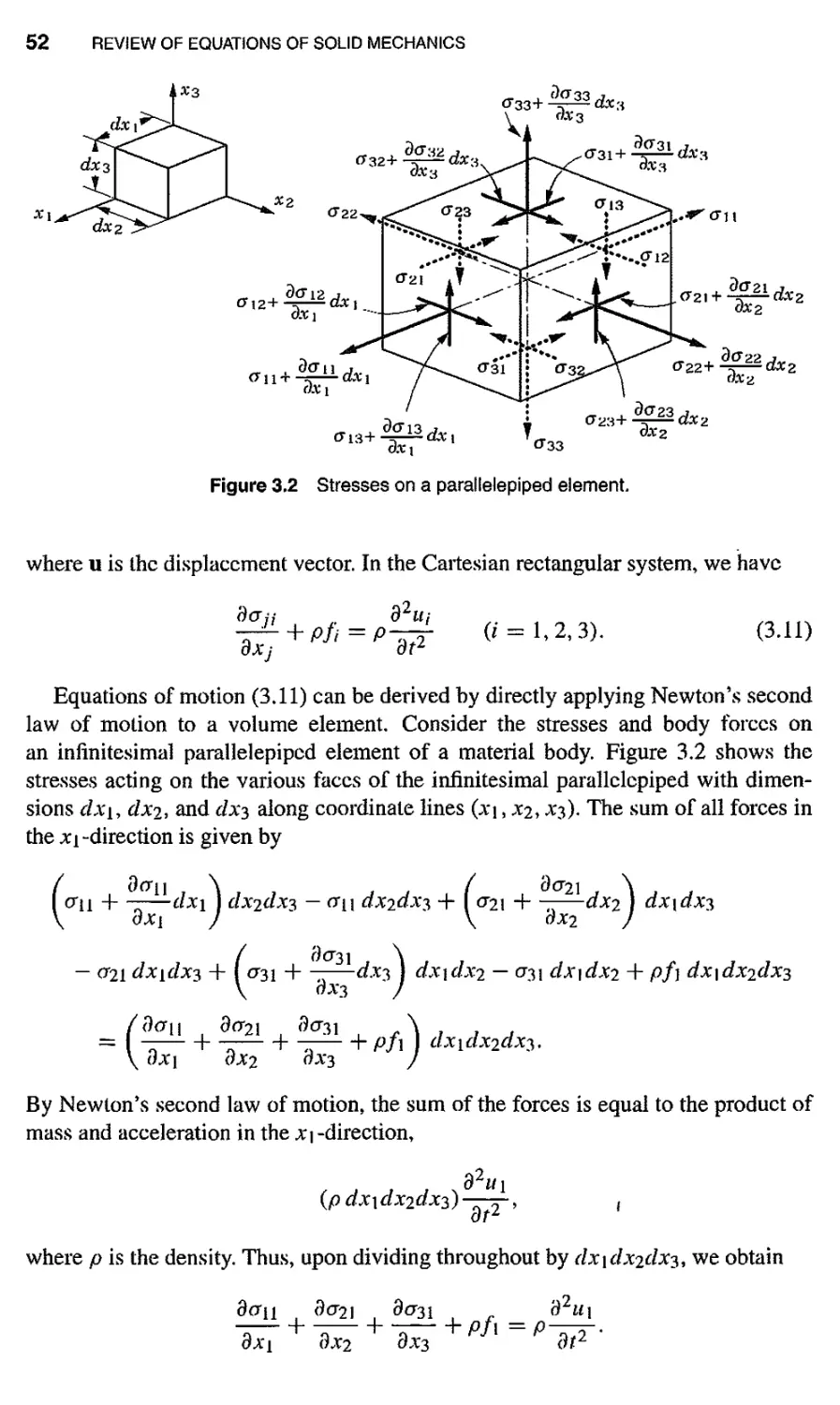
3.2.1 Equations of Motion / 50
3.2.2 Symmetry of Stress Tensor / 53
3.3 Kinematics of Deformation / 54
3.3.1 Strain Tensor / 54
3.3.2 Strain Compatibility Equations / 58
3.4 Constitutive Equations / 62
3.4.1 Introduction / 62
3.4.2 Generalized Hookers Law / 62
3.4.3 Plane Stress Constitutive Relations / 65
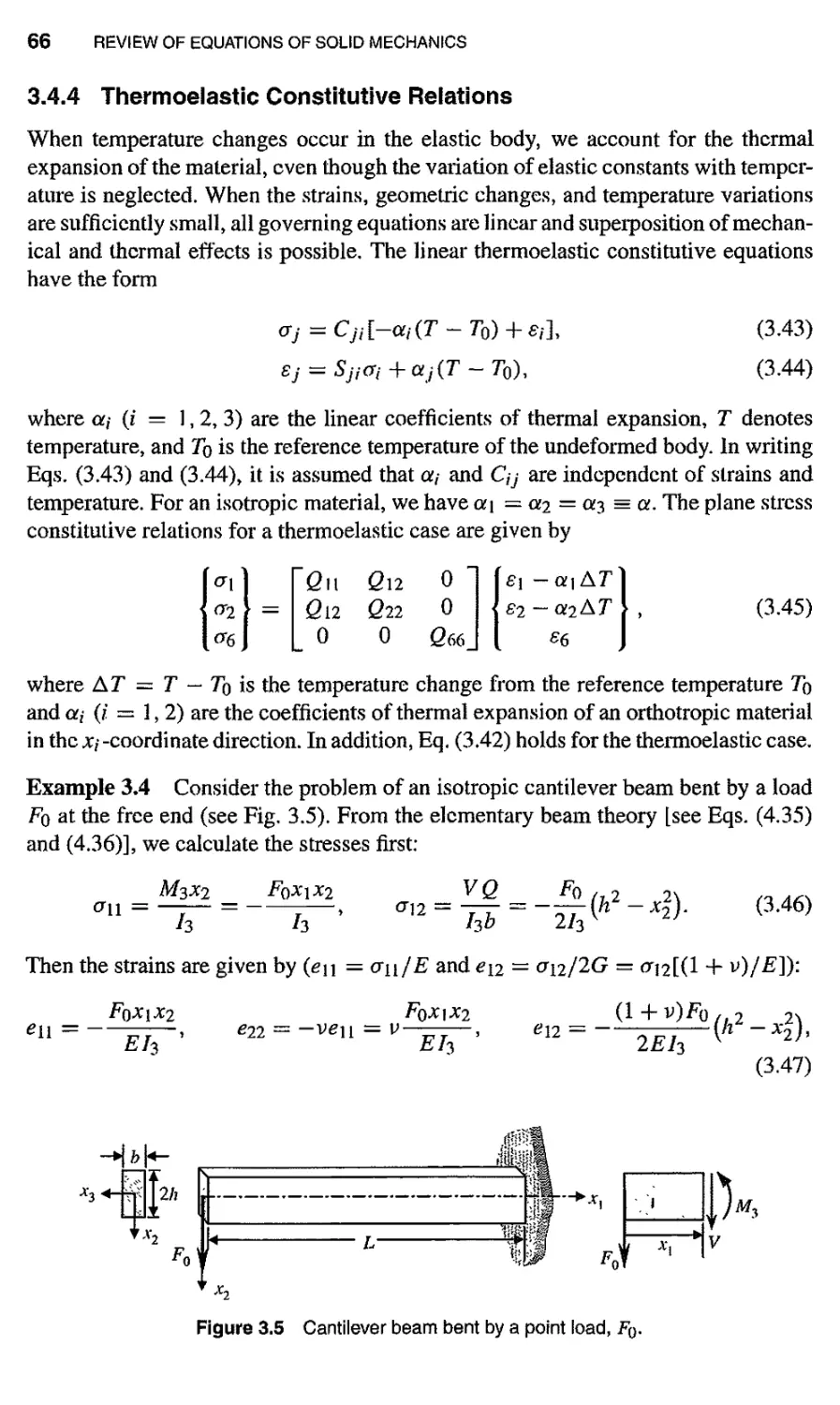
3.4.4 Thermoelastic Constitutive Relations / 66
Exercises / 69
References / 78
WORK, ENERGY, AND VARIATIONAL CALCULUS
4.1 Concepts of Work and Energy / 79
4.2 Strain Energy and Complementary Strain Energy / 84
4.3 Virtual Work / 95
4.4 Calculus of Variations / 102
4.4.1 The Variational Operator / 102
4.4.2 Functional / 106
4.4.3 The First Variation of a Functional / 106
4.4.4 Fundamental Lemma of Variational Calculus / 107
4.4.5 Externum of a Functional / 108 '
4.4.6 Euler Equations / 110
4.4.7 Natural and Essential Boundary Conditions / 112
4.4.8 Minimization of Functionals with Equality
Constraints / 117

CONTENTS JX
Exercises / 123
References / 132
5 ENERGY PRINCIPLES OF STRUCTURAL MECHANICS 133
5.1 Virtual Work Principles / 133
5.1.1 Introduction / 133
5.1.2 The Principle of Virtual Displacements / 133
5.1.3 Unit-Dummy-Displacement Method / 137
5.2 Principle of Total Potential Energy and Castigliano's
Theorem! / 142
5.2.1 Principle of Minimum Total Potential Energy / 142
5.2.2 Castigliano's Theorem T / 146
5.3 Principles of Virtual Forces and Complementary Potential
Energy / 151
5.4 Principle of Complementary Potential Energy and Castigliano's
Theorem TI / 156
5.5 Betli's and Maxwell's Reciprocity Theorems / 164
Exercises / 169
References / 176
6 DYNAMICAL SYSTEMS: HAMILTON'S PRINCIPLE 177
6.1 Introduction / 177
6.2 Hamilton's Principle for Particles and Rigid Bodies / 177
6.3 Hamilton's Principle for a Continuum / 183
6.4 Hamilton's Principle for Constrained Systems / 190
6.5 Rayleigh's Method / 196
Exercises / 198
References / 203
7 DIRECT VARIATIONAL METHODS 204
7.1 Introduction / 204
7.2 Concepts from Functional Analysis / 205
7.2.1 General Introduction / 205
7.2.2 Linear Vector Spaces / 206
7.2.3 Normed and Inner Product Spaces / 211

X CONTENTS
7.2.4 Transformations, and Linear and Bilinear
Forms / 215
7.2.5 Minimum of a Quadratic Functional / 216
7.3 The Ritz Method / 221
7.3.1 Introduction / 221
7.3.2 Description of the Method / 222
7.3.3 Properties of Approximation Functions / 225
7.3.4 Ritz Equations for the Parameters / 226
7.3.5 General Features of the Method / 230
7.3.6 Examples / 232
7.4 General Boundary-Value Problems / 245
7.4.1 Variational Formulations / 245
7.4.2 Ritz Approximations / 254
7.5 Weighted-Residual Methods / 259
7.5.1 Introduction / 259
7.5.2 Galerkin's Method / 262
7.5.3 Least-Squares Method / 263
7.5.4 Collocation Method / 263
7.5.5 Eigenvalue and Time-Dependent Problems / 264
7.5.6 Equations for Undetermined Parameters / 266
7.5.7 Examples / 267
7.6 Summary / 288
Exercises / 289
References / 297
8 THEORY AND ANALYSIS OF PLATES 299
8.1 Introduction / 299
8.1.1 General Comments / 299
8.1.2 An Overview of Plate/Shell Theories / 301
8.2 Classical Plate Theory / 305
8.2.1 Governing Equations of Circular Plates / 305
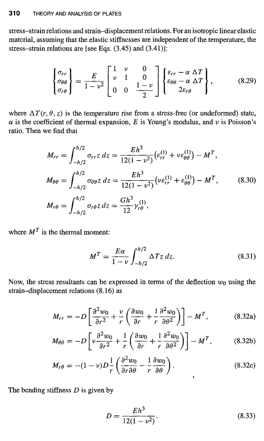
8.2.2 Analysis of Circular Plates / 312 ,
8.2.3 Governing Equations in Rectangular Coordinates / 334
8.2.4 Navier Solutions of Rectangular Plates / 342
8.2.5 Levy Solutions of Rectangular Plates / 356
8.2.6 Variational Solutions: Bending / 362
8.2.7 Variational Solutions: Vibration / 379

CONTENTS Xi
8.2.8 Variational Solutions: Buckling / 384
8.3 Shear Deformation Plate Theory / 396
8.3.1 Governing Equations of Circular Plates / 396
8.3.2 Governing Equations in Rectangular Coordinates / 398
8.3.3 Exact Solutions of Axisymmetric Circular Plates / 401
8.3.4 Exact Solutions of Rectangular Plates / 405
8.3.5 Relationships Between Bending Solutions of Classical and
Shear Deformation Theories / 412
8.3.6 Variational Solutions of Circular and Rectangular
Plates / 421
Exercises / 425
References / 430
9 THE FINITE ELEMENT METHOD 433
9.1 Introduction / 433
9.2 Finite Element Analysis of Bars / 434
9.2.1 Governing Equation / 435
9.2.2 Representation of the Domain by Finite Elements / 435
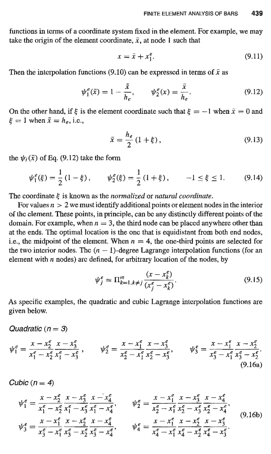
9.2.3 Approximation over an Element / 436
9.2.4 Weak Form / 441
9.2.5 Finite Element Equations / 442
9.2.6 Assembly (or Connectivity) of Elements / 445
9.2.7 Imposition of the Boundary Conditions / 448
9.2.8 Calculation of Reactions and Derivatives of Solution:
Postprocessing / 449
9.3 Finite Element Analysis of the Euler-Bernoulli Beam
Theory / 454
9.3.1 Governing Equation / 454
9.3.2 Weak Form over an Element / 455
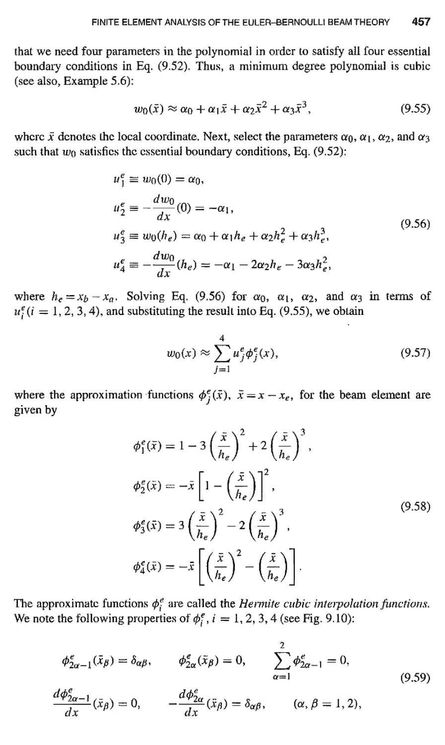
9.3.3 Derivation of the Approximation Functions / 456
9.3.4 Finite Element Model / 458
9.3.5 Assembly of Element Equations / 459
9.3.6 Imposition of Boundary Conditions / 461
9.4 Finite Element Models of the Timoshenko Beam Theory / 463
9.4.1 Governing Equations / 463
9.4.2 Displacement Finite Element Models / 464
9.4.3 Reduced Integration Element (RIE) / 466

Xli CONTENTS
9.4.4 Consistent Interpolation Element (CIE) / 467
9.4.5 Superconvergent Element (SCE) / 469
9.5 Finite Element Models of the Classical Plate Theory / 471
9.5.1 Introduction / 471
9.5.2 General Formulation / 472
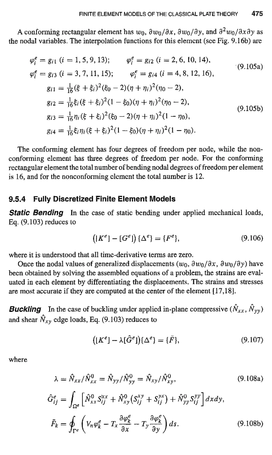
9.5.3 Conforming and Nonconforming Plate Elements / 474
9.5.4 Fully Discretized Finite Element Models / 475
9.6 Finite Element Models of the First-Order Shear Deformation Plate
Theory / 479
9.6.1 Governing Equations and Weak Forms / 479
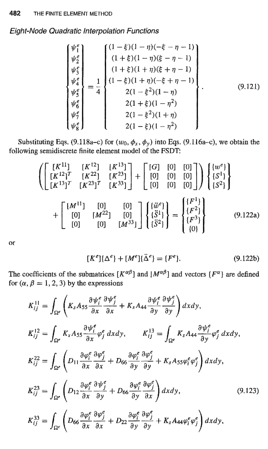
9.6.2 Finite Element Model / 480
9.6.3 Numerical Integration / 483
Exercises / 493
References / 499
10 MIXED VARIATIONAL FORMULATIONS 502
10.1 Introduction / 502
10.1.1 General Comments / 502
10.1.2 Mixed Variational Principles / 502
10.1.3 Extremum and Stationary Behavior of Functionals / 505
10.2 Stationary Variational Principles / 506
10.2.1 The Minimum Total Potential Energy Principle / 506
10.2.2 The Hellinger-Reissner Variational Principle / 508
10.2.3 The Reissner Variational Principle / 513
10.3 Variational Solutions Based on Mixed Formulations / 514
10.4 Mixed Finite Element Models of Beams / 517
10.4.1 The Euler-Bernoulli Beam Theory / 517
10.4.2 The Timoshenko Beam Theory / 523
10.5 Mixed Finite Element Models of the Classical Plate Theory / 527
10.5.1 Preliminary Comments / 527
10.5.2 Mixed Model I / 527
10.5.3 Mixed Model II / 532
10.6 Closure / 539
Exercises / 539
References / 542

CONTENTS XiM
ANSWERS/SOLUTIONS TO SELECTED PROBLEMS 544
INDEX 583
ABOUT THE AUTHOR
591

PREFACE
The increasing use of numerical and computational methods in engineering and
applied sciences has shed new light on the importance of energy principles and
variational methods. The number of engineering courses that make use of energy
principles and variational formulations and methods has also grown very rapidly
in recent years. In view of the increase in the use of the variational formulations
and methods (including the finite element method), there is a need to introduce
the concepts of energy principles and variational methods and their use in the
formulation and solution of problems of mechanics to both undergraduate and
beginning graduate students. This book, an extensively revised version of the author's
earlier book Energy and Variational Methods in Applied Mechanics, is intended for
senior undergraduate students and beginning graduate students in aerospace, civil, and
mechanical engineering and applied mechanics, who have had a course in fundamental
engineering subjects as well as in ordinary and partial differential equations.
The book is organized into ten chapters and is self-contained as far as the subject
matter is concerned. Chapter 1 presents a general introduction to the subject of
variational principles. Chapter 2 contains a brief review of the algebra and calculus
of vectors and Cartesian tensors. A review of the basic equations of linear solid
continuum mechanics is included in Chapter 3. These equations are frequently referred
to in subsequent chapters. Much of the material presented in Chapters 1 through 3
can be assigned as reading material, especially in a graduate class.
Chapter 4 deals with the concepts of work, energy, and the basic topics from
variational calculus, including Euler equations, the fundamental lemma of calculus
of variations, essential and natural boundary conditions, and minimization of
functionals without and with equality constraints. Virtual work and energy principles
and energy methods of solid and structural mechanics are presented in Chapter 5.
Chapter 6 is devoted to a discussion of Hamilton's principle for dynamical systems.
Classical variational methods of approximation (e.g., the methods of Ritz, Galerkin,
Kantorovich, etc.) are presented in Chapter 7. All of the concepts and methods
xv

XVi PREFACE
presented in Chapters 4 through 7 arc illustrated using bars and beams, although
the methods discussed in Chapter 7 are readily applicable to field problems whose
differential equations resemble those of bars and beams. Chapter 8 is dedicated to
applications of (he energy principles and variational methods developed in earlier
chapters to circular and rectangular plates. In the interest of completeness and for
use as a reference for approximate solutions, exact solutions are also included. The
finite element method is introduced in Chapter 9, with applications to beams and
plates. Displacement finite element models of Euler-Bernoulli and Timoshenko beam
theories and classical and first-order shear deformation plate theories are presented.
A unified approach, more general than that found in most solid mechanics books, is
used to introduce the finite element method. As a result, the student can readily extend
the method to other subject areas of solid mechanics as well as to other branches of
engineering. Lastly, the mixed variational principles of Hellinger and Reissner for
elasticity are derived in Chapter 10. Mixed variational formulations, including mixed
finite element models of beams and plates, are discussed.
Each chapter of the book contains many example problems and exercises that
illustrate, test, and broaden the understanding of the topics covered. A list of
references, by no means complete or up-to-date, is also provided at the end of each
chapter. Answers to selected problems arc included at the end of the book.
The book is suitable as a textbook for a senior undergraduate course or a first-year
graduate course on energy principles and variational methods taught in aerospace,
civil, and mechanical engineering and applied mechanics departments. To gain the
most from the text, the student should have a senior undergraduate or first-year
graduate standing in engineering. Some familiarity with basic courses in differential
equations, mechanics of materials, and dynamics would also be helpful.
T have benefited by the professional works, encouragement, and support of many
colleagues as well as students who have taught me how to explain complicated
concepts in simple terms. While it is not possible to name all of them, without
their help and support it would not have been possible for me to make some modest
contributions to the field of mechanics through teaching, research, and writing.
My sincere thanks are due to my teacher, Professor J. T, Odcn (University of Texas
at Austin), for the many things I learned from him which have been useful ail my
life. In the same vein I wish to thank Professor C. W. Bert (University of Oklahoma,
Norman) for giving me the opportunity to teach and develop into what I am. I am
very grateful for their mentorship, advice, and support.
Deep gratitude is due to my wife for her patience and support while I am occupied
with the writing of this book and others, and for her smile when I say every day "T
have so much to do."
Most books are not free of errors, especially those with many mathematical
equations and numbers. I wish to thank in advance those readers who are willing to
draw attention to typos and errors, using the e-mail address: jnreddy@hotmail.com.
J. N. Reddy
College Station, Texas

1
INTRODUCTION
1.1 PRELIMINARY COMMENTS
The phrase "energy methods" in the present study refers to methods that make use
of the total potential energy (i.e., strain energy and potential energy due to applied
loads) of a system to obtain values of an unknown displacement or force, at a
specific point of the system. These include Castigliano's theorems, unit-dummy-load
and unit-dummy-displacement methods, and Betti's and Maxwell's theorems. These
methods are often limited to the (exact) determination of generalized displacements or
forces at fixed points in the structure; in most cases, they cannot be used to detennine
the complete solution (i.e., displacements and/or forces) as a function of position in
the structure. The phrase 'Variational methods," on the other hand, refers to methods
that make use of the variational principles, such as the principles of virtual work and
the principle of minimum total potential energy, to determine approximate solutions
as continuous functions of position in a body. In the classical sense, a variational
principle has to do with the minimization or finding stationary values of a functional
with respect to a set of undetermined parameters introduced in the assumed
solution. The functional represents the total energy of the system in solid and structural
mechanics problems, and in other problems it is simply an integral representation of
the governing equations. In all cases, the functional includes all the intrinsic features
of the problem, such as the governing equations, boundary and/or initial conditions,
and constraint conditions.
1

2 INTRODUCTION
1.2 THE ROLE OF ENERGY METHODS AND VARIATIONAL
PRINCIPLES
Variational principles have always played an important role in mechanics. Variational
formulations can be useful in three related ways. First, many problems of
mechanics are posed in terms of finding the extremum (i.e., minima or maxima) and thus,
by their nature, can be formulated in terms of variational statements. Second, there
are problems that can be formulated by other means, such as by vector
mechanics (e.g., Newton's laws), but these can also be formulated by means of variational
pri nciples. Third, variational formulations form a powerful basis for obtaining
approximate solutions to practical problems, many of which are intractable otherwise. The
principle of minimum total potential energy, for example, can be regarded as a
substitute for the equations of equilibrium of an elastic body, as well as a basis for the
development of displacement finite element models that can be used to determine
approximate displacement and stress fields in the body. Variational formulations can
also serve to unify diverse fields, suggest new theories, and provide a powerful
means for studying the existence and uniqueness of solutions to problems. In many
cases they can also be used to establish upper and/or lower bounds on approximate
solutions,
1.3 SOME HISTORICAL COMMENTS
In modern times, the term "variational formulation" applies to a wide spectrum of
concepts having to do with weak, generalized, or direct variational formulations of
boundary- and initial-value problems. Still, many of the essential features of
variational methods remain the same as they were over 200 years ago when the first notions
of variational calculus began to be formulated.
Although Archimedes (287-212 B.C.) is generally credited with the first to use
work arguments in his study of levers, the most primitive ideas of variational
theory (the minimum hypothesis) are present in the writings of the Greek philosopher
Aristotle (384-322 B.C.), to be revived again by the Italian mathematician/engineer
Galileo (1564-1642), and finally formulated into a Principle of Least Time by the
French mathematician Fermat (1601-1665). The phrase virtual velocities was used
by Jean Bernoulli in 1717 in his letter to Varignon (1654-1722). The development of
early variational calculus, by which we mean the classical problems associated with
minimizing certain functionals, had to await the works of Newton (1642-1727) and
Leibniz (1646-1716). The earliest applications of such variational ideas included the
classical isoperimetric problem of finding among closed curves of given length the
one that encloses the greatest area, and Newton's problem of determining the solid of
revolution of "minimum resistance." In 1696, Jean Bernoulli proposed the problem of
the brachistochrone: among all curves connecting two points, find the curve traversed
in the shortest time by a particle under the influence of gravity. It stood as a challenge
to the mathematicians of their day to solve the problem using the rudimentary tools of

SOME HISTORICAL COMMENTS 3
analysis then available to them or whatever new ones they were capable of
developing. Solutions to this problem were presented by some of the greatest mathematicians
of the time: Leibniz, Jean Bernoulli's older brother Jacques Bernoulli, L'Hdpital, and
Newton.
The first step toward developing a general method for solving variational
problems was given by the Swiss genius Leonhard Euler (1707-1783) in 1732 when he
presented a "general solution of the isoperimetric problem," although Maupertuis is
credited with having put forward a law of minimal property of potential energy for
stable equilibrium in his Memoires de VAcademic des Sciences in 1740. It was in
Euler's 1732 work and subsequent publication of the principle of least action (in his
book Methodus inveniendi tineas curvas ...) in 1744 by Euler that variational
concepts found a welcome and permanent home in mechanics. He developed all ideas
surrounding the principle of minimum potential energy in his work on the Elastica,
and he demonstrated the relationship between his variational equations and those
governing the flexure and budding of thin rods.
A great impetus to the development of variational mechanics began in the
writings of Lagrange (1736-1813), first in his correspondence with Euler. Euler worked
intensely in developing Lagrange's method, but delayed publishing his results until
Lagrange's works were published in 1760 and 1761. Lagrange used d'Alembert's
principle to convert dynamics to statics and then used the principle of virtual
displacements to derive his famous equations governing the laws of dynamics in terms
of kinetic and potential energy. Euler's work, together with Lagrange's Mecanique
analytique of 1788, laid down the basis for the variational theory of dynamical
systems. Further generalizations appeared in the fundamental work of Hamilton in 1834.
Collectively, all these works have had a monumental impact on virtually every branch
of mechanics.
A more solid mathematical basis for variational theory began to be developed in
the eighteenth and early nineteenth century. Necessary conditions for the existence
of "minimizing curves" of certain functionals were studied during this period, and
we find among contributors of that era the familiar names of Legendre, Jacobi, and
Weierstrass. Legendre gave criteria for distinguishing between maxima and minima in
1786, without considering criteria for existence, and Jacobi gave sufficient conditions
for existence of extrema in 1837. Amore rigorous theory of existence of extrema was
put together by Weierstrass, who, with Erdmann, established in 1865 conditions on
extrema for variational problems involving corner behavior.
During the last half of the nineteenth century, the use of variational ideas was
widespread among leaders in theoretical mechanics. We mention the works of
Kirchhoff on plate theory, Lame, Green, and Kelvin on elasticity, and the works
of Bctti, Maxwell, Castigliano, Menabrea, and Engesser for discrete structural
systems. Lame was the first in 1852 to prove a work equation, named after his colleague
Clapeyron, for deformable bodies. Lame's equation was used by Maxwell [1] for the
solution of redundant frame works using the unit-dummy-load technique. In 1875
Castigliano published an extremum version of this technique, but attributed the idea
to Menabrea. A generalization of Castigliano's work is due to Engesser [2].

4 INTRODUCTION
Among prominent contributors to the subject near the end of the nineteenth century
and in the early years of the twentieth century, particularly in the area of variational
methods of approximation and their applications to physical problems, were Rayleigh
[3J, Ritz |4'J, and Galerkin [5]. Modern variational principles began in the 1950s with
the works of Hellinger [6] and Reissner [7,8] on mixed variational principles for
elasticity problems. A variety of generalizations of classical variational principles
have appeared, and we shall not describe them here.
In closing this section, we note that a short historical account of early variational
methods in mechanics can be found in the book of Lanczos [9] and a brief review
of certain aspects of the subject as it stood in the early 1950s can be found in the
book of Truesdell and Toupin [10]; additional information can be found in Smith's
history of mathematics [11] and in the historical treatises on mechanics by Mach [12],
Dugas [13], and Timoshenko [14]. Reference to much of the relevant contemporary
literature can be found in the books by Washizu [15] and Oden and Reddy [16].
Additional historical papers and textbooks on variational methods arc listed at the
end of this chapter (sec [17-56]).
1.4 PRESENT STUDY
The objective of the present study is to introduce energy methods and variational
principles of solid and structural mechanics and to illustrate their use in the derivation
and solution of the equations of applied mechanics, including plane elasticity, beams,
frames, and plates. Of course, variational formulations and methods presented in this
book are also applicable to problems outside solid mechanics. To equip the reader
with the necessary mathematical tools and background from the theory of elasticity
that are useful in the sequel, a review of vectors, matrices, tensors, and governing
equations of elasticity are provided in the next two chapters. To keep the scope of the
book within reasonable limits, only linear problems are considered. Although stability
and vibration problems are introduced via examples and exercises, a detailed study
of these topics is omitted.
In the following chapter we summarize the algebra and calculus of vectors and
tensors. Tn Chapter 3 we give a brief review of the equations of solid mechanics,
and in Chapter 4 we present the concepts of work and energy, energy principles, and
Castigliano's theorems of structural mechanics. In Chapter 5 we present principles of
virtual work, potential energy, and complementary energy. Chapter 6 is dedicated to
Hamilton's principle for dynamical systems, and in Chapter 7 we introduce the Ritz,
Galerkin, and weighted-residual methods. In Chapter 8, applications of variational
methods to the formulation of plate bending theories and their solution by variational
methods are presented. For the sake of completeness and comparison, analytical
solutions of bending, vibration, and budding of circular and rectangular plates are
also presented. An introduction to the finite element method and its application to
displacement finite element models of beams and plates is discussed in Chapter 9. The
final chapter, Chapter 10, is devoted to the discussion of mixed variational principles,

REFERENCES 5
and mixed finite clement models of beams and plates. To keep the scope of the book
within reasonable limits, theory and analysis of shells is not included.
REFERENCES
1. Maxwell, J. C. "On the calculation of the equilibrium and the stiffness of frames," Phil.
Mag. Set: 4, 27, 294 (1864).
2. Engesscr, E, "Uber sialisch unbestimmte Trager bei beliebigen Formanderungs Gesetze
und uber den Satz von der Kleinsten Erganzungsarbcit," Zeitschrift des Architekten und
Ingenieur-Vereins zu Hanover, 35, 733-744 (1889).
3. Lord Rayleigh, (John William Strutt), Theoiy of Sound, Macmillan, London, 1877.
Reprinted by Dover, New York (1945).
4. Ritz, W., "Uber eine neue Melhode zur Losung gewisser Variationsproblemc der
mathematischen Physik," Journal fur reine und angewandte Mathematik, 135, 1-61
(1908).
5. Galerkin, B. G, "Series solutions in rods and plates," Vestnik Inzhenerov i Tekhnikov, 19
(1915).
6. Hellinger, E., "Die allgcmeinen Ansatze der Mechanik der Kontinua," Enzyclopadie der
Mathematischen Wissenschaften IV, 4, 654-655 (1914).
7. Reissncr, E., "Note on the method of complementary energy," /. Math. Phys., 27,159-160
(1948).
8. Reissner, E., "On a variational theorem for finite deformation,"./. Math. Phys., 32, 129—
135(1953).
9. Lanczos, C, The Variational Principles of Mechanics, 4th edition, Dover, New York
(1986).
10. Tmesdell, C. A., and Toupin, R. A., "The classical field theories," Encyclopedia of
Physics, S. Fltigge (ed.), Springet-Veilag, Berlin (1960).
11. Smith, D. E., History of Mathematics, Vol. 1 and II, Dover, New York (1951).
12. Mach, E., The Science of Mechanics, translated and published by Court 1L(1919).
13. Dugas, R., A History of Mechanics, translated into English by J. R. Maddox, Dover,
New York (1988). First published by Editions du Griffon, Neuchatel, Switzerland in
1955.
14. Timoshenko, S. P., History of Strength of Materials, Dover, New York (1983). Originally
published in 1953 by McGraw-Hill, New York.
15. Washizu, K., Variational Methods in Elasticity and Plasticity, Pergamon Press, New York
(1967).
16. Oden, J. T., andReddy, J. N., Variational Principles in Theoretical Mechanics, 2nd edition,
Springer-Vcrlag, Berlin (1983).
17. Argyris, J. H,, and Kelsey, S., Energy Theorems and Structural Analysis, Buttcrworths,
London (1960).
18. Arthurs, A. M., Complementary Variational Principles, Oxford University Press, London
(1967).

6 INTRODUCTION
19. Becker, M., The Principles and Applications of Variational Methods, MIT Press,
Cambridge, MA (1964).
20. Biot, M. A., Variational Principles in Heat Transfer, Clarendon, London (1972).
21. Charlton, T. M., Principles of Structural Analysis, Longmans (1969).
22. Charlton, T. M., Energy Principles in Theory of Structures, Oxford University Press,
Oxford (1973).
23. Davics, G. A. O., Virtual Work in Structural Analysis, John Wiley, Chichester (1982).
24. Denn, M. M., Optimization by Variational Methods, McGraw-Hill, New York (1969).
25. Ekeland, I., and Tcmam, R., Convex Analysis and Variational Problems, North-Holland,
New York (1976).
26. Finlayson, B. A,, The Method of Weighted Residuals and Variational Principles, Academic
Press, New York (1972).
27. Forray, M. J., Variational Calculus in Science and Engineering, McGraw-Hill, New York
(1968).
28. Gregory, M. S,, An Introduction to Extremum Principles, Butterworths (1969).
29. Hestenes, M. R., Optimization Theory: The Finite Dimensional Case, John Wiley,
New York (1975).
30. Hiidebrand, F. B., Methods of Applied Mathematics, 2nd edition, Prentice-Hall,
Englewood Cliffs, NJ (1965).
31. Kantorovitch, L. V., and Krylov, V. J., Approximate Methods of Higher Analysis,
translated by C. D. Benster, Noordhoff, Groningen (1958).
32. Leipholz, H., Direct Variational Methods and Eigenvalue Problems in Engineerings
Noordhoff, Leyden (1977).
33. Lippmann, H., Extremum and Variational Principles in Mechanics, Springer-Veriag,
New York (1972).
34. Lovelock, D., Tensors, Differential Forms and Variational Principles, Wiley, New York
(1974).
35. McGuire, W., Gallagher, R. H., and Ziemian, R. D., Matrix Structural Analysis, 2nd
edition, John Wiley, New York (2000).
36. Mikhlin, S. G, Variational Methods in Mathematical Physics, Pergamon Press
(distributed by Macmillan), New York (1974).
37. Mikhlin, S, G, Mathematical Physics, An Advanced Course, North-Holland, Amsterdam
(1970).
38. Mikhlin, S. G, The Numerical Performance of Variational Methods, Wolters-Noordhoff,
Groningen (1971).
39. Oden, J. T., and Ripperger, E. A., Mechanics of Elastic Structures, 2nd edition,
Hemisphere/McGraw-Hill, New York (1981).
40. Parkus, H., Variational Principles in Thermo- and Magneto-Elasticity, Lecture Notes, No.
58, Springer-Verlag, New York (1972).
41. Petrov, L P., Variational Methods in Optimal Control Theory, translated from the 1965
Russian edition, Academic Press, New York (1968).

REFERENCES 7
42. Prenter, P. M., Splines and Variational Methods, John Wiley, New York (1975).
43. Reddy, J. N., An Introduction to the Finite Element Method, 2nd edition, McGraw-Hill,
New York (1993).
44. Reddy, J. N., and Rasmussen, M. L., Advanced Engineering Analysis, John Wiley,
New York (1982); reprinted by Krieger, Melbourne, FL (1990),
45. Reddy, J. N., Energy and Variational Methods in Applied Mechanics* John Wiley,
New York (1984).
46. Reddy, J. N., Applied Functional Analysis and Variational Methods in Engineering,
McGraw-Hill, New York (1986).
47. Reddy, J. N., Mechanics of Laminated Composite Plates, Theory and Analysis, CRC Press,
Boca Raton, FL (1997).
48. Reddy, J. N., Theory and Analysis of Elastic Plates, Taylor & Francis, Philadelphia (1999).
49. Rektorys, K., Variational Methods in Mathematics, Science and Engineering, Reidel,
Boston (1977).
50. Richards, T. R, Energy Methods in Stress Analysis, Ellis Horwood (distributed by
John Wiley & Sons), Chichester, UK (1977).
51. Rustagi, J. S., Variational Methods in Statistics, Academic Press, New York (1976).
52. Schechter, R. S., The Variational Methods in Engineering, McGraw-Hill, New York
(1967),
53. Shames, I. H., and Dym, C. L., Energy and Finite Element Methods in Structural
Mechanics, Hemisphere, Washington, DC (1985).
54. Shaw, F. S., Virtual Displacements and Analysis of Structures, Prentice-Hall, Englewood
Cliffs, NJ (1972).
55. Smith, D. K., Variational Methods in Optimization, Prentice-Hall, Englewood Cliffs, NJ
(1974).
56. Stacey, W. M., Variational Methods in Nuclear Reactor Physics, Academic Press,
New York (1974).

2
MATHEMATICAL
PRELIMINARIES
2.1 INTRODUCTION
Our approach in this book is evolutionary; that is, we wish to begin with concepts
that are simple and intuitive, and then generalize these concepls step by step into
a broader and more abstract body of analysis. This is a natural inductive approach,
more or less in accord with the development of the subject of variational methods.
In analyzing physical phenomena, we set up relations between various quantities
that characterize the phenomena (such as Newton's laws, energy conservation, etc.).
As a means of expressing a natural law, a coordinate system in a chosen frame of
reference can be introduced, and the various physical quantities involved can be expressed
in terms of measurements made in that system. The mathematical form of the law
thus depends upon the chosen coordinate system and may appear different in another
type of coordinate system. The laws of nature, however, should be independent of
the artificial choice of a coordinate system, and we may seek to represent the law
in a manner independent of a particular coordinate system. A way of doing this is
provided by vector and tensor analysis. When vector notation is used, a particular
coordinate system need not be introduced. Consequently, the use of vector notation
in formulating natural laws leaves them invariant to coordinate transformations. A
study of physical phenomena by means of vector equations often leads to a deeper
understanding of the problem in addition to bringing simplicity and versatility into
the analysis. t
The term vector is used often to imply a physical vector that has "magnitude and
direction" and obeys certain rules of vector addition and scalar multiplication. In the
sequel we consider more general, abstract objects than physical vectors, which are
also called vectors. It transpires that the physical vector is a special case of what is
known as a "vector from a linear vector space." Then the notion of vectors in modern
8

VECTORS 9
mathematical analysis is an abstraction of the elementary notion of a physical vector.
While the definition of a vector in abstract analysis does not require the vector to
have a magnitude, in nearly all cases of practical interest the vector is endowed with
a magnitude, in which case the vector is said to belong to a normed vector space.
Like physical vectors, which have direction and magnitude and satisfy the
parallelogram law of addition, tensors are more general objects that are endowed with
a magnitude and multiple direction(s) and satisfy rules of tensor addition and scalar
multiplication. In fact, vectors are often termed the first-order tensors. As will be
shown shortly, the stress (i.e., force per unit area) requires a magnitude and two
directions—one normal to the plane on which the stress is measured and the other is
the direction of the force—to specify it uniquely.
In this chapter we review basic elements of vector and tensor analysis that are of
use in the sequel. For additional reading, the books listed at the end of the chapter
[1-27] may be consulted.
2.2 VECTORS
2.2.1 Definition of a Vector
In the analysis of physical phenomena we are concerned with quantities that may be
classified according to the information needed to specify them completely. Consider
the following two groups:
Scalars Nonscalars
Mass Force
Temperature Moment
Density Stress
Volume Acceleration
Time Displacement
After units have been selected, the scalars arc given by a single number. Nonscalars
need not only a magnitude specified, but also additional information, such as direction.
Nonscalars that obey certain rules (such as the parallelogram law of addition) are
called vectors. Not all nonscalar quantities are vectors. The specification of a stress
requires not only a force, which is a vector, but also an area upon which the force
acts. A stress is a second-order tensor, as will be shown shortly.
In written or typed material, it is customary to place an arrow or a bar over the
letter denoting the vector, such as A. Sometimes the typesetter's mark of a tilde under
the letter is used. In printed material the vector letter is denoted by a boldface letter,
A, such as used in this book. The magnitude of the vector A is given by |A| or just A.
Two vectors A and B are equal if their magnitudes are equal, |A| = |B|, and if
their directions and sense arc equal. Consequently a vector is not changed if it is
moved parallel to itself. This means that the position of a vector in space may be

10 MATHEMATICAL PRELIMINARIES
B
A+B=B+A
° B
(a) (b)
Figure 2.1 (a) Addition of vectors, (b) Parallelogram law of addition.
chosen arbitrarily. In certain applications, however, the actual point of location of
a vector may be important (for instance, a moment or a force acting on a body). A
vector associated with a given point is known as a localized or bound vector.
Let A and B be any two vectors. Then we can add them as shown in Fig. 2. la.
The combination of the two diagrams in Fig. 2.1a gives the parallelogram shown in
Fig. 2.1b. Thus wc say the vectors add according to the parallelogram law of addition
so that
C = A + B=B + A. (2.1)
We thus see that vector addition is commutative.
Subtraction of vectors is earned out along the same lines. To form the difference
A — B, we write
A - B = A + (~B) (2.2)
and subtraction reduces to the operation of addition. The negative vector —B has the
same magnitude as B, but has the opposite sense.
With the rules of addition in place, we can define a (geometric) vector. A vector is
a quantity that possesses both magnitude and direction and obeys the parallelogram
law of addition. Obeying the law is important because there are quantities having both
magnitude and direction that do not obey this law. A finite rotation of a rigid body
is not a vector, although infinitesimal rotations are. The definition given above is a
geometrical definition. That vectors can be represented graphically is an incidental
rather than a fundamental feature of the vector concept.
A vector of unit length is called a unit vector. The unit vector may be defined as
follows:
&A = 7. ' (2.3)
A
We may now write
/^■iS?
A = Ae^.
(2.4)

VECTORS 11
Thus any vector may he represented as a product of its magnitude and a unit vector.
A unit vector is used to designate direction. It does not have any physical dimensions.
We denote a unit vector by a "hat" (caret) above the boldface letter.
A vector of zero magnitude is called a zero vector or a null vector. All null vectors
are considered equal to each other without consideration as to direction:
A + 0 = A and 0A = 0. (2.5)
The laws that govern addition, subtraction, and scalar multiplication of vectors are
identical with those governing the operations of scalar algebra.
2.2.2 Scalar and Vector Products
Besides addition, subtraction, and multiplication by a scalar, we must consider
multiplication of two vectors. There are several ways the product of two vectors can be
defined. We consider first the so-called scalar product. Let us recall the concept of
work. When a force F acts on a mass point and moves through an infinitesimal
displacement vector ds, the work done by the force vector is defined by the projection of
the force in the direction of the displacement times the magnitude of the displacement
(see Fig. 2.2). Such an operation may be defined for any two vectors. Since the result
of the product is a scalar, it is called the scalar product. We denote this product as
follows:
F ds = Fds cos 0, 0 < 0 < jr. (2.6)
The scalar product is also known as the dot product or inner product.
To understand the vector product, consider the concept of the moment due to a
force. Let us describe the moment about a point O of a force F acting at a point P,
such as shown in Fig. 2.3a. By definition, the magnitude of the moment is given by
M = FU F=|F|f (2.7)
where / is the lever arm for the force about the point O. If r denotes the vector OP
and 0 the angle between r and F as shown, such that 0 < 9 < n, we have I = r sin 0,
and thus
M = Fr sinO. (2.8)
F / !
*—> ■
ds
Figure 2.2 Representation of work.

12 MATHEMATICAL PRELIMINARIES
O^
\Wp
(a) (b)
Figure 2.3 (a) Representation of a moment, (b) Direction of rotation.
^ J
—/
1 \
C=AxB\A
X""
r_
7
*s'
\ r
s
\
(a) (b)
Figure 2.4 (a) Axis of rotation, (b) Representation of the vector.
A direction can now be assigned to the moment. Drawing the vectors F and r from
the common origin O, we note that the rotation due to F tends to bring r into F (see
Fig. 2.3b). Wc now set up an axis of rotation perpendicular to the plane formed by
F and r. Along this axis of rotation we set up a preferred direction as that in which
a right-handed screw would advance when turned in the direction of rotation due to
the moment (see Fig. 2.4a). Along this axis of rotation we draw a unit vector &m and
agree that it represents the direction of the moment M. Thus we have
M = Fr sin 0 e>
= r x F. (2.9)
According to this expression, M may be looked upon as resulting from a special
operation between the two vectors F and r. It is thus the basis for defining a product
between any two vectors. Since the result of such a product is a vector, it may be
called the vector product.
The vector product of two vectors A and B is a vector C whose magnitude is equal
to the product of the magnitude of A and B times the sine of the angle measured from
A to B such that 0 < 9 < k. and whose direction is specified by the condition that
C be perpendicular to the plane of the vectors A and B and' points in the direction
which a right-handed screw advances when turned so as to bring A into B.
The vector product is usually denoted by
C = AxB = AB sin(A, B) e, (2.10)

VECTORS 13
BxC A
Figure 2.5 Scalar triple product as the volume of a parallelepiped.
where sin(A> B) denotes the sine of the angle between vectors A and B. This product
is called the cross product, skew product, and also outer product, as well as the vector
product (see Fig. 2.4b).
Now consider the various products of three vectors:
A(B-C), A-(BxC), Ax (BxC), (2.11)
The product A(B • C) is merely a multiplication of the vector A by the scalar B • C.
The product A -(BxC) is a scalar. It can be seen that the product A • (B x C), except
for the algebraic sign, is the volume of the parallelepiped formed by the vectors A,
B, and C, as shown in Fig. 2.5.
We also note the following properties:
1. The dot and cross can be interchanged without changing the value:
ABxC = AxBC= [ABC]. (2.12)
2. A cyclical permutation of the order of the vectors leaves the result unchanged:
ABxC = CAxB = BCxA = [ABC], (2.13)
3. If the cyclic order is changed, the sign changes:
ABxC = -ACxB = -C-BxA = -B AxC. (2.14)
4. A necessary and sufficient condition for any three vectors, A, B, C to be copla-
nar is that A • (B x C) = 0, Note also that the scalar triple product is zero when
any two vectors are the same.
The product A x (B x C) is a vector normal to the plane formed by A and (BxC).
The vector (B x C), however, is perpendicular to the plane formed by B and C, This
means that A x (B x C) lies in the plane formed by B and C and is perpendicular to
A (see Fig. 2.6). Thus A x (B x C) can be expressed as a linear combination of B
andC:
Ax(BxC)= miB + n\C. (2,15)
p

14 MATHEMATICAL PRELIMINARIES
Figure 2.6 The vector triple product.
Figure 2.7 Plane perpendicular to A, and passing through the terminal point of B.
Likewise, we would find that
(A x B) x C = m2A + «2B. (2.16)
Thus the parentheses cannot be interchanged or removed. It can be shown that
m i = A • C, n i = —A • B,
and hence that
A x (B x C) = (A • C)B - (A ■ B)C. (2.17)
Example 2.1 The equation of a plane perpendicular to a vector A and passing
through the terminal point of vector B can be obtained without the use of any
coordinate system (see Fig. 2.7). Let O be the origin and B the terminal point of vector
B. Draw a directed line segment from O to Q, such that OQ is parallel to A and Q is
in the plane. Then OQ = aA, where a is a scalar. Let P be an arbitrary point on the
line BQ. If the position vector of the point P is r, then
BP = OP - OB = r - B.
i
Since BP is perpendicular to OQ = or A, we must have
BP OQ = 0 or (r - B) • A = 0,
which is the equation of the plane in question.

VECTORS 15
The perpendicular distance from point O to the plane is the magnitude of OQ.
However, we do not know its magnitude (or, a is not known). The distance is also
given by the projection of vector B along OQ:
OQ
d = B — = B- e*.
|OQ| *'
where e^ is the unit vector along A, e^ = A/A.
Example 2.2 Let A and B be any two vectors in space. Then vector A can be
expressed in terms of components along (i.e., parallel) and perpendicular to B: the
component of A along B is given by (A - e#), where e# = B/Z?. The component of
A perpendicular to B and in the plane of A and B is given by the vector triple product
e# x(Axeg). Thus,
A = (A ■ e5)e5 + e# x (A x e5). (a)
Alternately, using Eq. (a) with A = C = e^ and B = A, we obtain
e# x(AxeB)=A" (eB - A)e/y.
2.2.3 Components of a Vector
So far we have proceeded on a geometrical description of a vector as a directed line
segment. We now embark on an analytical description of a vector and some of the
operations associated with this description. Such a description yields a connection
between vectors and ordinary numbers and relates operation on vectors with those on
numbers. The analytical description is based on the notion of components of a vector.
In what follows, we shall consider a three-dimensional space, and the extensions
to n dimensions will be evident (except for a few exceptions). A set of n vectors is said
to be linearly dependent if a set of n numbers jSi,ft,...,Ai can be found such that
Pi Ai + fcA2 + ■ ■ • + AiA„ = 0, (2.18)
where Pi, fh>. *.<, fin cannot all be zero. If this expression cannot be satisfied, the
vectors are said to be linearly independent
In a three-dimensional space a set of no more than three linearly independent
vectors can be found. Let us choose any set and denote it as follows:
e1.e2.e3. (2.19)
This set is called a basis (or a base system).
It is clear from the concept of linear dependence that we can represent any vector
in three-dimensional space as a linear combination of the basis vectors (see Fig. 2.8):
A = Aiei + A2e2 + A3«v
(2.20)

16 MATHEMATICAL PRELIMINARIES
Figure 2.8 Components of a vector.
The vectors A\e], A2e2, and A3e3 are called the vector components of A, and Ai,
A2, and A3 are called scalar components or measure numbers of A associated with
the basis (e\, e2, 63), Also, we use the notation A — (A\, A2, A3) to denote a vector
by its components.
2.2.4 Summation Convention
It is useful to abbreviate a summation of terms by understanding that a repeated index
means summation over all values of that index. Thus the summation
3
A = ]TA/e/ (2.21)
1=1
can be shortened to
A = A,e;. (2.22)
The repeated index is a dummy index and thus can be replaced by any other symbol
that has not already been used. Thus we can also write
A = A,e; = A,„em, (2.23)
and so on,
When a basis is unit and orthogonal, that is, orthonormal, wc have
[eie2e3l=l. (2.24)
In many situations an orthonormal basis simplifies calculations.
For an orthonormal basis the vectors A and B can be written as
A = Aiei + A2e2 + A3e3 = A/e;
B = BLei + B2e2 + B3e3 = ^e,,
where e,- = e,- (/ = 1, 2, 3) is the orthonormal basis, and A/ and Bj are the
corresponding physical components (i.e., the components have the same physical dimensions as
the vector).

VECTORS 17
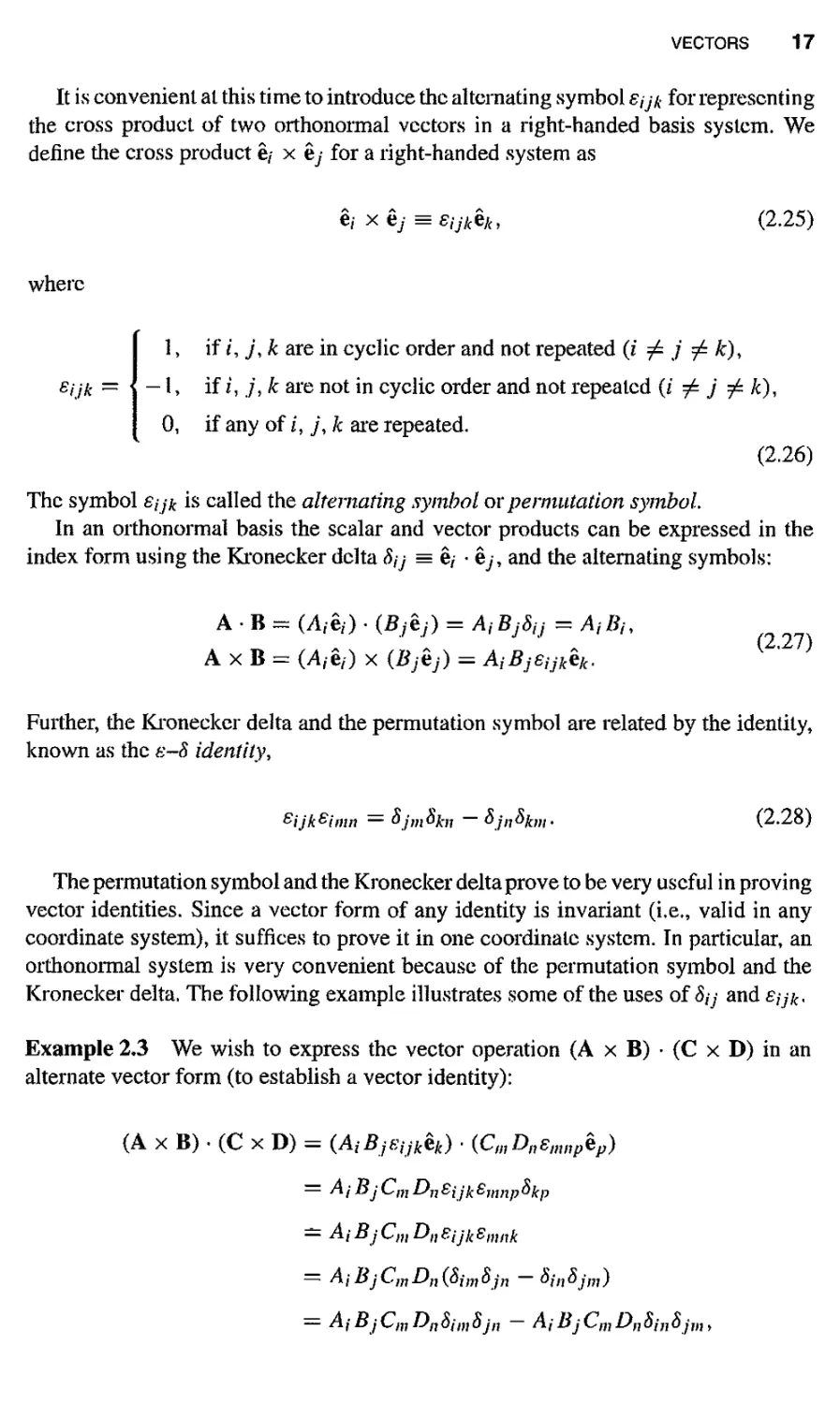
It is convenient at this time to introduce the alternating symbol Sjjk for representing
the cross product of two orthonormal vectors in a right-handed basis system. We
define the cross product e,- x ey for a right-handed system as
6/ X ey = Sijkfya
(2.25)
where
Sijk =
1, if /, j, k are in cyclic order and not repeated (i ^ j ^ /c),
— I, if z, 7, k are not in cyclic order and not repeated (i ^ j ^ /c),
0, if any of /, j\ k are repeated.
(2.26)
The symbol Sijk is called the alternating symbol or permutation symbol
In an orthonormal basis the scalar and vector products can be expressed in the
index form using the Kronecker delta 8jj = e, • ey, and the alternating symbols:
AB- (A/e*) • (Bjej) = AjBjSij = AtBh
A x B = (Ajtj) x (Bj&j) = AiBfsUkek.
(2.27)
Further, the Kronecker delta and the permutation symbol are related by the identity,
known as the 8-8 identity,
Gijk&imn — °jmbhi ~ bjn°kw
(2.28)
The permutation symbol and the Kronecker delta prove to be very useful in proving
vector identities. Since a vector form of any identity is invariant (i.e., valid in any
coordinate system), it suffices to prove it in one coordinate system. In particular, an
orthonormal system is very convenient because of the permutation symbol and the
Kronecker delta. The following example illustrates some of the uses of Si j and £;77c.
Example 23 We wish to express the vector operation (A x B) • (C x D) in an
alternate vector form (to establish a vector identity):
(A x B) • (C x D) = (AiBjEijk&k) ■ (C(nDne„wpep)
= ^ /' Bj C m Dn Eijk £mnp Okp
= A i Bj Cm On Sjjk Smnk
— AjBjC}J1Dn(8jmSjn —8jn8j}11)
= A j B j Cm On dim ojn — A; Bj Cm Dn o/;j bjm,

18 MATHEMATICAL PRELIMINARIES
where we have used the e-S identity (2.28). Since Cm8jm = C{ (or A/5,-m = Anu
etc.), we have
(AxB).(CxD)=: AjBjdOj - AiBjCjDf
^AidBjDj -AjDiBjCj
= (A . C)(B • D) - (A • D)(B ■ C). (a)
Although the above vector identity is established in an orthonormal coordinate
system, it holds in a general coordinate system. That is, the vector identity (a) is
invariant.
Example 2,4 Let e,- (/ = 1, 2, 3) be a set of orthonormal base vectors, and define
new light-handed coordinate base vectors by (ei • e2 = 0)
ei =
2eiH-2e2-he3
e2 =
ei -e2
V2 '
and
e3 = ei x e2 =
cj + e2 - 4C3
3v/2
An arbitrary vector A can be represented in either coordinate system
A — Aj&i = At*;.
The components of the vector in the two different coordinate systems are related by
{A} = Lj8]M}, ft,=c,-ey. (2.29)
The coefficients 0/y are called the direction cosines. Note that the first subscript of 0/y
comes from the barred coordinate system and the second subscript from the unbarred
system.
For the case at hand we have
0n =ei -ei = -,
021 =C2-ei = —,
V2
i
031 = 63 *ei =
012 = ei -e2 = -,
022 = e2 • e2 = -
013 = ei • e3 =
V5'
023 = e2 • e3 = 0,
3V2'
032 = e3 • e2 =
3a/T
033 = 63 • e3 = -
3^2*
or
m
3a/2
2-Jl 2V2 V2
3-3 0
1 1 -4

VECTORS 19
Z,jrJ
(x,y,z) = (x\ x2,x>)
^^zA
**uS%&
y^
X, X'
Figure 2.9 Rectangular Cartesian coordinates.
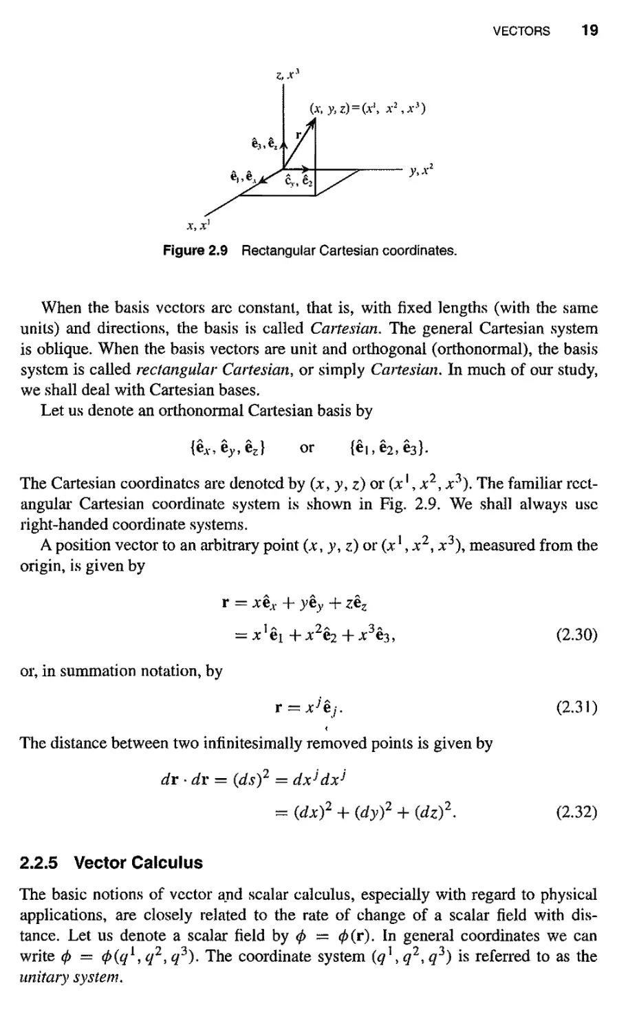
When the basis vectors arc constant, that is, with fixed lengths (with the same
units) and directions, the basis is called Cartesian. The general Cartesian system
is oblique. When the basis vectors are unit and orthogonal (orthonormal), the basis
system is called rectangular Cartesian, or simply Cartesian. In much of our study,
we shall deal with Cartesian bases.
Let us denote an orthonormal Cartesian basis by
{ev,ey,ez} or {ei,e2,e3}.
The Cartesian coordinates are denoted by (x, y9 z) or (x', x2, Jt3). The familiar
rectangular Cartesian coordinate system is shown in Fig. 2.9. We shall always use
right-handed coordinate systems.
A position vector to an arbitrary point (,v, j>, z) or (x!, x2, x3), measured from the
origin, is given by
r = xsx + yey + zez
= x] ei + A'2e2 + x%, (2.30)
or, in summation notation, by
r = xj%j. (2.31)
<
The distance between two infinitesimally removed points is given by
dx • dx = (ds)2 = dx}dx*
- {dx)2 + (dy)2 + (dz)2. (2.32)
2.2.5 Vector Calculus
The basic notions of vector and scalar calculus, especially with regard to physical
applications, are closely related to the rate of change of a scalar field with
distance. Let us denote a scalar field by <f> — 0(r). In general coordinates we can
write 0 = <p(qi,q2i q3)> The coordinate system (q\ q2, q3) is referred to as the
unitary system.

20 MATHEMATICAL PRELIMINARIES
We now define the unitary basis (ei, e2, e3) as follows:
d* #r 9r ,^^x
eis^' e2S^' e3S^- (Z33)
Hence, an arbitrary vector A is expressed as
A = A1 ex + A2e2 + A3e3, (2.34)
and a differential distance is denoted by
dr = dq[e[ + dq2£2 + dq3e^ = dg'e,-. (2.35)
Observe that the A's and dq's have superscripts whereas the unitary basis (ei, e2, £3)
has subscripts. The Jg1 are referred to as the contravariant components of the
differential vector dr and A' are the contravariant components of vector A. The unitary basis
can be described in terms of the rectangular Cartesian basis (ev, ey, ez) = (e\, e2, £3)
as follows:
V ~a^e'v a^' + a^
— = — e + —e + — fi
a#2 a#2 ' a#2 ■ a*?2
a?3 ~ dq^ + Bq**'* dq***
*2 = T~2 = Trzix + Tr&y + ^e„ (2.36a)
In the summation convention we have
dr dxj
e/s—r = —7e/, 1 = 1,2,3. (2.36b)
Associated with any arbitrary basis is another basis that can be derived from it. Wc
can construct this basis in the following way: Taking the scalar product of the vector
A in Eq. (2.34) with the cross product ei x e2, we obtain
A • (ei x e2) = A3e3 • (ei x e2)
since ej x e2 is perpendicular to both ei and e2. Solving for A3 gives
A3=A- eiXC2 X=A-^. (2.37a)
e3 • (ei x e2) leie2e3]
In similar fashion we can obtain the following expressions for
A^A-^, A* = A-£2L!L. (2.37b)
[eie2e3] [eie2e3]

VECTORS 21
We thus observe that wc can obtain the components A1, A2, and A3 by talcing the
scalar product of the vector A with special vectors, which we denote as follows:
cl = «* X e3 f c2 = e3 X et ^ c3 __ e» X e2 (238)
[eie2e33' [eie2<J3]' feie2e3l'
The set of vectors (e1, e2, e3) is called the dual or reciprocal basis. Notice from the
basic definitions that we have the following relations:
eiei=Sii\1' l=J . (2.39)
} J\0, i^j
It is possible, since the dual basis is linearly independent (the reader should verify
this), to express a vector A in terms of the dual basis:
A = Aie1 + A2e2 + A3e3. (2.40)
Notice now that the components associated with the dual basis have subscripts, and
A/ are the covariant components of A.
By an analogous process to that above we can show that the original basis can be
expressed in terms of the dual basis in the following way:
e2 x e3 e3 x e1 e'xe2
61 = [ele¥]' e2=fe1cVjt e3 = [e*eV]' ( °
Of course in the evaluation of the cross products we shall always use the right-hand
rule. It follows from the above expressions that
A^A-e1, A2 = A-e2, A3=A-e3, or A'^A-e'',
Ai = A ■ ei, A2 = A • e2, A3 = A • e3, or Ar- = A ■ e,-. (2.42)
Returning to the scalar field <j>, the differential change is given by
d<P = ^dql + ^dq2 + ?tdq\ (2.43)
The differentials dq[,dq2, def are components of dr [see Eq. (2.35)], We would
now like to write d(j> in such a way that we elucidate the direction as well as the
magnitude of dr. Since e1 • ei = 1, e2 • e2 = I, and e3 • e3 = 1, we can write
d<f> = e1 ^ ■ eydq1 + e2^ . e2dcj2 + e3^ ■ e3dq3
dql dql dq5

22 MATHEMATICAL PRELIMINARIES
Let us now denote the magnitude of dv by ds = \dr\. Then e = dr/ds is a unit vector
in the direction of dr, and we have
The derivative (d(j>/ds)z is called the directional derivative of <f>. We see that it is
the rate of change of 0 with respect to distance and that it depends on the direction e
in which the distance is taken.
The vector that is scalar multiplied by e can be obtained immediately whenever the
scalar field is given. Because the magnitude of this vector is equal to the maximum
value of the directional derivative, it is called the gradient vector and is denoted by
grad<£:
d0
d</>
d<f>
grad 0 = e' —T + ez —T + eJ —T
dq1 dq2
From this representation it can be seen that
dq
3'
(2.46)
dqv
dq2'
d<l>
are the covariant components of the gradient vector.
When the scalar function 0(r) is set equal to a constant, <£(r) = constant, a family
of surfaces is generated. A different surface is designated by different values of the
constant, and each surface is called a level surface (see Fig. 2.10). If the direction
in which the directional derivative is taken lies within a level surface, then d<f>/ds is
zero, since 0 is a constant on a level surface, Tn this case the unit vector e is tangent
to a level surface. It follows, therefore, that if d<p/ds is zero, then grad <f> must be
perpendicular to e and thus perpendicular to a level surface. Thus if any surface is
given by <j> (r) = constant, the unit normal to the surface is determined by
n = ±
grad<£
I grad 0|*
(2.47)
grad 0
Figure 2.10 Level surfaces.

VECTORS 23
The plus or minus sign appears because the direction of n may point in either direction
away from the surface. If the surface is closed, the usual convention is to take ii
pointing outward.
It is convenient to write the gradient vector as
grad^(e'A+e2_£_+e3_L^ (2.48)
and interpret grad<£ as some operator operating on <£, that is, grad0 = V0. This
operator is denoted by
and is called the del operator. The del operator is a vector differential operator, and
the "components" d/dq[, S/Bq2, and 3/q3 appear as covariant components.
It is important to note that whereas the del operator has some of the properties of
a vector, it does not have them all, because it is an operator. For instance V • A is
a scalar (called the divergence of A) whereas A • V is a scalar differential operator.
Thus the del operator does not commute in this sense.
In Cartesian systems we have the simple form
r\ q f\
Vse.f+ey- +cz —. (2.50a)
ox - ay oz
or, in the summation convention, we have
V = e/—. (2.50b)
The dot product of del operator with a vector is called the divergence of a vector
and denoted by
V-A = divA. (2.51)
Tf we take the divergence of the gradient vector, we have
div(grad <p) = V ♦ V</> = (V - V)0 = V2</>. (2.52)
The notation V2 = V ♦ V is called the Laplacian operator. In Cartesian systems this
reduces to the simple form
2 . p* a2* a24> d24>
The Laplacian of a scalar appears frequently in the partial differential equations
governing physical phenomena.

s Ihe del opcialor opeiaung on a veclor by means
1A = VxA (2 51.0
—w*|£ aw
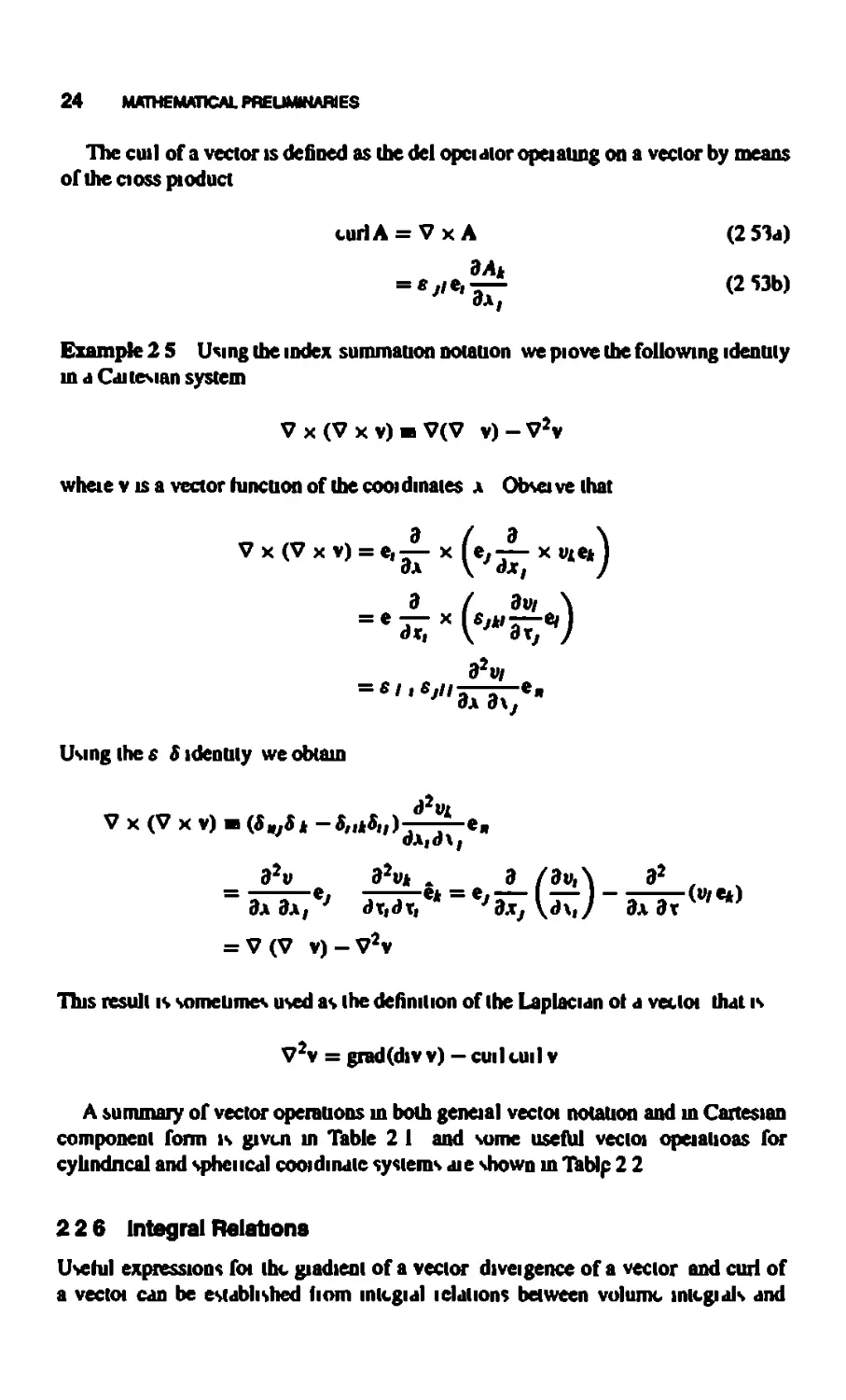
Example 25 Using ihe index summation Dotation we piove Ihe following identity
x(Vx»).7(V v)-V2v
«w.»..i«(»i«..)
= V(V v)-VJv
neumes used as Ihe definition of Ihe Laplacian ol a vecloi that is
V2v = grad(divv)-cuiluiilv
cyhndncal and sphcncal cooidinale systems die shown in Tablp 2 2
226
Usehil

(•i «2 «3) ai» th» CartMMn un
AxB
A IBxCI
Ax(BxC)-B(A C) C(A B)
Cajiettln Component Fram
10
"
12
13
14
U
.«
17
18
19
20
V (AxB) B (VxA) A (7x1)
V ((/A) = (/v° A + v°(/ A
V x (l/A) = Vl/ x A + 1/V x A
V(t/A) Vl/A + l/VA
Vx(AxB)-A(7 B)-B<V A) +
B VA-A VB
(VxA)xB = B 1VA (VA)T|
7 (Vl/) = V2l/
7 (VA) = VJA
V X V x A - V(V A) - (V V)A
(A V)B
A(V B)
r„j—<A,B,)
IL^
«y/jf(l/Aj)e
e,^-<lMje,)
•i/WrfljJ-Mi'/fcf
«V*«« •'l-fiT*
4>U
l2Vc
8'A,
*"'"'" 5737"'
^ir«
*«£
s=> -face S Lai
nl or sin face and n Ihe uml oulwaid normal anu • it V
: i differential volume element The following lelauoas are lalcen horn advanceu

26 MATHEMATICAL PRELIMINARIES
Table 2.2 The del and Laplace operators in cylindrical and spherical coordinate systems
Cylindrical coordinate system (i?, 0, z)
x = R cos <f>
y = R sin 0
z = z
eR = cos 0 eA- 4- sin 0 ey
e^ = — sin 0 eA- + cos 0 ey
ez =ez
9e/e . A A
-— = - sin 0 eA- + cos 0 ey = e^
o<p
d*(f> ,, . . „
-—J- — — cos 0 e,T — sin 0 ey = —e#
30
All other derivatives of the base vectors are zero.
"'■s
30^ a^
Spherical coordinate system (r, 0,0)
* = r sin 0 cos 0
y == r sin 0 sin 0
z = r cos 0
e> = sin 0 cos 0 e,r + sin 0 sin 0 ey + cos 0 ez
&0 = cos 0 cos 0 ex + cos 0 sin 0 e-y — sin 0 ez
e^ = — sin 0 ev + cos 0 e-y
3e,
do
= e$
= sin 0 e#
= -er
= cos 0 e^
30
3e#
a^
—7- = — sin 0 er — cos 0 e#
90
All other derivatives of the base vectors are zero.
3r r 30 rsin0 ^ 30
1 . 3
v2F=^(r2f)+^^HS)+
1
azF
r2sin20 30:
,2 1
Gradient Theorem
I grd&(j>dV = <A n<MS.
(2.54a)

VECTORS 27
Divergence Theorem.
Curl Theorem
f diwAdV = Sn-AdS,
/ curl A dV = A n x \dS.
(2.54b)
(2.54c)
Now let A = grad </> in Eq. (2.54b). Then the divergence theorem gives
/ div(grad0) dV = f V2(j> dV = (j) h grad <t> dS. (2.55)
Jv Jv Js
The quantity ii - grad </> is called the normal derivative of <p on the surface S, and is
denoted by
90
— = n • grad </) = n • V</>.
an
(2.56)
In a Cartesian system this becomes
8(f) 8<p d</> d4>
dn Bx dy Bz
(2.57)
where nx, ny, and nz are the direction cosines of the unit normal
n = nxex + nyey + nzez.
(2.58)
Example 2.6 This example illustrates the relation between the integral relations
(2.54a-c) and the so-called integration by parts, Consider a rectangular region R =
{(x, y): 0 < x < a, 0 < y < b] with boundary C, which is the union of line segments
C\, C2, C3, and C4 (see Fig, 2,11).
^
*
Q
nJt = -l,n=-*x|
•**x
dS=~dx
D / C
R
A ^ P
dS=dx
)ix= 1, ii =et
Figure 2.11 Integration over rectangular regions.

28 MATHEMATICAL PRELIMINARIES
Suppose that wc wish to evaluate the integral fR V2</>dxdy, From Eq. (2.55)
we have
/ V20 dxdy = f V • (V0) dxdy = <L^dS.
Jr Jr Jc 3«
The line integral can be simplified for the region under consideration as follows (note
that in two dimensions, the volume integral becomes an area integral):
Jc &* id in Jc2 dn J a 9n Jc4 on
= r(-BJ)\ **+?(-)\ *
Jo \ tyj lv-0 Jo Ydx/ \x=a
J a \^y/\y=b Jb \ dx)
i-dy)
x=0
The same result can be obtained by means of integration by parts:
= f(»A\ndy+r(°A)rdx
Jo \9x/ LY=0 Jo \dyj \y=o
=r[Gi)„r(S)J^
Thus integration by parts is a special case of the gradient or the divergence theorem.

TENSORS 29
2.3 TENSORS
2.3.1 Second-Order Tensors
To introduce the concept of a second-order tensor, also called a dyadic, we consider
the equilibrium of an element of a continuum acted upon by forces. The surface force
acting on a small element of area in a continuous medium depends not only on the
magnitude of the area but also upon the orientation of the area. Tt is customary to
denote the direction of a plane area by means of a unit vector drawn normal to that
plane (see Fig. 2.12a). To fix the direction of the normal, we assign a sense of travel
along the contour of the boundary of the plane area in question. The direction of the
normal is taken by convention as that in which a right-handed screw advances as it
is rotated according to the sense of travel along the boundary curve or contour (see
Fig. 2.12b). Let the unit normal vector be given by ii. Then the area can be denoted
by S = Sn.
If we denote by AF(n) the force on a small area hAS located at the position r (see
Fig. 2.13), the stress vector can be defined as follows:
t(n)
Hm
AF(n)
AS
(2.59)
We see that the stress vector is a point function of the unit normal n which denotes the
orientation of the surface AS. The component oft that is in the direction of ii is called
the normal stress. The component of t that is normal to n is called a shear stress.
Because of Newton's third law for action and reaction, we see that t(—n) = —t(fi).
\
(a) (b)
Figure 2.12 (a) Plane area as a vector, (b) Unit normal vector and sense of travel.
Figure 2-13 Force on an area element.

30 MATHEMATICAL PRELIMINARIES
Figure 2.14 Tetrahedral element In Cartesian coordinates.
At a fixed point r for each given unit vector n there is a stress vector t(n) acting
on the plane normal to n. Note that t(ii) is, in general, not in the direction of ii. It
is fruitful to establish a relationship between t and n. To do this, we now set up an
infinitesimal tetrahedron in Cartesian coordinates as shown in Fig. 2.14.
If —ti, —t2, —13, and t denote the stress vectors in the outward directions on the
faces of the infinitesimal tetrahedron whose areas are ASi, AS2, AS3, and AS,
respectively, we have by Newton's second law for the mass inside the tetrahedron,
tAS -1, ASi - t2AS2 -13Aft + pAVf = pAVa, (2.60)
where A V is the volume of the tetrahedron, p the density, f the body force per unit
mass, and a the acceleration. Since the total vector area of a closed surface is zero
[see the gradient theorem; set <j> — 1 in (2.54a)], we have
ASii - AStei - AS2e2 - AS3e3 = 0. (2.61)
It follows that
ASi = (ft ■ ci)AS, AS2 = (ii - e2)AS, AS3 = (n • e3)AS. (2.62)
The volume of the element A V can be expressed as
Ah
AV = —AS, (2.63)
where Ah is the perpendicular distance from the origin to the slant face. The result
in (2.63) can also be obtained from the divergence theorem (2.54b) by setting A — r.
Substitution of Eqs. (2.62) and (2.63) in (2.60) and dividing throughout by AS
reduces it to
t - (n eOti + (ft • e2)t2 + (ft • e3)t3 + /Aa - f). (2.64)
In the limit when the tetrahedron shrinks to a point, Ah -> 0, we are left with
t = (ft • ei)t| + (ft • e2)t2 + (ft • <b)t3
= (ft.e,)t/. (2.65)

TENSORS 31
It is now convenient to display the above equation as
t = fi.(eiti +e2t2 + e3t3). (2.66)
The terms in the parenthesis are to be treated as a dyadic, called stress dyadic or stress
tensor a:
a =Mi +e2t2 + e3t3. (2.67)
The stress tensor is a property of the medium that is independent of the ft. Thus,
we have
t(fi) = n • a (2.68)
and the dependence of t on ft has been explicitly displayed.
It is useful to resolve the stress vectors ti,t2, and t3 into their orthogonal
components. We have
t/ = aa ei + 07262 + <*i3*3
= auej (2.69)
for z = 1, 2, 3. Hence, the stress dyadic can be expressed in summation notation as
a =e/t/
= oye/ej. (2.70)
The component 07/ represents the stress (force perunit area) on an area perpendicular
to the ith coordinate and in the yth coordinate direction (see Fig. 2.15). The stress
vector t represents the vectorial stress on an area perpendicular to the direction ft.
<->
Equation (2.68) is Icnown as the Caiichy stress formula, and a is termed the Caiichy
stress tensor.
Figure 2.15 Definition of stress components in Cartesian rectangular coordinates.

32 MATHEMATICAL PRELIMINARIES
2.3.2 General Properties of a Dyadic
Because of its utilization in physical applications, a dyad is defined as two vectors
standing side by side and acting as a unit. A linear combination of dyads is called
a dyadic. Let Ai, A2,..., A„ and Bi, B2,..., B,7 be arbitrary vectors. Then we can
represent a dyadic as
O = A1B1 + A2B2 + • • • + A„B„. (2.71)
Here, we limit our discussion to Cartesian tensors. For a Cartesian tensor the basis
vectors are constants and thus do not take roles as variables in differentiation and
integration.
One of the properties of a dyadic is defined by the dot product with a vector, say V:
* . V = A, (Bi • V) + A2(B2 ■ V) + - • + A„ (B„ • V),
(2.72)
V • * = (V • A,)Bi + (V . A2)B2 + ■■• + (¥- A„)B„.
The dot operation with a vector produces another vector. In the first case the dyadic
acts as a prefactor and in the second case as a postfactor. The two operations in
general produce different vectors.
The conjugate, or transpose, of a dyadic is defined as the result obtained by the
interchange of the two vectors in each of the dyads:
T
% =B1Ai+B2A2-f- — + B,TA,J. (2.73)
It is clear that we have
v-* = * -v,
(2.74)
2.3.3 Nonion Form of a Dyadic
Let each of the vectors in the dyadic be represented in a given basis system. In
Cartesian system, we have
A,- =Aijtj,
(2.75)
B, = Bikek.
The summations on j and k are implied by the repeated indices.

TENSORS 33
We can display all of the components of a dyadic O by letting the k index run to
the right and the j index run downward:
* = 01iMl + 012^1 *2 +013M3
+ 02ie2ei + <t>22&2&2 + <tee2$3
+ 03l%ei + 032£3^2 + 033 $3 ^
(2.76)
This form is called the nonion form, Equation (2.63) illustrates that a dyadic in three-
dimensional space, or what we shall call a second-order tensor, has nine independent
components in general, each component associated with a certain dyad pair. The
components are thus said to be ordered. When the ordering is understood, such
as suggested by the nonion form (2.76), the explicit writing of the dyads can be
suppressed and the dyadic written as an array:
m =
011 012 ^13
021 022 023
031 032 033
and
♦»
$ =
'sr
$2
ie3j
1
> L*]'
ei 1
£2
e3J
(2.77)
This representation is simpler than Eq. (2.76), but it is taken to mean the same.
In the general scheme that is thus developed, vectors are called first-order tensors
and dyadics are called second-order tensors. Scalars are called zeroth-order tensors.
The generalization to third-order tensors thus leads, or is derived from, tricidics, or
three vectors standing side by side. It follows that higher-order tensors are developed
from polycidics.
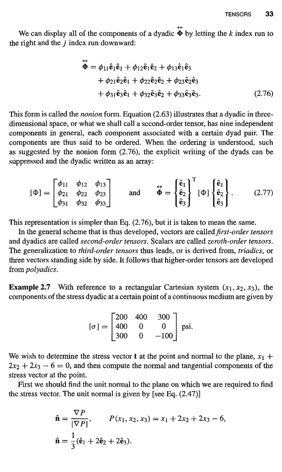
Example2.7 With reference to a rectangular Cartesian system (*i,*2»*3)» the
components of the stress dyadic at a certain point of a continuous medium are given by
\<r} =
200
400
300
400
0
0
300
0
-100
psi.
We wish to determine the stress vector t at the point and normal to the plane, x\ +
2x2 + 2jc3 —6 = 0, and then compute the normal and tangential components of the
stress vector at the point.
First we should find the unit normal to the plane on which we are required to find
the stress vector. The unit normal is given by [see Eq. (2.47)]
n =
VP
P(x\, X2, X3) = x\ + 2a'2 + 2x3 - 6,
n = -(ei +2e2 + 2e3).

34 MATHEMATICAL PRELIMINARIES
The components of the stress vector are displayed in an array
h
ti
ti
> =
200 400
400 0
300 0
300
0
-100
1
— i
3
1
2
2
1600
400
100
psi
or
t(n) = -(1600ei + 400e2 + 100e3) psi.
The normal component tn of the stress vector t on the plane is given by
., . 2600 .
/„ - t(n) • n = -jp psi,
and the tangential component is given by (the Pythagorean theorem)
ts = ^/itp - tl = 7(256+16+1)9-26x26 psi
VT78I
= 100- =468.9 psi.
9
A second-order Cartesian tensor O may be represented in barred and unbarred
coordinate systems as
The unit base vectors in the barred and unbarred systems are related by
^ OX j £ A /N A
(2.78)
where #/ denote the direction cosines between barred and unbarred systems [see
Eq. (2.29)]. Thus the components of a second-order tensor transform according to
hi = 4>ijfaPij or [4>] = [£]W>][£]T.
(2.79)
Tn right-handed orthogonal systems the determinant of the transformation mati'ix is
unity, and we have
m~l = [/?]T.
(2.80)
The unit tensor is defined as
I = e/e,-
(2.81)

TENSORS 35
With the help of the Kronecker delta symbol, this can be written alternatively as
I=Sijtiej. (2.82)
Clearly the unit tensor is symmetric.
The sum of the diagonal terms of a Cartesian tensor is called the trace of the tensor:
trace* = 0|7. (2.83)
The trace of a tensor is invariant, called the first invariant, and it is denoted by I\;
that is, it is invariant with coordinate transformations (0// = 0,7). The first, second,
and third invariants of a Cartesian tensor are given by
h = 0//, h = ^(0/;0,7 ~ 4>ii4>jj)> h = det[0] = |0|. (2.84)
The double-dot product between two dyadics is very useful in many problems. The
double-dot product between a dyad (AB) and another (CD) is defined as the scalar:
(AB) : (CD) = (B ■ C)(A . D). (2.85)
The double-dot product, by this definition, is commutative. The double-dot product
between two dyadics is given by
* : f - (0/ye/ey) : (irmnem*n)
= 0ij^niii(e/ -e/7)(e; • ew)
= 4>ijirmn&in8jm
Note that the double-dot product of a Cartesian tensor * with the unit tensor I
produces its trace /[ = 0//.
We note that the gradient of a vector is a second-order tensor:
dxj
hitj. (2.87)
It can be expressed as the sum of
VA = - —± + —- ) e,-e, + - I —^ - —M e/ei. (2.88)

36 MATHEMATICAL PRELIMINARIES
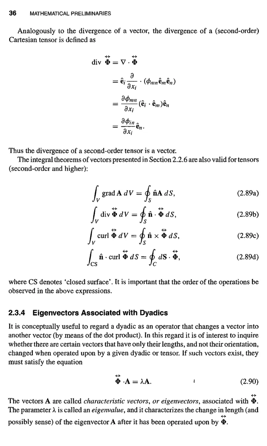
Analogously to the divergence of a vector, the divergence of a (second-order)
Cartesian tensor is defined as
div $ = V • $
= e/ 7 ' VVmn &m e/i)
OXj
= ——(e/ -e,,,)^
" 3* *"
Thus the divergence of a second-order tensor is a vector.
The integral theorems of vectors presented in Section 2.2.6 are also valid for tensors
(second-order and higher):
AdV = <p&AdS9 (2.89a)
/ grad
f div Z d V = <f> n • Z dS, (2.89b)
/ curl WV = inx$^, (2.89c)
/ n . curl Z dS = <f> dS • $, (2.89d)
where CS denotes 'closed surface'. It is important that the order of the operations be
observed in the above expressions.
2.3.4 Eigenvectors Associated with Dyadics
It is conceptually useful to regard a dyadic as an operator that changes a vector into
another vector (by means of the dot product). In this regard it is of interest to inquire
whether there are certain vectors that have only their lengths, and not their orientation,
changed when operated upon by a given dyadic or tensor. If such vectors exist, they
must satisfy the equation
I A = XA. 1 (2.90)
The vectors A are called characteristic vectors, or eigenvectors, associated with $.
The parameter X is called an eigenvalue, and it characterizes the change in length (and
possibly sense) of the eigenvector A after it has been operated upon by #.

TENSORS 37
Since A can be expressed as A = I -A, Eq. (2.90) can also be written as
(*-A?) A = 0. (2.91)
When written in matrix form for Cartesian components, this equation becomes
<j)\\ - X 012 013
021 022 - A. 023
031 032 033 - A.
A2
A3
= 0.
(2.92)
Because this is a homogeneous set of equations for A[y A2, A3, a nontrivial solution
will not exist unless the determinant of the matrix [$ — A I ] vanishes. The vanishing
of this determinant yields a cubic equation for X, called the characteristic equation,
the solution of which yields three values of A, that is, three eigenvalues X{, A2, and
A3. The character of these eigenvalues depends on the character of the dyadic O.
At least one of the eigenvalues must be real. The other two may be real and distinct,
real and repeated, or complex conjugates.
In the preponderance of practical problems, the dyadic 0 is symmetric, that is,
0 = 0, Of course, $ is always real in our considerations. For example, the moment-
of-inertia dyadic is symmetric, and the stress tensor a is usually but not always
symmetric. We limit our discussion to symmetric dyadics.
The vanishing of the determinant assures that three eigenvectors are not unique to
within a multiplicative constant, however, and an infinite number of solutions exist
having at least three different orientations. Since only orientation is important, it is
thus useful to represent the three eigenvectors by three unit eigenvectors e*, ej, e|,
denoting three different orientations, each associated with a particular eigenvalue.
Suppose now that Ai and A2 are two distinct eigenvalues and Ai and A2 are their
corresponding eigenvectors:
<& • A] = AiAj,
$ -A2 = A2A2.
(2.93a)
(2.93b)
Scalar product of the first equation by A2 and the second by Ai, and then subtraction,
yields
A2 • * - Ai - Ai • * • A2 = (Xi - A2)A) • A2.
(2.94)
Since # is symmetric, one can establish that the left-hand side of this equation
vanishes. Thus
0=(Xi-X2)Ai.A2.
(2.95)

38 MATHEMATICAL PRELIMINARIES
Now suppose that A i and A2 are complex conjugates such that X\ — A2 — 2* A1/, where
/ = V^T and Xa is the imaginary part of X\. Then A] ♦ A2 is always positive since
Ai and A2 are complex conjugate vectors associated with X\ and X2. it then follows
from Eq, (2.95) that Aj,- =0 and hence that the three eigenvalues associated with
a symmetric dyadic are all real.
Now assume that Ai and X2 are real and distinct such that Ai — A2 is not zero. It
then follows from Eq. (2,95) that Ai - A2 = 0. Thus the eigenvectors associated with
distinct eigenvalues of a symmetric dyadic are orthogonal. If the three eigenvalues
are all distinct, then the three eigenvectors are mutually orthogonal.
If X\ and X2 are distinct, but X3 is repeated, say A3 = A2, then A3 must also be
perpendicular to Aj as deducted by an argument similar to that for A2 stemming from
Eq, (2,95), Neither A2 nor A3 is preferred, and they are both arbitrary, except insofar
as they are both perpendicular to A1. It is useful, however, to select A3 such that it
is perpendicular to both Ai and A2. We do this by choosing A3 = Ai x A2 and thus
establishing a mutually orthogonal set of eigenvectors. This sort of behavior arises
when there is an axis of symmetry present in a problem.
In a Cartesian system the characteristic equation associated with a dyadic can be
expressed in the form
A3 - /1A2 - /2A - h = 0, (2.96)
where I\, I2, and I3 are the invariants associated with the matrix of <t>. The invariants
can also be expressed in terms of the eigenvalues,
h = Ai +A2 + A3, h = -(XJA2 + A2A3 +A3A,), h = A1A2A3. (2.97)
Finding the roots of the cubic Eq. (2.96) is not always easy. However, when the
matrix under consideration is of the form
[011 0 0 1
0 022 023 ,
L 0 032 033 J
one of the roots is Ai = 0n, and the remaining two roots can be found from the
quadratic equation
(022 - A)(033 - A) - 023032 = 0,
That is,
^2,3 = r ± -y (022 + 033)2 ~ 4(022033 ~ 023032)- (2.98)
In cases where one of the roots is not obvious, an alternative procedure given below
proves to be useful.

TENSORS 39
In the alternative method we seek the eigenvalues of the so-called deviatoric tensor
associated with 4>:
tij^frj-^kkSij. (2,99)
Note that
4>ii = 4>li ~ <Pkk = 0.
(2.100)
That is, the first invariant l[ of the deviatoric tensor is zero. As a result the
characteristic equation associated with the deviatoric tensor is of the form
{XfY - If2Xf -73=0,
(2.101)
where Xf is the eigenvalue, and 1^ and /^ are the second and third invariants of the
deviatoric tensor. The eigenvalues associated with [4>] itself can be computed from
A = A' + Ife, Ii = fyu4>v> /3 = l«'|.
(2.102)
The cubic equation in (2.101) is of a special form that allows a direct computation of
its roots. Equation (2.101) can be solved explicitly by introducing the transformation
l' = <5'0
1/2
COS Of,
which transforms (2.101) into
/l \3/2
21-/2) [4cos3a-3coso| = 1^.
The expression in square brackets is equal to cos 3a. Hence
3/2
cos 3a
-m
(2.103)
(2.104)
(2.105)
If a\ is the angle satisfying 0 < 3a 1 < n whose cosine is given by Eq. (2.105), then
3a 1, 3ai + 2jt, and 3a 1 — 2n all have the same cosine, and furnish three independent
roots of Eq. (2.103),
where
a\ =
cos
-l
1/2
cos a/,
i = l,2,3,
(2.106a)
2tt
<*2 = <*1 + "3"'
<*3
a\ -
2tt
3 '
(2.106b)
Finally we can compute A; from Eq. (2.102).

40 MATHEMATICAL PRELIMINARIES
Example 2.8 We wish to determine the eigenvalues and eigenvectors of the matrix
[01-
r2
1 \
o
1
4
1
Ol
1
2J
The characteristic equation is obtained by setting det ($,•/ — A 5//) to zero:
= (2 - A)[(4 - A.)(2 - A.) - 1] - 1 • (2 - A.) = 0,
2-A. 1 0
1 4-A. 1
0 1 2-A
or
(2-A)[(4-A-)(2-A.)-2] = 0.
Hence
At = 3 + V5 = 4.7321, A.2 =3-V3= 1.2679, A.3 = 2.
Alternatively,
r*'i =
-f i o
r 4-i i
2-5 ,
l2 = M$} ~ <l>ii<l>'jj) = -tijtij
'(-l),+(-I),+G),««'
10
T
52
27'
/^=dct(^) = -.
From Eq. (2.106b),
1
«i =
cos
,-1
'52 /^y/2'
54 V10 J
11.565°,
a2 = 131.565°, a3 = -108.435°,
and from Eq. (2.103),
X\ = 2.065384, A(, = -1.3987, A'3 = -0.66667.
Finally, using Eq. (2.102), we obtain the eigenvalues
A. 1 = 4.7321, X2 = 1.2679, A3 = 2.00.

EXERCISES 41
The eigenvector corresponding to A3 = 2, for example, is calculated as follows.
From ((pjj - Xi$jj)Aj = 0 we have
"2-2 J 0
1 4-2 1
0 1 2-2
Ax"
A2
,A3.
■ = 1
This gives
A2 = 0, Ai=-A3.
Using A] + A\ + A\
= 1, we obtain
A3 = ±-=(1,0,-1),
V2
for A3 = 2.
Similarly, the eigenvectors corresponding to X 1,2 = 3 ± \/3 are given by
A, = ±(3"j2 (l. (l + V3) , l) , for X! = 3 + V3,
A2 = ±^±^(l,(l-V3),l), forl2 = 3-V3.
EXERCISES
2.1 Find the equation of a line (or a set of lines) passing through the terminal point
of a vector A and in the direction of vector B.
2.2 Find the equation of a plane connecting the terminal points of vectors A, B,
and C. Assume that all three vectors arc referred to a common origin.
2.3 Prove the following vector identity without the use of a coordinate system (see
Example 2.2):
A x (B x Q = (A ■ C)B - (A • B)C.
2.4 If e is any unit vector and A an arbitrary vector, show that
A = (A - e)e + e x (A x e).
This identity shows that a vector can be resolved into a component parallel to
and one perpendicular to an arbitrary direction e.
2.5 Verify the following identities:
(a) 5,7 =3.
(c) SijSjk = fyk-
(e) £ijk£ijk = 6.
(b) 8jj8jj =<5//.
(d) EuijkGnjk = 2<5„
(0 AiA]eijk={).

42 MATHEMATICAL PRELIMINARIES
2.6 Using the index notation, prove the identity
(A x B) • (B x C) x (C x A) = (A • (B x C))2.
2.7 Prove the following vector identity in an orthonormal system using index-
summation notation:
(A x B) x (C x D) = [A • (C x D)]B - [B - (C x D]A.
2.8 Determine whether the following set of vectors is linearly independent:
A = ei-t-e2j B = e2 + e4, C = e3-he4, D = 6) + e2 + e3+e4.
Here e/ are orthonormal unit base vectors in a four-dimensional space.
2.9 Determine whether the following set of vectors is linearly independent:
A = 2ej — $2 + 63, B = e2 — £3, C = — ej + §2.
Here e,- are orthonormal unit base vectors in Sfi3.
2.10 Determine which of the following sets of vectors span tfi3:
(a) A = e, + 3e2 - 83, B = -4ei + 3e2 - 5e3, C = 2e} + e2 + e3.
(b) A = ei-f-e2, B = ei + e2 - 2e3, C = 61-63.
Here e,- are orthonormal unit base vectors in *R3.
2.11 Consider two rectangular Cartesian coordinate systems that are rotated with
respect to each other and have a common origin. Let one system be denoted
as a barred system, so that a position vector can be written in each of the
systems as
r = jc/e/,
= xjeJ>
where {£/} and {!/} are the respective orthonormal Cartesian bases in the
unbarred and barred systems. By requiring that the position vector r be
invariant under a rotation of the coordinate systems, deduce that the transformation
between the coordinates is given by
x\ — a\\x\ -f a\2X2 + 013*3
*2 = 021*1 + #22*2 + 023*3 /
*3 = 031*1 + 032*2 + ^33*3
or, more compactly,
Xj =ajjxj, ij = 1,2,3,

EXERCISES 43
where the terms au can be identified as the direction cosines
ciij = if • ey = cos(e/, e/).
Deduce further that the basis vectors obey the same transformation
e/ = aj e j,
and that the following orthogonality conditions hold:
2X1 Determine the transformation matrix relating the orthonormal basis vectors
(ei, e2, S3) and (e'p e^ ^)» when e^ are given by
(a) e\ is along the vector ei — 62 -I- $3 and e'2 is perpendicular to the plane
2x\ +3*2 + *3 -5 = 0.
(b) e\ is along the line segment connecting point (1 > — 1, 3) to (2, -2, 4) and
e£ = (-ei +e2+2e3)/V6.
(c) 63 = S3, and the angle between x\ -axis and ;ei-axis is 30°.
2.13 The angles between the barred and unbarred coordinate lines are given by
ei
e2
h
ei
60°
150°
90°
h
30°
60°
90°
£3
90°
90°
0°
Determine the direction cosines of the transformation.
2.14 The angles between the barred and unbarred coordinate lines are given by
xx
X2
*3
*1
45°
60°
120°
X2
90°
45°
45°
*3
45°
120°
60°
Determine the transformation matrix.
2.15 In a rectangular Cartesian coordinate system, find the length and direction
cosines of a vector A that extends from the point (1, — 1, 3) to the midpoint of
the line segment from the origin to the point (6, —6, 4).
2.16 The vectors A and B are defined as follows:
A=3i-4k,
B = 21 - 2j + k,
where (i, j, k) is an orthonormal basis.

44 MATHEMATICAL PRELIMINARIES
(a) Find the orthogonal projection of A in the direction of B.
(b) Find the angle between the positive directions of the vectors.
2.17 Prove the following identities (see Eq. (2.13) for the definition of [ABC]):
rfA^Al r d\d3\l
dt dt2 J ~ [ dt dP J '
2.18 Let r denote a position vector r = x\ e/ (r2 = jc,-jc,- ) and A an arbitrary constant
vector. Show that:
(a) grad(r) = }?. (b) grad(r") = nrn~2
r.
(c) V2(r,!) = n(n + l)r""2. (d) grad(r • A) = A.
(c) div(r x A) = 0. (f) curl(r x A) = -2A.
(g) div(rA) = |(r • A). (h) curl(rA) = i(r x A).
2.19 Let A and B be continuous vector functions of the position vector r with
continuous first derivatives, and let F and G be continuous scalar functions of
r with continuous first and second derivatives. Show that:
(a) curl(grad F) — 0.
(b) div(curl A) = 0.
(c) div(grad Fx grad G) = 0.
(d) grad(FG) = F grad G + G grad F,
(e) div(FA) = A- grad F + FdtvA.
(0 curl(FA) = F curl A - A x grad F.
(g) grad(A B) = A grad B + B grad A + A curl B + B curl A.
(h) div(A x B) = curl A • B - curl B . A.
(i) curl(AxB) = B-VA-A. VB + A divB-BdivA.
(j) (V x A) x A = A • VA - VA • A.
(k) V2(FG) = F V2G + 2VF VG + G V2F.
2.20 Show that the vector area of a closed surface is zero, that is,
i
s
2.21 Show that the volume enclosed by a surface S is '
volume = - (p grad(r2) • n dS,

EXERCISES 45
or
volume = - (b r ■ n dS.
lis
2.22 Let 0(r) be a scalar field. Show that
where 'd^/'dn = n • grad<£ is the derivative of 4> in the outward direction
normal to the surface.
2.23 In the divergence theorem (2.54b), set A = 0 grad ^ and A = \jf grad <f>
successively and obtain the integral forms
(a) / [0V2f + V0 . V^ldG = <& cj)^- rfr,
(b) J [^vV - ^v2tf>] da = <£ U^ - v^l rfr,
(c) £ [*vV - v20vV] *o = £ [*^(vV) - vV^l dr,
where £2 denotes a (2D or 3D) region with boundary I\ The first two identities
are sometimes called Green's first and second theorems.
2.24 Determine the rotation transformation matrix such that the new base vector e i is
along ei — £2 + e3, and £2 is along the normal to the plane 2x\ + 3*2 4- *3 = 5.
If T is the dyadic whose components in the unbarred system are given by
7ii = 1, Tn = 0, TX3 = -1, 722 = 3, T23 = -2, and T33 = 0, find the
components in the barred coordinates.
2.25 Show that the characteristic equation for a second-order tensor 07/ can be
expressed as
where
A3-/iA.2-/2A.-/3 =0,
h = -(IVijVjkVki — 3<yjj0jj<Jkk + OiiVjjVkk) = dct(or,y)
0
are the three invariants of the tensor.

46 MATHEMATICAL PRELIMINARIES
2.26 Find the eigenvalues and eigenvectors of the following matrices:
(a)
(c)
(e)
r4 -4
0"
-4 0 0
L° ° 3.
fl 0 0 "
0 3 -1
[0 -I 3 _
r3 5 8"
(5 10
8 0 2
(b)
(d)
(f)
2 -V3 0
-V3 4 0
0 0 4
"2 -11]
-10 1
1 1 2 J
"1 -1 Ol
-1 2 -1
0 -1 2
2.27 Evaluate the three invariants of the matrices in Exercise 2.26 and check them
against the invariants obtained by using the eigenvalues.
2.28 The components of a stress dyadic at a point, referred to the („yi , X2, x$) system,
are (in ksi = 1000 psi):
(i)
12 9
9 -12
0 0
(HO
0
0
6_
' 1
J.
(ii)
-3
3 1
2 —s/2
9
0
12
V2 1
~v/2
4
0 12'
-25 0
0 16
Find the following:
(a) The stress vector acting on a plane perpendicular to the vector 2ei — 2e2+e3
passing through the point.
(b) The magnitude of the stress vector and the angle between the stress vector
and the normal to the plane.
(c) The magnitudes of the normal and tangential components of the stress
vector.
2.29 Verify that
I .* = *• I =*.
2.30 If A is an arbitrary vector and <J> is an arbitrary dyadic, yerify that
(a) (T x A) • Z = A x Z.
(b) (A x T) • Z = A x 5.
(c) (vt> x A)1 = -A x <D

REFERENCES 47
REFERENCES
1. Aris, R., Vectors, Tensors, and the Basic Equations in Fluid Mechanics., Prentice-HalL
Englewood Cliffs, NJ (1962).
2. Bedford, F. W, and Dwivedi, T. D., Vector Calculus, McGraw-Hill, New York (1970).
3. Bellman, T. E., Introduction to Matrix Analysis, 2nd edition, McGraw-Hill, New York
(1970).
4. Borisenko, A. I., and Tarapo, I. E., Vector and Tensor Analysis with Applications, R. A.
Silverman (translator and editor), Prentice-Hall, Englewood Cliffs, NJ (1968).
5. Bourne, D. E., and Kendall, P. C, Vector Analysis and Cartesian Tensors, 2nd edition,
Academic Press, New York (1977).
6. Bowen, R. M., and Wang, C. C, Introduction to Vectors and Tensors, Plenum Press,
New York (1976).
7. Campbell, H. G, An Introduction to Matrices, Vectors and Linear Programming, Prentice-
Hall, Englewood Cliffs, NJ (1977).
8. Chambers, L. G, A Course in Vector Analysis, Chapman and Hall, London (1969).
9. Chisbolm, J. S. R. Vectors in Three-Dimensional Space, Cambridge University Press,
Cambridge (1978).
10. Chorlton, R, Vector and Tensor Methods, Halsted Press, New York (1964).
11. Coburn, N., Vector and Tensor Analysis, Macmillian, New York (1964).
12. Eisele, J. A., Applied Matrix and Tensor Analysis, Wiley-Intersciencc, New York (1970).
13. Gantmachcr, E R., The Theory of Matrices, Chelsea, New York (1959).
14. Graham, A., Matrix Theoiy and Applications for Engineers and Mathematicians, Halsted
Press, New York (1979).
15. Haskell, R. E., Introduction to Vectors and Cartesian Tensors, Prentice-Hall, Englewood
Cliffs, NJ (1972).
16. Hauge, B., An Introduction to Vector Analysis for Physicists and Engineers, 6th edition,
revised by D. Martin, Methuen, London (1970).
17. Jeffreys, H., Cartesian Tensors, Cambridge University Press, London (1965).
18. Karamchcti, K., Vector Analysis and Cartesian Tensors, Holden-Day, San Francisco
(1967).
19. Lanzcos, C, "Tensor calculus," in Handbook of Physics, E. U. Conder, and H. Odishaw
(eds.), Ch. 10, pp. Mil to 1-122. McGraw-Hill, New York (1958).
20. Lichncrowicz, A., Linear Algebra and Analysis, Holden-Day, San Francisco (1967).
21. Moon, P. H., and D. E. Spencer, Vectors, Van Nostrand, Princeton, NJ (1965).
22. Phillips, H. B., Vector Analysis, Wiley, New York (1933).
23. Rcddy, J. N., and Rasmussen, M. L., Advanced Engineering Analysis, John Wiley,
New York (1982); reprinted by Krieger, Melbourne, FL (1991).
24. Sokolnikoff, I. S., Tensor Analysis, John Wiley, New York (1933).
25. Wills, A. P., Vector Analysis with an Introduction to Tensor Analysis, Dover, New York
(1953).
26. Wrede, R. C, Introduction to Vector and Tensor Analysis, Dover, New York (1972).
27. Young, E. C, Vector and Tensor Analysis, Marcel Dekker, New York (1978).

3
REVIEW OF EQUATIONS OF
SOLID MECHANICS
3.1 INTRODUCTION
3.1.1 Classification of Equations
The objective of this chapter is to record the governing equations of a solid continuum
in a form suitable for use later in this book. The word continuum needs to be explained
first. Microscopically, a medium occupied by a matter, solid or fluid, is made of
discrete particles of protons, neutrons, and electrons. Macroscopicaliy, the medium
is assumed to contain no gaps or voids between material points of the medium so that
it can be divided indefinitely into smaller and smaller parts without encountering a
void. This concept allows us to shrink an arbitrarily small region to a point so that all
spatial derivatives of various quantities associated with the medium can be defined.
For example, if mass density p(x> t) of the medium is defined to be the mass per unit
volume, we assume that the limit
><*•'> %teo!£ (3-1}
exists (i.e., p is finite). Here Am denotes the mass of the matter occupying an
infinitesimal volume AV, xis the position vector, and t denotes time. Of course, the continuum
assumption may be violated when one considers matter at nanometer (10~9 m) or
atomic scale, and the continuum equations to be derived in this chapter may not be
applicable to problems at such scales. t
The governing equations of a continuum are derived using the following
conservation principles (or laws of physics):
1. Principle of conservation of mass.
2. Principle of conservation of linear momentum.
48

INTRODUCTION 49
3. Principle of conservation of angular momentum.
4. Principle of conservation of energy.
The above principles do not explicitly account for geometric changes or mechanical
response of the continuum. Without these, the equations derived from the conservation
principles are insufficient to determine the total response of the continuum. Therefore,
we must consider the following additional two sets of equations:
5. Kinematics (strain-displacement equations).
6. Constitutive equations (e.g., stress-strain relations).
Kinematics is a study of the geometry of motion and deformation without con-
sideration of the forces causing the motion. The constitutive equations describe the
mechanical behavior of the continuum and relate the dependent variables introduced
in the kinetic description (i.e., conservation of momenta and energy) to those in
the kinematic description. Since the resulting equations involve spatial (i.e., position)
coordinates and time, appropriate boundary and initial conditions are needed to
determine the solution. For a detailed derivation of the equations, the reader may consult
the books on continuum mechanics [1-31, elasticity [4-6], and fluid mechanics [7,8].
3.1.2 Descriptions of Motion
There are two alternative descriptions used to study the motion of a continuum. In the
first, one considers the motion of all matter passing through a fixed spatial location, as
shown in Fig. 3.1a. Here one is interested in various properties (e.g., velocity, pressure,
temperature, density, and so on) of the matter that instantly occupies the fixed spatial
location. This description is called the spatial description or the Eulerian description.
In the second, one focuses attention on a fixed set of material particles, irrespective
of their spatial locations (see Fig. 3. lb). The relative displacements of these particles
and the stress caused by external forces and temperature arc of interest in this case.
This description is known as the material description or the Lagrangian description.
The Eulerian description is most commonly used to study fluid flows and coupled
heat transfer and fluid flow, while the Lagrangian description is generally used to
study heat transfer, stress, and deformation of solid bodies.
(a) (b)
Figure 3.1 (a) Fixed region in space and mass moving through it. (b) Motion of a fixed
collection of material particles.

50 REVIEW OF EQUATIONS OF SOLID MECHANICS
In order to understand the difference between the material and spatial descriptions,
consider a continuum and identify a region of the continuum for our study. Let X
denote the position of an arbitrarily fixed point in the region (in both descriptions)
at time t = 0, and let us label the material particle that occupies position X with X
(a name given to the particle). For time / > 0, the point X in a spatial description
remains the same, but denoted by x. Although the current position x and initial position
X are the same in the spatial description, the particles occupying the position at these
two times are not the same (i.e., particle X no longer occupies the position x at time
t > 0), unless there is no motion. On the other hand, in a material description, where
attention is focused on a material particle, the particle X occupying the position X at
time / = 0 moves to a new position x at time t > 0.
To gain further understanding, consider representing a scalar quantity such as
the mass density p in the two descriptions. In a material description, the functional
variation of p is described with respect to the coordinate X occupied by the material
particle X in the region as
P = p(X,/). (3.2)
In spatial description, p is described with respect to the position in space, x, currently
occupied by a material particle in the continuum at time t as
P = P(x, r). (3.3)
In Eq. (3.2) a change in time t implies that the same material particle X has a different
density. The particle's current position x has been expressed in terms of its position
X at time t = 0. Thus, in material description, attention is focused on the material
particle. In Eq. (3.3), however, a change in time t implies that a different density is
observed at the same spatial location x, now probably occupied by a different material
particle. Therefore, in spatial description, attention is focused on spatial location.
3.2 CONSERVATION OF LINEAR AND ANGULAR MOMENTA
3.2.1 Equations of Motion
The principle of conservation of linear momentum, or Newton's second law of motion,
applied to a set of particles (or rigid body), can be stated as the time rate of change
of (linear) momentum of a collection of particles equals the net force exerted on the
collection. Written in vector form, the principle implies
— (m\) = F, (3.4)
at t
where m is the total mass, v the velocity, and F the resultant force on the collection
particles. For constant mass, Eq. (3.4) becomes
d\
F = 772-— = ma, (3.5)
at

CONSERVATION OF LINEAR AND ANGULAR MOMENTA 51
which is the familiar form of Newton's second law (i.e., force = mass x acceleration).
To derive the equation of motion applied to a control volume (i.e., either a fixed region
in space through which material flows or a fixed material body that is in motion), we
must identify the forces acting on it.
Forces acting on a control volume can be classified as internal and external. The
internal forces resist the tendency of one part of the region/body to be separated from
another part. The internal force per unit area is termed stress, as defined in Section
2.3. The external forces are those transmitted by the body. The external forces can be
further classified as body (or volume) forces and surface forces.
Body forces act on the distribution of mass inside the body. Examples of body
forces are provided by the gravitational and electromagnetic forces. Body forces are
usually measured per unit mass or unit volume of the body. Let f denote the body
force per unit mass. Consider an elemental volume dV inside V. The body force of
the elemental volume is equal to pdVf, Hence, the total body force of the control
volume is
/ pfdV. (3.6)
Jv
Surface forces are contact forces acting on the boundary surface of the body.
Examples of surface forces are provided by applied forces on the surface of the body.
Surface forces are reckoned per unit area. Let t denote the surface force per unit area
(or surface stress vector). The surface force on an elemental surface dS of the control
volume is tdS. The total surface force acting on the closed surface of the control
volume is
£> t dS. (3.7)
Since the stress vector t on the surface is related to the (internal) stress tensor a by
Cauchy's formula [see Eq. (2.68)],
t = n-cf\ (3.8)
where n denotes the unit normal to the surface, we can express the surface force as
n ■ o dS. *.
i<
fs
Using the divergence theorem (2.89b), we can write
<&A-adS= f V-ffdV. (3.9)
The principle of conservation of linear momentum as applied to a solid continuum
yields the result
V.Z + pf = p^, (3.10)

52 REViEW OF EQUATIONS OF SOLID MECHANICS
U-3
dxf>
dxn
TX3
*22^
ff»+Tg**-
<Tll+^ii<fa,
a21+3^1^-2
axz
OT2
Figure 3.2 Stresses on a parallelepiped element.
where u is the displacement vector. In the Cartesian rectangular system, we have
(3.11)
>°J<+pfi=p*« (/ = l,2,3).
dXj
dt2
Equations of motion (3.11) can be derived by directly applying Newton's second
law of motion to a volume element. Consider the stresses and body forces on
an infinitesimal parallelepiped element of a material body. Figure 3.2 shows the
stresses acting on the various faces of the infinitesimal parallelepiped with
dimensions dx[, dx2, and dx$ along coordinate lines (x\, X2, x$). The sum of all forces in
the ^indirection is given by
( &u + ~—dx\ ) dx2dx3 - <T[\ dx2dx$ + I cr2i + -—dxj ) dx\dxs
( d&3\ \
— a-i\ dx\dx-\ -f ( cT3i H dx-\ I dx\dxi — a-\\ dx\dx2 + pf) dx\dx2dx3
\ dX3 ' )
(da\\ dcr2\ daw \
= h -r— + h PJ\ dxldx2dx?>.
\ dx\ 0x2 0x3 }
By Newton's second law of motion, the sum of the forces is equal to the product of
mass and acceleration in the x\ -direction,
(pdx\dx2d.X3)—y> 1
where p is the density. Thus, upon dividing throughout by dx\dx2dx3, we obtain
dan 0(72i 3cr3i
3x[ 3x2 0x3
d2u\

CONSERVATION OF LINEAR AND ANGULAR MOMENTA 53
Similarly, the application of Newton's second law in the a*2- and x$-directions
gives respectively
dan %gii 9(J32 „ 3 ^2
^— + ~H— + ^— + ^2 = ^1^2~*
dX[ 3*2 3x3 3?z
3ai3 3(723 , 3(733 , ,. #2"3
9 a-i 3a'2 3a"3 3fz
or, in index notation,
3xy 3rz
which is the same as thai in Eq. (3.11). For static equilibrium, we set the time derivative
terms to zero and obtain the equilibrium equations
?PL+pfi=Q 0 = 1,2,3). (3.13)
dxj
3.2.2 Symmetry of Stress Tensor
The principle of conservation of angular momentum states that the time rate of change
of the total moment of momentum for a continuum is equal to the vector sum of the
moments of external forces acting on the continuum. In the absence of body couples
(i.e., volume-dependent couples), the principle leads to the symmetry of the stress
tensor. That is, the matrix of the stress components is symmetric:
^23 = ^32, 0*31 = Ci3> 0\i = cr2i.
Thus, there are only six stress components that are independent.
The symmetry of the stress tensor can also be established using Newton's second
law for moments. Consider the moment of all forces acting on the parallelepiped about
the A3-axis (sec Fig. 3.2). Using the right-handed screw rule for positive moment,
we obtain
( o-\2 + -7T^dxi ) dx2clx^ ~Y + ^12 dx2clx^ ~Y
- ( 0*21 + -—dx2 J dx\dx2 -r tai dxidxi) — = 0.
Dividing throughout by £ dx\dxidx^ and talcing the limit dx\ -> 0 and dx-2 -+ 0,
we obtain
0"I2 - 0*21 = 0.

54 REVIEW OF EQUATIONS OF SOLID MECHANICS
Similar considerations of moments about the jcj-axis and JC2-axis give, respectively,
the relations
3.3 KINEMATICS OF DEFORMATION
3.3.1 Strain Tensor
Kinematics is a study of the geometry of motion and deformation without
consideration of the forces causing them. Under the action of applied loads, a material body
gets displaced and deformed or strained. The word deformation refers to changes in
the geometry of the body. A body is said to undergo rigid body motion if the distance
between any two arbitrary points and the angle between any two infinitesimal line
segments in the body remains unchanged. The rigid-body motion does not alter the
shape of the body. Thus, a measure of the deformation is provided by the change
in the distance between points and angle between line segments in the body. Here
we develop a measure of straining of the body and introduce strain tensors using the
material description.
Consider a fixed mass occupying a region with volume V and closed surface S.
For simplicity, we also denote the region with V. A typical material particle in V
is labeled as X, and its location with respect to a rectangular Cartesian coordinate
system is denoted as X. Under the action of applied forces (and subjected to
geometric constraints), the body undergoes deformation and the particle X moves to a
new location x. Since all material parlicles of the body move, possibly by different
amounts, the body occupies a new region, as shown in Fig. 3.3.
To determine if the motion involved is a deformation (or straining), we must
compute the distance between two neighboring points after deformation. Let
P: (X\,X2, X3) and Q: (X{ + dXv, X2 + dX2) X3 + dX3) denote two arbitrary
material points in the body at time t = 0 (our reference configuration). Under the
action of externally applied forces, _the body deforms, and the points P and Q move
to new places: P: (x\9X2, x$) and Q: (x\ ~f dx\> x2 + dx2, x3 + dx3), respectively.
The motion of a particle X occupying position X in the undeformed body (i.e., the
reference configuration) to point x in the deformed body can be expressed by the
displacement vector
u = x —X or iti =xj — Xj. (3.14)
in the material description, the current position x of a material point is expressed in
terms of its position at time t = 0:
i
x = x(X, 0, Xi = xtiXi, X2, X3, 0 (/ = 1, 2, 3). (3.15)
By assumption, a continuous medium cannot have gaps or overlaps. Therefore, a
one-to-one correspondence exists between points in the undeformed body and points
in the deformed body. Consequently, a unique inverse to (3.15) exists.

dX-dX=(dS)2
KINEMATICS OF DEFORMATION 55
x2~X2
dx = (ds)2
i-Xt
Figure 3.3 Deformation of a material body.
Next, we wish to determine the change in the distance between points P and Q in
the deformed body and compare it with the distance between points P and Q in the
undeformcd body. The distances between points P and Q and points P and Q are
given, respectively, by
(dS)2 = dX-dX = dXidXi, (ds)2 = dx ♦ dx = dx\dxu (3,16)
where summation on repeated subscripts is implied. If dS ^ ds9 then we know that
the body has strained. Since the length of a vector is obtained by computing the
square of its length and then taking the square root of it, it is convenient to consider
the square of the distance between points. We have
(ds)2 - (dS)2 = dx • dx - dX . dX = dxmdxm - dXidXj
- (SN (w?*') -"•"•
dxm dx„
dXj dx,*
= 2£ijdXidXh
■dXjdX j — SjjdXjdX j
(3.17)
where sy are the components of the Green strain tensor at point P,
7 = EijEiitj,
(3.18a)

56 REVIEW OF EQUATIONS OF SOLID MECHANICS
with components
SiJ~ 2\dXiSXj iJJ'
(3.18b)
HereE/ denote the unit basis vectors in the rectangular Cartesian system (X[, X2, ^3).
The fact that £// are components of a second-order tensor will be established shortly.
Note that the Green strain tensor components are symmetric by definition. Also, the
change in the length of a line element is zero if and only if £/y = 0.
The strain components can be expressed in terms of the displacement components
at point P using Eq. (3,14):
— um + X„
fix,,
dun
dXi dXj
+ 5/1!/.
(3.19)
We have
Sij =
;(£+<-)(£+*-H
_ -J- / duj_ duj_ du„, du„, \
~ 2 \dXj dXj dXjdXj)'
In expanded notation, typical strain components are given by
(3.20)
du\ 1
/9»A2 (du2\2 /3«3'
\dXi) \dxj \8Xi,
i /du\ dii2 dil[ dll\ Sll2 dui 3«3 flW3 \
£n ^ 2 \dx~2 + Jx~i + Jx[ ax^ + Wv~dX2 + 'dx~\^x~2j
(3.21)
When the derivatives of the displacement components are small compared to unity,
their products can be neglected:
In this case, the strain components £/y become the infinitesimal strain components e\$:
en « *,-/ = - ( —- + —L = - ( —L + — . (3.23)
lJ 3 2 \8Xj dXf J 2 \3xj dxi J V J
Example 3.1 Consider a rectangular block of dimensions a x b x h, where h is
very small compared to a and /?. Suppose that the block is deformed into the diamond
shape shown in Fig. 3.4. By inspection, the geomeUy of the deformed body can be
described as follows: let (X[, X2, X$) denote the coordinates of a material point in
the undeformed configuration. In the deformed configuration, the material point has

KINEMATICS OF DEFORMATION 57
>*,
Figure 3.4 Undeformed and deformed rectangular block.
the coordinates
xx = Xx + -£*2,
b
a
A'3 & X3 (because h <£ a or b).
Thus, the displacement components of the material point are
v e°v
«3 = *3 - X3 = 0.
The strains are given by
811 = 2(7) '
$13 = £23 = £33 = 0.
£12= — + —,
2fr 2a
£22
J_/fo\2
2Ui '
The same results can be obtained using (lie elementary mechanics of materials
approach, where the strains are defined to be the ratio of the difference between the
final length and original length to the original jength. For example, a line element
A B in the undeformed body moves to position A B. Then the strain in the line AB is
given by
£11 = £ab =
AB-AB

58 REVIEW OF EQUATIONS OF SOLID MECHANICS
When eo/h and e$/a are small compared to unity, their squares can be neglected, and
the infinitesimal strain components are given by
eo
en^O, e22^0, en = ttt (a + b).
Lab
Now consider a line element oriented at an_angle from the Jti-axis. For example,
the diagonal line AD deforms and becomes A D in the deformed body. The normal
strain in A D is given by
, _ V(a + e0)2 + (b + e0)2 - Va2 + b2
Va^H?2
el+epja + b)
a2 + b2
Since ¥ is a second-order tensor, we can use the transformation relation in Eq. (2.79)
and obtain the same result. We have
*ii =PuPtj£ij
= fiupusn + Pnfii2£22 + PuP\2&\2 + /3i2/3ii£2i.
where
Pij = *i -ey.
In particular, we have fin = cos#, fi\2 = sin0, fin — cos0, fti = — sin0 and
0 = tan_1(/?/a). Hence,
s\, = cos2 0e j i + sin2 0^22 + 2 sin 0 cos Oen = £# -
Substituting for cos 0, sin 0, and £// into ej., we obtain
' _ a2 1 /go\2 ^2 l (eo\2 ? ab epfc + fr)
eil"a2+i22U/ a2 + b22\b) * a2 + b2 lab
__ gp + en (a + ft)
a2 + ft2 '
3.3.2 Strain Compatibility Equations '
When a sufficiently differentiable displacement field is given, the computation of
the strains is straightforward: one can make use of the equations in (3.20) or (3.23)
to compute the strains. However, when the strain components are given, the
determination of the displacements is not always possible because there are six strain
1 +2
N
el + eo(a + b)
a2 + b2

KINEMATICS OF DEFORMATION 59
components related to three displacement components. Stated in other words, there
are six differential equations involving three unknowns. Thus, the six equations should
be compatible with one another in the sense that any three equations should give the
same displacement field.
To understand the situation further, let us consider the two-dimensional case. The
strain-displacement relations of the linear theory are given by
dlt\
ox\
-r1 = e22, (3.24)
0X2
^~ + T" = 2e[2'
0X2 OX\
If €ij are given as functions of x\ and X2> they cannot be arbitrary: e\\, £22, and e\2
should have a relationship such that the three equations are compatible. This relation
can be derived as follows: differentiate the third equation with respect to A'i and X2
to obtain
d3lt[ d3«2 ^ d2<?i2
+ 9 =2 ' . (3.25)
3jci 9x\ dx^dx2 9x\ 9x2'
The third derivatives of u\ and 112 needed in Eq. (3.25) can be computed from the
first two equations in Eq. (3.24):
du\ d2e)\ d2U2 ox2e22
Bx\dxl 9x\ ' dx\dx2 dx\ '
Substituting these relations into Eq. (3,25), we obtain a relationship between the
derivatives of the strain components:
*Jln + S^ = 2plL. (3.26)
OX2 OX2 0X^X2
Equation (3.26) is called the compatibility equation for a two-dimensional strain field.
The discussion given above can be generalized to three-dimensional elasticity.
First we form the following derivatives of the strains defined in (3.23):
£/.;,*/ = jiMijki + ujjkl)> ekljj = jfckjij + w/,JWj)»

60 REVIEW OF EQUATIONS OF SOLID MECHANICS
Next, we add the first two equations and the last two equations separately:
eij,kl + ekijj = ?(Ujjki + Ujjkl + uuu + «/,*//).
We immediately note that the right-hand sides of the two expressions are the same
(note that the order of the subscripts following the comma is interchangeable).
Therefore, in Cartesian component form we have
e*jM + ekijj = eijM + **/,//, (3.27)
or in vector form (not shown here; see Exercise 3.33),
V x (V x £) = % (zero dyad). (3.28)
Equation (3.27) forms the necessary and sufficient conditions for the existence of
a single-valued displacement field (when (he strains are given). Although Eq. (3.27)
yields 81 equations for the three-dimensional case, only six of them are different from
each other, and those remaining are either trivial or linear combinations of the six
equations. These six equations arc given by
32eu t 82e22 _0 d2en
3*2 dx\ 3*10*2*
3*2 dx2 3*23*3'
d2eu , 32<?33 0 d2ei3
-r _ n =2:
dx] dx2 8*18x3'
3
dx
— /_^23 3£)l3 3fl2\ _ d2€\\
*i \ 3*1 3*2 3*3/ 3*23*3'
3 / 3^13 3^i2 3g23\ _ 32e22 „ ^
3*2 \ 3*2 3*3 3*1 / dx 13*3'
3 / 3^12
3*3 \ 3*3
3*23 3£n \ _ 32g33
3*1 3*2 / 3*i 3*2
For the two-dimensional case, the six equations reduce to a single equation
t
d2e\] 32<?22 32(?i2
—± + —^ - 2—±±_ = 0. (3.30)
3*2 3*2 3*i 3*2
It should be noted that the strain compatibility equations are satisfied automatically
when the strains arc computed from a displacement field. Thus, one needs to verify

KINEMATICS OF DEFORMATION 61
the compatibility conditions only when the strains are computed from stresses that
are in equilibrium.
<■*
Example 3.2 Given the strain tensor E = Errerer + Eoo^o^e in an axisymmetric
body (i.e., Err and Egg arc functions of r and z only), we wish to determine the
compatibility conditions on Err and Eoo-
Using the vector form of compatibility conditions, Eq. (3,28), we obtain
£ V7 S (dE™ , Eee-Err\ , , ^ 8£rrA A aEM A A
F = V x E = I -j— + I e2e<9 + -j^Wr ~ -^-*r*e*
n /SnT 9 /9E*0 , Eee-Err\f^ A.A
Vx(F) "V~ + ^~J(erXe*)ez
*2
9 £<96> /. „ x . , 1 /QEge , £00 - Err\ /A BeA A
-w(e'x^)e'M^+^~Jrx^Jez
^ 19£,, A 9e,\. 1 9£rr ,. „ . fle*
-rarrxWe'- + 9H^+^~)^xe^
a2^. /A A. A a2^ /A
Noting that
9er . 366,
~^" — ^ ■^" = ~e''> e,. xe0=ez, eexe2=e,., ezxer = e<>,
0(7 00
and that a tensor is zero only when all its components are zero, we obtain
... _3_ (3E$8 EBe-Err\ 1 /9£e# £<?,?-£,,A = Q
z dr \ dr r J r \ dr r )
d2E0e 1 9
eA: - -r^+ -■=-(£«•-£oe) = 0.
9r9z r az
9 /8£M , Eeo-E„\
. . d2E,r A A 92/^
w "ai2" ' ere'': ~~9?~
Example 3.3 We wish to check if the following two-dimensional strain field is
compatible:
en = c\x\ {x\ + xl), en = -c2x\, eyi = C3*J*2»

62 REVIEW OF EQUATIONS OF SOLID MECHANICS
where c\, c*2, and 6*3 are constants. Using Eq. (3.30), wc obtain
d2en , d2e22 n Pen 0 , n ,
—5- + -—5- - 2 = 2ci*i + 2c2Jri - 4c3jf|.
dx\ dx\ dx\dx2
Thus the strain field is not compatible, unless C[ + ci — 2c3 = 0.
3.4 CONSTITUTIVE EQUATIONS
3.4.1 Introduction
The kinematic relations and the mechanical and thermodynamic principles are
applicable to any continuum iiTespective of its physical constitution. Here we consider
equations characterizing the individual material and its reaction to applied loads.
These equations are called the constitutive equations. The formulation of the
constitutive equations for a given material is guided by certain rules (i.e., constitutive
axioms). We will not discuss them here but will review the linear constitutive relations
for solids undergoing small deformations.
A material body is said to be homogeneous if the material properties are the same
throughout the body (i.e., independent of position). In a heterogeneous body, the
material properties are a function of position. An anisotropic body is one that has
different values of a material property in different directions at a point, i.e., material
properties are direction-dependent. An isotropic body is one for which every material
property in all directions at a point is the same. An isotropic or anisotropic material can
be nonhomogeneous or homogeneous.
A material body is said to be ideally elastic when, under isothermal conditions,
the body recovers its original form completely upon removal of the forces causing
deformation, and there is a one-to-one relationship between the state of stress and
the state of strain. The constitutive equations described here do not include creep at
constant stress and stress relaxation at constant strain. Thus, the material coefficients
that specify the constitutive relationship between the stress and strain components are
assumed to be constant during the deformation. This docs not automatically imply that
we neglect temperature effects on deformation. We account for the thermal expansion
of the material, which can produce strains or stresses as large as those produced
by the applied mechanical forces. The dependence of the constitutive properties on
temperature and strains can be accounted for if required. Here, we review the basic
constitutive equations of linear elasticity (i.e., generalized Hooke's law) for small
displacements. (
3.4.2 Generalized Hooke's Law
The generalized Hooke's law relates the six components of stress to the six
components of strain with respect to the coordinate axes (x\, X2, ^3) aligned with the material

CONSTITUTIVE EQUATIONS 63
planes as
aU - Cijkf£kl*
(3.31)
where cr,y are the stress components, £// the strain components, and C/y*/ are the
elastic coefficients referred to the material coordinates. Alternatively, Eq, (3.31) can
be expressed in matrix form as
\ax
<T2
1^3
\a4
H5
[as:
k = i
^11 C\2 C13 Ci4 C15 Ci6
C2\ C22 C23 C24 C25 C26
Qm ^32 ^33 ^34 Q35 <^36
C41 C42 C43 C44 C45 C46
C51 ^52 C53 C54 C55 C56
Ql Q2 Cfi3 Q>4 C65 Q)6
(3.32)
The single subscript notation used in Eq, (3.32) for stresses and strains is called the
contracted notation or the Voigt-Kelvin notation:
(71=0-11, 0-2 = 0-22, 0-3=0-33, 04 = 023, 0-5=0-13, 0-6 = CT12,
£l=£ll, £2 = £22, £3 = £33, £4=2^23, «5 = 2fii3, £<> = 2si2.
(3.33)
The two-subscript components Qy are obtained from C,y*/ by the following change
of subscripts:
11 —^ 1, 22^2, 33-»3, 23^4, 13-► 5, 12-► 6.
The resulting Cjj are also symmetric (Cjj = Cy /) by virtue of the assumption that there
exists a potential function Uq = l/o(£//)» called the s/rawt energy density function,
whose derivative with respect to a strain component determines the corresponding
stress component:
an =
SUp
(3.34)
Such materials are termed hyperplastic materials. For hyperelastic materials, there
are only 21 independent coefficients of the matrix [C].
When three mutually orthogonal planes of material symmetry exist, the number
of elastic coefficients is reduced to 9, and such materials are called ortliotropic. The
stress-strain relations for an orthotopic material take the form
(3.35)
\a[
cr2
|<T3
|(T4
1 5
[(re
> =
Cn
cn
Cn
0
0
0
Cm
■Cn.
C23
0
0
0
Cn
Cn
C33
0
0
0
0
0
0
C44
0
0
0
0
0
0
c55
0
0
0
0
0
0
Q>6_
i
e\ 1
£2
£31
£4
85
S6\

64 REVIEW OF EQUATIONS OF SOLID MECHANICS
The inverse relations, strain-stress relations, are given by
Ui
r2
1*3
\s4
r5
[e*>.
► =
5ll Su S[J
Sn S22 S23
5|3 523 533
0 0 0
0 0
0 0
0
0
1
~e[
~~e[
v\z
Ei
0
0
0
_V2\_
'I1
E2
V23
~ E2
0
0
0
0
0
0
544
0
0
V31
£3
-M 0
f3
0
0
0
0
555
0
0"
0
0
0
0
566.
0-2
03 J
04 I
&5
tcr6j
0
£3
0
0
0
0
1
G23
0
0
0
0
1
0
0
0
1
G12J
(3.36)
where 5// denote the compliance coefficients, [S] = [C]_1, E[, £"2, £3 are Young's
moduli in 1,2, and 3 material directions, respectively, vy is Poisson's ratio, defined as
the ratio of transverse strain in the jth direction to the axial strain in the /th direction
when stressed in the /-direction, and G23, G13, G12 = shear moduli in the 2-3, 1-3,
and 1-2 planes, respectively. Since the compliance matrix [5] is the inverse of the
stiffness matrix \C\ and the inverse of a symmetric matrix is symmetric, it follows
that the compliance matrix [S] is also a symmetric matrix. This in turn implies that
the following reciprocal relations hold:
V21
E2
V12
Eil
V31
£3
V]3
E{;
V32
Ei
E2'
or, in short,
-^l — ~±- (no sum on /, j)
Ei
(3.37a)
(3.37b)
for z, v = 1, 2, 3. Thus, there arc only nine independent material coefficients,
£l, #2> £31 G23, G13, G12, Vl2» Vi3, V23,
/
for an orthotropic material.
When there exist no preferred directions in the material (i.e., the material has an
infinite number of planes of material symmetry), the number of independent elastic
coefficients reduces to 2. Such materials are called isotropic. For isotropic materials
we have E\ = £"2 = E3 = £, G12 = G13 = G23 = G, and v\2 = V23 = ^13 = v.

CONSTITUTIVE EQUATIONS 65
Of the three constants (£\ v, G)y only two are independent and the third one is related
to the other two by the relation
E
2(1+v)'
3.4.3 Plane Stress Constitutive Relations
(3.38)
kplane stress state is defined to be one in which all transverse stresses are negligible.
The strain-stress relations of an orthotropic body in plane stress state can be written as
Sn
5.2
0
Sl2
S22
0
0"
0
S(6_
r -k
«l\
cr6\
-L _M 0
Ei E2
Ei E2
G12J
(3.39)
0 0
The strain-stress relations (3.39) are inverted to obtain the stress-strain relations
(3.40)
where the Qjj, called the plane stress-reduced stiffnesses, are given by
<ri
<*2
<?6
Gn G12 0
Qu Q22 0
0 0 g66
Qn =
Ql2 =
Q22 =
S22
SuS22-Sf2 ~ I -V12V21'
Sn _ VV1E2
S11S22
'12
Sn
- fl2V21
E2
(3.41)
Si I S22 - 5?2 ! ~" V|2V21 '
Q66 = -z— = G\2-
■>66
Note that the reduced stiffnesses involve four independent material constants, Ei,
£2, v\2, and G12.
The transverse shear stresses arc related to the transverse shear strains in an
orthotropic material by the relations
G44 0
0 Qss
]{:)•
(3.42)
where Q44 = C44 = G23 and Q55 = C55 = G13.

66 REVIEW OF EQUATIONS OF SOLID MECHANICS
3.4.4 Thermoelastic Constitutive Relations
When temperature changes occur in the elastic body, we account for the thermal
expansion of the material, even though the variation of elastic constants with
temperature is neglected. When the strains, geometric changes, and temperature variations
are sufficiently small, all governing equations are linear and superposition of
mechanical and thermal effects is possible. The linear thermoelastic constitutive equations
have the form
<Tj=Cji[-ai(T-T0) + eil
Sj = SjjCTi +ctj(T~ 7b),
(3.43)
(3.44)
where a,- (i = 1, 2, 3) are the linear coefficients of thermal expansion, T denotes
temperature, and 7b is the reference temperature of the undeformed body. In writing
Eqs. (3.43) and (3.44), it is assumed that a\ and C\j are independent of strains and
temperature. For an isotropic material, we have a\ = a2 = «3 = a. The plane stress
constitutive relations for a thermoelastic case are given by
(3.45)
where AT = T - 7b is the temperature change from the reference temperature To
and at (i = 1, 2) are the coefficients of thermal expansion of an orthotropic material
in the x; -coordinate direction. In addition, Eq. (3.42) holds for the thermoelastic case.
Example 3.4 Consider the problem of an isotropic cantilever beam bent by a load
Fq at the free end (see Fig. 3.5). From the elementary beam theory [see Eqs. (4.35)
and (4.36)], we calculate the stresses first:
"1
<r2 i =
06\
Q\\
Qn
0
Cl2
Qn
0
0
0
666
£\ —a\AT
e2 - 012AT
S6
M3x2 Fqx\x2 VQ F0/72 2\
(3.46)
h h
Then the strains are given by (e\\ = o\\jE and eyi — o\2/2G = <ri2[(l H- v)/EJ):
en = —
F$X\X2
Eh '
ei2 = —veu = v-
FqX)X2
Eh '
(3.47)
M
^
7*3
Figure 3.5 Cantilever beam bent by a point load, Fq.

CONSTITUTIVE EQUATIONS 67
where v is the Poisson ratio, EI3 is the bending stiffness (E is Young's modulus
and I3 is the second moment of area about the *3-axis), and 2ft is the height of
the beam. Next, we determine if these strains are compatible. Substituting e/y into
Eq. (3.30), we obtain 0 + 0 = 0. Thus the strains satisfy the compatibility equations
in two dimensions. Although the two-dimensional strains are compatible, the three-
dimensional strains are not compatible. For example, using the additional strains,
e33 = ~veu, £13 = ^23 = 0, one can verify that all of the equations except the last
one in Eq. (3.29) are satisfied.
Example 3.5 Consider the cantilever beam problem of Example 3.4. The
displacement field in the beam according to the Euler-Bernoulli beam theory is given by
(see Example 4.3)
«i(*i,*2) = TFr(L2 " *?)*2, (3.48a)
«2<*i, *2) = -^r {x\ - 3Z,2*, + 2L3), (3.48b)
6EI3 x
and according to the Timoshenko beam theory (see Exercise 4.26), it is
«i(*l, x2) = ^r(L2 - x\)x2, (3.49a)
Zzii3
«2<*i. xi) = t~(x? - 3L2X] + 2L3) + -r^-{L - *,), (3.49b)
where Ks is the shear correction factor, and A is the area of cross section. The
transverse deflection u2 of the Timoshenko beam theory has an extra term due to the
inclusion of the transverse shear force/strain effect. For a rectangular beam of height
2ft and width b, we have A = 2bh and h = 2ftft3/3.
Since the strains are compatible in two-dimensional theory of elasticity, we wish
to compute the displacement field u = eiwi -f- §2^2 of the beam using the known
strains. Integrating the strains in Eq. (3.47), we obtain
3k 1 FoX[X2 F0xjx2 . - , . „ -n ,
en = — = =7— or u\ = ——^— + fi(x2)> (3.50a)
dx\ Eh 2EI3
3u2 vFqxix2 vFoxxx*
en = t— = —TT7— or u2 = ._. + /2(*i), (3.50b)
3*2 £/3 2E/3
where (/1, .ft) arc functions ofintegration. Substituting u\ and u2 into the definition
of the shear strain 2ei2, we obtain
= 3ki 3a2 = ft)-*? rf/i vP^l dh
6n 3x2 3xi ~~ 2EI3 dx2 2EH dx{

68 REVIEW OF EQUATIONS OF SOLID MECHANICS
But this must be equal to that calculated earlier [see Eq. (3.47)]:
Fqx\ df\ \>F<jx\ dh (1+V) „ /, 2 2\ ,, c,x
~iEh +dT2+-lEh + dTr~~^TFo(/l ~Xl)- a51)
Separating the x\ and xt terms, we obtain
_dft_ Jo_xz _ (1 + v)F0h2 = 4A _ (2 + i>)Fp 2
rfjcj 2E/3A'1 E/3 <fo2 2£73 *2'
Since the left side depends only on X] and the right side depends only on X2, and yet
the equality must hold, it follows that both sides should be equal to a constant, say co:
dfx (2+v)F0 2 _
dfi , F0 2 (l + v)F0/t2
xt = en.
Integrating the expressions for f[ and /2, we obtain
(2 + v)F0 3^
/i fe) = —t^t—*2 + cox2 + ci,
/2^l)
6e;3
^0 3 d + ^oA2
a:i — x\ - cox] + C2,
6£/3
EJ3
where c\ and c2 are constants of integration that are to be determined. The
displacements (u\, w2) are now given by
u\(xi,x2) =
«2(*1,*2)
Fo 2 (2 + i;)F0 3j
■*1*2 H 7-^7 *2 + Cn-*2 + Cl,
2EI3
6EI3
(3.52a)
(1 + v)F0h2 vFq 2 F0 3
fizT"*'*^1^^*1"^1"^ (3'52b)
The constants co, ci, and c2 can be evaluated using the boundary conditions on
the displacements. We impose the following boundary conditions:
wi(L,0) = 0, M2(L,0) = 0.
\dx2)
= 0.
(3.53)
(^,0)
Substituting the expressions for ui and «2 into the boundary conditions (3.53), we
obtain
«i(L,0)=0 -> c\ = 0
F0L3
u2a,o) = o
\9x2)
6EI3
FqL2
= 0 -> —
(L,0) 2£73
CtjL + C'2 =
(l + y)F0/7.^L
£J3
+ co = 0 or co =
FqL2
2Eh

EXERCISES 69
Finally, the displacement field of two-dimensional elasticity theory becomes
ui{xuX2) = 2iML2 ~xl)X2+iJiinrxl (3-54a)
+ m^(L_xi) + ^_wl <3,4b)
The values of the constants c, c\9 and ci depend on the boundary conditions used.
For example, if one uses (dit2/dx\) = 0 in place of (du1/8x2) = 0 at jci = L and
xz = 0, the resulting displacements would be
ll](X] >X2) = sfM7*2 ~ x*)x2 ~ (^FirX2^h2 ~x^ (3,55a)
ui{x\, x2) = ^-(xj - 3L2x{ + 2L3) + ^tXlxI (3.55b)
ois/3 ' 2E/3
A comparison of the elasticity solution (3.54a,b) against the Timoshenko beam
solution (3.49a,b) indicates that the elasticity solution has some higher-order terms
that are negligible (x2 ~ h). Also one can see that (GA - 3Eh/2[(i 4- v)h2]) the
shear correction factor is Ks = 2/3.
EXERCISES
3.1 Let an arbitrary region in a continuous medium be denoted by R and the
bounding, closed surface of this region be continuous and denoted by S. Let
each point on the bounding surface move with the velocity v.y. It can be shown
that the time derivative of the volume integral over some continuous function
g(r, /) is given by
j-j^Q(rj)dV^J(^-dV + £ Gv, . n dS. (a)
This expression for the differentiation of a volume integral with variable limits
is sometimes known as the three-dimensional Leibniz rule.
Let each element of mass in the medium move with the velocity v(r, /) and
consider a special region R such that the bounding surface S is attached to
a fixed set of material elements. Then each point of this surface moves itself
with the material velocity, that is, vs = v, and the region R thus contains
a fixed total amount of mass, since no mass crosses the boundary surface S.
To distinguish the time rate of change of an integral over this material region.

REVIEW OF EQUATIONS OF SOLID MECHANICS
we replace djdt by D/Dt and write
£tfRQ(r't)dvsLdldv+iQv-hds> (b>
which holds for a material region, that is, a region of fixed total mass. Show
that the relation between the time derivative following an arbitrary region and
the time derivative following a material region (fixed total mass) is
jt J Q(r, t)dV^^J 2(r, t)dV + j> Q(ys - v) • n dS. (c)
The velocity difference v — \s is the velocity of the material measured relative
to the velocity of the surface. The surface integral
(f> Q(v-vs)>ndS (d)
thus measures the total outflow of the property Q from the region R.
Let Q = p(r, t) denote the mass density of a continuous region. Then
conservation of mass for a material region requires that
Show that, for & fixed region (\s = 0), conservation of mass can also be
stated as
dt JR
pdV = -<p pvnclS (b)
or
/.
-£dV = -<* py-ndS. (c)
Interpret these equations physically.
In the field description of a continuous variable <j> = 0(r, t), let the field
position be a function of time such that r = r(f). Deduce that the total time
derivative of <£ can be written as
d<f> d(/) dr
^=a7 + ^,grad0- (a)
This arbitrary total time derivative corresponds to a change in <f> following a
change in r with time. If we let r correspond to the position of a fixed material
element, then dr/dt = v corresponds to the velocity of the material element.
To distinguish the time rates of change following a material element from other
arbitrary changes, we write
D<f> 3(f)

EXERCISES 71
This is the differential time rate of change of a field variable 0 (r, t) following
a material element. It is referred to as the material derivative, the substantial
derivative, or the Eulerian derivative. The corresponding material derivative
for integrals was defined in Exercise 3.2. By means of vector identities, show
that the continuity equation for mass conservation can be written as
Dp
—- + p div v = 0. (c)
4 The material derivative operator D/Dt corresponds to changes with respect
to a fixed mass, that is, p dV is constant with respect to this operator. Show
formally, by means of Leibniz's rule, the divergence theorem, and conservation
of mass, that
§; L>*dy-}.>%"■ w
5 Letting a finite volume R shrink to an infinitesimal volume dV, show, by
setting <f> = 1 in Leibniz's rule and by use of the divergence theorem, that
div v can be interpreted as
divv= hrn J- —(rfV). (a)
JV-+0dVDt
The right-hand side can be interpreted as the rate of volumetric strain following
a materia] particle, called the dilatation rate.
6 The acceleration of a material element in a continuum is described by
Dv d\ ,
_^_+v.gradv. (a)
Show by means of vector identities that the acceleration can also be written as
Z)v dv (v2\
_ = _+grad^_j_vxcurlv. (b)
This form displays the role of the vorticity vector, curl v.
7 Deduce that
Dy D /yy\
Note that (v • v)/2 = v2/2 is the kinetic energy per unit mass of a material
particle.

72
REVIEW OF EQUATIONS OF SOLID MECHANICS
3.8 Deduce that
/Dv\ DQ
curl I — 1 = + Q div v - Q . Vv, (a)
where Q = curl v is the vorticity vector,
3.9 Newton's second law of motion in its elementary form ma = F holds strictly
for a point particle of fixed mass m. For a material region of continuously
distributed mass, Newton's second law reads
DiL
Dt f pvdV = Ft (a)
where F is the sum of all the forces acting on the material in R. Deduce by
means of the results of Exercise 3.1 that the corresponding law of motion for
a region of variable mass is
— / pvdV = F + * pv(vv - v) • n dS,
dt JR Js
(b)
where vv is the velocity of points on the surface S bounding the variable mass
region R.
3.10 Newton's second law of motion applied to a continuum states that the rate of
change of momentum following a material region of fixed mass is equal to the
sum of all the forces on the region. When the forces are divided into surface
forces and body forces, Newton's second law reads:
■J- / pvdV = <&A-adS+ [ ptdV, (a)
Vt JR Js Jr
where a- is the surface stress tensor, f is the body force per unit mass, p is the
mass density, and v is the material velocity. Since the material particle mass
p dV is constant with respect to the material time derivative D/Dt, make use
of the divergence theorem and obtain the differential form of Newton's second
law of motion for a continuum:
p— = div a + pf. (b)
3.11 Multiply the continuity equation
dp
— + div(pv) = 0 (a)
at
i
by the velocity v and add the result to the left-hand side of the momentum
equation (Newton's second law) in Exercise 3.10. After use of vector identities,
obtain the result
d <*
~ Gov) + divGovv -<x)=pt, (b)
at

EXERCISES 73
which is called the conservation form of the momentum equation. The
combination pvv is called the momentum-flux tensor.
12 Take the scalar product with v of the equation for Newton's second law in
Exercise 3.10 and obtain the equation of change for the kinetic energy of a
material particle in a continuum:
£(£)-
v • div cr+pv- f. (a)
How do you interpret the rate-of-work terms on the right-hand side?
13 Let e denote the thermodynamic internal energy per unit mass of a material.
Then the equation of change for total energy of a material region can be written:
-^- / p(e+ yW = &&.c.YdS+ f pt-ydV-iq-ndS. (a)
The first two terms on the right-hand side describe the rate of work done on the
material region by the surface stresses and the body forces. The third integral
describes the net outflow of heat from the region, causing a decrease of energy
inside the region. The heat-flux vector q describes the magnitude and direction
of the flow of heat energy per unit time and per unit area.
By suitable operations, obtain the differential form of the energy equation:
p — I e -j- — J — div(<7 « v) -j- pi • v — div q. (a)
Subtract the contribution from kinetic energy and obtain
p—— = div(cr • v) — v • div a — div q. (b)
This is called the thermodynamic farm of the energy equation for a continuum.
14 The total rate of work done by the surface stresses per unit volume is given by
div(cr • v). The rate of work done by the resultant of the surface stresses per unit
volume is given by v • div cr. The difference between these two terms yields
the rate of work done by the surface stresses in deformation of the material
particle, per unit volume. Show that this can be written as
div(cr . vj — v • diva = a: (Vv)
= a: Vv (a symmetric)
= ^ a: [Vv -j- (Vv)1 ] (a symmetric), (a)

74 REVIEW OF EQUATIONS OF SOLID MECHANICS
3.15 Derive the transformation relations relating the normal and shear stresses,
an and os, on a plane whose normal is ii = cosflei -f sinflej to the stress
components an, (T22, and (7|2 = cT2i ontheei and 82 planes (seeFig. E3.15):
an — an cos2 0 + 0*22 sin 0 -f 2an sin 0 cos 0,
(a)
as — (022 — en) sin 0 cos 0 -f 0*12(cos2 0 - sin2 0).
Note that 0 is the angle measured from the positive xi-axis to the normal
to the inclined plane. Then show that the principal stresses at a point in a
two-dimensional body are given by
<?11 + (T22
2
fan -<T22\2 . 2
(b)
<y\\ + 022 _ //(TU -Q"22\
1 W" 2 ) TU«
-r
O'min = \ I ~ 1 + a
2
and that the orientation of the principal planes is given by
^ = -tan~1
f 2aI2 1
\_cr\i -(T22J
M,
°22
Figure E3.15
A
n
3.16 Determine whether the following stress fields are possible in a structural
member free of body forces:
x2
(a) gu = c\x\ + c2x2 + C3X[X2> <y\i = ™c"3y - ci*2*
^22 = t'4*l +C\X2-
(b) <7[[ = X2 ~ 2^fiA'2 + CX3, <J\2 = —X]X2 + x\,
^13 = -*1*3, 0-22 = x\, (T23 = -*2*3» ^33 = (*1 + A'2)*3-
(C) CX[i = 3X1 + 5^2, <Ti2 = 4^1 - 3X2, CT22 = 1X\ — 4,V*2.

EXERCISES 75
3.17 Given the following state of stress (au = 0,7):
an = -2*^ on = — 7 4- 4*1*2 + *3> cri3 = 1 + x\ — 3*2,
(722 == 3*f - 2*1 + 5*3, CT23 = 0, (T33 = -5 + ATI + 3*2 + 3*3,
determine the body force components for which the stress field describes a
state of equilibrium.
3.18 For the cantilever beam bent by a point load at the free end (see Fig, 3.5), the
bending moment A/3 about the x-3-axis is given by A/3 = — Fo*j • The bending
stress an is given by
A/3*2 FqX]X2
(Til = = ,
h h
where I3 is the moment of inertia of the cross section about the *3-axis. Starting
with this equation, use the two-dimensional equilibrium equations to determine
the stresses 0^2 and a\2 as functions of *i and *2.
3.19 Repeat Exercise 3.18 for the case in which the cantilever beam is bent by
uniformly distributed load ^o/unit length applied at the top (i.e.. at *2 — —h).
3.20 For the state of stress given in Exercise 3.17, determine the stress vector at
point (*i, *2, *3) on the plane x\ + *2 + *3 = constant. What are the normal
and shearing components of the stress vector at point (1,1,3)?
3.21 Find the principal stresses and their orientation at point (1,2,1) for the state of
stress given in Exercise 3.17.
3.22 Find the maximum principal stress and its orientation for the state of stress
[*] =
3.23 Find the linear strains associated with the displacements
u\ = [*i*2(2 - *i) - ci*2 + 6*2*2],
*2
3.24 The two-dimensional displacement field in a body is given by
it\ = *i \x\x2 + c\ (2(?2 + 3t*2*2 — *!)]>
/ 3 13
where C[ and C2 are constants. Find the linear and nonlinear strains.
3 5 8
5 1 0
8 0 2
psi.
•

76 REVIEW OF EQUATIONS OF SOLID MECHANICS
3.25 Determine the displacements and strains in the (xi , X2) system for the bodies
shown in Figure E3.25.
3.26 Determine the displacements and strains in the (x\, X2) system for the bodies
shown in Figure E3.26.
► jr.,*.
3.27 Find the linear strains associated with the displacement field
U [ = itf (X\, X2) + X301 (XI, X2),
lt2 = u\{X\ , X2) + *3#2(*l> X2),
K3 =Us(X[tX2).
3.28 Determine whether the following strain fields are possible in a continuous
body:
(a) [e] -
(b) M =
"(*?+*£) *
X}X2
4 J'
'X3 (x\ + x\) 2X1X2X3 X3
.*2
XI
2X|X2X3
X3 Xl X^
3.29 Find the normal and shear strains in the diagonal element of the rectangular
block in Exercise 3.25.
3.30 The biaxial state of strain at a point is given by e\\ =800 x 10~6 in./in.,
£22 = 200 x 10~6 in./in., £\2 = 400 x 10~6 in./in. Find the principal strains
and their directions.

EXERCISES 77
3.31 Find the axial strain in the diagonal element of Exercise 3.25, using (a) the
basic definition of normal strain, and (b) the strain transformation equations.
3.32 Using the definition of V and the nonion form of a, show that the equations
of motion in the cylindrical coordinate system arc given by
dcfrr , 1 dcrro , darz 1 d2ur
+ IT- + ~z h -far - GOO) + PoA = A>"
8r ' r 30 " 3z r^ "^ ' ™'-™ dt2>
3arg 1 aa^ 3oj?z 2o># 32
wo
9arz 1 daez d<rzz arz d2uz
dr r 36 dz r atL
3.33 Consider the displacement vector in a polar axisymmetric problem,
u = arer + uzez.
The strain tensor in the cylindrical coordinate system can be written in the
dyadic form as
s = err$rr + eee*e*e + szzezez + ero(*r*& + Mr)
+ ^z(ere2 + e2er) + e$z(eoez + eze#).
Show that the only nonzero linear strains are given by
du
dltr Ur 1 f'dur dltz\
z_
dz '
3.34 Using the definitions of V and u in the cylindrical coordinate system, show
that the linear strains are given by
dur 1 /1 dur duo u$\ 1 /dur duz\
£,.r = _ ffrt = _^-_ + ___j, 8n = -^— + —j,
ur 1 duo 1 (due 1 9«*\ duz
3.35 Establish the vector form of the strain compatibility conditions
V x (V x e)T = 0.
where e is the infinitesimal strain tensor.

78 REVIEW OF EQUATIONS OF SOLID MECHANICS
REFERENCES
1. Bird, R. B., Stewart, W. E., and Lightfoot, E. R, Transport Phenomena, John Wiley,
New York (I960).
2. Malvern, L. E., Introduction to the Mechanics of a Continuous Medium, Prenlice-HalJ,
Engiewood Cliffs, NJ (1969).
3. Reddy, J. N., and Rasmussen, M. L., Advanced Engineering Analysis, John Wiley,
New York (1982); reprinted by Kricger Publishing, Melbourne, FL(1991).
4. Bonet, J., and Wood, R, D., Nonlinear Continuum Mechanics for Finite Element Analysis,
Cambridge University Press, New York (1997).
5. Hjelmstad, K, D., Fundamentals of Structural Mechanics, Prentice-Hall, Englcwood
Cliffs, NJ (1997).
6. Ogden, R. W, Non-Linear Elastic Deformations, Ellis Horwood, Chichester, UK (1984).
7. Batchelor, G. K., An Introduction to Fluid Dynamics, Cambridge University Press,
Cambridge (1967).
8. Schlichting, H., Boundary-Layer Theory (translated by J. Kestin), 7th edition, McGraw-
Hill, New York (1979).

4
WORK, ENERGY, AND
VARIATIONAL CALCULUS
4.1 CONCEPTS OF WORK AND ENERGY
Consider a material particle, moving from point A to point B along some path in
space under the influence of a force F, which can be time-dependent. The position
of the particle is measured from a fixed origin by position vector r. Then the work
dW performed by the force F in moving the particle by an infinitesimal distance (or
displacement) dr = du along the path over an interval of time dt is defined as (see
Fig. 4.1a)
dW = F • du = F[ du[ + F2du2 + F$du$. (4.1)
In other words, work done is the product of the displacement and force in the direction
of the displacement. The total work done, W, by the force F in moving the particle
from point A to point B is given by
W= f F-rfu. (4.2)
By definition, work done is a scalar quantity, and it is positive whenever both
displacement and force have the same direction and negative if they are in the opposite
directions. Since u depends on the chosen reference frame, W also depends on the
choice of the reference frame. Thus, work is a relative quantity. However, work done
does not depend on the path but only the end points, W = Wr — Wa- If the reference
frame is chosen such that Wa = 0, then W — W#.
Analogous to the work done by a force, we can define the work done by a couple
(i.e., a pair of equal, opposite forces) M in moving through an infinitesimal rotation
79

80 WORK, ENERGY, AND VARIATIONAL CALCULUS
(a)
**,v
(b)
Figure 4.1 (a) Motion of a particle under the action of a force, (b) Motion of a particle under
the action of a moment.
dO as
dW =M- dO = Mi d0\ + M2d02 + M3 dO^
The total work done in a finite rotation from point A to point B is
W
-j:
M • d6.
(4.3)
(4.4)
From Eq. (4.1), it is clear that the rate of work done by force F in moving the
particle through an infinitesimal distance dr is F • dr/dt. But dr/dt = v is the
velocity of the particle. Hence, the rate of work done is equal to F« v. Now the work
done by a force F in moving through the infinitesimal distance dr is
rfW = F-dr = F. vd/.
Hence, the total work done during the time interval (t\ > t2) is
'F-vrfA. '
W
=i:<
(4.5)
The definition of work can be extended to material bodies, which can be viewed
as a collection of material particles. If work is done on all particles of the body, the
total work on the body is the sum of all such works. A particle of a deformable body

CONCEPTS OF WORK AND ENERGY 81
is generally subjected to internal and external forces. Then the total work done on a
particle is the sum of the work done by internal and external forces:
W = Wf + WE. (4.6)
If a body is subjected to external point forces F], F2,.,., F" that displace the
points of action by displacements Ari, Ar2,..., Ar„, respectively, then the work
done by the forces on the body during the time interval Af is the sum of the work
done by individual forces in moving through their respective displacements:
n n
WE = - J^F1' • Ar;- = - £V ■ v/ A/,
where v/ denotes the mean velocity Ar,/A/. The minus sign indicates that the work
is expended on the body as opposed to work stored in the body. If the time increment
At approaches zero, the sum approaches a limiting value that is represented by an
integral, as in Eq. (4.5).
Iff = f (x) is the distributed force (measured per unit volume) acting on a particle
occupying position x in a body with volume Q, and u = u(x) is the displacement of
the particle, then the work done on the particle is f • u. The work done on all particles
occupying the elemental volume d£2 is (f • u) dQ. Hence, the total work done on the
body is the sum of work done on all particles occupying the body:
WE = - I (t-VL)dQ.
In calculating the external work done, the applied (external) forces (or moments)
are assumed to be independent of the displacements (or rotations) they cause in a body.
Wg is sometimes called the potential energy due to applied loads and is denoted by V.
On the other hand, the internal forces generated inside the body due to the application
of the external loads are related to the displacements they move through by the
constitutive relations and strain-displacement relations. In general, the work done by
internal forces in moving through their respective finite displacements is not equal
to the work done by (or potential energy due to) external forces in moving through
their respective displacements. However, in using energy principles and variational
methods for solving problems, we only calculate the work done (internal as well
as external) by forces/moments in moving through a set of imagined infinitesimal
displacements/rotations. In this case, the sum of the internal work done and external
work done, with the minus sign in place, is equal to zero.
To understand further the difference between work done by external forces and
internal forces, consider a spring-mass system in static equilibrium (see Fig. 4.2a).
Suppose that the mass m is placed slowly (to eliminate dynamic effects) at the end
of the spring. The spring will elongate by an amount eo, measured from its unde-
formed state. In this case, the force is due to gravity and it is equal to F = nig.
Clearly, F is independent of the extension eo in the spring, and F does not change

82 WORK, ENERGY AND VARIATIONAL CALCULUS
F^mg
Fi
(b)
F =&?
"t
*
F =ke
(c)
de
Figure 4.2 A spring-mass system in equilibrium, (a) Elongation due to weight mg. (b) External
work done, (c) Internal work done.
during the course of the extension e, going from 0 to its final value eo (see Fig. 4.2b).
The work done by F is
We = -(FeQy
Next consider the force in the spring Fv, It goes from 0 to its final value as e goes
from 0 to eo (see Fig. 4.2c). The work done by Fs in moving through de is Fsde. To
obtain the total work done, we must integrate, because Fs depends on e, from 0 to e$\
Wi
pea
Fs (e) de.
Tf the spring is assumed to be linearly elastic with spring constant fc, we have Fs = ke.
Hence
W, = l-kel
t f
At equilibrium we have F/ = F, where Fy denotes the final force in the spring.
Now suppose that we wish to elongate the spring from eo to eo + Ae, Ae being
infinitesimally small. Then the additional (or incremental) work done by F = mg
and Fs = Fs (eo) are simply
AWe = —FAe = —mgAe, AWj = FsAe = /ten Ae,
which shows that AW/ — —AWe since F = Fs.
Example 4.1 Figure 4.3 shows a rigid link in equilibrium. The initial, no-load
position corresponds to 6 = 0, and the displacement to the equilibrium position is
small (i.e., 9 is small). We wish to determine the work done by external forces as
well as internal forces when the link is given an infinitesimal rotation A0 from its
equilibrium position. We shall assume that the springs are linearly elastic.

CONCEPTS OF WORK AND ENERGY 83
Figure 4.3 A rigid link in equilibrium.
The work done by external forces is given by
AWE = -(PAv + MA9)
= -(PL[sin(0 + A0)
*-PL(6 + AG-G)-
-sin6>] + MA0)
MAO = -(PL + M)A0.
Once again, the negative sign indicates that the work is done on the body.
The work done by internal force Fs in the extensional spring k\ and internal moment
Ms in the torsional spring ki is given by
AW/ = FsAv + MsA0
= k]vAv + k20A0
*(k]L2 + k2)eAe.
Note that AW/ = -AWe (because P - k\L6 and M = jfc20) or AWj +
A We = 0. As we shall see later, this is known as the principle of virtual displacements.
Energy is the capacity to do work. It is a measure of the capacity of all forces
that can be associated with matter to perform work. Work is performed on a body
through a change in energy. For example, consider Newton's second law of motion
for a material particle, F = m(d\/dt), where m is the mass and v is the velocity
vector. If r is the position vector from a fixed origin to the particle, the work done by
F in moving the particle through an infinitesimal distance dv is
d\ d\
dW = F • dv = m— • dr = m— • v dl
dt dt
d \ .
— — I -mvl
dt \2
dt.
where v is the magnitude of the velocity vector v = dr/dt. Since the kinetic energy
of the particle is K = (I/2)mi>2, it follows that
dW = ^-dt = dK or W = AKy
dt
(4.7)
where AK is the increment of kinetic energy resulting from work W. Equation (4.7)
states that the work done by a force is equal to the increase in the kinetic energy.

84 WORK, ENERGY, AND VARIATIONAL CALCULUS
4.2 STRAIN ENERGY AND COMPLEMENTARY STRAIN ENERGY
The first law of thermodynamics gives rise to the following energy equation (see
Exercise 3.13) in material description (with no heat generation):
p— = a : Vv-V q, (4.8)
dt
where e is the internal energy per unit mass, q the heat flux vector, a the Cauchy
stress tensor, and v the velocity vector. For elastic bodies under isothermal conditions,
the internal energy consists of only stored elastic strain energy, denoted pe = Uq
and measured per unit volume. Tn this case (i.e.. elastic bodies under isothermal
conditions), the energy equation takes the form
^ = ?:Vv (4.9)
dt
or (since v = du/dt)
dU0 = a : V(</u). (4.10)
Note that
V(du) = d(Vu) = rf (i[Vu + (Vu)T] + |[Vu - (Vu)T]j
= de + aco,
where s is the linear strain tensor and go is the rotation tensor. Since the stress tensor
is symmetric, the double-dot product o : co is zero, giving
dUo = ex : de
= 0ijd£U. (4.11)
Integrating the above equation, we obtain the expression for the strain energy density
of an elastic body:
U0 = I ' crnden. (4.12)
= / Wj df;ij-
JO
The existence of a scalar function Uq of strains such that the stresses are derivable
from t/o is of special importance. Such stresses satisfy the energy equation, and
consequently they are said to be conservative. We have from Eq. (4.11) the result
— -ay. (4.13)

STRAIN ENERGY AND COMPLEMENTARY STRAIN ENERGY 85
Often one assumes the existence of Uq(sjj) such that Eq. (4.13) holds (even for
nonlinear elastic bodies with large strains), and Eqs. (4.11) and (4.12) follow from
there. Wc assume that the expression in Eq. (4,12) is valid for all elastic (linear
or nonlinear) bodies with linear or nonlinear strain-displacement relations. When
thermal effects are to be included, one assumes the existence of a free energy function
ty, called Gibb\s free energy:
p*(eUt T) = UQ(sih T) - f>Tn(eih T), (4.14)
where T denotes temperature and ?? the specific entropy, such that
hold.
Equation (4.12) can also be arrived by considering the work done by internal forces
(i.e., stresses) in moving through displacements. First wc consider axial deformation
of a bar of area of cross section A. The free-body diagram of an element of length
dx\ of the bar is shown in Fig. 4.4a. Note that the element is in static equilibrium, and
we wish to determine the work done by the internal force associated with stress a^,
where the superscript / indicates that it is the final value of the quantity. Suppose that
the element is deformed slowly so that axial sU'ain varies from 0 to its final value e\l.
At any instant during the strain variation from e\\ tof-:\\ + den, we assume that <j\j
(due to en) is kept constant so that equilibrium is maintained. Then the work done
by Ao\i in moving through the displacement ds\\dx[ is
Ag\\ de\\dx{ — <7\\ d£\\(Adx\) = dUo(A dx\),
where dUo denotes the work done per unit volume. Referring to the stress-strain
diagram in Fig. 4,4b, dUo represents the elemental area under the stress-strain curve.
The complementary area over the curve is given by
dlly = £]\ d<T]\.
The total area under the curve is obtained by integrating from zero to the final value
of the strain (during which the stress changes according to its relation to the strain):
tfo = / <r\\de\\,
where the superscript / is omitted as the expression holds for any value of e. The
quantity Uq is laiown as the strain energy density. The complementary strain energy
density is given by
Jo

86 WORK, ENERGY, AND VARIATIONAL CALCULUS
U)
A _ _
dxi
dx\ — £\\ dx\
J l_
-Xy
I I
J L_
I H-4 dxi H
X\
(a)
(b)
Figure 4.4 Computation of strain energy for the uniaxial case, (a) Work done by force
a\ \A6x\. (b) Definitions of various energies.
The internal work done by Ao\[ over the whole element during the entire
deformation is
dW[ = / an de\\{Adx\) = Uo(Adx\)t
Jo
and the total work done (or energy stored) in the entire body is obtained by integrating
over the length of the bar:
Wj = I AUodxi.
-I
Jo
This is the internal energy stored in the body. U is called the strain energy and denoted
by U = Wj. Similarly, the complementary strain energy is
Wf
= </* = [" AUfjdxi.
Jo
Next, we extend the above discussion to the three-dimensional case. Consider
the rectangular parallelepiped element (taken from inside an elastic body) of sides
dx\,dx2, and dx$ shown in Fig. 4.5a. Suppose that the element is subjected to
a system of external forces that vary slowly until they reach their final values, so that
the equilibrium is maintained at all times. The forces due to the normal components
of stresses arc (negative of the same forces act on the opposite faces)
<7ii dx2dx$, on dx$dx\, 0*33 dx[d.X2,
and the forces due to the shear stresses on the six faces are
ai2dxidx^ an dx^dxz, oi\ dxidx$, 023 dx$dxi, cru dxidxz, ayi dx^dx\.

STRAIN ENERGY AND COMPLEMENTARY STRAIN ENERGY 87
Figure 4.5 Computation of strain energy for the three-dimensional case.
At any stage during the action of these forces, the faces of the parallelepiped will
undergo displacements in the normal directions by the amounts d£\\dx\, ds2idx2,
and dey$dx$, and distort by the amounts 2ds\2dx[, 2d£23dx2, and Ids^dx^, As
examples, the deformations caused by normal force an dx.2d.x3 and shear force
0*21 dxidx3, each acting alone, are shown in Fig. 4.5b. The work done by individual
forces can be summed to obtain the total work done by the simultaneous application
of all of the forces, because, for example, an x\ -directed force does no work in the
X2 or X3 directions. The work done, for instance, during the application of the force
an dxzdxi is given by (force times displacement)
(an dx2dxi)(d£]]dx\) = an deudV.
Similarly, the work done by the shear force 02\ dx]dx$ is given by
(a2 \dx\ dx$) (d£21 dx2) = a21 cI £21 d V.
The internal work done by ail forces in varying slowly from zero to their final values
is given by
<T]]deu+ <r\2de\2-\ 1- / crttd£33)dV

88 WORK, ENERGY, AND VARIATIONAL CALCULUS
where sum on repeated indices is implied but the limit corresponds to a fixed i and
j. The expression
U0= / CijdEr, (4.16)
Jo
is the strain energy per unit volume or simply the strain energy density. The
complementary strain energy density, C/q , can be computed from
J7*= P' ejjdcfi,. (4.17)
Jo
The total internal work done by internal forces is given by the integral of Uq over
the volume of the body, and it is denoted by U:
U= f U0dV, (4.18)
Jv
and it represents the mechanical energy stored in the body. It is called the strain energy
of the body. The complementary strain energy U* of an elastic body is defined by
[/*= f U£dV. (4.19)
Analogous to Eq. (4.13), the strains may be derived from the complementary strain
energy density function
Example 4.2 Consider the pin-connected structure shown in Fig. 4.6. The members
of the truss are made of an elastic material whose uniaxial stress-strain behavior in
tension and compression are given by
a ~ \ .—
(4.20)
E = Young's modulus
Aj- cross-sectional area of
the /ih member
Figure 4.6 Pin-connected structure (truss).

STRAIN ENERGY AND COMPLEMENTARY STRAIN ENERGY 89
We wish to compute the strain energy density E/o> the complementary strain energy
density U^, the strain energy £/, and the complementary strain energy U* of the
structure. To compute Uq, we must find the strains in each member of the structure.
On the other hand, U£ is computed using the stresses in each member. In both cases,
the ultimate result will be expressed in terms of the applied (known) load P. Of
course, because of the nonlinear stress-strain relation (4,20), Uo ^ Uq . However,
£A)/ + ^0/ for the ith member should equal the product (no sum on /) 07s,-.
In order to compute the stress and strain in each of the two members, we first
compute the forces. From the free-body diagram of joint A, the axial forces in each
member can be calculated as (F2 sin 30° = P and F\ + F2 cos 30° = 0)
Fi = -V3P, F2 = 2P.
Then the stresses in each member are calculated as (with rr = F/A)
IP
(4.21)
V3P
G\ = " , <*2 = —,
A{ A2
(4.22)
where A[ and A 2 denote the cross-sectional areas of members 1 and 2, respectively.
The strains are calculated using the stress-strain relation (4.20) (using e = ± <j2/E2):
e{ =■
3P2
£2 =
4PZ
~A2E2'
(4.23)
Then the strain energy density of each member of the structure is
Uqx
A]E2
p f£i , , , 2E V2 2V3P3
= <Xide\=\ (-EV^dei=-—(-ei)3/2 =
JO JO J
The strain energy of the structure is
U = f U0iclV+ f U02dV
= UoiAiL\ + U02A2L2
(4.24)
'/3V3P3Li\ (SP3L2
a a\e2 r
A\E*
(4.25)
where L; is the length of the /th member.

90 WORK, ENERGY, AND VARIATIONAL CALCULUS
The complementary strain energy density of each member of the structure is
(4.26)
82 d<J2
The complementary strain energy of the structure is
£/*^ f U*xdV+ f U*2dV
JV] JV2
= USlA\L^+US1A2L2
- I r/3V3P3LA /8P3L2\1
3^ A^ r\A\E*)y
(4.27)
Example 4.3 (Eider-Bernoulli Beam Theory) Consider bending of a sti'aight beam
according to the classical (Euler-Bernoulli) beam theory. We wish to compute the
strain energy density, complementary strain energy density, strain energy, and
complementary strain energy due to extension, bending, and transverse shear. For the
strain energy density computation, the strain will be expressed in terms of the axial
and transverse displacements, whereas for the complementary strain energy
density computation, the stress will be expressed in terms of the axial and transverse
forces, bending moment, and torque (valid only for circular cylindrical members).
The three modes of deformation are separable for straight members with small strains.
In particular, the following development treats bars as a subset of beams.
We begin with a review of the basic equations of bars and beams. The Euler-
Bernoulli hypothesis concerning the kinematics of bending deformation assumes
that straight lines perpendicular to the beam axis before deformation remain (a)
straight, (b) perpendicular to the tangent line to the beam axis, and (c) inextensi-
ble after deformation. These assumptions lead to the following displacement field
(see Fig. 4.7a):
u = uq(x) —z—t-,
dx
v = 0, w = WoC*0.
(4.28)
where (w, v, w) are the displacements of a point (x, y, z) along the x, y, and z
coordinates, respectively, and (wo, wo) are the displacements of the point (jc, 0,0). Under
the assumption of smallness of strains and rotations, the only nonzero strain is
erX =
duo
dx
d2WQ
l~d^'
(4.29)
Suppose that the beam is subjected to distributed axial force f(x) and transverse
load q (x). Summing the forces and moments on an element of the beam (see Fig. 4.7b)

STRAIN ENERGY AND COMPLEMENTARY STRAIN ENERGY 91
q(x)
M{x) t T t t t T j
M(x)+AM(x)
M{x)
>N(x)+AN(x)
N(x)
q{x)
a*
Gxx
VW V(jc)+4V(jr)
(c)
V(x) V(x)+AV(x)
(b)
Figure 4.7 Bending of beams, (a) Kinematics of deformation of an Euier-Bernoulli beam, (b)
Equilibrium of a beam element, (c) Definitions (or internal equilibrium) of stress resultants.
gives the following equilibrium equations:
dN
E'.-«= -£-/«
dx
^ dV
(4.30a)
(4.30b)
(4.30c)
where N(x) is the axial force, M{x) the bending moment, and V(x) the shear force.
These are known as the stress resultants and they can be defined in terms of the stresses
<jxx and <jxz on a cross section as (see Fig. 4.7c)
N(x)= [ crxxdA, M(x)
Ja
Ja
-L
rxxZ
dA, V(x) = / axzdA. (4.31)
Here A denotes the area of cross section. Note that for linear strain measures,
Eq. (430a), which governs the axial deformation of bars (i.e., axially loaded
members), is uncoupled from Eqs. (4.30b,c). Hence it can be solved independently of
beam equations (4.30b,c).

92 WORK, ENERGY, AND VARIATIONAL CALCULUS
The stress resultants (N, M) can be related back to the stress axx using the linear
elastic constitutive relation for an isotropic material as
(duo d2w0\
0ju = Es"ssE{i7-l-d^)- (432)
First, note that
N(x) = f <rvv dA = E^f dA = EA^, (4.33a)
J a dx J a dx
Mix) = ^ axxZ dA = EJA{^- zfg?) z dA = -EI^ (4.33b)
or
duo _ N d2wo __ M
Using the relations in Eq. (4.34) in Eq. (4.32), we obtain
(4.34)
A I
where / is the moment of inertia about the axis of bending ()>-axis) and z is the
transverse coordinate. Note that the x-axis is taken through the geometric centroid of
the cross section so that jAzdA =0.
The Euler-Bernoulli beam theory is inconsistent with the reality in the sense that the
shear stress computed through the stress-strain relation (axz = 2Gexz) is zero, since
exz = 0. Consequently, V(x) is zero as per the third equation of (4.31). However,
in computing the complementary strain energy, we assume that the shear strain is
derived from yxz = 2sxz = (<jxz/G) and shear stress is computed, as V is not zero
in reality but given by Eq. (4.30c), using the relation (see a book on mechanics of
materials for its derivation)
VQ
<r« = -r^. (4.36)
lb
Here Q(z) denotes the first moment of the hatched area (see Fig, 4.8a) about the
centroidal axis y of the entire cross section, and b is the width (or thickness) of the
cross section at z where the longitudinal shear stress (azx) acts. The hatched area is
only a portion of the total area of cross section that lies below the surface on which
the shear force acts; Q is the maximum at the centroid (i.e., z = 0), and axz is the
maximum wherever Q/b is the maximum.
A circular cylindrical member subjected to torque T about its longitudinal axis
develops shear stress ax$ in its cross section (see Fig. 4.8b). It can be shown that the
stress is related to the torque applied by the relation
Ojrf(r) = y, (4.37)

STRAIN ENERGY AND COMPLEMENTARY STRAIN ENERGY 93
■rfr
^Wa
(a)
(b)
Figure 4-8 (a) Calculation of transverse shear stress on a cross section, (b) Torsion of a
circular cylindrical member.
where 7* is tho radial distance from the axis of the beam to the location where <jxq
acts and ,/ is the polar moment of area of the entire cross section. For a solid circular
member of diameter d, we have J = nd4/32. The stress is the maximum at the outer
surface (i.e., r = d/2) of the member.
Returning to the computation of various energies, we shall compute them for all
components of stresses in a beam. For noncircular members, the part involving T
should be omitted. The strain energy density of the beam subjected to axial and
bending loads is given by
Uq
= / crXjc dexx = / Eexx dexx
Jo Jo
2 xx 2 \
duo d2wo\
dx dx2 J
(4.38)
and the strain energy becomes
(4.39)
For pure extension we set wq = 0, and for pure bending we set uq = 0, to obtain the
strain energy expression for bars and beams, respectively,
The strain energy density due to shearing by torque T is given by
rSxfi
Uo = 2 / crxe dex$ - I 4Gex$ dsxo = 2GexB.
Jo Jo
The complementary strain energy density of a linear elastic beam is
pox* . r<*xz r°xB
Uo = / sxx d<rxx + 2 / exz doxz + 2 / ex$ dax
Jo Jo Jo
(4.40)
o-:
1 2
2E 2G 2G
x$
(4.41)

94 WORK, ENERGY, AND VARIATIONAL CALCULUS
and the complementary strain energy becomes
U*= [ U$dV
Jv
where
fs
I2b2 J a
Q2(z)dA.
(4.43)
Example 4.4 Consider the frame structure shown in Fig. 4.9. Each member of the
structure has the same cross-sectional area A, moment of inertia /, and Young's
modulus E. The material of the frame is assumed to be linearly elastic. We wish to
compute the complementary strain energy of the frame structure.
The expressions for the axial and shear forces and bending moments for the two
parts of the beam are
MDB = Pv • x, Mb a = PV'b + Ph-x.
Vba^Piu
The complementary strain energy is U* = U^B + U^A [see Eq. (4.42)] with
JO
-^- 4- — (P xS1 4- fxPv
IE A + 2EI { ° } + 2GA
2EA + 6EI + 2GA'
FT" XX
y \\p„b
•T
M = P.,x ¥
Jr
i
M=Pb+P,,x
Figure 4.9 The frame structure of Example 4.4.

VIRTUAL WORK 95
u*ba = r
Jo
+ ■
1
2EA 2E7
(Pvb + Phx)2 +
2GA
Jjc
P.ffl
+ ■
1
2EA 2EJ
fa
^+PvPha2b+lp,
V)
+
2GA'
4.3 VIRTUAL WORK
We shall use the term configuration to mean the simultaneous position of all material
points of a body. From purely geometrical considerations, a given mechanical
system can take many possible configurations. The set of configurations that satisfy the
geometric constraints of the system is called the set of admissible configurations. Of
all admissible configurations, only one of them corresponds to the equilibrium
configuration under the applied loads; it is this configuration that also satisfies Newton's
second law (i.e., equilibrium of forces and moments). The admissible configurations
are restricted to a neighborhood of the true configuration so that they are obtained
from infinitesimal variations of the true configuration (i.e., infinitesimal movement of
the material points). During such variations, the geometric constraints of the system
are not violated and ail applied forces are fixed at their actual equilibrium values.
When a mechanical system experiences such variations in its equilibrium
configuration, it is said to undergo virtual displacements. These displacements need not have
any relationship with the actual displacements that might occur due to a change in the
loads and/or boundary conditions. The displacements are called virtual because they
are imagined to take place (i.e., hypothetical), with the actual loads acting at their
fixed values.
For example, consider a beam fixed at x = 0 and subjected to any arbitrary loading
(e.g., distributed as well as point loads), as shown in Fig. 4.10. The possible geometric
configurations that the beam can take under the loads may be expressed in terms of
the transverse deflection wq(x) and axial displacement uq(x). The support conditions
require that
u>o(0) — wo,
/dwp
L-
«0,
«o(0) = «o>
(4.44)
«„(0) = 0
t»0(0) = 0
<(0) = 0
<?W
z, w„ »
1Z T V * V * I T \m T T Vf >
=*fc
•Ax)
Figure 4.10 A cantilever beam with a set of arbitrary loads.

96 WORK, ENERGY, AND VARIATIONAL CALCULUS
where wq, Oq, and wo are constants (which arc zero for the beam shown in Fig. 4.10).
These are called the geometric boundary conditions. Boundary conditions that involve
specifying the forces applied on the beam are called force boundary conditions.
The set of all functions w(x) and u(x) that satisfy the geometric boundary
conditions (4.44) is the space of admissible configurations for this case. This space consists
of pairs of elements {(u>/, w/)} of the form
u)\ (x) = wq -f £o-v* + aiA'2, W2(x) = wo + Oqx -f a[X2 -f tf2*3,
u\(x) = uq -f b[Xy uiW ~ «0 + b\x -f b2X2, —
The pair (wo, «o) that also satisfies, in addition to the geometric boundary conditions,
the equilibrium equations and force boundary conditions (which require the precise
nature of the applied loads) of the problem is the equilibrium solution we seek. The
virtual displacements, 8wq(x) and 8uq(x), must be necessarily of the form
Swq = c\x , 8uq = d[X, 8wq = c\x 4- cix~, 8uq — d\x -f dix ,...,
so that they satisfy the homogeneous form of the specified geometric boundary
conditions:
8w0(0) = 0, (**p\ = o, 8uQ(0) = 0. (4.45)
Thus, the virtual displacements at the boundary points at which the geometric
conditions are specified, independent of the specified values, are necessarily zero.
The work done by the actual forces through a virtual displacement of the actual
configuration is called virtual work done by actual forces. If we denote the virtual
displacement by Su, the virtual work done by a constant force F is given by
SW = F-8u.
The virtual work done by actual forces in moving through virtual displacements
in a deformable body consists of two parts: virtual work done by internal forces,
8Wi, and virtual work done by external forces, 8We- These may be computed as
discussed next.
Consider a deformable body of volume V and closed surface area S. Suppose that
the body is subjected to a body force f(x) per unit mass (or pf per unit volume) of
the body, a specified surface force t(s) per unit area on a portion #2 of the boundary,
and specified displacement u on the remaining portion Si of the boundary such that
S = S{ U 1S2 and S\ D S2 = 0. For this case, the virtual displacement 8u(x) is any
function, small in magnitude (to keep the system in equilibrium), that satisfies the
requirement
5u = 0 on S].

VIRTUAL WORK 97
The virtual work done by actual forces f and t in moving through the virtual
displacement <5u is
8WE = - ( f pt • 5u dV + f t • 5u dSJ . (4.46)
The negative sign in front of the expression indicates that work is performed on
the body.
As a result of the application of the loads, the body develops internal forces in the
form of stresses. These stresses also perform work when the body is given a virtual
displacement. In this study, we shall be concerned mainly with only ideal systems.
An ideal system is one in which no work is dissipated by friction. We assume that
the virtual displacement <5u is applied slowly from zero to its final value. Associated
with the virtual displacement is the virtual strain (for the linear case),
6s = £[V0u) + (V(<5u))T], (4.47)
The internal virtual work stored in the body per unit volume, analogous to the
calculation of the strain energy, is the virtual strain energy density
/»8 s p Se.jj
8U0 = a : d(s7) - / crud(8£ij) = av/Se,-;, (448)
Jo Jo
irrespective of the constitutive behavior. The total internal virtual work stored in the
body is denoted by $ W(, and it is equal to
SWj = f 8U0dV= f aijSsjjdV. (4.49)
Jv Jv
Analogous to virtual displacements, we can also think of virtual forces. If a body
is imagined to be subjected to a set of self-equilibrating force system <5F, the virtual
work done by the virtual forces in moving through actual displacements u is given by
SW* = ,5F-u,
and it is called complementary virtual work. The complementary internal virtual work
and complementary external virtual work for a deformable body can be expressed,
following the ideas already presented, as
8W% = -(f p8f-udV+ f 8t-uds\ (4.50)
8U$ = eijSaij, (4.51)
8Wf = f '8U$ dV = [ sij 8aif dV. (4.52)
Jv Jv
Note that in selecting a virtual force system, one must make sure that they are in
equilibrium among themselves.

98 WORK, ENERGY, AND VARIATIONAL CALCULUS
Example 4.5 Consider the rigid link in Fig. 4.3 (Example 4.1). The initial, no-load
position corresponds to 0 = 0, and the displacement to the equilibrium position is
small (i.e., 0 is small). We wish to deteimine the virtual work done by external forces
as well as internal forces when the link is given an infinitesimal rotation 50 from its
equilibrium position.
The virtual work done by actual external forces is given by
SWE = -(P8v + M80)
= -(PL + M)8G.
The work done by internal force Fs in the extensional spring and internal moment
Ms in the torsional spring is given by
8Wi = Fs8v + M5S0
= k\v8v + k2080
« (k]L2 + k2)086.
Example 4.6 Consider the cantilever beam shown in Fig. 4.11a. Assume virtual
displacements 8uq(x) and 8wq(x) such that
5wo(0) = 0,
c18wq
dx
(0) = 0, *w0(0) = 0.
«b(0) = o
w0(0) = 0
w0'(u) = 0
z, %
q(x)
TTTTTTTTTTTTTTTr
■* «* L
^
•yw
(a) Actual geometry and forces
H(0) = 0
5<(0) = 0 k
5F
»
5F
(b) Virtual displacements and forces
Figure 4.11 The cantilever beam discussed in Example 4.6.

VIRTUAL WORK 99
Then the virtual work done by the actual forces in moving through virtual displacement
u)q(x) is given by
8WE = -\f fooSwo + f*uo)dx + FSwq(L) + P8u0(L) . (4.53a)
The virtual work done by internal forces is
SWr = [ 8U0 dV = / au8eij dV
Jv Jv
= / / 0\i8s\\ dAdx = / / oxx8sxx dAdx. (4.53b)
Jo J A JO J A
The virtual strains can be computed from the actual strains
duo d2WQ dSuQ d28wo
dx dx2 ' xx dx dx2
Then the virtual work is
8Wf = / crxx — z——5- dAdx
Jo J A \ dx dx1 J
[L{Ad8uo A,d28wp\ ^
where
N — I axx dA, M —I axxz dA.
The total virtual work done is
8W = 8Wi+8WR
- F8w0(L) - P8u0(L). (4.54a)
Note that no constitutive law is used in arriving at the result in Eq. (4.54a), but it
is understood that N and M are known in terms of the kinematic variables wo and
wolf we assume linear elastic behavior crxx = Eexx> then [see Eq. (4.34)]
dx dxL

100 WORK, ENERGY, AND VARIATIONAL CALCULUS
In this case the total virtual work done, which will be denoted by 511 to distinguish
it from 5 W, is dependent on the constitutive law. We have
sn fL (.jChiodSuo d2w0d28w0 \
- F8w0(L) - PSuq(L). (4.54b)
Now suppose that the cantilever beam is subject to the virtual force system shown
in Fig. 4.11b. The complementary virtual work done by external forces is
8W% = - \SFwo(L) + SPuq(L) - 8Fw0(0) + (8F - L) (^p) - 8Pu0(0) |
= -[8Fwo(L) + 8Puo(L)\.
The complementary virtual strain energy is computed assuming that the strains are of
the form
Then the complementary virtual internal energy is
SWf = / (en8(7n +2en5an) dV
Jv
=CL K*«+w")8a"+^'^dv
= f (e^8N + s^8M + 2s^8v)dx.
The total complementary virtual work is
SW* = f (ef>8N + s^SM + le^SV) dx - [SFw0(L) + SPu0(L)]. (4.55a)
Jo
Once again, if we use linear constitutive relations
e(0) = £
(i) = in. OfiW =
-« £A' "xx EI' xz GA'
Bq. (4.55a) becomes •
STl*= I (^N+~M+^8v)dx-[8FwQ(L)+t>Puo{L)l (4.55b)
Jo \EA El GA J

VIRTUAL WORK 101
Example 4.7 Consider the frame structure of Fig. 4.9. We wish to compute the
total complementary virtual work, 8W* = 8Wf + 8Wg. Assuming a linear elastic
constitutive relation, the virtual complementary strain energy can be written as
8Wf = 8lT
= fL\-
M f V
lEA EI GA
dx.
(4.56)
where (N,Mt V) are the axial force, bending moment, and shear force due to actual
internal forces, and (8N, <5M, 8V) are the virtual axial force, virtual moment, and
virtual transverse force in the structure. The stress resultants (N, M, V) in the two
segments of the structure can be expressed in terms of the applied external forces, Pv
and Pfu as (see Fig. 4.9)
Ndb = Ph> Nba = Pv, VDB = Pu,
Mdb = Pv - xy MBa = Pv-b + Ph-x.
Vba^Piu
(4.57a)
(4.57b)
If wc apply self-equilibrating virtual forces 8PV and 8Ph at point D as shown in
Fig. 4 J 2, the axial force and bending moment expressions due to the virtual forces
8PV and 8Ph for the two parts of the beam are
8NDB = Sft, 8NBA = 8PV> 8VDB = 8PV> 8VBA = 8Piu (4.58a)
8MDB = 8PV • a-, SMba = SPv • * + SPh • jc, (4.58b)
which can also be obtained by taking the first variation of the quantities in Eq. (4.57b).
However, in general, the virtual forces need not be the same as the actual forces.
p
W=8P,
4^
SM = SP„x f
■8P„
V \8PJ?
8P*
6Fh^%j5Pv +8Pfla 8V=8Ph^&
f8M=dPvb + 8Phx
8PV *8N=8PV
Figure 4.12 A frame structure with virtual forces.

102 WORK, ENERGY, AND VARIATIONAL CALCULUS
The virtual complementary strain energies due to virtual forces 8PV and SP/7 are
dx
s^A=f [jxSPv+jj(P»b+Phx) (SPvb+SPhx)+WtSPh]dx
\ Pva \ ( ,, ,a2M„
The total virtual complementary strain energy of the beam is the sum of 8U^B
and8U*A:
8W? = 8U*DB+8U*BA. (4.60)
The complementary virtual work done by external virtual forces is
5W| = -(v • 8PV + u • &Ph). (4.61)
We cannot express the displacements in ternis of the forces unless we know the
solution to the problem.
4,4 CALCULUS OF VARIATIONS
4.4.1 The Variational Operator
The delta operator 5 used in conjunction with virtual quantities has special importance
in variational methods. The operator is called the variational operator because it is
used to denote a variation (or change) in a given quantity. In this section, we discuss
certain operational properties of 8 and elements of variational calculus. Using these
tools, we can study the energy and variational principles of general problems.
Let u — u(x) be the true configuration (i.e., the one corresponding to equilibrium)
of a given mechanical system, and suppose that u = u on boundary S\ of the total
boundary S. Then an admissible configuration is of the form
u-u+av ' (4.62)
everywhere in the body, where v is an arbitrary function that satisfies the homogeneous
geometric boundary condition of the system
v = 0 on S\.
(4.63)

CALCULUS OF VARIATIONS 103
Here av is a variation of the given configuration u. It should be understood thai the
variations are small enough (i.e., a is small) not to disturb the equilibrium of the
system, and the variation is consistent with the geometric constraint of the system.
Equation (4.62) defines a set of varied configurations; an infinite number of
configurations u can be generated for a fixed v by assigning values to a. All of these
configurations satisfy the specified geometric boundary conditions on boundary Si,
and therefore they constitute the set of admissible configurations. For any v, all
configurations reduce to the actual one when a is zero. Therefore for any fixed x, av can
be viewed as a change or variation in the actual configuration u. This variation is
often denoted by Su:
„/du\ /dv\ d(av) dSu ,A,A^
Su=avi s( — )=a( — ) = -^ = —, (4.64)
\dx/ \dx/ ax dx
and Su is called Xhe first variation of w.
Next, consider a function of the dependent variable u and its derivative uf =
du/dx:
F = F(x,u9u'). (4.65)
For fixed *, the change in F associated with a variation in u (and hence uf) is
AF = F(„v, u + av, uf -f av') — F(x, w, uf)
= F(x, u, it ) + —av + —av
ou ow
^ (av)2 d2F 2(av)(av') 32F _{
dF dF , ,
= —av + —av' + 0(a2), (4.66)
aw ou'
where 0(a2) denotes terms of order a2 and higher. The first total variation of
F(x,u, uf) is defined by
8F
= a lim
[a-»o a J
(dF
= a[—v
\ou
BF ;
dF SF ,
OU Oil'
= —Su 4- —&u'. (4.67a)
du duf

104 WORK, ENERGY, AND VARIATIONAL CALCULUS
L
Alternatively, the first variation may be defined as
[dF(u -f av. u! -f otvf)
SF = or
[ da
dF dF ,
= -—ay + ~-ay
du du'
3F dF
= —Su + —Su'. (4.67b)
du du'
There is an analogy between the first variation of F and the total differential of F.
The total differential of F is
dF dF dF ,
dF = —dx + — du + — du'. (4.68)
dx du div
Since x is fixed during the variation of it to it -f Su, dx — 0, and the analogy between
SF in Eq. (4.67) anddF in Eq. (4.68) becomes apparent. That is, the variational
operator 8 acts like a differential operator with respect to the dependent variable. Indeed,
the laws of variation of sums, products, ratios, powers, and so forth are completely
analogous to the coiTesponding laws of differentiation; that is, the variational calculus
resembles the differential calculus. For example, if F[ = F\(u) and Fi = Fi(ii),
we have
(4.69)
If G = Giu, v, w) is a function of several dependent variables (and possibly their
derivatives), the total variation is the sum of partial variations:
8G = 8ltG + SvG + 8wG, (4.70)
where, for example, 8U denotes the partial variation with respect to u. The variational
operator can be interchanged with differential and integral operators:
„ (du\ dv d , x d yn x
(1) 8[ — )=a— = — (av) = —(Su).
\dx / dx dx dx
Ora \ pa pa pa
' udx) =a v dx = / av dx = / Su dx. (4.71)
o / Jo Jo Jo
(1) S(Fi ± F2) = SFi
(2) &{FXF2)
*<%)
(4) S(Fi)" =
±SF2.
= 8F[F2 + Fl8F2.
_ SFiF2
■■ «(F,)»-
- F\8F2
n '
]SFi.

CALCULUS OF VARIATIONS 105
For example, the expressions in Eqs. (4.54b) and (4.55b) can be expressed as
2
ort J fL \EA /dito\2 EI {d2w0\
dx
-Fwq(L)-Pu0(L)\,
8U"
-[T(
W
+
M2
+
/,v-
2£M 2EI 2GA
J dx -
Fwq(L) - Puo(L)
(4.72)
(4.73)
All of the above discussion can be extended to two dimensions and to functions F
that depend on more than one dependent variable in two or more dimensions. Let
F = F{x9 y, w, v, uX9 vX9 uy9 vy)9
where u — u(x, y) and v = v(x9y) arc dependent variables, and ux = du/dx,
uy = duf'dy, and so on. The first variation of F is given by
dF dF dF dF 3F 0 dF 0
SF = —&u + —«v + -—8ux + -r—Svx + t— *uy + — 5uy,
9w 3u 9wA- avx oily dvy '
and
8(F\(u9 v)F2(u, v)) = 8F](u9 v)F2 + SF2(u9 v)F\
Example 4.8 Consider the following functions of dependent variables:
, , * / //, 2 fdu\2 (d2u\ du
(a) f («, u , u ) = c\iC + c2 I — J + C3 I —3 I + c^ll~T^
(b) G(«, V, H , U ) = Ci« + C'2V + C3«U + C4 I —■ I + C5 I — ) + <?6 ——,
\dx J \dx J dx dx
where c,- denote functions of x only. The first variations arc
dF
a^7
3F 9F , dF „
(a) SF = -Su + —*«' + —-Su"
au ow du"
I\ du\ / du \ /dSu\ „ drii /d 8u\
dG dG ,
(b) 5lrG = — *« + v7 8u
du duf
= (2C1 W + C3V)bu + 2c4 — + Cfi —■ ) -—
\ dx dx J \ dx

106 WORK, ENERGY, AND VARIATIONAL CALCULUS
v „ dGc 3G.
%G = —8v+—Sv/
av avf
/ dv du\ /dSv\
= (2c2v + c3u)8v + 2c5— + c6— — .
\ dx ax) \ ax )
4.4.2 Functionals
In the study of variational formulations of continuum problems, wc encounter
functions of dependent variables that are themselves functions of other parameters, such
as position, time, and so on. In particular, integral expressions of dependent variables
and their derivatives are of interest. Such integral expressions are termed functionals.
A formal mathematical definition of a functional requires concepts from functional
analysis. Here we attempt to present the formal definition without a detailed review
of functional analysis, as it is outside the scope of the present study.
A functional / is a mapping (or operator) from a vector space U into the real
number field 9?. Thus, if u e U, then /(«) is a real number:
I :U -+ 9i. (4.74)
Note that /(•) is an operator and I (it) is a functional. For example, the integral
expression
I(u)= / \au(x)+ buf(x) +cuf(x)\dx, it =
Jo
du „ _ d2u
dx ' dx2'
qualifies as a functional for all integrable and square-integrable functions u(x) with
their first and second derivatives. Note that the value of the functional / (u) depends
on the choice of u.
A functional is said to be linear if
I (an + pv) = al(u) + pi(v) (4.75)
for allaf, y3 e ))i and dependent variables u and v. A quadratic functional is one which
satisfies the relation
I(au) = a2I(u) (4.76)
for all a € 9? and the dependent variable a.
4.4.3 The First Variation of a Functional
The first variation of a functional of u (and its derivatives) can be calculated as follows.
Let /(«) denote the integral defined in the interval (a, b):
fh du
I (it) = / F(jc, k, u')dx, u = —, (4.77)
Ja dx

CALCULUS OF VARIATIONS 107
where F is a function, in general, of x, u9 and du/dx. When the limits a and b are
independent of w, the first variation of the functional / (m) is
fb rb rb /flf dF \
8I(u)=8l F(x.u,uf)dx = / SFdx= I l—8u+—8u')dx. (4.78)
Ja Ja Ja \ <*" 3" /
When the limits of integration depend on the dependent variable, the Leibniz rule is
used to calculate the first variation. Suppose that the boundary points a and b depend
on w.Then
8T(u) = oc
— I F{x, u + av, u + av1) dx
<*<* Ja<u+av)
tf=0
Using the Leibniz rule, we obtain
fb
8I(u)= / 8F(x,u,u')dx + F(b,u(b)iu\b))8b-F(aMa),u\a))8a- (4.79)
Ja
Thus the variational operator can be used to compute the variation of any functional.
Example 4.9 Wc wish to determine the first variation of the following functionals:
~L [n /sJu\2 h - 1
dx.
(b)
(a) We have
, x r, x f \a (CIU\ b 2 r
(a) m=L [2U) +r-ju_
I(u) = I I -Vw • Vtf — fit I dx — / qu ds
5/(w) = / a 1- bwou — /ow I dx
Jo V "■* d* /
(b) In this case, we have
8I(u) = / (Vm • V8u - f8u)dx- q8u ds
Jo. Jr2
4.4.4 Fundamental Lemma of Variational Calculus
The fundamental lemma of calculus of variations is useful in obtaining differential
equations from integral statements. The lemma can be stated as follows: for arty
integrable function G, if the statement
f
Ja
G • 7] dx = 0
(4.80)

108 WORK, ENERGY, AND VARIATIONAL CALCULUS
holds for any arbitrary continuous function n(x), for all x in (a, b), then it follows
that G — 0 in (a, b). A mathematical proof of the lemma can be found in most books
on variational calculus. A simple proof of the lemma follows. Since r\ is arbitrary, it
can be replaced by G. We have
L
h
G2 dx = 0.
Since an integral of a positive function is positive, the above statement implies that
G = 0.
A more general statement of the fundamental lemma is as follows: Tf rj is arbitrary
in a < x < b and n(a) is arbitrary, then the statement
I
b
Gi] dx + B(a)i](a) = 0 (4.81a)
implies that
C = 0 in a <x < b and B(a) = 0, (4.8Jb)
because ij(x) is independent of i](a).
4.4,5 Extremum of a Functional
From elementary calculus it is known that a differentiate function /(*), a < x < b,
has an extremum (i.e., minimum or maximum) at a point A'o in the interval (a, b) only
if (necessary condition)
dj_
dx
The sufficient condition for maximum (or minimum) is that
= 0. (4.82)
.v=.r0
d2f A (_d2f
dx2
<0 (or^><)). (4.83)
Similarly, for a differential function f(x, y) in two dimensions, the necessary
condition for an extremum at the point (xq, );o) is that its total differential be zero at
U'o,J?o):
df df
df = ~- dx + -J-dy=0 at x = xq and y = y0. (4.84)
dx dy
If x and v are linearly independent (i.e., x and y are not constrained), Eq. (4.84)
implies '
df df
— = 0 and tt- = 0 (4.85)
dx dy
at x = xq and y = yo.

CALCULUS OF VARIATIONS 109
In the study of problems by variational principles and methods, we seek the
extremum of integrals of functions of functions, F = F(x, u(x), uf(x))—or
functional. Consider a simple, but typical, variational problem. Find a function u = u(x)
such that u(a) = ua and u(h) = lib, and
fb
I(u)= I F(x,u(x),uf(x))dx
Ja
(4.86)
is a minimum.
In analyzing the problem we are not interested in all functions w, but only in
those functions that satisfy the stated boundary (or end) conditions. The set of all
such functions is called, for obvious reasons, the set of competing functions (or set
of admissible functions). We shall denote the set by C. The problem is to seek an
element it from C which renders / a minimum. If u e C, then (w + a v) eC for every
v satisfying the conditions v(a) = v(b) — 0. The space of all such elements is called
the space of admissible variations, as already mentioned. Figure 4.13 shows a typical
competing function u(x) = a(x) + av(x) and a typical admissible variation v(x).
Let I (it) be a differentiate functional in the sense that
dl(u ~\-av, uf -f-ai/)
da
exists, and let C denote the space of competing functions. Then an element u € C is
said to yield a relative minimum, (maximum) for I(u) in C if
I(u)-I(u)>0 (<()).
(4.87)
If I (ft) assumes a relative minimum (maximum) at w e C relative to elements
ii G C, then it follows from the definition of the space of admissible variations
U and Eq. (4.87) that
l(u+av)-I(u) >0 (<0)
(4.88)
uQc) + aK*)
Figure 4.13 The variations of u(x).

110 WORK, ENERGY, AND VARIATIONAL CALCULUS
for all v e Hy \\v\\ < e> and a e W. Since u is the minimizer, any other function
u e C is of the form a = u H- av, and the actual minimizer is determined by setting
a = 0. Once u(x) and v(x) are assigned, l{u) is a function of a alone, say /(a).
Now a necessary condition for /(«) = /(a) to attain a minimum is that
^M = -£-[/(«+a W)]=0. (4.89)
On the other hand, / (it) attains its minimum at w, that is, a ~ 0. These two conditions
together imply (dI(<x)/da)\a=Q = 0, which is nothing but
*/(«) = 0. (4.90)
Analogous to the second necessary condition for ordinary functions, the second
necessary condition for a functional to assume a relative minimum (maximum) is that
the second variation 82l(u) is greater (less) than zero. The second variation S2I(u)
of a functional I (a) is given by
d2
r/(«0 = y|_
for all v e C and a € d\.
^M^[^nu+aV\
(4.91)
a=0
4.4.6 Euler Equations
We now return to the problem of determining the minimum of a functional:
rb
l(u) = / F(x,u,it)dxi (4.92)
Ja
subject to the end conditions
u(a) = uat u(b)^ab. (4.93)
It is clear that any candidate for the minimizer of the functional should satisfy the end
conditions in Eq. (4.93), and be sufficiently differentiate (twice in the present case,
as we shall see shortly). The set of all such functions is the set of admissible functions
or competing functions for the present case. Functions from the admissible set can be
viewed as smooth (i.e., differentiable twice) functions passing through points (a, ua)
and (by m/7), as shown in Fig. 4.13, Clearly, any element u eC (the set of competing
functions) has the form
u = u+avy (4.94)
j
where a is a small number and v is a sufficiently differentiable function that satisfies
the homogeneous form of the end conditions (because u must satisfy the specified
end conditions) in Eq, (4,93)
u(fl) = u(fc) = 0f (4.95)

CALCULUS OF VARIATIONS 111
and u is the function that minimizes the functional in Eq. (4.92). The set of all functions
v is the set of admissible variations, H. Now assuming that, for each admissible
function u, F(x,u, uf) exists and is continuously differentiable with respect to its
arguments, and / (w) takes one and only one real value, we seek the particular function
u(x) that makes the integral a minimum.
The necessary condition (4.89) for / to attain a minimum gives
dl(u + av)
da
I = \-r / F(xyujtf)dx\
iev=o Ida Ja J^o
rfdFdu dFdu'\\ , Cb (dF dF ,\ ,An^
= / ^T~ + rr:— dx = / — v + —v' dx, (4.96)
Ja \ du da du' da J lor==0 Ja \ au aw J
where it = u +av. Integrating the second term in the last equation by parts to transfer
differentiation from vtou, we obtain
n fb [dF d (dF\\ , (dF \
(4.97)
The boundary term vanished because v is zero at x = a and x = b [see Eq. (4.95)].
The fact that v is arbitrary inside the internal (a, b) and yet the equation should hold
implies, by the fundamental lemma of the calculus of variations, that the expression
in the square brackets is zero identically:
(£)-
[ — I = 0 in a < x < b. (4.98)
du dx l *"' '
Equation (4.98) is called the Eider equation of the functional in Eq. (4.92). Of all
the admissible functions, the one that satisfies (i.e., the solution of) Eq. (4.98) is the
tine minimizer of the functional /.
Next, consider the problem of finding (w, v), defined on a two-dimensional region
£2, such that the following functional is to be minimized:
I(u, v) = I F(xt y,u9vt uXy vx, uy, vy) dxdy (4.99)
where ux = dufdx, uy = du/dy, and so on. For the moment we assume that u and
v are specified on the boundary r of Q. The vanishing of the first variation of / («, v)
is written as
81 (u, v) = 8ltF(u, v) + 8vI(u, v) = 0.
Here 8U and 8V denote (partial) variations with respect to u and i?, respectively. We
have [see also Eq. (4.72)]
f faFo dF dF dF dF0 dF 1 7 ,
81 = I \ -—8u H 8ux H 8uy + —- Su + -—8vx + -—8vy \ dxdy,
Jn [ du aux diiy dv dvx dvy ' J
(4.100)

112 WORK, ENERGY, AND VARIATIONAL CALCULUS
The next step in the development involves the use of integration by parts, or the
gradient theorem on the second, third, fifth, and sixth terms in Eq. (4.100). Consider
the second term. We have
f dF 8Su , , f r 9 /9F \ 3 /3F\ 1 , ,
L ^i7dxdy=L b U;'v ~ Tx wJ 8u\dxdy
r dF r a /3F\
= <A -r—Sunx ds- I — I -— ) 5« dxrfy. (4.101)
/r 9k* Jq 9* \3«j/
Using a similar procedure on the other terms and collecting the coefficients of 5m and
Sv separately, we obtain
0=[\\9*±(*L)-°-(°L]\8u
JQ [I3u dx V dux) By \duyj]
Law 9x\dvxJ dy\dvyjj J >
f[/dF dF \ /dF dF \ 1
+ % Lfe"*+ 5^"'j'"+ fe"*+ VJ 8v\ds- (4102)
Since (u, v) are specified on r, 8u = 8v = 0 and the boundary expressions vanish.
Then, since 8u and Sv are arbitrary and independent of each other in ft, the
fundamental lemma yields the Euler equations
'dF 3 /3F\ 3 /3F\
8u: -5--^- 3— )"ir(^—) = °» (4-103a)
9 m 8x \3ux/ oy \3iiyJ
3F 3 /3F\ 3 /3F\
*v- T" " T" ( TT" I " T" ( ^- I = 0- (4.103b)
9v 9x \9ujr/ 9y \3vyJ
All of the foregoing discussion can be applied to the general case of a functional
involving p dependent variables with /nth-order partial derivatives with respect to n
independent variables. In this case there will be p Euler equations involving 2mth-
order derivatives in n independent variables.
4.4.7 Natural and Essential Boundary Conditions
First consider the problem of minimizing the functional in Eq. (4.92) subject to no
end conditions (hence 8v ^ 0 at x = a and x = b). The necessary condition for / to
attain a minimum yields, as before, Eq. (4.97). Now suppose that 3F/dul and v are
selected such that
t
3F
—-v = 0 for x = a and x = b. (4.104)
aw
Then using the fundamental lemma of the calculus of variations, we obtain the Euler
equation in Eq. (4.98).

CALCULUS OF VARIATIONS 113
Equation (4.104) is satisfied identically for any of the following combinations:
(i) v(a) = 0, v(b) = 0.
(ii) v(a) = 0. ^(« = 0.
3F (4.105)
(iii) — (a)=0, v(b) = 0.
dur
(iv) ^(<i) = 0, j£(fr)=0.
air air
The requirement that v — 0 at an end point is equivalent to the requirement that
u is specified (to be some value) at that point. The end conditions in (4.105) are
classified into two types: essential boundary conditions, which require the variation
of v and possibly its derivatives to vanish at the boundary, and natural boundary
conditions, which require the specification of the coefficients of the variations of v
and its derivatives. Thus we have
Essential Boundary Conditions
specify v = 0 or u = it on the boundary. (4.106a)
Natural Boundary Conditions
8F
—- = 0 on the boundary. (4.106b)
dir
In a given problem, only one of the four combinations given in Eq. (4.105) can
be specified. Problems in which all of the boundary conditions are of essential type
are called Dirichlet boundary-value problems, and those in which all of the
boundary conditions are of natural type are called Neumann boundaiy-value problems.
Mixed boundaiy-value problems arc those in which both essential and natural
boundary conditions arc specified. Essential boundary conditions are also known as Dirichlet
or geometric boundary conditions, and natural boundary conditions are known as
Neumann or dynamic boundaiy conditions.
As a general rule, the vanishing of the variation v (or Sit)—equivalently, the
specification of u—on the boundary constitutes the essential boundary condition,
and vanishing of the coefficient of the variation constitutes the natural boundary
condition. This rule applies to any functional in one, two, and three dimensions, and
integrands that are functions of one or more dependent variables and their derivatives
of any order.
Next consider the functional in Eq. (4.99), and suppose that («, v) are arbitrary on
T for the moment. It is easy to identify the natural and essential boundary conditions
of the problem from Eq. (4.102): in each of the pairings on boundary I\ specifying the
first element (which contains no variations of the dependent variables) constitutes the
natural boundary condition, and vanishing of the second element (or, equivalently,

114 WORK, ENERGY, AND VARIATIONAL CALCULUS
specifying the quantity in front of the variational operator) constitutes the essential
boundary condition. Thus we have either
u = it (specified) so that Su = 0 on I\ (4,107a)
v = v (specified) so that Sv = 0 on T, (4.107b)
or
dF dF
—nx + —ny =0 on T, (4,108a)
aux oily
dF dF
nK + ny = 0 onT. (4.108b)
dvx dvy
Equations (4J07a,b) represent the essentia) boundary conditions and Eqs. (4.108a,b)
the natural boundary conditions. The pair of elements («, v) are called the primary
variables and
SF dF J „ dF dF
Qx s —-nx + —ny and Qy = —nx + —ny
0UX dlly OVjc dVy
are called the secondary variables. Thus, specification of the primary variables
constitute essential boundary conditions and specification of the secondary variables
constitute natural boundary conditions. In general, one element of the each pair
(u, Qx) and (v, Qy) (but not both elements of the same pair) may be specified at
any point of the boundary. Thus there are four possible combinations of natural and
essential boundary conditions for the problem under discussion.
Example 4.10 Consider an elastic bar of length L, modulus of elasticity E, and area
of cross section A. Assume that it is fixed at the left end and subjected to distributed
axial load f(x) and point load P at the right end. The total potential energy functional
n = U + V of the bar is [see Eq. (4.39)1
„, x fL\EA (du\2 . "
dx-Pu(L), (4.109)
where it denotes the axial displacement of the bar. The first term in TT(w) represents
the strain energy U stored in the bar, and the second and third terms denote the work
done V on the bar by the distributed load / and point load P. We wish to determine
the Eulcr equation of the bar by requiring that 11 (it) be a minimum subject to the
geometric boundary condition w(0) = 0. As we shall see later, this, is known as the
principle of minimum total potential energy.
The first variation of 11 is given by (see Example 4,9)
Sn(ii) = f (eA^^- - fSu) dx - P8u(L).
J0 \ dx dx )

CALCULUS OF VARIATIONS 115
where Su is arbitrary in 0 < x < L and at x = L, but satisfies the condition
Su(0) = 0. To use the fundamental lemma of variational calculus, we must relieve
Sit of any differentiation. Integrating the first term by parts, we get
du ~|L
EA—Su\ -PSu(L)
<** Jo
\ dxJx=Q
The last term is zero because 8u(0) = 0. Setting the coefficients of Su in (0, L) and
£« at x = L to zero separately, we obtain the Euler equation and the natural (or force)
boundary condition of the problem:
Euler Equation
-— (eA—\ - / = 0, 0 < jc < L. (4110a)
Natural Boundary Condition
EA—-P=Q at* = L. (4.110b)
Thus, the solution u of Eqs. (4.110a,b) that satisfies w(0) = 0 is the minimizer of the
energy functional 11(a) in Eq. (4.109),
Equation (4.110a) can be obtained directly from Eqs. (4.98) by substituting
. EA(du\2 , dF r <)F ^clu
Example 4.11 The total potential energy of a linear elastic body in three dimensions,
subjected to body force f (measured per unit volume) and surface traction t on portion
S2 of the surface, is given by (summation on repeated indices is implied)
n(u) = \ U<rueu - fiiii^j dV - J fa dS> (4.111a)
where a, denote the displacement components. It is assumed that the body is subjected
to specified displacements on the remaining portion S\ of the surface, and therefore
the virtual displacements vanish there:
ii\ = Hi and Su,- = 0 on S\, (4.111b)

116 WORK, ENERGY, AND VARIATIONAL CALCULUS
The first term under the volume integral represents the strain energy density of the
elastic body, the second term represents the work done by the body force f, and the
surface integral denotes the work done by the specified traction t.
For an isotropic body the stress-strain relations are given by
ai} =2iieij+k8ijekkt (4.112)
where \x and X are the Lame constants. Hence,
Gij eij = 2/xeij eij + ken ekk, (4. J13a)
where in Eq. (4.113a) and in the following discussion, sum on repeated indices is
assumed. The linear strain-displacement relations of the linear theory are given by
«// = 2{UiJ+Ujj)' (4.113b)
where w/>7- = (duj/dxj). Substituting Eqs. (4.1 J3a,b) into Eq. (4.111a), we obtain
n(u) = / j(uij + ujjXuij + itjj) + -UjjitM ~ fitti dV - / t;iti dS.
(4.114)
Now we wish to derive the Euler equations associated with the functional in
Eq. (4. i 14) using the requirement <5I1 = 0 and S«/ = 0 on S\.
Setting the first variation of II to zero, we obtain
0 = / [-(««/,; + SiijjHujj + ujj) + kSuijUM - fiSui^ dV
- f tjiujdS, (4.115)
wherein the product rule of variation is used and similar terms are combined. Using
integration by parts,
i
/ 8ujj(ttij +Uj,i)dV = - / Sui(Uij +Ujj)jdV
Jv Jv
H- <i Siti (uij -h «y,i)n/ dS9

CALCULUS OF VARIATIONS 117
where nj denotes the jth direction cosine of the unit normal to the surface, we obtain
0 = / [—(w/.y + Ujj)jSUf - -r-("/,j + Ujj)j8uj - *■«*,*/5"/ ~ fiS^i] dV
+ f "xfaij + Ujj)(nj8ui + tiiSuj) + XukjniSuj dS - j StiiU dS
= / [-/*("/, / + " /,/)./ ~ XukM ~ fi] Siti dV
Jv
<b [ti(uij + ujj) + Xiikj^ij] njSui dS - / Sujti dS. (4.116)
+
In arriving at the last step, a change of dummy indices is made to combine terms.
Recognizing that the expression inside the square brackets of the closed surface
integral is nothing but <r;/ and <Jijiij = f,- by Cauchy's formula, we can write
<p tiSuj dS= I tjSuj dS+ tjSiti dS = / f/5w/ dS.
Js Jsi Js2 Js2
The integral over S\ is zero by virtue of Eq. (4.111 b). Hence, we have
0 = / [—AtC«/./ + «/,/),/ - A,«*.*/ - fi] Sui dV + I 8itj(tj - tj) dS.
JV ... j^
Using the fundamental lemma of calculus of variations, we set the coefficients of 5m,-
in V and Su, on S2 to zero separately and obtain
fi(uijj + ujjj) + Xituxi + fi = ° in V, (4.117a)
r,- — f>- = 0 onS2, (4.117b)
for * = 1,2,3. Equations (4.117a) are the well-known Navier's equations of
elasticity.
4.4.8 Minimization of Functionals with Equality Constraints
Tn the preceding sections, we devoted our attention to the determination of a function
that minimizes a given functional. The necessary condition leads to a differential
equation (the Eulcr equation) and (natural) boundary conditions governing the
function. It turns out that it is also a sufficient condition for linear problems, not requiring
the evaluation of the second variation of the functional. In the present section, we
consider ways to determine the minimum of quadratic functionals (i.e.,
functionals that involve quadratic terms of the dependent variables) with linear equality
constraints.

118 WORK, ENERGY, AND VARIATIONAL CALCULUS
Consider the problem of finding the minimum of a functional (assumed to be
quadratic in u and v),
Cb
I(u,v)= / F(x,u,u'>v,v)dx (4.118)
Jo
subject to the constraint
G(utu'tv,v') = Q. (4.119)
Tn addition, u and v should satisfy, as before, certain end conditions (or essential
boundary conditions) of the problem.
In the constrained minimization problems, the admissible functions should
not only satisfy the specified end conditions and be sufficiently continuous, but
they should satisfy the constraint conditions. Furthermore, the admissible
variations should be such that the constraint conditions are not violated. Here we
consider two separate methods of including the constraints in the (modified)
functional,
Lagrange Multiplier Method The necessary condition for the minimum of
I(u, v) in Eq. (4.118) is 81 = 0. We have
fb /dF dF dF dF \
0 = 81= (^Su + ^Su' + ^Sv+^-sAdx. (4.120)
}a \du du( dv dv1 }
Since u and v must satisfy the constraint condition (4.119), the variations 8u and <5u
are related by
dG dG , 3G 3G ,
0 = 8G = ~^8u + —8u' + —8v + —8v'. (4.121)
du dw dv ov'
The Lagrange multiplier method consists of multiplying Eq. (4.121) with an
arbitrary parameter X, integrating over the interval (a, b), and adding the result to
Eq. (4.120). The multiplier X is called the Lagrange multiplier. We have
-ns
dF , 6F dF.
Su + —8u' + — 8v + —Si/
duf dv dvf

CALCULUS OF VARIATIONS 119
The boundary terms vanish because 8v(a) = 8v(b) = 8u{a) = 8u(b) = 0. Since the
variations 8u and 8v are not both independent, we cannot conclude that their
coefficients are zero. Suppose the 8u is independent and 8v is related to 8u by Eq. (4.121).
We choose X such that the coefficient of 8v is zero. Then by the fundamental lemma
of variational calculus, it follows that (because 8u is arbitrary) the coefficient of 8u
is also zero. Thus we have
dlt
a
(F + XG)-^ IA_{F + XG)1 = o, (4.123a)
(F + W)-4~ \tti(F + *G)1 = 0. (4.123b)
ax \_dv/ J
Equations (4.123a,b) and (4.119) furnish three equations for the determination of
u, v, andX.
It is clear from Eq. (4.122) that Lagrange's method can be viewed as one of
determining u.v, and X by setting the first variation of the modified functional
L(w, v, X) = /(«, v) -h / XG(uy u\ v, vf)dx
Ja
= f (F + XG)dx (4.124)
Ja
to zero. The Euler equations of the functional are precisely Eqs. (4.123a,b) and (4.119).
Indeed, we have
0 = 8L= f
Ja
b
8(F + XG)dx
= f (8F + 8XG+X8G)dx
Ja
fb[(3F dG\ „ (dF 9G\ „ .
= / I — + *■ U« + I + X ) Su'
}a L\a« duj \du' du'J
(dF 8G\ c (dF 8G\ , , „, ~l
J a IL^W dlt dx \duf duf JJ
[dF dF d /dF 3G\1 )
[^+x^-rA^+k^)r+Gsxh (4125)
+
from which we obtain Eqs. (4.123a,b) and (4.119) by setting, respectively, the
coefficients of 8u and 8v9 and 8X, to zero.

120 WORK, ENERGY, AND VARIATIONAL CALCULUS
Penalty Function Method The penalty function method involves the reduction
of conditional extremum problems to extremum problems without constraints by
the introduction of a penalty function associated with the constraints. As applied to
the problem in (4.118) and (4.119), the technique involves seeking the minimum of a
modified functional obtained by adding a quadratic term associated with the constraint
in (4.119) (i.e., the constraint is approximately satisfied in the least-squares sense):
P(w, v) = /(if, v) + £ f [G(u, u\ u, v')]2dx, (4.126)
where y is the penalty parameter (a preassigned positive parameter), Setting the first
variation of P to zero, we obtain the Euler equations for the functional:
dF d fdF\ [BG d /„dGY] „ ,,,^x
li - TX (m) + * [G^ - Tx \Gm)\ = °' (4,27a)
dF d /dF\ I" 3G d /„9G\1 „ ,Atnnuo
^-d-x\M)+Y[G^-^ (C^)J = °- (412?b)
For successively large values of y, the solution of Eq. (4.127a,b) gets closer to the true
solution. We note that in the penalty function method the constraint is satisfied only
approximately, and that no additional unknowns are introduced into (he variational
formulation. Further, in the penalty function method an approximation to the Lagrange
multiplier can be computed from the solution (u(y), v(y)) of Eqs. (4.127a,b) by the
formula [compare Eqs. (4.127a,b) with Eq. (4.123a,b)]
\ = yG(u,u',v,v'). (4.128)
Both the Lagrange multiplier method and the penalty function method can.be
generalized for functional with many variables and constraints. Note that when the
constraint equation is a relationship involving constants, the Lagrange multiplier is
also a constant. For example,
fb
C[it - C2V = C3, / F(x, u(x), it (x))dx = C'i,
Ja
where ct (/' = 1, 2, 3) are constants, are constraint equations among numbers (note
that a definite integral of a function is a number).
Example 4.12 Given the problem of minimizing the functional
1 f'7
/ = - / (xy-yx)dt, , (a)
subject to the constraint
/,= Ai2 + J2)l/2*, (b)
Jf]

CALCULUS OF VARIATIONS 121
where t is a parameter, x — dxjdt, y = dy/dt, L is a constant, and x and y are
dependent variables, we wish to determine the Euler equations using the Lagrange
multiplier method.
The constraint condition can be viewed as an algebraic one in the sense that the
integral quantity is a number. Hence, the Lagrange multiplier is also a number. Thus,
we have
II = j / 2 &y ~ y*) dt + kfj y/x2 + y2dt - Lj
— I F(x, y, A., x, y) dt,
Jti
where X is the Lagrange multiplier, independent of t.
The two Euler equations, in addition to Eq. (b), are given by
8F d (9F\ n
Sx: [ — ) = 0,
dx dt\dx)
dF d /dF\ n
Sy: — =0,
} By dt \ dy J
(c)
or
Sx:
Sy:
2y dt
2X It
1 Xx
—y + -?=
2 s/x2 + y2
1
-x +
Xy
^T.
= 0,
= 0.
(d)
(e)
Example 4.13 Consider the problem of minimizing the functional
subject to the constraint
fL EI (d<j>\
dx — Fwq(L),
G(u^0)sf^+0 = O.
(4.129)
(4.130)
The functional represents the total potential energy of a cantilever beam subjected
to uniformly distributed load q and point load F at its free end. The constraint in
Eq. (4.130) represents the relation between the transverse deflection wo and rotation
(j> of a transverse normal line. The essential boundary conditions for the problem are
(see Fig. 4,10 for the geometry and coordinates)
wo(O) = 0(O) = O.
(4.13!)

122 WORK, ENERGY, AND VARIATIONAL CALCULUS
In the Lagrange multiplier method, the modified functional for the problem is
given by
nL{wo94>,V = n(wo,4>)+ f xr^ + Adx, (4.132)
where X(x) denotes the Lagrange multiplier. The Euler equations of the problem are
obtained by setting the partial variations of YIl with respect to ti>o, 0, and X to zero:
dX
8wYlL = 0: -f <? = 0. 0 <x <L. (4.133a)
ax
X-F = 0t at* = L. (4.133b)
SaIIl = 0: -4" (EI^f) + ^ = 0, 0 < * < L. (4.134a)
ax \ ax J
E/^=0, at* = Z,. (4.134b)
ax
Sxnf = 0: ^+0 = 0, 0<;t<L. (4.135)
ax
The Lagrange multiplier X(x) in the present case turns out to be the shear force, V(x).
In the penalty function method, the modified functional is given by
np(wi<p) = n(w0,<i>) + ^f (^7 + ^) dx- <4"-136>
The Euler equations are given by
8wYlp =0: -yj- (^p- + <p J + a = 0, 0 < x < L. (4.137a)
y (— + 0 J - F = 0, at * = L. (4.137b)
a#npS=0: ^±(eI^+Y{^+^)=09 0<x<L. (4.138a)
EI—=0t aUc=L. (4.138b)
a*
t
A comparison of Eq. (4.133b) with Eq. (4.137b) shows that the Lagrange multiplier
is related to 0 and u)q by
KX) = y(^ + 4>\ (4.139)

EXERCISES 123
For the choice of y = KSGA, Eq. (4.139) represents the shear force and shear-
strain relation in the Timoshenko beam theory (see Exercise 4.24):
X(x) ~ V(x) = KsGAyxz = K*GA U + -p J , (4.140)
where Ks is the shear correction factor, G the shear modulus, and A the area of cross
section of the beam.
EXERCISES
4.1 Consider the double pendulum shown in Fig. E4.1 at some instant of time.
Write the potential energy (only due to gravity) of the system assuming that
the energy is zero when 0A = 02 = 0. Neglect the weight of the pendulum bars
and assume that they are rigid.
Figure E4.1
4.2 Consider the rigid-body assemblage shown in Fig. E4.2 at some instant of time.
The bars are interconnected by hinges, and their relative rotations are resisted
by torsional springs located at each hinge. Write the potential energy of the
system assuming that the energy is zero when 0\ — 02 = 03 = 0. Include the
weight W of the rigid bars and assume that the displacements are small and
the torsional springs are linear.
/
H »► X
" IV
r
Figure E4.2

124 WORK, ENERGY, AND VARIATIONAL CALCULUS
4.3 The rigid link shown in Fig. E4.3 is in equilibrium when pinned at one end and
subjected to forces Fx and Fy and moment M as shown. Find the incremental
work done, AW*, when the link is subjected to increments AFXi AFy, and
AM. Express the answer only in terms of the increments AFA- and AFy.
u,Fx
Figure E4.3
4.4 Determine the strain energy and external work done for the bar with an end
linear elastic spring shown in Fig. E4.4.
E, A RiEid bar
■a frV^-w k
Figure E4.4
4.5 Determine the strain energy and external work done for the beam with an end
linear elastic spring shown in Fig. E4.5. Neglect the energy due to shear.
Vi\
^lllllll
p:
z, w0
E,I
Figure E4.5
4.6 Determine the total complementary strain energy due to bending as well as
shear for the beam shown in Fig. E4.6.
4.7 Repeat Exercise 4.5 when the spring behaves according to the relation Fs =
IcWq, wq being the elongation of the spring.
4.8 Determine the complementary strain energy of the structure shown in Fig. E4.8.
Include energies due to bending as well as torsion but neglect that due to
transverse shear forces.

EXERCISES 125
A
L BV
■ter
Y
L
c
—^KT
i^
2, w0 F0= 12 kN, L = 1 m,
£ = 205GPa,v=0,3,
A =1.25xl0"6m2,
I =0.260 4x10*6m4
Figure E4.6
<7o (N/m)
/>(N)
Figure E4.8
4.9 Consider the pin-connected structure shown in Fig. E4.9. Suppose that the
material of all members obeys the following stress-strain relation:
Ky/e% £ > 0,
-Kyf^e, e < 0,
where K is a constant. All members have the same cross-sectional area, A.
Write the complementary strain energy densities of the members, and the total
complementary strain energy of the structure.
q For all members
E»A (a and/? in ft.)
Figure E4.9
4.10 Determine (a) the strain energy and (b) the complementary strain energy of
the truss shown in Fig. E4.10. Assume clastic behavior of the form a = E^fe.
Express your answer in terms of displacements in the former case and applied

126
WORK, ENERGY, AND VARIATIONAL CALCULUS
loads in the latter case. Hint: You may have to use a displacement constraint
to determine the reactions in the truss members.
Figure E4.10
4.11 Identify admissible virtual displacements for the problem in Exercise 4.5.
4.12 Identify admissible virtual displacements for the problem in Exercise 4.8.
4.13 Identify admissible virtual forces for the problem in Exercise 4.4.
4.14 Identify admissible virtual forces for the problem in Exercise 4.6.
4.15 Identify admissible virtual forces for the problem in Exercise 4.9.
4.16 Write the total virtual work expression for the problem in Exercise 4.4.
4.17 Write the total virtual work expression for the problem in Exercise 4.5.
4.18 Write the total complementary virtual work expression for the problem in
Exercise 4,3.
4.19 Write the total complementary virtual work expression for the problem in
Exercise 4.4.
4.20 Write the total complementary virtual work expression for the problem in
Exercise 4.5.
4.21 Write the total complementary virtual work expression for the problem in
Exercise 4.8.
4.22 Write the total complementary virtual work expression for the problem in
Exercise 4.9.
4.23 Two rigid links are pin-connected at point A and to a rigid support at point O
as shown in Fig. E4.23. Compute the virtual work done by the forces due to
the virtual changes 80\ and 8O2 from the equilibrium configuration shown in
the figure.
4.24 A rigid bar supported by three linear elastic springs and subjected to load P and
moment M occupies the equilibrium configuration shown in Fig. E4.24. Write
the total complementary virtual work done, 8W*> and write the equilibrium
equations that the virtual forces 8P, SM, and 8F3 (virtual force in spring £3)
must satisfy.

EXERCISES 127
Figure £4.23
Figure E4.24
4.25 Write the virtual strain energy expression for the Euler-Bernoulli beam theory
with the following nonlinear strain-displacement relation:
duo 1 fdwo\ d2wo
dx 2\dxJ dx2
4.26 The Tlmoshenko beam theory is based on the displacement field
u(x9z) = Z((>(x),
(a)
w(x,z) = woOOi
where wo is the transverse deflection of a point on the midplane (i.e., z = 0)
of the plate and <p is the rotation of a transverse normal line about the )>-axis.
(i) Compute linear strains using the displacement field (a).
(ii) Write the expression for the total virtual work done by actual forces in
moving through the virtual displacements (8wo, 50), assuming that the beam
is loaded with a distributed transverse force q(x). Express the internal
virtual work in terms of the stress resultants
M = [ z<rxx dA, V = [ axz dA. (b)
J A J A

128 WORK, ENERGY, AND VARIATIONAL CALCULUS
4.27 The classical theojy of circular plates is based on the displacement field
uz(r,z) = woO"),
(a)
where wq is the transverse deflection of a point on the midplane (i.e., z = 0)
of the plate, the /'-coordinate is taken radially outward from the center of the
plate, the ^-coordinate along the thickness (or height) of the plate, and the
^-coordinate is taken along a circumference of the plate (see Fig. E4.27). In a
general case where applied loads and geometric boundary conditions are not
axisymmetric, the displacements (uri no, uz) along the coordinates (/*, 0, z)
are functions of /\ 0, and ^-coordinates. Assume that the applied loads and
boundary conditions are independent of the ^-coordinate (i.e., axisymmetric)
so that the displacement uq is identically zero and («r, uz) are only functions
of r andz.
MrB
Nre $■>
JVrt
Mro
Figure E4.27
(i) Compute linear strains using the displacement field in (a).
(ii) Write (he expression for the total virtual work done, S W = 8 Wj + 8 We,
assuming that the plate is subjected to transversely distributed load
a = q(r). Express the internal virtual work in terms of the moments
(see Fig. E4.27) '
fh/2
Mrr = / <
J-h/2
OyyZ dz,
fh/2
M$e = I ooozdz, (b)
J-h/2
where ary and cfqq are the radial and circumferential stresses, respectively.

EXERCISES 129
Calculate the first variation of the functional in Exercises 4.28-4.36. The following
notation is used:
u =
du
dx'
it ==
d2u
dx^'
ttr S
du
uu =
dxj
All variables other than those listed in the argument of the functional are assumed to
be functions of position.
4.28 7 (a) = /* Vl+(w')2 dx.
4.29 I {u) = /* uj\ +{u')2dx.
4.30 I(u) = /0l y/il+iuW/udx.
4.31 /(«) = ± /*{(u")2 + 2w V + (a')2 - 2m} Jjc.
4.32 n(«o.wo)
Jo
E4
djc 2 \ dx /
Ei(d*m V
" 2 V ^'2 /
-f<?wo
-Ptt0(L)-Af0—2(L).
>d;c
The boundary conditions are: «o(0) = 0, wo(0) = 0, and —— = 0.
V dx J0
4.33 /(«, v) = 5 j^(u2x + 2^-Uv + 2wyvy + v2 + 2/w + 2$v) djtdy.
4.34 /(w,v)=/ I—v-v + v-Vw +Qwldx- / gw d>s\
4.35 i(»i, «2* f) = / J -r(uij 4- Ujj)uij — Piiij \ dx\dx2 — I f\U\ dx\dx2
— f ffUf ds.
Js2
Uj = 0 on the boundary Si and Si U 52 = S, the total boundary.
xdxdy -f ^ /^ /c?^2 d;ef/;y — Jfi gw dxdy.
w = 0 and dw/dn = 0 on the boundary of the domain £2.
Express the next three problems in mathematical terms as one of minimizing
appropriate quantities, subjected to certain end conditions, and possibly some
constraints.
4.37 The Brachistochwne problem. Determine the curve y = y(x) connecting two
points, A: (0,0) and B: (x/,, v^), in a vertical plane such that a material particle,
sliding without friction under its own weight, travels from point A to point B
along the curve in the shortest time (see Fig. E4.37).

130 WORK, ENERGY, AND VARIATIONAL CALCULUS
Figure E4.37
4.38 Geodesic problem. Find the curve y = y(x) of minimum length joining two
given points, A: (a, ya) and B: (b, yj?), in the *j>-plane (see Fig. E4.38).
Bjo(b,yb)
4.39 Isoperimetric problem. Among all curves with a continuous derivative that
join two given points, A: {a, ya) and B: {b, yt,), and have the given length L,
find the one that encompasses the largest possible area.
Determine (a) the Euler equations and (b) the natural boundary conditions associated
with the functionals identified in Exercises 4.40-4.43. Specified essential boundary
conditions are shown if there are any.
4.40 Functional in Exercise 4.31.
4.41 Functional in Exercise 4,32.
4.42 Functional in Exercise 4.33.
4.43 Functional in Exercise 4.35.
4.44 Functional in Exercise 4.36.
4.45 Obtain the Euler equations and the natural boundary conditions associated with
the functional
n(w<>) =
which arises in connection with axisymmetric bending of polar orthotopic
annular plates with inner radius r\ and outer radius ro. Assume that the
deflection wq = 0 at r = ro, the outer radius of the plate.

EXERCISES 131
4.46 Derive the Euler equations and the natural and essential boundary
conditions associated with the Lagrange multiplier functional of the following
problem: Minimize the functional
+d - v) (^ + ^)21 dxdy -J^wo dxdy
subject to the constraints
—— + 0, = 0, —- + 4>y = 0.
ox By
Use two different Lagrange multipliers, say Xx and Xy, with the two constraints.
4.47 Repeat Exercise 4.46 with the penalty functional of the problem (i.e.,
construct the penalty functional and derive the Euler equations). Use two different
penalty parameters, say yx and yy9 with the two constraints. Note that the
penalty functional represents the total potential energy of the first-order shear
deformation plate theory (FSDT) discussed in Chapter 8 (for yx = yy =
KsGh> where Ks is the shear correction coefficient, G the shear modulus, and
h the thickness of the plate).
4.48 Consider the problem of maximizing the functional
rb
J (it) — I u(x)dx, u{a) = uQ, u{b) = m&,
Ja
subject to the constraint
™-CF®
2
dx-L — 0,
Use (a) the Lagrange multiplier method and (b) the penalty method to introduce
the constraint into /(w), and derive associated Euler equations. Note that the
constraint is an integral constraint.
4.49 Consider the problem of minimizing the functional
fb I (du\2
r(u) = / it J1 —I— I —— 1 dx, u(a) = ua, u(b) = lib,
/(
subject to the constraint
/•» I /du\2
dx — L.
ihm
Use (a) the Lagrange multiplier method and (b) the penalty function method
to introduce the constraint into the functional, and derive the Euler equations.

132 WORK, ENERGY, AND VARIATIONAL CALCULUS
4.50 Consider the problem of minimizing the functional
EI fL 2 fL
n(ii^), kxx) = — / kkk dx - / qwQ dx,
1 Jo Jo
subject to the constraint
d2w0
where wo is the tranverse deflection, q the distributed load, El is the flexural
stiffness, and L is the length of the beam. Construct a functional using the
Lagrange multiplier method and determine the Euler equations.
REFERENCES
1. Charlton, T. M., Principles of Structural Analysis, Longmans (1969).
2. Charlton, T. M., Energy Principles in Theory of Structures, Oxford University Press,
Oxford (1973).
3. Davies, G A. O., Virtual Work in Structural Analysis, John Wiley, Chichester, UK (1982).
4. Dym, C. L., and Shames, I. H., Solid Mechanics: A Variational Approach, McGraw-Hill,
New York (1973).
5. Hildebrand, F. B., Methods of Applied Mathematics, 2nd edition, Prentice-Hall,
Englewood CI iffs, NJ (1965).
6. McGuire, W., Gallagher, R. H., and Ziemian, R. D., Matrix Structural Analysis, 2nd
edition, John Wiley, New York (2000).
7. Mikhlin, S. G., Variational Methods in Mathematical Physics, Pergamon Press (distributed
by Macmillan), New York (1974).
8. Mikhlin, S. G, Mathematical Physics, An Advanced Course, North-Holland, Amsterdam
(1970).
9. Oden, J. T., and Rippcrger, E. A., Mechanics of Elastic Structures, 2nd edition,
Hemisphere/McGraw-Hill, New York (1981).
10. Reddy, J. N., An Introduction to the Finite Element Method, 2nd edition, McGraw-Hill,
New York (1993).
11. Rcddy, J. N., and Rasmussen, M. L„ Advanced Engineering Analysis, John Wiley,
New York (1982); reprinted by Krieger, Melbourne, FL (1990).
12. Reddy, J. N., Energy and Variational Methods in Applied Mechanics, John Wiley,
New York (1984).
13. Reddy, J. N., Applied Functional Analysis and Variational Methods in Engineerings
McGraw-Hill, New York (1986); reprinted by Krieger Publishing Co., Malabar, FLQ991).
14. Reddy, J. N., Theory and Analysis of Elastic Plates, Taylor & Francis, Philadelphia, PA
(1999).
15. Richards, T. H., Energy Methods in Stress Analysis, Ellis Horwood (distributed by
John Wiley & Sons), Chichester, UK (1977).

5
ENERGY PRINCIPLES OF
STRUCTURAL MECHANICS
5.1 VIRTUAL WORK PRINCIPLES
5.1.1 Introduction
In this chapter we study the virtual work and energy principles of solid mechanics.
These include the principles of virtual displacements and virtual forces, the principle
of minimum total potential energy, and the principle of maximum total complementary
energy. These principles will be used to derive the unit-dummy-displacement and unit-
dummy-load methods and Castigliano's theorems I and II of structural mechanics.
The variational principles will be used to derive the equations of equilibrium
or motion of deformable solids, including bars and beams. The use of energy
methods (i.e., unit-dummy-displacement and unit-dummy-load methods and Castigliano's
theorems) in the determination of point displacements and forces will be illustrated
with bars, beams, trusses, and frames. Betti's and Maxwell's reciprocity theorems will
also be discussed. Both direct variational methods (i.e., Ritz, Galerkin, and weighted-
residual methods) and the finite element method that make use of variational methods
will be discussed in subsequent chapters.
5.1.2 The Principle of Virtual Displacements
Recall from Section 4.2 that virtual work is the work done on a particle or a deformable
body by actual forces in moving through a hypothetical or virtual displacement that is
consistent with the geometric constraints. The applied forces are kept constant during
the virtual displacement. The principle of virtual displacements states that the virtual
work done by actual forces is zero if and only if the body is in equilibrium.
It is informative to consider the principle of virtual displacements for a particle
in static equilibrium. Suppose that the particle is in equilibrium under the action of
133

134 ENERGY PRINCIPLES OF STRUCTURAL MECHANICS
n concurrent forces Fi, F2,..., F„. Now suppose that the particle is given an arbitrary
virtual displacement 8u during which all forces along with their directions are fixed.
The total virtual work done by all forces is given by
8W = Fi • Su + F2 • Su + • • • + Fn • <5u
= (EF',)'*u- (5J)
Note that the expression in parentheses is the vector sum of all forces acting on
the particle. From vector mechanics we know that the sum is zero if the particle is in
equilibrium, giving 8 W = 0. Conversely, if 8 W = 0 and 8u is arbitrary, it follows
that YH! F/ = 0, i.e., the particle is in equilibrium. In other words, the particle is in
equilibrium if and only if 8 W = 0 for any choice of 8u. The statement 8 W — 0 is the
mathematical statement of the principle of virtual displacements for a particle. The
discussion can be extended to rigid bodies because a rigid body is merely a collection
of particles.
Next, we consider a generalization of the principle of virtual displacements to
deformable bodies. In deformable bodies, material points can move relative to one
another and do internal work in addition to the work done by external forces. Thus
we should consider the virtual work done by internal forces (i.e., stresses) as well as
that done by external forces.
Consider a continuous material occupying the volume V and in equilibrium under
the action of body forces f and surface tractions t Suppose that over portion Si of
the boundary displacements arc specified to be u. and on portion S2 tractions are
specified to be t. The boundary portions S\ and S2 are disjoint (i.e., do not overlap),
and their sum is the total boundary, S. Let u = (111,112,113) be the displacement
vector corresponding to the equilibrium configuration of the body, and let ay/ and s;j
be the associated stress and strain components, respectively. We make no assumption
concerning the constitutive behavior of the material body.
The set of admissible configurations is defined by sufficiently differentiable
displacement fields that satisfy the geometric boundary conditions: u = u on S\. Of all
such admissible configurations, the actual one corresponds to the equilibrium
configuration with the prescribed loads. In order to determine the displacement field u
corresponding to the equilibrium configuration, we let the body experience a virtual
displacement 5u from the equilibrium configuration. The virtual displacements are
arbitrary continuous functions except that they satisfy the homogeneous form of the
specified geometric boundary conditions, i.e., £u = 0 on 3i. The principle of virtual
work states that a continuous body is in equilibrium if and only if the virtual work of
all forces, internal and external, acting on the body is zero in a virtual displacement:
8W = &WI+8WE=Ot (5.2)
where 8Wj is the virtual work due to the internal forces and SWe is the virtual work
due to the external forces.

VIRTUAL WORK PRINCIPLES 135
The principle of virtual work is independent of any constitutive law, The principle
may be used to derive the equilibrium equations of deformable solids, as already
illustrated by Examples 4.10 and 4.11. Here we consider additional examples.
Example 5.1 (Euler-Bernoulli beam theory) In Example 4.3, we have discussed
the kinematic hypothesis of Euler-Bernoulli beam theory, and used a displacement
field consistent with the hypothesis (see also Fig. 4.7a). Here we use the principle of
virtual displacements to derive the governing equations of the Euler-Bernoulli beam
theory for the case of large deflections but small strains.
The displacement field of a beam under the Euler-Bernoulli kinematic hypothesis
is given by [see Eq. (4.28)]
dwo
u(xyy,z) = uo(x)-z—r-, i> = 0, w(x,ytz) = wo(x). (5.3)
ax
If we assume that the strains are small in the sense that the following terms are
negligible compared to du/dx,
/du\2
\dx) •
du du „ ,v
««■ -r-r, (5-4)
dx dz
the only nonzero nonlinear strain is given by
dx 2\ dx J dx2
We shall consider the bending and stretching of a beam on a linear clastic
foundation with foundation modulus k, and subjected to a distributed longitudinal load f(x)
and distributed transverse load q(x) at the top (see Fig. 4.7b). Then the external and
internal virtual works due to the virtual displacements Suo and Swq are given by
SWE = -\ I (fMSuQ + q(x)8w(x9—^JJ dx + / Fs8w(x^J dx\
= — / (f(x)8iiQ + q(x)Swo(x)) dx — I kwo(x)8wo(x) dx , (5.6)
SWj — I I crxx8sxx dxdA
Jo J A
fL f /dSiiQ dwodSwo d28wo\ _ . . /c _.
= / / <rxx —r- + -z : z—nr dxdA> <5-7)
Jo J A \ dx dx dx dx1 }
where L is the length and A the cross-sectional area of the beam. The foundation
reaction force Fs is replaced with Fs — —kwo(x) using the linear elastic constitutive
equation for the foundation.

136 ENERGY PRINCIPLES OF STRUCTURAL MECHANICS
The principle of virtual displacements requires that 8 W = SWj + SWe = 0, which
gives
0= fL f a (d8uu dwpdSwp d28wo\dAdx
Jo J a AA \ dx dx dx ' dx2 J
- I [ fSuo + (q - kwo) 8wq\ dx
Jo
= fL\N(d8u° dwQdSwo\ Afrf2^w°l
Jo L V dx dx dx J dx2 J
- / [/too + (q— kwo) 8wq] dx
Jo
fL\ dN p rf /^lf\ d2Af 1 f
= / ~—8uq - — -j—N Swq - —^-8w0 dx
Jo L dx dx \ dx / dx£ J
fL
- I lf&UQ + (cj — kwo) 8wo\ dx
Jo
r o (dwo dM\ o ,</Sw0~|L
where N and M are the stress resultants defined by
N = f <rxx dA, M= f <txxz d.A. (5.9)
J A J A
Hence, the Euler equations arc
dN
Su0: - — = f(x). (5.10)
dx
d2M d /dw0 \
Sw* -^-TA-^N)+kw°-q=*' (5-n)
in 0 < x < L.
Note that 8uq, 8wo, and dSwo/dx appear in the boundary terms. Hence, wo. u?0>
and dwo/dx are the primary variables of the theory, and their specification constitutes
the essential boundary conditions. Since nothing is said about the primary variables
being specified, S«o> 8wo, and dSwo/dx are arbitrary at x = 0 and x = L. Hence,
the natural boundary conditions are:
*=0. ^ + ^V=0, Af = 0. (5.12)
dx dx

VIRTUAL WORK PRINCIPLES 137
5.1.3 Unit-Dummy-Displacement Method
The principle of virtual work can also be used, in addition to deriving governing
equations of equilibrium, to directly determine reaction forces and displacements in
structural problems, in particular, truss and frame structures. If Ro is the force at point
O in a structure, we can prescribe a virtual displacement <5uo at the point. The virtual
strains due to the virtual displacement are determined from kinematic considerations.
Then the principle of virtual work reads as
Ro•Suo
= f^ij&e?jdV, (5.13)
where 07; are the actual stresses, and Ssf. are the virtual strains in the structure derived
from the virtual displacement 5uo, consistent with the geometric constraints. Since
<5uo is arbitrary, one can take Suq = c#, the unit vector along the force. If 8e9. are the
strains due to the unit virtual displacement at point O, then
= f *ijl
Jv
nO
Rq= J o-ijSefjdV. (5.14)
This procedure is called the imit-dummy-displacement method. The word "dummy"
is used historically to mean "virtual." Equation (5.14) is also valid for the case in
which Rq is replaced with a bending moment Mq\
-fv°,H
M0= aijSsfj dV. (5.15)
Equation (5.13) is more general than Eq. (5.14) in the sense that it is valid for an
arbitrary virtual displacement vector (i.e., it need not be a unit vector).
Equations (5.14) and (5.15) can be used to determine point loads and moments or
deflections and rotations of structures. Tf we were to use the unit-dummy-displacement
method for the determination of displacements, rotations, forces, and/or moments in
a bar, truss, beam, or frame structure, it is necessary that the displacement field
is represented in terms of displacements and/or rotations of discrete points in the
structure. In other words, we must identify generalized coordinates that can be used
to represent the deformation of the structure. Suppose that q\>q2,---,qn denote the
generalized coordinates of a structure. Then the principle of virtual displacements
can be stated as
0 = awfoi, 42,..., qn) = SWE + SWi
(dWE (3W/\
Since
8WE
sqi = F" (5-17)

138 ENERGY PRINCIPLES OF STRUCTURAL MECHANICS
we have
where F/ is a generalized force causing the generalized displacement <?/. The
generalized coordinate qi can be a displacement or a rotation, implying that F,- can be a
force or a moment. For linear elastic beams under axial and bending deformation, we
can write
,, _ /'' [*,*•>• (*S) + „ *»± (%»)]*. (5,8)
where it is understood that the axial displacement wo and transverse displacement wq
can be expressed in terms of the generalized coordinates <?/.
Two examples of application of the unit-dummy-displacement method are
presented next,
Example 5.2 Consider the truss shown in Fig. 5.1a. We wish to determine the
vertical displacement v and horizontal displacement u of point O using the unit-
dummy-displacement method. We shall assume linear elastic behavior and small
strains.
Assume virtual (or dummy) displacements of 8vq downward and 8uq horizontal
(see Fig. 5.1b) at point O so that <5uo = S«oeT 4 8vo&y. The load in this case is
R = 0eY 4- Pey. Then we have
R0 . Suo = 0 . Suq 4 P • 8vq
= I (Xjj8eij dV
Jv
= f"1 ^H'^U dx + J"' A™o™Se™ dx,
where A^ = A(2) = A, h[ = h, and hi = >/2/i. The actual stresses are computed in
terms of the actual displacements uq and vq of point O from the deformed geometiy
(a) (b)
Figure 5.1 (a) Original truss, (b) Truss with virtual displacements.

VIRTUAL WORK PRINCIPLES 139
of each member of the truss as follows:
*<{> = E^s™, <r<2) = EV>e™, £(,) = £(2) = E
4} = \ (V(A + «o)2 + w§ - ft) « y (5.19)
£<2> = -^ (,/(/,+ ,,„)* 4-(*-v0)2 - V&) - ^.
where the squares of wo/^ and vo/h were neglected in computing the strains (small
strain assumption). Similarly, the virtual strains Ss[^ and Se\^ can be computed as
(alternatively, the virtual strains can be computed by taking the variation of the actual
strains):
,e{» = ^o, feW = ffSLL**. (5.20)
Substituting Eqs. (5.19) and (5.20) in (5.18), we obtain
0 • Suo + P-8v0 = hAajf-^ + vW?^^
h ll 2h
= Uv™ + ;4f A{rff}) *tt° + (~7f Acrn}) 5v°* (5'21)
Since the variations 8uq and 6Do arc arbitrary, we can set them to (i) Suq = 1 and
Svq = 0, and then to (ii) 5wo = 0 and Svo = 1, to obtain the two relations for the two
displacements. Alternatively, collecting the coefficients of Su and Sv separately, we
arrive at
or
/>/? 2V2Ph Ph
UQ
vo = ^r~ + uo = —(1 + 2^/2). (5.22c)
A£ AE AE
Example 5.3 Consider a cantilever beam of length L and axial and bending
stiffnesses EA and EI, respectively. We wish to determine the generalized deflections of
the free end of the cantilever beam when it is subjected to transverse load Fo> bending
moment Mo, and axial load Pq at its free end (x = L; see Fig. 5.2). We shall use the
Euler-Bernoulli beam theory (see Example 5.1).
First we must write the displacements uo and wo in terms of the generalized
coordinates, which can be identified as the displacements of the free end, as discussed below.
Then we apply the unit-dummy-displacement method to determine the generalized
displacements in terms of the applied loads.

140 ENERGY PRINCIPLES OF STRUCTURAL MECHANICS
4-
*| M0
*■ x, uQ
Figure 5.2 A cantilever beam with end loads.
The axial displacement uq(x) is governed by the equation
EA-—=- = 0 ->■ «o00 = ai + fl2*. (5.23)
dx2
Using the only displacement boundary condition uq(0) = 0, we determine a\ — 0.
Then aj can be used as the generalized coordinate; it is useful to express ai in terms of
the axial displacement at the free end, ul- uq(L) = a^L or ci2 = uq{L)/L = ul/L.
Thus, we have (a — ul)
«oW = (^)Cl"
Then the unit-dummy-displacement method gives
P0 = / £i4-—— — </* = / fA7-dt = — ci,
Jo dx dc\ \ dx ) Jo L L L
or
n\ P°L
Similarly, we proceed to express wq(x) in terms of generalized coordinates q,
which must be identified. The equation governing wq(x) is
EI 4 = 0 -> wq(x) = «i -f- ^2^ 4- tf3*2 + a4Jt3. (5.24)
Using the two Icnown boundary conditions ?/;o(0) = 0 and (dwo/dx)(0) = 0, we
obtain ci[ = 0 and ^2 = 0. Next, we express a?> and a4 in terms of the displacement
and rotation at the free end, x = L\
w0(L) = wL -> wL = a3L2+a4L3\ ( -^ j =9L-+eL = 2a3L + 3a4L2.

VIRTUAL WORK PRINCIPLES 141
Thus wl = C2 and Ol = t'3 can be used as the generalized coordinates. Solving the
above equations for a^ and a^ in terms of wl and Ol, and substituting the result into
Eq. (5.25), we obtain
W0(X)==(4-4)C2+L("S + S)C3-
Now using the unit-dummy-load method, we obtain
p0 = [LEId2w° d (d2w°)dx
Jo dx2 dc2 \ dx2 J
Jo "* dx2 do, \ dx1 }
-H(*-MM4*MH'B+M)"
Upon carrying out the integration, we obtain
12EI 6EI 6EI 4EI
Fo = —7jTc2 - ~JTC3> M° = —7T6"2 + ~T~C3y
whose solution gives the deflection and rotation of the free end:
,__ F0L3 MQL2 fdw0\ F0L2 M0L
The procedure discussed in the above example to express the displacements uo(x)
and wq(x) in terms of unknown generalized displacement degrees of freedom holds
for any bar and beam structure. When a distributed load q (x) ^ 0, one may convert it
to a set of statically equivalent point loads F/ acting at the same points and directions
as the generalized displacements cv of the beam. For bars and beams with constant
EA and El but arbitrary load q(x), this procedure results in exact values of the
generalized displacements q. The procedure can be generalized to bars and beams
with arbitrary boundary conditions, geometric properties, and material properties.
However, in such cases the solutions obtained are approximate.
To further explain the idea, we express the displacement in terms of a linear
combination of undetermined parameters a and known functions <p/ that satisfy the
kinematic boundary conditions:*
N
mix) ~ J] cm(x). (5.25)
;=1

142 ENERGY PRINCIPLES OF STRUCTURAL MECHANICS
For example, the deflection of a simply supported beam under any combination of
loads can be expressed as
N
inx
<r~A . MIA,
woO) ~ 2^c'sin_f-'
/=1
where L is the length of the beam. This choice of functions satisfies the boundary
conditions u>o(0) = wo(L) = 0. By substituting the expansion (5.25) into Eq. (5.18)
with uq — 0, we obtain
"L Ejd2w0d28wo ^
._1 „u dx2 dx2
/v
Jjc
1=1
-t(r«&&-)-
7-1
5 c/
which gives, because of the independent nature of c,, the necessary equations for the
parameters c/:
Then the continuous (approximate) solution can be obtained from Eq. (5.25). These
ideas will be further discussed in Chapter 7 in connection with the Ritz method.
5.2 PRINCIPLE OF TOTAL POTENTIAL ENERGY AND
CASTIGLIANO'S THEOREM I
5.2.1 Principle of Minimum Total Potential Energy
The principle of virtual work discussed in the previous section is applicable to
any continuous body with arbitrary constitutive behavior (i.e., elastic or inelastic).
A special case of the principle of virtual work that deals with elastic (linear as well
as nonlinear) bodies is known as the principle of minimum total potential energy.
Recall that for elastic bodies (in the absence of temperature variations) there exists
a strain energy density function Uq such that [see Eq. (3.34)]
Gjj = -—. (5.27)

PRINCIPLE OF TOTAL POTENTIAL ENERGY AND CASTIGLIANO'S THEOREM I 143
The strain energy density Uq is a function of strains at a point and is assumed to be
positive definite. The principle of virtual displacements. 8W = 0, can be expressed
in terms of the strain energy density U$\
0 = 8W = / <ju8sjj dQ - \ J f • 8u dQ + / t • 8u dS
Ja Ssij ,J
-/
'S2
dQ + 8V
8U0 dQ + 8V = 8(U + V) = 811, (5.28)
where
or
-8V = - [ f f • 8u dtl + f i . ju rfsl,
V = -/f.udJ2+M.urf5L (5.29a)
and U is the strain energy:
U= f U0dtt. (5.29b)
Note that we have used a constitutive equation (5.27) in arriving at Eq. (5.28). If the
temperature changes are considered, the strain energy density Uo should be replaced
by p^, where ^ is the free-energy functional defined in Eqs. (4.14) and (4.15). The
sum V + U = FT is called the total potential energy of the elastic body, and the
statement
n =8(1) + V) =0 (5.30)
is known as the principle of minimum total potential energy.
The principle of virtual displacements as well as the principle of minimum total
potential energy give, when applied to an elastic body, the equilibrium equations
(3.13) as the Euler equations. The main difference between them is that principle of
virtual displacements gives the equilibrium equations in terms of stresses (or stress
resultants), whereas the principle of minimum total potential energy gives them in
terms of the displacements, because in the latter a constitutive relation is assumed to
replace the stresses in terms of the displacements.
Example 5.4 Consider the bending of a beam according to the Euler-Bernoulli
beam theory (see Example 5.1). We wish to construct the total potential energy
functional and then determine the governing equation and boundary conditions.

144 ENERGY PRINCIPLES OF STRUCTURAL MECHANICS
Z, M'o
Figure 5.3 A beam with applied loads.
Recall from Example 4.3 that the strain energy of a beam under the assumption of
small strains and displacements for the linear elastic case (i.e., obeying Hooke's law)
is given by Eq. (4.39):
HfR£)2-'(s?y
dx,
(5.31a)
where L is the length, A the cross-sectional area, / the second moment of area about
the axis (y) of bending, and E is Young's modulus of the beam. Suppose that the beam
is subjected to distributed axial force f(x) (measured per unit length), distributed
transverse load q(x) (measured per unit length), horizontal point load P at x = L,
transverse point load F at x = L, and bending moment Mq (counterclockwise) at
x = L, as shown in Fig. 5.3. Then the potential of applied forces is given by
=-[/"<■
(/ho + gw0) dx + Puq(L) + Fwo(L) + M0
(-SU
(5.31b)
Note that (—dwo/dx) is the rotation in the direction of the moment Mq. Hence, the
total potential energy of the beam is
n<*»»'=\ t h (^)2+E' (%?)' - 2(/u°+«,w)
['
- I Puo(L) + Fwo(L) - Mo^
dx
,v=L.
dx
(5.32)
Applying the principle of minimum total potential energy, SU = 0, and using the
tools of variational calculus we obtain (see Example 4.6)
o = sn= f (ea
duo dSuo
dx dx
d2wod2Swo\
+ El —r-z r^— I dx
dx2 dx
wq\
(fSuo + qSw0) dx + P8uq(L) + FSwq(L) - Mq
dSwo I 1
dx \x=iJ

PRINCIPLE OF TOTAL POTENTIAL ENERGY AND CASTIGLIANO'S THEOREM I
+ \ea-—8uq\ + \ei-1-t — r\EI^rr)SwQ
L dx Jo L dx dx dx \ dxz /
145
lC(/5-°
+ qSw0)dx + PSuo(L) + FSivq(L) - M0
dSwo I
dx \x=
J-
(5.33)
An examination of the boundary terms resulting from integration by parts shows that
the primary and secondary variables of the theory are
Pri mary variables: wo - u)q , .
dx
ci • ui i?AduQ d (j7id2w^\ trrci2w(>
Secondary variables: EA —-, — ( EI l, EI 2 .
It is clear that the secondary variables are nothing but the axial force A^(x), shear
force V(x) = dM/dx, and bending moment M(x). Only one element of each of the
pairs (no, N), (wq, V) and (—dwo/dx> M) may be specified at a point. Recall that
specification of a primary variable is an essential boundary condition and that of a
secondary variable is a natural boundary condition.
Returning to the expression in Eq. (5.33), first wc collect the coefficients of <5«o and
8wo in (0, L) together and set them to zero separately to obtain the Eulcr equations:
8u0: - 4" \EA~\ - f{x) =0, 0 < jc < L, (5.34)
dx \ dx J
Sw0: 4^(ET^¥)-Cl(x) = 0> 0<x<L. (5.35)
dx2 \ dx2 J
These equations are equivalent to those in Eqs. (5.10) and (5.11) (without the nonlinear
and elastic foundation terms).
Now considering all boundary terms in (5.33), we conclude that
8u0(Q) = 0,
\ dx / v==l
X d ( a
V dx2 Jx==0 \ dx /A.=0
o
i2WQ
dx2
Suo(L) = 0,
5w0(0) = 0,
|_ dx
SwQ(L) = 0,
=L \ dx Jx=L
(5.36)

146 ENERGY PRINCIPLES OF STRUCTURAL MECHANICS
If any of the quantities 8uq> 8wq, and dSwo/dx arc zero at x = 0 or x = L,
because of specified geometric boundary conditions there, the corresponding
expressions vanish; the vanishing of the coefficients of Suo, 8wo, and dSwo/dx at points
where the geometric boundary conditions arc not specified provides the natural
boundary conditions. For example, suppose that the beam is clamped at jc = 0 and free
at x = L. Then Siin(O) = 0, Swq(0) = 0, and d8wi)(0)/dx - 0, and the natural
boundary conditions become
L dx \X=L
5.2.2 Castigliano'sTheorem I
Like the unil-dummy-displacement method, which can be used to determine the
unknown point loads and displacements of structural systems composed of discrete
structural members, Castigliano's theorem allows one to compute displacements or
loads. Castigliano (1847-1884), an Italian mathematician and railroad engineer, was
mainly concerned with linear elastic materials. The generalization of Castigliano's
original Theorem I to the case in which displacements are nonlinear functions of
external forces is attributed to Engesser. In the present study we consider Castigliano's
theorems in a generalized form that are applicable to both linear and nonlinear elastic
materials.
Suppose that the displacement field (or geometric configuration) of a structure can
be expressed in terms of the displacements (and possibly rotations) of a finite number
of points x/ (j? = 1, 2,..., N) as
u(x) = £></>,• (x), (5.38)
f=i
where u, are unknown displacement parameters, called generalized displacements,
and (pi are known functions of position, called interpolation functions, with the
property that <(>i is unity at the ith point (i.e., x = x/) and zero at all other points (x/,
j jL /). Then it is possible to represent the strain energy U and potential V due to
applied loads in terms of the generalized displacements u/. The principle of minimum
total potential energy can be written as
BU 3V
8U = -8V or — • Suf = -— • Su/
3u/ ail/

PRINCIPLE OF TOTAL POTENTIAL ENERGY AND CASTIGLIANO'S THEOREM I 147
where sum on repeated indices is implied. Since
and 8u.j are arbitrary, it follows that
(£-*)-.-'
or
8U
= F/.
(539)
Equation (5.39) is known as the first theorem of Castigliano. For an elastic body, it
states that the rate of change of strain energy with respect to the displacement is equal
to the load causing the displacement. When applied to a structure with point loads F-t
(or moment A/;) moving through displacements «,- (or rotation 0,-), both having the
same sense, the theorem states that
diij
or
dU
30/
(5.40)
It is clear from the derivation that Castigliano\s Theorem 1 is a special case of the
principle of minimum total potential energy, and hence of the principle of virtual
displacements. Consequently, the theorem is equivalent to the unit-dummy-displaccment
method.
Example 5.5 Let us revisit the truss problem of Example 5.2. The strain energy
of the structure can be expressed in terms of the displacements it and v of point O
(see Fig, 5.1). We have
1 2 r
EA
Then by Castigliano's Theorem I, we have
0= — = EA
ou
it \f2 it — v
h +~2 2hT
P^ — = EA[()
dv \
V2u — v
~2 2/T
which gives
Ph
EA'
u = (1+2^2)
Ph
EA'

148 ENERGY PRINCIPLES OF STRUCTURAL MECHANICS
Example 5.6 Consider a free-free straight beam of constant bending stiffness EI
and subjected to point loads and moments, as shown in Fig. 5.4a, The equation
governing the equilibrium of the beam according to the Euler-Bernoulli beam theory
[see Examples 4.3, 5.1, and 5,3, and Eq. (5,35)] is
The solution to this homogeneous fourth-order equation is given by
wq(x) = tfi 4- ci2X -f a?>x H- a$x ,
(5.41)
(5.42)
where a\ (i — 1, 2, 3, 4) are constants of integration. We wish to express these
constants in terms of the deflections and rotations at the two ends of an arbitrary
beam of length L. Suppose that
( dwo\
\ dx Jx=s0
(5.43)
«3 == wo(L) = a\ + aiL + a^L2 + atl?,
«4 = f — I = — ti2 — la^L — 3a.4L2.
\ dx )X=L
Note from Eq. (5.43) that u\ and a3 are the values of the transverse deflection wo at
x = 0 and x — L, respectively, and it2 and 114 are the rotations —dwo/dx, measured
positive counterclockwise, at jc = 0 and x = L, respectively (see Fig, 5.4b), The four
equations relate the four constants ax to the four displacements iij9 called generalized
displacements, which serve as the generalized coordinates. These relations can be
inverted to solve for «/ in terms of a\. Then substituting the result into Eq, (5.42)
yields
4
wq(x) = <p\ (x)it[ + <p2(x)it2 + <P3(*)«3 + <P4(x)ii4 = £ p,-(*)w/, (5.44)
i = \
F\ + Cl\ F3 + ^, «, «3
(a) Generalized forces
(b) Generalized displacements
Figure 5.4 (a) Beam with end forces and moments (or generalized forces), (b) Generalized
displacements.

PRINCIPLE OF TOTAL POTENTIAL ENERGY AND CASTIGLIANO'S THEOREM I 149
where
<p\
A'\3
«-'-3(i)+j(i)
V2(X) = -X
1 -2
(l)-(l)2]
»w = (z)2(3-2i)'
(5.45)
The strain energy of the beam now can be expressed in terms of the generalized
coordinates as
"-¥f(£)'*
1 4 4
dx
/=1 ;-1
where
-rfjc.
(5.46a)
(5.46b)
/o Jjc2 dfjc2
Note that Kjj is symmetric (£/_/ = /T;,). The work done by applied forces is given by
*L 4
V = - '
/ <y(x)u;oW dx + /"", ^/«/
4
i = 1
where
# = / q(x)(pi(x)dx
Jo
(5.47a)
(5.47b)
and F( are the generalized forces associated with the generalized displacements «/.
Thus, F\ and F3 are the transverse forces at x = 0 and * = L, respectively, and Fi
and F4 are the bending moments at x = 0 and x = L, respectively (see Fig. 5.4a).
The transverse forces q\ and q$ and bending moments qi and 44 together are statically
equivalent to the distributed load q(x) on the beam.

150 ENERGY PRINCIPLES OF STRUCTURAL MECHANICS
%
TTTTTTTTTTTTTTX _
o
T
Figure 5.5 A beam fixed at x = 0 and supported by a spring at x = L
Using Castigliano's Theorem I, we write
dU
diij
7=1
or, in matrix form,
2EI
6 -3L -6 -3L"
-3L 2L2 3L L2
-6 3L 6 3L
-3L
3L 2L2
\u\
"2
«3
W4^
' = <
[<7l
</2
43
#4
> + <
[Fll
F2\
*3
lF4J
(5.48a)
(5.48b)
As a specific example, consider a beam fixed at x = 0 and spring supported
at x = L, and subjected to uniformly distributed load (see Fig. 5.5). We wish to
determine the compression in the spring, i.e., determine v)q(L).
For uniformly distributed load q == go, we have from Eq. (5.47b)
Un
l?2
|?3
l^.
C/oL
12
f 6 ]
-L|
6 1
t ]
(5.49)
The geometric boundary conditions require u \=U2 — 0. The force boundary
conditions require F3 = —Fs = —kwo(L) = —kui and F4 = 0. Thus we have
2EI
6 -3/, -6 -3L"
-3L 2L2 3L /,2
-6 3L 6 3L
-3/, L2 3L 2L2
f o'
0
«3
«4
12
[ 6 '
6
■ L
> + <
f ^ 1
^2 1
—/cm 3 j
0 J
(5.50)
or, setting up the equations for the unlaiown generalized displacements U3 and M4,
we obtain
L3 [3L 2L2J1«4) 12 \L\ + \ 0 J'

PRINCIPLES OF VIRTUAL FORCES AND COMPLEMENTARY POTENTIAL ENERGY 151
or
12EI 6£/1
L3 +k ~JT
6EI AEI
L2 L J
Solving for 113 and W4 by Cramer's rule, we obtain
i"4j 12 \l]
«3 = ^o(L) =
qoL4 1
H4 = —
%EJ (l + (kL3/3EI))9
gpL* (EI - (/cL3/24))
6EI (EI + (/cL3/3)) '
Note that when k = 0, wc obtain the deflection 113 and rotation 114 at the free end of
a cantilever beam under uniformly distributed load of intensity qo.
5.3 PRINCIPLES OF VIRTUAL FORCES AND COMPLEMENTARY
POTENTIAL ENERGY
Tn Section 5.1 we discussed the principle of virtual displacements. Naturally, the
virtual work done by virtual forces in moving through actual displacements should
have similar use. Here we formulate the principle of virtual forces. The basic idea
is that each particle in the body undergoes actual displacements until the stresses
developed satisfy the equations of equilibrium.
Consider single-valued, differentiate variations of a stress field So and body
forces St that satisfy the linear equilibrium equations both within the body and on its
boundaries:
V-5? + 5f = 0 inV, (5.51)
n • Scr = St on S2. (5.52)
We shall call such a stress field a statically admissible field of variation. These
virtual stresses and forces, except for self-equilibrating, are completely arbitrary and
independent of the true stresses and forces.
The external complementary virtual work is defined by
SWl = - [ u-8tdV- [ u-StdS, (5.53a)
Jv J s{
where u is the displacement vector, and St and St satisfy Eqs. (5.51) and (5.52). The
internal complementary virtual work is given by
SWf= [ T:8*dV, (5.53b)
Jv

152 ENERGY PRINCIPLES OF STRUCTURAL MECHANICS
where s are actual linear strains and 80 is the virtual stress field that satisfies Eqs.
(5.51) and (5.52).
The principle of complementary virtual work (or virtual forces) states that the
strains and displacements in a defonnable body are compatible and. consistent with
the constraints if and only if the total complementary virtual work is zero:
8Wf + 8Wl;=Q. (5.54)
Tt can be shown that the principle of virtual forces gives the kinematic relations
and geometric boundary conditions as the Eulcr equations. This is illustrated by
considering the rectangular component form of 8 W* and 8 Wg for a dcformable solid:
0 = f eijScrij dV - f UiSfi dV - / fi/Sf/ dS
JV ' Jv JS]
= / M^V dV ~ / Uj{-8<Tijj) dV - I UfnjSaij dS
Jv Jv Js\
= - / -ziuij + ujj) - Sfj 8aij dV + I («,- - Ui)nj8crij dS, (5.55)
where sum on repeated indices is assumed. Because Scfjj is arbitrary, wc obtain the
strain-displacement equations and the displacement boundary conditions as the Euler
equations
F<ij ~ -z(Mij + Ujj) = ° in V (5.56a)
ui — Hi =0 on S[. (5.56b)
The unit-dummy-load method is a special case of the complementary virtual work,
and it can be used to determine displacements and forces in structures. The basic idea
can be described by analogy with the unit-dummy-displacement method. If uq is the
true displacement at point O in an elastic structure, we can prescribe a virtual force
8Rq at the point. The application of virtual force induces a system of virtual stresses
Say that satisfy the equilibrium equations. Then from the principle of virtual forces
(5.54), we have (8WE = -uqSRo):
uoSRo - f SijSoZ dV. (5.57)
Once again, one can take «5/?o = 1 and calculate corresponding virtual internal stresses
8ojj. Equation (5.57) represents the unit-dummy-load method.
For the Eulcr-Bernoulli beams, Eq. (5.57) takes the form '
uqSPq + wqSFq + #o<5Mo + 4>o8Tq
fL ( N M V T \

PRINCIPLES OF VIRTUAL FORCES AND COMPLEMENTARY POTENTIAL ENERGY 153
(a) (b)
Figure 5.6 (a) Original truss, (b) Truss with virtual forces.
where (8Pq, <$^o» SMq, 8Tq) are the generalized virtual forces at point O, and
(«o> wo> #o, 0o) are the corresponding generalized displacements.
Example 5.7 Consider the frame structure shown in Fig. 5.6a. We wish to determine
the vertical displacement v and horizontal displacement it of point O using the unit-
dummy-load method. Assume virtual (or dummy) forces of SP downward and 8Q
horizontal (see Fig. 5.6b). Then we have
u-8Q + v-8P= f eijSajj dV = J2 f ' AU)e$8<rff dx, (5.59)
where A^ — A(2) = A and h\ — h, h^ = sflh. The actual stresses are computed
in terms of the actual forces in each member due to the applied load P. For static
equilibrium of the structure, the member forces are found to be
(5.60a)
(5.60b)
The virtual stresses are computed from virtual forces, which in turn are computed
from the virtual loads 8P and 8Q on the structure. We obtain
Fil) = p%
ence
F<2> = -V2P,
*" - EA'
(1) _ £ (2) _ _
p(2)_ ^P
£" ~ EA ■
~A~
<5F(1) = 8Q + 8P, SF(2) = -Jl8P,
(5.61a)
and
8a
a). SQ + SP
11
*>$=
*Jl8P
(5.61b)

154 ENERGY PRINCIPLES OF STRUCTURAL MECHANICS
Substituting Eqs. (5.60b) and (5.61b) in (5.59), we obtain
8Q + 8P P r- *Jl8P «JlP
or, collecting the coefficients of 8Q and 8P separately, we obtain
u = —, v = —- + 2V2—- = -—(I + 2V2).
EA EA EA AEX }
(5.62)
Example 5.8 Consider the overhang simply supported beam shown in Fig. 5.7a.
We wish to determine the rotation (or slope) at the left end of the beam using the
unit-dummy-load method.
Since no moment is applied at the left end where we wish to determine the rotation,
we assume a virtual moment of 8Mo at the left end (clockwise). The virtual moment
should be in self-equilibrium. A convenient set of self-equilibrating forces consist of
a force of 8Mo/20 downward at the left end and another force of 5 Mo/20 upward at
the other support (see Fig. 5.7b). Using the unit-dummy-load method, we obtain
0o
8M0 = ^t / Af(jc)*Af°(jc) dx,
EI Jo
(5.63)
where M(x) is the actual bending moment and 8M°(x) is the virtual bending moment
due to the virtual forces at any location x along the beam. We have (first we must
compute the reaction forces at the supports using static equilibrium of forces):
M(x) =
8MQ(x) =
3750* - 200*2,
3750* - 200*2 + 6250(x
20),
0<x< 20,
20 < x < 25,
8M0 - (^8Mo)x,
0,
0 < x < 20,
20 < x < 25.
(5.64a)
(5.64b)
g=400 lb/ft.
JV
Ol T T T T T T T T"f ] x ^
5%
20 ft
*z, wQ
5 ft
f §M0
20
20
ft *J"^ft
(a) (b)
Figure 5.7 (a) Given beam, (b) Virtual force system.
20

PRINCIPLES OF VIRTUAL FORCES AND COMPLEMENTARY POTENTIAL ENERGY 155
Using (5.64a,b) in (5.63) and evaluating the integral (the integral over the interval
[20 to 25] is zero), we obtain
0o
i />20
= "FT / (3750x ~ 200r2 ~ 187.5*2 + IOjc3) dx = -
EI Jq
7x 105
6EI '
(5.65)
Example 5.9 We wish to determine the horizontal and vertical displacements of
point A of the frame structure shown in Fig. 5.8a. We use a dummy vertical load
of SQ = 1 kN at point A to determine the vertical deflection. The self-equilibrating
virtual force system is shown in Fig. 5.8b.
We have
SQ
1
f M
• v = f —SMdx,
fa 0 fa Fax r2.5a pna
v = / tttO)dx + / -Trria + x) dx + / ~wr(^)dx
Jo EI Jo EI J0 EI
5F«*3 + 5^=35^ = aoS83(m)>
6E1
6EI
Similarly, we use a dummy horizontal load of SP = 1 kN at point A to determine the
horizontal deflection and find
8P
1-
M
~EI
SM dx,
-I
"=r^<o),"+rf(o)'"+i
Epa
EI
(—x) dx
3.125/W
= -0.0313 (m).
The negative sign for u indicates that the displacement is in the opposite direction to
the assumed dummy load. Thus, point A moves downward and to the left.
x
w—m „ w
i^OkN
fl = 2m
JE=200xJ0f,kN/m3
1= 200x10* mm4
CT
|SQ=lkN
1
5F=lkN
2a
2.5a
ZakN-m.^
Cx
A*"
2a
2.5a
lkN
2.5a
2.5a kN-m
r--l kN
(a) (b)
Figure 5.8 (a) Given frame structure, (b) Virtual force system.

156 ENERGY PRINCIPLES OF STRUCTURAL MECHANICS
5.4 PRINCIPLE OF COMPLEMENTARY POTENTIAL ENERGY AND
CASTIGLIANO'S THEOREM II
Noting that the complementary potential energy due to virtual loads, and the
complementary strain energy, are given by
8V* = 8W%, 8U* = 8W?) (5.66)
we can arrive at the principle of maximum complementary potential energy:
STl* = 8(U* + V*) = 0, (5.67)
where n* denotes the total complementary potential energy.
Analogous to the unit-dummy-load method, we can derive Castigliano's Theorem
II from the principle of maximum complementary energy. We have
STl* = 8U* + 8V* = Q -» 8U* = -8V*.
Tf £/* and 7* can be expressed in terms of point loads Fj, then we have
„. dU* ± dV*
8U* = —&Fi> *V* = -TrjrSFi = -Mfi.
dFj aF(
and
(£-*)
at/*
SFi^O or ~—=«/t (5.68)
dFj
Equation (5.67) represents Castigliano's Theorem IL Equation (5.67) is valid for
structures that are linearly elastic as well as nonlinearly elastic. When the material of
the structure is linearly elastic, we have Uq = Uq and U = U* in value. However,
U is always expressed in terms of displacements while U* is in terms of forces, and
Castigliano's Theorem I is based on U while Theorem II is based on 17*.
Castigliano's Theorem II, which is essentially the same as the unit-dummy-load
method, is used to determine deflections and slopes under applied point forces and
moments. However, when a structure does not have a load (or moment) at the point
at which displacement (or slope) is required, the determination of the displacement
(or slope) at that point requires the use of a fictitious (or dummy) load. For example,
consider a beam that is subjected to uniformly distributed load <7o, and point loads
F\, F2,..., etc. Suppose that we wish to determine the vertical deflection wo at a
point at which there is no point load. We introduce a fictitious vertical load 7? at
the point, and then write the complementary strain energy in tennis of tfo, R> and
F\t F2,..., etc. Then we use Castigliano's Theorem II to determine the desired
displacement at the point:
at/* I
dR l/?=0

PRINCIPLE OF COMPLEMENTARY POTENTIAL ENERGY AND CASTIGLIANO'S THEOREM II 157
Example 5.10 Consider the frame structure of Example 5.7 (see Fig. 5.6a). We
wish to determine the vertical displacement v and horizontal displacement u of point
O using Castigliano's Theorem IL
First, assume that there is a hypothetical load of Q applied in the horizontal
direction at point O. This is necessary because, unless U* is a function of Q, wc
cannot use Castigliano's Theorem TI to compute u. The complementary strain energy
of the structure now becomes
2h'v'E)
dV
A
2E
h
2EA
*(^)\va
{P2 + Q2 + 2PQ+2^/2P2).
Then, by Castigliano's Theorem II, we have
KvqJq^o
(dU*\ Ph. „ ~
Ph
~EAy
Example 5.11 Consider the pin-connected structure consisting of two bars and
supporting a load P (see Fig. 5.9). We assume that the bars have the same cross-sectional
area A, and are made of nonlinear elastic material whose stress-strain behavior is
given by
ic2
_ | Ey/e, e > 0,
or
e = <
w a^
(7 < 0.
Wc wish to determine (he vertical deflection using Castigliano's Theorem IT.
For both members:
E = Young's modulus
A = cross-sectional area
Figure 5.9 A two-member truss.

158 ENERGY PRINCIPLES OF STRUCTURAL MECHANICS
The forces in the horizontal and inclined members are given by
Fx = -s/3P, F2 = 2P -* a(1) =
The complementary strain energy of the structure is
<s/3P
a™ =
IP
_ /V3P3L 16^3P3L\
" \ E2A2 + 9E2A2 J
_ 25V5 P3L
9 E2A2'
The displacement v under the load P is given by
dU* 25 P2L
v =
3P J$E2A2%
Example 5.12 Consider the indeterminate beam structure shown in Fig. 5.10. We
wish to use Castigliano's Theorem II to determine the reaction force in the elastic
support at the center of the beam. We assume linear elastic behavior of the beam as
well as the support.
Suppose R is the reaction in the center support. Since the center member is replaced
with its reaction, we must consider the energy of the beam only. Due to symmetry, we
can consider only half the beam, which receives half the reaction R/2. For the linear
elastic case, neglecting the energy due to transverse shear forces, the complementary
strain energy is given by
(a)
\
tit*
nTHnunj
0 MR-%L) 1-^^LJ^) 5 {R r j
Tz, w>o ° R
Figure 5.10 The Indeterminate beam used in Example 5.12.

PRINCIPLE OF COMPLEMENTARY POTENTIAL ENERGY AND CASTIGLIANO'S THEOREM II 159
where
M(x) = - [- (qQL - R) x + q0x2] , 0 < x < -. (b)
Using Castigliano\s Theorem II, we obtain
du* « fL/2 M 8M ,
-iu0(0) = — = 2 / dx
3(R/2) J0 EI 3R
1 C1'!2
= ^y / [-(qoL - R)x + q0x ]x dx
= _L (_2^L + — + qoL*\
2EI \ 24 24 64 J
= JL (Jj^l. + rl3\
2EI \ 192 24 /" W
The minus sign indicates that wq(0) is taken (by the sign convention adopted) opposite
in sense to that of the reaction R. From the uniaxial deformation of the central support,
it is clear that
Hence, we have
m(0) = -§^j-. (5.69)
RLC = J_ (RL^ _ 5q0L4\
ECAC EI \ 48 384 /' { }
from which wc obtain
-1
R = SqpL* / Lc t L3 Y
(;
3S4EI \ACEC 4SEIJ
The center deflection is then given by
where kc = (ECAC)/LC. Note that if the central support is rigid, i.e., Ec = oo, Eq. (a)
gives the reaction R = 5qoL/S and deflection wq(0) = 0 at the midspan of a three-
point supported beam. If the central support is not present, i.e., Ec — 0 (hence
kc ~ 0), then R = 0 and the deflection becomes that of a simply supported beam
under uniform load:
Wo(0) = ^-. (e)
384£/ v '

160 ENERGY PRINCIPLES OF STRUCTURAL MECHANICS
Finally, if the energy due to transverse shear force is included, the total
complementary energy is
L/2 y2
JfL/Z jufL rLJL yZ
(f)
where the factor fs is a geometric factor defined by Eq. (4.43). For rectangular cross
sections it is equal to fs = 6/5. The shear force for the problem at hand is
V{x) = 1 [- (<?0L -R) + 2q0x], 0 < x < |.
Then Eq. (d) for the case with shear deformation becomes
R _ 1 (RL3 5<70L4\ 1 (RL gpL2\
kc ~ EI \~W 384 ) + IQGA \ 4 8 ) '
(g)
(h)
or
5q0L4
R 384E/Ur +
(- L" V1
\kc+4SEl) '
The deflection in Eq. (5.69) becomes
-l
W0(Q) = (*«*L + J^L) (i + *dL + JsLX , (5.7i)
0K J \3S4EI ^ SKsGAj \ 48 E/ AKSGAJ '
where Ks = \/fs is known as the shear correction factor. Clearly, shear deformation
has the effect of increasing the deflection.
Example 5.13 Castigliano's Theorem TI can be used to determine the reactions of an
indeterminate beam more easily than using the statics and kinematics of the problem.
As an example, consider the beam shown in Fig. 5.11. We wish to determine ihe
reactions at the right support.
Mi
rtmr
Rz
Figure 5.11 The Indeterminate beam used in Example 5.13.

PRINCIPLE OF COMPLEMENTARY POTENTIAL ENERGY AND CASTIGLIANO'STHEOREM II 161
First we write the expression for the bending moment,
*, x ** , / x\x x dM
dM
= 1,
0 < x < L.
The complementary strain energy is given by
"L M2
IE I
U*= f
Jo
dx.
Using Casligliano's Theorem II, we obtain
BU*
wQ(L) =
dR2
-fL
EI Jo
M-—dx,
o 3*2
dwo
dx
dU* 1 f1' dM ,
= = — / M dx.
T_L dM2 EI Jo 8M2
Since the deflection and rotation are zero at x = L, we obtain
•L r , ^ v „3
°-sl hft-(.T)l]"'-s(i,w'+5w'»
Solving the equations, we arrive at
R2 = —qoL,
20*
M2 = -1«>L>.
Example 5.14 Consider the structure shown in Fig. 5.12. We wish to determine the
transverse deflections of points A and B, assuming linear elastic behavior with £,G,
/, and / as the materia! and geometric parameters.
The structure has bending and torsional deformations. First we note that the
portion AB of the structure experiences only bending while the part BC experiences
E, I} A, J = constant
(m)
P(N)
Figure 5.12 The frame structure used in Example 5.14.

162 ENERGY PRINCIPLES OF STRUCTURAL MECHANICS
bending as well as torsion. Therefore, the strain energy of the structure involves
computing the bending energies of the two parts and the torsional energy of part BC.
The complementary strain energy (neglecting the energy due to shear) is given by
For the structure at hand, we have (U* = U%B + U^c):
1 fb 1 Ca 1 fa
The deflection at point A, by Castigliano's Theorem II, is given by
A dU* 1 /Pb3 q0bA\ 1 /F1 Ixfl3 1 /„, qob2\ ,
wA = = — ( + -^— I + — (P + gob) — + \Pb + ^— ab.
0 dP EI\3%JEIK *u 3 GJ V 2 /
(c)
Clearly, the unit dummy-load-method would give exactly the same expression as
above, except that the both sides of Eq. (c) would be multiplied by SP,
In order to determine the vertical deflection at point B, we introduce a dummy
vertical load SQ there (which is in equilibrium by the force SQ and bending moment
aSQ at the fixed end). The portion BC of the bar is in a state of pure bending due to
the dummy load SQ at B, The actual bending moment at any distance x from point
B toward C is M(x) = ~(P + qob)x. The virtual moment is SMB(x) = -SQ - x.
Note that the torque T = (Pb + qob2/2) docs not figure into the calculation because
ST due to SQ is zero. Using the unit-dummy-load method, we write
i
WBSQ= [a—MSMBdx={P+J°b) (fax2dx)sQ
Jo EI EI \Jq /
= jp + «bW8Q (d)

PRINCIPLE OF COMPLEMENTARY POTENTIAL ENERGY AND CASTIGLIANO'S THEOREM II 163
or
Wr, =
(P + qob)a3
3EI
(e)
The answer can be easily verified by noting that the deflection at the free end of a
cantilever beam of length L and end load Fq is FqL3/EI.
Example 5.15 Consider the frame structure shown in Fig. 5.13. We wish to
determine the reaction forces at support A using Castigliano's Theorem II. The material
obeys Hooke's law, and EA and El are constant throughout.
The expressions for the bending moment and axial force in each member can be
expressed in terms of the reactions at point A. The sense of the local coordinate along
the member length is indicated in the figures.
Member AB:
M|(x) = FAx- MA>
Ni(x) = -NA,
Member BC:
Jf~a
9Mi
= 0,
= x,
dMA
dM\
ufA
= 0,
= -1,
dMi
= 0,
SNa
M2(x) - FAa - MA + NAx,
3N2
3M2
JFa~
= a.
8M2
Im~a
= -1,
dM2
~3Na~
— x,
N2(x) = FA
Member CD:
Po,
dFA
= 1,
dN2
9Ma
= 0,
dN2
= 0.
M3(x) = FA(a-x) + P0x - A/A - Mo + NAa,
dM3 , 3M3
dMA
dN3
3MA
= -1,
= 0,
dNA
a/v3
= a,
N3(x)=NA,
dNA
dM3
JFa'
8N3
= a
x,
dFA
= 0,
3NA
= 1.
Fa- -*i
\A
mffi
'^
D|
Figure 5.13 The frame structure used in Example 5.15.

164 ENERGY PRINCIPLES OF STRUCTURAL MECHANICS
The complementary strain energy of the structure (neglecting the energy due to
shear) is given by
f^k \2EI 2EAi
\dx = U*(FA,NA,MA,Po,M0).
Since the support is rigid (i.e., all generalized displacements are zero), we have
dU*
= 0,
dU*
MA " dFA
Carrying out the integration, we obtain
= 0,
dU*
ufA
0.
2MAa2 + NAa3 +
°=MFAa3
EI V 3
0 = — (-2FAa2 + 3MAa -
or, in matrix form, we have
,3
3MAa2 4NAa3 Poa3
+
2
ft*3
M0a2\
+
2NAa
EA '
Mqcv
3NAa
6 2
2 A)"2 „
r Aa3 2a
a
3EI ' EA EI
3 5a3 a
-h
in
3a2
~2EI
3E1 EA
_2^
El
3a2
2EI
2a2-
El
3a_
~El J
ci J ,
NA
FA
MA
P0a3 M0a2
El
2EI
Poa3 Poa Mod2
~6e7 + ^EA+ 2EI
Poet2 M$a
2EI
EI
The coefficient matrix is known as the flexibility matrix.
5.5 BETTPS AND MAXWELL'S RECIPROCITY THEOREMS
The principle of superposition is said to hold for a solid body if the displacements
obtained under a given set of forces is equal to the sum of the individual displacements
that would be obtained by applying the single forces separately. Consider, for example,
the indeterminate beam shown in Fig. 5.14. The beam problem is equivalent to the
two beam problems shown there. At point A the beam experiences the deflections
Wq and Wy, due respectively to the distributed load qo and spring force Fs, Within
the restrictions of the linear Euler-Bernoulli beam theory, the deflections are linear
functions of the loads. Therefore, the principle of superposition is valid:
A q , s CftL
FSL3
SEI 3EI
(5.72)

BETTI'S AND MAXWELL'S RECIPROCITY THEOREMS 165
%
A t T T T T T T T ? T B
EI = constant
AjTT TTT Y T Tj^ ^
'* L
t *~* £
*Z,K><{
Figure 5.14 Representation of an indeterminate beam as a combination of two determinate
beams.
Because the spring force Fs is equal to kvj$y we can calculate wfi from Eq. (5,72):
^6 =
qoL*
8£/(l4-(/cL3/3£7))'
(573)
The procedure can be used to represent a complicated linear problem as a linear
combination of simple linear problems.
The principle of superposition is not valid for strain and potential energies because
they are quadratic functions of displacements and/or forces. In other words, when a
linear elastic body is subjected to more than one external force, the total work due to
external forces is not equal to the sum of the works that are obtained by applying the
single forces separately. However, there exist theorems that relate the work done by
two different forces applied in different orders. The present section is devoted to the
discussion of two reciprocity theorems for work done on structural systems.
Consider a linear elastic solid which is in equilibrium under the action of two
external forces, Fj and F2 (see Fig. 5.15). Since the order of application of the forces
is arbitrary, we suppose that force Fj is applied first. Let W\ be the work produced
by Fi. Then we apply force F2, which produces work W2. This work is the same
as that produced by force F2, if it alone were acting on the body. When force F2 is
applied, force Fi (which is already acting on the body) does additional work because
its point of application is displaced due to the deformation caused by force F2. Let
us denote this work by W12. Thus the total work done by the application of forces F\
and F2, Fi first and F2 next, is
W = Wi + W2+ Wi2.
(5.74a)

166 ENERGY PRINCIPLES OF STRUCTURAL MECHANICS
Figure 5.15 Configurations of an elastic body due to the application of loads Fj and F2.
— Undeformed configuration. --- Deformed configuration after the application of load F!.
Deformed configuration after the application of load F2.
Work W\2> which can be positive or negative, is zero if and only if the displacement
of the point of application of force Fj produced by force F2 is zero or perpendicular
to the direction of Fj.
Now suppose that we change the order of application. Then the total work done is
equal to
W= W\ + W2 + W2j, (5.74b)
where W21 is the work done by force ¥2 due to the application of force F\. The work
done in both cases should be the same because at the end the elastic body is loaded
by the same pair of external forces. Thus we have
W = W or IV12 = W21. (5^75)
Equation (5.75) is a mathematical statement of Betti's (1823-1892) reciprocity
theorem. Applied to a three-dimensional elastic body, Eq. (5.75) takes the form
/ fiiii dV+ I tjiii dS= fit; dV+ £■«,■ dS, (5.76)
JV JS2 Jv J S2
where Uj are the displacements produced by body forces f and surface forces t,-,
and it} are the displacements produced by body forces f and surface forces f/. The
left-hand side of Eq. (5.76), for example, denotes the work done by forces f) and U
in moving through the displacements w/ produced by forces // and t\. We now state
Betti's reciprocity theorem: if a linear elastic body is subjected to two different sets of
forces, the work done by the first system of forces in moving through the displacements
produced by the second system of forces is equal to the work ddne by the second
system of forces in moving through the displacements produced by the first system of
forces.
Example 5,16 Consider a cantilever beam of length L subjected to a concentrated
load Fo at the free end and to a uniformly distributed load of intensity #0 (see Fig. 5.16).

BETTI'S AND MAXWELL'S RECIPROCITY THEOREMS 167
^0
A t
JLT T T T T T T T |
£/ = constant
Figure 5.16 Configuration of a cantilever beam.
The deflection equation due to the concentrated load alone is
and the deflection equation due to the distributed load is
The work done by the load Fo in moving through the displacement due to the
application of the uniformly distributed load qo is
Wl2 = F0wl(0) =
SEI
The work done by the uniformly distiibuted load q$ in moving through the
displacement field due to the application of point load Fo is
W2\ = f 7§r(Jc3 - 3L2* + 2L3)?0dx =
Jo Ojfc/
which is in agreement with Wyi
An important special case of Betti's reciprocity theorem is given by Maxwell's
(1831-1879) reciprocity theorem. Maxwell's theorem was given in 1864, whereas
Betti's theorem was given in 1872. Therefore, it may be considered that Betti
generalized the work of Maxwell. We derive Maxwell's reciprocity theorem from
Betti's reciprocity theorem.
Consider a linear clastic solid subjected to force F1 of unit magnitude acting at
point A, and force F2 of unit magnitude acting at a different point B of the body.
Let uab be the displacement of point A in the direction of force F* produced by
unit force F2, and uba be the displacement of point B in the direction of force F2
produced by unit force F1 (see Fig. 5.17). From Betti's theorem it follows that
F1 • uAB = F2 • uba or uAB = uba* (5-77)
Equation (5.77) is a statement of Maxwell's theorem. If ei and e2 denote the
unit vectors along forces F1 and F2, respectively, Maxwell's theorem states that

168 ENERGY PRINCIPLES OF STRUCTURAL MECHANICS
Figure 5.17 Configurations of the body discussed in the Maxwell theorem.
W= 4,000 lb
4—\c
9ft
3ft
(a)
4,000 lb
4,000 lb
°bc B
•^ wc\
1
(b)
*H> WCB\
(c)
^M
Figure 5.18 The cantilever beam of Example 5.17.
the displacement of point A in the ei-direction produced by a unit force acting at
point B in the 62-direction is equal to the displacement of point B in the §2 direction
produced by a unit force acting at point A in the ei -direction.
We close this section with the following two examples that illustrate the usefulness
of MaxwelFs theorem.
Example 5,17 Consider a cantilever beam (E = 24x 106 psi, / = 120 in.4) of
length 12 ft subjected to a point load of 4000 lb at the free end. We wish to find
the deflection at a point 3 ft from the free end (see Fig. 5.18).
By Maxwell's theorem, the displacement wjjc at point B (x — 3 ft) produced by
the 4000 lb load at point C (x = 0) is equal to the deflection wcb at point C produced
by applying the 4000 lb load at point B. Let wb and 0b denote the deflection and
slope, respectively, at point B owing to load F = 4000 lb applied at point B. Then
the deflection at point B (x = 3 ft) caused by load F0 = 4000 lb at point C (jc - 0)

EXERCISES 169
FB FA Fc FD
Tff C +D
. £1 T-p is +l/ aj n ?C T# ,
WAB WCB l^DB WB
Figure 5.19 The simply supported beam of Example 5.18.
is (wB = FL3/3EI and 6b = FL2/2EI):
WBC = ™CB = WB + (3 X \2)0b
_ 4000(9 x 12)3 (3 x 12)4000(9 x 12)2
~ 3EI + 2EI
243 x 6000 x (12)3
24 x 106 x 120
= 0.8748 in.
Example 5.18 Consider a simply supported beam subjected to a point load Fb at
point B. The load produces deflections wab, wcw» and won at points A, C, and D,
respectively (see Fig. 5.19a). We wish to find the deflection wb at point B produced
by loads FA,FC, and FD (see Fig. 5.19b).
A unit load acting at point B produces displacements wab/Fb, wcb/F#, and
wdb/Fb at points A, C, andD, respectively. But, by Maxwell's theorem, wab/Fb*
wcb/Fb, and wor/Fb are the displacements of point B caused by a unit load acting
at points A, Cy and /), respectively. Therefore, the displacement at point B owing to
forces Fa, Fc, and Fq is given by
_ FAy)AB + Fcwcb + Fqwdb
FB
EXERCISES
5.1 Use the principle of virtual displacements to determine the governing equations
and natural boundary conditions associated with the problem in Exercise 4.4.
5.2 Use the principle of virtual displacements to determine the governing equations
and natural boundary conditions associated with the problem in Exercise 4.5.
5.3 Use the principle of virtual displacements to derive the equations governing the
Euler-Bernoulli beam theory with geometric nonlinearity. Use a distributed
transverse load of q = q(x) and assume that the displacement field is given by
u{x, y, z) = mow - z— y-~r~» u = 0, w(x, y, z) = wo(x)
dx dx

170 ENERGY PRINCIPLES OF STRUCTURAL MECHANICS
and the only nonzero strain is (nonlinear)
t \ du° .
dx
1 (dw0\2
c12wq d2wo
dx2
-y
dx2
Here uq and wo are the axial and transverse displacements of a point (x, y, 0)
in the beam. Your answer should be expressed in terms of the area-integrated
quantities [e.g., stress resultants of Eq. (5.9)].
5.4 The Timoshenko beam theory. The Euler-Bernoulli beam theory is based on
the assumption that a straight line transverse to the axis of the beam before
deformation remains (i) straight, (ii) inextensible, and (iii) normal to the
midplanc after deformation. In the Timoshenko beam theory, the first two
assumptions are kept but the normality condition is relaxed by assuming that
the rotation is independent of the slope (dwo/dx) of the beam. Using these
assumptions, the displacement field of the beam can be expressed as
u(x9 z) — woW + z<j)(x)
v = 0
w = wo(*)»
(a)
5.5
5.6
where (w, v, w) are the displacements of a point along the (x, y> z) coordinates,
(wo. wq) are the displacements of a point on the midplane of an undeformed
beam, and <j> is the rotation (about the y-axis) of a transverse normal line.
Derive the equations of equilibrium of the Timoshenko beam theory using the
principle of virtual displacements for the case of infinitesimal strains. Also
derive the natural boundary conditions of the theory.
Use the unit-dummy-displacement method to determine the displacement in
the direction of the applied load P in the structure in Exercise 4.10.
Use Castigliano's Theorem I to determine the axial forces in the wires of the
structure shown in Fig. E5.6. Assume small deformation.
Elastic
kjj&^a^^
1.5a
5.7 Use Castigliano's Theorem I to determine the unknown generalized
displacements and forces of the beam shown in Fig. E5.7. Use the results of
Example 5.7.

EXERCISES 171
P ,N
>fr ^ fr y >fr ¥ y y y
1zy wQ
Figure E5.7
5.8 Use the unit-dummy-load method to determine the horizontal and vertical
displacements at point D of the structure in Exercise 4.9.
5.9 Use the unit-dummy-load method to determine the center deflection of a simply
supported beam under uniformly distributed transverse load, q$.
5.10 Use the unit-dummy-load (moment) method to determine the rotation at x = L
in Exercise 5.7.
5.11 Use the unit-dummy-load method to determine a relationship between the lip
deflection we and deflection wc at the center of the beam shown in Fig. E5.11.
Figure E5.11
5.12 Use the unit-dummy-load method to determine the deflection at point B of the
beam shown in Fig. E5.12.
Yu;n
*D
Figure E5.12
5.13 Use the unit-dummy-load method to determine the force in the cable of the
cable-supported cantilever beam shown in Fig. E5.13.

172 ENERGY PRINCIPLES OF STRUCTURAL MECHANICS
ECJ^AC
5,14 Use the unit-dummy-load method to detemiine the rotation of joint B of the
frame shown in Fig. E5.14. Consider energy due to bending only.
F0=40k
9o
q0= 0.5 kip/ft.
a= 8 ft., b =12 ft.
E= 29x10° psi.
1= 240 in/1
*4 A
|L=16 ft.
Figure E5.14
5.15 Use the unit-dummy-load method to determine the vertical deflection of point
A of the structure in Fig. E5.15. Consider energies due lo both bending and
torsion.
P = 5kips
Q= 10 kips
a=6=5ft.
#=30xl06psi.
7= 144 in/1
J= 288 in.4
Figure E5.15
5.16
5.17
Consider the frame structure shown in Fig. 4.9 of Example 4.4. Each member
of the structure has the same geometric and material properties. Assume linear
elastic behavior. Determine the horizontal and vertical displacements at the
point of load application. Use the unit-dummy-load method.
Consider the pin-connected structure shown in Fig. E4.9. Suppose that the
material of all members obeys the following stress-strain relation:
a =
E^/s, s > 0,
-E^ey s < 0,

EXERCISES 173
where E is a constant. All members have the same cross-sectional area, A.
Determine the horizontal and vertical displacements at the point of load
application using the unit-dummy-load method.
5.18 Solve the problem in Exercise 5.6 using Castigliano's Theorem IT.
5.19 Use Castigliano's Theorem II to determine the compressive force and
displacements in the linear elastic spring (spring constant, k) supporting the free end
of a cantilever beam under a triangular distributed load (see Fig. E5.19).
%
Z, WQ
Figure E5.19
5.20 The thin curved beam shown in Fig. E5.20 has a radius of curvature Ry modulus
E9 and moment of inertia / about the axis of bending. Use Castigliano's
Theorem II to determine the vertical and horizontal deflections at the free end.
Include only energy due to bending.
x, u
5.21
5.22
The thin curved beam shown in Fig. E5.21 has a radius of curvature R, modulus
E, and moment of inertia / about the axis of bending. Use Castigliano's
Theorem II to determine the vertical and horizontal deflections at the free end.
Include only energy due to bending.
The thin curved beam shown in Fig. E5.22 has a radius of curvature R, modulus
E, and moment of inertia / about the axis of bending. The radial distributed
load (i.e., pressure) is constant, p per unit arc. Use Castigliano's Theorem II
to determine the horizontal and vertical deflections, Include only energy due
to bending.

174 ENERGY PRINCIPLES OF STRUCTURAL MECHANICS
Figure E5,21
p/unit arc
Figure E5.22
5.23 Determine the horizontal displacement of the curved beam problem of
Exercise 5.21 by accounting for the energy due to extension, bending, as
well as transverse shear.
5.24 Use Castighano's Theorem II to determine the rotation at the free end of
a spring-supported cantilever beam under uniformly distributed load (see
Fig. 5.14).
5.25 Determine the transverse deflection of the free end of the cantilever beam
shown in Fig. 5.16 using Castighano's Theorem II. Solve the problem (a)
neglecting the energy due to shear force V(x)y and (b) including the shear
energy [see Eq. (4.42); write the answer in terms of /TJ.
5.26 Determine the deflection at point C of the beam shown in Fig. E5.26 using
Castighano's Theorem II.
t
Z,WQ
Figure E5.26
5.27 Determine the slope at point A of the beam shown in Fig. E5.26 using
Castighano's Theorem II.
5.28 Use Castighano's Theorem II to determine the vertical and horizontal
deflections at point C of the statically determinate structure shown in Fig. E5.28.

EXERCISES 175
Assume that all connections are pin connections and that all members have the
same area of cross section (A) and modulus (£").
5.29 Suppose that the structure of Exercise 5.28 is made indeterminate by
replacing the roller at point D with a connection identical to that at point A (see
Fig. E5.29). Determine the reactions at points C and D.
1 A B C
L^ A
I $»/ >j
i 1
\y p
Figure E5.29
5.30
5.31
5.32
Prove Betti's theorem for a three-dimensional elastic solid.
Consider a simply supported beam of length L subjected to a concentrated
load Fo at the midspan and a bending moment Mq at the left end. Verify that
Betti's theorem holds.
Verify Maxwell's reciprocal relationship for the cantilever problem with two
different loadings shown in Fig. E5.32. You must determine the required
deflections and slopes to verify Maxwell's reciprocal relationship.
' A 71
-** x
— a-
'A, M0 B|
ztw0
Figure E5.32
5.33
5.34
Determine the deflection at the midspan of a cantilever beam subjected to
uniformly distributed load qo throughout the span and a point load Fo at the
free end (sec Fig. E5.33). Use Maxwell's theorem and superposition.
A load P = 4000 lb, acting at a point A of a beam produces 0.25 in. at point
B and 0.75 in, at point C of the beam. Find the deflection of point A produced
by loads of 4500 lb and 2000 lb acting at points B and C, respectively.

176 ENERGY PRINCIPLES OF STRUCTURAL MECHANICS
M H M T M T |.
1 EI = constant
Figure E5.33
REFERENCES
1. Maxwell, J. C, "On the calculation of the equilibrium and the stiffness of frames," Phil.
Mag. Ser. 4,27,294 (1864).
2. Engesser, F., "Ubcr statisch unbestimmte Trager bei beliebigen Formanderungsgcsetze
und iiber den Satz von der Kleinsten Erganzungsarbcit," Zeitschrift des Architekten und
Jngenieur-Vereins zu Hanover, 35 (1889).
3. Betti, E., "Teoria dellaJ clasticita," Nuavo Cimento, Serie 2, Tom Vll and VIK (1872).
4. Castigliano, A. C, "Intorno ai sistemi elastici," Dissertazione di Laurea presenlata all
Comniissione Esaminatrice dclla Reale Scuola degli Ingegneri di Torino, Vinccnzo Bona,
Turin, Italy (1873).
5. Lanczos, C, The Variational Principles of Mechanics, 4th edition, Dover, New York
(1986).
6. Argyris, J. H., and Kelsey, S., Energy Theorems and Structural Analysis, Butlerworths
(1954).
7. Davies, G. A. O., Virtual Work in Structural Analysis, John Wiley, Chichester, UK (1982).
8. Dym, C. L., and Shames, I. H., Solid Mechanics: A Variational Approach, McGraw-Hill,
New York (1973).
9. McGuire, W., Gallagher, R. II., and Ziemian, R. D., Matrix Structural Analysis, 2nd
edition, John Wiley, New York (2000).
10. Odcn, J. T., and Ripperger, E. A., Mechanics of Elastic Structures, 2nd edition,
Hemisphere/McGraw-Hill, New York (1981).
11. Reddy, J. N., Energy and Variational Methods in Applied Mechanics, John Wiley,
New York (1984).
12. Reddy, J. N.t Theory and Analysis of Elastic Plates, Taylor & Francis, Philadelphia (1999),
13. Richards, T, H., Energy Methods in Stress Analysis, Ellis Horwood, (distributed by
John Wiley & Sons), Chichester, UK (1977).
14. Shaw, F. S., Virtual Displacements and Analysis of Structures, Prenlice-Hall, Englewood
Cliffs, NJ (1972).
15. Volterra, E., and Gaines, J. H., Advanced Strength of Materials, Prcnti,cc-Hall, Englewood
Cliffs, NJ (1971).
16. Yang, Y. B., and Kuo, S. R., Theoiy and Analysis of Nonlinear Framed Structures, Prentice-
Hall, Englewood Cliffs, NJ (1994).

6
DYNAMICAL SYSTEMS:
HAMILTON'S PRINCIPLE
6.1 INTRODUCTION
The principles of virtual work and their special cases discussed in Chapter 5 were
limited to static equilibrium of solids. Hamilton's principle is a generalization of the
principle of virtual displacements to dynamics of systems of particles, rigid bodies,
or deformable solids. The principle assumes that the system under consideration is
characterized by two energy functions, a kinetic energy K and a potential energy 1~L
For discrete systems (i.e., systems with a finite number of degrees of freedom), these
energies can be described in terms of a finite number of generalized coordinates and
their derivatives with respect to time /. For continuous systems (i.e., systems that
cannot be described by a finite number of generalized coordinates), the energies can
be expressed in terms of the dependent variables (which are functions of position) of
the problem. Hamilton's principle reduces to the principle of virtual displacements
for systems that are in static equilibrium.
The present chapter is devoted to the application of Hamilton's principle to
dynamics of discrete systems as well as continuous systems. We begin the discussion with
Hamilton's principle for particles.
6.2 HAMILTON'S PRINCIPLE FOR PARTICLES AND RIGID BODIES
Consider a single particle of mass m moving under the influence of a force F = F(r).
The path r (f) followed by the particle is related to the force F and mass m by Newton's
second law of motion:
F(r) = m^. (6.1)
177

178 DYNAMICAL SYSTEMS: HAMILTON'S PRINCIPLE
A path that differs from the actual path is expressed as r-f- 5r, where 8r is the variation
of the path for any fixed time t. We suppose that the actual path r and the varied path
differ except at two distinct times t[ and t2, i.e., 8r(t\) = Srfa) = 0. Taking the
scalar product of Eq. (6. J) with the variation <5r\ and integrating with respect to time
between t\ and ?2, we obtain
n-$-»]
|m^4-F(r)|-*r</f =0.
Integration by parts of the first term in Eq. (6.2) yields
f'2 ( dr dSr r/v ,\J / dr \
= o.
(6.2)
(63)
The last term in Eq. (6.3) vanishes because 8r(t\) = Srfo) = 0. Also, note that
= SK, (6.4)
dr d8r
m — • —— = 8
dt dt
m dr dr
2 dt dt
where K is the kinetic energy of the particle:
1 dr dr 1
K = -m—- • — = -mv « v.
2 dt dt 2
Equation (6.3) now takes the form
rr2
/
(5AT+F-(5r)rfr = 0,
(6.5)
(6.6)
which is known as the general form of Hamilton's principle for a single particle.
Suppose that the force F is conservative (that is, the sum of the potential and kinetic
energies is conserved) such that it can be replaced by the gradient of a potential:
F = -grad V,
(6.7)
where V = V (r) is the potential energy due to the loads on the particle. Then Eq. (6.6)
can be expressed in the form
\\ (K -
V) dt = 0,
(6.8)
because
'dV dV 8V
grad V • <5r - -—8x.{ + ^—&x2 + -—Sx^ = 8V(x{,X2,X3).
ax\ ax-2 °x3
The difference between the kinetic and potential energies is called the Lagrangian
function:
L = K - V.
(6.9)

HAMILTON'S PRINCIPLE FOR PARTICLES AND RIGID BODIES 179
Note that for particles and rigid bodies considered here, the internal energy W> is
assumed to be zero (and We = V).
Equation (6.8) represents Hamilton's principle for the conservative motion of a
particle. It states that the motion of a particle acted on by conservative forces between
two arbitrary* instants of time t[ and ti is such that the line integral over the Lagrangian
function is an extremum for the path motion. Stated in other words, of all possible
paths that the particle could travel from its position at time t\ to its position at time
t2, its actual path will be one for which the integral
Ldt (6.10)
n
is an extremum (i.e., a minimum, maximum, or an inflection).
If the path r can be expressed in terms of the generalized coordinates q\ (i =
1,2,3), the Lagrangian function can be written in terms of q; and their time
derivatives:
L = L(q\, q2, qi, q\, qi, qiY (6.11)
Then from Section 4.4 the condition for the extremum of / results in the equation
(note that 8qi = 0 at t\ and (2):
81
L(qu qi, 43, q\, q%> qs) dt = 0
When all q-t are linearly independent (i.e., no constraints among <://), the variations
Sqi are independent for all ty except Bq\ = 0 at /[ and ft. Therefore, the coefficients
of 8q\, 8q2, and 8q?> vanish separately:
dq\ dt \dqij
These equations are called the Lagrange equations of motion. In Section 4.4.6 these
equations were also called the Euier equations. In the discussions to follow we shall
refer to these equations as the Euler-Lagrangc equations.
When the forces arc not conservative, we must deal with the general form of
Hamilton's principle in Eq. (6.6), Recognizing that F • Sr represents the virtual work
—8 Wk due to forces F, we can write Eq. (6.6) in the form
/ 8Kdt- \ 8WE dt = 0. (6.14)
Jt\ Jtx

180 DYNAMICAL SYSTEMS: HAMILTON'S PRINCIPLE
In this case, there exists no functional / that must be an extremum. If the virtual work
can be expressed in terms of the generalized coordinates qj by
8WE = - (QiSqi + Q2Sq2 + fi3%), (6.15)
where Q\ are the generalized forces, then we can write Eq. (6.14) as
and the Euler-Lagrange equations for the nonconservative forces are given by
3K d_(BK^
dqi dt \dcii
\ + Qi=0% / = 1,2,3. (6.17)
Example 6.1 Consider the spring-mass system shown in Fig. 6.1. First, consider
the case in which the mass is sliding on a smooth, frictionless surface (see Fig, 6. la).
The kinetic and potential energies (measured from the unstretched position of the
spring) are
K = -(a-)2, V = -x2- fx.
Hence the equation of motion is (L = K — V):
dx dt \dx )
which yields
mx+kx = /(/).
Next, suppose that the surface on which the mass m slides is dry and offers
resistance to motion (see Fig. 6.1b). For motion to begin, there must be a force acting on
the body that overcomes the resistance to motion. The friction force is parallel to the
surface, in the direction opposite to the motion, and proportional to the force normal
to the surface. The force normal to the surface in this case is the weight W = mg7
and the constant of proportionality is known as the static coefficient of friction fix.
a—jvw-Fh* i—wH
k , ,,
FS
-mg
(a) (b)
Figure 6.1 A spring-mass system, with the mass sliding on a surface.

HAMILTON'S PRINCIPLE FOR PARTICLES AND RIGID BODIES 181
The value of jxs varies from 0 (when the surface is frictionless) to 1, depending on the
surface finish and material. Once motion ensues, the value of the friction coefficient
drops to fik < /x.v, known as the kinematic friction coefficient. The friction force
remains constant in magnitude during the motion as long as the inertia force and the
force in the spring are sufficiently large to overcome the static friction.
Thus, in this case, the system involves a force that is nonconservativc. Denoting
the magnitude of the friction force by Fci = mgixk, we can write the equation of
motion as
d fdK\
dt \dl)
+ Q = 0, Q = -kx - sign(i) Fd + /(0,
where sign(i) denotes the sign of x (i.e., sign(i) is -hi when x is positive and — 1 if
x is negative). The above equation of motion can be separated into two equations as
m'x -h kx = —Fci + f(t) when x > 0, mx + kx = Fj -f f(t) when x < 0.
Example 6.2 Consider the motion of a pendulum in a plane, ideally speaking, the
pendulum i^ imagined to be a mass m (called the bob) attached at the end of a rigid
massless rod of length / that pivots about a fixed point O, as shown in Fig. 6.2. Hence,
q\ = / is fixed, q\ = 0, and 42 = 0 is the only independent generalized coordinate.
The coordinate 0 is measured from the vertical position. The force F acting on the
bob is the component of the gravitational force:
F = mg(— sin0e<9 + cos0er).
The component along er does no work (because / is a constant). The first component
is derivable from the potential (VV = —F):
V = - [-mgl(\ - cos0)| = mgl{\ - cos0).
(6.18a)
The expression signifies the potential energy of the pendulum bob at any instant of
time with respect to the static equilibrium position 0=0. The gradient operator in
Mm
mgsmO mg
Figure 6.2 Configuration of the pendulum.

182 DYNAMICAL SYSTEMS: HAMILTON'S PRINCIPLE
the present case is given by (r = /):
vt - a . *<> d
3r r 90
Thus the kinetic and potential energies are given by
m
~2
K = ?(/fl)2, V = mgl{\ -cos<9), (6.18b)
8K = mrOSO, 8V = mgl sin 080. (6.18c)
Therefore, the Lagrangian function L is a function of 0 and f). The Euler-Lagrange
equation is given by
30 dt\d0)
which yields
-mgl sin (9 - 4- (m/2«) = 0 or 0 + - sin 0 = 0. (6.19)
Equation (6.19) represents a second-order nonlinear differential equation governing
6. For small angular motions, Eq. (6.19) can be linearized by replacing sin 0 ~ 0:
0 + j0 = 0. (6.20)
Now suppose that the mass experiences a resistance force F* proportional to its
speed (i.e., the pendulum is suspended in a medium that offers resistance to motion).
According to Stake's law,
F* = -6ir palGeo, (6.21)
where \x is the viscosity of the surrounding medium, a is the radius of the
pendulum bob, and e# is the unit vector tangential to the circular path. The resistance
of the massless rod supporting the bob is neglected. The force F* is not derivable
from a potential function. Thus, we have one part of the force (i.e., gravitational
force) conservative and the other (i.e., viscous force) nonconservative. Hence, we
use Hamilton's principle expressed by Eq. (6.14) or Eq. (6.16) with
8WE = 8V -F* • (I80e0) = (mglsin0 + 671^112 6)80 = -Q80.
Then the equation of motion is given by [K = K(9)]: '
-L (dK
~"di \~d0
) + Q = Q or O + ^sm0 + ^^6^O. (6.22)
/ / m
The coefficient c = 67tafj,/m is called the damping coefficient.

HAMILTON'S PRINCIPLE FOR A CONTINUUM 183
Hamilton's principle in Eqs. (6.8) and (6.14) can be easily extended to a system
of N particles, hence to rigid bodies. We have
8 1 L(qj,qj)dt = 0 for conservative forces, (6.23)
Jt{
W2 rh
I 8K dt — / 8 We dt = 0 for nonconservative forces, (6,24)
Jt\ J(\
where
/ = 1 1=1
and m.j and r,- denote the mass and path of the *th particle. Of course, Eqs. (6.23) and
(6.24) apply to a rigid body, because a rigid body can be viewed as a set of particles
with f\\Qd positions 17 relative to the mass center.
6.3 HAMILTON'S PRINCIPLE FOR A CONTINUUM
Following essentially the same procedure as that used for discrete systems, we can
develop Hamilton's principle for the dynamics of deformable bodies. The main
difference between rigid bodies and deformable bodies is the presence of internal energy Wj
for deformable bodies. Newton's second law of motion applied to deformable bodies
expresses the global statement of the principle of conservation of linear momentum.
However, it should be noted that Newton's second law of motion for continuous
media is not sufficient to determine its motion u = u(x, t)\ the kinematic conditions
and constitutive equations derived in Chapter 3 are needed to completely determine
the motion.
Newton's second law of motion for a continuous body can be written in general
terms as
F - ma = 0, (6.26)
where m is the mass, a the acceleration vector, and F is the resultant of all forces acting
on the body. The actual path u = u(x, t) followed by a material particle in position x
in the body is varied, consistent with kinematic (essential) boundary conditions, to
u -f <Su, where 8n is the admissible variation (or virtual displacement) of the path.
We suppose that the varied path differs from the actual path except at initial and final
times, t\ and ?2> respectively. Thus, an admissible variation <5u satisfies the conditions
8u = 0 on Si for all r, (6.27a)
«u(x, t{) = Su(x, r2) = 0 for all x, (6.27b)

184 DYNAMICAL SYSTEMS: HAMILTON'S PRINCIPLE
where S[ denotes the portion of the boundary of the body where the displacement
vector u is specified. Note that the scalar product of Eq. (6.26) with <5u gives work
done at point x, because F, a, and u are vector functions of position (whereas the
work is a scalar). Integration of the product over the volume (and surface) of the body
gives the total work done by all points.
The work done on the body at time t by the resultant force in moving through the
virtual displacement 5u is given by
[ t-8udV + f i-8udS- f a : 8*Z dV9 (6.28)
Jv Js2 Jv
where f is the body force vector, t the specified surface traction vector, and a and e
are the stress and strain tensors. The last term in Eq. (6.28) represents the virtual work
of internal forces stored In the body. The strains 8 s are assumed to be compatible
in the sense that the strain-displacement relations (3.20) or (3.23) are satisfied. The
work done by the inertia force ma in moving through the virtual displacement <5u is
given by
where p is the mass density (which can be a function of position) of the medium, We
have, analogous to Eq. (6.2) for discrete systems, the result
f2 If p^--8udV - | f (t -Su-cr :8e)dV+ f t.8uds\\dt = Q
or
-f[/v4rl>+//'s"-?:8?>^i'H'''=0-
(6.30)
Tn arriving at the expression in Eq. (6.30), integration by parts is used on the first term;
the integrated terms vanish because of the initial and final conditions in Eq. (6.27b),
Equation (6.30) is known as the general form of Hamilton's principle for a continuous
medium (conservative or not, and elastic or not).
For an ideal elastic body, we recall from the previous discussions that the forces f
and t are conservative:
SV = -( f f -8udV+ f i-8uds\ , (6.31a)
and that there exists a strain energy density function (Jo = Uo(£ij) such that
crtf = ~. (6.31b)

HAMILTON'S PRINCIPLE FOR A CONTINUUM 185
Substituting Eqs. (6.31a,b) into Eq. (6.30), we obtain
8 [\k-(V + U)]dt = 0, (6.32)
where K and U are the kinetic and strain energies:
K = fylTt'ltdV- U = lVU°dV- (633)
Equation (6.32) represents Hamilton's principle for an elastic body (linear or
nonlinear). Recall that the sum of the strain energy and potential energy of
external forces, U + V, is called the total potential energy, IT, of the body. For bodies
involving no motion (i.e., forces are applied sufficiently slowly such that the motion is
independent of time, and the inertia forces are negligible), Hamilton's principle (6,32)
reduces to the principle of virtual displacements. Equation (6.32) may be viewed as
the dynamics version of the principle of virtual displacements.
The Eulcr-Lagrange equations associated with the Lagrangian, L = K — n, can
be obtained from Eq. (6.32):
L(u, Vu,u)dr
0 = 8 J
= f2\f fp~J-diva-f J -8udV+ f (t-i)-8uds\dt, (6.34)
where integration by parts, gradient theorems, and Eqs, (6.27a,b) were used in arriving
at Eq. (6.34) from Eq. (6.32). Because 8\x is arbitrary for t, t[ < t < ^ and for x in
V and also on 52, it follows that
<r>
P^-divcf-r-O inV, (635)
t - t = 0 on S2.
Equations (6.35) are the Euler-Lagrange equations for an elastic body.
Using the results of this section and the previous sections, one can derive
statements of Hamilton's principle corresponding to the principle of virtual forces (or
complementary potential energy) and stationary principles. These are left as exercises
for the reader.
Example 6.3 Consider the axial motion of an clastic bar of length L, area of cross
section A, modulus of elasticity E, mass density />, and subjected to distributed force
/ per unit length and an end load P. We wish to determine the equations of motion

186 DYNAMICAL SYSTEMS: HAMILTON'S PRINCIPLE
for the bar. The kinetic and total potential energies of the system are
n = / -crjjf-jjdV - / fudx - Pu(L)
Jv 2 Jo
= / —VxxGxx dx- I fu dx - Pu(L),
Jo * Jo
(6.36a)
(6.36b)
where u, <rJX, and exx are assumed to be functions of x and t only, and
«(0,r) = 0
du
S\x =
dx
(bar is fixed at x = 0),
(strain-displacement relation).
(6.37)
Substituting for K and fl from Eqs. (6.36a,b) into Eq. (6.32), we obtain
du
8u dt + pA—Su
dt
0=i, \L r*ir-Mta)+""
-(Aaxx-P)\x=LSu(L)\dt,
dx + PSu(L)\ dt
dx
Su dx — {Aaxx8u)
f
+ P8u(L)\ dt
o
8u dx
(6.38)
where Su(0, t) = 0 and 8u(xt t\) = Su(x912) = 0 are used to simplify the
expression. The Euler-Lagrange equations are obtained by setting the coefficients of 8u in
(0, L) and at x = L to zero separately:
l(pA^\--jt.(Aoxx)-f = 0, Q<x<L, (6.39a)
(A<7.„-)|t=/ -P = 0. (6.39b)

HAMILTON'S PRINCIPLE FOR A CONTINUUM 187
for all/,*i < t < t-2. For linear clastic materials, we have crxx = Esxx = E(du/dx),
and Eqs. (6.39a,b) become
_a^
St
Kr)-s(Ms)-'-ft 0<"<L' <6'40a)
K)
- P = 0. (6.40b)
x=L
Now suppose that the bar also experiences a nonconservative (viscous damping)
force proportional to the velocity:
F* = -pljL, (6.41)
where \x is the damping coefficient (a constant). Then the Euler-Lagrange equations
from Eq. (6.30) are given by
a
Yt
( 3u\ a / a \ a«
r ar) " ^ (£A W - f + " » = °' 0<X<L' (6-42a)
|A£—) -P = 0. (6.42b)
V 9xJx=L
The next example illustrates the use of Hamilton's principle to derive the
equations of motion associated with an assumed displacement field of a refined theory of
straight beams. The displacement field is often arrived at by placing certain kinematic
hypotheses on the system (see Reddy [7]).
Example 6A (Third-order beam theory) Consider the displacement field
n( SWq\
u(xt z, t) = uq(x, t) + z.(f>(x, t)-c\z \<j> + —— ,
V 9x ) (6.43)
w(x,Zy t) = U)q(x, t)>
where c\ = 4/(3/?2), «o is the axial displacement, wq the transverse displacement,
and 0 the rotation of a point on the centroidal axis x of the beam. The displacement
field is arrived at by (a) relaxing the Euler-Bernoulli hypotheses to let the straight
lines normal to the beam axis before deformation become (cubic) curves with arbitrary
slope at z = 0, and (b) requiring the transverse shear stress to vanish at the top and
bottom of the beam. Thus, the only restiiction from the Euler-Bernoulli beam theory
that is kept is w(x, z, f) = wq(x, t) (i.e., transverse deflection is independent of
the thickness coordinate z). The displacement field (6.43) accommodates quadratic
variation of transverse shear strain exz and shear stress crxz through the beam height,
as can be seen from the strains computed next.
Now suppose that the beam is subjected to a distributed transverse load of g(x, t)
along the length of the beam. Since we are primarily interested in deriving the
equations of motion and the nature of the boundary conditions of the beam that experiences

188 DYNAMICAL SYSTEMS: HAMILTON'S PRINCIPLE
a displacement field of the form in Eq. (6.43), we will not consider specific
geometric or force boundary conditions here. The procedure to obtain the equations
of motion and boundary conditions involves the following steps: (i) compute the
strains, (ii) compute the virtual energies required in Hamilton's principle, and (iii)
use Hamilton's principle and derive the Euler-Lagrange equations of motion and
identify the primary and secondary variables of the theory (which in turn help identify the
nature of the boundary conditions).
Although one can use the general nonlinear strain-displacement relations, here
we restrict the development to small strains and displacements. The linear strains
associated with the displacement field are
where
^XX — *'XX + Z8XX -h Z S.vjt ,
Yxz — Yxz * <• Yxz >
(0) _ ^0 (1) __ 90 (3) _ _,. (*± , 32«X)
(6.44a)
*xx " dx ' *xx ~ dx
,0) = _c. (** + ^M
*«?=* +
a , 3W<> (2) /a . dW°\
(6.44b)
and C2 = 4/A2. Note that j/YZ = 2£vz is a quadratic function of z. Hence, axz = Gy.rz
is also quadratic in z.
From the dynamic version of the principle of virtual displacements (i.e.,
Hamilton's principle for deformable bodies) we have
0 = jT jf'' fA [a„ («,«? + a*™ + e3^) + <*« («y<? + Ay®)] rfArfxA
-rr//{[----'(-^)]
x «ii0 + z<$0 - ctz3 f 50 4- —^ J + w0Swo IdAdxdt
fT fL
— I I qSwo dxdt
Jo Jo
0 JO
= fj (nxxSs^ + Mxx8e™ + PxxSs^ + Qx8y^ + RxSY^)dxdt
- I I I IquqSuq + \h4> ~ c\ ^(0+ -y- ) \W + <lSwo \ dxdt

HAMILTON'S PRINCIPLE FOR A CONTINUUM 189
-a:\{
9NXX d2uo\x
'dx
dt2
■)■
+
+
UwQH
d2w0-
+
/„>"
" dt2
Sua + MxxS<p - c\Pxx
dxdt
dSwo
dx
+
[Q-+c' (it - J'w+" *eS)] '-}„'* <"»
where all the terms involving | • ]J vanish on account of the assumption that all
variations and their derivatives are zero at f = 0 and t = T, and the new variables
introduced in arriving at the last expression are defined as follows:
Nxx
Mxx
Pxx
-C\i\*""- {fcl-Cteh*- <6-46a)
Mxx=Mxx-c}Pxx, Qx = Qx-c2Rx, ci = 3jj5. C2 = ^2 • (-6A6h^
J4 = U - c\h, K2 = h- 2ci U + c, 1$,
r-h/2
f"
It = / p(zY dz. (6.46c)
J-h/2
Note that /,- are zero for odd values of i (i.e., 1\ = 1$ = 1$ = 0).
Thus, the Euler-Lagrange equations are
dNju 32«o
BQX d2Pxx
8wq: -7— + c\ n , + q
dx
dx2
T a2uJ0 - /, a-V r B4w0 \
.. 3A?« ~ „ aV 93w0
"' ^x--Qx = K2WClJ4M^-
(6.47)
(6.48a)
(6.48b)

190 DYNAMICAL SYSTEMS: HAMILTON'S PRINCIPLE
The last two lines of Eq. (6.45) include the boundary terms, and they show that
the primary variables of the theory are (those with the variational symbol) uq, wq,
<t>, and dwo/dx. The corresponding secondary variables are the coefficients of 8ito>
5it»o, <50, and dSwo/dx:
xx •
(6.49)
When c\ =0 in Eq. (6.43), it corresponds to the displacement field of the
Timoshenko beam theory. Thus, the equations of motion of the Timoshenko beam
theory can be obtained directly from Eqs. (6.47)-(6.48a,b) by setting c\ = t'2 = 0:
8NXX T 32it0
dQx
dx
BMXX
dx
dx
+ q
-Qx
= '°-9^
92u>0
d2<p
= /29^'
(6.50)
(6.51a)
(6.51b)
The primary and secondary variables of the Timoshenko beam theory are: (wo* ^o, <t>)
anA(Nxx,Qx,Mxx).
6.4 HAMILTON'S PRINCIPLE FOR CONSTRAINED SYSTEMS
The kinematic relations that restrict a motion are called constraints. When the
relations are between generalized coordinates, and possible position and time, in the
form
G(/, q) = 0 for a discrete system, (6.52a)
G(x, f, u, grad u) = 0 for a continuous system, (6.52b)
they are called holonomic constraints. When the constraints are of inequality type or
relate q\ to qi, they are called nonholonomic constraints. We consider only holonomic
constraints here.
As discussed in Section 4.4.8, constraints can be included into the Lagrangian
function either by means of the Lagrange multipliers or by the penalty function
method. To illustrate the ideas for a dynamical system, we consider the motion of a
single particle whose motion is constrained by holonomic constraints:
GiC. <7l, 42, 43) = 0, G2(f, qu qi, qi) = 0. (6.53)

HAMILTON'S PRINCIPLE FOR CONSTRAINED SYSTEMS 191
The variation of these equations yields
3GU 3Gi 3G\
-r—8qi + ^Sqi + -r^Sqs = 0, (6.54a)
dq\ dq2 3q3
3G2 „ 3G2 3G2
—*</i + -r-^2 + T-^fcfe = 0. (6.54b)
oq\ oq2 3q3
Since there arc two constraints and three degrees of freedom, only one of the
variations 8q\, Sq2, and 8q?> is independent and the other two are related to the independent
ones by Eq. (6.53). We multiply Eq. (6.54a) by the Lagrange multiplier A,i and
Eq. (6.54b) by X2> integrate each equation over t\ to t2, and add the results to
Eq.(6.16):
Since the variations 8q\, 8q2i and 8q^ are not all independent, we cannot use the
usual argument to set the coefficients of 8qi (i = 1, 2, 3) to zero. However, the
Lagrange multipliers k{ and X2 are arbitrary. Therefore, we choose k± and X2 such
that the coefficients of two of the variations out of 8q\, 8q2i and 8q$ vanish. Since
the remaining variation is linearly independent, its coefficient should be zero. Thus
we obtain
dK d /3K\ SGl 3G2
for / = 1, 2, 3. Equations (6.56) together with (6.53) provide five equations for the
five unknowns (21, ?2,43. M» X2).
In the penalty function method, Hamilton's principle in Eq. (6.14) is modified
to read
f 2 8KP dt- f2 8WEdt + 8 f2 {^G\ + ^G|) dt = 0, (6.57)
where y\ and y2 are the penalty parameters, and Kp is the kinetic energy of the
constrained system. Since the constraint conditions (6.53) are now included, in the
least-squares sense, we suppose that the variations 8q\, 8q2, and 8qi are independent
of each other. Performing the variation indicated in Eq. (6.57), we obtain (after the
usual argument) the Euler-Lagrange equations
dKp d (3KP\ 3G] 3G2
P ' P X + Qi+Y\G{-^ + y2G2~=0. (6.58)
li dt \ 3q\ )
3cjj dt \ 8qj ) 3q\ 3qi
A comparison of Eq. (6.58) with Eq. (6.56) (Kp = K) shows that the Lagrange
multipliers X\ and k2 can be computed from
*i = yiGi, k2 = y2G2, (6.59)

192 DYNAMICAL SYSTEMS: HAMILTON'S PRINCIPLE
where G\ and Gj are given by Eq. (6.53) for the generalized coordinates q\
computed from Eq. (6.58); G\ and G2 thus computed are not identically zero because q\
computed from Eq. (6.58) are different from the true values, the error being inversely
proportional to the penalty parameters y\ and 3/2.
Example 6.5 To illustrate the ideas presented in the preceding paragraphs, we
reconsider the damped motion of a pendulum of Example 6.2. The generalized
coordinates are
q\ = r, C12 = 0, (6.60a)
and the constraint is
Gx(qi) = qi-l = Q. (6.60b)
The work done by external forces in moving through virtual displacement <5q is
given by
SWe = —F • <5q = — [mg(- sin 0e# 4- cos0er) - 6nfiarGeo] • (Sq\er + r&q2^e)
= —[ro£ cos0<fyi - r(mg sin6 + 6njjLar0)8q2] = —(Qi&qi + Qibqi) •
(6.61)
The ldnetic energy is given by
K = \ [(rf + (lef] = I (q\ + l2ql) = \m{W)\ (6.62)
For the Lagrange multiplier method, the Euler-Lagrange equations arc obtained
by substituting Eq. (6.62) and Q\ from (6.61) into Eq. (6.56):
—mr + mgcos0 -f X\ =0, (6.63a)
-ml26 - r(mg sin 0 + 6niiar9) = 0. (6.63b)
In view of the constraint condition (6.60b), we have r = 0, and Eqs. (6.63a,b) become
\{ = -mg cos0, 0 + -^^0 + f sin 0 = 0. (6.63c)
m I
The Lagrange multiplier X\ can be inteipreted as the force exerted on the pendulum
bob by the massless rod. It is the force necessary to oppose gravity and maintain the
motion of the bob in a circular arc.
In the penalty function method, the Euler-Lagrange equations arc obtained by
substituting Eqs. (6.61) and (6,62) into Eq. (6.58):
mg cos 0 + y\ (r - /) = 0, (6.64a)
-ml20 - r (mg sin 0 + 67tfiar6) = 0. (6.64b)

HAMILTON'S PRINCIPLE FOR CONSTRAINED SYSTEMS 193
A comparison of the first equation with the first equation in (6.63) shows that the
approximate Lagrange multiplier is given by
Myi) = Yi(r -0 = -nigcos0.
The error in the constraint is given by
mg cos 0
■/ = ■
which goes to zero as y\ goes to infinity.
Y\
The ideas discussed above for particles and rigid bodies can be readily extended
to deformable bodies by accounting for the internal energy due to deformation. In
particular, Eqs. (6.56) and (6.58) take the following forms:
Lagrange multiplier method
,c 3 fdLc\ 3 /dLc\ „ 3Gi ' dG2 „ „„,
7 dt\dcjij dx\dqitX/ dqi dqt
Penalty method
■H-"57"^"-5-r^+ Qi + wGi-r1 + K2G2—^ = 0. (6.66)
3qf dt \ dqi J dx \dq^T J dqi dqi
where q^x = (dqi/'dx), and Lc = Kc — (Uc -f Vc). The quantities KC9 UCi and Vc
arc the kinetic energy, strain energy, and the potential energy due to conservative
loads, respectively, of the constrained system. The next example illustrates the use of
Eqs. (6.65) and (6.66).
Example 6.6 The Lagrange function associated with the dynamics of an Euler-
Bernoulli beam is given by L = K — {U + V), where
dAdx
2"
K= fL tie.(dJ^_ ^i\ +1Cdw°\
Jo JA[2\dt zdxdt) +2 V at )
= fL [pA /auo\2 pl_ /a2w0\2 pA /dwp\
Jo [ 2 \ at J 2 \3xat) 2 \ at )
- fL \EA (3uA2 EL (d2w°\
~J0 [2 [dxj'+T\d^~)
V = - f ' [f(x,
Jo
dx,
(6.67a)
8x ) ' 2
>t)uQ + q(x,t)wo\dx.
(6.67b)
(6.67c)

194 DYNAMICAL SYSTEMS: HAMILTON'S PRINCIPLE
Here, «o denotes the axial displacement and wq the transverse displacement, which
are functions of x and /, and / and q are the axial and transverse distributed loads.
In arriving at the expressions for K and £/, we have used the fact that the x-axis
coincides with the geometric centroidal axis, fA z dA = 0.
Note that there is no constraint among the two dependent variables c/[ — «o an<i
q2 = wo, and L = L(uq, wo, Mq, Wq\ «o, ^0, Wq). Hence, the Euler-Lagrange
equations of the Euler-Bernoulli beam theory are given by
Swq:
8 wo:
dL
duo
SL
dwo
_a_
Ft
\duoJ dx \du0J
a (sl\ _^_(^\ °2 ('aL\_0
dt\dwo) + dx2\dwz) + dxdt\dw'0)~ '
Note that
^— = /. ttt- = Mk0. —- = -EAuQ,
Olio "Uq "wn
dL
= <7>
dwo
Hence we have
—- = pAwo,
dwo
dL
OWn
&--"*
8t V 9t J dx\ dx J J
3 ( 3w0\ 32 fe,91m\ d2 ( J2wo\
Now suppose that we introduce the function <£(x, t) such that
ox
(6.68a)
(6.68b)
(6.69)
Now the problem can be looked at as one of minimizing L subject to the constraint
in Eq. (6.69). We wish to determine the equations of motion of the beam using (a) the
Lagrange multiplier method and (b) the penalty method.
First we write out the expressions K, £/, and V for the constrained problem. We
have {V = Vc):
v fL \pA fduo\2 ^ pi (dct>\2 pA (dwo\7
K^J0 [t\it) +tU; +tUtJ
_ fL\EA fdu0\2 EI fd<p\2
dx,
(6.70a)
(6.70b)
and LC = KC- (Uc + Vc).

HAMILTON'S PRINCIPLE FOR CONSTRAINED SYSTEMS 195
(a) Lagrange multiplier method: We have
L, = Lc+f k(f + ^f\dx. (6.7la)
Hence, the Euler-Lagrange equations are
"°- du0 Sx \du'Q) dt \duo)
dw0 dx\dw'0J dt \dwoJ
dcp dx \dfyj dt \d4>o/
>ki IT-0-
We have
5wo: q-yx-jt {pA-dT) = °-
^ a* \ 3x/ 8f \ dt)
a^o
(b) Penalty method: In this case we have
Lp — Lc ~f-
UX*+S)'*-
Note that
Lp = Lp(uq, wq, <j>, u'q, WQy 0\ iiQy wo> <
Hence, the Euler-Lagrange equations are
*» '+h("%)-h{>*%)-°-

196 DYNAMICAL SYSTEMS: HAMILTON'S PRINCIPLE
Swq: q —
6.5 RAYLEIGH'S METHOD
For natural vibration of conservative systems, the Lagrangian function consists of
only the strain energy and kinetic energy, L = K — U. For an ideal mechanical
system (i.e., without thermal and other dissipative effects) the kinetic energy is the
maximum when the strain energy is zero, and vice versa. Thus, in the absence of
other energies, the principle of conservation of energy requires that
K-max — Umax*
(6.72)
Equation (6.72) merely implies that the maximum kinetic energy has the same value
as the maximum strain energy. However, at any given instant, the two energies are
not equal to each other but their sum is constant. For example, for the spring-mass
system shown in Fig. 6.3, we have
(6.73)
"-max — 2™{*max' ' "max — 2 ^max' *
If the system is in a state of natural vibration, then
x — A sin cot, xwax = A,
where A is the amplitude and co is the frequency of natural vibration. Therefore,
x = Ao> cos <ott xmax = Aco.
Then
±mA2a)2 = A*A2 -> a)2 = ~.
z z m
Thus, given the stiffness of the spring and mass attached to it, we can calculate the
natural frequency.
Fig u re 6.3 Asp ring-mass system.

RAYLEIGH'S METHOD 197
Extending the discussion to natural vibration of a continuous system, say to an
elastic bar, we have
where p is the mass density (measured per unit volume), E the Young's modulus, and
A is the area of cross section of the bar. Fot natural vibration, we have
u(x, t) = u„(x) sin(<w„r + 0/7), ii(x, t) = un(x)o)cos(a)nt 4- 0„).
Hence,
pAu^co* cos2 ((L>nt + 9n) dx,
2 fL . 2 , fL T,*(dun\ o Jn EA{dun/dx)2dx
o)l / pAul dx = EA —- dx or col = ^ JL^IZ—i ,
^0 Jo \dx LLoAuldx
Equating the maximum values of K and U (Kmax = Umax), we obtain
rL
it PAlll dx
(6.75)
The right-hand side of Eq. (6.75) is known as the Rayleigh quotient (see [9]) applied
to a bar. With an appropriate choice of the eigenfunctions uu (x), the Rayleigh quotient
allows us to compute the eigenvalue ajfr A suitable candidate for u„ (x) is the function
that is sufficiently differentiable as required in Eq. (6,75) and satisfies the geometric
boundary conditions of the problem, As we shall see in Chapter 7, the Rayleigh
quotient is a special case of the Ritz approximation. The Rayleigh quotient is good
for the estimation of fundamental frequencies.
Example 6.7 We wish to use the Rayleigh quotient to estimate the fundamental
frequency of vibration of a cantilever beam. For this case, the Rayleigh quotient
takes the form
2 f0LEI(dh»„/dx2)2dx
" = fl a 2 J ' (6J6)
JO PAwndx
where w„(x) is the eigenmode associated with the transverse motion of the beam.
A suitable candidate for the eigenfunction wi is provided by the deflection of the
beam under its own weight. For a cantilever beam, the deflection is given by
w0(x) = pA(x4 - 4a-3I + 6x2L2).

198 DYNAMICAL SYSTEMS: HAMILTON'S PRINCIPLE
Therefore, we choose wn(x) = x4 — 4x3L + 6x2L2> and compute the Rayleigh
quotient
^El[\2{x-L)2fdx
$ pA(x4 - 4x*L + 6x2L2)2dx
EI 144 x 63
pAL4 728
<wi =
The exact fundamental frequencies can be obtained by solving the transcendental
equation
cos X cosh X + 1 — 0,
The first root of this equation is \\ = 1.875, giving co\ = (3.5\6/L2)<s/EI/pA.
Thus, the solution estimated by the Rayleigh quotient is very accurate.
A higher-order frequency can be obtained only if we can find an appropriate
candidate for the corresponding eigenfunction. For example, in the case of a
simply supported beam, the eigenfunction associated with the nth mode is wn(x) =
sinOiTix/L), which can be used in the Rayleigh quotient to determine cou — (nn/L)2.
This turns out to be the exact value of the frequency because of the selection of the
exact eigenfunction for the simply supported beam.
EXERCISES
6.1-6.3 Derive the Lagrangian function for the linear spring, mass, and linear dash-
pot systems shown in Figs. E6.1-E6.3. Assume that motion starts from rest and that
the contact surfaces are free of friction. The constitutive equations for the spring and
dashpot are given by equations of the form Force = k x displacement, for springs
{k — spring constant), and Force = rj x velocity, for dashpots (rj = dashpot constant).
Figure E6.1
Rigid bar
Figure E6.2
-o—^Ffr)
Figure E6.3

EXERCISES 199
6.4 Derive the equations of motion for the double pendulum of Exercise 4.1,
6.5 Derive die equations of motion for the rigid-body assemblage of Exercise 4.2.
6.6 Consider a pendulum of mass mi with a flexible suspension, as shown in
Fig. E6.6. The hinge of the pendulum is in a block of mass mi, which can
move up and down between the frictionless guides. The block is connected by
a linear spring (of spring constant k) to an immovable support. The coordinate
x is measured from the position of the block in which the system remains
stationary. Derive the Euler-Lagrange equations of motion for the system.
Unstretched
length of
the spring
Figure E6.6
6,7 Consider a block of mass mi sliding on another block of mass m\, which in
turn slides on a horizontal surface, as shown in Fig. E6.7. Using u \ and itj
as coordinates, obtain the equations of motion. Assume that all surfaces are
frictionless.
«zA
\m2\s
Ah"1'
wmm.
—>u
B
Figure E6.7
6.8 Figure E6.8 represents a double pendulum that is suspended from a block
which moves horizontally with a prescribed motion, x = f{t). Derive the
Euler-Lagrange equations of motion of the pendulum when it oscillates in the
(*» y)-pl'dne under the action of gravity and prescribed motion.
6.9 Two masses m\ and mi are attached to the ends of an inextensible cord that
is suspended over a frictionless stationary pulley, as shown in Fig. E6.9. Find
the equations of motion of the system.
6.10 Repeat Exercise 6.9 for the case in which a monkey of mass m$ is climbing up
the cord above mass m\ with a speed vq relative to mass m\ (see Fig. E6.10).
6.11 Determine the motion of all masses in the suspended double-pulley problem
represented in Fig. E6.11.

200 DYNAMICAL SYSTEMS: HAMILTON'S PRINCIPLE
*=M
Figure E6.8
"#■
Figure E6.9
tHtl
J- 0
m2
®'™i
Figure E6.10
4m
2m
Figure E6.11
6.12 Derive the equations of motion of the system shown in Fig. E6.12. Assume
that the mass moment of inertia of the link about its mass center is J — mtf,
where Q is the radius of gyration.
6.13 Consider a cantilever beam supporting a lumped mass m at its end (/ is the
mass moment of inertia), as shown in Fig. E6.13. Derive the equations of
motion and natural boundary conditions for the problem (see Example 6.6).

EXERCISES 201
*-x
Figure E6.13
o
771, J
6.14 Derive the linear equations of motion of the Timoshenko beam theoiy, starting
with the displacement field
u(x9 z, t) = «ot*i /) + z<f>(x, t)9 v = 0,
w(x, z,0 = wo(x9t).
Assume that the beam is subjected to distributed axial load f(x9 t) and
transverse load q(x9 t)9 and that the a*-axis coincides with the geometric centroidal
axis. Compare your results with Eqs. (6.50M6.51a,b).
6.15 Express the equations of motion of the Timoshenko beam theoiy, Eqs.
(6.5 la,b), in terms of the generalized displacements (wo, 4>)- Assume linear
clastic behavior. In particular, show that
h[<H%+*).
+ /o
92wp
di2
= ?.
6.16 Rewrite the equations of motion of the Timoshenko beam theory from Exercise
6.15 solely in terms of the transverse deflection wq.
6.17 Consider the Euler-Bernoulli beam theory, whose displacement field is
given by
dwo
U(X, Z, 0 = Mot*, 0- Z-r—,
ax
v — 0, w(x9 z, t) = wq(x9 t).
Assume that the beam has two types of viscous (velocity-dependent) damping:
(1) viscous resistance to transverse displacement of the beam, and (2) a viscous
resistance to straining of the beam material. If the resistance to transverse

202 DYNAMICAL SYSTEMS: HAMILTON'S PRINCIPLE
velocity is denoted by c(x), the corresponding damping force is given by
#£>(*» 0 = c(x)wq. ^ the resistance to strain velocity is cSy the damping
stress is a^x = csexx. Derive the equations of motion of the beam with both
types of damping.
6.18 Derive the equations of motion of the Euler-Bernoulli beam theory (sec
Example 6.6) when the following nonlinear strain £xx is used:
"* ~ dx 2 V dx )
d2W0
6*19 Suppose that the displacements («i, «2, "3) along the three coordinate axes
x 1 = x, X2 = v, and X3 = z of a point (x ty,z) in the beam can be expressed as
r dw
LClaJ
Mi (JC, Z, 0 = m(a\ 0 + Z\Ci—+ C20(A% 0
M2(Jf,z,0 = 0, (a)
«3(jc,z,0 = iu(a:,0i
where (cj, 6*2) are constants, («i, W2, "3) denote the total displacements
along the x = jci , y — X2> and z — A'3 coordinates, respectively, of a point
(xy j>, z) in the beam, u(x, t) is the displacement of a point on the midplane,
w(x,t)is the transverse deflection of a point on the midplane, and <f> (x, t) is
the rotation of a transverse normal about the v-axis. Assume that the beam
is subjected to distributed transverse load q(x, t) and axial load f(x, f),
both measured per unit length.
(1) Compute the linear strains, using the strain-displacement relations.
(2) Use the dynamics version of the principle of virtual displacements and
the following definitions of stress resultants to (i) derive the
governing equations of motion (i.e., the Euier-Lagrange equations) and (ii)
identify the primary and secondary variables of the theory:
Nx = / axxdA% Qx- / <rxzdAt Mx = / z-<rxxdA
J A J A J A
(b)
Here Nx denotes the axial force, Qx is the transverse (shear) force,
and Mx is the bending moment. Your answer should be in terms of the
stress resultants defined in Eq. (b).
6.20 Derive the equations of motion of the Timoshenko bearn theory when the
strains exx and exz are given by
duo , i f9wo\2 d<j>

REFERENCES 203
6.21 Consider a rectangular membrane of dimensions a by b, and mass density
p, and subjected to distributed transverse load f(x, /). The membrane is
fixed at all points of its boundary. If the strain energy stored in the membrane
is given by
»-rn[(£),+®'
clxdy,
where 7b is the tension in the membrane and u is the transverse
displacement, determine the equation of motion.
6.22 Use the Rayleigh quotient to estimate the fundamental natural frequency
of a simply supported beam. Use the static deflection of the beam under
uniform load as the eigenfunction.
6.23 Use the Rayleigh quotient to estimate the fundamental natural frequency
of a fixed-hinged beam. Use
wi(x) = x2(2x2 - 5xL + 3L2).
6.24 Use the Rayleigh quotient to estimate the fundamental natural frequency
of a fixed-fixed beam. Use
w\(x) = x2(L -x)2.
REFERENCES
1. Lanczos, C, The Variational Principles of Mechanicsy 4th edition, Dover, New York
(1986).
2. Hildebrand, F. B„ Methods of Applied Mathematics, 2nd edition, Prentice-Hall,
Englewood Cliffs, NJ (1965).
3. Meirovitch, L., Analytical Methods in Vibrations, Macmillan, New York (1967).
4. Petrov, I. P., Variational Methods in Optimal Control Theory, translated from the 1965
Russian edition, Academic Press, New York (1968).
5. Reddy, J. N., and Rasmussen, M. L., Advanced Engineering Analysis, John Wiley,
New York (1982); reprinted by Krieger, Melbourne, FL (1990).
6. Rcddy, J. N., Energy and Variational Methods in Applied Mechanics, John Wiley,
New York (1984).
7. Reddy, J. N.} Theory and Analysis of Elastic Plates, Taylor & Francis, Philadelphia (1999).
8. Rayleigh, Lord (John William Strutt), Theory of Sound, 2nd edition, Vol. I, Macmillan,
London (1894); reprinted by Dover, New York (1945).
9. Clough, R. W., and Pcnzien, 1.; Dynamics of Structures, McGraw-Hill, New York (1975).
10. Weaver, Jr. W., Timoshenko, S. P., and Young, D. H., Vibration Problems in Engineering,
5th edition, John Wiley, New York (1990).

7
DIRECT VARIATIONAL
METHODS
7.1 INTRODUCTION
In Chapters 5 and 6 we saw how energy principles can be used to obtain governing
equations, associated boundary conditions, and, in certain simple cases, solutions
for displacements and forces at selective points of a structure. However, the energy
methods considered in Chapters 5 and 6 cannot be used, in general, to determine
continuous solutions to complex problems.
The present chapter deals with approximate methods that employ the variational
statements (i.e., either variational principles or weak formulations) to determine
continuous solutions of problems of mechanics. Recall that the energy principles contain,
in a single statement, the governing equation(s) and the natural boundary condition(s)
of the problem. The energy principles involved setting the first variation of an
appropriate functional with respect to the dependent variables to zero. The procedures of
the calculus of variations were then used to obtain the governing (Euler-Lagrange)
equations of the problem. In contrast, the methods described in this chapter seek a
solution in terms of adjustable parameters that are determined by substituting the
assumed solution into the functional and finding its extremum or stationary value
with respect to the parameters. Such solution methods are called direct methods,
because the approximate solutions arc obtained directly by using the same variational
principle that was used to derive the governing equations.
The assumed solutions in the variational methods are in the form of a finite linear
combination of undetermined parameters with appropriately chosen functions. This
amounts to representing a continuous function by a finite linear combination of
functions. Since the solution of a continuum problem in general cannot be represented
by a finite set of functions, error is introduced into the solution. Therefore, the
solution obtained is an approximation of the true solution for the equations describing a
204

CONCEPTS FROM FUNCTIONAL ANALYSIS 205
physical problem. As the number of linearly independent terms in the assumed
solution is increased, the error in the approximation will be reduced, and the assumed
solution converges to the desired solution.
The equations governing a physical problem themselves are approximate. The
approximations are introduced via several sources, including the geometry, the
representation of specified loads and displacements, and the material behavior. In the
present study, our primary interest is to deteimine accurate approximate solutions to
appropriate analytical descriptions of physical problems.
The variational methods of approximation described here include the classical
methods of Ritz, Galerkin, and Petrov-Galerkin (weighted residuals). Examples of
applications of these methods are drawn from the problems of bars, beams, torsion,
and membranes [1-23]. Applications of these methods to circular and rectangular
plates are considered in Chapter 8. We begin with some mathematical preliminaries.
7.2 CONCEPTS FROM FUNCTIONAL ANALYSIS
7.2.1 General Introduction
Before we discuss the variational methods of approximation, it is useful to equip
ourselves with certain mathematical concepts. These include the vector spaces, norm,
inner product, linear independence, orthogonality, and linear and bilinear forms of
functions. Since the objective of the present study is to learn about variational
methods, we limit our discussion here only to concepts that are pertinent in the context.
The reader already familiar with these concepts may browse through the section to
gain familiarity with the notation. Others who do not wish to burden themselves with
the formalism of functional analysis may skip this section; it would not prevent them
from gaining an understanding of the main ideas of variational methods.
A set X is any well-defined collection of things, which are called members or
elements of X In the present study we are concerned with collections of numbers,
sequences, functions, and functions of functions. Examples of sets are provided
below:
1. The set ))i of all real numbers.
2. The set C[0, L\ of all real-valued continuous functions f(x) defined on the
closed interval 0 < x < L.
3. The collection of all closed intervals, /,• = [*/, x/+i ], on the real line.
The following notation, very standard in mathematics, is adopted here:
C means "a subset of
(£ means "not a subset of
€ means "an element of
£ means "not a clement of (7.1)

206 DIRECT VARIATIONAL METHODS
V means "for all"
3 means "there exists"
3 means "such that".
One way of defining a set S is to specify two pieces of information: (1) assume
that each element of S is an element of a universal set (i.e., a well-known set), say
X, and (2) list the properties that elements of the universal set must satisfy in order
to be in S. For example, let X be the set of all sequences of complex numbers
x = {x\, JC2, *3, • • •} and S be all elements of X possessing the property
£|*„| < oo.
We shall use the following notation
Ioo
x eX: ^2\xn\ < oo
/7 = 1
(7.2)
which is read "5 is the set of all elements of X such that (the colon stands for 'such
thatJ)i:^il^l<cx>."
A set A c Sft is said to be bounded from above if there exists a real number fi
such that a < \x for all a € A. The real number \x is said to be an upper bound of
the set A, Similarly, a set A is said to be bounded from below if there exists a real
number y such that a > y for all a e A. The real number y is said to be a lower
bound of the set A, If a set A is bounded from above and from below, we say that A is
bounded. An upper (lower) bound M(m) for A is said to be the maximum (minimum)
of A C ))i if M G A (m e A). It should be noted that even a bounded set need not
have a maximum or a minimum. Every nonempty set of real numbers bounded from
above has a "least upper bound," and every nonempty set of real numbers bounded
from below has a "greatest lower bound." The least upper bound of a set A is denoted
by sup A ("supremum of A"), and the greatest lower bound of A is denoted by inf A
("infimum of A").
7.2.2 Linear Vector Spaces
As wc have seen in Chapter 2, the term vector is used often to imply a physical
vector that has "magnitude and direction" and obeys certain rules of vector addition
and scalar multiplication. These ideas can be extended to functions, which are also
called vectors, provided that the rules of vector addition and scalaj: multiplication are
defined. While the definition of a vector "from a linear vector space" does not require
the vector to have a magnitude, in nearly all cases of practical interest the vector is
endowed with a magnitude, called the norm. In such cases the vector is said to belong
to a normed vector space. We begin with a formal definition of an abstract vector
space.

CONCEPTS FROM FUNCTIONAL ANALYSIS 207
A collection of vectors, «, v, u;, ... is called a real linear vector space V over
the real number field SR if the following rules of vector addition and scalar
multiplication of a vector are satisfied by the elements of the vector space.
Vector Addition To every pair of vectors u and v there corresponds a unique
vector it 4- v e V, called the sum of u and v, with the following properties:
(la) u + v = v + u (commutative);
(lb) (it -h v) + w = u + (v + w) (associative);
(lc) there exists a unique vector, O, independent of u such that u + £> = u
for every it e V (existence of an identity element);
(Id) to every u there exists a unique vector, — u (that depends on w), such
that u ■+- (—u) = ® for every it e V (existence of the additive inverse
element). (7.3)
Scalar Multiplication To every vector u and every real number a e d\ there
corresponds a unique vector au e V, called the product of u and a, such that the
following properties hold:
(2a) a (fill) = (ap)u (associative);
(2b) (a + p)u = aw + /3 m (distributive w.r.t the scalar addition);
(2c) a(u + v) = an + av (distributive w.r.t. the vector addition);
(2d) l-« = «. 1. (7.4)
Note that in order to prove that a set of vectors qualifies as a vector space, one must
define the identity and inverse elements and prove the "closure property" u + v € V
and ait e V for all w, v e V and a e sJi.
A subset S of a vector space V is called a subspace of V, denoted 5 C V, if
5 itself is a vector space with respect to vector addition and scalar multiplication
defined over V.
Example 7.1
1. The set of ordered n-tuples (x\, x%, A3,..., jc„) of real numbers x\, A2,..., jc„
is called the Cartesian space, denoted Sft". A typical element of SB" is denoted
x = (a*i, *2, *3, •..»*n). The Cartesian space is a linear vector space with
respect to the usual rules of addition and scalar multiplication:
Vector addition: x + y = (*i + )'i, *2 + J'2,..., xn + y„) Vx, y <= JR".
Scalar multiplication: ax = (qtaj , ax2>.... aA„) Vx € $\" and a e 31.
The identity element is 0 = (0,0,0,...) (n zeros) and the inverse element is
the negative of the vector.

208 DIRECT VARIATIONAL METHODS
2. Let V be the set of all polynomials in x with real coefficients. A typical element
of V is of the form
p(x) = an -f a\x -f a-ix2 H ,
where ao, a\,... are real numbers. Then V is a linear vector space with respect
to the usual rules of addition and scalar multiplication. Also, the set Vn of
polynomials of degree less than or equal to degree n is also a linear vector space,
as can be verified (by the closure property). Moreover, Vn C P. However, the
set of polynomials of degree equal to n is not a vector space as the closure
property is violated. For example, consider the set of all cubic polynomials.
The sum of p\ (x) = 1 - 2x + 3x2 + 6x3 and p2 = -3 + 5x 4- 2x2 - 6x3 is
not a cubic polynomial.
3. Let C"[a, fe], where « > 0 is an integer, denote the set of all real-valued
functions u(x) defined on the interval a < x < b such that u is continuous, and the
derivatives dku/dxk of order k < n exist and are continuous on |a, b\. It can
be shown that C" [a, b] is a linear vector space with respect to the usual rules
of vector addition and scalar multiplication.
4. The set
So
= \u: u(x) e C2L0, L], -^— fflW^J + c(x)u = 0, 0 < x < L\
is a vector space with respect to the usual addition and scalar multiplication.
However, the set
S=\u:u(x)eC2\Q,Ll-— (a(x)'-^J+c{x)u = f(x), 0<x<L\
is not a linear vector space (why?).
5. Consider the transverse motion of a cable of length L, fixed at its ends (sec
Fig. 7.1). Let C[0, L] denote the set of all real-valued, continuous functions
a(x, t) defined on the closed interval 0 < x < L for any time t. The transverse
deflection h(-, 0 (i.e., configuration) of the cable at any time t can be viewed
as an element of C[0, /,]. However, not every element of C[(), L] is a possible
u(x,t^
Figure 7.1 Transverse motion of a cable fixed at both ends.

CONCEPTS FROM FUNCTIONAL ANALYSIS 209
configuration of the cable because all possible configurations must pass through
the points x = 0 and x = L; i.e., the boundary conditions w(0, t) = 0 and
w(L, r) = 0 must be satisfied. Let S be the subset of C[0, L] made up of ail
real-valued, continuous functions u{x, t) suchthat«(0, 0 = 0andw(L, /) = 0:
S = (u: u(x) e C[0, LJ, «((), r) = 0, «(L, /) = 0}.
Then S is a subspace of C[0, L], and all possible configurations (i.e.,
deflections) are contained in this space.
Let U and V be each a linear vector space. An ordered pair is a pair of elements
u € U and v G V where one of the elements is designated as the first member of
the pair and the other is designated as the second. We denote ordered pairs by (w, v)
with the obvious order. Then 17 x V is called a product space W with elements
w = («, v), it € U and v e V:
W = {w: w = (w, v), wet/, lie V},
which is also a linear vector space with respect to the following definitions of vector
addition and scalar multiplication of a vector in the product space V x V:
(Mi, V\) + (W2, V2) = ("1 + «2, "I + V2), (7.5a)
a(w, u) = (aw, av), a e d\ (7.5b)
for («i, ui), («2» ^2) 6 W = U x V with Hi, W2 € £/ and ui, t>2 € V7.
Consider an open-bounded domain Q C St3. Note that Q is a set of points x =
C*i, X2, xj). A real-valued function u(x) is said to be square-integrable in the domain
Q if the integrals (in the Lebesgue sense)
/ w(x)dx, /* |«(x)|2dx (7.6)
exist and are finite. The space of square-integrable functions u defined over a domain
£2 is called the L2 space:
L2(0)= |i#(x): /" |«(x)|2dxf. (7.7)
There is a corresponding space 7,00 (£2), which consists of all real-valued functions
w(x) defined in the domain Q such that there exists an N with the property that
l«(x)| < N.

210 DIRECT VARIATIONAL METHODS
Linear Independence Recall the concepts of coplanar and collinear vectors in
Euclidean space from Chapter 2. These concepts can be generalized to function
spaces. An expression of the form
n
a\it\ +<X2ii2 H = 2_2a'u' ^>%)
i=\
for all functions ut{x) and scalars a; e SW (real number field) is called a linear
combination of h/. The equation £? a/Wf = 0 is called a linear relation among the
functions w/. A set of n functions, ii[, U2> •. •, un, is said to be linearly dependent if
a set of n numbers, ot[, o^, ...,«„, not all of which are zero, can be found such that
the following linear relation holds:
n
£(*,«,=<>. (7.9)
If there does not exist at least one nonzero number among at such that the above
relation is satisfied, the vectors are said to be linearly independent
Example 7.2
1. Consider the following set of polynomials, {/?,•}, with
/?](*) = 1 +*, P2(x) = 1+A'2, p3(x) = I +X+X3,
Consider the linear relation
Ctipi +OL2P2 +<*3/>3 =0
for a/ € tft. Since the above relation must hold for all x, it follows that the
coefficients of powers of x must be zero separately. Collecting the coefficients
of various powers of jc and setting them to zero, we obtain
«i+c*2-h<*3 = 0, ai +«3=0, «2 = 0, a-} = 0.
The solution to these equations is trivial (i.e., all a,- = 0); hence, the set
(Pi. £>2, #3} is linearly independent.
2. If p^ is replaced by 774 = 2 -f x + x2, we see that the linear relation
<x\Pi + «2i?2 + &4P4 = 0
requires that
#1 + #2 + 2<*4 = 0, 0:1+0:4=0, a2 + Qf4=0.
An infinite number of solutions to the above set of equations exists. For example,
CK4 =1, <X\ =&2 = —1

CONCEPTS FROM FUNCTIONAL ANALYSIS 211
is a solution. Hence, the set {/?[, p2> pa] is linearly dependent. Indeed, p4 can
be expressed as a linear combination of p\ and pi\
P4 =aipi +a2/?2, ofi =a2 = 1.
7.2.3 Normed and Inner Product Spaces
Norm The concepts of distance between two points and length of a physical vector
can be generalized to abstract vectors, i.e., vectors that are functions. Let V be a linear
vector space over the real number field SW. We shall use the notation || • || to denote
the norm of real-valued functions w(x), xefic SR3. Then, associated with every
vector u € V\ there exists a real number || ■ || e dt, called the norm, that satisfies
certain rules, as discussed below. Thus the norm is the operation, || ■ || : V -* 5ft.
(1) Nonnegative:
(a) ||«|| >0 for alia.
(b) \\u\\ = 0onlyifw =0. (7JO)
(2) Homogeneous:||aw|| = \ot\ \\u\\.
(3) Triangle inequality:||« + v\\ < \\u\\ + ||i>||.
If ||a|| satisfies (ia), (2), and (3), it is called a seminorm, and is denoted by \u\.
A linear vector space endowed with a norm is called a normed vector space. A
linear subspace S of a normed vector space V is a linear subspace equipped with the
norm of V.
A norm || • || can be used to define a notion of distance between vectors, called
natural metric:
d(u, v) = ||u - v\\ for u, v € V. (7.11)
Examples of norms will be given shortly.
For I < p < oo, we define the Lebesgue spaces [see Eq. (7.7)]:
L/,(Q) = {ii:||ii||/i<oo}, (7.12)
where
\\u\\Lpm = \\u\\P = \f |u(x)|' dx\ ' < oo. (7.13)
For p — oo we set
llwllz^Q) s Hulloo = sup{|M(x)|: x e Q]. (7.14)
This is called the "sup-norm."

212 DIRECT VARIATIONAL METHODS
Two norms || • || i and || ■ H2 on a normed vector space V are said to be equivalent if
there exist positive numbers c\ and C2, independent of u e V, such that the following
double inequality holds:
Cilluili < \\u\\2 <C2\\uh.
(7.15)
A normed space V is called complete if every Cauchy sequence {uj} of elements of
V has a limit u € V. For a normed vector space, a Cauchy sequence is one such that
j It -* 0 as 7, /c
00,
|| Uj - Uk
and completeness means that
||u — Uj\\ -> 0 as j -» 00.
A normed vector space which is complete in its natural metric is called a Banach
space. A linear subspace of a Banach space is itself a Banach space if and only if the
subspace is complete.
Example 7.3
1. The n-dimensional Euclidean space St'1 is a Banach space with respect to the
Euclidean norm:
X ss
N
X>.2
(7.16)
2. The space C[0, 1] of real-valued continuous functions f(x) defined on the
closed interval [0, 1] with the sup-norm (7.14) is a Banach space. It is a
linear vector space with respect to the vector addition and scalar multiplication
defined as
(/ + *)(*) = fix) + *(*), («/)(*) = «/(*), a s 91.
Further, it is complete with respect to the sup-norm in (7.14):
Il/Hoos max|/(x)|.
3. Sobolev space, W"up(Q). Let Cm (Q) denote the set of all real-valued
functions with m continuous derivatives defined in Q G ffi3, and let C°°(Q) denote
the set of infinitely differcntiable continuous functions. We define on Cm(Q)
the norm, called the Sobolev norm,
Wuup
[ £ \Dau(x
-iVp
)\"dx
(7.17)
' \ct\<m

CONCEPTS FROM FUNCTIONAL ANALYSIS 213
for 1 < p < oo and for all u e Cm(&). In Eq. (7.17), a denotes an rc-tuple of
integers:
n
(7.18)
ai«i
For m = 1, n = 2, and 1 < p < oo, we have fa = (ai, 0C2), a\, <*2 = 0, 1], and
ll"lli,P = {( [l«
Ugcsh2 L
lp +
Sx
p
+
Aw
dxdy
i/p
(7.19)
The space Cm (Q) is not complete with respect to the Sobolev norm || « ||,„iP.
The completion of Cm (Q) with respect to the norm |[ * \\mtp is called the Sobolev
space of order (m, /?), denoted by Ww-p(£l). The completion of C(£2) is the
L2(Q) space. Hence the Sobolev space is a Banach space. Of course, the
Lebesque space LP(Q) is a special case of the Sobolev space Wm,p form = 0,
and L2(£2) is a special case of LP{Q) for p = 2, with the norms defined
in (7.13).
Tf U and V are each normed vector spaces, we can define a norm on the product
space U x V in one of the following ways:
(1) ||(»,i;)|| = ||ii||y + ||i;||v.
(2) ||(tt, v)\\ = (Nlf; + llO^, p > I. (7.20)
(3) ||(ji.v)||= max(||ii||c/f||i;||v).
Then U x V is a normed vector space with respect to any one of the above norms.
Inner Product Analogous to the scalar product of physical vectors, the inner
product of a pair of vectors it and v from an abstract vector space V is defined to
be a real number, denoted (wf v)y (i.e., (♦, -)v : V x V -+ W], which satisfies the
following rules for every u\, 112, u,v e V and a e ?i\:
(1) Symmetry: (w, v)y = (i>, w)y.
(2a) Homogeneous: (ecu, v)y =a(uy v)y.
(7.21)
(2b) Additive: (u\ + «2» u)y = («i > i>)k + ("2» u)y.
(3) Positive-definite: («, u)y > 0 for all w -fi 0.
One can define a number of inner products and associated natural norms for pairs
of functions that, along with their derivatives, are square-integrable. In particular,

214 DIRECT VARIATIONAL METHODS
the Sobolev space Wm>2(Q) = Hm (£2), which is also known as the Hilbert space of
order m, is endowed with the inner product
(u,v)m= [ ][] D*u(x)D*i;(x)dx, (7.22)
° |a|<w
for all w, v € Jfw(Q). Note that for m = 0, we have //0(J2) = L2(ti). Some special
cases of Eq. (7.22) are given by
(w, v)o = I uvdxdy, ||w||o = >/(u> M)o. (7.23a)
• x f / 9"9u 3«3iA 7 , „ n n r~ „™^
(m,w)i=/ wu+—^^^^H*"-^ Mil =v("iw)i» (7.23b)
Jq V 9x dx dy dy)
f ( du dv du dv d2u d2v
Jn \ dx dx dy dy dxdy ax ay
d2ud2v 32ud2v\ y , „ „ n — ,„„„ .
+ ^T^ + l^TT Ja'^', ll«lb = V(«7")2. (7.23c)
3xz dx1 dy1 dy1)
A linear vector space on which an inner product can be defined is called an inner
product space. A linear subspace S of an inner product space V is a subspace with
the inner product of V. Note that the square root of the inner product of a vector with
itself satisfies the axioms of a norm. Consequently, one can associate with every inner
product in vector space V a norm
(7.24)
The norm thus obtained is called the norm induced by the inner product. Since we can
associate with each inner product a norm, every inner product space is also a normed
vector space. It should be obvious to the reader that the converse does not hold in
general.
Orthogonality Two vectors w, v e V are said to be orthogonal if
(«,u)k=0, (7.25)
where (•, -)v denotes an inner product in V. Note that the concept of orthogonality
is a generalization of the familiar notion of perpendicularity of one vector to another
in Euclidean space. A set of mutually orthogonal vectors is called an orthogonal set.
A sequence of functions {<pj} in L2(^) is called orthonormal \i
'l>iU = J> ' (7.26)
0, ifi £j.
(<Pii<Pj)v = Sij =
Here <$/; denotes the Kronecker delta. It can be shown that every orthonormal system
is linearly independent.

CONCEPTS FROM FUNCTIONAL ANALYSIS 215
If two vectors u and v of an inner product space V are orthogonal, then the
Pythagorean theorem holds even in function spaces:
II" + wily = (« + Vy u + v)v = (m, u)y + 2(«, w)y + (v, v)y = ||«||y + ||v||^.
A set of functions {fy} is said to be complete in L2 (£2) if every piecewise continuous
function / can be approximated in ft by the sum X^=i cj4>j m sucn a wav that
can be made as small as we wish (by increasing n). This property of the
coordinate functions is the key to the proof of the convergence of the Ritz and Galerkin
approximations.
A complete (in its natural metric) inner product space is called a Hilbert space.
We mention without proof the fact that every inner product space (hence a nornied
space) has a completion.
The following lemma, referred to as the fundamental lemma of variational
calculus, plays an important role in variational theory.
Lemma 7.1 Let V be an inner product space. If (w, v)y=0 for all f e V,
then u = 0.
Proof: Since (a, v)v = 0 for all v, it must also hold for v = w. Then («, u)y = 0
implies that u = 0.
7.2.4 Transformations, and Linear and Bilinear Forms
A transformation T from a linear vector space U into another linear vector space V
(both vector spaces are defined on the same field of scalars) is a correspondence that
assigns to each element u e U a unique clement v = Tit e V. We use the terms
transformation, mapping, and operator interchangeably, and the transformation is
expressed as T : U —> V.
A transformation T : U -+ V, where U and V vector spaces that have the same
scalar field, is said to be linear if
1, T(au) = aT(u)t for all it e U, a e 9? (homogeneous);
2. T(u\ + u2) = T(u\) + T{u2)y for all «,, «2 € £/, (additive). (7,28)
Otherwise it is said to be a nonlinear transformation.
Transformations that map vectors (functions) into real numbers are of special
interest in the present study. Such transformations arc called functionals. A linear
transformation I : V -* ffl that maps a linear vector space V into the real number
field d\ is called a linear functional.

216 DIRECT VARIATIONAL METHODS
Similarly, a linear transformation that maps pairs of vectors («, v) e V x V into
real number field flt, or B(>, •) : V x V -► £fl, is called a bilinear form. Examples of
linear and bilinear forms are provided by
fb fh (du dv \
Ku) = / fudx, B{u, v) = I —— 4- uv I dx.
Ja Ja \dxdx J
A bilinear foim is said to be symmetric if it is symmetric in its arguments:
B(u,v) = B(vyu). (7.29)
7.2.5 Minimum of a Quadratic Functional
Consider an operator equation of the form
Au = /, (7.30)
where A is a certain operator (often a differential operator), A : VA -> H, and
/ e H is a given function. Here T>,\ denotes a set of elements from a Hilbert space
H. The denseness of Va in H is often assumed, but we will not discuss this topic in
the present study.
The differential equations
~^(EA^)=:J{X)' EA>0' 0<x<L, (7.31)
d2 / d2u\
wAEl**rm' EI>0' 0<X<L'
(7.32)
are special cases of the operator equation (7.30) with
A~ dx\tAdx)' A dx2\ "'dx2)'
respectively. In these cases, H — £2(0, L). The set Va for Eq. (7.31) consists of
functions from C2(0, L) and for (7.32) functions from C4(0, L).
An operator A : Va -> H is called symmetric (or self-adjoint) if
(Am, v)h = ("> Av)h (7.33)
holds for all uyv e Va, where (•, -)/f is the inner product in H. An operator A is
called strictly positive in D4 if it is symmetric in Va and if
(Aw, 1/)// > 0 holds for all u e £>/t and « ^ 0, (7.34a)
(Au, «)// = 0 if and only if u e VA and « = 0. (7.34b)

CONCEPTS FROM FUNCTIONAL ANALYSIS 217
A quadratic functional Q'.H —^ 9} is one that is quadratic in its arguments,
Q(au) = a2Q(u) for a e 9L Every bilinear form £(•, ■) can be used to generate a
quadratic form Q by setting
Q(tt) = B{u, u), u e H. (7.35)
The following results are of fundamental importance for the present study.
Theorem 7.1 If A is a strictly positive operator in T>a, then
Au — f in H
has at most one solution u e T>a in H.
Proof: Suppose that there exist two solutions U{, u-i € T>a- Then
Au\ = f and A112 = / -> A(wi — 1*2) = 0 m &
and
(A(wi — H2), "1 — «2)tf =0 -> M] — W2 = 0 or M| = «2 € Z^,
which was to be proved.
Theorem 7.2 Let A be a positive operator in T>a, f e #• Eet Eq. (7.30) have a
solution «o e X>/i. Then the quadratic functional
I(u)^{(Au,u)H -(/,«)// (136)
assumes its minimal value in T>a for the clement «o> i«e.,
I (it) > /(mo), and /(«) = I (no) only for w = wq.
Conversely, if /"(«) assumes its minimal value, among all u e T>a, for the element
«0, then uo is the solution of Eq. (7.30) (i.e., Auq = f).
Proof: First note that I(u) is defined for all it e Va- Let uq be the solution of
Eq. (7.30). Then / = Auq. Substituting for / into Eq. (7.36), we obtain for u e X^*:
I(u) = j(Am, u)h - (Awo, u)h
= £ [(Aw, w)ff - (Aw0,11)// - («, Auo)h]
= j [(Ait, u)H - (Auo, u)n - (Aw, uo)h)
= \ [(An, u)H - (Auo, 11)11 - (An, uo)h + (Auo, uo)h - (Awn. «o)#]
= \ [(A(u - w0), it - wo)// - (4«o. «o)f/J 1 (7.37)

218 DIRECT VARIATIONAL METHODS
where the linearity and symmetry of A, as well as the symmetry of the bilinear form,
are used in arriving at the last step. From Eq. (7.37) it follows that
/(«o) = -%(Auo> «o)/y- (7.38)
Next, we use the strictly positive property of A to conclude that
I{u)>I(uo) for ue Va, and I(u) = I(uq)
if and only if w = wo in V&. Consequently, if the equation A wo — f is satisfied,
then the functional /(«) assumes its minimal value in V& precisely for the element
u = mo-
Now suppose that / (w) assumes its minimal value in Va for the element wo. This
implies that
/ (wo + av)>I (wo) for ae%veT>A. (7.39)
Using again the symmetry of A and the symmetry of the inner product, one obtains
/(uo+au) = \{A(un + av)9uo + av)n - (/, wo + cnOw
= \ [(Ait0 + olAv, wo + av)n - 2(/, w0)// - 2a(/, v)H~\
= j[(Alio, «o)ff + <*(A v, «o)ff + «(Aw0, u)//
+ a2(Av, v)H - 2(/, wo)// - 2a(/, u)ff]
= £[(A«0, «o)ff + 2a(A«0, v)ff + oc2(Av, v)H
-2(/,«o)ff-2a(/,v)//]. (7.40)
Since wo € Z>a and f e H are fixed elements, it is obvious that for arbitrarily fixed
v e Va the function /(wo + <xv) is a quadratic function in the variable a. From
Eq. (7.39) it follows that the function has a local minimum at a = 0, which implies
that its first derivative is equal to zero at a = 0 [or, equivalently, the first variation
of / is zero; see Eq. (4.89)]:
— /(wo + au) =0,
Id* Ja=o
or by Eq. (7.40) that
(Aw0, v)H ~ (/, v)H = 0 or (Aw0 - /, v)H = 0.
Since v e H is arbitrary, by Lemma 7.1 it follows that A wo — / = K) in H.
Example 7.4 Consider the differential equation
~Tx (a{x)^) = /(J°* a(x) > a ° < x < L' (7,41)

CONCEPTS FROM FUNCTIONAL ANALYSIS 219
subjected to the boundary conditions
«(0) = 0,
u{L) = 0,
(7.42)
which arise in connection with the transverse deflection of cables. Here u(x) denotes
the deflection of a cable of original length L, tension a = a(x), and subjected to
distributed transverse load f{x) (see Fig. 7.2). The boundary conditions in Eq. (7.42)
indicate that the cable is fixed at x — 0 and x = L.
Let us choose H = 1/2(0, L), and define Va as the linear set of functions that
are continuous with their derivatives up to the second order inclusive in the interval
[0, L] and satisfy the end conditions in (7.42). Define the operator A on Va by
i (/ (
\u = I a
dx \
dx J
(7.43)
We now set out to prove that A is strictly positive on T>a> First, we note that A is
symmetric in Va'- For every u e T>a and v e Va, we have
(^w)H=r[^(flS)],,rfx
L dx J0 Jo dx \ dx)
fL < Jvdu /
= / a{x)-r--^dx
Jo
dx dx
(7.44)
L dx J0 Jq I dx \ dx)
(7.45)
where we have used the fact that w(0) = «(L) = v(0) = i>(L) = 0. Thus, A is
symmetric on Va. From Eq, (7.44), it follows that
fL (du\2
{Au, u)h = I a(x) I — ) dx for all it e Va-
Jo \dx)
(7.46)
Figure 7.2 Transverse deflection of a cable fixed at its ends.

220 DIRECT VARIATIONAL METHODS
Due to the fact that ^(jc) > 0 in [0, L], it follows from (7.46) that
(An, u)h > 0 for every u e VA\.
Moreover, if (An, u)H — 0, it follows that
du
— = 0 in [0, L].
dx
This in turn implies that
u(x) = c, constant in [0? L],
Since «(0) = 0, it follows that c = 0 or u(x) = 0 in fO, L]. This proves that ,4 is
strictly positive in P^.
The quadratic functional associated with Eqs. (7.41) and (7.42) is given by
1 1 fL (du\2 fL
n(u) = -(Au,u)H~(f\u)H = -j ci(x)l—\ dx-J fudx, (7.47)
which represents the total potential energy of the cable. The first term is the elastic
strain energy and the second term is the potential energy of the external load /(*).
Let uq(x) be the solution of Eqs. (7.41) and (7.42). Then / = Auq and we have
n(tt) = -(Auy u)h - (Alio, u)h
=\ ta{x) (s)dx - r \~i {a{x)C^)]"dx
= o / "W T~ dx- I a(x)-—— dx
2 J0 \dxj Jo dx dx
(7.48)
Since a(x)(uf - u'0)2 > 0, it is clear from Eq. (7.48) that U(u) is minimal in T>a if
and only if uf = HflinX^.Thus, if wo e T>a is the solution of Eqs. (7.41) and (7.42),
then the functional n (it) assumes its minimum for uo G Va<
Conversely, let uq e T>a be the element minimizing the functional Ti(u) in (7.47).
Let v e T>a be an arbitrary element from T>a and let a be an arbitrary real number.
Then the minimum of Tl(u) implies that (u = mq + <xv)
0= — n0in + au)
da
t*=0
d_
da
\[a{x)^Tx) dx-hfudx\a=a

THE RITZ METHOD 221
fL duodv fL
= / a(x)—-—dx- / fvdx
Jo dx dx J0
Since this result must hold for every v, it follows that
-£(^)-/=o taff=^«-
The above arguments are equivalent to the principle of minimum total potential
energy discussed in Chapter 5.
Recall that the operator A : T>a -> H is symmetric:
(Au, v)h = («, At;)// for «, v sVa
and positive definite on T*a, i.e., there exists a constant C > 0 so that
(Aw, «)/? > C||«]|2 holds for every u e VA. (7.49)
Hence, wc can define a new inner product (u, v)a on T>a as follows:
(m, u)a = (Aw, v)H for all «, u e V\. (7.50)
It can be easily verified that (w, i>)a satisfies the axioms (l)-(3) in Eq. (7.21) of an
inner product. The linear set VA with the inner product (7.50) constitutes a linear
vector space, called the energy space, and denoted by Ha • The norm and natural
metric follow from the definition in (7.50):
llwIIa = ("> ")*. d(u, v) = \\u - v\\A. (7.51)
The energy space HA can be shown to be complete with respect to the metric
defined in (7.51), and hence it is a HHbert space. Moreover, it can be shown that the
functional n (u) can be extended to all elements of Ha, that the functional assumes its
minimum at «o s Ha, and that the element uq is uniquely determined by the element
/ E H. These proofs are beyond the scope of the present study, and interested readers
may consult Refs. [4], and [12-15].
7.3 THE RITZ METHOD
7.3.1 Introduction
As discussed in Chapters 5 and 6, the principles of virtual displacements and forces as
applied to continuous systems can be used to determine the governing equations and
natural boundary conditions of the problem. The energy methods (e.g., unit-dummy-
force and unit-dummy-displacement methods and Castigliano's Theorems T and II)

222 DIRECT VARIATIONAL METHODS
derived from these principles were used to determine deflections and forces at selected
points. Here we consider a powerful method of determining approximate solutions
to the governing equations of a problem by directly using the variational statements
(i.e., virtual work principles, the principle of total potential energy, or the principle of
complementary energy). The method bypasses the derivation of the Euler equations
and goes directly from a variational statement of the problem to the solution of the
Euler equations. One such direct method was proposed by German engineer W, Ritz
(1878-1909).
7.3.2 Description of the Method
Consider the linear operator equation
Au = f in £2, (7.52)
where A is a strictly positive operator from Ha into H, and f € H. The solution wo
of Eq. (7.52) is the element wo e Ha that minimizes the quadratic functional
/(«) = Uu,u)A -*(«), (7.53)
where /(•) denotes a linear functional. In structural mechanics problems, the
functional I (it) represents the total potential energy and S J (it) = 0 yields Eq. (7.52) as
the Euler equation.
We seek an approximation Un(x) of wo00, f°r a fixec* and preselected N, in
the form
N
U0(X) R* UN(X) = Yl C'0/(*) + *>(*)> <7-54)
where (j>i(x) are the elements of a base in Ha, and c,- are as yet unknown real
constants. These constants are determined by the condition that /(t/jv) is the minimum.
Since {</>/} is a base in Ha, the solution wo € Ha can be approximated to
arbitrary accuracy by a suitable linear combination of its elements. Therefore, it can be
expected that the approximate solution Un , with constants determined by minimizing
the functional /(E///), will differ sufficiently slightly in Ha from the actual solution
wo if N is selected sufficiently large. This process of determining Un is known as the
Ritz method.
To fully illustrate the basic idea of the Ritz method described above, we consider the
axial deformation of a nonuniform bar with an end spring. The governing equation is
-4~ (eA(x)^-) = /(*), 0 < x < L, (7.55a)
ax \ ax J '
subjected to the boundary conditions
= P, (7.55b)
x=L
w(0)=0,
f du\
EA(x)— + ku(x)
, ax J

THE RITZ METHOD 223
where E denotes Young's modulus, A = A(x) the area of cross section, L the length,
k the spring constant, f(x) the distributed axial load, and P the axial load at x = L
(see Fig. 7.3). The space Ha in this case is the completion of the set T>a of functions
that are continuous with their derivatives up to the second order in [0, L].
As discussed earlier, the problem is equivalent to minimizing the total potential
energy functional II:
„, x rL\EA (du\2 ^
dx + - lu(L)]2 - Pu(L). (7.56)
The necessary condition for the minimum of II is
0 = STl = B(Su, it) - l(Su) or B(Su, u) = I(8u), (7.57a)
where £(•, •) is the bilinear form and /(♦) is the linear functional. Equation (7.57a)
is known as the variational problem associated with Eq. (7.52). The inner product in
Ha is defined by
(u,v)A = B(u,v). (7.57b)
For the specific case of Yl(u) in Eq. (7.56), the bilinear and linear forms are
fL du dv fL
B(u,v)= I EA-—-dx+ku(L)v(L), /(«)=/ fudx + Pu(L). (7.58)
Jo dx dx J0
The Euler equations andnatural boundary conditions associated with the minimization
of U(u) in Eq. (7.56) are
d ( du\
—T- EA~T I - / = 0 in 0 < x < L, (7.59a)
dx \ dx J
EA~ + ku-P=0 at x = L. (7.59b)
dx
The essential boundary condition of the problem is provided by the geometric
constraint
«(0) = 0. (7.59c)
The exact solution u to the problem is one that satisfies Eq. (7.59a) at every x e (0, L)
and the boundary conditions in Eqs. (7.59b,c). Thus, the solution of Eqs. (7.59a-c)
E,A f{x)
[EEHwwh
^x
Figure 7.3 Axial deformation of a nonuniform bar with an end spring.

224 DIRECT VARIATIONAL METHODS
is equivalent to minimizing U(u) over a set of functions that satisfy the condition
in (7.59c).
In the Ritz method, we seek an approximate solution Un (which may be exact if
we choose the right kind of approximate solution) to the problem as a finite linear
combination of the form (7.54). The reason for selecting the particular form of the
approximate solution will be apparent in the sequel. If we select (po and fa such that
Un satisfies the specified essential boundary condition, «(0) = 0, and substitute Un
into the total potential energy functional n in Eq. (7.56), we obtain n as a function
of the parameters c\, C2,..., c^ (after carrying out the indicated integration with
respect to x)\
TT = n(ci,c2,...,Civ).
Then c,- are determined (or adjusted) such that <5FT = 0; in other words, we minimize
n with respect to c,-9 i = 1, 2,..., N:
0 = «n = — Sci + —8c2 + • • • + —ScN = V -r-tcf.
dc\ dc2 9cyv .t ocj
Since the set {c{} is linearly independent, it follows that
— =0 fori = 1,2, ...,W (7.60a)
dej
or
[A]{c] = {b}. (7.60b)
Equations (7.60a,b) represents a set of N linear equations among c\, d,..., c#,
whose solution together with Eq. (7.54) yields the approximate solution Un(x). This
completes the description of the Ritz method.
Since the natural boundary conditions of the problem are included in the
variational statement, we require the approximate solution Un to satisfy only the essential
boundary conditions. In order for Un to satisfy the essential boundary conditions for
any c;, it is convenient to choose the approximation in the form (7.54) and require
(f>o(x) to satisfy the specified essential boundary conditions. For instance, if u(x) is
specified to be u at x = 0, we require <J)q(x) be such that 0o(O) = w. Then
N N
UN(0) = £>0,(O) -I- 0o(O) = X>*/(0) + u. (7.61a)
Since £//v(0) = u, it follows that
N
Y^CffriO) = 0 ->- 0/(0) = 0 for all i = 1, 2,..., N. (7.61b)
i=\

THE RITZ METHOD 225
Thus, <t>i(x) must satisfy the homogeneous form of specified essential boundary
conditions.
Equation (7.54) can be viewed as a representation of u in a component form;
the parameters c,- are the components (or coordinates) and {<£/} are the coordinate
functions. Another interpretation of Eq. (7.54) is provided by the finite Fourier series,
in which c/ are known as the Fourier coefficients.
7.3.3 Properties of Approximation Functions
The approximation functions 0o and 4>i should be such that the substitution of
Eq. (7.54) into SU or its equivalent results in N linearly independent equations for
the parameters cj (j = 1, 2,..., Af) so that the system has a solution. To ensure that
the algebraic equations resulting from the Ritz approximation have a solution, and the
approximate solution U^{x) converges to the true solution u(x) of the problem as
the value of N is increased, </>/(/= 1, 2,..., N) and <f>o must satisfy certain
requirements. Before we list the requirements, it is informative to discuss the concepts of
completeness of a set of functions and convergence of a sequence of approximations.
To make the ideas presented simple to understand, mathematical rigor is sacrificed.
Convergence A sequence [Un] of functions is said to converge to u if for each
e > 0 there is a number M > 0, depending on €, such that
|| UN (x) - u (x) || < € for all N > M,
where || * || denotes a norm of the enclosed quantity and u is called the limit of the
sequence. In the above statement, U^ represents the approximate solution and it the
true solution. The statement implies that the Af-parameter solution E/# can be made
as close to u as we wish, say within e, by choosing N to be greater than M = JV/(e),
provided that the approximate solution is convergent. While there is no formula to
determine M, a series of trials will help determine the value of N for which the
approximate solution Un is within the tolerance.
Completeness The concept of convergence of a sequence involves a limit of the
sequence. If the limit is not a part of the sequence {Vn}^=\ > then there is no hope of
attaining convergence. For example, if the true solution to a certain problem is of the
form u(x) = ax2 + bx3 + ex5, where a, b, and c arc constants, then the sequence of
approximations
£/l = ClA'3, U2 = CIA'3 + C2A-4, . . . , UN = QJC3 + C2X* + • • • + CNXN+2
will not converge to the true solution because the sequence does not contain the x2
term. The sequence is said to be incomplete. As a rule, in selecting an approximate
solution one should include all terms up to the highest-order term. If a certain term is
not a part of the true solution, like the x4 term, its coefficient will turn out to be zero
by the time all terms of the true solution are included in the approximation.

226 DIRECT VARIATIONAL METHODS
We now list the requirements of a convergent Ritz approximation (7.54):
1. </)q must satisfy the specified essential boundary conditions. When the specified
essential boundary conditions are homogeneous, then (po(x) = 0.
2. <pj e Ha (i = 1, 2,..., N) must satisfy the following three conditions:
(a) be continuous, as required by the variational statement being used;
(b) satisfy the homogeneous form of the specified essential boundary
conditions; and
(c) the set {<£,•} must be linearly independent and complete.
(7.62)
7.3.4 Rifz Equations for the Parameters
Returning to the problem of determining the approximate solution U^(x) of the bar
problem described by Eqs. (7,59a,b), we substitute Eq. (7.54) into the total potential
energy functional II:
x fL\ EA (4^ d<f>
n{cl,C2.....CN) = ]Q l—^cj-
£♦£-/!>*+*>
U=1
dx
+ o \J2ci<j>j(L)+<j>o(L)
KJ=i
I -plf^Cj4>j(L)+4Ki(L)y
Now differentiating n with respect to c\ (i = 1,2,..., N), we obtain N linearly
independent equations for the unknowns, ci, C2,..., c^. We ^ave
dci Jo
cl(j>i
d<f>j d<po
'*% 2"^+
7 = 1
dx
f<t>\
dx
+ /c0,(L) ^Cj<j>i(L) +*o(L) - P0i(L), (Eq. I)
KJ=*
9c2 Jo
N
dx I f^ dx dx '
N
dx
+ *^2(L) [ ^2cj<f>j(L) +<Pa(L) ] - P<h(L),
(Eq. 2)

THE RITZ METHOD 227
3c,- Jo
d(f>i
U=i
d<t>j d<f)Q
dx dx
dx
+ k<t>i(L) ( £c,tf>,(L) +MD I - P<t>i(L),
(Eq. 0
o-r-f
"%[£'>%+%)-'**
N
dx
+ k<j>N{L) ( J2cJ<l>j(L) + ML) ] - P4>n{L). (Eq. tf)
Note that Eq. i is the *"th equation of the set of N equations. The ith equation can be
written in the short form
N
0 = Y2"ijCj ~bi>
where the coefficients a\j and b\ are defined by
(7.63a)
Jo dx dx
bi=- f EA^^dx-kMLWiiL)
Jo dx dx
+ f f4>n
Jo
;dx + P<t>i(L).
The N equations can be written in matrix form as
[A]M = {b}.
(7.63b)
(7.64)
Equations (7.64) are called the equations for the Ritz parameters C{. Once c\ (i —
1, 2,..., N) are determined from Eq. (7.64), the approximate solution of the problem
is given by Eq. (7.54). This displacement can be used to evaluate strains and stresses:
du ^ y^\ d<j>i d<f>o
dx ~ ' dx dx

228 DIRECT VARIATIONAL METHODS
Equations (7.63a,b) can also be arrived at by substituting the Ritz approximation
(7.54) and its variation
iV
i=l
in the variational statement 8YI = 0, instead of substituting (7.54) in Ft and then
taking the variation with respect to c,-. This results in
N
/ = !
+/<0,(L) \^2cj4>j(L)+4>o(L) J - P0/(L) I .
Since 8c; arc arbitrary, we obtain the result in Eq. (7.63a).
Next we discuss the task of selecting the approximation functions 0o and 0/. The
properties listed in Eq. (7.62) provide guidelines for selecting the coordinate
functions 0o(a*) and 0/(x); they do not, however, give any formulae for generating the
functions. Thus, apart from the guidelines, the selection of the coordinate functions
is largely arbitrary, As a general rule, the coordinate functions 0,- should be selected
from an admissible set [i.e., those meeting the conditions in Eq. (7.62)], from the
lowest order to a desirable order, without missing any intermediate terms (i.e., the
completeness property). Also, 0o should be any lowest order (including zero) that
satisfied the specified essential boundary conditions of the problem; it has no continuity
(differentiability) requirement.
For the problem at hand, 0o = 0 since the specified essential boundary condition is
homogeneous. Next, we find 0i (a) such that <p\ (0) = 0 and differentiate at least once
with respect to x because n involves the first derivatives of it ^ U^. If an algebraic
polynomial is to be selected, the lowest-order polynomial that has a nonzero first
derivative is
01 (x) — a + bx,
where a and b are constants to be determined. The condition 0i (0) = 0 gives a = 0.
Since b is arbitrary, we take it to be unity (any nonzero constant will be absorbed
into C[). When N > 1, property 2(c) in Eq. (7.62) requires that 0/, i > 1, should be
selected such that the set {0/ }£L, is linearly independent and makes the set complete.
In the present case, this is done by choosing 02 to be x2. Clearly, <jfi{x) = x2 meets
the conditions 02(0) = 0, linearly independent of 0i (x) = x (i.e., 02 is not a constant
multiple of 0i), and the set [x, x2} is complete (i.e., no other admissible term up to
quadratic is omitted). In other words, in selecting coordinate functions of a given
degree, one should not omit any lower-order terms that arc admissible. Otherwise the
approximate solution will never converge to the exact solution, no matter how many
f
Jo
EA
dx
d</>j d(/>o
dx
dx
■f<tn
dx

THE R!TZ METHOD 229
terms are used in the Ritz approximation, as the exact solution may have those lower-
order terms that were omitted in the approximate solution. Note that faW = x -f x2
is also an admissible function that meets all requirements. Then
Ul(x) = C\<t>\ + C2$2 = C\X + C2X2, With C[ = C\ + C2, C'2 = C2>
which is equivalent to
U%(X) =C\(t>\ +C2<j)2.
Thus, one may select (pi = xl,i — 1, 2,..., N.
If trigonometric functions are to be selected, one may be tempted to select (p\ =
sm(nx/L), which satisfies the condition <p\ (0) = 0. However, this choice also gives
U\(L) = 0 since 01 (L) = 0. A better choice would be to select (p\(x) = sin(jtx/2L)y
or for N > 1, select 0/ = sin[(2i - 1 )nx/2L\\ this choice will yield a good solution.
For the choice of algebraic polynomials, the JV-parameter Ritz approximation for
the bar problem is
N
UN (x) = £ a^ (*), 0, (x) = x!, (7.66)
and the coefficients a// and b\ for
EA = a0 (2 - j-} , / = /0 (a constant), P = P0. (7.67)
are given by
= CO'] j (l-~) x'+J~2 dx + Jfc(L)'+>
= flvf +nVl ^L?+J~l + ^^> <7'68a)
(1 + J - l)(i + j)
Jo
1 + 1
bi = / f<Pi dx + P<Pi(L) = ^-(D'H"1 + pQ(Q(. (7.68b)
For one-term approximation (N = 1 and k — 0), we have
3 1 9
Cl — n—T I 2^L + pL\ = —
a\\ 9ciqL \6 J 3a0

230 DIRECT VARIATIONAL METHODS
and
foL + 2Po
U\(x) = r X.
3ao
For N — 2 and k = 0, we have
3 4 9 5 3
ail = 2a°L* an = a21 = ^a°L~> a22 ~ oaoZ/''
ft, = ~/0L2 + P0^ *2 = 3/oi3 + PqL2.
The Ritz equations can be written in matrix form as
6
whose solution by Cramer's rule is
Hence the two-parameter Ritz solution is
U rx) = W1±^Pox + 3(/>o-/oL)T2
13^o 13ao^
The exact solution of Eqs. (7.55a,b) with w(0) = 0, *: - 0, J?A = ao[2 - (*/£)],
and / = fo is
u(x) = x + log(l - —) (7.69a)
Table 7.1 contains a comparison of the Ritz coefficients c,- for Af = 1, 2,..., 8
with the exact coefficients in Eq. (7.69b) for L = 10 ft, a0 = J 80 x 106 lb, f0 = 0,
and Po = 10 kip. Clearly the Ritz coefficients c,- converge to the exact ones as AT
goes from 1 to 8.
7.3.5 General Features of the Method
Some general features of the Ritz method are listed below:
1. Ifthe approximate functions </>/(*) are selected to satisfy Eq. (7.62), theassumed
approximation Un(x) normally converges to the actual solution u(x) with an
increase in the number of parameters (i.e., AT -> oo). A mathematical proof
of such an assertion is not given here, but interested readers may consult the
references at the end of the chapter.

THE RITZ METHOD 231
Table 7.1 The Ritz coefficients*1 for the axiai deformation of an isotropic elastic bar
subjected to axial force
n c\ c2 c3 cA c5 c6 c7 c8
I
2
3
4
5
6
7
8
Exact
"*=*
37.037
25.641
28.219
27.691
27.794
27.775
27.778
27.778
27.778
f x 105+'\
12.821
4.409
7.788
6.701
7.009
6.929
6.948
6.944
2. For increasing values of N, the previously computed coefficients of the
algebraic equations (7.60b) remain unchanged (provided the previously selected
coordinate functions are not changed), and one must add newly computed
coefficients to the system of equations.
3. If the set of approximation functions {0;} chosen is an orthogonal set in the
sense B((pi, <}>j) = «(//)<$/,• (no sum on i and y), then one need not invert the
system of equations, and the solution is obtained as c,- = bi/an.
4. The Ritz method applies to all problems, linear or nonlinear, as long as the
variational problem
B(8u, u) = l(8u) (7,70)
is equivalent to the governing equation and natural boundary conditions. In
general, B(8u, u) is linear in 8u but may be nonlinear in it (and thus £(•,«)
may not be symmetric), and l(8u) is a linear functional.
5. If the variational problem used in the Ritz approximation is such that its bilinear
form is symmetric (in u and 8u)s the resulting algebraic equations are also
symmetric and, therefore, only elements above or below the main diagonal of
the coefficient matrix need to be computed.
6. If 811 (or B{8u,u)) is nonlinear in w., the resulting algebraic equations
[A({c})]{c} = {b} will also be nonlinear in the parameters c/. To solve such
nonlinear equations, a variety of numerical methods are available (e.g., the
Newton-Raphson method). Generally, there is more than one solution to the
set of nonlinear equations.
7. Since the strains are computed from the approximate displacements, the strains
and stresses are generally less accurate than the displacements,
8. The governing equation and natural boundary conditions of the problem are
satisfied only in the variational sense, and not in the differential equation sense.
4.879
0.000
3.389
1.904
2.453
2.272
2.315
3.029
-1.040
2.012
0.320
1.094
0.868
1.664
-1.142
1.447
-0.287
0.347
0.952
-0.980
1.136
0.145
0.560
-0.769
0.062
0.336
0.027

232 DIRECT VARIATIONAL METHODS
Therefore, the displacements obtained from the Ritz approximation generally
do not satisfy the equations of equilibrium pointwise.
9. Since a continuous system is approximated by a finite number of coordinates
(or degrees of freedom), the approximate system is less flexible than the aclual
system (recall that 11(h) < Tl(U) for any U that is not exact). Consequently,
the displacements obtained by the Ritz method using the principle of minimum
total potential energy converge to the exact displacement from below:
U\ < U2 < • • • < Un <£/,„•••< w, for m > 77, (7.71)
where U^ denotes the N-parameter Ritz approximation of u obtained from the
principle of minimum total potential energy. The displacements obtained from
the Ritz approximations based on the total complementary energy principle
provide an upper bound for the exact solution.
10. Although the discussion of the Ritz method in this section thus far is confined to
a linear solid mechanics problem, the method can be employed for any equation
that admits a variational formulation (in the sense discussed in Comment 4),
as will be illustrated through several examples shortly. However, the bounds
mentioned above do not hold unless the variational problem is based on a
minimum variational principle.
7.3.6 Examples
Tn this section we illustrate the application of the Ritz method to a variety of problems.
These include static, eigenvalue, and transient problems. As will be shown in the
sequel, the Ritz method can also be applied to problems that either do not admit a
quadratic functional or where one knows only the governing equations of the problem.
In the latter case, a way to develop the so-called weak form is discussed in Section 7.4.
Example 7.5 Consider a uniform cross-section bar of length L, with the left end
fixed and the right end connected to a rigid support via a linear elastic spring (with
spring constant /c), as shown in Fig. 7.4. We wish to determine the first two natural
axial frequencies of the bar using the Ritz method.
The kinetic energy K and the strain energy U associated with the axial motion of
the member are given by
fL pA /Su\2 , fL EA (du\2 k 9
K = L ~ {*) dx< U = L- (al) dx + 2[U(L'r)] • a72)
E,A
h
:hww\tI
»~x
Figure 7.4 Natural vibrations of a bar with an end spring.

THE RITZ METHOD 233
Substituting for K and (J from Eq. (7.72), and V = 0 in Hamilton's principle, we
obtain [8u(x, t\) = Su(x912) = 0 and 5w(0, t) = ()]:
0 = f2 8(K-U)dt
= / / (-My7Sw~EA^—^J^-fciiCL,^^"^,^ U^ (7.74)
We seek the periodic motion of the form
i«(;c, 0 - boW^, / = v73!, (7.75)
where o> is the frequency of natural vibration, and u$ (x) is the amplitude. Substituting
Eq. (7.75) into Eq. (7.74), we obtain
0 = / ( pA(d2uq8uq - EAC-4^£~~P^ | dx - ku0(L)8u0(L), (7.76)
Jo V «* «* /
where (Jco)2 = ~a)2, and j^e2i0)tdl, being nonzero, is factored out. Wc use
Eq. (7.76) to determine the values of co. Note that the Rayleigh quotient for the
problem at hand is given by
a? =
f0 EA(diio/dx)(d8uo/dx)dx + kuo(L)8uo(L)
j0 pAitQ8uQdx
The Euler equation and natural boundary condition associated with Eq. (7.76)
are
-4-{£A^ J -pAcD2iiQ = Q, 0<x<L, (7.77a)
dx \ dx J
dim
EA—^+ kitQ = 0 at x = L. (7.77b)
dx
The essential boundary condition is wo(0) = 0.
Anondimcnsionalization of the variables is used for simplicity:
x _ «o kh , co2pL2 ,„„™
x = t u = t- a = JX> x = Hh (7-78)

234 DIRECT VARIATIONAL METHODS
Then Eq. (7.76) becomes
0=/ (ku8u-^^)dx-au(l)8u(l). (7.79)
Jo \ dx dx )
The bar over the nondimensional variables will be omitted in the interest of brevity.
Further, in the following discussions, we shall assume that a = 1,
Substituting an /^-parameter Ritz approximation (obviously, we have <po = 0):
N
u(x) « Un(x) = ]Pc;0/(*)
j=1
into Eq. (7,79), we obtain
N
°=E
1 = 1
N
E
'{^^(I^^^^^]1
Because of the independent nature of <5c/, we obtain
\8cj.
c,\
and in matrix form
where
([A]-k[M])[c} = [0}9
(7.80a)
(7,80b)
aU =J ^^7dx+ c^(l)<^(l), my - J <^, dx. (7.80c)
Equation (7.80b) represents a matrix eigenvalue problem, and we obtain N
eigenvalues, A,,-, / = 1, 2,..., Af. An analytical method for finding eigenvalues and
eigenvectors was discussed in Chapter 2 (see Section 2.3.4).
For the problem at hand, the approximation functions can be taken as
Substituting <pt — x* into Eq. (7.80c), we obtain
(7.8 la)
ma = / <pi<pjdx = ——r
Jo i + J
^d^d^
J Jq dx dx
+ r
d* + fc(l)0y(l) =
U
i+j-1
+ 1.
(7.81b)

THE RITZ METHOD 235
Since we wish to determine two eigenvalues, we take N = 2 and obtain
77211 = 5, m\2 = |, m22 = 3, an - 2, a\2 = 2, a22 = 5,
and the matrix eigenvalue problem (7.80b) becomes
(B IH Dlsl-I!)-
For a nontrivial solution (i.e., c\ -fi 0, c2 / 0), the determinant of the coefficient
matrix in Eq. (7.82) is set to zero:
9 A 9 X
* 3 L 4
9 _ A 2 A
^435
= 0
or
15A2-640A-f 2400 = 0.
The quadratic equation has two roots:
aa*a* •> 00 ^. 2.038 /iF 6.206 [e
AA =4.1545, k2 = 38.512 -► ^ = /—, ^2 = J —.
L Y p L y /o
(7.83)
The eigenvectors are given by
U^=c^x + c^x2t
where cj° and cj* are calculated from Eq. (7.82) for A = A,,-, / = 1,2 (see
Example 2.8).
The exact values of X arc the roots of the transcendental equation
A + tanA = 0, (7.84)
whose first two roots are (co2 = X):
2.02875 [e 4.91318 [E
°*l = -irfa (0(a = —L-p- (7-85)
Note that the first approximate frequency is closer to the exact than the second.
If one selects <j>o and 0/ to satisfy the natural boundary condition also, the degree
of polynomials will inevitably go up. For example, the lowest-order function that
satisfies the homogeneous form (we still have </>o = 0) of the natural boundary

236 DIRECT VARIATIONAL METHODS
condition w'(l) + w(l) = 0 is
4>x = ?>x-2x2. (7.86)
The one-parameter solution with the choice of (j)\ in Eq. (7.84) gives Xi = 50/12 =
4.1667, which is no better than the two-parameter solution computed using <j>{ = x
and fa — A'2. Of course, solution ci$[ would yield a more accurate value for Ai than
the solution c\4>\. Although c\4>\ and C[(p\ + C2<p2 are of the same degree
(polynomials), the latter gives better accuracy for X\ because the number of parameters is
greater, which provides greater freedom to adjust the parameters.
Example 7.6 Consider a uniform cross-section bar of length L with the left end
fixed and the right end connected to a rigid support via a linear elastic spring with
spring constant k, Suppose that the bar is subjected to a body force /(*,/) (see
Fig. 7.4). We wish to determine the transient response of the bar under the assumption
that the motion starts from rest, i.e., the initial conditions of the problem are
w(x,0) = 0, m(jc,0)=0. (7.87)
The kinetic and strain energies associated with the axial motion of the bar are given
in Eq. (7.70). The potential energy due to f(x> /) is
V = - f J fudx.
Jt] Jo
Then Eq. (7.73) becomes
0 = f2\ f (-pA^-8u - EA^yt + /*") dx ~ k"(L> t)8u{L, t) \dt.
(7.88)
The Euler-Lagrangc equations associated with Eq. (7.88) are
±(EA*L\_±( Ate\ Qt 0<X<L. f>0t (789a)
dx \ dx J dt \ dt /
EA — + ku =0, at x = L\ t > 0. (7,89b)
dx
When one is interested in determining the time-dependent solution u(xy /) under
applied load f(x, /), the Ritz solution is sought in the form
u(x, t) « 5^cy(O0; W, <Pi - x\ (7.90)
7=1

THE RITZ METHOD 237
where Cj arc now time-dependent parameters to be determined for all times t > 0.
Substituting Eq. (7.90) into (7.88), we obtain
°=-£
7 = 1
/ 4>ifd>
Jo
c
~dt2
r ^-^ ^) ^+(r ^^^+^(,)^(i)) ^
= - E (m'J C-^T + a'JcJ ) + h>. ^7-91a)
where xt u, /, and t are nondimensionalized as
* = !• l7 = obzW /=i ' = wb' (7-9,b)
/o being a constant, and
m,7 = / 4>i<l>jdx>
Jo
Jo c/x dx
bi = I <t>if(x,t)dx.
Jo
For N = 1 and / = /o (or / = 1), we have
d2c\ , \d2c\ ^ 1
Wll¥+flllCl=t| °r 3^ + 2Cl==2'
The solution to the second-order differential equation is
ci(t) = A sin V6t + B cos V6* + \,
Hence the one-parameter Ritz solution is given by
U[ (a% /) = (A sin V6r + B cos \/6* + \)x,
where A and B are constants to be determined using the initial conditions. For zero
initial conditions
«(jt, 0) = 0, w(x,0) = 0, (7.92)
we can determine the constants as B = — 1 /4 and A = 0. The solution becomes
f/l (jt, /) = |(l - COS y/6t)x.

238 DIRECT VARIATIONAL METHODS
j^^^^^fr^fr^frj/
1
lz,w0
Figure 7.5 A simply supported beam under uniform (oad.
For N > 2, the resulting system of differential equations in time, Eq. (7.91a), may
be solved for c{(t) using the Laplace transform method or a numerical method, the
latter being more practical. In general, the initial conditions (7.92) cannot be satisfied
exactly, requiring approximation. Further, the numerical solution may be obtained
only for discrete values of time. For example, at time ts = sAt (i.e., the total time
interval is divided into a finite number of time steps of size At), wc would have
"n (x , is) = ^2 CJ &)0j (*)■
7=1
For more details of the ideas discussed here, see Example 7.17.
(7.93)
Example 7 J Consider a simply supported beam of length L. We wish to find
the transverse deflection of the beam under uniformly distributed transverse load
qo (see Fig. 7.5) using the Euler-Bernoulli beam theory. The principle of virtual
displacements for the problem becomes
°=iL(EI^d-^-Sw^)dx- (7-94a)
The essential boundary conditions are
w0(0) = wq(L) = 0. (7.94b)
We choose a two-parameter approximation of the form
wo ~ W2C*) = cj0i + c2(j)2 + 00, 8W2 = Sc\4>\ + Sc2(f>2, (7.95a)
where
4o = 0, 0i = x(L - jc), <fe = x2(L - *). (7.95b)
Substituting Eq. (7.95a) into Eq. (7.94a), we obtain
0 = / [El(8ci4>f[ + 8c24%){ci<l>i + C20£) - (^101 +&C2<h)]qodx
i/O

THE RITZ METHOD 239
where
2/2
= X) 12aUcj ~bi J5^ or
1=1 \j=\
fL d2<t>id2<j>j
0 = ^/aiJCj -bu
7=1
Jo
qo&dx-
For the particular choice of <j)\ in Eq. (7.95b), we have
EIL
4 2L "I f c,
2L 4L2
•](:
40^
c2 J 12 I L
and the solution of these equations yields the result
qoL2
C[ =
24ET
so that the two-parameter Ritz solution becomes
qoL*
C2 = 0,
W2(x) =
24E/
(f"S)
The exact solution of the problem is given by
q0L4 (x ^
. . qoL4 (x A'3 x4\
The maximum deflections according to the exact and Ritz solutions are
37 q0L4
Wq
(§>
5 ?0L4=0.0I302?0L4
384 EI
EI '
W2
©-
(7.96)
(7.97)
2352 £7
= 0.01042
EI
Thus the two-parameter Ritz approximation is about 20% in error.
The three-parameter Ritz approximation with fa = x3(L — x) yields
EIL
' 4 21 2L2 "»
2L 4L2 4L3
2L2 4L3 4.8L4
qoL3
12
2
L
0.6L2
(7.98)
and we obtain
r t 2 ^L
Cl=c2L = -c3L = _
The three-parameter Ritz solution coincides with the exact solution in Eq. (7.97).

240 DIRECT VARIATIONAL METHODS
Remark 1 If the beam is subjected to a point load Fq at x = L/2, instead of a uniform
load throughout the span of the beam (see Fig. 7.6), the exact solution will be in two
parts:
wq(x) =
FpL3
48 £7
FQL3
4SEI
H-4)-
L
0<*<-,
L
- < x < h.
2 ~ ~
(7.99)
Then it is clear that we must seek the Ritz solution also in two parts.
Suppose that we use the virtual work statement (or <$n = 0)
Jo
L d23wod2w0
EI—— z-^-dx — Fqowq
(§)
dx2 dx2
with the three-parameter approximation
Wj(x) = C]x(L - x) + t'2X2(L - x) + C3X3(L — jc),
(7.100)
(7.101)
we obtain the same coefficient matrix as in Eq. (7.94), because the bilinear form did
not change but the linear form changed, and the right-hand side is given by
FoL2
L
~2
L 4
The solution for the Ritz coefficients gives
F0L F0
c\
}2ET'
Q = —
12EI
C'3 = -
5*0
64E/L*
The Ritz solution does not coincide with the exact solution. In particular, the maximum
deflection predicted by the three-parameter Ritz approximation (7.101) is
W3
(-) = -
\2j 38
F0L3
FQL3
384 EI 54.S6E1'
Fu
Ll2 * L/2 >|
z,w0
Figure 7.6 A simply supported beam under center point load.

THE RITZ METHOD 241
whereas the exact value from Eq. (7.99) is
©-
MTl=i§7- (7-102)
The reason for the Ritz solution based on the variational problem (7.100) not being
exact even for a point load is that (7.100) does not account for the discontinuity in
the load. Note that the exact shear force, Q = EI(d^\vo/dx3)y is discontinuous
at jc = L/2, but the approximate one is continuous. Thus, we must modify the
variational problem, as discussed in Example 7.8.
Remark 2 One can also use trigonometric polynomials in place of algebraic
polynomials for the approximation functions (ft. For instance, the deflection of a simply
supported beam subjected to continuous distributed load q(x) can be represented by
. nx . 3nx ^nx
wo ^ C[ sin — + c2 sin — 1 h cN sm(2N - 1) —. (7.103)
The functions 0/ = sin(2/ — 1)(ttx/L) are linearly independent, and are complete if
all lower functions up to sin(2N - l)(nx/L) are included. When the load is sinusoidal,
. x . mnx
q (x) = c/0 sin (for fixed m), (7.104)
we obtain the exact solution (c\ = ci = • • • = c,„_j = cm+\ = • • • = cyv = 0):
, x . mnx c/qL4
w0(x) = cm sin ——, cm = 4 4. (7.105)
This solution cannot be represented using a finite set of algebraic functions (<£,},
although the Ritz solution with a finite number of terms may be very close to the
exact when evaluated at a point.
On the other hand, if the load is representable by an algebraic polynomial (e.g.,
q (x) is a constant, linear, or higher-order function of*), then the Ritz solution (7.103)
will not coincide with the exact solution (7.97) for any finite value of N, because the
sine-series representation of such a load is an infinite series. For example, when
q = c/o, a constant, then
, . x-^ 16</n . inx
q(x)=qo= V —~sin —-. (7.106)
/=ft. m L
However, the Ritz solution (7.103) converges rapidly, giving an accurate solution,
especially away from the ends, for a finite value of N.
Thus, in general, a judicious choice of approximation functions <pj based on the
source term q(x) will not only make the computational effort minimal, but also gives
an accurate solution.

242 DIRECT VARIATIONAL METHODS
Example 7.8 Here we consider a beam with discontinuous loading. As an example,
consider the beam shown in Fig. 7.6. We divide the beam into as many parts as there
are regions with continuous loading. Consider the ith part, located between x — Xj
and x = Xi+i. Within each part of the beam, the differential equation for wq(x) is
d2 /-rd2w\ , ,
Xj < X < Xj 4, \ ,
(7.107)
where q(x) is any distributed load in the part. We isolate the ith part and set up a free-
body diagram depicting the internal forces {Q\ , Q^) and moments (Af, , M% ), as
shown in Fig. 7.7. The total potential energy for the ah part is
f*>« I EI fd2w0\2 1 . ..</) / dwo\
M,
f(-
(7.108)
where the left end is labeled as 1 and the right end as 2.
To use the Ritz method, we must select approximation functions based on specified
boundary conditions. If we assume for the moment that all of the boundary conditions
are of natural type, then the Ritz approximation over the zth part may be assumed in
the form (see Example 5.6):
Wyix) — C\ + C2X + C?>X2 + C4.X3
_,„('>,
„<o
«<'*>
,(0
(')/
..<')
.(')/
<p\"(x)w™ + wwey + ifl'Ww? + fl'MOZ
3<0
(7.109)
M=0'
Q
'±±
pM = 0
M\
If" V Qf2' Q?1
Qf+ef2,=F0
Figure 7.7 Boundary, continuity, and equilibrium conditions for the beam of Example 7.8.

THE RITZ METHOD 243
where (Jc = x — x; and L, = jc/+i — Xj)
«.;>-
(7.110)
Substitution of Eq. (7.109) into 8Ylj
the Ritz equations for the i th part:
0 and carrying out the integration yields
2E,I,
where
6 -3Li -6 -3L,"
-3L, 2L? 3L, /.?
-6 3/,/ 6 3L/
-3L/
3L,< 2Lf
X'^
<
w(r
^r.
► r= ^
K}]
«2W
^
Ufl
► + «
[ fii'} 1
<
Gf
l"H
, (7.111a)
qf= I*"" q(i){x)<pf(x)dx.
(7.111b)
Here the superscript or subscript i on variables indicates that they belong to the ith
part. Note that the modulus of elasticity and moment of inertia arc assumed to be
constant within each part, while the load is arbitrary but continuous in each part. For
uniformly distributed load q^(x) — c/q on part /, we have
(7.111c)
„<'>1
1\
tf
iT
„(')
«4 J
, _ tf*"
12
! 6
-L
6
1 U
Equations (7.111a) relate the four generalized displacements (w\ , 0j
i(0 m(0 n(f)
Oh
o2
C/1 , Wn, , Or
2 >
to the four generalized forces (Q\\ M\\ Q%\ M$}). Obviously, four of the eight
variables should be known in order to solve the four equations. If there arc n parts,
there will be a total of An equations in 8/1 variables. Hence the remaining An variables
should be eliminated through known conditions (e.g., boundary conditions, continuity
conditions, and equilibrium conditions).
To illustrate the ideas, consider a simply supported beam with a point load Fq at
the center. Obviously, the beam needs to be divided into two parts, 0 < x < L/2 and
L/2 < x < L. The Ritz equations for the two parts are given below (E\ = Ej = E,
7X = I2 = /, L| = L2 = L/2, and q(x) = 0).

244 DIRECT VARIATIONAL METHODS
Parti:
)6EI
Part 2:
16£7
6 -1.5L -6 -1.5L
-1.5L 0.5Z,2 1.5L 0.25L
-6 1.5L 6 1.5L
-1.5L 0.25L 1.5L 0.5L2
6 -1.5L -6 -1.5L
-1.5/. 0.5L2 1.5L 0.25L
-6 1.5L 6 1.5L
-1.5L 0.25L 1.5L 0.5L2
N)_
^i(1)
U20
Ui>_
h<2)]
0™
Lf
Uf]
re» 1
M,(l>
fiH
.M^J
ffiPl
<H
fl2W
Uf>J
(7.112a)
(7.112b)
There are a total of eight equations in 16 variables. However, some of the variables
are duplicative and others are related. In particular, we have the following eight
conditions (see Fig. 7.7):
Boundary Conditions
w
U)
= 0,
w.
(2)
= 0,
M1(,)=0,
M<2)=0.
(7.113a)
Continuity Conditions
w.
(i)
w
(2)
ft<l) =
3 (2)
(7.113b)
Equilibrium Conditions
Q2[) + Q? = F6,
M^[) + M[2) = 0.
(7.113c)
Imposition of conditions in Eqs. (7.113a,b) is straightforward. However, to impose
the equilibrium conditions (7.113c), we must add the third equation in (7.112a) to the
first equation in (7.112b) and then, using the first condition of Eq. (7.113c) (conditions
in Eqs. (7.113a,b) are also used], we obtain
\6ET
where w(2l) = W2, 6>,(,) -
(1.5L@i + 12W2 - 1.5L©3) = F0,
(7.114a)
©i, 6{2V) - ©2, and 02<2) = ©3. Similarly, adding the
fourth equation in (7.112a) to the second equation in (7.112b) and then using the
second condition in (7.113c), we obtain
—— (0.25L©| + L2W2 + 1.5L©3) = 0.
(7.114b)

GENERAL BOUNDARY-VALUE PROBLEMS 245
Thus, we have a total of six equations: first two equations of Eq. (7.112a), the last two
equations of Eq. (7.112b), and two equations in Eqs. (7.114a,b) in six unknowns Q\\
©1, W2, ©2> ®3> and <2;> . Solving the middle four equations for (©1, W2, ©2, ©3),
we obtain
01 =-
FpL2
16E7'
W2 =
FpL3
48E7'
©2 = 0.0, ©3 =
FpL2
16E/'
(7.115)
and Q] ) and Q,\ ' can be computed to be —0.5Fo from the first equation of (7.112a)
and the last equation of (7.112b). The rotation ©2 at the center of the beam is correctly
predicted to be zero (why?). The four-parameter Ritz solution [but with the same
polynomial degree as in the two-parameter solution (7.95a,b)] becomes
w4(x) =
FqL3
48£7
<$^&vmm-i$
0 < X <
<-*</„
(7.116)
where x = x — L/2. Simplification of Eq. (7.116) gives the expression in Eq. (7.99);
thus, the Ritz solution matches with the exact solution.
The procedure described in this example closely resembles that of the finite element
method, which will be discussed in detail in Chapter 9, The procedure is valid for
all beam problems irrespective of the nature of the loading and boundary conditions.
In addition, the procedure gives exact values of the deflection wq(x) and rotation
—(divo/dx) Sit the end points of each part for all loads and boundary conditions,
provided that the flexural rigidity EI is constant within each part.
7.4 GENERAL BOUNDARY-VALUE PROBLEMS
All the examples presented in Section 7.3.3 utilized the minimum total potential
energy principle or Hamilton's principle. For problems outside the field of solid and
structural mechanics, the construction of an analog of the minimum total potential
energy principle is needed to derive the Ritz equations. Here the procedure for
constructing weak forms from differential equations and use of these statements in the
Ritz approximation are studied.
7.4.1 Variational Formulations
The steps involved in the weak- formulation of differential equations arc described
with the aid of three model equations: (1) a second-order equation in one dimension,
(2) a fourth-order equation in one dimension, and (3) a second-order equation in two
dimensions. These equations are quite general and they arise in a number of fields in
engineering and applied sciences. Most of the ideas in developing a weak form are

246 DIRECT VARIATIONAL METHODS
presented in connection with Model Equation 1. Model Equation 2 is used to illustrate
the weak form development for a higher-order equation, and Model Equation 3 is used
to extend the ideas to two dimensions.
Model Equation 1 Consider the problem of finding the function u(x) that satisfies
the differential equation
-— (ci(x)—\ + c(x)u ~f = 0 for 0 < x < L, (7.117a)
dx \ dx )
and the boundary conditions
( du\
«(()) = «o, \cll~')
= Py (7.117b)
x=L
where a = a(x)t c — c(x), f = /(*), wo, and P are the data (i.e., known quantities)
of the problem. Equation (7.117a) arises in connection with the analytical description
of many physical processes. For example, conduction and convection heat transfer
in a plane wall or fin (ID heat transfer), flow through channels and pipes, transverse
deflection of cables, axial deformation of bars, and many others. Table 7.2 contains a
list of several field problems described by (7.117a) when c(x) = 0. The mathematical
structure common to different fields is brought out in this table. Thus, if we can develop
a numerical procedure by which Eq. (7.117a) can be solved for all physically possible
boundary conditions, the procedure can be used to solve all field problems listed in
Table 7.2, as well as many others. This fact provides us with the motivation to use
Eq. (7.2) as a model second-order equation in one dimension. The motivation for
the development of the weak form and a step-by-step procedure for the weak form
development are discussed next.
In the Ritz method, we seek an approximate solution to Eq, (7.117a) in the form
N
UnM = J^cj4>i(x) + <Pq(x)9 (7.118)
7 = 1
and determine the unknown parameters Cj such that Eqs. (7.117a) and (7.117b)
are satisfied by the //-parameter approximate solution U^. For example, suppose
that L — 1, a = x, c = 1, wo = 1, / = 0, and P = 0; then we could take
N = 2 and write the approximate solution of (7.117a) in the form {<f>\ = x2 - 2x,
<f>2 =*3 ~ 3a\0o — 1):
uf*UN= a(x2 - 2x) + c2(x3 - 3x) + 1,
which satisfies the boundary conditions (7.117b) of the problem for any values of c\
and C2. Then the constants c.[ and C2 must be determined such that the approximate
solution C/yv satisfies Eq. (7.117a):
d ( du\ rt , x
-— [x— )+u = Q (a)
dx \ dx/

GENERAL BOUNDARY-VALUE PROBLEMS
247
Table 7.2 Some examples of second-order equation (7.117a) in one dimension:
: / for 0 < x < L
d ( du\
EBC: tf(0) = i/0; NBC: (a —
\ ch
xJx=L
Field
1. Cables
2. Bars
3, Heat
transfer
4. Pipe
flows
5. Viscous
flows
6, Seepage
7. Electrostatics
Primary
Variable
it
Transverse
deflection
Longitudinal
displacement
Temperature
Hydrostatic
pressure
Velocity
Fluid head
Electrical
potential
Coefficient*
a
T
EA
k
7tD4
128 At
M
e
6
Source
Term
/
Distributed
vertical force
Distributed
axial force
Internal heat
generation
Flow source
Pressure
gradient
Fluid flux
Charge
density
Secondary
Variable
P
Axial load
Axial load
Heat flux
Heat
Flow rate
Stress
Flow
Electric
flux
'<*E ~ Young's modulus; A = area of cross section; D = diameter of the pipe; k — thermal conductivity;
li = viscosity; T — tension; e = permeability; e = dielectric constant.
in some sense. If we require Up? to satisfy the above equation in the exact sense, we
obtain
dU,\i d2Ufj o 0
+ UN = -2c{(x - 1) - 3C2(x2 - I) - 2c\x - 6c2x2
dx
— x-
dx2
+ a {xl - 2x) + 6'2<y - 3*) + 1 = 0.
3
Since this expression must be zero at all jc, the coefficients of the various powers of
x must be zero:
1 + 2ci + 3c2 = 0,
-(6c i +3c2) = 0l
a - 9c2 = 0,
C2 = 0.
The above relations are inconsistent; hence there is no solution to the equations. If
we were able to find a unique solution to these equations, then Un = c\ (x2 — 2x) +
C2(x3 — 3x) -h 1 is the exact solution of the problem. Tt is not always possible for

248 DIRECT VARIATIONAL METHODS
arbitrary data of the problem to find the exact solution. An alternative is that we
may require the approximate solution Um to satisfy the differential equation (a) in a
weighted-integral sense,
/ w{x)Rdx = 0, (b)
Jo
where R is the residual (i.e., error) in the differential equation,
dUN d2UN
dx dx2-
and w(x) is a function, called the weight function, which is introduced to provide
as many independent relations among c/ as there are unknown parameters cj (j =
1,2,..., N). This is accomplished by selecting N independent functions for w(x).
For example, if we take the two choices w(x) = 1 and v)(x) = x9 which are linearly
independent, we obtain
0 = / 1 • R dx = (1 + 2ci + 3c2) + £(-6cj - 3c2) + £(n - 9c2) + |c2,
Jo
0 = / x • Ad* = £(1 + 2ci + 3q) + ^(-6c, - 3c2) + \{c\ - 9c2) + £c2,
Jo
or
2„ , 5^ | 3„ , 31, 1
ici + ±C2 = l, fa +%C2=$. (C)
These equations provide two linearly independent relations for C[ and c2 that can
be solved to obtain unique solution, c\ = 222/23 and c2 — —100/23, and the
approximate solution U2(x) becomes
U2(x) = c](x2-2x)+c2(x3~3x) + l = ?§(x2-2x)-l§(x3-3x)+\. (d)
Thus, integral statements of the type in (b) provide means for obtaining as many
algebraic equations as there are unknown coefficients in the approximation. There
are several variational methods, in addition to the Ritz method, in which
approximate solutions of the type u ^ Yl cj(l)j + 00 arc sought, and the coefficients cj arc
determined, as shown above, using an integral statement. These methods differ from
each other in the choice of the weight function w(x) and the integral statement used,
which in turn dictates the choice of the approximation functions <f>j and 0o- For the
moment we deal with the Ritz method of approximation.
As discussed above, the necessary and sufficient number of'algebraic relations
among the cj's can be obtained by recasting the differential equation (7.117) in a
weighted-integral form:
o=fwwh£(H£)+<"-']*• ail9)

GENERAL BOUNDARY-VALUE PROBLEMS 249
where w(x) denotes the weight function, which for the moment is arbitrary. For
u(x) ss Un (x) and each independent choice of w(x), we obtain an independent
algebraic equation relating all cy. A total of N independent equations are required to solve
for the N parameters c/. When a weighted-integral statement like Eq. (7.119) is used
to obtain the N equations among c/, the method is known as the weighted-residual
method, and it will be discussed in Section 7.5. Note that the use of Eq. (7.119)
precludes that Un(x) satisfies all specified boundary conditions and is differentiable as
many times as required in the differential equation.
To weaken the continuity (i.e., differentiability) required of U^(x) and therefore
of <pj(x)9 we trade the differentiation in (7.119) from u to w such that both u and
w are differentiated equally—once each in the present case. The resulting integral
form is termed the weak form of (7.117). This form is not only equivalent to (7.117)
but it also contains the natural boundary conditions of the problem, and therefore
/7yv(A') need not satisfy the natural boundary conditions. The three-step procedure of
constructing the weak form of (7.117) is discussed next.
The first step is to multiply the governing differential equation with a weight
function w and integrate over domain (0, L), giving Eq. (7.119). The second step is
to trade differentiation from u to t/;, using integration by parts. This is achieved as
follows. Consider the identity
—w
d / du\l _ d / du\ dw du
dx \ dx)\ dx\ dx) dx dx'
which is simply the product rule of differentiation applied to the product of two
functions, a(du/dx) and w. Integrating this identity over the domain, we obtain
_ fL \jL( —\] /.-_ fL jL( —\i. fL ——
Jo \_dx \ dx)\ " Jo dx \ dx) Jo dx dx
f duV' fL dwdu ,
= - wa~- + / a-——dx. (7.120b)
L dx J0 Jo dx dx
Substituting (7.120b) into (7.119), we arrive at the result
fL ( dwdu \ , T duV'
0=1 a—--— + cum - wf dx -\w- a— . (7.121)
J0 \ dx dx ' / L dx]0
The third and last step is to identify the primary and secondary variables of the
variational (or weak) form. This requires us to classify the boundary conditions of
each differenti al equation into essential (or geometric) and natural (or force) boundary
conditions. The classification i-s made uniquely by examining the boundary term
appearing in the second step of the weak form development, namely, Eq. (7. J 21):
T duV'

250 DIRECT VARIATIONAL METHODS
= P. (7.122a)
As a rule, the coefficient of the weight function in the boundary expression is called the
secondary variable, and its specification constitutes the natural or Neumann boundary
condition. The dependent unknown in the same form as the weight function in the
boundary expression is termed the primary variable, and its specification constitutes
the essential or Dirichlet boundary condition. For the mode) equation at hand, the
primary and secondary variables are
da _
u and a— = Q.
dx
Next, we denote the secondary variables at the end points by some symbols:
-«-(■£) L °-('£)
With the notation in (7.122a), the variational form becomes
0= f (a—^+cwu-wf)dx-w(0)Qo-w(L)QL. (7.122b)
Jo \ dx dx J
Now is the time to discuss the conditions on the weight function w(x). Clearly,
it should be differentiable at least once (like u(x) is). The Ritz method uses the
weak form, with w = <£/ to obtain the /th equation of the set of N relations among
c/'s. Thus, we require w(x) to satisfy the homogeneous form of specified essential
boundary conditions (i.e., to belong to the set of admissible variations). In the present
case, w(x) should be once differentiable and vanish at x = 0. Hence, the final weak
form is
0= / (a — ^+cwu-wf)dx-w(L)P. (7.123)
Jo \ dx dx J
This completes the three-step procedure of constructing the weak form. The weak
form in (7.123) contains two types of expressions: those containing both w and u; and
those containing only w. We group the former type into a single expression, called
the bilinear form:
f1' ( dw du \
B(w, u)= f a—— + cwu J dx- (7«124a)
We denote all terms containing only w (but not u) by l(w), called the linear form:
l(w)= f wfdx + w(L)P. (7.124b)
Jo
The statement (7.123) can now be expressed as one of finding u from the set
of admissible functions (i.e., differentiable at least once and satisfying the essential
boundary conditions) such that the variational problem
B(w,u) = l(w) (7.125)

GENERAL BOUNDARY-VALUE PROBLEMS 251
is satisfied for all w from the set of admissible variations. As seen before, the bilinear
form results directly in the coefficient matrix, while the linear form gives rise to
the right-hand-side column vector of the Ritz equations. Since £(-, •) is symmetric,
the functional associated with the variational problem (7.125) is given by Eq. (7,53)
(which represents the total potential energy in the case of bars or cables):
J(u) = -B{uyu)-l{u)
J0 2 \dx
)+r'
dx
-f
Jo
wfdx-w(L)P.
(7.126)
The weak form development up to Eq. (7.125) is valid even for the case in which
the coefficients a and c are functions of the dependent variable w, making the problem
nonlinear. In that case, B(iv, u) will be no longer a bilinear form and the functional
J(u) may not exist. However, to use the Ritz method one needs only the variational
statement (7.125), which always exists.
Model Equation 2 Here we consider a fourth-order differential equation of
the form
dx2
(«*£)
-j- c(x)u = /, 0 < x < L,
(7.127)
We will not be concerned with any specific boundary conditions, as the weak form
development naturally leads to the classification of the variables into primary and
secondary type, and their specification constitutes, respectively, the essential and the
natural type. This equation arises, for example, in connection with the bending of
straight beams, where u{x) denotes the transverse deflection, b(x) = E(x)I(x) the
bending rigidity, c{x) = k the foundation modulus (if any), and f(x) the distributed
transverse load.
The first two steps in the development of the weak form of the equation are
summarized below. Note that in this case we must transfer two derivatives to the weight
function so that both w and u are required to have the same order of continuity (or
differentiability).
Step 1:
°=lLMU%h
CM - f
dx.
(7.128)
Step 2:
n fL[ dw d /tA\ "I , f d (,d2u\

252 DIRECT VARIATIONAL METHODS
d2W d2U
fL/,d2wd2u \ f d (,d2u\\L [dw ,d2ulK
It is clear from the boundary expressions that the secondary variables are
-'2-^ d2u
A (1 fji\ —
(7.129)
(7.130a)
In the case of beams they represent the shear force and bending moment in the beam.
The primary variables are [w -> u and (dw/dx) -> (du/dx)]
w,
dx
(7.130b)
Step 3: Denoting the shear forces and bending moments at the two ends of the beam
as (proper signs arc inserted to make all of the Q's and M's have the negative sign in
the weak form; this also happens to be the correct definition of the bending moments
and shear forces on the left and right ends of the beam):
[dx V d*2/Ir=o ~ °' L ^21y=o
(7.131)
Then Eq. (7.129) takes the final form
« fL (, d2u> d2u J\ ,
0=1 [ b—^r —=• + cwu - wf]dx —
Jo \ dx2 dx2 ' /
ML.
w(0)Qo-w(L)QL
(-S)h-(-S)
ML.
(7.132)
The bilinear form, linear form, and functional for the problem arc
w- (d2wd2u
, , f' (,d2vi)d2u \ ,
(w, u) = I b-r-r-rs + cwu I «•*•">
Jo \ dx2 dx2 }
= j wf dx + w{0)Q0 + w(L)QL + (—£■)
. fL\b (d2u\\c 2 "
( du
■u(0)Qo-u(L)QL-l —
/(»;)
M0 +
(_dw\
\ dx)
M,„
M0
(-S)
ML.
(7.133)
In the case of beam bending, F(u) is nothing but the total potential energy T7(w).

GENERAL BOUNDARY-VALUE PROBLEMS 253
The weight function w(x) is required to be twice differentiable and to vanish at
the points where it and to du/dx are specified. Equation (7.132) can be specialized
to any beam with specific boundary conditions and loading.
Model Equation 3 Lastly, we consider the problem of determining the solution
w(a% v) to the partial differential equation
9 / du\ 3 / du\ r . n ,„, ^
-alK)-^K)+fl0W = / m* al34)
in a two-dimensional domain R. Here ao, ci\, a%, and / are known functions of
position (x, y) in /?. The function u is required to satisfy, in addition to the differential
equation (7.134), certain boundary conditions on the boundary S of R. The
variational formulation to be presented tells us the precise form of the essential and
natural boundary conditions of the equation. Equation (7.134) arises in many fields
of engineering, including in 2D heat transfer, stream function or velocity potential
formulation of inviscid flows, transverse deflections of a membrane, and torsion of a
cylindrical member.
The three-step procedure applied to Eq. (7.134) results in the following equations:
Step J:
°-fA-£ (fli£)_ h (a%)+aou ~f]dxdy- (7J35)
Step 2:
f ( 3w du dw du \ , f
0 = / I «i — — + a2 — — + aowu - wf ) dxdy
JR\ ox dx dy dy J
1 ( dlf $u \
-p Un—n* + ai-r-ny 1 ds9 (7.136)
where we used integration by parts [or the Green-Gauss theorem, Eq. (2.89)] to
transfer differentiation to w so that both u and w have the same order derivatives.
The boundary term shows that u is the primary variable while
Bu du
ct\—nx +a2—>
ax dy
is the secondary variable.
Step 3: The last step in the procedure is to impose the specified boundary
conditions. Suppose that u is specified on portion S\ and the natural boundary condition is

254 D! RECT VARIATIONAL METHODS
specified on the remaining portion S? of the boundary:
u = it on S\, ai —nx -h ci2 —nv = 8 on $2. (7.137)
dx ay '
Then w is arbitrary on S2 and equal to zero on S\. Consequently, Eq. (7.136)
simplifies to
f ( dw du dw du \ , , f A ,
0 = / ai ^T" ^ + fl2 — — + flow« - w/ <^J' - / w# rfJ. (7.138)
JR \ dx dx dy dy } Js2
The bilinear form, linear form, and functionals are
f ( dw du dw du \
B(w.u) = / ( a\ {"^2~^ hciQWii \dxdy, (7.139a)
JR \ dx dx dy dy )
l(w)= J wfdxdy+ J wgds, (7.139b)
Jr Js2
r x 1 /• r /9"\2 (du\2
dxcly
- f ufdxdy - f gu ds. (7.139c)
JR Js2
Once again, 1 (u) represents the total potential energy in the case of a membrane
problem.
7.4.2 Ritz Approximations
The Ritz method can be applied directly to the weak forms (7,124), (7.132), and
(7.138)—or into the variational problem
B(w,u) = l(w), (7.140)
Here we consider the case in which £(•, -) is a bilinear form. Substituting
N
u**Un = Y1CJ^J + 0o> w = <t>t, (7.141)
7 = 1
into Eq. (7.140) to obtain the /th equation
N
J^aijcj = bh 7 = 1,2 //, ' (7.142a)
where
afj - B(fc, 0y-), ft, = /(&) - * «>o, 0,-). (7.142b)

GENERAL BOUNDARY-VALUE PROBLEMS 255
The specific expressions of A,y and b\ of each model equation can be written using
the respective bilinear and linear forms. For example, for the third model equation,
we have
Clij = JR{a] ^^+a2^^7 + ao<pi<Pi)dxdy"
f ( 3<j>i d(j)o Scpi d<po \ f
h = / I 4>if - «i-—z "2 — - «o^/0o dxdy + / fcg dS.
Jr\ 3* ox dy dy ) Js2
(7.143)
Once fa and <po are selected, subject to the conditions stated in Section 7.2, the
coefficients of matrix [A] and column vector [b] can be computed, and the linear
algebraic equations in Eq. (7.142a) can be solved for the Ritz coefficients. We consider
specific examples next.
Example 7.9 We wish to solve the partial differential equation (Laplace's equation)
fd2u d2u\
subject to the boundary conditions (see Fig. 7.8):
u = 0 on x = 0, 1 and y = 0,
u = sin 7i x on y = 1.
(7.144b)
The weak form of the equation can be obtained as a special case from Eq. (7.138)
by setting / = 0, ci[ =ci2= 1, ao = 0, and ^2 = 0 (S\ = S):
Jo Jo \ Sx dx dy dy)
Figure 7.8 Domain and boundary conditions of the problem in Example 7.9.

256 DIRECT VARIATIONAL METHODS
The Ritz equations are given by Eq. (7.142a) with a,j and bj given by
J k h \Bx dx dy dy)
Jo Jo \ &x dx $y <>y /
(7.146)
Next we select <j>$ and 0/ for the problem. The function 0o is required to satisfy
the boundary conditions in Eq. (7.144b) because all of them are of the essential type.
The following choice for 0o meets the conditions:
00 = )> sin jtx.
(7 J 47a)
The functions 0;(/ = 1,2,..., n) arc required to satisfy the homogenous form of
Eq. (7.144b) and to be linearly independent. We choose
01 = sin7TA-sin7T3>,
02 = sin 7zx sin 27T v,
03 = sin lixx sin jt v, etc.
(7.147b)
From Eq. (7.146) we obtain
«,-[>
b, =
2'
0.
if* =j>
if i = 1,
if i ^ 1.
(i.e., [A] is diagonal),
(7.147c)
Hence, the Ritz solution becomes (c[ = —1/jt and all other c,- = 0):
Ui(x, y) = ci0i(a% ;0 + 4>o(x, y)
1
y sin 7TX sin nx sm ny = sin n x
7X
f y — — sinTr^j .
The exact solution of Eq. (7.144a) is given by
sin nx sinh ny
u(x,y) =
sinh7r
(7.148a)
(7.148b)
Example 7.10 Consider the following pair of coupled differential equations, which
arise in connection with the Timoshcnko beam theory (see Exercise 6.15):
dt2 '
2„
(7.149)
(7.150)

GENERAL BOUNDARY-VALUE PROBLEMS 257
where S is the shear stiffness (S = KSGA\ Ks is the shear correction coefficient,
G the shear modulus, and A the area of cross section), D the bending stiffness, wo
the transverse deflection, <px the rotation, q the distributed transverse load, and Iq
and I2 are mass inertias. Assume that Z), S, Iq, and I2 are constants. The "specified"
boundary conditions arc of the form (as will be clear from the third step of the weak
form)
-("EL-*- Kh-»- "•»">
-*(^7+*.)t 0=0>. s(^+*,)ti-fi2. <7.151b)
Wc wish to derive the Ritz equations of the problem.
First we develop the weak form of the equations using the three-step procedure.
Multiply the first equation with weight function V[ and the second one with weight
function v2 and integrate over the length of the beam to obtain
= ]0 \-sii{-9r++*)+viq-Im-wr
+ Qm(.0) + Q2v\(L), (7.152a)
+ M\ v2(0) + M2v2(L). (7.152b)
Note that integration by parts was used such that the expression wo,.v +0* is preserved,
as it enters the boundary term representing the shear force. Such considerations can

258 DIRECT VARIATIONAL METHODS
only be used by knowing the mechanics of the problem at hand. Also, note that the pair
of weight functions (v], vi) (from a product space of admissible variations) satisfy
the homogeneous form of specified essential boundary conditions on the pair (wo> <£*•)
(with the correspondence V[ ~ wq and V2 ^ <t>x)- Writing the bilinear form for the
problem is a little involved; one may treat u — (wo, <t>.\) and v = (v\, 1*2) as vectors
(from a vector space) and then write the bilinear form B(v, it).
Wc assume Ritz approximations of the form
M N
(7.153)
and derive the ordinary differential equations involving the time derivatives of d\ and
cv. From weak forms (7.152a,b) it is clear that all of the specified boundary conditions
are of the natural type. Hence ^oto = 0 and Oo(x) — 0.
Next wc substitute the approximations into the weak forms for wo(x) and <f>jc(x)9
and v\(x) = irt{x) and V2(x) = 0j(x), and obtain
-s"-£ It t£*+p'e'j+*'*' - ** \t "S*>
Jo
d2dj
IT2
dx
y-i y=i y=i
Jo
de, /A«w, t M l^dfj
-^Ig^l-^IE^+E^
;=i 7=1 ,/=i ' ai
(7.154)
(7.155)
where
A.
Jo dx dx Jo d*
} = [ Iofr^jdx, Fl=\ t^dx + Qiiri(Q) + Q2fi(L),
Jo Jo

WEIGHTED-RESIDUAL METHODS 259
°>i = [s,"d-td*- "w-fC"^* **')*•• (7'156)
Mfj = f hOiOj dx, Ff = M[9i(0) + M20i (L).
In matrix form, we can write this as
[A] \B]
[C] \D]
1 f{rf}l [IM1] [0] 1 Ud}\_ UF])\
JlWr [[0] |M2jJi^)-l{F2})'
(7.157a)
or
[K]{A} + [M]{A) = {Fl (7.157b)
In closing this section, we make a couple of additional comments on the Ritz
method. In developing the weak form, one should bear in mind that the boundary
terms obtained from the integration by parts should be physically meaningful. The
variational form used for the Ritz method does not have to be a quadratic functional,
but it should be a form that includes the natural boundary conditions of the problem.
Therefore, the Ritz method can be applied even to nonlinear problems. Of course, the
resulting simultaneous algebraic equations are nonlinear and there can be more than
one solution to the equations (see Example 7.20). The selection of approximation
functions becomes increasingly difficult with the dimension and shape of the domain.
7.5 WEIGHTED-RESIDUAL METHODS
7.5.1 Introduction
As discussed earlier, weighted-residual methods are those in which we seek
approximate solutions using a weighted-integral statement of the equation(s). To fix the ideas,
consider a boundary-value problem described by the operator equation
A{u) = f in ft, (7.158a)
subjected to boundary conditions
Bi(u) = ii on Fi, B2(u) = g on r2, (7.158b)
where A is a linear or nonlinear differential operator, u is the dependent variable, / is
a given force term in the domain ft, B\ and B2 are boundary operators associated with
essential and natural boundary conditions of the operator A, and it and g are specified
values on the portions Fi and-F2 of the boundary F of the domain. An example of
Eqs. (7.159a) and (7.159b) is given by
d ( du\ du
A(w) =—— [a— , Bi(u) = u, B2(u)=a — ,
dx \ dx } dx

260 DIRECT VARIATIONAL METHODS
V\ is the point x — 0, and F2 is the point x = L, The weighted-integral statement of
Eq. (7.159a) is
0 = /" w(x) [A(it) - f) dx. (7.159)
We seek a solution Un that satisfies the specified boundary conditions (7.158b) such
that the above equation is also satisfied. A complete discussion of the procedure will
be given shortly.
The weak form of the operator equation (7.158a) can be constructed whenever the
operator A permits the use of integration by parts [or gradient/divergence theorems
in Eqs. (2.89a,b)] to transfer part of the differentiation from the dependent variable
u to the weight function w and incorporate the natural boundary conditions of the
problem. In general, the weak form can be constructed if the operator A is expressible
as a product of two operators:
A = T*(aT) (7.160a)
where operator T* is called the adjoint of T and is related to T by
/ T(u)v rfx = / uT*(v) dx + <p Ci(w)C2(v) dS (7.160b)
Jo. J a Jr
for all u and v. Here £2 is domain with boundary F. The boundary operators C\ and C2
depend on the operator A. For example, when A = —(d/dx)\a(du/dx)]y operators
7\ 7*, Ci, and C2 are given by
dx dx
If A = —V2 = —V ■ V, then we have [u must be a scalar and v a vector function of
position in Eq. (7.160b)]:
T = V (grad), 7* = -V • (div), d = 1, C2 = n- .
The weak form of Eq. (7.158a,b), with A given by Eq. (7.160a), can be derived as
follows:
w\A(u)-f]dx
= f w[T*(aT(u))-f]dx
= J \T(w)(aT(u)) - wf]dx - £> B{(w)B2(u) dS,

WEIGHTED-RESIDUAL METHODS 261
where C\ = B\ and B2 = C2(aT(u)). Since B\ (w) = 0 on portion Ti (where B[(u)
is specified), and £200 = g on T2, with Ti -f Ta = T\ wc have
0= f {aT{w)T{u)-wf}dx- f Bi(w)g dS,
which is the weak form we set to derive.
Returning to the weighted-residual methods, we seek an approximate solution of
u in the form "(as in the Ritz method)
n
UN{x) = Y,Cj<l>j{x) + <h{x), (7.161)
7=1
where the parameters c/ are determined by requiring that the residual in the governing
equation due to the approximation
Kn = aIJ2 Cj4>j + 0o I - / ^ 0 (7.162)
be orthogonal to a set of TV linearly independent weight functions ^(x), which in
general are different from the approximation functions <£,•:
/ innN(xt {c}, {0}, f)dx = 0, (1 = 1,2,..., N). (7.163)
Jn
Equation (7.163) is the same as that obtained by substituting approximation (7.161)
into the weighted-residual statement (7.159). Tt provides N linearly independent
equations for the determination of the parameters c/. If A is a nonlinear operator, the
resulting algebraic equations will be nonlinear.
The approximation functions (0o, 0r) and weight functions V/ in a weighted-
residual method must satisfy the following conditions:
1. (f>j(j = 1, 2,..., N) should satisfy three conditions:
(a) Each 0, is continuous as required in the weighted-residual statement; i.e.,
4>j should be such that Un yields a nonzero value of A(Un).
(b) Each 4>j satisfies the homogeneous form, of all specified (i.e., essential as
well as natural) boundary conditions.
(c) The set [<pj} is linearly independent and complete.
2. 0o has the main purpose of satisfying all specified boundary conditions
associated with the equation. It is necessarily zero when the specified boundary
conditions are homogeneous.
3. The set {1/0} should be linearly independent. (7.164)

262 DIRECT VARIATIONAL METHODS
There are two main differences between the approximation functions used in the
Ritz method and those used in weighted-residual methods:
1. Continuity. The approximation functions used in the weighted-residual
methods arc required to have the same differentiability as in the differential equation,
whereas those used in the Ritz method must be differentiable as required by
the weak form.
2. Boundary conditions. The approximation functions used in the weighted-
residual method must satisfy the homogeneous form of both geometric and
force boundary conditions, whereas those used in the Ritz method must satisfy
the homogeneous form of only the essential boundary conditions, since the
natural boundary conditions are already included in the weak form.
Both of these differences require 0/ to be of a higher order than those used in the
Ritz method.
Various special cases of the weighted-residual method differ from each other due to
the choice of the weight function, ^r,-. The most commonly used weight functions are:
The Petrov-Galerkm method: ■*/// ^ 4>i •
Galerkin *s method: if, = (pi.
(7.165)
Least-squares method: yffj = A (<£/).
Collocation method: \jfi = 5(x — x,).
Here 8 (•) denotes the Dirac delta function. Although the least-squares method is listed
as a special case of the weighted-residual method here, it is based on the concept of
minimizing an integral statement. In general, the least-squares method is not a special
case of the weighted-residual method. These remarks will be discussed in more detail
below. In addition to the methods listed above, there are other variational methods
(methods in which the unknown parameters c,- are adjusted such that the governing
equations are satisfied in a certain sense). These include the subdomain method and
Trefftz method. These methods will also be discussed briefly in this chapter.
7.5.2 Galerkin's Method
The Galerkin method is a special case of the Petrov-Galerkin method in which the
approximation functions and the weighted functions are the same (<fr = ^). Hence,
the Galerkin integral is given by
/ 4>i1lN(x, {c}, {<£}, f)dx = 0, (1 = 1,2,..., N). (7.166)
If the Galerkin method is used for second-order or higher-order equations, it would
involve the use of higher-order coordinate functions and the solution of nonsymmetric
equations.

WEIGHTED-RESIDUAL METHODS 263
The Ritz and Galerkin methods yield the same set of algebraic equations for the
following two cases:
1. The specified boundary conditions of the problem are all of the essential type,
and therefore the requirements on fy and <po in both methods are the same.
2. The problem has both essential and natural boundary conditions, but the
coordinate functions used in the Galerkin method are also used in the Ritz
method.
7.5.3 Least-Squares Method
The least-squares method is based on the idea of minimizing the integral of the square
of the residual:
minimize I{c\, cj,..., cjv) = / 7£^(x, {c}, {<£}, /) dx. (7.167a)
We obtain (from SI = 0)
°= f ?^(x> M> i4>l f) **> (7.167b)
which, when A is a linear operator, becomes
0 = I A(4>i)KN(x, {c}, {<£}, /) dx. (7.167c)
Clearly, Eq. (7J 67c) is a special case of Eq. (7.163) with fi = M4>i)- The least-
squares method is more suitable for first-order equations. For eigenvalue problems
and time-dependent problems it is not suitable, as shown below. On the other hand,
the least-squares method is the only other method, in addition to the Ritz method, that
is based on the minimization of a functional. The least-squares method also results in
a positive-definite coefficient matrix.
7.5.4 Collocation Method
In the collocation method we require the residual to vanish at a selected number of
points x' in the domain:
KaKx'", {c}, {0}, /) = 0, (i -1,2,... ,.A0, (7.168a)
which can be written, with the help of the Dirac delta function, as
/ «(x - x')fttf(x, M, {<£}, /) dx = 0, (i = l,2 N). (7.168b)

264 DIRECT VARIATIONAL METHODS
Thus, the collocation method is a special case of the weighted-residual method (7.163)
with Y>7(x) = <$(x — x'). In the collocation method, one must choose as many
collocation points as there are undetermined parameters. In general, these points should
be distributed uniformly in the domain. Otherwise, ill-conditioned equations among
cj may result.
7.5.5 Eigenvalue and Time-Dependent Problems
Tt should be noted that if the problem at hand is an eigenvalue problem or a time-
dependent problem, the operator equation (7.158a) takes the following alternative
forms:
Eigenvalue Problem
A(u)-XC(u) = 0. (7.169)
Time-Dependent Problem
Mu) + A(u) = f(x,t). (7.170)
In Eq. (7.169), X is the eigenvalue, which is to be determined along with the
eigenvector u(x), and A and C are spatial differential operators. An example of the
equation is provided by the buckling of a beam column
d2u
d2 ( dlu\ ¥ dzu ^
where u denotes the lateral deflection and P is the axial compressive load. The
problem involves determining (he value of P and mode shape u(x) such that the
governing equation and certain end conditions of the beam are satisfied. The minimum
value of P is called the critical buckling load. Comparing the above equation with
Eq. (7.169), we see that
A' d2 /Td2u\
d2u\ , „ ^, , d2u
Tn Eq. (7.170), A is a spatial differential operator and At is a temporal differential
operator. Examples of Eq. (7.170) are provided by the equations of heat transfer in a
plane wall and axial motion of a bar, respectively:
du d / du\
pCv^-^{k^) = f(x't)'

WEIGHTED-RESIDUAL METHODS 265
In the first equation, u denotes temperature, p the density, cv specific heat at constant
volume, k the conductivity, and / is internal heat generation. Clearly, we have
du d ( du
At{u) = pcv — , A{u) - —— I
teat ax \ ax
In the second equation, u denotes the axial displacement, p the density, E Young's
modulus, Aq area of cross section, and / body force per unit length. In this case,
we have
d2lt ,, x 3 / au\
dtz dx \ dx J
Application of the weighted-residual method to Eqs. (7.169) and (7.170) follows
the same idea, i.e., Eq. (7.163) holds. However, two comments are in order.
1. In the case of time-dependent problems, the integral in Eq. (7.163) is still
over the spatial domain and the weight function \j/ is a function of the
spatial coordinate only. Thus, Eq. (7.163) leads to a set of ordinary differential
equations in time among cj(t). These need to be further approximated using
lime-approximation schemes.
2. In the case of the least-squares method, the question arises as to what should
be the weight function if/j. Let us examine the least-squares method first for the
linear eigenvalue problem (i.e., A and C are linear operators). Wc have
0 = 8 f ll2N
Jo,
dx, TlN = A(UN) - XC(UN)
£2
[4(0/) - XCifr)} KN dx, (i = l,2 N)
= 2]C {/ [A^ " XCWM [Mtj) - AC(0,)] dx\ cj.
Clearly, the eigenvalue problem becomes quadratic in X, which is not desirable
from a computational viewpoint.
In the case of time-dependent problems, we have
0 = 8 [ n2N dx, KN = A(UN) + At(UN)
=/
N 3
M<f>i) + J2</>k—At(ck)
TlNdx, (i = 1,2, ...,N).
which is also complicated. Thus, the least-squares method leads to complicated
systems of equations for eigenvalue or time-dependent problems. An alternative
is to use V// = A{<t>i) in all cases. This avoids the problems seen above.

266 DIRECT VARIATIONAL METHODS
It is possible to develop the so-called space-time approximations, i.e., to use the
variational methods, treating time as an additional coordinate. It is found that such
approaches are complicated, and they are not used in practice. Therefore, we will not
consider the space-time approximations in the present study.
7-5.6 Equations for Undetermined Parameters
Here we develop the discrete equations for the equilibrium, eigenvalue, and time-
dependent problems under the assumption that A is a linear operator, as is the case
with most problems considered in this study. The equations arc valid for all special
cases of the weighted-residual method except for the least-squares method. They are
also valid for the least-squares method if one accepts the use of A (<£/) for t/t/? which
is certainly true for equilibrium problems. For eigenvalue problems we assume that
all boundary conditions are homogeneous and therefore </>q = 0.
Equilibrium Problems We have
(N \ N
J2cj4>j+4>q\ =YtcJA(4>j) + A{<M, (7.171)
and Eq. (7.163) for the equilibrium equation (7.158a) becomes
JT \f ifiA(<t>j)dx\ cj - j fiU - A(0o)]dx = 0
or
N
J2 ctijcj - bi = 0 (i = 1,2,..., tf), [A]{c] = {&}, (7.172a)
where
ai} = [ i,iA((Pj)dx, bi = f ft 1/ - A(<M}dx. (7.172b)
Note that ay is not symmetric in general, even when fy = 4>\ (Galerkin's method).
It is symmetric in the least-squares method because rj/j = A{<j)j). Also, if (a) A is an
operator of the form in Eq. (7.160a), (b) ^ = 4>i, and (c) <j>{ satisfy the homogeneous
form of specified essential and natural boundary conditions, it can be shown that
au = / r(0/)a71(0/)dxt */ - I <t>ifdx+ f frgdS. . (7.172c)
Jo, Jn Jr2

WEIGHTED-RESIDUAL METHODS 267
Eigenvalue Problems For linear eigenvalue problem of the form in Eq. (7.169),
we have
£ U filA^j) - XCWtfdxJ cj = 0
7=1
or
N
J2(aU-k8ij)cj=0V = h29...,N), ([A]^k[G]){c} = [0}9 (7.173a)
7 = 1
where ay are defined by Eq. (7.172b) and
gii= [ ir;C(<t>j)dx. (7.173b)
Note that using Eqs. (7.173a,b) for the least-squares method amounts to using ^y =
A(0/); a\j is symmetric but gjj is unsymmetric.
Time-Dependent Problems For linear time-dependent problem of the form in
Eq, (7.170), we have
J2 if MM<t>j)cj +4>jMcj)\dx\ - / fi\f - A(<t>0)]dx = 0
or
N
X>,/c, + myA,(c;)) = 0 (i = 1, 2, ..., N)9 UJ{c} + X\M]{At(c)} = {0},
7-1
(7.174a)
where a,j are defined by Eq. (7.172b) and
muAt(cj)= / ilrtfjAticfidx. (7J74b)
Again recall that using Eqs. (7.174a,b) for the least-squares method amounts to using
fi = AM).
7.5.7 Examples
A number of examples arc considered here to illustrate the use of various weighted-
residual methods. Equilibrium, eigenvalue, and time-dependent problems are
considered.

268 DIRECT VARIATIONAL METHODS
Example 7.11 Consider the eigenvalue problem of Example 7.5 in a nondimen-
sional form [see Eqs. (7.77a,b)]:
d2u
Xu = 0, u(0) = 0,
du
}-« = 0 at jc = 1.
dx
In the weighted-residual method, 0; must satisfy not only the condition 0/ (0) = 0
but also the condition 0;'(1) + 0/(1) =0. The lowest-order function that satisfies the
two conditions is
.2
<t>\(x) = 3x-2xz.
(7.175)
The one-parameter Galerkin's solution for the natural frequency (see Example 7.5)
can be computed using
° = Ci/ol0,(^ + ^1)^ M V 3 '5
/ 10 4\
(a)
which gives (for nonzero c\) X = 50/12 = 4.167. If the same function is used for 0j
in the one-parameter Ritz solution, we obtain, as discussed in Example 7.5, the same
result as in the one-parameter Galerkin solution.
If we use the one-parameter collocation method with the collocation point at x =
0.5, we obtain [0i(O.5) = 1.0 and (d2<p\/dx2) = -4.0]:
O = ci0i(().5)
dx2 )
(f±
+ A0i(O.5)
v=0.5
or (-4 + X) a = 0,
which gives X = 4.
The one-parameter least-squares approximation with }f/\ = A(</>\) gives
which gives X = 4.8. If we use t/q = A((f>\) — A0i, we obtain
= (*A2-fX+16)c,,
whose roots are
A.1,2 = f ± gV'iiS ->- Ai = 7.6825,
A2 = 0.6508.
(b)
(c)
Neither root is closer to the exact value of 4.116. This indicates that the least-squares
method with i//y = A(0/) is perhaps more suitable than t/t; = A(0,) — XC((f>j).

WEIGHTED-RESIDUAL METHODS 269
Let us consider a two-parameter weighted-residual solution to the problem
U2(x) = ci0i(jc) + c2ct>2(x)y (d)
where 0i (a) is given by Eq. (7.175). To determine 02(•*), we begin with a polynomial
that is one degree higher than that used for <j>\:
02 (*) = a + bx + ex2 + dx3y
and obtain
#2(0) = 0 -> a = 0; ^2(D+02(1) = 0 -► 2fe+3c+4rf = 0ord = -\b~ \c.
We can arbitrarily pick the values of b and c, except that they are not both equal to
zero (for obvious reasons). Thus we have an infinite number of possibilities. If we
pick b = 0 and c — 4, we have d = — 3, and 02 becomes
02(X) = a + bx + ex2 + dx3 = Ax2 - 3a-3. (7.176a)
On the other hand, if wc choose b = 1 and c = 2, we have d — -2, and 02 becomes
02(X) =a + bx + ex2 + dx3 = * + 2a2 - 2x3 = <pi(x). (7.176b)
The set {0i, 02} is equivalent to the set {0i, (p2}4 Note that
U2(x) = ci0i (x) + c2<j)2(x)
= c\ Ox - 2x2) + c2(4x2 - 3a-3)
= 3cix + {-ley + 4c2)x2 - 3c2a3,
= ci (3a - 2a2) + c2(* + 2x2 - 2a3)
= (3c\ + c2) x + (~2d[ + 2c2) a2 - 2c2x3.
Comparing the two relations, we can show that
C{ = C\ — 0.5C2, ^2 = 1.5C2.
Hence, cither set will yield the same final solution for U2(x) or A.
Using 0i and 02 [from Eq. (7.176a)], wc compute the residual of the
approximation as
„ d2u2 - d2<t>x d24>2 .,._,_ . ,
R = ~~d^ ~ W2 = ~Cllx? ~C27^ -A(CI* +C2(h)

270 DIRECT VARIATIONAL METHODS
For the Galerkin method, we set the integral of the weighted residual to zero and
obtain
fl f{ r d2<pi d2<f>2 1
0 = / <p\ (x)R dx = I fa (x) -C] —y - Q —^ ~ * (c\ 01 + C2<f>2) dx
= K[\c\ 4- ^i2c2 - X (Afuci + W12C2),
r1 r1 r ^/20i d2<j)2 1
o = / 02C*)/?tf* = / <p2(x) -ci -^-2- - c'2_^r " A fr^* + C2^ dx
= ^21 Cl + /^22t'2 - A. (M21C1 + M22C2) •
In matrix form, we have
[*]{c}-X[M|{c} =={<)},
where
f[ d2(b; fl
First, for the choice of functions in Eqs. (7.176a) and (7.176b), we have
**L__4. ^ _ 8 - IS,,
dx1 dxL
Evaluating the integrals, we obtain
Ku=-j <t>i-^dx = J (3x-2x2)(4)dx = —,
Kn = ~ [ 01 %rr dx = / Q* " 2x2)(-8 + J8jc) rfx = J,
Jo ^ Jo 3
if21 = - / fa^rrdx = f (4x2 - 3x3)(4)dx = I
Jo «xz Jo 3
^22 = - / 02 ^ dx - / (4x2 - 3x3)(-8 + 18x)dx - ?§,
Jo d*z Jo 15
M\\= I fa fa dx = / (3* - 2x2)(3x - 2x2) dx = -,
Jo Jo 5
Mi2= / fafadx = / (3x-2*2)(4x2-3x3)dx = - = Af2i,
Jo Jo 5
M22 = f 0202 dx = f (4x2 - 3x3)(4x2 - 3x3) dx = ^,
Jo Jo 35

WEIGHTED-RESIDUAL METHODS 271
and
/MT50 35] _ ^ [28 2i]\fcil Jo)
v15L35 38J 35L21 i7J/i^r (o)*
For nontrivial solution, c\ ^ 0 and ci ^ 0, we set the determinant of the coefficient
matrix to zero to obtain the characteristic polynomial
675
which gives
1332
315 0
or
525- 148X4-5^ = 0,
(f)
X{ =4.121, A2 = 25.479.
(g)
Clearly, the value of X\ has improved over that computed using the one-parameter
approximation. The exact value of the second eigenvalue is 24.139.
Tf we were to use the collocation method, we may select x = 1 /3 and x = 2/3
as the collocation points, among other choices. We leave this as an exercise to the
reader.
Example 7.12 Next we consider the transient response of the problem discussed in
Example 7.6. The governing equations are
d2ii d2u _
w(0,f) = 0,
du
'dx
+ it = 0 at x = L for all t > 0,
with zero initial conditions. We use the one-parameter approximation u{x,t)
ci(t)(p\(x) with <f)\(x) defined inEq. (7.175).
For the Galerkin method, we obtain
whose (exact) solution is (V50/I2 ^ 2.0412):
4 d2d 10 5
°r 5^ + T'1 = 6' (a)
t'i(f) = A sin 2Mt + B cos2.04r + \.
For zero initial conditions, u(x, 0) = ii(x, 0) = 0 [or c\ (0) = 0 and c\ (0) = 0], the
total solution becomes {A — 0 and B = — ] /4):
ui(x, t) = 4(1 - cos2.040(3x - 2x2).
(b)
For the onc-paramctcr collocation method with the collocation point at x = 0.5,
we obtain
0 = 01(0.5)
-Cl {*?)
0.5
+ ^.(0.5) -1
or
d2ci
+ 4ci = 1,
(c)

272 DIRECT VARIATIONAL METHODS
so that
d(t) = A sin2/ + B cos 2/+ £,
and the one-parameter collocation solution becomes
Ul(x%t) = \(\- cos2/) (3* -2a2) . (d)
Example 7.13 Consider the simply supported beam problem of Example 7.7. Since
all specified boundary conditions are homogeneous, again we have 0o = 0. In the
Galerkin method, 4>i must satisfy the homogeneous form of all specified boundary
conditions (wq = Mxx = 0 at x = 0. L)\
fc=0, ^T=°- W
For the choice of algebraic polynomials, wc assume a five-parameter polynomial
because there are four conditions in Eq. (a):
<f>\ (,r) = a + tot + c*2 + <t/a3 + ejr4.
Using the boundary conditions, we find that
a = c = 0, M, + <:/L3 + eL4 = 0, ML + I2e£2 = 0.
Thus we have b = (?L3 and d = —2eL. The function <p\ is given by (taking eL4 = 1)
A' / X2 X3\
= l{1-21? + 1?)'
« = L{l-2T>+i?)- (b)
Substituting the one-parameter Galerkin approximation W\ = ci<£i into the
residual,
^ ^d4^ 24£/
Since the residual is already a constant (which implies thai the solution is exact), there
is no need to integrate the weighted residual over the domain. By setting K to zero
we obtain c\ = qoL4/(24EI), and the solution becomes
™-££[(iH(i)3+(i)4]-
which coincides with the exact solution. Note that the solution obtained is independent
of the particular weighted residual method. It can be shown that a one-parameter Ritz
solution with <j>\ given by Eq, (b) also yields the same exact solution (d).
Note that the solution to this problem is symmetric about x = L/2. Hence, we
can use a half-beam model to solve the problem. In using a half beam, we must
address the boundary conditions at x = L/2. The boundary condiliohs at this point

WEIGHTED-RESIDUAL METHODS 273
are that the slope is zero, (dwo/dx) = 0, and shear force is zero. Hence, for this
case, the approximation functions 0/ in the weighted-residual method must satisfy
the conditions
d2<bj L clcbi d?d>;
al* = O:0f=O, ~=0, and at.v = -: — = 0, ~rr=0.
dxl 2 ax ax5
Obviously, the function (f>\ {x) of Eq. (b) satisfies the above conditions. Another choice
of (pi is provided by
. (2i - \)7VX
4>i(x) = sin .
Example 7.14 Another weighted-residual method that has not been introduced
formally in this study is the subdomain method. In the subdomain method, we
divide the domain of the problem into as many subdomains as there are
undetermined parameters, q, and then on each subdomain we require the integral of the
residual IZn to be zero:
/ KN{x, [c], {<£}, /) dx = 0, (/ = 1, 2,..., N)t (7.177a)
where Qj is the zth subdomain. The method can be viewed as a piecewise application
of the weighted residual method with & = 1:
*i =
l' ****' (7.177b)
0, otherwise.
Obviously, in this method, negative errors can cancel positive errors to give zero
net error (unless 1Z^ is a positive function in £2,), although the sum of the absolute
values of the errors may be very large. The finite volume method that is popular in
fluid dynamics is based on ideas similar to the subdomain method.
As an example, we consider the beam problem of Example 7.13 (see Fig. 7.5).
Using the half-beam model with the following two-parameter approximation:
Vf2\x) = c\ sin — -f C2 sin ——, (a)
i-i l*
we determine approximate solutions using both the collocation method and the
subdomain method.
Collocation Method Using collocation points at x = L/4 and x — L/2, we obtain
,-wT /n\4 . * Px\4 . 3jrl
hI[C]\l) Sln4+C2(TJ ^tJ"90^0'
„J /7r\4 . n /3tt\4 . 3tt 1
EI[C]\I) *m2+C2\T) ^tJ"90 = 0'

274 DIRECT VARIATIONAL METHODS
which yield
"®Tf 8-tf]IS)-{!}■
or
Cl ~ 2?r4 £/ ' °2 162jt4 El
The two-parameter collocation solution becomes
H,*) = i^(195'55si"T+0114si°5r)- <b)
The maximum deflection, W2(L/2) = 1.205(q0L4/EIjt4) = (q0L4/SQ.SlEI), is
5% in error compared to the exact value (qoL4/76.$EI).
Subdomain Method We consider two subdomains, Q1 = (0, L/4) and Q.2 = (£/4,
L/2)? in the first half of the beam. For the same choice of coordinate functions as in
the collocation method, we obtain
Jo [C] EI \t) sin t+C2£/ It Jsm—" *°Jdx = 0j
A/4 f*7 It; s111t+^7vtJ ™—-*>
dx = 0,
or
»(!)4i(-i)«*«'(*)4£0+£)-
4 '
4 '
The solution of these equations is
V2+lq0L4 V2-1 ?o£4
Cl = , vr ,^77"^ C"2 =
4V5tt3 e/ ' " 108V2tt3 £/ '
and the solution W2 becomes
Q()L4 ( 7VX 37tx\
W2(x) = ^L 65.184 sin — + 0.414sin ). (c)
10$V2EIti3 V L L )
The center deflection obtained in the subdomain method, W2(L/2) = (<yo£4/
73,12£7), is —5% in error compared to the exact value.

WEIGHTED-RESIDUAL METHODS 275
*-x
Figure 7.9 A triangular membrane.
Example 7.15 Consider the equation
A{u) = V2u + Xu = 0 in ft,
u = 0 on T,
(a)
where ft is the triangular domain shown in Fig. 7.9 and T is its boundary Equation (a)
describes a nondimensional form of the equation governing the natural vibration of
a triangular membrane of side a, mass density p, and tension T (X = pa2co2/T, co
the frequency of vibration). We wish to determine the fundamental frequency (i.e.,
determine X) of vibration by using a one-parameter Galerldn approximation of the
problem.
The Galerkin method is based on the weighted-integral statement
°=H
(b)
The function <pi(x, y) must vanish on the boundary I\ Thus, we have
<j>i(x,0) = 0, 4>i(0, ;y) = 0, $\(x,y) ~ 0 on the line x + y - I = 0. (c)
Hence the choice for 4>\ (x, y) is
<t>i (*, y) = (x - 0)(y - 0)(x + y-l).
Hence we have
920, , d2<Pi
dx2
+
dy2
= 2(x + y). (d)
0
-"II
e/0 JO
1 r\-y
\2(x + y) + A,ry(jt + y - 1)\xy(x + y — I) dxdy
x = /q /o 3' 2(* + 3'Ky (,y + y - 1) </ay/)> =
(e)

276 DIRECT VARIATIONAL METHODS
Example 7.16 Consider the differential equation (Poisson's equation)
u = 0 on the boundary
(7.178)
in a square region. The origin of the coordinate system is taken at the center of the
domain, as shown in Fig. 7.10. The equation arises, among others, in connection
with (1) the transverse deflection of a membrane fixed on all sides and subjected to
uniform pressure fo, (2) the study of the torsion of a square cross-section prismatic
bar with /o = 2G0, where G denotes the shear modulus and 0 is the angle of twist
per unit length, and (3) conduction heat transfer in a square region with internal heat
generation of /n unit area. The function u denotes the deflection u in the case of a
membrane, the Prandtl stress function <I> in the case of the torsion problem, and the
temperature T in the case of conduction heat transfer.
The quadratic functional associated with Eq. (7.178) is given by
'«-m[(£),+®'-*:
dxdy,
(7.179)
which represents the total potential energy functional for the membrane problem
and the total complementary energy functional for the torsion problem. For the heat
conduction problem, /(«) does not have a physical meaning. The functional /(«)
can be derived by the weak form procedure outlined in Section 7.4.1. The boundary
condition in Eq. (7.178) is of the essential type. The natural boundary condition for
the equation involves the specification of du/dn, which is not the specified boundary
condition of the problem, unless a quadrant is used.
For the Galerkin method, we assume (0n = 0)
(7.180)
H = 0
7°j
\y
i
j
i
2a
'_
= 0 *
2a
Figure 7.10 The square domain of Example 7.16.

WEIGHTED-RESIDUAL METHODS 277
where
4>i = (a2 - x2){a2 - y\ <p2 = (x2 + y2)<j>{.....
(7.181)
Clearly, <pj are twice difterentiable with respect to x and y and satisfy the boundary
conditions. FromEq. (7.172b), wc have
/a pa pa pa
/ <t>jA(<f>j)dxd)\ bj = I / fafodxdy.
-a J—a J—a J —a
For N = 1, we have
256 _ 16./b
45 Cl "i?
and the one-parameter solution is given by
For the two-parameter approximation, we have
a
256
45
1024^2
525
az
1024^2 11264^4
525 " 4725 " J
:;i=v
f 16
9
I 45"
whose solution yields
ci =
I295/o
C2 =
525/o
4432a2 * 8864a4*
The two-parameter Galerkin solution of Eq. (7.178) is given by
U2(x, y) = ^[2590 + 525(i2 + f)](] - i2)(l - y2),
(7.182)
(7.183a)
(a)
(b)
(7.183b)
where x = x/a and y = y/a.
For the Ritz method, the same approximation functions as used in the Galcrkin
method must be used (why?), and we obtain
/a pa
I fofcdxdy.
-a J—a
(7 J 84)
Calculations will show that a,j and b\ are the same as those in Eq. (a). Therefore, the
Ritz and Galerkin solutions coincide.

278 DIRECT VARIATIONAL METHODS
The exact solution to Eq. (7.178) can be obtained using the separation of variables
method, and it is given by
x irfe n L cosh(«7r/2) J 2a
(7.185)
The exact solution at the center of the region is
w0(0,0) = 0.2942/ofl2.
whereas the two-parameter Galerkin/Ritz solution is 0.2922 foa2, which is only 0.68%
in error.
Examples 7.17 and 7.18 presented below illustrate the use of variational methods
for the solution of problems in two dimensions and time-dependent problems. The
approximation is selected such that the parameters c/ are functions of one coordinate
(say, time) and fa are functions of the remaining (say, spatial) coordinates, The
procedure used in Examples 7. J 7 and 7.18 to obtain ordinary differential equations from
partial differential equation(s) is termed the semidiscretization method or Kantorovich
method. The Levy method of solution to be discussed in Chapter 8 is also similar to
these methods, and all of them are based on the separation of variables concept.
Example 7.17 Consider the following nondimensionalized partial differential
equation (such as the one arising in transient heat transfer);
i7-^ = 0' 0<A'<2<
u(0j) = u(2,/) = 0 for/ > 0,
u(xA))= 1.0 forO <x <2.
Owing to the symmetry about x = 1, we solve the following equivalent problem:
Bit dht n
—- —=0, 0<jc < 1,
dt 3x2
du
w(0,f) = 0, —(Lr) = 0 forr>0,
dx
m(a;i0) = 1.0 for0<jt<l. '
(7.186a)
(7.186b)
(7.187)
Let us consider the following form of a one-parameter Galerkin approximation:
Ui(x, t) = a(t)4>i(a-) = c, (0(2* - x2). (7.188)

WEIGHTED-RESIDUAL METHODS 279
The function <pi(x), which is a function of x only, satisfies the boundary conditions
in Eq, (7.186b). We should determine a{t) such that the initial condition (7.187) is
satisfied. This requires that
ci(0) = l. (7.189)
Substituting Eq. (7.188) into Eq. (7.186a) and setting up the Galerkin integral, we
obtain
A'2)-c,(-2)
(2x — x2) dx
8 dc\ 4
= i5ir + 3cl- (7J90)
The solution of Eq. (7.190) is given by
Cl(0 = Ae~<s/2)t% ci (0) = 1 -> A = 1,
and the one-parameter Galerkin solution becomes
U\(x,t) = e~2-5t(2x -x2). (7.191)
The exact solution of Eqs. (7.186)-(7.187) is given by
B(l>0 = 2f;£^iiEi=£, *„ = ^±^. (7.192)
,,=o A" z
For a two-parameter Ritz approximation, wc seek the solution in the form
ii(at, t) « U2(x, t) = ci(O0i (x) + c2(r)<feto, (7.193)
where fa satisfy only the essential boundary condition, fa (0) = 0. Thus the functions
4>\(x)=x, <h(x)=x2 (7.194)
are admissible.
We use the weak form (for the Ritz approximation)
„ fl L (Bu 32u\ , /•' / au dfadu\ ,

280 DIRECT VARIATIONAL METHODS
Substituting Eqs. (7.193) and (7.194) into Eq. (7.195) and carrying out the integration,
we obtain
1 dc\ 1 clc2
3Tr + 4iF+cl+C2=0> (7]96a)
r£ + v£+c' + ^ = 0' (7-196b)
4 dt 5 dt 3
which must be solved subject to the initial condition in Eq. (7.187). It is clear that
there is no way in which the initial condition will be satisfied exactly by the selected
approximation (7.193). Therefore, we satisfy the initial condition in the Galerkin-
intcgral sense:
f \u(x, 0) - l]<f>j dx = 0, i = 1, 2, (7.197a)
Jo
which gives
^i(O) + £c2(0) = £, ±c,(0) + \c2(0) = f (7.197b)
Now we use the Laplace transform method to solve Eqs. (7.196a,b) and (7.197b).
Let c/ (s) denote the Laplace transform of c\ (/):
d <!)e-st dt. (7.198)
-OO
The Laplace transform of the derivative of c/ (/) is given by
Ltel=^(40-c/(O). (7.199)
Using Eq. (7,199), Eqs. (7,196a,b) can be transformed to
fa + l)ci + fa + \)c2 = $c\ (0) + ±c2(0), (7.200a)
fa + l)ci + fa + f )c2 = £c, (0) + ±c2(0). (7.200b)
The right-hand side can be substituted from Eq, (7.197b); and the resulting equations
can be solved for C[ (,v) and C2(s):
= ^_ K^ + ?)-|(^ + 1) _ 12.V + 240
Cl(5) " (., + 4)(.,+ ))_a, + l)2 " 3,*+104,+ 240' (7-20l3)
r-r,._ s^ + D-^ + O _ iav + 120
C2W - (J,+ $)<*, + !)-(*, + !)* - -^+,04,V240- (7'201b)
The inverse transform of Eqs. (7.20la,b) can be obtained by using the identity
L-1
s 4- eh I a\ — a „t ct\ — b ht
-^ = — e~at + — e~bt. (7.202)
Xs+a)(s + b)\ h-a a-b K }

WEIGHTED-RESIDUAL METHODS 281
Hence we have
a(t) = 1.640&T32'1807' + 2.3592e~2Amy (7.203a)
c2(t) = -(2.265<r321807' + 1.06fe_2-486r). (7.203b)
Equations (7.193) and (7.203a,b) together give the two-parameter Ritz solution.
The two variational solutions in Eqs. (7.191) and (7.193) are compared, for various
values of (a\ f), with the series solution (7.192) in Table 7.3. The two-parameter Ritz
Tabie 7.3 Comparison of the variational solutions with the series solution of a parabolic
equation with initial condition, u(x,0) = 1 [see Eqs. (7,186)-(7.187)]
X
0.2
0.4
0.6
0.8
1.0
0.2
0.4
0.6
0.8
1.0
0,2
0.4
0.6
0.8
1.0
0.2
0.4
0.6
0.8
1.0
0.2
0.4
0.6
0.8
1.0
0.2
0.4
0.6
0.8
1.0
Series Solution
Eq. (7.192)
0.4727
0.7938
0.9418
0.9880
0.9965
0.2135
0.4052
0.5560
0.6520
0.6848
0.1145
0.2177
0.2996
0.3522
0.3703
0.0617
0.1174
0.1616
0.1900
0.1997
0.0333
0.0633
0.0872
0.1025
0.1077
0.0097
0.0184
0.0254
0.0298
0.0313
Variational Solution
Eq. (7.191)
0.3177
0.5648
0.7413
0.8472
0.8825
0.1927
0.3426
0.4496
0.5139
0.5353
0.1031
0.1834
0.2407
0.2751
0.2865
0.0552
0.0981
0.1288
0.1472
0.1534
0.0296
0.0525
0.0690
0.0788
0.0821
0.0085
0.0151
0.0198
0.0226
0.0235
Eq. (7.193)
0.4265
0.7413
0.9443
1.0357
1.0154
0.2306
0.4152
0.5538
0.6466
0.6934
0.1238
0.2230
0.2975
0.3473
0.3725
0.0665
0.1198
0.1600
0.1866
0.2001
0.0357
0.0643
0.0858
0.1002
0.1075
0.0103
0.0186
0.0248
0.0289
0.0310

282 DIRECT VARIATIONAL METHODS
solution is more accurate than the one-parameter Galerkin solution and agrees more
closely with the series solution for large values of time.
Example 7.18 Consider the membrane/torsion problem considered in Example
7.16. Here we seek a one-parameter approximation of the form
Vi (x, y) = ci (x)0i 00 = a(x)(y2 - a2). (7.204a)
Since u = 0 on jc = ±a and on y = ±a, it follows that we must determine c\(x)
such that it satisfies the conditions
ci(-a) = ci(a)=0. (7.204b)
Substituting Eq. (7.204a) into the Galerkin integral (w & U\),
°-££K^+tfH**<* <"»*
wc obtain
~~ff/fl[(>2-fl2)^+2ci+^](y2^fl2)^ldx- (7,2o5b)
Performing the integration with respect to y and dividing thi'oughout by the coefficient
of d2c\/dx2> we obtain
-£(£-5*"-3)*-
An examination of the integrand in (7.206a) shows that C{ (x) is noUa. periodic function.
Hence, the integral vanishes only if the integrand is identically zero:
£-2P«-8-*

WEIGHTED-RESIDUAL METHODS 283
This completes the application of the Galerkin method. We can solve the ordinary
differential equation (7.206) either exactly or by an approximate method, such as the
Ritz or Galcrkin method. We consider the exact solution of Eq. (7.206) subjected to
the boundary conditions in Eq. (7.204b).
The exact solution of Eq. (7.206) is given by
a (x) = A cosh kx -h B sinh lex — —,
5
2a2'
(7.207)
Using the conditions in Eq. (7.204b), the constants of integration, A and B, arc
evaluated to be
A =
/o
2 cosh ka
The solution in Eq. (7.204a) becomes
.2 / tl2v
B=0.
«*<••'>-^-K) [-££]■
A two-parameter approximation of the form
U2(x, y) = (v2 - a2)[Cl(x) + c2(x)y2]
(7.209)
gives the differential equations
« ,d2c\ * <*2
15*' dx2
8
105
8 4d2c2 /4 4 2 \ 2^
+ W5a^-{3C^T5aC2) = 3f0
4d2a 8 6d2c2 (4a2 44 4 \ 2 2
5 <£x2 315 g?jc2 \ 15 105 / 15
(7.210)
with the boundary conditions
c\{-a) = C] (a) = c2(-a) = c2(a) = 0.
(7.211)
The simultaneous differential equations in Eq. (7.210) can be solved as follows:
let D = d/dx, D2 = d2/dx2, and so on. Then we can write Eq. (7.210) in the
operator form
-D2-4
15 " 3
8"! n2 _ 4^ 8^ n2 _ 44flf
-105 ^ 15 315^ 105.
8fl4 n2 4«2
105^ " 15
C2l = 15/0|a2
c\
(7.212)
Using Cramer's rule, but keeping in mind that D's operate on the quantities in front
of them, wc obtain
L(Cl) =
2 4o2
±f0a2 m&-
I/O
Sal
105 J
315 J
44a4
105

284 DIRECT VARIATIONAL METHODS
/ 8 44 A 2 , / 8 4 , 4a2\ 2 , ,
= (315° * - 105° ) 3/0 - (iSfl °" - 1?) 15** '
384
T575
ybfl4,
£(C2) =
8a2 r>2 4
15 U 3
8 /t4n2 4«
i/o
105 " /y 15 15^°"
= 0,
(7.213a)
(7.213b)
where £(■) is the determinant of the operator matrix in Eq. (7.212),
256«8
L =
33075
The general solutions of Eqs. (7.213a,b) are
("->+3y
(7.214)
ci(x) = —— + A\ cosh/ci* + A2 sinhfci* 4- A3 cosh fo* + A4 sinhk2X,
C2(x) — B\ cosh/qx + ^2sinhfcijr + Z?3COsh&2-x +fi4sinh/c2^, (7.215)
where A,- and Bj(i — 1, 2, 3, 4) are constants to be determined, and k\ and k\ are the
roots of the quadratic equation
28, 63 n
1*
Substituting Eq. (7.215) into the first equation in (7.213a), we obtain the relationships
k2 =14 -VI33, *? = 14 + Vl33.
(7.216)
(7.217)
Use of the boundary conditions in Eq. (7.211) gives A2 = A4 — 52 = #4 = 0, and
Ai cosh/qc/ + A3 cosh/^tf = 0.5 ft,
(7.218)
#1 cosh/qtf 4- £3 coshfotf = 0,
which can be solved along with Eq. (7.217) for A\, B\, A3, and #3, and we have
ci (*)= 0.5/o+0.516/0
cosh/ci.v
c2U) =-0.1138/0
cosh/q a
cosh /ciA'
■0.0156/0
cosh k2X
cosh/qtf
+ 0.11387b
cosh /c2« *
cosh £2*
cosh /c2fl
(7.219)

WEIGHTED-RESIDUAL METHODS 285
Table 7.4 Comparison of the solution u(x,0) of Eq. (7.178) obtained by the Galerkin/Ritz
and semidiscretization methods with the series solution21
Ritz-Galerkin Solution** Semidiscretization
Eqs.(7.183a,b) Eg. (7.209)
x/a
(y = 0)
0.0
0.1
0.2
0.3
0.4
0.5
0.6
0.7
0.8
0.9
1.0
1.0
Series Solution
Eq. (7.185)
0.29445
0.29194
0.28437
0.27158
0.25328
0.22909
0.19854
0.16104
0.11591
0.06239
-0.00038
0.67500
One
Parameter
0.31250
0.30937
0.30000
0.28437
0.26250
0.23437
0.20000
0.15937
0.11250
0.05937
0.00000
Shear stress,
0.62500
Two
Parameter
0.29219
0.28986
0.28278
0.27075
0.25340
0.23025
0.20065
0.16382
0.11884
0.06463
0.00000
<ryz{at0)
0.70284
One
Parameter
0.30261
0.30014
0.29266
0.27999
0.26180
0.23765
0.20693
0.16886
0.12250
0.06667
-0.00447
0.72636
Two
Parameter
0.29473
0.29222
0.28462
0.27177
0.25339
0.22909
0.19839
0.16072
0.11546
0.06203
0.00000
0.66416
a« = u/tfotf2; <ryz = ayz/fw-
^The Ritz and Galerkin solutions are the same for the same coordinate functions.
Equations (7.219) and (7.208a) together define the two-parameter solution of the
torsion problem.
A comparison of the solutions obtained using the Galerkin method and the semi-
discretization method (with one and two parameters) with the series solution of the
torsion problem is presented in Table 7.4. The table also includes the shearing stress,
ayz — —(du/dx), at x = a and y = 0. It is clear from the results that the two-
parameter solutions arc more accurate than the one-parameter solutions.
Example 7,19 (The Trefftz method) In all the variational methods discussed in this
chapter, the coordinate functions were selected such that they satisfied the boundary
conditions of the problem, and the unknown parameters were determined using a
variational procedure, such as the minimization of a quadratic functional or setting the
weighted residual to zero. An alternative approach that is complementary to the above
approach is to select the approximation functions to satisfy the governing differential
equation and determine the unknown parameters such that the boundary conditions are
satisfied in a variational/intcgral sense. This method is known as the Trefftz method,
and its application is illustrated via the torsion problem of Example 7.16.
The torsion of cylindrical members can be formulated alternatively in terms of the
conjugate function ^, which is related to the Prandtl stress function <S>:
* = * - —■ (x2 + y2) in Q, (7.220)

286 DIRECT VARIATIONAL METHODS
where /o = 2G0, as in Example 7.16. Consequently, ^ is governed by the Laplace
equation
VlV = 0 in Q = {(Jt% y): - fl < a-, }> < a},
subjected to the boundary condition
(7.221)
y = £l(x2 + y2) on T.
(7.222)
Note that a nonhomogeneous equation (i.e., Poisson's equation) with homogeneous
boundary conditions is transformed to a homogeneous equation (i.e., Laplace's
equation) with nonhomogeneous boundary conditions. For the square domain of Example
7.16, we wish to determine an approximate solution of Eqs. (7.221) and (7.222) using
Hie Trefftz method.
We select an Af-parameter approximation of the form
(7.223)
where </>/ are selected such that ^n satisfies the governing equation V2^ = 0
(i.e., 4>j should be harmonic functions). The parameters cj are determined by the
requirement that the boundary condition (7.222) is satisfied in an integral sense:
°=/r[*»-
-i
-j(x +y )
/o,
dn
ds
E^-f^+y2)
dn
ds
^^ijcj-bi,
(7.224)
where
tiJ ^ £d-tVJ Ui' U,=%4- --dn
As a specific example, we choose a one-parameter approximation with
'-4>j ds, b> = <p t (x2 + y2) ir>ds-
(7.225)
<j>x = x4 - 6x2y2 + /,
(7.226)

(7.227)
WEIGHTED-RESIDUAL METHODS 287
which satisfies the equation V20j = 0. We have
r,, = 4 f (4a3 - I2ax2)(a4 - 6a2x2 + x4) dx = ^a\
J—a 5 J
h=-f fo(-12x2a + 4a3)(x2 + a2)dx = ~a6f0,
J—a 3U
and the solution is given by
*'= "life <*4 - 6x2y2+A (?-228>
The Prandtl stress function <f> becomes
* = * - ^(x2 + y2) = —~£{*A - 6*V + /) - ^(x2 + y2). (7.229)
The maximum shear stress ayz is
a^(a, 0) = - ( —-i ) = 7/0fl = 0.833/0«.
V dx /(flt0) 6
The maximum shear stress is about 23.4% greater than the exact solution.
The Trefftz method has limited use, because it can only be utilized for Dirichlet-
type boundary-value problems (i.e., boundary-value problems in which the function is
specified on the boundary). Furthermore, it is not easy to find approximation functions
that satisfy the governing differential equations. Some of the hybrid finite element
models are based on ideas similar to the Trefftz method.
Example 7.20 Consider the nonlinear differential equation
d / du \
dx \ dx)
subject to the boundary conditions
/ du\
hi— )+!=(), 0 < x < 1, (7.230a)
■*>-* (£)
= 0. (7.230b)
v=0
We wish to determine a one-parameter Ritz solution to the problem.
The weak form of Eq. (7.230a) is given by
Jo L dx dx
+ w • 1
dx.
The boundary term is zero because w(l) = 0 and (du/dx)(0) = 0.
Let
u m JJ\ — c\(j>\ + 0o, with 0o = V2, 0i = 1

288 DIRECT VARIATIONAL METHODS
Substituting into the weak form, wc obtain
0=1 {[ci(l -x) + V2] (-l)(-c,) + (1 -x)J dx
= c\ [ci • £ 4- V2] + 5
or
c\ + 2V2c-! +1=0, (ci)i.2 = -V5± VT=T = -V2± 1.
Thus, there are two approximate solutions to the nonlinear problem. Wc must
choose one value of q using some meaningful criterion. We shall take the value of
C[ that yields the smallest integral of the residual in the differential equation:
Clearly, the smaller (in absolute value) root gives the smaller value of the residual.
Hence, we choose (c\)[ = — \fl + 1. The solution becomes
V\ = (1 - V2)(l - x) + V2 = 1 + (a/2 - 1)jc.
The exact solution is w(jc) = \/l -f x2. At ;t = 0 the approximate solution matches
with the exact.
7.6 SUMMARY
In this chapter, the Ritz and weighted-residual (e.g., Galerkin, least-squares, and
collocation) methods were presented and their application to simple problems was
illustrated. The Ritz method makes use of the weak form provided by the principle
of virtual displacements, the principles of minimum total potential energy, or the
one developed from the governing equations of the problem as discussed in Sections
7.4.J and 7.5.1. The key feature of the weak form is that it includes the
governing equation(s) as well as the natural boundary condition(s) of the problem. Hence,
the Ritz approximation is not required to satisfy the natural boundary conditions.
All weighted-residual methods, except the least-squares method, are based on an
weighted-integral statement of the governing equation(s), whereas the least-squares
method is based on the minimization of the square of the governing equation(s).
Thus, the integral statements used in all weighted-residual methods do not include
any boundary conditions as a part of the statements. Hence, the approximations chosen
for the weighted-residual methods are required to satisfy all (both natural and
essential) specified boundary conditions of the problem. Consequently, the approximation
functions are of higher order than those used in the Ritz method. The Ritz as well as
the weighted-residual methods may be used for linear and nonlinear differential
equations. However, in the case of the least-squares method, there arc some limitations, as

EXERCISES 289
discussed in Section 7.5.5. Although the least-squares method can be interpreted as
a special case of the weighted-residual methods for linear static problems, it is based
on an integral statement whose Euler equations, if derived, are not the same as the
governing equations. Thus, the least-squares method is quite different from the other
weighted-residual methods. Overall, the Ritz method is the most efficient method,
especially for solid and structural mechanics problems.
The single most difficult step in using the variational methods presented in this
chapter is the selection of the approximation functions. The requirements (7.62) and
(7,164) on the approximation functions merely provide the guidelines for their
selection. The selection of the approximation functions becomes even more difficult for
problems with irregular domains (i.e., noncircular and nonrectangular) or
discontinuous data (loading as well as geometry). Further, the generation of coefficient matrices
for the resulting algebraic equations cannot be automated for a class of problems that
differ from each other only in the geometry of the domain, boundary conditions, or
loading. These limitations of the classical variational methods can be overcome by
representing a given domain as a collection of geometrically simple subdomains for
which we can systematically generate the approximation functions (see Example 7,8).
One such technique, namely, the finite element method, is discussed in Chapter 9. The
finite element method is based on ideas similar to the classical variational methods,
especially in developing the system of algebraic equations for the unknown
coefficients, but the method views a given domain as a collection of conveniently chosen
subdomains that allow a systematic generation of the approximation functions.
EXERCISES
7.1 Let V be the vector space of all polynomials with real coefficients. Determine
which of the following subsets of V are subspaces:
(a) Sx=lp(x): p(\) = 0).
(b) S2 = {p(x): degree of p(x) = 3}.
(c) 53 = {p(x): degree of p(x) < 3}.
(d) 54 = {p(x): constant term is zero}.
7.2 Determine which of the following sets of vectors in St3 are linearly independent
over the real number field 3"i:
(a) {(-U,0),(-l,l,l),(-2,-l,l), (1,1,1)}.
(b) {(1,0,0), (1,1,0), (1,1,1)}.
(c) {(1, I, 1),(I,2,3), (2,-1,1)}.
7.3 Determine if the following sets of functions are linearly independent.
(a) {sin(77jrx/L)}fI=1, 0 <x <L.
(b) {x"(l-x)}l={), 0<x<).
(c) {1 + x + x2, 1 + 2x + 3jc2, 2 - 3jc + jc3}, 0 < x < 1.

DIRECT VARIATIONAL METHODS
7.4 Compute the L2 norm and the sup-norm of the following functions in the
interval indicated:
(a) u(x) = sin nx — x, on 0 < x < 1.
(b) u{x) ~xl/3, onO <x < 1.
(c) u(x) = cos nx + 2x — 1, on 0 < x < 1.
(d) «(*) = Vl -hx2, on 0 < A' < 1.
, x , x f 100 sin 100* a;, 0<x < 0.01
(e) h(a) = <
(0, 0.01 <x < 1.
7.5 Prove the following relations in a real inner product space:
(a) Parallelogram law: \\u + v\\2 + \\u - v\\2 = 2(\\u\\2 + \\vf).
(b) (utv) = $[\\u + v\\2-\\u-v\\2].
(c) IN|-NII<II«-*I|.
7.6 Let u = u(a) and v = \(x) be two vector functions of a:. Which one of the
following products qualifies as an inner product?
(a) (u,v) =/0Lu-vJa'.
(b) (u,v)=ft'u(L-x)-v(x)dx.
7.7 Compute the inner product of the following pairs of functions on the interval
indicated. Use the Z,2-inner product and the Z/1-inner product.
(a) 11 = A' — x2, v = sin nx, on 0 < x < 1.
(b) u = (1 + jc), v = 3x2 - 1, on -1 < jc < 1.
(c) u = sin7TA, v = cos7TA% on 0 < x < 1.
(d) w = sin nx, v ~ a + bx -\- ex2, on 0 < x < 1.
(e) w = sin jta- sin 717, v = (1 — x2 — )>2), on 0 < jc, )> < 1.
(f) it = (jc2 - a2)(y2 - b2), 0<x< a and 0<y<b.
7.8 Find the distance between the following pair of functions using the inner
product in Eq. (7.23a): it = x3 - 3x + 2 and v = (x - l)2, 0 < x < 1.
7.9 Check whether the following pair of functions are orthogonal in the Z,2(0,1)-
space: u(x) = 2 + 3x2 — x and v(x) = 3 + 3a' — 5a2.
7.10 Check whether the pair of functions in Exercise 7.9 arc orthogonal in the
//■(O, l)-space.
7.11 Determine the constants a and b such that w(x) = a+bx +(3a2 is orthogonal
in Z,2(0,1) to both u(x) and v(x) of Exercise 7.9.
7.12 Determine C if the indicated pairs of vectors are orthogonal in d\4:
(a) (1,C-1,2, l + C),(2C,4,C,i).
(b) (2, 1 - C, 4, 3C), (C, 1 + C, 3C> -7).

EXERCISES 291
7.13 Determine a vector in the space V of polynomials of degree 2 such that the
vector is orthogonal to the polynomials pi = 1 + x — 2x2 and p2 = — 2+
4jc+*2inL2(l,0).
7.14 Which of the following operators qualify as linear operators?
<*>*»--£(■£)■
(b) r(w) = V2w + 1.
(c) I(u) = f£K(x)^dx-u(0).
7.15 If 71) and 72 are linear operators defined on SR3 by T] (x) — (0, *i — X3, A'2 +
X3), 72(x) = (x2 — X3, 2xi — X2, *i), determine:
(a) 7i + T2.
(b) TiT2.
(c) T27i.
7.16 Find the matrix representing the linear transformation from dl4 into ffl3 with
respect to the standard bases of $\4 and $H3:
T(X\, X2, X3, X4) = (X\ + 2X2, 2X2 + X3, A'3 + X]).
7.17 Identify the linear and bilinear functionals:
(a) I(u9 v) = fQ Vw • Vvdxdy.
fa / tf2« d2v \
7 J 8 Determine which of the following operators represent bilinear forms:
(a) B: W2 x m2 -> % B(xy y) = (Xi + y\)2 - (xx - )>i)2.
(b) B: m2 x m2 -> S», B(x, y) = *D'2 - x2y\.
7.19 Consider the functional
B(u,v) = k\\u + v\\2-\\u-v\\2)
on an inner product space. Show that:
(a) #(*> •) is bilinear in u and u.
(b) For fixed u, fu(v) = B(uy v) is a (bounded) linear functional.
(c) B (h, v) satisfies the axioms of an inner product.
7.20 If / (it) is a quadratic functional, show that (a) its first variation is a bilinear
functional of u and Sw, and (b) its first variation is a linear functional of 8u.
Give admissible approximation functions, either algebraic or Uigonometric, for a
two-parameter Ritz approximation of problems in Exercises 7.21-7.27. Assume

292 DIRECT VARIATIONAL METHODS
that the total potential energy principle or weak form is used to construct the Ritz
approximation.
7.21 A cable suspended between points A : (0, 0) and B : (L, h) and subjected to
uniformly distributed transverse load of intensity fa.
7.22 A cantilever beam subjected to uniformly distributed load of intensity qo.
7.23 The symmetric half of the simply supported beam problem considered in
Example 7.7 (0 < x < L/2).
7.24 A beam clamped at the left end and simply supported at the right end, and
subjected to point load Fo at x = L/2.
7.25 A simply supported beam with a spring support at x = L/2, and subjected to
uniformly distributed load of intensity qo.
7.26 A square elastic membrane fixed on all its sides and subjected to a uniformly
distributed load of intensity /o.
7.27 A quadrant model (because of the biaxial symmetry) of the membrane problem
of Exercise 7.26.
7.28-7.34 Find the two-parameter Ritz approximation using algebraic polynomials
of the problems in Exercises 7.21-7.27 and compare the solutions with the exact
solutions when possible.
7.35 Find the first two natural frequencies of a cantilever beam. Take EI = (a -f
bx)~x where a and b are constants.
7.36 Find a two-parameter Ritz approximation of the transverse deflection of a
simply supported beam on an elastic foundation that is subjected to
uniformly distributed load. Use (a) algebraic polynomials and (b) trigonometric
polynomials.
7.37 Derive the matrix equations corresponding to the ^-parameter Ritz
approximation
WN = cxx2 + c2x3 + • ■ ■ + cNxN+]
of a cantilever beam with a uniformly distributed load, qo- Compute a,j and
bj in explicit form in terms of i, j. L, EI, and </o-
7.38 Use a two-parameter Ritz approximation with trigonometric functions to
determine the critical buckling load P of a simply supported beam.
7.39 Consider the budding of a uniform beam according to the Timoshenko beam
theory. The total potential energy functional for the problem can be written as
"<-*- uLH$)'+'(%+*)'-<(%)'
dx,
where wq(x) is the transverse deflection, <px is the rotation, D is the flexural
stiffness, S is the shear stiffness, and N is the axial compressive load. We wish
to determine the critical buckling load Ncr of a simply supported beam using

EXERCISES 293
7.40
7.41
the Rilz method. Assume a one-parameter approximation of wo and </>x and
determine the critical budding load.
Determine the N-parameter Ritz solution for the transient response of a simply
supported beam under step loading q(xj) — cjqH (t — fo) > where H(() denotes
the Hcaviside step function. Use trigonometric functions for 0,- (jc).
Show that the two-parameter Ritz solution for the transient response of the bar
considered in Example 7.6 yields the equations
B Ph aizi-ii
(a)
Use the Laplace transform method to determine the solution of these equations.
7.42 Derive the weak forms of the following nonlinear equations:
4 (£»-)-
dNx,
dx
d2Mxx
dx2
/<*).
= q(x),
0 < x < L,
0 < x < L,
(a)
(b)
where
Nxx = EA
tlllQ 1
lx~+2
m'
Mxx = -El
crwp
lb?*
7.43
7.44
7.45
Consider a uniform beam fixed at one end and supported by an elastic spring
(spring constant k) in the vertical direction. Assume that the beam is loaded
by a uniformly distributed load #o- Determine the one-parameter Ritz solution
using algebraic functions.
Consider the problem of finding the fundamental frequency of a circular
membrane of radius a, fixed at its edge. The governing equation for axisymmelric
vibration is
\_d_ / du\
r dr \ drJ
Xu = 0,
()</•< a,
where X is the frequency parameter and a is the deflection of the membrane,
(a) Construct the weak form, (b) use one-parameter Ritz approximation to
determine X, and (c) use two-parameter Ritz approximation to determine A.
Select trigonometric functions for <f>i(r).
Consider the problem of finding the solution of the equation
dlu
~d?
+ u+ x = 0,
0 < x < 1;
w(0) = i/(l) = 0.

294 DIRECT VARIATIONAL METHODS
(a) Develop the weak form, (b) assume TV-parameter Ritz approximation of
the form
UN(x) =x(\ - x)(c[ + c2x H h cNxN~[)
and obtain the Ritz equations for the unknown coefficients, and (c) determine
the two-parameter solution and compare it with the exact solution
sin jc
sinl
7.46 Consider the Bessel equation
2d2u . dti
—^ +x— + (* - 1)« = 0, 1 < x < 2
dxz ax
subject to the boundary conditions h(1) = 1 andw(2) = 2. Assume u — w+x
and reduce the equation to
dx \
dw \ x2 - 1 2
JC I W = AT, 1 < JC < 2,
djt / x
subject to the boundary conditions w(l) = w;(2) = 0. Determine a one-
parameter Ritz approximation of the problem and compare it with the analytical
solution
u(x) = 3.6Q12J[(x) +0.75i95Yl(x)i
where 7i and Y[ are Bessel functions of the first and second kind, respectively.
7.47 Derive the weak form and obtain a one-parameter Ritz solution of the problem
/32u d2u\ i .
— —t- -{ r- =1 in a unit square,
\3x2 dy2J
w(i,y) = «U, l) = o,
3jc 3v
The origin of the coordinate system is taken at the lower left corner of the unit
square.
7.48 Determine the two-parameter Petrov-Galerkin solution (with \j/\ = 1 and
\fr2 = x) of the following differential equation and compare, if possible, with
the exact solution:
~ = ——, 0 < x < J; M(0) - u'(l) = 0.
dx2- I + x

EXERCISES 295
7.49 Determine the two-parameter Petrov-Galerkin solution (with ^ = 1 and
\fs2 — x) of the following differential equation:
d r o du~\ ,
(1-hr2) — +u=sin7r*+3*-l, 0<;t<l; m(0)=h'(1)=0.
ax L a* J
7.50 Determine the one-parameter Galerkin solution of the equation
x\ d2WQm
d2 [/ x\
5? (2 + l)
dx2
x
+ kwo = ^oy-
that governs a cantilever beam on an elastic foundation and subjected to lineai'ly
varying load (from zero at the free end to go at the fixed end). Take k = L = 1
and #0 = 3, and use algebraic polynomials.
7.51 Determine a two-parameter Petrov-Galerkin solution (with Vi — i and
y/2 = xy) of the problem .
-V2« =0 inO < (x, y) < 1,
u = sin nx on y = 0,
u = 0 on all other sides.
7.52 Solve the nonlinear differential equation
/ du\
w(l) = V2, n'(0)=0.
f t „ _ + 1 = 0, 0 < x < 1,
ax
Use a one-parameter Petrov-Galerkin approximation with (a) 1//1 ~ 1 and
(b) i/f\ = x. Compare the results with the exact solution, u(x) = Vl -\-x2.
See Example 7.20.
7.53 Find the first two eigenvalues associated with the differential equation
d2u
— —^ = Xlt, 0 < X < 1,
w(0) =0, w(l) + «7(l) = 0.
Use the least-squares method. Use the operator definition A = —(d2/dx2) to
avoid increasing the degree of the characteristic polynomial for A.
7.54 Solve the Poisson equation
—V2w = /o in a unit square,
u =0 on the boundary.

296
DIRECT VARIATIONAL METHODS
using the following N-parameter Galerkin approximation:
N
Ut\ = Y^ cij sin inx sin jny.
7.55 Solve the nonlinear equation in Exercise 7.52 by the Galerkin method.
7.56 Find a two-parameter Galcrkin solution of a clamped (at both ends) beam
under uniformly distributed load.
7.57 Solve the equation in Exercise 7.49 using the least-squares method.
7.58 Solve the problem of Exercise 7.52 using the least-squares method.
7.59 Solve the equation in Exercise 7.53 using the least-squares method.
7.60 Solve the equation in Exercise 7.54 using the least-squares method.
7.61 Consider a cantilever beam of variable flcxural rigidity, EI = ao\2 — (x/L)2],
and carrying a distributed load, q = q$[\ — (x/L)]. Find a three-parameter
solution using the collocation method.
7.62 Repeat Exercise 7.52 using the collocation method.
7.63 Solve the differential equation in Exercise 7.53 by the collocation method.
7.64 Solve the problem in Exercise 7.54 using the one-point collocation method.
7.65 Consider the Laplace equation
-V2u =0, 0 < x < 1, 0 < y < oo,
u(0,y) = u(L,y) = 0 for y > 0,
u(x, 0) = x(\ - jc), u(x, co) = 0, 0 < x < 1.
Assuming an approximation of the form
u(x,y) = ci(y)x(l -x),
find the differential equation for c\ (y) and solve it exactly.
7.66 Use the semidiscretization method to find a two-parameter approximation of
the form
nx / x 3ttx
u(x, y) = c\ (y) cos — + c2(y) cos —-,
2a 2a
i
to determine an approximate solution of the torsion problem in Example 7.16.
7.67 Use the semidiscretization method to find a two-parameter approximation of
the form
U)(xt t) = 6*1 (/)(! — C0S27TA-),

REFERENCES 297
to determine an approximate solution of the equation
34w d2w
a*+W = 0' 0<x<1' t>0'
w = — = 0 at x = 0, 1 and / > 0,
dx
w = sinnx — nx(\ — x), — = 0 at t = 0, 0 < x < 1.
Use the Galerkin method to satisfy the initial conditions.
7.68 Consider the problem of finding the eigenvalues associated with the equation
V2u + Xu = 0 in Q; u = 0 on I\
where Q is a rectangle, —a < x < a and —b < y < b, and V is its boundary
(see Example 7.18). Assuming approximation of the form
V\=ci{x)4>\{y) = cx{x){y2-b2\
determine the first eigenvalue X\.
7.69 Repeat Exercise 7.68 with a two-parameter approximation of the form
U2 = ci{x)4>\ (y) + c2(x)<p2(y) = \c{(x) + c2(x)y2\(y2 - b2).
7.70 Solve the problem in Example 7.19 using a two-parameter approximation of
the form (which is more complete than the one-parameter approximation used
in Example 7.19, although it has no effect on the derivative of the solution)
*2= c\ +C2(x4 -6x2y2 + y4).
REFERENCES
1. Odcn, J. T., and Redely, J. NM Variational Methods in Theoretical Mechanics, 2nd edition,
Springer-Verlag, Berlin (1982).
2. Oden, J. T., and Ripperger, R. A., Mechanics of Elastic Structures, 2nd edition,
Hemisphere, New York (1981).
3. Reddy, J. N., Energy and Variational Methods in Applied Mechanics, John Wiley,
New York (1984).
4. Reddy, J. N., Applied Functional Analysis and Variational Methods in Engineering,
McGraw-Hill, New York, 1986; reprinted by Krieger, Melbourne, FL (1992).
5. Reddy, J. N., An Introduction to the Finite Element Method, 2nd edition, McGraw-Hill,
New York (1993).
6. Reddy, J. N., Theory and Analysis of Elastic Plates, Taylor & Francis, Philadelphia (1999).
7. Reddy, J. N., and Rasmussen, M. L., Advanced Engineering Analysis, John Wiley,
New York (1982); reprinted by Krieger, Melbourne, FL (1991).

298 DIRECT VARIATIONAL METHODS
8. Washizu, K., Variational Methods in Elasticity and Plasticity, 3rd edition, Pergamon
Press, New York (1982).
9. Timoshenko, S. P., and Woinowsky-Krieger, S., Theory of Plates and Shells, McGraw-Hill,
Singapore (1970).
10. Lanczos, C, The Variational Principles of Mechanics, University of Toronto Press,
Toronto (1964).
11. Langhaar, H. L., Energy Methods in Applied Mechanics, John Wiley, New York (1962).
12. Mikhlin, S. G, Variational Methods in Mathematical Physics, translated from the 1957
Russian edition by T. Boddington, Macmillan, New York (1964).
13. Mikhlin, S. G, The Problem of the Minimum of a Quadratic Functional, translated from
the 1952 Russian edition by A. Feinstein, Holdcn-Day, San Francisco (1965).
14. Mikhlin, S. G, An Advanced Course of Mathematical Physics, Elsevier, New York (1970).
15. Rektorys, K., Variational Methods in Mathematics, Science and Engineering, 2nd edition,
Reidel, Boston (1980).
16. Shaw, F. S,, Virtual Displacements and Analysis of Structures, Prentice-Hal J, Englewood
Cliffs, NJ (1972).
17. Dym, C. L., and Shames, I. H., Solid Mechanics: A Variational Approach, McGraw-Hill,
New York (1973).
18. Charlton, T M(> Energy Principles in Theory of Structures, Oxford University Press,
Oxford (1973).
19. Richards, T. H., Energy Methods in Stress Analysis, Ellis Horwood (distributed by John
Wiley & Sons), Chichester, UK (1977).
20. Davics, G A. O., Virtual Work in Structural Analysis, John Wiley, Chichester, UK (1982).
21. McGuire, W., Gallagher, R. R, and Ziemian, R. D„ Matrix Structural Analysis, 2nd
edition, John Wiley, New York (2000).
22. Kantorovich, L, V., "Some remarks on Ritz's method" (in Russian), Tr. Vyssh. Voen,
Morst lnzh. Strait Uchil., No. 3 (1941).
23. Kantorovitch, L. V., and Krylo v, V. I., Approximate Methods of Higher Analysis, translated
by C. D. Benster, Noordhoff, Groningen (1958).
24. Galerkin, B. G, "Series-solutions of some cases of equilibrium of elastic beams and plates"
(in Russian), Vest. Inzh. Teck., 1, 897-903 (1915).
25. Galerkin, B. G, "Bcrechung der frei gelagerten elliplschenPlatteauf Biegung," Z Agnew.
Math, Mech., 3(2), 113-117 (1923).
26. Rayleigh, Lord (John William Strutt), "Some general theorems relating to vibrations,**
Proc. Lond, Math. Soc, 4, 357-368 (1873).
27. Rayleigh, Lord (John William Strutt), Theory of Sound, 1st edition (1877); 2nd revised
edition, Dover, New York (1945).
28. Ritz, W, "Uber eine ncue Methode zur Losung gewisser Variationsprobleme der
mathernatischen Physik," Journal fur reine unci angewandte Mathematik, 135, 1-61
(1908).
29. Trefftz, E., "Zur Theoric der Slabilitat des elastischen Gleichgewichts," Z Angew. Math.
Mech., 13, 160-165(1923).
30. Trefftz, E., "Ein Gegenstuck zum Ritzschen Verfahrcn," Proc. 2nd Int. Congr. Appl
Mech., E. Meissner (cd.), Zurich, pp. 131-137 (1926).

8
THEORY AND ANALYSIS OF
PLATES
8,1 INTRODUCTION
8.1.1 General Comments
In this chapter we study bending, budding, and natural vibration of plate structures.
A plate is a flat structural element with planform dimensions much larger than its
thickness and is subjected to loads that cause bending deformation in addition to
stretching (see Fig, 8.1). Street manhole covers, table tops, side panels and roofs of
buildings and transportation vehicles, glass window panels, turbine disks, bulkheads,
and tank bottoms provide familiar examples of plate structures. A shell is initially a
curved structural element with thickness much smaller than the other dimensions. Like
a plate, a shell is subjected to loads that cause stretching and bending deformations.
Examples of shell structures are provided by pressure vessels, pipes, curved panels of
a variety of structures including automobiles and aerospace vehicles, tires, and roof
domes and sheds.
In most cases, the thickness of plate and shell structures is about one-tenth or
less of the smallest in-plane (i.e., within the plane) dimension. When the thickness
is one-twentieth of an in-plane dimension or less, they are termed thin; otherwise
they are said to be thick. Because of the smallness of the thickness dimension, it is
often not necessary to model plate and shell structures using 3D elasticity equations.
Simple 2D theories that arc based on some kinematic assumptions can be developed
to study deformation, stresses, natural frequencies, and global buckling loads of plate
and shell structures. In the present study, the governing equations of the 2D theories
are derived using the principle of virtual displacements for circular plates in
cylindrical coordinates and for noncircular plates in rectangular Cartesian coordinates.
Bending, buckling, and vibration solutions are obtained for particular cases of
299

300 THEORY AND ANALYSIS OF PLATES
Figure 8.1 Geometry of a plate with curved boundary.
geometry, boundary conditions, and loads using the energy and variational methods
developed in the earlier chapters.
The two-dimensional theories (in terms of the planform coordinates x and y) of
plates and shells arc developed from an assumed displacement or stress field. They
are often taken as a finite linear combination of unknown functions and the thickness
coordinate z. For example, the zth displacement component u\ is expanded as
N
7=0
where (x, y) are the coordinates in the plane of the plate, z the thickness
coordinate, t the time, and </y; are functions that describe the deformation and are to be
determined.
The equations governing <p, (j = 0, 1, 2,..., AT) are determined by the principle
of virtual displacements:
0= / (8U + 8V-8K)<H, (8.2)
Jo
where 8U, 8V, and 8K denote the virtual strain energy, virtual potential energy due
to external applied forces, and virtual kinetic energy, respectively. These quantities
are determined in terms of actual stresses and virtual strains, which depend on the
assumed displacement expansion (8.1). The integration over the domain of the plate
structure is represented as the tensor product of the integration over the midplane (mid
surface) of the plate (shell) and integration over the thickness, This is possibly due
to the explicit nature of the assumed displacement field in the thickness coordinate.
Thus, we can write
r rh/2 p
\ 0)tfV= / / Orftafe, (8.3)
J Vol. J-h/2 Jn0
where h denotes the total thickness of the plate and Qq denotes the undeformed
midplane of the plate, which is assumed to coincide with the jty-plane. Since all

INTRODUCTION 301
undetermined variables (p) are explicit functions of the thickness coordinate z,
the integration over plate thickness is carried out explicitly, reducing the problem
to a two-dimensional one. Consequently, the Euier-Lagrangc equations resulting
from Eq. (8,2) consist of differential equations involving the dependent variables
(pi (x, v, t) and thickness-averaged stress resultants, Rj}-
< , fh/2
*S'7)= / (z)m<xudz. (84)
J J-h/2
The stress resultants R;" can be written in terms of #y with the hel p of the assumed
constitutive equations (stress-strain relations) and strain-displacement relations.
More complete development of this procedure is forthcoming in this chapter.
The same approach is used when n.( denote stress components, except that the
basis of the derivation of the governing equations is the principle of virtual forces. In
the present book, the stress-based theories will receive very little attention.
8.1.2 An Overview of Plate/Shell Theories
There exist a number of plate and shell theories, and they differ from each other in
two principal ways: (1) the choice of the assumed field (i.e., displacement or stress),
and (2) the choice of terms in the expansion [i.e., number of terms and powers of the
thickness coordinate z retained in Eq. (8.1)]. The choice of the field is often restricted
to either displacements or stresses, although a mixed approach is possible. The number
of terms retained in the displacement or stress expansions is often limited, at most,
to cubic in thiclcness coordinate in the interest of keeping the theory simple. Thus, a
plate or shell theory can be developed for any combination of the field variables and
number of terms in the expansion of the variables. The number of theories further
multiply if different order expansions are used for different components of a field
variable and types of nonlinear terms included in the strain-displacement relations.
A general but brief review of various theories of plates is presented before closing
this section. The ideas arc also applicable to shells. No review of plate/shell theories
will be complete, as there are thousands of papers dealing with one aspect or the other
of the many combinations mentioned above.
Kirchhoff Plate Theory The simplest plate theory is known as the Kirchhoffplate
theory or simply the classical plate theory (CPT), which is an extension of the Euler-
Bernoulli beam theory (see Example 4.3) to two dimensions. The theory is based on
the following assumptions, known as the Kirchhoff hypotheses [11:
1. Straight lines perpendicular to the midplane (i.e., transverse normals) before
deformation remain straight after deformation.
2. The transverse normals do not experience elongation (i.e., they are
inextensible).

302 THEORY AND ANALYSIS OF PLATES
3. The transverse normals rotate such that they remain perpendicular to the mid
surface after deformation.
These assumptions allow us to describe the plate deformation in terms of certain
displacement quantities. Assumption (1) requires that the displacement field be a
linear function of the thickness coordinate z:
u(x9 y, z, r) = «o + zF\ (x, y, t)9
v(x, y, z, t) = do + zF2(x, y, 0, (8.5)
u>(*, y9 z, 0 = wq + zF3(a\ y, /).
where (wo, vo>wq, F\, F2, F$) are functions to be determined such that the
remaining two assumptions of the Kirchhoff hypothesis are satisfied. The inextensibility
assumption (2) requires that
-— = 0 -> F3 = 0 for all jc, y9 and t.
dz
Thus, w is independent of z, i.e., w = wq(x9 y, t). Assumption (3) requires that
(8.6)
dlt _ dw _ 3wq
dz dx dx
dv dw _ du)Q
dz dy dy
Hence, the displacement field (8.5) takes the forni
3 wo
u(x9 y, z, t) = w0(a% y91) - z-—,
ax
v(x9 y, z, 0 = vo(x, y91) - z——, (8.7)
dy
w(x9y9z,t) = wo(x9y9t).
Thus, the Kirchhoff plate deformation is completely determined by the functions
(wo, vo, u>n), which denote the displacements of a point on the midplane along the
three coordinate directions. Note that the displacement field (8.7) will result, as will
be seen shortly, in the neglect of all transverse strains, i.e., szz = sxz = syz = 0.
Displacement-Based Shear Deformation Theories The simplest
displacement-based plate theory that accounts for transverse shear strains is one based on the
displacement field [2-81 '
u(x9 y9 z) = "o + z<f>x(x* y),
v(xy y9 z) = vq + z<f>y(x9 y)9 (8.8)
w(x9y9z) = wo(x,y)9

INTRODUCTION 303
where <f>x and — <py denote rotations about the y and x axes, respectively:
In this theory, the normality restriction is removed by allowing for independent and
arbitrary rotations {(f>x, <f>y) of a transverse normal. The theory is known in the literature
as the Mindlin plate theory, although the use of the displacement field (8.8) and
associated plate theory were developed much earlier by Bassett |2], Hildebrand et al.
[31, and Hencky [4J. Mindlin [5J extended the theory developed by Hencky [4] to
the vibration of crystal plates. Hence, it would be incorrect to attribute the theory to
Mindlin alone. The theory is now being referred to as the first-order shear deformation
plate theory (FSDT); see Reddy [6-8].
Note that the classical plate theory (CPT) is also a first-order theory in the sense
that the first-order terms in the thickness coordinate are included; however, it is not
a shear deformation theory. As will be seen later in this chapter, the transverse shear
strains in FSDT are represented as constants through the plate thickness. Therefore,
the transverse shear stresses are also constant through the plate thickness, whereas the
stress equilibrium equations predict them to be quadratic. To make the shear forces
(Ca-i Qy) computed in the FSDT to be equal to those obtained using the transverse
shear stresses from the stress-equilibrium equations, shear correction factors were
introduced. In both CPT and FSDT, the plane-stress state assumption is used and the
plane-stress reduced form of the constitutive law is used. In both theories, the inex-
tensibility (i.e., ezz = 0) and/or straightness of transverse normals can be removed.
Such extensions lead to second- and higher-order theories of plates.
Second- and higher-order plate theories1 use higher-order polynomials [i.e., n > \
in Eq. (8.1)] in the expansion of the displacement components through the thickness
of the plate. The higher-order theories introduce additional unknowns that are often
difficult to interpret in physical terms.
A third-order plate theory with transverse inextensibility is based on the
displacement field [9-16]:
«(*, v, z, t) = uq(x, v, t) + f{z)<px(xy y9 0,
v(x, v, z, t) = vq(x, y, t) + f(z)(py(x, yy f), (8.10)
w(a\ y9z,t) = wo(x,ytt),
where f(z) is a cubic function of z. There are number of people who have used
a displacement field of the form (8.10), but they differ in actual form because of
the choice of variables; consequently, the resulting governing equations have
different looks. However, it can be shown that all third-order theories are special cases
The order referred here is to the degree n of the thickness coordinate in the displacement expansion and
not to the order of the governing differential equations.

304 THEORY AND ANALYSIS OF PLATES
of that derived by Reddy [9-11] for laminated plates and shells using the
displacement field in Eq. (8.10) and the principle of virtual displacements. The displacement
field (8.10) accommodates quadratic variation of transverse shear strains (and hence
stresses) and vanishing of transverse shear stresses on the top and bottom of a
plate. Thus, there is no need to use shear correction factors in a third-order plate
theory.
The third-order plate theory of Lcvinson [16J is based on the same displacement
field as in Eq. (8.10), but he used the equilibrium equations of the FSDT, i.e., he did
not use the principle of virtual displacements to derive the equilibrium equations. The
Levinson theory results in much simpler equations and does not involve the higher-
order stress resultants. However, the theory leads to an unsymmetric stiffness matrix
even for linear problems.
Stress-Based Theories The plate theories based on the expansion of the stress
field are due to Reissner [17-19] and Kromm [20,21], and the book by Pane [22]
contains chapters devoted to these theories and their extensions. In the Reissner plate
theory, the distribution of the stress components through the plate thickness, for the
static case, is assumed to be of the form
0xx = z-
12MYA-
A3 '
MM
Oyy = Z~
yy
<?X7 =
3&v
2/2
m
G?7 =
/?3
<JyZ =
<*xy = Z-
\2MXy
2h
-(!)
A3 '■
2"
-'(?)♦(?)'
(8.11a)
(8.11b)
(8.11c)
where (MXXi Myy,Mxy) are the bending moments per unit length, (Qx, Qy) the
shear forces per unit length, q is the distributed transverse load per unit area, and
h is the plate thickness. The stress field in Eq. (8.11a) is the same as that of the
classical plate theory (to be shown shortly); the transverse shear stress field in
Eqs. (8.11b,c) is the same as that obtained from 3D stress-equilibrium equations
after using the in-plane stress field from (8.11a). Thus, the in-plane stresses are
linear functions of z, the transverse shear stresses are quadratic functions of z, and
transverse normal stress is cubic in z. Obviously, these stress components satisfy
the stress-equilibrium equations of 3D elasticity, Eqs. (3.13). The transverse
displacement w of Reissner's theory is a function of (x,y,z), and this complicates
its determination. To make the theory tractable, Reissner introduced the thickness-
integrated transverse displacement (a "mean deflection with respect to the plate
thickness"):
3 fh/2 I /2z\
dz.
(8.12)

CLASSICAL PLATE THEORY 305
The refined theory of Kromm [20,211 is based on a more general stress distribution,
especially for the transverse shear stress components across the thickness of the plate.
For a complete description of theory and its governing equations, the reader may
consult the book by Pane |_22~|.
The stress-based theories have not received as much attention as the displacement-
based plate theories. This might be due to the fact that the stress-based
theories are relatively more complicated, and inconsistencies between the actual
(i.e., consistent with the assumed stress distributions) and adopted displacements
may exist.
In this chapter we consider only small strain and small displacement bending
deformation of plates; i.e., the stretching deformation is omitted in the derivation of
the governing equations, as the equations governing stretching deformation are not
coupled to bending deformation. Therefore, in the absence of loads that cause
stretching, the extensionai displacement field (uq, uo) is identically zero. We begin with an
assumed displacement field, compute strains, and then use Hamilton's principle (or
the dynamic version of the principle of virtual displacements) to derive the governing
equations of motion.
8.2 CLASSICAL PLATE THEORY
8.2.1 Governing Equations of Circular Plates
Consider a circular plate on a linear elastic foundation, with foundation modulus /c.
Let r denote the radial coordinate outward from the center of the plate, z the thickness
coordinate along the height of the plate, and 0 the coordinate along a circumference
Figure 8.2 A circular plate with stress resultants.

306 THEORY AND ANALYSIS OF PLATES
of the plate, as shown in Fig. 8.2. In a genera) case where applied loads and boundary
conditions are not axisymmetric, the displacements (ur, uq, uz) along the coordinates
(r, 0, z) are functions of r, 0, and z coordinates.
We begin with the following displacement field implied by the Kirchhoff
assumptions:
t a +\ dw°
or
uz(r>e,zit) = wo(r%0tt),
where wq is the transverse displacement at point (x, y) in the plate. The linear
strain components referred to the cylindrical coordinate system are given by (see
Exercise 3.34)
dllr Ur 1 dltg
or r r 30
8uz
dz
1 (\ diiy due u0\ /Q ...
^ = 2(7^ + ^7-yj' (8-14)
1 (duo 1 #wA 1 (Bur duz\
For the choice of the displacement field in Eq, (8.13), the only nonzero strains are
err = z*#\ s#e - tew* 2er0 = zyr00\ (8.15)
where
s(l) =
d2w0
' 3r2 '
- \ dr
(1) i (dm ^ i d2m\ ,Q1~
™ r \drd0 r 30 J'
(1) _ 2 /d2?jJo 1 dwp
Next we use Hamilton's principle
Ju
(8U + 8V-8K)dt=0, (8.17)

CLASSICAL PLATE THEORY 307
to derive the Euler-Lagrange equations. The virtual strain energy W is given by
rh/2
su
f f
= / / (O'rr^rr + ^99^66 + VrO&Yrd) dz rdrdO
JQq J-h/2
f r I* d2sw° iM fssm ^ id28m\
2 . /92«w<> L'dSwoX
—M,.q I
r \ drdO r d0 }
rdrdO,
(8.18)
where h is the plate thickness and (Mrr> Mro, Mqq) are the moments per unit length:
rh/2 rh/2
M>
orrz dz, Mob = / aeez dz,
-A/2 J-h/2 J-h/2
Mi
rh/2
ro = / <yrez dz.
J-l
(8.19)
The virtual total potential energy due to applied loads is calculated as follows.
Suppose that q = q(r, 0)is the distributed transverse load, Fs is the reaction force of
a linear elastic foundation, and (JV,T, N&0, N}$) are the compressive and shear forces
per unit length applied in the midplane of the plate. Wc have
8V
= — I (4 + Fs)8wq r drdO
-i [*-
Jn0 L
Swq ddwo a 1 3wq 1 SSwq
dr dr
r 30 r 30
+
rdrdO,
(8.20)
where the foundation force is given by Fs = —kwo, and k is the modulus of the
elastic foundation.
The virtual kinetic energy SK is
2dwodSwo z? Bwq 1 38wq . ft. 1
z ~ - 1—- -^ ^tt + woou>o r dr
dr dr
r dO r 30
Jn0 J-I
f [ /Bwo 38w0 , 1 dm dSw0\ . 1
= L r U7^ + ^i^ir)+Wu*JrdrM* (8*21)
rh/2
SK=I p
too «>-/*/2
where /o is the principal mass inertia, and I2 is the rotatory inertia:
h= / z2pdz=P—,
-h/2 J-h/2 1*
and the superposed dot on wq denotes differentiation with respect to t.
fh/2
h = I pdz = ph,
J-)
(8.22)

308 THEORY AND ANALYSIS OF PLATES
Next, substitute the expressions for 8U, 8V, and 8K into Eq. (8.17), and carry out
integration by parts with respect to /\ 0, and / to relieve 8wq of any derivatives. Note
that 8wo(ry 0, t\) = 0 and 8wq(i\ 0, (2) = 0. The mixed derivative term 328wo/3r30
in Eq. (8.18) requires special attention, instead of integrating by parts with respect to r
and then with respect to 0, or vice versa, it should be split into two terms so that the
integration by parts is carried out in a symmetric way:
d28wo
3r30
-drcW
f MrB(
d2Sw0
drdO
d28w0\ , ,
+ lm7)drde-
We obtain
-jTjU-H^-
dMoe 1 d2Mee &M,
dr r dO2 drdd
\e 2dMr$-]
9 r 36 J
+
+
r [ dr V dr J
1 a2wp
r* 96>2
m I<
(rMrrnr + Mrene) 0
r t °r
h~ ~„n + '0^0 J 8wqi' drd0dt
d8u)Q 1 / xjr xjr x 38wq
+ - (rMrtnr + Moon0) ■ a/.
+
[Tr<rM») +
SMrQ
30
Moo nr
+
ISMpo 3M}
r 30 +~di-
— + -Myo
no
r /3wq 1 0u)o \ ] „ f „, .
+/2 I —«f + -^^fno 1 [ Swo r drdOdt,
no
(8.23)
where (nr, no) are the direction cosines of unit normal n = nrer + /i^e^ to the
boundaiy T of the domain (midplane) Qq of the plate. Setting the coefficient of 8wq
to zero inside Qq, we obtain the Eulcr-Lagrange equation:
1 ra2
+
dMee \32Med d2Mr8 2dMre~\
dr r B92 drdd r 39 J
(8.24)

CLASSICAL PLATE THEORY 309
The natural boundary conditions follow from the boundary expressions in
Eq. (8.23). Assuming that Swq, dSwo/dr, and dSwo/30 are arbitrary, which means
that wq, dwuf'dr, and dwo/dO are not specified on the boundary, we obtain
8wq:
SSwq
dr
SSwo
rV,ny + Vgne = 0,
rMrrnr + Mre tig = 0,
rMyeiiy + M^ng = 0,
where Vr and Vq are the effective shear forces:
2 BO
K = Gr - - I rNrr— + Ntf— + ^ —,
r \ 9r 30 / Or
1 /a ] du)o a 9«>(A r 1
fir
n , 3M0B , ,,
re) + -TT- + M#-0
(8.25a)
(8.25b)
(8.25c)
(8.26a)
(8.26b)
(8.26c)
(8.26d)
The equation of motion, Eq. (8.24), can be expressed, in view of the definitions
(8.26c,d), as
-H£K2)+^SK('-SK('-S)]-
(8.27)
For the axisymmetric case (i.e., when the materia) properties, load, and boundary
conditions are independent of 0), Eq. (8.27) becomes
~T- (rfir) + too + -— (rJVrr—H ) + - -72 — r—^- + 70u*)
r Or r dr \ dr ) r [ Or \ dr /
(8.28)
for & < r < a> where a and fr are the outer and inner radii, respectively, of an annular
plate. For the solid circular plate,-we set b = 0.
This completes the derivation of the governing equations of a circular plate. The
equations are valid for any suitable constitutive behavior of the plate material.
In order to express the governing equations in terms of the displacement wq9 the
bending moments in Eq. (8.19) must be expressed in terms of the displacement wq via

310 THEORY AND ANALYSIS OF PLATES
stress-strain relations and strain-displacement relations. For an isotropic linear elastic
material, assuming that the elastic stiffnesses are independent of the temperature, the
stress-strain relations are I see Eqs. (3.45) and (3.4 l)J:
arr
E
1-v2
1 v 0
v 1 0
0 0 ^
srr — a AT
\ eee-a AT
2t>0
(8.29)
where AT(t\ 0, z) is the temperature rise from a stress-free (or undeformed) state,
a is the coefficient of thermal expansion, E is Young's modulus, and v is Poisson's
ratio. Then we find that
M;
rh/2
Eh3
12(1-v2)
Eh3
f
'rr = / Vrrt dz =
./-A/2
rh/2
7-A/2 12d - V2)
rh/2
Mro = I Or$zdz =
J-h/2
(8.30)
G/z3
12
v(1)
where MT is the thermal moment:
M'
Ea Ch'2
Ea f
~ 1 - v }_
ATzdz.
■A/2
(8.31)
Now, the stress resultants can be expressed in terms of the deflection wo using the
strain-displacement relations (8.16) as
Mr,
^-(l-v)/)-^—--—J.
(8.32a)
(8.32b)
(8.32c)
The bending stiffness D is given by
D =
Eh2
12(1 -v2)'
(8.33)

CLASSICAL PLATE THEORY 311
The equation of equilibrium (8.27) can now be written in terms of the deflection
wo as
ri a / a \ i a2 *| rl a / dw0\ i a2u>ol ,
ir a / 3w0\ ,
l a2w0
+ /QW0
ri a / dMT\ i
32Mrl
(8.34)
(8.35a)
r2 802
For the axisymmetric case, Eq. (8.34) simplifies to
7a7 |ra7 [^ (rirjJ| +kw°+ 7Tr Kirj
For the static case, Eq. (8.35a) becomes
(8.35b)
The standard boundary conditions for axisymmetric bending of solid circular plates
and annular plates (see Fig. 8.3) are listed in Table 8.1.
h T TTmmTTTTTTTMTTTTTT - A T JUIUJ.
fm"T
* a
2, W>o(>')
z, u>o(r)
Figure 8.3 Axisymmetric circular and annular plates.

312 THEORY AND ANALYSIS OF PLATES
Table 8.1 Typical boundary conditions for solid circular and annular plates
Plate Type/Edge
Free
Hinged
Clamped
r = 0 (for all cases)
r = a
r=b
dr
= 0
Qr
Mrr
Qr
Mrr
Qr
Mrr
= Qa
= Ma
= Qb
= Mh
= Qa
= Ma
Circular Plate
2n r Qr =
w0 = Q
Mrr = Ma
Annular Plate
wo = 0
Mrr = M^
WQ = 0
Mrr = Ma
-Go
WQ = 0
dr
w0 = 0
dr
wo = 0
dr
Qa* Qb, Mat and M/, arc distributed edge forces and moments and Q$ is a concentrated force.
8.2.2 Analysis of Circular Plates
Analytical Solutions: Bending Here, we develop analytical solutions of
isotropic circular plates for axi symmetric boundary conditions and loads (sec
Reddy [8| for additional details). For axisymrnetric circular plates with fc=0,
MT = 0, and Nn. = 0, Eq. (8.35b) simplifies to
7htt[,hffl]br[-'>hffl+>*>.
For the static case, this further simplifies to
D d f d p d ( divpX
r dr \ dr \_r dr \ dr J
= <!>
= q. (8.36a)
(8.36b)
and the stresses, bending moments, and shear force are related to the deflection by
Ez (d1
Gyy = -
: Ariup vdwp\
v*j \ dr2 r dr J '
Ez ( d2wo 1 dwo\
M,
(d2 wo vdwo\
rr = -V\ -T^r + --J- .
V dr
dr J
( d2wp 1 dwo\
-\d_ (rdmY\
jdr \ dr J]'
Qr = -D
(8.37a)
(8.37b)
(8.38a)
(8.38b)
(8.38c)

CLASSICAL PLATE THEORY 313
The general solution of Eq. (8.36b) can be obtained by successive integrations [see
Eq. (8.28)]:
~rQ(r) = j rq{r)dr + cu
d ( dw0\ f 1 f
Ddwo ^ ff(r) + r y _ ^ + r + 1^
dr 4 2 r
2 2
r r
Dwo(r) = F(r) + — (log r - i) C] + —c2 + c3 log r + c4,
(8.39)
(8.40)
(8.41)
(8.42)
where
F(r)= J - jr J - f rg(r)drdrdrdr9 F'(r) = - fr f - f rq{r)drdrdr,
(8.43)
and Cj (i = 1,2, 3,4) are constants of integration that will be evaluated using
boundary conditions. Note that
d2wo // , 1 , 1 1
drz 4 2 vz
(8.44)
For solid circular plates, the requirement that the slope be zero due to symmetry at
r = 0 yields c.3 = 0 |scc Eq. (8.41)1. Further, if there is no point load at r = 0, the
shear force is zero there, giving c\ = 0.
Example 8.1 Consider a clamped circular plate under distributed load. For this
case, c\ = c'3 = 0. The boundary conditions associated with the clamped outer edge
are wo = 0 anddwo/dr = 0 at r — <7 (seeFig. 8.4). These conditions yield
c2 = —
2F (a)
c4 = ~F(a) +
F (a)a
Qo
Qo
* hTTTTIMTTTTTfj _^ L
-* . a H
*2, Wiy(r)
h-* a
friz, iVo(r)
(a) (b)
Figure 8.4 A clamped circular plate under (a) a uniformly distributed load and (b) a point load.

314 THEORY AND ANALYSIS OF PLATES
For uniformly distributed load qo> wc have
qua2 qoa4
Hence the deflection becomes
,4/ ,2X2
64 D
and the maximum deflection occurs at the center of the plate (r — 0):
~4
m(r) _££(!_£.), (8.45)
^;»^v = 7777. (8.46)
Expressions for the bending moments and stresses become
2 r 2 *i
M,T(r) = *2fL I (1 + v) - (3 + v)^|, (8.47a)
2 r -2 ~i
JfM(r) = ^fL I (1 + v) - (1 + 3v)£j I, (8.47b)
*r(r.z) = ^[(l + v)-0 + v)^], (8.47c)
o»«(r, z) = ^^ [d + v) - (1 + 3v)^J . (8.47d)
The maximum (in magnitude) values of the bending moments are found to be at the
fixed edge:
*„<*) =-«£ Moo(a) = -V-*f. (8.48)
Hence, the maximum stress is given by
orr[a. --)= JJ3- = — (j) • (8-49)
For a solid circular plate with a point load £>o at the center, we require 2n (rQr)o =
-Qq. From Eq. (8.39) we obtain
Qo
The boundary conditions of the clamped edge at r = a give
2°^i in Goa2
c2 = -— (21oga - 1), c4 - —— -
4?T 167T

CLASSICAL PLATE THEORY 315
Hence, the solution becomes
Go"2 T r2 r2 /r\l
u,0('-) = T6^[,-^ + 2?lo8(«)j' (8-50)
Mrr(r) = -^ [l + (1 + v) log Q] , (8.51a)
Mooir) = ~ [v + (1 + v)log Q] . (8.51b)
The maximum deflection occurs at r = 0 and is given by
uw = -g^. (8.52)
Example 8.2 Consider a simply supported annular plate under uniformly
distributed load of intensity c/o- The boundary conditions are
At r = b: Mrr=0, (rfir) = 0, (8.53a)
AXr =cr. wo - 0, Mrr = 0. - (8.53b)
These conditions give c\ = —qob2/2 and
fl + 3v\q0b2 (3 + v\q0a2 anb2. q0b4 . a
(3 + v\q0b2a2 /l+v\ ?oa2/?4 , a
qoa4 f3 + v\q0a2{a2-b2) /3 + v\q0b2a2l
C4 = -^r + (jT^J—32—+{i=z)-i6-]x*a
+ 8^) W + {—v) lk^) l°ga ^
The deflection and bending moments become
A
(3+")[|-D2]-^<3+")[i+0I
WO
04 i
+ 4(1 + v)j82k [l - (£)2j +4(1 + v)^2logQ[ , (8.55a)

316 THEORY AND ANALYSIS OF PLATES
M09 = ^r-\{3 + V)
16
+
,-02]+^[(5v-1) + (3 + v)G)2]
4(l + v)^[l + Q2]j>
(8.55b)
where
a, =(3 + v)(l -p2)-4{l + v)P2K, a2 = (3 + v)+4(I +v)k,
K =
-^5 log ft /» = -.
For a simply supported solid circular plate under uniform load, we set b = 0 or
P = 0 (hence, ci = c3 = 0) in Eqs. (8.54)-(8.55a,b) and obtain
U)q =
Mqb
[v«/ 1+vU + 1 + vJ'
.^[0 + ,).(1+3.)(^.
64D
M,T = ^(3 +
JO
(8.56)
(8.57a)
(8.57b)
The maximum deflection, bending moments, and stresses occur at r — 0, and they are
W,:
ax ~ (fr^)
64/)*
Mmax = (3 + v)
16 '
^m«A- = 3(3 + V)
<7Qfl
8/i2 *
(8.58)
Finally, for a simply supported solid circular plate with a central point load Qq,
we have c\ = Qo/2n and C3 = 0. Using the boundary conditions wo(a) = 0 and
Mrr (a) = 0 gives
C2 = _g[Iogfl + ^|^)]1 C4=(|±J)
go«2
ltor
The solution for any r ^ 0 is given by
,2
7T Vfl/
<7/t04) = -
Cty0
/z3
3zGo
(T)-^ [(! + .)*. ©-(.-.)].
(8.59)
(8.60a)
(8.60b)

Mrr(r) =
God + v)
An
te«G)'
Go
M^(r) = ~ [(1 + M)log Q - (1 r- v)]
CLASSICAL PLATE THEORY 317
(8.61a)
(8.61b)
The maximum deflection is given by
Wmax = WQ(0) =
Qoa2
16tvD
m-
(8.62)
The stresses and bending moments cannot be calculated at r = 0 due to the
logarithmic singularity. The maximum finite stresses produced by load Qo on a very small
circular area of radius rc can be calculated using the so-called equivalent radius re in
Eqs. (8.60a,b) and (8.61a,b) (see Roark and Young [23]);
re = yi.6/f + A2 - 0.675/7
when rc > 1.7ft.
when rc < 1.7/?,
'« ™ rc
(8.63a)
(8.63b)
Analytical Solutions: Buckling Here we consider exact buckling solutions of
circular plates. Consider the shear force-deflection relation (8.38c):
Qr = -D
1 d / d2w0\ _ J.
r dr \ dr2 J r"A
d.U)Q
2 dr
(8.64a)
We write the equation in ternis of 0 = (dw$fdr)y which represents the angle between
the central axis of the plate and the normal to the deflected surface at any point (see
Fig. 8.5), as
°>--°W%)-$.
(8.64b)
For a circular plate under the action of uniform radial compressive force Nrr = No
per unit length, the shear force at any point is given by [an integration of Eq. (8.28),
for the static case with q = k = 0, gives the result, because Qr = 0 at r = 0 for
axisymrnctric mode]:
* dwn
Qr = Nrr~ = Nrr4>.
dr
(8.64c)
From Eqs. (8.64b,c) we obtain
-°[;U'%)-?*]-**
or
dr
( d<t>\
+
£H-a
(8.65)

318 THEORY AND ANALYSIS OF PLATES
Figure 8.5 Buckling of a circular plate under uniform radial compressive load.
Equation (8.65) can be recast in an alternative form by invoking the transformation
r = rat a2 = ~p (8.66)
and the alternative form of Eq. (8.65) is (with n = 1)
'i('-|)+'r"2-"2»*=0' <8-CT)
which is recognized as the Bessel differential equation of order n.
The general solution of Eq. (8.67) is
<Kr) = AMr) + BYtt<r)% (8.68)
where Jn is the Bessel function of the first kind of order ra, Yn is the Bessel function
of the second kind of order n, and A and B are constants to be determined using the
boundary conditions. In the case of buckling, we do not actually find these constants
but determine the stability criterion.
Example 8.3
Clamped Plate For a clamped plate, the boundary conditions are (dwo/dr is zero
at r = 0, a)
0(0) = 0, 4>(a) = 0. ' (8.69)
Using the general solution (8.68) for an isotropic plate, wc obtain
AJ} (0) + BYi(0) = 0, AJX(oca) + BY\ (aa) = 0, a2 - -~.

CLASSICAL PLATE THEORY 319
Since J\ (0) = 0 and Y[ (0) is unbounded, we must have B = 0. The fact that B = 0
reduces the second equation (since A ^ 0 for a nontrivial solution) to
J\ (aa) = 0, (8.70)
which is the stability criterion. The smallest root of Eq. (8.70) is aa = 3.8317. Thus
we have
Ncr= 14,682—. (8.71)
Simply Supported Plate For a simply supported plate, the boundary conditions are
(dwo/dr = 0 at r = 0 and Mrr = 0 at r = a)
*(0) = 0, [^7 + v7^1 =0- <8-72a)
The second boundary condition can be written in terms of r as
|~p + v^l =0. (8.72b)
ldr r lT=aa
Using the general solution (8.68), we obtain
A/i(0) + BYi(0) = 0, AJ[{aa) + BY[(aa) + — [AJ\(aa) + BY{(aa)\ = 0.
aa
The first equation gives 5 = 0, and the second equation, in view of B — 0 and the
identity
dJ„ I
-JL = jn_{(r)--Jn(^ (8.73)
dr r
gives
aaJ^ipta) - (1 - v)/i(aa) = 0, (8.74)
which is the stability condition for the simply supported plate. For v = 0.3, the
smallest root of the transcendental equation (8.74) is aa = 2.05. Hence the buckling
load becomes
#cr =4.198-^. (8.75)
a1
Simply Supported Plate with Rotational Restraint For a simply supported plate
with rotational restraint (see Fig. 8.6), the boundary conditions are
0(0)
= 0, D r-^ + i;0 +kRa4>(a) = 0J (8.76)

320
THEORY AND ANALYSIS OF PLATES
Torsional spring, kR
i a »4* a *■
*z, w(r)
Figure 8.6 Buckling of a rotationally restrained circular plate under uniform radial compressive
load.
Table 8.2 Buckling load factors N = Ncr(a2P) tor rotationally restrained circular plates
/*->
N -►
0
4.198
0.1
4.449
0.5
5.369
1
6.353
5
10.462
10
12.173
100
14.392
00
14.682
where /cj? denotes the rotational spring constant. We obtain
aaJfaa) - (I - v - P)J\(aa) = 0, 0 = —,
(8.77)
as the stability condition. When /if = 0, we obtain Eq. (8.74), and when (1 = oo,
we obtain Eq. (8.70) as special cases. Table 8.2 contains numerical values of the
buckling load factor N = Ncr(a2/D) for various values of the parameter, fi (for
v = 0.3).
Variational Solutions: Bending Next, we consider the Ritz and Galerkin
solutions for axisymmetric bending of circular plates, possibly on an elastic foundation.
Toward this end, we first write the variational statement (i.e., the weak form) needed
for the Ritz method. From the virtual work statement in Eq. (8.17), with (8U, SV)
from Eqs. (8.18) and (8.20), 8K = 0, and omitting terms involving derivatives with
respect to 0, we have
0 = -2tt
wo
1 cISwq
fa ( d28nxt „ --U „
/ Mrr J "+Moe ^-kwQ8wo+q&WQ-Nrr—rL—r^ )rdr
Jb \ "r r dr dr dr J
£ dwodSwo\
~d^
+ 27t\aQa8m(a)-bQbSwo(b)-aMa(^^j +bMh(^^\ 1

CLASSICAL PLATE THEORY 321
,2n r\D\(^+^)fp^+(v^+i^Yd^]
Jb l l\ d* r dr J dr1 \ dr1 r dr J r dr J
. # * * 1C7 dxvodSwo]
dr dr J
+ 2n [aQaSwo(a)—bQbSwo(b)]
+ 2n
/dSwo\ , . .. fd8wQ\
(8.78a)
where a and b denote the outer and inner radii of an annular plate, k is the spring
constant of the linear elastic foundation, D the bending stiffness, q the distributed
load, Qa and Qj7 the intensities of effective line loads (including in-plane compressive
force) at the outer and inner edges, respectively:
Qa =
Q ~ Nrr
dwo
17
Qb = \Q-Nrr^r] , (8.78b)
L dr \r=b
and Ma and M[} the distributed edge moments at the outer and inner edges,
respectively. When b — 0 (for a solid circular plate), we have M]? = 0 and 2nbQi7 = £>o>
go being the applied point load at the center of the plate. Equation (8.78a) is the
weak form used in the Ritz method.
The weak form (8,78a) should be modified if the edge r = a of the plate is elastically
restrained (see Fig. 8.7):
(rQr)r=a + kEw0(a) = 0, (-rM,),=a + kR (^\ - 0,
(8.79)
where kx and J<r are spring constants associated with extensional and rotational
springs, respectively. One can simulate the simply supported boundary condition
(/c£ = oo and kR = 0), the clamped boundary condition (fc# = oo and I<r = oo),
Rotational spring, kR
^%« la f a ^^
Extensional spring, kPi -5- j ~3*"*
*z, u>(r)
Figure 8.7 An elastically restrained annular plate.

322 THEORY AND ANALYSIS OF PLATES
and free edge condition (k^ = 0 and Izr = 0). Of course, similar expressions can be
written for the edge at r — a. The weak form (8.78a) takes the form
a n fa\,Jfd2wo , vdw0\d28wQ , / d2w0 , I dw0\ \ dSw0l
+ kwoSwo — q$wo - Wrr—p- —— irdr
A7- ar J
+ 27T [*^5iyo(a)wo(«) — bQb8wo(b)]
+ 27r|**(^^| +bMb(
+*'^)J-
(8.80)
Assume an TV-parameter solution of the form (assuming that all specified geometric
boundary conditions are homogeneous so that we can take 0oO') = 0):
7 = 1
(8.81)
The approximation functions <\>\ for the Ritz method must be continuous as required by
the weak form, linearly independent, and satisfy the homogeneous form of specified
essential boundary conditions.
Substituting (8.81) into Eq. (8.80), we obtain
or [AIM = {b}t
(8.82a)
where
Clfj—lTtD
[
d2<f>id2<t>j v/d^d2^ d24>jd4>j\ 1 d(j)id<j)j
dr2 dr2 r \ dr dr2 dr2 dr f r2 dr dr
rdr
(8.82b)
fa fa * d<t>i d<bi
+2/C7T / <k4>j rdr-ln \ Nrr-TLJ7L rdr,
Jb Jb dr dr
bi=2n j qb rdr-2jt\aQa<t>i(a)-bQbMb)-a +bMb\jf)
(8.82c)
Similar expressions can be obtained using the variational statement (8.80). Once 0/
are selected, a.;j and b\ can be computed by evaluating the integrals in Eqs. (8.82b,c),
and Eq. (8.82a) can be solved for C{ (I = 1,2,..., AT). Then, the solution is given by
Eq.(8.81).

CLASSICAL PLATE THEORY 323
For a weighted-residual method, we use the weighted-integral statement
Id ( .y dW0\ '
r dr,
(8.83)
where 1/// (r) is the weight function that takes different forms depending on the method
used. Substituting the N-parameter approximation of the form
N
wo(r) « WN(r) = ^cjtjir) + 0o(r)
7-1
(8.84)
into Eq. (8.83), we obtain Eq. (8.82a) with
atj ~2nD
(8.85a)
(8.85b)
The approximation functions fy must be continuous as required by the weighted-
integral statement (8.83), linearly independent, and satisfy the homogeneous form of
all specified boundary conditions, while <£o satisfy all specified boundary conditions.
Example 8.4 As a specific example, we consider a simply supported solid (b = 0)
circular plate under uniformly distributed load of intensity qo, as shown in Fig. 8.8.
Note that Nrr = 0 here.
?o
» I ' ' ' r t t t
T T T T 1 TJ-f fr
a
* z, w0(r)
Figure 8.8 A simply supported solid circular plate under uniformly distributed load.

324 THEORY AND ANALYSIS OF PLATES
Recall that for this problem the essential boundary conditions are
dr
w0(a) = 0,
and the natural boundary conditions are given by
Mrr = 0 at r = ay Qr = -
r
' d
— (rMrr)-M90
dr
= 0 at r = 0.
The natural boundary conditions will have no bearing on the selection of 0/ in the
Ritz method. Each 0,- must satisfy the homogeneous form of the geometric boundary
conditions
^(0)=0, 0/(a)=O.
dr
For the choice of algebraic polynomials, we assume
0i(r) —a\ + a2r + «3'*2,
and determine, using the above conditions, that 0:2 — 0 and <x\ + a$a2 — 0, Thus,
we have (for the choice of ot\ = 1)
01 = 1--.
or
The procedure can be used lo obtain a linearly independent and complete set of
functions:
..3
01 = 1
02 = 1-
*--©
rw+i
(8.86)
Substituting for 0/ from the above approximation into Eqs. (7.82b,c), and noting
that k = 0, we obtain
■2(^ + 1)
(8.87)
For N = 3 we have the algebraic equations
D
^2
4(1+y) 6(1+ v) 8(1+ v)
6(1+ v) 9(1.25 + v) 12(1.4+u)
8(1+ v) 12(1.4+ v) 16(f+v) J
C3
60
15
18
20
(8.88)

CLASSICAL PLATE THEORY 325
The one-, two- and three-parameter Ritz solutions are
.4 / „2>
*.(*•) = Cm
160(1 +
^0-?)'
W2(° = 80D\T+Tj I1 ~ ?J - 30^ V ~ ?j '
w,. <?o«4/6 + 2v\/ r2\ ^4/, >A\
= fof^ \5 + v _ 2 (3 + v\ (L\2 + (L\
64D [l + v \) +v)\a) W
(8.89)
The three-parameter solution (8.89) coincides with the exact solution in Eq. (8.56):
Example 8.5 Consider axisymmetric bending of a clamped (at r = a) solid circular
plate under uniformly distributed transverse load of intensity 40 (acting downward),
and with Nrr = 0. The boundary conditions are
wo(a) = 0, — = 0 at r = 0, a, (8.90a)
The three boundary conditions in Eq. (8.90a) are of the essential type while that in
(8.90b) is of a natural type.
Approximation Functions First, we discuss the selection of the approximation
functions. Obviously, </>$ is zero since all specified boundary conditions are
homogeneous. The choice of <\>\ depends on the method we use. We derive them for both the
Ritz and weighted-residual methods.
In the Ritz method the approximation functions are required to satisfy the
homogeneous form of only the geometric boundary conditions. Since there arc three essential
boundary conditions, we begin with a four-parameter polynomial,
01 (r) = cq + c\r + cir2 + c3r3,
and determine the constants (one of them is arbitrary but nonzero) such that the three
conditions
0,'(O) = O, 4>i(a) = 4>'i(a) = 0

326 THEORY AND ANALYSIS OF PLATES
are satisfied. We obtain (co = a3C3/2, c\ = 0, ci = —3ac3/2):
*i=l~3G)2+2©3- (8-91a)
Similarly, we pick the five-term polynomial for <j>2 and determine the constants (two
of them are arbitrary but the coefficient of the highest-order term, C4, should never
be taken as zero):
02 (>') = co + cir + c2r2 + c$r* + C4/-4.
We obtain
Co = \a: 6'3 + C\a , C\ — 0, C2 — — 2aC'3 ~ 2fl2C4,
For simplicity, we take C3 = 0 and obtain
<fe
-©T-
1- - . (8-9lb)
In the weighted-residual method, the approximation functions are required to
satisfy the homogeneous form of all specified boundary conditions. Since there are
four specified boundary conditions, we begin with a five-parameter polynomial,
4>\ (r) = co 4- cir + c2r2 + c3r3 + c4r4,
and determine the constants such that the four conditions
«<">-* *«-««-* {i;\;z(r*)]h-0
are satisfied. We obtain (co = aACA, c\ = 0, c2 = — 2a2C4, c$ = 0):
0)(r) = [l-Q2l . (8.92a)
Next, we pick the six-term polynomial for <p2 and determine the constants (two of
them are arbitrary but the coefficient of the highest-order term, cs, should not be taken
as zero):
<p2(r) = co 4- c\r + c2r2 + c$r3 + C4/'4 + c5r5.
We obtain
Co = a ca -f ^a cs, c\ = 0, c2 = —2a C4 — §« C5, C3 = 0,
and
*«-[i-0T-4«+H3-i©,+©']*

CLASSICAL PLATE THEORY 327
Since the first part is already represented by <j>\, wc set C4 = 0 and obtain
fc<r) = 3-5(£)2 + ©5- (8'92b)
Solutions For the two-parameter Ritz approximation, wc use the approximation
functions 0i and <fe from Eqs. (8.91a,b) and compute aij and b, from (8.82b,c) (note
that k, Qcl, Qb, Ma, and Mb are zero):
I^l—40--). ^r = -4[i-2(-)l.
r dr a1 \ a/ drl a2 I \a/\
64D
Thus, the two-parameter Ritz solution coincides with the exact solution in Eq. (8.45):
*4
uv y 64£>
[-©T-
Note that the one-parameter solution is given by {c\ — bi/a\\):
The maximum deflection obtained with the one-parameter Ritz method is in 10%
error.
In Galerkin's method, we first compute the residual using the functions in
Eqs, (8.92a,b). We have (<t>0 = 0):
dW2 d<j)\ d<f>2
dr dr dr
d2W2
dr2
-:©K-)V;K-)+©>
7 d2W2
V2W2 = —-± +
dr2
12
**-£<*"^7^-£■ + £(>•

328 THEORY AND ANALYSIS OF PLATES
Also, note that
d _ </ f </ ri d ( dWiXW r 64/r\ 225/r\2 1
Hence the coefficients «/y and b-t of Eqs. (8.92a,b) have the values
64D 120D 176/)
flII="&5- *I2 = ^"' *2, = ~^'
225/> , (?o«2 , H^o«2
and the solution of the Galerkin equations gives
C, = 64D' ca = a
Therefore, the two-parameter solution is the same as the one-parameter solution,
which coincides with the exact solution:
64D [ W
n2
ana ' i / /* \
u>o(r)
The next example illustrates the use of Betti/Maxwell reciprocity theorem in
obtaining the deflections of circular plates under asymmetric loading.
Example 8.6 Consider a circular plate of radius a with an axisymmetric boundary
condition, and subjected to an asymmetric loading of the type (sec Fig. 8.9):
q(r,9) = qo + q\-cosGt (8.93)
a
where qo represents the uniform part of the load for which the solution can be
determined for various axisymmetric boundary conditions. In particular, the deflection of
a clamped circular plate under a point load at the center is given by Eq. (8.50) and
that of a simply supported circular plate under a point load at the center is given by
Eq. (8.59). Here we wish to use the Betti/Maxwell reciprocity theorem to determine
the center deflection of a clamped plate under asymmetric distributed load.
By Maxwell's theorem, the work done by a point load (Qo = 1) at the center
of the plate due to the deflection (at the center) u;c caused by the distributed load
q(f% 6) is equal to the work done by the distributed load q{i\ 0) ,in moving through
the displacement wo(r) caused by the point load at the center. Hence, the center
deflection of a clamped circular plate under asymmetric load (8.93) is
-ifefM-SO-**:)
'■'"'"> = il£ (894)

CLASSICAL PLATE THEORY 329
q{r, 0) =qo + qi — cos0
qo-q
simply
supported
z, w0(r)
T " f | J ,T T M M M,
'S//S/
TTTTTTTTTT 1
X ^
a
1 z> w0(r)
Figure 8.9 A circular plate subjected to an asymmetric loading.
Variational Solutions: Vibration Determination of the natural frequencies of
circular plates with various boundary conditions by analytical means leads to
complicated equations involving Bessel functions (see [8,24-28]), and the solutions are
difficult to obtain, requiring the use of approximate methods of solution. Here we use
the Ritz method to determine the natural frequencies.
The equation of motion of an isotropic plate is given by (see Reddy [8])
d~wo
DV2V2w0 + kwo + I0^f - /2^(V2W) = 0,
(8.95a)
where /u = ph and h = ph3/12 are the principal and rotatory inertias, respectively,
and the Laplace operator V2 is defined in the polar coordinates as
*2
rdr V BrJ r2302
(8.95b)
For free harmonic motion (i.e., natural vibration), the deflection can be expressed as
w0(f\ 0, t) = w(r, 0) coscot, (8.96)
where co is the circular frequency of vibration (radians per unit time), and w is a
function of only r and 0. Substituting Eq. (8.96) into Eq. (8.95a), we obtain
DVlVzw + kw - Iqco2w + l2(olVlw = 0,
.2vy2,
(8.97)

330 THEORY AND ANALYSIS OF PLATES
The weak form of Eq. (8.97) is given by
d2w d28w
Jo, I
v /dwd28w 9Swd2w
+
+ -
v /dwd28
1 d2w 328w ld28w<Pw\
rF ar2 + 7"ae2~ 8r2 J
3r 3r2
1 32*t
/13u; 1 d2w\ n d8w_ 1 d28w\
° V "37 + r5 30V V "^ + 'r2~Mr)
/[ d2w 1 3uA /1 a2an; 1 d8w\
2d - v)d {-^-^-^) {--^ " ;* i*/
V^r^7 + P23^"30"/JJr
f 3w 3<5w 1 3w d8wy
Assume an N-parameter Ritz approximation of the form
N
wfa 0) « WN(rt 0) = ]£ cjMr> 0)'
7 = 1
Substituting Eq. (8.99) into Eq. (8.98), we obtain
N
circle.
0 = E(-S)+^)--V)^J
where a\: , a\, , and my are defined as
(8.98)
(8.99)
(8.100)
a'j ~ J a I dr2 Br2 \r Br r2 B92 ) \r Br r2 B92 J
vhfrBHj d<j>jd2<Pi id2(/>id24>j l d2<i>j d2<f>j\
r \ Br Br2 Br Br2 r BO2 Br2 r B02 Br2 J
1 }\rdrdO r2B9)\rBrB0 r2 B6
a?) =k I <pi<pj rdrdB,
rdrdB.
rdrdS,
(8.101a)
(8.101b)
(8.101c)

CLASSICAL PLATE THEORY 331
In matrix notation, Eq. (8.100) has the form of an eigenvalue problem:
([A(1) + A(2)] - a)2[M]){c} = {0}. (8.102)
For a nontrivial solution, the coefficient matrix in Eq. (8.102) should be singular, i.e.,
|[A(1)] + [A{2)] - w2\M]\ = 0. (8.103)
The above formulation is valid also for annular plates.
Example 8.7 As an example, consider free vibration of a clamped solid circular
plate. For a one-parameter (N — 1) Ritz solution, let
(j>{ (r, 0) = f\ (/•) cos nO
(8.104)
and compute crn , au , and ma as
\ r drd0t
x cos2?20 +2(J - v) C-fl - -7/1) sin2nO
a™ = k I / J\ J\ cos2 nO r drd0,
Jo Jo
mu=f f r(/o/l/l + /i7i)cos2n0 + /2^-/i/isin2/ie
(8.105a)
(8.105b)
rdrdO. (8.105c)
The conditions on the approximation functions arc
ft (r, 0) = ^P- = 0 at r = a, and — = 0 at r = 0, (8.106)
or dr
which translate into the conditions f[(a) = f[{a) — //(0) = 0. Clearly, (he choice
<r\2 /r\3
/lW.,-,(i)' + 2Q-
(8.107)
satisfies the conditions. Since
f,_ 6r 6r2 6 12r
it is clear that the integrals (for n > 0)
/•a 1 pa 1
/ -/i/r^. / -3/1/1*
Jo r Jo >*3

332
THEORY AND ANALYSIS OF PLATES
required in aKn} of Eq. (8.105a) do not exist because of the logarithmic singularity.
Thus /i (r) defined in Eq. (8.107) is not admissible for n > 0. The next function that
satisfies the boundary conditions f\{a) = f[{a) = f{(0) = 0 is
/,«-[.-Of-.-2 ©' + ©\ (8..08,
which is also not admissible for n > 0. The next admissible function is
™-:K)'H-2C)I+c-)'- <-»)
which will not present any problem in evaluating the integrals for n > 0.
Here we seek the fundamental frequency corresponding to the axisymmetric mode,
n = 0. For this case, we can use the function in (8.107) and obtain
a<X = 2nD f° (V^ + ^f[f[ + ^flf'l) r dr = 2n^
r f\f\
Jo
Ink
r dr = 2n -
3kal
35
m
u = lit jT (7b/i/i + hfifi) rdr = 2n Q^/o + ^/2)
Hence
0)
(9D 3ka2\ [3a2 T 3 1 !
D
^0
105 + (fa4/D)
i+7(/2//oa2),
(8.110)
Cleai'ly, rotatory inertia has the effect of reducing the frequency of vibration while the
elastic foundation modulus increases it. For a clamped isotropic plate without elastic
foundation (i.e., k = 0), the frequency parameter becomes {h = Ioh2/12)\
X2 = a)a2J— = \0241
-1 1/2
1 + 0.583-
h2
(8.111)
For very thin plates, say h/a — 0.01, the effect of rotatory inertia is negligible. Even
for h/a = 0.1, the effect is less than 1%. Note that the one-parameter Ritz solution
differs from the analytical solution a> = 10.216 listed in Table 5.5.1 (for m = n — 0)
of Reddy [8] by less than 0.5%!

CLASSICAL PLATE THEORY
333
For n = 1, the function in Eq. (8.109) may be used.. We obtain
-,(') _
7ZD
N-G-^HH-
(2) na2, fa2 1 \
«n =-60-*.- »«=jr(eo/o+6/2J-
The frequency parameter is given by
i2 2 MO
-1 1/2
480 +
60D
.1 +
10/2
a2/o
(8,112)
For a clamped isotropic plate without elastic foundation, the frequency for the case
m = 0, n — 1, becomes (h = fall2/12):
k2 = (oa2Jy= 21.909
1 +
5tf
6a2 J
1/2
(8.113)
When rotatory inertia is neglected, the frequency predicted by Eq. (8.113) differs
from the analytical solution co = 21.26 listed in Table 5.5.1 (for m = 0, n = 1) of
Reddy J.8J by only 3%.
For other values of n, one must select functions that are admissible (i.e., allow
evaluation of the integrals). Generally, higher values of n require higher-order
functions //(/*)•
Variational Solutions: Buckling Next, we consider buckling of circular plates
under uniform compression N in the middle plane of the plate (see Fig. 8.7). The
governing equation is
DV2V2w + NV2w = 0. (8.114)
The weak form of this equation is a slight modification of that given in Eq. (8.98):
0:
2w 328w _ v /dw d2Sw dSw d2w 1 d2w d28w
f f d2wd28w v /dwd28
0-G
r-2 3r2
i d2Sw d2w
7 de2 dr2
+
ffr dr2 + r 36>2 dr2
'dw 1 d2w
)0
3Sw 1 d28ws
+
+
N„/l'92w 1 dw\ (\
2(1 ~V)D (7^-^w)(7
dr ' r2 SO2
d28w 1 d8w\
drdO
r
2 86
*d8w dw . , f/i
-N — \rdrd0.
dr 3r
(8.115a)

334 THEORY AND ANALYSIS OF PLATES
The /^-parameter Ritz approximation (8.99) results in
{[A]-N[G]){c} = [Oh (8.115b)
where cnj are the same as aj^ in Eq. (8.101a) (with k — 0) and gu arc given by
Example 8.8 As an example, consider a clamped circular plate under uniform
compression. Since we are interested in the minimum buckling load, which occurs in
the axisymmetric mode (n = 0), we can use the one-parameter approximation (see
Example 8.6) W\ (r) = c\ f\ (r), where fx (r) is defined in Eq. (8.107). We obtain
9D -3 „ * 157)
a2 5 a1
which differs from Ihe exact solution in (8.71), 14.682(2>/a2), by 2.18%.
8.2.3 Governing Equations In Rectangular Coordinates
Here we consider the classical theory of plates in rectangular Cartesian coordinates.
We wish to develop the total Lagrangian functional and to use Hamilton's principle to
derive the equations of motion and natural boundary conditions for linear bending of a
plate according to the Kirchhoff hypotheses. Stretching deformation is not considered
as it can be uncoupled from bending deformation for the linear problem.
Let us denote, as before, the undeformed midplane of the plate with the symbol £2o>
and let it coincide with the xy-planc of the coordinate system with the z coordinate
along the thickness of the plate. The total domain of the plate is symbolically expressed
as the tensor product Q = £2o x (—h/2, h/2). The boundary of the total domain £2
consists of the top surface St(z = h/2), bottom surface Sj?(z = —h/2), and the
edge f = r x (—h/2, h/2). In general, f is a curved surface, with outward normal
ii = nxex 4- nyey, where nx and nY are the direction cosines of the unit normal (see
Fig. 8.10).
We begin with the following displacement field [cf. Eq. (8.7)], which is a direct
result of the Kirchhoff hypotheses in the pure bending case (see Fig. 8.11):
Swq diVQ l
u(x, y, z> t) = -z-—-, v(x, y, z, t) = -z-r—, w(x, y, z, t) = uuo(*» y> 0»
ox ay
(8.116)
where («, v, w;) denote the displacements of a material point in the (x, ys z)coordinate
directions at timer.

CLASSICAL PLATE THEORY 335
Figure 8.11 Kinematics of deformation of the classical plate theory in rectangular Cartesian
coordinates.
Assuming small strains and displacements, the linear strains can be computed
using Eq. (3.23). For the displacement field in Eq. (8.116), the linear strains are
_ d2wp _ d2w0 _ d2w0
*** ~ ~Z1*9 Bxy " "'W 6yy ~ ~ZT^'
exz = 0, eyz = 0, ezz = 0. (8.117)
Note that the transverse strains (exz, syzt £zz) are identically zero in the classical plate
theory.
Hamilton's principle can be used in two different forms: one way is to construct the
Lagrangian functional L = (U + V — K) and use Hamilton's principle (the dynamic
version of the principle of "minimum" potential energy):
0 = S Ldt=S (U + V-K)dtt (8.118a)
Jt[ Jt]
where (U9 V, K) are the total strain energy, potential energy due to applied loads, and
kinetic energy, respectively. The other way is to construct only the virtual Lagrangian
SL = SU -h <5 V — 8K and use Hamilton's principle in the form (the dynamic version

336 THEORY AND ANALYSIS OF PLATES
of the principle of virtual displacements):
0= [2&Ldt= f2(SU +SV-SK)dt. (8.118b)
The first way makes use of the constitutive equations to write U and the assumption
that the forces are conservative to write V, much the same way as in (he principle
of minimum total potential energy. The second way is general and does not require
the use of constitutive relations or the assumption that the forces are derivable from
a potential. Here we use the latter, but also give the expressions for (U, V, K) for
completeness.
The virtual strain energy SU is given by
8U = I I ((fxx&Gxx + cTyySeyy + 2aXySsxy) dzclxcly
JQq J-h/2
f ( 328wq c)28wp ^A/f 328w0\ j
(8.119)
where (Mxx, MYyy Mxy) are the moments per unit length (see Fig. 8.12):
r/i/2
-A/2
Mxx
My,
M
xy
-f
Jyy
7*y\
zdz.
(8.120)
To write U, we assume linear elastic behavior of the plate material and write [see
Eqs. (3.40) and (3.41)]
Jyy
7*y J
1-v2
J v 0
v 1 0
1 - v
0 0
Sxx
£v
yy
[2Sxy\
(8.121)
Figure 8.12 Definitions of moments and shear forces.

CLASSICAL PLATE THEORY 337
for an isotropic material and
<
<yxx)
Oyy \ =
0Xy)
[fill
2l2
0
for an orthotopic material, where
On Ei
1 - 1>12V21
266 = G\2,
012 =
E2
VU = V(2 —■
2l2 0
222 0
0 266
Vi2^2
1 - Vl2V2l'
t_yy
(8.122a)
l2s.v3J
222 =
£2
) — V12V21 '
(8.122b)
Then substituting Eq. (8.117) into Eq. (8.122a), and the result into Eq. (8.120),
gives
Mxx = -(d\
M,
d2w0
dx2
d2w0
+ Dl2
ryy = -(D^ + D"
cHwo
dy
92
9.
»2W0\
dx2 j '
(8.123a)
Mxy = -2D66-
d2wo
dxdy'
where
A3
121
Dij = ^Qi.h
h = plate thickness,
(8.123b)
For an isotropic plate we have (£j = £2 = E9 v\2 = 1^21 = v, and G12 = G =
£/[2(l + v)]):
DH=Z)22 = £> =
£/*3
12(1 -v2Y
The strain energy of an orthotropic plate is
Dn = vD, 2D66 = (l-v)D. (8.124)
= 2 / / [°u & + D22^' + 2Z),2^ve^ + 4D<* *? J dzdxdy
dxdy
(8.125)

338 THEORY AND ANALYSIS OF PLATES
The virtual work done by the applied distributed load q(x, y) on the top surface,
z = h/2, the applied transverse edge force V,u the applied normal edge moment M,m
on boundary V2 (a portion of the total boundary T of Qo), and the applied in-plane
compressive and shear forces (Nxx, Nyy, Nxy) is
-H/J*-~+^
Swq dSwo
17
+
/ <:/(a-, y)Swo rf*<ty + / ( V»Swo - M„„ —-^ J ds J
(8.126)
The potential energy due to applied loads is
- [ q(x,y)wQdxdy+f \Vnwo - Mnn^j ds\ . (8.127)
dxdy
+
The virtual kinetic energy is given by
/■A/2
r rh/2
8K — I I p (uSu + vSv + wSw) dz dxdy
JQii J-h/2
JaoJ-h/2 LV a* / V 9* / V <W V 3)' /
+ wo^wo
qWqSwq + h
dzdxdy
Wq dWQ 38wq
+-si-sr)]dxdy'
(8.128)
where p is the mass density and the superposed dot on a variable indicates time
derivative, tio = dwo/dt, and (/o, .fc) are the mass moments of inertia:
The kinetic energy is
K
= {f yo^^ + h
m1+m'
dxdy.
(8.130)

CLASSICAL PLATE THEORY 339
Now we have all the elements in place to apply Hamilton's principle (8.118b).
We have
r (%w
- Iqw08wo + h I —
32Swq
' 3y2
+ 2M.
328w0\
3xdv /
T . 0 . r /3wq3Swo 3wq38wo
v )
f- 3wo 38wo , a dwo 38wq
y \ dx dy dy dx )\ J
/ / qSwodxdy- I ivnSwo-Mlin——jds
/fi Una Jr2 \ 9re
Integrating terms by parts to relieve 8wq of any differentiation, we obtain
dt, (8.131a)
0
-f|jL[-pS
92M,v.v , 92MW 92M0,\
, /92w0 , 92u;0\
# /- dtun s. 3wq\ 3 (* 3wq - 3wq\
+TX (""17 + N-Hi) + Yy (""17 + N»-W) ~ *
8wq dxdy
I f dSwo , ., 38w0 38wo 38w0
% [M»n'-9T + M»'n>'-dy- + """'ST + M^^x~
8x-n>+ By
3Mxy \
\ dx 3y
h (i7'Ij+17"'j+ r-vi7+^17 J "*
' (""17 + "w'iv) "*] 5u,°ds ~ /, (^"5u,° ~ ^"
9<5u>o
On
ds > rff,
(8.131b)
where all tenns evaluated at t = t\ and t = t2 are zero (by assumption) and not
included in the above statement. The Euler-Lagrange equation is clearly
/92M,v,v „ 92M,VJ, 92MWA
9x2
+ 2-
+
+
9y9;t 9y2 /

340 THEORY AND ANALYSIS OF PLATES
Inspection of the boundary terms in (8.131b) indicates that w;o> 9wo/3x, and
dwo/dy are the primary variables, and
(a,+ *£)., + (fe +*£).,. md
Mxxnx + MXyfiy, Mxynx + Myyny, (8.133a)
are the secondary variables of the theory. Here Qx and Qy are defined as
V dx dyJ (8.133b)
rt _ 3MV.V 8Mvy
c-rs=~ar+"ar*
_<WV>. 9Afw,
In order to cast the boundary conditions on an edge arbitrarily oriented in the xy-
plane, we convert the derivatives with respect to x and y to those in terms of the normal
and tangential coordinates (n, s). If the unit outward normal vector ii is oriented at
an angle 0 counterclockwise from the positive jc-axis, then its direction cosines are
nx = cos 0 and ny = sin 0, Hence the transformation between the coordinate system
(77, s) and (x, y) is given by
ev = cos0 e„ — sin 0 es = nx en — ;?v e^,
« (8.134)
ey = sin 0 e„ + cos 0 es = ny e„ 4- nx es.
Hence the normal and tangential derivatives (dwo/dn, Bwo/ds) are related to the
derivatives (dwo/Bx, dwo/dy) by
^— = nx~- ny-—, -— = ny-— + «*-r-. (8.135)
dx dn ds dy dn ds
Using Eq. (8.135), we can rewrite the boundary expressions in (8.131b) as
38wq
°=f\ (v*nx + Vyny)8wo - [Mxxn] + 2Mxynxny + Myyn]){-
- [(Myy - Mxx)nxny + Mxy(n2x - n2yj\ ^ J ds
( (* * 38wo\
- / I V„8wq - Mn„ -^- I <fa
3/2

CLASSICAL PLATE THEORY 341
dSwo
= j> \\Vxnx + Vyiiy + ^- - Va\ 8w0 + (Mfm - Mfm)
(9/2
ds.
(8.136)
Here, Swq = 0 and (dSwo/dn) = 0 on F\ where wq and (dwo/dn) are specified, and
i 3wq
Mw„ = Mv.vrtJ + 2Mxynxny + Myyii2y,
(8.137a)
(8.137b)
K, = e.-(^Y— + *,„_ ) + /2—f
(8.138a)
A#,w = (M;7 - Mxx) nxny + M^. - n*). (8.138b)
Note that the expression involving BSwo/ds was integrated by parts to give
3Mns
Mtts—-ds =
r ds Jr ds
8wq ds - [MnsSwo\r ,
(8.139)
and the term [Mns8wo]r is set to zero since the end points of a closed smooth curve
coincide. For plates with corners (i.e., for polygonal plates), concentrated forces of
magnitude
Fc = -2Af„,
(8.140)
will be produced at the corners. The factor of 2 appears because Mns from two sides
of the corner arc added there. Finally, the natural boundary conditions are
Vxnx + Vyny + —^-Vn=Q%
as
Mtt.
Mnn =0 on To.
(8.141)
The first of the two boundary conditions is known as the Kirchhqfffree-edge condition.
Thus, the effective shear force is
Vn = Vxnx + Vyny + ^.
(8.142)
Equation (8.132) can be expressed in terms of the transverse deflection with the
help of moment-deflection relations (8.123a). We have
d*4 dxzdyz dy4
T* {""IT + N"-W) + 5? (""IT + N»!
WQ
dy
(8.143a)

342 THEORY AND ANALYSIS OF PLATES
for orthotropic plates, and
a /* 3wq ^ dwo\ , .. T (s2m d2m\ /01,„.x
+ Yy (N"l* + N» VJ = * - l0W° + h \J* + IF) ' <8J43b)
for isotropic plates, where D = Eh3/[\2(l - v2)],
8.2.4 Navier Solutions of Rectangular Plates
In this section we briefly discuss Navier solutions of isotropic rectangular plates for
bending, natural vibration, buckling, and transient response. Navier solutions can be
developed for simply supported rectangular plates in the following cases:
(1) bending solutions under arbitrary transverse load q(x, y);
(2) natural frequencies;
(3) buckling loads under in-plane biaxial compressive loads Nyy = yNxx — yNo;
and
(4) spatial part of the solution for the transient case.
Keeping the scope of this book in mind, only a brief discussion of analytical
solutions is presented. For additional information, the reader may consult the
books on plates [8,22,24-29], especially those by Reddy [8] and Timoshenko and
Woinowsky-Krieger [24].
The simply supported boundary conditions for a rectangular plate, for the choice
of coordinate system shown in Fig. 8.13, are
u>o(0, y, r) = 0, wo(a9 y, 0 = 0, u>o(*, 0, t) = 0, w0(x, 6, t) = 0,
(8.144a)
Mxx(0, y, 0 = 0, Mxx(a, y* 0 - 0, Myy(x, 0, /) = 0,
Myy(xtbt 0=0.
In Navier's method the displacement wq is expanded in double sine series with
unknown coefficients:
OO OQ
wq(x> y, 0 = Yl X W,,m(/) sin a,,,x sin £„)'>' (8.145a)
77=1 m=1
where
a,n = , A, = -p. (8.145b)
a b

CLASSICAL PLATE THEORY 343
WO=Myy = 0
Wq=Mxx-Q
. t
l
WQ=Myy = 0
7
j fe»
b
Figure 8.13 Geometry and coordinate system for a rectangular plate.
Here Wmn denote the coefficients (that depend on time t) to be determined such that
Eq. (8.143b) is satisfied everywhere in the domain of the plate for all t > 0. The choice
of expansion (8.145a) is dictated by the fact that the double sine series satisfies the
simply supported boundary conditions in (8.144a5b). Substitution of the expansion
(8.145a) into the governing equation (8.143a) or (8.143b) shows that the mechanical
load q may also be expanded in double sine series:
<?(*, y, 0 = E E *»"i(0 sin«n»*sin P*y>
4 fb fa
Qmn (0 = -r / / <? (■*, y, 0 sin am x sin p„ y dxdy.
ab Jo Jo
(8.146a)
(8.146b)
The coefficients qmn for various types of loads can be calculated using Eq. (8.146b)
(see Table 8.3 for typical loads; see Reddy [7,8]).
Substituting Eqs. (8.145a) and (8.146a) into Eq. (8.143b), we obtain
0 = E E (DK + 2a™ti + fi)W™ ' ("I + Y&)N* - qmn
+ [k + h{*l + A?)] Wllin } sin amx sin #,y (8.147)
for any (jc, y) and f > 0. Hence.it follows that
[lo + h{cti,+fi)]
d2W,m
dfi
+
\p{a2m + /3n2)2 - (a2 + yfi)No] Wmn = qma,
(8.148)

344 THEORY AND ANALYSIS OF PLATES
Table 8.3 Coefficients in the double sine series expansion of loads in Navier's method
Loading
Coefficients, qmn
Uniform load
16</o
Qmn — ~~y
nAmn
(m, n = 1, 3, 5,...)
Hydrostatic load
(m = 1,3,5,...)
(n = 1,2,3,...)
Point load
[i.e., Qq at (jt0, y0)]
4Q0 . mnxQ . /77r^o
^mii = ~r sln sin ~T"~
(/w,/i= 1,2,3,...)
Line load
q(x,y) = qo&(y-y6)
8tfo . niryo
Qmn —
sin -
ixbm ~" b
(m = 1,3,5,...)
(/? = 1,2,3,...)
for every pair of m and n and /; > 0. Equation (8. J 48) can be specialized to static
bending, natural vibration, or budding of simply supported rectangular plates. For
the transient case, the ordinary differential equation in time, Eq. (8.148), must be
solved subject to initial conditions on the deflection wq and velocity wq. We discuss
these cases next for isotropic plates.
Bending For the static bending response under applied transverse load q(x, y)
and in-plane biaxial compressive forces (No, yNo)> the coefficients Wmn (which are
constants) in the displacement expansion (8.145a) can be obtained from Eq. (8.148)

CLASSICAL PLATE THEORY 345
by setting time derivative terms to zero:
Wm„ = ? ^ = (8.149a)
[D(«2+^)2-(«2+^2)JVo]
and the static solution becomes
00 OO
woC*, 3;) = ^2 ^ ^"^ sin a'»A' sin &'3'' (8.149b)
/7=1 m=l
Note that the compressive force No has the effect of increasing the deflection (or
reduce the deflection when the in-plane forces are tensile).
When the in-plane compressive loads are zero, we have
wot*, )0 = 77-4 T] V . 2 fw" 2.2 sin awx sin £„y. (8.150b)
D7T4 *—' ^—' (mfv2 + nz)
where 5 is the plate aspect ratio, s = b/a, and the solution is
j 4 00 00
n—[ 777= I
The bending moments can be calculated from (s = b/a):
00 00 2
Mxx = D ^ X! IT (//?2,y2 + y/l2) ^"'" sin a'"x sin 0'1?'
71=1 77?= 1
00 00 2
M)7 = D J2 Yl ^i H*2*2 + r2) w»»> sin a'»x sin P*y> <8-] 5 ])
77 = 1 wi = l
2 00 00
Mxy = -(1 - v)-gTD ^ ^ mnWm„ cosamx cos/3„y.
7?=1 777—1
The shear forces (2a and 2}> can be computed using
Qx = -^- + -~- ^ 2^L^ Sxx Wm" cosa'»x sin ^z3;> (8.152a)
^} 7? = i 777=1
3MA,Y 3MYV
dx By
Qy = ~^~ + -~- = 2222 SyyW>»» sino^cos A,?, (8.152b)
7f=l 711 — 1
where
S^ = D{al + vamp*)% Syy = D(val + a,„p*). (8.152c)

346 THEORY AND ANALYSIS OF PLATES
The effective shear forces (i.e., reaction forces) Vx and Vy along the simply supported
edges x = a and y = b, respectively, can be calculated using
Vx(a9y)=Qx +
dMxy _ 3MXX
dx
+ 2-
dM
xy
'dy
= J2 S(_')W 5« Wm»sin pny>
n=] m=l
Vy(X, b) = gj, +
BM-.
xy
dx
23Mxy f dMyy
dx
+ ■
dy
(8.153a)
= ^^2 ^~^" ^ W"m si*1"'"*-
(8.153b)
where
5A,V = D[al + (2 - u)of/w^], 5^ = Z>[^ + (2 - v)a* ft,]. (8.153c)
Thus, the distribution of the reaction forces along the edges follows a sinusoidal form.
Similar expressions hold for Vx(0t y) and Vy(xt 0).
In addition to the reactions in Eqs. (8.153a,b) along the edges, the plate experiences
concentrated forces at the corners of a rectangular plate due to the twisting moment
Mxy per unit length (which has the dimensions of a force). The concentrated force at
the corner x = a a.nd y = b is given by
Fc = -2Mxy = 2(1 - v)D
dxdy
-*-)»EE(7)(f)H)-'.
(8.154)
«=1 ;n=l
For the pure bending case considered here, the stresses in a simply supported
rectangular plate are given by
Oyy
a*y J
Ez
(1 - v2)
1 v
V 1
0 0
0 "
0
1-v
2 -
[ d2w0
dx2
92i/j0
dy2
2**L
n=\m=\
3x3y
Rxx &inamx sin ft, y
Ryy sinamjt sinft?y
[— Rxy cosamx cos ft, y J
(8.155a)

CLASSICAL PLATE THEORY 347
where
n2E
R™ - b2(i _ ,2)
n2E
R = mns -ir- -.
} h2(\ + v)
(mrs2 + wr),
(ymV+n2),
(8.155b)
The maximum stresses occur at (x, yt z) = (a/2, b/2y ±h/2).
In the classical plate theory, the transverse stresses (axz, ayt, <rzz) are identically
zero when computed from the constitutive equations because the transverse shear
strains are zero. However, they can be computed using the 3D stress equilibrium
equations for any — h/2 < z < h/2:
an = -[Z (d-^L+d-^L)dz + C2{x,y), (8.156)
J-h/2 \ <>x (>y )
J_/7/2 V 9x dy )
where the stresses crxx, <rxy9 and <rvv are known from Eq. (8.155a) and C, are
functions to be determined using the conditions crxz(x, yt —h/2) = ayz(x9 y, —h/2) =
<?zz(x> y> -h/2) = 0. We obtain C, = 0 and
— 1
0>z
0yz
h2
8
h2\
8
p cos -
mnx ._ nny
sm ■
a
EL*;
n = l /«=1
oo oo
v^ v^ „vz . m7r* nny
(8.157a)
(8.157b)
"48
-3
1 +
(d:
„ . mnx , nny
„jn sin sm
n=l m=l
b '
(8.157c)
where
S£n = Sl3Wmn, S& = 523 Wmn, S«, = 533 W,„„,
(8.158a)

348 THEORY AND ANALYSIS OF PLATES
with Sjj defined by
523 = (TT^) (^ + *« &)• (8-158b)
Note that <ta.2 and cr^ are zero and azz = q at the top surface of the plate (z = h/2).
The transverse shear stress axz is the maximum at (x, y, z) = (0, 6/2, 0), o^ is
the maximum at (x, y, z) = (a/2, 0, 0), and the transverse normal stress azz is the
maximum at (x, y9 z) = (a/2, Z?/2, h/2),
Example 8.9 For an isotropic rectangular plate subjected to a uniformly distributed
load, the deflection is given by
n=i,3,... «i=l.3f...
The maximum of wq and Mxx are given by (.? = h/a)
l6qob4 « ~ (_1)((»»+»)/2)-l
wo(*,y) = —-T- > > — 2 2 2 , sin sin—-. (8.159)
D7T" ^^ *—' mn{misi+niy a b
«W =<«o r.r = n 6 >^ >, —, 22± 2x2. (8.160a)
x ' h=1,3,... m=l,3,...
(Mxx)max = Mxx(^ = ^ ± ± (-,)(0»+»)/2)-.
\ ' m — I ^ in- I 1
??=:!,3.... ro=L3,...
(m2J2 + W2)2
X / 22x 2^2' (8.160b)
mn(mzsz + rcz)z
For a square plate (£> = a) wc have
lfifloo4 v^ ^ (-D(('"+")/2)-' „..„,,
n=1,3,... m=l,3,...
I6q0b2
i?=l,3,... wi=1,3,..
A one-term solution is given by (v = 0.3)
(j*„w = ^£ E E (-o^^1 (,?;2trX- <8161b>
uw = -^s-=0.00416—,
(MxxW = 0.05338</0a2, (ff«)m« = 0.3203^-.

CLASSICAL PLATE THEORY 349
The deflection is about 2.4% in error compared to the solution obtained with m, n =
1, 3,..., 9. Thus, the series in Eq. (8.161a) converges rapidly. The expressions for
bending moments do not converge as rapidly. For m9n = 1, 3,..., 29, we obtain
4
wmax = 0.004062^-, (8, J 62a)
2
(MV,Y Wv = 0.04789 q0a2, (<rXJ[)max = 0.2816^-. (8.162b)
For an isotropic rectangular plate under a point load Qo at (xq> j>o)> the deflection
is given by
. mnxQ , nnyo
, , 4Go&2* ^ ^ sin—— *« — . mnx . nny
wo(x, y) = _ , ) } —t r ^ =-^— sin sin——.
Dn4 *-? 1-i (m2s2 + n2)2 a b
;i=l,3,... w~l,3,...
(8.163)
The center deflection when the load is applied at the center is given by
W{)
(a b\ 4Q0b2s ~ ~ 1
/i=l,3,... m=l,3,...
In the case of a square plate, the center deflection becomes
4<2o"z v^ v* l
^ Ti -Ti (m2+n2y
»=l,3.... m-1,3,...
The first term of the series yields (v = 0,3)
Onct2 Onct2
«W = 0.01027^- = 0.1121^3-,
{Mxx)max = O.LWQoa, (a,,W = 0.7903^.
Taking the first four terms (i.e., m,n= 1,3) of the series, we obtain
wmax = 0.01121^— = 0.1225^,
D Eh5
Qoa
(Mxx)max = 0.1990o«, (ff«W = 1.194
h2 '
The deflection is about 3.4% in error compared to the solution 0.0116 (Qq<i2/D)
obtained using m, n = 1,3,..., 19.

350 THEORY AND ANALYSIS OF PLATES
Table 8.4 Transverse deflections and stresses in Isotropic (v = 0.3) square and
rectangular plates subjected to various types of loads
Load
SL
UL(19)a
HL(I9)
PL (29)
SL
UL(19)
HL(19)
PL (29)
w
0.0280
0.0444
0.0222
0.1266
0.0908
0.1336
0.0668
0.1845
<rXx
0.1976
0.2873
0.1436
2.4350
dyy
Square Plates 0
0.1976
0.2873
0.1436
2.4350
°*y
= b/a =
0.1064
0.1946
0.0775
0.3658
Rectangular Plates (s = b/a
0.5088
0.7130
0.3565
2.3523
0.2024
0.2433
0.1217
1.8828
0.1149
0.2830
0.0579
0.0566
*XZ
1)
0.2387
0.4909
0.2455
1.0010
= 3)
0.4297
0.7221
0.3610
0,9032
°yz
0.2387
0.4909
0.1353
1.0010
0.1432
0.5110
0.0636
0.2257
aThe number in parentheses denotes the maximum values of ih and n used to evaluate the scries.
Table 8.4 contains the nondimensionalized maximum transverse deflections and
stresses of square and rectangular plates under various types of loads. The transverse
deflection and stresses are nondimensionalized as follows:
/Eh3\ ( h2 \
w = u^O, 0) -J— ; 5XX = crxx(a/2, b/2, h/2) -5— ) ,
\crgoJ \^0/
dyy = (Xyyia/2, b/2, h/2) (-£- J; axy = axy{a, b, -h/2) (-^— J ,
*xz = o>z(0, b/2, 0) (—\ ayz = *yZ(a/2% 0, 0) (—) . (8.
\aqoJ \aqoJ
166)
The loads considered are sinusoidal (SL), uniform (UL), hydrostatic (HL), or central
point load (PL). Since convergence for derivatives of a function is slower than the
function itself, the convergence is slower for stresses, which are calculated using the
derivatives of the deflection. In the case of the point load, convergence for stresses
will not be reached due to the stress singularity at the center of the plate.
Natural Vibration For natural vibration, the deflection is assumed to be periodic
in time:
CO OO
«*(*, * 0 = £ £ <»sin ^sin njv e''a","' (8-167a)
m=\ n=l
or
Wmn(t) = W«ei"»«>ty (8.167b)

CLASSICAL PLATE THEORY
351
where / = V—1 and o),mi is the frequency of natural vibration associated with the
(m, n)th mode shape (W®n is the amplitude of vibration):
. mnx njvy
sin sin—-1-.
a b
(8,168)
Substituting (8.167b) into Eq. (8.148), we obtain, for nonzero W^„, the result
*>{*l + ft?)2 - (a* + Ytf)No - a£fl[/o + K + ft?)/2] = 0, (8.169)
where am = inn/a and fin — rnt/b. Solving Eq. (8.169) for the natural frequency,
we obtain
2 *
COmii = —
/o*2
,2\2
{m2s2 + n2) - No(m2s2 + yn2)
where
70 = /o + /a
/mn\2 {nn\i~\
(v)+(t)J
j = -, (8.170)
(8.171)
For different values of m and /*, there corresponds a unique frequency co,7U1 and mode
shape given by Eq. (8.168). The in-plane compressive force as well as the rotatory
(or rotary) inertia h have the effect of reducing the magnitude of the frequency of
vibration and their relative effect depends on m and /z, and the plate thickness-to-side
ratio h/b. For most plates with h/b < 0.1, the rotary inertia may be neglected.
The smallest value of coJHn is called the fundamental frequency. When the rotatory
inertia h is neglected, the frequency of a rectangular isotropic plate without in-plane
forces No reduces to (/q = ph)
D
= ia*h:(ms +»)>
_b
a'
b2]j ph
For a square isotropic plate without rotary inertia, the frequency is
(8.172)
to,
a1 V ph v '
(8.173)
The fundamental frequency of a square isotropic plate is
2;r2
aA
(8.174)
Table 8.5 contains nondimensionalized frequencies comn of isotropic (v = 0.25)
plates for (m, n) = (1, 1), (1,2), and (2,1). The effect of rotary inertia is negligible
for plates with h/b < 0.1.

352 THEORY AND ANALYSIS OF PLATES
plates'
b/a
0.5
1.0
1.5
2.0
2.5
3.0
1 fanm -
w/o
1.250
2.000
3.250
5.000
7.250
i 0.000
<*>mn(hr
W||
0.01
1.250
2.000
3,250
4.999
7.248
9.996
tx*>JphlOl
0.1
1.249
1.998
3.246
4.990
7.228
9.959
w/o
4.250
5.000
6.250
8.000
10.250
13.000
o>\2
0.01
4.249
4.999
6.248
7.997
10.246
12.993
0.1
4.243
4.990
6.234
7.974
10.207
12.931
w/o
2.000
5.000
10.000
17.000
26.000
37.000
0)2\
0.01
2.000
4,999
9.996
16.988
25.972
36.944
0.1
1.998
4.990
9.959
16.882
25.726
36.450
aw/o = without rotary inertia; the second and third columns contain frequencies when the rotary inertia is
included for h/b — 0.01 and 0.1, respectively.
yN„
mmmmm
1 YiV0
Figure 8.14 Biaxial compression of a rectangular plate (Nxx = N$ and N§y = y NQ).
Buckling Analysis For buckling of rectangular plates under in-plane biaxial
compressive loads (see Fig. 8.14), Eq. (8.148) reduces, after omitting the time
derivative and load terms, to
[d(o& + fif - (o& + yP$)N0] Wm„ = 0,
which gives, for nonzero Wmn, the result
,2x2
/Vo(m, ri) =
nlD(sJ'ml + nl)
b2 s2m2 -f yn2
(8.175)
where s is the plate aspect ratio s = (b/a). For each choice of m and n there
corresponds a unique value of Nq. The critical buckling load is the smallest of No(m, n).
For a given plate this value is dictated by a particular combination of the values of
m and n, the value of y, plate geometry, and material properties. Next we present
critical buckling loads for various cases.

CLASSICAL PLATE THEORY 353
Biaxial Compression of a Plate For a rectangular isotropic plate under biaxial
compression (y = 1), the buckling load is
No(m, n) = -^r{m2s2 + n2),
(8.176)
where s is the plate aspect ratio s = bfa. Clearly, the critical buckling load occurs at
m. = n — i and it is equal to
Ncr = (l+S2)
7tZD
s =
(8.177a)
and for a square plate it reduces to
Ncr -
2n2D
(8.177b)
Biaxial Loading of a Plate When the edges x = 0, a of a square plate are subjected
to compressive load Nxx — No and the edges y = 0, b are subjected to tensile load
Nyy = —yNo, Eq. (8.175) becomes
n2D
No(m9n) = —=-
(m2+/z2)2
m2 — yn2
(8.178)
when yn2 < ;?z2. The minimum buckling load occurs for n = 1:
\ bz / 77izi'z — y
In theory, the minimum of No(m, 1) occurs when m2s2 = 1 + 2y. For a square plate
with y = 0.5, we find
8tt2Z>
tfo(lJ) = —2-.
W0(2, 1)= 7.1429
7T2D
= Mr.
(8.179b)
Uniaxial Compression of a Rectangular Plate When a rectangular plate is
subjected to uniform compressive load Wo on edges x = 0 and * = a, i.e., when y — 0,
the buckling load is given by
„ , , n2a2D (m2 n2\
N0(m, n) = 5— -r- + -5- ,
Ar , 1N n2D ( I a2\2
N0(m, 1) = —5- (« + —7T •
(8.180)
(8.181)

354 THEORY AND ANALYSIS OF PLATES
Table 8.6 Effect of plate aspect ratio on the nondimensionalized buckling loads N of
simply supported (SSSS) rectangular plates under uniform axial compression (y — 0)
and biaxial compression (y = 1)
a/b
0.5
1.0
1.5
N
6.250
4.000
4.340<2-
Y
i)a
= 0
a/b
2.0
2.5
3.0
N
4.000(2'1}
4.134'3'1)
4.000(3U)
a/b
0.5
1.0
1.5
Y =
N
5.000
2.000
1.444
1
a/b
2.0
2.5
3.0
N
1.250
1.160
1.111
a Denotes mode numbers (wi, /?) at which the critical buckling load occurred; (/??, n) = (1.1) for ail other
cases.
For a given aspect ratio, two different modes, m \ and 777.2, will have the same buckling
load when +Jm.\m2 = ajb. In particular, the point of intersection of curves m and
m + 1 occurs for aspect ratios
% = 72, VS, -s/12, V20,..., Vm2 + m.
Thus, there is a mode change at these aspect ratios from m half-waves to m + 1
half-waves. Putting m = 1 in Eq. (8.181), we find
n2D (a b\2
*—-?-(»+:)- (8-I82)
For a square plate we obtain
4tt2D
Table 8.6 shows the effect of plate avspect ratio and modulus ratio (orthotropy) on
the critical buckling loads N = Ncrb2/(7T2D) of rectangular isotropic (v = 0.3)
plates under uniform axial compression (y = 0) and biaxial compression (y = 1).
In all cases, the critical buckling mode is (m, n) = (1, 1), except as indicated.
Transient Analysis The determination of the solution wq(x, y, t) of Eq. (8.143a)
or (8.143b) for all times t > 0 under an applied load q(x, v, /) and known initial
conditions
mix, J>» 0) = do(xt y), —— (*, y, 0) = vq(x, y) for all k and v, (8.184)
at
where do and do are the initial displacement and velocity, respectively, is termed the
transient response. The transient response of simply supported rectangular plates can
be determined by assuming a solution of the form in Eq. (8.145a) and determining

CLASSICAL PLATE THEORY 355
the solution Wmn (/) of the ordinary differential equation in (8.148). It is necessary to
expand the nonzero initial displacement and velocity field in double sine series:
00 OO
do(x, y) = ^2 X! Dmn sina'nXsin P»y> (8.185a)
OO 00
vq(x, )')=^]^ Vmn sin amx sin pny, (8.185b)
H=l 771=1
where am = mx/a, pn = «7r/6, and D„m and Vm„ are given by
/),„„ = — / / d(jt,;y)sinam;tsin/5,?)'d*<tf;y. (8.186a)
flfr Jo Jo
4 r'7 /•*
Vmn = — / / v(*, )0 sin a,„x sin /3„>* djedy. (8.186b)
«frJo Jo
Equation (8.148) has the general form
KmnWm„(t) + M>™—^T = Imnif), (8.187a)
where
Knm = D(al + pff - NQ(al + ypj), Mmn = 70 + 72(<4 + A?)- (».187b)
The second-order differential equation (8.187a) can be solved either exactly or
numerically. The numerical solutions are often based on the finite difference methods.
To solve Eq. (8.187a) exactly, we first write it in the form
^ + (tF) w™ = T^WO - *„<0. (8.188)
dtl \MmnJ Mmn
The solution of Eq. (8.188) is given by
W,„„(0 = Cx^f + C2ek* + W*f (0. (8.189)
where C\ and C2 are constants to be determined using the initial conditions, W&n(t)
is the particular solution
W£/i(0=/ , NW v r-7—-— ^nif(t)dr, (8.190a)
J n(T)r2(T)-ri(r)r2(T)
with n(0 = £*ir and r2(0 — eXl\ and A,i and A2 are the roots of the equation
A2 + ^=0; Jl, =-»/*, ^2 = «>,i = vCTf/t =/£!!!. (8.190b)

356 THEORY AND ANALYSIS OF PLATES
The solution becomes
Wmn(t) = Acqs fit + B sin fJLt + W,Jn(0. (8.191a)
WLif) = jf- (^ f e-^q^it) dx - e~illt J* e^xqmn{x) dz\ . (8.191b)
Once the load distribution is known, the solution can be determined from Eq. (8.189).
For a step loading, qm„(t) = q%nH(t\ where H(t) denotes the Heaviside step
function, Eq. (8.191a) takes the form
W„w(t) = Amn cos fit + Bmn sin fit + —$°m. (8.192a)
Using the initial conditions (8.184), we obtain
Amn = Dmn - ^-q°n. Bma = ^2L. (8.192b)
Thus the final solution is given by
w0(x, y, t) = Y Y) Dmn cos pa + — sin (it + ^-(I - cos fit)
x sin amx sin #,>*• (8.193)
The coefficients qfnn were given in Table 8.3 for various types of load distributions.
The same holds for Dmn and VmfJ.
The exact solution of the differential equation (8.188) can also be obtained using
the Laplace transform method.
8.2.5 Levy Solutions of Rectangular Plates
The deflection of a rectangular plate with two opposite edges (x = 0, a) simply
supported and the other two edges (—b/2 < y < b/2) having arbitrary boundary
conditions (see Fig. 8.15) can be represented in the form (sec the semidiscretization
method of Examples 7.17-7.19):
OO
u>o(x, y) = J2 W»*W sma,,,*, (8.194)
i
which satisfies the simply supported boundary conditions on edges x = 0 andx = a.
Substituting the expansion (8.194) into the equilibrium equation of the plate,
<
£+>&+&-

CLASSICAL PLATE THEORY 357
simply supported
u>o=Mxx = 0
A
6/2
T
i
b/2
T
Figure 8.15 Geometry and coordinate system for a rectangular plate with sides x = o, a
simply supported.
I
II
If
If
L
T
a
1
1
1
i
»-
t»
we obtain an ordinary differential equation for Wm(y):
D(a*,Wm-2al-jv2
l2Wm d4Wni
dy2
4-
cly4
J = q»i,
where qm is defined by
2 /"'
3m00 = - I Q(x. y) sm or,,,a: d*,
« Jo
mjr
Otm =
(8.196)
(8.197)
Tabic 8.7 contains the coefficients q,„ for various types of loads. The solution of
Eq. (8.196) may be determined exactly or numerically. Here we discuss its exact
solution. One may also solve it using the Ritz method (see Rcddy [8]).
The solution Wm consists of the homogeneous solution W^ and particular solution
Wm. The homogeneous solution of Eq. (8.196) is
W*(y) = (Am + Bmy) cosh amy + (Cm + D,„y) sinha„,y.
The particular solution W,f2 is given by the solution of
«mWm 2a,,, dy2 + ^ - D.
*m rvm
Assuming solution of Eq. (8.199) in the form
oo
WZ(y) = Y,WmnS™P„y, fin =
n=\
expanding the load q,„ also in the same form:
oo
nn
T'
(8.198)
(8.199)
(8.200)
(8.201)

358 THEORY AND ANALYSIS OF PLATES
Table 8.7 Coefficients in the single trigonometric series expansion of loads in the Levy
method
Loading
Coefficients, qn (x)
Uniform load
<? =
Qn ■■
(n~-
m
nn
= 1,3,5,...)
Hydrostatic load
q(x
qn ■-
(n =
Poii
Qo
v y
= 2qo( \y1+l
nn
= 1,2,3,...)
it load
at (xq, )>o)
22o., v . nnyo
qn = -—S(x - x0) sin ——
D O
(« = 1,2,3,...)
Line load
q(xty)=qQd(y-yo)
2^o . nnyo
qn
b b
(n = I,2,3,...)
and substituting both into Eq. (8.199), we obtain
u>mn
(8.202)
The particular solution becomes
W;n{y)^ >-r— sin—-,
»=i
(8.203)

CLASSICAL PLATE THEORY 359
and the complete solution becomes
00
u>o(*. v) = ^ [(Aw + Bmy) ooshamy + (Cm + Dmy) sinha,„y + W,£] smamx,
(8.204)
i»=l
where W,£ is given by Eq. (8.203). The constants Am, B,fli Cw, and Dm must be
determined for the particular set of boundary conditions on edges y = ±b/2.
Example 8.10 Consider a rectangular plate simply supported on all four edges and
subjected to distributed bending moments along edges y = ±b/2 (see Fig. 8.16):
J to = }^ Mm sm <*,„*, am ,
w=1
with the coefficients Mm loiown from
Mn
_2 fa
a Jo
f(x)sinamx dx.
(8.205)
(8.206)
We wish to determine the deflections and bending moments throughout the plate using
the Levy solution procedure. The general solution (8.204) for rectangular plates with
simply supported edges x = 0, a is valid here except that the distributed load is zero:
q = 0 (hence, the particular solution is zero).
The boundary conditions on edges y = ±fe/2 are
wo = 0, Myy = f(x). (8.207a)
Since wq = 0 on y — ±b/2, the condition Myy = / on y = ±b/2 reduces to
-*>$? =/w.
Sy2
(8.207b)
f(x)=Myy(x,~b/2)
bj
2
FS^S^^S=S^^
i!mm
1 f(x)=Myy(x,b/2)
Figure 8.16 A simply supported rectangular plate with distributed moments along edges
y=±b/2.

360 THEORY AND ANALYSIS OF PLATES
Due to the symmetry of the problem about the x axis, woix, y) must be an even
function of y. This implies that Bm — Cm = 0, and Eq. (8.204) becomes
oo
wq(x, y) = ^^ (Am cosh a,„y + Dmy sinhamy) sina,„x. (8.208)
Using the boundary conditions (8.207a)? we obtain
a b n i u - n ClM'» - b ,o iAm
Am = - « Dm tanh am, /)„, = - ——, am = am -. (8.209)
2 2m7rL>coshar„, 2
The deflection becomes
u>o(*, 3?) = ^—pr T2 M>"~- rV- ( t tanh<5,„ cosha,„)> - >' sinha,7,)> J.
2^D ^ mcosha,,, \2 /
(8.210)
The distribution of bending moments for the problem can be computed using the
definitions in Eq. (8.123a).
Nondimensional deflections and bending moments of simply supported
rectangular plates with uniformly distributed moments of intensity / = A/o (or M,„ =
4Mo/mn9 m = I, 3, 5,...) are presented in Table 8.8 for various aspect ratios. The
results were computed using m — l, 3...., 9. The nondimensionalizations used are
as follows:
b D - l
For - < I: w = Wo(fl/2,0)—-x, M = Af(a/2,0) —,
« y M; (8.2H)
For - > l: w = wQ(a/2,0)- 7, M = Af (a/2, 0)—-.
a Mqci1 Mq
Example 8.11 Consider a rectangular plate with edges x = 0, a simply supported
and edges y = ±b/2 clamped, and subjected to distributed transverse load (see
Fig. 8.17). The clamped boundary conditions on edges y — ±b/2 are
u/o = 0, ^=0. (8.212)
dy
Table 8.8 Nondimensionalized center deflections and bending moments of simply
supported plates with applied edge moment along y= ±b/2
Variable b/a -> 0.5 0.75 1.0 1.5 2.0 3.0
w 0.0965 0.0620 0.0368 0.0280 0.0174 0.0055
Mxx 0.3873 0.4240 0.3938 0.2635 0.1530 0.0446
Myy 0.7701 0.4764 0.2562 0.0465 -0.0103 -0.0148

CLASSICAL PLATE THEORY 361
'///////////////////////,
b/T
b/T
V//////////////////////,
Figure 8.17 Geometry and coordinate system for a rectangular plate with sides x = 0, a
simply supported and y = ±b/2 clamped.
The general solution is given by
CO / OO \
wu(*> y) = ^2 ( Am cosh<xmy + Dmy sinhar,„.y + ^ Wm„ sin pny J sine*,,,*,
(8.213)
m=l
«=1
and its derivative is
CO
~T"r = 2^ ( a'"A»' sinhamy + A» smhawy + Dmamy coshct„
m = \
oo .
+ X! A' ^""r C0S #^ ) Sin a'«*'
Boundary conditions inEq. (8,212) give
Am = - - A« tanh am - Qm, An = " ^ r^ i
2 2m7r D cosh am
(8.214)
fim =
qm
cosh <5„
§« =£(-1)" H^wm
11=1
M,„ = am -f (1 — am tanham) tanh <£„,,
_ mn rin b
a b 2
(8.215)
where Wm„ is defined in Eq. (8.202):
Qmn
Dte+ftf
and <5fom are defined in Table 8.3 for various types of loads.
Table 8.9 contains nondimensionalized deflections and bending moments,
w = w0( r)xi02, Af = M( =■ ) x 10, (8.216)

362 THEORY AND ANALYSIS OF PLATES
Table 8.9 Maximum nondimensional deflections and bending moments in isotropic
(v - 0.3) rectangular plates with edges x = 0, a simply supported and edges y = ±b/2
clamped, and subjected to distributed loads
Variable
w(a/2, 0)
Mxx {a/2,0)
Myy (Cl/2,Q)
-Mxx(a/2,b/2)
-Myy(af2,h/2)
w(a/2, 0)
Afc, (a/2,0)
Myy (a/2,0)
-Mxx(a/2,b/2)
-Myy(a/2,b/2)
w(3a/4t0)
Mxx(3a/4J?/2)
MyyQafab/2)
-Mxx(a/2,3b/4)
-Myy(a/2,3b/4)
1=3
1.1681
1.1442
0.4214
0.3740
1.2467
0.5841
0.5721
0.2107
0.1870
0.6233
0.4368
0.5085
0.1803
0.1635
0.5449
1=2
0.8445
0.8693
0.4738
0.3574
1.1915
t = «
Uniform i
0.1917
0.2445
0.3326
0.2097
0.6990
a __ 3
T?~ 2
\oad, q = tfo
0.2476
0.1794
0.4067
0.2470
0.8233
l=*
0.2612
0.1441
0.4214
0.2535
0.8451
Hydrostatic load, q = qo(x/a)
0.4222
0.4346
0.2369
0.1787
0.5957
0.3218
0.4097
0.1997
0.1576
0.5254
0.0959
0.1222
0.1663
0.1048
0.3495
0.0841
0.1640
0.1562
0.1042
0.3475
0.1238
0.0897
0.2033
0.1235
0.4117
0.1313
0.1665
0.2276
0.1443
0.4810
0.1306
0.0721
0.2107
0.1267
0.4225
0.1614
0.1509
0.2705
0.1670
0.5566
b ~3
0.2619
0.1302
0.4201
0.2525
0.8417
0.1309
0.0651
0.2100
0.1263
0.4209
0.1884
0.1153
0.3055
0.1842
0.6140
w
-"»(i^)*'°2' *=M(^)*10' <8-2")
for various aspect ratios. The first set of nondimensionalizations is used for b > a
(the first three columns of values) and the second set is used for a > b (the last three
columns of values). The values are obtained using the first five terms of the series
(m = lf3 9).
8.2.6 Variational Solutions: Bending
Here we discuss application of the Riiz method to the bending of plates with various
boundary conditions. The virtual work statement for an orthotropic rectangular plate is
Jq l
32wq d2Swp /32wq32Sw0 d2w0d28w0\
11 dx2 dx2 + i2\dy2 dx2 + dx2 By2 )
_,Ark d2WQd25w0 , ^ d2w0 d28wp '1
+ 4D66^7^7-QmQ^ + #22~^r-i^> qSwo dxdy
i(
'dxdy dxdy dy2 dy2
-Mnn —^ + V„8w0 ds, (8.218)
an /

CLASSICAL PLATE THEORY 363
where Mnn and V„ arc the applied edge moment and effective shear force, respectively,
on the boundary T of the domain Q (the midplane of the plate).
We seek an N-parameter Ritz solution in the form
and substitute it into Eq. (8.218) to obtain
[R][c] = [Fl
(8.219)
(8.220)
where
R
u
r\ d2<t>i d2<t>j (a2^ d24>f ^ d2<t>i a24>i
dxdy,
(8.221a)
Fi" Lq<t>i dxdy+£ (^" ^"n it)ds' (8*22lb)
For rectangular plates, it is convenient to express the Ritz approximation
the form
in
N N
N N
W(x, y) * WN(x, y) = J2 HCV 4>ij(x, V) = £ Y,c,jXfWYj(y), (8.222)
; = I ; = 1 i=\ ./=1
where </>rj(*, )0 is expressed as a tensor product of the one-dimensional functions Xi
and Yj of x and }>, respectively. Substituting Eq. (8.222) into Eq. (8.218) (8wo>n =
5it>o = 0 or Mnn = 0, and yrt = 0 on T), we obtain
D„(xd2Yid2XpY +d2XiYX d2YA
if*pw idxdy cij ~ L LqXpYq dxdy
+
d2Yi d2Ya
= R
'{pqWJ)cU Fpi>
(8.223)

364 THEORY AND ANALYSIS OF PLATES
where
pb pa
R(pq)(ij) = / /
Jo Jo
d2X, d2Xp dX;dYjdXpdYq
^l^^-d^^+^-dJ-dy-^Tly-
+ .
d2Yj d2Y„
+ D22Xi-^lx, —*
dy2 p dy2
ply pa
Fpq = qXpYqdxdy.
Jo Jo
rb pa
«+ dx2
dxdy,
IjA»7y^)
(8.224a)
(8.224b)
One choice for X; and Yj is to use algebraic polynomials. A second choice is
provided by the characteristic equations of beams. Both sets of functions are given
here for typical boundary conditions (see Fig. 8.18). The notation CFSF, for example,
means that edgt x = 0 is clamped (C), edge x = a is free (F), edge y = 0 is simply
supported (S), and edge y = b is free. In the case of characteristic polynomials,
the roots A,/ arc to be determined by solving a transcendental equation. The first
few values of kja are given in Table 8.10, which is the same as Table 4.5.1 of
Reddy[8].
CFSF
CCCC
'L—
x
I SSSS ' I
Figure 8.18 Rectangular plates with various boundary conditions.

CLASSICAL PLATE THEORY 365
Table 8.10 Values of the constants and eigenvalues for natural vibration of plate strips
with various boundary conditions (x£ s *>n'o/D = (<Wa)4)« The classical plate theory
without rotary inertia is used
End Conditions at Characteristic Equation
x = 0 and x = a and Values of e„ = Xna
• Hinged-Hinged (S-S) sin en = 0, en = nn
© Fixed-Fixed (C-C) cos en cosh e„ - 1 = 0
e„ =4.730,7.853,...
• Fixed-Free (C-F) cos en cosh ew -f- 1 = 0
en = 1.875,4.694,...
• Free-Free (F-F) cos en cosh en — I = 0
ew =4.730,7.853,...
© Hinged-Fixed (S-C) tan en = tanh en
e„ =3.927,7.069,...
o Hinged-Free (S-F) tan en = tanh en
e„ = 3.927, 7.069,...
CCSS Plates
Algebraic Polynomials
w-(D'-gr
(8.225)
Characteristic Polynomials
X-,(x) = sin A/a' — sinh XjX + a,- (cosh A/a — cos A,-*),
. /27T^ (8.226a)
^00 = sin—,
where A,- are the roots of the characteristic equation
cos Xici cosh A/a - 1 = 0, (8.226b)
and a{ are defined by
sinh Xjci — sin Xjci ,„ ~~^ .
oti - ——^ J-. (8.226c)
cosh A,-a — cos A/a
CFSS P/ates
Algebraic Polynomials

366 THEORY AND ANALYSIS OF PLATES
Characteristic Polynomials
Xj (x) = sin XjX — sinh A/x + a,- (cosh XjX — cos Xjx) ,
. uny (8.228a)
y/00 = sin—,
sinh A;a -f sin A/a _ „^M v
cos A/a cosh A/a -h 1 = 0, a* = —— . (8.228b)
cosh A/a + cos Xi a
FFSS Plates
Algebraic Polynomials (n>1)
Characteristic Polynomials
Xj(x) = sin X(x + sinh A/ jc — a?/ (cosh A/x 4- cosA/x),
. n*)> (8.230a)
7/00 = sin—,
sinh A/a — sin A/a ~™i_s
cos A/a cosh A/a —1=0, a,- = — —. (8.230b)
cosh Xj a — cos A/a
SCSS Plates
Algebraic Polynomials
Characteristic Polynomials
Xj (x) = sinh A/a sin A/,v + sin A/a sinh A/ x,
. 72TO> (8.232a)
F/00 = sin——,
b
tan A/a - canh A/a = 0. (8.232b)
SFSS Plates
i
Algebraic Polynomials
*«-©'■ w(!)'-(ir- <8-»

CLASSICAL PLATE THEORY 367
Characteristic Polynomials
Xt (x) = sinh Xxa sin Xjx — sin Xja sinh a,x,
v , , . nny (8.234a)
7/00 = sin —,
tanX,-fl - tanh A,-a = 0. (8.234b)
CFFF Plates (N>1)
Algebraic Polynomials
XiM ^ ©'+1' Yjiy) = (l)J~]' (8-235)
Characteristic Polynomials
Xi(x) = sin a,x — sinh a,x 4- a,-(cosh a/x — cos A/x),
(8.236a)
7/O0 = sin jjbjy 4- sinh /x^ - #(cosh /^y + cos fijy),
cos Xja cosh Xja H- 1 = 0, cos iXjb cosh iijb — 1=0, (8.236b)
sinh X{a + sin A./a ^ sinh u/b — sin usb
<**• = —T7—7 r-. ^7 = —T^T ^T' (8-236c)
cosh A/ a -h cos a/ a cosh /x; & — cos /x / /?
CFSFP/ates
Algebraic Polynomials
Xi(x) = (~)l+i, Yj(y) = (£)' . (8.237)
Characteristic Polynomials
Xf (x) = sin XiX — sinh A,x + (Xj (cosh a;x — cos A/A') ,
(8,238a)
*0' 00 = sinn l*>j b sin /xy ;y — sin /xy- fc sinh jtx; y,
cos A,a coshXtci + 1=0, tan/x/fc - tanh/xyi = 0, (8.238b)
sinh a,-a 4- sin A;a
a/ = —rr r—■ (8.238c)
COShA;tf + COS A/fl
CCCC P/ates
Algebraic Polynomials

368 THEORY AND ANALYSIS OF PLATES
Characteristic Polynomials
Xj (x) = sin XiX — sinh X,x + a,- (cosh Xjx — cos A;x),
(8.240a)
Yj(y) = sinA/j> — sinh A ;)> 4- a /(cosh Xj y — cosAj)>),
cos A,- a cosh A/a - 1 = 0, (8.240b)
sinh A/a — sin kjct cosh A/a — cos X\a ,
oti = —— -*- = . ' , . ' ■ (8.240c)
cosh XjCi — cos Xta sinh X\a + sin A/a
The plate types presented above indicate how one can construct the approximation
functions for any combination of fixed, hinged, and free boundary conditions on the
four edges of a rectangular plate. The difficult task is to evaluate the integrals of these
functions as required in Eq. (8.22 la,b). One may use a symbolic manipulator, such
as Mathematica or Maple, to evaluate the integrals. Of course, one may also use
trigonometric functions, which have the orthogonality property, for certain boundary
conditions. In general, the Ritz method for general rectangular plates with arbitrary
boundary conditions is algebraically more complicated than a numerical method, such
as the finite element method.
Example 8.12 As an example of the application of the Ritz method to rectangular
plates with arbitrary boundary conditions, we consider a CCCC plate subjected to
distributed transverse load q(x, y). The approximation functions of Eqs. (8.239a,b)
or (8.240a-c) may be used in Eq. (8.222) (see Fig. 8.18 for the coordinate system).
First we consider the algebraic functions in Eqs. (8.239a,b) with N = 1 and
q — q$. Equation (8.223) for this case takes the form
0 =
or
(^){^D«+4D66{lL){-iL)
r 7 4 7 1 49
UDu + aW (°12 + 2D6(,) + ¥D22\ Cn = J'10'
The one-parameter Ritz solution becomes
qoa
— (?)
i-(§)T[HS)T
7Dn + 4(D12 + 2D66)*2 + 7D22*4'
where s = a/b denotes the plate aspect ratio. The maximum deflection occurs at
x = a/2 and y = b/2:
0.00342<?Qfl4
D„ + 0.5714(2?i2 + 2D6t)s2 + D22s4'

CLASSICAL PLATE THEORY 369
Next we use the characteristic functions in Eqs. (8.240a) for N = 1 (X[ = A .13/a
andai = 1.0178):
v , x . 4J3x . i- 4J3x . ™™/ t 4.73* 4.73.
X| (,v) = sm smh f- 1.0178 ( cosh cos
r9
/? b \ b b }
Evaluating the integrals, we obtain
'537
U816 324.829 „ x 537.181a 1
^ n + gfr (pi2 + 2Arc) + —^T—^22 cH = 0.715c/o^.
The maximum deflection is given by (X\ (a/2) = 7i(fe/2) = 1.6164):
).00348<r/0tf4
iyr
/a b\ 0,
\2' 2J ~ Z)n +0.6047(
6047(Z),2+2D66)^ + 2922^4,
(b)
For an isotropic square plate, the maximum deflection in Eq. (a) becomes
Wn(a/2J?/2) = QMm(qoa*/D), whereas Eq. (b) gives W\\{a/Xb/2) =
Q.Q0133{qoa4/D). The "exact" solution (see Timoshenko and Woinowski-Kricger
[241, P. 202) is 0,001260y0a4/Z)).
Example 8.13 Consider a uniformly loaded, isotropic, rectangular plate (a x b)
that has as its edges x = 0 and x = a simply supported, the edge y = 0 clamped,
and the edge y = b free (i.e., a SSCF plate; see Fig. 8.19). The geometric boundary
conditions of the problem are
u;n(0, y) = wo(a, y) = u>o(*, 0) = —-
= 0.
<*.0)
We wish to determine a one-parameter Ritz solution to the problem.
We choose an approximation of the form
u>o(x, y) ^ W\ (x, y) = C[(f>i (x9 y), 0i = ('-) sin —,
\b/ a
(a)
(b)
A
t>
*
'///////////////////////,
1 i
1 J
1 1
1 1
1 1
V II
Figure 8.19 A rectangular plate with sides x = 0, a simply supported, side y — 0 clamped,
and side y = 6 free.

370 THEORY AND ANALYSIS OF PLATES
which satisfies the geometric boundary conditions of the problem. Substituting Eq. (b)
into the total potential energy expression [see Eqs. (8.125) and (8.127)],
rb rar/*2.„.\2 /*2_\2 92^32
»«-!jU" (£)♦(£)♦
2v-
Wq
♦«-(Sf
dx2 dy2
b ra
dxdy
Jo Jo
qowo dxdy,
we obtain
^(l) (*) sin V+U^C0STJ
-ci / 90 7 sin-—dxdy
Jo Jo ^b/ a
+2(1-w)
ra rb
dxdy
, 4(1-V)ffz 2
+ ,9,a r
dy
8(1-
-3— / cos —ax / y ay}—cii?o / sin — dx / -r~dy
b* Jo a J0 J Jo a Jo b
a2b4
Dc\a [^ i7t4b 47V2 4q-v)7z2
U3 + 5a4 '
3a2b
a2b
2abc\qo
3n '
(c)
Using the principle of minimum total potential energy, 511 = (dU/dci)Sc] = 0, we
obtain
c\ —
20q0b4
s = b/a,
Dn [60 + 3jt V + 2forV(2 - 3v)]'
and the solution is given by
20qob4 /y\2 . nx
W]
, . Mqptr /yy = nx_
y D7i[60 + 3k4.<:4 +207T2s2(2-3v)]\b) Mn a '
The maximum deflection is
Wmax = Wl(£,b) = cu
(d)
(e)
which, for a square plate with v = 0.3, is equal to 0.0111%(qoa*/D).

CLASSICAL PLATE THEORY 371
Example 8.14 Here we solve the clamped plate problem using the semidiscrctc
approximation method of Chapter 7 (sec Example 7.19). Consider an isotropic,
clamped rectangular plate of dimensions 2a x 2b, and subjected to uniformly
distributed load #o« We seek a one-parameter solution of the form
2n2
Wi Or, v) - cx (*)*, (v) - C] (*)(/ - b")
(a)
For convenience, the origin of the coordinate system is taken at the center of the plate.
The approximation W\{x, y) must satisfy the boundary conditions (see Fig. 8.20)
jy,=0, dWi/dx^O atjc = ±fl,
W] = 0, 9 Wi /dy = 0 at )> = ±ft.
(b)
(c)
The boundary conditions in (c) are satisfied (because of the choice of <j)\) for any x.
To satisfy the boundary conditions in (b) for any y, the function c\ (x) is required to
satisfy the conditions
dc\
c\ = 0, —- =0 atx = ±a.
ax
The Galerkin integral of Eq. (8.195) over the domain (—h, b) is
<t>\ (y) dy,
(d)
fb r /d4w{ „ s4Wi d4w{\
°-D£[c
.2x2,
(r-*) <ty-
After performing the integration, we obtain
or
5 (256b4 d4ci 512b2 d2d 384 ^ 16qo\ _
7 ^ 315 dx4 105 ~dx* + 1^C1 "~ 15 DJ ~~
rf4ci _ d^ci_ 63 _ 21 tfo
(e)
I
y.w;»wA>Mw;/>M'.
Figure 8.20 A rectangular plate with sides x = ±a and y=±b clamped.

372 THEORY AND ANALYSIS OF PLATES
where £ = x/b. The homogeneous solution of Eq. (e) can be calculated using the
roots of the characteristic equation associated with Eq. (e):
d4 - 6d2 + — = 0 -* (rf2),f2 = 3 ± y/9 - (63/2) = 3 ± Z4.7434,
where / = v —* • To determine the roots d\ through d<\, we use the polar form
(</2)i,2 = x ± /}> = r(cos0 ± 1 sin 0) = re*'"*,
where x = 3, y = 4.7434, r = yjx2 + y2 = 5.6125, and 0 = tan"1 (.)'/•*) = 57.69°.
Therefore, we have
(tf)i_4 = ±Vre±ie/2 = ±Vr (cos ^ ± 1 sin ^ J
= ±(2.075 ±H. 143),
di =2.075 + /1.143, rf2 = 2.075-i 1.143,
d3 = -(2.075 + il.143), d4 = -(2.075 - 11.143).
Therefore, the homogeneous solution is given by
= A1 cosh a£ cos /?£ 4- A2 cosh a£ sin /:*§ + A3 sinh a% sin ^^
+ A4 sinh af cos £§, (f)
where or = 2.075, £ — 1.143, and £ = ,r//?. The particular solution is given by
C\p
63 \16DJ
24D
The general solution of Eq. (e) becomes
cj(§) = cift + ci/>- (g)
Because of the symmetry of the expected solution about the y-axis, it follows that
A2 = A4 = 0. The remaining constants A \ and A3 can be determined using boundary
conditions in (d) on c\ at x = d=a. We obtain
A1 cosh k\ cos /C2 4- A3 sinh k\ sin ki = —
24D'
Ai(— sinh/q cos/c2 cosh/q sin/c2 I
\b b }
(a 0 \
-f A3 — cosh/ci sin &2 + r sinh A: 1 cos ^2 I = 0,
• \b b J

CLASSICAL PLATE THEORY 373
where k\ = aajb and /q = fia/b. Solving these equations, we obtain
A _ fj± ( go \ A _ /f2 / go \
Al^MV24Z)>'5 A3~ m\24d)'
where a = 2.075, f$ = 1.143, and
/zo = P sinh /cj cosh k\ + a sin fe cos /<2,
/xi = -(acosh/cj sin/c2 -f/3sinh/q cosfo), (h)
fjL2 = a sinh &j cos /c2 — P cosh /ci sin /c2.
Thus, the one-parameter solution becomes
1 — cosh -—cos 1 smh — sin —- + 1 (y - /r) .
\fi0 b b no b b J J v '
(i)
W^y)=UD
The maximum deflection occurs at the center of the plate; for a square plate of
dimensions 2a x la, the maximum deflection is given by (k\ -> a = 2.075, fe —►
0= 1.143):
Wmax = 1*(0, 0) = ?£ (l + ^ = 0.4977^ = 0.0207-^4
24£> V Mo 7 24D Z)
For a square plate of dimension a x a, this reduces to (divide the above result with 16):
4
WW =0^)0129^-,
which is closer to the "exact" solution 0.00126(go<34/#) than that obtained in
Example 8.12.
Example 8.15 Much of the discussion presented in Example 8.14 is also valid
for a rectangular plate with edges y = ±b clamped and x = ±a simply supported
(see Fig. 8.21) and subjected to a uniformly distributed load. The general solution in
Eq. (f) is valid with the following boundary conditions on c\:
'J2c .
(a)
""""-(i^L.-1
These conditions give (a = 2.075 and p = 1.143):
A i cosh k\ cos &2 + A3 sinh k\ sin ki — —
IAD'

374 THEORY AND ANALYSIS OF PLATES
'{'"ft'?""'"""""'
V/////////A'//////////A
WMSMW
Figure 8.21 A rectangular plate with sides x=±a simply supported and sides y=±b
clamped.
A[ sinh k[ sin k2 — A$ cosh k\ cos ki =
The solution of these equations is given by
J70_
247)
\ 2*P )
AX=-
qo cosh k\ cos /c2 -f #o sinh fci sin fo
24D cosh2 /ci cos2 fe + sinh2 k\ sin2 /c2'
A3 =
qo «o cosh k\ cos /c2 + sinh 7q sin ^
24D cosh2 k\ cos2 /c2 + sinh2 k\ sin2 fc2'
(b)
where cio = [01 — a2) /2ap. For a square plate, the maximum deflection is
given by
^0, = ^, (0,0) = 0.0248
D
Example 8.16 The Galerldn solution of a simply supported rectangular plate using
trigonometric functions coincides with the Navier solution. To show this, we begin
with the approximation [see Eq. (8.145a)]
N N
IVQ
2_^(/)sin sin
i = \ 7=1
. ittx . jjty
which satisfies all of the boundary conditions in Eq. (8.144a,b). Substituting Wpj into
the (scmidiscrete) Galerldn integral:
[82WN d2WNY\
V 3jc2 + dy2 )\
q + IqWn - h ( „.,, + A , ) j sin — sm —— dxdy

CLASSICAL PLATE THEORY 375
for m, n = 1, 2,..., N, we obtain
rb pa
ft* ra
o= /
Jo Jo
N N
d2c
D(af + ^2cij + [l0 + h(af + ^)]^
. jtt^: . jny I . m.7rx . nny f ,
x sm sin — a } sm sm —-— axay.
a /? I a b
Since we can write
N N
b '
q(x, y, t) = 2^ 2^ <?U W sm sm "
and due to the orthogonality of the trigonometric functions
/ sin —
Jo a
we have
«/?
?rx . mux ,
— sm ax =
-(P\2c~„ + \[n±T
{.'
■,{„2 -
fori = m,
fori ^ m,
2x1 ^£»m
flf?2
' Qmn i
The expression in the curl brackets is identical to Eq. (8.148) with cmn = Wmn and
Nq = 0. Hence, for N ->■ oo the Galerkin solution is the same as the Navier solution.
The use of the same approximation functions in the Ritz method will also produce
the same result.
Example 8.17 Consider an isotropic equilateral triangular plate (see Fig. 8,22)
subjected to uniform transverse load of intensity q$. We wish to determine the deflection
using the Ritz method. Since the essential boundary conditions require wq = 0 on
Figure 8.22 An equilateral triangular plate with simply supported edges.

376 THEORY AND ANALYSIS OF PLATES
the edges, the approximation functions should vanish on the edges. A natural choice
for the first approximation function is the product of the equations of the edges
themselves.
The equations of the edges, with respect to the coordinate system shown, are
i + _ = 0 on BC.
a 3
1 x y
y/3a a
1 x y
2
3a/3
2
= 0 on AC,
= 0 on AB.
(a)
>/3 a a 3s/3
Hence a one-parameter Ritz approximation is of the form
„,„. „, _ „ (i +1) (-Li +1 - ^) (-Li -1 - -^
= C{<f>[(x,y), ci =
First note that
801 2x 3y2 3x2
Bx a2 a3 a*
320i 2 6x B2<t>\
3x2 a2 a}' By2
3C1.
B4>\ _ 2y
dy a2
2 6x
a2 a3 *
6xy
B2<j>\
BxBy
(b)
6y
Substituting the above expressions into Eq. (8.221 a,b), we obtain fDu = D22 = D,
Da = vD, and 2/^66 = (1 - v)D]:
R"'DfT
d2<f>i 32<pi /a20i d2<j>i B2<t>i a20i
a*2 Bx2
+
-<s
+ •
±on 920i 920! a2^j O20!
+ 2(1 - v)-^-^--^-^- +
3y2 9*2 Bx2 By2 J
dxdy
dxdy dxdy By2 By2
(4 36 24 \ / 2 6 36 \
=D U/0°+^/2°" jIi°)+2vD wTw+^/10" ^hv
36 / 1 36 T 12 \
+ 2(1 - v)D-sIm + D -jToo + -g fto + -5 Ao ,

CLASSICAL PLATE THEORY 377
/4A0 /20 h% 3/i2 , /3o\
where
him = / xmyn clxdy, Im = A0, /10 = Aqx, /ni = A0y,
* = 5 J2Xh y= 3 Jl*> /u = T2 (t2xw+9*>)' (°)
'» = £ (i:*? + 9^2) • '« = £ (E jf + 9j*) .
(x;, y,) are the coordinates of the three vertices of a triangle, and Aq is the area of a
triangle (Aq = a2/^/3). For the triangle in Fig. 8.22, we have
2a a a
X{ = -^-» X2 =X3 = --, yi = 0, y2 = -3'3 = -p,
3 3 V3
* = )" = 0, I io = Iqi = /n = 0, /20 = /o2 = -j^-,
/30 = l35-' 7,2 = —135"-
Substituting these values into the expressions for /^n and F\, we obtain
16/Mo tfo^o - <W4
Thus the one-parameter Ritz solution becomes
">*■>>-£[*-&-&->&&+&]■ «>
For an //-parameter Ritz approximation, one may use
4>i(x, v) = p{i-\){x, y)0</-l)O, y)t i = 2, 3, ..., N9
where /?; (,r, y) is a polynomial of degree /:
* y * y x2 y2
P\(xt y) = - 4- -, P2U, y) = -- + -t + ^o . - • ■ •
a a da az az

378 THEORY AND ANALYSIS OF PLATES
The exact deflection is given by [which can be verified by substitution into the
governing equation (8.195)]
(e)
Example 8.18 Consider a clamped, isotropic elliptic plate with major and minor
axes 2a and 2b, respectively (see Fig. 8.23). We wish to obtain a one-parameter
Galerkin solution for the case in which the plate is subjected to uniformly distributed
load qo- The boundary conditions are
u>0 ■■
0, = 0 or = 0, = 0 .
dn \ dx dy J
(8.241)
As before, we use the equation for the boundary of the ellipse but square it to
satisfy the deflection as well as slope boundary conditions:
x2 y2^2
Wi(x,y)-c\(p\(x,y) = ci [ 1 - -^ - p-
(8.242)
We have
W}_ = _& ( J? _ ?\ W = _*l ( _ x2 _ f\
dx a2\ a2 b2)' dy b2 \ a2 b2)'
8 84<pi
d«4>l 24
dx* ~ a4
aVi
Bx2dy2 a2b2'
8y4
24
b*'
Clearly, the boundary conditions in Eq. (8.241) are satisfied by the choice.
Substituting into the expression
K
(d4W
4Wi d4W) d4Wi
+ 2„ ' +
'dx20y2 dy4
) -qo,
Figure 8.23 A clamped elliptic plate.

CLASSICAL PLATE THEORY 379
wc obtain
/24 8 24\
n = clD{^ + 2^ + ¥)-qo' (8"243)
which is independent of a: and v. In this case, there is no need to evaluate the weighted
integral of the residual
//> ra
/ K4>\(x>y)dxdyt
-b J-a
as it yields only a constant multiple of the expression in Eq. (8.243). Thus we have
c = 4o
1 8D [(3/a4) + (2/a2b2) + (3/b4)] '
and the Galerkin solution, which coincides with the exact solution, is given by
When a = by the solution reduces to that of a circular plate (x2 + v2 = a2).
8.2.7 Variational Solutions: Vibration
This section is dedicated to the study of natural vibrations of rectangular plates by
the Ritz method. Equation (8.143), without the applied loads q and (Nxx, Nyy, Nxy),
reduces to
fd4w0 d*w0 d4w0\
V dx* + dx2dy2 + 3/ )
d2w0 ( dAWQ d4w0 \
where
h = Poh9 l2 = ^' (S245b)
For natural vibration, the solution is assumed to be periodic:
u>o(*, v,f) = w(x9y)ei0)t9

380
THEORY AND ANALYSIS OF PLATES
where / = \/^T and co is the frequency of natural vibration associated with mode
shape Wy and Eq. (8.245a) takes the form
)
,r /d2w d2w\
fd4w d4w d4w
\dx*
= 0.
(8.246)
We wish to find values of co such that Eq. (8.246) has a nontrivial solution w (mode
shape).
The weak form of Eq. (8.246) is
cbrut [d2wd2Sw /d2wd28w d2wd28w\
+ 2(1 -v)
32w 328w 32wd2>
+
dxdy dxdy dy
wd28wl
J~d^\
-co2 IowSw + h (
dw 88w dw B8w
dx 3x dy dy
)])
dxdy. (8.247)
Note that the weak form is based on the principle of minimum total potential energy
[and not Eq. (8.246) directly].
Using an N-parameter Ritz solution of the form
iV
W
(X, V) « ^Cy0;(x, )>)
7=1
in Eq. (8.247), we obtain the eigenvalue problem
([R]~co2[B])lc} = {0l
where
a2yk. a2
RU = f D
9^a^ (d2Jpid2<Pj &4>,a24>j
'dx2 Bx2 V \ dy2 dx2 Bx2 dy2
12(1 v)3^ ^ I 82fr*2»/
k 'dxdy dxdy dy2 By2
dxdy,
B'j-]a['°*>*j + h\j;-to +1717/
dxdy.
(8.248)
(8.249a)
(8.249b)
(8.249c)
Equation (8.249a) represents a standard eigenvalue problem, which must be solved
numerically.

CLASSICAL PLATE THEORY 381
As discussed earlier [see Eq. (8.222)], it is convenient to express the Ritz
approximation of rectangular plates in the form
N N
w(*. y) « Wmn(x, j) = JJ cu Xi(x)Yj(y)f
(8.250)
where the functions X; and Yj for various boundary conditions were given in
Eqs. (8.225)-(8.240). These functions satisfy only the geometric boundary conditions
of the problem. Substituting Eq. (8.250) into Eq. (8.247), we obtain Eq. (8.249a) in
which the coefficients R{ij){ki) of [R\ and coefficients £(//)(*/) of [#l are defined by
Jo Jo
d2X, d2Xp
dx2 J dx2
Yg+2(l-v)
dXi dYj dXp dYq
+JXl€$.**f.T. + ™TlX--
dx dy dx dy
2y- d2Ya\
dy2 dx2 q dx2
'j^p
dy2
+Xi
d2Y: d2Ya
-X
dy2 " dy2
dxdy,
^-rrh^^££^**«)]
(8.251a)
dxdy.
(8.251b)
The size of the matrix [R] is N2 x N2, and Eq. (8.249a) can be used to calculate the
first N2 frequencies of the infinite set.
Example 8.19 For an isotropic (v = 0.25) plate simply supported on all sides, wc
may select the following approximation functions:
<hj = X,(x)Yj(y)9
fx\'+l
j;y+1
For square plates with N = 2, the matrices [R] and [B] are given by
(a)
(b)
[R) =
[B] =
0.4346 0.2173 0.2173 0.1086
0.2173 0.2314 0.1086 0.1157
0.2173 0.1086 0.2314 0.1157
0.1086 0.1157 0.1157 0.0993
1.1111 0.5556 0.5556 0.2778
0.5556 0.3175 0.2778 0.1587
0.5556 0.2778 0.3175 0.1587
0.2778 0.1587 0.1587 0.0907
x 10
,-i
(c)
x 10'
l-5

382 THEORY AND ANALYSIS OF PLATES
where the following notation is used to store the coefficient
^11 = #iiji> ^12 = fin,12, ^13 = #11,21,
^21 = #12,11, #22 = #12,12, #23 = #12,21,
#31 = #21,11, #32 ~ #21,12, #33 = #21,21,
#41 = #22,11, #42 = #22,12, #43 = #22,21,
The first four frequencies (<omn = comna2V'ph/'D) are
o)U = 20.973, coi2 =. 58.992, w2[ = 59.007,
The exact frequencies from Eq. (8.173) are
a>n = 19.739, co[2 = cb2\ = 49.348, cb22 = 88.826.
i?14 = #n,22,
#24 = #12,22,
#34 = #21,22,
#44 = #22,22*
£22 = 92.529. (d)
(e)
For larger values of TV and M, the Ritz method will yield increasingly accurate and
more frequencies (see Licw et al. [29]).
Example 8.20 For a rectangular plate clamped on all sides, we may select the
following approximation functions:
<t>U = Xi(x)Yi(y),
w-(r'-2(5r+sr-
(a)
(b)
(c)
For isotropic (v = 0.25) square plates with N = 2, the matrices [R] and [#] are
given by
[#] =
[*] =
0.2902 0.1451 0.1451 0.0725
0.1451 0.1007 0.0725 0.0503
0.1451 0.0725 0.1007 0.0503
0.0725 0.0503 0.0503 0.0335
0.2520 0.1260 0.1260 0.0630
0,1260 0.0687 0.0630 0.0344
0.1260 0.0630 0.0687 0.0344
0.0630 0.0344 0.0344 0.0187
x 10"
(d)
x 10
-7
The first four nondimensionalized frequencies (comn = comna2*/ph/D) are
cou = 36.000, a>n = 74.296, oni = 74.297, ti22 = 108.592,
and the approximate frequencies (see Leissa [28]) are
o)U = 35.999, tin = 73.405, w2\ = 73.405, cb22 = 108.237.

CLASSICAL PLATE THEORY 383
Table 8.11 Effect of the plate aspect ratio on the nondimensionalized frequencies of
clamped isotropic (v = 0.25) rectangular plates
m
1
2
n
1
2
1
2
0.25
22.890
24.196
63.466
64.943
0.5
24.647
31.867
65.234
71.941
a>mn u Vph 1D t°r values of
0.667 1.0
27.047 36.000
41,899 74.296
69.297 74.297
80,394 108.592
a/b
1.5
60.856
94.273
151.419
180.887
2.0
98.590
127.466
260.938
287.766
Table 8.11 contains the first four natural frequencies of clamped rectangular plates.
The results are obtained with N = 2 fcf. Tables 4.28 and 4.29 on pages 63 and 64,
respectively, of Leissa [28]; no mention is made of the Poisson's ratio used]. The
mode shape is of the form
w(x, y) = Xi (ci YX + c2Y2) + X2 (c3Yx + cAY2) . (c)
The vectors {c}1 for the four modes in the case of a/b = 0.25, for example, are
given by
f10 1
1 0.0
| 0.0
[ 0.0
•■ M2='
f -°-5 ]
1.0
0.0
0.0
', (c}3=-
^ -0.50 '
0.08
1.00
0.16
>. (c}4=<
0.25 1
-0.50
-0.50
1.00 J
The vectors {c}{ for the four modes in the case of a/b = 1 are given by
f 1.0]
0.0
0.0 1
I o.o
► , (c}2=<
[ -°-51
1.0
0.0
0.0
•. W3='
[ -0.5 |
0.0
1.0
! 0.0
'. {€}*=■
' 0.25 ]
-0.50 1
-0.50 1
i 10° J
Example 8.21 Here we consider natural vibrations of rectangular plates with sides
x = 0, a and v = 0 clamped and side y — b simply supported (CCCS). For this case,
the approximation functions are given by
The first four natural frequencies of rectangular plates are presented in Table 8.12 for
various aspect ratios.
Additional examples of the natural vibration of rectangular plates with other
boundary conditions can be found in Leissa [28], Liew et al. [29], and Reddy [8].

384 THEORY AND ANALYSIS OF PLATES
Table 8.12 Effect of the plate aspect ratio on the nondimensionalized frequencies of
isotropic (v = 0.25) rectangular plates (CCCS)
Mode
(m,n)
0J)
(1,2)
(2J)
(2,2)
0.25
22.840
24.654
63.411
65.444
0.5
24.215
34.421
64.957
74.254
comna2*Jph/D for values of,
0.667 1.0
25.913 31.849
46.951 72.025
66.663 86.497
84.914 120.087
a/b
1.5
48.217
86.045
179.342
208.448
2.0
73.573
108.452
310.663
337.474
8.2.8 Variational Solutions: Buckling
Rectangular Plates Simply Supported Along Two Opposite Sides and
Compressed in the Direction Perpendicular to Those Sides In Section
8.2.6 we discussed bending solutions of rectangular plates simply supported along
two sides and having arbitrary boundary conditions on the other two sides. We used
the Levy method of solution. Here we consider the buckling of rectangular plates
simply supported along edges x = 0, a and subjected to uniform compression along
the same edges (see Fig. 8.24). From Eq. (8.143b), by setting the time derivative and
load terms to zero, and taking Nsx = No, Nyy = 0, and Nxy = 0, we obtain
In the Levy method, we assume a solution of the form
u>o(*, y) = ]P W,„(y) sina,„x, am = . (8.253)
That is, the plate buckles into m sinusoidal half waves. The assumed solution satisfies
the simply supported conditions
fd2WQ . B2vjq\
«* = <>, il(„ = -Df-^ + v-jjl=() at*=0,fl.
Substitution of (8.253) in (8.252) yields the equation
d4Wnt 2d2Wm ( 4 <4 w\ n /q>)*a\
~^T ~ 2am-^-j- + [am - — Noj Wm = 0, (8.254)
which must be solved using the boundary conditions on edges y = 0, b. Here we
wish to solve Eq. (8.254) using the Ritz method.

CLASSICAL PLATE THEORY 385
Simply
supported
No
H iV0
Figure 8.24 Buckling of rectangular plates simply supported along two opposite edges
(x = o, a) and subjected to uniform compressive forces on the same edges; other edges may
have any combination of boundary conditions.
The weak form of Eq. (8.254) is
*b[d2Wmd28Wm
f[
dry1 dy2
♦[(3
+
2«^^ + W - Noal)Wm8Wm~\ cly
m 0 2 dWm \ u vym
d2Wm dSWm
dy2 dy
(8.255)
where Nq = (Nq/D). For a simply supported edge [W = 0 and (d2W/dy2) = 0]
or a clamped edge LW — 0 and (dW/dy) = 0], the boundary terms in Eq. (8.255)
vanish identically. However, for a free edge the vanishing of bending moment and
effective shear force requires
d2Wm
-va£ 1*^=0,
^Wm 2dWm
(2- v)<x,r^— = 0.
dy2 -m' - - dy3 - —i" rfy
Hence, on a free edge, the boundary expression of Eq. (8.255) can be simplified to
(d3Wm 2dWm\
d2Wmd&W„
-,/?
dy2 dy
= -v< Wm
dSWm , dWm_w
dy dy
so that the weak form for SSSS, SSCC, and SSCS plates becomes
rh[d2W,nd2SWm
-rt
„ ? dW dSWm , a - 9W„ «„,
dy* dy* >^lfy-dT + tt-N»Z>)W->iW»
+ :
dy,
(8.256a)

386 THEORY AND ANALYSIS OF PLATES
and for SSSF and SSCF plates it is given by
fb [d2W,„ dzSW,„ . 0dWmdSW.
fb \d2Wm d2SWm 2 dWm dSWm 4 - 2 -j
0=Jo h^^/?~ + ^-dT~dT + ('" ~ "^"^-Jdy
1^
(8.256b)
o
Next we assume an N-parameter Ritz approximation of the form
N
W,,,O0~X>?V/O'), (8.257)
where <pj are the approximation functions [see Eqs. (8.225)-(8.240); replace x with
y and a with b]. Substituting the approximation (8.257) into the weak form (8.256b),
we obtain
where
([*]-JV0[5]) {*} = {<)}, (8.258a)
-alDvLj^ + ^p-w] , (8.258b)
L dy dy J0
Bjj = o£ / <p;<pj dy, am = . (8.258c)
Jo a
The boundary term in Rfj is nonzero only for SSSF and SSCF plates. Equation
(8.258a) has a nontrivial solution, a ^ 0, only if the determinant of the coefficient
matrix is zero:
\[R]-N0[B]\±0. (8.259)
Equation (8.259) yields an Nth-order polynomial in Nq that depends on m. Hence,
for any given aspect ratio a/b, the critical buckling load is the smallest value of No
for all in.
Table 8.13 contains numerical values of nondimensional critical buckling loads
Ncr = Ncrb2/(7t2D) obtained using the algebraic approximation functions given in
Eqs. (8.225)-(8.240) for various boundary conditions. The accuracy of the buckling
loads predicted by the three-parameter Ritz approximation is very good and in
agreement with the analytical solutions. Note that for certain aspect ratios there is a change
in the buckling mode.

CLASSICAL PLATE THEORY 387
Table 8.13 Nondimensionalized buckling loads N of rectangular isotropic (v = 0.25)
plates under uniform compression NXx = Wo (the Ritz solutions)
a/b
0.5
1.0
1.5
2.0
N
1
3
E
1
3
E
1
3
E
1
3
E
SSSS
6.334
6.250
6.250
4258
4.001
4.000
4.497a
4.341
4.340
4.258
4.001
4.000
sscc
7.725
7.693
7.691
8.606
8.605
8.604
7.120a
7.116
7.116
8.606
8.605
8.604
SSCS
7.915
6.860
6.853
8.149
5.741
5.740
7.040a
5.432
5.431
8.149
5.741
5.740
SSCF
4.896
4.526
4.518
2.050
1.699
1.698
1.751
1.339
1.339
1.915
1.386
1.386
SSSF
4.456
4.436
4.404
1.456
1.445
1.434
0.900
0.894
0.888
0.706
0.702
0.698
SSFF
4.000
3.958
—
1.000
0.972
—
0.988
0.426
—
0.250
0.238
—
"Denotes change to the next higher mode; E denotes the "exact" solution obtained in Section 8.2.
Formulation for Rectangular Plates with Arbitrary Boundary Conditions
In this section we consider buckling of orthotropic rectangular plates using the
Ritz method. Buckling problems of plates with combined bending and
compression or under pure in-plane shear stress do not permit analytical solutions; therefore,
it is useful to consider the Ritz method to solve such problems. The statement
of the principle of virtual displacements or the minimum total potential energy
for isotropic plates subjected to in-plane edge forces Nxx, Nyy, and Nxy can be
expressed as
pb pa
0=/ /
Jo Jo
ra2
D
82w d28w
+
•<$
S2w d28w 82w B2Sw
32w d28w d2wd28w
dxdy dxdy By2 dy2
* dw d8w - diu 88w
dx2 dy2
}
)
dx dx
w d8w
dx
+
dy dy
dw d8w
dx dy
))
dxdy.
(8.260)
In general, the applied edge forces are functions of position and they are independent
of each other. Let
Nxx = No, Nyy = Y\ No, Nxy = y2N0,
(8.261)
where No is a constant and y\ and y2 are possibly functions of position.

388 THEORY AND ANALYSIS OF PLATES
Using an N-parameter Ritz solution of the form
W
in Eq. (8,260), we obtain
7-1
([/?] - N0[B}) [c] = {0},
(8.262a)
where
pb pa
U=D /
Jo Jo
d2<pi d2<pj / d2(pi d2<pj d2(pi B2<pj
+ 2(1-v)
d2(pi B2<pj d2<pi d2<pj
dxdy,
Bxdydxdy dy2 By2
13 Jo Jo [^ dx Yi By By Y2\Bx By By Sx J
(8.262b)
dxdy.
(8.262c)
As discussed earlier, it is convenient to express the Ritz approximation of
rectangular plates in the form
M N
mix, y) » Wmn(x, y) = ^ Y1CU %i WY]()>)•
(8,263)
The functions X\ and Yj for various boundary conditions arc given in Eqs. (8.225)-
(8.240). Substituting Eq. (8.263) into Eq. (8.260), we obtain Eq. (8.262a) with the
following definitions of the coefficients:
pb pa
%« = 0 / /
Jo Jo
~d2X, d2Xk YY,yyd2Yj d2Y,
dx2~dl2~YjYl + XiXkly2l^
+ V\X' dx> dy2Y'+ dx2XkY'dy>
+ 2(1 -v)
dXj dXk dY^
dx dx dy
-— \dxdy9
9 dy J
(8.264a)
dYi
r r [dx, dxk dY; d]
+ n (^yB. + X^^-Yi)] dxdy. (8.264b)
\ dx dy dx dy ) \

CLASSICAL PLATE THEORY 389
Example 8.22 Consider a simply supported plate. For the choice of algebraic
functions
and for M = N = 1, we obtain
n( "2b 2 2a \
(a)
B"<" = ¥o + ^ + y2X°-
(b)
Note that the budding load under in-plane shear cannot be determined with a one-
parameter approximation. The buckling load under uniaxial compression along the
x-axis is given by setting y\ = 0:
., ^/I2b 20 I2a\
and the critical buckling load under biaxial compression is given by (y\ = 1):
, /6/> 10 6a\
For square isotropic plates, the above expressions become
D Dn2 . D Dn2
N?,. = 44-^ = 4.458^-, N*r = 22^ = 2.229^.
a2 a2 a2 a1
The exact values for the two cases are 4Dtc2/ci2 and 2D7c2/a2, respectively. The
results are in about — 11.5% error, and the values do not change for N — M — 2.
For a square isotropic plate clamped on all sides and subjected to uniaxial
compression (N"r) or biaxial compression (N%r)9 the buckling loads obtained using the
Ritz method with algebraic polynomials given in Eqs. (8.239a,b) are (for N = M —
1 or 2):
A^ = , 0.943^, <= 5.471^.
Example 8.23 Let us consider a simply supported rectangular plate (see Fig. 8.25)
with distributed in-plane forces applied in the middle plane of the plate on sides
x = 0, a. The distribution of the applied forces is assumed to be
ffXx = -Non = ~M) (l - co|) , (a)
where No is the magnitude of the compressive force at y — 0 and cq is a parameter
that defines the relative bending and compression. For example, co = 0 corresponds

390 THEORY AND ANALYSIS OF PLATES
No(l-co)
r MH3
JVo(l-Co)
Figure 8.25 Buckling of simply supported plates under combined bending and compression.
to the case of uniformly distributed compressive force, as discussed in Section 8.2,
and for cq = 2 we obtain the case of pure bending. All other values give a combination
of bending and compression or tension,
We seek the deflection of the buckled plate, which is simply supported on all sides,
in the form of a double sine series
N M
w(x, y) *tf WMN = 2-^2^ Cmn S!n Sm ~T~
n=\ m=\
b
(b)
that satisfies the geometric as well as the force boundary conditions of the problem.
Substituting Eq. (b) for w and
. pizx . qny
Sw = sin sm ™—
a b
into Eq. (8.260) with Nyy - Nxy = 0, we obtain
o-°EE-{(v)2(f)2+(T)2(f)2
«[(t)2(t)2+(v)2(t)'])"
;j=l m—1
N M M
/?=1 m=l 9=1
where /i and h are nonzero only when p = m and q = n:
-ff
Jq Jo
t/0 ./O
. mux . nny . pnx . ^;ry f , a/?
sin sm sm sm —— dxdy = —,
a b a b 4
mnx rnty pnx qny ab
cos cos cos cos dxdy — —,
a b a b 4

CLASSICAL PLATE THEORY 391
and Inq is defined as
'"-L[^-<)
mux pitx . nity . qny
cos cos sin —— sin —^- dxdy,
a a b b
which can be computed with the help of the following identities:
h
-L
. nny . any t
y sin —— sin —— ay
o b b
= — when n = a
4
= 0 when n ^ q and n ± q is an even number
b2 2nq
n2 (n2 — q2)2
Thus Inq = 0 if p ^m and
when n ^ q and n ± <? is an odd number.
/?<?
-id-?*)
when p =m. For any /7z and n, Eq. (c) becomes
°-[(7)4+(t)4+2(t)2(v)2}
*("/
A)
9 r™ ^L
8 ^^ 2/z#c,
7110
77,2 ~f fa2 ~~ ^^
(d)
where the summation is taken over all numbers q such that n ± q is an odd number.
Taking ?rc = 1 in Eq. (d), we obtain
D(j2+n2) ci/T = M,
s2b2
7ZA
/ co\ 8co ^ nqc\q
CUY 2)+ x2^(n2-q2)2
(e)
where s denotes the aspect ratio s = bja. A nontrivial solution, i.e., for nonzero cj/,
the determinant of the linear equations in (e) must be zero if the plate buckles.
For the one-parameter approximation (N = M = 1), we obtain
No-
7T2D
M2
tf + n*)
2x2
1
l-O.Sco1
(f)
which gives a satisfactory result only for small values of en, i.e., in cases where the
bending stresses are small compared with the uniform compressive stress. Higher-
order approximations yield sufficiently accurate results for the case of pure bending.
Table 8.14 contains critical buckling loads N = No(b2/7i2D) obtained using

392 THEORY AND ANALYSIS OF PLATES
Table 8.14 Nondimensionalized critical buckling loads A/of simply supported
rectangular isotropic plates under combined bending and compression
NXy — W0(1 - cQy/b) (the Ritz solutions)
co
a/b
0.4
0.5
0.6
2/3 0.75
0.8
0.9
1.0
1.5
2
4/3
1
4/5
2/3
29.1
18.7
15.1
13.3
10.8
25.6
—
—
—
—
24.1
12.9
9.7
8.3
7.1
23.9
—
—
—
—
24.1
11.5
8.4
7.1
6.1
24.4
11.2
8.1
6.9
6.0
25.6
—
—
—
__
25.6
11.0
7.8
6.6
5.8
24.1
11.5
8.4
7.1
6.1
Ng
Figure 8.26 Buckling of rectangular plates under the action of shearing stresses.
the two-parameter approximation, except for Co — 2, where the three-parameter
approximation was used (see [30]).
Example 8.24 When the plate is simply supported on all its edges and subjected
to uniformly distributed in-plane shear force Nxy = N®y (see Fig. 8.26), the Navier
or Levy solution procedure cannot be used to determine the critical budding load.
Hence we will seek an approximate solution hy a variational method.
Let us seek the solution in the form
N M
W, y) % WMn = > > cmn sin sin -—
ii a b
(a)
The approximate solution satisfies the geometric (w = 0) as well as the natural
Wya- = 0 on sides x = 0, a and MYY = 0 on sides y — 0, b) boundary
conditions of the problem. Therefore, both the Ritz and Galerkin methods yield the same
solutions.
The Galerkin solution is obtained by substituting Eq. (a) in the weighted-residual
statement
•-rrKS"
94
w
dx28y2
d4w\
By*)
2<
32
w
dx'dy
<Ppq dxdy. (b)

CLASSICAL PLATE THEORY 393
We obtain
()=-
Dab
(VHz-nf)1+&)']■
pq
N M
-<EE(")(")m
nq wwm
(c)
m = l n=\
where
fa mrtx . piix T /2a\ p 1 , 0
hup = / cos sin dx = I -=■ } 7-5 ~r for pA 96 mr
fh rnty . qny (2b\
lttq=]oco* — sin — <h>=[-2)
(q2-n2)
for q2^n2%
and the integral lmp is zero when p = m or p ± m is an even number, and Inq is zero
when </ = n or 4 ± n is an even number. The set of inn homogeneous equations (c)
define an eigenvalue problem
N M
/J a2 (A(»'"),(pcf) ~ ^xyO(nw)(pq))cmn = 0
(d)
([A]-<,[G]){c} = {()},
where
#fc
AHiu,M = DSmpS„^ [dial + 2alHappnpq + fl^*] 1
{jinn.pq — 2>&mPn Imp'nqt 0im = , pn = —r~.
a 0
Equation (d) has a nonirivial solution (i.e., cmn ^0) when the deteiminant of the
coefficient matrix is zero. Note that [A] is a diagonal matrix while [G ] is a nonpositive-
definite matrix; hence the solution of (d) requires an eigenvalue routine that is suitable
for nonpositivc-definite matrices, it is found that the solution of (d) converges very
slowly with increasing values of M and N. We note that [G] does not exist for
M = N=l.
For M = N = % we find from Eq. (d) the result (Gnj2 = Gu?2i = 0)
(\A" ° 1_a/0 T 0 G,2~|\ I en \_\0\
\[ 0 A22J vvLG2i 0 J;|c22]^ lOJ *
(e)
where the coefficients are given by
7T4Z> o 0
Gn = Giiji = G22 = ^22,22 = 0,
A22 s= ^22,22 = I6A11J1,
G12 = Gn,22 = G2t = G22jn =
32

394 THEORY AND ANALYSIS OF PLATES
Table 8.15 Nondimensionalized critical buckling loads N of rectangular isotropic
(v = 0.25) plates under uniform shear NXy = N$y
a/b
N
1.0
9.34
1.2
8.0
1.4
7.3
1.5
7.1
1.6
7.0
1.8
6.8
2.0
6.6
2.5
6.1
3
5.9
4
5.7
and s = bja is the plate aspect ratio. Setting the determinant of the coefficient matrix
in Eq. (e) to zero, we obtain
N0 _ , 9P7T4 2 2
The two signs indicate that the value of the critical budding load docs not depend
on sign.
Timoshenko and Gere [30] obtained the following equation for short isotropic
plates (a/b < 2) using a five-term (en, C22, C|3 = £31, C33 and C42) approximation:
81(1+j2)4
1 +
81 81 /I +s2\2 81_ / 1+j2 V
625 + 25 \9 + s2) +25 V1+9.V2/
where
_ b
a'
A = -
32abN$y
For a square plate, the above equation yields the critical budding load (N^y)cr —
9A(7t2D/b2)i whereas the value obtained with a larger (than 5) number of
equations give 9.34 in place of 9.4. Table 8.15 contains the critical budding
loads TV — (N®y)cr(b2/7t2D) obtained using a large number of parameters
(see [30]).
Example 8.25 Here we consider the budding of a clamped rectangular plate
under in-plane shear. The principle of the minimum total potential energy for this
case is
pb pa
Jo Jo
d2w d28w
dx2 dx2
(d2l
2w d2Sw d2w d28w"
+
2 dx2 dx2 dy2
d2w d28\D d2w d28w
( ~ V)~dxJy"dxdy + dy2 dy2
_<r
dSwdw dwdSw"
+
D \ dx dy dx dy
dxdy.
(a)

CLASSICAL PLATE THEORY
We assume a Ritz approximation of the form
N M
w
7 = 1 i = \
and we obtain
N M [ rb r«
° = D£E / f
d2Xj d2Xf
+ 2
dx2 J dx2 "
dXi dYj dXp dYq
Ya+Xt
d2Yj v d%
dy2 Xp dy2
dx dy dx dy
D \ dx J p dy dy dx qJ
Using the two-parameter approximation
w(x9y)^CiiXi(x)Yx(y)+C22X2(x)72(y)9
with
Xi(x) = sin sinh h 1.0178 ( cosh cos -
dxdy
Cii
X2&) = sin sinh
a
7.853*
73* \
r, rt,™ / i 7-853* 7.853jc
+ 0.9992 I cosh cos
a \ a a
Y[{y) = sin 4-^l - sinh ^ + 1.0178 (cosh AJ3y
7.853v
72(v) = sin — sinh
b
7.853y
/ 4.73v 4.73 v\
I cosh cos —-— I,
V b b )
„™„ ( , 7-8533' 7,%53y
+ 0.9992 cosh —-^- - cos ——^
wc obtain
where
-(
Au -N°yAi2
-N°yAl2 An
537.181 324.829 537
* a2b2 +
a|" l°r
c
C22
7.181 \
Aw =
23.107
A22 = 0
/3791.532 4227.255 3791.532N
l~?
+
a2b2
b*

396 THEORY AND ANALYSIS OF PLATES
For a nontrivial solution, the determinant of the coefficient matrix in Eq. (d) should
be zero, A[[A22 — AuAniN^)2 = 0. Solving for the budding load N®y, we obtain
A)2
The ± sign indicates that the shear buckling load may be either positive or negative.
For an isotropic square plate, we have a = b, and the shear buckling load becomes
#£=±1764, (e)
; a1
whereas the "exact" critical budding load is
D
a
The two-term Ritz solution (e) is over 21 % in error.
< = ±I45fi- (f)
This completes the discussion on the application of the Ritz method to the buckling
of rectangular plates.
8.3 SHEAR DEFORMATION PLATE THEORY
8.3.1 Governing Equations of Circular Plates
We begin with the following displacement field:
ue(r90tz) = z<h(r>0), (8.265)
uz(r,6,z) = u>o(r,0),
where wq is the transverse displacement and {<pr, <f>g) are rotations of a transverse
normal line about the (r, 0) coordinates. The quantities (wq, </>,., </)#) are called the
generalized displacements. For thin plates, i.e., when the plate in-plane characteristic
dimension to thickness ratio is on the order of 50 or greater, the rotation functions 0r
and 4>q will approach the respective slopes of the transverse deflection:
Bwq 1 dwo
The linear strain components referred to the cylindrical coordinate system are
given by
p _ -p(l) pao _ 7p(l>
1 dWO r,
2e?.e = <l>9 H tt- , 2ezr
r ad
2srg=zy%\
= *, + —.
(8.266a)
(8.266b)

SHEAR DEFORMATION PLATE THEORY 397
where
i a^ *a ^ (8.266c)
Since we are interested in deriving the equations of motion and the form of the
boundary conditions, we assume that the plate is subjected to transverse load q. Using
the principle of virtual displacements, SW = 0, we can write
0—1 I (<Trr&£rr + ^B$SS00 + <Jr9&YrB + Grz&Yrz + Otf&YzB) dz r drdO
JQ{) J-h/2
— / q8u)Q r drdO
+ fir (stf>, + ~ J + Q0 (gfa + ^ ^^) - qSwo] r drdO, (8.267a)
where ("also see Eq. (8.19)]
/•A/2 /-A/2
fio = /Cv / ^ dz, Gr = Ks / o>r rfz. (8.267b)
J-h/2 J-h/2
The Euler equations are
Sfa: -~ \^ (rAirr) + ^ - M*J + fir = 0, (8.268)
1 f d dMaa 1
Ho: — I — (rMre) + -zr + M>e \ + Qo = 0, (8.269)
r ]_dr d0 J
(8.270)
The natural boundary conditions are [in addition to Eqs. (8.25a-c)]
8<t>o
rMrrnr + Mrono=Of (8.271)
rMrotir + Meene = 0, (8.272)
rfir«r + G*/i*=0. (8.273)
The bending moments and shear forces are related to the displacements
(u/o,0r,0e)by
(8.274a)

398 THEORY AND ANALYSIS OF PLATES
[ dtby 1 / 13^\"
J^ = (l-v)Z>^— +r— -*j,
g* = Ks f <roz dz = KsGh Ue + \^f) ■
(8.274b)
(8.274c)
(8.274d)
(8.274c)
where Ks denotes the shear correction factor, D = Eh3/[12(1 — p2)], E Young's
modulus, G the shear modulus, v Poisson's ratio, and h the thickness of the plate.
8.3.2 Governing Equations in Rectangular Coordinates
Wc begin with the displacement field for the general case that includes in-plane
deformation and time dependency:
u(x% )', Zy t) = uq(x, y, t) + z4>x(x> )>> 0.
v(x, yt z, t) = vo(x, y, t) + z<t>y(x, y, /),
w(x,y>z,t) = wo(x>ytt).
(8.275)
As before, (mo, uoi u>o) denote the displacements of a point on the plane z = 0, and <f>x
and (f>y arc the rotations of a transverse normal about the y- and A'-axcs, respectively
(see Fig. 8.27).
The linear strains associated with the displacement field (8.275) are
or [e} = [e°} + z{elh (8.276a)
[ Sxx
Eyy
\Yyz
Yxz
[y*y.
► = A
axx
8°
*yy
Yyz
fxz
y°
L rxy J
- +Z «
\sl 1
byy
0 |
0
k)
{*°} =
duo
~~dx
dvp
dy
dW° JLA,
~r~+ vy
3y
dx
dllQ dvo
17 + "^
{e>} =
dc^
dx
d<l>y
dy
0
0
d(/)X d<t>y
dy dx
(8.276b)

SHEAR DEFORMATION PLATE THEORY 399
r^4
Figure 8.27 Undeformed and deformed geometries of an edge of a plate under the
assumptions of the first-order shear deformation plate theory (FSDT).
The governing equations of the first-order plate theory can be derived using the
dynamic version of the principle of virtual displacements (or Hamilton's principle of
Chapter 6):
0 = L {L [Nxx8s*x + Mxx*e**+ NyySe>>+ Myy8£>>+ Ns>*Y*y
+ Mxy8Yx\ + QxSy% + Qy8y$z + *«*>*">() - q&W
- /rj (AqSuo + VO&VQ + WqSwq) - h (4>x84>x + 4>y$4>y)
* Swq SSwq - dwo 38wo
Nxx~ ~ 'Vvv
Sx dx
dy dy
- / (Nnn&Un + N„s8us + Mnn8<f>n + M„s8<f>s + Qn8wo)ds
dt9 (8.277)
where k denotes the modulus of the elastic foundation, and the inertias (/o, h) were
defined in Eqs. (8.129), (Af„„, Mns) in Eq. (8.138a,b), the transverse shear forces
(fix. Qy) are defined by
Or
* 7-/I/2 l°"yz J
dz.
(8.278)

400 THEORY AND ANALYSIS OF PLATES
and in-plane forces (NXXi Nxy, Nyy) are defined by
fh/2 rh/2 rh/2
VXX = / <*XX dZ, Nyy = / (XXy ClZ, Nyy = / CTyy dZ. (8.279)
J-h/2 J-h/2 J-h/2
Nx
Here (Nxx, Nyy, Nxy) denote the applied in-planc compressive and shear forces on the
edges and (Nnn, Nnx) are defined in a manner similar to the moments in Eq. (8,138a,b),
The Eulcr-Lagrange equations are
8u0:
Svq:
dNxx dNxy
ox dy
dNXy i dNyy
dx
+
32uq
d2vo
dy = '°V
(8.280)
(8.281)
8QX SQy d /* dm t a 3wo\
d2WQ
S<f>x:
%:
-T,\!i»l? + N»17r'*-5!t'
9M„ + dhhy_ _ = Jd2<l>x
dx dy ' c)t2
dMXy dMyy 824>y
-JX- + -dy--Qy h~aW
The natural boundary conditions are
M,„, ■
- N„„ = 0, Nns - N„s = 0, Q„ - Q„ = 0,
- M„„ = 0, Mns - M„, = 0,
(8.282)
(8.283)
(8.284)
(8.285)
where
Qn 55 QXHX + Qy/ly.
(8.286)
The stress resultants in an isotropic plate are related to the generalized
displacements by
Nxx
Nyy
NXy
^A
I v 0
v 1 0
o o l~v
2 J
dx
dvp
By
duo dvo
il)7 + ~a7J
(8.287)

SHEAR DEFORMATION PLATE THEORY 401
Mxx
Myy
Mxy
Myy \ = D
I v 0
v 1 0
1 -v
0 0
2 J
a^.
dx
dy
dy dx
(8.288)
Qy
Qx
-*.»[J ',']
3w0
dy
dwQ
dx
+ <Av
(8.289)
where the extensional stiffness A and bending stiffness D are defined as:
Eh Eh3
A =
1-v2'
D =
12(1 -v2)'
In the present study we are interested in the bending deformation of plates, and it
is governed by Eqs. (8.282)-(8.284). These equations can be expressed in terms of
the generalized displacements (wo, <t>x, <£>>) by means of Eqs. (8.288) and (8.289):
S2w0
a /. du)0 - 'dwo\ 9 /. au>0 , - 3w0\
to (""17 + N»'l^) + Ty (""17 + N»ly-) '
(8.290)
D
&4>x a2^, (l-v) /a2&. a2^,
3jc
a^2 9y3xy
2^
Z)
a^ax
2 ya*3y ax2 y vax9y a^2
-w»(£+*)-*&-
(8.291)
(8.292)
8.3.3 Exact Solutions of Axisymmetric Circular Plates
For axisymmetric bending, the equilibrium equations (8.268) and (8.270) become
_l\d_
7 [17
(rMrr) - Mob
+ Q, = 0,
—r(rQr)-q=0,
r dr
(8.293)
(8.294)

402 THEORY AND ANALYSIS OF PLATES
where [see Eqs. (8.274a-e)]
Mrr = D(^ + v^\t (8.295)
Moe = D (v^- + ^\ , (8.296)
Qr^KsGhUr + ^\ (8.297)
andD = £/T3/[12(l-v2)].
Integration of Eq. (8.294) gives
= - / rq(r) dr
rQr = - / rq(r) dr + c\. (8.298)
Use of Eqs. (8.295), (8.296), and (8.298) in Eq. (8.293) and integration leads to the
result
DMr) = -F(r) + J(2logr - l)^i + ~c2 + -<*, (8.299)
where
F(r) = f - f r f - f rq(r) drdrdrdr. (8.300)
Finally, from Eqs. (8.297M8.299), we arrive at
_ dwo KsGh r ' >' ^ r 11
KsGh —- = - -^— -F + -(2 logr - 1)^ + -c2 + -c3
ar D L 4 2 r J
-~ I rq(r)dr + ~, (8.301)
KGh f r2 r2 1
K,GA w0(r) - - -^- -F(r) + — (logr - l)ci + — c2 + c3 logr
- I ~ I rq(r) dr + a log r + c4. (8.302)
The constants of integration, ci, c2, c3, and C4, are determined using the boundary
conditions. The derivative of <py is given by
D^L = _F" + r-(2\ogr + l)c, + ic2 - t^c3. (8303)
dr 4 2 2rz
For solid circular plates, the condition that the rotation <f>r be finite at /• =0 requires
c3 = 0 [from Eq. (8.299)], In addition, if the plate is not subjected to a point load at

SHEAR DEFORMATION PLATE THEORY 403
r = 0, the shear force must be zero there. This implies that [from Eq, (8.298)] C[ — 0.
Thus, for solid circular plates without a point load at the center, we must have
c\ = 0, c3 = 0. (8,304)
If a solid circular plate is subjected to a point load Qq at the center, we have
2x(rQr) = -fio at r = 0 -» c\ = -^. (8.305)
Obviously, conditions (8.304) and (8.305) are not meaningful for annular plates.
Example 8.26 Consider a clamped, solid circular plate of radius a. For this case,
C3 = 0. The boundary conditions associated with the clamped edge r = a are
wq(o) = 0, (pr(a) =0.
Uniform Load For uniform load of intensity c/o, we have c\ = 0 and
qua2 qua2 KsGh qoa4
C2-—^> C4 = —; h
8 4 D 64
Hence the deflection and rotation become
|4 / J2\2 „„„2
^W = ^-(l--|. (8.307)
Note that the deflection in (8,306) has two parts, one due to bending u^{r) and the
other due to shear Wq(v):
The bending deflection is the same as that predicted by the classical plate theory [see
Eq. (8.45)]. Thus, the effect of including transverse shear strain in the formulation
is to increase the deflection by w^(r). In other words, the classical plate theory
underpredicts deflection compared to the first-order shear deformation theory. We
also note that the rotation 0r, in the present case, is equal to
Mr) = --7^-. (8.309)
dr
That is, the rotation of a transverse normal is not affected by the shear deformation.
Also, note that (dw^/dr) is not zero at r = a.

404 THEORY AND ANALYSIS OF PLATES
The maximum deflection of the plate is
_ q0a4 qua2 _ q0a4
Wma* ' 64D + AlTGh - 64D
/ 8 h2 \
1 + ^ . (8.310)
For v = 0.3, Ks = 5/6, and h/a = 0.01 (a thin plate), the difference between
the maximum deflections predicted by the classical and first-order shear deformation
theories is 4.57 x 10~4, which is negligible. For h/a = 0.1 (a moderately thick plate)
it is 4.57 x 10~2, or 4.57%. Thus, the effect of shear deformation on the deflection
is greater for thick plates.
The expressions for the bending moments and stresses are the same as those in
Eqs. (8.47a-d) (why so?). The shear force Qr and shear stress crrz are given by
(2,(0 = K.Gk (* + ^) = K,Gkd-§. = -f (8.311a)
,ri(r) = G(* + ^)=-^. (8.311b)
Point Load For point load <2o at the center, we have
The boundary conditions of the clamped edge give
Co,-, „ KsGhQoa2 Q0
c2 = - (21ogfl - 1), c4 = —-j^ + ^rlogfl.
Hence the solution becomes
, . Qoa2
\6tcD
l-^ + 2^1og(-)l
a1 a1 \af \
Uo j r
(8.312)
(8.3)3)
0r(r) = -7-=-log-.
As before, the deflection predicted by the first-order shear deformation plate
theory has two parts: one due to bending and the other due to shear. The bending part
is the same as that predicted by the classical plate theory, and <j>r (r) = —(dw^/dr).
However, the shear part w^(r) is singular at r = 0, making it difficult to determine
the maximum deflection. .
Example 8.27 Here we consider a simply supported solid circular plate under
uniformly distributed load of intensity qo. The boundary conditions arc
at r = 0: (r Qf) = 0; at r = a: w0 = 0, Mrr = 0. (8.314)

SHEAR DEFORMATION PLATE THEORY 405
The constants of integration are calculated to be (ci = cj — 0)
_ q0a2 (3 + v) _ q0a2 KsGh. q0a4 (5 + v)
C2~ 8 (1 + y)' C4~ 4 + Z) 64 (1 + v)'
The deflection and rotation become
\6D a |_(1 + y) azJ
Note that the deflection is affected by shear deformation [the second term in
Eq. (8.315)]; however, for this problem the rotation is not affected by transverse
shear deformation.
The maximum deflection is
*~--«"-(?£) ^£s- <o,7a>
and the maximum rotation is equal to the negative of the slope at r = a:
3
4>max = Ma) = *f"_ v (8317b)
8Z)(1 -h v)
8.3.4 Exact Solutions of Rectangular Plates
As in the case of the classical plate theory, analytical solutions of the first-order shear
deformation plate theory can be developed for simply supported rectangular plates
using Navier's method and for rectangular plates with parallel edges simply supported
by Levy's (semidiscretization) method. Here we limit our discussion to the Navier
method of solution for the pure bending case (i.e., omit stretching deformation). The
Levy method of analysis for the first-order shear deformation plate theory is more
involved than the classical plate theory (as there are three equations to be solved even
for pure bending case), and details can be found in the books by Reddy [7,8].
The simply supported boundary conditions for the first-order shear deformation
plate theory (FSDT) can be expressed as (Fig. 8.28):
wq(x, 0, r) = 0, wot*, b, t) = 0, u;o(0, y, t) = 0, wo(a9 y, 0 = 0,
(8.318a)
&(*, 0, f) = 0, 4>x(x, b, t) = 0, 0,(0, y, t) = 0, 4>y(a, y, t) = 0,
(8.318b)
Myy{X, 0, t) = 0, Myy(X, k, *) = 0, UXX (0, )>, t) = 0, MXX{Cl, J, t) = 0.
(8.318c)

406 THEORY AND ANALYSIS OF PLATES
Myy = 0
lo0 = $y s 0
fw0=<fcy«0
| Myy = 0
Figure 8.28 The simply supported boundary conditions of the first-order shear deformation
theory.
The boundary conditions in Eqs. (8.318a-c) are satisfied by the following expansions:
OO OO
mix, y, 0 = 2^}^ W"m(t) sm sln i • (8.319a)
77=1 777=1
OO OO
&
WTTA' . 717T}?
0.v(x, yy 0 = ^2^2 Xm„(t) cos sin
;jr=l 777 = i
oo oo
b '
#y(*, >', 0 = > > ^inn (0 Sin COS -—,
(8.319b)
(8.319c)
77 = 1 «? = 1
where a and b denote the dimensions of the rectangular plate. The mechanical load
is also expanded in double sine series:
v—\ x~^ , s . mux , nny
q(x9 y> 0 = > > qmn (f) sin sin -—,
^—' z—' a b
/7=1 7/7=1
where
pa rb
Hmnit)
T / I 4 C*> )?' 0 sin Sln ~r~ dxdy.
ab Jo Jo ah
(8.320a)
(8.320b)
Substitution of Eqs. (8.319a-c) into Eqs. (8.290)-(8.292), with Nxy = 0, yields
the following equations for the coefficients (W,„fii Xmn, Ymn):
S\\ — A'll
J12
*13
S\2
S'22
*23
S\2
523
^33
^
W/NH
X-mn
*mn
► +
mil
0
0
0
m22
0
0
0
'"33
w™
X?)tn
i 'mn 1
► = H
Qmn
0
0
(8.321)

SHEAR DEFORMATION PLATE THEORY 407
where sjj and m,-y are defined by (for orthotropic plates)
jii = Ks(A5SafH + A44A?) + *. *U = ^v.v<4 + Nyytf,
sn = KxAss<*m> *13 = ^^44^1, ^22 = (/>ll«w + #660* + ^55).
*23 = (D,2 + D(s)ampn9 S33 = (#660& + />22j8^ + ^44),
77111 = /b» "»22 = ^2, OT33 = ^2, (8.322)
and (*,„ — mit/a and /J„ = 7i7r//3.
Bending Analysis The static solution can be obtained from Eq. (8,321) by setting
the time derivative terms to zero:
(8.323)
Solution of Eq. (8.323) for each m, n = 1, 2,... gives (Wfnn, Xmn, Ym„)9 which can
then be used to compute the solution (ivq, 4>x, </>y) from Eqs. (8.319a-c). We obtain
su
*12
S\3
S12
^22
*23
*13
S23
^33 _
' wmn'
X-mH
mwi
t = 1
&/TM
0
i o J
bo b\
Y,„„ = ^-Qm„, (8.324a)
where
*m« = *?l l ^0 + ^12^1 + A-13&21 ^0 = ^22^33 — $23*23.
/?1 = $23*13 - $12*33, bz = $12*23 ~ $22$13-
The bending moments are given by
00 00
Mxx = -D ^ ^ (am*™ + v#, F„m) sin aw* sin ft,?,
oo oo
Myy = -DYllL, (vamXmn + /37mH) sin a,„x sin /J,,)7.
(8.324b)
(8.325)
n=.\ m=l
oo oo
+ <*m Ymn) COS OfOTX COS ft,)',
n—\ m—\
and the shear forces can be computed from
oo oo
Qx = -^GA ]T ^ («;,iWffl/l + X,„„) cosafljj: sin^y,
oo oo
Qy = -KsGhY^Yl (^» W'"» + Ym>^ sin a'"* cos P«y'
M = l #« = !
(8.326)

408 THEORY AND ANALYSIS OF PLATES
The stresses can be computed using the constitutive equations:
Ez
<T,
ayy
(1 - v2)
(amXnw + vpnYmn) sine*,,,* sin finy
(vajnXmn + p„ Ymn) sin atnx sin pny
- (pnXmn + am Ymn) cosa,„x cos p„y
\<7yz\ _ Gj y^ y^ I (Ymn+PnWm„)smamxcosP„y
i °xz J £1 ,£i 1(X'"" + a'n W,,w ^ °°s a"f * sin ^" }' J
(8.327)
(8.328)
The transverse shear stresses can also be computed using 3D equilibrium equations
in terms of stresses. They are given by
&X7 = —-
h2
<r« = -T
'yz
-(f)2
(I)3'
x $ina,nxsml$nyt
(TuXmtt + T]2Ymn) co&amx smpny9
(TnX„m + TnYmn) sin amx cos pny9
(TllXmn + T32Ymn)
-3
■♦■?)
(8.329a)
where
r" = (i^2) («i + VA'J
ri2 =
2(1 - v)
&m Pn j
Tfe = ^^ (l^a* + tf) . (8329b)
?31 =
732 =
(1 - V2)
E
(1 ~ V2)
(0&+««£»).
Example 8.28 Numerical results for the deflection and stresses of simply supported,
isotropic, rectangular plates are presented here. The following nondimensionaliza-
tions are used:
W = tt>o
forUL,
w
= W°{lk)X
102 forSL,

SHEAR DEFORMATION PLATE THEORY 409
Table 8.16 Effect of the transverse shear deformation on deflections and stresses In
isotropic (v = 0.25) square (a = b) plates subjected to distributed loads".
Load
SL
UL(J9)C
b/h
10
20
50
100
CPT
10
20
50
100
CPT
w
0.2702
0.2600
0.2572
0.2568
0.2566
0.4259
0.4111
0.4070
0.4060
0.4062
<*xx
0.1900
0.1900
0.1900
0.1900
0.1900
0.2762
0.2762
0.2762
0.2762
0.2762
dyy
0.1900
0.1900
0.1900
0.1900
0.1900
0.2762
0.2762
0.2762
0.2762
0.2762
<rxy
0.1140
0.1140
0.1140
0.1140
0.1140
0.2085
0.2085
0.2085
0.2085
0.2085
&XZ
0.1910
0.2387b
0.1910
0.1910
0.1910
0.2387h
0.3927
0.4909b
0.3927
0.3927
0.3927
0.4909b
*yz
0.1910
0.2387b
0.1910
0.1910
0.1910
0.2387b
0.3927
0.4909b
0.3927
0.3927
0.3927
0.4909b
aSee Fig. 8.28 for llic plate geometry and coordinate system.
b Stresses computed using the stress equilibrium equations (8.329a,b); they are the same for aJJ ratios
of*//1.
cThe numbers in parentheses denotes the maximum values of m = n used to evaluate the scries.
*" = °xx Gfe)' dyy = "» Gfe)' *" = Gxy Gfe)'
*" = ffjr8(4)' ^ = ^(4)- (8-330)
Table 8.16 contains the maximum nondimensionalized deflections (w) and stresses
of simply supported square plates under sinusoidally distributed load (SL) and
uniformly distributed load (UL), and for different side-to-thickness ratios. The stresses
were evaluated at the locations indicated below:
. fa b h\ . fa b h\ _ / , h\
a**{rr2)' ""{rri)' ^^J*
The transverse shear stresses are calculated using the constitutive equations as well
as equilibrium equations. They are the maximum at the locations indicated below:
/ * h\ fa h\
Of course, the constitutively derived transverse stresses arc independent of the
^-coordinate. The nondimensionalized quantities in the classical plate theory are
independent of the side-to-thickness ratio. The influence of transverse shear deformation
is to increase the transverse deflection. The difference between the deflections
predicted by the first-order shear deformation theory and classical plate theory decreases
with the increase in the ratio a/h (see Fig. 8.29).

410 THEORY AND ANALYSIS OF PLATES
O.Ofr
I
'3
flection
0.08-
0.07t
0.06t
0.05 1
0.04"
0.03-
0.02-^
0.01-
71—\—I—S—l—l—l—i—l—'—l—I—*—l—I—i—'—'— y~ .".I
Uniform load
Sinusoidal load
isotropic
orthotropic
0.00-pn-! i | i r-n | c r t r | i t I tjtt\ iji n i| i jh ;ii hji I i ! prm
0 5 10 15 20 25 30 35 40 45 50
afh
Figure 8.29 Nondimensionalized center transverse deflection (w) versus side-to-thickness
ratio (a/h) for simply supported square plates.
Natural Vibration For natural vibration, we n&t the mechanical load to zero and
seek a periodic solution to Eq. (8.321) in the form
Wmn\t) — "mn^ ' Xmn{t) — &mne »
Ymn(t) = ¥%,/»',
(8.331)
and obtain the following 3x3 system of eigenvalue problem:
*u
S\2
S13
S\2
$21
J'23
svi
«?23
*33_
-CD2\
mn 0 0
0 WZ22 0
0 0 WI33
\\
1)1
TT mn
1 y0
Y°
► ^^ <
[0]
0
(8.332)
where sjj and my are defined in Eq. (8.322). Setting the determinant of the coefficient
matrix in Eq. (8.332) to zero yields a cubic equation for o)2.
If the rotatory inertia h is omitted (i.e., mn = WI33 = 0), the frequency equation
can be solved for o?\
(D
1 / ^13*23 - *12*33 -W23 - J13J22 \ /0 ,™.
= \s\\ s\2 - s[3 - (8.333)
Wli V S22S33 — S23523 ^22^33-^23^23 /
Example 8.29 Consider a simply supported rectangular plate. We wish to
determine the natural frequencies using the first-order shear deformation plate

SHEAR DEFORMATION PLATE THEORY 411
Table 8.17 Effect of the shear deformation, rotatory inertia, and shear correction
coefficient on nondimensionalized natural frequencies of simply supported plates
(a> = (o{^jh)y/JjE\ v = 0.3, a/h = 10)
cpTa
w/oRI
CPT
with RI
Ks
FSDT
w/oRI
FSDT
withRI
5.973
14.933
5.925
14.635
23.893 23.144
1.0
5/6
2/3
1.0
5/6
2/3
1.0
5/6
2/3
5.838
5.812
5.773
14.127
13.980
13.769
21.922
21.582
21.103
5.794
5.769
5.732
13.899
13.764
13.568
21.424
21.121
20.688
aw/o RI means without rotary inertia.
Table 8.18 Effect of shear deformation, material orthotropy, and rotatory inertia on
dimensionless fundamental frequencies of simply supported square plates
[£ = viaZ/ftJp/E, K= 5/6, v = 0,25]
Theory
FSDT
CPT
a/h-+
w-RIa
w/o-RI
(5.885)b
5
5.232
5.349
5.700
10
5.694
5.736
5.837
20
5.835
5.847
5.873
25
5.853
5.860
5.877
50
5.877
5.879
5.883
100
5.883
5.883
5.885
aw-RI - with rotatory inertia; w/o-RI = without rotatory inertia.
b Value in parentheses is the frequency without rotatory inertia.
theory. Using Eq. (8.333), we can compute the frequencies. Table 8.17 contains
the first four natural frequencies of square isotropic plates. The rotary inertia
(RI) has the effect of decreasing the frequencies. Table 8.18 contains
fundamental natural frequencies of square plates for various values of side-to-thickness
ratio a/b.
Buckling Analysis For buckling analysis, we assume that the only applied loads
are the in-plane compressive forces
N
yy
Nxx = Nq, Nyv = YN0, y = -^>
Nxx
(8.334)
and all other loads are zero (and k = 0), From Eq. (8.231) we have
*13 ^23 ^'33
1 i
\wmn]
X-mn
*mn
► = <
[0]
0
oj
(8.335)

412 THEORY AND ANALYSIS OF PLATES
For a nontrivial solution, the determinant of the coefficient matrix in Eq. (8.335) must
be zero. This gives the following expression for the buckling load:
NQ
\*l + Yfi)
(8.336)
KfAwAss Ks A$s KsAa4
co = Dua*n + 2 (Dl2 + 2Z>66) a* ft? + D72& cx = c2c3 - (c4)2 > 0,
c2 = Dnal + DeeP^ c3 = Art<4 + #22/^, c4 = (Dn 4- AaO awAi.
(8337)
The expression in (8.336) is of the form
i +/q
with k\ < hj which implies 1 > -—,
1 + /C2
indicating that transverse shear deformation has the effect of reducing the buckling
load.
Table 8.19 contains the critical buckling loads N = Ncrb2/(n2D22) as a function
of the plate aspectratio a/b, side-to-thickness ratio b/ h, and modulus ratio E\jEi for
uniaxial (y = 0) and biaxial (y = 1) compression. The classical plate theory (CPT)
results are also included for comparison. The effect of transverse shear deformation
is significant for lower aspect ratios, thick plates, and larger modular ratios. For
thin plates, irrespective of the aspect ratio and modular ratio, the budding loads
predicted by the shear deformation plate theory arc very close to those of the classical
plate theory.
8.3.5 Relationships Between Bending Solutions of Classical and
Shear Deformation Theories
From the analytical solutions of axisymmetric bending of circular plates, it is clear
that there exists a relationship between the solutions of the two theories, namely, the
classical (CPT) and first-order shear deformation (FSDT) theories. Indeed, Reddy
and Wang [31 ] developed such relationships using the similarity of the equations of
the two theories and the load equivalence (also see Wang et al. |32]), We present a
brief discussion of the relationships for the case of bending.
First, we consider axisymmetric bending of circular plates. The governing
equations of the two theories are summarized below. The superscripts on variables refer
to the theory (C for CPT and F for FSDT).
CPT
li(rQ') = ^ (8-338)

SHEAR DEFORMATION PLATE THEORY 413
Table 8.19 Buckling loads N of simply supported plates under in-plane uniform uniaxial
(y = o) and biaxial (y = 1) compression (Ks=5/6)
1/ a
y s
0 0.5
1.0
1.5
3.0
1 0.5
1.0
1.5
3.0
h
b
10
20
100
CPT
10
20
100
CPT
10
20
100
CPT
10
20
100
CPT
10
20
100
CPT
10
20
100
CPT
10
20
100
CPT
10
20
100
CPT
aDenotes mode numbers (m,
£ = '
5.523
6.051
6.242
6.250
3.800
3.948
3.998
4.000
4.045(2,1 )a
4.262(2J)
4,337^1>
4340(2,0
3.800^ ^
3.9480.0
3 998(3,l)
4.000(3>l)
4.418
4.841
4.993
5.000
1.900
1.974
1.999
2.000
1.391
1.431
1.444
1.444
1.079
1.103
1.111
1.111
^l -3
11.583
13.779
14.669
14,708
5.901
6.309
6.452
6.458
5.664
5.942
6.037
6.042
5.664<2-1)
5.942<2'1>
6.037^J)
6.042^ l>
9.405
11.070
11.737
11.767
3.015
3.173
3.227
3.229
1.788
1.841
1.858
1.859
1.151
1.172
1.179
1.179
£ = ">
23.781
35.615
42.398
42.737
11.205
12.832
13.460
13.488
8.354
8.959
9.173
9.182
8.354<2'U
8.959<2']>
9.173^
9.182<2-1)
15.191<^3>
21.565^-3>
25.241 <!'3)
25.427(1'3>
5.662
6.433
6.731
6.744
2.614
2.769
2.823
2.825
1.227
1.251
1.259
1.260
, 7?) al which the critical buckling load occurred; (m, n) — (1,
%=*
34.701
68.798
100.750
102.750
19.252
25.412
28.357
28.495
13.166
15.077
15.823
15.856
13.1660'1)
14.052
14.264
14.273
17.773(U>
30.073(M)
40.157<1'4>
40.784(i'4)
7.518<!'2>
9.308(1-2)
10.156<1'2>
10.196(1>2>
4.093
4.651
4.869
4.879
1.375
1.414
1.426
1.427
1) for all other
where
r /d2w£ vdu)n\
(8,339a)
(8.339b)

414 THEORY AND ANALYSIS OF PLATES
Ko
/ d2w% ldtv£\
FSDT
where
MrFr = D (^- + j<j>n , (8.341a)
M&> = D (v*£- + 1^ , (8.341b)
Q? = KsGhL? + ??f\. (8.341c)
Next, we introduce the moment sum
1 + v
Using Eqs. (8.338)-(8.342), we can show that
M = -^———. (8.342)
MF = D(^+l-(j>lSj = D~(r4>r)> (8.344)
1 d ( dMc\ 1 d ( dMF\
-vTA'-Trr-"' -rTr\r-dr)=-«> ***>
and
dMc d { wr* , - ~
r"dT = 57(rM^) " *& = '■fi?. (8.346)
dMF d , , Fx F F
r~rf7~ = 2^rJI/")" M°°= r2r • (8-347)
From Eqs. (8.338) and (8.340a), because the load q is the same, it follows that
rQ?=rQf + Ci, ' (8.348)
and from Eqs. (8.346)-(8.348) we have
dM1' dMc r r
r—^T = r~JP + Ci -»■ M ~ M + ci lo§'' + c2, (8.349)

SHEAR DEFORMATION PLATE THEORY 415
where C\ and C2 are constants of integration. Next, from Eqs. (8.343), (8.344), and
(8.349), we have
du£ C\r Cir C3
^^-^+4^(2l0g'"-i) + ^ + ^- (8350)
FinaUy, from Eqs. (8.341c), (8.346), (8.347), (8.349), and (8.350), we obtain
-**+jk{&+c-f)- (8-3S1)
dw^
dr
and noting that Q% — dMc/dt\ we have
F c, Mc .Cir2 , , Ci , C2r2 C3logr , C4
(8.352)
The four constants of integration are determined using the boundary conditions. The
boundary conditions for various cases are given below.
Free Edge
rQr = rQf = 0, rMf.r = rAf£ = 0. (8.353)
Simply Supported Edge
vug = w$ = 0, rAf£ = rAf£ = 0. (8.354)
Clamped Edge
du)
wf = wf = 0, <£,F = —^- = 0. (8.355)
So/M Circular Plate at r = 0 (i.e. at the plate center):
;/ du;£
A? = —SL =0, Ci = 0. (8.356)
dr
Example 8.30 Consider a circular plate of radius a and subjected to a linearly
varying axisymmetric load q — qo(] — r/a) (set q\ = 0 in Fig, 8.30). For simply
supported as well as clamped (at r = a) circular plates, the boundary conditions
(8.354) and (8.355) give
DMZ
d = C2 = C3 = 0 and C4 = —^f, (8.357)
where M% is the moment sum at the simply supported or clamped edge (r = a) of
the classical plate theory, and it is given as follows.

416 THEORY AND ANALYSIS OF PLATES
Ql-QQ
I
h T J T T 1 T T T T T T T T T T T T J T°
^Q^&
' z, wo(r)
Figure 8.30 Simply supported solid circular plate under linearly varying axisymmetric load.
Simply Supported Edge
Mc = M&(a) = DQ-v)dw<~
0 1 + v a
Clamped Edge
dr
DO -v)d2w9
dr2
d2w\
M«=-°dl,
Hence, the relationships (8.350) and (8.352) become
Mr) = -
dr '
c
F c MH')-M^
W° <r) = "'« + KsGh
(8.358a)
(8.358b)
(8.359a)
(8.359b)
The classical plate theory solution for such plates is given by (see Reddy [8])
C =
0 14400D
3(183 +43v) 10(71 +29v) /r\2
l + v
+ 255
+ v W
Q4-«(;)']
(8.360a)
for a simply supported plate, and
.4 r
0 14400D
129 - 290 (-)2 + 225 (-)* - 64 (~)5~| (8.360b)
for a clamped plate. Substitution of Eqs. (8.360a,b) into Eqs. (8.358a), and the result
into Eq. (8,359b), yields the deflection of the simply supported plate according to the
first-order plate theory:
f c , cloa
£s ['-»(;)'+*(:)']• «*»

SHEAR DEFORMATION PLATE THEORY 417
The maximum deflection is (occurs at r = 0)
i = «,!, +3^. (*•**)
Next, we consider the relationships between the bending solutions of the classical
plate theory and the first-order shear defomiation plate theory for polygonal plates
(i.e., plates with multiple straight edges). The equations of equilibrium of plates
according to the classical [Eq. (8.195)] and the first-order [Eqs. (8.290)-(8.292)]
plate theories can be expressed in terms of the deflection wq and the moment sum (or
Marcus moment) M. of each theory,
r A/fv + Af£ w MFX + MFV
MC^_^ ^ MF = _J^ JJt (g363)
as
14- v 1 + v
Mc
V2MC = -q, V2w% = -1—, (8.364a,b)
D
F
9 . F 9 / F MF \ MF
(8.365a,b)
where the superscripts C and F refer to quantities of the classical and first-order plate
theories, respectively, D is the flexural rigidity, and v Poisson's ratio. The moment
sum in each theory is related to the generalized displacements of the theory by the
relations
MF = D(d-^+d-p.). (8.366b)
From Eqs. (8.364a) and (8.365a), since q is the same in both equations, it follows
that
MF = Mc + DV2d>, (8.367)
where 4> is a function such that it satisfies the biharmonic equation
V44> = 0. (8.368)
Using this result in Eqs. (8.364b) and (8.365b), we arrive at the relationship
wF = < + P— + * - 4> (8.369a)
= ^ + 6W^0V2WoC + *-*' (8369b)

418 THEORY AND ANALYSIS OF PLATES
where ^ is a harmonic function that satisfies the Laplace equation
V2* = 0.
(8.370)
Note that the relationship (8.369b) is valid for all plates with arbitrary boundary
conditions and transverse load. One must determine <S> and ^ from Eqs. (8.368) and
(8.370), respectively, subject to the boundary conditions of the plate. It is difficult to
determine these functions for arbitrary geometries and boundary conditions.
In cases where wfi = w$ on the boundary of the polygonal plates and Mc is either
zero or equal to a constant M*c (which can be zero) over the boundary, ty — <f> simply
takes on the value of -M*c/{KsGh). However, if Mc varies over the boundary,
the functions * and 4> must be determined separately. Restricting our analysis to the
former case, Eq. (8.369a) can be written as
w£(x,y) = w£(x%y) +
Mc -M*c
KsGh
(8.371)
Equation (8.371) can be used to establish relationships between deflection
gradients, bending moments, twisting moment, and shear forces of the classical and
first-order shear deformation plate theories, as given below:
By
dx
H
8y
+
+
MFXX = Mg +
= <,+
= <v +
MF — Mc +
KsGh:
KsGh'
D(l-
(8.372a)
(8.372b)
-Myy+KsGh
2KsGh
D
KsGh
D(l-v) 8
KsGh Jx
D(l - v)
2KsGh
D
[s<fc'-«>+4(e'-^
£<0?-flf)-£<a,'-flf)]
(8.373a)
- £>(1- v) 9 .F „Cs
= M„cv + -±——L — (Qr - Qcy),
yy
M^ = M^y +
KsGh dy
£>(l-
2KsGh
?[i(of-flf) + i(ef-flf>].
(8.373b)
(8.373c)
The above relationships are exact if wfi = wfi at the boundaries and the Marcus
moments in both theories at the boundary are equal to the same constant.

SHEAR DEFORMATION PLATE THEORY 419
In the case of simply supported polygonal plates, it can be shown that the Marcus
moment (or moment sum) in the classical plate theory is zero along with the deflection:
Wq = Mc = 0 along the straight simply supported edges. (8.374)
In the first-order plate theory, the simply supported boundary condition involves
specifying, in addition to the deflection and normal bending moment, the tangential
rotation on the edge. This boundary condition is known as the simple support of the
"hard" type:
u£=0, Af£=0, & = 0, (8.375)
where n is the direction normal to the simply supported edge and s is the direction
tangential to the edge. Owing to these conditions, 3<ps/ds = 0 and the Marcus
moment MF is thus equal to zero. The boundary conditions of the FSDT for the
simply supported plate are therefore
Wq = MF = 0 along the straight simply supported edges. (8.376)
Since the Marcus moments at the boundaries of plates with any polygonal shape and
simply supported edges are equal to zero, Eq. (8.371) applies to such plates with
X*c=0.Wehave
/;• r Mc
< = <+ksTh' (8'377)
Equation (8.373) is an important relationship between the deflections Wq and wJq
of a simply supported polygonal plate. That is, if deflection of a simply supported
plate using the classical plate theory is available, we can immediately determine the
deflection according to the first-order theory for the same problem from Eq. (8.377),
thus bypassing the task of solving the equations of the first-order shear deformation
plate theory. Using the same reasoning, one may readily deduce that Eq. (8.371)
holds for simply supported polygonal plates under a constant distributed moment
M*K along their edges. For additional results on this topic, the reader may consult
the book by Wang et al. [32] and references therein.
Example 8.31 Consider the simply supported equilateral triangular plate of
Example 8.17. Equation (e) of that example contains the classical plate theory
analytical solution for the deflection of the plate under uniform load qo:
w° = %5 [* ~3f* ~ <? + ^ + ^](l- *2 - f)' (8-378)
where x = x/a and y = y/a (see Fig. 8.22). In view of Eq. (8.378), the Marcus
moment is given by
Mc = -DV2w% = ^- \x3 - 3xy2 - (x2 - f) + ^1. (8.379)

420 THEORY AND ANALYSIS OF PLATES
Therefore, the deflection wfi according to the first-order plate theory of the same
problem is given by Eq. (8.377) as
F qo<r
-lf-{x2+f) + =
27
4 -2 r:2
9~A —y
D
16 K,Ga2
(8.380)
Example 8.32 Consider a simply supported rectangular plate of side lengths a x b,
as shown in Fig. 8.13 for the classical plate theory and in Fig. 8.28 for the first-order
plate theory. The plate is subjected to a distributed load q(x> y). The deflection of
this problem according to the classical plate theory is given by Eq. (8.150b):
wt
. (m2 «2y a
. niTtX . 727TV
sm sin
* '
(8.381a)
where
n(r vi sin Sin -
a b
In view of Eq. (8.366a), the Marcus moment is given by
4 fh f° . mnx . nny , f
ab Jo Jo " u
(8.381b)
Qmn
~ (m2 n2\ a
, mnx . nny
sin sin—-. (8.382)
Using Eq. (8.377), the deflection w£ according to the first-order plate theory applied
to the simply supported rectangular plate under distributed load is given by
00 OO
< = ££
. Q«
i . (m2 n'\
. mnx . nny
sin sm —-—
a b
(8.383a)
where
Qnw — tfmn
i +
2/m2 n2\
6KSG
(8.383b)

SHEAR DEFORMATION PLATE THEORY 421
This solution can be verified to be the same as that in Eq. (8.319a) with Wnw defined
in Eq. (8324a). In particular, for a sinusoidally distributed load,
q(x» y) = <7o sin — sin —. (8384)
a b
The deflection becomes (qmn = qo)
F qob* |\ , 7r2a+s2)
W0 " ^4(1 + ^2)2 | ' "*" f>rnah2
L 6KsGb2
jtx . 7iy
sin — sm-p-, (8385)
a b
where s is the plate aspect ratio, s = bja.
8.3.6 Variational Solutions of Circular and Rectangular Plates
In this section we consider variational formulation of axisymrnelric bending of
circular plates and plates in rectangular Cartesian coordinates using the first-order shear
deformation plate theory. The variational fomiulation of the shear deformation plate
theory mirrors that of the classical plate theory. Note that one may use either the Ritz
method or the Galerkin method to solve the problem.
First, we consider axisymmctric circular plates. If we wish to use the Ritz method,
we must construct the weak form. The weak form based on the virtual work statement
(8.267a) is given by
Jo L V dr r ) dr \ dr r } r
+ K,Gh (V + ^) (s<f>r + ^) -0Sm]rdr. (8.386)
One must add additional terms corresponding to any applied loads and moments to
the above expression.
Next we seek Ritz approximation of the form
M N
w0(r)«J]fl/Vr/(r), <M'0 ~^bjvjir), (8387)
' = ! 7=1
where we assumed that all specified essential boundary conditions are homogeneous.
Substituting Eq. (8387) into the virtual work statement (8386) and collecting the
coefficients of 8aj and 5/?/, we obtain
-gM££H"'+sM^-4-
[ qf-,rdr, (8.388)

422 THEORY AND ANALYSIS OF PLATES
M
0 = KsGh £ IT n^j- r dr] aj + £ UxGh J* <pk<pj r dr
for k = 1,2,..., N. In matrix form, these equations can be written as
\[A] [B]}Ua}\_UF}\
[[B]r [C]\\{b}l-\{0}\
(8.390)
where
An = K,Gh r *h*h. ,dr, Bn = K,Gh [ ^-9jrdr,
Jo dr dr J0 dr
+ KsGh I <pk(pj rdr,
Jo
r
Fj = j q^i r dr.
Jo
(8.391)
Example 8.33 Consider a simply supported solid circular plate. We wish to seek
the Ritz approximation (8.387) with M = 2 and N — 1, and
Vr,(r) = l--f
a
in{r) = 1 --r, 0>i(r) =
which meet the essential boundary conditions of the problem: wq(ci) = 0 and
4>r(0) = 0. Evaluating the integrals in Eq. (8.391), we obtain (A = D/KsGh)
KsGh
12
whose solution is
6 8 -4a
8 12 -6a
-4a -6a 3a2 + 12(1 4- v)A
12
ai =0, a2 =
24
2 r
+ ■
(1 + v)D K;
—1
*i
2^0a3
3(1 + v)D
The Ritz solution becomes
„4 j
W2(r) =
*i(r) =
^oa
24D (1 +
2^0a3
v) V W 6JT,GA V W '
3(l + v)£>
v)£> W
(8.392)
(8.393)

SHEAR DEFORMATION PLATE THEORY 423
A close examination of the problem indicates that the deflection is symmetric and
the rotation is antisymmetric about r = 0. Hence, wo(r) is a symmetric function
and <j)r is an antisymmetric function of r. This also explains why a\ = 0 (only
when M > 1). This understanding helps in selecting proper functions and reducing
the effort. Thus, the solution in Eq. (8.393) amounts to using one-parameter (M = 1
and N = \) approximations with
r2 r
ir\(r) = 1 =■, <pi(r) = -.
a1 a
If a two-parameter approximation for wq and a two-parameter approximation for
<pr are used, with the following choice of approximation functions:
,2 „4 „ 3
in (r) = 1 - ^ ir2(r) = 1 - ^r, <pi (r) = -, <p2(r) = ^, (8.394)
the exact solution (see Example 8.27) would be obtained.
Next, we consider the variational formulation of plates in rectangular Cartesian
coordinates. While no numerical examples are included, the formulation should prove
useful in obtaining Ritz solutions of plates with arbitrary boundary conditions.
We begin with the weak form [which is the same as the virtual work statement
(8.277) specialized to the static, pure bending case]:
0 = /" [MxxSexxx + MyySslyy + MxySyx[y + QxiYxz + Qy^Yyz ~ cl8wo] dxdy
- <b (Mn„84>n + Mns&4>s + QnSw0) dsy
Jqo \ \9x dy J dx \ dx 8y J By
2 \ 8y dx J V dy dx J
- qSwo I dxdy - * {Mnn8<t>n + Mnx8(ps + Q„Sw0) ds. (8.395)
Assuming Ritz approximation of the form
N
m<* W^(x9y) = ^al-^I-(*f y),
i=\

424 THEORY AND ANALYSIS OF PLATES
M
4>x *<$>™(x,y) = J^bi<pj]\x>y)y
(8396)
M
4>*™*y(x,y) = J2cWi(x>fl>
1=1
and substituting into the weak form (8.395), we obtain the following Ritz equations:
(8.397a)
r [A] [*] [cii
[B\T [D] [E]
LiC|T [Ef [G]J
\[a)}
{b}
\{c}\
y = <
\{F1}
{F2}
{IF3}
where
B,j = / KsGh ^-<p{P dxdy,
Jsin ox }
C,j = f KsGh d-^-yf dxdy,
„<» *JX)
OS*'."'
^^ + Lzl^l^uKsGh(pj^?
Dn= f \d(
Jn0 [_ \ d* d* 2 By
9* dy 2 5)? 3jc
+ ■
i dxdy,
Jq0 |_ \ $y h} 2 3x dx J
Pi = / cifi dxdy + f Qnfi ds,
Jqq Jr
F? = £ (Mxxnx + Mxyny) <p\[) ds,
F? = d> (Mxynx + Myyny) <p<2) ds.
+ KsGh <p™<pf
dxdy,
(8.397b)
dxdy,
This completes the variational formulation of the first-order shear deformation
plate theory in rectangular Cartesian coordinates. Note that the geometric boundary
conditions involve specifying only (wo, <f>,x> <j>y)>

EXERCISES 425
EXERCISES
8,1 Obtain the Euler equations and the natural boundary conditions associated with
the functional
tt/ ^ n r(„ /d2u>o\2 2Di26lw0d2wo fldw0\
rdi\
which arises in connection with axisymmctric bending of polar orthotopic
annular plates with inner radius b and outer radius a. Assume that the deflection
wq = 0 at r = a, the outer radius of the plate.
8.2 Use the virtual work statement in Eq. (8.23) for the pure bending case to show
that the total potential energy functional for the bending of circular plates is
given by
d /* [/a2** idw0 i B2w0\2
+ - / ku)Q rdrdO — I qwQ r drdO.
8.3 Derive the Euler equation and natural boundary conditions of the functional
in Exercise 8.2.
8.4 Show that the exact deflection of a simply supported circular plate subjected
to applied bending moment Mrr = Ma at r = a is
2
21
rdrdO
.. MQa2 (x r2\
8.5 Determine the deflection and bending moments of a circular plate under
uniformly distributed transverse load c/o when the edge r = a is elastically
built-in. The boundary conditions are
wo(a) = 0, Mrr = p —- at r = a,
dr
where £ denotes rotational stiffness constant.

THEORY AND ANALYSIS OF PLATES
8.6 Show that the maximum deflection and bending moment of a simply supported
circular plate under linearly varying load q = qo(l — r/a) are
4800D
4 /183 + 43v\ 1# 2/71 + 29v\
id v~n^r)' Mmax=qoa l~72o-J •
8.7 Show that the maximum deflection and bending moment of a simply supported
circular plate under linearly varying load q = q\ (r/a) are
w„
qxa4 /6 + v\ 2/4 + A
8.8 Show that the deflection of a clamped circular plate under the load
CI = <lo(r2/a2) is given by
-<"=!£H02+G)6]-
8.9 Show that the expression for the deflection of a clamped (at the outer edge)
circular plate under linearly varying load q = qo(l — r/a) is
q0a4 { r2 r4 r5\
voir) = « J" 129 - 290^- + 225-j - 64-^ ).
14400D V a2 a4 a5 J
8.10 Show that the expressions for the deflection and bending moments of a clamped
(at the outer edge) circular plate under linearly varying load q = q\ (r/a) are
450D \ a1 a>}
45 L a
2 r 3 "1
M&0(r) = ^ (1 + v) - (1 +4v)^
45 L tt
8.11 Solve the problem in Exercise 8.7 by one-parameter Ritz approximation.
8.12 Solve the problem in Exercise 8.10 by one-parameter Ritz approximation.
8.13 Determine the fundamental frequency of a simply supported circular plate
using a one-parameter Ritz approximation.
8.14 Determine the fundamental frequency of a clamped circular plate using a two-
parameter Ritz approximation. Determine the eigenvector.
8.15 Determine the deflection at the center of a simply supported circular plate under
asymmetric loading given in Eq. (8.93) using the reciprocity theorem,
8.16 Determine the center deflection of a simply supported circular plate under
hydrostatic loading q(r) — qo(i — r/a) using the reciprocity theorem.

EXERCISES 427
8.17
8.18
8.19
8.20
8.21
Repeat Exercise 8.16 for a clamped circular plate.
Determine the center deflection of a clamped circular plate subjected to a point
load <2o at a distance b from the center (and for some 0) using the reciprocity
theorem.
Repeat Exercise 8.18 for a simply supported circular plate.
The total potential energy functional for the axisymmetric bending of a circular
plate on an elastic foundation and subjected to concentrated load go at the
center is given by
1 dwo d2WQ
T
+D
d
dw0\2 2
rdr - Qqwq(Q),
where v)q is the transverse deflection, a is the radius, D the flexural rigidity of
the plate, and k is the foundation modulus. Determine the two-parameter Ritz
solution in the form u?o(r) = C[ -f- C2f2.
Consider an isotropic, simply supported rectangular plate subjected to
hydrostatic load that varies linearly along the y-axis, as shown in Fig. E8.21 sec also
Table 8,3). Using the Navier solution method, determine the expressions for
deflection wo(xt y) and bending moment Mxx. What are the maximum values
of these quantities for a square plate?
Figure E8.21
8.22 Consider an isotropic rectangular plate, clamped at v = 0, simply supported
at x = 0, a and y = b (see Fig. E8.22), and subjected to uniformly
distributed load qo. Using the Levy method of solution, determine the expression
for deflection wo(x, y). What are the maximum values of the deflection and
bending moment for a square plate?
8.23 Consider a square isotropic plate, clamped at y — ±a/2, simply supported at
x — 0, a (see Fig. 8.17), and subjected to sinusoidal load
q{x,y) = </o sin—.
a

428 THEORY AND ANALYSIS OF PLATES
'//////////////
tr*
Figure E8.22
Use the Levy method of solution and determine the expression for
deflection wq(x, y), What are the maximum values of the deflection and bending
moment?
Give the algebraic functions X; and Yj required in the Ritz approximation (8.222)
for the following rectangular plates:
8.24 Plate with edges x = 0, a and y = 0 clamped and edge y = b simply supported*
8.25 Plate with edge x — 0 clamped and the remaining edges free.
8.26 Plate with edges x — 0, a and y = 0 clamped and edge y = b free.
8.27 Plate with edges x = 0 and y = 0 clamped and edges x = a and y = b free.
8.28 Determine a one-parameter Ritz solution of an isotropic rectangular plate with
edges x = 0, a clamped and edges y — 0, b simply supported, and subjected
to a uniformly distributed transverse load qo> Use the approximation
W(x
, y) = en I 1 - cos J sin —
(a)
8.29
8.30
to determine the maximum deflection of a square plate.
Determine a one-parameter Ritz solution of an isotropic rectangular plate with
edges x = 0, a clamped and edges y = 0, b simply supported, and subjected
to a center point load go- Use the approximation in Eq, (a) of Exercise 8.28,
Determine the maximum deflection of a square plate.
Determine a one-parameter Ritz solution of an isotropic rectangular plate with
all edges clamped and subjected to uniform load qo. Use the approximation
W(xt y) = en (l - cos ^\ (l - cos ^A , (a)
where the origin of the coordinate system is taken at the top left corner of the
plate with the y-axis down (i.e., 0 < x < a and 0 < y < b). Determine the
maximum deflection of a square plate.
8.31 Repeat Exercise 8.30 for a point load go at the center of the plate.

EXERCISES 429
8.32 Repeat Exercise 8.30 for an orthotopic plate, and determine the maximum
deflection forthecase D\\ = D0> D22 = 0.5Do, and Dn + £>66 = 1.248D0.
8.33 Determine the deflection surface wq(x, y) of the simply supported, isotropic,
equilateral triangular plate of Fig. 8.22 when the plate is subjected to a
point load Qq at the centroid (a% y) = (0, 0). Use the one-parameter Ritz
approximation of Example 8.17.
8.34 Consider the equilateral triangular plate of Fig. 8.22. Suppose that all
edges are simply supported and loaded by a uniform moment Mnn = Mq
along its edges. Use the one-parameter Ritz solution of Example 8.17 and
determine F[. The exact solution is
, , M0a2
wJo(*,;y) =
AD
Hint: Evaluate the line integral
s-© -©-©©+©-
(a)
«-jN-E+*£)*-
where T denotes the boundary of the triangle and (nAy ny) are the direction
cosines of the line segment.
8.35 Consider a clamped, isotropic elliptic plate with major and minor axes 2a and
lb, respectively. Obtain a one-parameter Galerkin solution for the case in
which the plate is subjected to distributed load q = qo(x/a).
8.36 Determine a one-parameter Ritz solution of a simply supported, isotropic
elliptic plate under uniformly distributed load.
Hint: Use
(a)
^O0=(l-^),
which satisfies the geometric boundary condition wq = 0.
8.37 Show that substitution of Eqs. (8.295) and (8.296) for Mrr and Moo into
Eq. (8.293) yields the result

430 THEORY AND ANALYSIS OF PLATES
8.38 Show that the one-parameter Ritz approximation (8.263) with Xj and
redefined by Eq. (a) of Example 8.22 yields the following critical buckling load
for a simply supported plate under combined bending and compression:
/\2b 20 12a \ 1
^-D(^ + ^ + ^Ja^o^)-
8.39 Show that the two-parameter Ritz approximation in Eq. (b) of Example 8.23
yields the equations [seeEq. (e) of Example 8.23]
C" 0C09^DCl2
/ a2\ a2
(l + ^j -"o^(l-0.5co)
/ a2\2 a1
(1+Vj -^o^(l-0.5co)
„ 16«2
-NoC09^DCU +
and show that the associated characteristic equation is
AX2 - BX -h C = 0,
where A = No(a2/7Z2D) and
-<—2-(^)2'
c\i = 0, (a)
(b)
(c)
8.40 Eliminate </>x and <pY from Eqs. (8.290)-(8.292) and express them in terms of
wo alone.
REFERENCES
1. Kirehhoff, G, Vorlesungen iiber mathematische Physik, Vol. 1, B. G. Tcubncr, Leipzig
(1876).
2. Bassett, A. B., "On the extension and flexure of cylindrical and spherical thin elastic
shells/' Phil Trans. Royal Soc. (London) Sen A, 181(6), 433-480 (1890).
3. Hildebrand, F. B., Reissner, E., and Thomas, G B., "Notes on the foundations of the
theory of small displacements of orthotropic shells," NACATN-1833, Washington, DC
(1949).

REFERENCES 431
4. Hencky, H., "Uber die Beriicksichtigung der Schubverzerrung in ebenen Platten," Ing.
Arch., 16, 72-76 (1947),
5. Mindlin, R. D., "Influence of rotatory inertia and shear on flexural motions of isotropic,
elastic plates," 7. AppL Meek, 18, 31-38 (1951).
6. Reddy, J. N., Energy and Variational Methods in Applied Mechanics, John Wiley,
New York (1984).
7. Reddy, J. N., Mechanics of Laminated Composite Plates: Theory and Analysis, CRC
Press, Boca Raton, FL(1997).
8. Reddy, J. N., Theory and Analysis of Elastic Plates, Taylor & Francis, Philadelphia (1999).
9. Reddy, J. N., "A simple higher-order theory for laminated composite plates," J. AppL
Meek, 51, 745-752 (1984).
10. Reddy, J. N., "A general non-linear third-order theory of plates with moderate thickness,"
Int. J. Non-Linear Meek, 25(6), 677-686 (1990).
11. Reddy, J. N., "A small strain and moderate rotation theory of laminated anisotropic plates,"
/. AppL Meek, 54, 623-626 (1987).
12. Vlasov, B. R, "Ob uravneniyakh tcovii isgiba plastinok [On the Equations of the Theory
of Bending of Flatesl," Izv. Akd. Nauk SSR, OTN, 4, 102-109 (1958).
13. Jemielita, G, "Techniczna tcoria plyt srednieej grubbosci [Technical Theory of Plates
with Moderate Thickness]", Rozprawy Insynierskie (Engineering Transactions), Polska
Akademia Nauk, 23(3), 483^199 (1975).
14. Schmidt, R., "A refined nonlinear theory for plates with transverse shear deformation,"
J, hid Math. Soc., 27(1), 23-38 (1977).
15. Krishna Murty, A. V., "Higher order theory for vibration of thick plates," AIAA J., 15( 12),
1823-1824(1977).
16. Levinson, M., "An accurate, simple theory of the statics and dynamics of elastic plates,"
Mech. Res. Commun,, 7(6), 343-350 (1980).
17. Reissner, E., "On the theory of bending of elastic plates," /. Math. Phys., 23, 184-191
(1944).
18. Reissner, E., "The effect of transverse shear deformation on the bending of elastic plates,"
J. AppL Meek, 12, 69-77 (1945).
19. Reissner, E., "Reflections on the theory of elastic plates," AppL Meek Rev., 38(11),
1453-1464(1985).
20. Kromm, A., "Verallgerneinerte Theorie der Plattenstatik," IngMrck, 21, 266 (1953).
21. Kromm, A., "Uber die Randqucrkrafte bei gestutzten Platten," Z angew. Math, Meek,
35,231(1955).
22. Pane, V, Theories of Elastic Plates, Noordhoff, Leyden (1975).
23. Roark, J. R., and Young, W. C, Formulas for Stress and Strain, McGraw-Hill, New York
(1975).
24. Timoshenko, S. P., and Woinowsky-Krieger, S., Theory of Plates and Shells, McGraw-Hill,
Singapore (1970).
25. Ugural, A. C, Stresses in Plates and Shells, 2nd edition, McGraw-Hill, New York (1999).
26. Szilard, R., Theory and Analysis of Plates: Classical and Numerical Methods, Prentice-
Hall, Englewood Cliffs, NJ (1974).
27. McFarland, D., Smith, B. L., and Bernhart, W. D., Analysis of Plates, Spartan Books,
Philadelphia (1972).

432 THEORY AND ANALYSIS OF PLATES
28. Leissa, A. W., Vibration of Plates, NASA, Washington, DC (1969).
29. Liew, K. M., Wang, C ML, Xiang, Y, and Kitipornchai, S„ Vibration ofMindlin Plates:
Programming the p-Version Ritz Method, Elsevier, Oxford (1998).
30. Timoshenko, S. R, and Gere, J. M., Theoiy of Elastic Stability, 2nd edition, McGraw-Hill,
New York (1961).
31. Reddy, J. N., and Wang, C. M., "Relationships between classical and shear deformation
theories of axisymmetric circular plates", AlAA /., 35(12), 1862-1868 (1997).
32. Wang, C. M., Reddy, J. N., and Lcc, K. H., Shear Deformable Beams and Plates:
Relationships with Classical Solutions, Elsevier, Oxford (2000).

9
THE FINITE ELEMENT
METHOD
9.1 INTRODUCTION
As was pointed out in Chapter 7, the traditional variational methods are ineffective
in solving problems that are geometrically complex, have discontinuous loads, or
involve discontinuous material or geometric properties. In such cases, the selection
of the coordinate functions is a formidable task. Even in cases where the coordinate
functions are available, the computation of associated coefficient matrices cannot
be automated for a fixed class problems (e.g., bars, beams, or plates) because the
coordinate functions arc not always algebraic polynomials and they depend on the
boundary conditions of the specific problem. Consequently, each time the essential
boundary conditions are changed for the same differential equation (i.e., the class
of problems is the same), the approximation functions are also changed and the
coefficient matrices have to be recalculated. This process is not readily adaptable to
computer programming.
The finite element method is a procedure that uses the philosophy of the
traditional variational methods to derive the equations relating undetermined coefficients.
However, the method differs in two ways from the traditional variational methods in
generating the equations of the problem. First, the approximation functions are often
algebraic polynomials that are developed using ideas from the interpolation theory;
second, the approximation functions are developed for subdomains into which a given
domain is divided. The subdomains, called finite elements, are geometrically simple
shapes that permit a systematic construction of the approximation functions over the
element. The division of the whole domain into finite elements not only simplifies
the task of generating the approximation functions, but also allows representation
of the solution over individual elements. Thus, geometric and/or material
discontinuities can be naturally included. Further, since the approximation functions are
433

434 THE FINITE ELEMENT METHOD
algebraic polynomials, the computation of the coefficient matrices of the
approximation can be automated on a computer. As will be shown shortly, the construction
of the approximation functions is systematic, and the process is independent of the
boundary conditions and data of the problem. In short, the finite element method is a
pieccwise application of classical variational methods. The undetermined parameters
often, but not always, represent the values of the dependent variables at a finite number
of preselected points, whose number and location dictate the degree and form of the
approximation functions used. The method is modular and therefore well suited for
electronic computation and the development of general-purpose computer programs.
The present study is intended to expose the reader to some of the basic concepts of
the finite element method. Therefore, the material presented is introductory in nature,
and confined to the basic finite elements of one- and two-dimensional problems of
solid mechanics, although the developments presented for these problems apply to
all field problems that are governed by the same differential equations (but may have
been arrived at using different physical principles). The reader may consult references
on the finite element method listed at the end of the chapter for further details (see,
for example, [1-5]).
The method is described and illustrated here for (1) one-dimensional second-order
equations governing bars, (2) one-dimensional fourth-order equations governing
Euler-Bernoulli beam theory, (3) pairs of coupled one-dimensional equations
governing the Timoshenko beam theory, (4) two-dimensional fourth-order equations
governing the classical plate theory, and (5) sets of coupled two-dimensional
equations governing the first-order plate theory. While the general procedure is the same
for all five classes of problems, the details differ from each other and therefore it
is best to consider the five classes of problems separately. The equations governing
these problems closely resemble the equations governing a variety of field problems,
e.g., heat transfer, ground water flow, electrostatics, and so on, and thus the
developments are readily applicable to those problems as well.
9.2 FINITE ELEMENT ANALYSIS OF BARS
9,2.1 Governing Equation
From earlier discussions, the governing equation of a bar is
~Tx iaJx) + CU " fM* ° < X < L' {9A)
where u(x) is the axial displacement, a{x) = E{x)A{x) the axial stiffness (E is
Young's modulus and A is the area of cross section), c = c(x) the. surface resistance
(zero in most problems), and / = f(x) is the body force per unit length. We are
interested in determining an approximate solution that satisfies Eq. (9.1) and
appropriate boundary conditions in some sense, say in an integral sense as in the variational
methods. In developing the finite element model, we wish to consider ail possible
boundary conditions that a bar can be subjected to.

FINITE ELEMENT ANALYSIS OF BARS 435
1
m
-V
* = 0
a2= a2{x) <73=constant
-V-A i k ■
^
JC = A 3 = L
Figure 9.1 A stepped composite bar with an end spring.
In order to account for all possible problem cases, we allow the data, a, cy and /, to
be continuous or discontinuous in the domain (0, L). For example, a tapered, stepped
composite shaft has discontinuities in its area of cross section as well as material
properties at a finite number of points along the length (see Fig. 9.1):
a(x) =
a\(x),
02(*)>
0 < x < X{y
X[ < X < X2,
(9.2)
a„(x), xn~\ <x <x„ = L.
Also, we must allow for various combinations of the two possible boundary conditions
that we derived for bar problems in Chapters 5-7:
it = specified or
a— + ku = specified,
dx
(9.3)
where k is the spring constant.
Thus, in a general case, we must seek approximate solution to Eq. (9.1) in each of
the subintervals of (0, L) in which the equation has continuous coefficients (i.e., a, t\
and / arc constant or continuous functions of x). A step-by-step procedure for the
finite element analysis of Eq. (9.1) for arbitrary variation of a, c, and /, and arbitrary
boundary conditions, is given below.
9.2.2 Representation of the Domain by Finite Elements
In the finite clement method, the given domain (0, L) is divided into a number of
subdomains or intervals, called finite elements. This is necessitated by one or both of
the following reasons: (1) It is easier to represent the solution u(x)> irrespective of the
degree of its variation with x, by a polynomial of a desired degree over each element
than to use a single polynomial to approximate u(x) over the entire domain. For
example, a linear polynomial over each element may be used to adequately represent
a cubic or higher-degree variation of it with x (sec Fig, 9.2). Obviously, the greater
the number of elements, the smaller is the error between the true solution and the
piecewise linear solution. (2) The actual solution is defined piecewise because of the
geometric and/or material discontinuities.

436
THE FINITE ELEMENT METHOD
u(p) A
Figure 9.2 Piecewise linear approximation of the solution u that is cubic.
eth element
Global node numbers Element node numbers
X*
<*••:*
12- n
»
^
:•*,**/*' 4-.*
*
o <>* a«<j>
tf
A]
7*«
Jill
12 3-- rt-1 n
-^ /te fr-
(a) Finite element mesh (b) A typical finite element
Figure 9.3 Subdivision of the domain into finite elements, and a typical finite element.
The collection of elements is called \he finite element mesh (see Fig. 9.3). The
number of divisions is analogous to th& number of parameters in the traditional
variational methods. Therefore, the larger the number of elements, the more accurate the
solution will be. The minimum number of subdivisions is equal to the number of
subdivisions created by the discontinuities in the data (i.e., loads, material properties,
and geometry) of the problem. An element or interval in one-dimensional problems
is a line of finite length.
The elements in a finite element mesh are connected to neighboring elements at
a finite number of points, called global nodes (see Fig. 9.3). The word "global"
refers to the whole problem as opposed to an clement. The end points of
individual elements are called element nodes, and they match with a pair of global nodes.
The relationship between the element nodes and global nodes will be discussed
below.
9.2.3 Approximation over an Element
Consider an arbitrary element, Q* — (xat xt,)> located between points x = xa = x\
and xh ^ x% in the domain. We isolate the element and study a variational
approximation of Eq. (9.1) using any one of the variational methods presented in Chapter 7.
In the classical variational methods, we seek approximation of the form
N
u(x) %5Ic,-<fcU)
(9,4)
»=i

FINITE ELEMENT ANALYSIS OF BARS 437
over the whole domain and determine relations among a such that Eq. (9.1) is satisfied
in the weak form or weighted-integral sense over the entire domain. In the finite
element method we seek a solution of the form
u(x) « ue(x) = J2 <#(*>, with #(*) = xh
(9.5)
/=i
over an element, and determine relations among a by satisfying Eq. (9.1) in a
variational (or weak form) sense over each element. Since the elements are
connected to each other at the nodes, the solutions from various elements connected at
a node must have the same value at that node. In order to enforce this continuity
(or uniqueness) of solution, it is convenient to express the solution over each element
in terrns of its values at n nodes of the element:
u€{x) = £c?0?(*) = X>f>fto.
(9.6)
/=!
r=l
where uet is the value of ue{x) at the zth node (i.e., ue[xi) = «p. Hence, by definition,
the functions rfrf satisfy the interpolation property
Vrf (JcJ) = *y.
(9.7)
That is, 1//7 is unity at its own node (i.e., the ith node) and zero at all other nodes.
If there are n nodes in the element, a polynomial with n terms is required to fit the
solution at the n points. Thus, each ij/f is a (n — .1) degree polynomial.
For example, when n = 2, we have
ue(x) = c* + c\x.
Using the definition ue(xf) — w?, we obtain
W^IJCi ) == tti ^ Ci -J- C-jXx , WglX'j I —— lln ^ C'-i -f- C<}X<2*
Solving for (cf, c|) in terms of («j, «£), we °btaM1
,1
HI
1
1
u,a
lA 1
c2 =
4
Substituting for c^ and c^ into Eq. (9.8), we obtain
„tW = 4+^ = <^#I + (^l).
XX —X
(9.8)
= (f^)": + (^)"|E|"ww' <9-9)

438 THE FINITE ELEMENT METHOD
where
*"-(!^)- *<»-{&■ <9,0)
Clearly, irf(x) satisfy the interpolation property in Eq. (9.7) (see Fig. 9.4). Thus the
nodal values u€. take the place of the undetermined parameters while -ff take the role
of the approximation functions in the traditional variational methods.
Alternatively, we can determine yjrf(x) using the interpolation property (9.7).
For example, for linear interpolation, the functions have the properties
Since V'f and t/t| must vanish at x\ and x\, respectively, we may write them as
V\ M = A(x- xe2), Irfa) = B(x- x\),
where the constants A and B are determined so that ifrf and y/| are unity at jcJ and
xf, respectively:
rx (jef) = 1 = >l(jcf — *!), *|(**) = ! = *(*! " *')•
The above equations give A = -l/he and B — \/he, where he denotes the length
of the element, he = x\ — x\ = xeb — xfr Hence the approximation functions irf(x)
are given by
ViW =
r2M =
he '
which ai*e the same as those listed in Eq. (9,10).
The interpolation functions \frf are defined over the clement Qe, and they are zero
outside the element. Hence they are said to have compact support. The
interpolation in which only the function alone is interpolated—and not its derivatives—is
known as the Lagrange interpolation, and the corresponding functions are termed
the Lagrange interpolation functions. It is convenient to express the interpolation
Figure 9.4 Linear interpolation functions.

FINITE ELEMENT ANALYSIS OF BARS 439
functions in terms of a coordinate system fixed in the element. For example, we may
take the origin of the element coordinate, x, at node i such that
x=x+x\. (9.11)
Then the interpolation functions (9.10) can be expressed in terms of x as
^(i)=l-~, *!<*) = f. (9.12)
On the other hand, if f is the element coordinate such that £ = -1 when x = 0 and
£ = 1 when* = he, i.e.,
* = y(l+*), (9.13)
the ^ (x) of Eq. (9.12) take the form
itf(f) = I (1 - £) , ^|(f) = 1 (1 + f), M < f < 1. (9,14)
The coordinate £ is known as the normalized or natural coordinate.
For values ;i > 2 we must identify additional points or element nodes in the interior
of the clement. These points, in principle, can be any distinctly different points of the
domain. For example, when n = 3, the third node can be placed anywhere other than
at the ends. The optimal location is the one that is equidistant from both end nodes,
i.e., the midpoint of the element. When n = 4, the one-third points are selected for
the two interior nodes. The (n — l)-degree Lagrange interpolation functions (for an
element with n nodes) arc defined, for arbitrary location of the nodes, by
As specific examples, the quadratic and cubic Lagrange interpolation functions are
given below.
Quadratic (n= 3)
„ X ~*** X i X """" X'x o ~~ ■'*' i X ™~ X^
r\ „e ve ,,e ^c ' Y2 _.e „e ve ,.e' ^3
*Y"c ... . V Y* "V* T* . V* "V* _ V V V ~Y*^ "V**
(9.16a)
tbic (n = 4)
Xi Xn Xt Ao Ai Xa
. A ~~ Ai A ~" Ao A ' ' X.\
ft = -—> ~ -,
A Ai A X-y X
Xn ' " -a | A«} At An
A4 ~ X\ A^ A%, JC4 "
- X€
x4
-A
-A
-A
(9.16b)

440 THE FINITE ELEMENT METHOD
For equally spaced nodal points, these functions have the following simpler form,
especially when expressed in terms of the local coordinate x (see Fig. 9.5):
Quadratic Functions
«w-4s('-c)-
««-£(-!;)■
Cubic Functions
(9.17)
(9.18)
«»-(-£)0-£)(-c)-
«<*-»£(-£) K) •
««-s(-S)(i-S)-
Note that the interpolation functions Vf to (i = 1, 2y..., «) depend only on
the geometry and position of the nodes in element Q? = (xa>Xb) = {xeL, xf}); they
do not depend on the solution or the boundary conditions of the problem. The
functions rfrf satisfy the interpolation property (9.7). In addition, wc note that
*f W + ^1 to + " ' + tn to - 1 or J2ff(x) = 1,
(9.19)
i=i
3
tl 2. ,
x=x i + & i- /j ■
i -i
(a)
^.
(b)
Figure 9.5 Quadratic interpolation functions.

FINITE ELEMENT ANALYSIS OF BARS 441
ui —b*»;::>- » •».,«•• ..*..:—
1 2 3 — n-\ n
(a) Element nodal forces
.P. &*» K->
12 3- n-\ ?i
(b) Element nodal forces
Figure 9.6 (a) A typical finite element with n nodes and nodal displacements, (b) A typical
finite element with n nodes and nodal forces,
which is sometimes referred to as "the partition of unity." This property is the direct
result of including the constant term in the approximation (9.8). For example, if the
solution is constant, say ce, over the entire element, then u\ = u€2 — • • • = uen = cc\
and we have
de = Ytu^f(x) = c£J2iff(x) -> l=£>fO).
i=i
j=i
/=!
9.2.4 Weak Form
Having established a systematic way of deriving the approximation functions needed
for the Ritz solution over an element, we now turn our attention to developing the
weak form of the governing equation (9.1) over the domain Qe — {xa, xi>) = (x*t xf})
of a typical element. A typical element with n nodes and nodal displacements is shown
in Fig. 9.6a, while Fig. 9.6b contains the n-node element with forces (i.e., a free-body
diagram of the element). The forces and displacements at the end nodes are defined by
/ du
«(*f) = «f,
— pe
«(*«) = "«'
aTx)
(9.20)
The nodal forces P2, P%,..., P^ arc externally applied (i.e., known) forces, if any.
The variational statement for the bar element in Fig, 9.6 is provided by the principle
of minimum total potential energy, 8Tle — 0:
-tr
EeAe (du\ c€ 2
/«
dx
~ P{ it £ — P2 U2
Peue
= [Ab (EeAe^^ + ceSu u - fSu) dx - V P^uek> (9.21)
where S is the variational symbol, and the subscript e on the variables indicates that
the variables are defined in element Qe.

442 THE FINITE ELEMENT METHOD
Since the model equation (9, l) also arises in fields other than solid and structural
mechanics, it is informative to discuss the procedure by which we can obtain the weak
form (9.21) from Eq. (9J) directly. As discussed in Chapter 7, we use the three-step
procedure to construct the weak form. We have
o=Cw[-T^£)+c-fh
fx»[ dwdu 1 , T / du\\Xb
= I a——-—|- cwu — wf \dx — \w ■ [ a-r- I
L L dxdx J L V dx)\Xa
rx»\ dwdu i ^4r / du\yi
= I a-:—;—hcwu - wf Idx - > \w • { a — I
4 I dxdx Jj ^ I dx)\xl
=£ [a^fx+cwu -wf]dx - g u;(^)p*'
k
(9.22a)
where x* — xa,xen — xt>, and
(-&-*
clu
dx
= Pt (*=2 n-l)t
(•£).-*
(9.22b)
and [-]p denotes the jump in the enclosed quantity at point P. Equation (9.22b)
is the same as Eq. (9.21) with the weight function w replaced by 8u and a = EA,
9.2.5 Finite Element Equations
We seek approximation of u(x) in the form
u(x) % u€(x) = J^ *)Vj (•*)■ w = 5»(A") ** X! KV'f (*)> (9-23)
where ty€. are the approximation functions derived earlier; they can be linear (n = 2),
quadratic (n = 3), or higher (/? > 3).
Substitution of Eq. (9.23) into Eq. (9.21) yields
fXb
Jx0
°<A-(p»it) (pm^(p<>"*) it*,*
-/(£>?*]
/?
dx-J^PfSu';
;=1

FINITE ELEMENT ANALYSIS OF BARS 443
-|>? (£[£' {^-T^^hh-iy*- *-«
=X>f
/=!
Y,KM-f?-P?\
U=i J
(9.24)
Since 8u\, Su^ .. -, Suen arc arbitrary and the above equation must hold for all
/ = 1,2,.,,, ji, we obtain
where
7=1 ;=i
(9.25a)
ht
dtie dM \
Ee(x)Ae{x)^r~^ + ceirffej dx,
ft = r M*wfdx = [ e M*wfmd** (9-25b)
dx dx
The coefficient matrix [Ke\ is called the stiffness matrix, and {Fe} = {ff) + [Pf]
is the force vector. Equation (9.25a) is often referred to as the finite element model of
the differential equation (9,1), and it provides n linear algebraic equations relating n
nodal values ue.y (j = i, 2,,,,, n),
The coefficient matrix [Ke], which is symmetric, and the source vector {fe} can
be evaluated for a given element type (i.e., linear, quadratic, etc.) and element data
(ae, ce> and fe). For element-wise constant values of ae, ce, and fe, the coefficients
Kfj and ff can easily be evaluated. For linear and quadratic elements, these matrices
are presented below.
Linear Element For a typical linear element of length he = Xb — xQ, we have
[K€] = ~
he
r i
[-i
-r
i_
6
'2 1]
J. 2 J
in =
/?*« f i
i
ae — EeAe.
(9.26a)
(9.26b)
lfa = ae-x and c = cet the coefficient matrix L^*] for a linear element can be
evaluated as
^-nmu -\
+ ■
efle
2 1
1 2
(9.27)

444 THE FINITE ELEMENT METHOD
where (A'pA'f) are global coordinates of node 1 and node 2 of the element
£2* =(xa,xb) = (jcf, jc|). The reader should verify this. Note that [Ke] in Eq. (9.27)
is the same as that in Eq, (9.26a) with ae replaced by the average value
-*avg
= ~(*i +4W
For example, in the study of bars with linearly varying cross section A but constant
modulus of elasticity £, we have
a{x) = EA(x)
-•(■
A\ +
¥lzA-x
where x is the local or element coordinate with origin at node 1, and A\ and A% are
areas of cross section at nodes 1 and 2, respectively. Then the element stiffness matrix
is the same as that of a constant cross-section bar with the cross-sectional area being
the average of the two ends, AaVg = (A\ + Ap/2.
When a(x) — ae = constant, and f(x) = fe = constant, and ce = 0, the finite
element equations corresponding to the linear element reduce to
Oe_
he
' 1 -1
-1 1
I -
fehe fl
1
+
(9.28a)
or
it* _rA = _
O
he
fehe + Pf,
■fr+fc-fa+x-
(9.28b)
Xb - xa = x\ - x\, we have
3he
7 -8
-8 16
1 -8
+ ■
ement
Cc*lc
tt* = (Xa,Xb)
"4 2-1"
2 16 2
-12 4
— {«£j , '^3)1 "C ~~
(9.29a)
{/*} =
/eA«f
(9.29b)
For arbitrary variation of the data ae> cey and fey numerical integration may be
used to evaluate the coefficients Kf- and // (see Reddy ]4]),

FINITE ELEMENT ANALYSIS OF BARS 445
9.2.6 Assembly (or Connectivity) of Elements
The finite element equations (9.25a) can be specialized to each one of the elements
in the mesh by assigning the values of xa, xy, ae, ce, etc. Because each of the
elements in the mesh is comiected to its neighboring elements at the global nodes,
and the displacement is continuous from one element to the next, one can relate
the nodal values of displacements at the interelemcnt connecting nodes. To this end,
let Uj denote the value of the displacement u(x) at the 7th global node. Then we
have the following correspondence between Ui and ue- (see Fig. 9.7a) of a linear
element mesh:
u\=Uu
u\ = it] ~ £/2, ■
u2 = "l+1 - ^H-l. ' ' ■ > U2 = UN + U
(930)
where N is the total number of linear elements connected in series. Equation (930)
relates the global displacements to local displacements and enforces interelement
continuity of the displacements (see Fig. 9.7a).
The assembly of clement equations is based on the satisfaction of the principle of
minimum total potential energy for the whole system:
*+l ATT
or
dUi
/ = 1,2....,W+1, (9.31)
Exact solution, u($)
Finite element solution, u.^)
Pf. '
1 eth element 2 (e + l)st element 3
(a)
he+x *• Global node
numbers
2 P| J>«-1
e+l
2^2
(b)
Figure 9.7 Connectivity of elements in one dimension, (a) Element-wise linear approximation
of the displacement and interelement continuity of the displacements, (b) Balance of element
forces at common nodes.

446
THE FINITE ELEMENT METHOD
where n is the sum of Ue for e = 1,2,..., N:
N 2
n = Enc = EE»HiE^-^
e=i
e=\ i = l
y=i
= h E [«TWj«f + *?2«2 " 2^) + "2(^21"J + *22«2 ~ 2*2)]
e=l
= |[«|(*:>,«{ + ^^ -2F/) + uftKlu\ + A^k* _2Ff) + ...
+ 4{Kitu\ + K2\u\ - 2F2') +"2(*!l«J + KiA-Wl) + • ■ 0
= $[£/,(X^l/i + /r,'2£/2 - 2F\) + U2{K2nU2 + Kf2U3 - 2F,2) + ...
+ U2(K2\U{ + K\2U2 - 2F2') + U3{KlxU2 + KlzUi - 2F22) + ■•■],
(9.32)
where, in arriving at the last line, the correspondence in Eq. (9.30) is used to
replace the element nodal displacements by the global nodal displacements. Using
Eq. (9.32) in Eq. (9.31), we obtain
KluUX + \{K\2 + K2\)U2 + ■ • ■ - Fi = 0,
F2 - F\ = °.
+2(^12 + ^21)^3 + ■
s(*?2 + ^21)^2 + (4> + K3n)U3 + ...-F2-F?=0,
(9.33a)
F»=0,
2(^12 + ^21)^ + *&</*+! - F« = 0.
Using the symmetry of the element stiffness matrices, Ke.. = Kfj, and the fact that
[Fe] = [fe] + {Pe}, we can write the above equations in the matrix form
U2
I/3
*l\
^12
0
0
0
k\2
Kii + Xu
KYl
0
0
0
^12
^22 + ^11
K22
0
k\2
-•+JCJ?
A12
0
0
0
K\2
K22
0N

FINITE ELEMENT ANALYSIS OF BARS 447
f rt 1
/2'+/l2
fN
■ + <
Pi + pf
y
P^-' + if
pN
it is clear from Eq. (9.33b) that the diagonal elements of stiffness matrices of
elements Qe and Qe+i add up at the common global node / = e + 1, and the global
stiffness coefficient Kjj is zero if global nodes / and J do not belong to the same
element. Thus the resulting global stiffness matrix is not only symmetric, but is also
banded, i.e., all entries beyond a diagonal parallel to the main diagonal, below and
above, are zero. This is a feature of all finite element equations, irrespective of the
differential equation being solved, and is a result of the piecewise definition of the
coordinate functions. Keeping in mind the general pattern of the assembled stiffness
matrix and force column, one can routinely assemble the element matrices for any
number of elements.
The assembly procedure for a general case is based on the following two
requirements:
1. Continuity of the primary variable(s) at the i nterelement boundary, as expressed
by Eq. (9.30).
2. Balance of secondary variables; i.e., the secondary variables from the elements
connected at a global node should add up to the value of the externally applied
secondary variable at the node.
The second condition for the mesh of two linear elements shown in Fig. 9.7b
requires
where JVj-l is the value of externally applied force at node e + 1 (see Fig. 9,7b).
These conditions require the addition of the second equation of element Qe to the
first equation of element Qe^] so that we can replace P£ + P^1 with Pe+[. This
reduces 2N equations to N + 1 equations, where N is the number of linear elements
connected in series, as shown in Fig. 9.7a, In general, if the ith node of element £2e is
connected to the jth node of element &, the balance of secondary variables requires
P? + pf = FK, (9.35)
where K is the global node number of the i th node of element Qe, which is the same
as the jth node of element Qf.

448 THE FINITE ELEMENT METHOD
9.2.7 Imposition of the Boundary Conditions
Equations (9.33b) contain more variables than the number of equations, prior to
applying the boundary conditions of the problem. In general, for the model
problem in Eq. (9.1), we must iaiow the value of either the primary variable u or the
secondary variable a(du/dx) at each node, including the boundary nodes. In all bar
problems, we have either a displacement u or a force a(du/dx) specified at a point.
If the displacement is specified at a global node, the corresponding nodal
displacement should be replaced by the specified value. To impose a specified force, recall
that Ff consists of contributions due to the disUibuted force f(x) and internal force
a(du/dx) at the nodes [see Eq. (9.25a)], Ff = ff + Pf, where Pf and ff are the
components defined in Eqs. (9.22b) and (9.25b), respectively. At any node where
the displacement is unknown, the externally applied point force at the node should
be equal to the sum of internal forces from all elements connected at the node. To
illusttate this point further, consider a bar fixed at the left end, mo = 0, and
subjected to distributed force / throughout the length of the bar and a point load Pq
at the right end, The fact that no point loads are specified at the intermediate nodes
implies that
P* + p.2 = 0,
ft2 + /T=0 P'
"l + /f = 0.
(9.36)
Then Eq. (9.33b) becomes
k\2 + k\y k\2
0 0
0 0
= <
1 f? + ff
f2N~[ + f?
L f2N + ?o t
> - «
0
0
k\2uq
0
0
...
»
0 "
0
K)2
A22J
' u2
(9.37)
which consists of N equations for the AT unknowns, Uj {I — 2,..., N + 1 )♦ Since the
right-hand column is completely known, one can use any standard solution procedure
to solve the linear algebraic equations.

FINITE ELEMENT ANALYSIS OF BARS 449
9.2.8 Calculation of Reactions and Derivatives of Solution;
Postprocessing
The displacement at any point can be computed using the equation
ue{x) =
mi (a-),
0<,y < hu
h[ <x< h2,
(9.38)
un(x), htf^\ <x<h
where ue(x) is the finite element solution of (9.23) in element £le. For example, if
w(*n), h[ < xq < h2i is desired, for a linear element we have
u2(xQ) = u^irl2\xo) + u^ir^ixo) = U2is{2)(x0) + t/atffW (9.39)
Similarly, the derivatives of ue(x) can be computed from
due
~dx~
£? dx
I>5—
7=1
dx
" dV-
7=1
AT
0 < x < h\,
/*i < x < h2i
/l/y„l < X < hflj.
(9,40)
It should be noted that the nodal values of the derivative computed from the two
elements sharing that node do not coincide, irrespective of the order of the elements,
because the continuity of the derivative is not imposed in the procedure. Therefore,
one must further process these values to assign a single value at the node (e.g.,
the weighted average of the values of the derivative from all elements connected at
the node).
The unknown reaction forces at any global node can be computed after the nodal
displacements Uj are computed. They can be computed from either (a) the definition
(9.22b) or (a) the element equations (9.25a). For the problem at hand, the first equation
of element i can be used to determine the reaction force at node 1 (U[ = uq):
Alternatively, P/ can be computed using the definition
(9.41a)
''-(-"£L

450 THE FINITE ELEMENT METHOD
The two values for Pt! from Eqs. (9.41a) and (9.41b) are the same only when the
distributed force f(x) is zero. The difference reduces as the number of elements is
increased (i.e., ff gets smaller in magnitude as the number of elements is increased).
This completes the description of the basic steps in the finite element analysis of
the model problem. The derivation of the coordinate functions is not a usual step
in the finite element formulation because these functions are already derived and
are available in textbooks. One should only select appropriate coordinate functions
for the problem at hand. The derivation is included here to illustrate the procedure.
Although we used the terminology of solid mechanics in the development of the finite
element equations, all the concepts are applicable to any physical problem described
by Eq. (9.1). In other words, if a computer program is developed to solve Eq. (9.1)
for any boundary conditions, then the program can be used to analyze not only bars
but all other physical problems described by the equation (e.g., transverse deflection
of cables, heat transfer in fins, flow through pipes, etc.; see Table 8.2). For additional
details, the reader may consult the textbook by Reddy [4]. In the following example,
we illustrate the steps involved in the finite element analysis of a composite bar.
Example 9.1 Consider the composite bar consisting of a tapered steel bar fastened
to an aluminum rod of uniform cross section, and subjected to loads as shown in
Fig. 9.8. We wish to determine the deformation in the bar using the linear elements.
The governing equations are given by
d (' x du\
-—\EsAs—\ = 0, 0<* </?i,
dx \ ax J
dx \ dx )
(9.42a)
i < x < h\ +Ii2 = L,
Stee1[a, = #,4,(*)]
Aluminum <a2= EaAa) ^Element® Element® Global node
-^— ^ 1 \ 2 \ 3 number
(c)
Po §; -^
2|1V-2P0 ^
' Pi I
/t,= 961n.,A2= 120 in.
(b)
®
Element nod
number
p\
_\ pi n A
^...,,.. ,.,„, „. „.
Pi + P? = 2P(1
Pt-Po
(d)
Figure 9.8 Axial deformation of a composite member, (a) Geometry and loading, (b) Finite
element representation, (o) Continuity of displacements, (d) Balance of forces.

FINITE ELEMENT ANALYSIS OF BARS 451
where the subscript s refers to sleel and a to aluminum. We need not worry about the
boundary conditions until step 4 of the analysis.
We take the following values of the data:
Es = 30 x 106 psi, As = (ci + C2X)2, Ea = 107 psi,
, 2 (9.42b)
4*= I in.2, /2i=96in„ £, = 216 in., P0 = 10,0001b.
Wc will follow the steps in the finite element analysis of the problem. In actual
practice, all the steps can be carried on a digital computer.
1. Finite Element Mesh. From the discontinuity in the material property, area of
cross section, and loading at x — ft i > we are required to divide the domain Q = (0, L)
into at least two elements: Q} — (0, h i) and fi2 — (ft [, L). For the mesh of two linear
elements, there will be three global nodes; if quadratic elements are used, then there
will be five global nodes.
2. Element Equations, For each element, whether linear or quadratic, the element
stiffness matrix and force vector are given by Eq. (9.25b), with
a€ = Ee(a\ + a\x) , ce - 0, fe = 0.
We now compute \Ke] using the linear interpolation functions.
The element stiffness matrix and force vector can be computed using either the
local coordinate x or the global coordinate x. If the local coordinate is used to evaluate
the coefficients, then the transformation from x to x (x = x + xe) should be used to
convert all functions of x to functions of x. We have
A|2 = A21 - -iin, A-22 " *ll>
or

452
THE FINITE ELEMENT METHOD
where [we have used the algebraic equalities, a2 — b2 = (a - b) (a + b) and a3, - b3 —
(a-b)(a2 + b2 + ab)]
Ae = (af) -h -(flf) (*«+i + *e + *<?*«+!) + ^2(^+1 + *e)-
(943b)
More specifically, we have {a[ = 1.5, a^ = —0.5/96, a^ = 1, a2 — 0, h[ — 96 in.,
A2= 120 in.):
(9.44)
3, Assembly 0/ Element Equations. For the two-element mesh we have from
Eq. (9.33b) the assembled set of equations
[*'] = ^ " ">'
m-is"10'!
r 1
[-1
1
-1
-1"
-i"
1
|. n-
{F2} =
hi
r*f
*?2
0
^21 ^22 +^11 *12
0
4,
^22J
t/2
U3
>a>
pf+p,
d(2)
(2)
For the problem at hand, these have the explicit form
r 4J5 _4J5 n
96 96 u
10'
4.75 4.75 , _1_ 1
96 96 -1" 120 120
L _L
120 120 J
0
^1
U2
t/3
,0)
»(')
.(2)
(2)
4. Imposition of Boundary Conditions. From Fig. 9.8, we have
«(0) = Ui = 0, P2(1) + P,(2) = 2P0, P2(2) = P0.
Using the boundary conditions, Eq, (9.46) can be written as
104
49.479 -49.479 0.000
-49.479 57.812 -8.333
0.000 -8.333 8.333
i
[°1
u2\ = <
u*\
r P(2))
1
2Po
. ^o J
5. Solution of Equations, From Eq. (9.47), we have
10'
[ -3
812
333
-8.333
8.333
_ {2P01 _ f20,0001
-|p0J "iio.oooj
(9.45)
(9.46)
(9.47)
or
U2 = 0.06063 in., U3 = 0.18063 in.
(9.48)

RNITE ELEMENT ANALYSIS OF BARS 453
6. Postprocessing of Results. The reaction force at the left end of the bar is given
by [either by definition (9.41b) or from the first equation of (9.46)]:
p[x) = 104(49.479C/l -49.479£/2) = -30,0001b.
The negative sign indicates that Pj ^ is acting opposite to the convention used in
Fig. 9.8, and therefore the reaction is acting away from the end (i.e., tensile force).
The magnitude of p[ * is consistent with the static equilibrium of the forces:
Pl(1)+2P0+Po-0
or
>(D
^" = -3^0 = -30,000 lb.
The axial displacement at any point x along the bar is given by
ue(x) =
u\l)f\]) +u{2[)f^) =: 0.06063^/96,
0<x< 96,
IufV{2) + 42)V'22) = -0.03537 + 0.001*, , 96 < x < 216,
(9.49a)
and its first derivative is given by
due _ f 0.06063/96, 0 < x < 96,
dx "" J 0.001, 96 < x < 216. (9' ^ }
The exact solution of Eq. (9.42a) subject to the boundary conditions
I£(0)=0,
is given by
(4) -(4)
= 2P0,
u(x) =
0.I28*/(288-*),
10.001(jc-32),
ch^_ (36.864/(288-;c)2,
dx "10.001,
0 < x < 96,
96 <* <216,
0 < x < 96,
96 <* <216.
(9.50a)
(9.50b)
In particular, the exact solution at nodes 2 and 3 is given by
u(96) = 0.064 in., w(216) = 0.1840 in.
Thus the two-element solution is about 1.8% off from the maximum displacement.
Next consider a two-element mesh of quadratic elements. The element matrix and
force vector for element 1 are
[K]] = 104
142.19
-159.37
17.18
-159.37
266.67
-107.29
17,18
-107.29
90.10
n=
P(»i
0
d(0

454
THE FINITE ELEMENT METHOD
Table 9.1 Comparison of the finite element solutions with the exact solution of the bar
problem in Example 9.1
x
(in.)
Linear
Quadratic
Exact
l + la 2+1 3 + 2 4 + 2
6 + 2
1 + 1
2 + 1
16
24
32
48
64
72
80
96
156
216
0.00753
0.01600
0.01600
0.02560
0.03657
0.04267
0.04923
0.06400
0.12392
0.18400
0.00752 —
— 0.01161
0.01164
— 0.02532
0.01593
0.03638
0.02553
— 0.04253
0.06063 0.06309 0.06359
0.18063 0.18309 0.18359
0.06377
0.12377
0.18377
0.01598
0.02557
0.03652
0.04916
0.06390
0.12390
0.18390
0.02572 0.02560
— 0.04268
0.06392
0.12392
0.18392
0.06399
0.12399
0.18399
*m + n means m elements in the interval (0, 96) and n elements in the interval (90, 216); all elements in
each interval arc of the same size.
The assembled stiffness matrix is of order 5x5, and it is of the form
[K] =
r*i\
Kb
K3l
0
_ 0
Ku
*22
^32
0
0
K\3
^23
*33 + *U
K21
K2
A31
0
0
K2
A12
^22
^32
0 I
0
K2
A13
K2
*23
^33J
After imposing boundary conditions {U{ - 0, P\ + P\ = 20,000, P2 = 10,000),
and solving the resulting 4x4 equations, we obtain
U2 = 0.02572 in., U3 = 0.06392 in., U4 = 0.12392in„ U5 = 0.18392in.
Obviously, the two-element solution obtained using the quadratic element is very
accurate.
A comparison of the finite clement solution obtained by various meshes of linear
and quadratic elements with the exact solution is presented in Table 9.1.
9.3 FINITE ELEMENT ANALYSIS OFTHE EULER-BERNOULLI BEAM
THEORY
9.3*1 Governing Equation
Here we consider the finite element formulation of the fourth-order equation
governing the bending of elastic beams according to the Euier-Bernoulli beam theory

FINITE ELEMENT ANALYSIS OF THE EULER-BERNOULLI BEAM THEORY 455
q(X)
w0,z
TT T T T M T TTTTTT TTT'
(a)
Xb-
-M e-th element
- xtt~
J J WsPM 8 1
N JV+1
1 2 e
(b)
Primary variables
(c)
Secondary variables
Figure 9.9 Finite element representation of a beam, (a) Geometry and loading on a straight
beam, (b) Finite element mesh, (c) Beam element with primary (displacement) and secondary
(force) degrees of freedom.
(see Examples 4.3 and 5.1). The equation governing the transverse deflection is given
by[seeEq. (5.35)]
dx2 V
£4?)-«=°-
0 < x < L,
(9,51)
where wq denotes the transverse deflection, EI the bending stiffness, and q the
distributed transverse load (see Fig. 9.9a). A finite element mesh of the beam is shown
in Fig. 9.9b. The basic steps in the formulation are the same as those discussed for
bars, but the specific mathematical details differ from those of second-order equations.
Since the basic terminology of the finite element method has already been introduced
in the preceding section, we go straight to the approximation over an element (see
Example 5,6).
9.3.2 Weak Form over an Element
A finite element for a beam is again a free-body diagram of a portion, Qe = (xa, xt,),
of a typical beam, as shown in Fig. 9.9c, with nodal displacements (primary variables)

456 THE FINITE ELEMENT METHOD
and forces (secondary variables), As discussed earlier, the choice of the nodal variables
is dictated by the variational formulation. From the total potential energy principle
for beams, we know that the essential boundary conditions involve the specification
of wq and dwo/dx:
du}0, , e , v dm.
-—(xa) = -ir2, w0(xb) = «3, ——
ax ax
(9.52)
Wo(xa) = U\, ~]—(xa) = ^'2> U>o(*&) = "3, ~T~^X^ ~ ~U4
and the natural boundary conditions involve the specification of bending moments
and shear forces [see Eq. (4.33b) for the moment-deflection relation and Eq, (4,30c)
for the moment-shear force relation; sec also Fig. 9.9c for the sign convention];
[=("£)L-^ ("£)L--* <953b)
The derivation of the weak form of Eq, (9.51) was discussed in Chapter 7,
Following the same procedure, we obtain the following weak form over an element:
-ew*)-as (-£)„• <9'54a>
where v is the weight function. The total potential energy functional for the beam
element is given by
-jcN
n*(wo) = / I ^^r ( ~£r) ~ Woq*
I clx - Q\u\ - g'tt* -' fi|«f - G5«5t
(9,54b)
where the sum X)/=i 2f "f represents the work done by the forces £^' and Q\ and
moments 2^ anc^ Q\ m moving and rotating the ends of the element through
displacement it\ and W3, and slopes ue2 and u\. The weak form (9.54a) is the same as the
statement of the principle of miniirium total potential energy, 8Ue — 0, with v = 8wo*
9.3,3 Derivation of the Approximation Functions
To derive the coordinate functions for the Ritz approximation of the function wo,
we must first select a polynomial that is continuous and complete up to the degree
required. It is clear from the functional Yle that the function we select should be twice-
differentiable to yield nonzero strain energy, and it should be cubic to yield nonzero
shear forces Q\ and Qe2. Another reason for selecting wq to be a cubic polynomial is

FINITE ELEMENT ANALYSIS OF THE EULER-BERNOULU BEAM THEORY 457
that we need four parameters in the polynomial in order to satisfy all four essential
boundary conditions in Eq, (9.52). Thus, a minimum degree polynomial is cubic
(see also, Example 5.6):
wo(x) % «o + &\x + aix2 + <*3X3>
(9,55)
where x denotes the local coordinate. Next, select the parameters ao, &{> #2, and #3
such that u>o satisfies the essential boundary conditions, Eq. (9.52):
it\ = wj0(0) = ofo,
ax
(9.56)
W3 = wo(he) = ao + a\he + ajhl 4- 0:3/1;!,
«4 = —TT^e) = -«i - 2a2/7e - 3a3/^,
where h.e—x^-xa> Solving Eq. (9.56) for ao, «i> «2> and as in terms of
uUi = 1, 2, 3,4), and substituting the result into Eq. (9.55), we obtain
(9.57)
where the approximation functions <f>^(x), x=x—xe, for the beam element are
given by
*fm-i-3(£)2+2(i)3,
<t>%{x) = -x
he) \
(9.58)
The approximate functions <pf are called the Hermite cubic interpolation functions.
We note the following properties of (p?, i = 1, 2, 3, 4 (see Fig. 9.10):
0far-l t^) = ^' ^2a (*fi) = 0> Yl *2or-1 = °>
a=l
(9.59)
**L-
2ff-l
dx
(xp) = 0,
-^C*/J) = **/>. (a, 0 = 1, 2),

458 THE FINITE ELEMENT METHOD
Figure 9.10 Hermite cubic interpolation functions for the beam element.
where x\ — 0 and X2 = he are the local coordinates of nodes 1 and 2 of clement
Qe = (xe, xe+\), and xe is the global coordinate of global node e.
It should be noted that by including the slopes u^ and ueA as nodal quantities, we
will be able to enforce the slope continuity at the interelement boundaries during the
assembly process. Of course, the total potential energy formulation of the governing
equation yields slopes as part of the essential boundary conditions. All dependent
variables and their derivatives that enter the specification of the essential boundary
conditions of a problem always end up as the nodal variables, and they take the role
of the undetermined coefficients of the Ritz method.
9.3.4 Finite Element Model
To derive the Ritz equations corresponding to the functional in Eq, (9.54), we
substitute Eq. (9.57) for we into Ue, and set its derivatives with respect to each
ue., j = 1,2, 3,4, to zero:
Ue"(«|, «2, u\, ttj) = /
Xh=Xe+\
Xc
E«5
d2<p<j
^e^e
2 X^'1 dx2
E»7tfW
\i=\
dx
-Hq>i
4 4
irr*i(r'E,,M^X
-iED*
i=l J=\
dx2 dx2 ' I ■'
- X>? (£**'*# ** + #)
, = 1 ^e
4/4
98 5 E E«f^-2^ >
;=i y=i
(9.60a)

FINITE ELEMENT ANALYSIS OF THE EULER-BERNOULLI BEAM THEORY 459
3TT
3«f
7 = 1
(9.60b)
where
In Eq. (9.60c) it is understood that 0? are expressed in terms of the global coordinate
jc. In the element coordinate i, Eq. (9.60c) takes the simple form,
Kfj - j EeIe-^^-dx, Ff = j qe<j>f dx + Ql (9.60d)
where Eey fe, and qe are the transformed functions,
Ee = Ee(x), Ie = Ie(x)i qe = q(x).
For the case in which Ee> Ie, and q€ are constant over the element Q€, the stiffness
matrix [Ke] and force vector {Fe} are given by
\K£} = -
- 6
-3Ae
-6
_-3Ae
-3ft,
3he
hi
-6
3fte
6
3fte
-3Ae"|
/i2
3he
2/t2 J
1 ' 12
f 6 ]
-he
6
I /*e 1
• + '
fen
Ifij]
(9.6
h .
1)
where the label e on the variables is omitted in the interest of brevity. One can show
that the first column of the force vector represents the "statically equivalent" forces
and moments at the nodes due to uniformly distributed load q§ over the element.
This element gives, for element-wise constant values of EI, the exact values of wq
and dwo/dx at the nodes for any load q(x)> and thus it is called a superconvergent
element.
9.3.5 Assembly of Element Equations
The assembly procedure for the beam clement is analogous to that described for the
bar element. The difference is that in the beam element there are two unknowns, called
degrees of freedom, per node. Consequently, at every global node thaL is shared by
two elements, the elements in the last two rows and columns of /th element overlap
with the elements in the first two rows and columns of (/ + l)th element. For a

460 THE FINITE ELEMENT METHOD
Element node Global node
numbers numbers
, * N
©
(b)
Figure 9.11 Assembly of two beam finite elements, (a) Continuity of generalized
displacements, (b) Balance of generalized displacements.
three-element case, the assembled force vector and stiffness matrix are shown below
(see Fig. 9.11):
{*"} =
+
e3-
(3)
(3)
(9,62a)
[*H =
*!,
K.
K
K
41
0
0
0
0
K[2
Kn
K32
K42
0
0
0
0
*13
K22>
^33 + ^11
^43 + ^21
*31
*4*1
0
0
*!4
*24
^3l4+^l22
44*~ 22
*32
**
0
0
0
0
*?3
*l>
4j + *11
at43+a:21
*31
^41
0
0
A14
^24
^34 + ^12
^44 + ^22
^2
*&
0
0
0
0
Kn
K23
^33
^43
0
0
0
0
4t
34
a:
^44.
(9.62b)

FINITE ELEMENT ANALYSIS OF THE EULER-BERNOULLI BEAM THEORY 461
9.3,6 Imposition of Boundary Conditions
The boundary conditions on the generalized displacements can be imposed in the
manner described earlier for bars. The boundary (or equilibrium) conditions on forces
are imposed by modifying the second column of the assembled force vector [see
Eq. (9.62a)]. If, for example, the force at the 7th global node is specified to be Fq>
and the moment at Kth global node Ls specified to be Mo, then the following assembled
coefficients get modified:
Qi~l + Q\ - fi). Q*~[ + Qi= Mo.
(9.63)
If no force or moment i s specified at a nodal point that is unconstrained, it is understood
that the force and moment are specified to be zero there.
The solution and postcomputation of the displacements and their derivatives at
various points of the beam follow along the same lines as that described for bar
problems. We now consider a specific example to illustrate the steps involved in the
finite element analysis of beams.
Example 9.2 Consider the indeterminate beam shown in Fig. 9.12. The beam is
made of steel (E — 30 x 106 psi) and the cross-sectional dimensions are 2 x 3 in.
(7=4.5 in,4). We are interested in finding the deflection wo and its derivatives using
the Euler-Bernoulli beam finite element.
Because of the discontinuity in loading, the beam should be divided into three
elements: Q] - (0, 16), £22 = (16, 36), and Q3 = (36,48); the element lengths are;
h\ = 16 in., /i2 — 20 in., and A3 = 12 in.
<?"fc) ql7\x)
20 lb/In.
30 lb/in,
w, z 4
±
TTTTTTTTTTTTTTi W
I^MI
16 in. 20 in. 12 in.
R> = 500 lbs.
\ © J © \®\
t/1=o u3 u5=o u7
Ql Qi + QNOQl + Q? Ql=F0
QV £
Figure 9.12 Finite element modeling of an indeterminate beam.

462 THE FINITE ELEMENT METHOD
The element equations for all three elements arc readily available from Eq. (9.61).
The only exception is that the load vector for element 1, which has linearly varying
distributed load, must be computed. The load variation is given by
70)M
-(*>-£)■
qi2)(x) = 20.
/<3>(A-) = 0,
and their contribution to the element nodes can be computed using Eq. (9.60d). For
element 1, we have
q} = j (30-^x\4>}(x)dx
(» = 1,2,3,4).
Wc have
{«'} =
216.00
-554.67
184.00
512.00
k2) =
200.00
-666,77
200.00
666.67
{<H - {0}.
(9.64)
The element stiffness matrices can be computed from Eq. (9.61) by substituting
appropriate values of/*, £\ and /. For example* for element 1 we have (h[ = 16 in.,
EI = 135 x 106 lb.-in.2):
[K[] = 106
0.3955 -3.1641
-3,1641 33.7500
-0.3955 3.1641
-3.1641 16.8750
-0.3955 -3,1641
3.1641 16.8750
0.3955 3,1641.
3.1641 33.750
The assembled matrix for this mesh is of the same form as given in Eq. (9.62b).
The boundary conditions for the problem are
tuo(0) = 0 -► U[ = 0,
ax
0,
uj0(36) = 0 -> Us = 0,
63 + 61=°' 64 + 62 = °. 64 + 62=0, fi*=500, Ql = Q.
(9,65)
Note that Q\t Q\, and 63 -f 6 j are the reactions that are not known, and are to be
calculated in the postcomputation. Since the specified essential boundary conditions
are homogeneous, one can delete the rows and columns corresponding to the specified
displacements (he,, delete rows and columns 1,2, and 5) and solve the remaining five
equations for U3, U4, £/$, Ujy and U%:
t/3 = -0.000322 in.
J77^ 0.00515 in,,
U4 = 0.0000593 rad,
Uz = -0.000518 rad.
t/6 =-0.0002513 rad,
(9.66)
As stated before, these nodal values are exact for any number of elements.

FINITE ELEMENT MODELS OF THE TIMOSHENKO BEAM THEORY 463
The exact solution to the problem can be obtained by integrating the moment-
deflection expression (d2wo/dx2) — —M/EI [see Eq. (4.33b)J, in which the bending
moment can be readily obtained in terms of the reactions at the supports and applied
loads. The deflection in the three intervals of the beam is given by (large numbers
were rounded to whole numbers):
wq(x) =
L(26S.543x2-— *3 + :^J_ A 0<jr<16,
11 \ 15 4 192 ) ~ ~
1 / 16384 5120 ccnnnn2 m 3 5 A „
+ _^^x +55.2097^2 + -—x2 + 7x4 y 16 <x <36,
<A \ 3 3 15 6 /
^^6554368-506066*+I2000x2-^*3), 36<jc<48.
E
J
El
It can be verified that the nodal values in Eq. (9.66) are exact,
A comparison of the finite element results for deflections, slopes, and bending
moments (calculated in the postcomputation) at points other than the nodes arc
compared with the exact values in Table 9.2 for three different meshes. The values of
deflections, slopes, and bending moments were computed using the finite element
solution (9.57) and its derivatives.
9.4 FINITE ELEMENT MODELS OF THE TIMOSHENKO BEAM THEORY
9.4.1 Governing Equations
The displacement field of the Timoshenko beam theory (sec Problems 4.26, 5.4, and
6.15, and Examples 6.4 and 7.10; see also Rcddy [5-7]), for the pure bending case, is
u{x, z) — zcp(x), v = 0, w(x, z) — woO), (9.67)
where wo is the transverse deflection and <p the rotation of a transverse normal line
about the v-axis. The strains and stresses of the Timoshenko beam theory arc
d<f> . . dw0 _ _
e.Yx = z— = ZKxx* YxZ = <P + —r-» <*xx = E£xx* <Txz = Gyxz-
ax dx
(9.68)
The balance of internal moments and transverse forces give the relations
M(x) = f zoxx dA = EI^f Q(x) = KS f axz dA = GAKS U + ^ J ,
(9.69)
and the equilibrium of moments and trans verse forces give
G-^0. f = -qM. (9.70)
dx dx

464 THE FINITE ELEMENT METHOD
Table 9.2 Comparison of the finite element solution with the exact solution of the beam
problem considered in Example 9-2
x
2.0
6.0
12.0
21.0
31.0
42.0
/Va
3
5
6
3
5
6
3
5
6
3
5
6
3
5
6
3
5
6
U)Q X
FEM
-0.8570
4.1405
5.2319
-18.4510
8.3936
9.4751
-138.2300
-122.5900
-122.5900
-674.3600
-643.4900
-643.4900
-812,9300
-782.0700
-782.0700
2174.9000
2174.9000
2174.9000
106
Exact
5.3739
9.6048
-120.8100
-639.6300
-778.1900
2174.8000
(-dw0/dx)
FEM
1.1553
-3,3386
-4.1558
8.8348
4.4199
5.2323
33.7760
39.6630
39.6630
71.5620
62.3030
62.3030
-83.7970
-74.5370
-74.5370
-451,3600
-451.3600 -
-451.3600
x 106
Exact
-4.1552
5,2328
39.6720
62.3020
-74.5390
451.3600
~{d2wQ/d.
FEM
-1.0250
0.4663
0.4638
-2.8147
-4.3456
-4.3431
-5.4992
-5.4794
-5.4794
3.5507
3.5507
3.5507
27.5210
27.5210
27.5210
22.2220
22.2220
22.2220
x1) x 106
Exact
0.3219
-4.4727
-5.9238
2.9335
26.9040
22.2220
a3-Elements h\ = 16, h2 = 20. A3 = 12. 5-Elements: h\ == 8> h2 = 8, A3 = 10, A4 = 10, A5 = 12.
6-Elements: A { = 4, h2 - 4, A3 = 8, A4 = 10, A5 = 10, A6 =12.
Here, q (x) is the distributed transverse load, E Young's modulus, G the shear
modulus, A the area of cross section, / the moment of inertia, and Ks the shear correction
factor. Using (9.69) in (9,70), we obtain the following equilibrium equations:
ax \ ax J \ ax J
dx
GAi
= q(x). (9.72)
In the following, a number of displacement finite element models of these
equations are presented for element-wise constant properties, E = Ee> G = Ge, A — Ae,
and/ = Je,
9.4.2 Displacement Finite Element Models
The displacement finite clement model of the Timoshenko beam theory is constructed
using the principle of minimum total potential energy, or equivalently, using the

FINITE ELEMENT MODELS OF THE TJMOSHENKO BEAM THEORY 465
weak form,
0 = jT [e.U^ + OAK, (* + ^) (* + ^) - *(,)*«*] «/,
- V/5w0fe) - VbeSw0(xb) - Mea84>(xa) - MebS<t>(xb) (9.73)
and
-Q{xa) =
G.A.K, (*£+*)
Mea = -M{xu) = - [^4^1
vf} a Gfo) = [g€a,js:, (^ + <*-)
= M(xb) = fa/,^] •
L ^Jx=.v*
(9.74)
M;
Suppose that too and $ are approximated as
(9.75)
where (WJ, <J>p are the nodal values of (wq, 4>) and (V^j, £>p are the associated
interpolation functions. Substitution of (9.75) for w<$ and <f>, and Su>o = iff and
50 = p? into Eq. (9.73), yields the finite element model
[Kn] [Kl2]l i{W}\ _ UF1}
12iT r]r22-|J I ($} f — 1/p2
[[Ki2]J [K2
if2}]'
(9.76)
where
KsGeAe-^L<pefdx>
fXb I dy* d<pe{ \
*i=r ^dx+w<*«>+wc**).
Jx„
/f = M>f(*a) + M^f(^).
(9.77)

466 THE FINITE ELEMENT METHOD
Ql = Ml Q'4 = K
(a) Generalized displacements (b) Generalized forces
Figure 9.13 Displacement finite element for the Timoshenko beam theory.
9.4,3 Reduced Integration Element (RIE)
For a linear interpolation of wq and <f> (i.e., m — n = 2; see Fig. 9.13) and exact
evaluation of (he integrals of Eq. (9.77), Eq. (9.76) takes the form
GeAf>Ks
6he
' 6 -6 -3he -3he'
—6 6 3he 3he
-3he 3he 2h]k ti*%
-3he 3he h2e$ 2hjk_l
<
\wr
\W2
M
' ='
\q*\
0
0 .
► + \
\K)
Wb\
(9.78)
or, rearranging the equations, we obtain
6 — 3he —6
—3he 2h^k 3he
(2EeIe\
\ mo*5 /
-6
-3K
3he
h2A
6
3he
-3he-
h2eH
3he
2h*\\
"Wex
M
i- = -i
Kl
0
0.
y + <
\Q\\
\Q\\
IfijJ
(9.79)
where Q\ = V/, Qe2 = W«, <2^ = V£, fij = M|, and
qf=r"ffqdx 0 = 1,2),
J.v„
Mo = i2A, $ = 1 - 6A,
A =
£«/«
GeAeKsh2'
A = 1+3A.
(9.80)
(9.81)
Tn the thin beam limit, the effect of shear deformation must vanish, i.e.,
A -*■ 0. Then the first two equations of (9.79) imply the following relation among
(Wf,W|,^,4>p:
m+p^H.
(9.82)
which is equivalent to the (Kirchhoff) constraint <j> + (dwo/dx) = 0 (or shear strain
yxz — 0). The last two equations of (9.79), in view of (9.82), yield the constraint
he
= 0.
(9.83)

FINITE ELEMENT MODELS OF THE T1MOSHENKO BEAM THEORY 467
This is equivalent to d<j)/dx = 0, which is an incorrect condition to be satisfied as it
forces the curvature and hence the bending energy to zero. Thus, the finite element
equations in (9,79), in an effort to satisfy the constraints (9.82) and (9.83), will yield
the trivial solution W* =
W% = $ \ — $2 — 0- This is known in the finite element
literature as shear locking.
The Kirchhoff condition (9.82) suggests that wq and <p be interpolated such that
dwo/dx is a polynomial of the same order as <p. If wq is approximated using a linear
polynomial (a minimum requirement), then <p should be a constant. Since the
minimum continuity requirement on <j> is also linear, it follows that wq be approximated
using a quadratic polynomial. This is termed a consistent interpolation. Alternatively,
both wo and <p appearing in the bending energy may be approximated with linear
polynomials while <p appearing in the shear energy is treated as a constant. This can
be achieved by using numerical integration with one Gauss point to evaluate the shear
stiffness. This procedure is known in the literature as the reduced integration of the
shear stiffness. It amounts to evaluating the second term of Kfj- in Eq, (9.77) with
one-point integration as opposed to two-point integration required to exactly evaluate
the integral. This results in the element equations
6
-3he
-6
-3ft,
—3he —6 —3he
A2(1.5+6A) 3he h2(\.5-6A)
3he 6 3he
h2e(\.5-6A) 3he h2(1.5+6A)
'Wf
<J>f
W|
.*!.
K
0
«5
0
+
QV
(9.84)
This element is designated as the reduced integration element (RIE). In the thin (or
slender) beam limit, these element equations reduce to only one constraint, namely,
the Kirchhoff condition in Eq. (9.82). While the element does not lock, it does not
yield exact displacements at the nodes. However, with a sufficient number of elements
in the mesh of a problem, one does get a very accurate solution.
9.4.4 Consistent Interpolation Element (CIE)
As suggested earlier, if we use a quadratic approximation of u>o and linear
approximation of <S>, Eq. (9.76) yields the following 5x5 system of equations:
GAKS
6Ju
14
-16
2 — 5he —he
-16
2
5A,
-he
32
-16
4he
-4he
-16
14
K
5A*
Ahe
he
2h2eX
*%
-Ah
5he
h]S
1h\Y
<
W\'
\w?
n
of
m.
, = ,
[tfl
i%
?!
0
0
'+<
'v;|
Qec\
n\
K\
Ml
, (9.85)
where (V/, V£, M^, M£) are the generalized forces defined in Eq. (9.74), W* and
Qec are the deflection and applied external load, respectively, at the center node of the

468 THE FINITE ELEMENT METHOD
% = M[
ef-v; <?.• qi=v£
{a) Generalized displacements (b) Generalized forces
Figure 9.14 Consistent finite element model of the Timoshenko beam theory.
quadratic element, and
?f=/ V'f
qdx (i — 1, 2, c).
(9.86)
This element is designated as the consistent interpolation element (CIE) (see
Fig. 9,14).
The center degree of freedom W* may be condensed out to reduce the system
(9,85) to a 4 x 4 system of equations. The second equation of (9.85) can be used to
express W* in terms of Wf, W|, 4>*, 4>2> </*> anc* Qc:
w;
6h
32G(
^^m--m -»
Substituting for W* from Eq. (9.87) into the remaining equations of (9.85)
[i.e., eliminating W* from Eq. (9.85)], we obtain
(2EeI€\
\ 1^1 )
6 — 3he —6 — 3he
-3hc h*(\.5 + 6A) 3he A2(1.5-6A)
-6
-3he
3he 6
fc*(1.5 -6A) 3fctf
3/t*
ft*(l.5 + 6A)
1*1+ 2#'
I -&•*«
11{ + W
-neh
• + ■
[Q'l
ia^i
(9,88)
where qec = #* + Qec. For simplicity, but without the loss of generality, we will
assume that Qec — 0 so that q* = qecr Note that the element has the same stiffness
matrix as the reduced integration element but a different load vector. The load vector
is equivalent to that of the Euler-Bernoulli beam clement [see Eq. (9.61)]. In fact, for
uniform load q> the load vector in Eq. (9.88) is identical to that of the Euier-Bemoulli
beam element. Note that the elimination qfWc is not possible for the dynamic case
because of the presence of Wc.

FINITE ELEMENT MODELS OF THE TIMOSHENKO BEAM THEORY 469
9.4.5 Superconvergent Element (SCE)
The next choice of consistent intcipolation is to use the Lagrange cubic polynomials
for wq and quadratic polynomials for <f>. This will lead to a 7 x 7 system of equations.
The displacement degrees of freedom associated with the interior nodes can again be
condensed out, for the static case, to obtain a 4 x 4 system of equations. Here we
will not consider this approach. Instead, we consider the Hermite cubic intcipolation
of w\] and a related quadratic approximation of 0 (see Reddy [5,7]). The 4x4
system of equations thus obtained yield exact values of the nodal displacements for
the Timoshenko beam theory, as in the case of Euler-Bemoulli beam element. Such
elements are called superconvergent elements.
The exact solution of Eqs. (9.71) and (9.72) for the homogeneous case (analogous to
what was done in Example 5.3 in connection with the Euler-Bernoulli beam theory) is
«*<*> = ~±j (alX-+a2^+a,x + a^ + ^- («„), (9,
89)
x2
E14>{x)=a\—+ aix + a3, (9.90)
where ai through 04 are the constants of integration. Note that the constants ai, #2,
and a-*, appearing in Eq. (9.90) are the same as those in Eq. (9.89). Thus, Eqs. (9.89)
and (9.90) suggest that one may use cuhic approximation of wq and an
interdependent quadratic approximation of 4>. The resulting finite element is termed the
interdependent interpolation element (HE).
The constants a, appearing in Eqs. (9.89) and (9.90) can be expressed in terms
of the nodal values of w<$ and <j> (see Example 5.5). Then Eqs. (9.89) and (9.90)
take the form
Af = Wf, Ae2 = Of, A| = W|, AJ = t>e2, (9.92)
where \jrf and <pf are the approximation functions
i
tfrf = -[/i-12A»j-<3-2i,)u2],
*1 = --[(1-»J)2»> + 6A(1-ij)u],
V'! = -[(3-2ij)^ + 12A>j]i
(9.93)

470 THE FINITE ELEMENT METHOD
he\L
6
J hejJi
<pl=-(3r12-2r1 + 12Ar}).
(9.94)
Here, i] is the nondimensional local coordinate
x xc(
(9.95)
(9.96a)
At = I + 12A.
Substitution of Eq. (9.91) into Eq. (9.73) yields the finite element model
[Ke]{tf} = [qe} + {Q%
where
qei = / irfq{x)dx9
J.xa
and Q* = Vf, <2£ = Mf\ 63 = V2*' and g* = Mf. Equation (9.96a) has the explicit
form [see Eq. (9.81) for the definitions of § and X]:
(2EeTe\
6 — 3he —6 —3he
-3he 2h2ek 3he h*%
—6 3he 6 3he
-3h€ ti*$ 3he 2h2eX
\Wf]
Wi\
y = i
fflf]
«2
kl
. + ,
en
IgsI
Q5I
gsJ
(9,97)
As stated earlier, this element leads to the exact nodal values for any distribution of
the transverse load q(x)> provided that the bending stiffness EI and shear stiffness
KSGA are element-wise constant. In the thin beam limit, Eq, (9.97) reduces to the
Euler-Bernoulli beam equations (9.61), and it experiences no shear locking.
Example 9.3 Consider a simply supported beam. The following data are used:
E = 10°
v = 0.25,
K =
40= 1.
Two different beam length-to-height ratios, L/H = 10 and 100, aTe considered.
Table 9.3 shows a comparison of the finite element solutions obtained with one, two,
and four elements in half beam with the exact beam solutions for two different types
of loads, namely, uniform load and sinusoidal load. Clearly, more than two elements

FINITE ELEMENT MODELS OF THE CLASSICAL PLATE THEORY 471
Table 9.3 Comparison of the finite element solutions with the exact maximum deflection
and rotation of a simply supported isotropic beam (A/= number of elements used in half
beam)
wq x 102 -0 x 103
Element N-l N = 2 N = 4 N = \ N =2 N =4
Uniform had (L/ H = 10)
R1H 0.09750 0.14438 0.15609 0.37500
CIE 0.12875 0.15219 0.15805 0.50000
IIEa 0.16000 0.16000 0.16000 0.50000
EBEa 0.15265 0.15265 0.15265 0.50000
Uniform load{L/H = 100)
R1E 0.09379 0.14066 0.15238 0.37500
CIE 0.12504 0.14847 0.15433 0.50000
HEa 0.15629 0.15629 0,15629 0.50000
EBEa 0.15265 0.15265 0.15265 0.50000
Sinusoidal load {L/ H = 100)
RIE 0.07639 0.11079 0.12007 0.30543
CIE 0.09679 0.11682 0.12163 0.38705
IIEa 0.12322 0.12322 0.12322 0.38702
EBEa 0.12319 0.12319 0.12319 0.38702
"Exact values compared to the respective beam theories.
of CIE and RIE are required to obtain acceptable solutions. On the other hand, ITE
yields exact nodal values with one element.
9.5 FINITE ELEMENT MODELS OF THE CLASSICAL PLATE THEORY
9.5.1 introduction
Here we develop displacement finite clement models of the equations governing the
motion of plates according to the classical plate theory (CPT). While many of the basic
ideas of the finite element method from one-dimensional beam problems carry over
to two-dimensional plate problems, finite element models of plates are considerably
more complicated due to the fact that two-dimensional problems are described by
partial differential equations over geometrically complex regions. The boundary T of
a two-dimensional domain £1 is, in general, a curve. Therefore, the two-dimensional
finite elements must be simple geometric shapes that can be used to approximate
the geometry of a given two-dimensional domain as well as the solution over it.
Consequently, the finite element solution will have errors due to the approximation
of the solution as well as the geometry of the domain.
In two dimensions, there is more than one geometric shape that can be used as
a finite element (see Fig. 9.15). The interpolation functions depend not only on the
0.46875
0.50000
0.50000
0.50000
0.46875
0.50000
0.50000
0.50000
0.36702
0.38702
0.38702
0.38702
0.49219
0.50000
0.50000
0.50000
0.49219
0.50000
0.50000
0.50000
0.38204
0.38702
0.38702
0.38702

472 THE FINITE ELEMENT METHOD
Triangular element Quadrilateral element
Figure 9.15 Finite element discretization of a two-dimensional domain using triangular and
quadrilateral elements.
number of nodes in the element, but also on the shape of the element. The shape of
the element must be such that its geometry is uniquely defined by a set of points,
which serve as the element nodes in the development of the interpolation functions.
A triangular element is the simplest geometric shape, followed by a rectangle.
9.5.2 General Formulation
Here we consider the general case of the dynamic response of plates subjected to
in-plane compressive and shear forces. The virtual work statement of the classical
plate theoiy over typical finite element Qe is given by [from Eq. (8.131a), except that
the time derivative terms arc integrated by parts in time]:
A] Jae L
Mr. - 2——MXy Z-T-My
38wo ( - dm ~ dwo\ BSwq (« dw0 * 8wq\
~ "aT [N"TT + ""If) - IT \N"1T + N»-&)
+ TqSwqwo + h — — + -t ;r- ™ SwM dxdydt
\ 3x dx dy dy } J
+C i (~SwoVn+i!?Tx+*wT')dsdu i9M)
where
Tx = Mxxnx + MXytiy, Ty = Mxfnx + Myyny, (9.99a)
*-(!£^-»»S-»«£-*£S)«'

FINITE ELEMENT MODELS OF THE CLASSICAL PLATE THEORY 473
Here (nx, ny) denote the direction cosines of the unit normal on the element
boundary T*, (M.v.v> Mxyy Myy) are defined by Eq. (8.120), and (Nxx, Nxy, Nyy) are the
in-plane compressive and shear forces. It is clear from the variational statement (9.98)
that the finite elements based on the classical plate theory require continuity of the
transverse deflection and its normal derivative across element boundaries. Also, to
satisfy the constant displacement (rigid-body mode) and constant strain requirements,
the polynomial expansion for wq should be a complete quadratic.
Let us assume finite clement approximation of the form
n
wQ{x, y, 0 = J2 A/(0?y(*. 30, (9.100)
where Ay are the values of wq and its derivatives at the nodes, and <pe. are the
interpolation functions, the specific form of which will depend on the geometry of the
element and the nodal degrees of freedom interpolated. Substituting approximations
(9.100) for wq and <pf for the virtual displacement 8wq into Eq. (9.98), we obtain the
/th equation of the finite element model:
D(^-G?>y + ««A5] = /7f (9.101)
7=1
where i>j = 1, 2,..., n. The coefficients of the stiffness matrix Kf. = K"?-, mass
matrix M*. = Me>^ geometric stiffness (or stability) matrix G*. = G^, and force
vectors Ff and Ff1 are defined as follows;
Kfj = f D\T^X + v(7V™»' + T,fxx) + 2(1 - v)T*?xy + T?™]dxdy,
M?j = fjhSf? + h{Sff + Sff)]dxdy,
7 = f 4<Pi dxdy + j> (vn<p* - Tx ^ - Ty M\ ds> (9.102a)
F,
where
and £, ?/, f, and \x take on the symbols x and y. In matrix notation, Eq. (9.101) can
be expressed as
(\Ke\ - \Ge}) {Ae} + [Me]{Ae] = {Fe}. (9.103)

474 THE FINITE ELEMENT METHOD
This completes the finite element model development of the classical laminate
theory. The finite element model in Eq. (9.103) is called a displacement finite
element model because it is based on equations of motion expressed in terms of
the displacements, and the generalized displacements are the primary nodal degrees
of freedom.
9.5.3 Conforming and Nonconforming Plate Elements
There exists a large body of literature on tiiangular and rectangular plate-bending
finite elements of isotropic or orthotopic plates based on the classical plate theory
(see, e.g., [8-16]). There are two kinds of pi ate-bending elements of the classical
plate theory, A conforming element is one in which the interelement continuity of wq,
6X = dwo/dx, and 0y = dwo/dy (or dw^jdn) are satisfied, and a nonconforming
element is one in which the continuity of the normal slope, Swo/dn, is not satisfied.
A nonconforming rectangular element has wo, 0Y, and 0y as the nodal variables
(see Fig. 9.16a). The normal slope variation is cubic along an edge, whereas there are
only two values of Bwo/Sn available on the edge, Therefore, the cubic polynomial
for the normal derivative of wo is not the same on the edge common to two elements.
The interpolation functions for this element can be expressed compactly as
<pf = gii (i = 1, 4,7,10); <p* = gl2 (i = 2, 5, 8, 11),
P? = g,-3(i = 3,6,9,12),
Si I = *0 + &)(1 + >7o)(2 + £o + no ~ ¥ - rj1),
S/2 = ^0-l)(l+>7o)(l+So)2,
£/3 = ^/(W ~ 1)0 + W + W)2,
£ = (x - xc)/2, n = (y- yc)/h> lb = ttt>
(9.104a)
(9.104b)
*70 = W»
where 2a and 2b are the sides of the rectangle, and (xCi yc) are the global coordinates
of the center of the rectangle.
u ^x dy dxdy
(a) Nonconforming element (b) Conforming element
Figure 9.16 (a) Nonconforming and (b) conforming rectangular elements.

FINITE ELEMENT MODELS OF THE CLASSICAL PLATE THEORY 475
A conforming rectangular element has wo, Swq/3x, Owo/rty, and 32wo/3xdy as
the nodal variables. The interpolation functions for this element (see Fig. 9.16b) are
< - gn 0' = 1, 5,9,13); <pf = m (i = 2y 6, 1.0, 14),
tf = gn (i = 3, 7,11,15); < - gi4 (I = 4, 8, 12,16),
g/i = t^« + £/)2(?o - 2)0? + w)2(»to - 2),
*/2 = ^/« + l/)2(l " So)0? + »?/)2ft0 - 2),
S/3 = JtMS + ft)2«0 - 2)fo + 1?,)2(1 - 170),
5/4 - T^ftW« + fr)2(l - &)0? + *?/)2(l " %).
The conforming element has four degrees of freedom per node, while the
nonconforming element has three degrees of freedom per node. For the conforming
rectangular element the total number of bending nodal degrees of freedom per element
is 16, and for the nonconforming clement the total number is 12.
9.5.4 Fully Discref ized Finite Element Models
Static Bending In the case of static bending under applied mechanical loads,
Eq. (9.103) reduces to
(\Ke]-[Ge]){Ae} = iF% (9.106)
where it is understood that all time-derivative terms are zero.
Once the nodal values of generalized displacements (wq9 dwo/dx, dwo/dy) have
been obtained by solving the assembled equations of a problem, the strains are
evaluated in each element by differentiating the displacements. The strains and stresses
are most accurate if they are computed at the center of the element [17,18].
Buckling In the case of buckling under applied in-plane compressive (Nxx, Nyy)
and shear Nxy edge loads, Eq. (9.103) reduces to
([K€]-k[Gel)[*e) = {Fl (9.107)
where
A = Nxx/N°x = Nyy/N°, = Nxy/N%, (9.108a)
Glj = f \N°xS?f + N°y(Sf? + Sff) + N°yS>?] dxdy,
Fk = l(vn4-Tx^~Ty^)ds. (9.108b)
(9.105a)
(9.105b)

476 THE FINITE ELEMENT METHOD
Natural Vibration In the case of natural vibration, the response of the plate is
assumed to be periodic. Equation (9.103) becomes
([/H - o?[Me]){Ae] = [Fel (9.109)
where co denotes the frequency of natural vibration.
Transient Response In the case of transient response, Eq. (9.103) must be
integrated with respect to time t to determine the nodal values Ay (0 as functions of time.
Here we consider the Newmark family of time-integration schemes [1,3,19,201 that
is used widely in structural dynamics.
In the Newmark method, the first and second time derivatives are approximated as
{A*W, = {A*}, +*i{A'}.? + ^{A'Wi,
(9.11 Oa)
{A<Wi - 03 ({A*Wi ~ {A*U - ci4[Ae}s - a5{'£'}Si
where the superposed dot denotes differentiation with respect to time,
2 _, (I- Y)
ci[ = (1 —ot)dts, ci2 = adts, a$ = 0 , 04 = dts 03, CI5 — —,
Y(dts)2 y
(9.110b)
dt is the time increment, dts = ^4.1 - ts, and {-}s, for example, denotes the value of
the enclosed vector at time ts.
The parameters a and y in the Newmark scheme are selected such that the scheme
is either stable or conditionally stable; i.e., the error introduced through the time
approximation (9.110a) does not grow unboundedly with time. All schemes for which
y > a > 1/2 are unconditionally stable. Schemes for which y < a and a > 0.5 are
conditionally stable, and the stability condition is
dt < dtcy - |><W (a - y) ]~]/\ (9.111)
where comax denotes the maximum frequency associated with the finite element
equations (9.109) for the same mesh.
The Newmark family contains the following widely used schemes:
a = \, y = \, the constant average acceleration method (stable).
a = \, y = ^, the linear acceleration method (conditionally stable).
a = \, y = 0, the centered difference method (conditionally stable).
a = \, y = 2, the backward difference method (stable). (9.112)
Using Eq. (9.110a), Eq. (9.103) can be expressed as
[K<][we}s+{ = {Fe)> (9J13a)

FINITE ELEMENT MODELS OF THE CLASSICAL PLATE THEORY 477
where
[K*] = (IX'Wi - [GeU0+a3\Me]s+u
{F*} = [Fe}s+i + [M€Ui {a3{Aeh +a4{A*h +a5{fr)s),
(9.113b)
Note that for the centered difference scheme (y — 0), it is necessary to use an
alternative form of Eq. (9.113a).
Equation (9.113a) represents a system of algebraic equations among the (discrete)
values of [Ae(t)} at timer = f.y+i in terms of known values at time/ — /^. At the first
time step (i.e., s = 0), the values {A*}0 = {A*(0)} and {A*}0 = {A*(0)J arc known
from the initial conditions of the problem, and Eq. (9,101) is used to determine {A£'}o
at f = 0:
[Aeh = [Merl {{Fe} - (\K*] - [Ge\) (Ae}0}. (9.114)
The conforming (C) and nonconforming (NC) rectangular finite elements
discussed herein arc used to analyze plates for bending and natural vibration response,
and the results are presented in the next two examples. We shall use the
notation "m x n mesh" to indicate that m elements along the *-axis and n elements
along the y-axis are used. In the case of the conforming element, \t is
necessary that the cross-derivative 32wo/dxdy also be set to zero at the center of the
plate when a quarter-plate model is used, otherwise the results will be less
accurate. The stresses in the finite element analysis were computed at the center of the
elements.
Example 9.4 Consider a rectangular isotropic (v = 0.25) plate with simply
supported edges, and subjected to uniformly distributed load of intensity q$. Due to the
symmetry, a quadrant of the plate may be used as the computational domain. Full
integration (i.e., 4x4 Gauss rule) was used to evaluate the stiffness coefficients in
both elements, although the nonconforming element gave the same results for 3x3
Gauss rule. The geometric boundary conditions of the computational domain (see the
shaded quadrant in Fig. 9.17) are
dwo dwn
—- = 0 at x = 0; —- = 0 at y = 0, (9.115a)
dx dy
w0 = ~^0 at a- = -; wo = ~^ = 0 aty = -. (9.1I5b)
ax 2 ay 2
In addition, 32wo/Bx3y = 0 was used at x = y = 0 for the conforming element.
The boundary conditions (for CPT) along the symmetry lines are shown in Fig. 9.17.
Table 9.4 shows a comparison of finite clement solutions with the
analytical solutions developed in Chapter 8. The series solutions were evaluated using
m,« = ], 3,..,, 19. The exact maximum deflection occurs at x = y = 0, maximum
stresses axx and cryy occur at (0,0, h/2), and the maximum shear stress axy occurs
at {a/2, b/2, —h/2). The locations of the maximum normal stresses are (a/8, b/S),

478 THE FINITE ELEMENT METHOD
b
2
b
2
«<.-g*o
n
«^°=0
^■©•-o
":^ -r-^iJ^Computational
domain
Symmetry conditions:
|£°=Oats = 0;j^0=oat,y = 0
Figure 9.17 Symmetry boundary conditions for rectangular plates.
Table 9.4 A comparison of the maximum transverse deflections and stressesa of simply
supported (SSSS) square plates under uniform load
Variable
w
&XX
(Tyy
&xy
Nonconforming
2x2
4.8571
0.2405
0.2405
0.1713
4x4
4.6425
0.2673
0.2673
0.1964
8x8
4.5883
0.2740
0.2740
0.2050
2x2
4.7388
0.2259
0.2259
0.1669
Conforming
4x4
4.5952
0.2637
0.2637
0.1935
8x8
4.5734
0.2732
0.2732
0.2040
Analytical
Solution
4.5701
0.2762
0.2762
0.2085
*w = 102lu>QE2h3/(qoa4)l a = ah2/(q0«2).
Table 9.5 Maximum transverse deflections and stresses" of clamped (CCCC), isotropic
(> ~ 0.25) square plates under uniform load
Variable
wb
&xx
dyy
*xy
2x2
1.5731
0.0987
0.0987
0.0497
Nonconforming
4x4
1.4653
0.1238
0.1238
0.0222
8x8
1.4342
0.1301
0.1301
0.0067
2x2
1.7245
0.1115
0.1115
0.0700
Conforming
4x4
1.5327
0.1247
0.1247
0.0297
8x8
1.4539
0.1305
0.1305
0.0086
au; = lQ2[w0E2h*/(qoa4)\t d = crh2/{q{)a2).
b The analytical solution (see Example 8.12) is 1.4231.
(a/16, 6/16), and (fl/32T 6/32) for uniform meshes 2 x 2, 4 x 4, and 8 x 8,
respectively, while those of axy are (3tf/8> 36/8), (7a/\6, 76/16), and (15a/32f156/32)
for the three meshes.
Similar results are presented in Table 9.5 for a clamped square plate. Reduced
integration (i.e., 3x3 Gauss rule) was used to evaluate the stiffness coefficients in
both elements. The locations of the normal and shear stresses reported for the three

FINITE ELEMENT MODELS OF THE FIRST-ORDER SHEAR DEFORMATION PLATE THEORY 479
Table 9.6 A comparison of the fundamental frequencies1 of simply supported (SSSS)
and clamped (CCCC) rectangular plates
a/b
0.5
1.0
1,5
2.0
2x2
4.8301
1.9736
1.4144
i.2074
SSSS Plates
4x4
4.9752
1.9959
1.4395
1,2439
Exact
4.9003
1.9838
1.4359
1.2436
2x2
7,8213
3.3103
2.3435
1,9551
CCCC Plates
4x4
9.1185
3.5203
2.5861
2.2781
Rilza
9.9891
3.6476
2.7404
2.4973
*<b^co(b2/n2Wph/D22.
b Rilz — Ritz solution discussed in Chapter 8.
meshes are:
a-^2x2: (a/8,A/8); 4x4: (a/16,6/16): 8x8: (a/32,A/32);
r^2x2: (3«/8,3*/8); 4x4: {la/\6Jh/\b)\ 8x8: (15a/32,15A/32).
These stresses are not necessarily the maximum ones in the plate. For
example, for an 8 x 8 mesh the maximum normal stress in the plate is found to be
0.2316 at (0.46875a, 0.03125*, -A/2) and the maximum shear stress is 0.0225 at
(0.28125a, 0.09375/?, -A/2) for the nonconforming element.
Both conforming and nonconforming elements show good convergence. Since the
stresses in the finite element analysis are computed at locations different from the
analytical solutions, they are expected to be different. A mesh refinement not only
improves the accuracy of the solution, but the Gauss point locations also get closer
to the true locations of the maximum values.
Example 9,5 Next consider natural vibrations of isotropic rectangular plates.
Table 9.6 contains fundamental frequencies for isotropic (v = 0.25) simply supported
and clamped plates. The results were obtained using the conforming plate-bending
element. Only a quadrant was modeled and rotary inertia was included (b/h — 0.1).
Because a quadrant is used to model the problem, only symmetric vibration modes
can be calculated.
9,6 FINITE ELEMENT MODELS OF THE FIRST-ORDER SHEAR
DEFORMATION PLATE THEORY
9.6.1 Governing Equations and Weak Forms
Here we develop the finite element models of the equations governing the first-order
shear deformation plate theory (FDST). We consider the linear equations of motion
of FSDTfrom Eqs. (8.282)-(8.284) that are expressed in terms of the stress resultants
(MXXi Myy% Mxy, Qx, Qy) defined in Eqs. (8.288) and (8.289). These equations are

480 THE FINfTE ELEMENT METHOD
expressed in terms of the generalized displacements Oo? <px, <t>y) m Ec!s> (8.290)-
(8.292). The weak forms of Eqs. (8.282)-(8.284) are given by
w0 dSwo S-wq
Qx 4- — Qy - Sw0q + IoSwo—pr-
'38wq
~BJc
°-(\7
• (""17 + ""17 J + U7" {"»-* + "»V J J *""
-0 (2.v«v + Qyny) Swq ds, (9.116a)
(9.116b)
0 = /, ( 17^ + ^TMyy + s<pyQy + Wvll/dxdy ~~ &.TyS<py ds'
C9.116c)
where
?i = Afr.r^ + Af,^, 7> = MA7nA. 4- Myyny.
We note from the boundary terms in Eqs. (9.116a-c) that (wq, </>x, 4>y) are the primary
variables and (Qn> TXt Ty) are the secondary variables, where
Qn = Qxnx + Qyny. (9.117b)
Unlike in the classical plate theory, the rotations (<px, <py) are independent of wq. Note
also that no derivatives of wq are in the list of the primary variables and therefore the
finite element to be developed is called a C° element.
9.6.2 Finite Element Model
The dependent variables (wq, <px,(j>y) can ail be approximated using the Lagrange
interpolation functions, and, in principle, wq and (<pXi <f>y) can be approximated with
differing degrees of functions. Let
n
mix, y, t) = ^2wj(t)fej(x, y), (9.118a)
7=1

FINITE ELEMENT MODELS OF THE FIRST-ORDER SHEAR DEFORMATION PLATE THEORY
481
fr7
? * :
clL±
-7-*
"••:.':7'.-.
■ =.- 5' •
Tiff
6*
M
4
>■ 8-■-'.'
V-'.-
:■ : 7 ':
•:'©:'-.:':-;
■v': 9 ;;■■;.:.
3
6$
(a) Bilinear element (b) 8-node quadratic element (c) 9-nodc quadratic element
Figure 9.18 Linear and quadratic rectangular elements.
4>Ax>y,0 = yEfS}{t)<pej(x9y),
/7
(9.118b)
(9.118c)
where (\jfe., <pej) are Lagrange interpolation functions, and (wj , £j, 5"?) are the nodal
values of (u^o, 4>x>4>y\ respectively. One can use linear, quadratic, or higher-order
interpolation functions for each of the variables. Here we use rectangular elements.
The linear and quadratic Lagrange interpolation functions of rectangular elements
(see Fig. 9.18) are given below in terms of the element coordinates (|, ??), called
the natural coordinates. The subscripts of these functions ^\ correspond to the node
numbers shown in Fig. 9 J 8. For a derivation of these functions, see Reddy [4,32].
Bilinear Interpolation Functions
(9.119)
[*fl
n
n
\fi\
i
4
r(i-|)(i-„)|
(1 + 1X1-;?)
(l+|)(i + )?)|
1(1-§)(!+>?) J
Nine-Node Quadratic Interpolation Functions
n
n
n
(l - $)(1 -17)<-£ - ij - l) + (l - l2)d - n2)
(l + $)<i -17)<§ - n - i) + (i - £2)(i - >?2)
(1 +|)(1 + »?)(£ + >? - 1) + (1 -£2)(1 - V2)
(l - £)(i + ,?)(-£ + J? - i) + (i - t2)(i - n2)
2(1 - |2)(1 - )?) - (1 - £2)(1 - ,j2)
2(l+|)(l->72)-(J.-?2)(l-,?2)
2(l-?2)(l+)7)-(l-^2)(l-J?2)
2(l-£)(l-}72)-(i-£2)(l-)72)
4(l-f2)(l-?/2)
(9.120)

482
THE FINITE ELEMENT METHOD
(9.121)
Eight-Node Quadratic Interpolation Functions
(]-£)(J-)7)(-£-??-l)l
(l + £)(l-ij)(!-!?-l)
(l+f)(l + »7)« + i/-l)
(1-1)0 +»?)(-? + »j-l)
2(l-£2)(l-i,)
2(l+£)(l->72)
2(l-f2)(l+»j)
2(l-£)(l-„2)
Substituting Eqs. (9.118a-c) for (u;o, <f>x, 4>y) into Eqs. (9.116a~c), we obtain the
following semidiscrete finite element model of the FSDT:
[Kn] [K12] {Kn]~l
[Kl2]T [K22] [K73]
[Kn]T [K23f [K*]
\*v
ki
m
M
Hi
\n
Wi
m\
i
\G] [0] [0]"|
[0] [0] [0]
[0] [0] [0]J
\
/
[{«/}]
}{Sl)\
{S2>
[Mu]
[0]
[0]
[0]
[M22]
[0]
[0] 1
[0]
[M33J
<
f{«»e]
{S1}
{S2}
\{F1}
{F2}
{F3}
{0}
(9.122a)
or
[Ke]{Ae} + [Me]{Ke} = [Fe]
The coefficients of the submatrices [KaP] and \MaP]
for (a, y3 = 1,2,3) by the expressions
(9.122b)
and vectors [Fa} are defined
K = / KSA55^—L + KsA^^—L dxdy,
J Jo? \ dx dx dy dy J
42= / KsA55^p-<pej dxdy, K}f = / KsAjp-<pejdxdy,
J Jw ox J J Jo* dy J
dxdy,
(9.123)

FINITE ELEMENT MODELS OF THE FIRST-ORDER SHEAR DEFORMATION PLATE THEORY 483
(a) Bilinear FSDT element
(b) Quadratic FSDT element
Figure 9.19 C° rectangular plate-bending finite elements for the first-order shear deformation
plate theory.
A*}} = f Mf** dxdy, Mff = f htftf dxdy = Af*
J or Jw
Ff] = f tjirfdxdy+f Qnffds,
Ff=i Tx<pfds> Ff = <L Tytfds.
Here Djj are the bending stiffnesses and A44. and A55 are shear stiffnesses of an
orthotopic plate:
A>6 =
Erf3
12(1 » V12U21)'
G]2h3
D22 =
E2h3
12
12(1- V[2v2\)
^44 = G23h, A55 = G13A.
D[2 = v\2D22l
(9.124)
When the bilinear interpolation functions are used with tyf = <p? for all generalized
displacements (wo, 4>x><PyX the element stiffness matrices are of the order 12 x 12;
for the nine-node quadratic element they are 27 x 27 (see Fig. 9.19).
The C° plate-bending element of Eq. (9.122b) is among the simplest available in
the literature. It is known, when lower-order (quadratic or less) equal interpolation
of the transverse deflection and rotations is used, that the elements experience shear
locking (similar to the Timoshenko beam element). A commonly used technique
to alleviate the problem of shear loclcing is to under-integrate the transverse shear
parts of stiffness coefficients (i.e., all coefficients in Kf? that contain A44 and A55).
To better understand what is reduced integration in the present context, we visit
briefly the concept of numerical integration using the Gauss-Legendre quadrature.
For alternative finite element models of the FSDT, the reader may consult the papers
[21-26] listed at the end of the chapter.
9.6.3 Numerical Integration
Numerical integration schemes, such as the Gauss-Legendre numerical integration
scheme, require the integral to be evaluated on a specific domain or with respect to a

484 THE FINITE ELEMENT METHOD
• •frv;--
-«
Qe, Physical element
Master element
Figure 9,20 Transformation between the domain on which an integral is defined (actual
element domain) and the domain on which the integral is evaluated.
specific coordinate system. Gauss quadrature, for example, requires the integral to be
expressed over a square region £2 of dimension 2x2 and for the coordinate system
(£, ?/) be such that —!<($, r\) < 1. The coordinates (£, rj) are called normalized
or natural coordinates. Thus, the transformation between (xt y) and {£, r/) of a given
integral expression defined over an element W to one on the domain Q facilitates
the use of Gauss-Legendrc quadrature to evaluate integrals. The element Q is called
a master element (see Reddy [4], chap. 9).
The transformation between Qe and Q is accomplished by a coordinate
transformation of the form (see Fig. 9.20)
(9.125)
j=i
while a typical dependent variable u{x, y) is approximated by
7=1 7=1
(9.126)
where ifr* denote the interpolation functions of the master element Q and ij/j are
interpolation functions of a typical element Qe over which u is approximated. The
trans formation (9.125) maps a point (x, y) in a typical element Sle of the mesh to a
point (£, rj) in the master element £2, and vice versa if the Jacobian of the
transformation is positive-definite. The positive-definite requirement of the Jacobian dictates
admissible geometries of elements in a mesh (see Reddy [4], pp. 421-448).
The interpolation functions xj/j used for the approximation of the dependent
variable are, in general, different from tM used in the approximation of the geometry.
Depending on the relative degree of approximations used for the geometiy and

FINITE ELEMENT MODELS OF THE FIRST-ORDER SHEAR DEFORMATION PLATE THEORY 485
the dependent variable(s), the finite element formulations are classified into three
categories:
(a) Superparametric formulation (m > n). The polynomial degree of
approximation used for the geometry is of higher order than that used for the dependent
variable.
(b) Isoparametric foundation (m = n)t Equal degree of approximation is used
for both geometry and dependent variables.
(c) Subparametric formulation (m < n)> Higher-order approximation of the
dependent variable is used.
For example, the nonconforming and conforming finite elements are based on higher-
order interpolation (e.g., cubic or higher order) of the deflection wq while the
geometry is represented by linear or quadratic interpolation functions. Hence the
formulation falls into the subparametric category. The first-order shear deformation
plate-bending elements presented here are based on the isoparametric formulation.
Next, consider the evaluation of the integral
/*= [ Fe(x,y)dxdy. (9.127)
The integrand Fe (x, y) in the present case consists of the elastic coefficients Df. and
A(jj and the interpolation functions t//f and their derivatives. Hence, if D]-} and A*.
are constant within the element Qe, Fe{x, y) is a polynomial of x and y of a certain
degree, depending on the degree of iff.
When a Gauss rule is used, the integral in (9.127) is expressed in terms of the
natural coordinates (£, 77) as
-/
Fe(Xiy)dxdy
Fe(x($,ri),y($,ri))\J<\dSdii
F($>ri)d$dTi, (9.128)
where \Je\ is the determinant of the matrix of coordinate transformation, called the
Jacobian:
[■/'] =
dx dy
dx dy
di] di] J
(9.129)
For straight-sided elements | Je | is a constant, and the polynomial degree of F€ (§, t})
is the same as that of Fe („v, y).

486 THE FINITE ELEMENT METHOD
"-ff--|
.«-ff
ff, ' *-ff
L^. A--
i I
i
T\=0 [f----$—
--ff-
Figure 9.21 Gauss points in a master rectangular element.
The numerical evaluation of Ie by the Gauss quadrature amounts to evaluating
the integrand at a number of points in &e, called Gauss points, multiplying the
function values with so-called Gauss weights, and adding them up:
(9.130)
where (f/, r]j) are the coordinates of the (7, J) Gauss point in Qe, Wj and Wj are
the corresponding Gauss weights, and (M, N) are the number of Gauss points in each
coordinate direction (see Fig. 9.21). If F(£, r}) is a polynomial of degree p in £ and
degree q in r}7 then the choice
M =
> + l"
W =
tf+1
(9.131)
gives the exact value of the integral Ie. Here [•] denotes the nearest integer equal
to or greater than the enclosed value. For example, for the C° elements based on
isoparametric formulation, the interpolation functions are of the same degree in both
£ and r]. Hence, for the evaluation of the stiffness coefficients, we have M = N\
and p = q are at most equal to twice the degree r of the polynomials (of £ or i\) in
V'/Cf»*i)> This can be seen by examining the coefficients Kf? (a — i, 2, 3), which
contain the products yfrfi/rj. Thus we have
M
T2r + 1 "1
r = order of the element.
(9.132)
Note that r — 1 for the linear element and r — 1 for the quadratic element. The
Gauss rule M x N means that M Gauss points in the §-coordinate direction and N
Gauss points in the ^-coordinate direction. If N x N is the full Gauss rule, then
(N — 1) x (N - 1) is the reduced Gauss rule.
Equation (9.122b) can be simplified for static bending, buckling, natural vibration,
and transient analysis, as described for the classical plate element in Section 9.5.4.
The simplifications are obvious and are therefore not repeated here. Numerical results
for bending, buckling, and natural vibration will be discussed next.

FINITE ELEMENT MODELS OF THE FIRST-ORDER SHEAR DEFORMATION PLATE THEORY 487
Example 9.6 This example is designed to illustrate the effect of full and reduced
integration Gauss rules used to evaluate the stiffness coefficients on the
deflections and stresses. We consider a simply supported, isotropic square plate under
the (sinusoidal) load
7VX 7iy
q{x>y) = qocos — cos —, (9.133)
a a
where the origin of the coordinate system is taken at the center of the plate,
-a/2 < x < a/2, -a/2 < y < a/2, and -A/2 < z < h/2. Because of the
biaxial symmetry of the solution, the quadrant 0 < x < a/2 and 0 < y < a/2 is
used as the computational domain.
We use the notation nh for n x n uniform mesh of linear rectangular elements,
nQS for n x n uniform mesh of eight-node quadratic elements, and «Q9 for n x n
uniform mesh of nine-node quadratic elements in a quarter plate. Three different
Gauss rules are used to evaluate the stiffness coefficients:
1. Full integration (F). All stiffness coefficients [K01^] of Eq. (9.123) are evaluated
using the integration rule N x N that would yield their exact values.
2. Selective (mixed) integration (S). All terms of the stiffness coefficients except
those containing A44 and 455 are evaluated using the full integration rule,
and the terms involving A44 and A55 are evaluated using the reduced
integration rule.
3. Reduced integration (R). All stiffness coefficients [KaP] of Eq. (9.123) are
evaluated using the reduced integration rule (N — J) x (N — 1).
Various stresses in the finite clement analysis are evaluated at the reduced Gauss
points as indicated below:
VxAa, A, -I (TyylA, A, ^V crxy(Bt B, --V
axz(B,A) atz = ±^, cryz(A,B) atz = 0,
where the values of (A, B) are given in Table 9.7.
Table 9.7 The Gauss point locations at which the stresses are computed in the finite
element analysis
Coord. Exact 2L 4L 8L 2Q8/2Q9 4Q8/4Q9
A 0.0 0.125a 0.0625« 0.03125a 0.05283a 0.02642a
B 0.5a 0.375a 0.4375a 0.46875a 0.44717a 0.47358a

488 THE FINITE ELEMENT METHOD
The maximum deflection and stresses obtained for the problem are presented in
Table 9.8. The following nondimensionalizations are used:
w = iVQ(Ay A) x 10
D
crqo
h\ h2
9 '
azq0
*»-a»{A'A4)^'
&xz = -o>z(5, A) ,
aqo
&xx ^Vxx{A,A, -\
Gyz = -ayz{AtB) .
aq0
(9 J 35)
An examination of the numerical results presented in Table 9.8 shows that the
FSDT finite element with equal interpolation of ail generalized displacements does
not experience shear locking for thick plates even when the full integration rule is used.
Shear locking is evident when the element is used to model thin plates {a/h > 100)
with the full integration rule (P). Also, higher-order elements show less sensitivity
for locking but with slower convergence. The element behaves uniformly well for
thin and thick plates when the reduced (R) or selectively reduced integration (S) rule
is used. It is clear that the effect of shear deformation is to increase the deflections.
It should be noted that the nondimensionalization in Eq. (9.210) is such that the CPT
solution is independent of the side-to-thickness ratio.
Higher-order elements or refined meshes of lower-order elements experience
relatively less locking, but sometimes at the expense of rate of convergence. With
the suggested Gauss rule, highly distorted elements tend to have slower rates of
convergence but they give reasonably accurate results.
Plates composed of multiple layers are called laminated plates {see Reddy [27]
and Fig. 9.22). A laminated plate composed of multiple orthotropic layers, with the
material axes (x\, X2) of each layer oriented at either 0° or 90° to the plate axes (x, y\
has the following bending moment-deflection relationships:
Mxx
Du
Dn
0
Dn
D22
0
0 "
0
D<%_
\sL
*!,-
k
(9.136)
where el are the bending strains, defined by Eq. (8.117) for the CPT andEq. (8.276b)
for the FSDT The laminate bending stiffnesses Djj are defined by
n
Dv-iEc/W+i-^-
(9.137a)
k=l
Here N denotes tht total number of layers in the laminate, zk is the z-coordinate of
the bottom of the /cth layer (measured in the positive ^-direction), and Q\^ are the

09
Q)
CO
CL
E CD
14
■* sr
s «
e?t
18
■— o
ona
(0/9
« JB
C CO
2 c
I E
T3 CO
c —
O TS
C ©
<1> fc
£&
c a.
o =
— w
s*
•^ ct
£ S
1? «
c o
T*lte
a> <a
o <u
o zi
o c
3= <^
W »
c
oo o
43 ^
to to
|2 T3
Ol
c
■D
CO
"co
o
to
3
r
'w
o
1
T>
a>
n
3
a)
n
«b
ib
^
•^
•b
:<
ib
•si
i>
P
3
o
^
<3
in i/5 Tf vo oo in
"nj- ^ en cN m so
!> Tj- C-
cn 1— m
vn 00 00
on Tt m cN r--
i> in m os os
OO CO OO 00 00
OOO OOO OOO OOO OO
m in "d- sooo r- ^r r* o^m cn r-
-3- -*t cn in id ui cn«»««rr) 1-- v> m o\ o^
in *n \D so so o in oc 00 ocoooo 0000
odd odd odd odd do
os in tn r- cn 00 cn
t^-oo soocoo so o c—
,000c o o os oooo
000 poo oj —1 —«
odd odd odd
O so vO cn CN
000 cn cn
00000
0 r-
— 00
0. cn
— cN
d d
0 r-
—1 0C
o\ m
—1 <N
d d
§§
d d
»n
^f
m
O
m
-d-
m
—H
d
Os
O
8
d
sO
xr
in
O
so
Tf
V^
—"
d
in
t>
00
0
d
-3-
cn
so
O
^d-
m
•so
«—<
d
0
Os
00
O
d
r-
sO
m
0
r-
sO
in
»—
d
m
m
8
d
oc
m
so
O
00
m
NO
*-H
d
vn
00
Os
O
d
Os
•n
sO
O
Os
\n
sc
—•
d
0
Os
s
d
m
00
0
cn
««H
00
•—H
d
CN
-3-
8
d
^t
00
0
2
oc
—*
d
00
0
0
d
r-
cn
oc
0
i>
cn
00
r—t
O
cn
r^
O
d
so
Tt
00
0
so
^
00
T—
O
cn
00
2
0
■^r
in
00
O
^r
in
00
•—H
O
SO
0
d
0
m
00
0
O
m
oc
—1
d
SO
O
^2
d
ON
0O
O
Os
*-m
00
—H
d
cn
CN
d
SO
Os
00
0
SO
Os
oc
—^
d
CN
m
d
0 r-
—■ 00
as cn
-H CN
d d
O r-
H OC
os m
—■ CN
0 d
0 0
"* ^r
d d
■^toccn cNmoc o — 00
Tj-moo o ^ cn n 00 x
r-^r^- Tfsosc -vf r-* r-
o ,— ~-« ^ ^ _ _ _ _-
odd odd odd
-^foocn cn in 00 so •— 00
-^rmoo o ti- n cnoooo
r*- •* "* Ttscso "d-r-r-
O —I —« -H-H—• 1-. 1
odd odd odd
cn —1 •«- — o in osOcn
oor-cN sccn-h r-r-00
c^fvnso ^ i> r*- h o \C
-^CNCN CNCNCN CNCNCN
odd odd odd
CN
oc
—
0
IN
0O
T—<
O
CN
00
SO
CN
55
00
'-*
0
Tf
^
00
WM
0
cn
O
r-
CN
00
i-H
O


ptoe
if—
O
cn
O
r-
CN
r^
00
"—•
0
_H
r-
00
•»H
O
r-
a\
sO
CN
SO
OC
00
—<
0
so
00
00
T—<
0
CN
O
r-
CN
3
t:
■C^
1
p^,
Anal
006
1—1
0
0
0
Os
•—•
0
CN
O
r--
CN
O
O
0^
—'
O
O
O
Os.
1-^
O
sO
sO
in
CN
^
cs
^
1 ement
&i
•—
m
0
0
0
m
0
O
0
SO
CN
O
O
oc cn
m 00
-t tj-
**" T—'
O O
00 cn
m 00
^r ^t-
•^— 1—1
0 0
>— CN
cn r*-
^- ^f
CN CN
cninoo o h oc ^h^^ r* so
CNxhcn h- 00 oc cn -tf- ^- i>oo
cnsoso or--r- r-0000 oooo
odd odd odd do
cninoc o^^oo — -^ ^t -—so
cN^cn r-oooo cn "«t •* r-00
cnsosc or-r- r-0000 oooo
odd odd tzi ^S (z> <z> d>
odd do
cn cn <— -it, in
cn 00 00 o cn rt
»-h m m —< m m
CN CN CN O CN CN
odd odd
**fr Os Os CN oc
OS sO so sO so
-^t- ir< m m m
CN CN CN CN CN
d cS <5 c5 c5
CN CN CN
1
Ph ftS Cr?
OS OS OS
33
^ ^- -rf "^t
PU P^ W
1 j l
Os Cs Os
CN CN CN
co a?
00
313
CN cN CN
IlHpfCO tlH^c/} ^^^ CO
^^_,^. "* TJ- Tf cNcNCN
00
to
80
o
Os OS
d d
§§
OS Os
00 SC
VO so
m m
cn cn
d d
Ph

490 THE FINITE ELEMENT METHOD
Figure 9.22 The layer numbering and coordinate system used for a typrca! laminated plate.
elastic stiffnesses of the kth layer referred to the plate coordinates (x, y):
1 - v\2vk2l'
Olk)-
v21cl
o,
m
0,
^66 = G
12»
m=
U44 -^23*
Ek
k k '
V12V2l
6{k) - Gk
(9.137b)
The engineering constants E\, E\, G\v Gk2V and v\2 referred to the principal material
axes of the /cth layer. Note that in laminated plates the principal material axis A-3 is
always taken along the plate axis z that is transverse to the plane of the laminae.
Example 9.7 Consider a square sandwich plate subjected to sinusoidally distiibuted
transverse loading. The sandwich plate is treated as a three-layer plate with different
thickness of the face sheets (layers 1 and 3) and the core (layer 2). The face sheets
are assumed to be orthotopic, with the principal material coordinates (jq, *2, x-$)
coinciding with the plate axes (x, y, z), and the material properties are given by
Ei = 25£2,
G23 = 0.2£2,
E2 = 10*psi,
vl2 = 0.25.
r\2
Gi3=().5£2,
(9.138a)
The core material is assumed to be transversely isotropic and is characterized by the
following material properties:
Ex ^£2=106psi,
G13 = G23 = 0.06 x 106psi, vn = 0.25,

FINITE ELEMENT MODELS OF THE FIRST-ORDER SHEAR DEFORMATION PLATE THEORY 491
—- =0.(116 x M6mi. K„ = 5
2(1 + Vi2)
G\2 = 0/1 , .. x = 0.016 x i06psi, ** = f • (SU38b)
Each face sheet is assumed to be one-tenth of the total thickness of the sandwich
plate. The finite clement results obtained with a uniform 4x4 mesh of eight-node
quadratic elements with reduced integration (4Q8-R) are compared with the exact
solutions based on FSDT and elasticity solution (ELS) of Pagano [28] in Table 9.9.
The deflection is nondimensionalized as
w = w0(0.0) x 102 ( ^—). (9.139a)
The stresses are nondimensionalized as inEq. (9.135), and their locations with respect
to a coordinate system whose origin is at the center of Che plate are as follows:
*,(o,o.£), ^(0,0^), ^(|.|.-|)-
(9.139b)
The results of Table 9.9 indicate that the effect of shear deformation on
deflections is significant in sandwich plates even at large values of a/h (i.e., the thin
plate range). The equilibrium-derived transverse shear stresses [see, for example,
Eqs. (8.l44a-c) for the CLPT] are very close to those predicted by the elasticity
theory for aj h > 10, while those computed from constitutive equations are considerably
Table 9.9 Comparison of nondimensionalized maximum deflections and stresses in
simply supported sandwich plates subjected to sinusoidal load (hf = h^ — 0.1 h,
h2 = 0.8/7, K3 = 5/6)
a/h
10
20
100
Source
ELSa
Exactb
FEM
ELS
Exact
FEM
ELS
Exact
FEM
CLPT
w
—
1.5604
1.5603
—
1.0524
1.0523
—
0.8852
0.8851
0.8782
V.xx
1.153
1.0457
1.0384
1.110
1.0831
1.0755
1.098
1.0964
1.0887
1.0970
5yy
0.1104
0.0798
0.0792
0.0700
0.0612
0.0608
0.0550
0.0546
0.0542
0.0543
&xy
0.0717
0.0552
0.0548
0.0511
0.0466
0.0462
0.0437
0.0435
0.0432
0.0433
&XZ
0.300
0.1374
(0.3134)
0.1365
0.317
0.1409
(0.3213)
0.1399
0.324
0.1422
(0.3242)
0.1412
(0.3243)
ayz
0.0527
0.0293
(0.0408)c
0.0278
0.0361
0.0234
(0.0325)
0.0233
0.0297
0.0213
(0.0296)
0.0161
(0.0295)
a3D elasticity solution from [40j.
hBased on the first-order shear deformation plate theoiy (FSDT).
cValues computed from equilibrium equations.

492 THE FINITE ELEMENT METHOD
0.0 0.1 0.2 0.3 0.4 0.000 0.025 0.050 0.075 0.100 0.125
Stress, gxz (0,b/2,z) Stress, oyz {a/2, 0,z)
Figure 9.23 Distribution of shear stresses through the thickness of a simply supported
sandwich plate under sinusoidal load, (a) aXz> (b) cryz-
underestimated for small sidc-to-thickness ratios. The transverse shear stress
component ayz is significantly overestimated by CLPT. Figures 9.23a and 9.23b show the
variation of the transverse shear stresses through the thickness of the sandwich plates
for side-to-thickness ratios a/h = 2,10, and 100.
The same sandwich plate discussed above is analyzed for simply supported and
clamped boundary conditions when a uniformly distributed load is used. Once again
a quarter-plate model is used with 4x4 mesh of quadratic FSDT elements and 8x8
mesh of CPT conforming cubic elements. The results are presented in Table 9.10*
The effect of shear deformation on the deflections is even more significant in clamped
plates than in simply supported plates.
Example 9.8 Here we consider natural vibration of a simply supported laminated
plate. The plate is made of four orthotopic layers. The principal material axes (^i, X2)
of the first and fourth layers coincide with the plate axes while those of the middle
two layers are oriented at 90° to the plate axes (x, y). Such a laminate is designated
as (0/90/90/0) or simply (0/90)iV> where the latter notation implies that the laminate
is a symmetric (about the midplanc) laminate. The material properties of each layer
(or lamina) are taken to be
E[ = 4QE2, G[2 = C13 = 0.6E2> G23 = 0.5E2, v\2 = 0.25.
(9.140)
A 2 x 2 mesh in a quarter plate is used to obtain the results (rotary inertia included).
Effects of side-to-thickness ratio, integration, and type of element on the nondi-
mensionalized fundamental frequency w = co(a2/h)yfp/E2 can be seen from the
results presented in Table 9.11. From the results obtained, it is clear that both the
reduced integration (R) and selective integration (S) rules give good results for a
wide range of side-to-thickness ratios.

EXERCISES 493
Table 9.10 Nondimensionallzed maximum deflections and stresses in square sandwich
plates with (a) simply supported and (b) clamped boundary conditions (hi = h3 = 0,1 h,
h2 = 0.8/7, Ks = 5/6)
a/h Source w x 10w axx dyy 5Xy &xz &yz
(a) Simply supported plate under uniformly distributed load
2.3370 1.5430 0.0883 0.1136 0.2396 0.0991
1.3671 1.5964 0.0526 0.0916 0.2433 0.0881
1.3359 1.5978 0.0514 0.0906 0.2394 0.0880
1.3296 1.5830 0.0509 0.0906 — —
(b) Clamped plate under uniformly distributed had
1.2654 0.5018 0.0550 0.0120 0.2318 0,1445
0,3111 0.5356 0.0108 0.0039 0.2406 0.1160
0.2785 0.5347 0.0094 0.0030 0.2400 0.1148
0.2951 0.5401 0.0145 0.0605 — —
518 x 8 mesh of conforming cubic elements with full integration for stiffness coefficient evaluation and
one-point Gauss rule for stresses.
bThc 4Q9-S clement gives the same results as 4Q9-R.
Table 9.11 Effects of side-to-thickness ratio, integration, and type of element on the
nondimensionallzed fundamental frequency w of simply supported square laminates
(0/90/90/0)
10
50
100
CLPT
10
50
100
CLPT
4Q8-R
4Q8-R
4Q8-R
8CC-Fa
4Q9-Rb
4Q9-R
4Q9-R
8CC-Fa
a/h
2
10
100
Serendipity Element
F
5.502
15.174
19.171
R
5.503
15.179
18.841
S
5.501
15.159
18.808
Lagrange Element
F
5.502
15.182
19.225
R
5.503
15.193
18.883
S
5.501
15.172
18.933
Exact
5.500
15.143
18.836
d
dx
du
dx
EXERCISES
9.1 Derive the finite element model of the equation
= /, 0<jc<1,
for the boundary conditions of the type
T du 1
u(0) = w, (1+*)— +u\ = q,
L dx Jv=l
and solve the problem for the data / = 0, u — 1, and q = 0. Use two linear
finite elements.
9.2 Use the following procedure to derive the cubic interpolation functions for a
line clement with equally spaced (four) nodes. Set up the local coordinate x at

494 THE FINITE ELEMENT METHOD
the left-end node (i.e., node 1), and then use the interpolation property of ^7,
$i(xj) = Su> 1,7 = 1.2,3,4,
to write ty as a polynomial that vanishes at all xj, xj ^ x,\
\fri(x) = c\{x - x2){x - xi)(x - x4),
lfa(*) - c2(x - x\)(x - X3)(x - m),
and determine C[, c2, etc., such that V'l t*;i) = 1, V^fe) == U etc.
Use the minimum possible number of linear finite elements to analyze the axially
loaded structures of Exercises 9.3-9.9,
9.3 Find the stresses and compressions in each section of the composite member
shown in Fig. E9.3. Use Es = 30 x 106 psi, EQ = 107 psi, Eb = 15 x 106 psi,
and the minimum number of linear elements.
Aluminum (Aa=6 in.2)
Figure E9.3
9.4 A solid circular brass cylinder (Eb — 15 x I06psi, ds — 0.25 in.) is encased
in a hollow circular steel shell {Es — 30 x 106psi, cls = 0.21 in*)« A load
of P = 1,3301b compresses the assembly as shown in Fig, E9.4. Determine
(a) the compression and (b) the compressive forces and stresses in the steel
shell and brass cylinder. Use the minimum number of linear finite elements.
Assume that the Poisson effect is negligible.
9.5 A rectangular steel bar (Es = 30 x 106 psi) of length 24 in, has a slot in the
middle half of its length, as shown in Fig. E9.5. Determine the displacement
of the ends due to the axial loads P — 2,000 lb. Use the minimum number of
linear elements.
9.6 The two members in Fig. E9.6 are fastened together and to rigid walls. If the
members arc stress-free before they are loaded, what will be the stresses and
deformations in each after the two 50,0001b. loads are applied? Use Es =
30 x I06 psi and E(l — 107 psi; the aluminum rod is 2 in. in diameter and the
steel rod is 1.5 in. in diameter.

EXERCISES 495
:1,3301b
P K
6 in.
6 in. 6 in. 6 in.
Figure E9.5
Aluminum
" 20 in.
Figure E9.6
9.7 The aluminum and steel pipes shown in Fig. E9J are fastened to rigid
supports at ends A and B and to a rigid plate C at their junction. Determine the
displacement of point C and stresses in the aluminum and steel pipes, Use Lhc
minimum number of linear finite elements.
P:=50kN
Steel (E, =20 0 GPa, A3=60 mm2)
p 30cm
Aluminum (E(t = 70 GPa,Aft=60 0 mm)
Figure E9.7

496 THE FINITE ELEMENT METHOD
9.8 A steel bar ABC is pin-supported at its upper end A to an immovable wall
and loaded by a force F\ at its lower end C, as shown in Fig. E9.8. A rigid
horizontal beam BDE is pinned to the vertical bar at B, supported at point D,
and carries a load F2 at end E. Determine the displacements «# and uc at
points B and C.
20 in.
E=30xW*psi
30 in.
L
30 in. *\* 25iri7-
D
II,
• A2=0.25 in2.
F2=6,000 lb
f
F. -2.000 lb
Figure E9.S
9.9 Repeat Exercise 9.8 when point C is spring-supported (see Fig. E9,9).
-&
D
E
13
w
Fx =2,000 lb F2 =6,000 lb
k -1,000 lb/in.
Figure E9.9
9.10-9.17 Use the minimum possible number of Euler-Bernoulli beam elements to
analyze (Le.> determine deflections and slopes at the nodes of) the beam structures
shown in Figs. E9.10-E9.17,

EXERCISES 497
Steel members (Es = 30x l()c psj)
200 lb/in.
/
4inL
i 4 in. t
• 1 2 in:—H*" *\
Figure E9.10
600 lb/ft
1,000 1b
¥ftttfftf
"
•8 ft.
4 ft—M
£7 = 6 x 108lbtn.2
Figure E9.12
200 N/m
1 kN Steel members
(£,.-200GPa)
1.5 hxdm. |TWOTMW 15 in.dia. ,fH|HjH
V.3 cm :di&;
5kN-m
2 cm dia=
-w«-
12 cm 12 cm
Figure E9.11
"►I
HHHmmm
z,w0
Figure E9.13
^0=1,000 lb
k
1 ft
g0= 500 lb/ft.
>j^: 5 ft^ 5 ft*** 5 ft ^5 ft^
#7~ constant
Figure E9.14
S0= 500 N/m^ F0=1,000 N
^mm ^iir i
p
,^.^
T
z,wn
5 in ^L 5 m J^ 5 m
#7= constant
Figure E9.15
<?0= 1,000 lb/ft
Fn= 1,000 lb
H 8 ft *\* 6 ft H
7£7= constant
z,w0
Figure E9.16
9.18 Construct the finite element model, based on the weak form, of the following
differential equation, which arises in connection with the buckling of columns:
irAE1i^)+N^^ 0<X<L'

498 THE FINITE ELEMENT METHOD
U, U3
Figure E9.17
where N is the buckling load to be determined and EI is the flexural
rigidity,
9.19 Evaluate the finite element matrices of Exercise 9.18 using the Hermite cubic
polynomials. Take EI constant and make use of the results already available
in the text.
9.20 Find the critical buckling load of a simply supported beam using the least
number of Euler-Bernoulli beam elements. This problem requires the solution
of an eigenvalue problem.
9.21 The axi symmetric bending of a thin, uniform thickness, circular plate can be
described by a one-dimensional differential equation. For isotropic material
the differential equation is given by [sec Eqs. (8.36) and (8.80)]
1 d V ( d*w d2w\ ldw~\ r/ N ^
where r is the radial coordinate and D = Eh3/[12(1 — v2)\ is the
bending stiffness. Derive the variational formulation and associated finite element
model of the equation over a typical element.
9.22 The differential equations governing axisymmctric bending of circular plates
according to the first-order shear deformation plate theory are
where As$, Du, ^I2» and D22 are plate material stiffnesses, <j) is the rotation,
wo is the transverse deflection, and q is the transverse load. Develop (a) the
weak form of the equations over an clement and (b) the finite element model
of the equations.

REFERENCES 499
9.23 Consider the fourth-order equation governing the Euler-Bernoulli beam
theory. Suppose that a two-node element is employed, with three primary
variables at each node (tuo, 0, and /c), where 0 — dwo/dx and k = d2w$/dx2.
Show that the associated Hermite interpolation functions are given by
A'3 V4 X5 ( X2 X3 X4\
2 3 \ 3 4 5
r x^\ , txJ x* sx
X (. ~.X ~X* X" \ , .„■*" *~X~* ,X*
4n = Y{1-\+3^~^l ^=-10^+15^-6^,
/ x2 x3 x4\ x2 (x x2 x3\
where x is the element coordinate with the origin at node 1.
9.24 Consider the weak form (9.54a) of the Euler-BernouUi beam element.
Use a three-node element with two degrees of freedom (wq,&), where
6 = —dwo/dx. Derive the Hermite interpolation functions for the clement.
Compute the element stiffness matrix and force vector.
9.25 Give the variational formulation and associated finite clement model of the
equation
3 / du du\ d ( du du\ .
~^~ C^T"+C^— -7-U-2i™+C22—)+co« = /, in ft. (a)
dx \ dx dy / dy \ dx By/
The coefficients c;j (i> j — 1, 2) and co and the source term / are given
functions of position (x, y) in the domain Q. Equation (a) arises in the study of a
number of engineering problems, including torsion of constant cross-section
members, conduction heat transfer, irrotational flow in a viscid fluid, transverse
deflection of a membrane, and so on.
REFERENCES
1, Bathe, K. J., Finite Element Procedures, Prentice-Hall, Englcwood Cliffs, NJ (1996).
2. Burnett, D. S., Finite Element Analysis, Addison-Wesley, Reading, MA (1987).
3. Hughes, T. J. R., The Finite Element Method? Linear Static and Dynamic Finite Element
Analysis, Prentice-Hall, Englewood Cliffs, NJ (1987).
4, Reddy, J, N,, An Introduction to the Finite Element Method, 2nd edition, McGraw-Hill,
New York (1993),
5* Rcddy, J. N., "On locking-free shear deformable beam finite elements," Comput Methods
AppL Meek Engng,, 149, 113-132 (1997).
6, Rcddy, J. N., "On the dynamic behavior of the Timoshcnko beam finite elements," Sadhana
(Journal of the Indian Academy of Sciences), 24, 175-198 (1999).
7. Reddy, J. N., "On the derivation of the supcrconvergentTimoshenko beam finite clement,"
Int. J. Comput. Civil Struct. Engng., 1(2), 71-84 (2000).

500 THE RNITE ELEMENT METHOD
8, Zienkiewicz, O. C, and Cheung, Y. 1C, "The finite element method for analysis of
elastic isotropic and orthotopic slabs," Proc. Inst. Civ. Engrs., London, 28, 471-488
(1964).
9. Bazeley, G. R, Cheung, Y K., Irons, B. JVi, and Zienkiewicz, O. CM "Triangular elements
in bending: conforming and non-conforming solutions/' Proc. Cortf Matrix Methods in
Structural Mechanics, Air Force Institute of Technology, WPAFB, Dayton, Ohio, AFFDL-
TR-66-80, 547-576 (1965),
10. Bogner, R KM Fox, R. L,, and Schmidt, L. A., Jr., "The generation of interelement-
compatible stiffness and mass matrices by the use of interpolation formulas/* Proc. Conf.
Matrix Methods in Structural Mechanics, Air Force Institute of Technology, WPAFB,
Dayton, Ohio, AFFDL-TR-66-80, 397-443 (1965).
11. Clough R. W., and Tocher, J. L,, "Finite element stiffness matrices for analysis of plate
bending," Pwc. Conf. Matrix Methods in Structural Mechanics, Air Force Institute of
Technology, WPAFB, Dayton, Ohio, AFFDL-TR-66-80, 515-546 (1965).
12. Herrmann, L. R. "Finite element bending analysis for plates,*' Proc, ASCE, J. En grig.
Meek Div., 93(8), 13-26 (1967).
13. Fraeijis de Veubeke, B., "A conforming finite element for plate bending," Int. J. Solids
Slruct.,4(\), 95-108 (1968).
14. Irons, B. M., "A conforming quartic triangular element for plate bending,'* Int. J.
Numerical Methods Engng., 1, 29-45 (1969).
15. Melosh, R. J., "Basis of derivation of matrices for the direct stiffness method," AIAA /.,
1, 1631-1637(1963).
16. Hrabok, M. M., andHrudcy, T ML, "Areview and catalog of plate bending finite elements,"
Comput. Struct, 19(3), 479-495 (1984).
17. Barlow, J., "Optimal stress location in finite element models,'* Int. J. Numerical Methods
Engng., 10, 243-251 (1976).
18. Barlow, J., "More on optimal stress points: reduced integration element distortions and
error estimation," Int. J. Numerical Methods Engng, 28,1486-1.504 (1989).
19. Newmark, N. M., "A method for computation of structural dynamics," ./. Engng. Mech.,
85,67-94(1959).
20. Nickell, R. E., "On the stability of approximation operators in problems of structural
dynamics," Int. J. Solids Struct., 7, 301-319 (1971),
21. Hughes, T. J. R., Cohen, ML, and Haroun, M„ "Reduced and selective integration
techniques in the finite element analysis of plates," Nucl. Engng. Design, 46, 203-222
(1981),
22. Belytschko, T., Tsay, C. S., and Liu, W K„ "Stabilization matrix for the bilinear Mindlin
plate clement," Comput. Methods Appl. Meek Engng., 29, 313-327 (1981),
23. Bathe, K. J., and Dvorkin, E. NL, "A four-node plate bending clement based on
Mindlin/Reissner plate theory and mixed interpolation," Int. J. Numerical Methods
Engng., 21, 367-383 (1985).
24. Huang, H, C, and Hinton, E., "A nine-node Lagrangian plate element wilh enhanced
shear interpolation," Engng. Comput, 1,369-379 (1984).
25. Reddy, J. N., "Simple finite elements with relaxed continuity for non-linear analysis of
plates," Proc. 3rd Int. Conf. on Finite Element Methods, University of New South Wales,
Sydney, 2-6 July (1979).

REFERENCES 501
26. Reddy, J. N., "A penalty plate-bending element for the analysis of laminated anisotropic
composite plates," Int. J. Numerical Methods Engng., 15(8), 1187-1206 (1980),
27. Reddy, J. N.> Median ics of Laminated Composite Plates, Theory and A nalysis, CRC Press,
Boca Raton, FL (1997).
28. Pagano, N. J., "Exact solutions for rectangular bidirectional composites and sandwich
plates," J. Composite Mater., 4, 20-24 (1970).

10
MIXED VARIATIONAL
FORMULATIONS
10.1 INTRODUCTION
10.1.1 General Comments
Tn this chapter we will cover mixed variational principles and their applications.
We define a "mixed" (or sometimes called "hybrid") variational formulation as one
where secondary variables of the conventional formulation are also treated as
dependent variables along with the primary variables. Most often these formulations are
developed with the objective of determining the secondary variables, which are often
quantities of practical interest, directly rather than from postcompulations.
In this chapter we will present a brief exposure of mixed variational principles
of elasticity, including Reissner's variational principle and the Hellinger-Reissner
variational principles |_1»2]. Use of variational methods as well as the finite clement
method to determine solutions based on the mixed variational formulations will also
be discussed.
10.1.2 Mixed Variational Principles
To illustrate the basic ideas in the development of mixed variational principles,
we shall consider the simple case of axial deformation of a bar. From equilibrium
considerations (see Example 4.3) we have
-— = f (*), 0 < x < Lt N = f axx dA, (10.1)
dx ' J a
where L is the length of the bar, / is the body force along the axis i, and aA-x is the
axial stress in the bar. The axial force N is related to the axial displacement u through
502

INTRODUCTION 503
the kinematic and constitutive relations
du
*™ = T, °xx=Egxx% (10.2)
dx
by [substitute Eqs. (10.2) into the definition of TV in Eq. (10.1)]
du du N
N = EAT~ or ___=o. (10.3)
dx dx EA
Substituting Eq. (10.3) for N in Eq, (10.1), we arrive at
d ( du\
-— (EAfa) = /(*>■ 0 < * < L. (10,4)
The conventional (or displacement) variational formulation is based on Eq. (10.4).
Consequently, the displacement it is the primary dependent variable of the
formulation, and TV is postcomputed from the known displacement using Eq. (10.3). The
variational (or weak) formulation of Eq. (10.4) is obtained by either following the
steps presented in Section 7.4.1 (Model Equation 1) or using the principle of
minimum total potential energy. The total potential energy functional is given by [see
Eq. (4.109)]
[L\EA (du\2
dx-WPU (10.5)
where WPL stands for work done by applied point loads. Equation (10.4) is the Euler
cquation of this functional.
Tn a mixed formulation, we treat Eqs. (10.1) and (10.3) as a pair of coupled
equations in two independent variables u and TV. The mixed variational formulation of
this pair can be developed using the same steps as discussed in Section 7.4.1 (or see
Examples 7.10 and 7.11). We have
fL ( dN \
o=L ""hfe-'r*' (,o'6a)
°-jf «(£-£)<•• (i06b)
where w\ and w% are the weight functions, which may be interpreted as follows.
If w\ ' f dx were to represent-the work done, w\ must be an axial displacement.
Similarly, W2 • (dujdx)dx represents work done if w2 is an axial force. Thus, w\ — Su
and W2 ~ <$TV, Since TV appears without differential in Eq. (10.6b), in the interest of
lowering the order of approximation used for TV, we carry out the integration by parts
of the first term in Eq. (10.6a). One reason is that we do not wish to make u a secondary

504 MIXED VARIATIONAL FORMULATIONS
variable by carrying out integration by pails of the first term in Eq. (10.6b). There are
other reasons that will be apparent below. We obtain
° = foW*{-%-f)dX
Now it is clear that, since w\ ~ w, w is the primai'y vaiiable and TV is the secondary
variable. Note that N is also an independent variable of the fonnulation but it is not
a primary variable.
Equations (10.7a;b) can be written, since W\ = Su and it>2 = <$ N are linearly
independent, as
0 = / ( ^W - Suf + SAf^ - -^rSW ) dx - f«wW|J
Jo \ dx dx EA }
=6C(%N-^-fi)dx-[suN],»- (,a8)
The boundary term can be simplified for a specific problem. Whenever it is specified
at x = 0 or x = L, <5w is zero there. If « is not specified at a boundary point, then
N is known (either as zero or some specified value) at that point. Suppose that it is
zero at x — 0 (essential boundary condition) and u is not specified at x = L, but N
is specified to be P at a* = L. Then we have
0 = 5
' /'L {du N2 \
I {TxN-2EA-fVdX-U(L)P,
(10.9)
This is the mixed formulation associated with Eqs, (10,1) and (.10,3). Clearly, the
functional
nm(M|JV) = jf ^N-J^-fiSdx-u{L)P (10,10)
yields Eqs. (10.1) and (10.3) as its Euler equations along with the natural boundary
condition
N-P=0 atx = L. (10.11)
In otlier words, SUfn — 0 is equivalent to Eqs. (10.1), (10.3), and (10.11). Note that
n,„ does not attain a minimum or maximum with respect to u and N. It may be
minimum with respect to u but maximum with respect to N. Thus the mixed variational

INTRODUCTION 505
principle can be stated as: find (u, N) such that
o = mm = suiim + sNnm, or sunm = o
and
** nm = o.
(10.12)
10.1.3 Extremum and Stationary Behavior of Functional
It can be shown that U(u) of Eq, (10,5) attains a minimum when u is the solution of
Eq. (10.4) and satisfies the boundary conditions
M(0) = H0=0,
(10.13)
To establish this, suppose that u{x) = u(x) + av(x) is an arbitrary element from
the set of admissible functions (i.e., it satisfies the specified geometric
boundary conditions and is differentiable as required by the functional Fl), where a is
the solution of Eq. (.10,4), a is a real number, and v is an element from the
space of admissible variations (i.e., v satisfies the homogeneous form of the
specified geometric boundary conditions and is differentiable as required by n). Then
we have
dx — u(L)P
dx -u(L)P
™>-f [¥(£)-"
«7/¥(£)2-
r rL ( du dv \ ,
„, x 2 fL EA /clv\2 ,
Jo L dx V dx)
+ <
+ <
v dx + a
EA—-P
dx
= Tl(tt) + a2 I — [ — | dx > n(«'
JQ 2 \dxj
v{L)
(10.14)
where in arriving at the last step we have used the fact that u satisfies Eqs. (10.4)
and (10.13). It is clear from Eq. (10.13) that 11(5) > U(u) for any a ^ 0, and
U(tt) — Tl(u) if and only if a = 0 (i.e., u = u). Hence n(«) attains its minimum
only at u = u, and for any other, admissible function u we have 11(5) > U(tt). This
is essentially the statement of the principle of minimum total potential energy [see
Eqs. (4.87M4.90) and (5.30)].

506 MIXED VARIATIONAL FORMULATIONS
Next, we establish the stationarity of I1w(m, AT). Let w = u+av and// = N+fiQ,
where a and /? are real numbers, and (u, N) satisfy Eqs. (10.1) and (10.3) inside the
domain, Eq. (10.11) at x = L, and u = 0 at x = 0, Then
2EA
N2
CL (du N2 \
+ <x\[ \^-N-fv\dx-v{L)p\
P2 fL Q2 fL dv
2 J0 IE A * Jo dx
= nm(u,N)~^ £-dx+ap —Qdx> (10.15b)
The third and fourth lines of Eq. (10.15a) vanish by virtue of Eqs. (10J), (10.3),
and (10.11). It is clear that Tlm(u, N) decreases from its value at equilibrium when u
is kept at its actual value u (i.e., a — 0) and TV is changed to N — N + PQ; that is,
(10.15a)
Ilm(ufN)< Um(u9N).
(10.16a)
The value of the functional is unchanged when N is kept at its actual value (i.e.,
p = 0) and u is changed to u = u + av. In fact, if the end x = L is connected to an
elastic spring, one can show that
nm(u,N)>Tlm(u,N). (10.16b)
Thus, IIW exhibits a stationary behavior and not an extremum character.
10.2 STATIONARY VARIATIONAL PRINCIPLES
10.2.1 The Minimum Total Potential Energy Principle
The principles of minimum total potential energy and maximum total complementary
energy are both externum principles. Recall from Eq. (4.87) that a functional II (u)
is a minimum at the displacement vector u if and only if
n(u) > n(u)
and the equality holds only if n = u.
for all u
(10.17)

STATIONARY VARIATIONAL PRINCIPLES 507
To show that the total potential energy of a linear elasticity body is the minimum
at its equilibrium configuration, consider the total potential energy functional [of
an anisotropic, linear elastic body under the assumption of infinitesimal strains; cf.
Eq. (4.114)1:
n(u) = f (-Cijk(ek}eu - fan) dV - J fa ds, (10.18a)
where u is the displacement vector, f is the body force vector, t is the specified
traction vector on boundary 52 of the volume V occupied by the body, Cjjm are the
components of the fourth-order elasticity tensor, and e/y are the components of the
infinitesimal strain tensor:
*y = ^("/,j+";.*). (10.18b)
In Eqs, (10.18a,b), summation on repeated indices is implied, and a comma followed
by a subscript i denotes differentiation with respect to *,-. The geometric boundary
condition on u is
u-=u on Si, (10.19)
where S\ + Sj = S, the total boundary of V.
Let u be the true displacement field and u be an arbitrary but admissible
displacement field. Then u is of the form
u — u-hav,
where v is a sufficiently differentiate function that satisfies the homogeneous form
of the essential boundary condition v = © on Si. From Eq, (10.18a), we have
n(u + ay) = / -Cjjki (eid + ctgu) (eij + agu) - f; (uj + at//)
dV
- f ti(u; +av{)ds,
'Si
where
8ij = 2^./ + ^)-
Collecting the terms, we obtain (because Cjjkt — Q/,7)
n(u) = n(u) + a \ I (-fiVi + Cijkjekigij + ~Cijk}gugkl) dV - fa ds
(10.20)

508 MIXED VARIATIONAL FORMULATIONS
Using the equilibrium equations, we can write
- / fjVidV= / (TijjVf dV = / CijkieujVidV
= - / CijkieklVijdV + f CijkiekiViiijds
= ~ I CiJk,ekigijdV+ [ fads* (10.21)
Jv Js2
where the condition v; = 0 on S\ is used in arriving at the last step. Substituting
Eq. (10.21) into Eq. (10.20), wc obtain
a2 f
n(u) = n(u) + — J QjMigijgki dv. (io.22)
In view of the nonncgative nature of the second term on the right-hand side of
Eq. (10.22), it follows that
n(u)> n(u), (10.23)
and Il(u) = n(u) only if the quadratic expression \Cijkigijgki is zero. Due to the
positive-definiteness of the strain energy density, the quadratic expression is zero
only if Vj — 0, which in turn implies u\ — ii\, Thus, Eq. (10.23) implies that of
all admissible displacement fields the body can assume, the true one is that which
makes the total potential energy a minimum. Therefore, the total potential energy
principle is a minimum principle. Similar arguments can be made for the total
complementary energy. It should be noted that the consideration of whether a functional
is minimum or maximum does not enter the calculation of the Euler equations. Such
a consideration may be used in determining approximate solutions.
10.2.2 The Hellinger-Reissner Variational Principle
A stationai'y principle is one in which the functional attains neither a minimum nor
a maximum in its arguments. In fact, a functional can attain a maximum with respect to
one set of variables (while the others are fixed) and a minimum with respect to another
set of variables involved in the functional, as discussed earlier. An example of such
functional is provided by the functional based on the Lagrange multiplier method
(see Section 4.4.8). For example, the functional in Eq. (4.132) attains a minimum
with respect to (woy <f>) and a maximum with respect to X. Stationary principles,
also called mixed variational principles, are of special importance in the analysis
of structures. Here wc consider the Hellinger-Reissner variational principle [3-6]
for an elastic body. The stationai'y functional is constructed from the equations of
an elastic continuum by treating all the dependent variables as independent of each
other, The stationary conditions of the principle are the strain-displacement equations,

STATIONARY VARIATIONAL PRINCIPLES 509
stress—strain equations, stress-equilibrium equations, and both natural and essential
boundary conditions—in short, all of the governing equations of elasticity (see Odcn
and Reddy [ 1]). Here we consider the principle for an elastic body undergoing large
displacements (static case).
Recall the total potential energy functional FI from Eq. (4J14):
n(u) = / -(itij 4- ujj)(Uij + ujj) + -u}jukj( - flu,-
dV
- / tiW ds, (10.24)
Js2
where \i and A. denote the Lame constants. In writing the total potential energy
functional n, it was assumed that the displacements and strains are related by a kinematic
relationship (10.18b) and that the displacement field satisfies the specified boundary
conditions on Si [see Eq. (10.19)1, The principle of minimum total potential energy
gives (see Example 4.11) the equilibrium equations (4.117a) and traction boundary
conditions (4.117b) as the Euler equations:
ix(tiijj + iijjj) + Xukjki + fi = 0 in V, (10.25a)
*/ = [jj, (tijj + "/,;) + htik.k&ij] rtj = f} on 52. (10.25b)
Here rij denote the components of the unit normal vector on the boundary S of the
volume V occupied by the elastic body.
Now suppose that we wish to include the strain-displacement relations (3.20)
£ij = 2(w/.j + Ujj + umjumj) (10.26)
and displacement boundary conditions (10.19)
Ui - hi (i = 1, 2, 3) on Si (10.27)
into the variational statement by treating them as constraints. Toward this end, we
first rewrite the total potential energy functional II of Eq. (10.24) in terms of the
nonlinear strains [i.e., revert to Eq. (10.18a)]:
n(K/, fjj) = / (Uo(s{i) - fnu)dV - f tun ds% (10.28)
Jv Js2
where Uq is the strain energy density function. Next, let Xjj = A/,- (i, 7 = 1,2,3) and
/X}(i = 1, 2, 3) he the Lagrange multipliers associated with the strain-displacement
relations (10.26) and the displacement boundary conditions (10.27), respectively.

510 MIXED VARIATIONAL FORMULATIONS
Using the Lagrange multiplier method, we introduce the new functional:
XlHw(Mi,Sfj,kij, fXi) = II(w/, Sij) - / fii (iii - &i) ds
+ / XU [l(uU + UJJ + umJumj) - Eij] dV
J V
= / {[I (UU + UJJ + UmjUmj) ~ £ij\ XU + ^ofoy)
- fjui }dV - I fii (it; - it;) ds - I fat ds (10.29)
where 5} -f 52 — 5 is the total boundary, and uf and i\ are the specified displacement
and traction components, respectively, on Si and S2.
We now wish to check if the Euler equations of the new functional n hw are indeed
die governing equations of elasticity. Setting the first variation of Ylnw to zero,
0 = snHW s 8unHW + 8£nHW + skn„w + sfJinHW, (10.30)
and noting that the variations in u, s, k and \jl are arbitrary, it follows that
Suriw = o, 8anHw = o, hnHw = o, 8flnHW = o. (10.31)
Caixying out the variations with respect to the dependent variables, we obtain
SUhw = / [{faij +$uj,i +&umiiuntj+umt;8umj)kjj - fiSui]dV
j v
— / fifSuf ds — I ijSui ds -h / I —detjXjj -f 8eij ) dV
J Si Js2 Jv \ fey /
+ / [k{uUi + uiJ + UmjUm, /) - Sif]8X.ij dV - I &flj(Uj - Ui)ds
= / Suij(Si„, -f Uij„)kmJ 4- f j-^ - kij 1 8eij - fjSuj dV
+ I [l(uU + UJJ + umjUmj) ~ Sij]8Xij dV
JV
— I iXi&iiids— f ij8uids— I 8fj,i(u; — u{)ds. (10.32)
JS) JS2 JSi
Using integration by parts, the first term in Eq. (1032) can be expressed as
/ 8ujj(8im + ui>m)kmj dV = - I kmj(8;m + «,>) Mi dV
Jv Jv ,J
+ / njkmJ(Sjm + Ui,m)8uj ds. (10.33)

STATIONARY VARIATIONAL PRINCIPLES 511
Substituting Eq, (10.33) into Eq. (10.32), and setting the coefficients of 8w, <$£,*/, and
8Xjj in V, Siii on S] and 52, and 8 m on S\ to zero, we obtain
Su(: frmjtfim + Uitm)]j + fi = 0 in V, (J0.34)
S£ij: i^ _ Ai7 =0 in V, (10.35)
5A/;-: ±(m,j + itjj + umjumj) - 8ij =0 in V, (10.36)
<5w/: njXmj (8im + u/ilrt) - /*/ = 0 on 5i, (10.37)
Sw/: njkmj(8im + m/,/m) - ft = 0 on 52, (10.38)
5/i/: «/ - Ui = 0 on 5i. (10,39)
Equations (10.35) and (10.37) can be interpreted as the definitions of the Lagrange
multipliers Xfj and m, respectively. Clearly, they have the meaning of stress and
traction components, respectively. Thus the functional Tlfiw gives the
equilibrium equations (10.34), constitutive equations (10.35), strain-displacement relations
(10.36), traction boundary conditions (10.38), and displacement boundary conditions
(10,39) as the Euler equations. Consequently, finding the stationary values of YIhw
is stated as a variational principle, and it is termed the Heiiinger-Reissner variational
principle for an elastic body.
Example 10.1 Consider the following equations of the Euler-Bernoulli theory of
beams:
Kinematics k = — ^1 w(0) = Wq (10.40)
dx1
dw d v
Constitutive equation M - EIk, - —(0) = #o (10,41)
Kinetics (equilibrium)
d2w
M= EIk,
d2M __
dx2
w(0) = wq
dw
- — (O)=0O
dx
M(L) = M
dM
dx
(10.42)
where wo and $o denote specified displacement and rotation, respectively. The
Heiiinger-Reissner type variational principle for the Euler-Bernoulli beams is
given by
fL /d2w \
nffwOi;,*,*,^!,/^) = nOO-f- / I-j-j+zrJXrfjc + Mi N(0) -wo]
->2[(
+'wi(S)L+*
(10.43)
where T\(k) is the total potential energy functional expressed in terms of the
curvature k . The functional n accounts for the moment and shear force boundary conditions

512 MIXED VARIATIONAL FORMULATIONS
because they arc the natural boundary conditions for FL We have
( dw\\
+ fll[w(0)- W()] + M2
(10.44)
The Euler equations of functional Tluw are
8k:
8w\
SX:
dSw
dx
8w:
Sfx\:
8fi2:
ElK+k:
= 0,
d2k
dx1
d2w
dx1
-X(0)+/t2 = 0,
^ \lx~)
+ Mi=0,
0
xv(0) — wo — 0,
-r-(0) +
fo = 0.
inO <
jc < L,
inO < x < L,
inO < a- < L,
k(L) + ML = 0,
(I)
+ Vl = 0,
(10.45)
(10.46)
(10.47)
(10.48)
(10.49)
(10.50)
(10.51)
From a comparison of Eqs. (I0.40M10-42) with (10.45M10.49), we note that the
Lagrange multipliers X, jA{, and fX2 are given by
X{X) — ~M(x)y /JL[
- (dM\
ix2 = -M(0).
(10.52)
Example 10,2 Here we develop a mixed formulation of the Timoshenko beam
theory. In this formulation the displacements (wo, 4>) and strains (/c_™, yxz)are treated
as the dependent variables. The variational statement associated with this mixed
formulation is given by the stationarity of the following functional (see Oden and
ReddylUp. 116):
U?" = f [EI (S - 5*") "" + GAK< (l7 + * ~ 5y") "< - qW«
- Vxwo(0) - V2U>o(L) - Afi0(O) - M24>(L)9
dx
(10.53)

STATIONARY VARIATIONAL PRINCIPLES 513
where
V{ = [-GAKsyxz]0, V2 = [GAKsyxz]L,
MX = I-EIkxx]o, M2 = \Elicxx]L. (10.54)
The Euler-Lagrange equations associated with the functional in Eq. (10.53) are
wo: - -T- [GAKsyxz] - q = 0, (10.55)
ax
8$: - — [EIkkx] + GAK,Yxz=Q, (10.56)
ax
dd>
Stcxx: -f-Kxx=0, (10.57)
ax
8yxz: 0^ + 4>)-Yxz=0- (10.58)
Note that the first two equations represent the equilibrium equations (9.72) and (9.71)
expressed in terms of the curvature kxx and shear strain yxz, while the last two
equations are the kinematic relations [see Eq. (9.68)].
10.2.3 The Reissner Variational Principle
A special case of the Hellinger-Reissner variational principle is the Reissner principle,
which is obtained by eliminating strains eij by assuming that the strains are related
to the stresses a-tj = X// by the constitutive relations
8U(
£ji =
3 9cfU
£, U$ = <rjjSij-UQ. (10.59)
where Uq is the complementary strain energy density. Then wc obtain frornEq. (10.29)
n«(tt/, <Jij) = / [\{iti,i + ujj + umjumj)aij - U$(cTij) - fiU(]dV
Jv
- I t((iii - Cij)ds - / t{Uids. (10,60)
JS] Js2
The Euler equations are given by Eqs. (10,34), (10.37)-(i0.39), and
Scrij\ i(uij + uJti + umjitmj) - —^ =0 in V. (10.61)

514 MIXED VARIATIONAL FORMULATIONS
10.3 VARIATIONAL SOLUTIONS BASED ON MIXED
FORMULATIONS
The advantage of slationary principles lies in incorporating all of the governing
equations into a single functional. Such functionais form the basis of a variety of new finite
element models that often yield better accuracies for stresses than the displacement
finite element models (which are based on the total potential energy functional).
The variational methods presented in Chapter 7 can also be used to determine
solutions of problems based on mixed formulations. The variational methods require a
variational statement to determine the undetermined parameters of the approximation,
and the variational statement can be anything that is equivalent to the governing
equations. Thus the Ritz solution, for example, of an Euler-Bernoulli beam can be
determined using the principle of minimum potential energy or a mixed variational
principle/statement. The conditions on the approximation functions are dictated by the
variational principle. If all governing equations as well as the boundary conditions are
included in the variational statement, then the approximation functions are required
to satisfy only the continuity requirements. Here we illustrate these ideas through an
example.
Example 10.3 Consider the bending of a beam using the Euler-Bemoulli beam
theory. The governing equations are [see Eqs, (4.30b,c) and (4.34)]
d2wo M
-^-jj=°< (1062a)
d2M
—£2=1- 00.62b)
In Examples 7.7 and 7.8 we have solved the Euler-Bernoulli beam problem using the
principle of minimum total potential energy, whose Euler equation is the fourth-order
equation governing the deflection:
which is obtained by combining Eqs. (10.62a,b) above. Here we wish to consider a
mixed formulation in which both wq(x) and M(x) are treated as dependent variables
with independent approximations. That is, we solve Eqs. (10.62a,b) simultaneously
(without eliminating M). For comparison purposes, we shall also solve the same
problem using the Ritz method based on the principle of minimum total potential energy.
As a specific example problem, we consider a cantilever beam under uniformly
distributed load, <jo- The boundary conditions are
wo(0) - 0}
/dwo
\~dx~
= 0,
x=0
M(L)=0, V^^(^
= 0. (10.64)
x=L

VARIATIONAL SOLUTIONS BASED ON MIXED FORMULATIONS 515
In the Ritz approximation based on the minimum total potential energy principle
we use the two-parameter approximation W2(x) = c\x2 + C2*3 (which satisfies only
the geometric boundary conditions) and obtain the solution
The bending moment obtained from this Ritz solution is
M2(,) = _£/^ = _^!(5_6^)) M2(0) = -^. (10.66)
The exact solutions for wq(x) and M(x) are given by
*,« = -«£ (,-£)*, «(0)
Thus the two-parameter Ritz solution based on the total potential energy principle
(or displacement model) yields exact maximum deflection, but maximum bending
moment is in 16.67% error,
Let us consider the pair in Eqs, (10.62a,b) and construct their weak forms. Using
the three-step procedure, we obtain after two steps
0 = i ~r-r -viqvXdx-Ux'-j-] , (10.68)
J0 \ dx dx J [ dx J0
where (ui, 1^2) are the weight functions.
To physically interpret the weight functions, we examine the expressions in the
integrands. The most obvious one to interpret is the product v\qodx. In order for
it to have the units of "work done," v\ should have the meaning of displacement.
Thus, v\ ~ wo* Since (M/EI) dx has the units of rotation, i>2 must have the units
of a moment, giving vi ~ M. This information is needed in developing the weak
forms (and later in applying the Ritz method, where we must replace v\ and V2 with
the proper approximation functions). It is clear that V[ must be zero at points where
u>n is specified, and V2 should be zero where M is specified. It is also clear from
the boundary expressions in Eqs. (10.68) and (10.69) that wq and M are the primary
8E7*
q*L2
(10.67)

516
MIXED VARIATIONAL FORMULATIONS
variables, while dwo/dx (rotation) and dM/dx (shear force) are the secondary
variables. Thus, the nature of the boundary conditions (i.e., classification into essential
and natural) depends on the set of equations used.
Returning to the wealc form development, we use the specified boundary conditions
in Eq. (10.64) to simplify the boundary terms [(dwo/dx)(0) = 0, (dM/dx)(L) = 0,
v\ (0) = 0, and V2(L) = 0 maice all boundary terms vanish] and obtain the final weak
forms;
Jo \ dx dx )
Jo \dx dx EI J
(10.70)
(10.71)
Let us consider the two-parameter Ritz approximations of wq and M\
W2M - a\<p\ (x) + tf2<feM = a\x + C12X2,
M2(x) = btinix) + hfaW = fci(L - x) + b2(L - x)2,
(10.72)
which satisfy the specified essential boundary conditions [w(0) = 0 and M(L) = 0].
Tn general, there is a relationship between the number of parameters chosen for
wq(x) and M(x) to insure the invertibility of the resulting algebraic equations for the
unknown parameters (af, b{).
Substituting Eq, (10.72) for wq and M» and V[ = 4>i and ^2 == ^f into Eqs. (10.70)
and (10,71), we obtain
Jo
Jo
dfa I ^
777 2^>
dx
dfti
2
- 4>m
dx =0,
d4j
^[X-ft-k*^*
J=l
2
W=1
i = 1,2,
dx = 0,
In matrix form, we have
2
2 2
J2KJiaJ-T,Gubi = 0>
/=1 y=l
(10.73)
i = 1, 2.
(10.74)
(10.75a)
where
Kij = i H7-dTdx' Gij = ^JJo **'dx> fi = h «* dx
(10.75b)

MIXED FINITE ELEMENT MODELS OF BEAMS 517
Evaluating the integrals for the choice of 0; and fa from Eq. (10.72), we obtain
[*]■
# \L\
[G] =
1
EI
[L3
3
L4
. 4
L4]
4
L5
5 _
{/} =
c/oL2
I2L •
Solving the first equation in (10.75a) for /?\s yields
b\ = 0,
Substituting for b's in the second equation of (10.75a), and solving for a's„ we obtain
b2 = -*>.
2
ai =
1 flo^3
20 EI
oi
3 c/qL2
40 £/
The two-parameter Ritz solutions based on the mixed formulation are
W2(.
} 40E/ \ L L2/'
2 V L/ '
W2(L) =
<?oL4
Af2(*) = -
M2(0) = -
8£7 '
(10.76)
Note that maximum values of both deflection and moment coincide with the exact
values, and that the expression for the bending moment coincides with the exact
solution. Although the maximum deflection predicted by the mixed Ritz approximation
coincides with the exact solution, the deflection obtained violates the slope
boundary condition at x — 0 (which is a natural boundary condition in the present case).
Thus, the mixed variational formulation gives more accurate solutions for the force
variable because they are approximated independently; however, the accuracy of the
displacements is somewhat degraded. It can be improved by increasing the number
of parameters (note that the polynomial degree used for wq is only 2 in the mixed
formulation, while it is 3 in the displacement formulation). In cases where the
analysis is carried out to support design based on stresses, it is desirable to have accurate
values of the force variables.
Table 10.1 contains a comparison of pointwise deflections, slope, bending moment,
and shear force obtained by the two approaches with the exact solution.
10.4 MIXED FINITE ELEMENT MODELS OF BEAMS
10 A1 The Euler-Bernoulli Beam Theory
Governing Equations and Weak Forms Here, we develop a mixed finite
element model of the equations governing the Euler-Bernouili beam theory. Consider
the following equations of the Euler-Bcrnoulli beam theory [see Eqs. (10.62a,b)

S
3
£
o
o
CO >
O C
1.1
(0
to
Z
o
L_
<
MUL
O
LL
_J
<
Z
o
ATI
VARI
D
LU
X
2
00
u>
cj>
£
8
CO
7i
to
■o
•o
(D
N
75
a_
O
C
<D
Ul
r
■a
a>
seal
t
o
C
0
CO
TO
a
£
o
O
r-
©
^
0)
.a
TO
H
c
2
o
a
is
C £
o o
r* " m
= O is
TO 0 3
^ (O C
* £
c ~
o a
'•5 c
IS
2|
Q. >
Q.T3
TO 0
*1
DC =
w "5
<u £
* il
£iT
TO M
TO*
H
4= CO
£ E
a
o
s
P5
a
o
q=l
a>
Q
>
S
x:
Oviomomomomo
ooN^oocJoo^riNOO
in •* m cs -h r- ooooo
ooooooooooo
I I I I I I I I I I I
r-r-t-r-c^r-c-r-r-cocn
Tfc^mc^c^i— ^oooo
o o © o o d o o o d d
I I I I I I I I I I t
0"no<no<nomo«no
OO<N"d-00CN00-*J-<NOO
vi-Trcn<Nr-i,—.ooooo
I I I I I [ I I I J I
oc*-oocooooi>or-o
ooooooooo — —i
oddoooddo'dd
oor--»nor~-omr-oo
oc^r-M5oo—«r-enooom
ooo^cSTtmt^avOcN
OOOOOOOOOr^-i
Ocor-^^cn-stcor-coo
CMooocorr^in-HflO»ri
ooo-Hc^Tj-tnr-a^oiN
OOOOOOOOO— —<
dddddododdd
o
J*
ooddddddddd
^dddddddddd
o*no*no^Omo«no
»nVDooo\T— c^^'nr^ooo
0000^— ^^-h—'i— <N
ododdddddoo
I I I i I I I I I I I
OtNovir^ooorJc^mr-
CO\ncN\0iOQ0\ncS\0
gcnr-ocNTt-vo^or-r-vo
OO—I^^T-HT-Hr^r-^-1
ddddodooooo
0(NninhoooMn<nh
O <n i— QjO>0\£lN^\D\D
OOO-H^—«-H-Hr-.^-^-|
dddddododdd
O^H<Ncr>'3"|nNOr-*oocJ\0
ooodddddddd
II
I CO
5i
k*\
^
cm
^3
^5
0)
£
a
*
bl
•3
'-4- +-»
O G
ia
E *■>
is «*
(D 1-4
> a>
* fe
aj O
S .2
"B &
c a>
° ca
o ^
J'-fc
S IS
§ &
CO ^
3§
c
■I42
OH g
§
3 S
CO us
s-8
E >
o
GO J±h
c^ rp
^ ^ .
if & s
O 43
i->
C3

MIXED FINITE ELEMENT MODELS OF BEAMS 519
We have [see Eqs. (10.68) and (10,69)]
(10.78a)
fx*> (dv\ dM \ - , -
Jx0 \dx dx J
dv2dw0 M\
V2 dx - V2(xa)®\ + V2(Xb)®2,
dx dx EI
(10.78b)
where (i>i, U2) are the weight functions that have the inteipretation of (see Example
10,3) virtual deflection 8wq and virtual moment <5M, respectively, and
*~(£L-
" _ (dM\
2~\dx )x=Xb '
01 = (**\ , e2 = Lip) .
\ dx )x=Xa \ dx JXSSXb
(10.79)
Weak Form Finite Element Model The weak forms (10.78) suggest that both
wo and M may be approximated using the Lagrange interpolation. Suppose that wq
and M are approximated as
wq(x) to "^ Wffc (*), M(x) to ^ Mifi (*),
1 = 1 1 = 1
(10.80)
where ($,-, \j/j) are the Lagrange interpolation functions of different degree used for
wo and My respectively. Substituting Eq. (10.80) for wo and M, and V[ = <pj and
v2 = i/j into Eqs. (10.78a,b), we obtain
% E-^l-*
Ja-
d;c
/</
m
rfjc-g; (/ = 1,2, ...,w), (10,81a)
diff} f ^ rf0y
(i = lt2t...,n).
1
e7
iME*^
d*-(-l)/+l0f
(10,81b)
or
X] KfjM] = ft + Of, £ K^w) - J^ G^M) = (-ly+^f, (10.82a)
7=1 ;=i
where
*5-jC*^- ^r^- ^/>-
(10.82b)

520 MIXED VARIATIONAL FORMULATIONS
In matrix notation, we have
[Ke]{Me] = (/'} + {Q% [Kef{we] - [Ge]{Me] = {<=><% (10.83a)
or
where
[0] [K*]
[Ke]T -[Ge]
ife} + {Qe)
i+l&e
0f = (-l)'+1©;
(! 0.83b)
(10.83c)
The pair of matrix equations (10.83a) in nodal values of the displacements and
moments may be reduced to a single matrix equation in [we] and {(H)e). Solving the
second equation in (10.83a) for [Me], wc obtain
{Me} = [GTl([Kef{we} - {B*}).
Substituting the result into the first equation in (10.83a), we obtain
[JH[GT,[JH"IV} - [Ke][Ge]-l{®e) = {f) + {Qe}.
We can now write Eqs. (10.84a,b) in a single matrix equation as
'[Ke][Gerl[Ke]T -[Ke][Ge]~l
-[Gerl\Kef [Ge}~}
lwe)
if) + {Qe)
-{M<}
(10.84a)
(10.84b)
(10.85)
For the choice of linear interpolation of both wq and M, we obtain
[Ke\ = -
He
1 -1
-1 I
[Ge] =
2 i
1 2
[Ge]
e->~\
2E(.ie r
he [-
2 -1
1 2
6Eele
\Gerl\Ke]J =
in =
\f!
l/f
hi
:-i -a-
[Ke][Ger][Ke]T =
\2Eele
hi
1 -1
-1 1
[GT,l*'lT = ([JH[<?T1)T.
(10.86)
Hence, Eq. (10.85) becomes
6 —3he —6 — 3he
2E„L I -3he 2h2e 3he hi
—6 3he 6 3he
_-3he hi 3he 2h2e j
f/fl
0
ft
0
+
21
21
2!
[Oil
(10.87)

MIXED FINITE ELEMENT MODELS OF BEAMS 521
Interestingly, the stiffness matrix of the mixed finite element model with linear
interpolation of both wq and M is the same as that of the displacement finite element model
derived in Section 9.3 using the C1 (Hermite cubic) interpolation. However, the load
vector differs in the sense that the mixed model does not contain contributions of
distributed load q{x) to the nodal moments.
Weighted-Residual Finite Element Models It is possible to construct a
mixed finite element model of Eqs. (10,77a,b) using a weighted-residual
formulation. As will be seen shortly, this model requires higher-order approximations
of both wo and M because they must satisfy both essential and natural
boundary conditions. This leads to a complicated set of finite element equations that
are not practical. Here we present the main ideas behind the development of the
model.
The weighted-residual statement of Eqs. (10.77a,b) is
j2„
fXf> ( d2w0 M\ ,
o=l »{-■*?-v**- (ia89)
where (v\, 1*2) are the weight functions. A close examination of the above statements
indicate that v\^ M and i>2 ~ wq. Using approximations of the form
WW * Y, A'^0) W> M^ * J2 Ay^2)(*), (10.90)
1=1 i=i
we obtain the following Galcrkin (i.e., v\ ~ <pj and V2 ~ <p\ ) finite element model:
[[«"] [£>£jj({Ae)| {{0}}' (WM)
where
A?
For Hermite cubic inteipolation of both wq and Af, we have <p\{) — (p^2). The
coefficient matrix in Eq. (10.91) is not symmetric.

522 MIXED VARIATIONAL FORMULATIONS
The least-squares finite element model of the pair (10.77a,b) is based on the
variational statement
[*» I" fdhvo M\2 (d2M \
„ fx»\ (cfiwo M\/d2Sw0 SM\ (d2M \d28M~\,
=2L r\^+^){-d^+'^)+P2{^+vii^\dx'
or
. fx"d28w0 (d2w0 M\
« rV(To,./^2™0 M\ EIp2d2SM /d2M \
dx.
(10.93)
(10.94)
where (pi, P2) are weights used to make the entire statement have the same units.
Substituting the approximation (10.90) into Eqs. (10.93) and (10.94), wc obtain
[B«\T [De]\\{A'}\ ({0}
(10.95)
where
, {«> (Elp-td2^ cl\f m (2)\ e p^f
^
Af
** d2^ d29)
en
a!*2
■</;c.
(10.96)
Obviously, p\ and p2 should be selected such that EI(p2/pi) has the dimension
ofl/L2.
We close this section with the comment that finite element models other than the
displacement finite element model are not commonly used in practice. In fact, finite
element models based on the Timoshenko beam theory that accounts for transverse
shear strain yxz may be used to analyze beams irrespective of whether shear
deformation is significant. The next section is devoted to the discussion of Timoshenko
beam finite elements.

MIXED FINITE ELEMENT MODELS OF BEAMS 523
10.4.2 TheTimoshenko Beam Theory
Governing Equations The governing equations of the Timoshenko beam theory
for pure bending arc given by (see Eqs. (9.71) and (9.72); also see Reddy [J7-19])
Here q{x) denotes the disti'ibuted transverse load, E Young's modulus, G the shear
modulus, A the area of cross section, / the moment of inertia, and Ks the shear
correction factor.
Displacement finite clement models of Eqs. (10.97) and (10.98) were presented
in Section 9,4.2. Here we shall discuss a number of mixed finite element models of
these equations or their equivalent.
Genera! Finite Element Model The mixed finite element model to be discussed
here is based on the stationary functional (10.53) in which the displacements (u;o, <p)
and strains (kxx, yxz) are treated as the dependent variables (see Example 10.2). The
Euler equations of this functional are given in Eqs. (10.55)^(10.58).
The weak forms associated with Eqs. (10.55)-(10.58) over a typical element Qe —
(*„,**) are
I lGAKs—JLyxz _ 8woq\ dx _ Va&w(xa) - VbSrvo(xb) = 0, (10.99)
/ b (eIC—^kxx + GAK,8^yxzj dx - Ma84>(pca) - Mb&4>(xh) = 0, (10.100)
jXh EISkxx (^ - kxx) dx = 0, (10.101)
jXt GAKs&Yxz (^ + 4> ~ Yxz} dx = 0, (10.102)
(10.103)
where
V{ = [-GAKsYxzlc*, V2 = [GAKsYxzU>
MX = I -EItcxx]Xa , M2 = [EIicxx]Xb.
Let the variables (tun, <!>, kxx, yxz) be approximated as
m n p q
w^j2+?)wh ^J2^?^er <^E^3)/q' y*z~Y,*Vtp
;=i y=i j=i y=i
(10.104)

524 MIXED VARIATIONAL FORMULATIONS
where (W*t $y, JCcj, Tp are the nodal values of (wq, <p, icXXi yxz) and if^(x) (a —
1, 2, 3,4) are the associated interpolation functions whose choice is yet to be made.
Substituting (10.104) into (10.99)-(9.102), we obtain the following finite element
model:
101
fO]
[01
\Aef
[0]
[0]
[Be]T
[Ce]T
where
r0| [A«] '
\.Be] [C*\
~[De] [0]
[0] -[Ge]
•
'{We}'
{Te}
► = <
{F<y
[0)
(0)
fl»J
• + '
'{V«}1
(0)
(0} J
(10.105a)
xbGAK^r^
ax J
Jx0
Jxa
<% = f
Jxa
GAK^ff dx,
v\ — Yct »
Ve = V?
Bf,
D?.= f"El^tyfdx,
J.Xa
Jx>
-,(!>
Qlry'dx,
Aff = A£, M* = M£.
(10.105b)
A couple of observations are in order concerning the finite element model in
Eq. (10.105a), We note that \Ae] is a vector [Ae] when yX7 is approximated as a
constant, Fq. In addition, the first equation of (10.105a) has the form
GeAeKs
r-f
0
0
[ i
>r0=.
fFf]
.n
.K.
\ +'
fv'l
0
0
. Ill J
(10.106)
when ido is interpolated using quadratic or higher-order polynomials. The nonzero
entries correspond to the deflection degrees of freedom at node 1 and node m. For
linear interpolation of u;o, wehavem = 2andEq. (10.106) is correct. However, when
m > 2, Eq. (10.106) implies that Ff = 0 for i — 2,..., m — 1, which, in general,
is not true. Thus, either the distributed load is zero or it is converted to generalized
point forces at the end nodes through the Hermite cubic polynomials <pj of Eq. (9.58).
In the latter case, the force components can be added to V£ and Vf and the moment
components to M\ and M\ at nodes 1 and m, respectively.
ASD-LLCC Element For linear (L) interpolation of (wo9<f>) and constant (C)
representation of (kxx, yxz), an(i f°r constant values of EI and GAKS> the element

MIXED FINITE ELEMENT MODELS OF BEAMS 525
equations become (in = n = 2 and p = q — 1)
GeAeKs
"H:a+
Vf|
E'ele
^+g^t|!)'-J";)
Km 2
{-i i}
$«
\<$>%
- />«r§ = o,
- /^/cg = o.
(10.107)
(10.108)
(10.109)
(10.110)
Solving Eqs. (10.110) and (10.109) for /Co and T0 and substituting into Eqs. (10.107)
and (10.108) (i.e., condensing out /Co and To), we arrive at the following 4x4
system of equations:
GAK,
4
—2he
_4
-2he
-2he -'
A2fl + 4A) 2h
2he 4
A*(1-4A) 2/t
-2A "
(1 - 4A)
2he
(1+4A)
i
W^
*i
W|
.*2-
► — <
Kj
0
?!
;0;
, 4- .
Gil
GSI
G5
GSJ
4/z,
(10.111)
where A = Eele/GeAeKsh2e, These arc exactly the same equations obtained in the
displacement formulation with the linear interpolation of wq and 4> and using one-
point Gauss quadrature to evaluate the shear stiffnesses. The element was refeired
to as the reduced integi'ation element (RTE). Thus the assumed strain-displacement
formulation eliminates the need for reduced integration concepts.
ASD-QLCC Element A quadratic interpolation of iuo, linear interpolation of <f>,
and constant representation ofKxx and yxz will also yield the same stiffness matrix as
in Eq. (10. II1), However, as noted earlier, the distributed load q must be calculated
using Hermite cubic polynomials (pi (i — 1, 2, 3,4):
•»
=/
,('0
q(x)<pi(x)dx,
(10.112)
and the force components of q\ } and q\ must be added to V/ and Vg, and the
moment components q^ and q\ to M\ and M|, respectively:
f 7f-'
Mf
\n
l*ff.
r
k — \
V2' + *,W
A/|+^'
(A)
(10.113)

526 MIXED VARIATIONAL FORMULATIONS
Thus the load vector is the same as that of the Euler-Bernoulli beam equations. This
element was referred to as the consistent interpolation element (CIE).
ASD-HQLC Element Suppose that the distributed load is represented using
Eq. (10.112). A Lagrange cubic interpolation of wo, quadratic interpolation of <p,
linear interpolation of kxx, and constant representation of yxz yields the equations
GeAeKsl 1iJro=u{L (10.114)
^>p. 'p.
k*ele
-5
-1
[-5
4
L i
-1-
-4
5 J
\K\\
GeAeKshe
CI
4}r0=-
I'J
\ Me]
0
Ml
4
-4
6
PS
{-1 1)
♦S"
4 1}
*?
4><
*?}-Aerg = o,
(10.115)
(10.116)
(10.117)
where the end nodes of the element arc designated as "1" and "2," and the middle node
as "c," and the interior nodal degrees of freedom associated with w are omitted as
they do not contribute to the equations. Solving Eq. (10.116) for {K} andEq. (10.117)
for To, and substituting the result into Eqs. (10.114) and (10.115), we obtain
(10.118)
*!1
(10.119)
where Se = GeAeKs and A = (EeIe/Se). The second equation of (10.119) can be
used to eliminate <Pec from Eqs. (10.118) and (10.119). Thus, we obtain
-6 I I Wf I I-3A.
6 Wwfrl 3/»,
"-3A,
-3A.
3A
3/?
1I3M-
-3/t
3/).
2/^A
tit
2h2eX
M)-
(10.120)
(10.121)

MIXED FINITE ELEMENT MODELS OF THE CLASSICAL PLATE THEORY 527
Superposing Eqs. (10.120) and (10.121), we obtain
2EeIe
ixh]
6
-3he
-6
_-3he
-3he -6
2h2X 3he
3/ze 6
h2£ 3he
-3he~
h2ei;
3he
2h2X_
■ wf'
$>\
Wf
w2\
1 f Ve
1
! \K
\n
1 U|
(10.122)
The stiffness matrix is the same as that of the superconvergent clement derived
in (9.97); however, the load vector is different. It is the same when either the
applied load q is element-wise uniform or the load vector is computed using
Eq. (9.96b).
It should be noted that the degree of the polynomial interpolation used for iuo does
not enter the equations presented in all models discussed in this section. However, the
load representation implies that wq be interpolated with Hermite cubic polynomials
<pf of Eq. (9.58) or <pf of Eq. (9.94),
10.5 MIXED FINITE ELEMENT MODELS OF THE CLASSICAL PLATE
THEORY
10.5.1 Preliminary Comments
As mentioned in the previous section, a conforming plate finite element based on
the displacement formulation of the classical plate theory is algebraically complex
and computationally demanding. A quintic polynomial would satisfy the
continuity requirements at element interfaces, and results in 21 degrees of freedom per
element. The continuity requirements can be relaxed by reformulating the fourth-
order equation (8.143a) as a set of second-order equations in terms of the deflection
and bending moments. Such a formulation is called a mixed formulation. Here we
discuss two such models for the static bending of orthotopic plates (see Reddy
and Tsay [20,21]), There exist many other papers dealing with mixed and hybrid
formulations based on modified total potential energy functional, modified
complementary energy functional, and variants of the Hellinger-Reissner and Hu-Washizu
principles.
10.5.2 Mixed Model I
Governing Equations Consider the following set of equations [cf. Eqs. (8.123a)
and 8.132)]:
d2Mx- ^ 2d2Mxy |
dx2
dxdy
Mxx = -(
32M
^ 82wq n
(10.123)

528 MIXED VARIATIONAL FORMULATIONS
*" = -Hsr + D^)' (,0-,24)
S2Wq
Mxy = -2D66—-,
dxdy
where Djj are the bending stiffnesses of an orthotopic plate [see Eq. (8.123b)]:
Du - Qu — 9 (ij - 1,2,6), (10.125a)
and the elastic stiffnesses Q{j are defined in terms of the principal moduli (E\, Z^X
shear modulus Gj2, and Poisson's ratio v\2 as
Q\\—-. > Gl2 = - , Ql2
l-V12V2l 1-V12V21 I — P12V21 ,ln104-Uv
(10.125b)
£?66 — Gi2, V2| = ^12 — -
Substitution of Eqs. (10.124) into Eq. (10.123) leads to the fourth-order equation
in Eq. (8.143a), whose finite element models were discussed in Section 9.5. Here we
formulate a mixed finite element model of Eqs. (10.123) and (10.124), which involve
second-order equations among the dependent variables (wn> MXXt Myyt Mxy).
First we express Lhc three equations in (10.124) in the alternative form
32wc\ , - _
-^ = -(D22M,.,-D12M„,),
«2
-j^- = - {bnMxx - DnM„) , (10.126)
t
dx'dy
where
3 wq t
Dij = ^T. Do = DX1D22 - D2n. (10.127)
Weak Forms The weak forms ofEqs.(10.123)and(10.126)ovcra typical element
£2e can be derived using the inverse procedure described in Section 7.4.1. We have
A t \Mwq (BMXX , BMxy\ , dSwo (BMyy dMxy\ s ~\ , ,
f \(BMXX SMKV\ /'dMxv dMYV\ 1

MIXED FINITE ELEMENT MODELS OF THE CLASSICAL PLATE THEORY 529
dxdy
0 = / ^r~r^ " SM^(°22MXX - D[2Myy)
Jne I ox dx
f S\V{)
- <2> 5MLl—n, ds,
f [dWQdSMyy ,- '
(10.129)
dxdy
— (t 8Myy ——n v as,
By
(10.130)
It is clear that the primary variables of the formulation are
WQ9 MXX, Myy, MXy,
and the secondary variables are
(dMxx dMxy\ (dMxy 3Myy\
(10.131)
(10.132a)
dwp
dx
-nx*
dwp
dy
-fly,
3wq dwQ
dx
-nv +
By
(10.132b)
Note that the natural boundary conditions involving the bending moments in the
displacement formulations become the essential boundary conditions in the mixed
formulation.
The functional associated wilh the weak forms (10.128)—(10.131) is given by
[see Eq. (7.53)|
/f (A) = f\j (~D2iM2xx 4- 2bnMxxMyy - DuM*.
D66 xy)
i {Mxxexnx + Myyeyny + Mxy(0xny + 0ynx) + Q{lw0]ds»
(10.133a)
where
0X =
dwp
3X '
0y = ^
> dy
A - (W[)9MXX,Myy,MXy).
(10.133b)
The condition SJ[ = 0 gives Eqs. (10.123) and (10,126) as the Euler equations.

530 MIXED VARIATIONAL FORMULATIONS
Finite Element Model Let (w^ Mxx, Myy, Mxy) be interpolated by expressions
of the form
wo = 52«^,(1\ MA,V = J^Mxi^\ Myy - £A^f \
i=l /=! i~l
Mxy = J^Mxyif?\ (10.134)
/=!
where ifrr1 \ (a = 1, 2, 3, 4) are appropriate interpolation functions. Substituting
Eq. (10.134) into Eqs, (10.128)-(10.131) [or substituting Eq. (10.134) into 7i and
setting the partial variations of J\ with respect to wj> MXj, Myj> and Mxyj to zero
separately], we obtain
(10.135)
n*11]
symm.
[Ki2] [K]3] [ATl4]1
[K22] [K23] [K24]
[K33] [K34]
[Ku]_
f {w] 1
Wv}
{My}
[{MXy)\
\{F'}
{F2}
\{F3}
[{F4}
where
K}}=0t ij= 1,2,..., r,
„ f dxlr} of2.
7 Jae 3jc dx
„ f dxfrj of3
1 Jti, Jy
.,s,
dy
i = l,2,.
,r; j = 1,2, ...,p,
i = l,2,...,r; j — \,2,...,q,
jx ay oy ax i
K22 = j {-Dn)*ftfdxdy, i, j = 1,2,...,s,
^Lm+ff)^
Kj?= [ (-Dl2)^2fjdxdy,
i-1,2, ...,s; j = l,2,...,p,
Kff = Q, i = l,2,...,s; j = \,2,...,q,
KV = / {-DuWftfdxdy, i,j=\,2,...,p,
(10.136)
Kff = 0t i = l,2.
5 • • • > J-'J
y = l,2,...,9,
Jcie J

MIXED FINITE ELEMENT MODELS OF THE CLASSICAL PLATE THEORY 531
F/ = / qyfrj- dxdy + <b Qnf\ dst i = 1, 2,,,., i\
Ff=fb 9xnxjr?ds, i = l,2>...,s,
F? = <b Oyfiy \frf ds\ z = 1,2,..., p,
F*=j> (0ynx + exnyW? ds, 1 = 1,2,...,$.
An examination of the weak forms in Eqs. (10.128)—(10.131) shows that the
following minimum continuity conditions are required of the interpolations
functions irf (a = 1, 2, 3, 4) used in Eq, (10.134):
Vy — linear in x and linear in y,
tyf = linear in x and constant in y,
'tf/j — linear in y and constant in a- ,
tyf = linear in x and linear in y.
(10.137)
For a rectangular element, the interpolation functions ijrf that meet the minimum
requirements are
tf?=l
a b b
and ty} and \/rf are the bilinear functions of a rectangular element [see Eq. (9.119)].
The rectangular element associated with this choice of interpolation functions is
shown in Fig. 10.1b. The coefficient matrices in Eq. (10.136) can be easily
evaluated for this element. For instance, we have (a and b are the side lengths of the
^^~
4 ••••"•
'.'■■: at/each node.:
t."-,:-
(a) Mixed model IA
Mx{
Ms
yz
trr
T
W '
^——
"-.. w0, MryQt four
:: corner, nodes
' ffi
—f
^7
T
iu
Mv:
(b) Mixed model IB
Figure 10.1 Mixed plate-bending elements based on CPT. (a) Rectangular element I A.
(b) Rectangular element IB.

532 MIXED VARIATIONAL FORMULATIONS
rectangular element):
2a
[K22] = -D22^
r i
-l
-l
i
-n
i
i
-ij
[K"l
a
2b
' 1
1
-1
-1
-1
-1
1
1
2 1
1 2
r b
W] = -DU
2 1
1 2
(10.139)
etc. The element stiffness matrix is of the order 12 x 12.
Another choice of \jrf is provided by (sec Fig. 10.1 a):
^r.1 = \jrf — i//? = -ftf = bilinear functions of a rectangular element. (10.140)
Computation of the coefficient matrices is simple and straightforward. The resulting
stiffness matrix is of the order 16 x 16.
10.5.3 Mixed Model II
Governing Equations A simplified mixed model can be derived by
eliminating the twisting moment Mxy from equations (10.123) and (10.126). We have
[cf. Eq. (8.132)J
82MX
47)66
34wq B2M-
dx2 8x2dy2
d2w0
+
yy
By2
XvWq
•('
+ A/3 JV,
dx2
+ 2N6
32wo
dxdy
+ N2
d2w0
dy2
) =1,
(10.141a)
_Ji = _ (Dl2Mxx + DnMyy)
d2u>o
dy2
= -(Di.2M.xx+DuMyy),
(10.141b)
where, in the interest of solving the natural vibration frequencies and buckling
loads, the contributions of the inertia term (neglecting the rotary inertia) and in-
plane compressive and shear forces are added through the parameters kv and Xi,, with
do = Ph)
A„ = !r,ar
X,,=
N„ = Nyy = Nx,
N\ N2 N6
(10.141c)
Here h denotes the plate thickness and (Nxx, Nyy, Nxy) the in-plane compressive and
shear forces.

MIXED FINITE ELEMENT MODELS OF THE CLASSICAL PLATE THEORY 533
Weak Forms The weak forms of Eqs< (10.141a,b) over a typical element Qe are
0:
w0 dMxx dSw0 BMyy B2Sw0 B2w0 \
— + — ^- + 4D66 —-r- ^-^~ ~ (?SwQ dxdy
dx dy dy dxdy dxdy }
wo^wo + \b
' BSwqBwq dSwodwo
jVj —-- ■ — \- i\2-
dx dx
By By
+ N*\^^ + ^^)\\dxdy
*("
dx dy dy dx
2
)])•
f Sw0Q„ - 2Df,6-^-(80xny + 80ynx)] ds, (10.142)
°-/j£^-«*.<»»«»-wh
dy
— d> SMyxBxnx ds,
0 = L I dy dy "SMyy (DnMyy " DnM**)\ dxdy.
— (I) SMyyOylly ds.
The primary and secondary variables of the formulation are
WO, MXXi Myyy
(10.143)
0xnx = -r— nx, 9yny = ——ny,
dx oy
(10.144)
(10.145a)
(10.145b)
where V„ is the effective shear force (Kirchhoff free edge condition) [cf. (8.142)]:
dMns
V„ = Q„ +
ds
Qn = QxTlX + Qylly,
(10.145c)
Qx = Qx~*b[Ni~+N6:
dw0\
The functional associated with Eqs. (10.142)-(10.144) is
J2(wo, Mx, My) = J ^(-D22M^X + 2DnMxxMyy - DnM^, - X„wg)
(10.145d)
~2kh

534
MIXED VARIATIONAL FORMULATIONS
dWQdMXfX t SwodMyy
+
Bx Bx By By
rd2w0\2 ] , ,
■2D66t—-) -qw0\dxdy
- f (MXX0XHX + MyyOyfly + V„ Wq) <tS.
(10.146)
Finite Element Model An examination of the weak forms (10.143) and (10.144)
reveals thatthe minimum continuity conditions of the interpolation functions yjrf (a —
1,2,3) are the same as those listed in Eq. (10.137). Therefore, the interpolation
functions of Eq. (10.138) or Eq. (10.140) can be used. The corresponding rectangular
elements are shown in Fig. 10.2.
The finite element model of Eqs. (10.142M10.J44) is obtained by substituting the
approximations in Eq. (10.134). We obtain
r[Jr'
]] [Ki2\ [KB]
[K22] \K2i]
[symm. [AT33j_
= •
\{Fi)]
{F2)
[{F3}}
' +K •
<
I
\[S]{w}
(0)
I «o
}
{w} 1
(M,)
{My}\
>
\
t + h <
\[G]{w}]
[0} }
[ {°} 1
where
9V/ d2f}
K}j = 4D66 /
Kn= f dlt°Ji
42=/(-
Bx Bx
djr} Bf)
By By
dxdy, ij= 1,2,..., r,
dxdy, i = l,2, ...,r; .7 = 1,2,.
dxdy,
D22)if?ir]dxdy,
i = 1,2 r; j = lt2,
i,j = 1,2, ...^j,
(10.147a)
>s9
4. ■■:"■: ;:.:;: "3
. : W& M^ My.;.■'■■■
■: at eaich node..
(a) Mixed model I1A
K
.-■■3
>$
•7'.-.
8 at/each node5T
(b) Mixed model IIB
Kim.
A£
■J-2
4- .•.:••• " v-:- ;.-...■ 3.
$
. w/0at.faur . V
?■.!: comer nodes'
MvZ
Myl
(c) Mixed model IIC
Figure 10.2 Mixed rectanglular plate-bending elements based on CPT. (a) Mixed model IIA.
(b) Mixed model IIB. (c) Mixed model IIC.

MIXED FINITE ELEMENT MODELS OF THE CLASSICAL PLATE THEORY 535
Kff = f {~Du)fff) dxdy, 1 = 1,2,..., s; j=\,2,...,p,
Kff = f (-Du)fltfdxdy, l,j = 1,2,..., p,
i = / Hfi
/ dxdy + (p Vn \jf/ <:/.?, i = 1,2,..., r,
f)2 = A Oxnxtfds, i = 1,2 j,
J}3 = A Oynyxlrfds\ / = 1,2 /?,
5'7 - / ^/^/ rf*<ty • z\ j = 1, 2,..., r,
a^i a^j av// »*j /a*/ a*j a*/ a^j
ox ox oy oy \ ax ay ay ox
ij = 1,2,...,}-.
This completes the development of the mixed finite element models. A number
of plate problems are analyzed using the mixed rectangular elements developed in
this section, and the results are discussed in the examples presented below.
Example 10.4 The four mixed plate elements discussed above are used to
analyze bending of rectangular plates with simply supported and clamped boundary
conditions. The bending analysis is carried out using the following types of mixed
elements.
Mixed Model I Bilinear approximations are used for deflection w and moments
Mv, My, and Mxy (mixed model IA). Thus the clement has four nodes and four
degrees of freedom at each node (see Fig. 10,2a), resulting in a 16 x 16 element
stiffness matrix.
Mixed Model II This model is subdivided into three models depending on the type
of interpolation used. In mixed model 1IA, bilinear interpolation of wq, MXXy and
Myy is used; in mixed model IIB, quadratic (serendipity) interpolation is used (see
Fig. 10.2b,c), These elements have stiffness matrices of order 12 x 12 and 24 x 24,
respectively. In mixed model TIC, bilinear approximations are used for deflection wq
and partial linear approximations for Mxx and Myy. The four corner nodes each have
one deflection degree of freedom. Midnodes on the sides perpendicular to the y-axis
have one degree of freedom Myy, and midnodes on the sides perpendicular to the
x-axis have one degree of freedom Mxx. This element results in a 8 x 8 element
stiffness matrix.

536 IWXED VARIATIONAL FORMULATIONS
Table 10.2 Maximum deflection and bending moment of simply supported, square,
isotropic (v = 0.3) plate under uniformly distributed load
. „ , Mixed Models
Mesh
Size IA IIA IIB IIC Herrmann [22]
Central Deflection, (w0D/rq0a4)U)2 (0.4062)a
1 x 1 0.4613 {16)b 0.3906 (12) 0.3867 (24) 0.4943 (8) 0.9018 (6)
2x2 0.4237(36) 0.4082(27) 0.4053(63) 0.4289(21) 0.5127(15)
4x4 0.4106(100) 0.4069(75) 0.4062(195) 0.4117(65) 0.4316(45)
6x6 0.4082 (196) 0.4066 (147) 0.4062 (399) 0,4087 (133) 0.4174 (101)
Bending Moment at the Center, (Mxx/qoa2)\0 (0.4789)C
1 xl
2x2
4x4
6x6
0.7196
0.5246
0.4891
0.4834
0.6094
0.5049
0.4849
0.4851
0.3813
0.4818
0.4788
0.4789
0.3482
0.4498
0.4721
0.4579
0.328
0.446
0.471
0.476
aExact solution from Eq. (8.162a).
bNumbcr of degrees of freedom in ihc mesh of a quarter plate model.
cExact solution from Eq. (8.162b).
Table 10.3 Maximum deflection and bending moment of clamped, square, isotropic
(v = 0.3) plate under uniformly distributed load
Mesh
Size
1 x 1
2x2
4x4
6x6
1 x 1
2x2
4x4
6x6
IA
0.1664 (16)b
0.1529(36)
0.1339(100)
0.1299(196)
Mixed Models
IIA IIB IIC
Central Deflection, (w0D/q0a4)H}2 (0.1265)a
0.1563 (12) 0.1466 (24) 0.2278 (8)
0.1480(27) 0.1260(63) 0.1627(21)
0.1325 (75) 0.1264 (195) 0.1359 (65)
0.1292 (147) 0.1265 (399) 0.1307 (133)
Bending Moment at the Center, (Mxx/q§a2)\Q (0.231)»
0.5193
0.3166
0.2478
0.2374
0.4875 0.2056 0.2487
0.2899 0.2248 0.2432
0.2443 0.2287 0.2339
0.2358 0.2290 0.2313
Herrmann [22]
0.7440 (6)
0.2854(15)
0.1696(45)
0.1463 (101)
0.208
0.242
0.235
0.232
aFrom Timoshenko and Woinowski-Kriegcr [23]; also see Example 8,12.
^Number of degrees of freedom in the mesh of a quarter plate model.
The mixed finite element solutions are presented in Tables 10.2 and 10.3 for
isotropic plates and in Table 10.4 for orthotropic plates. The orthotropic properties
used are:
Glass-epoxy plates: E\ = 7.8 x 106psi, E2 = 2.6 x I06pst>
v[2 = 0.25, Gi2 = 13 x 106 psi.

MIXED FINITE ELEMENT MODELS OF THE CLASSICAL PLATE THEORY 537
Table 10,4 Maximum deflection and bending moments of simply supported, square,
orthotopic plates under uniformly distributed transverse load [w= {wQH/q0a4^03,
H= £?12 + 2D66; Mxx = (My^/q^a2)^ Myy « {Myyfq0a*)M)2]
Mesh
1 X 1
2x2
4x4
6x6
8x8
Exacta
i x 1
2x2
4x4
6x6
8x8
Exacta
w
2.9737
3.1041
3.0930
3.0901
3.0890
3.0876
0.9348
0.9346
0.9220
0.9208
0.9204
0.9200
aFromReddy[24].
IIA
Mxx
Myy
w
Gkiss-Epoxy Plates
0.9435
0.8078
0.7737
0.7676
0.7654
0.7628
3.6290
2.8937
2.7851
2.7685
2.7628
2.7556
2.9412
3.3081
3.0872
3.0876
3.0876
3.0876
Graphite-Epoxy Plates
1.6152
1.3570
1.2845
1.2740
1.2704
1.2659
0.6720
0.2860
0.3143
0.3252
0.3270
0.3271
Table 10.5 Natural frequencies {Xv = co2ph a*/D) of \
clamped square isotropic (v = 0.3) plates
Mesh
1 x 1
2x2
3x3
4x4
Hinged
(Exact: 389.636)
IIA
576.000
431.529
407.809
399.766
Graphite-epoxy plates:
im
408.439
390.461
389.792
389.685
£l = 31,8x 106psi,
vi2 = 0.3J,
0.9207
0.9224
0.9198
0.9199
0.9200
0.9200
IIB
Mxx
0.57 J 8
0.7687
0.7627
0.7628
0.7628
0.7628
0.9491
1.3094
1.2661
1.2658
1.2658
1.2659
Myy
2.2297
2.7849
2.7556
2.7556
2.7556
2.7556
0.3800
0.3370
0.3274
0.3272
0.3272
0.3271
simply supported (or hinged) and
Clamped
(Exact: 1295.28)
HA
1440.000
1361.283
1325.837
1312.403
E2=L02
Gn = 0.96
x 106psi,
x 106psi.
IIB
1355.077
1303.380
1298,051
1296.114
The present finite element solutions for center deflection and bending moments are
compared with various finite element solutions available in the literature. From (he
numerical results it is clem' that mixed models IIA and IIB are the best among the
mixed models discussed here.
Example 10*5 Fundamental frequencies and buckling loads of plates are presented
for (he following cases:
(1) vibration of simply supported and clamped square plates (Table 10.5);

538
MIXED VARIATIONAL FORMULATIONS
Mode
1
2
3
4
1
2
3
4
Table 10.6
Mesh
2x 1
4x2
Frequency parameters (k]/2 = coePy/ph/D) of cantilever plates
Present Analysis
HA
3.27
14.46
22.89
51.28
3.41
14.55
22.64
49.93
IIB
3.46
14,60
22.49
49.07
3.44
14.76
21.51
48.13
Anderson
[25]
3.99
1.5.30
21.16
49.47
3.44
14.76
21.60
48.28
Barton [26f
Ritz
3.47
14.93
21.26
48.71
3.47
14.93
21.26
48.71
Test
3.42
14.52
20.86
46.90
3.42
14.52
20.86
46.90
P1unketta
L27]
3.50
14.50
21.70
48.10
3.50
14.50
21.70
48.10
aResults are independent of mesh.
Table 10.7 Buckling coefficients (lb) for simply supported and clamped, square,
isotropic (v = 0.3) plates under uniform edge loads
Load Case
(Exact)a
Uniaxial
(S: 4.00)
(C: 10.07)
Biaxial
(S: 2.00)
(C: 5.30)
Shearb
(S: 9.34)
(C: 14.71)
Mesh
2x2
3x3
4x4
8x8
2x2
3x3
4x4
8x8
2x2
3x3
4x4
8x8
Simply Supported
HA
4.2095
4.0922
4.0517
4.0129
2.1048
2.0461
2.0258
2.0064
—
14.3220
11.1499
10.2898
IIB
4.0063
4.0012
4.0004
4.0000
2.0031
2.0006
2.0002
2.0000
14.4124
9.6758
9.3816
9.3403
Carson and
Newton [28]
4.0158
4.0032
4.0010
4.0007
—
—
—
—
10.016
9.418
—
—
I1A
11.530
10.688
10.412
10.156
6.0592
5.6339
5.4868
5.3487
—
25.7773
18.5902
16.7104
Clampec
IIB
10.2009
10.1107
10.0866
10.0748
5.3746
5.3233
5.3102
5.3040
29.3967
15.4640
14.8361
14.7123
1
Carson and
Newton |28]
—
__
—
—
5.3622
5.3660
5.3271
5.3054
23.264
15.043
—
—
"FromTimoshenko and Gere [29] and Rcddy [30]; S :
bObtained using full plate model.
- simply supported; C = clamped.
(2) vibration of rectangular cantilever plate (Table 10.6); and
(3) budding of simply supported and clamped square plates under various edge
loads (Table 10.7).
In summary, the mixed finite element models of plates give accurate results for
deflections, stress, buckling loads, and natural frequencies. The mixed models give
more accurate results when compared to certain conforming and nonconforming
elements. Further, the mixed finite elements are algebraically less complex, and involve
less "element forming" efforts.

EXERCISES 539
10.6 CLOSURE
In this chapter, mixed variational formulations of problems of solid mechanics are
presented. The construction of functionals associated with the Hellinger-Reissner
and Reissner variational principles was developed for simple problems of beams. The
use of the variational methods to determine approximate solutions as well as finite
element models based on the mixed variational statements is illustrated via beam
theories. Alternative mixed variational formulations of the classical plate theory were
also developed and their finite element models were derived. Mixed formulations and
associated finite element models of the first-order shear deformation theory are not
included here, but they can be found in Refs. 31 and 32.
There exists a vast literature on mixed and so-called hybrid formulations (see, for
example, [33-35]). Finite element models based on these elements have received
mixed success. Finite element models based on mixed formulations in which the
strains are treated as independent variables (e.g., see Section 10.4.2) have enjoyed
better success.
EXERCISES
Derive the Euler equations of the stationary functionals in Exercises 10.1-10.4.
10,1
w,v) = / (-— v.v + v-gradu-/uj
— / quds — f
Js2 Jsi
dV
n • v(w — u)ds.
10.2
103
10.4
/(",*,*)
dx — Fqw(L).
=f[¥(£)2+/-eH
/(«!, "2. P) = / y7yiuU + UJJ)UU - PuU I dx\dX2 - I tjlli
ds.
I(w, 4>u4>2> *1.*2)
2 7a [V3*1/ ■ \3*2/ "a*i 3*2 * \9x2 dxj
f r /3w \ fdw t \
xdxidx2+ Ma 1-01 1+^2(7—H-02)-.;
dx\dx2-

540 MIXED VARIATIONAL FORMULATIONS
10>5 Derive the Hellinger-Reissner functional for the bar problem of Section
10.1.2 [i.e., Eqs. (10.2)-(i0,4) and (10.13)].
10.6 Derive the stationary functional corresponding to the problem of minimizing
the functional
/(«,■) - / [fajj +Ujti)Uij - fiUj^dV - / fa; ds
subject to the constraint w,-if- = 0.
10*7 (Washizu's Principle [4,7-10]). Derive the following generalized Washizu
functional:
Tlw(uiteij1(Xij)= I {[j(«i,j + ujj +umsjiimj) - et-j]oij
j v
+ pty - fiiti) dV - I (itf — ii})ti ds - I till; ds,
where £//> <r\j, «/» and /? are subject to independent variations, and ^ =
^(e/y, T) is the Gibb's free-energy function.
10.8 Derive the Euler equations of the Washizu functional by requiring that
the actual state of equilibrium of a body subjected to mechanical and
thermal loads is associated with a stationary value of the functional Tl\y in
Exercise 10.7.
10»9 Modify the Hellinger-Reissner variational principle for elastic bodies acted
upon by mechanical and thermal loads.
10.10 The mixed variational principle for axisymmetric bending of circular plates
requires <5TT,„ — 0, where
n,n(w0. Mr, M9) = n f'\ KsGi3h U + ^ J + 2Mr^ + *MB<f>
+ D22M} - 2D{2MrMe + DnM$ - Iqw^rdi%
where a is the radius of the plate, Ks the shear correction factor, and
Obtain the Euler equations of the functional.
10.11 The principle of minimum total potential energy for axisymmetric bending of
polar orthotopic plates according to the first-order shear deformation theory

EXERCISES 541
requires 8T\(wo, 0) = 0, where
Sn(Wo,0)=f[(D)1^+/>12J)^+i(z),2^+z)2^)^
+ Ass
{»%)(»+<7*)-<-.
rdr
(a)
where b is the inner radius and a the outer radius. Derive the displacement
finite element model of the equations. In particular, show that the finite
clement model is of the form (i.e., define the matrix coefficients of the following
equation):
[ IK11] [K*2]] Uw}\ _ \{F}\
12 Derive the mixed finite element model for the annular plates using the
following variational statement:
ISM,
+
^ + (DuMe-D]2Mr)
SM$ — cj8wq\ rdr,
whereQ = AssW+dwo/dr)andDtJ = Du/D0> D0 = DnD\2-DuD22>
Show that the linitc element model is of the form
" [*"] [Kn] [03 |01 "
\K22] [K2*] [K24]
symmetric IA"33] \.K34}
[Ku]_
[ lw) •
J {</>}
j [Mr]
[{Mo},
'{F}
{0}
{0}
.(0}
13 Derive the functional in Eq. (10.133a) by identifying 5(A, SA) and 1(8A),
where A = (u>o, Mxx, Myy) Mxy), and then using Eq. (7.53):
J(A) = ±fl(A,<SA)-/(5A).
14 Verify the element matrices in Eq. (10.) 39).
15 Evaluate the element matrices in Eq. (10.147a,b) for mixed mode) HA.

542 MIXED VARIATIONAL FORMULATIONS
REFERENCES
1. Oden, J, T., and Reddy, J. N., Variational Methods in Theoretical Mechanics, 2nd edition,
Springer-Verlag, Berlin (1982).
2. Reddy, J. N., Energy and Variational Methods in Applied Mechanics* John Wiley,
New York (1984).
3. Hellinger, E., "Die allegerneinen Ansatze dcr Mechanik der Kontinua," Art. 30 in
Encyclopddie der Mathematischen Wissenschaften, 4, 654-655, F. Klein and C. Muller
(eds.), Leipzig, Teubner (1914).
4. Hu, Hai-Chang, "On some variational principles in the theory of elasticity and the theory
of plasticity," Set. Sinica> 4, 33-54 (1955).
5. Reissner, R, "On a variational theorem in elasticity," /. Math. Phy.y 29, 90-95 (1950).
6. Reissner. E., "On variational principles of elasticity," Proc. Symp. Appl. Math., 8, t-6
(1958).
7. Washizu, IC, "The relations between the energy theorems applicable in structural theory/'
Phil Mag. J. Set. 7th Ser., 26, 617-635 (1938).
8. Washizu, K., "On the variational principles of elasticity and plasticity," Aeroelastic
Research Laboratory, MIT Tech. Rep. 25-18, MIT, Cambridge, MA (1955).
9. Washizu, K., "Variational principles in continuum mechanics," Department of
Aeronautical Engineering Report, 62-2, University of Washington, Seattle, WA (1962).
10. Washizu, K., Variational Methods in Elasticity and Plasticity, 3rd edition, Pergamon
Press, New York (1982).
11. Gurtin, M. D., "A note on the principle of minimum potential energy for linear anisotropic
elastic solids," Q. I Appl. Math, 20, 379-382 (1963).
12. Tonti, E., "On the mathematical structure of a large class of physical theories," Acad. Naz.
dei Lincei, Serie III 52, 48-56 (1972).
13. Oden, J. T., and Reddy, J. N., "On dual complementary variational principles in
mathematical physics," Int. J. Engng. Sci.y 12,1-29 (1974).
14. Reddy, J. N., "A note on mixed variational principles for initial-value problems," Q. J.
Mech. Appl Mech., 28(1), 123-132 (1975).
15. Reddy, J. N., "Modified Gurtin's variational principles in the linear dynamic theory of
viscoelasticity," Int. J. Solids Struct., 12, 227-235 (1976).
16. Reddy, J. N., "On complementary variational principles for the linear theory of plates,"
./. Struct Mech., 4(4), 417-436 (1976).
17. Reddy, J. NM "On locking-free shear deformablc beam finite elements," Comput, Methods
Appl Meek Engng., 149, 113-132 (1997).
18. Reddy, J. N., "On the dynamic behavior of the Timoshenko beam finite elements," Sadhana
{Journal of the Indian Academy of Sciences), 24, 175-198 (1999).
19. Reddy, J. N., "On the derivation of the superconvergent Timoshenko beam fi nite element,"
Int. J. Comput Civ. Struct. Engng., 1(2), 71-84 (2000).
20. Reddy, J. N., and Tsay, C. S., "Mixed rectangular finite elements for plate bending," Proc.
Oklahoma Acad. ScLt 47, 144-148 (1977).
21. Reddy, J. R, and Tsay, C. SM "Stability and vibration of thin rectangular plates by
simplified mixed finite elements," J. Sound Vibration, 55(2), 289-302 (1977).
22. Herrmann, L, R„ "Finite element bending analysis for plates," Proc. ASCE, J. Engng.
Mech. Div., 93(8), 13-26 (1967).

REFERENCES 543
23. Ti moshcnko, S. R , and Woinowsky- Krieger, S., Theory of Plates and Shells, McGraw-Hill,
Singapore (1970).
24. Reddy, J. N., Mechanics of Laminated Composite Plates, Theory and Analysis, CRC Press,
Boca Raton, FL (1997).
25. Anderson, B. W., "Vibration of triangular cantilever plates," J. Appl. Mech., 18(4), 129-
134(1954).
26. Barton, M. V,, "Vibration of rectangular and skew cantilever plates/' J. Appl. Mech., 18,
129-134(1951).
27. Plunkett, R-, "Natural frequencies of uniform and non-uniform rectangular cantilever
plates/* 7. Mech. Engng. Set, 5,146-156 (1963).
28. Carson, W. G, and Newton, R. E., "Plate buckling analysis using a fully compatible finite
element/MMA I, 7(3), 527-529 (1969).
29. Timoshenko, S. P., and Gere, J. MM Theory of Elastic Stability, 2nd edition, McGraw-Hill,
New York (1961).
30. Reddy, J. N., Theory and Analysis of Elastic Plates, Taylor & Francis, Philadelphia (1999).
31. Putcha, N. S., and Reddy, J. N., "A mixed shear flexible finite clement for the analysis of
laminated plates," Comput. Methods Appl. Mech. Engng., 44, 213-227 (1984).
32. Reddy, J. N., and Sandidge, D., "Mixed finite element models for laminated composite
plates," J, Engng. Indust, 109, 39^15 (1987).
33. Pian, T. H. H., and Tong, P., "Basis of finite element methods for solid continua,'* Int. J.
Numerical Methods Engng., 1, 3-28 (1969).
34. Tong, P., "New displacement hybrid finite element methods for solid continua," Int. J.
Numerical Methods Engng., 2, 73-85 (1970).
35. Neai, B. K., Henshell, R, D., and Edwards, G, "Hybrid plate bending elements," J. Sound
Vibration, 23(1), 101-112(1972).

ANSWERS/SOLUTIONS TO
SELECTED PROBLEMS
Chapter 2
2.1 The required equation is given by C • [A - (A • e^e^] = 0 (or any multiple
of it).
2.2 A necessary and sufficient condition for the three vectors to be coplanar is that
(A - B) x (B - C) ■ (A - C) = 0,
which provides an equation for the required plane.
23 We begin with the left side of the equality and arrive at the right side:
A x (B x C) = A/e/ x (ejSjkfBjCfc) = AiBjCk£jMepuhp
= (Sjphi - 8jiSkP)A;BjCkep = AiBjQej - A,-B/Qejt
= (A • C)B - (A ■ B)C.
2.4 This follows from Exercise 2.3.
2.5 (a) 8u = flu + <522 + 533 = 1 + 1 + 1 = 3.
(c) FjjSjk — J^i<5i/(+^2^2it + ^3%'Cleariy,thefirsttermiszerounlessA: —
1. If Jc = 1, the remaining two terms are zero, giving Fj\, Similarly, the
second term is zero unless k = 2, which makes the first and third terms zero
so that the result is Fa. Finally, the third term is zero unless k = 3, which
makes the first two terms zero, giving F/3. Thus, FijSjk is equal to F^.
(e) Follows from part (d).
2.6 Note that B x C ■ A = A x B < C.
544

ANSWERSySOLUTIONS TO SELECTED PROBLEMS 545
2.8 Let A = (1,1,0,0), B = (0, 1,0,1), C = (0,0, 1, 1) and D - (1,1, 1, 1).
Then the relation
aA + pB + yC + fjiD = 0
implies
a + //, = 0, a + jSH-At = 0, K + M = 0, p + y + n = Q
whose solution is a — y = —/u,. Hence, the vectors arc linearly dependent.
2.10 (a) The set is linearly dependent and does not span ))i3.
(b) The set is linearly independent. In particular, the vectors &i, £2, and $3 are
represented by the vectors A, B, and C as
e! = -iA + ±B + C, e2 = ±A + |B - C, e3 = -£A + ^B,
Hence the set (A, B, C) spans 9?3.
2.11 Follows as outlined in the problem statement.
2.12 (a) We have &[ = -^(^i **** £2 + %); ^ = n, the unit normal to the plane;
finally, the third basis vector in an orthonormal system is related to the
other two vectors by §3 = e'j x ef2. Thus, the two coordinate systems are
related by (note the matrix of direction cosines)
1
V3
2
>/l4
-4
V42
-1
V3
3
vT4
1
V42
I -1
V3
I
VIS
5
V42-I
(b) Transformation matrix relating (ey,, &2> 63) to (ei, £2, £3) is given by
[A]:
V3
j_
1
V6
i
1
V6
1 -,
V3 V3
7! 0
2
V6-
(°y = «/•«/)•
(c)
[A] =
/3
2
1
"2
f
2
V3
2
0 0

ANSWERS/SOLUTIONS TO SELECTED PR08LEMS
2.14 Follows from the definition
\A] =
0 4. "I
V2
I
2 V2 2
_I _L I
L 2 ^ 2
2.15 The direction cosines are (2/3, -2/3, -1/3).
2.16 (a) A • B = 6 - 4 = 2.
(b) The angle between A and B is 0 = 82.34°.
2.18 (a) We have
(b) We have
a
- "
grad(r") = ei—-(xjxj)"'2 = ^-(xyxy)^2^1^,
(n-2)/2 _ wrfl-2r>
= nejXi(xjXj)
(c) We have, in view of the result in (b),
VV) = T^-tr") = n{n - 2)r"-3|^r/ + nrn-%
dXjdxj dXj
= n(n- 2)r"-3—jcf + 3«r""2
r
[n(« - 2) + 3n]r"^ = n(n + l)r
»«-2
(e)
div(r x A) = e, • —(SjkiXjAkei) = £;*/S„ f TT^fc + xj y^ )
= (0 + 0) = 0.
(g)
div(,-A) = e,- • ^-(rAjej) = e, • ey (^Ay) - 2A/ = Ir • A.
2.19 (a) Since 'd2FjdXidxj is symmetric in i and 7, we obtain V x (VF)
V dxij \J'dxjJ Jk kdxidxj

(d)
ANSWERS/SOLUTIONS TO SELECTED PROBLEMS 547
grad(FG) = e,£- (FG) = * [ ^G + F^\
— (FG)-*-(—r ■ -°G>
= VFG + FVG.
(g) First, show that
V(A-B) = VA-B+VB-A (1)
and
A x curl B = VB . A - A • VB. (2)
From Eqs. (1) and (2) the required vector identity follows.
(h)
. 3 . (3Ai 3Bk
div (A x B) = ei—(8jkiAjBkei) - £,•/* ^r-Bk + A;—-
0Xj ' ' \axi dxj
— curl A • B — curl B • A,
a)
3 A ■
(V x A) x A = e/,-*—^-e* x (Apep)
oxi
_ dAj . _ dAj A
OXj OXj
= ^lAiej - **lA& = A . VA - VA . A.
9*,- j dxj J
2.20 Follows from the gradient theorem, Eq. (2.54a).
2.21 Note that dr/dxj = xjr and grad(r2) = 2r. Then use the divergence theorem
to obtain the result.
2.23 The integral relations are obvious. For example, the identity in (a) is obtained
by substituting A = <f> Vij/ for A into Eq. (2.54b). The identity in (b) follows
directly from (a) by interchanging <p and \fs and subtracting the resulting identity
from the one in (a). Finally, identity (c) follows from (b) by replacing \fr
with V V.
2.24 See Exercise 2.12(a) for the base vectors of the barred coordinate system in
terms of the unbarred system; the matrix of direction cosines [A] is given
there. Then the components of the dyad in the barred coordinate system are
[f] = IA][T][A]T.

548 ANSWERS/SOLUTIONS TO SELECTED PROBLEMS
2.25 First establish the identity that the determinant of 3 x 3 matrix [A] is given by
\A\ = £ijk<*ua2jazk = £eijke™tai>ajsakt. (1)
Then write the characteristic polynomial associated with the three-dimensional
stress matrix [a] as \\a — Xl\\ = 0, and expand the determinant as in (1).
2.26 (a) Clearly, k\ = 3 is an eigenvalue of the matrix. The remaining two
eigenvalues are A2 — 2(1 + V5), A3 = 2(1 - \/5). The eigenvector associated
with X{ = 3 is A<'> = ±(0, 0, 1). Similarly, A(2) = ±(-0.851, 0.526, 0)
andA(3> = ±(0.526,0.851,0).
(c) The eigenvalues are Ai — 4, X2 = 2, A3 = I. The eigenvectors are
A(1) = ±-Uo, 1t -1), A(2) = ±4=(0> U 1),
V2 V2
A(3) = ±4=<1,0,0).
(e) The eigenvalues are Ai = 11.824, A2 = 1.285, A3 = -7.109. The
eigenvector associated with X\ is
A(1) = ±(0.5239,0.2462, 0.4396).
(f) The eigenvalues arc
A| = 3.247, X2= 1.555, A3 = 0.198.
2.27 The invarianLs of a matrix [A] in terms of its coefficients #// as well as its
eigenvalues are
I\ = an = an -ha22 + *33> 1% - -fauajj ~ atjaji), h = \A\,
IX = Xi + X2 + A3, h = -± [(Xi + X2 + A3)2 - A2 - A2 -A2] ,
/3 = X1X2A3.
(a) Using the actual matrix coefficients, we obtain
/1 =4 + 0 + 3 = 7,
h = ~\ [(7)(7) - 2«22 _ 2a23 - 2af3 - a2, - a\2 - a2,]
'= -\ [49 - 2 x 16 - (4)2 - (3)2] = 4,
/3 =-(-4) [(-4)3-0] = -48.

ANSWERS/SOLUTIONS TO SELECTED PROBLEMS 549
(c) Using the actual matrix coefficients, we obtain
/, = 1 + 3 + 3 = 7,
h = _ i [49 _ 2(-l)2 - (I)2 - (3)2 - <3)2] = -14,
/3 = (1)K3)(3)»(-1)(-1)]=8.
(e) Using the matrix coefficients, we obtain
h = 3 + 1 + 2 = 6,
h = ~k [(6)2 - 2(5)2 - 2(8)2 - (3)2 - (I)2 - (2)2] - -78,
/3 = 3[(l)(2)-01-5f(5)(2)-0] + 8[0-(8)(l)]=:-108.
Using the eigenvalues, we obtain
h = 11.824+1.285-7.109 = 6,
I2 = -i [(6)2 - (11.824)2 - (1.285)2 - (-7.109)2] = -78,
h = (11.824)(1.285)(-7.109) = -108.
2,28 (i) We have tfi = 2(ei + 7e2 + e3). un = 7.33 ksi and us = 12.26 k&i.
(iii) The stress vector is given by tA = (7+\/2)ei -(8-hv/2)e2+4(l+v/2)e3.
2.30 (c) We have (0 x A)T = ^Aks/«(eje/)T = <fr7A/c£^/e/ef- = -0Ue/c) x
((pijejei) = A x (<J>)X.
Chapter 3
Exercises 3.1-3.14 in this chapter are designed to review general principles of
continuum mechanics. Many of them have specific directions to cany out the proofs.
Therefore, the answers are already given in the problem statements, The proofs are
easier to establish if one uses the index notation in rectangular Cartesian coordinates.
3.1 The result follows from subtracting Eq. (b) from Eq. (a) of the problem
statement.
3.5 Let Q — 1 in Eq. (b) of Exercise 3.1 and obtain
— [ dV = l v . xi dS = [ div v dV.
Ot JR fs Jr
By shrinking the volume to an infinitesimal volume rfV,we have
— (dV)^div\dV or diVv= lim ~L — (dV).
Dt cfv^o dV Dt

ANSWERS/SOLUTIONS TO SELECTED PROBLEMS
3.6 Show that grad(u2/2) — v x curl v — v • grad v.
3.7 Follows from the product rule of differentiation.
3.8 This is an interesting (perhaps difficult) exercise. It requires the establishment
of the following identities [see Exercises 2.19(b), 2.19(i), and 2.19(j)l:
V-(VxA)=0, (1)
(V x A) x A = A . VA - VA • A, (2)
Vx (AxB) = B- VA-A- VB +AdivB - BdivA. (3)
Next, begin with the definition of the material derivative of the velocity vector
to establish the required identity,
3*9 Follows directly from Eq. (c) of Exercise 3 J by replacing Q with p\.
3.10 Follows dii'ectly from Eq, (a) of Exercise 3.4 and the divergence theorem.
3.12 Follows directly from Exercises 3.7 and 3,10.
3.14 We have
div(a . v) - e,-— * ((JjkZjh ' vmem)
d dajk dvk
= — fakVk) = Vk-— + ova —
ox; oxi ax,-
= div a • v-j- a : (Vv) .
3.16 Check the equilibrium equations for ft = ft = ft = 0. (a) Not possible, (b)
Not possible, (c) Possible.
3.17 The body force components are ft = 0, ft — 0, and ft — —4.
3.18 The stresses are
^—£(#-4),
2/3
CT22
3.19 The stresses are
#oJCl tut 2\
"° («•-—)■
22 6/3 2/3 2b
3.20
1 (1,1.3)
1
-3
-14
7'
10 .
tn = - y psi,
ts = 8.576 psi.

ANSWERS/SOLUTIONS TO SELECTED PROBLEMS 551
3.21 The eigenvalues are
Ai = 6,856, A2 = -10.533, A3 = -3.323.
The eigenvectors are
A(1) = ±(0,42, 0.0498, -0.905), A{2) = ±(0.257, -0.964,0.066),
A(3)= ±(0.870, 0.261, 0,418).
3.22 The eigenvalues (or principal stresses) are
Ai = 11.824 (psi), A2 = -7.109 (psi), A3 - 1.285 (psi),
The maximum stress is a\ — 11.824 psi and the plane of maximum stress is
given by n(1) = ±(0.730,0.337,0.594).
3.23 The linear strains are
£ii =2(\-X])x2\ 2^12 = (3c2+C3)^| "2^1; e22 = -2c3(l-X[)x2.
3.25 The displacements are given by
u\ — x\ - Xi = — X2, «2 - *2 - %2 = 0,
b
from which the strains can be computed.
3.26 The displacements are given by
it[ =zx[-X\= \j^J X2% 112 = 0,
3.28 Check for compatibility of strains: (a) yes. (b) no.
3.29 Use the strain transformation equations to obtain efn{—efn) = eo/2b, and
e'n(=e's) = 0.
3.30 The principal strains computed using the eigenvalue approach arc A] =0 and
A2 = 10 x 10~4 (inVin.). The principal directions are A^l) = -^(2, 1) and
0 = 26.57° (clockwise from the x-axis),
3.31 See answer to Exercise 3.29.
3.32 To express the vector form of the equilibrium equations
in cylindrical coordinates (r, 0, z), express a in nonion form, and the del
operator V, the body force vector f, and the displacement vector u in the

552 ANSWERS/SOLUTIONS TO SELECTED PROBLEMS
cylindrical coordinate system. Next, carry out the operations indicated in the
equilibrium equation (i.e., take the divergence of the stress tensor, noting
the dot product between the basis vectors) and collect the coefficients of various
base vectors to obtain the required result.
3.33 The linear strain tensor in vector form is defined by
Ks = \ [Vu + (Vu)7] (1)
where
_ .9L 3±.3 9c, A dee .
dr r 30 dz 30 BO
Using Eq. (2) and the displacement vector
u — urer + wzez, (3)
evaluate the expressions needed in the vector definition of the strain tensor,
3.34 A special case of Exercise 3.33.
3*35 Begin with the requirement that
B2Ui _ d2ut
dxj'dxk dXkdxj
Thus, wjk is symmetric in ./ and k> Hence,
dhu 3 (3ui\ 3
0 = a^'w = s^aTk [to]) = ejkl^k(eiJ + ^
Differentiate with respect to xm and multiply with £,-„,„ to obtain
V = GjkfGimn\€ij,kni i ^ij,ktn) = &jkt€imn€ij,km*
which is the component form the required identity. By multiplying with e„ and
e/, one can obtain the vector identity-
Chapter 4
4.1 V = (mi + nt2)gLi(i - cos#i) + m2gL2(l - cos02)-
4.2 V = (WL/4)Q02 + 56% + 02) + ifAtff + k2(02 - 0{)2 + /c3(03 - 02fl
4.3 The increment of complementary work done is given by A VF* = (« + vO) x
AFV + [v - (L + u)0]AFy (assuming small 0).

ANSWERS/SOLUTIONS TO SELECTED PROBLEMS 553
4.5 The strain energy and work done by external applied loads are
4.6 The total complementary strain energy is (Ra — $ kN) W* = 74,9 +
0.244/* (N-m), Clearly, the strain energy due to transverse shear is very
small compared to that due to bending.
4.8 The complementary strain energy is given by
4.9 The total complementary strain energy of the structure is the sum of the
complementary strain energies of the members:
«"-£['- (£)'««'« $)'+<$]■
4.10 The strain energy and complementary strain energy are given by
19 . _ r _. /50\a P3
U = —AEv+fv,
-GO
25 \57/ ?>E1A1'
4*11 The admissible virtual displacements are
dSwn
Swq = 0, =0 at* = 0.
dx
4.13 There are several possibilities. For example, if 8P is applied at jc = L (much
as P in the figure), then it should be in equilibrium such that
8P - 8RA - 8RC = 0,
where 8Ra is the virtual tensile force at the left end and 8RC is the virtual
compressive force at the right end.
4.15 One possibility is to apply a vertical force (downward) of 8 P at point D, and
0.55 P (upward) each at points A and B.
4.16 The total virtual work expression for the problem is
&W=[ EAC-^^dx+ku0(L)8u0(L)--\ [ f(x)8uodx + PSu0(L)
Jo dx dx Uo

554 ANSWERS/SOLUTIONS TO SELECTED PROBLEMS
4.18
4.19
The total virtual work is 8 W* = (v - OL cos 0)SFy + (u + 0L sin 6)8 Fx. For
small 0, we have v ~0L and u — 0.
The total complementary virtual work expression for the problem is
8W"
= / —-8N dx - SPbuo(L) + 78FBF,,
Jo FA k
4.21
4.23
4.24
where it is assumed that a virtual force 8Pb is applied to the right at x = L.
For this problem, we have 8W* = SWf + &W%> where 8W* = 8U* and U*
is given in Exercise 4.8* The virtual work done by a virtual force 8P applied
at point A is SWg — —wfiSP, where wfi is the vertical deflection at point A
in the direction of the virtual load 8P.
The total virtual work done is 8W* = L\(Fycos9[ - Fxsm0\)80] +
L2{Fy cos 02 ~ F* sin $2)862.
Denote the forces and extensions in the three springs by (F\, F2, F3) and
(vi, V2, V3), respectively, with similar notation for the virtual forces. Then the
total virtual work done is
SW*-8F3
(vi - v2)~ + v$-v2\ + 8F(v2 -v) + 8M
a
L a
~B
4.25
The virtual strain energy is
Jo 1 \ dx dx clx J
d2S
U>0
" dx*
dx.
4.27
The linear strain-displacement relations in cylindrical coordinates, for the
axisymmetric case, are (see Section 8.2.1 for complete developments):
1 fdur
Br?. =
3
r
£77 —
duz
dz * dr
)r )
eFe = 0, Gtf = 0.
(c)
4.29
4.31
5/
Ja
Vi + ("')2
8u' + Jl + («02 to
dx.
81= f (u"Su" + Su"u' + u"Su' + u'Su' - Su)dx.
Ja

ANSWERS/SOLUTIONS TO SELECTED PROBLEMS 555
4.33
81 — I (UX8UX 4" SUjcVx + UX$VX -h dllyVy -h UySVy + VySVy
+ f8u + g8v)dxdy.
4.35
SI — f [/jl (SiijjUij + UjjSujj) — PSuij — 5P«r\/]jA*irf^2
./ft
— / fiSu{dx]dx2— I U&Uids.
4.37 The total time taken by a particle in going from point A to point B is given by
T = -^= f J1 ' *"'—' dx ~= /(«).
Jo V w
J_ /"* ll + (du/dx)2
4,38
The problem consists of finding the curve of minimum length joining the
two given points A: (a, ya) and B: (6, y^). Mathematically, this amounts to
minimizing the integral
'-jCMs)*"'00-
4.40
4,41
The Euler equations are
w"" - u" - 1 = 0, ina<j<i,
w'-w"' = 0, w" + w'=:0, atx = a,fc.
The Euler equations are
lx'
= 0, 0<x<L,
d I dw
dx I dx
2 V dx /
dw 1 /dw\2~\] d2 ( d2w\
dx 2\dxJ J J rfjc2 V dx2/
Ev4
!w 1 /du^
dw
d
,v=L
du
dx
+
1 /d»;\2] d (EId2u)\\
2\dx) J dx V dx2)\
-P=0,
,v=Z.
-Mo=0.

556 ANSWERS/SOLUTIONS TO SELECTED PROBLEMS
4.42 The Euler equations are
-UXX ~ 1>JC.V - Vyy + / := 0, -UXX - Uyy ~ Vyy + g = 0 1R
("A" + Vjf)^ + Vytly = 0, «.v«,v + (tiy + Vy)tly — 0 On
4*43 The Euler equations are
V- (-liUJ " ";,0") ~ PJ ~ fi = ° in n»
ja («/,j' -f My\/) ny - Pti/ — tj — 0 on ,$2.
4,44 The Euler equation and the natural boundary conditions are given by
dsw n rs2w d2w\ n ,
—-: ^l-r-y + ^TTT ^ ° at* =0, a for any y,
ox \ dxA oyA J
3Sw „ / 32v) \
—: (1 ~v)D[-jf^-7 ) =° at * =0, a for any y,
a2i
aSw _ /a2u;
aiy — Q,b for any x,
95 w
17"'
(1 - v)£> ( ^H = 0 at y = 0, ft for any
x.
4.45 The Euler equation and the natural boundary conditions are
d2 ( d2w0\ d ( ldw0\ . .
/ d2WQ ^ dwo\
I D)|r—y + Dyi-— 1=0 at ;• = r,- and r = ro,
4.46 The Euler equations are
at r = fj.
d,v a?
a2£v a2<^, a /a0A- a0y\
a2^, a2&. a /a^ 80v\

ANSWERS/SOLUTIONS TO SELECTED PROBLEMS 557
(4)
ay
and the natural boundary conditions are
a wo , n „, &WQ
M*: —-+£r=0, Sky: —ii + 0 =0t
Ox 9y
84>t
50_
V 9* ty )
■v: D(\ - v) -r1 + "X2- 1= 0 at x - 0, a tor any y,
' \ 9)' a* /
<5d>v: d[^- + v— )=0 at j> = 0, Mor any x,
\ d)> 9x )
rv: D(l -v)( -~ + -P- ) =0 at y = 0, Mor any *.
fife:
4.47 The Euler equations are
(5)
(6)
(7)
(8)
** ^2fe ^ 92fe 'd {3<t>xB4>y\ fdw0^.\ n
^ a>>2 a*ay dx V a^ a* / V 3)' /
4.48
(a) The Euler equation is
1 + Y
dx
):fM—
dit
dx
/duY
\dx~)
= 0. (1)
(b) The Euler equations are
Su:
'4
du
dx
'i+
m\
= 0,
8k:
cFg
1 afjc - L = 0.
(2)
(3)

558 ANSWERS/SOLUTIONS TO SELECTED PROBLEMS
Clearly, a comparison of Eq, (2) with (1) shows that
X = y
4.50 The Euler equations are
lh(f,
J dx — L
8exx: EIkxx -h A = 0; 5X: kxx
d2WQ
~dx^
— 0; Swq:
(4)
d2X
Chapter 5
5.1 The Euler equations are
-i(EAj?)-m=0> 0<X<L'
duo'
EA-
dx
+ ku0(L) - P = 0.
5 A The Euler equations are
dN , dQ n dM „ „
dx dx dx
The boundary expressions indicate that «o» wo> and <p are the primary variables
and jV, M, and Q are the secondary} variables of the problem. Thus the natural
boundary conditions involve specifying JV, M, and Q.
5.5 v = (50P/51AE)2.
5,6 The (tensile) forces in the wires are
3M0
Pb =
ML'
Pc =
4Mq
Til'
5.7 The slope atx — L and reactions are
1 /^2 \ <y0L2 _ 3 (qoL2 \
2 "
5.8 v = (2595/32)(P2/A2E2), where L, = 60 in., L3 = 48 in., and L4 = 36 in.
(with the understanding that A and K = £ are in sq. in. and psi, respectively).
5.9 wc = (5«>i*/384E/).

5J0
5.11
ANSWERS/SOLUTIONS TQ SELECTED PROBLEMS 559
00 = -{MoL/AEI) + {qQL3/4ZEI).
w<
_ u^ ^ _ /25FqL3+^0L4\
2 ~ \ 768£7 )'
5.12
5.13
Note that this is one of many relations between wc and wc that can be obtained
depending on the choice of the virtual forces. It can be verified that the above
relationship is exact.
wu = (5F0a3/6EI).
The force Fc in the cable is
-i
FC =
ErA
c , Lb 2 , Lfr . 2
-h ^ cos a + -„ . sin a
£/>/U
3EbIh
Ml
sin a
F0.
5.14
5.15
5.16
The slope atB is 0B = (170.67/EI) clockwise.
The structure has bending and torsional deformations (see Example 5.14):
1
WA =
Qa3 (P + Q)by
+ ±iQa*b).
EI
The displacements are
6EI
1
Phb
5.17
5.18
5J9
u^6EI^Pva2b + 2Ph^ + ^i'
We have u = 0 and v = (2595/32)(P2/A2E2), where L* = 60 in., L3 =
48 in., and L4 = 36 in. (with the understanding that A and £ are in sq. in. and
psi, respectively).
(Pc=4Mo/ni).
w(L) =
\\ + (kL3/3EI))
30£7 \\ + (kL3/3EI)
As a special case, the deflection at the free end of the beam when not supported
by a spring is obtained by setting k = 0.
5.20 The displacements are
w =
PR3K
4EI '
u —
PR3
2EI

560 ANSWERS/SOLUTJONS TO SELECTED PROBLEMS
5.21 The displacements are
FR^tt 2FR3
s 2EI EI
5.22 The displacements are
2pR* 3jtpR4
u = —eT> v = —2FT'
5.23 The displacement is
FRn FR3n fsFRn
tin = - H H ■ -.
2EA 2EI 2GA
5.24 The deflection (up) and the slope in clockwise direction at point A are
quL4 { ktfy1 _ qpL3 [3 - (kL*/SEI)^
Wa-~JeT\] + JeI) ' °A- 6£7L3 + (^3/^oJ
5.25 The deflection is
1 /F0L3 q0L4\ t . u L ,
WA ~ ~Fi \ ~Y~+ ~1T~ I (wlthout shcar)-
1 /F0l3 qoL*\ fs ( qQL2\
5.26 v>c = w0(Q = (dU*/dF0) = (F0b2L/3El).
5.27 (BA = F0ab/6EI).
5.28 The vertical and horizontal displacements are given by
5.29 The reactions are Dy - QA4P and Cy = 0.56?.
5.31 The work done by Fq in moving through the displacement wba is
FqMqL2
Wba=F0wba = -££;-.
The work done by Mq in moving through the rotation Gab is
WAb = Mo6ab =
MqFqL2
16E1
Thus, Wba = Wab-

ANSWERS/SOLUTIONS TO SELECTED PROBLEMS 561
5.33 The deflection at the midspan is
°\2J \48EI ^ 3Z4EI )
5.34 From Maxwell's theorem, we have
Fb • wba + Fc • wCA = FA • wAb + Fa • ™ac = FA • wAy
wA = wAB + wAc< Fa = 4,0001b, FB = 4,500 lb, Fc - 2,000lb.
Chapter 6
61 The Lagrangian L of the system is
L = -U = --[ktxf + (*2 + k3)(x2 - xi)2 + h(xi - xi)2\
63 The rate of the complementary Lagrangian function is
( F F \
8L* = -i{8F, -x2SFd-±x8F = (-- +x ]8F.
\ *i n )
6.4 The Euler-Lagrange equations arc given by
501: —W2//1^20102sin(0i - 02) — (mi + m2)gL\ sin0i
- j[(mi +m2)/?0i +m2LiL2cos(0i - 02)02] = 0,
S02: m2Z,]Z,20i02 sin(0i - 02) - migL% sin 02
- m2^\\\B2 + LiL2cos(0[ - 02)0i] = 0.
6.5 The total kinetic energy of the rigid bar assemblage is
K = ^^(20? + 402 + 02 + 90!02 + 30203 + 30i03).
6.6 The Lagrangian function is
L =^mi [/202 -hi2 - 2x19 sin0] + \m2x2
H- mig(x - / cos0) + m2gx + ^/c(a' + A)2,
where ft is the elongation in the spring due to the masses:
h = -{w\ +m2).
k

ANSWERS/SOLUTIONS TO SELECTED PROBLEMS
6.7 The Lagrangian is given by
L = \m\it\ + )pm(u2 + ii\- V2u\U2) + 4jW2£"2*
6.9 The equation of motion is
/m[-m2\
6.10 The equation of motion is
(m\ - mz — m-A
Xl = —;—~r~^ )8'
\m\ +1112 + "13/
6J1 i'i=*/23.
6.12 The equations of motion arc
m(x +10 cos0 - W2 sin0) + Lv = F,
m[lx cos 0 + (I2 + £22)£] + m#/ sin 0 = 2aFcos9.
6.13 The natural boundary conditions become
p/ „ 0 + m—« —- EI—-?- = 0, at* — L,
OA-ar2 a/2 ax \ a*2 /
a2^0 , a3w0 n . r
EI—-T- + J „ 0 =Q> at„r —L.
ax2 a* a/2
6.14 The Euler-Lagrange equations are
Suq: f +
dx
3 / 3w0\ n
The boundary expressions indicate that uq , w;o, and <£ are the primary variables
and yv^-, Afvjr, and gA- are the secondary variables of the problem. Thus the
natural boundary conditions involve specifying Mxx and Qx.
6.15 The stress resultants are
Mxx = EI^-,
ax
Qx = KsGA(j£ + <ty

ANSWERS/SOLUTIONS TO SELECTED PROBLEMS 563
6.17 The equation of motion is
a2 / _a2t
3x St
( rdw\ 9 ( JW\ d2Mx<
d2 / d3w \ dw
r; ICS ^ ,, — C-~ h q = 0.
6.18 The Euler-Lagrange equations are given by
Suq: - pAiio + —^ = 0, (a)
ox
d2w0 B ( T dw0\ d2Mxx
SW0: -PAu« + pI-^ + -(N„—) + -^ + q = 0. (b)
6.19 The Euler-Lagrange equations are
B2u 3NX , n
ax
S^: ~C2pI{Ci3X^+C2w)+C2^r-C2Qx=0-
6.20 The Euler-Lagrange equations are
x aNXi a ( a«0\ _
^: - -~ + Or + ^7
6.21 The equation of motion is
a / 3«\ a / du\ a ( du\
6.22 a,! = (9.8766/Z,2)V£///oA.
6.23 wi = (15.45 /L2)jET/pA.
6.24 o>, = (22A5/L2)*S(EI/pA).

564 ANSWERS/SOLUTIONS TO SELECTED PROBLEMS
Chapter 7
7.1 (a) A subspace. (b) Not a subspace. (c) A subspace. (d) A subspace.
7.2 (a) Linearly dependent, (b) Linearly independent, (c) Linearly independent
7.3 (a) Linearly independent, (b) Linearly independent, (c) Linearly dependent;
same as Exercise 7.2(c).
7.4 (a) ||u||o = y l - £, sup-norm = 1.
(c) II"Ho = 7i-£, sup-norm = 0.207.
(e) ||u||o = \/50, sup-norm = 100.
7.6 (a) Qualifies as an inner product, (b) Qualifies as an inner product (note that it
is symmetric and positive-definite).
7.7 (a)(«,i;)o = 47r31 (utv){ = £(i + ^).
(c) (m, v)o = 0, (k, u)i=0.
(e) («, v)0 - £( - l + £ + £ + £), (w, vh - (ii, u)0 + $.
7.8 ||«-i;||§ = (33/35).
7»9 The functions are not orthogonal
7,10 The functions are not orthogonal.
Zll a = 1037/270 and b = 362/135.
7.12 (a) C = 1/3. (b) C = (-7 ± V50)/2.
7.14 (a) LineaT. (b) Nonlinear, (c) Linear.
7.15 (a) (7i + T2)(x) = U2 - *3»3*i - x2 - *3, *i + x2 + *3>.
(c) (727,)(x) = (*, -x2 -2x3,0:3 -xu0).
7.16 The transformation matrix is
12 0 0
0 2 10
10 10
7J7 (a) Bilinear; it is a linear functional in v for fixed it. (b) Linear functional in
v for fixed u.
7.18 (a) A bilinear form, (b) A bilinear form,
7,20 (a) 81 is linear in it because / (u) is quadratic in w. The first variation of any
functional is always linear in Sir, thus, 81 is linear in both u and 8u.
(b) 81 is always linear in Su. Since /(«) is a functional, its first variation is
also functional, linear in Su.

ANSWERS/SOLUTIONS TO SELECTED PROBLEMS 565
7.21 0o — (h/L)x, 0i = x(L - x), and 02 = x2(L — x). The trigonometric
functions are
, . nx , Jinx
0o = h stn —, 0„ = sin ——.
7,23 0i = x(L - x) and 02 00 = x\\L - x) or x{\l? - x2).
7,25 See Exercise 7.23.
7*27 0i = (x —a)(y — fo), which violates the biaxial symmetry, 02 = (x2 — a2)x
(y2-b2i
7.28 The solution becomes
7.29 The solution is W2(x) = (q0L4/24EI)(5(x2/L2) - 2(jc3/L3)).
7.30 The Ritz solution is
r4 / v -2 „3'
W/ ^°L (AX X AX \
7.31 The Ritz solution is
™ FoL3 f.x2 x3 x4\
W2 = 64£7(7F-127J + 5FJ'
7.32 The Ritz solution is
gpL4/, , l2SEI\fx x2\ q0L4 / 30EA/3* x3\
7.33 See Example 7.16.
7.34 The one-parameter solution is given by
The two-parameter solution is given by
The one-parameter solution with a trigonometric function is
32/0 7i x ity
U] = -r- COS —- COS .
7T4 2 2

ANSWERS/SOLUTIONS TO SELECTED PROBLEMS
7.36 (a) Let 4>\ = x(L — x), 02 ~ *2(L — x). The solution becomes
12A V 420/
/,2LI2 u
A = 12(EI)2L4 + — -f —ElkL*.
* 25200 105
7.38 The critical buckling load is Ncr = 9.87(E //L2).
7.39 The critical buckling load is
,2
Ncr~ L2 V (n^D/L^ + s)1
7.40 For a beam simply supported at both ends and subjected to a suddenly applied
unifomily distributed load q = qQH(t), the solution is
wo(x, 0 = -^ T — (1 - cos V) sin —- (7)
n ~ nKn L
n—\
for n odd.
7.41 The two-parameter Ritz solution is
ui{x, t) — C[(t)x +C2(t)x2t
where
cx(t) = 4
C2(t) = —
^ (1 - cos 00 + % (1 - cos y0 J ,
]•
A2 „ _ , B2
3 IP2 yl
where
t*2 = 30, ^ = 24, £2 = 4.155, y2 = 38.512,
y2 - £2 y2 - £2 yl - fiz Yl - ft*
7A3 The one-parameter solution is
™-354£W£)2-

ANSWERS/SOLUTIONS TO SELECTED PROBLEMS 567
7*44 (a) For one-parameter approximation w(r) «* U\(r) — c\cos{7xr/2a)y one
has X = 5.832/a 2.
(b) For two-parameter approximation U2O4) = c\ cos(7rr/2a) + C2Cos(37rr/
2a), the smaller root is X - 5192/a2.
IAS The solution is
/71 7 \
7.46 The solution is
W\(x) = 0.8111(1 -x)(2-x) -> 1/i(jc)== 0.8111(1-*)(2-*)+*-
7.47 This is a special case of Exercise 7.34.
7.49 For the choice U2(x) = ci(2x — x2) + C2@x — x3), one obtains
516-126* 120-1307T
C\ = , CO —
433* 433tt
7.50 (b) For two-parameter Galerldn approximation with
01 = (x - L)2{x2 + 2Lx + 3L2), <f>2(x) = (x - L)3(3x2 + 4Lx + 3L2),
one obtains c\ = 0.01374 and c2 = 0.00228.
7.51 Approximation of the type U2 — ci0i + C202 + <£o with
00 = (1 — )') sin 71x, 0i = sin nx sin 7T)\ 02 = sin 2tt.v sin 2jtj.
yields c.\ — —jt/8 and C2 = tt/24.
7.52 (a) The solution is
42 0
4
(b) For^i — jc, we obtain two values of c\. The choice c\ = V2 —V3 yields
the smaller value of £ = J0 7£dx,
7.53 The eigenvalues are X \ = 4.212, X2 = 34.188.
7.57 The solution is given by
U2(x) = 0.1763(2* - x2) - 0.15(3* - *3).
7.58 Let u = a/2 + (1 — x2)c\, and obtain
£/i = \/2 - 0.326 + 0.326jc2.

ANSWERS/SOLUTIONS TO SELECTED PROBLEMS
7.59 The eigenvalues are X\ = 4.212 and X2 - 34.188.
7*60 See Exercise 7.54.
7.61 Let W^(x) = c\x2 -J- c2x3 4- C3X4, and obtain C3 — 0 and
foL2 f0L
c\ - —— and c2 = -T7—*
4an 36c/o
7.62 The solution is
U\ = (-2V2 + V6)(l - x2) + V2 =: 1.0355 + 0.3789a:2.
7.63 See Exercises 7.53 and 7.59. The eigenvalues are Ai — 3.785andX2 — 19,753.
7.64 The one-parameter approximation t/i — C[ \ sin nx sin ny yields c\ \ =
(fo/2n2), which is about half the value of the first term in Exercise 7.54
(c„ =8/b/*4).
7.65 The solution is U\ (x> y) = e~^0y (x - r2).
7.67 The solution is given by
W\ (jc, t) — ci(Q) cos at (1 - cos2jtjc) .
7*68 For solution of the form U\ = c\ (x)(y2 — b2), one obtains
7T2 10
*l =7^? +
(2a)2 (2b)2'
whereas the exact value is
X =
2 2
n 7r
(2a)2 (2b)2'
7.69 For the two-parameter approximation of the form
U2 = [ci(x) + c2(x)y2](y2-b\
one obtains
n2 9.871
Al ~ m2 + (2/7)2 •
7.70 A two-parameter approximation of the form (which is more complete than the
one-parameter approximation, although it has no effect on the derivative of
(he solution)
*2 = ci + c2(x*-6x2y2 + y4)

ANSWERS/SOLUTIONS TO SELECTED PROBLEMS 569
yields
53 /• 2
Cl=180/oa'
--J-k
C2~ 144 a2'
Chapter 8
8.1 The Euler equation and the natural boundary conditions at the inner edge are
given by
Id2/ d2w0\ i d {Dndwo\
7-d^{D^^-)---Tr\—^)-q=Q
d ( r, d2w0\ , DndwQ
rr{rD"-d?r) +
d
"dr
„ d2wo ^
= 0>
= 0,
b < r < a,
at r = by
at r - b.
r dr
dw0
dr2 + °22^
Note that the terms involving D\2 cancel out.
8.3 The Euler equation is
n a / a\ l a2 in a / 3w0\ i a2u;o"| , ,
8.4 The deflection due to the applied edge moment Ma at r = a is
W0(r) = V,Vi f sr> ( ' 2 ) •
2(1 + v)D \ a1}
8.5 The solution is given by
wo
M,,
64D [(l + v)D + p
a l(l + v)D + Pa\\a) W J"
16
' , (3 + v)D + pa
Mfl6 =
16
d + f)
(l+p)D + /3a
(1+3
O2]
8.6 This is a special case of the loading shown in Fig. 830 (set qi — 0). For a
lineaily distributed load of the type
*<D = *>(!-£)

ANSWERS/SOLUTIONS TO SELECTED PROBLEMS
one obtains
d - ---?- (F'\a) + V-F'(a)) = ---- /ZI±___\ ,
2 (1 + v) V w ^ a K }) (1 + v) V 360 ; '
c4 - - [Fia) + -c2j - -^ (^^~j •
8.7 This is a special case of the loading shown in Fig. 8.30 (set qo — 0). One
obtains
_ 2q\a2 /4+iA _ q\aA (& + v\
;2" "(i + v) \~45~)' C4" o + v) V^so"/'
<?2
8.8 c2 - ~(\2q0a2/516) and c4 = {2q0a4/576).
S3 c2 = -(29c/0fl2/360) and c4 = (I29qaa4/14400).
8,10 C2 = -(2gi«2/45) and c4 = (3q{a4/450).
8*11 The solution is
.4 / a <
8,12 The solution is
™~„0-S)-
Clearly, the solution is no? acceptable.
8>13 Assume solution of the form (for n = 0)
r2
Wi(r) = c^ifr, 0) = ci/Kr), /Kr) - 1 - --,
8.14
and obtain
See Example 8,7,
CO =
4.899
: a2 ]j
ph
, The fundamental frequency is
M--
The eigenvector is
ph<o2
= D
10439
ftW = (,- £)' + 0.325 (l-£)\

ANSWERS/SOLUTIONS TO SELECTED PROBLEMS 571
8.15 The center deflection of a simply supported plate under asymmetric load is
.2
wc =
%a
SD
8.16 The deflection is
wc
8.17 The deflection is
/3j-_u\ a2 _ a2! _ qoa*_ /5 + iA
\l + v/ 4 8 J "" (AD \l+v)'
_ g0a4 /5 + v 6 + v\
= (l + v)D V"~64 150") '
43 ?0a4
' 4800 D
The solution coincides with the solution at r = 0 given in Exercise 8.9.
8.20 The solution is given by
c\ =
C2 =
7ta2k
Go
„ , l/32Z>(l + iQ , 1^
-1
7Ttf4/<
8>22 The boundary conditions are
at j? = 0: u;o ~ 0,
Swq
— 0; at y — b: wq = 0,
B2w0
By ~' ""•/ "'*" ~w "' By2
= 0.
In view of the boundary conditions, the constants A,n, Bmi Cm, and Dm are
found to be
An7 —
4ff0a4
/727T
**w — ^//ii
(--m —
An =
2<7o« 2 cosh /?„, — 2 cosh fim — fim sinh #„
m5n5D cosh /}„, sinh /8,„ — fim
Am 2(^) sinh fl„ cosh fl„ - (^)sinh fim - (^)2frcoshfl,:
2 cosher sinh pm -/3m
where /?in — (mitb/a). In the-case of a square plate the maximum deflection
and maximum bending moment are found to be
wo(a/2t b/2) « 0,0028
MVA-(a/2,0) ^0.08(?0«2-

572 ANSWERS/SOLUTIONS TO SELECTED PROBLEMS
8*24 This is a CCCS plate. Hence we choose
8.26 This is a CCCF plate. Hence, we choose
8.28 The choice
Wi(x, y) = en 1 — cos sin
coO =cu f 1 -cos j
b
gives
8?0fl4
en =
[I6D11 + 8 (Dl2 + 2Z)66) j2/*2 + 3D22*4rt4] nx5'
where.? = a/fc.
8.30 We obtain
_ c/pa4 __ a
C" " 4tt4[3Du +2(Z)12 + 2D66).92 + 3D2254] ' * ~ 6"
For isotropic case, it reduces to
qoa4 a
Cil = 4tt4D(3 + 2s2 + 3*4) ' S==b'
8.31 The only difference belwecn this exercise and Exercise 8.30 is in the load. One
obtains
= Qoa4 , _ £
CU ^7r4[3Du+2(Di2 + 2D66)^ + 3D2254] ' ' " b'
8.32 One obtains en = 0?oa4)/(27.984jr4Z>o)anduW' = (qoa4)/(6.9967i4D0) =
0.00l41qoa4/D0.
8.33 One has (A0 = a2/*/3) c\ = Qoa2/(36<>/3D).
8.34 Evaluate
F| = <f> Mo—- ds, — = n* — + nyr-i

ANSWERS/SOLUTIONS TO SELECTED PROBLEMS 573
and the direction cosines nx and ny on BC, CA, and AB are Icnown from
n =
-eA-
2ev i- 2 e3,
2eA- 2 e3,
on BC
on CA
on AB.
Thus
373
on AB, BC, and CA. Hence, d\ = M0a2/4D (A0 = a2/^D).
8.35 Then Galerkin's method yields
= 00
24[5(Di{/a4) + 2{Dl2/a2b2) + (D22/b4)]'
For the isotropic case, the solution is (s = a/b)
, , qoa4(x/a) ( x2 y2\2
m(X>y) = 24D(s* + 2s2 + 5){l~^-l?) •
8*36 For the isotropic case, the one-parameter Ritz solution is given by (s = a/b)
»o(xj) =
V a2 b2)
8D(l + 2vs2 + s4)
8.40 The resulting equation is
d2w<)
9f2
2
Chapter 9
9.1 The FE solution is
t/2 = i, t/3 = i, P,(1) = 2.5t/,-2.5£/2 = §.
The exact solution is
Ho(x) = J - y1,"*"?. no(0.5) = 0.7605, ho(I.O) = 0.5906.
1 + log 2

574 ANSWERS/SOLUTIONS TO SELECTED PROBLEMS
9.3 The solution is
t/2=0.2xl0-3in., f/3 = -0.3333 xl0"3in., U4 = -0.8667 x 10-3 in.
The forces in each member can be computed from the element equations:
p([) r= 3,0001b, P2(2) = -2,0001b, />2(2) = -2,0001b.
9.4 The compression is U2 = -0.002996 a* 0.003 in. The clement forces PJb)
and pP are />f} = -551.59 lb and P2('° = -778.41 lb. The stresses in steel
and brass are ax = 22.47 ksi (compressive), Ob = 11.24ksi (compressive).
9.5 The displacements are U2 = 0.4444 in. and U3 — 1.9444 in.
9.6 The aluminum member is elongated and the steel member is compressed by
the amount U2 — 0.0134 in. The reaction forces and stresses are
/>2(1) = -21,052.6 lb, a(1) = 6701.25 psi,
P2(2) = -78,947 lb, cr(2) = -44,675.1 psi.
9.7 The displacement is U% = 0.3 mm. The forces and stresses in steel and
aluminum pipes are
P2(1) = 36.364 kN, cs = 606.06 MPa;
p™ = -63.636 kN, aa = -106.06 MPa.
9.8 First we must find the force acting at point B to be P = 50001b downward.
The solution is
U2 = uB = 0.01167 in., U3 = «c = 0.01967 in.
9.9 The solution is
U2 = uB= 0.01163 in., I/3 = uc = 0.01956 in.
Note that if we had taken k — 105 lb/in., we would have obtained
U2 = ub = 0.00957 in., f/3 = uc = 0.01255 in.
Thus one may use the value of k to simulate elastic restraint at point C
9.10 Exploit the symmetry about the middle of the beam and use two beam elements
to analyze the problem. The generalized displacements are
£/2 = -0.00312, <73 = 0.01077in., tf4 = -0.001833, U5 =0.01673 in.

ANSWERS/SOLUTIONS TO SELECTED PROBLEMS 575
The reaction force at the left support and the internal bending moment at the
center are
q[{) = -1200 lb (up), Qf] = 8400 lb-in. (counterclockwise).
9.11 The solution is
03 = -0.03529 cm, 04 = 0.01438, 06 = 0.06376.
9.12 The solution is
02 = -0.001792, C/4 = 0,000512, 05 = 0.03686 in., 06 = -0.001408.
9.13 One-element mesh can be used. The solution is given by
[)L4 „ qoL3
Ui =
qui
u4.
6EI 1 +
('♦£)
9,14 This problem can be modeled with four elements with h\ — A2 = A3 = A4 =
5'. The main objective here is to represent the applied loads appropriately. The
global node 2 will have a downward load of 1,000 lb and bending moment of
1,000 ft-lb (CCW). The total size of the assembled global stiffness matrix is
10 x 10. The solution is given by
02 = 0.12187, 03 = -0.45660ft, 04 = 0.03021, 05 =-0,32986 ft,
06 = -0,06979, 08=0.001042, 09 = -0.39583 ft, 0IO =0.10521,
where 0/ = Uj(EI x 10~5). The bending moment at a: — 2.5 ft, for example,
is given by
A-=2.5
d2<fif
;=i
+ U3
dx2
d24>± Tidl4>\
x=2.5h
2^T
dx2
+ 04
dx2
= 1833.33 Ib-ft.
*=2.5
The shear force at x = 2.5 ft is given by Vc = 733.33 lb.
9.15 The primary objccLive of this problem is to compute the force vector for
element 1. One obtains (qo = 500 and h — 5)
{q ' 60
( 9 1
\-2h
1 21 1
[ 3/i
' 375.00]
-416.67 |
875.00 1
625.00 J

576 ANSWERS/SOLUTIONS TO SELECTED PROBLEMS
The solution is given by
U2 = -0.24826, t/3 = 0.99537, U4 = -0.1111 i, U5 = 0.98380,
t/6 = 0.11806, t/8 = 0.23611,
where {/,• = £/;(£/ x 10"5).
9.16 The components of the force vector due to the distributed load are
<*».- Q.
The solution is
26
1-4*1
14
[ 3fti
t/3 = —0.94151, £4 = 0.19413,
. = ■
r 3,466.7
-4,266.7
1,866.7
3,200.0
U5 =
= -2.2503
where £/,- ~ U; (EI x 10 6). The bending moment and shear force at x = 3 ft,
for example, are Mc = -28,133ft-lb and Vc = 3,866.71b. The values at
x = 0 are M(0) = -39,733 ft-lb and V(0) = 3,866.71b.
9.17 The global stiffness matrix is 6 x 6, which can be expressed as
EI
u
24 +
EI
0
-12
-6L
k\I?
' EI
0
0
8L2
6L
2L2
0
0
12 +
-12
6L
/c2L3
6L
0
0
EI
-6L
2L2
6L
4L2
0
0
hi?
EI
0
12 +
hL3
6L
EI
0
0
0
0
6L
42
9.18 The finite element model is
[Ke]{Ae}-X[Ge]{AG} = {Qe},
where {A6"} and {Qe} are the columns of nodal generalized displacement and
force degrees of freedom of the Euler-Bemoulli beam element. The matrices
\Ke] and [Ge], known as the stiffness and stability matrices, are defined by
pA—^-^dx,
ax ax
(5)
and <j>? are the Hermite cubic interpolation functions.

ANSWERS/SOLUTIONS TO SELECTED PROBLEMS 577
9.19 The numerical form of the stiffness matrices [Ke] is given in Eq. (9.61). The
expression for the stability matrix [Ge] for the Hermite cubic interpolation is
given by
[Ge] =
30/2
36 -3k -36 -3h
-3/i Ah2 3h -h2
-36 3h 36 3h
-3A -h2 3h Ah2
9.20 The finite element model of the equation is of the form
[Ke]{Ae)~Ncr[GettAe) = {Qe}.
. Using one element in half beam, the condensed form of the above equation
for the case at hand is
/2£7j~2ft2 3/i
V h3 L3/* 6J
. 1
~Ncr3Qh
'Ah2 3ft'
3/? 36
DISH!}
Then, Ncr is given by the smallest eigenvalue JVcr = 9.9439(£7/L2).
9.21 The finite element model is given by
where
rn7
[Ke][ue] = {fe} + {Qe}
" d2<p,- d24>j I (dfr d2<j>j d2<pi d<t>j
/■''*
qf = / rq<t>i
Jr„
+D22
dr.
1 d<pi d<f>j~\
T2 dr dr J
r dr,
Set D\\ = D21 = D and Dn — vD for the isotropic case.
9.22 The finite element model is given by substituting the approximation
m n
and V{ = yjfj and i>2 = <f>i into the weak forms. We obtain
\[K"] [^12]1|W]_|{F1}}

578 ANSWERS/SOLUTIONS TO SELECTED PROBLEMS
where
<8'£'**%%*• *4'-jf>£**-'*
+ (I~+rA55\fii,j
P1'
Ffmf
rffi dr + in{ra)Qx + ^(r6)j23,
Fil = 4>i(ra)Q2 + 4>i(rh)Q4.
Note that both yf/} and fa are the Lagrange interpolation functions.
9.23 Let wq(x) ^ c\ + c^x + c^x2 + C4X3 -J- C5JC4 + ^6-t5, where if is the local
coordinate with the origin at node 1. Evaluating wq, 0 == dwo/dx, and k =s
d2Wo/dx2 at nodes 1 and 2 (i.e., at a; = 0 and x — /?), we obtain
wi
01
K\
W2
<h\
«2 \
'
"10 0
0 1 0
0 0 2
1 ft ft2
0 1 2ft
0 0 2
0
0
0
ft3
3ft2
6ft
0
0
0
ft4
4ft3
12ft2
0
0
0
ft5
5ft4
20ft3
[ci
c2
C3
CA
C5
C6
Invert the equations to solve for c\ and substitute into wo(x) ^ C[ + <?2* +
C3X2 + C4X3 4- C5X4 + C6^5 to obtain the result.
9.24 The stiffness matrix is
[JH =
£7
70ft3
" 1200
600ft
30ft2
-1200
600ft
-30ft2
600ft
384ft2
22ft3
-600ft
216ft2
-8ft3
30ft2
22ft3
6ft4
-30ft2
8ft3
ft4
-1200
-600ft
-30ft2
1200
-600ft
30ft2
600ft
216ft2
8ft3
-600ft
384ft2
-22ft3
-30ft2"
-8ft3
ft4
30ft2
-22ft3
6ft4
9.25 The finite element model is
£^>5 = /,' + Gf,
j=i

ANSWERS/SOLUTIONS TO SELECTED PROBLEMS 579
where
*H,t
dx dx ox dy dy dx
dfi dirt \
dy dy )
ft= [ ftf dxdy, ef = <£ Vi^ds.
Chapter 10
10.1 The Euler equations are
Sy: v + grad u = 0,
k
Su: ~ (V • v + f) = 0, in V,
8u: n • v — q = 0 onS2,
8\: u — h = 0, on Si.
10.2 The Euler equations are
50:
— (e!^-\ + A. = 0, 0 < * < L,
Sw: - — + / = 0, 0<;t<L,
SA.: 0 +—=0, 0<.x<L,
J*
50: £7 — =0 atx = 0,L,
d* *
Su;: X(0) = 0 and k{L) - Vb = 0.
10.3 The natural boundary conditions are (since Suj is arbitrary on S = Si + S2)
f^(uij + u-jyOnj ~ Pni — 0 on Si,
/x(w,,j 4- ttjj)nj — Pnt — tj = 0 on S2.
10.4 See answer to Exercise 4.46.

580 ANSWERS/SOLUTIONS TO SELECTED PROBLEMS
10.5 The Euier equations of this functional arc
8e\\: EAbxx + X = 0, in 0 < x < L>
du
SX: sxx =0, in 0 < x < L,
ax
dk
Su: — = /, in 0 < x < L,
dx
Su: - X(L) - P = 0,
Su: «(0) — «o — 0.
10.7 Follows from the discussion presented in Section 102.2, where
Il(}ii9Sij,T)= J \pV(eu,T)-fiiii)dV- f fads.
Jv Js2
Note that U0 in Eqs. (10.28) is replaced by p*.
10.9 ThefunctionalinEq. (10«28)shouldbemodifiedtoincludetheheatconduction
equations and Uo should be replaced by p^. The functional is given by
f fl ST BT I
n,iW(uitEfj,<Tij, T) = Tlw(iti>Sij,0ij, T)+ I -kij — — -QT UIV,
where dissipation terms are neglected.
10.10 The Eulcr equations are
d
Swq
84>
KsGnh
dr
K*+S)]
qr = 0,
: KsGi3hU + ^y-£{rMr) + M$=0,
d<p
SMr: -I- + D21Mr - Di2Me = 0,
dr
SMB: 4> + r(DnM9 - D12Mr) = 0.
10.11 The matrix coeffici ents are

ANSWERS/SOLUTIONS TO SELECTED PROBLEMS 581
fi = / q^i rdr.
10.12 The coefficients K?f(a, 0 = 1,2) are defined in Exercise 10,11; additional
coefficients are defined as follows:
K}j = f Diirinti dr9 K% = - P Di21n1rjr<tr,
K# = fb D,i^; r dr} Kff = f * As^fj r dr,

Addition:
parallelogram law of, 10
of vectors, 207
Adjoint, 260
Alternating (permutation) symbol, 17
Angular momentum, conservation of, 53-54
Anisotropic bodies, 62
Approximation, 4
Approximation functions, 225-226
Archimedes, 2
Aristotle, 2
Banach spaces, 212
Bars, finite element analysis of, 434-454
approximation over an clement, 436-^441
assembly (connectivity) of elements, 444-447
boundary conditions, imposition of, 448
domain representation by finite elements, 435-436
finite element equations, 442-444
governing equation, 434-435
reactions/derivatives of solution, calculation of,
449-454
weak form of governing equation, 441-442
Basis:
dual, 21
orlhonormal, 16
reciprocal, 21
Bending;
circular plates:
analytical solutions, 312-317
variational solutions, 320-329,421^24
in classical plate theory:
circular plates, 312-317,320-329
fully discretized finite element models, 475
Levy solutions of rectangular plates, 359-362
Navier solutions of rectangular plates, 344-350
and shear deformation theory, 412-421
variational solutions. 362-379
rectangular plates:
Levy solulions, 359-362
Navier solutions, 344-350
Index
shear deformation plate theory, 407-410
variational solutions, 421^-24
Bernoulli, Jacques, 3
Bernoulli, Jean, 2
Bcsscl differential equation of order n, 318
Betti, Enrico, 3
Betti's reciprocity theorem, 166-167
Bilinear forms, 216
Body (volume) forces, 51
Boundary conditions:
bars, finite element analysis of, 448
bendiug of plates, 362-368
Dirichlet, 113,250
essential (geometric), 96, U 2-117,249
Enler-Bernoulli beam theory, 461-463
natural (force), 96,112-117.250
Boundary-value problems, 245-259
Ritz approximations, 254-259
variational formulations, 245-254
Bounded from above/below, 206
Brachistochrone, 2-3
Buckling:
circular plates:
analytical solutions, 317-320
variational solutions, 333-334
in classical plate theory:
circular plates, 317-320, 333-334
fully discretized finite element models, 475
Navier solutions of rectangular plates, 352-354
variational solutions, 384-396
rectangular plates:
Navier solutions, 352-354
shear deformation plate theory, 411-412
variational solutions, 384-396
Buckling load, criticul, 264, 352
Calculus of variations, see Variational calculus
Cartesian, 19
Cartesian spaces, 207
Castigliano, 3
Castigliano's Theorem I, 146-151
583

584 INDEX
Castigliano's Theorem II, 156-164
Cauchy stress formula, 31
Cauchy stress tensor, 3 i
CCCC plates, 367- 368
CCSS plates, 365
CFFF plates, 367
CFSF plates, 367
CFSS plates, 365-366
Change, rate of, 22
Characteristic equation, 37
Characteristic vectors, see Eigenvectors
C1E, see Consistent interpolation element
Circular plates:
bending in:
analytical solutions, 312-317
variational solutions, 320-329,421-424
buckling in:
analytical solutions, 317-320
variational solutions, 333-334
shear deformation plate theoiy:
exact solutions of axisymmetric circular plates,
401-405
governing equations, 396-398
vibration in, 329-333
Ciapeyron, 3
Classical plate theory (CPT), 128, 301-302, 305-396
bending:
circular plates, 312-317, 320-329
fully discretized finite element models, 475
Le"vy solutions of rectangular plates, 359-362
Navier solutions of rectangular plates, 344-350
and shear deformation theory, 412^121
variational solutions, 362-379
buckling:
circular plates, 317-320, 333 334
fully discretized finite element models, 475
Navier solutions of rectangular plates, 352-354
variational solutions, 384-396
circular plates, 305-334
bending, 312-317, 320-329
buckling, 317-320, 333-334
governing equations, 305-312
vibration, 329-333
finite element models of, 471-479
conforming/nonconformmg plate elements,
474-475
fully discretized finite element models. 475-479
general formulation, 472^474
governing equations:
of circular plates, 305-312
in rectangular coordinates, 334-342
Le'vy solutions of rectangular plates, 359-362
mixed finite clement models of, 527-538
mixed model 1,527-532
mixed model IT, 532-535
Navier solutions of rectangular plates, 342-356
bending, 344-350
buckling analysis, 352-354
natural vibration, 350-352
transient analysis, 354-356
variational solutions:
bending, 362-379
buckling, 384-396
vibration, 379-384
vibration;
circular plates, 317-320,329-333
fully discretized finite element models, 476
Navier solutions of rectangular plates, 350-352
variational solutions, 379-384
Collocation method, 263-264
Complementary potential energy, principle of maximum,
156
Complementary strain energy, 85-95
of an elastic body, 88
definition of. 86
Complementary strain energy density, 85
Complementary virtual work, 97, 151-155
Completeness:
and convergence, 225
of normed vector spaces, 212
of set of functions, 215
Components, 225
contravariant, 20
covaiiant.21,22
physical, 16
scalar, 16
of u vector, 15
Configurations. 95
Conforming elements, 474-475
Conjugate (trans(x>se) of dyadic, 32
Conservation of angular momentum, 53-54
Conservation of linear momentum, 50-53
Conservative stresses. 84
Consistent inleipolatioii clement (CIE), 467^68
Constitutive equations, 49,62-69
generalized Hooke's law, 62-65
plane stress, 65
thermoelustic, 65-69
Constrained systems, Hamilton's principle for,
190-196
Constraints, 190
Continuous systems, 177
Continuum, 48, 183-190
Contracted notation, 63
Contravariant components, 20
Convergence, 225-226
Coordinate functions, 225
Coordinate systems, 8
Comer behavior, 3
Cosines, direction, 18
Covariant components, 21,22
CPT, xee Classical plate theory
Critical buckling load, 264, 362
Cross product, 13
Curl of a vector, 24
Curl theorem, 27
Damping coefficient, 182
Deformable bodies, 3
Deformation, kinematics of, 54-62
strain compatibility equations, 58-62
strain tensor, 54-58
Hegrocs of freedom, 459
Del operator, 23,26
Descriptions of motion, 49-50
Deviatoric tensor, 39
Differential operators, 23
Directional derivative, 22
Direction cosines. 18
Direct variational methods (direct methods),
204-289
functional analysis, 205-221
linear vector spaces, 206-211

INDEX 585
minimum of a quadratic functional, 216-221
normcd and inner product spaces, 211-215
transformations, lincnr and bilinear. 215-216
general boundary-value problems, 245-259
Ritz approximations, 254-259
variational formulations, 245-254
Ritz method, 221-245
approximation functions, properties of, 225-226
description of, 222-225
examples illustrating, 232-245
with general boundary-value problems, 254-259
general features of, 230 -232
parameters, equations for, 226-230
weighted-residual methods, 259-288
collocation method, 263-264
eigenvalue and time-dependent problems,
264-266
examples illustrating, 267-288
Gherkin's method, 262-263
least-squares method. 263
for undetermined parameters, 266-267
Dirichlet boundary conditions, 113, 250
Dirichlcl boundary-value problems, 113
Discrete structural systems, 3
Displacements:
generalized, 146,396
virtual, 3. 83, 95, 133-136
Displacement-based shear tie formation theories,
302-304
Displacement finite clement models. 474
Divergence:
of second-oider tensor, 36
of a vector, 23
Divergence tlworcm, 27
Dot product:
double-, 35
of dyadic and vector, 32
Double-dot product, 35
Dual basis, 21
Dummy index, 16
Dyads, 32
Dyadic(s), 29-31
conjugate (transpose) of, 32
divergence of, 36
dot product of, with vector, 32
double-dot product between two, 35
eigenvectors associated with, 36-41
nonion form of, 32-36
stress, 31
symmetiic, 37 -38
Dynamic (Neumann) boundary conditions, 113
Dynamics, laws of, 3
£-5 identity, 17-18
Eigenvalues, 36-40,264-267
Eigenvectors, 36-41
Elastica (Euler), 3
Elaslicily, 3
hypcrelasticity, 63
ideal, 62
Elements (of a stf), 205
Element nodes, 436
Energy:
complementary strain energy, 85-95
definition of, 83
kinetic, 177
potential, 81, 177.
principle of minimum total, 142-146
total, 143
strain energy, 84-95
Energy methods, 1
Engesser, 3, 146
Entropy, specific* 85
Equations for the Ritz parameters, 227
Equilibrium problems, 266
Erdmann, 3
Essential (geometric) boundary conditions, 96,
112-117,249
Euclidean norm, 212
Euler* Leonhurd, 3
Euler-Bemoulli beam theory, 67, 152-153,164, 170,
194,201
examples illustrating, 90-94, 135-136,187
finite element analysis of, 454-463
approximation functions, derivation of,
456- 458
assembly of element equations, 459-460
boundary conditions, imposition of. 461-463
finite element model, 458-459
governing equation, 454^455
weak form over an element, 455-456
mixed finite element models of. 517-522
governing equatious and weak forms, 517-519
weak form finite element model, 519-521
wcighied-residual finite element models,
521-522
Eider equations, 110-132
Eulerian (spatial) description, 49
Kulerian (substantial) derivative, 71
Euler-Lagrange equations, 188 -190
External forces, 51
Extrema, 3
Extremum of a functional, 108 ! 10, 505-506
Pennat, Pierre de, 2
EFSS plates, 366
Finite element mesh, 436
Finite element method, 433-493
bars, analysis of, 434-454
approximation over an element, 436-441
assembly (connectivity) of elements, 444-447
calculation of reactions and derivatives of
solution: postprocessing, 449-454
domain representation by finite elements,
435^36
Hnile element equations* 442-444
governing equation, 434-435
imposition of boundary conditions, 448
weak form, 44M42
classical plate theory models, 471^179
conforming and nonconforming plate elements,
474-^175
fully discretized linile element models,
475-479
general formulation, 472-474
Euler-Bernoulli beam theoiy, 454-463
assembly of clcmcni equations, 459-460
derivation of approximation functions, 456-458
finite clement model, 458^59
governing equation, 454-455
imposition of boundary conditions, 461^463
weak form over an element, 455-456

586 INDEX
Finite element method (continued)
first-order shear deformation plate theory models,
479-493
finite element model, 480-483
governing equations and weak forms, 479-480
numerical integration, 483-493
mixed variational formulations:
beam*, 517-527
classical plate tlieory, 527-538
Timoshenko beam theory models, 463-471
consistent interpolation element, 467-468
displacement fmiie clement models, 464—466
governing equations, 463-464
reduced integration element, 466-467
sirpcrconvergait clement, 468-471
Finite elements, 433
First-order shear deformation plate theory (FSDT),
303-304
boundary conditions for, 405
and classical plate theory, 412
finite element models of, 479-493
governing equations and weak forms, 479-480
numerical integration, 483-493
potential energy of, 131
First-order tensors, 9, 33. See also Vector(s)
First variation, 103,106-107
Fixed region, 70
Fixed spatial location, 49
Flexibility matrix, 164
Forces:
body vs. surface, 51
friction, 180-181
internal vs. external, 51
principle of complementary virtual, 152-155
Force (natural) boundaiy conditions, 96, 112-117, 249,
250
Force systems, self-equilibrating, 97
Formulation, variational, 2
Fourier coefficients, 225
Free energy function, 85
Frequency, fundamental, 351
Friction forces, 180-181
FSDT, see First-order shear deformation plate theory
Functional(s), L 106-107, 2(5
Euler equations with, 110-112
externum of a, 108-110,505-506
first variation of a, 106-107
linear. 106,215
minimization of, with equality constraints, 117-123
Lagrange multiplier method, 118-119
penalty function method, 120-123
minimizing curves of, 3
and natural/essential boundary conditions, 112-117
quadratic, 106
Funclionn? analysis, 205-221
inner product, 213-214
linear vector spaces, 206-211
and linear independence, 209-210
scalar multiplication in, 207
vector addition in, 207
minimum of a quadratic functional, 216-221
norm, 211-213
orthogonality, 214-215
transformations, linear and bilinear, 215-216
Fundamental frequency, 351
Fundamental lemma of variational calculus, 107-108,
215
Galerkin,B.G.,4
Galerkin method, 262-263
Galileo, 2
Generalized displacements, 146,396
Generalized Hookc's law, 62-65
Geometric (Diricblct) boundary conditions, 113
Geometric (essential) boundary conditions, 96, 112-117,
249
Gibb's free energy, 85
Global nodes, 436
Gradient vector, 22
Greatest lower bound, 206
Green, George, 3
Green's first and second theorems, 45
Hamilton, William, 3
Hamilton's principle, 177-198
for constrained systems, 190-196
for a continuum, 183-190
general foim of, 178
for particles, 177-183
Rayleigh's method, 196-198
for rigid bodies, 183
Heaviside step function, 356
Hel linger, li.,4
Hellinger-Rcissner variation principle, 508-513
Hermitc cubic interpolation functions. 457-458
Heterogeneous bodies, 62
Hilbcrt space, 214,215
Holonomic constraints, 190
Homogenous bodies, 62
Homogenous form, 225
Hooke's law, generated, 62-65
Hybrid variational formulations, see Mixed variational
formulations
Hyperelastic materials, 63
Ideally elastic bodies, 62
Ideal systems, 97
TIF (interdependent interpolation element), 469
Infinitesimal distance, 79
infinitesimal strain, 56
inner product, 213-214
Inner product spaces, 214
Integral relations, 24-28
Interdependent inteipolalion clement (UK), 469
Internal forces, 51
Interpolation functions, 146
Tsopcrimetric problem, 2
Isotropic bodies, 62
Isotropic materials, 6*1
Jacobi, Carl Gustav, 3
Kantorovich method, 278
Kelvin, Baron, 3
Kinematics, 49
of defonnalion, 54-62
strain compatibility equations, 58-62
strain tensor, 54-58
Kinetic energy, 177
Kirchhoff, Gustav Robert, 3
Kirchhoff hypotheses, 301-302
Kirchhoff plate theory, 301-302. See also Classical plate
theory
Kronecker delta, 17

INDEX 587
Lagrange, Joseph-Louis, 3
Lagrange equations of motion, 179-180
Lagrange interpolation functions, 438-439
Lagrange multiplier, IJ 8-119
Lagrangian function, 178-179
Lagrangian (material) description, 49-50
Lame*, Gabriel , 3
Laminated plates, 477
Laplacian operators, 23,26
Law of minimal properly of potential energy for stable
equilibrium, 3
Least action, principle of, 3
Least-squares method, 263
Least Time, Principle of, 2
Least upper bound, 206
Lebcsgue spaces, 211
Legendrc, Adrien-Marie, 3
Leibniz, Gottfried, 2,3
Leibniz rule, 69
l^vel surfaces, 22
Levy method, 278, 359-362
L'H6pital,3
Limit (of a sequence), 225
Linear combinations, 219
Linear dependence, 219
Linear form, 250
Linear functionals, 106,215
Linear independence, 15,219-220
Linear momentum, conservation of, 50-53
Linear relations, 219
Linear vector spaces, 206-211
addition in, 207
and linear independence, 209-210
scalar multiplication in, 207
Lower bound, 206
Mapping, 215
Master element, 484
Material derivative, 71
Material (Lagrangian) description, 49-50
Maupertuis, Picrre-J^ouis dc, 3
Maxima. 3
Maximum complementary potential energy, principle of,
156
Maxwell, James Clerk, 3
Maxwell's reciprocity theorem, 167-169
Me~chamque analyilque (J ^grange), 3
Members (of a set), 205
Memoires de VAcademic des Sciences (Maupertuis), 3
Menabrea, 3
Miudlin plate theory, 303
Minima, 3
Minimizing curves, 3
Minimum of a quadratic functional, 216-221
Minimum potential energyx 3
Minimum total potential energy, 2
Minimum total potential energy, principle of, 142-146
Mixed boundary-value problems, 113
Mixed variational formulations, 502-539
extrcmum and stationary behavior of functionais,
505-506
mixed finite element models;
of beams, 517-527
of classical plate theory. 527-538
principles of, 502-505
stationary variational principles, 506-513
Heliinger-Reissner variation principle, 508-513
minimum of total potential energy, 506-508
Rcissner variation principle, 513
variational solutions based on, 514-517
Moment, II, 12
Momentum;
conservation of angular, 53-54
conservation of linear, 50-53
Momentum-flux tensor, 73
Motion:
descriptions of, 49-50
equations of, 50-53
Lagrange equations of, 179-180
rigid-body, 54
Multiplication, vector
dot product, 32, 35
inner product, 213-214
scalar multiplication, 207
Natural (force) boundary conditions, 96, 112-117, 249,
250
Natuiallawsv8
Natural metric, 211
Natural (noi-malivied) coordinate, 439,484
Natural norms, 213
Natural vibration, 350-352,410-411,476
Navier solutions of rectangular plates, 342-356
bending, 344-350
buckling analysis, 352-354
biaxial compression, 353
uniaxial compression, 353,354
natural vibration, 350-352
transient analysis, 354-356
Neumann boundary-value problems, 113
Neumann (dynamic) boundary conditions, 113
Ncwmark family, 476
Newton, Tsaac, 2.3
Newton-Raphson method, 231
Newton's second law of motion, 30,50-53,72, 177, 183
Newton's third law of motion, 29
Nodes:
clement, 436
global, 436
Nonconforming elements, 474
Nonholonomic constraints, 190
Nonion form (dyadics), 32-36
Nonscalars, 9
Normal derivative* 27
Normalized (natural) coordinate, 439,484
Normal stress, 29
Nomiccl vector spaces, 211, 212
Norm (of a vector), 206, 211-213
Null (zero) vector, 11
Operators, 215
strictly positive, 216
symmetric, 216
Ordered pairs, 209
Orthogonality, 214-215
Ormonormal basis, 16
Ortlionormal vectors, 214
Orthotropic materials, 63
Outer product, 13
Parallelepiped, 13
Parallelogram law of addition, 10

588 INDEX
Panicles, Hamilton's principle for, 177-183
Penalty function method, 120-123
Penalty parameter, 120
Pendulum, 181-182
Permutation (alternating) symbol, 17
Perpendicular to a level surface, 22
Physical components, 16
Physical vectors, 8,9
Plane stress constitutive relutions, 65
Plane stress-reduced stiffnesses, 65
Plane stress stales, 65
Plates, 299-300,477
Plate theories, 3, 301^24
bending solutions in, 412-421
classical, sec Classical plate theory
displacement-based shear deformation theories,
302-304
high-order, 303-304
Kirchhoff plate theory, 301-302
Mindlin plate theory, 303
Reissner plate theory, 304
shear deformation, 396-424
exact solutions of rectangular plates, 405-412
governing equations in rectangular coordinates,
398-401
governing equations of circular plates, 396-398
variations solutions of circular and rectangular
plates, 421^24
stress-based theories, 304-305
Poisson's ratio, 64
Polyadics, 33
Postfactors, 32
Potential energy, 81, 177
minimum of total. 506-508
principle of maximum complementary, 156
principle of minimum total, 142-146
total, 143
Prefactors, 32
Primary variables, 114
Product space, 209
Pythagorean theorem, 34
Quadratic functional (s). 106,216-221
Rate of change* 22
Rayleigh, Lord, 4
Rayleigh quotient, 197
Rayleigh's method, 196-198
Real linear vector spaces, 207
Reciprocal basis, 21
Reciprocity theorem(s):
Betti's, 166-167
Maxwell's, 167-169
Rectangular Cartesian, 19
Rectangular plates:
bending in:
Levy solutions, 359-362
Navier solutions, 344-350
variational solutions, 421-424
buckling in;
Navier solutions, 352- -354
variational solutions, 384-396
vibration in, 350-352
Reduced integration, 467
Reduced integration element (RIE), 466-467
Reissner. II., 4
Reissner plate theory, 304
Reissner variation principle, 513
Residuals, 248
RIE, see Reduced integration element
Rigid bodies. Hamilton's principle for, 183
Rigid-body motion, 54
Ritz, W., 4,222
Ritz method, 197,221-245
approximation functions, properties of, 225-226
description or, 222-225
examples illustrating, 232-245
with general boundary-value problems, 254-259
general features of, 230-232
parameters, equations for the, 226-230
weighted-residual methods vs., 262
Scalar components, 16
Scalar differential operators. 23
Scalar products, 11-15
SCSS plates, 366
Secondary variables, 114,250
Second-order tensors, 29. See also Dyadics
Self-adjoint operators, 216
Self-equilibrating force systems, 97
Self-equilibrating stresses/forces, 151
Scmidiscreti/alion method, 278
Seminorm, 211
Sense of travel, 29
Sequence, limit of a, 225
Sets, 205-206
Set of admissible configurations, 95
Set of competing (admissible) functions, 109
SFSS plates, 366-367
Shear deformation plate Ihcory, 396-424
bending solution of classical plate Ihcory vs., 412-421
exact solutions of axisymmelric circular plates,
401-405
exact solutions of rectangular plates, 405-412
bending analysis, 407^110
buckling analysis, 411-412
natural vibration, 410-411
first-order, 131
governing equations in rectangular coordinates,
398-401
governing equations of circular plates, 396-398
variations solutions of circular and rectangular plates,
421^24
Shear stress, 29
Shells, 299-300
Shell theories, 301-305
displacement-based shear deformation theories,
302-304
and Kirchhoff plate theory, 301-302
•stress-based theories, 304-305
Skew product, 13
Sobolev norm, 212-213
Sobolev spaces, 212-213
Solid continuum, 48
Solid mechanics, equations of, 48-69
angular momentum, conservation of, 53-54
classification of, 48-49
constitutive equations, 62-69
generalized Hooke's law, 62-65
plane stress, 65
thermoelastic, 65-69
deformation, kinematics of, 54-62

INDEX 589
strain compatibility equations, 58-62
strain tensor, 54-58
Hooke's law, generalized, 62-65
linear momentum, conservation of, 50-53
motion:
descriptions of, 49-50
equations of, 50-53
plane stress constitutive relations, 65
strain compatibility equations, 58-62
strain tensor, 54-58
stress tensor, symmetry of, 53-54
thcrmoelaslic constitutive relations, 66-69
Space-time approximations, 266
Spatial (Eulerian) description, 49
Specific entropy, 85
Spring-mass systems, 81-82
Square-integrable functions, 209
Statically admissible field of variation, 151
Stationary variational principles, 506-513
Hellinger-Reissncr variation principle, 508-513
minimum of total potential energy, 506-508
Reissner variation principle, 513
Stake's law, 182
Strain, infinitesimal, 56
Strain compatibility equations. 58-62
Strain energy, 84-95
of an elastic body, 88
definition of, 86
Strain energy density, 85, 86
Strain energy density function, 63
Strain tensor, 54-58
Stress(es):
conservative, 84
normal, 29
shear, 29
Stress-based plate theories, 304-305
Stress tensor, 31
Cauchy,31
definition of, 31
symmetry of, 53-54
Stress vector, 29.33-34
Strictly positive operators, 216
Structural mechanics, 133-169
potential energy:
complementary. 156-164
total, 142-151
reciprocity theorems, 164-169
virtual forces, 151-155
virtual work, 133-142
principle of virtual displacements, 133-142
unit-dummy-dHplacement method, 137—142
Subdomain method, 273
Subspaces, 207
Substantial (Eulerian) derivative, 71
Summation of vectors, 16-19
Supeiconvcrgent elements, 459.469-471
Sup-norm, 211
Surface forces, 51
Surfaces* level, 22
Symmetric bilinear forms, 216
Symmetric dyadic, 37-38
Symmetric uperatoi-s, 216
Symmetry (of stress tensor), 53-54
Tensor(s), 9
deviatoric, 39
first-order, 9,33. See afro Vector(s)
momentum-Rux, 73
second-order (dyadics), 29-41
eigenvectors associated with, 36-41
genera! properties of, 32
nonion form of, 32-36
strain, 54-58
stress, 31,53-54
symmetry of stress, 53-54
third-order, 33
trace of a, 35
unit, 34-35
zcroth-order, 33
Thermodynamic form (of energy equation for a
continuum), 73
Thermoclaslic constitutive relations, 66-69
Thin shells and plates, 299
Third-order beam theory, 187-190
Third-oitler tensors. 33
Time-dependent problems, weighted-residual methods
with, 264-267
Timoshenkobeam theory, 67, 127, 170,190, 256
displacement finite clement models of, 463-471
consistent intej-polation clement, 467-468
displacement finite element models, 464-466
governing equations, 463-464
reduced integration element, 466-467
supcrconvergent element, 468-471
mixed finite clement models of, 523-527
ASD-HQLC element, 526-527
ASD-LLCC clement, 524-525
ASD-QLCC element, 525-526
general finite clement model, 523-524
governing equations. 523-527
Total potential energy, 1, 2,143,506-508
Trace of a tensor, 35
Transformations, 215-216
Transient analysis, 354-356
Transient response, 354
Transpose (conjugate) of dyadic, 32
Trefftz method, 285
Triple product, vector, 13-14
Undetennined parameters, 204, 266-267
Unitary system, 19
Unit-dummy-displuccment method, 137-142
Unit-dummy-load techniques, 3
Unit tensor, 34-35
Unit vector, 10-11
Upper bound, 206
Variables:
primary, 114
secondai"y, 114
Vaiiution(s):
definition of, 103
first, 103
Variational calculus, 2, 102-123
boundary conditions, natural and essential,
112417
Euler equations, 110 412
functional, 106-107
extremum of, 108-110
first variation of, 106-107
fundamental lemma of, 107-108,215

590 INDEX
Variational calculus (combined)
minimization uf functional with equality constraints,
117-123
Lagrange multiplier method, 118-119
penally function method, 118-119
mixed variational formulations, 514-517
operator, variational, 102-106
Variational formulation, 2
Variational methods, 1
direct, see Direct variational methods
history of, 2-4
Variational operator, 102-106
Variational principles, 1,2
Variational problem, 223
Veclor(s), 8-28
abstract, 8-9
addition of, 207
characteristic, see Eigenvectors
components of, 15
curl of a, 24
defined, 9-11
divergence of a. 23
as firsi-ordcr tensors, 9
gradient, 22
inner product of, 213-214
integral relations, 24-28
multiplication of;
dot product, 32, 35
inner product, 213-214
scalar multiplication, 207
as nonscHlars. 9
norm of, 206. 21 i-213
notation for, 9-10
null, 11
orthogonal, 214-215
orthonormal, 214
physical, R, 9
products of, 11-15
scalar multiplication of, 207
stress, 29, 33-34
summation convention, 16-19
unit, 10-11
vorticity, 71
zero, 11
Vector calculus, 19-26
Vector components, 16
Vector differential operators, 23
Vector from h linear vector space, 8
Vector products, 32-15
Vector spaces:
linear, 206-211
linear independence, 209-210
scular multiplication, 207
vector addition, 207
normed,206,211
subspaces of, 207
Vibration:
circular plates, 317-320, 329-333
natural, 350-352.410-411,476
Navier solutions of rectangular plates, 350-352
rectangular plates:
Navier solutions, 350-352
shear deformation plate theory* 410-411
shear deformation plate theory, 4-10-411
variational solutions, 379-384
Virtual displacements, 3> 83,95. 133-136
Virtual forces, principle of, 151-155
Vutual velocities, 2
Virtual work, 95-102
complementary, 97,151-155
definition of, 96
and principle of minimum total potential energy,
142-146
in unit-dummy-displacement method, 137-142
and virtual displacements, 133-136
Voigt-Kelvin notation, 63
Volume (body) forces, 51
Vorticity vector, 71
Weak forms, 245
Weierstrass, Karl Theodor, 3
Weighted-residual methods, 259-288
collocation method, 263-264
eigenvalue and time-dependent problemSj 264—266
examples illustrating, 267-288
Galcrkin's method, 262-263
least-squares method, 263
Ritz method vs., 262
for undetermined parameters, 266-267
Weight function(s), 248v 250, 261
Work, 11,79-83
definition of, 79-81
by external vs. internal forces, 81-83
virtual, 95-102. See also Virtual work
Young's modulus, 64
Zero (null) vector, 11
Zeroth-order tensors, 33

ABOUT THE AUTHOR
J. N. Reddy is a D istinguished Professor and the holder of the Oscar S. Wyatt Endowed
Chair in the Department of Mechanical Engineering at Texas A&M University,
College Station, Texas. Prior to this current position, he was the Clifton C. Garvin
Professor in the Department of Engineering Science and Mechanics at Virginia
Polytechnic Institute and State University (VPI&SU), Blacksburg, Virginia,
Professor Reddy is internationally known for his contributions to variational
principles and methods, refined theories and finite element models of laminated
composite plates and shells, and finite element analysis of problems in fluid mechanics
and heat transfer, as well as in solid mechanics. He is the author of over 260 journal
papers and 12 other books, including An Inti'oduction to the Finite Element Method,
McGraw-Hill, 1984 (second edition, 1993); Energy and Variational Methods in
Applied Mechanics, John Wiley & Sons, 1984; Applied Functional Analysis and
Variational Methods in Engineering, McGraw-Hill, 1986; Mechanics of Laminated
Composite Plates: Theory and Analysis, CRC Press, 1997; and Theory and Analysis
of Elastic Plates, Taylor & Francis, 1999.......
Professor Reddy has received both teaching and research awards from the
institutions where he taught. Hehas received, numerous national awards including
the Walter L. Huber Civil Engineering;: Research Prize of the American Society
of Civil Engineers (ASCE), the Worcester Reed ...Warner Medal and the Charles
Russ Richards Memorial Award of.the! American: Society, of Mechanical Engineers
(ASME), the 1997 Archie Higdori Distinguished Educator Award from the American
Society of Engineering Education (ASEE), the 1998 Nathan M. Newmark Medal
from ASCE, arid the 2000 Excellence in the Field of Composites Award from the
American Society of Composites. He is a Fellow of ASCE, ASME, the American
Academy of Mechanics (AAM), the U.S. Association of Computational Mechanics
(USACM), the International Association of Computational Mechanics (IACM),
and the Aeronautical Society of India (ASI). He is- the main editor of the journal
Mechanics oj Composite Materials and Structures, editor of International Journal
591

592 ABOUT THE AUTHOR
of Computational Engineering Science (World Scientific Publishers, Singapore)
and International Journal of Structural Stability and Dynamics (World Scienliiic
Publishers, Singapore), and serves on the editorial boards of over two dozen journals,
including International Journal for Numerical Methods in Engineering, International
Journal for Numerical Methods in Fluids, and Engineering Structures.