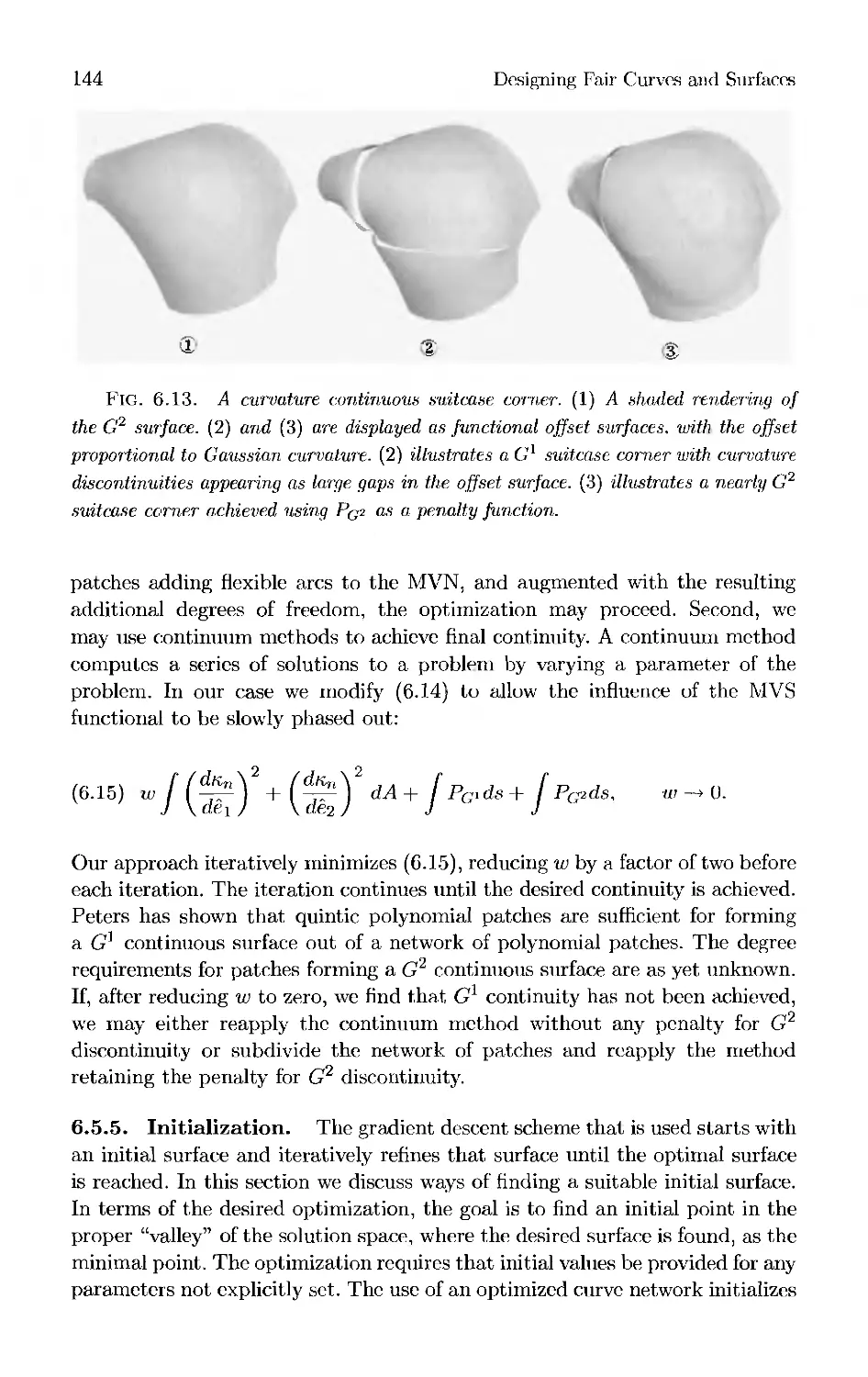
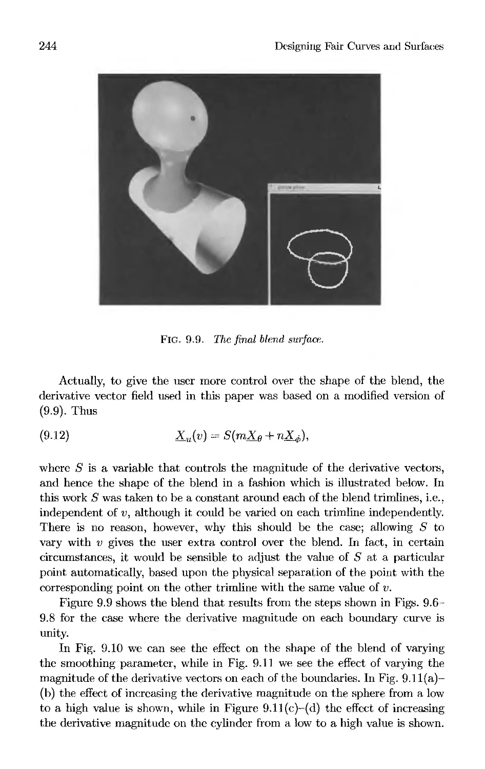
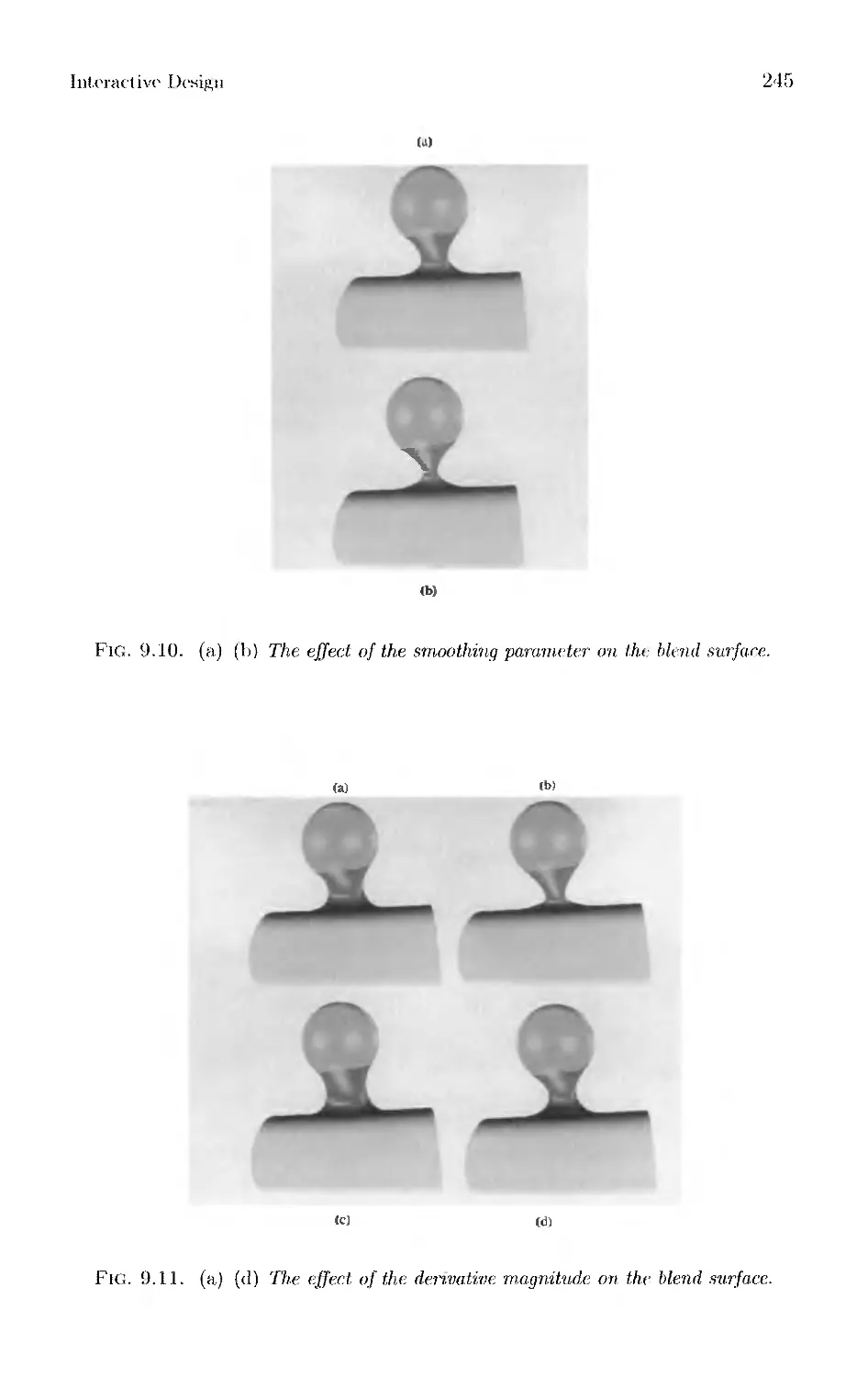
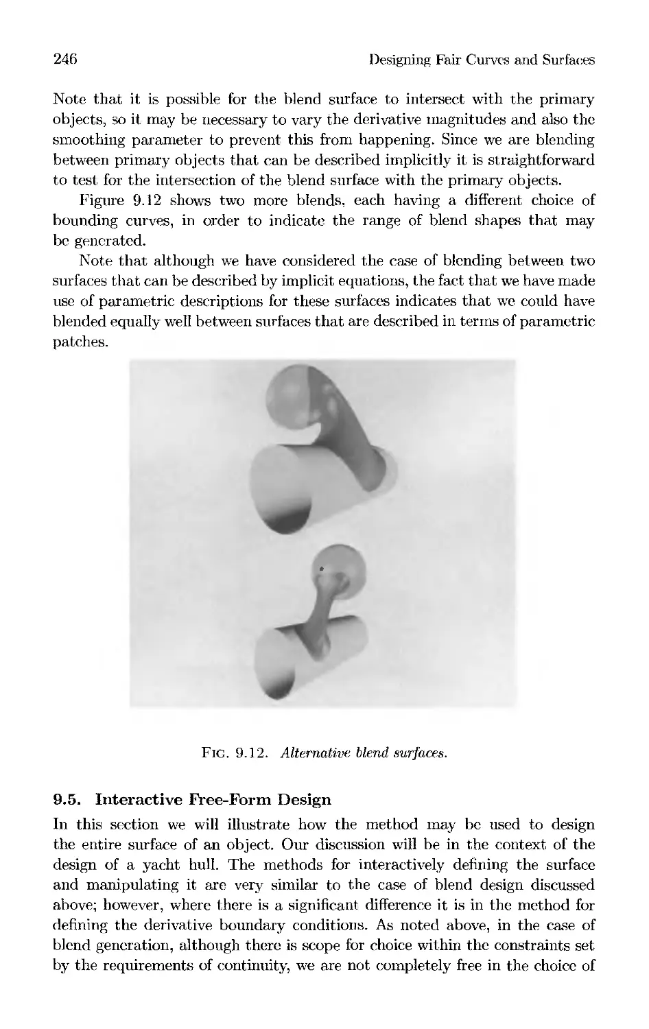
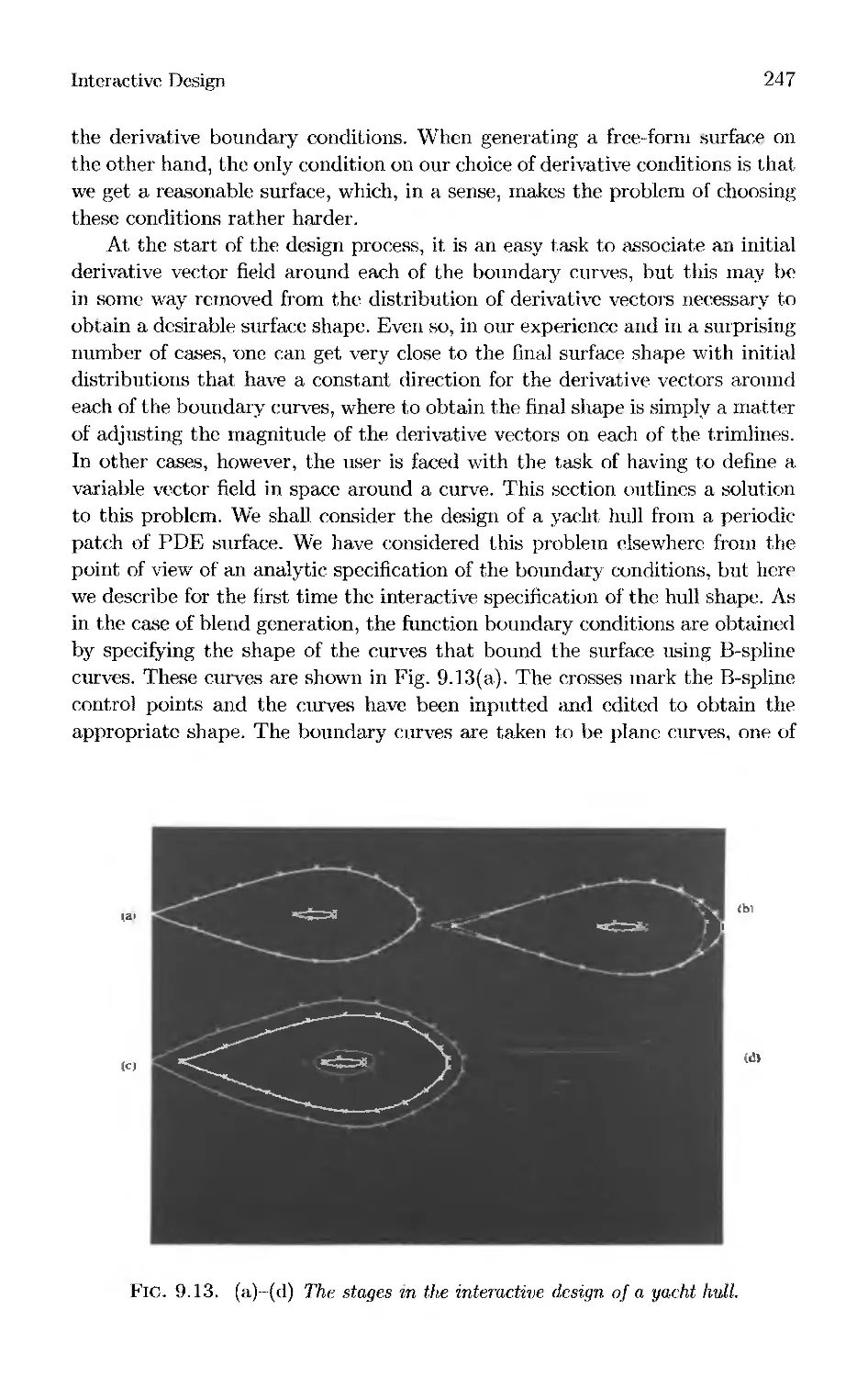
/


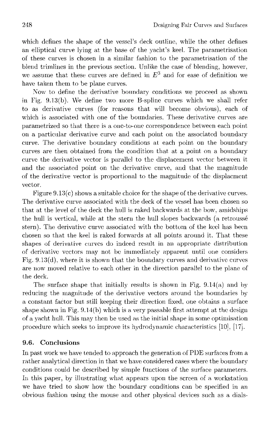


Text
Designing
Fair Curves
and Surfaces
Shape Quality in
Geometric Modeling
and Computer-Aided Design
Edited by
Nickolas S. Sapidis
51HJTL
\
Designing
Fair Curves
and Surfaces
Geometric Design Publications
Editor
Gerald E. Farin
Arizona State University
Farin, Gerald E., editor, Geometric Modeling: Algorithms and New Trends (1987)
Farin, Gerald E., editor, NURBS for Curve and Surface Design (1991)
Barnhill, Robert E., editor, Geometry Processing for Design and Manufacturing (1992)
Hagen, Hans, editor, Curve and Surface Design (1992)
Hagen, Hans, editor, Topics in Surface Modeling (1992)
Goldman, Ronald N., and Lyche, Tom, editors, Knot Insertion and Deletion Algorithms for
B-Spline Curves and Surfaces (1993)
Sapidis, Nickolas S., editor, Designing Fair Curves and Surfaces: Shape Quality in Geometric
Modeling and Computer-Aided Design (1994)
Designing
Fair Curves
and Surfaces
Shape Quality in
Geometric Modeling
and Computer-Aided Design
Edited by
Nickolas S. Sapidis
National Technical University
of Athens
BiaJTL.
Philadelphia
Society for Industrial and Applied Mathematics
Library of Congress Cataloging-in-Publication Data
Designing fair curves and surfaces : shape quality in geometric
modeling and computer-aided design / edited by Nickloas S. Sapidis.
p. cm. — (Geometric design publications)
Includes bibliographical references and index.
ISBN 0-89871-332-3
1. Curves, Algebraic—Data processing. 2. Surfaces—Data
processing. 3. Computer-aided design. I. Sapidis, Nickolas S.
II. Series.
QA567.D47 1994
745.4'01'516352—dc20 94-26850
Cover art reprinted with permission from K. G. Pigounakis and P. D. Kaklis, created at the
Ship-Design Laboratory of the National Technical University of Athens, Greece.
Sponsored by SIAM Activity Group on Geometric Design.
All rights reserved. Printed in the United States of America. No part of this book may be
reproduced, stored, or transmitted in any manner without the written permission of the
Publisher. For information, write the Society for Industrial and Applied Mathematics,
3600 University City Science Center, Philadelphia, PA 19104-2688.
Copyright © 1994 by the Society for Industrial and Applied Mathematics,
is a registered trademark.
To Robert Barnhill
and
the Computer-Aided Geometric Design Research Group
This page intentionally left blank
List of Contributors
J.A. Ayers, Mathematics Department, General Motors Research Laboratory, Warren, MI
48090-9055.
Klaus-Peter Beier, Department of Naval Architecture and Marine Engineering,
University of Michigan, 2600 Draper, NA & ME Bldg., Ann Arbor, MI 48109-2145.
Malcolm I. G. Bloor, Department of Applied Mathematical Studies, The University of
Leeds, Leeds LS2 9JT, United Kingdom.
H.G. Burchard, Department of Mathematics, Oklahoma State University, Stillwater, OK
74078-0613.
Yifan Chen, Ford Motor Company, P.O. Box 2053/MD3135, Room 3135, SRL, Dearborn,
MI 48121.
Matthias Eck, Department of Computer Science and Engineering, University of
Washington, 423 Sieg Hall, FR-35, Seattle, WA 98195.
Mark Feldman, CAMAX Corporation, 7851 Metro Parkway, Minneapolis, MN 55425.
W.H. Frey, Mathematics Department, General Motors Research Laboratory, Warren. MI
48090-9055.
Tim Gallagher, 48 Nottinghill Road, Brighton, MA 02135.
Alexandros I. Ginnis, Department of Naval Architecture and Marine Engineering. National
Technical University of Athens, Heroon Polytechneiou 9, Zografou 157 73, Athens, Greece.
Rainer Jaspert, Department of Mathematics, University of Science and Technology,
AG 3, Schlossgartenstr. 7 D-64289, Darmstadt, Germany.
Alan K. Jones, Geometry and Optimization, Orgn. G-6413, M/S 7L-21,
Boeing Computer Services, Seattle, WA 98124-0346.
Panagiotis D. Kaklis, Department of Naval Architecture and Marine Engineering, National
Technical University of Athens, Heroon Polytechneiou 9, Zografou 157 73, Athens, Greece.
Henry P. Moreton, MS 6L-005, Silicon Graphics, 2011 N. Shoreline Blvd.. Mountain
View, CA 94039-7311.
J6rg Peters, Department of Computer Science, Purdue University, West Lafayette, IN
47907-1398.
Bruce Piper, Department of Mathematical Sciences, Rensselaer Polytechnic
Institute, Troy, NY 12180.
Thomas Rando, 11 Bush Hill Drive, Niantic, CT 06357
Alyn Rockwood, Department of Computer Science and Engineering, Arizona State
University, Tempe, AZ 85287.
John Roulier, Computer Science and Engineering Department, University of Connecticut,
U155, Storrs, CT 06269-0001.
Nickolas S. Sapidis, Department of Naval Architecture and Marine Engineering, National
Technical University of Athens, Heroon Polytechneiou 9, Zografou 157 73, Athens, Greece.
Carlo H. Sequin, Computer Science Division, Department of Electrical
Engineering and Computer Science, University of California, Berkeley, CA 94720.
Michael J. Wilson, Department of Applied Mathematical Studies, The
University of Leeds, Leeds LS2, United Kingdom.
Yan Zhao, Santa Teresa Laboratory, IBM Corporation, L53/F423, San Jose, CA 95141.
Contents I
xi Preface
Part 1 Fairing Point Sets and Curves
3 Chapter 1 Approximation with Aesthetic Constraints
H. G. Burehard, J. A. Ayers, W. H. Frey, and N. S. Sapidis
29 Chapter 2 Curvature Integration through Constrained Optimization
Alan K. Jones
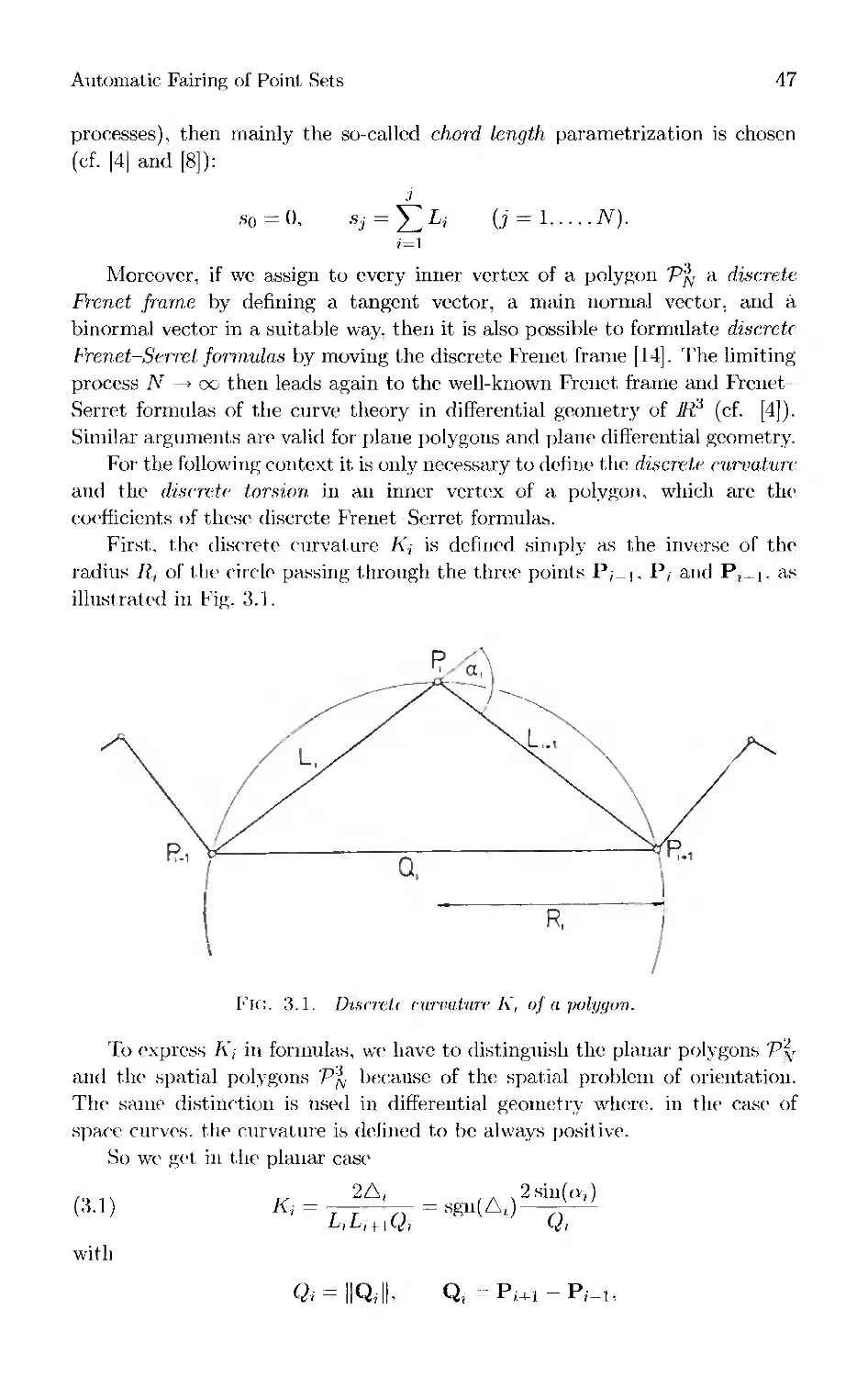
45 Chapter 3 Automatic Fairing of Point Sets
Matthias Eck and Rainer Jaspert
61 Chapter 4 Tight String Method to Fair Piecewise Linear Curves
Mark Feldman
Part 2 Designing Fair Surfaces
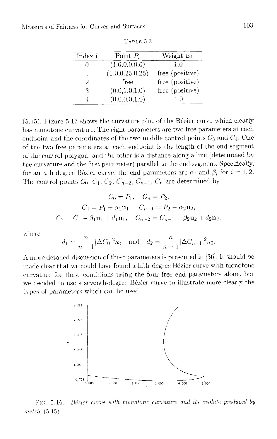
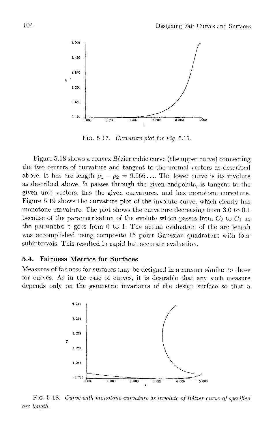
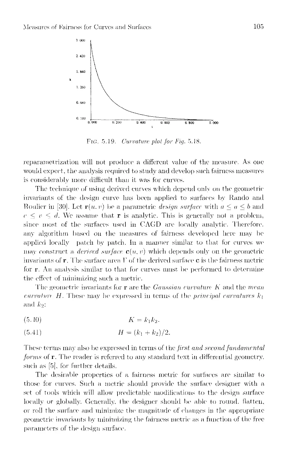
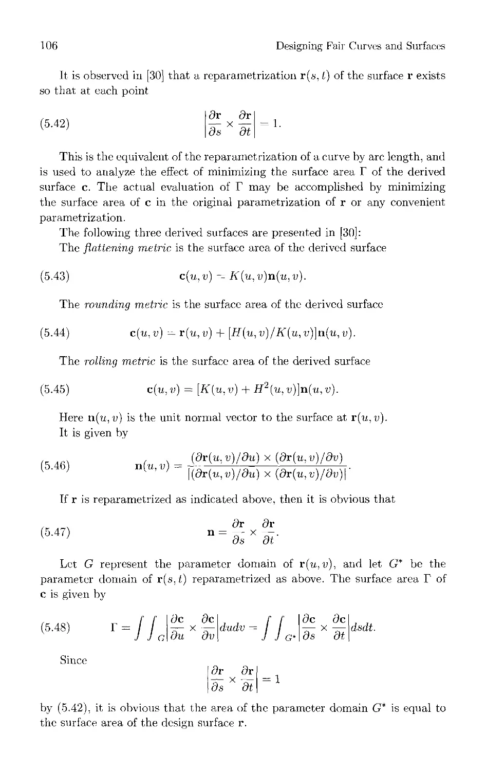
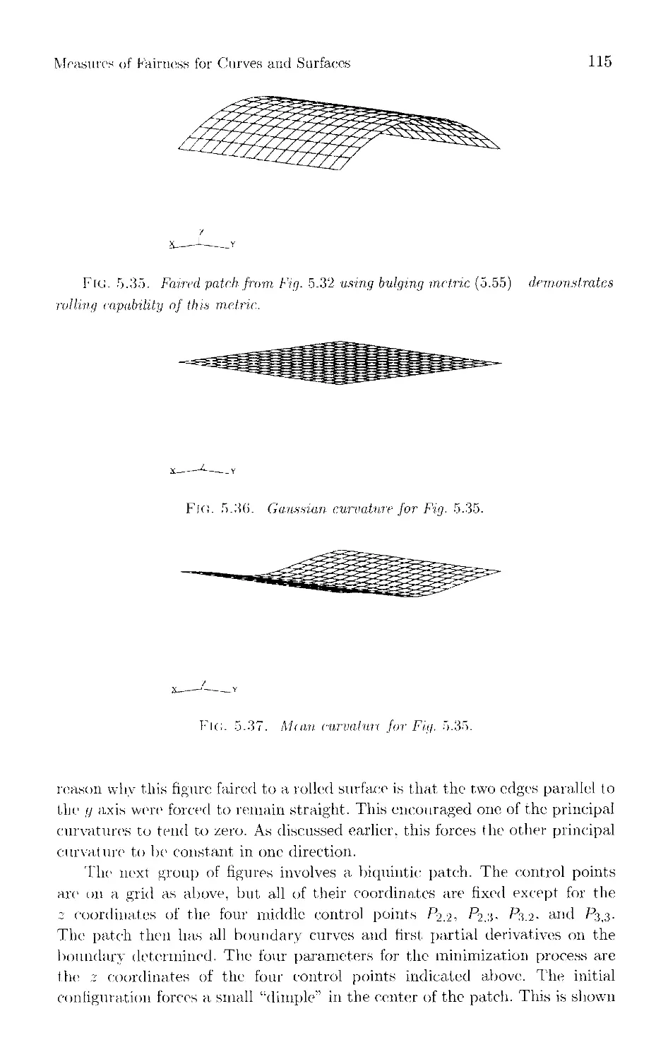
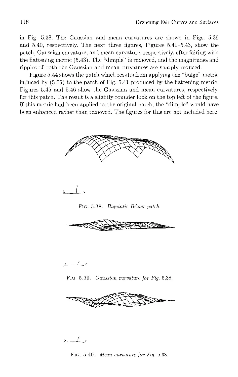
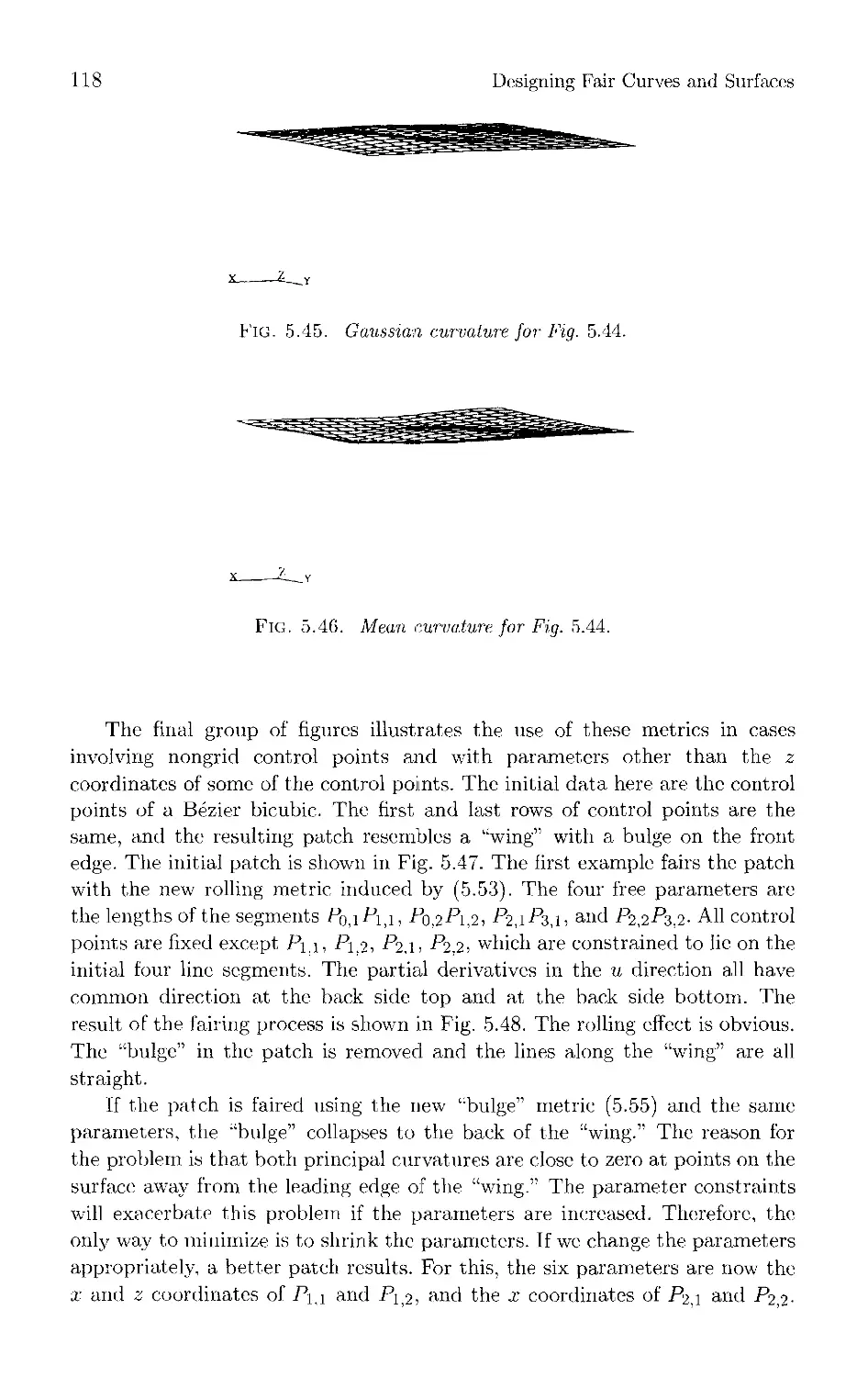
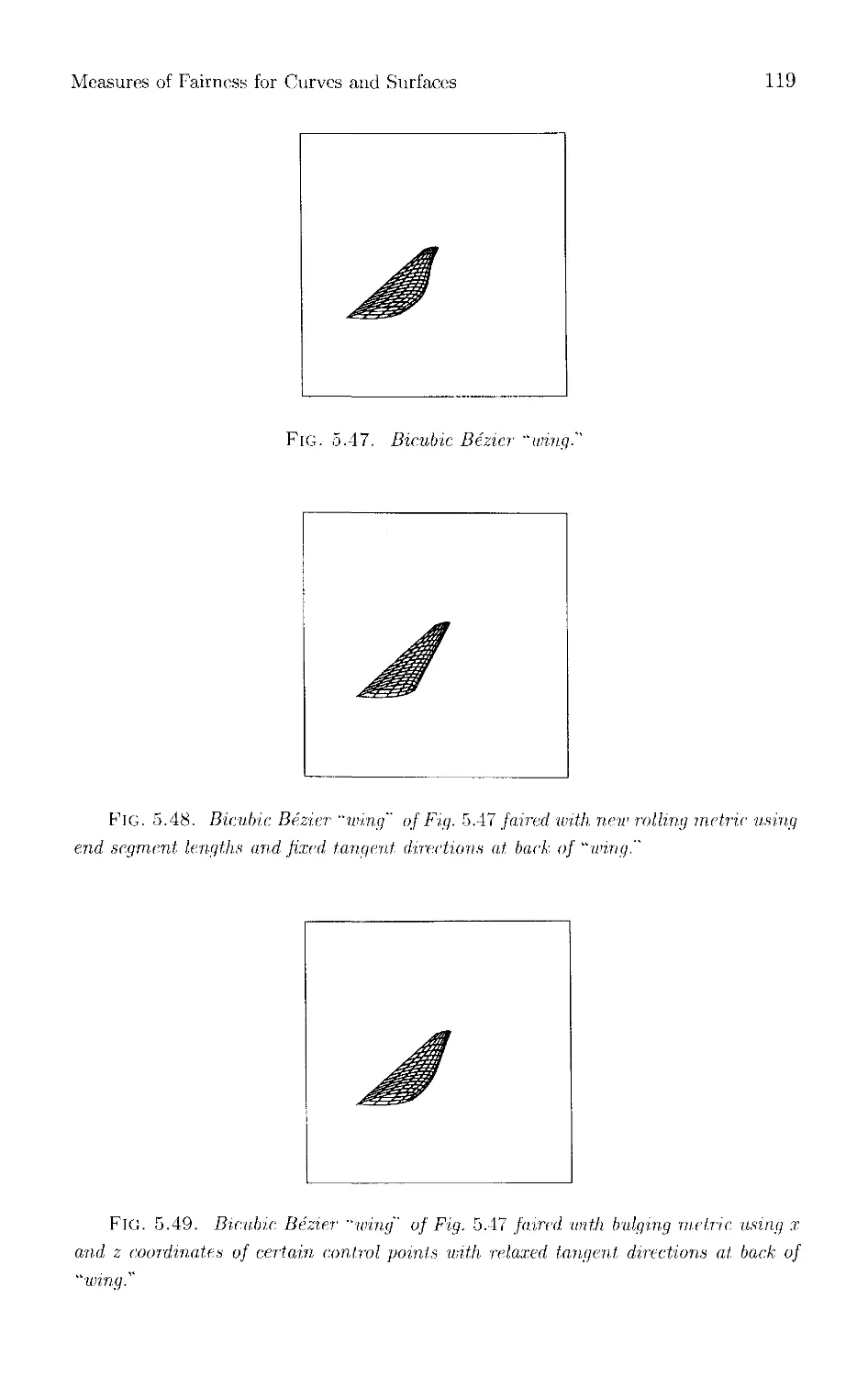
75 Chapter 5 Measures of Fairness for Curves and Surfaces
John Roulier and Thomas Rando
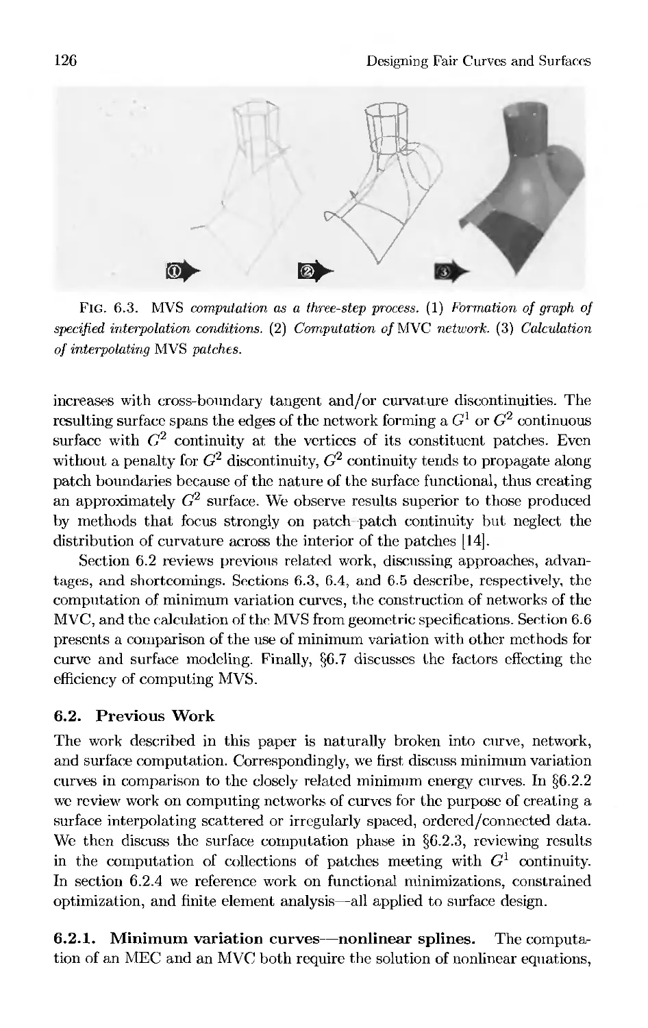
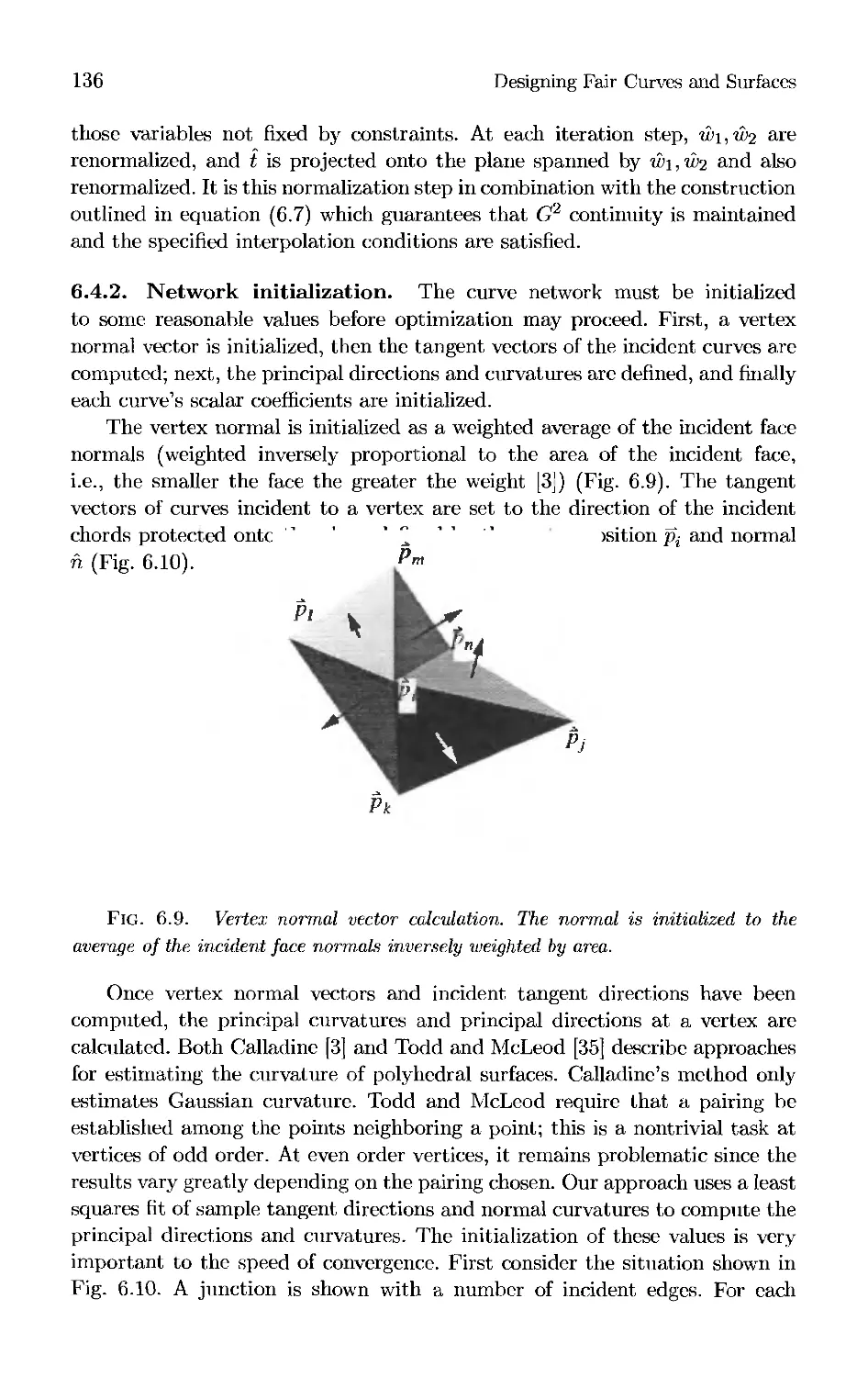
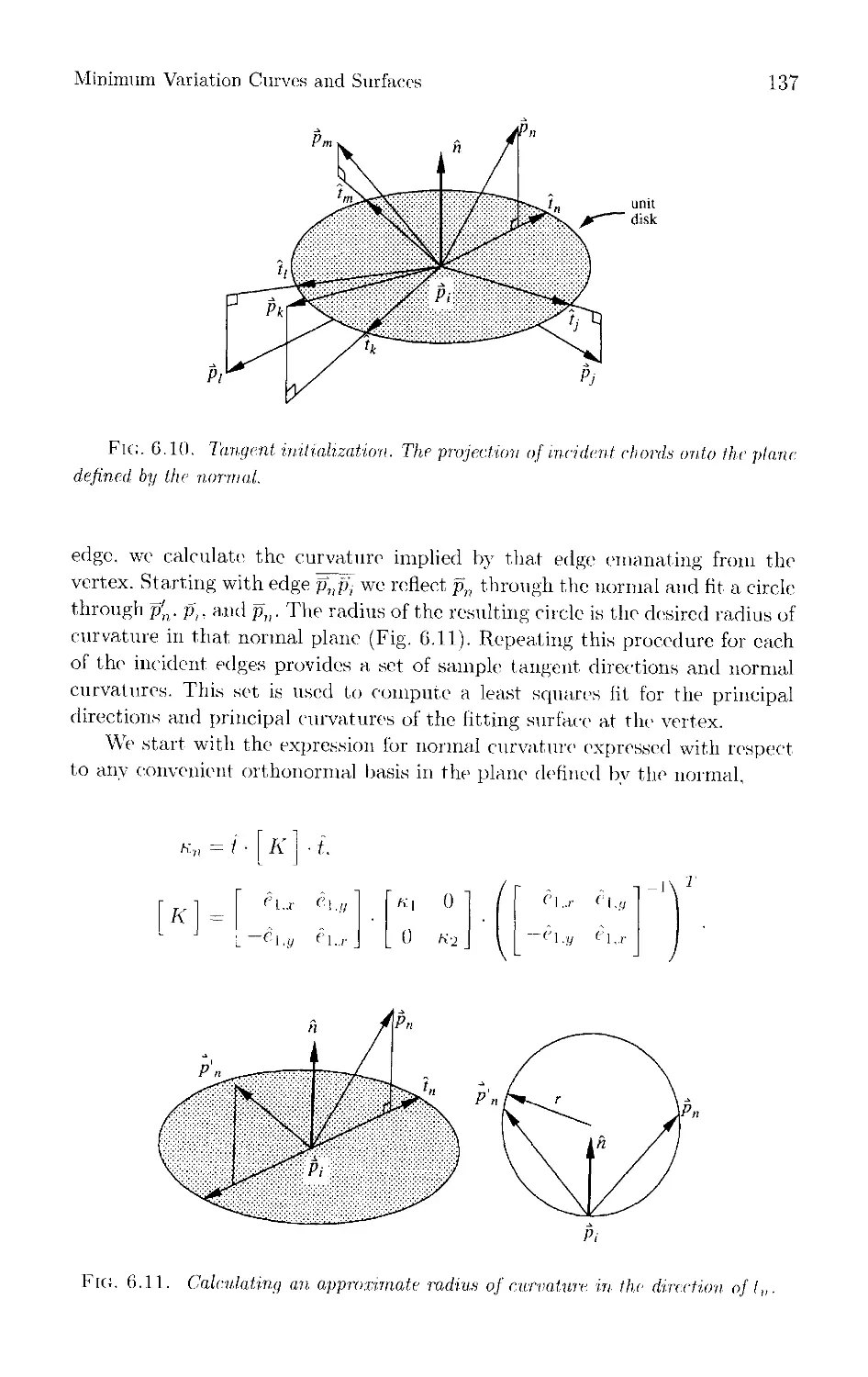
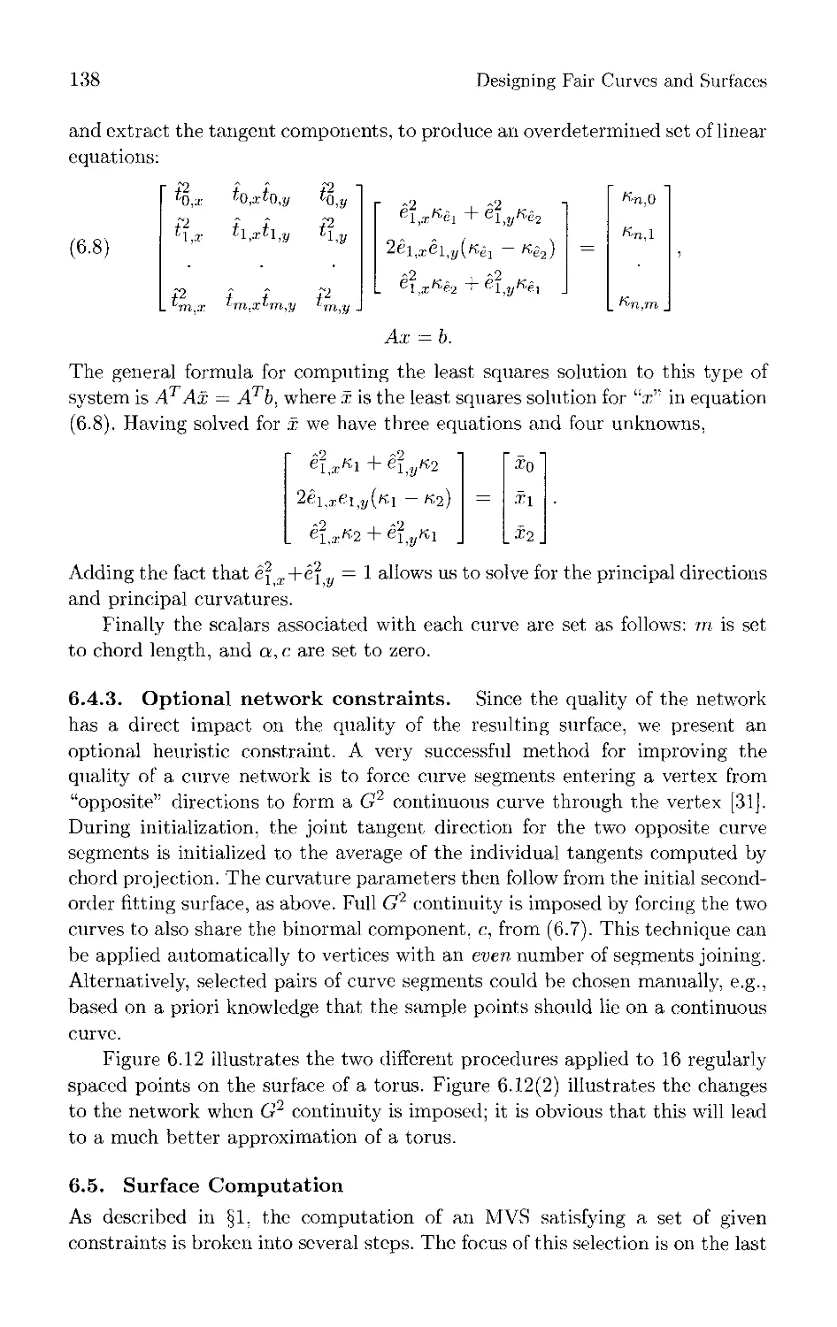
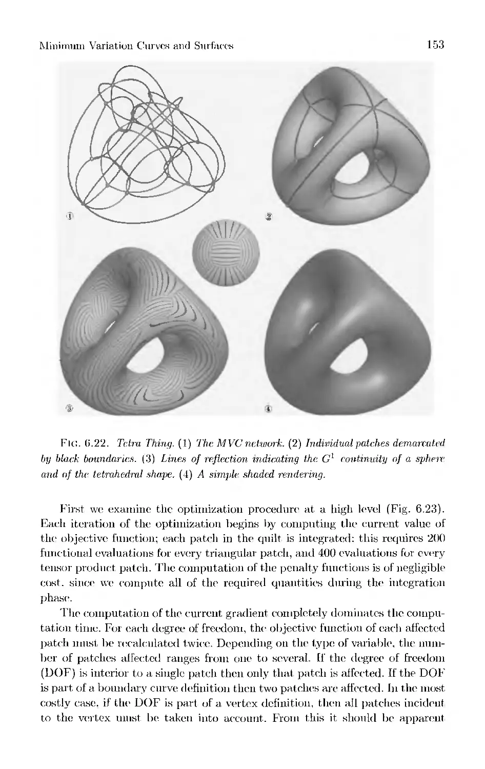
123 Chapter 6 Minimum Variation Curves and Surfaces for Computer-Aided
Geometric Design
Henry P. Moreton and Carlo H. Sequin
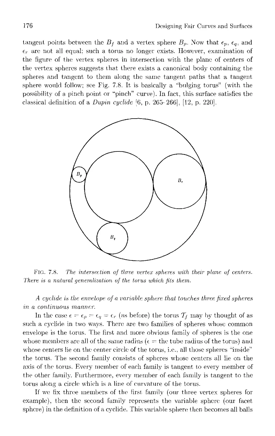
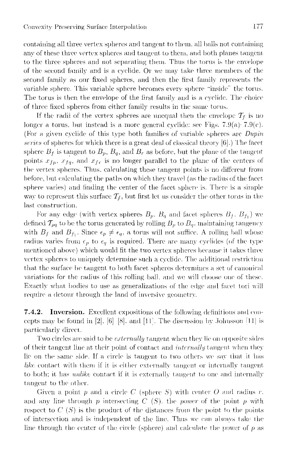
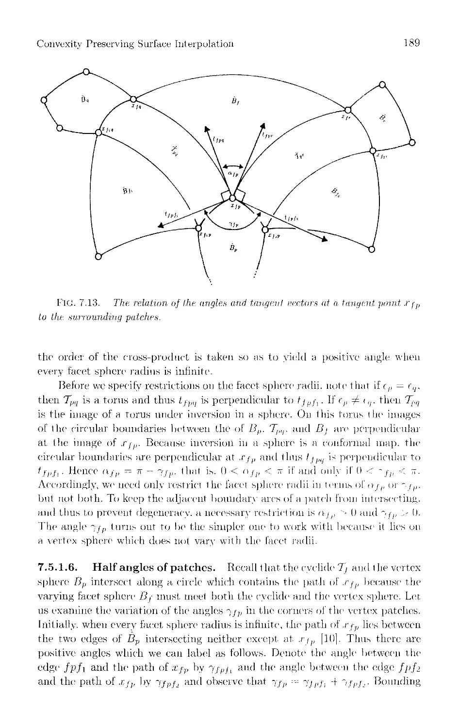
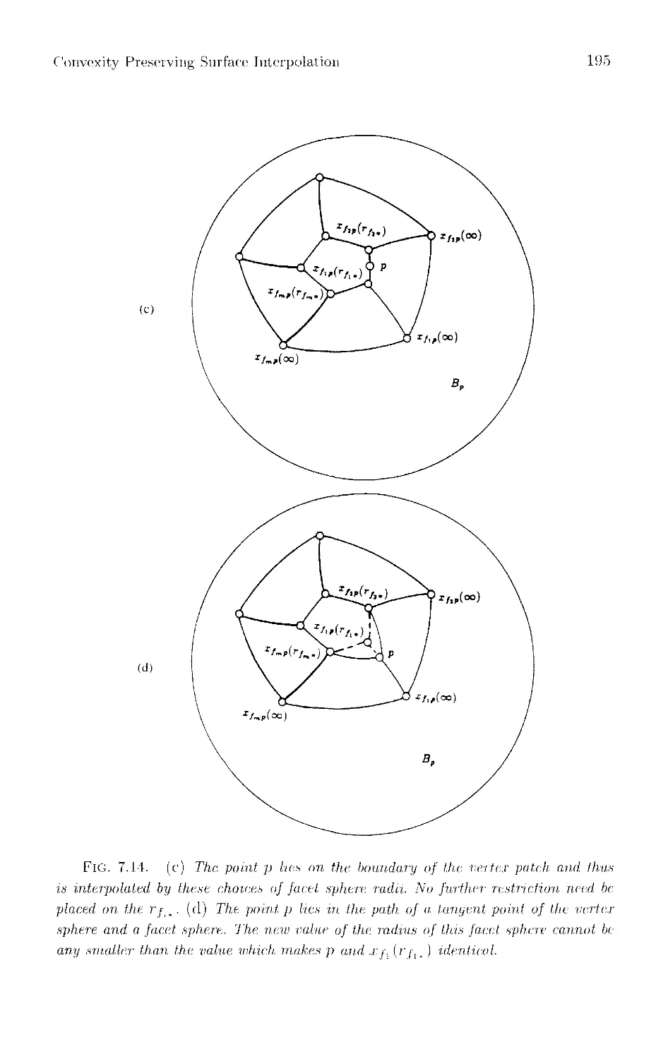
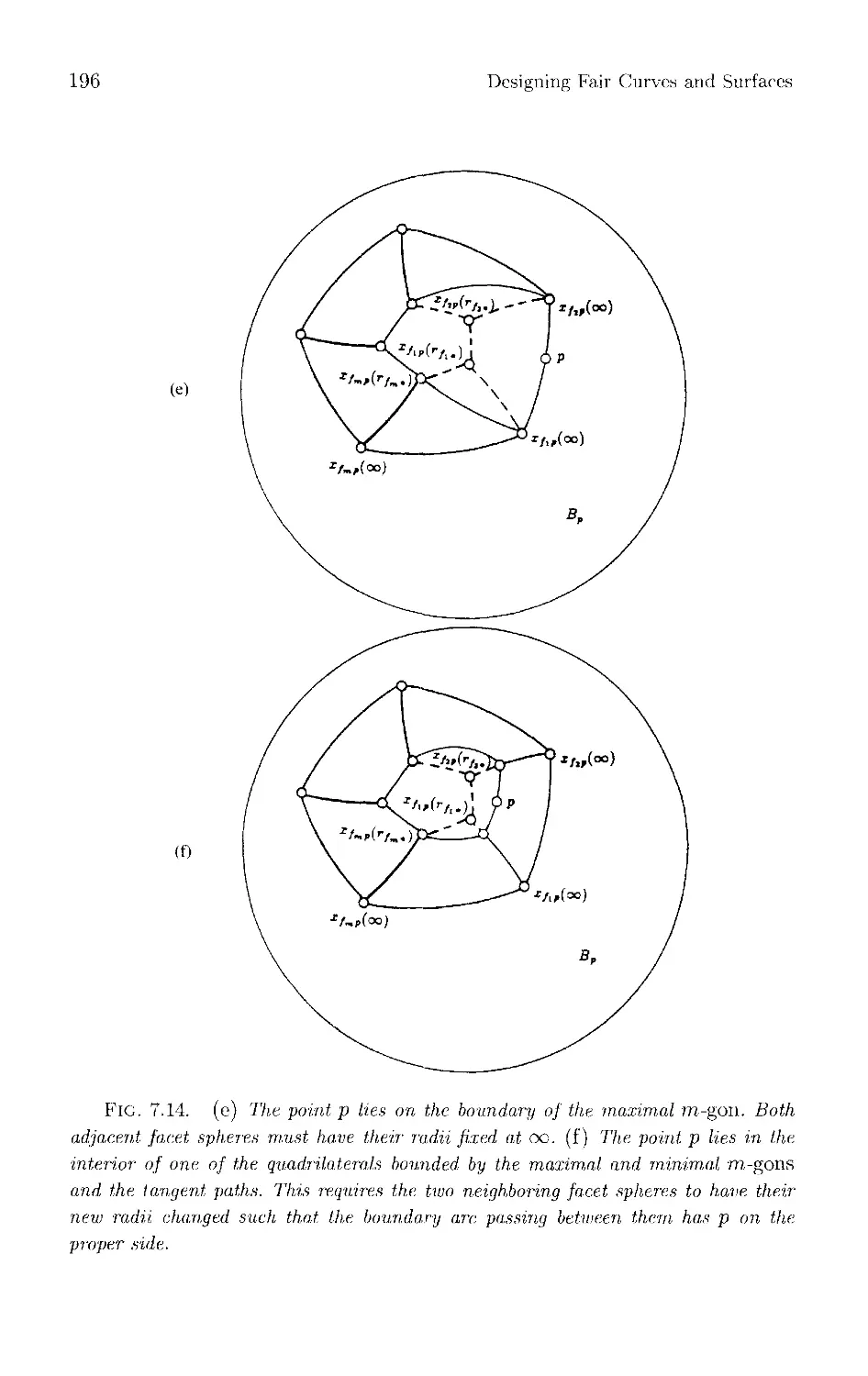
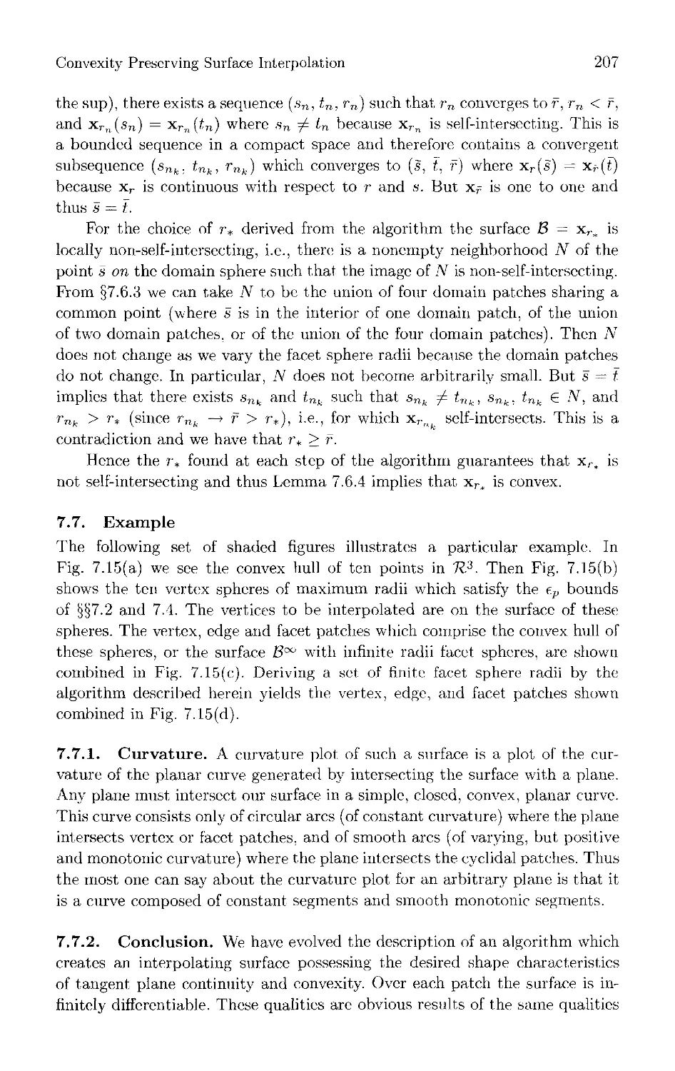
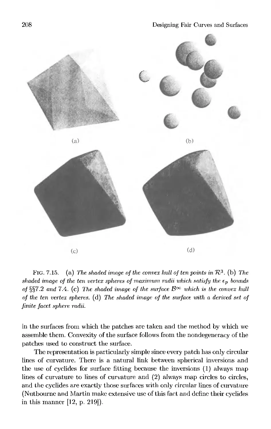
161 Chapter 7 Convexity Preserving Surface Interpolation
Tim Gallagher and Bruce Piper
Part 3 Interactive Techniques for Aesthetic Surface Design
213 Chapters The Highlight Band, a Simplified Reflection Model for
Interactive Smoothness Evaluation
Klaus-Peter Beier and Yifan Chen
231 Chapter 9 Interactive Design Using Partial Differential Equations
Malcolm I. G. Bloor and Michael J. Wilson
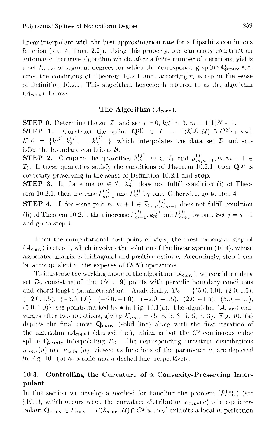
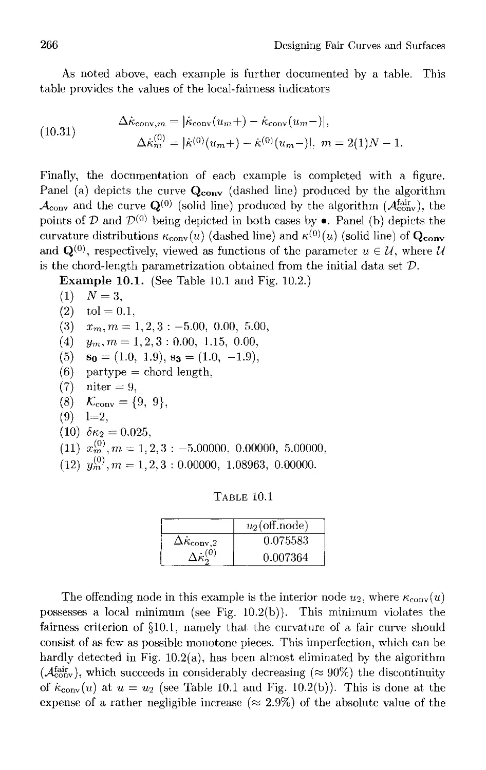
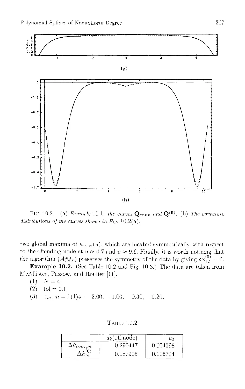
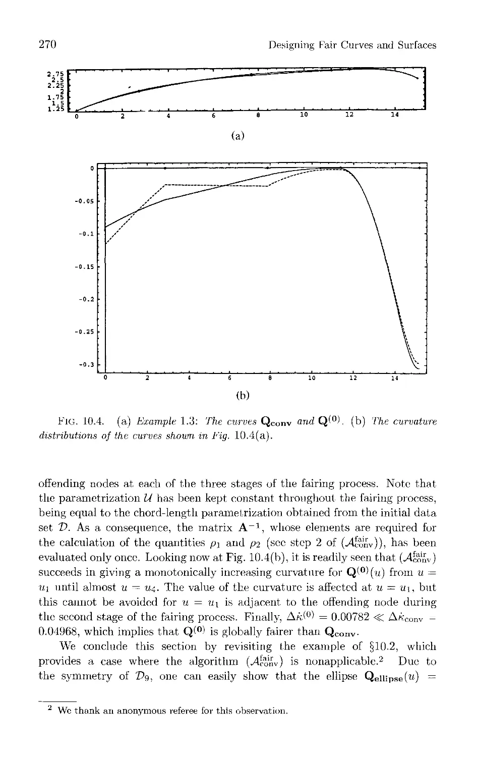
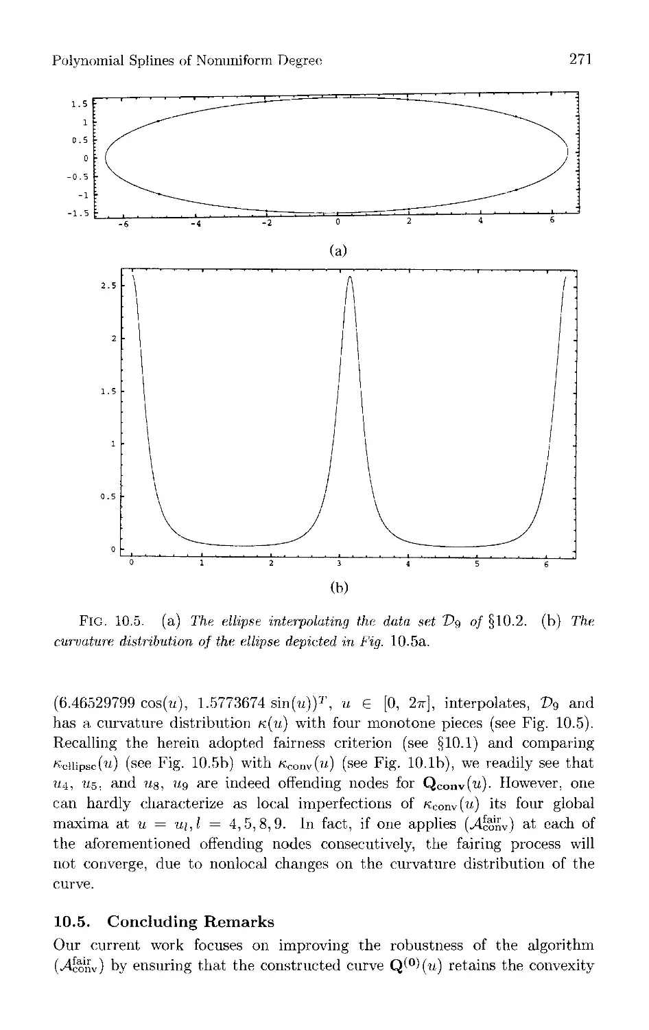
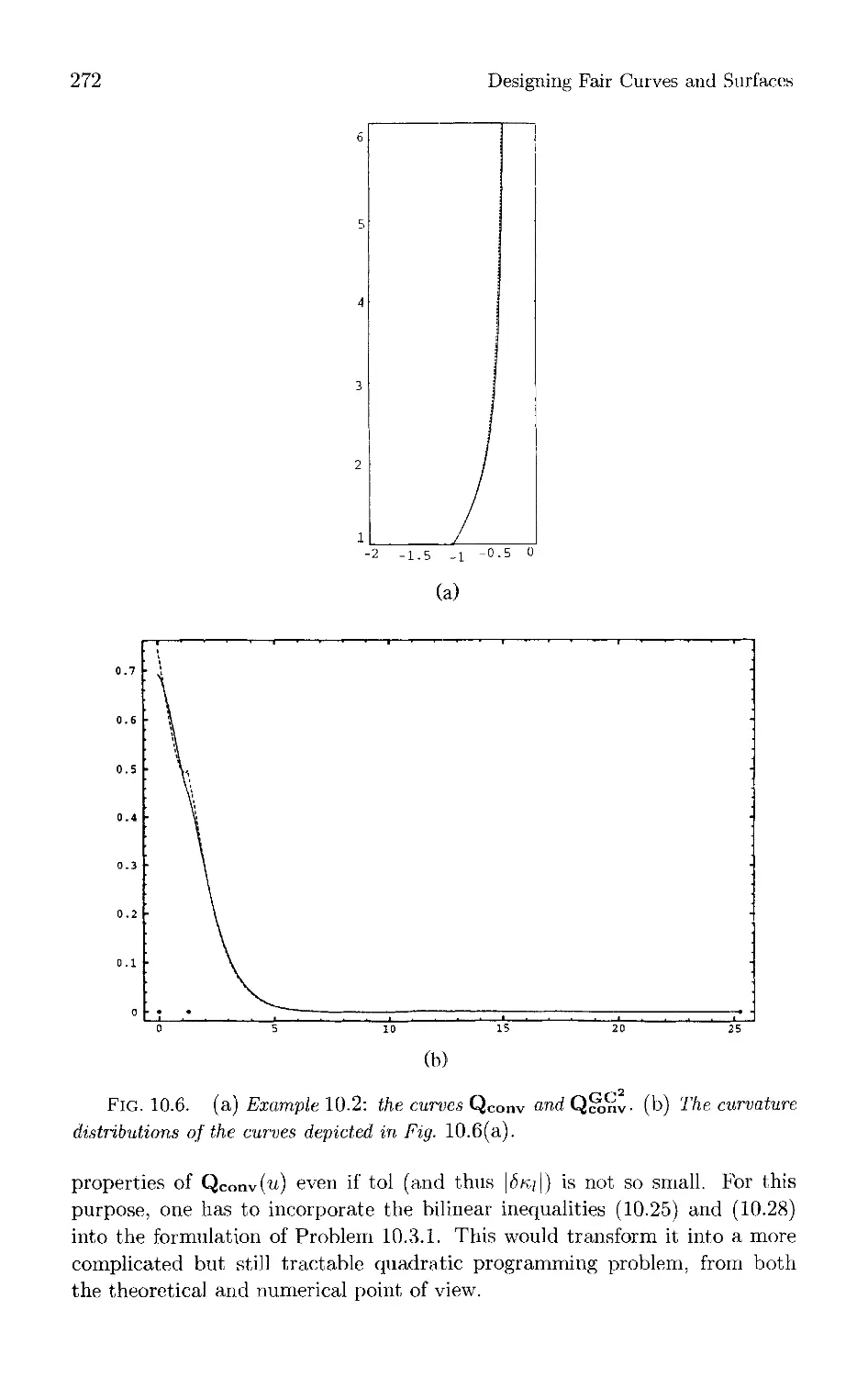
253 Chapter 10 Polynomial Splines of Nonuniform Degree: Controlling
Convexity and Fairness
Alexandras I. Ginnis, Panagiotis D. Kaklis, and Nickokis S. Sapidis
Part 4 Special Applications
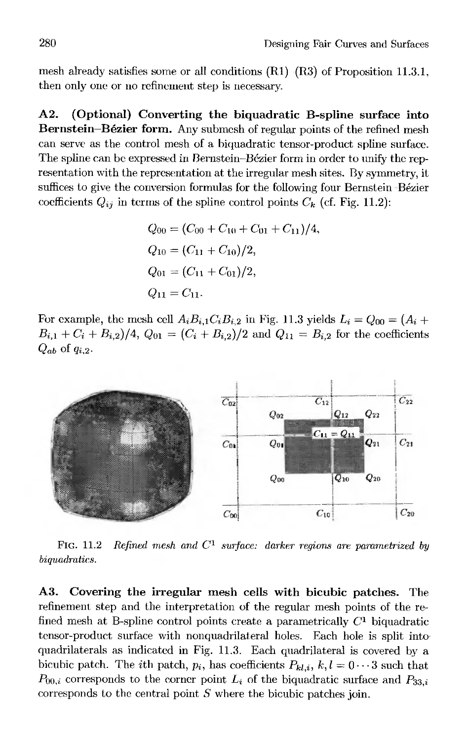
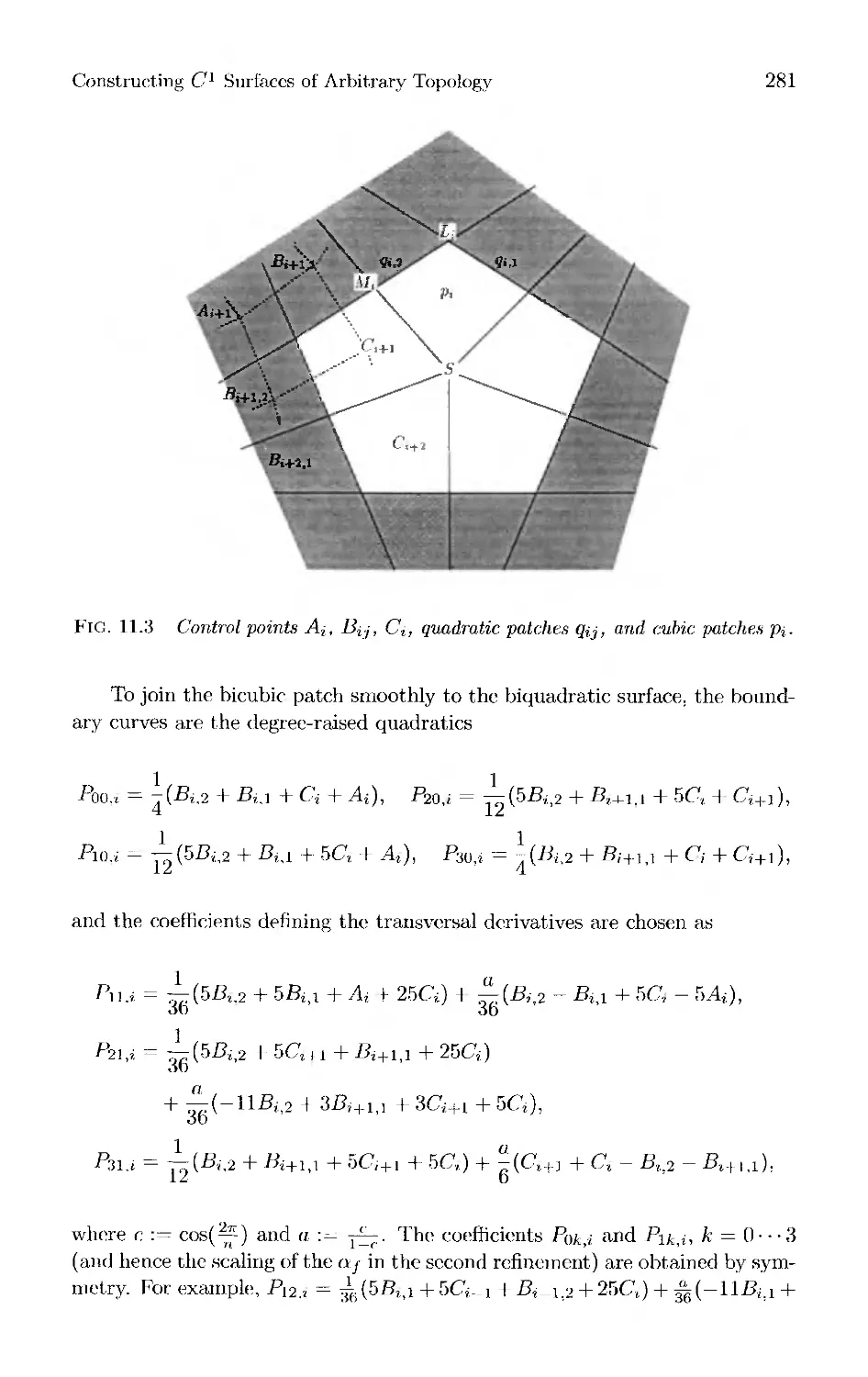
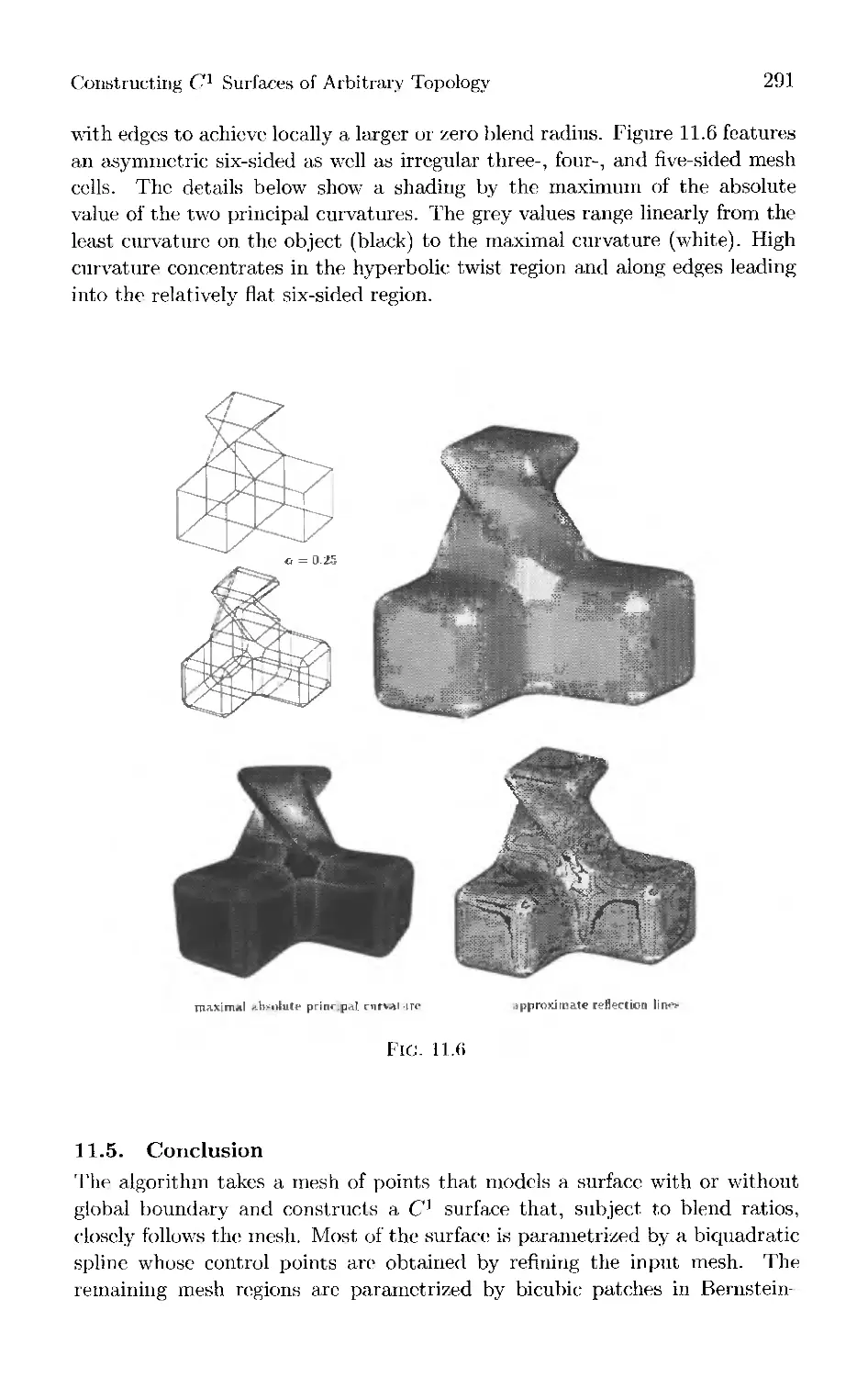
277 Chapter 11 Constructing C Surfaces of Arbitrary Topology Using
Biquadratic and Bicubic Splines
Jorg Peters
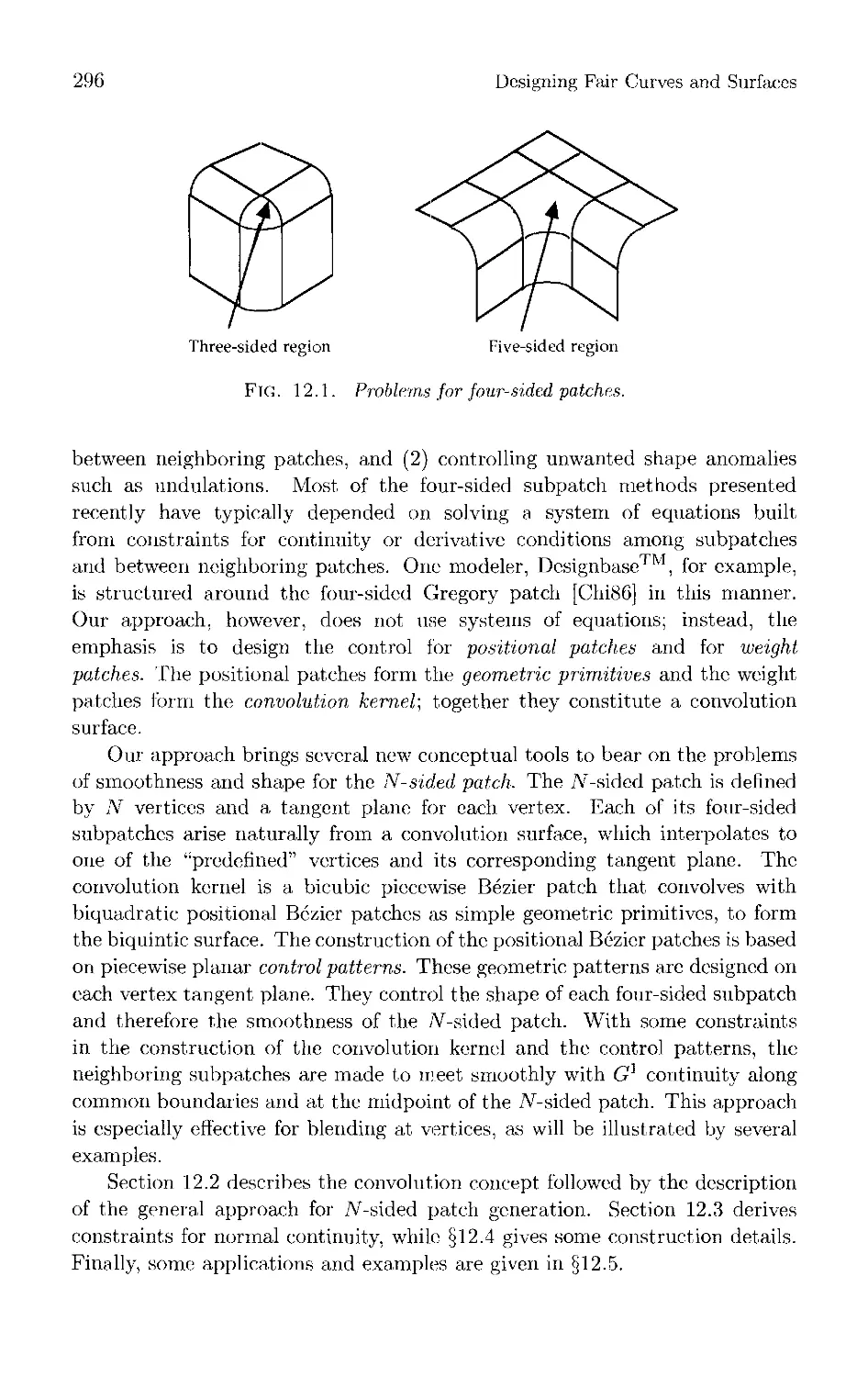
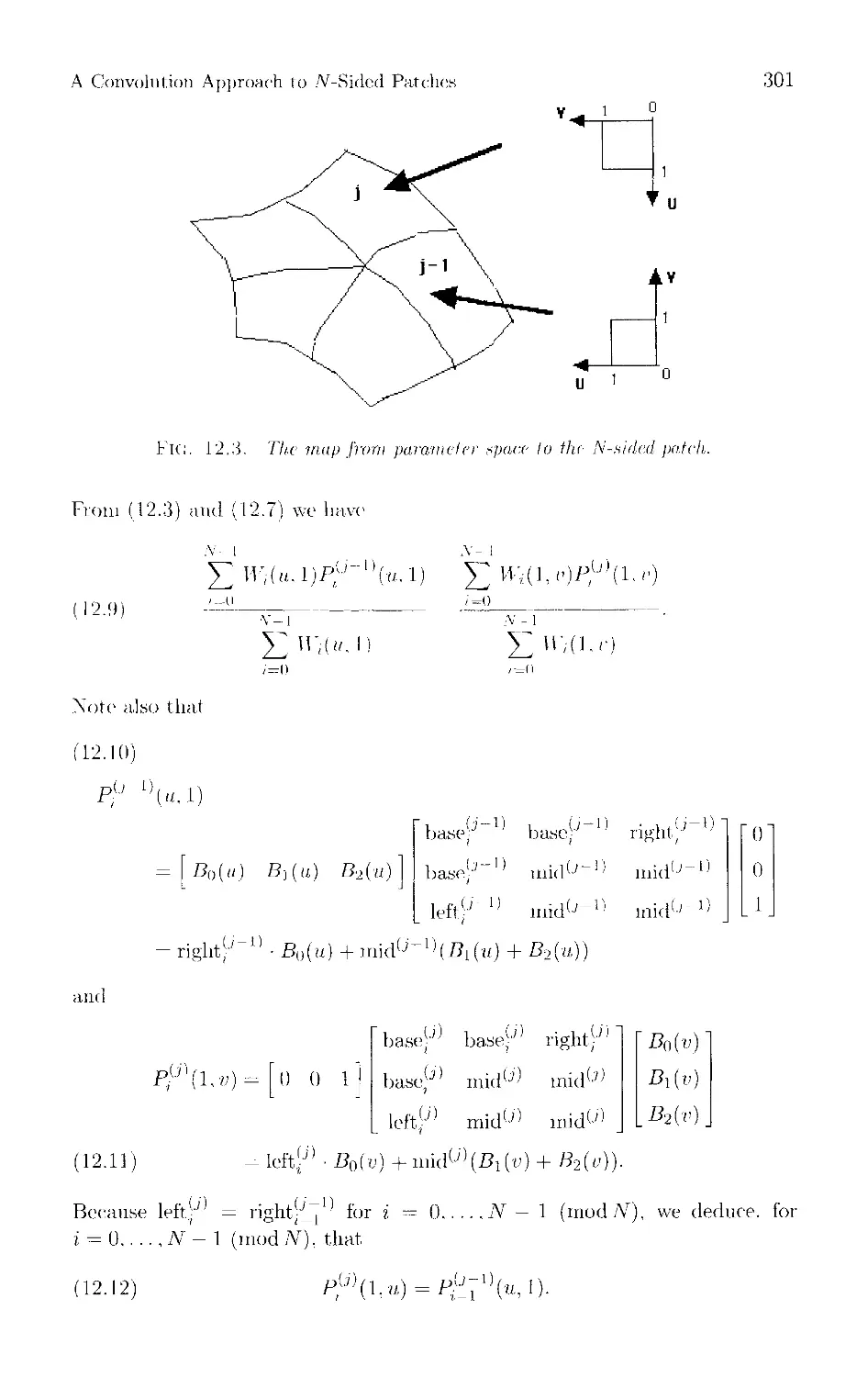
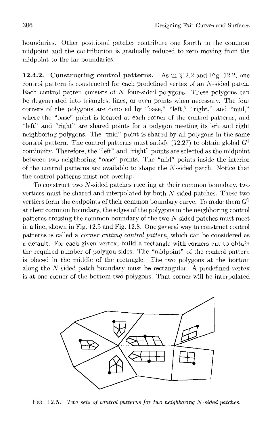
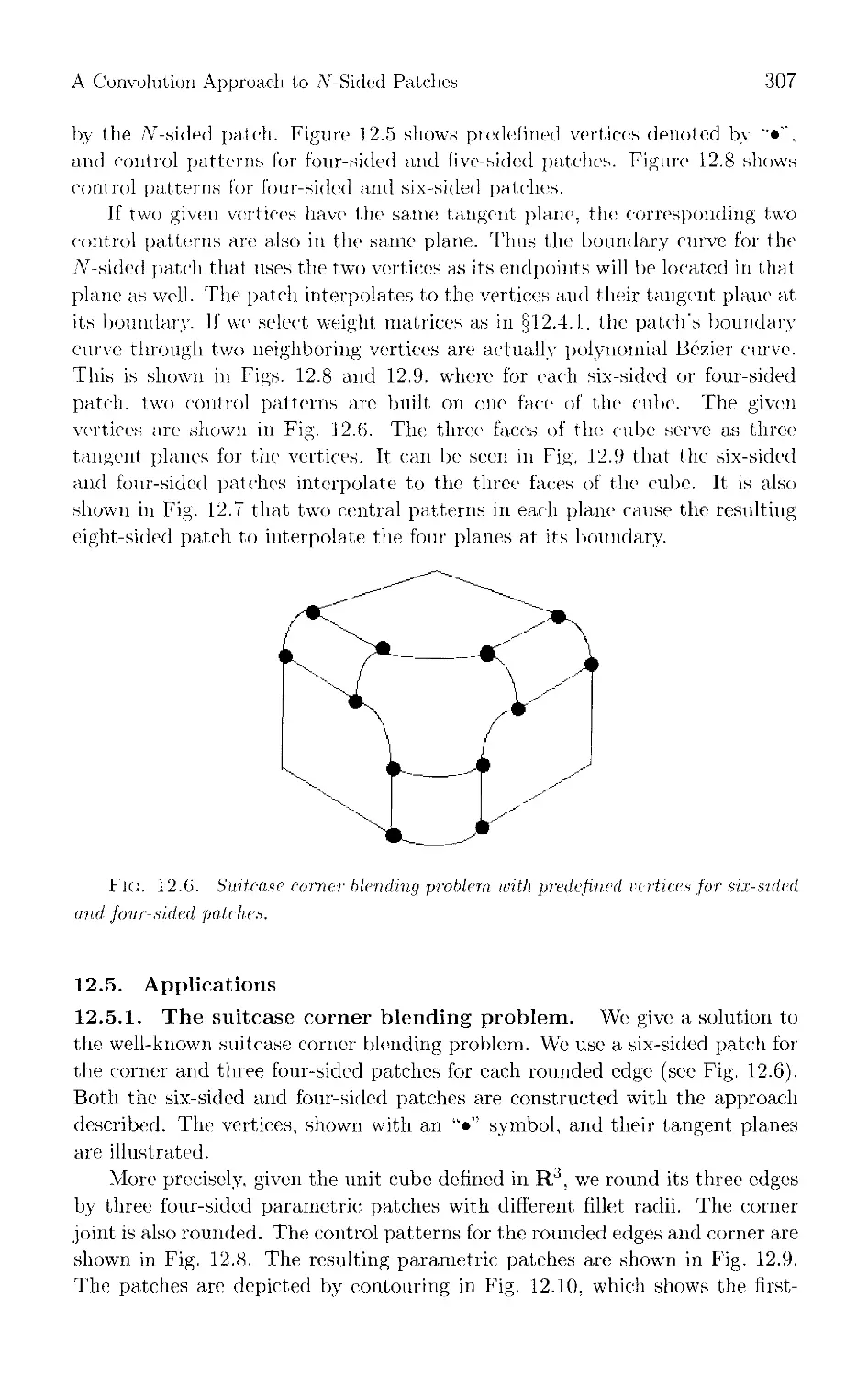
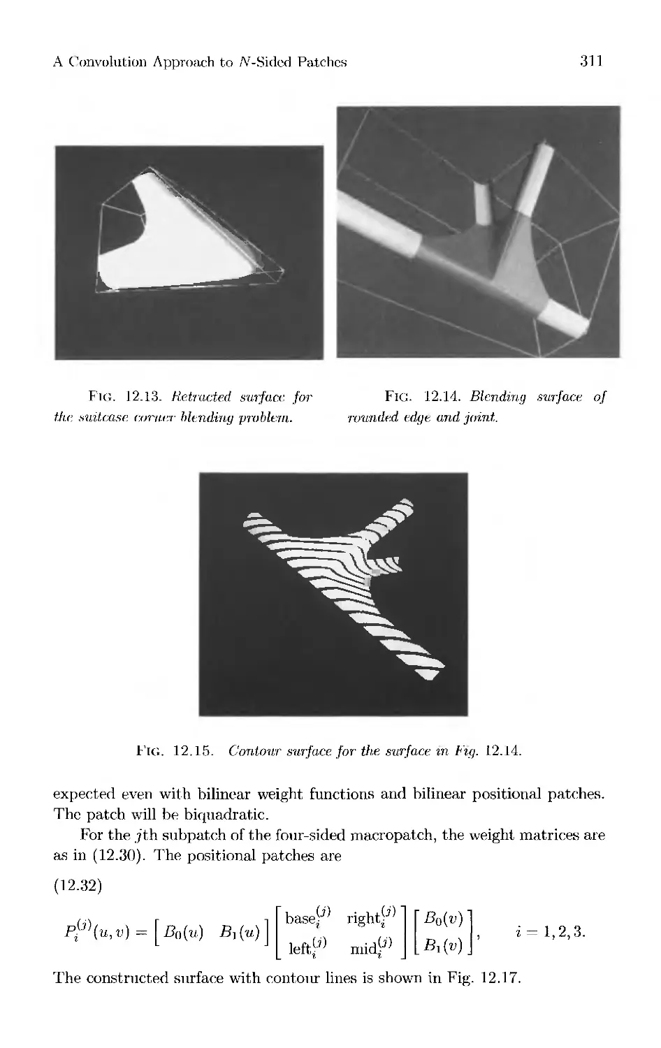
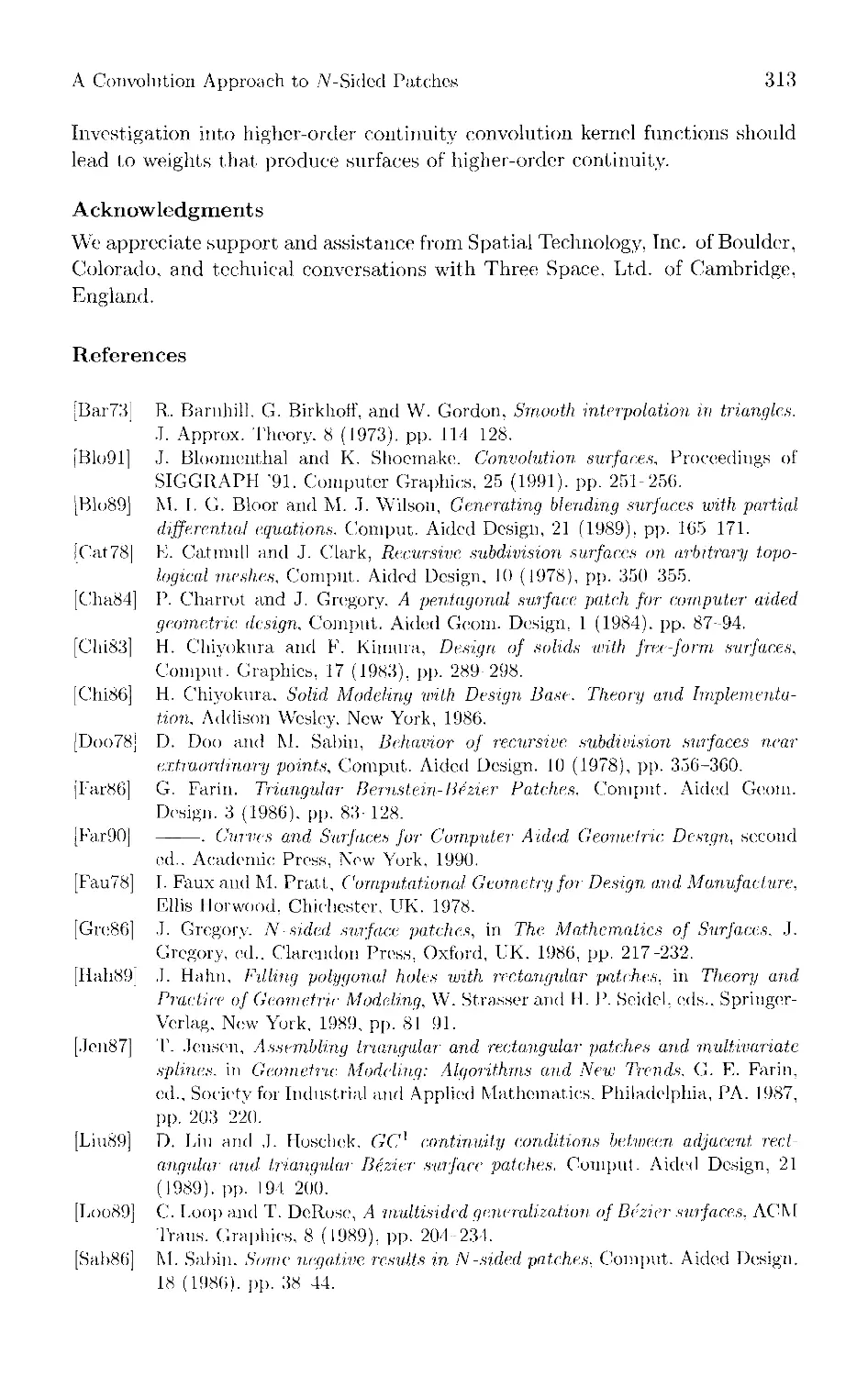
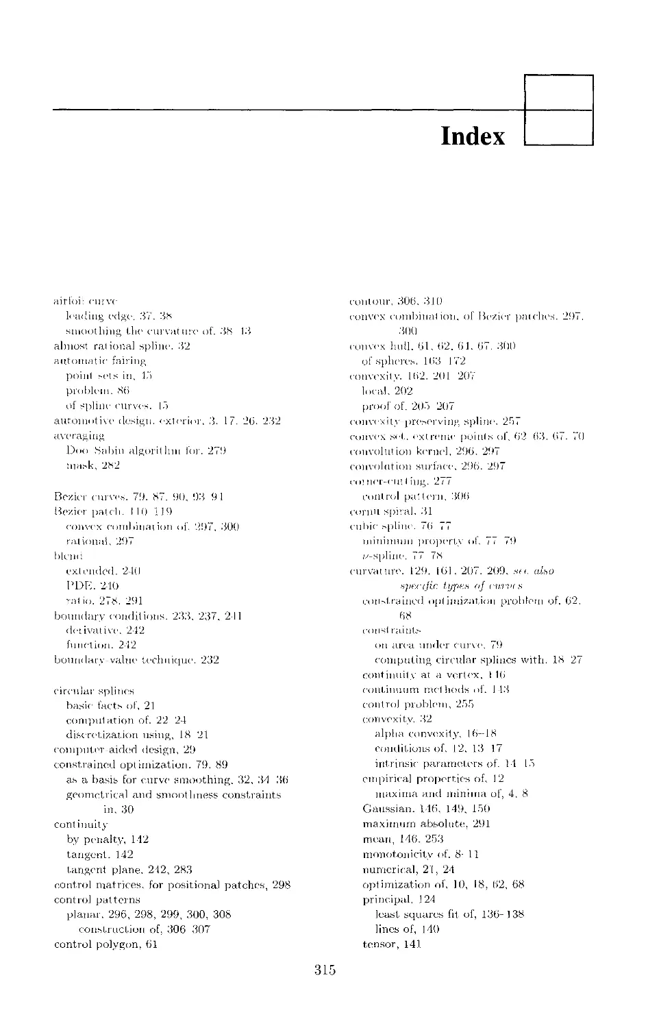
295 Chapter 12 A Convolution Approach to A'-Sided Patches and Vertex Blending
Yan Zhao and Alyn Rockwood
315 Index
This page intentionally left blank
Preface
The present volume is a collection of papers focusing on the aesthetic aspects of geometric
modeling, i.e., the problem of "fair" or "visually pleasing" curve/surface construction, which
is of vital importance in many areas of work and especially in industrial design and styling.
Current research deals with the issues of (i) mathematically defining "fairness" or "shape
quality," (ii) developing new curve and surface schemes that guarantee fairness, and (iii)
assisting a user in identifying shape aberrations in a surface model and removing them without
destroying the principal shape characteristics of the model. The papers included in this book
address the above issues for the cases of point sets, curves, and surfaces, and are highlighted
below. Although the papers vary in terms of the problems considered and the solutions
proposed, there is a common theme in quite a few of them. This common theme is the "principle
of simplest shape" — an idea that is generally applied in the fine arts — which implies that
"fair" shapes are always free of unessential features and simple in design (structure).
Part 1. The paper by Burchard, Ayers, Frey, and Sapidis deals with the problem of defining
visual pleasantness for parametric curves, and proposes new definitions related to the
"principle of simplest shape." Jones presents procedures, based on constraint optimization, that
allow a user to prescribe various features of the curvature of a curve. The last two papers, one
by Eck and Jaspert and one by Feldman, focus on fairing point sets, a problem that has received
little attention from the research community, although it is very important in industrial
applications (e.g., for processing digitized points or trim curves of surfaces). Eck and Jaspert
use concepts from "difference geometry" to study the shape of a point set, while Feldman's
algorithm is based on the mechanical model of a tight string.
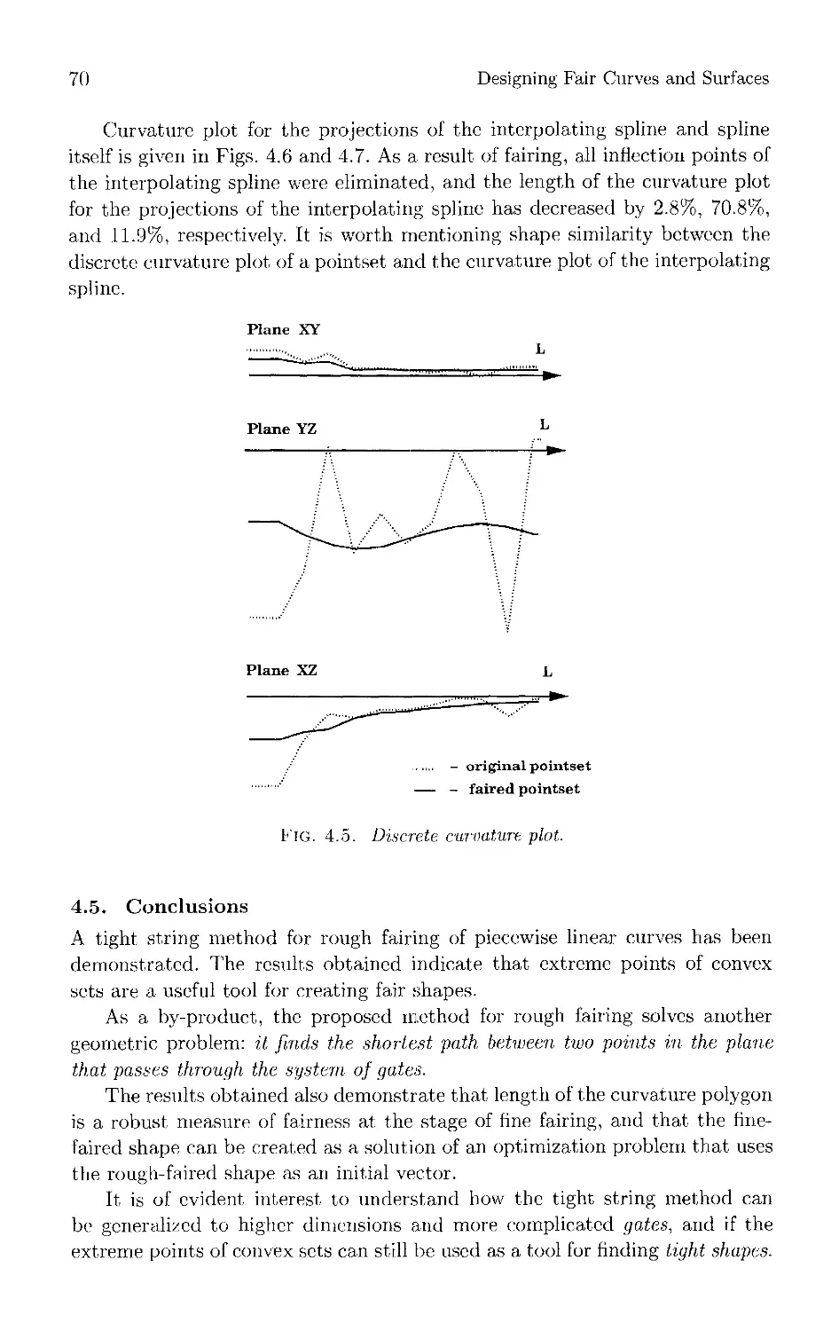
Part 2. Roulier and Rando discuss existing and new fairness metrics for curves and
surfaces, evaluate their effectiveness, and offer implementation strategies. The paper by
Moreton and Sequin focuses on curvature variation as a measure of fairness and employs it to
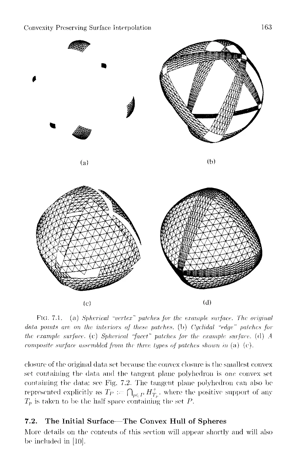
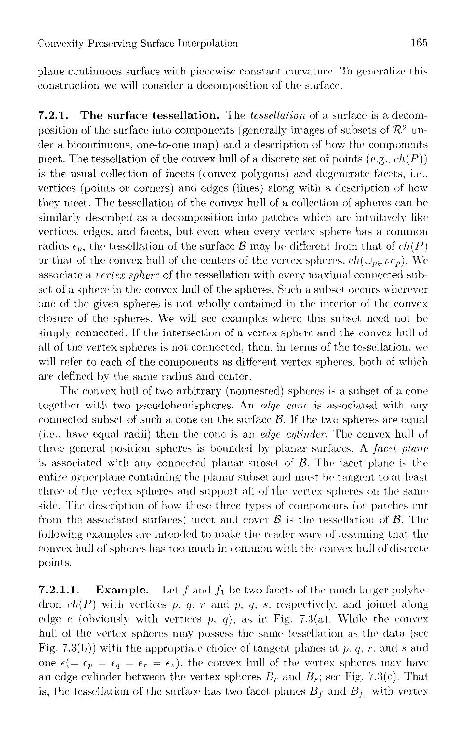
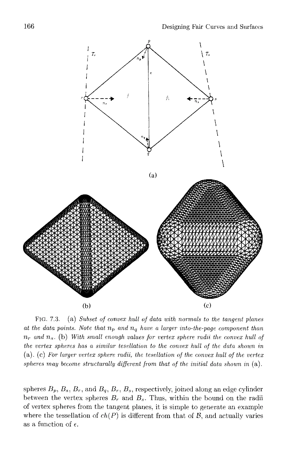
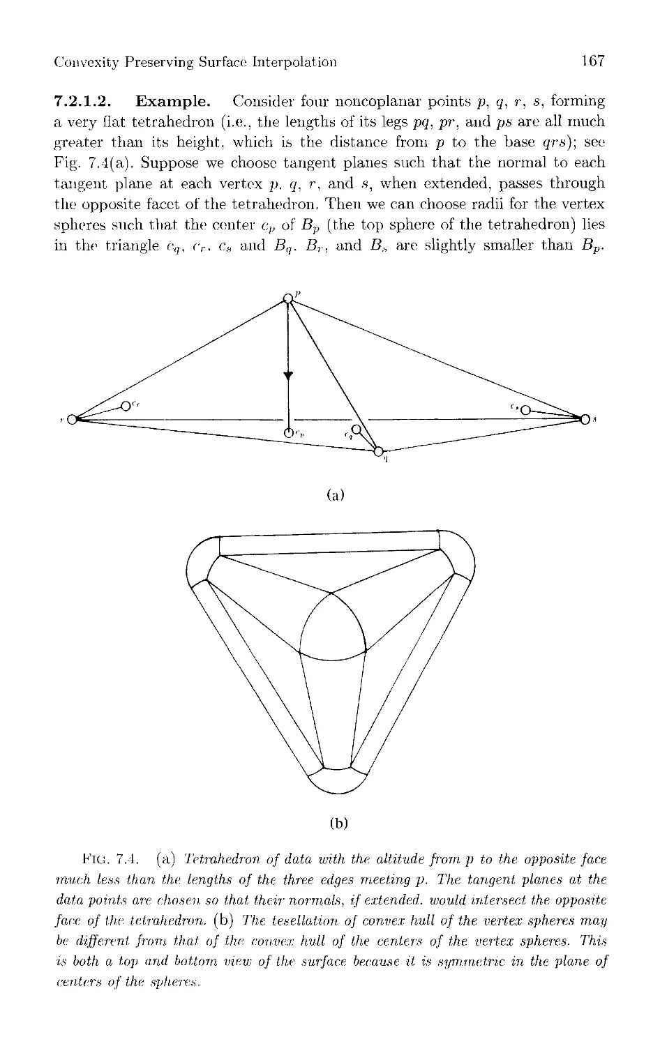
develop a new surface modeling technique. In the last paper in Part 2. Gallagher and Piper build
on the "principle of simplest shape" and present an algorithm that constructs a composite
surface interpolating discrete data by assembling spherical and cylindrical patches.
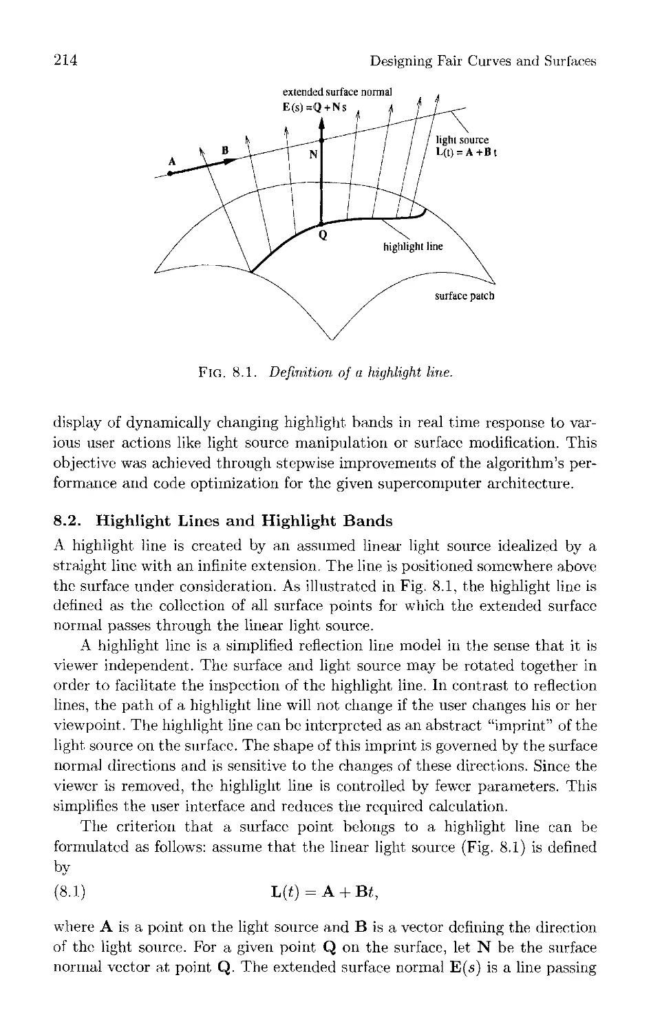
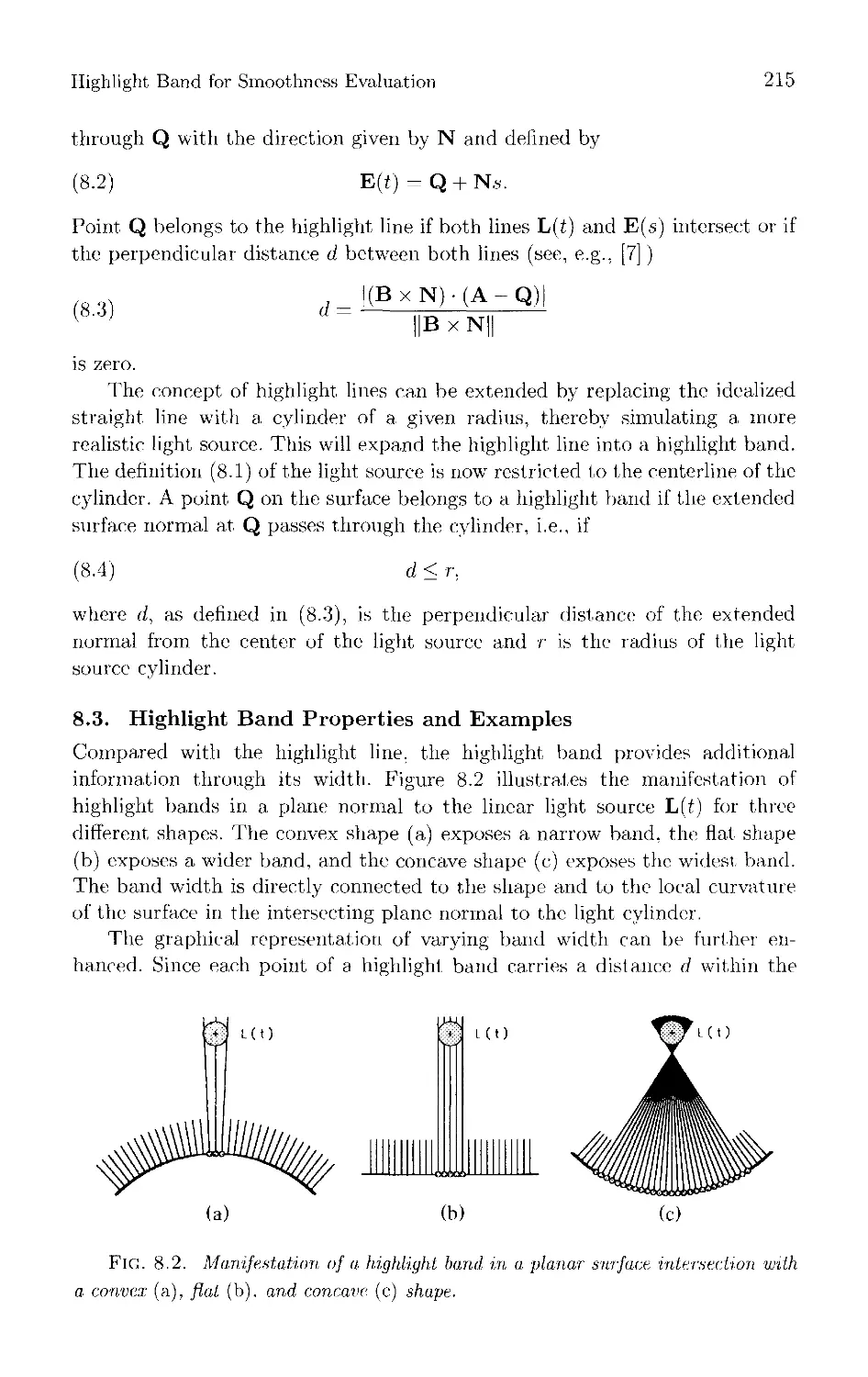
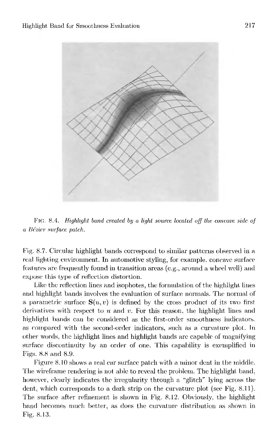
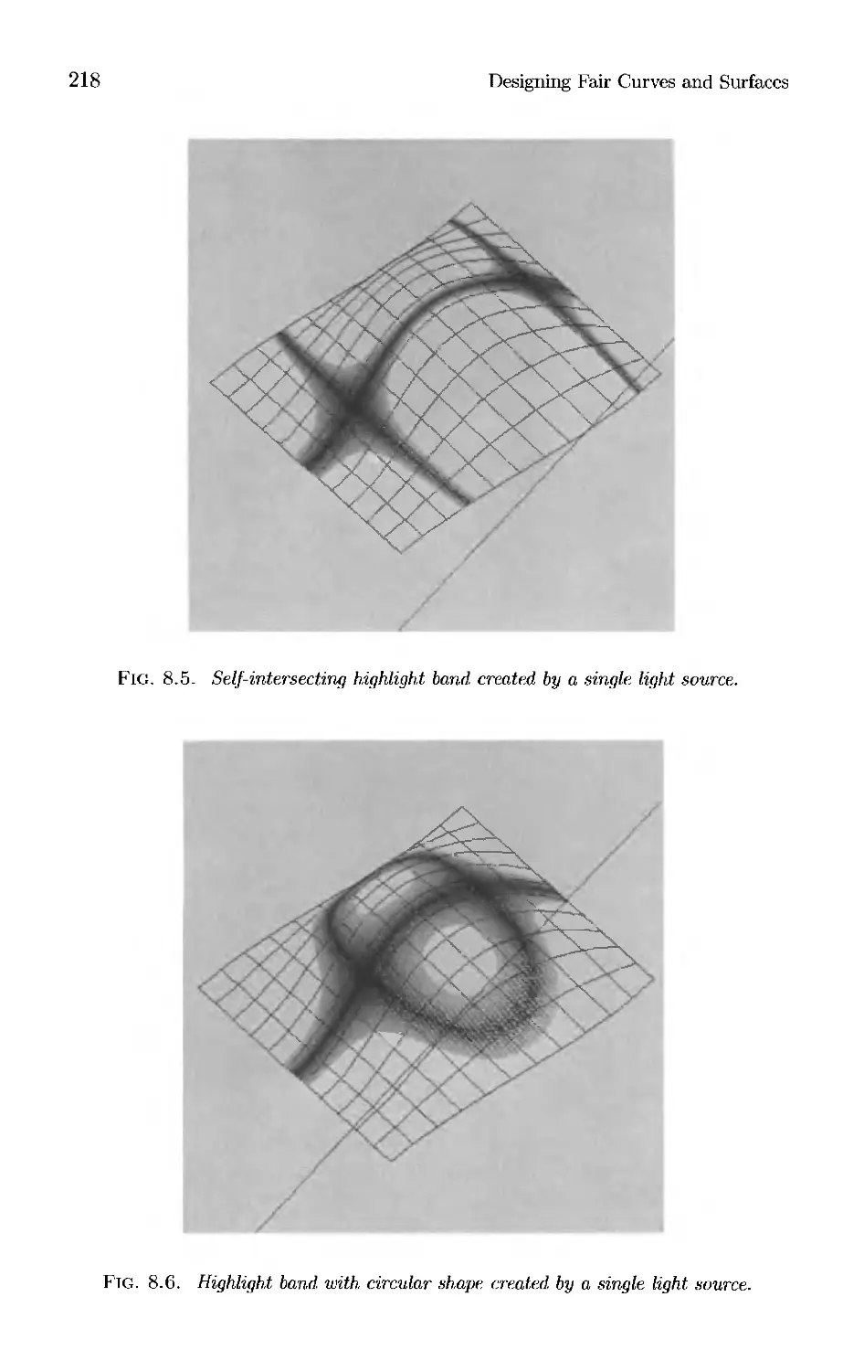
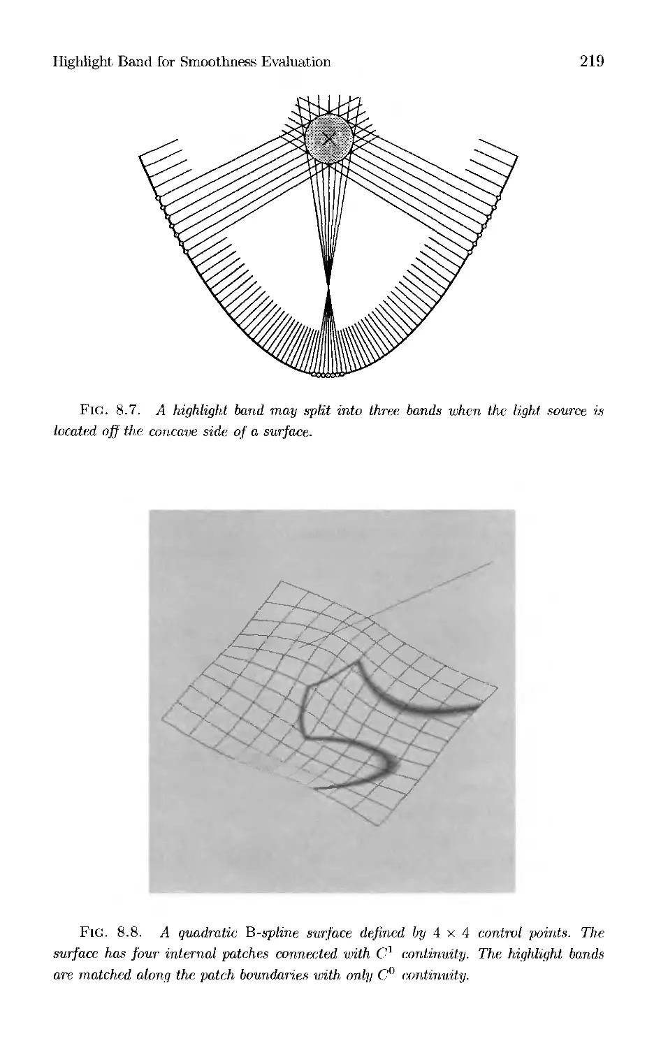
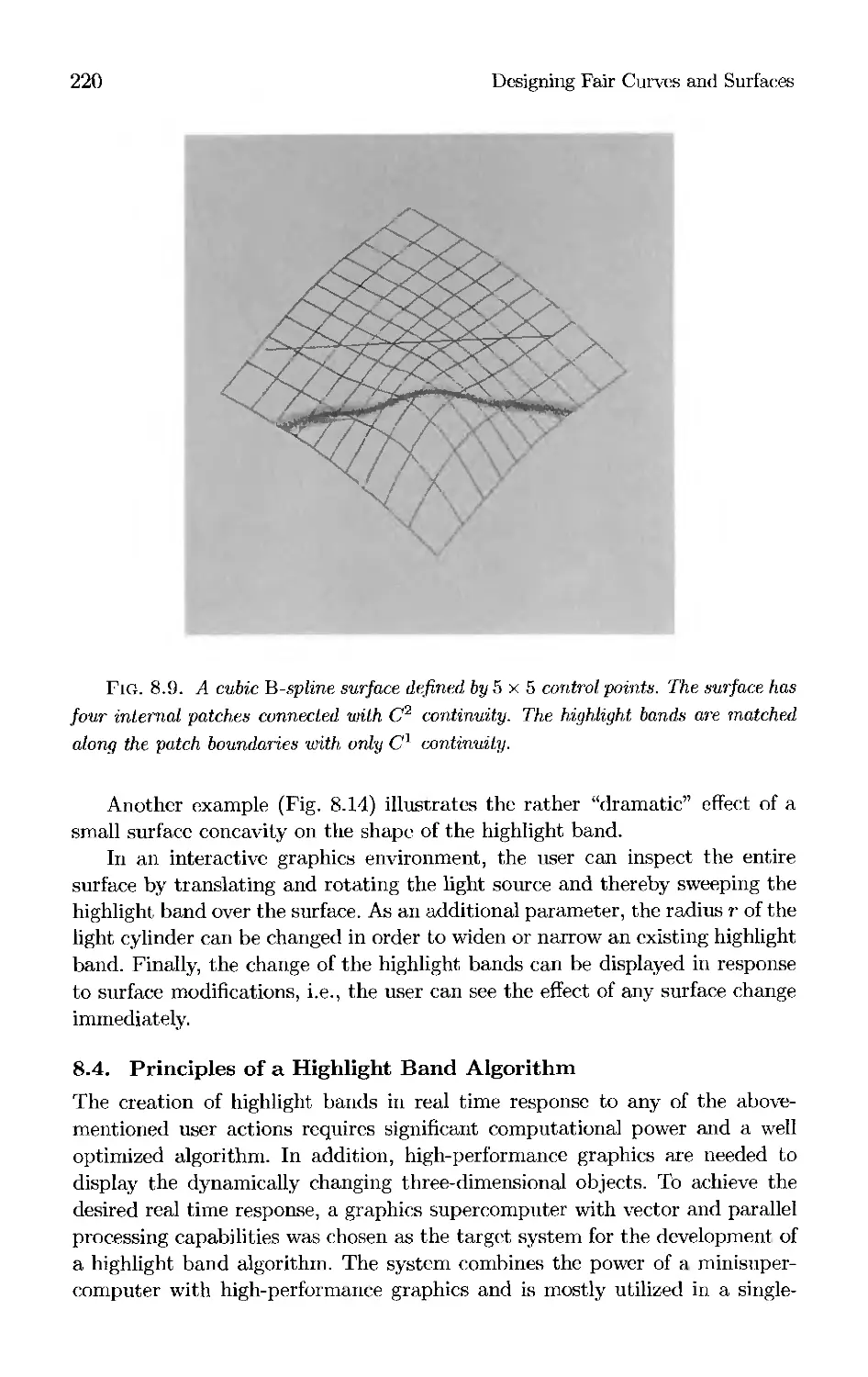
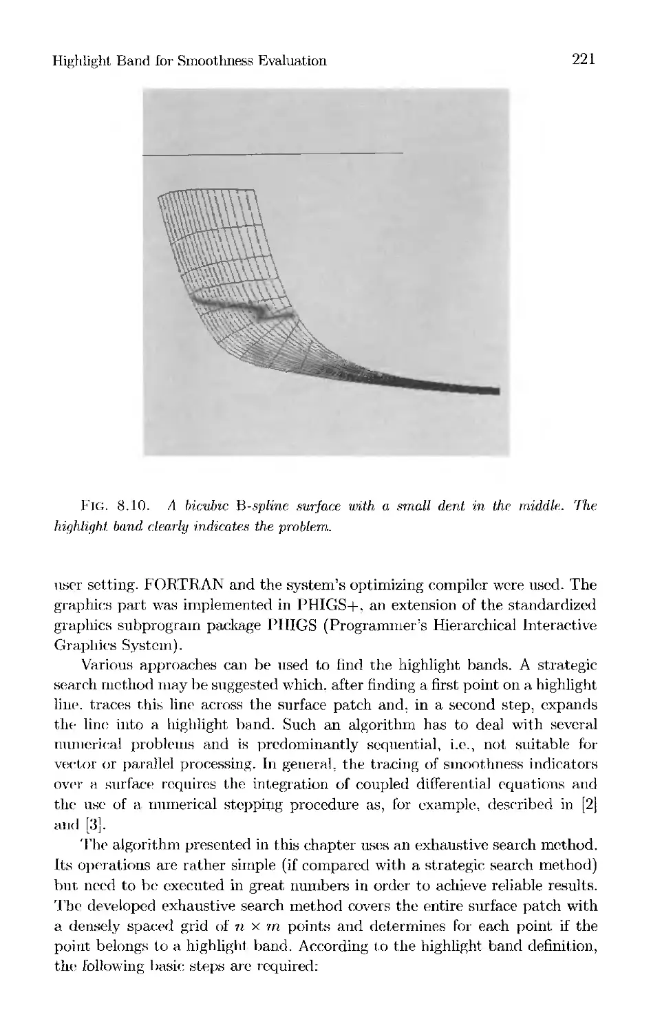
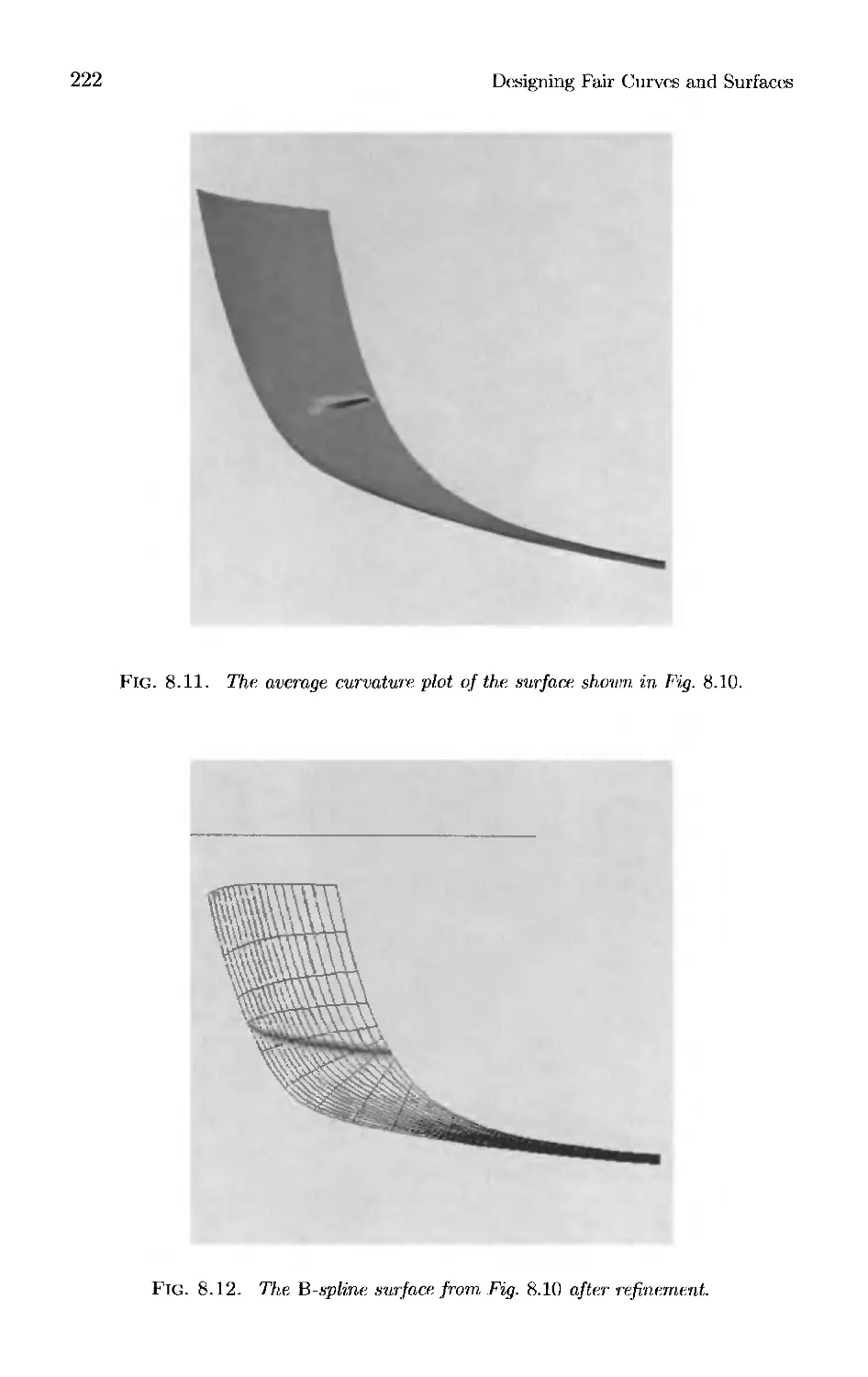
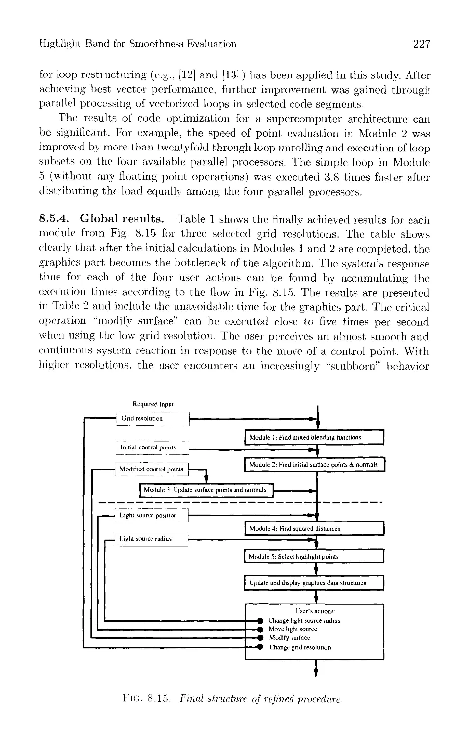
Part 3. Beier and Chen present a simplified model for calculating "reflection lines" on
a surface and demonstrate its usefulness for fully interactive surface analysis and modification.
The paper by Bloor and Wilson demonstrates that the partial differential equation method
produces fair surfaces, and proposes techniques for interactive design of surfaces. Part 3 is
concluded by the work of Ginnis, Kaklis. and Sapidis introducing a new family of polynomial
splines that allow for direct manipulation of the curvature of a parametric interpolator)' curve.
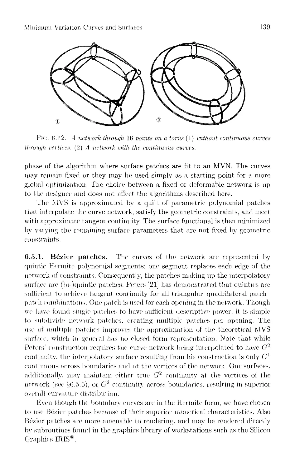
Part 4. The two papers included here reconsider some well-known design problems
focusing on the fairness of the constructed surfaces. More specifically, Peters uses biquadratic
and bicubic splines to develop a new technique for C' surface interpolation, while Zhao and
Rockwood propose a convolution approach to produce "fair" solutions to the problems of N -
sided patch design and vertex blending.
This volume evolved, in part, from presentations given at the Second S1AM Conference
on Geometric Design held in Tempe, Arizona, in November 1991. Also, certain experts were
invited to contribute papers. A total of twenty papers were submitted during the spring and
summer of 1992, of which twelve were selected for publication on the basis of a peer-review
process. Each paper was refereed by at least two reviewers. I would like to thank Robert E.
Barnhill, the Organizing Committee, and the S1AM staff for their efforts in organizing the
XI
Xll
Preface
Second SIAM/GD Conference, and for their help in initiating this book. I especially want to
thank Gerald Farin for his continuous advice and encouragement in all stages of this project,
and William Frey, Hans Hagen, and Ramon Sarraga for their suggestions and ideas. Also, I
thank Susan Ciambrano for her cooperation on the paperwork and preparation of the
manuscript. Finally, I would like to express my appreciation to the reviewers for their diligence;
their names are listed below. This book was prepared while I was working in the Computer
Science Department of General Motors Research Laboratories and it would not have been
possible without the encouragement and support of Drs. Robert Tilove and Paul Besl, and the
Head of the Department, Dr. George Dodd. I also thank the GM Design Staff, in particular Jeff
Stevens and Tom Sanderson, for sponsoring my work during the last two years.
Nickolas S. Sapidis
Warren, Ml
Referees
Antony DeRose
Hans Hagen
Weston Meyer
Steven Pruess
Carlo Sequin
Gerald Farin
Alan Jones
Henry Moreton
Alyn Rockwood
Joe Warren
David Field
Panagiotis Kaklis
Jorg Peters
John Roulier
Andrew Worsey
William Frey
Michael Lounsbery
Bruce Piper
Ramon Sarraga
Part
Fairing Point Sets and Curves
This page intentionally left blank
Chapter
Approximation with
Aesthetic Constraints
H.G. Burchard, J.A. Ayers, W.H. Frey, and N.S. Sapidis
1.1. Introduction
In this chapter, we address the problem of fitting a "fair" curve through or near
a set of given points. ^Fairness" in this case means that the curve must not only
be "smooth" in some mathematical sense, but also that it must be pleasing
to the eye. In other words, there are aesthetic considerations that constrain
the curve-fitting operation. This problem arises in many areas of industrial
design, whenever the appearance of a product is important for potential buyers.
Prominent among such products are automobiles, and since our experience is
primarily in the auto industry, wo address the subject from this point of view.
Most of the approach presented here was developed and implemented by two
of us (Burchard and Ayers) at General Motors in the mid-1960s. But the ideas
described should be useful to workers iu all areas of computer-aided aesthetic
geometric design.
In the traditional manual system for designing the exterior surfaces of
automobiles, the "clay model" is the master- source of information about the
design [l(j\ It is accompanied by the so-called blackboard drawing, a full-size
drawing on paper of the throe standard views of a oar. which contains various
plane- projections of the design lines and section lines of the present and past
versions of the clay model. Iufonnation from the clay model is transferred to
the blackboard drawing by measuring points on the model and plotting them
on the drawing. The •'boardman'' then draws a smooth curve through or near
these1 points. To complete the cycle, information from the blackboard drawing
may be used to reshape the clay model by means of templates cut to the shape
of lines on the drawing.
In this chapter we shall examine the role of the boardman more closely, and
explore- how mathematical curve fitting or curve design would have t,o work if
it is to create mathematical curves as satisfactory to the designer as the ones
produced manually by the boardman.
3
4
Designing Fair Curves and Surfaces
1.1.1. The curve-fitting problem. The work of the boardrnan is similar
to that of other draftsmen who are faced with essentially the same problem at
other stages of the design process [21, pp. 211-213]. Given a list of points Pi
in an (x, y)-plane
Pi = (xi,yi), i = l,...,n,
he needs to construct a smooth curve passing through or near these points
that captures the "design intent." These same points can also be used as input
data for a curve-fitting computer program. But the boardman is actually given
much more information than just the points Pi, and this information must also
be made available for the computer program. How can this be done?
The boardman gets this additional information by studying the clay model,
asking the designer about his intentions, and above all by using his own
aesthetic judgement to tell him whether his line is "good looking" and consistent
with other design lines on the car. Also based on this information is the board-
man's decision on the deviations of the data points P{. He may first attempt
to fit the data within a standard tolerance, but he may revise this tolerance if
one of the points turns out to be "wild" (i.e., has a much larger deviation) —
which ordinarily would be due to either an error in measuring or plotting, or
a depression in the clay.
But the most important decisions of the boardman as he strives for the best
looking line occur when he detects "ogees" (S-shaped segments), "fiat spots,"
"buckles," or "bumps" as he judges the overall shape of the curve. He may
use expressions like "accelerating" or "decelerating," or determine whether a
"bend," "break," or "corner" is "sharp" or "rounded." He may discard a line
because it looks "bulgy" or "knobby," etc. To do his job properly, he must
be able to decide, or know from some other source, if and where ogees,
maxima, and minima of the curvature, corners, and flat segments are supposed to
occur. This sensitivity to the visual properties and features of curves is
standard practice among artists, as can be seen, for example, in a book by Nelms
[21, pp. 31-34].
1.1.2. The principle of simplest shape. Generally speaking, the board-
man will try to draw a curve in which ogees and other key features occur the
minimum number of times within the design intent. We may say that he
follows the principle of simplest shape, an idea that is generally applied in the
fine arts. Beautiful objects, it is said, are uncluttered, i.e., free of unessential
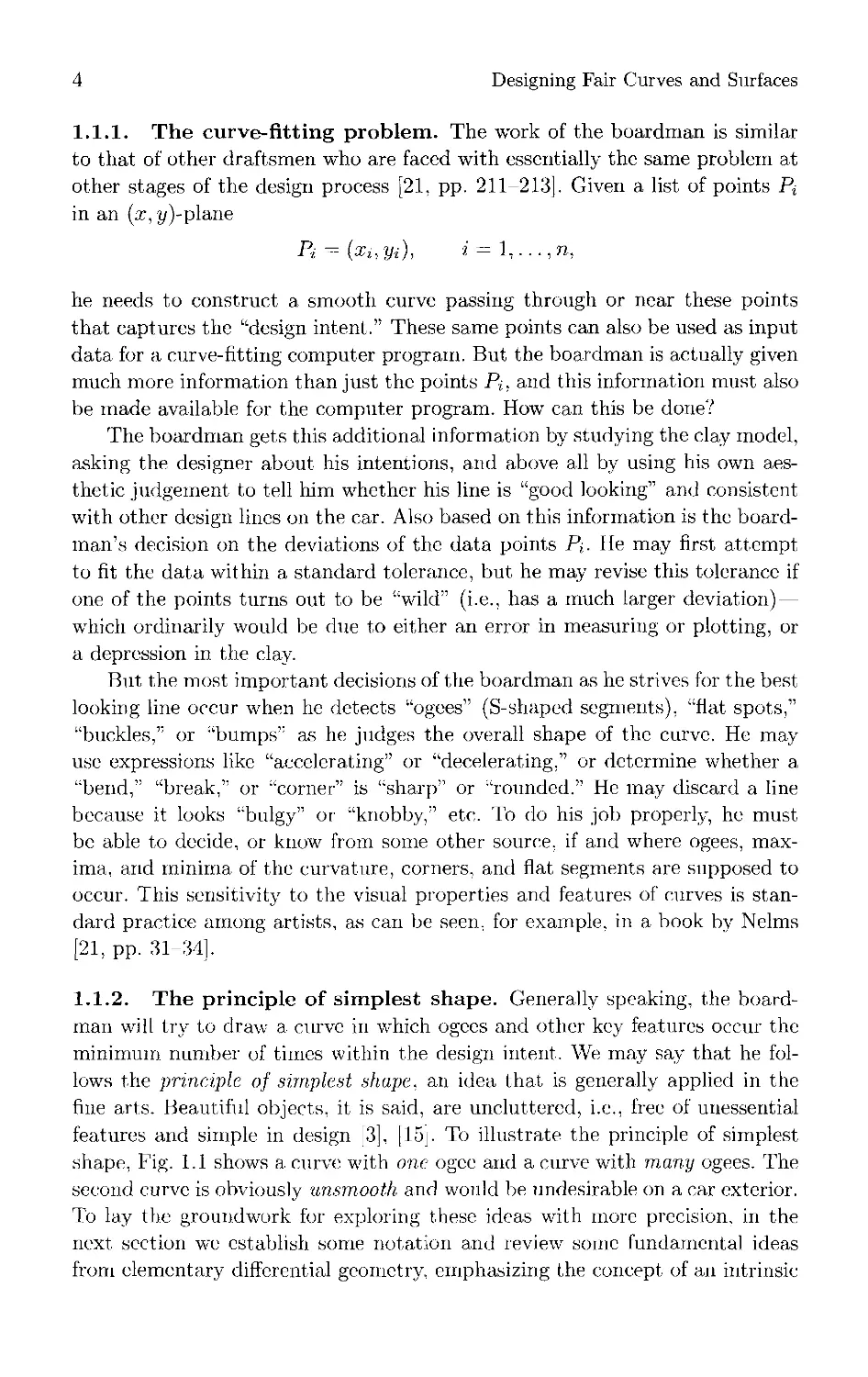
features and simple in design [3], [15j. To illustrate the principle of simplest
shape, Fig. 1.1 shows a curve with one ogee and a curve with many ogees. The
second curve is obviously unsmooth and would be undesirable on a car exterior.
To lay the groundwork for exploring these ideas with more precision, in the
next section we establish some notation and review some fundamental ideas
from elementary differential geometry, emphasizing the concept of an intrinsic
Approximation with Aesthetic Constraints
Fig. 1.1. (a) A curve, with one. ogee, (b) A curve with many ogees.
equation of a curve or a class of curves, i.e.. a condition on the curvature. As we
shall see, the visual features which concern the boardman are easily translated
into certain corresponding mathematical properties of the intrinsic equation.
1.2. Differential Geometry of Plane Curves
In this section we briefly review certain fundamental concepts of the elementary
differential geometry of plane curves and establish appropriate notation. The
restriction to plane curves is in line with the boardman's work dealing with
plane projections of design lines. The following considerations may be applied
simultaneously to the several standard projections.
1.2.1. Parametric C -curves. We can represent plane curves in several
different, ways. FTowever parametric representations have overwhelming
advantages for investigating the aesthetic properties of curves. Our notation and
terminology follow closely those of standard texts in differential geometry fl-)|-
[25,. We shall assume that any curve of interest is a curve segment lying in a
Euclidean plane with a Cartesian (./•. </)-coordinate system, as shown in Fig. 1.2.
The parameter / is an independent real variable with domain in a bounded arid
closed interval [«./>;. and the curve is defined as a continuous vector function
c(7) = (.r(t). y(t)) . We assume; throughout that the tangent vector c'(t) exists
and is a continuous function of /. Tn other words, the curve is always of class
Cn. Included among the C1-curves are the C^'-curves (k > 1). for which all
derivatives for / = 1 k exist and are continuous.
1.2.2. Arc length. We can think of each point c(/) as the position at time
/ of a particle moving along the curve. Arc length. ,s = s{t), measured along the
curve from the initial point c(a) of the curve to the point c(f). is the distance
travelled by the particle since1 time t = a. With c'(f) = (.r'(t). g'(t))1 we may
6
Designing Fair Curves and Surfaces
t = a
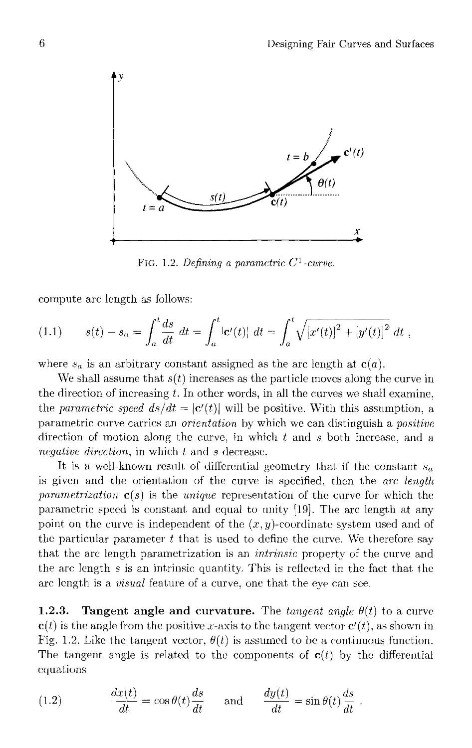
Fig. 1.2. Defining a parametric C1 -curve.
compute arc length as follows
^ds
(1.1)
»(*)
Sa =
dt
dt
\c'{t)\ dt
= f\l\x'(t)? + [v'{ttdt
where sa is an arbitrary constant assigned as the arc length at c(a).
We shall assume that s(t) increases as the particle moves along the curve in
the direction of increasing t. In other words, in all the curves we shall examine.
the parametric speed ds/dt = \c'(t)\ will be positive. With this assumption, a
parametric curve carries an orientation by which we can distinguish a positive
direction of motion along the curve, in which t and s both increase, and a
negative direction, in which t and s decrease.
It is a well-known result, of differential geometry that if the constant sa
is given and the orientation of the curve is specified, then the arc length
parametrization c(s) is the unique representation of the curve for which the
parametric speed is constant and equal to unity [19]. The arc length at any
point on the curve is independent of the (x, y)-coordinate system used and of
the particular parameter t that is used to define the curve. We therefore say
that the arc length parametrization is an intrinsic property of the curve and
the arc length s is an intrinsic quantity. This is reflected in the fact that the
arc length is a visual feature of a curve, one that the eye can see.
1.2.3. Tangent angle and curvature. The tangent angle 9{t) to a curve
c(i) is the angle from the positive x-axis to the tangent, vector c'(t), as shown in
Fig. 1.2. Like the tangent vector, 6{i) is assumed to be a continuous function.
The tangent angle is related to the components of c(i) by the differential
equations
'1-2)
dxit) n. ^ds
—^ = cos (9 (t) —
dt y ' dt
a dy^ ■ a<+\ds
and —:— =sm6>m —
dt K ' dt
Approximation with Aesthetic Constraints
7
The curvature k is defined to be the amount of bending of the curve at any
point on the curve where 9{t) is differentiable. More precisely, k, is the derivative
of the tangent angle 6 with respect to arc length:
dO dO ids
(1.3) k(s) = — = -— / — .
■ ' ■ ' ds dtl dt
Like the arc length, the curvature at any point of a curve is an intrinsic
quantity, independent of the parametrization and the position or orientation in the
Cartesian coordinate system. Similarly, the curvature and its reciprocal R, the
radius of curvature, defined by
(1.4) fl(s) = J_ K^0,
are visual features of a curve.
Notice that definition (1.3) implies that curvature is a signed quantity,
positive if the curve is turning to the left (increasing 0), 'negative if it is turning
to the right (decreasing 0), when traversed in the positive direction. Equation
(1.3) also reveals the intimate connection between the tangent angle 0 and the
curvature. In particular, if the function k(s) is given, then we caii integrate
(1.3) to obtain
(1.5) e(s)-0(fi„)= I n{a)da .
This shows that the net change in the tangent angle from ,s = sa to a generic
point s on the curve depends only on the intrinsic quantities k and s. and
therefore 9(s) — 0(s„) is also an intrinsic quantity. Like the arc length and
the curvature, it is a visual quantity depending only upon the shape of the
curve.
1.2.4. Intrinsic equation. Another important result from differential
geometry is that if a given function k,(s) is piecewisc continuous (has at most a
finite number of jump discontinuities), then equations (1.2) and (1.3) can
always be integrated to obtain the curve c(t) (up to a translation and a rotation)
[2-r)|. The equation
(1.6) k = k(.s)
is known as the intrinsic equation of c(t). This representation is of critical
importance to our analysis since it completely defines the shape of a curve
independent of its orientation or position within the (.r.y)-coordinate system.
Plots of k versus ,s are now a widely used tool for designing and modifying
plane curves [llj. [17], [20].
8 Designing Fair Curves and Surfaces
We can also talk about the intrinsic equation of a class of curves. To
illustrate, consider the equation
(,7) ^>=0.
This equation is not of the form (1.6), but integrating it twice gives
(1.8) k(s) = cs + oI,
where c and d are arbitrary constants. For fixed c and d, (1.8) is the intrinsic
equation of a curve, namely an Euler spiral. Thus the differential equation (1.7)
characterizes all Euler spirals intrinsically, and is therefore the intrinsic
equation of all Euler spirals. In the following sections we shall explore conditions
still more general in form, for example, the condition
(1.9) ^ > 0 .
ds*'
While this is an inequality rather than an equation, it is an intrinsic condition
characterizing a particular class of curves (which includes all Euler spirals).
1.3. Aesthetics and Monotonicity of Curvature
1.3.1. Visual properties and the intrinsic equation. There is an
essential fact inherent in our discussion that must be brought out: all of the features
about which the boardman must make decisions are mathematical properties
of the intrinsic equation (1.6). This is clear a priori, since a plane curve is
completely specified by its intrinsic equation.
Moreover, translating the visual properties of a curve into mathematical
properties of its intrinsic equation is relatively straightforward, since k and s
are of a visual nature themselves. In fact, those visual properties of a curve
that affect the aesthetic qualities of concern to the boardman and designers
correspond to exact metric properties, and these in turn translate into specific
mathematical equivalents: an ogee is a point where k changes sign. In between
ogees the curve is either convex or concave, or k has constant sign, i.e., k > 0
or k < 0. A flat spot is a minimum of \k,\. A buckle, bump, corner, or break is
a maximum of |k|. In between maxima and minima of |k| the curve is either
accelerating or decelerating, which translates into \k\ being either m.onotone
increasing or decreasing.
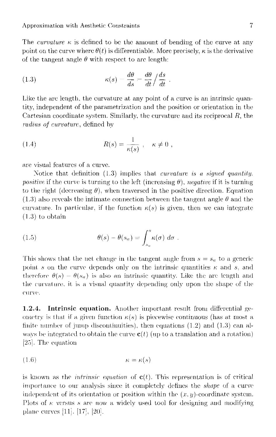
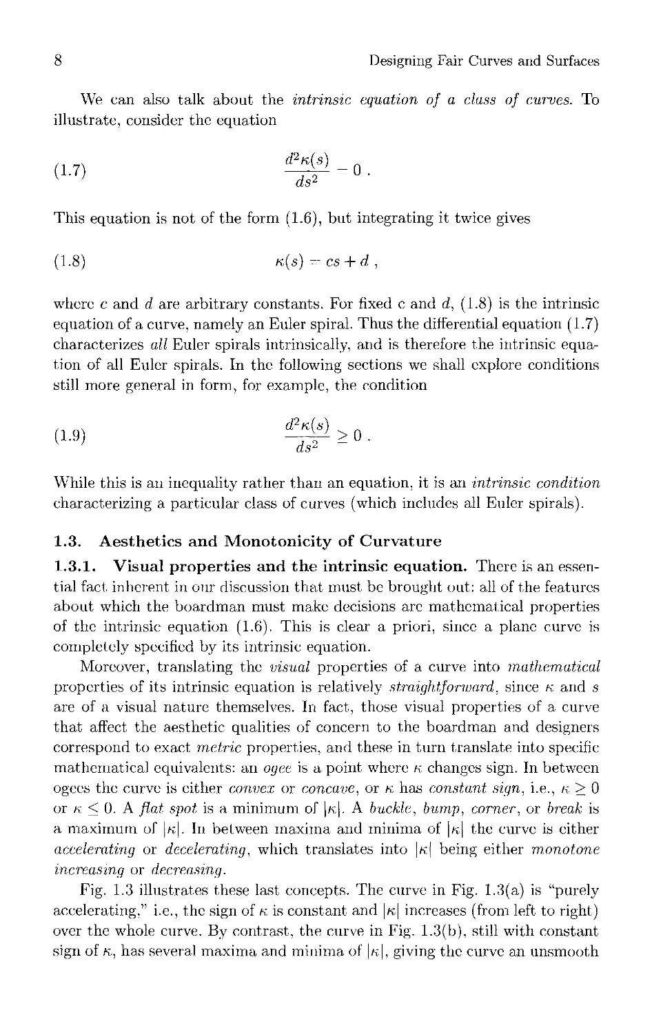
Fig. 1.3 illustrates these last concepts. The curve in Fig. 1.3(a) is "purely
accelerating," i.e., the sign of k is constant and |k| increases (from left to right)
over the whole curve. By contrast, the curve in Fig. 1.3(b), still with constant
sign of k, has several maxima and minima of |k|, giving the curve an imsmooth
Approximation with Aesthetic Constraints
9
(a)
(b)
FlO. 1.3. (a) A curve with monotone curvature, (b) The curvature of this curve
has several local maxima and minima.
appearance compared with the one above. This again illustrates the principle
of simplest shape; cf. <-jl.1.2.
We can summarize these remarks as follows: constraints or aesthetic re-
quircments for a plane curve can be expressed as fairly simple
mathematical conditions on the 'intrinsic equation, i.e., as conditions on the function
K(.sj.
1.3.2. Monotonicity conditions on the curvature. To develop a
computer program that can produce1 curves as good as a draftsman can draw, we
need a "complete set" of aesthetic constraints (and their translation into
curvature conditions) used by draftsmen in judging the quality of curves. Some
of these conditions emerge if we apply the principle; of simplest shape to the
number of ogee's, and of minima and maxima of k. We list these conditions
under (a) (el), below. Their significance is illustrated in Figs, f.l and 1.3.
10
Designing Fair Curves and Surfaces
(a) Sign changes and maxima and minima of the curvature possess obvious
visual equivalents. By the principle of simplest shape, the numbers of
occurrences of each of these features should be kept as small as possible subject
to and consistent with the design intent. This implies that their numbers and
locations should be determined explicitly. Some ways to do this are described
in (b)-(d).
(b) If data points Pi (i = 1,..., n) for a plane curve are given (points
measured from a model or a drawing), then the numbers and locations of sign
changes of k, as well as of the maxima and minima of k. can be specified as
additional input information for a computer program intended to compute a
smooth, aesthetically pleasing curve passing through the data points. That
this can actually be done by a draftsman with minimal mathematical training
should be clear from the Introduction, since the same or at least analogous
decisions would be made by him on the drawing board.
(c) Using the principle of simplest shape, we can try to write a computer
program to replace the draftsman by computing numbers and locations of sign
changes and maxima and minima of k. More specifically, given a tolerance e, a
program may be written to find the minimal numbers of such features
necessary to approximate the data within tolerance e. Simultaneously, the computer
program can try to optimize their locations, i.e., it can try to come as close
to the data points as possible, subject to the limitation on the number of sign
changes, maxima and minima of k. The justification of this approach is that
the draftsman does something quite similar, as described in the Introduction
to this chapter.
(d) Approaches (b) and (c) both have their difficulties. For example, a
designer sometimes may not be able to specify locations of sign changes of
k with sufficient accuracy. This problem could be managed by the following
scheme. First the designer specifies numbers and locations of sign changes,
maxima and minima of n approximately—according to (b). This information
can then be checked and locations optimized—according to (c). The
optimization of locations of sign changes, maxima and minima of k, may be expected to
appreciably decrease the deviations of data points from a computed curve. In
other situations these locations may not be variable due to design constraints.
Any restriction on the number of maxima and minima of k is equivalent
to a restriction on the number of separate curve segments where the curvature
k is monotone (increasing or decreasing). Therefore, we refer to the
conditions (a)-(d) on maxima and minima of k as monotonicity conditions on the
curvature. Considering curves of class C3, we could say that monotonicity
conditions are sign conditions on dnjds, and we shall do this for convenience,
even though our curves are only C2 or even piecewise C2. In such cases one
can define monotonicity as constancy of the sign of the difference quotient
Ak/As = (k(s2) — k(si))/(s2 — si). Accordingly, wc can say that conditions
(a)-(d) amount to specifying the signs of k and dn/ds {or Ak/As) at each,
point of the curve.
Approximation with Aesthetic Constraints
11
Monotonicity of the curvature is important for a variety of curve design
applications [12]. [22], [23]. Many curves (most spirals, for example)
inherently have monotone curvature, and conditions for curvature monotonicity
of some nonspiral curves have been established [14], [24]. However, although
monotonicity conditions form a partial set of aesthetic constraints for the
fitting of plane curves, they are not a complete set. Additional conditions--on
the convexity of k are also needed. We discuss these beginning in the next
section.
1.4. Aesthetics and Convexity of Curvature
1.4.1. The styling radius. A common practice in engineering is to round
off the sharp corners of an object using a circular arc, as shown in Fig. 1.4(a).
The resulting curve, sometimes called a simple radius, consists of two straight
line segments connected by the circular arc. The curvature distribution of this
curve1 is displayed in Fig. 1.4(b). Tn this case k.(,s) has two jump discontinuities.
Observe, however, that h(s) has no sign changes (the curve has no ogee) and
the curve can be divided (at the midpoint of the arc) into two symmetric
segments with monotone curvature. This indicates that the curve should be
considered rather smooth in light of our earlier- remarks. Nonetheless, artists
and designers feel that this curve is not attractive. To remedy this, when they
need to draw a smooth corner linking two relatively Hat curves, they use a
device known as a sfyhn.g radius.
A styling radius is a template made by first cutting a piece of material such
as plexiglass to a simple radius and then "shaving olf" a bit when1 the circular
arc joins the straight lines, as shown in Fig. 1.5. This makes the transition
between the Hat ends and the strongly bent corner more gradual. Artists might
say that the simple radius looks "knobby" or "bulgy" as opposed to a styling
radius. 44k1 styling radius shown in Fig. 1.5 was constructed from two
symmetric cubic parametric curves that join at the point of maximum curvature. As
with the original curve, the curvature distribution consists of two symmetric
parts, one of which is monotone decreasing (shown in Fig. 1.5). and the other,
monotone increasing.
In view of this example, where1 we have a curve1 with minimally piece-
wise1 monotone curvature1 which is not deemed attractive, we need to discover
additiemal conditions em k in order to obtain a "cemiplote set" of aesthetic
constraints for matlieMiiaticai eurve'-fairing.
1.4.2. The need for a smooth curvature distribution. It seems
plausible1 that the attractiveness of the1 styling radius (Fig. 1.5) versus the original
eairve1 (Fig. 1.4(a)) is related to its hupmwel curvature distribution, especially
the1 elimination of the jumps in k(,s). For an heuristic argument, one might
imagine that the1 eye1, in scanning the curve1 and sensing the curvature,
receives a stimulus relateel to the size of k. If k. changes suddenly, so will the
stimulus anel this may give rise to an unpleasant sensation.
12
Designing Fair Curves and Surfaces
(a)
R
(b)
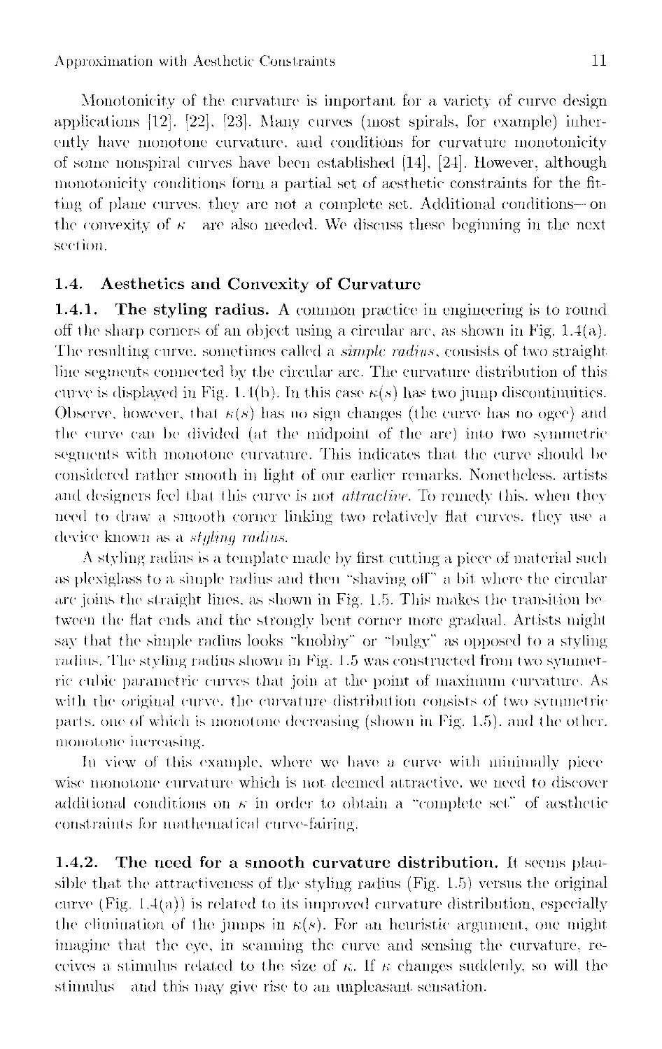
FlG. 1.4. Simple radius (a) constructed by rounding a corner using a circular
arc, and its curvature distribution (b).
A similar situation occurs when a vehicle is driven from a straight road into
a curve of constant radius. Passengers experience a sudden (jump) change in
the side force (centripetal acceleration). To reduce this unpleasant sensation on
high speed roads (and to improve safety), engineers routinely design transition
curves (usually Euler spirals) between straight and circular road sections [1],
These replace the discontinuous curvature plot of the plane view of the roadway
by one that is continuous (in this case, piccewise linear).
For our purposes, we need to find mathematical conditions which eliminate
jumps in the curvature and constrain the shape of the curve to be more
attractive, more like the styling radius. As we explain in the sections that follow, our
solution to this problem involves the use of convexity conditions (and
generalized convexity conditions) on the curvature. This was suggested to us by an
empirical observation: In all of the curvature plots we computed for automobile
design lines, a shape like that shown in Fig. 1.6 recurred: the point or points
Approximation with Aesthetic Constraints
13
FlG. i.5. A styling radius constructed from a simple radius, and the eurvature
distribution of half of the styling radius.
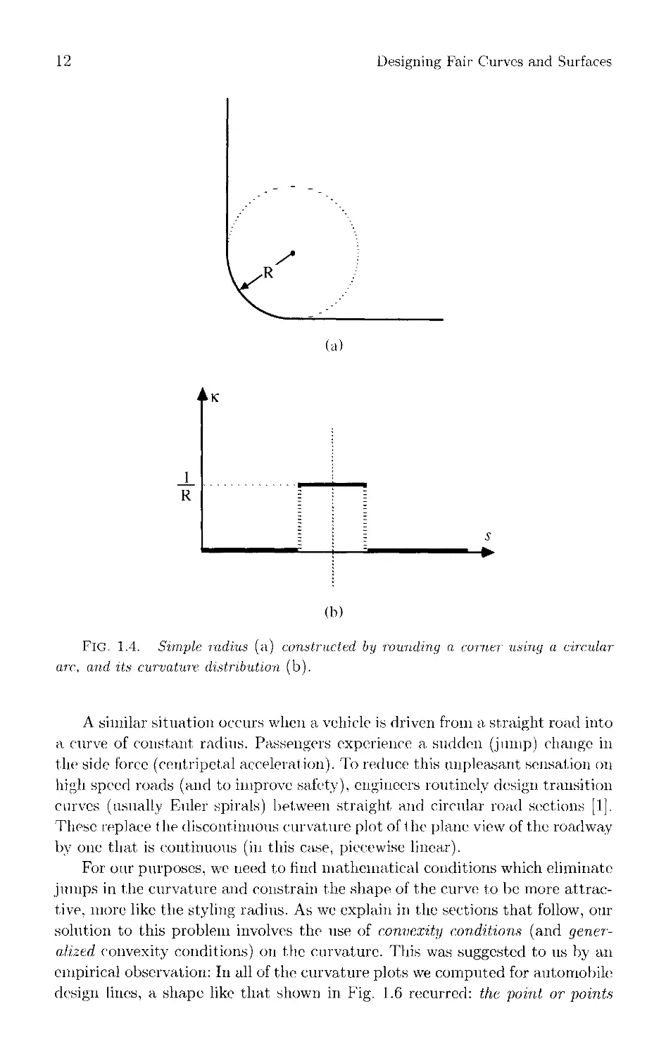
of maximum absolute, value of the curvature divide (.s) the plot of \n\ versus s
■into distinct sections, each of which is convex.1 Consequently, at any
maximum of \k\ the slope dn/ds is discontinuous. This slope1 discontinuity in k(,s) is
an advantage in that it unambiguously identifies a unique design feature and
its location. As an explanation for these empirical observations we offer that
design lines have characteristic shapes. This is reflected in the fact that their
intrinsic equation k -— /v(,s) has concentrated high curvature magnitudes on
short ares. Broad curvature maxima with concave1 |k(.s)| simply do nol occur.
1.5. Conditions for Convexity of Curvature
We shall now assume that our curve of interest has been partitioned into
distinct segments in such a manner that for each the curvature k and its first
derivative d.H./ds both have constant signs. In other words, the points where
sign changes of curvature (ogees), or maxima, and minima of curvature occur
have been identified, and we can now focus our attention on any one of these
segments with monotone curvature of constant sign.
1.5.1. Curvature convexity made precise. For convexity considerations,
we are only interested in the properties of the magnitude or absolute1 value1 of
1 When the graph of a function is convex downwards (concave upwards) wo shall follow
the usual convention and call it simply convex [7, p. 246], concave in the opposite case.
14
Designing Fair Curves and Surfaces
|K|
S
-►
FIG. 1.6. The point of maximum absolute value of the curvature divides the plot
of \k(s)\ vs. s into convex sections.
the curvature |k|, as was explained above. Consider a curve segment of class
C4. When referring to convexity of the curvature \k\ we mean the condition
;i.io)
d?\
ds1
>0 .
For curves that are merely piecewise C2, we define convexity of |k| as mono-
tonicity of the difference quotient
:i.in
k(s3)|
\K (S2\
>
K(S2
l«(SOI
S'3 - S2
S2 ~ S\
if 51 < S2 < «3
For convenience, we shall refer to convexity of |k| simply as a sign condition
on d2\n\/ds2 as in (1.10). All the statements to be made can be translated to
the more general case (1.11).
1.5.2. Intrinsic parameters. In order to study conditions of convexity of
curvature more closely, it turns out that we need to understand how these
conditions relate to various allowable parametrizations. To be geometrically
meaningful, all such conditions must be expressed in terms of the intrinsic
equation of a curve. However, only those parameters t that are closely related
to the geometry of the curve, i.e., to the intrinsic equation, reflect intrinsic
properties of a curve. Such a close relationship is present, for example, if the
parametric speed \ds/dt\ is a positive continuous function g(\n\) of the
curvature K,
(1.12)
ds
~dt.
= .9(N)>0
In this case we shall say that, the allowable parameter t is an intrinsic
parameter.
Suppose now that t is some intrinsic parameter. Compared with the simple
visual interpretations of sign(K.) and sign(dK/ds) discussed in §1.3, the
condition of convexity of the curvature is more difficult to explain and, admittedly,
Approximation with Aesthetic Constraints
15
not as well understood. This appears to be related to certain mathematical
facts, as follows: If k = n(t) has constant sign on a segment of a curve, then
it does so also for any other allowable parameter. Likewise if k = n{t) is a
monotone function of f, then it is also monotone as a function of any other
allowable parameter. However, |k| may well be convex as a function of the
intrinsic parameter t but not for some other intrinsic parameter. To see this,
consider a curve with the intrinsic equation
k = s2 , 1 < s < 2 .
Then \k\ is a convex function of s. But if we introduce the allowable parameter
t = k'2, we get
|k| = Vt , 1 < t < 16 ,
and \fi is not a convex function of t.
This example shows that we can expect to obtain convexity conditions
of different geometric significance (and hence different aesthetic meaning) by
considering convexity conditions of the form
(1-13) ^H>0
for various intrinsic parameters t.
1.5.3. Intrinsic convexity conditions. If t is an intrinsic parameter, we
consider intrinsic convexity conditions of the form (1.13), and show that such
conditions are equivalent to a condition of the form
(1.14) ^_/(|K|)>0)
where f{\n\) is some twice differetitiable function of |«;|. Both conditions (1.13)
and (1-14) may be called intrinsic convexity conditions on \k\. Carrying out
the indicated differentiations and using (1.12) leads to the inequalities
;i.i5)
tf2|K.| d fd\n\ds\ds d fd\n\ ds
dt2 ds \ ds dt J dt ds \ ds
and
dt
It
d fd\n\
ds V ds
3(l«l))-y(N)>0
Evidently conditions (1.15) and (1.16) are equivalent, provided it is known that
;i-i7) /'(N) = .9(i«i
ds
~dt
>0
16
Designing Fair Curves and Surfaces
Hence, we see that the condition of convexity of \k\ with respect to an intrinsic
parameter t is equivalent to the condition of convexity of a function f(\n\)
with respect to arc length, s, the definition of t and its relation to f{\n\) being
contained in (1-17). Henceforth we shall assume that }{\k\) and <7(|«|) satisfy
(1.17), and therefore that (1-15) and (1.16) are equivalent.
1.5.4. Example. As we might expect from (1.5), the tangent angle 6 turns
out, to be an intrinsic parameter. To sec this we write, using (1.3),
(1.18) (log 1*1)' = ^
\k\
ds
~6B
>0 (k/0).
Clearly the requirement (1.12) for an intrinsic parameter is satisfied if .9(|k|) =
1/|k|. Moreover, (1.18) is of the form (1.17) with /(|k|) = logj/tj. Applying
the above results, we then find that the following two convexity conditions are
equivalent:
d2\n\
(1.W) -&>»
and
;i.2o) _iog|«|>o
d2_
da"1
In words, the condition of convexity of k with respect to 9 is equivalent to the
condition of logarithmic convexity of k with respect to s.
1.5.5. Another form of the convexity condition. Convexity condition
(1.14) can be written in still another form, by carrying out the differentiation
in (1.16) and using /'(|k:|) > 0, namely
(1.2D * w> H-h'nM)
ds2' ' - V ds ) /'(|k|) '
Thus an intrinsic convexity condition on | k | amounts to imposing a lower bound
on (d2\n\)J'ds2. From this it can be seen that such conditions have varying
strength depending on the size of the lower bound.
1.5.6. Alpha convexity. We propose in this chapter that a safe and
workable method of ensuring aesthetically pleasing curves may be obtained by
imposing on the curves a sufficiently strong form of curvature convexity condition.
Ideally a designer should have a family of such conditions from which to choose.
In this section we define such a family, and in the remainder of the chapter we
explore the effectiveness of this approach.
Approximation with Aesthetic Constraints
17
We choose a family of conditions, referred to as a-convexity conditions, for
which the strength depends on a single parameter a in a simple way. In (1.14)
let
\n\a . a > 0;
(1.22) f(\K\) = f„(\K\) = { log |4 a = 0:
-\K,\n , a < 0.
When equality is required in (1.14) instead of the inequality we obtain the
intrinsic equation d2fa(\n\)/ds2 = 0. This includes some well-known families
of curves [27] which are thus seen to be a-convex:
• a = 1: Euler spirals, also called Cornu spirals or clothoids. /(|«'|) — j\\k\ —
k is linear in ,s\ k — as + b.
• a = - 1: logarithmic or equiangular spirals.
• a = —2: involutes of circles. Involutes of circle have interesting and
possibly useful mathematical properties. The radius of curvature R is a linear
function of the tangent angle 0. i.e.. R = a.6 + b. This can be integrated
exactly giving a curve with linear parameters if 0 is used as the allowable
intrinsic parameter.
With the function / defined by (1.22). formula (1.21) now reads
(1-23) !PM>(1_n)ii
dsz | K. |
We considered the ease a ~ 0 in §1.5.4. Evidently the strength of (1-23)
increases as a decreases and vice versa.
1.6. Alphaconvexity and Aesthetics
By imposing condition (1.23) on the curvature, jumps are indeed eliminated
because of a classical result that a convex function on an open interval must be
continuous. In spite of this true mathematical fact, tests have shown that the
condition (d2\H.\)/ds2 > 0 still permits curves that may be unsatisfactory for
automobile exteriors, and in fact subject to objections similar to those made
against the curve in Fig. 1.4(a) that gave1 rise to the styling radius. In an effort
to elucidate this situation, we conducted further experiments which seemed to
indicate that replacing the condition
ft'2 I K \
(1.24) ^>0
dsz
(cv-convexity with a = 1) by the condition
d2 log Ik.I
(1-25) *' ' >0
dsz
(cv-convexity with a - 0) produced perfectly acceptable curves.
18
Designing Fair Curves and Surfaces
In trying to explain why the condition (1.25) of logarithmic convexity of
k is sufficient and the condition (1.24) of ordinary convexity is not, we first
point out that (1.25) is stronger than (1.24). This can be seen from (1.23),
where a — 0 gives (1.25) and q = 1 gives (1-24). Furthermore, a curvature plot
obtained when (1.24) is used in our optimizer tends to look like the one shown
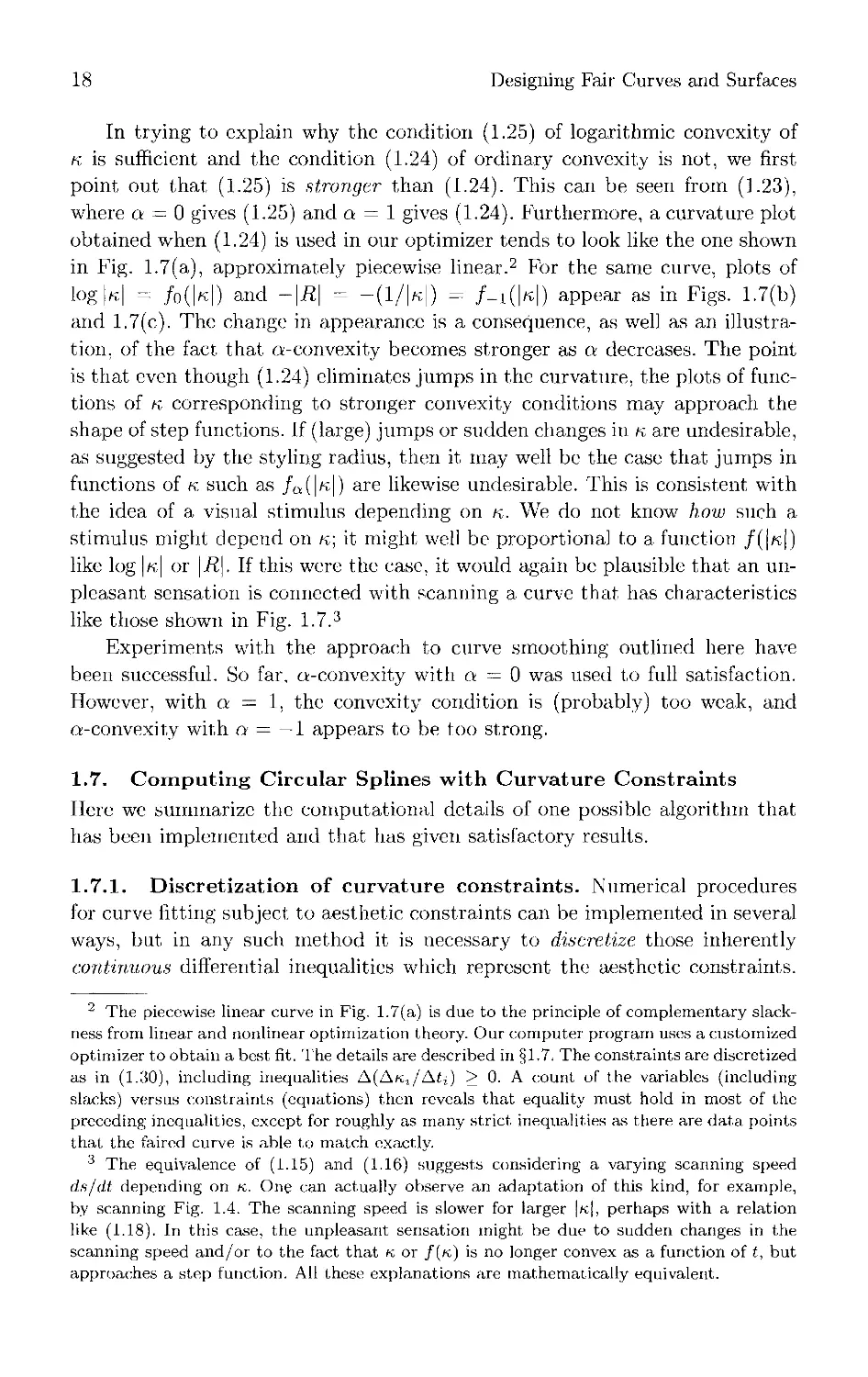
in Fig. 1.7(a), approximately piecewise linear.2 For the same curve, plots of
log |K| = Jo(\k\) and —\R\ = —(1/|k|) — /_i(|/c|) appear as in Figs. 1.7(b)
and 1.7(c). The change in appearance is a consequence, as well as an
illustration, of the fact that a-convexity becomes stronger as a decreases. The point
is that even though (1.24) eliminates jumps in the curvature, the plots of
functions of k corresponding to stronger convexity conditions may approach the
shape of step functions. If (large) jumps or sudden changes in k are undesirable,
as suggested by the styling radius, then it may well be the case that jumps in
functions of k such as /(j(|k|) are likewise undesirable. This is consistent with
the idea of a visual stimulus depending on k. We do not know how such a
stimulus might depend on k; it might well be proportional to a function /(|k|)
like log |k| or \R\. If this were the case, it would again be plausible that an
unpleasant sensation is connected with scanning a curve that has characteristics
like those shown in Fig. 1.7.3
Experiments with the approach to curve smoothing outlined here have
been successful. So far. en-convexity with a = 0 was used to full satisfaction.
However, with a — 1, the convexity condition is (probably) too weak, and
a-convexity with a = — 1 appears to be too strong.
1.7. Computing Circular Splines with Curvature Constraints
Here we summarize the computational details of one possible algorithm that
has been implemented and that has given satisfactory results.
1.7.1. Discretization of curvature constraints. Numerical procedures
for curve fitting subject, to aesthetic constraints can be implemented in several
ways, but in any such method it is necessary to discretize those inherently
continuous differential inequalities which represent the aesthetic constraints.
2 The piecewise linear curve in Fig. 1.7(a) is due to the principle of complementary
slackness from linear and nonlinear optimization theory. Our computer program uses a customized
optimizer to obtain a best fit. The details are described in §1.7. The constraints are discretized
as in (1.30), including inequalities A(Afcl/At;.) > 0. A count of the variables (including
slacks) versus constraints (equations) then reveals that equality must hold in most of the
preceding inequalities, except for roughly as many strict inequalities as there are data points
that the faired curve is able to match exactly.
3 The equivalence of (115) and (1.16) suggests considering a varying scanning speed
ds/dt depending on k. One can actually observe an adaptation of this kind, for example,
by scanning Fig. 1.4. The scanning speed is slower for larger |k|, perhaps with a relation
like (1.18). In this case, the unpleasant sensation might be due to sudden changes in the
scanning speed and/or to the fact that k or /(«;) is no longer convex as a function of t, but
approaches a step function. All these explanations are mathematically equivalent.
Approximation with Aesthetic Constraints
19
(a)
log|tc|
(b)
(c)
Fig. 1.7. AlUwuc/h 'k| = \n(s)\ is jar from being a step function, fids may not
be true for some junctions J{\k\). e.g.. ,/(|k|) = —l/[h'|.
To simplify, the following discussion is restricted to the situation of a curve
consisting of a single segment with constant signs of the curvature, its first
and second derivatives with respect to some allowable parameter t,
(1.26)
K > 0,
>0. ^>0-
dt
2 ~
At this point we settle on a definite choice of intrinsic parameter, the
tangent angle t = 0. This occurs for /(k) = /«(«), with a — 0; cf. §1.5.4. This
means that we require logarithmic convexity of k with respect to arc length, a
fairly strong grade of convexity condition, yet not excessive. According to our
20
Designing Fair Curves and Surfaces
experiments this condition appears to be suitable for general purpose
automotive design.
There are several options for carrying out the required discretization. One
way is the approximation by some type of spline function for which it is easy to
enforce the aesthetic constraints. Discretization by means of circular splines,
i.e., C1-curves made up of circular arcs, is attractive due to the inherent
simplicity of geometry and algebra connected with circles. Of course, the circular
arcs of the spline must be sufficiently short so that the jumps in curvature
between arcs are too small to be noticeable (because, after all, convexity of |k|
was introduced to eliminate jumps in the first place). This is discussed further
below. A circular spline with short arcs and monotone curvature satisfying a
discretized form of convexity, that we discuss next, would be indistinguishable
to a working tolerance from a curve with genuinely log-convex curvature.
Finally, we note that the procedure described below could also be used, with the
appropriate modifications, for computing various kinds of splines other than
circular splines, for instance parabolic or cubic Fowler Wilson splines [13],
subject to tt-convexity for any real a.
That a circular spline with sufficiently short circular arcs can be an
acceptable discretization of a curve with monotone and logarithmically convex
curvature is fairly obvious. This approximation is justified because of the need
to ultimately produce control points for N/C drafting or milling. Given raw
data from a clay model or drawing, the N/C control points must be selected
from an aesthetically acceptable, curve, and they must be placed sufficiently
close to each other along the curve so that straight line interpolation between
adjacent points produces a polygonal approximation that is indistinguishable
from the smooth curve to within a working tolerance e. Of course, today some
N/C equipment can move a tool along circular arcs, in addition to straight line
segments. Now imagine replacing the linear segments between control points
by the arcs of a circular spline. It seems plausible, and our experience confirms,
that a Cl circular spline could be made to "hug" much closer to the ideal curve
than the line segments of the N/C polygon and hence that a circular spline
with knots at the N/C control points can provide an acceptable discretization
for aesthetic curvature constraints (1.26) to within a working tolerance from
the data.
With raw production data the point spacing usually would not be
sufficiently close. In this case extra points may be filled in. Such preliminary fill-in
is allowed to be fairly crude because the final computed spline will satisfy the
aesthetic curvature constraints, even if the raw filled points are not within
tolerance. A familiar formula expresses the chord length L of a circle of curvature
k given the chord height e, L — vN_1 (8f - 4e2 |k|). Given the curvature of an
arc of a circular spline this formula guarantees tolerance e for deviation from
the curve by limiting the chord length L (one neglects the e2-term because, it
seems, that curvatures k»1 tend not to occur along design lines).
Approximation with Aesthetic Constraints
21
1.7.2. Basic facts of circular splines. Given data points (xi,yi), i =
1,..., n. we abbreviate Ax, = xt-\ i — Xi, Ay, = y,+i - yl. and chord lengths
U = y/{Axi)* + (Ayi)2, A/* = y/{Axi + Ax, ^ + (Ay, + Ay,_02 .
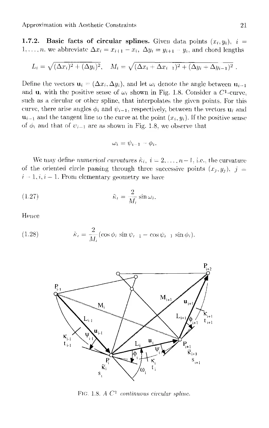
Define the vectors u^ = (Ax,, Ay,), and let w,- denote the angle between u,_i
and u, with the positive sense of u>i shown in Fig. 1.8. Consider a C^-curve,
such as a circular or other spline, that interpolates the given points. For this
curve, there arise angles 6% and ipi-i, respectively, between the vectors u, and
Uj_! and the tangent line to the curve at the point (x-i, yi). If the positive sense
of 0i and that of iiU-\ are as shown in Fig. 1.8, we observe that
i^j = i'i-i - <pi.
We may define numerical curvatures hi, i = 2 -n— I. i.e.. the curvature
of the oriented circle passing through three successive points (x-,,y3). j =
/ — 1, iy i + 1. From elementary geometry we have
:i.27:
Mi
Slllt
Hence
(1.28)
Mi
(cos (j), sin'(/;, _ i — cos tp,. -1 sin <p-,,).
Fig. 1.8. A Cl continuous circular spline.
22
Designing Fair Curves and Surfaces
This is the tangency condition that must be satisfied by the angles <f>i and
tpi-i, in order for the segments of the curve to combine into a 6n-curve as was
stipulated.
For circular splines we may simplify (1.28). Denote by k% the curvature of
the ith circular segment of the spline. From the properties of circles we have
ipi = —4>i and sin^j = — \hiKi. Therefore (1.28) takes on the form
(1.29) L{-i COS0, Ki-i + Li COS (j>i-i Ki = M,K,;.
These tangency conditions constitute a set of nonlinear equations that must
be solved subject to discretized aesthetic constraints
(1.30) m > 0, AKi > 0, A-^- > 0,
where we associate the parameter value t, and the spline curvature m with the
midpoint of the zth circular arc of the spline (due to the need of harmonizing
the At, with the quantities Ak, which relate to two adjacent circular arcs). It
is convenient to associate the arc length ,s7- with the ith point so that Asi «
Lx. Discretizing (1.18), we obtain the relationship At pa kAs. Using this, the
log-convexity inequality in (1.30) may be discretized over intervals from the
midpoint of one spline segment to the midpoint of the next by letting
, , , As7; + ASi+i
(1.31) AKi = Ki+i - Ki and AU = Ki+i .
Use of the numerical curvature hi. in the expression for At,; is justified in §1.7.4.
1.7.3. Computational procedure. The game plan is to linearize the
entire problem and then to use the simplex algorithm of linear programming to
solve the discretized approximation problem.4 The nonlinearity of the
problem requires that we carry out an iterative procedure, analogous to Newton's
method, at least in principle. In our experience the first iteration step has
almost always given satisfactory answers, but an iterative repetition of the first
step is easy to implement. We describe some of the details of the first iteration
briefly, under the following headings.
Fill-in, optimal spacing. Often, the spacing of the raw data points (picked
from a clay model) is far from optimal for reasons of practicality. Therefore,
points must be filled in to achieve optimal point spacing. Filled points optimally
spaced along connecting straight lines or circles may be estimated in a fairly
reliable manner, provided that the raw data points are spaced reasonably far
apart. Again, it is important to remember there is no need to have the filled
points improve the definition of the curve implied by the raw data points.
4 For an application of linear programming to the fairing of ships' lines, see [2].
Approximation with Aesthetic Constraints
23
since this will be taken care of by enforcing the aesthetic constraints. The
chord height formula can be stated in the form 8e = kL2 (neglecting the e2-
term). however, in terms of numerical curvatures we interpret this in the form
32f = k,+1(As, +A.s,'+i)2 because k;+i relates to two successive arcs. With the
simplification L — As, justified because of small angles (pi due to the optimal
spacing, we substitute from the preceding formula in formula (1.31),
Am + A.?7+1 Li-r Li+i
The actual computation uses the numerical curvatures R-, in a more indirect
way to guarantee that segments are not too long. All points, original (i.e.,
raw) or filled, are numbered consecutively (x,.yl). i = 1 r?.,The original
data, which are the only ones to contain any information regarding the faired
curve, are known as (.TmjO)--;</inj(/,)): i = 1,... ,'aong'. with inj(i) the entries of
a suitable integer array that are computed at the time of fill-in.
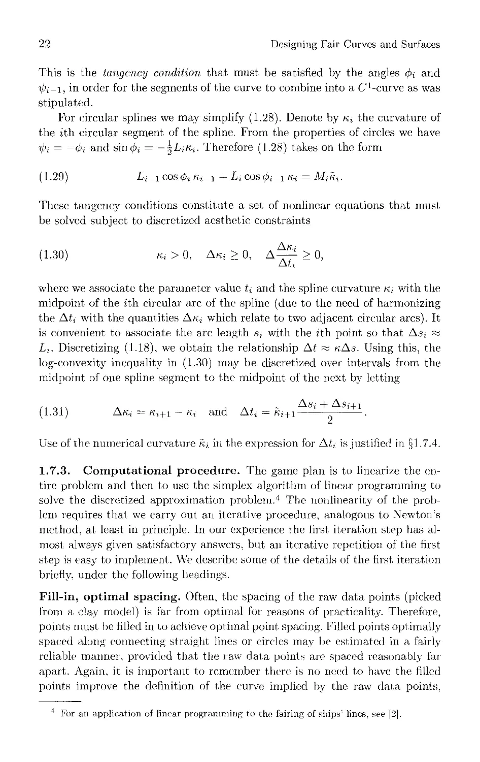
Approximate tangent vectors and normal vectors, displacements.
Approximate tangent vectors tv, and orthogonal to these, approximate normal
vectors n, can also be estimated from the raw data. As shown in Fig. 1.9. the
input points, raw or filled, are to be displaced by an amount b; in the direction
of the normal vectors n, and the desired N/C control points computed in the
form
Pig. 1.9. Input and output points.
24
Designing Fair Curves and Surfaces
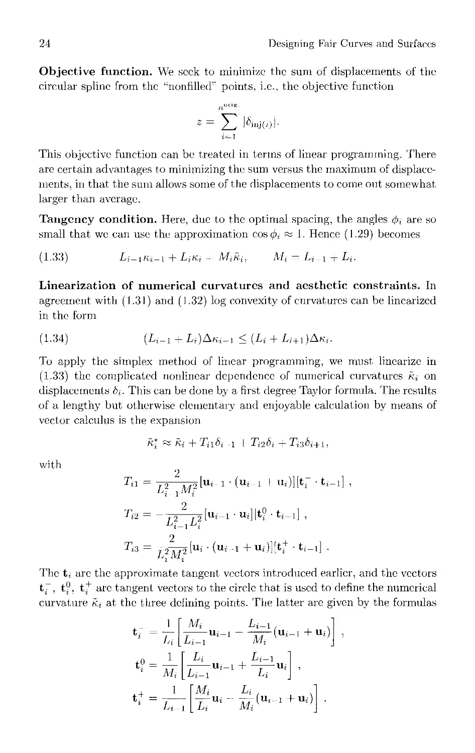
Objective function. We seek to minimize the sum of displacements of the
circular spline from the "nonfilled" points, i.e., the objective function
«or,K
4^1
This objective function can be treated in terms of linear programming. There
are certain advantages to minimizing the sum versus the maximum of
displacements, in that the sum allows some of the displacements to come out somewhat
larger than average.
Tangency condition. Here, due to the optimal spacing, the angles fa are so
small that we can use the approximation cos<^>, pa 1. Hence (1.29) becomes
(1.33)
Lj-iKi-i + LiKj — Miki, Mi = Li-i + Li.
Linearization of numerical curvatures and aesthetic constraints. In
agreement with (1.31) and (1.32) log convexity of curvatures can be linearized
in the form
;i.34)
(Z-i-i + L7-)Akj_i < (Li + Lj+i)Ak.j.
To apply the simplex method of linear programming, we must linearize in
(1.33) the complicated nonlinear dependence of numerical curvatures ki on
displacements bL. This can be done by a first degree Taylor formula. The results
of a lengthy but otherwise elementary and enjoyable calculation by means of
vector calculus is the expansion
with
Ta
Ki + Ti\8i -1 + Ti^Si + Ti36i-\-L,
2
%-iM?
Ui-l • IUi_i
u.
tr • ti
Ti2 = -y2 J2 [Ui_i • Uj][t° • tj_i]
i — 1 i
-i3
[Ui ■ (Ui-l +Ui)}[tf ■ ti-l]
The tj are the approximate tangent vectors introduced earlier, and the vectors
t4~, t°, tf are tangent vectors to the circle that is used to define the numerical
curvature ki at the three defining points. The latter are given by the formulas
t? =
i
u
i
Mj
Li-!
L
Ui-l
i-l
-Ui_i
L.
~Mi
Li-\
Ul-] +U,;
u;
i-l
Approximation with Aesthetic Constraints 25
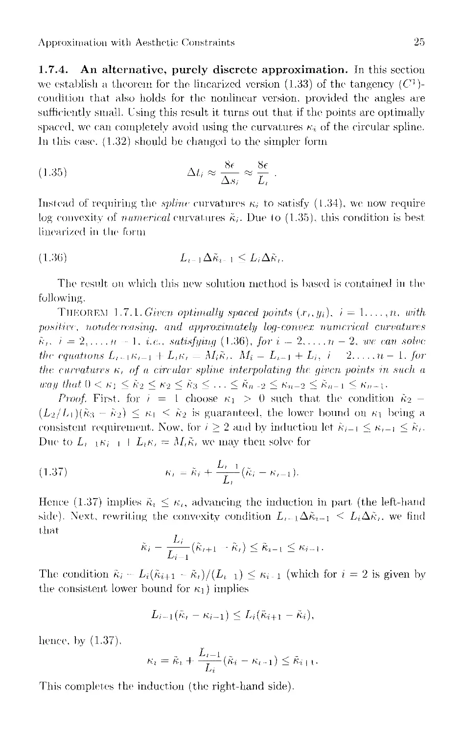
1.7.4. An alternative, purely discrete approximation. In this section
we establish a theorem for the linearized version (1.33) of the tangency (C1)-
eondition that also holds for the nonlinear version, provided the angles are
sufficiently small. Using this result it turns out that if the points are optimally
spaced, we can completely avoid using the curvatures «-.,; of the circular spline.
In this ease. (1.32) should be changed to the simpler form
., ,r, . 8c 8e
(1.35) At,■ « — « - .
As,- L,
Instead of requiring the spline curvatures k, to satisfy (1.34), we now require
log convexity of numerical curvatures k,-. Due to (1.35), this condition is best
linearized in the Conn
(1.36) L,_iAfi-.i_ i < LjAh,.
The result on which this new solution method is based is contained in the
following.
Thkorem 1.7.1. Given optimally spaced points (.cy,). i — l....,n, with
positive, nond.ee ceasing, and approximately log-convex numerical curvatures
k,, i' — 2,.... it — 1. i.e., satisfying (1.36), for i -- 2,.. . . n — 2, we can solve
the equations L,..\ k,-\ + L,k, = M;k,. M-L — L,.-j + L,, i 2 u — 1. for
the curvatures k, of a circular spline interpolating the given points in such a
Way that 0 < K] < h'2 < K-l < k$ < • • ■ < K« -2 < K.n-2 < kn-l < K„-[.
Proof. First, for / = 1 choose n\ > 0 such that the condition k-z -
(L-2/'/vi )(A/{ - £■_>) < k.[ < K2 is guaranteed, the lower bound on h\ being a
consistent requirement. Now, for / > 2 and by induction let k;_i < k,_i < k;.
Due to L, ih'j i I L,k, = M,k, we may then solve1 for
(1 -37) K, = K7- H '- (k; - K,-i).
Hence (1-37) implies kt < k.,, advancing the induction in part (the left-hand
side). Next, rewriting the convexity condition L,^iAk,_i < LtAk,, we find
that
Kj - —— (k, + i - k,) < ht-i < Kj-].
L-i-i
The condition k, — Lt(ki+i - k,)/(Ll i) < m-i (which for i = 2 is given by
the consistent lower bound for K\) implies
Li-i(k, - m-i) < L.j(ki+i - kt),
hence, by (1.37),
Hi = K;. H (Ki - Kt-l) < Kl+1.
This completes the induction (the right-hand side).
26
Designing Fair Curves and Surfaces
Due to this result, we can avoid computing explicit mathematical
representations for spline curves, from which we can pick the N/C control points,
because Theorem 1.7.1 guarantees that a satisfactory circular spline exists that,
interpolates the control points. Moreover, optimal spacing (cf. above, §1.7.3)
guarantees that polygonal line interpolation is visually indistinguishable from
the curve. This results in a considerable reduction in the number of variables
that need to be carried in the simplex algorithm and thus amounts to a savings
in execution time.
1.8. Smoothing and Aesthetics
Here we summarize how our approach to curve smoothing relates to other
aspects of the subject.
Spline smoothing has a long history in the automobile industry. An early
reference is de Boor's work on bicubic spline interpolation [5].
Curvature monotonicity and convexity may be viewed as nonlinear forms of
generalized convexity conditions. The general subject of approximation under
higher order generalized convexity was studied by one of us [8]-[10].
We emphasize that our approach concerns only limited aspects of the
aesthetics of curves and surfaces. We consider only plane sections of automobile
body surfaces, and we view these sections in isolation, each being a single line
(curve). Moreover, we consider only those aspects of the single line that concern
"smoothness" or "fairness," meaning "freedom from undesirable wiggles" —
with some appropriate definition of "wiggle." This concept appears to include
global as well as local properties of a curve, but there might be global properties
of curves other than fairness that are relevant to aesthetics.
Our concept of "smoothness" does not seem to be too different from the
one used in the mathematical discipline of smoothing, in which aesthetic
considerations clearly play a role [4], [18 , [26]. The principle of simplest shape
appears to be generally applicable. We feel that this is the reason for the
success of smoothing with cubic splines with a minimal number of optimal knots
[5], [6]. In cubic spline smoothing algorithms one can measure the "simplicity
of shape" by counting the number of cubic segments used to represent the
curve. In this sense, this approach is an application of the principle of simplest
shape in a way quite analogous to that of counting the number of sign changes,
as well as maxima, and minima of k having been discussed earlier.
On the other hand, in geometric modeling of exterior automotive design
lines aesthetics is all that matters, while in mathematical smoothing, aesthetic
considerations only enter in when a "complete theory" of the processes
producing the data to be smoothed is not available. If a "complete theory" is
available, mathematical smoothing reduces to parameter estimation. (Part of
the "complete theory" is usually the assumption that errors are due to
random noise, normally distributed and superimposed on the "basic" process.)
Lacking such a "complete theory," mathematical smoothing may attempt to
Approximation with Aesthetic Constraints
27
simulate manual smoothing, which can be done by fitting a curve through the
"cloud" of data by means of French curves. It is here that aesthetics enters
into mathematical smoothing. Our experience suggests that for automobile
lines a "complete theory'' of curve fairness can be provided by the principle of
simplest shape and an analysis of curvature properties like the ones we have
studied here.
References
[1] K. G. Baass. The use of clothoid templates in highway design. Transportation
Forum, 1 (1984). pp. 47 52.
[2] S. A. Berger and W. C. Webster, An application of linear programming to the
fairing of ship's lines, in Recent Advances in Mathematical Programming, R. L.
Graves and P. Wolfe, eds., Mac Graw-Hill, New York, 1963.
[3] G. D. Bhkhoff. Aesthetic Measure, Harvard University Press. Cambridge. MA,
19.:J3.
[4J M. T. L. Bizley, A measure of smoothness and a new principle of graduation. .1.
Inst. Actuaries. 84 (1958). pp. 125 144.
[5. C. R. de Boor, Bicubic spline interpolation, J. Math. Phys.. 41 (1902), pp. 212
218.
[01 C. R. de Boor and J. R. Rice, Least-squares approximation by cubic splines.
I: Fixed knots, and II: Variable knots, reports GSD TR 20 and CSD TR 21.
Computer Science Department. Purdue University. West Lafayette. IN, 1908.
[7] I. N. Bronshtehi and K. A. Semendyayev, Handbook of Mathematics. k. A.
Hirsch, editor of English translation, Verlag Harri Doiitseh. Van Nostra.nd Rein-
hold Company, New York. 1985.
-8' H. G. Burehard. Interpolation and approximation by generalized convex
functions. Ph.D. Thesis. Purdue University, West Lafayette. IN. 1968.
[9j . Extremal positive splines, with applications, in Approximation Theory.
G. G. Lorentz. ed.. Academic Press. New York (1973). pp. 291 291.
[10] . E.rtrcmal positive splines with applications to interpolation and ap-
pro.nmaiion by generalized, convex functions. Bull. Ainer. Math. Soc.. 79 (1973)
pp. 959 963.
[11] G. Farm. Curves and. Surfaces for Computer Aided Ceometr/.c Design. Academic
Press, Boston. 1988.
[12, G. Farm and N. Sapidis. Curvature and the fairness of carves and surfaces. IEEE
Computer Graphics and Applications, 9. 2 (198!)) pp. 52 57.
[13] A. 11. Fowler and C. W. Wilson. Cubic spline, a curve fitting routine, report
Y-l 100. Oak Ridge National Laboratory, Oak R.idge, TN, 1963.
[1 1] W. II. Frev and D. A. Field. Designing Bezier conic segments -with monotone
curvature. General Motors Research Publication GMR-7485. GM Research
Laboratories. Warren, Ml. 1991.
[15] P. .1. Grille. Form, Function, and Design. Dover. New York. 1975.
[16] G. Howard. Evolution of Motorcar Shapes and Design. International Association
for Vehicle Design, lnterseionce Enterprises. Ltd., Geneva. Switzerland. 1985.
[17] .1. I. Jones. .4 system for designing and appro xirnat nig aesthetically smooth curves
with iriteraelv'i graphic controls. Ph.D. Thesis. University of Detroit. Detroit.
MI. 1970.
28
Designing Fair Curves and Surfaces
[18] P. Lancaster and K. Salkauskas, Curve and Surface Fitting: an Introduction,
Academic Press, London, 1986.
[19] M. M. Lipschutz, Theory and Problems of Differential Geometry, Schaum's
Outline Series, McGraw-Hill, New York, 1969.
[20] E. Mehlum, Non-linear splines, in Computer Aided Geometric Design, R. E.
Barnhill and R. F. Riesenfeld, eds., Academic Press, Boston, MA, 1974.
[21] H. Nelms, Thinking with a Pencil, Barnes & Noble Division, Harper and Row,
New York, 1984.
[22] J. Roulier, T. Rando, and B, Piper, Fairness and monotone curvature, in
Approximation Theory and Functional Analysis, C. K. Chui, cd., Academic Press,
Boston, MA, 1990.
[23] N. Sapidis and G. Farin, Automatic fairing algorithm for B-spline curves, Com-
put. Aided Design, 22, 2 (1990), pp. 121-129.
[24] N. S. Sapidis and W. H. Frey, Controlling the curvature of a quadratic Bezier
curve, Cornput. Aided Geom. Design, 9 (1992), pp. 85-91.
[25] D. J. Struik, Differential Geometry, Constable and Co., Ltd., London, 1950.
[26] E. T. Whittaker and G. G. Robinson, The Calculus of Observations, fourth ed.,
Blackie and Son Ltd, London, 1944.
[27] R. C. Yates, Curves and their Properties, reprint by the National Council of
Teachers of Mathematics, Washington, D.C., of the original 1952 edition by J.
W. Edwards, Ann Arbor, MI, 1974.
Chapter
Curvature Integration through
Constrained Optimization
Alan K. Jones
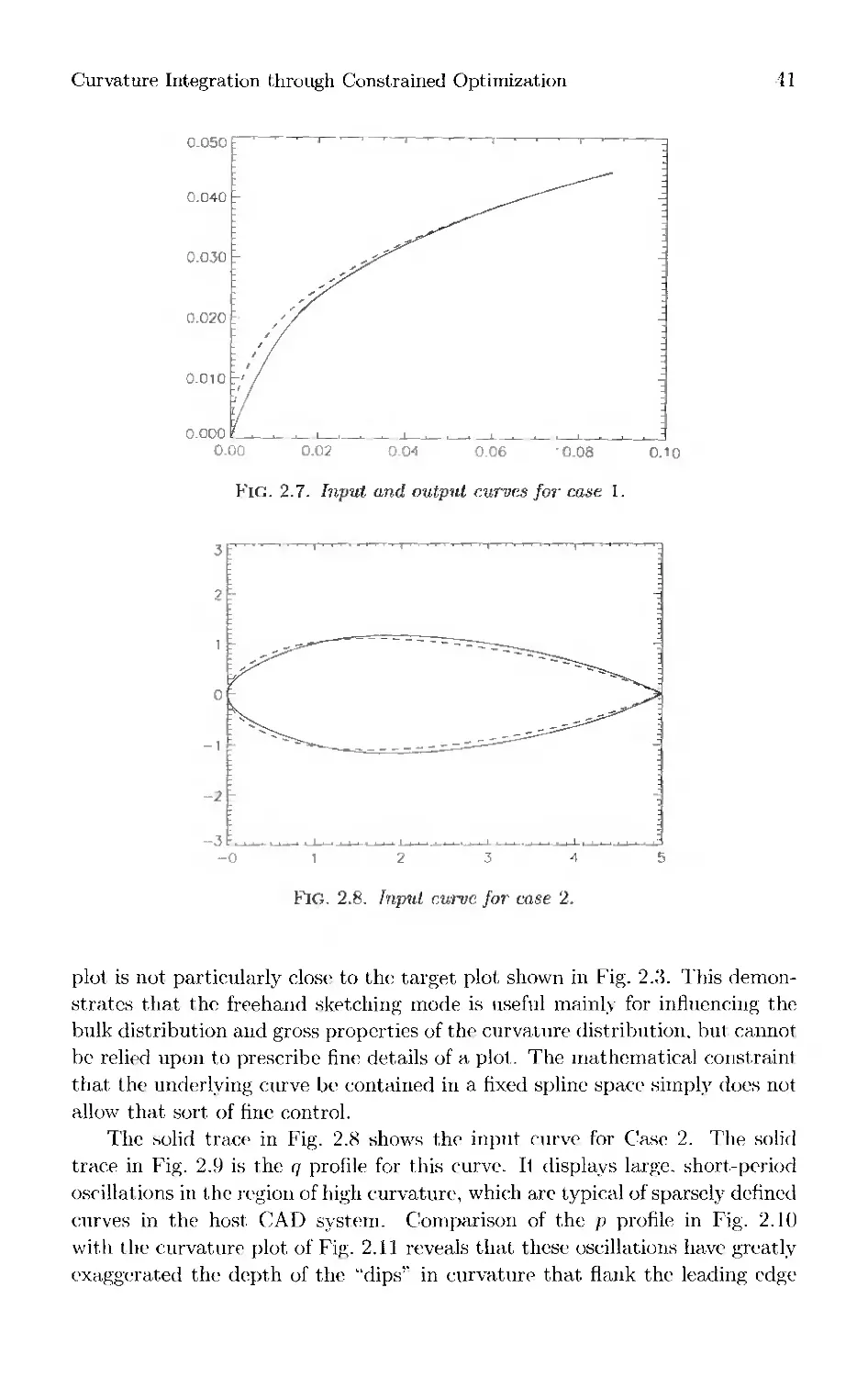
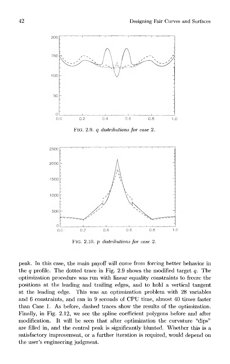
2.1. Introduction
To an aerodynamicist, smoothness of a curve is defined in terms of the
qualitative features of its curvature profile. Some of these features, such as the lack of
isolated sharp peaks or extraneous zero crossings, arc straightforward. Some of
them are not, and can be lumped into the requirement that the curvature plot
"looks right'" to an experienced engineer. But an airfoil curve must possess
other properties as well in order to be useful. It must meet spanwise defining
member curves, at least at the leading and trailing edges, and possibly at.
intermediate locations. It must, have prescribed tangent vectors, at, least at the
leading and trailing edges. Finally, but not trivially, it must be expressible in
the mathematical basis used by the CAD (computer-aided design) system at
hand. Curvature profiles which can be obtained from curves satisfying these
background constraints will be called feasible profiles.
If the desired qualitative features of the curvature distribution can be
characterized adequately by additional constraints or penalty terms, (hen it is
possible to regard the curve design as a single constrained optimization problem,
and solve it accordingly. The observations of §2.4 may be of some use in this
regard. Unfortunately, such optimization problems do not always have
solutions, and one is faced with exploring tradeoffs. Even more commonly, the
smoothness criteria are imprecise. An engineer may decide that a curvature
plot "should not be so rough in this region." or ''should have more of the
curvature concentrated over there." Thus, there is room for a man-in-the-loop mode
in which the space of feasible profiles is manually explored by an experienced
engineer. This also happens to coincide with the habits of thought and work
of many such users. Constrained optimization is an appropriate technique in
this mode as well, allowing the user to, in effect, sketch a portion of the target
curvature profile freehand, and then project the modified profile into the space
of feasible profiles.
This chapter discusses the current state of curvature modification
procedures, and suggests that they can be significantly improved by a combination
29
30
Designing Fair Curves and Surfaces
of spline technology and modern software for constrained optimization. It is
organized as follows. Sections 2.2 and 2.3 discuss both the problem and the
currently available solutions. Section 2.4 provides the key technical insight,
namely that the curvature of a polynomial spline curve is almost a ratio of
splines, and a great deal of control can be exerted over the curvature
distribution by manipulating these auxiliary splines. Sections 2.5 and 2.6 describe the
application of this principle, and §2.7 presents typical experimental results.
2.2. The Problem
The problem is to find a smooth, feasible curvature profile and its associated
airfoil curve. The curvature profile of a planar parametric curve, denoted by
c, is the signed curvature expressed as a function of the curve parameter. For
a given curve design problem, a feasible profile will be one that corresponds to
a curve satisfying the following requirements.
(1) Mathematical constraints. The curve must be chosen from a specified
function space. In this study, we will assume it is a parametric (nonrational)
polynomial spline. Furthermore, because the airfoil must be embedded in a
wing surface, typically represented as a parametric tensor product polynomial
spline, we will also assume that the polynomial degree and knot set have been
fixed a priori.
(2) Geometrical constraints. In this study, we will consider only linear
equality constraints. The curve must pass through prescribed points and/or
possess prescribed tangent vectors. Again, because the curve is regarded as
embedded in a tensor product spline surface, these constraints will be imposed
at specified parameter values. From the user's point of view, the tangent
conditions to be fixed will be Gl, not C1. That is, the ratios of parametric
derivatives are significant, not the individual components. However, the two
become equivalent in cases where the velocity magnitudes can be held constant.
(3) Smoothness constraints. Smoothness is an inherently ill-defined term.
The following classes of criteria, by no means exhaustive, are among those
that subjectively determine smoothness of a curvature profile. It should be
emphasized that these criteria are not just aesthetic judgments on the part
of the designer, as is often the case, for example, in automobile body design.
They do correspond to objective aerodynamic properties of the airfoil.
(a) Inequality constraints. Keep the profile positive (negative), monotone,
or convex over certain parameter intervals.
(b) High frequency features. Prevent high, narrow peaks, and general
"roughness" associated with high-frequency components in a signal.
(c) Low frequency features. Prescribe the bulk distribution of curvature.
Smoothness criteria of the inequality constraint type can be directly
incorporated into a constrained optimization procedure. It is likely that criteria
of the second type, which corresponds intuitively to band limiting the Fourier
transform of the curvature profile, can be incorporated also, although that
Curvature Integration through Constrained Optimization 31
effort is beyond the scope of this chapter. Criteria of the third type, however,
seem better adapted to interactive graphical input.
2.3. Current State of the Art
User's typically envision the design process as the following.
(1) Construct a curve by some means, and examine its curvature profile,
regarded typically as a string of plot points.
(2) Modify the profile interactively to make it smooth. Move individual
points or groups of points, apply smoothing filters, etc. Call the result the
target profile.
(3) Iterate the following steps as needed.
(a) Apply heuristics to modify the target profile to allow the geometric
constraints to be satisfied.
(b) Integrate the modified target profile numerically and obtain a dense set
of values (and derivatives) along the resulting ideal curve.
(c) Best-fit the ideal curve with a curve satisfying the mathematical
constraints.
(d) Check that the geometric constraints and smoothness criteria are
satisfied.
The best-fitting procedure in the above cannot simply minimize least-
squares deviation from the ideal curve locations at a dense set of plot points.
In general, this gives no hope of reproducing the target profile. At a
minimum, the fitting procedure must attempt to reproduce first- and second-order
derivative data of the ideal curve. Better still, the objective function should
measure directly deviations from the modified target curvature profile.
Furthermore, the deviation measure chosen must give information at every point
in the interval. It is not enough just to sample at a dense set of discrete
points.
We mention in passing an approach that has been adopted in the past, to
finesse this issue. This is to approximate the modified target profile up to
tolerance by a low degree spline, and then to define the corresponding curve
procedurally as a solution to a system of differential equations which guarantees
that its curvature distribution is exactly that spline. See, for example, [1] or
§1.1.2.4 of [4]. In the special case of piecewise constant c, the resulting curve is
piecewise circular, but cannot of course have curvature continuity. Curvature
profiles which are polynomial splines of nonzero degree do not integrate to
give spline curves. For linear c, the solution is the so-called Cornu spiral.
Generating points along such a curve requires numerical evaluation of Fresnel
integrals, of the form
C(s) = f cos{na2/2)da,
(2-1) J°
S{s) = / sill(7TCr2/2)(icr.
Jo
32
Designing Fair Curves and Surfaces
See [3] for a numerical evaluation of these. A system to construct and
evaluate curves which arc piecewise Cornu spirals is described in [8]—[13]. A
related but fundamentally different approach is taken in [2], where C1 piecewise
smooth curves are constructed to minimize the L2 norm of curvature subject
to various interpolation constraints. We summarize both approaches by
emphasizing that the computation involved is nontrivial, and that the resulting
curves do not satisfy our mathematical constraints.
2.4. Viewing Curvature Profiles as (Almost) Rational Splines
Let c be a target curvature profile, and c the one actually obtained. Some
mechanism must be found to bound an appropriate function norm of c—c. Now,
if c and c were in fact splines, then it would be enough to express them with a
common knot set and degree and measure the distance between corresponding
coefficients a and C4. For example, an upper bound on
\\C - c\\oo = SUp \c(t) ~ c(t)\
is given by max|c; - di\. This would not be a suitable objective function
for a constrained optimization problem because the max function destroys
continuity. A similar but more useful norm is
N
(2-2) ||<:-£||^t = ^|c,--c,-|2(ii+n+] -h),
i=l
which was shown in [6] and [7] to be equivalent to the usual L2 norm \\c — c||| =
/ \c(t) - c(t)\2dt. Here n is the degree of the splines and t = {t\ ^iv+n+i}
is the knot set.
Unfortunately, as we have seen, c is not a spline in general if the underlying
curve is. However, c is completely determined by two auxiliary functions which
are splines, and hence can be controlled by such means. We will now see just
how much mileage can be gained out of that simple observation.
Write a typical point on the curve as (.r(.s), jy(.s)), where x and y are splines,
and let the curvature at parameter value s be given by c(s).
Recall that
where
p = xi] — iix.
(2.4) J J
q = (x)2 + {y)2,
where dots represent differentiation with respect to the curve parameter.
Curvature Integration through Constrained Optimization 33
If x and y are polynomial splines, then p and q are also splines, which
we call, respectively, the curvature numerator and the curvature denominator.
These are the auxiliary splines that will form the basis of our calculations. If
x' and y are of degree n and class Ck, then q is of degree 2n - 2 and class
Ck~l, while p is of class Ck 2, and formally of degree In — 3. It is well known,
and easy to see by expanding (x,y) locally in a power basis, that p is in fact
of degree 2n — 4. Here, and throughout this paper, we adopt the convention
that CJ actually means C,max(~1,J'). A curve is of class C-1 if it. is piecewise
smooth, with only jump discontinuities.
A well-known corollary of the above calculation is the following.
Proposition 2.4.1. The curvature of a nonsingular parametric spline
curve is non-negative over the parametric interval [a, b\ if the curvature
numerator spline p is nonnegative there.
Here nonsingular means that the first parametric derivative never vanishes.
Repeated differentiation of the curvature formula yields two similar results.
Proposition 2.1.2. The curvature profile of a nonsingular C2 parametric,
spline curve is monotone increasing over the para/metric interval [a, b] if the
splint: r — 2pq — 3pq is nonnegative there.
Proposition 2.4.3. The curvature profile of a nonsingular C* parametric
spline curve is convex up over the parametric interval [a, b] if the. spline Apq2 —
l'2pqq + I5pq2 - tipqq is nonnegative there.
The differentiability requirements on the plane curve can be relaxed with
due care, but the result is to add additional constraints. For example, we have
the following.
Proposition 2.4.4. The curvature profile of a nonsingular parametric
upline curve is monotone increasing over the parametric interval [a:b] if the
spline 2pq — 'ipq is nonnegative wherever it exists in that interval, and if at
each knot t of the p spline, the value jump Ap(t) e_ p(/-i_) - pit-) > 0.
la practice, we force nonnegativity of splines like p or r over an entire
interval [a,b\ by requiring that the spline coefficients corresponding to the B-
splines whose supports intersect [a. b] are nonnegative, and noting that the
B-splines themselves are nonnegative. This is a sufficient but not necessary
condition, and ran occasionally be too strong in the sense that the solutions
simply fail to exist. However, it is straightforward to code, and mathematically
tractable from the point of view of modern optimization codes. Since the
splines p and q are quadratic expressions in the coefficients of the curve (x.y).
these propositions describe algebraic inequality constraints of degrees 2. 1, and
(i. respectively, on the spline coefficients of (x.y). Constraints such as those on
Ap are quadratic inequality constraints of a particularly simple form, involving
only differences of coefficients of p.
Proposition 2.4.1 gives a. test for convexity of a spline curve which is much
simpler to code than the tests proposed in Theorem 3.7 of [.r>], which were based
on purely geometric criteria for the convexity of the curve's spline polygon. It
has not yet been shown that these two tests are logically equivalent in every
34
Designing Fair Curves and Surfaces
case. However, brute force computation verifies the equivalence for a Bezier
cubic curve, and we conjecture that it is true in general. In any case, it is
advisable to express p using its actual degree of 2n — 4, where x and y have
degree n, rather than the naive estimate 2n — 3. Artificial degree raising of
the numerator spline does not produce a "tighter" bound, but simply adds
redundant constraints.
Propositions 2.4.2 and 2.4.4 appear to be a new observation, and have
applications in automating the elimination of "spikes" and "wiggles" from
curvature profiles. We will refer to
(2.5) r = 2pq - 3pq
as the curvature slope numerator. It is a spline of class Ck~3 and degree 4n —7.
No additional cancellation of high-order terms occurs in general.
Proposition 2.4.3, however, is of doubtful practical value, since most users
do not need to micro-manage their curvature profiles to this extent. Note
also that this condition ensures convexity only when the curvature is plotted
against the curve parameter. A curvature versus arclength plot, for example,
could still fail to be convex.
2.5. An Optimization-Based Algorithm
In light of the above, the algorithm of §2.2 can be recast as follows.
(1) Define mathematical constraints, i.e., spline degree and knot set.
(2) Define geometrical constraints as linear equality constraints on the
spline coefficients.
(3) Define an initial guess curve satisfying the mathematical constraints
and as many of the geometrical constraints as can easily be done.
(4) Iterate as needed.
(a) Define smoothness inequality constraints, i.e., regions where curvature
must be positive (negative), or monotone increasing (decreasing).
(b) Define qualitative curvature constraints, i.e., regions in which the
curvature should qualitatively resemble a user-provided target profile,
expressed as a pair (p, q) of target curvature numerator and denominator
splines.
(c) Find a curve satisfying the mathematical, geometrical, and smoothness
inequality constraints whose associated p and q splines are closest (in
some sense) to p and q.
(d) Check the smoothness properties of the resulting curve.
Techniques for obtaining p and q through interactive modification of p
and q profiles are discussed in the next section. Note that, if no qualitative
smoothness constraints are imposed, we can simply set p and q to be those of
the initial guess curve.
All of the serious computation involved is hidden in step 4(c), where it
can be handled by off-the-shelf software for solving constrained optimization
Curvature Integration through Constrained Optimization
35
problems. Thus, all three stages of the original algorithm, integration,
approximation, and imposition of constraints, can be combined into a. single operation
and solved automatically. The fitting tolerance can be measured in the
curvature domain, where it belongs, and the geometrical constraints are imposed
on the physical curve, where they belong.
The next question is, hew do we measure closeness of (p, q) to (p, q)'? The
most straightforward answer is just to best-fit p and q separately, as follows.
Problem 1. "Minimize the objective functional
Pi(j-;;y) = \\p\\2t2,t + \\(l\\%.u
subject to the linear equality constraints on x. y, x, y that give interpolation of
the specified locations and tangents, and the nonlinear inequality constraints
that determine the sign of curvature and/or its slope. The optimization
variables are just the spline coefficients of the functions .r and y. Here t and u are
the knot vectors appropriate to the functions p and q, respectively.
This is a quadratic programming problem with linear equality constraints,
and quadratic and quartic inequality constraints. If necessary, the Hessians
can be written out explicitly, and there is additional structure that we may be
able to exploit. The functions p,(.r; y) and qj(.r;y) are block (antisymmetric,
and each block is banded because of the local support of B-splines. Note that
eliminating unnecessary inequality constraints will simplify this stage
considerably.
In practice, the unweighted least-squares problem described above does
not- work well for at least two reasons. First, it ignores the question of relative
scaling between the norms of p and q. Second, it is inappropriate to give equal
weight to errors in all of the coefficients because of the very large dynamic
range typical of curvature distributions around an airfoil. The qualitative
shape of the target distribution is better preserved if instead relative errors of
the form (p, — p,)/}H are controlled. This will discourage the optimizer from,
say. introducing ripples into previously flat regions of the curvature profile
while removing a notch from a peak.
Once this idea is adopted, an estimate of the relative scaling of p and q
norms is suggested by the calculation
(2.6) Ac = A(p<r:j/2) « Ap<r;V2 - -pq-^/^Aq.
which we can write as
(2.7)
Ac _ Ap 3 Aq
c p 2 q
Thus, the contribution to the relative error in c of relative changes in q is
3/2 that of relative changes in p, which motivates the following.
36
Designing Fair Curves and Surfaces
Problem 2. Minimize the objective functional
P2(x;y) = E(^) V^n-3 - *) + I E(^)2(^n-! - Uj),
subject to the constraints of Problem 1.
So far the p and q splines have been handled independently, with their own
natural orders and knot sets, and only weakly coupled by the definition of the
objective function in Problem 2. Better results may come from writing the two
splines in a common form, as a Ck~2 spline of degree In — 2, over a knot set v.
The objective functional can then be enhanced with the cross terms omitted
from Problem 2, yielding the next problem.
Problem 3. Minimize the objective functional
subject to the constraints of Problem 1.
2.6. Implementation Details
The implementation approach described in this paper was chosen specifically
to work with an existing CAD system in which airfoil curves typically have the
following properties.
(1) They are stored as parametric polynomial splines, usually nonrational.
(2) They are densely defined, with tens or hundreds of spline coefficients
per curve. However, it is usually not desirable to add additional knots.
(3) They are approximately arc length parametrized; variations in
parametric velocity are negligible compared to variations in curvature.
Where qualitative smoothness constraints are required, the target splines
(p, q) are constructed by interactive modification of the splines (p, q) associated
with the initial guess curve. This takes place in two phases.
In the first phase, the denominator q is modified to remove behaviors that
are identified with undesired features of the curvature profile. In practice, any
sort of variation at all in q usually turns out to be undesirable, so we typically
try to impose q ss constant. The best feasible approximation to this can
be achieved by minimizing in the £2 norm the coefficient vector of the spline
xx + yy. However, in the host CAD system, q is typically almost constant.
See, for example, Fig. 2.4. Hence, in most cases, it is reasonable to take q — q,
and the q modification step is omitted.
In the second phase, the user adjusts the spline coefficients pk interactively.
Ideally, visual feedback would be available, consisting of the spline polygon of
p superimposed on the plot of p/q. However, with well-behaved q, this has not
proved necessary.
Curvature Integration through Constrained Optimization 37
A consequence of the very large knot arrays characteristic of the host
system is that the spline polygon for the curvature numerator p has a large number
of vertices. Thus it is impractical to manipulate it vertex-by-vertex. Probably
the right way to deal with this problem is to use [6] to approximate p by a
spline with a much sparser knot set, hence there are much fewer vertices on
its spline polygon, then manipulate these sparse vertices individually to get
a qualitatively good curvature profile, then perform knot addition to find the
corresponding polygon with respect to the full knot set. The method actually
implemented in the test code is cruder in concept but similar in effect for the
test, curves we have seen. The spline polygon of p is itself regarded as a piece-
wise linear curve, with the coefficient value pi plotted at a parameter value
given by the average of knots tt through tl+2n-s- The user is then allowed
to replace individual p, values, or to specify linear variation of the p, (with
respect to the curve parameter) over a particular range of L
The objective function described in Problem 2 has been found the most
satisfactory in practice. Note that this is only possible because our concerns are
typically for regions around the leading edge of an airfoil, where p is bounded
away from zero, so the relative error norm makes sense. We note in passing
that the spline representations for p, q, r, etc.. were actually generated, not
Informal differentiation and multiplication of the B-spline series, but rather by
oversampling and least-squares fitting. That is, pick the points ,s, so that they
uniquely determine the splines p and q, given their known degrees and knot
sets. Then the difference between the norms Yl(p(si) ~ P(-s;))2 all(J YliPk ~~
Pa)2 is just the linear transformation that takes the data (p(.s,)} to the spline
coefficients {pi,}- Similarly, this is also true for q. This procedure was adopted
primarily to speed up code development for proof of concept purposes. The
resulting code may execute slightly slower, but there is little or no loss in
accuracy.
Two classes of geometric linear equality constraints have been
implemented. First, discrete point locations or parametric first, derivatives can
be "frozen*" at values read off the input curve. Second, a vertical or
horizontal tangent can be specified at any point, without fixing the magnitude
of the parametric derivative. In addition, one type of nonlinear inequality
constraint is supported. Curvature monotonicity constraints as prescribed by
Proposition 2.4.4 may be specified in the following manner. The user enters a
parameter value ti>oa.k where the curvature peak is to be located. The region
of the curve to be modified is then assumed to have nionotonically increasing
curvature for t < tpoak, and nionotonically decreasing curvature for t > ipcak-
No attempt has been made to implement the optimization step efficiently
by exploiting its special structure as described in §2.5. For proof of concept, it
has been coded in a very naive fashion, with gradients and Hessians evaluated
by the optimization package using finite differences. Performance in this mode
is not impressive. A large case such as the first example in the next section
can take tens of seconds on a typical engineering workstation.
38
Designing Fair Curves and Surfaces
2.7. Examples
Two test cases will be reported, both of which are C1 cubic splines with
airfoillike geometry. Case 1 is taken from a curve defined by 203 spline coefficients.
This density is typical of the host CAD system, and, again typically, the
parametric speed q is nearly constant. Case 2 is at the opposite extreme. This
is a very sparsely defined curve with only 14 coefficients, where the curvature
irregularities are in fact dominated by the variation in q.
Figure 2.1 shows an analytically defined symmetrical airfoil. Case 1 is a
curve fit to the upper half of this shape, and extended by reflection symmetry.
Figure 2.2 shows the curvature behavior for the this curve, with the lower
surface trailing edge at parameter value — 1, the leading edge at parameter value
0 and the upper surface trailing edge at parameter value +1. The "sawtooth"
curvature at the leading edge is a serious defect.
0.6
0.4
0.2
0.0
0.2
0.4
f> P
0
;
^
^_-
{
{
c
1 "■
0.7
■ —i— i
Zi.A
i . i
o.s
1 '
o.s
' ' 1
■
=H
-
-
FiG. 2.1. An analytically defined airfoil.
so |
20
Ci_
-C.5
CO
0.5
1.0
Fig. 2.2. Curvature plot of the, airfoil.
Curvature Integration through Constrained Optimization
39
The solid trace in Fig. 2.3 is a blowup of the curvature plot in the leading
edge area. (From now on, only the upper surface will be plotted.) The solid
trace in Fig. 2.4 shows q, which is nearly constant.
Thus, the solid trace in Fig. 2.5, which is the p function plotted over this
interval, closely mimics the form of the curvature plot. The dotted curve in
Fig. 2.5 shows the target p distribution after interactive manipulation to force
p(0) = 50 and linear variation of p between parameter values 0 and 0.03. The
target q distribution is unchanged from the input curve. The dotted trace in
Fig. 2.3 shows the curvature distribution implied by the target p and q. The
optimization procedure was run with linear equality constraints forcing the
leading edge position to be fixed and the leading edge tangent to be vertical,
together with a nonlinear inequality constraint to force the curvature to be
monotone decreasing over the top half of the airfoil. Nothing outside the
60
50
40
30
20
10
0
- ■ H ■ ■ ■ ■ ■ j ■ . ■ ■ i . - j
i
- \
\ \
: %
r" *
V
J. \
''•\.
■ ^ i""""""'^
*r ^T'^m
-f
l^^^
'- "^^-^^^^
^t*~"~~^r=:~=~^-=-^^-=-
1 < 1 1
:
:
-j
:
:
-j
-
:
:
-_
:
:
-;
)
■\
:
., —— l
i
O.OO 0.02 0.04 0.06 0.08 0.10
Fig. 2.X Curvature behavior near the leading edge.
0.00 0.02 0.04 0.06 0.08
Fig. 2.4. q distributions for case 1.
o.io
40
Designing Fair Curves and Surfaces
parameter interval [0,0.1] was altered. This was an optimization problem with
16 variables and 36 constraints, and took almost 6 minutes of CPU time on a
Sun SPARCstation IPX. The p, q, and curvature distributions of the output
curve are the dashed traces in Figs. 2.3 2.5.
The solid and dashed traces in Fig. 2.6 show the r distributions of the
input and output curves. It will be seen that r > 0 everywhere in the output
curve, as required.
Finally, the solid and dashed traces in Fig. 2.7 show the input and output
curves, respectively, in the leading edge region. Note that the input curve did
not satisfy the symmetry condition that the leading edge tangent be vertical.
The output curve does satisfy this constraint, and has eliminated the
"sawtooth1'' curvature behavior as well. On the other hand, the output curvature
60
■ifi
40
30
20
10
0
* '
-
L*
-*'\
- "-\
'^
lb
— \
: \
■v
■s
'.^
-
0.00
0 02 0.04 0.06 008 0.10
FIG. 2.5. p distributions for case 1.
4000
2000
-2000
-4000L .
0.00
\
\
\
. r . ,
"
1
0.02
0 04
0.06
0.08
0.10
FlG. 2.6. r distributions for case 1.
Curvature Integration through Constrained Optimization
41
0.050
0.040
0.030
0.020
0.010
0.000
0.00
0.02 0.01 0.06 0.08 0.10
Fig. 2.7. Input and output curves for case I.
-2
-3f
12 3-1
Fig. 2.8. Input curve for case 2.
plot is not particularly close to the target plot shown in Fig. 2.W. This
demonstrates that the freehand sketching mode is useful mainly for influencing the
bulk distribution and gross properties of the curvature distribution, bill cannot
be relied upon to prescribe fine details of a plot. The mathematical constraint
that the underlying curve be contained in a fixed spline space simply does not
allow that sort of fine control.
The solid trace in Fig. 2.8 shows the input curve for Case 2. The solid
trace in Fig. 2.9 is the q profile for this curve. II displays large, short-period
oscillations in the region of high curvature, which arc typical of sparsely defined
curves in the host CAD system. Comparison of the p profile in Fig. 2.10
with the curvature plot of Fig. 2.11 reveals that these oscillations have greatly
exaggerated the depth of the "dips'" in curvature that flank the leading edge
42 Designing Fair Curves and Surfaces
200
150
100
50
0
0.0 0.2 0.4 0.6 0.8 1.0
Fig. 2.9. q distributions for case 2
2500
2000
1500
1000
500
0
0 0 0.7 0.1 0.6 0.8 1.0
Fig. 2.10. p distributions for case 2.
peak. In this case, the main payoff will come from forcing better behavior in
the q profile. The dotted trace in Fig. 2.9 shows the modified target q. The
optimization procedure was run with linear equality constraints to freeze the
positions at the leading and trailing edges, and to hold a vertical tangent
at the leading edge. This was an optimization problem with 28 variables
and 6 constraints, and ran in 9 seconds of CPU time, almost 40 times faster
than Case 1. As before, dashed traces show the results of the optimization.
Finally, in Fig. 2.12, we see the spline coefficient polygons before and after
modification. It will be seen that after optimization the curvature "dips"
are filled in, and the central peak is significantly blunted. Whether this is a
satisfactory improvement, or a further iteration is required, would depend on
the user's engineering judgment.
Curvature Integration through Constrained Optimization 43
2.5
2.0
1.5
1.0
0.5
0.0
0
FlO. 2.11. Curvature plots for case 2.
3
2
1
0
-1
-2
-3
-0.0 1.0 2.0 3.0 4.0 5.0
FIG. 2.12. Spline, polygons for case 2.
References
[1] J. A. Adams, The intrinsic method for curve definition, CAD. 7 (1975). pp. 243
249.
[2j G. Brunnctt, Properties of Minimal-Energy Splines, in Curve and Surface
Design, H. Hagen. ed., Society for Industrial and Applied Mathematics,
Philadelphia, PA, 1992.
[3] W. J. Cody, Chebyshev approximations for the Fresnel -integrals. Math Comp.,
11 (1988), pp. 450-453.
[4] I. D. Faux and M. J. Pratt, Computational Geometry for Design and
Manufacture, Ellis Horwood, Chichester, UK, 1979.
[5] D. R. Ferguson, P. D. Frank, and A. K. Jones, Surface shape, control using
constrained optimization on the B-spline representation, Comput. Aided Gcom.
Design, 5 (1988), pp. 87-103.
_1_I.J_1 l_l.l_C .-J ,
44
Designing Fair Curves and Surfaces
[6] T. Lyche and K. Morken, Knot removal for parametric B-spline curves and
surfaces, Comput. Aided Geom. Design, 4 (1987), pp. 217-230.
[7] , A data reduction strategy for splines with applications to the
approximation of functions and data. IMA J. Numer. Anal., 8 (1988) pp. 185-208.
[8] A. W. Nutbourne, P. M. McClellan, and R. M. L. Kensit, Curvature profiles for
plane curves, CAD, 4 (1972), pp. 176-184.
[9] , A cubic spline package part 2 — the mathematics, CAD, 5 (1973), pp. 7-
13.
[10] T. K. Pal and A. W. Nutbourne, Two-dimensional curve synthesis using linear
curvature elements, CAD, 9 (1977), pp. 121-134.
[11] , Intrinsic spline curve with local control, CAD, 10 (1978), pp. 19-29.
[12] , Mean tangent rotational angles and curvature integration, CAD, 10
(1978), pp. 30-34.
[13] A. Schechter, Synthesis of 2d curves by blending PL curvature profiles, CAD, 10
(1978), pp. 8-18.
Chapter
Automatic Fairing of Point Sets
Matthias Eck and Rainer Jaspert
3.1. Introduction
It is a frequent problem that appears in the everyday life of a CAD system:
working on measured data points that came, for example, from digitizing
processes. Therefore, such a system must have the capability to handle possible
deviations or data errors in order to avoid problems during later calculations.
The most common way of solving this task in the case of planar data is to
determine an approximating spline curve which minimizes a certain fairness
functional (cf. [3]. [7j. and [9]). In [13] a remarkable iterative and local
procedure is described that makes use of the geometry of the curve.
At first an initial cubic B-spline curve X is determined which interpolates
the planar data points P, = X(t,). Then with help of the local fairness
criterion' ~,- = |k(<(~) - A.(r/~)|. and the global fairness criterion £, = J2izr-
the actual fairing procedure works as follows.
1. Find the largest zr
2. Fair the curve in the area of X(fy) by a local procedure called ""knot
removal knot reinsertion."
3. Determine the new criteria £, and £ .
1. If £ < £ then goto step 1.
else undo last iteration and exit.
As illustrated in [13], this automatic fairing procedure works well.
In contrast to such curve-oriented algorithms, the heuristic method given
in [12] modifies the data points nonautoniatically by improving their first (or
second) divided differences plot.
Therefore, the aim of this chapter is to deduce an automatic and local
fairing process according to [13] for- given planar or spatial point sets which is
based on direct manipulations of the data.
1 ti{t ) (respectively, £(/"* )) denotes the left-handed (respectively, right-handed) first derivative of
Ihe curvature with respect to are length, at the point X(/,).
45
46
Designing Fair Curves and Surfaces
The idea is to interpret the point set as an open or closed polygon. Then it
results that difference geometry is advantageous in formulating suitable fairness
criteria as the polygons are a simple model of this theory. For this reason the
basic ideas of difference geometry are gone over before the proper planar and
spatial discrete fairing algorithms are described.
An ineffective and nonautomatic proposal of such a planar algorithm was
worked out in [16] and therefore is not considered in this chapter.
3.2. Basic Ideas of Difference Geometry
The development of the nearly 60-year-old theory of difference geometry is
outlined in the textbook of Sauer [14] which provides a simple and readable
introduction.
The polygons VdN :— (Pn, Pi,... . P,v) = (P?)£o are tne simplest models
of difference geometry. They represent the polygonal connection of the N + 1
vertices or points P; £ Std.
A polygon is called closed if, first, the additional condition P0 = P7v is
fulfilled and, second, each vertex is an inner vertex. Otherwise it is called open
and possesses the inner vertices Pi,..., Pjv_i.
If we interpret such a polygon VdN as a discrete curve in M , then usual
differential geometry of planar (d = 2) or spatial (d = 3) curves is contained in
difference geometry as a limit. This is described in the following paragraphs.
Assume a regular parametric curve X(f), t 6 [a, b], to be given in Rd. Then
we associate a polygon V% with the curve X by the N+l vertices P,; — X(£;).
The sequence r = (U)fL0 of parameter values has to increase strictly monotone
fulfilling to = a and t^ = b.
Now, the length ,sA of this polygon VdN is simply the sum of the edge
lengths
N
5jV = ^L?; with Li = ||Lj|| and L,- = P; - P;_i.
?:=i
During the limiting process N —>• oo (meaning a repeated refinement of the
parameter sequence r and therefore of the polygon Vff), the polygon length
sN tends (together with max7{L?;} —> 0) to the following limiting value s(a,b):
fb
s{a,b) = lim sN = / ||X'(«)||du,
N^oo Ja
which is the well-known formula for the arc length of the curve in the interval
The above has been frequently used in CAGD (computer-aided geometric
design) to approximate the arc length parametrization s = s(a,t). For
example, if suitable parameter values (si)fL0 for a given point set (Pj)^0
have to be determined (in order to start interpolation or approximation
Automatic Fairing of Point Sets
47
processes), then mainly the so-called chord length parametrization is chosen
(cf. [4] and [8]):
■so = 0,
EL< U
1.
.N).
Moreover, if we assign to every inner vertex of a polygon V% a discrete
Frenet frame by defining a tangent vector, a main normal vector, and a
binormal vector in a suitable way. then it is also possible to formulate discrete
Frenet-Serret formulas by moving the discrete Frenet frame [14]. The limiting
process N -» oo then leads again to the well-known Frenet frame and Frenet
Serret formulas of the curve theory in differential geometry of M3 (cf. [4]).
Similar arguments are valid for plane polygons and plane differential geometry.
For the following context it is only necessary to define the discrete curvature
and the discrete torsion in an inner vertex of a polygon, which are the
coefficients of these discrete Frenet Serret formulas,.
First, the discrete curvature K{ is defined simply as the inverse of the
radius 11, of the circle passing through the three points P, ), P, and P,^. as
illustrated in Fig. 3.1.
Fie;. 3.1. Dificrelt curvature k~, of a polygon.
To express A", in formulas, we have to distinguish the planar polygons V%
and the spatial polygons V% because of the spatial problem of orientation.
The same distinction is used in differential geometry where, in the case of
space curves, the curvature is defined to be always positive.
So we get in the planar cast1
(3.1)
with
Ki
2A,
sgu(At)
2sin(fv,)
Q,
Qi = IIQ,
Q, = Pi-
P,
1:
48
Designing Fair Curves and Surfaces
cos(qj)
Aj = det(Lj,Li+i),
Li • Lj+t
0 < OU < IT
and the sign function sgn() as usual. Finally, in the spatial case,
2sin(aj)
(3.2)
Ki
Ql
Second, the discrete torsion 7] is defined in the space with help of the angle
j3i between the osculating planes through Pj_2, Pi-i, P* and Pj_i, Pj, P,+i
(see Fig. 3.2):
(3.3)
with
Ti = .. .. = sgnfAj-
Vi-iVi
Li '
COs(ft) = Ni_! • Ni, 0 < 0i < 7T,
V;
Ns-
K:
;, Vi = I« x Li+i ^ 0, ^ = ||Vi||,
Ai = det(Li L,Li,L.;+i).
If V,_i = 0 or Vi = 0 we define Tj to be zero as no deviation of the polygon
Pi_2, Pi-i, Pi, P«+i from a plane occurs.
In formula (3.3) there is the obvious handicap that no unique assignment of
7], to a vertex of the polygon is possible because of the nonsymnietric definition.
To avoid this, we symmetrize the discrete torsion by
(3.4)
Ti
LtTl+\ + Lt+iTj
Li 4 Z/i-i i
i-2
L
i-i
//,
'K
%>L
///
1.1
a,
Fig. 3.2. Discrete torsion Tx of a polygon.
Automatic Fairing of Point Sets
49
This equation can be derived by linear interpolation of T) and X,-+i
according to the parameter values t{ —f and t± -\—y1. This choice of the
parametrization may seem artificial but it represents the fact that, e.g., XJ
corresponds to P,_i as well as to Pt. The resulting linear polynomial T(t) is
r«) = r, + —!i-(f,+1-T,) (,.-«, +1
So it is obvious that T, — A(i(). Furthermore we can use 'l\t) to determine
a (later needed) approximation of the first derivative of T., in the inner vertex
P,:
(3-5) ri=T'{ti) = T ~~ (ti+l-f-
If we proceed in the same way to determine the first and second derivatives
of the discrete curvature K, with help of the quadratic interpolating polynomial
K(t) of Kj-], K,, and Kl+i according to the chord length parametrization, we
(3.6) A,, = A [t,)= Lx h Ll+l
(3.7) K? = K'\U)= 2 (Ki+*-Ki K'~K^
L-; + A,+i V L;+i l-i
Rcvwrks
•
Vertices P, with K, = 0 are called inflection, points.
The straight polygons (respectively, plane polygons) are characterized by
o,- --- 0 (respectively, ij; — 0) or equivalent K, — 0 (respectively. 7) — 0)
for all /.
L,. Ki, and T, are euclidean invariants, i.e.. they are not changed by a
rigid motion. On the other hand, this is not true for scaling. Therefore,
before fairing, we scale the data in all directions by a scaling factor
A = Ar/,sA, to compare data sets of different magnitude (up to general
affine transformations). After (he fairing process thev are rescaled bv
A-1.
A polygon V'\, is (except for rigid body motions) defined uniquely by
all edge lengths A,-, all curvatures K-,, and all torsions T,. This polygon
can be constructed stepwise. We assume the first three points Pq, Pi.
and P-2 to be given so that L\. A2, and K\ are fulfilled. The position
of these three points in space is not unique, but with help of a rigid
body motion any other position is possible. Then the next point P,; is
uniquely evaluated by help of the length A; and the two angles 02 and
ih- which are implicitly given by A'2 and X2. Repeating this procedure
for Pi and so on. we finally obtain the whole polygon.
50
Designing Fair Curves and Surfaces
• More accurate values of K[. K'l (respectively, T[) could be achieved
by interpolating polynomials of degree higher than two (respectively,
one). This would increase the globality of the algorithm since more
values of Kj and Tj are incorporated in the evaluations of the above
derivatives. Additionally, higher-order polynomial approximations may
introduce unwanted oscillations; thus wc are not going to consider this
idea below.
• For the evaluation of T\ and T/y-i in the case of open polygons, the two
points P_i and P,v+i are necessary and these can, e.g., be defined as
lying on the line through Po and Pi, respectively, P,v_i and P,v-
3.3. Fairness Criteria
It is a major point in every existing fairing algorithm to find suitable fairness
criteria, as most "definitions" of fairness are subjective and mathematically
not unique (cf. [4] and [13]). Therefore, we are interested only in practical
concepts which are useful for the problem considered here.
In most of the literature, a curve is declared to be fair if it minimizes the
energy functional / = J K2(s)ds (where s is the arc length) which possesses a
physical meaning (cf. [10] and [11]). A fair curve in such a sense has to fulfill
the following two differential equations:
(3.8) k" + -k3 - kt2 = 0,
(3.9) k't+-kt' = 0.
These equations were developed by Radon (cf. [1] and [15]) by determing
the first variation of /. Now to get practical and suitable fairness criteria in
the case of fairing of polygons (or discrete curves), we proceeded as follows:
First, we took a sufficiently large number of points belonging to a smooth
curve (e.g., a cubic space curve) in order to get a smooth polygon. Then
we perturbed a lot of points of this point set slightly. Afterwards, we
examined all the curve invariants together with their derivatives which appear
in equations (3.8) and (3.9) of Radon using the discrete curvatures and discrete
torsions as introduced in §3.2.
After a systematic study of these results, we concluded that the values of
K'l and T[ are the most significant characteristics of a perturbed vertex P,.
This means that fairing with respect to K'l and T[ has the best fairing influence
on the curvature and torsion plots of the polygon.
Therefore, we will use the following fairness criteria similarly to [13]:
local fairness: zq = (Kl)2 + (T/)2 in the spatial case,
Zi = (Kl)2 in the planar case.
global fairness: £ = j> z.;.
Automatic Fairing of Point Sets 51
Remarks.
• Here the discrete values arc squared to avoid numerical problems in later
calculations.
• In the spatial case both values of the local fairness criterion are weighted
in a nearly equal manner because of the prescaling by factor A.
• Please note that in the planar case the used fairness criteria are very
close to the ones used in [13] which are described in §3.f. Using (3.7) we
can approximately rewrite the second derivative of the discrete curvature
as K" =s j (K'l+l - K') by the assumption of nearly equal point distances
(L; « L for all i).
After completing, the derivation of the fairness indicators, we separately
describe the actual fairing processes for the planar and the spatial polygons in
the following two sections. This is necessary because some peculiarities occur
in the spatial case.
3.4. Planar Fairing Algorithm
The planar (as well as the spatial) fairing process will be organized iteratively
by fairing only one point or inner vertex (denoted in the following by P;) of
the given polygon V\ in each iteration.
In order to restrict the possible new positions P* of the point Pj to the
neighbourhood of P;, we allow the new point P* to lie on the1 straight line G
defined below. That represents a heavy constraint for the fairing process, yet
it produces a number of advantages (discussed in the remarks later on). This
line G is defined by
G(/,) = Py+,JC, with X;^aPj + 1+/fV'--P/.
whereby P* = G(/7). as illustrated in Fig. 3.3.
Remarks.
• The definition of G(//) makes sense only at points P, with nonzero
curvature (A"y ^ 0).
• The positive1 numbers o and H can be chosen arbitrarily. For example,
each of the two choices o = 1 and 0 = f or a = |L; • Q-| and
3 = jLy + i • Q;| has the advantage that the final polygon has a nearly
uniform structure (meaning that, no unwanted gaps occur). Next we will
mainly use the second choice.
• Fairing at P; is a local procedure since only the curvatures A';-_i
A';+i and K"._2 ^T+2 aro changed. The1 calculation of these values
is numerically stable as only divisions by (he lengths L, and Q, are
necessary, which are always nonzero.
• Replacing P; by P* — G(jl) in the expression of K" (see (3.7)) gives a
term which, unfortunately, depends on Ji in a highly nonlinear manner.
This means that Ji, cannot be calculated explicitly in order to minimize
the. local fairness criterion Zj — (K")2. This nonlinear effect is illustrated
52
Designing Fair Curves and Surfaces
in Fig. 3.4. Here the graph of the local criterion zj is shown depending
on JL for the case of only five perturbed points where Pj is the midpoint
and has the largest deviation.
For the proper fairing algorithm it is necessary to limit the variable JL in
an interval. To determine such an admissible range [jSmin,/Iniax] we proceed in
two steps.
R-;
a
R-i
ZP.
i~G(W
Fig. 3.3. Changing of the point Pj on the line G.
>P.2
FlG. 3.4. The local fairness criterion depending on ft.
Automatic Fairing of Point Sots
53
First, we determine the intersection points Hj = G(/i.<i), respectively,
H-2 = G(fi-2) of the lines through P/-2 and P;-i respectively. P, ( t and P,_2
with the line G (see Fig. 3.3). Then we set
/tmin = min{0,/xi,/i2} and //,I1]ax = max{l. /n . /^}.
Second, we incorporate a given distance1 tolerance ( > 0 by determining
the two real solutions /i.-j and m (with /i^ < /u) of the quadratic equation
Py — P*,: = f- Then we calculate the boundaries of the final interval:
/llllin -- maxj//,,,;,,.//;,} and Jlmilx = inin{/Wx-/'l}-
Remarks.
• For practical applications c should not exceed ^ (recall the prescaling).
In general the magnitude of f depends on the degree of deviation in the
given data,.
• N' Hi (or similarly H2) does not exist because of parallelism, we use1
/'iniii = nrin{().//■.>} and /<„iax = max{ 1, /<■_>}.
• Using /;,,,;„ and //inax preserves local convexity (or similarly concavity)
in the data: if Kf x > 0. Kj > 0 and Kj+l > 0. then also K*_i > 0.
K* > 0 and A"*, { > 0 after changing of P; to P*.
All of the derived ideas from above are integrated in (he following planar
fairing algorithm (cf. :2]):
Discrete Curvature Method
0. Determine the initial £°.
1. Find the largest ,:y with I\, ^ 0.
2. Determine ft t" [/i,,,;,,.//,,,^] by nonlinear optimization so that z* is
minimized with the constraint £ > £*.
3. Replace the changed values.
1. If convergence has been achieved exit else goto step 1.
Remarks.
• It is of further advantage to restrict the maximal number of possible
modifications of each point to, e.g.. five. This prevents the algorithm
from significantly altering the polygon at a particular point.
• For the nonlinear optimization process in each step it is necessary to use
more than one initial value to treat the problem of local minima (cf. [5|).
The proper optimization is carried out by the routine DNCONF of the
LV1SL library (used for the spatial algorithm, too).
• If sharp corners are wanted in any area of the polygon, then an angle
criterion has to be used before executing the algorithm in order to detect
such regions and leave them unchanged.
54
Designing Fair Curves and Surfaces
To illustrate the working mode of the planar fairing method we consider
an academic example. We take 31 equidistant points of the strophoid
and perturb any 24 inner vertices of this polygon with help of random numbers
(Fig. 3.5). The amount of perturbation is nearly 30% in relation to the scaling
factor A. In Fig. 3.6, we show the discrete curvature (of the 29 inner vertices)
as a function of the chord length of the polygon. The deviations are obvious
as all plots are compared with the exact ones (dashed lines).
The initial global criterion £° has nearly the value 284, whereas the faired
polygon, Fig. 3.7, has £ ^ 0.1. This result was obtained after 120 iterations.
The polygon is smooth, although the original polygon cannot be reconstructed
in detail because of the relatively large perturbation.
Also the graph of the discrete curvature is smoother now and has no
unwanted changes in the sign (Fig. 3.8). This is very important for further
calculations with the polygon. Two further examples are presented and
discussed in [2].
3.5. Spatial Fairing Algorithm
The main structure of the spatial algorithm is similar to the one of the planar
algorithm described in the previous section.
Again, the first step is to define a possible new position (denoted by P*)
of a point Pj chosen for fairing in any iteration step. Here it would be too
restrictive to limit the point P* on any particular line (as done in the planar
case). Thus, we allow this new point to be anywhere on the plane
E(n,v) = Pj -{-fiXj + vNj,
Fig. 3.5. 31 perturbed points of a strophoid.
Automatic Fairing of Point Sets
55
15.0
ChO'd length
30,0
Fig. .3.6. Curvature plot of Fig. 3.5.
Fig. 'A.7. 31 faired points of a strophoul.
where the normal vector N; is given by (3). Then we consider two fixed
parameters ]J, and V to determine the new position by P* — E(/7, V).
Remarks.
• This choice of P* ensures a nearly uniform structure of the resulting
smoothed polygon as in the planar- case.
• Fairing at P, is a local procedure as only Kj-i &j+\- K'j-2
i\'"+2, Tj_2 Tj+2; and T' 2 T, ( 2 are changed. Hut in contrast
56
Designing Fair Curves and Surfaces
3
U
0,0
16.0
chord length
Fig. 3.8. Curvature plot of Fig. 3.7.
to the discrete curvatures (compare with the planar case) the numerical
computations of the discrete torsion values are problematic. The reason
for this can be seen in (3) where we divide by the length Vj in order to
obtain the discrete normal Nj. Otherwise the fact that Vj becomes very
small during any step of the optimization process generally cannot be
avoided. Therefore, a modified definition of the normal Nj is used to
make the numerical calculations more stable:
N;
|V;|
with
V, =V, 1+5QVj+Vj+1
So the normal is given by five points and depends only on V/_i and Vj+i
if Vj is vanishing. Here, the factor 50 is chosen arbitrarily. Numerical
tests have shown that this factor influences the result only slightly if it
is chosen much larger than 10.
• Again, the local criterion zj — (K'j)2 + {T')2 depends nonlinearly on ~p
and v.
An a priori determination of admissible ranges for the variables ZZ and V
(as described in the planar case) is not possible in the case of spatial fairing, so
we use the distance tolerance condition IIP,-
p*l
v
< e directly as a, constraint
for the optimization in the following algorithm:
Discrete Curvature-Torsi on Method
0. Determine the initial £°.
1. Find the largest zt with Kj ^ 0.
2. Determine Jl and V by nonlinear optimization so that z* is minimized
with the constraints £ > £* and ||Pj — P*|| < e.
3. Replace the changed values.
4. If convergence has been achieved exit else goto step ].
So far the algorithm is mainly like the planar one. However, problems
occur in the spatial case if the data set is locally nearly planar. (Remember
that the discrete curvature has no sign!) So it can happen that points are
changed into the opposite direction than expected in order to minimize the
local criterion Zj.
Automatic Fairing of Point Sets
57
To avoid this misbehaviour of the algorithm, it is advantageous to define
local signs for the curvatures Kj-]- Kj and Kj+\- These signs are used
exclusively for the calculation of the quantity A''' due to equation (3.7). For this
purpose, the five points Pj-2 Pyt2 are projected onto the plane defined
by the normal N; and tlie point Pr Then we determine the local signs of
Kj-]. Kj and K-l+\ relative to this local plane with help of the five projected
points in the same way as in the planar situation. Thus, the number of sign
changes can be 0. 1. or 2 as pointed out in detail in [6].
Those additional modifications provide good results, as illustrated in the
following example of 42 points of the screwing line:
X(o -
/ sill(27Ti)
C0s(27Tf:
t G iO.fl
32, (r
:iy2
\2-l
In Fig. 3.9 two different projections of the polygon are illustrated. It can be
seen that all 40 inner points are slightly perturbed in all three dimensions with
help of random numbers, fn Fig. 3.10 the associated diagrams of the discrete
curvatures and torsions (of the1 inner vertices) are shown in comparison to the
original (not perturbed) ones.
bio. ,'3.9. 42 perturbed points of a screwing live (two different projeetions).
The result of the spatial fairing algorithm (Fig. 3.11) is obtained after
nearly 200 iterations using a slightly modified version of the algorithm as
follows: (a) the algorithm is allowed to operate on a specific point at most
once (this produces a more rrj/ulur fairing of the points), and (b) during
the first two iterations of the algorithm, the local fairness criterion used is
Zj = <r>(A'')2 -] (T')'2. so that at first fairing is focused on curvature.
The graphs of the discrete curvature as well as the discrete torsion are
smoother after fairing, although the torsion plot has more changes in the sign
58 Designing Fair Curves and Surfaces
o chord length
Fig. 3.10. Curvature and torsion plots of Fig. 3.9.
than the one of the original polygon (Fig. 3.12). The perturbation of the
polygon was too large for exactly reconstructing the torsion plot.
3.6. Concluding Remarks
The methods described in this chapter aim at solving the problem of fairing
planar and spatial point sets. The fairing is accomplished by using some
geometrical invariants from difference geometry like discrete curvature and
discrete torsion. The planar and the spatial fairing algorithms are different in
some way as the theory distinguishes between the two- and three-dimensional
case.
Both algorithms are working on principle by iteratively changing only one
point in each iteration step in order to minimize a local criterion (we have also
tested the changing of two points in each step without obtaining good results).
Although the problem is inherently nonlinear, the proposed fairing techniques
are simple yet effective, as the discussed examples demonstrate.
Furthermore it is guaranteed that in every iteration, (a) the faired point
is within a given distance tolerance from the original point, and (b) a global
fairness criterion is also decreased (this is important for ensuring that the final
point set is, as a whole, fairer than the initial one). Finally, we note that the
Auiomatic Fairing of Point Sets
59
Kici. 3.11. 42 faired points of a. screwing line {two different projections).
CD
> O
5
c
o o
chord length
chord length
Flo. 3.12. Curvature ami fortiori -plots of Fi<j. 3.11.
planar algorithm gtiarantees shape prc.scrnati.ov by restricting modification of
points.
Regarding stability, we have observed that the planar algorithm performs
satisfactorily even with large deviations in the point sot (assuming that the
points are not too irregular i.e.. the point set includes no gaps). On the
other hand, the spatial algorithm does have some stability problems due to
sonic- insufficiencies of the theory of difference geometry in three- dimensions
(see ^3.2). Nevertheless, the- proposed algorithm gives good results for data
which are not too rough (sex- Figs. 3.9 3.12).
60
Designing Fair Curves and Surfaces
Acknowledgments
The authors thank the Editor, Nickolas S. Sapidis, for many helpful hints and
comments.
References
W. Blaschke, Vorlesungen ueber Differentialgeometrie I. Third ed., Chelsea, New
York, 1967.
M. Eck, Geometrische Verfahren zur dreidimensionalen Osteotomieplanung. Ph.D
thesis, Tech. Hochschulc Darmstadt, Germany, 1991.
G. Farin, G. Rein, N. Sapidis, and A. J. Worsey, Fairing cubic B-spline curves.
Comput. Aided Geom. Design, 4 (1987), pp. 91-103.
G. Farin, Curves and Surfaces for Computer Aided Geometric Design. A Practical
Guide. Academic Press, New York, 1988.
R. Fletcher, Practical Methods of Optimization. John Wiley, New York. 1990.
T. N. T. Goodman, Inflection on curves in two and three dimensions. Comput.
Aided Geom. Design, 8 (1991), pp. 37-50.
M. Hosaka, Theory of curves and surface synthesis and their smooth fitting.
Information Processing in Japan, 9 (1969), pp. 60-68.
J. Hosehek and D. Lasscr, Grundlagen der geometrischen Dalenoerarbeitung.
Teubuer, Leipzig, Germany, 1989.
J. A. P. Kjellander, Smoothing of cubic parametric splines. Comput. Aided Design,
15 (1983), pp. 288-293.
E. T. Y. Lee, Energy, fairness and a counterexample. Comput. Aided Design, 22
(1990), pp. 37-40.
H. Meier and H. Nowacki, Interpolating curves with gradual changes in curvature.
Comput. Aided Geom. Design, 4 (1987), pp. 297-306.
W. Renz, Interactive, smoothing of digitized point data. Comput. Aided Design,
14 (1982), pp. 267 269.
N. Sapidis and G. Farin, Automatic fairing algorithm for B-spline curves.
Comput, Aided Design, 22 (1990), pp. 121-129.
R. Sauer, Differenzengeometrie. Springer-Verlag, New York, 1970.
G. Schulze, Elastische Wege and Ni.chllineare Splines im CAGD. Ph.D thesis,
University of Kaiserslautern, Germany, 1990.
[16] B. Su and D. Liu, Computational Geometry. Curve and Surface Modelling,
Academic Press, New York. 1989.
Chapter
Tight String Method to Fair
Piecewise Linear Curves
Mark Feldman
4.1. Introduction
By fairing of a piecewise linear curve (PLC), or a pointset, we mean adjusting
its vertices within given tolerance bands while minimizing variation in discrete
curvature.
In computer-aided design (CAD), fairing of a PLC plays an important
role. A PLC usually emerges as a set, of sampled points of a three-dimensional
object, or as a sequence of measured parameters of a physical process.
For example?, a clay model of an automobile body is produced by a designer
at a certain stage of the design process. The model is then digitized along the
feature lines, and PLCs thus obtained are used to create a computer model of
the automobile body.
Another general example of a PLC is a control polygon of a B-splinc curve.
B-spline curves possess a number of properties that make them
indispensable for CAD applications. The- following three items are the key properties
that allow the shape of a B-splinc1 curve to be improved by fairing its control
polygon:
• B-spline curves have the variation diminishing property.
• B-spline curves have1 the1 local control property.
• B-splinc curves preserve the maximum perturbation distance.
The last property means that if the control polygon of a B-spline curve is
perturbed, the distance between the perturbed and the original B-spline curve
is not greater than the maximum of the perturbation distances of the control
points. This property simply follows from the convex hull property.
To the best of this author's knowledge, there an1 few publications and
reports on fairing of PLCs (see [2]. [4], and [6]).
hi this chapter, we introduce an approach to a fairing procedure that has
been developed and implemented at Camax Systems, Inc.(see [8]) which meets
the following requirements:
• Fair nonuniformly spaced pointsets with large deflections.
61
62
Designing Fair Curves and Surfaces
• Create a faired pointset to conform to given tolerances.
• Create a faired pointset with a minimal number of inflection points.
• Make the curvature of the faired pointset vary evenly.
The fairing procedure is implemented in two stages:
(1) Rough fairing.
(2) Fine fairing.
The mechanical analogy to the rough fairing process would be the
transformation of the shape of a string put loosely through the tolerance gates
(the original shape) and then tightened by pulling its ends (the tight string
shape).
We introduce a finite algorithm that recursively creates a rough-faired
shape from the extreme points of convex sets.
The rough fairing stage creates the shape that satisfies all the above
requirements except for the last, i.e., this shape does not have even curvature
variation.
The fine fairing stage makes this necessary improvement by using the tight
string shape as an initial vector for the optimization procedure, and the number
of the inflection points of the tight string shape as well as the tolerance gates
as constraints.
Using the length of the curvature polygon as a measure of even curvature
variation, we find the fine-faired shape as a solution of the constrained
optimization problem.
4.2. Extreme Points of Convex Sets
In this section, we recall some definitions and facts from the theory of convex
sets (see [1] and [7] for more details).
Let X be a linear vector space, and let K be a subset of X.
Definition 4.2.1. K is called convex if for every ki, k2 G K, and
0 < a < 1, ak\ + (1 - a)k2 G K.
Definition 4.2.2. The convex hull of K is a minimal convex set that
contains K. We denote the convex hull of K by CTt(K).
Definition 4.2.3. A nonempty subset A C K is called an extreme subset
of K, if for every k\, k2 G K, and 0 < a < 1, ak\ + (1 - a)k2 G A implies k\,
k2 eA.
Definition 4.2.4. An extreme subset of K which consists of a single point
is called an extreme point.
Example. If K is a cube in i?3, vertices, edges, and facets are the extreme
subsets of K, and vertices are the extreme points of K.
Definition 4.2.5. Let f be a real function whose domain is a subset K
of Rm. The set {(k,a)\k G K, a € R},a > f{k)} is called the epigraph of f
and is denoted by epi(/). We define f to be a convex function on K if epi(/)
is convex as a subset of Rn'fl. A concave function on K is a function whose
negative is convex.
Tight String Method
63
Fact 4.2.1. CTi(K) can be constructed by taking convex combinations of
the points of K, i.e., Cri(K) = {E«i^*'» e A', o, > 0, £a; - 1}.
Fact 4.2.2. 7/c is an extreme point ofCH(K), then e G K.
Fact 4.2.3. Let K = {P,}, [i = 1 n) be a finite set of points m R"\
and E he the set of extreme points ofCri(K). Then E is not empty, and E is
a. subset of K.
FACT 4.2.4. Let V,Q be two closed polygons without self-intersections in
R , and let V he within Q. If the region hounded by V is convex, the length of
V is not greater than the length of Q.
Fact 4.2.5. Let f be. a real function whose domain K C R1" is convex.
Then f is convex on K if and only if f({Y — a)k\ + ak2) < (l — a)f(ki) + af(k2).
0 < a < 1, for every k\ and k2 'in, K.
Fact 4.2.3 follows from Fact 4.2.1. Fact 4.2.2, and the following theorem.
Theorem 4.2.1 (Krein-Milman, 1940). If K vs a convex compact subset in
a locally convex linear topological space and E is the set of extreme points of
K, then K is equal to the closure of the convex: trull of E.
4.3. Rough Fairing Process
In this section, we introduce an algorithm to find the shape of a tight string
that passes through the tolerance gates.
Let (Lj, Xj) (i = (),....??) be a two-dimensional point set, such that the first
coordinate /. is strictly monotonic.
We define a tolerance gate G-, (I = [),... , n) as a segment [(Li, A",• + LoToli),
(Lt.X, + UpTol,)}, where the upper tolerance UpTol, is greater than or equal
to the lower tolerance LoTol,, and LoToIq = UpTolo, LoToln = UpTolri.
For each position i, 0 < / < n, we will find a solution value Xh (or a
solution point P, — (L,.X,)) such that (1) P, belongs to the tolerance gate G,;
(2) points P,(i — {).... ,??) form a tight string shape.
We will call the pointset V = {Pi} (i = 0 o) a solution pointset, and
the polygon through these points a solution polygon.
We will call tin1 pointset Q = {Q,} (i = 0 n) a feasible pointset if Qt
belongs to the tolerance gate G,(i = {),... ,n). The polygon through points Qj
will be called a feasible polygon.
For any two-dimensional pointset Qt(i = (),...,n), a segment [Qj,Q)ii]
(0 < j < n 1) is called an inflection segment if the two shapes Q,-\,
Qj. Qj+}. and Qj. Q,^\. Qj+2 are such that one is concave, and one is
convex.
We will say that (i[, i2) (0 < 'i < n-,0 < ?2 < n) is an unsolved interval at
some stage of recursion, if we have the following:
(1) positions i,\ and i,2 are already solved:
(2) /, + 1 < i2:
(3) all positions between /| and i2 are not solved yet.
We denote by SL(I\,P<2) a straight line through points P], P2.
64
Designing Fair Curves and Surfaces
If P(x,t\) and Q(x,t2) are two points in the plane, we will say that Q is
located above (below) P. if £2 is greater (less) than t\.
Tight String Algorithm
1. Initialization
Solve the first and the last position by setting Xq = Xq + LoToIq, Xn =
Xn + LoToln.
2. Perform recursive step until all positions are solved
For each unsolved interval {i\, 12)
• create pointset
Sia = Sia(i\, 12) — {Ai = (Lj, X + LoToli) : i\ < i < i2 and A\ is located
above the SL(Pj1, Pi2)}, where la stands for lower above
• create pointset
Svb = Suh(ii,i2) = {Bj =^(Li,Xi + UpToli) ; h < i < i2 and B{ is
located below the SL(Pil,Pi2)}, where ub stands for upper below
• create pointset
S = S(h, i2) = Sla U Sab U {PM} U {4}
S includes only solution points i\ and Pj2, i.e., Sja and Sub are both
empty sets, then all the positions between i\ and i2 are solved.
For each i, i\ < i < i2l set Xj equal to the second coordinate of the
point that belongs to the SL(Pjx, Pi,2) and has the first coordinate equal
to L.j.
In other words, position all the solution points points Pi, i\ < i < %i, on
the SL(Pn,P12).
We call these positions (points) indifferent because they are not active
in forming the shape of the tight string.
• else
find the convex hull CH(S) of the pointset S
for each point Ai € Sia (B{ G Sub):
if Aj (Bi) is an extreme point ofCH(S), position i is solved. Set P; equal
to Ai{Bi).
Now we will discuss some important properties of the tight string algorithm
and the solution polygon.
Property 4.3.1. The tight string algorithm is finite, i.e., all the positions
will be solved after a finite number of steps.
The proof follows simply from Fact 4.2.3.
Property 4.3.2. Let (?'i,«2) be an unsolved interval at some step of
the recursion. Then every solution point Pi, ii < i < i2, belongs to the
CH(S(h,i2)).
Tight String Method
65
Proof. It, is sufficient to show that, if (j\,J2), ?i < ji < J'2 < '2. is an
unsolved interval and P,-,, PJ2 belong to the C7i(S(i\J.2))-. then every solution
P;, ji < i < J2. belongs to the CH(S(i],i2)) (see Fig. 4.2).
If i is an indifferent position, the proof follows simply from the fact that
P% belongs to the SL(Pn,Pj2).
Let, us assume that P% belongs to 5/a(ji .J2) (the case of S.,,1, is analogous).
Now we have to consider the following three cases:
(a) P, is located above the SL(Pn, Pl2).
In this case, Pt belongs to Sia(ii, 12). Therefore, P, belongs to S(i 1,12) and
to the CH{S(i 1,12)-
(b) P, is located on the S'P(PM. P(2). This case is trivial.
(c) P, is located below the 5L(PJ], Pl2).
Because of the assumption above, Pt is located above the SL(Pn, P/2).
Therefore P, belongs to the CH{P^, P,-2, Pn. P/2), that is included in
CH(S{h,i-2)). □
Property 4.3.3. Let three sequential solution points P,. P, (i. P,+2 form a
concave {convex) shape. If Pj+i is not an indifferent point, it is a lower {upper)
point of the tolerance gate G,+\.
Proof. Let P,vi be located above the SP(P,,P,+2)- he., 3 points form a
concave shape (the convex case is analogous). It is sufficient to show that P,,^ 1
is not an upper point of the tolerance gate.
Let us assume, on the contrary, that P,+i is an upper point of G,+\.
Suppose that, a solution Pi+\ was found when some unsolved interval (11.12),
i\ < i.i + 2 < /2, was solved. Thus P^ 1 is located below the SL(P;]. P;.2)
because P, + i can only belong to Sub(i\.i2)-
Now, we have Pl+\ located above the SL(Pj. Pi+2) ail<l below the
SL(PU. Pl2). Therefore Ph { belongs to the CU{ P,t, P/2, /». P,-_2). so it can
be represented as a convex combination of these 4 points, and is not equal
to any of them. As it follows from Property 4.3.2. P, and P,+2 belong lo
the C7i(S(ii. I2)). Therefore. P, is not an extreme point of CH(S(i\. /■;>))■ This
contradiction completes the proof.
Theorem 4.3.1. From all feasible polygons, the solution polygon has a
minimal number of inflection segments, and minimal length.
Proof. Let V = {P,} (i -- 0..... n) be a solution polygon. Without loss of
generality we can assume that V does not have indifferent points.
A. First we will prove that V has a minimal number of inflection segments.
In order to simplify the proof, let us assume first that V has one inflection
segment, namely [P,„, jP^ + Ij. Without loss of generality, we can assume that
shape Po P,„, P,0+i is concave, and the shape P,(). Ph)^.\ Pn is convex.
As it follows from Property 4.3.3, P,0 is the lower point of G,0, and P,„^i
is the upper point of G,-„+i-
Let Q -- {Qi} (i — 0,...,u) be a feasible polygon. As it follows from
the conclusion above, Q;(l is not below P,(l. and Q,-„_i is not above P(l+i-
66
Designing Fair Curves and Surfaces
Therefore segments [Qi0,Qi0+i] and \Pi0-,Pi0+i] have at least one common
point, namely T.
Let ns assume that T is an end point of the segment [Pi0, Pl0+{\; for
definiteness, let T coincide with Pi0. As far as QZo+i is not located above
Pi0+i, it is clear that Q{0 is located above the SL[Qq,Qjj0+]}. This shows
that the portion of the polygon Q between positions 0 and io + 1 is not
convex. Analogously, the portion of the polygon Q between positions i0 and
n is not concave. This proves that the polygon Q has at least one inflection
segment.
Now assume that T is not the end point of the segment [Pi0, Pj0+\}- As far
as Pi0 is located above the SL[Po,T], it is clear that Qin is located above the
same line, and the portion of the polygon Q that begins at Qq and ends at T
is not convex. Analogously, the portion of the polygon Q that begins at T and
ends at Qn is not concave, and therefore Q has at least one inflection segment.
Now let us consider the general case. As has been already shown, the
solution polygon V and the feasible polygon Q intersect each other within
each inflection segment of the polygon V ■
Let m, be the number of the inflection segments of V, and let Tj, (j =
l,...,m) be the sequence of the intersection points within the inflection
segments. We add to this sequence two end points, namely To = Pq and
Tm+i — Pn- Now for each j = 1,... ,m., we can consider portions of polygons
V and Q from the point Tj-\ to the point Tj+j. These portions coincide at
the ends, and the solution polygon has only one inflection segment between
Tj_i and Tj+\. Therefore, we can apply the reasoning above to show that the
feasible polygon Q has at least one inflection segment between 7)_i and T,/+1.
This completes the proof of §A.
B. Now we will prove that polygon V has minimal length. Let us first
assume that V has no inflection segments. Without loss of generality, we can
assume that V is concave.
As it follows from Property 4.3.3, every point Qi is positioned not below the
point Pi(i = 0,..., n). As far as Qq = Pq and Qn = Pn, we can conclude that
the closed polygon P0,..., Pn, Pq is within the closed polygon Qq, ..., Qn- Qo-
From the definition of a convex function, it is easy to see that polygon
Pq, ..., Pn, Pq bounds a convex region. Therefore we can apply Fact 4.2.4 to
prove that the length of V is not greater than the length of Q.
To prove the general case, we use the same approach as in §A. That is, for
each j = 0,..., m, consider portions of V and Q that begin at Tj and end at
Tj+i, and apply to them the reasoning above. This completes the proof of the
theorem.
The process of rough fairing is illustrated in Figs. 4.1 and 4.2. We conclude
this section with a complexity analysis of the tight string algorithm.
PROPOSITION 4.3.1. The tight string algorithm can be performed in 0(N2)
time, where N is the number of points in a two-dimensional pointset. A concave
{convex) tight string shape can be constructed in O(N) time.
Tight String Method
67
Ji X
- original shape
- tight string shape
- tolerance gates
Pos.2 - indifferent position
o
4
o
5
Fig. 4.1. Shape transformation after rough fairing.
(0,6) - unsolved interval
Extreme points of convex hull that belong to S , : A , A
Extreme points of convex hull that belong to S .: B
Positions solved: 1,3,5
Solutions : P = A ; P = A„; P = Be
"X
v^
Bl
o
B2
o ^~
A2
°3
A3
— original shape
- convex hull CH(S)
straigh line SL( P , P )
0 - tolerance gates
Pos.2 - indifferent position
:::-<^^r
1-^——"~ ° A,
A 5
A4
L
KlG. 1.2. Hough fairing: main step of recursion.
Proof. As is shown in [5]. the convex hull of a A'-vertex polygon without
self-intersections can be constructed in O(N) time. Taking into account that
all other employed computational procedures are linear in A*, we can conclude
that each recursive step can be performed in 0(A) time. As far as the number
of unsolved positions decreases at least by one at each step of recursion, 0(N2)
gives us a worst-case performance time.
68
Designing Fair Curves and Surfaces
Assume now that the tight string shape is concave (convex). It is easy to
see that all the positions that are not solved at the first step of recursion are
the indifferent positions. Therefore, it will take no more than 0(Ar) time to
position each unsolved point onto the appropriate straight line. □
4.4. Fine Fairing Process
The stage of rough fairing builds the shape that satisfies all the aforementioned
requirements except for the last, i.e., that the shape has an even curvature
variation. We will further consider the length of the curvature polygon as a
measure for even curvature variation.
The stage of fine fairing minimizes the length of the curvature polygon by
using the vector {Xi} (i = 0,... ,n) as an initial vector for the optimization
procedure, and the number of the inflection segments of the tight string shape
as well as the tolerance gates as constraints.
Let Ci denote the discrete curvature at point P% that is a signed reciprocal of
the radius of a circle built through points Pt-\, Pi, P?;+i (the sign is set to minus
if points Pi-i, Pi, Pl+\ form a concave shape, and is set to plus otherwise).
Let LCRV POL{Pi){i — 0, ...,n) denote the length of the curvature
polygon that is the polygon built through points (Lj, Ci)(i = 0,..., n).
We find the fine-faired shape as a solution of the following optimization
problem.
Optimization problem
Find Xi(i = 0, ...,n) that minimize LCRVPOL((Li,Xi)) subject to the
following constraints:
(A) Xi belongs to Gi(i = 0,..., n);
(B) the number of sign changes in the sequence {Ci} is not greater than
the number of sign changes in the sequence {Ci} (i = 0...., n).
This is a multivariate constraint optimization problem with a simple bound
constraint (A) and a nonsmooth constraint (B).
Although in theory constraint (B) seems to be redundant, it is sometimes
necessary in practical implementation, especially in the case of almost flat
shapes. Methods for solving the optimization problem depend on whether only
constraint (A) or both constraints (A) and (B) are chosen (see [3] for possible
methods to solve this optimization problem).
The process of fine fairing is illustrated in Fig. 4.3.
Remark 4.4.1. So far, we have discussed fairing of two-dimensional
pointsets. If a three-dimensional pointset, (Xi, Y{, Z{)(i — 0, ...,n) has to be
faired, practical and sound results can be achieved by fairing each of the three
two-dimensional pointsets (L.t, Xi), (L%, Yj), and (Li, Zi) (i = 0,..., n), where
Li is the cumulative chordal length of the original pointset.
An example of such a approach is illustrated in Figs. 4.4-4.7. The initial
set of 69 data points was obtained by digitizing along the feature line of a clay
Tight String Method
69
X, C
o
Curvature plot
O
- original shape
- rough faired shape
- fine faired shape
- tolerance gates
Fig. 1.3. Fmc furring.
model of a car hood (see Fig. 4.4). Because of the large dellections of data
points, input tolerances varied from 0.5 to 2 nun. After the stage of rough
failing the initial pointset was reduced to 13 points that captured the shape.
The fine fairing procedure was applied to eaeli of the three two-dimensional
pointsets (L,.Xj). (Lj.Yi). and (L,,Z,). As a result of fairing, all inflection
points were eliminated, and the length of the curvature polygon has decreased
by l.9LA. 62.0%, and 10.8l/<. respectively. Discrete curvature plot for the
projections of the initial and faired pointsel onto coordinate planes is given
in Fig. ho.
- original pointset
- faired pointset
Fig. 1.4. Fairing of digitized data poinia.
70
Designing Fair Curves and Surfaces
Curvature plot for the projections of the interpolating spline and spline
itself is given in Figs. 4.6 and 4.7. As a result of fairing, all inflection points of
the interpolating spline were eliminated, and the length of the curvature plot
for the projections of the interpolating spline has decreased by 2.8%, 70.8%,
and 11.9%, respectively. It is worth mentioning shape similarity between the
discrete curvature plot of a pointset and the curvature plot of the interpolating
spline.
Plane XY
Plane YZ
Plane XZ
- original pointset
— - faired pointset
Fig. 4.5. Discrete curvature plot.
4.5. Conclusions
A tight string method for rough fairing of piecewise linear curves has been
demonstrated. The results obtained indicate that extreme points of convex
sets are a useful tool for creating fair shapes.
As a by-product, the proposed method for rough fairing solves another
geometric problem: it finds the shortest path between two points in the plane
that passes through the system of gates.
The results obtained also demonstrate that length of the curvature polygon
is a robust measure of fairness at the stage of fine fairing, and that the fine-
faired shape can be created as a solution of an optimization problem that uses
the rough-faired shape as an initial vector.
It is of evident interest to understand how the tight string method can
be generalized to higher dimensions and more complicated gates, and if the
extreme points of convex sets can still be used as a tool for finding tight shapes.
Tight String Method
71
- original pointset
- faired pointset
Plane XY
Plane YZ
Plane XZ
Fig. 4.6. Curvatvre plot of the interpolating spline.
original pointset
faired pointset
L
FlG. 4.7. Three-dimensional curvature plot of the interpolating spline.
72
Designing Fair Curves and Surfaces
One of the important questions is how to build a tight net from a rectangular
grid of points in a three-dimensional space.
4.6. Acknowledgments
I would like to thank Camax Systems, Inc. for allowing me to publish these
results, and my colleagues at Camax for help in preparation of the chapter.
I am also grateful to Professor E. Fabes for a fruitful discussion, and to the
referees and the editor for their valuable comments.
References
[]] N. Dunford and J. T. Schwartz, Linear Operators, Part 1: General Theory,
Interscience Publishers, New York, London. 1958.
[2] M. Feldman, Optimized Fairing of Digitized Curves, Second SIAM Conference
on Geometric Design, Tempe, Arizona, 1991, Society for Industrial and Applied
Mathematics, Philadelphia, PA, extended abstracts, p. 8.
[3] P. Gill, W. Murray, and M. H. Wright, Practical, Optimization, Academic Press,
London,1981.
[4] I. O'Neil, Convexity of Data with Errors, presentation at Second SIAM Conference
on Geometric Design, Tempe, AZ, 1991.
[5] F. P. Preparata and M. Sharnos, Computational Geometry, Springer-Verlag, New
York, 1985.
[6] W. Renz, Interactive Smoothing of Digitized Point Data, Comput. Aided Des., 14
(1982), pp. 267-269.
[7] R. T. Rockafellar, Convex Analysis, Princeton University Press, Princeton, NJ,
1970.
[8] CAM AND™ CAD/CAM Software, Reference Manual, Release 5.0,
Minneapolis, MN, 1992.
Part
Designing Fair Surfaces
This page intentionally left blank
Chapter
Measures of Fairness for
Curves and Surfaces
John Roulier and Thomas Rando
5.1. Introduction
The concepts of fairness and faired curves play an important but elusive role in
the held of computer-aided geometric design (CAGD). For curves. CAGD must
provide tools to solve two related problems: the design of curves from scratch
and the fitting of curves to predetermined constraints, such as positional
constraints, tangency conditions, and specified curvatures, as well as others. In
both cases the ultimate shape of the curve is often of paramount importance
to the end user. Some shape aspects of curves are explicitly required: these
include (local as well as global) convexity, monotonicity. the presence (or
absence) of cusps, and monotone, curvature. While it may not always be a
simple matter to capture these shape characteristics in curves, which must
simultaneously satisfy other design constraints, algorithms do exist for most
easels. A key characteristic of these shape aspects, however-, is that each has
a precise1 mathematical formulation: there is no question whether the shape
requirement has been satisfied for a given curve.
However, after all the design constraints have been met and the well-
defined shape characteristics have been captured, a linal judgment on the shape
of the curve often remains. At this stage, the designer stops hearing precise
requirements and begins hearing terms like "sweetness" and "aesthetics." The
faired curve must not only satisfy all the precise shape requirements imposed
on it, but it must also satisfy the subjective judgments of a wide range of
critics.
This is the crux of the fairness problem. The notion of fairness is not simply
subjective', ambigimus, and nndeiinod it is inherently unelefinable. Yet this
has ne>t prevented researchers from attempting to formulate' a mathematical
definition for fairness. In order to make a real contribution to the designer
whe) is requireel to create faireel curves, debates over which is the' best way to
measure' fairness should yield to the study of a host of fairness metrics and
fairness algorithms. Researchers in CAGD should proviele' a wide selection of
75
76
Designing Fair Curves and Surfaces
fairness metrics to the designers of curves along with reliable descriptions
of the ramifications of each of the metrics. This applies not just to fairness
in the aesthetic sense but also to fairness as it relates to (imprecisely defined)
functional requirements imposed on a design curve. The fairness metrics should
be applicable locally as well as globally; they should be designed to give
ultimate control over the shape of the curve to the designer himself—the final
arbiter of the fairness of the designed curve.
5.1.1. Background. Shape control for curves in CAGD is a fertile research
area. In this section we summarize some of the more prominent developments
and techniques. However, we will deal mainly with topics connected with
the subjective notion of fairness. There are several lines along which fairness
research can be organized: the cubic spline and its descendants, variational
approaches to fairness, subjective definitions of fairness, numerical approaches,
and the definition of new fairness criteria.
The design of faired curves begins with the original spline curves, which
were defined physically rather than mathematically. In this early scenario, the
designer produced smooth curves through a series of points by placing metal
weights at the designated points. The spline, a thin, elastic wooden beam, was
then passed through the weights. The spline traced out a smooth, interpolating
curve, which quite often was sufficiently pleasing in appearance. The resulting
curve minimizes the strain energy of the spline, which is given by
(5.1) f(K{s))2ds.
The term k(s) is the curvature as a function of arc length s of the curve
under consideration.
The behavior induced by the minimization of the strain energy of the curve
can be analyzed from (5.1). One tendency of this criterion is that the average
curvature over the length of the curve tends to be minimized; however, spikes
in the value of the curvature are penalized by the squaring of the curvature.
In effect, the criterion tends to level the curvature function while keeping it,
on the average, as low as possible.
The first mathematically formulated faired curve to gain widespread
acceptance was the cubic interpolatory spline. The cubic spline emulated some
of the desirable behavior of the original spline curve. The cubic spline is a
piecewise polynomial which interpolates a series of data points with a single
cubic segment between each pair of points. Moreover, the cubic spline maintains
C2 continuity at each joint. In addition to all these properties, the cubic spline
also possesses the serendipitous property that among all C2 functions which
interpolate the data points at the proper parameter values and satisfy the given
end conditions, the cubic spline r minimizes the value of
(5.2) J(r"(t))2dt.
Measures of Fairness for Curves and Surfaces
77
For a parametric curve r. the quantity (5.2) is a vector of the values that
are obtained for each coordinate function of the curve. Thus, for a curve in R:'\
(5.2) becomes
j{v"(t)?dt = (f(x"(t.))2dt, f{y"(t)fdt. f(z"(t)fd^.
Since this is a vector quantity, we minimize a norm of this vector--such as the
Euclidean norm. This property is called the ''minimum property" of the cubic
spline, and it accounts for the characterization of the cubic spline as a faired
curve. However, it should be noted that this property is. in a sense, spurious.
The ''minimum property" produces a faired curve only insofar as it simulates
the minimum strain energy criterion, and this holds exactly only for curves that
are parametrized by arc length. The "minimum property" is a simplification of
the minimum strain energy property, which in real applications yields results
that can be quite different from the results that would have obtained from the
minimum strain energy criterion.
A significant amount of research has been devoted to improvements to
the cubic spline. One shortcoming of the cubic spline is that it occasionally
introduces inflection points that are not warranted by the data being
interpolated. Oddly enough, this drawback is not a result of the discrepancy between
the ''minimum property'' and the minimum strain energy criterion. Rather, it
is a result of the fact that minimizing either of the quantities (5.1) or (5.2)
fails to penalize inflections- changes in the sign of the signed curvature. The
first attempt to deal with this problem was the spline in tension introduced
by Schweikert in [38] and derived by an alternate1 approach by Oline in [Gj.
Schweikert characterizes a faired curve as a piecewise C2 curve with at most
one inflection point in each segment and with any straight line segments
spanning entire segments. The spline in tension can be characterized as representing
an elastic beam (as in the cubic spline) but one that also responds to tension
induced by pulling its ends. The degree of pulling at the ends is represented by
the tension parameter o. The spline in tension exhibits the same smoothness
conditions as the cubic spline but the fairness requirement is that the quantity
/" — of vary linearly in each segment. When <\ is zero, the spline in tension
reduces to the cubic spline, and as o approaches infinity, the spline in tension
approaches a piecewise linear interpolant of the data points.
The second major improvement to the cubic spline was the //-spline, as
described by Nielson in [26;. One problem with the original spline in tension was
that its final representation entailed hyperbolic functions. Nielson developed
an interpolating curve that preserved much of the functionality of the spline
in tension yet had a piecewise polynomial representation that made if more
suitable for CAGD. The added flexibility of the //-spline was achieved by
changing the smoothness constraints of the interpolant. In the parametric
case the (/-spline provides an interpolant with G2 continuity at the joins (as
compared to the C2 continuity of the previous splines). Note that G2 continuity
78
Designing Fair Curves and Surfaces
is the common term for second-order geometric continuity. This means that
the curve is C2 in the arc length parametrization but may not be C2 in the
current parametrization. Moreover, the i/-spline introduces a scries of tension
parameters, one for each segment. When all the tension parameters are zero,
the i/-spline reduces to the cubic spline, and as all the tension parameters
approach infinity, the //-spline approaches a piecewise linear interpolant to the
data points. Consequently, the i/-spline enforces a new fairness criterion
(5.3) f (r"(t)fdt + Y^ vi[r'{ui)f = "as small as possible,"
where the Ui are the parameter values of the joins and the v% are tension
parameters.
The spline in tension approach provides an effective way to produce an
interpolant to data points efficiently according to the fairness criteria described
above. If there is a drawback to the approach, it is that the shape manipulation
of the curve generally consists of the systematic flattening of the curve or of
the offending segments. There may be some fairness applications in which
flattening is not an acceptable option.
A second area of fairness research centers around the use of variational
methods for the design of faired curves. One prominent development in this
area is the nonlinear spline of Mehlum in [21]. Mehlum characterizes a nonlinear
spline as a piecewise analytical function, with continuity constraints on its first
few derivatives at the joins. The nonlinear spline interpolates to given data
points, and in each segment presents some adjustable parameters that are
available for shape control. Mehlum begins with a familiar fairness criterion,
which he restates as
(5.4) / (K(s))2ds = "as small as possible,"
h
where L is the total arc length of the curve and k is a suitable measure
of curvature. Mehlum imposes the constraints that (5.4) be minimized and
that the resulting curve be parametrized by arc length. He uses the calculus
of variations to derive formulations for the intrinsic equations for k(s) and
t(s) of the faired curve. In the process the value L becomes a user-provided
quantity that can be regarded as a kind of tension parameter. Mehlunrs
method avoids the approximation in the fairness criterion that is implicit in
the cubic spline approach. Because the results of this approach rely on the arc
length parametrization, the difficult implementation problem for the nonlinear
spline is the computation (or approximation) of the position vectors of the new
curve from the intrinsic equations.
All the previous fairness criteria have captured the subjectivity of the
phenomenon by virtue of the averaging implicit in the integration of the shape
measures. The paper [8] by Farin and Sapidis endorses a subjective definition of
Measures of Fairness for Curves and Surfaces
79
fairness that avoids integration but concentrates instead on the curvature plot
of the design curve: ''''A curve is fair if its curvature plot consists of relatively
few monotone pieces."
According to this criterion, one manifestation of a fairness violation is a
slope discontinuity in the curvature plot of the design curve. This condition is
especially apparent at the joins of spline curves which are not K] continuous.
Note that A*1 is the notation for a parametric curve whose curvature plot is C1
as a function of arc length. Farin and Sapidis describe a method for the fairing
of B-splme curves (and surfaces) by which such discontinuities are discovered
and remedied by a process of knot removal and new knot insertion. After this
process the curvature plot typically consists of fewer monotone pieces. The
Farin Sapidis process is basically a local process, although the global fairness
of the curve can in some sense be measured by a summation of the individual
(absolute) slope discontinuities.
Another approach is to use numerical methods for the design of faired
curves. Within this approach there are various avenues available. Nowacki,
Liu. and Lu in [27] describe a method for the creation of faired, planar,
parametric Bezier curves. Nowacki uses a variational approach to impose a
fairness criterion and a set of constraints on the curve to be faired. The
constraints include interpolation constraints, end condition constraints, and
even constraints on the area under the curve. The most significant constraint,
however, is that the resulting curve must be in Bezier form. In order to
accomplish all this with variational methods, it is necessary to simplify the
fairness criterion. Consequently, Nowacki uses the second derivative criterion
from the "minimum property" of the cubic spline. The variational problem
then becomes the optimization of a functional, using free parameters (beyond
those1 needed for the explicit, constraints) to minimize the fairness measure.
The solution to the variation problem, thus posed, corresponds to the solution
of a nonlinear system of equations for which Nowacki relies upon traditional
numerical methods.
A second numerical approach can be characterized as more of a brute force
approach. Lott and Pullin in [19] describe such an approach (in the context
of failing B-spline surfaces). In this approach a curve is described by a
combination of parameters, some constrained arid some free, for shape adjustment.
Automatic fairing of the curve1 is achieved by applying nonlinear optimization
methods to the1 free1 parameters, using a pre-established fairness criterion as
the objective function. In this approach, particular attention must be paid to
implementation techniques needed to expedite the process. For example, [19]
recommends the mathematical simplification of the fairness criterion even to
the point of sacrificing the parametric invariance of the criterion. In addition.
T9] explores techniques to minimize the number of free parameters, efficient
quadrature1 techniques, anel suitable nonlinear optimization methods. Another
significant issue is whether to use constrained or unconstraineel optimization
methoels. Although constrained optimization is generally much slower, some
80
Designing Fair Curves and Surfaces
problems require that the faired curve be constrained to remain close to the
original design curve.
Finally, one last approach (see Moreton and Sequin [22], [23], Rando and
Roulier [29], [30], and Rando [32]) is to derive and analyze new fairness
criteria for curves (and surfaces). In this chapter we plan to expand upon
this approach. We intend to establish guidelines and techniques for the
derivation of suitable fairness criteria. The aim will be to derive a collection
of new fairness criteria and to analyze the implications of the criteria both
theoretically and empirically. Moreover, we plan to explore the issues that
arise in the process of implementing these new fairness criteria using nonlinear
optimization techniques. In fact, we have found that some implementation
strategies have set the stage for the discovery of additional new fairness criteria.
5.2. Fairness Metrics for Curves
The construction of a system for the design of fair curves requires a method of
assessing whether or not a curve is fair. Even with such a method, it may occur
that many curves satisfy the criteria for fairness, and yet to the designer it may
be obvious that some of these curves are "fairer" than others. For example,
a designer may want to design a planar curve passing through given points
and having specified unit tangent vectors at each of the points. The fairness
criteria may be that the curve avoid extraneous inflection points. Many curves
may satisfy these criteria, but some may exhibit undesirable properties such as
regions with sharp bends and regions with nearly flat spots while others may
not have these undesirable properties. In Fig. 5.1 the two curves pass through
two given points with given unit tangent vectors. The curve on the top has
undesirable properties as described above, while the lower curve has no areas
like this. It might be judged then that the lower curve is "fairer" than the
upper curve even though both of the curves are fair.
It is desirable for this reason that a method for discriminating levels
of fairness be developed. That is, a numerical measure of the fairness of a
.000 .0.600 -oiOO 0.200 0,600 1.000
Fig. 5.1. Lower curve 'fairer" than upper curve.
Measures of Fairness for Curves and Surfaces 8 1
curve is needed so that algorithms to determine the level of fairness can be
developed. Such a measure will be called a fairness metric. Strictly speaking,
such measures of fairness will not be metrics in the mathematical sense of the
word. We use the term loosely as a measure.
The development of such fairness metrics must take into account the fact
that fairness criteria are very subjective. The perception of fairness will vary
from application to application and from designer to designer. No one measure
of fairness will suffice for every situation. Yet there are several widely accepted
properties which are considered indicators of fairness. We will present several
fairness metrics based on these properties as tools from which the designer
may choose. In addition, we will present algorithms which use these metrics to
construct the fairest curve satisfying a given fairness criterion in addition to
other given constraints. Such constructions can be used to encourage various
fairness tendencies in different, situations and even in different regions of a
composite curve.
ft is desirable that any such metric should not depend on the1 parametriza-
tion used for a parametric curve. Rather, it should depend only on the
geometric invariants of the curve, 'thus, two dilferent parametrizations of the
same curve will have1 the same measure of fairness, and the measure of
fairness for any parametric curve1 may be computed using the most convenient
parametrization usually the one inherent in the typo of curve being used.
In this situation, a reparatnetrization solely for the purpose of computing the
fairness metric can be avoided.
The geometric invariants for curves which we will use1 are the concepts of
curvature, radius e>f curvature1, torsion, unit normal vector, unit tangent vector,
unit binomial vector, and are' length. These concepts are independent erf any
allowable1 parametrization up te> a sign. The sign will have1 no e'H'oct on the
measure of fairness.
The1 Fre-net Se-rrot formulas (see [9]) for parametric curves are useful in the
analysis of the fairness metrics. Let p and r be the1 radius of curvature and
torsion, respectively, let k be1 the1 curvature, auel let t, n. and b be the unit
tangent, normal, aire! binomial vectors, respectively, for r. The Frenet Serret
formulas using are- length parametrization are
(5.5) t = r'.
(5.6) t' = h-n.
(5.7) n' = -Kt 4 rb.
(5.8) b' = rn.
The arc length of a parametric curve r with parameter t f [o.b] is
(5.9) .%.-= / W(t)\dt.
82
Designing Fair Curves and Surfaces
We first derive a specific fairness metric to demonstrate the main approach we
will take. Let r be a parametric curve. Let c be the parametric curve consisting
of the centers of curvature of r. Then r is called the design curve, and c is
called the derived curve. Let Sc be the arc length of the curve c. Note that Sc
is independent of the parametrization of r. We define the fairness measure of
r to be
(5.10) fi = Sc.
Typically, r will depend on a finite number of parameters such as control
points. Some of these parameters may be determined by the particular problem,
such as end conditions involving interpolation, tangency, curvature, etc. The
remaining free parameters may be chosen to minimize p while ensuring that r
satisfies the constraints inherent in the problem.
The effect of minimizing p in this case is to make the arc of the centers of
curvature as short as possible. Heuristically, this should "pull" the centers of
curvature to a small region thus making r as near to being a circle as possible.
The idea here is that a circle is widely considered to be a fair curve since it
is devoid of any changes in curvature wliich could produce sharp bends and
nearly flat regions. Let r and p be the torsion and radius of curvature of r,
respectively, and let n be the unit normal vector. The formula for c is
(5.11) c(t) = r{t) + p(t)n(t).
We will show that this metric yields
(5.12) AX= [Sr\p2T2 + (ff)*]Wds,
Jo
where Sr is the arc length of r. (See also Rando and Roulier [29] and Roulier,
Rando, and Piper [36].)
The derivation of (5.12) from (5.10) is presented in [29] and [36]. We
reproduce it here for completeness. Note that from (5.11) we get
c' = r' + p'n + pri.
Observe also that pn = 1 if neither p nor k is zero. A substitution using
this observation, (5.5), and (5.7) gives
c' = p'n + prb.
It now follows from the orthogonality of unit vectors n and b that
This last equation gives (5.12).
Measures of Fairness for Curves and Surfaces
83
The integral in (5.12) is with respect to are length ,s of r. but p is
independent of the parametrization. We may evaluate p as the arc lengtii of
the curve of centers of curvature1 c in whatever parametrization is used with r.
The equation (5.12) expresses analytically the effect of minimizing p. That is.
large values of p. r. and p' are minimized. Thus the tendency is to bring the
curve as much as possible into a plane by making r small. The presence of the
p2 term enforces the tendency to bring the curve close to a. circular arc rather
than a section of a straight line, while the presence of the (p')- term tends to
eliminate sharp bends and flat spots. If the original curve r is a planar curve,
then r = 0 and (5.12) reduces to
(5.13) p, - fbr\p'\ds,
the total variation of p (Rudin [37]). (See the next section for the definition.)
In this case, the curve c is the evolute of r.
In any event, minimizing /; here tends to minimize the magnitude of the
rate of change of the radius of curvature p of r. Obviously, one must avoid
inflection points in the curves r to be considered since the arc length of the
arc of the centers of curvature will be infinite for such a curve. To observe
this, note that p = \/h and that k = 0 at an inflection point. If there is no
curve from the given family which satisfies the given constraints without an
inflection point, then this metric cannot be used.
We may use this approach to generate additional fairness metrics. The
general approach then is to produce derived curve c depending only on the
geometric invariants of the design curve r so that minimizing the arc lengtii
of c has the desired fairing effect on r. The arc length of such curves c will
therefore be independent of the parametrization of r. The relationship of c to
the fairness metrics which follow will not be as intuitive as in the previous case,
but an analytical examination of the metric will reveal its properties. We will
list a few such curves c in Table 5.1 with their metrics.
The derivation of each of these is accomplished in a similar maimer as
above for (5.12) using the Frenet Serret formulas and the fact that t. n. and
b are mutually orthogonal unit vectors.
The first. (5.14). is just the metric presented earlier. Note that c = ph in
(5.18) gives the same metric. The second (5.15) is perhaps the most useful of the
metrics. It tends to minimize the rate of change of curvature and the magnitude
of the torsion. Note that we will refer to the tendency to minimize the rate
of change of the curvature or the rate of change of the radius of curvature as
smoothing. Unlike the first metric, this metric is applicable even when r has
an inflection point. In the planar case it reduces to the total variation of the
curvature. In the general case, the tendency will be to "pull" the curve into
a plane due to the t2 term, while the presence of the (k/)2 term avoids sharp
bends by minimizing the overall rate of change of curvature. The presence of
the k2 term encourages a tendency toward a straight line segment rather than
84 Designing Fair Curves and Surfaces
Table 5.1
Metric ,-, v Fairness metric p, — Sc R2 i?3
(5.14)
(5.15)
(5.16)
(5.17)
(5.18)
(5.19)
(5.20)
(5.21)
r + pn
nh
nn
Kt
pb
n
A
P2t
a circular arc as in the first metric. In the planar case both of the metrics
tend to smooth the design curve when minimized, while in the nonplanar
case the first tends to round the curve and the second tends to flatten the
curve in addition to smoothing it. For these reasons, we may refer to the first
metric as a rounding metric and to the second metric as a flattening metric
in the nonplanar case. In the planar case both are smoothing metrics. The
third metric (5.16) and fourth metric (5.17) enhance the tendency toward a
straight line in the planar case due to the presence of the k4 term. The fourth
eliminates the tendency to force the curve into the osculating plane because
the t2 term is not present. Nevertheless, both of these can be considered to be
flattening or straightening, and smoothing in both the planar and nonplanar
cases. The sixth metric (5.19) tends to force the curve into a plane and to a
straight line segment without enforcing the avoidance of sharp changes in the
curvature. The integrand in (5.19) is called the total curvature in Mehluru [21].
Finally, the last two metrics given by (5.20) and (5.21) encourage smoothing
and rounding in both the planar and nonplanar cases. In addition, (5.20) tends
to pull the design curve into a plane due to the presence of the t2 term.
We now discuss another metric inspired by the notion of spherical
curvature. The centers of spherical curvature of a parametric curve r(s) parametrized
by arc length is given in [18] as
(5.22) c(s) = r + pn + p'crb,
where p = 1/k is the radius of curvature and a = 1/r is called the radius of
torsion.
/<f'[pV + (p')2]1/2& Smooths |™°*s
J*[«V+ («')»]■/'& Smooths §™°^
tfVr* + M>+«•]'/»* |-~ts f£££
fSW.^, /„/\2ii/2j0 Smooths Smooths
Jo lK + \h ) I ' as Straightens Flattens
£V** + UW* Smooths g^
/05r[r2 + K2]1/2ds Straightens Flattens
rSriA 2/ /\2 , 4^2 , 2ii/2j„ Smooths Smooths
Jo [*P(P) +PT +p)l ds Roundg Roundg
fSrU n*( n'\2 + n2ii/2rf Smooths Smooths
Jo W\P) +P\ as Rounds Rounds
Measures of Fairness for Curves and Surfaces 85
The radius of spherical curvature is given by
(5.23) C = \(>n + Abj = [p2 + (A)2]1/2-
It is well known that a parametric curve r lies on a sphere if either k' ^ 0
ami C, = constant, or k' = r = 0 (k # 0) (cf. [12] pp. 160-161). In the latter
ease, the curve is planar and the metrics (5.14) and (5.15) given above apply. In
the first case, if the total variation of the radius of spherical curvature is zero,
then the curve lies on a sphere. Thus, the next metric is the total variation
ofc,.
(5.21) i<= [" \C(s)\ds,
Jo
where from (5.23) we see thai
fr9n p'a((p/a)+p"a + p'a')
[°^> ^ (ft I (p'a)2)i/2 ■
A simpler metric related to this is based on the fact that (' = 0 if the term
in the right side of the numerator above is zero. Thus, if the minimum of the
following metric is zero, then so is the previous one. In fact, if k' ^ 0 and all
of the terms are defined, then the minimum of the previous metric is zero if
and only if the minimum of the next is zero.
fs,
(5.26) // = / \v{s)\ds.
where1
(5.27) u- {p/a)+p"a + /)V.
An examination of the centers of spherical curvature (5.22) reveals that
c' = t -r p'n + pri + {p"a + p'(j')h + pah'.
We may now apply the Frenet Scrret formulas (5.5) (5.8) and the facts that
pK 1 and Ta = 1 to this to obtain
c' =((p/a) + p"a + p'a')h.
This last observation together with the fact that b is a unit vector gives
c' • c' \{p/cr) + p"a -r p'a'}2 — if1. Thus. (5.26) also represents the arc length
of the centers of spherical curvature. This means that if k' 7^ 0 and all of the
terms are defined, the total variation of the radius of spherical curvature is
zero if wnd only if the arc length, of the centers of spherical curvature is zero.
Therefore, minimizing the metric (5.26) tends to "pull" the curve to the surface
of a sphere.
86
Designing Fair Curves and Surfaces
We also note that combinations of the metrics given here may be used to
create new metrics which take advantage of the beneficial properties of each.
For example, if we want to enhance the tendency to flatten and straighten
which is implied in metric (5.15) while retaining the tendency to smooth, we
can combine it with metric (5.19). This can be accomplished by minimizing
the quantity
»= /S"[«V + («')2]1/2^+ fST[r2 + K2]^2ds.
Jo Jo
This is equivalent to minimizing the sum of the arc lengths of the derived
curves c = Kb and c = n for these two metrics. This concept will be discussed
further in the next section.
5.3. Implementation Issues
As noted in the previous section, the definition of fairness metrics for the design
of parametric curves is a necessary first step toward facilities for the automatic
generation of faired curves; however, difficult implementation issues remain
to be addressed. The proposed metrics are designed to be amenable with the
most general parametric curves. Nevertheless, implementation improvements
are possible for many popular CAGD curve types. In this section we will
describe both the generic algorithms as well as some specialized algorithms that
are suitable for specific types of curves. Moreover, we examine the ramifications
of applying these algorithms not just to single segment parametric curves but
to spline curves as well.
Although the most salient implementation issues center around the
algorithms that are chosen for any particular curve type, the software engineering
aspects of the automatic generation of faired curves also entail some
interesting problems. Our approach to the design of faired curves relies on the
use of standard unconstrained optimization. Our implementation strategy has
concentrated on an object-oriented programming approach to computer-aided
geometric design.
The automatic fairness problem is as follows: a design curve r is created,
subject to certain design constraints. The design curve is a parametric curve
that is defined by a finite set of values, some of which are fixed by the design
requirements, some of which are free to act as shape adjustment variables. The
automatic generation of a faired curve in this scenario consists of the choice
of a set of values for the free variables such that the resulting curve minimizes
one of the fairness metrics described previously.
The algorithm follows.
Algorithm 5.1.
1. Choose a fairness metric fi to use for fairing.
2. Determine the free variables for the problem at hand, and express [i as
a function of these free variables.
Measures of Fairness for Curves and Surfaces 87
3. Choose a method for the evaluation of the function /; determined above.
4. Choose a minimization algorithm a,nd suitable starting values for the
algorithm to minimize p, and perform the minimization using the
evaluation method chosen in the previous step.
Note that step 4 can be terminated at any time that the user is satisfied
with the fairness of the curve in question since the process results in
progressively fairer curves. This can be done by setting loose stopping criteria or by
allowing a user interrupt in the implementation.
In the basic case, the design curve r is a simple, bounded regular curve.
The design curve thus represents a mapping r from a closed interval [a. b] in
R to R2 or to /?'*. The design curve is assumed to be analytic -this is not an
unreasonable imposition because in the basic case, the curve is assumed to be
a single segment. The design curve is described by the arbitrary parameter /
over the closed interval [a, b). The function
.s = s{1) = / \r'(u)\du. a < / < b
J a
describes the arc length of the design curve, and provides an allowable change
of parameter's on the interval [aJ)]. Sr represents the total arc length of the
design curve over the interval [a,b] as in (5.9). Specific fairness metrics may
impose further restrictions on the allowable shape characteristics of the design
curve.
In a typical problem the design curve r is a cubic Bezier curve segment
that is constrained to start at Pq and to end at P[. The tangent directions
at the ends are also fixed by the design requirements. The only free variables
available for shape adjustment, then, are the magnitudes d\ and d-2 of the end
tangent vectors. The fairness metric is a functional defined on the mapping r.
that takes the form
fS'
p = l m{s)ds
io
and since1 the design curve r is a function of the free shape variables, v =
(di.d-z). the fairness metric becomes a function of these variables. The faired
curve in this problem is the curve1 for which p(v) attains a minimum. The
function m(.s) is a real valued function, whose domain corresponds to the arc
length of the design curve1.
As discussed in the previous section, the fairness of the design curve should
be related exclusively to the geometry of the curve. It should not be affected by
changes to nongeometric aspects of the design curve. Specifically, since curves
in CAGD are often parametric curves, the fairness measure for a curve must
remain constant irrespective of changes to the parametrization to the curve.
Consequently, the fairness description function, m(«). will consist exclusively
of the geometric invariants k, p, and r of the design curve; arid their- derivatives.
As seen earlier, these values describe the shape aspects of the curve and provide
an insight into the1 shape influences of each of the fairness metrics.
88
Designing Fair Curves and Surfaces
When the fairness metric is equivalent to the arc length of a derived
curve c as described in the previous section, this relationship can be exploited
for the efficient evaluation of these fairness metrics. If the derived curve is
evaluated at multiple, evenly spaced parametric intervals, the resulting total
chord length offers a rough approximation of the arc length of the derived
curve and, consequently, of the fairness metric. This technique provides a useful
starting technique for automatic generation of the faired curve because of its
speed of execution and because of the simplicity of the programming—all the
computations can be carried out in the arbitrary parametrization of the design
curve. Because the technique is an uncontrolled approximation, however, it
is generally not suitable for exacting fairness problems. Our experience has
indicated that the use of the chord length evaluation technique results in curves
with curvature plots that for the most part maintain a steady, low curvature
value but which exhibit spikes in the curvature values between the evaluation
points. These spikes represent significant, local deviations of the derived curve
from its chord segment approximation in occasional segments of the derived
curve. The resultant design curves are nearly linear for most of their length—
with intermittent, brief regions of very high curvature.
An alternate approach to the evaluation of fairness metrics relies on
adaptive quadrature. (One example is Romberg integration as implemented
in [28].) This approach can be used to avoid the problems attendant with the
chord length method. Adaptive quadrature can be programmed to attain more
accurate approximations to the fairness metric. In some cases, for example,
when the fairness metric is utilized as an averaging of the shape quantities
across the curve, a very high degree of accuracy is not strictly required.
However, when the fairness metric is used to reproduce exact representations
of known shape features (for example, circular arcs, curves on spheres, conic
sections), a high degree of accuracy in the evaluation of the fairness metric
is a necessity. The problem with the adaptive quadrature approach is that
it is significantly slower than the chord length approach; and this deficiency
is exacerbated in the nonlinear optimization code, which depends on many
function evaluations. For fairness metrics that are associated with derived
curves, adaptive quadrature can, of course, be applied to the computation
of the arc length of the derived curve; in addition, it is possible to employ an
adaptive quadrature technique directly for an approximation of the fairness
function fi.
The selection of a nonlinear optimization code is itself a difficult
implementation issue. For many problems it is necessary to impose constraints on
the faired design curve. One common constraint used (cf. Ferguson [10]) is
that the faired curve remains "close" to the original curve being faired. This
constraint is especially important for fairness metrics that minimize curvature
and torsion; if the geometric constraints imposed by the fixed parameters in
the problem definition permit new curves that are of unlimited arc length, an
unconstrained optimization code may fail to find a reasonable solution. Be-
Measures of Fairness for Curves and Surfaces
89
cause the curvature and torsion of the new curve of unbounded arc length
may approach zero, the fairness metric of such curves may be misleadingly
small. Nevertheless, it is often possible to define the basic geometric
constraints of the problem so that such cases are prohibited. In this case it is
possible to choose an unconstrained optimization code. The advantage of such
a choice is that the unconstrained optimization code is an order of
magnitude faster than the constrained optimization code. We have tried a number
of unconstrained optimization algorithms in our implementation. The pattern
search technique of Hooke and Jeeves (cf. [14]) is easy to code and does not
require the computation of gradients; the same advantages apply to the
simplex method of Nelder and Meade in [25]. For the most part, however, we have
used the Fletcher-Reeves method of conjugate gradient descent as described
in [28].
The approaches described above have the advantage of generality; they can
be employed for any design curve that can be described parametrically with the
first few derivatives available. However, our experience with these1 algorithms
has demonstrated the need for faster and/or more accurate techniques for the
evaluation of the fairness metrics. We have had success here by exploiting
characteristics of some fairness metrics in conjunction with the characteristics
of some design curve representation forms. These improvements are made, of
course, at the expense of the generality of the algorithms.
A new fairness evaluation technique arises when the fairness metric can be
expressed as the total variation of some invariant shape function of the design
curve. The total variation of a. function / defined on an interval [o.b] follows
from the establishment of a partition c of [a. b] when; e = (.r(). x\ x„). that
is, a — .Co < X\ < • ■ • < ./:„ = b.
Dkfinition r>.3.i. Let
(5.28) T(c;/)-^!/(.n) /(.■■;_, )|.
(-1
The total variation of f on \o.b] is given by
(5.29) l/„V)=suPr(A:/).
Moreover, if / is of bounded variation on [o.b] and / is absolutely continuous,
then
(5.30) !/"(/)= /VwKr.
The crucial property of the total variation, in the present context, is that
/ is monotone on [a. b] if and only if
(5.31) V„'(/)-|/(ft)-/(a)|.
90
Designing Fair Curves and Surfaces
The notions of total variation and derived fairness curves come together
in the study of planar evolutes (see, for example, [39]). As noted above, the
derived curve (5.11) (also (5,14)) for a planar design curve is the planar evolute
of the design curve. The planar evolute is a regular curve if for the design curve
p' ^ 0, that is, the radius of curvature is a monotone function. Moreover,
since k ~ 1/p ^ 0, the curvature of the design curve is also a monotone
function. The element of arc length of the evolute is \p'\ds, where s is the arc
length parameter of the design curve. Consequently, for each segment of the
design curve [c, d\ with monotone curvature, the arc length of the evolute is
given by
(5.32) Ldc = \p(d)-p(c)\.
By a similar argument, it can be shown that for planar design curves with
monotone curvature, the arc length of the derived curve c = Kb is given by
(5.33) L* = \K(d) - k(c)\.
The points on the curve at which k' — 0 are called the vertices of the
curve. For the evaluation of these metrics, then, the problem becomes one of
locating the vertices of the curve—between which each segment has monotone
curvature. Roulier, Rando, and Piper in [36] show that for any Bezier curve the
problem of finding the vertices of the curve can be reduced to the problem of
finding the roots of a nqnparametric Bezier curve on a closed interval. In fact,
it is not difficult to show that the same holds for rational Bezier curves. For
a robust root-finding algorithm, it is possible to exploit the properties of non-
parametric Bezier curves, such as end interpolation, the variation diminishing
property, the convex hull property, and to use the deCasteljau subdivision
algorithm, in order to bracket regions containing single zero points. With this
information, a numerical method such as Brent's method (cf. [28]) can be used
to find the root quickly.
Finally, the total variation evaluation technique suggests a justification for
the study of other fairness metrics. There are fairness metrics that recommend
themselves first because they lend themselves to evaluation by the total
variation approach. Their utility in a CAGD environment may be established
if examination of the metrics reveals shape behaviors that prove useful to the
designers of faired curves. The idea is to begin with a function of the shape
invariants of the design curve such as
(5.34) h = kV.
The total variation of (5.34) is
(5.35) VQSr(h) = 2 [ ' \k'kt2 + tt'k2\cLs.
Jo
Measures of Fairness for Curves and Surfaces
91
This quantity contains "'averaged" information about the shape of the
design curve: it is geometrieally invariant arid can be computed by finding
the zeros of the derivative of (5.34). Examination of the metric reveals that in
the plane, the metric vanishes; consequently, it is applicable only to twisted
curves. By a similar process, the shape function
(5.36) h = k2 + t2
yields the following fairness metric:
(5.37) V*-(h) = 2 / ikk' + TT'\ds.
Jo
This metric is applicable even when the torsion of the design curve vanishes.
All the preceding metrics and algorithms have been described in terms of
single segment, parametric: curves; however, these approaches can be easily
extended to spline curves. Some additional considerations come into play. One
concern is the behavior of the fairness metric at the knots. For the fairness
metrics themselves, if the design curve; is not of sufficient smoothness, the
fairness metric function will contain discontinuities. Tn general, this will cause-
problems in the evaluation of the fairness metric. For fairness metrics associated
with derived curves, it is possible to expand the definition of the derived
curve to include the linear segments that join the discontinuous segments
of the derived curve. Minimization of this function tends to diminish the
discontinuities in the derived curve while it minimizes the overall arc length of
the derived curve segments.
We have also found that it is possible, to extend the vertices method of
evaluation for fairness metrics to B-spline curves. For B-splines, the function
that characterize:-, the roots of the applicable shape function can be stated as a
nonpararnet tic B-spline curve. This is possible because the curves in each knot
segment are well defined and the continuity requirements at each knot are also
known. Consequently, it is possible to transform from the piecewise polynomial
representation of the: function to tin1 B-spline representation. The resulting
nonparametric B-spline is equivalent to the piecewise1 functiem; however, it can
be> represented with fewer control ordinatcs.
5.3.1. Software engineering considerations. One final implementation
issue* involves the software1 engineering of a system for the1 automatic fairing
of cuives. We- have1 chosen to implement our algorithms using object-oriented
design and object-oriented programming in the C++ language. As a result of
this decision, we have' deweilopexl a. library of curve1 (and surface) classes with
a myriad of computational methods, which is potentially of value to CAGD
resewcluTs (among others). A primary benefit of the object-oriented approach
is that a problem domain (such as the classes of curve representations) can be
implemented in various levels of abstraction. At any level in the inheritance
92
Designing Fair Curves and Surfaces
hierarchy, curve classes can be reused by others, who will be relieved of the
burden of reproducing and testing the fundamental operations associated with
that class of curves. Moreover, the basic curve functionality can be extended
by future users of libraries so that specialized classes can be produced for ad
hoc purposes without disturbing the basic, generic functionality.
In attempting to use an object-oriented approach in a CAGD domain,
we have encountered several interesting implementation issues. The object-
oriented approach begins with the definition of a hierarchy of object classes
for the problem domain. In the realm of CAGD, the notion of a class of
curves being a generalization of another class is often discussed; however,
there is no consensus on the nature of such an inheritance hierarchy (cf. [1]).
Moreover, specialization of curve classes is usually achieved by the restriction
of certain classes. For example, a Bezier curve is a rational Bezier curve with
equal weights. Object-oriented languages such as C++ do not easily support
this type of specialization. Another issue surrounds the need for efficiency in
the computational methods. The object-oriented approach stresses high level
programming constructs before speed of execution. However, we have found
that it is possible to exploit the hybrid nature of the C++ programming
language to implement classes that exploit the computational efficiency of
procedural programming languages.
On the other hand, the object-oriented approach offers some structural
affinities to the CAGD domain. We found that it was straightforward to
implement our curve classes underneath a parametric evaluator. In this
architecture, many of the operations that can be applied to any parametric
curve are collectetl in a high-level parametric curve class. The operations
include such things as the computation of curvature and torsion and the
signatures for the evaluation and differentiation of the parametric curve. In
fact, nearly all the computation of fairness quantities has been centralized in
this class. As a result, a new curve representation can be added to the library in
such a way that it automatically inherits all the machinery for the generation
of faired curves.
Finally, we designed our CAGD curve classes with an eye to the
standardized sharing of geometric data. The incipient STEP (cf. [16]) standard for the
digital exchange of product data has specified an object-oriented representation
of geometric data—including curves, surfaces, and solids. When this standard
is in place, it will be possible to share geometric data between applications not
only by means of text files (similar to an IGES [17] data exchange) but also
by means of a standard interface to a database representation of the
geometry. Our curve classes have been designed to be compatible with the STEP
geometry representations.
In some areas of software engineering (such as the development of graphical
user interfaces), object-oriented programming has already demonstrated its
efficacy. Object-oriented programming has not yet been widely accepted
for CAGD applications. This is unfortunate because the classes of objects
Measures of Fairness for Curves and Surfaces
93
in CACD are relatively stable. Consequently, object-oriented programming
offers the promise of providing high-level programming constructs with many
benefits. A properly constructed object-oriented architecture could provide
the CACD developer with reusable and extensible code: it could provide the
CACD researcher with a programming environment in which the low-level,
machine-dependent details of CAGI) algorithms could be avoided; it could
provide structures through which CAGD data could be shared among diverse
users.
5.3.2. Monotone curvature. As was indicated earlier, a function / of
bounded variation on closed interval [a, b] is monotone if and only if the total
variation of / satisfies
(5-38) V„b(f)^\f(b) -f(a)\.
The right side of (5.38) represents the absolute minimum attainable for the
total variation of / on [a,b]. Therefore, this minimum can be attained if and
only if / is monotone on [a. b], and no lower value of V[f (/) can ever be attained.
With these1 comments in mind, it is obvious from (■r).li) and (5.15) that
for planar curves, the fairness metrics are the total variations of the radius
of curvature and curvature, respectively. If a parametric curve r satisfying
the constraints imposed (including fixed values r(n) arid r(6) at the endpoints
a and b) exists that has monotone radius of curvature (or curvature), then
minimizing (5.14) (or (5.15)) will produce a curve with monotone radius of
curvature (or curvature). The main difference between the two metrics is that
(5.14) produces monotone radius of curvature which requires that the curvature
be bounded away from zero, while (5.15) allows an inflection point if the signed
curvature is used in the planar case.
These ideas have been discussed extensively in [36]. Tn addition, a theorem
stating exactly when a parametric curve r satisfying endpoint constraints
on position, tangency direction, and curvature value is a convex curve with
monotone curvature has been stated there as well. A theorem was also stated
regarding Bezier curves. That, is, given end conditions as above, which satisfy
the necessary and sufficient conditions for a convex curve with monotone
curvature for n sufficiently large, there is a Bezier curve of degree v. satisfying
the constraints and which is also a convex curve with monotone curvature.
Additional results on monotone curvature can be found in the paper by Frey
and Field [11].
The point to remember then, is that if a curve from the family under
consideration exists with monotone curvature, then minimizing these metrics
will find one. Moreover, if the constraints involve specifying the curvature at the
endpoints, then one can determine immediately at the end of the minimization
process if the resulting curve has monotone curvature. That is the minimum
value1 of the fairness metric must equal the absolute value of the difference of
the radius of curvature1 (or curvature) at the endpoints.
94
Designing Fair Curves and Surfaces
The facts discussed here also suggest an alternate approach. That is,
instead of setting up a minimization problem, set up a root-finding problem.
For example, if a curve with monotone curvature is sought with curvatures ki
and K2 specified at the endpoints, solve the equation
(5.39) j.i = \k2 — K{\
as a function of the free parameters. If such a curve exists then this will find
it, otherwise, the process will not converge to a solution.
Finally, for convex curves with monotone curvature and given end tangent
directions and radii of curvature pi and P2-, a third approach is suggested by
Roulier in [34]. That is, first produce a curve c which is convex, passes through
the centers of curvature, and whose arc length is \p2 — p\ |, then produce curve
r as the planar involute of c which passes through the given endpoints. It
is known that r will have monotone curvature and be convex. The difference
between this and the previous approaches is that the curve c will be the first
curve constructed— for example, a Bezier curve, and the curve r will be an
involute of c—that is not a Bezier curve.
Theory and algorithms are presented in [34] which produce a Bezier curve
satisfying such end constraints and having a prescribed arc length. These
algorithms are fast and require finding the unique root of a function of a single
variable. The starting values for the iterative solution are chosen automatically,
and convergence is guaranteed. Thus the curve c, and therefore the curve r,
are found quickly without the guesswork involved in selecting starting values
for multivariable problems. The negative aspect to this is that the design curve
r produced is not a Bezier curve or other standard construct. The reader is
referred to [34] and [35] for further discussion.
The three approaches to monotone curvature discussed in this section each
have advantages and disadvantages as described above. The first approach
which involves minimizing the fairness metrics (5.14) or (5.15) has the
advantage over the other two approaches in that even if the family of curves has
no member with monotone curvature, the minimization process will produce a
curve with curvature as close as possible to being monotone in the sense that
the total variation of the curvature is minimized. The second approach will
fail to converge in such a case since it will be attempting to solve a nonlinear
system of equations for which there is no solution. The third approach will
produce a curve with monotone curvature if one exists at all, but if no such
curve exists this approach will fail. If the user has verified that a curve with
monotone curvature exists for the given constraints, then the third approach
will produce the fastest solution since it reduces the problem to solving a single
nonlinear equation of a single variable and automatically chooses appropriate
starting values. In summary then, the first and third approaches appear to
be the most useful. We will present some examples of these in the next
section.
Measures of Fairness for Curves and Surfaces 95
Since the first approach is just Algorithm 5.1 presented above using
one of the two specific metrics (5.14) or (5.15), wc will not list it here.
We simply remind the user that the constraints for such a problem usually
involve specifying curvatures at the endpoints in addition to interpolation
and tangencv conditions. We list the steps of the third approach below in
Algorithm 5.2. Ilecall that this approach uses the algorithm for generating a
Bezier curve of a specified arc length and constructing an involute of this curve.
The second algorithm follows.
Algorithm 5.2.
1. Set up the conditions constraining the problem. That is, specify the
endpoints P[ and Py, the unit tangent vectors n i and u2, and the
curvatures 0 < K\ < k-2 of the design curve r to be constructed.
2. Construct the normal vectors ni and ti2 perpendicular to the unit
vectors ui and U2. respectively, and the corresponding centers of
curvature C\ and C-2- {C\ is the point on the directed line through
P\ in the direction ni distance p\ = 1/kj from Pi. and C-2 is similarly
defined.)
3. Find a convex Bezier curve Bn passing through C\ and Co tangent to
iii and ri2, respectively, with arc length equal to p\ — p-i — 1/k-i — l//t2-
4. Construct the design curve r as an involute of Dn. That is. start at C-i
and for each point Br,{t) (which is parametrized so that Bn(Q) = C2)
calculate r(t) = Bv{t) (p2 + S{t))u{t) where
--It-
and S(t) is the arc length of the segment of Bn from Bri(0) — Cn to
BM).
5.3.3. Examples. Although it is possible to predict the behavior of many
of the new fairness metrics based solely on an analysis of the shape quantities
involved, it is also informative to see how the fairness criteria work on actual
cases. We have selected a small group of examples which illustrate some of
the salient tendencies of the various metrics. It is important to recognize
that while some pairs of fairness criteria result in curves that an; visually
quite distinct, other pairs of fairness criteria result in curves that are visually
indistinguishable. In these cases we rely on shape interrogation tools such
as plots of curvature, torsion, or total curvature to identify the subtle shape
differences in the faired curves.
For the first set of examples we used a two-segment, cubic NURB (which
has a uniform knot vector (0.0,1.0,2.0)) with the control points and weights
given in Table 5.2:
96
Designing Fair Curves and Surfaces
Table 5.2
Index i Point F\ Weight Wj,
0 (0.0,0.0,01)) L0
1 (1.0,0.0,0.0) free (positive)
2 free free (positive)
3 (2.0,0.5,0.5) free (positive)
4 (1.0,1.0,1.0) 1.0
In effect, the endpoints and the end tangent directions are fixed, the
degree of the curves is fixed. However, there is considerable flexibility for
shape alteration provided by a free control point and three free weights. In
the examples that follow, the starting values for the free weights was 1.0, and
the starting value for the free control point was (2.0, 0.25, 0.333).
Within the geometric constraints of the problem, it is possible that the
faired curve turn out to be planar—however, it is not mandatory. Under
these circumstances, an effective implementation strategy would be to further
constrain the geometry of the problem so that the result, will of necessity lie
in a plane. The simplified problem will consist of fewer free parameters and
may be in a form that is easier to solve. The planar faired result can then be
calculated and evaluated for suitability. If necessary, the original problem can
then be solved for a possible alternative (nonplanar) result.
The examples that follow implement only the primitive fairness metrics
described in the previous section; however, from these results it is possible
to envision the effects of building composite metrics. Specifically, the results
of the logical ANDs and logical ORs of shape quantities are quite apparent.
Figures 5.2 and 5.3 depict the faired curves that are produced by applying
metrics (5.14) and (5.15), respectively. Even a visual examination of the curves
reveals that metric (5.14) yields a faired curve that is not quite as smooth—
Fig. 5.2. NURB faired by (5.14).
Measures of Fairness for Curves and Surfaces
97
Fig. 5.3. NURB faired by (5.15).
that has sharper turns. Metric (5.15) produces a curve with a smaller curvature
overall.
Figures 5.4 5.7 are the curvature and torsion plots of the two faired curves.
These plots indicate that the curvature of the faired curve of metric (5.14)
never gets very close to zero; this would, of course, result, in a large value for
/;. Accordingly, the torsion for (his curve oscillates but exhibits no extreme
spikes. In contrast, the curvature for the faired curve of metric (5.15) does
nearly vanish at one point, and in the neighborhood of this point, there is a
surge in the torsion of the curve. The multiplication of curvature and torsion
in the fairness metric suggests a logical OR of the two quantities. In regions
of small curvature, large torsion is tolerated, and in regions of small torsion,
large curvature is tolerated.
Fig. 5.4. Curvature plot for Fig. 5.2.
98
Designing Fair Curves and Surfaces
Fig. 5.5. Torsion plot for Fig. 5.2.
Fig. 5.6. Curvature plot for Fig. 5.3.
Figures 5.8 and 5.9 depict the faired curve and its curvature plot for metric
(5.16). The analysis in the previous section suggests that this faired curve
should be similar to the faired curve of metric (5.15). In this example, the
plots of the two faired curve are visually similar. In fact, the curvature plots
of the two curves have analogous profiles. Both plots nearly vanish near the
parameter value 0.5; both have concomitant surges in the torsion in that region.
Moreover, the torsion for both curves nearly vanishes in the parameter range
(1.0, 2.0), as the curve is nearly flattened into a plane. However, the faired
curve of metric (5.16) consistently exhibits a lower curvature the effect of the
k4 term in metric (5.16).
Measures of Fairness for Curves and Surfaces 99
icrslon
-It, ■
Fit;. 5.7. Torsion plot for Fig. 5.3.
Fig. 5.8. NURB Jaii-at by (5.16).
Figures 5.10 and 5.11 depict the faired curve from metric (5.19), and the
plot of its total curvature, respectively. From the total curvature plot it is
apparent that the curvature for the faired curve remains consistently small.
The torsion virtually vanishes for the length of the curve indicating that the
faired curve is planar. Consequently, the total curvature essentially corresponds
to the curvature; and is small for the most of the length of the curve. This curve
dot's not exhibit, the surges in total curvature that appeal' in the previous
metrics in the regions in which low curvature compensates for high torsion.
This metric illustrates the effect of a logical AND of the values of curvature
and torsion: both values are held low for the length of the faired curve.
figures 5.12 5.14 depict the faired curve, the curvature plot, and the
torsion plot for metric (5.20). This curve is visually distinct from the previous
curvc\s. The curvature is consistently low tor the faired curve: however, it never
r
100
Designing Fair Curves and Surfaces
-J
FlG. 5.9. Curvature plot for- Fig. 5.8.
Fig. 5.10. NURB faired by (5.19).
cjrvi". ~r <
0.5
1.5
Fig. 5.11. Total curvature plot for Fig. 5.10.
Measures of Fairness for Curves and Surfaces
101
Fig. 5.12. NURB faired by (5.20).
curvature
80-
60--
43-
20-
FlG. 5.13. Curvature plot for Fig. 5.12.
approaches very close to zero (since this would result in large values for the
radius of curvature). In contrast to the preceding metrics, regions of high
curvature (i.e., low radius of curvature) coincide with regions of high torsion.
This phenomenon manifests itself in the plot of the faired curve as a quick turn
near the middle of the curve.
Figure 5.15 (based on new geometric constraints) depicts a curve faired
according to the spherical curvature metric (5.26). The constraints for this
problem are in Table 5.3.
The starting values for the minimization process are (0.5, 1.0, 0.75) for
the free point, and 1.0 for each free weight. The fairness value for the faired
curve is 2.1 so the curve does not lie completely on a sphere; however, the plot
indicates that this is the tendency of this faired curve.
102
Designing Fair Curves and Surfaces
I
Fig. 5.14. Torsion plot for Fig. 5.12.
Fig. 5.15. NUR.B with different constraints faired by (5.26).
The last two examples for curves illustrate the use of the algorithms
for monotone curvature. The end conditions for interpolation tangency and
curvature are given as follows.
Pi = (0,0), P2 = (5,0),
ui = (0.92106, -.389420), u2 = (0.070737,0.99749).
K\ = 0.1, K2 = 3.0.
Figure 5.16 shows a seventh-degree Bezier curve (the lower curve) together
with its planar evolute (the upper curve). The Bezier curve has monotone
curvature, and the planar evolute has arc length pj — p2 = 9.666 ... which is the
minimum attainable. The actual metric, used in the minimization process was
Measures of Fairness for Curves and Surfaces
103
Table 5.3
Index i
Point Pi
Weight Wj
0
1
2
3
4
(1.0,0.0,0.0)
1.0,0.25,0.25)
free
(0.0,1-0,1.0)
(0.0,0.0,1.0)
1.0
free (positive)
free (positive)
free (positive)
1.0
(5.15). Figure 5.17 shows the curvature plot of the Bezier curve which clearly
has monotone curvature. The eight parameters are two free parameters at each
eiulpoint and the coordinates of the two middle control points C3 and C4. One
of the two free parameters at each endpoint is the length of the end segment
of the control polygon, and the other is a distance along a line (determined by
the curvature and the first parameter) parallel to the end segment. Specifically,
for an nth degree Bezier curve, the end parameters are a, and 3t for i = 1,2.
The control points Co. Ci, C2, C„_2, Cn-\. C„ are determined by
6*0 = ^, Cn = P2.
C[ = P[+ o-iui, C„_i = Po- 02U2,
C2 = C\+ d\u\ 4- d\ni, Cn-2 = Cn_i - [32U2 + d2n2.
where
rfi -
n
|ACo| K[ and d-i =
n
|ACn-i| K2-
n — 1' n —
A more detailed discussion of these parameters is presented in [36]. It should be
made clear that we could have found a fifth-degree Bezier curve with monotone
curvature for these conditions using the four free end parameters alone, but
we decided to use a seventh-degree Bezier curve to illustrate more clearly the
types of parameters which can be used.
0.01* 1.000 2. ooo 3.000 4.000 5 000
Fig. 5.16. Bezier curve with monotone curvature and its e.volute produced by
me trie (5.15).
104
Designing Fair Curves and Surfaces
tCoOO 0.200 0.4O0 0.6O00.800 1.000
Fig. 5.17. Curvature plot for Fig. 5.16.
Figure 5.18 shows a convex Bezier cubic curve (the upper curve) connecting
the two centers of curvature and tangent to the normal vectors as described
above. It has arc length p\ — pi = 9.666.. .. The lower curve is its involute
as described above. It passes through the given endpoints, is tangent to the
given unit vectors, has the given curvatures, and has monotone curvature.
Figure 5.19 shows the curvature plot of the involute curve, which clearly has
monotone curvature. The plot shows the curvature decreasing from 3.0 to 0.1
because of the parametrization of the evolute which passes from C2 to C\ as
the parameter t goes from 0 to 1. The actual evaluation of the arc length
was accomplished using composite 15 point Gaussian quadrature with four
subintervals. This resulted in rapid but accurate evaluation.
5.4. Fairness Metrics for Surfaces
Measures of fairness for surfaces may be designed in a manner similar to those
for curves. As in the case of curves, it is desirable that any such measure
depends only on the geometric invariants of the design surface so that a
1.000 2.000 3,000 4.000 5.000
Fig. 5.18. Curve with monotone curvature as involute of Bezier curve of specified
arc length.
Measures of Fairness for Curves and Surfaces
105
3 (XII)
2- 420 \
1.840 \
1. 260 \
0. 6K0 \^
0. 100 , ' ~ r
0. 000 0. 200 0. 400 0. 600 0. 800 1. 000
Fig. 5.19. Curvatmr. plot for Fig. 5.18.
reparametrization will not produce a different value of the measure. As one
would expect, the analysis required to study and develop such fairness measures
is considerably more difficult than it was for curves.
The technique of using derived curves which depend only on the geometric
invariants of the design curve has been applied to surfaces by Rando and
Roulier in [30]. Let r(u.v) be a parametric design surface with a < a < b and
c < c < d. We assume that r is analytic. This is generally not a problem,
since most of the surfaces used in CAGD are locally analytic. Therefore,
any algorithm based on the measures of fairness developed here may be
applied locally patch by patch. In a maimer similar to that for curves we
may construct, a denned surface c(w, v) which depends only on the geometric
invariants of r. The surface area, V of the derived surface c is the fairness metric
for r. An analysis similar to that for curves must be performed to determine
the effect of minimizing such a metric.
The geometric invariants for r are the Gaussian, curvature K and the mean
curvalvrt H. These may be expressed in terms of the principal curvatures A'j
and k-y
(5.10) A' = M'2-
(0.41) H = (h+k2)/2.
These terms may also be expressed in terms of the first and second fundamental
forms of r. The reader is referred to any standard text in differential geometry,
such as [5], for further details.
The desirable properties of a fairness metric for surfaces arc1 similar to
those for curves. Such a metric should provide the surface designer with a
set of tools which will allow predictable modifications to the design surface
locally or globally. Generally, the designer should be able to round, flatten,
or roll the surface and minimize the magnitude of changes in the appropriate
geometric invariants by minimizing the fairness metric as a function of the free
parameters of the design surface1.
106
Designing Fair Curves and Surfaces
It is observed in [30] that a reparametrization r(s,t) of the surface r exists
so that at each point
(5.42)
dr dr
ds dt
= 1.
This is the equivalent of the reparametrization of a curve by arc length, and
is used to analyze the effect of minimizing the surface area T of the derived
surface c. The actual evaluation of F may be accomplished by minimizing
the surface area of c in the original parametrization of r or any convenient
parametrization.
The following three derived surfaces are presented in [30]:
The flattening metric is the surface area of the derived surface
(5.43) c(u,v) = K(u,v)n(u,v).
The rounding metric is the surface area of the derived surface
(5.44) c(u, v) = r(n, v) + [H(u, v)/K(u, v)]n(u, v).
The rolling metric is the surface area of the derived surface
(5.45) c(w,w) = [K(u,v) + H2(u,v)}n(u,v).
Here n(u, v) is the unit normal vector to the surface at r(u,v).
It is given by
(5.46)
n(u,v) —
(dr(u,v)/du) x (dr(u,v)/dv)
(5.47)
\(dr(u,v)/du) x (dr(u,v)/dv)\'
If r is reparametrized as indicated above, then it is obvious that
dr dr
n = —- x —,
ds dt
Let G represent the parameter domain of r(n, v), and let G* be the
parameter domain of r(s,t) reparametrized as above. The surface area T of
c is given by
(5.48)
Since
r =
G
dc dc
du dv
dudv
G*
dc dc
— x —
ds dt
dsdt.
dr dr
d~sX'dt
1
by (5.42), it is obvious that the area of the parameter domain G* is equal to
the surface area of the design surface r.
Measures of Fairness for Curves and Surfaces
107
The analysis of the effect of minimizing the surface area of a given derived
surface depends on the representation of T as given in (5.48) in terms of
the geometric invariants given above. Note that in addition to (5.42), the
reparamctrization of r may be done in such a way that the parameter curves
are lines of curvature and so that the arc lengths of the two families of curvature
lines may serve as invariant parameters. See [5] and [12]. The analysis is carried
out on the reparametrized form of the problem since in addition to (5.42) we
also have the nice properties that
dr dv dv dr
ds dt as dt
are mutually orthogonal unit vectors. In addition, the formulas of Rodrigues
are valid for this parametrization:
On dr
(As as
(5.49)
On dr
~7T~ = ~A"2 —•
dt dt
For the flattening metric (5.43), we have c = An. An application of (5.49)
to the two partial derivatives of c gives
dc dl< T , dr
tt = 7-n- Kk,—
OS OS OS
and
dc OK dr
Tims, the normal vector to c is
dc dc
d7s x l)t
dK
dt
\dr 1
— x n
ds
-A'A-i— -
Kh
dK
!h
r dr]
n x —
dt_
+ kik-2KJ— x —.
ds of
The fact that the vectors in the right-hand side of the above equation are
mutually orthogonal unit vectors and (5.40) gives the integrand of the fairness
metric (5.48) for derived curve c as given in (5.43):
(5.50)
dc <9c
fa* ft.
I A'I
, dK
k[-dl
h
0K_
K
1/2
An examination of (5.50) reveals that minimizing the surface area of c
given by (5.43) tends to encourage minimizing the magnitude of the Gaussian
curvature K and extreme changes in the Gaussian curvature along the lines of
curvature. Thus, the tendency is to flatten the design surface r.
A similar analysis of the other two derived surfaces (5.44) and (5.45)
yields expressions which reveal their properties as well. The rounding metric
108
Designing Fair Curves and Surfaces
c(u, v) -= r(tt, ?.>) + [H(u, v)/K(u. v)]n(u, v) given by (5.44) gives:
(5.51)
dc dc
— x -—-
ds dt
■—
;i - Qh)2(l - Qk2)2 + (l - Qkx)2i dQ
+ (1 - Qk2)
dQV
ds)
1/2
dt
where Q = H(s, t)/K(s, t).
The rolling metric c(u, i>) = [K(u,v) + H2(u, v)]n(u,v) given by (5.45)
gives
(5.52)
<9c dc
ds dt
\W\
*i-tt- + [k2-^- ) + W2RZ
dt
ds
where W = K + H2.
An analysis of (5.51) reveals that minimizing the metric generated by the
derived surface given by (5.44) tends to minimize the magnitudes oil — Qki and
1 — Qk2. This minimum is zero when k\ = k2. Thus, a tendency of minimizing
this metric is to pull the surface to a sphere. A similar analysis of (5.52) reveals
that minimizing it tends to make the surface more cylindrical or conical. For
further details on these see [30].
A new metric which also is a rolling metric is generated by the derived
surface given by
(5.53)
c(u, v) = H(u, v)n(u, v).
A similar analysis of this derived surface gives the integrand
(5.54)
dc dc
d~s~Xlh
dH
dt
= \H\ fc,^- + fc^ +H2K2
dH\:
11/2
ds J
Minimizing this metric tends to force H = 0, or K = 0 and (for example)
fei 7^ 0 and
dH
Thus, the tendency is to force the design surface either to a planar, cylindrical,
or possibly a conical shape.
We introduce another new metric with derived surface
(5.55)
c\u,v)
-n{u,v).
2(2H2(u,v)-K(u,v))'
A similar analysis of this derived surface gives the integrand
(5.56)
c?c dc
lfsXl)i
\R\
, dR\2 / dB\2 „2 ~
1/2
Measures of Fairness for Curves and Surfaces 109
where
R(s. t) =
Note that it, is easv to see that
2(2H2{s.t) - K(ti,l))'
Also, observe that
and
*-*? + *£■
ox 2^J^nt
,r. ) Ok-i i ; dk'2
Dt " (A-? + A:|)2
Minimizing this metric tends to force small values of R and small values of
A-9^~ and k\(jjf while not allowing both A'i — 0 and ky = 0. The tendency of
minimizing this metric is to roll the design surface if the constraints and the
initial conditions (such as A-j = constant) warrant, but it will not flatten the
surface. For example, if A'i = 0 everywhere, then the metric minimizes to zero
if '-jj^ = 0 everywhere, that is. if k-2 is constant as a function of s for fixed t.
This can be observed from the equations above. If the initial conditions and
constraints do not allow one of the principal curvatures to be a constant, then
minimizing this metric will tend to make a slight bulge or rounding but not a
spherical shape. Unlike the rounding metric given by the derived surface (5.44)
which is undefined if either A'i = 0 or k-> ~ 0. this metric is defined as long
as the principal curvatures are not both zero to start with. In practice, this
metric is applicable in most surface fairing situations as long as the starting
conditions for the minimization are not too severe. Some of the examples to
follow will illusri'ate those comments.
Examples of the application of the first three metrics to surfaces appear
in \'M)\. The examples which we will present, here will concentrate mainly on
the flattening metric given by derived surface1 (5.43) and the two new metrics
given by derived surfaces (o.frf) and (5.55). The general algorithm for surface
fairing i* the same as Algorithm 5.1 for curves.
Algorithm 5.3.
1. Choose a fairness metric T and its associated derived surface to use for
fairing.
2. Determine the free variables for the problem at hand, and express T as
a function of these free variables.
T Choose a method for the evaluation of the function F determined above.
One relatively easy way to estimate the value of T is to calculate an array
of points on the derived surface c(it,r) in the original parametrization
and estimate the1 surface area from these.
110
Designing Fair Curves and Surfaces
4. Choose a minimization algorithm and suitable starting values for the
algorithm to minimize T, and perform the minimization using the
evaluation method chosen in the previous step.
5.4.1. Examples. The examples included here have some common aspects.
All of the examples involve fairing a single Bezier patch with certain
constraints. In all cases, the fairness metric T is estimated by calculating an 11x11
point grid using the original parametrization on the derived surface c(ut.Vj),
where Ui = i/10 and Vj = j/10 for i = 0,1,..., 10 and j = 0,1..... 10. The
fairness metric is then approximated as the sum of the areas of the triangles
with vertices pj, Pj+i,?, Pjuj+i and with vertices p.7, Pij+i, Pj+ij+i,
respectively, for i = 0,1,..., 9 and j = 0,1,... , 9. This is admittedly somewhat
crude, but it has the advantage of being relatively easy to implement since
it requires no calculations or special functions beyond those required to
evaluate c(u,v) and no reparametrizations. As we will see, the results are quite
satisfactory for the examples presented below.
The first group of examples apply some of the metrics to the generation
of a bicubic Bezier patch for grid control points of the form PM- = (xi,yj,Zij)
where x; = ^'/3 and j/j = j/3 for i = 0,..., 3 and j = 0,.... 3. The eight end
control points P^ for j = 0 and j = 3 and i = 0,..., 3 are fixed, and the
x and y coordinates of the remaining eight control points are also fixed. The
free variables then will be the eight z coordinates Zij for j — 1 and j = 2 and
i = 0,.... 3. This will allow us to easily observe the results which follow from
the fairing with the individual metrics.
The first figure is an initial bicubic Bezier patch. The graph of the patch
is shown in Fig. 5.20, and the graphs of the Gaussian curvature and mean
curvature are shown in Figs. 5.21 and 5.22, respectively. Figure 5.23 shows the
graph of this surface faired with the flattening metric induced by the derived
surface (5.43). Figures 5.24 and 5.25 show the Gaussian and mean curvatures,
respectively, for the faired surface. The flattening effect is evident when the
faired surface and the original are compared. An examination of the Gaussian
Fig. 5.20. Unfaired bicubic Bezier patch.
Measures of Fairness for Curves and Surfaces
111
Fig. 5.21. Gaussian curvature for Fig. 5.20.
Fk;. 5.22. Mean curvature for Fig. 5.20.
\_.-J—
'"k;. 5.23. Faired with flattening metric (5.4,3).
.Y._.-'~-_Y
Fic;. 5.24. Gaussian curvature for Fig. 5.23.
112 Designing Fair Curves and Surfaces
Fig. 5.25. Mean curvature for Fig. 5.23.
curvature plots shows that the faired surface has a flatter Gaussian curvature
closer to zero overall.
The next group of figures shows the result of fairing the same initial surface
as above with the new rolling metric induced by the derived surface given by
(5.53). Figure 5.26 shows the faired patch, and Figs. 5.27 and 5.28 show the
Gaussian and mean curvatures, respectively, for this patch. The rolling effect
of fairing with this metric is clearly evident from these figures. The Gaussian
curvature is zero everywhere, and the mean curvature is constant along lines
parallel to the y axis. Thus, one of the principal curvatures is zero everywhere,
and the other is constant along lines parallel to the y axis.
We next applied the new "bulging" metric induced by the derived surface
given by (5,55) to the original patch. Figure 5.29 shows the faired patch, and
Figs. 5.30 and 5.31 show the Gaussian and mean curvatures, respectively. The
"bulging" effect is evident near the top of Fig. 5.29 as a slightly sharper bend.
The Gaussian and mean curvature plots clearly show a higher magnitude near
the center than those in Figs. 5.21 and 5.22 for the original patch.
To show the rolling ability of the metric induced by (5.55), we modified
the original patch so that the two edges parallel to the y axis are straight
and parallel. The plot of this patch is shown in Fig. 5.32, and its Gaussian
and mean curvatures are shown in Figs. 5.33 and 5.34, respectively. The faired
patch is shown in Fig. 5.35, and its Gaussian and mean curvatures are shown in
Figs. 5.36 and 5.37, respectively. The rolling effect is clearly evident here. The
Fig. 5.26. Faired with new rolling metric (5.53).
Measures of Fairness for Curves and Surfaces
113
Fig. 5.27. Gaussian curvature for Fig. 5.26.
Fig. 5.28. Menu curva.tit.rc for Fig. 5.2G.
Fig. 5.2.0. Faired with bulging metric (5.55).
Fig. 5.30. Gaussian curvature for Fig. 5.29.
Designing Fair Curves and Surfaces
Fig. 5.31. Mean curvature for Fig. 5.29.
Fig. 5.32. Modified bicubic, patch.
Fig. 5.33. Gaussian curvature for Fig. 5.32.
FlG. 5.34. Mean curvature for Fig. 5.32.
Measures of Fairness for Curves and Surfaces
115
Fig. 5.35. Faired patch from Fig. 5.32 using bulging metric (5.55) demonstrates
rolling capability of this metric.
Fig. 5.36. Gaussian curvature for Fig. 5.35.
Fig. 5.37. Mian curvature for Fig. 5.35.
reason why this figure faired to a rolled surfa.ee is that the two edges parallel to
the tj axis wore forced to remain straight. This encouraged one of the principal
curvatures to tend to zero. As discussed earlier, this forces the other principal
curvature to be constant in one direction.
The- next group of figures involves a biquintic patch. The control points
are on a grid as above, but all of their coordinates are fixed except for the
z coordinates of the four middle control points P2.2, P-2M- ft.2- and P^j.
The patch then has all boundary curves and hrst partial derivatives on the
boundary determined. The four parameters for the minimization process are
the z coordinates of the four control points indicated above. The initial
conliguratiou forces a small "dimple" in the center of the patch. This is shown
116
Designing Fair Curves and Surfaces
in Fig. 5.38. The Gaussian and mean curvatures are shown in Figs. 5.39
and 5.40, respectively. The next three figures, Figures 5.41-5.43, show the
patch, Gaussian curvature, and mean curvature, respectively, after fairing with
the flattening metric (5.43). The "dimple" is removed, and the magnitudes and
ripples of both the Gaussian and mean curvatures are sharply reduced.
Figure 5.44 shows the patch which results from applying the "bulge" metric
induced by (5.55) to the patch of Fig. 5.41 produced by the flattening metric.
Figures 5.45 and 5.46 show the Gaussian and mean curvatures, respectively,
for this patch. The result is a slightly rounder look on the top left of the figure.
If this metric had been applied to the original patch, the "dimple" would have
been enhanced rather than removed. The figures for this are not included here.
x I y
Fig. 5.38. Biquintic Bezier patch.
Fig. 5.39. Gaussian curvature for Fig. 5.38.
x i y
Fig. 5.40. Mean curvature for Fig. 5.38.
Measures of Fairness for Curves and Surfaces
117
Kic. 5. 11. Faired patch, of Fig. 5.38 with flattening metric (5.43).
Fig. 5.42. Gaussian curvature for Fig. 5.11.
Fig. 5.13. Mean curvature for Fig. 5.41.
Fig. 5.44. Faired patch of Fig. 5.41 with bulging metric (5.55)
118 Designing Fair Curves and Surfaces
Fig. 5.45. Gaussian curvature for Fig. 5.44.
Fig. 5.46. Mean curvature for Fig. 5.44.
The final group of figures illustrates the use of these metrics in cases
involving nongrid control points and with parameters other than the z
coordinates of some of the control points. The initial data here are the control
points of a Bezier bicubic. The first and last rows of control points are the
same, and the resulting patch resembles a ''wing" with a bulge on the front
edge. The initial patch is shown in Fig. 5.47. The first example fairs the patch
with the new rolling metric induced by (5.53). The four free parameters are
the lengths of the segments Po,iPi,i, Po,2Pi,2i p2,iP3,ii and P2,2P3,2- All control
points are fixed except Pi.!, Pi,2, p2,i, P2.l1 which are constrained to lie on the
initial four line segments. The partial derivatives in the u direction all have
common direction at the back side top and at the back side bottom. The
result of the fairing process is shown in Fig. 5.48. The rolling effect is obvious.
The "bulge" in the patch is removed and the lines along the "wing" are all
straight.
If the patch is faired using the new "bulge" metric (5.55) and the same
parameters, the "bulge" collapses to the back of the "wing." The reason for
the problem is that both principal curvatures are close to zero at points on the
surface away from the leading edge of the "wing." The parameter constraints
will exacerbate this problem if the parameters are increased. Therefore, the
only way to minimize is to shrink the parameters. If we change the parameters
appropriately, a better patch results. For this, the six parameters are now the
x and z coordinates of Pu and Pi^, and the x coordinates of P2J and P2,2-
Measures of Fairness for Curves and Surfaces
119
Fig. 5.47. Bicubic Bezier "wing.'"
Fig. 5.48. Bicubic Bezier "wing" of Fig. 5.47 faired with new rolling metric using
end segment lengths and fixed tangent directions at back of "wing."
Fig. 5.49. Bicubic Bezier "wing" of Fig. 5.47 faired with bulging metric using x
and z coordinates of certain control points with relaxed tangent directions at back of
"wing."
120
Designing Fair Curves and Surfaces
The resulting patch is shown in Fig. 5.49. Note that the "bulge" is smoothed
out and less severe than in Fig. 5.47.
5.5. Conclusion
A wide variety of fairness metrics for parametric curves and surfaces have been
presented and discussed. A successful application of these metrics to practical
problems requires an understanding of the effect of minimizing the metric
under the given constraints as well as an understanding of the minimization
algorithm used as well as the technique for evaluating the metric. The results
can be quite good when the metrics are used properly. The derived curve and
derived surface approach is particularly useful in that it allows the use of the
original parametrization for the evaluation of the metric as well as an easy way
to evaluate it.
References
[1] P. J. Barry and R. Goldman, What is the natural generalization of a Bezier curve!
in Mathematical Methods in Computer Aided Geometric Design, T. Lyche and
L. Schumaker, eds., Academic Press, New York, 1989, pp. 71-86.
[2] W. Boehm, G. Farin, and J. Kahmann, A survey of curve and surface methods
in CAGD, Comput. Aided Geom. Design, 1 (1984), pp. 1-60.
[3] C. dc Boor, A Practical Guide to Splines, Springer-Vcrlag, New York, 1978.
[4] H. G. Burchard, J. A. Ayers, W. H. Frey, and N. S. Sapidis, Approximation with
aesthetic constraints, Research Report GMR-7814, General Motors Research Lab,
Warren, MI, 1992.
[5] M. P. do Carmo, Differential Geometry of Curves and Surfaces, Prentice-Hall,
Englcwood Cliffs, NJ, 1976.
[6] A. K. Clinc, Scalar- and planar-valued curve fitting using splines under tension,
Coram. ACM, 17 (1974), pp. 219-220.
[7] G. Farin, Curves and Surfaces for Computer Aided Geometric Design, Academic
Press, New York, 1988.
[8] G. Farin and N. Sapidis, Curvature and the fairness of curves and surfaces, IEEE
Comput. Graph. Appl., 3 (1989), pp. 52-57.
[9] I. D. Faux and M. J. Pratt, Computational Geometry for Design and Manufacture,
Ellis Horwood, Chichester, England, 1979.
[10] D. Ferguson, P. Frank, and A. Jones, Surface slope control using constrained
optimization on the B-spline representation, Comput. Aided Geom. Design, 5
(1988), pp. 87-103.
[11] W. H. Frey and D. A. Field, Designing Bezier conic segments with monotone
curvature, Tech. Rcpt. GMR-7485, General Motors Research Laboratories, Warren,
MI, 1991.
[12] H. W. Guggenheimcr, Differential Geometry, Dover, New York, 1977.
[13] D. Hill. E. Passow, and L. Raymon, Approximation with interpolatory constraints,
Illinois J. Math., 20 (1976), pp. 65-71.
[14] R. Hookc and T. A. Jeeves, Direct search solution of numerical and statistical
problems, J. Assoc. Comput. Mach., 8 (1961), pp. 212-229.
Measures of Fairness for Curves and Surfaces 121
[15
[16
[17
[is;
[19
[20
[21
[22
[23
[24
[25
[26
[27
[28
[29
[30
[31
[32
[33
[34
,1. Hoschek, Detecting regions with undesirable curvature, Comput. Aided Gcom.
Design. 1 (1984). pp. 183 192.
ISO/DIS 1 10303-42. Industrial Automation Systems and Integration—Product
Data Representation and Exchange- Part 42: Integrated Resourses, Geometric
and Topological Representation, February 1993, available from International
Standards Organization (ISO).
Initial Graphics Exchange Specification (IGES), Version 4.0, NBSIR 88-3813,
P. R. Kennieott, od., U.S. Dcpt. of Commerce, NBS, Gaithcrsburg, MD, 1989.
E. Kroyszig. Differential Geometry, Dover, New York, 1959.
N. J. Lott and D. Pulliu, Method for fairing B-spline surfaces, Comput. Aided
Design. 20 (1988). pp. 597-604.
D. McAllister and J. A. Roulier, An algorithm for computing a shape preserving
osculatory quadratic spline, ACM Trans. Math. Software, 7 (1981), pp. 331 347.
E. Mehhun. Nonlinear splines, in Computer Aided Geometric Design, R. E.
Barnhill and R. F. Ricsenfcld. eds.. Academic Press. New York. 1974. pp. 173
208.
H. Moreton and C. Sequin, Minimum variation curves and surfaces for computer-
aided geometric design, in Designing Fair Curves and Surfaces, N. S. Sa-
pidis. od.. Society for Industrial and Applied Mathematics. Philadelphia, 1994.
pp. 123 159.
. Functional optimization for fair surface design, Comput. Graph.. 26 (1992),
pp. 167 176.
F. Mmichineyer. Mathematical ship lines and surfaces. Marine Technology. 19
(1982). pp. 219 227.
.]. A. Noldor and R. Mead. Simplex method for function minimization. Computer
.].. 7 (1965). pp. 308 313.
G. Nielson. Some pieceurise polynomial alternatives to splines under tension, in
Computer Aided Geometric Design, R. E. Barnhill and R. F. Riesenfcld. eds.,
Academic Press. New York. 1974, pp. 209-235.
H. Nowacki. D. Liu, and X. Lu. Fairing Bezier curves with constraints. Comput.
Aided Geom. Design. 7 (1990). pp. 43 55.
W. Press. Numerical Recipes in (', Cambridge University Press, Cambridge. UK.
1988.
T. Rando and .1. A. Roulier, Fair curves and surfaces, in Approximation Theory
VI: Volume1 2. C. K. Chui. L. L. Schumaker, and J. D. Ward. eds.. Academic
Press. New York. 1989. pp. 553 556.
. Designing faired parametric surfaces, Comput. Aided Design. 23 (1991),
pp. 192 497.
. Algorithms for local convexity of Bezier curves and surfaces in Curves and
Surfaces. P. .1. Laurent, A. LeMehaute, and L. L. Schumaker. eds.. Academic
Press. New York. 1991, pp. 403 406.
T. Rando. Automatic Fairness in Computer Aided Geometric Design, Ph.D.
dissertation. University of Connecticut. Storrs. CT. 1990.
J. Roulier. Bezier curves of positive curvature, Comput. Aided Geom. Design, 5
(1988), pp. 59 70.
, Specifying the arc length of Bezier curves, Comput. Aided Geom. Design.
10 (1993). pp. 25 56.
. Curves with monotone curvature from Bezier curves of specified arc length,
122 Designing Fair Curves and Surfaces
in Geometric Modeling for Product Realization, P. Wilson, M. Wozny, and
M. Pratt, eds., IFIP Transactions B-8, North-Holland, Amsterdam, 1993.
[36] J. A. Roulier, T. Rando, and B. Piper, Fairness and monotone curvature, in
Approximation Theory and Functional Analysis, C. K. Chui, ed., Academic Press,
Boston, 1990, pp. 177-199.
[37] W. Rudin, Principles of Mathematical Analysis, McGraw-Hill, New York, 1974.
[38] D. G. Schweikert, An interpolation curve using a spline in tension, J. Math. Phys.,
45 (1966), pp. 312-317.
[39] J. Stoker, Differential Geometry, Wiley, New York, 1969.
Chapter
Minimum Variation Curves and Surfaces
for Computer-Aided Geometric Design
Henry P. Moreton and Carlo H. Sequin
6.1. Introduction
In this paper we introduce curvature variation as a fairness metric, the
Minimum Variation Curve (MVC), the Minimum Variation Network (MVN),
and the Minimum Variation Surface (MVS). These curves and surfaces are
computed to satisfy a set of interpolation conditions while minimizing a fairness
functional that measures the variation of curvature.
A traditional measure of the fairness of curves is the arc length integral of
the squared magnitude of curvature.
(6.1) /'||«(«)H2^-
Jo
This integral is proportional to the strain energy of an idealized thin beam
forced into the shape of the curve. A curve minimizing functional (6.1) is called
a Minimal Energy Curve (MEC). In this work we present a new fairness metric
based on the derivative or variation of curvature. Here we minimize the arc
length integral of the squared magnitude of the derivative of curvature with
respect to arc length,
dK(s)
(6-2) /'
d.
,s
da
The curve minimizing this functional is a Minimum Variation Curve
(MVC). There are several advantages of an MVC over an MEC. First, the
MVC exhibits higher-order continuity, where the MEC is G:i and the MVC
is G1 [19]. Second, the MVC naturally forms circular arcs. Third, the MVC
allows for the specification of tangent and/or curvature at all points, where the
MEC only provides for the specification of tangent direction. Fourth, the MVC
is naturally convexity preserving: it is guaranteed not to have any extraneous
points of inflection [29].
Analogous to curves, a common measure of surface fairness is the strain
energy of a, thin plate; this is proportional to the area integral of the sum of
123
124
Designing Fair Curves and Surfaces
the principal curvatures squared,
/
Ki + k2 dA.
Again we have developed a fairness metric that minimizes the variation of
curvature. In this case we minimize the variation of the normal curvature in
the principal directions,1
(6.3)
j(p_)\(^\-dA
.de\)
de2)
The normal curvature at a point on a surface in a direction specified by a
surface tangent vector is determined from the intersection curve of the surface
with the plane spanned by the surface normal and the given tangent vector.
The principal directions, e\ and e2, and the principal curvatures, ki and k2,
at a point on a surface are the directions and magnitudes of the minimum and
maximum of all possible normal curvatures at that point [5] (Fig. 6.1).
Si
®
Fig. 6.1. (1) Normal curvature in direction t: The curvature of the curve formed
by the intersection of the surface and a plane P containing the normal and tangent.
(2) Principal directions and principal curvatures: The directions and magnitudes of
the maximum and minimum normal curvature.
Similar to the MVC functional, the MVS functional evaluates to zero
for cyclides, e.g., spheres, cylinders, cones, and tori. The MVS also exhibits
superior fairness and higher-order continuity.
Minimum variation curves are specified by an ordered set of interpolation
conditions, each consisting of position and, optionally, tangent and curvature
(Fig. 6.2). Discontinuities can also be introduced where necessary; in Fig. 6.2(4)
In this paper we use the convention that x indicates that x is a unit vector.
Minimum Variation Curves and Surfaces
125
FlG. 6.2. Curve specification through interpolation conditions and corresponding
graphical symbols. (1) Three points. (2) A point and a point tangent. (3) A point
tangent and a point curvature. (4) A curvature discontinuity.
a curvature discontinuity is introduced to allow circular arcs to be formed. In
general, the minimum variation curve resulting from a given set of interpolation
conditions has no closed form representation. The MVC discussed here is
approximated using piecewise parametric quintic polynomial curves. This
choice permits simple communication with existing modeling systems whose
curves are also based on a polynomial representation, e.g.. Bezier and B-spline.
Once the interpolation conditions are specified, an initial curve approximation
satisfying the interpolation conditions is computed using heuristics that are
designed to produce an initial shape close to the final MVC. Numerical
techniques are then used to iteratively minimize the curvature variation
functional while maintaining compliance with the given set of interpolation
conditions and G2 continuity. Note that G2 continuity must be maintained
because of the order of the terms in the functional (6.2). An intuitive
explanation for requiring G2 continuity is that if G2 continuity were not
enforced, piecewise circular curves would be formed.
Surface modeling and calculation is carried out as a three-step process
(Fig. 6.3). First, the interpolation conditions of the surface are specified.
Surface interpolation conditions consist of positions, and optionally, tangents
(surface normals), and principal curvatures and directions. These specification
tuples are interconnected, forming a graph of geometric specifications. Second,
a G2 continuous network of MVC. the minimum variation network (MVN),
is computed matching the given surface geometries. Finally, quadrilateral or
triangular quintic surface patches are placed in the openings of the network and
used to approximate the MVS. The patches are initialized to interpolate the
edges of the network, to meet with G2 continuity at the vertices, and to satisfy
the specified geometric interpolation conditions. Similar to the computation
of the MVC, the MVS is computed iteratively using numerical techniques to
simultaneously minimize the fairness functional plus a penalty function that
126
Designing Fair Curves and Surfaces
5>
Fig. 6.3. MVS computation as a three-step process. (1) Formation of graph of
specified interpolation conditions. (2) Computation of MVC network. (3) Calculation
of interpolating MVS patches.
increases with cross-boundary tangent and/or curvature discontinuities. The
resulting surface spans the edges of the network forming a Gl or G2 continuous
surface with G2 continuity at the vertices of its constituent patches. Even
without a penalty for G2 discontinuity, G2 continuity tends to propagate along
patch boundaries because of the nature of the surface functional, thus creating
an approximately G2 surface. We observe results superior to those produced
by methods that focus strongly on patch patch continuity but neglect the
distribution of curvature across the interior of the patches [14].
Section 6.2 reviews previous related work, discussing approaches,
advantages, and shortcomings. Sections 6.3, 6.4, and 6.5 describe, respectively, the
computation of minimum variation curves, the construction of networks of the
MVC, and the calculation of the MVS from geometric specifications. Section 6.6
presents a comparison of the use of minimum variation with other methods for
curve and surface modeling. Finally, §6.7 discusses the factors effecting the
efficiency of computing MVS.
6.2. Previous Work
The work described in this paper is naturally broken into curve, network,
and surface computation. Correspondingly, we first discuss minimum variation
curves in comparison to the closely related minimum energy curves. In §6.2.2
we review work on computing networks of curves for the purpose of creating a
surface interpolating scattered or irregularly spaced, ordered/connected data.
We then discuss the surface computation phase in §6.2.3, reviewing results
in the computation of collections of patches meeting with G1 continuity.
In section 6.2.4 we reference work on functional minimizations, constrained
optimization, and finite element analysis—all applied to surface design.
6.2.1. Minimum variation curves—nonlinear splines. The
computation of an MEC and an MVC both require the solution of nonlinear equations,
Minimum Variation Curves and Surfaces
127
thus they are called nonlinear splines. Most algorithms for the computation
of an MEC calculate discrete points on the curve, as in [13], for example. In
contrast. Mehlum's algorithm [15] computes a G1 approximation composed of
circular arcs.
Independent of our work, Roulier, Rando, and Piper [29] outline an
algorithm for the computation of individual Bezier segments that minimize
a fairness metric. They mention equation (6.2) as one such metric. Their
algorithm uses a simple "direct search method" to find the Bezier segment
that minimizes the fairness metric. They also present a theorem stating the
natural convexity of MVCs:
If the constraints involve given unit tangent vectors and curvature values at the
first and last points, and if the family contains at least one curve with monotone
curvature satisfying these conditions, then any curve from the family which minimizes
5,- (functional (2)) will have monotone curvature.
In other independent work Ohlin [19], [18] discusses the computation of the
MEC and the MVC using a 0(s) representation. In this scheme, 9 is the angle
formed with the x axis, and ,s is the arc length parameter. Once a solution
is computed in 0(.t) form, it is approximated by a conventional, parametric
quintic representation.
Our work computes the MVC that satisfies a set of interpolation conditions.
We find a differentiable curve that minimizes (6.2) while interpolating specified
positions, tangent directions, and curvatures. The curve is computed and
approximated with a piecewise polynomial representation.
6.2.2. Minimum norm networks. A minimum norm network (MNN) is
a network of curves meeting with specified continuity that minimize an energy
norm. Such networks are typically used as a stepping stone or building block
in the construction of a scattered data interpolant. Nielson [16] introduced the
MNN using linear energy terms to produce a Cl network and a resulting G1
surface. Nielson and Franke [17] compare several techniques that operate on
triangulated points. Pottmann [24] presents a generalization of the MNN to
produce a C2 surface.
In our surface modeling scheme, the network is an MNN where the energy
norm is the curvature variation functional (6.2). The MVN is G2 continuous
and satisfies the given set of interpolation conditions. This network is either
used as a fixed framework, into which MVS patches are fit. or it is used to
initialize the surface for a more global minimization during which the network
is allowed to flex and deform.
6.2.3. G1 continuous patch assemblies. Peters [22] provides a good
classification and review of Gl interpolation techniques. All of the methods
discussed are constructive, tising heuristics to set those degrees of freedom
that are neither fixed by continuity constraints nor set as side effects of the
construction method. These methods rely on the computation of a network of
curves that interpolate the data, subject to varying continuity and connectivity
128
Designing Fair Curves and Surfaces
constraints. Peters has done a great deal of work on the construction of
geometrically continuous surfaces. His most recent work outlines a method for
creating uCk" surfaces. Most relevant to this discussion, Peters [21] has shown
that a curve network maintaining G2 continuity is necessary and sufficient for
the construction of a Gl surface. This result assumes that a single polynomial
patch is placed in each network opening, and that the opening boundaries are
fixed. In addition, there are no restrictions on the order of (i.e., the number of
edges joining) the network nodes. Our work combines the construction of a Gl
continuous surface with the setting of the unconstrained degrees of freedom to
form a fair Gl continuous surface. No explicit G1 or G2 construction is used;
rather, a suitable penalty function is incorporated into the objective function.
6.2.4. Optimization, minimization, and finite element analysis. In
[36] a system using finite difference methods for the computation of smooth
surfaces is described. The system minimizes the total energy of a fictitious
elastic plate. In [25] Pramila describes techniques for ship hull design that
employ finite element analysis to minimize a quadratic functional approximating
strain energy. Celniker and Gossard [4] present a free-form design system that
uses finite element analysis to simulate physical models. Interactive
deformation is carried out by simulating forces applied to the subject model. Surfaces
are represented by triangular patches meeting with C1 continuity. Linearized
approximations are used to model physical deformations.
Rando and Roulier [28] propose several specialized geometrically based
fairness functionals. These functionals are referred to as "flattening," "rounding,"
and "rolling." They apply these functionals to Bezier patches. Some of the
Bezier control points are fixed in order to guarantee continuity, while others
are varied to minimize the functionals.
Hagen and Schulze [9] use the calculus of variations to fit generalized Coons
patches to three-dimensional data. The resulting patches minimize a strain
energy fairness criterion. The analysis uses simplifying approximations to limit
the complexity of calculations.
Most recently, Kallay and Ravani [12] discuss a method for determining
"optimal" twist vectors of the surface formed by a rectangular mesh of cubic
curves. In their work, twist vectors are computed minimizing a quadratic
energy term.
Our work uses higher-order patches and the full nonlinear expression of
functional (6.3) to achieve the highest possible surface quality with the fewest
underlying patches.
6.3. Curve Computation
We cast the problem of computing the MVC as a nonlinear optimization/finite
element problem. The curve is broken into a series of quintic polynomial
elements satisfying the given geometric and continuity constraints. The curve
integral minimized using a gradient descent optimization procedure. A heuris-
Minimum Variation Curves and Surfaces
129
tically chosen starting curve greatly accelerates convergence toward minimum
variation.
6.3.1. Curve representation through Hermite elements. There are
several possible representations for a quintic polynomial element (e.g., B-spline
and Bezier). We chose the Hermite form because of the ease with which
the geometric specifications can be mapped to the defining parameters of
the Hermite segments. Also, a simple change of basis converts this form to
other polynomial representations that are typically used in geometric modeling
systems. Quintic Hermite curves are specified by the position of the endpoints
and by the first two parametric derivatives at these locations. In vector notation
this can be expressed as
C(f) =
' c(o) ■
C'(0)
C"(0)
C"(l)
C'(l)
- C(l) .
r
~H0(ty
Hi(t)
H2(t)
H;i(t)
H,(t)
.W).
where Hj(t) are quintic blending functions. The computation of Hj(t) is
described in [6]. The mapping from the geometric to the parametric description
of the curve is carried out using the following equations for element i:
(6.4)
(6.5)
C,(0)=p„
CAi)=f>,Al.
C"(0) = mfl0)Kj + «'(,;,o)'»«(,,o) h*
C'O) = "'(U)K'+1 +fv(/.l)"'-(i.1)^41-
where pt, /,.,-. k; are the position, tangent direction, and curvature; vector at one
end of the curve. The tangent direction is computed to be
h = C'il\\C'i\
and the curvature is
k, =
(r;; x c'D x c\
' lic'ii-1 '
Note that in the context of the MVC functional (6.2) curvature is defined as
C' x C"
K,
\C'\
130
Designing Fair Curves and Surfaces
During the minimization, the scalar m^o) and fnuu in equations (6.4) and
(6.5) must be constrained to be positive; this is because if either va\ became
negative then the corresponding C\ would reverse direction. We impose this
constraint by using mf rather than m^.
C'i(0) = mfiiO)ti)
Ci(1) = m(i,i)^+i,
C'/(0) = mfifi)Ki + a{ifl)m2{h0)U
mi jjKj+i + a^m^ii+i.
A curve is made up of a sequence of vertices connected by quintic elements. G2
curves are pieced together from these elements by sharing geometric
specifications at the common points. Data structures associated with the vertices hold
the point, tangent, and curvature information, while data structures associated
with the connecting elements hold the parameters ctufi), au,i)i and m(jm, m(i,i)
(Fig. 6.4). Each element is denned by three data structures; two structures are
associated with the vertices at the element's endpoints and one structure is
associated with the element itself. By distributing the curve/element
specification in this way, adjacent elements share vertex structures and are guaranteed
to meet with curvature continuity. Note that discontinuities can be introduced
by giving adjacent elements independent geometric specifications (Fig. 6.4).
m(i, o)'a(;, 0)
1 + 1,0
m («.»)• a(i.l)
Pl + I. fI
i+l,bf
Fig. 6.4. Schematic view of curve representation. On the left is a G2 joint where
incident curves share the full geometric specification. On the right is a G1 joint where
incident curves have independent curvatures.
6.3.2. Parametric functionals. The MVC curvature functional (6.2) is
defined in terms of an integral of a function over arc length. To evaluate
this functional and its gradient in the context of the parametric piecewise
polynomial curves described in §6.3.1, the functional must be converted to
a compatible form and evaluated in a piecewise fashion. The value of the
functional for the curve as a whole is computed as the sum of the values of the
functional for each element. In the first conversion step the arc-length-based
definition
I'd)2-
Minimum Variation Curves and Surfaces
131
is changed to an integral of a function of the curve C(t) parameterized by t of
the form
"\f(C(t))dt.
The bounds, ot.fi, of the integral are set to 0 and 1, since the Hermite
representation is parameterized with t varying from 0 to 1. The differential
with respect to s is converted to a differential in t. Since
dt 1
-f = -= then ds = llCmII dt.
ds \\C'{t)\\ " V ;"
where
nc'(t)ii = (c'{t)-c'(t)y<"2.
Finally, the derivative of curvature with respect to arc length dK/ds transforms
to {dn/dt){dt jds). These two steps yield
' dii2 , f'fds, dA2,.-,, ,„ , f1 d.K2 , fl dn2 1
— ds = / — — \\C (t )\(it, / — f/s= / — -= dt.
o ds ./o \dt ds) " w" ./o f/.s ./o dt \\C'(t)\\
Finally, we find the expression for ds/dt in term of the parametric derivatives
of the curve. C(t). The expression for curvature is
(6.6) ^ = ^0^0^
ll^'WIP ''
Taking the derivative of (6.6) with respect to / yields
(Ik vda — udv
where
(/ =
du =
v =
dv =
dt
-- C'{t) x
= C'(t) x
--\\c'(t)\f
-- 3||C'(/)
V1
C"(t).
C'"(t).
:i
\\2(C'(t)
■C"(t))
6.3.3. Minimization. We use conjugate gradient descent to iteratively
minimize the fairness functional [27], The curve is represented as a point in 7^"
corresponding to its n degrees of freedom. There is one degree of freedom for
each variable or coefficient not fixed by geometric or continuity constraints.
Each iteration step consists of computing the gradient with respect to all
the degrees of freedom and then computing a conjugate direction using the
Polak Ribiere method [27]. Finally, a line minimization is performed to find
the minimum of the functional in the conjugate direction. Iteration continues
132
Designing Fair Curves and Surfaces
until the gradient has very small magnitude indicating a (local) minimum.
This optimization algorithm requires the evaluation of the functional and
its partial derivatives with respect to all the available degrees of freedom.
Because it has no closed form solution, the evaluation of the functional
must be performed using numerical techniques. This is accomplished using
20 point Gauss-Legendre quadrature [27]. Similarly, the partial derivatives are
in integral form and are computed using the same quadrature rules.
6.3.4. Initialization. The descent scheme described in the previous section
starts with an initial curve and iteratively refines that curve until the optimal
curve is achieved. In this section we discuss the problem of finding a suitable
initial curve, i.e., one that lies in trie same "valley" of the solution space
in which the minimum lies. The optimization procedure requires that initial
values be provided for all parameters not explicitly set. Several researchers
have studied the problem of finding an interpolating curve for an ordered set
of points, e.g., [32] and [33]. The formulas that we use for the initial guess
are a combination of some of these approaches. The values of rrijo and mn of
equations (6.4) and (6.5) and in Fig. 6.4 are related to the arc length of the
curve and are initialized to the chord length \\pt — pi+i\\. The parameters q;jo
and an specify the nature of the parameterization at the endpoints; we set
them to 0, causing the curve to be arc length parameterized at its endpoints;
the first and second derivatives are orthogonal. The tangent directions are
set to the weighted average of the incident chord directions. The chords are
inversely weighted relative to their length (Fig. 6.5):
ft-i ~ ft
lift
Pi -Pj+i
"T TfZT ~ Tf
+ 111
Up,- -ft
u =
I
H
/
&
\
Fig. 6.5. The tangent computed as the average of incident chords.
The magnitude of the curvature vector Kt at each interpolation is set
equal to the curvature of the circle that interpolates the given point and its
two neighbors (Fig. 6.6). The direction of curvature is perpendicular to the
previously determined tangent direction and is in the plane of the three points
defining the circle. Note that curvature vector is not necessarily in the direction
Minimum Variation Curves and Surfaces
133
Fig. ().(>. Curvature vectors initialized by fitting circles through adjacent points.
of the radius of this circle. Infinite radii result from three colinear points and
indicate1 zero curvature.
In the case where the subject curve is not closed and the elements at the
ends of the curve have endpoints that do not have two neighbors, a construction
is used that will lead to a symmetrical curve segment over this end element. The
tangent direction is set to the tangent direction at the other endpoint mirrored
about the perpendicular plane through the midpoint of the intervening chord
(Fig. (5.7). The curvature vector has length equal to the magnitude of curvature
of the single initialized neighbor and direction perpendicular to the tangent in
the plane defined by the tangent and chord.
h
image of t j
reflecting plane
Fig. 6.7. Construction of tangent direction at the open cndpoinl. p». of a curve.
Our heuristic technique for selecting an optimization starting point has
proven to he efficient and robust. Given a set of geometric constraints to
interpolate, our approach to initialization places the starting point of the
optimization near a desirable local minimum.
6.3.5. Existence, uniqueness, and sensitivity. Because the MEC has
been much more widely studied (since the 17th century), we discuss results
from these studies and relate them to the relatively new MVC. In [10] Jerome
discusses the necessary and sufficient conditions for the existence of an MEC.
134
Designing Fair Curves and Surfaces
To the authors' knowledge there has been no study of the uniqueness of the
MVC.
In [7] Fisher and Jerome discuss the stable and unstable equilibrium of an
MEC. An MEC is said to be at stable equilibrium if it holds its shape in the
absence of an arc length constraint. In most practical applications we seek the
stable equilibrium solution that has the shortest length. This suggests the use
of the continuum method, the approach of computing the MVC by initially
placing the curve under tension (by penalizing arc length) and gradually
relaxing the tension until stable equilibrium is achieved and no tension remains.
Figure 6.8 illustrates two MVCs for the same set of geometric constraints. In
addition to the positional constraints, the curvature at the central point is
fixed. In comparing the two solutions, note that while the solution without the
loop is shorter, it has a larger MVC functional value.
Fig. 6.8. Multiple MVCs from one specification. (1) The MVC resulting from an
initial curve containing a loop. (2) The MVC resulting from an initial curve without
a loop. Note that while curve (2) is probably the desired curve, curve (1) has a lower
MVC functional value. The curves are specified by five positional constraints (small
circles) and a single curvature constraint (large circle) at the center of the curve. Note
how the MVC distributes the high curvature at its midpoint.
6.3.6. Multielement segments. Because of the limited descriptive power
of polynomial elements, a single element can only approximate the ideal
minimal variation curve. To improve the approximation, multiple elements can
be inserted between vertices. In practice, a single element per constraint pair
is normally sufficient. For many applications requiring high quality curves it is
Minimum Variation Curves and Surfaces
135
not so important that the minimal variation curve is accurately approximated,
only that its desirable curvature properties are realized.
6.4. Minimum Variation Network Computation
Minimum variation networks (MVN) are used to initialize the boundaries of the
patches from which the surface' is composed. Since we can only use quadrilateral
or triangular patches, we have to make sure that the network derived from
the graph connecting the given constraint points meets these requirements; if
necessary, openings with more than four sides can be subdivided. Many of the
techniques used in computing the network are used in the computation of an
MVS. where the initial shape of the curve network is allowed to change. In this
section we outline the methods used to compute the G'2 curve network.
6.4.1. Network representation and continuity. The network of curves
is defined via the parameters of a virtual second-order "fitting" surface at
each vertex of the1 network and a description of how each curve segment
emerges from within the fitting surfaces specihed at its endpoiuts. Each fitting
surface is defined by the vertex position p, the conjugate directions W\,W2,
and the normal curvatures in these directions, kWi.kw,,. Conjugate directions
are equivalent to principal directions in that coupled with the associated
curvatures, they fully characterize the curvature of a surface at a point [5].
Conjugate directions are more amenable to optimization because they do not
have1 to be constrained to mutual orthogonality. The network is represented by
quintic Hermitc curves. These Hcrmite curves are defined by the positions and
first two parametric derivatives at their endpoints. Each curve in the network
is defined by the position p. tangent direction t, and three scalar parameters,
vi. a. c. at each endpoint. The mapping from these values to the parameters
defining the corresponding Hcrmite curve is
P"
(6.7)
p = if.
h
K,
K
/" =
• = H„h + eh.
= i-
=
K ] • I
W\ '
W-2
'
'I
i
m2/.
in h + (\nrt.
fi x t.
0
0
0
0"
0
0
(
V
in i
W-2
II
'l\
J
Note the the curvature of the curve is the sum of two orthogonal components;
Kn, the component in the normal direction, is a function of the fitting surface
and the tangent direction of the curve at its endpoint: r, the component in
the binomial direction, is independent of the fitting surface and represents the
curvature of the curve "within the surface."
Using the same techniques employed in curve computation, the MVC
functional is minimized using conjugate gradient descent to iteratively adjust
136
Designing Fair Curves and Surfaces
those variables not fixed by constraints. At each iteration step, wi,W2 are
renormalized, and t is projected onto the plane spanned by w\, W2 and also
renormalized. It is this normalization step in combination with the construction
outlined in equation (6.7) which guarantees that G2 continuity is maintained
and the specified interpolation conditions are satisfied.
6.4.2. Network initialization. The curve network must be initialized
to some reasonable values before optimization may proceed. First, a vertex
normal vector is initialized, then the tangent vectors of the incident curves are
computed; next, the principal directions and curvatures are defined, and finally
each curve's scalar coefficients are initialized.
The vertex normal is initialized as a weighted average of the incident face
normals (weighted inversely proportional to the area of the incident face,
i.e., the smaller the face the greater the weight [3]) (Fig. 6.9). The tangent
vectors of curves incident to a vertex are set to the direction of the incident
chords protected ontc '' ' ^ ' ' " >sition fi and normal
n (Fig. 6.10). p
P, y
m
'"t
\
Pk
Fig. 6.9. Vertex normal vector calculation. The normal is initialized to the
average of the incident face normals inversely weighted by area.
Once vertex normal vectors and incident tangent directions have been
computed, the principal curvatures and principal directions at a vertex are
calculated. Both Calladine [3] and Todd and McLeod [35] describe approaches
for estimating the curvature of polyhedral surfaces. Calladine's method only
estimates Gaussian curvature. Todd and McLeod require that a pairing be
established among the points neighboring a point; this is a nontrivial task at
vertices of odd order. At even order vertices, it remains problematic since the
results vary greatly depending on the pairing chosen. Our approach uses a least
squares fit of sample tangent directions and normal curvatures to compute the
principal directions and curvatures. The initialization of these values is very
important to the speed of convergence. First consider the situation shown in
Fig. 6.10. A junction is shown with a number of incident edges. For each
Minimum Variation Curves and Surfaces
137
Fig. 6.10. Tangent initialization. The projection of incident chords onto the plane
defined by the normal.
edge, we calculate the curvature implied by that edge emanating from the
vertex. Starting with edge fj^ we reflect % through the normal and fit a circle
through p'n. p), and pn. The radius of the resulting circle is the desired radius of
curvature in that normal plane (Fig. 6.11). Repeating this procedure for each
of the incident edges provides a set of sample tangent directions and normal
curvatures. This set is used to compute a least scjuares fit for the principal
directions and principal curvatures of the fitting surface at the vertex.
We start with the expression for normal curvature expressed with respect
to any convenient orthonormal basis in the plane defined by the normal,
K
i ■ K ■ i.
el.x ('l.ii
~('-i.y ('l,.r
K| 0
0 K-2
('\.s (-'l.ti
-i -V
Fig. 6.11.
Calculating an approximate radius of curvature in the direction of /„.
138
Designing Fair Curves and Surfaces
and extract the tangent components, to produce an overdetermined set of linear
equations:
(6.S
Vx to,xto,y t(},y
f2
n
t\jX tl,xtl,y t\
P i t i2
Lm,x Lm,xLm,y Lm,y
*-1 *1
el,xKei ' el,yK,e-2
~2 "2
Ax = b.
The general formula for computing the least squares solution to this type of
system is A7 Ax = ATb, where x is the least squares solution for "x" in equation
(6.8). Having solved for x we have three equations and four unknowns,
e\xKX + elyK2
2eltXeity(Ki - k2)
~2 A2
^1 x^2 r 6j y^l
—
Xq
Xl
_X2
Adding the fact that e\ x+e\ — 1 allows us to solve for the principal directions
and principal curvatures.
Finally the scalars associated with each curve are set as follows: m is set
to chord length, and a, c are set to zero.
6.4.3. Optional network constraints. Since the quality of the network
has a direct impact on the quality of the resulting surface, we present an
optional heuristic constraint. A very successful method for improving the
quality of a curve network is to force curve segments entering a vertex from
"opposite" directions to form a G2 continuous curve through the vertex [31].
During initialization, the joint tangent direction for the two opposite curve
segments is initialized to the average of the individual tangents computed by
chord projection. The curvature parameters then follow from the initial second-
order fitting surface, as above. Full G2 continuity is imposed by forcing the two
curves to also share the binormal component, c, from (6.7). This technique can
be applied automatically to vertices with an even number of segments joining.
Alternatively, selected pairs of curve segments could be chosen manually, e.g.,
based on a priori knowledge that the sample points should lie on a continuous
curve.
Figure 6.12 illustrates the two different procedures applied to 16 regularly
spaced points on the surface of a torus. Figure 6.12(2) illustrates the changes
to the network when G2 continuity is imposed; it is obvious that this will lead
to a much better approximation of a torus.
6.5. Surface Computation
As described in §1, the computation of an MVS satisfying a set of given
constraints is broken into several steps. The focus of this selection is on the last
Minimum Variation Curves and Surfaces
139
Fig. 6.12. A network through 16 points on a torus (1) without continuous amoves
through vertices. (2) A network with the continuous curves.
phase of the algorithm where surface patches are fit to an MVN. The curves
may remain fixed or they may be used simply as a starting point for a more
global optimization. The choice between a fixed or deformable network is up
to the designer and does not affect the algorithms described here.
The MVS is approximated by a quilt of parametric polynomial patches
that interpolate the curve network, satisfy the geometric constraints, and meet
with approximate tangent continuity. The surface functional is then minimized
by varying the remaining surface parameters that are not hxed by geometric
constraints.
6.5.1. Bezier patches. The curves of the network are represented by
quintic Hermite polynomial segments; one segment replaces each edge of the
network of constraints. Consequently, the patches making up the interpolatory
surface art1 (bi-)quintic patches. Peters [21] has demonstrated that quintics arc
sufficient to achieve1 tangent continuity for all triangular quadrilateral patch
patch combinations. One patch is used for each opening in the network. Though
we have found single patches to have sufficient descriptive power, it is simple
to subdivide network patches, creating multiple patches per opening. The
use of multiple patches improves the approximation of the theoretical MVS
surface, which in general lias no closed form representation. Note that while
Peters' construction requires the curve network being interpolated to have G
continuity, the interpolatory surface resulting from his construction is only Gl
continuous across boundaries and at the vertices of the network. Our surfaces,
additionally, may maintain either true G2 continuity at the vertices of the
network (see §6.5.6). or G2 continuity across boundaries, resulting in superior
overall curvature1 distribution.
Even though the boundary curves are in the Hermite form, we have chosen
to use Bezier patches because of their superior numerical characteristics. Also
Bezier patches are more amenable to rendering, and may be rendered directly
by subroutines found in the graphics library of workstations such as the Silicon
Graphics IRIS®.
140
Designing Fair Curves and Surfaces
6.5.2. Fairness functionals. Our choice of functional for minimization
was prompted by the need for very high quality surfaces with predictable,
intuitive behavior, and the desire to capture shapes commonly used in
geometric modeling. This can be achieved by minimizing the variation of
curvature, rather than its magnitude. Our approach minimizes the area integral
of the sum of the squared magnitudes of the derivatives of the normal
curvatures taken in the principal directions:
Like the MVC functional, the MVS functional has associated shapes that are
optimal in the sense that the functional evaluates to zero. In the case of the
MVS functional, those shapes belong to a special family of curved surfaces
called cyclides [2], [26] which includes spheres, cylinders, cones, and tori. They
all have lines of principal curvature where the associated normal curvature
remains constant. Lines of principal curvature are the paths of minimum and
maximum normal curvature across a surface.
6.5.3. Parametric functionals. The fairness functional for surfaces (6.9)
is defined in terms of an area integral. It is computed for each patch, and
the value of the functional for the whole surface is the sum of the values
for each patch. To evaluate the functional and its gradient in the context of
the parametric polynomial patches described in §6.5.1, the functional must be
converted to a compatible form. Here we outline the calculations necessary to
evaluate the functional. The area-based definition is converted to integrals of
functions of the independent parameters u and v in S(u,v). For quadrilateral
patches, the bounds of the integrals are set to vary over the unit square, and
the differential with respect to area is converted to differentials in u and v,
j£,jC((=r)'+(£)>"*""*-
where
\\SuxSv\\ = y/EG-F*
and
ft = •-'it ' ^m
(6.10) F = SU-SV,
Lr = Ov ■ Ov.
The variables E, F, and G, are from the first fundamental form from differential
geometry [5]. The principal curvatures «i and ki are the normal curvatures in
the principal directions. Thus the problem of computing &Knj&e\ and d,Knjdei
Minimum Variation Curves and Surfaces
141
becomes one of computing dK\/dei and dn^/de^- First we find expressions for
these in terms of derivatives taken in the parametric directions.
dn\
de\
du dv
dn2 ak2 a . dn2 d
de.2 du dv
where
S„
9 /ll 9 II 9—9 /ll 9
Next we define the derivatives of k\, K2 taken in the parametric directions
using simple parametric derivatives:
dnj
du
dn,
du
I 9
oV,
df
1
15,
Finally, the parametric derivatives of K\ and «2 are computed from an
expression derived from the fact that the principal directions are the eigenvalues of
the curvature tensor. The expression for the curvature tensor is
an a,2i
«12 a-22
where
(6.11)
an
a 12
/-F - (G
EG - F1'2'
A21
«22
g*1 ~ /G
FF - F2'
e = h ■ 5„„,
/ = n • Su„.
.o = n- 5,,,,,
e*1 ' /^
EG-F2'
fF-gE
EG - F'2'
F, F, and G are defined as in equation (6.10) and e, /, and g are the terms of
the second fundamental form from differential geometry [5].
Since k\, K2 and e\, <=2 are the eigenvalues and eigenvectors of the curvature
tensor, we get the following expressions:
"11 +0.22±
4a 12 «2i - 2ana22
Kj
(') = 1 «u - 0-22 ±
ah
2
+ 4«|2a2i
2a 11 a22 + 0-22
2«i2 y
('h
142
Designing Fair Curves and Surfaces
These expressions are in terms of the surface parameters u and v. Using the
chain rule, it is simple to compute the required parametric derivatives. Note
that in computing the parametric derivatives of e, /, and g, it is helpful to
have a simple way of computing nu and nv, the vector-valued derivatives of
the unit surface normal with respect to the surface parameters u and v.
nu = Ki(Su ■ ei)ei + k2{Su • e2)e2,
fiv - Ki(Sv ■ ei)ei + k2(Sv ■ e2)e2.
6.5.4. Continuity by penalty. We have described how our functional is
evaluated. To complete the objective function that is being minimized we
add to it a penalty function P for lack of continuity. This penalty function
evaluates to zero when surfaces meet continuously and increases sharply
with the magnitude of discontinuity. Because of the nature of gradient-based
optimization, it is important for this penalty function to have zero gradient
VP at its minimum point. In §6.5.4.1 we discuss the formulation of a penalty
function for tangent continuity and in §6.5.4.2 we present a similar penalty
function for G2 continuity.
6.5.4.1. Tangent continuity. In this section we present a penalty function
for incorporating tangent continuity into a surface optimization; the method is
based on the numerical integration of a cross-boundary discontinuity function.
We may form such a penalty function from parameterization-independent
measures by computing the surface normal along either side of the patch-
patch boundary. One such function integrates a function of the cosine of the
angle formed by the normals
(6.12) PG1 = (1 - (fia ■ hb)f.
Note that as (fia ■ fib) approaches one, VPqi approaches zero.
This equation is satisfactory except that it is not strongly positive for
large discontinuities; in fact its magnitude is limited to 2.0. Equation (6.13)
computes a function of (6.12) such that its values range from 0 to oo;
(6.13) pGl = r^#^
\l + {na-nb)
as in equation (6.12), as (na ■ fib) approaches one, VPGi approaches zero.
Similarly, as (na ■ fib) approaches minus one, VPqi grows without bound.
Since the normal vector is computed as part of evaluating the fairness
functional, and the fairness functional is integrated using the Lobatto quadrature,
we use the same quadrature rule to integrate (6.13). To determine the
number of quadrature points required in the evaluation of / Pq\ we consider that
a polynomial of order n is identically zero if it is equal to zero at n distinct
Minimum Variation Curves and Surfaces
143
locations. In this case (6.13) is a degenerate rational polynomial whose roots
correspond to the roots of the determinant of the partial derivatives of the
incident patches. This determinant is an order 15 polynomial, thus if (6.13) is
sampled at least 15 times, we are guaranteed that if the result is zero then the
function itself is also zero.
6.5.4.2. Curvature continuity. The problem of constructing a G2
continuous network of polynomial patches is extremely difficult to solve exactly,
due to the second-order analogue of the twist compatibility problem [22]. Our
penalty based method avoids this problem by using methods similar to the Gl
penalty function to push the optimization toward a G2 continuous solution. We
construct the penalty function from the geometric measures of curvature. k\.
K2- Pi- <V Pegna and Wolter [20] show that given a pair of patches that meet
with Gl continuity, patches need only have equal normal curvatures in a single
transverse direction in order to ensure G2 continuity. From this observation
we derive a penalty function measuring the difference in normal curvature in
the direction perpendicular to the patch patch boundary. The normal
curvature k„ in any surface tangent direction / is sn — a'i(ci ■ i)2 + ni(e2 ■ t)2:
therefore, because c\ J_ co, the normal curvature in the direction i. t is
±Ktl = Ko(ri ■ t)2 + K\(f'2 ■ t)'2- If we refer to Lh„ on adjacent patches as
k„. Kb- °'ir G1 penalty function is PCi2 = (na — a'/,)2. Note that this function
has the necessary property that the gradient is zero when h„ — K[, = 0. In order
to determine the number of samples required to accurately integrate this
function, we could use a similar argument based on the order of the polynomials
involved in its evaluation. Since the polynomial order is prohibitively high, we
sample this function with the same density as the Gx penalty and the MVS
functional. We have found this to significantly improve1 the quality of
problematic surfaces. For example, the suitcase corner blend computed with only
G] penalties has large curvature discontinuities as shown in Fig. 6.13(2). In
Fig. 6.13(3) we see the results of applying our penalty for curvature
discontinuity; the resulting surface is nearly curvature continuous: Fig. 6.13(1) is a
shaded rendering of the approximately G2 surface.
6.5.4.3. Continuum methods. The G1 (§6.5.4.1) and G2 (§6.5.4.2)
penalty functions are combined with the MVS functional to form the objective
function
<«■»> ./(t)2 + (^)%M+/p«'* + /p-'"-
Minimizing this objective function alone does not guarantee G2 or even Gl
continuity. This is because using a single quintic patch in each network opening"
may not provide sufficient degrees of freedom to accurately approximate the
theoretical minimum variation surface. Two solutions to this problem are
possible. First, each patch of the network may be subdivided into multiple
144
Designing Fair Curves and Surfaces
* T §
Fig. 6.13. .A curvature continuous suitcase corner. (1) .A shaded rendering of
the G2 surface. (2) and (3) are displayed as functional offset surfaces, with the offset
proportional to Gaussian curvature. (2) illustrates a G1 suitcase corner with curvature
discontinuities appearing as large gaps in the offset surface. (3) illustrates a nearly G2
suitcase corner achieved using Pqi as a penalty junction.
patches adding flexible arcs to the MVN, and augmented with the resulting
additional degrees of freedom, the optimization may proceed. Second, we
may use continuum methods to achieve final continuity. A continuum method
computes a series of solutions to a problem by varying a parameter of the
problem. In our case we modify (6.14) to allow the influence of the MVS
functional to be slowly phased out:
(6-15) t"/(t)2 + (S)2^+/Pc'rfs+/PG"is-
■w
Our approach iteratively minimizes (6.15), reducing w by a factor of two before
each iteration. The iteration continues until the desired continuity is achieved.
Peters has shown that quintic polynomial patches are sufficient for forming
a G1 continuous surface out of a network of polynomial patches. The degree
requirements for patches forming a G2 continuous surface are as yet unknown.
If, after reducing w to zero, we find that, G1 continuity has not been achieved,
we may either reapply the continuum method without any penalty for G2
discontinuity or subdivide the network of patches and reapply the method
retaining the penalty for G2 discontinuity.
6.5.5. Initialization. The gradient descent scheme that is used starts with
an initial surface and iteratively refines that surface until the optimal surface
is reached. In this section we discuss ways of finding a suitable initial surface.
In terms of the desired optimization, the goal is to find an initial point in the
proper "valley" of the solution space, where the desired surface is found, as the
minimal point. The optimization requires that initial values be provided for any
parameters not explicitly set. The use of an optimized curve network initializes
Minimum Variation Curves and Surfaces 145
the control points on the perimeter of each patch. The interior control points
are set so as to (1) achieve approximate G1 continuity and (2) cancel the
high-order derivatives at the patch corners. The first step initializes the twelve
control points adjacent to the perimeter (cone, cylinder), and the second step
initializes the four points in the center of the patch (cube) (Fig. 6.14). The
heuristic used to position the control points adjacent to the perimeter uses
linear interpolation of the normal vectors and magnitudes of difference vectors.
Figure 6.14 and equation (6.16) demonstrate the approach, with the calculation
of pl;i (note that ||#'|| = 1):
Pi3 = Po:i + F'3,
F'3 = \\F'3\\F^
(6.i6) iinii = ?iinii + ?iinih
H2 x wq3 + H!s x n0;i
\H!2 x fim + H!A x %$
7^oo + 7 "of)
b
2
-noo +
5
5
3„
5
H =
"0:i
Alternatively, one could also use the construction due to Peters [21].
Finally, we position all the interior control points so that the twist vector
and the third- and fourth-order derivatives are zero at the corners of the patch:
S,„.(u.v) = (). Svuv(v,v) = 0,
Suvr(n. r) = 0. S,,ni„r(n,. r) = 0.
H.C= {0.1}.
We have found this final technique to be simple and robust for a large variety
of problems.
6.5.6. G2 vertices. As an alternative to the G2 penalty functions described
in §6.5.4.2 we may construct the network of patches to meet with G2 continuity
at the vertices only- and maintain this continuity by construction during the
minimization process. Because of the nature of the fairness functional, the
G2 continuity tends to "propagate'' along the patch patch boundaries. A
comparison of surfaces with and without G2 vertex continuity shows those
with G2 continuity to have superior overall curvature distribution.
The construction used to maintain G2 vertex continuity of the surface is a
simple extension of the construction used to maintain G'2 compatibility of the
MVN (§6.4). An additional step is carried out after the principal curvatures
at the vertices of the network have been established. This extra step of the
146
Designing Fair Curves and Surfaces
Pi*
F5
*\j ihr, 1
Fig. 6.14. The control points of a biquintic Bezier patch are grouped as the 20
perimeter control points (sphere), the 12 adjacent control points (cone, cylinder), and
the four central control points (cube). As an example of initialization, p\s is computed
by linearly interpolating the surface normal vectors at the corners and the magnitudes
of the corresponding difference vectors.
construction requires that the twist vectors at the incident patch corners be
compatible with the established curvatures, and thus / = h- Suv. The value of
/ is computed from the formulas for mean and Gaussian curvature:
P ■ eg P
Gaussian = k,i K2 =
EG-F2
and
gE - 2fF + eG
mean = /q + k,2 = — ^Q~_~pi '
where, as in (6.10) and (6.11),
E = SI
f = 0Xi ' Ovi
G = S2V,
c — n ■ ouu,
f = fl ' Juii-
g — n • d vv.
The twist vector is adjusted to satisfy f — h- Suv. This is accomplished by
forcing the tip of Suv to lie in the plane perpendicular to h offset by distance
/ (Fig. 6.15).
Minimum Variation Curves and Surfaces 147
J I
Fig. 6.15. Construction of a G2 vertex.
6.6. Examples, Comparisons, and Applications
6.6.1. Minimum variation curves. In order to evaluate the utility of the
MVC, we discuss a simple demonstration problem and compare the MVC with
other curve representations on two test examples.
6.6.1.1. A sample problem: Corner blending. In this example, eight
positional constraints are set symmetrically near the corners of a two-
dimensional box: the goal is to round the corners of the box. Two possible
solutions to the blending problem are presented. Figure 6.16(1) illustrates the
case where tangent and curvature (k, = 0) constraints are specified at the eight
points. These constraints result in a continuous curvature plot, with value zero
along the sides of the box. The second solution (Fig. 6.16(2)) permits curvature
discontinuities at the blend boundaries, which in turn allow the MVC to form
circular blends at the corners of the square. In comparison, the first blend
alternative is curvature continuous at the expense of a maximum curvature that
is about 1.5 times the curvature of the circular arcs in the second solution.
6.6.1.2. A comparison of MVC, MEC, and natural splines.
Figure 6.17 highlights the differences in fairness exhibited by a natural spline,
an MEC, and an MVC constrained to pass through a given set of positional
constraints [37]. Though the three resulting curves are nearly indistinguishable
on paper, the curvature plots emphasize the differences between these three
curve generation techniques. The natural spline has a. '"spiky" c-urvature plot
148
Designing Fair Curves and Surfaces
position, tangent,
and zero curvature
constraint
position & tangent
constraint and
curvature discontinuity
®
Fig. 6.16. (1) A curvature continuous blend specified with position, tangent, and
zero curvature constraints. (2) A circular blend specified with position and tangent
constraints, and curvature discontinuities.
Minimum Variation Curves and Surfaces
149
Fig. 6.17. A comparison of a chord length parameterized natural spline. MEC.
and MVC. Note that the MVC has a much smoother curvature distribution. Also,
while the natural spline and MEC have zero curvature at their endpoints. the MVC
has constant curvature at its endpoints. i.e.. the derivative, of curvature. •«,■ zero.
with peaks at several of the constraint points, and zero curvature at the end-
points. The MEC exhibits a considerably smoother curvature plot with slope
discontinuities at the interpolated points, and zero curvature at the endpoints.
Finally, the MVC has a very smooth curvature plot, free of sharp peaks and
corners, and has constant curvature at the endpoints. Note also that the MVC
has a lower maximum curvature.
6.6.1.3. MVC versus MEC space curves. In this example we examine
the characteristics of MVC and MEC space curves. Figure 6.18 is a schematic
view of the constraints used in this example. Figure 6.19 shows the MVC to be
smoother and of slightly lower maximum curvature. Note, however, that the
MVC, unlike the MEC, is torsion continuous.
6.6.2. Minimum variation surfaces. In order to evaluate the quality
and usefulness of MVS, we examine a few interpolation and design problems.
Special rendering techniques are used to assist in the evaluation of the quality
of these surfaces. Functional shading is used to examine the distribution of
curvature. In this case, Gaussian curvature is used to control the intensity of
the surface. Lines of reflection are used to demonstrate Gl and G2 continuity
[23]. They are generated by assuming that the surface is highly reflective and
150 Designing Fair Curves and Surfaces
Fk;. (i. IS. .4 simple set of positional constraints for a space nvrvc.
MVC MEC
FIG. fi.19. Curvature and torsion plots for the MVC (1) and the MEC
(2) resnltijiq from the cimstraint set. shown in Fig. 6.18.
is placed inside a large box with lines drawn on its walls. The surface is then
rendered using environment mapping [1], [8]. Generally, smooth surfaces have
smooth lines of reflection. G2 surfaces discontinuities appear as kinks or G1
discontinuities in the lines of reflection. G1 surface discontinuities cause the
lines of reflection to break up or become completely discontinuous. Finally,
functional offset surfaces are used to illustrate the distribution of Gaussian
curvature over the surface. The offset surfaces are computed by an offset
from the original surface proportional to Gaussian curvature. Discontinuities
of curvature appear as gaps in the resulting offset surface; discontinuities of
the gradient of curvature appear as creases in the surface.
Minimum Variation Curves and Surfaces
151
6.6.2.1. Spheres. The test task is to fit a surface through the eight corners
of a cube. In Fig. 6.20 we compare the MVS functional with four other
functionals; shading and offset are proportional to Gaussian curvature. In
Fig. 6.20(2), only the Gl penalty function is minimized; in 6.20(3), only the G1
and G2 penalty functions are minimized, in 6.20(4) a linearized approximation
to strain energy is used resulting in improved curvature distribution; in 6.20(5)
true strain energy is minimized, producing a surface with fairly uniform
curvature. Finally, in 6.20(6) an MVS surface fitted to the corners of a cube
produces a very close approximation to a sphere.
I
<D f) %
® <S ®
Fkj. 6.20. Surfaces interpolating the. eight corners of a cube. (1) The MVN and
MVS interpolating the cube. Pse/udocoloiing combined with functional offset surfaces
illustrate the differences among the different objective functions. (2) G1 penalty alone.
(3) G1 + G2 penalties. (4) Linearized strain energy. (5) Strain energy. (6) MVS.
6.6.2.2. Three handles. Figure 6.21 illustrates the application of the
MVS to a more complicated example. In Fig. 6.21(1) we provide the MVN
interpolated to create the G^-MVS. Figure 6.21(2) illustrates the surface
rendered with lines of reflection. In Fig. 6.21, strain energy (6.21(3) and 6.21(4))
and the MVS functional (6.21(5) and 6.21(6)) are compared. The differences
are subtle; curvature varies more smoothly and is distributed more evenly over
the MVS.
6.6.2.3. Tetrahedral frame. Figure 6.22 demonstrates how the MVS can
handle a. difficult blending problem in the shape of a tetrahedral frame.
152
Designing Fair Curves and Surfaces
3>
S ' 3*
Fig. 6.21. The MVN used in the computation of the surfaces is shown in (1).
(2) is a rendering of the MVS with lines of reflection, demonstrating G1 and ~ G2
continuity. (3) and (4) show the Gaussian pseudocolored and Gaussian offset surface
resulting from the surface computed using strain energy as an objective function. (5)
and (6) illustrate these same rendering styles for the surface computed using curvature
variation as an objective function. Curvature is more evenly distributed across the
MVS.
Figure 6.22(1) shows the minimum variation network (MVN); 6.22(2) shows
the openings of the network filled, with the individual patches demarcated by
black borders; 6.22(3) exhibits lines of reflection, and 6.22(4) is a simple lighted
rendering. This example has caused considerable headaches for other surface
generation systems.
6.7. Efficiency
In this section we discuss the cost of computing the MVS, what part of
the optimization process dominates the expense, how to estimate relative
computation times, and how computation times might be reduced. It is logical
to discuss computational expense in terms of the number of times that the
functional must be evaluated at a point on the surface.
Minimum Variation Curves and Surfaces
153
\
/
\
I /
(U >
Flc:. 6.22. Tctra Thing. (1) The MVC network. (2) Individual patches demarcated
by block boundaries. (3) Lines of reflection indicating the Gl continuity of a sphere
and of the tetrahe.dml shape. (4) A simple shaded rendering.
First we examine the optimization procedure at a high level (Fig. 6.23).
Each iteration of the optimization begins by computing the current value of
the objective function; each patch in the quilt is integrated: this requires 200
functional evaluations for every triangular patch, and 400 evaluations for every
tensor product patch. The computation of the penalty functions is of negligible
cost, since1 we compute all of the required quantities during the integration
phase.
The computation of the current gradient completely dominates the
computation time. For each degree of freedom, the objective function of each affected
patch must, be recalculated twice. Depending on the type of variable, the
number of patches affected ranges from one to several. If the degree of freedom
(DOF) is interior to a single patch then only that patch is affected. If the DOF
is part of a boundary curve definition then two patches are affected. In the most
costly case, if the DOF is part of a vertex definition, then all patches incident
to the vertex must be. taken into account. From this it should be apparent
154
Designing Fair Curves and Surfaces
<
r
Compute
Objective
Function
{
Compute
Gradient
«L done?
Compute
Conjugate
Direction
{
Line
Minimize
Integrate
over each
Patch
_L"
Compute
Penalty
along each
Boundary
r
for each DOF
Compute Objective Function
Affected Patches
(twice)
Bracket
Minimum
Parabolic
Search
VJ
Fig. 6.23. Optimization overview.
that it is possible to compute an MVS with fixed curve network much more
quickly than a surface with only point constraints. In the case of the flexible
MVN, not only is the number of the DOF increased, but the cost of
computing the associated partial derivatives is disproportionately higher because the
number of patches associated with each DOF is higher. The cost of computing
the conjugate direction and performing the line minimization is comparatively
low.
We now consider a concrete example, the computation of the MVS sphere in
Fig. 6.20. Because of its symmetry, this problem has only twelve DOF, and each
of these is limited to the interior of a patch. In Fig. 6.24 we display a plot of the
number of iterations versus the log of the normalized objective function. The
optimization, including problem input, initialization, optimization, and result
output, took approximately 91 seconds to complete and a total of 510 tensor
product patch integrations were performed. Assuming no overhead whatsoever,
each integration took ~ 0.18 seconds. Given the total number of iterations, we
may also compute what portion of the 510 integrations were devoted to gradient
computation. This optimization problem took 17 iterations, or ~ 5.3 seconds
per iteration. Each iteration required a partial derivative computation for each
of 12 DOF; each partial derivative requires two integrations. This accounts
for a total of 408 integrations, which is roughly 80% of the computation. This
percentage is conservative, since as the number of DOF grows, the number of
integrations required for gradient computation increases much more quickly
Minimum Variation Curves and Surfaces
155
# of iterations
Fig. 6.24. Sphere - number of iterations versus log (functional). Here we show
the convergence of the optimization of the MVS sphere m Fig. 6.20. The optimization
took approximately 91 seconds to complete. Taking advantage, of symmetry, the number
of DOF was reduced to 12.
than the itegrations required for line minimization and objective function
calculation. To understand why this is the case, consider two optimization
problems, one of which requires one more tensor product patch than the other.
In the larger problem, we gain at least 48 degrees of freedom corresponding
to the 16 control points on the interior of the additional patch. These 48
additional DOF require 96 integrations to the gradient computation, while the
additional patch introduces only one additional integration in the evaluation of
the objective function and one additional integration in the line minimization
loop.
This particular optimization problem converges quickly. This is due to the
fact that the solution has zero "energy." The computation of more general
surfaces, such as the one defined by two position constraints (Fig 6.25).
converges more slowly (Fig. 6.26). In this case the optimization has 29 degrees
of freedom: these DOF are from the curvature at the corners of the patch, the
curves of the network, and the interior of the patch, all reduced by symmetry.
The optimization took about 30 minutes to complete, and used a total of 8646
integrations distributed over 136 iterations. To compute the fraction of this
total that is devoted to derivative calculation, wc multiply twice the number
of DOF by the number of iterations, yielding a total of 7888 integrations, or
about 91% of the total.
156
Designing Fair Curves and Surfaces
Fig. 6.25. OnePatch—an isometric view of a surface defined by two point
constraints, all other degrees of freedom were used to optimize the surface.
20
40 60
# of iterations
80
100
Fig. 6.26. OnePatch—number of iterations versus log [functional). This plot
illustrates the convergence of the optimization of the MVS sculpture in Fig. 6.25.
The optimization took approximately 30 minutes to complete. Taking advantage of
symmetry, the number of DOF was reduced to 29.
Minimum Variation Curves and Surfaces
157
From these examples, we see that improvement in the efficiency of the
integration of the functional will have a direct impact on the efficiency of
the algorithm. Countcrintuitively, we have found that reducing the number of
integration points actually slows the optimization process. This is because the
accuracy of the gradient computation suffers and the descent scheme spends
lots of time "wandering around." In order to improve performance, work needs
to be aimed at restructuring the functional so that it may be integrated
analytically.
6.8. Conclusions
Throughout our work we have observed that minimizing the variation of
curvature rather than the magnitude of curvature leads to smoother and more
pleasing curves or surfaces. In many cases the differences are small, and curves
computed with different functionals are almost indistinguishable. However,
an analysis of their curvature distribution reveals significant differences. For
the MVC the extremal magnitudes of curvature are smaller, and they exhibit
smoothly varying and uniformly distributed curvature.
For surfaces, the differences can be more obvious, particularly when we try
to fit a smooth surface of nontrivial topology through a sparse set of constraint
points. The1 tetrahedral frame, and to a lesser degree even the torus, are cases in
point,. Previous attempts at modeling these surfaces from just 20 or 16 points,
respectively, have readily resulted in G{ continuous surfaces, but these surfaces
typically have shown undesirable bulges or ripples.
Admittedly, the presented optimization-based approaches to creating
smooth interpolating curves and surfaces are much slower than the
constructive approaches widely discussed in the literature on computer-aided geometric
design. However, for interactive design, the optimization procedure can be
terminated earlier, resulting in faster but cruder approximations of the ideal MVS
in the early stages of the design. Only in the final refinement, stages of a
design would the process be run to a very fine approximation: however, in that
phase, run-times of several minutes or even hours may well be acceptable. In
any case, this issue will probably become less important as faster
multiprocessor workstations become the norm rather than the exception. For applications
where; the quality of curved forms really counts, the MVC and the MVS provide
solutions that are superior to other procedures.
Acknowledgments
The authors thank Silicon Graphics, Inc. for its generous support.
References
[1] .]. F. Blinn, Texture and reflection in computer generated images, Comm. ACM,
10 (1976), pp. 542 547.
[2] W. Bohm, On cyclides in geometric modeling, Coniput. Aided Geom. Design,
7 (1990). pp. 243 255.
158 Designing Fair Curves and Surfaces
[3] C. R. Calladine, Gaussian curvature and shell structures, The Mathematics of
Surfaces, Clarendon Press, Oxford, England, 1986, pp. 179-196.
[4] G. Celniker and D. Gossard, Deformable curve and surface finite-elements for
free-form shape design, Computer Graphics 25, 4 (1991), pp. 257-266.
[5] M. P. Do Carmo, Differential Geometry of Curves and Surfaces, Prentice Hall,
Englewood Cliffs, NJ, 1976, p. 145.
[6] G. Farin, Curves and Surfaces for Computer Aided Geometric Design, A Practical
Guide, second ed., Academic Press, San Diego, CA, 1990.
[7] S. D. Fisher and J. W. Jerome, Stable and unstable elastica equilibrium and the
problem of minimum curvature, J. Math. Anal. Appl., 53 (1976), pp. 367-376.
[8] N. Greene, Environment mapping and other applications of world projections,
IEEE Computer Graphics and Applications, 11 (1986), pp. 21-29.
[9] H. Hagen and G. Schulze, Automatic smoothing with geometric surface patches,
Computer Aided Geometric Design, 4 (1987), pp. 231-236.
[10] J. W. Jerome, Smooth interpolating curves of prescribed length and
minimum curvature, Proceedings of the American Mathematical Society, 51 (1975),
pp. 62-66.
[11] A. K. Jones, Nonrectangular surface patches with curvature continuity, Comput.
Aided Design, 6 (1988), pp. 325-335.
[12] M. Kallay and B. Ravani, Optimal twist vectors as a tool for interpolating a
network of curves with a minimum energy surface, Comput. Aided Gcom. Design,
6 (1990), pp. 465-473.
[13] M. A. Malcolm, On the computation of nonlinear spline functions, SIAM J.
Numcr. Anal., 15 (1977), pp. 254-282.
[14] S. Mann, C. Loop, M. Lounsbery, D. Meyers, J. Painter, T. DeRose, and
K. Sloan, A survey of parametric scattered data fitting using triangular inter-
polants in Curve and Surface Modeling, H. Hagen, ed., Society for Industrial and
Applied Mathematics, Philadelphia, PA, 1992.
[15] E. Mehlum, Nonlinear splines, in Computer Aided Geometric Design, R. E.
Barnhill and R. F. Riesenfcld, eds., Academic Press, Orlando, FL, 1974.
[16] G. M. Nielson, A method for interpolating scattered data based upon a minimum
norm network, Mathematics of Computation, 161 (1983), pp. 253-271.
[17] G. M. Nielson and R. Franke, Surface construction based upon triangulations,
in Surfaces in CAGD, R. E. Barnhill and W. Bohm, eds., North-Holland,
Amsterdam, 1983.
[18] S. C. Ohlin, Splines for Engineers, Eurographics '87, G. Marechal, ed., North-
Holland, Amsterdam, pp. 555-565.
[19] , 2-D and 3-D curve interpolation by consistent splines, IBM Ncderland NV,
CAD/CAM Systems Support Group, Amsterdam, 1985.
[20] J. Pegna and F. E. Wolter, A simple practical criterion to guarantee second
order smoothness of blend surfaces, in Advances in Design Automation—1989—
Volume One—Computer-Aided and Computational Design, B. Ravani, ed.,
ASME, Montreal, Quebec, Canada, September 17-21, 1989.
[21] J. Peters, Smooth interpolation of a mesh of curves, Constr. Approx., 7 (1991),
pp. 221-247.
[22] , Local smooth surface interpolation : a classification, Comput. Aided Gcom.
Design, 7 (1990), pp. 191-195.
[23] T. Poeschl, Detecting surface irregularities using isophotes, Comput. Aided Gcom.
Design, 1 (1984), pp. 163-168.
Minimum Variation Curves and Surfaces 159
[24]
[25]
[26]
[27
[2s;
[29
[30
[31
[32
[33
[34
[35
[36
[37
II. Pottirianii. Scattered data interpolation based upon gencrahzcd rnmnnurn norm
networks. Constr. Approx. 7(1991) pp. 247 256.
A. Pramila. Ship hull surface using finite elements. International Shipbuilding
Progress. 25 (1987). pp. 97 107.
M. J. Pratt. Cychdes in computer aided geometric design. Comput. Aided Geom.
Design. 7(1990). pp. 221 242.
W. II. Press. 13. P. Flaimery. S. A. Teukolsky. and W. T. Vetterling. Numerical
Recipes in C. Cambridge University Press. 1988.
T. Rando and J. A. Roulier. Designing faired parametric surfaces. Comput. Aided
Design. 23 (1991). pp. 492 497.
.1. Roulier. T. Rando, and B. Piper, Fairness and monotone curvature.
Approximation Theory and Functional Analysis. C. K. Chui. ed.. Academic Press. New
York. 1991.
R. F. Sarraga. C' interpolation of generally unrestricted cubic Bezicr curves.
Computer Aided Geometric Design. 6 (1987). pp. 23 40.
L. A. Shirmaii and C. H. Sequin. Procedural construction of pat eh-boundary
curves, in Curves and Surfaces. L. L. Sehmnaker. ed.. Academic Press. Boston.
1991.
. Curve interpolation with geometrically continuous splines. Comput. Aided
Design. 5 (1992). pp. 267 277.
. Curve interpolation with curvature continuous splines. Comput. Aided
Design. 5 (1992). pp. 278 286.
. Local surface interpolation with Bezicr patches. Comput. Aided Geom.
Design. 24 (1987). pp. 279 295.
P. II. Todd and R. .1. Y. McLeod. Numerical estimation of the curvature of
surfaces. Computer-Aided Design, 18 (1986). pp. 33 37.
C. .1. K. Williams. Use of structural analogy in generation of smooth surfaces for
engineering purposes. Computer-Aided Design, 19 (1987). pp. .310 322.
C. H. Woodford. Smooth curve interpolation. BIT. 9 (1969). pp. 69 77.
This page intentionally left blank
Chapter
Convexity Preserving
Surface Interpolation
Tim Gallagher and Bruce Piper
7.1. Introduction
Given a discrete set of points in 1Z'*, we desire an algorithm to interpolate the
points with a smooth, convex surface. Furthermore, we want the final surface to
reflect any shape characteristics present in the initial data, while maintaining
a visual simplicity that directly conveys these characteristics to a designer.
As designers demand more efficient, spatially intuitive algorithms for the
computer-aided design and processing of surfaces, it becomes essential to
understand geometric shape characteristics. The convexity, smoothness, or
curvature of a surface is often more important than the choice of functions used
to represent the surface. In this chapter we consider a surface design algorithm
which emphasizes particular shape characteristics by composing simple
surfaces which already possess the qualities we desire1. In fact, "simpler" surface
descriptions will often lead to faster and better solutions precisely because they
allow the designers to work in the spatially intuitive1 terms they understand [9].
There are, at present, effective methods to find convex surfaces which
approximate given data, including one by Andersson et al. [1]. There it is noted
that not only is convexity the basic and most frequently required shape
characteristic, but also that designing a smooth convex approximating surface to
given data is very difficult because it is a nonlinear, constrained optimization
problem with many variables and constraints. This complexity is in part a
reflection of the representation of the surface. It would be advantageous if the
choice of representation facilitated both a formal statement of the convexity of
the final surface and the designer's intuition of convexity.
We begin with the convex hull of a certain set of equal spheres in §7.2
and generalize characteristics of this hull in terms of planes, cones, cylinders,
spheres, tori, and cyclides. In an attempt to build up intuition we start with the
simpler cases, leaving full analyses of the surfaces until we arrive at our most
general case. The parametrization of the surfaces will be of secondary
importance, but in any case there are direct techniques to get rational parametriza-
tions; see [3] and [12]. Proceeding from the simplest case of the convex hull of
161
162
Designing Fair Curves and Surfaces
a set of spheres, each of the same radius, we replace the planar subsets of the
surface with spherical components in §7.3. This replacement is not done
haphazardly, but by a continuous deformation of the surface under constraints to
be specified later. This requires replacing the cylindrical subsets with toroidal
components in §§7.3.1 and 7.3.2. With further generalizing, we allow the radii
of the initial spheres to be unequal in §7.4, requiring the toroidal components
to be replaced with cyclidal ones. A particular cyclide is conveniently
represented as the image of a simpler surface under an inversion in a sphere which
is dependent on the spheres to be fit by the cyclide. Sections 7.2 and 7.3 are
intended more to develop intuition, while §§7.4 and 7.5 focus on calculations and
rigorous constraints. Proof that the derived surfaces do satisfy many fairness
properties is presented in §7.6.
Examples of the three types of components for a specific surface may be
seen unassembled in Figs. 7.1(a)-7.1(c), and assembled in Fig. 7.1(d).
Figure 7.1(a) consists of spherical patches which interpolate the initial data points
in the interior of the patches, Fig. 7.1(b) consists of spherical patches which
provide smooth surfaces between these interpolating patches, and Fig. 7.1(c)
consists of the cyclidal patches which fill in the remaining edge gaps.
7.1.1. Definitions. For any subset of 1Z3, a plane supports the set if and
only if the set lies entirely on one side of the plane (including in the plane
itself). A half space is the portion of space on one side of a plane, always taken
to be closed unless otherwise specified. The positive support of a plane is that
half space defined by the plane and containing some reference (herein assumed
to be the given points unless otherwise noted). Thus if / is a plane (or a facet
of a polyhedron) then Hf is the closed half space bounded by the plane of
/ and containing the reference. The following three statements can serve as
definitions of a convex set: (1) the line segment between any two points of the
set is contained in the set, or (2) for each point on the boundary of the set
there exists a (hyper)plane containing the point and supporting the set, or (3)
the set can be represented as the intersection of half spaces. A convex surface
is then the boundary of a convex set. We will use the convex closure of a set
X to mean the intersection of all closed convex supersets of the set, written
cc(X), and the convex hull of X to mean the boundary of the convex closure
of X, written ch(X).
The algorithm accepts as input a convex set of discrete data P and a set of
tangent planes {Tp}p^p. Here P convex means that the data lie on their convex
hull. It is assumed that each tangent plane Tp has already been chosen such
that it is the desired/required tangent plane to the final surface at the point of
interpolation p, and furthermore that Tp is consistent with convexity, i.e., that
it supports the data. A vector originating in a plane is inward pointing if it lies
in the positive support of the plane. Each tangent plane Tp can be represented
by the point p and the inward pointing unit normal, np, to the plane. The set
of tangent planes defines a convex polyhedron which must contain the convex
Convexity Preserving Surface Interpolation
163
(a)
(b)
(c)
(d)
Fig. 7.1. (a) Spherical "vertex" patches for the example surface. The original
data points are on the, interiors of these patches, (b) Cyclidal "edge" patches for
the example surface, (c) Spherical "facet" patches for the example surface, (d) A
composite surface assembled from the three types of patches shown m (a) (c).
closure of the original data set because the convex closure is the smallest convex
set containing the data and the tangent plane polyhedron is one convex set
containing the data; see Fig. 7.2. The tangent plane polyhedron can also be
represented explicitly as Tp :-— f).,e[>H^ . where the positive support of any
Tp is taken to be the half space containing the set P.
7.2. The Initial Surface—The Convex Hull of Spheres
More details on the contents of this section will appear shortly and will also
bo included in [10].
164
Designing Fair Curves and Surfaces
Fig. 7.2. Relationship of the tangent plane polyhedron to the convex hull of the
data points. The chosen tangent planes are represented by the broken lines.
We begin by considering each vertex p, the tangent plane Tp, and the
tangent plane polyhedron, and then by constructing a sphere tangent to Tp at
p, in the positive support of Tv. Thus if the radius of the sphere Bp is ep, the
center of the sphere is cp = p + epnp. This vertex sphere, Bpi interpolates p
and is convex. We impose two restrictions on the radii of the vertex spheres. If
the radius of a vertex sphere is zero, then the final surface will have a corner
at p, i.e., it will not be smooth. It may be the case that the tangent plane
polyhedron is such that the radius of some vertex sphere must be zero. For
instance, this may happen if certain data points are linear combinations of the
others. In such a case any convex interpolating surface must have a corner at
the point. Since we are herein primarily concerned with smooth surfaces, for
the remainder of this discussion it will be assumed that the data are such that
none of the vertex spheres is so constrained. We do not entirely discount such
cases because they may prove useful in the design process, but they do not
require specific mention (cf. [10]).
Because any convex interpolating surface with the Tp as tangent planes
must lie in the tangent plane polyhedron, we will not allow the radius to
be so large that some Bp is not wholly contained in this polyhedron. Thus
the allowable range for this radius is ep > 0 and ep small enough such that
every vertex sphere is contained in the tangent plane polyhedron. Now define
B to be the convex hull of the union of the set of vertex spheres, thus B :=
c/i((J GP Bp). This surface, we claim, is an interpolating, convex, and tangent
Convexity Preserving Surface Interpolation
165
plane continuous surface with piecewise constant curvature. To generalize this
construction we will consider a decomposition of the surface.
7.2.1. The surface tessellation. The tessellation of a surface is a
decomposition of the surface into components (generally images of subsets of TV-
under a bicontinuous, one-to-one map) and a description of how the components
meet. The tessellation of the convex hull of a discrete set of points (e.g., ch(P))
is the usual collection of facets (convex polygons) and degenerate facets, i.e..
vertices (points or corners) and edges (lines) along with a description of how
they meet. The tessellation of the convex hull of a collection of spheres can be
similarly described as a decomposition into patches which are intuitively like
vertices, edges, and facets, but even when every vertex sphere has a common
radius fp, the tessellation of the surface B may be different from that of ch{P)
or that of the convex hull of the centers of the vertex spheres. ch(Up€pcp). We
associate a vertex sphere, of the tessellation with every maximal connected
subset of a sphere in the convex hull of the spheres. Such a subset occurs wherever
one of the given spheres is not wholly contained in the interior of the convex
closure of the spheres. We will see examples where this subset need not be
simply connected. If the intersection of a vertex sphere and the convex hull of
all of the vertex spheres is not connected, then, in terms of the tessellation, we
will refer to each of the components as different vertex spheres, both of which
are defined by the same radius and center.
The convex hull of two arbitrary (nonnested) spheres is a subset of a cone
together with two pseudohemispheres. An edge cone is associated with any
connected subset of such a cone on the surface B. If the two spheres are equal
(i.e.. have equal radii) then the cone is an edge cylinder. The convex hull of
three general position spheres is bounded by planar surfaces. A facet plane
is associated with any connected planar subset of B. The facet plane is the
entire hyperplane containing the planar subset arid must be tangent to at least
three of the vertex spheres and support all of the vertex spheres on the same
side. The description of how these three types of components (or patches cut
from the associated surfaces) meet and cover B is the tessellation of B. The
following examples are intended to make the reader wary of assuming that the
convex hull of spheres has too much in common with the convex hull of discrete
points.
7.2.1.1. Example. Let / and j\ be two facets of the much larger
polyhedron cfi(P) with vertices p. q, r and p, q, s. respectively, and joined along
edge c (obviously with vertices p. q), as in Fig. 7.3(a). While the convex
hull of the vertex spheres may possess the same tessellation as the data (see
Fig. 7.3(b)) with the appropriate1 choice of tangent planes at. p. q, r. and s and
one e(= ep = eq = er = eiS), the convex hull of the vertex spheres may have
an edge cylinder between the vertex spheres Dr and Z?s; see Fig. 7.3(c). That
is, the tessellation of the surface has two facet planes Bj and Bfi with vertex
Designing Fair Curves and Surfaces
(b) (c)
Fig. 7.3. (a) Subset of convex hull of data with normals to the tangent planes
at the data points. Note that np and nq have a larger into-the-page component than
nr and ns. (b) With small enough values for vertex sphere radii the convex hull of
the vertex spheres has a similar tesellation to the convex hull of the data shown in
(a), (c) For larger vertex sphere radii, the tesellation of the convex hull of the vertex
spheres may become structurally different from that of the initial data shown in (a).
spheres Bp, Bs, BT, and Bq, Br, Bs, respectively, joined along an edge cylinder
between the vertex spheres BT and Bs. Thus, within the bound on the radii
of vertex spheres from the tangent planes, it is simple to generate an example
where the tessellation of ch(P) is different from that of B, and actually varies
as a function of e.
Convexity Preserving Surface Interpolation
167
7.2.1.2. Example. Consider four noncoplanar points p, q, r, s, forming
a very flat tetrahedron (i.e., the lengths of its legs pq, pr, and ps are all much
greater than its height, which is the distance from p to the base qrs); see
Fig. 7.4(a). Suppose we choose tangent planes such that the normal to each
tangent plane at each vertex p. q, r, and s, when extended, passes through
the opposite facet of the tetrahedron. Then we can choose radii for the vertex
spheres such that the center cp of Bp (the top sphere of the tetrahedron) lies
in the triangle c,q, cr, cs and Bq. Br. and Bs are slightly smaller than Bp.
(a)
(b)
Fig. 7.4. (a) Tetrahedron of data with the altitude from p to the opposite face
much less than the lengths of the three edges meeting p. The tangent planes at the
data points are chosen so that their normals, if extended, would intersect the opposite
face of the tetrahedron, (b) The tesellatum of convex hull of the vertex spheres may
be different from that of the convex hull of the centers of the vertex spheres. This
is both a top and bottom view of the surface because it is symmetric in the plane of
centers of the spheres.
168
Designing Fair Curves and Surfaces
The tessellation of ch{Bv, Bq, Br, Bs) is that of two tetrahedrons sharing a
common face, i.e., six facet planes, nine edge cylinders, and five vertex spheres,
which is symmetrical in the plane of cv, cq, and cr; see Fig. 7.4(b). Thus the
structure of ch(P) (a tetrahedron) and c/i((J gp cp) (a triangle) are different
from each other and from that of the surface B. Note that the tessellation of
B includes the sphere Bp twice, i.e., as a different vertex sphere for each place
it bulges out from B, but while the point p must be interpolated by one such
bulge there is no point that must be interpolated by the other bulge. (This
difference will be pertinent later in §7.5.5.) Before beginning the
decomposition of B, it is necessary to understand its tessellation. Hence we require an
algorithm to generate the convex hull of an arbitrary collection of spheres. The
authors are preparing a paper on such an algorithm which will also be included
in [10].
7.2.2. Generating the convex hull of spheres. Such an algorithm is not
as straightforward as one for the convex hull of a finite set of points. The
algorithm is essentially a Jarvis march [13, p. 104] on the collection of centers
of spheres with an ep offset at each step; however, special cases arise. Although
in the case of a finite set of points, a point that is in the positive support of
every facet of a polyhedron is in the interior of the body, it is possible for a
sphere to be in the positive support of every facet plane but still be outside
the body, i.e., to contribute to the convex hull. There are now two separate
cases to consider. In the first case the sphere lies in the positive support of two
facet planes but outside of the edge cone between them, and in the second case
the sphere lies in the positive support of every facet plane of a vertex sphere,
and inside every edge cone of the vertex sphere, but outside of the vertex
sphere.
In the first case the tessellation is normal. The new vertex sphere Bq
is connected by two new edge cones to the old vertex spheres, and by two
facet planes which each connect to the old edge cone. The analogy with the
tessellation of the convex hull of a discrete set of points is strained because
such a point never has only two edges and two facets, but it holds because the
sphere is joined by four other surfaces.
In the second case the tessellation changes radically. The new vertex sphere
Bq is connected only to the old vertex sphere by a conical edge cone; see
Fig. 7.5. This new edge cone is not bounded by any facets at all. A new sphere
Br may be chosen such that it can "see" part of the vertex sphere Bq and
no other part of the surface, including the new link edge cone created by the
addition of Bq. This creates a second link edge cone between Bq and BT and
we can repeat this process indefinitely as long as each successive sphere shrinks
to fit outside the body, but it "sees" only a portion of a vertex sphere. (It is
in this way that link edge cones are responsible for spherical subsets of the
convex hull which may not be simply connected.) Note that link edge cones do
not touch facet planes. For the remainder of this paper vertex, edge, and facet
Convexity Preserving Surface Interpolation 169
I''u:. 7."). '1 /ii'o-rfimcnsional r/o.s.s section <>j (in cminjth irluix link edge roues
can c.nsl m the co'nrc.r hull, of sphcri s.
will refer to tessellation components of the surface being constructed, i.e.. u.ol
of the convex hull of the original set P.
7.2.3. Calculation of tessellation components. Again, initially we
restrict every vortex sphere radius to he equal (e - e;, = (q — c, = ... etc.).
Recall the surface B :- ('h[V) ,(-p ^i>) auc^ visualize1 the components as follows.
Consider any connected planar subset of this convex surface1. The1
corresponding facet plane must touch at least three vertex spheres Bp. B,r and B, . Define
III to he the face I plane tangent to 1 lie vertex spheres Bp. B,r and B, of that
facet, which positively supports every vertex sphere1, where the positive1 support
of a facet plane is taken to be the1 half space1 containing the set P. The1 facet
inane1 will be parallel with the1 plane of centers of the vertex spheres because
the1 confers lie1 on one siele of the plane and are all the distance1 i: from it. Then
170
Designing Fair Curves and Surfaces
the facet patch Bf, the trimmed surface cut from Bf, is the convex hull of the
points of taiigoncy of the plane Bf and the vertex spheres of that facet. That
is, the facet patch is a triangle (in general) with
xfp:= BfDBp, xfq:= BfC\Bqi xfr:=BfnBr
as vertices. Data storage should be such that the vertices in every facet are
ordered consistently, so that
_ {cq - cp) x (cr - cp)
1 \\(cq -Cp) X (cr ~ Cp)\\
is the inward pointing unit normal to the facet patch. The tangent points are
then
Xfp = CP~ ePnf-- Xfl = C</ ~ elnf' Xfr = Cr -erTlf.
Next consider any two vertex spheres Bv and Bq sharing facet planes Bf
and Bfx and define Tpq to be the edge cylinder uniquely determined by the
two spheres. This cylinder is tangent to the vertex spheres in great circles of
the vertex spheres. The edge patch Tpq, the trimmed surface cut from 7pq, is
the subset of Tpq bounded between these two great circles and the two facet
patches of the edge; see Fig. 7.6. This is a four-sided patch with corners x,fp,
Xfip, Xfg, and Xfiq. The side of the patch between XfP and XflP is the arc of
the great circle of Bp in the plane of cp, Xfp, and XflP. The side between Xfp
and x/g is the straight line between the two points, and the cylinder Tpq and
the plane Bf meet tangentially along this line. Note that some of the special
cases (cf. §7.2.2) that arise in the convex hull of arbitrary spheres cannot occur
when the radii of the spheres are equal except for the extremely degenerate
case when the centers of such (three or more) spheres are colinear. In this case
the intermediate spheres meet the surface (a cylinder) in circles only, i.e., in
subsets of empty area. Accordingly we ignore such an extreme case.
Finally, for any vertex sphere Bp of B the vertex patch Bp is the spherical
m-gon on Bp with the tangent points of Bp and its rn adjacent facet planes
as vertices, and the great circle arcs between Bp and its m adjacent edge
cylinders as edges. Examples of these patches may be seen in Figs. 7.1(a)-
7.1(c) with further examples of vertex patches in Figs. 7.14(a)-7.14(f). We can
now describe the surface B as the union of these three types of patches.
7.2.4. Patches as maps of 7Z2. Because the surface B is convex,
tessellation divides B into a family of cusp free, nonintersecting patches bounded
by straight lines and great circles on planes, cylinders/cones, and spheres.
Representations for such patches may be found in [3] and [12]. Planes,
cylinders/cones, and spheres are regular (cusp-free) surfaces [4] and thus a
neighborhood of each point on each surface is the image under some homeomorphism
(bicontinuous and one to one) x : D c 'fl2 —► TZ3, of a domain D. Each patch is
Convexity Preserving Surface Interpolation
171
Fk;. 7.6. An edge patch when vertex spheres arc equal and facet spheres have,
infinite radius, i.e.. a subset of a cylinder.
the image of a subset of the inverse image of the surface from which the patch
is trimmed. Because the boundary of each patch is composed of line segments
or circular arcs which intersect with each other only at their common tangent
points, i.e., the x fp. the domain of each patch is a simply connected subset of
D bounded by a simple closed curve. Later (in §7.6) we will utilize a different
domain for our patches, but for now this shall suffice.
7.2.5. Summary. We specifically chose the vertex sphere radii <=,, such that
the surface B would possess the tangent plane Tp at p for every p G P (cl\
§7.2. cp restrictions), hence the surface interpolates the data. Furthermore,
this surface is clearly convex by the definition of the convex hull.
This surface is also tangent plane continuous. This should be intuitive
because we are taking the convex hull of the vertex spheres, bodies which are
smooth initially. Over each patch this i.s obvious because spheres, planes, and
172
Designing Fair Curves and Surfaces
cylinders are smooth. There are then three types of boundaries to consider:
vertex-facet, vertex- edge and facet-edge. Each consists of points at which the
tangent plane of the patch on either siide of the boundary is identical because
the surfaces from which the patches are cut are tangent along this boundary
cut. Thus every supporting plane which touches the convex hull of the vertex
spheres must be tangent to the convex hull because it is tangent to the sphere,
cylinder (or cone), or plane at the points where it touches the surface. A more
detailed proof of tangent plane continuity may be found in [10].
Although the constructed surface possesses most of the desired
characteristics, it is poor from a design standpoint because the distribution of curvature is
very uneven and rigid. While a greater curvature near vertices seems intuitive,
it is aesthetically unpleasant that the curvature should be zero except at the
vertices, or that a designer should be limited to planar patches. To modify this,
we will now generalize the types of surfaces from which we cut the patches.
7.3. Varying Facet Sphere Radii (Equal Vertex Spheres)
Replacing the flat facet planes with more general surfaces will require
different surfaces to fit the edges where facet planes meet. In particular, the torus
becomes an essential tool for surface fitting.
7.3.1. The torus. A torus may be defined as the surface of revolution of a
circle about some line in the plane of the circle, or the envelope of a sphere
revolved about some line. This line is the axis of the torus. The radius of the
revolving circle (or sphere) is the tube radius of the torus. The center of this
revolving circle (sphere) sweeps out the center circle of the torus, and the
radius of the center circle is the radius of the torus. The plane of the torus is
the plane of the center circle of the torus and intersects the axis of the torus
perpendicularly at the center of the torus.
Remark. The envelope of a revolved sphere is the same as the envelope
of the sphere being rolled along a circular path.
7.3.2. Facet spheres, facet tori, and tangent points. Instead of
considering each Bf as a plane tangent to the vertex spheres of a facet, think of
it as a sphere of infinite radius, rf = oo. Let us examine what happens as
rf decreases from infinity through some finite values and the shrinking sphere
remains tangent to the same vertex spheres. As we vary these radii in a
continuous fashion we are continuously deforming the surface in a smooth manner.
The most important constraint on such a deformation is that we maintain the
initial tessellation of the surface because only then will our intuition be free to
examine the surface behavior locally, knowing how the different patches meet.
To preserve convexity we only consider the case where the facet sphere contains
the vertex spheres of that facet.
Remark. There is a very special case which occurs when tangent planes
to four or more data points and vertex sphere radii are chosen so that (1) these
Convexity Preserving Surface Interpolation
173
vertex spheres share a facet plane, and (2) their tangent points do not lie on
a circle. In this case the facet sphere is constrained to remain a plane because
in general a varying sphere cannot be kept tangent to four spheres.
Otherwise, in the generic case, there exists a unique torus. 7}, defined by
the three vertex spheres of the facet /. This torus is defined by a center circle
and a tube radius. The circle is uniquely dehned by the centers of the vertex
spheres, say c0. cq. and cr, and the, tube radius is c(= ep — cq = er).
What happens to the tangent point of a facet sphere and one of its vertex
spheres as the radius of the facet sphere changes? If the facet sphere remains
tangent to the three vertex spheres then it must remain tangent to this torus.
The tangent point of Bp and Bf can be calculated as the unique point on the
line of centers of the vertex and facet sphere, a distance cp from the center of
the vertex sphere and rj from the center of the facet sphere. This point is also
the intersection of the facet sphere and the ray from the center of the facet
sphere through the1 center of the vertex sphere. Thus.
(7.D •<•/„ - '-./^^h +- Cf = -^-(r.p - ef) + cp.
ll(fV-f:/)H rf~fi>
From the one extreme of /y = oo and Dj being a plane atop the torus a,s
before, to the other extreme of r/ = ''/'mUi (the radius of the torus added to
the radius of the vertex spheres) and Bf being the sphere of minimum radius
containing the three vertex spheres, the point oftangency between a facet and
vertex sphere must travel along a quarter arc of a great circle of the vertex
sphere because this point is always on the surface of the torus. During this
transition the center of the facet sphere, cy. travels from infinity to the center
of the torus. The point Cf may be calculated as follows. Because the facet
sphere is symmetric with respect to the vertex spheres (since they are equal),
the center must lie on the axis of the torus. If c-j is the center of the torus,
there exist only two points on the line {cr t A/y■■ — oc < A < oc} (nj defined
in CJ7.2.3) and the distance /y -- e away from all three centers cp. c(/, and r,.
Since iif is inward pointing we take the value of A > 0. Observe that the
tangent points vary continuously with the radius of a facet sphere. The trace
of the1 point of tangency between a facet sphere Bf and a vertex sphere Bp
as the radius /y of the facet sphere varies is called the path of x fp\ explicitly
{■'\M'7)I'7 ^ '7 ^ oc)-
Now we have1 a one parameter family of spheres. ry - < Vf < oc. from
which to cut facet patches, but a stricter lower bound on the radius of each
may be required to preserve the tessellation. We shall postpone a rigorous
development of bounds to preserve interpolation and convexity until §7.5.
7.3.3. Patches and their boundaries. Suppose we choose some fixed facet
spheres. For 1 he edge patches, consider vertex spheres Bp and Bq sharing facet
spheres Bf and Bft. These facet spheres will generally intersect in a circle,
and cannot be fitted with a. cylinder, but we can roll one vertex sphere to the
174
Designing Fair Curves and Surfaces
other while maintaining tangcncy with the two facet spheres. Because the two
facet spheres meet in a circle, the envelope of the rolling sphere is an arc of a
torus, Tpq; see Fig. 7.7. The axis of this torus is the line of centers of the two
facet spheres {(1 — X)Cf + Ac/, | — oc < A < oo}. The four sides of the edge
patch Tpq are circular arcs which are subsets of lines of curvature of the torus.
Two are great circles of its vertex spheres as before. The other two are traced
out as the tangent point between one facet and vertex sphere Xfp (or Xfiv) is
rotated to the tangent point between that facet sphere and the edge's other
vertex sphere Xfq (or £/]g) about the axis of Tvq.
The three-sided facet patch Bf has three such arcs; note, that these arcs
are not from great circles of the facet sphere Bf. To calculate such an arc
one needs two endpoints and a center. (Generally two endpoints and a
center determine two arcs of a circle, but later we will place constraints on the
patches so that we always know which arc we mean.) The endpoints we have
*/.»
Fig. 7.7. An edge patch with equal vertex spheres and finite radii facet spheres.
Note that the edge torus is the rotation of either of the vertex spheres about the line
of centers of the facet spheres.
Convexity Preserving Surface Interpolation
175
already (,rfv and -l'fq), and the center is simply the closest point on the line of
centers of the facet spheres to the line of the endpoints of the are because the
plane which contains the boundary are is perpendicular to the axis of the edge
torus Tm.
The vertex patch Bp is still a spherical m-gon with the tangent points with
its facet spheres as vertices and great circles where it meets its edge tori for
boundary arcs.
As we vary the radius of a facet patch the tangent points and boundaries
continuously deform through a series of circular arcs. Provided certain
conditions arc? met. these arcs deform "nicely/" i.e., roughly so that the boundary of
the inverse image of each patch (cf. §7.2.4) remains a simple closed curve. If
this is preserved then our patches can still be consistently defined as the ima.ge
of the simply connected region bounded by the curve.
7.3.4. Bounds on facet sphere radii. The primary reason to restrict the
radii of the facet spheres is to insure that the surface tessellation remains the
same, allowing tis to speak of bounds (which are possibly more strict) such
that the surface remains cusp free and locally non-self-intersecting, and to
guarantee interpolation of the data points. Each of these considerations can be
more clearly addressed in §7.5 after further generalization.
7.3.5. Summary. We take the union of the three types of patches hi §7.3.3
for our generalization of B. Instead of spheres, planes, and cylinders we have
spheres and tori, with the original surface being the special case with every
facet sphere of infinite radius. With certain restrictions on facet sphere radii,
which will be explicit in §7.5.5. the new surface still possesses the tangent plane
7), at p for every p 6 P and thus it interpolates the data.
While the new surface is a better design tool than the original, it requires
each vertex sphere to be of the same radius r. Next we further generalize the
descriptions of patch sources to allow each vertex sphere to have a different
radius.
7.4. Unequal Vertex Sphere Radii
We begin, as before, by defining a vertex sphere Bp for each /; G P, but now
each sphere is of a different radius ep > (). where each cp is chosen such that
the vertex sphere lies within the tangent plane polyhedron. The convex hull
of the vertex spheres is now composed of subsets of spheres and planes as in
the initial case, and subsets of cones as mentioned in §7.2.1. It has a similar
tessellation except for conical instead of cylindrical edge components and it
is possible to have link edge cones as well. These unequal vertex sphere radii
require generalized surfaces for the facet and edge tori which we now explore.
7.4.1. The Dupin cyclide. In §7.3.2 we considered the torus Tf (uniquely
defined by the three vertex spheres of the facet /) to visualize the paths of
176
Designing Fair Curves and Surfaces
tangent points between the Bj and a vertex sphere Bp. Now that ep, e9, and
er are not all equal; such a torus no longer exists. However, examination of
the figure of the vertex spheres in intersection with the plane of centers of
the vertex spheres suggests that there exists a canonical body containing the
spheres and tangent to them along the same tangent paths that a tangent
sphere would follow; see Fig. 7.8. It is basically a ''bulging torus" (with the
possibility of a pinch point or "pinch" curve). In fact, this surface satisfies the
classical definition of a Dupin cyclide [6, p. 265-266], [12, p. 220].
Fig. 7.8. The intersection of three vertex spheres with their plane of centers.
There is a natural generalization of the torus which fits them.
A cyclide in the envelope of a variable sphere that touches three fixed spheres
in a continuous manner.
In the case e = ep = eq = e,- (as before) the torus Tj may by thought of as
such a cyclide in two ways. There are two families of spheres whose common
envelope is the torus. The first and more obvious family of spheres is the one
whose members are all of the same radius (e = the tube radius of the torus) and
whose centers lie on the center circle of the torus, i.e., all those spheres "inside"
the torus. The second family consists of spheres whose centers all lie on the
axis of the torus. Every member of each family is tangent to every member of
the other family. Furthermore, every member of each family is tangent to the
torus along a circle which is a line of curvature of the torus.
If we fix three members of the first family (our three vertex spheres for
example), then the second family represents the variable sphere (our facet
sphere) in the definition of a cyclide. This variable sphere then becomes all balls
Convexity Preserving Surface Interpolation 177
containing all three vertex spheres and tangent to them, all balls not containing
any of these three vertex spheres and tangent to them, and both planes tangent
to the three spheres and not separating them. Thus Ihe torus is the envelope
of the second family and is a cyclide. Or we may take three; members of the
second family as our fixed spheres, and then the first family represents the
variable sphere. This variable sphere becomes every sphere "inside the torus.
The torus is then the envelope of the first family and is a cyclide. The choice
of three fixed spheres from either family results in the same torus.
If the radii of the vertex spheres are unequal then the envelope! Tf is no
longer a torus, but instead is a more general cyclide: see Figs. 7.9(a) 7.9(c).
(For a given cyclide of this type both families of variable spheres are Dupiu
series of spheres for which there is a great deal of classical theory [G].) The facet
sphere Bf is tangent to Bp, Bg, and B, as before, but the plane of the tangent
points Xfp, .Vfq, and Xf,- is no longer parallel to the plane of the centers of
the vertex spheres. Thus, calculating these tangent points is no different from
before, but calculating the paths on which they travel (as the radius of the facet
sphere varies) and finding the center of the facet sphere is. There is a simple
way to represent this surface Tf, but first let us consider the other torus in the
last construction.
For any edge (with vertex spheres Bp. Bq and facet spheres Bf. Bfx) we
defined Tpq to be the torus generated by rolling Bp to B(j, maintaining tangency
with Bf and Bfl. Since ep ^ e,,. a torus will not suffice. A rolling ball whose
radius varies from ep to eq is required. There are many cyclides (of the type
mentioned above) which would fit the two vertex spheres because it takes three
vertex spheres to uniquely determine such a cyclide. The additional restriction
that the surface be tangent to both facet spheres determines a set of canonical
variations for the radius of this rolling ball, and we will choose one of these.
Exactly what bodies to use as generalizations of the edge1 and facet tori will
require a detour through the land of inversive geometry.
7.4.2. Inversion. Excellent expositions of the following definitions and
concepts may be found in [2]. [6] [8]. and [II]. The discussion by .lohnsson 111] is
particularly direct.
Two circles are said to be externally tangent when they lie on opposite sides
of their tangent line at their point of contact and internal!)/ tangent when they
lie on the same side. If a circle is tangent to two others we say that it has
like contact with them if it is cither externally tangent or internally tangent
to both; it has unlike contact if it is externally tangent to one and internally
tangent to the other.
Given a point p and a circle1 C (sphere S) with center 0 and radius r.
and any line through p intersecting C (S), the power of the point p with
respect to C (S) is the product of the distances from the point to the points
of intersection and is independent of the line. Thus we can always take the
line through the center of the circle (sphere) and calculate the power of p as
178 Designing Fair Curves and Surfaces
(a)
(c)
FlG. 7.9. (a) Cyclide seen from a side view, (b) Cyclide seen from, a top view.
(c) Generic cyclide containing three unequal vertex spheres.
('onvexity Preserving Surface Interpolation 1 79
(\\0~p\\—r)-(\\0—p\\+r). The radical axis {plane) of two circles (spheres) is the
line (plane) of points having equal power with respect to the circles (spheres).
The radical axes (planes) of pairs of three fixed circles (spheres) meet in a
point (line) called the radical center (axis) of the three circles (spheres). The
point of intersection of two such axes has equal power with re.spect to all three
circles and thus lies on the third axis. (Of course, if the centers of the three
circles or spheres are colinear then this point is the ideal point at infinity.) The
point on the line of centers of two spheres and on their radical plane is the
radical center of the two spheres.
Given a point p and a circle C (sphere S) with center 0 and radius r, the
inverse of p with respect to C (S) is the point p' on the ray from O through
p such that \\0 - p\\ ■ \\G — p'\\ = r2. This is equivalent to
Vi~0 + r4p-0)
lb-oil2'
Clearly this is an involution, i.e., // is the inverse of p if and only if p is the
inverse of//. If we define the image of the center of inversion to be the ideal
point and extend R:i to Ric with this point, then this inversion is a conformal
mapping [6*. p. 228] of R'ic onto itself, 1$ : Ri^ —► 11^, and maps circles to
circles and spheres to spheres (where lines and planes are circles and spheres
containing the ideal point and line, respectively). However, the center of a
circle (sphere) does not map to the center of its image circle (sphere) because
the map is not linear. If K is some subset of R%^. we write A"' = Is(K). where
the prime notation will always refer to the image of an inversion in the sphere
S or the1 circle ('. Given any two circles (spheres), the intersection of their line
of centers with a line through the endpoints of parallel radii (line segments
from the center to the boundaries) is their (external) center of similitude, and
is independent of the angle the radii make with \\\e line of centers. This is the
center of a dilatation of one into the other. Clearly this point cannot lie between
the two centers on flic1 line through them. For any two circles (spheres) there
always exists at least one rni.dcirrle (rrridsphcrc) which inverts the two given
circles (spheres) into each other. In the older literature1 this is also referred
to as the circle (sphere) of antisimilitudc. The newer term is due to Coxeter
[7. p. 121]. The center of a inidcircle (nhdsphere) is the center of similitude
of the two given circles (spheres). Because the two points nearest each other
on the two circles (spheres) are mutually inverse, p and //. and we know the
center of inversion O, we can calculate the radius from ||0 —p|| • \\0 — p'\\ — r2.
Clearly the inidcircle (nhdsphere) of two equal circles (spheres) is the midline
(midplane) of the two. which is partial justification for calling inversion in a
circle or sphere- reflection in a circle or sphere.
Theorem 7.4.1. The. image, of a cuclide under inversion in a sphere, is
anotlirr eyelid/'.
Proof. Fix a sphere of inversion. Since spheres invert into spheres the three
iixed spheres and one variable sphere in the definition of a. eyclide are mapped
180
Designing Fair Curves and Surfaces
to another three fixed spheres and one variable sphere. And because the map
preserves coincidence, the image of the variable sphere will touch the images
of the three fixed spheres in a continuous manner. Thus the envelope of the
image of the variable sphere satisfies the definition of a cyclide.
Before we invert any of the cyclides let us consider some useful theorems.
Theorem 7.4.2 [8. p. 119]. Two nonintersecting [planar) circles can
always be inverted into two concentric, [planar] circles.
Thus two nonintersecting spheres can always be inverted into two
concentric spheres.
Theorem 7.4.3 [11, p. 97]. Any two [planar] circles can be transformed
by inversion into equal [planar] circles.
Thus any two spheres can be transformed by inversion into equal spheres.
This is accomplished by inversion in a circle (sphere) centered on the mid-
circle (midsphere) of the two circles (spheres). Intuitively, the midcircle (mid-
sphere) is mapped to a line (plane) through which the two circles (spheres) are
each reflections of the other.
Theorem 7.4.4 [11, p. 56]. The inverse of the center of a given circle
is the same as the inverse of the center of inversion with regard to the circle
inverse to the given circle.
Thus (in terms of spheres) if spheres K and K' with centers Ok and Ok> ,
respectively, are mutually inverse with respect to the sphere S with center O,
then
(7.2) Is(Ok) = Ik>(0).
COROLLARY 7.4.1 [11, p. 56]. To construct the inverse of a given circle by
locating its center, find the inverse of the center of inversion with regard to it,
and then invert this point with regard to the circle of inversion.
Again in terms of spheres, we have
(7.3) 0K, = Is(Is{0K>)) = Is(Ik(0)).
7.4.3. Circles of tangency (boundary arcs). Every boundary curve of
the tessellation is a subset of the intersection where two surfaces (associated
with connected subsets of the surface B) meet tangentially, either facet-edge
or vertex-edge, both of which are the intersection of a sphere and a cyclide.
Likewise the path traced on a vertex sphere by its tangent point with a facet
sphere (as the radius of the facet sphere varies) is the intersection of a sphere
with a cyclide. Thus it is often necessary to calculate this locus of points. This
section explains that such a locus is indeed a subset of a circle by demonstrating
that it is the intersection of two spheres. The center of this circle can be
calculated as the radical center of the two spheres.
Consider again the facet sphere Bf with vertex spheres Bp, Bq, and Br of
three unequal radii as the fixed spheres of a cyclide, Tf. which is the envelope
Convexity Preserving Surface Interpolation
181
of a variable sphere tangent to all three in a continuous manner. If T; can be
inverted into a torus 77, this is optimal. In such a case, as we saw in §7.3.2.
since B'p. B'q; and B'r are equal, the image of the variable facet, sphere1 B', is
tangent, to the images of the vertex spheres along great circles of these images.
Since circles are mapped to circles (because every circle is the intersection
of two spheres which are mapped to two intersecting spheres), the inverse of
the great circle 77 1 B'v is a circle on Bp with a center other than cp. If Tf
cannot be inverted into a torus, an inversion is still useful, and one can examine
characteristics of the cyclide through those of its image.
Let us examine the intersection of the cyclide with the plane of centers of
the three1 vertex spheres; recall Fig. 7.8. Intersecting the vortex spheres with
this plane yields three great circles: C],. Cq. and Cr. Because the convex hull
of the set of all vortex spheres has a facet plane tangent to Bp. B,,. and Br.
we know that vov( of the three circles can lie such that every line segment
between it and one of the other two -intersects tl/.c thud circle. This is a greater
restriction than that none of the three lies in the convex closure of the other
two. In particular we have that none of the three circles can contain either
of the others. So. because none is in the convex closure of the other two.
there always exists a. circle of minimum radius containing arid touching all
three circles: call this C\. This circle is internally tangent to the given three
and is a great circle of the sphere. S\. of minimum radius which contains all
three vertex spheres, and this sphere is a member of the variable family of
the cyclide. Being internally tangent, to C,,. Cq. and (',. (\ has like1 contact
with all three. According to Coolidge [G, p. 1G8] the condition that none of
the circles contains either of the others ensures that there exists a second real
circle having like contact with the circle's Cp, Cq. and Cr. This is a subset of
the> larger problem of Apollonius: sen1 [G] and [1 1]. If the discs bouneled by tl^se1
circles have empty intersection, then this second circle is external te> the three1
give>n e'ircles. If the1 eliscs have a nonempty intersection, them the1 second circle
is internal te> the1 given throe. If the1 intersection of the1 discs is a single point.
the1 point ran be1 considered an internally or externally tangent circle of zero
radius. Sen1 Fig. 7.10 for examples of these1 cases. In any case, this circle. CV is
a great circle of a. sphere. S-2-, which is a. member of the1 variable family of the
cyclide and this sphere may be1 thoughf of as the1 smallest such member. The1
sphere S\ is the1 smallest sphere1 containing the cyclide, and S-> is the sphere1
fitting the "hole" in its "center." Depending on how (\ and C-2 intersect, we
can greatly simplify the: cyclide1 with an inversion. Fit her they are1 nested and
separated, nested and tangent, or intersect at two points: sec the1 left column
of Fig. 7.11. (Because C\ contains Ct>. C'q. and C,. and because Ci touches Cv.
Cq. and C,, C\ must contain at least three points of ( o. Thus the only cases
arc- the three mentioned.)
In the first case1 we1 invert S\ and S-i into concentric1 spheres in a sphea'e
of inversion S with center O at the external center of similitude of the1 two
(cf. Theorem 7.4.2). see the top row of Fig. 7.11. Observe that the image
182 Designing Fair Curves and Surfaces
Fig. 7.10. Various ways that two circles (dashed lines) can have like tangency
with three given circles (solid lines) provided that none of the three contains either of
the other two given circles.
Fig. 7.11. The left column represents the three possible types of cyclides which fit
any three given spheres sharing a planar subset of the convex hull. The right column
is the respective images of these three cyclides under a special inversion meant to
simplify them.
Convexity Preserving Surface Interpolation
183
of the cyclide is now a torus and thus the image of the circle of tangency
(between Tf and Bp) is a great circle of the image B'p of the vertex sphere Bv
(because the torus is the envelope of the revolving sphere). This great circle
is the intersection of the image vertex sphere and H, the plane determined by
the four points Xfp(oo)', J"/p(''/)', Ob1 , and oc. Thus the circle of tangency
is the intersection of Bp and Is{H). where I,s{H) is the sphere determined
by xfp(oo),xfp(rf)JBll(0) = /s(/s(/bp(0))) = Is(Obi) (from (7.3)), and
O — 75(00). Observe that these last two points are fixed, i.e.. they are not
functions of the facet sphere radii.
In the second case we invert the cyclide in a sphere S with center O at the
point of tangency of Si and S2; see the center row of Fig. 7.11. The images of
C\ and C2 are two parallel lines with the three equal images of the circles Cv,
Cq. and Cr between them. The images of 5i and 52 are planes, and the image
of the cyclide is a cylinder with the three image spheres inside. Thus the image
of the circle of tangency is a great circle of one image sphere. As in the first
case, we choose the image of the plane of this great circle as the second sphere
from which to generate the radical center of the circle of tangency.
For the last case the intersection of the cyclide with the plane of centers of
the vertex spheres is the two intersecting circles C\ and C2; see the bottom row
of Fig. 7.11. Call these two points of intersection a and 6, and invert in sphere
5 with center O = a. The images of C\ and C2 are straight lines intersecting
at the image of b with the images of Cv, Cq, and Cr in one sector. The image
of the cyclide is a double semi-infinite cone with vertex Is(b) = b', and the
images of the three spheres are spheres in (one half of) the cone, and their
centers all lie on the axis of the cone. The image of a circle of tangency is not
a great circle, but it is the intersection of B'p and a sphere K' (which we are
now defining in the image space) centered at b' and orthogonal to the cone and
B'p where they meet. Thus the pre-image K of this sphere K' will intersect
Bp in its circle of tangency with the cyclide. The center of this image (i.e., the
sphere we a.re looking for) is Is{TK'(0)) (from equation (7.3)) and its radius
is the distance between this center and Xfp.
Hence in all cases the locus of the points of tangency between a sphere and
cyclide is a circle and one can calculate its center via one of the three previous
constructions.
Computationally it is far simpler to compute the circle of tangency between
a vertex sphere and a facet cyclide by computing Xfp{vf) for three different
values of rj. Every other circle of tangency on the surface will be the
intersection of a sphere with a cyclide which is the inversion of a torus, i.e., the second
and third cases above are not strictly necessary to consider for computational
purposes.
7.4.4. Centers of facet spheres and tangent points. Finding the centers
of the facet spheres is simple. If there exists an inversion such that the image
of the cyclide 7} is a torus 77 (i.e., as required by Theorem 7.4.2. d IIC2 = 0),
184
Designing Fair Curves and Surfaces
then the center of the image of the facet sphere is on the perpendicular to the
plane of the torus through the center of the torus. Applying (7.3) to the center
of the image of the facet sphere gives the center of Bf, Obs = Ic{Ib' (Oj).
However, there is a simpler way to calculate this center. It must satisfy the set
of equations
(7.4) \\0bs - Cp\\ = Tf - ep, \\Oj3f -Cq\\=Tf -£q, \\Q B f - Cr || = Tf ~ Cr,
which is equivalent to 0bs being a point of intersection of three spheres
centered at cp, Cq, and cr of radii r/ — ep, r/ — eq, and r/ — er. respectively. These
three spheres intersect pairwise in their radical planes, which intersect in the
radical axis of the spheres. This line contains the radical center of the great
circles (of the vertex spheres intersected with the plane of their centers) and
intersects each sphere twice (once if r/ — ''/min)- Solving for where this line
intersects the sphere of radius r/ — ep centered at cp yields two points. We
want the one in the positive support of the plane of the centers of the spheres.
With the vertices ordered so that nj is inward pointing, this is easy. Thus, to
reiterate, Obs is the point on the ray at the radical center of the three circles
(intersections of vertex spheres with the plane of their centers) in the
positive support of the plane of centers, perpendicular to the plane of centers, and
rf ~ tp from cp. In practice this is much simpler than performing the double
inversion of (7.3), although it may be less intuitive.
It may be the case that the cyclide Tf cannot be inverted into a torus (i.e.,
C\ n C<i t^ 0). This torus was just a device to facilitate visualization of the
tangent paths and the centers of facet spheres. The calculation (from (7.4)) of
the centers of a facet sphere is clearly independent of being able to invert the
cyclide into a torus because there always exists a minimum sphere containing
the three vertex spheres of the facet. Calculating the center of the arc of the
tangent path Xfp(rf) in these other cases was covered in §7.4.3.
Together with (7.1) we can now solve for the tangent points which are still
the endpoints of the boundary arcs.
7.4.5. Edge cyclides. Recall the edge cyclide Tpq with unequal vertex
spheres Bp, Bq and facet spheres Bf. BfL. We can invert Bp and Bq into two
equal spheres (in a point on their midsphere Bpq by Theorem 7.4.3) which
can then be fit with some torus called the image torus because it is the image
under inversion of the desired cyclide; inverting this image torus yields an edge
cyclide. The term image torus will be reserved for the inversion in a sphere of
an edge cyclide. The choice of this torus is not unique because the two equal
spheres (the images of the two vertex spheres) can be fit with many tori. In the
previous case (e = ep = eq) the torus was the envelope of an e-ball as it rolled
from Bp to Bq (tangent to Bj and £?/,), where this rolling was equivalent
to revolving Bp about the line of centers of Bf and B^. Thus (because
tangency is preserved) the image torus must be tangent to B'f and B'f . i.e.,
Convexity Preserving Surface Interpolation
185
its axis is the line of the centers of B',- and B', . This is enough to uniquely
determine a torus once we have fixed an inversion, but we have many choices
for an inversion and will choose it to satisfy two more conditions.
7.4.5.3. Radial monotonicity. The first condition on the edge patch is
that the arc between Bp and Bq possess radial monotonicity, i.e., the maximum
and minimum radii of the e-ball as it rolls from Bp to Bq are cp and cq. This
is a desirable characteristic because we would like to not introduce curvature
variations into the edge patch that are not explicit in the two vertex and two
facet spheres, i.e.. radial monotonicity gives a minimal variation of the radius
of the rolling ball. A sufficient condition to insure radial monotonicity of the
patch is that the centers of B'p and B'q are not separated by the plane through
the center. 0. of the sphere of inversion, S, and the axis of the image torus,
because the centers of the maximum and minimum interior spheres of the
cyclide are on this plane. The axis of the image torus is the line of centers of
the images (under inversion) of the facet spheres sharing the vertex spheres.
Thus the plane of O and the axis of the image torus is the plane of 0 and the
centers of the images of the facet spheres, which is also the plane of O and the
centers of the facet spheres. So radial monotonicity is guaranteed if and only
if the plane of O. Cf. and Cf1 does not separate cp and rq.
The1 midsphere. Bpq. of Bp and Bq separates their centers cp and cq so
that Bpq and the line through cp and cq intersect in two points, one between
cp and cq. and one which is not between them and is on the side of the line of
the smaller vertex sphere. If O is chosen as this second point, then the plane of
(). <-f, and Cj\ intersects the line through cp and cq in O which is not between
c;, and cq. and thus there exists a radially monotonic arc of the edge cyclide
between the two vertex spheres.
Of course, there1 arc1 two arcs of the cyclide "between" Bp and Bq (refer
to Fig. 7.8). and only when these spheres are the smallest and largest interior
spheres of the cyclide will both arcs be radially monotonia When this is not the
case, we never want to choose the radially nonmonotonic arc. Initially when
every facet sphere is a inane and the edge cyclide' is a cone, it is clear that
our- patch is from the shorter "arc." As we decrease the facet sphere radii and
continuously deform an edge cyclide we continue to have the shorter, radially
monotonic arc until the line through cj and r/-, crosses the line through cp and
c,r When these two lines intersect, then the vertex spheres are the extreme
interior spheres of the cyclide. If either of the facet sphere radii decrease further,
then we no longer obtain the radially monotonic arc. If the tessellation of the
convex hull of the vertex spheres is the same as the tessellation of the convex
hull of tlie center* of the vertex spheres, then the previous bounds of the r/mii,
are sufficient to guarantee that the line of centers of the facet spheres does not
cross the line of centers of the vertex spheres. However, if the tessellations are
different (cf. examples of §7.2) then the radii of the facet spheres may require
further restriction (specified in §7..r>.1.3). Even when the edge cyclide is a torus
186
Designing Fair Curves and Surfaces
and radial monotonicity is automatic it is sensible to impose such a bound
because then it is symmetric with the generic edge cyclide case, and we are
guaranteed that the arcs of the cyclide (torus) belonging to facet patches are
less than n and thus we can consistently choose the correct patch from the
surface of the cyclide (cf. §7.6.3 for precise bounds).
7.4.5.4. Continuity of the map. Continuity of the map means that as
ep and tg approach some common e, the generated edge cyclide approaches a
torus. Radial monotonicity is sufficient to ensure this continuity because as the
two vertex spheres become equal, their midsphere approaches their midplane,
and the second intersection of their line of centers with this midsphere
approaches the ideal point. As the center of inversion approaches the ideal point
the inversion approaches the identity map and thus the inverse image of the
image torus of the cyclide approaches a torus.
7.4.6. Patches. Again, the edge patch Tvq to be cut from the edge cyclide
Tpq is a four-sided patch; see Fig. 7.12. These four sides are arcs of circular
lines of curvature of the cyclide. Examine first the sides bounding the vertex
spheres. Since the edge patches are always lifted from cyclides which have been
inverted into tori, we can use the first case of §7.4.4 to calculate the circles of
tangency, i.e., the boundary arcs. Because the same cyclide is determined if
we roll an e-ball from Bp to Bq while tangent to and inside Bj- and B^, or
if we roll an e-ball from Bf to Bfi while tangent to and outside Bp and Bq
xt\1
I;,r^$^sL\
/^NT^
/ \B« v*
/ \
/
/
/
1 <$\
1
\ /
Y
_____
/
I
1
\
\
"~^ ^
\
\ *'■
5u—-
I/vP ""*•■
\
\
\
c" 1 °p
/
/
\
\
\
\
^-. \
^
Fig. 7.12. An edge patch with unequal vertex spheres and finite radii facet
spheres.
Convexity Preserving Surface Interpolation
187
(while the radius of the rolling (-ball varies appropriately for each case), that
const ruction is symmetric in its treatment of the vertex spheres and the facet
spheres. That is. to calculate the remaining two sides of the- edge patch which
are shared with facet patches, where we have the endpoints Xfv and s fq and
need the center of the arc, we can apply the same technique by fixing a sphere
of inversion S. with center O. mapping Bf and Bfx to equal spheres. We can
then consider that the image torus T/Iq is formed by "rolling" B'f to B', tangent
to B'p and B'q.
Until we varied the radii of the vertex spheres it was unnecessary to
consider link edge patches because they did not exist. Now. however, they arc
possible. A link edge patch, by definition, is the conical subset of the convex
hull of its two vortex spheres. The boundary where a link edge patch meets
either of its vertex patches is a circle on the surface1 of the vertex sphere and
is straightforward to calculate.
Facet patches are determined as before, i.e.. their boundaries are the arcs
they share with the edge patches adjacent to them. After specifying the facet
and edge patches, what are wc loft with for vertex patches? The. rn points of
intersection of a vortex sphere and its in facet spheres are still the vertices of
a spherical m-gon. The edges of this m-gon are no longer arcs of great circles,
but arcs of circles specified above where the edge cyclide and vertex sphere arc1
tangent.
There1 is a special east1 of vertex patches which can occur. If a vertex sphere
has a link edge, then the vertex patch is not simply connected, i.e.. it has a
"hole" where the link edge meets it, and the domain of the patch will likewise
have a "hole." Thus it will have two boundaries, one exterior composed of
tangent arcs with edge cyclide patches as usual, and one interior which is the
circle whore the link edge meets the vertex sphere. Note that a vertex sphere
may have1 many such "holes" if it has many link edges.
7.4.7. Summary. Again, take the union of these1 facet, edge, and vertex
patches for the generalization of/?. Once the, radii of the facet spheres are lixod.
the surface is uniquely determined. The- new surface is an intorpolant because
it possesses the tangent plane Tv at. p for every p € P (cf. §7.5.5). Tangent.
plant1 continuity follows because the surfaces from which 1 ho patches are cut
are tangent along patch boundaries. This surface possesses a better distribution
of curvature than its predecessors, and it is far more flexible, allowing unequal
vertex spheres and variable1 facet spheres.
7.5. Bounds on the Radii of Facet Spheres
Two things should be1 intuitively clear. First, when every facet sphere
radius is very large (i.e.. its curvature is within some suitably small
neighborhood of -zero) the surface behaves nicely. Second, if any of the radii
become too small things may go wrong. We would like to characterize what can
go wrong and what "too small" is. anel then restrict the facet sphere radii
188
Designing Fair Curves and Surfaces
from such cases. The rest of this section is concerned with specifying
terminology relating the facet sphere radii to the degeneracy of all three types
of patches (§7.5.1), and outlining a geometric algorithm for continuously
decreasing the radii in a manner that preserves the tessellation of our surface
(§7.5.4) and the interpolation of the initial data (§7.5.5). We then argue that
the algorithm is sufficient to prevent the degeneracy of the patches under
the types of continuous deformations associated with varying the facet sphere
radii (§7.5.6).
Until now, this chapter has focused on establishing the reader's intuition.
The rest of §7.5 establishes a technical description of this intuition. Section 7.6
applies this technicality to defend shape characteristics of the surface.
7.5.1. Degenerate patches. Because maintaining the tessellation of the
surface allows us to describe the deformed surface in terms of the original
convex hull of spheres, we require a technical description of how this tessellation
can collapse. We shall say that a patch is nondegenemte if it is the image
under a bicontinuous, one to one map of a simply connected domain of 7Z2
bounded by a simple closed curve which maps the boundary of the domain
to the boundary of the patch (cf. §7.2.4). Otherwise the patch is degenerate.
Since, for our surface, our patches are cut from portions of surfaces that do not
self-intersect, this is equivalent to saying that a patch is degenerate if any of
two boundary arcs intersect except pairwise at the vertex-facet tangent points
which are the corners of the patch, or equivalently that its inverse image (under
the map from 1Z2 as in §7.2.4) has a nonsimple boundary.
We need to be sure that the patches can always be defined as being on one
side of their boundary arcs, i.e., that the "inside" of the domain is bounded by
a simple closed curve and thus clearly defined. As long as the patches remain
nondegenerate, this definition of the patches is clear and will allow us to make
certain statements about the convexity of the surface. Before we describe how
patches can become degenerate we must develop necessary terminology.
7.5.1.5. Interior angles of patches. Let be given a facet sphere Bf
with vertex spheres Bp, Bq, and Br, and facet spheres Bjx sharing Bp and
Bq. and Bj2 sharing Bp and Br. and let Tpq and Tpr be the appropriate edge
cyclides; see Fig. 7.13. Consider the point Xfp of contact of Bf. Bp, Tpq, and
Tpr. and the tangent plane TXfp to all four surfaces at that point. WTe know
that the boundary arcs between the pairs of adjacent patches are circles. The
intersection of the planes of these circles with TXfp yields four vectors in TXfp
with origins at Xfp in the directions of the boundaries away from xjp. Calling
these vectors tfpq, tfpr, tfpf1, and tfpf2 (refer to Fig. 7.13), we see that they
are tangent to the four circular arcs at the point xfp. Denote the angle between
tfpq and tfpr by afp and the angle between tfpfx and tfpf2 by ^fp. We assign
sign to these angles by taking the cross-product of the two vectors and dotting
the result with the vector from Xfp to the center of the vertex sphere, where
Convexity Preserving Surface Interpolation
189
FlG. 7.13. The, relation of the, angles and tangent vectors at a tangent point x f
to tfie surrounding patches.
the order of the cross-product is taken so as to yield a positive angle when
every facet sphere radius is infinite.
Before we specify restrictions on the facet sphere radii, note1 that iff,, = eq.
then Tpq is a torus and thus t,fpq is perpendicular to t jl,j\ ■ If fP ~-A ' <r then Tpq
is the image of a torus under inversion in a sphere. On this torus the images
of the circular boundaries between the of Bp. Tptl. and Bf are perpendicular
at the image of Xfp. Because inversion in a sphere is a confonnal map. the
circular boundaries are perpendicular at Xfp and thus t fpq is perpendicular to
tfpf,. Hence (\fp — it — "■/,,. that is. 0 < n/,, < tt if and only it 0 ■< ~ fp < it.
Accordingly, we need only restrict the facet sphere radii in terms of <v/,, or -./,,.
but not both. To keep the adjacent boundary arcs of a patch from intersecting,
and thus to prevent degeneracy, a necessary restriction is njp "~> 0 and ~,fp > I).
The angle ^jp turns out to be the simpler one to work with because it lies on
a vertex sphere1 which does not vary with the facet radii.
7.5.1.6. Half angles of patches. Recall that the cyclidc 7} and the vertex
sphere Bp intersect along a circle which contains the path of .Cfp because1 the
varying facet sphere Bf must meet both the cyclide and the vertex sphere. Let
us examine the variation of the angles ~>/p in the corners of the vertex patches.
Initially, when every facet sphere radius is infinite, the path of :r fp lies between
the two edges of Bv intersecting neither except at Xjp [10]. Thus there arc
positive angles which we can label as follows. Denote the angle between the
edge fpfi and the path of Xfp by 7/>/, and the angle between the edge fpfz
and the path of x,jp by 7/P/2 and observe that -■/,, :- 7/,,/j + 7/>/.,- Bounding
190
Designing Fair Curves and Surfaces
each half angle between 0 and | will not only bound 7/p between 0 and -k
(and ajp between 0 and n), but will restrict them symmetrically and more
independently of each other. Thus instead of considering 7/p as a function of
r/, r/j, and r/2, we consider 7/p/x as a function of r/ and ry,.
7.5.1.7. Monotonicity of angles. The claim is that each of these half
angles varies monotonically with the radii of the facet spheres. The algorithm
will make use of this fact to guarantee behavior of these angles as facet sphere
radii are varied. Let Tf and Tjx be the cyclides associated with the vertex
spheres of the facets Bf and Bj1, respectively. Then we define the circles Cv =
Tpq n Bp, Cf = TfnBp, and Cfl = Tfl n Bp. Note that Cf contains the path
of Xfp. The angle 7/p^ is between Cp and Cf at Xfp, and the angle 7/ip/
is between Cp and C/, at xjlP. If we fix rj and decrease r/15 how do these
angles vary? Recall in §7.4.5 we saw how to generate an edge cyclide with
an inversion in a sphere, S, with center, O. on the midsphere of two vertex
spheres; see Fig. 7.12. Because this inversion is conformal, we can examine the
angles between the images (under inversion) of these circles on the image of
the vertex sphere. Because Tpq is a torus, C'p is a great circle of B'p and x'f is
fixed since rj is fixed, and as we vary r^, C'v rotates about the line through
x'f and the center Ob> of the image of the vertex sphere. Thus the second
intersection of C'p and C\ travels in a fixed direction around the circle C'p and
the angle between the two circles must therefore vary monotonically. Hence
the angle 7/p/j decreases monotonically and 7/ip/ increases monotonically.
Similarly, if we fix rj1 and decrease 77. then 7flP/ monotonically decreases and
7/p/i monotonically increases.
7.5.1.8. Angles and path cross: Nondegeneracy. In addition to
keeping the angle 7/p nonzero, it is also necessary to prevent the edges of patches
from crossing. In this section we examine how the adjacent edges of a vertex
patch can cross.
Now consider the second intersections of Cp with Cf or C/, (other than
x,fp or XfLP. respectively) as we vary rjl or i*f, respectively. Fix ry and decrease
ry, and examine the image of the inversion where Cp is a great circle of B'p. We
wish to avoid the edge of the vertex patch (which is a subset of Cp) crossing
the tangent path of x,fp (a subset of Cf) as we vary the facet sphere radii.
Since decreasing rj1 is a rotation of C'p about the axis of Bp through x'f and
On', there are three cases to consider.
If Cf is a great circle of B'v then both points of intersection of C'p and Cf
are fixed. Thus the second intersection of the two circles cannot move, and the
edge fpfi cannot cross the path of x,fp until 7/,,^ — 0 and Cp = Cf and x/ip
is on the circle Cf of the path of Xfp.
If Cf is not a great circle of B'v then the second intersection is not fixed and
it moves along the fixed circle C, a,s rfY decreases. If the side of B'v bounded
by Cf arid containing fpfi is larger than a hemisphere of J3P, then the second
Convexity Preserving Surface Interpolation
191
intersection moves along C'f a.way from x'f (rjmin) and toward x'rp(oo). Thus
the second intersection of'Cp and Cf encounters the path of xjp when 7/p/j = 0
and Cp is tangent to Cf at Xfp and before .x/lP crosses j)ath of x,fp.
If the side of B[, bounded by C\ and containing fpf\ is less than a
hemisphere of Bp, then the second intersection moves along C'f toward x'fp(rfin.n)
and away from x',- Joe). Thus the second intersection of Cp and Cf
encounters the path of x,fp when XflP is on the path of Xfv (x,fiP is then the second
intersection) and 7/p/, > 0.
Similarly fixing ff\ and decreasing ry has an analogous effect, so that if we
do not. let any of the facet sphere radii decrease so much that (1) any tangent
point crosses the plane of the path of an adjacent tangent point, and (2) any
angle 7/,,/, becomes less than zero or greater than ^, we are always assured
of the following: that for every facet vertex pair /. /;, 0 < a.fv < vr and 0 <
"iff, < i". and that two neighboring edges of a vertex patch are nonintersccting,
and moreover that we maintain a symmetry between the facet sphere radii
such (hat we can decrease them one at a time in any order. To test for these
conditions we can check the following: (1) The tangent point XflP is on the
path of Xfp if and only if the facet sphere Bfv is tangent to the other vertex
sphere. B,. of the facet sphere Bf, i.e.. \\cfx - cr\\ = ff, — (,-. (2) The angle
7/P/, is zero if and only if Cp arid Cr are tangent at Xfp, or. equivalently. if
the distance between the two intersections of these circles becomes zero. The
angle is a right angle if and only if the two circles are perpendicular at X/p.
This is equivalent, to their image circles. CP and C'r. under the inversion being
perpendicular at the image, x',- r of the tangent point. In the image Cp is a
great circle of the sphere upon which both image circles lie, thus the condition
is equivalent to the center of tlie image circle CJ being in the plane of the
image circle C"p.
7.5.2. Restricting the arc length of an edge cyclide. As mentioned
in §7.4.5.1. for a given edge cyclide it may be necessary to restrict some facet
sphere1 radii such that, the line1 of centers of the two facet spheres does not cross
the line of centers of tlie vertex spheres during the continuous deformation of
the surface. This section establishes a symmetrical bound on the radii ?y and
ff{ of tlie two facet spheres, ft is suilicient to prevent the four points Cf. ey,.
c,,, and cq from becoming coplanar. which is equivalent to the four points Xfp,
Xfu,, cp, and cq being coplanar. On the surface of the vertex sphere Bp this
is equivalent to the (plane1 of the1) great circle through x-fp anel Xf:P (which
varies with /y and r/J not e'H>ssing the two points of intersection of the line
through cp anel cq with Bv (which are fixexl). Any plane thremgh cp anel cq
which supports Xfp(oo) and Xfu,(oc) on the same side1 will suilice as a, bound
on tlie points ,/y,, and .'.'/,,,, but we require one irrespective of the order in which
we consider rj anel r/,. The two points Xfp(oc) and XflP(oc) each determine
one plane with the pair of points cp anel cq thus defining two great circles on
Bp through the line1 of cp anel cq. We choose the plane; of the groat circle on Bp
192
Designing Fair Curves and Surfaces
which bisects the angle between these two and supports both points x/p(oc)
and x/ip(oo). This plane is then used to bound the paths of the tangent points
Xfp and Xfip, which in turn bounds the radii of the facet spheres.
7.5.3. Separation of edge patches. It, is useful, as we will see in §7.6.3,
to be able to say that two edge patches Tpq and Tpr which meet at Xfp cannot
otherwise intersect. It is sufficient (as we will see later) to show that the
boundary arcs of Tpq from Xfp to Xfg and of Tpr from Xfp to Xfr are separated by
some planes. Maintaining the bounds on the half angles defined above, these
boundaries are separated if neither x,fq nor Xfr cross the plane of the path of
Xfp.
7.5.4. A geometric algorithm for nondegenerate patches. Visual
tweaking of the facet sphere radii is easy because the geometric constraints
are obvious to the eye. However, one would like a simple automated algorithm
to arrive at some fair solution of finite values for the facet sphere radii.
Geometrically, maintaining the nondegeneracy of patches requires
maintaining the following conditions on the facet sphere radii and the associated
tangent points:
(7.5a) Xfp must lie on the original are of the tangent path between x/p(oo)
and Xfp{rfmitl). This is equivalent to requiring Bf to always contain its
vertex spheres;
(7.5b) Xfp is restricted to remain on the original sides (the sides they were on
when all facet spheres were of infinite radius) of the paths of XflP and
Xf.2P on Bp (cf. §7.5.1.4). This is equivalent to requiring Bf to always
contain every vertex sphere of any facet sphere with which it shares two
vertex spheres;
(7.5c) Xfq and Xfr are restricted to remain on their original sides of the plane
of the path of Xfp (cf. §7.5.3);
(7.5d) the line through c/ and c/, is restricted to not cross the line through
cp and cq (cf. §§7.4.5.1 and 7.5.2);
(7.5e) every half angle at every tangent point remains properly bounded, i.e.,
0 < Ifph < f (cf- §7.5.1.4).
With one further constraint to keep the vertex patches nondegenerate
(which we shall mention in §7.5.5), these conditions suffice to maintain
nondegeneracy of all of the patches. The planes determining conditions (7.5a)-(7.5d)
are fixed before, and regardless of, any choice of the facet sphere radii.
Condition (7.5e) varies with the radii. We rely on sufficient (instead of strictly
necessary) bounds to maintain the symmetry of the algorithm, thus
plucking a sequence of particular solutions from the nonlinear haze. First we solve
for each r/ such that (7.5a)-(7.5c) are satisfied and call the most restrictive
(largest value) over each facet sphere for all of its vertex spheres the new r/miri.
This preprocessing is a symmetric restriction, i.e., the order in which we find
these bounds on the radii of the facet spheres is irrelevant. In some cases (cf.
Convexity Preserving Surface Interpolation
193
§7.1.5.1) it is never necessary to further restrict the radii to preserve (7.5(1).
but in any event a symmetric bound can be applied to the radii (ef. §7.5.2) if
necessary and r/imn is replaced with the new value if it is larger than the old
value.
In the iterative portion of the algorithm we hold every facet sphere radii
but one. say /'/■. fixed then we solve for the minimum value of /y which preserves
condition (7.oo) for each vertex sphere tangent to the facet sphere. Choose the
largest of these bounds over all of the vertex spheres of the facet sphere1 and
call this value /■/ + . Perform this operation for each facet sphere radius, holding
every other oik- at the original value. The nionotonie variation of the angles
(ef. §7.5.1.3) is crucial to the patches remaining well behaved. Again note that
this method of restricting the facet sphere radii is symmetrical as mentioned
above. Fixing each /'/• --- /•/■» (the new value) we see that condition (7.5e) is
altered, possibly allowing further reduction of some1 of the facet sphere radii.
but the first four conditions do not vary with the choice1 of the facet sphere
radii. We can perform several iterations, but any choices found must satisfy
interpolation constraints (covered in the next section) before we proceed to the
next iteration.
There are many redundant- calculations in such an algorithm which are
worth considering to improve efficiency. For instance, .vft, can cross the plane
of the path of .r f ;, if and only if .rj, crosses the plane of the path of .'/,,,-
7.5.5. Interpolation constraints. There are multiple types of
interpolation constraints on the- algorithm. The most obvious are those1 to ensure that
the surface interpolates the original data points. These are treated first. Then
there arc1 constraints to guarantee that the link edge's are1 preserved. There are1
also constraints on the algorithm to maintain uoudegeueracy of patches which
are most easily implemented as interpolation constraints.
Consider the1 spherical m-gon of the1 vertex patch Bv with vertices .r f,,,(/'/, )
for /' ~- 0. 1.2. ... ni 1: see Fig. 7.1 la. Each edge of this ///-gon is the circular
arc of the- intersection between the1 vertex sphere1 Bp and the the' edge torus
'TjH( bounded by the points -/'/-,,,(/'/,) and ./■/, ,,,1'r^, |. When /y, — x. for
/' - 0. 1.2. ... in 1. B is the convex hull of spheres and the1 point p must be
in this ni-gou (referred to as the iria.vnruil ///-gon) because1 we chose the' vertex
sphere radii such that the tangent plane Tp would meet the surface B at the
point i>. thus preserving interpolation. If /y, — /y,, for / - 0.1.2....?/; — 1.
where /■/,* is dete'iniineel in §7.5.1. then it may be1 that p is no longer in the
?//-gon. which we1 will refer to as the minimal m-gon (for each iteration of
the geometric algorithm!). There are five simple case's to conside'r de'peneling
on where1 the point /; is located: (l) in the1 interior of the minimal ///-gon
(Fig. 7.14b). (2) on an edge of the minimal //(-gon (Fig. 7.14e). (3) on the1 path
ol a tangent petint. between the1 maximal ami minimal ///-gem (Fig. 7.14(1). (4)
e>n the1 eelge of the- maximal ///-gon (Fig. 7.14c). or (5) in one of /// spherical
ejuadrilatea'als bounded by two tangent arcs anel an edge1 e'aeli of the' maximal
194
Designing Fair Curves and Surfaces
(a)
(b)
Fig. 7.14. (a) The vertex sphere Bp and its maximal m-gon are compared to a
minimal m-gon after one iteration of the quick algorithm, (b) The point p lies in the
interior of the vertex patch and thus is interpolated by these choices of facet sphere
radii. No further restriction need be placed on the r/t>.
Convexity Preserving Surface Interpolation
195
FlG. 7.14. (c) The point p lies on the boundary of the vertex patch and thus
is interpolated by these choices of facet sphere radii. No further restriction need be
placed on the r/,.. (d) The point p lies in the path of a tangent point of Die vertex
sphere and a facet sphere. The new value of the radius of this facet sphere cannot be
any smaller than the value which makes p and Xfl [rfl,) identical.
196
Designing Fair Curves and Surfaces
(e)
(0
FlG. 7.14. (e) The point p lies on the boundary of the maximal m-gon. Both
adjacent facet spheres must have their radii fixed at oc. (f) The. point p lies in the
interior of one of the quadrilaterals bounded by the maxim.al and minimal -m-gons
and the. Iangent paths. This requires the two neighboring facet spheres to have their
new radii changed such thai, the boundary arc passing between them has p on the.
proper side.
Convexity Preserving Surface Interpolation
197
m-gon and the minimal m-gon (Fig. 7.14f). The maximal m-gon is decomposed
into rn + 1 regions: rn such quadrilaterals and the minimal m-gon. If p is in
this minimal m-gon (or on an edge of it), then interpolation puis no further
restrictions on the rft*. If p is on a tangent path of XftP. i.e., there exists a finite
?Y > /'/■,* such that p = x/-,,,(/'/;), then this r^, becomes the new r^,*. and the
other facet spheres tangent to Bp are not further restricted. If p is on an edge
of the m-gon between Xfll,{rx:) and Xfi+lP(oc), then r^» and r/-i+!* are fixed at
oc. but the other facets are not further restricted. If p lies in the interior of one
of these cniadrilaterals then we choose new values for r/,Y and /"/•,_,.-,* such that
p lies on the circular boundary arc on the vertex sphere between x flP(r /-,*) and
.)•/-,.,/)(''/',, i*)- Then1, are many such choices and any one will suffice, provided
that it is chosen symmetrically with respect to the two radii. Any choice of
the radii must ensure; that the boundary are between the tangent, points does
not cross the point p as it deforms from the initial boundary arc between
.rIr(r^) and .v ^, , ,,(oc). The deformation of this are is not clear because it
is not necessarily a great circle of Bv. However, if we consider the inverse of
the diagram in the sphere used to generate the edge eyehole which shares this
boundary, then the image of the boundary is a great circle of the image of the
vertex sphere1. As in the method outlined in §7.5.2. take as a bounding plane
on the paths of the (images of the) tangent points SfiP and XfH,p the plane
of the great circle1 on the image of the vertex sphere, which supports Xfp(oc)
and ./•/■ . lP(^) and bisects the angle of the great circles through each of them
and the image1 of the point p. This then provides a symmetric bound in the1
original space. For each facet sphere we choose the most restrictive bound over
all of its vertex spheres to be the bound on its radius.
There are senile special cases to consider due to unusual tessellations of
the surface1. If we arc1 considering decreasing the radius of a facet sphere which
touches a vertex sphere which touches a link edge patch, then the link edge (or
conical subset) meets the vertex sphere1 in a circle1. This circle lies within the1
maximal m-gon. and no r f will be made so small that ,r j p lies within this circle.
Thus a link edge places an additional restriction on the radius of every facet
sphere tangent to a vertex sphere: ol a link eulge1. II a verl ex sphere has multiple
link eelge-s the-n each must remain inside the m-gon as the facet sphere radii
are' decreased. The cases are1 similar to the cases outlined above for the1 elata
point although the1 circle of intersection may extend into more than one1 of the
spherical quadrilaterals so that restriction would have1 to be1 made on multiple
facet sphere radii to accommodate the link edge1. In such a, case the relevant
Caret sphere radii should be restricted in a manner which is symmetrical; this is
because1, for example, the link eelge1 and the two adjacent tangent points of any
tangent point put an absolute minimum bound on the radius of the facet sphere
of the given tangent point, which might in turn restrict the radii of the facet
sphere1 of the' adjacent tangemt points to :x:. Choosing a symmetrical bound in
this case1 is slightly more1 complicated than for the interpolation of the point p.
Performing the1 same1 inversion described in the previous paragraph, we have
198
Designing Fair Curves and Surfaces
that the boundary arcs in the image space are great circles of the image sphere.
Now let us restrict our attention to one particular quadrilateral, which the link
edge circle intersects the interior of, and let it be the one bounded by the paths
of x,fp and Xf,p. Remember that we are in the image space now. Fixing rj we
decrease Tf1 until one of three things happens: x', meets the (image of the)
link edge circle, x'r meets the end of the (image of the) path arc, or the
great circle boundary becomes tangent to the (image of the) link edge circle
at a point Zfi inside the (image) quadrilateral. Fixing r^ and decreasing 77
we have three similar cases, where in the last case we label the point 27. Due
to symmetry there are really only six combinations of occurrences to consider.
Remember that we are trying to choose a plane of a great circle on the image
of Bp to bound the tangent points and thus the facet sphere radii. For brevity
we outline only one such case.
Suppose independently decreasing each radius results in the third
occurrence mentioned, wherein the great circle boundary becomes tangent to the
(image of the) link edge circle at a point ZfY inside the (image) quadrilateral.
Then, for a bound, we choose the (plane of the) great circle tangent to the
(image of the) link edge circle at the midpoint of the are between the
tangent points zj and Zfx of the boundary arcs to the link edge circle. This plane
bounds the paths of the tangent points which then provides bounds on the
facet sphere radii. The other combinations of occurrences have similar
solutions. Each case provides bounds on the radii of the facet spheres tangent to
the vertex sphere once the bounding great circles are mapped back through
the inversion. The most restrictive of the bounds over each facet sphere should
be chosen as the interpolation bound. It should be noted that an arbitrary but
finite number of link edges can possibly meet the vertex sphere and thus such
interpolation bounds should be calculated as the most restrictive over all of
the link edges of the vertex sphere, and then over all vertex spheres of a facet
sphere.
Preserving interpolation of the data may thus require that some of the 77*
found in one iteration of the geometric algorithm in §7.5.4 not be used, but
instead be increased as specified above, before proceeding to set 77 = 77* for
every facet sphere and further iterating the algorithm. Again, the monotonic
variation of the angles of the patches forces the patches to be well behaved
enough for this to work. Of course, those facet sphere radii fixed by
interpolation constraints will not be changed by further iterations.
Another special case can occur even when the vertex radii are all equal.
As mentioned in the example of §7.2.1.2, it is possible for a vertex patch to
have 110 data point to be interpolated. In this case the only restriction on the
radii of the facet spheres tangent to this vertex patch is that its facet patches
(and hence the vertex patch) do not degenerate.
Finally there is a special constraint which is not immediately one of
interpolation, but which we treat in this manner for simplicity. For each pair of
edge eyclides which share a vertex sphere but are not adjacent, we cannot allow
Convexity Preserving Surface Interpolation
199
their circular boundaries on the vertex sphere to intersect (the patch would be
degenerate) (ef. §-7.5.6). Because, these boundaries can behave quite poorly, we
separate them in a manner which is a balance between simplicity and
symmetry with the ease of adjacent edges. Consider each such pair of cyclides when
every facet sphere radius is infinite. Their boundaries are two lixed circular'
arcs on the vertex sphere. Choose the great circle on the vertex sphere which
bisects the angle between the (planes of the) two circles and separates them.
Then prevent either of the boundaries from crossing this circle by exactly the
same method that the boundaries were prevented from crossing the link edge
circles above. This provides the final set of restrictions on the facet radii and
again can be performed as a preprocessing step, not varying with the facet
radii, because it is dependent on the initial surface only.
At each iteration any choice of facet sphere radii between the old choices
from the previous iteration and the minimum new choice's will ensure nonde-
generate patches. This is so because, of the symmetric nature of the geometric
algorithm and because interpolation is ensured at every iteration. The
algorithm is designed so that a radius is never increased to preserve interpolation,
instead a radius is never decreased so far that this becomes necessary.
Moreover, because facet sphere radii never need be increased, there is no danger of
choosing some value1 that will invalidate the current choicer for the other facet
sphere radii.
7.5.6. Preventing degenerate patches via continuous deformations.
In this section we prove that the given algorithm creates nondegenerate
patches.
There are two ways for a facet, patch to degenerate by a continuous
deformation of its boundaries. Initially, when all of the facet sphere radii are
infinite^, each facet patch is a planar triangle' (with interior angles between 0
and it). Likewise, the inverse under the' map x of e>ur patch (cf. §7.2.4) is a
simply cejimected domain (some triangle) bounded by a simple' cleised curve'.
TIu'ii. be'cause we' only e'ontinuously eleform the1 fae'et patch. Bf e'an l>ee"'e>me'
elege'nerate if anel only if we' can finel a continuems elefbrmat ieui which makes
the beMinelark's inle'rse'ct one' another. Because the tangeait points which are'
tlie' image's e)f the corners of the' elomain are1 always ehstinet. the bounelaries
can intersect one1 another in only two cases: (I) Two boundary arcs meet in a
see'emel point otheT than their e-eimineni tangent point. (2) One' of the1 bounelary
arcs crosses both e>f the othe'i's. We' can place' algebraie1 ce)iulitiems on both eases
as follows.
If we fix the radii ry, and rf, and allow /y to decrease, the angle ety,
decreases anel can become zero or negative. If n y, is negative, then the two
Iwundary ares betwee'ii the fae'et patch anel the' two edge patches intersect as
in case (1) anel Bf is degenerate. This is prevented by (7.5e).
While decreasing ?y decreases r>/?M decreasing ry, or iy_, increases Oy,
which cemlel thus hecemie greater than it. There are' twe) possible ways for the
200
Designing Fair Curves and Surfaces
domain triangle to continuously deform as in case (2). It must be that one of
the corners of the circular triangle has crossed one of the edges, and thus, for
some intermediate value, must have been on the interior of that edge as in the
two possible subcases: (2a) Both arcs sharing the corner lie on the same side
of the crossed arc. (2b) The two arcs sharing the corner he on opposite sides of
the crossed arc. Case (2b) cannot occur because the corner on the boundary
cannot be continuously moved off of the boundary without two boundary arcs
intersecting, and thus (2b) could not be arrived at by a continuous deformation
of the domain triangle with no intersecting boundary arcs. Case (2a) can be
arrived at via a continuous deformation but the interior angle afp at the corner
on the boundary arc must be greater than n and thus must have passed through
the value tt which we had disallowed in (7.5e).
Vertex patches are generally more complica.ted than facet patches simply
because they have more sides. Vertex patches degenerate if they become non-
simple and preventing cv/p (or -yfp) from exceeding zero or vr will guarantee
that adjacent sides of a vertex patch do not intersect. This is prevented by
(7.5b) and (7.5e). However, there may be many sides to a vertex patch which
require further restrictions. The special interpolation constraint of the previous
section will suffice to keep these other boundaries separated.
Because the four corner angles of an edge patch are right angles, an edge
patch can degenerate (by our original definition) if and only if two opposite
sides of the patch intersect. However, because every edge cyclide is the image of
a torus, the radius of the rolling e-ball which determines the cyclide can never
be zero, and thus two opposite boundaries of an edge cyclide must always be
separated by the radical plane of the two spheres (which share those boundaries
with it) and to which it is tangent. As the radii of the two facet spheres Bf and
Dfx approach equal values and the facet spheres approach equal spheres, the
"width," or the distance across the edge patch between them, approaches zero.
When the radii are equal and the spheres are equal, the two boundary arcs
of the edge patch are identical. Hence an edge patch is degenerate if the two
facet spheres it is tangent to are the same sphere, in which case the edge patch
can be considered as a patch of zero circa and ignored. The radii r f and r^ of
the facet spheres can become equal if and only if the tangent points Xfp(rf)
and a;^p(r/i) are identical (and the tangent points xjq(rj-) and Xfiq(7,fl) are
identical, but this is the same condition). Thus it is clear how the "width"
of the edge patch approaches zero, i.e., how the edge patch degenerates. By
the above argument, any larger values for the facet sphere radii result in a
nondegenerate edge patch. If we allow these radii to be even smaller than this,
i.e., so that both of the tangent points have crossed the path of the other,
then we have the ugly case where the interior of the patch Bf intersects the
interior of the patch Bjl, the edge patch no longer supports either of the facets
patches, and the edge patch meets each of the facet patches in a cusp. An edge
patch is also considered degenerate in this case and we thus avoid the crossing
of tangent paths with constraint (7.5b).
Convexity Preserving Surface; Interpolation
201
7.5.7. Summary. The minimum valid radii for the facet spheres are the
minimum radii such that the tessellation remains the same, every patch in the
tessellation is nondegencrate and interpolation of the data points is preserved.
Some characteristics of the tessellation are preserved with interpolation
constraints. To solve this rigorously requires a nonlinear optimization algorithm,
because while the constraints on the tangent, points in terms of the neighboring
tangent points (or equivalent ly on the centers of the facet spheres in terms of
the centers of the neighboring facet spheres) are linear, these points are not
linear functions of the radii of the facet spheres, and the radii of each is
dependent on the radii of every neighbor. We have constructed symmetric bounds on
the radii to find particular solutions to this problem. Solving for the bounds
of each iteration involves only algebraic conditions no worse than quadratic
equations. Virtually every condition is based on intersecting certain circles on
certain spheres.
7.6. Convexity
Proceeding along lines of argument suggested by do Car mo 4] we first show
that the surface possesses certain local properties everywhere. Then, because
the surface is a continuous deformation of a convex surface, we will see that
our bounds on the facet sphere radii are sufficient to preserve convexity.
We will refer to the initial surface, the convex hull of the vertex spheres,
as B* to distinguish it from the surface B with generic facet, sphere radii.
We considered patch domains as subsets of R2 in fj7.2.4: in this section it
will be convenient to treat them as subsets of a sphere. We can choose some
point inside the convex closure of the surface as the center of a unit sphere.
<S. and (because tlie surface is convex) the projection of the surface onto the
sphere is a homeomorphism between the surface and the sphere. Using this
unit sphere as the domain for each patch has the advantage that (because
both the sphere and the surface are closed) the manner in which all of the
patches meet and all of the patch domains meet is similar. Thus the surface
can be considered as a homeomorphic map x : 5 —> B. Note that the domains
of the patches are fixed by the tessellation of the initial surface Sx and it is the
parameterized map from the domain to the surface which varies as we deform
the surface. Thus, x is a projection only initially for the surface B~*- and, in
general, as x varies with the facet sphere radii, it is not a projection. The
nondegeneracy of a patch is equivalent to the map of its boundary being one1
to one.
A property holds locally near a point on the surface if and only if there
is a nonempty domain neighborhood of the inverse; of the point such that
the property holds for the image, of that neighborhood. This definition of
local is a crucial distinction between a neighborhood of a point in 3-space.
and a neighborhood on the surface. We shall say a surface is locally
convex if there is a neighborhood on the surface; of every point such that the
neighborhood is on one side of the tangent plane to the' surface at that
202
Designing Fair Curves and Surfaces
point (cf. the second definition of a convex set in §7.1.1). (This is
different from do Carmo:s definition [4. p. 174] because his surfaces are defined
to be non-self-intersecting and therefore his neighborhoods of points on
the surface can be defined as "balls'* in 3-space. We must begin with this
weaker definition in terms of neighborhoods on the surface.) A surface is
locally non-self-intersecting if the map from the domain is locally one to
one.
At every point on the generic surface B there exists a unique and well-
defined tangent plane. This is clear at the interior point of any patch. On any
patch boundary, the patches sharing the boundary meet tangentially and so
have a common tangent plane.
7.6.1. Local convexity. Every patch is convex and thus locally convex at
any interior point. Because there is a well-defined tangent plane everywhere,
the tangent plane to a point on the boundary of a patch is the same for all
patches sharing that point. We want to show that there is a neighborhood of
that point on the surface which is on one side of the tangent plane at that
point.
If the point is a tangent point Xfp, then the tangent plane to all four
patches sharing the point is the plane tangent to the facet sphere at Xfp. Since
the vertex sphere and both edge cyclides are contained in the facet sphere and
the tangent plane supports the facet sphere because it is convex, the tangent
plane supports all four patches on the same side.
Similarly, along the boundary between a facet patch and an edge patch
there is a unique tangent plane at each point. The edge cyclide is the envelope
of a variable sphere internally tangent to the facet sphere. Thus the tangent
plane supports the facet sphere and everything inside of it (especially the
cyclide) on the same side.
At any point along the boundary between a vertex sphere and an edge
cyclide there is also a unique tangent plane. It is tangent to the cyclide at a
point on the convex hull of the cyclide and so it supports the convex hull of
the cyclide, which in turn contains the vertex sphere. Thus both patches are
supported on the same side of the tangent plane.
Hence we have shown that the surface is locally convex.
7.6.2. Cusp free. Initially Z3°° is convex and therefore cusp free everywhere,
particularly at the point Xfp(oo). We first show that B is cusp free at the point
Xfp(rf) if 77 > 77*. Recall Fig. 7.13 and the notation of §7.5.1. If 77 > 77*,
then none of the four angles at Xfp(rj) in the tangent plane TXf can become
zero or negative and so none of the four sectors defined by the tangent vectors
can overlap.
Intersect B with any plane H ^ TXfp containing Xfv(rf). Then / = HC\TXfp
is a line which contains Xyv(rf) and lies in the tangent plane, and the curve
H D B is composed of two arcs which are smooth and meet at Xjp(rf). The
Convexity Preserving Surface Interpolation
203
curve passes from one patch to another of the four at the tangent point with
a well defined tangent line /. Either the curve has a cusp at TfP{rf) or it has
a. continuous tangent vector. The curve has a cusp if and only if the tangent
vectors to the two ares away from Xfp(rf) coincide. These two tangent vectors
lie- on / in T, f/> through Xfp(rf)< and so each of these two vectors to the curve at
x Ip and away from xjp is in one of these sectors, depending on which patches
II intersects. Because none of these four sectors can overlap, the two tangent
vectors cannot he in the same1 sector and cannot coincide. Thus the curve has
no cusp at x tp. Because the choice of H was arbitrary, the surface B has no
cusp at Xfp if rf > rf*,.
If a patch is nondegenerate then the patch must locally lie on one side of
the plane of each of its boundary arcs. Thus two adjacent patches can meet
in a cusp if and only if they meet in a cusp along the entire boundary arc,
including the endpoints. We have, just seen that this cannot happen, provided
the bounds of the algorithm are maintained.
Hence the surface is cusp free everywhere, and therefore tangent plane
continuous, if Vf > r/■„.
7.6.3. Locally nori-self-intersecting. Again, at any point interior to a
patch the desired property is clear. What about at a boundary point between
patches? It is sufficient (and convenient for the proof in ^7.6.4) to show that
at any tangent point Xfp the four patches (Bf.Tpq. Bp,Tpr) sharing the
tangent point intersect only along their common boundaries. Because two unequal
tangent spheres can meet at only one point, it is obvious that 13 f D Bp — Xfp.
Each of the four boundary arcs is shared by a sphere and a eyclide, thus it
is suflieieut to consider only one of the four possible cases: the rest an1 similar.
The facet sphere1 13f and an edge eyclide Tpq must intersect in a circle. If the
patches Bf and 7m intersect at all. it must be in a subset of this circle. But
by definition the only subset of the circle that is in Tpq is the arc between x fp
and .r/-,, it shares with Bf. Thus the two patches can intersect nowhere else.
The only case left is to show that Tpq nTp, = Xjp. We proceed to show-
that Tpq and Tpr are supported on opposite sides of the plane of the path of
Xfp on Bp: call it Hfp. The method is to show that there is a convex cone
(a four-sided pyramid) containing each edge1 patch which is separated by the
plane from the other cone.
First, we need to show that the plane of the four corner tangent points
supports the patch (that these four points are coplanar is not difficult [12]).
The1 edge eyclide Tpq (which can be visualized as a torus for this argument)
is divided into four patches by the four lines of curvature (circles) Cf. C/-,.
Cp. and Cq. where the first two are intersections of the eyclide with its facet
spheres and the second two are intersections of the eyclide with its vertex
spheres. Observe that Cf and Cy, can only lie in the portion of the eyclide
which is convex, i.e.. where the Gaussian curvature is greater than, or equal to,
zero, or equivalent Iy. that portion of the eyclide on its convex hull. TpqC\c}i(Tpq).
204
Designing Fair Curves and Surfaces
These four circles define four patches and our observation implies that two of
them are convex; call them patch 1 and patch 2, where patch 1 is the patch
bounded by the arcs of Cf and C/x which are less than n. Call the other patch
between Cf and C/, patch 3, and the other patch between Cp and Cq patch
4. We will refer to the plane of the four tangent points Xfp, Xfq, x/l9, and
xhv (which are the pairwise intersections of the lines of curvature on Tvq) as
the base plane. Observe that the base plane cuts each circle into two arcs and
that either patches 1 and 4 or patches 2 and 3 have all four of their boundary
arcs on the same side of the base plane. Specifically, either patch 1 or patch 2,
but not both, has all four boundary arcs on the same side of the base plane.
Finally, observe that one of the convex patches has all four of its arcs on one
side of the base plane if and only if its arcs of Cf and Cfx are less than ir.
Thus, if we specify that our patch be both convex and be bounded by arcs of
Cf and Cf1, which are less than n, then we can choose only the patch with all
four arcs on one side of the base plane with arcs of Cf and Cf1 less than n,
i.e., patch 1.
Remark. This argument is also justification for the claim made
throughout this chapter that each boundary arc requires only two endpoints and a
center to be uniquely determined. Because of restriction (7.5d) we always choose
those arcs of Cf and C/, which are less than ir, and because of the preceding
argument we always choose those arcs of Cv and Cq which are on the same
side of the base plane as the first two arcs. The interior of the patch is likewise
uniquely defined.
Nutbourne and Martin [12, p. 260] derive an explicit formula for the
directed distance of a point in the interior of the patch from the base plane. It
can be shown [10] that this distance function is always nonncgative for our edge
patch since the two vectors tfvq and tfpr (cf. §7.5.1) both lie on the same side
of the base plane (this was partially the purpose of the preceding argument).
Since the directed distance function is always of one sign the edge patch is
indeed supported by this base plane.
Then, again recalling the notation of §7.5, our edge patch is bounded by
the following: the base plane of Xfp, XflP, Xfiq, and xj-q; the plane of tfpq, Xfq,
and Xfp; the plane of t/p/,, XflP, and Xfp; and the plane of tfpq and tfpfl.
These four planes are concurrent at Xfp and thus the edge patch is contained
in the convex cone bounded by the four vectors tfpq, tfPfi: Xfq — XfP, and
XflP — Xfp. If we can show that these four vectors are on the same side of Hfp
then we have shown that this edge patch is siipported by the plane. Since Xfp
is in the plane Hfp, restriction (7.5e) requires tfpq and tfpfx to remain on the
same side of Hfp, and (7.5b) and (7.5c) require Xfq and x,fip to remain on the
same side of Hfp. Because tfpq is Xfq — Xfp initially, these four vectors are
always on the same side of Hfp.
And because Hfp separates Xf2r and Xfip, (7.5b) requires that Tpq and
Tpr are supported and separated by Hfp, i.e., Tpq D Tpr desired.
Thus we have not only shown that the surface is locally non-self-intersecting,
Convexity Preserving Surface Interpolation
205
we have also shown that any two adjacent patches (i.e., two patches which
shared boundary points in the initial convex hull of spheres) cannot intersect
elsewhere.
7.6.4. Proof of convexity. We have shown that if every patch is nonde-
generate, the surface B is locally convex, cusp free, tangent plane continuous,
and locally non-self-intersecting.
Lemma 7.6.1. The pointwise limit of a convergent sequence of compact
convex surfaces is a convex surface.
Proof. See §4.6.4 of [10].
For the following discussion the reader may wish to refer to remarks by
do Carmo [4, pp. 371-387, especially Remark 2, p. 387]. We now proceed to
prove the convexity of the surface B with facet sphere radii as derived by
the algorithm of §7.5. Because of the symmetric nature of the algorithm it is
sufficient to show that the variation of the radius of one facet sphere leaves B
convex, and we may begin by varying the known convex surface B™.
Let x : S —-> B be a bicontinuous and one-to-one map of the domain
unit sphere (cf. §7.6) onto the surface. Fixing every facet sphere radius except
r = r/, xr(s) is then a continuous function of r and ,s. where a G S and \s\ = 1.
Define f = sup {r | xr is self-intersecting}. Trivially, if r > r then xr does not
self-intersect.
For our purposes, we define the Gauss map [cf. 4, p. 136] on the surface to
be the map which carries each point on the surface to its unit normal vector
(at the origin). The range of the Gauss map is the unit sphere.
Lemma 7.6.2 [4, p. 374-375]. Let it : B —-> D be a local horne.o7norphi.srn.
B compact and B connected. Then vr is a covering map.
Lemma 7.6.3 [4, p. 382]. Let vr : B —-> B be a covering map. B arcwise
connected, and B simply connected. Then it is a homeomorphism.
Arcwise connected is also referred to as pathconnected in the literature.
A set is arcwise connected if any two points in the set can be joined by a
continuous path in the set.
Lemma 7.6.4. If r > max(r,r»), then xr is convex.
Proof. If the surface xT-(= B) is non-sclf-intersecting, equivalently if xr is
one to one, and tangent plane continuous (which requires that r > r„) then the
Gauss map [4, p. 136] of xr(= B) onto the unit sphere is well defined. (Note
that a well-defined tangent plane everywhere on a parameterized surface is not
as strong as a well-defined tangent at every point on a surface in 3-space. If a
parameterized surface self-intersects at a point, it may still have a well-defined
tangent plane at this point for each domain point which maps to it. This is
why we require the non-self-intersecting condition for this lemma.) Our goal is
to show that the Gauss map is one to one. The surface xT- may have straight
lines, or zero Gaussian curvature, on some flat facet patches, edge cones, or link
edges which prevents the Gauss map from being one to one. We circumvent
this by defining x* by deforming these subsets of the surface by an arbitrarily
206
Designing Fair Curves and Surfaces
small variation as follows. Let 6 be some arbitrarily small but positive number.
Study of the conditions of the algorithm of §7.5 reveals that there must exist
a nonempty neighborhood on the surface of each initial tangent point x/p(oo)
such that we can choose a sufficiently small 6 > 0 and the radius of any flat
facet sphere can be defined as r/ = 1/6 without violating the conditions. None
of those restrictions forces any facet sphere radius to be infinite. This still
leaves two types of subsets with zero Gaussian curvature, namely link edges
and those facet spheres forced to remain planes (cf. remark of §7.3.2). For each
such facet we can select one of its vertex spheres and change the radius slightly
ep = ep ± 8 so that it is possible to choose a finite radius for the facet sphere
Vf = 1/6. Each link edge is the surface of revolution of one of its straight lines
about the line of centers of its vertex spheres. It is possible to replace this
straight line by an arc of a circle of radius 1/6 and generate a new link edge
by rotating it about the same line of centers. We can choose 6 small enough
such that this new link edge is still convex and meets its vertex spheres in
a convex, tangent plane continuous manner [10]. The new surface xr can be
made arbitrarily close to xr by letting 6 approach zero, and xr is locally strictly
convex everywhere (the Gaussian curvature is strictly positive where defined).
Thus the Gauss map on x* is locally one to one, or locally homeomorphic, for
any sufficiently small 6 > 0.
If x* is non-sclf-intersecting (which requires that r > f) then, because x£
is compact and the unit sphere is connected, the Gauss map is a covering map
by Lemma 2. (Note that, the non-self-intersection of x£ is necessary to extend
do Carmo's proof.) Furthermore, because the unit sphere is simply connected
and Xr is connected, we have that the Gauss map is a homeomorphism, i.e., it
is globally one to one from Lemma 7.6.3. Following the reasoning of a remark
by do Carmo [4, p. 387, Remark 2] we see that since the Gauss map is a
hoineoinorpfiism; each unit vector of TV> appears exactly once as a unit normal
vector to x*. Taking a plane normal to this vector and away from the surface
(i.e., which does not intersect the surface) and displacing it parallel to itself
until it meets the surface, we observe that the plane must meet the point which
is the inverse under the Gauss map of this vector before it meets any other
point on the surface. Thus we conclude that x£ lies on one side of each of its
tangent planes. Thus xr is convex if r is greater than f and r*. Finally, if we let
6 approach zero then Lemma 7.6.1 implies that xr is convex if r > max(f, r*),
and the lemma is finished.
Because Xr = lim xr as r converges to f and r < f where each xr is convex,
Lemma 7.6.1 implies that Xf is convex. In particular, x^ does not self-intersect,
i.e., it is one to one.
Proposition 7.6.1. 7/r* is the new value of a facet sphere radius derived
from one step of the algorithm of §7.5 then xrt is convex.
Proof. By Lemma 7.6.2 and the above comment it suffices to show that
r* > r. For a contradiction, assume that r* < f. Then by the definition of f and
because x? does not self-intersect (i.e., because f is not in the set of which it is
Convexity Preserving Surface Interpolation
207
the sup), there exists a sequence (,sn, tn, rn) such that rn converges to f, rn < f,
and xrri(sn) = xrTi(£n) where ,sn ^ tn because xrn is self-intersecting. This is
a bounded sequence in a compact space and therefore contains a convergent
subsequence (snk, tnk, rnk) which converges to (s, t, f) where xr(s) = Xf(£)
because xr is continuous with respect to r and s. But Xf is one to one and
thus 5 = i.
For the choice of r* derived from the algorithm the surface B = xr„ is
locally non-self-intersecting, i.e., there is a nonempty neighborhood N of the
point s on the domain sphere such that the image of iV is non-self-intersecting.
From §7.6.3 we can take iV to be the union of four domain patches sharing a
common point (where s is in the interior of one domain patch, of the union
of two domain patches, or of the union of the four domain patches). Then AT
does not change as we vary the facet sphere radii because the domain patches
do not change. In particular, iV does not become arbitrarily small. But s = t
implies that there exists snk and tnk such that snk / tnk, snk, tnk € N, and
rnk > r* (since r1lk —> f > r*), i.e., for which xr„ self-intersects. This is a
contradiction and we have that r* > f.
Hence the r* found at each step of the algorithm guarantees that xr, is
not self-intersecting and thus Lemma 7.6.4 implies that xri is convex.
7.7. Example
The following set of shaded figures illustrates a particular example. In
Fig. 7.15(a) we see the convex hull of ten points in 1Z3. Then Fig. 7.15(b)
shows the ten vertex spheres of maximum radii which satisfy the ep bounds
of §§7.2 and 7.4. The vertices to be interpolated are on the surface of these
spheres. The vertex, edge and facet patches which comprise the convex hull of
these spheres, or the surface B°° with infinite radii facet spheres, are shown
combined in Fig. 7.15(c). Deriving a set of finite, facet sphere radii by the
algorithm described herein yields the vertex, edge, and facet patches shown
combined in Fig. 7.15(d).
7.7.1. Curvature. A curvature plot of such a surface is a plot of the
curvature of the planar curve generated by intersecting the surface with a plane.
Any plane must intersect our surface in a simple, closed, convex, planar curve.
This curve consists only of circular arcs (of constant curvature) where the plane
intersects vertex or facet patches, and of smooth arcs (of varying, but positive
and monotonic curvature) where the plane intersects the cyclidal patches. Thus
the most one can say about the curvature plot for an arbitrary plane is that it
is a curve composed of constant segments and smooth monotonic segments.
7.7.2. Conclusion. We have evolved the description of an algorithm which
creates an interpolating surface possessing the desired shape characteristics
of tangent plane continuity and convexity. Over each patch the surface is
infinitely differcntiable. These qualities are obvious results of the same qualities
208
Designing Fair Curves and Surfaces
(b)
y K
(c) (d)
Fig. 7.15. (a) The shaded image of the convex hull of ten points in 7^3. (b) The
shaded image of the ten vertex spheres of maximum radii which satisfy the ep bounds
of §§7.2 and 7.4. (c) The shaded image of the surface £?°° which is the convex hull
of the ten vertex spheres, (d) The shaded image of the surface with a derived set of
finite facet sphere radii.
in the surfaces from which the patches are taken and the method by which we
assemble them. Convexity of the surface follows from the nondegeneracy of the
patches used to construct the surface.
The representation is particularly simple since every patch has only circular
lines of curvature. There is a natural link between spherical inversions and
the use of cyclides for surface fitting because the inversions (1) always map
lines of curvature to lines of curvature and (2) always map circles to circles,
and the cyclides are exactly those surfaces with only circular lines of curvature
(Nutbourne and Martin make extensive use of this fact and define their cyclides
in this manner [12, p. 219]).
V***
(a)
Convexity Preserving Surface Interpolation
209
The radially mono tonic behavior of each edge cyclide implies that the data
points are at points of maximum curvature of the surface. Concentration of
curvature at the vertex spheres is intentional because this provides designers
with information on how the data points will be treated and even how to
specify data points for the surface in mind. The distribution of curvature is
fairly flexible within the bounds set by the tangent plane polyhedron and the
algorithm of §7.5.4. The algorithm provides a symmetrical way to increase the
curvature of each facet patch while maintaining convexity.
The symmetry of the bounds on the facet sphere radii in the algorithm
of §7.5 insures that the algorithm will consistently generate the same surface
given the same initial data. This is important because even if we could decide
on criteria for an optimally minimal set of facet sphere radii, generally it would
not be unique.
Acknowledgments
The first author thanks the Department of Defense and the Air Force Office
of Scientific Research for support during this research.
References
[1] E. Andersson. R. Andersson, M. Boman, T. Elmroth, B. Dahlberg, and B.
Johansson, Automatic construction of surfaces with prescribed shape, Cornput.
Aided Design, 20 (1988), pp. 317-324.
[2] M. S. R. Anjaneyulu, Elements of Modern Pure Geometry, Asia Publishing
House, 1964.
[3] W. Boehm and D. Hansford, Parametric representation of quadric surfaces.
Math. Model. Numer. Anal., 26 (1992), pp. 191-200.
[4] M. do Carino, Differential Geometry of Curves and Surfaces, Prentice-Hall, En-
glewood Cliffs, NJ, 1976.
[5] S. Chern, Curves and Surfaces in Euclidean Space in Studies in Global Geometry
and Analysis. The Mathematical Association of America, 4 (1967), pp. 16- 56.
[6] J. L. Coolidge. Treatise on the Circle and. the Sphere, Chelsea, New York, 1971
(Oxford, 1916).
[7] H. S. M. Coxctcr, Geometry Revisited, Mathematical Association of America,
Washington, DC, 1967.
[8] H. Eves, Fundamentals of Geometry, Allyn and Bacon, Boston, MA, 1969.
[9] G. Farin, Editorial, Cornput. Aided Design, 20 (1988).
[10] T. Gallagher, Ph.D. dissertation, Department of Mathematical Sciences,
Rensselaer Polytechnic Institute, Troy, NY, 1992.
[1 1] R. A. Johnsson, Advanced Euclidean Geometry {Modern Geometry), Dover, New
York, 1960 (Houghton and Mifflin, 1929).
[12] A. Nutbourne and H. Martin. Differential Geometry Applied to Curve and
Surface Design Volume 1: Foundations, Ellis Horwood Limited, 1988.
[13] K. Preparata and M. Shamos, Computational Geometry, Springer-Verlag, New
York, 1985.
This page intentionally left blank
Part
Interactive Techniques for
Aesthetic Surface Design
This page intentionally left blank
Chapter
8
The Highlight Band, a Simplified
Reflection Model for Interactive
Smoothness Evaluation
Klaus-Peter Beier and Yifan Chen
8.1. Introduction
The design of surfaces plays an important role in various industries, particularly
in automotive design, ship design, and aerospace design [1]. Graphics-oriented
computer-aided design tools are in use for the creation and manipulation of
surfaces and a host of supporting mathematical methods has been developed
in the past. Bezier and B-spline representations are most commonly used, and
the NURBS (the Non-Uniform Rational B-Spline) has become almost an
industry standard for curve and surface representation. The design of surfaces
can be governed by various objectives ranging from satisfying geometric
conditions or manufacturing aspects to aerodynamic, hydrodynamic, or aesthetical
requirements. A common goal is a "smooth" surface, a design criterion which
is difficult to define in quantitative terms. Various visual methods are in use,
allowing the evaluation of smoothness and the detection of otherwise
invisible shape irregularities. Such surface analysis methods include the display of
curvature maps, geodesic paths, isophotes, reflection lines, and other
indicators (e.g., [2]-[5]). The resulting patterns are sensitive indicators and become
distorted in areas of surface irregularities. While some of these methods, e.g.,
curvature maps, display "artificial" indicators, reflection lines are more "nat-
urar and easier to comprehend. By simulating the effect of a realistic lighting
environment, the reflection of a linear light source on an assumed glossy surface
is calculated and displayed for a given viewer's position.
In the following sections, a simplified reflection line model called
highlight lines will be introduced and will be expanded into the concept of
highlight bands. The model is viewer independent and suitable for fast, interactive
smoothness evaluation. The properties of highlight bands are explained and
application examples are given. A robust algorithm for the finding of these
highlight bands is presented. The algorithm was designed for optimal
performance on a given graphics supercomputer with vector and parallel processing
capabilities [6]. The major objective in the algorithm's development was the
213
214
Designing Fair Curves and Surfaces
Fig. 8.1. Definition of a highlight line.
display of dynamically changing highlight bands in real time response to
various user actions like light source manipulation or surface modification. This
objective was achieved through stepwise improvements of the algorithm's
performance and code optimization for the given supercomputer architecture.
8.2. Highlight Lines and Highlight Bands
A highlight line is created by an assumed linear light source idealized by a
straight line with an infinite extension. The line is positioned somewhere above
the surface under consideration. As illustrated in Fig. 8.1, the highlight line is
defined as the collection of all surface points for which the extended surface
normal passes through the linear light, source.
A highlight line is a simplified reflection line model in the sense that it is
viewer independent. The surface and light source may be rotated together in
order to facilitate the inspection of the highlight line. In contrast to reflection
lines, the path of a highlight line will not change if the user changes his or her
viewpoint. The highlight line can be interpreted as an abstract "imprint" of the
light source on the surface. The shape of this imprint is governed by the surface
normal directions and is sensitive to the changes of these directions. Since the
viewer is removed, the highlight line is controlled by fewer parameters. This
simplifies the user interface and reduces the required calculation.
The criterion that a surface point belongs to a highlight line can be
formulated as follows: assume that the linear light source (Fig. 8.1) is defined
by
(8.1) L(t) = A + Bt,
where A is a point on the light source and B is a vector defining the direction
of the light source. For a given point Q on the surface, let N be the surface
normal vector at point Q. The extended surface normal E(s) is a line passing
Highlight Band for Smoothness Evaluation
215
through Q with the direction given by N and defined by
(8.2) E(i) = Q + Ns.
Point Q belongs to the highlight line if both lines L(i) and E(s) intersect or if
the perpendicular distance d between both lines (see, e.g., [7])
(8.3)
(B x N) - (A - Q)
IIBxNH
is zero.
The concept of highlight lines can be extended by replacing the idealized
straight line with a cylinder of a given radius, thereby simulating a more
realistic light source. This will expand the highlight line into a highlight band.
The definition (8.1) of the light source is now restricted to the centerline of the
cylinder. A point Q on the surface belongs to a highlight band if the extended
surface normal at Q passes through the cylinder, i.e., if
(8.4)
d<r.
where d, as defined in (8.3), is the perpendicular distance of the extended
normal from the center of the light source and r is the radius of the light
source cylinder.
8.3. Highlight Band Properties and Examples
Compared with the highlight line, the highlight band provides additional
information through its width. Figure 8.2 illustrates the manifestation of
highlight bands in a plane normal to the linear light source L(t) for three
different, shapes. The convex shape (a) exposes a narrow band, the flat shape
(b) exposes a wider band, and the concave shape (e) exposes the widest band.
The band width is directly connected to the shape and to the local curvature
of the surface in the intersecting plane normal to the light cylinder.
The graphical representation of varying band width can be further
enhanced. Since ea,ch point of a highlight band carries a distance d within the
n
L(t)
(b)
Fig. 8.2. Manifestation of a highlight band in a planar surface intersection with
a convex (a), flat (b). and concave (c) shape.
216
Designing Fair Curves and Surfaces
range 0 < d < r, this piece of information can be used to color-code or
gray-shade the point. In all following highlight band graphs, a dark intensity
is used for points where the normal extension passes through the center of
the cylindrical light source (d = 0); a light intensity indicates that the normal
extension is tangential to the light source cylinder (d = r). The color-coding or
gray-shading scheme allows the viewer to recognize the path of the highlight
line within the highlight band and provides additional information related to
the normal changes within the band.
In Fig. 8.3, a cylindrical light source (represented by a straight line) is
placed at the convex side of a cubic Bezier surface. The resulting highlight
band indicates the transition from flat (at the patch boundaries) to increasingly
convex in the center of the patch through a decreasing width of the band.
Figure 8.4 shows the opposite effect. The light source is now placed at the
concave side of the same patch and the resulting highlight band becomes wider
at the center. Note that the band width at the patch boundaries in Fig. 8.3 is
greater than shown in Fig. 8.4 due to the different location of the light source.
More complex highlight bands are shown in Figs. 8.5 and 8.6. These graphs
illustrate the manifestation of intersecting bands and circular shapes created
by a single light source. The resulting band patterns are typical for concave
shapes where a highlight band may split into three bands as evident from
Fig. 8.3. Highlight band created by a light source located off the. convex side of a
Bezier surface patch.
Highlight Band for Smoothness Evaluation
217
Fig. 8.4. Highlight band created by a light source located off the. concave side of
a Bezier surface patch.
Fig. 8.7. Circular highlight bands correspond to similar patterns observed in a
real lighting environment. In automotive styling, for example, concave surface
features are frequently found in transition areas (e.g., around a wheel well) and
expose this type of reflection distortion.
Like the reflection lines and isophotes, the formulation of the highlight lines
and highlight bands involves the evaluation of surface normals. The normal of
a parametric surface S(n, v) is defined by the cross product of its two first
derivatives with respect to u and v. For this reason, the highlight lines and
highlight bands can be considered as the first-order smoothness indicators.
as compared with the second-order indicators, such as a curvature plot. In
other words, the highlight lines and highlight bands are capable of magnifying
surface discontinuity by an order of one. This capability is exemplified in
Figs. 8.8 and 8.9.
Figure 8.10 shows a real car surface patch with a minor dent in the middle.
The wireframe rendering is not able to reveal the problem. The highlight band,
however, clearly indicates the irregularity through a "'glitch" lying across the
dent, which corresponds to a dark strip on the curvature plot (see Fig. 8.11).
The surface after refinement is shown in Fig. 8.12. Obviously, the highlight
band becomes much better, as does the curvature distribution as shown in
Fig. 8.13.
218
Designing Fair Curves and Surfaces
Fig. 8.5. Self-intersecting highlight band created by a single light source.
\
\ \
^ ^ *
Fig. 8.6. Highlight band with circular shape created by a single light source.
Highlight Band for Smoothness Evaluation
Fig. 8.7. A highlight band may split into three bands when the light source is
located off the concave side of a surface.
Fig. 8.8. A quadratic B-spline surface defined by 4 x 4 control points. The
surface has four internal patches connected with C1 continuity. The highlight bands
are matched along the patch boundaries with only C° continuity.
220
Designing Fair Curves and Surfaces
Fig. 8.9. A cubic B-spline surface defined by5x5 control points. The surface has
four internal patches connected with C2 continuity. The highlight bands are matched
along the patch boundaries with only C1 continuity.
Another example (Fig. 8.14) illustrates the rather "dramatic" effect of a
small surface concavity on the shape of the highlight band.
In an interactive graphics environment, the user can inspect the entire
surface by translating and rotating the light source and thereby sweeping the
highlight band over the surface. As an additional parameter, the radius r of the
light cylinder can be changed in order to widen or narrow an existing highlight
band. Finally, the change of the highlight bands can be displayed in response
to surface modifications, i.e., the user can see the effect of any surface change
immediately.
8.4. Principles of a Highlight Band Algorithm
The creation of highlight bands in real time response to any of the above-
mentioned user actions requires significant computational power and a well
optimized algorithm. In addition, high-performance graphics are needed to
display the dynamically changing three-dimensional objects. To achieve the
desired real time response, a graphics supercomputer with vector and parallel
processing capabilities was chosen as the target system for the development of
a highlight band algorithm. The system combines the power of a minisuper-
computer with high-performance graphics and is mostly utilized in a single-
Highlight Band for Smoothness Evaluation
221
Fig. 8.10. A bicubic B-splme surface with a small dent in the middle. The
highlight band clearly indicates the problem.
user setting. FORTRAN and the system's optimizing compiler were used. The
graphics part was implemented in PHIGS+, an extension of the standardized
graphics subprogram package PHIGS (Programmer's Hierarchical Interactive
Graphics System).
Various approaches can be used to find the highlight bands. A strategic
search method may be suggested which, after finding a first point on a highlight
line, traces this line across the surface patch and. in a second step, expands
the line into a highlight band. Such an algorithm has to deal with several
numerical problems and is predominantly sequential, i.e., not suitable for
vector or parallel processing. In general, the tra.cing of smoothness indicators
over a surface requires the integration of coupled differential equations and
the use of a numerical stepping procedure as, for example, described in [2]
and [3].
The algorithm presented in this chapter uses an exhaustive search method.
Its operations are rather simple (if compared with a strategic search method)
but. need to be executed in great numbers in order to achieve reliable results.
The developed exhaustive search method covers the entire surface patch with
a densely spaced grid of n x rn points and determines for each point if the
point belongs to a highlight band. According to the highlight band definition,
the following basic steps are required:
222
Designing Fair Curves and Surfaces
FIG. 8.11- The average curvature plot of the surface shown in Fig. 8.10.
Fig. 8.12. The B-spline surface from Fig. 8.10 after refinement.
Highlight Band for Smoothne.ss Evaluation
223
Fig. 8.13. The average curvature plot of the refined surface in Fig. 8.12.
Fig. 8.14. A small concavity on a surface dramatically affects the shape of the
highlight band.
224
Designing Fair Curves and Surfaces
Step (A): Find all points Qij on a given point grid (1 < i < n; 1 < j < m).
Step (B): Find all normals N, j for all points Qjj.
Step (C): Find all distances d\j between N,j and the light centerline.
Step (D): Select the points where dij < r.
Step (E): Display the selected points using a color-coding or gray-shading
scheme.
The density or resolution of the point grid (n x m) is instrumental for
achieving reliable results and accurate highlight band shapes. A resolution is
sufficient if the selected highlight points, when displayed, blend together into a
continuously colored band. In Figs. 8.3-8.6, a resolution of 320 x 320 grid points
has been used. The algorithm requires an enormous amount of operations. For
the sample resolution, more than 100,000 point vectors Q, normal vectors N,
and distances d need to be calculated. However, these operations are identical
within each step, independent from each other and, therefore, extremely well
suited for vector and parallel processing. With additional optimization of the
individual steps, the objective of real time response has been successfully
achieved on the target system. The method described can serve as an example
for the solution of similar problems where an exhaustive search with high
resolution offers the most reliable and accurate results.
8.5. Development of an Optimal Performing Code
The exhaustive search method, characterized by large amounts of mostly
identical and independent operations, promised to perform best on a
supercomputer architecture. Optimal performance, however, does not come
automatically. A multiphase code improvement process was required to gain the desired
real time response. The underlying concept for this process will be described
briefly in the following sections. A more detailed description of the entire
optimization process is given in [8].
As the single criterion for code improvement, the elapsed wall clock
time for executing steps (A)-(E) was used. This is in contrast to the
performance measure Mflops (millions of floating point operation per second)
commonly used to assess code optimization on a given supercomputer with
a known theoretical peak performance (also measured in Mflops). Time-
consuming floating point operations are the most critical parts in scientific and
engineering computation and, therefore, code development for supercomputers
concentrates around the Mflops measure.
The first task in code development is to estimate the number of required
floating point operations in a first operational version of the code. The second
task is to reduce the number of floating point operations to a minimum
through a careful analysis of the algorithm and through appropriate code
decomposition. The last task concentrates on executing as many floating
point operations per time unit as possible by restructuring the code for
optimal use of the vector and parallel processors. In this phase, the achieved
Highlight Band for Smoothness Evaluation
225
Mflops performance (together with other run-time statistics) is inspected as an
indicator for unused system resources and the remaining potential for speed
improvement.
Throughout the three stages, progress in code optimization was constantly
measured in terms of wall clock time by using a bicubic Bezier patch (e.g., [9])
as a benchmark surface.
8.5.1. Analysis of floating point operations. The calculation of surface
points (step (A)), surface normals (step (B)), and distances (step (C)) contain
all the floating point operations of the algorithm. Step (D) (select points)
consists only of a loop with an IF statement. The final step (E) deals
predominately with the creation, transformation, and display of graphics data
structures. Although time consuming, step (E) will not be discussed in this
paper since the use of an existing PHIGS+ implementation restricts the
optimization of the processes involved. However, the time used by step (E)
must be included in the total response time assessment,.
In a first operational code version, a point Q on the benchmark Bezier
surface was found using
4 4
(8.5) Q(u, v) -, Y, E Bk(u)Di(v)Pu
and the surface normal N from
(8.6) N(u,t!)-Qu(u,i.)xQ„(«,i.).
To avoid the computationally expensive square root operation in (8.3). the
squared distance
rs 7] f2 ((BxN)-(A-Q))2
[ ' (BxN)-(BxN)
was calculated and I he selection criterion (8.4) was modified into
(8.8) <12 < r2.
Close to 500 floating point operations are required in steps (A) (C) to find
Q, N, and d2 for a single surface point when using (8.5) (8.7) directly. For the
sample grid resolution of 320 x 320 points, approximately 50 million floating
point operations need to be executed. This sizable number of operations must
be executed several times per second in order to achieve real time response
for the highlight band generation. A total time of 18.1 seconds for a single
highlight band calculation on the benchmark surface was measured on a
Stardent GS2000 graphics supercomputer. This is far from real time response.
Yet code improvement with the goal to reduce the total time to below one
second seems to be feasible: the vector processor of the target system has a
theoretical peak performance of 80 Mflops which indicates a sufficient margin
226
Designing Fair Curves and Surfaces
for speed improvement. Furthermore, the basic equations (8.5) and (8.6) can
be processed in a more efficient way.
8.5.2. Code decomposition. A closer look at steps (A)-(D) reveals that
not all operations need to be executed for each of the possible user actions.
Moving the light source requires only steps (D) and (E) with the relative
inexpensive calculations in (8.7). Changing the light source radius involves
only a loop over the selection criterion (8.8). Steps (A) and (B) are critical and
need to be executed during surface modification. The commonly used technique
of precalculated blending functions [10], [11] was introduced to improve the
performance of these steps. For each grid point, a set of specially derived mixed
blending functions for use in point and normal evaluation is calculated at the
beginning of the process and the initial surface points and normals are found.
If the user modifies the surface by moving a control point, the following, which
is a very efficient updating mechanism, caii be applied:
(8-9) Q[new](u,v) = Q[oId] («,*>) + (Pfc,Z[new] ~ Pfc,i[oM])fiM*,lKu)>
where
(8.10) BMktl(u,v) = Bk{u)Bi{v)
is one of the precalculated mixed blending functions. A similar updating
mechanism can be derived for the tangent vectors Qu and Q„ in (8.6).
Figure 8.15 illustrates the resulting modular structure of the algorithm.
Besides the graphics part, up to five modules arc executed in response to the
four user actions listed at the bottom. The dashed line in Fig. 8.15 indicates
a status where the surface points Q and the normals N are available. The
modules above can be replaced if a different surface type is used. The modules
below the dashed line are independent of the surface definition.
In the refined procedure, the maximum number of floating point operations
required in response to interactive user actions (Modules 3, 4, and 5) has been
significantly reduced to a total of 60 per surface point. The precalculation
of the various mixed blending functions (Module 1) and the finding of the
initial surface points and normals (Module 2) is still computationally intensive
(340 floating point operations per surface point). Modules 1 and 2, however,
are uncritical for the response time to the user actions considered. They are
executed once during a startup phase at the beginning of the process and need
to be repeated only if the user changes the grid resolution.
8.5.3. Code optimization for vector and parallel processing. In
the final phase, the code was fine-tuned for optimal performance on the
vector and parallel processing architecture of the target system. The algorithm
consists almost entirely of FORTRAN DO-loops and is, therefore, well suited
for vectorization. All loops were inspected separately and, if appropriate,
restructured for improved vector performance. A host of well-known techniques
Highlight Band for Smoothness Evaluation
227
for loop restructuring (e.g., [12] and [13]) has been applied in this study. After
achieving best vector performance, further improvement was gained through
parallel processing of vectorized loops in selected code segments.
The results of code optimization for a supercomputer architecture can
be significant. For example, the speed of point evaluation in Module 2 was
improved by more than twentyfold through loop unrolling and execution of loop
subsets on the four available parallel processors. The simple loop in Module
5 (without any floating point operations) was executed 3.8 times faster after
distributing the load equally among the four parallel processors.
8.5.4. Global results. Table 1 shows the finally achieved results for each
module from Fig. 8.15 for three selected grid resolutions. The table shows
clearly that after the initial calculations in Modules 1 and 2 are completed, the
graphics part becomes the bottleneck of the algorithm. The system's response
time for each of the four user actions can be found by accumulating the
execution times according to the flow in Fig. 8.15. The results are presented
in Table 2 and include the unavoidable time for the graphics part. The critical
operation "modify surface" can be executed close to five times per second
when using the low grid resolution. The user perceives an almost smooth and
continuous system reaction in response to the move of a control point. With
higher resolutions, the user encounters an increasingly "stubborn" behavior
Required Input
Grid resolution
_>
A
Initial control points
I Module J; Find mixed blending functions
E
Modified control points
Module 2: Find initial surface points & normals
I Module 3: Update surface points and normals L.
Light source position
Light source radius
-*" '
Module 4: Find squared distances
a
Module 5: Select highlight points
Update and display graphics data structures
User's actions;
Change light source radius
Move light source
-# Modify surface
-• Change grid resolution
Ftg. 8.15. Final structure of refined procedure.
228
Designing Fair Curves and Surfaces
Table 8.1
Final execution time (wall clock) in seconds of each module from Fig. 8.15 for
three different grid resolutions.
Grid resolution n x m:
Total number of points:
Module 1: Find mixed blending
functions
Module 2: Find initial points and
normals
Module 3: Update points and normals
Module 4: Find squared distances
Module 5: Select highlight points
Update and display graphics
structures
200 x 200
40,000
0.078
0.258
0.013
0.032
0.022
0.15
300 x 300
90,000
0.170
0.580
0.030
0.071
0.048
0.25
400 x 400
160,000
0.294
1.032
0.054
0.127
0.087
0.30
Table 8.2
Response time in seconds for the four user actions from Fig. 8.15.
Grid resolution n x m:
Total number of points:
Change grid resolution
Modify surface
Move light source
Change light source radius
200 x 200
40,000
0.54
0.22
0.20
0.17
300 x 300
90,000
1.12
0.40
0.37
0.30
400 x 400
160,000
1.84
0.57
0.51
0.39
of the system. Obviously, further attempts to improve the performance must
concentrate on the graphics part, for example, by replacing the PHIGS+ calls
through a direct use of the target system's low-level graphics primitives. In
addition, Modules 1 and 2 (although uncritical for most of the user actions)
could be further optimized by exploiting the coherence of the surface patch
and the regularity of the point grid used.
8.6. Conclusion
The highlight band is a sensitive tool and, similar to other normal based
smoothness indicators, magnifies surface discontinuities by an order of one.
The changing band width, however, provides additional information and
increases the sensitivity through supplementary pattern shapes. Furthermore,
the highlight band is a viewer-independent, simplified reflection model and,
therefore, easy to understand without special mathematical training. The
tool is controlled by a minimum number of parameters and creates reflection
patterns which correspond to patterns observed in a real lighting environment.
This intuitive behavior combined with the ease of use in an interactive
Highlight Band for Smoothness Evaluation
229
graphics environment has already gained appreciation and acceptance during
a first introduction in automotive styling. Besides the detection of surface
irregularities, the highlight bands have also been found useful in assessing and
changing the overall character of an already smooth surface.
The presented exhaustive search algorithm is robust and can handle all
cases of highlight band patterns. The algorithm's implementation for a graphics
supercomputer provided real time response in the generation of the highlight,
bands. This goal, however, was not easily achieved. Obviously, the presented
problem approaches the limits of the target system's capabilities. Future
performance improvement in hardware and software will pave the road for
further development of similar or even more complex algorithms.
Acknowledgments
The authors thank EDS Corporation and General Motors Corporation for
sponsoring this study through generous research grants. Additional help from
Ichiro Ueno and Dimitris Papageorgiou in preparing this paper is appreciated.
Furthermore, the editor and the reviewers provided valuable and useful
comments and suggestions.
References
[1] K.-P. Beier. Free-Form Shape Design and Graphical, Control of Shape Quality.
in Proceedings IN CARP '89, Fourth International Conference on CAD, CAM,
Robotics and Factories of the Future, Vol. 1, B. L. Juncja. Tate-MeGraw-Hill,
New York, pp. 7 16, New Delhi. India. December 1989.
[2] J. M. Beck, R. T. Farouki. and J. K. Hinds, Surface Analysts Methods, IKRF
Computer Graphics and Applications, December (198G), pp. 18-36.
[3] T. Poesehl. Detecting Surface Irregularities Using Isophoics. Comput. Aided
Geom. Design, i (1984). pp. 163 168.
[4j R. Klass, Correction of Local Surface Irregularities Using Reflection Lines.
Comput. Aided Design. 12 (1986). pp. 73 76.
|5] H. llageti. Tli. Schreiber. and K. Gseliwind. Methods for Surface Interrogation.
Proceedings of the First IEEE Conference on Visualization. Visualization "90.
A. Kaufman, ed.. IEEE Computer Society Press. New York. 1990, pp. 187 193.
[6] R. Fiehera, The Graphics Supercomputers. Computer Graphics World. 11 (1988).
pj). 61 60.
[7j G. A. Korn and T. M. Korn, Mathematical Handbook for Scientists and Engineers.
second ed.. McGraw-Hill. New York. 1968. pp. 71 72.
[8] K.-P. Beier and Y. ('hen. Implementation of a Highlight Band Algorithm, on a
Graphics Supercomputer. Technical R.eport, Department of Naval Architecture
and Marine Engineering. University of Michigan, Ann Arbor. MI. August 1990.
[9j D. F. Rogers and .1. A. Adams, Mathematical Elements for Computer Graphics,
McGraw-Hill. New York, 1976.
[10J D. F. Rogers and S. G. Satterfield. Dynamic B-upline Surfaces. Proceedings
of ICCAS '82, Fourth International Conference on Computer Applications in
Automation of Shipyard Operation and Ship Design, North-Holland. Amsterdam,
1982, pp. 189 196.
230
Designing Fair Curves and Surfaces
[11] D. F. Rogers and L. A. Adlum, Dynamic rational B-spline surfaces, Comput.
Aided Geom. Design, 22 (1990), pp. 609-616.
[12] J. M. Levesque and J. W. Williamson, A Guidebook to Foriran on Supercomputers,
Academic Press, Inc., New York, 1989.
[13] J. J. Dongarra and S. C. Eisenstat, Squeezing the Most out of an Algorithm in
CRAY FORTRAN, ACM Trans. Math. Software, 10 (1984), pp. 219-230.
Chapter
Interactive Design Using
Partial Differential Equations
Malcolm I.G. Bloor and Michael J. Wilson
9.1. Introduction
Broadly speaking, the uses to which CAD (computer-aided design) systems are
put lie somewhere in a spectrum, the extremes of which are shape design and
shape representation. Although what often happens in practice is a process
which lies somewhere in between, the aim of this paper is to describe a
technique which is nearer to design than representation. Jensen, Petersen, and
Watkins [1] characterise the current role of CAD in engineering design as the
digitising of the clay models which are the first physical embodiments of a
new design concept being developed by the stylist. However, they describe a
future state in which stylists would be able to use CAD systems to directly
create a model of their design concept, i.e., as though they were working with
"electronic clay."
In CAD it is usual to generate curves or surfaces using mathematical
representations based upon polynomial functions of a single parameter in the
case of curves or two parameters in the case of surfaces. The type of polynomial
functions used gives the various forms of curve and surface representations,
e.g., Bezier curves and surfaces [2], [3], B-splines [2], [3], rational B-splincs
[4]; surface design using such curve/surface representations has been discussed
by a number of authors. Tiller [5], for instance, describes a method of using
rational B-spline curves to produce a variety of different surface shapes. He
describes this method as "skinning.'' It creates a surface by defining a series
of plane cross-sectional profiles through which the surface must pass; these
can be arranged along a "path profile" which serves to orient the cross
sections and order them in space. Woodward [6] also describes a variety of
techniques for producing free-form surfaces which can be collectively labelled
with the term "cross-sectional design." In a later work, Woodward [7] goes
on to describe in some detail interactive skinning techniques using B-spline
surface interpolation which, by defining an object in "outline"' by a collection
of projection and section curves, enables him to produce a wide variety of
231
232
Designing Fair Curves and Surfaces
shapes. More recently, Jensen, Petersen, and Watkins [1] have described, using
the example of automobile styling, a system for geometric modelling which
aims at allowing a designer to create a shape by specifying a series of "feature
lines" between which the system generates surfaces.
This paper discusses how the PDE (partial differential equation) method
for surface design can be used for the interactive specification of the shape of
new objects. The PDE method is a method for surface generation which
produces functionally useful surfaces as the solutions of suitably chosen boundary-
value problems, in particular as solutions to elliptic partial differential
equations. The method was first discussed in the context of blend generation where
the object was basically to find a function which was, in a certain sense,
"smooth" or "fair," and which satisfied certain contintuity conditions along
its boundaries [8]. The use of the method to generate sculptured surfaces has
also been discussed and it has been demonstrated that surfaces serving a wide
variety of functions could be produced, e.g., ship hulls and propeller blades [9].
This method is primarily a technique for surface generation rather than
surface representation, and so the ultimate criteria by which its results are judged
should be based upon how well the objects so described meet their functional
objectives, whether they are aesthetic or more quantitative in nature. To this
end, a certain amount of work has been carried out on the integration of the
geometric design of PDE surfaces with their intended functionality [10].
The technique is a boundary-value approach whereby boundary conditions
imposed around the edges of a surface patch control the internal shape of the
surface, and this paper is concerned with the question of how the boundary
conditions may be interactively chosen in order to produce desired surface
shapes. The question of the choice of boundary condition has been partially
addressed in earlier work [9], and this paper will further elaborate this theme
by means of a qualitative discussion with examples drawn from a session at a
workstation.
Previously, a variety of methods have been used to generate PDE surfaces.
In some circumstances, for certain boundary conditions, it is possible to
obtain surface solutions in closed form, and computationally this makes
the calculation—and recalculation in response to user manipulation—of such
surfaces very efficient. In the case of general boundary conditions, however,
a numerical solution to a PDE must be sought, and a number of different
techniques have been used, e.g., finite difference [9], finite element [11], and
collocation [12]. Although some of these are very efficient as far as numerical
methods go, given the present state of CPU performance in the workstations
commonly available it does take longer than a fraction of a second to generate
a solution and as far as interactive design is concerned this is not ideal.
However, a method will be described elsewhere whereby solutions to the
generating PDEs may be obtained in closed form for most cases of practical
interest [13]. Thus, the interactive manipulation of closed form surfaces is a
practical proposition, given a workstation of moderate computational power
Interactive 1 )esign
233
and provided the workstation's three-dimensional graphics performance is
adequate. In the work described here it is important to bear in mind that
the changes in a surface that result from user manipulation are to all intents
and purposes instantaneous, thus allowing a designer to work in real-time.
9.2. The PDE Method
The PDE method produces a surface as a solution to a suitably chosen
partial differential equation. Past work has concentrated upon solutions to
the following equation:
This equation is solved over some finite region O of the {u,v) parameter
plane, subject to boundary conditions on the solution which usually specify
how X and its normal derivative -g^ vary along dQ. The three components of
the function X are the Euclidean coordinate functions of points on the surface
given parameterically in terms of the two parameters u and (> which define a
coordinate system on the surface. Note that in the simplest cases (9.1) is solved
independently for the :r, y. and z coordinates.
The partial differential operator in (9.1) represents a smoothing process
in which the value of the function at any point on the surface is. in a certain
sense, an average of the surrounding values. In this way a surface is obtained
as a smooth transition between the boundary conditions imposed on both the
function and its first derivative. The parameter a controls the relative rates
of smoothing between the u and v parameter directions, and for this reason
has been called the smoothing parameter in earlier work [19j. although this is
really a smoothing bias parameter. To see that the partial differential operator
in (9.1) constitutes a smoothing operation, consider (9.2):
We can in principal write down the solution of this equation using a Green's
function [18]. If we denote the dependent variable by 0, where <p may be either
.Tv y. or z in the present context, then the value of <p at any point P in ft is
given bv
(9.3) " ,(P)= i f *,*¥>- AC («*)*.
- ' y ' 2tt Jan &n \dnjc
where A is the "modified" Laplacian operator (^ + a2|^) in u and t\ the
subscript c denotes values on the boundary (90, and ^ denotes the partial
derivative in the direction of the outward normal to the contour dil. The area
fi is enclosed by dil. The Green's function G for the biharmonic equation at a
fixed point P is a function of Q in O and must satisfy the following:
234
Designing Fair Curves and Surfaces
(1) A2G = 0infi.
(2) G = 0 and fg = 0 on dSl
(3) G(Q) -> r2 ln(r)/4 as r -> 0, where r = \PQ\.
(4) G(Q) has no other singularities in Q or on dQ.
The integral on the right-hand side of (9.3) represents the smoothing of the
function and its normal derivative specified on the boundary. That is, at any
point P in Q, (t> is a weighted average of its value and the value of its normal
derivative over the bounding contour.
When one is concerned with the interactive design of a surface it is essential
that the designer sitting at a workstation gets an intuitive understanding of
the way in which the shape of the surface may be changed by user control.
In the case of B-splinc surfaces, given an initial shape with its associated set
of control points, the designer can think of the control points as being in
some sense elastically linked with neighbouring regions of the surface, and the
manipulation of the surface through changes in the position of the control
points becomes intuitive and for simple systems, predictable. However as the
surface becomes more complex the relationship between the surface and its
control points is less easily discerned and for practical applications design from
"scratch" using this approach is extremely difficult. Local limited modifications
to existing surfaces represented in this way, however, can still be handled in
this fashion.
For the case of surfaces developed as solutions to a boundary-value
problem, it is clear that the designer cannot be expected to be familiar with the
solution of elliptic partial differential equations and the mathematics of how
the boundary conditions and equation parameters influence the solution. A
methodology must therefore be developed which allows the designer to operate
in an instinctive way in order to produce the desired surface shape. In other
words the details of the mathematical resolution of the boundary-value problem
must be hidden from view.
It has been demonstrated that complex practical surfaces can be generated
by this method, frequently using only a single patch [9]. The scope for effective
interactive control of the surface is great since only a limited number of
parameters govern the rich variety of shapes which can be obtained by virtue of
the boundary-value nature of the problem. Furthermore, the surfaces generated
are smooth (in fact infinitely differentiable [18]) and fair: variation in the
interior of the surface cannot exceed that imposed by the boundary conditions.
This is indicated by the following argument. Writing &2(j> = 0 for the PDE in
(9.2), note that a solution to this equation also satisfies the equation A(f> = /,
where the function / satisfies A/ = 0. Now by considering a small contour
around a point in the (u, v) plane, Green's theorem indicates that / (= A<^>)
is a measure of the average directional derivative of <p normal to the contour,
i.e., the extent to which (t> is locally "peaked"; and since A/ = 0 we know
that the extremal values of / occur on the boundaries. Hence the tendency for
extremal values of the coordinate functions of PDE surfaces to occur at the
Interactive Design
235
FlG. 9.1. The variation in mean curvature over the surface of a PDE blend
between two intersecting cylinders.
patch boundaries. Fig. 9.1 shows the distribution of mean curvature over the
surface of a blend between two cylinders that intersect at right angles [8]. Note
that the largest variations in curvature take place nearest the boundaries, in
particular the bottom boundary.
In considering the design of surfaces it is sensible to distinguish between
free-form surfaces and blend surfaces in the sense that for blend-like surfaces
the freedom of action with the boundary conditions is rather more limited than
in the free-form case. However, where a free-form surface comprises a number
of solution patches joined together, apart from the first surface formed, this
problem has an element of the restrictions of the blend problem. In view of
these considerations, it is prudent to deal with the two cases separately.
First of all we consider a free-form surface generated as a single patch.
Since the surface is to be a solution of (9.1) subject to appropriate boundary
conditions, it is necessary to have a very fast solver so that as the smoothing
parameters in the PDE and the boundary conditions are changed, the resulting
surface can be viewed "immediately," by which we mean moving picture speed.
It is not within the scope of this chapter to discuss solution methods; suffice it to
say that we have a solver capable of producing the necessary data on a thousand
topologically rectangular elements to produce a shaded image on a Silicon
Graphics 4D/420VGX in about one hundredth of a second. In particular, we
use solutions of a biharmonic-like (9.1), modified so that solutions satisfying
the boundary conditions can be found in closed form. This means that we have
an explicit expression for the the surface X at any value of u and v.
236
Designing Fair Curves and Surfaces
The main purpose of this paper, however, is to consider the imposition of
the boundary conditions in graphical form such that the basic form of the
resulting surface shape can be foreseen by the designer. For instance, the
function value X can be dealt with straightforwardly since this is simply a
question of drawing some boundary shape on the screen and imposing the
parametrisation of these curves. For the purposes of illustration we shall
consider a surface which is periodic in the parameter v. We will then go
on to consider the interactive design of a blend surface between two simple
primary objects, and then finally we will consider the free-form design of a yacht
hull.
9.3. The Design and Manipulation of a Simple Surface
A simple example of the process is shown in Fig. 9.2, which shows the stage
in the interactive generation of a surface at a workstation. We will assume
that we are solving (9.1) over the (u, v) region [0,1] x [0,1], and that we are
considering solutions that are periodic in the v direction.
In Fig. 9.2(a), two (closed) space curves are defined by input from the
mouse; in this particular case the curves are defined in terms of periodic cubic
B-splines. These curves are the "images" of the isoparametric lines u — 0 and
u = 1, and are the curves that will bound the patch of surface we are about to
create.
IT
Q ■ O
N
{a> (b)
W (d)
Fig. 9.2. (a)-(d) The stages in the user specification of the function boundary
conditions for a simple PDE surface.
Interactive Design
237
Figure 9.2(b) shows the parametrisation of these bounding curves in terms
of ?>; the designer is free to choose this parametrisation (within the
constraints of periodicity) and in this example, for simplicity, we have settled
upon arc-length parametrisation, i.e., at all points on the boundary curves
\(dX(v))/dv\ =■ 1. Note that given the shape produced by an initial
parametrisation. other parametrisations may be appropriate where the necessary changes
to the original parametrisation can often be judged from the initial shape. For
clarity the bounding curves u — 0, I have been defined as plane curves, and
Fig. 9.2(c) shows the separation of these in 3-space (which the designer can
change interactively).
So far in the design process we have effectively determined the boundary
conditions on the function X. and we now need to define the boundary
i) X
conditions on -rj== -which we will refer to as the derivative vector. Here, this
3X
entails defining the vector field -g^ along each of the curves u — 0,1. The
f) X
direction of the vector g^ determines the direction in which the iso-v lines
leave the patch boundaries, while its magnitude gives the "speed" of the iso-v
lines. In the interest of clarity we will (initially) consider the case where the
derivative vector field on u = 0 is independent of v in both magnitude and
direction, and likewise the derivative vector field on u = 1. Note that in this
example the derivative vectors on u = 0 are all "vertical" while the derivative
vectors on u — 1 are all "horizontal."
The surface that results by solving (9.1) with these boundary conditions is
shown in Fig. 9.2(d); note that a=l/2. The surface is rendered by calculating
the function X(«, o) over a rectangular (u,v) mesh, and thus generating a
faceted approximation to the surface. Since the surface is given parameterically
in terms of u and v. it is a simple task to calculate the surface normal at each
point on the mesh. The graphics hardware of the Silicon Graphics workstation
(4D/420VGX) on which these calculations were performed then produces the
shaded image. A visual representation of the derivative vectors is shown by the
lines drawn at certain points along the boundary curves.
Figure 9.3(a) (d) illustrates the effect of the boundary derivative vectors
on the surface by a sequence where their magnitude is varied on each boundary
successively. The derivative magnitude is varied on a particular boundary by
"clicking" on one of the individual vectors and then moving the mouse, the
change in the derivative magnitudes being proportional to the displacement of
the mouse. The relative magnitude of the derivative vectors can be judged from
the length of the lines. Note that in Fig. 9.3(d) the direction of the derivative
vectors on u — 0 has been reversed.
Figure 9.4(a) (d) shows the effect of the smoothing parameter a upon the
surface; the magnitude of a is low in Fig. 9.4(a) and high in Fig. 9.4(d). As
discussed in earlier work this parameter controls the rate at which the boundary
conditions arc propagated into the interior of the surface patch. Where a is
large the boundary conditions decay rapidly away from the boundary and a
238
Designing Fair Curves and Surfaces
(a) (b)
»<>
[dt
FlG. 9.3. The effect of the derivative vectors.
la) (b)
Id)
Fig. 9.4. (a)-(d) The effect of the smoothing parameter.
Interactive Design
239
"waisting" appearance in the surface is produced; whereas when a is small the
influence of the boundary conditions is preserved for some distance away from
the boundary. The particular workstation on which these calculations were
performed comes equipped with a "dials-and-buttons" box, and the value of a
was varied by movements of one of the dials.
In Fig. 9.5(a) (d) a variation in the magnitude of the derivative vectors has
been introduced on one the boundaries. In Fig. 9.5(a) because the value of the
smoothing parameter is too large the effect of this variation is not apparent in
the shape of the surface: the variations in derivative are being smoothed out in
the vicinity of the boundary. Subsequently, in Figs. 9.5(b) (d), the value of a
is reduced and "ridges" appear in the surface adjacent to those regions of the
boundary where the derivative magnitudes are relatively small.
Having introduced the sort of shape changes that can easily be effected
by a user sitting at a workstation, we consider in the next section how such
techniques may be used in the interactive design of a blend surface.
9.4. Interactive Blend Design
In blending we are often given the primary surfaces which define the bulk of
an object's shape, and we seek secondary surfaces to form a smooth transition
between the primary surfaces. This may be for aesthetic considerations, or
(ai (b)
< I
I 1,['
ic) (dl
Fig. 9.5. (a)-(d) The combined effect of smoothing parameter and derivative
vectors.
240
Designing Fair Curves and Surfaces
perhaps for more functional reasons, such as the relief of potential stress
concentrations [14], or so that it can be manufactured.
Cheng et al. [15] have indicated how the PDE method may be used
to generate PDE blends between simple quadric solids and also between
parametric surfaces. In this work it was assumed that the primary surfaces
were intersecting and that the boundary conditions for the PDE blend surfaces
were automatically generated by offsetting from the intersection curve in the
parameter planes of the intersecting surfaces. In some cirumstances, however,
one can envisage that the designer may want to exercise more control over the
creation of a blending surface, or perhaps the blend is of the "extended" type
(see the discussion below) and so there are no intersection curves from which
to start. In these cases the blend can be specified interactively, and one method
by which this can be achieved is now described. Figure 9.6 shows a sphere and
a cylinder. The sphere is positioned near the cylinder but does not intersect it.
The purpose of what follows is to generate a connecting surface between these
two objects which blends smoothly between them with continuity of tangent
plane. Usually blends are between intersecting surfaces, but we can look at this
surface as an example of an "extended" blend. This is a surface whose specific
shape is not particularly important so long as it satisfies certain constraints
(e.g., mass, strength, and clearance) and joins certain functional surfaces whose
shape is determined by their interaction with adjacent parts with which they
are in contact. It has been pointed out to the authors (by D.C. Gossard,
Dept. of Mechanical Engineering, MIT) that many mechanical parts are of this
type.
Fig. 9.6. Primary surfaces to be blended between.
Interactive Design
241
Figure 9.6 also shows a window (inset) representing the individual
parameter planes of the sphere and cylinder, which in this case are based upon the
usual spherical polar and cylindrical polar coordinate systems. Note that for
brevity both parameter planes are represented in the same window. To
generate a blend between the sphere and cylinder we carry out the following steps,
which are illustrated in Figs. 9.6-9.9. Just as in the previous example, wc can
input two B-spline curves using the mouse, but in this case one curve is defined
in the parameter plane of the sphere while the other is defined in the parameter
plane of the cylinder. As the figures show, the workstation used in this example
allows us to display the curves in the two-dimensional space of the parameter
planes, and also the curves they map to in E^, Notice that since the curves are
defined in the parameter planes of the primary surfaces, the curves bounding
the blend arc guaranteed to lie on the primary surfaces in E3, thus
satisfying the requirement of function continuity. As before we will assume that the
curves bounding the blend are the iso-lines u — 0,1. These boundary curves
are defined in the parameter planes of both primitives by expressions of the
form
(9.4) 0 = 0(t).i<j> = <j>(t),
where the surface parameters 8 and <p are in this case expressed as periodic
B-spline functions of the parameter t (note they are closed curves), and the
primitives are given paramctrically in terms of 8 and <i> thus
(9.5) Xv = Xp{0,ij>).
It is then convenient to generate the function boundary conditions X(0,c) and
X(l,'u) by assuming that around the relevant boundary curve dv = dt, e.g., for
the boundary condition on X(l,t?) we put
(9.6) K(i.,v + vo) = Xp(e(t).0(t)).
where o0 is a constant.
Figure 9.6 shows the two boundary curves (the blend trimlines as they are
sometimes referred to) as initially defined by the mouse in the parameter planes
of the two primitives. These curves then appear in E'' on the surface of the
primitives, and can be given the desired shape in E* by manipulating them in
the parameter planes of the primitives. So that the user can see what is going
on. in this part of the process the primitives can be translated and rotated
in space (in this case by means of the dials-and-buttons). and have also been
rendered transparent. Even though the boundary curves are manipulated In-
translating their control points about the parameter planes of the primitives.
by getting real-time feedback from the screen the user can very quickly gain a
feel of how the points should be moved in order to obtain a suitable shape for
the curves in EA. Figure 9.7 indicates how the shape of the boundary curves
in EA are affected by changes to their shape in the parameter planes. This
achievement is now described.
242
Designing Fair Curves and Surfaces
°9
Fig. 9.7. Modification of trimline shape.
The next step in the process is to decide upon the parametrisation of the
boundary curves. To some extent this has already been determined by the
assumption that on each boundary curve dv = dt, and by the rotational sense
in which we orginally defined the two curves in the parameter planes—in the
same sense, preferably. We do need to decide, however, which points on the
two curves have the same value of v. This can be achieved in the following way:
on each boundary curve a number of "reference" points, equally spaced in v,
are plotted; then a point on each of the two boundary curves is selected using
the mouse, and it is specified that these two points have the same value of v.
This process is illustrated in Fig. 9.8.
Note that the boundary curves have also been discretized. This is because
a faceted approximation is used to render the blend surface, and the discrete
points on the curves shown in Fig. 9.8 correspond to the corner vertices of the
facets at edge of the blend.
Having decided how v varies around the boundary curves and hence the
function boundary conditions, the next step is to generate the derivative
boundary conditions. There are a variety of ways of doing this within the
constraints set by the requirement of tangent plane continuity. One method is
to take the boundary curve on each of the primitives
(9.7) X(t) = X(0(t),cp(t))
(where for clarity we temporarily dropped the subscript p used in
equation (9.5)), and then calculate its velocity vector
Interactive Design
243
Fig. 9.8. Choosing the parametrisation.
v , dt ^edt .^p dt
where Xe and A^, ar0 the coordinate vectors for the surface [16]. A suitable
choice for the derivative boundary conditions A„(0, v) and A.u(l,i!) is any
vector field that is nowhere parallel to the vector field defined in equation (9.8)
and which also lies in the tangent plane of the primary surface. The choice that
has been made here is to use on both boundaries a vector field of the following
form:
(9.9) Xjv) = mX9 + nX^
where the relation between v and the curve parameter I is as defined above.
The scalar quantities m and n are functions of position and are selected on the
basis that
n fE+F^\
(9.10) — ^ - 7Z ■
where E (= AV2G)> F(= X^.X^), G(= A^.A^,) are the components of the
first fundamental form for the surface [16]. This ensures that the derivative
vectors Xu are perpendicular to the boundary curves: there is also the further
condition on m and n that
(9- H) (inXjD + nX^ . (m.X0 + nX_^j = 1.
Note that being a linear sum of the coordinate vectors ensures that the vector
field defined in equation (9.9) lies in the tangent plane of the primary surface.
244
Designing Fair Curves and Surfaces
<d
FIG. 9.9. The final blend surface.
Actually, to give the user more control over the shape of the blend, the
derivative vector field used in this paper was based on a modified version of
(9.9). Thus
(9.12) Xu(v) = S(m2L6 + nXj),
where S is a variable that controls the magnitude of the derivative vectors,
and hence the shape of the blend in a fashion which is illustrated below. In
this work S was taken to be a constant around each of the blend trimlines, i.e.,
independent of v, although it could be varied on each trimline independently.
There is no reason, however, why this should be the case; allowing S to
vary with v gives the user extra control over the blend. In fact, in certain
circumstances, it would be sensible to adjust the value of S at a particular
point automatically, based upon the physical separation of the point with the
corresponding point on the other trimline with the same value of v.
Figure 9.9 shows the blend that results from the steps shown in Figs. 9.6
9.8 for the case where the derivative magnitude on each boundary curve is
unity.
In Fig. 9.10 we can see the effect on the shape of the blend of varying
the smoothing parameter, while in Fig. 9.11 we see the effect of varying the
magnitude of the derivative vectors on each of the boundaries. In Fig. 9.11(a)-
(b) the effect of increasing the derivative magnitude on the sphere from a low
to a high value is shown, while in Figure 9.11(c)-(d) the effect of increasing
the derivative magnitude on the cylinder from a low to a high value is shown.
Interactive Design
<j>
245
(b)
FlG. 9.10. (a) (b) The effect, of the smoothing parameter on the blend surface.
(a) it»
<C) (d)
FlG. 9.11. (a) (d) The effect of the derivative magnitude on the blend surface.
246
Designing Fair Curves and Surfaces
Note that it is possible for the blend surface to intersect with the primary
objects, so it may be necessary to vary the derivative magnitudes and also the
smoothing parameter to prevent this from happening. Since we are blending
between primary objects that can be described implicitly it is straightforward
to test for the intersection of the blend surface with the primary objects.
Figure 9.12 shows two more blends, each having a different choice of
bounding curves, in order to indicate the range of blend shapes that may
be generated.
Note that although we have considered the case of blending between two
surfaces that can be described by itxiplicit equations, the fact that we have made
use of parametric descriptions for these surfaces indicates that we could have
blended equally well between surfaces that are described in terms of parametric
patches.
Fig. 9.12. Alternative blend surfaces.
9.5. Interactive Free-Form Design
In this section we will illustrate how the method may be used to design
the entire surface of an object. Our discussion will be in the context of the
design of a yacht hull. The methods for interactively defining the surface
and manipulating it are very similar to the case of blend design discussed
above; however, where there is a significant difference it is in the method for
defining the derivative boundary conditions. As noted above, in the case of
blend generation, although there is scope for choice within the constraints set
by the requirements of continuity, we are not completely free in the choice of
Interactive Design
247
the derivative boundary conditions. When generating a free-form surface on
the other hand, the only condition on our choice of derivative conditions is that
we get a reasonable surface, which, in a sense, makes the problem of choosing
these conditions rather harder.
At the start of the design process, it is an easy task to associate an initial
derivative vector field around each of the boundary curves, but this may be
in some way removed from the distribution of derivative vectors necessary to
obtain a desirable surface shape. Even so, in our experience and in a surprising
number of cases, 'one can get, very close to the final surface shape with initial
distributions that have a constant direction for the derivative vectors around
each of the boundary curves, where to obtain the final shape is simply a matter
of adjusting the magnitude of the derivative vectors on each of the trimlines.
In other cases, however, the user is faced with the task of having to define a
variable vector field in space around a curve. This section outlines a solution
to this problem. We shall consider the design of a yacht hull from a periodic
patch of PDE surface. We have considered this problem elsewhere from the
point of view of an analytic specification of the boundary conditions, but here
we describe for the first time the interactive specification of the hull shape. As
in the case of blend generation, the function boundary conditions are obtained
by specifying the shape of the curves that bound the surface using B-spline
curves. These curves are shown in Fig. 9.13(a). The crosses mark the B-spline
control points and the curves have been inputted and edited to obtain the
appropriate shape. The boundary curves are taken to be plane curves, one of
>
(bl
(*, - —— ■ «»
Fig. 9.13. (a)-(d) The stages in the interactive design of a yacht hull.
248
Designing Fair Curves and Surfaces
which defines the shape of the vessel's deck outline, while the other defines
an elliptical curve lying at the base of the yacht's keel. The parametrisation
of these curves is chosen in a similar fashion to the parametrisation of the
blend trimlines in the previous section. Unlike the case of blending, however,
we assume that these curves are defined in E3 and for ease of definition we
have taken them to be plane curves.
Nov/ to define the derivative boundary conditions we proceed as shown
in Fig. 9.13(b). We define two more B-spline curves which we shall refer
to as derivative curves (for reasons that will become obvious), each of
which is associated with one of the boundaries. These derivative curves are
parametrized so that there is a one-to-one correspondence between each point
on a particular derivative curve and each point on the associated boundary
curve. The derivative boundary conditions at each point on the boundary
curves are then obtained from the condition that at a point on a boundary
curve the derivative vector is parallel to the displacement vector between it
and the associated point on the derivative curve, and that the magnitude
of the derivative vector is proportional to the magnitude of the displacmcnt
vector.
Figure 9.13(c) shows a suitable choice for the shape of the derivative curves.
The derivative curve associated with the deck of the vessel has been chosen so
that at the level of the deck the hull is raked backwards at the bow, amidships
the hull is vertical, while at the stern the hull slopes backwards (a retrousse
stern). The derivative curve associated with the bottom of the keel has been
chosen so that the keel is raked forwards at all points around it. That these
shapes of derivative curves do indeed result in an appropriate distribution
of derivative vectors may not be immediately apparent until one considers
Fig. 9.13(d), where it is shown that the boundary curves and derivative curves
are now moved relative to each other in the direction parallel to the plane of
the deck.
The surface shape that initially results is shown in Fig. 9.14(a) and by
reducing the magnitude of the derivative vectors around the boundaries by
a constant factor but still keeping their direction fixed, one obtains a surface
shape shown in Fig. 9.14(b) which is a very passable first attempt at the design
of a yacht hull. This may then be used as the initial shape in some optimisation
procedure which seeks to improve its hydrodynamic characteristics [10], [17].
9.6. Conclusions
In past work we have tended to approach the generation of PDE surfaces from a
rather analytical direction in that we have considered cases where the boundary
conditions could be described by simple functions of the surface parameters.
In this paper, by illustrating what appears upon the screen of a workstation
we have tried to show how the boundary conditions can be specified in an
obvious fashion using the mouse and other physical devices such as a dials-
Interactive Design
249
/
Fig. 9.14. (a) (b) Adjusting the derivative magnitudes to obtain the desired shape.
il
/
FlG. 0.15. Boot shape designed interactively at workstation.
250
Designing Fair Curves and Surfaces
and-buttons box, and that the reaction of the surface to the user manipulation
is intuitively reasonable: in short, we have tried to show how a designer could
use the system.
The problems and examples given so far have, for convenience, bounding
curves which are planar. This is not at all necessary, and an example is shown
in Fig. 9.15 where a boot shape has been designed interactively. However,
there still may be difficulties in representing realistically on a screen the
three-dimensionality of anything but very simple free curves drawn in space.
This problem requires further work. Another example of free-form interactive
aesthetic design is illustrated in Fig. 9.16. The shape of the wine glass is
obtained from three boundary-value problems and parameters governing the
shape are controlled through the dials-and-buttons box so that a whole variety
of shapes may be produced until one suitable for selection is obtained. An
added feature is that geometric constraints are easily imposed in this system
so that, for example, the volume of a vessel may be held constant while the
shape is changed. This is facilitated by the analytic nature of the solution to
the problem, so that properties are readily calculated and constraints are used
for given functional dependencies between parameters.
Fig. 9.16. A wine glass designed interactively at a workstation-, note that the
wine glass has been rendered transparent.
Interactive Design
251
Acknowledgments
The authors thank the Science and Engineering Research Council for financial
support, and Chris Parradine of the IBM Winchester Scientific Centre for
interesting discussions.
References
[1] T. \V. Jensen. C. S. Petersen, and M. A. Watkins. Practical curves and surfaces
for a, geometric modeler. Comp. Aided. Geoin. Design. 8 (1991). pp. 357 369.
[21 I. D. Faux and M. J. Pratt, Computational Geometry for Design and Manufacture.
Ellis Horwood. Chichester. UK, 1979.
[3] M. E. Mortenson. Geometric Modeling. Wiley Tnterseicuco. New York. 1985.
[4] L. Piegl and W. 'filler. Curve and surface constructions using rational B-sphnes.
Comput. Aided Design. 19 (1987). pp. 185 498.
[5] W. Tiller. Rational B-splines for Curve and Surface Represent at urn. IEEE
Comput. Graphics Applications, (1983). pp. CI (if).
[()] C. D.Woodward. Cross-sectiomd design of B-spline surfaces. Comput. and
Graphics. 11. (1987). pp. 193 201.
[7] . Skinning techniques for interactive B-spline, surface interpolation. Comput.
Aided Design. 20 (1988). pp. 441 451.
[8] M. I. G. Bloor and M. J. Wilson. Generating blend surfaces using partial
differential equations, Comput. Aided Design. 21 (1989). pp. 165 171.
[9] , Using parf-ial differential equations to generate free-form surfaces. Comput.
Aided Design. 22 (1990). pp. 202 212.
[10] T. W. Lowe. 1U. I. G. Bloor, and M. J. Wilson. Functionality in blend design.
Comput. Aided Design, 22 (1990), pp. 655 665.
[11] .). M. Brown, M. I. G. Bloor, M. S. Bloor. and M. J. Wilson. Generation and
modification of non-uniform B-splinc surface approximations to PDE surfaces
using flic finite-clement method, in Advances in Design Automation. Computer
Aided and Computational Design, Vol. 1, B. Ravani. ed.. American Society of
Mechanical Engineering, (1990), pp. 265 272.
[12] M. I. G. Bloor and M. J. Wilson. Representing PDE surfaces in terms of B-splines,
Comput. Aided Design. 22 (1990). pp. 321 331.
[13] . A fast solver for the PDF method, in preparation.
[14] .1. R. Woodwark. Blends in geometric modelling, in The Mathematics of Surfaces
II, R. R. Martin, ed.. Oxford University Press. Oxford. UK, 1987. pp. 255 297.
[15] S. Y. Cheng, M. I. G. Bloor, A. Saia. and M. J. Wilson. Blending between quadrjic
solids using partial differential equations, in Advances in Design Automation,
Vol. 1 Computer Aided and Computational Design. B.Ravani. ed.. ASME. (1990).
pp. 257 263.
[16] J. J. Stoker, Differential Geometry, WileyTnterscienec. New York. 1969.
[17] T. W. Lowe. M. I. G, Bloor, and M, J. Wilson. Functionality in surface design,
in Advances in Design Automation, Computer Aided and Computational Design,
Vol. 1, B. Ravani, ed.. ASME, (1990). pp. 43 50.
[18] E. Zaudercr, Partial Differential Equations of Applied Mathematics Wiley-
Inte.rseieuce. New York, 1983.
[19] M. 1. G. Bloor and M. J. Wilson, Blend design as a boundary-value problem. W.
Straher and II.-P. Seidel. eds., in Theory and Practise of Geometric Modelling,
Springer-Verlag, Berlin, 1989, pp. 221 234.
This page intentionally left blank
Chapter
Polynomial Splines of Nonuniform
10
Degree: Controlling Convexity and Fairness
Alexandros I. Ginnis, Panagiotis D. Kaklis, and Nickolas S. Sapidis
10.1. Formulation of the Problem
The work presented in this paper is motivated by the following problem.
Problem (V). Let V = {Im = (xm,ym)T,m, = l(l)iV} be a set of points
in the plane with Im ^ Im+i, m = 1(1)AT — 1, and U = {111,112, ■ ■ ■ ,un}
a set of ordered real numbers with u\ < u<2 < ■ ■ ■ < un- Construct a C2-
continuous spline Q(w),u € [ui.-ujv], which satisfies the following conditions:
(i) Q interpolates the data set V with parametrization U, i.e., Q(u?„) = Im,
m = 1(1)A''; (ii) Q satisfies appropriate conditions B at the boundary points
Ii and In of V; (iii) Q preserves the "shape" implied by the data V; (iv) Q is
"'fair" (or "visually pleasing"').
The above problem is the combination of two important problems in
computer-aided geometric design, namely the shape-preserving
interpolation problem ('Pshapo) -- {(i)-(hi)} and the fairing problem (Pfair) =
{(iappr)- (iv)}. where (iapPr) is a weak form of the interpolation constraint
(i). that is. (iappr) = {Q approximates the data set V with para/metnzation
14}. In the context of parametric interpolation, (Pshapn) ran be phrased as
the problem of ensuring that the interpolatory spline Q preserves the local
convexity properties implied by T) and B (see. e.g.. Roulier [1]. McAllister and
Roulier [2], Goodman and Unsworth [3] and references therein). A solution to
this problem, henceforth referred to as the convexity-preserving interpolation
problem and denoted by (Vconv(U,T>,B)), has been obtained by Kaklis and
Sapidis [4], employing a new family of C2-continuous parametric polynomial
splines of nonuniform degree, i.e., polynomial splines where degree is permitted
to vary from segment to segment (for the nonparametric' case see Kaklis and
Pandelis [5]). A simple algorithm is developed in [4] for automatically finding
appropriate segment degrees for which the resulting QCOnv preserves the
convexity properties implied by (D,B). Although a curve Qconv produced by the
above algorithm is usually visually pleasing (see the examples in [4] and [5]),
one cannot guara.nt.ee that QCOnv satisfies any particular fairness criterion.
253
254
Designing Fair Curves and Surfaces
The present work aims at complementing the algorithm given in [4] with
an interactive technique allowing the designer to remove local imperfections
from the curvature Kconv(u) of Qconv («), so that the final curve Q(u) remains
convexity-preserving and satisfies the following criterion.
Fairness Criterion. The curvature k{u) o/Q(u), viewed as a junction
of the parameter u, must consist of as few monotone pieces as possible.
See, e.g., Farin and Sapidis [6], Sapidis and Farin [7], Roulier, Rando, and Piper
[8] and the references therein. The technique is based on the assumption that
the imperfection is located at an interior offending node ui, I € {2,..., N — 1},
specified either by the designer or by an appropriate criterion, e.g., defining the
offending node to.be the one at which the first-order discontinuity of k(u) =
dK{u)/du is maximised, which is the criterion of Sapidis and Farin [6]. The
basic idea of the technique developed herein is to modify the curvature
distribution Kconv(u) of Qconv («) at the offending node u\ by suitably perturbing only
the corresponding interpolation point Ii within the range of a small tolerance
tol, i.e., the point set X>\Ii, the paramctrization, and the segment degrees of the
spline are not allowed to change. In this connection, we formulate the following
problem.
Problem (7>S&v). Let Q conv be the solution of the convexity-preserving
interpolation problem (VConv(M, X>, Bj) in the class of C2-continuous parametric
splines of nonuniform degree. Let Qconv possess a fairness imperfection at an
interior offending node u = u\ J £ {2,..., N — 1} and let tol be a given small
tolerance for the points in V. Find the nearest point Ii to Ii so that the
following constraints hold true:
(i) ||Ii — 11|| < tol, where || ■ || denotes the Euclidean distance in the plane.
(ii) If V — {Ii, I2,..., Ii,..., In} then (V, B) and (£>, B) are equivalent
from the convexity-information point of view.
(iii) Let Q be the C2-continuous parametric polynomial spline of a
nonuniform degree, which interpolates T> with parametrization U, satisfies the
boundary conditions B and possesses the same segment-degree distribution with
Qconv Then Q preserves the convexity properties of (V. B).
(iv) At the offending node m, Q is fairer than Qconv and, away from m,
Q is at least as fair as Qconv -
The contents of the paper are organised as follows. In §10.2 we develop
the algorithm («4Conv) for solving the convexity-preservation problem (Peony)
in the class T of parametric polynomial splines of nonuniform degree (see (10.1)
and (10.2)). The algorithm (ACOnv) is automatic, with computational cost of
O(N) operations per iteration, and produces a locally convex C2-continuous
curve (see Definition 10.2.1 and Theorem 10.2.1), which exhibits at most one
inflection point in each parameter segment |um,um+]], m — l(l)iV — 1 (see
Corollary 10.2.1). In §10.3 we develop the algorithm (^4Conv) for solving the
problem (Pconv) under the hypothesis that the offending node m, as well as
the amount Ski by which kcoi1v(ui) should be modified, are given (see Hypoth-
Polynomial Splines of Nonuniform Degree
255
esis 10.3.1 and Problem 10.3.1). The resulting nonlinear curvature-control
problem is solved to the leading order of approximation with respect to the
small parameter tol. It is then shown that if tol and \Ski\ are sufficiently
small, then the algorithm (Allmv) provides a solution to the problem (Pconv)
(see Theorem 10.3.1 and Questions 10.3.1-10.3.3, as well as their
corresponding answers). Under the hypothesis that ui and Ski are specified, (Al^nv) is
automatic with a computational cost of O(N) operations. In §1.4 we discuss
the numerical performance of («4conv) in the case of four data sets. The work
concludes with §10.5, which contains some brief remarks on our current work,
aiming at improving the robustness of the algorithm (.4conv)-
10.2. Constructing Convexity-Preserving Interpolants
In this section we develop a method for solving the convexity-preservation
problem (Vcom (DM,B)). To start with, let K = {fci, fe,..., fc/v 1} be a set
of positive integers with km > 3, m = \(\)N — 1. We denote by T{K,.U)
a new class of parametric polynomial splines of nonuniform degree Q(u) --=
(Qi('u), Q-2(u))T.u t [u\,un}, defined by
,in^ Q(w) = M1 ~t) + Wi* + h2mQmFm(l - t) + tijnQm+1Fm(t),
(10-1)
u € \um,um + {\, t e [0,1],
where
(10.2a) bm(t.) - -— —, t = — . hm = um_i - «TO,
Km\Km — 1) tint
(10.2b) Qm = (Qlmi Q2m)T, Qrm = QiXum), i = 1, 2,
and the dot accent denotes differentiation with respect to the global parameter
u. Note that if km = 3. m = l(l)Ar — 1, then Q reduces to the classical cubic
spline.
The problem of finding a (72-continuous spline in F(tCM), which
interpolates the data set V and satisfies conventional boundary conditions B, namely
type I (given Qi,Qn), type II (given Qi,Qn) or periodic boundary
conditions in the case of closed curves (Qi = Qn>Qi = Qn), admits a unique
solution (see Theorem 2.1 in [4]). More specifically, this problem can be
equivalent ty formulated as a pair of two uncoupled linear systems with respect to the
second-order parametric nodal derivatives Qim.m, - l(l)iV,?' = 1,2. Both
systems share a common coefficient matrix A, which is symmetric and strongly
diagonally dominant. Moreover, A is tridiagonal in the case of type I and
type II boundary conditions, whereas A is cyclic-tridiagonal in the case of
256
Designing Fair Curves and Surfaces
periodic boundary conditions. In the remainder of this and the forthcoming
sections, and without loss of generality, we restrict ourselves to type I
boundary conditions only. If this is the case, the tangent vectors at Ii and In are
specified by the designer, say,
(10.3) Qi = So = (Sio, S2o)T, QN = SN = {SiN, S>2N)T,
and the abovementioned linear systems can be compactly written as follows:
(10.4) em_iQm_i + (dm-i + 4)Qm + emQm+1 = bm, m = l(l)N,
where
(10.5a) eo = do = 0, e^ = djv = 0,
(10.5b) em = hrn/km(km, - 1), dm = hm/km, m = 1(1)AT - 1,
and
(10.6a) bm = (bim,b2m)T, bim = sim - Si,m-i> i = 1,2,
with
(10.6b) Slm = (Xm+l-Xm)/hm, S2m = (Vm+1 ~ ym)/hm, fXl = l(l)iV-l.
Wc now proceed to investigate the possibility of constructing interpolatory
splines Qef = T(K,U) ft C2[u\,un], which preserve the convexity
information provided by the data set V and the boundary conditions B. To do so,
we first define the so-called augmented polygonal arc Ct>b, which connects the
points Io,Ii, • - • ,IN)In+i> where
(10.7a) I0 = (xo,yo)T, x0 = xi - Ziosio, yo = y\ - hQS2Q,
and
(10.7b)
In+1 — {XN+l,yN+l)Ti
XN+1 = Xn + tlNSiN, VN+1 = VN + flNS2N-
with ho, hpf being two arbitrary positive numbers. Furthermore, given a pair
of two-dimensional vectors a = (ai, a2)T and b = {b\.b2)T, we define the scalar
quantity
(10.8) a x b := aifo - 02&i = |a||b| sin#,
Polynomial Splines of Nonuniform Degree
257
where 6 is the angle from a to b in an anticlockwise direction. Note that a x b
is but the z coordinate of the standard vector product between the three-
dimensional vectors a = (oi,a2,0)T and b = (&i,&2,0)T. Then the convexity
information contained in the augmented polygonal arc Ct>b can be adequately
characterised by the sign properties of the quantities
(10.9) Pm = (Im - Im_i) x (Im+1 - Im), in = l(l)N.
In the present work we shall restrict ourselves to data sets V and type I
boundary conditions B for which Pm ^ 0. m = 1(1)AT; in other words, the augmented
polygonal arc Ct>b should not contain triplets of colinear vertices. We are now
ready to precisely define the notion of convexity-preserving interpolation in P.
Definition 10.2.1. A spline QgT, which interpolates V and satisfi.es
B, will be called convexity-preserving (c-p) provided that the curvature n(u) of
Q(u) satisfies the following: (i) n(um)Pm > 0, m = l(l)iV, (ii) if PmPm+i > 0
for some raG {!....,N — 1}, then n(u)Pw, > 0 for u € [um. um+i]-
The above definition can be alternatively stated in terms of the
anticlockwise angle 9m-i,m from Im — Im-i toIm+i—Im (see. e.g., Roulier [9]).
Furthermore, Definition 10.2.1 preserves local, not global, convexity, and its apparent
weakness is that it allows for more than one inflection point in the interior of a
parameter segment [?im, um+i] for which PmPm+\ < 0.1 However, as it will be
shown in the sequel, a c-p spline cannot possess more than one inflection point
in [um.um+\].m = 1(1)AT — 1 (see Corollary 10.2.1). Finally, Definition 10.2.1
can be readily enriched to handle data sets containing triplets of colinear points
(see [4, Def. 2.1]).
We shall now derive a set of sufficient conditions ensuring c-p interpolation
in r in the sense of the above definition. For this purpose, we introduce the
index sets 1= {1, 2... ., N),
(10.10) Zi = {in G 1 : Pm + „Pm+n + i > 0 for either n = -1 or 0}.
and set the curvature k(u) of Q in the form
(10.11) K(u)= ^M X(u) = Q(u)xQ{v).
The denominator in the rational expression (10.11) for k{v) is nonnegative.
Accordingly, any set of conditions, inducing the validity of Definition 10.2.1,
should be expressed in terms of the numerator \{u). In this connection, we
give the following alternative representation for
(10.12)
\{u) = XmFm(l —t) + \m+\F",{t) + hmHrn,m + lfm(t)~ U £ [um,Um+1),
1 We thank Professor J. Roulier for raising this issue.
258
Designing Fair Curves and Surfaces
where
(10.13a) Xm = X(um), //m,m+I = Qm+l X Qr
fkm-2(l _ ^fcm-2
(10.13b) <pm{t) = ± -f , t € [0,1].
The prime in (10.12) denotes differentiation with respect to the local parameter
t. Combining Definition 10.2.1 with formula (10.12) permits obtaining a set
of sufficient conditions for c-p interpolation in F in terms of nodal quantities
only, namely the quantities Xm and /im,m+i- More specifically, one can prove
(see [4, Lemma 3.2]) the following theorem.
THEOREM 10.2.1. Let Q € F interpolate the data set V and satisfy the
boundary conditions B and the following conditions: (i) XmPm > 0 for m G I,
(ii) if m G T\ and fim+n,m+n+iPm, < 0 for n = -1 and/or 0, then
(10.14)
\flm+n,m+n+i\ < h~l1_n2k™ + "--1(km+n ~ 1) • mm {|Am+n|, |Am+„+i|}.
Then Q is c-p.
Furthermore, the following result holds true.
Corollary 10.2.1 IfQeF satisfies the conditions of Theorem 10.2.1,
then it can possess at most one inflection point in [um,um+i],m = l(l)iV — 1.
Proof. Given that in the present work, Pm. ^ 0, m = 1(1)N, and Q
satisfies the conditions of Theorem 10.2.1, it is easily seen that inflection points
may occur only in the interior of parameter segments [ttm,«m+i] for which
PmPm+i < 0, equivalently AmAm+i < 0. Let, e.g., Am > 0, Am+i < 0 and
< 0. Then, if u = u* is an inflection point of Q(u) in (u
the numerator X(u) of the curvature k(u) must vanish at this point, i.e.,
X(w) = 0. Using now (10.12) and (10.13), the previous equality can be
written as
;io.i5)
Am = g{t*) with g(t) = -Am+.i ( I - hmjimtm+i
l-tj km-l
t* = (u*-um)/hm, M*e[0,l].
Since g'(t) > 0, wc readily conclude that the equation Am = g(t*)
possesses only one solution t* in [0.1]. This completes the proof of
Corollary 10.2.1. D
The splines of the family F possess a very important asymptotic
property, which implies a similarity with the various families of splines in tension.
This property may be summarised as follows: as the segment degrees increase
globally, i.e., km —> oo, m = 1(1)AT — 1, Q G f tends to the corresponding
Polynomial Splines of Nonuniform Degree
259
linear interpolant with the best approximation rate for a Lipschitz continuous
function (see [4, Thm. 2.2]). Using this property, one can easily construct an
automatic iterative algorithm which, after a finite number of iterations, yields
a set JCcom <>f segment degrees for which the corresponding spline Qconv
satisfies the conditions of Theorem 10.2.1 and. accordingly, is e-p in the sense
of Definition 10.2.1. This algorithm, henceforth referred to as the algorithm
(A-onv), follows.
The Algorithm (Aonv)-
STEP 0. Determine the set, I, and set ./ -- 0, k$ =- 3, m = 1(1)A - 1.
STEP 1. Construct the spline Q(i) £ T =- T(KU),U) D C2[«i,u,v],
K,U) = {k[3).k}2'\. ...k^-l-t}. which interpolates the data set V and
satisfies the boundary conditions B.
STEP 2. Compute the quantities A™. , m £ X\ and j.ijt m+i,m:m + 1 G
I]. If these quantities satisfy the conditions of Theorem 10.2.1, then Q(-i) is
convexity-preserving in the sense of Definition 10.2.1 and stop.
STEP 3. If. for some m G I, A^ does not, fulfill condition (i) of
Theorem 10.2.1, then increase k\^\ l and At„, by one. Otherwise, go to step 4.
STEP 4. If, for some pair m.m + 1 Gli, /./,„ „)J_1 does not fulfill condition
(ii) of Theorem 10.2.1, then increase fc„'_j, km and kn]+l by one. Set j — j + 1
and go to step 1.
From the computational cost point of view, the most expensive step of
(A-onv) is step 1, which involves the solution of the linear system (10.4), whose
associated matrix is tridiagonal and positive definite. Accordingly, step 1 can
be accomplished at the expense of O(N) operations.
To illustrate the working mode of the algorithm (Aconv), we consider a data
set Z>9 consisting of nine (,'V - 9) points with periodic boundary conditions
and chord-length parametri/alion. Analytically, T>% {(5.0,1.0), (2.0.1.5).
(2.0,1.5). (-5.0,1.0). (-5.0.-1.0). (-2.0,-1.5), (2.0.-1.5), (5.0,-1.0),
(5.0. 1.0)}: see points marked by • in Fig. 10.1(a). The algorithm (Aconv)
converges after two iterations, giving /CCOnV = {5, 5, 5. 3. 5, 5, 5, 3}. Fig. 10.f (a)
depicts the final curve QCOnv (solid line) along with the first iteration of
the algorithm (Aonv) (dashed line), which is but the C2-continuous cubic
spline Qcubic interpolating D<). The corresponding curvature distributions
KcoiivO-O and ftv.ubic(u), viewed as functions of the parameter u. are depicted
in Fig. 10.1(b) as a solid and a dashed line, respectively.
10.3. Controlling the Curvature of a Convexity-Preserving
Interpolant
In this section we develop a method for handling the problem (Pconv) (see
§10.1), which occurs when the curvature distribution Kconv(u) of a c-p
interpolant Qconv G /(onv = r(K,conv,U) DC2[u1,un] exhibits a local imperfection
260 Designing Fair Curves arid Surfaces
(b)
Fig. 10.1. (a) Application of the algorithm (^4Conv) on the data set T>%. (b)
The curvature distributions of the curves shown in Fig. 10.1(a).
at an interior offending node m,l £ {2,..., N - 1}. This method relies on the
following hypothesis.
Hypothesis 10.3.1. The offending node u\ and the amount Ski, by which
Kconv(w) should be modified at u — ui, arc given.
Under the above hypothesis, we formulate the next problem.
PROBLEM 10.3.1. Find the nearest point I,* toll, for which ||I1-I1*|| < tol
and
(10.16) k*(ui) - Kconv(ui) = Ski,
where k*(u) denotes the curvature distribution of the spline Q* € Tconvi which
interpolates the perturbed data set2> = {Ii,I2,...,IJ',...,In} and satisfies
the boundary conditions B.
Polynomial Splines of Nonuniform Degree
261
In the sequel we shall construct an approximate, regarding condition
(10.16), solution to the above nonlinear problem, and then use it for
handling (Pconv)- To start with, we note that since QConv and Q* belong to
the same family .Tconv* they share the same parametrization U and the same
segment-degree distribution KConv- As a consequence, the linear systems (10.4)
specifying the vectors {{QconV,im}'m=1)T and ({Q*m}m=])T,i = 1,2, have the
same left-hand side matrix A. Furthermore, given that the interpolated
data V and V* differ in the Ith point only, we have that the right-hand side
vectors of the aforementioned systems differ in the elements of the (/ — l)th,
Ith, and (I ■+- l)th rows. Taking into account the above remarks and setting
t>Qim = Qtm - Qconvdm, and (6x1i,6x2i)T = I,* - Ii, we arrive at the following
formula:
(10.17a)
where
(10.17b)
8Qim = Dm6xd, I, m e {2,..., N - 1}, i = 1,2,
Dn
A
-i
J__4-1f-i- + iU4-1 -
with Aml denoting the element appearing in the ruth row and Ith column of
the inverse A"1 of matrix A.
The formula analogous to (10.17a) for the first-order nodal parametric
derivatives 8Qim can be obtained by appealing to representation formulae
(10.1), which, after differentiating with respect to the global parameter u,
yields, in combination with formulae (10.17), the following result:
(10.18a)
where
(10.18b)
tQim — bSim — (dmDm + fm-Dm+l) 6xtl,
I,me {2,...,N-l},i - 1,2,
bSim = <
fail
-6xu
y hi
0 for m, ^l-\,l,}
for m■ = I — 1,
for m = I.
and the quantities di,ei are defined by (10.5).
Assuming that Q* and Qconv represent regular curves and using the fact
that, due to the constraint, ||Ij — Ii]| < tol, the quantities to-u,i — 1,2, are
as small as the tolerance tol, we ar'rive after some straightforward asymptotic
algebra at the following asymptotic approximation for the difference
(10.19a)
K*(Ul) - Kc
{ut) = pitou + p2to.2i + 0(6xu6xji,i,j = 1.2).
262
Designing Fair Curves and Surfaces
where
(10.19b) Pi = -(^- + Didi + Di+1ei)m + D^ii, i = l,2,
with
(10.20a)
v\\ = al 3/2Q2i - 3al 1KiQiU
vzx = -ol{ Q\i - 3«; K1Q21, ki = k(u(),
and
(10.20b) S11 =-a^3/2Q2i, &i=a-3/2Qu, <*, = <& + <&.
Using now (10.19a), the basic constraint (10.16) of Problem 10.3.1 can be
approximated by the linear one,
(10.21) Plbx{$ + p2txi2ii ~ Ski = 0,
which is accurate up to terms of order 0(Sxi( , i = 1,2) or equivalently O(tol).
In this approximate form. Problem 10.3.1 is geometrically equivalent to finding
the intersection between the line (10.21) and its perpendicular from the point
(0, 0), and then checking if this intersection point lies within the disk (6xv )2 +
(&4?)2 ^to12-lt is then
easy to prove the following theorem.
Theorem 10.3.1. If \pi\ + \p2\ ^0 and \6ki\ < (p\ + p22)l'2to\, then
I* = I j°) + o(tol) where l|0) = I, + (faff, 8x(^)T
with 8x), = —^ o, i = 1,2.
Pi + pi
Let us now comment on the conditions I/O1I + I/O2I 7^ 0 and \Ski\ < (p2+p^)l/2tol7
which are necessary for the validity of Theorem 10.3.1. The first constraint is
a "hard" one, for if pi = p2 = 0, then (10.22) becomes meaningless. To handle
such a case, one should enrich (10.19a) with higher-order terms. However,
p\ = pi = 0 means that a small perturbation of Ii produces only higher-
order changes to the curvature of Qconv Since this strongly disagrees with the
numerical experience (that the curvature of Qconv is strongly affected when a
single point Ii is moved), we can safely assume that in general, \p\ | + \pi\ ^ 0.
On the other hand, the constraint \6k\\ < (p\ + p^y^tol is ''soft'' in the sense
that if the tolerance tol is given and the quantities pi,i = 1,2, are calculated,
we can provide the designer with an upper bound for the permitted \6ki\.
The question if the approximate solution Ij of Problem 10.3.1 is of any
use for handling the problem (T'conv) arises. This question can be broken down
into the following three questions.
Polynomial Splines of Nonuniform Degree
263
Question 10.3.1. Let VW = {I1J2,... ,lj0), - -. ,In}- Are (V(°),B)
and (V, B) equivalent from the convexity-information point of view'!
Question 10.3.2. LeiQW be the spline, which interpolates V(°K satisfies
B, and belongs to rconv Is Q(°' c-p?
Question 10.3.3. Is Q(°) fairer than Qconv?
Regarding Question 10.3.1, we first recall that the initial configuration
(D,B) satisfies the condition Pm ^ 0, m = 1(1)7V (see equation (10.8)). Then
since X>(°) and V differ in the Zth point only, it is easy to show that the
inequalities
(10.23) PmP{I] > 0, m = 1-1,1,1 + 1,
are necessary and sufficient conditions for (D(°),#) and (V,B) to be
equivalent from the convexity-information point of view. Now, using an alternative
definition for Pm, namely
(10.24) tm = X7n — ]Ym — XmYm^\, Xm = xm11 — xm, Ym = ym\ i —ym,
inequalities (10.23) can be expressed in terms of the quantities 6xtl ,i = 1,2,
as follows:
(10.25a) -P{ _, Y4 2 bx{$ + Pi 1X1-2 bx§> + Pf_, > 0.
(10.25b) P,(Yi + Yi^Sx^ - Pi(Xi + AVi) 6x{°] + Pf > 0.
(10.25c) -Pi+iYl+1 5x^ + pn iXm bx^ + Pf+l > 0.
We can now give the following answer.
Answer to Question 10.3.1. (X>(°), B) and (V.B) are equivalent from
the convexity-information point of view if and only if the, linear inequalities
(10.25) hold true, which is the case if the tolerance tol is sufficiently small.
Assuming that the answer to Question 10.3.1 is in the affirmative, we
proceed to investigate Question 10.3.2. Since (V(0),B) and (V.B) arc
equivalent from the convexity-information point of view, we have that l\ = I]
(see (10.10)). Recall that Theorem 10.2.1 provides a set of inequalities on
\\n ,ni € T\, and fJm m+1, m,m + 1 e T\ (see (10.10) and (10.13)). ensuring
that Q(°» is c-p in the sense of Definition 10.2.1. Using (10.17a) and (10.18a)
we arrive, after some elementary algebra, at the following expression for
(10.26) A„, = ACOnv,m +- o-ibx\, + a2bx'2°l' + an^x^bx^. m G Ji,
(10.27)
/i(0) - ,/ , + T,/Sr(0) +7-^r(0)+T,-Jtfr(0)/>r{0)
m,rn + 1 £ X\,
264
Designing Fair Curves and Surfaces
where ACOnv,m, Hconv,m,m+i, <?i, n,i = l,2,cri2 and T12 are constants depending
on Qconv only. By means of (10.26) and (10.27) the sufficient conditions of
Theorem 10.2.1 can finally be expressed, after some lengthy but
straightforward algebra, as a set of M bilinear inequalities of the form
(10.28) eoi + eii&r!? + 6yte2? + WzffM? > °- j = 1} ■ • •'M'
with £oj,&j,i = 1, 2 and £i2j being constants depending on QCOnv only. Given
now that QCOnv is c-p, it is easy to prove that (10.28) holds true if 6xu ,i — 1,2,
are sufficiently small. Thus we can give the following answer.
Answer to Question 10.3.2. Let (X>(°),#) and {V,B) be equivalent
from the convexity-information point of view. If (10-28) holds true then
Q(°)(it) is c-p, which is the case if the tolerance tol is sufficiently small.
Let us now consider Question 10.3.3. In order to compare the fairness
of Q(°) with that of Qconv, we investigate the behaviour of the difference
Qconv(u) — Q(°)(-u) as u moves away from the offending node ui. Since both
Q(°) and Q conv belong to the class .Tconv, this problem reduces to the problem
of studying the difference \Q\rl — QConv,im\ as \l —m\ increases. Using a result
due to Kershaw [10]. who derives sharp estimates for the elements of the inverse
of a class of tridiagonal matrices, we get the following inequalities:
(10.29) |Qco™ ~ Q?2\ < 40) £p 2-K-H, * = 1,2,
"■min
where
c\°> = 0{8x\l}), i = 1,2, fcmax = max{fcconv,m,m = / - 1,1},
fl().30)
hmia = min{/im, m = 1 — 1,1}.
Thus we have the following answer.
Answer to Question 10.3.3. If the tolerance tol is sufficiently small,
then (a) at the offending nodeui the curvature o/Q(°) has the desired value, (b)
in parameter segments [um,um+i], located sufficiently far from the offending
node ui, Q(°)(u) will be at least as fair as Qconv{u) is.
Adopting Hypothesis 10.3.1 and taking into account Theorem 10.3.1, as
well as the material collected in the form of questions and answers (see
Questions 10.3.1-10.3.3 and their corresponding answers), we propose the following
algorithm (.4conv) for solving the problem (T'conv)-
The Algorithm (J&£v).
STEP 0. Let the data set V, the parameterization U, the boundary conditions
B, and the tolerance tol be given.
STEP 1. Solve the convexity-preserving interpolation problem VCOnv(T),U, B)
using the algorithm (Aonv). Let Qconv(w) G rc0nV = T(JCconv,U)nC2[ui,uN}
Polynomial Splines of Nonuniform Degree
265
be the convexity-preserving spline produced by (Axmv) and reConv('«) its
curvature distribution.
STEP 2. Locate the offending node ui,l, G {2, ...,N - 1} and specify the
amount 6ki by which Kconv(ui) has to be modified. Evaluate the quantities pi
and p2 and, if \6ki\ > {p\ + p\y/2to\, modify 8ki so that |^«r^| = (p\ + p^^tol.
STEP 3. Move Ii to its new position l/0) according to Theorem 10.3.1.
Calculate the spline Q(°)(u) G rconv, which interpolates Z>(°) and satisfies the
boundary conditions B, and stop.
From the computational cost point of view, the most expensive step of («4Conv)
is step 2, where the quantities pi and p2 are to be evaluated. Recalling their
defining formula (10.19b), we readily see that these quantities require the
calculation of the elements of, at most, two rows of the inverse of the matrix
associated with the systems (10.4). Accordingly, the most expensive step of
(-4eoYiV) has a computational cost of O(N) operations.
10.4. Numerical Results
We shall now present and discuss the results of applying the algorithm («4conv),
developed in the preceding section, to three data sets. All calculations were
done in double precision on an AT-486 PC-system by using the computer-
algebra system MATHEMATTCA and its graphics utilities.
Each example is documented by a list, a table, and two figures. The
contents of the list are described analytically as follows:
(1) N: the number of points of the data set V.
(2) tol: the tolerance for the points in T>.
(3) xm. m = 1(1)N: the .r-coordinates, with respect to an arbitrary
coordinate system O'xy, of the interpolation points of the initial data set T>.
(I) ym. m = l(l)N: the ^-coordinates, with respect to the coordinate
system O'xy, of the interpolation points of T>.
(f>) btans: the boundary tangent vectors so and sn (recall that in the
present work we deal with type I boundary conditions only).
(6) partype: the type of parametrization used, e.g., partype = chord
length.
(7) niter: the number of iterations performed by the algorithm (-4Conv)
until the convexity-preserving spline Qconv is obtained.
(8) K,conv: the degrees distribution of Qconv-
(9) 1: the order of the offending node U(.
(10) bn\: the amount by which the curvature kcoi1v(u) of QConv(u) should
be modified at u = m.
(II) Xm . m = 1(1)N: the x-coordinates, with respect to the coordinate
system O'xy, of the interpolation points of the final data set X>(°) produced by
the algorithm {Al^!lv).
(12) ym . m — 1(1)N: the, y-coordinates, with respect to the coordinate
system O'xy, of the interpolation points of Z?(°).
266
Designing Fair Curves and Surfaces
As noted above, each example is further documented by a table,
table provides the values of the local-fairness indicators
This
(10.31)
(Um+) ~ Kconv(Um-)|,
k(°\um+) - k(°)(um-)\, m = 2(1)JV - 1.
Ak(0)
Finally, the documentation of each example is completed with a figure.
Panel (a) depicts the curve Qconv (dashed line) produced by the algorithm
^4conv and the curve Q(°) (solid line) produced by the algorithm (>4conv), the
points of V and X>(°) being depicted in both cases by •. Panel (b) depicts the
curvature distributions Kconv(u) (dashed line) and k(°)(u) (solid line) of QCOnv
and Q(°), respectively, viewed as functions of the parameter u G U, where U
is the chord-length parametrization obtained from the initial data set V.
Example 10.1. (See Table 10.1 and Fig. 10.2.)
(1)
(2)
(3)
(4)
(5)
(6)
(7)
(8)
(9)
N = 3,
tol = 0.1,
Xm, YTl = 1,^,3 :
ym,m = 1,2,3 :
so = (1.0, 1.9),
-5.00, 0.00, 5.00,
0.00, 1.15,
S3 = (1.0, -
partype = chord length,
niter = 9,
/Qonv = {9, 9},
1=2,
(10) 6k2 = 0.025,
(11)
x&\m = 1,2,3
: -5.00000,
0.00,
-1.9),
0.0000
(12) y£\m = 1,2,3 : 0.00000, 1.08963, 0.00000.
Table 10.1
^KConv,2
a40)
U2 (off. node)
0.075583
0.007364
The offending node in this example is the interior node U2, where Kcxmv{u)
possesses a local minimum (see Fig. 10.2(b)). This minimum violates the
fairness criterion of §10.1, namely that the curvature of a fair curve should
consist of as few as possible monotone pieces. This imperfection, which can be
hardly detected in Fig. 10.2(a), has been almost eliminated by the algorithm
(^<x!tnv ), which succeeds in considerably decreasing (« 90%) the discontinuity
of k,conv(u) at u = U2 (see Table 10.1 and Fig. 10.2(b)). This is done at the
expense of a rather negligible increase (« 2.9%) of the absolute value of the
Polynomial Splines of Nonuniform Degree
267
(a)
(b)
Fig. 10.2. (a,) Example 10.1: the curves Qconv and Q(°). (b) The curvature
distributions of the curves shown in Fig. 10.2(a).
two global maxima, of Krunv(u), which are located symmetrically with respect
to the offending node at u zs 0.7 and u « 9.6. Finally, it is worth noticing that
fair
(ii
preserves the symmetry of the data by giving 6x12
= 0.
the algorithm (Ac,
Example 10.2. (See Table 10.2 and Fig. 10.3.) The data are taken from
McAllister, Passow, and Roulier [11].
(1) N = 4.
(2) tol = 0.1,
(3) xm,m = 1(1)4 : -2.00, -1.00, -0.30, -0.20,
Tabi.k 10.2
«2 (off.node)
0.290447
0.087905
u:i
0.004098
0.006704
268
Designing Fair Curves and Surfaces
(a)
20
(b)
Fig. 10.3. (a) Example 10.2: the curves Qconv and Q("). (b) The curvature
distributions of the curves shown in Fig. 10.3(a).
(4) ym,m= 1(1)4 : 0.25, 1.00, 11.11, 25.00,
(5) so = (1.0, 0.25), s4 = (0.01, 2.50),
(6) partype = chord length,
(7) niter = 7,
(8) K conv —
{3, 10, 10},
Polynomial Splines of Nonuniform Degree
269
(9) 1 = 2,
(10) f)K2 = -0.12,
(11) Am = 1(1)4 : -2.00000, -1.01883, -0.30000, -0.20000.
(12) y£\m= 1(1)4 : 0.25000, 1.09362, 11.11000, 25.00000.
Tabic 10.2 and Fig. 10.3 readily imply that (^o'nv) has removed the
local maximum of Kconv(u) at the offending node u = U2- On the other hand,
A«4 is greater than AKCOnv,3, which is however insignificant, for both these
discontinuities are very small with respect to the corresponding ones at the
offending node. In any case, one could further reduce Ak3 by applying (Al^mv)
at u — ua, although u = u<2 is still the offending node for Q(°)(u) (see the next
example where (,4£onv) is successively applied at three neighbouring nodes).
Finally, it should be noted that the global-fairness indicator
<V-1
(10.32) A/c= J2 Ak">
of Q(°) is obviously better than that of Qconv (Ak(0) = 0.094609 « Akcoi1v =
0.294545.)
Table 10.3
«2
(2nd off.node)
0.02965
0.00509
«3
(1st off.node)
0.01617
0.00102
(3rd off.node)
0.00386
0.00171
Example 10.3. (Sec Table 10.3 and Fig. 10.4.)
(1) AT = 5,
(2) tol = 0.1,
(3) xm,7n = 1(1)5 : 0.00000, 2.73000, 7.70181, 11.20070, 15.00000,
(4) ym,m = 1(1)5 : 1.15000, 1.95000, 2.66064, 2.82994. 2.45000,
(5) so = (0.91, 0.39), s5 = (1.00, -0.50),
(C) partype = chord length,
(7) niter = 2,
(8) /Cconv = {3, 3, 4, 4},
(9) 1 = 3, 2, 4,
(10) 6k3 = 0.015, f>K-2 = -0.015, 6k4 = 0.015,
(11) Am = 1(1)5: 0.00000, 2.72000, 7.70464, 11.20250, 15.00000,
(12) A™ = 1(1)5 : 1-15000, 1.98914, 2.60583, 2.79255, 2.45000.
In this example, the algorithm (_4conv) has been successively applied at
the interior nodes u = 113, u = ui and u = U4, which happen to be the
270 Designing Fair Curves and Surfaces
(b)
Fig. 10.4. (a) Example 1.3: The curves Qconv and QW. (b) The curvature
distributions of the curves shown in Fig. 10.4(a).
offending nodes at each of the three stages of the fairing process. Note that
the parametrization U has been kept constant throughout the fairing process,
being equal to the chord-length parametrization obtained from the initial data
set V. As a consequence, the matrix A-1, whose elements are required for
the calculation of the quantities p\ and pi (sec step 2 of (Al^nv)), has been
evaluated only once. Looking now at Fig. 10.4(b), it is readily seen that (Al^nv)
succeeds in giving a monotonically increasing curvature for Q(°)(u) from u =
u\ until almost u = U4. The value of the curvature is affected at u = ui, but
this cannot be avoided for u — u\ is adjacent to the offending node during
the second stage of the fairing process. Finally, A«(°) = 0.00782 « A
0.04968, which implies that Q(°) is globally fairer than Qconv
We conclude this section by revisiting the example of §10.2, which
provides a case where the algorithm (.4conv) is nonapplicable.2 Due to
the symmetry of Vq, one can easily show that the ellipse Qeiiipse(^) =
2 We thank an anonymous referee for this observation.
Polynomial Splines of Nonuniform Degree
271
Fig. 10.5. (a) The ellipse interpolating the data set Vg of §10.2. (b) The
curvature distribution of the ellipse depicted in Fig. 10.5a.
(6.46529799 cos(u), 1.5773674 sin(u))T, u G [0, 2vr], interpolates, Vg and
has a curvature distribution k(u) with four monotone pieces (see Fig. 10.5).
Recalling the herein adopted fairness criterion (see §10.1) and comparing
Kenipsc{u) (see Fig. 10.5b) with Kconv(u) (see Fig. 10.1b), we readily see that
7x4, 7x5, and txs, ug are indeed offending nodes for QConv(«)- However, one
can hardly characterize as local imperfections of KCOm{u) its four global
maxima at u = ui,l = 4,5,8,9. In fact, if one applies («4conv) at each of
the aforementioned offending nodes consecutively, the fairing process will
not converge, due to nonlocal changes on the curvature distribution of the
curve.
10.5. Concluding Remarks
Our current work focuses on improving the robustness of the algorithm
) by ensuring that the constructed curve Q(°)(«) retains the convexity
272
Designing Fair Curves and Surfaces
0.7 - A
0.6-1
0.5 ■ \,
0.4 ■ \
0.3 ■ \
0.2 ■ \
0.1 ■ \
o . . • - . .
(b)
Fig. 10.6. (a) Example 10.2: the curves Qconv and Q
distributions of the curves depicted in Fig. 10.6(a).
conv-
(b) The curvature
properties of QCOnV(«) even if tol (and thus \6ki\) is not so small. For this
purpose, one has to incorporate the bilinear inequalities (10.25) and (10.28)
into the formulation of Problem 10.3.1. This would transform it into a more
complicated but still tractable quadratic programming problem, from both
the theoretical and numerical point of view.
Polynomial Splines of Nonuniform Degree
273
Furthermore, we intend to improve (_4Conv) and (_4conv) by replacing
the requirement of C2-continuity, adopted in §10.2, by the weaker and
more geometric one of GC2-continuity. Recall that the GC2-continuity
conditions have a,s follows: Q(nm+) — awQ(um—), am > 0, Q(wm+) =
amQ(um —) + ftmQ(um —), m — 2(1)AT — 1. The idea is to use, in addition to
the interpolation points Im, the shape parameters (am, 0m) for constructing
GC2-continuous convexity-preserving and fair interpolants. We expect that
by introducing two additional degrees of freedom for each offending node we
will be able to diminish the deviation of the interpolation points from their
initial position. To illustrate this possibility, we go back to Example 10.2
and only change the shape parameter 02 from zero to 02 = —0.2 Although
the resulting curve Q§>nv(«) (solid line in Fig. 10.6(a)) slightly deviates from
Qconv('«) (dashed line in Fig. 10.6(a)), Q§SV(") is fairer than QConv(u);
which can be readily seen from the corresponding curvature plots k^v(u)
(solid line in Fig. 10.6(b)) and kCohv(m) (dashed line in Fig. 10.6(b)). In
fact, K,S,m-(w) is monotonic along [7x1,1x4], that is, Q£Lnv(u) satisfies the
fairness criterion adopted in §10.1 and thus 112 is no longer an offending
node for it. Finally, one could also argue that Q§Sv(u) is fairer than
Q(°)(it). produced by the algorithm (^4conv) (compare k££v(u) with re(°)(u) in
Fig. 10.3(b))!
Acknowledgments
The authors express their sincere thanks to Professor G. Farin for many useful
discussions on curve-fairing and his critical remarks on an earlier version of
this paper. Very special thanks arc also due to Professor J. Roulicr and an
anonymous referee for the thorough review of the manuscript.
References
[1] J. A. Roulier, Constrained interpolation, S1AM J. Sci. Statist. Comput., 1
(1980), pp. 333-344.
[2] D. F. McAllister and J. A. Roulier, An algorithm for computing shape-preserving
oscillatory quadratic spline, ACM Trans. Math. Software, 7 (1981), pp. 331 347.
[3] T. N. T. Goodman and K. Unsworth, Shape-preserving interpolation by curvature
continuous parametric curves, Comput. Aided Ceorn. Design, 5 (1988), pp. 323-
340.
[4] P. 1). Kaklis and N. S. Sapidis. Convexity-preserving interpolator^ parametric
splines of non-uniform polynomial degree. Comput. Aided Ceom. Design, to
appear.
[5] P. D. Kaklis and D. G. Pandelis, Convexity-preserving polynomial splines of
non-uniform degree, IMA J. Numer. Anal., 10 (1990), pp. 223 234.
[6] G. Farin and N. S. Sapidis, Curvature and the, fairness of curves and surfaces,
IEEE Comput. Graphics Applications, 9 (1989), pp. 52 57.
[7] , Automatic fairing algorithm for B-spline curves. Comput. Aided
Design, 22 (1990), pp. 121 129.
274
Designing Fair Curves and Surfaces
[8] J. Roulier, T. Rando, and B. Piper, Fairness and monotone curvature, in
Approximation Theory and Functional Analysis, C. K. Chui, ed., Academic Press,
Boston, 1990.
[9] J. A. Roulier, Bezier curves of positive, curvature, Comput. Aided Geom. Design,
5 (1988), pp. 59-70.
[10] D. Kershaw, Inequalities of the elements of the inverse of a certain tridiagonal
matrix, Math. Comp., 24 (1970), pp. 155-158.
[11] D. F. McAllister, E. Passow, and J. A. Roulier, Algorithms for computing shape
preserving spline interpolants to data, Math. Comp., 31 (1977), pp. 717-725.
Part
Special Applications
This page intentionally left blank
Chapter
Constructing C1 Surfaces of Arbitrary
11
Topology Using Biquadratic and Bicubic Splines
Jorg Peters
11.1. Introduction
The algorithm of this chapter combines two approaches to building smooth
free-form surfaces, generalized subdivision and composing surfaces from
patches. The result is a low degree polynomial surface representation with
B-spline-like control via the input mesh of points. The simplicity of the
construction allows for detailed control of the surface shape.
Cutting off corners and edges to smooth a polytope is a geometrically
intuitive design paradigm. Algorithmically, it is realized by generalized
subdivision. Given an input mesh of points delineating a surface, the algorithms of
[4], [61, [14], [8], etc., create at each stage a refined mesh of points by
averaging neighboring points of the current mesh. Where the mesh is regular, i.e.,
wdiere eacli mesh point is surrounded by exactly four quadrilateral cells, the
mesh can be interpreted as a B-spline control mesh and the refinement of the
mesh as knot insertion. Thus the limit surface has a standard parametrization
of low degree. Unfortunately, regular meshes can only model very restricted
geometric configurations. Modeling real world objects without singularity, and
such that the. mesh conforms with the features, generally requires an
irregular mesh; for such meshes generalized subdivision methods do not provide an
explicit parametrization of the limit surface. This makes it tricky to
establish elementary properties like tangent plane continuity of the limit surface
(see, e.g., [7] and [l]-[3]). and represents a major obstacle for integrating these
techniques with other computer-aided design representations.
Assembling surfaces from patches is a second design paradigm. A
number of surface constructions for irregular meshes have been derived over the
last decade [10]. Compared to the standard tensor-product B-spline
representation, these constructions either sacrifice the low degree of the surfaces
(e.g., [20] and [12]) or depart from the standard polynomial representation
(e.g., [5] and [16]). However, I he main drawback of the patching approach
seems to arise from the very tool that allows it to model complex smooth
surfaces, namely reparametrization when crossing from one patch to the next.
277
278
Designing Fair Curves and Surfaces
This shifts the focus from the geometry of the modeling problem to clever
uses of the chain rule. Thus the algorithms of [9], [13], and [17] fix the
reparametrizations a priori dependent only on the number of the patches
joining at a mesh point; in order to match geometric data, a large sparse linear
system is solved. This makes it tricky to reason a priori about the shape of the
surface.
The algorithm proposed here reconciles the subdivision paradigm with the
parametric approach. It generalizes the standard biquadratic tensor-product
spline representation to splines over irregular meshes. In particular, there
are no regularity restrictions on the input mesh as in [21]. The underlying
idea is to use a small number of subdivisions to give the surface its rough
shape and separate irregular mesh regions. Then a biquadratic C1 spline can
be fit over the regular mesh regions and the remaining mesh holes can be
covered by a composite of bicubic patches. The result is a polynomial surface
of low degree. Since no system of equations has to be solved to determine
the parametrization, but rather the input mesh points are averaged such that
de Casteljau's algorithm generates a C1 surface in the limit, the method is
a generalized subdivision algorithm. Additionally, one can interpolate the
vertices of the input mesh and normals at the vertices without solving systems
of equations.
The structure of the chapter is as follows. Section 2 states the algorithm.
Section 3 establishes the consistency and continuity of the resulting surfaces
and proves simple shape properties. Section 4 gives examples and §5
summarizes the findings.
11.2. The Algorithm
The three steps of the algorithm are as follows:
• Refining the input mesh to isolate irregular mesh points by regular B-
spline control points.
• (Optional) Converting the quadratic B-spline surface into Bernstcin-
Bezier form to make the representation uniform.
• Covering the irregular mesh cells with bicubic patches.
The input is any mesh of points such that at most two cells abut along
any edge. The mesh cells need not be planar, and there is no constraint on
the number of edges to a cell or the number of cells meeting at a vertex. The
mesh may model a bivariate surface of arbitrary topological structure and with
or without boundary. Each cell / of the input mesh has a shape parameter
a/, called blend ratio. The blend ratio is a number between zero and one.
A smaller ratio results in a surface that follows the input mesh more closely
and changes the normal direction more rapidly close to the mesh edges. The
output of the algorithm are the Bernstein-Bezier coefficients of biquadratic
and bicubic patches that parametrize a tangent-plane continuous surface. The
surface interpolates the centroid, the average of the vertices, of each cell of the
input mesh.
Constructing CJ Surfaces of Arbitrary Topology
279
l-a,
FlG. 11.1 Two steps of the, Doo- Sabin algorithm.
The end of this section gives two simple extensions of the algorithm that
guarantee interpolation of the mesh vertices and allow for a rational surface
representation.
Al. Refining the input mesh to separate irregular mesh points by
layers of regular B-spline control points. The refinement gives the object
its rough shape and isolates nonquadrilateral mesh cells. It consists of two steps
of Doo and Sabin's averaging procedure [7]. At each step, s new points are
created for each s-sidcd cell. Each new point connects to four new points, two
generated at the two adjacent vertices of the same cell and two corresponding
to adjacent cells of the same old mesh point (cf. Fig. 11.1). A new point
corresponding to a vertex V of the cell / with centroid S and n edges has the
coordinates (1 - ctf)V + ajS in the first step and
(1 — a)V + aS, a :— ct/(l — cos(2-7r/n))
in the second step.
After refining the mesh, each mesh point is surrounded by four cells. If the
mesh point is regular, that is, if all four cells have exactly four edges, then the
nine mesh points defining the cells can be interpreted as the control mesh of
a quadratic spline. To guarantee a C1 construction also at the irregular mesh
points, the refined mesh has to be perturbed in some cases. Let Bij be the
mesh points edge-adjacent to the vertex Ct of an n-sided cell of the refined
mesh (cf. Fig. 11.3) and define
E : =
1 s 2
2n ^^
-lY+iB.
1,3-
-A. j = l
If n is even and greater than four, then the BitJ arc replaced by Bjj + (—l)i+iE.
If aj = i uniformly, the cells of the refined quadrilateral mesh correspond
to the same quadratic and can be stored more efficiently [6, p. 163]. If the input
280
Designing Fair Curves and Surfaces
mesh already satisfies some or all conditions (Rl) (R3) of Proposition 11.3.1,
then only one or no refinement step is necessary.
A2. (Optional) Converting the biquadratic B-spline surface into
Bernstein—Bezier form. Any submcsh of regular points of the refined mesh
can serve as the control mesh of a biquadratic tensor-product spline surface.
The spline can be expressed in Bernstein-Bezier form in order to unify the
representation with the representation at the irregular mesh sites. By symmetry, it
suffices to give the conversion formulas for the following four Bernstein Bezier
coefficients Qij in terms of the spline control points Ck (cf. Fig. 11.2):
Qoo = (Coo + do + Coi + Cii)/4,
Qio = (Cn + Cio)/2,
Qoi — (Cn + Cbi)/2,
Qn — Cn-
For example, the mesh cell AiB^idBi^ in Fig. 11.3 yields Li = Qoo = {Ai +
Biti + Ci + ££;2)/4, Qoi = {Ci + Bit2)/2 and Qn — Bii2 for the coefficients
Qab of qt,2-
FlG. 11.2 Refined mesh and C1 surface: darker regions are parametrized by
biquadratics.
A3. Covering the irregular mesh cells with bicubic patches. The
refinement step and the interpretation of the regular mesh points of the
refined mesh at B-spline control points create a parametrically C1 biquadratic
tensor-product surface with nonquadrilateral holes. Each hole is split into
quadrilaterals as indicated in Fig. 11.3. Each quadrilateral is covered by a
bicubic patch. The ith patch, pi, has coefficients Pki,i, k, I = 0 • • • 3 such that
^bo,t corresponds to the corner point Li of the biquadratic surface and P^i
corresponds to the central point S where the bicubic patches join.
Constructing C1 Surfaces of Arbitrary Topology
281
-&+i^-'
B.+1.1
FlG. 11.3 Control points Ai, Bij, C,, quadratic patches qij, and cubic patches pi.
To join the bicubic patch smoothly to the biquadratic surface, the
boundary curves are the degree-raised quadratics
-Poo,, = ^(Bi.2 + Bi.i +d+ Ai), P20,i = j={5Bit2 + B,+i.i + 5Ct -| Cl+i),
Pw.i - ^(5^,2 + Bitl + 5C% + At), P3o,? = -(Bi.2 + Bi+i,i + G + G+i),
and the coefficients defining the transversal derivatives are chosen as
Pus = ~(5B1.2 + 5J3U + Ai f 25G) 4 ^{Bit2 - Biti + 5C, - 5Ai),
3o 6b
P2i,i = ^{5Bi,2 t 5C,u + Bi+iA + 25C0
6b
+ ^-(-UBi.2 4 3£,-+i,i +3Ci+1 +5Ci),
Pin., = ^(B,-,2 + i*+i,i + 5C,+1 + 5G) + ^(G+i +a- Bx.2 - 5l+lil),
where r := cos(^) and a :— j^. The coefficients Pojt,; and P\k,i, k = 0 • • • 3
(and hence the scaling of the a/ in the second refinement) are obtained by
symmetry. For example, P\2j = ±>{f>BlA + 5G-i + #t-i.2 + 25C,) + ^(-lll^i +
282
Designing Fair Curves and Surfaces
3i?i-i,2 + 3Cj_i + 5d). The definition of the surface is completed by setting
n
P33,i = S=-YiCi,
n
4a
P32,i = p23.i+l = S + —
V*COS[ l\P31,i+l,
P22,t
-E?=i(-l)J'^i+j if n is odd,
^ ELifa - »(-l)J'^+i if n ^ even.
The scalar a £ [0,1] is a shape parameter proportional to the diameter of the
tangent plane of first differences (cf. |15, Fig. 3]) and therefore similar to the
blend ratio of the Doo-Sabin algorithm. Its default setting is a = 1. The
vector Ei := (1 — c)P32,i + cPzi,% is an average of the interior coefficients of the
boundary curve.
11.2.1. Extensions of the algorithm.
Ala. Interpolation at the vertices of the input mesh. After the first
of two refinements in step Al, move the control points d, i = 1 ■ ■ -n whose
construction involves S by S — ^ EIL) ^ ^or eac^ verrex $ or" *ne input mesh.
Then S is the centroid of the resulting cell and will be interpolated. Similarly,
one can interpolate normals at the vertices.
A2a. Conic blends and rational patches. To obtain conic blends and,
more generally, rational surfaces, treat the control points as vectors in ]R and
the fourth coordinate as an additional shape parameter. If P, Q : [0, l]2 i—> 1R3
and p, q : [0, l]2 i—> IR and P — Q and p = q along a boundary shared by the
functions P/p and Q/q, then the continuity conditions (see §11.3.2)
Dl(9-o<j)=D1- 4=>
\9 J P
q{DiP - DiQD^W - rhQDi<j>W) = Q(DlP - DigDnfiW - D2qDl(j>m)
hold along that boundary if the masks of the algorithm are applied to the
coefficients of (P,p) € H4. That is, the fourth coordinate corresponds to
the rational weight function. For example, choosing the weight component
of two neighboring control points in the regular mesh to be 3 rather than 1
(and keeping the other weight components at 1) yields two circular arcs with
weights (112) and one conic with weights (232) in between:
weights of the control points 113 11
weights of three quadratic boundary curves
weights of the control points 1
1
1
1
2
3
3
3
2
1
1
1
Constructing C1 Surfaces of Arbitrary Topology
283
In general, the algorithm works for constructing bivariate surfaces in IRn.
A3a. An alternative choice of the tangent plane at S. By default,
the tangent coefficients P32,, at S should be constructed symmetrically from
the existing data. Since the tangent coefficients P31 at M are constructed
by applying a mask to the control points, B.l} and C%, one can simplify the
formulae by making P32,; depend only on the Ch and ignoring the contribution
of the Bxi.
4a ^ (27T,\Cl+l + C,+l+t
n 4a vA / 2tt
P32., = S + — > cos —/
37?, z—' V n
11.3. Structure, Smoothness, and Shape of the Surface
This section analyzes the construction. The first part examines the refinement
process. The second part proves consistency and smoothness of the surface.
The third part discusses shape properties of the resulting surface. The fourth
part considers the special case of triangular mesh cells.
11.3.1. Mesh structure. Denote as c-c every pair of non-four-sided cells
arising from two adjacent non-four-sided cells or from two adjacent non-four-
valent vertices, and denote as v-c every pair of non-four-sided cells arising from
a non-four-sided cell and its non-four-valent vertex.
Proposition 11.3.1. The two refinements in step AI generate a, mesh
with the following properties: (Rl) every interior control point has four
neighbors, (R.2) every c-c pair is separated by three layers of quadrilateral cells, and
(113) every v-c pair is separated by one layer of quadrilateral cells.
Proof. Since every new control point is connected to two new points on the
same original cell and across to the edges of that cell, (Rl) already holds after
one step. Each step separates any two cells by one layer of quadrilateral cells.
This implies (R.2) and (R3) follows since every v-c pair still has a common
vertex after the first refinement.
Corollary 11.3.2. The control points Bij of a c-c parr of cells are
distinct. The perturbation of any B,tJ docs not alter the control points of a cell
that contains the centroid of a cell of the input mesh.
Concerning the shape, we observe that since the endpoints of the new
and old edges together with the centroid form similar triangles, the refinement
leaves all facet-cell edges parallel to the original facet cells.
11.3.2. Smoothness. This section shows that splines generated by the
surface form a vector space. Unless o-j- (f. (0,1) the surface pieces join with
oriented tangent plane eontinuity, which is characterized as the agreement of
the derivatives of two maps p and q from 1R2 to IR" after reparametrization
by a map ip from IR2 to IR2 that connects the domains ilv and Qq of p and q:
p = q o p> and D\p = D\(qo <p) along Ep,
284
Designing Fair Curves and Surfaces
where <p(Ep) = Eq, Ep and Eq are edges of fip and £lq, respectively. D\ denotes
differentiation in-the direction perpendicular to Ep and the connecting map ip
maps interior points of £lg to exterior points of f2p, thus avoiding cusps. The
components of <p are i^M and <^t2l.
Theorem 11.3.3. The surfaces generated by the algorithm are tangent
plane continuous. Surfaces generated from input meshes with the same
connectivity and the same blend ratio for corresponding cells form a vector space.
The proof of the first part of the theorem is divided into four lemmas. The
first lemma proves smoothness between the biquadratic patches, the second
and third lemmas between biquadratics and bicubics at Li and Mi, and the
fourth lemma between bicubics at S (cf. Fig. 11.3). It suffices to show that
the cubic polynomials Di(jpi — qtj o fa) and D\(j>i~i — pi o ^) and their D2
derivatives vanish at Li, Mi and S since this implies that they vanish
identically. The vector space property follows from the linearity of the algorithm
for fixed blend ratios and connecting maps and also from the observation that
two surfaces generated from input meshes with the same connectivity have a
natural correspondence of abutting patches and hence are joined by the same
connecting map.
Lemma 11.3.4. The conversion of the regular mesh points in step A2
generates the Bernstein-Bezier coefficients of a parametrically C1 surface
equivalent to the biquadratic tensor-product spline.
Proof Since the centroid of any four points is also the intersection of lines
through opposite midpoints, the transversal derivatives across any boundary
agree pairwise. That is, we have Diqi = D\q2 and if = id for adjacent patches
q\ and qi as claimed.
Lemma 11.3.5. The extensions of the biquadratic patches q%^\ and qi,2
define the mixed derivative ofpt at L, consistently.
Proof. Choose the coordinate system such that Pi(0,0) = Li and Pi(l, 0) =
Mi. Then for each patch qij, j = 1,2, the patch pi is chosen such that
Pi = Qi,j ° 4>i,i and Djpi = Dj(qij o faj) along the common boundary, where
a := j—, c := cos(^f), and
0i,i := id + t-[t2
a
o(l-t2)
4>i,i := id + t\ti
a(l-ii)
a
For simplicity, we drop the subscript i and do not explicitly mention that we
evaluate at the origin.
We need to show that
(L) D1D2(qi o 4>i) - DtD2p = DxDi{qi o 02).
Expanding the left-hand side of (L) according to the chain rule and noting that
D2<f>i — (0,1) and £>i02 = (1,0), we have
D1D2qx + D1q1D1D2(l)ll] + D2qiD1Lh<l>[? = DxD2qi + aiDm + a2D2qi.
Constructing Cl Surfaces of Arbitrary Topology 285
The expression for the right-hand side is obtained by symmetry. By
construction of the complex, D\D2qi = A + C — Z?i — B2 = OxD^qi and Djqi = D3q\.
Thus the left-hand side of (L) equals the right-hand side and uniqueness of the
mixed derivative D\D2P follows.
Lemma 11.3.6. The patches join smoothly at Mb.
Proof. We choose the coordinate system such that Pi(Q, 0) = M, and
p,(l,()) = Li+1. Then
% = ^(?uo<i), m = 0,l,
Dippi-! = D?(qj-i,2 o #._li2), m = 0,1,
along the common boundary, where a := y£^, c := cos(-^r). and
0-_1.2M1.fc) - <Pli{tut2) - id + ot2(l -*i)
We show that this choice of reparametrization is consistent with the
smooth join of the bicubic patches
(M) Dfpi-x - Df(pi o 00, m - 0,1, ^ := id + M2 _",. ■
For simplicity, we do not mention explicitly in the following that wc evaluate at
the origin. For m = 0, we checkpi-\ = pi oip'it D2pi-i = (l + a)D2q,-i.2 = (1 +
a)D2QiA = D2(piOij/i). and Dipi-i = Diqi-1,2 = Atfu = Dip, = Di(pioU!,l).
For m = 1. we observe that D\D2q%-\;2 = D\D2qi,\, D\qi li2 = Di^.i, and
hence
D2Dip,,^i = D2A(9i-i,2 ° </>■_, ,2)
--- (1 + a)D\D2qi-\y2 + a(£>i</i-i,2 + ^297:-1,2)
= D2Di(qi,i o^j) + 2aD2qi.i
= D2I>iPi + -: £>2Pi-
1 + o,
The claim follows since D2D\(pi o ?//) = D2Z?!Pi - 2cD\Pi and -~ = -2c.
Lemma 11.3.7. 77ie bicubic patches meet smoothly at S.
Proof. We choose the coordinate system such that j>.; (0, 0) = pi-i (0,0) = 5
and /?i(l, 0) = Mj and show that
(T) Dipi-i = Di(pi o i/j2), where V» := W + h{l ~ *a)
ti
1
0
.2c. '
286 Designing Fair Curves and Surfaces
In Bernstein-Bezier form this yields four constraints. Since two of these hold
at M by the previous lemma, we need only show that
(13) 2(1 - c)S = Pb2,i-i - 2CP32,? + P32,J+1,
(14) 2((1 - C)P32,1 + cP3hl) = P22,t-1 + P22,i = 2E{,
to establish tangent plane continuity between adjacent bicubics pi and pi-\.
Constraint (I3) holds since
Ecos( —i j(P3i,i-i -2cP3i,i + P31M1)
i=\ \ - /
= ^ftl,^C08(^(t-l))+C08(^(i + l))-2
, 2vr\ /2vr.
cos I — cos —1
n ) \n
If n is odd, then
P22,i-i + P22,i = - J^(-iy(Ei+j-i + Ei+j) = 2El
as required by (I4). If n is even, then
j=i j=\ 1=1 v j
since £"=1(-1)'cos^j) = ° and Y?j=\{-V)ipz\j = ° since the d cancel
and the perturbation forces E := XX=i X]j=i(~l)i+J^j = 0- (E = 0 is also
a necessary constraint for solvability.) Therefore ^Z^=1(—1)JjE7j = 0 and
—2 n
P22,i-i + Pi2,i = — V(n - j)(-l)j(Ei+i_i + £f+J-)
n f—'
as required.
Remark. The join between the bicubic patches with the above connecting
map leaves three coefficients at S free to choose. Since E = 0, it is always
possible to solve the least squares problem
EllP32,,-^32,,||2 + E||P^-P22,
mm
i=l i=\
Constructing C1 Surfaces of Arbitrary Topology
287
subject to the constraints (I3) and (I4), where P3*2 ,, P22 , are desirable
locations obtained, say, from degree-raising. The particular solution used in the
algorithm has the advantage of being explicit and symmetric. We also note
that if n — 4, and hence a — 0, then the patches generated by step A3 are
biquadratic rather than bicubic.
11.3.3. Shape considerations. This section shows that the surface is
locally flat exactly when the input mesh is locally flat. It also characterizes
monotonicity for symmetric data and proves that the surface tautly
interpolates the input mesh when the blend ratios are zero.
Proposition 11.3.8. A biquadratic patch with center coefficient Q\ 1
generated %n step A2 has zero curvature if and only if the four cells surrounding
the rneshpoint C\\ = Qu are coplanar. Two adjacent coplanar cells give rise
to a linear boundary curve.
Proof. The 9 by 9 system of equations relating the control points to the
Bernstein Bezicr coefficients is of full rank. While the linearity of the boundary
curve! follows from coplanarity. the reverse does not hold, because the system
is 3 by 6.
Proposition J 1.3.9. The curvature at S is zero if and only if p«.,. i =
1 • ■ • s and S lie in the same plane.
Proof. According to Lemma 11.3.7. all P32.1 and S lie in the same tangent
plane. Lei P(n) be the component of P normal to that plane. If some P31., do
not lie in that plane, then the curvature of the ith boundary curve is nonzero
and the Pn.i do nol all lie in the plane either. The latter follows by
contradiction from/4: 2cP:u,i = 2((l-r)P;i2,,(rO+cP3i.,(n)) = P22.,-1(ri)+iWri) = U.
Conversely, if all P31., lie in the tangent plane, then the normal components of
all P:\2.1 and Pri.i are zero by construction.
COROLLARY 11.3.10. // all C, and (P;,i + B.i:i)j2 are in the same plane.,
then the. normal curaalure.s at S arc zero. If additionally all A, and (P,,,i —
B<;>)j2 are in the common plane, then, the bicubic patch, is flat.
To analyze monotonicity of the surface, define the averages Sp : =
\J2"I^1 Pm.i and S'r := ^X^=i ^'- Assume local symmetry of the control
mesh at S. i.e., ,l,-i, B.,\-Cj, and Ct\ 1 can be obtained from A,. Bn. and C,
by a rotation by ^ and local convexity of the control mesh, i.e.. the extensions
of the cells spanned by A,. B,j. and C, i = 1 • ■ ■ s form a convex cone. Let.
ft* > 1 be the smallest value such that Sc: + 8*(Sp — Sc) intersects the cone.
Then we can more generally choose P33,,. — S = Sc + 8(Sp — Sc). Setting
ft — 0 guarantees interpolation at the centroid.
Lkmma 11,3.11. If the control mesh, is locally convex and symmetric, then
for s > 4 the boundary curves arc convex if 1 < ft < 8*; for s = 3. ft = 1
is sufficient. If s > 4, then th.e components Pij(n) of the coefficients normal
to th.e. tangent plane are. 'rnonotonically increasinq witli i + j if and ordy if
A(n) > ^D(n).
288
Designing Fair Curves and Surfaces
Proof. Due to symmetry the C7; are coplanar and we may denote the
normal distance of a point P from that plane by P(n). Dropping the subscripts of
the control points we have A(n) < B(n) < C(n) = 0 < p = Ps2,i(n) = S(n).
By symmetry, the curve with coefficients [P3o,i, 3P3i,i, 3P.32,i, p33,i] constructed
in step A3 falls into a perpendicular plane. Since 1 < a = j^ for s > 4 and
B(n) < 0,
-P3M(n) = --^B(n) > 0.
o
That is, the plane through the Ct separates the Mi from the plane in which S
and the coefficients P$2,i lie if S = Sc- The boundary cubic has therefore an
inflection in the Bernstein-Bezier polygon unless p > 1, i.e., S(n) > P3i,,;(ra).
For s > 4, set A(n) =: kB(n), k > 1, and b := l-^ < 0. Since p > 1,
Ps3(n) = Pai(n) + ekB(n), e > 0. Then
Pn P13 P23 P33
P02 P2 P22 P32
P01 Pn P21 P31
Poo P10 P20 P30
n
1
2
1
2
1 1 k
2 T 12
l,fc
2^4
6
6+|
10 , l-5aj.
36 "*" 36 ^
1 + A
2 ^ 12
(1 + 6)6 {l + c)b
(l + (l-c)e)6 (l + e)6
6+f 6
1 1
2 2
£1
n .
We check the following four nontrivial difficult cases for monotonicity.
P22(n) < P2i(n)
P2i(n) <P20(n)
Pn(n)<P10(n)
P12H < Pn(n)
(l_c)f6<0<-,
, a 3-4a n 1
6 + - = < 0 < -,
9 18 2'
10 - 18 + k - 3k - 5ak 8 + 7k
< ^~ <0,
36
6 - 80 - 10 - fc + 5afc
36
36
<0.
The last relation is responsible for the extra condition on the normal component
of the Ai and Btj.
Lemma 11.3.12. An edge between two cells with zero cut ratios is
interpolated. Planar cells with zero cut ratios are covered by a planar surface.
Proof Step A3 applies at two types of irregularities in the mesh. A vertex
irregularity originates from a vertex of the input mesh that does not have four
neighbors. Here all points At, Bij, Ct, and hence all patches are coalesced into
one input mesh point if the ratio is zero and hence the point is interpolated
Constructing C1 Surfaces of Arbitrary Topology
289
by the surface. A cell irregularity originates from a cell of the input mesh
that is not quadrilateral. Here the points Ai, Bij, and C, are coalesced into
their respective input mesh point, say Li, and the quadratic border patches
degenerate into straight lines L, Mi and L, Mt-\ where Mt = (Lt+i + Li)/2.
Since the cubic construction averages the Lt and the L% are coplanar, the
second claim follows.
For a similar surface construction, [18] establishes that the surface lies in
the convex hull of the control mesh.
11.3.4. A remark on parametric C1 continuity, bicubic patches, and
triangular mesh cells. Choosing the extension across the boundaries of the
biquadratic complex to be parametrically C1, i.e., selecting <bx.j to be the
identity, leads in general to an inconsistent system of equations for bicubics.
In particular, Di</y has to be at least quadratic, since DiD\t\)^ (0. 0) is zero
rather than —2c. This results in n additional constraints but only one of n
tangent coefficients and one of n twist coefficients may be chosen freely in
addition to S. Therefore, in general one cannot cover an ??-sided hole with
bicubics that extend a biquadratic patch complex parametrically C1 across its
boundary.
An exception occurs for n = 3 due to the fact that three points always
lie in a plane. One can then choose the boundary curves to be the quadratic
p,-i(o. t) = Pi{[), t) = M41 - ty- + (a + cl+1)t(i -1) + 5*2,
(t)jj — id and w, :— id + t\(l — ta)2
and
5=(ri+Ca+(73)/3,
P32,i - ('iC,- + 4C,--, I r-C,-. i)/9,
1 ll2
P22,,- - T(7Ci + CJ + 1 + 0-,) + -d - - £(-im,2 + ^ + l,l).
This solution can also be applied if the surrounding patch complex is bicubic
resulting in the construction of [11, Figs. 4.1 4.3]. Figure 1 1.4 compares the
distribution of the Bernstein-Bezier coefficients.
11.4. Examples
Figures 11.5 and 11.6 illustrate the flexibility of the algorithm with respect
to the mesh and the blend ratio. The regular mesh regions are covered by a
darker shaded biquadratic spline complex. The second object uses a = 0.15
everywhere in the first refinement except at the mesh points labeled a = 0.0
and a — 0.5. This illustrates a more general rule for associating blend ratios
290
Designing Fair Curves and Surfaces
Fig. 11.4 Coefficient distribution for <p = id + t\ti
[o(l-
*a)
and <fi = id.
a = C5
*i- fl.tt
■S-« :« "St":j-.:
^i' v ^ ._BJ=OieC:
" """■ q?s&?s-:
3&S™ §"*$■
.jffi
1.
MP
C.o
Fig. 11.5
Constructing C1 Surfaces of Arbitrary Topology
291
with edges to achieve locally a larger or zero blend radius. Figure 11.6 features
an asymmetric six-sided as well as irregular three-, four-, and five-sided mesh
cells. The details below show a shading by the maximum of the absolute
value of the two principal curvatures. The grey values range linearly from the
least curvature on the object (black) to the maximal curvature (white). High
curvature concentrates in the hyperbolic twist region and along edges leading
into the relatively flat six-sided region.
mAXinMl ibyiJutf prinr.p^I riirv-n-iri' ipproximate reflection lin»
Fig. ll.fi
11.5. Conclusion
The algorithm takes a mesh of points that models a surface with or without
global boundary and constructs a C1 surface that, subject to blend ratios,
closely follows the mesh. Most of the surface is parametrized by a biquadratic
spline whose control points are obtained by refining the input mesh. The
remaining mesh regions are parametrized by bicubic: patches in Bernstein
292
Designing Fair Curves and Surfaces
Bezier form. The construction can be extended to rational patches and to
interpolate at the vertices of the input mesh.
The algorithm uses a number of known ideas and techniques, for example,
interpreting the regular mesh points as control points of a tensor-product spline
and refining a mesh. However, the refinement is used for a new and different
purpose. Rather than iterating to the limit, it is only applied twice. This gives
the surface its rough shape and creates a new mesh with separated
irregularities. The quadratic reparametrization joining the biquadratic spline complex
with the bicubic patches is the key to filling an n-sided hole with tensor product
patches of low degree.
The strong points of the algorithm are its low degree, tensor-product
representation, and the simplicity of the construction. The algorithm defines an
interpolating spline space for modeling surfaces of arbitrary topology. The
low degree of the parametrization and the construction by averaging limit
the potential for introducing extraneous features when smoothing the input
mesh.
References
[1] A. A. Ball and D. J. T. Storry, A matrix approach to the analysis of recursively
generated B-spline surfaces, Comput. Aided Design 18 (1986), pp. 437-442.
[2] , Conditions for tangent plane continuity over recursively generated B-
spline surfaces, ACM TOG 7 (1988), pp. 83-102.
[3] , Design of an n-sided surface patch from Hermite boundary data,
Comput. Aided Geom. Design 6 (1989), pp. 111-120.
[4] E. Catmull and J. Clark, Recursively generated B-spline surfaces on arbitrary
topological meshes, Comput. Aided Design 10 (1978), pp. 350 355.
[5] H. Chiyokura and F. Kimura, Design of Solids with Free-form Surfaces,
Computer Graphics, 17 (1983), pp. 289-298.
[6] D. Doo, A subdivision algorithm for smoothing down irregularly shaped
polyhedrons, in Proceedings on Interactive Techniques in Computer Aided Design,
Bologna, 1978, pp. 157-165.
[7] D. Doo and M. Sabin, Behaviour of recursive division surfaces near extraordinary
points, Comput. Aided Design 10 (1978), pp. 350-355.
[8] N. Dyn, D. Levin, and D. Liu, Interpolator^) convexity preserving subdivision
schemes for curves and surfaces, preprint, 1992.
[9] T. N. T. Goodman, Closed surfaces defined from biquadratic splines,
Constructive Approximation, 7 (1991), pp. 149-160.
[10] J. A. Gregory, Smooth parametric surfaces and n-sided patches, in Computation
of Curves and Surfaces, W. Dahmen, M. Gasca, and C.A. Micchelli, eds., Kluwer
Academic Publishers, Dordrecht, Germany, 1990, pp. 457-498.
[11] J. A. Gregory and J. Zhou, Filling polygonal holes with bicubic patches, TR-05-
91, Brunei University,Uxbridge, UB8 3PH, England, March 1991.
[12] J. M. Hahn, Filling polygonal holes with rectangular patches, Theory and Practice
of Geometric Modeling, W. Strafier and H.-P. Seidel, eds., Springer-Verlag, New
York, 1989.
[13] K. Hollig and H. Mogerle, G-splines, Comput. Aided Geom. Design 7 (1989),
pp. 197-207.
Constructing C1 Surfaces of Arbitrary Topology
293
[14] C. Loop, Smooth subdivision surfaces based on triangles, Master's thesis,
University of Utah, Salt Lake City, UT, 1987.
[15] , A G1 triangular spline surface of arbitrary topological type. Comput.
Aided Geom. Design 11 (1994), pp. 303-330.
[16] C. Loop and T. DeRose, Generalized B-spline surfaces of arbitrary topology.
Proceedings of Siggraph, Association of Computing Machinery, New York, 1990.
[17] H. Mogerlc, G-splines hoherer Ordnung, thesis, Math. Inst. A, University of
Stuttgart. Germany, 1992.
[18] J. Peters, Smooth splines over irregular meshes built from few polynomial pieces
of low degree, CSD-TR-93-019, Purdue University, West Lafayette, IN, March
1993.
[19] M. Sabin, Non-rectangular surface patches suitable for inclusion in a B-spline
surface, in P. ten Hagen, ed., Proceedings of Eurographics, 1983, North Holland,
Amsterdam, 1983, pp. 57-69.
[20] R. F. Sarraga, G1 Interpolation of Generally Unrestricted Cubic Bezier curves.
Comput. Aided Geom. Design 4 (1987), pp. 23 40.
[21] J. J. van Wijk, Bicubic patches for approximating non-rectangular control-point
meshes, Comput. Aided Geom. Design 3 (1984). pp. 1-13.
This page intentionally left blank
Chapter
A Convolution Approach to
12
N- Sided Patches and Vertex Blending
Yan Zhao and Alyn Rockwood
12.1. Introduction and Background
Most commercial surface modelers used today employ four-sided patches
joined together in what is topologically equivalent to a rectangular grid (e.g.,
Catia™, Geomod™, Euclid™, STRfM™. etc.). This is due primarily to the
convenience of generalizing curve definitions by incorporating two orthogonal
parameters into one surface. Coons' methods and the more specific tensor
product approaches are examples [Far90]. However, objects that are not
topologically a rectangular mesh create difficult problems for these methods
(sec Fig. 12.1). This creates the need for multisided or "Ar-sided" patches.
A number of schemes for creating such patches have been developed and
proposed. Objects of general topology require such patches.
Initial attempts to solve the topology problem used four-sided Coons'
patches degenerated to obtain three-sided patches [Fau78], Special case three-
and five-sided patches have been developed that use similar methods [Bar73].
[Far86]. [Cha84j. Another approach combined three-sided and four-sided
patches into one more general patch [Jen87]. A popular technique joined four-
sided patches at a common midpoint to form Ar-sided "macropatches" [Chi83],
[Var87]. [Hah89], [Sar87]. Recently, the definition of homogeneous, smooth
A-sided patches has been developed [Var87]. [Loc>89], [Blo89j.
There are advantages and disadvantages to each of the above approaches.
The degenerate patches make derivative computations awkward [Fau78].
Homogeneous A-sided patches arc usually high degree, computationally
expensive, and require special handling routines. From a practical point of view, the
macropatch techniques with four-sided subpatches meeting at a common
midpoint have a strong implementation advantage; they can be easily integrated
into existing systems.
We adopt this four-sided approach as well. The main problems to
overcome with these kinds of approaches are (1) defining smoothness among
subpatches, e.g., at the midpoint where all subpatches join together and
295
296 Designing Fair Curves and Surfaces
Three-sided region Five-sided region
Fig. 12.1. Problems for four-sided patches.
between neighboring patches, and (2) controlling unwanted shape anomalies
such as undulations. Most of the four-sided subpatch methods presented
recently have typically depended on solving a system of equations built
from constraints for continuity or derivative conditions among subpatches
and between neighboring patches. One modeler, Dcsignbase™, for example,
is structured around the four-sided Gregory patch [Chi86] in this manner.
Our approach, however, does not use systems of equations; instead, the
emphasis is to design the control for positional patches and for weight
patches. The positional patches form the geometric primitives and the weight
patches form the convolution kernel; together they constitute a convolution
surface.
Our approach brings several new conceptual tools to bear on the problems
of smoothness and shape for the N-sided patch. The iV-sided patch is defined
by N vertices and a tangent plane for each vertex. Each of its four-sided
subpatches arise naturally from a convolution surface, which interpolates to
one of the "predefined" vertices and its corresponding tangent plane. The
convolution kernel is a bicubic piccewise Bezier patch that convolves with
biquadratic positional Bezier patches as simple geometric primitives, to form
the biquintic surface. The construction of the positional Bezier patches is based
on piecewise planar control patterns. These geometric patterns arc designed on
each vertex tangent plane. They control the shape of each four-sided subpatch
and therefore the smoothness of the 7V-sided patch. With some constraints
in the construction of the convolution kernel and the control patterns, the
neighboring subpatches are made to meet smoothly with G1 continuity along
common boundaries and at the midpoint of the iV-sided patch. This approach
is especially effective for blending at vertices, as will be illustrated by several
examples.
Section 12.2 describes the convolution concept followed by the description
of the general approach for iV-sided patch generation. Section 12.3 derives
constraints for normal continuity, while §12.4 gives some construction details.
Finally, some applications and examples are given in §12.5.
A Convolution Approach to A-Sided Patches
297
12.2. The AT-sided Patch
Convolution surfaces incorporate the smooth blending power and easy ma-
nipulability of potential surfaces while expanding simple geometric primitives
[Blo91]. A bivariate convolution surface is given by
(12.1) S{x, y) = (W * P)(x, y) = f W(u - x, v - y)P{u, v)dudv,
where W(x,y) is the convolution kernel and P(x.y) defines a geometric
primitive function. Let P{u,v) be a piecewise function consisting of several
local parametric patches, denoted as Pj(u,v). i — 0,..., Ar — 1 for an Ar-
sided patch. Let the kernel function W(u,v) be piecewise with W,(u,v),
i = 0,. . ., N — 1 as N local parametric patches. Therefore
N-\
(12.2) S(u,v)= J2Wd>'^')P,(u,v)-
Functionally. Wt(u, v), i — {)...., N — 1 behave as weights and S(u, v) as the
weighted sum of the geometric patches Pi(u, v), i = 0 N - 1. Therefore, we
call Wi{u,v) the weight function, weight patch, or simply weight, and Pt(u,v)
is the positional patch.
The Ar-sided patch interpolates Ar predefined vertices and tangent planes
at each vertex. One four-sided subpatch is formed for each vertex and its
tangent plane. The four-sided subpatch is generated by
(12.3) S^ (u, v) - -i^^ , j = 0 N - 1
;=0
and the A'-sided surface patch is the union of the Ar subpatches,
N- 1
S(u.v) = \J S(j){u,v).
j-0
Formula (12.3) generalizes (12.2) by dividing by the sum of the weights to make
a convex combination, with the assumption that W,{u,v) > 0. Each four-sided
subpatch forms a rational surface patch. Traditional rational Bezier patches
use weighted sums of control points; we use weighted sums for positional
patches. In the special case, if wc make
N 1
YiWi{u,v) = l!
i'=0
a polynomial patch results.
298
Designing Fair Curves and Surfaces
We define positional patches as biquadratic Bezier patches,
(12.4)
pV)(u,v)=\B0(u) B1(u) B2(u
p^W pj^Ol p\j)02
p\j)10 #11 n0)12
.,0)
.0)
pY'2d pV* 21 pY'22
U)<
B0(v)
[B2(v)
where the control points in the matrix are obtained from control patterns
inscribed on the tangent planes of the vertices of the iV-sided patch. For
example, let N = 3 and let the three vertices Pq, pi, P2 lie on the axial planes,
that is, x = 0, y = 0, and z = 0. Assume the tangent plane for each vertex to
be the axial planes as well. See Fig. 12.2.
base
(i)
<0)
righto
FlG. 12.2. Vertices, tangent planes, and control patterns for a three-sided patch.
A control pattern is constructed for each of the three given vertices on
their tangent planes. Each pattern consists of three four-sided polygons.
Neighboring polygons share a common edge and all polygons share a common
midpoint. Denote the vertices for each polygon in the control pattern as "base,"
"left," "right," and "mid." Where "base" is the vertex not shared with any-
other polygons, "left" and "right" arc shared with the left and right neighboring
polygons, respectively, and "mid" is shared by all polygons. The right-hand
object in Fig. 12.2 is the control pattern 0, located on the plane z = 0.
The vertices for each polygon in the control patterns correspond to control
matrices for the positional patches by
(12.5)
p.p'00
p?ho
p\j)20
p?0l
p?ll
p^l
p(f)02~
p^U
pf 22 _
=
" basep}
base^
. ieftF}
base,-
mid^
mid^
right,^
midW
mid^
A Convolution Approach to TV-Sided Patches
299
where the superscript j = 0,.... N — 1 indicates the control pattern and also
indexes the vertex tangent plane. The subscript i■ — 0,..., TV — 1 indexes the
polygons within the jth control pattern. The N given vertices for the JV-sidcd
patch are assigned to basep . They are interpolated in their tangent planes
by the resulting TV-sided patch. The other base'f\ with i / 0, are on the
jth tangent plane with the z'th polygon that is numbered counterclockwise.
The choice of the base" and control patterns influences the shape of the AT-
sided patch. The midpoints mid1--^ can be adjusted inside the control pattern
interior. The overall shape and curvature at the patch's midpoint depend
strongly on the positions of the control pattern midpoints. If the midpoints
in the control patterns are moved toward the joining center of the control
patterns, the curvature at the midpoint of the patches is larger. The resulting
surface becomes sharper at the joint. If the midpoints in the control patterns
are moved away from the joining center of the control patterns, the curvature
at the midpoint of the patches is smaller, and the resulting surface is flatter
around the joint. We call this effect the thurnbweight effect; the sharper patch
has the larger thurnbweight. All of the midpoints in the control patterns map
to the same point on the TV-sided patch where the subpatches join. By global
Gl continuity requirements, detailed in §12.4, the "left" and "right" points
must be located in the middle of any two neighboring "base" points. Note
that lcft^ = rightji" 1} for i = 0,..., N - 1 (mod TV).
Consider again the configuration in Fig. 12.2, in which the three shaded
polygons in the control patterns contribute to S^°\u, v) as control points in the
matrices of P; (u,v). The zeroth polygon in control pattern 0 contributes to
P0 (u,v), ^he first polygon in control pattern 2 contributes to PJ (u,v), and
the second polygon in control pattern 1 contributes to P£ (u,v). In general,
P, (u. v) in formula (12.3) is contributed by the ith polygon in control pattern
TV + j — ?'. As mentioned, the ordering for control patterns is counterclockwise.
For each vertex of the TV-sided patch, one control pattern will be built. The
ordering for the four-sided polygon inside one control pattern is also from 0 to
N - 1 counterclockwise, beginning with the given vertex of the TV-sided patch.
The weight functions are formed by Kth degree Be/ier patches:
(12.6)
W,j\u, v)
= Da(u) DUu)
BK{u)
u>jl0 Will
WiKO WiKl
wiOK
WiKK
B0(v)
Bi(v)
BK(v)
The polynomial degree K and the control points in the weight matrices are
determined by the continuity requirements and by keeping the polynomial
300
Designing Fair Curves and Surfaces
degree K as low as possible. We show later that weight functions with K = 3
can be constructed for any iV-sided patch. For N = 4, we can construct a
weight function with K — 1. More detail is found in §§12.3 and 12.4.
The parameter space for the iV-sided patch lies in R2, with (it, v) G [0, l]2.
All four-sided subpatches are mapped from the same parameter space. See
Fig. 12.3.
Notice 'that each subpatch is defined by convex combinations of Bczier
patches P,
(i),
u,v)
which are the convex combination of control patterns.
Therefore subpatches lie in the convex hull of their control patterns and so
does the N-sided macropatch.
12.3. Normal Continuity for the iV-sided Patch
For neighboring subpatches S'^"1^(u, 1) and S^\l,v), j — 0, ...,N - 1
(modiV) in Fig. 12.3, the requirements for normal (G1) continuity are
(12.7)
Su~1)(u,l) = S^{l,v)
and
( dSV-Vfav) dS^j^{u,v)
du
dv
v=l
dSU-Vfav) dSV-Vfav)
(12.8) <
du
dv
v=l
dSW(u,v) dS^(u,v)
X
du
dv
u=l
(u,v) dS^(u,v)
X
du
dv
«=i
~ X —
du
dv
lim —
'"-i 0S(J-D(u,w) dSti-V{u,v)
~ X
du
asW\
u,v)
X
dv
dS®(u,
v=l
,. du dv
— nm
v^1 dS^(u,v) dSW(u,v)
u=l
du
x
dv
u=l
(«,«)# (1,1),
(«,«) = (1,1).
Formula (12.7) is the requirement for positional values to match along
the common boundary, the C° requirement. Formula (12.8) is for the
normal vectors of the neighboring subpatches to match across their common
boundaries.
A Convolution Approach to A~-Sided Patches
V^ 1 °
1
u '
0
Fl(;. 12.3. The map from parameter space to the N-sided patcfi.
From (12.3) and (12.7) we have
A'- I A- i
Y«';(«■i)PlJ \u.i) YWi(hi')p,(i.
12.9)
/=o
v-i
Y "'<■(»<')
A -1
E u'<(].<-)
Note also that
(12.10)
base- base- right/
basep~" mid0^5 mid0"0
leftp" 1} mid(j-n mid0-1)
= right0"11 • B0(u) + imdu'yHB{{u) + D2{u))
= [D0{u) B](«) C2(«)]
and
P^(hv) =
0 0 1
base0) basep' right01
basejj) mid0'-1 mid0)
lcft!j) mid0'5 mid0)
"-W
Dx{v)
_B2(v)_
(i2.n;
left/' ■ Bo('t') + mid0^^) + «2(y)).
>U)
dj'-i)
Because left/' = right-i, ' for i = 0 N - 1 (modAr), we deduce.
i = 0 JV — 1 (modJV), that
(12.12) P0)(Lu) = P(°71)Kl).
302
Designing Fair Curves and Surfaces
Let Wi(l, u) = Wi^i(u, 1), then the control points in the weight control point
matrices satisfy
'12.13)
wiKk = Wi-ikK, i = 0,..., N - 1,
where K is the degree of the weight patches, and k = 0,..., K. Therefore,
In (12.8), we have
(12.14)
du
N-i.
v.=l
N-]
E
dPU~})(u
N-l
=0
du
OWdU, V
z=0 UU J i=0
i=0
f?U
x;wi(t*,i)^",;(«,i]
i=0
7V-1
E^K1)
i-0
(12.15)
dv
N-l
v=l
op;
^Wiiu,!)—^
tf-i),
«,«
A'-l
i=0
<9v
+E'
,(,_!) (?u)^(^
i=0
f?V li.'=l
AT-1
-E
8Wi(u, v)
N-l
i=0
dv
i=i^M/,(n,l)P^^(U,l)
i=0
A'-l
E^l^1)
i=0
N-l
i-0
n2
(12.16)
7V-1
u=l
E^d,
>y-i)
JV-1
-E
0Wi («,u)
\u=l
N-l
N-l
E^
i=0
(i-i),
l.v
5Wi(«,v)
<9«
a=l
iV-1
E^i1^)
i=0
i=0
<9-u
=i£w-i(M)^~i;(i,
•JV-1
?;-o
n2
A Convolution Approach to iV-Sidcd Patches
303
(12.17)
dSlj)(u,v)\
N 1
vjH.-a.,,,^^)^^-.,,,,,^!-
i=0
dv
.V-l r.
;"=()
&■
(=0
iV-1
E^E»i.n.«!r"f-»)
(=0
di
i'=0
where
(12.18)
(12.19)
(12.20)
(12.21)
(12.22)
(12.23)
(12.24)
(12.25)
0W,(u. v)
Ou
dWAu,V.
N- 1
_ = K ^(wiKk - WiK - \.k)Bk(i
fc-0
u=i
da
dWi{u,v)
dv i»=i
= ^WikK-DBk.(u),
A-=o
A"
a-=o
aw;-(«.i')
dv
du lu=i
dP,0) (■»,■<;) |
C?/^U)(«,t')j
dv '«=i
dP,(j)(u,w)
= AT Y,{w,k:K - Hj,-fc, A' - l)Bk(u),
*■-()
2i?o(w)-(lcftJU')-base,(j))!
= right|J,/)/?o(«) + uM^iDB^u) + DB2{u)),
lefty'DB0(v) + miSj) {DB^v) + DB2(v)),
dv
U)
v = \
= 2B0{u)-(right?> -basej
*Jjh
Here DBi(u) is the derivative of the Bernstein polynomial Bi(u) of degree
two. Inserting (12.18)-(12.25) into (12.14)-(12.17), and using the relationships
(12.12) and (12.13), we see that formula (12.8) is satisfied by the following
constraints:
;i2.26)
(12.27)
iViKk — WiK — 1, k = Wi-ik. K — 1 — wt _i/c, K,
i = 0,...,N-l, mod(iV); k = 0,...,K,
l(J')
Aj)
(i-i)
Jj-i)
left}-" - base^ = base^x ' - right^1',
i,j = 0,. ..,iV — 1, rnod(iV).
304
Designing Fair Curves and Surfaces
Hence, for the ith weight matrix, the difference of the bottom row and the
next row up equals the difference of the next to the right column and the right
column in the (i — l)th weight matrix. For the vertices of the polygons in the
control patterns, the vector from the '"left" point to the "base" point in the
ith polygon should equal the vector from the "base" point to the 'Tight" point
in the (i — l)th polygon in the same control pattern. As shown in the right
figure of Fig. 12.2, we should have
left! — basei — baseo — right0,
left2 — base2 = basei — right 1:
lefto - baseo = basc2 — right2,
More detail about constructions of weight matrices and control patterns is
discussed in the next section.
12.4. The Construction of Weight Functions and Control Patterns
12.4.1. Constructing weight functions. Note that in (12.6) the
construction of the weight functions depends entirely upon the control points of
the weight matrices. The choice of the control points must satisfy equations
(12.13) and (12.26) in order to get a patch that maintains normal continuity
and vertex interpolation properties. For computational and geometric
simplicity, we select the polynomial degree K as low as possible. For general iV-sided
patches with N > 3, we can find the control points in weight matrices to
construct weight function with K = 3. For the four-sided macropatch, we can find
control points in weight matrices that make K — 1. Consider the general case
with K = 3 first, that is,
(12.28)
Wi(u,v)
B0(u) B1(u) B2(u) Bs{u)
w,Q0 tUjOl wfil wtQ3
ujjlO Will will Wjl3
WjlO Will Will WilZ
u;7;30 Wi'il Wi32 mt33
B0(v)
Bi(v)
B2(v)
B3(v)
One reasonable choice for the weight matrices, which distribute the weights
evenly, is
(12.29)
W0 =
1.0
1.0
0.75
0.5
1.0
1.0
0.75
0.5
0.75
0.75
0.25
0.25
0.5 "
0.5
0.25
0.25
wx =
0.
0.
0.25
0.5
0.
0.
0.25
0.5
0.
0.
0.25
0.25
0.
0.
0.25
0.25
A Convolution Approach to Ar-Sidcd Patches
305
\\
A"-l
0.
0.
0.
0.
0. 0.25
0. 0.25
0. 0.25
0. 0.25
= WN 2
0
.5
0.5
0.25
0.25 _
"0.
0.
0.
0.
1
0.
0.
0.
0.
0.
0.
0.25
0.25
0.
0.
0.25
0.25
Wo
This is used for the six-sided patch and four-sided patches in Figs. 12.9 12.13
and also for the eight-sided patch in Figs. 12.14 and 12.15. The four-sided
patches in Figs. 12.16 and 12.17 use bilinear weight functions and bilinear
positional patches. With K = 1. the weight matrices are
(12.30)
W'o
W-2
1.0 0.5
0.5 0.25
0 0
0 0.25
W,
W-t
0 0
0.5 0.25
0 0.5
0 0.25
Notice the way the weight matrices are built. They form a control net for
global C1 piecewise Bezier weight patches. An example for AT = 5 is shown in
Fig. 12.4.
The weight matrix in Wq{u,v) forces each vertex base() in the positional
patch P(, (u, ('), j = 0 N — 1, to be interpolated at u = v = 0 by subpatch
5(J)(u. (.'), a« described in (12.3). The major contribution to S'-'^u, v) comes
from P(
■>U)
U)
>U),
i'). P\ (u, v) and P^rLj(u,v), two neighboring positional patches
)f P{) (v,v) that construct subpatch S^J'(u,v), contribute one half on their
shared boundaries with Pq (>l,v) and contribute less going away from the
W(U,V)
FlG. 12.4. Control net for global C1 piecewise weight patches of N — 5.
306
Designing Fair Curves and Surfaces
boundaries. Other positional patches contribute one fourth to the common
midpoint and the contribution is gradually reduced to zero moving from the
midpoint to the far boundaries.
12.4.2. Constructing control patterns. As in §12.2 and Fig. 12.2, one
control pattern is constructed for each predefined vertex of an -/V-sided patch.
Each control patten consists of N four-sided polygons. These polygons can
be degenerated into triangles, lines, or even points when necessary. The four
corners of the polygons are denoted by "base," "left," "right,'' and "mid,"
where the "base" point is located at each corner of the control patterns, and
"left" and "right" are shared points for a polygon meeting its left and right
neighboring polygons. The "mid" point is shared by all polygons in the same
control pattern. The control patterns must satisfy (12.27) to obtain global G1
continuity. Therefore, the "left" and "right" points are selected as the midpoint
between two neighboring "base" points. The "mid" points inside the interior
of the control patterns are available to shape the iV-sided patch. Notice that
the control patterns must not overlap.
To construct two iV-sided patches meeting at their common boundary, two
vertices must be shared and interpolated by both iV-sided patches. These two
vertices form the endpoints of their common boundary curve. To make them G1
at their common boundary, the edges of the polygons in the neighboring control
patterns crossing the common boundary of the two Ar-sided patches must meet
in a line, shown in Fig. 12.5 and Fig. 12.8. One general way to construct control
patterns is called a corner cutting control pattern, which can be considered as
a, default. For each given vertex, build a rectangle with corners cut to obtain
the required number of polygon sides. The "midpoint" of the control pattern
is placed in the middle of the rectangle. The two polygons at the bottom
along the iV-sided patch boundary must be rectangular. A predefined vertex
is at one corner of the bottom two polygons. That corner will be interpolated
FlG. 12.5. Two sets of control patterns for two neighboring N-sided patches.
A Convolution Approach to Ar-Sided Patches
307
by the A7-sided patch. Figure 12.5 shows predefined vertices denoted by '•'.
and control patterns for four-sided and five-sided patches. Figure 12.8 shows
control patterns for four-sided and six-sided patches.
If two given vertices have the same tangent plane, the corresponding two
control patterns are also in the same plane. Thus the boundary curve for the
A7-sided patch that uses the two vertices as its endpoints will be located in that
plane as well. The patch interpolates to the vertices and their tangent plane at
its boundary. If we select weight matrices as in §12.4.1, the patch's boundary
curve through two neighboring vertices are actually polynomial Bezier curve.
This is shown in Figs. 12.8 and 12.9. where for each six-sided or four-sided
patch, two control patterns are built on one face of the cube. The given
vertices are shown in Fig. 12.6. The three faces of the cube serve as three
tangent planes for the vertices. It can be seen in Pig, 12.9 that the six-sided
and four-sided patches interpolate to the three faces of the cube. It is also
shown in Fig. 12.7 that two central patterns in each plane cause the resulting
eight-sided patch to interpolate the four planes at its boundary.
Fie;. 12.6. Suitcase corner blending problem with predefined vertices for six-sided
and- fovr-sided patches.
12.5. Applications
12.5.1. The suitcase corner blending problem. We give a solution to
the well-known suitcase corner blending problem. We use a six-sided patch for
the corner and three four-sided patches for each rounded edge (see Fig. 12.6).
Both the six-sided and four-sided patches are constructed with the approach
described. The vertices, shown with an "•" symbol, and their tangent planes
are illustrated.
More precisely, given the unit cube defined in R3, we round its three edges
by three four-sided parametric patches with different fillet radii. The corner
joint is also rounded. The control patterns for the rounded edges and corner are
shown in Fig. 12.8. The resulting parametric patches are shown in Fig. 12.9.
The patches are depicted by contouring in Fig. 12.10. which shows the first-
308
Designing Fair Curves and Surfaces
FlG. 12.7. Object with outlines of its control patterns and vertices for blending
patch at the joint.
%^
m
Fig. 12.8. Control patterns for
six-sided and four-sided patches in
suitcase corner blends.
Fig. 12.9. Six-sided and four-
sided patches for suitcase corner
blends.
order geometric continuity. The patches with isophote patterns are shown in
Fig. 12.11. They indicate second-order continuity. The control patterns for
the three rounded edges differ only in size. For each edge to be rounded, four
vertices and their four control patterns determine the rounding radius. The
vertices for the six-sided patch match the vertices for the rounded edges. In
the control patterns for the corner, moving the ''mid" point in each control
pattern towards the corner increases the thumbweight of the blending surface
patch at the corner. Moving the "mid" point away from the corner causes a
flattened corner surface. This is shown in Fig. 12.12.
The weight matrices for each subpatch of the four-sided patches are the
same as described in (12.29), with TV == 4. The weight matrices for each sub-
patch of the six-sided patch use (12.29) with N = 6. For surface rendering, the
normal computations for each of the blending patches are computed separately
A Convolution Approach to TV-Sided Patches
309
Fie;. 12.10. Contour surface for FlG. 12.11. Isophote for the
the surface in Fig. 12.9. surface in Fig. 12.9.
from their subpatches, as
dSU)(u,v) dS^(u.v)
x '
du Ov
The partial derivatives are obtained directly from the surface formulas (12.3)
(12.5) and (12.28). At the corner point for each subpatch, where (u.v) = (0.0)
and (u, r) = (1,1), all partial derivatives arc zero. To evaluate the normal at
these points, we get approximate normals, for example.
(12.31)
AS&{u,v) AS^{u,v)
Au
x
«=i A
v
v=-\
by using backward differencing. We then average the approximate normals if
more than one subpatch meets at the corner points.
The A'-sided patch surface can be easily "retracted" by a transformation
of its control patterns. A retracted surface for the suitcase blend in Fig. 12.9
is shown in Fig. 12.13. In addition to satisfying the corner blending problem,
the Ar-sidcd macropatch is also an example for the solution of the ''AT-hole"
problem [Loo89]. Figure 12.6 is an example for N 6. the six-sided hole is
shown in the middle. The left figure in Fig. 12.1 can also be described as a
suitcase corner blending problem with its corner blending patch being three-
sided, or as an "AT-hole" problem with N = 3. The control patterns for the
three-sided patch are shown in Fig. 12.2.
12.5.2. Blending rounded edges and a joint. Consider the object,
shown in Fig. 12.7. There are three boundary edges and one intersection edge
leading to a common point. All edges need to be rounded, and the joint needs
to be blended. We use an eight-sided patch here to construct the blending
patch at the joining area. The outlines of their control patterns and the eight
310
Designing Fair Curves and Surfaces
Ftg. 12.12. "Thumbwe.ighV effects through "mid;' -point changes in control
pattern of the six-sided patch.
predefined vertices are shown in Fig. 12.7. The rounded edges are constructed
by translatiorial surfaces based on the boundary curves and the crossbouudary
tangent directions of the eight-sided blending patch. The resulting object
surface is shown in Fig. 12.14. Contour lines on the constructed surface
are shown in Fig. 12.15. Bicubic piecewise weight function and biquadratic
positional patches are used, as described in §12.4. The corner blending patch
is a biquintic eight-sided patch.
12.5.3. Blending of a rounded edge cube intersecting a plane. See
Fig. 12.16. A cube is located on a plane. The two edges of the cube intersecting
the plane are rounded with different radii as well as the vertical edge of the
cube. A blending surface patch at the joint is needed. As before, four-sided
patches are used for blending edges. A four-sided patch is also used for the
blending patch at the joint. For the four-sided patches, good results can be
A Convolution Approach to A?-Sided Patches
311
Ftg. 12.13. Retracted surface for
the, suitcase corner blending problem.
Fig. 12.14. Blending surface of
rounded edge and joint.
Fig. 12.15. Contour surface for the surface in Fig. 12.14.
expected even with bilinear weight functions and bilinear positional patches.
The patch will be biquadratic.
For the jth siibpatch of the four-sided macropatch, the weight matrices are
as in (12.30). The positional patches are
(12.32)
basejj) rightjj)
left.
U) mid0)
B0(v)
Bl(v)
i = 1,2,3.
The constructed surface with contour lines is shown in Fig. 12.17.
312 Designing Fair Curves and Surfaces
Fig. 12.16. Blends of a rounded edge cube intersecting a plane.
Fig. 12.17- Contour surfaces for the surface in Fig. 12.16.
12.6. Conclusion
Our approach to iV-sided surface patches is based on convolution concept
and vertex blending, where continuity and shape questions are formulated in
terms of such concepts as weights and control patterns. Design constraints
are seen in terms of pattern geometries, crossboundary surface information,
and weight matrices. Overall shape is altered by the thumbweight facility and
the location of the control patterns. Because the constructed weight functions
are always positive, the resulting surface patch is in the convex hull of its
control patterns. Visual interrogation of the blending surface via contouring
and isophotes has confirmed the generally pleasing shape of the blends obtained
from our approach.
Several examples are given. We expect to apply these ideas to many more
problems such as the general vertex blend and the general iV-hole problem.
A Convolution Approach to A'-Sided Patches
313
Investigation into higher-order continuity convolution kernel functions should
lead to weights that produce surfaces of higher-order continuity.
Acknowledgments
We appreciate support and assistance from Spatial Technology, Inc. of Boulder,
Colorado, and technical conversations with Three Space, Ltd. of Cambridge,
England.
References
[Bar73] R. Barnhill. G. Birkhoff, and W. Gordon, Smooth interpolation in triangles.
J. Approx. Theory. 8 (1973). pp. 114 128.
[Bk>91] J. Bloomenthal and K. Shoernake. Convolution surfaces. Proceedings of
SIGGRAPH '91. Computer Graphics, 25 (1991). pp. 251-256.
[Blo89] M. I. G. Bloor and M. .1. Wilson, Generating blending surfaces with partial
differential equations, Comput. Aided Design, 21 (1989), pp. 165 171.
[Cat78] E. Catmull and J. Clark, Recursive subdivision surfaces on arbitrary
topological mesh.es, Comput. Aided Design, 10 (1978), pp. 350 355.
[Cha84] P. Charrot and J. Gregory, A pentagonal surface patch for computer aided
geometric design, Comput. Aided Gcoin. Design, 1 (1984). pp. 87-94.
[Chi83] H. Chiyoknra and F. Khimra, Design of solids with free-form surfaces,
Comput. Graphics, 17 (1983), pp. 289 298.
[Chi86] H. Chiyoknra. Solid Modeling with Design Base. Theory and
Implementation. Addison Wesley. New York, 1986.
[Doo78] D. Doo and M. Sabin, Behavior of recursive subdivision surfaces near
extraordinary points, Comput. Aided Design. 10 (1978), pp. 356-360.
[Far86] G. Farin. Triangular Bernstein-Bczier Patches, Comput. Aided Geom.
Design. 3 (1986). pp. 83- 128.
[Fa,r90] . Curves and Surfaces for Computer Aided Geometric Design, second
od.. Academic Press, Now York, 1990.
[Fau78] I. Faux and M. Pratt, Computational Geometry for Design and Manufacture,
Ellis Horwood, Chichester, UK. 1978.
[Gre86] J. Gregory. N-sided surface patches, in The Mathematics of Surfaces, J.
Gregory, ed.. Clarendon Press, Oxford, UK. 1986, pp. 217-232.
[Hah89] .1. Hahn, Filling polygonal holes with rectangular patches, in Theory and
Practice of Geometric Modeling, W. St.ra.sser and H. P. Scidel, eds., Springer-
Vcrlag. New York, 1989, pp. 81-91.
[Jen87] T. Jensen, Assembling triangular and rectangular patches and multivariate,
splines, in Geometric Modeling: Algorithms and New Trends, G. E. Farin,
ed.. Society for Industrial and Applied Mathematics. Philadelphia, PA. 1987,
pp. 203 220.
[Liu89] D. Liu and .1. Hoschek, GC] continuity conditions between adjacent,
rectangular and triangular Bczier surface patches. Comput. Aided Design, 21
(1989). pp. 194 200.
[Loo89] C. Loop and T. DeRose, A multisidcd generalization of Bczier surfaces, ACM
'lYans. Graphics, 8 (1989), pp. 204-234.
[Sah86] M. Sabin, Some negative results in N-sided patches, Comput. Aided Design.
18 (1986). pp. 38 44.
314
Designing Fair Curves and Surfaces
[Sar87] R. Sarraga, G1 interpolation of generally unrestricted cubic Bezier curves,
Comput. Aided Geom. Design, 4 (1987), pp. 23-40.
[Sch46] I. Schoenberg, Contribution to the problem of approximation of equidistant
data by analytic functions, Quart. Appl. Math., 4 (1946), pp. 45-99.
[Var87] R. Varady. Survey and New Results in N-sided Patch Generation, in The
Mathematics of Surfaces II, R. Martin, ed., Clarendon Press, Oxford, 1987,
pp. 203-236.
[Vee82] P. Veenman, The design of sculptured surfaces using recursive subdivision
techniques, Proc. of the Conf. on CAD/CAM Technology in Mech. Eng.,
Massachusetts Institute of Technology, Cambridge, MA, 1982, pp. 54-63.
airfoil euivc
leading edge. 37. 38
smoothing the curvature of. 38 13
almost rational spline. 32
automatic fairing
poinl mMs in, 15
problem. 86
of spline curves. 15
automotive design, exterior, 3. 17. 26. 232
averaging
Doo .Sabin algorithm for. 279
mask, 282
Bczicr curves. 7!). 87. 90, 93 9 1
Bezier patch. 110 119
convex combination of. 297, 300
rational, 297
blend
exlended. 240
PDR. 210
ratio. 278. 291
boundary conditions. 23.3, 237, 211
derivative. 242
function. 242
boundary-value technique. 232
circular splines
basic facts of, 21
compul ation of. 22 24
discretization using, 18 21
computer-aided design, 29
constrained optimization. 79, 89
as a basis for curve smoothing. 32, 34 3fj
geometrical and smoothness constraints
in, 30
continuity
by penalty, 142
tangent. 142
tangent plane. 242, 283
control matrices, for positional patches, 298
control patterns
planar. 296, 298, 299, 300, 308
construction of, 306 307
control polygon, 61
Index
contour, 306, 310
convex combination, of Bezier patches. 297.
300
convex hull, (il, 62. 61. 67. 300
of spheres, 163 172
convexity. 162. 201 207
local, 202
proof of. 205 207
convexity-preserving spline, 257
convex set. cxt rente points of, 62 63. 67. 70
convolution kernel, 296. 297
convolution surface, 296. 297
comer-rut I ing. 277
control pal tern, 306
cornu spiral. 31
cubic spline. 76 77
minimum property of. 77 79
//-spline. 77 7S
curvature. 129. 1(>1. 207. 209, so: also
s]>C:<ijic type.s of tu-nn ,s
constrained optimization problem of. 62.
68
const raiuts
on area under curve. 79
computing circular splines with. 18 27
continuity at a vertex, 1 16
continuum met hods of, 143
control problem, 255
convexity, .32
alpha convexity, 16-18
conditions of, 12. 13 17
intrinsic parameters of. 14 15
empirical properties of, 12
maxima and minima of, 4, 8
Gaussian. 116, 149, 150
maximum absolute, 291
mean, 146. 253
monotonicity of. 8- 11
numerical, 21, 24
optimization of, 10, 18, 62, 68
principal, 124
least squares fit of, 136- 138
lines of, 140
tensor, 141
315
316
INDEX
curve fitting
aesthetic constraints of, 3—27
analysis using parametric
representations, 5
intrinsic equation of, 4, 7-8
problem, 4
smoothing, 26-27
use of styling radius for, 11
cusp-free surfaces, 202-203
cyclide, 162, 163f, 175, 178f, 185, 186f
Dupin, 175-177
edge, 184-185
design
concept. 231
engineering, 231
free-form, 236
interactive, 234, 239-246
interactive free-form, 246-248
real-time, 241
designer's intuition, 161, 209
difference geometry of polygons, 46-50
arc length, 46
chord length parameterization. 46
closed, 46
derivatives of, 49
discrete curvature, 46, 47
discrete Frenet frame, 47
discrete Frenet-Serret frame, 47
discrete torsion. 47
euclidean invariants. 49
inflection points, 49
open, 46
osculating planes. 48
rigid body motions, 49
Discrete Curvature Method, 53
Discrete Curvature—Torsion Method, 56
discrete F'renet frame, 47
discrete Frenet-Serret frame, 47
facet spheres, 172—175
bounds on the radii of. 187-201
faired curves, 75-120
curvature plot, 79
fairness metrics, 80-86
arc length, 81, 87, 94, 95
centers of spherical curvature, 84
and derived curves, 82, 83
and design curves, 82, 83
flattening, 84
Frenet-Serret formulas and 81, 83, 85
geometric invariants. 81, 87
implementation of, 86-104
algorithms for, 86-87, 95
planar evolute, 90
radius of spherical curvature, 84
rounding, 84
smoothing, 84
total variation, 89
smoothness, 83
variational methods, 78
fairing problem, 253
fairness criteria, 254
for curves, 76, 78
discrete, 50
global, 50
local, 50
metrics, 80—86
implementation of, 86-104
fairness metrics
for curves, 80-86
adaptive quadrature in, 87
algorithms for, 86-87, 95
examples. 95—104
implementation of, 86-104
software engineering and, 81-93
total variation, 89
for monotone curvature, 89 90, 93
typical problem in, 87
for surfaces, 104-119
algorithm for, 109-110
derived surface. 105
flattening, 106. 107. 110-119
Gaussian curvature, 105, 110-119
geometric invariants, 104, 105
mean curvature, 105, 110-119
principal curvature, 105
rolling, 106, 108, 110-119
rounding, 106. 107-108, 110-119
surface area, 105
feasible polygon, 63, 65
inflection segment of, 63, 65, 66, 68
finite element analysis, of smooth surfaces.
128
Frcsnel integral, 31
Gaussian curvature, 146
functional offset surfaces in, 150
Gauss map, 205-206
geometric primitive, 296, 297
Hermite curves, 129
highlight bands
application examples
discontinuity magnification, 217,
219f-220f
irregularity detection, 217, 220,
221f-223f
real time manipulation, 220
computational algorithm
basic steps of, 221, 224
exhaustive search method, 221
principles of, 221
resolution, choices of, 224
defined, 215
graphical representation, 215-216
optimal performing code
code decomposition, 226, 227f
INDEX
317
floating point operations, analysis of,
225-226
global results, 227-228, 228t
vector and parallel processing, 226 227
properties
band shape, manifestation of, 216-217,
218f-219f
band width, manifestation of, 215-216,
2l7f
highlight lines
defined, 214-215
model of, 214
interpolation
interpolation curves, 132
inversion, of surfaces, 177-183, 185
of points, 282
surfaces, 161, 193-199
isophote patterns. 307
Krein-Milman, theorem of, 63
linear curves, piecewise, 61
rough and fine fairing of. 62, 66, 69, 70
lines of principal curvature, 140
lines of reflection. 149
mesh
irregular, 279
of points, 277
refinement, 279, 283
regular, 277. 279
minimization, of fairness functional, 131
minimum energy curve (MEC), 126
comparison with MVC and natural splines,
147
definition, 123
space curves. 149
minimum norm networks, 127
minimum variation curve (MVC)
calculation of, 131
comparison with natural spline and MEC,
147
computation of, 128
convexity preserving, 123
existence and uniqueness of, 133
functional of, 130
initialization for minimization, 132
and nonlinear splines, 126-127
previous work on, 126-127
space curves, 149
specification of, 124, 125f
minimum variation networks (MVN)
computation of, 135
continuity of, 135
initialization for minimization, 1.36
optional continuity constraints, 138, 139f
previous work on, 127
representation of, 135
minimum variation surface (MVS)
continuity of penalty, 142
computation of. 1.38
functional of, 140
initialization for minimization, 144
optimization of, 153
tangent continuity and, 142
mouse, use in interactive design, 237, 241
natural spline, comparison with MVC and
MEC, 147
nonlinear optimization. 128
nonlinear splines, 127
nonuniform degree, polynomial splines of,
253, 255-259
norm, of a spline curve, 32
A'-sided patches, 297-300
four-sided subpatch, 296
homogeneous, 295
normal continuity for, 300-304
offending node. 254
optimization
constrained, 79, 89
as a basis for curve smoothing, 32, 34
geometrical and smoothness constrain
in, 30
nonlinear, 128
of smooth surfaces, 128, 248
optimization problem, constrained, 62, 68
parallel processing, application of, see
highlight bands
parametrization, 235, 242, 248
patch
bicubic, 278, 280 282, 285, 289
degenerate, 295
A'-sided. 297-304
polynomial, 297
positional, 296, 297. 298
rational, 282
weight, 296, 297, 302
PDE blends, 240
PDE method, 232, 233-236
piecewise linear curves. 61
rough and fine fairing of, 62, 66, 68, 70
planar fairing algorithm, 51 -54
Discrete Curvature Method, 53
and distance tolerance, 53
nonlinear optimization, 53
and shape preservation, 59
and stability, 59
plane curves
differential geometry of. 5
analysis using parametric
representations, 5
arc length, 5
318
INDEX
plane curves, differential geometry
of, (continued)
curvature of, 7
bulk distribution of, 30, 41
denominator of, 33
high and low frequency features of, 30
modification of, 29
monotone, 33, 37, 39
nonnegative, 33
numerator of, 33
profile, 30, 38f, 43f
slope numerator of, 34
intrinsic equation, 7-8
intrinsic condition, 8
tangent angle of, 6
principal curvature
definition of, 124
least squares fit of, 136 138
lines of, 140
principal direction
definition of, 124
least squares fit of, 136-138
principle of simplest shape, 4
reparametrization, 278, 283
shape parameter, 278
shape-preserving interpolation problem, 253
space curve, 149
spatial fairing algorithm, 54-58
Discrete Curvature-Torsion Method, 56
spline
almost rational, 32
biquadratic, conversion to
Bernstein-Bezier form, 280
circular, 18-24
convexity preserving, 257
cubic, 76-79
natural, 147
nonlinear, 127
tensor-product, biquadratic, 278, 284
spline curve
automatic fairing of, 45
Bezier, 79, 87, 90
B-spline, 79, 91
cubic interpolatory, 76, 79
fairness metrics and, 91
natural, 147
nonlinear, 127
norm of, 32
v-spline, 77-78
strain energy, of a thin plate, 123
styling radius, 11
subdivision, generalized, 277
surface
algorithm for fairing, 109—110
blend, 235
composed from patches, 277
cusp free, 202-203
design of, 161, 209, 236 239
effect of smoothing parameter on, 237—239
fairness metrics for, 104-119
examples of, 110-119
free-form, 235, 247
smooth, 277
functional, 240
interpolation, 161, 193-199
inversion, 177-183, 185
retracted, 309
sculptured, 232
shape of, 287
tessellation, 165, 168-170
tangent continuity, 142
tessellation, of a surface, 165, 168 170
thumbweight effect, 299, 308
tight string algorithm, 64, 66
recursive step of, 64, 67
tight string shape, 62, 64, 66, 68, 70
indifferent position of, 64, 67, 68
tolerance gate, 62-63, 65, 67
shortest path through the system of, 70
unconstrained optimization, 79, 86, 89
vector processing, application of, see
highlight bands
weight functions, of patches, 299, 304-306
weight matrices, for patches, 299, 304-306,
308