/


Text
Frontispiece: let A be a ring and M an .A-module ..
London Mathematical Society Student Texts 29
Undergraduate Commutative
Algebra
Miles Reid
University of Warwick
Cambridge
W UNIVERSITY PRESS
Published by the Press Syndicate of the University of Cambridge
The Pitt Building, Trumpington Street, Cambridge CB2 1RP
40 West 20th Street, New York, NY 10011-4211, USA
10 Stamford Road, Oakleigh, Melbourne 3166, Australia
© Cambridge University Press 1995
First published 1995
Printed in Great Britain at the University Press, Cambridge
A catalogue record for this book is available from the British Library
Library of Congress cataloging in publication data
Reid, Miles (Miles A.)
Undergraduate commutative algebra / Miles Reid.
p. cm. - (London Mathematical Society student texts; 29)
Includes bibliographical references
ISBN 0 521 45255 4. - ISBN 0 521 45889 7 (pbk.)
1. Commutative algebra. I. Title. II. Series.
QA251.3.R45 1995
512'.24-dc20 94-27644 CIP
ISBN 0 52145255 4 hardback
ISBN 0 52145889 7 paperback
Contents
rrom
nsptece: lei a oe a ring ana m an A-moame ...
Illustrations
Preface
0
0.1
0.2
0.3
0.4
0.5
0.6
0.7
0.8
0.9
0.10
0.11
Hello!
Where we're going
Some definitions
The elementary theory of factorisation
A first view of the bridge
The geometric side - the case of a hypersurface
Z versus k[X]
Examples
Reasons for studying commutative algebra
Discussion of contents
Who the book is for
What you're supposed to know
Exercises to Chapter 0
1
1.1
1.2
1.3
1.4
1.5
1.6
1.7
1.8
Basics
Convention
Ideals
Prime and maximal ideals, the definition of Spec A
Easy examples
Worked examples: Specfc[X,y] and SpecZ[X]
The geometric interpretation
Zorn's lemma
Existence of maximal ideals
page iv
xi
xiii
1
1
2
2
3
3
5
7
10
12
13
13
14
19
19
19
20
21
22
23
25
26
Vll
viii Contents
1.9
1.10
1.11
1.12
1.13
1.14
1.15
Plenty of prime ideals
Nilpotents and the nilradical
Discussion of zerodivisors
Radical of an ideal
Local ring
First examples of local rings
Power series rings and local rings
Exercises to Chapter 1
2
2.1
2.2
2.3
2.4
2.5
2.6
2.7
2.8
2.9
2.10
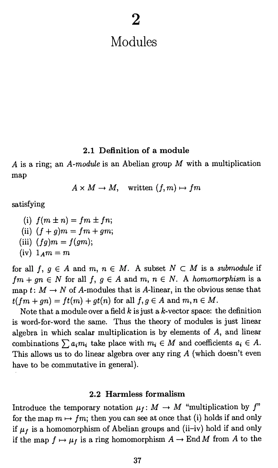
Modules
Definition of a module
Harmless formalism
The homomorphism and isomorphism theorems
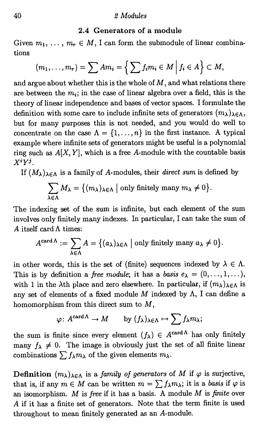
Generators of a module
Examples
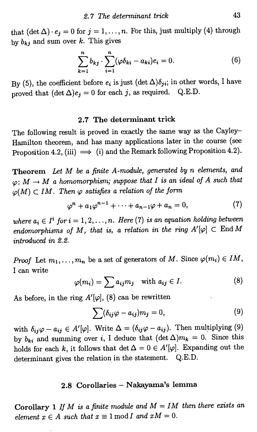
The Cayley-Hamilton theorem
The determinant trick
Corollaries - Nakayama's lemma
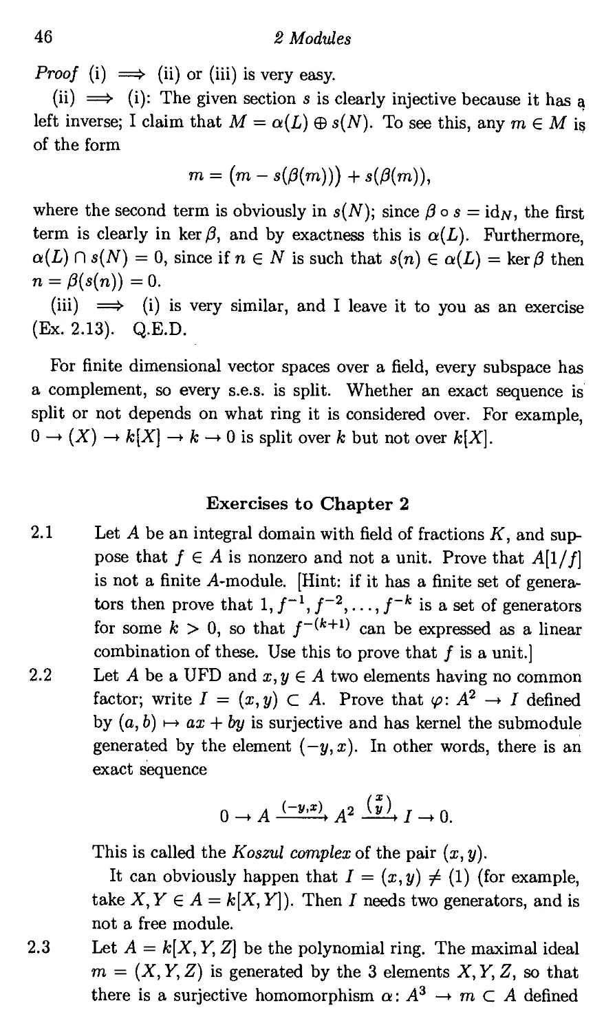
Exact sequences
Split exact sequences
Exercises to Chapter 2
3
3.1
3.2
3.3
3.4
3.5
3.6
Noetherian rings
The ascending chain condition
Noetherian rings
Examples
Noetherian modules
Properties of Noetherian modules
The Hilbert basis theorem
Exercises to Chapter 3
4
4.1
4.2
4.3
4.4
4.5
4.6
4.7
4.8
4.9
Finite extensions and Noether normalisation
Finite and integral A- algebras
Finite versus integral
Tower laws
Integral closure
Preview: nonsingularity and normal rings
Noether normalisation
Proof of Claim
Another proof of Noether normalisation
Field extensions
27
27
28
29
31
31
32
33
37
37
37
38
40
41
41
43
43
44
45
46
49
49
50
51
52
53
54
55
58
59
60
61
61
62
63
64
65
66
Contents ix
4.10 The weak Nullstellensatz 67
Exercises to Chapter 4 67
5 The Nullstellensatz and Spec A 70
5.1 Weak Nullstellensatz 70
5.2 Maximal ideals of k[X\,..., Xn] and points of kn 70
5.3 Definition of a variety 71
5.4 Remark on algebraically nonclosed k 72
5.5 The correspondences V and / 72
5.6 The Nullstellensatz 73
5.7 Irreducible varieties 74
5.8 The Nullstellensatz and Spec A 75
5.9 The Zariski topology on a variety 75
5.10 The Zariski topology on a variety is Noetherian 76
5.11 Decomposition into irreducibles 76
5.12 The Zariski topology on a general Spec .A 77
5.13 Spec A for a Noetherian ring 78
5.14 Varieties versus Spec A 80
Exercises to Chapter 5 82
6 Rings of fractions S~*A and localisation 84
6.1 The construction of S~ 1A 84
6.2 Easy properties 86
6.3 Ideals in A and 5~M 87
6.4 Localisation 88
6.5 Modules of fractions 89
6.6 Exactness of S~J 90
6.7 Localisation commutes with taking quotients 91
6.8 Localise and localise again 92
Exercises to Chapter 6 92
7 Primary decomposition 95
7.1 The support of a module SuppM 96
7.2 Discussion 97
7.3 Definition of Ass M 98
7.4 Properties of Ass M 99
7.5 Relation between Supp and Ass 100
7.6 Disassembling a module 103
7.7 The definition of primary ideal 103
7.8 Primary ideals and Ass 105
7.9 Primary decomposition 105
x 0 Contents
7.10 Discussion: motivation and examples 106
7.11 Existence of primary decomposition 108
7.12 Primary decomposition and Ass(j4/J) 109
7.13 Primary ideals and localisation 109
Exercises to Chapter 7 110
112
112
113
113
114
116
117
118
119
121
121
122
123
124
126
129
129
130
132
135
139
141
142
143
144
145
146
149
150
8
8.1
8.2
8.3
8.4
8.5
8.6
8.7
8.8
8.9
8.10
8.11
8.12
8.13
DVRs and normal integral domains
Introduction
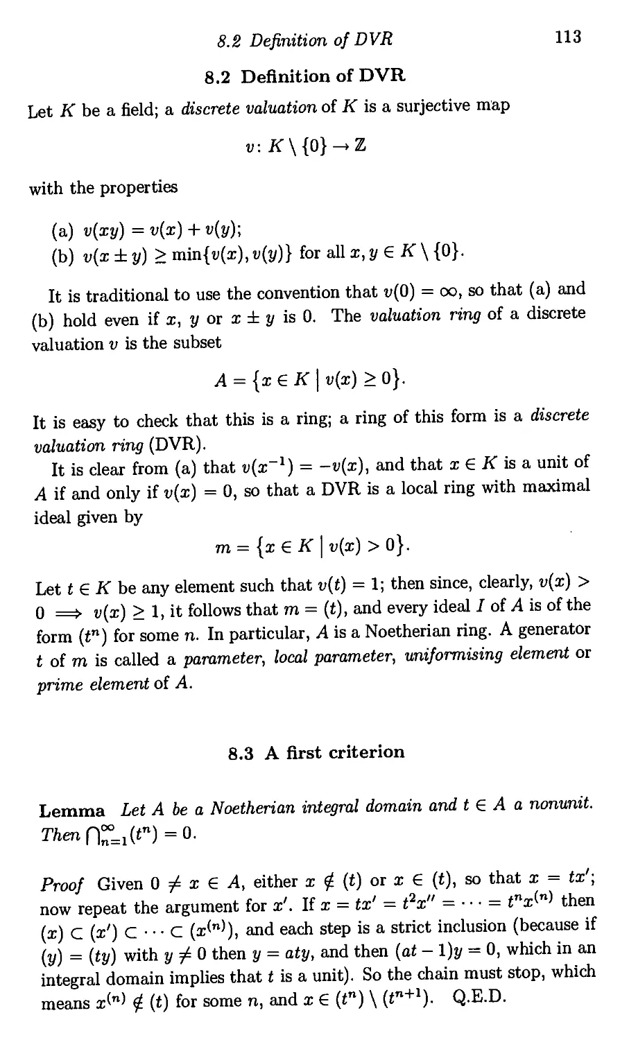
Definition of DVR
A first criterion
The Main Theorem on DVRs
General valuation rings
Examples of general valuation rings
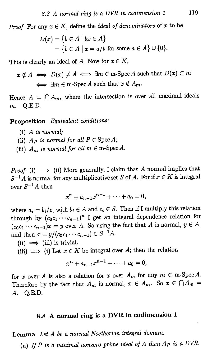
Normal is a local condition
A normal ring is a DVR in codimension 1
Geometric picture
Intersection of DVRs
Finiteness of normalisation
Proof of Theorem 8.11
Appendix: Trace and separability
Exercises to Chapter 8
9
9.1
9.2
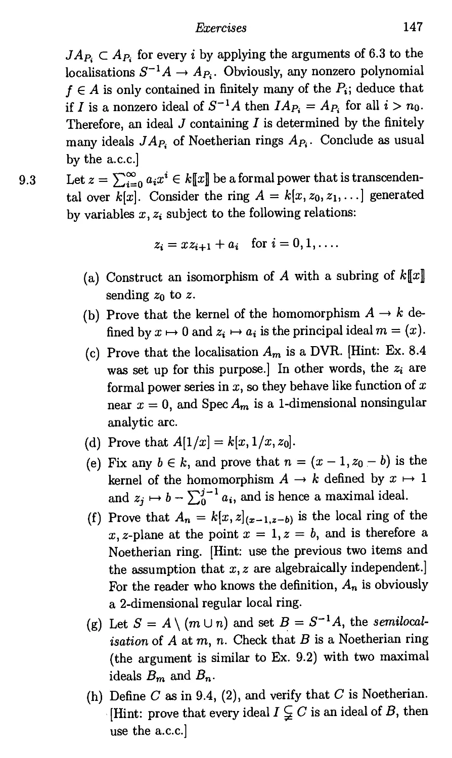
9.3
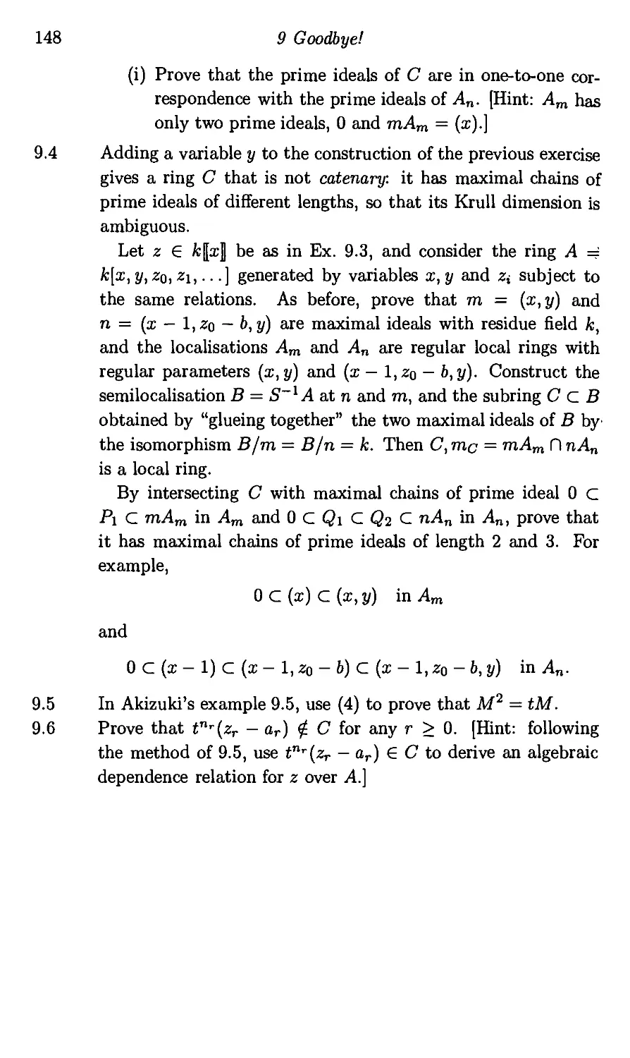
9.4
9.5
9.6
9.7
9.8
9.9
9.10
Goodbye!
Where we've come from
Where to go from here
Tidying up some loose ends
Noetherian is not enough
Akizuki's example
Scheme theory
Abstract versus applied algebra
Sketch history
The problem of algebra in teaching
How the book came to be written
Exercises to Chapter 9
Bibliography
Index
Illustrations
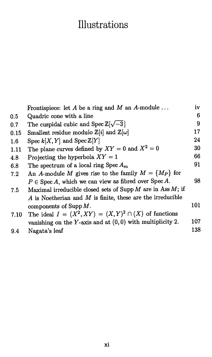
Frontispiece: let A be a ring and M an A-module ... iv
0.5 Quadric cone with a line 6
0.7 The cuspidal cubic and SpecZt-/^] 9
0.15 Smallest residue modulo Z[i] and Z[w] 17
1.6 Spec k[X,Y] and SpecZ\Y] 24
1.11 The plane curves denned by XY = 0 and X2 = 0 30
4.8 Projecting the hyperbola XY = 1 66
6.8 The spectrum of a local ring Spec Am 91
7.2 An A-module M gives rise to the family M = {Mp} for
P ? SpecA, which we can view as fibred over Spec A 98
7.5 Maximal irreducible closed sets of Supp M are in Ass M; if
A is Noetherian and M is finite, these are the irreducible
components of Supp M. 101
7.10 The ideal / = {X2,XY) = {X,Yf D (X) of functions
vanishing on the V-axis and at @,0) with multiplicity 2. 107
9.4 Nagata's leaf 138
XI
Preface
These are notes from a commutative algebra
course taught at the University of Warwick sev-
several times since 1978. In addition to standard
material, the book contrasts the methods and ide-
ideology of abstract algebra as practiced in the 20th
century with its concrete applications in algebraic
geometry and algebraic number theory.
xm
0
Hello!
This chapter contains a preliminary discussion of the aims and philo-
philosophy of the book, and is not logically part of the course. Some of
the material may be harder to follow here than when it is treated more
formally later in the book, so if you get stuck on something, don't worry
too much, just skip on to the next item.
0.1 Where we're going
The purpose of this course is to build one of the bridges between alge-
algebra and geometry. Not the Erlangen program (linking geometries via
transformation groups with abstract group theory) but a quite different
bridge linking rings A and geometric objects X; the basic idea is that
it is often possible to view a ring A as a certain ring of functions on a
space X, to recover X as the set of maximal or prime ideals of A, and to
derive pleasure and profit from the two-way traffic between the different
worlds on each side.
Algebra here means rings, always commutative with a 1, and usually
closely related to a polynomial ring k[x\,... ,xn\ or I\x\,... ,xn] over a
field k or the integers Z, or a ring obtained from one of these by taking
a quotient by an ideal, a ring of fractions, a power series completion,
and so on; also their ideals and modules. In this book, A usually stands
for a ring and k for a field, and I sometimes use these notations without
comment. We're interested in questions such as zerodivisors (that is,
0 7^ x,y ? A such that xy = 0 E A), factorisation (that is, writing
o 6 A as a product o = b Yip™' with b invertible and p* prime elements),
similar questions for ideals, prime ideals, extension rings A C B, etc.
The study of rings of this type includes most of algebraic number
theory and a large fraction of algebraic geometry. The methods for
1
2 0 Hello!
studying them, by and large, are either simple algebraic arguments, or
depend on the link with geometry which I want to introduce here. Thus,
for example, rings have a dimension theory, in which dim k[x\,..., xn] =
n and dimZ[zi,..., xn] = n + 1 (yes, n + 1 is right!), and already the
language suggests a cocktail of two different subjects. The same holds
for local ring, an idea at the very heart of commutative algebra.
0.2 Some definitions
Before describing briefly the geometric side and some aspects of the
bridge, I recall a few very elementary algebraic topics and introduce
some definitions, which I hope are mostly already familiar.
Let A be a ring, commutative with a 1. Zerodivisors of A are nonzero
elements x, y ? A such that xy = 0. If A has no zerodivisors and A ^ 0,
it is an integral domain; note that 0 ^ 1 is part of the definition of
integral domain. An integral domain is contained in a unique field K
such that every element of K is a fraction a/b with o, b ? A and 6^0;
this is the field of fractions of A, sometimes written K — Prac A, and I
assume you understand its construction. An element x ? A is invertible
or a unit of A if it has an inverse in A, that is, there exists y ? A such
that xy = 1.
An element x ? A is nilpotent if xn = 0 for some n. Prove for yourself
that x nilpotent implies that 1 — x is invertible in A. [Hint: write out
A — a;) as a power series.] Prove also that x and y nilpotent implies
that ax + by is nilpotent for all o, b ? A, so that the set of nilpotent
elements of A is an ideal, the nilradical nilrad A [Hint: use the binomial
theorem.] An element x ? A is idempotent if x2 = x. Obviously if x
is idempotent then so is x' = 1 — x, and then x + x' = 1 and xx' = 0
(please check all this for yourself), so that x and x' are complementary
orthogonal idempotents; now by writing o = ax + ax' for any o ? A, you
see that A is a direct sum of rings A = A\ © Ai, where A\ = Ax and
A2 = Ax'.
0.3 The elementary theory of factorisation
Suppose that A is an integral domain. A nonzero element x ? A is
irreducible if x itself is not invertible, and x = yz with y, z ? A implies
that either y or z is invertible. x ? A is a prime element if it is not a
unit, and x | yz implies either x | y or x | z. It is trivial to see that
prime implies irreducible, but the other way round is false in general.
0.4 A first view of the bridge 3
A is a UFD (unique factorisation domain) if (i) every element x factors
as a product of finitely many irreducibles x = J\ Xj with X{ irreducible,
and (ii) irreducible implies prime.
Proposition In a UFD A, the expression of x = bjjp^ as a product
of irreducibles with pi \ pj is unique (up to invertible elements).
I assume you know this. Otherwise, see any textbook on algebra, for
example, [C], [H & H], Chapter 4 or [W]. In the following sections, I need
to assume that the polynomial ring k[x\,..., xn] is a UFD; the proof of
this is discussed in Exs. 0.8-9 below.
0.4 A first view of the bridge
For simplicity, and to be able to describe in a few intuitive words a rep-
representative case of the geometric side, suppose that k is an algebraically
closed field, for example k = C. Then the polynomial ring k[x\,.. .,xn]
is a ring of functions on kn, because a polynomial g ? k[x\,..., xn] is a
function g = g(x\,.. -,xn) of X\,...,xn. Moreover, evaluating a poly-
polynomial at a point P = (oi,.. -,an) ? kn determines a homomorphism
k[xi,...,xn) —> k defined by g >-» g(P), whose kernel is the maximal
ideal mp = (x\ — Oi,..., xn — an) (see Ex. 1.15). This is the correspon-
correspondence between a ring A and a space X in ideal form: A = k[x\,.. -,xn]
is the ring of polynomial functions on X = kn, and the points of X
correspond to maximal ideals of A.
0.5 The geometric side — the case of a hypersurface
Suppose that 0 ^ F ? k[x\,..., xn]\ then the locus
X = V(F) = {P = K ... ,oB) | F(P) = 0}ckn
is a hypersurface. It is (n — l)-dimensional because you can (almost
always) use the equation F = 0 to solve for a\ in terms of 02, • ¦ •, an.
Now consider the quotient ring A = k[x\,..., xn]/(F), that is, the ring
of residue classes modulo the ideal generated by F. Then an element
g ? A defines a fc-valued function on X: indeed, if g is the class in A
of a polynomial g~ ? k[x\,... ,xn] then for x ? X the value g(x) = lj(x)
does not depend on the choice of <jf.
Now we can see (fairly light-weight) traffic passing over the bridge.
First, to what extent can A be viewed as a ring of functions on XI
0 Hello!
(i) If F has no multiple factors, say F = Ylfc with /j \ fj, then it
can be shown that F generates the ideal of all functions vanishing
on X. (You can try the proof as an exercise after Chapter 5, see
Ex. 5.5.) It follows from this that an element g ? A is uniquely
determined by the corresponding function g: X —> k, so that A
is contained in the ring of A;-valued functions on X.
On the other hand, if F has a multiple factor, say F = fkg with
k > 2 then also fg = 0 everywhere on X, and hence F does not
generate the ideal of all functions vanishing on A". At the same
time, A has nonzero nilpotent elements (because x = im fg ? A
satisfies xk = 0). In this case, it is not reasonable to try to view
the nilpotent element a; as a function on X, because it is zero
everywhere on X. Thus
F has a multiple factor
<==> more functions vanish on X than (F)
<==> A has nilpotent elements
A has nonzero elements that are 0 as functions on X.
(ii) If F has a factorisation F = /1/2, where /i,/2 are polynomials
with no common factors, then A has zerodivisors (because X\ =
im/i, x-i = im/2 satisfy ii ^ 0,12 ^ 0 but X\X2 = 0); this
corresponds to a decomposition X = X\ U X2 of X as a union of
two smaller hypersurfaces Xi given by /j = 0 for i = 1,2. Thus
A has zerodivisors (not nilpotents)
X is reducible: X = Ai U A2.
That is, something in algebra equals something in geometry.
(iii) I mentioned complementary orthogonal idempotents and direct
sums of rings in 0.2; you can't get much more abstract algebraic
than that. However, it is easy to see that A has nontrivial idem-
idempotents if and only if X is a disjoint union of two hypersurfaces,
X = X\ U X2. If k = C, this just means that X c C" is a dis-
disconnected topological space; you can't get much more geometric
than that. The ring of functions (say, continuous) on a discon-
disconnected space X = Xy UX2 is a direct sum of the rings of functions
on A"i and AY
(iv) We will see that there is a close relation between ideals I C A
and subvarieties of X; we can already see that if / c A is an ideal
then it defines a subvariety V(I) C X, the subset of P ? X where
0.6 Z versus k [X] 5
f(P) = 0 for all the functions / ? /. But this is quite a long story
that I defer until later. For the time being, I state without proof
the following result (a special case of the weak Nullstellensatz,
see Theorem 4.10 and 5.1).
Proposition Maximal ideals of A are in one-to-one correspondence
with points P ? X. That is,
P = (a1,...,an)eX <-+ mP = (x1-au...,xn-an)cA.
To repeat my refrain, something in algebra (the maximal ideals of A)
equals something in geometry (the points of X).
(v) Assume that F ? k[x\,. ..,xn] is irreducible, so that A is an
integral domain. When is A = k[x\,.. .,xn]/(F) a UFD?
For example, if F = xz - y2 ? k[x, y, z] then xz = y2 holds in
the quotient ring A, whereas it is not hard to check that x, y, z are
irreducible; therefore A is not a UFD. Now draw the picture of
the locus X : (xz = y2), which is the ordinary quadric cone (see
Figure 0.5). I will come back to this picture several times later in
the book. Observe that X is a cone, and so contains lots of lines,
for example, the lines L\ c X defined by x = A2z, y = Xz; these
are codimension 1 subvarieties of X.
I take A = 0 to simplify the notation, so consider the line
L = Lq C X defined by x = y = 0. The special feature of
X is that the ideal It, C A of functions vanishing on L is not
generated by one element. In fact //, = (x, y), but y also vanishes
along a second line y = z = 0, whereas x vanishes along L with
multiplicity 2. Geometrically, this corresponds to the fact that
the plane x = 0 is everywhere tangent to X along L; or, to put it
another way, at any point where z ^ 0,1 have x = y2/z. In this
sense, L is not locally defined by one equation.
In other words, the geometric question of codimension 1 sub-
varieties and how to define them by equations is closely related
to the algebraic question of unique factorisation in the ring A.
0.6 Z versus k[X]
The comparison between the ring of integers Z and the polynomial ring
k[X] in a single variable over a field k is one of the central points to be
made at the outset in a commutative algebra course. From the algebraic
0 Hello!
Figure 0.5. Quadric cone with a line
point of view, these two rings are very similar in many formal respects,
and yet they are very different in substance. (Compare also Exs. 0.10-12
and the worked example 1.5.)
Points of similarity Recall that Z and k[X] are both Euclidean rings,
that is, integral domains satisfying "division with remainder" or the
"Euclidean algorithm": for any o, b, there exists an expression o = bq + r
with r less than b. The ideal theory of the two rings proceeds in parallel
from this fact: from division with remainder it follows easily that every
ideal is principal (generated by one element), either @) or (/) for an
element /. I assume you know all this (see Exs. 0.1-9), including how
you deduce the familiar af + bg = h property of the highest common
factor h = hcf(f,g), unique factorisation, etc.; if not, see, for example,
[C]or [H&H], Chapter 4.
Points of difference Obviously Z and k[X] are as different as chalk
and cheese, but it is worthwhile trying to pin down the difference. I
give two illustrations. First an algebraic statement: k[X] contains a
field, whereas Z doesn't. As you know, for any ring A, there is a unique
0.7 Examples 7
homomorphism t: Z —¦ A: after taking 1 >-» 1,4, the rest is forced. If A
contains a field then t factors through the prime subfield, either Fp or
Q. If a ring A contains a field A; as a subring, then A and any .A-module
are fc-vector spaces. In the case A — Z, there is obviously no way of
embedding either Fp or Q into A. The same holds for A = Z/(p2), with
p a prime number: the additive group Z/(p2) is not a vector space over
any field; see Ex. 0.10. For this reason, one sometimes says that a ring
containing a field k has equal characteristic char k (either 0 or p), whereas
a ring like Z has unequal characteristic, in the sense that the ring itself
has characteristic 0, but it has residue fields Fp of characteristic p.
Here is another difference: k[X] contains variables. To put it alge-
algebraically, a typical maximal ideal of k[X] is (X), and it makes sense to
differentiate with respect to X; that is, there is a fc-linear map
4^7 ¦ k[X] -> k[X], defined by xn >-> nxn~l for all n,
aX
with the properties and applications that you know about. By contrast,
the maximal ideals of Z are B), C), E), etc., and
d_ d_ d_
d2' d3' d5'"'
are of course completely meaningless. There is no nonzero derivation of
Z to anything.
To put it another way, multiplication by a natural number n is the
additive operation oh a + ¦ ¦ ¦ + a (with n summands), and therefore
this operation, and the ideal (n) generated by n, are already determined
by the additive structure.
0.7 Examples
Recall that we intend to study extension rings of Z and of k, and that
the distinctions in 0.6 will carry over to these. I continue the theme of
0.6 with two slightly more substantial examples from algebraic geometry
and algebraic number theory illustrating this and other points.
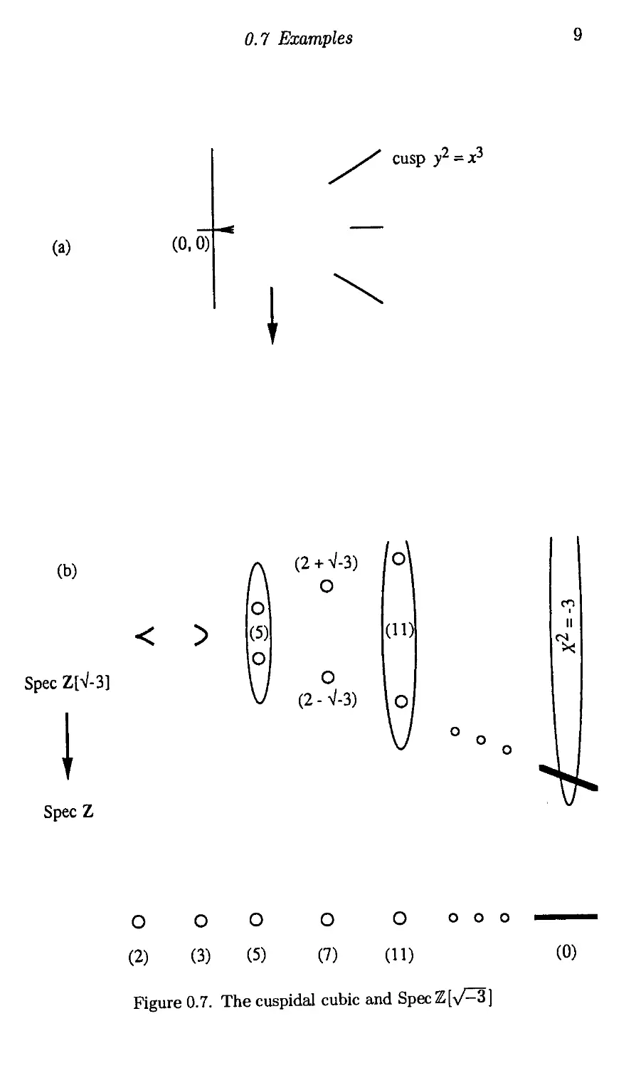
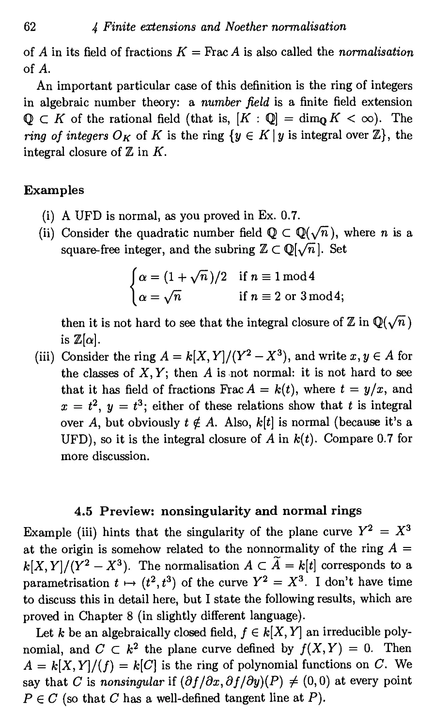
Example 1 Suppose that k is an algebraically closed field of charac-
characteristic ? 2, and let A be the ring A = k[X,Y]/(Y2 - X3). By the
correspondence of 0.5, A is a ring of functions on the plane curve C C k2
given by Y2 = X3. See Figure 0.7(a).
Now A can be viewed as the extension ring /c[X][\/X^] obtained by
adjoining the square root of X3 to k[X]. If (X - a) is a maximal ideal
8 0 Hello!
of k[X] with a ? /c, it is contained in maximal ideals (X - a, Y — /?), ¦
corresponding to the square roots /3 = i-s/o3"; there are obviously two of'
these if a ^ 0, and one otherwise. These ideals require two generators..
Moreover, it is easy to see that the elements X and Y are irreducible in
A, but not prime: indeed, Y2 = X3 in A, so that X | Y2, but X \ Y.
At this point, observe that I am doing something fairly silly by taking
the square root of X3. It is clearly much more sensible to take the square
root of X instead. Let A' = k[t] where t = Y/X = y/X\ this is a slightly
bigger ring that A. Then in it, X = t2 and Y = t3 ? A' = k[t], so that
A' is just a polynomial ring, so of course it is a UFD, and every ideal is
principal.
Example 2 Now consider B = Z[\/^3], the extension ring obtained by
adjoining ^/^3 to Z. What are its maximal ideals? If P is a nonzero
prime ideal of B then P D Z is a nonzero prime ideal of Z, so of the form
(p); we say that P lies over p. I check first that every prime number
p ^ 2,3 either splits as a product p = f+f~ of two prime elements of B,
or remains a prime element of 5, and, in particular, any prime ideal of
B not lying over 2 is principal. Indeed, any p = 1 mod 6 can be written
as p = 3o2 + b2 with o,6 ? Z; this was proved in 1760 by Euler, and
is worked out in Ex. 0.14. Thus p factors in B as a product of two
irreducible elements p = /+/_, with f± =b± o-\/^3; for example,
It is easy to check that B/(f±) = Fp, so that f± are two prime elements
of B lying over p. If p = 5 mod 6 then X2 + 3 is irreducible in FP[X] by
quadratic reciprocity (see Ex. 0.13), and B/{p) ~ WP[X]/(X2 + 3) = Fp2
is a field, so that p is a prime element of B. It is also not hard to check
that (\Z^3) = SZeZ-/1^ c B, so that 5/(-/^3) = F3, and again
V^3 is a prime element of B.
However, 2 is bad in B: you can easily prove it is irreducible, because
(o + 6-/I3)(o - bV^) = a2 + 3b2 ^ 2 for any a,b ? Z,
but it is not a prime element since 22 = A + V^3)(l - -s/^3). Thus
the prime ideal over 2 in B is B,1 + \/—3), which needs 2 generators.
At this point, anyone who knows algebraic number theory will see that
I am doing something fairly silly by taking the square root of —3. It is
clearly much more sensible to take u> = (-1 + y/^3 )/2 instead; note that
u> = expB7ri/3) is a primitive cube root of 1, satisfying J1 + w + 1 = 0.
Let B' — Z[w], a slightly bigger ring than B. The analysis of its prime
0.7 Examples
(a)
@,0)
cusp >2 =
(b)
Spec Z[V-3]
< >
B + V-3)
O
B-V-3)
11
SpecZ
O OO O O
B) C) E) G) A1)
Figure 0.7. The cuspidal cubic and Sp
ooo
@)
10 0 Hello!
ideals is exactly as for B except above 2, which is a prime element of
B', because B'/B) = F2[u>] = F4, a quadratic extension field of F2. In
fact you can prove that B' is a UFD (see Ex. 0.16).
Figure 0.7(b) draws the prime ideals of B = Z[-s/^3] in schematic
form. I draw two points in a bubble over the primes p = 5 mod 6 to rep-
represent the single prime p ? B, because I have in mind the two conjugate
points X = ± 1/—3 of the X-line defined over Fp2.
0.8 Reasons for studying commutative algebra
Commutative algebra is the crossroads between algebraic number theory,
algebraic geometry and abstract algebra. Although much of the material
of this book develops techniques of algebra, it should be clear that my
main interest is the applications of these ideas to geometry and number
theory.
a. Algebraic number theory Galois theory studies field extensions,
with motivation coming from the study of polynomials and their roots;
thus, corresponding to a polynomial
f(X) = anXn + an-iXn~l + ¦ ¦ ¦ + a0 ? k[X]
with coefficients in a field /c, one knows how to build a field extension
k C K over which / has a root, or splits into linear factors. It often
happens that k contains a subring A C k of interest, for example Z C Q,
such that the coefficients of / are contained in A; we might then want
to study a subring of K corresponding to A, for example the subring
B generated by A and the roots of /. As a famous example, let e =
expB7rz/n) = i/I ? C; over the ring B = Z[e], a number of the form
xn — zn with x and z coprime factorises into n factors:
n-l
xn -zn= Ylix-^z).
i=0
Suppose we happened to know that B = Z[e] is a UFD; then comparing
two factorisations into primes coming from the left and right sides of
n^1^ ~?%z) = Vn would obviously impose very strong restrictions on
integer solutions of xn + yn = zn, and in fact it is known that this can
be used to prove that there are only the trivial solutions with x or y or
z = 0; see, for example, [B&Sh], Chapter III, 1.1. Unfortunately, Z[e]
0.8 Reasons for studying commutative algebra 11
is not usually a UFD for large n, so you have to work harder if you want
to prove this statement for all n and claim the due reward.
Rings like Z[e] (or B' = Z[w] in 0.7) are called rings of integers of
number fields, and the study of their ideals in the 19th century, in the
context of Kummer's study of Fermat's last theorem (now Wiles' theo-
theorem), marks the start of commutative algebra.
b. Algebraic geometry Quite generally, an algebraic variety V C kn
has a coordinate ring
k[V] = k[Xi,.. .,Xn]/Ix = {polynomial functions y>: V —> /c},
and the study of k[V] gives lots of information about V. From the point
of view of ring theory, every integral domain that is a finitely generated
/c-algebra occurs as k[V] for some variety V.
For example, if you study a plane curve such as C: (y2 = a;3) C k2,
you will rapidly come to the conclusion that its properties are closely
related to those of the ring A = k[X,Y]/(Y2 - X3). Thus, as we saw
in 0.7, Example 1, A can be embedded in a bigger ring A' = k[t] with
X = t2, Y = t3, which corresponds to the parametrisation x = t2, y = t3
of the curve C. The fact that the origin @,0) is a singular point of C is
reflected in the algebra, as we saw in 0.7, and will see in several places
below.
c. Abstract algebra Commutative rings were studied extensively at
the turn of the century: as I have just sketched, they occurred in the 19th
century as the rings of integers of number fields, and as the rings k[V]
associated with algebraic varieties V c kn. In either case, these are quo-
quotients of polynomial rings A = Z^i,.. .,?„]//or A = k[x\,.. .,?„]//; in
the early 20th century, notably in the work of Hilbert, Emmy Noether,
Krull, Emil Artin and others, they occurred as abstract structures sat-
satisfying the ring axioms, and whatever other axioms were needed to get
reasonable results, notably the a.c.c. (ascending chain condition, see
Chapter 3). A very important motivating idea for the development of
algebra in the 1910s and 1920s was the fact that the abstract approach
is often simpler and more general, and yields many of the results for the
concrete quotients of polynomial rings with considerably less effort; see,
for example, Remark 1.5. In this vein, this course discusses a number of
results which are showcases of the methods of abstract algebra; at the
same time, I point out some problems where the abstract approach has
its limitations.
12 0 Hello!
In conclusion, rings of the form I\X\,...,Xn]/I or k[Xi,...,Xn]/I
for suitable ideals I are important in both algebraic geometry and alge-
algebraic number theory, and have also been central to the development of
algebra.
0.9 Discussion of contents
The course can be viewed as a continuation of an algebra course on
rings and modules, as taught in the second or third year in many British
universities. The book covers roughly the same material as Atiyah and
Macdonald [A&M], Chaps. 1-8, but is cheaper, has more pictures, and
is considerably more opinionated.
However, rather than talking about abstract algebra for its own sake,
my main aim is to discuss and exploit the idea that a commutative ring
A can be thought of as the ring of functions on a space X = Spec A.
Here are some points I will try to emphasise along these lines:
A) Prime spectrum Spec A The attempt to re-establish the space X
as the spectrum or prime spectrum, the set of prime ideals of A.
In important cases, the prime ideals are controlled by maximal
ideals.
B) Geometric rings and the Nullstellensatz A ring that can be written
as the coordinate ring A — k[V] of a variety V is by definition a
ring of functions on V, and the correspondence between geometry
and algebra is especially close in this case.
C) Localisation A ring of fractions A[l/f] corresponds to restricting
functions on X to the open subset Xf = {x ? X \ f(x) ^ 0}.
D) Primary decomposition A module can be pictured as a geometric
object living over a subset of X (see the Frontispiece).
E) Integral extensions and normalisation
F) Discrete valuation rings Discrete valuation rings (DVRs) are the
best kind of UFDs, having only one prime. The idea of a discrete
valuation corresponds closely to the idea of measuring the power
of a prime p dividing an integer, or the order of zeros and poles
of a function on a normal algebraic variety or complex analytic
space.
G) A Noetherian normal ring is an intersection of DVRs. This re-
result was somehow omitted from [A & M], but is very important.
The statement and its proof is an exemplary chain of abstract al-
algebraic reasoning. However, the result includes (i) the statement
0.10 Who the book is for 13
that a meromorphic function on a complex manifold having no
poles in codimension one is holomorphic, and (ii) the characteri-
characterisation of algebraic integers among all algebraic numbers in terms
of p-adic valuations.
(8) Finiteness of normalisation An algebraic result that provides the
ring of integers of a number field, and the resolution of singu-
singularities of algebraic curves. At the same time, it gives a salutary
reminder: finiteness of normalisation holds for practically all rings
of importance in the world, but not for all Noetherian rings.
0.10 Who the book is for
Although this course will give the student intending to study algebraic
geometry or complex analytic geometry an introduction to basic mate-
material in commutative algebra, an equally important objective is to make
accessible to algebraists and number theorists the benefits of geometric
intuition in studying commutative rings. However uncomfortably they
fit into the framework of axioms and abstract arguments, the pictures
in this book are (in my opinion) what commutative algebra is all about.
If you are the kind of student of algebra who suffers from vertigo when
more than one or two logical steps above the axioms, you may convince
yourself that all the material is entirely rigorous, and, if so desired, treat
the geometric stuff as fanciful digressions. Or maybe my approach is
just not for you; by all means study the excellent book of Atiyah and
Macdonald [A&M] instead.
0.11 What you're supposed to know
As already mentioned, this course assumes some prior knowledge of fields
and rings, for example, polynomial rings, the elementary theory of fac-
factorisation, division with remainder and its application to proving that
Z and k[X] are PIDs (principal ideal domains), therefore UFDs. This
stuff is treated in any number of books, for example [C], [H&H], Chap-
Chapter 4 or [W]. The first few (very easy!) exercises to this section sketch
some standard material I will assume later, for example the fact that
the polynomial rings Z[ii,.. .,xn] and fc^i,.. .,xn] are UFDs. I also
use some basic material in set theory, notably the definition of partially
ordered set, but I give a discussion of Zorn's lemma and the a.c.c. from
first principles.
This course is intended for advanced undergraduates or beginning
14 0 Hello!
graduate students, and in addition to background from algebra it as
sumes basic facts from analysis such as radius of convergence of a power
series and the definition of a topological space. On the other hand, I
develop modules from scratch and (except for Appendix 8.13 to Chap-
Chapter 8) do not assume any material from Galois theory beyond the simple
lemma on primitive field extensions sketched in Ex. 0.5.
The relation between commutative algebra, algebraic geometry and al-
algebraic number theory is symbiotic, and the student will derive valuable
motivation from an interest in one or other of these subjects. However, I
have tried to keep this course reasonably self-contained, sometimes at the
expense of repeating material that is covered perfectly well elsewhere.
Exercises to Chapter 0
Exercises 1-9 are intended to sketch out some material which
you are supposed to know.
0.1 Let A be any ring, and consider the polynomial ring A[T}. Prove
that T is not a zerodivisor in A[T]. Generalise the argument to
prove that a monic polynomial
(a polynomial with leading coefficient 1) is not a zerodivisor in
A[T\.
0.2 Let A be any ring, a ? A and / ? A[T\. Prove that there exists
an expression f = (T — a)q + r with q ? A[T] and r ? A. [Hint:
subtract off a suitable multiple of (T — o) to cancel the leading
term, then use induction on deg/.] By substituting T = a,
show that r = f(a). (This result is often called the remainder
theorem in algebra textbooks.)
0.3 Remind yourself that (i) Z and k[T] are Euclidean rings, that is,
they have division with remainder (see [C], [H&H], Chapter 4
or [W]); (ii) a ring having division with remainder is a PID; and
(iii) a PID is a UFD.
0.4 Let A[T] be the polynomial ring over a ring A, and B any ring.
Suppose that ip: A —> B is a given ring homomorphism; show
that ring homomorphisms I\\)\ A[T] —> B extending <p are in one-
to-one correspondence with elements of B.
0.5 Remind yourself that (i) a nonzero prime ideal me k[T] is of
the form (/) with / an irreducible polynomial, and the quotient
ring k[T]/m is a finite algebraic extension field of k in which /
Exercises 15
has a root; and (ii) if A is a ring containing a field k and a ? A
any element then the subring fc[a] C A generated by k and a is
isomorphic to k[T] or is a field extension of the form k[T]/(f)
with / irreducible.
0.6 Let B = k[T] with k a field; a k-automorphism of B is a ring
homomorphism tp: B —> B that is the identity on k and is an
automorphism of B (that is, one-to-one and onto), (i) Describe
the group Aut/t B of k-automorphisms of B; (ii) now do the
same for the field K = k(T) of rational functions. [Hint: use
Ex. 0.4. The answer to (ii) is in terms of 2 x 2 matrixes.]
0.7 Let A be a UFD, K its field of fractions and / ? A[T] a monic
polynomial (defined in Ex. 0.1 above). Prove that if / has a root
a ? K then in fact a ? A. [Hint: you can probably remember
this for Z C Q; write a = p/q where p, q have no common
factors, and consider the equation f{p/q) = 0.]
0.8 Let A be a UFD and K its field of fractions. A polynomial
is primitive if its coefficients b, have no common factors in A
(other than units). Prove Gauss' lemma: the product of two
primitive polynomials is primitive.
A polynomial / ? K[T] has a reduced expression f = afo
where a ? K, and /o ? A is primitive, unique up to multiplying
by a unit. (This just amounts to clearing denominators and
taking out any common factor.) The point of Gauss' lemma is
that if / = o/o and g = bgo are reduced expressions for / and g
then fg = (a6)(/o<7o) is a reduced expression for fg.
0.9 Prove that A a UFD implies A[T\ a UFD. [Hint: you know
that K[T] is a UFD, where K = Frac A. Use Gauss' lemma
to compare factorisation in K[T] and A[T].] Deduce that the
polynomial rings Z[xi,..., xn] and k[xi,..., xn] are UFDs.
0.10 Let k = Fp = Z/(p) be the finite field with p elements. Compare
the two rings k[T]/(Tn) and Z/(pn) for n > 2. Show that their
elements can be written respectively in the form
Oo + air + '-. + ttn-iT" or a0 + a.ip + ¦ ¦ ¦ + an_1pn~1
with a* ? {0,1,...,p— 1} for i = 0,..., n — 1; determine the ad-
addition and multiplication of these power series in the two rings,
and note that they differ only by the p-adic "carry".
16 0 Hello!
0.11 Prove that the ring Z/(p") for n > 2 does not contain a field, an
cannot be made into a vector space over Fp in a way compatibl
with its Abelian group structure.
0.12 Show that it makes sense to take infinite power series
ao + aiT+--- + anTn + --- or ao + a1p + --- + anpn + ¦
and add and multiply them according to the rules you worked
out in Ex. 0.10. The ring of all such power series are respectively
the formal power series ring in one variable /c[TJ and the rino
of p-adic integers Zp.
0.13 Use quadratic reciprocity to prove that —3 is a quadratic residue
mod p if and only if p = 2 or p = 1 mod 6. Deduce that
= 5mod6.
0.14 Prove that a prime number p = Imod6 is of the form 3a2 +;
b2 with o,6 ? Z. [Hint (due to Axel Thue [N], supplied to
me by Alan Robinson): pick any a ? Z with a2 = — 3mod#
(this is possible by Ex. 0.13). Consider x — ay as (x,y) run'
independently through the integers in [0, ^/p]; there are > p
pairs (x, y), hence they are not all distinct modp. If X\ — ayi =
X2 — ay2 then
(xi - x2J + 3(yi - y2J = Np with N = 1,2 or 3.
Now iV = 2 is impossible, and if iV = 3 you can divide through.]
0.15 Prove that the ring of Gaussian integers Z[z], where i2 = —1, has
division with remainder with respect to the function "absolute
value squared" d(x + yi) = x2 + y2. Deduce that it is a principal
ideal domain, hence a UFD. [Hint: any complex number z is of
the form z = a + 0, with integral part a ? I\i\ and smallest
residue /3 in the shaded square of Figure 0.15(a). Apply this to
a fraction (c + di)/(a + bi) to get division with remainder
c + di = (a + bi)a + (a + bi)/3.
The reason that the argument works is that the shaded square
of Figure 0.15(a) is contained inside the unit disk.]
0.16 Prove that the ring Z[w] is a UFD, where w2 + w +1 = 0. [Hint:
as in the previous question, prove that Z[w] has division with
Exercises
17
l+co
Figure 0.15. Smallest residue modulo Z[i] and
(b)
remainder with respect to the function "absolute value squared"
d(a + buj) = (a + buj)(a + buj2) = a2-ab + b2, see Figure 0.15(b).]
0.17 Use the result of Ex. 0.16 to deduce another proof of the fact
that any prime p = 1 mod 6 is of the form 3a2 + b2.
0.18 (Harder) Prove the cases n = 3 and n = 4 of Fermat's last
theorem (see 0.8 and [B&Sh], Chapter III, 1.1).
0.19 Study the ring B = Z[\/5 ] in the spirit of 0.7. A maximal ideal
P of B lies over a prime (p) = PAZ of Z. If p ^ 2,5, then either
(i) 5 is a quadratic residue mod p, and then p factors in B as a
product of two elements p = fif2, and B/(/i) = B/(f2) = Fp,
so that /i are /2 are prime elements of B (you can prove this
by a minor modification of the method of Ex. 0.14); or (ii) 5
is a quadratic nonresidue mod p, and then B/(p) = Fp[\/5]
is a quadratic field extension of Fp, so that p remains a prime
element in B. (By quadratic reciprocity, the first happens if and
only if p = ±1 mod 5, for example, 11 = D — \/5 )D + \/5 )•)
Also \/5 is a prime element of B over 5, because (\/5) =
Z5 ©Z\/5 C B, giving B/(\/5) = F5. However, 2 is bad in B:
it is an irreducible element, because
(o\/5 + 6)(o\/5 - 6) = 5o2 - b2 ^ 2 for any a, b G Z
18 0 Hello!
(argue mod 4), but not a prime element since
Thus the prime ideal over 2 in B is B, \/5 + 1), which needs 2
generators.
0.20 Consider the ring B' = Z[r] where r = A + \/5)/2 is the soj
called "golden ratio", which satisfies r2 = t + 1. Show that
every maximal ideal of B' is principal. [Hint: compare O.7.] ;
0.21 Show that an element a + br is a unit of B' (that is, is invertible
in B') if and only if N(a + br) = a2 + ab - b2 = ±1. Prove that
the multiplicative group of units of B' is generated by ±l,r:
[Hint: for the first part, note that
c + dr _ (c + rfr)(a + 6(l-r)) _ (c + dr)(a + b(l - t))
a + br ~ {a + br){a + b{l - t)) ~ a2 + ab-b2
For the second part, if a + br is a unit then so is ±r(a + br)
±(b + (a + b)r) and ±(r - l)(a + br) = ±F - o + ar); one of
these operations allows you to reduce max{|o|, |6|} until you get
down to 1.]
0.22 Prove that Z[r] is a UFD. [Hint (provided by Jack Button):
write iV(a + br) = a2 + ab — b2. The aim is to show that Z[r]
satisfies division with remainder with respect to the function
d(a + br) = \N(a + br)\ = |o2 + ab - b2\. As in Exs. 0.15-16,
every element of Q[r] has a smallest residue r + st mod Z[r] in
a "shaded" square, with r, s ? [—1/2,1/2], and then obviously
\N(r+sr)\ <3/4.]
0.23 (Harder) Let / ? A; if / is reducible then the principal ideal
(/) is contained in a bigger principal ideal (f\). Consider the
following conditions on a ring A:
(a) A is a UFD;
(b) every increasing chain (/i) C (.fc) C ••• C (/„) C •••
of principal ideals is eventually stationary, that is (fk) =
(fk+i) = ¦•¦ for some/c;
(c) any element can be written as a product of irreducible
elements.
Prove that (i) =$¦ (ii) and (iii), and that (ii) => (iii). Find
counterexamples to the implications (iii) => (i) and (ii) =>
(i). Find a ring not satisfying (iii). Find a counterexample to
the implication (iii) => (ii).
1
Basics
1.1 Convention
I assume that the student already knows the definition of ring and ring
homomorphism (see for example [A &M], p. 1); however, throughout this
course, a ring A is also assumed to be commutative (that is, ab = ba)
and to have an identity element 1 = 1^ ? A; a ring homomorphism
\p: A —> B is assumed to satisfy v?Aa) = 1b 6 B, and a subring of a ring
is assumed to share the same identity element. I will use this convention
from now on, usually without mention. See also the discussion in 1.11.
1.2 Ideals
By definition, an ideal of a ring A is a subset I C A such that 0 ? I, and
cf + bg ? I for all a, 6 ? A, and f,g ? I.
That is, I can form linear combinations of elements of I with coefficients
in A, and the result is still in I; I write (/i, {2) or Af\ + Aji for the
ideal generated by elements f\, $1 ? A, and analogous notation such as
(E)+fA+J for the ideal generated by a set E, an element / and an ideal
J. Notice that 0 is an ideal (I write 0 or {0} or @) indiscriminately), as
is A itself, and
1 ? J «=> I = A) = A.
The following result explains the definition and main function of ideals,
and is assumed known:
Proposition
(i) The kernel of a ring homomorphism ip: A—> B is an ideal.
19
20 1 Basics
(ii) If I C A is an ideal then there exists a ring A/1 and a surjectiv
homomorphism ip: A —> A/1 such that ker tp — I; the pair Af'>
and y> is uniquely defined up to isomorphism. The standard md>
tp: A—> A/1 is called the quotient homomorphism.
(iii) In the notation of (ii), the map
<p~1: I ideals of A/1 \ —> < ideals of A containing I \
is a one-to-one correspondence.
1.3 Prime and maximal ideals, the definition of Spec A
Definition S c A is a multiplicative set if
1 ? S and f,geS ==> fg e S.
An ideal P C A is prime if its complement A \ P is a multiplicative set,
Thus a prime ideal P C A is an ideal such that P ^ A (because I insist
that 1 ? S, so that 1 ? P), and fg ? P implies / ? P or g ? P; a rin'
A is an integral domain (or integral ring, or domain) if 0 C A is a primd
ideal. |
An ideal me Ais maximal if m ^ A, but there is no ideal I strictly'
between m and A, in other words,
m C I C A 1
> => m = J or J = A.
with I an ideal
Vacuous remark Having 1 ^ P and 0 ^ 1 as part of the definition of
a prime ideal and an integral domain is a convenient way of sidestepping'
awkward anomalies. You have probably seen this kind of question before^!
in the form: do you allow 1 as a prime number? I don't. \
A ring A has distinguished elements 0a and 1a- It is convenient in
lots of arguments to allow A = Aa) as an ideal. For this reason, the
wise allow the possibility 0a = 1a, but then of course A = {0}, with
the addition and multiplication tables you can work out. Content-free
considerations of this nature are referred to collectively as empty set:
theory. Compare Ex. 1.20.
The following result is easy, and I assume it known:
Proposition
(i) P is prime <$=> A/P is an integral domain;
1.4 Easy examples 21
(ii) m is maximal <$=> A/m is a field.
For any prime ideal P, the field of fractions k(P) = Fra,c(A/P) of the
integral domain A/P is called the residue field at P. Thus every prime
"ideal P is obtained as the kernel of a homomorphism A —> K of A to a
iield K, namely, the composite A -» A/P <—* k(P) = Frac(A/P).
The prime spectrum or Spec of a ring A is the set of prime ideals of
'A, that is,
Spec A = {P | P C A is a prime ideal}.
The maximal spectrum m-Spec A is the set of maximal ideals of A.
1.4 Easy examples
A) A ring A; is a field if and only if 0 C k is maximal (think about
it!).
B) The prime ideals of Z are familiar: SpecZ = {0, B), C), E),...}.
C) If k is a field and A = k[X] then a prime ideal of A is 0 or (/)
for / an irreducible polynomial. That is,
Spec k[X] = {0} U {(/) | / is an irreducible polynomial}.
If k is algebraically closed, then the only irreducible polynomials
are of the form (unit) • (X — a), with a ? k, so that prime ideals
are 0 and (X — a) with a ? k. That is, for k algebraically closed,
Spec A = {0} U k.
D) In the polynomial ring k[X, Y] in 2 variables,
OC(X)C(X,Y)
are all prime ideals, but only the last is maximal. More gen-
generally, if (o, b) ? k2 then m(Qi(,) = (X — o, Y — b) is a maxi-
maximal ideal of k[X, Y], and the quotient homomorphism k[X, Y] —>
/c[X,y]/m(Q;,) = k is the map f(X, Y) i-+ f(a,b) "evaluate at
(o, b)" (see Ex. 1.15). Thus as discussed in 0.5, (iv), viewing
k[X, Y] as the ring of functions on the (X,Y)-p\a,ne k2 gives an
interpretation of algebra (some of the maximal ideals of k[X, Y])
in terms of geometry (points of k2).
E) Similarly, if p is a prime number, then 0, (p), (X) and (p, X) are
all prime ideals of Z[X], but only the last is maximal.
22 1 Basics
1.5 Worked examples: Spec/c[X,r] and SpecZ[X]
I now consider Spec A in the more complicated cases D) A = k [X, Y
and E) Z[X] from the end of 1.4. At the same time as getting practice
at working with prime ideals, I take the opportunity to rub in the mesi
sage of 0.6, the analogy between k[X] and Z; although these rings ar
quite different in substance, the algebraic treatment of them is entirel
parallel. I change the notation Z[X] >-+ Z[Y] to avoid confusing mysel
in the analogy.
Proposition The prime ideals of k[X, Y] are as follows:
0; (/) for irreducible f(X, Y) ? k[X, Y\; and maximal ideals m.
Moreover, each maximal ideal is of the form m = (p, g) where p =
p(X) ? k[X] is an irreducible polynomial in X (not a unit), and g ?
k[X, Y] a polynomial whose reduction modulop is an irreducible elemen
~g ? (k[X]/(p))[Y\; therefore the quotient k[X,Y]/m is a finite algebraic
extension field of k.
The prime ideals ofZ[Y] are as follows:
0; (/) for irreducible f ? Z[Y]; and maximal ideals m.
Moreover, each maximal ideal is of the form m = (p,g) where p is a
prime number and g ? Z[Y] a polynomial whose reduction modulo p is
an irreducible element ~g ? Fp[y]; therefore the quotient Z[Y]/m is
finite algebraic extension field of?p.
Proof Write B = k[X] and K = k{X) in the first case, and B = Z and
K = Q in the second. Then in either case, B is a PID and K its field"
of fractions, and the ring under study is A = B\Y\. If a prime ideal P,
of B[Y] is 0 or principal then there is nothing to prove, so that I can
assume that P contains two elements f\, fi with no common factor in
B[Y\.
Step 1 I claim that /i, fi also have no common factor in K\Y\.
This is an exercise in clearing denominators using Gauss' lemma (see^
Ex. 0.8). By contradiction, suppose that f\ = hg\ and fi = /152 with
fo)fli>fl2 ? K\Y\ and deg/i > 1. As in Ex. 0.8, there exist reduced ex-
expressions h — aho, 51 = 6171 and gi = 6272 with a,b\,bi ? K, and
^0O1O2 primitive elements of B[Y] (recall that this means their coeffi-;
cients have no common factors). Now by Gauss' lemma /1071 and
1.6 The geometric interpretation 23
are again primitive, so that /i = hgi = (a61)(/i07i) ? B[Y] implies that
a6i ? B, and similarly a&2 ? -B. Therefore fto | /i, /2i a contradiction.
5tep 2 The ideal of A generated by f\ and ji has nonzero intersection
with B, that is, (/i,/j)nfl^0.
Indeed, if[y] is a PID, and hcf(/i, /2) — 1, and therefore there exist
a,b ? ^"[y] such that a/i +6/2 = 1. If c ? B is a common denominator
of all the coefficients of a and b then B 3 (ca)/i + (c6)/2 = c.
Note that the arguments so far have only used the fact that B is a
UFD.
Step 3 If P is a prime ideal of A — B[Y] then B n P is a prime ideal of
B. We have seen in Steps 1-2 that if P is not principal then BfiP^O.
Now B is a PID, so that any nonzero prime ideal is maximal. The
proposition follows from this.
Remark You can read through the above proof for k[X] C k{X) only,
or for Z C Q only, or more abstractly, thinking of B c K as a general
PID in its ring of fractions. The abstract algebraic approach is of course
easier and more general, and applies directly to the concrete cases. This
gives you a good feel for the attraction of the subject.
1.6 The geometric interpretation
The maximal ideals of k [X, Y] have a geometric meaning: first think of
the case of an algebraically closed field k. Then a maximal ideal is of
the form (X — a, Y — b), corresponding to a point X = a, Y = 6 of the
plane k2.
In the general case, k[X, Y]/m = F is an algebraic extension field of
k. The quotient homomorphism k[X, Y] —> F maps X >—* a, Y i—> 6, and
m = k[X,Y]n(X-a,Y-b)c F[X,Y],
where (X — a, Y — b) is the maximal ideal of F[X, Y]. In other words,
since k is not algebraically closed, if you want a geometric interpretation
of this maximal ideal as a point of the (X, K)-plane, you must allow X, Y
to take values in the extension field F, in the same way that pairs of
complex conjugate roots help to understand roots of real polynomials.
In this case, Steps 1-2 of the proof consist of eliminating Y from the
two equations fi(X, Y) = f2(X,Y) = 0 to get a single equation p(X)
24
1 Basics
(X, 10-plane
I
f(x,y) = 0
Spec Z[X]
I
SpecZ
O O O
B) C) E)
O
(P)
@)
Figure 1.6. Spec/c[X,Y] and SpecZ[y]
1.7 Zorn's lemma 25
for X: because p & (fi, {2) it follows that fi(X, Y) = f2(X, Y) = 0 =»
p{X) = 0.
The prime ideals (/) correspond to the irreducible curves (/ = 0) in
fc2, and 0 to the whole plane k2. See Figure 1.6(a).
The maximal ideal m = (p, g) of SpecZ[V] corresponds in the same
way to the point g(Y) — 0 of the IMine over the field Fp. Since Fp is not
algebraically closed, we must take roots of g(Y) = 0 in an extension field
pf Fp. In more detail, the field F = WP[Y]/(g) is an algebraic extension
of Fp in which 5 has a root Y = a, and the quotient homomorphism
Z[Y] —> F is given by /•—>/•—+ f{a).
I am now going to draw SpecZ[F] schematically as Figure 1.6(b),
although I know it is hard to follow when you first see it - don't worry
too much about it. SpecZ[V] is pictured by analogy with Spec/c[X, Y]
as a kind of surface, the union of the y-lines over Fp for each p.
The prime ideals (/) with / ? Z[Y] are of two kinds: either / = p is
a prime number, or / = f(Y) has deg > 1 and remains irreducible in
Q[Y], thus defining a field extension L = Q[Y]/(f), that is, a point of
the IMine over Q. I add (p) to the picture as the "curve" formed by
the y-line over Fp, and (/) as the curve passing through all the points
J(Y) = 0 in the fibre over each p.
1.7 Zorn's lemma
The next two sections are concerned with the existence of prime ideals
- recall that an overall aim is to discuss a fairly general ring A as a ring
of functions on Spec A, so I must at least show that A has lots of prime
ideals.
This section is a preliminary digression in set theory. Many proofs in
algebra involve a kind of infinite induction called transfinite induction
that uses the axiom of choice, one of the axioms of set theory. One form
of this axiom popular with algebraists is Zorn's lemma; as we will see
below, it is very convenient to use. I treat this here because it is not
properly taught in some undergraduate courses (for example, at Warwick
in recent years).
Let E be a partially ordered set. Given a subset S c S, an upper
bound of S is an element u ? E such that s < u for all s ? S. A maximal
element of E is an element m ? E such that m < s does not hold for
any s ? E. A subset S C E is totally ordered if for every pair si, s2 ? S
of elements of S, either «i < S2 or s2 < «i.
26 1 Basics
Axiom (Zorn's lemma) Suppose that E is a nonempty set with (j
partial order <, and that any totally ordered subset ScS has an upper
bound in E. Then E has a maximal element.
The idea of transfinite induction is as follows: if s ? E is not itself
maximal, then I can choose s' such that s < s', and so on, to get
s<s' <¦¦¦< sw <¦•
This is a totally ordered subset, so has an upper bound in E; if the;
upper bound of the s^ is still not maximal, I can extend the totally
ordered set some more. This cannot prove the axiom, because I need,
to make new choices at each stage (infinitely often). That is, there is
never anything to stop me making finitely many choices, but logically
ipeaking, I need a new axiom to be able to make infinitely many. It
is proved in set theory that Zorn's lemma is equivalent to the axiom of
jice (see Ex. 1.19).
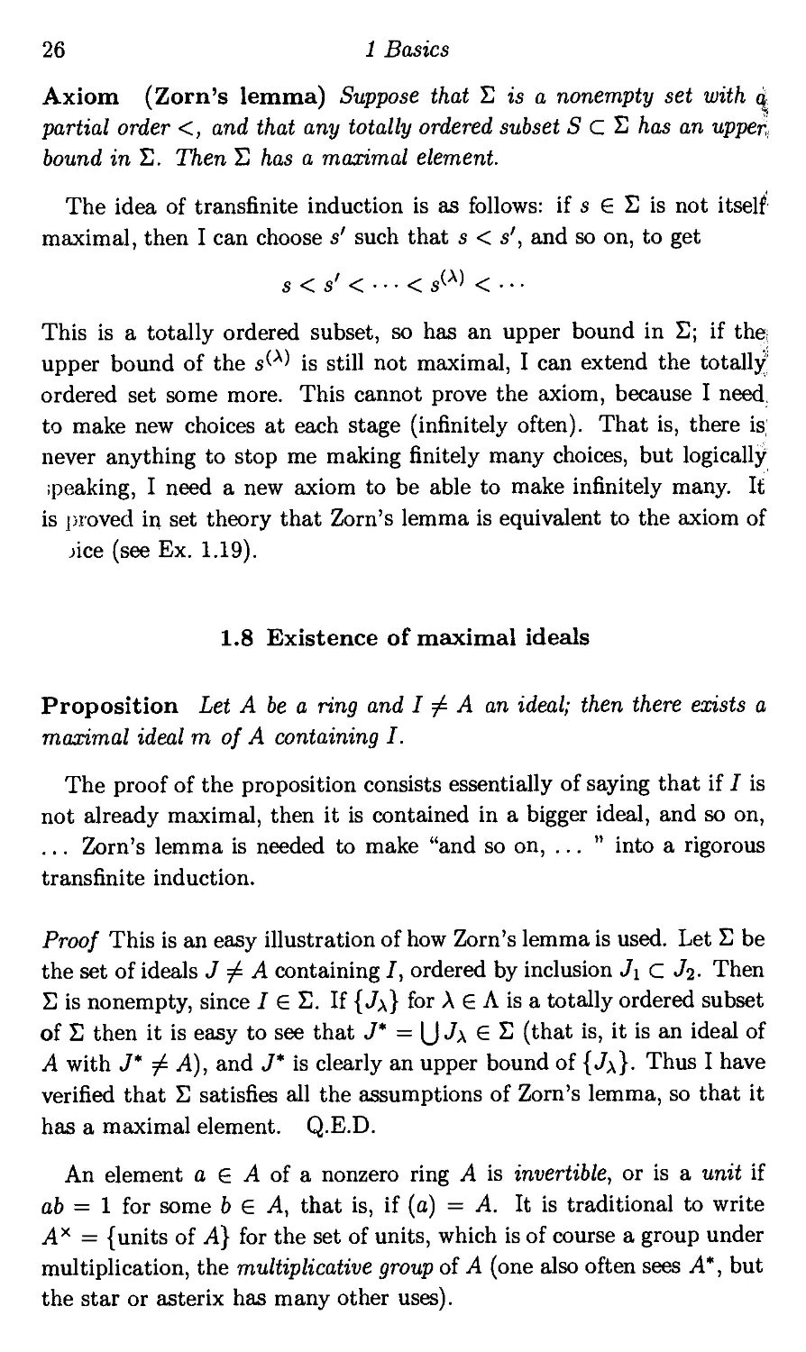
1.8 Existence of maximal ideals
Proposition Let A be a ring and I ^ A an ideal; then there exists a
maximal ideal m of A containing I.
The proof of the proposition consists essentially of saying that if I is
not already maximal, then it is contained in a bigger ideal, and so on,
... Zorn's lemma is needed to make "and so on, ... " into a rigorous
transfinite induction.
Proof This is an easy illustration of how Zorn's lemma is used. Let E be
the set of ideals J ^ A containing I, ordered by inclusion J\ C Ji- Then
E is nonempty, since I ? E. If {J\} for A ? A is a totally ordered subset
of E then it is easy to see that J* = \J J\ ? E (that is, it is an ideal of
A with J* ^ A), and J* is clearly an upper bound of {J\}. Thus I have
verified that E satisfies all the assumptions of Zorn's lemma, so that it
has a maximal element. Q.E.D.
An element o ? A of a nonzero ring A is invertible, or is a unit if
ab = 1 for some b ? A, that is, if (a) = A. It is traditional to write
A* = {units of A} for the set of units, which is of course a group under
multiplication, the multiplicative group of A (one also often sees A*, but
the star or asterix has many other uses).
1.9 Plenty of prime ideals 27
Corollary A = A* U \Jm (disjoint union); that is, an element f ? A
is either a unit, or is contained in a maximal ideal, and not both.
Proof If o ? m for some maximal ideal m then, of course, o is not a unit;
conversely, if o is not a unit then (a) ^ A, so that by the proposition, it
is contained in a maximal ideal. Q.E.D.
1.9 Plenty of prime ideals
The previous proposition can be strengthened as follows, to give the
existence of prime ideals.
Proposition Let A be a ring, S a multiplicative set, and I an ideal of
A disjoint from S; then there exists a prime ideal P of A containing I
and disjoint from S.
Proof Suppose that I can find an ideal P D I maximal subject to the
condition P n S = 0. I claim that P is a prime ideal. For if /, g ^ P
then each of the ideals P + Af and P + Ag is strictly bigger than P,
and therefore intersects S. Suppose that p + af, q + bg ? S for p, q ? P
and o, b ? A; then, using the fact that S is multiplicative,
S 3 (p + af){q + bg) =pq + pbg + qaf + abfg = p' + abfg,
with p' ? P. Now since P n S = 0, it follows that fg<?P.
Therefore, it is enough to find an ideal P D I with P n S = 0 and
maximal subject to this condition. This is proved using Zorn's lemma
in the same way as Proposition 1.8. Let E be the set of ideals J of A
containing J and disjoint from S. Repeating the proof of Proposition 1.8
word-for-word gives that E has a maximal element. Q.E.D.
1.10 Nilpotents and the nilradical
You already know that o ? A is nilpotent if a" = 0 for some n > 0, and
that the set of all nilpotent elements of A is an ideal of A, the nilradical
nilrad.4 (compare 0.2). A ring A is reduced if nilradA = 0, that is, A
has no nonzero nilpotents. Proposition 1.9 implies the following result.
28 1 Basics
Corollary nilrad A is the intersection of all prime ideals P of A, that
is,
nilrad A = f\ P. (*)
PeSpec A
In other words, f ? A is not nilpotent if and only if there is a prime
ideal P ? Spec A such that f <? P.
Proof If / is nilpotent then it obviously belongs to every prime ideal P.
Conversely, suppose that / is not nilpotent; I claim that there exists a
prime ideal P $ f. For this, consider the multiplicative set generated
by /, that is,
Then 0^5 because / is not nilpotent. I apply Proposition 1.9 to
this S and 1 = 0, and get a prime ideal P such that P n S = 0, so
ft P. Q.E.D.
1.11 Discussion of zerodivisors
An idempotent is an element e ? A for which e2 = e; it is easy to see
(compare 0.2) that A has an idempotent e ^ 0,1 if and only if it is a
direct sum of rings A = A\ © A2 with Ai = Ae and Ai = A[\ — e).
Pedantry Notice that the inclusion A\ <-^> A\ © A?, is not a subring
according to Convention 1.1, because the 1 of A\ maps to A,0), which
is not the 1 of A\ © Ai. It is however, an ideal, even a principal ideal.
Also, A\ is a ring of fractions of A\ © Ai (in the sense of Chapter 6)
under the projection map A\ © Ai -» A\.
The point of these definitions is as follows. If a ring A is an integral
domain, it obviously has no nilpotents or idempotents other than 0 and
1, and 0 is a prime ideal, and therefore the only minimal prime ideal. If A
is not an integral domain, then it has zerodivisors f,g ^ 0 with fg = 0.
There are two essentially different ways this can happen, exemplified by
k[X,Y]/(Y2) and k[X,Y]/(XY). In the first case A = k[X,Y]/(Y2)
contains a nonzero element Y of square 0; that is, fg = O where / is
contained in all the prime ideals P containing g (in the present instance,
f = g — Y). In the second case the relation is XY = 0, where X
and Y belong to different minimal prime ideals (X) and (Y). The ring
A = k[X, Y}/(XY) is a subring of the direct sum k[X] © k[Y], with X
1.12 Radical of an ideal 29
and Y mapping to a non-zerodivisor in one factor and to zero in the
other, so that their product is zero.
Proposition Let A be a ring with zerodivisors. Then A has either
nonzero nilpotent elements, or more than one minimal prime ideal.
Proof I can assume that nilradA = 0, that is, that A has no nilpotent
elements. By Corollary 1.10, 0 = f]P, with the intersection taken over
all prime ideals P ? Spec A. However, if Pi D Pi are prime ideals then
in taking this intersection, I can just omit Pi. On the other hand, it is
easy to see that every prime ideal contains a minimal prime ideal (see
Ex. 1.18); therefore 0 = f] P with the intersection taken over all minimal
primes. If there is only one minimal prime P then P = 0 and A is an
integral domain. Q.E.D.
The proposition becomes more significant later in the book: by Corol-
Corollary 5.13, a Noetherian ring has only finitely many minimal prime ideals
Pt. If A is reduced, this means that it has an inclusion into a direct sum
A <-¦ 0"=i A/Pi, just as in the above example XY = 0. See Ex. 1.13.
Geometrically, k[X, Y\/{XY) is the ring of functions on the union of
the two coordinate axes in k2, given by (XY = 0) c k2; its minimal
prime ideals (X) and (Y) correspond to the two components, and the
direct sum k[X] © k[Y] is the ring of functions on the disjoint union of
the two axes.
The geometric picture of nilpotents is in the spirit of a nonrigorous
introduction to calculus, where one may talk about a "number ? so
small that e2 = 0", and use this to calculate the derivative f'(x) of a
polynomial by the formula f(x + e) = f(x) + ef'(x). This is of course
nonsense in the context of an element of the real field, but is perfectly
sensible and useful in algebra. Thus the element Y ? k[X, Y]/(Y2) is
pictured as the function on the X-axis with values in k[e]/(e2 = 0) which
remembers the ^-derivative (df/8Y)(x, 0) of f(X, Y) ? k[X, Y] at each
point (x,0). Higher order nilpotents can be used to give an algebraic
treatment of Taylor expansions of polynomials up to any order.
1.12 Radical of an ideal
Let I be an ideal of A. The radical of I is the set
radI = {/ ? A | /" ? I for some n};
30
1 Basics
XY = 0
X2 =
Figure 1.11. The plane curves defined by XY = 0 and X2 = 0
(this is sometimes also written Vl)- Obviously, nilradA = radO. If
ip: A —> A/1 is the quotient homomorphism, rad/ consists exactly of
the elements of A that map to nilpotents of A/1, that is
in particular, of course, rad / is an ideal (you can of course check this
directly). We say that / is a radical ideal if / = rad/.
Corollary rad/ is the intersection of all prime ideals P ofA containing
I, that is
rad/=
P.
PeSpec A
PDI
(Here if I = A the empty intersection means the whole ring A.)
Proof Since the prime ideals of A containing / are exactly the ideals
of the form f~1(Q) with Q prime in A/1, the result comes on taking
ip~l of the two sides of (*) in Corollary 1.10. Alternatively, it is easy to
argue directly: if /" ^ / for any n then
1.13 Local ring 31
is a multiplicative set disjoint from J, and therefore by Proposition 1.9,
there exists a prime ideal P containing I and disjoint from S. In par-
particular / $. P. Q.E.D.
Corollaries 1.10 and 1.12 are a rather easy analogue of the Nullstellen-
satz (see Theorem 5.6), a point I will discuss in detail in 5.14, (iv) below.
1.13 Local ring
I now introduce one of the key notions of the course. A ring is local if it
has a unique maximal ideal m. By Corollary 1.9,
A is local <==> A has only one maximal ideal
<==> all the nonunits of A form an ideal.
Another equivalent condition is that A has a maximal ideal m such that
1 + m C Ax; compare Ex. 1.10. One often writes A D m or {A,m) or
(A, m, k) for a local ring A, its maximal ideal m and the residue field
k = A/m.
You're probably not yet aware of any local rings, other than fields.
I introduce in Chapter 6 below the algebraic procedure of localisation,
which constructs local rings out of any ring. For example, if P is a prime
ideal of an integral domain A, and K = Frac A is the field of fractions
of A, then
is a local subring of K. Indeed, allowing any g ^ P to appear in de-
denominators has the effect of sabotaging any ideal not contained in P.
We will see many times in the rest of the course that localisation can be
used to reduce all kinds of questions concerning arbitrary rings to local
rings. See, for example, Proposition 8.7.
1.14 First examples of local rings
Here are two examples of localisation: suppose that in Z, I am interested
in divisibility by a particular prime number, say 5. Then for n € Z,
obviously
n is divisible by 5 in Z «=$> n is divisible by 5 in Z[l/2,1/3,1/7];
32 1 Basics
that is, allowing prime factors 2, 3 or 7 into the denominators has no
effect on divisibility by 5. So I might as well go the whole hog, and allow
any prime factor other than 5 in the denominator, setting
ZE) = {q e Q | q = a/b with a, b <E Z, 5 \ b).
Then it is easy to see that
q = a/b is a unit of ZE) ¦*=> 5 \ a.
Therefore
nonunits of ZE) = {a/b € ZE) | 5 | a} = 5ZE);
this is an ideal, so that ZE) is a local ring with maximal ideal 5ZE), and
residue field ZE)/5ZE) *? Z/E) = F5.
In the same way, if I am working in k[X] and only interested in divis-
divisibility of polynomials by powers of X, then I can replace k[X] by rings
such as fe[X][l/(X + 1), 1/(X2 + 1)] in which some other polynomials
are made invertible, or go the whole hog and set
k[X]w = {he k(X) \h = f/g with f,ge k[X], X \ g)
= {he k(X) \h = f/g with f,ge k[X],g{0) ? 0}.
Since f/g is invertible in A;[X](x) if X \ f, it follows that this is a
local ring, with maximal ideal generated by X. Note that an element of
fe[X](x) is a rational function whose denominator does not vanish at 0,
so can be viewed as a function defined near 0.
1.15 Power series rings and local rings
Here are two examples of local rings appearing in other areas of human
endeavour. First the formal power series ring fe[X], which is familiar
from calculations with power series when you don't worry about con-
convergence. Let k be a field, and define the formal power series ring in a
variable X over k by
fe[Xj = {formal power series in X with coefficients in k}
oo
= 1^2 anXH with an € k\
n=0
(compare Ex. 0.12). If / = ao + a\X + aiX2 + ¦ ¦ ¦ is a formal power
series then / has an inverse in fe|X] if and only if ao ^ 0. Because in
Exercises 33
this case / = ao(l + Xg) with some g € fe[X], and
r1 = ao-1(i-xff+xv-¦¦¦)•
It is easy to check that this is a well-defined power series, since the
coefficient of Xn comes only from the first (n + 1) terms of the infinite
sum. Therefore
/ <E fcJXl is a nonunit «=> a0 = 0 «=> / € (X),
so that fcjX] is a local ring with maximal ideal (X).
Note that k[X] C fc|X], and, by what I just said, any polynomial
g € k[X] with g@) ^ 0 is invertible in fe[X], so that the local ring
fe[X](x) described above can be viewed as a subring of the formal power
series ring, fe[X](x) C fe[X|; this inclusion takes a rational function
h = f/g defined near 0 to its Taylor series at 0.
Now in the case k = R or C, we can also discuss convergent power
series. We know from analysis that a power series / = Yl'n'=o anXn in a
variable X has radius of convergence pii\an\ < const ¦ p~n for all n. In
other words, / has positive radius of convergence if and only if
,. log|an|
hmsup ¦—L < oo.
n
Then / is convergent on a small disc around 0, and can be viewed as an
analytic function near 0.
Let R{X} or C{X} be the set of power series with radius of con-
convergence > 0. It is easy to see from elementary properties of analytic
functions that /-1 is an analytic function represented by a convergent
power series if and only if ao ^ 0. Thus again R{X} or C{X} is a local
ring with maximal ideal (X).
The local ring C{X} occurs in complex function theory as the ring of
germs of analytic (= holomorphic) functions around 0; here germ means
that every / € C{X} is an analytic function on a neighbourhood U of
0 (the neighbourhood U depends on /). The field of fractions of C{.X}
is the field of Laurent power series, or germs of meromorphic functions
around 0. For most algebraic purposes, C{X} is very similar to C[XJ.
The same ideas apply to continuous functions near the origin, compare
3.3.
Exercises to Chapter 1
1.1 Give an example of a ring A and ideals /, J such that IUJ is not
34 1 Basics
an ideal; in your example, what is the smallest ideal containing
/ and J?
1.2 The product of two ideals / and J is denned as the set of all
sums ^2 figi with /j € /, g± € J. Give an example in which
1.3 Let A = k[X,Y]/{XY). Show that any element of A has a
unique representation in the form
a + f(X)X + g(Y)Y with a e k,f € k{X],g e k[Y].
How do you multiply two such elements?
Prove that A has exactly two minimal prime ideals. If pos-
possible, find ideals /, J, K to contradict each of the following
statements:
(a) JJ = J n J;
(b) (J + J)(/nJ) = JJ;
(c) / n (J + K) = (I n J) + (/ n K).
1.4 Two ideals / and J are strongly coprime it I + J = A. Check
that this is the usual notion of coprime for A = Z or k[X]. Prove
that if / and J are strongly coprime then
13 = J n J and A/IJ S (A/1) x (A/J).
Prove also that if / and J are strongly coprime then so are J"
and J" for n > 1.
1.5 Let ip: A —> B be & ring homomorphism. Prove that ip-1 takes
prime ideals of B to prime ideals of A. In particular if A C B
and P is a prime ideal of B then A n P is a prime ideal of A.
1.6 Prove or give a counterexample:
(a) the intersection of two prime ideals is prime;
(b) the ideal Pi + Pi generated by 2 prime ideals P\,Pi is
again prime;
(c) if ip: A —y B is a ring homomorphism then ip~l takes
maximal ideals of B to maximal ideals of A;
(d) the map ip~l of Proposition 1.2 takes maximal ideals of
A/1 to maximal ideals of A.
1.7 Give an example of a ring A and a multiplicative set 5 such
that A \ S is not a prime ideal. Read again the definition of
multiplicative set and prime ideal in 1.3, and check that all is
right.
Exercises 35
1.8 Prove that, as asserted in 0.2, the set nilradA of nilpotent el-
elements of A is an ideal; similarly, for any ideal /, the radical
rad J (denned in 1.12) is again an ideal.
1.9 (a) If a is a unit and x is nilpotent, prove that a + x is again
a unit. [Hint: expand A + x/a) as a power series to
guess the inverse.]
(b) Let A be a ring, and / C nilradA an ideal; if x € A maps
to an invertible element of A/1, prove that x is invertible
in A.
1.10 Think through the equivalent conditions in the definition of local
ring in 1.13. In particular, let A be a ring and / a maximal ideal
such that 1 + x is a unit for every x € /, and prove that A is a
local ring. Does the implication still hold if I is not maximal?
1.11 Find the nilpotent and idempotent elements of Z/(n), where
n = 6, 12, pq, pq2 or ]~Jpini (where p, q, pi are distinct prime
numbers).
1.12 (a) If / and J are ideals and P a prime ideal, prove that
IJCP «=> injQP *=> /or JcP.
(b) If /, Ji, Ji C A are ideals, prove that / C J\ UJ2 implies
either / C J\ or I C J2- If in addition P is a prime ideal
and / C Ji U J2 U P, prove that / C Ji or J2 or P. [Hint:
compare [A&M], Proposition 1.11.]
1.13 If .A is a reduced ring and has finitely many minimal prime ideals
Pi then A <-+ ®"=1 A/Pi] moreover, the image has nonzero
intersection with each summand. Compare the discussion in
1.11.
1.14 Let / = /(xi,..., xn) be an analytic function (of real variables)
in a neighbourhood of a point P = (ai,...,an) € K". By
considering the Taylor series expansion of / about P, convince
yourself that /(ai,..., a.n) = 0 if and only if / has an expression
/ = ZXX» ~ a«)" 9i w^tn 9i analytic functions near 01,..., an.
Analytic functions near P form a ring. Deduce that the ideal
of analytic functions vanishing at P = (ai,..., an) is generated
by {xi -ai,...,xn -an}.
1.15 Let a = (ai,..., an) € fe", and consider the map
ea: k[xi,...,xn] >-> k
denned by / i-» f(ai,...,an); in other words, ea is the map
36 1 Basics
given by considering a polynomial f(x) as a function and evalu-
evaluating it at x = a. Prove that ker eo = (zi - ai,..., xn - an).
[Hint: do this in two steps: Step 1, the case a = @, ...,0).
Step 2, a coordinate change y% = Xi - a*.] Deduce that the
ideal (xi — a.i,...,xn — an) is a maximal ideal of k[xi,..., xn\.
Compare with the remainder theorem (see Ex. 0.2).
1.16 Now let a = (ai,..., an) € Kn, where k C K is an algebraic field
extension. Determine the image and kernel of the evaluation
map eo: k[xi, ...,xn]i-*K denned by / i-» /(ai,..., an). Prove
that (xi —ai,...,xn — an) nfc[zi,.. .,xn] is a maximal ideal of
k[xi,..., xn] (the intersection takes place in K[xi,..., xn]).
1.17 Describe SpecR[X] in terms of C. [Hint: list the irreducible
polynomials / € R[X], and say how they factorise in C[X].]
1.18 Use Zorn's lemma to prove that any prime ideal P contains a
minimal prime ideal.
1.19 Use Zorn's lemma to prove the following version of the axiom
of choice: a surjective map /:I->7 between sets has a right
inverse g: Y —* X such that / o g = idy; in other words, it
is possible to choose one inverse image for each y € Y all at
the same time. [Hint: let ? be the set of pairs (U, 7), where
U C Y and 7: U —* X is a map such that f(j(y)) = y for all
y &U; introduce a suitable partial order < on ? (the "obvious"
one), prove that it satisfies the assumptions of Zorn's lemma,
and show that a maximal element of ? does what I said.]
1.20 Sun WuKong, The Monkey King in Wu Cheng-En's famous
novel "Journey to the West", has "Aware of Vacuity" as his
given name (Arthur Waley's translation). Show that Spec A = 0
if and only if A = {0} (compare 1.3). In this case, describe how
to view A as the ring of functions on Spec .A (there's really
nothing in it!).
2
Modules
2.1 Definition of a module
A is a ring; an A-module is an Abelian group M with a multiplication
map
Ax M —y M, written (/, m) i-» fm
satisfying
(i) f(m ± n) = fm ± fn;
(ii) {f + g)m = fm + gm;
(iii) (fg)m = f(gm);
(iv) l^rn = m
for all f,g&A and m, n € M. A subset N C M is a submodule if
/m + gn ? N for all f, g ? A and m, n e N. A homomorphism is a
map t: M —> N of A-modules that is A-linear, in the obvious sense that
t(/m + pn) = /?(m) + gt(n) for all f,g ? A and m,n € M.
Note that a module over a field k is just a k-vector space: the definition
is word-for-word the same. Thus the theory of modules is just linear
algebra in which scalar multiplication is by elements of A, and linear
combinations ?} a^mi take place with m^ e M and coefficients a* € A.
This allows us to do linear algebra over any ring A (which doesn't even
have to be commutative in general).
2.2 Harmless formalism
Introduce the temporary notation /if. M —* M "multiplication by /"
for the map m i—*• fm; then you can see at once that (i) holds if and only
if /if is a homomorphism of Abelian groups and (ii-iv) hold if and only
if the map / i-» /if is a ring homomorphism A —* End M from A to the
37
38 2 Modules
noncommutative ring of endomorphisms of M (that is, homomorphisms
of the Abelian group M to itself). Notice that /if is .A-linear (that
is, f(am + bn) = a(fm) + b(fn)), and that this fact depends on the
assumption that A is commutative.
As far as M is concerned, n(A) C End M is the only part of A that
matters, and I sometimes write A' = IJ.(A). If ji is injective, then A = A',
and linear algebra in M reflects all the properties of A; in traditional
algebraic terminology, M is a faithful A-module.
If M is an A-module and <p: M —* M an A-linear endomorphism
of M, I write A'[ip] C EndM for the subring generated by A and the
action of <p, that is, the ring generated by /if for / € A and ip; this is a
commutative ring, since <p is A-linear. This formal construction makes
M a module over A'[ip], so that the map ip becomes multiplication by
a ring element. Notice that multiplication in the ring A'[ip] C EndM
coincides with composition of maps M —> M. This notation will be
applied in 2.6-2.7 below.
Examples A ring A is a module over itself, and a submodule / C A is
the same thing as an ideal. An Abelian group is a Z-module in an obvious
way; in fact the rules for manipulating modules in general are in many
respects based on those for Abelian groups. If A is a subring A C B of
a ring B then multiplication in B makes B into an A-module; similarly,
a 5-module M can be viewed as an A-module by just restricting scalar
multiplication to elements of A.
The most important modules in commutative algebra are those closely
related to the ring itself, for example, ideals of A or extension rings
B D A, or sums and quotients of these. However, there is no advantage
in working with a more restricted class of modules.
2.3 The homomorphism and isomorphism theorems
The proof of the following proposition is exactly the same as for vector
spaces, and I do not spend time on it.
Proposition
A) The kernel ker<^ C M and image ivaip C N of an A-module
homomorphism ip: M —* N are submodules.
B) If N C M is a given submodule, there exists a quotient module
M/N and a surjective quotient map ip: M —* M/N such that
2.3 The homomorphism and isomorphism theorems 39
kevip = N. The elements of M/N can be constructed as equiva-
equivalence classes of elements m € M modulo N, or as cosets m + N
of N in M.
C) In (l
Isomorphism theorems
(i) If L C M C N are submodules then
N/M = ()
(ii) If N is a module, and L,McN are submodules then
(M + L)/L = M/(MnL).
In either case, equality stands for a canonical isomorphism.
Note that (II) can be interpreted as saying that if L <(. M then there
are two possible ways of making sense of the expression M/L, by in-
increasing M until it contains L, or by decreasing L until it is contained
in M, and these both give the same result.
Proof Both of these follow from the Proposition, C) via an argument
of the form: Step 1, construct a map; and Step 2, calculate its kernel.
(I) First of all, I claim that there is a well-defined homomorphism
<p: N/L —* N/M. Indeed, take some element a € N/L; since N —* N/L
is surjective, there is an n € N mapping to a, and I set
ip(a) = image of n in N/M;
this is well denned because L C M. It is easy to check that ip is A-linear.
Second, I claim that ker <p = M/L, since clearly
tp(a) = 0 «=> n&M «=> a € M/L.
Therefore I have ip: N/L —* N/M with ker ip = M/L, so that the result
follows from C) of the Proposition.
The proof of (II) is similar: the composite <p: M —* (M + L)/L of
the inclusion M C M + L and the projection M + L —> (M + L)/L is
A-linear and satisfies ker <p = L n M. Q.E.D.
40 2 Modules
2.4 Generators of a module
Given mi, ... , mr € M, I can form the submodule of linear combina-
combinations
J2 {J2 } cM>
... ,mr) = J2Ami = {J2fiTni e M
and argue about whether this is the whole of M, and what relations there
are between the m^; in the case of linear algebra over a field, this is the
theory of linear independence and bases of vector spaces. I formulate the
definition with some care to include infinite sets of generators (m\)\?A,
but for many purposes this is not needed, and you would do well to
concentrate on the case A = {1,... ,n} in the first instance. A typical
example where infinite sets of generators might be useful is a polynomial
ring such as A[X, Y], which is a free A-module with the countable basis
X^i.
If {M\)\?A is a family of A-modules, their direct sum is defined by
^2 Mx = {(mx)\eA | only finitely many mx ^ 0}.
ASA
The indexing set of the sum is infinite, but each element of the sum
involves only finitely many indexes. In particular, I can take the sum of
A itself card A times:
Ac&tdA := Y^ A = {KUeA I only finitely many ax ± 0}.
in other words, this is the set of (finite) sequences indexed by A € A.
This is by definition a free module; it has a basis e\ = @,..., 1,...),
with 1 in the Ath place and zero elsewhere. In particular, if (m^AeA is
any set of elements of a fixed module M indexed by A, I can define a
homomorphism from this direct sum to M,
ip:ACMdA^M by (
the sum is finite since every element (f\) € Ac&TdA has only finitely
many fx =fc 0. The image is obviously just the set of all finite linear
combinations ?} f\m\ of the given elements m\.
Definition (m^AeA is a family of generators of M if ip is surjective,
that is, if any m € M can be written m = ?} f\m\; it is a basis if ip is
an isomorphism. M is free if it has a basis. A module M is finite over
A if it has a finite set of generators. Note that the term finite is used
throughout to mean finitely generated as an A-module.
2.5 Examples 41
2.5 Examples
Formally speaking, the definition just given is exactly like that of a basis
of a vector space over a field. However, every vector space (say, finite
dimensional) has a basis: every irredundant set of generators is a basis,
and so is every maximal set of linearly independent elements. None of
this is true for modules over a ring A, as illustrated by the following
examples, which can be summed up in the slogan "a free module is a
lucky accident". However, free modules are also important because a
general module can be studied in terms of them using a presentation by
generators and relations (see, for example, Ex. 3.4).
A) If A is an integral domain and 0 ^ / € A then A[l/f] is usually
not finitely generated as an A-module: A[l/f] = A + Af'1 +
Af~2-\— , sojl,/,/,...} is a set of generators. See Ex. 2.1.
B) The module A/1 is generated by 1 element (the image of 1^), but
is not free if / ^ 0; a module of the form A/1 is sometimes called
a cyclic module.
C) In A = k[X, Y], the maximal ideal M = (X, Y) is generated by
two elements, but is not a free module: the map <p: A2 —* M is
given by (/, g) .-» fX + gY, and has kernel {{hY, -hX) \heA}.
See Ex. 2.2
D) Even when M is free, an irredundant family of generators is not
necessarily a basis; for example, A = k[X], M = A and (X, 1— X).
2.6 The Cayley-Hamilton theorem
If N is an n x n matrix over an algebraically closed field k, considered
as a endomorphism N: kn —> kn, then if N is "fairly general", it can
be diagonalised; that is, N can be written as the diagonal matrix N =
diag(Ai,..., Xn) by choosing a basis of kn made up of eigenvectors e».
Now (N - \i ¦ In)ei = 0, where /„ is the identity n xn matrix, and it
follows that the product of the n factors {N — \ ¦ In) kills every basis
element e*, so that
(N-X1-In)---(N-Xn-In) = 0 A)
(the factors commute, of course). On the other hand, pn(x) = FK^"^*)
is the characteristic polynomial of N, that is, p^ = det(x • In — N), and
hence A) says that Pn(N) = 0. The Cayley-Hamilton theorem says
that the same thing holds for any n x n matrix with entries in any
(commutative) ring A.
42 2 Modules
Theorem Let Abe a commutative ring, N = (ay) annxn matrix with
entries in A, and write pn(x) = det(z ¦ In - N). This is a polynomial
of degree n inx with coefficients in A and leading coefficient 1.
Then Pn{N) = 0 (as an nx n matrix).
Note that this is an array of n2 identities in the entries Ojj of N.
You'll get some feel for the statement by writing it out explicitly for
n = 2,3,...; see Ex. 2.4.
Proof Write ip: An —y An for the homomorphism of the free module An
corresponding to N, that is, the map taking
efc = @,...,l,...,0)^@,...,l,...,0)JV = (afcl,...,afcn), B)
the fcth row of N. Let A'[ip] be the commutative subring of End A"
discussed in 2.2, that is, the subring ofnxn matrixes generated by the
scalar multiples of /„ and N.
Viewing An as an A'[(^]-module in the natural way, I get the equations
n
ipek = ^2akiei for k = 1,.. .,n, C)
t=i
which I can rewrite
^fct ~ flfct)ei = 0 (Ski is the Kronecker symbol). D)
Now let A = (<p6ki — flfct), which is an n x n matrix with coefficients in
A'[p).
I claim that det A = 0 in A'[ip]. Since Pn(x) = det(x • /„ - N) € A[x]
and A[x] —* A'[ip] is a homomorphism (so commutes with the algebraic
operations involved in taking determinant), it follows that Pn(x) maps
to pn(N) = det A, so that the claim implies the theorem.
To prove the claim, let adj A = (bkj) be the adjoint matrix of A. This
is the matrix whose entry bkj is the (j, fe)th factor of A (that is, (-l)J+fc
times the (n -1) x (n -1) determinant obtained by deleting the jth row
and feth column of A), and
(adj A) ¦ A = A ¦ (adj A) = det A ¦ /„ E)
is just the familiar rule for evaluating a determinant along the rows or
columns. Now det A € A'[ip] C End An, so that it is enough to prove
2.7 The determinant trick 43
that (det A) • ej = 0 for j = 1,..., n. For this, just multiply D) through
by bkj and sum over k. This gives
= 0. F)
fc=i t=i
By E), the coefficient before e» is just (det ANj»; in other words, I have
proved that (det A)ej = 0 for each j, as required. Q.E.D.
2.7 The determinant trick
The following result is proved in exactly the same way as the Cayley-
Hamilton theorem, and has many applications later in the course (see
Proposition 4.2, (iii) =>¦ (i) and the Remark following Proposition 4.2).
Theorem Let M be a finite A-module, generated by n elements, and
ip: M —y M a homomorphism; suppose that I is an ideal of A such that
<p{M) C IM. Then tp satisfies a relation of the form
n = Q, G)
where aj € /* for i= 1,2,..., n. Here G) is an equation holding between
endomorphisms of M, that is, a relation in the ring A'[ip] C EndM
introduced in 2.2.
Proof Let mi,..., mn be a set of generators of M. Since ip(rrii) € IM,
I can write
atjmj with ajj €/. (8)
As before, in the ring A'[ip], (8) can be rewritten
with 6ij<p — aij € -A'^]- Write A = (8ij<p — ffltj). Then multiplying (9)
by bki and summing over i, I deduce that (det A)m/t = 0. Since this
holds for each k, it follows that det A = 0 € ^'[v]- Expanding out the
determinant gives the relation in the statement. Q.E.D.
2.8 Corollaries — Nakayama's lemma
Corollary 1 If M is a finite module and M = IM then there exists an
element x € A such that x = 1 mod/ and xM = 0.
44 2 Modules
Proof Apply the determinant trick 2.7 to the identity map idm € A'[ip].
Since Am)* = 1m, the relation takes the form A + b)idM = 0, where
b = ai + --- + ane I. Q.E.D.
Corollary 2 (Nakayama's lemma) Let (A, m) be a local ring (defined
in 1.13), and M a finite A-module; then M = mM implies that M = 0.
More generally, the same conclusion holds if M = IM with I an ideal
such that {1+1) C A*.
This is a simple but important result that allows us to make many
deductions about properties of M as an A-module from properties of
M/mM as a vector space over the residue field k = A/m, so reducing
the study of finite modules over a local ring to finite dimensional vector
spaces. It is not hard to prove directly, without using Theorem 2.7; for
this, see Ex. 2.5.
Proof Apply the previous corollary. Then since x = lmodJ it follows
that x is aunit of A, so that xM = 0 implies M = x~1-xM = 0. Q.E.D.
Corollary 3 Let (A, m) be a local ring, M an A-module, and N C M a
submodule; suppose that M/N is finite over A, and that M = N + mM;
then N = M.
In particular, if M is finite over A, and ifS\,..., sn € M are elements
whose images span the k-vector space M = M/mM, then si,...,sn
generate M.
Proof Since m(M/N) = M/N, Nakayama's lemma (Corollary 2.8.2)
gives M/N = 0. Q.E.D.
Note that the finiteness condition is essential; for example, let A =
2E) C Q be the example of local ring given in 1.14, with maximal ideal
5ZE), and consider Q as A-module. Then obviously Q = 5Q, but Q ^ 0;
the point is that Q = A + A^ + A^ -\ is not finite over A.
2.9 Exact sequences
Suppose that L, M and N are A-modules, and
(9)
is a sequence of homomorphisms. (9) is exact at M if im a = ker /3; this
means that the composite /3 o a = 0, and that a maps surjectively to
2.10 Split exact sequences 45
ker /3. A longer sequence ¦¦• —y M\ —y Mi —y M3 —y ¦ ¦ ¦ is exact if it is
exact at each term.
Special
0^
L^
cases:
0-
M
L-
>M
-y L —¦
_^
+ JI
N -
N -
M
-.0
> JV
->0
is
is
is
is
exact
exact
exact
exact
«=>
«=>
<=>
a
a
V
is injective;
is surjective;
: L^ker/3;
induces M/a(L) ^y N.
By analogy with the kernel of a map, one defines the cokernel of a
homomorphism a: L —y M to be the module cokera = M/a(L); then
the conclusion in the final case can be written /3: coker a ^-y N.
Most importantly,
0->iwMAw-.0 is exact «=* L C M and N = M/L,
under the natural identifications induced by a and /3. A sequence with
this property is called a short exact sequence (s.e.s.).
It would be possible to replace exact sequences by more direct argu-
arguments wherever they occur in this course, but I use them as a convenient
language, which you probably need to become familiar with in any case.
Treating exact sequences in a systematic way is the main subject of
homological algebra, which is a major item of technology in 20th century
math.
2.10 Split exact sequences
Proposition-Definition Let
0 -» L ^U M ¦?* N -y 0
be a s.e.s. of A-modules. Then 3 equivalent conditions:
(i) there exists an isomorphism M = L(&N under which a is given
by mi-y (m, 0) and 0 by (m, n) i-» n;
(ii) there exists a section of /3, that is, a map s: N —y M such that
/3os = idjv;
(iii) there exists a retraction of a, that is, a map r: M —y L such that
roa = id/,.
If this happens the sequence is a split exact sequence.
46 2 Modules
Proof (i) => (ii) or (iii) is very easy.
(ii) =>¦ (i): The given section s is clearly injective because it has 3
left inverse; I claim that M = a(L) © s(N). To see this, any m € M is
of the form
m= (m - s(C(m))) + s(C(m)),
where the second term is obviously in s(N); since /9 o s = idjv, the first
term is clearly in ker/3, and by exactness this is ct(L). Furthermore,
a(L) fl s(N) = 0, since if n € N is such that s(n) € a(L) = ker/3 then
n = /3(s(n)) =0.
(iii) => (i) is very similar, and I leave it to you as an exercise
(Ex. 2.13). Q.E.D.
For finite dimensional vector spaces over a field, every subspace has
a complement, so every s.e.s. is split. Whether an exact sequence is
split or not depends on what ring it is considered over. For example,
0->(X)-> k{X] -* k -* 0 is split over k but not over k[X\.
Exercises to Chapter 2
2.1 Let A be an integral domain with field of fractions K, and sup-
suppose that / € A is nonzero and not a unit. Prove that -A[l//]
is not a finite A-module. [Hint: if it has a finite set of genera-
generators then prove that l,f~l, f~2,. ¦ ¦, f~k is a set of generators
for some k > 0, so that /"~(fc+1) can be expressed as a linear
combination of these. Use this to prove that / is a unit.]
2.2 Let A be a UFD and x, y € A two elements having no common
factor; write / = (x,y) C A. Prove that ip: A2 —y I defined
by (a, b) 1—» ax + by is surjective and has kernel the submodule
generated by the element (— y, x). In other words, there is an
exact sequence
This is called the Koszul complex of the pair (x, y).
It can obviously happen that / = (x,y) ^ A) (for example,
take X, Y € A = k[X, Y]). Then / needs two generators, and is
not a free module.
2.3 Let A = k[X, Y, Z) be the polynomial ring. The maximal ideal
m = (X, Y, Z) is generated by the 3 elements X, Y, Z, so that
there is a surjective homomorphism a: A3 —* m C A defined
Exercises 47
by (/, g, h) i-» fX + gY + hZ. Prove that the kernel of a can
be generated by 3 elements u, v, w € A3. Find the kernel of the
surjective map /3: A3 —y ker a, and deduce that there is an exact
sequence
0 _» A -* A3 A 43 A m -» 0.
[Hint: as in Ex. 2.2, the only relations are stupid skewsymme-
tries.]
2.4 Verify the Cayley-Hamilton theorem (see 2.6) for n = 2 and 3;
if you have access to a computer algebra system, do the same
for n = 4 and 5.
2.5 Prove Nakayama's lemma from first principles, by induction on
the minimum number of generators of M.
2.6 (A,m,k) is a local ring, M a finite A-module and si,...,sn €
M; write si,... ,sn € M = M/mM for their images under the
quotient map. Prove that s i,..., sn form a basis of M if and
only if si,..., sn form a minimal generating set of M.
2.7 A is a local ring; prove that An and Am are isomorphic as
A-modules if and only if n = m. Now apply the existence of
maximal ideals 1.8 to prove the same for any (commutative)
ring A.
2.8 If A is a ring, and / a finitely generated ideal satisfying I = I2,
prove that I is generated by a single idempotent element. [Hint:
you have to take the statement of Corollary 2.8.1 very literally.]
2.9 0->I-»M->W->Oisa s.e.s. of A-modules; prove that if N
and L are finite over A, then so is M.
2.10 Mi, Mi C N are submodules of a given A-module N; prove that
if Mi + Mi and Mi n Mi are finite over A then so are Mi and
M?.. [Hint: apply Ex. 2.9 to a suitable s.e.s.]
2.11 Let ¦ ¦ • —> Mr_i -^-y MT —^+ Mr+i —y ¦ ¦ ¦ be an exact se-
sequence of modules; by setting Lr = imoy C Mr, show how
to break up any long exact sequence into a number of s.e.s.'s
0->Lr-tMr-t Lr+l -y 0.
2.12 Prove that if 0 -* Vi -* V2 -y ¦ ¦ ¦ -y Vn -y 0 is an exact
sequence of vector spaces over a field k then $^(—1)* dim Vi = 0;
this allows you to calculate the dimension of one of them if you
know all the others. [Hint: you already know the case n = 3;
now use Ex. 2.11 and induction.]
2.13 Prove (iii) implies (i) in Proposition 2.10.
48 2 Modules
2.14 Criticise the following misstatement of Proposition 2.10: given
a s.e.s. 0 —* L —* M —> N —* 0,
M ^ L®N <==> 3 section s: N -» M of /3.
2.15 Prove the following lemma about exact sequences: let
0 —* Mi —y Mi —> M3 —y 0
0 —y N\ —* N2 —* A/3 —> 0
be a commutative diagram of A-modules with exact rows; then
oil and 0:3 isomorphisms implies 0:2 an isomorphism.
2.16 Give your own proof of the Snake lemma: if
Mi -> M2 -> M3 -> 0
0-» M -» N2 -» iV3
is a commutative diagram of A-modules with exact rows then
there is a "snake" homomorphism 6: ker 0:3 —* coker a 1 (the
cokernel is defined in 2.9) that fits together with the induced
homomorphisms kerai —* ker 0:2 —* ker 0:3 and coker a 1 —*
coker 0:2 —* coker 0:3 to make a six term exact sequence
ker a 1 —* ker 0:2 —* ker 0:3
—> coker oil —y coker 0:2 —* coker 0:3.
[Hint: see for example [A&M], Proposition 2.10, or any book
on algebraic topology or homological algebra.]
2.17 Give an alternative statement and proof of the first isomorphism
theorem, Theorem 2.3, (I) in terms of exact sequences and the
Snake lemma:
0
0
L
i
i
-» M/L
i
0
= L
i
i
-> N/L
i
0
-> 0
1
-> N/M
1
—* coker
1
0
-> 0
-> 0
3
Noetherian rings
In a paper of 1890, Hilbert proved that any ideal of a polynomial ring
k[Xi,...,Xn] over a field is finitely generated, and used this result sub-
subsequently in 1893 in his proof that rings of invariants are finitely gen-
generated. His abstract methods of proving the existence of finite sets of
generators without explicitly constructing them were denounced at the
time as "theology, not mathematics". Work of Emmy Noether in the
1920s introduced the ascending chain condition, and used it systemati-
systematically as a very convenient finiteness condition on a ring (see for example
Theorem 7.11 below). Practically all the rings ever used in applications
of commutative algebra are Noetherian. The heart's desire of any true
algebraist, faced with a result on rings and modules that uses concrete
assumptions, is to generalise the argument to work for all Noetherian
rings.
3.1 The ascending chain condition
A partially ordered set ? has the ascending chain condition (a.c.c.) if
every chain
Sl < S2 < ¦¦ ¦ < Sk <¦ ¦¦
eventually breaks off, that is, s/t = Sk+i = ¦ ¦ • for some k. This is a
finiteness condition in logic that allows arguments by induction, even
when the partially ordered set ? is infinite. It is easy to see that a
partially ordered set ? has the a.c.c. if and only if every nonempty
subset ScS has a maximal element: if 0 ^ S C ? does not have a
maximal element, then choose si € S, and for each Sk, an element Sk+i
with Sk < Sfc+i, thus contradicting the a.c.c. For details see Ex. 3.10.
Vector subspaces of a finite dimensional vector space satisfy the a.c.c:
49
50 3 Noetherian rings
the length of a strictly increasing chain is bounded by the dimension.
The negative integers satisfy the a.c.c: after choosing -10,000,000,
say, the length of any strictly increasing chain is bounded. It is perhaps
superfluous to remark that the a.c.c. does not say that the set ? is finite,
nor that the length of a chain is bounded, nor even that after making
some finite number of choices si < • • • < s/t the length of chains after Sk
is bounded.
3.2 Noetherian rings
Proposition-Definition Let A be a ring; 3 equivalent conditions:
(i) The set ? of ideals of A has the a.c.c; in other words, every
increasing chain of ideals
h C h C • • ¦ C I* C • ¦ •
eventually stops, that is Ik = h+i = • • • for some k.
(ii) Every nonempty set S of ideals has a maximal element.
(iii) Every ideal I C A is finitely generated.
If these conditions hold then A is Noetherian.
Proof Here (i) ¦?=> (ii) is the purely logical statement about partially
ordered sets already discussed, whereas (i) or (ii) •?=> (iii) is directly
concerned with rings and ideals.
(i) => (iii) Pick /i € /, then if possible fi € / \ (/i), and so on. At
each step, if / ? (/i,..., /fc), pick fk+i € / \ (/i,..., /*)• Then by the
a.c.c. (i), the chain of ideals
must break off at some stage, and this can only happen if (/i,..., fk) =
I. This proof involves an implicit appeal to the axiom of choice. It is
perhaps cleaner to do (i) =>¦ (ii) purely in set theory, then argue as
follows.
(ii) =>¦ (iii) Let / be an ideal of A, and consider the set S of finitely
generated ideals contained in /. Then 0 € S, so that S has a maximal
element J by (ii). But then J = I, since any element / € J \ I would
give rise to a strictly bigger finitely generated ideal J ^ (J, /) C /.
(iii) => (i) Let I\ c h C ¦ ¦ ¦ C Ik C ¦ ¦ ¦ be an increasing chain.
Then you check at once that J = |J Ik is again an ideal. If J is finitely
3.3 Examples 51
generated then J = (/i, ...,/„) and each fa € Jfc(, so that setting fc =
maxfej gives J = Ik, and the buck stops here. Q.E.D.
Remarks
(i) Most rings of interest are Noetherian; this is a very convenient
condition to work with. At first sight, more concrete conditions
(such as A finitely generated over k or over Z) might seem more
attractive, but as a rule, the Noetherian condition is both more
general and more practical to work with.
(ii) The descending chain condition (d.c.c.) on a partially ordered
set is defined in a similar way; for example, the set of natural
numbers N with the usual order satisfies the d.c.c. A ring whose
ideals satisfy the d.c.c. is called an Artinian ring. This is also a
very important notion, but is more special: the d.c.c. for rings
turns out to be very much stronger than the a.c.c. (and implies it).
See Exs. 3.8-9, as well as [A&M], Chapter 8 or [M], Chapter 1,
Theorem 3.2.
3.3 Examples
I will give lots of examples of Noetherian rings later. Here are three
examples of non-Noetherian rings:
A) The polynomial ring k[Xi,.. .,Xn,...] in an infinite number of
indeterminates is obviously non-Noetherian.
B) Consider the ring A\ of polynomials in x, y of the form f(x, y) =
a + xg(x,y) with a a constant and g € fe[x,y]; that is, / involves
no pure power xp of y with j > 0. In other words,
= {/(z,y) =
*'i ^ °- and * > ° if 3
= k[x,xy,xy2,...,xyn,...\.
It is clear that (x,xy, xy2,...) is a maximal ideal, and is not
finitely generated. (It looks as if it should be generated by x,
but, of course, y,y2,... are not elements of the ring.) Thus A\
is not Noetherian.
52 3 Noetherian rings
C) A rather similar example is the ring Ai of polynomials in x, y, y~
of the form a(x, y) + xb(x, y, j/); that is,
M = [f(x, y)=^2 ayiV * > 0, and j > 0 if i = 0j
In this ring x = (x/y) ¦ y, and x/y = (x/y2) ¦ y, etc., so that the
element a; does not have a factorisation into irreducibles, and
(x) C (x/y) C (x/y2) c • • •
is an infinite ascending chain.
D) Consider 0 € R; a function germ at 0 is an equivalence class of
continuous functions /: [/-»R defined on an arbitrarily small
neighbourhood U of 0 in R; two germs f:U—*R and g: V —* R
are equal by definition if and only if there exists a neighbourhood
W of 0 with W C U fl V such that f\\\r = 9\\y- Function germs
form a ring ?o- This is a local ring, since the set of all function
germs / such that /@) = 0 is a maximal ideal mo (the kernel
of evaluation at 0), and any function germ / ^ mo is invertible.
Compare the ring of analytic function germs discussed in 1.15.
However, the ideal mo is not finitely generated. Indeed, sup-
suppose that fi are any finite number of function germs vanishing
at 0; if g = ?} a*/* with at continuous functions of x, then we
obviously get a bound |<7(z)| < const, x max|/j(x)| as x —* 0.
But, of course, there are functions g vanishing at 0, but van-
vanishing much more slowly than max|/j(x)|. For example, set
G(x) = max{|i|, |/»(x)|} and g(x) = y/G(x); then
5(x)/max{|x|, |/j(x)|} —> oo as x —> 0.
3.4 Noetherian modules
Definition An A-module M is Noetherian if the submodules of M have
the a.c.c, that is, any increasing chain M\ C Mi C • • • C Mfc C • • • of
submodules eventually stops. Just as before, it is equivalent to say that
any nonempty set of submodules of M has a maximal element, or that
every submodule of M is finite.
3.5 Properties of Noetherian modules 53
Proposition Let 0 —* L -—* M —> N —y 0 be a s.e.s. of A-modules.
Then
M is Noetherian •?=*¦ L and N are.
Proof =*¦ is easy, because ascending chains of submodules in L and
N correspond one-to-one to certain ascending chains in M.
4= Suppose Mi C M2 C • • • C Mfc c • • • is an increasing chain of
submodules of M; then identifying a(L) with L and taking intersection
gives a chain
of submodules of L, and applying /3 gives a chain
/3(M1)C/3(M2)c---C/3(Mfc)C---
of submodules of N. Each of these two chains eventually stops, by
the assumption on L and N, so that I need only prove the following
statement:
Lemma For submodules, M\ C Mi C M,
Lr\M1=LnM2 and /3(Mi) =/3(M2) =4- Mi = M2.
Proof Indeed, if m € M2 then /3(m) € /3(Mi) = /3(M2), so that there
is an n € Mi such that 0(m) = 0(n). Then 0(m - n) = 0, so that
m - n € M2 n ker /3 = Mi n ker /3. Hence me Mi. Q.E.D.
3.5 Properties of Noetherian modules
Corollary
(i) //Mi are Noetherian modules (for i = l,...,r) then 0J"=1 Mt is
Noetherian.
(ii) If A is a Noetherian ring, then an A-module M is Noetherian if
and only if it is finite over A.
(iii) If A is a Noetherian ring, M a finite A-module, then any sub-
module N C M is again finite.
(iv) If A is a Noetherian ring and <p: A —* B a ring homomorphism
such that B is a finite A-module, then B is a Noetherian ring.
54 3 Noetherian rings
Proof (i) A direct sum Mi ©M2 is a particular case of an exact sequence
(compare Proposition 2.10), so that Proposition 3.4 proves (i) when
r = 2. The case r > 2 follows by an easy induction.
(ii) If M is finite then there is a surjective homomorphism AT —* M —*
0 for some r, so that M is a quotient M = Ar /N for some submodule
N C Ar; now Ar is a Noetherian module by (i), so M Noetherian follows
by the implication =>¦ of Proposition 3.4. Conversely, M Noetherian
obviously implies M finite.
(iii) This just uses the previous implications: M finite and A Noe-
Noetherian implies that M is Noetherian, so that N is Noetherian, which
implies that N is a finite .A-module.
(iv) B is Noetherian as an A-module; but ideals of B are submodules
of B as an .A-submodule, so that B is a Noetherian ring. Q.E.D.
3.6 The Hilbert basis theorem
The following result provides many examples of Noetherian rings, and is
the main motivation behind the use of the a.c.c. in commutative algebra.
Note that in Hilbert's day, a "basis" of a module meant simply a family
of generators.
Theorem (Hilbert basis theorem) If A is a Noetherian ring then
so is the polynomial ring A[X].
Proof I prove that any ideal / C A[X] is finitely generated. For this,
define auxiliary sets Jn C A by
Jn = {a <E A I 3/ € / such that / = aXn + ^-iX" + ¦ ¦ ¦ + b0}.
In other words, Jn is the set of leading coefficients of elements of / of
degree n. Then it is easy to check that Jn is an ideal (using the fact that
/ is an ideal), and that Jn C Jn+i (because for / € /, also Xf € /),
and therefore
Ji C J2 C ¦ ¦ ¦ C Jfc C ¦ ¦ ¦
is an increasing chain of ideals. Using the assumption that A is Noe-
Noetherian, I deduce that Jn = Jn+i = ¦ ¦ ¦ for some n.
For each m < n, the ideal Jm C A is finitely generated, say Jm =
(fflm.i, ¦ ¦ ¦, "¦m,rm)', and by definition of Jm, for each am,j with 1 < j < rm
there is a polynomial fmj € / of degree m having the leading coefficient
Exercises 55
. This allows me to write down a finite set
{fm,j} m<n (*)
of elements of /.
I now claim that the finite set (*) generates /. Indeed, for any poly-
polynomial / € /, if / has degree m then its leading coefficient a is in Jm,
hence if m > n, then a ? Jm = Jn, so that a = ?} Mm with bi € A and
/ - ?} 6tXm-"/nij has degree < m; similarly, if m < n, then a € Jm, so
that a = J2biam,i with 6, € A and / - ?}6t/m]» has degree < m. By
induction on m it follows that / can be written as a linear combination
of the finitely many elements (*). This proves that any ideal of A[X] is
finitely generated. Q.E.D.
Corollary If A is a Noetherian ring, and <p: A —> B a ring homomor-
phism such that B is a finitely generated extension ring of ip(A), then
B is Noetherian. In particular, any finitely generated algebra over Z or
over a field k is Noetherian.
Proof The assumption is that B is a quotient of a polynomial ring,
B = A[Xi,.. .,Xn]/I for some ideal /. Now by Theorem 3.6 and an
obvious induction, A Noetherian implies that so is -A[Xi,..., Xn], and
by Corollary 3.5, (iv), A[Xi,...,Xn] is Noetherian implies that so is
...,Xn}/I. Q.E.D.
Exercises to Chapter 3
3.1 A subring of a Noetherian ring is Noetherian, true or false?
3.2 Let k be a field and A D k a ring which is finite dimensional as
a fe-vector space; prove that A is Noetherian and Artinian (see
3.2 for the definition).
3.3 Let A be a ring and It,..., 1^ ideals such that each A/U is a
Noetherian ring. Prove that 0 A/Ii is a Noetherian A-module,
and deduce that if f] I{ = 0 then A is also Noetherian.
3.4 Prove that if A is a Noetherian ring and M a finite A-module,
then there exists an exact sequence Aq -^ Av —* M —* 0. That
is, M has a presentation as an A-module in terms of finitely
many generators and relations.
3.5 Let 0—> L —> M —* N —»0bean exact sequence, and M\,Mi
two submodules of M; decide whether the following implication
56 3 Noetherian rings
holds:
C(Mi) = C(M2) and a'1 (Mi) = a~1(M2) => Mj = M2.
3.6 If A is a Noetherian ring, prove that any surjective ring homo-
morphism <p: A —* A is also injective. [Hint: consider the chain
of ideals ker <p C ker <?>2 C ¦ • ¦. If you can't do it from this hint,
compare the proof of Lemma 7.11 and Ex. 7.5.]
3.7 Consider the Z-module M = (Z[l/p])/Z; prove that any sub-
module N C M is either finite (as a set) or the whole of M.
Deduce that M is an Artinian Z-module; prove that it is not
finitely generated (so not Noetherian).
3.8 Let A be an Artinian integral domain (see 3.2 for the definition).
Prove that A is a field. [Hint: for / € A, the d.c.c. applied to
(/) D (/2) D ¦ ¦ ¦ D (/fc) gives a relation fk = afk+1.\ Deduce
that every prime ideal of an Artinian ring is maximal.
3.9 Let A, m be an Artinian local ring (see 1.13 and 3.2). Prove that
the maximal ideal m is nilpotent. More precisely, the d.c.c.
gives that mk = mk+1 for some k > 0. Prove that mk = 0.
[Hint: suppose by contradiction that mk ^ 0; let / be minimal
among the ideals of A with I ¦ mk ^ 0. Prove that / = (x) is
principal, then apply Nakayama's lemma 2.8.2 to it. Compare
[M], Chapter 1, Theorem 3.2.]
3.10 The argument given in 3.1 to prove that the a.c.c. on a partially
ordered set ? implies the maximal condition involved making
a countable number of choices, so it used implicitly a form of
the axiom of choice. Write out a formal argument using Zorn's
lemma. [Hint: Let A be the set of finite chains a : si < s2 < • • •
of E, ordered by inclusion (that is, a < a' holds for two chains
a, a' if a is an initial segment of a'). Use the a.c.c. to prove
that a totally ordered subset of A has a maximal element.] An
alternative proof based on the axiom of choice is given in [M],
p. 14.
3.11 (Harder) Prove that if A is a Noetherian ring then so is the for-
formal power series ring A[X]. [Hint: as in the proof of the Hilbert
basis theorem, consider an ideal / C -Apf]], and auxiliary ideals
Jn = {a € A | 3/ € / such that / = aXn + bn+1Xn+1 +•¦¦};
show that the Jn form an increasing chain of ideals of A, and us-
using this, find a finite set of power series to generate /. Compare
[M], Chapter 1, Theorem 3.3.]
Exercises 57
3.12 (Harder) Prove I. S. Cohen's theorem that if all the prime ideals
of a ring A are finitely generated, then A is Noetherian. [Hint:
the idea is simple: consider the set of all ideals which are not
finitely generated; then Step 1. By Zorn's lemma, this has a
maximal element P, and Step 2. P must be prime. See [M],
Chapter 1, Theorem 3.4.]
Finite ring extensions and
Noether normalisation
As you know, if k C K is a field extension, an element y € K is algebraic
over k if it satisfies an algebraic dependence relation
f{y) = anyn + ¦ ¦ ¦ + a.iy + a0 = 0,
with some nonzero polynomial / € k[Y\; without loss of generality,
an ^ 0. Over a field, it costs nothing to divide the relation through by
an, so we almost always just assume that an = 1, say that / is monic,
and think no more about it. Over a more general ring A, however, you
can't just divide by an. A relation
/(») =Vn+ an-iyn~l + ¦ ¦ ¦ + ai» + a0 = 0
with a monic polynomial / € A[Y] is called an integral dependence
relation for y; the distinction between algebraic dependence and integral
dependence is crucial. This notion leads at once to the ring of integers
Ok of a number field K, which is the basic definition of algebraic number
theory.
The close relation between integral dependence and finiteness condi-
conditions in a ring extension A C B gives a convenient algebraic method for
handling integral dependence: for example, it proves that if J/i, J/2 € B
are integral over A, then so are j/i + yi and j/ij/2> without the need for
calculating their integral dependence relations explicitly. These finite-
ness conditions lead naturally to Noether normalisation, which will be
the key to the Nullstellensatz in the following chapter. At the same
time, I give a brief introductory discussion in 4.5 of the relation between
normal (integrally closed) rings and nonsingular algebraic curves, which
is an ultimate aim of the final chapters of this book.
4-1 Finite and integral A-algebras 59
4.1 Finite and integral A-algebras
Let A be a ring; an A-algebra B is by definition a ring B with a given ring
homomorphism ip: A —y B. The point is that B is then an A-module,
with the multiplication defined by ip(a) ¦ b. An important case of this
is when A c B, when B is also called an extension ring of A; we can
usually reduce to this case by writing <p(A) = A' C B.
Definition Let B be an A-algebra.
(i) B is a finite A-algebra (or is finite over A) if it is finite as an
A-module.
(ii) An element y € B is integral over A if there exists a monic poly-
polynomial f{Y) = Yn + an-iYn~l + • ¦ ¦ + a0 € A'[Y\ such that
f(y)=yn + an-1yn-l + --- + aQ = 0. A)
The algebra B is integral over A if every b € B is integral. (The
terminology integral domains and integral extension are unre-
unrelated.)
In terms of B viewed as an A-module, the integral dependence relation
A) is a linear relation
lA-yn +an_1-2/"-1 +... + ao-lB=O B)
between the powers of y, with coefficients in A, and such that the highest
power yn has coefficient 1.
Examples
(i) Z[l/3] is not integral over Z, and for / € k[X] an irreducible
polynomial, fe[X][l//] is not integral over k[X]; more generally,
by Ex. 0.7, if A is a UFD with field of fractions K then no element
of K \ A is integral over A. These extensions are also not finite
by Ex. 2.1.
(ii) k[X2] C k[X] is an integral extension.
(iii) Z C Z[t] is integral, where r = A + \/5)/2 is the "golden ratio",
because t2 - t— 1 = 0; on the other hand a = A + \/3)/2 is not
integral over Z (because a2 - a = 1/2).
60 4 Finite extensions and Noether normalisation
4.2 Finite versus integral
Proposition Let ip: A -* B be an A-algebra, and y € B; then three
equivalent conditions:
(i) y is integral over A.
(ii) The subring A'[y] C B generated by A' = ip(A) and y is finite
over A.
(iii) There exists an A-subalgebra C C B such that A'[y] C C and C
is finite over A.
Proof (i) ==>¦ (ii) Exactly as in field theory, if y satisfies a relation
A) then A'[y] is generated by 1, y,..., yn~l. Indeed, given any element
bmym ^ \-hy + boe A'[y], if m > n then subtracting bmym~n times
the relation A) kills the leading term.
(ii) =>¦ (iii) is trivial: just take C = A'[y\.
(iii) =>¦ (i) Consider the A-module homomorphism / = fiy: C —* C
defined by multiplication by y. Then C is a finite A-module, so that I
can apply the determinant trick 2.7 to /. This gives a relation
/" + an_! • /"-1 -| h a0 = 0 (as endomorphisms C —> C).
However, /'(I) = y ¦ y- ¦ -y ¦ 1 (i times) = y%, so that this gives the
required relation. Q.E.D.
Remark To prove (iii) =*¦ (i) for a field extension A = k C C, we just
say that 1, y, y2,... are infinitely many elements of the finite dimensional
vector space C, and deduce a linear dependence relation between them,
which without loss of generality is a monic polynomial relation for y over
k. This direct line of argument does not work at this level of generality
(see below for some attempts), which is why I used the determinant trick.
In fact, this is the main use of the determinant trick in commutative
algebra.
Alternative proof of (ii) => (i) Because A'[y] = Yl^o Ay% C B, if it
is finite over A then obviously A'[y] = ^"-q-Aj/* for some n. Then
yn+i g Y^~q Ay1 gives the required integral dependence relation for y.
Alternative proof of (iii) =» (i), assuming A is Noetherian If I add the
assumption that A is Noetherian, then C is a Noetherian module (by
4-3 Tower laws 61
Corollary 3.5); then ^i=0 Ay1 form an ascending chain of submodules
of C, therefore yn+1 € ?]"_0 Ay% for some n, and I conclude as before.
4.3 Tower laws
For simplicity of notation, from now on I only deal with extension rings
A C B; it will usually be clear whether some fact actually holds more
generally for any .A-algebra B.
Proposition Let B be an A-algebra.
(a) // A C B C C are extension rings such that C is a finite B-
algebra and B a finite A-algebra, then C is finite over A.
(b) Ifyi,...,ymeBare integral over A then A[yi,..., ym] is finite
over A; in particular, every f € A[yi,..., ym] is integral over A.
(c) If Ac B C C with C integral over B and B integral over A then
C is integral over A.
(d) The subset A = {y € B \ y is integral over A} C B is a subring
of B; moreover, ifyeBis integral over A then y € A, so that
A =A.
Proof (a) is proved exactly as for field extensions, and is left as an easy
exercise.
(b) A —y A[yi] is finite by Proposition 4.2, (i) =>¦ (ii). The result
for A[yi,..., ym] follows by induction using (a).
(c) Let z € C\ then z satisfies a relation zn +bn-izn~1 -\ h bo = 0,
with bo,...,bn-i € B. Now each bi is integral over A, so each of the steps
A C A[bo,..., bn-i] C A[bo, ¦ ¦ ¦, bn-i, z] is finite, and thus z belongs to
an intermediate algebra A C A[bo, ¦¦-,bn_i,z] C C which is finite over
A; this is condition 4.2, (iii).
For the first part of (d), note that if a, /3 € A then a ± /3 and a/3 are
both elements of A[a, /3], which by (b) is finite over A. The last part is
clear from (c). Q.E.D.
4.4 Integral closure
Definition The ring A appearing in Proposition 4.3, (d) is the integral
closure of A in B; if A = A then A is integrally closed in B. An integral
domain A is normal if it is integrally closed in its field of fractions, that is,
if A = A C K — Frac A; for any integral domain A, the integral closure
62 4 Finite extensions and Noether normalisation
of A in its field of fractions K = Frac A is also called the normalisation
of A
An important particular case of this definition is the ring of integers
in algebraic number theory: a number field is a finite field extension
Q C K of the rational field (that is, [K : Q] = dimQi^ < oo). The
ring of integers Ok of K is the ring {y € K \ y is integral over Z}, the
integral closure of Z in K.
Examples
(i) A UFD is normal, as you proved in Ex. 0.7.
(ii) Consider the quadratic number field Q C Q(\/n), where n is a
square-free integer, and the subring Z C Q[\/^]- Set
\a = ^ if n = 2 or 3mod4;
then it is not hard to see that the integral closure of Z in
is 1[a\.
(iii) Consider the ring A = k[X, Y]/(Y2 -X3), and write x, y <E A for
the classes of X, Y; then A is not normal: it is not hard to see
that it has field of fractions Frac A = k(t), where t = y/x, and
x = i2, y = t3; either of these relations show that t is integral
over A, but obviously t ? A. Also, k[t] is normal (because it's a
UFD), so it is the integral closure of A in k(t). Compare 0.7 for
more discussion.
4.5 Preview: nonsingularity and normal rings
Example (iii) hints that the singularity of the plane curve Y2 = X3
at the origin is somehow related to the nonnormality of the ring A =
k[X,Y]/(Y2 -X3). The normalisation A C A = k[t] corresponds to a
parametrisation t >-> (t2,t3) of the curve Y2 = X3. I don't have time
to discuss this in detail here, but I state the following results, which are
proved in Chapter 8 (in slightly different language).
Let k be an algebraically closed field, / € k[X, Y] an irreducible poly-
polynomial, and C C k2 the plane curve denned by f(X, Y) = 0. Then
A = k[X, Y]/(f) = k[C] is the ring of polynomial functions on C. We
say that C is nonsingular if (df/dx,df/dy)(P) ^ @,0) at every point
P e C (so that C has a well-defined tangent line at P).
4-6 Noether normalisation 63
Fact 1 A is normal «=> C is nonsingular.
Fact 2 Let A C K = Frac A be the normalisation of A. Then there is a
nonsingular algebraic curve C (contained in some kn) with the property
that the normalisation A = k\C\ is the ring of polynomial functions on
C, and the inclusion A C A corresponds to a polynomial map C —> C
between algebraic curves. That is, the normalisation of A corresponds
to a resolution of singularities; for example, the above parametrisation
k->C given by ty-* (i2,*3).
Thus, amazingly, the same algebraic apparatus gives the ring of inte-
integers of a number field and the nonsingularity of algebraic curves.
4.6 Noether normalisation
For the rest of this section k is a field, and A a fc-algebra.
Definition Elements j/i, • • .,J/n € A are algebraically independent over
k if the natural surjection k\Y\,..., Yn] —y k[yi,..., yn] is an isomor-
isomorphism, where the left-hand side is the polynomial ring. This just means
that there are no nonzero polynomial relations F(yi,...,yn) = 0 with
coefficients in k.
Recall that a fc-algebra A is finitely generated (f.g.) over fc if A =
k[yi, ¦ ¦ ¦,yn\ for some finite set j/i,...,yn.
Theorem (Noether normalisation lemma) Let kbe a field, and A
a f.g. k-algebra; then there exist elements z\,..., zm € A such that
(i) Zi,...,zm are algebraically independent over fc;
(ii) A is finite over B = k[zi,..., zm].
That is, a f.g. extension fc C A can be written as a composite
kcB = k[z1,...,zm}cA,
where fc C B is a polynomial extension, and B C A is finite. This is a
rough structure theorem for finitely generated fc-algebras.
Main Claim Suppose that A = k[yi,...,yn], and that
is such that F(yi,...,yn) = 0. Then there exist j/J,..., j/*_! € A such
that yn is integral over A* = k[y\,.. ¦, y^-i] o-nd A = A*[yn\.
64 4 Finite extensions and Noether normalisation
Proof of Theorem, assuming the claim This is an easy induction on the
number n of generators of A: if n = 0, there's nothing to prove. If n > 0
and j/i,..., yn are algebraically independent over k, then again there's
nothing to prove. So suppose that t/i,..., yn are algebraically dependent
over k, and let 0 ^ F € fc[Yi,..., Yn] be such that F(yi, ...,yn) = 0;
then, by the claim, there exist y\,..., t/*_! € A such that yn is integral
over A* = k[y\,..., y^_j] and A = A*[yn\.
Now by the inductive hypothesis applied to A*, there exist elements
Z\,..., zm € A* that are algebraically independent over k and with A*
finite over B = k\z\,..., zm\. Now since yn is integral over A*, it follows
that A*[yn] is finite over A*, so that each step B C A* C A*[yn] = A is
finite, and A is finite over B, as required. Q.E.D.
4.7 Proof of Claim
Let n,..., rn_i > 1 be integers (to be specified later), and set
»?=»<-»» fort = l,...,n-l.
Then define G € A by G(»I, ...,»;_!,»») = *"(»? + »?> Vn) = 0. I view
this as a relation for yn over fe[j/i,.. -, 2/«—i ]» and endeavour to prove that
it is an integral dependence relation for suitable choice of ri,..., rn-\.
Since F is a polynomial in y\,..., yn, I can write it as a sum of mono-
monomials
where m = (mi,..., mn), and each am ^ 0. Therefore
When I expand out, each summand amY[(yi + Vn)* has a unique
term of highest order in yn, namely amt/n ' '; now suppose that I can
arrange that
m jt w! =4
Then max{?) nrrii | m such that am ^ 0} is achieved in only one sum-
summand, so that there can be no cancellation, and the highest order term
in yn occurring in G is the term amy^ ' ' coming from this; this is am
times a pure power of yn, so that G is the field element am ^ 0 times
a monic polynomial in yn. Therefore I only need to prove the following
result.
4.8 Another proof of Noether normalisation 65
Horrible lemma Given a finite set {Ym} of monomials in Yl}..., Yn,
there exists a system of integers wi,...,iun_i,wn = 1 (called weights^
such that the weight of a monomial
distinguishes the monomial, that is,
m^m' =» w(Ym) ? w(Ym>).
Proof By induction on n, the case n = 1 being trivial. Write each
monomial as Y™lYm>, with m' = (m2,.-.,mn). Then I get a finite
set of monomials {Ym } in the n - 1 variables Y2,.. .,Yn, so that I
can choose weights wi, ¦ ¦ ¦, wn to distinguish these. Now if I just choose
wi > max u;(Ym ), the weights w\,...,wn clearly distinguish the {Ym}.
In other words, I can force a lex ordering of monomials by weighting Y\
much more heavily than Y2,...,Yn, and Y2 much more heavily than
Y3,...,Yn,etc.
This completes the proof of Theorem 4.6. Q.E.D.
4.8 Another proof of Noether normalisation
The proof of the main claim just given is due to Nagata in the 1950s.
There is an alternative proof traditional in algebraic geometry, which
works if the field k is infinite. Let ai,..., an_i € k, and set
yZ=yi-ctiyn for i = 1,.. .,n - 1.
Then it's not hard to see that if k is infinite, the a* can be chosen so that
F(Vi + OiiVn, Vn) = 0 is a monic relation for yn over k[y*,..., j?_i]- See
Ex. 4.11 for details, or any textbook on algebraic geometry, for example,
[UAG], §3.
Example To illustrate the above proof, consider A = k[X, Y]/(XY~1).
Then Y is algebraic over k[X] (in fact, Y = X'1 € k{X)), but not
integral over k[X}. This corresponds to the fact that the hyperbola
XY = 1 has the line X = 0 as an asymptotic line, so that its projection
to the X-axis has a "missing" root over X = 0. If I take X' = X - eY as
the basic transcendental element of A instead of X, the relation becomes
(X' + eY)Y = 1, which is monic in Y if e ^ 0. This corresponds
66
4 Finite extensions and Noether normalisation
Figure 4.8. Projecting the hyperbola XY = 1
geometrically to tilting the hyperbola a little before projecting, so that
it no longer has a vertical asymptotic line. See Figure 4.8.
The moral of either proof is that for any choice j/i,..., yn-i, we'll be
fairly unlucky if yn is not integral over k[yi,.. -,2/n-i]. Perturbing the
choice of j/i,..., j/n_i, I can guarantee to avoid the unlucky accident.
4.9 Field extensions
Proposition Let A C B be an integral extension of integral domains;
then
A is a field «=> B is a field.
Proof =>¦ Let 0 ^ x € B; then there is a monic relation
with at € A, and I can assume that ao ^ 0, since otherwise I could
cancel x. Now A is a field, therefore
x-1 = -Oq ^z"-1 + an_!x"-2 + --- + a2x + ai)eB.
4.10 The weak Nullstellensatz 67
Similarly, if B is a field and 0 =fi x € A then x~l € B, and so x
is integral over A. So there is a relation of the form
and therefore
x = -an-i - an_2x xn~la0 <E A. Q.E.D.
4.10 The weak Nullstellensatz
Theorem (Weak Nullstellensatz) Let k be afield, andK a k-algebra
which
(i) is finitely generated as a k-algebra; and
(ii) is a field.
Then K is algebraic over k, so that k C K is a finite field extension;
that is, [K : k] < oo.
Proof By Noether normalisation, there exist elements zi,. ..,zm € K
which are algebraically independent, and such that K is finite over A =
k[z\, ¦.., zm\. But now we're in the situation of Proposition 4.9: Aq K
is integral, K is a field, so therefore A is a field. Because z\,..., zm € K
are algebraically independent, A = k[zi,..., zm] is a polynomial ring in
m indeterminates, and this is a field only if m — 0, and K is finite over
k itself. Q.E.D.
Exercises to Chapter 4
4.1 (a) fe[X2] C k[X] is a finite extension, hence integral. Find
the integral dependence relation for any / € k[X\.
(b) Find the integral dependence relation over Z satisfied by
an element a + br € Z[t], where r is the "golden ratio"
(see 4.1).
4.2 A C B is a ring extension. If y, z € B satisfy quadratic integral
dependence relations y2 + ay + b — 0 and z2 + cz + d = 0 over
A, find explicit integral dependence relations for y + z and yz.
[Hint: start by assuming 1/2 € A and completing the square.]
4.3 If y, z € B are integral over a subring A, use elementary sym-
symmetric functions to prove that so are y + z and yz. [Hint: there
exists an extension ring in which the monic relations /, g for
68 4 Finite extensions and Noether normalisation
y, z split into linear factors. The coefficients of /, g are the elr
ementary symmetric functions in the roots yit Zj. You have td
prove that the elementary symmetric functions in yt + Zj can
be expressed in terms of them.] Trying to calculate explicitly
the monic relation for y + z in any case with deg /, deg g > 3
will convince you of the advantage of the more abstract "finite
versus integral" method.
4.4 Let n be a square-free integer, and consider the quadratic num-;
ber field k = Q(i/n); prove that a — a + 61/n € k is inte-|
gral over Z if and only if either a, 6 € Z or n e 1 mod 4 and
4.5 Let A = k[X,Y]/{Y2 - X2 - X3). As in 4.4, Example (iii)
prove that the normalisation of A is k[t] where t = Y/X.
4.6 Let A = k[X], and / € A; then set B = k[X,Y]/{Y2 - /).
Find the necessary and sufficient condition that / must satisfy
in order for B to be an integral domain. Assume this holds, and
write K for the field of fraction of B, that is K = fe(X)(v7)l
For any a € K, write down a polynomial h(T) € A[T] such that
h(a) = 0. [Hint: Write a = a + b^/J with a, b € K{X).\
Show that B is normal if and only if / has no square factors.
If B is not normal, show how to obtain its normalisation in
terms of /.
4.7 Find the normalisation of the rings (i) k{X, Y]/(Y3 - X5), and
4.8 Let n € Z be a number not divisible by any p3. Find the nor-
normalisation of Z[v^n]. [Hint: suppose n = l2m; then the field
Q( v^n) also contains y/lm2. Write any element of Q( tfn) in the
form a = a + btfn + c\/lm2 with a,b,c € Q, and calculate its
minimal polynomial over Q.]
4.9 Let k be an arbitrary field, and
A = k[X, Y, Z\/{X2 -Y*-1,XZ- 1);
find a,/3ek such that A is integral over B = k[X + aY + /3Z],
and for your choice write down a set of generators of A as a
fi-module.
4.10 Suppose k — Fq is a finite field with q elements; give an ex-
example of / € fc[X,Y] such that for every a € k, the ring
A = k[X, Y]/(f) is not finitely generated as a module over
Ba = k[X - aY]. (In other words, the alternative proof of
Exercises 69
4.8 does not work in this case.) [Hint: use the fact that aq = a
for all a € fe.]
4.11 Assuming that the field fe is infinite, complete the alternative
proof of the Main Claim 4.6 discussed in 4.8: let ai,..., an_i €
fc, and set y% — & - a»j/n for i = 1,..., n - 1. Then in A,
u..., y*n-i, Vn) = F(y* + aiVn, yn) = 0.
If F has degree d, then the coefficient of y% in G is
G = F*(o!i,..., an-i, 1) ¦ y^ + lower order terms in yn,
where F* is the homogeneous piece of F of degree d. Prove that
for an infinite field k, and any homogeneous F« / 0, there exist
elements ai,...,an-i € fe such that F,(alr..,ttn.i,l) ^ 0.
Then for this choice, the relation G(yl,..., J/* _t, yn) = 0 is an
integral dependence relation for yn over A' = k[y\,.. .,y^_l\.
4.12 (i) Let A C B be a finite ring extension and P C A & prime
ideal; prove that there exists at least one prime ideal Q
of B with Q fl A = P. [Hint: use Nakayama's lemma to
deduce that PB / B]
(ii) If fe is a field and fe C B a finite ring extension, prove
that B has only finitely many prime ideals Q. [Hint:
prove that, if P is a prime ideal, then fc(P) = B/P is
a field extension of fe. Let B = k[xi,...,xn], and let
fi(xi) — 0 be relations for x» over fe. Then there exists a
field extension fe C K in which /, has a full set of roots
ctij. Every field extension fe C k(P) (up to isomorphism)
is obtained by sending each x» to some otij, which gives
only finitely many choices.]
(iii) Look forward to Ex. 6.7 to see that in the general situa-
situation of (i), there are only finitely many prime ideals Q of
B with QC\A = P.
5
The Nullstellensatz and
the geometry of Spec A
This chapter is the core of the book. In it, I introduce the relation
between varieties V C kn and f.g. /c-algebras A = k[Xi,..., Xn]/I, and
prove the Nullstellensatz. The bridge between rings and spaces which is
the main theme of the book takes a very concrete form when A = k[V] is
the coordinate ring of a variety V C kn over an algebraically closed field
k. In addition, I discuss how this ideal case can be used to illuminate
the study of quite general rings.
5.1 Weak Nullstellensatz
Let k be a field, and consider the polynomial ring k[Xi,..., Xn] in n vari-
variables. For any maximal ideal m, the residue field K = k[Xi,..., Xn]/m
satisfies the conditions of the weak Nullstellensatz 4.10, so that K is a
finite algebraic extension of k.
If I write «!,...,«„ G K for the residue classes otXi,...,Xn, the quo-
quotient homomorphism k[X\ ,...,Xn]—*K = k[X\,..., Xn]/m is given by
f(X\,..., Xn) >-> /(ai,..., an), that is, evaluating polynomials / at the
point ai,.. .,an e Kn.
5.2 Maximal ideals of k[X\,..., Xn] and points of kn
Corollary Suppose in addition that k is algebraically closed. Then
every maximal ideal of A = k[Xi,..., Xn] is of the form
m = (X\ — oi,..., Xn - an) for some oi,..., an G k;
the map k[Xi,..., Xn] —> k[Xi,..., Xn]/m = k is just the natural "eval-
"evaluation" map f(Xi,..., Xn) t-> /(oi,..., on).
70
5.3 Definition of a variety 71
Hence there is a natural one-to-one correspondence
kn <-+ m-SpecA given by (<n,..., an) *-* (Xi - alt..., Xn - an).
As an easy exercise, think through what this means in the case n = 1.
Also, work out how the case n = 2 of the theorem follows from the
worked example 1.5.
Proof Let K = k[Xi,...,Xn]/m; then k C K is an algebraic extension.
But since k is algebraically closed, k = K. In other words, the copy
of k contained as a subring in the /c-algebra A = k[Xi,..., Xn] maps
isomorphically to the quotient k[Xx,..., Xn]/m.
If Xi G A maps to a* in the quotient K = k then the same element
ai G k C A also maps to a^ so Xi — Oj G m for i = 1,..., n, and
therefore m D {Xi - oi,..., Xn - an). However, (Xi - ai,..., Xn - an)
is obviously a maximal ideal of k[Xi,..., Xn], because (for example) it
is a k-vector subspace of codimension 1. (You've already seen a better
proof in Ex. 1.15.) Q.E.D.
5.3 Definition of a variety
Let fcbea field. A variety V c kn is a subset of the form
V = V(J) = {P = (fll>..., an) G kn | f(P) = 0 for all / G J},
where J C k\Xy,...,Xn] is an ideal. Note that J = (/i,...,/m) is
finitely generated, so that a variety V is defined by
that is, it is a subset V c kn defined as the simultaneous solutions of a
number of polynomial equations.
Proposition Suppose that k is an algebraically closed field and that
A = k[xi,.. .,?„] is a finitely generated k-algebra of the form A =
k[Xi,...,Xn]/J, where J is an ideal ofk[Xi,..., Xn]. (Here I'm using
the notation to mean that Xi = Xi modJ.)
Then every maximal ideal of A is of the form (x\ - oi,..., xn — an)
for some point (oi,...,on) G V(J). Therefore there is a one-to-one
correspondence
V(J) +-+m-SpecA given by (d,.. .,on) +~+ {xx - en,.. .,xn - an).
72 5 The Nullstellensatz and Spec A
Proof The ideals of A are given by ideals of k[Xi,..., Xn] containing
J. So every maximal ideal of A is of the form (xj — oj,..., xn — an) for
some oj,..., an such that
JC (Xi - o1,...,Xn-on).
However, since (Xi - ai,..., Xn - an) is just the kernel of the evaluation
map / t-> /(oi,..., on), it follows that
J C {Xi - 01,..., Xn - an) <=>¦ f{au..., an) = 0 for every / G J,
that is, (o1,...,on) 6 7(J). Q.E.D.
5.4 Remark on algebraically nonclosed k
Throughout the discussion of varieties, I assume that k is algebraically
closed for simplicity and to avoid appealing to definitions and results
of Galois theory. It is not hard to give statements of the above re-:
suits for any field. For example, for any field k, every maximal ideal
of k[Xi,..., Xn] is given in the following way: take a finite algebraic
extension k C K, and a point (ai,...,an) G Kn; consider the ideal
{Xi-ai,...,Xn- an) of K[Xi, ...,Xn] and set
m = (Xi -ai,...,Xn -an)nk[Xi,...,Xn}.
The effect of taking the intersection with k[Xi,.. .,Xn] is to consider
(oi,..., on) G Kn up to conjugacy over k in the sense of Galois theory.
See Ex. 1.16 and Exs. 5.6-7.
5.5 The correspondences V and I
A variety X C kn is by definition equal to X = V(J), where J is an
ideal of k[Xi,...,Xn]\ so V gives a map
{ideals of k[Xu..., Xn}} -^ {subsets X of A;n}.
There is a correspondence going the other way:
{subsets X oikn} -^ {ideals of k[Xu ..., Xn}},
defined by taking a subset X C kn into the ideal
I{X) = {/ G k[Xu...,Xn}\ f(P) = 0 for all P G X}.
5.6 The Nullstellensatz 73
V and / satisfy a number of formal properties, such as reversing inclu-
inclusions:
Jc/^ V(J) D V(J') and X cY ^ I(X) D I(Y).
Several others are discussed in 5.9 below and in the exercises. Tautolog-
ically, X C V(I(X)) for any subset X, and X = V(I(X)) if and only if
X is a variety. Conversely, J C I(V(J)) for any ideal J.
5.6 The Nullstellensatz
Theorem (Nullstellensatz) Let k be an algebraically closed field.
(a) IfJ$k[Xi,...,Xn] thenV{J)^%.
(b) I(V{ J)) = rad J; in other words, for f G k[Xi, ...,Xn],
f{P) =OforallPeV <=>¦ fn G J for some n.
Remarks
(i) The name of the theorem "zeros theorem" comes from the state-
statement (a): given a set of polynomials that generate a nontriv-
ial ideal, they have at least one simultaneous zero. Note that
the theorem is of course false if k is not algebraically closed: if
/ G k[X] is a polynomial of degree > 2 with no roots in k then
(/) ^ k[X] but V(/) = 0, so (a) fails; moreover I(V(f)) = k[X],
so (b) also fails.
(ii) Contrast the statement (b) with Corollary 1.12, which said that
radJ= f] P.
PeSpec A
PDI
The Nullstellensatz is stronger than it in two respects: firstly (b)
says that we can take the intersection just over maximal ideals
of k[Xi,..., Xn}; secondly we have a very nice description of the
maximal ideals in terms of points (oj,..., on) of n-dimensional
space kn. See 5.14 for more discussion. Corollary 1.12 could
reasonably be called the easy Nullstellensatz.
Proof (a) This is easy, given Corollary 5.2. If J is a nontrivial ideal, it
is contained in a maximal ideal m = (Xi - ai,..., Xn - an), and hence
P = (au...,an)eV(J).
74 5 The Nullstellensatz and Spec A
(b) is a consequence of (a), but requires the special trick invented
by S. Rabinowitch in 1929; suppose / G k[Xi,...,Xn] is such that
f(P) = 0 for every point P G V(J). I introduce the auxiliary variable
Y, and consider the ideal
J' = (J,fY-l)ck[X1,...,Xn,Y}.
Then a point of V(J') is an (n + l)-tuple (oi,..., an,b) of elements
of k such that (o1,...,on) G V(J) and 6/(oi,..., on) = 1; that is,
P G V{J) and /(P) ^ 0. Therefore F(J') = 0. By (a), this means that
in k[Xi,..., Xn, Y], there is an identity
iG J.
If I multiply both sides by /m, I can arrange that Y only appears in
combination as fY, that is,
This is an identity between polynomials, so it remains true if I substitute
fY = 1. This gives fm G J, as required. Q.E.D.
5.7 Irreducible varieties
Definition A variety X C kn is irreducible if it is nonempty and not
the union of two proper subvarieties; that is, if
X = Xi U X2 for varieties Xu X2 => X = Xx or X2.
See Exs. 5.2-4 for examples.
Proposition A variety X is irreducible if and only if I{X) is prime.
Proof Set I = I(X); if I is not prime then let /, g G A \ I be such
that fg G 7; now define new ideals J\ = G,/) and J2 = G,5). Then
since / ? I{X), it follows that V(JX) C X, and similarly V(J2) ? X,
and so X = V(Ji) U V(J2) is reducible. The converse is similar (see
Ex. 5.1). Q.E.D.
5.8 The Nullstellensatz and Spec A 75
5.8 The Nullstellensatz and Spec A
Corollary Let k be an algebraically closed field. Then V and I induce
one-to-one correspondences
fradical ideals J of 1 f 1
i u v v i f *"* I varieties X C kn)
\ K[Aj,. . ., AnJ J
u u
( prime ideals P of 1 f irreducible varieties!
\ *[*!,...,Xn] J " \ Xckn J
Therefore,
Speck[Xi,..., Xn] = {irreducible varieties X Ckn).
Proposition Let A = k[xi,...,xn] be a finitely generated k-algebra
(where k is an algebraically closed field); write J for the ideal of relations
holding between xx,...,xn, so that A = k[Xi,.. .,Xn]/J. Then there is
a one-to-one correspondence
Spec A <-» {irreducible subvarieties X C V(J)}.
Proof We already know by Proposition 5.3 that maximal ideals corre-
correspond one-to-one with points of V(J). Prime ideals of A correspond to
prime ideals of k[Xi,..., Xn] containing J; so by Corollary 5.8, every
prime ideal P of A is of the form P = I(X) mod J for an irreducible
variety X C kn with J C P = I(X). This condition is equivalent to
V(J) D V(P) = V(I(X)) = X. Q.E.D.
5.9 The Zariski topology on a variety
It is easy to see that varieties X c kn form the closed sets of a topology
on kn, since
(i) the union of two varieties is again a variety:
V{I) U V{J) = V{I n J) = V{IJ)\
(ii) if Xi = V{Ji) is any family of varieties then their intersection is
again a variety: f\Xi = V(%2 Ji)-
The Zariski topology on a variety Y is denned by taking the subvari-
subvarieties X c Y as the closed sets. This is quite different from the usual
(Euclidean) topology of Kn or Cn. Subvarieties of Kn or Cn are of
76 5 The Nullstellensatz and Spec A
course closed in the Euclidean topology, because polynomials are con-
continuous functions. But the Zariski topology is much weaker: a small
Euclidean ball is not the complement of an algebraic variety, so not a
Zariski open set.
The Zariski topology is a very weak topology, that is, it has very few
closed sets: for example, in the case n = 1, any nonzero ideal of the
polynomial ring k[X] is of the form (/), and V(f) = {roots of /} C k
is a finite set. This is the cofinite topology on k (the nonempty open
sets are the complements of finite sets): it is obviously not Hausdorff. In
fact the topology of an irreducible variety X is the opposite of Hausdorff:
since X is not the union of two proper closed subsets, any two nonempty
open sets have nonempty intersection.
5.10 The Zariski topology on a variety is Noetherian
Proposition
(i) Any decreasing chain V\ D Vi D ¦ ¦ ¦ of varieties ofkn eventually
stops.
(ii) Any nonempty set E of varieties of kn has a minimal element.
A topological space X is Noetherian if its closed sets have the d.c.c.
Thus the proposition states that the Zariski topology on kn is Noether-
Noetherian.
Proof As in 3.1, (i) «=> (ii) is formal. To prove (i), note that a
decreasing chain V\ D Vi D ¦ ¦ ¦ of varieties of kn corresponds to an
increasing chain /(Vi) C I(Vi) C ••• of ideals of k[Xi,..., Xn]. By
the Noetherian property of k[Xi,..., Xn], this chain stops with I(Vk) =
I(Vk+i ) = •••, and therefore Vk = Vk+i = • • •. Q.E.D.
5.11 Decomposition into irreducibles
Theorem Let X C kn be a variety; then X has a decomposition
X = Xx U X2 U • • • U Xk, (*)
with each Xi irreducible. By omitting some of the terms if necessary, I
can arrange that the expression (*) satisfies Xi <?. Xj for i ^ j, and then
it is unique up to renumbering the components.
5.12 The Zariski topology on a general Spec A 77
The Xi are the irreducible components of the variety X. In the case
of a hypersurface X = V(f) C kn, where k is algebraically closed, the
components of X correspond to the distinct irreducible factors of / (see
Ex. 5.4). The irreducible decomposition of a variety X generalises the
idea of factorising an element of a ring as a product of irreducible factors.
Proof If X is not irreducible then X = X\ U X2 with Xi,X2 ^ X.
Continuing in the same way with X\ and X2 gives a strictly decreasing
chain of subvarieties of X, which must stop by the Noetherian property
of the topology.
Here is a neat way of doing the Noetherian induction: let E be the
set of varieties with no decomposition of the form (*). The assertion is
that E = 0. If E ^ 0 then, by the Noetherian property, E has a minimal
element, say X; now X is not itself irreducible, so X = X\ U X2 with
X\,Xi § X. However, by the minimality of X, each of Xi and X2
does have a decomposition (*), and putting them together gives one for
X. This contradiction proves that E = 0. The uniqueness statement is
easy. Q.E.D.
Corollary A radical ideal J ofk[Xi,..., Xn] (see 1.12) is an intersec-
intersection of finitely many prime ideals.
Proof Indeed, if the variety X = V(J) has the irreducible decomposition
(*) then obviously
Now each I(Xi) is a prime ideal by Proposition 5.7, and the Null-
stellensatz, together with the assumption that J is radical, gives that
J = I{X). Q.E.D.
5.12 The Zariski topology on a general Spec A
Now I want to give some idea of the geometry of Spec A for any ring A.
As a set,
Spec A = {prime ideals of A}.
78 5 The Nullstellensatz and Spec A
Definition The Zariski topology of Spec A is the topology whose closed
sets are of the form
V{I) = {P<ESpecA\PDl}
where 7 is an ideal of A.
Note that 7 c P means that every / G 7 maps to 0 in the map
A —» A/P; I have already introduced in 1.3 the formal point of view that
points of Spec A are in one-to-one correspondence with homomorphisms
of A to fields, with P corresponding to the composite A -» A/P <—*
k{P) = Frac(A/P). If I write /(P) for the image of / and call it "eval-
"evaluation at P", then VG) = {P G Spec A | f(P) = 0 for all / G 7}, by
analogy with the definition of a variety VG) in 5.3. I will sometimes
refer to VG) as the "variety" of 7 (to mean closed set).
Why does this define a topology? Obviously, f\a€A VGQ) = V(?7Q),
and both 0 and Spec A are of the form VG). As in 5.9 above, it is not
hard to see that
VGi) U V(/a) = V(hh) = V(/i n/a).
Indeed, the inclusions C are obvious; conversely, if P is a prime ideal
and P ^ VGi) U V(h) then P does not contain either I\ or h, and I
can choose / G I\ \ P and g G h \ P to get the product fg G I\ fl h and
fg <? P, hence P g V{h n 72).
A closed set can be written in the form VG) in more than one way:
notice that VG) = V(rad7). You can pass back from subsets of Spec 4
to ideals of A by taking intersections of prime ideals, that is, sending
X C Spec A to J(X) = C[p€x P- BY Corollary 1.12, if V = VG) then
rad7 = f]P€V P, so that V can be written uniquely as VG) with 7 a
radical ideal. Thus V is a one-to-one correspondence from radical ideals
of A to closed sets of Spec A. Notice that this is a formal analogue of
the Nullstellensatz which is not deep, depending only on the easy result
Corollary 1.12.
We have the same definition of irreducible closed set, and by copying
the proof of Proposition 5.7, we can prove that X = V( J) is irreducible
if and only if rad J = 1(X) = f]P€X P 1S prime (see Ex. 5.8).
5.13 Spec .A for a Noetherian ring
If A is a Noetherian ring then the Zariski topology on Spec A is Noether-
Noetherian, since its closed sets are of the form VG) for suitable ideals 7. Also,
5.13 Spec .A for a Noetherian ring 79
the same argument as in Theorem 5.11 proves that any closed subset of
Spec A is the union of a finite number of irreducible closed sets.
Corollary
(i) If I is an ideal of a Noetherian ring A then the set of prime ideals
containing I has a finite number of minimal elements Pi.
(ii) rad/ = f]Pi, where the intersection is taken over the finitely
many Pi of (i).
(iii) In particular, a Noetherian ring A containing zerodivisors either
has nonzero nilpotents or has a finite number > 2 of minimal
primes. Compare the discussion in 1.11 and Ex. 1.13.
Proof (i) The prime ideals containing I are in one-to-one correspondence
with irreducible subvarieties of VG), and the irreducible components of
V(/) are exactly the maximal elements among these.
(ii) By Corollary 1.12, rad/ = f]P with the intersection taken over
all primes containing 7; but by (i), I can just take the intersection over
the finitely many minimal ones.
(iii) The proof is as in 1.11. If nilradA ^ 0 then A has nilpotents.
The alternative is 0 = radO = f]Pi, with P* the minimal prime ideals of
A. If there is only 1 of these then 0 = Pi is prime, so A is an integral
domain. Q.E.D.
Remark The information contained in the Zariski topology of Spec A
for a Noetherian ring A is neither more nor less than the inclusion re-
relations between prime ideals. More precisely, a subset X C Spec A is
closed in the Zariski topology if and only if the following two conditions
hold:
(a) P G X ==>¦ V(P) C X. In other words, for P, Q G Spec A with
P C Q, if P G X then also QeX.
(b) There are only finitely many minimal elements Pi G X.
In other words, a Zariski closed set X = \J V(Pi) consists of a finite
set of primes Pi, together with all the primes Q containing any of these.
The proof is an exercise in the formalism, see Ex. 5.10.
80 5 The Nullstellensatz and Spec A
5.14 Varieties versus Spec A
Definition Let k be an algebraically closed field; a geometric ring is &<
finitely generated /c-algebra A which is reduced (no nonzero nilpotents).;
That is, A = k[Xi,..., Xn]/I, where I = rad/ is a radical ideal.
To conclude this section, I want to compare and contrast briefly the va^1
riety X = V(I) C kn associated with a geometric ring k[Xi,...,Xn]/i;,
and the construction Spec A for a general ring A.
The geometric case For a geometric ring A, the formal set-up is as
t/"\1 Innro'
follows:
1 The maximal spectrum is a variety m-Spec A = V = V(I) c /cn=
by Proposition 5.3; Spec A itself is determined in terms of V as;1
the set of irreducible subvarieties of V.
2 A is a ring of functions on V. Indeed, A = k[Xi,. ..,Xn\/Ij
where / = rad/ = {polynomials vanishing at all P G V}. So any
/ G A can be viewed as a polynomial function /: V —» k; that is,|
a function that can be written as a polynomial in the coordinates]
Xi of the ambient space kn. In this connection, A should be;
thought of as determined by V, and we write A = k[V], and call
it the coordinate ring of V.
3 V has a Zariski topology: for J c A, let J C k[Xi,..., Xn] be the
ideal corresponding to J; then V(J) = V(J) c V(I). Moreover,
the topology is defined by ideals of A, as follows: if we identify a
point PgF with the maximal ideal mp = {x\ — ai,..., xn — on),
of A as in Proposition 5.3, then
P 6 V(J) ^=> mpDJ.
4 The Nullstellensatz 5.6 says that C\q€V tuq = 0; moreover, for
any P G Spec A,
mQ = P
Q€V(P)
5 Polynomial maps: if V C kn and W c km are varieties then
algebraic geometry tells us that a polynomial map /: V —> W
is determined by a unique /c-algebra homomorphism $: k[W] —»
k[V], and conversely. For details, see any textbook on algebraic
geometry, for example, [UAG], Proposition 4.5.
5.14 Varieties versus Spec A 81
The general case Now let A be an arbitrary ring, and examine the
extent to which Spec A can provide analogues of the above statements.
I Spec .A is a set; in general we don't know anything about the
relation between Spec A and m-Spec A, so that we are obliged to
work with Spec A.
II An analogue of B): for any P G Spec A, define f(P) to be the
residue of / modulo P,
f:Py-> /(P) = fmodPe A/P C Frac(A/P) = k(P).
In general this is a rather peculiar "function", since for different
P it takes values in different fields k(P), a bit like a vector field
on a manifold M, whose value at a point P is an element of the
tangent space TpM. So for example, n G Z is the "function" on
Spec Z given by
|@)Kn?Q
\p t-> nmodp.
However, in the geometric case, this can be identified with the
way in which / G k[V] is viewed as a function on V:
/(o1,...,on) = /modmP, where mP = (zi -au .. .,xn-an).
The special feature of the geometric case, as mentioned in the
proof of Corollary 5.2, is that the ring A = k[V] contains a
field k mapping isomorphically under each quotient map k[V] —»
k[V]/m. Thus the residue fields k(m) are all identified.
III The Zariski topology on Spec A is an exact analogue of the Zariski
topology on V.
IV The weak analogue of the Nullstellensatz is Corollary 1.10 and
Corollary 1.12:
P = radO = nilradA
PeSpec A
That is, in the functional language of (ii), if f(P) — 0 for all P G
Spec .A, then / is nilpotent. Or in other words, if A is reduced,
an element / G A is uniquely determined by the corresponding
function P >-» /(P) G k{P) for all P G Spec A.
V If p: B —> A is a ring morphism then ap: Spec A —» Spec B
is defined by P >-> p~l(P). This is continuous in the Zariski
topology, and is a close analogue of E). See Ex. 5.11.
82 5 The Nullstellensatz and Spec A
Remark A little imagination is called for in this analogy: you have tt
draw Spec Z as the points 2,3,5,7,..., 163,..., @) strung out as a "line"
with the generic point @) as an everywhere dense "laundry mark", and
look back at the weird pictures of Figures 0.7 and 1.6. Actually, one
essential ingredient is still missing from the analogy, namely, the local
ring AP and the localisation map / t-> //I G Ap corresponding to every
prime P G Spec A. Find out all about this in the next thrilling chapter.
Exercises to Chapter 5
5.1 Complete the proof of Proposition 5.7: I(X) is prime implies
that X C kn is irreducible.
5.2 Describe the irreducible components of V(J) C k3, for each of
the following 3 ideals J C k[X, Y, Z\:
A) {Y2-X4,X2-2X3-X2Y + 2XY + Y2-Y),
B) (XY + YZ + XZ,XYZ)
C) {{X-Z){X-Y){X-2Z),X2-Y2Z).
5.3 For each of the varieties V(J) of Ex. 5.2, find if possible an
element / G I(V(J)) with f$J.
5.4 Let k be algebraically closed. For / G k[Xi,...,Xn], write
V(/) C kn for the hypersurface defined by / = 0. Prove that
if / is irreducible and f \ g then V(f) (f. V(g). [Hint: there!
are two different methods of proof: either use the NSS, or elim-j
inate one of the variables as in 1.5.] Deduce that the irreducible
components of a hypersurface V{g) C kn are of the form V(fi)
where g = const • Y[ /"' •
5.5 Let k be algebraically closed and F G k[Xi,...,Xn] a reduced
polynomial (that is, F = Y[ fi with fa f fj distinct irreducible
factors). Set V = V(F) C kn. Prove that F generates I(V).
5.6 Let k be a field, not necessarily algebraically closed. For an
ideal J c k[Xi,..., Xn], and an extension field k C K, define
a K-valued point of V(J) to be a point (oi,..., an) G Kn such
that f(ai,..., on) = 0 for all / G J. State and prove a version
of the Nullstellensatz in terms of K-valued points of V( J) for
all algebraic extension fields K of k. (Compare 5.4.)
5.7 This exercise is for the student who knows Galois theory. Let k
be a field and k C K a Galois field extension with Galois group
Exercises 83
G = Ga\(K/k). Prove that two If-valued points (a^.. . ,an)
and (bi,..., 6n) of V(J) correspond to the same maximal ideal
of k[Xy,..., Xn] if and only if there is an element a G G such
that (o1,...,on) = (a(bi),.. .,a(bn)). [Hint: how do you do
this if n = 1?]
5.8 If A is a Noetherian ring, prove that a closed set X C Spec A is
irreducible if and only if J(X) = f]P€X P *s prime. [Hint: set
I = 1{X). As in the proof of Proposition 5.7, suppose I is not
prime, so there exists f,gfil with fg G I. Consider
X = V(I,f)UV(I,g).
Conversely, if X = X\ U Xi with strictly smaller closed sets
-^1,-^2, you have to show that 7 = T{X\) nTiX^) is not prime.]
5.9 Prove that V(P) C Spec A is the closure in the Zariski topology
of the point P.
5.10 Prove Remark 5.13.
5.11 If tp: B —» A is aring homomorphism, show that aip: SpecA —»
Spec B denned by af(P) = ip~l(P) is well denned and continu-
continuous for the Zariski topology.
5.12 Let A and B be geometric rings over an algebraically closed field
k, and f,atp as in Ex. 5.11. Describe atp as a polynomial map
between the varieties V and W corresponding to A and B.
6
Rings of fractions S
and localisation
The material of this chapter is rather elementary, and most of it could
have been included more-or-less anywhere earlier in the course. As men-
mentioned in 1.13, localisation is a notion that allows us to reduce many
questions of commutative algebra to the case of local rings. The ideas
and results of this section, particularly localisation at a prime, are used
throughout Chapters 7 and 8.
6.1 The construction of S~lA
Given an integral domain A and a subset S not containing 0, we can
consider the subring
A[S~1} = A[{l/s\s G S}} C K,
where K = Frac A is the field of fractions of A. The construction of
S~lA is slightly more general, because it allows S to have zerodivisors.
Definition Let A be a ring and S C A a multiplicative set (that is,
1 G S, and st G S for all s,t E S). Introduce the following relation ~ on
Ax S:
(a, s) ~ F, t) <=> 3u G S such that u(at - bs) = 0;
it will be proved shortly that ~ is an equivalence relation. Write a/s for
the class of (a, s). Note that the more simple-minded relation at = bs
is not an equivalence relation, see Example 1 below and Ex. 6.1. Then
the ring of fractions of A with respect to 5 is
84
6.1 The construction of S~l A 85
with ring operations defined by the usual arithmetic operations on frac-
fractions:
a b (at ±bs) a b ab
- ± - = -, and - • - = —.
s t st s t st
Proposition
(i) ~ is on equivalence relation.
(ii) The ring operations are well defined, and S~lA is a ring.
(iii) ip: A —> S~*A given by a t-> a/1 is a ring homomorphism.
The two most popular and useful choices of multiplicative sets are
S = {1, /, f2, ¦..} for an element / G A (considered in more detail in
Lemma 6.2) and S = A \ P for a prime ideal P (see 6.4).
Proof This is all just tedious verification. Suppose that (a, s) ~ (a', s') ~
(a", a"). Then
3u such that u(as' - a's) = 0 and 3u' such that u'(a's" - a"s') = 0,
and therefore
uu's'{as" - a"a) = u's"{u{as' - a's)) + us{u'{a's" - a"a')) = 0.
Therefore (a, s) ~ (a", s"), because uu's' G S.
Similarly, it is not hard to see that the arithmetic operations are well
defined and define a ring structure on S~1A. For example,
(a, s) ~ (a', s') => 3u G 5 such that u(as' - a's) = 0.
Therefore for any F, t)
0 = ubt{as' - a's) = u(abs't - a'bst) =*¦ ab/st = a'b/s't.
(iii) is similarly easy. Q.E.D.
Example 1 Consider A = k[X,Y]/{XY) and S = {l,X,X2,...}.
Then S^A = fcpf.X-1]; note that
= k[X]Ck[X,X-1}.
So ip kills off Y first, then just add in X to the integral domain k[X}.
86 6 Rings of fractions S l A and localisation
Example 2 Consider A = k[X,Y]/(Y2); then k{X)[Y}/(Y2) is the ring
of fractions S A, where S = {a{X) + b{X)Y | a(X) ± 0}.
6.2 Easy properties
(a) kerip = {a G A | 3s G 5 such that so = 0}; this is clear from the
definition of ~.
(b) S~lA = 0 <=>¦ 0 G S <=>¦ 5 contains a nilpotent element.
(c) If S'1 A ^ 0 then <p(S) consists of units (since A/s) • (s/1) = 1).
In fact tp: A —» 5 A is the universal ring with this property. The
point is just that if /: A —» B is a ring homomorphism and f(S)
consists of units, then there exists a unique ring homomorphism
/': S~lA —» B with the property that / is the composite A —»
5 A —» B (of course, /' is given by a/s »-> f{a)/f(s)). The ring
5-1j4 and the homomorphism are uniquely determined by this
property (see Ex. 6.11).
Lemma For f G A, write S = {1, f,f2,...}, and Aj = S~lA. Then
A, a A[X]/(Xf - 1).
Proof Define a ring homomorphism a: A[X] —> A/ by a(o) = </?(a) =
a/1 for o 6 i and a(X) = 1//; then a is clearly surjective. I have
to prove that kera = (Xf — 1). The inclusion D is obvious. So take
h G kera, and let's prove that h G {Xf - 1).
Step 1 I claim first that fn ¦ h(X) G {Xf - 1) for some n.
To see this in more detail, note that h = h{X) satisfies h{l/f) =
0 G Af, that is, fn ¦ h{\/f) = 0 G A for some n > deg/. Then
/n • h{X) = G{fX) where G = G{Y) G A[y] satisfies G(l) = 0. By
the remainder theorem, G{Y) = {Y - 1) • Gi(Y) for some polynomial
d{Y), so that r • &(X) = G{fX) = {fX - 1) ¦ Gi{fX).
Step 2 The point now is that / and Xf — 1 are coprime, so that
fn ¦ h{X) G (Xf - 1) =* fc(X) G (Xf - 1).
Indeed, l = X/-(X/-l),so that by taking nth powers and using the
binomial theorem, I get
1 = Xnfn + a-(Xf-l) for some a G A[X\.
6.3 Ideals in A and S~lA 87
Therefore h{X) = Xnfn-h{X) + a-{Xf -l)-h(X) <E {Xf -I). Q.E.D.
6.3 Ideals in A and S^A
Quite generally, given a ring homomorphism ip: A —* B, there is a cor-
correspondence
e: {ideals of A} -> {ideals of B) given by e{I) = f(I)B = IB
(called "extension") and
r: {ideals of B} —> {ideals of A) given by r(J) = ip~l J
(called "restriction", and often written Af\J). Now set B = S~1A. I
sometimes write S~lI = e(I) = tp(I) ¦ B.
Proposition
(a) For any ideal J of S~lA, I have e(r(J)) = J.
(b) For any ideal I of A, I have
r(e(I)) = {a€ A\as? I for some s G S}.
(c) // P is prime and P D S = 0 then e(P) = S^P is a prime ideal
ofS~lA.
Proof (a) If b/s G J then b G f~lJ, so b/s G e(r(J)); this proves
J C e(r(J)), and the inclusion the other way round is trivial.
(b) If a G r(e(I)) then a/I = b/t G 5 A for some bel,t€ S. Now
there exists u G S such that uto = ub G /, so that s = ut G 5 knocks o
into /. The inclusion the other way round is again trivial.
(c) is an easy exercise based on (b). Q.E.D.
Corollary
(i) For an ideal I of A, the necessary and sufficient condition for
r(e(/)) = 1 is
as e I => 06/ for all s G S. (*)
(ii) Therefore e and r define inverse one-to-one correspondences
{ideals of A satisfying (*)} <-» {ideals of S~1A}.
It follows in particular that S~*A is Noetherian if A is.
(iii) r{e{I)) = A <=^> e{I) = S~lA
88 6 Rings of fractions S l A and localisation
(iv) If P is a prime ideal of A such that P D S = 0 then (*) holds for
P, andr(e(P)) = P; thereforer: SpecS A •-> Spec A identifies
Spec S~*A with the subset {P G Spec A \ P n S = 0} C Spec A.
This all follows directly from the proposition. A slightly different
description of r(e(/)) in terms of primary decomposition is given later
(see Proposition 7.13).
6.4 Localisation
Localisation is a particular case of ring of fractions; a slightly less general
case of it was discussed in 1.13. If P is a prime ideal then S = A \ P is
a multiplicative set; set Ap = S~lA.
Proposition a/s G Ap is a unit of Ap «=> a fi P. Therefore Ap is
a local ring, with maximal ideal e(P) = PAp.
The local ring {Ap, PAp) is called the localisation of A at P.
Proof 4= is obvious since (a/s) ¦ (s/a) = 1.
==> If (a/s) ¦ (b/t) = 1, there exists u G S such that u(st - ab) = 0,
which implies that uab = ust ? P. Therefore, because P is an ideal,
also a?P. Q.E.D.
Recall from 1.13 and Ex. 1.10 that a local ring (A, m) is characterised
in any of the three following ways:
(a) A has a unique maximal ideal m;
(b) m = {nonunits of A} is an ideal;
(c) m C A is a maximal ideal and x G m ==> 1 + x is a unit.
Examples Two standard examples were given in 1.14:
Z(P) = {a/b G Q | a, b G Z such that p f 6}
for p a prime number, and
_a) = {f/gek(X)\(X-a)\g}
for a G k. The second of these can be described as the subring of the
rational function field k(X) consisting of functions which are regular,
(that is, well defined) at the point a G k. Thus it is a ring of germs
' of functions defined locally near a G k. Other local rings of germs of
functions were described in 1.15 and 3.3, (iii).
6.5 Modules of fractions 89
More generally, if k is algebraically closed, P G Speck[X\,.. .,Xn]
a prime ideal and V C kn the corresponding irreducible variety, the
localisation k[X\,..., Xn]p of the polynomial ring at P is the subring of
the rational function field k(Xi,..., Xn) consisting of quotients h = f/g
with g ^ 0 on V. Thus h is regular at "most" points of V; in fact, the
set of points at which it is regular is a dense open set in the Zariski
topology of V. So "local ring" means "ring of rational functions defined
locally near a general point of V".
6.5 Modules of fractions
Proposition Let A be a ring, S a multiplicative set of A, and S~lA
the ring of fractions of A with respect to S. Then modules over S~lA
can be naturally identified with A-modules M having the property that
the multiplication map /xs: M —> M is bijective for all s G S.
Proof If M is an S~l A-module then I can consider it as an A-module by
(a, m) >-> (a/1) • m. Then multiplication by s G S is obviously bijective.
You can see the converse by looking at the structure map A —» End M
(as in 2.2) and muttering something about the universal property of
A-tS-1 A as in 6.2, (c).
More concretely, if M is an A-module such that /xs: M —» M is bijec-
bijective for all seS, then I can define an action of S~l A on M by setting
(a/s) • m = a ¦ /xj^m). This is well defined: a/s = b/t implies that
there exists u G S such that uat = ubs, and therefore u6/xs = uafit as
maps M —» M, and 6/xs = a/it, because multiplication by u is one-to-
one. Q.E.D.
Definition Let M be an A-module, S C A a multiplicative set; then
S~1M is the S^'-A-module defined as follows: define the equivalence
relation ~ on M x S as before
(m, s) ~ (n, t) «=> 3u G S such that utm = usn,
and set S~lM = (M x S)/ ~. Then define the module operations by
m/s ± n/t = (mt ± ns)/st and (a/s) • (n/t) = an/st. Checking that this
works is just a repetition of what was said (and left unsaid) in 6.1.
If S = A \ P then S~l M is a module over the local ring S~l A = Ap,
and is also written S~lM = Mp.
90 6 Rings of fractions S 1A and localisation
Remarks
(i) M —» S~1M has the universal property (as in 6.2, (c)) for homo-
morphisms of M to an S^'A-module.
(ii) If you know about tensor products, then S~XM = S~1A^a M;
if you don't, ignore this remark.
6.6 Exactness of S
The construction of S~XM is functorial in M: in other words, an A-lineai
map g: M —» N induces a map g': S~1M —» S~1N by the formula
g'{m/s) = g{m)/s.
Proposition If L —* M —> N is an exact sequence then so is
This property is expressed by saying that 5 is an exact functor. It
follows in particular that localisation at a prime P preserves short exact
sequences and direct sum of modules.
Proof Let m/s ?S~XM. Then
0'{m/s) = 0 •<=*• 3u e S such that u0{m) = 0
3u e S such that 0(um) = 0.
Using the fact that im a = ker 0 in the original sequence gives
3u € S and 3n € L such that um = a(n)
3ue S and 3n € L such that m/s = a'{n/us). Q.E.D.
Corollary (i) If L C M and N = M/L then
S^LCS^M and S^N = S^M/S^L.
(ii) If L,L'cM are submodules then
Proof (i) follows directly, (ii) by considering the exact sequence
'. Q.E.D.
6.7 Localisation commutes with taking quotients
6.7 Localisation commutes with taking quotients
91
As usual, A is a ring, S a multiplicative set and I an ideal; write T for
the image of S in A/I. Then 5/ = / • S^A is an ideal of S~lA, and
I can take the quotient ring S~1A/S~1I. On the other hand, I can take
the quotient A/1 first, then localise to get T~1(A/I).
Corollary T-l{A/I) ? 5A/5/. In particular, for a prime ideal
P, the field AP/PAP is equal to the field of fractions k{P) = Fiac{A/P)
of the integral domain A/P.
In other words, we can construct the local ring Ap, PAp as in 6.4 and
then pass to its residue field; this gives the same thing as the residue
field k{P) of A at P discussed in 1.3 and 5.12.
Proof The quotient ring A/I can be viewed just as an A-module, and
then the ring of fractions T~1(A/I) equals the module of fractions
S~1(A/I). Corollary 6.6, (i) then gives an isomorphism of modules
T-\A/I) = S^iA/I) ^ 5A/5/, and it's easy to see that this is
a ring homomorphism. Q.E.D.
You have already seen a particular case in 1.14: Z(p) is a local ring with
maximal ideal pZ(p), and residue field Z(p)/pZ(p) = Z/(p) = Fp. Another
case is when A = k[Xi,...,Xn] and P = I(V) is the ideal defining
(/=0)
Figure 6.8. The spectrum of a local ring Spec Am
92 6 Rings of fractions S A and localisation
an irreducible variety V. Then the corollary says that the following
two different procedures give the same field k(V). First pass to the
quotient ring k[V] = A/I(V), which is the coordinate ring of V, the
ring of polynomial functions on V. This is an integral domain since
7(V) is prime (see Proposition 5.7), so I can take its field of fractions
k(V) = Frac k[V\. Alternatively, take the localisation Ap, and then pass
to the quotient ring Ap/PAp. Here, as described at the end of 6.4, Ap
is the subring of the rational function field k(Xi,. ..,Xn) consisting of
fractions f/g with g fi I(V), and passing to the quotient ring means
working modulo those fractions f/g with / € 7(V), or in other words,
only taking account of f/g as a function on V (more precisely, on a
dense open set of V, since f/g is regular at P € V with g(P) ^ 0).
This field k(V) can be viewed as the field of rational functions on V,
and is called the function field of V.
6.8 Localise and localise again
If P C Q are prime ideals then, of course, P D (A \ Q) = 0, so that PAq
is a prime ideal of Aq by Proposition 6.3, (c). One sees easily that Ap
is the localisation of Aq at PAq. See Ex. 6.13 for details.
For example, let A = k[X, Y] be the ring of polynomial functions on
the (X, y)-plane k2, and m = (X, Y) the maximal ideal of the origin
@,0). Then Am is the local ring of @,0) € k2, consisting of all rational
functions f/g with g@,0) ^ 0. Now although Am has only one maximal
ideal, Spec Am is still an object with lots of substance (see Figure 6.8).
Namely, Am has a prime ideal for every irreducible curve through @,0).
Indeed, if p € m is an irreducible polynomial defining a curve C : (p = 0)
passing through @,0), then (p) C m and pAm is a prime ideal. The
localisation A{p) = {Am)pAm = {f/g\p\ g} C k(X,Y) is a bigger ring
than Am, consisting of all rational functions f/g on k2 defined at all
sufficiently general points of C.
Exercises to Chapter 6
6.1 Find a ring A and a multiplicative set S such that the relation
(a, s) ~ (b, t) <=$¦ at = bs is not an equivalence relation. [Hint:
S must contain zerodivisors.]
6.2 Prove that addition a/s + b/t = (at + bs)/st on S~lA is well
defined, and that S~lA satisfies the distributive law.
Exercises 93
6.3 (a) Let A = A' x A"; prove that A' and A" are rings of
fractions of A.
(b) Now suppose that A' and A" are integral domains, and
A C A' x A" a subring that maps surjectively to each
factor; let S be a multiplicative set of A. State and prove
the necessary and sufficient condition that S must satisfy
in order for S A to be a ring of fractions of A'. [Hint:
start by considering k[X,Y]/(XY) C k[X] x k[Y] as in
Ex. 1.3.]
6.4 (a) Give an example of a ring A and distinct multiplicative
sets S, T such that S~1A = T~1A.
(b) Prove that for fixed S, there is a maximal multiplicative
set T with this property, defined by
T = {t € A | at € S for some a € A}.
6.5 Find all intermediate rings Z C A C Q. [Hint: as a starter,
consider the subring Z[2/3] C Q. Is 1/3 € Z[2/3]?]
6.6 Let Mi C M be submodules indexed by some set J, for which
M = X^igjMi- Suppose that 5 is a multiplicative set, and
S~1Mi = 0 for all i € J. Make an original discovery concerning
S~lM.
6.7 Complete the proof from Ex. 4.12 that if A C B is finite and P
a prime ideal of A then there is at least one and at most finitely
many prime ideals Q of B with Q D A = P. [Hint: you can
reduce to the case P = 0 by passing to the quotient modulo
P; now localise to reduce to the case that A is a field, and use
Ex. 4.12, (ii).]
6.8 If 5 = {l,/,/2,...} is a multiplicative set of A, prove that
Spec(A/) C Spec A is the complement of the closed set V(/)
(see Corollary 6.3).
6.9 A = k[V] is the coordinate ring of a variety V C kn, and / € A.
Prove that -A[l//] is the coordinate ring of a variety Vf C kn+1,
which is in natural one-to-one correspondence with the open set
V\ V(/). Compare [UAG], 4.13.
6.10 Prove that an element f/g € k[Xi,.. -,Xn]p is a well-defined
function on a Zariski open set of kn that intersects V = V(P) C
kn in a dense open set of V (see 6.4).
The remaining exercises of this section are concerned with the
idea of universal mapping property (UMP) and its many ele-
elementary applications in algebra.
94 6 Rings of fractions S A and localisation
6.11 Prove that the ring S~XA and the homomorphism A —» S~*A is,
uniquely determined (up to isomorphism) by its UMP discussed
in Remark 6.2, (c). [Hint: suppose that both A —» A' and
A —» A" have the stated UMP for S. Prove that there exist
mutually inverse maps A' —» A" and A" —» A'.]
6.12 Give an alternative proof of Lemma 6.2 based on the UMP of
S-'A.
6.13 Let S C T be multiplicative sets of a ring A. Write A' = 5-1>l
and </?: A —» A' for the ring of fractions w.r.t. S and T' = f(T).
Prove that T A = T'~XA'. In other words, a composite of two
localisations is a localisation. [Hint: the easiest way to do this
is to use the UMP of 6.2, (c) and Ex. 6.11.]
As a particular case, prove that if P C Q are prime ideals,
then Ap is a localisation of Aq at the prime ideal PAq. Com-
Compare 6.8.
6.14 The polynomial ring A[X] has a homomorphism A —» A[X] and
a distinguished element X € A[X\. Prove that A -» A[X] has
the UMP for a ring homomorphism A —> B and an element
b € B, and is uniquely determined by it (up to isomorphism).
[Hint: compare Ex. O.4.] In other words, you can take this
UMP as the definition of the polynomial ring A[X], and regard
all that mumbo-jumbo about sequences ao, oi,..., an € A and
formal ring operations etc. as a construction proving that the
UMP has a solution.
6.15 Find a UMP description of the quotient ring A/1 by an ideal 7;
show that you can take this as the definition of A/1, and regard
all that mumbo-jumbo about equivalence relations and cosets
etc. as a construction proving that the UMP has a solution.
Give a proof of Proposition 6.7 based on putting together the
UMPsof S-Mand A/1.
7
Primary decomposition
Factorisation into primes can be expressed in terms of intersection of
ideals: if n = Yip"* is a prime factorisation in a UFD such as Z then
(n) = PKpD- Writing a variety V = \jVi as a union of irreducible
varieties expresses the radical ideal 7(V) C k[Xi,. ..,Xn] as an inter-
intersection of primes 7(V) = f\Pi, where the Pi = I{Vi) are the finitely
many minimal primes containing / (see Theorem 5.11). Corollary 5.13,
(ii) was a formal statement to the same effect for a radical ideal I of any
Noetherian ring. This expression of an ideal as an intersection of prime
ideals is an analogue of factorisation into primes that has extremely wide
generalisations. To allow for ideals that are not radical, I have to gener-
generalise prime ideals to primary ideals, for example, an ideal such as (pn)
in Z.
Another interpretation of factorisation into irreducibles, say in a UFD
A, is to think of the factors of / = Y[ /"' as the elements of A that are
zerodivisors for the module M = A/(f), and the irreducible factors as
the "extremal" zerodivisors, killing the smallest submodule of M, or
generating the biggest ideal of A. This chapter starts with primary
decomposition of modules in the style of Bourbaki, Supp and Ass and
all that Jazz. We will see that if A is Noetherian, a finite A-module
M "lives over" a closed subset Supp M of Spec A, as depicted in the
Frontispiece; we relate this to zerodivisors of M in A, and interpret the
irreducible components of Supp M in terms of associated primes.
From 7.7 on, I return to the pre-Bourbaki tradition: primary de-
decomposition in polynomial rings goes back to the 19th century German
school, and the abstract algebraic treatment in 7.11, which is simpler
and much more general, was Emmy Noether's first major contribution
to algebra around 1920, and probably the main reason Noetherian rings
are named after her.
95
96 7 Primary decomposition
7.1 The support of a module SuppM
Definition Let M be an A-module. The support of M is the subset
SuppM = {Pe Spec A | MP ^ 0} C Spec A.
Recall that Mp = S~lM is the module of fractions with respect to
S = A\P.
For m € M, the annihilator of m is the ideal Ann m or Ann^ m defined
by Ann m = {/ € A \ fm = 0}; similarly, AnnM = {/ € A \ fM = 0}.
An element / € A is a zerodivisor for M if /m = 0 for some 0/mEM,
Recall from 5.12 that an ideal / of A corresponds to the subset VG) =
{P € Spec A | P D I}, which is by definition a closed set of the Zariski
topology on Spec A.
Proposition
(i) If M is a module generated by a single element x and I = Ann x
(so that M ^ A/1) then SuppM = VG).
(ii) M = Zi€JMi => SuppM = Ui€jSuppMi.
(Hi) IfLcMandN = M/L then SuppM = SuppLUSuppN.
(iv) If M is finite over A then SuppM = V(AnnM), and is a closed
subset of Spec A.
(v) IfPE SuppM then V(P) C SuppM.
Proof (i) By definition of a module of fractions (see 6.5),
- = 0 € Mp <=> sx = 0 for some s <fc P
The really hard part of the proof is figuring out how to negate this
complicated sentiment:
-^0 <^=* ?DAnni = J^.PeV(J).
(ii) is clear: Mj C M, so that by Corollary 6.6, (i), (Mj)p C Mp.
Also if (Mi)p = 0 for all i € / then every element of M is killed by some
s<?P, so that MP = 0.
(iii) follows from Proposition 6.6, since 0—>L—»M—> N —»0 exact
implies that 0 —» Lp —* Mp —* Np —» 0 is exact for every P € Spec A.
7.2 Discussion 97
(iv) follows from (i) and (ii): if {mi,..., m^} is a family of generators
of M then
SuppM = (JSupp Ann = |J V(Ann(mi))
i
= V(f|Ann(mi)) = V(AnnM),
i
where I'm using the obvious fact (compare Ex. l.(t;)(a) or 5.12) that for
P a prime ideal, P D f| U if and only if P D Ii for some i.
(v) is easy: Q € V(P) «=>¦ QD P, so that A\QcA\P, hence MP
is a localisation of
mp = (Ayp)-^ = (Aypr^^VQ)-^) = (MQ)P.
(Compare 6.8.) Thus MP ± 0 implies that Mq ^ 0. Q.E.D.
7.2 Discussion
The idea of the above definition is as follows: corresponding to the
A-module M, consider all the localisations Mp, which are modules over
Ap. I picture the disjoint union M. = LJ Mp as a family living over
Spec A, as in Figure 7.2. The Ap-module Mp is called the stalk of M
over P. This picture suggests at once a number of fun activities: for
example, an element m € M gives rise to a family {mp = m/1 € Mp}
of elements, one in each stalk (see also Ex. 7.1).
The definition of Supp M is concerned simply with marking out the
subset of Spec A where Mp ^ 0. Proposition 7.1, (iii) says that this is
a closed subset of the Zariski topology (at least for a finite module M).
As we know from Remark 5.13, a Zariski closed set X C Spec A is made
up (at least in the Noetherian case) of a finite number of minimal primes
Pi corresponding to the components Vi = V(Pi) of X, together with,the
points of the Zariski closure V(Pi) of Pi, that is, prime ideals Q D Pi.
We're going to see that, under finiteness assumptions on A and M,
it's possible to associate in a natural way a finite number of primes Pi
with a module M (determined in terms of the zerodivisors of M), such
that
SuppM =
For example, if A is an integral domain and M = A, then 0 is the only
element of A that kills anything in M, and @) € SuppM, since the
localisation at @) is just the field of fractions A@) = FracA Then,
98
7 Primary decomposition
UMP
SpeCi4
Figure 7.2. An .A-module M gives rise to the family M
P € Spec A, which we can view as fibred over Spec A.
P
for
of course, every Ap ^ 0, so that SuppA is the whole of Spec A. The
point of view adopted here is that the minimal prime @) is the really
important one, and all the other are in SuppM merely because they
contain @).
7.3 Definition of Ass M
Definition Let A be a ring and M an A-module. An assassin^ (or
associated prime) of M is an ideal P of A such that
f An example of N. Bourbaki's sense of humour at its most exuberant.
7.4 Properties of Ass M 99
(i) PeSpecA;
(ii) M contains a submodule isomorphic to A/P; or equivalently,
3x E M such that P = Ann re.
Write AssM = {assassins of M}.
Each P € Ass M obviously contains Ann M = flmeM Ann Tn-
Example Let n € Z, n = paqP for two primes p ^ g; then the Z-module
Z/(n) has Ass(Z/(n)) = {(p), (q)}. For m = pQ~1g^modn € Z/(n) has
Annm = (p), and similarly for g; also, Z/(l) C Z/(n) is only possible if
I | n, so no other primes are possible.
This example illustrates the idea that the assassins p and q are the
irreducible factors of n; the approach to primary decomposition based
on modules and assassins of A/I generalises this point of view. Note
that the set of zerodivisors of Z/(n) in Z is obviously just (p) U (g); the
prime factors p, q are distinguished by the fact that they are zerodivisors,
but kill the smallest possible submodules of Z/(n).
7.4 Properties of AssM
Proposition
(a) Let x € M be such that Ann x = P is prime; then
0 ^ y ? Ax => Ann y = P.
In particular, Ass(A/P) = {P} for any P € Spec A.
(b) Consider the set of ideals of A of the form
{Annx | 0 ^ x € M};
then any maximal element of this set is prime, so in Ass M.
(c) If A is Noetherian then M ^ 0 => AssM ^ 0.
(d) IfL CM andN = M/L then AssM C AssLU AssiV.
For applications, the implication (c) is the most important result of
this chapter. Compare the proofs below, and Step 2 of the proof of
Theorem 8.4.
Proof (a) The point is just that the submodule Ax C M is isomorphic
to A/P. Because this is an integral domain (if viewed as a ring), it
follows that any nonzero element y € A/P has Ann^ y = P.
100 7 Primary decomposition
(b) Suppose that x € M is chosen so that P = Annx is maximal
among annihilators of elements; I claim that P is prime. For fg € Ann x,
means fgx = 0. There are two possibilities: if gx = 0 then g € P; if
0 ^ gx ? M then Ann(gx) D Annx, so by the assumption that Annx
is maximal, Ann(gx) = Annx = P, and thus fgx = 0 gives / € P.
(c) If A is Noetherian and M ^ 0, the set of ideals
{A
nnx
is nonempty, and so has a maximal element, therefore Ass M ^ 0.
(d) If M contains a submodule isomorphic to A/P, there are two
possible cases: either {A/P) nL = 0; then A/P maps isomorphically to
a submodule of N, and hence P € AssN. Or {A/P) nl^O; then any
0 ^ x € A/P D L has Ann x = P by (a), giving P € Ass L. Q.E.D.
Corollary If A is Noetherian and M an A-module, then
{zerodivisors for M in A} = \^j P.
PeAssM
Proof Because if 0 ^ m € M, every a € Ann m is contained in an ideal
Ann x which is maximal of this form, so is in Ass M (by Proposition 7.4,
(b)). Q.E.D.
Example N = M/L may have assassins not in AssM. For example,
Ass(Z/B)) = {B)}, but B) ? AssZ. Thus in an exact sequence like
0-^ZAZ-^ Z/(n) -> 0,
the assassins of the quotient N = Z/(n) have nothing to do with either
of the two modules L = Z or M = Z, but everything to do with the
special nature of the inclusion L «-+ M.
7.5 Relation between Supp and Ass
Theorem Let M be a module over a ring A. Then AssM C SuppM;
in fact,
P € AssM =*• V{P) C SuppM.
(As discussed in 5.13, V{P) is the closure of P in the Zariski topology
of Spec A.)
7.5 Relation between Supp and Ass
101
Figure 7.5. Maximal irreducible closed sets of SuppM are in AssM; if A is
Noetherian and M is finite, these are the irreducible components of Supp M.
Suppose in addition that A is Noetherian. Then a minimal element
P € SuppM is in AssM.
Recall that P € SuppM implies V{P) C SuppM. The second part of
the theorem means that if V(P) C Supp M is an irreducible component
(or, more generally, a maximal irreducible closed set of SuppM) then
P € AssM. See Figure 7.5
Proof By Corollary 6.7, the localisation (A/P)p of the integral domain
102 7 Primary decomposition
A/P is just the residue field k(P) at P (viewed as an A-module). If
A/P C M then 0 ^ k(P) = {A/P)P C MP, so P € SuppM. The
same argument gives V{P) C Supp M: indeed, for a prime Q D P, the
localisation (A/P)q is a ring of fractions intermediate between A/P and
k{P), so 0 ^ (A/P)q C Mq, hence Q e SuppM.
Let P € Supp M be a minimal element; then Mp ^ 0, but Mq = 0
for any smaller prime ideal Q ^ P. The proof that P € AssM consists
of two steps: after localising at P and viewing Mp as a Ap-module, I
can prove that Ass^p Mp = {PAp}, essentially by a logical elimination.
Then I have to know how to prove results by reducing to the local case,
in other words, how to carry the assumptions down to the local case,
and carry the conclusions back up to A.
First of all, consider Mp as a module over the localisation B =
Ap. Then Mp ^ 0, so by Proposition 7.4, (c), since B is Noetherian,
Assb Mp ^ 0; but I claim that Mq> = 0 for any prime ideal Q' C Ap
other than the maximal ideal PAp. Indeed, by Corollary 6.3, (iv), any
prime ideal Q' of B is of the form Q' = QB for a prime ideal Q C P of
A, and {Mp)q> = Mq, so that by the assumption SuppB Mp = {PAp};
that is, it has support consisting of the maximal ideal only. Therefore
0 ^ Asss MP C SuppB MP = {PAp}, and so AssB MP = {PAP}.
Thus there is some 0 ^ m/s € Mp such that Anns(m/s) = PAp.
Now m maps to a nonzero element under the localisation map M —» Mp)
given any two elements t,u fi P, they map to units of B, so u cannot kill
tm, and hence Ann tm C P. The difficulty is that it might be a strictly
smaller ideal. I claim that there exists t € A\P such that Ann(tm) = P.
Indeed, I can tweak m by multiplying it by some t € A \ P so that
any given element / € P kills tm: for (//I) • {m/s) = 0 in Mp implies
that there exists t € A \ P such that ftm = tfm = 0. Now P is finitely
generated (once more using A Noetherian), so suppose P = (/i,..., fk),
and let ti E A\P be such that fitim = 0. If I set t = Y[ti then Ann(tm)
contains fi,- ¦ .,fk, hence P = Ann(tm). Q.E.D.
Corollary Let M be a finite module over a Noetherian ring A; then
n
SuppM =\JV{Pt),
i=i
where the Pi for i = 1,..., n are the finitely many minimal primes con-
containing AnnM; each Pi € AssM.
Proof By Proposition 7.1, (iv), SuppM = V(AnnM); by Theorem 5.13,
7.6 Disassembling a module 103
the set V(Ann M) has finitely many minimal elements {Pi,..., Pfc}, and
V(AnnM) = \JV{Pi). By the theorem, these are in AssM. Q.E.D.
7.6 Disassembling a module
The following result, saying that any finite module over a Noetherian
ring can be expressed as a successive extension of modules A/Pi with
Pi prime ideals, is a key method in the study of modules. I propose the
English word disassembly as an equivalent of the French term devissage
(meaning something like "unscrewing" or "taking apart") which is tra-
traditional in the subject.
Theorem If A is a Noetherian ring and M a finite A-module, there
exists a chain of submodules
0 = Mo C Mi C • • • C Mn = M
such that Mi/Mi-i ^ A/Pi, where Pt € Spec A for i = l,...,n.
Then
AssMc{Pi,...,Pn},
and in particular Ass M is a finite set.
Proof By Proposition 7.4, (c), AssM ^ 0, so that there exists Mi C
M with Mi = A/P\. I construct the rest of the chain by the same
argument applied to M/Mi\ suppose that M) C Mi C • ¦ ¦ C Mj are
already constructed, and M/Mi ^ 0; then Ass(M/Mj) ^ 0, so there
exists a submodule M' C M/Mi with M' = A/Pi+i. Then writing
Mj+i C M for the inverse image of M' continues the chain. Finally, the
chain must eventually stop with Mn = M, because M is a Noetherian
module. Q.E.D.
7.7 The definition of primary ideal
I turn now from the study of modules such as A/1 to the ideals them-
themselves. An ideal Q of A is primary if Q ^ A and for f,g ? A,
fg EQ =*¦ / € Q or gn € Q for some n > 0.
104 7 Primary decomposition
Equivalently, A/Q ^ 0, and all its zerodivisors are nilpotent. If Q i§!
primary, set P = rad<5; then P is prime, because
fge P => fngn e Q =$. either fn € <? or gnm € <?
=> either / or g € P.
Definition An ideal Q is P-primary (or is a primary ideal belonging to
P) if Q is primary and P = rad Q.
Example 1 Think of (pn) in Z; if I'm trying to knock an integer g fi (pn)
into (pn) by multiplying it by /, then p must divide /.
Suppose Q is P-primary and P is finitely generated. Then
Pm C Q C P for some m > 0.
Indeed, let P = (/i,..., /&); then /tni € Q for suitable rij € N, since
P = radQ. Then for m > ^(rij — 1), every monomial of degree m in
/i,..., A is a multiple of /tni for some i, so in Q.
Example 2 This condition is not sufficient: consider the ideal
I = (X2,XY)Ck[X,Y]]
then rad/ = (X), and (X2) C 7 C (X). But / is not primary, be-
because XY € /, but X fi I and Yn fi I for any n. This is a favourite
counterexample, and I will come back to it several times.
Lemma If Q is an ideal such that rad<5 = m is maximal then Q is
m-primary.
Proof Suppose f e A\Q, and let I = {g € A | fg ? Q}; then 7 is an
ideal of A, and Q C 7 ^ A. So 7 must be contained in a maximal ideal.
However, m is the only prime ideal containing Q, hence 7 C m. This
proves
fg eQ and f $Q =*¦ g Em = i&dQ,
so gn € Q for some n. Q.E.D.
7.8 Primary ideals and Ass 105
7.8 Primary ideals and Ass
Theorem Let A be a Noetherian ring and Q an ideal of A; then
Q is P-primary <=$> Ass(A/Q) = {P}.
The two sides are slightly different ways of saying that when multi-
multiplying / ? Q by g € A, you can only get fg € Q by having g € P. The
proofs of each implication, although easy, use the results of the chapter
so far, and need the assumption that A is Noetherian.
Proof => Suppose Q is primary and P = radQ. Then the zerodivisors
of A/Q are contained in P, so that for any nonzero x € A/Q
Q C Ann x C P = radQ, and therefore rad(Ann x) = P.
Therefore Anna; can only be a prime if it is equal to P. Moreover,
Ass A/Q ? 0 by Proposition 7.4, (c).
<= The main claim is that if Ass(A/Q) = {P} then
=*¦ rad(AnnM) = P.
Indeed, by Corollary 1.12/rad(AnnM) is the intersection of all prime
ideals P' D Ann M. I need only take the intersection over the minimal
primes P' D Ann M; these are the minimal elements of Supp M, so by
Theorem 7.5 in AssM. But ks&{A/Q) = {P} gives Ass(M) = {P} for
every O^MC A/Q. This proves the claim.
Now Q = Ann(A/Q) satisfies rad<5 = P. Let f,g € A be elements
with fg e Q but f ^ Q. Then setting J = fmodQ € A/Q, I get
g € Ann/ C rad(Ann/) = P, so gn € Q. Hence Q is a P-primary
ideal. Q.E.D.
7.9 Primary decomposition
Definition Let A be a ring, I C A an ideal; a primary decomposition
of 7 is an expression
with each Qi primary. (*) is a shortest primary decomposition of 7 if
@ ^ S Hiatj Qi f°r each 3 (that is, no term Qj is redundant);
(ii) Qi is Pi-primary with Pi ^ P, for i ^ j.
106 7 Primary decomposition
Given any decomposition, you can easily make it shortest by ignoring
the redundant terms, and grouping together the Qi belonging to the
same P, using the following obvious lemma.
Lemma If Qi and Qi are P-primary then so is Q\ C[Q%-
Proof Do it yourself.
7.10 Discussion: motivation and examples
The rest of this chapter aims to prove existence and two partial unique-
uniqueness results for primary decompositions. I start by discussing the geo-
geometric motivation behind primary decomposition and giving two stan-
standard counterexamples, which show that primary components are not.
unique in general.
Let A = k[X\,...,Xn] be the polynomial ring over an algebraically
closed field k, and I a radical ideal; then by the Nullstellensatz, I = f\Pi,
where Pi = I(Vi) is the prime ideal corresponding to the irreducible
components of the variety X = V(I). Now let A be a Noetherian ring
and I C A any ideal. The idea behind primary decomposition is to
express the condition / € / for an element / € A as a number of
conditions f ? Qi imposed at the prime ideals Pi, where the Qi are
Pi-primary ideals. In the geometric set-up, these can usually be viewed
as geometric conditions imposed along the irreducible varieties Vi, for
example, requiring / to have multiplicities > fii along Vi, or imposing
vanishing along Vi plus some tangency conditions on derivatives of /.
Example 1 Write m = {X, Y) C k[X, Y] for the maximal ideal of the
origin @,0). Consider the ideal I = {X2,XY) = m ¦ (X) C k[X,Y}.
Every / € / is a polynomial f(X, Y) that vanishes along X = 0, and
has multiplicity > 2 at the origin. Conversely any polynomial satisfying
these two conditions is a multiple gX with g € m. Therefore I has the
primary decomposition I = (X) D (X, YJ (see Figure 7.10). The two
primary components belong to the prime ideals (X) and m. Requiring
/ € (X) is the condition that /@, y) = 0 for any sufficiently general
point y of the line X = 0.
However, I can equally well be written as
/ = (X2, XY) = {X) n (X2, Y - aX) for any a e k.
The second m-primary component (X2, Y — aX) = m2 + (Y — aX) is
7.10 Discussion: motivation and examples
107
XY =
= XY=0
Figure 7.10. The ideal I = {X2,XY) = {X,YJ n {X) of functions vanishing
on the K-axis and at @,0) with multiplicity 2.
the ideal of polynomials that vanish at the origin, and have linear term
proportional to Y-aX. Geometrically, if you look at a curve containing
X = 0, then requiring it to be tangent to a line Y = aX is equivalent
to requiring it to be singular at the origin.
An important point to observe is that along V* always means at suf-
sufficiently general points of Vj. If you impose a vanishing condition along
Vi and some further conditions along a subvariety Wi C Vj, the ideal
you get will have at least two primary components, as in Example 1.
Missing out some implicit conditions holding at a smaller locus of Vj is
an easy error to make.
Example 2 Let A = k[x, y, z}/(xz - y2), and P = (x,y). This is the
example of Figure 0.5: A = k[V] is the coordinate ring of the ordinary
quadric cone V C k3 defined by xz = y2, and P the ideal of functions
vanishing along the line L : (x = y = 0). You might reasonably expect
P2 to be the ideal of all functions vanishing twice along L, but this is not
true: x vanishes twice along L, but is not in P2. In fact x vanishes twice
at every sufficiently general point of L (because of x = y2/z), but the
elements of P also vanish at @,0,0), so P2 satisfies an extra condition
at @,0,0). You can easily see that in A,
P2 = {x2,xy,y2) = x- (i,y,z) = (i)n (x,y,zJ.
108 7 Primary decomposition
7.11 Existence of primary decomposition
This is the result of Emmy Noether referred to in the introduction to
this chapter, and its proof is a showpiece of abstract algebra.
Theorem In a Noetherian ring A, every ideal I has a primary decom-
decomposition.
Definition An ideal I C A is indecomposable if it cannot be written as
an intersection of two strictly bigger ideals, that is, if
I = J D K with J, K ideals =*¦ I = J or I = K.
For example, a prime ideal is indecomposable.
The proof of the theorem consists of the following two steps:
Step 1 In a Noetherian ring A, every ideal 7 is an intersection of a finite
number of indecomposable ideals.
Proof This is proved by the standard Noetherian induction argument we
have already seen several times: let E be the set of ideals not expressible
as an intersection of indecomposables. I claim E = 0. For if E ^ 0 then E
has a maximal element, say I € E, which cannot be indecomposable, so
I = Jf\K with J, K strictly bigger ideals. Then by maximality J, K ? E,
so that they are intersections of finitely many indecomposables, hence
so is I.
Step 2 In a Noetherian ring A, every indecomposable ideal Q is primary.
Proof Note that Q C A is indecomposable <=> 0 C A/Q is indecom-
indecomposable, and the same thing for primary, so that it is enough to prove
the following:
Lemma If B is a Noetherian ring then
0 C B is indecomposable =$¦ 0 C B is primary.
Proof Let x,y € B with xy = 0. Then y € Ann x. Consider the chain
Anns C Ann(x2) C • • • C Ann(xn) C ¦ ¦ • .
7.12 Primary decomposition andAss(A/I) 109
By the ascending chain condition, Ann(xn) = Ann(xn+1) for some n.
Now I claim that
(xn)n(y)=0.
For if a € (xn) n (y) then ax = 0 (since a is also a multiple of y), and
on the other hand, a = bxn; but then ax = bxn+1, so b € Ann(xn+1) =
Ann(xn), that is, a = bxn = 0.
Hence if 0 is indecomposable, xy = 0 => xn = 0 or y = 0, so 0 is
primary. Q.E.D.
7.12 Primary decomposition and Ass(A/I)
Theorem Ast uniqueness theorem) Let A be Noetherian, I C A an
ideal, and let I = (\=1 Qi be a shortest primary decomposition, where
Qi is Pi-primary. Then
Ass(A/I) = {P1,...,Pk},
and in particular, the set of primes {Pi,..., Pk} is uniquely determined
by I.
Proof From I = f\i=1 Qi it follows that there is a natural diagonal
inclusion map
@ (**)
Hence Ass(A/I) C U Ass(A/Qi) = {Pu ..., Pk}. On the other hand, by
the irredundancy condition, for any j,
and of course, under the inclusion (**), N maps to zero in each com-
component A/Qi for i ^ j. Hence 0 ^ N ^-> A/Qj. By Theorem 7.8,
Ass(A/Qj) = {Pj}. Therefore A/1 contains a submodule N with 0 ^
AssN C {Pj}, and so Pj e Ass(A/I). Q.E.D.
7.13 Primary ideals and localisation
Corollary 6.3, (iv) said that on passing to a ring of fractions A —> 5 A,
a prime ideal P disjoint from S goes to a prime ideal P' = e(P) = S~*P
of S~1A, and ip~1(P') = P. The same (rather trivial) proof based on
110 7 Primary decomposition
Proposition 6.3, (b) shows that if Q is P-primary then Q' = S~XQ is;
P'-primary and f~1(Q') = Q.
Proposition Let A be a ring, S a multiplicative set. Let
be a shortest primary decomposition of an ideal I of A, with Pi = i&dQi:
Renumber the factors so that S n Pj = 0 ifi = l,...,m and S n Pi ^ 0
if i = m + 1,... ,n. Then
m
S-1I=f]S~1Qi and p^!) = Qi n • ¦ ¦ nQm.
t=i
Proof The first statement follows from Corollary 6.6, (ii), and the second
from what I said before the proposition. Q.E.D.
Corollary Bnd uniqueness theorem) Let I = f\Qt be a primaryh
decomposition of I, with Pi = radQj. Suppose that Pi is a minimal
element of {P\,.. ,,Pn}. Then setting S = A\Pi, we have
in particular, Qi is uniquely determined by I and Pi, So the primary
component belonging to a minimal prime is uniquely determined.
Exercises to Chapter 7
7.1 If M is an .A-module, show that M can be identified with a
certain subset of the sections of M —> Spec A as in 7.2, with
m € M corresponding to the function P >-» m/1 € Mp. If S
is a multiplicative set, 5-1M can be identified with a subset of
partially defined sections, defined for P with P n S = 0.
7.2 Let M = Z/B) © Z viewed as a Z-module; then (i) prove that
AssM = {@), B)}, and (ii) show that there exist two submodr
ules Mi, M2 c M such that Mi, M2 = Z and M = Mi + M2.
7.3 If M = Mi + M2 then Ass M = Ass Mi U Ass M2, true or false?
7.4 Give an example of a ring A and an ideal / which is not primary,
but satisfies the condition fg ? I => fn ? I oi gn ? I for some
n. [Hint: that is, find a nonprimary ideal whose radical is prime;
there's only one counterexample in primary decomposition!]
Exercises 111
7.5 Let M be a Noetherian module and y>: M —> M a homomor-
phism. Use the method of proof of Lemma 7.11, Step 2 to
prove that ker <pn n im y>" = 0 for some n > 0 (sometimes
called "Fitting's lemma").
7.6 Prove Proposition 6.3, (c) and the statement at the start of 7.13.
7.7 Show that if <p: A —> B is a ring homomorphism and Q C B is
a P-primary ideal then y~l(<3) C A is (yj~1(P))-primary.
7.8 Let A = k[X, Y, Z], and let / be the ideal (XY, X - YZ)\ find
a primary decomposition I = Q\ n ¦ ¦ • n Qn, and determine
Pi = radQj. [Hint: to guess the result, draw the variety V(I).
To prove it, note that the variety X = YZ is the graph of
a function, so isomorphic to the (Y, Z)-plane; consider A —>
k[Y, Z] sending X to YZ, and use Ex. 7.7.]
7.9 In the notation of Ex. 7.8, write B = A/1 for the quotient ring;
find elements of B annihilated by each of the primes Pj.
7.10 Let A = k[X,Y,Z]/{XZ - Y2) and P = (X,Y) (as in 7.10,
Example 2), and set M = A/P2.
(a) Determine AssM. [Hint: use 7.10, Example 2 and Theo-
Theorem 7.12.]
(b) Find elements of M annihilated by each assassin.
(c) Find a chain of submodules M\ C • • ¦ C Mn = M as in
Theorem 7.6.
7.11 The two examples of primary decomposition discussed in 7.10
were in k[X,Y] or k[X,Y,Z]/I. Find similar examples in 1[Y)
or 1[Y,Z\II.
8
DVRs and normal integral domains
8.1 Introduction
I gave two elementary examples of local rings in 1.14:
ZW = {a/b€Q\p\b} and k[X]{X) = {f/g € k(X) \ X \g}.
These are both local integral domains with a very particular property:
the maximal ideal m is generated by one element t; every element of the
ring can be written tn • u with u a unit. Indeed, any nonzero element of
Z(p) is of the form pna/b with p { a and p f b.
In a similar way, the ring C{z} of convergent power series
O = {f{z) = ^aiZ1 | en € C and \a.i\ < \/pi for some p > 0}
discussed in 1.15 has the property that every / € C{z} is of the form
f = znf, where /' is a unit.
To give an informal definition, a discrete valuation ring (DVR) is a
unique factorisation domain A with only one prime element t. The the-
theory of factorisation in such a ring is thus very simple: the only question
is what power of t divides an element of A. It gives rise to a valuation
v:A\0^N.
DVRs are a key tool both in number theory and in geometry. In
algebraic number theory, any ideal / of the ring of integers of a number
field has a factorisation as a product / = IIP?' of prime ideals, and it is
DVRs that provide the exponents aj. In analytic geometry, meromorphic
functions on a complex manifold have zeros or poles along codimension
1 submanifolds, and valuations corresponds to the geometric idea of
counting the order of zero or pole. In algebraic geometry, the same idea
applies to zeros or poles of rational functions.
8.2 Definition of DVR 113
8.2 Definition of DVR
Let K be a field; a discrete valuation of K is a surjective map
v:
with the properties
(a) v(xy) = v(x) + v(y);
(b) v(x ±y) > min{i/(a;), v(y)} for all x, y € K \ {0}.
It is traditional to use the convention that v@) = oo, so that (a) and
(b) hold even if x, y or x ± y is 0. The valuation ring of a discrete
valuation v is the subset
A = {x € K | v(x) > 0}.
It is easy to check that this is a ring; a ring of this form is a discrete
valuation ring (DVR).
It is clear from (a) that v(x~1) = -v(x), and that x € K is a unit of
A if and only if v(x) = 0, so that a DVR is a local ring with maximal
ideal given by
m = {x € K | v(x) > 0}.
Let t € K be any element such that v{t) = 1; then since, clearly, v(x) >
0 => v(x) > 1, it follows that m = (t), and every ideal I of A is of the
form (tn) for some n. In particular, A is a Noetherian ring. A generator
t of m is called a parameter, local parameter, uniformising element or
prime element of .A.
8.3 A first criterion
Lemma Let A be a Noetherian integral domain and t ? A a nonunit.
Proof Given 0 ^ x € A, either x ? (t) or x € (?), so that x = tx';
now repeat the argument for x'. li x = tx' = t2x" = ¦ • • = tnx^ then
(x) C (x1) C • • • C (z(")), and each step is a strict inclusion (because if
(y) = (*2/) with y ^ 0 then ?/ = aty, and then (at — l)y = 0, which in an
integral domain implies that t is a unit). So the chain must stop, which
means x^ $ (t) for some n, and x € (tn) \ (tn+1). Q.E.D.
114 8 DVRs and normal integral domains
Proposition Let (A, m) be a local integral domain with principal max-
maximal ideal m, say m = (t) for some t ^ 0. Moreover, assume that
n^Li(*n) = 0, which holds automatically by the preceding lemma if A is
Noetherian.
(i) Every 0 ^ x € A is of the form x = tnu with n > 0 and u a unit.
(ii) Define v(x) = n, where x = tnu as in (i), and
v(x/y) = v(x) - v(y) for all x/y € K = FracA;
then v is a discrete valuation of K and A its valuation ring.
(iii) Every nonzero ideal I of A is of the form I = (tn) for some n > 0.
Proof (i) If x € (tn) \ (tn+1) then x = tnu with u $ m, that is, u is a
unit.
(ii) If z ? K then v(z) = n € Z if and only if z = tnu, where u is a unit
of A, so v: K \ 0 —» Z is well defined, and is a surjective homomorphism;
obviously z € A if and only if v(z) > 0. If y ^ 0 and v(x) > v(y) then
x/y = tau € A, where a = v(x) - v(y) > 0 and u is a unit, so that
(x ± y)/y = tau ± 1 € A and v(x ± y) > v(y).
Note that if v(x) > v(y), the same argument gives (x±y)/y = tau±l ?
A with a > 0, so that tau + 1 is a unit of A, therefore v(x ± y) = v(y).
(iii) Let n = min{i> | / contains an element x = tvu with u a unit}.
Then it is easy to see that / = (tn). Q.E.D.
Remark If (A, m) is a Noetherian local ring and m = (t), the same
argument gives that either A is a DVR or tn = 0. Compare the two
examples in Ex. 0.10.
8.4 The Main Theorem on DVRs
Recall from Chapter 4 that an element x € B of an extension ring A C B
is integral over A if it satisfies a monic relation
xn + an_ixn~1H hao = 0, with at ? A.
Let A be an integral domain with field of fractions K = Frac A; then A
is normal if any element x € K that is integral over A belongs to A.
Theorem Let A be a ring; then
| A is Noetherian, normal, and Spec .A = {0, m)
A is a DVR <> I
I where m^=0 is a maximal ideal.
8.4 The Main Theorem on DVRs 115
The condition on Spec .A means exactly that A is a local integral
domain with no prime ideals intermediate between 0 and m. This can
be expressed by saying that the maximal ideal m is a minimal nonzero
prime, or that A is a 1-dimensional local integral domain.
Theorem 8.4 is the main result on DVRs. On the left-hand side, the
conditions defining a DVR are very specific and restrictive. In contrast,
the conditions on the right are all general abstract algebraic statements.
The usefulness of the implication <= emerges later in this chapter: start-
starting from a fairly general ring, taking the normalisation and the localisa-
localisation at a codimension 1 (= minimal nonzero) prime ideal produces rings
satisfying all the conditions on the right. This reduces many questions
of algebra, geometry and arithmetic to DVRs.
Proof => is easy. We have seen that DVR implies Noetherian, and
obviously
DVR => UFD =>¦ normal
(compare 4.4 and Ex. 0.7). Also every nonzero ideal of a DVR A is of
the form mn for some n, so Spec A = {0, m}.
To prove *=, I must show that Spec 4 = {0,m} with m j= 0 and A
normal implies that m is principal. The fact that A is then a DVR will
follow from Proposition 8.3. Write K = FracA for the field of fractions.
Step 1 m ^ m2. Any ideal I of A is a finite .A-module, so ml = I would
imply / = 0 by Nakayama's lemma 2.8.2.
Step 2 I choose any element x € m\m2, and prove that m = (x). For
this, consider the .A-module M = m/(x), and, by contradiction, assume
that M^O. Then by Proposition 7.4, (c), Ass M ^ 0. This means that
there exists some element 0^t/?m\(i) such that my C (x). (This is
key point of the proof; note how primary decomposition comes in here.)
Step 3 Let x, y be as in Step 2, and consider y/x e K. Then y/x $ A
but (y/x)m C A, and is an ideal of A. There are two cases:
Case (y/x)m = A This means that yy1 /x = 1 for some y' € m, but
then x = yy1 for y, y' € m, which contradicts x ? m2.
116 8 DVRs and normal integral domains
Case (y/x)m C m In this case, I claim that y/x is integral over A,
This follows by the determinant trick 2.7, just as in the proof of Proper-
sition 4.2, (iii) => (i): m is a finite .A-module, and multiplication by
y/x is a linear map <p: m —> m. So ip satisfies a monic relation
as an endomorphism of m. But applying this to any 0 ^ z € m gives
({y/x)n + an-j^/z)" + • • • + ao)z = 0 with a,- € 4,
and since .A is an integral domain and z j= 0, the claim follows.
Step 4 Since j//z is integral over A, and A is normal, j//z € A; thus
y € (x), and this contradiction proves that m = (x). Q.E.D.
8.5 General valuation rings
Definition Let A be an integral domain and K = FracA its field of
fractions. Then A is a valuation ring if
for every nonzero element x € K, either x or x € A.
A partial order > on a set V is a total order if for all a, b € F,
exactly one of a > b, a = b or a < b holds.
An ordered group T is an Abelian group (written additively) with a total
order > compatible with the addition law, in the sense that a > b and
a' > b' implies a + a' > b + b'. Examples: Z, Q, R with the usual order.
Z © Z with the lex order, that is, the order defined by
(m, n) > (m', n') <=> m > m' or m = m' and n > n'.
In this order, A,0) > @, n) for every n € Z.
Let K* = K \ 0 and A* = unitsD), and write T = Kx/Ax. This is
an Abelian group which we write additively, that is, [a] + [b] = [ab] for
a, b € K*. Give F the partial order > defined by p > 0 <=> p = [a]
for a € A. In other words, for a, b € K,
[b] > [a] holds in the order of F <=$¦ b/a € A.
This just amounts to the familiar idea of taking divisibility in A as a
partial order: [a] < [b] if and only if a | b.
8.6 Examples of general valuation rings 117
Proposition A is a valuation ring if and only if > is a total order on
F = K*/A*. If this holds, the quotient map v: Kx —> F satisfies the
two conditions
(a) v(xy) = v(x) + v(y) and
(b) v(x ±y)> min{i;(z), v(y)}.
Moreover, if F is an ordered group and v: K* —> F a surjective map
satisfying (a) and (b), then the subset A = {a € K | v(a) > 0} U {0} is
a valuation ring, and F = K*/A*.
In this set-up, i/: Kx —> F is called a valuation, and F = K* /A* the
value group of v.
Proof To say that > is a total order means that for a,b € K, exactly
one of the three cases
a/b € A but b/a $ A; a/b € A*; or b/a € A but a/b $ A
holds, which is the same thing as the definition of valuation ring. The
rest is easy. Q.E.D.
8.6 Examples of general valuation rings
Just as with discrete valuation rings, it is easy to see that a valuation
ring A is a local ring with maximal ideal m = {a € A | v(a) > 0}. It
might appear at first sight from the definition that a general valuation
ring is more or less the same as a discrete valuation ring, but nothing
could be further from the truth, as we see in the next result.
Theorem Let A be a valuation ring. Then the following conditions are
equivalent:
(i) A is Noetherian;
(ii) A is a DVR.
Proof (ii) => (i) has already been discussed. For (i) => (ii), note
that in a valuation ring A, any finitely generated ideal / is principal; for
if I = (zi,..., zn), then assuming each xt ^ 0, either Zi/z2 € A, so that
/ = (z2,...,zn), or x2/xi € A, ... . Assume (i). Then the maximal
ideal m of A is finitely generated, so principal, say m = (t), and (ii)
follows by Proposition 8.3. Q.E.D.
118 8 DVRs and normal integral domains
General valuation rings arise naturally from maximal conditions 6n
subring A C K. They also play an important role in some treatment^
of resolution of singularities. For more details, see [A&M], Chapter^
or [M], Chapter 4.
Example 1 If A is a DVR with m = (t), construct the ring A^ =|
(Jn ^(t1/") by adjoining all the nth roots of t. It is easy to see that
this is a valuation ring with value group V = Q. The maximal idea]
™oo C Aoo consists of elements divisible by some positive fractional
power of t, but this is not finitely generated.
Example 2 Let k(x,y) be a function field in two independent vari-
ables. Then there is a valuation v of k(x, y) with values in the ordered
group Z ©Z with lex order such that v(x) = A,0) and v(y) = @,1).
Since A,0) > @, n) for every n, the valuation ring A of v must clearly
contain y and x/yn for every n. It is easy to see that f/g € A for
every f,g € k[x, y] with g $ (x, y), and it can be seen that A =
k[x,y}{x<y)[x/yn\n = 0,l,...\.
One way of checking this is in terms of composite valuations: there is
a discrete valuation v\: k(x, y) —» Z that counts the power of x dividing
a rational function, that is V\(f/g) = n —m, where xn \ f and xm | g
are the maximal powers of x dividing / and g. The valuation ring
A\ C k(x, y) of V\ is k(y)[x](x), with maximal ideal generated by x, and
residue field k(y). The second component 1/2 of the valuation v comes
from counting the power of y dividing the residue. For more details, see
Ex. 8.7 or [M], Chapter 4, Theorem 10.1.
8.7 Normal is a local condition
The next topic is the application of DVRs to give a characterisation of
normal Noetherian rings. Let A be an integral domain and K = Frac A
its field of fractions. I start with an easy characterisation of the normal
property of A in local terms.
Lemma Ap C K for each P € Spec A, and
A= f] AP= f| AmcK.
P&Spec A mGm-Spec A
For all P, the local ring is just the subset Ap C K of all fractions
a/b € K for a,b € A and b $ P, and the intersections take place in K.
8.8 A normal ring is a DVR in codimension 1 119
Proof For any x € K, define the ideal of denominators of x to be
D(x) = {b € A | bx € A}
= {be A\x = a/b for some ae A}l) {0}.
This is clearly an ideal of A. Now for x ? K,
x ? A <==*- D(z) ^ A <=> 3m € m-Spec A such that D(x) C m
3m € m-Spec.A such that x $ Am.
Hence A = f\Am, where the intersection is over all maximal ideals
m. Q.E.D.
Proposition Equivalent conditions:
(i) A is normal;
(ii) Ap is normal for all P € Spec A;
(iii) Am is normal for all m € m-SpecA
Proof (i) => (ii) More generally, I claim that A normal implies that
S~*A is normal for any multiplicative set 5 of A. For if x € K is integral
over S~XA then
zn + an-jz" + • • • + a0 = 0,
where a< = bi/ci with bi € A and q € 5. Then if I multiply this relation
through by {cqC\ • • ¦ cn-\)n I get an integral dependence relation for
(coci • ¦ ¦ cn-\)x = y over A. So using the fact that A is normal, y ? A,
and then x = y/(coci • • ¦ cn-i) € S~1A.
(ii) =*¦ (iii) is trivial.
(iii) =$¦ (i) Let x ? K be integral over A; then the relation
Xn + ttn-iX" + • • • + a0 = 0,
for x over A is also a relation for x over Am for any m € m-SpecA
Therefore by the fact that Am is normal, x € Am. So x € f\Am =
A. Q.E.D.
8.8 A normal ring is a DVR in codimension 1
Lemma Let A be a normal Noetherian integral domain.
(a) If P is a minimal nonzero prime ideal of A then Ap is a DVR.
120 8 DVRs and normal integral domains
(b) Suppose that 0^7 = (x) C A is a principal ideal; then
P € Ass A/1 => P is a minimal nonzero prime ideal.
Proof (a) Ap is normal by Proposition 8.7, (i) ==> (ii), and Noetherian
by Corollary 6.3, (ii). Also by Corollary 6.3, (iv),
Spec AP = {0,PAP}.
Now PAp is a nonzero maximal ideal, so that the result follows from
Theorem 8.4.
(b) I break this up into steps:
Step 1 Reduction to a local ring. Write (B, m) = {AP,PAP) and /' =
IB = xB. Then B, m and /' satisfy all the assumptions of (b): by
Corollary 6.7, B/I' = AP/IAP = 5-1(i4/J) where 5 = A\P. Moreover,
if P € Ass A/1 then by Proposition 7.13, m € Ass(B/I'). If I succeed
in proving that m is a minimal nonzero prime of B then P is a minimal
nonzero prime of A by Corollary 6.3, (iv); hence it is enough to prove
(b) with A replaced by the local ring B and P by the maximal ideal m.
Step 2 Now m € Ass(B/(x)), so that there exist y € B \ (x) with
my C (x); then y/x € K = FracB satisfies m(y/x) C B. I claim
that m = (t) where t = x/y. Exactly as in the proof of Theorem 8.4,
m(y/x) C B is an ideal, so that there are two possibilities:
Case m(y/x) C m Then by the same argument as in Theorem 8.4, Step
3, y/x is integral over B, hence in B (using the normality of B). This
contradicts the choice of y.
Case m{y/x) = B Then 1 e m(y/x) means that 1 = t{y/x) for some
t € m; then for any a & m, a(y/x) = a/t € B, so that a € (t).
Step 3 Since m = (t), Proposition 8.3 implies that B is a DVR, and m
is a minimal nonzero prime ideal. Q.E.D.
8.9 Geometric picture 121
8.9 Geometric picture
If X is an irreducible variety and A = k[X], a minimal nonzero prime
P of A corresponds to a codimension 1 subvariety Y C X, that is, a
hypersurface in X. If X is normal then
AP={f/gek(X)\g^OonY}
consists of rational functions on X defined in a neighbourhood of most
points of Y. The first part of Lemma 8.8 states that this is a DVR: the
valuation measures the order of zero or pole of a function along Y.
The second part of Lemma 8.8 says that, for any function x € k[X],
any component of the variety V(x) C X defined by x = 0 has codimen-
codimension 1. In other words, if a polynomial function on a normal variety
has zeros then it has zeros along hypersurfaces. The following result has
a similar geometric interpretation: if X is a normal variety then any
element x € k(X) is either in k[X], or has poles along a codimension 1
subvariety. Thus A = k[X] C k(X) can be characterised as the set of
rational functions with no poles along hypersurfaces of X.
8.10 Intersection of DVRs
Theorem Let A be a normal Noetherian integral domain, and K its
field of fractions. Then
A = f]AP,
where the intersection is taken over minimal nonzero primes P of A. In
particular, A is an intersection of DVRs.
Proof The inclusion c is trivial, so I only need to prove D. Let x =
b/c € K, and set
D = D(x) = {denominators of x} = {a € A | ax € A};
then D = {a € A | ab € (c)} = Ann(U), where b € A/(c) is the class of
b.
Suppose that x $ A, or equivalently, that 6^0. First, I claim that
D c P for some P e Ass(i4/(c)). Indeed, D = Ann(b) for some 0 ^ b €
A/(c). Since A is Noetherian, D is contained in a maximal ideal of this
form, and by Proposition 7.4, (b), this is an element of Ass(.A/(c)).
122 8 DVRs and normal integral domains
Then by Lemma 8.8, (b), any P € Ass(.A/(c)) is a minimal nonzero
prime; but if D c P then x ? Ap. This proves that
x ? A => x ? Ap for some minimal nonzero prime P. Q.E.D.
8.11 Finiteness of normalisation
Suppose that A is an integral domain (say, Noetherian, or finitely gen-
generated over a field) and A C K = Frac A its field of fractions. Let A be
the integral closure of A in K (defined in 4.4).
General Question Is A a finite A-module?
The answer to this is no in general, but the counterexamples, due to,
Akizuki and Nagata, are very complicated (see 9.4-9.5). It does hold
under extra assumptions, and then A remains Noetherian, or finitely
generated over a subfield, if A was. In many cases, we can then replace
the study of A by that of A.
Theorem Let A be a normal Noetherian ring, K = Frac A and K C L
a finite separable field extension. Set B C L for the integral closure of
A in L.
Then B is a finite A-module, and in particular is a Noetherian ring.
Corollary
(i) Let A be an integral domain that is finitely generated over a field
k; then A is a finite A-module.
(ii) Suppose that L is an algebraic number field and B the ring of
integers of L; that is, L is a finite extension field Q C L with
[L : Q] < oo and B is the integral closure of Z in L. Then B is
a finite Z-module.
The significance of this result for the resolution of singularities of
algebraic curves was discussed in 4.5.
Proof (i) By the Noether normalisation lemma 4.6,1 can assume that
kc k[zi,...,zr] c A,
where z\,..., zr are algebraically independent over k and A is finite
over k[z\,..., zr\; I can moreover assume that K = Frac .A is a separable
8.12 Proof of Theorem 8.11 123
extension oi k(z\,.. .,zr). Then A is the integral closure oi k[z\,..., zr]
in K, so that Theorem 8.11 is applicable, (ii) follows directly. Q.E.D.
Note that the rings A and B in either case (i) or (ii) are normal Noe-
therian rings, so by Theorem 8.10 are intersections of DVRs. This allows
us to use DVRs as a systematic method in both algebraic geometry and
algebraic number theory.
8.12 Proof of Theorem 8.11
The aim is to express B as a submodule of a finite .A-module
Bey Axt c L,
t=l
and then to conclude by Corollary 3.5, (iii).
Without loss of generality, I can assume that L/K is a Galois exten-
extension. (Indeed, if not, let L\ be the Galois closure of L/K and B\ the
integral closure of A in L\\ if B\ is a finite .A-module, the same holds
for B.)
If L/K is a Galois extension, with G = Gal(L/K), then set
Tr(x) = ]T g(x) eK for x € L.
(See the appendix 8.13 for more details).
Proposition Let L/K be a Galois extension.
(a) IfbEB thenTr(b) ? A.
(b) The map (x, y) >-> Ti(xy) defines a nondegenerate bilinear form
LxL^K.
Proof of (a) Consider the polynomial $(z) = Y\gea(x - g(b)), which is
invariant under G. Therefore all its coefficients are elements of K. On
the other hand b € B is integral over A, hence so is g(b) for every g € G.
Therefore all the coefficients of $(z) are integral over A, hence jn A, and
TrF) € A, because it is one of the coefficients of $(i).
For the proof of (b), see Theorem 8.13 below or [M], Chapter 9, §26.
124 8 DVRs and normal integral domains
Proof of Theorem 8.11 Choose elements j/i,...,j/n € B forming an
L-basis of K. Then since Tx{xy) is a nondegenerate bilinear form, there
exists a dual basis x\,..., xn € L of L/K such that
Tr(xi2/j) = f>ij (Kronecker delta).
Then
and therefore B is contained in a finite ,4-module. To prove (*), note
that any b € B can be written b = ? cix< w*th ci € K, since the xt
form a basis of L/K. But then for each j, we know Tr(fa/j) € .A by the
Proposition, (a) and on the other hand, since Tr(xij/j) = 6ij, I have
Cj. Q.E.D.
8.13 Appendix: Trace and separability
This appendix is pure Galois theory, and is provided to make the proof
of Theorem 8.11 self-contained.
Definition of the trace If K C L is a finite field extension then the
trace map Trl/k '• L —> K is defined as follows: for a € L, write
fa(X) = Xd + ^X*-1 + ¦¦¦ + c^X + cd e K[X]
for the minimal polynomial of a (so that the primitive extension gener-
generated by a is K(a) ^ K[X]/(fa)), and set
) = -[L : K(a)]Cl.
If fa splits as fa(X) = rii=i(-^ ~ a«) over some extension field of K
then the coefficients of fa are ± the elementary symmetric functions of
the roots oi,... ,a<i, and in particular — c\ = 5Zat! hence TiL/K(a) =
[L : K(a)] • ^ ai- In the special case that K C L is Galois with group
G = Gal(V-K) then TrL/K(a) = ?geG <?(<*).
Remark An alternative definition of the trace map, which I do not need
here, applies to any finite JC-algebra L, not necessarily commutative:
let fia: L —> L be the multiplication map y >-> ay, and set Trl/k{°) =
Tr(/ia), the trace in the sense of linear algebra.
8.13 Appendix: Trace and separability 125
It is easy to see that Ttl/k '• L —> K is JC-linear, and is either zero or
surjective (because the image K is 1-dimensional).
Lemma Let K C L = K{a) be a primitive field extension of degree d,
and suppose that Tr/,/x(o!fe) = 0/or k = l,...,d. Then a is inseparable,
p\d and TrL/A: = 0.
Proof Suppose that a is separable. Then the minimal polynomial of a
has d distinct roots oi,..., ad in some big enough field extension, which
are the conjugates of a. Then the conjugates of ak are af,. ..,ajj,
and TrL/K(<xk) is the sums of powers TrL/K(ak) = ?fc = ^2ai- The
assumption of the lemma is that Efc = 0 for k = 1,..., d.
Now there is a famous formula called Newton's rule that expresses
the sums of powers Efc recursively in terms of the elementary symmetric
functions ctj = (—1)*cj:
Efe - a{Lk-i + <72Efe_2 + (-l^-^fc-iEi + {-l)kkak = 0
(for k<d).
Since Efe = 0, this implies that kck = 0 for k = 1,..., d. However,
d ^ 0, since fa is an irreducible polynomial, and therefore d = 0 in
A;, that is, p = char If > 0 and p \ d. Hence also (d — k)ck = 0 for
k = 0,..., d, that is, fa is a polynomial in Xp only, as required. Q.E.D.
Theorem Let K C L be a separable finite field extension. Then
(x,y)>->TrL/K(xy)
defines a nondegenerate symmetric bilinear form L x L —> K over K.
Proof The fact that Trl/k(xv) is bilinear and symmetric in x and y
follows obviously, because Trl/k is -K-Hnear. To prove it is nondegen-
nondegenerate, I assume that some element a ? L satisfies TrL/K(ay) = 0 f°r
every y € L and prove that K C L is inseparable.
It is an exercise to see that if K C K\ C L is an intermediate field,
then
Consider the intermediate field K C K(a) C L; then for all y,
0 = TxL/K{ay) = TrK(a)/K (TrL/K{a)(ay))
/K (aTrL/K{ct)(y)).
126 8 DVRs and normal integral domains
Now if TiL/K(a) = 0) since [L : K(a)] < [L : K], it follows by induction
that L is inseparable over K(a), hence also over K. The alternative is
that TrL/K(a) is surjective to K(a). In this case the expression in the
inner bracket is an arbitrary element of K(a), so that TrK^a)/K(ak) = 0
for all A;, and the result follows by the lemma. Q.E.D.
Exercises to Chapter 8
8.1 Using Nakayama's lemma, show that if (A, m) is a Noetherian
local ring then the maximal ideal m is principal if and only if
m/m2 is 1-dimensional over k = A/m. Deduce from Proposi-
Proposition 8.3 that A is a DVR if and only if A is Noetherian, local with
Spec .A = {0,m}, and m/m2 is 1-dimensional over k = A/m.
8.2 DVRs and nonsingular curves Let A; be an algebraically
closed field and / € k[X, Y] an irreducible nonconstant poly-
polynomial of the form
f = l(X,Y) + g(X,Y)
with l(X, Y) = aX + bY and g € {X, YJ; set R = k[X,Y)/{f)
and P = (X,Y)/(f), and {A,m) = (RP,mP). Prove that A is
a DVR if and only if I j= 0. [Hint: use Ex. 8.1.]
The result says that A is a DVR if and only if the plane curve
C : (/ = 0) C k2 is nonsingular at @,0).
8.3 Completion of DVR Let A be a DVR with parameter t. A
sequence s0, «i, ¦ ¦ • of elements of A is a t-adic Cauchy sequence
if
(Vi) Cn0) such that (\/n,m>n0) sn - sm € («*).
Introduce an equivalence relation on Cauchy sequences (the "ob-
"obvious" one), and define addition and multiplication operations
to make classes of Cauchy sequences into a ring A, the comple-
completion of A. Prove that A is a DVR with the same parameter t,
and that A/tnA = A/tnA for all n > 0.
Show that the rings fc[xj and Zp of Ex. 0.12 are the respective
completions of the DVRs A; [a;] C) and Z(p) of 1.14.
An equivalence class of Cauchy sequences Sj can be written
(nonuniquely, of course) as a power series in the parameter t:
z = a0 + aitni + a2tn2 + ¦¦¦ ,
with di ? A and 0 < n\ < n^ < ¦ ¦ ¦ ¦
Exercises 127
8.4 Let A be an intermediate ring k[x] C A C fc[xj (ring of formal
power series, see Ex. 0.12), and suppose that A is local with
maximal ideal (x). Prove that A is a DVR, and in particular A
is Noetherian. [Hint: use Proposition 8.3.]
Local rings of this type include the localisation of very com-
complicated rings, but they are all covered by the theory of DVRs.
They can be viewed from an analytic point of view as rings of
power series with curious convergence conditions.
8.5 Let A be a DVR and z0 = z = a0 + a^ + a2tni H € A as
in Ex. 8.3. Define elements zr € A by
zQ - first r terms
zr = - — = ar + ar+1tm^ + ¦ ¦ ¦ , A)
where mr+i = nr+i — nr; observe the identities
B)
and set B = A[zq,Zi,...] C A. Prove that there is a ring
homomorphism B —> k = A/(t) sending t >-» 0 and zr >-> ar,
with kernel the principal ideal (t).
Therefore (t) is a maximal ideal. Prove that the localisation
B(t) is a DVR. [Hint: Argue exactly as in Ex. 8.4.]
The interesting case of this construction is when zq is trans-
transcendental over A. (For DVRs of interest, A usually has infi-
infinite transcendence degree over A.) Then A C B^ is an ex-
extension of DVRs with the same parameter t, but with B^ of
transcendence degree 1 over A. For example if A = C[t] and
zq has positive radius of convergence, consider the analytic arc
C : [z = Zo(t)) C C2. Then B(t) is the ring of regular functions
near 0 on C that are rational functions in z, t.
8.6 Let A be a general valuation ring, m its maximal ideal and
P Cm another prime ideal. Prove that there is a valuation ring
B D A such that P is the maximal ideal of B; and A/P is a
valuation ring of the field B/P.
8.7 Let C = k[Y](Yy, this is a valuation ring of k(Y). Set K = k(Y)
and let B = JC[X](X); this is a valuation ring of K[X]; finally,
let A c B be the inverse image of C under the surjection B -»
K = B/(X). Prove that A is a valuation ring whose value group
is K*/A* ^Z®Z with lex order.
8.8 Exercises to Appendix 8.13: (i) Prove Newton's rule, (ii) Prove
that TtL/K = TrKl/KoTiL/Ki for an intermediate field K C
128 8 DVRs and normal integral domains
K\ C L. (iii) Prove that a finite extension K C L is inseparable
if and only if Tr/,/# = 0.
9
Goodbye!
This final chapter starts with an overview, relating the material of the
book to more advanced subjects. There is a brief discussion of extra
topics that I would like to have included, but that would have stretched
the material beyond what can be covered in a 30 hour undergraduate
lecture course. In 9.4-9.5 I treat some counterexamples, for example to
finiteness of normalisation, that are traditionally regarded as "difficult".
Apart from the evangelical aspiration of making these examples acces-
accessible to a wider public, my purpose here is to illustrate some ways in
which Noetherian rings can be more general than geometric rings k[V],
while retaining a strong geometric flavour.
I also discuss in 9.7-9.9 the current sociological status of algebra in
math. With research experience restricted to algebraic geometry, I do
not claim any particular authority to write on algebra, but it is clear that
there is room in the subject for views other than those of professional
algebraists.
9.1 Where we've come from
Chapters 1-4 and 6 discuss fairly harmless general ideas in algebra such
as generators of a module and Noetherian rings. The material is stan-
standard, but I have mixed in some more substantial things like the picture
of Spec 2>[X, Y] in Chapter 1 and the discussion of resolution of singu-
singularities of curves in Chapter 4, partly in the hope of keeping the reader
awake.
Chapters 5, 7 and 8 are three substantial individual topics, and the
undergraduate exam always contains questions on at least two of these
three chapters. Chapter 5 shows how to view a geometric ring A as
the coordinate ring A = k[V] of an algebraic variety; it proves that
129
130 9 Goodbye!
Spec A is the set of irreducible subvarieties X C V, and introduces the
Zariski topology on Spec A both in the context of the coordinate ring
A;[V], and for general rings. The Zariski topology on an affine variety
is a more or less tautological definition, but it has two really important
applications. The first is in algebraic geometry, where more general va-
varieties (for example, projective varieties) arise by glueing affine varieties
together along Zariski open sets; the key point here is that a rational
function / € k(V) = Prac k[V] is regular on a dense Zariski open set
of V (namely, where a denominator of / is nonzero), so that we know
what local functions there should be on the glued-up variety. (See, for
example, [Shi] for a proper treatment.) The second is the generalisa-
generalisation to the spectrum Spec A of a general ring, which makes the intuition
arising from the geometric case applicable in a very wide context. It is
no exaggeration to say that this analogy provides the inspiration for the
whole of commutative algebra, and the driving force behind many of its
successes.
Chapter 7 discusses how the language of the geometry of Spec A ap-
applies to ideals and modules, and how this relates to the classical and
Bourbakist notions of primary decomposition. As I discuss in more de-
detail in 9.3, the material of Chapter 8 on DVRs and normal rings lays
the foundations for working with normal varieties and their divisors and
functions.
9.2 Where to go from here
This course has been used several times as an M.Sc. course together with
extra reading, made up from the following topics covered in [A&M],
Chapters 10-11.
(i) 7-adic completion of rings For example, the ring of formal power
series klX\,..., Xn} can be viewed in terms of Taylor series of polyno-
polynomials at the origin up to any order. In other words,
where m = (X\,.. .,Xn) is the maximal ideal, and k[X]/mh the ring
of Taylor series up to order k - 1. For many purposes of algebra and
algebraic geometry, formal power series expansions are a reasonable sub-
substitute for the convergent power series of complex analysis (see for ex-
example [Shi], Chapter II, 2.2). The p-adic completion of a number field
9.2 Where to go from here 131
at a prime plays a similar fundamental role in number theory (see for
example [B&Sh], Chapter 1, §§3-6 and Chapter 4).
(ii) Dimension theory of local rings Dimension and codimension
have appeared subliminally several times in the text. There are four
completely different treatments of dimension in algebraic geometry and
commutative algebra. Most intuitive are the two definitions of dimension
of an algebraic variety discussed in [UAG], §6 and [Shi], Chapter I, §6
and Chapter II, 1.4 in terms of the transcendence degree of the function
field, and the dimension of the tangent space at a general point. Next
is the Krull dimension of a ring A, defined as the maximum length of
chains of prime ideals
Po C Pi C • • • C Pn C A
Compare the remark after Theorem 8.4. By the Nullstellensatz cor-
correspondence Corollary 5.8, if A = k[V], this just boils down to the
maximum length of chains of irreducible subvarieties
VDX0DXiD---DXn.
(Compare [Shi], Chapter I, 6.2.)
The fourth definition is the least intuitive, but technically the most
powerful and far-reaching. It is in terms of Hilbert functions and their
asymptotic behaviour: the idea, roughly, is that the polynomial ring
k[Xi,..., Xn] has (n*r) monomials of degree < r, that is,
1
dim* k[X\,..., Xn]/mr+ = —rn + (lower order terms).
n!
Equivalently, dimmr/mr+1 ~ (l/(n —l)!)rn * as n —> oo. For a general
Noetherian local ring A, m, note that mr/mr+1 is a finite dimensional
vector space over k = A/m (even if A does not contain a field). Thus
dim A can be measured in terms of the asymptotic growth as r —> oo of
dim mr/mr+1. Working out this idea leads to the professional's defini-
definition of dimension, as well as spin-offs in a number of contexts, such as
multiplicities and intersection numbers.
(iii) Regular local rings We've seen that a DVR is a 1-dimensional
local ring A,m with principal maximal ideal m = (t). In general, one
proves that for an n-dimensional local ring A, m, the maximal ideal needs
> n generators. Equality here is the defining condition of a regular local
ring; elements U such that m = (t\,..., tn) are regular local parameters
132 9 Goodbye!
of m. A regular local ring enjoys good properties analogous to DVRs.
For example, in the geometric case (over an algebraically closed field),
the local ring Ox,p is regular if and only if P G X is a nonsingular
point, and then (*i, ...,?„) are analogues of analytic coordinates on an
n-dimensional manifold. In particular, elements of Ox,p have Taylor
expansions in the (t\,.. .,?„), that is, Ox.p/mp — k[t\,.. .,tn]/mr for
any r.
9.3 Tidying up some loose ends
I gather here a number of useful corollaries and applications. Most
are fairly substantial foundational results that follow directly from the
results in the main text, but which did not fit in there for lack of space
or the appropriate language. For simplicity, I assume in what follows
that varieties are defined over an algebraically closed field.
(a) Branched covers and Noether normalisation In algebraic geo-
geometry, there is a one-to-one correspondence between polynomial maps
of varieties /: V —> W and ring homomorphisms ip: k[W] —> k[V] be-
between their coordinate rings (see, for example, [UAG], Theorem 4.5 or
[Shi], Chapter I, 2.3). If A;[V] is the coordinate ring of a variety V, an
inclusion map k[xi,.. .,xn] C A;[V] corresponds to the polynomial map
¦k : V —> kn defined by x\,..., xn.
A particular case is the linear projection tt: V(F) —> kn of a hyper-
surface V(F) C kn+1 defined by x\%..., xn. This was mentioned at the
start of 0.5, where I said cryptically that you can almost always solve
F = 0 for zo in terms of a;i,...,xn. You can think of tt: V(F) -+
A;" as a branched cover, but it is not finite in general: it may happen
that above some particular value P = (a\,..., an) € A;", the equation
F(xo,ai,.. .,an) is identically equal to 0 (so that f~lP is the whole
X-line), or a nonzero constant (so that ir~1(P) = 0).
Noether normalisation (Theorem 4.6) proves that the coordinate ring
of a variety k[V] can be expressed as a finite extension of a polynomial
ring. If k[yi,.. .,yn] C k[V] is finite, the corresponding projection map
¦k : V —> kn defined by y\ ,...,?/„ is a finite branched cover: every point
P G kn has a nonempty finite set of inverse images. This was proved in
Ex. 4.12.
The geometric meaning of finite is as follows: if x G k[V] is integral
9.3 Tidying up some loose ends 133
over k[yi,.. .,yn] with monic relation
F(x, y)=xn + an-ixn~l + • • • + axx + a0 = 0, A)
then A) determines a finite nonempty set of values of x for every P =
B/1) • • • i Vn) € kn. In fact, since F is monic and its coefficients d are
polynomials in y, you can view the set of roots of A) as depending
continuously on y. When k = C (with the classical topology), it is
easy to bound the roots of A) in terms of (ai,...,an). Then when
y runs through a bounded set in C", the set of roots of A) are also
bounded. Therefore tt : V —> Cn has the property that the inverse image
of a compact set is compact, or in other words, tt is proper. Slightly
less precisely, we express this by saying that tt : V —> C" does not lose
solutions going off to infinity. In fact it can be proved that the number
of points of ¦k~1{P) is constant over a dense Zariski open set of kn, and
drops over a closed set, the branch locus of tt. See for example [Shi],
Chapter II, 6.3.
(b) DVRs and nonsingular algebraic curves li C C kn is an al-
algebraic curve and PeCa point then, by definition, C is nonsingular
at P if and only if the tangent line is well defined (compare [UAG], §7
or [Shi], Chapter I). It follows at once from the simple criterion Propo-
Proposition 8.3 and from Nakayama's lemma (as in Ex. 8.1) that P € C is
nonsingular if and only if the local ring Oc,p is a DVR (compare also
Ex. 8.2).
Next, since Oc,p is a 1-dimensional Noetherian local ring, the main
result on DVRs, Theorem 8.4, says that Oc,p is a DVR if and only if it is
normal. Finally, the "normal is a local condition" result Proposition 8.7
gives that k[C] is normal if and only if all its local rings Oc,p are. The
conclusion is that C is a nonsingular curve if and only if k[C] is normal.
(c) Resolution of singularities of algebraic curves If C C kn is an
irreducible curve, a resolution of singularities of C is a polynomial map
¦k : C —> C, where C is a nonsingular curve, and the map tt is finite, and
an isomorphism outside the singularities of C.
Finiteness of normalisation (Theorem 8.11) provides the resolution of
singularities of curves in an automatic way: indeed, if C has coordi-
coordinate ring k[C] = k[xi,..., xn]/Ic, let k[C] be its normalisation (that is,
the integral closure of k[C] in the field of fractions k(C), compare 4.4).
Then by Theorem 8.11, k[C] is again a finitely generated algebra over
fc, so corresponds to a curve C with a finite polynomial map C —> C.
134 9 Goodbye!
Moreover, the coordinate ring k[C] is normal, so that C is nonsingular
by what I just said.
For a completely different approach at a fairly elementary level to
resolution of curve singularities, see [F].
(d) Projective varieties and normalisation Finiteness of normali-
normalisation is also a key technical result for working with projective varieties.
A projective variety V is something isomorphic to a closed subvariety of
some FN; it has an open cover by affine varieties V having coordinate
rings k[V'] to which the ideas of Chapter 5 are applicable.
As a typical example, if C is a nonsingular projective curve and
/: C —> P" a nonconstant map, the image B = f(C) is an irreducible
curve, and C is the normalisation of B in the extension of function fields
k(B) C k{C). It follows from this, first, that the nonsingular curve C
is uniquely determined by B and the field extension k(B) C k(C) (that
is, C and the cover C —> B is uniquely determined by any open affine
piece of C). Secondly, the morphism /: C —> B is finite, in the sense
that over any affine piece B' C B the inverse image C = f~1(B') is an
affine piece of C, and the coordinate ring k[C] is finite over k[B'\.
This result is in many cases an easy alternative to Serre's finiteness
theorem on the direct image of a coherent sheaf. Among its straight-
straightforward applications are the theorem that the only regular functions on
a projective variety are constant, and the theorem that for a morphism
/: C —> B between nonsingular curves the number of inverse images
f~1(b) (with multiplicities) is constant, equal to [k[C] : k[B]] (see, for
example, [Shi], Chapter III, 2.1, Theorem 1).
(e) Dedekind domains and unique factorisation Let A be the ring
of integers A = Ok of a number field K, or the coordinate ring A = k[C]
of a nonsingular algebraic curve C. Then, as mentioned in 0.8, (a), A
is not necessarily a UFD. However, it has unique factorisation of ideals
into prime ideals, a fact that is the origin of the term ideal (short for
ideal number).
This follows easily from the results of Chapters 7-8. Clearly, in either
case, A is a Noetherian integral domain that is 1-dimensional (every
nonzero prime ideal P is maximal) and normal. A ring satisfying these
conditions is called a Dedekind domain. Thus every localisation Ap is a
DVR by the main theorem on DVRs, Theorem 8.4. If 0 ^ / is an ideal
of A then its localisation at P is an ideal of Ap, therefore is of the form
(tp) C Ap for some n > 0. There are only finitely many prime ideals
9.4 Noetherian is not enough 135
{Pi} for which nt ^ 0; these are the elements of Ass A/1, or the prime
divisors of /. Thus
1 =
For more details, consult [M], Chapter 4, §11, [A&M], Chapter 9 or
[B&Sh], Chapter 3, §6.
(f) Divisors on a normal variety and the class group In contrast
to the case of curves, there is no easy way of getting a resolution of
singularities in dimension > 2; the definition of resolution itself is beyond
the scope of this book. However, the normalisation X of a variety X is
a normal variety, and is therefore nonsingular in codimension 1, so that
the ideas of Chapter 8 apply to it. As mentioned in 8.9, the theory of
DVRs gives a precise meaning to zeros and poles of rational functions:
a rational function / = g/h € k{X) is regular and invertible where
g, h ^ 0, which is the complement of a Zariski closed set S(f). For each
codimension 1 subvariety F C S(f) (there are only finitely many), the
local ring fc[-X]/(r) = Ox,r is a DVR, and the divisor of / is defined to
be
div / = y^ ^r(/) = zeros of / - poles of /.
rcs(f)
There is no harm in extending the sum to all codimension 1 subvarieties
T C X, since vr(f) = 0 if F is not a component of S(f).
On a normal variety X, a finite sum ?4 riiFi of codimension 1 irre-
irreducible subvarieties F, C X is called a divisor. Divisors are important in
discussing functions on global varieties, for example, the Riemann-Roch
theorem on a nonsingular projective curve (see [F] or [Shi], Chapter III,
1.5 and 6.6). However, divisors also provide local invariants of singu-
singular affine varieties (or, more generally, of normal rings). The divisor
class group C\X is the group of divisors modulo the divisors of ratio-
rational functions. It is analogous on the one hand to the ideal class group
of algebraic number theory, and on the other to a homology group of
a topological space. An example was discussed in 0.5 in terms of the
relation between unique factorisation and the question of whether the
ideal of a codimension 1 subvariety is generated by one element.
9.4 Noetherian is not enough
It may seem disappointing that, after all the success obtained using only
the ring axioms and the a.c.c, further progress on a number of questions
136 9 Goodbye!
depends on assumptions of a concrete nature, so that the heart's desire
of the algebraist mentioned at the start of Chapter 3 has to remain
forever unrequited. Grothendieck (in [EGA], IV2, 7.8) has developed a
theory of "excellent rings" (following Akizuki, Zariski and Nagata), that
assembles everything you might ever need as a list of extra axioms, but
it seems that this will always remain an obscure appendix in the final
chapter of commutative algebra textbooks: "Le lecteur notera que les
resultats les plus delicats du §7 ne serviront qu'assez peu dans la suite".
The catch-phrase "counterexamples due to Akizuki, Nagata, Zariski,
etc. are too difficult to treat here" when discussing questions such as
Krull dimension and chain conditions for prime ideals, and finiteness of
normalisation is a time-honoured tradition in commutative algebra text-
textbooks (comparable to the use of fascist letters ^3 and m, etc., for prime
and maximal ideals). This does little to stimulate enthusiasm for the
subject, and only discourages the reader in an already obscure literature;
I discuss here three counterexamples (taken, with some simplifications,
from the famous "unreadable" appendix to [Nagata]) to show some of
the ideas involved. The following section treats the first and most famous
counterexample of all, due to Akizuki. All the rings here are integral
domains over a field A;, but, of course, not finitely generated over it.
A) Counterexample to finiteness of normalisation Let k C K be
an infinite algebraic field extension, and consider the formal power series
rings k\x\ and K\x\ (see Ex. 0.12), and the intermediate subring
k\x\ CAC K\x\
defined by / = ? cnx1 € A if and only if the field k(ao, 01,...) gener-
generated by its coefficients is finite over A;; you can think of the condition
[k(ao,ai, ¦ ..) : k] < 00 as a convergence requirement on /. In other
words,
[k':k]<oo
where the union takes place over all finite field extensions k C k' con-
contained in K. Alternatively, one sees easily that A = A;[[a:]][If] C K\x\
or A = k\x\ <8>k K. Now A is a local ring with principal maximal ideal
m = (x) and Hn>o m" = ®> hence is a DVR by Lemma 8.3.
Now suppose, if possible, that z = zq = ? bixi ? K\x} is a power
series which is integral over A but not in A, that is, [k(bo, b\,...) : k] =
9.4 Noetherian is not enough 137
oo. Write
E, i-n z ~ nrst n terms
biX% " = for n > 0.
i>n X
Then obviously, by the formula just given, zn G FraCi4[z]. Suppose, if
possible, that all the zn are also integral over A. Then A[z] is a counter-
counterexample to finiteness of normalisation. Indeed, if finite, A[z] would be a
Noetherian ,4-module, so that the ascending chain
Az0 c Az0 + Az\ c • • • C
i=0
would have to stop. Hence the Zj would be .A-linear combinations of
zo,..., zn- But then the leading coefficients bj of all the Zj would have
to be fc-linear combinations of b0,..., bn, contradicting the assumption
[k(bo,bu...):k]=oo.
Finally, the construction is really possible, but needs inseparable ex-
extensions. Recall first the rule (a + b)p = ap + bp in characteristic p. This
means that the pth power of a power series (or polynomial) / = X) aix%
is given by fp = ]T apxpl (that is, it is just the power series in xp with
coefficients the pth powers of those of /). For the example, let F be
a field of characteristic p such that Fp = F, and let K = F(to,ti,...)
and k = Kp = F(?q, t\,...), where to,t\,... are independent transcen-
dentals. Then the power series / = Yl^1 e K$xl does everything I
said.
It is not hard to see that the normalisation B = A[z] is again a DVR
with maximal ideal xB (see Ex. 9.1).
B) Counterexample to chain conditions Nagata constructs an in-
integral domain A having maximal ideals m and n such that the residue
fields are equal A/m = A/n = A;, the localisations Am and An are Noe-
Noetherian, and Am and An are regular local rings of different dimensions.
For specific examples, see Ex. 9.3-4 or [Nagata], pp. 204-5. I use the
functional notation / h-» /(m) G A/m = k and / i-> f(n) G A/n = k for
the two quotient maps.
It is easy to see that if we set S = A \ (m U n) and B = S~XA
then the semilocalisation B has only two maximal ideals mB and nB,
and is Noetherian (see Ex. 9-2). By the usual "quotient commutes with
localisation" result Corollary 6.7, B/mB = A/m = k and B/nB =
A/n = k, and I continue to use the functional notation / h-> f(m) etc.
for elements of B.
138
9 Goodbye!
Figure 9.4. Nagata's leaf
Now "glue together" the two maximal ideals of B by setting
It is obvious that there exists an element t G A such that t G m and
t — 1 G n, so that f(t-l)eC. It follows that t G B is integral over C,
and B = C + Ct. The formulas here are exactly those that glue together
the two points 0,1 G k of the t-line into the nodal cubic (t2 -t,t3-t2).
You should think of the two branches as germs of analytic manifolds
crossing transversally at a point.
However, the novelty is that the two branches have different dimen-
dimensions, as illustrated in Figure 9.4. Not surprisingly, questions concerning
the dimension of the ring C and the codimension of its prime ideals lead
to curious answers. For example, if dim.Am = 2 and dim.An = 3 then the
two branches of the leaf Spec Am and Spec An are 2- and 3-dimensional,
and contain maximal chains of irreducible subvarieties of lengths 2 and 3
respectively, giving maximal chains of irreducible subvarieties of Spec C
of different lengths. See Ex. 9.4 for details.
C) Counterexample to finite dimension Choose an increasing se-
sequence of integers 0 < ai < • • • < Oi < • • •, and let A = ^[{aitf}^]
be the polynomial ring in countably many variables {a;^} indexed by
i = 1,... and j = 1,..., aj. Then Pi = (xa,..., xiai) is a prime ideal of
9.5 Akizuki's example 139
A for each i, and the localisation at Pi is
APi = k({xVj}w#) [xilt...,i^](liii ilioj))
that is, a polynomial ring in a, variables over a field localised at the
origin. Set S = A\ (|J™i Pi)- Then S^M is Nagata's counterexample.
Imagine the infinite dimensional vector space k°° with coordinates Xij,
and for each i the subspace Vj of codimension en defined by Xn = • • • =
xiai = 0. Then S~*A is the ring of rational functions which are regular
at the generic point of each V*. Because S~1A has each of the Ap{ as a
localisation, it has Krull dimension > a,i for each i.
However, any / € A only vanishes on finitely many of the Vj, so a
nonzero ideal I of S~*A is determined by finitely many nontrivial ideals
IApt in the Noetherian rings Apt. From this remark, the proof that
S~XA is Noetherian is an easy exercise in the style of Chapters 3 and 6
(see Ex. 9.2).
9.5 Akizuki's example
I take up again the example B = .A[zo,zi,...] and the notation from
Ex. 8.5, p. 127. Assume that (a) the coefficients ar of the power series
z are units, and (b) the exponents nr satisfy nr > 2nr_i + 2 for every
r > 1, where no = 0; in other words, the differences mr = nr - nr_i
grow like 2mr > nr + 2. (For example, the smallest possible choice is
nr = 2Br - 1) = 0,2,6,14,30,....)
Now set
It is clear that B is integral over C, and that FracB = FracC = K(z),
where K = Frac A, so that B is the normalisation of C.
Theorem M = (t, t(zo — ao)) C C is a maximal ideal with C/M =
k = A/(t), and the localisation Cm has the following properties:
(i) Bm is integral over Cm, so that Bm = Cm (the normalisation).
(ii) Cm is a l-dimensional Noetherian local ring.
(iii) Bm is not finite as a Cm-module.
Proof I refer to Ex. 8.5, A) and B), and continue numbering formulas
140 9 Goodbye!
from there. A) gives
r-l r-l
tnrzr = Zo-^2 ai*nS with Y^ aitni e A- C)
t=0 t=0
Manipulating the identities B-3) gives two standard tricks. First, the
difference between t(zo - ao) and t"r+1(zr - ar) is an element of A for
any r > 0. This allows me to replace t"i+1(z, - a,) wherever it appears
by an element of A plus tn>+1(zj - a.j) with j > i.
Second, consider the identity
Now both terms on the right are in tC: the second, because of C) and
the assumption 2mr > nr + 2 ((b) above). A first consequence is that
the kernel of the map C -» k defined by the evaluation t h-» 0 and Zi h-» a,
is the maximal ideal M = (t, t(zo - ao)).
The second trick allows me to replace (zj_i - a,_iJ wherever it ap-
appears by
t2mi (zi - aiJ + multiple of tni+2(zi - ai) + element of A.
Performing these two tricks repeatedly gives that, for any specified r > 0
and N > 0, any element f G C can be written
f = X + Ytnr+1 (zr - or) + tNZ, with X, Y € A and Z € C. E)
Claim For 0 ^ / G M, the principal ideal fCu contains a power oft.
Proof of Claim There exists N such that / $ tNA. Choose r with
nr > N — 1, and consider the expression E). Then necessarily X = tnu
with n < N and u a unit of A. Dividing through by u, I assume that
X =tn, and
/ = t"(l + tN-nZ) + Ytn-+\zT - Or).
To prove the claim, multiply / by g = tn(l+tN~nZ) - Ytnr+1 (zr -ar):
fg = t2n{\ + tN~nZJ - Y2t2n*+2{zr - arJ.
This is obviously of the form t2n times an element o(C\M. Q.E.D.
I prove that the local ring Cm is Noetherian and 1-dimensional. It
is clear from E) that Cm/^Cm is generated over A/(tN) by 1 and
t"r+1zr, and therefore is a Noetherian .A-module. Now any nonzero
9.6 Scheme theory 141
ideal I C Cm contains tN for some N, and then the quotient ring Cm/I
is also Noetherian. Therefore bigger ideals I C J C Cm have the a.c.c.
A nonzero prime ideal of Cm contains some tN, and therefore also t and
t(z0 - oo), so that SpecCM = {0,MCM}-
Under the assumption that z is transcendental, I now prove that Bm
is not finite over Cm , arguing by contradiction. Since Cm is Noetherian,
if Bm were finite, it would be a Noetherian CAf-module. Consider the
ascending chain of submodules generated by {(z* - Oj)} ; for some r,
I get a relation
r-l
zr -ar = ^?>i(zi-ai) with pi e Cm-
Writing gi = /j//r e CM gives
r-l
/r(zr-aP) = 5]/((zi-0i) with /o,...,/r€C and /r ? M. F)
i=0
Now multiplying F) by t"r and using C) gives
fr(z - X>t"O = X>tn"-"'(z - Y^a^). G)
j=0 t=0 j=0
Now all the /, € C are polynomials in z with coefficients in A, and
the left-hand side is a unit times z (because fr tf- M), whereas every
coefficient on the right-hand side is divisible by t. Therefore G) is a
nontrivial polynomial relation F(z) = 0 with coefficients in A. This
contradiction completes the proof of the theorem. Q.E.D.
9.6 Scheme theory
This book has discussed the spectrum of a ring Spec A and its geometry
as a kind of cheap formal analogue of the Nullstellensatz correspondence
(see especially 5.14). This discussion can be taken as a first introduction
to the theory of affine schemes. In this theory, the pictures of Spec A
occuring at different places in the book become genuinely meaningful.
The idea is that on top of the set Spec A and its Zariski topology, one
must add a sheaf of rings, thought of as the functions on open sets of A.
This sheaf is essentially built out of the local ring Ap over each point P,
as hinted in Figure 7.2 and Ex. 7.1. Scheme theory is now more or less
universally accepted as the foundation of algebraic geometry, and is an
essential ingredient in many areas of number theory and commutative
142 9 Goodbye!
algebra. The student interested in pursuing this line should look at
[E&H], [Shi], [red] or [Hartshorne].
9.7 Abstract versus applied algebra
This book has enthusiastically pursued the integration of algebra and
several of its substantial applications. As the student may already have
noticed with distaste, this means that the book mixes up the examr
pies and applications together with the formal axiomatic material, even
when this makes the algebra apparently more complicated and harder to
understand. I regard the book as a modest contribution to a currently
well-established swing in fashion in world math against compartment-
compartmentalised abstract algebra. There is no lack of distinguished references for
this tendency, for example Atiyah's interview [A], the algebra textbooks
of Michael Artin [Ar] and Kostrikin and Manin [K&M], and Shafare-
vich's extended essay on the meaning of algebra [Sh2].
In a nutshell, the argument is as follows: the abstract treatment of
algebra, as exemplified by the work of David Hilbert, Emil Artin and
Emmy Noether in the early 20th century, isolated the logical workings
at the heart of very many mathematical calculations. The advantage is
that you can recognise a group or a vector space at the centre of your
arguments, and then you don't have to do everything all over again every
time you meet one of them, because the basic material in group theory or
linear algebra has already been worked out. The development of many
areas of math (for example, the classification of simple Lie algebras)
would be unthinkable without the abstract foundations.
The more applied view goes as follows: surely, algebra is not purely the
definitions of "sets with structure" and the logical development of their
properties from axioms - there would be no point in doing it unless it
meant something. The ideas of algebra apply across the whole of math
and science: in geometry and physics, but also in areas as diverse as
pure logic, combinatorics, chemistry, other areas of abstract algebra,
computer science, etc.
I discuss the background to this trend over the next few sections, re-
restricting myself mainly to algebra as it affects undergraduate teaching in
British universities in the late 20th century. The history of the Bourbaki
movement, the introduction of rigorous analysis in Britain, or the rise
and subsequent almost total eclipse of mathematical logic would make
separate interesting stories. I would like to make it clear that there is
nothing personal in my diatribe against pure algebra - indeed (as they
9.8 Sketch history 143
say) some of my best friends are algebraists. My comments really refer
mainly to algebra in the context of teaching, and I don't wish to imply
criticism of the way other people do their research: for many research
problems, abstract methods will often be the appropriate tool for the
job. In Aristotle's words (quoted by Tom Korner), "it is the mark of the
educated mind to use for each subject the degree of exactitude which it
admits".
9.8 Sketch history
Algebra in the modern sense, with the set-theoretic foundations of math,
is a 20th century phenomenon, an exact contemporary of "modernism"
in art, literature and music, of the amazing superstition called psycho-
psychoanalysis, and of the disastrous political ideologies of the 20th century.
Abstract algebra scarcely existed in British universities until after the
second world war.
It seems to me that an important background element in the history
of British universities is that Britain was a world empire in the 19th
century, and we were not going to take lessons from the Germans, even
if they were world leaders in many areas of academic science (a clear
enough perspective viewed from the U.S. or Japan). The handful of
British pure mathematicians, if amiable and occasionally brilliant gentle-
gentlemen, were bumbling amateurs compared to the professors of Berlin,
Konigsberg and Gottingen, and were critically handicapped by the lack
of the Ph.D. research degree. The willful destruction of the German
scientific school by the Nazis and the high profile of advanced science in
the British and U.S. war effort during the second world war changed all
that.
By all accounts, at least one of the formative influences on British
postwar math was extremely applied: the Bletchley Park school (the
"Enigma" project) used permutation groups and methods of mathemat-
mathematical logic in intelligence gathering and decoding, with applications to
antisubmarine warfare.
The postwar introduction of set theory, abstract group theory and rig-
rigorous analysis into undergraduate courses seems to have been something
of a revolution. Changes of outlook like this do not happen in isolation.
Modern abstract ideas and standards of rigour were in the air from the
late 19th century, and, in an unsystematic way, a few British mathemati-
mathematicians had been among the leaders in set theory and other modern areas.
Whole new research areas such as topology were occupying some of the
144 9 Goodbye!
best minds. There must have been reaction against the old syllabus
and the way it was taught. But it was probably the wartime disloca-
dislocation of academic life that enabled a relatively small group of committed
young mathematicians, many returning from wartime research work in
defence establishments, to substantially revise the early stages of the
undergraduate courses to introduce the new material.
The abstract axiomatic methods in algebra are simple and clean and
powerful, and give essentially for nothing results that could previously
only be obtained by complicated calculations. The idea that you can
throw out all the old stuff that made up the bulk of university math
teaching and replace it with more modern material that had previously
been considered much too advanced has an obvious appeal. The new
syllabus in algebra (and other subjects) was rapidly established as the
new orthodoxy, and algebraists were very soon committed to the abstract
approach.
The problems were slow to emerge. I discuss what I see as two inter-
interrelated drawbacks: the divorce of algebra from the rest of the math
world, and the unsuitability of the purely abstract approach in teaching
a general undergraduate audience. The first of these is purely a matter
of opinion - I consider it regrettable and unhealthy that the algebra
seminar seems to form a ghetto with its own internal language, attitudes,
criterions for success and mechanisms for reproduction, and no visible
interest in what the rest of the world is doing.
9.9 The problem of algebra in teaching
The problem in teaching occupies a quite different status, and it seems
to me that it is not at all recognised: the problem is that the abstract
point of view in teaching leads to isolation from the motivations and ap-
applications of the subject. For example, differential operators are typical
examples of linear maps, used all over pure and applied math, but it is
a safe bet that the linear algebra lecturer will not mention them: after
all, logically speaking, differentiation is more complicated than an axiom
about /(Au + /it;), and working with infinite dimensional vector spaces
would clearly needlessly disconcert the students. In the same way, if the
applied people want students to study coordinate geometry in R3, let
them set up their own course - the student who understands that the
applied lecturer's R3 is an example of the algebra lecturer's vector spaces
will be at an unexpected advantage. Similar examples occur at every
point of contact between algebra and other subjects; under the system
9.10 How the book came to be written 145
of abstract axioms, the algebraist is never going to take responsibility
for relating to the applications of his subject outside algebra.
No subject has suffered as badly from the insistence on the abstract
treatment as group theory. When I was a first year undergraduate in
Cambridge in 1966, it had been more or less settled, presumably after
some debate, that the Sylow theorems for finite groups were too hard for
Algebra IA; since then, the notion of quotient group, and subsequently
the definitions of conjugacy and normal subgroup have been squeezed
out as too difficult for the first year. Thus our algebraists have cut out
most of the course, but stick to the dogma that a group is a set with
a binary operation satisfying various axioms. Groups can be taught as
symmetry groups (geometric transformation groups), and the abstract
definition of group held back until the student knows enough examples
and methods of calculation to motivate all the definitions, and to see
the point of isomorphism of groups.
The schizophrenia between abstract groups and transformation groups
comes to the surface in some amusing quirks - for example, the textbooks
that define an "abstract group of operators", or the students (year after
year) who insist that the binary operation GxG-»Gona group should
satisfy closure under E1,92) '-* 9\Q2 as one of the group axioms.
It seems to me that the abstract approach has weaknesses even within
the framework of abstract algebra. In recent years, the Warwick 3rd year
has featured a course on Lie algebras. I've no doubt that the course is
extremely well given, but it's still possible to find students who get good
grades, and know all the bookwork in the course, but who still don't
know that nxn matrixes over R with bracket [A, B] = AB - BA is an
example of a Lie algebra, and R" with Av = matrix times a vector an
example of a representation or a module. The student who knows just
this one example can make good sense of the entire course. Of course,
given a chance, any self-respecting geometer, applied mathematician or
physicist would insist on muddling things up by differentiating the group
law at the origin, and explaining what happens to the associative law,
etc. Is it conceivable that there are people about who introduce the
Jacobi identity as a bald axiom?
9.10 How the book came to be written
I have lectured this material five or six times since first coming to War-
Warwick in 1978, and my notes have been used more recently for 3rd year
reading courses, and as part of the requirement for an M.Sc. reading
146 9 Goodbye!
course. At first I had great difficulty sorting out what I wanted to say in
commutative algebra from the more geometric material that went into
[UAG]. At the same time, several of my colleagues have told me that it
would be a waste of time just rewriting [A & M], so I've had to make an
effort to distinguish my presentation from theirs.
The title of the book and the pictures are intended to be provocative.
Acknowledgements
Much of the material is cribbed consciously or unconsciously from the
wonderful books of Atiyah and Macdonald [A & M] and Matsumura [M];
in particular I have used as exercises several really pretty ideas from
[M]. Colin McLarty made a whole series of useful comments on the text
and the exercises, and urged me to fill out the motivation at a num-
number of points. Jack Button and Alan Robinson helped with references
to number theory; I would also like to thank Gavin Brown and many
Warwick students for questions and corrections, and Charudatta Hajar-
navis, David Epstein and John Moody for remarks used in the text. I
am grateful to David Fowler and Jeremy Gray for offering advice (not
necessarily followed) on my historical digression.
Jokes
I have written myself innumerable little "to do" notes in the course
of preparing the final draft of this book. I hope that most have been
tidied up somehow or other, but one in particular stubbornly resists all
attempts, and I leave it as a challenge for future generations:
Think of some jokes? Curiously, it is much harder to
make jokes in an algebra course than in geometry.
Exercises to Chapter 9
9.1 Let B = A[z] be as in 9.4, A). By using the fact that B is
integral over A prove that every nonzero maximal ideal of B
lies over Ax. Deduce that B is a local ring. Now the usual
argument of Proposition 8.3 gives that B is a DVR with local
parameter x.
9.2 Prove that the ring S~XA of 9.4, C) is Noetherian. [Hint: prove
that an ideal J C S"'A is uniquely determined by the ideals
Exercises 147
JAp. C Api for every i by applying the arguments of 6.3 to the
localisations S~lA —> Apt. Obviously, any nonzero polynomial
/ G A is only contained in finitely many of the P^ deduce that
if 7 is a nonzero ideal of S~XA then IApt = Api for all i > tlq.
Therefore, an ideal J containing I is determined by the finitely
many ideals JApt of Noetherian rings Apt. Conclude as usual
by the a.c.c]
9.3 Let z = X)^o aix% ^ kl%l be a formal power that is transcenden-
transcendental over k[x\. Consider the ring A = k[x,zo,zi,...] generated
by variables x, Zi subject to the following relations:
Zi = xzi+i + a, for i = 0,1,
(a) Construct an isomorphism of A with a subring of k\x\
sending zo to z.
(b) Prove that the kernel of the homomorphism A —> k de-
defined by x i—> 0 and Zj i-> a, is the principal ideal m = (x).
(c) Prove that the localisation Am is a DVR. [Hint: Ex. 8.4
was set up for this purpose.] In other words, the z, are
formal power series in x, so they behave like function of x
near x = 0, and Spec Am is a 1-dimensional nonsingular
analytic arc.
(d) Prove that A[l/x] = k[x, l/x,z0].
(e) Fix any b G fc, and prove that n = (x - 1, zq — b) is the
kernel of the homomorphism A —> k defined by x \-> 1
and Zj i-> b — X)o~ a») an(^ *s hence a maximal ideal.
(f) Prove that An = &[a:, z](x-i,z-6) is the local ring of the
a;,z-plane at the point x = l,z = b, and is therefore a
Noetherian ring. [Hint: use the previous two items and
the assumption that x, z are algebraically independent.]
For the reader who knows the definition, An is obviously
a 2-dimensional regular local ring.
(g) Let S = A\(mUn) and set B = S~lA, the semilocal-
isation of A at m, n. Check that B is a Noetherian ring
(the argument is similar to Ex. 9.2) with two maximal
ideals Bm and Bn.
(h) Define C as in 9.4, B), and verify that C is Noetherian.
[Hint: prove that every ideal I ^ C is an ideal of B, then
use the a.c.c]
148 9 Goodbye!
(i) Prove that the prime ideals of C are in one-to-one cor-
correspondence with the prime ideals of An. [Hint: Am has
only two prime ideals, 0 and mAm = (x).]
9.4 Adding a variable y to the construction of the previous exercise
gives a ring C that is not catenary: it has maximal chains of
prime ideals of different lengths, so that its Krull dimension is
ambiguous.
Let z € klxj be as in Ex. 9.3, and consider the ring A =
k[x, y, zq, z\, ...] generated by variables x, y and Zj subject to
the same relations. As before, prove that m — (x,y) and
n = (x - l,zo - b, y) are maximal ideals with residue field A;,
and the localisations Am and An are regular local rings with
regular parameters (x,y) and (x - 1,zq - b,y). Construct the
semilocalisation B = S~XA at n and m, and the subring C C B
obtained by "glueing together" the two maximal ideals of B by
the isomorphism B/m = B/n = k. Then C, me = mAm n n.An
is a local ring.
By intersecting C with maximal chains of prime ideal 0 C
Pi C mAm in Am and 0 C Q\ C Q2 C nAn in An, prove that
it has maximal chains of prime ideals of length 2 and 3. For
example,
OC(i)C (x, y) in Am
and
0 C (x - 1) C (x - 1, z0 - b) C (x - 1, z0 - 6, ?/) in An.
9.5 In Akizuki's example 9.5, use D) to prove that M2 = tM.
9.6 Prove that tnr(zr - aT) $ C for any r > 0. [Hint: following
the method of 9.5, use tnr(zr - ar) e C to derive an algebraic
dependence relation for z over A.]
Bibliography
[Akizuki] Y. Akizuki, Einige Bemerkungen iiber primare Integrit&tsbereiche
mit Teilerkettensatz, Proc. Phys.-Math. Soc. Japan, 17 A935),
pp. 327-336
[A] An interview with Michael Atiyah, Math. Intelligencer 6:1 A984), 9-19
[Ar] M. Artin, Algebra, Prentice-Hall, Englewood Clifls, NJ, 1991
[A & M] M. F. Atiyah and I. Macdonald, Introduction to commutative algebra,
Addison-Wesley, Reading, Mass., 1969
[B&Sh] Z. I. Borevich and I. R. Shafarevich, Number theory, Nauka, Moscow,
1972; English translation: Academic Press, New York, 1976
[C] P. M. Cohn, Algebra, Wiley, London, 1989
[E&H] D. Eisenbud and J. Harris, Schemes: The language of modern
algebraic geometry, Wadsworth and Brooks/Cole, Pacific Grove, CA,
1992
[EGA] A. Grothendieck and J. Dieudonne, Elements de gdometrie algebrique,
IV, (Seconde Partie), Publications Math. IHES 24, 1965
[F] W. Fulton, Algebraic curves, Addison-Wesley, Redwood City, CA, 1989
[H & H] B. Hartley and T. O. Hawkes, Rings, modules and linear algebra,
Chapman and Hall, London, 1970
[Hartshorne] R. Hartshome, Algebraic geometry, Springer, Berlin, Heidelberg,
New York, 1977
[K& M] A. I. Kostrikin and Yu. I. Manin, Linear algebra and geometry,
Moscow Univ. Press, Moscow, 1980; English translation: Gordon and
Breach, New York, London, 1989
[M] H. Matsumura, Commutative ring theory, Cambridge, 1985
[red] D. Mumford, The red book of varieties and schemes (it's actually yellow),
Springer LNM 1358, Springer, Berlin, Heidelberg, New York, 1988
[Nagata] M. Nagata, Local rings, John Wiley Interscience, New York,
London, 1962
[N] T. Nagell, Introduction to number theory, Chelsea, New York, 1964
[UAG] M. Reid, Undergraduate algebraic geometry, C.U.P., Cambridge, 1988
[Shi] I. R. Shafarevich, Basic algebraic geometry B vols.), Springer, Berlin,
Heidelberg, New York, 1994
[Sh2] I. R. Shafarevich, Basic notions of algebra, Springer Encycl. of Math.
Sciences 11, Springer, Berlin, Heidelberg, New York, 1990
[W] B. L. van der Waerden, Algebra B vols), Springer, Berlin, Heidelberg,
New York, 1991
149
Index
S~l is exact, 90-92
SpecZ[V], 25
Z versus k[X], 5-10, 22
1-dimensional local integral domain, 115
a.c.c. (ascending chain condition), 11,
13, 49, 52, 56, 109
abstract versus concrete, 11, 12, 23, 49,
51, 95, 115, 136
algebraic
curve, 7, 11
number theory, 8-11, 16-18, 25, 58,
112
variety, see variety
algebraically
closed field, 3, 70
independent elements, 63
nonclosed field, 72, 73, 82
anal germs, 33, 35, 52, 112, 127
analytic arc, 127
annihilator Ann^t M, 96
Artinian
local ring, 56
module, 56
ring, 51, 55, 56
assassin Ass M, 98-109
associated prime Ass M, 98
axiom of choice, 25, 26, 36, 50, 56
basis of free module, 40
Bourbaki, Nicholas, 95, 98
Cayley-Hamilton theorem, 41-43, 47
chain conditions, 11, 18, 26, 49-53, 76,
103, 108
characteristic char A;, 7
codimension 1
prime ideal, see minimal nonzero
prime ideal
subvariety, 5, 112, 121
cokernel cokeiip, 45
completion of DVR, 126
composite valuation, 118, 127
coordinate ring k[V], 3, 12, 70, 80, 92,
121
correspondences V and /, 72
cusp Y2 = X3, 7-8, 11, 62
cyclic module, 41
d.c.c. (descending chain condition), 51,
56
devissage, 103
Dedekind domain, 134
determinant trick, 41-44, 60, 116
dimension, 115
dimension theory, 2, 131
direct sum
of modules, 40, 45, 53-54
of rings A\ ® A2, 2, 4, 28-29
disassembling a module, 103, 111
discrete valuation, 113
division with remainder, 6, 14, 16
DVR (discrete valuation ring), 12,
112-117, 119-123
easy Nullstellensatz, 31, 73, 78, 81
elementary symmetric functions, 68,
124, 125
empty set theory, 20, 36
endomorphism of module, 38, 41-43
equal characteristic, 7
Euclidean ring, 6, 14, 16-18
evaluation map /1-+ f(P), 3, 21, 35, 36
70-72, 78, 81
exact sequence, 44-48, 54
existence
of assassin, 99, 102, 115
of maximal ideals, 26
of primary decomposition, 106,
108-109
150
Index
151
of prime ideals, 25-27
f.g. (finitely generated) algebra, 49, 55,
63, 70, 75, 80
factorisation, 2-3, 10, 18, 95
faithful A-module, 38
field extension, 15, 25, 58, 62, 66-67, 82,
122
field of fractions K = FVac A, 2, 84
finite
A-algebra, 53, 58-61, 63, 69, 93,
122-124
and integral, 58-61, 68
branched cover, 132
module, 40, 43-44, 47, 53-54, 123
finitely generated ideal, 49-51
finiteness
conditions, 40, 49, 58-60
of normalisation, 13, 122-124,136
Fitting's lemma, 56, 109, 111
formal power series ring A[XJ, 16, 32,
56, 127, 130
free module, 40-41
function field k(V), 92, 93
Galois theory, 10, 14, 72, 82, 123
Gauss' lemma, 15, 22
generators of module, 40, 43
geometric
ring, 80
view, 1, 3-5, 12, 21, 23-25, 29, 70, 78,
106
geometry, 70, 75, 95
of Spec A, 77-82,97
germ, 33, 52
golden ratio t, 18, 59, 67
Hilbert basis theorem, 49, 54-56
Hilbert, David, 11, 49
history, 11, 49, 142-144
homological algebra, 48
hypersurface V(F) C kn, 3
ideal, 19
in localisation, 87, 109
maximal, see maximal ideal
of denominators, 119
prime, see prime ideal
idempotent, 2, 4, 28
image imtp, 38, 44
indecomposable ideal, 108-109
inseparable field extension, 128, 137
integral
algebra, 59
and finite, 58-61, 68
closure A, 61
dependence, 58
domain, 2, 99
element over A, 58-61
extension, 59
integrally closed, 61
intersection
of DVRs, 12, 121-122
of minimal prime ideals, 29, 77, 79
of prime ideals, 28-30, 95, 105
invertible element, 2, 26, 86
irreducible
components, 28-29, 76-77, 82, 95,
101, 106
element, 2, 8
variety, 74-75, 82, 83, 92
isomorphism theorem, 38-39, 48
kernel ker</>, 19, 38-39, 45
Koszul complex, 46-47
linear algebra, 37, 41
local
parameter of DVR, 113
property, 118
ring, 2, 31-33, 35, 47, 82, 84, 88, 112,
118
localisation AP, 31-32, 82, 84-92
maximal
condition, 56
element, 25, 49, 50
ideal, 3, 20-21, 35, 70, 72
spectrum m-Spec A, 21, 80, 119
minimal
element of SuppM, 101
nonzero prime ideal, 115, 119-121
polynomial, 15, 124, 125
prime ideal, 28, 79, 95, 98, 105
mixed characteristic, 7, 16
module, 37
of fractions S~lM, 89-90, 96
monic polynomial, 14, 58, 66
multiplicative set, 20, 27-28, 31, 34,
84-85
Nakayama's lemma, 43-44, 47, 69
Newton's rule, 125
nilpotent, 4
element, 2, 4, 27-29, 86, 104
ideal, 56
nilradical nilradA, 2, 27, 29, 35, 81
Noether normalisation, 58, 63-67, 122,
132
Noether, Emmy, 11, 49, 63, 95
Noetherian
induction, 49-57, 76-77, 79, 108
module, 52-54
ring, 49-51, 54-57, 95, 99, 135-141
152
Index
topology, 76
non-Noetherian ring, 51
noncommutative ring, 37, 38
nonsingular, 62, 133
normal
integral domain, 61, 114
Noetherian ring, 118-122
normalisation A, 61-63, 68, 122-124,
133
Nullstellensatz, 3, 5, 31, 58, 70-75, 80,
82
number field, 62
and algebraic curve, 7-10, 62-63
and normal variety, 112
ordered group, 116-118
partially ordered set, 13, 25, 36, 49
picture, i, 13, 29, 121, 141, 146
PID (principal ideal domain), 13, 14, 22
plane curve, 7
poles, see zeros and poles
polynomial
map, 80, 83
ring A[xu...,xn], 3, 15, 35, 49, 55,
63, 106
presentation of module, 41, 55
primary
decomposition, i, 12, 88, 95-111,115
ideal, 95, 103-111
prime
element, 2
element of DVR, 113
ideal, 20-29, 74, 78, 87, 95, 100
spectrum, see spectrum Spec A
primitive
extension K C K(a), 14, 15, 124
polynomial, 15, 22
principal ideal, 6, 14, 22, 112, 114
product of ideals IJ, 34
quadratic number field Q(y/n), 62, 68
quadratic reciprocity, 16
quadric cone, 5, 107
quotient
module M/N, 38
ring A/1, 20, 91
radical rad/, 29, 104
radical ideal / = rad /, 30, 77-78, 95
radius of convergence p, 33
reduced
ideal, 80
polynomial, 4, 82
ring, 27, 35
reducible variety X = X\ U X2, 4, 74
reduction to local ring, 31, 84, 88, 102,
110, 120
regular local ring, 131
remainder theorem, 14, 36
residue field at P, 21, 91
resolution of singularities, 13, 62-63,
133
ring
of analytic functions, 35
of fractions S~lA, 12, 84-94
of functions, 1, 12, 52, 80, 81, 89
of germs, 33
of integers OK, 8-10, 13, 16-18, 58,
62
scheme theory, 141
separable field extension, 122-126, 128
set theory, see Zorn's lemma
short exact sequence (s.e.s.), 45-47
shortest primary decomposition, 105
singular plane curve, 7, 62
Snake lemma, 48
spectrum Spec A, 12, 21-25, 75, 77-82,
115, 130
SpecZ[X], 22
split exact sequence, 45-46, 48
strongly coprime ideals, 34
subring A' C EndM, 38, 42-43
subvariety, 4
support Supp M, 96-98, 100-103
tangent plane, 5
Taylor series, 29, 130
total order, 116-117
trace TrL/K, 123-126
transfinite induction, 25, 36
UFD (unique factorisation domain), 3,
13-15, 18
UFD is normal, 15, 62
UMP (universal mapping property), 14,
86, 93-94
unequal characteristic, 7
unique factorisation, 2-3, 14
uniqueness of primary decomposition,
109-110
unit, 2, 26, 86
vacuity, 20, 36
valuation ring, 113, 116-118
value group of valuation, 117
variety V(/) C Spec A, 78-79, 96-97
variety V C kn, 3, 11, 70-77, 80, 89, 92,
121
weak Nullstellensatz, 3-5, 67, 70-72
weight of monomial w(Ym), 65
Index 153
Zariski topology, 75-81, 83, 96-97,100,
130
zerodivisor, 1-2, 4, 28-29, 79, 84, 85, 92
for M, 95, 96, 100
zeros and poles, 12, 112, 121
zeros theorem, 73
Zorn's lemma, 13, 25-27, 36, 56