James E. Humphreys
James E. Humphreys is presently Professor of Mathematics at the
University of Massachusetts at Amherst. Before this, he held the posts
of Assistant Professor of Mathematics at the University of Oregon and
Associate Professor of Mathematics at New York University. His main
research interests include group theory and Lie algebras. He
graduated from Oberlin College in 1961. He did graduate work in philosophy
and mathematics at Cornell University and later received his Ph.D.
from Yale University in 1966. In 1972, Springer-Verlag published his
first book, "Introduction to Lie Algebras and Representation Theory"
(Graduate Texts in Mathematics Vol. 9).
ISBN 0-387-90108-6
m
>
ISBN 0-387-90108-6
ISBN 3-540-90108-6

James E. Humphreys
Linear
Algebraic
Groups
Springer-Verlag

Graduate Texts in Mathematics
1 Takeuti/Zaring. Introduction to Axiomatic
Set Theory. 2nd ed.
2 Oxtoby. Measure and Category. 2nd ed.
3 Schaefer. Topological Vector Spaces.
4 Hilton/Stammbach. A Course in
Homological Algebra.
5 Mac Lane. Categories for the Working
Mathematician.
6 Hughes/Piper. Projective Planes.
7 Serre. A Course in Arithmetic.
8 Takeuti/Zaring. Axiomatic Set Theory.
9 Humphreys. Introduction to Lie Algebras
and Representation Theory.
10 Cohen. A Course in Simple Homotopy
Theory.
11 Conway. Functions of One Complex
Variable I. 2nd ed.
12 Beals. Advanced Mathematical Analysis.
13 Anderson/Fuller. Rings and Categories of
Modules. 2nd ed.
14 Golubitsky/Guillemin. Stable Mappings
and Their Singularities.
15 Berberian. Lectures in Functional Analysis
and Operator Theory.
16 Winter. The Structure of Fields.
17 Rosenblatt. Random Processes. 2nd ed.
18 Halmos. Measure Theory.
19 Halmos. A Hilbert Space Problem Book.
2nd ed.
20 Husemoller. Fibre Bundles. 3rd ed.
21 Humphreys. Linear Algebraic Groups.
22 Barnes/Mack. An Algebraic Introduction to
Mathematical Logic.
23 Greub. Linear Algebra. 4th ed.
24 Holmes. Geometric Functional Analysis and
Its Applications.
25 Hewitt/Stromberg. Real and Abstract
Analysis.
26 Manes. Algebraic Theories.
27 Kelley. General Topology.
28 Zariski/Samuel. Commutative Algebra.
Vol.1.
29 Zariski/Samuel. Commutative Algebra.
Vol.11.
30 Jacobson. Lectures in Abstract Algebra I.
Basic Concepts.
31 Jacobson. Lectures in Abstract Algebra II.
Linear Algebra.
32 Jacobson. Lectures in Abstract Algebra III.
Theory of Fields and Galois Theory.
33 Hirsch. Differential Topology.
34 Spitzer. Principles of Random Walk. 2nd ed.
35 Wermer. Banach Algebras and Several
Complex Variables. 2nd ed.
36 Kelley/Namioka et al. Linear Topological
Spaces.
37 Monk. Mathematical Logic.
38 Grauert/Fritzsche. Several Complex
Variables.
39 Arveson. An Invitation to C*-Algebras.
40 Kemeny/Snell/Knapp. Denumerable Markov
Chains. 2nd ed.
41 Apostol. Modular Functions and Dirichlet
Series in Number Theory. 2nd ed.
42 Serre. Linear Representations of Finite
Groups.
43 Gillman/Jerison. Rings of Continuous
Functions.
44 Kendig. Elementary Algebraic Geometry.
45 Loeve. Probability Theory I. 4th ed.
46 Loeve. Probability Theory II. 4th ed.
47 Moise. Geometric Topology in Dimensions 2
and 3.
48 Sachs/Wu. General Relativity for
Mathematicians.
49 Gruenberg/Weir. Linear Geometry. 2nd ed.
50 Edwards. Fermat's Last Theorem.
51 Klingenberg. A Course in Differential
Geometry.
52 Hartshorne. Algebraic Geometry.
53 Manin. A Course in Mathematical Logic.
54 GraverAVatkins. Combinatorics with
Emphasis on the Theory of Graphs.
55 Brown/Pearcy. Introduction to Operator
Theory I: Elements of Functional Analysis.
56 MasSey. Algebraic Topology: An
Introduction.
57 Crowell/Fox. Introduction to Knot Theory.
58 Koblitz. p-adic Numbers, p-adic Analysis,
and Zeta-Functions. 2nd ed.
59 Lang. Cyclotomic Fields.
60 Arnold. Mathematical Methods in Classical
Mechanics. 2nd ed.
61 Whitehead. Elements of Homotopy Theory.
62 Kargapolov/Merlzjakov. Fundamentals of
the Theory of Groups.
63 Bollobas. Graph Theory.
64 Edwards. Fourier Series. Vol. I. 2nd ed.
continued after index

James E. Humphreys
Linear Algebraic Groups
%j
Springer-Verlag
New York Berlin Heidelberg London Paris
Tokyo Hong Kong Barcelona Budapest

Graduate Texts in Mathematics
Editorial Board
J.H. Ewing F.W. Gehring P.R. Halmos

James E. Humphreys
Department of Mathematics and Statistics
University of Massachusetts
Amherst, MA 01003
USA
Editorial Board
J.H.Ewing F. W. Gehring P.R.Halmos
Department of Department of Department of
Mathematics Mathematics Mathematics
Indiana University University of Michigan Santa Clara University
Bloomington, IN 47405 Ann Arbor, MI 48109 Santa Clara, C A 95053
USA USA USA
Mathematics Subject Classification (1991): 20G15
Library of Congress Cataloging in Publication Data
Humphreys, James E
Linear algebraic groups.
(Graduate texts in mathematics; v. 21)
Bibliography: p.
1. Linear algebraic groups. I. Title. II. Series.
QA171.H83 512'.2 74-22237
Printed on acid-free paper.
© 1975, 1981 by Springer-Verlag New York Inc.
All rights reserved. This work may not be translated or copied in whole or in part without the
written permission of the publisher (Springer-Verlag New York, Inc., 175 Fifth Avenue, New
York, NY 10010, USA), except for brief excerpts in connection with reviews or scholarly analysis.
Use in connection with any form of information storage and retrieval, electronic adaptation,
computer software, or by similar or dissimilar methodology now known or hereafter developed
is forbidden.
The use of general descriptive names, trade names, trademarks, etc., in this publication, even if
the former are not especially identified, is not to be taken as a sign that such names, as
understood by the Trade Marks and Merchandise Marks Act, may accordingly be used freely by
anyone.
Printed and bound by Braun-Brumfield, Ann Arbor, Michigan.
Printed in the United States of America.
9 8 7 6 5 4 (Corrected fourth printing, 1995)
ISBN 0-387-90108-6 Springer-Verlag New York Berlin Heidelberg
ISBN 3-540-90108-6 Springer-Verlag Berlin Heidelberg New York

To My Parents

Preface to the Second Printing
For this printing, I have corrected some errors and made numerous minor
changes in the interest of clarity. The most significant corrections occur in
Sections 4.2, 4.3, 5.5, 30.3, 32.1, and 32.3. I have also updated the
bibliography to some extent. Thanks are due to a number of readers who took the
trouble to point out errors, or obscurities; especially helpful were the detailed
comments of Jose Antonio Vargas.
James E. Humphreys
Vll

Preface to the First Printing
Over the last two decades the Borel-Chevalley theory of linear algebraic
groups (as further developed by Borel, Steinberg, Tits, and others) has made
possible significant progress in a number of areas: semisimple Lie groups
and arithmetic subgroups, p-adic groups, classical linear groups, finite
simple groups, invariant theory, etc. Unfortunately, the subject has not
been as accessible as it ought to be, in part due to the fairly substantial
background in algebraic geometry assumed by Chevalley [8], Borel [4],
Borel, Tits [1]. The difficulty of the theory also stems in part from the fact
that the main results culminate a long series of arguments which are hard
to "see through" from beginning to end. In writing this introductory text,
aimed at the second year graduate level, I have tried to take these factors
into account.
First, the requisite algebraic geometry has been treated in full in Chapter
I, modulo some more-or-less standard results from commutative algebra
(quoted in §0), e.g., the theorem that a regular local ring is an integrally
closed domain. The treatment is intentionally somewhat crude and is not
at all scheme-oriented. In fact, everything is done over an algebraically
closed field K (of arbitrary characteristic), even though most of the eventual
applications involve a field of definition k. I believe this can be justified as
follows. In order to work over k from the outset, it would be necessary to
spend a good deal of time perfecting the foundations, and then the only
rationality statements proved along the way would be of a minor sort (cf.
(34.2)). The deeper rationality properties can only be appreciated after the
reader has reached Chapter X. (A survey of such results, without proofs,
is given in Chapter XII.)
Second, a special effort has been made to render the exposition
transparent. Except for a digression into characteristic 0 in Chapter V, the
development from Chapter II to Chapter XI is fairly "linear", covering
the foundations, the structure of connected solvable groups, and then the
structure, representations and classification of reductive groups. The lecture
notes of Borel [4], which constitute an improvement of the methods in
Chevalley [8], are the basic source for Chapters II-IV, VI-X, while Chapter
XI is a hybrid of Chevalley [8] and SGAD. From §27 on the basic facts
about root systems are used constantly; these are listed (with suitable
references) in the Appendix. Apart from §0, the Appendix, and a reference to
a theorem of Burnside in (17.5), the text is self-contained. But the reader is
asked to verify some minor points as exercises.
While the proofs of theorems mostly follow Borel [4], a number of
improvements have been made, among them Borel's new proof of the
normalizer theorem (23.1), which he kindly communicated to me.
IX

Preface to the First Printing
Over the last two decades the Borel-Chevalley theory of linear algebraic
groups (as further developed by Borel, Steinberg, Tits, and others) has made
possible significant progress in a number of areas: semisimple Lie groups
and arithmetic subgroups, p-adic groups, classical linear groups, finite
simple groups, invariant theory, etc. Unfortunately, the subject has not
been as accessible as it ought to be, in part due to the fairly substantial
background in algebraic geometry assumed by Chevalley [8], Borel [4],
Borel, Tits [1]. The difficulty of the theory also stems in part from the fact
that the main results culminate a long series of arguments which are hard
to "see through" from beginning to end. In writing this introductory text,
aimed at the second year graduate level, I have tried to take these factors
into account.
First, the requisite algebraic geometry has been treated in full in Chapter
I, modulo some more-or-less standard results from commutative algebra
(quoted in §0), e.g., the theorem that a regular local ring is an integrally
closed domain. The treatment is intentionally somewhat crude and is not
at all scheme-oriented. In fact, everything is done over an algebraically
closed field K (of arbitrary characteristic), even though most of the eventual
applications involve a field of definition k. I believe this can be justified as
follows. In order to work over k from the outset, it would be necessary to
spend a good deal of time perfecting the foundations, and then the only
rationality statements proved along the way would be of a minor sort (cf.
(34.2)). The deeper rationality properties, can only be appreciated after the
reader has reached Chapter X. (A survey of such results, without proofs,
is given in Chapter XII.)
Second, a special effort has been made to render the exposition
transparent. Except for a digression into characteristic 0 in Chapter V, the
development from Chapter II to Chapter XI is fairly "linear", covering
the foundations, the structure of connected solvable groups, and then the
structure, representations and classification of reductive groups. The lecture
notes of Borel [4], which constitute an improvement of the methods in
Chevalley [8], are the basic source for Chapters II-IV, VI-X, while Chapter
XI is a hybrid of Chevalley [8] and SGAD. From §27 on the basic facts
about root systems are used constantly; these are listed (with suitable
references) in the Appendix. Apart from §0, the Appendix, and a reference to
a theorem of Burnside in (17.5), the text is self-contained. But the reader is
asked to verify some minor points as exercises.
While the proofs of theorems mostly follow Borel [4], a number of
improvements have been made, among them Borel's new proof of the
normalizer theorem (23.1), which he kindly communicated to me.
IX

X
Preface to the First Printing
I had an opportunity to lecture on some of this material at Queen Mary
College in 1969, and at New York University in 1971-72. Several colleagues
have made valuable suggestions after looking at a preliminary version of
the manuscript; I especially want to thank Gerhard Hochschild, George
Seligman, and Ferdinand Veldkamp. I also want to thank Michael J. DeRise
for his help. Finally, I want to acknowledge the support of the National
Science Foundation and the excellent typing of Helen Samoraj and her staff.
James E. Humphreys
Conventions
K* = multiplicative group of the field K
char K = characteristic of K
char exp K = characteristic exponent of K, i.e., max {1, char K}
det = determinant
Tr = trace
Card = cardinality
Jl = direct sum

Table of Contents
I. Algebraic Geometry
0. Some Commutative Algebra
1.
4.
Affine and Projective Varieties
1.1 Ideals and Affine Varieties
Zariski Topology on Affine Space
Irreducible Components
Products of Affine Varieties
Affine Algebras and Morphisms
Projective Varieties
1.2
1.3
1.4
1.5
1.6
1.7
1.8
Products of Projective
Flag Varieties .
Varieties
Varieties .
2.1 Local Rings
2.2 Prevarieties
2.3 Morphisms
2.4 Products .
2.5 Hausdorff Axiom
Dimension
3.1 Dimension of a Variety
3.2 Dimension of a Subvariety .
3.3 Dimension Theorem .
3.4 Consequences .
Morphisms ....
4.1 Fibres of a Morphism
4.2 Finite Morphisms
4.3 Image of a Morphism
4.4 Constructible Sets
4.5 Open Morphisms
4.6 Bijective Morphisms .
4.7 Birational Morphisms
Tangent Spaces
5.1 Zariski Tangent Space
5.2 Existence of Simple Points .
5.3 Local Ring of a Simple Point
5.4 Differential of a Morphism .
5.5 Differential Criterion for Separability
XI

Complete Varieties ....
6.1 Basic Properties
6.2 Completeness of Projective Varieties
6.3 Varieties Isomorphic to P1 .
6.4 Automorphisms of P1
II. Afflne Algebraic Groups
Basic Concepts and Examples
7.1 The Notion of Algebraic Group .
7.2 Some Classical Groups
7.3 Identity Component .
7.4 Subgroups and Homomorphisms.
7.5 Generation by Irreducible Subsets
7.6 Hopf Algebras ....
Actions of Algebraic Groups on Varieties
8.1 Group Actions ....
8.2 Actions of Algebraic Groups
8.3 Closed Orbits ....
8.4 Semidirect Products .
8.5 Translation of Functions
8.6 Linearization of Affine Groups .
III. Lie Algebras
Lie Algebra of an Algebraic Group
9.1 Lie Algebras and Tangent Spaces
9.2 Convolution ....
9.3 Examples .....
9.4 Subgroups and Lie Subalgebras .
9.5 Dual Numbers ....
Differentiation .....
10.1 Some Elementary Formulas
10.2 Differential of Right Translation
10.3 The Adjoint Representation
10.4 Differential of Ad .
10.5 Commutators ....
10.6 Centralizers ....
10.7 Automorphisms and Derivations
IV. Homogeneous Spaces
Construction of Certain Representations
11.1 Action on Exterior Powers
11.2 A Theorem of Chevalley .
11.3 Passage to Projective Space

Table of Contents
xm
11.4 Characters and Semi-Invariants
11.5 Normal Subgroups .
12. Quotients ....
12.1 Universal Mapping Property
12.2 Topology of Y.
12.3 Functions on Y
12.4 Complements .
12.5 Characteristic 0
V. Characteristic 0 Theory
13. Correspondence Between Groups and Lie Algebras
13.1 The Lattice Correspondence
13.2 Invariants and Invariant Subspaces
13.3 Normal Subgroups and Ideals .
13.4 Centers and Centralizers .
13.5 Semisimple Groups and Lie Algebras
14. Semisimple Groups ....
14.1 The Adjoint Representation
14.2 Subgroups of a Semisimple Group
14.3 Complete Reducibility of Representations
VI. Semisimple and Unipotent Elements
15. Jordan-Chevalley Decomposition
15.1 Decomposition of a Single Endomorphism .
15.2 GL(«, K) and gl(«, K) . . . .
15.3 Jordan Decomposition in Algebraic Groups
15.4 Commuting Sets of Endomorphisms .
15.5 Structure of Commutative Algebraic Groups
16. Diagonalizable Groups
16.1 Characters and (/-Groups .
16.2 Tori
16.3 Rigidity of Diagonalizable Groups
16.4 Weights and Roots .
VH. Solvable Groups
17. Nilpotent and Solvable Groups .
17.1 A Group-Theoretic Lemma
17.2 Commutator Groups
17.3 Solvable Groups
17.4 Nilpotent Groups .
17.5 Unipotent Groups .
17.6 Lie-Kolchin Theorem

XIV
Table of Contents
18. Semisimple Elements.
18.1 Global and Infinitesimal Centralizers
18.2 Closed Conjugacy Classes .
18.3 Action of a Semisimple Element on a Uni potent Group
18.4 Action of a Diagonalizable Group
19. Connected Solvable Groups
19.1 An Exact Sequence .
19.2 The Nilpotent Case .
19.3 The General Case
19.4 Normalizer and Centralizer
19.5 Solvable and Unipotent Radicals
20. One Dimensional Groups .
20.1 Commutativity of G .
20.2 Vector Groups and e-Groups
20.3 Properties of ^-Polynomials
20.4 Automorphisms of Vector Groups
20.5 The Main Theorem .
VIII. Borel Subgroups
21. Fixed Point and Conjugacy Theorems .
21.1 Review of Complete Varieties ...
21.2 Fixed Point Theorem ....
21.3 Conjugacy of Borel Subgroups and Maximal Tori
21.4 Further Consequences
22. Density and Connectedness Theorems .
22.1 The Main Lemma .
22.2 Density Theorem
22.3 Connectedness Theorem .
22.4 Borel Subgroups of CG(S).
22.5 Cartan Subgroups: Summary
23. Normalizer Theorem.
23.1 Statement of the Theorem
23.2 Proof of the Theorem
23.3 The Variety G/B
23.4 Summary
IX. Centralizers of Tori
24. Regular and Singular Tori .
24.1 Weyl Groups ....
24.2 Regular Tori ....
24.3 Singular Tori and Roots .
24.4 Regular 1-Parameter Subgroups

Table of Contents
xv
25. Action of a Maximal Torus on G/B
25.1 Action of a 1-Parameter Subgroup
25.2 Existence of Enough Fixed Points
25.3 Groups of Semisimple Rank 1
25.4 Weyl Chambers
26. The Unipotent Radical
26.1 Characterization of RU(G)
26.2 Some Consequences .
26.3 The Groups Ua
X. Structure of Reductive Groups
27. The Root System
27.1 Abstract Root Systems
27.2 The Integrality Axiom
27.3 Simple Roots .
27.4 The Automorphism Group of a Semisimple
27.5 Simple Components .
28. Bruhat Decomposition
28.1 T-Stable Subgroups of Bu .
28.2 Groups of Semisimple Rank 1
28.3 The Bruhat Decomposition
28.4 Normal Form in G .
28.5 Complements .
29. Tits Systems ....
29.1 Axioms ....
29.2 Bruhat Decomposition
29.3 Parabolic Subgroups
29.4 Generators and Relations for W
29.5 Normal Subgroups of G .
30. Parabolic Subgroups .
30.1 Standard Parabolic Subgroups
30.2 Levi Decompositions
30.3 Parabolic Subgroups Associated to Certain
Unipotent Groups ....
Group
185
30.4 Maximal Subgroups and Maximal Unipotent Subgroups 187
XI. Representations and Classification of Semisimple Groups 188
31. Representations ......
31.1 Weights
31.2 Maximal Vectors
31.3 Irreducible Representations
31.4 Construction of Irreducible Representations
188
188
189
190
191

XVI
Table of Contents
31.5 Multiplicities and Minimal Highest Weights
31.6 Contragredients and Invariant Bilinear Forms
32. Isomorphism Theorem
32.1 The Classification Problem
32.2 Extension of (pT to N(T)
32.3 Extension of <PT to Za
32.4 Extension of % to TUa
32.5 Extension of % to B .
32.6 Multiplicativity of <P .
33. Root Systems of Rank 2
33.1 Reformulation of (A), (B);
33.2 Some Preliminaries .
33.3 Type A2 .
33.4 Type B2 .
33.5 Type G2 .
33.6 The Existence Problem
(C)
XII. Survey of Rationality Properties
34. Fields of Definition .
34.1 Foundations .
34.2 Review of Earlier Chapters
34.3 Tori - . . . .
34.4 Some Basic Theorems
34.5 Borel-Tits Structure Theory
34.6 An Example: Orthogonal Groups
35. Special Cases ....
35.1 Split and Quasisplit Groups
35.2 Finite Fields .
35.3 The Real Field
35.4 Local Fields .
35.5 Classification .
Appendix. Root Systems .
Bibliography .
Index of Terminology
Index of Symbols
251

Chapter I
Algebraic Geometry
0. Some Commutative Algebra
Algebraic geometry is heavily dependent on commutative algebra, the
study of commutative rings and fields (notably those arising from
polynomial rings in many variables); indeed, it is impossible to draw a sharp line
between the geometry and the algebra. For reference, we assemble in this
section some basic concepts and results (without proof) of an algebraic
nature. The theorems stated are in most cases "standard" and readily accessible
in the literature, though not always encountered in a graduate algebra course.
We shall give explicit references, usually by chapter and section, to the
following books:
L = S. Lang, Algebra, Reading, Mass.: Addison-Wesley 1965.
ZS = O. Zariski, P. Samuel, Commutative Algebra, 2 vol., Princeton:
Van Nostrand 1958, 1960.
AM = M. F. Atiyah, I. G. Macdonald, Introduction to Commutative
Algebra, Reading, Mass.: Addison-Wesley 1969.
J = N. Jacobson, Basic Algebra II, San Francisco: W. H. Freeman 1980.
There are of course other good sources for this material, e.g., Bourbaki
or van der Waerden. We remark that [AM] is an especially suitable reference
for our purposes, even though some theorems there are set up as exercises.
All rings are assumed to be commutative (with 1).
0.1 A ring R is noetherian o each ideal ofR is finitely generated <=> R has
ACC (ascending chain condition) on ideals <=> each nonempty collection of ideals
has a maximal element, relative to inclusion. Any homomorphic image of a
noetherian ring is noetherian. [L, VI§1~\ [AM, Ch. 6, 7]. Hilbert Basis Theorem:
If R is noetherian, so is i?[T] (polynomial ring in one indeterminate). In
particular, for afield K, K[Tl5 T2,... , T„] is noetherian. [L, VI §2] [ZS, IV §1]
[AM, 7.5].
0.2 IfK is afield, K[T1;..., T„] is a UFD (uniquefactorization domain).
[L, F§6].
0.3 Weak Nullstellensatz: Let K be afield, L = K[x1;..., x„] a finitely
generated extension ring ofK. IfL is afield, then all x; are algebraic over K.
[L, X §2] [ZS, VII §3] [AM, 5.24; Ch. 5, ex. 18; 7.9].
0.4 Let L/K be afield extension. Elements xu . .., xd e L are algebraically
independent over K if no nonzero polynomial /(I-!,.. . ,Td) over K satisfies
1

2
Algebraic Geometry
f{xu ..., xd) = 0. A maximal subset ofL algebraically independent over K is
called a transcendence basis of L/K. Its cardinality is a uniquely defined number,
the transcendence degree tr. deg.K L. If L = K(xi,..., x„), a transcendence basis
can be chosen from among the xh say xi, • • •, xd. Then K(xl5..., xd) is purely
transcendental over K and L/K(xl5..., xd) is {finite) algebraic. [L, X §1]
[ZS,//§12] [J, 5.72].
Liiroth Theorem: Let L = K(T) be a simple, purely transcendental
extension ofK. Then any subfield ofL properly including K is also a simple, purely
transcendental extension. [J, 8.13].
0.5 Let E/F be a finite field extension. There is a map iVE/F: E -+ F, called
the norm, which induces a homomorphism of multiplicative groups E* -+ F*,
such that NE/F{a) is a power of the constant term of the minimal polynomial of
a over F, and in particular, NE/F{a) = a[E:F] whenever aeF. To define the
norm, view E as a vector space over F. For each a e E, x I—> ax defines a linear
transformation E -+ E; let NE/F{a) be its determinant. [L, VIII §5] [ZS,//§10].
0.6 Let R => S be an extension of rings. An element xe Ris integral over
S <z> x is a root of a monic polynomial over S <=> the subring S\_x] of R is a
finitely generated S-module <=> the ring S\_x] acts on some finitely generated
S-module V faithfully {i.e., y.V = 0 implies y = 0). R is integral over S if
each element of R is integral over S. The integral closure of S in R is the set
{a subring) ofR consisting of all elements ofR integral over S. IfR is an integral
domain, with field of fractions F, R is said to be integrally closed if R equals
its integral closure in F. If R is integrally closed, so is the polynomial ring
U[T]. [L,/X§1] [ZS, F§1] [AM, Ch.5]
0.7 Noether Normalization Lemma: Let K be an arbitrary field, R =
K[xl5..., x„] afinitely generated integral domain over K with field of fractions
F, d = tr. deg.K F. Then there exist elements yu ..., yde R such that R is
integral over K[yl5..., yd] {and the yt are algebraically independent over K).
[L, X §4] [ZS, V §4] [AM, Ch. 5, ex. 16].
0.8 Let R/S be a ring extension, with R integral over S.
Going Up Theorem: If P is a prime {resp. maximal) ideal of S, there
exists a prime {resp. maximal) ideal Q of R for which Q n S = P. [L, /X§1]
[ZS, V §2] [AM, 5.10, 5.II].
Going Down Theorem: Let S be integrally closed. If P^ => P2 are prime
ideals ofS, 2i a prime ideal of R for which Ql n S = Pu there exists a prime
ideal Q2 c QJor which Q2 n S = P2. [ZS, V §3] [AM, 5.16].
Extension Theorem: Let R/S be an integral extension, K an algebraically
closed field. Then any homomorphism (p:S -+ K extends to a homomorphism
</)':/?-+ K. Ifx e R,ae K,(p can first be extended to a homomorphism S\_x] -+ K

0. Some Commutative Algebra
3
sending x to a (then be further extended to R, R being integral over S[x]),
provided f(x) = 0 implies f^a) = Oforf(T) e S[T] (/,,(1-) the polynomial over
K gotten by applying q> to each coefficient of /(T)). [L, J.3f§3] [AM, Ch. 5~\.
0.9 Let Pu ..., Pnbe prime ideals in a ring R. If an ideal lies in the union
of the Ph it must already lie in one of them. [ZS, IV §6, Remark p. 215\.
0.10 Let Sbea multiplicative set in a ring R(0¢S,l eS,a,beS => abeS).
The generalized ring of quotients S_1R is constructed using equivalence
classes of pairs (r, s)e R x S, where (r, s) ~ (r1, s') means that for some s" e S,
s"(rs' — r's) = 0. The (prime) ideals of S~lR correspond bijectively to the
(prime) ideals of R not meeting S. In case R is an integral domain, with field
of fractions F, S_1R may be identified with the set of fractions r/s in F. In
general, the canonical map R^> S_1R (sending r to the class of(r, 1)) is injective
only when S contains no zero divisors. For example, take S = {x"\n e Z+} for
x not nilpotent, to obtain S_1R, denoted Rx; R is a subring of Rx provided x
is not a zero divisor. Or take S = R — P, P a prime ideal. Then S_1R is
denoted RP and is a local ring (i.e., has a unique maximal ideal PRP, consisting
of the nonunits ofRP). The prime ideals ofRP correspond naturally to the prime
ideals ofR contained in P. IfR is an integrally closed domain, then so is RP. If
R is noetherian, so is RP. IfM is a maximal ideal, the fields R/M and RM/MRM
are naturally isomorphic; the canonical map R -* RM induces a vector space
isomorphism ofM/M2 onto MRM/(MRM)2. [L, II §3] [AM, Ch.3\.
0.11 Nakayama Lemma: Let R be a ring, M a maximal ideal, V a
finitely generated R-modulefor which V = MV. Then there exists x$M such
that xV = 0. In particular, ifR is local (with unique maximal ideal M), x must
be a unit and therefore V = 0. [AM,2.5, 2.6] [L, IX §1].
0.12 IfR is a (noetherian) local ring with maximal ideal M, the powers of
M can be taken as a fundamental system of neighborhoods of 0 for a topology
(the M-adic topology) on R. This topology is Hausdorff, since
[AM, §10] [ZS, IV §7, VIII §2]. The Krull dimension of R is the maximum
length k of a chain of prime ideals 0 ^ P^ ^ P2 ^ '' ' 5 Pk 5 ^- V tn^s
equals the minimum number of generators of M, R is called regular. Theorem:
A regular local ring is an integral domain, integrally closed (in its field of
fractions). [AM, Ch. II~\ [ZS, VIII§U; cf. Appendix 7].
0.13 Let I be an ideal in a noetherian ring R, and let Pu . .. ,Ptbe the
minimal prime ideals containing I. The image of P^ n • ■ • n Pt in R/I is
the nilradical of R/I, a nilpotent ideal. In particular, for large enough n,
P\ P\-Pnt <= (Pir> ■■■ n Pt)" <= I. [AM, 7.15] [L, VI §4].
0.14 Afield extension E/F r's separable if either char F = 0, or else char
F = p > 0 and the pth powers of elements xl5..., xn e E linearly independent
over F are again so. This generalizes the usual notion when E/F r's finite.

4
Algebraic Geometry
E = F(xl5.. . ,xn) is separably generated over F if E is a finite separable
extension of a purely transcendental extension of F. For finitely generated
extensions E/F, "separably generated" is equivalent to "separable", and E/F
is automatically separable when F is perfect. //FcLcE,E/F separable,
then L/F is separable. If F a |_ <= E, E/L and L/F separable, then E/F /s
separable [ZS, 77 §13] [L, ^§6] [J, «.7<].
0.15 ^4 derivation 5: E -»• L (E afield, L an extension field ofE), is a map
which satisfies d(x + y) = d(x) + d(y) and S(xy) = x 5(y) + 5(x) y. J/F is a
subfield ofE, 5 is called an F-derivation if in addition 5(x) = Ofor all x e F (so
5 is V-linear). The space DerF(E, L) of all F-derivations E —► L is a vector space
over L, whose dimension is tr. deg.F E if E/F is separably generated. E/F is
separable if and only if all derivations F -»• L extend to derivations E -»• L (L
an extension field ofE). If char E = p > 0, all derivations ofE vanish on the
subfield E" of pth powers. [ZS, 77 §17] [J, 8.15~\ [L, X §7].
1. Affine and Projective Varieties
In this section we consider subsets of affine or projective space defined
by polynomial equations, with special attention being paid to the way in
which geometric properties of these sets translate into algebraic properties
of polynomial rings. K always denotes an algebraically closed field, of
arbitrary characteristic.
1.1. Ideals and Affine Varieties
The set K" = K x • • • x K will be called affine n-space and denoted A".
By affine variety will be meant (provisionally) the set of common zeros in
A" of a finite collection of polynomials. Evidently we have in mind curves,
surfaces, and the like. But the collection of polynomials defining a geometric
configuration can vary quite a bit without affecting the geometry, so we aim
for a tighter correspondence between geometry and algebra. As a first step,
notice that the ideal in K[T] = K[Tl5..., T„] generated by a set of
polynomials {fJT)} has precisely the same common zeros as {fJT)}. Moreover, the
Hilbert Basis Theorem (0.1) asserts that each ideal in K[T] has a finite set of
generators, so every ideal corresponds to an affine variety. Unfortunately,
this correspondence is not 1-1: e.g., the ideals generated by T and by T2 are
distinct, but have the same zero set {0} in A1. We shall see shortly how to
deal with this phenomenon.
Formally, we can assign to each ideal 7 in K[T] the set ~f~(I) of its common
zeros in A", and to each subset X <= A" the collection J'(X) of all polynomials
vanishing on X. It is clear that ^(X) is an ideal, and that we have inclusions:
X <= V(f(X)\
I <= J(f(I)).

1.1. Ideals and Affine Varieties
5
Of course, neither of these need be an equality (examples?). Let us examine
more closely the second inclusion. By definition, the radical %/T of an ideal
I is {/CD e K[T] |/(T)r e I for some r ^ 0}. This is easily seen to be an ideal,
including I. If /(T) fails to vanish at x = (xu ..., x„), then f(T)r also fails
to vanish at x for each r ^ 0. From this it follows that VI <= ,/(-^(/)), which
refines the above inclusion. Indeed, we now get equality—a fact which is
crucial but not at all intuitively obvious.
Theorem (Hilbert's Nullstellensatz). If I is any ideal in K[Tl5..., T„],
then VI = J{f{t)).
Proof. In view of the finite generation of I, the theorem is equivalent to
the statement: "Given /(T), fSJ),..., /S(T) in K[T], such that /(T) vanishes at
every common zero of the fi(T) in A", there exist r ^ 0 and gf1(T),...,
3s(T)€K[T] for which /CO' = £ 0iCD/(T)."
i=l
We show first that this statement follows from the assertion:
(*) Iff (/) = 0 then 7 = K[T].
(Notice that this is just a special case of the theorem, since only the ideal
K[T] can have K[T] as radical!) Indeed, given /(T), /i(T),...,/S(T) as
indicated, we can introduce a new indeterminate T0 and consider the collection
of polynomials in n + 1 indeterminates, /i(T),..., /S(T), 1 — T0/(T). These
have no common zero in A"+1, thanks to the original condition imposed on
/(T), so (*) implies that they generate the unit ideal. Find polynomials
h{(T0, . . . , T„) and h(Y0, . . . , T„) for which 1 = ^CD,, T)A(T) + • • • +
hJJo, T)/Sf") + h(Y0, T)(l - T0/(T)). Then substitute 1//(T) for T0
throughout, and multiply both sides by a sufficiently high power f(Y)r to clear
denominators. This yields a relation of the desired sort.
It remains to prove (*), or equivalently, to show that a proper ideal in
K[T] has at least one common zero in A". (In the special case n = 1, this
would follow directly from the fact that K is algebraically closed.) Let us
attempt naively to construct a common zero. By Zorn's Lemma, I lies in some
maximal ideal of K[T], and common zeros of the latter will serve for I as
well; so we might as well assume that I is maximal. Then the residue class
ring L = K[T]/7 is a field; K may be identified with the residue classes of
scalar polynomials. If we write t{ for the residue class of T;, it is clear that
L = K[tl5 ...,£„] (the smallest subring of L containing K and the tt).
Moreover, the n-tuple (tu ..., t„) is by construction a common zero of the
polynomials in I. If we could identify L with K, the t, could already be found inside
K. But K is algebraically closed, so for this it would be enough to show that
the t{ are algebraic over K, which is precisely the content of (0.3). D
The Nullstellensatz ("zeros theorem") implies that the operators ~f~, J* set
up a 1-1 correspondence between the collection of all radical ideals in K[T]
(ideals equal to their radical) and the collection of all affine varieties in A".

6
Algebraic Geometry
Indeed, if X = V(I\ then J?{X) = J{-T{I)) = VI, so that X may be
recovered as "V{^(X)) (I and%/T having the same set of common zeros). On
the other hand, if I = -Jl, then I may be recovered as J(Y~{f)). Notice that
the correspondences X I—> J(X) and 11—> ~V(I) are inclusion-reversing. So the
noetherian property of K[T] implies DCC (descending chain condition) on
the collection of affine varieties in A".
Examples of radical ideals are prime (in particular, maximal) ideals. We
shall examine in (1.3) the varieties corresponding to prime ideals. For the
moment, just consider the case X = V{I\ I maximal. The Nullstellensatz
guarantees that X is nonempty, so let x e X. Clearly I <= =/({x}) J K[T],
so I = Jf({x}) by maximality, and X = f^(I) = f^(^{{x})) = {x}. On the
other hand, if x e A", then/(T) I—> f(x) defines a homomorphism of K[T] onto
K, whose kernel J{ {x}) is maximal because K is a field. Thus the points of
A" correspond 1-1 to the maximal ideals of K[T].
A linear variety through x e A" is the zero set of linear polynomials of
the form £a;(T; — x,). This is just a vector subspace of A" if the latter is
viewed as a vector space with origin x. From the Nullstellensatz (or linear
algebra!) we deduce that any linear polynomial vanishing on such a variety
is a K-linear combination of the given ones.
1.2. Zariski Topology on Affine Space
If K were the field of complex numbers, A" could be given the usual
topology of complex n-space. Then the zero set of a polynomial /(T) would
be closed, being the inverse image of the closed set {0} in C under the
continuous mapping x f—>/(x). The set of common zeros of a collection of
polynomials would equally well be closed, being the intersection of closed
sets. Of course, complex n-space has plenty of other closed sets which are
unobtainable in this way, as is clear already in case n = 1.
The idea of topologizing affine n-space by decreeing that the closed sets
are to be precisely the affine varieties turns out to be very fruitful. This is
called the Zariski topology. Naturally, it has to be checked that the axioms
for a topology are satisfied: (1) A" and 0 are certainly closed, as the respective
zero sets of the ideals (0) and K[T]. (2) If I, J are two ideals, then clearly
"V{i) u "V{ J) <= "V{1 n J). To establish the reverse inclusion, suppose x is a
zero of I n J, but not of 7 or J. Say /(T) e I, g{T) e J, with/(x) ^ 0, g(x) ^ 0.
Since /(T)g(T) e I n J, we must have f(x)g(x) = 0, which is absurd. This
argument implies that finite unions of closed sets are closed. (3) Let Ia be an
arbitrary collection of ideals, so ^, 7a is the ideal generated by this
collection. Then it is clear that ("^^"(/J = ^"(Xa 4X i-e-, arbitrary intersections of
closed sets are closed.
What sort of topology is this? Points are closed, since x = (xu ..., x„)
is the only common zero of the polynomials Tj — xu ..., T„ — x„. But the
Hausdorff separation axiom fails. This is evident already in the case of A1,

1.3. Irreducible Components
7
where the proper closed sets are precisely the finite sets (so no two nonempty
open sets can be disjoint). The reader who is accustomed to spaces with good
separation properties must therefore exercise some care in reasoning about
the Zariski topology. For example, the DCC on closed sets (resulting from
Hilbert's Basis Theorem) implies the ACC on open sets, or equivalently, the
maximal condition. This shows that A" is a compact space. But in the absence
of the Hausdorff property, one cannot use sequential convergence arguments
or the like; for this reason, one sometimes uses the term quasicompact in this
situation, reserving the term "compact" for compact Hausdorff spaces.
In a qualitative sense, all nonempty open sets in A" are "large" (think of
the complement of a curve in A2 or of a surface in A3). Since a closed set
y{T) is the intersection of the zero sets of the various /(T) e I, a typical
nonempty open set can be written as the union of principal open sets—sets of
nonzeros of individual polynomials. These therefore form a basis for the
topology, but are still not very "small". For example, GL(«, K) is the
principal open set in A"2 denned by the nonvanishing of det (Ty); GL(«, K)
denotes here the group of all invertible n x n matrices over K.
1.3. Irreducible Components
In topology one often studies connectedness properties. But the union
of two intersecting curves in A" is connected, while at the same time capable
of being analyzed further into "components." This suggests a different
emphasis, based on a somewhat different topological property. For use later
on, we formulate this in general terms.
Let X be a topological space. Then X is said to be irreducible if X cannot
be written as the union of two proper, nonempty, closed subsets. A subspace
Y of X is called irreducible if it is irreducible as a topological space (with
the induced topology). Notice that X is irreducible if and only if any two
nonempty open sets in X have nonempty intersection, or equivalently, any
nonempty open set is dense. Evidently an irreducible space is connected, but
not conversely.
Proposition A. Let X be a topological space.
(a) A subspace Y ofX is irreducible if and only if its closure Y is irreducible.
(b)If(p:X -* X' is a continuous map, and X is irreducible, then so is <p(X).
Proof, (a) In view of the preceding remarks, Y is irreducible if and only
if the intersection of two open subsets of X, each meeting Y, also meets Y;
and similarly for Y. But an open set meets Y if and only if it meets Y.
(b) If U, V are open sets in X' which meet <p(X), we have to show that
U n V meets <p(X) as well. But (p~l(U), <p~l(V) are (nonempty) open sets
in X, so they have nonempty intersection (X being irreducible), whose image
under q> lies in U n V n <p(X). []

10
Algebraic Geometry
the distinct polynomial functions on X are in 1-1 correspondence with the
elements of the residue class ring K\T~\IJ(X). We denote this ring K[Z] and
call it the affine algebra of X (or the algebra of polynomial functions on X).
It is a finitely generated algebra over K, which is reduced (i.e., has no nonzero
nilpotent elements), in view of the fact that <f{X) is its own radical. When X
is irreducible, i.e., when ,f(X) is a prime ideal (Proposition L3C), K[Z] is
an integral domain. So we may form its field of fractions, denoted K(X) and
called the field of rational functions on X. This is a finitely generated field
extension of K. Although we are sometimes compelled to work with reducible
varieties, we shall often be able to base our arguments on the irreducible case,
where the function field is an indispensable tool.
The affine algebra K[Z] stands in the same relation to X as K[T] does
to A". With its aid we can begin to formulate a more intrinsic notion of
"affine variety", thereby liberating X from the ambient space A". To begin
with, X is a noetherian topological space (in the Zariski topology), with basis
consisting of principal open subsets Xf = {x e X\f(x) ¥= 0} for fe K[Z].
It is easy to see that the closed subsets of X correspond 1-1 with the radical
ideals of K[Z] (by adapting the Nullstellensatz from K[T] to K[T~\/j?(X)),
the irreducible ones belonging to prime ideals. In particular, we find that
the points of X are in 1-1 correspondence with the maximal ideals of K[Z],
or with the K-algebra homomorphisms K[X] -»• K. So X is in a sense
recoverable from K[Z].
Indeed, let R be an arbitrary reduced, finitely generated commutative
algebra over K, say R = K[tl5..., £„] (the number n and this choice of generators
being nonunique). Then R is a homomorphic image of K[Tl5..., T„], which
is "universal" among the commutative, associative K-algebras on n
generators. Moreover, the fact that R is reduced just says that the kernel of the
epimorphism sending T,- to tt is a radical ideal I. So R is isomorphic to the
affine algebra of the variety X a A" defined by I. This points the way to an
equivalence of categories, to which we shall return shortly. One advantage
of this approach is that it enables us to give to any principal open subset Xf
of an irreducible affine variety X its own structure of affine variety (in an affine
space of higher dimension): Define R to be the subring of K(X) generated by
K[Z] along with l/f, and notice that R is automatically a (reduced) finitely
generated K-algebra. Moreover, the maximal ideals of R correspond 1-1
with their intersections with K[X], which are just the maximal ideals
excluding f. In turn, the points of the affine variety denned by R correspond
naturally to the points of Xf. What we have done, in effect, is to identify
points ofI; c I <= A" with points (xu ..., x„, l//(x)) in A" + 1.
Next let X <= A", Y a Am, be arbitrary affine varieties. By a morphism
cp:X -»• Y we mean a mapping of the form cp(xu ..., x„) = (i/^x),..., iAm(x)),
where i/^ e K[Z]. Notice that a morphism X -*■ Y is always induced by a
morphism A" -»• Am (use any pre-images of the i/^ in K[A"] = K[T]), and that
a morphism X -*■ A1 is the same thing as a polynomial function on X.
A morphism <p:X -> Y is continuous for the Zariski topologies involved.

1.6. Projective Varieties
11
Indeed, if Z <= Y is the set of zeros of polynomial functions f{ on Y, then
cp~ 1(Z) is the set of zeros of the polynomial functions ft ° (p on X.
Withamorphism <p:X-> Y is associated its comorphism <p*:K[Y] -»• K[Z]
denned by (p*(f) = f° (p. It is obvious that the image of <p* does lie in K[Z],
that cp* is a homomorphism of K-algebras, and that the usual functorial
properties hold: 1* = identity, (cp o i//)* = \j/* o q>*. Moreover, knowledge of
cp* is tantamount to knowledge of cp: K[Y] is generated (as K-algebra) by the
restrictions to Y of the coordinate functions Jlt..., Tm on Am, call them tt,
and (p*(tt) is just the function \j/t used above to define cp. This shows that every
K-algebra homomorphism K[Y] -»• K[Z] arises as the comorphism of some
morphism X -*■ Y.
The preceding discussion establishes, in effect, a (contravariant)
equivalence between the category of affine K-algebras (with the K-algebra homomor-
phisms as morphisms) and the category of affine varieties (with morphisms
as denned above). This more intrinsic way to view affine varieties, cut loose
from specific embeddings in affine space, will be explored further in §2. The
"product" introduced in (1.4) turns out to be a categorical product, and
corresponds in fact to the tensor product of K-algebras (which is known to be the
"coproduct" in the category of commutative rings).
Suppose <p:X ~> Y is a morphism for which <p(X) is dense in Y. Then
cp* is injective (cf Exercise 11 or (2.5) below). In particular, if X and Y are
irreducible, cp* induces an embedding of K(Y) into K(X).
1.6. Projective Varieties
Geometers have long recognized the advantages of working in "projective
space", where the behavior of loci at infinity can be put on an equal footing
with the behavior elsewhere. From the algebraic viewpoint, the theory of
projective varieties runs parallel to that of affine varieties, with homogeneous
polynomials taking the place of arbitrary polynomials. We shall give only a
brief introduction here, adequate for the later applications. In §2 the affine
and projective theories will be subsumed under an abstract theory of
"varieties", while in §6 the "completeness" of projective varieties (analogous to
compactness) will be discussed systematically.
Projective n-space P" may be denned to be the set of equivalence classes
of K"+1 - {(0, 0,..., 0)} relative to the equivalence relation:
(x0, Xj,..., x„) ~ (y0, j>i,..., y„)
if and only if there exists a e K* such that yt = axt for all i. Intuitively, P"
is just the collection of all lines through the origin in K"+1. Sometimes it is
convenient, when working with a vector space V of dimension n + 1, to
identify the set of all 1-dimensional subspaces of V with P"; we write P(K)
for P" in this case.
Each point in P" can be described by homogeneous coordinates x0,
x1,.. ., x„, which are not unique but may be multiplied by any nonzero

12
Algebraic Geometry
scalar. If a locus in P" is to be described by polynomial equations (in indeter-
minates X0, Xu ..., X„), this nonuniqueness forces us to require that the
polynomials be homogeneous. Recall that f(X0,..., X„) is homogeneous of
degree d if it is a linear combination of monomials X^X^ • • • X'n" with
Y}j = d. Such a polynomial satisfies f(ax0,..., axn) = adf(x0,..., x„); in
particular, if it takes the value 0 for one set of homogeneous coordinates of
a point in P", it takes the value 0 for any other choice.
Now we can topologize P" by taking a closed set to be the common zeros
of a collection of homogeneous polynomials, or equally well of the ideal they
generate. Notice that the ideal generated by some homogeneous polynomials
is a homogeneous ideal (i.e., contains the homogeneous parts of all its
elements). It is a straightforward matter to define operators "T, jf, as in the
affine case, thereby setting up an inclusion-reversing correspondence between
projective varieties (closed subsets of P") and homogeneous ideals. As in the
affine case, ideals of the form J{X) are radical ideals. There is a version here
of the Nullstellensatz, which requires only a minor adjustment. Namely, the
ideal 70 generated by X0, • • •, X„ is proper, but clearly has no common zero
in P" (since the origin of K" + 1 has been discarded). So we are led to the
following formulation, which the reader can easily verify using the affine
Nullstellensatz (1.1 ):
Proposition. The operators y, J* set up a 1-1 inclusion-reversing
correspondence between the closed subsets of P" and the homogeneous radical
ideals o/K[X0,..., X„] other than I0. []
The discussion of irreducible components in (1.3) applies here as well.
In particular, the irreducible projective varieties belong to the homogeneous
prime ideals (other than 70).
As in the affine case, the principal open sets form a basis for the Zariski
topology on P". Certain of these are especially useful, because they are
naturally isomorphic to affine n-space. (This provides a suggestive link with
the affine case, to be exploited in the general discussion of "varieties" in
§2.) Let U; be the set of points in P" having fh homogeneous coordinate
nonzero. Then Ut corresponds 1-1 with the points of A", via (x0,..., x„) I—>
(—,..., -^, -^,..., — ). These quotients of homogeneous coordinates
are called affine coordinates on Ut (0 =¾ i =¾ «), Notice that the U{ cover P".
The correspondence between {7; and A" is not just set-theoretic: the
Zariski topologies also correspond. To see this, introduce indeterminates
Tl5.. ., T„. To each polynomial f(Ju ..., T„) we may associate a
homogeneous polynomial Xf8/ /(X0/X„ ..., X^/X,, X, + 1/X,,..., X„/X;), where
deg. f is the largest degree of any monomial occurring in /(T). Then if X <= A"
is the zero set of certain polynomials /(T), the image of X in Ut is the
intersection of Ut with the zero set in P" of the corresponding "homogenized"
polynomials. In the reverse direction, let X <= P" be the zero set of certain

1.7. Products of Projective Varieties
13
homogeneous polynomials /(X0,..., X„). For each i, consider f(X0/Xb ...,
X.-x/X,, 1,X, + 1/X„ ..., X„/X;) = gfTi, ..., T„). It is clear that In
^corresponds to the zero set in A" of these polynomials g(T).
The main point of the preceding discussion is that a subset of P" is closed
if and only if its intersections with the affine open sets Ut are all closed ({7;
being identified canonically with A"). More generally, if X is closed in P",
a subset Y of X is closed in X (or in P") if and only if all Y n Ut are closed.
This "affine criterion" will be put to good use immediately.
1.7. Products of Projective Varieties
Let X <= P", 7 <= Pm be two projective varieties. If there is to be a
"product" of X and Y, its underlying set ought to be the Cartesian product.
But this set cannot be straightforwardly identified with a subset of P" x Pm,
due to the vagaries of homogeneous coordinates. Instead, we must resort to
a more elaborate embedding. To this end, we map the Cartesian product
P" x Pm into P", where q = (n + l)(m +1)- 1, by the recipe: <p((x0,... ,x„),
(j>o. • • •. ym)) = (x0yo, ■■■■> x0ym, Xj,y0,..., xxym,..., xny0,..., xnyj. Note
that this is unambiguous.
We want to show that the image of q> is closed in P9, using the affine
criterion developed in (1.6). Denote the homogeneous coordinates on P" by X;,
on Pm by Yj, and on P« by ZtJ (0 < i < n, 0 < j < m). Let P?, Pf, Pg be the
corresponding affine open subsets, with affine coordinates Sh T,-, Uy.
Evidently q> maps P" x P? into Py. For ease of notation, we treat just the
(typical) case i=j = 0. In affine coordinates, q> sends ((^,..., .?„), (^,...,^))
to (..., ukt,...), where ukl = skte (k, I ^ 1), uk0 = sk, uoe = tt. So the image
in Pf)0 is just the locus of the equations \Jke = Ut0U0f (k, t ^ 1). This shows
that the image of q> is closed, as asserted.
Moreover, it is easy to invert q> on each affine open set such as P%0: Send
(..., ukt,...) to ((w10,..., w„0), (w01, w02,..., u0m)). So q> actually induces
isomorphisms of the affine products P" x P™ onto their images. This allows us
finally to deal with arbitrary closed sets X <= P", Y <= Pm. X is the union
of its intersections X; with the P", and each X; is closed in the affine space
P"; similarly for Y. Thanks to (1.4), X-% x Y} is closed in P" x PJ and hence
maps isomorphically onto a closed subset of the affine open set <p(P" x P?)
in <p (P" x Pm). It follows from the affine criterion (1.6) that q> (X x Y) is
closed in <p (P" x Pm), which in turn is closed in P9. To sum up:
Proposition. The map cp: P" x Pm -»• p"m+n+m defined above is a bijection
onto a closed subset. IfX is closed in P" and Y is closed in Pm, then cp(X x Y)
is closed inV""+n+m. Q
Thus the Cartesian product of two projective varieties can be identified
with another projective variety. Fortunately, the way in which this is done
turns out to conform well with the categorical notion of "product" (2.4).

14
Algebraic Geometry
1.8. Flag Varieties
Some of the most interesting examples of projective varieties (from our
point of view) result from the following construction, which goes back to
Grassmann.
Let V be an n-dimensional vector space over K, with exterior algebra AV
(the quotient of the tensor algebra on V by the ideal generated by all v ® v,
v e V). Recall that AV is a finite dimensional graded algebra over K, with
A0 V = K, A1 V = V. If vu..., v„ is an ordered basis of V, then the I I wedge
(or exterior) products vH a ■ ■ • a vid (ij < i2 < ■ ■ • < id) form a basis of AdV.
Notice that A"V is 1-dimensional, i.e., the wedge product of an arbitrary basis
of V is well-determined up to a nonzero scalar multiple. If W is a subspace
of V, then AdW may be identified canonically with a subspace of AdV.
The preceding remarks show that there is a map \j/ from the collection
©d(F) of all ^-dimensional subspaces of V into P(AdF), denned by sending a
subspace D to the point in projective space belonging to AdD (d ^ 1). We
assert that \j> is injective. Indeed, let D, D' be two ^-dimensional subspaces.
Choose a basis of V so that vu ..., vd span D, while vr,..., ur+d_ i span D'.
ThenujA ■•■ Avd cannot be proportional to vr a ■•• AUr+d_i unless r = 1, i.e.,
unless D = D'.
In order to endow ®d(V) with the structure of a projective variety, it now
suffices to check that the image of \j/ is closed. Thanks to the affine criterion
(1.6), it is enough to do this on affine open sets which cover P(AdF). (Of
course, the extreme cases d = l,d = n, require no checking, since then ®d(V)
is respectively P{V) or a point.)
Fix an ordered basis (vu..., vn) of V and the associated basis elements
vtlA ■ ■ ■ Avid of AdV. A typical affine open set U in P(AdF) then consists of
points whose homogeneous coordinate relative to (say) i^a ■ ■ ■ Avd is
nonzero. Let us show that Im \j/ intersects this U in a closed subset. Set D0 =
span of vu ..., vd. Clearly, \j/(D) belongs to U if and only if the natural
projection of V onto D0 maps D isomorphically onto D0. In this case, the
inverse images of v i,..., vd comprise a basis of D having the form: vt + xt(D),
where x;(D) = Y,j>d auvi- (And this is the only basis of D having this form.)
The wedge product looks like:
UlA ■ ' • AVd + X (VtA ■ ■ ■ AXt(D)A ■ ■ ■ AVd) + (*),
where (*) involves basis vectors with two or more of vu..., vd omitted. Here
«iA ■■■ Axt(D)A ■■■ Avd = Y,j><iaij(viA "' avja '" Aud),withUysubstituted
for vt. Thus ±au (1 < i < d, d + 1 < j < n) may be recovered as the
coefficient of the basis element v^a ■ ■ ■ au;a ■ ■ • Avd avj (vt omitted), in the wedge
product of the above basis of D. Furthermore, the coefficients in (*) are
obviously polynomial functions of the aVj, independent of D.
Conversely, if we prescribe the d(n — d) scalars afj- arbitrarily, it is clear
that the resulting vectors vt + x;(D) span a ^-dimensional subspace of F

1.8. Flag Varieties
15
whose image under \j/ lies in U. The upshot is that Im \j/ n U consists of all
points with (affine) coordinates (... a;j..., fila^)...), where the atJ are
arbitrary and the fk are polynomial functions on Adi"~d). This set can be viewed
as the graph of a morphism from Ad("~d) into another affine space. As such,
it is closed in the Zariski product topology (cf. Exercise 8); and in turn
Im i// n U is closed in U (cf. (1.4)).
The Grassmann varieties ©d(F) lead us to other projective varieties, as
follows. A flag in V is, by definition, a chain 0 <= Vl <=■■■<= Vk = V of
subspaces of V, each properly included in the next. A full flag is one for
which k = dim V (i.e., dim Vi + 1/Vi = 1). %(V) denotes the collection of all
full flags of V. We want to give it the structure of projective variety (to be
called the flag variety of V).
Thanks to (1.7), it is possible to give the Cartesian product ©i(K) x
(52(F) x • • • x ©„(F) the structure of a projective variety. %{V) identifies in
an obvious way with a subset, which we need only show to be closed. To
avoid cumbersome notation, we just consider the product ®d{V) x (5d+1(V).
Once it is proved that the set S of pairs (D, D') for which D <= D' is closed,
the reader should have no difficulty in completing the argument.
As before, we may fix a basis vu ..., vn of V, and consider the various
affine open subsets of P(AdK), P(Ad+1K), whose products cover the product
variety. We can limit our attention to pairs such as U, U', where U is denned
as before relative to j^a ■ • • AVd, and U' consists of points in P(Ad + 1F) with
nonzero coordinate relative to i^a ■ ■ • Avd+1. (The set S is already covered
by products of the form U x 17'.) If D (resp. D') has image in U (resp. Ur),
we get (as before) canonical bases: vt + xt(D), 1 < i =¾ d; v{ + y;{D'), 1 <
i < d + 1. Here xt(D) = £/>d a^Vj, y&D') = "Zj>d+i ^ify A quick
computation with these bases shows that D <= D' if and only if x;(D) = yt(D') +
«;,d+i(fd+i + yd+i(D')) f°r 1 < i < d. This in turn translates into certain
polynomial conditions on the atj, bV], whence S intersects U x U' in a
closed set.
Exercises
1. If I, J are ideals in K[T1:..., T„], recall that IJ is the ideal consisting of
all sums of products /(T)a(T)(/(T) e I, g(T) e J). Prove that "T(IJ) =
1^(1 n J). Show by example that IJ may be included properly in I n J.
2. Each radical ideal in K[T1:..., T„] is an intersection of prime ideals.
3. Any subspace of a noetherian topological space is also noetherian.
4. Let X be a noetherian topological space, Y a subspace having irreducible
components Yu ..., Y„. Prove that the Y; are the irreducible components
of Y.
5. Find an open subset of A2 which (with its given Zariski topology) cannot
be isomorphic to any affine variety. [Delete the point (0, 0).]
6. Show that a map between affine varieties which is continuous for the
Zariski topologies need not be a morphism. [Consider A1 -+ A1.]

16
Algebraic Geometry
7. Prove that projection onto one of the coordinates defines a morphism
A" -»• A1, which in general fails to send closed sets to closed sets.
8. The graph of a morphism X -»• Y (X, Y affine varieties) is closed in
X x Y. What if X, Y are projective varieties ?
9. Complete the proof in (1.8) that $(V) is closed in the product
(S^V) x • ■ ■ x ©„(!/).
10. Show that every automorphism of A1 (= bijective morphism whose
inverse is again a morphism) has the form: xHox + b (a e K*, b e K).
11. If cp:X -»• Y is a morphism of affine varieties for which cp(X) is dense
in Y, then (p*:K[Y] -»• K[Z] is injective.
12. Let X be an irreducible affine variety, f e K(X). The set of points x e X
at which f is defined (i.e., f can be written as g/h, with g, h e K[Z] and
/i(x) 7^ 0) is open.
Notes
Good references for the sort of algebraic geometry we require are
Dieudonne [14], Hartshorne [1], Mumford [3, Chapter I] and Shafarevich
[1]. PI-
2. Varieties
The notion of "prevariety" is introduced here, as a common generalization
of the notions of affine and projective variety. After defining morphisms and
products, we discuss in (2.5) the additional assumption ("Hausdorff axiom")
which characterizes "varieties".
2.1. Local Rings
A point on a projective variety has an open neighborhood which looks
just like an affine variety. It is this "local" behavior which suggests the correct
route to follow. There is an analogy with the theory of manifolds, where each
point has a neighborhood indistinguishable from an open set in euclidean
space. But the Zariski topology does not separate points in the ordinary way;
so our construction will lead (in the irreducible case) to a covering by affine
open sets which overlap a great deal.
To pinpoint the local behavior of an affine variety X, assume first that
X is irreducible, with function field K(Z). Consider the rational functions f
which are defined at x e X, i.e., for which there is an expression f = g/h
(g, h e K[Z]) with h(x) ^ 0. One sees easily that these functions form a ring
(9X including K[Z], which we call the local ring of x on X. In fact, (9X results
from the construction described in (0.10) and is a "local ring" in the technical
sense: If R = K[Z], P = J>(x), then RP = (9X. The unique maximal ideal wax
of (9X consists of all rational functions representable as g/h (g, h e K[Z]),
where g(x) = 0, h(x) ^ 0.

2.2. Prevarieties
17
The local rings of an irreducible affine variety X actually determine K[X]
(hence determine X), as the following proposition shows.
Proposition. Let X be an irreducible affine variety. Then K[X] = f|xe^x-
Proof. K[Z] is evidently included in all &x. Conversely, let f e K(X) be
in all &x. This means that for a given x, f = g/h for some g, he K[Z] such
that h(x) 7^ 0. Of course, this representation of/ is not unique. We consider
the ideal I generated by all possible denominators h, as x ranges over X. If
7 were a proper ideal in K[Z], it would have a common zero (by the analogue
for X of the Nullstellensatz (1.1)), which is impossible. So I = K[X], allowing
us to write 1 = £^, with/ = gjhi for each i. Thus, / = Y^itie KD^]- D
2.2. Prevarieties
Let X be an irreducible affine variety. To each (nonempty) open subset
U <= X, we may associate the subring of K(Z) consisting of functions which
are regular (or everywhere denned) on V:
xel/
For example, Proposition 2.1 shows that $x(X) = K[X] or, more generally,
thatC^CXf) = K[Zy] = K[Z]y (since the local rings of points on the affine
variety Xf coincide with those on X).
(9X is an example of a sheaf of functions on X. For our purposes, a sheaf
of functions on a topological space X is a function y which assigns to each
open U <= X a K-algebra ^(¢7) consisting of K-valued functions on U, subject
to two further requirements:
(51) If U <= V are two open sets, and / e 6f{V), then /| (7 e ^((7).
(52) Let U be an open set covered by open subsets Ut (i running over
some index set I). Given/ e Sf(U^, suppose that/ agrees with/} on 1/} n Uj
for all ;',;' e I. Then there exists / e Sf(U) whose restriction to U{ is / (r e 7).
If Xis an arbitrary affine variety, with irreducible components Xh define
as follows a sheaf of functions on X which extends all 6X.. For an open
neighborhood U of x e X, call /: ¢7 -»• K regular at x if there exist g, he K[X]
and an open V <= U containing x such that for all y e V, h(y) ^ 0 and/(y) =
g(y)/h(y). Then let <PX(17) be the ring of functions which are regular at all
points of U. In particular, (9X(X) = K[X] (adapt the proof of Proposition 2.1).
In case X is an irreducible affine variety," we can recover the local rings
(9X as stalks of the sheaf &x: The open sets containing a given point x form
an inverse system, relative to inclusion, and it is immediate that (9X =
lim &X(U) (direct limit over these ¢7), since in this case the direct limit is just
v
the union (in K(Z)). (This suggests denning (9X as such a direct limit when
X is not irreducible.)

18
Algebraic Geometry
With the example P" in mind, we next define a prevariety X to be a
noetherian topological space, endowed with a sheaf (9X of K-valued functions,
such that Xis the union of finitely many open subsets U„ each isomorphic to
an affine variety when given the restricted sheaf of functions (9X\U-V It is clear
how &x induces a sheaf of functions on any open subset of X. The notion of
isomorphism between pairs (X, (9X) and (Y, (9Y) is also clear (cf. (2.3) below):
We require a homeomorphism X-* Y which induces an isomorphism of
K-algebras &Y(V) -»• (9X(U) for corresponding open sets U, V. The elements
of &X(U) are called the regular functions on U. The open sets U; above are
called affine open subsets of X. More generally, we give this name to any open
subset of X which, with its induced sheaf of functions, is isomorphic to an
affine variety. So the topology of X has a basis consisting of affine open sets
(coming from principal open subsets of affine varieties).
Let us see that X = P" qualifies as an irreducible prevariety, given the
Zariski topology and a covering by open subsets U; (each corresponding to
A"), as in (1.6). The sheaf (9X has to be defined so as to induce on Ut the sheaf
canonically attached to A". But this is easy enough. First attach to x e Ut
its local ring (9X in K(A"); note that this is independent of the choice of U{
containing x. Then define (9X(U) = [\xeV (9X, to get the desired sheaf on X.
Arbitrary projective varieties X a P" can be given an induced structure
of prevariety. This is true more generally for open or closed subsets of a
prevariety X, as follows. If U is open in X, then (9X restricts to a sheaf of
functions on the (noetherian) space U, and U is a union of affine open
sets. If Z is closed in X, define (9Z(U) for an open subset U of Z to be the
set of functions f: U -*■ K satisfying the condition: each x e U has an open
neighborhood F in ^ such that f=g on Un V for some ge(9x(V). A
covering of X by affine open sets induces a similar covering of Z, making Z
a prevariety.
Call a subset of a topological space locally closed if it is the intersection
of an open set and a closed set. We call the locally closed subsets of a
prevariety X, with their induced sheaves of functions described above, the
subprevarieties of X. Actually, the cases of interest to us all turn out
to be obtainable as open subsets of projective varieties: these are called
quasiprojective varieties. But it is more natural to work in a slightly more
general framework.
Notice that when X is an irreducible prevariety, covered by affine open
sets Uh the irreducibility forces Ut n Uj to be nonempty. It follows that
Uh Uj must have the same function field, which we call the function field
K(X)ofX.
2.3. Morphisms
A mapping <p:X -> Y (X, Y prevarieties) should be called a morphism
only if it respects the essential structure of X: its topology and its sheaf of
functions. So we impose the following two conditions:

2.3. Morphisms
19
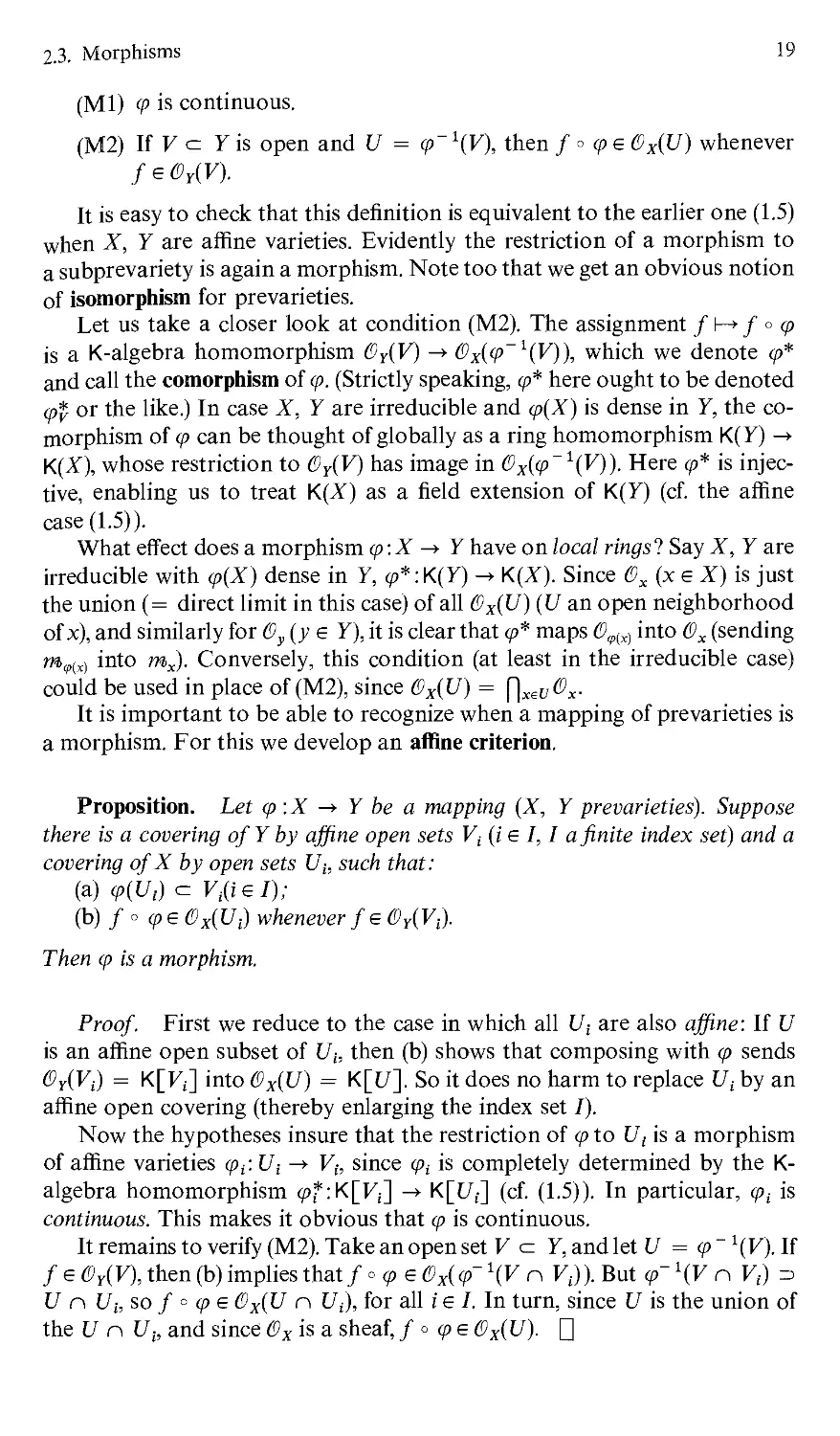
(Ml) (p is continuous.
(M2) If V <= 7 is open and U = cp~ \V), then f ° (pe 0X{U) whenever
f 6 W).
It is easy to check that this definition is equivalent to the earlier one (1.5)
when X, Y are affine varieties. Evidently the restriction of a morphism to
a subprevariety is again a morphism. Note too that we get an obvious notion
of isomorphism for prevarieties.
Let us take a closer look at condition (M2). The assignment f\-+f°q>
is a K-algebra homomorphism (9Y(V) -* (9x(cp~ 1{V)), which we denote cp*
and call the comorphism of cp. (Strictly speaking, cp* here ought to be denoted
q% or the like.) In case X, Y are irreducible and cp(X) is dense in Y, the
comorphism of cp can be thought of globally as a ring homomorphism K(Y) -»•
K(X), whose restriction to (9Y(V) has image in (9x((p~1(V)). Here cp* is injec-
tive, enabling us to treat K(Z) as a field extension of K(Y) (cf. the affine
case (1.5)).
What effect does a morphism (p:X -► Y have on local rings? Say X, Y are
irreducible with cp{X) dense in Y, cp*: K( Y) -»• K(Z). Since (9X (x e X) is just
the union (= direct limit in this case) of all (9X(U) (U an open neighborhood
of x), and similarly for (9y (y e Y), it is clear that cp* maps (9^ into (9X (sending
m?M into mx). Conversely, this condition (at least in the irreducible case)
could be used in place of (M2), since (9X{U) = \]xeV&x.
It is important to be able to recognize when a mapping of prevarieties is
a morphism. For this we develop an affine criterion.
Proposition. Let (p :X -»• Y be a mapping (X, Y prevarieties). Suppose
there is a covering of Y by affine open sets Vt (i € I, I a finite index set) and a
covering ofX by open sets Uh such that:
(a) <p(Ut)<= Vliel);
(b) f o (pe&xiUi) whenever fe (9Y{Vi).
Then cp is a morphism.
Proof. First we reduce to the case in which all Ut are also affine: If U
is an affine open subset of Ub then (b) shows that composing with <p sends
&Y{Vi) = K[F;] into (9X{U) = K[(7]. So it does no harm to replace U, by an
affine open covering (thereby enlarging the index set I).
Now the hypotheses insure that the restriction of cp to Ut is a morphism
of affine varieties (Pi'.Ui -*■ V{, since cpt is completely determined by the K-
algebra homomorphism <p*:K[F;] -+ K[(7;] (cf. (1.5)). In particular, q>t is
continuous. This makes it obvious that cp is continuous.
It remains to verify (M2). Take an open set V <= Y, and let U = cp ~ 1(V). If
f e &Y(V), then (b) implies that/ ° cp e (9x{<f \V n V,)). But <p~ \V n V,) =>
U n Ub so / ° cp e (9X( U n Ut), for all i e I. In turn, since U is the union of
the U n Ut, and since (9X is a sheaf, / ° cpe (9X(U). []

20
Algebraic Geometry
For the rest of this subsection we concentrate on irreducible prevarieties.
It is clear that a regular function f e (9X(X) defines a morphism X -*■ A1,
but of course a rational function need not be regular (cf. projective varieties!).
Nonetheless, given /e K(Z), and given an affine covering {(7,-} of X, the
subset of U{ where f is defined is open (Exercise 1.12), so the subset U of
X where f is defined is also open. Thus f induces a morphism U -»• A1. In
turn, the subset of U on which f ^ 0 is open and may be denoted Xf.
Similarly, we can define -f~(f) = {x e X \ f{x) = 0} for f e (9 X{X), as in the
affine case.
Two irreducible prevarieties X, Y may have function fields related by a
monomorphism a: K(Y) -»• K(X). We claim that a induces a "partial
morphism", i.e., a morphism from a (nonempty) open subset of X into Y whose
comorphism is essentially o. Indeed, we may first replace X, Y by affine open
subsets; this has no effect on the function fields. Thus K(Y) is of the form
K(fu ..., /„), where K[ Y] = K[/l5..., /„]. Set gt = a(ft) e K(X). Cut down
as above, to an open subset of X on which all g{ are defined, then further to
an affine open set U for which all gt e K[(7]. Now a takes K[Y] into K[(7],
so there is a unique morphism U -»• Y having this as comorphism.
Finally, we introduce the notion of birational morphism : q> :X -»• Y is
birational if q>* is an isomorphism of K( Y) onto K(X). Irreducible prevarieties
with isomorphic function fields are called birationally equivalent; they need
not be isomorphic (cf. A" and P").
2.4. Products
For pairs of affine or projective varieties, we were able to give the same
type of structure to the cartesian product set (cf. (1.4), (1.7)). For arbitrary
prevarieties, the categorical notion of "product" is our surest guide. Given
objects X, Y, a product of X and Y consists of an object Z, together with
morphisms n^.Z-* X, n2:Z-> Y (projections), satisfying the universal
mapping property: For any object W and any morphisms cp^.W -* X,
(p2:W -> Y, there exists a unique morphism \j/: W -»• Z such that %$ = cpt
(i = 1, 2). The definition is constructed so as to insure the uniqueness of
the product, if it exists, but the existence has to be settled by a specific
construction.
For prevarieties X, Y, the underlying set of a product prevariety would
have to be the cartesian product: apply the universal property to morphisms
W -»• {x}, W -»• {y}, where W is a prevariety consisting of a single point, to
conclude that points of Z correspond bijectively to pairs (x, y). The
construction in (1.7) suggests that we give X x Y the structure of a prevariety by
patching together products of various affine open subsets of X, Y. So we
begin by examining more closely the affine situation.
Proposition. Let X <= A", Y <= Am be affine varieties, with R = K[Z],
S = K[Y]. Endow the cartesian product X x Y with the Zariski product
topology {1-4). Then:

2,4. Products
21
(a) X x Y, with the projections pr^. X x Y -» X and pr2'- X x Y -» Y,
is a product (in the categorical sense) of the prevarieties X,Y, and K.[X x Y] s
(b) //(x, |)eX x Y, 0(x_ j,) r's tfte localization of(9x ®K 0, at tfte (maximal)
ideal mx ®&y + 0X® my.
Proof, (a) First we pin down the affine algebra of X x Y, which by its
construction is a closed subset of A"+m. Via the projections, polynomial
functions on X, Y induce polynomial functions on X x Y. Assign to a pair
(g,h)eR x S the polynomial function f(x, y) = g(x)h(y) on X x Y. This
assignment is bilinear in each variable g, h, so it induces a K-algebra ho-
momorphism cr:i? ®K S -► K[Z x Y]. It is clear that each polynomial in
m + n indeterminates Tu ..., T„, 1^,..., Um can be expressed as a finite
sum of products g(T)h(\j). This shows that a is surjective (polynomial
functions on X x Y being the restrictions of polynomial functions on Am+").
r
To show that a is injective, let / = £ fl; ® hi be sent to 0. We may
assume that f is written with r minimal. In case f ^ 0, we claim that r = 1.
Indeed, not all /i( are 0 in this case, so we can fix some y e Y for which not
all hi(y) = 0. Since J^g^h^y) = 0 for all x e X, we get £^0)^ = 0 in R,
i.e., the g; are linearly dependent over K. If r > 1, we could reduce by one
the number of gt and get a contradiction to the minimality of r. So r = 1.
Now the argument shows that gl = 0, so/ = 0.
It remains to verify the universal mapping property for X x Y. Given a
prevariety W and morphisms (pi'.W -> X, <p2:W -> Y, we have to construct
a suitable morphism i/z-.W -> X x Y. There is a unique such mapping of sets
which makes q>t = pr; ° \j/. To check that it is a morphism, we use the affine
criterion (2.3). X x Y is affine, so it just has to be seen that \j/ pulls back
polynomial functions on X x Y to regular functions on W. K[X x Y] being
generated by the pullbacks of K[Z], K[ Y] under pr;, and the cpt being
morphisms by assumption, the conclusion follows.
(b) If X, Y are irreducible, so is X x Y (1.4); part (a) shows that R ®K S
is an integral domain, with fraction field isomorphic to K(X x Y). Now we
have inclusions R® S <= (9X<2) (9y <= (9(Xt y). Since 0(x_ j,, is the localization of
R ® S at the ideal w(x j,,, it is equally well the localization of (9X ® (9y at
its ideal m vanishing at (x, y). Evidently mx (g) (9y + (9X (g) my cz m.
Conversely, let f = Y^gi®hi€ m, with gt e <DX, ht e (9y. If gt(x) = a,, ht(y) = bt,
then/ - Yafri = Yidi - at) <g) ht + j>, <g) (ft, - fe,)e mx ®(9y + ®x® my.
This forces Yj^^i = 0 and concludes the proof. []
The proposition shows that X x Y has intrinsic meaning in the category
of prevarieties, when X and Y are affine, independent of any particular
embeddings in affine space.
In order to treat the arbitrary prevarieties X, Y, we concentrate first on
the irreducible ones. To endow the cartesian product X x Y with the
structure of prevariety, we have to specify a topology and a covering by affine

22
Algebraic Geometry
open sets. For all affine open sets U <= X, V <= Y, and all finite sets of
polynomial functions f on U, g; on F, we decree that the principal open sets
(U x F)x/.g should be basic open sets in X x Y. Notice that these sets do
form a basis for a topology, since the intersection of two of them is another
of the same type. Moreover, the description of the affine algebra of U x F
in part (a) of the proposition shows that the topology induced on U x F
coincides with the Zariski product topology there.
The function field of X x Y will have to be that of U x F, where
U <= X, V <= Y are affine open sets. Since K[(7 x F] = K[(7] <g) K[F], it
is evident that K((7 x F) can be described as the field of fractions of (the
integral domain!) K(U) (g) K(F). Call this field F. Part (b) of the proposition
forces us to define the local ring of (x, y) e X x Y to be the localization of
(9X (g) (9y at mx (g) (9y + (9X (g) mr In turn, we get a sheaf of functions on
X x Y by assigning to each open set ¢7 the intersection of all $(x j,,, (x, y) e ¢7.
(This agrees on each product of affine open sets with the affine product
already defined.) It is clear that X x Y thus acquires the structure of pre-
variety. Moreover, the set-theoretic projections onto X, Y are morphisms:
use the affine criterion (2.3).
To check the universal mapping property, let W be a prevariety, with
morphisms ¢^: W -> X, q>2: W -> Y. As before, there is a unique map of sets
\j/: W -»• X x Y for which <p, = pr; ° \j/. We appeal to the affine criterion (2.3)
to prove that \j/ is a morphism: By construction, products U x F of affine
open sets in X, Y are affine open sets which cover X x Y. Open sets of the form
W" = ¢^1^) n ^2 1(^0 cover W, and the universal property of U x F
shows that the restriction of i/' to W is a morphism.
This takes care of the irreducible case. For arbitrary prevarieties X, Y,
having irreducible components Xt, Y-p we form the prevarieties Xt x Y,- as
above. We then topologize I x 7by declaring that a set is open if and only
if its intersection with each Xi x Yj is open. Finally, we endow X x Y with
a sheaf of functions as in (2.2). It is then a routine matter to verify that X x Y
is a categorical product. Therefore:
Theorem. Products exist in the category of prevarieties. []
The reader should check that the construction of products of projective
varieties (1.7) is duplicated abstractly by the foregoing process. However, the
embedding in projective space specified in (1.7) is needed in order to see that
the resulting product is again projective.
2.5. Hausdorff Axiom
It is possible to concoct examples of prevarieties which are geometrically
pathological. For instance, let X be covered by two copies U, V of A1, with
x e U equal to x e F except when x = 0 ("the affine line with a point
doubled").

2.5. Hausdorff Axiom
23
A prevariety X is called a variety if it satisfies the Hausdorff axiom:
The diagonal A(X) = {(x, x)|xe X) is closed in X x X. (In the category of
topological spaces, with X x X given the ordinary product topology, this
condition is equivalent to the usual Hausdorff separation axiom.) An
equivalent condition is this: (*) For morphisms q>, \j>: Y -»• X, Y any prevariety,
{ye Y\<p(y) = iA(y)} is closed in Y. Indeed, by applying (*) to the situation
pri
X x X =t X, we get A(X) closed in X x X; in the other direction, use the
pr2
set-up 7 ^ I x I 4 I, the inverse image of A(X) being {ye Y\q>(y) =
The example above fails to pass the test (*), if we take the two maps
A1 ^> U <= X, A1 -> V <= X, since A1 - {0} is not closed in A1. On the other
hand, varieties do abound.
Examples: (1) An affine variety is a variety. (The diagonal is clearly given
by polynomial conditions.)
(2) Subprevarieties of a variety are again varieties. These are therefore
called subvarieties.
(3) If X, Y are varieties, so is X x Y.
(4) A projective variety is a variety. (This results from the following nice
criterion.)
Lemma. Let X be a prevariety, and assume that each pair x, ye X lie in
some affine open subset ofX. Then X is a variety.
Proof. Given a prevariety Y and morphisms q>, \j/: Y -* X, let Z =
{ye Y\<p(y) = il/(y)}. We have to show that Z is closed. If ze Z, set x =
q>(z), y = \j/(z). By hypothesis, x and y lie in some affine open set V. Then
U = <p_1(F) n \j/~l(V) is an open neighborhood of z, which must meet Z.
But Z n U = {ye U\cp'{y) = \j/'{y)}, where <p', \jj':U -»• V are the
restrictions. Since V is a variety, Z n U is closed in U. This means that U - (Z n V')
is an open set not meeting Z, so in particular it cannot contain z. We conclude
that zeZ. []
The following proposition shows why it is better to deal with varieties
than with prevarieties:
Proposition. Let Y be a variety, X any prevariety.
(a) If (p:X -> Y is a morphism, the graph r,, = {(x, (p(x))|x e X} is closed
inX x Y.
(b) lf(f>, i//:X —> Y are morphisms which agree on a dense subset ofX, then
Proof, (a) r^, is the inverse image of A( Y) under the morphism X x Y -»
Y x Y which sends (x, y) to (cp(x), y)).

24
Algebraic Geometry
(b) The set {x e X\cp{x) = \p(x)} is closed in X since Y is a variety It is
dense by assumption, so it coincides with X. []
In practice, we shall deal only with varieties in what follows: affine and
projective varieties, their subvarieties, their products.
Exercises
1. Show that the definition of "morphism" (2.3) agrees with that given for
affine varieties in (1.5).
2. If cp: A1 -»• A1 is a birational morphism, then q> is necessarily an
isomorphism.
3. Let char K = p > 0. Show that the assignment T; \—> Tf determines a
K-algebra monomorphism K[T] -> K[T], which is the comorphism of a
morphism cp:A" -»• A" (called the Frobenius map). Describe cp explicitly.
4. Let X, Y be prevarieties. Prove that the projections X x Y -»• X,
X x Y -*■ Y are open maps (i.e., send open sets to open sets). Must they
send closed sets to closed sets?
5. If X, Y are prevarieties, and W is open (resp. closed) in X, then W x Y
is open (resp. closed) in X x Y.
6. Prove that a topological space X is T2 if and only if {(x, x)\x e X) is
closed in X x X (given the ordinary product topology).
7. Let cp, \j/:Y -»• X be morphisms (X, 7 prevarieties). Prove that {ye Y\
<p(y) = "M-H)} is locally closed in Y.
8. If 7 is a prevariety for which Proposition 2.5 (a) (resp. (b)) holds for all
prevarieties X, then Y is a variety.
9. Let (p:X -»• Y be a morphism of varieties. Prove that p^ induces an
isomorphism of the graph r <= X x Y onto X.
Notes
We have followed Mumford [3,1 §6]. The current terminology is "variety"
(resp. "separated variety") in place of our "prevariety" (resp. "variety"); but
we prefer to follow the older usage, since all prevarieties we shall encounter
are in fact varieties.
3. Dimension
Intuitively, a point is 0-dimensional, a curve 1-dimensional, a surface
2-dimensional. The object of this section is to give precise algebraic meaning
to the geometric notion of dimension. This in turn will allow us to describe
the behavior of varieties under morphisms, in the following section.
3.1. Dimension of a Variety
With an irreducible variety X is associated its field K(X) of rational
functions. As a finitely generated field extension of K, K(X) has finite tran-

3 2. Dimension of a Subvariety
25
scendence degree over K (0.4), abbreviated tr. deg.K K(X). This number is
called the dimension of X, written dim X. For example, dim A" = dimP" = n.
So the dimension measures the maximum number of algebraically
independent functions on X (or the number of "parameters" required to describe X).
In case X has more than one irreducible component, say X = X1 u • • • u X„
it is reasonable to define dim X as max (dim Xt).
Let X be irreducible. Since K(Z) = K(U) for any affine open subset U,
dim X = dim U. Similarly, dim X = dim Xf for any/ e K(X). For example,
GL(«, K) is the principal open subset of A"2 denned by nonvanishing of the
determinant, so its dimension is n2.
Proposition. Let X, Y be irreducible varieties of respective dimension
m, n. Then dim X x Y = m + n.
Proof. In view of the preceding remarks, we may as well assume that
X, Y are affine, with X <= Ap, Y <= A". (The reader who prefers to avoid
embedding X and Y in affine spaces can proceed more intrinsically by using
the identification K[Z] <g) K[Y] = K\_X x Y] (2.4).) If S1;.. ., Sp (resp.
T1;. ■., Tg) are the coordinates on Ap (resp. A"), their restrictions st (resp. tt)
generate K(Z) (resp. K(Y)). From these generating sets we can extract
transcendence bases (0.4), say su ..., sm and ti,..., t„. It is clear that K(X x Y) =
K(si,. .., sp, tu ..., tq) and that K(X x Y) is algebraic over the subfield
K(s1;.. ., sm, tu .. ., tn). So it suffices to show that the latter field is purely
transcendental over K. Suppose there is a polynomial relation f(su . .., sm,
tu ..., tn) = 0. Then for each fixed x = (x1;..., xp) = (s^x),..., sp(x))e X,
the polynomial function /(x1;.. ., xm,tu ..., t„) vanishes on Y. The
algebraic independence of the tt forces all coefficients g{xx,..., xm) of the
polynomial f(x i,..., xm, T1;..., T„) to be zero. In turn, each fif(si;..-, sm) = 0
(since xe X was arbitrary), so the algebraic independence of the st forces all
g(Su ..., Sm) = 0. Finally, /(S^ ..., Sm, Tj,..., T„) = 0. Q
3.2. Dimension of a Subvariety
The following is a first step toward understanding how dimension varies
inside a given variety.
Proposition. Let X be an irreducible variety, Y a proper, closed,
irreducible subset. Then dim Y < dim X.
Proof. It is harmless to assume that X is affine, say of dimension d. Let
R = K[Z], R = K[Y] ^ R/P (where P is a nonzero prime ideal of R). It is
clear that transcendence bases for K(X), K(Y) can already be found in R, R.
Suppose dim Y ^ d, and select algebraically independent elements x1;. ..,
xdeR (images of x1;..., xd e R, which are clearly algebraically independent
as well). Let f e P be nonzero. Since dim X = d, there must be a nontrivial

26
Algebraic Geometry
polynomial relation g(f, x1;..., xd) = 0, where g(T0, T1;..., Td) e K[T].
Because f ^ 0, we may assume that T0 does not divide all monomials in
g(T0, T1;..., Td), i.e., /1(^,..., ld) = g(0, Tu .. . , Td) is nonzero. Now
/i(x!,..., xd) = 0, contradicting the independence of the xt. []
Define the codimension codim^y of a subvariety Y of X to be dim X —
dim 7.
Corollary. Let X be an irreducible affine variety, Y a closed irreducible
subset of codimension 1. Then Y is a component of ^( f) for some f e K[X].
Proof. By assumption, Y ^ X, so there is a nonzero f e K[Z]
vanishing on Y. Then 7 <= 1^(/) 5 ^- Let Z be an irreducible component of
'f(f) containing Y. The proposition says that dim Z < dim X, while dim
Y < dim Z, with equality only if Y = Z. Since codim^ 7=1, equality
must hold. []
In the situation of the corollary, it is not usually possible to arrange that
7 be precisely 1^(/). However, this can be done when 7 has codimension 1
in some affine space A", or more generally, when K[X] is a unique
factorization domain (Exercise 6).
If subvarieties of codimension 1 (and hence, by induction, subvarieties
of all possible dimensions) are to exist, the corollary indicates the shape they
must have. We aim next for a converse to the corollary.
3.3. Dimension Theorem
The zero set in A" of a single nonscalar polynomial/(T^ ..., T„) is called
a hypersurface; its irreducible components are just the hypersurfaces denned
by the various irreducible factors of /(T). More generally, when X is an affine
variety, a nonzero nonunit /e K[I] defines a hypersurface in X (whose
components are not so easy to characterize unless K[Z] happens to be a
unique factorization domain). For example, SL(w, K) is a hypersurface in
GL(«, K), or in A"2, denned by det (T(j) = 1.
Proposition. All irreducible components of a hypersurface in A" have
codimension 1.
Proof. It suffices to look at the zero set X of an irreducible polynomial
p(T). We can assume that (say) T„ actually occurs in p(T) (which is nonscalar
by assumption). Let tx be the restriction of T( to X, so K(X) = K(t1;..., t„).
We claim that tl,... ,tn_l are algebraically independent over K. Otherwise
there exists a nontrivial polynomial relation g(tu ..., t„_i) = 0, whence
g(T1,..., T„_i) vanishes on X; but J~(X) = (p(T)), forcing g(T) to be a
multiple of p(T). This is impossible, since T„ occurs in p(T) but not in g(T).
We conclude that dim X ^ n-l, which must be an equality in view of
Proposition 3.2. []

3 3. Dimension Theorem
27
We want to generalize this result to arbitrary affine varieties. Two
technical tools are needed: Noether's Normalization Lemma (0.7) and the norm
map iVE/F: E -»• F for a finite field extension E/F (0.5).
Theorem. Let X be an irreducible affine variety, 0 ^ /e K[X] a nonunit,
Y an irreducible component of 'f(f). Then 7 has codimension 1 in X.
Proof. Let P = J?(Y) c K[Z], and let 7lr..., Yt be the components of
ir{f) other than Y, P; = J{Y{). The Nullstellensatz (1.1) implies thatV(7) =
P n Pi n • ■ • n Pt. Choose g e Pi n • ■ ■ n Pt — P (g exists, since 7 is not
contained in Yt u • • • u 7,). Then Z9 is an (irreducible) affine variety having
the same dimension as X, and Y n Xgis precisely the zero set of f in Xg.
Since 7 n I, is a principal open set in 7, it suffices to prove that its
codimension in Xg is 1. So we might as well assume at the outset that 7 = i^(f),
p = VW-
Now we apply the Normalization Lemma (0.7) to the domain R = K[X]:
R is integral over a subring S which is isomorphic to K[T1;..., Td], d =
dim X. Let E = K(X), F = field of fractions of S; so E/F is finite. Notice that
jVE/F takes elements of R into S. Indeed, if he R, then ft satisfies a monic
polynomial equation over S, and by the definition of "norm", NE/F(h) is a
power of the constant term.
Set /0 = iVE/F (/) eS. We claim that f0eP=JU). Say fk+ ajk~'+ ■■■ +
ak = 0 (at e S), with /0 = (%)m (by the preceding paragraph). Then 0 = (/k +
fll/*- ^--- + a^r* = /(/*- V"1 + • • • + %_ lflT ^ + /0, so /0 is an
i?-multiple of/.
If V(/o) denotes the radical of (/0) in S, what we have just shown implies
that V(/o) c P n S. The reverse inclusion also holds: Let g e P n S, so in
particular, g e >/(/) and g' = /¾ for some I e Z+,heR. Take norms to get
gf'[E:F] = NE/F(g') = NE/F(/)iVE/F(fr), where the first equality holds because
gf e S and the second because iVE/F is multiplicative. As remarked earlier,
NWF(h) € S, so we conclude that a power of g is an S-multiple of/0, as claimed.
Now we have replaced the prime ideal P = %/(/) m R by the prime ideal
P n S = V(/0) in S. The advantage of this is that S is a unique factorization
domain. In particular, since the radical of (/0) is prime, it is very easy to see
that (up to a unit multiple) /0 is just a power of an irreducible polynomial p,
whence P n S is just the principal ideal (p). It is clear that p is nonscalar.
If S is viewed as the affine algebra of Ad, then P n S defines a hypersurface
in Ad, which has codimension 1 (by the preceding proposition). This means
that the fraction field of S/(P n S) has transcendence degree d — 1 over K.
On the other hand, R integral over S clearly implies that R/P is integral over
S/(P n S), so the two fraction fields have equal transcendence degree. But the
fraction field of R/P is K(7); therefore, dim 7 = d - 1. []
The theorem can easily be reformulated as an assertion about an arbitrary
irreducible variety X: If U is open in X, and 0 ^ /e (9X(U) is a nonunit, then
each irreducible component of the zero set of / in U has codimension 1 in X.

28
Algebraic Geometry
(Deduce this from the theorem by cutting down to an affine open subset of
U which meets the irreducible component in question.)
3.4. Consequences
Theorem 3.3 guarantees that an n-dimensional variety X has irreducible
closed subsets of all dimensions less than n. More precisely:
Corollary A. Let X be an irreducible variety, 7 a closed irreducible
subset of codimension r ^ 1. Then there exist closed irreducible subsets Yt ofcodi-
mension 1 < i < r, such that Y^ -=> Y2 => ■" • => Yr = Y.
Proof. It suffices to prove this for an affine open subset of X which
meets Y, so we may as well let X be affine. For r = 1, there is nothing to
prove. Proceed inductively. Since Y ^ X, there exists/ ^ 0 in =/(7), and 7
lies in some irreducible component Y^ of 1^(/). But Theorem 3.3 says that
codim^ Y1 = 1. By induction, Y± has closed irreducible subsets of the required
type, going down to 7. []
Another obvious induction yields:
Corollary B. Let X be an irreducible variety, fu ... ,fe &X(X). Then
each irreducible component ofir(fi,... ,fr) has codimension at most r. []
The inequality cannot be improved (e.g., let _/i = f2 = • • ■ = f). But we
can say something useful in the other direction, which accords with the
geometric idea that a surface (resp. curve, point) in 3-space should be definable
by one (resp. two, three) polynomial equations.
Corollary C. Let X be an irreducible affine variety, 7 a closed irreducible
subset of codimension r ^ 1. Then 7 is a component ofir(fu ... ,fr)for some
choice off e K[Z].
Proof. It is easier to prove a more general statement: Given closed
irreducible subsets fj d y2 d ■ • o Yn with codim^ 7; = i, there exist/ e K[X]
such that all components of T^(/i,..., fq) have codimension q in X and such
that Yq is one of these components (1 < q < r). (This really is a more general
statement, thanks to Corollary A.)
The proof goes by induction on q (r being fixed). For q = 1, we appeal
first to Corollary 3.2 for the existence of fu and then to Theorem 3.3 for the
fact that all components of T^(/i) have codimension 1.
Assume that /i,...,/g-1 have been found. Let Zt = Yq_ l5 Z2,..., Zm be
the components of T^(/i,..., fq-1). Since each has codimension q — 1, none
can lie in Yq; so ^(Z() does not include J(Yq) (1 ^ i < m). The ideals ^(Z()
being prime, it follows (0.9) that their union also does not include <f(Yq).
Choose fq vanishing on Yq but not vanishing identically on any Zt. If Z is

4.1. Fibres of a Morphism
29
any component of ^( fi,... ,fq), then Z of course lies in one of the
components Z( of T^(/i, • • • ,/g-i), as well as in T^(/g). Theorem 3.3 implies that
'f(fq) n ^i nas codimension 1 in Z( (since fq does not vanish on Z(), hence
codimension q in X. On the other hand, Corollary B says that codim^ Z < q.
So Z must have codimension precisely q. Since /g vanishes on Yq, and Yg
has codimension q, we also conclude that Yq is one of the components of
n/i. ••■»/«)• d
Exercises
1. A variety has dimension 0 if and only if it is a finite set of points.
2. Show that the dimension of the Grassmann variety ®d(V) of d-dimen-
sional subspaces of an n-dimensional vector space V (1.8) is d(n — d).
Try to determine the dimension of the flag variety %{V).
3. Let X be an arbitrary variety, Y a closed subset. Prove that dim Y <
dimZ.
4. The dimension of an irreducible variety X is the largest d for which
there exists a chain of (nonempty) closed irreducible subsets X0 c Xl a
X2 <=•••<= Xd = X (all inclusions proper).
5. In a variety X, the closed irreducible sets satisfy ACC.
6. Let X be an irreducible affine variety for which K[Z] is a unique
factorization domain, e.g., X = A". Prove that each closed subset Y of
codimension 1 has the form 'f(f) for some /e K[Z]. [Treat first the case:
Y irreducible. Show that minimal prime ideals of K[X] are principal.]
Notes
The exposition here follows Mumford [3,1 §7].
4. Morphisms
In the study of linear algebraic groups, two kinds of morphisms will be
especially prominent: group homomorphisms (which are simultaneously
required to be morphisms of varieties) and canonical maps G -»• G/H (where
the coset space has to be given a suitable structure of variety, not necessarily
affine). This section provides the essential tools for the study of these and
other morphisms. The proofs depend heavily on considerations of dimension.
As in §3, it is usually enough to treat irreducible varieties, which can often
(though not always) be assumed to be affine.
4.1. Fibres of a Morphism
By definition, the fibres of a morphism q>: X -*■ Y are the closed sets
9 ~ 1( y), y e Y. (If (p were a group homomorphism, these would be cosets of

30
Algebraic Geometry
Ker cp.) We want to examine the dimensions of fibres and, in particular, to
prove that they are not "too small". Of course, q>~ 1(y) is empty if y ^ Im cp,
so care must be taken in the formulation below. More generally, we shall
consider sets cp~1(W), where W = Y is closed and irreducible.
It usually does no harm to replace Y by the closure of <p(X); this facilitates
dimension comparisons. When X is irreducible and q>(X) is dense in Y, we
say that cp is dominant. We could say the same when X is not irreducible, but
instead we reserve the term "dominant" for the following more special
situation: cp maps each component of X onto a dense subset of some
component of Y, and cp(X) is dense in Y. Even when cp is dominant, the restriction
of cp to an irreducible component of <p~1(W) (W closed irreducible in Y)
certainly need not be dominant, viewed as a morphism from this component
to W. But when it is so, we say that the component in question dominates W.
One other remark: When cp:X -> Y is dominant, X and Y irreducible, then
cp* induces an injection of K( Y) into K(X); in particular, dim X ^ dim Y.
Theorem. Let <p:X —► Y be a dominant morphism of irreducible varieties,
and set r = dim X — dim Y. Let W be a closed irreducible subset of Y. If Z
is an irreducible component of<p~1(W) which dominates W, then dim Z ^
dim W + r.In particular, ify e cp(X), each component ofcp~1(y) has dimension
at least r.
Proof. If U is an affine open subset of Y which meets W, then U n W
is dense in W. For comparison of dimensions, we could therefore replace
Y by U and X by the open subvariety <p~ 1(U). So we might as well assume
at the outset that Y is affine.
Let s = codimr W. According to Corollary C of (3.4), W is a
component of TT(/!,..., /s) for suitable f e K[ Y]. Setting gt = (?*(/;) e (9X(X),
we conclude that Z lies in i^(gu ..., gs). Since Z is irreducible, it lies in
some component Z0 of this set. But W = cp{Z), by assumption, while
<p(Z) c: <p(Z0) = T^(/i, • • • ,fs). W being a component of T^(/i,..., fs),
it follows that cp(Z) = <p(Z0) = W, whence Z0 = cp~ 1(W). But Z is a
component of q>~ \W), so Z = Z0. i.e., Z is a component of i^(gu ..., gs).
Now Corollary B of (3.4) says that codim* Z < s. The theorem follows at
once. []
In the situation of the theorem, we now know that (nonempty) fibres
of (p are not too small. Next we have to ask whether they can be "too big".
A simple geometric example helps to illustrate the possibilities: Define
<p:A2 -*■ A2 by cp(x, y) = (xy, y). The image consists of the complement of
the "x-axis" along with the origin (0, 0). This is easily seen to be dense, so q>
is dominant (though not surjective). If U is the principal open set in A2
denned by y ^ 0, then cp induces a bijection from U = (p~l(U) onto U,
which is even an isomorphism of varieties. But the fibre cp~1((0, 0)) is 1-
dimensional, consisting of all points (x, 0).

4.2. Finite Morphisms
31
This example suggests that we look for an open set in the target variety
above which all fibres have the "correct" dimension: dim X - dim Y. But
if such an open set is to exist, it must lie in q>(X). So the study of fibres of
m leads also to the study of the image of cp. In preparation for the main
theorem (4.3), we look briefly at a special type of morphism which turns out to
be surjective.
4.2. Finite Morphisms
Let cp :X -»• Y be a morphism of affine varieties. If K[Z] is integral over
the subring (p*K[Y], we call cp finite. Notice that if X, Y are irreducible, and
if cp is also dominant, then K(X) is a finite algebraic extension of <p*K(Y);
so dim X = dim Y.
As a nonexample, take (p(x, y) = (xy, y), discussed at the end of (4.1). Here
(p^KfSi, S2] -»• K[Tl5 T2] is injective and sends Sj to T{T2, S2 to T2. It is
easy to see that, e.g., Tj fails to be integral over Kp^Tj, T2]. But this also
follows from our next result.
Proposition. Let cp:X -► Y be a finite, dominant morphism of affine
varieties.
(a) If Z is closed in X, then (p(Z) is closed in Y, and the restriction of cp
to Z is finite. In particular, <p is surjective.
(b) Let X, Y be irreducible, with K[Y] integrally closed. IfW is a closed
irreducible subset of Y, and Z is any component of<p~1(W), then q>(Z) = W.
Proof. Let R = K[Z], S = K[Y]. Since cp is dominant, cp* is injective;
we abuse notation by viewing S as a subring of R (of which R is an integral
extension by assumption). If I is an ideal of R, then R/I may be regarded
naturally as an extension of S/(I n S). This extension is clearly integral as well.
(a) Now let Z = TT(7) be closed in X, where I = £{Z). Then cp maps Z
into the zero set Z' of I' = I n S, which is a radical ideal of S (hence equal
to =/(Z')). The corresponding affine algebras are R/I and S/I n S, so the
preceding remark shows that cp:Z -»• Z' is again finite (and dominant). It
suffices now to prove that any finite dominant morphism is surjective. If
y e Y, then to say that (p(x) = y is just to say that cp* sends the local ring of
y into that of x, or that cp* sends the maximal ideal M' of S vanishing at y
into the maximal ideal M of R vanishing at x. To show that cp is surjective,
we therefore have to show that M' lies in some maximal ideal M of R (S still
being viewed as a subring of R). But this follows from the Going Up Theorem
(0.8), since R is integral over S.
(b) According to part (a), the restriction of (p to Z is again finite, so cp(Z)
is closed, irreducible. Now it suffices to show that dim Z = dim W. If
I = <f(Z), F = J~(W), then I is a minimal prime ideal of R for which
I n S =3 /'. In turn, the Going Down Theorem (0.8) implies that I n S = I'.

32
Algebraic Geometry
But as before, R/I is integral over S/I', so the corresponding extension of
fields of fractions is algebraic and the dimensions coincide. []
4.3. Image of a Morphism
Noether's Normalization Lemma (0.7) says that a finitely generated
domain over K can be built up in two steps: a purely transcendental extension
followed by an integral extension. In order to deal with a pair of irreducible
affine varieties related by a dominant morphism cp:X -> Y, we have to
develop a relativized version of this.
Let S <= R be two finitely generated domains over K, with respective
fields of fractions E <= F. Denote by R' the localization of R with respect to
the multiplicative system S* of nonzero elements of S (0.10). Of course, R'
still has F as field of fractions. On the other hand, R' includes E and can thus
be viewed as a finitely generated E-algebra. The Normalization Lemma says
that R' is integral over E[xl5 . .., xr] for some x; e R' which are algebraically
independent over E. It is clear that the xt can be chosen to lie in R (since
any denominators occurring are units in E). It is also clear that r = tr. deg. EF.
Now compare the integral extension E[x1;..., xr] <= R' with the
extension S[xl5..., xr] <= R. The latter need not be integral. But R is finitely
generated over S, and each generator satisfies a monic polynomial over
E[xl5..., xr]. By choosing a suitable common denominator f e S, we can
therefore guarantee that Rf is integral over Sf[xu . . ., xr] (Rf, Sf the rings
of quotients gotten by allowing powers of f as denominators). This set-up
will be used to prove the following key theorem.
Theorem. Let <p:X -► Ybe a dominant morphism of irreducible varieties,
r = dim X — dim Y. Then (a) Y has a nonempty open set U such that U <=
<p(X); (b) if all local rings of points of Y are integrally closed, we can choose
U in part (a) to have the property: if W <= Y is an irreducible closed set which
meets U, and ifZ is a component of<p~1(W) which meets (p~l{lJ), then dim
Z = dim W + r.
Proof. As in the proof of Theorem 4.1, it is harmless to replace Y by
an affine open subset. We can also assume that X is affine: If we have found
suitable open sets Ut <= Y for the restrictions of q> to finitely many affine
open sets Xt which cover X, then U = f);{7; clearly satisfies both (a) and (b).
Let R = K[Z], S = K[Y]; view S as a subring of R via cp* and use the
method described above to find x1;..., xr e R, f e S such that Rf is integral
over Sf\_xu ..., xr], the latter being isomorphic to a polynomial ring over
Sf. Now Rf, Sf are the respective affine algebras of the principal open sets
X f, Yf (1.5); so Sjfxj,..., xr] may be viewed as the affine algebra of Yf x Ar.
The restriction of q> to Xf can be factored asXf ^ Yf x Ar 5 7^-, where \j) is
afinite morphism (and dominant). Set U = Yf, and notice that cp~ 1(U) = Xf.
Thanks to Proposition 4.2, \j/ is surjective, as is pr^ Therefore U does lie
in cp(X), proving (a). For (b), we may as well let X = Xf, U = Y = Yf, with

4 4. Constructible Sets
33
the above factorization q> = p^ ° \jj (i// finite). The assumption on local rings
forces K[Y] = Sf to be integrally closed (2.1); so Sf\_xl,..., xr] is also
integrally closed (0.6). If W is a closed irreducible subset of Y, Z any
component of cp~1(W), then Z is a component of \j/~l(W x Ar) and therefore
maps onto W x Ar, with dim Z = dim xp(Z) = dimW + r (4.2) (b). Q
It would actually be enough in (b) to assume that local rings are integrally
closed for points in a nonempty open set; this much turns out to be
automatically true: cf, (5.2) and (5.3).
For use in (21.1) we record explicitly an assertion which is contained in
the above proof when r = 0.
Corollary (of proof). Let <p:X -»• Y be a bijective morphism of irreducible
varieties. Then dim X = dim Y and there exist ajfine open subsets U a X,
V <= Y, such that <p(U) <= V and <p\U is a finite morphism. []
4.4. Constructible Sets
Part (a) of Theorem 4.3 can be used to characterize the image of an
arbitrary morphism. Recall that a subset of a topological space X is said to be
locally closed if it is the intersection of an open set with a closed set. Call a
finite union of locally closed sets constructible. (The constructible sets
comprise the smallest collection of subsets of X containing all open and closed
sets, and closed under the boolean operations, cf. Exercise 3.) Note that a
constructible subset of a variety contains a dense open subset of its closure.
Theorem. Let <p:X -> Y be a morphism of varieties. Then q> maps
constructible sets to constructible sets; in particular, (p(X) is constructible.
Proof. A locally closed subset of X is itself a variety, so clearly it suffices
to prove that <p(X) is constructible. In turn, we may as well assume that X,
Y are irreducible. Proceed by induction on dim Y, there being nothing to
prove when this is 0. By induction, we need only consider dominant q>.
Choose an open subset U of Y contained in q>(X), using Theorem 4.3(a).
Then the irreducible components Wu ..., Wt of Y — U have smaller
dimension than Y (Proposition 3.2). The restrictions of cp to the various components
Ztj of q>~ 1(Wi) then have images which are constructible in Wt (by induction),
hence also constructible in Y. Therefore, q>(X) is constructible, being the
union of U and the finitely many (p(Z{}). []
This theorem will be used repeatedly. Another fact, based on a similar
induction, will be handy in one later argument (5.2). It is called the "upper
semicontinuity of dimension".
Proposition. Let cp:X -+ Y be a dominant morphism of irreducible
varieties. For xe X, let e9(x) be the maximum dimension of any component of
(p~1((p(x)) containing x. Then for all n e Z+, {xeZ|e9(x) ^ «} is closed
inX.

34
Algebraic Geometry
Proof. Use induction on dim Y. Choose U <= <p(X) as in Theorem 4.3,
and set r = dim X - dim Y, En{q>) = {x e X\s9{x) ^ «}. Theorem 4.1
implies that £p(x) ^ r, so that £„((/>) = X is closed whenever w < r. On the
other hand, Theorem 4.3 insures that £„(<p) <= X — (p~l(U) whenever n > r.
Let Wu ...,Wtbe the irreducible components of Y — U, Ztj the various
components of q>~\Wt), cpij'Zij■,-* W{ the restriction of (p. Since dim Wi < dim Y,
the induction hypothesis says that E„{q>t]) is closed in Zy (hence in X). But
for n > r, £„(<?) = [J,-,; E„((pt}), a finite union of closed sets. []
4.5. Open Morphisms
The example at the end of (4.1) shows that the image of an open set under
a morphism <p:X -> Y need not be open. This is traceable to the fact that
not all components of q>~ \W) (W closed, irreducible) need be of the same
dimension. Such behavior is essentially confined to the complement of an
open set in Y, thanks to Theorem 4.3 (b); so in a sufficiently "homogeneous"
situation, the hypothesis of the following theorem will be fulfilled.
Theorem. Let <p:X —► Y be a dominant morphism of irreducible varieties,
r = dim X — dim Y. Assume that for each closed irreducible subset W <= Y,
all irreducible components of cp~1(W) have dimension r + dim W. Then q>
maps open sets to open sets.
Proof. The hypothesis implies in particular that cp is surjective and that
all irreducible components of cp~ 1{W) dominate W.
Let x e X and let U be any open neighborhood of x. We have to show
that q>(x) = y lies in the interior of <p(U) = V. Suppose not. Then y lies in
the closure of Y — V. Because V is constructible (Theorem 4.4), Y — V is
constructible. Thus y lies in the closure C of some locally closed set 0 n C
contained in Y — V (where 0 is open in Y and C can be assumed to be
irreducible, so that OnCis dense in C). By hypothesis, the irreducible
components of C = <p_1(C) have equal dimension, and each dominates C.
So 0' = (p~ 1(0) meets each such component ,0' n C is therefore dense in C".
But 0' n C = cp ~ \0 n C) lies in the closed set X - U, forcing C <= X - U.
Since x e C, this is absurd. []
This theorem will be applied in §12 to the canonical map G -»• G/H,
where G is a linear algebraic group and H a closed subgroup (the
homogeneous space G/H being given a suitable structure of variety).
4.6. Bijective Morphisms
When a morphism is bijective, there is no mystery about either its fibres
or its image. But its topological behavior and the effect of its comorphism
on functions can be quite subtle. Here we are concerned mainly with the

4 6. Bijective Morphisms
35
latter. The Frobenius map A1 -»• A1, x \—> xp (where char K = p > 0),
illustrates how inseparability can complicate the whole question. (But even in
characteristic 0 one cannot assert that a bijective morphism is an
isomorphism, cf. Exercise 5.) The following theorem will be of great technical value
in the study of homogeneous spaces in Chapter IV.
Theorem. Let <p:X -> Ybe a dominant, injective morphism of irreducible
varieties. Then K(X) is a finite, purely inseparable extension of<p*K(Y).
Proof. Since cp is dominant, cp* is injective, so we may identify K(Y)
with <p*K(Y). Theorem 4.3 implies that dim X = dim Y. Therefore, K{X) is
a finitely generated algebraic extension of K(Y), i.e., a finite extension.
The function fields do not change if we replace X, Y by nonempty open
subsets. As a first reduction, let F be the separable closure of K(Y) in K(X)
(= the set of elements of K(X) which are separable over K(Y)). As a finitely
generated extension of K, F may be viewed as the function field of some
variety Z. Then the remarks in (2.3) allow us to factor cp as the composite
of two (injective) morphisms X -*■ Z, Z -> Y, after cutting X, Z, Y down to
suitable open sets. It suffices then to prove that Z -»• Y is birational, i.e., it
suffices to prove the theorem when K(X)/K(Y) is separable.
Let n = [K(X):K(Y)]. To show that n = 1, we shall find some ye Y
whose fibre <p~1(y) has cardinality at least n.
The theorem of the primitive element allows us to choose a single
generator f of K(X) over K(Y), whose minimal polynomial has the form p(T) =
n- 1
T" + X 9^1 (#' e K(^) )• Tne separability further implies that f is not a root
> = o
of p'(T). Now X and Y may be replaced by open subsets so that the rational
functions f, gt (i.e., q>*gi) are everywhere defined on X. We may also assume
that Y is ajfine, with g{e S = K[ Y]. Then f is integral over S, so R = S[/]
is integral over S. If U is an affine open subset of X, q>* induces inclusions
S <= R a K[{7]. The ring R is an affine algebra in its own right, so it belongs
to some affine variety X', and the factorization of cp* corresponds to
U ->■ X' ->■ Y. But K((7) = K(X), while R has fraction field K(Y)(/) = K(X).
So it suffices to prove that the finite morphism \j/ :X' -> Yis birational. Unlike
cp, this morphism might not be injective. But its restriction to a nonempty
open set must be so: The image of U in X' contains a dense open set U' (4.3),
and after deleting from it its intersection with the proper closed subset
\I/~1(\I/(X' - U')) we are left with fibres consisting of single points. In turn,
the image of this open set in Y contains a dense open subset V.
Now consider the fibre *ff~1(y), yeY. The point y corresponds to a K-
algebra homomorphism ey:S -*■ K, while the various xef 1(y) correspond
to homomorphisms ex:R -»• K extending ey. Integrality of R over S already
guarantees at least one extension of ey (cf. (4.2)), but we need to be more
precise in order to get n distinct extensions.

36
Algebraic Geometry
Since f is a root of p(T), f(x) is a root of the polynomial ps(T) gotten by
applying e = sy to each coefficient. We claim that for suitable choice of y,
pe(T) has n distinct roots (i.e., is a separable polynomial over K). For this we
look at derivatives. Separability of p(T) over K(Y) implies that p'(f) ^ 0.
Since f is integral over S, p'(f) is also; so there is a monic polynomial q(T) =
Tm + Y)1^1 (^ € S) of which p\f) is a root (and we can assume that h0 ^ 0,
since p'(f) ^ 0). Choose yeV for which h0(y) ^ 0. If i//(x) = y, the
choice of y clearly implies that p'(f)(x) ^ 0; in turn, f(x) cannot be a root
of Pe(T). This justifies our claim that pJJ) is separable over K for e = er
For each of the n roots a of ps(J), we can now construct a point xeif_1(y)
such that f(x) = a, thus completing the proof. The problem is to extend e
to a homomorphism e': R -»• K for which e'(/) = a. By a standard extension
theorem (0.8), this can be done provided we know that for each h(T) e S[T],
the condition ft(/) = 0 implies he(a) = 0. But p(T) is the minimal polynomial
of/ over K(Y), so /i(/) = 0 yields h(T) = p(T)fe(T) (fe(T) a polynomial over
K(Y), hence over S since p(T) is monic and both h(T), p(T) e S[Tj). From
ps(a) = 0 we get he(a) = 0, as required. []
4.7. Birational Morphisms
A birational morphism need not be an isomorphism (cf. A1 -»• P1 or the
example at the end of (4.1)); but it is not too far from being one.
Proposition. Let <p:X -+ Y be a birational morphism (X, Y irreducible).
Then there is a nonempty open set U <= Y such that <p induces an isomorphism
of(p~\U) onto U.
Proof. It does no harm to assume that Y is affine; set S = K[Y]. Let
Kclbe any affine open set, R = K[F]. Consider W = q>(X - V), all of
whose irreducible components have lower dimension than Y (since the
components of X — V are of smaller dimension than X, and dim X = dim Y).
W being a proper closed subset of Y, we can find 0 ^ f e S such that f
vanishes on W, whence q>~ 1(Yf) = Xv,f <= V. Replacing Y by Yf and X by
X^j-, we may therefore assume that both X and Y are affine, with respective
affine algebras R and S. By assumption, q>* maps the field of fractions of S
isomorphically onto that of R. Let fu . .. ,fn generate R over K, where ft =
(p*gtlq>*h (gh h e S). It is clear that q>* maps the ring of quotients Sh
isomorphically onto Rv,h. So we choose ¢7=¾. []
Exercises
1. The fibres of a finite morphism cp:X -+ Y (X, Y affine) are all finite.
2. Exhibit a subset of A2 which is constructible, but not locally closed.
3. The constructible subsets of a topological space X form the boolean
algebra generated by the open (or closed) subsets of X: the smallest

5,1. Zariski Tangent Space
37
collection containing all open sets, and closed under finite unions and
complements.
4. For the example in (4.1), verify Proposition 4.4 directly by finding the
sets En(<p).
5. Define q>: A1 -»• A2 by q>(x) = (x2, x3). Verify that X = Im q> is closed in
A2, and that q>: A1 -»• X is bijective, bicontinuous and birational, but not
an isomorphism.
Notes
(4.1)-(4.4) are based on Mumford [3,1 §8]. The proof of Theorem 4.5 is
adapted from Chevalley [10, V, V, Prop. 3]; a somewhat more special
criterion for openness, adequate for our needs in §12, is developed in Steinberg
[13, appendix to 2.11]. The proof of Theorem 4.6 is adapted from Chevalley
[10, II, V, Prop. 1 and Corollary].
5. Tangent Spaces
The tangent line to a curve at a given point is a good local approximation,
whenever it is unambiguously defined, i.e., whenever the point in question
is not a double point, cusp point, or other singularity. In this section we
develop an intrinsic algebraic notion of tangent space to a variety at a point,
which in the case of an algebraic group will be seen in §9 to carry the
additional structure of a Lie algebra. The idea is to linearize problems and thereby
simplify them. For our purposes it will be enough to consider those points
which lie on only one irreducible component of a variety. So we assume,
unless otherwise noted, that all varieties are irreducible.
5.1. Zariski Tangent Space
First we try to formulate geometrically the idea of "tangent space to a
variety X at a point x". If X were a curve in A2 defined by a single equation
/(Ti> T2) = 0, we would describe the tangent (or tangents) at x = (xu x2) as
the locus of the linear polynomial—~(x)(T1 - xt) + -r=-(x)(T2 - x2). This
c I i c l 2
locus consists of a straight line through x, unless both partial derivatives
vanish at x.
By analogy, suppose IcA"is defined by polynomials f(Tu ..., T„). Set
" 8f
dxf = X ~^F (x)(Jt ~ xd- Then write Tan(Z)x for the linear variety in A"
i= 1 <3T;
defined by the vanishing of all dxf as /(T) ranges over J(X). It is easy to
see that for any finite set of generators of ^(X), the corresponding
^/generate the ideal of Tan(Z)x (Exercise 1); so this geometric tangent space may

38
Algebraic Geometry
be computed explicitly in some cases. Notice that the tangent space to a
linear variety (such as A" itself) is just the variety.
If X is an arbitrary variety (not necessarily affine), we could choose an
embedding in some A" for an affine open neighborhood of x e X and thus
define Tan(X)x as above. But this procedure is hardly intrinsic, since it
depends on the choices made. Instead, we look for an algebraic description
of the tangent space in terms of the local ring (9X.
For the moment, let X <= A" be affine, and let M = J(x) be the maximal
ideal of R = K[Z] vanishing at x. Since R/M can be identified with K, the
i?/M-module M/M2 is a vector space over K (finite dimensional, since M
is a finitely generated i?-module). Now dxf, for arbitrary /(T) e K[T], can
be viewed as a linear function on A" (x being the "origin"), hence as a linear
function on the vector subspace Tan(X)x of A". Since all dxf (/(T) e J(X))
vanish on Tan(X)x by definition, dxf is determined by the image of /(T) in
R = K\T\/<f(X). We can therefore write dxf for./ e R. It is evident that dx
becomes in this way a K-linear map from R to the dual space of Tan(X)x.
It is surjective, because a linear function g on Tan(X)x is the restriction of a
linear function on A" (origin at x), given by a linear polynomial /(T) whose
dxf is the given g.
Since R = K + M (vector space direct sum), and since dx (constant) = 0,
we may as well view dx as a map from M onto the dual space of Tan(X)x.
We claim that Ker dx = M2. Suppose dxf (/ e M) vanishes on Tan(Z)x, /
the image of some nonconstant /(T) e K[T]. By construction, dxf = ")jiidxfi
for some at e K, /(T) e J(X). Setting g(T) = /(T) - £a(/-(T), we see that dxg
vanishes on all of A", i.e., is identically 0. Since /(T) was nonconstant, we may
assume that g(T) is also. Then g(T) must contain no linear term, i.e., g(T)
belongs to the square of the ideal (T1;..., T„). The image of this ideal in R
is M, and g(T) has the same image / in R as /(T), so we conclude that / e M2,
as asserted.
This identification of Tan(Z)x with the dual space (M/M2)* falls short of
giving an intrinsic notion of tangent space. But it is easy to pass to the local
hng((9x, mx): Since (9X = RM,mx = MRM, there is a canonical isomorphism
from the i?/M-module M/M2 onto the $x/wax-module mx/m2, induced by
the inclusion R -*■ RM (0.10). We can therefore cut loose entirely from the
embedding of X in A" and define the tangent space &~(X)X of X at x to be
the dual vector space (mx/m2)* over K = (9X/mx. This definition makes
sense, of course, when X is an arbitrary irreducible variety (and even when
X is reducible, provided we take care with the definition of &x). As a matter
of notation, we use letters x, y, z... to denote elements of 2T(X)X. (On a
blackboard, ordinary capital letters might be used.)
A slightly different view of the tangent space is useful in some contexts.
Define a point derivation 5:(9x -* K to be a map that behaves like a K-
derivation of &x followed by evaluation at x, i.e., 5 is to be a K-linear map
satisfying
(*) S(fg) = S(f)-g(x) + f(x)-5(g).

5.2. Existence of Simple Points
39
It is clear that the point derivations of &x form a vector space over K, call it
a}) . We claim that 3)x is naturally isomorphic to 9~{X)X. Indeed, if f e (9X is
constant or belongs to mx, (*) shows that 5(f) = 0 for 5 e @>x. Therefore,
§ is completely determined by its effect on mx, or by its induced effect on
,nx/mx. This injects 3X into 3~(X)X. In the other direction, a K-linear map
m /ml -> K defines by composition with mx -»• mx/mx a K-linear map
m -> K, which can be extended to (9X = K + mx by sending constants to 0.
Then (*) is easy to check.
So there is a certain amount of flexibility in the way tangent spaces are
thought of. For example, the tangent space of A" (or P") at a point x is
geometrically just A", viewed as a vector space with origin x; algebraically, the
tangent space is the set of point derivations Y®i ^r (x) of the local ring of x
in K(T!,..., T„).
When X is the disjoint union of irreducible components, or just when x
lies on a unique component Y, we can define 2T(X)X to be 3?~(Y)X. (Or we can
use the dual space of mx/mx, for a suitably denned local ring &x in the
general case.)
Tangent spaces behave as expected relative to the formation of products:
Proposition. Let X, Y be (irreducible) varieties, x e X, yeY. Then
ST(Xx Y\x,y)^3T(X)x®3T(Y)y.
Proof. This is obvious if we use the geometric description of tangent
spaces. In algebraic terms, the assertion follows from the fact that $(Xj y) is the
localization of (9X (g) (9y at the maximal ideal mx (g) (9y + (9X (g) my, cf.
Proposition 2.4. []
5.2. Existence of Simple Points
In the case of a curve in affine space, the space of tangents at a point has
(vector space) dimension 1 unless the point is "singular", and then the
dimension goes up. We shall see shortly that dim ST(X)X ^ dim X for any variety. If
equality holds, x is called a simple point of X. If all points of X are simple,
X is called smooth (or nonsingular).
It is clear from the definition that A" and P" are smooth varieties, and it
follows from Proposition 5.1 that the product of smooth varieties is smooth
(cf. Proposition 3.1). But it is not so clear that an arbitrary variety possesses
any simple points at all. Consider the special case of an irreducible hyper-
surface X in A", where ^(X) is the ideal generated by a single irreducible
polynomial /(Tl5... ,T„). Ifx = (xl5... ,x„)eX, the calculation in (5.1) shows
" 8f
that Tan(Z)x is the zero set of the linear polynomial £ j,— MO"; — xt).

40
Algebraic Geometry
Since dim X = n — 1, it follows that x will be simple unless this poly-
Pi f
nomial vanishes on A", i.e., unless all partial derivatives -— vanish at x
(then dim Tan(Z)x = n). If char K = 0, this last condition cannot occur for
every x e X, else /(T) would be constant. The same is true when char K =
P f
p > 0: simultaneous vanishing of all -— on X would force all powers of T;
o 11
in /(T) to be multiples of p, so that /(T) = g(T)p for some g(Y), contrary to
the assumed irreducibility. Therefore X does have some simple points. In
fact, the argument shows that they form a (dense) open set. Using this we
can prove:
Theorem. Let X be any (irreducible) variety. Then dim &~(X)X ^ dim X
for all xeX, with equality holding for x in some dense open subset.
Proof. K(Z) is a separably generated extension of K (0.14), i.e., K(X) is a
separable algebraic extension of a subfield L = K(tu ..., td), the latter being
purely transcendental over K (d = dim X). The theorem of the primitive
element allows us to find a single generator t0 of the extension K(X)/L Let
/(T0)eL[T0] be its minimal polynomial. This defines a rational function
/(T0, Tl5..., ld) e K(T0, Tl5..., Td), defined on an affine open subset of Ad+1,
where its set of zeros Y is a hypersurface with function field K(Y)
isomorphic to K(X). It follows from the remarks in (2.3) and Proposition 4.7
that some nonempty open sets in X and Y are isomorphic. The points
ye Y where dim ST{Y)y = dim Y = d form a dense open subset of Y, so in
particular dim &~(X)X = dimX = d for all x in some dense open subset of X.
Next we apply the "upper semicontinuity of dimension" (Proposition 4.4)
to get information about dim &~(X)X for arbitrary x e X. Here it is enough
to let X be an affine open neighborhood of x. So view X as a closed subset
of some A" and view all tangent spaces as linear subvarieties of A". The pairs
(x, y)eX x A" for which y e Tan(Z)x are easily seen to form a closed subset T
of the product. Projection onto the first factor defines a morphism cp:T -*■ X,
whose fibre cp~ 1(x) has the dimension of &~(X)X. For each m, Xm = {x e X\
dim &~(X)X ^ m] is closed in X (4.4). But Xd was seen above to be dense
in X, so Xd = X. []
5.3. Local Ring of a Simple Point
The inequality dim &~(X)X ^ dim X (5.2) may be interpreted as stating
that no fewer than dim X "local parameters" are required to determine x.
To make this idea precise, we need a general lemma.
Lemma. Let Rbe a noetherian local ring, with unique maximal ideal M.
Then M is generated as R-module by f,.. ., fno M/M2 is generated as
R/M-module by the images of'fu ...,/„.

« 3 Local Ring of a Simple Point
41
Proof. This is obvious in one direction. So let the images of the /(
generate M/M2, and let N be the i?-submodule of M generated by /ls.. ., /„.
The finitely generated .R-module M/N then satisfies: M{M/N) = M/N.
According to Nakayama's Lemma (0.11), M/N = 0, i.e., M = N. []
In particular, the minimal number of generators n of the ideal mx coincides
with the vector space dimension of mx/mx, or of its dual space .T(X)X. When
x is a simple point, so that n = dim X, such a minimal set of generators
f,---,fn is called a set of uniformising parameters at x. We claim that
/i, • • • ifn must be algebraically independent. It suffices to prove this in case
X is affine and the f are regular functions generating J(x). Look at the
morphism <p:X -> A" defined by <p{y) = (f^y),. . . ,f„(y)). If the f are not
independent, the closure of the image of q> has dimension < n, so by (4.1) all
components of the fibres are of positive dimension. But <p^1((p(x)) =
<p_1(0) = {x}, which is a contradiction.
A further aspect of (9X (x arbitrary) will be useful in (5.5) below. The powers
of mx can be taken as a fundamental system of neighborhoods of 0 for a
Hausdorff topology (the mx-adic topology) on (9X (0.12). Then if the images
of/i, • ■ ■, fn in w*x/m^ span this vector space, the subring K[/l5. . ., /„] is
dense in (9X: Indeed, an arbitrary f e (9X is congruent (mod mx) to a
polynomial of degree < 1 in the f, then (mod ml) to a polynomial of degree
^2, and so on.
For a (noetherian) local ring (R, M), the Krull dimension of R is defined
to be the greatest length k of any chain 0(^P1^P2<^'^^M = Pk of prime
ideals. In the case of &x, we observe that the Krull dimension is just dim X.
Indeed, we may assume that X is affine, so that (9X = K[X]^W. J^(x) being a
maximal ideal of K[Z], it follows from the dimension theorem (cf. Exercise
3.4) that dim X is the length of a maximal chain of distinct prime ideals
between 0 and J(x). But the prime ideals of K[Z] contained in <f(x)
correspond 1-1 with the prime ideals of (9X.
A local ring (R, M) is called regular if its Krull dimension coincides with
the minimal number of generators of M (= dimR/MM/M2, by the lemma).
It is a general fact (0.12) that a regular local ring is an integral domain,
integrally closed (in its field of fractions). The discussion above establishes:
Theorem A. Let xe X be a simple point on the (irreducible) variety X.
Then &x is a regular local ring, hence is integrally closed in K(X). []
With appreciably more labor, it can be shown that a regular local ring
is even a UFD. We shall need to know this only when dim X = 1, where it
is easy to give a direct proof (Exercise 2).
The fact that the local ring of a simple point is integrally closed will enable
us to apply the following result in the study of homogeneous spaces (12.3).
Theorem B. Let X be an irreducible variety, xe X a point whose local
ring &x is integrally closed, fe K(X) a function not in &x. Then there exists a

42
Algebraic Geometry
subvariety 7 of X containing x, such that f = l/fe&yfor some yeY and
such that f takes the value 0 on Y whenever it is defined.
Proof. Let R = (9X. Then I = {g e R\gf e R) is a proper ideal of R
(since/ $ R by assumption), hence contained in mx. Let P = Pu P2,. ■ ■, P,
be the distinct minimal primes of I in R (these lie in mx), cf. (0.13). For large
enough n, P"P"2 • • • P" <= I. For i > 1, it is clear that Pt generates the unit
ideal in the local ring RP <= K(X), so that P"RP <= IRP. In particular, since
If <= R, P"f <= (If)Rp <= RP. Choose k ^ 0 as small as possible so that
Pkf <= RP (then k > 0), and let g e Pk'1f,g i RP (then Pg lies in RP).
R being integrally closed (by hypothesis), RP is also (0.10). Now g $ RP,
so g cannot be integral over RP. It follows (0.6) that multiplication by g
could not stabilize the finitely generated i?P-module PRP, i.e., PRPg <£ PRP
(although Pg <= RP). In other words, Pg generates the unit ideal in RP, hence
contains a unit of RP. Therefore l/g e PRP; in fact, Pi?P = (l/g)RP.
Now ft = //gf* e fPkRP <= 1?P (by choice of /c). Observe that h is a wnrt in
RP: otherwise h e Pi?P = (l/g)RP, or f/g1""1 e i?P (contradicting the choice
of k). So 1// = ft-1(l/gr*) e PRP. If 7 is the zero set of P (i.e., of the pullback
of P in the affine algebra of some affine open subset of X containing x), this
means that 1// defines a rational function on Y and vanishes whenever
denned. Moreover, xe Y. []
5.4. Differential of a Morphism
Let cp:X -»• 7 be a morphism of (irreducible) varieties. If x e X, y = cp{x),
then q>* maps (<Py, »,) into (Gx, mx). By composition with q>*, a linear
function x on mx/ mx therefore induces a linear function dcpx(x) on my/ my.
The resulting map d(px:?F(X)x -* 3~{Y)y is evidently K-linear. We call it the
differential of q> at x.
Differentiation has the expected functorial properties: If q> :X -»• X is the
identity map, so is rf (px. If q>: X -»• 7 and i/f: 7 -»• Z are morphisms, with x e X,
<p(x) = y e 7, ^( y) = zeZ, then d(^ ° <p)x = di//y ° rf(px:^(Z)x -»• ^(Z)z.
For computational purposes, an explicit recipe is sometimes useful. Say
X <= A", 7 <= Am, so ¢) is given by m coordinate functions (^((1^ ..., T„). Let
x e X, y = q>(x), and identify the respective tangent spaces with subspaces of
K", Km. This just identifies a = {au ...,a„)eK" with the point derivation
(9X -► K induced by £<3;-— (followed by evaluation at x). Then dq>x(a) =
(bu ..., 5J, where ^ = ^-^ Ma< (Exercise 3)-
One important example is provided by the determinant, where det:
GL(«, K) -»• GL(1, K) <= A1 is given by a single polynomial in n2 indeter-
minates T,-j (1 < i, j < «). Since GL(«, K) is an affine open subset of A"2, its
tangent space at each point is just K"2. It is convenient to view this vector
space as the set M(«, K) of all n x n matrices. Then a quick calculation with

5.5. Differential Criterion for Separability
43
the above formula for d<pe yields the result: d(det)e(a) = an + a22 + " '' +
a „e M(l, K) = K. In other words, the differential of the determinant is the
trace.
A couple of other computations will be referred to later :
(1) If <p: A" -* A" is a linear map, then d(px may be identified with cp,
if T(An)x is identified with A".
(2) Let V be an n-dimensional vector space over K, and let cp: V — {0} -»•
P(V) be the canonical map, V — {0} being viewed as an open subset of affine
n-space. Let 0/ceF, and consider dcpv, where ,9~(V — {0})„ is identified
with V. If v is taken as a first basis vector, the map cp can be described in
corresponding affine coordinates by (p(xu ..., x„) = (x2/x1, x3/xi, ..., x„/xi).
It follows readily that the kernel of the linear map dcpv is precisely the subspace
Kv (and therefore dcpv is surjective, by comparison of dimensions).
(3) If Y is a subvariety of X, ye Y, then the inclusion map i: Y -> X
induces a monomorphism diy:!T{Y)y -*■ 3~{X)y. So we view the former as a
subspace of the latter.
5.5. Differential Criterion for Separability
A field extension E/F is said to be separable if either char F = 0, or else
charF = p and the p'h powers of elements xl5. . ., xr e E linearly independent
over F are again linearly independent over F (0.14). Extensions of a perfect
field are always separable; in particular, function fields of irreducible
varieties are separable over K. For finitely generated extensions of F, "separable"
is equivalent to "separably generated".
For our purposes, the question of separability comes up in connection
with dominant morphisms <p:X -► Y of irreducible varieties. Here q>*
identifies K(Y) with a subfield of K(Z), over which K(X) is finitely generated
but not always separable. For example, the Frobenius map x I—► xp is a
bijective morphism A1 -»• A1, whose comorphism maps K(A^ = K(T) onto
the subfield K(T") (cf. Theorem 4.6). If K(X)/(p*K(Y) is separable, we call the
morphism q> separable. In characteristic 0, all morphisms are therefore
separable. For the time being let char K = p > 0.
To test for separability of a finitely generated field extension, we study
the behavior of derivations (0.15). If E/F is separably generated (= separable),
Q) the vector space over L of F-derivations E -»• L (L some extension field of
E), then dimL 3 = tr. deg.F E. Thus for an irreducible variety X, dim X =
dimL Der (K(Z), L) for any extension L of K(X). (Since all derivations vanish
on Kp = K, we can write Der in place of DerK.) Moreover, an extension E/F
is separable if (and only if) all derivations F -> L extend to derivations
E -+ L (L an extension of E). In case <p:X -+ Y is a dominant morphism of
irreducible varieties, we may view K(Y) as a subfield of K(X) via q>*. Say
n = dim X, d = dim Y, and consider the restriction map Der (K(Z), K(Z)) -»•
Der (K(Y), K(X)). This will be surjective iff the kernel DerK(r) (K(Z), K(X))
has dimension n — d over K(X). (In general, the dimension is ^ n — d.)

44
Algebraic Geometry
Theorem. Let cp:X -> Ybe a dominant morphism of irreducible varieties.
Suppose that x and <p(x) = y are simple points. If d(px:£T(X)x -*■ ST{Y)y is
surjective, then q> is separable.
Proof. We view K(Y) as a subfield of K(X), hence (9y as a subring of
(9X. It suffices to show that dimK(Ar) Der^ (K(X), K(X)) = n - d, where
n = dim X, d = dim 7. Since the dimension is ^ n — d in any case, we
have to show that any n — d + 1 K(Y)-derivations Dt of K(X) are linearly
dependent over K(X). After multiplication by nonzero elements of K(X),
the Dt can be assumed to map &x into itself. Then it is obvious that Dk maps
mrx into m*"1 (r ^ 1). This implies that Dk is continuous at 0 for the mx-adic
topology on &x, hence (being linear) is continuous everywhere.
Now the surjectivity of dcpx means that the transpose map my/my -»•
mx/ml is injective. Both x and y being simple, this allows us to extend a set
fi, ■ ■ ■ ,fd of uniformising parameters at y to such a set /l5..., /„ at x. The
resulting subring R = K[/l5..., /„] of (9X is a polynomial ring, dense in the
mx-adic topology on (9X. The restrictions of the Dk define derivations from
the polynomial ring S = K[/d+1,..., /„] to K(X), or from the fraction field
F of S, whose transcendence degree over K is n — d. Separability of F/K
implies that the restrictions of the Dk to F must be linearly dependent over
K(Z). Thus ^¾¾ = 0 on S for some gk (not all 0), which can be taken to lie
in &x. This equation holds on the dense subring R of &x, because the Dk
vanish on /l5..., fd by assumption. Since the mx-adic topology is Hausdorff
and the Dk are continuous, the same equation holds on &x, hence on K(X). []
An explicit calculation based on the criterion in the theorem will be
carried out in (6.4). The theorem will later play an essential role in the study
of quotient morphisms (11.3).
Exercises
1. Let X be an affine variety, X <= A". If ^(T),... ,f(T) generate S(X),
prove that dxfu ..., dxf generate the ideal of Tan(AT)x, for x e X.
2. Let dim X = 1, x e X simple. Prove that (9X is a UFD. [Show that, up
to units, a generator of mx is the only irreducible element of (9X, hence
that (9X is a PID with unique nonzero prime ideal mx.~\
3. Verify the formula for dcpx in (5.4).
4. The canonical morphism V — {0} -»• P(F) is separable.
Notes
For Theorem B of (5.3), see Chevalley [8, expose 8, lemme 1]. Theorem 5.5
has a converse, not needed here: If q> is separable, then dcpx is surjective for
some x (with x and <p(x) simple points), indeed for all x in some nonempty
open set. See Borel [4, AG 17.3], Dieudonne [14, vol. 2, 6.4].

6.1. Basic Properties
45
6. Complete Varieties
The facts about completeness in (6.1) and (6.2) will play an important role
from §21 on, in the study of homogeneous spaces G/H which are projective
varieties. Some rather special observations about P1 are made in (6.3) and
(6 4); to be applied at a crucial stage of the structure theory of reductive groups
(25.3).
6.1. Basic Properties
A variety X is called complete if for all varieties 7, pr2:X x 7 -»• 7 is a
closed map (i.e., sends closed sets to closed sets). The geometric meaning of
completeness is not made intuitively obvious by this definition, but a kind of
"compactness" is intended. Indeed, for nice enough Hausdorff spaces, the
criterion just stated (with X x 7 given the ordinary product topology) is
equivalent to compactness.
Evidently a single point, viewed as a variety, is complete. It is also clear
that X is complete if and only if all its irreducible components are, and that
the auxiliary varieties 7 in the definition can be taken to be irreducible (and
even affine) if a given variety X is to be tested for completeness. What is not
so clear is that "interesting" complete varieties exist. It will be shown in (6.2)
that projective varieties pass the test. On the other hand, not all varieties are
complete: The locus of the equation T^ = 1 in A1 x A1 projects to a
nonclosed subset of A1, so A1 cannot be complete.
We assemble here a list of elementary facts about completeness, some of
which should remind the reader of properties enjoyed by compact Hausdorff
spaces.
Proposition. Let X, 7 be varieties.
(a) If X is complete and 7 is closed in X, then 7 is complete.
(b) IfX and 7 are complete, then X x 7 is complete.
(c) Ifcp:X -+ Y is a morphism and X is complete, then cp(X) is closed and
complete.
(d) If 7 is a complete subvariety ofX, then 7 is closed.
(e) If X is complete and affine, then dim X = 0.
(f) A complete quasiprojective variety is projective.
Proof, (a) (b) These follow at once from the definitions.
(c) Since we are dealing with varieties, the graph of q> is closed in X x 7
(2.5). Its image under pr2 is <p(X), which is closed because X is complete. To
test cp(X) for completeness, we can assume 7 = cp(X). For any variety Z,
consider pr2:X x Z ->■ Z, pr'2:7 x Z ->Z.IfW is closed in 7 x Z, then
pr'2(W) = pr2((? x l)~1(W) is closed in Z because X is complete.

46
Algebraic Geometry
(d) Apply (c) to the inclusion morphism Y -»• X.
(e) As remarked above, A1 is not complete. In view of (c), the only
morphisms X -> A1 from an irreducible complete variety X are the constant
maps. So a complete irreducible affine variety X satisfies K[X] = K, forcing
X to be a point.
(f) This follows from (d). []
6.2. Completeness of Projective Varieties
Theorem. Any projective variety is complete.
Proof. ThankstoProposition6.1(a),itisenoughtoshowthatpr2:P" x Y
-> Y is closed, for any variety Y. We can even assume that Y is irreducible
and affine, with affine algebra R. The affine open sets Ut = P" x Y cover
the product. If X0,..., X„ are homogeneous coordinates on P", then the
affine algebra of Ut can be described as R( = i?[X0/X;,..., X„/X;]. (X0/X,-,...,
X„/X; are affine coordinates on P", as in (1.6).)
Take any closed set Z in P" x Y, and any point y eY — pr2(Z). We want
to find a neighborhood of y in Y of the form Yf which is disjoint from pr2(Z).
This amounts to finding/e i?,/^M = J>( y\ such that /vanishes on pr2(Z),
i.e., such that the pullback of / in Rt belongs to J(Zj) for all i, Z-t = Z r\ Ut.
The existence of such / will follow from a version of Nakayama's Lemma,
applied to a suitable .R-module, which we now proceed to construct.
First, consider the polynomial ring S = R[X0,..., X„], with natural
grading S = £Sm. We construct a homogeneous ideal I (= S by letting Im
consist of all /(X0, ...,X„)eSm such that f(XJXb ..., X„/X;) e ./(Zj) for
each i.
Next fix i, and let / e ^(Z,). We claim that multiplication by a sufficiently
high power of X,- will take / into I. Indeed, if we view / as a polynomial in
X0/X;,..., X„/X;, then Xff becomes a homogeneous polynomial (of degree m)
in X0,..., X„ for large m. In turn, (XflXJ)f e Rj vanishes on Z; n Uj =
Zj n Ut, while (XT+l/Xf + 1)f vanishes at all points of Z} not in U,. Since;
is arbitrary, we conclude that Xf+ 1/ lies in Jm + 1.
Now Z; and P" x {y} are disjoint closed subsets of the affine variety Uh
so their ideals ^(Zt) and MRt generate the unit ideal Rt. In particular, there
exists an equation 1=/ + £y m,-^-, where / e J^(Z;), m,-j e M, gfy e Rt.
Thanks to the preceding paragraph, multiplication by a sufficiently high
power of X; takes / into I. We can choose this power large enough to work
in these equations for all i, and to take all gtj into S as well. So we obtain:
X™ e Im + MSm (for all i). Enlarging m even more, we can get all monomials
of degree m in X0,..., X„ to lie in Im + MSm. This implies that Sm = Im + MSm.
Now apply (0.11) to the finitely generated .R-module SJIm, which satisfies:
M(SjIm) = SJIm. The conclusion is that there exists / e i?, / ^ M, such that
/ annihilates SJIm. Thus/Sm <= Im; in particular,/Xf e Im, so that/ vanishes
on pr2(Z). []

4. Automorphisms of P1
47
5 3. Varieties Isomorphic to P1
The local ring &x of a simple point on an irreducible variety X is an
integrally closed domain (Theorem 5.3 A). This can easily be strengthened
to the statement that (9X is a UFD when dim X = 1 (Exercise 5.2). In this
case the maximal ideal mx is principal, therefore generated by an irreducible
element q. Since &x — mx consists of units, it is clear that q is (essentially)
the only irreducible element of (9X. This implies that (9X is a valuation ring,
i.e., for each f e K(X), either f e (9X or else 1// e 0X. Indeed, if f = g/h
, n e c>x), then we may assume that not both g, h are divisible by q; so
either g or h is a unit in (9X.
Now specialize to the case in which K(X) = K(T), the function field of
A1 or P1, and assume that all points of X are simple. The preceding discussion
shows that either T or 1/T belongs to each local ring (9X. It is an elementary
exercise to determine all the valuation rings in K(T) which include either
K[T] or K[l/T]: they are (aside from K(T)) precisely the local rings belonging
to the points of P1 (Exercise 2). Notice too that there cannot be any proper
inclusions between pairs of these valuation rings.
Theorem. Let X be a smooth variety of dimension 1, and let cp-.P1 -*■ X
be a dominant morphism. Then X is isomorphic to P1 (although q> need not
be an isomorphism).
Proof. Thanks to Proposition 6.1 (c), q> is surjective, and X is complete
(and irreducible). q>* identifies K(X) with a subfield of KQP1) = K(T) having
transcendence degree 1 over K. According to Liiroth's Theorem (0.4), every
such subfield of K(T) is isomorphic to K(T). So we identify K(X) with K(T)
and show that this, coupled with the completeness of X, forces X to be
isomorphic to P1.
Let f g e K(X) correspond respectively to T, 1/T. As remarked above, the
fact that (9X (x e X) is a valuation ring implies that either f e (9X or g e (9X;
when both f,ge (9X, we have f(x)g(x) = 1. The (open) subsets U, V of X
on which f, g are denned cover X. We can define a morphism U -»• P1 (resp.
V -»• P1) by sending x to the point whose homogeneous coordinates are
(f(x), 1) (resp. (\,g(x)). Since f(x)g(x) = IforxeU n V, these patch together
to yield a morphism \j/:X -»• P1(2.3).
Because X is complete, \j/ is surjective (Proposition 6.1 (c)). By
construction, \j/* is an isomorphism of function fields. To conclude that \j/ is an
isomorphism, it remains to show that \j/* maps local rings of P1 isomorphi-
cally onto local rings of X. But, as remarked above, there are no proper
inclusions among the valuation rings of K(T) in question. []
6.4. Automorphisms of P1
For use in (25.3), we have to determine the group Aut P1 of
automorphisms of the projective line. First we exhibit some particular automorphisms,

48
Algebraic Geometry
induced by the natural action of GL(2, K) on the nonzero vectors in K2.
We may view this action as a permutation of the lines (through the origin)
in K2, which is doubly transitive: Any pair of distinct lines may be sent to
any other pair of distinct lines, since GL(2, K) acts transitively on bases of
K2. The scalar matrices I ), a e K*, leave lines stable, so we obtain an
\0 a J
action of PGL(2, K) =_GL(2, K)/K*. Denote this group by G, and write the
a b
image of I | as
c d
Now P1 can be thought of as the set of all lines through the origin in
K2, a typical point of P1 being written as
(x, y e K, not both 0), with
y.
a b
c d
ax
ay
for all a e K*. So G acts on P1 as a group of permutations:
ax + by
ex + dy
. Moreover, it is clear that each element of G defines
an automorphism of P1 as variety.
Theorem. PGL(2, K) = Aut P1.
Proof. The idea is to characterize an automorphism of P1 by its effect
on the triple (0, 1, oo), where 0
0
1
1 =
1
1
, 00 =
1
0
. (Here P1
A1 u {oo}, the points
corresponding to the points of the affine line.)
Define a map piGMP1 x P1 x P1 by cp(g) = (#(0), g{\), 0(00)), i.e.,
a b
c d
a + b
c + d
. If <p(g) = (0,l,oo), then g
Oa
10
01
which implies that q> (being G-equivariant) is injective. If (x, y, z) is a triple of
distinct points of P1, we can find as follows an element of G sending (0,1, oo) to
( r"~
(x, y, z). First use the double transitivity of G to send (x, y, z) into I 0, , oo
'u"1 0
7^ 0, oo (and thus uv # 0). In turn,
where
0
sends I 0,
, oo
to (0, 1, oo).
Now let a be an arbitrary automorphism of P1. Then (cr(0), cr(l), <r(oo))
is a triple of distinct points, which by the preceding argument has the form
(gf(0), g(\), gf(oo)) for some g e G. The automorphism x = a~1g therefore
fixes 0,1, oo. In particular, t restricts to an automorphism of A1 <= P1. Such
an automorphism is easily seen to have the form: a )—>ra + s (r e K*, s e K),
cf. Exercise 1.10. Since 0, 1 are fixed, we conclude that t = 1 and a =
geG. □
The map q> introduced in the preceding proof turns out, under closer
scrutiny, to be a morphism (even an isomorphism) of affine varieties. GL(2, K)

6.4. Automorphisms of P1
49
can of course be regarded as a principal open subset of A4, and the orbit map
,/,:GL(2, K) -> Y c P1 x P1 x P1 denned by i/,(g) = (#(0), ¢(1), g(oo)) is
clearly a morphism {Y = Im ¢)). In Chapter IV we shall see how to regard
PGL(2, K) as a 3-dimensional affine variety, so that the canonical map
7t:GL(2, K) -»• PGL(2, K) is a morphism (and so that q> is a morphism). The
factorization \j/ = q>n will then imply that cp is separable, provided we know
that \j/ is. (This in turn will be seen in (12.4) to imply that (p:PGL(2, K) -► Y
is an isomorphism of varieties.)
Let us use the differential criterion (5.5) to verify that \j/ is separable.
Evidently GL(2, K) is smooth (either as a principal open subset of A4, or as
an "algebraic group" (7.1)). Since Y has a transitive group of automorphisms,
the fact (5.2) that some points are simple forces all points to be simple. So
we need only verify the surjectivity of (say) di//e, where e = I J. For this
we identify the tangent space at e with M(2, K) (i.e., A4) and apply the formula
of (5.4).
Recall (1.7) how P1 x P1 x P1 is embedded inP7> sends (a |to|
\c dj \\_d
., I, which has homogeneous coordinates (ab(a + b), ab(c + d),
c + d] \_c_\J
bc{a + b), bc(c + d), ad(a + b), ad(c + d), cd(a + b), cd(c + d)). Note that
\j/(e) belongs to the affine open set in P7 specified by nonvanishing of the 6th
coordinate. So in affine coordinates, \j/ is given in a neighborhood of e by
seven coordinate functions, e.g., i/^O^, T2, T3, T4) = l2(^i + T2)/T4(T3 + T4).
The partial derivatives must then be evaluated at e. Set x = I I, y =
00J 100
0 0
. A routine calculation (Exercise 3) shows that di//e sends x to
(0, 0, 0, 0,' 1, 0, 0), y to (1, 1, 0, 0, 1, 0, 0), z to (0, 0, 0, 0, -1, 1, 1). The image
of d\j/e is therefore a 3-dimensional subspace of the 3-dimensional space
■^~( }%(«)■ Conclusion : \j> is separable.
Once it is established in (12.4) that q> is an isomorphism, it will follow
that for any algebraic group H (7.1) acting on P1, there is a morphism
H -* PGL(2, K) giving the action. Indeed, the effect of an automorphism of
P1 on the triple (0, 1, oo) completely determines the automorphism, as shown
above; so we have only to compose the orbit map H -»• Y with the inverse
of cp.
Exercises
1. Must every dominant morphism P1 -»• P1 be an isomorphism?
2. Prove that a valuation ring R in K(T) which includes K[T] and is distinct
from K(T) must consist of all f(T)/g(T), where f(T), g{T) e K[T] are
relatively prime and where some fixed linear polynomial 1 — a does not

50
Algebraic Geometry
divide g(T). Describe similarly the valuation rings which include K[l/T].
Show that no proper inclusions exist between pairs of such valuation
rings.
3. Verify the differential calculation at the end of (6.4).
Notes
The proof (due to Grothendieck) of Theorem 6.2 is reproduced from
Mumford [3,1 §9]. For some facts about curves which include Theorem 6.3,
consult Mumford [3, III §8, Theorem 5]. The discussion in (6.4) is taken from
Borel [4, 10.8]. Theorem 6.4 is a special case of the Fundamental Theorem of
Projective Geometry.

Chapter II
Affine Algebraic Groups
7. Basic Concepts and Examples
7.1. The Notion of Algebraic Group
Let G be a variety (irreducible or not) endowed with the structure of a
group. If the two maps /j,: G x G -> G, where n{x, y) = xy, and i:G -*■ G, where
i(x) = x"1, are morphisms of varieties, we call G an algebraic group. The
reader who is familiar with the concept of "analytic group" will see here an
obvious parallel. But there is a subtle difference: G x G is here given the
Zariski topology rather than the product topology, so an algebraic group is
not a topological group (except in dimension 0). Indeed, G is T1 without being
T2 (except in dimension 0), while a 7\ topological group is automatically T2.
Translation by an element yeG (x\—>xy) is clearly an isomorphism of
varieties G -* G, and therefore all geometric properties at one point of G can
be transferred to any other point, by suitable choice of y. For example, since
G has simple points (5.2), all points must be simple: G is smooth.
There is an obvious notion of isomorphism: algebraic groups G and G' are
called isomorphic if there exists an isomorphism of varieties q>: G -* G' which
is simultaneously an isomorphism of groups. An automorphism of G is an
isomorphism of G onto G. An algebraic group whose underlying variety is
complete (6.1) is called an abelian variety. We shall not attempt to study
these here (see Notes below). Instead we always reserve the term "algebraic
group" for those groups whose underlying varieties are affine, unless the
contrary is expressly stated. With this convention in mind, we proceed to
list some examples.
The additive group Ga is the affine line A1 with group law n(x, y) = x + y
(so i(x) = — x, e = 0). The multiplicative group Gm is the affine open subset
K* <= A1 with group law jx{x, y) = xy (so i(x) = x'1, e = 1). Each of these
groups is irreducible (as a variety) and 1-dimensional; after a substantial
amount of preparation, we shall eventually be able to prove that (up to
isomorphism) they are the only algebraic groups with these two properties
(§20). Generalizing the additive. group, we see that affine n-space A" has a
natural (additive) structure of algebraic group. In each of these examples the
underlying group is commutative.
Denote by GL(«, K) the set of all n x n invertible matrices with entries
in K; this is a group under matrix multiplication, called the general linear
group. The set M(«, K) of all n x n matrices over K may be identified with A"2,
and GL(«, K) with the principal open subset defined by the nonvanishing of
the polynomial det. Viewed thus as an affine variety, GL(«, K) has its algebra
51

52
Affine Algebraic Groups
of polynomial functions generated by (the restrictions of) the n2 coordinate
functions T;j- along with l/det(T;j). The formulas for matrix multiplication
and inversion make it clear that GL(«, K) is an algebraic group. Notice
that Gm is the same thing as GL(1, K).
It is easy to construct further examples, based on the obvious fact that
a closed subgroup of an algebraic group is again an algebraic group. For
instance, the group T(w, K) of all upper triangular n x n matrices is the set
of zeros in GL(«, K) of the polynomials T,y (r > J), while the subgroup D(«, K)
(resp. U(«, K)) consisting of diagonal matrices (resp. upper triangular matrices
with all diagonal entries 1) is closed for similar reasons. Notice that U(2, K)
is naturally isomorphic to Ga.
In another direction, given a (not necessarily associative) finite
dimensional algebra 21, the group Aut 21 of its algebra automorphisms may be
regarded as a subgroup of GL(«, K) by choosing a basis for 21 (n = dim 21);
in fact, it is readily seen to be a closed subgroup (Exercise 3).
We mention finally that the direct product of two (or more) algebraic
groups, i.e., the usual direct product of groups endowed with the Zariski
topology, is again an algebraic group. For example, D(n, K) may be viewed
as the direct product of n copies of Gm, while affine n-space may be viewed
as the direct product of n copies of Ga.
7.2. Some Classical Groups
We introduce next some families of linear groups which play a central
role in the theory to be developed in this book. The parameter ( is in each
case the dimension of the (closed) subgroup of diagonal matrices in the group
under discussion.
A{: The special linear group SL(^ + 1, K) consists of the matrices of
determinant 1 in GL(l + 1, K); it is clearly a group (because of the product
rule for det) and is closed (being the set of zeros of det(T;j) — 1). Since it is
defined by a single polynomial, SL(^ + 1, K)isahypersurfaceinM(^ + 1, K)
(3.3), so its dimension is (( + 1)2 - 1 = (2 + 2(.
C{: The symplectic group Sp(2^, K) consists of all x e GL(2^, K) satisfying
0J\ / 0J\ , ( 1\ ,
I x = I I, where J = I . • I, x = transpose of x. It is
immediate that Sp(2^, K) is a group. That it is closed follows from the fact that
the indicated equation imposes certain (mildly complicated) polynomial
conditions on x. In this case the dimension is difficult to compute directly.
B{ : This is the special orthogonal group SO(2^ + 1, K); if char K ^ 2, it
/10 0\
consists of all x e SL(2^ + 1, K) which satisfy 'xsx = s, where s = 0 0 J .
\0J0/
Again it is easy to check that this condition defines a closed subgroup of
the general linear group.
D{: This is another special orthogonal group SO(2^, K), defined by the

7.3. Identity Component
53
same condition as Bt, 'xsx = s, where s is now I 1 (if char K ^ 2).
The symplectic and special orthogonal groups arise geometrically as
groups of linear transformations preserving certain skew-symmetric (resp.
symmetric) bilinear forms. When char K = 2, special care has to be taken
with the definitions, cf. Dieudonne [13], Carter [1, Ch. 1].
7.3. Identity Component
Let G be an algebraic group. We assert that only one irreducible
component of G can pass through e. Indeed, let Xu .. ., Xm be the distinct
components containing e. The image of the irreducible variety X1 x ••• x Xm
(1.4) under the product morphism is an irreducible subset Xx- • • Xm of G,
which again contains e. So X1 ■ ■ ■ Xm lies in some X;. On the other hand,
each of the components Xu ..., Xm clearly lies in X1 • ■ ■ Xm. This forces
m = 1. Denote by G° this unique irreducible component of e, and call it the
identity component of G.
Proposition. Let G be an algebraic group.
(a) G° is a normal subgroup of finite index in G, whose cosets are the
connected as well as irreducible components ofG.
(b) Each closed subgroup of finite index in G contains G°.
Proof, (a) For each x e G°, x~1G° is an irreducible component of G
passing through e, so x~1G° = G°. Therefore, G° = (G°)_1, and further,
G°G° = G°, i.e., G° is a (closed) subgroup of G. For any x e G, xG°x-1 is
also an irreducible component of G containing e, so xG°x~1 = G° and G°
is normal. Its (left or right) cosets are translates of G°, hence must also be
irreducible components of G; there can only be finitely many of them (G
being a noetherian space). Since they are disjoint, these are also the connected
components of G.
(b) If H is a closed subgroup of finite index in G, then each of its finitely
many left cosets is also closed and so is the union of those distinct from H.
As the complement of this closed set, H must be open. Therefore the left
cosets of H partition G° into a finite union of open sets; since G° is connected
and meets H, we get G° <= H. 0
Henceforth we shall refer to an algebraic group G as connected when
G = G°, because the term "irreducible" has an entirely different meaning
in the context of linear groups or group representations.
Most of the groups encountered above are in fact connected, e.g., Ga and
Gm. That GL(«, K) is connected follows from its being a principal open set in
an affine space. However, the connectedness of SL(«, K) and other classical
groups is not apparent from the definition alone, so a more indirect method
must be developed (7.5). While our main interest will be in connected
algebraic groups, certain disconnected ones will be forced upon us (e.g., the group
of "monomial" matrices in GL(«, K), cf. Exercise 7).

54 • Affine Algebraic Groups
7.4. Subgroups and Homomorphisms
The following lemma is trivial but useful.
Lemma. Let U, V be two dense open subsets of an algebraic group G.
Then G = U ■ V.
Proof. Since inversion is a homeomorphism, V1 is again a dense open
set. So is its translate xV~1 (for any given x e G). Therefore, U must meet
xV~1, forcing x e U ■ V. Q
We have already pointed out that a closed subgroup of an algebraic
group is again an algebraic group. What can be said about an arbitrary
subgroup?
Proposition A. Let H be a subgroup of the algebraic group G, E its
closure.
(a) H is a subgroup ofG.
(b) If H is constructible, then E = E.
Proof, (a) Inversion being a homeomorphism, it is clear that H~1 =
H"1 = H. Similarly, translation by xe H is a homeomorphism, so xH =
xH = H, i.e., HH <= H. In turn, if x e H, Ex c H, so Ex = Ex <= E. This
says that E is a group.
(b) If E is constructible, it contains a dense open subset U of E. Since
E is a group, by part (a), the lemma above shows that E = U ■ U <=
EE = E. □
Corollary. Let A, B be closed subgroups of an algebraic group G. If B
normalizes A, then AB is a closed subgroup ofG.
Proof. Since B <= NG(A), AB is a subgroup. As the image of A x B
under the product morphism G x G -»• G, it is constructible (4.4), therefore
closed, by part (b) of the proposition. []
By definition, a morphism of algebraic groups is a group homomorphism
cp:G -> G' which is also a morphism of varieties.
Proposition B. Let (p:G -»• G' be a morphism of algebraic groups. Then:
(a) Ker q> is a closed subgroup ofG.
(b) Im (p is a closed subgroup of G'.
(c) cp(G°) = <p{G)°.
(d) dim G = dim Ker q> + dim Im q>.
Proof, (a) q> is continuous and Ker q> is the inverse image of the closed
set {e}.
(b) cp(G) is a subgroup of G'. It is also a constructible subset of G' (4.4),
so it is closed by part (b) of Proposition A.
(c) <p(G°) is closed (part (b)) and connected (= irreducible), hence lies

7.5. Generation by Irreducible Subsets
55
in q>(G)°. Being of finite index in <p(G), it must equal cp(G)°, thanks to
Proposition 7.3(b).
(d) Theorem 4.3 implies that dim G — dim q>(G) = dim cp~ 1(x) for some
(indeed, for "most") x e (p(G). But all fibres <p_1(x) have the dimension of
Ker cp, so we are done. []
A good example to keep in mind is det:GL(n, K) -»• GL(1, K) = Gm,
which is evidently a morphism of algebraic groups. The image is Gm, the
kernel SL(n, K). From part (d) of the corollary we recover the fact that dim
SL(«, K) = n2 - 1.
When the target group under a morphism is GL(«, K), we say that q> is a
rational representation. In this connection, it is sometimes desirable to view
GL(V) as an algebraic group (V = n-dimensional vector space over K). Since
a change of basis in K" corresponds to an inner automorphism x I—► yxy~1
in GL(n, K), the Zariski topology on GL(F) can be specified unambiguously
by an arbitrary choice of basis for V, identifying V with K".
7.5. Generation by Irreducible Subsets
It is essentially an exercise in linear algebra to show that SL(«, K) is
generated by subgroups Utj (i ¥= j), where Utj consists of all matrices with
l's on the diagonal, arbitrary entry in the (i,j) position, and O's elsewhere.
(In the same spirit, U(«, K) is generated by those Utj for which i < j.) Evidently
Uij is isomorphic (as algebraic group) to Ga, since multiplication of such
matrices just involves addition of the (i,j) entries. Our next proposition,
based on the use of constructible sets in (7.4), allows us to deduce from the
connectedness of Ga that SL(«, K) is connected. The same technique can of
course be applied to other groups.
First, a definition. Given an arbitrary subset M of an algebraic group G,
denote by stf(M) the intersection of all closed subgroups of G containing M.
This is the smallest closed subgroup of G containing M; we call it the group
closure of M.
Proposition. Let G be an algebraic group, I an index set, fi-Xi -»• G
(i e I) a family of moronisms from irreducible varieties Xh such that eeY}= f(Xj)
for each ie I. Set M = (Jie/ Y}. Then:
(a) s#(M) is a connected subgroup ofG.
(b) For some finite sequence a = (a(l),..., a(n)) in I, stf(M) = 7¾) • • • 7¾
(e,= +1)-
Proof. It is harmless to enlarge I so as to insure that the morphisms
x l—► fix)"1 from Xt to G also occur. For each finite sequence a = (a(l),...,
a{n)) in I, set Ya = Ya(1) • • • Ya(n). As the image of the irreducible variety
-¾l) x • • • x Xa(n) under the morphism fail) x • • • x fa(n) composed with
multiplication in G, Ya is constructible (4.4), and Ya is an irreducible variety
(1.3) passing through e. Using the maximal condition on irreducible closed
subsets of G°, we can therefore find a sequence a for which Ya is maximal.

56
Affine Algebraic Groups
Given any two finite sequences b, c in I, we claim that (*) Yb% a Y(i
(b, c),
where (b, c) is the longer sequence obtained by juxtaposition. The proof is in
two steps. For x e Y„ the (continuous) map y \—> yx sends Yb into Y(i> c), hence
Yb into F(ijC), i.e., YbYc <= %btC). In turn, xe % sends Yc into Yibc), hence Yc
as well.
Because Ya is maximal, and e lies in each Y6, (*) implies that
Ya c YaYb C Y(a, 6) = ia
for any b. Setting b = a, we have Ya stable under multiplication. Choosing
b such that Yb = Y~1 (cf. first sentence of proof), we also have Ya stable under
inversion. Conclusion: Ya is a closed subgroup of G containing all Y; (f e I),
so 1^ = sd{M\ proving (a). Moreover, since Ya is constructible, Lemma 7.4
shows that Ya = Ya- Ya = y(a> a), so the sequence (a, a) satisfies (b). []
Corollary. Let G be an algebraic group, Yt (i e T) a family of closed
connected subgroups of G which generate G (as an abstract group). Then G is
connected. []
The proposition itself (not just its corollary) will be of further use in (17.2)
when we consider the closure and connectedness properties of commutator
groups.
7.6. Hopf Algebras
An affine variety is completely determined by its affine algebra (1.5).
Therefore it is interesting to reformulate the axioms for an (affine) algebraic
group G as a set of conditions on the algebra A = K[G]. If e is viewed as
a morphism from a group of one element into G (K being the affine
algebra!), then e*:A -*■ K sends /l—»/(e). From jx:G x G -* G we obtain
A, sending /M £& <g) ht if J[xy) = Yj9i(x)h(y). Tor.G^G
corresponds i*:A -»• A, where (r*/)(x) = fix"1). It is also useful to write
p:G -*■ G for the constant morphism p(x) = e. Then p*:A -> A satisfies
(P*f)(x) = f(e).
Now the group axioms for G (associative law, identity, inverses), as given
by the commutativity of the lefthand diagrams, translate into corresponding
conditions for (A, e*, jx*, i*, p*)\
H*®1

7.6. Hopf Algebras
57
Notice that p* is the composite of e*: A -> K and the natural inclusion K —> A.
Therefore, to define a structure of algebraic group on the variety corresponding
to A, we need only specify maps e*, n*, i* making the three diagrams commute.
(Then A becomes an example of a Hopf algebra with identity.)
It is instructive to write down the group law for some of our earlier
examples. Ga has K[T] as affine algebra, so it is enough to say what the various
maps do to T:e*(T) = 0, n*(T) = (T <g> 1) + (1 <g> T), r*(T) = -T. Gm has
K[T,T-1] as its affine algebra, and e*(T) = 1, /t*(T) = T® T, r*(T) = T_1.
For GL(«, K) we have A = K[TU, T12,..., T„„, cT1], d = det (Tl}). Here
e*CTy) = St„ii*(Yt}) = E/.Tift®Tft;,r*(Ti;) = (-l)^"1 det (Trs)r#J,s#, (The
reader should verify these formulas.)
Exercises
1. Prove that Ga and Gm are not isomorphic.
2. Show that T(n, K), D(n, K), U(«, K) have respective dimensions n(n + 1)/2,
n, n(n — 1)/2.
3. Let 21 be a finite dimensional K-algebra. Prove that Aut 21 is a closed
subgroup of GL(2I).
4. The only automorphisms of Gm (as algebraic group) are x \—> x, x I—► x~1,
while Aut Ga = K*
5. A closed subset of an algebraic group which contains e and is closed
under taking products is a subgroup of G.
6. G° is a characteristic subgroup of G, i.e., stable under all automorphisms
of G.
1. Let N <= GL(«, K) be the group of monomial matrices, i.e., matrices having
precisely one nonzero entry in each row and each column. Prove that
N is a closed subgroup of GL(«, K), with N° = D(«, K) and \_N: JV°] = n!
[Note that the finite group N/N° is isomorphic to the symmetric group
s„.]
8. Prove that T(«, K), D(«, K), U(«, K) are all connected.
9. In Proposition 7.5 (b), show that n can be taken to be < 2 dim G.
10. Show by example that the subgroup of an algebraic group generated by
two non-irreducible closed subsets need not be closed. [Use the cyclic
subgroups of GL(2, C) generated by I I and I 1.]
11. Let G be a connected algebraic group. Prove that any finite normal
subgroup H lies in the center Z(G) = {xe G\xy = yx for all ye G}.
[Consider the morphism G -> H defined by x \—> xyx'1, y e H.~]
12. Define a morphism GxGxGxG^GxG by fixfi, and let X be
be the inverse image of the diagonal {(x, x)\xe G}. If G is connected,
prove that X is a closed irreducible subset of G x G x G x G. [Note
that (w, x, j/, z) I—>(w,x,y) induces an isomorphism of X onto G x G x G.]

58
Affine Algebraic Groups
Notes
The idea of (7.5) goes back to Chevalley [4, §7]. For the theory of abelian
varieties consult Lang [2], Mumford [2], Weil [1].
8. Actions of Algebraic Groups on Varieties
In studying algebraic groups we shall very often exploit their actions on
themselves or on other naturally associated varieties. The present section
introduces most of the relevant machinery, and then uses some of it to prove
that every (affine) algebraic group is isomorphic to a closed subgroup of
some GL(n, K).
8.1. Group Actions
If G is an abstract group, X a set, we say that G acts on X if there is a
map cp:G x X -> X, denoted for brevity by <p(x, y) = x . y, such that:
(Al) xi. (x2 • y) = (x1x2) • y for xt e G, y e X;
(A2) e . y = y for all yeX.
These two conditions can also be construed as the requirement that (p induce
a group homomorphism from G to the symmetric group on X. The triple
(G, X, cp) is sometimes called an algebraic transformation space.
Let G act on X. We say that G acts transitively if G . y = X for arbitrary
y e X. In any case, the set G . y is called the orbit of y; evidently the distinct
orbits under G form a partition of X, and G acts (transitively) on each orbit.
XG denotes the set of fixed points of G (i.e., the set of those y e X whose
G-orbit consists of y alone). In general, if y e X, we define the isotropy group
(or stabilizer) of y to be Gy = {xe G\x . y = y}. It is clear that Gy is a group.
Moreover, the orbit map G -* G . y denned by x \—> x . y induces a bijection
G/Gy -> G . y. In case z = x. y for some x e G, it is easy to check that the
isotropy groups Gy and Gz are conjugate \xGyX~1 = Gz. If His any subgroup
of G, there is a natural transitive action of G on the left coset space G/H
(yH h-► xyH), H being the isotropy group of the coset H. In view of the
preceding remarks, every transitive action of G has essentially this form.
Consider now some natural actions of G on itself. For xeG,yh» xyx~1 =
Int x(y) defines an action by inner automorphisms, with corresponding
homomorphism G -> Aut G. (Here the kernel is Z(G), the center of G, and
the image Int G is easily seen to be a normal subgroup of Aut G.) The orbit
of y is its conjugacy class, the isotropy group its centralizer CG(y). The set of
fixed points is just Z(G).
G also acts on itself as a group of left (resp. right) translations, via y \—> xy
(resp. y\—>yx_1). These actions are evidently transitive and the isotropy
groups trivial.

8.2. Actions of Algebraic Groups
59
8.2. Actions of Algebraic Groups
Let G be an algebraic group, X a variety. If we are given a morphism
(p:G x X -> X such that axioms (Al),(A2)of (8.1) are satisfied, we say that G
acts morphically on X (or just "acts", if no confusion is possible). For example,
the actions of G on itself described above are clearly of this type. As in (8.1),
we have the notions of orbit, isotropy group,.... Another useful notion is
that of transporter: TranG(Y, Z) = {x e G\x ■ Y <= Z}, where Y and Z are
subsets of X. Finally, write CG(Y) = f|yer Gy; this is the centralizer of Fin G.
Proposition. Let the algebraic group G act morphically on the variety X.
Let Y, Z be subsets ofX, with Z closed.
(a) TranG(Y, Z) is a closed subset ofG.
(b) For each yeX, Gy is a closed subgroup of G; in particular, CG(Y)
is closed.
(c) The fixed point set of xe G is closed in X; in particular, XG is closed.
(d) If G is connected, G stabilizes each irreducible component of X, hence
acts trivially on X in case X is finite.
Proof. For each y e X, the orbit map <py:G -> X (x \—> x ■ y) is the
composite of x \—* (x, y) and cp; therefore it is a morphism. As y runs over
Y, the various inverse images q>~ 1(Z) are closed in G (because Z is closed
in X) and TranG( Y, Z) is their intersection, whence (a). Since Gy = TranG({y},
{y}), Gy is a closed subgroup of G, thanks to (a). In turn, CG(Y) = f]ysY Gy,
so (b) follows.
For (c), let x e G, and consider the morphism \j/:X -»• X x X denned
by y \—> (y, x • y). The fixed point set Xx is precisely the inverse image under
\j> of the diagonal, which is closed (X being a variety (2.5)); (c) follows.
Finally, let G be connected. The stabilizer H in G of an irreducible
component of X is closed, thanks to part (a), and is a subgroup. Since G permutes
the finitely many components of X, H has finite index in G. Therefore
(Proposition 7.3 (b)) H = G. []
Corollary. Let G be an algebraic group, H a closed subgroup. Then
NG(H) and CG(H) are closed subgroups, as is CG(x)for xeG. (Here NG(H) =
{x e G\xHx~1 = H}, the normalizer of H in G.)
Proof. For CG(H) or CG(x) this results from part (b) of the proposition,
if we let G act on itself by inner automorphisms. For NG(H) it results from
part (a) and the fact that NG(H) = TranG(H, H). Indeed, the automorphism
Int y (y e G) maps H to a closed subgroup of G of the same dimension as H,
whose identity component is of index [H:H°]. So Int x maps H into H if
and only if it maps H onto H. []
We shall frequently use the fact that normalizers, centralizers, and fixed
point sets are closed. Orbits, however, are often not closed (conjugacy classes

60
Affine Algebraic Groups
in G, for example), cf. (8.3) below. It may be well to emphasize also that the
connectedness of normalizers and centralizers is not to be taken for granted.
Some of the most subtle arguments in later chapters will involve precisely
this question.
Suppose next that <p:G -* GL(T) is a (rational) representation of the
algebraic group G. If we identify V with affine n-space (n = dim V), it is clear
that the recipe x. v = cp(x)(v) (x e G, v e V) defines an action of G on V.
In this case we may call V a (rational) G-module. For later reference we record
here some related notions and constructions.
Associated with (p is the dual or contragredient representation G -> GL( V*),
where V* is the dual vector space. This is denned by the rule: (x.f)(v) =
f(x~1. v), where/ e V*, v e V, x e G. We have to write x~1 in order to insure
that y . (x. /) = (yx). f. If dual bases for V, V* are chosen, it becomes clear
at once that the dual representation really is a rational representation of G.
Next, consider a pair of representations q>:G -> GL(V), \j/:G -* GL(W).
The tensor product space V ® W has as basis all vt ® w} if vt (resp. w}) runs
over a basis of V (resp. W). We can make x e G act on V ® W by requiring
thatx . (vt (g) Wj) = (x . vt) (g) (x . Wj) and extending linearly. (Of course, there
is no need to choose bases, if we appeal directly to the universal property of
a tensor product.) It is clear that this defines a (rational) representation
G -> GL(F <g) W).
It is a standard fact that the vector space V* ® V identifies naturally
with the vector space End V, with/ ® v corresponding to the endomorphism
w h-»f(w)v of V. Therefore, a (rational) representation G -»• GL(F) induces an
action of G on End V, which is in fact the action sending t e End V to xtx~1
(x e G). The reader can check that a fixed point of G in End V is just a G-
module homomorphism V -* V.
When G acts on two varieties X, Y, a morphism <p:X -»• Y is called
G-equivariant provided <p(z . x) = z. cp(x) for all z e G, x e X. For example,
a subgroup G of GL(F) acts on itself by left multiplication as well as on V. If
v e V, the resulting orbit map G -»• V (sending z to z. v) is a G-equivariant
morphism. (Cf. also Exercise 6.)
8.3. Closed Orbits
Proposition. Let the algebraic group G act morphically on the (nonempty)
variety X. Then each orbit is a smooth, locally closed subset ofX, whose
boundary is a union of orbits of strictly lower dimension. In particular, orbits of minimal
dimension are closed (so closed orbits exist).
Proof. Say Y = G. y is the orbit of y e X. As the image of G under the
orbit map, Y is constructible (4.4), hence contains an open dense subset of Y.
But G acts transitively on Y (leaving Y stable), so Y is smooth and contains
a neighborhood in Y of each of its points, i.e.,. Y is open in Y. Therefore,
Y — Y is closed and of strictly lower dimension than Y. Being G-stable, this
boundary is just the union of other G-orbits. []

8.5. Translation of Functions
61
This proposition will be of great use later on. It comes into play when X
is not known in advance to have any points fixed by G.
8.4. Semidirect Products
An action of one group on another (as group automorphisms) permits
construction of a larger group. First recall the (abstract) group-theoretic
construction: When G acts (as a group of automorphisms) on N, the cartesian
product N x G becomes a group if we define (xi, j>i)(x2, y2) = (^iCVi ■ x2),
y1y2)- This is called a semidirect product and is denoted N XI G. Of course,
the direct product N x G arises as a special case of this construction (when G
acts trivially on N). N is embedded as a normal subgroup via x \—> (x, e),
and G as a subgroup via y \—> (e, y), so that each element of N XI G may be
written uniquely in the form xy (x e N, y e G). The action of G on N is now
realized by inner automorphisms. This construction may be summarized by
an exact sequence (in which a is the canonical "section" just described, n the
projection onto the second factor):
e -+ N -+N >4 G^+G -+e
a
How can we recognize a semidirect product? Given a group G' with
subgroups N and G (N being normal), G acts on N by inner automorphisms,
allowing us to construct a semidirect product N XI G. It is easy to check that
the homomorphism N XI G -+ G' denned by (x, y) \-+ xy is an isomorphism
precisely when G' = NG and N n G = e.
This entire discussion can be carried over almost word-for-word to the
case of algebraic groups. If G, N are algebraic groups and G acts morphically
on N, then the variety N x G becomes an algebraic group N XI G under the
above recipe, and the maps i, it, o are morphisms of algebraic groups.
In the reverse direction, a given algebraic group G', with closed subgroups
G and N (N being normal), will be identifiable in the above way with N XI G
provided the natural morphism N XI G -+ G' is an isomorphism of algebraic
groups. (For this it is not always enough that the morphism be an
isomorphism of abstract groups.) Example: T(«, K) is easily seen to be the semi-
direct product (as algebraic group) of its subgroups D(«, K) and U(n, K),
the latter being normal (Exercise 2).
8.5. Translation of Functions
When an algebraic group G acts on an affine variety X (e.g., on itself),
we also obtain interesting linear actions of G on the affine algebra K[X]
and certain of its finite dimensional subspaces. Namely, denote by xx the
comorphism attached to the morphism y \—* x~~1. y (x e G, ye X). So if
f e K[X], y € X, (zxf)(y) = f(x~1. y). The inverse appears here in order to
insure that v.G -+ GL(K[X]), where t(x) = xx, is a group homomorphism.
We call tx translation of functions by x. Notice that rx is actually a K-algebra
automorphism of K[X].

62
Affine Algebraic Groups
For example, when X = G,G acts on itself by left (resp. right) translations
(8.1): y \—► xy (resp. y \-> yx"1). The associated morphism introduced above
is then y \—> x~~ 1y (resp. y \—> yx), and its comorphism kx (resp. px) is called
left (resp. right) translation of functions by x:
ipjty) = f(yx).
As above, k:G ->■ GL(K[G]) and p:G ->■ GL(K[G]), where k(x) = kx and
p(x) = px, are both group homomorphisms. Moreover, kx and py obviously
commute (for each pair x, ye G). These operators will prove to be extremely
useful in what follows. As a sample, we use right translation to characterize
membership in a closed subgroup:
Lemma. Let H be a closed subgroup of an algebraic group G, I the ideal
o/K[G] vanishing on H. Then H = {xe G\px(I) <= /}.
Proof. In one direction, let xe H. Iff e I, (pxf)(y) = f(yx) = 0 for all
y e H (since yx e H), so pxf e I. In the reverse direction, let px(I) <= I. In
particular, if f e I, then pxf vanishes at e e H, i.e., f(x) = 0. So x e H. []
8.6. Linearization of Affine Groups
It was observed in (7.1) that any closed subgroup of GL(n, K) is an (affine)
algebraic group. The converse is also true, as we shall see by constructing a
finite dimensional subspace of K[G] on which G acts by translations. First
we lay the groundwork.
Proposition. Let the algebraic group G act morphically on an affine
variety X, and let F be a finite dimensional subspace o/K[X].
(a) There exists a finite dimensional subspace E o/K[X] including F which
is stable under all translations xx (x e G).
(b) F itself is stable under all xx (x e G) if and only if (p*F <= K[G] ®K F,
where <p:G x X-*Xis given by q>(x, y) = x"1 . y.
Proof (a) We may assume that F is the span of a single f e K[X] (and
"add up" the resulting spaces E afterward). Write (non-uniquely) q>*f =
YJi ® g, e K[G] ® K[X]. For each x e G, y e X, (rxf)(y) = f(x~ K y) =
Y.fi(x)8i(y)> whence xxf = Y.fi(x)Si- The functions gt therefore span a
finite dimensional subspace of K[X] which contains all translates off. So the
space E spanned by all ixf does the trick.
(b) If q>*F <= K[G] ® F, then the proof of part (a) shows that the
functions g; can be taken to lie in F, i.e., F is stable under all xx (x e G). Conversely,
let F be stable under translations, and extend a vector space basis {ft} off to
a basis {/,} u {g,} of K[X]. If <p*f = 5/,(8/, + £s, ® 9;, we have xxf =
Y^ri(x)fi + Y.sj(x)8j- Since this belongs to F, the functions Sj must vanish
identically on G (and hence be 0), i.e., q>*F <= K[G] (g) F. []

8.6. Linearization of Affine Groups
63
Theorem. Let G be an (affine) algebraic group. Then G is isomorphic to
a closed subgroup of some GL(«, K).
Proof. Choose generators f , ■ ,f„ for the affine algebra K[G]. By
applying part (a) of the preceding proposition to the span F of the /•, we can
find a larger finite dimensional subspace E of K[G] stable under all right
translations px (x e G). Changing notation, we may assume that fx ,., /„ is a
vector space basis of E (and generates K[G]). If q>: G x G -»• G is given by
cp(x, y) = yx, use part (b) of the proposition to write cp*ft = Y.imij ®//>
where mt] e K[G]. Then (pjd(y) = Myx) = £my(x)/,( jO, whence pxf =
£;my(x)/}. In other words, the matrix of px\E (relative to the basis f ,., f„)
is (my(x)). This shows that \j/:G -»• GL(«, K), where \j/(x) = (mtJ(x)), is a
morphism of algebraic groups.
Notice that fix) = flex) = ^m;j(x)/}(e), or /( = X/Ke)mu- This shows
that the mi} also generate K[G]; in particular, \j/ is injective. Moreover, the
image group G' = \j/{G) is closed in GL(«, K) (part (b) of Proposition 7.4 B).
To complete the proof, we therefore need only show that \j/ is an isomorphism
of varieties. But the restrictions to G' of the coordinate functions T^- are sent
by \j>* to the respective my, which were just shown to generate K[G]. So \j>*
is surjective, hence it identifies K[G'] with K[G]. []
Just as Cayley's theorem in group theory reduces the study of abstract
groups to that of permutation groups, this theorem reduces the study of
(affine) algebraic groups to that of linear groups. However, the "arbitrariness"
of the concrete representation chosen makes us prefer to remain mostly in
the general context. For our purposes, the theorem will be useful mainly as
a technical aid in certain proofs: we embed a given group into a general
linear group (as a closed subgroup) and then exploit the special properties
of matrices (e.g., behavior of eigenvalues). This procedure is hardly very
elegant, and could often be avoided, but it does make some of the proofs
more transparent.
In a sense, the action of G on K[G] by right translations already contains
all information about the linear representations of G. We shall exploit heavily
the passage from x to px in the next chapter.
Exercises
G denotes an arbitrary algebraic group.
1. Let GL(«, K) act in the usual way on K" (identified with affine n-space).
Prove that there are precisely two orbits, one closed and one not.
2. Verify the assertion (8.4) that T(«, K) is the semidirect product of D(«, K)
and U(«, K).
3. K[G] is the union of finite dimensional subspaces stable under right
translations by G.
4. Each finite dimensional subspace of K[G] lies in a finite dimensional
subspace stable under all Xx and px (x e G).

64
Affine Algebraic Groups
5. Show that the following recipe defines on A2 the structure of (connected)
algebraic group. Let char K = p > 0, and let q, r be powers of p. Define
(a, b) • (c, d) = (a + c, b + d + aq<f). In case q ^ r, notice that this
group is not commutative. Try to find a closed subgroup of U(5, K)
isomorphic to this group.
6. GL(F) acts morphically on V — {0} (viewed as an open set in affine
space) and on P(F). The canonical map V — {0} -»• P(F) is a G-equi-
variant morphism for any closed subgroup G of GL(F).
7. Let V be a G-module which is isomorphic to the G-module V* (8.2).
Prove that there exists a nondegenerate bilinear form /?: V xF^K
which is invariant under G in the sense that /?(x .v,x.w) = fi(v, w) for
all x 6 G, v, w e V.
8. In GL(«, K), the normalizer of D(«, K) is the group N of monomial
matrices (cf. Exercise 7.7).
Notes
For an intrinsic approach to affine algebraic groups, based on their Hopf
algebras rather than on their realizations as linear groups, see Hochschild [8].
For an introduction to affine group schemes, see Waterhouse [1].

Chapter III
Lie Algebras
9. Lie Algebra of an Algebraic Group
9.1. Lie Algebras and Tangent Spaces
The object of this section is to attach to an algebraic group a Lie
algebra (in a suitably functorial way). For our purpose, a Lie algebra over
K is a subspace of an associative K-algebra which is closed under the bracket
operation \x, y] = xy — yx. An important example is the general linear
algebra gl(n, K), which is the associative algebra M(n, K) viewed as Lie
algebra. (This will turn out to be essentially the Lie algebra of GL(«, K).)
Let G be an algebraic group, A = K[G]. Recall (8.5) that G acts on A
via left (resp. right) translation: (Xxf)(y) = f(x~ V) (resp. (pxf)(y) = f(yx)).
The bracket of two derivations of A (meaning K-derivations) is again a
derivation; therefore, Der A is a Lie algebra. So is the subspace i?(G) =
{8 € Der A\5XX = XXS for all x e G) = space of left invariant derivations of
A, since the bracket of two derivations which commute with Xx obviously
does likewise. We call Jjf(G) the Lie algebra of G.
Several natural questions arise at this point: (1) Is Z£(Gi) finite dimensional,
and if so, what is its dimension? (2) How does a morphism of algebraic
groups <p\G ->■ G' relate the two Lie algebras JS?(G), if(G')? (3) How does
the structure of £P(G) reflect the group structure of G? (4) If H is a closed
subgroup of G, how is <£{H) related to <£{G)1
Considerable light can be cast on these matters by comparing £f(G)
with the tangent space 3T(G)e (5.1). Recall that ST{G)e is identified with
ST(G°)e; it has the structure of a vector space over K, of dimension equal to
dim G (since e is a simple point (7.1)). We shall usually write g for ST{G)e.
Given a morphism q>:G -*■ G' which sends e to e (e.g., a morphism of algebraic
groups), we obtain a linear map d(pe: g -»• g'. Differentiation has the functorial
properties (5.4): d(\G)e = 18, d(\j/ ° (p)e = d\j/e ° d<pe.We also know that $~(G)e
may be described algebraically as the space of point derivations from the
local ring at e into K. But such derivations are already uniquely determined
by their effect on the subring A = K[G]. This suggests that we might pass
from ££{G) to g by evaluating functions at e. Formally, we define a K-linear
map 0:JS?(G) - 9 by (0,5)(/) = (8f)(e) (5 € <£{G\ f e A).
Theorem. Let G be an algebraic group, g = 2?~(G)e, ££{G) as above. Then
0:i?(G) -»• g is a vector space isomorphism. In case cp:G -»• G' is a morphism
of algebraic groups, d(pe: g -»• g' is a homomorphism of Lie algebras (g, g'
being given the bracket product of£f(G), Hf(G')).
65

66
Lie Algebras
The proof will be given in (9.2). Since that proof is rather formal, it may
be well to explain informally the underlying idea. If we follow any derivation
5: A -> A by evaluation at x e G, we obtain a tangent vector at x. (So 5
determines a "tangent vector field" on G, assigning to each point of G a
tangent vector.) Left invariance of 5 simply means that the tangent vector
at e determined by 5 is "sent" (via left translations) to the various tangent
vectors at other points x determined by 5. Therefore, 5 ought to be uniquely
determined by the tangent vector f \—► (Sf)(e) (and any tangent vector at e
should give rise to such a 5).
The theorem answers questions (1) and (2) above. (Questions (3) and (4)
will also be dealt with shortly.) When q>: G -»• G' is a morphism of algebraic
groups, we shall write d(p in place of d(pe. Consider, for example, the inner
automorphism Int x (y) = xyx"1 (x, ye G). Its differential d(Int x) will be
of great importance; we denote it by Ad x. According to the theorem, Ad x
is an automorphism of the Lie algebra g: the invertibility follows from the
fact that (Ad x)(Ad x"1) = d(Int x) ° d(Int x"1) = d(Int e) = lg. Indeed,
(Ad x)(Ad y) = Ad xy, so Ad: G -> Aut g <= GL(g) is a homomorphism (of
abstract groups), the adjoint representation of G.
It is interesting to compute explicitly the effect of Ad x on «S? (G) (via the
identification 9). We claim that Ad x(<5) = px8px 1- (This is reasonable: since
right and left translations commute, the right side is again in i?(G).) If
Ad x(<5) = 8', then by definition, (<5'/)(e) = 8{(p*f)(e) for all f e K[G], where
(p = Int x. This applies in particular to functions of the form pxf. But
(p*(Pxf)(y) = (PxfXxyx"1) = /(xy) = (Ax-if)(y), i.e., (p*{pj) = Xx-,f. Now
(d'px)(f)(e) = ^,-./)(6) = K-W)(e) (8 is left invariant!) = (8f)(x) =
px5(f)(e). This shows that 5' = px8px 1, as claimed.
9.2. Convolution
In order to prove Theorem 9.1, we construct a backward map n: g -»• ^{G\
sending a tangent vector x to a derivation *x (called right convolution by x):
(/*x)(x) = x{Xx-,f) (xeGjeA).
It has to be checked first that *x really is a left invariant derivation of A.
If x, y € G, f, g e A, we have:
(fg*x)(x) = x{Xx-ifg))
= x( (lx->f)(lx-,g))
= x(lx-1/)6f(x) + f{x)x{Xx->g)
= ((/*x)# + /(0*x))(x)
(so *x is a derivation, K-linearity being obvious), and
{Xy{f*x)){x) = {f*x){y-'x)
= x(4-./)
= x(Ax-.(V))
= ((A,/)*x)(x)
(so *x is left invariant).

9.3. Examples
67
Now it is clear that rj is a K-linear map. To see that it is inverse to 9, we
must compute the two composites rj ° 9 and 9 °q:
(f*9(d))(x) = mik-J)
= Wx-*f)(e)
= KAffiie)
= (Sf)(x)
(so for d € <£(G\ (j/ ° 9)(6) = 5), and
0(**)(f) = (/*x)(e)
= AK-J)
= x(/)
(so for x e g, (9 ° r])(x) = x).
It remains to show that if q>:G -»• G' is a morphism of algebraic
groups, then d<p: g -»• g' preserves the bracket operation. For x, y e g, let
x' = dcp(x), y' = d(p(y). Let /' e K[G'] and write f = q>*f. By definition,
[x',y'](/') = (/'*y'*x')(e) - (/'*x'*yO(e) = x'(/'*y') - y'(/'*x') =
x(<?*(/'*y')) - y(<P*(/'*x'))- On the other hand, dq>(\_x, y]) sends /' to
(/*y*x)(e) - (/*x*y)(e) = x(/*y) - y(/*x). We claim that each term is
equal to the corresponding term in the preceding equation; for this it
suffices to prove that /*x = <p*(/'*x'), i.e., that (q>*f')*x = (p*(f'*dcp(x)).
Each side is a function on G, so we test the values at x e G:((p*f'*x)(x) =
x(Xx-iq>*f% while (/'*<Wx) )(«,(*)) = ^(x)(l,(x)-/') = xfo,*^-./')).
Finally, it suffices to prove that Xx-i(p*f = ^(X^-if), which follows
immediately when we evaluate both sides at y e G. rj
9.3. Examples
Let G = Ga, so K[(7] = K[T]. The Lie algebra £?(G) is 1-dimensional,
so its bracket operation is identically 0. We claim that the derivation <5 = -—
dl
is left invariant (hence spans Z£(G)). For this it suffices to test the polynomial
T, letting xe G be arbitrary: A_X<5T = l_xl = 1, while 6X_XT = S(T + x) =
^T = 1.
Next let G = Gm, K[G] = K[T, T_1] (the ring of Laurent polynomials).
Again £P(G) is 1-dimensional. If we specify <5T = T, then 5 extends in one
and only one way to a derivation of K[T, T~1], which is in fact left invariant
(since S(aT) = aST for a e K*).
These two examples are easy enough to work out by ad hoc methods.
But for groups of larger dimension, a more systematic procedure is needed
for calculation of £P(G). Since the tangent space is often more readily
accessible to us than the abstractly denned space of left invariant derivations, it
is advantageous to introduce the bracket operation directly into 3~(G)e. This
we shall do via an associative product x ■ y for tangent vectors at e, which
of course must involve in some way the group operation. For A = K[G],

68
Lie Algebras
write /i*f = Y^fi ® 9t(f> fu 9i e A), where p:G x G -»• G is the given
multiplication in G. If x, y e5r(G)e are viewed as derivations A -*■ K, then it makes
sense to define a K-linear map x®y:A®A->Kby(x® y)(/ ® g) = (x/)(yg)
(check that this is unambiguous by starting with a bilinear map i x i -» K).
Then let x ■ y = (x (g) y) ° /x* :^4 -»• K.
Rather than verify directly that x ■ y is an associative operation and that
[x, y] = x ■ y — y ■ x corresponds to the Lie bracket in £P(G), we just note
that via 6:££{G) 2^ g, the ordinary associative product (*x)(*y) goes over into
x ■ y. Observe first that if p*f = Y^fi ® 9i> then
/*x = Y.M9i)-
(Evaluate both sides at x e G, and use the fact that Xx-if = J]/j(x)gfj.) Now,
by definition, (x ■ y)(/) = XX/iMfl'i)- ®n tne °ther hand, using the
observation just made,
((/*y)*x)(e) = (C£fM)*x)(e) = (%ft**)v(9t))(e)
= TXfMgt).
We can now compute the Lie algebra of G = GL(«, K). Since G is an open
set in affine «2-space, its tangent space at e has as canonical basis the various
partial differentiation operators <3/<3Ti; followed by evaluation at the identity
matrix. It is convenient therefore to specify a tangent vector x by the n2
numbers xi} = x(Ty), arranged in a square matrix. With this convention, we
have (x ■ y)(T;;) = (x <g) y)(£ft Ta <g) Jh}) = ^ xihyhJ (the usual matrix
product). In other words, the K-linear map x \—* (xtj) of g into M(«, K) identifies
g as Lie algebra with gl(«, K). (The map is injective, since only the 0 tangent
vector kills all T;j, hence surjective, since the dimensions are both n2.) All we
have done here is to view g as the "geometric" tangent space to G at e (namely,
affine «2-space), with e translated to 0.
9.4. Subgroups and Lie Subalgebras
Let H be a closed subgroup of the algebraic group G. The inclusion
y\: H -»• G is an isomorphism onto a closed subgroup: yf maps K [G] onto
K[H] = K \G~\jI (I the ideal vanishing on H). Therefore, dr]e identifies ST{H)e
with the subspace of 2T{G)e consisting of those x for which x(7) = 0. But rj
is also a morphism of algebraic groups, so drj:i) -*■ g is a Lie algebra homo-
morphism, which allows us to view h as a Lie subalgebra of g (9.1). Recall
(Lemma 8.5) that H may be characterized as the set of all x e G for which
px(I) <= I. There is a similar characterization of f), based on right convolution:
Lemma. Let H be a closed subgroup ofG, I the ideal of K[G] vanishing
on H. Then h = {x e g|7*x <= /}.
Proof. In one direction, let x e h. If f e I, xe H, then (/*x)(x) =
x(2.x-if) = 0 since kx- if again belongs to I. So /*x e I. In the reverse direction,

9.5. Dual Numbers
69
let x e g satisfy 7*x <= I. If f e I, then (/*x)(e) = x(Ae-i/) = x(/) = 0 (since
e e H), forcing x e h. []
This lemma is not of much practical use in computing h (but will be of
some theoretical use later on). Instead, one can frequently describe an
algebraic group as a closed subgroup of some GL(«, K) and then compute
explicitly its Lie algebra as a subalgebra of gl(«, K).
Take T(n, K), for example. This may be viewed as the principal open set
in A"("+1,/2 (embedded in the obvious way in A"2) denned by the nonvanishing
of det, so the tangent space at e is this affine space. In other words, after
translating the tangent space from e to 0, the Lie algebra of T(w, K) is the
set t(«, K) of all upper triangular matrices. Similarly, the Lie algebra of
D(«, K) is the set b(«, K) of all diagonal matrices. U(«, K) is the closed subset
of M(«, K) denned by vanishing of the linear polynomials Tu — 1, JtJ (i > j),
so according to (5.1) its tangent space at e (again translated to 0) consists
of all matrices having zeros on or below the diagonal. This Lie algebra is
(perversely) denoted rt(«, K). Notice that in each of these cases, the dimension
of the group (or Lie algebra) is easy to compute; this is not always true, of
course.
Consider also SL(«, K), the zero set of f(T) = det(T;j) — 1. As noted in
(5.4), Y. -^r- (e)Tij = Y T"' so according to (5.1), the Lie algebra of SL(«, K)
i,j ® ' ij '
lies in the set s\(n, K) of matrices of trace 0. But in each case the dimension
is n2 — 1 (cf. (7.2)), so equality must hold.
9.5. Dual Numbers
There is another way to view the Lie algebra, within a scheme-theoretic
framework. We shall indicate this briefly, referring the reader to Borel [4]
and Demazure, Gabriel [1] for a rigorous development. The present
subsection is not needed elsewhere in the text.
Let G be an algebraic group, A = K[G]. The points of G correspond 1-1
to the maximal ideals of A (1.5), or to the K-algebra homomorphisms A -> K.
We just write Hom(^4, K) for the latter. To x e G corresponds the homo-
morphism ex, where sx(f) = f(x). How does the multiplication \i in G
carry over to Hom(^4, K)? Given x, yeG, we just form the composite
A £ A <g) A *^> K (g) K -»• K, the last arrow being multiplication in K.
If K is replaced by an arbitrary (commutative) K-algebra B, the set of
K-algebra homomorphisms Hom(^4, B) acquires a group structure in a similar
way. This is thought of as the "points of G in B". So G is now viewed as a
functor which assigns to each K-algebra B a group G(B) = Hom(^4, B). For
example, in place of the single group GL(n, K) we could study the functor
GL„ which assigns to B the group GL(«, B). Similarly, Ga and Gm could be
viewed as functors.
The algebra of dual numbers is denned to be K[T]/(T2), or K[<5] (where
<52 = 0). A typical element of this algebra is therefore of the form a + b§

70
Lie Algebras
(a, be K). If G is a functor of the type just described, we write 3~(G) = G(K[<5])
and call this the tangent bundle of G. In effect, this will be an assemblage of
all the tangent spaces at points of G(K). The inclusion K -»• K[<5] and the
projection K[<5] -> K (a + bd \—> a) induce group homomorphisms G(K) -»• &~{G),
2T{G) -* G(K), leading in turn to a split exact sequence, in which the kernel
is interpreted as the tangent space at e:
0 ->■ g ->■ T{G) ->■ G(K) ->■ e.
Indeed, a typical element of &~{G) can be written in the form ex + 5x, where
xeG and xeJ~(G)x; this homomorphism ^ -»• K[<5] sends/l—>-£x(/) + <5x(/).
The product (ex + Sx)(£y + <5y) equals sxy + <5(exy + e,,x).
This set-up, once justified, makes certain computations to be encountered
in §10 quite natural and transparent. For example, Ad x is just the restriction
to g of Int ex. More generally, a morphism of algebraic groups q>:G -»• G'
induces a homomorphism 3~{G) -»• 3~{G'\ whose restriction to g is just dcp.
This makes it possible to compute certain differentials very directly.
Exercises
1. Let G be a closed subgroup of GL(«, K), J the ideal of all polynomials in
K[T;y] vanishing on G. Prove that G = {xe GL(«, K)|pxJ = J}, g =
{x e gl(«, K)|J*x <= J}. [Compare J with the ideal I of K[TV, 1/det]
vanishing on G, and adapt Lemmas 8.5, 9.4.]
2. Let G = SL(2, K), with g = sl(2, K). Relative to the basis h =
x = (),y = ()ofg, compute the matrix of Ad x (x e G).
3. Let char K = p > 0. A Lie p-algebra (or restricted Lie algebra) is a Lie
algebra closed under the associative pth power operation, e.g., gl(«, K)
or sl(«, K).
(a) If 21 is any K-algebra, Der 21 is a Lie p-algebra.
(b) If G is an algebraic group, i?(G) is a Lie p-algebra.
(c) Let G = Ga (resp. Gm), 5 as in (9.3). Then 5" = 0 (resp. S" = 5).
(d) If cp: G -»• G' is a morphism of algebraic groups, then dtp is a
homomorphism of Lie p-algebras, i.e., d(p(x)p = d(p(xp).
Notes
This chapter is based on Borel [4, §3]; however, he places greater
emphasis on dual numbers.
10. Differentiation
Passage from G to g helps to "linearize" a number of questions. This
technique is especially useful in dealing with morphisms. In the present
section we shall compute the differentials of several morphisms and draw a few

10.2. Differential of Right Translation
71
immediate conclusions, e.g., that the Lie algebra of a closed normal subgroup
is an ideal.
10.1. Some Elementary Formulas
Let G be an algebraic group, with product p:G x G -*■ G and inverse
i: G -*■ G. To calculate &\i(e< e), recall first that ST{G x G\e< e) is canonically
isomorphic to 3T(G)e 0 3-{G)e = 909 (5.1). If/e K[G], write tff = £/, ®9i,
so f(xy) = E/(x)gf;(y). In particular: (*) f = £&((?)/ = TM^Qi- Now if
(x, y) e 2T(G x G)(e> e) (x, y e g), we have by definition z = dn(e, e)(x> y)> where
z(f) = (x, y)(^/i ® 9i) = Ex(/Me) + E^(e)v(6f!-)- But in view of formula
(*) this is the same as applying x + y to f so dp{e< e)(x, y) = x + y. (This
indicates that addition in g is the infinitesimal analogue of multiplication
in G.)
Next we compute die: g -»• g. Consider G ^ G x G -¾ G. Since the
composite sends every x to e, the differential sends all x e g to 0. Using the
fact that d{\) = 1 along with the fact that d(\,i) = (d(l), d(i)), we get:
0 = d{/j.o(l, i))e(x) = dn(e<e){d{\, i)e(x)) = dn(e<e){x, die(x)) = x + die(x),
thanks to the above formula for d\i(e<ey Therefore, die(x) = — x (i.e.,
negation in g is the analogue of inversion in G).
Another interesting morphism is conjugation of a fixed xe G:q>x(y) =
yxy'1 (ye G). This does not send e to e (unless x = e), so we consider
first the morphism \j/(y) = xy~1x~1. Evidently \j/ = Int x ° i, so dxj/J^) =
d(Int x)(die(x)) = Adx(-x) = - Ad x(x), where Ad x is by definition d(Int x)
(9.1). In turn, consider yx(y) = yxy~ 1x~1 (the commutator morphism relative
to x), which may be realized as the composite G (—^l G x G A- G. If x e g,
(dyx)e(x) = dnie, e)(x> #eM) = x - Ad x(x) = (1 - Ad x)(x). Finally, the
original conjugacy class morphism <px is just G^4 G x G A G, where e(y) = x
for all y e G. (Later on we shall use this description in terms of yx to study the
separability of (px.)
It may be well to summarize what we have obtained:
Proposition. Let G be an algebraic group. Then for all x, y e g:
(a) dnie, e)(x, y) = x + y.
(b) dip) = -x.
(c) (dyx)e(x) = (1 - Ad x)(x), where yx(y) = yxy~ *x~1 (x, y e G). Q
One further remark will be useful in adapting results about GL(«, K) to
its closed subgroups: If H is a closed subgroup of an algebraic group G,
then the differential of the restriction to H of a morphism (p of G (sending
e to e) is the restriction to h of the differential d(pe (i.e., restriction commutes
with differentiation). This is obvious from the definitions.
10.2. Differential of Right Translation
Recall from (8.5) that G acts on K[G] by left and right translations:
$xf)(y) = f{x~ 1y), (pxf)(y) = f(yx)- Tne resulting group homomorphisms

72
Lie Algebras
X, p:G -»• GL(K[G]) cannot themselves be regarded as morphisms of
algebraic groups, since K[G] is infinite dimensional. However, K[G] is the union
of finite dimensional subspaces stable under all px (or all Xx). If E is such a
subspace (stable under all px), with basis (fu ., /„), then we saw that pxf =
Yj mtj(x)fs, where the comorphism cp* of the given action q>: G x E -»• E
sends f to Yj mi; ® //■ (Cf- Proposition 8.6 and the proof of Theorem 8.6.)
It follows that \j)(x) = {mi;(x)) defines a morphism \j/:G -*■ GL(«, K), the
matrix representation associated with the given basis of E. Notice too that
the subspace of K[G] spanned by the m^ includes E and all its left
translates; this follows from the calculation: (Xx-if)(y) = f(xy) = Yimij(y)f}(x)
(remember that the action here of G on E involves right multiplication in G).
It is interesting to compute the differential d\j>: g -»• gl(«, K). If x e g, then
by definition the matrix d\j/(x) has as (i, j) entry the result of applying x to the
pullback of the (i,j) coordinate function. But ^*Ty = ml7, as remarked above,
so d\j/(x) = (x(m^)). On the other hand, consider the action of x on the given
basis of E by right convolution: (ft*x)(x) = x(Xx^ft) = x(X//K*)"1;;) =
Yj fj(x)x(mij\ using the expression above for Xx-if. In other words, x leaves
E stable and has matrix (x(m;j)) relative to the basis {fu ., f„). To summarize:
Proposition. Acting by right convolution, g leaves stable every subspace
o/K[G] stable under right translation by G. On a finite dimensional, G-stable
subspace, the differential of right translation is right convolution. []
We could, of course, replace "right" by "left". Notice that the proposition
sheds some light on the analogy between Lemma 8.5 and Lemma 9.4.
10.3. The Adjoint Representation
The action of G on K[G] by right translation is especially useful in
constructing (finite dimensional) linear representations of G with good
properties; this will become apparent in Chapter IV. However, the adjoint action
of G on g is more readily computable, and gives rather decisive information
about G in case char K = 0. It is in any case a valuable tool. In order to
study this action, we begin with GL(«, K) and then adapt our findings to its
closed subgroups.
Recall (9.1) that for a fixed x e G, Ad x was denned to be the differential
of the automorphism Int x of G; Ad x is therefore an automorphism of g
(as Lie algebra). If we think of g as if(G), the left invariant derivations of
K[G], then Ad x acts as 5 \—> p^p'1 (9.1), which is suggestive of the concrete
situation for GL(«, K).
Consider then the special case G = GL(«, K), with g = gl(«, K). We begin
by describing explicitly the action of G (resp. g) on K[G] by translation (resp.
convolution). For this it is sufficient to look at the effect on the coordinate
functions Ty, since this determines the effect on 1/det Ty. Denote by T the
matrix whose (f, j) entry is Ty.
Lemma A. Let x e GL(«, K), x e gl(«, K). Then pxTl7 (resp. lxT;y, resp.
T,y*x) is the (i,j) entry of the matrix Tx (resp. x~ 1T, resp. Tx).

10.4. Differential of Ad
73
Proof If y € GL(«, K), (pxTu)(y) = Ti}(yx) = Eft ylhxhj = E* Tift(y)xhj =
(Tx)ij(y), and similarly for left translation. Using this, we get
(T;j*x)(y) = x(2.rJu) = xCZyaJhA = E-^x(Tfc;)
= E ytithj = E Jih(yKj = (Txhiy)- U
I: I:
With these descriptions in hand, it is easy to compute Ad x.
Lemma B. Let x e GL(«, K), x e gl(n, K). Then Ad x(x) = xxx-1 (matrix
product).
Proof. It suffices to check that each side has the same effect on Ttj.
Adx(x)(Tiy) = px(*x)p;1(T!7)
= PxM(Tx-%
= PxfEETaXw**/1)
= E E E ( ~^im Xml Xlh Xhj )
h I m \ J
= (TX X X"1);;
= x x x_1(Tl7).
Here we have used Lemma A repeatedly. []
Corollary. Ad:GL(n, K) -»• GL(«2, K) is a morphism of algebraic groups
(relative to any choice of basis for gl(«, K)).
Proof. This is clear from the explicit formula given in Lemma B. []
Consider now the general case. Thanks to Theorem 8.6, any algebraic
group G may be regarded as a closed subgroup of some GL(n, K); in this
way g becomes identified with a Lie subalgebra of gl(n, K). Moreover, if
xeG, then IntG(x) is the restriction to G of IntGL(„ K)(x). Since restriction
commutes with differentiation (10.1), we conclude that AdG(x) is the
restriction to g of AdGL(„ K)(x). Therefore Lemma B and its Corollary carry over
intact to the general case:
Proposition. Let G be an algebraic group. Then Ad:G -»• GL(g) is a
morphism of algebraic groups. In case G is a closed subgroup of GL(«, K),
Ad x is just conjugation by x (x e G). []
10.4. Differential of Ad
Let G be an algebraic group. For each individual x in G, we obtained
Ad x by differentiating the morphism Int x (at e). But in turn, Ad: G -»• GL(g)
turned out to be a morphism of algebraic groups (10.3), whose differential is

74
Lie Algebras
therefore a Lie algebra homomorphism g -»• gl(g) (also called a representation,
since the image lies in some gl(m, K)).
Theorem. The differential of Ad is ad, where ad x(y) = [x, y], for x,
y eg.
Proof. As in (10.3), we treat first the special case G = GL(«, K), g =
gl(«, K). If x € G, then Ad x is the image of x under the composite map
G{H} G x Ga-^GL(g) x GL(g) A GL(g), where r(x) = x"1,/; is the product
morphism, and a(x) (resp. t(x)) is the operation of left (resp. right)
multiplication by x in g. It has to be observed that o, % are morphisms (of varieties),
which send e to the identity matrix. We can make this obvious, and at the
same time compute the differentials, if we work with the standard basis of
g consisting of the matrices ey (having 1 in the (r, j) position and 0 elsewhere).
The (i,j) entry of the matrix xelm is just xa (if m = j), 0 otherwise. Therefore
the matrix of o(x) in GL(«2, K) may be divided into n x n blocks, a typical
block containing in one column (say the mth) the entries from one column
(say the Ith) of x, and zeros elsewhere. This shows not only that a (or t) is
a morphism, but also that the entries of a(x) (or t(x) ) are linear polynomials
of the simplest kind in the coefficients of x. It follows that, for example,
dae(x) = left multiplication by x in g (x e g).
We already computed in (10.1) the differentials of i and \i. Therefore,
d(Ad) is given by the recipe: x h-► (x, — x) \—> left multiplication by x minus
right multiplication by x, i.e., d(Ad)x(y) = xy — yx = [x, y].
In the general case, we use Theorem 8.6 to identify G with a closed
subgroup of some GL(«, K) and then use the fact (10.1) that restriction
commutes with differentiation to adapt the preceding results to G. []
It is worth remarking that, just as Ad x is a Lie algebra automorphism
(not just an invertible linear transformation), so too ad x has a further
property beyond being a linear transformation of g. It follows from (indeed,
is equivalent to) the Jacobi identity for Lie algebras that ad x is a derivation
of 9-
It is also worth remarking that Ker ad is precisely the center 3(g) of g
(those elements "commuting" with all elements of g). On the other hand, if
x e Z(G), then Int x = 1 and hence Ad x = 1, i.e., Z(G) <= Ker Ad. It turns
out that equality holds in characteristic 0 (13.4); otherwise there are
exceptions (cf. Exercise 3).
The preceding theorem allows us to see more clearly the nature of the
correspondence G \—> g from the category of algebraic groups to the category
of Lie algebras.
Corollary A. Let H be a closed normal subgroup of the algebraic group G.
Then h is an ideal in g (i.e., [x, y] e h whenever x e g, ye h).
Proof. To say that H is normal is to say that all Int x (x e G) stabilize H;
hence all Ad x (xe G) stabilize h. If we extend a basis of h to a basis

10.5. Commutators
75
of g, the matrix of Ad x therefore has the form
, and clearly the matrix
v°
of d(Ad)x (x e g) inherits this form. But d(kd) = ad, so it follows that
[x, b] c h (x € g). □
As a variant of this corollary, we deduce:
Corollary B. Let H be a closed subgroup of the algebraic group G, N =
Ng(H) its normalizer. Then rt <= rtg(h) = {x e g|[x, b] <= h}.
Proof. We know that N is closed (Corollary 8.2), so rt is defined.
Applying Corollary A to the normal subgroup H of N, we see that h is an
ideal in rt, hence that rt normalizes h. []
When char K = 0, the inclusion in the corollary is actually equality
(Exercise 13.1). But this (like numerous other Lie algebra properties) has
exceptions in prime characteristic, cf. Exercise 4.
10.5. Commutators
The commutator morphism yx:G -* G, defined by yx(y) = y x y~1x~1,
has been seen to have differential (at e) 1 - Adx:g -»• g. (Proposition 10.1 (c)).
Proposition. Let A, B be closed subgroups of the algebraic group G, and
let C be the closure of the group (A, B) generated by commutators. Then c
contains all elements y — Ad x(y), x — Ad y(x), [x, y] (x e A, x e a, y e B,
yeb).
Proof. For x e A, yx maps B -* C, so the differential 1 — Ad x maps
b -»• c. This yields all elements of the first type listed, and similarly for the
second type. Next, for x e a, consider the morphism q>: B -»• c (c viewed as an
affine space) defined by q>( y) = x — Ad y(x). (We just showed that the image
lies in c.) Since (p maps e to 0, we can compute d(pe:b -* c (c being viewed as
its own tangent space at 0). But d(Ad) = ad (Theorem 10.4), so dcpfy) =
- [y. xl = [x. y]lies in c- D
Just as the sum and the negative in g are infinitesimal analogues of the
product and the inverse in G (10.1), the bracket [x, y] is now seen to be
analogous to the commutator in G (each measures the extent of departure from
commutativity).
Corollary. Let G be an algebraic group, H the closure of (G, G). Then
b includes [g, g] (= set of all linear combinations of elements [x, y],
x,yeg); D
It will be seen later on (17.2) that (G, G) is always closed. The inclusion
b = [g, g] is actually an equality in case char K = 0, but may be strict
otherwise (Exercise 3).

76
Lie Algebras
10.6. Centralizers
Consider further the commutator map yx: G -> G for fixed x e G. The
fibre y^l(e) is just CG(x). From the fact (10.1) that (dyx)e = 1 — Ad x, we
conclude that i?(CG(x)) is contained in c8(x) = {x e g|Ad x(x) = x} (the
infinitesimal centralizer of x). As usual, this inclusion need not be an equality
in prime characteristic (cf. Exercise 3). But in case G = GL(«, K), the
situation is always favorable. Indeed, the fixed points of Ad x in g are just the
matrices commuting with x (Lemma B of (10.3)), so CG(x) consists of the
invertible matrices in c8(x); in other words, CG(x) is a principal open subset
of the affine space c8(x), so the dimensions are equal. Coupled with the
inclusion just noted, we get:
Proposition. Let G be an algebraic group, x e G. Then if (CG(x)) <= c8(x).
If G = GL(n, K), then equality holds. []
10.7. Automorphisms and Derivations
The purpose of this subsection is to make precise the following assertion:
When an algebraic group G acts as a group of automorphisms, g acts as a
Lie algebra of derivations. This has already been observed in connection
with the adjoint representation (10.4), for example.
We begin by examining more closely the actions of G on dual spaces and
on tensor product spaces (8.2). For brevity, we shall denote by x. v the vector
q>(x)(v), when cp:G -> GL(F) is a rational representation. Similarly, x . v =
d(p(x)(v), for x e g.
Proposition. Let G be an algebraic group, and let q> :G -> GL(F),
\j/:G -> GL (W) be rational representations.
(a) G acts on V* by the rule: (x .f)(v) = fix'1 . v), while g acts by the
rule: (x. f)(v) = — /(x . v), where x e G, x e g, f e V*, v e V.
(b) G acts on V® W by the rule: x . (v ® w) = x . v ® x . w, while g
acts by the rule: x.(v<S)w) = x.v<S)w + v ® x .w, where x e G, x e g,
and v ®w is a typical generator ofV®W.
Proof, (a) The action of G is prescribed as in (8.2). If we fix a basis of
V and write q>(x) as a matrix, then it is clear that the matrix of x acting on
V* (relative to the dual basis) is just the transpose inverse matrix. Thanks to
(10.1), the differential of x I—► x_1 is x h-► — x, while the transposition map
GL(«, K) -> GL(«, K) obviously has as differential the transposition map
gl(«, K) -> gl(«, K) (the morphism in question being given by linear
polynomials). So x acts on V* as indicated.
(b) As remarked in (8.2), the action of G is denned (either via explicit
choice of bases or via the universal property of tensor products). Fix bases
(f J,..., v„) of V and (wu ..., wm) of W. Relative to these bases, let the action
of a typical x e G be given by an n x n matrix (at!) and an m x m matrix

10.7. Automorphisms and Derivations
77
(btj). For V ® W we take the basis elements vr ® ws (in some order), so that
G acts via a matrix representation t : G -> GL(m«, K). The matrix entry in
the (r, j) row and (r, s) column is clearly airbjs. x factors as the composite of
two morphisms G <^% GL(«, K) x GL(m, K) -> GL(m«, K), the second being
given by the coordinate recipe: Zijrs = X,vYjV Here we are just dealing with
a morphism of affine n2 + m2-space into affine («m)2-space, so the
differential is easy to compute using the method of (5.4). If (ctj) and (di;) are typical
elements of gl(«, K) and gl(m, K), the differential takes the pair of them to the
matrix whose entry in the (r, j) row and (r, s) column is SJscir + Sirdjs. But
this is precisely the rule asserted in the statement of the proposition. []
Part (b) of the proposition extends at once to tensor products involving
three or more factors. In particular, the action of GL(F) on the tensor
algebra 2(F) as a group of algebra automorphisms has as infinitesimal
analogue an action of gl(F) on 2(F) as a Lie algebra of derivations. Since
GL(F) leaves stable the ideal of 2(F) which is factored out to obtain the
exterior algebra AF(1.8), we obtain analogous actions of GL(F) and gl(F)
on the latter. (This will be important in (11.1) below.)
In order to reach the general assertion made at the outset, we have to
note that whenever a closed subgroup of GL(F) fixes a nonzero vector
veV, its Lie algebra kills that vector. This is easy to verify (cf. Exercise 2).
In either case, we refer to the vector as an invariant.
Corollary. Let 21 be a finite dimensional K-algebra (not necessary
associative), and let Gbea closed subgroup o/GL(2I) consisting of algebra
automorphisms. Then g consists of derivations o/2I.
Proof. To give 21 the structure of K-algebra is just to specify a bilinear
map 21 x 21 -> 21, or equivalently, a K-linear map 21 ® 21 -»• 21. But there
is a standard identification (cf. (8.2)) of Jlom(V,W) with V* ® W, so the
K-algebra structure on 21 is given by an element t e (21 ® 21)* ® 21 =
21* (¾ 21* (g) 21. For x e GL(2I) to be an automorphism of A, it is necessary
and sufficient that t be an invariant of x (as is easy to check). Therefore, the
preceding remark shows that t must be an invariant of g. We just have to
unpack this a bit to conclude that g consists of derivations.
From the proposition and the identifications just made, we deduce
that the action of x e gl(21) on Hom(2I ® 21, 21) is given by the explicit
rule: (x . f)(v (g) w) = x . (f(v ® w)) - f(x . v ® w + i>®x.w), where
f e Hom(2I <S> 21, 21), v, w e 21. In particular, to say that x . t = 0 is just to
say that x . (vw) = (x . v)w + v(x . w), where the algebra product is indicated
by juxtaposition. []
Exercises
1. Let G be a closed subgroup of GL(«, K). If G leaves stable a subspace W
of K", prove that g c gl(«, K) does likewise. Converse?

78
Lie Algebras
2. If all elements of a closed subgroup G of GL(«, K) fix a vector in K", all
elements of g send that vector to 0.
3. Let char K = p > 0. The following example shows that Ker Ad may be
/flO 0\
larger than Z(G):G <= GL(3, K) consists of all matrices I 0 av b 1, a ^ 0.
\0 0 1/
It is a closed connected, noncommutative group having dimension 2.
/a0 0\
The Lie algebra g consists of all matrices 0 0 b 1 (a, b e K), and is com-
\0 0 0/
mutative. Moreover, e = Z(G) 5 Ker Ad S G.
4. Let char K = 2, G = SL(2, K), B = T(2, K) n G. Verify that iVG(B) = B,
whereas rtg(b) = g (cf. Corollary B of Theorem 10.4).
5. Let H be a closed subgroup of the algebraic group G, C = CG(H). Prove
that c c c9(h) = {x€9|[x,h] = 0}.
6. Let H be a closed subgroup of the algebraic group G, x e G. Prove that
Adx(h) = if (Intx(H)).
7. Describe explicitly the matrices in GL(«, K) (resp. gl(«, K)) which
commute with a given diagonal matrix (cf. Proposition 10.6).
Notes
The example in Exercise 3 is taken from Chevalley [4, pp. 145-146].

Chapter TV
Homogeneous Spaces
11. Construction of Certain Representations
Given an algebraic group G and a closed subgroup H, how can the
homogeneous space G/H (or H \G) be endowed with a "reasonable" structure
of variety? This is a subtle question, in part because one is forced to accept
non-affme varieties (for certain H). In this section we show how to construct
a G-orbit in projective space having H as isotropy group, and then refine
the construction in case H is a normal subgroup. In the next section we shall
verify that the variety so constructed has the properties demanded of a
"quotient".
11.1. Action on Exterior Powers
We shall need some simple facts from linear algebra.
Recall (10.7) how GL(«, K) and gl(«, K) act on exterior powers of the
vector space W = K". If M is a ^-dimensional subspace of W, it is especially
useful to look at the action on L = AdM, which is a 1-dimensional subspace
of V = AdW.
Lemma. With the notation just introduced, let xeGL(W), x e q\(W).
Then
(a) (Adx)L = L if and only ifx(M) = M,
(b) (dAd){x)L <= L if and only if AM) <= M.
Proof. In each case, the "if" part is clear. For (a), choose a basis (wu.,wn)
of W such that M is spanned by wu ., wd and x(M) by wt+ u ., wt+d for some
I ^ 0. We just have to show that I = 0. Now w1a ■ ■ ■ a wd spans L, and is
sent by Adx to a (nonzero) multiple of itself (by assumption). But clearly Adx
sends it to a multiple of w1+1a ■ ■ ■ AWl+d, forcing I = 0.
For (b), choose a basis of M so that x maps the span of the first part of
the basis back into M and sends all other vectors in M outside M. Then
construct some y e gl( W) agreeing with x on the first part of this basis, but
acting as 0 on the remainder of the basis for M. Evidently y leaves M stable,
so (dAd)(y) leaves L stable. Therefore x — y still verifies the hypothesis of (b).
If we can show that x — y stabilizes M, it will follow that x does. So we may
replace x by x — y. This allows us to assume that M intersects x(M) trivially.
Now let w!,., wd be a basis of M, chosen so that x(wj,..., x(wc) form a basis of
x(M), while x(wc + l) = ■ ■ ■ = x(wd) = 0. By definition, (rfAd)(x)(w1A ■ ■ ■ Awd) =
£,■ h^a ■ ■ ■ ax(w;)a ■ ■ ■ Awd. This is by assumption a multiple of WjA ■ ■ ■ Awd.
79

80
Homogeneous Spaces
But the vectors h^a ■ ■ ■ ax(w()a ■ ■ ■ A\vd are linearly independent, or else 0,
and none is equal to w1a • • • A\vd. Conclusion: x(w() = 0 (1 < i < d), so
x stabilizes M (by sending M to 0). []
11.2. A Theorem of Chevalley
Theorem. Let G be an algebraic group, 77 a closed subgroup. Then there
is a rational representation cp:G -> GL(F) and a one dimensional subspace
LofV such that:
77 = {x e G\(p{x)L = L},
h = {x e Q\d(p(x)L <= L}.
Proof. Let 7 be the ideal in K[G] vanishing on 77. Then 7 is finitely
generated, and the span of a finite generating set lies in a. finite dimensional
subspace W of K[G] stable under all px (x e G) (Proposition 8.6). Set M =
W n 7 (so M generates /). Notice that M is stable under all px (x e 77), since
77 = {x e G|px7 = 7} (Lemma 8.5). In turn, M is stable under all *x(x e h)
(Proposition 10.2). We claim, in fact, that if = {xe G\pxM = M}, h =
{x e g|M*x <= M}. Say pxM = M (x e G). Since I is the ideal of A = K[G]
generated by M, we have px7 = px(MA) = px(M)px{A) = MA = I, forcing
xeH (Lemma 8.5). Say M*x <= M (x e g). Then the product rule for
derivations yields: 7*x = (MA)*x <= (M*x)A + M{A*x) <= MA = 7, and therefore
x e h (Lemma 9.4).
What we have just obtained is a good first approximation to the theorem.
It remains only to compress M to a line, which can be achieved by passing
to V = AdW, L = AdM (d = dim M). Let q>:G -► GL(F) be the d"1 exterior
power of the representation constructed above. The desired characterizations
of H, h then follow at once from Lemma 11.1. []
This theorem of Chevalley is useful not only in the present context but
also in the study of representations of G, where it helps to prove the existence
of certain key representations, and in several other situations.
11.3. Passage to Projective Space
As in (11.2), let 77 be a closed subgroup of the algebraic group G. The
choice of the rational representation <p:G -> GL(F) and the line Lin V serves
to identify 77 with the isotropy group in G of the point [L] in P(F)
corresponding to L. In this way the homogeneous space G/77 is made to
correspond (set-theoretically) to the orbit in P(F) of the point [L]. According
to (8.3), such an orbit is itself a variety (quasiprojective, being open in its
closure).
We have to make more explicit the infinitesimal behavior of the mor-
phism n:G -> P(F) denned byxh> (p(x)[L\ = [q>(x)L\. The canonical map
a:V — {0} -> P(F) has as differential at v (= any vector spanning L) a
linear map whose kernel is precisely L (5.4). Fix v, and consider the orbit map

11.4. Characters and Semi-Invariants
81
co:GL(V) -> V defined by co(x) = x(v). Relative to a basis v = vuv2, ■ ■ ■ ,vn
of V, co just assigns to a matrix its first column. In particular, a> is given by
linear polynomials, so dco is given in the same way: dcoe(x) = x(t>) (x e gl(F)).
Combining these observations, we conclude that dne sends x e g to the
image of dcp(x)(v) in the tangent space to P(T) at [L]. In particular, thanks
to Theorem 11.2, h is precisely Ker dne. By dimension comparison, dne is
surjective, and therefore (5.5) the morphism n is separable. Notice too that
% is G-equivariant (G acting on itself by left multiplication), cf. (8.2) and
Exercise 8.6.
11.4. Characters and Semi-Invariants
In order to refine the preceding construction when H is a normal
subgroup of G, we have to introduce the notion of character of an algebraic
group G. This is by definition any morphism of algebraic groups %:G -> Gm,
e.g., det:GL(«, K) -> Gm. If Xi, Xi are two characters of G, so is their "product"
1^X2, defined by (X1X2KX) = Xi(x)%2(x)- This gives to the set X(G) of all
characters the structure of commutative group. It should be noted that some
groups have no nontrivial characters, e.g., Ga and SL(«, K) (Exercise 2), while
other groups have many, e.g., D(«, K). This will be explored in §16.
Characters arise in connection with linear representations, as follows.
Let G be a closed subgroup of GL(F). For each x e X(G), define Vx =
{v e V\x . v = %(x)v for all x e G}. Evidently Vx is a G-stable subspace of
V (possibly 0). Any nonzero element of Vx is called a semi-invariant of G, of
weight X- Conversely, if v is any nonzero vector which spans a G-stable line
in V, then it is clear that x. v = xix)v defines a character x of G-
More generally, if cp:G -> GL(F) is a rational representation, then the
semi-invariants of G in V are by definition those of cp(G). Notice that
composition with cp induces an injective group homomorphism X(cp(G)) -> X(G),
so that Vx may be denned in the obvious way for any x e X(G) coming from
a character of cp(G).
Lemma. Let cp:G —> GL(F) be a rational representation. Then the sub-
spaces Vx, x g X(G), are linearly independent; in particular, only finitely many
of them are nonzero.
Proof. Otherwise we can choose minimal n > 2 and nonzero vectors
vt e VXi (for distinct Xv 1 < i < n) such that v 1 + ■ ■ ■ + v„ = 0. Since the
Xi are distinct, xi(x) ^ x2(x) for some x e G. But 0 = q>(x)C£v{) = Y,Xi(x)Vi,
so Y<Xi(x)~1Xi(x)vi = 0- The coefficient of v2 is different from 1; so we can
subtract this equation from the equation £i>; = 0 to obtain a nontrivial
dependence involving =¾ n — 1 characters, contradicting the choice of n. □
Let us vary the situation slightly by assuming that N is a closed normal
subgroup of G and by limiting our attention to the spaces Vx for x e X(iV).
We claim that each element of cp(G) maps Vx into some Vx: For this we may

82
Homogeneous Spaces
as well assume that G a GL(F). If x e G, y e N, then yx . v = x(x~ 1yx). v =
x.x(x~1yx)v — x(x~1yx)x.v (veVx), and the function yh-+x(x~1yx) is
evidently a character %' of N. So x maps Vx into Vx: Indeed, this calculation
shows that G acts naturally on X(iV), so we could write x' = x ■ X-
11.5. Normal Subgroups
Theorem. Let G be an algebraic group, N a closed normal subgroup ofG.
Then there is a rational representation \j/\G -> GL(W) such that N = Ker \j/
and rt = Ker d\j/.
Proof. Use Theorem 11.2 to construct a morphism cp:G -> GL(F) and
a line L in V whose stabilizer in G (resp. g) is JV (resp. rt). Since JV just acts
on L by scalar multiplications, there is an associated character Xo e X(JV).
Consider the sum in V of all nonzero subspaces Vx (x e X(iV)): thanks to
Lemma 11.4, this sum is direct (so only finitely many x appear) and of course
includes L. Moreover, we saw in (11.4) that cp(G) permutes the various Vx,
since N is normal in G. So it is harmless to assume that V itself is the sum of
the Vx, N acting on each of these by scalar multiplications.
Now let W be the subspace of End V consisting of those endomorphisms
which stabilize each Vx, x e X(iV). There is a natural isomorphism W =
| | End Vx. (Think of W as consisting of all block diagonal matrices with
blocks of sizes dim Vx.) If we view End V as q\(V), then GL(F) acts via the
adjoint representation, Ad x being conjugation by x (Proposition 10.3). Notice
that the subgroup q>(G) stabilizes W, since q>(G) permutes the Vx and W
stabilizes each. Accordingly, we obtain a group homomorphism \j/:G -> GL(W).
\j/ is just q>, followed by Ad, followed by restriction to the subspace W of
q\{V); so \j/ is a rational representation.
It remains to check Ker \j/ and Ker d\j>. If x e N, then cp(x) acts as a scalar
on each Vx, so conjugating by <p(x) has no effect on W, i.e., x e Ker \j/.
Conversely, let x e G, \j/(x) = e. This means that (p(x) stabilizes each Vx and
commutes with End Vx. But the center of End Vx is the set of scalars, so <p(x)
acts on each Vx as a scalar. In particular, (p(x) stabilizes L <= Vx , forcing
x e N (Theorem 11.2). Therefore, N = Ker \j>.
For d\j/ the argument is similar, using the fact that d(Ad) = ad (Theorem
10.4). If x e rt, then dcp(x) acts (via dx) as a scalar on each Vx, so that &d(d(p(x))
is 0 on W, and x e Ker d\j>. Conversely, if x e Ker d\j/, then ad(d(p(x)) is 0 on
W, so d(p(x) stabilizes each Vx and commutes with End Vx, hence acts on
Vx as a scalar. In particular, dcp(x)L <= L, forcing x e rt. []
With the aid of this theorem, we can give the abstract group G/N the
structure of (affine) algebraic group by identifying it with \j)(G). However,
some further work is needed in order to guarantee that this procedure is
independent of the choices made and leads to good universal properties. In
any case, the construction implies that the Lie algebra of \j)(G) will be the
quotient Lie algebra g/rt.

12.1. Universal Mapping Property
83
Exercises
1. Prove that X(Gm) is an infinite cyclic group. What about the character
' group of D(«,K)?
2. Prove that Ga and SL(«, K) have no nontrivial characters.
3. In (11.2), the representation cp:G -> GL(F) can be chosen to be a mono-
morphism of algebraic groups.
Notes
The material in this section (and the next) is drawn from Borel [4,
Chapter II].
12. Quotients
12.1. Universal Mapping Property
Given a closed subgroup H of an algebraic group G, there is a separable,
G-equivariant morphism n:G -> Y (Y a G-orbit in some P(F)) whose fibres
are precisely the cosets xH (11.3). In case H is normal in G, Y may be taken
to be an (affine) algebraic group and n a group homomorphism (11.5). The
problem now is to show that the pair (n, Y) satisfies the obvious requirement:
(*). Given a variety X and a morphism q>:G -> X whose nonempty fibres
are unions of cosets xH, there exists a unique morphism \j/: Y -> X such that
\jj ° 71 = (p.
This condition, applied to any other n':G -> Y' we might have
constructed by the method of §11, would show quickly that Y' has to be
isomorphic (as variety) to Y by a unique \j/ for which \j/ ° % = n'. This in turn would
entitle us to call Y the homogeneous space G/H and to call n the canonical
morphism. (An entirely analogous argument leads, of course, to the space
H\G of cosets Hx.) It just remains to prove:
Theorem. The pair (n, Y) satisfies the condition (*).
For the proof, we make use of the facts about morphisms developed in (4.5)
and (4.6), as well as a result from (5.3). The details will be given in (12.2), (12.3).
But first we reformulate (*). The uniqueness of the required morphism
\j/\ Y -> X (if it exists) will be obvious, since n(x) has to be sent to cp(x) for all
x e G (and n is surjective). In order to construct \j>, three aspects of Y have
to be dealt with (cf. (2.3)).
(1) Y as a set. By construction, Y corresponds to the set of cosets xH
and 7i to the map x h-► xH. Thanks to the hypothesis on q>, this insures the
existence of a set-theoretic map \j/:Y -> X such that \j> ° n = q>.
(2) Y as a topological space. The mapping \j/\ Y -> X in (1) must be shown
to be continuous. For this, it is enough to show that Y has the quotient
topology, i.e., that U is open in Y if (and only if) n~1 (U) is open in G. Because we

84
Homogeneous Spaces
are dealing with a group, this is equivalent to the apparently stronger
requirement that 7i be an open mapping. Indeed, let U be open in G. Then
7t_1(7t((7)) is the union of those cosets which meet U; but this is the same as
the union of all H-translates of U, which is a union of open sets and therefore
open. So n(U) must be open (if Y has the quotient topology). It will be verified
in (12.2) that n is in fact open.
(3) Y as a space with sheaf of functions. Besides being continuous, \j/
must induce homomorphisms (9X(U) -> $y(i/f_1((/)) for all open sets U <= X.
The hypothesis on q> implies that for all such U, cp* maps (9X(U) into the
regular functions on qT^^U) which take constant value on each coset xH.
So it would be enough to know n*(9Y(\l/~1U) consists of all such functions:
then \jj*((9x{U)) would automatically be included in $y(i//-1(7), thanks to
the way \j/ is denned. This will be verified in (12.3).
The preceding remarks reduce the proof of the theorem to checking two
properties of (71, Y). We claim that it is enough to do this under the further
assumption that G is connected. Indeed, suppose the connected case is done.
Let H' = G° n H, Y' = orbit under G° of some point y e Y, n':G° -> Y'
the orbit map. Since H' has finite index in H, its Lie algebra is also h. By the
original construction of Y, H' is the full isotropy group of y in G°, while its
Lie algebra h is the full isotropy algebra of y in g = if(G°). The connected
case then shows that the pair (n', Y') has the two properties discussed above.
Now the G-equivariance of n allows us to transfer these properties to (7c, Y).
12.2. Topology of Y
Theorem 4.5 provides a criterion for a dominant morphism of irreducible
varieties to be open. So we just have to verify the hypothesis there for the case
n: G -> Y. Since G acts transitively on Y, and Y has some simple points (5.2),
all its points are simple; so their local rings are integrally closed (Theorem
5.3A). Therefore we can select an open set U <= Y as in Theorem 4.3(b).
According to that theorem, for each closed irreducible W <= Y which meets
U, the components of n~1(W) meeting 7t_1({7) all have the "correct"
dimension. Since G acts transitively on Y, the G-translates of U cover Y (and the
G-translates of 7t_1({7) cover G). This makes it clear that all components of
all n~1(W) have the correct dimension, so (4.5) applies.
12.3. Functions on Y
First we want to show that a polynomial function f e K[G] which
is constant on the cosets xH is the pullback under n* of a rational
function on Y. (Recall that G is being assumed to be connected, so that K(Y) is
available.) For this, consider the set-up: G A 7 x A1 5 7, where cp(x) =
(n(x), f(x)). The composite is just n. If X is the closure in Y x A1 of cp(G),
then X is irreducible and p^ induces a surjective morphism \j/:X -> Y. By
construction, n is separable, so the same is true of \j/.

12.5. Characteristic 0
85
Now <p(G) contains a (dense) open subset of X (4.3). Since f is constant
on fibres of n, the restriction of \j> to this open set is clearly injective, as well as
dominant and separable. So Theorem 4.6 may be applied. The conclusion
is that \j/* maps K(Y) isomorphically onto K(X). But in the above set-up,
pr2'-Y x A1 -> A1 induces on X a morphism g:X -> A1 (i.e., a regular
function). Since g e K(X), there exists a rational function /ieK(7) for which
g = \j/*h. Finally, notice that q>*g = cp*\j/*h = n*h agrees everywhere on G
with the function f. So f = n*h, as desired.
Next we want to show that the rational function h e K( Y) just constructed
is a regular function on Y. Since all points of Y are simple Theorem 5.3B
shows that unless h is everywhere denned on Y, \jh is denned somewhere
and then takes the value 0. But then n*(l/h) = 1// must also take the value 0,
which is absurd (since f e K[G]).
Notice that the preceding argument applies almost verbatim when we
replace Y by an open subset U (whose points are again all simple!) and G
by 7t_1((7). So in fact we have shown that each f e (9G(n~ 1(U)) constant on
cosets of H is the pullback n*h for some h e (9Y(U). This completes the proof
of Theorem 12.1. []
12.4. Complements
(1) The proof of Theorem 12.1 involved in effect the verification of the
following assertion:
If G is an algebraic group, Y a variety on which G acts, n:G —> Y a sur-
jective, separable, G-equivariant morphism whose fibres are the cosets xH
(H a closed subgroup of G), then the variety Y is determined uniquely up to
isomorphism.
This may be applied in particular when H = e, to complete the discussion
ofG = PGL(2, K) in (6.4). Recall the orbit map <p:G -► Y <= P1 x P1 x P1,
which was shown to be bijective and separable. The conclusion now is that
<p is an isomorphism.
(2) Given G and a closed subgroup H, it is natural to ask when the variety
G/H is affine or projective or neither. When H is normal, G/H has been seen
to be affine. On the other hand, important examples in which G/H is
projective will emerge in Chapter VIII (cf. Exercise 3 below). Quite a bit is
known about the nature of G/H in general (see Notes).
12.5. Characteristic 0
In case char K = 0, questions of separability do not arise. This has
important implications for the algebraic group—Lie algebra correspondence,
to be explored in the following chapter.
Theorem. Let char K = 0. (a) If q>\G -> G is a morphism of algebraic
groups, then Ker dcp = <£(Ker q>). (b) If A, B are closed subgroups of an
algebraic group G, then a n b = &(A n B).

86
Homogeneous Spaces
Proof, (a) We may assume that q> is surjective. Since q> is separable,
remark (1) in (12.4) allows us to identify cp with the canonical morphism
G -> G/Ker q>; then the conclusion follows from the construction in (11.5).
(b) Let 7i: G -> G/B be the canonical morphism. So Ker dne = b. Consider the
restriction n':A —> n(A). This morphism has as fibres the cosets x(A n B),
and is automatically separable (char K = 0). The remark (1) in (12.4) allows
us to identify n' with the canonical morphism A -> A/(A n B). Therefore
Ker dn'e = $£{A n B). But evidently Ker dn'e = a n Ker ^7te = a n b. fj
Exercises
1. Let G be an algebraic group with closed subgroups A, B. Prove that
a n b = Jjf(A n B) if and only if the restriction to A of the canonical
morphism n: G -> G/B is again separable.
2. Let G be a connected algebraic group, H a closed subgroup. Then H acts
naturally on K(G) as a group of automorphisms, and K(G/H) is
isomorphic to the subfield K(G)H fixed by H.
3. Prove that GL(«, K)/T(«, K) is isomorphic to the flag variety g(K") (1.8).
Use this to compute the dimension of the latter (cf. Exercise 3.2).
4. Let X, Y be varieties on which an algebraic group G acts transitively,
and let cp:X -> Y be a surjective, G-equivariant morphism. Prove that
q> is an open map.
Notes
Concerning the nature of G/H, see Bialynicki-Birula [1], Borel [3, pp.
45-49], Matsushima [1], Rosenlicht [4], as well as the references for Hilbert's
14th Problem listed in the Notes to §14 below.

Chapter V
Characteristic 0 Theory
This chapter constitutes a brief digression into the case when char K = 0.
None of the results proved here will be essential elsewhere in the text.
In §13 only a mild acquaintance with Lie algebras is presupposed, but in
§14 the reader is expected to know some of the main theorems about semi-
simple Lie algebras. A few notions will be met here which make their formal
appearance somewhat later in the text.
13. Correspondence Between Groups and Lie Algebras
13.1. The Lattice Correspondence
Some examples in the previous chapters (e.g., Exercises 10.3, 10.4) have
indicated that algebraic groups and their Lie algebras can behave in divergent
ways in prime characteristic. More evidence of this will surface in Chapter VI.
Inseparability of certain field extensions is to blame; this being absent in
characteristic 0, the Lie algebra reflects quite faithfully what goes on in the
group.
Separability of morphisms implies on the one hand that whenever
cp:G -> G' is a morphism of algebraic groups, Ker d<p = if(Ker q>). On the
other hand, the separability of certain quotient morphisms implies that the
Lie algebra of an intersection of closed subgroups is the intersection of
the Lie algebras (12.5). These facts are the key to everything we prove in
the present section.
Theorem. Let G be a connected algebraic group. The correspondence
H (—► h is 1-1 and inclusion preserving between the collection of closed
connected subgroups H of G and the collection of their Lie algebras, regarded as
subalgebras of q.
Proof. Use Theorem 12.5. []
A subalgebra «S? (H) = h of g is referred to as algebraic. It is not an easy
matter to determine precisely which subalgebras of g come under this
heading, e.g., when G = GL(«, K), g = gl(«, K). However, quite a bit is known
(see Notes below).
The theorem is deficient in another respect: it does not spell out the
behavior of normal subgroups. In any characteristic, it is true that the Lie
algebra of a closed normal subgroup of G is an ideal in g (Corollary 10.4A).
We shall prove shortly that the converse is true in characteristic 0, provided
we limit our attention to connected groups (why is this necessary?).
87

88
Characteristic 0 Theory
13.2. Invariants and Invariant Subspaces
Suppose H is a closed subgroup of some GL(F). It is true in any
characteristic (cf. Exercises 10.1,10.2) that h leaves stable the subspaces of V stabilized
by H and kills the vectors which are fixed by H. Both of these statements can
be strengthened in the following way. Consider a subspace W of V, and let
Gw = {x € GL(V)\x(W) = W}, 9ff={xe gI(F)|x(W) <= W). Similarly, for
veV, define G„ = {x e GL(F)|x(i>) = v} and g„={xe gI(F)|x(i>) = 0}. The
groups Gw, Gv are closed in GL(F) (8.2), while qw and g„ are Lie subalgebras
of q\{V). We claim that (in any characteristic): i£{Gw) = qw and JS?(G„) =g„.
The proofs are based on dimension comparisons. Take a basis v i,..., v„ of
V such that vu ... ,vm span W (resp. such that i>! = v). Then qw (resp. g„)
may be identified with a linear variety of dimension n(n — m) + m2 (resp.
n2 — n) in A"2, and Gw (resp. G„) with an affine open subset of this linear
variety. (Strictly speaking, in the case of Gv one has to translate by the identity
matrix.) Since i£{Gw) <= qw, SC(Gv) <= g„ (by the exercises cited), equality
must hold.
Theorem. Let H be any closed subgroup of GL(V). If W is a subspace
of V (resp. v e V), define closed subgroups Gw, Gv of GL(V) as above, and let
Hw = H nGw,Hv = H n G„. Then ^{Hw) = h n qw, £e(Hv) = h n g„.
Proof. Apply the previous remarks along with Theorem 12.5. []
Notice that if cp:H -> GL(F) is a rational representation, the fact that
d<p(t)) = J£{(p(H)) allows us to apply the theorem in the form: H and h leave
stable the same subspaces of V (resp. have the same invariants in V).
Invariants were used in (10.7) to show that the Lie algebra of the
automorphism group of a finite dimensional K-algebra consists of derivations.
This can be strengthened in characteristic 0.
Corollary. Let 31 be a finite dimensional K-algebra, H = Aut 21. Then
h = Der 31, the full algebra of derivations.
Proof. The proof of Corollary 10.7 shows that x e GL(3I) is an
automorphism if and only if it fixes a certain tensor t e 31* ® 21* ® 31, while
x e gl(31) is a derivation if and only if it kills t. Now apply the theorem above
(and the comment following it). []
For example, when 31 is the Cayley algebra (a certain 8-dimensional
nonassociative algebra over K), Aut 31 has Der 31 as its Lie algebra. The
latter is known to be a simple Lie algebra of type G2, which implies that Aut
31 is "almost simple"; cf. §14 for further applications in this direction.
13.3. Normal Subgroups and Ideals
Theorem. Let G be a connected algebraic group, H a closed connected
subgroup. Then h is an ideal in g if and only if H is normal in G.

13.5. Semisimple Groups and Lie Algebras
89
Proof. The "if" part is already known. Suppose h is an ideal in g, and
consider JV = {x e G|Ad x(h) = h}. According to Theorem 13.2 (and the
remark following it), rt = {x e g|d(Ad)x(h) <= h} = {x e g|ad x(h) <= h} = g
(since ad is the differential of Ad (10.4)). Because G is connected, this forces
N = G- Now if x e G, if (Int x(H)) = Ad x(h) = h. The two connected groups
H and xHx'1 have the same Lie algebra, so they must coincide (Theorem
13.1). D
A variation on this proof shows that the Lie algebra of NG(H) is the
normalizer of h in g (Exercise 1).
13.4. Centers and Centralizers
Theorem. Let G be a connected algebraic group.
(a) Ifx e G, J2?(CG(x)) = cB(x) (= {x e g|Ad x(x) = x}).
(b) Ker Ad = Z(G), and its Lie algebra is Ker ad = 3(g).
Proof, (a) Proposition 10.6 shows that this is true when G = GL(«, K),
g = gl(«, K). In general, embed G as a closed subgroup of some GL(«, K)
(Theorem 8.6). Then CG(x) = G n CGL(„. K)(x), while cg(x) = g n cgI(„ K)(x). So
Theorem 12.5 applies.
(b) Separability of morphisms implies that JV = Ker Ad has as Lie
algebra Ker d(Ad) = Ker ad (10.4), but this is by definition 3(g). It remains to
show that JV = Z(G). We already know that Ad x = 1 for x e Z(G) (since Ad x
is the differential of Int x). Conversely, if Ad x = 1, then cg(x) = g; but this
coincides (by (a)) with if(CG(x)), forcing CG(x) = G, or x e Z(G). []
13.5. Semisimple Groups and Lie Algebras
Theorem 13.4(b) shows that a connected algebraic group G is
commutative if and only if its Lie algebra is commutative, i.e., [x, y] = 0 for all x, y e g.
By definition, a Lie algebra of positive dimension is semisimple if it has no
nonzero commutative ideal. This suggests that we call a connected algebraic
group of positive dimension semisimple if it has no closed connected
commutative normal subgroup except e. (A different, but equivalent, definition
will be given in (19.5).) Now we can prove:
Theorem. A connected algebraic group G is semisimple if and only if g
is semisimple.
Proof. Let g be semisimple. If JV is a closed connected commutative
normal subgroup of G, then rt is a commutative ideal of g (use the easy half
of Theorem 13.3 and the remarks above). So rt = 0, forcing JV = e.
Conversely, let G be semisimple and let rt be a commutative ideal of g.
Define H = CG(rt)°. Then h = cg(rt) (this follows from Theorem 13.2, cf.
Exercise 2). Since rt is an ideal, the Jacobi identity shows at once that h is

90
Characteristic 0 Theory
also an ideal (including rt, since rt is commutative, as part of its center). Thanks
to Theorem 13.3, H must be normal in G; as a result Z = Z(H)° is also
normal in G. By Theorem 13.4(b), 3 is the center off), and therefore includes n.
But G is semisimple, so Z = e, 3 = 0. This forces rt = 0. Q
Quite a lot is known about semisimple Lie algebras, so this theorem is
especially significant, as we shall see in the following section.
Exercises
1. Let G be a connected algebraic group, H a closed connected subgroup.
Prove that if (NG(H)) = rt9(h) (cf. Corollary 10.4B) and that if (CG(H)) =
c9(h) (cf. Exercise 10.5).
2. Let G be a connected algebraic group, rt a subalgebra of g. Prove that
if(CG(n)) = cg(rt) (= {xeg|_[x,y] = 0 for all y e rt}.
3. Prove that SL(2, K) is semisimple.
Notes
The correspondence between linear algebraic groups and Lie algebras was
first developed in depth by Chevalley [4] [5], relying on formal exponential
power series; for another approach, cf. Hochschild [8]. Further results may
be found in Borel [4, §7] and in Demazure, Gabriel [1, II §6]. Some questions
about algebraic Lie algebras are treated in Hochschild [2] [7], Humphreys
[1], Seligman [1] [2] [3].
14. Semisimple Groups
As in §13, we assume that char K = 0. We also assume that the reader
is familiar with the theory of semisimple Lie algebras.
14.1. The Adjoint Representation
In general, Ker Ad = Z(G) and its Lie algebra is Ker ad = 3(g) (13.4).
When G is semisimple, g is also semisimple (13.5), so 3(g) = 0 and Z(G) is
finite. More interesting in this case are the images of Ad and ad.
Theorem. Let G be semisimple. Then Ad G = (Aut g)° and ad g = Der g.
Proof. It is known that all derivations of a semisimple Lie algebra are
"inner" (i.e., of the form ad x), since the Killing form is nondegenerate. Thus
ad g = Der g. In turn, Corollary 13.2 says that Der g is the Lie algebra of
Aut g. Since Ker Ad = Z(G) is finite, while Ker ad = 0, the dimensions of
G, g, Ad G, Aut g, Der g all coincide. In particular, AdGc (Aut g)° forces
equality to hold. []

14.2. Subgroups of a Semisimple Group
91
This theorem goes a long way toward a classification of semisimple
algebraic groups (in characteristic 0). It shows already that if G, G' are
semisimple groups whose Lie algebras g, g' are isomorphic, then G/Z(G) is
isomorphic to G'/Z(G'). (Thus G and G' are "locally isomorphic", to borrow
the language of Lie group theory.) Now the classification of semisimple Lie
algebras is completely known, thanks to the classical work of W. Killing and
E. Cartan: g is determined (up to isomorphism) by its "root system" (see
Appendix), which is a disjoint union of irreducible root systems belonging
to the (unique) simple ideals of which the Lie algebra is a direct sum. The
irreducible root systems comprise four infinite families A(, B(, C{, De and
five exceptional types E6, E7, E8, F4, G2.
To complete the picture, one of course has to pin down Z(G). It turns
out (via representation theory, for example) that Z(G) must be isomorphic
to a subgroup of the "fundamental group" of the root system (cf. Appendix),
denned to be the weight lattice modulo the root lattice. For example, in type
Ai this group has order 2; so SL(2, K) and PGL(2, K) will be the only semi-
simple groups of type Aj.
Remarkably enough, the classification of semisimple groups in prime
characteristic (Chapter XI) leads to virtually the same results. The Lie algebra
no longer plays so much of a role, but the root system emerges in due course
as a crucial invariant of the group. All of this, however, requires a considerable
amount of further work. This further work does lead to much more detailed
information about the groups than can be gotten from the Lie algebra alone
in characteristic 0, so the extra effort is worthwhile even for the reader
interested just in this case.
14.2. Subgroups of a Semisimple Group
Let G again be a semisimple group. It is interesting to see what the known
structure of g can tell us about the closed subgroups of G. As stated in (13.1),
it is generally difficult to decide whether a given subalgebra h of g plays
the role of J5f(H). But the nice correspondence between normalizers (or
centralizers) can sometimes be exploited.
Consider, for example, the canonical decomposition of g as a direct sum
of simple ideals g1;.. ., g(, to which we alluded in (14.1). (A nonzero Lie
algebra is simple if it is noncommutative and has no proper ideals.) Here
c9(92 © " ' © 9r) = 9i> and this is the Lie algebra of CG(g2 © ■ ■ ■ © g() (cf.
Exercise 13.2). Call the identity component of the latter group Gv Then G^
is normal in G (13.3). If G^ had a proper closed connected normal subgroup
H, then h would be a proper ideal of g1; contradicting the simplicity. So G±
is almost simple (i.e., noncommutative and having no proper closed connected
normal subgroups). Construct G2,..., Gt in similar fashion. Since [g; g^-J =
0 for i ^ j, we see quickly that G,- centralizes Gj. Moreover, G = G^- ■ ■ Gt
(since the right side is a closed subgroup whose Lie algebra includes g), and

92
Characteristic 0 Theory
each G; intersects the remaining product in a central (hence finite) subgroup.
So G is decomposed as an "almost direct" product.
In another direction, the reader familiar with Cartan and Borel sub-
algebras of g, each of which is its own normalizer, will have no difficulty
in constructing corresponding subgroups of G. Such subgroups will be
introduced in arbitrary characteristic later in the text, as (respectively)
"maximal tori" and "Borel subgroups". It will then be shown, using some
algebraic geometry, that all subgroups of G of either species are conjugate
in G. As a result, in characteristic 0 the Cartan (resp. Borel) subalgebras of
g must all be conjugate under Ad G. This latter result is of course well known
(but not easy to prove!), if Ad G is denned directly as the subgroup of Aut g
generated by "inner" automorphisms exp ad n (ad n nilpotent).
14.3. Complete Reducibility of Representations
A basic theorem of Weyl states that every (finite dimensional)
representation p:a -> gl(F) of a semisimple Lie algebra is completely reducible. This
means that each subspace of V stable under p(a) has a complement with
the same property. Thus V can be written as a direct sum of subspaces stable
under p(g), each having no proper subspace stable under p(g). In view of
Theorem 13.2, rational representations of a semisimple algebraic group are
also completely reducible. This fact has an important application to Hilbert's
Fourteenth Problem, which we now sketch.
GL(«, K) acts naturally on K" and hence on the symmetric algebra of this
vector space, which may be identified with the polynomial algebra R =
K[Ti,..., T„]. This is a "rational" action in the sense that R is the union
of finite dimensional subspaces stable under GL(«, K), on each of which
GL(«, K) acts rationally: To see this, notice that R has a natural grading
(based on degree) which the group action respects. If G is an arbitrary
subgroup of GL(«, K), denote by RG the set of its fixed points in R. Evidently
RG is a K-algebra. Hilbert's question was: Must RG be finitely generated (as
aK-algebra)? The answer is affirmative in many cases of interest, as we shall
see; but in 1958 M. Nagata produced an example for which the answer is
no (K of any characteristic).
Since G and its Zariski closure have the same invariants, G might as well
be assumed to be closed in GL(«, K).
Theorem. Let G be a closed subgroup of GL(«, K), acting naturally on
R = K[T1:..., T„]. Assume that all rational representations of G are
completely reducible. Then RG is a finitely generated K-algebra.
Proof. First observe that if G fixes a polynomial, it also fixes the
homogeneous parts of this polynomial, so RG inherits the grading from R. Complete
reducibility of the representation of G on the individual graded pieces of R

14.3. Complete Reducibility of Representations
93
then allows us to write R = RG © S, where S is the sum of all subspaces of
R on which G acts irreducibly but nontrivially. Evidently RG n RGS = 0.
Since RGS is stable under the action of G, complete reducibility further
implies that RGS <= S.
Now we can show that the ring RG is noetherian. If I is an ideal of RG,
IR = IRG © IS <= I © S (since RG stabilizes I and S), whence IR n RG =
I. So extending and then restricting an ideal of RG gets us back to the given
ideal. This implies that RG satisfies ACC on ideals, since R does.
In particular, the homogeneous ideal in RG consisting of polynomials of
positive degree has a finite set of generators, which may be assumed to be
homogeneous. Call them fu ..., ft. We claim that every homogeneous
f e RG of positive degree is a polynomial in the /-, from which it will follow
that RG = K[/i, ...,/]. Start with/ = £a(//, where at e RG is homogeneous
and can be assumed to be of degree = deg / — deg /-^0 (or else at = 0 if
deg / < deg /). Then either at e K or 0 < deg at < deg /, in which case
induction can be used, fj
One reason for being interested in the finite generation of rings of
invariants is this: When an algebraic group G acts on an affine variety X, the set
Y of its orbits in X can often be given the structure of a variety in such a
way that the canonical map G -> Y is a morphism with good universal
properties. For example, X could be an algebraic group containing G, with
G acting on X by left or right translations; then Y is the set of right or left
cosets (cf. Chapter IV). Once such a "quotient" is constructed, it is natural
to ask whether the underlying variety is affine or not. If it is to be affine, the
only plausible candidate for its affine algebra is the ring of invariants K[X]G
(the polynomial functions on X taking constant value on each G-orbit). So
one is led to ask whether this ring is finitely generated. Conversely, if G acts
on X and if K[X]G is known to be finitely generated, one can attempt to
impose a corresponding structure of affine variety on the set of G-orbits, in
such a way that the orbit map has a suitable universal property. For this
one may have to add supplementary conditions, e.g., that the orbits all be
closed in X.
The preceding theorem deals only with the case in which the variety X
has K[T1:..., T„] as its ring of polynomial functions. But the general case
can be reduced to this one (Exercise 2), since K[X] is a homomorphic image
of such a ring. The conclusion is that K[X]G is finitely generated, provided
all rational representations of G are completely reducible.
Exercises
1. Let G be an algebraic group, R a finitely generated (commutative) K-
algebra on which G acts as a group of algebra automorphisms. We say
that G acts "rationally" on R if each element of R lies in a finite
dimensional G-stable subspace which affords a rational representation of G.
Let G act rationally on two such algebras R, R', and let <p:R -> R' be

94
Characteristic 0 Theory
a G-equivariant epimorphism. Assuming that all rational representations
of G are completely reducible, prove that q> maps RG onto R'G.
2. Let the algebraic group G act on an affine variety X. Assuming that all
rational representations of G are completely reducible, prove that K[X]G
is a finitely generated K-algebra. [Use Exercise 1 to reduce this to
Theorem 14.3.]
Notes
For the theory of semisimple Lie algebras consult Jacobson [1], Serre [2],
Humphreys [6]. The literature on invariant theory and Hilbert's 14th
Problem is extensive, cf. Cline, Parshall, Scott [1], Dieudonne, Carrell [1],
Fogarty [1], Formanek, Procesi [1], Grosshans [4], Haboush [2] [3],
Hochschild, Mostow [4], Hochster, Roberts [1], Humphreys [9] [10], Kac,
Popov, Vinberg [1], Mumford [1], Nagata [l]-[3], Oberst [1], Popov [5]
[6], Richardson [5], Schwarz [1] [2], Seshadri [l]-[3], Springer [7],
Takeuchi [1].

Chapter VI
Semisimple and Unipotent Elements
15. Jordan-Chevalley Decomposition
The Jordan normal form (diagonal plus nilpotent) for a single linear
transformation has a multiplicative counterpart (diagonal times unipotent)
in GL(«, K). The main result of this section (Theorem 15.3) asserts that a
closed subgroup of GL(«, K) contains these components of each of its
elements. From this we can deduce to some extent the structure of a commutative
algebraic group (15.5).
15.1. Decomposition of a Single Endomorphism
Let x e End V, V a finite dimensional vector space over K. Then x is
nilpotent if x" = 0 for some n (equivalently, if 0 is the sole eigenvalue of x).
At the other extreme, x is called semisimple if the minimal polynomial of x
has distinct roots (if and only if x is diagonalizable over K). Evidently, 0 is
the only endomorphism of V which is both nilpotent and semisimple. Indeed,
the following (additive) Jordan decomposition is well known:
Lemma A. Let x e End V.
(a) There exist unique xs, x„ e End V satisfying the conditions: x =
xs + x„, xs is semisimple, x„ is nilpotent, xsx„ = x„xs-
(b) There exist polynomials p(T), q(T) in one variable, without constant
term, such that xs = p(x), x„ = q(x). In particular, xs and x„ commute with
any endomorphism of V which commutes with x.
(c) If A a B a V are subspaces, and x maps B into A, then so do xs and x„.
(d) If xy = yx (y e End V), then (x + y)s = xs + ys and (x + y)„ =
x„ + y„. D
In case x e GL(F), its eigenvalues are nonzero and thus xs e GL(F).
Therefore, we can write xu = 1 + xs_1x„, thereby obtaining a (multiplicative)
Jordan decomposition x = xsxu. Notice that xs_1x„ is nilpotent (since x„ is,
and xs~1 commutes with it). We call an invertible endomorphism unipotent
if it is the sum of the identity and a nilpotent endomorphism, or equivalently,
if its sole eigenvalue is 1. We just showed how to write x as product of
commuting semisimple and unipotent endomorphisms. If x = sw is any such
decomposition, then x = s(l + n) (n nilpotent, ns = sn), or x = s + sn
(s semisimple, sn nilpotent, s commuting with sn). By part (a) of Lemma A,
95

96
Semisimple and Unipotent Elements
s = xs and sn = xn, whence also u = 1 + n = xu. This proves (in view of
Lemma A):
Lemma B. Let x e GL(F).
(a) There exist unique xs, xu e GL(F) satisfying the conditions: x = xsxu,
xs is semisimple, xu is unipotent, xsxu = xuxs-
(b) xs, xu commute with any endomorphism of V which commutes with x.
(c) If A is a subspace of V stable under x, then A is stable under xs, xu.
(d) Ifxy = yx(ye GL(F)), then (xy)s = xsys, (xy)u = xuyu. Q
We call xs the semisimple part and xu the unipotent part of x. Note that
if x is both semisimple and unipotent, then x = 1.
It is sometimes useful to allow V to be infinite dimensional, even though
the notions "semisimple" and "unipotent" do not carry over directly to this
case. If x e GL(V), and if V is the union of finite dimensional subspaces
stable under x, then the decompositions x\W = (x\W)s (x\W)u exist for all
such subspaces W- Moreover, the restriction of a semisimple (resp. unipotent)
endomorphism to an intersection W n W is of the same type, so it is clear
that we can piece together the various (x|W)s (resp. (x|W)u) to obtain in-
vertible endomorphisms of V, of which x is the product. These may again
be denoted xs, xu, and called the Jordan parts of x. It is important to observe
(using part (c) of Lemma B) that xs and xu leave stable every subspace of
V, finite dimensional or not, which is stable under x. Similar remarks of
course apply to the additive Jordan decomposition.
The behavior of semisimple endomorphisms is much the same in both
zero and prime characteristics. But not so for unipotents. When 0 < p =
char K, we claim that x e GL(F) is unipotent if and only if xp' = 1 for
some t ^ 0. Indeed, if x = 1 + n (n nilpotent), then for large enough t,
np' = 0, whence xp' = (1 + nf = 1 + np' = 1. (The argument is reversible.)
When char K = 0, the picture is totally different, since a unipotent
element # 1 of GL(F) must have infinite order (Exercise 5). In this case the
nature of unipotent elements can be made clear by introducing exponential
and logarithmic power series. If n e End V is nilpotent, the series exp n =
£ nl/i\ is a polynomial and therefore defines an element of GL(F), which
is unipotent (being the sum of 1 and a nilpotent endomorphism). If x e GL(F)
00
is unipotent, then x— 1 is nilpotent and the series log x= £ (— l)I + 1(x— l)'/i
is a polynomial which defines a nilpotent endomorphism of V. Thanks to the
usual formal identities for power series, exp (log x) = x and log (exp n) = n.
Lemma C. Let char K = 0. If x e GL(F) is unipotent, x # 1, the map
<p(a) = exp (an) (n = log x) defines an isomorphism of Ga onto a closed
subgroup of GL(V), which is the unique smallest closed subgroup of GL(V)
containing x. In particular, every connected closed l-dimensional subgroup of
GL(F) which contains a unipotent element # 1 must be isomorphic to Ga.

15.2. GL(n, K) and gl(n, K)
97
Proof. The assignment cp(a) = exp (an) defines a morphism of varieties
Ga -> GL(F), which is a homomorphism by virtue of the formal identity
exp ((T + T')«) = (exp T«)(exp 1'ri). (This holds in the formal power series
ring in two variables T, T' over the commutative subring K[«] of End V.)
Moreover, ¢)(1) = x. To show that cp is an isomorphism, we just note that
an = log exp (an) = log cp(a) = £ (— 1)'+1 (^>(a) — 1)Vi is a polynomial in
i= 1
cp(a). Finally, since x has infinite order, the closure of the subgroup it generates
in GL(K) has dimension at least 1, hence must coincide with the closed
subgroup <p(Ga) of dimension 1. []
15.2. GL(«, K) and gl(«, K)
If G is an arbitrary subgroup of GL(«, K), there is no reason to expect G
to contain the semisimple and the unipotent part of each of its elements.
If G is closed, however, this does turn out to be the case. (And, for good
measure, g also turns out to contain the semisimple and the nilpotent part in
gl(«, K) of each of its elements.) The reason for this becomes transparent if
we recall the criterion for membership in G (resp. g) given by Lemma 8.5
(resp. Lemma 9.4). For example, given x e G, one wants to know that pXs
leaves stable the ideal I <= K[GL(«, K)] vanishing on G. In view of the
discussion in (15.1), it would be enough to know that px is the "semisimple
part" of px. Accordingly, we look first at this question (which has nothing
to do with G).
Proposition. Let G = GL(«, K), g = gl(«, K). IfxeG (resp. x e g), then
px (resp. *x) has Jordan decomposition pxpXu (resp. *xs + *x„).
Proof. Since K[G] is the union of finite dimensional subspaces stable
under all px (hence under all *x, cf. Proposition 10.2), Jordan decompositions
do exist. Moreover, px = pXipXii (resp. *x = *xs + *x„), and the operators
commute, so it will be enough to show that px- and *xs are semisimple, that
pXii is unipotent, and that *x„ is nilpotent.
K[G] is the ring of quotients of the polynomial ring K[T] in n2 indeter-
minates T^ obtained by allowing powers of d = det (T^) as denominators.
It is clear from Lemma 10.3A that K[T] is stable under both right translation
and right convolution. Moreover, it is easy to describe how G and g act on d:
First, (pxd)(y) = det (yx) = det y • det x, so pxd = det x • d. This shows that
the space spanned by d is G-stable, hence (Proposition 10.2) g-stable, with
d*x = Tr (x)d, in view of the fact (5.4) that the differential of det is trace. From
this we see how to describe the action of px or *x on K[G] once the action on
K[T] is known.
In particular, if px|K[T] is semisimple, then px is semisimple (d being an
eigenvector of px in any case). If px|K[T] is unipotent, then its eigenvalue det
x on the space spanned by d must be 1, so it is clear that px is unipotent.

98
Semisimple and Unipotent Elements
Similarly, if *x|K[T] is semisimple (resp. nilpotent), then so is *x. (Recall that
*x acts on /(T)/dr by the quotient rule for derivations.) Therefore it will be
enough to consider the actions of px, *x on K[T] in place of K[G].
Set E = End V, where V = K", and regard G as the subset GL(F) of
E, while g = gl(F) = E. K[T] may be identified with the symmetric
algebra S(JE*) on the dual space of E. If x e E, define'an endomorphism rx:E ->
E by rx{y) = yx, and let rx*:E* -* E* be its transpose. Then we see that
px (resp. *x) is just the canonical extension of rx* (resp. r*) to an
automorphism (resp. derivation) of S(J5*), cf. Lemma 10.3A. So it just has to be
verified that the property of being semisimple or unipotent (resp. semisimple
or nilpotent) is preserved at each step when we pass from x to rx to rx* to px
(resp. from x to rx to rx* to *x). The passage from rx to rx* poses no problem.
To go from the action on E* to the action on S(£*) we first act on tensor
powers of E* (cf. Exercise 1), then factor out from the tensor algebra the
appropriate ideal (which is stable under the given action) to reach S(J5*);
so again there is no problem. It remains to treat the passage from x to rx
(x e E).
Consider the separate cases. If x e E is semisimple, choose a basis
(i>!,..., i>„) of V consisting of eigenvectors, so that x . v{ = api for some
at e K. Take the corresponding basis e^ for E, where ^(¾) = Sjk vh so
rxetj = afiij. This shows that rx is semisimple. If x e E is nilpotent, say x' —
0, then (rx)'(y) = yx' = 0 for all y eE, so rx is nilpotent. If x = 1 + n is
unipotent, say n' = 0, then rx = 1 + r„, so (rx — If = 0 and rx is unipotent.
(As an alternative to treating these cases, notice that when E is identified
canonically with V* ® V, rx corresponds to the endomorphism x* (x) 1.) []
15.3. Jordan Decomposition in Algebraic Groups
In order to treat the general case, we look more closely at right translation
and convolution, for arbitrary algebraic groups. These are, in the first place,
faithful representations of G, g. In the second place, translation and
convolution behave well when we pass from G to a closed subgroup H. Indeed,
if x e H, then the following diagram commutes:
K[G] ^ K[G]
K[H] j* K[H]
(where px on top is right translation for x viewed as an element of G, and
where the vertical maps are canonical). For right convolution one has the
same sort of diagram. Similarly, let q>: G -»• G' be an epimorphism of algebraic
groups, so cp* identifies K[G'] with a subring of K[G]. If x e G, then clearly
p9(x) may be viewed as the restriction of px to this subring (and *d(p(x) as
the restriction of *x).

15.4. Commuting Sets of Endomorphisms
99
Theorem. Let G be an algebraic group.
(a) If xe G, there exist unique elements s, ue G such that: x = su, s and
u commute, ps is semisimple, pu is unipotent. (Then we call s the semisimple
part of x, written xs, and u the unipotent part, written xu.)
(b) If x e g, there exist unique elements s, n e g such that: x = s + n,
[s, n] = 0, *s is semisimple, *n is nilpotent. (We write s = xs, n = x„, and
call these the semisimple and nilpotent parts of x.)
(c) If q>:G -* G' is a morphism of algebraic groups, then (p(x)s = (p(xs),
<p(x)u = <p(xu), dcp(x)s = d<p(xs), and d(p(x)„ = dcp(x„)for all x e G, x e g.
Proof. We may embed G as a closed subgroup of some GL(«, K)
(Theorem 8.6). If I is the ideal in K[GL(«, K)] denning G, then the criterion
for x e GL(«, K) (resp. x e gl(«, K)) to be in G (resp. g) is that px (resp. *x)
stabilize I (Lemmas 8.5, 9.4). Now let x e G, and let x = su be its Jordan
decomposition in GL(«, K). Thanks to Proposition 15.2, (px)s = ps and
(Px)u = Pu- The remarks in (15.1) then show that both of these operators
stabilize I, so that s, ue G. This yields the desired decomposition of x in
G, in view of the preceding remarks (the uniqueness being a consequence of
the faithfulness of p). For x e g, the argument is parallel. So (a) and (b) are
proved.
Next consider <p:G -+ G', which factors into two morphisms: the epi-
morphism G -+ <p(G), followed by the inclusion <p(G) -+ G'. It suffices to
treat each of these cases separately. In case q> is an epimorphism, we noted
above that right translation by (p(x) is essentially the restriction of px to
K[G'] viewed as a subring of K[G] (and similarly for right convolution).
But the restriction of a semisimple (resp. unipotent) operator to a subspace
is again of the same type. It follows that pp(JC) = pV(X)Pvi?Cu) is the Jordan
decomposition of p^x), hence that <p(xs) = <p(x)s, <p(xu) = (p(x)u (and similarly
for d(p(x)). In case cp is an inclusion, the situation is just like the one
considered above (G viewed as a closed subgroup of GL(«, K)). []
The theorem shows that in any algebraic group G, the subsets Gs =
{x e G\x = xs} and Gu = {x e G\x = xu} are intrinsically denned and
intersect in e. (Similarly, we can define gs and g„; these intersect in 0.) Part (c)
of the theorem insures that morphisms of algebraic groups (and their
differentials) preserve these sets: cp(Gs) = cp(G)s, etc. Moreover, Gu and g„
are closed sets (g being given the topology of an affine space). To see this,
just observe that the set of all unipotent (resp. nilpotent) matrices in GL(«, K)
(resp. M(«, K)) is closed, being the zero set of the polynomials implied by
(x — 1)" = 0 (resp. x" = 0). By contrast, Gs is rarely a closed subset of G.
15.4. Commuting Sets of Endomorphisms
A subset M of M(«, K) is said to be diagonalizable (resp. trigonalizable)
if there exists x e GL(n, K) such that xMx"1 <= b(«, K) (resp. t(«, K)).

100
Semisimple and Unipotent Elements
Proposition. If' M a M(n, K) is a commuting set of matrices, then M is
trigonalizable. In case M has a subset N consisting of semisimple matrices,
N can be diagonalized at the same time.
Proof. Set V = K" and proceed by induction on n.
If x e M, a e K, the subspace W = Ker (x — a ■ 1) is evidently stable
under the endomorphisms of V which commute with x (hence is stable under
M). Unless M consists of scalar matrices (then we are done), it is
possible to choose x and a so that 0 # W # V. By induction, there exists
0 # vi e W such that Ki>, is M-stable. Applying the induction hypothesis
next to the induced action of M on V/Kvi, we obtain v2, ■ ,v„eV completing
the basis for V, such that M stabilizes each subspace Kt>i + • • • + Kvt
(1 < f < n). The transition from the canonical basis of V to (v 1:., v„)
therefore trigonalizes M.
To adapt the argument to N, we may assume N does not already consist
of scalar matrices. In the argument above, choose x to lie in N. Since x is
semisimple, V = W © W, where the sum W of remaining eigenspaces of
x is nonzero. As before, both W and W are M-stable. The induction
hypothesis allows us to choose bases of W, W which trigonalize M while
simultaneously diagonalizing N. []
15.5. Structure of Commutative Algebraic Groups
Theorem. Let G be a commutative algebraic group. Then Gs, Gu are
closed subgroups, connected if G is, and the product map cp:Gs x Gu -»• G
is an isomorphism of algebraic groups. Moreover, i?(Gs) = gs and i?(G„) = g„.
Proof. That Gs, Gu are subgroups of G follows from Lemma B (d) of
(15.1). We already observed (15.3) that Gu is closed. Moreover, Theorem 15.3
makes it clear that <p is a group isomorphism. Now embed G in some GL(«, K).
Proposition 15.4 allows us to assume without loss of generality that G <=
T(«, K) and then that Gs <= D(«, K). This forces Gs = G n D(«, K), so Gs
is also closed. Moreover, q> is a morphism of algebraic groups.
It has to be shown that the reverse map is a morphism. For this it suffices
to show that x I—► xs and x I—* xu are morphisms. But the second is if the
first is, since xu = xs~1 x. Now if x e G, the eigenvalues of x (with multiplicity)
are those of its diagonal part. But xs is also diagonal and has precisely these
same eigenvalues; moreover, xs is a polynomial in x (15.1), so xs must simply
be the diagonal part of x. It follows that xh>x,isa morphism. Furthermore,
when G is connected, so are Gs, Gu (these being the images of G under the
morphisms x I—► xs, x I—► xu).
The chosen embedding of G in T(«, K) shows also that i?(Gs) <= t>(«, K),
if(Gu) <= n(«, K). Therefore, if(Gs) c gs and if(Gu) <= g„. But <p is an
isomorphism, so if(Gs) © i?(Gu) = g. Since also g = gs + g„ (with
uniqueness of expression), this forces each inclusion to be equality. []

16.1. Characters and d-Groups
101
Exercises
1. Let xeGL(F), ye Gh{W). Prove that (x ® y)s = xs ® ys and that
(x ® y)u = xu ® j/„.
2. Let 41 be a finite dimensional K-algebra. If x e Aut 41 (resp. x e Der 41),
then xs, xu e Aut 21 (resp. xs, x„ e Der 31).
3. Show that the semisimple (resp. unipotent) elements of SL(«, K) (n ^ 2)
do not form a subgroup.
In the remaining exercises, char K = 0.
4. Find a subgroup of GL(2, K) which does not contain the semisimple
and unipotent parts of all its elements.
5. An element of GL(n, K) having finite order must be semisimple.
6. Prove that any closed subgroup of GL(«, K) consisting of unipotent
elements is connected.
7. Prove that every nontrivial rational representation Ga -»• GL(F) has
the form indicated in Lemma 15.1C.
8. Prove that exp and log set up a bijection between the set of nilpotent
matrices in M(«, K) and the set of unipotent matrices in GL(n, K).
9. An element x e GL(F) is unipotent if and only if there exists a rational
representation Ga -»• GL(F) whose image contains x.
10. If U is a closed subgroup of GL(F) consisting of unipotent elements,
show that log x(x e U) belongs to u.
11. Prove that any 1-dimensional algebraic group consisting of unipotent
elements is isomorphic to Ga.
Notes
The treatment here follows Borel [4, §4]; cf. the predecessor of Borel,
Springer [1], which appears in AGDS. The proof of Theorem 15.3 in
Chevalley [8, 4-10] is more complicated and less transparent. For the origins
of this theorem, see Kolchin [2], Chevalley [4], Borel [1].
16. Diagonalizahle Groups
16.1. Characters and (/-Groups
It is natural to call an algebraic group G diagonalizahle if it is isomorphic
to a closed subgroup of the diagonal group D(«, K) for some n. In that case
G is evidently commutative and consists of semisimple elements. Conversely,
if G has these two properties and if we embed G in some GL(«, K), then it
follows from (15.4) that G is conjugate in GL(«, K) to a subgroup of D(«, K).
Notice that closed subgroups and homomorphic images of a diagonalizahle
group are again diagonalizahle (since such groups are commutative and
consist of semisimple elements).

102
Semisimple and Unipotent Elements
The precise structure of a diagonalizable group G is not immediately
obvious from the definition. For example, we would like to know that if
G is n-dimensional and connected, then G is isomorphic to D(«, K). We
would also like to know how (in principle) to describe all the closed subgroups
of D(«, K), for a given n. Recall (11.4) the notion of (rational) character of
an algebraic group G. This is by definition any morphism of algebraic groups
X'.G -> Gm. If x, iA are two characters of G, we obtain another character by
multiplying their values: (x^)(x) = #(x)i//(x). In this way we obtain an
abelian group X(G), the character group of G. Notice that X(G) can be
viewed as a subset of K[G].
D(«, K) has plenty of characters, e.g., the various coordinate functions
X;:diag (a^,..., a„)l—► a-v (Indeed, X(D(«, K)) is free abelian of rank n,
with basis Xu • • •, X«) By contrast, a group such as SL(«, K) which is perfect
(equal to its own derived group) has no nontrivial character (Exercise 3).
The idea now is to characterize diagonalizable groups as those algebraic
groups possessing enough characters to separate points. We shall need the
following familiar lemma.
Lemma. Let G be an (abstract) group, X the set of all homomorphisms
G —> K*. Then X is a linearly independent subset of the space of all ^.-valued
functions on G.
Proof. Suppose not. Let ^,..., x„eX be linearly dependent, with
n-l
n > 1 as small as possible; say E aiXi + Xn = 0 (¾ e K). Since Xi # In,
we can find y e G such that Xi(y) ^ Xn(y)- F°r arbitrary x e G we get two
equations:
n-l
E aiXi(x)xt(y) + Xn(x)Xn{y) = o,
i=l
n-l
E aiXi(x)Xn(y) + Xn(x)Xn(y) = o.
i=l
n-l
Subtracting, we are left with E aiiXi{y) ~ Xn{y))Xi = 0, not all coefficients 0,
i= 1
which contradicts the minimality of n. []
Now define an algebraic group G to be a <i-group if K[G] has a basis
consisting of characters. (The lemma shows that this is equivalent to requiring
that X(G) be a basis of K[G].) For example, D(«, K) is a d-group, since any
polynomial function is a combination of monomials constructed from the
coordinate functions and their inverses. When G, G' are ^-groups, a morphism
(p:G -»• G' of algebraic groups yields a group homomorphism (p°:X(Gr) -»•
X(G), the restriction of <p*:K[G'] -»• K[G]. Conversely, a group
homomorphism X(G') -»• X(G) extends (since these are bases) to a homomorphism
of K-algebras K[G'] -> K[G] and in turn defines a morphism G -*■ G'.

16.2. Ton
103
Proposition, (a) If H is a closed subgroup of a d-group G, then H is
also a d-group and is the intersection of kernels of some characters of G. In
particular, diagonalizable groups are d-groups.
(b) Any d-group is diagonalizable.
Proof, (a) The canonical homomorphism (p:K[G] -»• K[H] induced
by restriction is surjective. Evidently the restriction to H of a character of
G is a character of H, so K[H] is spanned by characters and H is a d-group.
Next let f e <f(H), say f = Y,aiXi, Xie X(G). Thanks to the lemma above
(applied to H), those Xi having the same restriction to H have coefficients
summing to 0, so J(H) is spanned by various g = YPiXi witn YPt = ®> a"
Xi being equal on H. In turn, g = XiK where h = YPi(X\lXi ~ 1)- We
conclude that J(H) is generated as an ideal by various 6—1, with 6 =
Xi 1Xie X(G). Since D(«, K) is a d-group, we also conclude that diagonalizable
groups are d-groups.
(b) Let G be a d-group. Since K[G] is a finitely generated K-algebra and
spanned by X(G), it is generated as K-algebra by some finite set of characters
Xi, ■ ■ ■, In- Define q>:G ->Gm x ■ ■ ■ x Gm = D(«, K) by ^(x) = (*,(x),...,
V
n copies
X„(x)). Evidently <p is a morphism of algebraic groups, with trivial kernel
(because the %i generate K[G]). In particular, G must be commutative and
must consist of semisimple elements, i.e., G is diagonalizable. []
There is a notion dual to "character" which will be handy later on. If
G is a d-group, any morphism of algebraic groups A:Gm -> G is called
a one parameter multiplicative subgroup of G (by abuse of language),
abbreviated 1-psg. The set of these is denoted Y(G). It becomes an abelian group
if we define a product (A/x)(a) = X(a)y{a). Notice that the composite of a
1-psg k with a character ^ of G yields a morphism of algebraic groups
Gm -> Gm, i.e., an element of X(Gm) = Z. This allows us to define a natural
pairing X(D) x Y(D) -> Z, denoted (x, ^), under which X(D) and Y(D)
become dual Z-modules if D is connected (Exercise 4). As a matter of notation,
we shall write the groups X(D), Y(D) additively from now on.
16.2. Tori
The characters of a d-group (= diagonalizable group) may be used to
good advantage.
Lemma A. Let G be a d-group. Then X(G) is a finitely generated abelian
group.
Proof. If G c D(«, K), X(G) is a homomorphic image of X(D(«, K)) = Z".
(The lemma actually holds for arbitrary G: Exercise 12.) []

104
Semisimple and Unipotent Elements
The structure of a finitely generated abelian group A is well known:
A = Zr © B, where B is a finite subgroup of A ( = set of all elements of
finite order) and r = rank A is a well determined nonnegative integer.
Observe that when char K = p j= 0, the character group A = X(G) of an
algebraic group has no p-torsion (since K has no nontrivial p'h roots of
unity). This shows that not every group A can appear as an X(G); but we
shall see below that p-torsion creates the only exceptions.
Lemma B. If G is a connected algebraic group, X(G) is torsion-free.
Proof. If x e X(G), the image x{G) in Gm is connected. The only
connected subgroups of Gm being itself and 1, we conclude that nx # 0 (n > 0)
unless x = 0. Q
The reader may be familiar with the duality theory of locally compact
abelian groups, in which (compact) tori correspond to (discrete) free abelian
groups. This analogy and other considerations lead us to call an algebraic
group a torus if it is isomorphic to some D(«, K). The following lemma
will be useful in (27.4).
Lemma C. Let The a torus. Ifxi, ■ ■ ■, Xr e X(T) are linearly independent,
and Ci,..., cre Gm, there exists t e T for which Xt(t) = ct (1 < f < r).
Proof. It makes sense to describe characters as "linearly independent",
since X(T) is free abelian. Define <p:T->Gm x ••• x Gm (r copies) by
^(t) = {xi{i), ■ ■ ■, Xr(t))- The characters YP1^ (m* e z) are a^ distinct, so
the functions J]xTl (in multiplicative notation) are linearly independent over
K in K[T] (Lemma 16.1). It follows that Xu ■ ■ ■, Xr are algebraically
independent in K(T), so q>* is injective and q> is dominant. Being a morphism
of algebraic groups, (p is therefore surjective. []
It is time to lay bare the structure of an arbitrary d-group.
Theorem. Let G be a d-group. Then G = Q° x H (direct product of
algebraic groups), where G° is a torus and H is a finite group (not uniquely
determined in general) of order prime to p (= char exp K). In particular, a
connected d-group is a torus.
Proof. We must find a suitable complement H for G° in G. To
begin with we may assume that G is a closed subgroup of D = D(«, K)
for some n. If X(G) has rank r, the inclusion G°<-> D induces a surjective
homomorphism Z" = X(D) ^- X(G°) = Zr. This allows us to use the
characteristic property of free (= projective) Z-modules to obtain a splitting
X(D) = Ker q> © Zr. As a subgroup of the free abelian group X(D), Ker
(p has a basis yA,..., xn-n to which we may add a basis Xn-r + i, ■ ■ ■, Xn
of Zr (mapped by (p onto a basis of X(G0)). It is clear that xh->diag
(Xi(x), •••, Xn(x)) defines an automorphism of D, identifying G° with the

16.3. Rigidity of Diagonalizable Groups
105
group of diagonal matrices whose first n — r coordinates are equal to 1.
If D' = {diag (au ..., a„)\a„-r + 1 = • • • = a„ = 1}, then D = D' x G°
(direct product of algebraic groups). Therefore, G = H x G°, where H' =
D' n G = G/G°. Finally, H has order prime to p, since 1 is the only p'h
root of unity. []
Though not needed later it may be helpful to summarize the connection
between ^-groups and finitely generated abelian groups having no p-torsion.
Call 3 and si the respective categories having these groups as their objects
and having the obvious morphisms. To a d-group D we of course associate
X(D), while to a morphism q>: D -»• D' of ^-groups we associate the group
homomorphism (p°:X(Dr) -*■ X(D) gotten by composing cp with characters
of D'. This yields a (contravariant) functor F: @> -> si.
How can we go in the reverse direction? Given a finitely generated
abelian group A, we can always form its group algebra K[^4], which is
described informally as consisting of the finite formal K-linear combinations
of elements of A, the product of two such elements being determined by the
distributive law and the product in A. Rigorously, K[^4] is defined to be
the vector space of K-valued functions on A having finite support, with
convolution product. Since A is finitely generated, K[^4] is obviously a
finitely generated commutative K-algebra. It is easy to see that the absence
of p-torsion in A is equivalent to the absence of nilpotent elements in K[^4].
In particular, we obtain an affine algebra for each object A of si, thereby
defining an affine variety. But K[^4] also has a Hopf algebra structure
(coming from the group law in A), which gives us an affine algebraic group
(cf. (7.6)), call it D(A). What are its characters? Each aeA, viewed as a
function on D(A), actually defines a character; the comorphism sends T to a,
where K[Gm] = K[T, T-1]. This identifies A with a subset of X(D(A)). But
A spans K[D(.4)], so D(A) is a d-group and A = X(D(A)). Conclusion:
A \—> D(A) (along with the induced action on morphisms) is a contravariant
functor si -»'3 whose composite in either order with F is equivalent to the
identity. Therefore si and Q) are canonically equivalent under F.
16.3. Rigidity of Diagonalizable Groups
We have shown that a d-group is isomorphic to a direct product of
algebraic groups Gm x • • • x Gm x H, with H finite (of order relatively
prime to the characteristic exponent p of K). This description is quite
satisfactory if the d-group is taken in isolation. But more often we shall be
interested in ^-groups of more complicated algebraic groups, e.g., D(«, K)
in GL(«, K). The main result to be established in this subsection says that
a d-group is "rigid", i.e., admits "few" nontrivial automorphisms; in
particular, the normalizer of a d-group in an ambient algebraic group is not much
bigger than the centralizer.
Rigidity will follow from two basic facts about elements of finite order
in a d-group: (a) they are a dense subset, and (b) there are only finitely many
of them of given order. To prove these facts, notice that it suffices to treat the

106
Semisimple and Unipotent Elements
case G = Gm. The elements of K* of finite order are just the mth roots of
unity (m e Z+), of which there are at most m for each fixed m. Since K is
algebraically closed, there exist infinitely many distinct roots of unity in
K*; since Gm is connected and one dimensional, the closure of this torsion
subgroup is therefore Gm. (One can be a bit more precise about counting
roots of unity: if (p, m) = 1, there are exactly (p(m) elements of order m in
K*, (p the Euler function.)
The following argument is axiomatized to emphasize the precise
assumptions needed.
Proposition. Let cp:V x G -> H be a morphism of varieties, where:
(a) G is an algebraic group whose elements of finite order form a dense
subset;
(b) H is an algebraic group containing only finitely many elements of
order m (for each m > 0);
(c) Vis a connected variety;
(d) for xe V,cpx:G -* H (sending y \—> cp(x, y)) is a group homomorphism.
Then x I—► <px is constant (x e V).
Proof. Define for yeG, 4>y(x) = <p(x, y), so \\iy: V -»• H is a morphism.
When y has finite order, the image of \jty is finite, thanks to (b) (d). But V is
connected, by (c), so this image must reduce to a point. In other words,
for y of finite order in G, q>(x, y) = cp(x', y) for all x, x' e V, i.e., q>x(y) = <px{y).
Therefore tyx'tyx1 sends a dense subset of G (thanks to (a)) onto e. Conclusion:
9x = </V f°r all x, x e V. []
Corollary. Let G be a diagonalizable subgroup of an algebraic group G'.
Then NG(G)° = CG{G)°.
Proof. Set G = H in the proposition, so (a) (b) hold by the preceding
remarks. Then let V = NG{G)°, and define cp: V x G -»• G by q>(x, y) — xyx~1.
Evidently (c) and (d) are satisfied. That q>x is constant implies that cpx — q>e,
i.e., that all xe NG{G)° actually centralize G. Conversely, of course, CG{G)° <=
NG{G)°. U
As an example, the normalizer of D(«, K) in GL(«, K) is the group of
monomial matrices; the centralizer of D(«, K) being itself, the quotient is
finite, isomorphic to Sn. On the other hand, D(«, K) is a self-normalizing
subgroup of the group T(«, K).
16.4. Weights and Roots
Let D be a diagonalizable subgroup of an algebraic group G. We have
just seen that D is rather "rigid" under the action of G by inner
automorphisms. It is also important to turn the question around and to see how D
acts on G. For example, when D is the diagonal subgroup of G = SL(«, K),

16.4. Weights and Roots
107
it can be seen that D stabilizes certain one dimensional unipotent subgroups
of G corresponding to the root system in the Lie algebra case (char K = 0).
In general, Int x (xe D) is an automorphism of G, so its differential
Ad x is an automorphism of g. Ad being a morphism of algebraic groups
(10.3), Ad D is a diagonalizable subgroup of Aut g <= GL(g). Whenever we
are given a d-group H in some GL(F), it is convenient to write V as a direct
sum of subspaces Va, a e X(H), where
Va = {v e V\x . v = a(x)v for all x e H).
Those a for which Va # 0 are the weights of H in V (11.4). In particular,
returning to the situation D c G, Ad D c GL(g), we obtain weights of
D (i.e., of Ad D) in g. The nonzero ones are called the roots of G relative to D,
the set of these being denoted <P(G, D) (or just <P when no confusion can
exist). Corresponding to the weight 0 we have the fixed point space qd,
which of course includes b (but may be bigger). With this notation we have
a decomposition: g = of © J_[ ga, # = <P(G, D). When G is "semisimple"
and D is chosen to be a torus of maximal dimension, we shall eventually be
able to show that <P is an abstract root system in the sense of the Appendix
and that G is (almost) characterized by <P. Indeed, the decomposition of
g just obtained will turn out to be the classical Cartan decomposition when
char K = 0. But all of this requires a substantial amount of groundwork.
To conclude this section we prove a modest, but useful, proposition.
Proposition. Let D be a connected d-subgroup of G (i-e., a torus), H a
closed subgroup of G stabilized by Int D. Then there exists xe D such that
Ch(x) = CH(D) and c^x) = c^D). In particular, CG(D) coincides with the
centralizer of some element ofD.
Proof. We can assume that G = GL(F) for some V. Write V =
Vi © • • • © Vr, where Vt belongs to the weight <x; e X(D). Since D is connected,
Ker (aiaJrl)(( # j) has codimension one in D; it is therefore possible to
find xe D not in any of these (finitely many) subgroups. View M =
GL(Fi) x • • • x GL(Fr) as a closed subgroup of GL(F) in the obvious way.
Then it follows readily that CH(x) = M n H = CH(D), C(,(x) = m n h = c,,(D)
(by direct calculation). []
If D is a d-group which acts as a group of automorphisms of G (not
necessarily inner), then D also acts as a group of automorphisms of g. This
leads again to a set <P(G, D) consisting of the nonzero weights of D in g.
Exercises
1. Give an example of an algebraic group which consists of semisimple
elements but is not diagonalizable.
2. If G is a d-group, g consists of semisimple elements.
3. If G = (G, G), then X(G) = 0.

108
Semisimple and Unipotent Elements
4. Let T be a torus. Show that X(T) and Y(T) are dual Z-modules under
the natural pairing <#, 1> e Z. How does this fail if T is replaced by
a nonconnected d-group?
5. Let T be a torus, m a positive integer. Prove that the morphism xhx™
maps T onto T and is bijective if m is a power of p, separable if (p, m) = 1
(p = char exp K).
6. Prove that a connected subgroup of a d-group is a direct factor. [Cf.
the proof of Theorem 16.2.]
7. Assume K is not the algebraic closure of a finite field. If T is a torus,
show that T is the closure of the cyclic subgroup generated by one of
its elements. [Note that K* contains free abelian groups of arbitrarily
large finite rank.]
8. The differential of a character x'-G -> Gmis a. linear function dx'.Q -*■ K.
If G is a torus and X(G) has basis Xu ■ ■ ■, Xm prove that dx = 0 if and
only if x = pZaiXi (¾ e Z).
9. Let T = SL(«, K) n D(«, K), # : T -»• Gm the character sending diag
(a1:..., an) \—> aiCi[~+\ for fixed i < n. Construct a 1-psg A:Gm -»• T such
that <z, A> = 2.
10. For which xe D(«, K) is it true that CGL((liK)(x) = CGL(MjK)(D(«, K))?
11. Verify the details of the equivalence between @> and jrf outlined in (16.2).
12. Let G be an algebraic group, H = f|zeX(G) Ker x- Prove that (a) H is a
closed normal subgroup, (b) G/H is diagonalizable, (c) X(G) = X(G/H).
In particular, X(G) is finitely generated. Describe X(GL(«, K)).
13. The elements xe D described in Proposition 16.4 form a dense subset
ofD.
Notes
The categorical framework sketched in (16.2) is developed extensively
in SGAD; cf. Borel [4,8.12], Demazure, Gabriel [1, II, §1,2.11], Waterhouse
[1,2.2].

Chapter VII
Solvable Groups
17. Nilpotent and Solvable Groups
The usual notions of "nilpotent" and "solvable" group adapt very well to
the study of algebraic groups, because the various commutator groups
involved turn out to be closed (17.2). To prove this we need a purely group-
theoretic fact, which is developed in (17.1) to avoid a later interruption.
In (17.5) and (17.6) we shall see to what extent a solvable linear group can
be put in triangular form. The result of (17.5) is essential later on, while that
of (17.6) will be proved again in §21 using some high powered machinery
(the proof here is, by contrast, quite elementary).
17.1. A Group-Theoretic Lemma
Recall that (x, y) denotes the commutator xyx_1y_1, when x, y are
elements of a group G. If A, B are two subgroups of G, the subgroup of G
generated by all (x, y), x e A, y e B, will be denoted by (A, B). The identity
(*) z(xyx"1y"1)z~1 = (zxz~1)(zyz~1)(zxz-1)"1(zyz~1)"1
shows that (A, B) is normal in G if both A and B are normal.
Our first result will be a corollary of the main lemma, but is needed to
obtain the latter.
Lemma A. Let [G:Z(G)\ = n < oo. Then (G, G) is finite.
Proof. Let S be the set of all commutators in G, so S generates (G, G).
It is clear that (x, y) depends only on the cosets of x, y modulo Z(G); in
particular, Card S =¾ n2. Given a product of commutators, any two can
be made adjacent by suitable conjugation, e.g., (xi, yi)(x2, y2)(x3, )^) =
(xi, j>i)(x3, y3){z~ 1x2z, z" 1y2z), where z = (x3, y3). Therefore it is enough to
show that the (n + If power of an element of S is the product of n elements
of S, in order to conclude that each element of (G, G) is the product of at
most n3 factors from S. This in turn will clearly force (G, G) to be finite.
Now (x, y)" e Z(G), allowing us to rewrite (x, y)n+1 as y~ 1(x, yfy(x, y) =
y~ 1( (x, y)" ~ 1(x, y2) )y, a product of n commutators. []
It is only the finiteness of S which counts in this lemma, not the size of
G/Z(G), but this fact requires a more subtle proof. The following lemma of
R. Baer goes through under an even weaker hypothesis (see Notes), but we
need only the stated version.
109

110
Solvable Groups
Lemma B. Let A, B be normal subgroups of G, and suppose the set
S = {(x, y)\x e A, ye B} is finite. Then (A, B) is finite.
Proof. It does no harm to assume that G = AB. G permutes the set S
(acting via inner automorphisms, as in (*) above). If H is the kernel of the
resulting homomorphism G -* symmetric group on S, then clearly H is
normal and of finite index in G. Moreover, H centralizes C = (A, B). It
follows that H n C is central in C and of finite index. By Lemma A, (C, C)
is finite (as well as normal in G, since C <1 G). So we can replace G by G/(C, C),
i.e., we can assume that C is abelian.
Now the commutators (x, y), x e A, y e C, lie in S and commute with each
other. C being abelian, (x, y)2 = (xyx_1)2y~2 = (x, y2) is another such
commutator. This clearly forces (A, C) to be finite (as well as normal in G).
Replacing G by G/(A, C), we may further assume that A centralizes C. This
implies that the square of an arbitrary commutator is again a commutator.
It follows that (A, B) is finite. □
17.2. Commutator Groups
If A and B are arbitrary closed (e.g., finite) subgroups of an algebraic
group G, the group (A, B) generated by commutators xyx~ 1y~1 (xe A, ye B)
unfortunately need not be closed (Exercise 1). The situation improves when
A or B is connected, or when both A and B are normal in G. (In fact, if A is
only required to normalize B, part (b) of the following proposition remains
true; but this requires a more elaborate version of Lemma 17.1B.)
Proposition. Let A, B be closed subgroups of an algebraic group G.
(a) If A is connected, then (A, B) is closed and connected.
(b) If A and B are normal in G, then (A, B) is closed (and normal in G).
In particular, (G, G) is always closed.
Proof, (a) Associate with each y e B the morphism cpy:A -> G defined
by (py(x) = xyx~1y~1. Since A is connected, and cpy(e) = e, Proposition 7.5
shows that the group generated by all q>y(A) (y e E) is closed and connected;
but this is by definition (A, B).
(b) It follows from part (a) that (A°, B) and (A, B°) are closed, connected
(as well as normal) subgroups of G, so their product C has the same properties
(cf. Corollary 7.4). To show that (A, E) is closed, it therefore suffices to show
that C has finite index in (A, B), which is a purely group-theoretic question.
In the abstract group G/C, the image of A° (resp. B°) centralizes the image
of B (resp. A). Since \_A:A°~\ and [5:5°] are finite, this implies that there are
only finitely many commutators in G/C constructible from the images of
A and B. Lemma 17.IB then guarantees that (A, B)/C is finite. []
17.3. Solvable Groups
Recall that an abstract group G is solvable if its derived series terminates
in e, this series being defined inductively by 3>°G = G,®i + 1G = (3lG, 3>lG)

17.4. Nilpotent Groups
111
(J ;* 0). In case G is an algebraic group, 21 G = (G, G) is a closed normal
subgroup of G, connected if G is (Proposition 17.2). By induction, the same
holds true for all 3lG. Therefore, the abstract notion of solvability is well
suited for use here. For example, if G is a connected solvable algebraic group
of positive dimension, then dim (G, G) < dim G. (This fact is handy in
inductive arguments.) It is easy to see that an algebraic group G is solvable
if and only if there exists a chain G = G0 => Gl => • • • :d Gn = e of closed
subgroups for which (Gh Gt) <= Gi + 1 (0 =¾ i < n), cf. Exercise 4.
The following group-theoretic facts are well known.
Lemma, (a) Subgroups and homomorphic images of a solvable group
are solvable.
(b) If N is a normal solvable subgroup of G for which G/N is solvable,
then G is itself solvable.
(c) If A, B are normal solvable subgroups of G, so is AB. []
Since the theory of finite solvable groups is rather elaborate in its own
right, it is unrealistic to expect a detailed description of all solvable algebraic
groups. But the connected ones turn out to be fairly manageable. A good
example to keep in mind is the upper triangular group T(«, K). Since the
diagonal entries in the product of two upper triangular matrices are just the
respective products of diagonal entries, it is clear that the derived group of
T = T(«, K) lies in U = U(«, K). (This can be refined. We know that U is
generated by subgroups UtJ = {1 + aet]\a e K}, i < j, each isomorphic to
Ga. According to Proposition 17.2(a), (D, Ut]) ~ Uy is closed and connected,
where D = D(«, K), and clearly this group is nontrivial. As a result, Ui} =
(D, Ut]) <= (T, T), forcing(T, T) = U.)
Consider in turn the commutation in U. It is convenient to approach this
a bit indirectly. Denote by X the full set of upper triangular matrices, viewed
as an associative subalgebra of M(«, K) (rather than as the Lie algebra
t(«, K)). Evidently the subset 91 of matrices with 0 diagonal is a 2-sided ideal
of£ (as a Lie algebra, 91 is rt(«, K)). So each ideal power 91fc (h ^ 1), consisting
of sums of ft-fold products from 91, is again a 2-sided ideal. It is easy to see
that yth is the linear span of all ei} (/ — i > h). Now U = 1 + 91, so we
conclude from this that Uh = 1 + 91fc is a closed normal subgroup of U,
with (Uh, U{) <= Uh+i. In particular, U is solvable. This shows that T is
solvable.
As a sort of converse, it will be seen in (17.6) that every connected solvable
algebraic group is isomorphic to a closed subgroup of some T(«, K).
17.4. Nilpotent Groups
The descending central series of a group G is denned inductively by
%°G = G, <<f'+1G = (G, TG). Each TG is normal in G. Thanks again to
Proposition 17.2, these are closed subgroups when G is an algebraic group
(connected if G is). G is called nilpotent provided VG = e for some n.
Evidently a commutative group is nilpotent; on the other hand, a nilpotent

112
Solvable Groups
group is solvable, because of the inclusion 3lG <= <^'G. The calculations made
in (17.3) actually show that U(«, K) is nilpotent, whereas T(«, K) (n ^ 2) is not.
For later use, define G°° = n <<f (G).
We recall a few familiar facts from group theory.
Lemma, (a) Subgroups and homomorphic images of a nilpotent group
are nilpotent.
(b) IfG/Z(G) is nilpotent, then G is nilpotent.
(c) Let G be nilpotent. Ifn is the greatest index for which ^"G ^ e, then
<£"G <= Z(G); in particular, Z(G) ^ e (unless G = e).
(d) Let G be nilpotent, H a proper subgroup of G. Then H is properly
included in NG(H). []
For algebraic groups, there are a couple of important refinements:
Proposition. Let G be a connected nilpotent algebraic group of positive
dimension. Then:
(a) Z(G) has positive dimension.
(b) If H is a proper closed subgroup of G, then dim H < dim NG(H).
In particular, if codim H = 1, then H is normal in G.
Proof, (a) Since all ^'G are connected, part (c) of the lemma shows that
Z(G)° * e.
(b) Use induction on dim G. If Z = Z(G)° is included in H, pass to the
connected nilpotent group GjZ (of lower dimension than G, thanks to (a)).
By induction, the image of H is of lower dimension than its normalizer,
being a proper subgroup of G/Z; so the same holds true for H. If Z is not
included in H, then ZH is a subgroup of NG(H) having larger dimension
thanH. □
17.5. Unipotent Groups
A subgroup of an algebraic group is called unipotent if all its elements are
unipotent (15.1). Example: U(«, K). We intend to prove that a unipotent
linear group (closed or not) is conjugate to a subgroup of U(«, K), hence
is nilpotent. This may be viewed as a generalization of the fact that finite
p-groups are nilpotent, since in the case char K = p > 0, an endomorphism
is unipotent if and only if its order in GL(F) is a power of p.
Theorem. Let G be a unipotent subgroup o/GL(F), 0 ^ Vfinite
dimensional. Then G has a common eigenvector in V, i.e., a nonzero vector fixed by
all elements ofG.
Proof. Suppose V has a proper nonzero subspace W stable under G.
Then the image of G in GL(WQ is unipotent, and a vector in W fixed by this
group is also a vector in V fixed by G. Therefore, we may assume from the
outset that V is an irreducible G-module. This will allow us to invoke a
standard (though nontrivial) theorem of Burnside: If R is a subalgebra of End V

17.6. Lie-Kolchin Theorem
113
which acts irreducibly on V, then R = End V. (For a proof, cf. S. Lang,
Algebra, XVII, §3.)
Now the assumption that G is unipotent implies Tr(x) = Tr(l) =
(dim V) ■ 1 for all xe G. Writing a typical xeGas 1 + n (n nilpotent),
we deduce that for arbitrary yeG, Tr(y) = Tr(xy) = Tr((l + n)y) =
Tr(y) + Tr(ny), or Tr(ny) = 0. The K-linear combinations y of elements of
G therefore satisfy the same equation. But these form a subalgebra R of
End V, acting irreducibly on V (since G does). Burnside's Theorem implies
that for all x = 1 + n e G, all y e End V, Tr(ny) = 0. By taking « in matrix
form and letting y vary over the standard unit matrices eih we see that all
entries of n are 0, i.e., G consists only of 1 (and dim V = 1). []
Under the assumption that G <= GL(F) is unipotent, the theorem yields
a common eigenvector t>i. If Vx = Ki^, G acts on F/Fi, the image of G in
GL(F/Fi) being again unipotent. Induction on dim V therefore allows us
to conclude that V has a full flag of subspaces stable under G. In matrix terms:
Corollary. If G is a unipotent subgroup ofGL(n, K), then G is conjugate
to a subgroup ofU(n, K). In particular, G is nilpotent. []
There is no corresponding theorem for subgroups of GL(F) consisting
of semisimple elements; indeed, examples of such groups are quite varied
(cf. Exercise 6). (So we do not want to waste the term "semisimple group"
on this concept! Cf. (19.5) below.) After further study of solvable groups we
shall, in partial compensation, be able to prove that a closed connected
subgroup of GL(F) consisting of semisimple elements must be a torus (Exercise
21.2).
17.6. Lie-Kolchin Theorem
Theorem 17.5 and its corollary may be viewed as the precise analogue
of Engel's Theorem for Lie algebras. We can also prove a good analogue of
Lie's Theorem (if we impose a connectedness assumption); this works in
arbitrary characteristic, although the Lie algebra theorem does not.
Theorem. Let G be a connected solvable subgroup of GL(F), 0 ^ V
finite dimensional. Then G has a common eigenvector in V.
Proof. We may assume that G is closed (cf. Exercise 2). The theorem
follows at once from Proposition 15.4, if G is commutative. To proceed in
general, we use induction on n = dim V and on d = derived length of G
(the least d for which S>dG = e). The cases n = 1, d = 1 have just been
disposed of.
Suppose V has a nonzero proper subspace W stable under G. If a basis
of W is extended to a basis of V, the matrices representing G have the form
V(x)
0
*
m

114
Solvable Groups
Evidently the group of all such matrices is closed in GL(«, K), and the homo-
morphism x \-* cp(x) is a morphism of algebraic groups. G being connected,
(p(G) a GL( W) is also connected, as well as solvable (17.3). Since n > dim W,
we can find a common eigenvector for <p(G) in W, hence for G in V.
This leaves the case in which G acts irreducibly on V. As in the proof of
Theorem 17.5, we have to show now that n = 1. Set G' = (G, G), so G' is
normal in G, connected (17.2), and solvable of derived length d — 1. By
induction, G' has a common eigenvector in V, i.e., a semi-invariant (11.4). Let
W be the span of all such vectors in F Then Lemma 11.4 implies that G'
acts diagonally on W. The discussion in (11.4) shows also that Wis G-stable,
so W = F by irreducibility. Since G' acts diagonally on V, G' is commutative
(i.e., d «S 2).
Take y e G'. What we have just said shows that for each x e G, the matrix
of xyx"1 (relative to a basis of V on which y acts diagonally) is again diagonal.
Being conjugate to the matrix of y, it has the same eigenvalues (possibly
permuted), which limits xyx~1 to a finite number of possibilities. Thus, the
image of G under the morphism xl—► xyx'1 is both finite and connected,
hence consists only of y. In other words, G' <= Z(G).
Now we appeal to Schur's Lemma, which is standard (and also very
easy to prove): cf. S. Lang, Algebra, XVII, §1. This guarantees (since K is
algebraically closed and G acts irreducibly on V) that G' consists of scalars.
But any commutator of matrices has determinant 1, so the scalars in G'
are n'h roots of unity (of which K contains at most n). This forces G to be
finite, as well as connected, i.e., G' = e and d = 1, n = 1. []
This theorem, usually referred to as the Lie-Kolchin Theorem, will be
proved again in §21, in a way which does not depend on the intervening
application in §19. So the present proof, though elementary, could be omitted.
Exercises
1. Find an algebraic group G having two closed subgroups A, B for which
(A, B) is not closed. [Cf. Exercise 7.10.]
2. Let G be an algebraic group, H a (not necessarily closed) subgroup. If
H is commutative (resp. nilpotent, solvable, unipotent), prove that H
has the same property.
3. Let G be an algebraic group. Use Lemma 17.1 A to prove directly that
(G, G) is closed, avoiding Lemma 17.IB.
4. An algebraic group G is solvable if and only if there is a chain G =
GuDGp-'oG^e of closed subgroups such that (Gh Gt) <= Gi + 1
(0 < i < n). Give an analogous criterion for G to be nilpotent.
5. Let G be a nilpotent algebraic group (not necessarily connected). Prove
that Z(G) has positive dimension if G does.
6. Prove that SO(3, R) (= group of 3 x 3 real orthogonal matrices of
det 1) is a connected subgroup of SL(3, C) consisting of semisimple
elements, but is not commutative.

17.6. Lie-Kolchin Theorem
115
7. Show as follows that U = U(«, K) has a chain of closed connected
subgroups, each normal in U and of codimension 1 in the preceding one.
Order the pairs (i,j) with /' < j by the rule: (i, j) < (k, I) if j < I or if
j = I and i > k. So the ascending order is: (1, 2); (2, 3), (1, 3); (3, 4), (2, 4),
(1, 4); ..., (2, «), (1, «). Set Ul} = {xeU\xkl = 0 for (k, 1) < (i, j)}, and
verify that the chain U => Ul2 => U23 => ••• => Uln => e has the asserted
properties. Verify too that each UtJ is normalized by D(«, K).
8. Let G be a unipotent algebraic group acting on an affine variety X. Prove
that all G- orbits are closed in X. In particular, all conjugacy classes of
G are closed. [Consider the action of G on K[Z] by translations (8.6).
If Yis a nonclosed orbit, the ideal in K[X] vanishing on Y is smaller than
the ideal vanishing on Y — Y, and G acts on the quotient. Apply Theorem
17.5 to a finite dimensional G-stable subspace.]
Notes
Lemma 17.1A goes back to I. Schur, while Lemma 17.1B (in a stronger
version) is due to R. Baer, cf. Rosenlicht [5] or Borel [4, pp. 111-114].
Theorem 17.5 was proved by Kolchin [2, pp. 775-776] (for another approach,
see Demazure, Gabriel [1, IV §2]). Theorem 17.6 appears in Kolchin [1, pp.
19-20], cf. Steinberg [18].
18. Semisimple Elements
In §16 we studied the structure of a commutative algebraic group
consisting of semisimple elements and looked at how such a group acts upon
(or is acted on by) an ambient group. This action can be described to a certain
extent in terms of a single semisimple element s. We have to analyze now
some of the more subtle aspects of this situation, with a view toward proving
a structure theorem for solvable groups in §19.
To motivate what follows, it is instructive to look at the way g decomposes
under Ad s (which is also semisimple): g = cs(s) © n, where rt is the sum of
eigenspaces for eigenvalues of Ad s different from 1. Is there a corresponding
decomposition in G? On the one hand, the group CG(s) ought to correspond
to cg(s), i.e., the latter ought to be the Lie algebra of the former. This is true
for semisimple s (18.1) (but fails sometimes for other elements of G when
char K ^ 0). What should correspond to rt is less obvious. The conjugacy
class ClG(s) has the right dimension. It turns out to be closed (not just locally
closed) when s is semisimple (18.2), and its translate M = ClG(s)s~l turns
out to have rt as its tangent space at e. When we generalize this situation
to the case where s acts (by conjugation) on a connected unipotent subgroup
U of G we obtain finally a very precise decomposition in U of the above
type (18.3).

116
Solvable Groups
18.1. Global and Infinitesimal Centralizers
Let G = GL(«, K), g = gl(n, K). It was shown in (10.6) that for arbitrary
x e G, CG(x) has as Lie algebra precisely c8(x). When char K = 0, this is true
for any algebraic group (13.4), but unfortunately it can fail in characteristic
p. The problem arises in connection with the bad behavior of unipotent
elements, and disappears when we limit attention to semisimple elements.
Consider a closed subgroup H of G = GL(«, K) which is normalized
by a semisimple element s e G. Evidently CH(s) = H n CG(s), forcing
££(CH(s)) <= h n JS?(CG(s)) = h n c8(s) = c^s). To prove the reverse
inclusion we must in effect show that c^s) is not "too big". But since Ad s is
semisimple, we have a decomposition h = c^s) © n' (cf. beginning of this
section), rt' being the sum of nontrivial eigenspaces, and it is therefore
sufficient to show that rt' is not "too small".
The conjugacy class ClG(s) is a locally closed set (8.3) of dimension
complementary to dim CG(s) (cf. Theorem 4.3). Its translate M = Cl^s'1
passes through e, so we can consider its tangent space 3~(M)e = m to be a
subspace of ST{G)e = g. We shall see below that m coincides with the space
rt defined earlier: g = c8(s) ©rt. Now M n H => M', the analogous sub-
variety of H (of dimension complementary to dim CH(s)), and the tangent
space m' lies in m n h = rt n h = rt'. This time the inclusion works in our
favor: dim m' < dim rt' implies that codim CH(s) in H = dimM' =¾ dimrt' =
codim c^s) in h, whence dim c^s) < dim CH(s), as desired.
It remains to be shown that m = rt. (This concerns only G, not H.)
Recall that the morphism ys:G -> G defined by ys(x) = xsx~1s~1 has as
differential the linear map 1 — Ad s: g -> g (10.1). Evidently M = ys{G), so
(1 - Ad s) g <= m. On the other hand, it is plain that Ker (dys) = c8(s) and
Im (dys) = rt, so in particular m => n. But we already know all the
dimensions involved, since c8(s) = JS?(CG(s)): dim m = dim M = codim CG(s) =
codim c8(s) = dim rt. Therefore, m = rt. To summarize:
Proposition. Let H be a closed subgroup ofGL(n, K), normalized by a
semisimple element s e GL(«, K). Then c^s) = £C(CH(s)), and the sum of all
nontrivial eigenspaces of Ad s in h is the tangent space ofClH(s)s~1. []
(Notice that the proposition remains true if we substitute for GL(«, K)
any algebraic subgroup containing H and s.)
It is worthwhile to interpret this result in geometric terms. With G, H,
s as before, consider the conjugacy class morphism
cp:H -► ClH(s),
where <p(x) = xsx"1. This is just the composite of ys and translation by s;
the latter being an isomorphism, we see that Ker (dq>)e = Ker (dys)e = c^s) =
^(CH(s)). Since the fibres of q> are the cosets of CH(s), this implies that cp is
separable (5.5). From remark (1) in (12.4) we then conclude:

18.2. Closed Conjugacy Classes
117
Corollary A. G, H, s as before. The conjugacy class morphism <p:H -*■
CIh(s) may be identified with the canonical morphism H -> H/CH(s). []
At the outset we discussed the problem of imitating the decomposition
h = C[,(s) © n' in H. Since n' is precisely the tangent space of M' = ClH(s)s ~1,
by the above proof, and since ch(s) is the Lie algebra of CH(s), we obtain the
following partial solution:
Corollary B. G, H, s as before. Let t:CH(s) x M' -> H be the product
morphism. Then dz{l,t e) is an isomorphism c^s) © m' ~ h. Moreover, d(ys\M') =
(1 — Ad s)|m.:m' -> m' is an isomorphism. []
18.2. Closed Conjugacy Classes
Proposition. Let H be a closed subgroup ofG = GL(«, K) normalized by
a semisimple element s e G. Then ClH(s) is closed.
Proof. If x is an endomorphism of a finite dimensional vector space, T
an indeterminate, denote by m(x, T) (resp. c(x, T)) the minimal (resp.
characteristic) polynomial of x. Recall that x is semisimple if and only if m(x, T)
has no repeated roots.
Now define W = {xe NG(H)\m(s, x) = 0 and c(Ad x|h, T) = c(Ad sjh, T)}.
Evidently W is a closed subset of NG(H) (hence of G), stable under
conjugation by H. The first condition defining Wrequires that each xeWsatisfy
the minimal polynomial of s, which has no multiple roots (by assumption);
therefore m(x, T) has no multiple roots, and x is also semisimple. Then
Proposition 18.1 applies to the action of x on H:dim ClH(x) = codim
CH(x) = codim c^x) = dim h — m^x), where m^x) = multiplicity of the
eigenvalue 1 of Ad x|h. But the second condition defining W forces m^x) =
m^s), whence all H-orbits in W have equal dimension. By Proposition 8.3,
all orbits ClH(x) are closed in W, hence in G. In particular, ClH(s) is closed. []
There is an analogous result for the H- orbit of a semisimple element of
g: Exercise 6. As in (18.1) we note that GL(«, K) may be replaced by a closed
subgroup G containing H, s.
The reader may wonder to what extent conjugacy classes of non-semi-
simple elements fail to be closed. This information is not needed elsewhere
in the book, so we shall only indicate briefly what is true. If H is a
commutative algebraic group, then each class consists of a single element, hence is
surely closed. The classes of a unipotent group are also closed (Exercise 17.8).
But if H is reductive (19.5), then the only closed classes are the semisimple
ones. (See Steinberg [13], pp. 92-93.) It is easy to see why this should be so in
some cases. For example, in GL(«, K) the matrices 1 + aei; for fixed i ^ j
form a one dimensional unipotent group normalized by D(«, K), and all such
matrices with a ^ 0 are easily seen to be conjugate. But then the closure of the
conjugacy class of 1 + e;j in GL(«, K) will include 1 (Exercise 5), which is in
a class by itself.

118
Solvable Groups
18.3. Action of a Semisimple Element on a Unipotent Group
When H is a closed subgroup of an algebraic group G, normalized by a
semisimple element s e G, Proposition 18.2 shows that M = ClH(s)s~l is
closed in H (and irreducible whenever H is connected, being the image of
H under the morphism ys). On the other hand, C = CH(s) is a closed
subgroup of H. If we know that H is connected and that the product morphism
x.C x M -> H is bijective, we can conclude that C'is also connected: The
image of C° x M (call it D) is constructible (4.4) and its finitely many left
translates are disjoint and cover H. Since D is irreducible, D = H. But then
the left translates of D contain disjoint open subsets of H, which is possible
only if D = H. Unfortunately, x need not be bijective and C need not be
connected, unless we restrict the choice of H. We are going to require now
that H be unipotent. This allows us to exploit fully the Jordan decomposition
and also to use induction on dim H, based on the fact that H is a nilpotent
group (Corollary 17.5).
Theorem. Let U be a connected unipotent subgroup of an algebraic group
G,se Ga semisimple element normalizing U. Define ys(x) = xsx~ 1s~1 (x e G),
M = ys(U), C = Cv(s). Then:
(a) C is a closed subgroup and M a closed connected subvariety of U.
(b) The product morphism t: C x M-> U is bijective, so C is connected.
(c) y = ys\M is a bijection of M onto itself.
Proof. The preceding remarks imply (a), while for (b) it will suffice to
show that t is bijective. For (c), we must show y bijective. We proceed in
steps, the first of which is obvious.
(1) If xe U, yeC, then ys{xy) = ys{x) = ys{x)ys(y), while y^yxy'1) =
yisi^y'1 (and thus CM = MC).
(2) IfxeZ(U),ye U,thenys(xy) = ys(x)ys(y),whenceys(x_1) = ys(x)_1.
Write ys(xy) = xysy~1x~1s~1 = x(ysy~1s~1)x~1(xsx~1s~1). When x is
central, this equals ys(y)ys(x). But ys(xy) = ys(yx), so the assertion follows.
(3) In case U is abelian, t is bijective. Since U = Z(U), part (2) shows that
ys: U -> U is a group homomorphism. Its image is M, by definition, and its
kernel is evidently C. Since M is now a group, t is a group homomorphism,
therefore surjective (since dim U = dim C + dim M). If x e C, y e M and
t(x, y) = xy = e, then writing y = ys(u) for some u e U, we have s~1x =
us~lu~^; but s and x commute, so the left side must be the Jordan
decomposition of the semisimple element us'1^1, forcing x = e = y. This shows
that t is also injective.
(4) t is always bijective. Here we use induction on dim U. U being
nilpotent, there is a nontrivial connected subgroup V of Z(U) normalized
by s (e.g., the identity component of Z(U), cf.(17.4)(a)). If V = Z(U) = U,
we can appeal to (3). Otherwise we consider the smaller dimensional
connected unipotent group U' = U/V. Notice that s, U both lie in NG(V),
while Fis a normal subgroup, so we can set s' = n(s), n:NG(V) -> NG(V)/V

18.4. Action of a Diagonalizable Group
119
the canonical morphism. The triple (G', U', s'), where G' = NG(V)/V, satisfies
the original assumptions on (G, U, s), so by induction the product morphism
x':Cv{s') x M' -> U' is bijective, where M' = ys{U') = n(M). The induction
hypothesis applies equally well to (G, V, s), so that r0:Cv(s) x ys(V) -> V is
bijective.
Now we can prove % injective. Let zlx = z2y (zt e C, x, y e M), or zx = y
(z = Z21z1eC). Apply n to this equation; since n(z)eCv{s') and 7t(x),
7t(y)eM', the injectivity of t' yields n(z) = e, or z e V. Write x = ys(u),
y — ys(v)> so z(usu~l) = vsv'1. The left side is the Jordan decomposition of
the semisimple element vsv'1 (since V <= Z(U)), whence z = e and x = y,
as desired.
Finally we have to show x surjective. Notice first that ys{V) c M n K
Conversely, any ij e F has the form zy (ye ys(F), z e CF(s)) because t0 is
surjective; if in addition ve M, then u = ye ys(V) since t is injective. This
equality ys(V) = M n V can be used in turn to show that Cv(s') = 71(C),
as follows. Let n(x) = x' (x e U) commute with n(s) = s'. Then ys{x') = e, or
y/x) e Ker 7t n M = F n M = ys(V), or ys(x) = ys(i>) (v e V). But V <= Z(U),
so (2) implies that v~1xe C, n(v~1x) = n(x) as claimed.
To show that t is surjective is now easy.
U = CMV (t' is surjective, n(M) = M', n(C) = Cv{s'))
= CVM (V <= Z(U))
= CCv(s)ys{V)M (t0 is surjective)
= CM (since ys(F)M = M by (2)).
(5) y is bijective. By part (1) and the surjectivity of t in (4), M = ys(U) =
yJ(CM) = ys(M), so y is surjective. If ys(x) = y/y) for x,yeM, then xy~1 e C
and t(e, x) = x(xy~1, y), whence xy~1 = e (t being injective), x = y. []
The connectedness of C^s) is going to be crucial later on. Instead of
obtaining it directly we resorted to an admittedly roundabout argument;
this illustrates the fact that connectedness properties of centralizers (etc.)
are often quite subtle. However, it should be pointed out that when 0 =
char K, a unipotent group (such as Cv(s)) is always connected (Exercise 15.6).
The bijectivity of x and of y would, in any case, still have to be proved more
or less as above, for later use.
18.4. Action of a Diagonalizable Group
Let G be any algebraic group. Besides studying the fixed points of a single
semisimple element of G on a closed subgroup H, we shall have to investigate
the action of a d-group D. For example, do global and infinitesimal
centralizers still correspond as in (18.1)?
Proposition A. Let H be a closed subgroup ofG normalized by a d-group
D. Then if(CH(D)) = cft(D).

120
Solvable Groups
Proof. If H° <= CH{D), there is nothing to prove. Otherwise use
induction on dim H, starting at dimension 0. Find s e D for which H' = CH(s)
has smaller dimension than H. Of course, CH(D) <= H'. Thanks to
Proposition 18.1, c,,(s) = f/; therefore ¢,,(/)) <= f/. Using these facts and induction,
we have &(CH(D)) = J?(CH{D)) = c„{D) = cb(D) n h/ = cb(D). Q
Whenever a d-group D acts on.an algebraic group H, Proposition A
implies that the Lie algebra of the closed subgroup HD consists of the fixed
points of D on h. Indeed, just take G to be the semidirect product of D with
H, cf. (8.4).
Corollary. Let the d-group D act on algebraic groups H, H', and let
<p:H -> H' be an epimorphism equivariant with respect to these actions of D.
Then (p maps the identity component ofHD onto that ofH'D.
Proof. <p may be factored as H -> H/K -> H', each morphism D-
equivariant (K = Ker <p). Since the second arrow is bijective, we may assume
that <p is separable, H' = H/K. This means that Ker dcp = f. Since D acts
diagonalizably on h, we can find a D-invariant subspace n complementary to
f; then n is mapped isomorphically onto h/ by d(p, the fixed points of D on
n corresponding to the fixed points of D on h/. The proposition shows that
dim KD = dim iD, while dim H'D = dim h'fl = dim hfl - dim lD.
Combining, we get dim H'D = dim hfl - dim KD = dim HD - dim KD = dim q>{HD).
Since <p maps the identity component of HD into that of H'D, this yields the
desired surjectivity. Q
Finally, we consider the analogue of (18.3).
Proposition B. Let U be a connected closed unipotent subgroup ofG,
normalized by a d-group D. Then CV(D) is connected.
Proof. If D centralizes U there is nothing to prove. Otherwise use
induction on dim U. Find s e D not centralizing U. Then U' = Cv(s) is connected
(Theorem 18.3) and includes CV(D), so we may replace U by U' and appeal
to induction. []
It is worth remarking that Proposition B and the Corollary of
Proposition A make no mention of Lie algebras. However, neither of these would
be so easy to prove without the aid of infinitesimal techniques.
Exercises
1. Let G = PGL(2, C), s = diag(i, - i), where i2 =-1. Show that CG(s)
has two connected components.
2. Let G = GL(V), H a closed subgroup of G. Assume: (*) h has a
complementary subspace n> in g invariant under Ad H. Prove that if x e H,
then ClG(x) n H is the union of finitely many H-conjugacy classes. Prove

18.4. Action of a Diagonalizable Group
121
an analogous statement for C/G(x) n h, x e h. [Compare dimensions as
in (18.1).]
3. Use Exercise 2 to show that SL(«, K) has only finitely many classes of
unipotent elements, provided char K does not divide n. (Or appeal to the
Jordan normal form for arbitrary «.) What can you say about other
classical groups?
4. Under assumption (*) of Exercise 2, prove that global and infinitesimal
centralizers in H, b correspond for arbitrary x e G.
5. Prove the assertion made in (18.2), that the class of 1 + eu in GL(«, K)
(or SL(«, K)) fails to be closed. Exhibit nonclosed unipotent classes in
the other classical groups.
6. Let H be a closed subgroup of an algebraic group G. An element xeg
is said to normalize H if Ad y(x) — x e b for all y e H (and in that
case [xb] <= b). Prove that if x is semisimple and normalizes H, then
{Ad y(x)\y e H} is closed in g. [Imitate the proof of Proposition 18.2.]
7. Let G = SL(2, K), s = diag {a, a~l),a^ ± 1. Then CG{s) = D(2, K) n G.
Show that CG(s) intersects Clods'1 in {1, diag(a~2, a2)}. Is the map x
of Theorem 18.3 surjective in this case?
8. Prove the analogue of Theorem 18.3 when s is replaced by a unipotent
element u and U is replaced by a torus T, assuming that i?(Cr(«)) =
ct(«).
9. In Theorem 18.3, prove that x and y are isomorphisms of varieties.
[For separability, cf. Corollary B of Proposition 18.1.]
10. Let G be a connected 1-dimensional algebraic group. Prove first that each
semisimple element of G lies in Z(G), then deduce that G = Z(G).
Notes
Theorem 18.3 appears in Borel [1], but the emphasis on the
correspondence between global and infinitesimal centralizers (18.1) is more recent, cf.
Borel [4, §9], Borel, Tits [1, §10], Borel, Springer [1] (and its predecessor
in AGDS). Further discussion of closed conjugacy classes may be found in
Borel, Harish-Chandra [1]. The techniques of (18.1) (cf. Exercises 2, 3, 4) are
applied to the study of unipotent conjugacy classes in Richardson [1]; cf.
Springer, Steinberg [1,1.5.2].
19. Connected Solvable Groups
In this section we obtain a description of an arbitrary connected solvable
algebraic group as semidirect product of a torus and a (normal) unipotent
subgroup. For this we make rather full use of the results of §16 and §18,
along with the fundamental Lie-Kolchin Theorem (17.6).

122
Solvable Groups
19.1. An Exact Sequence
If G is a connected solvable algebraic group, the Lie-Kolchin Theorem
allows us to regard G as a subgroup of some T(w, K). For the latter there is
a (split) exact sequence:
1 -> U(«, K) -> T(«, K) ^ D(«, K) -> 1.
Restriction to G yields immediately:
(*) 1 -► G„ -► G -^» T' -► 1.
Here Gu = G n U(w, K) is the closed normal subgroup of G consisting of all
unipotent elements of G, while T' = 7t(G) is a closed connected subgroup of
D(«, K), hence a torus (Proposition 16.2). G/Gu being abelian, Gu includes
(G, G).
We claim that Gu is connected. This is true in the commutative case (15.5),
in particular for the group G/(G, G) = G' = G's x G'u. Let <p:G -> G' be the
canonical morphism. Evidently G„ <= cp~l(G'u). Conversely, the inclusion
(G, G) = Kerp <= G„ forces ^'(G^) <= G„. Now (G, G) and G^ are both
connected (cf. (17.2)), so our claim follows at once.
By intersecting G„ with successive terms of a suitable normal series of
U(n, K) (Exercise 17.7), taking identity components, and eliminating
repetitions, we see that G„ has a chain of connected subgroups, each normal in G
and each of codimension one in the preceding.
It has to be shown that the exact sequence is split. For this it will suffice
to prove that G actually includes a torus T of the same dimension as T',
for in that case T n G„ = e is obvious, if(T) n if(G„) = 0 is almost as
obvious (15.3), and n(T) = V for reasons of dimension. We shall also prove
that any two maximal tori of G are conjugate. (This result eventually plays
the role which is played in Lie algebra theory by the conjugacy of Cartan
subalgebras.) The abelian case is already done (15.5), so we treat next the
nilpotent case.
19.2. The Nilpotent Case
When G is solvable, the set Gs of all semisimple elements need not be
closed and need not be a subgroup (cf. G = T(«, K), n > 1).
Proposition. Let G be a connected solvable algebraic group. Then G is
nilpotent if and only ifGs is a subgroup, in which case Gs is closed and G =
Gs x Gu.
Proof. Let Gs be a subgroup of G. In the exact sequence (*) of (19.1), n
injects Gs into T, so Gs is commutative and hence Gs is a d-group, forcing
Gs = Gs. Clearly n maps Gs onto T', so (*) splits: G is a semidirect product
Gs IX G„. But Gs is obviously normal in G, so in fact the product is direct. In
particular, Gs and G„ commute elementwise, so Gs c Z(G) (this follows also

19.3. The General Case
123
from the rigidity of ^-groups, Corollary 16.3). Now G/Z(G) is isomorphic to
a quotient of the nilpotent group Gu (17.5), so G is nilpotent (Lemma 17.4(b)).
In the other direction, suppose G is nilpotent. We have to show that Gs
is a subgroup; for this it is clearly enough to show that any pair of semisimple
elements x, y commute (the product of commuting semisimple elements
being again semisimple). But xyx~ly~l = ze(G,G) a Gu, xyx~l = zy. If
we can show that y commutes with all unipotents, it will follow that the right
side is the Jordan decomposition of the semisimple element xyx~l, whence
z = e and xy = yx as desired. To show that y e Gs centralizes Gu, recall the
set-up of Theorem 18.3: y acts on the connected unipotent group Gu, M =
yy(Gu), and yy:M -» M is bijective (part (c)). But then M <= G°°. Since G is
nilpotent, M = {e} and y centralizes Gu. []
It is worth emphasizing that a connected nilpotent group has a unique
maximal torus (namely, Gs), so the question of conjugacy does not arise here.
19.3. The General Case
Theorem. Let G be a connected solvable algebraic group. Then;
(a) Gu is a closed connected normal subgroup ofG including (G, G), and Gu
has a chain of closed connected subgroups, each normal in G and each of
codimension one in the next.
(b) The maximal tori ofG are conjugate under Gx, and if T is one of these,
G = TXGU.
Proof. The assertions in (a) have been proved in (19.1). For (b), use
induction on dim G (starting at dimension 0). The first task is to locate a
torus in G which projects onto T in the exact sequence (*) of (19.1), from
which it will follow that G = T IX Gu. If G is nilpotent, Proposition 19.2
does the job. Otherwise it is clear that we can find a noncentral semisimple
element s e G, so H = CG(s)° has lower dimension than G. If D is the closure
of <s> in G, the morphism n:G -> G/Gu = T' is equivariant with respect to
D, the action of n(D) on T' being trivial since T' is commutative. Applying
the Corollary of Proposition 18.4A, we see that n(H) = T'. This shows that
Hu has codimension equal to dim T. By induction, H includes a torus of this
dimension, which is clearly a maximal torus of G.
Fix such a maximal torus T of G. As a first step in showing that all other
maximal tori are conjugate to T, we claim that any semisimple element
s e G has a conjugate (under G°°) in T. If G is nilpotent, T = Gs (19.2), and
there is nothing to prove. Otherwise G °° <= Gu is nontrivial, as well as
connected and unipotent (hence nilpotent thanks to Corollary 17.5). The identity
component N of Z(G°°) therefore has positive dimension, and is clearly
normal in G. Under the canonical map cp:G -> G/N = G', Gm maps onto
G'm. Write G' = S IX G'u, S = <p(T). By induction, cp(s) has a conjugate
(p{x)(p(s)(p(x)~1 in S, (p(x) e G'm (where we may assume x e G°°). This means
that s is (/""-conjugate to xsx~l eNT. Changing notation, it will suffice to

124
Solvable Groups
prove that any semisimple element s e NT is conjugate under AT to an element
of T. Write s = nt {teT, neN) and apply Theorem 18.3(b) to the action
of t on N: n = zyt(u), for some zeCN(t), ueN, whence s = zutu~lt~lt =
z(utu~'). But z is unipotent and (JV being abelian) commutes with u as well
as t, so the right side is the Jordan decomposition of s, forcing z = e.
Conclusion: u~1su = te T.
Finally, let S be any other maximal torus of G. By Proposition 16.4,
there exists s e S having the same centralizer in G as S, The preceding
paragraph allows us to assume, after replacing S by a conjugate, that se T, But
then T <= CG(s) = CG(S). Therefore, (ST)° is a torus (= connected d-group)
including the maximal tori S, T. Conclusion: S = T, []
In proving that all maximal tori of G are conjugate, we actually showed
more:
Corollary (of proof). Let G be a connected solvable group. Then each
semisimple (resp. unipotent) element ofG lies in a maximal torus (resp. a
maximal connected unipotent subgroup). []
Later on we will be able to remove the word "solvable" from this
statement, by proving that any connected algebraic group is the union of
connected solvable subgroups (22.2).
The structure theorem we have proved gives a satisfactory picture of an
arbitrary connected solvable group, with one important exception: It does
not pin down the exact structure of a one dimensional group. In fact, Ga and
Gm are the only possibilities (this will be shown in the following section), but
the unipotent case (when char K > 0) is a bit tricky to settle.
19.4. Normalizer and Centralizer
To round out our discussion of solvable groups, we record some useful
information which is peculiar to the solvable case (cf. Exercise 1).
Proposition. Let H be a subgroup (not necessarily closed) of a connected
solvable group G, H consisting of semisimple elements. Then
(a) H is included in a torus;
(b) CG(H) = NG(H) is connected.
Proof. The canonical map %:G -> G/Gu, restricted to the subgroup H,
is injective, since H consists of semisimple elements. In view of Theorem 19.3,
G/Gu is a torus (and therefore H is commutative). Now if x e NG(H) and
yeH, n(x) commutes with n(y), so n(xyx~l) = n(y), forcing xyx~l = y.
Thus CG(H) = NG{H).
Now fix a maximal torus T of G. If H <= Z(G), Corollary 19.3 shows that
each element of H already lies in T (and, of course, CG(H) = G is connected).
Otherwise find s e H, s ^ Z(G). Corollary 19.3 allows us to replace T by a

19.5. Solvable and Unipotent Radicals
125
conjugate which contains s, so T <= CG(s). This makes it clear that CG(s) =
T IX CGu(s). But CGXs) is connected (Theorem 18.3), so CG(s) is connected,
includes H, and has smaller dimension than G. By induction on dim G, H is
conjugate in CG(s) to a subgroup of T, and moreover, CG(H) = CCo(s)(H) is
connected. []
19.5. Solvable and Unipotent Radicals
Modulo §20, we are now prepared to tackle the general structure theory
of algebraic groups. This is a good time to introduce the key notions of
"semisimple" group and "reductive" group. We could have done so a little
earlier, but that would not have had any practical value. In conjunction with
Corollary 7.4, Lemma 17.3(c) shows that an arbitrary algebraic group G
possesses a unique largest normal solvable subgroup, which is automatically
closed. Its identity component is then the largest connected normal solvable
subgroup of G; we call it the radical of G, denoted R(G). The subgroup of
R(G) consisting of all its unipotent elements is normal in G; we call it the
unipotent radical of G, denoted RU(G). It may be characterized as the largest
connected normal unipotent subgroup of G.
If R(G) is trivial and G ^ e is connected, we call G semisimple (example:
SL(«, K)). If RU(G) is trivial and G ^ e is connected, we call G reductive
(examples: GL(«, K), any torus, any semisimple group). Starting with an
arbitrary connected algebraic group G, we obviously get a semisimple group
G/R(G) and a reductive group G/RU(G), unless G = R(G) or G = i?u(G).
Therefore, the study of an arbitrary G reduces to some extent to the study of
a finite group G/G°, a semisimple (or reductive) group, and a connected
solvable (or unipotent) group. Of course, the way in which these pieces fit
together (the extension problem) also has to be considered; it may in practice
be rather intractable. The remainder of this book will be concerned largely
with reductive groups. It is very difficult (as we shall see) to make use of the
assumption that G has no normal connected unipotent subgroup. But some
preliminary remarks can be made.
Lemma. Let G be reductive. Then R(G) = Z(G)° is a torus which has
only a finite intersection with (G, G).
Proof. That R(G) is a torus follows from (19.1). Rigidity (Corollary 16.3)
implies that G = NG(R(G))° = CG(R(G))°, so R(G) is central; conversely,
of course, Z = Z(G)° always lies in R(G). For the remaining assertion, embed
G in some GL(F) and write V = II Va (a ranging over the weights of Z
in V, cf. (16.4)). Evidently the centralizer of Z in GL(F) is the subgroup
consisting of corresponding block diagonal matrices, which we write as Y[
GL(FJ. It includes G. Therefore (G, G) lies in \\ SL(PQ, while each block of
a matrix in Z is a scalar matrix. Since there are only finitely many scalar
matrices of a given size having determinant 1, our assertion is proved. []

126
Solvable Groups
Later on (27.5) we will be able to prove that a reductive group G is the
product of its center and derived group (the intersection being finite, by the
above lemma). The reader might try this now, in order to appreciate the
difficulty of using the assumption RU(G) = e.
Exercises
1. Show by examples that the assertions in Proposition 19.4 fail if G is not
required to be solvable: H may fail to be commutative, may fail to lie in
a torus even if it is commutative, etc.
2. Let G be a connected solvable algebraic group. Prove that i?(G„) is the
set of all nilpotent elements of g. If G is nilpotent, i?(Gs) is the set of all
semisimple elements of g.
3. Let G be a connected solvable algebraic group. If T is a maximal torus
of G, then CG{T) is nilpotent.
4. If G is a connected solvable algebraic group, Z(G)S is the intersection of
all maximal tori of G.
5. If G is any connected algebraic group, T a torus in Z(G), prove that
(G, G) n Tis finite. [Cf. Lemma 19.5.]
6. A closed connected normal subgroup of positive dimension in a semi-
simple (resp. reductive) group is again semisimple (resp. reductive).
7. Let G be a connected algebraic group of positive dimension. Prove that
G is semisimple if and only if G has no closed connected commutative
normal subgroup except e.
Notes
Theorem 19.3 is due to Borel [1], cf. Borel [4, 10.6].
20. One Dimensional Groups
The aim of this section is to prove that Gm and Ga are the only connected
one dimensional algebraic groups. We first show that such a group is
commutative, hence consists entirely of semisimple elements or of unipotent
elements. The only difficult case—that of a unipotent group in characteristic
p—is treated in the more general context of "e-groups" (not needed elsewhere
in the text), to bring out an analogy with ^-groups. Other treatments of the
one dimensional groups are indicated in the Notes.
20.1. Commutativity of G
Let G be a connected one dimensional algebraic group. Since (G, G) is
connected, either G is commutative or else G = (G, G). The powerful
structure theory of the next chapter would easily rule out the second possibility;

20.2. Vector Groups and e-Groups
127
but we can reason in an elementary way, as follows. The assumption that
G = (G, G) forces Ad G = (Ad G, Ad G) to lie in SL(g) (= 1, g being one
dimensional). In particular, if s e G is semisimple, cg(s) = g implies that
CG(s) = G, since G is connected (Proposition 18.1). This means that all
semisimple elements of G lie in Z(G), which must of course be finite. Now
G/Z(G) = G' is again connected and one dimensional, but has no semisimple
elements except e. Therefore G' is unipotent, hence nilpotent (Corollary 17.5).
In turn G is nilpotent (Lemma 17.4 (b)), contradicting the assumption that
G = (G, G).
G being commutative, Theorem 15.5 applies: either G = Gs or G = Gu.
In the first case G is a connected d-group, hence a torus (Theorem 16.2),
hence isomorphic to Gm. In the second case, if char K = 0, Lemma 15.1C
and Exercise 15.11 show that G is isomorphic to Ga. If char K = p > 0,
notice that x I—> xp is a morphism of algebraic groups G -> G, with image
Gp connected and unequal to G. Therefore Gp = e (we say G has exponent p
in this case). It is not at all obvious that G is isomorphic to Ga. In the
remainder of this section we shall study closely the structure of commutative
groups of exponent p, obtaining the desired theorem on one dimensional
groups as a by-product.
20.2. Vector Groups and e-Groups
Until further notice, char K = p > 0. Let us call e-group any commutative
algebraic group G of exponent p (G is then unipotent). One example is a
finite elementary abelian p-group Z/pZ x • • • x Z/pZ. Another relevant
example is affine n-space K" regarded as Ga x • • • x Ga: any e-group
isomorphic to one of the latter will be called a vector group. The group operation
is often written additively.
There is a good analogy between tori and vector groups, or more
generally, between ^-groups and e-groups. Let us recall some salient properties of
the former from §16: (a) Any d-group is isomorphic to a closed subgroup of a
torus, (b) Any closed subgroup of a torus is the intersection of kernels of
characters, (c) A closed connected d-group is a torus (and a direct factor of any
larger torus). In this subsection we prove the analogue of the first of these
(with a refinement not possible for ^-groups, cf. Exercise 3).
Proposition. Any e-group G is isomorphic to a closed subgroup of some
vector group, which can be chosen to be of dimension 1 larger than G.
Proof. We attempt to imitate the maps log, exp in characteristic 0 (15.1).
Begin with G <= GL(«, K) for some n. Let 91 be the subspace of M(n, K)
spanned by the matrices x - 1 (x e G), 21 = K + 91 => G. The equation
(x - 1)( y - 1) = (xy - 1) - (x - 1) - (y - 1) shows that 91 is closed
under multiplication, hence that 21 is a commutative ring having 91 as an
ideal. Because G has exponent p, (x - l)p = 0 (x e G) and therefore yp = 0

128
Solvable Groups
for all y e 9t. The commuting set 9t of nilpotent matrices can be
simultaneously trigonalized (Proposition 15.4). It follows that all /c-fold products
from 9t are 0 if k is chosen large enough, i.e., 91 is a nilpotent ideal of 51
(cf. (17.3)). Note that 1 + 91 is a closed subgroup of GL(«, K).
Since xp = 0 for all x e 91, we may define a truncated exponential
p-i
exp'(x) = Y, *klk\, which clearly lies in 1 + 91 <= 21. It is easy to check
/t = 0
(Exercise 4) that exp'(ax) exp'(bx) = exp'( (a + b)x) for a, b e K. Therefore
we can define, relative to an ordered basis (x,,.. . , xt) of 91, specified below,
a morphism cp: 9t-» 1 + 91 by setting <p(£a;Xj) = Y\eW(aixi)- This is a
morphism of algebraic groups, 91 being given its natural additive
structure of vector group. Note that G lies in 1 + 91, though not obviously in
Im cp.
We want to show that cp has an inverse morphism. For this we use the
nilpotence of 91: Define (p relative to an ordered basis (x,,..., xt) of 91 such
that each 9tfc is spanned by a final segment. Let T;, Uf be two sets of t indeter-
minates, and write Tlexp'(T,Xj) = 1 +£U;X;. Expansion of the left side
reveals at once that U, = T,- +fi(Jl,...,Tl_l),fl some polynomial in ;'— 1
variables. Invertibility of (p is then a matter of expressing the Tt in terms of
the^.ButT, = U,,T2= U2-/2(T,)= U2 - /,(11,),... .Therefore we can
proceed recursively.
From this construction it follows that G does lie in Im (p and that (p ~l
maps G isomorphically onto a closed subgroup of the vector group 91.
Now let V be any vector group (written additively), G a closed subgroup
of codimension ^ 2 in V. We will replace V by a vector group 1 dimension
smaller, containing an isomorphic copy of G; induction then completes the
argument.
It is an elementary geometric fact (Exercise 5) that the union of all lines
through 0 passing through other points of G cannot exhaust V, since codim
G ^ 2. Identify (canonically) Fwith £P(V). Then the linear subspace i?(G)
of if(V) — V obviously cannot exhaust what remains of V, since it too has
codimension at least 2. Therefore we can locate x e V such that no nonzero
scalar multiple of x lies in G or if(G). Let X — Kx, and let n: V -> W =
V/X be the canonical morphism. Because of the identification V = £P(V), it
is clear that Ker dn = £?(X) = X, X viewed as vector subgroup of V. By
choice of x, Ker n n G = 0 = Ker dn n i?(G), so n\G is bijective and
separable, hence an isomorphism of G onto n(G), cf. remark (1) of (12.4). []
20.3. Properties of p-Polynomials
A character of an algebraic group G is simply a morphism of algebraic
groups G -> Gm. The obvious unipotent counterpart would be a morphism
(p.G -> Ga. What form must cp take when K has prime characteristic p?
Since Ga is isomorphic (as variety) to the affine line K, cp is given by a single
polynomial. Consider first the case where G is a vector group K" (written
additively).

20.3. Properties of p-Polynomials
129
Lemma A. Letf(T1,...,T„)beanaclditivepolynomial,i.e.,f(al + bu...,
an + b„) =/(«,,...,«„) + f(bu ..., b„)for all (a), (b) e K". Then f(T) is a
p-polynomial, i.e., f(T) is a linear combination of terms T( (r ^ 0).
Proof. Use induction on the degree of /(T) and denote by (Dtf){T)
the "partial derivative" of /(T) with respect to T;. From the assumed identity
/0"! + fll,..., T„ + flj = /0") + f(a), (a) e K", we obtain (DJ)(1 + a) =
(/),/)(1). Therefore the polynomial (D;/)(T) takes constant value ct on K",
and all partial derivatives of /(T) — (c^Ti + • • • + c„T„) are 0. It is easy
to check that any polynomial with this property has the form g(Tpu ..., Tp),
g(T) e K[T]. Since K is algebraically closed, arbitrary (a), (b) e K" satisfy at =
df,bt = ef for some d;, eteK. So g(a + b) = g((d1 + e^,... ,(d„ + e„)p) =
f(d + e) — Y,ci(di + £j) = g(a) + g(b). Now g(T) is additive but of smaller
degree than /(T), so by induction g(T) (hence also /(T)) is a p-polynomial. []
Conversely, of course, any p-polynomial defines a morphism of algebraic
groups K" —► Ga. We shall abuse terminology by identifying the polynomial
and the morphism it affords. Evidently the kernel of a nonzero p-polynomial
(i.e., the set of zeros of /(T)) is a closed subgroup of K" (of codimension one).
This property actually characterizes p-polynomials:
Lemma B. Let /(T1;..., T„) be a squarefree polynomial, viewed as a
morphism K" —► K. If the set of zeros off(T) is a subgroup ofK", then /(T) is
a p-polynomial.
Proof. We may assume that /(T) ^ 0. To prove that /(T) is a p-
polynomial, it will suffice (by Lemma A) to prove that it is additive. Let G
be its set of zeros. If (a) e G, /(T + a) has the same set of zeros as /(T), because
G is a group. But /(T) is squarefree, so the Nullstellensatz and the fact that
K[T] is a UFD force /(T + a) = y(a)/(T) for some nonzero scalar y(a). If (a),
(b) e G, then in turn y(a + b)f(T) =f(T + a + b) = y(b)f(J + a) = y(a)y(b)f(T).
The function y.G —► Gm is therefore a homomorphism, hence identically 1,
because G is a p-group while Gm has no p-torsion. This says that f(T + a) =
/(T) for all (a) e G.
Turning this around, for all (a) e K", the polynomial /(T + a) — /(a) 7^ 0
vanishes on G, and is clearly squarefree. This yields a function <5: K" -> Gm,
satisfying /(T + a) — /(a) = ^(a)/(T). For any (b) e K", direct calculation shows
that f(T + a + b)= f(a) + 5(a)f(b) + S(a)d{b)f(T), while also f(l + a + b) =
f(a + b) + S(a + b)f(T). Comparing highest terms, we deduce that 5 is a
homomorphism, hence trivial, i.e., /(T + a) = /(a) + /(T) for all {a) e K".
This proves that f is additive on K". fj
In (20.2) we proved that e-groups are the same thing as closed subgroups
of vector groups, and that a given e-group can even be realized as such a
subgroup of codimension 1. Now we can go a step further.
Proposition. Let V be a vector group (say V = K"), G a closed subgroup
of codimension 1. Then there exists a p-polynomial (in n variables) having G
as its set of zeros.

130
Solvable Groups
Proof. By the results of §3 (cf. Exercise 3.6), G is the set of zeros of some
polynomial /(T) e K[T], which may be assumed to be squarefree. Then
Lemma B says that /(T) must be a p-polynomial. []
20.4. Automorphisms of Vector Groups
To show that a connected d-group is a torus, we first embedded the given
group in a torus, then found an automorphism of the torus which would take
this subgroup onto a canonical subtorus. An analogous procedure works for
e-groups. We shall construct automorphisms by using induction on degrees,
so it is convenient to make a definition: Let f{Tu ..., T„) = ^ ]Tr cirTf be
a p-polynomial. If r(i) is the largest exponent for which cir ^ 0, the principal
part of f(T) is the polynomial clr(1)Tf'" + • ■ • + cnr(n)l^"\
Proposition. Let V = K"(« > 1). Let f(T) be a p-polynomial, viewed as a
morphism of algebraic groups V —► Ga. Then there exists an automorphism cp
of V(i.e., a change of coordinates T, I—► U () such that the kernel 0//(11) = /(T) ° q>
contains all {a, 0,..., 0) e V.
Proof. Write the principal part of /(T) as £( c;Tf'', for brevity. Evidently
a permutation of T1;..., T„ induces an automorphism of V, so we may assume
that all c; ^ 0 (otherwise we are done) and that r(l) ^ r(2) ^---^ r(«).
Proceed by induction on ^r(i). If this is 0, then /(T) is a linear polynomial,
and a linear change of variables T; I—»U; does the trick. In general, find a
zero (a) e V for the principal part of /(T). Say ^ = a2 = ■ ■ • = am_1 =
0 7^ am. The following equations define an automorphism in F (Exercise 6):
Ui =T,
Um-1 = Tm_!
Um+i = Tm+i + am+iTm
i'i -i- „.w-rw)
U„ = T„ + a„Tpm .
After substituting U; for T,- in /(T), we obtain a new p-polynomial: g(T) =
£ CjTf"1 + I ^ c,-flf"")T^""'+ (lower degree terms). By the choice of (a),
i^m \i = m /
the sum of degrees in the principal part of g(T) is smaller than £/(;'). So the
induction hypothesis applies. []
If V = K", let Vi be the set of vectors having all coordinates 0 except
possibly the ;'"*.
n
Corollary. With V = K" = \\ Vi as above, let G be a closed connected
subgroup of V. Then there exists an automorphism cp of V such that <p(G) is

20.5. The Main Theorem
131
the direct product of some of the canonical subgroups Vt of V. In particular,
G is itself a vector group.
Proof. Use induction on n (for n = 1, there is nothing to prove).
Consider first the case: dim G = n — 1. By Proposition 20.3, G is the kernel of
some p-polynomial f(T) (viewed as a morphism V -> Ga), Then the above
proposition yields an automorphism cp of V such that cp(G) includes V^. If
n
H is the projection of cp(G) on F= [] Vh then clearly cp{G) = V1 x H.
1 = 2
Since H has codimension 1 in V (and is connected), induction yields an
automorphism of V, which extends to an automorphism of V fixing Vu
mapping H onto a product of some of the V;.
n
In case dim G < n — 1, define J7' = n ^' as above, and project G to
;=2
a closed connected subgroup G' of V. By induction, there is an automorphism
cp' of V sending G' onto a product of some V;. Extend cp' to cp:V-> F
(<p|Pi = l^i) as above. Then cp(G) lies in the product of fewer than n of the
Vh so we can throw away the others and appeal again to induction. []
20.5. The Main Theorem
From the preceding description of e-groups we obtain as a special case
the fact that a connected 1-dimensional e-group G is isomorphic to Ga. The
reader interested only in this result can take a few (but very few) shortcuts.
The essential line of argument is this: G is isomorphic to a closed subgroup
of the vector group K2 (20.2), hence is precisely the set of zeros of a p-
polynomial in two variables (20.3). Using this p-polynomial, one constructs
an automorphism of K2 such that the image of G includes (hence equals) a
canonical copy of Ga (20.4).
Since a connected 1-dimensional unipotent group is commutative (20.1),
hence of exponent p, hence an e-group, this completes the proof of the main
theorem:
Theorem. Let K have arbitrary characteristic. Up to isomorphism, the
only connected l-dimensional algebraic groups are Ga and Gm. []
Exercises
1. In (20.1), prove that G is commutative by using (18.2) in place of (18.1):
semisimple conjugacy classes are closed (and connected), hence trivial.
2. In (20.1), prove that G is commutative without invoking §18, as follows:
Let x £ Z(G). The class of x is infinite, hence dense (as well as locally
closed); deduce that its complement is finite. Assume G <= GL(«, K),
Ci(y) = ith coefficient of characteristic polynomial of ye G. Then cp(y) =
(c0{y),..., c„(y)) defines a morphism G ->■ K"+1 with finite image.
Conclude that G is unipotent, hence nilpotent.

132
Solvable Groups
Show that a d-group cannot always be embedded in a torus as a closed
subgroup of codimension 1.
Let char K = p > 0. If xe M(n, K), xp = 0, show that exp' (ax) exp'(frx) =
exp'( (a + b)x) for a,beK, where exp' is the truncated exponential (20.2).
On the other hand, if x, ye M(n, K) commute and if xp = 0 = yp, it
need not be the case that exp' (x + y) = exp' (x) exp' (y): e.g., let 2 =
char K, and take x
01001
0000
0001
,0000,
y =
0010
0001
0000
,0000
Let Vbe an affine variety in A" of codimension ^ 2. Prove that {ax\a e K,
x e V} is properly contained in A". [Consider K x F.]
Let char K = p > 0. Verify that the change of variable T,-1—► U, described
in the proof of Proposition 20.4 induces an automorphism of V. Try to
formulate necessary and sufficient conditions for a collection of n p-
polynomials to define an automorphism of V.
Let char K = p > 0. Prove that each closed subgroup of a vector group
is the intersection of kernels of p-polynomials.
Notes
The material in this section is drawn from Tits [9, III.3.3]. An earlier
proof of Theorem 20.5, given by Grothendieck in Chevalley [8, expose 7], is
sketched in Borel [4,11.6]; yet another proof appears in Borel [4,10.7-10.9].
The study of commutative unipotent groups (and group schemes) can be
pursued in Demazure, Gabriel [1], Kraft [1], Oort [1], Seligman [4] [5],
Serre [1, VII §2], Tits [9], Schoeller [1], Simon [1], Nakamura [1] [2].
The example in Exercise 4 was furnished by George Seligman.

Chapter VIII
Borel Subgroups
21. Fixed Point and Conjugacy Theorems
The structure of connected solvable groups is made clear enough by the
results of the preceding chapter. What is still lacking is insight into the
interaction between an arbitrary algebraic group and its subgroups of this
type. Borel's fixed point theorem (21.2) provides this insight. Here, for the
first time, we make essential use of homogeneous spaces G/H which are
projective (or complete) varieties. G will denote an arbitrary algebraic group,
assumed from (21.3) on to be connected.
21.1. Review of Complete Varieties
For the reader's convenience we shall list those properties of complete
varieties which are needed in the sequel. By definition, a variety X is complete
if, for all varieties Y, the projection map X x Y -► Y is closed. In Chapter I
the following facts were proved:
(a) A closed subvariety of a complete (resp. projective) variety is complete
(resp. projective), cf. (6.1) and (1.6).
(b) If cp: X -> Y is a morphism of varieties, with X complete, then the
image is closed in Y, and complete (6.1).
(c) A complete affine variety has dimension 0 (6.1).
(d) Projective varieties are complete (6.2); complete quasiprojective
varieties are projective (6.1).
(e) The flag variety $(V) of a finite dimensional vector space V is
projective (1.8), hence complete.
Besides these facts, we need a lemma.
Lemma. Let G act transitively on two irreducible varieties X, Y, and let
cp:X —► Y be a bijective, G-equivariant morphism. IfYis complete, then X is
complete.
Proof. Notice that the assertion is not obvious, though in the reverse
direction it would be (cf. (b) above). Thanks to (6.1), it just has to be shown
that pr2: X x Z —► Z is closed for all affine varieties Z. Since Y is complete,
it suffices to prove that <p x 1:X x Z -> Y x Z is closed.
Corollary 4.3 yields affine open subsets U <= X, V <= Y such that cp(U) <= V
and cp\ U is a finite morphism. Let R, S, T be the respective affine algebras
of U, V, Z. Since R is integral over S, it is trivial to check that R ® T is
integral over S ® T. Therefore <p x 1:U x Z -> V x Z is also a finite
133

134
Borel Subgroups
morphism (cf. (2.4)); in particular, it is a closed map (4.2). Because G acts
transitively on X, Y, and q> is G-equivariant, X (resp. Y) is covered by
finitely many translates x;. U (resp. x( . V) for some x( e G. It follows that
¢) x l:X x Z —► Y x Zis closed. []
21.2. Fixed Point Theorem
Theorem. Let G be a connected solvable algebraic group, and let X be a
(nonempty) complete variety on which G acts. Then G has a fixed point in X.
Proof. If dim G = 0, G = e and there is nothing to prove. Proceed by
induction on dim G. H = (G, G) is connected (17.2), solvable, and of lower
dimension (G being solvable), so by induction the set Y of fixed points of H
in X is nonempty. Y is closed (Proposition 8.2), hence complete (21.1)(a).
G keeps Y stable, because H is normal in G, so we may as well replace X
by 7.
This leaves us with the situation: H <= GxforallxeX(= Y). In particular,
all isotropy groups are normal in G, so G/Gx is an affine variety. Choose
x e X whose orbit G . x is closed, hence again complete: this is possible, by
Proposition 8.3. Now the canonical morphism G/Gx -> G . x is bijective, with
the left side affine and the right side complete. According to Lemma 21.1,
G/Gx is complete. By (21.1)(c), G = Gx, so x is the desired fixed point. []
We use the theorem first to obtain a new proof of the Lie-Kolchin
Theorem (17.6). Let G be a closed connected solvable subgroup of GL(V). Then
G acts on the flag variety 5(F), which is complete (21.1)(e), so G fixes a flag
0 = V0 <= V1 <= ■ ■ ■ c V„ = V. In other words, G is triangular for suitable
choice of basis in V.
Next we shall apply the fixed point theorem in a more essential way.
21.3. Conjugacy of Borel Subgroups and Maximal Tori
A Borel subgroup of G is a closed connected solvable subgroup properly
included in no other (the word "closed" being redundant). Since Borel
subgroups of G and of G° coincide, we shall always assume in what follows that
G is connected. A connected solvable subgroup of largest possible dimension
in G is evidently a Borel subgroup; but it is not obvious that every Borel
subgroup has the same dimension. This emerges from a stronger result:
Theorem. Let B be any Borel subgroup of G. Then G/B is a projective
variety, and all other Borel subgroups are conjugate to B.
Proof. Begin with a Borel subgroup S of largest possible dimension.
Represent G in some GL(V) with a 1-dimensional subspace V1 whose
stabilizer in G is precisely S (Theorem 11.2). The induced action of S on

21.3. Conjugacy of Borel Subgroups and Maximal Tori
135
V/Vt is trigonalizable, thanks to Lie-Kolchin (17.6), so there is a full
flag 0 <= Vi <= • • • c V stabilized by S, call it f. In fact, S is the isotropy
group of/ in G, by choice of Vt. It follows that the induced morphism of
G/S onto the orbit of/ in g(T) is bijective. On the other hand, the stabilizer
of any flag is solvable and therefore has dimension no bigger than dim S.
It follows that the orbit of/ has smallest possible dimension, hence is closed
(8.3). So the orbit is complete (21.1)(a)(e). This forces G/S to be complete
(Lemma 21.1), hence projective (21.1)(d).
Now the given Borel subgroup B acts by left multiplication on the
complete variety G/S. By Theorem 21.2, it fixes a point xS, i.e., BxS = xS,
or x_1Bx <= S. Each of these being a Borel subgroup, we conclude that
x~lBx = S. From this both assertions of the theorem follow. []
Corollary A. The maximal tori (resp. maximal connected unipotent
subgroups) of G are those of the Borel subgroups ofG, and are all conjugate.
Proof. Let T be a maximal torus of G, U a maximal connected unipotent
subgroup. Evidently T is included in some Borel subgroup B, so it is a
maximal torus of B, to which all other maximal tori of B are conjugate
(Theorem 19.3). Similarly, U lies in some Borel subgroup B', with U = B'u
by maximality. Since all Borel subgroups of G are conjugate, the corollary
follows, rj
Call the common dimension of the maximal tori of G the rank of G. For
example, SL(w, K) has rank n — 1.
The fact that G/B is a projective variety may appear at this point to be
merely incidental, but in fact the geometry of this variety is of central
importance in what follows. Let us just observe now that G/B is the largest
homogeneous space for G having the structure of projective variety. Indeed, if
H is any closed subgroup of G such that G/H is projective, then B fixes a
point and therefore has a conjugate in H, forcing dim G/H < dim G/B.
Conversely, if H is a closed subgroup including B, then G/B —► G/H is a surjective
morphism from a complete variety, forcing G/H to be complete (21.1)(b). But
then G/H is projective (21.1)(d), since all homogeneous spaces are quasi -
projective by construction (11.3). This discussion leads us to define a special
class of closed subgroups P of G: P is parabolic if and only if G/P is projective
(equivalently, complete). We have shown:
Corollary B. A closed subgroup ofG is parabolic if and only if it includes
a Borel subgroup. In particular, a connected subgroup H of G is a Borel
subgroup if and only if H is solvable and G/H projective. []
For example, let G = GL(«, K), B = T(«, K). The Lie-Kolchin Theorem
implies that B is a Borel subgroup of G. Of course, G/B is just the orbit in
g(K") of the standard flag (i.e., g(K") itself). Which parabolic subgroups of
G include 5? If (eu .. . , en) is the standard basis of K", then for each partial
flag (eu ..., e((1)) <= (eu ..., ei{2)) <= ■ • ■ , the stabilizer in G is evidently a

136
Borel Subgroups
closed subgroup including B. In GL(3, K) the two parabolic subgroups other
than B and G which arise this way consist of matrices in one of the forms
'*
0
,<->
*
*
/
*
00
*
*
The characterization of Borel subgroups given in Corollary B can be
used to good advantage to describe their behavior under homomorphisms.
Corollary C. Let <p:G —► G' be an epimorphism of (connected) algebraic
groups. Let H be a Borel subgroup (resp. parabolic subgroup, maximal torus,
maximal connected unipotent subgroup) ofG. Then <p(H) is a subgroup of the
same type in G' and all such subgroups ofG' are obtained in this way.
Proof. In view of Corollaries A, B, it suffices to prove this when H = B
is a Borel subgroup. Evidently B' = <p(B) is connected and solvable. But the
natural map G —► G' —► G'/B' induces a surjective morphism G/B —► G'/B',
forcing the latter to be complete (21.1)(b), i.e., B' is a parabolic subgroup of
G'. Corollary B then says it is a Borel subgroup. Since some Borel subgroup
of G' has the form (p(B), it follows from the conjugacy theorem (for G') that
all do. □
21.4. Further Consequences
At this point it is easy to carry over to an arbitrary connected group G
some facts proved in the preceding chapter for solvable groups. The results
we obtain are still a bit crude, but will be refined in subsequent sections.
Proposition A. An automorphism o of G which fixes all elements of a
Borel subgroup B must be the identity.
Proof. The morphism q>:G -> G, q>(x) = <j(x)x~1, sends B to e, hence
factors through G -> G/B. By Theorem 21.3 and (21.1)(b), cp(G) is closed
(therefore affine) and complete. By (21.1)(c), (p(G) = e. []
Corollary. Z(G)° <= Z(B) <= CG(B) = Z(G).
Proof. Z(G)° is connected and solvable, hence lies in some Borel
subgroup of G. Conjugating the latter onto B (Theorem 21.3) leaves Z(G)°
unmoved, so the first inclusion follows. The second inclusion is obvious, as
is the inclusion Z(G) <= CG(B). Finally, if x e CG(B), then a = Int x satisfies
the hypothesis of the proposition, forcing Int x = 1, x e Z(G). []
Later on (Corollary 22.2B) we shall see that Z(B) — Z(G), but this is not
yet obvious.

21.4. Further Consequences
137
Proposition B. (a) If some Borel subgroup B is nilpotent (in particular,
ifB = Bsor B = Bu), then G = B.
(b) G is nilpotent if and only if G has just one maximal torus.
Proof, (a) Note first that if B = Bs or B = Bu, then B is a torus or a
unipotent group (Theorem 19.3), hence nilpotent in either case. Whenever B
is nilpotent, of positive dimension, its center also has positive dimension
(Proposition 17.4(a)). But Z(G)° <= Z(B) <= Z(G), by the preceding corollary.
So we can pass to the lower dimensional group G/Z(G)°, in which B/Z(G)°
is a nilpotent Borel subgroup (this is obvious even without Corollary C of
(21.3)). By induction, these groups are equal, so G = B follows. (The induction
starts with dim G = 0.)
(b) We know from (19.2) that a nilpotent group has a unique maximal
torus. Conversely, if T is the only maximal torus of G and B some Borel
group containing it, then B must be nilpotent (19.2) (19.3), forcing B = G
by part (a). □
Corollary. Let T be a maximal torus of G, C = CG(T)°. Then C is
nilpotent and C = NG(C)°.
Proof. T is the unique maximal torus of C, thanks to the conjugacy
theorem (Corollary 21.3A), hence C is nilpotent, by the proposition just
proved. Evidently T is normal in NG(C)°, hence also central, by rigidity of
tori (Corollary 16.3). []
The connected centralizer C of a maximal torus T of G is often called a
Cartan subgroup because of the analogy with Cartan subalgebras (nilpotent
and self-normalizing) in Lie algebra theory. It will be shown in §22 that
CG(T) is already connected (if G is); but in general NG(C) need not be.
Exercises
G denotes a connected algebraic group.
1. Prove that rank G = 0 if and only if G is unipotent.
2. Prove that a torus may be characterized as a connected algebraic group
consisting of semisimple elements.
3. Let T be a torus which is normal in G, and suppose G/T is also a torus.
Prove that G is a torus.
4. If dim G < 2, then G is solvable.
5. Let H be a closed subgroup of G. Denote by L a Borel subgroup (resp.
maximal torus, maximal connected unipotent subgroup) of H. Prove
that L = (H n M)° for a suitable subgroup M of G of the same type.
If H is normal in G, show that any such (H n M)° is a Borel subgroup
(resp.,...) of H. What can you say about parabolic subgroups of HI
6. The radical (resp. unipotent radical) of G is the identity component in
the intersection of all Borel subgroups (resp., of their unipotent parts).

138
Borel Subgroups
7. Verify that every subgroup of GL(3, K) including T(3, K) is the stabilizer
of some partial flag (hence is automatically closed), and is connected
and self-normalizing.
8. Let B be a Borel subgroup of G, Fa finite dimensional rational G-module.
Then the fixed points of B in V coincide with the fixed points of G. [Look
at the orbit map G -> G ■ x for a 5-fixed point x.]
9. Let P be a parabolic subgroup of G. Then the Borel subgroups of P are
also Borel subgroups of G.
10. If B is a Borel subgroup of G, then B = NG(B)° (and similarly for
parabolic subgroups).
11. Let cp: G -> G' be an epimorphism of connected algebraic groups. If T is
a maximal torus of G, T = q>(T), prove that the Cartan subgroup CG(T)°
is mapped by cp onto the Cartan subgroup CG,(T')°.
12. Let T be a maximal torus of G, C = CG(T)°. Show that any Borel
subgroup of G which includes T must also include C.
Notes
The theorems of this section originate with Borel [1], cf. Borel [4,
§10-11]. The proof of Lemma 21.1 is taken from Steinberg [13, appendix
to 2.11]. Sweedler [1] has another proof of the conjugacy of Borel subgroups,
which does not require the construction of homogeneous spaces.
22. Density and Connectedness Theorems
If G is a connected solvable group, then each semisimple (resp. unipotent)
element of G lies in a maximal torus (resp. maximal connected unipotent
subgroup), and the centralizer of a torus in G is always connected (cf.
Proposition 19.4). In this section we shall extend these results to an
arbitrary connected algebraic group, via its Borel subgroups. Unless otherwise
specified, G always denotes a connected group.
22.1. The Main Lemma
First we ask what can be said about the union of all conjugates of a
closed subgroup H of G. The special assumptions made about H in parts
(a), (b) of the following lemma will turn out to be true when H is (respectively)
a Borel subgroup or a Cartan subgroup.
Lemma. Let H be a closed connected subgroup of G, and set X =
UxeGXtf*"1-
(a) If G/H is complete, then X is closed.
(b) If some element of H fixes only finitely many points of G/H, then X
contains an open subset ofG (in particular, X is dense).

22.2. Density Theorem
139
Proof. Since X is rather hard to study directly, we make use of some
auxiliary morphisms:
G x G^G x G 4. (G/H) x G 3 g/H.
Here (p(x, y) = (x, xyx-1), so cp is clearly an isomorphism of varieties,
while if/ (x, j/) = (xH, y). Notice that \p may be viewed as the canonical
morphism G x G -> (G x G)/(H x e), so i// is an open map (12.2). Let
M = <A ° <p(G x H); evidently, X = pr2(M).
To prove (a), it suffices (by the definition of complete variety) to prove
that M is closed. In turn it suffices (if/ being an open map) to prove that
il/"1(M) is closed. Now cp(G x H) <= i//_1(M), and the former is closed
because cp is an isomorphism of varieties, so we need only show that equality
holds. Let (x, y) e G x G with (xH, y) e M, i.e., y = xzx~1 for some zefl.
Then (x, y) = <p(x, z) e q>(G x H), as desired.
Next consider (b). Since X is constructible (as the image of the morphism
pr2 ° i^ ° q> (4.4)), it is enough to show that X is dense in G, or that dim X =
dim G. We showed in general that M is closed, and we can easily compute
its dimension: prx maps M onto G/H, and the fibre over xH of this morphism
is clearly isomorphic to xHx-1, so dim M = dim G/H + dimH = dim G. On
the other hand, the assumption of (b) says that the fibre of pr2: M -> X <= G
over at least one element of H is O-dimensional (and, of course, nonempty).
Moreover, M is connected because H is. It follows that the fibres of pr2 in
M are "generically" finite (Theorems 4.1, 4.3). Since dim M = dim G, we
conclude that pr2 is dominant and X = G. []
22.2. Density Theorem
Let T be a maximal torus of G, C = CG(T)°. We know that C is nilpotent
(Corollary of Proposition 21.4B), hence C = T x Cu (Proposition 19.2).
Furthermore, there exists a semisimple element t e T such that C = CG(t)°
(Proposition 16.4). We claim that the group H = C and the element t meet
the requirement of Lemma 22.1(b). Indeed, t fixes a point xC e G/C precisely
whenx~ 1tx e C. Thenx_1txe Cs = T, so T <= CG(x~1tx)° = x~1CG(t)°x =
x_1Cx, or xTx-1 <= C. This forces xTx-1 = T, xCx-1 = C. But C =
NG(C)° (Corollary of Proposition 21.4B), so this allows only finitely many
choices for xC.
Thanks to (21.3), the choice H = B (any Borel subgroup) meets the
requirement of Lemma 22.1(a), so we can state:
Theorem. Let B be a Borel subgroup of G, T a maximal torus of G,
C = CG(T)° a Cartan subgroup. Then the union of all conjugates ofB (resp.
T, resp. Bu) is G (resp. Gs, resp. Gu). Moreover, the union of the conjugates of
C contains a (dense) open subset of G.

140
Borel Subgroups
Proof. The statement about C follows from Lemma 22.1(b) and the
preceding remarks. C lies in some conjugate of B, so it follows that the
union of all conjugates of B is also dense in G; by Lemma 22.1(a), it is closed,
hence equal to G. The statement about T now follows from Proposition 19.4,
while that about Bu is obvious. []
Corollary A. Each semisimple (resp. unipotent) element of G lies in a
connected nilpotent subgroup of G. []
Corollary B. If B is any Borel group of G, then Z(G) = Z(B).
Proof. As a consequence of the conjugacy of Borel subgroups, we
already showed (Corollary of Proposition 21.4A) that Z(G)°<= Z(B) <= Z(G).
If x e Z(G\ the theorem above shows that x lies in some Borel subgroup,
hence (by the conjugacy theorem) in all B. []
There is a Lie algebra analogue of the theorem, which asserts that g is
the union of its Borel subalgebras. The proof is based on a straightforward
analogue of Lemma 22.1, but the final step requires more detailed information
than we have yet, cf. Borel [4, 14.16].
22.3. Connectedness Theorem
The following result is very useful (and somewhat surprising).
Theorem. Let S be a torus in G. Then CG(S) is connected.
Proof. If G is solvable, this is already known (Proposition 19.4). To
reduce the general case to this one, it suffices to show that there exists a Borel
subgroup which includes both S and a given element x e CG(S): then x must
lie in CG(S)°, as desired. According to Theorem 22.2, x does lie in some
conjugate of a given Borel subgroup B, i.e., the fixed point set X of x in
G/B is nonempty. X is closed in G/B, hence complete. Since S commutes
with x, S leaves X stable and therefore has a fixed point (21.2). This yields the
required Borel group. []
Corollary A. The Cartan subgroups of G are precisely the centralizers
of maximal tori. []
Corollary B. If xeG is semisimple and centralizes a torus S of G, then
{x} u S lies in a torus of G.
Proof. The proof of the theorem allows us to place x, S in a Borel
subgroup, so we may assume that G is solvable. But then CG(S) is connected
and solvable; S lies in some (hence every) maximal torus of CG(S), and
one of these contains x (Corollary 19.3). []

22.4. Borel Subgroups of CG(S)
141
22.4. Borel Subgroups of CG(S)
If B is a Borel subgroup and H an arbitrary closed subgroup of G, it is
hardly to be expected that B n H will be a Borel subgroup of H, or even
be connected. But when H is the centralizer of a torus contained in B, this
does turn out to be the case. (Since the Borel subgroups of H are all conjugate,
it will follow that all of them are gotten in this fashion.)
Let B be a fixed Borel subgroup of G, containing the torus S, C = CG(S).
Consider how S acts on the variety G/B. Its fixed point set X is closed
(Proposition 8.2(c)), hence complete (21.1)(a), and C evidently stabilizes X.
Since C is connected (22.3), it must in fact stabilize each irreducible component
of X (Proposition 8.2(d)). These components are also complete, being closed
inZ.
Theorem. Let S be a torus in G, C = CG(S), B a Borel subgroup of G
containing S, X the set of fixed points of S in G/B, Y any irreducible component
ofX. Then C acts transitively on Y.
Proof. We noted already that C stabilizes Y. Let us assume (without
loss of generality) that B is the isotropy group of some y e Y. It has to be
shown that C. y = Y. Equivalently, if Z is the inverse image of Y under the
canonical map G -> G/B, it has to be shown that CB = Z.
Notice that Z is an irreducible variety, since Y is irreducible and the
canonical map has irreducible fibres. Moreover, z~1Sz c B for z e Z, by
construction. So the morphism Z x S -> B denned by (z, s) i-> z~ lsz makes sense. Let
q> be the composite of this with the canonical map B —► B/Bu. For fixed z e Z,
the resulting morphism S -> B/Bu is clearly a homomorphism of tori. Z
being connected, it follows from rigidity (16.3) that this map is independent
of z. But e e Z, so we conclude: z~ 1sz = s (mod Bu) for all z e Z, s e S. In
particular, z~1Sz lies in the connected solvable group SBU, of which both
it and S are maximal tori. Thanks to (19.3), there exists ueBu such that
w_1z_1Szw = S, or zu e N = NG(S). This proves that CB <= Z <= AT5. But
[AT: C] is finite (16.3), forcing dim CB = dim Z = dim NB. Finally, CB = Z,
since both are irreducible. []
Corollary. CB(S) = C n, B is a Borel subgroup of C (and all Borel
subgroups of C are obtained in this way).
Proof. Let X and Y be as before, with B the isotropy group of a point
y e Y. Y is a complete variety and, according to the theorem, is the orbit
of y under C. The isotropy group of y in C is just C n B = CB(S). Therefore,
C/C n B is complete (Lemma 21.1). Now the criterion of Corollary 21.3B
is applicable: CnBis solvable, and connected (19.4), so it must be a Borel
subgroup of C. fj

142
Borel Subgroups
22.5. Cartan Subgroups: Summary
If S is any torus of G, we have seen that CG(S) is connected (22.3). In
particular, a Cartan subgroup may now be described simply as the centralizer
of a maximal torus (Corollary 22.3A). Since all maximal tori are conjugate
(21.3), so are all Cartan subgroups. Let C = CG(T) be one of them. We
showed in (21.4) that C is nilpotent and that C = NG(C)°. Being nilpotent,
C = T x Cu (T the unique maximal torus of C). Moreover, the union of
the conjugates of C includes an open subset of G (and is therefore dense),
thanks to (22.2).
In case G is reductive, it will turn out later on (§26) that Cu = e, C = T.
(For semisimple or reductive Lie algebras in characteristic 0, the analogous
result is proved fairly soon, by a Killing form argument. Here it is not so
easy.) The emphasis therefore will be placed on maximal tori rather than on
Cartan subgroups. This is consistent also with the fact that semisimple
elements (and tori) behave rather uniformly in characteristics 0 and p, whereas
unipotent elements do not.
Exercises
G denotes a connected algebraic group.
1. Z(G)S is the intersection of all maximal tori in G.
2. If x e G has semisimple part xs, then x e CG(xs)°. Must x lie in CG(xu)°?
3. Let B be a Borel subgroup of G, U = Bu. Prove that B = NG{Uf.
[Show that U = Hu, where H = NG(U)°; deduce that H/U is a torus.]
4. Deduce from Exercise 3 that if P is any parabolic subgroup of G (e.g.,
P = B), then P = NG(P)° (cf. Exercise 21.10). [When char K = p > 0,
U may be thought of as a "p-sylow subgroup" of G; this result then
resembles a well-known theorem about finite groups.]
5. If cp:G -> G' is an epimorphism of algebraic groups, the Cartan
subgroups of G' are precisely the images of the Cartan subgroups of G.
[Cf. Exercise 21.11.]
6. A Cartan subgroup of G is maximal among the (not necessarily closed)
nilpotent subgroups of G, but not every maximal nilpotent subgroup
need be a Cartan subgroup.
7. Suppose some (hence every) maximal torus T of G is equal to CG(T). Then
the set of semisimple elements s e G for which CG(s) is a torus contains
a nonempty open set. (Such elements are called regular semisimple.)
8. For SL(«, K) and other classical groups, prove directly that each element
of G lies in some Borel subgroup and that the centralizer of a maximal
torus is itself.
9. Let C be a closed connected nilpotent subgroup of G, with C = NG(C)°.
Prove that C is a Cartan subgroup of G.
10. If x e G is semisimple, must CG(x) be connected?

23.1. Statement of the Theorem
143
Notes
This material is based on Borel [4, §10-11], which in turn is based on
Borel [1].
23. Normalizer Theorem
As in the previous section, G will denote a connected algebraic group. To
make effective use of the Borel subgroups of G, we have to prove one more
rather subtle fact, that B = NG(B). That B has finite index in its normalizer
is not hard to see (cf. Exercises 21.10, 22.4), so this may be viewed as another
connectedness theorem.
23.1. Statement of the Theorem
First, we prove a fact just alluded to.
Lemma. Let B be a Borel subgroup of G, N = NG(B). Then B = N°.
Proof. Evidently B is a Borel subgroup of N°. Thanks to the conjugacy
theorem (21.3) and the fact that B is normal in N°, B is the sole Borel subgroup
of N°. The density theorem (22.2) then forces B = N°. '[]
Next we state the main theorem, to be proved in (23.2), and derive some
corollaries.
Theorem. Let B be a Borel subgroup of G. Then B = NG(B).
Corollary A. B is maximal in the collection of solvable (not necessarily
connected or closed) subgroups of G.
Proof. If S is a maximal solvable subgroup of G, then evidently S is
closed. If S => B, then S° = B (by definition of Borel subgroup), whence
S c NG(B) = B. 0
In general, however, there exist maximal solvable subgroups of G which
are not Borel subgroups (see Notes). They are necessarily disconnected and
of lower dimension than B (Exercise 1). Notice that Corollary A is actually
equivalent to the theorem (Exercise 2).
Corollary B. Let P be a parabolic subgroup of G. Then P = NG(P). In
particular, P is connected.
Proof. By definition, P includes some Borel subgroup B of G. Let
x e NG(P). Then both B and xBx~1 are Borel subgroups of P°, so they are
conjugate by some y e P° (21.3). In turn, xy e NG(E) = B (thanks to the
theorem). But then xy, y e P° together force x e P°, i.e., P° = P = NG{P). fj

144
Borel Subgroups
Corollary C. Let P, Q be parabolic subgroups of G, both of which include
a Borel subgroup B. If P, Q are conjugate in G, then P = Q.
Proof. Let x_1Px = Q. Then B and x_15x are two Borel subgroups
of the connected group Q, so there exists y e Q such that B = y~ 1x~ 1Bxy.
Therefore xy e NG(B) = B, forcing x e Q and P = Q. []
This shows that the number of conjugacy classes of parabolic subgroups
of G is precisely the number of parabolic subgroups containing a given B.
Corollary D. Let B be a Borel subgroup of G, U = Bu. ThenB = NG(V).
Proof. Set JV = NG(U). Since U is a maximal connected unipotent
subgroup of JV°, it contains a conjugate of every unipotent element of JV°
(Theorem 22.2). But U is normal in JV°, so we conclude that N°/U consists
of semisimple elements and hence is a torus (cf. Exercise 21.2). In particular,
JV° is solvable. Since B <= JV°, we get B = JV°. But B = NG(B), so finally
JV ° = JV. □
23.2. Proof of the Theorem
We are given a Borel subgroup B, with normalizer JV (where B = JV°,
thanks to Lemma 23.1). To show that JV = 5, we proceed by induction on
dim G. It is clear that R(G) lies in all Borel subgroups of G (cf. Exercise 21.6),
so we may assume without loss of generality that G is positive dimensional
and semisimple: otherwise the induction hypothesis applies to G/R(G).
Let x e JV, and let T be any maximal torus of G contained in B. Then
xTx~1 is another such torus, so there exists y e B for which yxTx~ ly ~1 = T
(Corollary 21.3A). Evidently x belongs to B if and only if yx does, so we
may as well assume at the outset that x e NG(T). Let S = CT(x)°, a subtorus
of T. Two cases are possible:
Case 1. S ^ e.
Then C = CG(S) has nontrivial radical, so C is a proper subgroup of G.
According to (22.4), B' = B n C is a Borel subgroup of C. Moreover, C is
connected (22.3). The induction hypothesis says that NC(B') = B'. But x lies
in C and normalizes B, so x e NC(B') = B' <= B.
Case 2. S = e.
Since x normalizes T, while T is commutative, a quick calculation shows
that the commutator morphism yx: T -> T (sending t to txt" 1x~1) is actually
a group homomorphism with kernel CT(x). This is finite, because S = e, so
yx must be surjective, for reasons of dimension (Proposition 7.4B). Therefore
T lies in (M, M), where M is the subgroup of JV generated by x and B. As
a result, £ = TBU lies in the subgroup of M generated by Bu and (M, M).
Now choose a rational representation p:G -> GL(V), where V contains

23.4. Summary
145
a line D whose isotropy group in G is precisely M (Theorem 11.2). Let
X: M -> Gm be the associated character. Then x is trivial on (M, M) as well
as on the unipotent group Bu; so % is trivial on B. If 0 ^ v e V spans D,
this implies that p induces a morphism G/5 —► Y = orbit of u under p(G).
Since G/5 is complete, its image Y is closed in V (hence affine) as well as
complete, by (21.1)(b). But then Y is a point (21.1)(c). Therefore G = M.
Since G is connected and [M:5] < oo (Lemma 23.1), this forces G = B,
which is absurd. []
23.3. The Variety G/B
Let B be any Borel subgroup of G (thanks to the conjugacy theorem, it
makes no real difference which B we choose). The normalizer theorem enables
us to identify the collection 93 of all Borel subgroups of G with the projective
variety G/B. Indeed, if B' e 93, then B' has a fixed point xB on G/B (i.e.,
x~lB'x = B). If yB is any fixed point of B', then xBx^1 = B' = yBy~\
or y~lxe NG(B) = 5, whence xB = y5. This shows that the assignment
B' \—> xB is unambiguous. It is surjective, since xBx'11—► x5 for arbitrary
x e G. Finally, it is obviously injective.
Under the 1-1 correspondence just described, the natural action of G on
93(5' I—► xB'x^1) evidently goes over into the natural action of G on G/B
(yB I—► xyB). In particular, for any subgroup H of G, the set of all Borel
groups (if any) containing H corresponds to the set of fixed points of H on
G/B. We shall denote these sets respectively by 93H and (G/B)H. The first is
of course intrinsically defined, while the second is dependent on the choice
of B.
23.4. Summary
The results of this chapter form the essential foundation for the study
of reductive groups in subsequent chapters. To make reference easier and
to etch these results more sharply in the reader's mind, we summarize
briefly the main ones (G is a connected group):
(a) All Borel subgroups (resp. all maximal tori) of G are conjugate (21.3).
(b) If B is a Borel subgroup, then G/B is a projective variety (21.3).
(c) A closed subgroup P of G includes a Borel subgroup if and only if
G/P is a complete variety (then P is called parabolic) (21.3).
(d) The union of all Borel subgroups of G is G itself (22.2).
(e) If S is any torus of G, CG(S) is connected; in case S is maximal,
CG(S) is nilpotent and of finite index in its normalizer, and lies in every
Borel subgroup which includes S (22.3). For any torus S, any Borel subgroup
B of G containing S, B n CG{S) is a Borel subgroup of CG(S) (22.4).
(f) If P is a parabolic subgroup of G, P = NG(P) (23.1). In particular,
if B is a Borel subgroup, G/B may be identified with the collection 93 of all
Borel subgroups of G (23.3).

146
Borel Subgroups
All of these results depend in turn on Borel's fixed point theorem (21.2):
If X is a nonempty complete variety on which a connected solvable algebraic
group G acts, then there exists a point of X fixed by G.
Exercises
G denotes a connected algebraic group.
1. Let S be a maximal solvable subgroup of G, S not a Borel subgroup.
Prove that S is closed, disconnected, and of lower dimension than any
Borel subgroup of G.
2. Prove that Theorem 23.1 is equivalent to its Corollary A.
3. Let B be a Borel subgroup of G. If P, Q are parabolic subgroups of G
which include B, prove that P <= Q implies RU(P) = Ru(2)-
4. For G = SL(«, K), describe the parabolic subgroups including B =
G n T(«, K), and deduce that the number of conjugacy classes of para-
bolics in G is 2"_1 (n — 1 = rank G). Treat the other classical groups
similarly.
5. If T is a maximal torus of G, the number of distinct Borel subgroups
including T is finite, equal to [NG(T):CG(T)].
6. If char K = 0, B a Borel subgroup of G, then b is a maximal solvable
subalgebra of g, ng(b) = b, and NG{b) = B.
7. If char K = 0, why is it obvious that every unipotent element normalizing
a Borel subgroup B of G must belong to B ?
8. Prove that a closed subgroup H of G is a Borel subgroup if and only
if H is solvable and G/H is complete.
Notes
Theorem 23.1 was first proved by Chevalley [8, expose 9], thereby paving
the way for the further structure and classification theory. The elegant proof
given here is due to Borel (1973 Buenos Aires lectures). Maximal solvable
subgroups of algebraic groups are investigated by Platonov [4], who shows
that they form only finitely many conjugacy classes.

Chapter IX
Centralizers of Tori
Throughout this chapter G denotes a connected algebraic group.
The collection 93 of all Borel subgroups of G may be identified with the
variety G/B, for any fixed B in 93 (23.3). The action of G on 93 induced by
conjugation corresponds to left multiplication on G/B. Here we shall examine
how various tori S and their centralizers act on 93. Since CG(S) is itself
connected (22.3), and often of smaller dimension than G, it is possible to reduce
many questions to the case of "semisimple rank 1", where the action on 93
yields decisive information about the structure of G.
24. Regular and Singular Tori
It is useful to categorize a torus S in G by its number of fixed points on
93 (i.e., by the number of Borel subgroups it lies in). If 93s is finite, call S
regular; otherwise call S singular. (In Chevalley [8], Borel [4], the term
"semiregular" is used in place of "regular".) For example, we shall soon see
that a maximal torus is regular, while in cases like SL(«, K), the identity
component in the kernel of a root turns out to be a singular torus.
24.1. Weyl groups
Let S be any torus in G. Because of the rigidity of tori (16.3), NG(S)/CG(S)
is a finite group, called the Weyl group of Grelative to Sand denoted W(G, S).
Since all maximal tori are conjugate, all their Weyl groups are isomorphic;
such a group will be called simply the Weyl group of G.
Lemma. Let T be a maximal torus ofG, C = CG(T). Then C lies in every
Borel subgroup which contains T.
Proof. Since C is connected (22.3) and nilpotent (21.4), at least one Borel
subgroup B includes C. If B' = xBx^1 is also in 93T, then T and xTx^1 are
maximal tori of B', hence are conjugate by some y e B'. So y(xCx~ 1)y_ 1 =
C <= B', as required. []
The lemma implies that C acts trivially on the set 93T. On the other hand,
N = NG(T) obviously permutes 93T, so we obtain an action of W = N/C on
93T
Proposition A. Let T be a maximal torus of G, W = W(G, T). Then W
permutes the set 93T simply transitively. In particular, Card 93T = \w\ is finite,
so T is regular.
147

148
Centralizers of Tori
Proof. First we show that W acts transitively. Let Bu B2 e 93T. The
conjugacy theorem shows that xB2x~l = Bu for some xeG. Since xTx-1
and T are maximal tori of Bu there also exists yeBu such that yxTx~ 1y ~1 =
T, so z = yx e NG(T). But zB2z~1 = 5l5 so the coset of z in W sends _B2 to
To say that W acts simply transitively is just to say that the isotropy
group in WofBeS7 is trivial, i.e., that if x e NG(T) satisfies xBx~1 = B,
then x e CG(T). But NG(B) = B (23.1), while N^T) = C^T) (19.4), so this
follows. []
To prepare for the semisimple (or reductive) case, we ask how passage
to G/R(G) affects W. In general, if T is a maximal torus of G and cp:G -> G'
an epimorphism, we know that X" = q>(T) is a maximal torus of G' (Corollary
21.3C).
Proposition B. Let cp:G —► G'bean epimorphism of algebraic groups, with
T and T = (p(T) respective maximal tori. Then cp induces surjective maps
93T -> 93'7' and W(G, T) -> W(G', X"), w/iic/i are a/so injective in case Ker ¢)
lies in all Borel subgroups ofG.
Proof If B is a Borel subgroup of G containing T, then 5' = cp(B) is a
Borel subgroup of G' containing X" (Corollary 21.3C), so 23r -> 93'r is
defined. Since cp(NG(T)) c JVG-(T'), <j»(CG(T)) c CG.(T'), it is clear that W =
W(G, T) -> W(G', T) = W is also defined.
cp induces a surjection S -> S' (again by Corollary 21.3C). If 5'e93'T,
then each Borel subgroup ofH = <p~ 1(B')J is a Borel subgroup of G mapped
by cp onto B'; but T is a maximal torus of H, so it lies in one of these. This
shows that 93r -> S'r is surjective. In case Ker cp lies in all Borel subgroups
of G, 93 -> S' becomes injective as well.
For the Weyl groups, we exploit their simple transitivity (Proposition A).
Choose B e 93T, set 5' = <p(B), and use the vertical (bijective) orbit maps to
construct a commutative diagram:
W -> W
i i
Surjectivity of the top map comes from the just proved surjectivity of the
bottom map; injectivity likewise follows in case 93 -> 93' is injective. fj
Recall that R(G) is the identity component in the intersection of all Borel
subgroups of G (Exercise 21.6), so the proposition yields bijections in the
important special cases: G' = G/R(G), G' = G/RU(G).
Before discussing arbitrary subtori of T, let us note that the Weyl group
W acts naturally on the root system $ = <P(G, T) as a finite group of
permutations. Indeed, for any torus T the natural action of the normalizer on
X(T), Y(T) induces an action of W = NG(T)/CG{T) (Exercise 8).
Correspondingly, N = NG(T) (and hence W) permutes the eigenspaces of T in g

24.3. Singular Tori and Roots
149
along with the roots. Explicitly, (aa)(t) = <x(n 1tn) ifneN represents aeW.
In turn, W permutes the root spaces ga (via Ad N): Ad «(ga) = gff(a) (cf. (16.4)).
242. Regular Tori
Let S be an arbitrary torus, C = CG(S). In (22.4) we studied the set 93s
of Borel groups containing S, which may be identified with a closed subset X
of some G/B, B => S. The connected group C stabilizes, and in fact acts
transitively on, each irreducible component Y of X. Therefore, the complete
variety Y looks just like C/CB(S). From this we deduced in particular that
CB(S) is a Borel subgroup of C.
Recall that S is called regular if 93s is finite. For example, maximal tori
are regular (Proposition 24.1 A).
Proposition. Let S be a torus in G, C = CG(S). Then S is regular if and
only ifC is solvable. In that case C lies in every Borel subgroup ofG containing
S, and for each maximal torus T containing S, 93T = 93s.
Proof. As above, identify 93 s with a closed subset X of some G/B,
B 3 S. The irreducible components Y of X all have dimension equal to the
codimension in C of a Borel subgroup of C. As a result, S is regular <=> 93s
is finite <=> C is a Borel subgroup of itself (i.e., C is solvable). The argument
shows also that for regular S, C lies in each Borel subgroup of G containing
S (i.e., C fixes each point of 93s). In particular, since any maximal torus T
containing S lies in C, 93T = 93 s. □
24.3. Singular Tori and Roots
A torus S <= G is singular if 93 s is infinite, or equivalently (by
Proposition 24.2), if C = CG(S) is nonsolvable. The largest tori of this kind arise in
connection with roots, as follows. Recall that if T is a maximal torus of G,
the roots of G relative to T are the nontrivial weights of Ad T in g:
g = cg(T) 0 ]_[ ga,
where ga = {x e g|Ad t(x) = a(t)x, teT},ae X(T). (Cf. (16.4).)
Since Ad T is diagonalizable, we can split off a complement to i?(H) in
g stable under Ad T for any closed subgroup H of G normalized by T. In
particular, take H to be I( T), the identity component in the intersection of
all Borel subgroups of G containing T, and write
9 = JS?(/(T))0|J_a;.
Notice that CG(T) <= I(T) (Lemma 24.1), so T <= <P. It is clear that T is
independent of the choice of complement. (Eventually we shall show that
I(T) = T ■ RU(G).)

150
Centralizers of Tori
With this set-up, define Ta = (Ker a)° <= T for a e ^. Evidently Ta is a
torus of codimension 1 in T. We intend to show that Ta is singular.
Proposition. Let Sbe a torus in G,T a maximal torus containing it. Then
S is singular if and only ifSa Ta for some a e IP.
Proof. Let S be singular. Then C = CG(S) is nonsolvable (24.2); in
particular, C has larger dimension than the solvable group C n I(T), so the
space of fixed points of S in g is not wholly included in if(/(T)). If S fixes
x e g, it also fixes the various gi components of x, so we conclude that
S <= Ker a for at least one a e IP. But then S <= Tx.
Conversely, let S <= Ta for some a e IP. If S is not singular, then C must be
solvable and lie in all Borel subgroups of G including S; in particular,
C <= I(T). Since the global and infinitesimal centralizers of S correspond
(Proposition 18.4A), all the fixed points of S in g must lie in if (7(T)), contrary
to the definition of IP. []
Corollary. For a e IP, set Za = CG(Ta). Then Ga = Z^jR{Z^ is a semi-
simple group of rank 1.
Proof. Since Ta is singular, the connected group Za is not solvable (24.2).
Therefore Ga is semisimple. But Ta <= Z(Za)° <= -R(Za), so rank Ga = 1. []
In §25 we shall prove that Ga is "locally isomorphic" to PGL(2, K); in
particular, its dimension is 3. (This fact will be a first step in showing that
IP is an abstract root system in the sense of the Appendix.) The proof is
closely tied up with showing that the Weyl group of G is not "too small".
In case it has not already occurred to the reader, we point out that we have
yet to prove the existence of more than one Borel subgroup containing a
given maximal torus (in case G is nonsolvable).
24.4. Regular 1-Parameter Subgroups
Fix a maximal torus T of G. At the opposite extreme from the singular
tori Ta, a e IP (24.3), which have codimension 1 in T, are certain regular sub-
tori of dimension 1. Call a 1-parameter subgroup X e Y(T) regular if the
torus A(Gm) <= T is regular. Write Y(T)reg for the set of all regular 1-psg's.
Provided dim T > 0, we can show that such 1-psg's abound. They will play
a vital role in §25.
Proposition. 1 e Y(T) is regular <=> <<x, 1) ^ 0 for all ae1?.
Proof. Thanks to Proposition 24.3, S = A(Gm) is singular if and only if
S <= Ta for some aef. But this happens if and only if <a, A> = 0 for some
a e IP, by the way the dual pairing of X(T) and Y(T) is denned, fj

24.4. Regular 1-Parameter Subgroups
151
Exercises
1. If Sis a torus in G, X = 93s, all irreducible components of X have
dimension equal to the dimension of the variety of Borel subgroups of CG(S).
Show by example that these components need not be permuted
transitively by W(G, S).
2. Let T be a maximal torus of G, S a subtorus of T. Prove that T fixes a
point in each irreducible component of 93s, and deduce that the number
of such components is less than or equal to \W(G, T)\.
3. For G = SL(«, K) (or other classical group), prove that the group I(T)
in (24.3) is equal to T, so that Y = <P(G, T).
4. Prove that Za (24.3) has Weyl group of order 2. [Use Proposition 24.1B.]
Describe the Za occurring in SL(«, K).
5. Prove that a subtorus of the diagonal torus in SL(«, K) is regular if and
only if it contains a regular semisimple element (Exercise 22.7).
6. Let T be a maximal torus of G, S a subtorus of T. Then S is regular <*-
CG{S) <= I(T) <* 93s = 93T.
7. If S is a singular torus of G, dim CG(S) 2* rank G + 2.
8. Let T be a torus in G, W = W(G, T), X = X(T), Y = Y(T), If o e W has
coset representative n e NG(T), show that the following formulas yield
an action of W on X, Y independent of the choice of n:
ta)(0 = tirChn) (teT.xeX),
{oX){a) = nk{d)n~x (a e Gm, k e Y).
Verify that <oy>, ok} = <*, A> for a e W, X e X, X e Y.
Notes
This chapter follows, with minor expository changes, Borel [4, Chapter
IV].
25. Action of a Maximal Torus on GIB
Any maximal torus T of G fixes at least one point of G/B, but at most
finitely many (24.1). In particular, the action of T on G/B is highly nontrivial
when G ^ B. We shall prove that T fixes precisely two points of G/B when
dim G/B = 1, and fixes at least three points when dim G/B > 1 (25.2). At
the same time we shall obtain a good description of G/R(G) in case this
group has rank 1 (to be applied when G is the centralizer Za of a singular
torus % in a larger connected group).
For all of this, we use 1-psg's l:Gm -> T and extend the resulting action
of Gm on G/B to P1 = Gm u {0} u {oo}. In order to study G/B concretely,
we can map G into some GL(F) and find a point in P(F) whose precise
stabilizer in G is B, thereby identifying G/B with the G-orbit of this point in
P(F) (11.3). This orbit is of course closed, because G/B is complete. We can

152
Centralizers of Tori
even arrange matters so that the image of G/B in P(T) lies in no hyperplane,
simply by replacing V by the subspace spanned by the preimage of G/B under
n:V — {0} -> P(T). (Similarly, we could realize G/P concretely, P any
parabolic subgroup of G.)
25.1. Action of a 1-Parameter Subgroup
(In this subsection G plays no role.)
Let T be a torus in GL(F) (maximal or otherwise), with 1-psg l:Gm -> T.
Then Gm acts (via 1) on P(F). To make this action explicit, choose a basis
(v l5..., vn) of V consisting of eigenvectors for T. The weights of T in V
are the restrictions yu ..., y„ of the corresponding coordinate functions;
they generate X(T). Set m,- = <y,-, 1>. If i> = E^1"* e F, t e Gm, we have by
definition: l(t). v = ^a;t'"i>;. The action of Gm on P(F) is gotten by passing
from i> ;/ 0 to 7t(f) = [f].
Fix an arbitrary nonzero vector ve V,v = Y,a<vi- For reasons which will
soon become clear, we wish to extend the orbit map t ^> A(t)[f] to a mor-
phism P1 -> P(F). Here we view P1 as covered by the two affme open
subsets K* u {0}, K* u {oo}, so it suffices to extend q> to each of these.
(Actually, the existence of an extension of q> to P1 can be proved quite generally
when the target variety is complete; but we need an explicit description.)
With m; = (yh 1) as above, let m0 (resp. m°) be the minimum (resp.
maximum) value of m; for ie I = {i\at / 0}. Set /0 = {ie l\mt = m0},
7° = {iel\m, = m0}. Notice that for t e K*, [d] = [rm°f] = [rm°f].
Accordingly, we can express q> in two ways: <p0(t) = [^aitmi~"l°vi~] makes
sense even when t = 0, while (p°(t) = [^a;tm'_m f,-] makes sense when t = oo.
(In each case the vector in brackets is nonzero in V.) Evidently <p0, cp° define
morphisms of the respective affme lines K* u {0}, K* u {oo} into P(F)
which agree with q> on K*, so they yield the desired morphism P1 -> P(F)
(2.3). The images of 0, oo will be denoted A(0)[i>], A(co)[i>]:
l(oo)[t>]
E ttiVi
,iel0
E aiVi
.te/°
These explicit formulas show that A(Gm) fixes each of the two points 1(0) [f] and
l(oo)[t>] in P(F). (This was our motive for constructing them.) It still has to
be decided when these two points are distinct. But this is easy: 1(0)[i>] =
1(oo) [t>] <* 70 = 7° <* m0 = m° <* t> is an eigenvector of the torus
l(Gm) <=> [f] is fixed by l(Gm). In the contrary case, it is easy to see that
l(t)[f] is fixed only for t = 0, oo (Exercise 1).
One further observation: If 1 had been chosen so that the mt = <y;, 1)
for distinct yt were all distinct, then the eigenvectors of T and of l(Gm) would
coincide. In this case, we would have: l(0)[i>] = l(oo)[i>] <* T fixes [i>].
Such a choice of 1 is always possible, since X(T) x Y(T) -> Z is a dual
pairing and since the yt generate X(T).

25.2. Existence of Enough Fixed Points
153
25.2. Existence of Enough Fixed Points
First we prove an auxiliary geometric lemma.
Lemma. Let Wbe a subspace of codimension 1 in a vector space V, X an
irreducible closed subvariety ofP(V) not wholly contained in I*(W). If dim
X > 0, then X meets P(W), and each irreducible component of their
intersection has codimension 1 in X.
Proof. If X n P(W) were empty, then X would be a complete closed
subset of the affine variety P(F) - P{W), forcing dim X = 0 (21.1)(c). Now
the remaining assertion follows from Theorem 3.3, combined with Corollary
3.2. □
Theorem. Let T <= GL(F) be a torus, acting naturally on P(V). Let X
be an irreducible closed set in P(V) stabilized by T.
(a) If dim X ^ 1, T fixes at least two points of X.
(b) If dim X ^ 2, T fixes at least three points of X.
Proof. Let (vu . .., vn) be a basis of V consisting of eigenvectors for
T, with corresponding weights yt e X(T). Choose X e Y(T) so that mt = <y;, 1)
are distinct when the y; are distinct. As remarked at the end of (25.1), T and
l(Gm) then have precisely the same fixed points in P(T). So we may as well
assume that T = A(Gm).
(a) Since dim X ^ 1, X is infinite. In case T fixes all points of X, we
therefore have nothing to prove. Otherwise let [i>] e X be not fixed by T.
Following the recipe in (25.1) for this choice of v, we get two distinct fixed
points A(0)[t>] and A(oo)[i>] in P(F). But the associated morphism P1 -> P(F)
has closed image (21.1)(b), and X is closed, so these points must lie in X.
(b) As in the proof of (a), we may assume that some [t>] in X is not
fixed by T. Using the notation of (25.1) (for this choice of v), order the basis
of V so that ml = m° has the maximum value for basis vectors involved
in v. Let W be the subspace of V spanned by v2,..., vn; so [i>] $ P(W), and
X ¢. P(W). Then the lemma shows that the irreducible components of
X nP(W) have codimension 1 in X. They are obviously stable under T
(since X and W are), and of dimension at least 1 (since dim X ^ 2). Let Y be
one of these components. Then part (a) implies that T fixes at least two points
of Y. It remains to find a third fixed point. By choice of v, A(oo)[i>] =
EfeJ° aivi] d°es not 'ie m P( W)' but is fixed by T, so this does the trick. Q
We now deduce from the theorem that G has sufficiently many Borel
subgroups containing a given maximal torus T.
Corollary A. Let P be a proper parabolic subgroup of G, T any torus in
G. Then T fixes at least two points of G/P (resp. at least three, when

154
Centralizers of Tori
dim G/P > 1). In particular, a maximal torus lies in at least two Borel
subgroups (resp. at least three, when dim G/B > 1).
Proof. As remarked at the beginning of this section, G may be mapped
into some GL(F) in such a way that G/P is isomorphic to the orbit X of
some point in P(F); we can even guarantee that X lies in no hyperplane.
Since G/P is complete and irreducible, X is closed and irreducible (21.1)(a).
T stabilizes X, so the theorem applies. []
This corollary can be formulated also as an assertion that the Weyl
group of G is not "too small", in view of Proposition 24.1 A:
Corollary B. Let B be a Borel subgroup of G, T a maximal torus,
W = NG(T)/CG(T) the Weyl group of G relative to T. If dim G/B ^ 1
(resp. 2s 2), then \W\ ^ 2 (resp. ^ 3). □
Corollary C. Let T be a maximal torus of G. Then G is generated by
the set 93 T of Borel subgroups containing T.
Proof. Use induction on dim G. The subgroup P of G generated by
93T is evidently parabolic. Suppose P / G. By Corollary A, there is at least
one conjugate P' of P containing T, with P' / P. But T is a maximal torus
of P', and the Borel subgroups of P' containing T are also Borel subgroups
of G (Exercise 21.9). The latter generate P', by induction, forcing P' <= P,
which is absurd. []
Later on it will be shown that two suitably chosen elements of 93 T already
suffice to generate G. For example, when G = SL(«, K), take the upper and
the lower triangular groups (Exercise 2).
25.3. Groups of Semisimple Rank 1
We can use (25.2) along with (6.3), (6.4), to obtain a description of semi-
simple groups of rank 1. The semisimple rank, rankssG (resp. reductive
rank, rankredG) is the rank of G/R(G) (resp. G/RU(G)). For example, SL(2, K),
GL(2, K), PGL(2, K), and the groups Za (24.3) all have semisimple rank 1,
while GL(2, K) has reductive rank 2.
Theorem. Let T be a maximal torus ofG, W = W(G, T). The following
statements are equivalent:
(a) RankssG = 1.
(b) \W\ = 2.
(c) Card 93T = 2.
(d) Dim G/B = 1.
(e) G/B ^ P1.
(f) There exists an epimorphism (p:G -> PGL(2, K), with (Ker q>)° = R(G).

25.3. Groups of Semisimple Rank 1
155
Proof, (a) => (b) Since every Borel subgroup includes R(G), the Borel
subgroups of G including T correspond 1-1 with those of G' = G/R(G)
including the image V = T/(T n R(G)), and the number in each case
is the order of the respective Weyl group W, W (Proposition 24.IB). But
dim T = 1, by assumption, and Aut Gm = Z/2Z (Exercise 7.4), so \W\ =
\W'\ < 2. On the other hand, G is nonsolvable by assumption, so \w\ ^2
by Corollary 25.2B.
(b) => (c) The equivalence of (b) and (c) (24.1) was just noted.
(c) => (d) Since T lies in two distinct Borel subgroups, G/B has dimension
at least 1. If dim G/B ^ 2, then Corollary 25.2A says that Card 93 T ^ 3,
contrary to (c).
(d) => (e) Let dim G/B = 1. As in (25.1), we may construct a nonconstant
morphism P1 -> G/B a P(V) relative to any regular 1-psg leY(T), T a
maximal torus of G. Its image is closed, because P1 is complete (21.1)(b),
hence equal to G/B, because G/B is irreducible and of dimension 1. This
implies that G/B is isomorphic to P1 (6.3).
(e) => (f) G acts as a group of automorphisms of G/B = P1. But we
know that Aut P1 = PGL(2, K), whence a morphism of algebraic groups
<p:G -> PGL(2, K) (6.4). Evidently Ker q> is the intersection of all Borel
subgroups of G, so (Ker cp)° = R(G) (cf. Exercise 21.6). Since G' = G/R(G) is non-
solvable, its dimension is at least 3 (Exercise 21.4), forcing <p to be an epi-
morphism.
(f) => (a) This is clear. []
The theorem tells us a considerable amount about the structure of a
semisimple group of rank 1, notably that its dimension must be 3. More
generally, we get information about reductive groups of semisimple rank 1,
which will turn out to be applicable to the groups Za when G is reductive:
Corollary. Let G be reductive, rankssG = 1, T a maximal torus of G,
Z = Z(Gf. Then:
(a) (G, G) is semisimple, of dimension 3.
(b) G = (G, G) ■ Z, the intersection of(G, G) with Z being finite.
(c) CG(T) = T, and in particular, Z(G) a T.
(d) If<p:G^> PGL(2, K) is an epimorphism, Ker q> = Z(G).
Proof. We get from part (f) of the theorem an epimorphism <p:G —►
PGL(2, K), with (Ker <p)° = R{G). Since G is reductive, R{G) = Z and is
a torus (Lemma 19.5). On the other hand, PGL(2, K) is its own derived
group: for example, otherwise the derived group would be solvable (Exercise
21.4), contrary to the semisimplicity of PGL(2, K). It follows that q> maps
(G, G) onto PGL(2, K). Combined with the fact that (G, G) is connected
(17.2) and the fact that (G, G) n Z is finite (19.5), this proves both (a) and (b).
It is easy to see that a maximal torus in PGL(2, K) is its own centralizer,
by computing in SL(2, K), so CG(T) and T have the same image under q>,
forcing T <= CG(T) <= T ■ Ker cp. But T has finite index in the right side,
while CG(T) is connected (22.3). So (c) and (d) follow, fj

156
Centralizers of Tori
25.4. Weyl Chambers
Let us look more closely at Borel subgroups of the centralizer of a singular
torus.
Fix a maximal torus T of G. For each a e f (24.3), % = (Ker a)° is a
singular subtorus of T, whose centralizer Za has semisimple rank 1. From
Theorem 25.3 (in fact, already from Exercise 24.4) it follows that
Wa = W(Za, T) has order 2, so the maximal torus T of Za lies in precisely
two Borel subgroups (say 5a and B'J of Za. Since Ta includes CG(T), Wa
may be identified canonically with a subgroup of W = W(G, T); denote a
generator by <r„ and choose some representative na of aa in NZ(T). Then
naBan~1 = 5a- For each B e 93T, we know (22.4) that B n Z„ is a Borel
subgroup of Za, hence is either 5a or 5a. Say B n Za = 5a, so «a5«a~1 n Za =
5a. Then it is clear that precisely half the elements of W (whose order is
even!) send B to other Borel subgroups with the same property; thus a
induces a natural partition of 93T. We can make this partition more
recognizable if we formulate it in terms of 1-psg's.
The idea is to assign to each 1 e Y(T)reg a Borel subgroup B(X) containing
T, in such a way that B(X) n Za = B„, precisely when <<x, 1) > 0. Since 1
is regular if and only if <<x, 1)/0 for all a e f (24.4), this idea is certainly
reasonable. Of course, the correspondence 11—> B(X) will be many-to-one,
since Card 93 T = | W\ is finite.
Choose a representation G -> GL(F), so that G/B is identified with the
orbit X of a point of P(F) (X being contained in no hyperplane P{W)).
As in the set-up of (25.1), let mt = (yh A> for 1 e Y(T)reg. Order the basis
(i>i,... ,v„) of F so that m° = ml = ■ ■ ■ = mr > mr+1 ^ ■ ■ ■ ^ m„ = m0.
Let W be the span of (v2, ■ ■ ■, vn). By construction, X does not lie wholly
within P(W), so we may choose [f] = [^a,-f(]eZwithai / 0. The discussion
in (25.1) shows that A(Gm) fixes the point l(oo)[f] = [ait^ + ■■■ + arfj.
Because 1 is regular, we can argue that r = 1: Otherwise we can find infinitely
many distinct points in X of the type [t/] = [f i + bv2 + ■ ■ ■ ] for distinct b,
since X cannot lie in the union of P( W) and only finitely many other hyper-
planes defined by conditions "5 = ratio of second to first coordinate".
So we can find infinitely many distinct fixed points A(oo)[i>'] of A(Gm) in
X, contradicting the regularity of A. Therefore, r = 1, A(oo)[i>] = [f,].
Consider the neighborhood U = X — (X n P(W0) of [i>i]. The preceding
argument shows that A(oo)[t/] = [t>i] for all [t/] e U. This singles out the
fixed point [i^] of A(Gm) for special attention: the corresponding Borel
group is denoted B(X). Notice that T fixes [f i] (1 being regular), so B(X) e 93T,
as desired.
The Weyl group W permutes 93T simply transitively (24.1). On the other
hand, Wacts naturally on Y(T) via (ok){a) = nX(a)n~1 (n any representative
of a in NG(T)); this action satisfies {ax, aX} = <*, X} for x e X(T), X e Y(T)
(Exercise 24.8). Since X is regular <* <<x, 1)/0 for all nef, this shows
that W permutes Y(T)reg. We claim that the two actions of W respect the
map X h-> 5(1). Let a e Wbe represented by n e NG(T). Concretely,« permutes

25.4. Weyl Chambers
157
the eigenspaces of T in V, hence permutes the weights yt and the integers
mi = i.li, ^-)- But then the above recipe singles out the fixed point \n . v{$
of aX(Gm) and labels the corresponding Borel group nB(X)n~1 as B(aX).
This proves our claim. In particular, the correspondence X h-»B(l) is onto
93T. Write ¢(£) = {Xe Y(T)reg\B = B(X)} for each B e ST, and call this
the Weyl chamber of B (relative to T). The (nonempty) sets ¢(5) therefore
form a disjoint partition of Y(T)reg.
Return now to the discussion of Za (a e f) which began this subsection,
with (Ta, na, etc. Choose X0 e Y(T)reg so that <<x, A0> > 0, set B = B(X0), and
de/me 5a = 5 n Za, £^ = «a5a«~ *. Then 5a, £^ are the two Borel subgroups
of Za containing T. Moreover, since craa = —a (in additive notation!),
we see from the W-equivariance of the map X I—> 5(1) that <<x, A> > 0
precisely when B(X) n Za = Ba. To summarize our findings:
Proposition. Fix a maximal torus T ofG, and assign to each X e Y(T)reg
a Borel subgroup B(X) containing T, as above. Let a e f, Za = CG(%). Then
the two Borel subgroups Ba, B'a ofZa containing T may be labelled so that for all
X € Y(T)reg, <a, X} > 0 precisely when B(X) n Zx = Bx. [J
Exercises
1. In the notation of (25.1), suppose that A(0)[i>] ^ l(oo)[t>]. Prove that
no other point X(t) [v] can be fixed by X(Gm).
2. Let G = SL(«, K) (or other classical group). Show that G is generated
by two suitably chosen Borel subgroups.
3. Fix a maximal torus T of G. Then G is generated by all CB(S), B ranging
over 93T and S ranging over the subtori of codimension 1 in T.
4. Let G be a reductive group of semisimple rank 1, T a maximal torus,
<p = <p(G, T), W = W(G, T). Prove that:
(a) Ker Ad = Z(G).
(b) # = {a, — a} for some a e X(T), with era = — a if a generates W.
(c) If B, B' are the two Borel subgroups containing T, then B n B' =
T, while 5U and B'u are isomorphic to Ga.
(d) g = t 0 ga 0 g_a, with ga = &{BU\ g_a = &(B'U) (for suitable
labelling of a, — a).
5. Exhibit three reductive groups of dimension 4 and semisimple rank 1
which are pairwise nonisomorphic (as algebraic groups). [To show non-
isomorphism when char K = 2, compare Lie algebras.]
26. The Unipotent Radical
Let T be a fixed maximal torus of G. We are going to prove that RJfi)
equals the unipotent radical of the intersection of all Borel subgroups

158
Centralizers of Tori
containing T. Coupled with the earlier description of the groups Za, this
will yield a reasonably clear picture of the root system of a reductive group.
26.1. Characterization of Ru(G)
First we prove a lemma which insures the existence of enough regular
1-psg's. Recall from (24.3) the set >F of roots "outside" I(T)U.
Lemma. Let a, jS e *F be nonproportional. Then there exists X e Y(T)reg
for which <<x, X} > 0 and </?, A> < 0.
Proof. The criterion for X e Y(T) to be regular is that <y, l>/0 for
all y € Y (24.4). The free abelian groups X(T) and Y(T), of rank n = dim T,
become dual vector spaces over Q if we tensor with Q over Z and extend
the pairing <y, 1). In this setting a, jS are linearly independent vectors,
while the condition for regularity is that X avoid finitely many hyperplanes
(including those "orthogonal" to a, jS). So it is geometrically obvious that
the conditions of the lemma can be met by some Q-linear combination of
1-psg's: a and jS simply have to lie on different sides of the hyperplane
orthogonal to this vector. (The reader should supply an algebraic proof.)
Multiplying by a common denominator of the coefficients gets us back into
Y(T), where the conditions of the lemma are still satisfied. □
As in (24.3), I(T) denotes the identity component in the intersection of
the (finitely many) Borel subgroups containing T.
Theorem. RU(G) = I(T)U.
Proof. Abbreviate I(T)U by U. Since RU(G) lies in Bu for all Borel
subgroups B, it is clear that RU(G) <= U. To get the reverse inclusion, it will
be enough to show that U < G. But G is generated by the Borel subgroups
containing T (Corollary 25.2C). In turn we claim that B e 93T is generated by
its subgroups CB(S), where S ranges over the subtori of codimension 1 in T:
Let A be the subgroup of B so generated. Since CB(T) <= CB(S), all occurrences
of the weight 0 in b occur in a (global and infinitesimal centralizers of tori
correspond: Proposition 18.4A). If a is a nontrivial weight, S = (Ker <x)° has
codimension 1 in T, so all occurrences of a in b already occur in a (for the same
reason). Conclusion: a = b, hence A = B (since A a B and B is connected).
This reduces matters to showing that U is normalized by all CB(S),
S as above. If S is regular, then CB(S) = CG(S) lies in all Borel subgroups
containing T(24.2), hence in I(T), so there is nothing to prove. Next let S
be singular, so S = (Ker <x)° = Ta for some a e f(24.3). Here C^T,) = Zac\B
is one of the two Borel subgroups 5a, B'^ of Za (25.4). We can even say which
it is if we write B = B(X) for some (nonunique) X e Y(T)reg: Za n B = 5a <*•
<a, X} > 0 (25.4). Note also that RU(ZJ lies in all Borel subgroups of Za,
hence in all B e 93T; so Za involves the roots + a (with multiplicity 1) together
with various unknown roots of U.

26.2. Some Consequences
159
It is awkward to prove directly that Ba (or B'^) normalizes U. Instead
let us look at the root structure as a whole for some guidance. This is shown
schematically in Figure 1.
9/6
-a, -/3,...
Here IP = {+<x, + /3,. ..}, while various y,S,... over which we have no
control (some may be 0) occur in u. Varying the choice of B e 93T just replaces
some of the roots in IP by their negatives. Ba involves (besides 0 weights
corresponding to t) a along with some unknown weights occurring in u.
Our strategy is to find a closed subgroup H of Bu containing both U
and (BJu, with U of codimension one in H. Then Proposition 17.4(b) will
force U to be normal in H.
Let H be the unipotent radical of the intersection of all B e 93T for
which B n Za = 5a. This amounts (25.4) to intersecting those 5(1)„,
1 e Y(T)reg, for which <<x, 1> > 0. It is clear tnat I/ and (5JU lie in H, so
we just have to compare dimensions. For this it suffices to show that u has
dimension one less than h. Now H is stable under conjugation by T, so
h is the sum of u and certain g^ for /3e IP (notation of (24.3)), a included.
Among the latter roots none can appear along with its negative (cf. Figure 1),
so for /3 7^ a, we deduce from (25.3) that /3 and a are nonproportional. The
above lemma furnishes a regular 1-psg 1 satisfying: <<x, 1> > 0, </3, 1> < 0.
Thus 5(1) nZp = B'p, while H c 5(1). Assuming that /? (but not -/3)
occurs in h, this forces CH(Tp) = e. But global and infinitesimal centralizers
of tori correspond (18.4A), so /3 cannot occur in h after all. We conclude
that only a occurs in h outside u. Since dim g» = 1 (25.3), the proof is
complete. []
26.2. Some Consequences
With Theorem 26.1 in hand, it is possible (for the first time) to exploit
fully the assumption that a group is reductive.
Corollary A. Let G be reductive, S any subtorus of T. Then:
(a) CG(S) is reductive.
(b) If S is regular, then CG(S) = T. In particular, the Carton subgroups
of G are just the maximal tori, and Z(G) <= T.
Proof. Let C = CG{S). Theorem 26.1, applied to C, shows that RU(C)
is the unipotent part of the intersection of all Borel subgroups of C containing
the maximal torus T of C. This in turn lies in I{T)U = e, proving (a). In case
t
bu/u
0, 0, . . . a, P, . . . y,S,
Figure 1

160
Centralizers of Tori
S is regular, C is solvable (24.2) as well as reductive, i.e., C is a torus. So (b)
follows. □
The fact that centralizers of tori in reductive groups are again reductive
often makes it possible to use inductive arguments (which is why we
emphasize these rather than semisimple groups).
Corollary B. Let G be reductive, <P = <P(G, T). Then:
(a) <P = Y,and<P = -<P.
(b) g = t © JJ^ ga, with dim ga = 1.
(c) The singular tori of codimension 1 in T are the Ta = (Ker a)°, a e #.
(d) Let Za = CG(Tx) (a e #). Then Za is a reductive group of semisimple
rank 1, with 3a = t©ga©g_a. Moreover, the Za generate G.
(e) Z(G)°=(flrfr/.
(f) The rank of the subgroup R ofX(T) generated by <P is equal to rankssG.
Proof. Assertions (a), (b), (c), and the first part of (d) are all immediate,
in view of Corollary A and (25.3). That the Za generate G follows from the
fact that they generate a closed subgroup of G having Lie algebra g (cf. (b)).
Consider (e). According to Corollary A, Z(G) <= T, forcing Z(G)° <= Ta
for all a. Conversely, if te Ta for all a, then t centralizes every Za; these
generate G (by (d)), so te Z(G). As to (f), we need only prove this when
G is semisimple. Let R' be the annihilator of R in Y(T), relative to the dual
pairing X(T) x Y(T) -> Z. It just has to be shown that R' = 0. Now
<<x, A> = 0 for all a e $ means that l(Gm) <= Ker a, hence that A(Gm) <= Ta,
for all a. By (e), A(Gm) <= Z(G)°, which is trivial because G is semisimple.
Therefore 1 = 0. □
Corollary C. Let G be reductive. For each Borel subgroup B containing
T, there exists B~ e 93T such that B n B~ = T. Then g = b~ + b =
u" © t © u, where B = TU, B~ = TU~.
Proof. We know that B = B(X) for some regular 1-psg X, and that
each <xe$ satisfies <A, <x> ^ 0 (cf. Corollary B). Set B~ = B( — X). For
each a e ¢, Zar\B and Zx n B~ are therefore the two Borel subgroups
of Za containing T (25.4). In view of part (b) of Corollary B, B n B~ = T,
while g decomposes as indicated. []
B ~ is in fact unique (Exercise 6); it is called the Borel subgroup opposite
B (relative to T).
26.3. The Groups Ua
Let G henceforth be reductive, $ = <P(G, T), W = W(G, T). So far we
have studied roots as characters of T, permuted by W (or JV). The
decomposition g = t©J_[ae<j,ga offers a more concrete portrayal of ¢, making it
clear (for example) that dim G = rank G + Card <P.

26.3. The Groups J7a
161
The root system may even be viewed as living within G itself, in the
following sense. For each a, e <P, ga is the Lie algebra of the unipotent part
Ua of one of the two Borel subgroups of Za containing T (part (d) of Corollary
26.2B). In fact, Ua is the unique connected T-stable subgroup of G having
Lie algebra ga. (This is clear if char K = 0, cf. (13.1)). For suppose Va satisfies
these conditions. Since its Lie algebra consists of nilpotent elements, V^
must be unipotent rather than toral (cf. (20.5)). Moreover, H = TVa is a
connected solvable subgroup of G, so it lies in some B e 93T. Since Ta
centralizes h = t + ga, Ta must also centralize H: global and infinitesimal
centralizers of tori correspond (Proposition 18.4A). Therefore, Va <= B n Za
(one of the two Borel subgroups of Za containing T), forcing Va = Ua.
Theorem. Let G be reductive, a e $.
(a) There exists a unique connected T-stable subgroup {7a of G having
Lie algebra ga (and Ua <= Za).
(b) IfneN represents a e W, then nU^n'1 = Ua{a).
(c) There exists an isomorphism £a:Ga -> (7a such that for all te T,
x e Ga, t£a(x)t~1 = ea(a(t)x).
(d) G is generated by the groups (7a (a e #), along with T.
Proof We just verified (a). Since ^(nU^n'1) = Ad n(£e(Ua)) =
Ad «(ga) = go(0t) (24.1), while «(7a«_1 is obviously connected and T-stable,
(b) follows from (a). For (d), use part (d) of Corollary 26.2B.
It remains to prove (c). The fact that Ua is a connected 1-dimensional
unipotent group insures the existence of some isomorphism e: Ga -> {7a (20.5).
The action of T on Ua by inner automorphisms therefore yields an action
on Ga, hence a morphism of algebraic groups T -> Aut Ga = Gm (cf. Exercise
7.4), i.e., a character y of T. Thus t£(x)t_1 = e(y(t)x). For each t e T, there
is a corresponding commutative diagram, the left vertical arrow being
multiplication by y(t):
1 1 Int t
Ga^ Ux
If we identify the Lie algebra of Ga with K, the differential of multiplication
by y(t) is again multiplication by y(t), while d(Int t) = Ad t. It follows that
Ad t(x) = y(t)x for x e ga, which forces y = a. So we can set £a = £. □
The proof of (c) shows that any isomorphism Ga -> {7a will be compatible
with the action of T; but for emphasis we call such an isomorphism admissible.
It is unique only up to a scalar factor (i.e., an automorphism of Ga), which
amounts to the choice of a basis for ga.
Exercises
G denotes a reductive group.
1. Let S be any torus in a connected group H. Prove that CR{H) (S) =
RU(CH(S)).

162
Centralizers of Tori
2. Z(G) is the intersection of all maximal tori of G.
3. A subtorus of G is regular if and only if it contains a regular semisimple
element (Exercise 22.7).
4. Z(G) = fU Ker «■
5. If x e g is semisimple, then CG(x)° is reductive.
6. Prove that B~ in Corollary 26.2C is unique.
7. All elements of {7a (other than e) are conjugate in G.
8. The character group of a maximal torus in Ad G is generated by roots.
9. Find the index in X(T) of the subgroup R generated by # when G —
SL(«, K) (or other classical group). What is the structure of X(T)/R?
10. The groups (7a generate (G, G).
11. If 5 is a Borel subgroup containing the maximal torus T, then
NG(T) nB = Z
12. G is generated by its semisimple elements.
13. If B is a Borel subgroup of G, (B, B) = Bu.
14. Let H be a connected algebraic group, with maximal torus T. Then
RU(H) is the unipotent part of the intersection of all Borel subgroups of
H containing T.

Chapter X
Structure of Reductive Groups
By studying the actions of tori and their centralizers on G/B, we showed
in Chapter IX that a reductive group is generated by the centralizers of
singular tori (the latter being precisely the connected kernels of roots).
Moreover, we showed that the quotient of such a centralizer by its center
is essentially PGL(2, K). The goal of this chapter is a more detailed description
of G: properties of the root system, structure of normal subgroups of G,
"normal form" for elements of G, structure of parabolic subgroups.
Except in §29, G will denote a reductive group, T a fixed maximal torus,
<P = <Z>(G, T), W = W(G, T), X = X(T), Y = Y(T).
27. The Root System
Our first objective is to prove that <P is an abstract root system, in the
sense of the Appendix. This will lead in turn to a determination of the closed
normal subgroups of G.
27.1. Abstract Root Systems
Given a finite dimensional vector space E over R, an abstract root system
in E consists of a subset f of E satisfying the following axioms;
(Rl) ¥ is finite, spans E, and does not contain 0.
(R2) If a e W, the only multiples of a in ¥ are +<x.
(R3) If a e f, there exists a reflection ta relative to a which leaves f
stable.
(R4) If a, p e *F, then ta(jS) - jS is an integral multiple of a.
Recall (A.l) that ta in (R3) is uniquely determined by a, so (R4) is
unambiguous. Moreover, ta = t_a, andta(jS) — jS is in any case a scalar multiple
of a. The rank of ¥ is dim E. The abstract Weyl group W(¥) is the (finite)
subgroup of GL(E) generated by all ta (a e ¥).
With these notions in hand, we can formulate the main result of this
section.
Theorem. Let G be semisimple, E = R(g)z X. Then <P is an abstract root
system in E, whose rank is rank G and whose abstract Weyl group is isomorphic
to W.
The proof of (R4) will be given in (27.2), but the other points can be
settled right away. (Rl) follows from part (f) of Corollary 26.2B, while (R2)
is a consequence of the fact (25.3) that ±a are the only roots of Za relative to
T. The study of Za also yields a unique nontrivial element da e W{Za, T) <= W
163

164
Structure of Reductive Groups
(cf. Proposition 24.IB), which sends a to —a (and has order 2). This is our
candidate for reflection relative to a. For <ra to be a reflection, it should fix
pointwise a subgroup of corank 1 in X. Select a 1-psg X for which <raA = —A;
then the subgroup of X consisting of characters % for which <#, A> = 0 does
the trick. (R3) requires that cra stabilize #, but this was observed earlier for
arbitrary elements of W {24.1) (26.3).
Once (R4) has been verified, the abstract Weyl group W(<P) may be
identified with the subgroup of W generated by all aa (a e #). We can then
conclude that W{<P) = W by noting that each acts simply transitively on a
set of the same cardinality: W(<P) does so on the collection of abstract Weyl
chambers in E (A.4), while W does so on the set 23T(24.1), or equivalently, on
the set of Weyl chambers in Y. To see that the sets in question have the same
number of elements, it is enough to observe that after extending scalars to R
and identifying E with E* = R ®z Y, the two notions of Weyl chamber
coincide. Indeed, one looks in each case at the connected components in
the complement of the union of hyperplanes "orthogonal" to roots.
While the theorem applies directly only to semisimple groups, there is
no difficulty about treating an arbitrary reductive group. The roots of G
and of (G, G) (or G/Z(G)°) are in natural 1-1 correspondence, and the Weyl
groups may be identified (24.1).
In case G = SL(n, K), it is easy to see that <P is the abstract root system
whose Dynkin diagram (A.7) has type A„_! (Exercise 1); other classical
groups lead to types B, C, D.
27.2. The Integrality Axiom
In order to verify (R4) we have to look concretely at the way in which
W permutes <P. If a e W is represented by n e NG(T), then Ad n maps Qp onto
g„OT (24.1). Theorem 26.3 shows that this infinitesimal action actually
derives from the action of Int n on the collection of subgroups {Ua, a e #},
viz., nUpn'1 = U„(py Recall further that for each /? e <P, there exists a
(nonunique) isomorphism ef:Ga -> Uf such that for all t e T, tEp(x)t~l =
s0(t)x). We have to deal with the case a = u,(ae <P), /3 arbitrary.
The strategy is to show that Ad Za stabilizes the subspace m = ^g/j+fa
(feeZ); since aa has a representative in JVZa(T), this will imply (R4). Now
Za is generated by T, Ua, f/-a (Theorem 26.3), and Ad T certainly stabilizes
m. It is therefore enough (by symmetry) to show that Ad Ua also does.
Notice that our problem has been reduced to one concerning the reductive
group Z„, acting on g via the adjoint representation of G. There is really
nothing special here about Ad. Rather, the essential situation is this: A
reductive group G is represented in some GL(F), where a weight x relative
to Tis singled out (16.4). (For example, take Ad: Za -> GL(g) and the weight
P.) It just has to be shown that (7a stabilizes ^ Vx+ka, or merely that (7a
sends Vx into YXx+iw (where we can specify that fee Z+.) This more general
formulation will be applied in §31 to the study of representations of G.

27.3. Simple Roots
165
It is technically convenient to consider only those representations
p\G -> GL(V) for which Ker p <= Z(G). Actually, by the end of this section
it will be clear that Ker Ad = Z(G) for any reductive group G. In the case
of the restricted Ad:Za -> GL(g), comparison with the homomorphic image
PGL(2, K) of Za implies directly that the kernel in question is central. Indeed,
PGL(2, K) is nonsolvable and therefore cannot have a proper closed normal
subgroup of positive dimension (cf. Exercise 21.4). In turn, since T ¢ Ker Ad,
the restriction of Ad to Za cannot be trivial, so its kernel must lie in the
center of Za.
Proposition. Let p:G —> GL(V) be a rational representation, with
Ker p <= Z(G). Let Vxbe a weight space relative to p(T). Ifae<P, then p(f/a)
sends Vx into ^lVx+ka (k e Z+).
Proof. Since Ker p <= Z(G) <= T, there is no loss of generality in
replacing G by the linear group p(G), which can be viewed as a matrix group
if we choose a basis for V, say consisting of weight vectors relative to T. Since
TUa lies in a Borel group, the Lie-Kolchin Theorem even allows us to take
Ua in upper triangular (unipotent) form, while T consists of diagonal matrices
t = diag (t1,..., t„).Notice that if u e U, t e T, the matrix tut'1 has (i,j)
entry tfj 1uiJ.
Now we exploit the isomorphism ea:Ga -> {7a. Concretely, e^x)^ must be
a polynomial in x, say c0 + ctx + ■ ■ ■ + cmxm (ck e K independent of x).
Therefore ea(a(t)x),-y = c0 + Ci(a(t)x) + ■ ■ ■ + cm(a(t)mxm). But this is also
equal to tfj 1sa(x)iJ, since tex(x)t~1 = sja.(t)x). Equating these two results, we
have a polynomial equation valid for all x e K:
c0(l - tfjl) + Ci(a(t) - t-tj l)x + ■ ■ ■ + ■ ■ ■ + cm(oi(t)m - tttJ- '(x" = 0.
K being an infinite field, all coefficients must vanish. Whenever ck ^ 0, we
must therefore have ak = y, where y is the character t \—> tttj1 of T. Since a
is not trivial, this implies that at most one ck can be nonzero, and then
£A,x)lj = Ckx ■
Let us see what this means in terms of weights. Say the /* basis vector
is of weight %, i.e., %(t) = t-y Then Ua sends this vector to a sum of vectors
of weights n(t) = tt. Our calculation shows that those n which actually occur
must satisfy '.nx-1 = nonnegative power of a. In additive notation, this says
that r\ = x + ka. (for some k e Z+). []
As remarked earlier, this proposition completes the proof of Theorem
27.1.
27.3. Simple Roots
Now that 4> is known to be an abstract root system, all the results
summarized in the Appendix are available. Recall (A.4) that a base of <P is a
subset A = {<x1;... ,a.e}, (= rank <P, which spans E (hence is a basis of E)
and relative to which each root a has a (unique) expression a = J/i<X;, where

166
Structure of Reductive Groups
the C; are integers of like sign. The elements of A are called simple roots. Bases
do exist; in fact, W = W{<P) permutes them simply transitively, and each root
lies in at least one base. Moreover, Wis generated by the reflections aa_ (as A),
for any base A (A. 5).
In view of the discussion in (27.1), the following objects correspond 1-1
in a natural way and are permuted simply transitively by W: bases, Weyl
chambers in E, Weyl chambers in Y, Borel subgroups containing T. In
particular, each choice of B e 93 T amounts to a choice of A, or to a choice of
positive roots <P+ (those for which all ct 2* 0 above). If B = B(X), X e Yreg,
then a is positive precisely when <a, 1> > 0.
The generation of W by {aa, a e A} leads to an analogous statement
about G.
Theorem. Let Abe a base of <P. Then G is generated by the Za (a e A),
or equivalently, by T along with all Ua (±a e A).
Proof. The subgroup H of G generated by the Za (a e A) includes T as
well as representatives of all a e W (since the cra, a e A, generate W). So the
Lie algebra h includes t along with all root spaces g^ (a e A, a e W). As
recalled above, these <j(a) exhaust ¢, forcing h = g and hence H = G.
Theorem 26.3 (d) completes the proof. []
27.4. The Automorphism Group of a Semisimple Group
In (27.5) we shall show that a semisimple group is the product of its
"simple" subgroups, which correspond to the irreducible components of the
root system. But first we have to get some information about automorphisms.
Assume that G is semisimple, and denote by Aut G the (abstract) group
consisting of all algebraic group automorphisms of G. Int G is a normal
subgroup. Another subgroup of Aut G, denoted D, consists of those
automorphisms which leave stable a given maximal torus T and a Borel subgroup
B containing it.
We fix the choice of B, which amounts to fixing a base A of $ (27.3). Each
a e D induces in an obvious way an automorphism 8 of ¢, since a(T) = T.
Since moreover a(B) = B, a stabilizes A. Therefore $ belongs to the group
r of diagram (or graph) automorphisms of <P (A.8). The correspondence uh»J
is evidently a group homomorphism D -> r.
Theorem. Let G be semisimple.
(a) Aut G = (Int G)D.
(b) The natural map D —> T induces a monomorphism Aut G/Int G —> T;
in particular, Int G has finite index in Aut G.
Proof, (a) If a e Aut G, the conjugacy of Borel groups yields x e G such
that Int x(a(B)) = B. In turn, the maximal tori T and X(t(T)x_1 of B are
conjugate by some y e B, so that Int y ° Int x ° a = Int( yx) ° a belongs to D.

27.5. Simple Components
167
(b) It suffices to show that (Int G) n D is the precise kernel of the homo-
morphism D -> r, thanks to part (a). In one direction, this is easy: If Int x lies
in D, then x normalizes B (hence lies in B by Theorem 23.1) and x normalizes
T (i.e., xeN = NG(T)). But N n B = T (cf. Proposition 19.4, Corollary
26.2A). So Int x induces the identity automorphism of <P.
In the other direction, let a e D induce the identity on #. We have to show
that a is inner. For each a e A, select as in (26.3) an isomorphism £a: Ga -> {7a.
By assumption, a(UJ = .Ua, so there exists ca e K* such that (r(ea(x)) =
ea(cax) for all x e K. (Recall that Aut Ga = K*, cf. Exercise 7.4.) In turn, the
linear independence of the set A enables us to select t e T for which a(t) =
ca(a e A) (Lemma 16.2C). After replacing a by (Int t~ 1)cr, we may assume that
each ca = 1. The new a does nothing to (7a {cue A). In turn, if t e Tis arbitrary,
a.(a(t)) = <x(t) (a e A). G being semisimple, n Ker a (a e A, or a e #) is finite
[part (e) of Corollary 26.2B]. So the homomorphism ti—>(7(t)£_1 has a
finite, but connected, image, forcing a(t) = t for all t e T. Now a fixes Ta
and therefore stabilizes Za (a e A), acting on its Borel subgroup TUX as the
identity; so a is the identity on Za (Proposition 21.4A). But the Za (a e J)
generate G (Theorem 27.3), forcing <r = 1. This means that the original a
was inner. Q
27.5. Simple Components
As in (27.4), we assume that G is semisimple. Any closed connected normal
subgroup 7^ e is also semisimple: its radical is a characteristic subgroup,
hence normal in G. Now we are in a position to describe these subgroups.
Theorem. Let G be semisimple, and let {G;\i e 1} be the minimal closed
connected normal subgroups of positive dimension. Then:
(a) Ifi*j,(G:,Gj) = e.
(b) I is finite, say I = {1,.. . , «}, and the product morphism Gl x • • • x G„
-> G is surjective, with finite kernel.
(c) An arbitrary closed connected normal subgroup of G is the product of
those Gt which it contains, and is centralized by the remaining ones.
(d) G = (G, G).
(e) G is generated by the groups Ua ( + <x e A).
Proof, (a) (Gt, Gj) is a closed connected normal subgroup of G contained
in both Gi and Gj, so it must be e, by minimality.
(b) Let J = {i(l),..., i(r)} <= I. It follows from (a) that the product map
7i: Gj(1) x ■ • ■ x Gj(r) ->• G is a morphism of algebraic groups. In particular,
^1(1)''' Gi(r) is a closed connected normal subgroup of G, semisimple in its
own right. It also follows from (a) that any other G; (r $ J) centralizes this
group, so Gt n GiW • • • Gt(r) is finite. As a result, Ker n must be finite, and
for large enough J the collection must be exhausted, i.e., I is finite. Say
I = {1,..., «}, H = ,Gi ■ ■ ■ G„. It remains to show that H = G.
The action of G on H by inner automorphisms yields a group
homomorphism \j/:G -*■ Aut H, with \j/(H) = Int H. Since H is semisimple, Int H

168
Structure of Reductive Group:
has finite index in Aut H (Theorem 27.4). On the other hand, Ker \j/ = CG{H);
call its identity component H'. Then H H' has finite index in G, hence equals
G by connectedness. Since H <\ G, H' is also semisimple. Its minimal closed
connected normal subgroups ^ e centralize H and are therefore also normal
in G, but then they are among the Gt and lie in H. This is absurd unless
H' = e, H = G.
(c) Let H be an arbitrary closed connected normal subgroup of G, H ^ e.
The argument in (b) shows that each Gt (i e I) either lies in H or centralizes H.
From this we deduce that the minimal closed connected normal subgroups
of H are certain of the Gh and then (as in (b)) that H is their product.
(d) The derived group of G; is a characteristic subgroup, hence normal in
G, since Gt is not commutative, minimality forces (Gt, Gt) = Gt. Thanks to
parts (a) and (b), (G, G) = (G1; GJ • • ■ (G„, Gn) = G,--Gn = G.
(e) Since G is generated by T along with the Ua (+<x e A) (Theorem 27.3),
the group H generated by the {7a alone is closed, connected, and normal in
G, while G/H is a torus. But then H => (G, G), so (d) forces H = G. []
It is an immediate consequence of part (d) that a reductive group G is the
product of its center and derived group, the intersection being finite (cf.
Lemma 19.5). For the reductive groups Za this was already observed in
Corollary 25.3.
Recall (A.7) that <P is called irreducible if it (or equivalently, A) cannot
be partitioned into two disjoint "orthogonal" subsets, and that <P decomposes
uniquely into the disjoint union #t u ■ ■ ■ u <Pt of irreducible root systems
(in subspaces of E). Consider what happens when a, jS lie in different
components. First of all, no jS + fox (k e Z) can be a root except jS itself. So
Proposition 27.2 implies that Ad Za stabilizes the 1-dimensional space g^; in
particular, Ad Ua acts trivially (being unipotent). If x e {7a, ^(xllpx'1) =
Adx(g/;) = Qp, so from Proposition 26.3 (a) we conclude that xU^x'1 = Up,
i.e., Ua normalizes Up. By symmetry, Up normalizes {7a. It follows that
({/„, Up) = e. This argument shows that the subgroups H; of G generated by
the Ua for a e <Pt centralize each other, and together generate G (part (e)
of theorem). Therefore the Ht are closed connected normal subgroups, whose
product is G. According to the theorem, each Ht is a product of certain Gj.
But it cannot be a product of several, since the roots occurring in distinct Gj
are "orthogonal". To summarize:
Corollary. The decomposition G = Gj. ■ ■ • G„ corresponds precisely to
the decomposition of<P into its irreducible components. Q
As a byproduct of the preceding arguments, we see that each Gt is non-
commutative and has no closed connected normal subgroups other than
itself and e. Such an algebraic group is called simple (or almost simple, if we
wish to emphasize that the group need not be simple as an abstract group).
Example: SL(«, K). It will be shown in §29 that when G is a simple algebraic
group, the abstract group G/Z(G) is simple in the usual sense of having no
proper normal subgroup ^ e.

28.1. T-Stable Subgroups of Bu
169
Exercises
1. Verify that SL(«, K) has root system of type An_!.
2. Let a, jS e A (a base of #). Prove that Za, Zp generate a reductive subgroup
of semisimple rank 2 in G (if a ^ jS).
3. What can you say about Aut G (G reductive)?
4. Let G be semisimple. If <P has t irreducible components, G has precisely
2l closed connected normal subgroups.
5. Prove that Ker Ad = Z(G).
6. A proper closed normal subgroup of an almost simple group G lies in
Z(G).
7. If H is a closed normal subgroup of G, T a maximal torus of G, then
T n H is a maximal torus of H.
Notes
The treatment here differs somewhat from that in Borel [4, §14]; the use
of Proposition 27.2 was suggested by Steinberg, cf. Steinberg [10, Lemma 72]
or [13, 3.3], Humphreys [1, Lemma 2.1].
28. Bruhat Decomposition
As in §27, G will be a reductive group, T a maximal torus. We fix a
Borel subgroup B of G containing T (i.e., we fix a base A of #) and set U = Bu,
N = NG(T).
The object now is to develop a normal form for elements of G,
parametrized by B and the Weyl group W. In case G = GL(n, K), the reader should
already be familiar with the underlying idea. A given matrix can be multiplied
on the left and on the right by diagonal or upper triangular unipotent matrices
(corresponding to elementary row and column operations) until it becomes
just a permutation matrix (a representative of W in N). With a little more
care, this decomposition G = BNB can be made unique (the representatives
of W in N having been fixed).
28.1. T-Stable Subgroups of Bu
The Lie algebra of U = Bu is just the direct sum of 1-dimensional root
spaces ga (a > 0), with [ga, g^] <= ga+/J. (A precise description of structure
constants is, however, difficult to obtain at this point.) We have to develop
analogous information about U itself, or more generally, about its T-stable
subgroups, e.g., ({/„, Up) or U n nUn~l (n e N). If H is a T-stable closed
subgroup of U, h is stable under Ad T and is therefore just the sum of certain
ga. We want to show that H is the product of the corresponding groups Ua.
More precisely, we say that an algebraic group H is directly spanned by its
closed subgroups H1;. .., H„ in the given order if the product morphism
Hj x ■ ■ ■ x H„ -> H is bijective. (If we know that b = hi © ■ ■ ■ © b„, this

170
Structure of Reductive Groups
morphism will also be separable; since the varieties involved are smooth, it
can then be shown to be an isomorphism of varieties, by invoking a special
case of Zariski's Main Theorem. We shall obtain this more directly in cases
of interest to us, cf. (28.5) below.)
It is important to notice that T acts on U without fixing any element
other than e (26.2).
Proposition. Let H be a closed, T-stable subgroup of U. Then H is
connected and is directly spanned by those {7a for which ua = ga lies in b
(taken in any order).
Proof Let f = <P(H, T), so b = \_[aeV ga. Order f in any way as
(<xi,..., <x„), and let n:Uai x ■ ■ ■ x Uan -> H be the product morphism.
This makes sense, because for a e Y, (7a = CuiTJ does lie in H (apply
Proposition 18.4A to the action of Ta on H). We have to show that n is
bijective (which will imply that H is connected). We use induction on dim H;
but for this purpose we assume only that U is a connected unipotent group
on which T acts without nontrivial fixed points, while u is the direct sum of
1-dimensional eigenspaces for T corresponding to characters a with distinct
connected kernels Ta.
First we treat the case in which H is connected. If H is commutative,
then 7i is actually a homomorphism, with Ker n finite and T-stable.
connected group T must permute the finite set Ker n trivially (Proposition
8.2(d)), forcing Ker n <= fixed point set of T on H = e. On the other hand,
Im 7i is a closed subgroup of the same dimension as H, so it coincides with
H (H being connected).
Even if H is not commutative, it is nilpotent and therefore has a center
of positive dimension (Proposition 17.4(a)), which is evidently T-stable. The
commutative case shows that Z = Z(H)° is directly spanned by those {7a
it contains (in any order!). Notice that it is enough to prove that n is bijective
when the central {7a are pushed to the end in the chosen ordering; say these
are UXt+1,..., Uv If cp:H -> H/Z is the canonical map, then T acts in a
natural way on H/Z. By induction on dimension, (p(H) is directly spanned
by q>(Uan),... ,(p{Uak) in the given order. This implies that H is directly
spanned by UXi,..., UXn.
Finally, we drop the assumption that H is connected. The preceding
argument gives the structure of both U and H°, allowing us in particular
to write U = H°V, where V is the product of those (7a not in H°. So H is
the set-theoretic product of H° and H n V. But H n V is finite, T-stable,
hence trivial (as in the argument above). []
Notice that the proposition leaves unsettled the question: Which subsets
¥ of <P+ actually belong to T-stable subgroups of Ul But we can single
out some interesting examples. Let o e W be represented by ne N. Then
nUn~1 is independent of the choice of coset representative, since T normalizes
U, so we may allow ourselves to write aUa'1. Similarly, we write aU^o'1

28.2. Groups of Semisimple Rank 1
171
(= [/„(„)). If B~ — TU~ is the Borel subgroup containing T opposite
to B (26.2), we have T-stable subgroups of U: Ua = U n aUa^1, U'a =
U n aU~a_1. Their respective sets of roots partition <P+:
$: = {*> Ola-1 (a) >0},
<P; = {a>0|ff_1(a)<0}.
The proposition shows that U = UaU'a = U'aUa (a e W); but in general
this direct span is not a semidirect product.
Consider what happens when a e A, a = cra. Since a is simple, aa permutes
the positive roots other than a (A.5). Thus U^ has codimension 1 in U (and
U = UaU ). From Proposition 17.4 we conclude that U^ is normal in U.
Even more is true: Since al = e, U^ is also normalized by cra (i.e., by NZi(T)).
It follows that U^ is normalized by Za. This will be exploited presently.
28.2. Groups of Semisimple Rank 1
First, a couple of general observations. Since T lies in B, the double coset
BnB is independent of the choice of n representing a given a eW = N/T.
It is convenient to write BaB in this case (as we wrote aUa'1 in (28.1)).
The mixture of roman and greek letters should suffice to warn the reader
not to take this notation too literally. Observe next that if we wish to verify
the equality G = BNB, it is enough to do so for the image of G under a
morphism of algebraic groups whose kernel lies in Z(G). More precisely,
given <p:G -> G', with Ker <p c Z(G) c T, G' = <p(G) is again reductive
(or trivial), with Borel subgroup B' = cp(B), maximal torus T = <p(T),
normalizer N' = cp(N). So G' = B'N'B' will imply G = BNB (or vice versa).
Proposition. Suppose rankss(G) = 1. Then G = B u BaB (disjoint
union), where a is the nontrivial element of W. Moreover, BaB = UaTU,
and ifneN is a fixed representative of a, each element of this double coset
has a unique expression of the form untu' (u, «' e U,te T).
Proof. Recall (Corollary 25.3) that there exists an epimorphism G ->
PGL(2, K) having Z(G) as kernel. In view of the preceding remarks, it is
enough to prove all assertions when G = SL(2, K). That the union is disjoint
is clear, since two double cosets are either equal or disjoint, while Nn B = T.
It is also evident that BaB = UaTU. We just have to show that each element
of G not in B has a unique expression of the indicated form. By direct
calculation (when c ^ 0):
/a b\ _ /1 ac_1\ /0 - c_1\ /1 c~H
\c d) ~ \0 1 ) \c 0 ) \0 1
When a representative of a is fixed, e.g.,

172
Structure of Reductive Group:
the diagonal part is clearly determined by c. The reader can easily check
the other uniqueness assertions. []
This result can be given a geometric interpretation. With G still of
semisimple rank 1, consider how U acts on the (1-dimensional) variety G/B,
which is essentially P1. U of course fixes the point corresponding to B (and
no other). The second Borel subgroup containing T corresponds to the
point aB (i.e., nB for n representing a), and according to the proposition
its (/-orbit exhausts what is left of G/B.
28.3. The Bruhat Decomposition
Now we can derive the Bruhat decomposition of G, to be refined to a
normal form in (28.4).
Theorem. G = [}aeW BaB (disjoint union), with BaB = BtB if and only
if a = t in W.
Proof. According to Theorem 27.3, G is generated by the groups Za for
a simple. Proposition 28.2 shows that Za <= BWB. To show that G = BWB,
it will therefore suffice to show that BWB is closed under (left) multiplication
by Za, a e A. At the end of (28.1) we observed that U = U„Ua and that Za
normalizes U„a. So any element of Za (notably a representative of aa) can
be moved past U„a.
Let aB = x0 (a e W) be a point of G/B corresponding to one of the | W\
Borel subgroups which contain T. The stabilizer of x0 in Za is one of its two
Borel subgroups (label it BJ containing T (25.4). Therefore, ZJBa maps
1-1 onto the orbit of x0 under Za, the map being equivariant with respect
to Za. The geometric interpretation following Proposition 28.2 shows that
this orbit can be written as (7a. x0 u Uxaa. x0 (regardless of whether Ux
lies in 5a or in its opposite).
Combining these two paragraphs, we obtain: ZaBaB = ZaUaUaaB =
U^ Z«aB = U^ U^aB u {/„_ U^a^B = BaB u Ba^aB. In particular, ZaBWB <=
BWB, as required.
Two double cosets BaB, BxB are either disjoint or identical, so it
remains to prove that equality can hold only if a = x. For this we use the
fact that N n B = T, along with the preceding calculation in the form:
aaBa <= BaB u BaaaB (a e W, a. e A). Since the aa (a e A) generate W, it is
natural to exploit the length function (A.5) on W: 1(a) = minimum t such that
c = <?a(i)''' <7a(f), a(0 e ^- Clearly 1(a) = 1 precisely when a = aa(a, e A),
while 1(e) = 0.
Assume BaB = BtB, with (say) ((a) < t(x), and use induction on 1(a). If
1(a) = 0, a = e, so B = BtB forces t to normalize B; but B n N = T, so t = e.
In general, write a = a^a* (a e A), with ((a*) = ((a) — 1. From BaB = BtB
we get (7a(7*5 <= BtB, hence (because er^ = e) &*B <= a^BTB <= 5t5 u BaxTB.
Two cases are possible:
(a) d*5 <= £t5. Then 5cr*5 = 5t5, so by induction a* = t,
contradicting ((a*) < t(a) < ((t).

28.5. Complements
173
(b) o*B <= BoazB. Then 5(7*5 = BoazB. Evidently l{a*) s? l(axz), so by
induction a* = oaT, whence a = aaa* = a\x = z, as desired. []
An axiomatic version of the Bruhat decomposition (devised by J. Tits)
will be presented in §29. The key axiom, contained in the above proof that
G = BWB, is as follows.
Corollary (of proof). If a e A, a e W, then axBa <= BoB u BaaaB. \J
It is also worthwhile to note an easy corollary of the theorem itself,
which is by no means obvious at an earlier stage.
Corollary. Let B' be any Borel subgroup of G. Then B n B' is connected
and includes a maximal torus ofG.
Proof. We know that B' is conjugate to B (21.3). The theorem allows
us to write a conjugating element in the form uob (u e U, o e W, b e B);
so B' = ugBg~1u^. But oTo^1 = T, while wTw-1 <= B, so the maximal
torus T = wTo'1^1 of B' is included in B. Writing B = T'U, we have
B n B' = T'H, where H = B n B' n U is closed and T'-stable. According
to Proposition 28.1, H is connected; so B n B' is connected. []
28.4. Normal Form in G
The double coset BoB can also be written as UoB or as UoTU, but
the two (/-components of an element are not uniquely determined, except
in the rank 1 case treated in (28.2). In general, a portion of U can be moved
past a (and T) and combined with the other copy of U. With this refinement,
the decomposition does turn out to be unique.
Recall the discussion at the end of (28.1), where for each a e W we
partitioned the positive roots and wrote U = UaU'a = U'aUa (direct span).
This implies that BoB = UoB = U'aUaoB = U'aoB, since a'^V.a <= U.
Theorem. For each a e W, fix a coset representative n(o) e N. Then
each element x e G can be written in the form x = u'n{o)tu, where o e W,
t e T, u e U, u' e U'„ are all determined uniquely by x.
Proof. The existence of such a decomposition, along with the fact that
x determines the choice of a, follows from Theorem 28.3 and the preceding
remarks. Suppose we also have x = v'n(a)t0v (v eU, v' e U'a, t0 e T). Then
tu = (n(<jy1(u'~1v')n(<j))t0v. But the expression in parentheses belongs to
o~lU'ao c U~, while U~ n B = e, so this expression is e and u' = v'.
Moreover, tu = t0v, forcing t = t0 and u = v (since T n U = e). []
28.5. Complements
So far we have ignored the topological aspect of the Bruhat
decomposition. Let B~ = TU~ be as before , and let a0 be the (unique) element
of W sending B to B~.

174
Structure of Reductive Groups
Proposition. The product map n:U x B -> G defines a bijection of
UxB onto an open subset QofG (called the big cell).
Proof. Since U~ n B = e, n is certainly injective. Moreover, dim Q =
dim u~ + dim b = dim g = dim G, so the constructible set Q contains a
dense open subset of G. But Q is the translate by cr0 of the double coset
Ba0B. Thus it suffices to show that Ba0B is open, or that Ba0 . x0 is open
in G/B (x0 the point corresponding to B). Being a full 5-orbit as well as a
constructible set, Ba0 . x0 is actually open in its closure (8.3); but we observed
that the latter is G/B. rj
The fact that Q is open in G can be made more precise: Take a basis
of g including an xa e ga for each a e <P along with a basis of t, and form
the mth exterior power of g, on which G acts via the adjoint representation
(m = Card <P + ). Let f be the coordinate function on G corresponding to the
exterior product of those x„ for which a, > 0. Then f is clearly a polynomial
function on G, and it can be shown that Q is precisely the principal open
set consisting of nonzeros of f in G. (See Notes below.)
In the following chapter it will be important to know that n: U~ x B -> Q
is actually an isomorphism of varieties. Indeed, n is bijective and separable,
the latter because its differential maps u~ © b isomorphically onto g (=
tangent space to Q at e), cf. (5.5). This implies that n is birational (4.6), hence
that its restriction to some dense open subset of U" x B is an isomorphism
(4.7). The collection of all such open sets has a maximal element (thanks to
ACC), call it O. But n is (left) (/"-equivariant and (right) 5-equivariant, so
O must be stable under left multiplication by U~ and right multiplication
by B (thanks to maximality). It follows that O = U~ x B.
This argument exploits (as in §12) the homogeneity resulting from group
actions. In fact, a version of Zariski's Main Theorem would show more
generally that a separable bijective morphism of varieties is an isomorphism
provided that the target variety is smooth (or just "normal").
The product map Ua x U'a -> U in (28.1) can be shown to be an
isomorphism of varieties by imitating the preceding argument. In Chapter XI we
shall also need this sort of result for more than two factors, e.g., we shall
need to know that the product map Uai x ■ ■ ■ x Uam -> U is an isomorphism
of varieties when o^,.. ., <xm are the positive roots in any order. This fact may
be proved inductively, using the existence of a series of T-stable connected
normal subgroups of U each of codimension 1 in the next (Theorem 19.3),
along with Proposition 28.1.
Exercises
1. The assignment H \—* b is an injection of the collection of all T-stable
subgroups of U into the collection of all T-stable subalgebras of u.
2. Let H, xHx'1 be T-stable closed subgroups of U, where xeU. Prove
that H = xHx'1. [Use Proposition 28.1 and induction on dim U,
passing to U/Up for some Up <= Z(U).~\

28.5. Complements
175
3. Let a, P e #+. Prove that ({/„, Up) is included in the product (in any
order) of those U;a+jp for which i, j > 0 and roc + ijS e <P.
4. Write down some explicit formulas for commutators in U involving
U„, Up when G = SL(3, K), Sp(4, K).
5. Complete the proof of uniqueness in (28.2).
6. Call two Borel subgroups distant if their intersection is a torus (necessarily
maximal, thanks to Corollary 28.3). If B', B" are both distant from B,
prove that B' is conjugate to B" by some element of B.
7. Prove that dim U'a = ((a), a e W. [Use (A.5).]
(ab\
8. Let G = SL(2, K), Q as in (28.5). Prove that belongs to Q if and
only if a ;/ 0. (More generally, when G = SL(«, K), the criterion for
xeGto lie in Q is that all principal diagonal minors of x be nonzero.)
9. Let H be an algebraic group, <p:G -> H a homomorphism of abstract
groups. If cp\B is a morphism, prove that q> is a morphism. [Use £2 =
IT x B.~]
10. Assuming the truth of Corollary 28.3, deduce the existence half of
Theorem 28.3, i.e., the assertion that G = BNB.
11. Give another proof of the uniqueness assertion in Theorem 28.3, along
the following lines: If BaB = BxB, then for chosen representatives n(a),
n(i) e JV, there exist b, b' e B such that bn(a) = n(i)b'. For arbitrary
te T, bn(<j)tn(<j)~1b~1 = n(T)b'£b'_1n(T)_1 e B. Rewrite the left side as
n(a)tn(<j)~1v and the right side as (w(t)£w(t)~^(71(1)1/71(1)-1) for some v,
v' e Bu, and conclude that a = 1.
Notes
The Bruhat decomposition was first observed in the framework of
classical linear Lie groups; it was then exploited in the study of finite simple
groups and algebraic groups by Chevalley [7] [8], and subsequently axiom-
atized by Tits [3]. In Steinberg [13, 2.14], the Bruhat decomposition is
obtained directly for some classical groups. For a more precise description
of the big cell (28.5) and the role it plays, cf. Chevalley [11], Borel [6, 4.5].
29. Tits Systems
Inspired by Chevalley's Tohoku paper [7], Tits devised an efficient set of
axioms to describe the structure of Chevalley's simple groups (and the
variations of them constructed afterwards), thereby obtaining a unified
simplicity proof for all types. The resulting "Tits systems" are to be found
in all reductive algebraic groups, as well as in their subgroups (perhaps finite)
consisting of matrices over certain subfields of K. They also occur, in a rather
different way, in simple algebraic groups over local fields (cf. (35.4)). Because

176
Structure of Reductive Groups
the axiomatic development is quite useful and uncluttered, we shall present
it here, even though our only applications are to reductive groups over K.
Besides obtaining a more precise description of parabolic subgroups, we
shall deduce from the axioms a useful presentation of the Weyl group, to be
applied in an essential way in §32, and a simplicity criterion which implies
that a simple algebraic group over K has no proper normal subgroups outside
its center. (This latter result is not used elsewhere in the text).
To avoid proliferation of notation and to render the proofs somewhat
more intuitive, we retain in the axioms much of the notation already
introduced :G,B,T,N,W,. ... However, the roots of G relative to T do not appear
explicitly. Implicitly, the choice of B fixes a set of simple roots, hence a set
S of simple reflections (which generate W); we shall reserve the letter p for
these reflections, but allow o to denote any element of W.
29.1. Axioms
Let G be a group generated by two subgroups B and JV, where T = B n JV
is normal in JV. Denote the quotient group N/T by W, and suppose that Wis
generated by a subset S consisting of involutions (elements of order 2).
Notation such as BoB or oB or Bo (o e W) is permitted, since two
representatives of o in JV differ only by an element of T, and T <= B. We call
(G, B, JV, S) a Tits system provided the following axioms are satisfied:
(Tl) If p e S, o e W, then pBo <= BoB u BpoB.
(T2) If peS,pBp ^ B.
W is called the Weyl group of the Tits system, while Card S is the rank.
In most applications, the rank is finite, but W can be either finite or infinite.
(In any case, no restrictions on either cardinality need be made in advance.)
We call B, or any of its conjugates in G, a Borel subgroup of G.
Axiom (Tl) just expresses the fact that the product of the two double
cosets BpB and BoB (with p e S) lies in the union of the two double cosets
indicated. The apparent asymmetry can be removed if we take inverses and
use the assumption that p2 = e:
(Tl') If p e S, o e W, then oBp <= BoB u BopB.
The example of a Tits system which ought to come to mind is that in
which G is a reductive group, B a Borel subgroup including a maximal torus
T,N = NG(T) (so T = B n JV), W = N/T the Weyl group, and S the set of
simple reflections corresponding to the base of the root system determined
by B. We know that G is generated by the Borel subgroups containing T
(Corollary 25.2C), hence by B and JV, while S consists of involutions and
generates W (27.3). Axiom (Tl) is just Corollary 28.3, while axiom (T2) follows
from the fact that W acts simply transitively on 93T (24.1). One cautionary
word: In this example, Card S is the rank of the root system, i.e., the semisimple
rank of G. So the rank of the Tits system is not necessarily the full rank of G.
(The point is that the center of G plays no role here.)

29.3. Parabolic Subgroups
177
29.2. Bruhat Decomposition
Henceforth (G, B, N, S) denotes a Tits system, with Weyl group W. Call
an expression a = pi ■ ■ ■ pk(pteS) reduced if k is as small as possible, and
write ((a) = k (this is the length of a, relative to S). By convention, ((a) = 0
if and only if a = e. Evidently ((g) = 1 if and only if a e S.
For each subset I <= S, let Wi be the subgroup of W generated by I.
Set P7 = BV^B (product set), so P0 = B.
Theorem, (a) IflcS, P7 is a subgroup ofG (in particular, Ps = BWB
coincides with G, since B and N generate G).
(b) For a, a' e W, BaB = Ba'B if and only ifa = a'.
Proof, (a) P/ is closed under taking inverses and under left
multiplication by B, so it suffices to check closure under left multiplication by p e I.
But (Tl) implies that pBWtB <= BWfi u BpWiB <= P7.
(b) The "only if" part needs proof. For this we repeat the argument in
(28.3). Proceed by induction on 1(a), which we may assume < ((a'). If 1(a) = 0,
a = e and the assumption reads: B = Ba'B. So a representative of a' in
N lies in B. But B n N = T, so a' = e. For the induction step, let BaB =
Ba'B, with t(a) ^ 1. Write a = pa*(peS) with ((a*) = ((a) - 1.
Therefore, aB = pa*B <= Ba'B, or a*B <= pBa'B (because p2 = e). Using (Tl),
a*B <= Ba'B u Bpa'B. In particular, Ba*B coincides with one of these
double cosets.
Suppose Ba*B = Ba'B. By induction, a* = a', contrary to the fact that
t(a*) < 1(a) < ((a'). Therefore, Ba*B = Bpa'B. Clearly ((a*) < t(pa'), so
induction implies that a* = pa', or pa* = a', or a = a'. []
Notice that axiom (T2) has not yet been invoked.
29.3. Parabolic Subgroups
We are going to make axiom (Tl) more precise by relating the inclusion
there to the lengths of elements of W. This information will then be used to
show that the only subgroups of G containing B are the groups P7 of (29.2).
Notice that (Tl), along with part (b) of Theorem 29.2, allows us to state
(forpeS):
(*) pBa <= BpaB <*> pBa n BaB = 0.
Lemma A. Let p e S,a e W.
(a) t(pa) ^ ((a) implies pBa <= BpaB.
(b) t(pa) < ((a) implies pBa n BaB ^ 0.
(c) ((pa) = 1(a) + 1.
Proof. The conclusions of (a) and (b) are incompatible, thanks to (*),
so ((pa) 7^ ((a). On the other hand, l(pa) obviously cannot differ by more
than 1 from 1(a). So (c) will follow from (a), (b).

178
Structure of Reductive Groups
(a) Use induction on ((a), the case 1(a) = 0 being obvious. Write
a = a'p', where p' e S and ((a1) = 1(a) — 1. Suppose the conclusion is false,
i.e., pBa meets BaB. Right multiplication by p' yields: pBa' n BaBp' ^
0. But {(pa1) 2s f(pa'p') - 1 = /(per) - 1 > <f(cr) - 1 = {(a'). By
induction, pBa' <= Bpa'B, forcing 5(j5p' n 5pcr'5 ^ 0. In turn, (TV) says that
BaBp' <= Bct5 u Bap'B = BaB u 5cr'5. Therefore, Bpa'B intersects (hence
equals) one of these double cosets. By Theorem 29.2(b), either pa' = a
(absurd, since ((a') < ((a) < t(po) by assumption), or else pa' = a', p = e
(absurd, since p has order 2). This contradiction shows that (a) is true.
(b) Here we use both axioms. (Tl) implies that pBp <= BpB u B;
therefore, (T2) says in effect that pBp n BpB ^ 0. Multiplying on the right by pa,
we get pBa n BpBpa ^ 0. But by assumption, t(p2a) = ((a) > l(po), so
part (a) forces BpBpa <= 5cr5, whence pBa n 5cr5 ^ 0. []
As a consequence of (c), the number of p's in any expression (reduced or
not) for a e W has the same parity as 1(a).
Lemma B. Let a = p\ ■ • • pk (reduced form), I = {pi,. . ., pk}. Then
the group Pj is generated by B and aBa1, or by B and a.
Proof. Set a' = p^a, so t(a') < 1(a). Part (b) of Lemma A says that
P\Ba meets BaB; in particular, px e BaBa 1B, which lies in the group
generated by B and aBa'1. Using induction on 1(a), we may assume already
that p2,.., Pk lie in the group generated by B and a'Ba'~l = p1aBa~1pl.
Combining these two steps, we conclude that P/ = BWjB is generated
by B and aBa'1. But <5, aBa'1} <= <£?, a} <=- Pu so equality holds
throughout. []
It follows from Lemma B that the set of p e S occurring in a reduced
expression for a is determined uniquely by a (Exercise 4). Some other
consequences of the lemma are of more immediate interest:
Lemma C. S is precisely the set of those a e W for which B u BaB is a
group (so G, B, N determine S uniquely), and S is a minimal generating set
for W.
Proof. If I = {p}, peS, then W1 = {e, p} and P, = £u BpB is a
group, thanks to Theorem 29.2(a). Conversely, if B u BaB is a group,
and <t = Pi""" Pk is a reduced expression, then {pi,...,Pk} c (.B,a} =
B u BaB, by Lemma B. Since p; has order 2, it follows from Theorem 29.2(b)
that pi = a, whence a e S (and k = 1).
Finally, suppose a subset S' <= S generates W. It is obvious that (G, B,
N, S') is again a Tits system, with Weyl group W, so the conclusion just
reached is that S' may be characterized as the set of those a e W for which
B u BaB is a group. In particular, S <= S'. \J
Lemma D. Let a eW, and let I, J <= S. If aPia'1 <= P}, then a ePj
(i.e., all coset representatives of a belong to Pj).

29.4. Generators and Relations for W
179
Proof. By hypothesis, both B and 0B0 ~1 lie in Pj, so the coset
representatives of a do, by Lemma B. []
Call a subgroup of G parabolic if it includes a Borel subgroup (i.e., a
conjugate of B). We can now prove that every parabolic subgroup is
conjugate to some P/.
Theorem, (a) The only subgroups of G containing B are those of the
form P/; I <= S.
(b) If Pi is conjugate to Pj, then Pi = Pj.
(c) NG{Pi) = Pi {in particular, NG{B) = B).
(d) If W1 <= Wj, then I <= J.
(e) IfPj <= Pj, then I <= J.
Proof, (a) By Theorem 29.2(a), any subgroup H of G including B is the
union of certain double cosets BoB. Let I be the set of all p e S appearing in
reduced expressions for such a eW. Then clearly H <= P7. On the other
hand, Lemma B implies that P7 <= H.
(b) Since B and N (or W) generate G, two subgroups containing B are
conjugate in G only if they are conjugate by some a e W. But then Lemma
D applies.
(c) Apply Lemma D again.
(d) Each p e I is a product of certain elements of J, so Lemma C forces
I <= J.
(e) If P, <= Pj, Wi <= Pj and then W1 <= 1¾ (Theorem 29.2(b)), whence
I <= J by part (d). Q
The theorem shows that the lattice of subgroups of G containing B is
isomorphic to the lattice of subsets of S (ordered by inclusion), or to the
lattice of subgroups Wt of W.
29A. Generators and Relations for W
When a Tits system has rank 1, its Weyl group is generated by a single
element p, subject to the sole relation p2 = e. In case the rank is 2, W has
two generators p1;p2, and these satisfy at least the relations pf = e(i = 1,2).
If pxp2 has finite order (say m), then W is a homomorphic image of the
abstract group whose presentation is <p1; p2|p2 = e = (PiP2)m>- It is well
known (and easy to prove) that the latter group is isomorphic to the dihedral
group Dm of order 2m. But W also has order 2m: Otherwise it would equal
its cyclic subgroup <Pip2) of order m, so there would be a unique subgroup
<Pi) = <P2> of order 2, which is absurd. This shows that W is dihedral. In
case pxp2 has infinite order, W is clearly isomorphic to the infinite dihedral
group D^, with presentation <pl5 p2|p2 = e>.
For notational ease, we shall assume that S has finite cardinality I (though
the following arguments go through for a generating set of arbitrary size). By
definition, a Coxeter group of rank I is a group with generators p;(l < i < •£)

180
Structure of Reductive Groups
and denning relations (pipj)'n<-'-j) = e, where m(i, i) = 1 and 2 < m(i,j) =
m(j, r) < oo for i ^ j. (When m(i,j) = oo, we simply omit the corresponding
relation.) The preceding discussion shows already that the Weyl group of a
Tits system of rank <2 is a Coxeter group. Our aim is to prove this in
general. As a first step, let us observe that W satisfies an exchange condition.
Lemma. Let o e W have reduced expression p;(1) ■ ■ ■ pi(f). Suppose that
t{Pi((»o) < ((a). Then there exists s, 1 < s =¾ t, such that pi(0)pi(l)- ■■ pi(s-^ =
Pi(l) ' ' ' Pi(s)-
Proof. By Lemma A of (29.3), pii0)B <= BaBo~1B, which (by repeated
application of (Tl)) lies in the union of all double cosets Bopi[nj ■ ■ ■ pi{„r)B,
where r < t and t ^ nx > n2 > • • • > nr ^ 1. In particular, thanks to
Theorem 29.2, pi(0) is equal to one (and only one!) of the indicated elements
of W. But ((a) = t and t{pi(0)) = 1, so it is clear that r = t — 1, therefore
that only one pi(s) has been omitted. It is this choice of s which verifies the
lemma. []
Theorem. Let m(i,j) (< oo) be the order of ptpj in W{\ < i, ./<£). Let
n:W -> W be the canonical epimorphism, where W is the Coxeter group
{pi, 1 < i < (\{PiPi)m(1']) — e}. Then n is an isomorphism.
Proof. (1) The first step is to show that if pi(1) ■ ■ ■ pi(f) and py(1) ■ ■ ■ pj(f)
are two reduced expressions for the same element a of W, then P;(i)""-
Put) = Pj(i)''' Pj(t) in W. For this we use induction on t, the case t = 1 being
trivial. Assume the result proved for lengths < t. As an abbreviation, let us
write (r(l),... ,i(s)) ~ (;'(1),... ,j(s)) when pi(1) ■ ■ ■ p((s) = py(1) ■ ■ ■ p/(s) and
these expressions are reduced. So our assumption is that (r'(l),..., i(t)) ~
(m...,m).
Since left multiplication by j(l) reduces the length of a, the exchange
condition allows us to find s, 1 < s < t, for which (r(l),..., i(s)) ~ (/(1),
i(l),..., i(s - 1)). Therefore, (./(1),..., j(t)) ~ (i(l),..., i(t)) ~ (;(1), /(1),...,
r(s-l), i(s + 1),..., i(t)), whence (/(2),...,j(i)) -(/(1),..., r(s - 1), /(s+ 1),...,
r(t)). By induction, pK2) ■ ■ ■ pm = pi(1) ■ ■ ■ pi(s- i)P((s +1} ■ ■ ■ p-m, or pJa) ■ ■ ■
P,\t) = PswPiw ''' Pi(s-i)Pi(S+i) ■ ■ ■ Puty In case s < t, induction also yields
PUD ''' Pus)""" Pirn = PjwPiw ■ ■ ■ Pi(s-i)Pi(s + i) ■ ■ ■ Put), which completes the
proof.
This leaves the case s — t, where p/(1) ■ ■ ■ pj(t) = p;(1)p;(1) ■ ■ ■ P;a-i) (an(i
j(l) # /(1)). The original problem has been replaced by one concerning
(/(1), /(2),..., i(t)) ~ (j(l), /(1),..., i(t - 1)). Repeat the above argument,
this time using left multiplication by /(1) to reduce length; either the
induction step is completed or else we are left with (/(1),/(1), /(1),..., i(t — 2)) ~
(/(1), /(1), • • •, /(£ — 1)). This leads finally to sequences of length t involving
only /(1),/(1) (in alternation). To say that the corresponding elements of W

29.5. Normal Subgroups of G
181
are equal (and reduced) is just to say that Ms m = m(i(l), ./(1)), since the
subgroup of W generated by pj(1) and pj{1) has been seen above to be dihedral.
In particular, since (pj(1)p,-(1))m = e, while each (p;)2 = e, we get the induction
step.
(2) Step (1) allows us to define unambiguously a function cp:W -> W by
letting (p(pi{1) ■ ■ ■ Put)) = Pi(i)''' Put) whenever the first expression is reduced.
Evidently n (p = lw, so q> is injective. It will suffice to prove (p surjective,
or that Im (p (which contains all generators p;) is a subgroup of W. Since
Im (p is obviously closed under inverses (the p; and p; being involutions), it
is enough just to show that Im q> is closed under left multiplication by all
Pnoy Say Pho)Phd ■ ■ ■ Pm is reduced. Then pm <p(piw ■ ■ ■ piit)) = q>{p-m ■ ■ ■
pi[t)), so there is nothing to prove. Otherwise, the exchange condition allows
us to write Pu0)PiW ■ ■ ■ Pi(S-i)Pi(S+i)"" 'Put) = Pud' " Puty By step (1), the
corresponding equation is true in W. Multiply both sides by p;(0) (noting that
Pi(0) = e) to finish the proof. []
A striking feature of a Coxeter group (such as W) is that its denning
relations come from (Coxeter) subgroups of rank ^ 2. In §32 we shall see a
similar phenomenon in reductive algebraic groups, which enables us to
reduce the classification problem to the case of rank 2.
29.5. Normal Subgroups of G
Lemma. Let H be a normal subgroup ofG. Then there is a partition S =
I u J such that I, J commute elementwise and HB = P/.
Proof. Since H is normal, HB is a parabolic subgroup, therefore equal
to some Pj (Theorem 29.3(a)). Let J = S - I. We have to show that I and J
commute elementwise. Let /' = {p e S\BpB n H # 0}. We claim that I = I'.
Since HB = Pi, the inclusion I <= I' is clear. Conversely, if BpB meets H,
then BpB <= HB, so p e I by Theorem 29.2.
Now take p el, p' e J. Clearly £{pp') 2* 1 = t(p'), so Lemma A of (29.3)
says that pBp' <= Bpp'B, or p'BpBp' <= p'Bpp'B <= Bpp'B u Bp'pp'B (Tl).
By the preceding paragraph, H meets BpB; since H is normal, it also meets
the conjugate p'BpBp' (p'2 = e), which lies in the indicated union of double
cosets. Therefore H meets one of these cosets, and either pp' or p'pp' lies in
Wi. The first is absurd, so p'pp' e Wi n W,^^^ = W,n{PtP^ = W^ = {e, p}
(here we use Theorem 29.3(d), cf. Exercise 5). Clearly p'pp' # e, so p'pp' = p,
showing that p and p' commute. []
Any partition of S into subsets I, J which commute elementwise yields a
decomposition of W as a direct product Wi x Wj. If no nontrivial
decomposition of this sort is possible, we call W irreducible. In this case, a normal
subgroup of G must (according to the lemma) be rather "large" or else be
contained in B, hence in all conjugates of B. Let us write Z = [\xeGxBx~l.
(When G is a reductive group, Z will be the center of G.) In order to obtain
a useful simplicity criterion, we need to impose further conditions.

182
Structure of Reductive Groups
Theorem. Let W be irreducible, and assume that G is generated by the
conjugates of a normal solvable subgroup U ofB, while G = (G, G). Then G/Z
is simple (or trivial).
Proof. It just has to be shown that a normal subgroup H of G not
included in Z is equal to G. Thanks to the lemma and the irreducibility of
W, G = HB. The normality of U in B forces the subgroup HU already to
contain all //^-conjugates of U (i.e., all G conjugates); the latter generate G,
so in fact G = HU.
A standard isomorphism theorem shows that U/(U n H) ^ HU/H s
G/H. The left side is solvable (since U is), while the right side is its own derived
group (since this is true of G), forcing G = H. []
Corollary. Let G be a simple algebraic group, Z its (finite) center. Then
G/Z is simple as an abstract group.
Proof. For U take Bu (or even B itself!). Then use Theorem 27.5. []
We remark that for a finite (or other) subgroup of an algebraic group,
which need not equal its derived group, a less restrictive formulation of the
theorem is needed. (Cf. PGL(2, k), k a subfield of K; its derived group, usually
PSL(2, k), may be a proper subgroup.) As before, let W be irreducible. Require
U to be a normal solvable subgroup of B for which B = TU, and require
G' = (G', G'), where G' is the (normal) subgroup of G generated by all
conjugates of U. Then one can show that each subgroup of G normalized by G'
is included in Z or else includes G'; in particular, G'/(G' n Z) is simple (or
trivial).
Exercises
(G, B, N, S) is a Tits system, with Weyl group W.
1. For each subset I <= S, (P/; B, NI} I) is a Tits system with Weyl group
Wi; here Nt denotes the inverse image of Wt in N.
2. If (T2) is replaced by the requirement that pBp ~~1 i B (p e S), then the
fact that S consists of involutions can be deduced from the other
assumptions. [Note that Bp~1B meets BpB, so B <= BpBpB.]
3. Let (T = Pi ■ ■ ■ pk, with ((a) = k. Prove that BoB = (Bp1B)(Bp2B) ■ ■ ■
(BpkB). [Use Lemma 29.3A].
4. Deduce from Lemma 29.3B that the set of p e S occurring in a reduced
expression for a e W is uniquely determined by a.
5. Prove that WInJ = VftnWj for I, J <= S.
6. Let I be an index set, and let G' be a group which permutes I doubly
transitively. Fix distinct i, j e I, and set B' = {n e G'\n(i) = i}, N' =
{n e G'\n{i,j} = {i,j}}. Show that V = B' n JV' is normal in N', and
that W = N'/T has order 2. If S' = {p}, where p generates W, prove
that (G', B', N', S') is a Tits system of rank 1.

30.1. Standard Parabolic Subgroups
183
7. Let (G, B, N, S) have rank 1, S = {p}, so G = B u BpB. G permutes G/B
(via left multiplication), with B = {x e G\x B = B} and N the subgroup
of G stabilizing the set {B, pB}. Prove that G acts doubly transitively on
G/B (cf Exercise 6).
8. A Tits system is said to be saturated if f)xeJvx5x_1 = T (in general, this
intersection includes T). Call the intersection T, and let N' = <JV, T>.
Prove that W = N'/T is canonically isomorphic to W = N/T. If S'
corresponds to S (under this isomorphism), prove that (G, B, N', S') is a
saturated Tits system (with Weyl group W).
9. Prove that S can be partitioned uniquely into elementwise commuting
sets Iu ..., It so that W = WH x ■ ■ ■ x WIt and no further partition is
possible.
10. In the proof of Theorem 29.5, show that the assumption that U is
solvable may be weakened to require only that each nontrivial homo-
morphic image of U is distinct from its derived group. (S„ satisfies this
requirement, for example).
Notes
For Tits systems and their applications to finite groups of Lie type, cf.
Tits [3] [5] [6] [7] [12] (etc.), Bourbaki [1, Ch. 4], Carter [1], Curtis [3].
30. Parabolic Subgroups
We return to the situation of §28: G is a reductive group, T a maximal
torus, B a Borel subgroup containing T, A the corresponding base of ¢.
Starting with the general description of parabolic subgroups in Tits
systems (29.3), we shall investigate in more detail the internal structure of such
subgroups of G. In particular, we shall show that a parabolic subgroup is the
semidirect product of its unipotent radical and a reductive subgroup, the
latter determined up to conjugacy (30.2). Then we shall use parabolic
subgroups to get more information about the unipotent subgroups of G. Much
of the material in this section is essential in the applications of algebraic
groups, but only (30.1) is needed for the classification theory in Chapter XI.
30.1. Standard Parabolic Subgroups
In the context of Tits systems, Theorem 29.3 asserts that the conjugacy
classes of parabolic subgroups of G correspond 1-1 with those groups
which contain B. We call the latter the standard parabolic subgroups of G
(relative to B). They correspond 1-1 to the 2e subsets of A (( = rankss(G)),
with I <= A belonging to P/ = BWiB. Here Wi is the subgroup of ^generated
by {(7a|<x e /}. Of course, all of this could have been deduced directly from the
Bruhat decomposition of G, without the formalism of §29. (Note that we use
I to denote a subset of A rather than a subset of {cra|a e A) as in §29.)

184
Structure of Reductive Groups
It is clear that i?(P/) = t©J_[ga, where a ranges over some set of roots
0 including <P + . Our first task is to determine 0. Since global and
infinitesimal centralizers of tori correspond (18.4), we see that a negative root a
lies in 0 if and only if Za <= P7. By construction, if cra e Wh then Za =
Bx u 5a<Ta5a <= P/ (where Bx = B n Za). Now W/ is the Weyl group of the
root system consisting of all Z-linear combinations of I in # (A.6). It follows
that all such roots lie in 0. Conversely, suppose that a pair {a, —a} is
contained in 0. Then cra e W/5 due to the uniqueness in the Bruhat decomposition.
In turn, this shows that a is orthogonal to the orthogonal complement of the
subspace spanned by I (in the euclidean space E where # lives); so a is an
R-linear combination of 7 and hence (being a root) a Z-linear combination.
Let us summarize this discussion:
Theorem, (a) Each parabolic subgroup ofG is conjugate to one and only
one subgroup P/ = BWfB, where I <= A.
(b) The roots of Pi relative to T are those in<t>+ along with those roots in
<t>~ which are 'L-linear combinations of I. []
30.2. Levi Decompositions
Consider the unipotent radical V = Ru{Pi) of a standard parabolic
subgroup. At the two extremes I = A, I = 0, we have no trouble describing V.
In general, being a T-stable subgroup of U = Bm V must be the product (in
any order) of those {7a which it contains (28.1). We claim that these a are
precisely the positive roots not in ¥ = subsystem of $ spanned by I. Indeed,
T is mapped isomorphically onto a maximal torus of the reductive group
Pi/V (since t n o = 0), whose roots may therefore be identified with certain
pairs of roots +a of P/ relative to T. In view of Theorem 30.1(b), all such
pairs must lie in f. On the other hand, no pair +a can occur in o, so our
claim follows.
The Lie algebra of Pt decomposes neatly as I + o (direct sum), where
1 = t©J_[ga (a e ¥). Since [ga, g^] <= ga + /J, I is even a subalgebra, while o
is an ideal (because V <1 Pi). Is there a corresponding decomposition of Pj
as a semidirect product LV1 If so, we call it a Levi decomposition, and we
call L a Levi factor. Notice that L must be reductive. (In general, such a
decomposition (reductive times unipotent radical) exists in an arbitrary
connected algebraic group when char K = 0, but need not exist when char K
is prime.)
In the case of P/, there are several approaches to the construction of L.
We could, for example, take the subgroup generated by T along with all
{7a (a e f). But then it would have to be shown that the group is not too big,
i.e., does not contain other (7a as well. Alternatively, we could construct Las
a set, since we know what its Bruhat decomposition must look like, and then
verify that the set is a group. For this purpose we would take as our candidate
for Borel subgroup of L the group B' = B n P/ (B~ the Borel subgroup of
G opposite B, relative to T), so that L = B'VftB'.

30.3. Parabolic Subgroups Associated to Certain Unipotent Groups
185
A third approach is more satisfactory. We begin with the torus Z =
(f)ae/ Ker a)° and define L = CG(Z). Then L is automatically reductive,
thanks to Corollary 26.2A. Those roots which are trivial on Z are just the
roots in f (since the characters of T trivial on Z are R-linear combinations
of I). In particular, I = t ©J_[ga (a e f) <= i£{Pj). Since global and
infinitesimal centralizers of tori correspond, it follows that L c Pt and then that
Pj = LV (since the Lie algebra of this subgroup is if (P/)). Since I n o = 0,
L n V is finite as well as T-stable, so L n V = e (28.1). The semidirect product
P1 = L X Fis not just group-theoretic: since the differential of the product
map 7t: L x V -> P/ is an isomorphism of vector spaces I © o -> if (P7), it
can be shown that n is an isomorphism of varieties. (But we shall not pursue
this here.)
Notice that Z is nothing but the connected center of L, so that ZV =
R(Pj). If L' were another Levi factor of P/; it is clear that its connected center
Z' would also be a maximal torus of R(Pi), while L' = CG(Z'). But then
xZ'x~l = Z for some x e V (Theorem 19.3), so we would have xL'x~ l = L.
This establishes:
Theorem. Any parabolic subgroup P of G has a Levi decomposition
P = LV (V = RU(P)), and any two Levi factors are conjugate by an element
ofv. Q
When P ^ G, we have V ^ e. So the reductive group L has smaller
semisimple rank than G. This provides an extremely useful inductive method
for studying various properties of reductive groups (e.g., representations).
30.3. Parabolic Subgroups Associated to Certain Unipotent Groups
Let U be a closed, but not necessarily connected, unipotent subgroup of
G. Define iVj. = NG{U), [/j. = U ■ RJiNi), and then (inductively) Nt =
NG(Ui-i), Ut = [/,-_! ■ Ru(Nt). Since unipotent radicals are connected, it is
clear that either dim C/(+1 > dim Ut or else Ui + 1 = Ut. In particular, these
two sequences of closed subgroups of G must stabilize, say Uk-l = Uk =
■ ■■tNk = Nk+1 = ■ ■ ■ . Set 0>(U) = Nk, V = Uk. The first thing to observe
is that any automorphism of U of the form Int x(xeG) stabilizes JVi, hence
RJiNi.), hence Uu ■ ■ ■ , hence 3P{U). Therefore, NG(U) normalizes 0>{U).
Suppose next that that U lies in some Borel subgroup of G (this cannot
be taken for granted if U is not connected!). Thanks to the following lemma,
the same is true for each [/*.
Lemma. Let H be an algebraic group, B a Borel subgroup and A a
subset of B. If S is a connected solvable subgroup of H normalizing A, then
S ■ A lies in some Borel subgroup ofH.
Proof. By assumption, the (closed) set X of fixed points of A in H/B
is nonempty, and S stabilizes X. Since S is connected and solvable, it fixes
a point of X (21.2), i.e., S lies in a Borel subgroup containing A. []

186
Structure of Reductive Groups
Returning to our construction, V = Uk includes the unipotent radical of
NG(V), as well as U. Assuming that U (hence V) lies in some Borel subgroup,
we shall prove that 3P{ U) is parabolic and that V is connected. From this it
will follow that NG(U) <= 2P{U), since parabolic subgroups are their own
normalizers (Corollary 23.1B), and also that U <= Ru(0>(U)) = V.
Proposition. Let V be a closed unipotent subgroup of G, N = NG(V).
Assume that V lies in some Borel subgroup ofG, and that V => RU(N) (equiv-
alently, V° = RU(N)). Then N is a parabolic subgroup ofG, with V = Ru(N).
Proof. Let B be a Borel subgroup of G which includes V, and set S =
(B n JV)°. Then S lies in a Borel subgroup B^ of IV, and we can choose an
"opposite" nB<ji~x{n e JV), i.e., RU(B1 n nB^'1) = RU(N) (apply Corollary
26.2C to N°/R„(N)). Evidently this choice implies that RU(N n B n B') c
J?„(I) = F°, where 5' = nBn^1. On the other hand, « normalizes V, so F
lies in the unipotent part of the solvable group N n B n B', forcing V° =
RU{N n B n B'). Now Bnff is connected (Corollary 28.3), so V c
RU(B n 5')- If dim F < dim RU(B n 5'), the normalizer of F in this group
would have larger dimension than V [Proposition 17.4(b)], contradicting
RU{N nBnB')= V°. Therefore, V = RU{B n B'\ whence B n B' c N
(and F is connected). But B n B' includes a maximal torus T of G (Corollary
28.3 again), so N has maximal rank in G.
Now we can use the root system of G to show that N is parabolic. Let
A be the base of <P determined by B, and let ¥ be the set of roots of N relative
to T: these are the roots <xe <P for which Ux <= F, along with pairs +jS
corresponding to the roots of the reductive group N°/V relative to the
canonical image of T. Consider a e A. If Ux <= F, then a e f. Otherwise
C/a <= 5 but C/a ¢ F, forcing L/a ¢: B', and in turn, C/_a <= B'. Let 5" =
oxBox; its roots are those of B, except that — a replaces a: the simple reflection
da permutes the positive roots other than a (A.5). Now L/_a normalizes both
B' and i?u(5 n 5"), hence also RU{B n B' n B") = RU(B n 5') = F So
-aef. Since L?_a ¢- F, the pair +a must belong to f. It follows that
A <= f, and therefore B c N.
We conclude that IV is parabolic; indeed, JV is the standard parabolic
subgroup (relative to B, T) determined by the subset {a e A\Ua ¢- V}. Q
From the discussion preceding the proposition we draw an immediate
inference:
Corollary A. Let U be a closed unipotent subgroup of G contained in
some Borel subgroup. Then the group P = SP{V) constructed above is parabolic,
with NG(U) <= p andU <= RU(P). Q
Since each connected unipotent group does lie in a Borel subgroup, we
also deduce:
Corollary B. Let U be a connected unipotent subgroup of G. If U =
RU{NG(U)), then JVG(L/) is parabolic. \J

30.4. Maximal Subgroups and Maximal Unipotent Subgroups
187
30.4. Maximal Subgroups and Maximal Unipotent Subgroups
The results of (30.3) lead to the following rather striking theorem.
Theorem, (a) Let H be a maximal (proper) closed subgroup of G. Then
either H° is reductive or else H is parabolic.
(b) Each unipotent subgroup ofG lies in some Borel subgroup; in
particular, the maximal unipotent subgroups ofG are the unipotent radicals of Borel
subgroups.
Proof, (a) If H° is not reductive, then U = RU(H) is nontrivial. G being
reductive, NG(U) is therefore a proper closed subgroup of G, including H.
Maximality of H forces H = NG(U). Then Corollary B of (30.3) says that
H is parabolic.
(b) We proceed by induction on dim G. Let U be a unipotent subgroup
of G (not necessarily closed or connected), U ^ e. Since U is nilpotent (17.5),
its center is nontrivial. Choose e ^ u e Z(U). The closure U^ of the subgroup
generated by u lies in the unipotent part of some Borel subgroup of G,
since u does (by the density theorem (22.2)). So we obtain from Corollary A
of (30.3) a parabolic subgroup P = ^(U^ such that U <= NG(Ui.) <= p and
e j; U1 <= RU(P). In particular, P ^ G. Pass to the reductive group P/RU(P),
of lower dimension than G. The image of U is a unipotent group (15.3),
therefore contained (by induction) in some Borel subgroup of P/RU(P). It
follows that U lies in a Borel subgroup of P, which in turn lies in (actually
equals) a Borel subgroup of G. []
We remark that part (b) extends at once to an arbitrary connected group
G (not necessarily reductive). In characteristic 0, all unipotent groups are
known to be connected (Exercise 15.6), so we have proved nothing new. In
characteristic p, (b) asserts in effect that maximal "p-subgroups" of G exist
and are conjugate (cf. the Sylow theorems for finite groups).
Exercises
1. Determine the standard parabolic subgroups of GL(«, K) (relative to
T(n, K)) and their dimensions. Describe their Levi factors.
2. Describe the parabolic subgroups of Sp(4, K) and their Levi factors.
3. Let H be a closed subgroup of G containing T along with at least one
of Ux, [/_„ (for each <xe <P). Prove that H is parabolic. (Example:
H = (P n P')Ru(Pl where P and P' are parabolic.)
4. If P is parabolic, U = RU{P), then P = NG(U).
Notes
The discussion in (30.1), (30.2) is based on Borel, Tits [1]; however, they
also consider fields of definition. Similarly, (30.3) and (30.4) are drawn from
Borel, Tits [2J. Part (b) of Theorem 30.4 is essentially due to Platonov [2],
while the proof of Proposition 30.3 is based on Platonov [4].

Chapter XI
Representations and Classification of
Semisimple Groups
In order to classify (up to isomorphism) the possible semisimple algebraic
groups, we have to get a little information about their representations.
For this purpose, (31.1)-(31.3), and the first few paragraphs of (31.4), will
be essential. The reader is of course encouraged to read the rest of §31, even
though this is not essential to the further development.
31. Representations
In this section we explore the rational representations of a semisimple
group G. As in the Cartan-Weyl theory for semisimple Lie algebras over C,
the irreducible ones turn out to be parametrized by "highest weights".
Let T be a maximal torus of G, B = TU a Borel subgroup containing
T, B~ = TU~ the opposite Borel subgroup containing T, A the base of
# determined by B.
31.1. Weights
If p.G -> GL(F) is a rational representation, the weights of p are the
images in X(T) of the weights of p(T) in V (16.4), via the canonical homo-
morphism X(p(T)) -> X(T). Of course, p has only finitely many weights,
since V is finite dimensional. It is often convenient to view V directly as a
G-module, so that a weight space Vx is described as {v e V\t. v = X(t)v
for all t e T}. We call dim Vx the multiplicity of the weight A. Notice that
W permutes the weights of p. More precisely, if n e NG(T) represents a e W,
then n.Vx= VaW; so all weights in a W-orbit have the same multiplicity.
It is always possible to find an isomorphism of G onto a closed subgroup
of some GL(F) (8.6). In this case, the weights of the representation generate
the group X(T). In general, Ker p will be a closed normal subgroup of G,
for which there are a limited number of choices (27.5). For example, in case
G is almost simple, Ker p is either all of G or else a finite normal (hence
central) subgroup. In this latter situation, the weights of p generate a
subgroup of finite index in X(T). When p = Ad the same is true for any semi-
simple group: Corollary 26.2B(f). The weights of the adjoint representation
are just the roots (each with multiplicity 1) and the trivial weight 0 (with
multiplicity I = rank G).
Let us see what can be said about the weights of an arbitrary rational
representation p:G -> GL(F). By applying Proposition 27.2 to the group
p(G), which is either semisimple or trivial, and lifting back to G, we see
188

31.2. Maximal Vectors
189
that for any a, e ¢, p(Ux) maps a weight space Vx into JVA+te (fc e Z + ).
It follows that p{Z^ stabilizes ^Vx+ka (fe e Z); in particular, <r„(A) is of
the form k + fax. But in the framework of abstract root systems (27.1),
da acts in E = R ®z X(T) as a reflection: <t„(A) = 1 — ' a (where the
(a, a)
2(1, a)
inner product is W-invanant). The conclusion is that the number
(a, a)
is an integer. By definition, k is therefore an abstract weight (A. 9).
The abstract weights in E form a lattice A (free abelian group of rank I)
which contains the root lattice Ar as a subgroup of finite index. If
A = {<Xi,..., a.(}, A has a corresponding basis {ku. . . , k(} consisting of
fundamental dominant weights, where 2(1;, <Xy)/(<Xy, ay) = <5;y. Recall further
that each abstract weight is conjugate under W to precisely one dominant
weight, where £c(Aj (c( e Z) is called dominant whenever all c( ^ 0 (A. 10).
Combining these observations, we conclude that all weights of rational
representations are abstract weights; therefore, X(T) consists of abstract
weights and the index of the root lattice in X(T) is bounded by a constant
depending only on #. For example, let rank G = 1. Then At = <Xi/2, so
[/1:/1,.] = 2. This allows only two possibilities for the position of X(T). In
general, we call A/X( T) the fundamental group of G (because of a close analogy
with the topology of compact Lie groups), denoted n(G). When this is trivial,
we call G simply connected (or of universal type). At the opposite extreme,
whenX(T) = Ar, we say that G is of adjoint type (e.g., Ad G for any semisimple
G). In this language, SL(2, K) is simply connected and PGL(2, K) is adjoint.
Evidently the fundamental group of G is an important invariant, which
must be taken into account if we wish to arrive at a classification of semi-
simple groups.
31.2. Maximal Vectors
Given a rational representation p:G -> GL(F), V ^ 0, the Lie-Kolchin
Theorem insures the existence of a 1-dimensional subspace of V stable
under p(B). By definition, a maximal vector v e V is a vector which spans
such a subspace; equivalently, 0 ^ v lies in some weight space Vx and is
fixed by all p(L/a), a > 0. This notion of course depends on the choice of B.
In what follows we tacitly exclude the case 7=0 (but not the case in which
dim V = 1), so that maximal vectors always exist.
Proposition. Let V be a (rational) G-module, v+ a maximal vector of
weight 1, V the G-submodule generated by v + . Then the weights of V are
of the form k — ]Tcaa (a e #+, ca 6 Z+), and k itself has multiplicity 1.
Moreover, V has a unique maximal submodule.
Proof. As remarked in (31.1), it follows from Proposition 27.2 that
for any a, Ux sends Vx into £VA+te (keZ+). More precisely, if x e Ua,

190 • Representations and Classification of Semisimple Groups
x . v+ = v+ + (sum of vectors of weights X + k<x,k > 0). Successive
application of elements of U~ therefore yields sums of vectors of weights
X - £ca<x (a e $+, ca e Z+), with v+ the only vector of weight X occurring.
Now the subspace of V spanned by U~ . v+ is also the subspace spanned
by U~B . v+ = Q . v+, where Q is known to be dense in G (28.5). It follows
that this is the same as the subspace V spanned by G . v+. Finally, each
proper submodule of V is a sum of weight spaces for weights distinct from
X, so the sum of all these submodules is still proper. []
The lattice A of abstract weights is partially ordered by; X > \i if X — ^
is a sum (possibly 0) of positive roots (A. 10). So the proposition shows
that X is the highest weight of V, all other weights being < X. The reasoning
which shows that each abstract weight is W-conjugate to precisely one
dominant weight shows also that a dominant weight X satisfies: X ^ a(X)
for all ae W (A.10). Since Wpermutes the weights of V, this establishes:
Corollary. In the notation of the proposition, X is a dominant weight. []
31.3. Irreducible Representations
A G-module V ¥= 0 is irreducible if it has no G-stable subspaces except 0
and itself. This is the case, for example, if G = SL(«, K) acts on V = K"
in the natural way, since G then permutes transitively the 1-dimensional
subspaces of V. Any G-module V, being finite dimensional, has a composition
series with irreducible composition factors, which makes it especially
interesting to know what the irreducible modules look like.
We remark that in characteristic 0, Weyl's theorem on complete re-
ducibility can be used to show that each G-module splits into a direct sum
of irreducible submodules, cf. (14.3); but in prime characteristic this fails.
There is a weaker condition called geometric reductivity which all
reductive groups satisfy: Given a G-module V with a maximal submodule
W of codimension 1, such that G acts trivially on V/W, say V = Kv + W,
there is a symmetric power of V which contains a G-invariant polynomial
involving v. This condition was conjectured by Mumford [1] and later
proved by Haboush [2], cf. Seshadri [3], It is adequate to insure finite
generation of rings of invariants, as in (14.3); see Nagata [2],
Proposition 31.2 shows that in case V is irreducible, V must coincide
with the submodule V generated by a maximal vector. In turn, the weight X
is singled out for special attention.
Theorem. Let V be an irreducible (rational) G-module.
(a) There is a unique B-stable 1-dimensional subspace, spanned by a
maximal vector of some dominant weight X, whose multiplicity is 1. (X is called
the highest weight of V.)
(b) All other weights of V are of the form X — ]Tcaa (a e <P+, ca e Z+).
They are permuted by W, with W-conjugate weights having the same
multiplicity.

31.4. Construction of Irreducible Representations
191
(c) If V is another irreducible G-module, of highest weight 1', then V is
isomorphic to V (as G-module) if and only if' 1 = 1'.
Proof, (a) (b) We have already observed, on the strength of Proposition
31.2, that V is generated by a maximal vector v+ of (dominant) weight 1,
that 1 has multiplicity 1, and that all other weights are lower in the partial
ordering. If V had a maximal vector nonproportional to v+, its weight n
would have to be distinct from 1, with \i < 1. But the same reasoning,
applied to fi, would force 1 < [i, which is absurd. This proves all of (a) and
(b), except for the last assertion of (b), which was already remarked in (31.1).
(c) If V is isomorphic to V', it follows at once from (a) that 1 = 1'.
For the converse, consider the G-module V © V and its projections onto
V, V (which are G-module homomorphisms). Let v e V, v' e V be respective
maximal vectors of weight 1 = 1'. Then (v, v') is a maximal vector of weight
1 in V © V, so the submodule V" which it generates has 1 as weight only
with multiplicity 1 (31.2). Regarding Fand V as submodules of V ®V,
it follows in particular that v ¢ V", v' ¢ V" (neither of these being proportional
to (f, v')). So V n V", V n V" are proper submodules of V, V, hence 0
(by irreducibility). This shows that the two projections map V" isomor-
phically onto (nonzero) submodules of V, V, which must be all of V, V
(by irreducibility). Thus V is isomorphic to V. []
31.4. Construction of Irreducible Representations
The arguments in (31.3) closely parallel those for semisimple Lie algebras
over C. There remains the problem of constructing an irreducible G-module
of highest weight 1, for each dominant 1 e X(T). The solution here is less
direct than in the case of Lie algebras.
First, we observe that it is enough to construct a G-module containing
a maximal vector of weight 1. Indeed, Proposition 31.2 shows that the sub-
module generated by this vector has a maximal submodule excluding 1
as a weight, so we need only pass to the (irreducible) quotient module.
This observation is useful in the context of tensor products. Say V has a
maximal vector v of weight 1 and V has a maximal vector v' of weight 1'.
If t e T, t. (v <g) v') = t. v ® t. v' = X(t)X'(t) v ® v', while if u e U, u ■ (v ® v') =
v ® v'; so v ® v' is a maximal vector in V ® V of weight 1 + 1' (additive
notation). This shows that the existence of an irreducible module of highest
weight 1+1' follows from the existence of irreducible modules of highest
weights 1, 1'. (Similarly for arbitrary finite sums.)
Still, an actual construction of some sort is needed in order to get things
started. For this we recall Chevalley's Theorem 11.2. Each simple root
aeA determines a maximal parabolic subgroup P&-^}, cf. (30.1). Say
A = {als..., at}, Pt = Pa_{„,.}. For each i, choose a rational representation
G -> GL(Vi) with a line Ki>; in Vt whose isotropy group in G is precisely
Pi. Each <t„ (k 7^ r) has a representative in Ph which fixes vt. By construction,

192
Representations and Classification of Semisimple Groups
Vi is a maximal vector of some (dominant) weight pt = ^djXj. S° for k ^ i,
we have <?ak{P-i) = Pi, forcing dk = 0. On the other hand, G does not act
trivially on vt, so pt is a positive multiple d;A(.
Combine the two preceding paragraphs: If X = ]TcjA; (cf e Z +) belongs
to X(T), then dA is a positive Z-linear combination of the /X; = d;A; (where
d = ]~[ d()> hence occurs as highest weight of an irreducible G-module.
This is a first approximation to what we want.
To develop the right strategy, suppose for the moment that we already
have an irreducible G-module V of highest weight X, with a maximal vector
t> + . Let V be the subspace spanned by all weight vectors of weights other
than X, so V = Ki>+ © V (as vector space). Let r + e V* be the linear function
which takes value 1 at v+ and value 0 on V. Then define a function cx on
G by cx(x) = r+(x . i>+). It is clear that cx e K[G], and that x . v+ = cx(x)v +
(mod V) for all x e G. (Think of cx as a "coordinate function".) We deduce
that for all x e B~, y e G, z e B:
(*) cx{xyz) = l(x)cx(y)l(z),
where 1 is viewed as a function on B~ or 5 by defining A(L7") = 1(1/) = 1.
Indeed, just use the above congruence along with the fact that V is stable
under B~ (cf. Proposition 27.2). As a special case of (*) we get cx(xy) = X(y)
for x e U~, yeB. Since Q = U~B is dense in G (28.5), this implies that
cx is completely determined by X. Moreover, (*) shows that cx is a maximal
vector of weight 1 in K[G], where G acts by right translations: (pxf){y) =
f(yx). Recall (8.6) that K[G] is the union of finite dimensional G-stable
subspaces. It follows that K[G] itself contains a submodule of the type
described in Proposition 31.2, so that passage to an irreducible quotient
yields a copy of F(cf. (31.3)).
Now abandon the assumption that V exists. The preceding discussion
tells us where to look in K[G] for a maximal vector of weight L But does
cx exist? Note that it is possible to define a polynomial function on Q by
the rule: c(xy) = 1(y) (xe U~, y e B). Since Q is open in G, K(£2) = K(G)
and c is at least a rational function on G. All we need show now is that c is
everywhere defined (cf. Proposition 2.1). Thanks to Theorem 5.3B, it will
even suffice to show that some (positive) power of c is everywhere defined.
Take d as above, so the dominant weight dX does occur as highest weight
of an irreducible G-module, and cdX exists in K[G]. On Q, cdX coincides
with cd. Q being dense in G, it follows that cd is everywhere defined, as required.
We have proved:
Theorem. Let X e X(T) be dominant. Then there exists an irreducible
G-module of highest weight X. \J
The role of the polynomial function cx introduced above can be made
more precise. With X e X(T) a dominant weight, viewed as a function on
B or B~, define Fx = {/ e K\_G]\f{xy) = X(x)f(y) for xeB~, ysG).
Evidently Fx is a subspace of K[G], stable under right translations. Moreover,

31.6. Contragredients and Invariant Bilinear Forms
193
the equation (*) shows that cA e Fx. Suppose F is an irreducible G-submodule
of Fx (necessarily finite dimensional), with a maximal vector/"1" of weight /x.
We claim that fi = X and that f + is proportional to cx. Since f + is a maximal
vector, f + {xy) = /j.(y)f+(x) for xeG, yeB. In particular, for all teT,
f + (e) = f+(ter1) = n(t~l)f + (te) = ^r1)X(t)f+(e) (this last because
/ + e FA). To deduce that X = [i, it just has to be observed that /+(<?) ^ 0.
Since X{U~) = 1, f+(xy) = / + (y) for x e U~, y e G; taking ye£, we get
(**)/ + (xy) = f + {e)n{y). If/+(e) were 0, / + would therefore vanish on Q =
U~B, hence on G, contrary to/"1" ^ 0. Now! = /x follows. Comparison with
(**) shows that on Q, f+ = /+(e)cA; by density, /+ is proportional to cA,
as claimed.
This discussion shows that an irreducible G-module of highest weight X
can be constructed canonically in K[G], as the submodule generated by
cA. When char K = 0, a complete reducibility argument shows further that
this submodule is precisely Fx. When char K is prime, this is usually not
the case (but FA can still be proved to be finite dimensional).
31.5. Multiplicities and Minimal Highest Weights
Let AeX(T) be dominant. Theorems 31.3 and 31.4 show that there
exists one and (up to isomorphism) only one irreducible G-module of
highest weight X, call it V(X). The weights of V(X) are certain dominant
/j. e X(T) satisfying /x < 1, along with all cr(/x) (a e W), W-conjugate weights
having the same multiplicity. Moreover, X and its W-conjugates occur
with multiplicity 1. A satisfactory description of V(X) (e.g., a determination
of its dimension) would certainly require detailed knowledge of these
multiplicities. When char K = 0, Lie algebra theory provides rather complete
information (formulas of Weyl, Freudenthal, Kostant). Unfortunately, far
less is known in prime characteristic.
One case in which the structure of V(X) is reasonably transparent occurs
when X is minimal, i.e., when no weight \i < X is also dominant. In this
case, the weights are just the W-conjugates of X, and dim V(X) is the cardinality
of the W-orbit of X. It is not too difficult to determine, for each irreducible
root system <P, exactly which X e A are minimal. Of course, 0 is always
minimal (and yields the trivial 1-dimensional representation of G). For
SL(£ + 1, K), the other minimal weights are just the fundamental dominant
weights Xu ..., X( (e.g., li occurs as highest weight of the natural I + 1-
dimensional representation). For root systems other than A,, there are fewer
nonzero minimal weights, all of them again occurring among the fundamental
weights.
31.6. Contragredients and Invariant Bilinear Forms
Let V = V(X), X e X(T) dominant. Recall that the dual space V* also
affords a rational representation of G, where G acts according to the rule
(x . f)(v) = f^1 . v) (x e G, /e V*, ve V), cf. (8.2). It is clear that the

194
Representations and Classification of Semisimple Groups
G-submodules of V* are in 1-1 correspondence with the G-submodules
of V, with inclusions reversed. Therefore V* is also irreducible, hence
isomorphic to V(p) for some \i e X(T).
It is not hard to find a maximal vector in V*, hence to determine p.
As in (31.4), write V = Ki> + © V (v+ a maximal vector), and require r+ e V*
to take value 1 at i>+, 0 on V. If xeB~, it follows that (x.r+)(v+) =
r+(x~1 . v+) = l(x_1), while for v e V, (x . r+)(v) = 0, since B~ stabilizes
V. In other words, x . r+ = l(x~1)r + . This says that r+ is a maximal vector
of weight — A relative to the opposite Borel group B~. Now W has a unique
element cr0 which interchanges B and 5", so it follows that V* has highest
weight - (T0(l) relative to 5.
It is known that <r0 = — 1 for precisely the following irreducible root
systems: Als B,, C(, D( (I even), E7, E8, F4, G2. In these cases V* is therefore
always isomorphic (as G-module) to V. Even when a0 ¥= — 1, it can of course
happen that — o0(X) = X for certain L
Suppose that Fis in fact isomorphic to V*. This gives rise to a G-invariant
bilinear form on V, as follows. Since Fis irreducible, HomG(F, F) is easily
seen to be 1-dimensional (Schur's Lemma). But under the standard
identification (8.2) of Hom(F, F) with F* ® F, this subspace goes over to the space
of G-invariants. In turn, V* <g> V = V* <g> V* = (V <g> V)* may be viewed
as the space of all bilinear forms on F So we get a G-invariant bilinear
form, which is unique (up to scalar multiples).
Suppose, for example, that G is a simply connected group of type C2.
From (31.5) one gets an irreducible representation p.G -> GL(4, K), whose
highest weight is minimal. The G-invariant bilinear form on F = K4 can
then be shown to be "alternating", from which it follows that the image
of G lies in Sp(4, K). Comparing dimensions, one sees that the image must
be all of Sp(4, K), while Ker p = e. A little further argument shows that
G is isomorphic as algebraic group to Sp(4, K). This presupposes that G
is simply connected: otherwise the highest weight in question would not
lie in X(T). But if we had introduced "projective" representations (as in
Chevalley [8]), we could have used this method to classify all groups of
type C2.
Exercises
1. Let char K = 2. Prove that SL(2, K) and PGL(2, K) are isomorphic
as abstract groups, but have distinct fundamental groups.
2. Show that Ad is an irreducible representation of SL(3, K) unless char
K = 3.
3. Let F be an irreducible G-module of highest weight 1, and define v+,
r+, cx as in (31.4). For v e V,r e F*, define cr_ v(x) = r(x . v) for all xe G.
Note that pxcr<v = cr,x.„ and that cx = cr+ v+. Show that v h»cr+ v
defines a G-module isomorphism of F onto the G-submodule of K[G]
generated by ch

32.1. The Classification Problem
195
4. Keep the notation of Exercise 3. Set I = |aezl|(Ta(l) = X] and let
Wi be the corresponding subgroup of W, Pi ~ BWiB. Verify that P7
is the isotropy group in G of Kt> + . Using the Bruhat decomposition,
show that cx (x n(a)y) = X(y) for x e U~, y e B, a e Wi, while on other
double cosets the value of cA is 0.
5. Let G be a simply connected, simple algebraic group of type A2. Prove
that G is isomorphic (at least as an abstract group) to SL(3, K).
Notes
We have followed Borel [6] [8], Steinberg [10, §12], Steinberg [13,
3.3-3.4]. Projective representations are studied in Chevalley [8, exposes
15, 16]. For recent work in prime characteristic, cf Andersen [l]-[6],
Ballard [1], Carter, Lusztig [1], Cline, Parshall, Scott [l]-[5], Donkin
[l]-[4], Green [1], Humphreys [5]-[ll], Jantzen [l]-[6], Lusztig [4],
Sullivan [5]-[9], Verma [1], P. W. Winter [1].
32. Isomorphism Theorem
In this section and the next we shall prove that a simple algebraic group
G is determined up to isomorphism by its root system and its fundamental
group, except for D, when I ^ 6 is even and the fundamental group has
order 2 (then two groups can occur). More generally, we consider the case
when G is semisimple. Let T be a maximal torus of G, B a Borel subgroup
containing T, A the corresponding base of #, JV = N(T), W = N/T. Recall
that for each root a, Za = CG(T^) (where Ta = (Ker a)°) is a reductive group
of semisimple rank 1, with Borel subgroups TUa and Tl/_a containing T,
and Weyl group Wa <= W generated by the "reflection" ax.
Besides the groups Za we shall have to consider certain reductive
subgroups of semisimple rank 2 in G. For each pair of distinct simple roots a,
P, let Za/, = CG((TX n Tp)°). As the centralizer of a torus, Za/, is reductive,
thanks to Corollary 26.2A, It is not difficult to see that JS?(Za/() = t © ]_]_ g„
sum over all y in the root subsystem #a/; of rank 2 having {a, /?} as base,
(For example, use the fact that global and infinitesimal centralizers of tori
correspond.) The reader who has studied (30,2) will recognize Za/, as a Levi
factor of the standard parabolic subgroup P^jy As a matter of notation,
let Zap = Za when a = jS.
32.1. The Classification Problem
Assume first that G is simple, i.e., that its root system <P is irreducible
(27.5). Theorem 27.1 affirms that # is an abstract root system, in the sense of
the Appendix; the classification of the latter being known, <P is a suitable
invariant to work with. Another invariant of G is the fundamental group

196
Representations and Classification of Semisimple Groups
n(G) = A/X(T), where A is the full lattice of abstract weights (31.1). Our
efforts in §32 and §33 will be devoted to the proof of the following result:
Theorem. If G, G' are simple algebraic groups having isomorphic root
systems and isomorphic fundamental groups, then G and G' are isomorphic
(as algebraic groups), unless the root system is De(£ ^ 6 even) and the
fundamental group has order 2, in which case there may be two distinct isomorphism
types.
The reader who is acquainted with the isomorphism theorem for semi-
simple Lie algebras over C will see that this is the best possible group-
theoretic analogue. In fact, the proof we shall give resembles to some extent
the Lie algebra proof; but it is much harder to construct a group isomorphism
than to construct a Lie algebra isomorphism. We shall outline the method
of proof in this subsection, then go on to fill in the details and to reduce the
problem to rank 2, which will be treated separately in §33.
The theorem was first proved by Chevalley [8] in the more comprehensive
setting of isogenies. By definition, an isogeny q>: G -> G' is an epimorphism
of algebraic groups whose kernel is finite (for example, Ad: G -> Ad G when
G is semisimple). Chevalley classified the possible isogenies, including
isomorphisms, which can exist between semisimple groups. These are almost
all of the sort we might expect, e.g., from SL(«, K) to the quotient by its
center. But there are some unexpected isogenies between groups of type
B^ and Ct in characteristic 2, or between a group of type F4 (resp. G2) and
itself in characteristic 2 (resp. 3). We shall not enter into these constructions.
How can we begin to exploit the hypothesis of the theorem, in order to
arrive eventually at an isomorphism (p:G -> G'l Let T, B', <P' (etc.) have the
obvious significance for G'. Set E = R ® X(T), E' = R ® X(T'). By
assumption, there is a vector space isomorphism f: E -> E' sending <P onto #' and
preserving the Cartan integers <<x, jS> (a, jS e A). If A and A' are the respective
lattices of abstract weights, then f automatically maps A onto A'.
Now A =3 X(T) => Ar (= subgroup generated by $), thanks to (31.1).
Similarly, A' => X(T') => A'r. The second part of the hypothesis says that
A/X(T) is isomorphic to A'/X(T). In all cases except D, (( even), A/Ar is a
cyclic group (A.9) and therefore has a unique subgroup of each possible
order; it follows in such cases that f must map X(T) onto X(T'). When # is
of type De ({ even), and n(G) of order 2, this need not be the case. If £ = 4,
it is easy to see that graph automorphisms leave A and <P stable while
interchanging any pair of subgroups of index 2 in A; thus/can be modified to
map X(T) onto X(T'). If ( ^ 6, a graph automorphism only interchanges
two of the three intermediate groups (Exercise 2), so we must add the explicit
assumption that/sends X(T) to X(T'). (Otherwise G, G' need not be
isomorphic.)
The study of tori and characters (16.2) shows that an isomorphism
between X(T) and X(T') induces uniquely an isomorphism between T and T
(as algebraic groups). Strictly speaking, this works contravariantly:/_1:

32.1. The Classification Problem
197
X(T') -> X(T) belongs to a morphism <pT'-T -> T'. The remaining problem is
to extend q>T to an isomorphism of algebraic groups cp.G -> G'. Formulated
thus, the problem can be stated when G is semisimple (not necessarily
simple). Here the theorem to be proved is:
Theorem'. Let G, G' be semisimple groups with respective maximal tori
T, T', and root systems #, #'. If cpT:T -> T is an isomorphism whose
associated map X(T') —> X(T) induces an isomorphism between #' and <f>, then cpT
can be extended to an isomorphism of G onto G'.
The set-theoretic definition of q> will rest on the Bruhat normal form (28.4).
To avoid a notational conflict here, and also to avoid a proliferation of primed
objects, let us write H for G' and discard V, #', etc. Instead of giving explicit
names to certain subgroups of H, we shall refer to them as the subgroups
which "correspond" to T, B, U, U~, Ua, Za, etc. The correspondence in
question is of course based on the given isomorphism cpT and the attached
isomorphism of root systems. It will become clear to the reader that all the
essential manipulations occur within G.
In (32.2) we shall show how to extend q>T to <pN:N —> H, provided the
analogous extension exists for certain of the subgroups Zaf of semisimple
rank 1 or 2 in G. In (32.3) we shall show how to extend q>T to an isomorphism
of algebraic groups from Za (a e A) onto the corresponding subgroup of H.
Then in (32.4), (32.5), we shall show how to extend q>T to <pB:B -> H in a way
compatible with all q>z.\Ua, again provided the analogous extension can be
made for subgroups of semisimple rank 2. The rank 2 verifications on which
these extensions are conditional will be deferred until §33, because they
involve rather detailed calculations for the individual root systems of rank 2.
Assume for the moment that <pN and <pB have been defined. According to
(28.4), each xe G has a unique expression of the form x = u'n(a)tu (a e W,
t€ T,u€ U,u' € U'a). This depends on a prior choice of coset representative
n(o) e JV for each aeW; but no matter what choice is made, the iV-component
n = n(o)t is uniquely determined by x. Therefore we can define a function
(p:G -> H by the recipe q>(x) = (pB(u')(pN(n)(pB(u). It is by no means obvious
that q> is a group homomorphism or that q> is a morphism of varieties. The
former question is the harder one to settle. Subject to rank 2 conditions,
whose proof is deferred to §33, we shall verify the multiplicativity of q> in
(32.6). Once this is settled, we can then apply the following general criterion
to conclude that q> is a morphism:
Lemma. Let G be semisimple, B a Borel subgroup, H another algebraic
group. Ifcp'.G -> H is a homomorphism of abstract groups whose restriction to
B is a morphism, then <p is a morphism.
Proof. Recall (28.5) the isomorphism (of varieties) U~ x B^Q = U~B.
Here U~ = o0(U), where a0 e W interchanges positive and negative roots.
Because q> is a group homomorphism and U~ is conjugate to U in G, the

198
Representations and Classification of Semisimple Groups
hypothesis implies that <p\U is a morphism. But the following diagram
commutes (the maps being the obvious ones):
U~ x B -+ <p(U~) x <p(B)
I I
Q -+ <p{Q)
It follows that cp\Q is a morphism (similarly for the translates of Q). Since Q is
open in G (28.5), q> is given by rational functions on G, which are everywhere
defined, i.e., belong to K [G] (Proposition 2.1). Therefore q> is a morphism. []
32.2. Extension of ^T to N(T)
According to Theorem 29.4, W is generated by the elements cra (a e zl),
subject only to the relations: (axap)m(a'w = e, where m(a, jS) denotes the order
of o^p in W (in particular, m(<x, a) = 1). Our task here is to transmute this
presentation of W into a presentation of JV, in which the relations will be
those for T along with others coming from pairs of simple roots.
Consider the exact sequence:
If this sequence were split (which it usually is not), our task would be simple.
In general, we can select arbitrary representatives nx e JV for the <ra (a e A)
and assert that these elements along with T suffice to generate JV. Next, set
fa/) = (»a»/))m<a'f) e T. We claim that these relations, along with relations
defining T, suffice to determine JV uniquely. In other words:
Proposition. Let \jj:T —> H be a homomorphism of abstract groups, and
let hae H (a e A). Then \jj can be extended to a homomorphism N —> H,
sending na to ha (a e A), if and only if {hjipf^' ® = ^(taf) for all a, jS e A.
Proof. The "only if" part is clear. Suppose the condition is satisfied, and
introduce a free group W* on ( generators n* (a e A). Associate to n* the
automorphism t \—> natn^1 of T, thus obtaining canonically a homomorphism
W* -> Aut T. Denote by N* the resulting semidirect product W* IX T (where
T is identified with a subgroup of JV*). Next factor out the smallest normal
subgroup of JV* containing the elements t~p1(n*n^)m^'P) (a, jS e A), and call
the resulting factor group JV. Evidently JV is a homomorphic image of JV,
with T (in JV*) being mapped isomorphically onto a subgroup of JV (also
called T) and then onto T (in JV). It is also clear that i//: T -+ H extends
(uniquely) to a homomorphism JV -> H sending \ to ha (a e A), where na is
the image of n*.
All that remains is to show that the canonical map JV -> JV is an
isomorphism. For this it suffices to show that the epimorphism N/T -+ N/T = W
is an isomorphism, which just requires that the two groups in question have
the same (finite) cardinality. But N/T is generated by elements (images of

32.3. Extension of <pT to Za
199
na, a. e A) which satisfy the denning relations of W (Theorem 29.4), so this
group is a homomorphic image of W. It therefore cannot be bigger than
W. D
Return now to the situation of (32.1), where cpT: T -> H is given. In order
to extend cpT to cpN:N -> H, we must select elements nx e N (a e A), thus
determining elements ta/, e T (a, /3 e zl), and then select images /i„ in H for
which (Khp)Ma'P) = (pT(txp). All of this depends only on what happens in
the groups Zaf of semisimple rank 1 or 2. The rank 1 case will be studied
in (32.3) and the rank 2 cases in §33. Notice that since G, H have isomorphic
Weyl groups, <pN will automatically be a group isomorphism. It will also be
a morphism of varieties, since cpT is such and [N:T~\ < oo.
32.3. Extension of <pT to Za
Let us recall what we know about reductive groups of semisimple rank 1.
To avoid notational problems, just call the group in question Za, +a being
the roots relative to a maximal torus T (a positive relative to a Borel group
5a =3 T). Let U±a be the corresponding root groups in Bx and its opposite,
and let <t„ be the nontrivial element of the Weyl group.
According to (25.3), ZJBa is isomorphic to P1, and the natural action
of Za on this homogeneous space induces an epimorphism of algebraic
groups 7i: Za -> PGL(2, K). The connected kernel here is R(ZX) = Z(Zaf.
More precisely, we can say that Ker n = Z(Za) <= T (Corollary 25.3).
The action of Ua on Za/5a is straightforward to describe (28.2), if the
coset representatives L/a(Ta are taken to form a copy of A1 in P1 (the remaining
point of P1 corresponds to the coset Ba). In effect, Ga just acts on Ga by
translations, while fixing the point at infinity. This implies that the restriction
of 7i to [/„ is separable, as well as bijective and Ga-equivariant (Ga acting in
the evident way). So n\Ua is an isomorphism of algebraic groups (12.4).
By symmetry, n\U-a is also an isomorphism. For concreteness, we can
even select admissible isomorphisms ea:Ga -> Ua, e_a:Ga -> [/_a> so that
nfeM) =
Ix
01
tfs-.W) =
10
xl
(notation of (6.4)). With this choice,
7i(T) is the "diagonal" subgroup of PGL(2, K). We can go a step further, by
fixing a representative na of aa in NZa(T): define n„ = ea(l)e_a(— l)ea(l), so
7l(«a) =
01
-10
. Then t„ =
is sent to
"-1
0
0"
-1
—
"1 0"
0 1
These choices having been made for Za, let Z'a, be another reductive
group of semisimple rank 1, and use primes to denote corresponding objects.
Proposition. With the above notation, let cpT:T —> T' be an isomorphism
of tori whose associated isomorphism X(T') -> X(T) sends a' to a. Then <pT
can be extended in one and only one way to an isomorphism of algebraic groups
(p:Za^> Z'a, so that <p(ea(x)) = s'a{x) (x e Ga) and <p(«a) = n'^.

200
Representations and Classification of Semisimple Groups
Proof. It clearly suffices to treat the derived groups; so we assume that
Za, Z'a. are semisimple (of rank 1). The uniqueness of cp (if it exists) is clear,
since T, «a, Ua generate Za. It is also clear how to define an isomorphism of
varieties between the corresponding big cells Qx, Q'x,:(p(e_ j(x)tej[y)) =
s'-a{x)(pT(t)s'a,(y). Next we exploit the epimorphisms n, n' onto PGL(2, K) to
construct a common "covering" S as indicated in the diagram (where
n'cp = % when defined):
Start with the closed subgroup R = {(z, z') e Za x Z'a]n(z) = n'(z')} (why
is it closed?); then set S = R°, and let p, p' be the respective projections.
Evidently np = n'p'. Since n, n' are surjective, so are the projections of R
onto the two factors of the product. It follows that p, p' are surjective.
Each has a finite kernel, since n and n' do. In particular, S is semisimple of
rank 1. The backward morphism t \-*{t, q>(t)) e R maps T isomorphically
onto a maximal torus of S, from which it follows that the restrictions of p, p'
to the corresponding big cell of S are isomorphisms onto Q^, £2^,, with (pp =
p' whenever defined.
At this stage q> is given by rational functions on Za (Qa being an open
subset). We claim that q> is everywhere defined and is then a group homo-
morphism. Say xe S, z = p(x), z' = p'(x). Denote by A0> 1, A' the respective
left translations in S, Za, Z'x- induced by these elements. The following
equations hold whenever both sides are defined. First of all, cpp = p' implies
k'cpp = l'p', which in turn equals p'A0 (p' being a homomorphism). But
p'l0 = (ppl0 — (pip (p being a homomorphism). Because p is surjective, it
follows that (*) k'q> = cpk. So if <p is defined at y e Za, it is also defined at
A(y) = zy, by the recipe cp(zy) = /t'(p{y) = z'(p(y). Since z was arbitrary, q>
is everywhere defined. From (*) and (pp = p' we then conclude that <p is
a homomorphism.
The construction of cp forces (p(nx) = n'^. To see that cp is an
isomorphism, one just repeats the argument in the reverse direction to obtain
its inverse. Q
Corollary. A semisimple group of rank 1 is isomorphic to SL(2, K) or
PGL(2, K).
Proof. As remarked in (31.1), a group whose root system has type k^
must be of either simply connected or adjoint type. In these respective cases,
the character group of a maximal torus is naturally isomorphic to the group
X(T) = X(Gm) = Z for SL(2, K) or PGL(2, K), with the positive root a
corresponding to 2 (resp. 1). Then the proposition takes over. []

32.4. Extension of <pr to TUy
201
32.4. Extension of cpT to TUa
In (32.3) we saw how to extend cpT to an isomorphism of Za onto the
corresponding subgroup of H, for any root a (say a e <P+). The choice of
ga: Ga -> Ux was somewhat arbitrary there, giving us no reason to expect
all of the maps <pZi to be compatible, i.e., to admit some common extension
to G. So let us begin by constructing extensions q>Zi only for simple roots a;
here the choices are "independent". Denote by cpa the restriction of <pZi
to Ua, and by na the distinguished representative of aa denned in (32.3):
na = sx(l)s-a(-l)sx(l), while tx = /7^( = tj. Set ha = (pZi(nJ.
According to (32.2), cpT can be extended to a homomorphism cpN:N^>H,
sending na \->ha (a e zl), provided the following condition is met:
(A) (p^) = (hjitf*1-* for all <t,pe Adhere Ue = («a«/;)m(a'w, ™(«, j3) =
order of <ra<Tp in W.
This condition will be verified in §33, but in the meantime we shall assume
it is true and utilize cpN freely. By construction, cpN and cpZi agree on NZt(T).
How can cpT be extended to B ? We insist, of course, that such an extension
should agree with cpa (a e A), and should send every Ua (a > 0) to the
corresponding subgroup of H. In particular, if Uaf (a, jS e A) denotes U n Za/;,
we require that the following condition be satisfied:
(B) For each pair a, jSezl, there is an isomorphism cpap (of algebraic
groups) from Uap onto the corresponding subgroup ofH, such that cpap extends
both q>a and q>p.
Like condition (A) above, this just involves rank 2 and will be verified in
§33. For the remainder of §32 we assume its truth.
If cpT is to be extended not only to B, but eventually to G, even more
is required. Say jS is a positive root, sent by o e W to a simple root a, and
let ne N represent a. (For brevity, we write n = a) Then nUpn~1 = Ua,
or Up = «_1{7a«. If there is to be a homomorphism cp:G -> H extending
both <pN and <pa, this equation tells us how <p must be defined on Up. But
there is a catch: jS might be sent to a by another element of W, and jS might
also be sent to another simple root. We have to be certain that the choices
made do not affect the definition of cpp'.Up -> H. This problem arises already
in rank 2, where the crucial condition to verify turns out to be the following
((pX0 as in (B)):
(C) Let a, /? e A. If y e ¢2^ with y # a, then Int /i„ ° q>af agrees on Uy
with cpap ° Int «a.
Like (A) and (B), this condition will be checked in §33; for now we accept
it and proceed to show that <pa can be defined consistently for all roots a
(positive or negative).
Proposition. Assume (A), (B), (C) above, so that <pN and cpx, <pxp (a, ft e A)
are defined. Then there exists for each ae <P an isomorphism q>a of Ua onto

202
Representations and Classification of Semisimple Groups
the corresponding subgroup of H, satisfying:
(a) IfaeA, <pa agrees with the given morphism, and <p-a = <pzJ(/_a.
(b) If a, /?e A and y e ¢^, then <py = (pap\Uy.
(c) If ne N, and n(a) = jS (a, jS e $), then Int (pN(n) ° <px agrees with
q>p ° Int n on Ua.
Proof. This proceeds in steps. Set Nap = NZaf(T).
(1) Let a, fie A, a ■£ fi. If ne Naf and n(a) = a, (resp. n(a) = ft), then
on Ua, Int <pN(n) ° (p„ agrees with cpa ° Int « (resp. q>p ° Int «).
Write n = ny/ • • nyi t for some te Tandy; e {a, /?}. In case « = t(so«(a) =
a), the assertion follows from the construction of q>Za. So we can assume that
n = n7k ■ ■ ■ nyi and use induction on k. When k = 1, n = na or np. In fact,
since cra permutes the set (¾ — {a} (A.5), it is clear that n # n„ (so we are
in the case «(<x) = a). Condition (C) can then be applied (in view of condition
(B)).
For the induction step, consider the sequence of roots <xf = ayii ■ ■ ■
(TTl(a) e #a/). If all <xf e ¢^, repeated application of condition (C) completes
the proof, just as in the case k = 1. Otherwise find £ < k for which <xf is
positive but ai+l is negative. The only positive root which ayi sends to a
negative root being yh we get a, = a or jS. Now write « = ri'ri, where ri =
ayt_i ■ ■ ■ an, n" = ayy ■ ■ ■ ayi. Observe that each of ri, n" satisfies the original
hypothesis on n (with the roles of a and jS possibly interchanged for «").
Induction finishes the argument.
(2) Let a, P e A, and suppose n(a) = ft, n e N. Then Int <pN(ri) ° q>a agrees
with q>p ° Int n on Ua.
Note that this would follow at once from step (1) if a, # jS and n e N^,
or even if a = jS and n e N^ for some other simple root y. To reduce matters
to one of these situations, we appeal to a lemma of Tits (A. 12), which yields a
sequence of simple roots y0 = a, y u ..., yk = jS, and a sequence <j0, ..., ok-1
from W, such that: n = ak-1- • • a0, ot(yi) = yi+1 (0 < j < /c — 1). The
lemma also asserts that for each i there exists St e A for which oi e Wy.d. and
7(+i = 7f or ^i- So step (1) may be applied repeatedly.
(3) Let a e ¢, n, ri e N. Suppose n(<x) = P e A and n'(a) = ft e A. Then
Int <?jv(«)-1 ° <Pp ° Int n agrees with Int (pN(n')~1 ° <pf. ° Int ri on Ua.
It just has to be shown that Int (pN(n'n~ ^ ° q>p agrees with q>p> ° Int(«'«~ ^
on Up. But this follows from step (2).
(4) Now we are in a position to define cpa for all a. e <P, in a way
consistent with the cases already covered by (B). There exists a simple root jS
and anneJV for which n(a) = jS (A.4). For x e Ua, we then define <pa(x) to be
Int (pN{n)~ 1q>p Int n(x). According to step (3), this recipe does not depend on
which jS and n we chose. In particular, parts (a) and (b) of the proposition
follow. Moreover, cpa is clearly an isomorphism of Ux onto the corresponding
subgroup of H (since q>p is an isomorphism). Finally, the construction,
coupled with step (3), implies (c). []

32.5. Extension of <pT to B
203
32.5. Extension of cpT to B
Assumptions (A), (B), (C) of (32.4) remain in force. The morphisms cpa
(a e <P + ) constructed in Proposition 32.4, can now be combined with cpT to
yield an isomorphism (of varieties) from B onto the corresponding Borel
subgroup of H. Indeed, B is isomorphic (as variety) to T x UX1 x • • • x Uam,
where the positive roots au ..., <xm are ordered in any way (28.5). So
<Pt x tym x ''' x </>am induces the desired isomorphism cpB. Of course,
this much could have been accomplished by defining the q>a arbitrarily
(each of the 1-dimensional unipotent groups involved being isomorphic to
Ga). But we also want cpB to be a group homomorphism. For this the main
point to be settled involves the commutation in U. Proposition 28.1 says
that the T-stable closed subgroup (Ua, Up) (where a, jS e <P+) is the product
of those Uy it contains. Using the technique of Proposition 27.2 we can
determine the possible y which occur and at the same time obtain a fairly precise
commutator formula.
Lemma. Let a, jS e # + , and let f be the set of all roots of the form m + sjS
(r, s positive integers). Fix any admissible isomorphisms ed:Ga -> Ud. Then
(ea(x), Sf(y)) = J]ey(cx,p,yxrys), where the product is taken over all y =
ra + sfl e f (in some fixed order) and where c„_ p. y e K is independent of x, y.
In particular, (Ux, Up) = e if ¥ = ty (e.g., if a + /3 <£ <P (A.4)).
Proof. Order the positive roots als..., am in some way compatible with
the chosen ordering of f; as above, the product map UX1 x • • • UXm -> U
is an isomorphism of varieties. Next define a morphism \jj: Ga x Ga -> U
by \jj(x, y) = (ea(x), sp(y)) = sa(x)sp(y)sa(-x)sp(-y). The image has "normal
form" eai(pi(x, y)) • • • eam(pm(x, y)), where the pt are polynomials in two
variables:
Pi(X,Y)= X at^W.
By definition of i//, i//(x, 0) = e = i//(0, y), so that XY actually divides p;(X, Y)
(i.e., r, s > 0 whenever ati r< s # 0).
To pin down the image of \jt, we conjugate \jj(x, y) by t e T and write
the result in two different ways. On the one hand, (ea(a(t)x), Sp(P(t)y)) =
]~[; sx.(pi(a(t)x, fl(t)y)). But the right side equals ]~j; ea.(<X;(t)p;(x, y)).
Comparison reveals that au r, s = 0 unless a{ = ra + sjS (r, s > 0), in which case
r and s are uniquely determined by i (it may be assumed that a. and jS are
linearly independent). From this the lemma follows. []
The lemma shows that the group law in U is determined by the group
laws in certain "rank 2" subgroups. In case a, jS are simple roots, the subgroup
in question is Uap, and cpap = cpB\ Uap is a group isomorphism by assumption
(B) of (32.4). In general, let a, jS be positive roots, which may be assumed to be
distinct (since cpa is already a group isomorphism). According to (A.4), there
exist a e W and y, S e A so that <r(<x) = y while o(fi) e ¢^. Say a = n(ne N).

204 • Representations and Classification of Semisimple Groups
Then Proposition 32.4(c), combined with the fact the q>yd is a group homo-
morphism, allows us to conclude that q>B preserves the commutator formula
for a, jS developed in the lemma. From this it follows readily that cpB\ U is an
isomorphism of algebraic groups. In turn, cpB respects the action of T (by
conjugation) on each Ua, again by Proposition 32.4(c). So cpB is a group
isomorphism.
We remark that the verification of (B) to be made in §33 will yield very
explicit descriptions of the constants which occur in the commutator formula
above, for pairs of positive roots.
32.6. Multiplicativity of q>
Still working under the assumptions (A), (B), (C) of (32.4), we may now
define as in (32.1) a set-theoretic bijection cp:G -> H which extends both
<pN and cpB, and whose restriction to the big cell Q is an isomorphism of
varieties. The proof of Theorem 32.1 will be completed (modulo (A), (B), (C))
if we can show that cp is a group homomorphism, since that will in turn force
q> to be an isomorphism of varieties. The restrictions of q> to N, U, U~, Za
(a e A) are already known to be morphisms of algebraic groups.
To simplify matters, let us show that it suffices to prove that cp is "generi-
cally" multiplicative, i.e., that <p(xy) = (p(x)(p(y) whenever x, y, xy all lie in Q.
Indeed, the following lemma implies that if cp\Q has this property, then it
admits an extension (unique, thanks to Proposition 2.5(b)) to a morphism
cp':G -> H which is multiplicative. Since Q n Za is dense in Za (a e A), cp'
must agree with cp on Za. But the Za generate G, so q>' must coincide with cp.
Lemma. Let Gu G2 be connected algebraic groups, U an open (nonempty)
subset of Gu \fj:U -> G2 a morphism such that \}/(xy) = i//(x)i//(y) whenever
x, y, xy e U. Then \jj extends (uniquely) to a morphism of algebraic groups
!//:(?! —> G2.
Proof. Lemma 7.4 says that Gi = U ■ U. This suggests (in fact, dictates)
a recipe for i//. If x e G^ can be written as x = yz (y, z e U), we should set
i//(x) = \jj(y)\jj(z). For this to define a function, however, it is essential that (*)
\j/(y)\j/(z) = \p-(y')4>(z') whenever y', z' e U and yz = y'z'. Once this point is
settled, i// will automatically be a morphism, since its restriction to each
translate xU (x e U) is a morphism. In turn, i// will automatically be
multiplicative. To see this, observe first that the subset V of U x U,
consisting of pairs (x, y) for which xy e U, is dense in Gt x G^. V is the
intersection of the open sets U x U and /x-1({7), where n'.G^ x G^ -> G^
is the product. Further, the morphism G^ x G^ -> G2 defined by (x, y) I—►
i//(xy)i//(y)-1i//'(x)-1 agrees on V with the constant morphism (x,y)\—>e,
so it must agree everywhere (Proposition 2.5(b) again).
It remains to prove (*). Denote by Di (resp. D2) the diagonal in Gj x Gi
(resp. G2 x G2); so Dx and D2 are closed sets (2.5). Let X be the inverse image
of Dj under the morphism (U x U) x (U x U)"^'G1 x Gu and let Y be

32.6. Multiplicativity of <p
205
the inverse image of D2 under the composite morphism (U x U) x (U x U)
*x*x*xt (G2 x G2) x (G2 x G2) "-4" G2 x G2. Then both X and 7 are
closed in U x (7 x U x (7. It is easy to see that X is irreducible (Exercise
7.12), since (w, x, y, z) I—► (w, x, y) induces an isomorphism of varieties from
the inverse image of D± in (G± x GJ x (G± x Gx) onto G± x Gi x Gi,
and X is an open subset of the first of these.
If the open set V in U x U is defined as above, the original hypothesis
on \p implies that X' = (V x V) n X is contained in 7. But X' is open
(therefore dense) in the irreducible closed set X, so the closedness of 7
forces X <= 7. []
The remaining task of this section is to prove that cp\Q is "generically"
multiplicative.
Proposition. Assume (A), (B), (C) o/(32.4), and define (p:G -> H as afrofe.
7/x, y, xy e £2, t/ie« <p(xy) = (p(x)cp(y).
Proof. A number of preliminary steps will be required, involving <p and
not just cp\Q. We lean heavily on the fact that the restrictions of q> to Za,
N, U, U~ are already known to be group homomorphisms.
(1) Let ne N represent the element of W which interchanges positive and
negative roots, so nUn'1 = U~, nU'n'1 = U. Then for all ueU (resp.
we U~), cp(nun~l) = (p(n)<p(u)(p(n~1).
Since cp\U and cp\U~ are group homomorphisms, this is an immediate
consequence of Proposition 32.4(c).
(2) Let we B,v e B~, xe Q. Then cp(vxu) = (p(v)(p(x)(p(u).
Write v = i>i£i, x = v2t2u2, u = t3u3 (vt€ U~, t;e T, w; e U). Then
by definition, (p(v)(p(x)(p(u) = (^1)^1)^2)^2)^(^2)^3)^(^3)- Similarly,
<P(VXU) = (p(Vit1V2tl1t1t2t3tJ1U2t3U3) = (p(VltiV2ti1)(p(t1t2t3)(p(t31U2t3U3),
this last because t1f2tr1 e U~ and tj1w2t3 e U. Since (p\U and (p\U~ are
homomorphisms, the left and right terms can be factored further. Comparison
with the first equation leaves us with the following equations to verify:
(pit^u^i) = <p(t3 ^(uzVfe).
But these follow readily from Proposition 32.4(c), thanks to the way cp is
defined on U, U '.
(3) Leta,€A,xeQ.lf\ninaL{x)liesinQ,then(p(naLxn~1) = <p(na)<p(x)(p(na)-1.
Write x = t>x_atxaw, with t e T, x_ae {/_„ xae Ua, v in the product of
all U-p and w in the product of all Up (jS e <P+ — {a}). These latter products
are normalized by Int «a, since cra permutes <P+ — {a} (A.5). When x = w
or v, the desired formula therefore follows from Proposition 32.4(c). Thanks
to step (2), it is enough to verify the formula when x = x_atxa e Za. But
<p\Zx is already known (32.3) to be a homomorphism, and nx e Za.
(4) Let n e N, x e Q. If Int «(x) e Q, then cp(nxn~1) = (p(n)(p(x)(p(n)~'l.

206
Representations and Classification of Semisimple Groups
This is true for n e T, by Proposition 32.4(c) and the way q> is defined. It
is also true when n = na (a e A), by step (3). Any n can be built up from an
element of T and a sequence of such elements na, but we cannot be sure that
the successive images of x all lie in Q, so the general case is not a trivial
consequence of these special cases. Instead, notice that the two sides of the
desired formula define morphisms of Q n Int (n~~ 1)Q into H. For these mor-
phisms to coincide, it is sufficient to verify that: (*) There exists an open
subset V„ of Q (depending on n) such that Int n(V„) <= Q and such that q> ° Int n
agrees with Int cp(n) ° cp on V„. In turn, it is enough to prove that if (*) holds
for ri e JV, then it holds for n = n'n^ (a e A). Let Vn, be given and define
V„ = Q n Int (na)~ ^,, so that Int n(V„) <= Int n'(V'n) <= Q. If xe V„,
then Int n(x) = Int ri ° Int na(x). Since Int na(x) e V„,, <p(Int n(x)) = <p(Int ri
(Int n„)(x)) = Int (p(n')(cp(lnt «a(x)), by hypothesis. By step (3), <p(lnt «a(x)) =
Int <p(nx)(<p(x)), which yields (*).
(5) The proof of the proposition can now be completed. If x, x' e Q,
write x = vtu, x' = v't'u' (v, v' e U~; t, t' e T; u, u' e U), so xx' = vtuv't'u'.
Thanks to step (2) and the fact that U~QU = O, it is enough to show that
uv' e Q implies cp(uv') = q>{u)q>(v'). As in step (1), let n e N send U to U~,
so that
<p(u) = (p(n) 1cp(nun ^{n),
<p(v') = (p(n)~ 1(p(nv'v~ ^^(n).
Then (p(u)cp(v') = (p(n)~ 1q>(nun~ 1)(p(nu'n~ ^(pin). Since nun'1 eU~, nv'n"1 e U,
the two inner terms may be combined (by definition of cp). The assumption
that uv' e Q now allows us to complete the proof by appealing to step (4). []
Exercises
1. Assume that all semisimple algebraic groups are known. To what extent
can you classify all reductive groups? (Cf. Springer [8].)
2. For a root system <P of type D( (( even), there exists a graph automorphism
leaving A and <P stable and interchanging two of the three subgroups
of index 2inA; but unless I = 4, there is no automorphism of A which
leaves $ stable and interchanges one of these two subgroups with the
third.
3. Deduce from Theorem 32.1 that if G is of simply connected or of adjoint
type, every graph automorphism of <P induces an automorphism of G
(cf. Theorem 27.4). To what extent is this true for G of arbitrary type?
4. Deduce from Theorem 32.1 that all semisimple groups of type E8 (resp.
F4, resp. G2) are isomorphic.
5. Up to isomorphism, there exist precisely three distinct reductive groups
over K having dimension 4 and semisimple rank 1. (Cf. Exercise 25.5.)
6. According to (32.3), (Z„ ZJ is isomorphic either to SL(2, K) or to
PGL(2, K). Prove that the former is always the case if G is simply
connected, while the latter is not always the case if G is adjoint. [Let A„ be
the fundamental dominant weight relative to a, a e A. Its restriction to a
maximal torus of (Za, Za) is a weight X for which both aaX = X — a.
and aaX = —1.]

33.1. Reformulation of (A), (B), (C)
207
Notes
Theorem 32.1 (or a more general version, dealing with isogenies and not
just isomorphisms) is due to Chevalley [8, exposes 23,24]. However, the
method of proof followed here is closer to that of SGAD, expose XXIII,
except for Proposition 32.3, which is based on Chevalley [8, expose 18].
Lemma 32.6 comes from SGAD, expose XVIII.
33. Root Systems of Rank 2
Retain the notation of §32.
33.1. Reformulation of (A), (B), (C)
The extension of cpT: T -> H to an isomorphism cp:G -> H was carried
out under several assumptions involving the canonical rank 1 or 2 subsystems
<Pap of <P (a, jS e A). These assumptions were formulated as follows in (32.4):
(A) cpT(t«p) = (Khpr^VforalloLjeA^heret^ = {njipT^w, m{a, 0) =
order ofoa<Tp in W.
(B) For each pair a, jS e A, there is an isomorphism cp^ (of algebraic groups)
from U^p onto the corresponding subgroup of H, such that cpxp extends both
<px and <pp.
(C) Let a, jS e A. If y e #a+^ with y # a, then Int ha ° q>af agrees on Uy with
9afi ° Int "a-
Notice that when a = jS, (B) and (C) are vacuous, while (A) is satisfied by
virtue of the classification of rank 1 groups in (32.3).
Ostensibly these three statements involve the pair of groups G, H. But to
verify them it is actually sufficient to work inside G alone. All we have to
show is that the choices made (ea, e_a, hence nx, for a e A) completely
determine the elements txfi, the commutation in Uap and the action of Int n„ on
certain root groups. Then the corresponding choices in H must lead to
corresponding results. (This approach amounts to providing generators and
relations for G.) With this in mind, let us reformulate (A), (B), (C).
To prove (A) it will be enough to express taf in terms of ta and tp in a
way depending only on which root system of rank 2 is involved, since we
already know that ta and tp are well determined by the given data.
For (B) we shall prescribe eY:Ga -> Uy for each y e #^ in a way depending
only on the root system, then show that the constants occurring in the
commutator formulas (Lemma 32.5) for all pairs of roots in #^ are completely
determined. So the group-theoretic structure of U^p will just depend on the
root system. On the other hand, it is easy to construct an isomorphism of
varieties from Uaf onto the corresponding subgroup of H (cf. (32.5)); the use
of the ey and corresponding s'y- will insure that this is a group homomorphism.
As an example of how ey is to be prescribed, consider type A2, where the

208
Representations and Classification of Semisimple Groups
positive roots are a, jS, oc + p. We are already given ea and rip, so we just set
ea + /)W = IQt »/)(fiaW)- (Of course, it is then a problem to decide how this
is related to the other natural choice, where a and jS are interchanged.) In
this case, we shall complete the description of the group law in Uap by
verifying that (6/j( jO, £„(x)) = ea + p(xy), while e„+/j(z) commutes with everything.
Next consider (C). The requirement that y # a, just insures that 5 = ax(y)
is again positive, so ey and ed are given (cf. the preceding discussion of (B)).
Following sy with Int na yields another admissible isomorphism Ga -> Ug,
which we shall relate to ed in a way depending only on the root system. This
will guarantee the same relationship in H, thereby proving (C). For example,
in the discussion above of type A2 we left open the question of how Int na ° Sp
would be related toea+/;;itwillbe shown that n!lep(x)n~1 = saL + p( — x)(xe Ga).
This sort of conclusion can be expressed a bit more efficiently if we use the
Lie algebra. The choice of an admissible isomorphism sy: Ga -> Uy really
amounts to a choice of basis vector xT = dsy(l) for gy, cf. (26.3). This choice
can only vary by a scalar multiple, i.e., by an automorphism of Ga. The
equation above is then equivalent to: Ad na(Xp) = — xa+p, the choice xa+/; =
Ad «/;(xa) having been made earlier.
Whenever we define xT for a nonsimple positive root y by a recipe of the
form xy = Ad rip(xx) (a, ft e A), we also decree that x_y = Ad rip(x-a). Having
defined both ey and e_y, we can then set ny = ey(l)e_y(—l)ey(l). In this
way, Int rip transfers the canonical choices made in Za over to Zr As a
result, we can compute: npnanp~1 = (npSa(l)rip 1)(ripe^x(— \)rip 1)(n/(ea(l)np ^ =
ey(l)e_y(-l)ey(l) = nr
There are just four root systems of rank 2 (A.7): At x Au A2, B2 (= C2),
G2. Only G2 will require lengthy calculations. It may be well to point out
that G2 cannot play the role of #a/; inside any irreducible root system other
than itself; so the isomorphism theorem for types A — F does not depend
at all on these calculations.
It is also worth remarking that the fundamental group of G only influences
the nature of the elements ta (i.e., whether ta = e or not). The root system
alone determines the other relations involved in (A), (B), (C).
33.2. Some Preliminaries
Before tackling the root systems A2, B2, G2, we have to make a few general
observations.
The commutator formula (Lemma 32.5) was stated for pairs of positive
roots, but of course it applies whenever two roots can be made positive by
a suitable choice of base. We shall very frequently use the fact that ((7a, Up) = e
when a + jS i <P, in order to rearrange formulas. In particular, when neither
a, + jS nor a — fi is a root, the definition of na shows that Ad nJ^Xp) = Xp
and also that narip = ripna. These considerations already settle the case
Ai x Ai:

33.3. Type A2
209
Proposition. Let <Pa/, be of type Al x Als with positive roots a, jS. Then:
(a) taP = (nanp)2 = txtfi = [npna)2 = tPx.
(b) (U„ Up) = e.
(c) Ad wa(xp) = xp, Ad np{xa) = xa. □
The other information we need concerns the elements ta: What can be
said about /?(£„) or about nptxrip 1 when /? e A ?
Recall (A.ll) the notion of dual root system #*. This is the set of vectors
a* = 2a/(a, a) in the euclidean space E where $ is denned. In the cases A2,
B2, G2, #* is a root system of the same type; but a long root a gives rise to
a short root a* when there are two root lengths involved. The Weyl group
of #* is canonically isomorphic to W, with (Ta(jS*) = jS* — </?*, a*>a* =
j3* - <a, /5>a*, where <<x, £> = 2(a, /5)/(/5, j3).
Our aim is to construct a copy of #* directly in Y(T), so that in the
natural pairing X(T) x Y(T) -> Z, we shall have </?, <x*> equal to the Cartan
integer </J, <x>. For each a e J, (Za, Za) is isomorphic to SL(2, K) or to
PGL(2, K) (32.3). In either case, the assignment x (—»I _ t J yields a 1-psg
y:Gm ->Tn (Za, Za) for which ta = y(— 1) and for which <<x, y> = 2 (i.e.
<x(y(x)) = x2). This is our candidate for a*.
Now (Za, Za) lies in each maximal parabolic subgroup PA_ !yS. (jS # a) and
then fixes a vector (in some rational representation of G) whose weight is
a positive multiple of the fundamental dominant weight lp attached to jS (cf.
first three paragraphs of (31.4)). It follows that for some positive c, A£(y(x)) = 1
for all x € Gm, or (clp, y> = 0. The vector spaces R ® Y(T) and E = R ® X(T)
are in duality via the pairing, and y therefore corresponds to the unique
linear function on E which assigns 2 to a, 0 to all Xf (/? # a). But in the natural
pairing of E with itself via (,), a* plays precisely this role (A.ll). As a result,
we obtain a base {<x*|<x e A} for a root system in R ® Y(T) isomorphic to $*,
with </?, <x*> = </?, <x> (a, /3 e J), cf. (A.l 1). The action of Wis then consistent
with Exercise 24.8.
The following basic formulas are now evident:
(a) ]3(ta) = |3(a*(-l)) = (-l)<ft">;
(b) npt«njl = (ff„a*)(-l) = (a* - <jS, a>/3*)(—1)
= 0^(-1)^(-1)-^ = t^-<ft">(a, jSeJ).
33.3. Type A2
Proposition. Let #a/; fre of type A2, wft/i positive roots a, jS, a + j3. Set
xa+/, = Ad np(xa). T/ien;
(a) taf = (Wa«/;)3 = e = («/;«a)3 = tpa.
(b) For a// x, y e Ga, fi/;(y)ea(x) = ea(x)e^(y)ea+^(xy).
(c) Ad«a(x^) = -xa+/(, Ad«a(xa+/;) = xp, Ad Vxa+/,) = -xa.

210 . Representations and Classification of Semisimple Groups
Proof. Since <<x, jS> = </?, <x> = - 1 (A.7), we have <x(fy) = jS(ta) = -1
(33.2)(a). From the definition of xa+/, we deduce that Ad «/,(xa+/,) = <x(£/,)xa =
— xa, as asserted in (c). On the other hand, Ad na(X/,) = frxa+/, for some b eK,
whence Ad n„(xa+/,) = /?(ta)fr-1X/, = -b~1Xp. So the other assertions in (c)
require b to be — 1.
Lemma 32.5 says that for some a e K independent of x, y, the following
identity holds'.
(1) £/j(j>)ea(x) = ex(x)ep(y)saL+p{axy).
To prove (b) we have to show that a = 1. First apply Int rip to both sides of
(1), to get:
(2) e _ ¢( - y)ea + p(x) = ea+/,(x)e _,,(- y)ea( - axy).
By definition, nps^rip1 = ea+/,(x), or
(3) £/,(l)e_/,(-l)£/,(l)£a(x)£/,(-l)£_/,(l)£/,(-l) = Sa + f(x).
Since a + 2j3 ^ #, this can be rewritten:
(4) £/,(l)fia(x)£/,(-l) = £_/,(l)fia + /,(x)£_/,(-l).
Applying (1) to the left side (with y = 1) and (2) to the right side (with y = ~ 1),
this becomes:
(5) £a(x)£/,(l)ea + /,(ax)£/,(-l) = £a+/,(x)£_/,(l)fia(ax)£_/,(-l).
Because a + 2jS, a — jS, 2a + jS ^ ¢, (5) can be rewritten:
(6) ea(x)ea+/,(ax) = ea(ax)ea + /,(x).
It follows that a = \, proving (b). Next apply Int na to both sides of (1):
(7) s*+e(by)e-a(-x) = e-x(-x)saL + p{by)sp{-b'1xy).
From «ae/,( y)nZ1 = ea+/,(&j>) we derive (by the sort of argument that led to (4)):
(8) ea(l)e/,(y)ea(-1) = e_a(l)ea+^)8_a(-1).
Now apply (1) to the left side and (7) to the right side of (8):
(9) £/,( yK+p{-y) = sp(-b~ 1y)sx+p(by).
This forces b = — 1, proving (c). It remains to prove (a). Start with the
equation:
(10) «„«/,«„ = «a»/)»a~ *»a = "a+Va,
where njipn^1 is evaluated using «p = £,,(1)2-,,(-1)8/,(1), as described in
(33.1). From (10) and (33.2) (formula (b)), we get:
(11) npnjnpnjip = npn~+ptxnfi = «,,«„r+W ^-^°0 b = "A = "a"1-
From this (a) follows. []

33.4. Type B2 211
33.4. Type B2
Proposition. Let #a/, be of type B2, with positive roots a, jS, a + jS, 2a + jS.
Set xa+/, = Ad n„(xa), x2a + /, = Ad n^Xp). T/ien:
(a) ta/, = («an„)4 = ta = («/)«a)4 = t„a.
(b) For x, y e Ga, e^e (x)e/,(y)ea+/,(xy)e2a+^(x2y), w/n'/e ea+/,(y) •
£aM = sx(x)sa+p(y)s2a+p(2xy).
(c) Ad na(xa+/,) = -xa+/,, Ad njx2a+f) = xfi, Ad n„(xa+/,) = -xa,
Ad n„(x2a+/,) = x2a+/,.
Proof. Since <a,jS> = —1,</3, a> = — 2, we have a^) = — 1,/3(0 = 1
(33.2). From the definitions of xa+/, and x2a+/, we deduce that Ad «/,(xa+/,) =
a.(tp)xa = — xa and that Ad na(x2a+/,) = fi{Qxp = Xp, as asserted in (c).
Moreover, Ad np(x2a+p) = x2x+p because 2a + 2/?, 2a ^ <P (33.2). To complete the
proof of (o), we must show that d = — 1, where Ad «a(xa+/,) = dx^+p.
Lemma 32.5 yields scalars a, b, c e K (independent of x, y e Ga) such that
the following formulas hold:
(1) £/OKM = ^(x)ep(y)ex+p(axy)82x+p(bx2yl
(2) £*+p(y)eJ.x) = ea(x)ea+/,(y)e2a+/,(cxy).
To prove (b) we have to show that a = b = 1, c = 2. Apply Int na to both
sides of (1) (resp. (2)), to get:
(3) S2a+p(y)s-J.-x) = S-aL(-x)s2aL+p(y)sai+p(adxy)sp(bx2y),
(4) eaL+p{dy)B-x{-x) = e-a:(-x)eai+p(dy)ep(cxy).
Similarly, apply Int rip to both sides of (1):
(5) e-p(-y)eai+p(x) = ea+„(x)e_ p(- y)ea(- axy)e2ai+p(bx2y).
From np£a(x)np 1 = £a+/,(x) and the fact that a + 2/3 ^ # we obtain:
(6) e^(l)ea(x)e^(-l) = e-p(l)eaL+p(x)e-p(-l).
Applying (1) to the left side (with y = 1) and (5) to the right side (with y = - 1),
this becomes :
(7) ea(x)e^(l)ea+^(ax)e2a+^x2)e^(-1)
= ea+^(x)e-^(l)ea(ax)e2a+^(-5x2)e_^(- 1).
Because a + 2jS, 2a + 2jS, a — jS, 2a ^ <P, this can be rearranged:
(8) ea(x)ea+/,(ax)e2a+/,(frx2) = ea+/,(x)ea(ax)e2a+/,(-5x2).
In turn, (2) can be applied to the right side to yield:
(9) ea(x)ea+/,(ax)e2a+/,(5x2) = ex(ax)ex+p(x)B2a+p((ac - b)x2),
whence a = 1 and c = 2b. From H/^yK"' = 62a+/0) and the fact that
3a + /? ^ # we next obtain:
(10) fia(l)e/0)fia(- 1) = e-a(l)£2a+/;(y)e-a(- 1)-

212 ■ Representations and Classification of Semisimple Groups
After (1) is applied to the left side, (3) to the right side, this becomes:
(11) Sf(y)sx+p(-ay)s2X+p(by) = s2x+p(y)ex+p(ady)ep(by).
Since Ua+p, U2x+p, Up all commute, we conclude at once that b = 1, — a = ad,
whence a = b = I, c = 2, d = — 1. This completes the proof of (b) and (c).
It remains to prove (a). To begin with:
(12) «a«/)»a = nxnfin~% = n2x+ptx.
In turn,
(13) nfnxnpnanp = ^^+/)¾1¾-^°% = n2*+ptatp,
because </?, a> = -2 and tj = e. Then:
(14) («a«/))3«a = {nan2z+tinz1){natatpn~1)taL
= yiptj-pt^ "• ta = npt^tp.
Finally, (14) implies that («/;«a)4 = ta = {nanp)A. []
33.5. Type G2
Proposition. Let <PapbeoftypeG2,with positive roots a, jS, a + jS, 2a + /?,
3a + ft, 3a+ 2/1. Set xx+p = Ad w/((xa), x2a+„ = Ad «a(xa+,,), x3a+fi = - Ad na(xfi),
x3a + 2/) = Ad«/,(x3a+/)). Then:
(a) ta/, = ((Ta<T^)6 = e = {opof = fya.
(b) For all x, y e Ga,
£/)( y)fia(x) = ea(x)e/;( y)ea+/)(xy)e2a+/)(^2 y)£3a+/)(x3 y)fi3a+2p(x3y2);
£a+/)(y)£a(x) = £a(x)£a+„(y)£2a+/)(2xy)£3a+/,(3x2y)£3a + 2/)(3xy2);
£2a+/)(y)ea(x) = £a(x)£2a+/)(y)£3a+/)(3xy);
e3a+/)(y)e/)(x) = £/;(x)£3a+/)(y)£3a+2/)(-xy);
£2a+/)(j;)ea+/)(x) = £a+/)We2a+/)(y)e3a+2/)(3xy).
(c) Ad «a(x2a+/)) = -xa+/), Ad na(x3a+/)) = Xp, Ad na(x3a + 2/;) = x3a + 2/;,
Adn^+p) = -xa, Ad «/,(x2a+/)) = x2a+/), Ad n,;(x3a+2/,) = -x3a+/).
Proo/. Since <a, jS> = -1, </?, a> = - 3, we have /?(£„) = <x(fy) =-1.
From the definitions we deduce that:
(1) AdnpiXz+p) = a.{tp)xaL = -xa,
(2) Ad «a(x2a+/;) = a(ta)j3(ta)xa+/, = -xa+/;,
(3) Ad«a(x3a+/;) = -P{Qxp = Xp,
(4) Adnp(x3a+2p) = oc(tp)3P(tp)x3aL+p = -x3aL+p.
Since (3a + 2/3) + a, (2a + /3) + /? <£ ¢, we also get:
(5) Adna(x3a + 2/;) = x3a+2/;,
(6) Ad np(x2aL+p) = x2aL + p.
Statements (1)-(6) dispose of (c).

33.5. Type G2
213
Turning next to (b), we use Lemma 32.5 to obtain scalars a, b, c, d, e, f,
g, h, i (independent of x, y) such that the following formulas hold:
(7) fi/OKM = £a(x)e/)(y)ea+/)(axy)e2a+/)(fcx2y)e3a+/,(cx3y)e3a + 2/)(^x3y2),
(8) ea+/)(y)ea(x) = zx(x)ex + fi{y)E2aL+li{exy)£3aL+li{fx2y)E3aL + 2fj{gxy2),
(9) £2a + /)(y)£a(x) = fia(x)e2a + /)(j;)e3a + /)(^Xy),
(10) s3x + p(y)Sf(x) = Sf(x)a3x+p(y)a3x + 2fi(ixy).
Letting Int nf act on both sides of (7), (9), (10), we obtain (respectively):
(11) s-fi(-y)sa+fi(x)
= ea+p(x)s -p(- y)sa( - axy)s2aL+p(bx2y)s3a + 2/,(cx3y)e3a+p{- dx3y2),
(12) £2a+/)(y)ea + /)(x) = ex+p(x)s2a+p(y)s3x + 2p(hxy),
(13) £3a+2/)(y)e-/)(-x) = s-f(-x)s3a+2f(y)s3a+^-ixy).
Similarly, let Int na act on both sides of (7):
(14) e3a+/,(-y)e_a(-x)
= e-a(-x)e3a+/)(-y)e2a+/)(axy)ea+/,(-5x2y)e/,(cx3y)e3a+/,(rfx3y2).
Because a + 2jS ^ #, the equation npej(x)nji* = ea + /s(x) simplifies to:
(15) ep(l)sx(x)sp(-l) = s-f(l)sa+f(x)s-f(-l).
Using first (7) and then (10), the left side of (15) can be written:
(16) e„(l)e.(x)e,(-l)
= ea(x)e/;(l)ea+/)(ax)e2a+/)(fex2)e3a+/,(cx3)e3a + 2/,(rfx3)e/,(-1)
= £a(x)e/)(l)ea+/)(ax)e2a+/,(5x2)e/,(-l)e3a+/,(cx3)e3a + 2/)((rf - ci)x3)
= ea(x)ea+^(ax)e2a+/,(5x2)e3a+^(cx3)e3a + 2/,((rf - d)x3).
Using first (11) and then (13), the right side of (15) can be written:
(17) e-^lta+pMe-^-1)
= ea+0(x)e-/,(l)ea(ax)e2si+/,(-5x2)e3a + 2/,(-cx3)e3a+/,(-rfx3)e-0(-l)
= ea+/,(x)ea(ax)e2a+/,(-5x2)e3a + 20(-cx3)e3a+/,((d - d)x3).
In turn, (8) transforms the right side of (17) into:
(18) ex(ax)eaL+li(x)e2aL+li(aex2)e3aL+p(a2fx3)e3aL + 2li(agx3)
£2a+/)(-frx2)£3a + 2/,(-cx3)£3a+/,((d - d)x3)
= ea(ax)ea+/,(x)e2a+/(((ae - b)x2)e3ai+li((a2f + ci - d)x3)
83. + 2/)((^ - c)x3).
Comparison of (16) and (18) yields:
(19) a = 1, e = 2b, c + d = f + ci, f = g.
Because 4<x + /? ^ #, the equation n.e^y)^ 1 = £3aL+p{ — y) can be simplified
to:
(20) 6.(1)8,0)8.(-1) = 8-.(l)e3.+/;(-y)e-a(-l).

214 • Representations and Classification of Semisimple Groups
Apply (7) to the left side to obtain:
(21) sa(l)s^y)sa(-l) = ep(y)eaL+p(-ay)e2ai+ii(by)e3aL+ii(-cy)e3aL + 2ii(-dy2).
Apply (14), (12), (10) successively to the right side of (20) to obtain:
(22) e_a(l)fi3a+/;(-y)£_a(-l)
= £3a+/)(- y)£2a+/)(ay)£a+/)(- by)sp(cy)s3x + 2p(dy2)
= £3a+/)(- y)£a+/)(- by)s2a+p(ay)e3aL + 2/,( - abhy2)ep(cy)e3aL + 2p{dy2)
= e/)(cy)e3a+/)(-y)ea+/)(-Me2a+/)(ay)e3« + 2/)((^ - " - afr%2)
= £/)(cy)£a+/)(-Me2a+/)(ay)e3a+/)(-y)£3a + 2/)((d - cf - abh)y2).
Comparison of (21) and (22) yields:
(23) c = 1, a = b, d — ci — abh = — d.
Together with (19), this implies:
(24) a = b = c = 1, e = 2, / = #, d + 1 = / + f, 2d = h + i.
Next we use the equation «/)fi3a+/;(x)«^x = 63„ + 2/j(x), which becomes:
(25) sf(l)e3x+p(x)Sf(-l) = s-f(l)s3x + 2p(x)a-p(-l).
Transform the left side by (10) and the right side by (13) to obtain:
(26) s3a+/)(x)e3a + 2/)(- ix) = s3x + 2p(x)s3x+p(~ixX
whence i = — 1. Finally, use the equation «aea-^(yKT1 = e2a+/)(y)> in the
form:
(27) ea(l)ea+/;(y)ea(-l) = e_a(l)ea(-l)e2a+^(y)ea(l)e_a(-l).
Transform the left side by (8) and the right side by (9) to obtain:
(28) ea+/)(y)e2a+/)(-ey)e3a+/)(/y)e3a + 2/)(-6'y2)
= e-a(l)S2a+/)(y)e3a + /)(Me-a(- 1)-
Moving £_„(— 1) to the left, past s3a+p(hy) and then past e2aL+p(y), introduces
no further e3a+/) term in the right side of (28). Accordingly, the right side of
(28) has the form:
(29) £„ + „( )fi2a + /)( )£/)( )£3a+/)(Me3a+ 2/)( ),
the missing parameters being of no consequence. Comparison with the left
side of (28) shows that f =h. Combined with (24) and the fact that i = — 1,
this shows that
(30) a = b = c = d=\, e = 2, f = g = h = 3, (=-1,
thus proving the first four formulas in (b). The fifth formula in (b) follows
from (12), since h = 3.
It remains to prove (a). We proceed as before:
(31) «a»/)»a = njlpn'H,, = «3"a + /)ta.

33.6. The Existence Problem
215
(32)
(33)
(34)
(35)
npin^np)2
«a(»/)»a)3
»i(»a»/))4
«a(«/)«a)5
Finally, (n^npf --
- 1 -
= «a«3a + 2/!«a
= »/)»3a + 2/)»0
= «a«3a+/)na":
= («/)«a)6 = <?■
l(npt0
- 1 _
V
l(«at/i
D
t«/) *)fy =
»3a+ 2/)-
= n3aL+ptp
'«a_1)t/) =
W3a + 2/)V/i
nptptata =
■t„ =
Up1
«3<
z + 2/)fa-
33.6. The Existence Problem
Together with the discussion in (33.1), Propositions 33.2-33.5 dispose of
assumptions (A), (B), (C), thereby completing the proof of Theorem 32.1.
It is natural to ask whether semisimple groups of all possible types exist.
The answer is yes, but we shall not attempt to give a complete proof, only
an outline of the methods involved. First consider the simple types A — G.
Some groups of type A(, B(, C(, D( are already known (cf. Exercise 27.1).
It is not too hard to verify that SL(^ + 1, K) and Sp(2^, K) are simply
connected, of respective types A(, C(. In turn, the image of SL(^ + 1, K) (resp.
Sp(2^, K)) in PGL(^ + 1, K) (resp. PGL(2^, K)) is an adjoint group of the
same type, denoted PSL(^ + 1, K) (resp. PSp(2^, K)). (Since K is algebraically
closed, PSL( 1+ 1, K) in fact equals PGL(^ + 1, K), but over arbitrary fields
these groups can differ.) For the root system C(, [.4:.4,.] = 2, so there are
no further groups to be found. For the root system A(, [/1:/1,.] = (+1, and
each divisor of I + 1 corresponds to a possible intermediate group X(T). In
case K has ( + I distinct I + 1st roots of unity (i.e., in case p \ (I + 1), p =
char K), the corresponding scalar matrices form the center of SL(^ + 1, K),
and one gets distinct groups of all desired types by factoring out the various
subgroups of this center. This approach is not quite adequate if p | (I + 1), since
then we get too few distinct groups. The problem is that isomorphic abstract
groups need not be isomorphic as algebraic groups. To make a systematic
construction of the groups of type A (, it is probably best to utilize exterior
powers of the natural ( + I dimensional representation of SL(^ + 1, K), cf.
Chevalley [8], expose 20.
Turning to types B(, D(, one can show that SO(2^ +1, K) = PSO(2^ +1, K)
is an adjoint group of type B(, while SO(2^, K) is of type D( and has
fundamental group of order 2, the corresponding adjoint group being PSO(2/, K).
The only missing groups are the simply connected ones, which turn out to
be the "spin" groups associated with certain Clifford algebras, and the
"half-spin" groups for even I > 6.
A group of type G2 (resp. F4) can also be constructed explicitly, as the
automorphism group of the 8-dimensional Cayley algebra (resp. the
exceptional 27-dimensional Jordan algebra). In these cases there is only one
distinct group of each type, since the roots span the full lattice of abstract
weights. Groups of type E6, E7, E8 can also be treated in similar (but more
elaborate) ways.

216
Representations and Classification of Semisimple Groups
Chevalley [7] gave a uniform construction of the groups of adjoint type
(which also yields related groups over arbitrary fields). First he showed how
to select an especially good basis for the semisimple Lie algebra over C
having root system <P; in particular, all structure constants are integral. (This
of course presupposes the existence theorem for such Lie algebras.) Next he
introduced a group of Lie algebra automorphisms, generated by those of the
type "exp ad xa", which leaves stable the Z-span of the Chevalley basis. This
group can be viewed as a matrix group "over Z", whose entries may then be
specialized to elements of an arbitrary field.
The construction of Chevalley groups is also described in Carter [1],
Humphreys [6], Steinberg [10]. To show that the groups so constructed over
K are simple algebraic groups of respective types A — G, one has to develop
structural information leading to the Bruhat decomposition. In effect, one
has to show that the groups are simple as abstract groups, cf. Theorem 29.5.
The problem here is mainly group-theoretic, since the Chevalley groups
over K are by construction connected algebraic groups, being generated
by 1-dimensional unipotent subgroups.
It still remains to pass from the existence of adjoint groups to a general
existence theorem. In Chevalley [8], expose 23, there is a construction of a
simply connected group of any given type, provided some group of that type
already exists. The construction is based on the existence of "projective
representations", which we have not discussed here. From this the existence
of semisimple groups having all possible fundamental groups can be
established by arguments like those stated above.
There is another method, based on the use of linear representations, which
also leads to a construction of all possible types. By imitating Chevalley's
original construction, with the adjoint representation of the Lie algebra
replaced by other representations, one can construct matrix groups over K for
which X(T) occupies any desired position between A and Ar. This method is
described in Humphreys [6], Steinberg [10]. It utilizes Kostant's Z-form of
the universal enveloping algebra.
Exercises
1. Assuming that simple algebraic groups of all possible types exist, discuss
how to prove that semisimple groups of all types exist.
2. Formulate explicit generators and relations for a semisimple group G
(viewed as an abstract group).
Notes
The calculations in (33.3)-(33.5) are reproduced from SGAD, expose
XXIII. The method of Chevalley [8] is entirely different: he gives an
explicit classification of the groups of rank 2 via their projective and linear
representations.

Chapter XII
Survey of Rationality Properties
This chapter summarizes, with examples but without proof, many of
the known properties of algebraic groups relative to fields of definition.
As before, K denotes an algebraically closed field. If k is an arbitrary subfield
of K, we are interested in the closed subgroups of GL(«, K) which are defined
by polynomials with coefficients in k. Some general theory is developed in
§34, to be followed by a discussion of special fields (finite, real, p-adic) in
§35.
34. Fields of Definition
34.1. Foundations
A closed set X in A" is said to be k-closed if X is the set of zeros of some
collection of polynomials having coefficients in k. It is easy to check that
the k-closed sets are the closed sets of a topology on A", called the Zariski
k-topology. So far, so good. But there is a subtle difficulty with this notion.
To say that X = V(I) for some ideal 7 generated by its intersection with
k[Tj,..., T„] is not to say that J(X) has this property. (Recall from (1.1)
that J(X) is the radical of 7, which may be larger than 7.) In case J(X)
does happen to be generated by k-polynomials, we say that X is defined
over k.
The property of being defined over k turns out to be more valuable than
the weaker property of being k-closcd It is also more difficult (as a rule)
to verify. For example, the matrices in M(«, K) commuting with a given
matrix in M(«, k) obviously form a k-closed set, but the full ideal vanishing
on this set is not readily described, so that its generation by k-polynomials
remains uncertain. The problem here is brought into focus by the following
result:
Lemma. If X is k-closed in A", then X is defined over a finite, purely
inseparable extension ofk.
When k is perfect (e.g., of characteristic 0), the two notions therefore
coincide. Quite a lot of the theory to be summarized below becomes
appreciably simpler in the perfect case; then one can frequently verify that a
group or other variety is defined over k by showing that it is stable under
the galois group of K/k. However, most of the interesting results remain
valid for arbitrary k, so it is rather unsatisfying to limit oneself to perfect
fields. And imperfect fields do arise naturally in the arithmetic applications
of algebraic groups.
217

218
Survey of Rationality Properties
The definitions given above are adequate so long as one deals only
with closed subsets of affine spaces. To say what it means for an arbitrary
variety to be defined over k, one has first to make this notion more intrinsic
in the affine case, i.e., one has to look directly at the affine algebra K[X].
When X is defined over k,j?(X) is generated by Sk(X) = /(X)nk[T, T„],
so we obtain a k-algebra k[X] = k[T]/,/k(X). Then K[X] = K <g)k k[X].
This k-structure on K[X] is the intrinsic feature to emphasize. With its
aid one can then formulate the general idea of "variety defined over k",
via affine open coverings. We shall not enter into the details, but shall
assume that the notion is well founded.
If X is a closed subset of A" defined over k, we let X(k) = X n k" be
its set (possibly empty) of k-rational points. This subset of X is in fact
intrinsically defined and can be introduced for any variety defined over k. In the
affine case, when X <= A" and Y<= Am are defined over k, we say that a
morphism cp:X -> Yis defined over k (or is a k-morphism) if the coordinate
functions all lie in k[T,,. .. ,T„]. This notion too can be made intrinsic
and then generalized to arbitrary varieties.
Once the foundations are well established, it is fairly easy to fill in the
"relative" aspects of the earlier chapters (aspects relative to fields of
definitions). However, it would have been somewhat distracting to do this from
the outset, since the rationality proofs are usually unrelated to the group-
theoretic arguments.
34.2. Review of Earlier Chapters
Here we shall indicate, section by section, some of the rationality
assertions which can be established in the framework of Chapters II-IV, VI.
(7.1) Let G be an algebraic group. If G, along with fi:G x G -> G and
i: G -> G, are defined over k, we say that G is defined over k, or is a k-group.
Examples: Ga, Gm, GL(«, K), SL(«, K), T(«, K) (etc.) are defined over the prime
field of K. A direct product of k-groups is a k-group. If G is a k-group, the set
G(k) of its k-rational points is a subgroup of G. For example, GL(«, K)(k) =
GL(«, k).
(7.3) If G is a k-group, so is G°.
(7.4) Let cp:G -> G' be a k-morphism of k-groups. Then the image of
cp is a k-subgroup of G' (but the kernel need not be defined over k).
(7.5) In the proposition, let G be a k-group, and let the/- be k-morphisms
from varieties Xt defined over k. Then st?(M) is defined over k. In the corollary,
G is therefore defined over k if all Yt are.
(8.2) Given q>:G x X -> X, say that G acts k-morphically on X if cp,
G, X are all defined over k. In the proposition, let G act k-morphically on X.
If 7 c X(k) and Z is k-closed, then TranG(Y, Z) is k-closed, as is CG(Y).
Also, XG is k-closed.
(8.3) When a k-group G acts morphically on X, its orbits are varieties
defined over k, and the orbit maps are k-morphisms.

34.4. Some Basic Theorems
219
(8.6) In the proposition, let G be a k-group acting k-morphically on X.
Given F, the subspace E in (a) can be chosen to be denned over k (relative
to the k-structure on K[X]). In the theorem, if G is a k-group, then there
exists a k-isomorphism of G onto a k-subgroup of GL(«, K).
(9.1) If G is a k-group, its Lie algebra has a natural k-structure, with
g = K <g)k g(k).
(10.3) If G is a k-group, Ad is a k-morphism.
(11.2) In the theorem, let G and H be defined over k. Then V may be
chosen with a k-structure so that L is defined over k and so that cp is a
k-morphism.
(11.5) In the theorem, let G and N be defined over k. Then \j/ may be
taken to be a k-morphism, Gh(W) being given the structure of k-group.
(12.1) When G, H are k-groups, the variety Yand the morphism n: G -> Y
can be taken to be defined over k.
(15.1) In Lemma B, let Gh(V) be a k-group, where V and hence End V
has been given a k-structure. If x e GL(F)(k) (or GL(«, k) in matrix form),
and k is perfect, then xs, x„ are also k-rational; but in general a purely
inseparable extension of k is required.
(15.3) If G is a k-group and xe G(k), then xs, x„ e G(k) provided k is
perfect. A similar statement holds for elements of g(k). The set Gu is k-closed
if G is a k-group.
34.3. Tori
A torus T defined over k is referred to simply as a k-torus. Let X(T)k
denote the subgroup of X(T) consisting of characters T -> Gm which are
k-morphisms. We call T k-split in case X(T)k spans k[T]. Equivalently,
T is k-isomorphic to Gm x • • • x Gm (d copies, d = dim T); then
T(k) = k* x • • • x k*. At the opposite extreme, Tis called k-anisotropic in
case X(T)k = 0.
Theorem. Let T be a k-torus.
(a) There exists a finite galois extension of k over which T becomes split.
(b) There exist unique subtori T', T" of T defined over k, such that:
T = T'T", T is k-split, T" is k-anisotropic. Here T is the largest k-split
subtorus of T, T" the largest [(.-anisotropic subtorus. T" is the identity
component in the intersection of kernels of the characters of T defined over k.
What do k-anisotropic tori look like? When k = R the answer will be
given in (35.3).
34.4. Some Basic Theorems
The main theme of this book has been the structure of reductive groups.
In order to "relativize" the results on root systems, Bruhat decomposition,
etc., we have to see which of the subgroups of a reductive group G defined

220
Survey of Rationality Properties
over k are themselves defined over k. Let us call G k- split if G has a maximal
torus T which is k-split (34.3) and if in addition the associated admissible
isomorphisms ea:Ga -> {7a can be taken to be k-isomorphisms (Ua being
required to be defined over k). In this case the entire structure theory of G
adapts quite satisfactorily to the group G(k). For example, GL(«, K) is
split over any subfield of K, so that GL(«, k) has a "Bruhat decomposition"
of its own. Call G k-anisotropic if it has no k-split tori of positive dimension.
The first deep results of the relative theory are summarized in the
following theorem.
Theorem. Let Gbe a connected k-group. Then:
(a) G has a maximal torus defined over k.
(b) If G is reductive, G is k-split if and only if some maximal torus of G
is k-split. In particular (cf (34.3)), G splits over a finite galois extension ofk.
(c) If G is reductive, S a k-torus in G, then CG(S) is reductive and defined
over k. Moreover, S is contained in some maximal torus defined over k.
(d) If G is reductive and k is infinite, G(k) is Zariski-dense in G. (This is
true for any G if k is perfect, but can fail otherwise.)
These results, which take quite a bit of labor to prove, suggest already
that tori and their centralizers will play a large role in the structure theory
of a reductive group over k. By contrast, G need not possess any Borel
subgroups defined over k (cf. (35.1)).
34.5. Borel-Tits Structure Theory
G denotes a reductive group defined over k. Choose a k-split torus S
in G of largest possible dimension (which may be 0). Its dimension is an
invariant of G (thanks to the following theorem), called the k-rank. The
k-rank is 0 if and only if G is k-anisotropic. Define the k-roots k# of G to
be the nonzero weights of Ad S. (In case S is a maximal torus, these are just
the usual roots.) Let Z = CG(S), N = NG(S); the finite group kW = N/Z
is called the k-Weyl group.
Theorem A. (a) The maximal k-split tori of G are all conjugate under
G(k).
(b) Z is a reductive k-group and its derived group is k-anisotropic.
(c) k# is a (possibly nonreduced) abstract root system in a suitable euclidean
space, whose Weyl group is isomorphic to kW.
It has to be explained that by removing axiom (R2) in (A.2) we obtain
a slightly more general notion of abstract root system in which a, 2a can
both be roots. When this happens, the root system is called nonreduced.
But the only irreducible system of this type is the union of types B( and C(,
long roots in Bt being identified with short roots in C,. (This is called the
system of type BC(.) So no "new" Weyl groups occur.

34.6. An Example: Orthogonal Groups
221
The proof of Theorem A is closely tied up with the study of parabolic
subgroups of G denned over k, among which the Borel subgroups may or
may not occur.
Theorem B. Let P be minimal among the parabolic k-subgroups of G.
(a) All other minimal k-parabolics are conjugate to P under G(k).
(b) P contains a maximal k-split torus S, and Z = CG(S) is a Levi factor
(30.2) of P. Moreover, RU(P) is defined over k, and the k-roots occurring in
RU{P) form a positive subsystem of k<P.
This theorem shows that minimal k-parabolic subgroups play the role
of Borel subgroups in the relative theory, while maximal k-split tori play
the role of maximal tori.
Theorem C. Let P be a minimal k-parabolic subgroup of G, S <= P a
maximal k-split torus of G, U = RU(P), N = NG(S), Z = CG(S). Then:
(a) N = N(k) ■ Z, so G(k) contains a full set of representatives of kW.
(b) G(k) is the disjoint union over kW of double cosets U(k)N(k)U(k)
(relative Bruhat decomposition). Indeed, G(k) has a Tits system (29.1)
determined by P(k) and N(k) along with canonical generators of kW.
There is also a precise normal form in G(k), analogous to (28.4). But it
should be pointed out that "root groups" are now no longer 1-dimensional
(or even commutative) in general, so the internal structure of U(k) is not
completely transparent. It should also be pointed out that the preceding
theorems tell us nothing at all about the structure of G(k) when G is k-
anisotropic. Examples show that this can vary considerably, depending
on the nature of k. However, it is known when k is perfect that G(k) must
consist of semisimple elements.
If G is not k-anisotropic, let G+ be the subgroup of G(k) generated by
all U(k), where U runs over the unipotent radicals of the minimal k-parabolic
subgroups of G. When G is simple the quotient of G+ by its center is, for
most k, a simple group (Tits [6]). When G is semisimple and simply connected,
it happens for many fields k that G(k) = G+; but Platonov [13] has found
cases in which equality fails to hold.
34.6. An Example: Orthogonal Groups
Some of the preceding theorems can be illustrated effectively by means
of an example. Let char K ^ 2, and let G = SO(q), the special orthogonal
group of a nondegenerate quadratic form q over k. If the form is denned
on an n-dimensional vector space, and if its "Witt index" (= dimension
of a maximal totally isotropic subspace) is r, the matrix of the associated
bilinear form relative to a suitable basis becomes:
0 0 J"
o <2o o
J 0 0
, J =
.1'
1' 0

222
Survey of Rationality Properties
Here Q0 is the matrix of an "anisotropic" quadratic form q0 on a space of
dimension n — 2r (a form not taking the value 0 except at 0).
Then a maximal k-split torus S of G consists of block diagonal matrices
diag {A, B, C), where A = diag (au ..., ar), C = diag (aP_1,..., af1), and
B is the identity matrix. In turn, the group Z = CG{S) is the direct product
of S and SO(q0), the latter group being k-anisotropic. For a minimal k-
parabolic subgroup P containing S we can take the group of matrices:
"Pi Pi iY
o p4 p5 ,
0 0 P6
where Pu P6 are r x r upper triangular matrices, P4 e SO(q0), and
det Pi ■ det P6 = 1. (P6 depends on Pt and P3, while P5 depends on P1;
^2> ^4-) The unipotent radical U of P then consists of matrices (with C/l5
{76 unipotent):
~tfl ^2 ^3_
0 / t/5 ,
0 0 t/6_
subject to similar dependence requirements.
Closer study leads to an explicit description of the corresponding
positive k-roots; e.g., send a typical matrix in S (as described above) to
atar+\ (1 < i < r). In case n — 2r = 0 or 1, G is k-split (of respective type
Dr or Br). In case n — 2r = 2, Z is actually a maximal torus (denned over
k but not k-split), while P is a Borel subgroup. This is the so-called "quasisplit"
case, to be discussed in (35.1).
Notes
General foundations for the theory of affine algebraic groups over
arbitrary fields are laid in Rosenlicht [1] [2] [4] [6], Weil [2] [3] (cf. also
Borel [1]), using an older language of algebraic geometry. The scheme
approach is used in SGAD and in Demazure, Gabriel [1]. Borel [4, AG]
attempts to provide a foundation adequate for the theory outlined in this
section, without the full generality of schemes. For algebraic groups over
perfect fields, cf. Godement [1], Satake [1] [5]. The theorems in (34.4),
(34.5) are proved in Borel [4, Chapter V], Borel, Tits [1]; cf. also Borel,
Tits [2]-[5], Borel, Springer [1] (and its predecessor in AGDS). Borel [3]
treats the example in (34.6) in more detail.
35. Special Cases
In this section G denotes a semisimple group denned over k. We shall
give some indications as to how the structure of G(k) varies when special
choices are made for k, then conclude by discussing the classification problem.

35.1. Split and Quasisplit Groups
223
35.1. Split and Quasisplit Groups
According to (34.4), G is k-split if and only if some maximal torus T of
G is k-split. Then the structure theory of (34.5) reduces to that of Chapter X,
with k<P = <P, kW = W, etc. In turn, Chapter XI provides a classification
of all such groups (modulo the existence theorem). The construction in
Chevalley [7] may be viewed as providing for arbitrary k a concrete model
of G(k), when G is k-split of adjoint type. However, in Chevalley's framework
the emphasis is placed not on G(k) but on what is usually a proper subgroup,
generated by unipotent elements, because the latter group is almost always
simple. For example, in type A (, G(k) = PGL(^ + 1, k), while the "Chevalley
group" of this type is PSL(^ + 1, k). Nowadays it is common to mean by
Chevalley group any of the groups canonically associated with a k-split
group G (not necessarily of adjoint type): the group G(k), its derived group,
the quotient of either by its center, etc.
Call G k-quasisplit if G has a Borel subgroup denned over k. The example
in (34.6) indicates that this can happen even when G fails to be k-split. We
can describe more precisely what is known; say G is of simple type and
k-quasisplit but not k-split. Then a maximal k-split torus S has as centralizer
a larger k-torus T, which is maximal in G and lies in a Borel k-subgroup B.
Certain roots relative to T become "dependent" when restricted to S, the
k-rank being smaller than the absolute rank. It is known that this can happen
only when <P admits a nontrivial graph automorphism (A.8), therefore only
when <P is of type A( {( > 2), D(, E6.
Consider A3, for example, with simple roots <xl5 a2, a.3 and remaining
positive roots o^ + <x2, «2 + a3> ai + a2 + «3- On restriction to S, o^ and
a3 become identical (call the common value p\), while a2 becomes a character
/?2- It turns out that p\ and /?2 form a base for k#, the other positive roots
being p\ + /?2 (occurring with multiplicity 2) and 2p\ + /?2. Thus k# is of
type C2. In this case G(k) can be described as a type of special unitary group.
Given a field k and a root system of type At (I > 2), D(, or E6, there
does exist a k-quasisplit (but not k-split) group of this type. The relative
root system k$ is of type Cr (resp. BCr) when $ is of type A2r_ 1 (resp. A2r),
of type F4 when <P is of type E6, of type Br when $ is of type Dr+1 (with
yet another possibility when <P is of type D4, namely G2). For example, the
six simple roots of E6 lead to the four simple roots of F4 as indicated by
loops around the nodes in the Dynkin diagram:
Over a finite field k these quasisplit groups yield new families of finite
simple groups (often called "twisted" to distinguish them from the original

224
Survey of Rationality Properties
Chevalley groups). This was first appreciated by Hertzig, Steinberg, and
Tits, who approached these groups independently from several directions.
When char k = 2, 3, some further twisted groups were obtained by Ree
and Suzuki from the root systems of types B2, G2, F4, where graph
automorphisms would exist if root lengths were ignored. Carter [1] and Steinberg
[10] give rather thorough expositions of all these constructions.
35.2. Finite Fields
We have mentioned the importance of the k-split and k-quasisplit groups
in the theory of finite simple groups. Indeed, the finite simple groups of
"Lie type" along with the alternating groups account for all but a handful
of the presently known simple groups. It is natural to ask whether other
groups G(k) can be exploited, apart from those already discussed. The
answer is no.
Theorem. If k is finite, G is automatically k-quasisplit.
The proof rests on a theorem of Lang [1], which asserts that the morphism
G -> G defined by x\—>x~1xlq] is surjective. Here q = Card k and [g]
indicates, in case G is taken to be a matrix group, the operation of raising
all matrix entries to the q'h power. (This operation can be described more
intrinsically. Note that it does map G into G when G is defined over k.)
The criterion for a subgroup H of G to be defined over k is just that H = Hlql.
Using this, we deduce the theorem as follows. Let B be any Borel subgroup
of G. Then Blq] is another such, so there exists x e G with x_B[9]x_1 = B.
Using Lang's result, x = y~ 1y[q] for some y e G, or yBy~1 = yxB[q]x~ 1y~1 =
yg]5[g](yg])-i = (yfij,-i)M. So yBy'1 is defined over k.
This same argument yields part (a) of Theorem 34.4 when k is finite,
and leads as well to some conjugacy results.
35.3. The Real Field
When k = R, the theory of semisimple k-groups is very closely related
to the theory of semisimple Lie groups. Indeed, G(R) is a Lie group of this
type, but is not necessarily connected in the real topology (or "usual
topology"), by which we mean the euclidean topology on R" relativized
to subgroups of GL(«, R). It is not true, however, that every semisimple
Lie group can be realized as a linear group (e.g., the universal covering
group of SL(«, R) has no such realization).
We can summarize some of the salient facts as follows.
Theorem, (a) If G is a closed subgroup of some GL(«, K), then G(R)
is a closed subgroup of GL(«, R) in the usual topology, and is therefore a Lie
group. IfH is any closed subgroup of G, H(R) is similarly a Lie group.
(b) The connected component of the identity o/G(R) in the usual topology
has finite index in G(R).

35.4. Local Fields
225
(c) When G is of simply connected type, G(R) is connected in the usual
topology (but need not be simply connected in the topological sense).
(d) If G' is reductive and R-anisotropic in the sense of (34.4), then G'(R)
is connected and compact in the usual topology.
(e) If H is a compact subgroup of GL(«, R), then H = G'(R) for some
reductive R-subgroup G' of GL(«, K), i.e., all compact linear Lie groups are
"algebraic".
It is worth remarking also the behavior of tori denned over R. At one
extreme, if T is an R-split torus of dimension d, then T(R) = R* x ■ ■ ■ x R*
(in particular, the identity component of T(R) in the usual topology has
index 2d). At the other extreme, if T is R-anisotropic, then T(R) is compact
and connected, according to part (d) of the theorem. When dim T = 1, it can
be shown that T is R-isomorphic to SO(2, K), hence that T(R) = SO(2, R),
which is topologically just a 1-torus. In higher dimensions, T(R) is then a
d-torus. This helps to explain the terminology introduced in (16.2).
35.4. Local Fields
When k is the completion of some field relative to a discrete nonarchi-
medean valuation, we may refer to it as a "local field". (Terminology varies
quite a bit; for example, sometimes one also refers to R and C as local
fields.) An elaborate theory of simple algebraic groups over local fields has
been developed in recent years, beginning with Iwahori, Matsumoto [1] and
culminating in the work of Bruhat, Tits [l]-[6]. Since this theory is rather
formidable, we shall try to introduce the reader to it by means of the simplest
example, SL2.
Let v be the given valuation on k, R the corresponding ring of integers,
P = nR its unique maximal ideal, k = R/P the residue class field. For
example, k might be Qp, the p-adic completion of Q (p some rational prime);
then R is Zp, the ring of p-adic integers, n may be taken to be p, and k is the
field of p elements.
Let ^ = SL(2, k). As a simple algebraic group, split over the prime field
of K, SL(2, K) has a Tits system (§29) which adapts readily to each subfield
of K. In particular, <& already has a Tits system of rank 1, with Weyl group of
order 2, etc. But ^ also has another Tits system (with infinite Weyl group)
which reflects more strikingly the special properties of the field k. Let us
introduce the various constituents $t, Jf, if, iV of this system.
For Jf we take the "usual" one, the group of all monomial matrices in
'S. But for 38 we take the group of all matrices I ) for which a,deR — P,
b e R, c e P. Notice that 3$ is the inverse of the upper triangular group in
SL(2, k) under the natural homomorphism SL(2, R) -»• SL(2, k). Now ST =
3ft n Jf just consists of the matrices diag (a, a~1), a e R — P, and is readily
seen to be normal in Jf. The quotient group iV is generated by a set ^ of
two elements s0, Sj., each of order 2, where s0 is the coset of I and Si is

226
Survey of Rationality Properties
the coset of f ). It is not hard to verify that si = e = si gives a com-
V-tiO )
plete set of defining relations for iV, so iV is the infinite dihedral group.
Theorem. (^, 01, Jf, £f) is a Tits system in <&.
Only axiom (Tl) requires any labor. The idea of the proof is to exploit
the usual Bruhat decomposition in SL(2, k) by "lifting" it to SL(2, R). Some
inductions on length in IV are also involved.
Since if has cardinality 2, (29.3) implies that there must be four
"parabolic" subgroups containing 01. Besides 08 and ^, there is one obvious
candidate: ^0 = SL(2, R). The other one is less obvious. Take 0}1 to be the
group of all matrices I I with a, d e R,b en~1R,c enR = P. Notice that
0>o n 0>1 = 01.
When k is a locally compact field, <& acquires from its embedding in k4
the structure of locally compact topological group. Then 0>o, 0X are two
types of maximal compact subgroup of ^, and one can proceed in this
framework to do some harmonic analysis. One can also exploit the "building"
(here a tree) attached to the Tits system to prove that any discrete subgroup
of <& having no elements ^ e of finite order must be free.
35.5. Classification
Given an arbitrary field k, how can one hope to classify all possible semi-
simple k-groups? The group G is already "known" over K (or even over a
finite galois extension of k, according to (34.4)). To compare the behavior
over k and K, it is useful to "align" the root systems. As in (34.5), choose a
maximal k-split torus S lying in a minimal k-parabolic subgroup P. Then
find a maximal torus T of G containing S, contained in P, and defined over
k (cf. (34.4)). If the choices are made carefully, one can arrange for the base
kA of k# determined by P to consist of all the nontrivial restrictions to S of
roots relative to T in a base A of <P.
If G is k-anisotropic, one cannot hope to say much in this context
(k arbitrary), so the classification proceeds modulo the determination of all
anisotropic groups. (As mentioned earlier, the latter will depend heavily on
the nature of k.) The structure theory of (34.5) yields in general a maximal
reductive k-anisotropic subgroup M of G: take the product of the derived
group of Z = CG(S) and the maximal anisotropic k-torus in the center of Z
(the latter being complementary to S). We call M the anisotropic kernel of
G; it is well determined by G (up to k-isomorphism).
The classification theorem of Tits says (roughly) that G is defined (up to
k-isomorphism) by the giving of its anisotropic kernel (or just the derived
group), its K-isomorphism class, and its "index". Without attempting a more
precise statement, let us indicate what the index is. Certain roots a e A have
trivial restriction to S. If A 0 is the set of these, A 0 forms a base for the root

35.5. Classification
227
system of the derived group of Z. The giving of A and A 0 (via the Dynkin
diagram of <P) constitutes part of the index. The remaining information
involves a certain galois group action on A (or on the Dynkin diagram), whose
orbits are shown by enclosing the corresponding nodes of the diagram in a
common loop. Simple roots in the same orbit have the same restriction to S,
determining therefore a single element of kA.
A couple of examples may be helpful. When G is k-quasisplit (35.1),
A0 = 0 and all nodes are circled; then G is k-split if and only if each galois
orbit in A consists of a single root. (Cf. the picture of E6 in (35.1).) For E7,
the diagram indicates that A0 has three elements (not circled), while kA has
four elements; here k<P turns out to be of simple type F4.
£)
Tits has made a determination of all "admissible" diagrams of this sort,
i.e., those which really do correspond to some group G over some field k.
The diagram just discussed occurs, for example, when k = Ror when k is a
p- adic field, but of course not when k is finite (35.2).
Notes
Quasisplit groups over finite fields are treated in Hertzig [2], Steinberg
[2] [6], Tits [2] [6]. Theorem 35.2, due to Lang [1], was generalized by
Steinberg [11]. For finite groups of Lie type, cf. Carter [1], Curtis [3],
Steinberg [10]. Results summarized in (35.3) are scattered throughout the
literature, cf. Borel [3], Borel, Tits [1, §14] [3, §4], Chevalley [2] [4] [5,
VI §5, no. 2], Matsumoto [1], and the papers of Hochschild, Mostow. For
simple groups over local fields, see Iwahori, Matsumoto [1], Bruhat, Tits
[l]-[6]. The example SL2 is worked out in more detail in Humphreys
[4, §15]; cf. Ihara [1]. The classification problem over a perfect field is dealt
with by Satake [1] [5], and in full generality by Tits in an article in AGDS
(cf. Selbach [1]).

Appendix. Root Systems
Here we summarize, without proof, some basic properties of root systems.
For fuller details consult, e.g., Bourbaki [1, Ch. VI], Humphreys [6, Ch. Ill],
Serre [2, Ch. V], Steinberg [10, Appendix], SGAD, expose XXI.
(A. 1) Let E be a finite dimensional vector space over R. Define a reflection,
relative to a nonzero vector a e E, to be a linear transformation which sends
a to —a and fixes pointwise a subspace of codimension 1. Such a
transformation (which might more accurately be dubbed a "prereflection") is
clearly its own inverse, but is not uniquely determined by a. Nevertheless,
if IP is a finite set of nonzero vectors spanning E, and if a reflection x relative
to a e IP maps IP into itself, then x is uniquely determined by a.
(A.2) An (abstract) root system in the real vector space E is a subset
IP of E satisfying:
(Rl) IP is finite, spans E, and does not contain 0. (The elements of IP
are called roots.)
(R2) If a e IP, the only multiples of a in IP are + a.
(R3) If a e IP, there exists a reflection xa relative to a which leaves IP
stable.
(R4) If a, /? e IP, then xa(fi) — /? is an integral multiple of a.
If IP' is an abstract root system in E', then IP' is said to be isomorphic
to IP if there exists an isomorphism of vector spaces from E' onto E which
maps IP' to IP and preserves the integers which occur in (R4).
Thanks to (A.1), xa in (R3) is uniquely determined by a, so (R4) is
unambiguous. Call I = dim E the rank of IP.
(A.3) Let IP be a root system in E. Since IP spans E, and is finite, the group
W(!P) <= GL(E) generated by the xa is also finite; it is called the Weyl group
of IP and abbreviated as W. There is an inner product (a, /?) on E relative
to which W consists of orthogonal transformations. The formula for xa
becomes: xa(f5) = /? — < /?, a > a, where < /?, a > = 2()5, a)/(a, a).
(A.4) A subset A of IP is called a base if A = {a1;..., a(} is a basis of E,
relative to which each a e Y has a (unique) expression a = £c;a;, where
the C; are integers of like sign. Bases exist; W permutes the collection of
bases simply transitively, and every root lies in at least one base. Bases
correspond 1 -1 to Weyl chambers in E, which are the connected components
in the complement of the union of hyperplanes orthogonal to roots. Elements
of a base A are called simple roots. The roots which are nonnegative (resp.
nonpositive) combinations of A comprise the set •P"1" (resp. IP-) of positive
(resp. negative) roots. If a, /? are linearly independent, then there exist y,
5 e A and a e W such that a(a) = y, while <r()S) is a Z+-linear combination
of y, d. If a, P e "P+ but a + ft $ IP, then m + sfi $ IP (r, s > 1).
(A.5) Let A be a base of IP. Then W is generated by {ia\<x e A). The
length l(x) of x eW (relative to A) is defined to be the smallest t for which
229

230
Appendix. Root Systems
t = zx ■ ■ ■ t, (t; reflection relative to some simple root). Then ((x) equals
the number of positive roots a for which t(a) is negative. In particular,
ta (a. e A) permutes XF+ — {a}.
(A.6) Let A be a base of *F, A' a subset of J. The roots which lie in the
subspace E' of E spanned by A' form an abstract root system in E' having
A' as a base; its Weyl group may be identified with the subgroup of W
generated by all xa (a e A').
(A.7) ¥ is called irreducible if it (or equivalently, a base A) cannot be
partitioned into the union of two mutually orthogonal proper subsets. Every
root system is the disjoint union of (uniquely determined) irreducible root
systems in suitable subspaces of E. Up to isomorphism, the irreducible root
systems correspond 1-1 to the following Dynkin diagrams:
A, (( > 1):
B( (( ^ 2):
C( (( > 3):
D( (( ^ 4):
E6: •
E7: •-
E«: •-
^=
1
-• • • •
=^
The nodes in the diagram correspond to the simple roots. Nodes belonging
to a, p are joined by <<x, /?></?, a> bonds, with an arrow pointing to the
shorter of the two roots if they are of unequal length. The order m(<x, /?) of
TaTp in W is 2, 3, 4, or 6, according to whether a and /? are joined by 0, 1,
2, or 3 bonds (a ^ /?). The giving of the Dynkin diagram is equivalent to
the giving of the matrix of Cartan integers <<x, /?> (a, /? e A).
In rank 2 there are just four distinct root systems, having the indicated
Cartan integers:
A, x A,
'2 0
0 2
2 -1
1 2
B2
2 -2
-1 2
2 -1
-3 2
(a long, P short)
(a short, /? long).

Appendix. Root Systems
231
(A.8) The automorphism group of IP is the semidirect product of W
(which is normal) and the group r of graph (or diagram) automorphisms.
When IP is irreducible, r is trivial except for types A, (I ^ 2), D(, E6.
(A.9) A vector X e E is called an abstract weight provided all <A, <x> e Z
(a e Y). These vectors form a lattice A, in which the lattice Ar spanned by
IP is a subgroup of finite index. If A = {al5..., <x() is a base of f, /l has
a corresponding basis of fundamental dominant weights {A1?..., A^} for
which <Aj, <Xj> = dij (Kronecker delta). The fundamental group A/Ar has the
following structure for the irreducible types:
A,:Z/(( + 1)Z
B(, C„ E7: Z/2Z
D, (( even): Z/2Z x Z/2Z
D, (( odd): Z/4Z
E6:Z/3Z
E8,F4,G2:0
(A.10) Given A = {al,..., a(} and Xl,.. ., Xe as in (A.9), call X =
£c,A, dominant if all c, e Z+. Each X e A is W-conjugate to one and only
one dominant weight. E is partially ordered by: X > /x if X — \i is a sum
(possibly 0) of positive roots. (This ordering depends on A.) If X e /l is
dominant, then 1 ^ a(X) for all a eW.
(A. 11) The vectors a* = 2<x/(<x, a) (a e f) form a root system in E, called
the dual of f. The Cartan integer <<x*, /?*> is equal to </?, <x>. The Weyl group
of IP* is canonically isomorphic to W (via cra* h-» cra). If E is identified with
its dual space by means of the inner product, a* (a e A) becomes identified
with the (unique) linear function on E taking value 2 at a and value 0 at all
fundamental dominant weights Xp (A.9) corresponding to simple roots /? ^ a.
(The uniqueness of this linear function follows from the fact that a along
with these Xf form a basis of E.)
(A.12) The following lemma due to Tits is needed in (32.4). Since it is
not so well known as the preceding results, we reproduce here the proof
given in SGAD, expose XXI, 5.6.
Lemma. Let a, /? e A and suppose a(a) = /? (a e W). Then there exist
lo = «> ?i) ■ ■ ■ > Ik = fi in A and elements a0, <Ti,..., ok-1 e W satisfying
the following conditions:
(a) a = (Tfc-! ■ ■■ <r0.
(b) (T,(y,) = y,+ 1(0 < i < & - 1).
(c) Let 0 < i ^ fe — 1. If yt ^ y,+ i, cr,- e W^yi+1, w/w'Ze f/"yE = yi+i, t/iere
exists ^; e A for which at e WyA.
Proof Let n(<r) = Card("P + n - <r_ ^IP +)). According to (A.5), n(a) =
number of positive roots y for which a~1(y) is negative = l(<?~1) = 1(a). In
particular, n(a) = 0 implies a = e, in which case there is nothing to prove.
Proceed by induction on n(a).

232
Appendix. Root Systems
If n(a) > 0, there exists y e A with a(y) < 0 (otherwise a = e). Set y0 = a
and consider the subsystem !PW, one of whose possible sets of positive roots is
<r~ \lF +) n fjV/, call it 0. Thanks to (A.4), (A.6), there exists <r0 e W£,,, such that
cro(0) = f.^,. Set t = <t<To 1. Now each of o\/0, ay stabilizes 0' = f+ -
¢^ (A.5), so <r0 e Wyoy does likewise. It follows that 0' n -(j_1(!P + ) =
0'n -t"1^-1-). On the other hand, «"+, n -^(^+) = «",t» ^ -ffo(0) =
IF,,+ n -^w = 0, while ye IF+, n -(^(^+). This shows that n(t) < n(<r).
Define yt = <r0(yo) (= ffo(a))- By assumption, y0 e <r_1(J), so y0 belongs
to the base a'1(A) n IF,,,,,, of !PW, which lies in 0 = 0-(^(^+). Therefore
y0 e <To *(J n IF,,+,) <= o-q 1(J). So yi is si'mp/e and lies in IFr+. If yj ^ y0, this
forces yi = y, so /? = t(yi). The proof of the lemma may now be completed
by induction. Q

Bibliography
The following list of articles and books includes the essential source
material on linear algebraic groups as well as a broad sampling of related work.
This sampling is somewhat arbitrary and tends to ignore those articles whose
primary emphasis is on Lie groups, arithmetic groups, finite groups, etc. In
spite of this limitation, the listing may help to orient the reader to the rather
extensive literature of the last two decades.
The articles in the volume Algebraic Groups and Discontinuous
Subgroups (abbreviated AGDS), edited by A. Borel and G. D. Mostow, are not
listed individually here. They give a good indication of the state of the subject
in 1965, although some are now superseded by newer developments.
One further note: If an article in Russian is not available in translation,
a reference to Mathematical Reviews (MR) is added.
E. Abe, T. Kanno, [1] Some remarks on algebraic groups. Tohoku Math. J. 11, 376-384 (1959).
AGDS = A. Borel, G. D. Mostow [1]
H. H. Andersen, [1] Cohomology of line bundles on G/B, Ann. Sci. Ecole Norm. Sup. (4) 12,
85-100 (1979). [2] The first cohomology group of a line bundle on G/B, Invent. Math. 51,
287-296 (1979). [3] The strong linkage principle, J. Reine Angew. Math. 315, 53-59 (1980).
[4] On the structure of Weyl modules, Math. Z. 170, 1-14 (1980). [5] Vanishing theorems
and induced representations, J. Algebra 62, 86-100 (1980). [6] The Frobenius morphism on
the cohomology of homogeneous vector bundles on GIB, Ann. of Math. 112, 113-121 (1980).
P. P. Andre, [1] k-regular elements in semisimple algebraic groups. Trans. Amer. Math. Soc. 201,
105-124(1975).
P. Bala, R. W. Carter, [1] The classification of unipotent and nilpotent elements. Indag. Math.
36, 94-97 (1974). [2] Classes of unipotent elements in simple algebraic groups, Math. Proc.
Camb. Phil. Soc, I. 79, 401-425 (1976); II. 80, 1-18 (1976).
J. W. Ballard, [1] Injective modules for restricted enveloping algebras, Math. Z. 163, 57-63
(1978). [2] Projective modules for finite Chevalley groups, Traits. Amer. Math. Soc. 245,
221-249(1978).
H. Behr, [1] Zur starken Approximation in algebraischen Gruppen iiber globalen Korpern.
J. Reine Angew. Math. 229, 107-116 (1968). [2] Endliche Erzeugbarkeit arithmetischer
Gruppen iiber Funktionenkopern. Invent. Math. 7, 1-32 (1969). [3] Explizite Presentation
von Chevalleygruppen iiber Z, Math. Z. 141, 235-241(1975).
S. Berman, R. V. Moody, [1] Extensions of Chevalley groups, Israel J. Math. 22, 42-51 (1975).
A. Bialynicki-Birula, [1] On homogeneous affine spaces of linear algebraic groups. Amer. J.
Math. 85, 577-582 (1963). [2] Some theorems on actions of algebraic groups. Ann. of Math.
98, 480-497 (1973). [3] Remarks on the action of an algebraic torus on k", Bull. Acad. Polon.
Sci. Ser. Sci. Math. Astron. Phys., I. 14, 177-181 (1966); II. 15, 123-125 (1967). [4] On fixed
points of torus actions on projective varieties, Bull. Acad. Polon. Sci. Ser. Sci. Math. Astron.
Phys. 22, 1097-1101 (1974). [5] Some properties of the decompositions of algebraic varieties
determined by actions of a torus, Bull. Acad. Polon. Sci. Ser. Sci. Math. Astron. Phys. 24,
667-674 (1976). [6] On algebraic actions of SL(2), Bull. Acad. Polon. Sci. Ser. Sci. Math.
Astron. Phys. 26, 293-294 (1978).
A. Bialynicki-Birula, G. Hochschild, G. D. Mostow, [1] Extensions of representations of
algebraic linear groups, Amer. J. Math. 85, 131-144 (1963).
D. Birkes, [1] Orbits of linear algebraic groups. Ann. of Math. 93, 459-475 (1971).
A. Borel, [1] Groupes lineaires algebriques. Ann. of Math. 64, 20-80 (1956). [2] Some finiteness
properties of adele groups over number fields. Inst. Hautes Etudes Sci. Publ. Math. 16,
101-126 (1963). [3] Introduction aux groupes arithmetiques. Paris: Hermann 1969. [4] Linear
Algebraic Groups, notes by H. Bass. New York: W. A. Benjamin 1969. [5] On the
automorphisms of certain subgroups of semi-simple Lie groups. In: Algebraic Geometry, ed. S.
Abhyankar, pp. 43-74. London: Oxford Univ. Press 1969. [6] Properties and linear
representations of Chevalley groups. In: Seminar on Algebraic Groups and Related Finite Groups,
Led. Notes in Math. 131, pp. 1-55. Berlin-Heidelberg-New York: Springer 1970. [7] Co-
homologie reelle stable de groupes S-arithmetiques classiques. C. R. Acad. Sci. Paris 274,
233

234
Bibliography
1700-1702 (1972). [8] Linear representations of semi-simple algebraic groups. In Proc
Symp. Pure Math. 29, pp. 421-440. Providence: Amer. Math. Soc. 1975. [9] Admissible
representations of a semi-simple group over a local field with vectors fixed under an Iwahori
subgroup, Invent. Math. 35, 233-259 (1976). [10] Stable real cohomology of arithmetic
groups, Ann. Sci. Ecole Norm. Sup. (4) 7, 235-272 (1974).
A. Borel, G. Harder, [1] Existence of discrete cocompact subgroups of reductive groups over
local fields, J. Reine Angew. Math. 298, 53-64 (1978).
A. Borel, Harish-Chandra, [1] Arithmetic subgroups of algebraic groups. Ann. of Math. 75
485-535(1962).
A. Borel, G. D. Mostow, ed., [1] Algebraic Groups and Discontinuous Subgroups. Proc. Symp.
Pure Math. IX. Providence: Amer. Math. Soc. 1966.
A. Borel, J. -P. Serre, [1] Theoremes de finitude en cohomologie galoisienne. Comm. Math.
Helv. 39, 111-164 (1964). [2] Adjonction de coins aux espaces symetriques. Applications a
la cohomologie des groupes arithmetiques. C. R. Acad. Sci. Paris 271, 1156-1158 (1970).
[3] Cohomologie a supports compacts des immeubles de Bruhat-Tits. Applications a la
cohomologie des groupes S-arithmetiques. C. R. Acad. Sci. Paris 272, 110-113 (1971).
[4] Corners and arithmetic groups. Comm. Math. Helv. 48, 436-491 (1973). [5] Cohomologie
d'immeubles et de groupes S-arithmetiques, Topology 15, 211 -232 (1976).
A. Borel, T. A. Springer, [1] Rationality properties of linear algebraic groups II. Tohoku Math.
/.20,443-497(1968).
A. Borel, J. Tits, [1] Groupes reductifs. Inst. Hautes Etudes Sci. Publ. Math. 27, 55-150 (1965).
[2] Elements unipotents et sous-groupes paraboliques de groupes reductifs I. Invent. Math.
12, 95-104 (1971). [3] Complements a l'article "Groupes reductifs". Inst. Hautes Etudes
Sci. Publ. Math. 41,253-276 (1972). [4] Homomorphismes "abstracts" de groupes algebriques
simples, Ann. of Math. 97, 499-571 (1973). [5] Theoremes de structure et de conjugaison
pour les groupes algebriques lineaires, C. R. Acad. Sci. Paris 287, 55-57 (1978).
W. Borho, H. Kraft, [1] Uber Bahnen und deren Deformationen bei linearen Aktionen re-
duktiver Gruppen, Comment. Math. Helv. 54, 61-104 (1979).
N. Bourbaki, [1] Groupes et algebres de Lie. Paris: Hermann. Ch. 1 (2nd ed.), 1971; Ch. 2-3,
1972; Ch. 4-6, 1968; Ch. 7-8, 1975.
E. Brieskorn, [1] Singular elements of semi-simple algebraic groups. In: Actes, Congres Intern.
Math. 1970, t. 2, pp. 279-284. Paris: Gauthier-Villars 1971. [2] Die Fundamentalgruppe des
Raumes der regularen Orbits einer endlichen komplexen Spiegelungsgruppe. Invent. Math.
12, 57-61 (1971).
F. Bruhat, J. Tits, [1] Groupes algebriques simples sur un corps local. In: Proceedings of a
Conference on Local Fields, pp. 23-36. Berlin-Heidelberg-New York: Springer 1967.
[2] BN-paires de type affine et donnees radicielles. C. R. Acad. Sci. Paris 263, 598-601 (1966).
[3] Groupes simples residuellement deployes sur un corps local. C. R. Acad. Sci. Paris 263,
766-768 (1966). [4] Groupes algebriques simples sur un corps local. C. R. Acad. Sci. Paris
263, 822-825 (1966). [5] Groupes algebriques simples sur un corps local; cohomologie
galoisienne, decompositions d'lwasawa et de Cartan. C. R. Acad. Sci. Paris 263, 867-869
(1966). [6] Groupes reductifs sur un corps local. Inst. Hautes Etudes Sci. Publ. Math. 41,
5-252(1972).
N. Burgoyne, C. Williamson, [1] On a theorem of Borel and Tits for finite Chevalley groups,
Arch. Math. 27, 489-491 (1976).
H. Carayol, [1] Le degre de symetrie d'une variete algebrique, Bull. Sci. Math. 99, 135-143
(1975).
R. W. Carter, [1] Simple Groups of Lie Type. London-New York: Wiley 1972. [2] Centralizers
of semisimple elements in finite groups of Lie type, Proc. London Math. Soc. 37, 491-507
(1978).
R. W. Carter, E. Cline, [1] The submodule structure of Weyl modules for groups of type At.
In: Proc. Conf. on Finite Groups, pp. 303-311. New York: Academic Press 1976.
R. W. Carter, G. B. Elkington, [1] A note on the parametrization of conjugacy classes. J. Algebra
20, 350-354(1972).
R. W. Carter, G. Lusztig, [1] On the modular representations of the general linear and symmetric
groups. Math. Z. 136, 193-242 (1974).
P. Cartier, [1] Groupes algebriques et groupes formels. In: Colloq. Theorie des Groupes Alge-.
briques (Bruxelles, 1962), pp. 87-111. Paris: Gauthier-Villars 1962.
P. J. Cassidy, [1] Differential algebraic groups. Amer. J. Math. 94, 891-954 (1972). [2] Uni-
potent differential algebraic groups. In: Contributions to Algebra, pp. 83-115. New York-San
Francisco-London: Academic Press 1977.
C. Chevalley, [1] A new relationship between matrices. Amer. J. Math. 65, 521-531 (1943).
[2] Theory of Lie Groups. Princeton: Princeton Univ. Press 1946. [3] Algebraic Lie algebras.
Ann. of Math. 48, 91 -100 (1947). [4] Theorie des groupes de Lie. Tome II, Groupes algebriques.
Paris: Hermann 1951. [5] Theorie des groupes de Lie. Tome III, Theoremes generaux sur les
algebres de Lie. Paris: Hermann 1955. [6] On algebraic group varieties. J. Math. Soc. Japan
6, 303-324 (1954). [7] Sur certains groupes simples. Tohoku Math. J. 7, 14-66 (1955). [8]

Bibliography
235
Seminaire sur la classification des groupes de Lie algebriques. Paris: Ecole Norm. Sup. 1956-
1958. [9] La theorie des groupes algebriques. In: Proc. Int. Congress Mathematicians
(Edinburgh 1958), pp. 53-68. Cambridge Univ. Press 1960. [10] Fondements de la geometrie
algebrique. Paris: Secretariat Mathematique 1958. [11] Certains schemas de groupes semi-
simples. Sem. Bourbaki (1960-61), Exp. 219. New York: W. A. Benjamin 1966.
E. Cline, [1] Ext1 for SL2, Comm. in Algebra 7, 107-111 (1979).
E. Cline, B. Parshall, L. Scott, [1] Induced modules and amne quotients, Math. Ann. 230, 1-14
(1977). [2] Induced modules and extensions of representations, Invent. Math. 47, 41-51
(1978). [3] Induced modules and extensions of representations II, J. London Math. Soc. 20,
403-414 (1979). [4] Cohomology, hyperalgebras, and representations, J. Algebra 63, 98-123
(1980). [5] On the tensor product theorem for algebraic groups, J. Algebra 63, 264-267 (1980).
E. Cline, B. Parshall, L. Scott, W. van der Kallen, [1] Rational and generic cohomology, Invent.
Math. 39, 143-163 (1977).
C. W. Curtis, [1] Representations of Lie algebras of classical type with applications to linear
groups. J. Math. Mech. 9, 307-326 (1960). [2] The classical groups as a source of algebraic
problems. Amer. Math. Monthly 74, Part II of No. 1, 80-91 (1967). [3] Chevalley groups
and related topics. In: Finite Simple Groups, ed. M. B. Powell, G. Higman, pp. 135-189.
London-New York: Academic Press 1971.
P. Deligne, G. Lusztig, [1] Representations of reductive groups over finite fields, Ann. of Math.
103, 103-161 (1976).
M. Demazure, [1] Schemas en groupes reductifs. Bull. Soc. Math. France 93, 369-413 (1965).
[2] Sous-groupes algebriques de rang maximum du groupe de Cremona. Ann. Sci. Ecole
Norm. Sup. (4) 3, 507-588 (1971). [3] Desingularisation des varietes de Schubert generalises.
Ann. Sci. Ecole Norm. Sup. (4) 7, 53-88 (1974). [4] Une demonstration algebrique d'un
theoremedeBott, Invent. Math. 5, 349-356(1968). [5] Avery simple proof of Bott's theorem,
Invent. Math. 33, 271 -272 (1976). [6] Automorphismes et deformations des varietes de Borel,
Invent. Math. 39, 179-186 (1977). [7] Sur la structure birationnelle de Bu, Invent. Math. 55,
177-183 (1979).
M. Demazure, P. Gabriel, [1] Groupes Algebriques. Tome I: Geometrie algebrique, gen'eralit'es,
groupes commutatifs. Paris: Masson, Amsterdam: North-Holland 1970.
M. Demazure, A. Grothendieck, [1] Schemas en Groupes. Led. Notes in Math. 151, 152, 153.
Berlin-Heidelberg-New York: Springer 1970.
V. V. Deodhar, [1] On central extensions of rational points of algebraic groups. Amer. J. Math.
100, 303-386 (1978).
J. Dieudonne, [1] Sur les groupes de Lie algebriques sur un corps de caracteristique p > 0.
Rend. Circ. Mat. Palermo 1, 380-402 (1952). [2] Sur quelques groupes de Lie abeliens sur
un corps de caracteristique p > 0. Arch. Math. 5, 274-281 (1954); correction, ibid. 6, 88
(1955). [3] Groupes de Lie et hyperalgebres de Lie sur un corps de caracteristique p > 0,
Comm. Math. Helv. 28, 87-118 (1954). [4] Lie groups and Lie hyperalgebras over a field of
characteristic p > 0. II. Amer. J. Math. 11, 218-244 (1955). [5] Groupes de Lie et
hyperalgebres de Lie sur un corps de caracteristiquep > 0. III. Math. Z. 63, 53-75 (1955). [6] Lie
groups and Lie hyperalgebras over a field of characteristic p > 0. IV. Amer. J. Math. 11,
429-452 (1955). [7] Groupes de Lie et hyperalgebres de Lie sur un corps de caracteristique
p > 0. V. Bull. Soc. Math. France 84, 207-239 (1956). [8] Lie groups and Lie hyperalgebras
over a field of characteristic p > 0. VI. Amer. J. Math. 79, 331-388 (1957). [9] Groupes de
Lie et hyperalgebres de Lie sur un corps de caracteristique p > 0. VII. Math. Ann. 134,
114-133 (1957). [10] Les algebres de Lie simples associees aux groupes simples algebriques
sur un corps de caracteristique p > 0. Rend. Circ. Mat. Palermo 6, 198-204 (1957). [11] Lie
groups and Lie hyperalgebras over a field of characteristic p > 0. VIII. Amer. J. Math. 80,
740-772 (1958). [12] Remarques sur la reduction mod. p des groupes lineaires algebriques.
Osaka J. Math. 10, 75-82 (1958). [13] La geometrie des groupes classiques. 3rd ed. Berlin-
Heidelberg-New York: Springer 1971. [14] Cours de geometrie algebrique (2 vol.). Paris:
Presses Universitaires de France 1974.
J. Dieudonne, J. B. Carrell, [1] Invariant theory, old and new. Advances in Math. 4, 1-80 (1970).
S. Donkin, [1] Hopf complements and injective comodules for algebraic groups, Proc. London
Math. Soc. 40, 298-319 (1980). [2] Rationally injective modules for semisimple algebraic
groups as direct limits, Bull. London Math. Soc. 12, 99-102 (1980). [3] On a question of
Verma, J. London Math. Soc. 21, 445-455 (1980). [4] The blocks of a semisimple algebraic
group, J. Algebra 67, 36-53 (1980).
J.-C. Douai, [1] Sur la 2-cohomologie galoisienne des groupes algebriques, C. R. Acad. Sci.
Paris 276, 989-991 (1973). [2] 2-cohomologie galoisienne des groupes semi-simples definis
sur les corps locaux, C. R. Acad. Sci. Paris 280, 321-323 (1975). [3] Cohomologie galoisienne
des groupes semi-simples definis sur les corps globaux, C. R. Acad. Sci. Paris 281, 1077-1080
(1975).
S. D. Ekong, [1] Sur les automorphismes de certains groupes algebriques affines semi-simples,
Publ. Dep. Math. (Lyon) 11, fasc. 3, 29-38 (1974). [2] Sur les groupes algebriques affines
algebriquement complets, Publ. Dep. Math. (Lyon) 12, fasc. 2, 71-81 (1975). [3] Some results

236
Bibliography
on automorphisms of affine algebraic groups, J. Mathematical Phys. 19, 2546-2554 (1978).
G. B. Elkington, [1] Centralizers of unipotent elements in semisimple algebraic groups.
J. Algebra 23, 137-163 (1972).
S. Endo, T. Miyata, [1] On a classification of the function fields of algebraic tori, Nagoya Math. J.
56,85-104(1975).
A. Fauntleroy, [1] Rational points of commutator subgroups of solvable algebraic groups,
Trans. Amer. Math. Soc. 194, 249-275 (1974). [2] Defining normal subgroups of unipotent
algebraic groups, Proc. Amer. Math. Soc. 50, 14-19 (1975). [3] Automorphism groups of
unipotent groups of Chevalley type, Pacific J. Math. 66, 373-390(1976).
J. Fogarty, [1] Invariant Theory. New York: W. A. Benjamin 1969.
E. Formanek, C. Procesi, [1] Mumford's conjecture for the general linear group, Advances in
Math. 19,292-305(1976).
H. Freudenthal, H. de Vries, [1] Linear Lie Groups. New York-London: Academic Press 1969.
E. M. Friedlander, [1] Exceptional isogenics and the classifying spaces of simple Lie groups,
Ann. of Math. 101, 510-520(1975).
H. Garland, [1] p-adic curvature and a conjecture of Serre. Bull. Amer. Math. Soc. 78, 259-261
(1972). [2] p-adic curvature and the cohomology of discrete subgroups of p-adic groups.
Ann. of Math. 97, 375-423 (1973).
V. Gatti, E. Viniberghi, [1] Spinors of 13-dimensional space, Advances in Math. 30, 137-155
(1978).
R. Godement, [1] Groupes lineaires algebriques sur un corps parfait. Sem. Bourbaki (1960-61),
Exp. 206. New York: W. A. Benjamin 1966.
M. Goto, [1] Products of two semi-algebraic groups, J. Math. Soc. Japan 25, 71-74 (1973).
[2] On an integer associated with an algebraic group, J. Math. Soc. Japan 29, 161-163 (1977).
[3] Index of exponential map of a semi-algebraic group, Amer. J. Math. 100, 837-849 (1978).
S. J. Gottlieb, [1] Algebraic automorphisms of algebraic groups with stable maximal tori,
Pacific J. Math. 72, 461-470 (1977).
J.A. Green,-[1] Locally finite representations, J. Algebra4l, 137-171 (1976).
F. Grosshans, [1] Orthogonal representations of algebraic groups. Trans. Amer. Math. Soc.
137, 519-531 (1969). [2] Representations of algebraic groups preserving quaternion skew-
hermitian forms. Proc. Amer. Math. Soc. 24, 497-501 (1970). [3] Semi-simple algebraic
groups defined over a real closed field. Amer. J. Math. 94, 473-485 (1972). [4] Observable
groups and Hilbert's fourteenth problem. Amer. J. Math. 95, 229-253 (1973). [5] Open sets
of points with good stabilizers. Bull. Amer. Math. Soc. 80, 518-521 (1974).
W. J. Haboush, \\] Deformation theoretic methods in the theory of algebraic transformation
spaces. J. Math. Kyoto Univ. 14, 341-370 (1974). [2] Reductive groups are geometrically
reductive. Ann. of Math. 102, 67-84(1975). [3] Homogeneous vector bundles and reductive
subgroups of reductive algebraic groups, Amer. J. Math. 100, 1123-1137 (1978). [4] A short
proof of the Kempf vanishing theorem, Invent. Math. 56, 109-112(1980).
G. Harder, [1] Uber einen Satz von E. Cartan. Ahh. Math. Sem. Univ. Hamburg 28, 208-214
(1965). [2] Uber die Galoiskohomologie halbeinfacher Matrizengruppen. I. Math. Z. 90,
404-428 (1965). II. ibid. 92, 396-415 (1966). [3] Halbeinfache Gruppenschemata uber
Dedekindringen. Invent. Math. 4, 165-191 (1967). [4] Halbeinfache Gruppenschemata uber
vollstandigen Kurven. Invent. Math. 6, 107-149 (1968). [5] Bericht uber neuere Resultate der
Galoiskohomologie halbeinfacher Gruppen. Jber. Deutsch. Math.-Verein 70, 182-216(1968).
[6] Eine Bemerkung zum schwachen Approximationssatz. Arch. Math. 19, 465-471 (1968).
[7] Minkowskische Reduktionstheorie tiber Funktionenkorpern. Invent. Math. 7, 33-54
(1969). [8] A Gauss-Bonnet formula for discrete arithmetically defined groups. Ann. Sci.
Ecole Norm. Sup. (4) 4, 409-455 (1971). [9] Chevalley groups over function fields and auto-
morphic forms. Ann. of Math. 100, 249-306 (1974). [10] Uber die Galoiskohomologie
halbeinfacher algebraischer Gruppen, III, J. Reine Angew. Math. 274/275, 125-138 (1975).
[11] Die Kohomologie S-arithmetischer Gruppen uber Funktionenkorpern, Invent. Math. 42,
135-175(1977).
S. J. Haris, [1] Some irreducible representations of exceptional algebraic groups. Amer. J. Math.
93, 75-106 (1971). [2] Admissible representations for split reductive groups defined over a
function field, Osaka J. Math. 15, 101-116 (1978). [3] Complete reducibility of admissible
representations over function fields, Pacific J. Math. 79, 487-492 (1978).
R. Hartshorne, [1] Algebraic Geometry. Berlin-Heidelberg-New York: Springer 1977.
R. A. Herb, N. R. O'Brian, [1] A characterization of unipotent, semisimple and regular elements
in a reductive algebraic group, Bull. London Math. Soc. 8, 233-238 (1976).
D. Hertzig, [1] The structure of Frobenius algebraic groups, Amer. J. Math. 83, 421-431 (1961).
[2] Forms of algebraic groups. Proc. Amer. Math. Soc. 12, 657-660 (1961). [3] Cohomology of
algebraic groups. J. Algebra 6, 317-334 (1967). [4] Fixed-point-free automorphisms of
algebraic tori. Amer. J. Math. 90, 1041 -1047 (1968). [5] Cohomology of certain Steinberg groups.
Bull. Amer. Math. Soc. 75, 35-36 (1969).
W. H. Hesselink, [1] Singularities in the nilpotent scheme of a classical group, Trans. Amer.
Math. Soc. 222, 1-32 (1976). [2] Cohomology and the resolution of the nilpotent variety,

Bibliography
237
Math. Ann. 223, 249-252 (1976). [3] Polarizations in the classical groups, Math. Z. 160,
217-234(1978). [4] Uniform instability in reductive groups, J. Reine Angew. Math. 303/304,
74-96 (1978). [5] The normality of closures of orbits in a Lie algebra, Comment. Math.
Helv. 54, 105-110 (1979). [6] Desingularizations of varieties of nullforms, Invent. Math. 55,
141-163(1979).
H. Hijikata, [1] A note on the groups of type G2 and F4. J. Math. Soc. Japan 15,159-164(1963).
[2] On the structure of semi-simple algebraic groups over valuation fields I, Japan. J. Math. 1,
225-300(1975).
G. Hochschild, [1] Algebraic Lie algebras and representative functions. Illinois J. Math. 3,
499-523 (1959); supplement, ibid. 4, 609-618 (1960). [2] On the algebraic hull of a Lie algebra.
Proc. Amer. Math. Soc. 11, 195-199 (1960). [3] Cohomology of algebraic linear groups.
Illinois J. Math. 5, 492-519 (1961). [4] Cohomology of affine algebraic homogeneous spaces.
Illinois J. Math. 11, 635-643 (1967). [5] Coverings of pro-affine algebraic groups. Pacific
J. Math. 35, 399-415 (1970). [6] Algebraic groups and Hopf algebras. Illinois J. Math. 14,
52-65 (1970). [7] Note on algebraic Lie algebras. Proc. Amer. Math. Soc. 29, 10-16 (1971).
[8] Introduction to Affine Algebraic Groups. San Francisco: Holden-Day 1971. [9]
Automorphism towers of affine algebraic groups. J. Algebra 22, 365-373 (1972). [10] Lie algebra
cohomology and affine algebraic groups. Illinois J. Math. 18, 170-176 (1974). [11] Rational
injective modules of algebraic groups, Proc. Amer. Math. Soc. 14, 880-883 (1963). [12]
Algebraic automorphism groups, Illinois J. Math. 19, 131-144 (1975).
G. Hochschild, G. D. Mostow, [1] Pro-affine algebraic groups. Amer. J. Math. 91, 1127-1140
(1969). [2] Automorphisms of affine algebraic groups. J. Algebra 13, 535-543 (1969). [3]
Analytic and rational automorphisms of complex algebraic groups. J. Algebra 25, 146-151
(1973). [4] Unipotent groups in invariant theory. Proc. Nat. Acad. Sci. U.S.A. 70, 646-648
(1973).
M. Hochster, J. L. Roberts, [1] Rings of invariants of reductive groups acting on regular rings
are Cohen-Macaulay, Advances in Math. 13, 115-175 (1974).
R. T. Hoobler, [1] Etale homotopy theory of algebraic groups, J. Pure Appl. Alg. 8, 119-128
(1976).
R. Hooke, [1] Linear p-adic groups and their Lie algebras. Ann. of Math. 43, 641-655 (1942).
J. E. Humphreys, [1] Algebraic groups and modular Lie algebras. Mem Amer. Math. Soc. 71
(1967). [2] Existence of Levi factors in certain algebraic groups. Pacific J. Math. 23, 543-546
(1967). [3] On the automorphisms of infinite Chevalley groups. Canad. J. Math. 21, 908-911
(1969). [4] Arithmetic Groups, mimeographed lecture notes. New York: Courant Institute of
Mathematical Sciences 1971. [5] Modular representations of classical Lie algebras and semi-
simple groups. J. Algebra 19, 51-79(1971). [6] Introduction to Lie Algebras and Representation
Theory. Berlin-Heidelberg-New York: Springer 1972. [7] Projective modules for SL(2, q),
J. Algebra 25, 513-518 (1973). [8] Ordinary and Modular Representations of Chevalley Groups.
Led. Notes in Math. 528. Berlin-Heidelberg-New York: Springer 1976. [9].On the hyper-
algebra of a semisimple algebraic group. In: Contributions to Algebra, pp. 203-210. New
York-San Francisco-London: Academic Press 1977. [10] Hilbert's fourteenth problem,
Amer. Math. Monthly 85, 341-353 (1978). [11] Weyl modules and Bott's theorem in
characteristic p. In: Lie Theories and their Applications, pp. 474-483. Queen's Papers in Pure and
Appl. Math. No. 48, Kingston, Ont: Queen's University 1978.
J. E. Humphreys, J. C. Jantzen, [1] Blocks and indecomposable modules for semisimple algebraic
groups, J. Algebra 54, 494-503 (1978).
J. E. Humphreys, D. -N. Verma, [1] Projective modules for finite Chevalley groups. Bull. Amer.
Math. Soc. 79, 467-468 (1973).
J. Igusa, [1] On certain representations of semi-simple algebraic groups and the arithmetic of the
corresponding invariants. I. Invent. Math. 12, 62-94 (1971).
Y. Ihara, [1] On discrete subgroups of the two by two projective linear group over p-adic fields.
J. Math. Soc. Japan 18, 219-235 (1966).
B. Iversen, [1] A fixed point formula for action of tori on algebraic varieties. Invent. Math. 16,
229-236 (1972). [2] The geometry of algebraic groups, Advances in Math. 20, 57-85 (1976).
[3] Brauer group of a linear algebraic group, J. Algebra 42, 295-301 (1976).
N. Iwahori, [1] On the structure of a Hecke ring of a Chevalley group over a finite field. J. Fac.
Sci. Univ. Tokyo 10, 215-235 (1964).
N. Iwahori, H. Matsumoto, [1] On some Bruhat decomposition and the structure of the Hecke
rings of p-adic Chevalley groups. Inst. Hautes Etudes Sci. Publ. Math. 25, 5-48 (1965).
K. Iyanaga, [1] On certain double coset spaces of algebraic groups. J. Math. Soc. Japan 23,
103-122(1971).
N. Jacobson, [1] Lie Algebras. New York: Interscience 1962.
V. I. Jancevskii, [1] Simple algebras with involution, and unitary groups, Mat. Sb. 93, 368-380
(1974) = Math. USSR-Sb. 22, 372-385 (1974). [2] Reduced unitary ^theory. Applications
to algebraic groups, Mat. Sb. 110, 579-596 (1979).
J. C. Jantzen, [1] Darstellungen halbeinfacher algebraischer Gruppen und zugeordnete kontra-
variante Formen. Bonner Math. Schriften 67. Bonn: Math. Inst, der Universitat 1973. [2] Zur

238
Bibliography
Charakterformel gewisser Darstellungen halbeinfacher Gruppen und Lie-Algebren. Math.
Z., 140, 127-149 (1974). [3] Darstellungen halbeinfacher Gruppen und kontravariante
Formen, J. Reine Angew. Math. 290, 117-141 (1977). [4] Uber das Dekompositionsverhalten
gewisser modularer Darstellungen halbeinfacher Gruppen und ihrer Lie-Algebren, J. Algebra
49, 441-469 (1977). [5] Uber Darstellungen hoherer Frobenius-Kerne halbeinfacher algebra-
ischer Gruppen, Math. Z. 164,271-292(1979). [6] Darstellungen halbeinfacher Gruppen und
ihrer Frobenius-Kerne, J. Reine Angew. Math. 317, 157-199 (1980).
M. Jarden, [1] Torsion in linear algebraic groups over large algebraic fields, Arch. Math. 32,
445-451 (1979).
A. V. Jeyakumar, [1] Principal indecomposable representations for the group SL(2, q), J.
Algebra 30, 444-458 (1974).
D. S. Johnston, R. W. Richardson, [1] Conjugacy classes in parabolic subgroups of semisimple
algebraic groups II, Bull. London Math. Soc. 9, 245-250 (1977).
V. G. Kac, [1] On the question of classifying orbit spaces of linear algebraic groups [Russian],
Uspehi Mat. Nauk 30, no. 6, 173-174 (1975); MR 57#9863.
V. G. Kac, V. L. Popov, E. B. Vinberg, [1] Sur les groupes lineaires algebriques dont l'algebre
des invariants est libre, C. R. Acad. Sci. Paris 283, 875-878 (1976).
V. Kac, B. Weisfeiler, [1] Coadjoint action of a semi-simple algebraic group and the center of the
enveloping algebra in characteristic p, Indag. Math. 38, 136-151 (1976).
W. L. J. van der Kallen, [1] Infinitesimally Central Extensions of Chevalley Groups. Lect. Notes
in Math. 356. Berlin-Heidelberg-New York: Springer 1973. [2] The Schur multipliers of
SL(3,Z) and SL(4,Z), Math, Ann. 212, 47-49 (1974). [3] Another presentation for Steinberg
groups, Indag. Math. 39, 304-312 (1977). [4] Infinitesimally central extensions of Spin-, in
characteristic 2, J. Pure Appl. Alg. 14, 39-50 (1979).
W. van der Kallen, M. R. Stein [1] On the Schur multipliers of Steinberg and Chevalley groups
over commutative rings, Math. Z. 155, 83-94 (1977).
T. Kambayashi, [1] Projective representations of algebraic linear groups of transformations.
Amer. J. Math. 88, 199-205 (1966). [2] On certain algebraic groups attached to local number-
fields, J. Reine Angew. Math. 273, 41-48 (1975).
T. Kambayashi, G. Margrave, [1] On homomorphisms from algebraic groups to GLJZ),
Proc. Amer. Math. Soc. 74, 223-226 (1979).
T. Kambayashi, M. Miyanishi, M. Takeuchi, [1] Unipotent Algebraic Groups. Lect. Notes in
Math. 414. Berlin-Heidelberg-New York: Springer 1974.
I. L. Kantor, [1] Invariants of homogeneous spaces with parabolic stationary subgroups,
Dokl. Akad. Nauk SSSR 215, 249-252 (1974) = Soviet Math. Dokl. 15, 452-457 (1974).
I. Kaplansky, [1] An Introduction to Differential Algebra. Paris: Hermann 1957.
O. H. Kegel, [1] tjber algebraische Gruppen mit nicht-trivialer Partition, J. Reine Angew. Math.
220, 68-73 (1965).
G. R. Kempf, [1] Linear systems on homogeneous spaces, Ann. of Math. 103, 557-591 (1976).
[2] Instability in invariant theory, Ann. of Math. 108, 299-316 (1978). [3] The Grothendieck-
Cousin complex of an induced representation, Advances in Math. 29, 310-396 (1978).
H. Kimura, [1] Relative cohomology of algebraic linear groups. II. Nagoya Math. J. 26, 89-99
(1966).
M. Kneser, [1] Starke Approximation in algebraischen Gruppen. I. J. Reine Angew. Math. 218,
190-203 (1965). [2] Galois-Kohomologie halbeinfacher algebraischer Gruppen tiber p-
adischen Korpern. I. Math. Z. 88, 40-47 (1965); II. ibid. 89, 250-272 (1965). [3] Semisimple
algebraic groups. In: Algebraic Number Theory, ed. J. W. S. Cassels, A. Frohlich, pp. 250-265.
Washington, D.C.: Thompson 1967. [4] Normal subgroups of integral orthogonal groups. In:
Algebraic K-Theory and its Geometric Applications. Lect. Notes in Math. 108. Berlin-
Heidelberg-New York: Springer 1969. [5] Lectures on Galois Cohomology of Classical Groups.
Bombay; Tata Inst, of Fundamental Research 1969. [6] Normalteiler ganzzahliger Spin-
gruppen, J. Reine Angew. Math. 311/312, 191-214 (1979).
E. R. Kolchin, [1] Algebraic matric groups and the Picard-Vessiot theory of homogeneous
linear ordinary differential equations. Ann. of Math. 49, 1-42 (1948). [2] On certain concepts
in the theory of algebraic matric groups. Ann. of Math. 49, 774-789 (1948). [3] Differential
Algebra and Algebraic Groups. New York-London: Academic Press 1973.
J. Kovacic, [1] Pro-algebraic groups and the Galois theory of differential fields. Amer. J. Math.
95, 507-536 (1973).
H. Kraft, [1] Kommutative Algebraische Gruppen und Ringe. Lect. Notes in Math. 455, Berlin-
Heidelberg-New York : Springer 1975. [2] Parametrisierung von Konjugationsklassen in
st„, Math. Ann. 234, 209-220 (1978).
R. E. Kutz, [1] Cohen-Macaulay rings and ideal theory in rings of invariants of algebraic groups,
Trans. Amer. Math. Soc. 194, 115-129 (1974).
K. F. Lai, [1] On the Tamagawa number of quasi-split groups, Bull. Amer. Math. Soc. 82,
300-302 (1976). [2] Tamagawa numbers of reductive algebraic groups, Compositio Math.
41, 153-188(1980).

Bibliography
239
Lakshmi Bai, C. Musili, C. S. Seshadri, [1] Cohomology of line bundles on G/B. Ann. Sci. Ecole
Norm. Sup. (4) 7, 89-138 (1974).
S. Lang, [1] Algebraic groups over finite fields. Amer. J. Math. 78, 555-563 (1956). [2] Abelian
Varieties. New York: Interscience 1959.
R. P. Langlands, [1] Euler Products. Yale Math. Monographs 1. New Haven-London: Yale
Univ. Press 1971.
M. Lazard, [1] Sur le nilpotence de certains groupes algebriques. C. R. Acad. Sci. Paris 241,
1687-1689 (1955). [2] Groupes analytiques p-adiques. Inst. Hautes Etudes Sci. Publ. Math.
26, 1-219(1965).
Lee Dong Hoon, [1] On the group of automorphisms of affine algebraic groups, Trans. Amer.
Math. Soc. 237, 145-152(1978).
0. Loos, [1] On algebraic groups defined by Jordan pairs, Nagoya Math. J. 74, 23-66 (1979).
B. Lou, [1] The centralizer of a regular unipotent element in a semisimple algebraic group.
Bull. Amer. Math. Soc. 74, 1144-1147(1968).
D. Luna, [1] Sur les orbites fermees des groupes algebriques reductifs. Invent. Math. 16, 1-5
(1972). [2] Slices etales, Bull. Soc. Math. France, Memoire 33, 81-105 (1973). [3] Adherences
d'orbite et invariants, Invent. Math. 29, 231-238 (1975).
D. Luna, R. W. Richardson, [1] A generalization of the Chevalley restriction theorem, Duke
Math. J. 46, 487-496 (1979).
D. Luna, T. Vust, [1] Un theoreme sur les orbites affines des groupes algebriques semi-simples.
Ann. Scuola Norm. Sup. Pisa (3) 27, 527-535 (1973).
G. Lusztig, [1] A note on counting nilpotent matrices of fixed rank, Bull. London Math. Soc.
8, 77-80 (1976). [2] On the finiteness of the number of unipotent classes, Invent. Math. 34,
201-213 (1976). [3] Representations of Finite Chevalley Groups. C.B.M.S. Regional Conf.
Series in Math. No. 39, Providence, R.I.: Amer. Math. Soc. 1978. [4] Hecke algebras and
Jantzen's generic decomposition patterns, Advances in Math. 37, 121-164 (1980).
G. Lusztig, N. Spaltenstein, [1] Induced unipotent classes, J. London Math. Soc. 19, 41-52
(1979).
1. G. Macdonald, [1] Spherical functions on a p-adic Chevalley group. Bull. Amer. Math. Soc.
74, 520-525 (1968). [2] Spherical Functions on a Group of p-adic Type. Madras: Ramanujan
Inst. 1971.
A. R. Magid, [1] Left algebraic groups, J. Algebra 35, 253-272 (1975). [2] Covering spaces of
algebraic groups, Amer. Math. Monthly 83, 614-621 (1976). [3] Analytic subgroups of affine
algebraic groups, Duke Math. J. 44, 875-882 (1977). [4] Analytic left algebraic groups, Amer.
J. Math. 99, 1045-1059 (1977). [5] Analytic left algebraic groups, II, Trans. Amer. Math.
Soc. 238, 165-177 (1978). [6] Brauer groups of linear algebraic groups with characters, Proc.
Amer. Math. Soc. 71, 164-168 (1978). [7] Separated (^-actions, Proc. Amer. Math. Soc. 76,
35-38(1979).
G. A. Margulis, [1] Arithmetic properties of discrete subgroups, Uspehi Mat. Nauk 29, no. 1,
49-98 (1974) = Russian Math. Surveys 29, 107-156 (1974). [2] Cobounded subgroups in
algebraic groups over local fields, Funkcional. Anal, i Prilozen. 11, no. 2, 45-57 (1977) =
Functional Anal. Appl. 11, 119-128 (1977).
L. Markus, [1] Exponentials in algebraic matrix groups. Advances in Math. 11, 351-367 (1973).
R. Marlin, [1] Anneaux de Chow des groupes algebriques SU(n), Sp(n), SO(n), Spin(n), G2, F4.
C. R. Acad. Sci. Pans 279, 119-122 (1974).
J. G. M. Mars, [1] Les nombres de Tamagawa de certains groupes exceptionnels. Bull. Soc.
Math. France 94, 97-140 (1966). [2] Solution d'un probleme pose par A. Weil. C. R. Acad.
Sci. Paris 266, 484-486 (1968). [3] The Tamagawa number of 2A„. Ann. of Math. 89, 557-574
(1969). [4] Les nombres de Tamagawa de groupes semi-simples. Sem. Bourbaki (1968-69),
Exp. 351. Led. Notes in Math. 179. Berlin-Heidelberg-New York: Springer 1971.
H. Matsumoto, [1] Quelques remarques sur les groupes de Lie algebriques reels. J. Math. Soc.
Japan 16, 419-446 (1964). [2] Generateurs et relations des groupes de Weyl generalises.
C. R. Acad. Sci. Paris 258, 3419-3422 (1964). [3] Un theoreme de Sylow pour les groupes
semi-simples p-adiques. C. R. Acad. Sci. Paris 262, 425-427 (1966). [4] Sur les groupes semi-
simples deployes sur un anneau principal. C. R. Acad. Sci. Paris 262, 1040-1042 (1966).
[5] Sur les sous-groupes arithmetiques des groupes semi-simples deployes. Ann. Sci. Ecole
Norm. Sup. (4) 2, 1-62 (1969). [6] Fonctions spheriques surun groupe semi-simple p-adique.
C. R. Acad. Sci. Paris 269, 829-832 (1969).
Y. Matsushima, [1] Espaces homogenes de Stein des groupes de Lie complexes. Nagoya Math. J.
16, 205-218 (1960).
H -M. Meyer, U. Oberst, [1] Fixpunkt- und Struktursatze fur affine, algebraische Gruppen-
schemata in Charakteristik p, Math. Ann. 227, 67-96 (1977).
M. V. Milovanov, [1] Determination of solvable algebraic groups by dense integral subgroups,
Mat. Zametki 18, 719-730 (1975) = Math. Notes 18, 1019-1024 (1975).
F. Minbashian, [1] Pro-affine algebraic groups. Amer. J. Math. 95, 174-192 (1973). [2] The
automorphism groups of algebraic groups, J. Algebra 43, 122-128 (1976).

240
Bibliography
M. Miyanishi, [1] On the algebraic fundamental group of an algebraic group. J. Math. Kyoto
Univ. 12, 351-367(1972). [2] Une caracterisation d'un groupe algebrique simplement connexe,
Illinois J. Math. 16, 639-650 (1972). [3] Some remarks on algebraic homogeneous vector
bundles. In: Number Theory, Algebraic Geometry and Commutative Algebra, in honor of
Y. Akizuki, pp. 71-93. Tokyo: Kinokuniya 1973.
C. Moore, [1] Group extensions of p-adic and adelic linear groups. Inst. Hautes Etudes Sci
Publ. Math. 35, 5-70 (1968).
G. D. Mostow, [1] Self-adjoint groups. Ann. of Math. 62, 44-55 (1955). [2] Fully reducible
subgroups of algebraic groups. Amer. J. Math. 78, 200-221 (1956).
D. Mumford, [1] Geometric Invariant Theory. Berlin-Heidelberg-New York: Springer 1965.
[2] Abelian Varieties. London: Oxford Univ. Press 1970. [3] Introduction to Algebraic
Geometry, preliminary version of Chapters I—III. Cambridge: Harvard Univ. Math. Dept.
M. Nagata, [1] Complete reducibility of rational representations of a matric group. J. Math.
Kyoto Univ. 1, 87-99 (1961). [2] Invariants of a group in an affine ring. J. Math. Kyoto Univ.
3, 369-377 (1964). [3] Lectures on the Fourteenth Problem of Hilbert. Bombay: Tata Inst.
of Fundamental Research 1965.
T. Nakamura, [1] A remark on unipotent groups of characteristic p > 0. Kodai Math. Sem.
Rep. 23, 127-130(1971). [2] On commutative unipotent groups defined by Seligman. J. Math.
Soc. Japan 23, 377-383 (1972).
T. Neuvonen, [1] A complete reducibility criterion with an application to representations of
semisimple groups, J. Algebra 60, 282-299 (1979).
E. A. Nisnevic, [1] Affine homogeneous spaces and finite subgroups of arithmetic groups over
function fields, Funkcional. Anal, i Prilozen. 11, no. 1, 73-74 (1977) = Functional Anal. Appl
11, 64-66 (1977).
P. Norman, [1] A fixed point criterion for linear reductivity, Proc. Amer. Math. Soc. 50, 95-96
(1975).
D. G. Northcott, [1] Affine Sets and Affine Groups. London Math. Soc. Lect. Notes 39.
Cambridge: Cambridge Univ. Press 1980.
G. A. Noskov, [1] Algebraic groups with regular automorphism groups, Mat. Sb. 103, 358-366
(1977) = Math. USSR-Sb. 32, 305-312 (1977).
U. Oberst, [1] Affine Quotientenschemata nach affinen, algebraischen Gruppen und induzierte
Darstellungen, J. Algebra 44, 503-538 (1977).
U. Oberst, H. -J. Schneider, [1] Uber Untergruppen endlicher algebraiscrler Gruppen, Manu-
scripta Math. 8, 217-241 (1973).
T. Ono [1] Arithmetic of orthogonal groups. J. Math. Soc. Japan 1, 79-91 (1955). [2] Sur les
groupes de Chevalley. J. Math. Soc. Japan 10, 307-313 (1958). [3] Sur la reduction modulo p
des groupes lineaires algebriques. Osaka J. Math. 10,57-73 (1958). [4] Arithmetic of algebraic
tori. Ann. of Math. 74, 101-139 (1961). [5] On the field of definition of Borel subgroups of
semi-simple algebraic groups. J. Math. Soc. Japan 15, 392-395 (1963). [6] On the Tamagawa
number of algebraic tori. Ann. of Math. 78, 47-73 (1963). [7] On the relative theory of
Tamagawa numbers. Ann. of Math. 82, 88-111 (1965). [8] On algebraic groups and discontinuous
groups. Nagoya Math. J. 27, 279-322 (1966). [9] A remark on Gaussian sums and algebraic
groups J. Math. Kyoto Univ. 13, 139-142 (1973).
F. Oort, [1] Commutative Group Schemes. Lect. Notes in Math. 15. Berlin-Heidelberg-New
York: Springer 1966. [2] Algebraic group schemes in characteristic zero are reduced. Invent.
Math. 2, 79-80 (1966).
B. Parshall, [1] Regular elements in algebraic groups of prime characteristic. Proc. Amer. Math.
Soc. 39, 57-62 (1973). [2] A class of unipotent elements in a simple algebraic group, J. Algebra
36, 26-37 (1975).
B. Parshall, L. Scott, [1] An imprimitivity theorem for algebraic groups, Indag. Math. 42,
39-47 (1980).
V. P. Platonov, [1] Automorphisms of algebraic groups. Dokl. Akad. Nauk SSSR 168, 1257-
1260 (1966) = Soviet Math. Dokl. 1, 825-829 (1966). [2] Theory of algebraic linear groups
and periodic groups. Izv. Akad. Nauk SSSR Ser. Mat. 30, 573-620 (1966) = Amer. Math.
Soc. Transl. Sec 2, Vol. 69, 61-110 (1968). [3] Invariance theorems and algebraic groups with
an almost-regular automorphism. Izv. Akad. Nauk SSSR Ser. Mat. 31, 687-696 (1967) =
Math. USSR-Izv. 1, 667-676 (1967). [4] Proof of the finiteness hypothesis for the solvable
subgroups of algebraic groups. Sibirski Mat. Z. 10, 1084-1090 (1969) = Siberian Math. J.
10, 800-804 (1969). [5] The problem of strong approximation and the Kneser-Tits conjecture
for algebraic groups. Izv. Akad. Nauk SSSR Ser. Mat. 33, 1211-1219 (1969) = Math.
USSR-Izv. 3, 1139-1147 (1969). Addendum. Izv. Akad. Nauk SSSR Ser. Mat. 34, 775-777
(1970) = Math. USSR-Izv. 4, 784-786 (1970). [6] The congruence problem for solvable
integral groups. Dokl. Akad. Nauk BSSR 15, 869-872 (1971). [Russian] MR 44 #4009.
[7] On the genus problem in arithmetical groups, Dokl. Akad. Nauk SSSR 200, 793-796
(1971) = Soviet Math. Dokl. 12, 1503-1507 (1971). [8] On the maximality problem for
arithmetic groups, Dokl. Akad. Nauk SSSR 200, 530-533 (1971) = Soviet Math. Dokl. 12,
1431-1435 (1971). [9] The arithmetic theory of linear algebraic groups and number theory,

Bibliography
241
Trudy Mat. Inst. Steklov. 132, 162-168 (1973) = Proc. Steklov Inst. Math. 132, 184-191
(1973). [10] Arithmetic and structural problems in linear algebraic groups. In: Proc. Internat.
Congress Math. (Vancouver, 1974), vol. 1, pp. 471-476. Montreal: Canad. Math. Congress
1975. [Amer. Math. Soc. Transl. (2) 109, 21-26 (1977).] [11] Dieudonne's conjecture, and
the nonsurjectivity on k-points of coverings of algebraic groups, Dokl. Akad. Nauk SSSR
216, 986-989 (1974) = Soviet Math. Dokl. 15, 927-931 (1974). [12] Algebraic groups, J.
Soviet Math. 4, 463-482 (1975). [13] The Tannaka-Artin problem and reduced K-theory,
Izv. Akad. Nauk SSSR Ser. Mat. 40, 227-261 (1976) = Math. USSR-Izv. 10, 211-243 (1976).
[14] On approximation in algebraic groups over arbitrary fields, Dokl. Akad. Nauk SSSR
229 no. 4, 804-807(1976) = Soviet Math. Dokl. 17, 1107-1111 (1976). [15] Algebraic groups
and reduced Jf-theory. In: Proc. Internat. Congress Math. (Helsinki, 1978).
V. P. Platonov, A. A. Bondarenko, A. S. Rapincuk, [1] Class numbers of algebraic groups,
Dokl. Akad. Nauk SSSR 245, no. 1, 28-31 (1979) = Soviet Math.-Dokl. 20, 265-267 (1979).
[2] Class numbers and groups of algebraic groups, Izv. Akad. Nauk SSSR Ser. Mat. 43,
603-627 (1979) = Math. USSR-Izv. 14, 547-569 (1980).
V. P. Platonov, V. I. Jancevskii, [1] The structure of unitary groups and the commutator group
of a simple algebra over global fields. Dokl. Akad. Nauk SSSR 208, 541-544 (1973) = Soviet
Math. Dokl. 14, 132-136(1973). [2] On the Kneser-Tits conjecture for unitary groups, Dokl.
Akad. Nauk SSSR 225, 48-51 (1975) = Soviet Math. Dokl. 16, 1456-1460 (1975).
V. P. Platonov, M. V. Milovanov, [1] Determination of algebraic groups by arithmetic
subgroups. Dokl. Akad. Nauk SSSR 209, 43-46 (1973) = Soviet Math. Dokl. 14, 331-335 (1973).
V. P. Platonov, A. S. Rapincuk, [1] On the group of rational points of three-dimensional groups,
Dokl. Akad. Nauk SSSR 247, no. 2, 279-282 (1979) = Soviet Math-Dokl. 20, 693-697
(1979).
K. Pommerening, [1] Uber die unipotenten Klassen reduktiver Gruppen, J. Algebra 49, 525-536
(1977). [2] Observable radizielle Untergruppen von halbeinfachen algebraischen Gruppen,
Math. Z. 165, 243-250 (1979).
V. L. Popov, [1] Criteria for the stability of the action of semisimple group on a factorial variety.
Izv. Akad. Nauk SSSR Ser. Mat. 34, 523-531 (1970) = Math. USSR-Izv. 4, 527-535 (1970).
[2] On the stability of the action of an algebraic group on an algebraic variety. Izv. Akad.
Nauk SSSR Ser. Mat. 36, 371-385 (1972) = Math. USSR-Izv. 6, 367-379 (1972). [3] Picard
groups of homogeneous spaces of linear algebraic groups and one-dimensional homogeneous
vector bundles, Izv. Akad. Nauk SSSR Ser. Mat. 38, 294-322 (1974) = Math. USSR-Izv. 8,
301-327 (1974). [4] Classification of three-dimensional affine algebraic varieties that are
quasi-homogeneous with respect to an algebraic group, Izv. Akad. Nauk SSSR Ser. Mat.
39, 566-609, 703 (1975) = Math. USSR-Izv. 9, 535-576 (1975). [5] Representations with a
free module of covariants, Funkcional. Anal, i Prilozen. 10, no. 3, 91—92 (1976) = Functional
Anal. Appl. 10, 242-244 (1976). [6] Hilbert's theorem on invariants, Dokl. Akad. Nauk SSSR
249, no 3, 551-555 (1979) = Soviet Math. Dokl. 20, 1318-1322 (1979).
G. Prasad, [1] Triviality of certain automorphisms of semi-simple groups over local fields,
Math. Ann. 218, 219-227 (1975). [2] Strong approximation for semi-simple groups over
function fields, Ann. of Math. 105, 553-572 (1977).
G. Prasad, M. S. Raghunathan, [1] Cartan subgroups and lattices in semi-simple groups. Ann.
of Math. 96, 296-317 (1972).
M. S. Raghunathan, [1] Cohomology of arithmetic subgroups of algebraic groups. I. Ann. of
Math. 86,409-424 (1967). II. ibid. 87,279-304(1968). [2] A noteon quotients of real algebraic
groups by arithmetic subgroups. Invent. Math. 4, 318-335 (1968). [3] Discrete Subgroups of
Lie Groups. Berlin-Heidelberg-New York: Springer 1972. [4] On the congruence subgroup
problem, Inst. Hautes Etudes Sci. Publ. Math. 46, 107-161 (1976). [5] A note on orbits of
reductive groups, J. Indian Math. Soc. 38, 65-70 (1974).
R. Ree, [1] On some simple groups defined by C. Chevalley. Trans. Amer. Math. Soc. 84,
392-400 (1957). [2] Construction of certain semi-simple groups. Canad. J. Math. 16, 490-508
(1964). [3] Commutators in semi-simple algebraic groups. Proc. Amer. Math. Soc. 15,457-460
(1964).
R. W. Richardson, Jr., [1] Conjugacy classes in Lie algebras and algebraic groups. Ann. of Math.
86, 1-15 (1967). [2] Principal orbit types for algebraic transformation spaces in characteristic
zero. Invent. Math. 16, 6-14 (1972). [3] Conjugacy classes in parabolic subgroups of semi-
simple algebraic groups. Bull. London Math. Soc. 6, 21-24 (1974). [4] The conjugating
representation of a semisimple algebraic group, Bull. Amer. Math. Soc. 82, 933-935 (1976). [5]
Affine coset spaces of reductive algebraic groups, Bull. London Math. Soc. 9, 38-41 (1977).
[6] Commuting varieties of semisimple Lie algebras and algebraic groups, Compositio Math.
38, 311-327 (1979). [7] The conjugating representation of a semisimple group, Invent. Math.
54, 229-245 (1979).
C. Riehm, [1] The congruence subgroup problem over local fields. Amer. J. Math. 92, 771-778
(1970).
A. Robert, Introduction to Algebraic Geometry through Affine Algebraic Groups. Queen's Papers
in Pure and Appl. Math. No. 44. Kingston, Ont.: Queen's University 1976.

242
Bibliography
M. Rosenlicht, [1] Some basic theorems on algebraic groups. Amer. J. Math. 78, 401-443(1956).
[2] Some rationality questions on algebraic groups. Ann. Mat. Pura Appl. 43, 25-50 (1957).
[3] Toroidal algebraic groups. Proc. Amer. Math. Soc. 12, 984-988 (1961). [4] On quotient
varieties and the affine embedding of certain homogeneous spaces. Trans. Amer. Math. Soc.
101, 211-223 (1961). [5] On a result of Baer. Proc. Amer. Math. Soc. 13, 99-101 (1962).
[6] Questions of rationality for solvable algebraic groups over nonperfect fields. Ann. Mat.
Pura Appl. 61,97-120(1963).
G. Rousseau, [1] Immeubles spheriques et theorie des invariants, C. R. Acad. Sci. Paris 286,
247-250(1978).
A. A. Saromet, [1] Abstract isomorphisms of solvable algebraic groups, Dokl. Akad. Nauk
SSSR 223, 53-55 (1975) = Soviet Math. Dokl. 16, 842-844 (1975).
I. Satake, [1] On the theory of reductive algebraic groups over a perfect field. J. Math. Soc.
Japan 15, 210-235 (1963). [2] Theory of spherical functions on reductive algebraic groups
over p-adic fields. Inst. Hautes Etudes Sci. Publ. Math. 18, 5-69 (1963). [3] Symplectic
representations of algebraic groups satisfying a certain analyticity condition. Acta Math. 117,
215-279 (1967). [4] On a certain invariant of the groups of type E6 and E-,. J. Math. Soc.
Japan 20, 322-335 (1968). [5] Classification Theory of Semi-Simple Algebraic Groups. New
York: Marcel Dekker 1971.
M. Sato, T. Kimura, [1] A classification of irreducible prehomogeneous vector spaces and their
relative invariants, Nagoya Math. J. 65, 1-155 (1977).
D. Schattschneider, [1] On restricted roots of semi-simple algebraic groups. J. Math. Soc. Japan
21,94-115(1969).
C. Schoeller, [1] Groupes affines, commutatifs, unipotents sur un corps non parfait. Bull. Soc.
Math. France 100, 241-300 (1972).
G. W. Schwarz, [1] Representations of simple Lie groups with regular rings of invariants,
Invent. Math. 49, 167-191 (1978). [2] Representations of simple Lie groups with a free module
of covariants, Invent. Math. 50, 1-12 (1978).
M. Selbach, [1] Klassifikationstheorie halbeinfacher algebraischer Gruppen. Bonner Math.
Schriften 83. Bonn: Math. Inst, der Universitat 1976.
G. B. Seligman, [1] Algebraic Groups, mimeographed lecture notes. New Haven: Yale Univ.
Math. Dept. 1964. [2] Modular Lie Algebras. Berlin-Heidelberg-New York: Springer 1967.
[3] Algebraic Lie algebras. Bull. Amer. Math. Soc. 74, 1051-1065 (1968). [4] On some
commutative unipotent groups. Invent. Math. 5,129-137 (1968). [5] On two-dimensional algebraic
groups. Scripta Math. 29, 453-465 (1973).
J. -P. Serre, [1] Groupes algebriques et corps de classes. Paris: Hermann 1959. [2] Algebres de Lie
semi-simples complexes. New York: W. A. Benjamin 1966. [3] Groupes de congruence. Sem.
Bourbaki(1966-67),Exp.330. New York: W. A. Benjamin 1968. [4] Groupes de Grothendieck
des schemas en groupes reductifs deployes. Inst. Hautes Etudes Sci. Publ. Math. 34, 37-52
(1968). [5] Le probleme des groupes de congruence pour SL2. Ann. of Math. 92, 489-527
(1970). [6] Cohomologie des groupes discrets. In: Prospects in Mathematics, Ann. of Math.
Studies 70, pp. 77-169. Princeton: Princeton Univ. Press 1971. [7] Arbres, amalgames, SL2,
Asterisque No. 46, Soc. Math. France, 1977.
F. J. Servedio, [1] Prehomogeneous vector spaces and varieties, Trans. Amer. Math. Soc. 176,
421-444(1973).
C. S. Seshadri, [1] Mumford's conjecture for GL(2) and applications. In: Algebraic Geometry,
ed. S. Abhyankar, pp. 347-371. London: Oxford Univ. Press 1969. [2] Quotient spaces
mudulo reductive algebraic groups. Ann. of Math. 95, 511-556 (1972). [3] Theory of moduli.
In: Proc. Symp. Pure Math. 29, pp. 263-304. Providence: Amer. Math. Soc. 1975.
SGAD = M. Demazure, A. Grothendieck [1]
I. R. Shafarevich, [1] Foundations of algebraic geometry. Russian Math. Surveys 24, No. 6,
1-178 (1969). [2] Basic Algebraic Geometry. Berlin-Heidelberg-New York: Springer 1974.
A. -M. Simon, [1] Structure des groupes unipotents commutatifs. C. R. Acad. Sci. Paris 276,
347-349 (1973).
K.-Y. C. Sit, [1] On bounded elements of linear algebraic groups, Trans. Amer. Math. Soc.
209,185-198(1975).
P. Slodowy, [1] Einfache Singularitaten und einfache algebraische Gruppen. Regensburger
Math. Schriften 2. Regensburg: Fachbereich Math, der Universitat 1978.
C. Soule, [1] The cohomology of SL3(Z), Topology 17, 1-22 (1978).
N. Spaltenstein, [1] The fixed point set of a unipotent transformation on the flag manifold,
Indag. Math. 38, 452-456 (1976). [2] On the fixed point set of a unipotent element on the
variety of Borel subgroups, Topology 16, 203-204 (1977).
T. A. Springer, [1] Some arithmetical results on semi-simple Lie algebras. Inst. Hautes Etudes
Sci. Publ. Math. 30, 115-141 (1966). [2] A note on centralizers in semi-simple groups. Indag.
Math. 28, 75-77 (1966). [3] Weyl's character formula for algebraic groups. Invent. Math. 5,
85-105 (1968). [4] The unipotent variety of a semisimple group. In: Algebraic Geometry, ed.
S. Abhyankar, pp. 373-391. London: Oxford Univ. Press 1969. [5] Jordan Algebras and
Algebraic Groups. Berlin-Heidelberg-New York: Springer 1973. [6] Trigonometric sums,

Bibliography
243
Green functions of finite groups and representations of Weyl groups, Invent. Math. 36,
173-207 (1976). [7] Invariant Theory. Led. Notes in Math. 585. Berlin-Heidelberg-New
York: Springer 1977. [8] Reductive groups. In: Proc. Symp. Pure Math. 33, Part 1, pp. 3-27.
Providence: Amer. Math. Soc. 1979.
T. A. Springer, R. Steinberg, [1] Conjugacy classes. In: Seminar on Algebraic Groups and Related
Finite Groups, Led. Notes in Math. 131, pp. 167-266. Berlin-Heidelberg-New York: Springer
1970.
M. R. Stein, [1] Generators, relations and coverings of Chevalley groups over commutative
rings, Amer. J. Math. 93, 965-1004 (1971). [2] The Schur multipliers of Sp6(Z), Spin8(Z),
Spin7(Z), and F4(Z), Math. Ann. 215, 165-172 (1975). [3] Stability theorems for Kt, K2, and
related functors modeled on Chevalley groups, Japan. J. Math. 4, 77-108 (1978).
R. Steinberg, [1] Prime power representations of finite linear groups. I. Canad. J. Math. 8,
580-591 (1956). II. ibid. 9, 347-351 (1957). [2] Variations on a theme of Chevalley. Pacific J.
Math. 9, 875-891 (1959). [3] The simplicity of certain groups. Pacific J. Math. 10, 1039-1041
(1960). [4] Automorphisms of finite linear groups. Canad. J. Math. 12, 606-615 (1960). [5]
Automorphisms of classical Lie algebras. Pacific J. Math. 11, 1119-1129 (1961). [6] Genera-
teurs, relations et revetements de groupes algebriques. In: Colloq. Theorie des Groupes
Algebriques (Bruxelles, 1962), pp. 113-127. Paris: Gauthier-Villars 1962. [7] Representations
of algebraic groups. Nagoya Math. J. 22, 33-56 (1963). [8] Regular elements of semisimple
algebraic groups. Inst. Hautes Etudes Sci. Publ. Math. 25,49-80(1965). [9] Classes of elements
of semisimple algebraic groups. In: Proc. Intl. Congress of Mathematicians (Moscow 1966),
pp. 277-284. Moscow: Mir 1968. [10] Lectures on Chevalley Groups, mimeographed lecture
notes. New Haven: Yale Univ. Math. Dept. 1968. [11] Endomorphisms of linear algebraic
groups. Mem. Amer. Math. Soc. 80 (1968). [12] Algebraic groups and finite groups. Illinois
J. Math. 13, 81-86 (1969). [13] Conjugacy Classes in Algebraic Groups. Led. Notes in Math.
366. Berlin-Heidelberg-New York: Springer 1974. [14] Abstract homomorphisms of simple
algebraic groups. Sem. Bourbaki (1972-73), Exp. 435. Led. Notes in Math. 383. Berlin-
Heidelberg-New York: Springer 1974. [15] Torsion in reductive groups, Advances in Math.
15, 63-92 (1975). [16] On a theorem of Pittie, Topology 14, 173-177 (1975). [17] On the
desingularization of the unipotent variety, Invent. Math. 36, 209-224(1976). [18] On theorems
of Lie-Kolchin, Borel, and Lang. In: Contributions to Algebra, pp. 349-354. New York-San
Francisco-London: Academic Press 1977. [19] Conjugacy in semisimple algebraic groups,
J. Algebra 55, 348-350 (1978).
D. J. Sterling, [1] Coverings of algebraic groups and Lie algebras of classical type, Pacific J.
Math. 14, 1449-1462 (1964).
U. Stuhler, [1] Unipotente und nilpotente Klassen in einfachen Gruppen und Liealgebren vom
Typ G2. Indag. Math. 33, 365-378 (1971).
J. B. Sullivan, [1] Automorphisms of affine unipotent groups in positive characteristic. J.
Algebra 26, 140-151 (1973). [2] A decomposition theorem for pro-affine solvable algebraic
groups over algebraically closed fields. Amer. J. Math. 94, 221-228 (1973). [3] A proof of
the finite generation of invariants of a normal subgroup, Pacific J. Math. 51, 571-572 (1974).
[4] Completely reducible actions of connected algebraic groups on finite-dimensional
associative algebras, Illinois J. Math. 20, 425-433 (1976). [5] Some representation theory for the
modular general linear groups, J. Algebra 45, 516-535 (1977). [6] Representations of the
hyperalgebra of an algebraic group, Amer. J. Math. 100, 643-652 (1978). [7] Relations
between the cohomology of an algebraic group and its infinitesimal subgroups, Amer. J.
Math. 100, 995-1014 (1978). [8] Simply connected groups, the hyperalgebra, and Verma's
conjecture, Amer. J. Math. 100, 1015-1019 (1978). [9] The representative functions on the
hyperalgebra, J. Algebra 61, 28-36 (1979).
K. Suzuki, [1] On parabolic subgroups of Chevalley groups over local rings, Tohoku Math. J.
28,57-66(1976).
M. E. Sweedler, [1] Conjugacy of Borel subgroups, an easy proof, Advances in Math. 20,
86-100 (1976).
E. J. Taft, [1] Cohomology of algebraic groups and invariant splitting of algebras, Bull. Amer.
Math. Soc. 73, 106-108 (1967).
M. Takeuchi, [1] A note on geometrically reductive groups. J. Fac. Sci. Univ. Tokyo 20, 387-396
(1973). [2] Tangent coalgebras and hyperalgebras I, Japan. J. Math. 42, 1-143 (1974). [3]
On coverings and hyperalgebras of affine algebraic groups, Trans. Amer. Math. Soc. 211,
249-275 (1975). [4] On coverings and hyperalgebras of affine algebraic groups II, J. Fac. Sci.
Univ. Tokyo 23, no. 2, 419-434 (1976).
T. Tasaka, [1] On the quasi-split simple algebraic groups defined over an algebraic number field.
J. Fac. Sci. Univ. Tokyo 15, 147-168 (1968). [2] On the second cohomology groups of the
fundamental groups of simple algebraic groups over perfect fields. J. Math. Soc. Japan 21,
244-258 (1969). [3] Sur les groupes algebriques semi-simples deployes, J. Math. Soc. Japan
20, 390-399 (1968).
J. Tits, [1] Sur la classification des groupes algebriques semisimples. C. R. Acad. Sci. Paris 249,
1438-1440 (1959). [2] Sur la trialite et certains groupes qui s'en deduisent. Inst. Hautes Etudes

244
Bibliography
Sci. Publ. Math. 2, 13-60 (1959). [3] Theoreme de Bruhat et sous-groupes paraboliques.
C. R. Acad. Sci. Paris 254, 2910-2912 (1962). [4] Groupes semi-simples isotropes. In: Colloq.
Theorie des Groupes Algebriques (Bruxelles, 1962), pp. 137-147. Paris: Gauthier-Villars 1962.
[5] Groupes simples et geometries associees. In: Proc. Intl. Congress of Mathematicians, pp.
197-221. Stockholm 1962. [6] Algebraic and abstract simple groups. Ann. of Math. 80,
313-329 (1964). [7] Structures et groupes de Weyl. Sem. Bourbaki (1964-65), Exp. 288. New
York: W. A. Benjamin 1966. [8] Normalisateurs de tores. I. Groupes de Coxeter etendues.
J. Algebra 4, 96-116 (1966). [9] Lectures on Algebraic Groups, mimeographed lecture notes.
New Haven: Yale Univ. Math. Dept. 1967. [10] Representations lineaires irreductibles d'un
groupe r6ductif sur un corps quelconque. J. Reine Angew. Math. 247, 196-220 (1971).
[11] Free subgroups in linear groups. J. Algebra 20, 250-270 (1972). [12] Buildings of Spherical
Type and Finite BN-pairs. Led. Notes in Math. 386. Berlin-Heidelberg-New York: Springer
1974. [13] Homomorphismes "abstraits" de groupes de Lie, Symposia Math. (INDAM) 13,
pp. 479-499. London-New York: Academic Press 1974. [14] On buildings and their
applications. In: Proc. Internal. Congress Math. (Vancouver, 1974), vol. 1, pp. 209-220. Montreal:
Canad. Math. Congress 1975. [15] Systemes generateurs de groupes de congruence, C. R.
Acad. Sci. Paris 283, 693-695 (1976). [16] Non-existence de certains polygones generalises,
I, Invent. Math. 36, 275-284 (1976). [17] Endliche Spiegelungsgruppen, die als Weylgruppen
auftreten, Invent. Math. 43, 283-295 (1977). [18] A "theorem of Lie-Kolchin" for trees. In:
Contributions to Algebra, pp. 377-388. New York-San Francisco-London: Academic Press
1977. [ 19] Groupes de Whitehead de groupes algebriques simples sur un corps, Sem. Bourbaki,
Exp. 505. Lect. Notes in Math. 611. Berlin-Heidelberg-New York: Springer 1978. [20]
Reductive groups over local fields. In: Proc. Symp. Pure Math. 33, Part 1, pp. 29-69.
Providence: Amer. Math. Soc. 1979.
G. M. Tomanov, [1] The Frattini subgroup of algebraic groups, Dokl. Akad. Nauk BSSR 23,
no. 3,205-208(1979).
B. Ju. Veisfeiler, [1] A certain property of semisimple algebraic groups. Funkcional. Anal, i
Prilozen. 2, no. 2, 84-85 (1968) = Functional Anal. Appl. 2, 257-258 (1968). [2] Certain
properties of singular semisimple algebraic groups over non-closed fields. Trudy Moskov. Mat.
Obsc.20, 111-136(1969) = Trans. Moscow Math. Soc. 20, 109-134 (1971). [3] A remark on
certain algebraic groups. Funkcional. Anal, i Prilozen. 4, no. 1,91 (1970) = Functional Anal.
Appl. 4, 81-82 (1970). [4] Semisimple algebraic groups which are split over a quadratic
extension. Izv. Akad. Nauk SSSR Ser. Mat. 35, 56-71 (1971) = Math. USSR-Izv. 5, 57-72
(1971). [5] Hasse principle for algebraic groups split over a quadratic extension. Funkcional.
Anal, i Prilozen. 6, no. 2, 21-23 (1972) = Functional Anal. Appl. 6, 102-104 (1972). [6] A
class of unipotent subgroups of semisimple algebraic groups [Russian], Uspehi Mat. Nauk
21, no. 2, 222-223 (1966); MR 33 #2634.
B. Ju. Veisfeiler, I. V. Dolgacev, [1] Unipotent group schemes over integral rings, Izv. Akad.
Nauk SSSR Ser. Mat. 38, 757-799 (1974) = Math. USSR-Izv. 8, 761-800 (1974).
B. Ju Veisfeiler, V. G. Kac, [1] Exponentials in Lie algebras of characteristic p. Izv. Akad. Nauk
SSSR Ser. Mat. 35, 762-788 (1971) = Math. USSR-Izv. 5, 777-803 (1971).
F. D. Veldkamp, [1] Representations of algebraic groups of type F4 in characteristic 2. J. Algebra
16, 326-339 (1970). [2] The center of the universal enveloping algebra of a Lie algebra in
characteristic p. Ann. Sci. Ecole Norm. Sup. (4) 5, 217-240 (1972). [3] Roots and maximal
tori in finite forms of semisimple algebraic groups. Math. Ann. 207, 301-314 (1974). [4]
Regular elements in anisotropic tori. In: Contributions to Algebra, pp. 389-424. New
York-San Francisco-London: Academic Press 1977. [5] Regular characters and regular
elements, Comm. in Algebra 5, 1259-1273 (1977).
D. -N. Verma, [1] Role of affine Weyl groups in the representation theory of algebraic Chevalley
groups and their Lie algebras. In: Lie Groups and their Representations, ed. I. M. Gel'fand.
New York: Halsted 1975.
E. B. Vinberg, [1] Rings of definition of dense subgroups of semisimple linear groups, Izv.
Akad. Nauk SSSR Ser. Mat. 35, 45-55 (1971) = Math. USSR-Izv. 5, 45-55 (1971). [2] On
the linear groups associated to periodic automorphisms of semisimple algebraic groups,
Dokl. Akad. Nauk SSSR 221, 767-770 (1975) = Soviet Math. Dokl. 16, 406-409 (1975).
V. E. Voskresenskii, [1] Two-dimensional algebraic tori. Izv. Akad. Nauk SSSR Ser. Mat. 29,
239-244 (1965) = Amer. Math. Soc. Transl. Ser. 2, Vol. 73, 190-195 (1968). [2] On two-
dimensional algebraic tori. II. Izv. Akad. Nauk SSSR Ser. Mat. 31, 711 -716 (1967) = Math.
USSR-Izv. 1, 691-696 (1967). [3] Picard groups of linear algebraic groups. In: Studies in
Number Theory, No.3,pp.7-16.Saratov: Izdat. Saratov. Univ. 1969 [Russian], MR42 #5999.
[4] On the birational equivalence of linear algebraic groups. Dokl. Akad. Nauk SSSR 188,
978-981 (1969) = Soviet Math. Dokl. 10, 1212-1215 (1969). [5] Birational properties of
linear algebraic groups. Izv. Akad. Nauk SSSR Ser. Mat.34,3-19 (\970) = Math, USSR-Izv.
4, 1-18 (1970). [6] Rationality of certain algebraic tori. Izv. Akad. Nauk SSSR Ser. Mat. 35,
1037-1046 (1971) = Math. USSR-Izv. 5, 1049-1056 (1971). [7] The geometry of linear
algebraic groups, Trudy Mat. Inst. Steklov 132, 151-161 (1973); MR 49 #7267. [8] Stable
equivalence of algebraic tori, Izv. Akad. Nauk SSSR Ser. Mat. 38, 3-1 (1974) = Math.

Bibliography
245
USSR-Izv. 8, 1-7 (1974). [9] The birational invariants of algebraic tori [Russian], Uspehi
Mat. Nauk 30, no. 2, 207-208 (1975); MR 58 #5701. [10] Some questions of the birational
geometry of algebraic tori, Proc. Internal. Congress Math. (Vancouver, B. C, 1974), Vol. 1,
pp. 343-347. Montreal: Canad. Math. Congress 1975 [11] Algebraic Tori. Moscow. Izdat.
Nauka. MR 58 #22078.
T. Vust, [1] Sur le type principal d'orbites d'un module rationnel, Comment. Math. Helv. 49,
408-416(1974).
W. C. Waterhouse, [1] Introduction to Affine Group Schemes. Berlin-Heidelberg-New York:
Springer 1979.
B. A. F. Wehrfritz, [1] Infinite Linear Groups. Berlin-Heidelberg-New York: Springer 1973.
A. Weil, [1] Varietes abeliennes et courbes algebriques. Paris: Hermann 1948. [2] On algebraic
groups of transformations. Amer. J. Math. 11, 355-391 (1955). [3] On algebraic groups and
homogeneous spaces. Amer. J. Math. 11, 493-512 (1955). [4] Algebras with involutions and
the classical groups. J. Indian Math. Soc. 24, 589-623 (1961). [5] Adeles and algebraic groups.
Princeton: Inst. Advanced Study 1961.
B. Weisfeiler, [1] On abstract monomorphisms of &>forms of PGL(2), J. Algebra 57, 522-543
(1979). [2] On abstract homomorphisms of anisotropic algebraic groups over real-closed
fields, J. Algebra 60, 485-519 (1979).
H. Weyl, [1] The Classical Groups. Princeton: Princeton Univ. Press 1946.
E. N. Wilson, [1] Extensions of homomorphisms of parabolic subgroups, Canad. J. Math. 24,
947-956 (1972).
D. J. Winter, [1] On automorphisms of algebraic groups. Bull. Amer. Math. Soc. 72, 706-708
(1966). [2] Algebraic group automorphisms having finite fixed point sets. Proc. Amer. Math.
Soc. 18, 371-377 (1967). [3] Fixed points and stable subgroups of algebraic group
automorphisms. Proc. Amer. Math. Soc. 18, 1107-1113 (1967). [4] On groups of automorphisms of
Lie algebras. J. Algebra 8, 131-142 (1968). [5] Solvable subgroups and their Lie algebras in
characteristic p, Canad. J. Math. 31, 308-311 (1979).
P. W. Winter, [1] On the modular representation theory of the two-dimensional special linear
group over an algebraically closed field, J. London Math. Soc. 16, 237-252 (1977).
A. E. Zalesskil, [1] A remark on the triangular linear group. Vesci Akad. Navuk BSSR Ser.
Fiz.—Mat. Navuk 1968, no. 2, 129-131. [Russian]. MR 38 #5944.

Index of Terminology
Abelian variety, 51
Abstract root system, 163, 229
Abstract weight, 189,231
Abstract Weyl group, 163, 229
Action of a group, 58
Acts k-morphically, 218
Acts morphically, 59
Additive group, 51
Adjoint representation, 66, 74
Adjoint type, 189
Admissible, 161
Affine algebra, 10
Affine coordinates, 12
Affine criterion, 19
Affine n-space, 4
Affine open set, 13, 18
Affine variety, 4
Algebraic group, 51
Algebraic Lie algebra, 87
Algebraic transformation space, 58
Algebraically independent, 2
Almost simple, 91, 168
Anisotropic, 219, 220
Anisotropic kernel, 226
Automorphism of algebraic group,
Base of abstract root system, 165, 229
Big cell, 174
Birational morphism, 20
Birationally equivalent, 20
Borel Fixed Point Theorem, 134
Borel subgroup, 134, 176
Bracket operation, 65
Bruhat decomposition, 172
Burnside's Theorem, 113
Canonical morphism, 83
Cartan integer, 230
Cartan subgroup, 137
Center of a group, 57, 58
Center of a Lie algebra, 74
Centralizer, 58, 59, 76
Character, 81, 102
Character group, 102
Chevalley group, 216, 223
Closed set, 6, 12
Codimension, 26
Commutative Lie algebra, 89
Commutator, 109
Commutator morphism, 71
Comorphism, 11, 19
Complete variety, 45, 133
Completely reducible, 92
Conjugacy class, 58
Connected algebraic group, 53
Constructible set, 33
Contragredient, 60
Convolution, 66
Coxeter group, 179
rf-group, 102
Defined over k, 217, 218
Derivation, 4
Derived series, 110
Descending central series, 111
Diagonal, 23
Diagonalizable, 99
Diagonalizable group, 101
Diagram automorphism, 166, 231
Differential of a morphism, 42
Dimension of a variety, 25
Direct product of algebraic groups, 52
Directly spanned, 169
Distant Borel subgroups, 175
Dominant morphism, 30
Dominant weight, 189, 231
Dominates, 30
Dual numbers, 69
Dual representation, 60
Dual root system, 209, 231
Dynkin diagram, 230
e-group, 127
Equivariant, 60
Exchange condition, 180
Exponent, 127
Extension Theorem, 2
Exterior algebra, 14
Fibre of a morphism, 29
Finite morphism, 31
Fixed point, 58
Flag, 15
247

248
Flag variety, 15
Frobenius map, 24
Full flag, 15
Function field, 10, 18
Fundamental dominant weight, 189, 231
Fundamental group, 189, 231
G-equivariant, 60
G-module, 60
General linear algebra, 65
General linear group, 7, 51
Generalized ring of quotients, 3
Geometrically reductive, 190
Going Up Theorem, 2
Graph automorphism, 166, 231
Graph of a morphism, 23
Grassmann variety, 15
Group algebra, 105
Group closure, 55
Hausdorff axiom, 23
Highest weight, 190
Hilbert Basis Theorem, 1
Hilbert Nullstellensatz, 5
Hilbert's Fourteenth Problem, 92
Homogeneous coordinates, 11
Homogeneous ideal, 12
Homogeneous polynomial, 12
Homogeneous space, 83
Hopf algebra, 57
Hypersurface, 26
Ideal of a Lie algebra, 74
Identity component, 53
Infinitesimal centralizer, 76
Inner automorphism, 58
Integral closure, 2
Integral element, 2
Integral ring extension, 2
Integrally closed, 2
Invariant, 77
Irreducible components, 8
Irreducible prevariety, 18
Irreducible representation, 190
Irreducible root system, 168, 230
Irreducible topological space, 7
Irreducible Weyl group, 181
Isogeny, 196
Isomorphism of algebraic groups, 51
Isomorphism of prevarieties, 19
Isomorphism of root systems, 229
Index of Terminology
Isotropy group, 58
Jacobi identity, 74
Jordan decomposition, 95
k-anisotropic, 219, 220
k-closed, 217
k-group, 218
k-morphism, 218
k-quasisplit, 223
k-rank, 220
k-rational points, 218
k-roots, 220
k-split, 219, 220
k-torus, 219
k-Weyl group, 220
Krull dimension, 3, 41
Left invariant derivation, 65
Left translation, 58, 62
Length in Weyl group, 177, 229
Levi decomposition, 184
Levi factor, 184
Lie algebra, 65
Lie-Kolchin Theorem, 114
Lie p-algebra, 70
Linear variety, 6
Local ring, 3, 16
Locally closed, 18
Luroth Theorem, 2
M-adic topology, 3
Maximal vector, 189
Minimal weight, 193
Module for algebraic group, 60
Monomial matrix, 57
Morphically, 59
Morphism of affine varieties, 10
Morphism of algebraic groups, 54
Morphism of prevarieties, 18
Multiplicative group, 51
Multiplicative set, 3
Multiplicity of a weight, 188
Nakayama Lemma, 3
Negative root, 229
Nilpotent endomorphism, 95
Nilpotent group, 111
Nilpotent part, 99
Noether Normalization Lemma, 2
Noetherian ring, 1
Noetherian topological space, 8

Index of Terminology
Nonreduced root system, 220
Nonsingular variety, 39
Norm, 2
Normalizer, 59
Nullstellensatz, 1, 5
One parameter multiplicative subgroi
103
Opposite Borel subgroup, 160
Orbit, 58
Orbit map, 58
p-polynomial, 129
Parabolic subgroup, 135, 179
Point derivation, 38
Polynomial function, 9
Positive root, 166,229
Prevariety, 18
Principal open set, 7, 10
Principal part, 130
Product, 20
Projections, 20
Projective n-space, 11
Projective variety, 12
Purely transcendental, 2
Quasicompact, 7
Quasiprojective variety, 18
Quasisplit, 223
Radical ideal, 5
Radical of an algebraic group, 125
Radical of an ideal, 5
Rank of abstract root system, 163, 229
Rank of algebraic group, 135
Rank of Tits system, 176
Rational function, 10
Rational representation, 55
Reduced, 177
Reduced algebra, 10
Reductive group, 125
Reductive rank, 154
Reflection, 229
Regular function, 17, 18
Regular local ring, 3, 41
Regular one parameter subgroup, 150
Regular semisimple element, 142
Regular torus, 147
Relative Bruhat decomposition, 221
Restricted Lie algebra, 70
Right convolution, 66
249
Right translation, 58, 62
Rigidity, 105
Root, 107, 229
Root system, 229
Saturated Tits system, 183
'> Schur's Lemma, 114
Semidirect product, 61
Semi-invariant, 81
Semisimple algebraic group, 89, 125
Semisimple endomorphism, 95
Semisimple Lie algebra, 89
Semisimple part, 96, 99
Semisimple rank, 154
Separable field extension, 3, 43
Separable morphism, 43
Separably generated, 3, 40
Sheaf of functions, 17
Simple algebraic group, 168
Simple Lie algebra, 91
Simple point, 39
Simple root, 166, 229
Simply connected algebraic group, 189
Singular torus, 147
Smooth variety, 39
Solvable group, 110
Special linear group, 52
Special orthogonal group, 52
Split, 219, 220
Stabilizer, 58
Stalk, 17
Standard parabolic subgroup, 183
Subprevariety, 18
Subvariety, 23
Symplectic group, 52
Tangent bundle, 70
Tangent space, 38
Tensor product representation, 60
Tits system, 176
Torus, 104
Transcendence basis, 2
Transcendence degree, 2
Transitive action, 58
Translation of functions, 61
Transporter, 59
Trigonalizable, 99
Uniformising parameters, 41
Unipotent endomorphism, 95
Unipotent group, 112
Unipotent part, 96, 99

250
Index of Terminology
Unipotent radical, 125
Universal type, 189
Valuation ring, 47
Variety, 23
Vector group, 127
Weight, 81, 107, 188
Weight space, 188
Weyl chamber, 157,229
Weyl group, 147, 176, 229
Zariski k-topology, 217
Zariski product topology, 9
Zariski tangent space, 38
Zariski topology, 6

Index of Symbols
ACC
UFD
tr. deg.KL
We/f
SXR
A"
r(i)
J(X)
VI
DCC
GL(n, K)
K[X]
K(X)
Xf
V*
P"
P(V)
®d(V)
5( ^)
(&., mx)
&x(U)
nn
A(X)
r9
dimX
codimxy
Tan(X)x
9~{X)X
d<px
PGL(2, K)
Ga
Gm
T(n, K)
D(n, K)
U(n, K)
SL(n, K)
Sp(n, K)
SO(n, K)
G°
j/(M)
Z(G)
Int x
XG
CG(Y)
NG(H)
TranG(7, Z)
A XI G
A,
Px
ascending chain condition
unique factorization domain
transcendence degree
norm
generalized ring of quotients
affine n-space
zero set of ideal I
ideal vanishing on X
radical of ideal I
descending chain condition
general linear group
affine algebra of X
function field of X
principal open set
comorphism
projective n-space
projective space associated to V
Grassmann variety
flag variety
local ring at x
regular functions on U
zero set of f
diagonal of X
graph of <p
dimension of X
codimension of Y in X
geometric tangent space of X at x
tangent space of X at x
differential of <p at x
GL(2, K)/K*
additive group
multiplicative group
upper triangular group
diagonal group
upper triangular unipotent group
special linear group
symplectic group
special orthogonal group
identity component of G
group closure
center of G
inner automorphism
fixed points of G in X
centralizer of Y in G
normalizer of H in G
transporter
semidirect product
left translation
right translation
1
1
2
2
3
4
4
4
5
6
7,51
10
10
10,20
11, 19
11
11
14
15
16
17
20
23
23
25
26
37
38
42
48
51
51
52
52
52
52
52
52
53
55
57
58
58
59
59
59
61
62
62
251

252
Index of Symbols
2(G)
9
gi(», K)
Ad
*x
t(«, K)
b(n, K)
n(», K)
sl(n, K)
ad
3(9)
n9(W
Cg(x)
c9(W
X(G)
CG(n)
xs
xu
exp n
logx
xs
x„
Gs
G„
1-psg
Y(G)
<xA>
<P(G, D)
2>;G
(G,G)
TG
G"
C/G(s)
i?(G)
K{G)
93
W(G, S)
/(T)
T.
z«
Y(T)re9
rankssG
rankredG
B{k)
<Z{B)
0
B~
u«
8a
A
fl
%)
Lie algebra of G
tangent space of G at e
general linear algebra
adjoint representation of G
right convolution by x
Lie algebra of T(n, K)
Lie algebra of D(n, K)
Lie algebra of U(n, K)
Lie algebra of SL(n, K)
adjoint representation of g
center of g
normalizer of b in g
fixed points of Ad x in g
centralizer of b in g
character group of G
centralizer of n in G
semisimple part of x
unipotent part of x
exponential
logarithm
semisimple part of x
nilpotent part of x
semisimple elements of G
unipotent elements of G
one parameter multiplicative subgroup
group of 1-psg's of G
pairing of X(D) and Y(D)
roots of G relative to D
j'th term of derived series
derived group of G
fth term of descending central series
intersection of all 'tf'G
conjugacy class of s in G
radical of G
unipotent radical of G
variety of Borel subgroups
Weyl group of G relative to S
identity component in intersection of Borel subgroups
containing T
(Kera)0
CG(Ta)
regular 1-psg's
semisimple rank of G
reductive rank of G
Borel subgroup associated with X
Weyl chamber of B
roots of G relative to T
opposite Borel group
root group
admissible isomorphism
base of <P
sets partitioning (p +
big cell
length
65
65
65
66
66
69
69
69
69
74
74
75
76
78
81
59,89
96,99
96,99
96
96
99
99
99
99
103
103
103
107
110
110
111
112
116
125
125
145
147
149, 158
150
150
150
154
154
156
157
160
160
161
161
165
171
174
177

Index of Symbols
253
n(G) fundamental group of G 189
A,Ar weight and root lattices 189
V(A) irreducible module of highest weight X 193
k <Z> k-roots 220
k W k-Weyl group 220
<a, /J> Cartan integer 229

Graduate Texts in Mathematics
continued from page ii
65 Wells. Differential Analysis on Complex
Manifolds. 2nd ed.
66 Waterhouse. Introduction to Affine Group
Schemes.
67 Serre. Local Fields.
68 Weidmann. Lineal- Operators in Hilbert
Spaces.
69 Lang. Cyclotomic Fields II.
70 Massey. Singular Homology Theory.
71 Farkas/Kra. Riemann Surfaces. 2nd ed.
72 Stillwell. Classical Topology and
Combinatorial Group Theory. 2nd ed.
73 Hungerford. Algebra.
74 Davenport. Multiplicative Number Theory.
2nd ed.
75 Hochschild. Basic Theory of Algebraic
Groups and Lie Algebras.
76 Iitaka. Algebraic Geometry.
77 Hecke. Lectures on the Theory of Algebraic
Numbers.
78 Burris/Sankappanavar. A Course in
Universal Algebra.
79 Walters. An Introduction to Ergodic
Theory.
80 Robinson. A Course in the Theory of
Groups.
81 Forster. Lectures on Riemann Surfaces.
82 Bott/Tu. Differential Forms in Algebraic
Topology.
83 Washington. Introduction to Cyclotomic
Fields.
84 Ireland/Rosen. A Classical Introduction to
Modern Number Theory. 2nd ed.
85 Edwards. Fourier Series. Vol. II. 2nd ed.
86 van Lint. Introduction to Coding Theory.
2nd ed.
87 Brown. Cohomology of Groups.
88 Pierce. Associative Algebras.
89 Lang. Introduction to Algebraic and Abelian
Functions. 2nd ed.
90 Br0ndsted. An Introduction to Convex
Polytopes.
91 Beardon. On the Geometry of Discrete
Groups.
92 Diestel. Sequences and Series in Banach
Spaces.
93 Dubrovin/Fomenko/Novikov. Modern
Geometry—Methods and Applications. Part
I. 2nd ed.
94 Warner. Foundations of Differentiable
Manifolds and Lie Groups.
95 Shiryayev. Probability.
96 Conway. A Course in Functional Analysis.
2nd ed.
97 Koblitz. Introduction to Elliptic Curves and
Modular Forms. 2nd ed.
98 B rocker/Tom Dieck. Representations of
Compact Lie Groups.
99 Grove/Benson. Finite Reflection Groups.
2nd ed.
100 Berg/Christensen/Ressel. Harmonic
Analysis on Semigroups: Theory of Positive
Definite and Related Functions.
101 Edwards. Galois Theory.
102 Varadarajan. Lie Groups, Lie Algebras and
Their Representations.
103 Lang. Complex Analysis. 3rd ed.
104 Dubrovin/Fomenko/Novikov. Modern
Geometry—Methods and Applications.
Part II.
105 Lang. 5L2(R).
106 Silverman. The Arithmetic of Elliptic
Curves.
107 Olver. Applications of Lie Groups to
Differential Equations. 2nd ed.
108 Range. Holomorphic Functions and Integral
Representations in Several Complex
Variables.
109 Lehto. Univalent Functions and Teichmiiller
Spaces.
110 Lang. Algebraic Number Theory.
111 Husemoller. Elliptic Curves.
112 Lang. Elliptic Functions.
113 Karatzas/Shreve. Brownian Motion and
Stochastic Calculus. 2nd ed.
114 Koblitz. A Course in Number Theory and
Cryptography. 2nd ed.
115 Berger/Gostiaux. Differential Geometry:
Manifolds, Curves, and Surfaces.
116 Kelley/Srintvasan. Measure and Integral.
Vol. I.
117 Serre. Algebraic Groups and Class Fields.
118 Pedersen. Analysis Now.
119 Rotman. An Introduction to Algebraic
Topology.
120 Ziemer. Weakly Differentiable Functions:
Sobolev Spaces and Functions of Bounded
Variation.

121 Lang. Cyclotomic Fields I and II. Combined
2nd ed.
122 Remmert. Theory of Complex Functions.
Readings in Mathematics
123 Ebbinghaus/Hermes et al. Numbers.
Readings in Mathematics
124 Dubrovin/Fomenko/Novikov. Modem
Geometry—Methods and Applications. Part
III.
125 Berenstein/Gay. Complex Variables: An
Introduction.
126 Borel. Linear Algebraic Groups.
127 Massey. A Basic Course in Algebraic
Topology.
128 Rauch. Partial Differential Equations.
129 Fulton/Harris. Representation Theory: A
First Course.
Readings in Mathematics
130 Dodson/Poston. Tensor Geometry.
131 Lam. A First Course in Noncommutative
Rings.
132 Beardon. Iteration of Rational Functions.
133 Harris. Algebraic Geometry: A First Course.
134 Roman. Coding and Information Theory.
135 Roman. Advanced Linear Algebra.
136 Adkins/Weintraub. Algebra: An Approach
via Module Theory.
137 AxlEr/Bourdon/Ramey. Harmonic Function
Theory.
138 Cohen. A Course in Computational
Algebraic Number Theory.
139 Bredon. Topology and Geometry.
140 Aubin. Optima and Equilibria. An
Introduction to Nonlinear Analysis.
141 Becker/Weispfenning/Kredel. Grobner
Bases. A Computational Approach to
Commutative Algebra.
142 Lang. Real and Functional Analysis. 3rd
143 Doob. Measure Theory.
144 Dennis/Farb. Noncommutative
Algebra.
145 Vick. Homology Theory. An
Introduction to Algebraic Topology.
2nd ed.
146 Bridges. Computability: A
Mathematical Sketchbook.
147 Rosenberg. Algebraic A>Theory and
Its Applications.
148 Rotman. An Introduction to the
Theory of Groups. 4th ed.
149 RatcliFFE. Foundations of Hyperbolic
Manifolds.
150 Eisenbud. Commutative Algebra with
a View Toward Algebraic Geometry.
151 Silverman. Advanced Topics in the
Arithmetic of Elliptic Curves.
152 Ziegler. Lectures on Poly topes.
153 Fulton. Algebraic Topology: A First
Course.
154 Brown/Pearcy. An Introduction to
Analysis.
155 Kassel. Quantum Groups.
156 Kechris. Classical Descriptive Set
Theory.
157 Malliavin. Integration and
Probability.
158 Roman. Field Theory.
159 Conway. Functions of One Complex
Variable II.