/


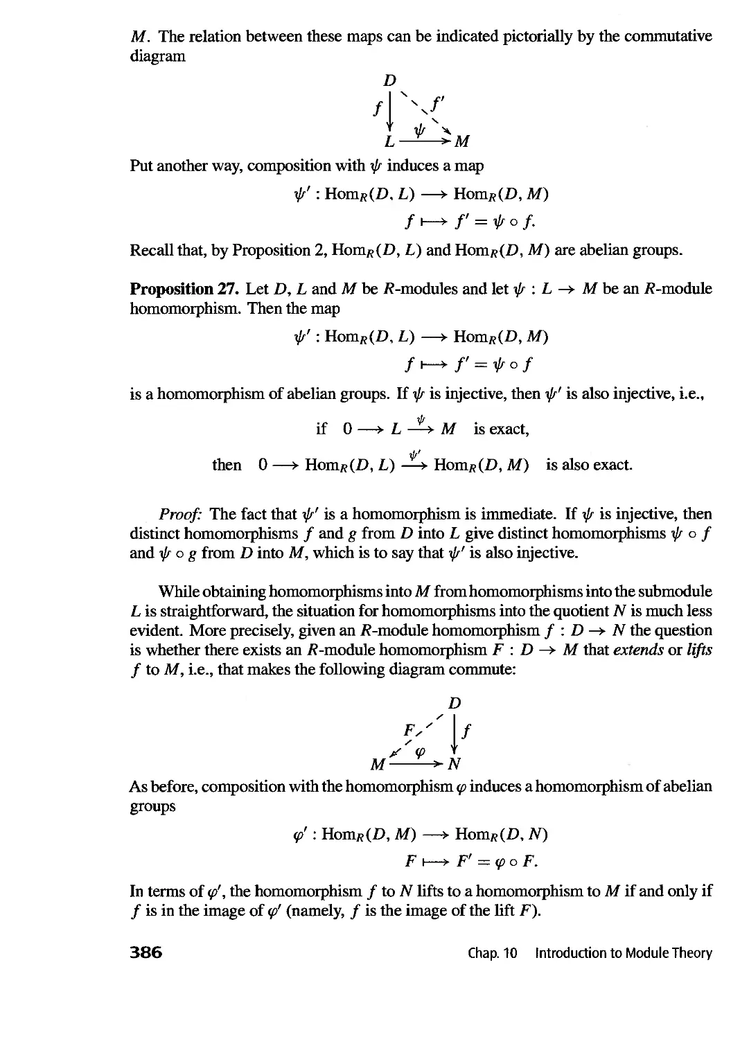
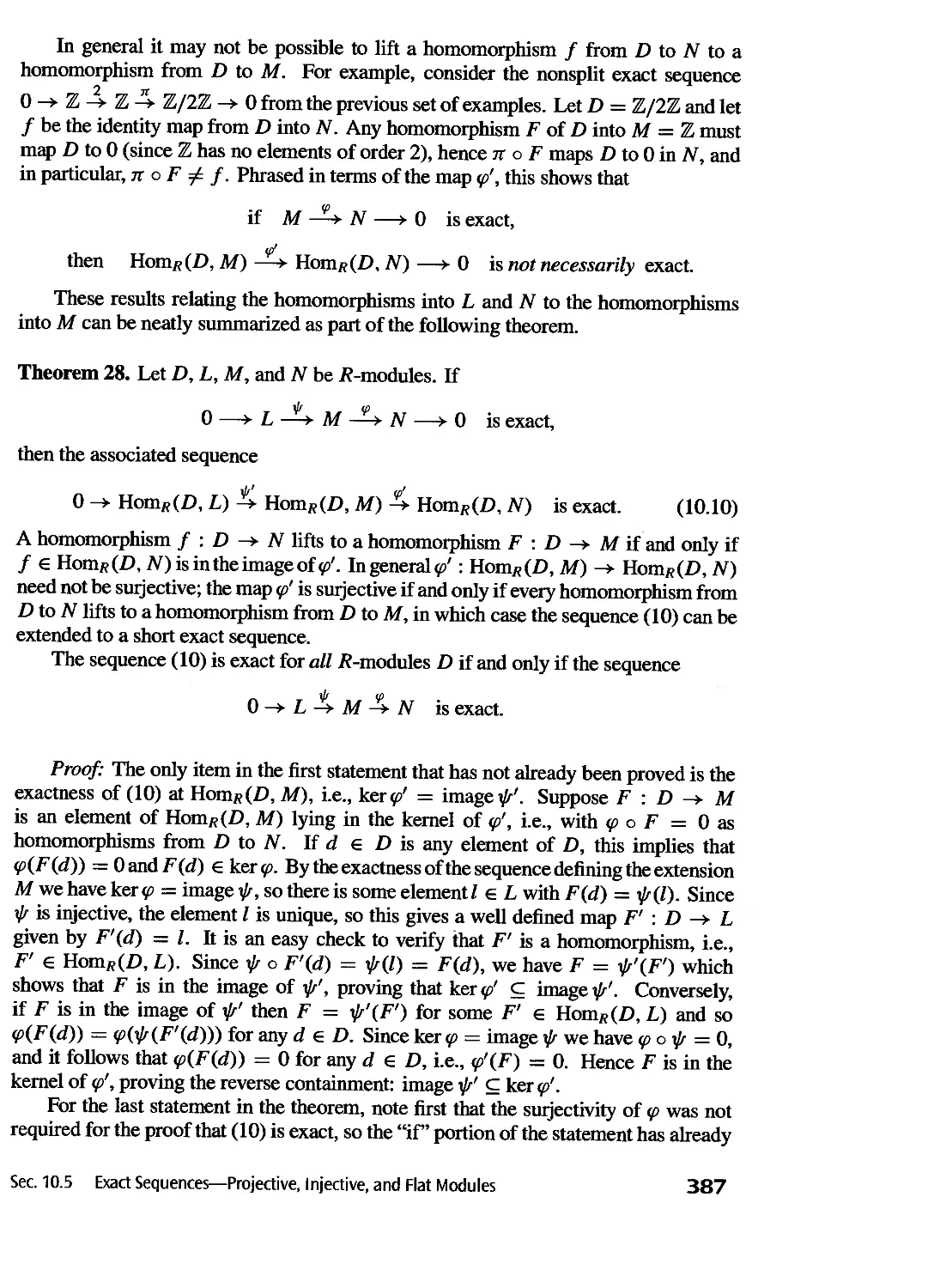


Text
.'
==:;:00
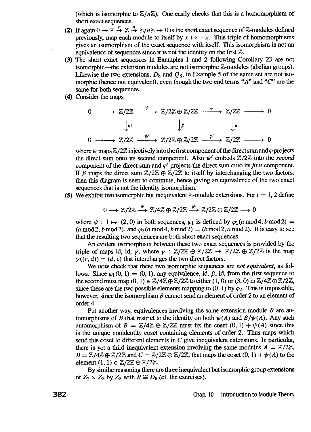
- '1:1'
_ '1:1'
II)
o
.....
...--
o
g BSTRACT
I
=== M
,
ALGEBRA
THIRD EDIT-ION
DAVID S. DUMMIT
RICHARD M. FOOTE
Dedicated to our families
especially
Janice, Evan, and Krysta
and
Zsuzsanna, Peter, Karoline, and Alexandra
f-I(A)
alb
(a, b)
IAI,lxl
Z,Z+
Q,Q+
R +
C,C x
ZjnZ
(ZjnZ) x
AxB
H G
Zn
D2n
Sn, Sri.
An
Qs
V4
IF'N
GLn(F), GL(V)
SLn(F)
A B
CG(A), NG(A)
Z(G)
G s
(A), (x)
G={...I...)
ker cp, im cp
N G
gH, Hg
IG: HI
Aut( G)
Sylp(G)
np
[x, y]
HXJK
!HI
R X
R[x], R[XI, ..., x n ]
RG,FG
Ch
fuv Ai, lim Ai
Zp,Qp
A(l)B
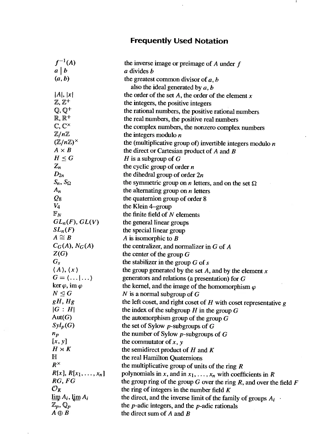
Frequently Used Notation
the inverse image or preimage of A under f
a divides b
the greatest common divisor of a, b
also the ideal generated by a, b
the order of the set A, the order of the element x
the integers, the positive integers
the rational numbers, the positive rational numbers
the real numbers, the positive real numbers
the complex numbers, the nonzero complex numbers
the integers modulo n
the (multiplicative group of) invertible integers modulo n
the direct or Cartesian product of A and B
H is a subgroup of G
the cyclic group of order n
the dihedral group of order 2n
the symmetric group on n letters, and on the set Q
the alternating group on n letters
the quaternion group of order 8
the Klein 4-group
the finite field of N elements
the general linear groups
the special linear group
A is isomorphic to B
the centralizer, and normalizer in G of A
the center of the group G
the stabilizer in the group G of s
the group generated by the set A, and by the element x
generators and relations (a presentation) for G
the kernel, and the image of the homomorphism cp
N is a normal subgroup of G
the left coset, and right coset of H with coset representative g
the index of the subgroup H in the group G
the automorphism group of the group G
the set of Sylow p-subgroups of G
the number of Sylow p-subgroups of G
the commutator of x, y
the semidirect product of H and K
the real Hamilton Quaternions
the multiplicative group of units of the ring R
polynomials in x, and in Xl, . . . ,X n with coefficients in R
the group ring of the group G over the ring R, and over the field F
the ring of integers in the number field K
the direct, and the inverse limit of the family of groups Ai
the p-adic integers, and the p-adic rationals
the direct sum of A and B
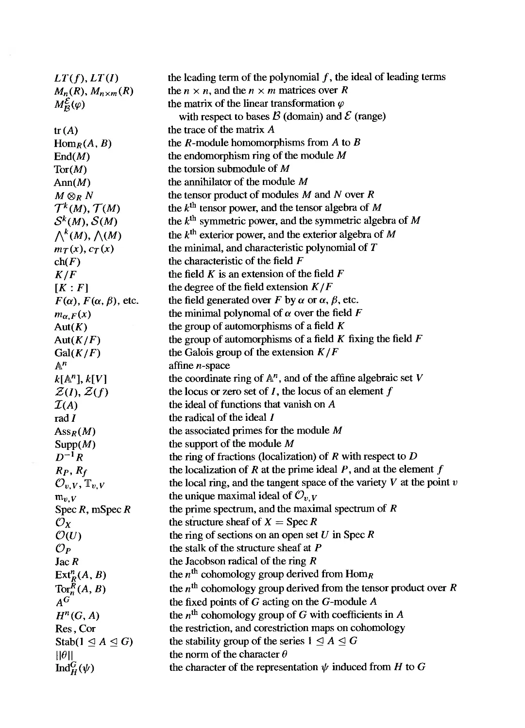
LT(f), LT(I)
Mn(R), Mnxm(R)
M (q;)
tr (A)
HomR(A, B)
End(M)
Tor(M)
Ann(M)
M0RN
Tk(M), T(M)
Sk(M), S(M)
f\k(M), f\(M)
mT(x), CT(X)
ch(F)
KIF
[K: F]
F(ex), F(ex, {J), etc.
ma,F(x)
Aut(K)
Aut(K / F)
Gal(K/F)
An
k[A n ], k[V]
Z(I), Z(f)
I(A)
radl
ASSR(M)
Supp(M)
D-IR
Rp,Rf
Ov,v, 'JI'v,v
mv,V
SpecR, mSpecR
Ox
O(U)
Op
JacR
Ext (A, B)
Tor:; (A, B)
A G
Hn(G, A)
Res, Cor
Stab(l A G)
11811
Ind (1/f)
the leading term of the polynomial f, the ideal of leading terms
the n x n, and the n x m matrices over R
the matrix of the linear transformation q;
with respect to bases 13 (domain) and £. (range)
the trace of the matrix A
the R-module homomorphisms from A to B
the endomorphism ring of the module M
the torsion submodule of M
the annihilator of the module M
the tensor product of modules M and N over R
the k th tensor power, and the tensor algebra of M
the k th symmetric power, and the symmetric algebra of M
the k th exterior power, and the exterior algebra of M
the minimal, and characteristic polynomial of T
the characteristic of the field F
the field K is an extension of the field F
the degree of the field extension KIF
the field generated over F by ex or ex, {J, etc.
the minimal polynomal of ex over the field F
the group of automorphisms of a field K
the group of automorphisms of a field K fixing the field F
the Galois group of the extension KIF
affine n-space
the coordinate ring of An, and of the affine algebraic set V
the locus or zero set of l, the locus of an element f
the ideal of functions that vanish on A
the radical of the ideall
the associated primes for the module M
the support of the module M
the ring of fractions (localization) of R with respect to D
the localization of R at the prime ideal P, and at the element f
the local ring, and the tangent space of the variety V at the point v
the unique maximal ideal of Ov, v
the prime spectrum, and the maximal spectrum of R
the structure sheaf of X = Spec R
the ring of sections on an open set U in Spec R
the stalk of the structure sheaf at P
the Jacobson radical of the ring R
the nth cohomology group derived from HomR
the nth cohomology group derived from the tensor product over R
the fixed points of G acting on the G-module A
the nth cohomology group of G with coefficients in A
the restriction, and corestriction maps on cohomology
the stability group of the series 1 A G
the norm of the character 8
the character of the representation 1/f induced from H to G
ABSTRACT ALGEBRA
Third Edition
David S. Dummit
University of Vermont
Richa rd M. Foote
University of Vermont
John Wiley & Sons, Inc.
ASSOCIATE PUBLISHER Laurie Rosatone
ASSISTANT EDITOR Jennifer Battista
FREELANCE DEVELOPMENTAL EDITOR Anne Scanlan-Rohrer
SENIOR MARKETING MANAGER Julie Z. Lindstrom
SENIOR PRODUCTION EDITOR Ken Santor
COVER DESIGNER Michael Jung
This book was typeset using the Y & Y TeX System with DVIWindo. The text was set in Times Roman
using MathTime from Y & Y, Inc. Titles were set in OceanSans. This book was printed by Malloy Inc.
and the cover was printed by Phoenix Color Corporation.
This book is printed on acid-free paper.
Copyright @ 2004 John Wiley and Sons, Inc. All rights reserved.
No part of this publication may be reproduced, stored in a retrieva1 system or transmitted in any form or by
any means, electronic, mechanical, photocopying, recording, scanning, or otherwise, except as pennitted
under Sections 107 or 108 of the 1976 United States Copyright Act, without either the prior written
permission of the Publisher, or authorization through payment of the appropriate per-copy fee to the
Copyright Clearance Center, Inc., 222 Rosewood Drive, Danvers, MA 01923, (508) 750-8400. fax (508) 750-
4470. Requests to the Publisher for permission should be addressed to the Permissions Department, John
Wiley & Sons, Inc.,lll River Street, Hoboken, NJ 07030. (201)748-6011, fax (201)748-6008. E-mail:
PERMREQ@WILEY.COM.
To order books or for customer service please calli-BOO-CALL WILEY (225-5945).
ISBN 0-471-43334-9
WIE 0-471-45234-3
Printed in the United States of America.
10987654321
Dedicated to our families
especially
Janice, Evan, and Krysta
and
Zsuzsanna, Peter, Karoline, and Alexandra
Preface xi
Contents
Preliminaries 1
0.1 Basics 1
0.2 Properties of the Integers 4
0.3 Z / n Z : The Integers Modulo n 8
Part 1- GROUP THEORY 13
Chapter 1 Introduction to Groups 16
1.1 Basic Axioms and Examples 16
1.2 Dihedral Groups 23
1.3 Symmetric Groups 29
1.4 Matrix Groups 34
1.5 The Quaternion Group 36
1.6 Homomorphisms and Isomorphisms 36
1.7 Group Actions 41
Chapter 2
2.1
2.2
2.3
2.4
2.5
Contents
Subgroups 46
Definition and Examples 46
Centralizers and Normalizers, Stabilizers and Kernels
49
Cyclic Groups and Cyclic Subgroups 54
Subgroups Generated by Subsets of a Group 61
The Lattice of Subgroups of a Group 66
v
Chapter 3
3.1
3.2
3.3
3.4
3.5
Chapter 4
4.1
4.2
Chapter 5
5.1
5.2
Chapter 6
6.1
6.2
6.3
Chapter 7
7.1
7.2
vi
Quotient Groups and Homomorphisms 73
Definitions and Examples 73
More on Cosets and Lagrange's Theorem 89
The Isomorphism Theorems 97
Composition Series and the Holder Program 101
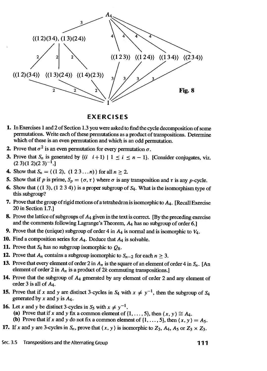
Transpositions and the Alternating Group 106
4.3
Group Actions 112
Group Actions and Permutation Representations 112
Groups Acting on Themselves by Left Multiplication-Cayley's
Theorem 118
Groups Acting on Themselves by Conjugation-The Class
Equation 122
Automorphisms 133
The Sylow Theorems 139
The Simplicity of An 149
4.4
4.5
4.6
5.3
5.4
5.5
Direct and Semidirect Products and Abelian Groups 152
Direct Products 152
The Fundamental Theorem of Finitely Generated Abelian
Groups 158
Table of Groups of Small Order 167
Recognizing Direct Products 169
Semidirect Products 175
Further Topics in Group Theory 188
p-groups, Nilpotent Groups, and Solvable Groups
Applications in Groups of Medium Order 201
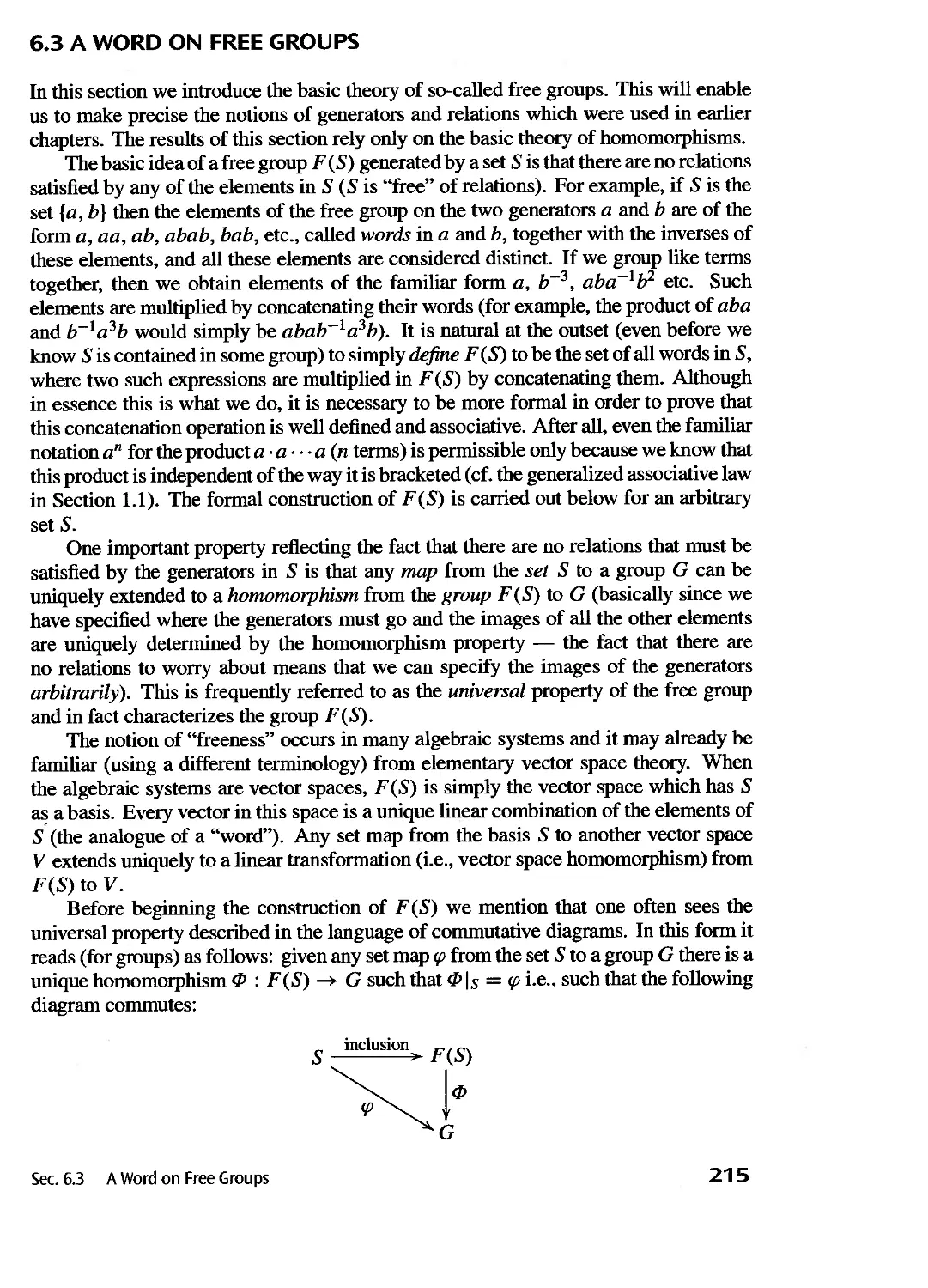
A Word on Free Groups 215
188
Part II - RING THEORY 222
7.3
7.4
7.5
7.6
Introduction to Rings 223
Basic Definitions and Examples 223
Examples: Polynomial Rings, Matrix Rings, and Group
Rings 233
Ring Homomorphisms an Quotient Rings 239
Properties of Ideals 251
Rings of Fractions 260
The Chinese Remainder Theorem 265
Contents
Chapter 8
8.1
8.2
8.3
Chapter 9
9.1
9.2
9.3
9.4
9.5
9.6
Chapter 10
10.1
10.2
10.3
10.4
10.5
Chapter 11
11.1
11.2
11.3
11.4
11.5
Chapter 12
12.1
12.2
12.3
Contents
Euclidean Domains. Principal Ideal Domains and
Unique Factorization Domains 270
Euclidean Domains 270
Principal Ideal Domains (P.I.D.s) 279
Unique Factorization Domains (U.F.D.s) 283
Polynomial Rings 295
Definitions and Basic Properties 295
Polynomial Rings over Fields I 299
Polynomial Rings that are Unique Factorization Domains
303
Irreducibility Criteria 307
Polynomial Rings over Fields II 313
polynomials in Several Variables over a Field and Grobner
Bases 315
Part III - MODULES AND VECTOR SPACES 336
Introduction to Module Theory 337
Basic Definitions and Examples 337
Quotient Modules and Module Homomorphisms 345
Generation of Modules, Direct Sums, and Free Modules
351
Tensor products of Modules 359
Exact Sequences-Projective, Injective, and Flat Modules
378
VectorSpaces 408
Definitions and Basic Theory 408
The Matrix of a Linear Transformation 415
Dual Vector Spaces 431
Determinants 435
Tensor Algebras, Symmetric and Exterior Algebras
Modules over Principal Ideal Domains
The Basic Theory 458
The Rational Canonical Form 472
The Jordan Canonical Form 491
456
441
vii
Chapter 13
J 13.1
13.2
13.3
13.4
13.5
13.6
Chapter 14
14.1
14.2
14.3
14.4
14.5
14.6
14.7
14.8
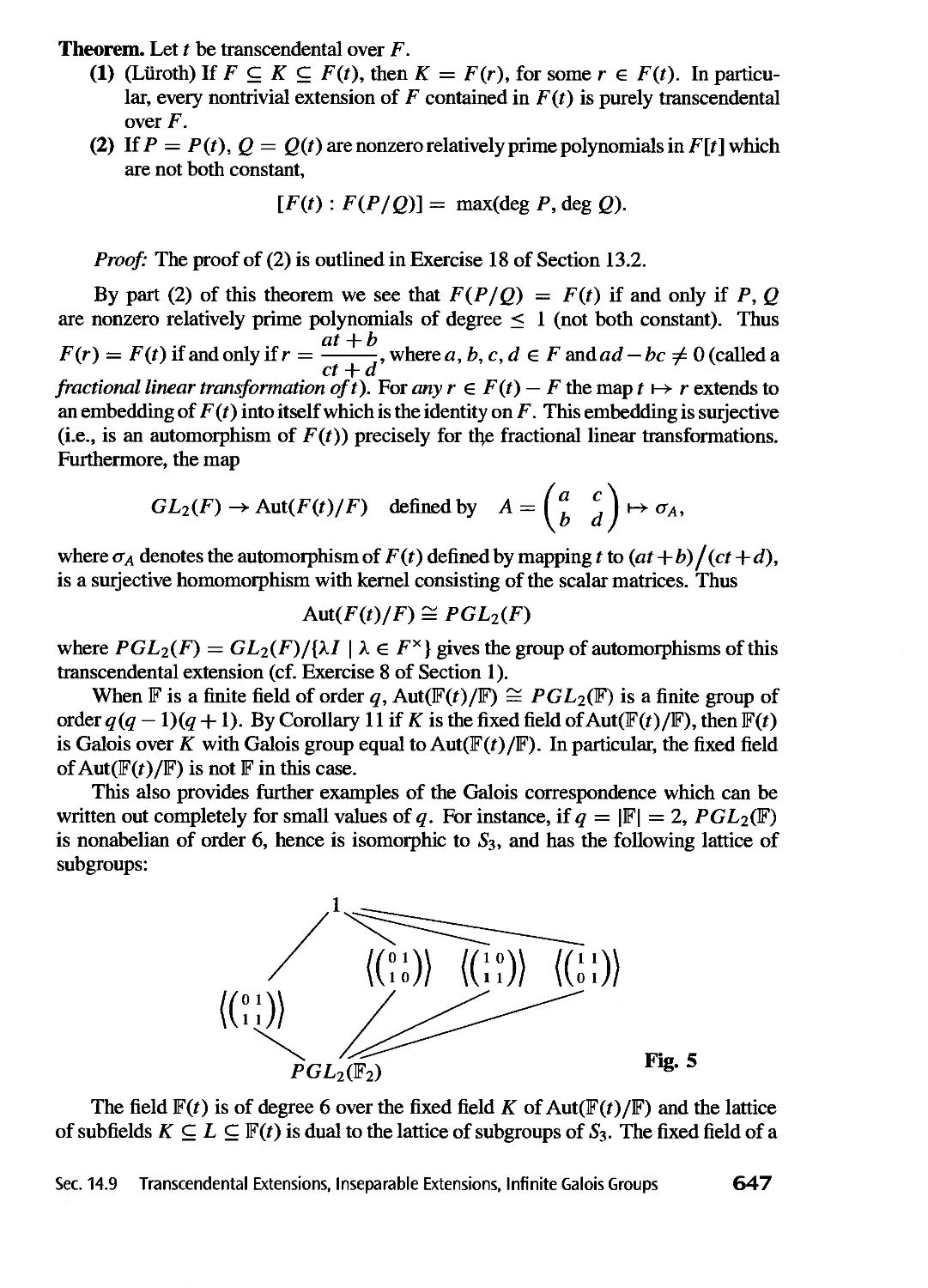
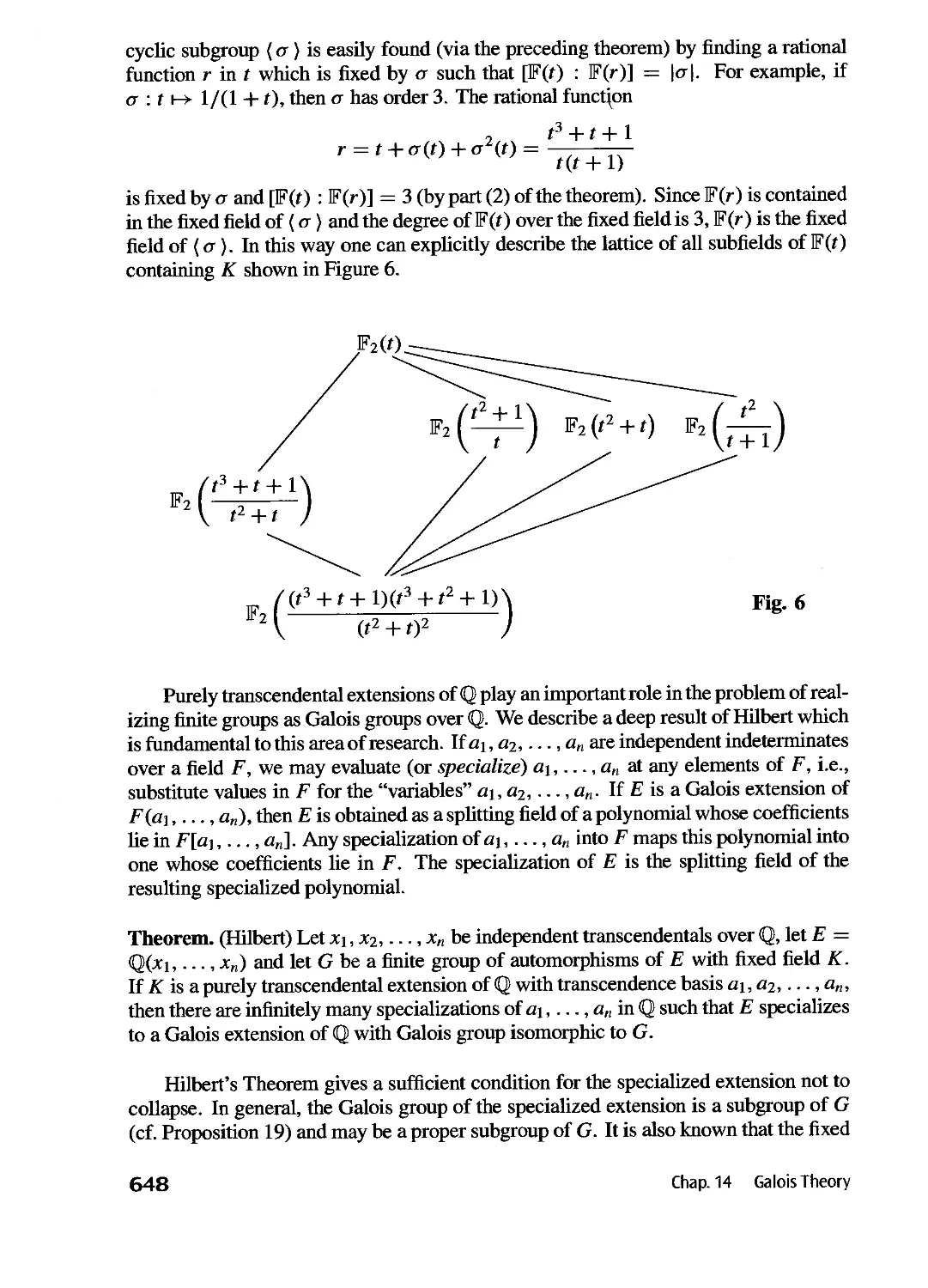
14.9
Part IV - FIELD THEORY AND GALOIS THEORY 509
Field Theory 510
Basic Theory of Field Extensions 510
Algebra ic Extensions 520
Classical Straightedge and Compass Constructions
Splitting Fields and Algebraic Closures 536
Separable and Inseparable Extensions 545
Cyclotomic Polynomials and Extensions 552
531
Galois Theory 558
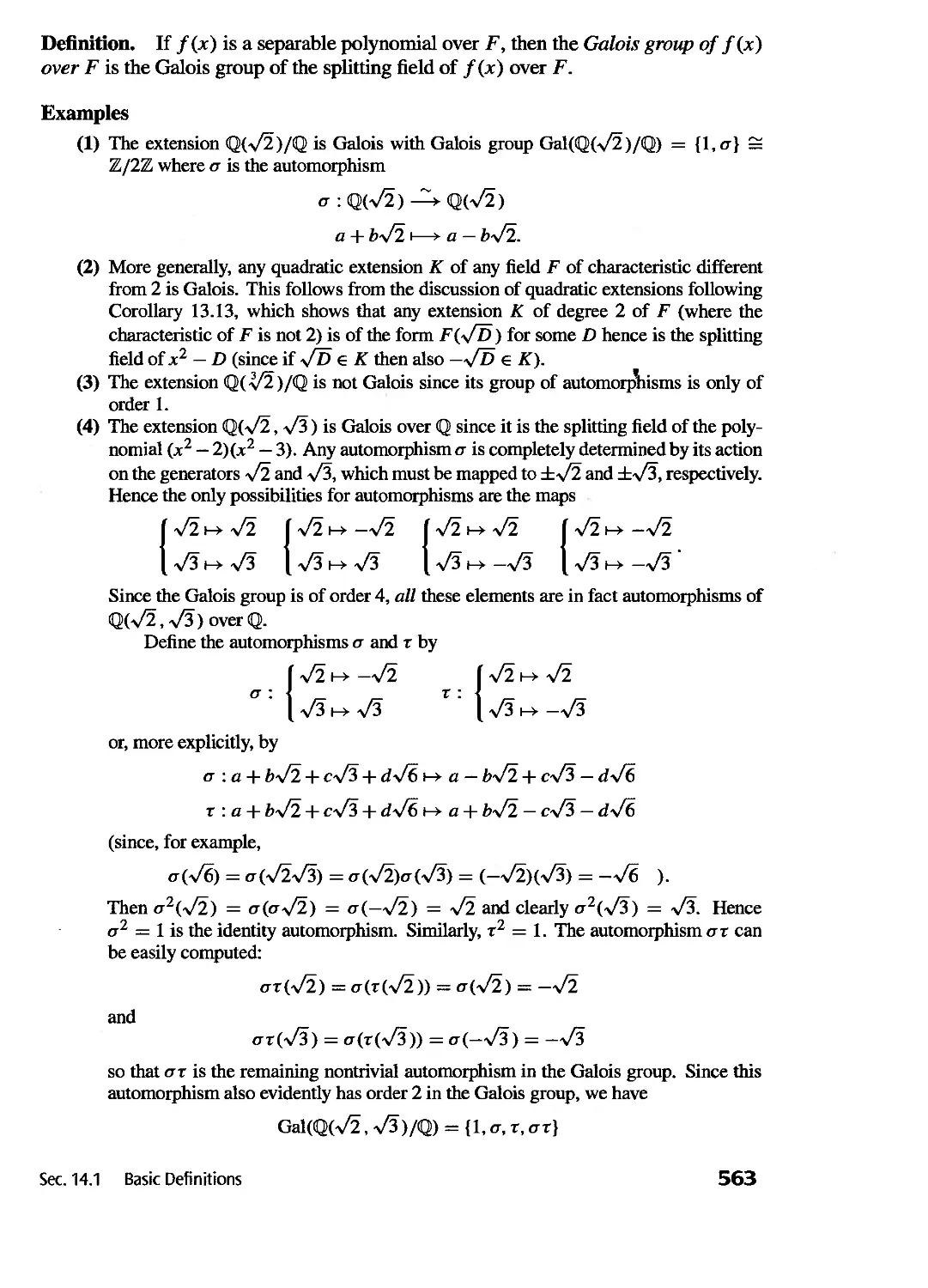
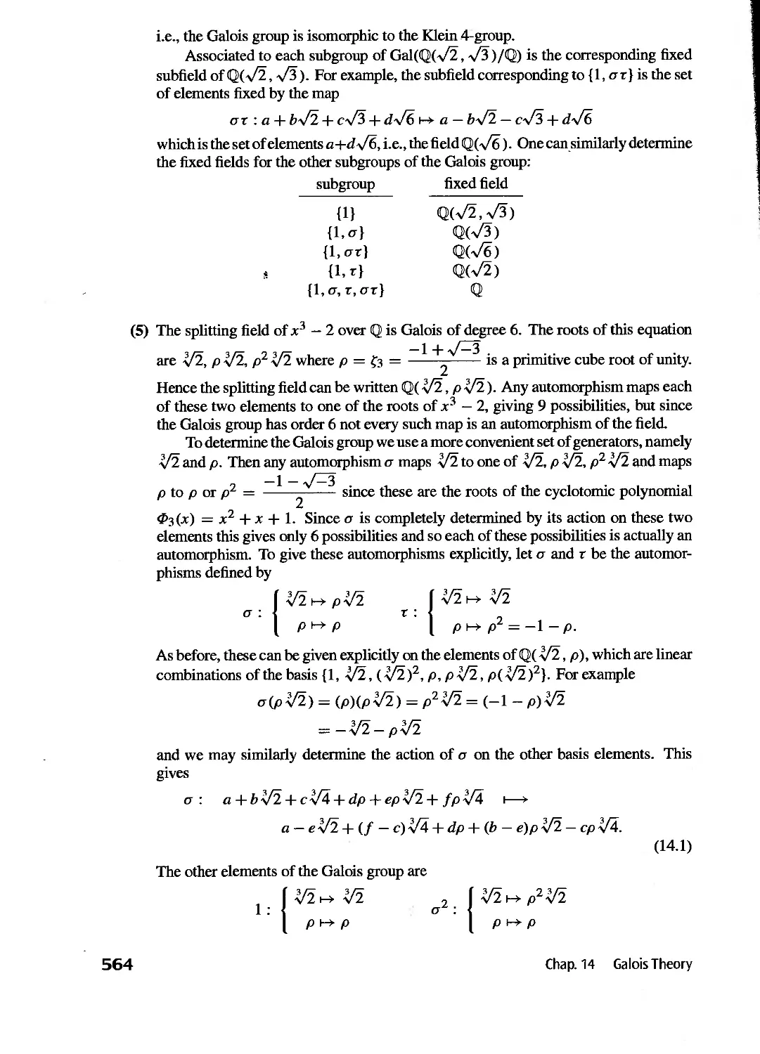
Basic Definitions 558
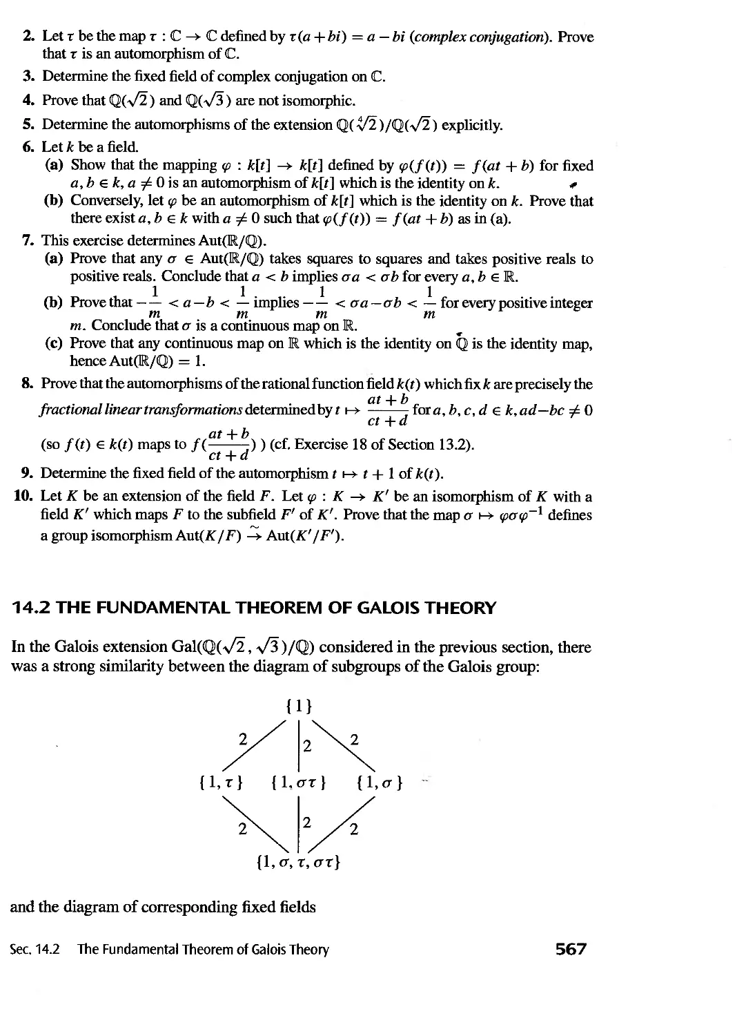
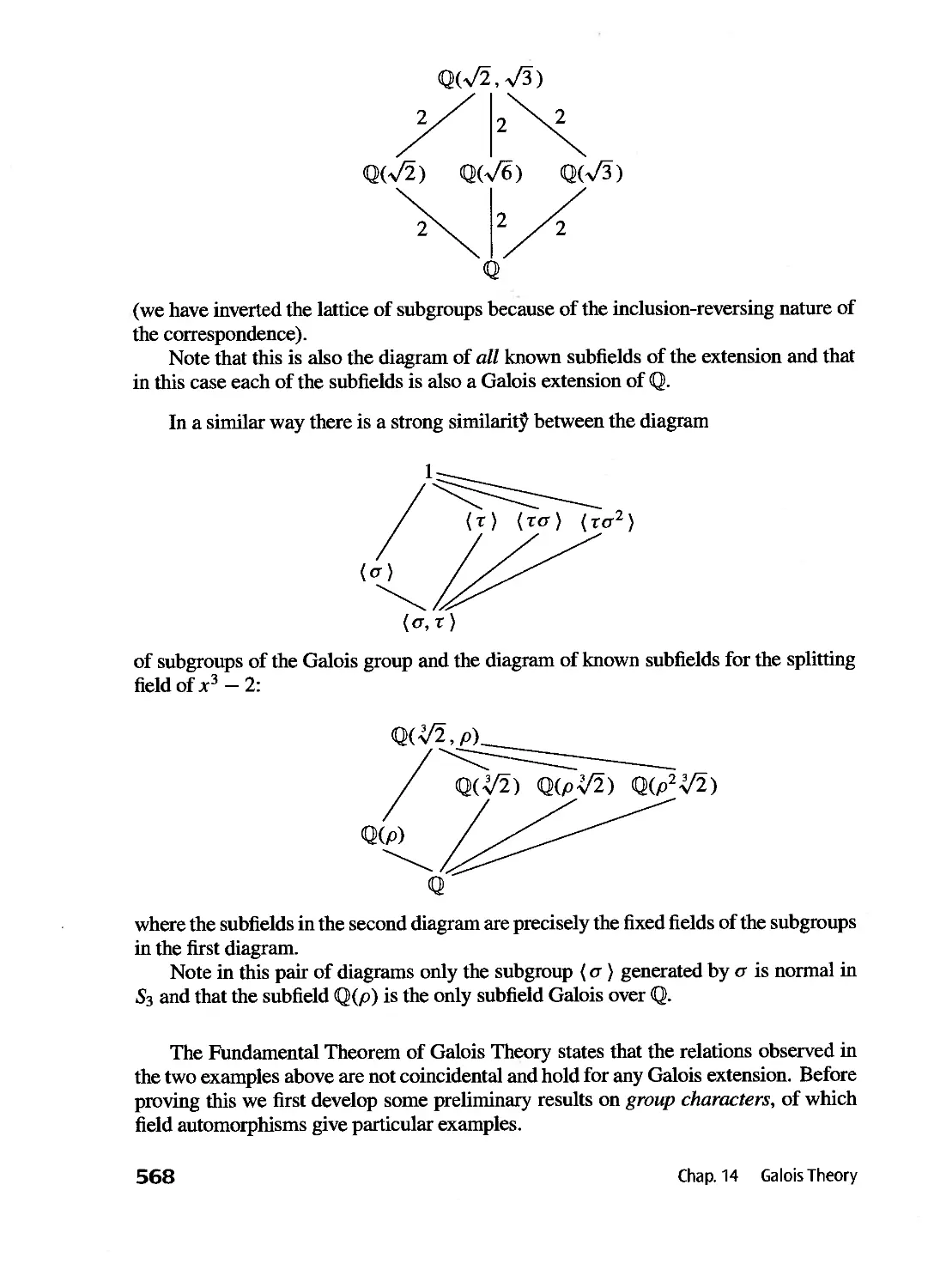
The Fundamental Theorem of Galois Theory 567
Finite Fields 585
Composite Extensions and Simple Extensions 591
Cyclotomic Extensions and Abelian Extensions over CQ
596
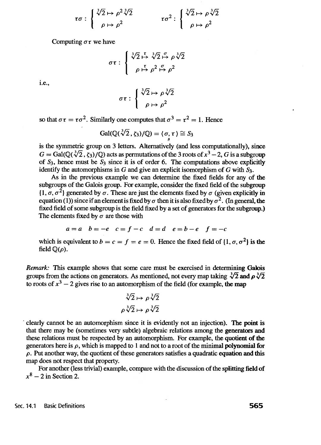
Galois Groups of Polynomials 606
Solvable and Radical Extensions: Insolvability ofthe Quintic
625
Computation of Galois Groups over CQ 640
Transcendental Extensions, Inseparable Extensions, Infinite
Galois Groups 645
Part V - AN INTRODUCTION TO COMMUTATIVE RINGS,
ALGEBRAIC GEOMETRY, AND
HOMOLOGICAL ALGEBRA 655
Chapter 15
15.1
15.2
15.3
15.4
15.5
Commutative Rings and Algebraic Geometry 656
Noetherian Rings and Affine Algebraic Sets 656
Radicals and Affine Varieties 673
Integral Extensions and Hilbert's Nullstellensatz 691
localization 706
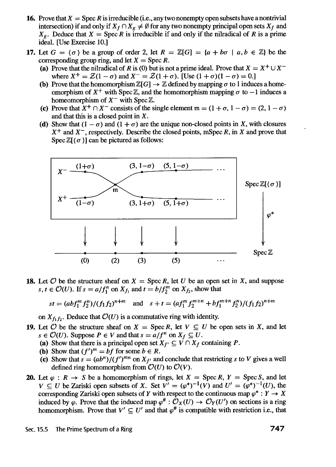
The Prime Spectrum of a Ring 731
Artinian Rings, Discrete Valuation Rings, and
Dedekind Domains 750
16.1 Artinian Rings 750
16.2 Discrete Valuation Rings 755
16.3 Dedekind Domains 764
Chapter 16
viii
Contents
Chapter 17 Introduction to Homological Algebra and
Group Cohomology 776
17.1 Introduction to Homological Algebra-Ext and Tor 777
17.2 The Cohomology of Groups 798
17.3 Crossed Homomorphisms and H 1 (G. A) 814
17.4 Group Extensions. Factor Sets and H 2 (G. A) 824
Chapter 18
18.1
18.2
18.3
Chapter 19
19.1
19.2
19.3
Part VI - INTRODUCTION TO THE REPRESENTATION
THEORY OF FINITE GROUPS 839
Representation Theory and Character Theory 840
Linear Actions and Modules over Group Rings 840
Wedderburn's Theorem and Some Consequences 854
Character Theory and the Orthogonality Relations 864
Examples and Applications of Character Theory
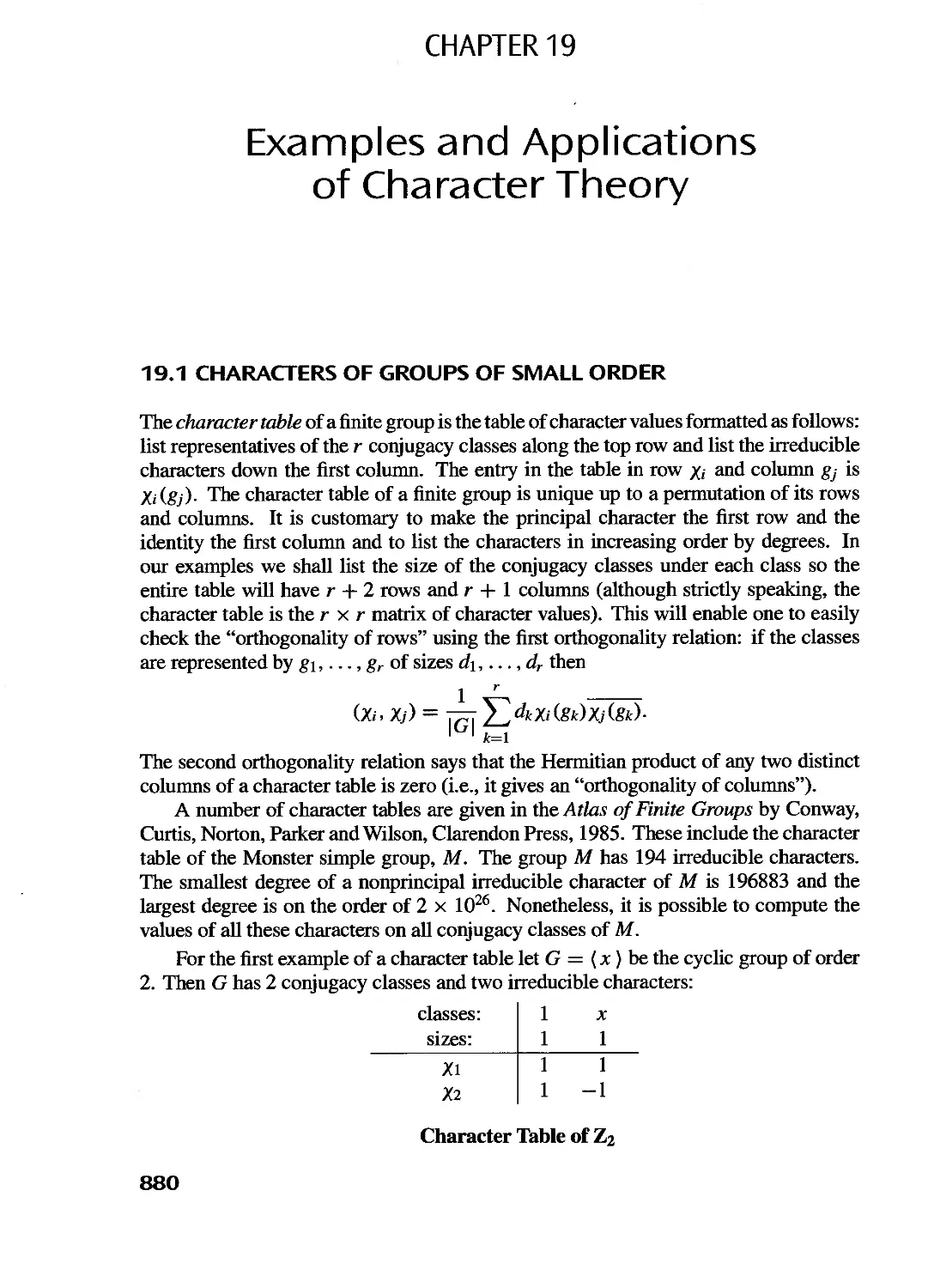
Characters of Groups of Small Order 880
Theorems of Burnside and Hall 886
Introduction to the Theory of Induced Characters
880
892
Appendix I: Cartesian Products and Zorn's Lemma 905
Appendix II: Category Theory 911
Index 919
Contents ix
Preface to the Third Edition
The principal change from the second edition is the addition of Grobner bases to this
edition. The basic theory is introduced in a new Section 9.6. Applications to solving
systems of polynomial equations (elimination theory) appear at the end of this section,
rounding it out as a self-contained foundation in the topic. Additional applications and
examples are then woven into the treatment of affine algebraic sets and k-algebra homo-
morphisms in Chapter 15. Although the theory in the latter chapter remains independent
of Grobner bases, the new applications, examples and computational techniques sig-
nificantly enhance the development, and we recommend that Section 9.6 be read either
as a segue to or in parallel with Chapter 15. A wealth of exercises involving Grobner
bases, both computational and theoretical in nature, have been added in Section 9.6
and Chapter 15. Preliminary exercises on Grobner bases can (and should, as an aid to
understanding the algorithms) be done by hand, but more extensive computations, and
in particular most of the use of Grobner bases in the exercises in Chapter 15, will likely
require computer assisted computation.
Other changes include a streamlining of the classification of simple groups of order
168 (Section 6.2), with the addition of a uniqueness proof via the projective plane of
order 2. Some other proofs or portions of the text have been revised slightly. A number
of new exercises have been added throughout the book, primarily at the ends of sections
in order to preserve as much as possible the numbering schemes of earlier editions.
In particular, exercises have been added on free modules over noncommutative rings
(10.3), on Krull dimension (15.3), and on flat modules (10.5 and 17.1).
As with previous editions, the text contains substantially more than can normally
be covered in a one year course. A basic introductory (one year) course should probably
include Part I up through Section 5.3, Part IT through Section 9.5, Sections 10.1, 10.2,
10.3,11.1,11.2 and Part IV. Chapter 12 should also be covered, either before or after
Part IV. Additional topics from Chapters 5, 6, 9, 10 and 11 may be interspersed in such
a course, or covered at the end as time permits.
Sections 10.4 and 10.5 are at a slightly higher level of difficulty than the initial
sections of Chapter 10, and can be deferred on a first reading for those following the text
sequentially. The latter section on properties of exact sequences, although quite long,
maintains coherence through a parallel treatment of three basic functors in respective
subsections.
Beyond the core material, the third edition provides significant flexibility for stu-
dents and instructors wishing to pursue a number of important areas of modem algebra,
xi
either in the fonn of independent study or courses. For example, well integrated one-
semester courses for students with some prior algebra background might include the
following: Section 9.6 and Chapters 15 and 16; or Chapters 10 and 17; or Chapters 5,
6 and Part VI. Each of these would also provide a solid background for a follow-up
course delving more deeply into one of many possible areas: algebraic number theory,
algebraic topology, algebraic geometry, representation theory, Lie groups, etc.
The choice of new material and the style for developing and integrating it into the
text are in consonance with a basic theme in the book: the power and beauty that accrues
from a rich interplay between different areas of mathematics. The emphasis throughout
has been to motivate the introduction and development of important algebraic concepts
using as many examples as possible. We have not attempted to be encyclopedic, but
have tried to touch on many of the central themes in elementary algebra in a manner
suggesting the very natural development of these ideas.
A number of important ideas and results appear in the exercises. This is not because
they are not significant, rather because they did not fit easily into the flow of the text
but were too important to leave out entirely. Sequences of exercises on one topic
are prefaced with some remarks and are structured so that they may be read without
actually doing the exercises. In some instances, new material is introduced first in
the exercises-()ften a few sections before it appears in the text-so that students may
obtain an easier introduction to it by doing these exercises (e.g., Lagrange's Theorem
appears in the exercises in Section 1.7 and in the text in Section 3.2). All the exercises
are within the scope of the text and hints are given [in brackets] where we felt they were
needed. Exercises we felt might be less straightforward are usually phrased so as to
provide the answer to the exercise; as well many exercises have been broken down into
a sequence of more routine exercises in order to make them more accessible.
We have also purposely minimized the functorial language in the text in order to
keep the presentation as elementary as possible. We have refrained from providing
specific references for additional reading when there are many fine choices readily
available. Also, while we have endeavored to include as many fundamental topics as
possible, we apologize if for reasons of space or personal taste we have neglected any
of the reader's particular favorites.
We are deeply grateful to and would like here to thank the many students and
colleagues around the world who, over more than 15 years, have offered valuable
comments, insights and encouragement-their continuing support and interest have
motivated our writing of this third edition.
David Dummit
Richard Foote
June, 2003
xii
Preface
Prel i m i na ries
Some results and notation that are used throughout the text are collected in this chapter
for convenience. Students may wish to review this chapter quickly at first and then read
each section more carefully again as the concepts appear in the course of the text.
0.1 BASICS
The basics of set theory: sets, n, u, E, etc. should be familiar to the reader. Our
notation for subsets of a given set A will be
B = {a E A I . .. (conditions on a) ...}.
The order or cardinality of a set A will be denoted by IAI. If A is a finite set the order
of A is simply the number of elements of A.
It is important to understand how to test whether a particular x E A lies in a subset
B of A (d. Exercises 1-4). The Cartesian product of two sets A and B is the collection
A x B = {(a, b) I a E A, bE B}, of ordered pairs of elements from A and B.
We shall use the following notation for some common sets of numbers:
(1) Z = to, ::1:1, ::1:2, ::1:3, . . . } denotes the integers (the Z is for the German word for
numbers: "Zahlen").
(2) <Q = {afb I a, bE Z, b =I O} denotes the rational numbers (or rationals).
(3) JR = {all decimal expansions ::I: dldz... dn.alaZa3"'} denotes the real numbers
(or reals).
(4) (C = {a + bi I a, b E JR, i 2 = -I} denotes the complex numbers.
(5) Z+, <Q+ and JR+ will denote the positive (nonzero) elements in Z, <Q and JR, respec-
tively.
We shall use the notation f : A -+ B or A B to denote a function f from A
to B and the value of f at a is denoted f(a) (i.e., we shall apply all our functions on
the left). We use the words function and map interchangeably. The set A is called the
domain of f and B is called the codomain of f. The notation f : a H- b or a H- b if f
is understood indicates that f(a) = b, i.e., the function is being specified on elements.
If the function f is not specified on elements it is important in general to check
that f is well defined, Le., is unambiguously determined. For example, if the set A
is the union of two subsets Al and Az then one can try to specify a function from A
1
to the set (0, I} by declaring that f is to map everything in Al to 0 and is to map
everything in Az to 1. This unambiguously defines f unless Al and Az have elements
in common (in which case it is not clear whether these elements should map to 0 or to
1). Checking that this f is well defined therefore amounts to checking that Al and Az
have no intersection.
The set
f(A) = (b E Bib = f(a), for some a E A}
is a subset of B, called the range or image of f (or the image of A under f). For each
subset C of B the set
f-I(C) = (a E A I f(a) E C}
consisting of the elements of A mapping into C under f is called the preimage or inverse
image of C under f. For each b E B, the preimage of {b} under f is called the fiber of
f over b. Note that f- l is not in general a function and that the fibers of f generally
contain many elements since there may be many elements of A mapping to the element
b.
If f : A -+ B and g : B -+ C, then the composite map g 0 f : A -+ C is defined
by
(g 0 f)(a) = g(f(a».
Let f: A -+ B.
(1) f is injective or is an injection if whenever al # az, then f(al) # f(az).
(2) f is surjective or is a surjection if for all b E B there is some a E A such that
f(a) = b, i.e., the image of f is all of B. Note that since a function always maps
onto its range (by definition) it is necessary to specify the codomain B in order for
the question of surjectivity to be meaningful.
(3) f is bijective or is a bijection if it is both injective and surjective. If such a bijection
f exists from A to B, we say A and B are in bijective correspondence.
(4) f has a left inverse if there is a function g : B -+ A such that g 0 f : A -+ A is
the identity map on A, i.e., (g 0 f)(a) = a, for all a E A.
(5) f has a right inverse if there is a function h : B -+ A such that f 0 h : B -+ B is
the identity map on B.
Proposition 1. Let f : A -+ B.
(1) The map f is injective if and only if f has a left inverse.
(2) The map f is surjective if and only if f has a right inverse.
(3) The map f is a bijection if and only if there exists g : B -+ A such that fog
is the identity map on B and g 0 f is the identity map on A.
(4) If A and B are finite sets with the same number of elements (i.e., IAI = IBI),
then f : A -+ B is bijective if and only if f is injective if and only if f is
surjective.
Proof: Exercise.
In the situation of part (3) of the proposition above the map g is necessarily unique
and we shall say g is the 2-sided inverse (or simply the inverse) of f.
2
Preliminaries
A permutation of a set A is simply a bijection from A to itself.
If A £; Band f : B --+ C, we denote the restriction of f to A by fiA. When the
domain we are considering is understood we shall occasionally denote f IA again simply
as f even though these are fonnally different functions (their domains are different).
If A £; Band g : A --+ C and there is a function f : B --+ C such that flA = g,
we shall say f is an extension of g to B (such a map f need not exist nor be unique).
Let A be a nonempty set.
(1) AbinaryrelationonasetA isasubsetRofAxA and we write a 'V bif(a, b) E R.
(2) The relation 'V on A is said to be:
(a) reflexive if a 'V a, for all a E A,
(b) symmetric if a 'V b implies b rv a for all a, bE A,
(c) transitive if a rv b and b rv c implies a rv C for all a, b, c E A.
A relation is an equivalence relation if it is reflexive, symmetric and transitive.
(3) If rv defines an equivalence relation on A, then the equivalence class of a E A is
defined to be {x E A I x 'Va}. Elements of the equivalence class of a are said
to be equivalent to a. If C is an equivalence class, any element of C is called a
representative of the class C.
(4) A partition of A is any collection {Ai liE I} of non empty subsets of A (I some
indexing set) such that
(a) A = UieIA i , and
(b) Ai n Aj = 0, for all i, j E I with i =I j
Le., A is the disjoint union of the sets in the partition.
The notions of an equivalence relation on A and a partition of A are the same:
Proposition 2. Let A be a nonempty set.
(1) If rv defines an equivalence relation on A then the set of equivalence classes of
rv fonn a partition of A.
(2) If {Ai liE I} is a partition of A then there is an equivalence relation on A
whose equivalence classes are precisely the sets Ai, i E I.
Proof: Omitted.
Finally, we shall assume the reader is familiar with proofs by induction.
EXERCISES
In Exercises 1 to 4 let A be the set of 2 x 2 matrices with real number entries. Recall that
matrix multiplication is defined by
( : : ) ( ;) = (:; : :: :: )
Let
M= ( D
Sect. 0.1 Basics
3
and let
13 = {X E A I MX = XM}.
1. Determine which of the following elements of A lie in 13:
( U' C U' ( ), C ), ( ), ( ).
2. Prove that if P, Q E 13, then P+ Q E 13 (where + denotes the usual sum of two matrices).
3. Prove that if P, Q E 13, then p. Q E 13 (where . denotes the usual product of two matrices).
4. Find conditions on p, q, r, s which determine precisely when ( ) E 13.
5. Determine whether the following functions 1 are well defined:
(a) 1 : Q -+- Z defined by I(ajb) = a.
(b) 1 : Q -+- Q defined by I(ajb) = a Z jb z .
6. Determine whether the function 1 : + -+- Z defined by mapping a real number r to the
first digit to the right of the decimal point in a decimal expansion of r is well defined.
7. Let 1 : A -+- B be a surjective map of sets. Prove that the relation
a ....., b if and only if I(a) = I(b)
is an equivalence relation whose equivalence classes are the fibers of I.
0.2 PROPERTIES OF THE INTEGERS
The following properties of the integers IE (many familiar from elementary arithmetic)
will be proved in a more general context in the ring theory of Chapter 8, but it will
be necessary to use them in Part I (of course, none of the ring theory proofs of these
properties will rely on the group theory).
(1) (Well Ordering of IE) If A is any nonempty subset of IE+, there is some element
mEA such that m ::: a, for all a E A (m is called a minimal element of A).
(2) If a, b E IE with a #- 0, we say a divides b if there is an element c E IE such that
b = ac. In this case we write a I b; if a does not divide b we write a f b.
(3) If a, bE&;; - to}, there is a unique positive integer d, called the greatest common
divisor of a and b (or g.c.d. of a and b), satisfying:
(a) d I a and d I b (so d is a common divisor of a and b), and
(b) if e I a and e I b, then e I d (so d is the greatest such divisor).
The g.c.d. of a and b will be denoted by (a, b). If (a, b) = 1, we say that a and b
are relatively prime.
(4) If a, b E IE - to}, there is a unique positive integer 1, called the least common
multiple of a and b (or l.c.m. of a and b), satisfying:
(a) a 11 and b 11 (so 1 is a common multiple of a and b), and
(b) if a I m and b I m, then 11 m (so 1 is the least such multiple).
The connection between the greatest common divisor d and the least common
multiple 1 of two integers a and b is given by dl = ab.
(5) The Division Algorithm: if a, b E IE - to}, then there exist unique q, r E IE such
that
a = qb + r and 0::: r < Ibl,
4
Preliminaries
where q is the quotient and r the remainder. This is the usual "long division"
familiar from elementary arithmetic.
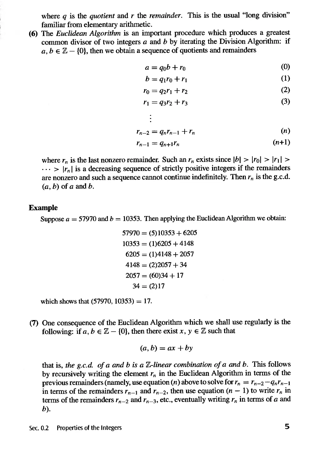
(6) The Euclidean Algorithm is an important procedure which produces a greatest
common divisor of two integers a and b by iterating the Division Algorithm: if
a, bE Z - {OJ, then we obtain a sequence of quotients and remainders
a = qob + ro
b = qlro + rl
ro = qZrl + rz
rl = q3 r Z + r3
(0)
(1)
(2)
(3)
rn-z = qnrn-l + r n
rn-l = qn+lrn
(n)
(n+l)
where r n is the last nonzero remainder. Such an r n exists since Ibl > Irol > Irll >
. .. > Ir n I is a decreasing sequence of strictly positive integers if the remainders
are nonzero and such a sequence cannot continue indefinitely. Then r n is the g.c.d.
(a, b) of a and b.
Example
Suppose a = 57970 and b = 10353. Then applying the Euclidean Algorithm we obtain:
57970 = (5)10353 + 6205
10353 = (1)6205 + 4148
6205 = (1)4148 + 2057
4148 = (2)2057 + 34
2057 = (60)34 + 17
34 = (2)17
which shows that (57970,10353) = 17.
(7) One consequence of the Euclidean Algorithm which we shall use regularly is the
following: if a, b E Z - {OJ, then there exist x, y E Z such that
(a, b) = ax + by
that is, the g.c.d. of a and b is a Z-linear combination of a and b. This follows
by recursively writing the element r n in the Euclidean Algorithm in terms of the
previous remainders (namely, use equation (n) above to solve for r n = r n-Z -qn r n-l
in tenns of the remainders rn-l and rn-z, then use equation (n - 1) to write r n in
terms of the remainders r n -2 and r n -3, etc., eventually writing r n in tenns of a and
b).
See. 0.2 Properties of the Integers
5
Example
Suppose a = 57970 and b = 10353, whose greatest common divisor we computed above to
be 17. From the fifth equation (the next to last equation) in the Euclidean Algorithm applied
to these two integers we solve for their greatest common divisor: 17 = 2057 - (60)34.
The fourth equation then shows that 34 = 4148 - (2)2057, so substituting this expression
for the previous remainder 34 gives the equation 17 = 2057 - (60)[4148 - (2)2057], i.e.,
17 = (121)2057 - (60)4148. Solving the third equation for 2057 and substituting gives
17 = (121)[6205 - (1)4148] - (60)4148 = (121)6205 - (181)4148. Using the second
equation to solve for 4148 and then the first equation to solve for 6205 we finally obtain
17 = (302)57970 - (1691)10353
as can easily be checked directly. Hence the equation ax + by = (a, b) for the greatest
common divisor of a and b in this example has the solution x = 302 and y = -1691. Note
that it is relatively unlikely that this relation would have been found simply by guessing.
The integers x and y in (7) above are not unique. In the example with a = 57970
and b = 10353 we determined one solution to be x = 302 and y = -1691, for
instance, and it is relatively simple to check that x = - 307 and y = 1719 also
satisfy 57970x + 10353 y = 17. The general solution for x and y is known (cf. the
exercises below and in Chapter 8).
(8) An element P of Z+ is called a prime if P > 1 and the only positive divisors of P are
1 and P (initially, the word prime will refer only to positive integers). An integer
n > 1 which is not prime is called composite. For example, 2,3,5,7,11,13,17,19,...
are primes and 4,6,8,9,10,12,14,15,16,18,... are composite.
An important property of primes (which in fact can be used to define the primes
(cf. Exercise 3» is the following: if p is a prime and P I ab, for some a, b E Z,
then either p I a or p lb.
(9) The Fundamental Theorem of Arithmetic says: if nEZ, n > 1, then n can
be factored uniquely into the product of primes, i.e., there are distinct primes
PI, P2, . . . , Ps and positive integers aI, a2, . . . , as such that
n = pr l p;2 . . . P s .
This factorization is unique in the sense that if qt, q2, . . . , qt are any distinct primes
and fh, fh, . . . , f3t positive integers such that
/31 /32 /3,
n = qt q2 ... qt ,
then s = t and if we arrange the two sets of primes in increasing order, then qi = Pi
and ai = f3i, 1 i s. For example, n = 1852423848 = 2 3 3 2 11 2 19 3 31 and this
decomposition into the product of primes is unique.
Suppose the positive integers a and b are expressed as products of prime powers:
_ a] a2 as b /31 f32 /3s
a - PI P2 ... Ps ' = Pt P2 ... Ps
where Pt, P2, ..., Ps are distinct and the exponents are :::: O(weallowtheexponents
to be 0 here so that the products are taken over the same set of primes - the exponent
will be 0 if that prime is not actually a divisor). Then the greatest common divisor
of a and b is
( b) - min(alo/31) min(a2,/3z) min(a,,/3s)
a, - Pt P2 ... Ps
6
Preliminaries
(and the least common multiple is obtained by instead taking the maximum of the
(Xi and f3i instead of the minimum).
Example
In the example above, a = 57970 and b = 10353 can befactored as a = 2 . 5 . 11 . 17 . 31
and b = 3.7. 17.29, from which we can immediately conclude that their greatest common
divisor is 17. Note, however, that for large integers it is extremely difficult to determine
their prime factorizations (several common codes in current use are based on this difficulty,
in fact), so that this is not an effective method to determine greatest common divisors in
general. The Euclidean Algorithm will produce greatest common divisors quite rapidly
without the need for the prime factorization of a and b.
(10) The Euler rp-function is defined as follows: for n E Z+ let rp(n) be the number of
positive integers a'::: n with a relatively prime to n, i.e., (a, n) = 1. For example,
rp(12) = 4 since 1, 5, 7 and 11 are the only positive integers less than or equal
to 12 which have no factors in common with 12. Similarly, rp(1) = 1, rp(2) = 1,
rp(3) = 2, rp(4) = 2, rp(5) = 4, rp(6) = 2, etc. For primes p, rp(p) = p - 1, and,
more generally, for all a 2:: 1 we have the formula
rp(pa) = pO _ pa-l = pa-l(p _ 1).
The function rp is multiplicative in the sense that
rp(ab) = rp(a)rp(b)
if (a, b) = 1
(note that it is important here that a and b be relatively prime). Together with the for-
mula above this gives a general formula for the values of rp : if n = p 1 p 2 . . . p s ,
then
rp(n) = rp(p l)rp(p 2)... rp(p s)
- al-l ( 1) a2-1 ( 1) as-l ( I )
- PI PI - Pz pz - ... Ps Ps - .
For example, rp(12) = rp(2 z )rp(3) = 2 1 (2 - 1)3°(3 - 1) = 4. The reader should
note that we shall use the letter rp for many different functions throughout the text
so when we want this letter to denote Euler's function we shall be careful to indicate
this explicitly.
EXERCISES
1. For each of the following pairs of integers a and b, determine their greatest common
divisor, their least common multiple, and write their greatest common divisor in the form
ax + by for some integers x and y.
(a) a = 20, b = 13.
(b) a = 69, b = 372.
(c) a = 792, b = 275.
(d) a = 11391, b = 5673.
(e) a = 1761, b = 1567.
(1) a = 507885, b = 60808.
2. Prove that if the integer k divides the integers a and b then k divides as + bt for every pair
of integers s and t.
See. 0.2 Properties of the Integers
7
3. Prove that if n is composite then there are integers a and b such that n divides ab but n
does not divide either a or b.
4. Let a, b and N be fixed integers with a and b nonzero and let d = (a, b) be the greatest
common divisor of a and b. Suppose xo and YO are particular solutions to ax + by = N
(i.e., axo + byo = N). Prove for any integer t that the integers
b a
x = xo + -t and y = yo - -t
d d
are also solutions to ax + by = N (this is in fact the general solution).
S. Determine the value cp(n) for each integer n 30 where cp denotes the Euler cp-function.
6. Prove the Well Ordering Property of Z by induction and prove the minimal element is
unique.
7. If p is a prime prove that there do not exist nonzero integers a and b such that a 2 = pb 2
(i.e., .[P is not a rational number).
8. Let p be a prime, n E Z+. Find a formula for the largest power of p which divides
n! = n(n - l)(n - 2) . . .2 . I (it involves the greatest integer function).
9. Write a computer program to determine the greatest common divisor (a, b) of two integers
a and b and to express (a, b) in the form ax + by for some integers x and y.
10. Prove for any given positive integer N there exist only finitely many integers n with
cp(n) = N where cp denotes Euler's cp-function. Conclude in particular that cp(n) tends to
infinity as n tends to infinity.
11. Prove that if d divides n then cp(d) divides cp(n) where cp denotes Euler's cp-function.
0.3 ZJn Z: THE INTEGERS MODULO n
Let n be a fixed positive integer. Define a relation on Z by
a "'-' b if and only if n I (b - a).
Clearly a '" a, and a "'-' b implies b "'-' a for any integers a and b, so this
relation is trivially reflexive and symmetric. If a "'-' b and b "'-' c then n divides a - b
and n divides b - c so n also divides the sum of these two integers, i.e., n divides
(a - b) + (b - c) = a - c, so a "'-' c and the relation is transitive. Hence this is an
equivalence relation. Write a == b (mod n) (read: a is congruent to b mod n) if a "'-' b.
For any k E Z we shall denote the equivalence class of a by ii - this is called the
congruence class or residue class of a mod n and consists of the integers which differ
from a by an integral multiple of n, i.e.,
a = {a + kn I k E Z}
= {a, a :I:: n, a :I:: 2n, a :I:: 3n, . . . }.
There are precisely n distinct equivalence classes mod n, namely
0, 1, 2, . . . , n - 1
determined by the possible remainders after division by n and these residue classes
partition the integers Z. The set of equivalence classes under this equivalence relation
8
Preliminaries
will be denoted by ZjnZ and called the integers modulo n (or the integers mod n).
The motivation for this notation will become clearer when we discuss quotient groups
and quotient rings. Note that for different n's the equivalence relation and equivalence
classes are different so we shall always be careful to fix n first before using the bar
notation. The process of finding the equivalence class mod n of some integer a is often
referred to as reducing a mod n. This terminology also frequently refers to finding the
smallest nonnegative integer congruent to a mod n (the least residue of a mod n).
We can define an addition and a multiplication for the elements of ZjnZ, defining
modular arithmetic as follows: for a, bE ZjnZ, define their sum and product by
a+b= a+b
and
a . b = ab.
What this means is the following: given any two elements a and b in Zj nZ, to compute
their sum (respectively, their product) take any representative integer a in the class
a and any representative integer b in the class b and add (respectively, multiply) the
integers a and b as usual in Z and then take the equivalence class containing the result.
The following Theorem 3 asserts that this is well defined, i.e., does not depend on the
choice of representatives taken for the elements a and b of Zj nZ.
Example
Suppose n = 12 and consider ZjI2Z, which consists of the twelve residue classes
0, L 2, .. . , IT
determined by the twelve p ssible remainders of an integer after division by 12. The
elements in the residue class 5, for example, are the integers which leave a remainder of 5
when divided by 12 (the integers congruent to 5 mod 12). Any integer congruent to 5 mod
12 (such as 5, 17, 29, ... or -7, -19, ... ) will serve as a representative for the residue class
5. Note that Zj12Z consists of the twelve elements above (and each of these elements of
Zj12Z consists of an infinite number of usual integers).
Suppose now that a = 5 and b = 8. The most obvious representative for a is the integer
5 and similarly 8 is the most obvious representative for b. Using these representatives for
the residue classes we obtain 5 + 8 = 13 = I since 13 and IHe in the same class modulo
n = 12. Had we instead taken the representative 17, say, for a (note that 5 and 17 do lie in
the same residue cla ss modulo 12) and the representative -28, say, for b, we would obtain
5 + 8 = (17 - 28) = -11 = I and as we mentioned the result does not depend on the
choice of representatives chosen. The product of these two classes is a.b = 5.8 = 40 = 4,
also independent of the representatives chosen.
Theorem 3. The operations of addition and multiplication on ZjnZ defined above
are both well defined, that is, they do not depend on the choices of representatives for
the classes i nvolved. M ore preci sely, if aI, az E Z and b l , bz E Z with al = b l and
az = bz, then al + az = b l + bz and alaZ = blbz , i.e., if
al == b l (mod n) and az == b2 (mod n)
then
al + az == b l + b2 (mod n) and alaZ == blbz (mod n).
See. 0.3 Z/nZ: The Integers Modulon
9
Proof: Suppose al == b l (mod n), i.e., al - bl is divisible by n. Then al = bl + sn
for some integer s. Similarly, a2 == b2 (mod n) means a2 = b2 + tn for some integer t.
Thenal +a2 = (b l +b 2 )+(s+t)n sothatal +a2 == b l +b2 (mod n), which shows that
the sum of the residue classes is independent of the representatives chosen. Similarly,
ala2 = (bl+sn)(bz+tn) = blb2+(blt+b2s+stn)nshowsthatala2 == b l b 2 (mod n)
and so the product of the residue classes is also independent of the representatives
chosen, completing the proof.
We shall see later that the process of adding equivalence classes by adding their
representatives is a special case of a more general construction (the construction of
a quotient). This notion of adding equivalence classes is already a familiar one in
the context of adding rational numbers: each rational number a/b is really a class of
expressions: a/b = 2a/2b = -3a/ - 3b etc. and we often change representatives
(for instance, take common denominators) in order to add two fractions (for example
1/2 + 1/3 is computed by taking instead the equivalent representatives 3/6 for 1/2
and 2/6 for 1/3 to obtain 1/2 + 1/3 = 3/6 + 2/6 = 5/6). The notion of modular
arithmetic is also familiar: to find the hour of day after adding or subtracting some
number of hours we reduce mod 12 and find the least residue.
It is important to be able to think of the equivalence classes of some equivalence
relation as elements which can be manipulated (as we do, for example, with fractions)
rather than as sets. Consistent with this attitude, we shall frequently denote the elements
of 7/./ n7/. simply by to, 1, . . . , n - I} where addition and multiplication are reduced mod
n. It is important to remember, however, that the elements of 7/./ n7/. are not integers, but
rather collections of usual integers, and the arithmetic is quite different. For example,
5 + 8 is not 1 in the integers 7/. as it was in the example of 7/./I27/. above.
The fact that one Can define arithmetic in 7/./n7/. has many important applications
in elementary number theory. As one simple example we compute the last two digits in
the number 2 1000 . First observe that the last two digits give the remainder of 2 1000 after
we divide by 100 so we are interested in the residue class mod 100 containing 2 1000 .
We compute 2 10 = 1024 == 24 (mod 100), so then 2 20 = (210)2 == 24 2 = 576 == 76
(mod 100). Then 2 40 = (220)2 == 76 2 = 5776 == 76 (mod 100). Similarly 2 80 ==
2 160 == 2 320 == 2 640 == 76 (mod 100). Finally, 2 1000 = 26402320240 == 76.76.76 == 76
(mod 100) so the final two digits are 76.
An important subset of 7/./ n7/. consists of the collection of residue classes which
have a multiplicative inverse in 7/./ n7/.:
(7/./n7/.)X = {ii E 7/./n7/. I there exists C E 7/./n7/. with ii . c = i}.
Some of the following exercises outline a proof that (7/./n7/.)X is also the collection
of residue classes whose representatives are relatively prime to n, which proves the
following proposition.
Proposition 4. (7/./n7/.Y = {ii E 7/./n7/.1 (a, n) = I}.
It is easy to see that if any representative of ii is relatively prime to n then all
representatives are relatively prime to n so that the set on the right in the proposition is
well defined.
10
Preliminaries
Example
For n = 9 we obtain (Zj9Z)X = {I, 2, 4, 5, 7, 8} from the proposition. The multiplicative
inverses of these elements are {I, 5, 7, 2, 4, 8}, respectively.
If a is an integer relatively prime to n then the Euclidean Algorithm produces integers
x and y satisfying ax + ny = 1, hence ax == 1 (mod n), so that x is the multiplicative
inverse of ii in 7/.,/ n7/.,. This gives an efficient method for computing multiplicative
inverses in 7/.,/n7/.,.
Example
Suppose n = 60 and a = 17. Applying the Euclidean Algorithm we obtain
60= (3)17+9
17=(1)9+8
9 = (1)8 + 1
so that a and n are relatively prime, and (-7) 17 + (2)60 = 1. Hence -7 = 53 is the
multiplicative inverse of 17 in Zj60Z.
EXERCISES
1. Write down explicitly all the elements in the residue classes of Z/18Z.
2. Prove that the distinct equivalence classes in ZjnZ are precisely 0, L 2,..., n - 1 (use
the Division Algorithm).
3. Prove that if a = an IOn + an-l IO n - 1 + . . . + allO + ao is any positive integer then
a == an + an-l + ... + al + ao (mod 9) (note that this is the usual arithmetic rule that
the remainder after division by 9 is the same as the sum of the decimal digits mod 9 - in
particular an integer is divisible by 9 if and only if the sum of its digits is divisible by 9)
[note that 10 == 1 (mod 9)].
4. Compute the remainder when 37 100 is divided by 29.
5. Compute the last two digits of 9 1500 .
6. Prove that the squares of the elements in Z/4Z are just 0 and 1.
7. Prove for any integers a and b that a 2 + b 2 never leaves a remainder of 3 when divided by
4 (use the previous exercise).
8. Prove that the equation a 2 + b 2 = 3c 2 has no solutions in nonzero integers a, band c.
[Consider the equation mod 4 as in the previous two exercises and show that a, band c
would all have to be divisible by 2. Then each of a 2 , b 2 and c 2 has a factor of 4 and by
dividing through by 4 show that there would be a smaller set of solutions to the original
equation. Iterate to reach a contradiction.]
9. Prove that the square of any odd integer always leaves a remainder of 1 when divided by
8.
10. Prove that the number of elements of (ZjnZ)X is cp(n) where cp denotes the Euler cp-
function.
11. Prove that if ii, jj E (ZjnZ) X , then ii . jj E (ZjnZ) X .
See. 0.3 Z/nZ: The Integers Modulo n
11
12. Let nEZ, n > 1, and let a E Z with 1 a n. Prove if a and n are not relatively prime,
there exists an integer b with 1 b < n such that ab = 0 (mod n) and deduce that there
cannot be an integer c such that ac = 1 (mod n).
13. Let nEZ, n > 1, and let a E Z with 1 a n. Prove that if a and n are relatively prime
then there is an integer c such that ac = 1 (mod n) ;ruse the fact that the g.c.d. of two
integers is a Z-linear combination of the integers].
14. Conclude from the previous two exercises that (ZjnZ) x is the set of elements ii of ZjnZ
with (a, n) = 1 and hence prove Proposition 4. Verify this directly in the case n = 12.
15. For each of the following pairs of integers a and n, show that a is relatively prime to n and
determine the multiplicative inverse of ii in Zj nZ.
(a) a = 13, n = 20.
(b) a = 69, n = 89.
(c) a = 1891, n = 3797.
(d) a = 6003722857, n = 77695236973. [The Euclidean Algorithm requires only 3
steps for these integers.]
16. Write a computer program to add and multiply mod n, for any n given as input. The output
of these operations should be the least residues of the sums and products of two integers.
Also include the feature that if (a, n) = 1, an integer c between 1 and n - 1 such that
ii . C = 1 may be printed on request. (Your program should not, of course, simply quote
"mod" functions already built into many systems).
,
12
Preliminaries
Pa rt I
GROUP THEORY
The modem treatment of abstract algebra begins with the disarmingly simple abstract
definition of a group. This simple definition quickly leads to difficult questions involving
the structure of such objects. There are many specific examples of groups and the power
of the abstract point of view becomes apparent when results for all of these examples
are obtained by proving a single result for the abstract group.
The notion of a group did not simply spring into existence, however, but is rather the
culmination of a long period of mathematical investigation, the first formal definition
of an abstract group in the form in which we use it appearing in 1882. 1 The definition
of an abstract group has its origins in extremely old problems in algebraic equations,
number theory, and geometry, and arose because very similar techniques were found
to be applicable in a variety of situations. As Otto Holder (1859-1937) observed, one
of the essential characteristics of mathematics is that after applying a certain algorithm
or method of proof one then considers the scope and limits of the method. As a result,
properties possessed by a number of interesting objects are frequently abstracted and
the question raised: can one determine all the objects possessing these properties?
Attempting to answer such a question also frequently adds considerable understanding
of the original objects under consideration. It is in this fashion that the definition of an
abstract group evolved into what is, for us, the starting point of abstract algebra.
We illustrate with a few of the disparate situations in which the ideas later formalized
into the notion of an abstract group were used.
(1) In number theory the very object of study, the set of integers, is an example of a
group. Consider for example what we refer to as "Euler's Theorem" (cf. Exercise
22 of Section 3.2), one extremely simple example of which is that a 40 has last two
digits 01 if a is any integer not divisible by 2 nor by 5. This was proved in 1761
by Leonhard Euler (1707-1783) using "group-theoretic" ideas of Joseph Louis
Lagrange (1736-1813), long before the first formal definition of a group. Prom
our perspective, one now proves "Lagrange's Theorem" (cf. Theorem 8 of Section
3.2), applying these techniques abstracted to an arbitrary group".and then recovers
Euler's Theorem (and many others) as a special case.
t For most of the historical comments below, see the excellent bookA History of Algebra, by B. L.
van der Waerden, Springer-Verlag, 1980 and the references there, particularly The Genesis of the Abstract
Group Concept: A Contribution to the History of the Origin of Abstract Group Theory (translated from
the German by Abe Shenitzer), by H. Wussing, MIT Press, 1984. See also Number Theory, An Approach
Through History from Hammurapai to Legendre, by A. Weil, Birkhiiuser, 1984.
13
(2) Investigations into the question of rational solutions to algebraic equations of the
fonn yZ = x 3 - 2x (there are infinitely many, for example (0, 0), (-1, 1), (2, 2),
(9/4, -21/8), (-1/169,239/2197)) showed that connecting any two solutions by
a straight line and computing the intersection of this line with the curve yZ =
x 3 - 2x produces another solution. Such "Diophantine equations," among others,
were considered by Pierre de Fennat (1601-1655) (this one was solved by him in
1644), by Euler, by Lagrange around 1777, and others. In 1730 Euler raised the
question of detennining the indefinite integral J dx / ,J 1 - x 4 of the "lernniscatic
differential" dx/ ,Jl - x 4 , used in detennining the arC length along an ellipse (the
question had also been considered by Gottfried Wilhelm Leibniz (1646-1716) and
Johannes Bernoulli (1667-1748)). In 1752 Euler proved a "multiplication fonnula"
for such elliptic integrals (using ideas of G.c. di Fagnano (1682-1766), received
by Euler in 1751), which shows how two elliptic integrals give rise to a third,
bringing into existence the theory of elliptic functions in analysis. In 1834 Carl
Gustav Jacob Jacobi (1804-1851) observed thatthe work of Euler on solving certain
Diophantine equations amounted to writing the multiplication fonnula for certain
elliptic integrals. Today the curve above is referred to as an "elliptic curve" and
these questions are viewed as two different aspects of the same thing - the fact
that this geometric operation on points can be used to give the set of points on an
elliptic curve the structure of a group. The study of the "arithmetic" of these groups
is an active area of current research. z
(3) By 1824 it was known that there are fonnulas giving the roots of quadratic, cubic
and quartic equations (extending the familiar quadratic fonnula for the roots of
ax z + bx + c = 0). In 1824, however, Niels Henrik Abel (1802-1829) proved
that such a fonnula for the roots of a quintic is impossible (cf. Corollary 40 of
Section 14.7). The proof is based on the idea of examining what happens when
the roots are pennuted amongst themselves (for example, interchanging two of the
roots). The collection of such pennutations has the structure of a group (called,
naturally enough, a "pennutation group"). This idea culminated in the beautiful
work of Evariste Galois (1811-1832) in 1830-32, working with explicit groups
of "substitutions." Today this work is referred to as Galois Theory (and is the
subject of the fourth part of this text). Similar explicit groups were being used
in geometry as collections of geometric transfonnations (translations, reflections,
etc.) by Arthur Cayley (1821-1895) around 1850, Camille Jordan (1838-1922)
around 1867, Felix Klein (1849-1925) around 1870, etc., and the application of
groups to geometry is still extremely active in current research into the structure of
3-space, 4-space, etc. The same group arising in the study of the solvability of the
quintic arises in the study of the rigid motions of an icosahedron in geometry and
in the study of elliptic functions in analysis.
The precursors of today's abstract group can be traced back many years, even
before the groups of "substitutions" of Galois. The fonnal definition of an abstract
group which is our starting point appeared in 1882 in the work of Walter Dyck (1856-
1934), an assistant to Felix Klein, and also in the work of Heinrich Weber (1842-1913)
2S ee The Arithmetic of Elliptic Curves by J. Silverman, Springer-Verlag, 1986.
14
in the same year.
It is frequently the case in mathematics research to find specific application of
an idea before having that idea extracted and presented as an item of interest in its
own right (for example, Galois used the notion of a "quotient group" implicitly in his
investigations in 1830 and the definition of an abstract quotient group is due to HOlder in
1889). It is important to realize, with or without the historical context, that the reason the
abstract definitions are made is because it is useful to isolate specific characteristics and
consider what structure is imposed on an object having these characteristics. The notion
of the structure of an algebraic object (which is made more precise by the concept of
an isomorphism - which considers when two apparently different objects are in some
sense the same) is a major theme which will recur throughout the t xt.
15
CHAPTER 1
Introduction to Groups
1.1 BASIC AXIOMS AND EXAMPLES
In this section the basic algebraic structure to be studied in Part I is introduced and some
examples are given.
Definition.
(1) A binary operation * on a set G is a function * : G x G --+ G. For any a, bEG
we shall write a * b for *(a, b).
(2) A binary operation * on a set G is associative if for all a, b, c E G we have
a*(b*c) = (a*b)*c.
(3) If * is a binary operation on a set G we say elements a and b of G commute if
a * b = b * a. We say * (or G) is commutative if for all a, bEG, a * b = b * a.
Examples
(1) + (usual addition) is a commutative binary operation on Z (or on Q, , or C respec-
tively).
(2) x (usual multiplication) is a commutative binary operation on Z (or on Q, , or C
respectively).
(3) - (usual subtraction) is a noncommutative binary operation on Z, where -(a, b) =
a-b. The map a -a is not a binary operation (not binary).
(4) - is not a binary operation on Z+ (nor Q+, +) because for a, b E Z+ with a < b,
a - b Z+, that is, - does not map Z+ x Z+ into Z+.
(5) Taking the vector cross-product of two vectors in 3-space 3 is a binary operation
which is not associative and not commutative.
Suppose that * is a binary operation on a set G and H is a subset of G. If the
restriction of * to H is a binary operation on H, i.e., for all a, b E H, a * b E H,
then H is said to be closed under *. Observe that if * is an associative (respectively,
commutative) binary operation on G and * restricted to some subset H of G is a binary
operation on H, then * is automatically associative (respectively, commutative) on H
as well.
Definition.
(1) A group is an ordered pair (G, *) where G is a set and * is a binary operation
on G satisfying the following axioms:
16
(i) (a * b) * c = a * (b * c), for all a, b, c E G, i.e., * is associative,
(ii) there exists an element e in G, called an identity of G, such that for all
a E G we have a *e = e*a = a,
(iii) for each a E G there is an element a-I of G, called an inverse of a,
such that a *a- l = a-I *a = e.
(2) The group (G, *) is called obelion (or commutative) if a * b = b * a for all
a,b E G.
We shall immediately become less formal and say G is a group under * if (G, *) is
a group (or just G is a group when the operation * is clear from the context). Also, we
say G is ajinite group if in addition G is a finite set. Note that axiom (ii) ensures that
a group is always nonempty.
Examples
(1) Z, Q, and C are groups under + with e = 0 and a-I = -a, for all a.
(2) Q - to}, - to}, C - to}, Q+, + are groups under x with e = 1 and a-I = ,
a
for all a. Note however that Z - to} is not a group under x because although x is an
associative binary operation on Z - to}, the element 2 (for instance) does not have an
inverse in Z - to}.
We have glossed over the fact that the associative law holds in these familiar ex-
amples. For Z under + this is a consequence of the axiom of associativity for addition
of natural numbers. The associative law for Q under + follows from the associative
law for Z - a proof of this will be outlined later when we rigorously construct Q from
Z (cf. Section 7.5). The associative laws for IR and, in turn, C under + are proved
in elementary analysis courses when IR is constructed by completing Q - ultimately,
associativity is again a consequence of associativity for Z. The associative axiom for
multiplication may be established via a similar development, starting first with Z. Since
IR and C will be used largely for illustrative purposes and we shall not construct IR frorn
Q (although we shall construct C from IR) we shall take the associative laws (under +
and x ) for IR and C as given.
Examples (continued)
(3) The axioms for a vector space V include those axioms which specify that (V, +) is an
abelian group (the operation + is called vector addition). Thus any vector space such
as n is, in particular, an additive group.
(4) For n E Z+, ZjnZ is an abelian group under the operation + of addition of residue
classes as described in Chapter O. We shall prove in Chapter 3 (in a more general
context) that this binary operation + is well defined and associative; for now we take
this for granted. The identity in this group is the element () and for each a E ZjnZ,
the inverse of a is -a . Henceforth, when we talk about the group Z/nZ it will be
understood that the group operation is addition of classes mod n.
(5) For n E Z+, the set (Z/nZ)X of equivalence classes a which have multiplicative
inverses mod n is an abelian group under multiplication of residue classes as described
in Chapter O. Again, we shall take for granted (for the moment) that this operation
is well defined and associative. The identity of this group is the element 1 and, by
See. 1.1 Basic Axioms and Examples
17
'definition of (ZjnZ) x , each element has a multiplicative inverse. Henceforth, when
we talk about the group (ZjnZV it will be understood that the group operation is
multiplication of classes mod n.
(6) If (A, *) and (B, 0) are groups, we can form a new group A x B, called their direct
product, whose elements are those in the Cartesian product
A x B = {(a, b) I a E A, b E B}
and whose operation is defined componentwise:
(aI, bJ)(az, bz) = (al * az, bl 0 bz).
For example, if we take A = B = (both operations addition), x is the familiar
Euclidean plane. The proof that the direct product of two groups is again a group is
left as a straightforward exercise (later) - the proof that each group axiom holds in
A x B is a consequence of that axiom holding in both A and B together with the fact
that the operation in A x B is defined componentwise.
There should be no confusion between the groups 'lL/n'lL (under addition) and
('lL / n'lL) x (under multiplication), even though the latter is a subset of the fonner - the
superscript x will always indicate that the operation is multiplication.
Before continuing with more elaborate examples we prove two basic results which
in particular enable us to talk about the identity and the inverse of an element.
Proposition 1. If G is a group under the operation * , then
(1) the identity of G is unique
(2) for each a E G, a-I is uniquely determined
(3) (a-l)-l = a for all a E G
(4) (a*b)-l = (b- l ) * (a-I)
(5) for any aI, az, . . . , an E G the value of al * az * . . . * an is independent of how
the expression is bracketed (this is called the generalized associative law).
Proof" (1) If f and g are both identities, then by axiom (ii) of the definition of a
group f * g = f (take a = f and e = g). By the same axiom f * g = g (take a = g
and e = f). Thus f = g, and the identity is unique.
(2) Assume b and c are both inverses of a and let e be the identity of G. By axiom
(iii), a *b = e and c *a = e. Thus
=c*(a*b)
=(c*a)*b
=e*b
=b
(definition of e - axiom (ii»
(since e = a * b)
(associative law)
(sincee = c*a)
(axiom (ii».
c = c*e
(3) To show (a-l)-l = a is exactly the problem of showing a is the inverse of a -I
(since by part (2) a has a unique inverse). Reading the definition of a-I, with the roles
of a and a-I mentally interchanged shows that a satisfies the defining property for the
inverse of a-I, hence a is the inverse of a-I.
18
Chap. 1 Introduction to Groups
(4) Let c = (a*b)-l sobydefinitionofc, (a*b)*c = e. By the associative law
a* (b*c) = e.
Multiply both sides on the left by a-I to get
a-I * (a*(b*c» = a-I *e.
The associative law on the left hand side and the definition of e on the right give
(a-l*a)*(b*c) =a- l
so
e*(b*c) =a- l
hence
b*c=a- l .
Now multiply both sides on the left by b- l and simplify similarly:
b- l * (b*c) = b- l *a- l
(b- l *b) *c = b- l *a- l
e *c = b- l *a- l
c = b- l *a- l ,
as claimed.
(5) This is left as a good exercise using induction on n. First show the result is true
for n = 1, 2, and 3. Next assume for any k < n that any bracketing of a product of k
elements, b l * bz * . . . * bk can be reduced (without altering the value of the product) to
an expression of the form
b l * (b z * (b3 * (. . . * b k » . . .).
Now argue that any bracketing of the product al * az * ... * an must break into 2
subproducts, say (al *az *... *ak) * (ak+1 *ak+Z *... * an), where each sub-product
is bracketed in some fashion. Apply the induction assumption to each of these two
sub-products and finally reduce the result to the form al * (az * (a3 * (. . . *a n » . ..) to
complete the induction.
Note that throughout the proof of Proposition 1 we were careful not to change
the order of any products (unless permitted by axioms (ii) and (iii» since G may be
non-abelian.
Notation:
(1) For an abstract group G it is tiresome to keep writing the operation * throughout
our calculations. Henceforth (except when necessary) our abstract groups G, H,
etc. will always be written with the operation as . and a . b will always be written
as ab. In view of the generalized associative law, products of three or more group
elements will not be bracketed (although the operation is still a binary operation).
Finally, for an abstract group G (operation .) we denote the identity of G by 1.
See. 1.1 Basic Axioms and Examples
19
(2) For any group G (operation . implied) and x E G and n E Z+ since the product
xx. . . x (n terms) does not depend on how it is bracketed, we shall denote it by x n .
Denote X-IX-I. .. X-I (n terms) by X-no Let xO = 1, the identity of G.
This new notation is pleasantly concise. Of course, when we are dealing with
specific groups, we shall use the natural (given) operation. For example, when the
operation is +, the identity will be denoted by 0 and for any elernent a, the inverse a-I
will be written -a anda+a+... +a (n > o terms) will bewrittenna; -a -a...-a
(n terms) will be written -na and Oa = o.
Proposition 2. Let G be a group and let a, bEG. The equations ax = b and ya = b
have unique solutions for x, y E G. In particular, the left and right cancellation laws
hold in G, i.e.,
(1) if au = av, then u = v, and
(2) if ub = vb, then u = v.
Proof: We can solve ax = b by rnultiplying both sides on the left by a-I and
simplifying to get x = a-lb. The tmiqueness of x follows because a-I is unique.
Similarly, if ya = b, y = ba- l . If au = av, rnultiply both sides on the left by a-I and
simplify to get u = v. Similarly, the right cancellation law holds.
One consequence of Proposition 2 is that if a is any elernent of G and for sorne
bEG, ab = e or ba = e, then b = a-I, i.e., we do not have to show both equations
hold. Also, if for sorne bEG, ab = a (or ba = a), then b rnust be the identity of G,
i.e., we do not have to check bx = xb = x for all x E G.
Definition. For G a group and x E G define the order of x to be the srnallest positive
integer n such that x n = 1, and denote this integer by Ixl. In this case x is said to be of
order n. If no positive power of x is the identity, the order of x is defined to be infinity
and x is said to be of infinite order.
The symbol for the order of x should not be confused with the absolute value symbol
(when G JR we shall be careful to distinguish the two). It may seern injudicious to
choose the same symbol for order of an elernent as the one used to denote the cardinality
(or order) of a set, however, we shall see that the order of an elernent in a group is the
same as the cardinality of the set of all its (distinct) powers so the two uses of the word
"order" are naturally related.
Examples
(1) An element of a group has order 1 if and only if it is the identity.
(2) In the additive groups Z, Q, or C every nonzero (i.e., nonidentity) element has
infinite order.
(3) In the multiplicative groups - {O} or Q - {O} the element -1 has order 2 and all
other nonidentity elements have infinite order.
(4) In the additive group Zj9Z the element 6 has order 3, since 6 #- 0,6+6 = 12 = 3 #- 0,
but 6 + 6 + 6 = 18 = 0, the identity in this group. Recall that in an additive group the
powers of an element are the integer multiples of the element. Similarly, the order of
the element 5 is 9, since 45 is the smallest positive multiple of 5 that is divisible by 9.
20
Chap. 1 Introduction to Groups
(5) In the multiplicative group (Zj7Z) x , the powers of the element 2 are 2,4, 8 = L the
identity in this group, so 2 has order 3. Similarly, the element :3 has order 6, since 3 6
is the smallest positive power of 3 that is congruent to 1 modulo 7.
Definition. Let G = {gJ, gz, ..., gn} be a finite group with gl = 1. The multiplica-
tion table or group table of G is the n x n matrix whose i, j entry is the group element
gigj.
For a finite group the multiplication table contains, in some sense, all the information
about the group. Computationally, however, it is an unwieldly object (being of size the
square of the group order) and visually it is not a very useful object for detennining
properties of the group. One might think of a group table as the analogue of having a
table of all the distances between pairs of cities in the country. Such a table is useful
and, in essence, captures all the distance relationships, yet a rnap (better yet, a rnap with
all the distances labelled on it) is a much easier tool to work with. Part of our initial
development of the theory of groups (finite groups in particular) is directed towards a
more conceptual way of visualizing the internal structure of groups.
EXERCISES
Let G be a group.
1. Determine which of the following binary operations are associative:
(a) the operation * on Z defined by a * b = a - b
(b) the operation * on defined by a * b = a + b + ab
(c) the operation * on Q defined by a * b = a + b
5
(d) the operation * on Z x Z defined by (a, b) * (c, d) = (ad + bc, bd)
(e) the operation * on Q - {OJ defined by a * b = .
b
2. Decide which of the binary operations in the preceding exercise are commutative.
3. Prove that addition of residue classes in ZjnZ is associative (you may assume it is well
defined).
4. Prove that multiplication of residue classes in ZjnZ is associative (you may assume it is
well defined).
5. Prove for all n > 1 that Zj nZ is not a group under multiplication of residue classes.
6. Determine which of the following sets are groups under addition:
(a) the set of rational numbers (including 0 = 011) in lowest terms whose denominators
are odd
(b) the set of rational numbers (including 0 = 011) in lowest terms whose denominators
are even
(c) the set of rational numbers of absolute value < 1
(d) the set of rational numbers of absolute value::: 1 together with 0
(e) the set of rational numbers with denominators equal to 1 or 2
(I) the set of rational numbers with denominators equal to 1, 2 or 3.
7. Let G = {x E I 0 x < l} and for x, y E G let x * y be the fractional part of x + y
(i.e., x * y = x + y - [x + y] where [a] is the greatest integer less than or equal to a).
Prove that * is a well defined binary operation on G and that G is an abelian group under
* (called the real numbers mod 1).
See. 1.1 Basic Axioms and Examples
21
8. LetG = {z Eel Zn = 1 forsomen E Z+}.
(a) Prove that G is a group under multiplication (called the group of roots of unity in C).
(b) Prove that G is not a group under addition.
9. Let G = {a + b-Ji E I a, b E Q}.
(a) Prove that G is a group under addition.
(b) Prove that the nonzero elements of G are a group under multiplication. ["Rationalize
the denominators" to find multiplicative inverses.]
10. Prove that a finite group is abelian if and only if its group table is a symmetric matrix.
11. Find the orders of each element of the additive group ZjI2Z.
12. Find the orders of the following elements of the multiplicative group (ZjI2Z)x: I, -1,
5,7, -7, 13 .
13. Find the orders of the following elements of the additive group Zj36Z: I, 2, 6, 9, 10, 12,
-1, -10 , -18 .
14. Find the orders of the following elements of the multiplicative group (Zj36Z) x : I, -1,
5, 13, -13, 17 .
15 Pr th ( ) -1 -I -I -I fi 11 G
. ove at ala2... an = an an-I'" a l or a aJ, a2, .. . ,an E .
16. Let x be an element of G. Prove that x 2 = 1 if and only if Ix I is either 1 or 2.
17. Let x be an element of G. Provethatiflxl = n for some positive integern then x-I = x n - l .
18. Let x and y be elements ofG. Prove thatxy = yx if and only if y-Ixy = x if and only if
x-Iy-Ixy = 1.
19. Let x E G and let a, b E Z+.
(a) Prove that x a + b =xax b and (xa)b =x ab .
(b) Prove that (xa)-l = x-a.
(c) Establish part (a) for arbitrary integers a and b (positive, negative or zero).
20. For x an element in G show that x and x-I have the same order.
21. Let G be a finite group and let x be an element of G of order n. Prove that if n is odd, then
x = (x 2 )k for some k.
22. If x and g are elements of the group G, prove that Ixl = Ig-Ixgl. Deduce that labl = Ibal
for all a, bEG.
23. Suppose x E G and Ixl = n < 00. If n = st for some positive integers sand t, prove that
Ixsi = t.
24. If a and b are commuting elements of G, prove that (ab)n = an b n for all n E Z. [Do this
by induction for positive n first.]
25. Prove that if x 2 = 1 for all x E G then G is abelian.
26. Assume H is a nonempty subset of (G, *) which is closed under the binary operation on
G and is closed under inverses, i.e., for all h and k E H, hk and h -I E H. Prove that H is
a group under the operation * restricted to H (such a subset H is called a subgroup of G).
TJ. Prove that if x is an element of the group G then {x n I n E Z} is a subgroup (cf. the
preceding exercise) of G (called the cyclic subgroup of G generated by x).
28. Let (A, *) and (B, 0) be groups and let A x B be their direct product (as defined in Example
6). Verify all the group axioms for A x B:
(a) prove that the associative law holds: for all (ai,bi) E A x B,i = 1,2,3
(aJ, bl)[(a2, hz)(a3, b3)] = [(aI, bl)(a2, b2)](a3, b3),
22
Chap. 1 Introduction to Groups
(b) prove that (1, 1) is the identity of Ax B, and
(c) prove that the inverse of (a, b) is (a-I, b- l ).
29. Prove that A x B is an abelian group if and only if both A and B are abelian.
30. Prove that the elements (a, 1) and (I, b) of A x B commute and deduce that the order of
(a, b) is the least common multiple of lal and Ibl.
31. Prove that any finite group G of even order contains an element of order 2. [Let t (G) be
the set {g E Gig oft g-l}. Show that t(G) has an even number of elements and every
nonidentity element of G - t(G) has order 2.] .
32. If x is an element of finite order n in G, prove that the elements 1, x, x 2 , . . . , x n - l are all
distinct. Deduce that Ixl IGI.
33. Let x be an element of finite order n in G.
(a) Prove that if n is odd then xi oft x- i for all i = 1,2, . .. ,n - 1.
(b) Prove that if n = 2k and 1 i < n then xi = x- i if and only if i = k.
34. If x is an element of infinite order in G, prove that the elements x n , n E Z are all distinct.
35. If x is an element of finite order n in G, use the Division Algorithm to show that any
integral power of x equals one of the elements in the set {I, x, x2,..., xn-l} (so these are
all the distinct elements of the cyclic subgroup (cf. Exercise 27 above) of G generated by
x).
36. Assume G = {l, a, b, c} is a group of order 4 with identity 1. Assume also that G has no
elements of order 4 (so by Exercise 32, every element has order 3). Use the cancellation
laws to show that there is a unique group table for G. Deduce that G is abelian.
1.2 DIHEDRAL GROUPS
An important family of examples of groups is the class of groups whose elements are
symmetries of geometric objects. The simplest subclass is when the geometric objects
are regular planar figures.
For each n E Z+, n ::: 3 let D2n be the set of symmetries of a regular n-gon, where
a symmetry is any rigid motion of the n-gon which can be effected by taking a copy
of the n-gon, moving this copy in any fashion in 3-space and then placing the copy
back on the original n-gon so it exactly covers it. More precisely, we can describe the
symmetries by first choosing a labelling of the n vertices, for example as shown in the
following figure.
/
'"
/
/
/
See. 1.2 Dihedral Groups
23
Then each symmetry s can be described uniquely by the corresponding permutation (J
of {I, 2, 3,..., n} where if the symmetry s puts vertex i in the place where vertex j
was originally, then (J is the permutation sending i to j. For instance, if s is a rotation
of 2n/n radians clockwise about the center of the n-gon, then (J is the permutation
sending i to i + 1, 1 i n - 1, and (J(n) = 1. Now make D2n into a group by
defining s t for s, t E D2n to be the symmetry obtained by first applying t then s to
the n-gon (note that we are viewing symmetries as functions on the n-gon, so st is just
function composition - read as usual from right to left). If s, t effect the permutations
(J, r, respectively on the vertices, then st effects (J 0 r. The binary operation on D2n
is associative since composition of functions is associative. The identity of D2n is the
identity symmetry (which leaves all vertices fixed), denoted by 1, and the inverse of
s E D2n is the symmetry which reverses all rigid motions of s (so if s effects permutation
(J on the vertices, s -I effects (J -I). In the next paragraph we show
ID2nl = 2n
and so D2n is called the dihedral group of order 2n. In some texts this group is written
Dn; however, D2n (where the subscript gives the order of the group rather than the
number of vertices) is more common in the group theory literature.
To find the order I D2n I observe that given any vertex i, there is a symmetry which
sends vertex I into position i. Since vertex 2 is adjacent to vertex 1, vertex 2 must
end up in position i + 1 or i-I (where n + I is 1 and 1 - 1 is n, i.e., the integers
labelling the vertices are read mod n ). Moreover, by following the first symmetry by a
reflection about the line through vertex i and the center of the n-gon one sees that vertex
2 can be sent to either position i + 1 or i-I by some symmetry. Thus there are n . 2
positions the ordered pair of vertices 1, 2 may be sent to upon applying symmetries.
Since symmetries are rigid motions one sees that once the position of the ordered pair
of vertices 1, 2 has been specified, the action of the symmetry on all remaining vertices
is completely determined. Thus there are exactly 2n symmetries of a regular n-gon. We
can, moreover, explicitly exhibit 2n symmetries. These symmetries are the n rotations
about the center through 2n i / n radian, 0 i n - 1, and the n reflections through the
n lines of symmetry (if n is odd, each symmetry line passes through a vertex and the
mid-point of the opposite side; if n is even, there are n /2 lines of symmetry which pass
through 2 opposite vertices and n/2 which perpendicularly bisect two opposite sides).
For example, if n = 4 and we draw a square at the origin in an x, y plane, the lines of
symmetry are
y
, /y
, /
4 , / I
, /
, /
, /
/ , X
/ ,
/ "
3 / , 2
/ ,
/ 'y
=x
=-x
24
Chap. 1 Introduction to Groups
the lines x = 0 (y-axis), y = 0 (x-axis), y = x and y = -x (note that "reflection"
through the origin is not a reflection but a rotation of 1C radians).
Since dihedral groups will be used extensively as an example throughout the text
we fix some notation and mention some calculations which will simplify future com-
putations and assist in viewing D 2n as an abstract group (rather than having to return to
the geometric setting at every instance). Fix a regular n-gon centered at the origin in an
x, y plane and label the vertices consecutively from 1 to n in a clockwise manner. Let r
be the rotation clockwise about the origin through 21C / n radian. Let s be the reflection
about the line of symmetry through vertex 1 and the origin (we use the same letters for
each n, but the context will always make n clear). We leave the details of the following
calculations as an exercise (for the most part we shall be working with D6 and Ds, so
the reader may wish to try these exercises for n = 3 and n = 4 first):
(1) 1, r, r 2 ,..., r n - l are all distinct and r n = 1, so Irl = n.
(2) Isl = 2.
(3) s =I r i for any i.
(4) sri =I sr j , for all 0 :::: i, j :::: n -1 withi =I j, so
D2n = {I, r, r 2 ,..., rn-l, s, sr, sr 2 ,..., srn-l}
i.e., each element can be written uniquely in the form skri for some k = 0 or
landO::::i ::::n-l.
(5) rs = sr- l . [First work out what permutation s effects on {I, 2, ..., n} and
then work out separately what each side in this equation does to vertices 1
and 2.] This shows in particular that rand s do not commute so that D2n is
non-abelian.
(6) r i s = sr- i , for all 0 :::: i :::: n. [Proceed by induction on i and use the fact that
ri+l s = r(r i s) together with the preceding calculation.] This indicates how to
commute s with powers of r.
Having done these calculations, we now observe that the complete multiplication
table of D2n can be written in terms r and s alone, that is, all the elements of D2n have a
(unique) representation in the form skri, k = 0 or 1 and 0 :::: i :::: n - 1, and any product
of two elements in this form can be reduced to another in the same form using only
"relations" (1), (2) and (6) (reducing all exponents mod n). For example, if n = 12,
(sr 9 )(sr 6 ) = s(r 9 s)r 6 = s(sr- 9 )r 6 = s2r- 9 + 6 = r- 3 = r 9 .
Generators and Relations
The use of the generators r and s for the dihedral group provides a simple and succinct
way of computing in D2n' We can similarly introduce the notions of generators and
relations for arbitrary groups. It is useful to have these concepts early (before their
formal justification) since they provide simple ways of describing and computing in
many groups. Generators will be discussed in greater detail in Section 2.4, and both
concepts wi11 be treated rigorously in Section 6.3 when we introduce the notion of free
groups.
See. 1.2 Dihedral Groups
25
A subset S of elements of a group G with the property that every element of G
can be written as a (finite) product of elements of S and their inverses is called a set of
generators of G. We shall indicate this notationally by writing G = (S) and say G
is generated by S or S generates G. For example, the integer I is a generator for the
additive group Z of integers since every integer is a sum of a finite number of + I's and
-I's, so Z = (I). By property (4) of D 2n the set S = {r, s} is a set of generators of
D 2n , so D 2n = (r, s). We shall see later that in a finite group G the set S generates
G if every element of G is a finite product of elements of S (i.e., it is not necessary to
include the inverses of the elements of S as well).
Any equations in a general group G that the generators satisfy are called relations
in G. Thus in D 2n we have relations: r n = I, s2 = I and rs = sr- l . Moreover, in
D 2n these three relations have the additional property that any other relation between
elements of the group may be derived from these three (this is not immediately obvious;
-it follows from the fact that we can determine exactly when two group elements are
equal by using only these three relations).
In general, if some group G is generated by a subset S and there is some collection
of relations, say R I , R2, ..., Rm (here each R i is an equation in the elements from
S U (I}) such that any relation among the elements of S can be deduced from these, we
shall call these generators and relations a presentation of G and write
G = (S I R I , R2, . .. , Rm ).
One presentation for the dihedral group D 2n (using the generators and relations above)
is then
D2n = (r, s I r n = s2 = I, r s = sr -I ).
(1.1)
We shall see that using this presentation to describe D 2n (rather than always reverting
to the original geometric description) will greatly simplify working with these groups.
Presentations give an easy way of describing many groups, but there are a number of
subtleties that need to be considered. One of these is that in an arbitrary presentation it
may be difficult (or even impossible) to tell when two elements of the group (expressed
in terms of the given generators) are equal. As a result it may not be evident what the
order of the presented group is, or even whether the group is finite or infinite!' For
example, one can show that (Xl. YI I Xf = Yf = (XIYI)2 = I) is a presentation of a
group of order 4, whereas (X2, Y2 I xi = yi = (X2Y2)3 = I) is a presentation of an
infinite group (cf. the exercises).
Another subtlety is that even in quite simple presentations, some "collapsing" may
occur because the relations are intertwined in some unobvious way, i.e., there may be
"hidden," or implicit, relations that are not explicitly given in the presentation but rather
are consequences of the specified ones. This collapsing makes it difficult in general to
determine even a lower bound for the size of the group being presented. For example,
suppose one mimicked the presentation of D2n in an attempt to create another group by
defining:
X 2n = (x,y I x n = y2 = 1, xy = yx2). (1.2)
The "commutation" relation xY = yx2 determines how to commute Y and x (i.e., how
to "move" Y from the right of x to the left), so that just as in the group D 2n every element
in this group can be written in the form yk Xi with all the powers of y on the left and all
26
Chap. 1 Introduction to Groups
the powers of x on the right. Also, by the first two relations any powers of x and y can be
reduced so that i lies between 0 and n - 1 and k is 0 or 1. One might therefore suppose
that X2n is again a group of order 2n. This is not the case because in this group there is
a "hidden" relation obtained from the relation x = xy2 (since y2 = 1) by applying the
commutation relation and the associative law repeatedly to move the y's to the left:
x = xl = (xy)y = (yx 2 )y = (yx)(xy) = (yx)(yx 2 )
= y(xy)x 2 = y(yx 2 )x 2 = lx 4 = x 4 .
Since x 4 = x it follows by the cancellation laws that x 3 = 1 in X2n, and from the
discussion above it follows that X2n has order at most 6 for any n. Even more collapsing
may occur, depending on the value of n (see the exercises).
As another example, consider the presentation
y = (u, v I u 4 = v 3 = 1, uv = v 2 u 2 ).
(1.3)
In this case it is tempting to guess that Y is a group of order 12, but again there are
additional implicit relations. In fact this group Y degenerates to the trivial group of
order 1, i.e., u and v satisfy the additional relations u = 1 and v = 1 (a proof is outlined
in the exercises).
This kind of collapsing does not occur for the presentation of D2n because we
showed by independent (geometric) means that there is a group of order 2n with gen-
erators rand s and satisfying the relations in (1). As a result, a group with only these
relations must have order at least 2n. On the other hand, it is easy to see (using the
same sort of argument for X2n above and the commutation relation r s = sr- l ) that any
group defined by the generators and relations in (1) has order at most 2n. It follows that
the group with presentation (1) has order exactly 2n and also that this group is indeed
the group of symmetries of the regular n-gon.
The additional information we have for the presentation (1) is the existence of a
group of known order satisfying this information. In contrast, we have no independent
knowledge about any groups satisfying the relations in either (2) or (3). Without such
independent "lower bound" information we might not even be able to determine whether
a given presentation just describes the trivial group, as in (3).
While in general it is necessary to be extremely careful in prescribing groups by
presentations, the use of presentations for known groups is a powerful conceptual and
computational tool. Additional results about presentations, including more elaborate
examples, appear in Section 6.3.
EXERCISES
In these exercises, D2n has the usual presentation D2n = (r, s I r n = s2 = 1, r s = s r -I ).
1. Compute the order of each of the elements in the following groups:
(a) D6 (b) Ds (c) DIO.
2. Use the generators and relations above to show that if x is any element of D2n which is
not a power of r, then rx = xr- l .
3. Use the generators and relations above to show that every element of D2n which is not a
See. 1.2 Dihedral Groups
27
power of r has order 2. Deduce that D2n is generated by the two elements s and sr, both
of which have order 2.
4. If n = 2k is even and n :::: 4, show that z = r k is an element of order 2 which commutes
with all elements of D2n. Show also that z is the only nonidentity element of D2n which
commutes with all elements of D2n. [cf. Exercise 33 of Section 1.]
5. If n is odd and n :::: 3, show that the identity is the only element of D2n which commutes
with all elements of D2n. [ef. Exercise 33 of Section 1.]
6. Let x and Y be elements of order 2 in any group G. Prove that if t = xy then tx = xt- 1
(so that if n = IxYI < 00 then x, t satisfy the same relations in G as s, r do in D2n).
7. Show that (a, b I a 2 = b 2 = (ab)n = 1 ) gives a presentation for D2n in terms of the two
generators a = s and b = sr of order 2 computed in Exercise 3 above. [Show that the
relations for r and s follow from the relations for a and b and, conversely, the relations for
a and b follow from those for r and s .]
8. Find the order of the cyclic subgroup of D2n generated by r (cf. Exercise 27 of Section 1).
In each of Exercises 9 to 13 you can find the order of the group of rigid motions in 3 (also called
the group of rotations) of the given Platonic solid by following the proof for the order of D2n:
find the number of positions to which an adjacent pair of vertices can be sent. Alternatively,
you can find the number of places to which a given face may be sent and, once a face is fixed,
the number of positions to which a vertex on that face may be sent.
9. Let G be the group of rigid motions in 3 of a tetrahedron. Show that I GI = 12.
10. Let G be the group of rigid motions in 3 of a cube. Show that IGI = 24.
11. Let G be the group of rigid motions in 3 of an octahedron. Show that IGI = 24.
12. Let G be the group of rigid motions in 3 of a dodecahedron. Show that IGI = 60.
13. Let G be the group of rigid motions in 3 of an icosahedron. Show that IGI = 60.
14. Find a set of generators for Z.
15. Find a set of generators and relations for Zj nZ.
16. Show that the group (Xl, YI I Xf = Yf = (XIYd = I) is the dihedral group D4 (where
Xl may be replaced by the letter r and YI by s). [Show that the last relation is the same as:
XIYI = ylxjl.]
17. Let X2n be the group whose presentation is displayed in (1.2).
(a) Show that if n = 3k, then X2n has order 6, and it has the same generators and relations
as D6 when X is replaced by r and Y by s.
(b) Show that if (3, n) = 1, then X satisfies the additional relation: X = 1. In this case
deduce that X2n has order 2. [Use the facts that x n = 1 and x 3 = 1.]
18. Let Y be the group whose presentation is displayed in (1.3).
(a) Show that v 2 = v-I. [Use the relation: v 3 = 1.]
(b) Show that v commutes with u 3 . [Show that v 2 u 3 v = u 3 by writing the left hand side
as (v 2 u 2 )(uv) and using the relations to reduce this to the right hand side. Then use
part (a).]
(c) Show that v commutes with u. [Show that u 9 = u and then use part (b).]
(d) Show that uv = 1. [Use part (c) and the last relation.]
(e) Show that u = 1, deduce that v = 1, and conclude that Y = 1. [Use part (d) and the
equation u 4 v 3 = 1.]
28
Chap. 1 Introduction to Groups
1.3 SYMMETRIC GROUPS
Let Q be any nonernpty set and let SQ be the set of all bijections frorn Q to itself (i.e.,
the set of all permutations of Q). The set SQ is a group under function cornposition: o.
Note that 0 is a binary operation on SQ since if a : Q --+ Q and "C : Q --+ Q are both
bijections, then a 0 "C is also a bijection frorn Q to Q. Since function cornposition is
associative in general, 0 is associative. The identity of SQ is the permutation 1 defined
by l(a) = a, for all a E Q. For every permutation a there is a (2-sided) inverse
function, a-I: Q --+ Q satisfying a 0 a-I = a- t 0 a = 1. Thus, all the group axiorns
hold for (SQ, 0). This group is called the symmetric group on the set Q. It is important
to recognize that the elements of SQ are the permutations of Q, not the elements of Q
itself.
In the special case when Q = {I, 2, 3, ..., n}, the symmetric group on Q is de-
noted Sn, the symmetric group of degree n. l The group Sn will play an important role
throughout the text both as a group of considerable interest in its own right and as a
rneans of illustrating and rnotivating the general theory.
First we show that the order of Sn is n!. The permutations of {I, 2, 3, ..., n} are
precisely the injective functions of this set to itself because it is finite (Proposition 0.1)
and we can count the number of injective functions. An injective function a can send
the number 1 to any ofthe n elernents of {l, 2, 3, ..., n}; a(2) can then be anyone of
the elernents of this set except a(1) (so there are n - 1 choices for a (2»; a(3) can be
any elernent except a(1) or a(2) (so there are n - 2 choices for a(3», and so on. Thus
there are precisely n . (n - 1) . (n - 2) . . . 2 . 1 = n! possible injective functions frorn
{I, 2, 3, ..., n} to itself. Hence there are precisely n! permutations of {l, 2, 3, ..., n}
so there are precisely n! elernents in Sn.
We now describe an efficient notation for writing elernents a of Sn which we shall
use throughout the text and which is called the cycle decomposition.
A cycle is a string of integers which represents the elernent of Sn which cyclically
permutes these integers (and fixes all other integers). The cycle (al az ... am) is the
permutation which sends ai to ai+h 1 .::: i .::: m - 1 and sends am to al. For example
(213) is the permutation which rnaps 2 to 1, 1 to 3 and 3 to 2. In general, for each
a E Sn the numbers frorn 1 to n will be rearranged and grouped into k cycles of the
form
(al az. . . am1)(am1+1 am1+z.. . am)' . . (amk_1+1 amk_1+Z... a mk )
frorn which the action of a on any number frorn 1 to n can easily be read, as follows.
For any x E {I, 2, 3,..., n} first locate x in the above expression. If x is not followed
immediately by a right parenthesis ( i.e., x is not at the right end of one of the k cycles),
then a(x) is the integer appearing immediately to the right of x. If x is followed by a
right parenthesis, then a (x) is the number which is at the start of the cycle ending with
x (i.e., if x = amp for sorne i, then a (x) = ami_1+1 (where mo is taken to be 0». We
can represent this description of a by
I We shall see in Section 6 that the structure of SQ depends only on the cardinality of Q , not on the
particular elements of Q itself, so if Q is any finite set with n elements, then SQ "looks like" Sn.
See. 1.3 Symmetric Groups
29
C a1 --+ a2 --+ . . . --+ amI -:)
C a mI +1 --+ a mI +2 --+ ... a m2 -:)
C a mk _ I +1 --+ a mk _ I +2 --+ ... --+ a mk -:)
The product of all the cycles is called the cycle decomposition of a.
We now give an algorithm for computing the cycle decomposition of an element a
of Sn and work through the algorithm with a specific permutation. We defer the proof
of this algorithm and full analysis of the uniqueness aspects of the cycle decomposition
until Chapter 4.
Let n = 13 and let a E S13 be defined by
a(l) = 12, a(2) = 13, a(3) = 3,
a(6) = 9, a(7) = 5, a(8) = 10,
a(11) = 7, a(12) = 8, a(13) = 2.
a(4) = 1,
a(9) = 6.
a(5) = 11,
a(lO) = 4,
Cycle Decomposition Algorithm
Method Example
To start a new cycle pick the smallest element of {I, 2, . . . . n} (1
which has not yet appeared in a previous cycle - call it a (if
you are just starting, a = 1); begin the new cycle: (a
Read off a(a) from the given description of a - call it b. If a(1) = 12 = b, 12 #. 1 so write:
b = a, close the cycle with a rifcht parenthesis (without writing (112
b down); this completes a cyc e - return to step 1. If b #. a,
write b next to a in this cycle: (a b
Read off a (b) from the given description of a - call it c. If a(12) = 8, 8 #. 1 so continue the
c = a, close the cycle with a right parenthesis to com lete the cycle as: (1128
cycle - return to step 1. If c =F a, write c next to in this
cycle: (a b c Repeat this step using the number c as the new
value for b until the cycle closes.
Naturally this process stops when all the numbers from {I, 2, . . . , n} have appeared
in some cycle. For the particular a in the example this gives
a = (1128 10 4)(2 13)(3)(5 11 7)(69).
The length of a cycle is the number of integers which appear in it. A cycle of length
t is called a t-cycle. Two cycles are called disjoint if they have no numbers in common.
30
Chap. 1 Introduction to Groups
Thus the element a above is the product of 5 (pairwise) disjoint cycles: a 5-cycle, a
2-cycle, a I-cycle, a 3-cycle, and another 2-cycle.
Henceforth we adopt the convention that I-cycles will not be written. Thus if some
integer, i, does not appear in the cycle decomposition of a permutation T it is understood
that T (i) = i, i.e., that T fixes i. The identity permutation of Sn has cycle decomposition
(1)(2)... (n) and will be written simply as 1. Hence the final step ofthe algorithm is:
Cycle Decomposition Algorithm (cont.)
I Final srep, Remo ,II 'Ycre. .'length I
The cycle decomposition for the particular a in the example is therefore
a = (1128 10 4)(2 13)(5 11 7)(69)
This convention has the advantage that the cycle decomposition of an element T of
Sn is also the cycle decomposition of the permutation in Sm for m ::: n which acts as T
on {I, 2, 3, . . . , n} and fixes each element of {n + 1, n + 2, . . . , m}. Thus, for example,
(12) is the permutation which interchanges 1 and 2 and fixes all larger integers-whether
viewed in Sz, S3 or S4, etc.
As another example, the 6 elements of S3 have the following cycle decompositions:
The group 83
Values of Uj Cycle Decomposition of Uj
ui(l) = 1, ui(2) = 2, ui(3) = 3 1
u2(1) = 1, u2(2) = 3, u2(3) = 2 (23)
u3(1) = 3, u3(2) = 2, u3(3) = 1 (13)
u4(1) = 2, u4(2) = 1, u4(3) = 3 (12)
u5(1) = 2, u5(2) = 3, u5(3) = 1 (1 2 3)
For any a E Sn, the cycle decomposition of a-I is obtained by writing the num-
bers in each cycle of the cycle decomposition of a in reverse order. For example, if
a = (112 8 10 4)(2 13)(5 II 7)(69) is the element of S13 described before then
a-I = (4 10 8 12 1)(13 2)(7 11 5)(96).
Computing products in Sn is straightforward, keeping in mind that when computing
a 0 T in Sn one reads the permutations from right to left. One simply "follows" the
elements under the successive permutations. For example, in the product (1 2 3) 0
(1 2)(3 4) the number 1 is sent to 2 by the first permutation, then 2 is sent to 3 by
the second permutation, hence the composite maps I to 3. To compute the cycle
decomposition of the product we need next to see what happens to 3. It is sent first to 4,
See. 1.3 Symmetric Groups
31
then 4 is fixed, so 3 is mapped to 4 by the composite map. Similarly, 4 is first mapped to
3 then 3 is mapped to 1, completing this cycle in the product: (134). Finally, 2 is sent
to 1, then 1 is sent to 2 so 2 is fixed by this product and so (1 23) 0 (1 2)(34) = (1 34)
is the cycle decomposition of the product.
As additional examples,
(12) 0 (13) = (1 3 2)
In particular this shows that
Sn is a non-abelian group for all n ::::: 3.
and
(1 3) 0 (1 2) = (1 2 3).
Each cycle (al a2 . . . am) in a cycle decomposition can be viewed as the permutation
which cyclically permutes aI, az, . . . , am and fixes all other integers. Since disjoint
cycles permute numbers which lie in disjoint sets it follows that
disjoint cycles commute.
Thus rearranging the cycles in any product of disjoint cycles (in particular, in a cycle
decomposition) does not change the permutation.
Also, since a given cycle, (al az . . . am), permutes {aI, az, . . . , am} cyclically, the
numbers in the cycle itself can be cyclically permuted without altering the permutation,
I.e.,
(al a2 . . . am) = (az a3 . . . am al) = (a3 a4 . . . am al az) = .. .
= (am al aZ'" am-I).
Thus, for instance, (1 2) = (2 1) and (1 234) = (34 1 2). By convention, the smallest
number appearing in the cycle is usually written first.
One must exercise some care working with cycles since a permutation may be
written in many ways as an arbitrary product of cycles. For instance, in S3, (1 2 3) =
(1 2)(23) = (1 3)(1 32)(1 3) etc. But, (as we shall prove) the cycle decomposition of
each permutation is the unique way of expressing a permutation as a product of disjoint
cycles (up to rearranging its cycles and cyclically permuting the numbers within each
cycle). Reducing an arbitrary product of cycles to a product of disjoint cycles allows
us to determine at a glance whether or not two permutations are the same. Another
advantage to this notation is that it is an exercise (outlined below) to prove that the order
of a pennutation is the l.c.m. of the lengths of the cycles in its cycle decomposition.
EXERCISES
1. Let a be the permutation
1r+3
2r+4
3r+5
4r+2
5 r+ 1
and let, be the permutation
lr+5 2r+3
3r+2
4r+4
5r+1.
Find the cycle decompositions of each of the following permutations: a, " a Z , a" ,a,
and ,za.
32
Chap. 1 Introduction to Groups
2. Let a be the permutation
1 1-+ 13 21-+2 3 1-+ 15 41-+ 14 5 1-+ 10
61-+6 7 1-+ 12 81-+3 91-+4 10 1-+ 1
11 1-+ 7 12 1-+ 9 13 1-+ 5 14 1-+ 11 15 1-+ 8
and let T be the permutation
1 1-+ 14 21-+9 3 1-+ 10 41-+2 5 1-+ 12
61-+6 71-+5 8 1-+ 11 9 1-+ 15 10 1-+ 3
11 1-+ 8 12 1-+ 7 13 1-+ 4 14 1-+ 1 15 1-+ 13.
Find the cycle decompositions of the following permutations: a, T, a Z , aT, TO', and TZa.
3. For each of the permutations whose cycle decompositions were computed in the preceding
two exercises compute its order.
4. Compute the order of each of the elements in the following groups: (a) S3 (b) S4.
5. Find the order of (1 12 8 10 4)(2 13)(5 11 7)(6 9).
6. Write out the cycle decomposition of each element of order 4 in S4.
7. Write out the cycle decomposition of each element of order 2 in S4.
8. Prove that if Q = {l, 2, 3, ...} then SQ is an infinite group (do not say oo! = (0).
9. (a) Let a be the 12-cycle (1 2345 6789 10 11 12). For which positive integers i is
a i also a 12-cycle?
(b) Let T be the 8-cycle (1 2 3 4 5 6 7 8). For which positive integers i is T i also an
8-cycle?
(c) Let w be the 14-cycle (1 2 3 45 6 7 8 9 10 11 12 13 14). For which positive integers
i is wi also a 14-cycle?
10. Prove that if a isthem-cycle(al az .,. am), thenforalli E {I, 2,..., m}, ai(ak) = aHi,
where k + i is replaced by its least residue mod m when k + i > m. Deduce that 10' I = m.
11. Let a be the m-cycle (1 2 ... m). Show that a i is also an m-cycle if and only if i is
relatively prime to m.
12. (a) If T = (1 2)(3 4)(5 6)(7 8)(9 10) determine whether there is a n-cycle a (n :::: 10)
with T = a k for some integer k.
(b) If T = (1 2)(345) determine whether there is an n-cycle a (n :::: 5) with T = a k for
some integer k.
13. Show that an element has order 2 in Sn if and only if its cycle decomposition is a product
of commuting 2-cycles.
14. Let p be a prime. Show that an element has order p in Sn if and only if its cycle decom-
position is a product of commuting p-cycles. Show by an explicit example that this need
not be the case if p is not prime.
15. Prove that the order of an element in Sn equals the least common multiple of the lengths
of the cycles in its cycle decomposition. [Use Exercise 10 and Exercise 24 of Section 1.]
16. Show that if n :::: m then the number of m-cycles in Sn is given by
n(n - l)(n - 2) . . . (n - m + 1)
m
[Count the number of ways of forming an m-cycle and divide by the number of represen-
tations of a particular m-cycle.]
See. 1.3 Symmetric Groups
33
17. Show that if n ;::: 4 then the number of permutations in Sn which are the product of two
disjoint 2-cyc1es is n(n - 1)(n - 2)(n - 3)j8.
18. Find all numbers n such that Ss contains an element of order n. [Use Exercise 15.]
19. Find all numbers n such that S7 contains an element of order n. [Use Exercise 15.]
20. Find a set of generators and relations for S3.
1.4 MATRIX GROUPS
In this section we introduce the notion of matrix groups where the coefficients come
from fields. This example of a family of groups will be used for illustrative purposes
in Part I and will be studied in more detail in the chapters on vector spaces.
A field is the "smallest" mathematical structure in which we can perform all the
arithmetic operations +, -, x, and -7 (division by nonzero elements), so in particular
every nonzero element must have a multiplicative inverse. We shall study fields more
thoroughly later and in this part of the text the only fields F we shall encounter will
be (Q, and 7/.,/ p7/." where p is a prime. The example 7/.,/ p7/., is a finite field, which, to
emphasize that it is a field, we shall denote by IFp. For the sake of completeness we
include here the precise definition of a field.
Definition.
(1) Afield is a set F together with two binary operations + and. on F such that
(F, +) is an abeliangroup (call its identity 0) and(F - {O},.) is also anabelian
group, and the following distributive law holds:
a . (b + c) = (a . b) + (a . c),
(2) For any field F let F X = F - {OJ.
for all a, b, c E F.
All the vector space theory, the theory of matrices and linear transformations and
the theory of determinants when the scalars come from is true, mutatis mutandis,
when the scalars come from an arbitrary field F. When we use this theory in Part I we
shall state explicitly what facts on fields we are assuming.
For each n E 7/.,+ let GLn(F) be the set of all n x n matrices whose entries come
from F and whose determinant is nonzero, i.e.,
GLn(F) = {A I A is an n x n matrix with entries from F and det(A) #- O},
where the determinant of any matrix A with entries from F can be computed by the
same formulas used when F = R For arbitrary n x n matrices A and B let AB be the
product of these matrices as computed by the same rules as when F = R This product
is associative. Also, since det(AB) = det(A) . det(B), it follows that if det(A) #- 0
and det(B) #- 0, then det(AB) #- 0, so G Ln (F) is closed under matrix multiplication.
Furthermore, det(A) #- 0 if and only if A has a matrix inverse (and this inverse can be
computed by the same adjoint formula used when F = ), so each A E GLn(F) has
an inverse, A-I, in GLn(F):
AA- 1 = A-I A = I,
34
Chap. 1 Introduction to Groups
where I is the n x n identity matrix. Thus GLn(F) is a group under matrix multipli-
cation, called the general linear group of degree n.
The following results will be proved in Part III but are recorded now for convenience:
(1) if F is a field and IFI < 00, then IFI = pm for some prime p and integer m
(2) if IFI = q < 00, then IGLn(F)1 = (qn - l)(qn _ q)(qn _ qZ)... (qn _ qn-l).
EXERCISES
Let F be a field and let n E Z+.
1. Prove that IGLz(IF'z)I = 6.
2. Write out all the elements of GLz(IF'z) and compute the order of each element.
3. Show that GLz(Fz) is non-abelian.
4. Show that if n is not prime then ZjnZ is not a field.
5. Show that G Ln (F) is a finite group if and only if F has a finite number of elements.
6. If IFI = q is finite prove that IGLn(F)1 < qn 2 .
7. Let p be a prime. Prove thatthe order of G Lz (F p) is p4 - p3 - pZ + p (do not just quote
the order formula in this section). [Subtract the number of 2 x 2 matrices which are not
invertible from the total number of 2 x 2 matrices over IF' P' You may use the fact that a
2 x 2 matrix is not invertible if and only if one row is a multiple of the other.]
8. Show that G Ln (F) is non-abelian for any n 2 and any F.
9. Prove that the binary operation of matrix multiplication of 2 x 2 matrices with real number
entries is associative.
10. Let G = {( ) I a, b, c E , a i= 0, C i= O}.
(a) Compute the product of ( ) and (
matrix multiplication.
(b) Find the matrix inverse of ( ) and deduce that G is closed under inverses.
(c) Deduce that G is a subgroup of GLz( ) (cf. Exercise 26, Section 1).
(d) Prove that the set of elements of G whose two diagonal entries are equal (i.e., a = c)
is also a subgroup of GLz( ).
b Z ) to show that G is closed under
Cz
The next exercise introduces the Heisenberg group over the field F and develops some of its
basic properties. When F = this group plays an important role in quantum mechanics
and signal theory by giving a group theoretic interpretation (due to H. Weyl) of Heisenberg's
Uncertainty Principle. Note also that the Heisenberg group may be defined more generally -
for example, with entries in Z.
( 1 a b )
ll. Let H(F) = { 0 1 c I a, b, C E F} - called the Heisenberg group over F. Let
001
( 1 a b ) ( 1 d e )
x= 01 C andY= 01 f beelementsofH(F).
00100 1
(a) Compute the matrix product XY and deduce that H(F) is closed under matrix mul-
tiplication. Exhibit explicit matrices such that XY i= YX (so that H(F) is always
non-abelian).
See. 1.4 Matrix Groups
35
(b) Find an explicit formula for the matrix inverse X-I and deduce that H(F) is closed
under inverses.
(c) Prove the associative law for H(F) and deduce that H(F) is a group of order 1£1 3 .
(Do not assume that matrix multiplication is associative.)
(d) Find the order of each element of the finite group H(Zj2Z).
(e) Prove that every nonidentity element of the group H ( ) has infinite order.
1.5 THE QUATERNION GROUP
The quaternion group, Qs, is defined by
Qs = {l, -1, i, -i, j, - j, k, -k}
with product. computed as follows:
1 . a = a . 1 = a,
for all a E Qs
(-1). (-1) = 1,
(-l).a=a.(-l)=-a, forallaEQs
i.i=j.j=k.k=-l
;. j = k,
j.k = i,
k. i = j,
j . i = -k
k . j = -i
i . k = - j.
As usual, we shall henceforth write ab for a . b. It is tedious to check the associative
law (we shall prove this later by less computational means), but the other axioms are
easily checked. Note that Qs is a non-abelian group of order 8.
EXERCISES
1. Compute the order of each of the elements in Qs.
2. Write out the group tables-for S3, Ds and Qs.
3. Find a set of generators and relations for Qs.
1.6 HOMOMORPHISMS AND ISOMORPHISMS
In this section we make precise the notion of when two groups "look the same," that is,
have exactly the same group-theoretic structure. This is the notion of an isomorphism
between two groups. We first define the notion of a homomorphism about which we
shall have a great deal more to say later.
Definition. Let (G, *) and (H, 0) be groups. A map ({J : G H such that
({J(X * y) = ({J(x) 0 ({J(Y),
for all x, Y E G
is called a homomorphism.
36
Chap. 1 Introduction to Groups
When the group operations for G and H are not explicitly written, the homomor-
phism condition becomes simply
q;(xy) = q;(x)q;(y)
but it is important to keep in mind that the product xy on the left is computed in G
and the product q;(x)q;(y) on the right is computed in H. Intuitively, a map q; is a
homomorphism if it respects the group structures of its domain and codornain.
Definition. The map q; : G --+ H is called an isomorphism and G and H are said to
be isomorphic or of the same isomorphism type, written G H, if
(1) q; is a homomorphism (i.e., q;(xy) = q;(x )q;(y», and
(2) q; is a bijection.
In other words, the groups G and H are isomorphic if there is a bijection between
them which preserves the group operations. Intuitively, G and H are the same group
except that the elements and the operations may be written differently in G and H.
Thus any property which G has which depends only on the group structure of G (i.e.,
can be derived from the group axiorns - for example, commutativity of the group) also
holds in H. Note that this formally justifies writing all our group operations as . since
changing the symbol of the operation does not change the isomorphism type.
Examples
(1) For any group G, G G. The identity map provides an obvious isomorphism but
not, in general, the only isomorphism from G to itself. More generally, let g be
any nonempty collection of groups. It is easy to check that the relation is an
equivalence relation on g and the equivalence classes are called isomorphism classes.
This accounts for the somewhat symmetric wording of the definition of "isomorphism."
(2) The exponential map exp : --+ + defined by exp(x) = ex, where e is the base of
the natural logarithm, is an isomorphism from ( , +) to ( +, x). Exp is a bijection
since it has an inverse function (namely loge) and exp preserves the group operations
since e X + Y = eX e Y . In this example both the elements and the operations are different
yet the two groups are isomorphic, that is, as groups they have identical structures.
(3) In this example we show that the isomorphism type of a symmetric group depends
only on the cardinality of the underlying set being permuted.
Let b. and Q be nonempty sets. The symmetric groups Sf'}. and SQ are isomorphic
if 1b.1 = IQI. We can see this intuitively as follows: given that 1b.1 = IQI, there is a
bijection 0 from b. onto Q. Think of the elements of b. and Q as being glued together
via 0, i.e., each x E b. is glued to O(x) E Q. To obtain a map q; : Sf'}. --+ SQ let a E Sf'}.
be a permutation of b. and let q;( a) be the permutation of Q which moves the elements
of Q in the same way a moves the corresponding glued elements of b.; that is, if
a(x) = y,forsomex, y E b., thenq;(a)(O(x» = O(y) in Q. Since the set bijection 0
has an inverse, one can easily check that the map between symmetric groups also has
an inverse. The precise technical definition of the map q; and the straightforward, albeit
tedious, checking of the properties which ensure q; is an isomorphism are relegated to
the following exercises.
Conversely, if Sf'}. SQ, then 1b.1 = IQI; we prove this only when the underlying
See. 1.6 Homomorphisms and Isomorphisms
37
sets are finite (when both 11 and Q are infinite sets the proof is harder and will be
given as an exercise in Chapter 4). Since any isomorphism between two groups G
and H is, a priori, a bijection between them, a necessary condition for isomorphism
is I Sf.. I = ISQI. When 11 is a finite set of order n, then ISf..1 = nL We actually only
proved this for Sn, however the same reasoning applies for Sf... Similarly, if Q is a
finite setoforderm, then ISQI = mL Thus if Sf.. and SQ are isomorphic thenn! = m!,
so m = n, i.e., 1111 = IQI.
Many more examples of isomorphisms will appear throughout the text. When
we study different structures (rings, fields, vector spaces, etc.) we shall formulate
corresponding notions of isomorphisms between respective structures. One of the
central problems in mathematics is to determine what properties of a structure specify
its isomorphism type ( i.e., to prove that if G is an object with some structure (such as a
group) and G has property P, then any other similarly structured object (group) X with
property P is isomorphic to G). Theorems of this type are referred to as classification
theorems. For example, we shall prove that
any non-abelian group of order 6 is isomorphic 10 S3
(so here G is the group S3 and P is the property "non-abelian and of order 6"). From
this classification theorem we obtain D6 S3 and G L2 OF 2) S3 without having to
find explicit maps between these groups. Note that it is not true that any group of order
6 is isomorphic to S3. In fact we shall prove that up to isomorphism there are precisely
two groups of order 6: S3 and 7lj671 (i.e., any group of order 6 is isomorphic to one
of these two groups and S3 is not isomorphic to 7lj671). Note that the conclusion is
less specific (there are two possible types); however, the hypotheses are easier to check
(namely, check to see if the order is 6). Results of the latter type are also referred to as
classifications. Generally speaking it is subtle and difficult, even in specific instances,
to determine whether or not two groups (or other mathematical objects) are isomorphic
- constructing an explicit map between them which preserves the group operations
or proving no such map exists is, except in tiny cases, computationally unfeasible as
indicated already in trying to prove the above classification of groups of order 6 without
further theory.
It is occasionally easy to see that two given groups are not isomorphic. For example,
the exercises below assert that if q; : G --+ H is an isomorphism, then, in particular,
(a) IGI = IHI
(b) G is abelian if and only if H is abelian
(c) for all x E G, Ixl = 1q;(x)l.
Thus S3 and 7lj671 are not isomorphic (as indicated above) since one is abelian and the
other is not. Also, (JR - {O}, x) and (JR, +) cannot be isomorphic because in (JR - {O}, x)
the element -1 has order 2 whereas (JR, +) has no element of order 2, contrary to (c).
Finally, we record one very useful fact that we shall prove later (when we discuss
free groups) dealing with the question of homomorphisms and isomorphisms between
two groups given by generators and relations:
Let G be a finite group of order n for which we have a presentation and let
S = {SI, ..., sm} be the generators. Let H be another group and {rl, ..., r m } be el-
ements of H. Suppose that any relation satisfied in G by the Si is also satisfied in H
38
Chap. 1 Introduction to Groups
when each Si is replaced by ri. Then there is a (unique) homomorphism q; : G -+ H
which maps Si to ri. If we have a presentation for G, then we need only check the
relations specified by this presentation (since, by definition of a presentation, every
relation can be deduced from the relations given in the presentation). If H is generated
by the elements {rJ,..., r m }, then q; is surjective (any product of the r/s is the image
of the corresponding product of the Si'S). If, in addition, H has the same (finite) or-
der as G, then any surjective map is necessarily injective, Le., q; is an isomorphism:
G H. Intuitively, we can map the generators of G to any elements of H and obtain
a homomorphism provided that the relations in G are still satisfied.
Readers may already be familiar with the corresponding statement for vector spaces.
Suppose V is a finite dimensional vector space of dimension n with basis S and W is
another vector space. Then we can specify a linear transformation from V to W by
mapping the elements of S to arbitrary vectors in W (here there are no relations to
satisfy). If W is also of dimension n and the chosen vectors in W span W (and so are a
basis for W) then this linear transformation is invertible (a vector space isomorphism).
Examples
(1) Recall that D2n = {r, s I r n = s2 = 1, sr = r- l s}. Suppose H is a group containing
elements a andb with an = 1, b 2 = 1 andba = a-lb. Then there is a homomorphism
from D2n to H mapping r to a and s to b. For instance, let k be an integer dividing n
with k 3 and let D2k = (rJ, Sl I rf = sf = 1, slrl = r 1 1 Sl)' Define
q;: D2n D2k by q;(r) = rl andq;(s) = Sl.
If we write n = km, then since rf = 1, also rr = (rf)m = 1. Thus the three relations
satisfied by r, s in Dzn are satisfied by T1, Sl in Dzk. Thus q; extends (uniquely) to a
homomorphism from D2n to D2k. Since {rJ, Sl} generates D2k, q; is surjective. This
homomorphism is not an isomorphism if k < n.
(2) Following up on the preceding example, let G = D6 be as presented above. Check
that in H = S3 the elements a = (123) and b = (12) satisfy the relations: a 3 = 1,
b 2 = 1 and ba = ab- l . Thus there is a homomorphism from D6 to S3 which sends
r a and s b. One may further check that S3 is generated by a and b, so this
homomorphism is surjective. Since D6 and S3 both have order 6, this homomorphism
is an isomorphism: D6 S3.
Note that the element a in the examples above need not have order n ( i.e., n need
not be the smallest power of a giving the identity in H) and similarly b need not have
order 2 (for example b could well be the identity if a = a-I). This allows us to more
easily construct homomorphisms and is in keeping with the idea that the generators and
relations for a group G constitute a complete set of data for the group structure of G.
EXERCISES
Let G and H be groups.
1. Let q; : G H be a homomorphism.
(a) Prove that q;(x n ) = q;(x)n for all n E Z+.
(b) Do part (a) for n = -1 and deduce that q;(xn) = q;(x)n for all n E Z.
See. 1.6 Homomorphisms and Isomorphisms
39
2. If cp : G --+ H is an isomorphism, prove that Icp(x) I = Ixl for all x E G. Deduce that any
two isomorphic groups have the same number of elements of order n for each n E Z+. Is
the result true if cp is only assumed to be a homomorphism?
3. If cp : G --+ H is an isomorphism, prove that G is abelian if and only if H is abelian. If
cp : G --+ H is a homomorphism, what additional conditions on cp (if any) are sufficient to
ensme that if G is abelian, then so is H?
4. Prove that the multiplicative groups - {O} and C - {O} are not isomorphic.
5. Prove that the additive groups and Q are not isomorphic.
6. Prove that the additive groups Z and Q are not isomorphic.
7. Prove that Ds and Qs are not isomorphic.
8. Prove that if n i= m, Sn and Sm are not isomorphic.
9. Prove that D24 and S4 are not isomorphic.
10. Fill in the details of the proof that the symmetric groups Sf). and SQ are isomorphic if
I I = IQI as follows: let 0 : --+ Q be a bijection. Define
cp: Sf). --+ SQ by cp(o') = 000' 00- 1 for all a E Sf).
and prove the following:
(a) cp is well defined, that is, if a is a permutation of then 00 0'00- 1 is a permutation
ofQ.
(b) cp is a bijection from Sf). onto SQ. [Find a 2-sided inverse for cp.]
(c) cp is a homomorphism, that is, cp(o' 0 T) = cp(o') 0 cp(T).
Note the similarity to the change of basis or similarity transformations for matrices (we
shall see the connections between these later in the text).
11. Let A and B be groups. Prove that A x B B x A.
12. Let A, B,andCbegroupsandletG = AxBandH = B xC. ProvethatGxC AxH.
13. Let G and H be groups and let cp : G --+ H be a homomorphism. Prove that the image
of cp, cp(G), is a subgroup of H (cf. Exercise 26 of Section 1). Prove that if cp is injective
then G cp(G).
14. Let G and H be groups and let cp : G --+ H be a homomorphism. Define the kernel of
cp to be {g E G I cp(g) = lH} (so the kernel is the set of elements in G which map to
the identity of H, i.e., is the fiber over the identity of H). Prove that the kernel of cp is a
subgroup (cf. Exercise 26 of Section 1) of G. Prove that cp is injective if and only if the
kernel of cp is the identity subgroup of G.
15. Define a map 7r : z --+ by 7r«x, y» = x. Prove that 7r is a homomorphism and find
the kernel of 7r (cf. Exercise 14).
16. Let A and B be groups and let G be their direct product, A x B. Prove that the maps
7r1 : G --+ A and 7rz : G --+ B defined by 7r1«a, b» = a and 7rz«a, b» = bare
homomorphisms and find their kernels (cf. Exercise 14).
17. Let G be any group. Prove that the map from G to itself defined by g 1-+ g-l is a
homomorphism if and only if G is abelian.
18. Let G be any group. Prove that the map from G to itself defined by g 1-+ gZ is a homo-
morphism if and only if G is abelian.
19. Let G = {z Eel Zn = 1 for some n E Z+}. Prove that for any fixed integer k > 1
the map from G to itself defined by z 1-+ Zk is a surjective homomorphism but is not an
isomorphism.
40
Chap. 1 Introduction to Groups
20. Let G be a group and let Aut( G) be the set of all isomorphisms from G onto G. Prove that
Aut(G) is a group under function composition (called the automorphism group of G and
the elements of Aut( G) are called automorphisms of G).
21. Prove that for each fixed nonzero k E Q the map from Q to itself defined by q f-+ kq is an
automorphism of Q (cf. Exercise 20).
22. Let A be an abelian group and fix some k E Z. Prove that the map a f-+ a k is a homomor-
phism from A to itself. If k = -1 prove that this homomorphism is an isomorphism (i.e.,
is an automorphism of A).
23. Let G be a finite group which possesses an automorphism a (cf. Exercise 20) such that
a(g) = g if and only if g = 1. If a Z is the identity map from G to G, prove that G is
abelian (such an automorphism a is called fixed point free of order 2). [Show that every
element of G can be written in the form x -I a (x) and apply a to such an expression.]
24. Let G be a finite group and let x and y be distinct elements of order 2 in G that generate
G. Prove that G D2n, where n = Ixyl. [See Exercise 6 in Section 2.]
25. Let n E Z+, let rand s be the usual generators of DZ n and let 0 = 2n / n.
()P th th . ( cosO -SinO ) . th . fth Ii J:'
a rove at e matrIx . 0 0 IS e matrIx 0 e near trans ormatl0n
sm cos
which rotates the x, y plane about the origin in a counterclockwise direction by 0
radians.
(b) Prove that the map q; : DZ n --+ GLz(R) defined on generators by
(r)= ( C?SO -sinO ) and q;(S)= ( O I 0 1 )
q; smO cosO
extends to a homomorphism of DZ n into GLz( ).
(c) Prove that the homomorphism q; in part (b) is injective.
26. Let i and j be the generators of Qs described in Section 5. Prove that the map q; from Qs
to G Lz (C) defined on generators by
. ( H 0 )
q;(l) = ° -H
and
q;(j) = ( 1)
extends to a homomorphism. Prove that q; is injective.
1.7 GROUP ACTIONS
In this section we introduce the precise definition of a group acting on a set and present
some examples. Group actions will be a powerful tool which we shall use both for
proving theorems for abstract groups and for unravelling the structure of specific ex-
amples. Moreover, the concept of an "action" is a theme which will recur throughout
the text as a method for studying an algebraic object by seeing how it can act on other
structures.
Definition. A group action of a group G on a set A is a map from G x A to A (written
as g-a, for all g E G and a E A) satisfying the following properties:
(1) gl.(gZ.a) = (glgZ).a, for all gl, gz E G, a E A, and
(2) I-a = a, for all a EA.
See. 1.7 Group Actions
41
We shall immediately become less formal and say G is a group acting on a set A.
The expression g.a will usually be written simply as ga when there is no danger of
confusing this map with, say, the group operation (remember,. is not a binary operation
and ga is always a member of A). Note that on the left hand side of the equation in
property (1) gz.a is an element of A so it makes sense to act on this by gl. On the
right hand side of this equation the product (glgZ) is taken in G and the resulting group
element acts on the set element a.
Before giving some examples of group actions we make some observations. Let
the group G act on the set A. For each fixed g E G we get a map O"g defined by
O"g : A --+ A
O"g(a) = g.a.
We prove two important facts:
(i) for each fixed g E G, O"g is a permutation of A, and
(ii) the map from G to SA defined by g 1-+ O"g is a homomorphism.
To see that 0" g is a permutation of A we show that as a set map from A to A it has a
2-sided inverse, namely O"g-l (it is then a permutation by Proposition 1 of Section 0.1).
For alI a E A
(O"g-l 0 O"g)(a) = O"g-l (O"g(a»
= g-l.(g.a)
= (g-lg).a
= l.a = a
(by definition of function composition)
(by definition of O"g-l and O"g)
(by property (1) of an action)
(by property (2) of an action).
This proves O"g-l oO"g is the identity map from A to A. Since g was arbitrary, we may
interchange the roles of g and g-l to obtain O"g OO"g-1 is also the identity map on A.
Thus O"g has a 2-sided inverse, hence is a permutation of A.
To check assertion (ii) above let q; : G --+ SA be defined by q;(g) = O"g. Note that
part (i) shows that O"g is indeed an element of SA. To see that q; is a homomorphism
we must prove q;(glgZ) = q;(gl) 0 q;(gz) (recall that SA is a group under function
composition). The permutations q;(glgZ) andq;(gl) oq;(gz) are equal if and only if their
values agree on every element a E A. For all a E A
(by definition of q;)
(by definition of O"glg)
(by property (1) of an action)
(by definition of O"gl and O"g)
(by definition of q;).
q;(glgZ)(a) = O"glgZ(a)
= (glgZ).a
= gl'(gZ .a)
= O"g] (O"gZ (a»
= (q;(gl) 0 q;(gz»(a)
This proves assertion (ii) above.
Intuitively, a group action of G on a set A just means that every element g in G acts
as a permutation on A in a manner consistent with the group operations in G; assertions
(i) and (ii) above make this precise. The homomorphism from G to SA given above is
42
Chap. 1 Introduction to Groups
called the permutation representation associated to the given action. It is easy to see
that this process is reversible in the sense that if q; : G ---* SA is any homomorphism
from a group G to the symmetric group on a set A, then the map from G x A to A
defined by
g . a = q;(g)(a)
for all g E G, and all a E A
satisfies the properties of a group action of G on A. Thus actions of a group G on a
set A and the homomorphisms from G into the symmetric group SA are in bijective
correspondence (Le., are essentially the same notion, phrased in different tenninology).
We should also note that the definition of an action might have been more precisely
named a left action since the group elernents appear on the left of the set elements. We
could similarly define the notion of a right action.
Examples
Let G be a group and A a nonempty set. In each of the following examples the check of
properties (1) and (2) of an action are left as exercises.
(1) Let ga = a, for all g E G , a E A. Properties (1) and (2) of a group action follow
immediately. This action is called the trivial action and G is said to act trivially on
A. Note that distinct elements of G induce the same permutation on A (in this case
the identity permutation). The associated permutation representation G -* SA is the
trivial homomorphism which maps every element of G to the identity.
If G acts on a set B and distinct elements of G induce distinct permutations of
B, the action is said to be faithful. A faithful action is therefore one in which the
associated permutation representation is injective.
The kemelofthe actionofG on Bisdefinedto be{g E G 19b = b forallb E B},
namely the elements of G which fix all the elements of B. For the trivial action, the
kernel of the action is all of G and this action is not faithful when I G I > 1.
(2) The axioms for a vector space V over a field F include the two axioms that the
multiplicative group F X act on the set V. Thus vector spaces are familiar examples
of actions of multiplicative groups of fields where there is even more structure (in
particular, V must be an abelian group) which can be exploited. In the special case
when V = n and F = the action is specified by
a(rJ, rz, . .., rn) = (arJ, arZ, .. ., arn)
for all a E , (rJ, rz,..., rn) E n, where aTj is just multiplication of two real
numbers.
(3) For any nonempty set A the symmetric group SA acts on A by O'.a = O'(a), for all
a E SA, a EA. The associated permutation representation is the identity map from
SA to itself.
(4) If we fix a labelling of the vertices of a regular n-gon, each element a of DZ n gives
rise to a permutation O'a of {I, 2, ..., n} by the way the symmetry a permutes the
corresponding vertices. The map of D2n x {I, 2, ..., n} onto {l, 2, ..., n} defined
by (a, i) -* O'a(i) defines a group action of DZ n on {l, 2, ..., n}. In keeping with
our notation for group actions we can now dispense with the formal and cumbersome
notation O'a(i) and write ai in its place. Note that this action is faithful: distinct
symmetries of a regular n-gon induce distinct permutations of the vertices.
When n = 3 the action of D6 on the three (labelled) vertices of a triangle gives
an injective homomorphism from D6 to S3. Since these groups have the same order,
this map must also be surjective, i.e., is an isomorphism: D6 S3. This is another
See. 1.7 Group Actions
43
proof of the same fact we established via generators and relations in the preceding
section. Geometrically it says that any permutation of the vertices of a triangle is a
symmetry. The analogous statement is not true for any n-gon with n :::: 4 Gust by order
considerations we cannot have D2n isomorphic to Sn for any n :::: 4).
(5) Let G be any group and let A = G. Define a map from G x A to A by g.a = ga,
for each g E G and a E A, where ga on the right hand side is the product of g and
a in the group G. This gives a group action of G on itself, where each (fixed) g E G
permutes the elements of G by left multiplication:
g : a 1--+ ga
for all a E G
(or, if G is written additively, we get a 1--+ g + a and call this left translation). This
action is called the left regular action of G on itself. By the cancellation laws, this
action is faithful (check this).
Other examples of actions are given in the exercises.
EXERCISES
1. Let F be a field. Show that the multiplicative group of nonzero elements of F (denoted
by F X ) acts on the set F by g.a = ga, where g E F X , a E F and ga is the usual product
in F of the two field elements (state clearly which axioms in the definition of a field are
used).
2. Show that the additive group Z acts on itself by z.a = z + a for all z, a E Z.
3. Show that the additive group acts on the x, y plane x by r. (x, y) = (x + ry, y).
4. Let G be a group acting on a set A and fix some a E A. Show that the following sets are
subgroups of G (cf. Exercise 26 of Section 1):
(a) the kernel of the action,
(b) {g E G I ga = a} - this subgroup is called the stabilizer of a in G.
5. Prove that the kernel of an action of the group G on the set A is the same as the kernel of
the corresponding permutation representation G SA (cf. Exercise 14 in Section 6).
6. Prove that a group G acts faithfully on a set A if and only if the kernel of the action is the
set consisting only of the identity.
7. Prove that in Example 2 in this section the action is faithful.
8. Let A be a nonempty set and let k be a positive integer with k IA I. The symmetric group
SA acts on the set B consisting of all subsets of A of cardinality k by a . {aI, . . . , ak} =
{a(aJ), ..., a (ak)}.
(a) Prove that this is a group action.
(b) Describe explicitly how the elements (12) and (123) act on the six 2-element subsets
of {l, 2, 3, 4}.
9. Do both parts of the preceding exercise with "ordered k-tuples" in place of "k-element
subsets," where the action on k-tuples is defined as above but with set braces replaced by
parentheses (note that, for example, the 2-tuples (1,2) and (2,1) are different even though
the sets {l, 2} and {2, I} are the same, so the sets being acted upon are different).
10. With reference to the preceding two exercises determine:
(a) for which values of k the action of Sn on k-element subsets is faithful, and
(b) for which values of k the action of Sn on ordered k-tuples is faithful.
44
Chap. 1 Introduction to Groups
11. Write out the cycle decomposition of the eight permutations in S4 corresponding to the
elements of Ds given by the action of Ds on the vertices of a square (where the vertices
of the square are labelled as in Section 2).
12. Assume n is an even positive integer and show that D2n acts on the set consisting of pairs
of opposite vertices of a regular n-gon. Find the kernel of this action (label vertices as
usual).
13. Find the kernel of the left regular action.
14. Let G be a group and let A = G. Show that if G is non-abelian then the maps defined by
g.a = ag for all g, a E G do not satisfy the axioms of a (left) group action of G on itself.
15. Let G be any group and let A = G. Show that the maps defined by g.a = ag- l for all
g, a E G do satisfy the axioms of a (left) group action of G on itself.
16. Let G be any group and let A = G. Show that the maps defined by g.a = gag- 1 for all
g, a E G do satisfy the axioms of a (left) group action (this action of G on itself is called
conjugation).
17. Let G be a group and let G act on itself by left conjugation, so each g E G maps G to G
by
x gxg- l .
For fixed g E G, prove that conjugation by g is an isomorphism from G onto itself (i.e.,
is an automorphism of G - cf. Exercise 20, Section 6). Deduce that x and gxg- l have
the same order for all x in G and that for any subset A of G, IAI = IgAg-11 (here
gAg- I = {gag- l I a E A}).
18. Let H be a group acting on a set A. Prove that the relation on A defined by
a b if and only if a = hb for some h E H
is an equivalence relation. (For each x E A the equivalence class of x under is called
the orbit of x under the action of H. The orbits under the action of H partition the set A.)
19. Let H be a subgroup (cf. Exercise 26 of Section I) of the finite group G and let H act on
G (here A = G) by left multiplication. Let x E G and let 0 be the orbit of x under the
action of H. Prove that the map
H 0 defined by h hx
is a bijection (hence all orbits have cardinality IHI ). From this and the preceding exercise
deduce Lagrange's Theorem:
ifG is afinite group and H is a subgroup ofG then IHI divides IGI.
20. Show that the group of rigid motions of a tetrahedron is isomorphic to a subgroup (cf.
Exercise 26 of Section I) of S4.
21. Show that the group of rigid motions of a cube is isomorphic to S4. [This group acts on
the set of four pairs of opposite vertices.]
22. Show that the group of rigid motions of an octahedron is isomorphic to a subgroup (cf.
Exercise 26 of Section I) of S4. [This group acts on the set of four pairs of opposite faces.]
Deduce that the groups of rigid motions of a cube and an octahedron are isomorphic. (These
groups are isomorphic because these solids are "dual" - see Introduction to Geometry
by H. Coxeter, Wiley, 1961. We shall see later that the groups of rigid motions of the
dodecahedron and icosahedron are isomorphic as well- these solids are also dual.)
23. Explain why the action of the group of rigid motions of a cube on the set of three pairs of
opposite faces is not faithful. Find the kernel of this action.
See. 1.7 Group Actions
4S
CHAPTER 2
Subgroups
2.1 DEFINITION AND EXAMPLES
One basic method for unravelling the structure of any mathematical object which is
defined by a set of axioms is to study subsets of that object which also satisfy the
same axioms. We begin this program by discussing subgroups of a group. A second
basic method for unravelling structure is to study quotients of an object; the notion of
a quotient group, which is a way (rougWy speaking) of collapsing one group onto a
smaller group, will be dealt with in the next chapter. Both of these themes will recur
throughout the text as we study subgroups and quotient groups of a group, subrings and
quotient rings of a ring, subspaces and quotient spaces of a vector space, etc.
Definition. Let G be a group. The subset H of G is a subgroup of G if H is nonempty
and H is closed under products and inverses (i.e., x, y E H implies X-I E Hand
xy E H). If H is a subgroup of G we shall write H ::: G.
Subgroups of G are just subsets of G which are themselves groups with respect
to the operation defined in G, i.e., the binary operation on G restricts to give a binary
operation on H which is associative, has an identity in H, and has inverses in H for all
the elements of H.
When we say that H is a subgroup of G we shall always mean that the operation
for the group H is the operation on G restricted to H (in general it is possible that the
subset H has the structure of a group with respect to some operation other than the
operation on G restricted to H, cf. Example 5(a) following). As we have been doing for
functions restricted to a subset, we shall denote the operation for G and the operation
for the subgroup H by the same syrnbol. If H ::: G and H =f=. G we shall write H < G
to emphasize that the containment is proper.
If H is a subgroup of G then, since the operation for H is the operation for G
restricted to H, any equation in the subgroup H may also be viewed as an equation in
the group G. Thus the cancellation laws for G imply that the identity for H is the same
as the identity of G (in particular, every subgroup must contain 1, the identity of G)
and the inverse of an element x in H is the same as the inverse of x when considered
as an element of G (so the notation X-I is unambiguous).
46
Examples
(1) Z Q and Q with the operation of addition.
(2) Any group G has two subgroups: H = G and H = {l}; the latter is called the trivial
subgroup and will henceforth be denoted by 1.
(3) If G = D2n is the dihedral group of order 2n, let H be {I, r, r 2 , ..., rn-l}, the set of
all rotations in G. Since the product of two rotations is again a rotation and the inverse
of a rotation is also a rotation it follows that H is a subgroup of Dzn of order n.
(4) The set of even integers is a subgroup of the group of all integers under addition.
(5) Some examples of subsets which are not subgroups:
(a) Q - {OJ under multiplication is not a subgroup of under addition even though
both are groups and Q - {OJ is a subset of ; the operation of multiplication on
Q - [OJ is not the restriction of the operation of addition on .
(b) Z+ (under addition) is not a subgroup of Z (under addition) because although
Z+ is closed under +, it does not contain the identity, 0, of Z and although each
x E Z+ has an additive inverse, -x, in Z, -x fj Z+ , i.e., Z+ is not closed under
the operation of taking inverses (in particular, Z+ is not a group under addition).
For analogous reasons, (Z - {OJ, x) is not a subgroup of (Q - {OJ, x).
(c) D6 is not a subgroup of Ds since the former is not even a subset of the latter.
(6) The relation "is a subgroup of' is transitive: if H is a subgroup of a group G and K
is a subgroup of H, then K is also a subgroup of G.
As we saw in Chapter I, even for easy examples checking that all the group axiorns
(especially the associative law) hold for any given binary operation Can be tedious at
best. Once we know that we have a group, however, checking that a subset of it is (or
is not) a subgroup is a much easier task, since all we need to check is closure under
multiplication and under taking inverses. The next proposition shows that these can be
amalgamated into a single test and also shows that for finite groups it suffices to check
for closure under multiplication.
Proposition 1. (The Subgroup Criterion) A subset H of a group G is a subgroup if and
only if
(1) H i= 0, and
(2) for all x, y E H, xy-l E H.
Furthennore, if H is finite, then it suffices to check that H is nonempty and closed
under multiplication.
Proof" If H is a subgroup of G, then certainly (1) and (2) hold because H contains
the identity of G and the inverse of each of its elements and because H is closed under
multiplication.
It remains to show conversely that if H satisfies both (1) and (2), then H G. Let
x be any element in H (such x exists by property (1». Let y = x and apply property
(2) to deduce that I = xx- t E H, so H contains the identity of G. Then, again by (2),
since H contains I and x, H contains the element lX-I, i.e., X-I E H and H is closed
under taking inverses. Finally, if x and y are any two elements of H, then H contains
x and y-l by what we have just proved, so by (2), H also contains x(y-t)-l = xy.
Hence H is also closed under multiplication, which proves H is a subgroup of G.
See. 2.1 Definition and Examples
47
Suppose now that H is finite and closed under multiplication and let x be any
element in H. Then there are only finitely many distinct elements among x, x 2 , x 3 , . . .
and so x a = x b for some integers a, b with b > a. If n = b - a, then x n = I so in
particular every element x E His of finite order. Thenx n - l = X-I is an element of H,
so H is automatically also closed under inverses.
EXERCISES
Let G be a group.
1. In each of (a) - (e) prove that the specified subset is a subgroup of the given group:
(a) the set of complex numbers of the form a + ai, a E IR (under addition)
(b) the set of complex numbers of absolute value 1, i.e., the unit circle in the complex
plane (under multiplication)
(c) for fixed n E Z+ the set of rational numbers whose denominators divide n (under
addition)
(d) for fixed n E Z+ the set of rational numbers whose denominators are relatively prime
to n (under addition)
(e) the set of nonzero real numbers whose square is a rational number (under multiplica-
tion).
2. In each of (a) - (e) prove that the specified subset is not a subgroup of the given group:
(a) the set of2-cycles in Sn for n ::: 3
(b) the set of reflections in D2n for n ::: 3
(c) for n a composite integer> 1 and G a group containing an element of order n, the set
{x E G Ilxl = n} U {I}
(d) the set of (positive and negative) odd integers in Z together with 0
(e) the set of real numbers whose square is a rational number (under addition).
3. Show that the following subsets of the dihedral group Ds are actually subgroups:
(a) {l,r 2 ,s,sr 2 }, (b) {1,r 2 ,sr,sr 3 }.
4. Give an explicit example of a group G and an infinite subset H of G that is closed under
the group operation but is not a subgroup of G.
5. Prove that G cannot have a subgroup H with IHI = n - 1, where n = IGI > 2.
6. Let G be an abelian group. Prove that {g E G Ilgl < oo} is a subgroup of G (called the
torsion subgroup of G). Give an explicit example where this set is not a subgroup when
G is non-abelian.
7. Fix some n E Z with n > 1. Find the torsion subgroup (cf. the previous exercise) of
Z x (ZjnZ). Show that the set of elements of infinite order together with the identity is
not a subgroup of this direct product.
8. Let Hand K be subgroups of G. Prove that H U K is a subgroup if and only if either
H K or K H.
9. Let G = G Ln (F), where F is any field. Define
SLn(F) = {A E GLn(F) I det(A) = I}
(called the special linear group). Prove that SLn(F) GLn(F).
10. (a) Prove that if Hand K are subgroups of G then so is their intersection H n K.
(b) Prove that the intersection of an arbitrary nonempty collection of subgroups of G is
again a subgroup of G (do not assume the collection is countable).
11. Let A and B be groups. Prove that the following sets are subgroups of the direct product
AxB:
48
Chap. 2 Subgroups
(a) {(a, 1) I a E A}
(b) {(I, b) I bE B}
(c) {(a, a) I a E A}, where here we assume B = A (called the diagonal subgroup).
12. Let A be an abelian group and fix some n E Z. Prove that the following sets are subgroups
of A:
(a) {an I a E A}
(b) {a E A I an = I}.
13. Let H be a subgroup of the additive group of rational numbers with the property that
Ijx E H for every nonzero element x of H. Prove that H = 0 or Q.
14. Show that {x E D2n I x 2 = I} is not a subgroup of D2n (here n 3).
15. Let HI H2 . . . be an ascending chain of subgroups of G. Prove that U l Hi is a
subgroup of G.
16. Letn E Z+ and let Fbeafield. Prove that the set ((aij) E GLn(F) I ajj = 0 for all i > j}
is a subgroup of GLn (F) (called the group of upper triangular matrices).
17. Letn E Z+ and let Fbeafield. Prove that the set ((aij) E GLn(F) I aij = 0 for all i > j,
and aji = 1 for all i} is a subgroup of GLn (F).
2.2 CENTRALIZERS AND NORMALIZERS, STABILIZERS AND KERNELS
We now introduce some important families of subgroups of an arbitrary group G which
in particular provide many examples of subgroups. Let A be any nonempty subset
ofG.
Definition. Define CG(A) = {g E G I gag- l = a for all a E A}. This subset of G
is called the centralizer of A in G. Since gag- l = a if and only if ga = ag, CG(A) is
the set of elements of G which commute with every element of A.
We show CG(A) is a subgroup of G. First of all, CG(A) =I /2J because 1 E CG(A):
the definition of the identity specifies that la = aI, for all a E G (in particular, for
all a E A) so 1 satisfies the defining condition for membership in CG(A). Secondly,
assume x, y E CG(A), that is, for all a E A, xax- l = a and yay-l = a (note that
this does not mean xy = yx). Observe first that since yay-l = a, multiplying both
sides of this first on the left by y-l, then on the right by y and then simplifying gives
a = y-Iay, i.e., y-l E CG(A) so that CG(A) is closed under taking inverses. Now
(xy)a(xy)-l = (xy)a(y-Ix- l )
= x(yay-l)x- l
= xax- l
=a
(by Proposition 1.1(4) applied to (xy)-l )
(by the associative law)
(since y E CG(A) )
(since x E CG(A) )
so xy E CG(A) and CG(A) is closed under products, hence CG(A) ::: G.
In the special case when A = {a} we shall write simply CG(a) instead of CG({a}).
In this case an E CG(a) for all n E Z.
See. 2.2 Centralizers and Normalizers, Stabilizers and Kernels
49
For example, in an abelian group G, CG(A) = G, for all subsets A. One can
check by inspection that CQs(i) = {:f:l, :f:i}. Sorne other examples are specified in the
exerCIses.
We shall shortly discuss how to minimize the calculation of commutativities be-
tween single group elernents which appears to be inherent in the cornputation of cen-
tralizers (and other subgroups of a similar nature).
Definition. Define Z(G) = {g E G I gx = xg for all x E G}, the set of elernents
commuting with all the elernents of G. This subset of G is called the center of G.
Note that Z(G) = CG(G), so the argument above proves Z(G) G as a special
case. As an exercise, the reader may wish to prove Z(G) is a subgroup directly.
Definition. Define gAg- I = {gag- l I a E A}. Define the normalizer of A in G to
be the set NG(A) = {g E G I gAg- I = A}.
Notice that if g E CG(A), then gag- l = a E A for all a E A so CG(A) NGCA).
The proof that NG(A) is a subgroup of G follows the same steps which dernonstrated
that C G (A) G with appropriate rnodifications.
Examples
(1) IfGisabelianthenalltheelementsofGcommute,soZ(G) = G. Similarly,CG(A) =
NG(A) = G for any subset A of G since gag- l = gg-la = a for every g E G and
every a E A.
(2) Let G = Ds be the dihedral group of order 8 with the usual generators rand sand
let A = {l, r, r Z , r 3 } be the subgroup of rotations in Ds. We show that CDS (A) = A.
Since all powers of r commute with each other, A CDs (A). Since sr = r-Is =1= rs
the element s does not commute with all members of A, i.e., s f/. CDs (A). Finally, the
elements of Ds that are not in A are all of the form sri for some i E to, 1,2, 3}. If
the element sri were in CDs (A) then since CDs (A) is a subgroup which contains r we
would also have the element s = (sri)(r- i ) in CDS (A), a contradiction. This shows
CDS (A) = A. _
(3) As in the preceding example let G = Ds and let A = {I, r, r Z , r 3 }. We show that
N Ds (A) = Ds. Since, in general, the centralizer of a subset is contained in its nor-
malizer,.A N Ds (A). Next compute that
sAs- I = {sls- 1 , srs- l , srZs- l , sr 3 s- l } = {I, r 3 , r Z , r} = A,
sothats E NDs(A). (Note that the set sAs- I equals the set A even though the elements
in these two sets appear in different orders - this is because s is in the normalizer of
A but not in the centralizer of A.) Now both rand s belong to the subgroup NDs(A)
and hence sirj E NDs(A) for all integers i and j, that is, every element of Ds is in
N Ds (A) (recall that rand s generate Ds). Since Ds N Dg (A) we have N Ds (A) = Ds
(the reverse containment being obvious from the definition of a normalizer).
(4) We show that the center of Ds is the subgroup {l, r Z }. First observe that the center
of any group G is contained in CdA) for any subset A of G. Thus by Example 2
above Z(Ds) CDs (A) = A, where A = {I, r, r Z , r 3 }. The calculation in Example
2 shows that r and similarly r 3 are not in Z(Ds), so Z(Ds) {I, r Z }. To show the
so
Chap. 2 Subgroups
reverse inclusion note that r commutes with r Z and calculate that s also commutes
with r Z . Since r and s generate Ds, every element of Ds commutes with r Z (and 1),
hence {I, rZ} Z(Ds) and so equality holds.
(5) LetG = S3andletAbethesubgroup{1, (12)}. We explain why CS 3 (A) = Ns 3 (A) =
A. One can compute directly that CS 3 (A) = A, using the ideas in Example 2 above to
minimize the calculations. Alternatively, since an element commutes with its powers,
A CS 3 (A). By Lagrange's Theorem (Exercise 19 in Section 1.7) the order of the
subgroup CS 3 (A) of S3 divides IS31 = 6. Also by Lagrange's Theorem applied to the
subgroup A of the group CS 3 (A) we have that 2 IICs3 (A) I. The only possibilities
are: ICs3(A)1 = 2 or 6. If the latter occurs, Cs 3 (A) = S3, i.e., A Z(S3); this is a
contradiction because (12) does not commute with (123). Thus ICs3 (A) I = 2 and so
A = CS 3 (A).
Next note that NS 3 (A) = A because a E Ns 3 (A) if and only if
{ala-I, a(12)a- l } = {1, (l2)}.
Since ala- l = 1, this equality of sets occurs if and only if a(12)a- 1 = (12) as
well, i.e., if and only if a E CS 3 (A).
The center of S3 is the identity because Z(S3) CS 3 (A) = A and (12) i Z(S3).
Stabilizers and Kernels of Group Actions
The fact that the normalizer of A in G, the centralizer of A in G, and the center of G
are all subgroups can be deduced as special cases of results on group actions, indicating
that the structure of G is reflected by the sets on which it acts, as follows: if G is a
group acting on a set Sand s is some fixed element of S, the stabilizer of s in G is the
set
G s = {g E Gig. s = s}
(see Exercise 4 in Section 1.7). We show briefly that G s ::: G: first lEGs by axiom
(2) of an action. Also, if y E G s ,
s = 1 . s = (y-Iy) . S
= y-l . (y. s) (by axiom (1) of an action)
= y-l . s (since y E G s )
so y-l E G s as well. Finally, if x, y E Gs. then
(xy) . s = x . (y . s) (by axiom (1) of an action)
= x.s (sincey E G s )
= s (since x E G s ).
This proves G s is a subgroup I of G. A similar (but easier) argument proves that the
kernel of an action is a subgroup, where the kernel of the action of G on S is defined as
{g E Gig. s = s, for all s E S}
(see Exercise 1 in Section 1.7).
INotice how the steps to prove G s is a subgroup are the same as those to prove CG(A) G with
axiom (1) of an action taking the place of the associative law.
See. 2.2 Centralizers and Normalizers, Stabilizers and Kernels
51
Examples
(1) The group G = Ds acts on the set A of four vertices of a square (cf. Example 4 in
Section 1.7). The stabilizer of any vertex a is the subgroup {1, t} of Ds, where tis
the reflection about the line of symmetry passing through vertex a and the center of
the square. The kernel of this action is the identity subgroup since only the identity
symmetry fixes every vertex.
(2) The group G = Ds also acts on the set A whose elements are the two unordered pairs
of opposite vertices (in the labelling of Figure 2 in Section 1.2, A = { {1, 3}, {2,4} n.
The kernel of the action of Ds on this set A is the subgroup {l, s, r Z , sr z } and for either
element a E A the stabilizer of a in Ds equals the kernel of the action.
Finally, we observe that the fact that centralizers, normalizers and kernels are sub-
groups is a special case of the facts that stabilizers and kernels of actions are subgroups
(this will be discussed further in Chapter 4). Let S = peG), the collection of all subsets
of G, and let G act on S by conjugation, that is, for each g E G and each B G let
g: B gBg- I where gBg- I = {gbg- l I b E B}
(see Exercise 16 in Section 1.7). Under this action, it is easy to check that NG(A) is
precisely the stabilizer of A in G (i.e., NG(A) = G s where s = A E peG» , so NG(A)
is a subgroup of G.
Next let the group NGCA) act on the set S = A by conjugation, i.e., for all g E
NGCA) and a E A
g: a t-+ gag-I.
Note that this does map A to A by the definition of NGCA) and so gives an action on
A. Here it is easy to check that CG(A) is precisely the kernel of this action, hence
CG(A) ::: NG(A); by transitivity of the relation ":::," CGCA) ::: G. Finally, Z(G) is the
kernel of G acting on S = G by conjugation. so Z(G) ::: G.
EXERCISES
1. Prove that CGCA) = {g E Gig-lag = a for all a E A}.
2. Prove that CdZ(G» = G and deduce that NG(Z(G» = G.
3. Prove that if A and B are subsets of G with A B then CG(B) is a subgroup of CdA).
4. For each of S3, Ds, and Qs compute the centralizers of each element and find the center of
each group. Does Lagrange's Theorem (Exercise 19 in Section 1.7) simplify your work?
5. In each of parts (a) to (c) show that for the specified group G and subgroup A of G,
CG(A) = A and NdA) = G.
(a) G = S3 and A = {l, (123), (1 32)}.
(b) G = Ds and A = {1,s,r z ,sr z }.
(c) G = DIO and A = {1, r, r Z , r 3 , r 4 }.
6. Let H be a subgroup of the group G.
(a) Show that H NG(H). Give an example to show that this is not necessarily true if
H is not a subgroup.
(b) Show that H CG(H) if and only if H is abelian.
7. Let n E Z with n ::: 3. Prove the following:
(a) Z(Dz n ) = 1 if n is odd
52
Chap. 2 Subgroups
(b) Z(D2n) = {I, rk} if n = 2k.
8. Let G = Sn, fix an i E {I, 2, ..., n} and let Gi = {o- E G I o-(i) = i} (the stabilizer of i in
G). Use group actions to prove that Gi is a subgroup of G. Find IGil.
9. For any subgroup H of G and any nonempty subset A of G define NH(A) to be the set
{h E H I hAh- 1 = A}. Show that NH(A) = NG(A) n H and deduce that NH(A) is a
subgroup of H (note that A need not be a subset of H).
10. Let H be a subgroup of order 2 in G. Show that NG(H) = CG(H). Deduce that if
NG(H) = G then H Z(G).
11. Prove that Z(G) NG(A) for any subset A of G.
12. Let R be the set of all polynomials with integer coefficients in the independent variables
Xl, X2, X3, X4 i.e., the members of R are finite sums of elements of the form ax 1 X;2 X;3 X 4 ,
where a is any integer and rl, . . . , r4 are nonnegative integers. For example,
12xlxlx4 - 18xix3 + 11xr x 2 x jx1 3 (*)
is a typical element of R. Each 0- E S4 gives a permutation of {Xl. ..., X4} by defining
0- . Xi = Xcr(i)' This may be extended to a map from R to R by defining
0- . p(XI, X2, X3, X4) = p(xcr(l), X cr (2) , X cr (3) , X cr (4)
for all p(XI, X2, X3, X4) E R (i.e., 0- simply permutes the indices of the variables). For
example, if 0- = (1 2)(34) and p(XI,..., X4) is the polynomial in (*) above, then
0-' P(XI,X2,X3,X4) = 12x xix3 -18xrX4 + 11x xlxlx 3
12 7 5 18 3 11 6 23 3
= xlx2 x 3 - xIX4 + Xlx2 x 3 x4'
(a) Let p = p(XI. ..., X4) be the polynomial in (*) above, let 0- = (1 2 3 4) and let
T = (123). Compute 0- . p, T' (0-' p), (T 00-)' p, and (0- OT)' p.
(b) Prove that these definitions give a (left) group action of S4 on R.
(c) Exhibit all permutations in S4 that stabilize X4 and prove that they form a subgroup
isomorphic to S3.
(d) Exhibit all permutations in S4 that stabilize the element Xl + X2 and prove that they
form an abelian subgroup of order 4.
(e) Exhibit all permutations in S4 that stabilize the element XIX2 + X3X4 and prove that
they form a subgroup isomorphic to the dihedral group of order 8.
(I) Show that the permutations in S4 that stabilize the element (Xl + X2)(X3 + X4) are
exactly the same as those found in part (e). (The two polynomials appearing in parts
(e) and (f) and the subgroup that stabilizes them will play an important role in the
study of roots of quartic equations in Section 14.6.)
13. Let n be a positive integer and let R be the set of all polynomials with integer coefficients in
the independent variables Xl, X2, . . . , X n , i.e., the members of R are finite sums of elements
of the form ax 1 X;2 . . . x n, where a is any integer and rl, . . . , r n are nonnegative integers.
For each 0- E Sn define a map
0- : R R by 0- . P(XI, X2, ..., Xn) = p(Xcr(l) , x cr (2), ..., Xcrl n )'
Prove that this defines a (left) group action of Sn on R.
14. Let H(F) be the Heisenberg group over the field F introduced in Exercise 11 of Section
1.4. Determine which matrices lie in the center of H(F) and prove that Z(H(F» is
isomorphic to the additive group F.
See. 2.2 Centralizers and Normalizers, Stabilizers and Kernels
53
2.3 CYCLIC GROUPS AND CYCLIC SUBGROUPS
Let G be any group and let x be any element of G. One way of forming a subgroup H
of G is by letting H be the set of all integer (positive, negative and zero) powers of x
(this guarantees closure under inverses and products at least as far as x is concerned).
In this section we study groups which are generated by one element.
Definition. A group H is cyclic if H can be generated by a single element, i.e., there
is some element x E H such that H = {x n I n E Z} (where as usual the operation is
multiplication).
In additive notation H is cyclic if H = {nx I n E Z}. In both cases we shall write
H = (x) and say H is generated by x (and x is a generator of H). A cyclic group
may have more than one generator. For example, if H = (x), then also H = (x-I)
because (x-l)n = x- n and as n runs over all integers so does -n so that
{x n In E Z} = {(x-l)n In E Z}.
We shall shortly show how to determine all generators for a given cyclic group H. One
should note that the elements of (x) are powers of x (or multiples of x, in groups
written additively) and not integers. It is not necessarily true that all powers of x are
distinct. Also, by the laws for exponents (Exercise 19 in Section 1.1) cyclic groups are
abelian.
Examples
(1) Let G = D2n = {r, s I r n = s2 = 1, rs = sr- l }, n ::: 3 and let H be the subgroup
of all rotations of the n-gon. Thus H = {r} and the distinct elements of H are
1, r, r 2 , ..., r n - l (these are all the distinct powers of r). In particular, IHI = n and
the generator, r, of H has order n. The powers of r "cycle" (forward and backward)
with period n, that is,
r n = I, rn+l = r, rn+2 = r 2 , ..,
r- 1 = rn-l, r- 2 = r n - 2 , ... etc.
In general, to write any power of r, say r t , in the form r k , for some k between 0 and
n - 1 use the Division Algorithm to write
t = nq + k, where 0 k < n,
so that
r t = r nq + k = (rn)qr k = l q r k = r k .
For example, in Ds, r 4 = 1 so r l05 = r 4 (26)+1 = rand r- 42 = r 4 (-1l)+2 = r 2 .
Observe that D2n itself is not a cyclic group since it is non-abelian.
(2) Let H = Z with operation +. Thus H = {I) (here 1 is the integer 1 and the identity
of H is 0) and each element in H can be written uniquely in the form n . 1, for some
n E Z. In contrast to the preceding example, multiples of the generator are all distinct
and we need to take both positive, negative and zero multiples of the generator to
obtain all elements of H. In this example IHI and the order of the generator 1 are
both 00. Note also that H = {-I} since each integer x can be written (uniquely) as
(-x)(-I).
54
Chap. 2 Subgroups
Before discussing cyclic groups further we prove that the various properties of finite
and infinite cyclic groups we observed in the preceding two examples are generic. This
proposition also validates the claim (in Chapter I) that the use of the terminology for
"order" of an element and the use of the symbol I I are consistent with the notion of
order of a set.
Proposition 2. If H = (x), then IHI = Ixl (where if one side of this equality is
infinite, so is the other). More specifically
(1) iflHI = n < 00, thenx n = I and I, x, x 2 , ..., xn-l are allthe distinct elements
of H, and
(2) if I HI = 00, then x n =II for all n =I 0 and x a =I x b for all a =I b in Z.
Proof: Let Ix I = n and first consider the case when n < 00. The elernents
I, x, x 2 , . . . , x n - l are distinct because if x a = x b , with, say, 0 ::: a < b < n, then
x b - a = x O = I, contrary to n being the smallest positive power of x giving the identity.
Thus H has at least n elements and it remains to show that these are all of them. As we
did in Example I, if x t is any power of x, use the Division Algorithm to write t = nq +k,
where 0 ::: k < n, so
x t =x nq + k = (xn)qx k = Iqx k =x k E {1,x,x 2 , ...,xn-l},
as desired.
Next suppose Ix I = 00 so no positive power of x is the identity. If x a = x b , for
some a and b with, say, a < b, then x b - a = I, a contradiction. Distinct powers of x
are distinct elements of H so I HI = 00. This completes the proof of the proposition.
Note that the proof of the proposition gives the method for reducing arbitrary
powers of a generator in a finite cyclic group to the "least residue" powers. It is not a
coincidence that the calculations of distinct powers of a generator of a cyclic group of
order n are carried out via arithmetic in Zj nZ. Theorem 4 following proves that these
two groups are isomorphic.
First we need an easy proposition.
Proposition 3. Let G be an arbitrary group, x E G and let m, n E Z. If x n = I and
x m = I, then x d = I, where d = (m, n). In particular, if x m = I for some m E Z, then
Ix I divides m.
Proof: By the Euclidean Algorithm (see Section 0.2 (6» there exist integers rand
s such that d = mr + ns, where d is the g.c.d. of m and n. Thus
x d = x mr + ns = (xmY(xny = IrIs = 1.
This proves the first assertion.
If x m = I, let n = Ix I. If m = 0, certainly n I m, so we may assume m =I O. Since
some nonzero power of x is the identity, n < 00. Let d = (m, n) so by the preceding
result x d = 1. Since 0 < d ::: nand n is the smallest positive power of x which gives
the identity, we must have d = n, that is, n I m, as asserted.
See. 2.3 Cyclic Groups and Cyclic Subgroups
55
Theorem 4. Any two cyclic groups of the same order are isomorphic. More specifically,
(1) if n E Z+ and (x ) and (y ) are both cyclic groups of order n, then the map
q;: (x) ---+ (y)
xk l
is well defined and is an isomorphism
(2) if (x ) is an infinite cyclic group, the map
q;:Z---+(x)
k xk
is well defined and is an isomorphism.
Proof: Suppose (x ) and ( y ) are both cyclic groups of order n. Let q; : (x) ---+ (y)
be defined by q;(x k ) = yk; we must first prove q; is well defined, that is,
if x r = x S , then q;(x r ) = q;(X S ).
Since x r - s = 1, Proposition 3 implies n I r - s. Write r = tn + s so
q;(x r ) = q;(x tn + s )
= ytn+s
= (yn)t yS
= yS = q;(XS).
This proves q; is well defined. It is immediate from the laws of exponents that q;(x a x b ) =
q;(xa)q;(x b ) (check this), that is, q; is a homomorphism. Since the element yk of (y)
is the image of xk under q;, this map is surjective. Since both groups have the same
finite order, any surjection from one to the other is a bijection, so q; is an isomorphism
(alternatively, q; has an obvious two-sided inverse).
If (x) is an infinite cyclic group, let q; : Z ---+ (x) be defined by q;(k) = x k . Note
that this map is already well defined since there is no ambiguity in the representation
of elements in the domain. Since (by Proposition 2) x a =I x b , for all distinct a, b E Z,
q; is injective. By definition of a cyclic group, q; is surjective. As above, the laws of
exponents ensure q; is a homomorphism, hence q; is an isomorphism, completing the
proof.
We chose to use the rotation group ( r ) as our prototypical example of a finite cyclic
group of order n (instead of the isomorphic group ZjnZ) since we shall usually write
our cyclic groups multiplicatively:
Notation: For each n E Z+, let Zn be the cyclic group of order n (written multiplica-
tively).
Up to isomorphism, Zn is the unique cyclic group of order nand Zn ZjnZ. On
occasion when we find additive notation advantageous we shall use the latter group as
56
Chap. 2 Subgroups
our representative of the isomorphism class of cyclic groups of order n. We shall occa-
sionally say "let {x } be the infinite cyclic group" (written multiplicatively), however
we shall always use Z (additively) to represent the infinite cyclic group.
As noted earlier, a given cyclic group may have more than one generator. The next
two propositions determine precisely which powers of x generate the group {x }.
Proposition 5. Let G be a group, let x E G and let a E Z - {O}.
(1) If Ix I = 00, then Ix a I = 00.
n
(2) If Ixl = n < 00, then Ixal = -.
(n, a)
(3) In particular, if Ixl = n < 00 and a is a positive integer dividing n, then
n
Ixal =-.
a
Proof" (1) By way of contradiction assume Ixl = 00 but Ixal = m < 00. By
definition of order
1 = (xa)m = x am .
Also,
x-am = (x am )-1 = 1-1 = 1.
Now one of am or -am is positive (since neither a nor m is 0) so some positive power of
x is the identity. This contradicts the hypothesis Ix I = 00, so the assumption Ix a I < 00
must be false, that is, (1) holds.
(2) Under the notation of (2) let
y = x a , (n, a) = d and write n = db, a = dc,
for suitable b, c E Z with b > O. Since d is the greatest common divisor of n and a,
the integers b and c are relatively prime:
(b, c) = 1.
To establish (2) we must show Iyl = b. First note that
yb = xab = x dcb = (xdb)c = (xn)C = IC = I
so, by Proposition 3 applied to {y), we see that Iyl divides b. Let k = Iyl. Then
x ak = yk = 1
so by Proposition 3 applied to {x}, n I ak, i.e., db I dck. Thus b I ck. Since band c
have no factors in common, b must divide k. Since b and k are positive integers which
divide each other, b = k, which proves (2).
(3) This is a special case of (2) recorded for future reference.
Proposition 6. Let H = {x}.
(1) Assume Ix I = 00. Then H = {x a } if and only if a = :f:1.
(2) Assume Ixl = n < 00. Then H = {x a } if and only if (a, n) = 1. In particular,
the number of generators of H is q;(n) (where q; is Euler's q;-function).
See. 2.3 Cyclic Groups and Cyclic Subgroups
57
Proof: We leave (1) as an exercise. In (2) if Ix I = n < 00, Proposition 2 says x a
generates a subgroup of H of order Ix a I. This subgroup equals all of H if and only if
Ixal = Ixl. By Proposition 5,
Ixal = Ixl if and only if = n, i.e. if and only if (a, n) = 1.
(a, n)
Since cp(n) is, by definition, the number of a E {l, 2,..., n} such that (a, n) = 1, this
is the number of generators of H.
Example
Proposition 6 tells precisely which residue classes mod n generate ZjnZ: namely, ii gen-
erates ZjnZ if and only if (a, n) = 1. For instance, L 5, 7 and IT are the generators of
Zj12Z and q;(12) = 4.
The final theorem in this section gives the complete subgroup structure of a cyclic
group.
Theorem 7. Let H = (x) be a cyclic group.
(1) Every subgroup of H is cyclic. More precisely, if K .:::: H, then either K = {I}
or K = (x d ), where d is the srnallest positive integer such that x d E K.
(2) If IHI = 00, then for any distinct nonnegative integers a and b, (x a ) #-
(x b ). Furthermore, for every integer m, (x m ) = (x 1ml ), where Iml denotes
the absolute value of m, so that the nontrivial subgroups of H correspond
bijectively with the integers 1,2,3, . . . .
(3) If IHI = n < 00, then for each positive integer a dividing n there is a unique
n
subgroup of H of order a. This subgroup is the cyclic group (x d ), where d = -.
a
Furthermore, for every integer m, (x m ) = (x(n,m)), so that the subgroups of
H correspond bijectively with the positive divisors of n.
Proof: (1) Let K .:::: H. If K = {I}, the proposition is true for this subgroup, so we
assume K #- {I}. Thus there exists some a#-O such that x a E K. If a < 0 then since
K is a group also x-a = (xa)-l E K. Hence K always contains some positive power
of x. Let
P = {b I b E Z+ and x b E K}.
By the above, P is a nonempty set of positive integers. By the Well Ordering Principle
(Section 0.2) P has a minimum element - call it d. Since K is a subgroup and x d E K,
(x d ) .:::: K. Since K is a subgroup of H, any element of K is of the form x a for some
integer a. By the Division Algorithm write
a = qd + r 0 .:::: r < d.
Thenx r = x(a-qd) = xa(xd)-q is an element of K since bothx a andx d are elements of
K. By theminimalityofditfollowsthatr = 0, i.e., a = qdandsox a = (xd)q E (x d ).
This gives the reverse containment K .:::: (x d ) which proves (1).
We leave the proof of (2) as an exercise (the reasoning is similar to and easier than
the proof of (3) which follows).
58
Chap. 2 Subgroups
n
(3) Assume IHI = n < 00 and a I n. Let d = - and apply Proposition 5(3) to
a
obtain that (x d ) is a subgroup of order a, showing the existence of a subgroup of order
a. To show uniqueness, suppose K is any subgroup of H of order a. By part (1) we
have
K = (x b )
where b is the smallest positive integer such that x b E K. By Proposition 5
n b n
-=a=IKI=lx 1=-,
d ,
so d = (n. b). In particular, d I b. Since b is a multiple of d, x b E (x d ), hence
K = (x b ) ::: (x d ).
Since I{xd)1 = a = IKI , we have K = (x d ).
The final assertion of (3) follows from the observation that (x m ) is a subgroup of
(x(n,m) ) (check this) and, it follows from Proposition 5(2) and Proposition 2 that they
have the same order. Since (n, m) is certainly a divisor of n, this shows that every
subgroup of H arises from a divisor of n, completing the proof.
Examples
(1) We can use Proposition 6 and Theorem 7 to list all the subgroups of ZjnZ for any
given n. For example, the subgroups of Zj12Z are
(a) Zj12Z = (1) = {5} = (7) = {IT} (orderl2)
(b) {2} = { 1O } (order 6)
(c) (3}={9}(order4)
(d) { } = {8} (order 3)
(e) {6} (order 2)
(I) {O} (orderl).
The inclusions between them are given by
{ii} {b} ifandonlyif(b, 12) I (a, 12), 1 a,b 12.
(2) We can also combine the results of this section with those of the preceding one. For
example, we can obtain subgroups of a group G by forming CG ({ x }) and N G « x }),
for each x E G. One can check that an element g in G commutes with x if and only
if g commutes with all powers of x, hence
CG{{x}) = CG(x).
As noted in Exercise 6, Section 2, {x} N G ( ( x }) but equality need not hold. For
instance, if G = Qs and x = i,
CG({i})={:l::l,:l::i)={i} and NG{{i})=Qs.
Note that we already observed the first of the above two equalities and the second is
most easily computed using the result of Exercise 24 following.
See. 2.3 Cyclic Groups and Cyclic Subgroups
S9
EXERCISES
1. Find all subgroups of Z45 = {x}, giving a generator for each. Describe the containments
between these subgroups.
2. If x is an element of the finite group G and Ix I = IGI, prove that G = {x}. Give an
explicit example to show that this result need not be true if G is an infinite group.
3. Find all generators for Zj48Z.
4. Find all generators for Zj202Z.
5. Find the number of generators for Zj49000Z.
6. In Zj48Z write out all elements of {a} for every a. Find all inclusions between subgroups
in Zj48Z.
7. LetZ48 = {x} andusetheisomorphismZj48Z Z48 given by 11-+ x to list all subgroups
of Z48 as computed in the preceding exercise.
8. Let Z48 = {x}. For which integers a does the map CPa defined by CPa : 11-+ x a extend to
an isomorphism from Zj48Z onto Z48.
9. Let Z36 = {x}. For which integers a does the map 1/fa defined by 1/fa : 11-+ x a extend
to a well defined homomorphism from Zj48Z into Z36. Can 1/fa ever be a surjective
homomorphism?
10. What is the order of 30 in Zj54Z? Write out all of the elements and their orders in { 30 }.
11. Find all cyclic subgroups of D8. Find a proper subgroup of D8 which is not cyclic.
12. Prove that the following groups are not cyclic:
(a) Zz x Zz
(b) Zz x Z
(c) Z x Z.
13. Prove that the following pairs of groups are not isomorphic:
(a) Z x Zz andZ
(b) Q x Zz and Q.
14. Let a = (1 23 4 5 6 7 89 10 11 12). For each of the following integers a compute aa:
a = 13,65,626,1195, -6, -81, -570 and -1211.
15. Prove that Q x Q is not cyclic.
16. Assume Ix I = nand Iyl = m. Suppose that x and y commute: xy = yx. Prove that
Ixyl divides the least common multiple of m and n. Need this be true if x and y do not
commute? Give an example of commuting elements x, y such that the order of xy is not
equal to the least common multiple of Ixl and Iyl.
17. Find a presentation for Zn with one generator.
18. Show that if H is any group and h is an element of H with h n = 1, then there is a unique
homomorphism from Zn = {x} to H such that x 1-+ h.
19. Show that if H is any group and h is an element of H, then there is a unique homomorphism
from Z to H such that 11-+ h.
20. Let p be a prime and let n be a positive integer. Show that if x is an element of the group
G such that x p " = 1 then Ixl = pm for some m n.
21. Let p be an odd prime and let n be a positive integer. Use the Binomial Theorem to show
n-l n-2
that (1 + p)P == 1 (mod pn) but (1 + p)P =f; 1 (mod pn). Deduce that 1 + p is an
element of order pn-l in the multiplicative group (Zjpnz) x .
60
Chap. 2 Subgroups
22. Letnbeaninteger 3. Use the Binomial Theorem to show that (1+22)2.-2 == l(mod2 n )
but (1 + 22)2.-3 =1= 1 (mod 2 n ). Deduce that 5 is an element of order 2 n - 2 in the multi-
plicative group (Zj2nZ) x .
23. Show that (Zj2nZ) x is not cyclic for any n 3. [Find two distinct subgroups of order 2.]
24. Let G be a finite group and let x E G.
(a) Prove that if g E Nd{x» then gxg- l = x a for some a E Z.
(b) Prove conversely that if gxg- l = x a for some a E Z then g E NG({x». [Show
first that gxkg-l = (gxg-l)k = x ak for any integer k, so that g {x) g-l {x}. If
x has order n, show the elements gx i g-l, i = 0,1,..., n - I are distinct, so that
Ig {x} g-ll = I{x}l = n and conclude that g {x} g-l = {x }.]
Note that this cuts down some of the work in computing normalizers of cyclic subgroups
since one does not have to check ghg- l E {x} for every hE {x}.
25. Let G be a cyclic group of order n and let k be an integer relatively prime to n. Prove
that the map x xk is smjective. Use Lagrange's Theorem (Exercise 19, Section 1.7)
to prove the same is true for any finite group of order n. (For such k each element has a
k th root in G. It follows from Cauchy's Theorem in Section 3.2 that if k is not relatively
prime to the order of G then the map x xk is not smjective.)
26. Let Zn be a cyclic group of order n and for each integer a let
aa : Zn Zn by aa(x) = x a for all x E Zn.
(a) Prove that aa is an automorphism of Zn if and only if a and n are relatively prime
(automorphisms were introduced in Exercise 20, Section 1.6).
(b) Prove thata a = ab if and only if a == b(modn).
(c) Prove that every automorphism of Zn is equal to aa for some integer a.
(d) Provethataaoab = aab. Deduce that the mapa aa is an isomorphism of (ZjnZ) x
onto the automorphism group of Zn (so Aut(Zn) is an abelian group of order q;(n».
2.4 SUBGROUPS GENERATED BY SUBSETS OF A GROUP
The rnethod of forming cyclic subgroups of a given group is a special case of the general
technique where one forms the subgroup generated by an arbitrary subset of a group. In
the case of cyclic subgroups one takes a singleton subset {x} of the group G and forms
all integral powers of x, which amounts to closing the set {x} under the group operation
and the process of taking inverses. The resulting subgroup is the srnallest subgroup of
G which contains the set [x} (srnallest in the sense that if H is any subgroup which
contains {x}, then H contains (x ». Another way of saying this is that (x) is the unique
minimal elernent of the set of subgroups of G containing x (ordered under inclusion).
In this section we investigate analogues of this when {x} is replaced by an arbitrary
subset of G.
Throughout mathernatics the following therne recurs: given an object G (such as
a group, field, vector space, etc.) and a subset A of G, is there a unique minimal
subobject of G (subgroup, subfield, subspace, etc.) which contains A and, if so, how
are the elernents of this subobject cornputed? Students rnay already have encountered
this question in the study of vector spaces. When G is a vector space (with, say, real
number scalars) and A = {VI. V2, " . , V n }, then there is a unique srnallest subspace of
See. 2.4 Subgroups Generated by Subsets of a Group
61
G which contains A, namely the (linear) span of VI, V2,..., V n and each vector in this
span can be written as k1Vl + k2V2 +... + knv n , for some kt...., k n E R When A is
a single nonzero vector, v, the span of {v} is simply the I-dimensional subspace or line
containing v and every element of this subspace is of the form kv for some k E JR. This
is the analogue in the theory of vector spaces of cyclic subgroups of a group. Note that
the I-dimensional subspaces contain kv, where k E JR, not just kv, where k E Z; the
reason being that a subspace must be closed under all the vector space operations (e.g.,
scalar multiplication) not just the group operation of vector addition.
Let G be any group and let A be any subset of G. We now make precise the notion
of the subgroup of G generated by A. We prove that because the intersection of any set
of subgroups of G is also a subgroup of G, the subgroup generated by A is the unique
smallest subgroup of G containing A; it is " smallest" in the sense of being the minimal
element of the set of all subgroups containing A. We show that the elements of this
subgroup are obtained by closing the given subset under the group operation (and taking
inverses). In succeeding parts of the text when we develop the theory of other algebraic
objects we shal] refer to this section as the paradigm in proving that a given subset
is contained in a unique smallest subobject and that the elements of this subobject are
obtained by closing the subset under the operations which define the object. Since in the
l tter chapters the details will be omitted, students should acquire a solid understanding
of the process at this point.
In order to proceed we need only the following.
Proposition 8. If A is any nonempty collection of subgroups of G, then the intersection
of all members of A is also a subgroup of G.
Proof: This is an easy application of the subgroup criterion (see also Exercise 10,
Section I). Let
K= nH.
HeA
Since each H E A is a subgroup, I E H, so I E K, that is, K I- 0. If a, b E K,
then a, b E H, for all H E A. Since each H is a group, ab- 1 E H, for all H, hence
ab- l E K. Proposition I gives that K G.
Definition. If A is any subset of the group G define
(A) = n H.
ACH
H-;G
This is called the subgroup of G generated by A.
Thus (A) is the intersection of all subgroups of G containing A. It is a subgroup
of G by Proposition 8 applied to the set A = {H G I A H} (A is nonempty since
G E A). Since A lies in each HE A., A is a subsetoftheirintersection, (A). Note that
( A ) is the unique minimal element of A as follows: (A) is a subgroup of G containing
A, so (A) E A; and any element of A contains the intersection of all elements in A,
i.e., contains (A).
62
Chap. 2 Subgroups
When A is the finite set {aI, az, ..., an} we write (aI, az, ..., an) for the group
generated by aI, az, ..., an instead of ({aI, az, ..., an})' If A and B are two subsets
of G we shall write (A, B) in place of (A U B).
This "top down" approach to defining ( A ) proves existence and uniqueness of the
smallest subgroup of G containing A but is not too enlightening as to how to construct
the elements in it. As the word "generates" suggests we now define the set which is the
closure of A under the group operation (and the process of taking inverses) and prove
this set equals ( A ). Let
A = {a la 2 ... a n In E Z, n ::: 0 and ai E A, €i = :1:1 for each i)
where A = {I} if A = 0, so that A is the set of all finite products (called words) of
elements of A and inverses of elements of A. Note that the ai's need not be distinct,
so a Z is written aa in the notation defining A . Note also that A is not assumed to be a
finite (or even countable) set.
Proposition 9. A = (A).
Proof: We first prove A is a subgroup. Note that A =I 0 (even if A = 0). If
a, bE A with a = a I 2.. .a n andb = b lb ... b , then
b - l EI E2 En b -0n b - m-1 b - l
a = a l a z ... an . m m-l". I
(where we used Exercise 15 of Section 1.1 to compute b- l ). Thus ab- l is a product
of elements of A raised to powers :1:1, hence ab- l E A . Proposition 1 implies A is a
subgroup of G.
Since each a E A may be written aI, it follows that A A, hence ( A) A . But
( A ) is a group containing A and, since it is closed under the group operation and the
process of taking inverses, (A) contains each element of the form a l 2 . . . a n, that
is, A (A). This completes the proof of the proposition.
We now use ( A) in place of A and may take the definition of A as an equivalent
definition of ( A ). As noted above, in this equivalent definition of ( A ), products of the
forma .a, a.a .a, a .a- l , etc. could have been simplified toa Z , a 3 , 1, etc. respectively,
so another way of writing ( A) is
(A) = {a la 2 ... a n I for each i, ai E A, £Xi E Z, ai =I ai+l and n E Z+}.
In fact, when A = {x} this was our definition of (A).
If G is abelian, we could commute the ai's and so collect all powers of a given
generator together. For instance, if A were the finite subset {aI, az, ..., ad of the
abelian group G, one easily checks that
(A) = {a la 2 . . . a k I £Xi E Z for each i}.
If in this situation we further assume that each ai has finite order d i , for all i, then
since there are exactly d i distinct powers of ai, the total number of distinct products of
the form a l a 2 . . . a k is at most dl dz . . . db that is,
I{A)I dldz...dk.
See. 2.4 Subgroups Generated by Subsets of a Group
63
----.
It may happen that aa b fJ = a Y b even though aa =I- a Y and b fJ =I- b . We shall explore
exactly when this happens when we study direct products in Chapter 5.
When G is non-abelian the situation is much more complicated. For example, let
G = Ds and let rand s be the usual generators of Ds (note that the notation Ds = (r, s )
is consistent with the notation introduced in Section 1.2). Let a = s, let b = rs and
let A = {a, b}. Since both sand r (= rs . s) belong to (a, b), G = (a, b), i.e., Gis
also generated by a and b. Both a and b have order 2, however Ds has order 8. This
means that it is not possible to write every element of Ds in the fonn aa b fJ , a, f3 E Z.
More specifically, the product aba cannot be simplified to a product of the fonn aa b fJ .
In fact, if G = D2n for any n > 2, and r, s, a, b are defined in the same way as above,
it is still true that
lal = Ibl = 2, D2n = (a, b) and ID2nl = 2n.
This means that for large n, long products of the fonn abab . . . ab cannot be further
simplified. In particular, this illustrates that, unlike the abelian (or, better yet, cyclic)
group case, the order of a (finite) group cannot even be bounded once we know the
orders of the elements in some generating set.
Another example of this phenomenon is Sn:
Sn = ((12), (123... n) ).
Thus Sn is generated by an element of order 2 together with one of order n, yet I Sn I = n!
(we shall prove these statements later after developing some more techniques).
One final example emphasizes the fact that if G is non-abelian, subgroups of G
generated by more than one element of G may be quite complicated. Let
G = GL 2 (R), a = ( ), b = (1 2 )
so a 2 = b 2 = 1 but ab = (1 2 ). It is easy to see that ab has infinite order, so
( a, b ) is an infinite subgroup of G L 2 (R) which is generated by two elements of order
2.
These examples illustrate that when IAI :::: 2 it is difficult, in general, to compute
even the order of the subgroup generated by A, let alone any other structural properties.
It is therefore impractical to gather much information about subgroups of a non-abelian
group created by taking random subsets A and trying to write out the elements of (or
other infonnation about) (A). For certain "well chosen" subsets A, even of a non-
abelian group G, we shall be able to make both theoretical and computational use of
the subgroup generated by A. One example of this might be when we want to find
a subgroup of G which contains (x) properly; we might search for some element y
which commutes with x (i.e., y E CG(x» and fonn (x, y). It is easy to check that
the latter group is abelian, so its order is bounded by Ixllyl. Alternatively, we might
instead take y in N G «( X ) - in this case the same order bound holds and the structure
of (x, y) is again not too complicated (as we shall see in the next chapter).
The complications which arise for non-abelian groups are generally not quite as
serious when we study other basic algebraic systems because of the additional algebraic
structure imposed.
64
Chap. 2 Subgroups
EXERCISES
1. Prove that if H is a subgroup of G then { H} = H.
2. Prove that if A is a subset of B then {A} {B}. Give an example where A B with
A:ji B but {A} = {B}.
3. Prove that if H is an abelian subgroup of a group G then (H, Z(G)} is abelian. Give an
explicit example of an abelian subgroup H of a group G such that (H, CG(H)} is not
abelian.
4. Prove that if H is a subgroup of G then H is generated by the set H - {I}.
5. Prove that the subgroup generated by any two distinct elements of order 2 in S3 is all of
S3.
6. Prove that the subgroup of S4 generated by (1 2) and (1 2)(34) is a noncyclic group of
order 4.
7. Prove that the subgroup of S4 generated by (1 2) and (1 3)(2 4) is isomorphic to the
dihedral group of order 8.
8. Prove that S4 = { (1 234), (1 243) }.
9. ProvethatSL2(JF3)iStheSUbgroUPOfGL2(IF'3)generatedbY( )and( ). [Re-
call from Exercise 9 of Section 1 that SL2(IF'3) is the subgroup of matrices of determinant
1. You may assume this subgroup has order 24 - this will be an exercise in Section 3.2.]
10. Prove that the subgroup of SL2(JF3) generated by ( l) and ( 1) is isomorphic
to the quaternion group of order 8. [Use a presentation for Q8.]
11. Show that SL2(JF3) and S4 are two nonisomorphic groups of order 24.
12. Prove that the subgroup of upper triangular matrices in GL3(JF2) is isomorphic to the
dihedral group of order 8 (cf. Exercise 16, Section 1). [First find the order of this subgroup.]
13. Prove that the multiplicative group of positive rational numbers is generated by the set
{i I p is a prime }.
14. A group H is called finitely generated if there is a finite set A such that H = {A}.
(a) Prove that every finite group is finitely generated.
(b) Prove that Z is finitely generated.
(c) Prove that every finitely generated subgroup of the additive group Q is cyclic. [If H
1
is a finitely generated subgroup of Q, show that H { k }, where k is the product of
all the denominators which appear in a set of generators for H.]
(d) Prove that Q is not finitely generated.
15. Exhibit a proper subgroup of Q which is not cyclic.
16. A subgroup M of a group G is called a maximal subgroup if M =t- G and the only subgroups
of G which contain M are M and G.
(a) Prove that if H is a proper subgroup of the finite group G then there is a maximal
subgroup of G containing H.
(b) Show that the subgroup of all rotations in a dihedral group is a maximal subgroup.
(c) Show that if G = {x } is a cyclic group of order n 1 then a subgroup H is maximal
if and only H = {x P } for some prime p dividing n.
17. This is an exercise involving Zorn's Lemma (see Appendix I) to prove that every nontrivial
finitely generated group possesses maximal subgroups. Let G be a finitely generated
See. 2.4 Subgroups Generated by Subsets of a Group
65
group, say G = {gl, gZ, . . . , gn }, and let S be the set of all proper subgroups of G. Then
S is partially ordered by inclusion. Let C be a chain in S.
(a) Prove that the union, H, of all the subgroups in C is a subgroup of G.
(b) Prove that H is a proper subgroup. [If not, each gi must lie in H and so must lie in
some element of the chain C. Use the definition of a chain to arrive at a contradiction.]
(c) Use Zorn's Lemma to show that S has a maximal element (which is, by definition, a
maximal subgroup).
18. Letp be a prime and let Z = {z Eel zp" = 1 forsomen E Z+}(soZisthemultiplicative
group of all p-power roots of unity in q. For each k E Z+ let Hk = {z E Z I Zpk = I}
(the group of pkth roots of unity). Prove the following:
(a) Hk Hm ifandonlyifk m
(b) Hk is cyclic for all k (assume that for any n E Z+, {e zJrit / n I t = 0, 1, ..., n - l} is
the set of all nth roots of 1 in q
(c) every proper subgroup of Z equals Hk for some k E Z+ (in particular. every proper
subgroup of Z is finite and cyclic)
(d) Z is not finitely generated.
19. A nontrivial abelian group A (written multiplicatively) is called divisible if for each element
a E A and each nonzero integer k there is an element x E A such that xk = a, i.e., each
element has a k th root in A (in additive notation, each element is the k th multiple of some
element of A).
(a) Prove that the additive group of rational numbers, Q, is divisible.
(b) Prove that no finite abelian group is divisible.
20. Prove that if A and B are nontrivial abelian groups, then A x B is divisible if and only if
both A and B are divisible groups.
2.5 THE LATTICE OF SUBGROUPS OF A GROUP
In this section we describe a graph associated with a group which depicts the relation-
ships among its subgroups. This graph, called the lattice z of subgroups of the group, is
a good way of "visualizing" a group - it certainly illuminates the structure of a group
better than the group table. We shall be using lattice diagrams, or parts of thern, to
describe both specific groups and certain properties of general groups throughout the
chapters on group theory. Moreover, the lattice of subgroups of a group will play an
important role in Galois Theory.
The lattice of subgroups of a given finite group G is constructed as follows: plot
all subgroups of G starting at the bottorn with 1, ending at the top with G and, roughly
speaking, with subgroups of larger order positioned higher on the page than those of
smaller order. Draw paths upwards between subgroups using the rule that there will
be a line upward frorn A to B if A :::: B and there are no subgroups properly between
A and B. Thus if A :::: B there is a path (possibly many paths) upward frorn A to B
passing through a chain of intermediate subgroups (and a path downward frorn B to
A if B 2:: A). The initial positioning of the subgroups on the page, which is, a priori,
sornewhat arbitrary, can often (with practice) be chosen to produce a simple picture.
Notice that for any pair of subgroups H and K of G the unique smallest subgroup
ZThe term "lattice" has a precise mathematical meaning in terms of partially ordered sets.
66
Chap. 2 Subgroups
which contains both of them, namely (H, K) (called the join of H and K), may be
read off from the lattice as follows: trace paths upwards from H and K until a common
subgroup A which contains H and K is reached (note that G itself always contains all
subgroups so at least one such A exists). To ensure that A = (H, K ) make sure there is
no Al :::: A (indicated by a downward path from A to AI) with both H and K contained
in A I (otherwise replace A with A I and repeat the process to see if A I = (H, K ). By
a symmetric process one can read off the largest subgroup of G which is contained in
both H and K, namely their intersection (which is a subgroup by Proposition 8).
There are some limitations to this process, in particular it cannot be carried out per
se for infinite groups. Even for finite groups of relatively srnall order, lattices can be
quite complicated (see the book Groups of Order 2 n , n :::: 6 by M. Hall and J. Senior,
Macmillan, 1964, for some hair-raising examples). At the end of this section we shall
describe how parts of a lattice may be drawn and used even for infinite groups.
Note that isomorphic groups have the same lattices (i.e., the same directed graphs).
Nonisomorphic groups may also have identical lattices (this happens for two groups of
order 16 - see the following exercises). Since the lattice of subgroups is only part of
the data we shall carry in our descriptors of a group, this will not be a serious drawback
(indeed, it might even be useful in seeing when two nonisomorphic groups have some
common properties).
Examples
Except for the cyclic groups (Example 1) we have not proved that the following lattices
are correct (e.g., contain all subgroups of the given group or have the right joins and
intersections). For the moment we shall take these facts as given and, as we build up more
theory in the course of the text, we shall assign as exercises the proofs that these are indeed
correct.
(1) For G = Zn ZjnZ, by Theorem 7 the lattice of subgroups of G is the lattice of
divisors of n (that is, the divisors of n are written on a page with n at the bottom, 1 at
the top and paths upwards from a to b if b I a). Some specific examples for various
values of n follow.
Zj2Z = { 1 }
I
{ 2 } = {OJ
Zj4Z = { 1} (note: {1) = (3 })
I
{2}
I
{ 4} = {OJ
Zj8Z = {1 } (note: {1) = {3 } = (5) = (7})
I
{2}
I
{4}
I
{ 8 } {OJ
See. 2.5 The lattice of Subgroups of a Group 67
In general, if p is a prime, the lattice of Zj Z is
(2(/\
\/(31
( 6) = to}
ZjpnZ
I
(p)
I
(p2 )
I
(p3)
I
I
(pn-I)
I
(pn)
= (l)
= to}
(2 (Z/l\
/ \ (3)
(4) /
\ / (6)
( 12) = to}
(2) The Klein 4-group (Viergruppe), V4, is the group of order 4 with multiplication table
V4
1 a b c /I
1 1 a b c
a a 1 c b and lattice (a) (b) (c)
b b c 1 a I/
c c b a 1
I
Note that V4 is abelian and is not isomorphic to Z4 (why?). We shall see that Ds has
an isomorphic copy of V4 as a subgroup, so it will not be necessary to check that the
associative law holds for the binary operation defined above.
68
Chap. 2 Subgroups
(3) The lattice of S3 is
S3 23»
«(1 /
1
(4) Using our usual notation for Ds = {r, s }, the lattice of Ds is
Dg
/I
{ s, r 2 } { r } { r s, r 2 }
/I I/I
{s} {r 2 s} {r 2 } {rs} {r 3 s}
I
1
(5) The lattice of subgroups of Qs is
Qg
/I
{i} {j} {k}
I/
{-I }
I
1
See. 2.5 The Lattice of Subgroups of a Group
69
(6) The lattice of Dl6 is not a planar graph (cannot be drawn on a plane without lines
crossing). One way of drawing it is
D16
/
{s, r Z } { r } {sr, r Z }
/ /
{sr Z , r 4 } { s, r 4 } {r z } {sr 3 , r 4 } {sr 5 , r 4 }
/'\ ' d\ 7\
I \ I \
{sr 6 } {sr Z } { sr 4 } { s } {r 4 } {sr 3 } {sr 7 } {sr 5 } {sr}
1
In many instances in both theoretical proofs and specific examples we shall be
interested only in information concerning two (or some small number of) subgroups of
a given group and their interrelationships. To depict these graphically we shall draw a
sub lattice of the entire group lattice which contains the relevant joins and intersections.
An unbroken line in such a sublattice will not, in general, mean that there is no subgroup
in between the endpoints of the line. These partial lattices for groups will also be used
when we are dealing with infinite groups. For example, if we wished to discuss only
the relationship between the subgroups (sr z , r 4 ) and (r z ) of D l6 we would draw the
sublattice
70
Dl6
I
{ s, r Z }
/
{sr Z ,r 4 } {r z }
/
{r 4 }
I
1
Chap. 2 Subgroups
Note that ( s, r Z ) and ( r 4 ) are precisely the join and intersection, respectively, of these
two subgroups in D 1 6.
Finally, given the lattice of subgroups of a group, it is relatively easy to compute
normalizers and centralizers. For example, in Ds we can see that CDs (s) = (s, r Z ) be-
cause we first calculate that r Z E CDs (s) (see Section 2). This proves ( s, rZ) :::: CDs (s)
(note that an element always belongs to its own centralizer). The only subgroups which
contain (s, rZ) are that subgroup itself and all of Ds. We cannot have C DB (s) = Ds
because r does not commute with s (i.e., r f/. C DB (s». This leaves only the claimed
possibility for CDs (s).
EXERCISES
1. Let H and K be subgroups of G. Exhibit all possible sublattices which show only G, 1,
H, K and their joins and intersections. What distinguishes the different drawings?
2. In each of (a) to (d) list all subgroups of Dl6 that satisfy the given condition.
(a) Subgroups that are contained in {sr 2 , r 4 }
(b) Subgroups that are contained in {sr 7 , r 4 }
(c) Subgroups that contain {r 4 }
(d) Subgroups that contain {s }.
3. Show that the subgroup {s, r Z } of Ds is isomorphic to V4.
4. Use the given lattice to find all pairs of elements that generate Ds (there are 12 pairs).
5. Use the given lattice to find all elements x E Dl6 such that Dl6 = {x, s} (there are 16
such elements x).
6. Use the given lattices to help find the centralizers of every element in the following groups:
(a) Ds (b) Qs (c) S3 (d) D16.
7. Find the center of D16.
8. In each of the following groups find the normalizer of each subgroup:
(a) S3 (b) Qs.
9. Draw the lattices of subgroups of the following groups:
(a) Zj16Z (b) Zj24Z (c) Zj48Z. [See Exercise 6 in Section 3.]
10. Classify groups of order 4 by proving that if IGI = 4 then G Z4 or G V4. [See
Exercise 36, Section 1.1.]
11. Consider the group of order 16 with the following presentation:
QDl6 = {a, T I as = T Z = 1, aT = Ta 3 }
(called the quasidihedral or semidihedral group of order 16). This group has three sub-
groups of order 8: {T, a Z } Ds, {a} Zs and {a Z , aT} Qs and every proper
subgroup is contained in one of these three subgroups. Fill in the missing subgroups in the
lattice of all subgroups of the quasidihedral group on the following page, exhibiting each
subgroup with at most two generators. (This is another example of a nonplanar lattice.)
The next three examples lead to two nonisomorphic groups that have the same lattice of sub-
groups.
12. The group A = Zz x Z4 = {a, b I a Z = b 4 = 1, ab = ba} has order 8 and has
three subgroups of order 4: {a, b Z } V4, {b} Z4 and {ab} Z4 and every proper
See. 2.5 The lattice of Subgroups of a Group
71
G
/
{O' 2 ,T} {a} {O' 2 ,w}
/ /
{**}
{ 0'4, T }
{**}
{**}
{**}
/'\
{ w 2 } { ** }
subgroup is contained in one of these three. Draw the lattice of all subgroups of A, giving
each subgroup in terms of at most two generators.
13. The group G = Zz x Zs = {x, y I xZ = yS = 1, xy = yx} has order 16 and has three
subgroups of order 8: {x, yZ} Zz x Z4, {y} Zs and {xy} Zs and every proper
subgroup is contained in one of these three. Draw the lattice of all subgroups of G, giving
each subgroup in terms of at most two generators (cf. Exercise 12).
14. Let M be the group of order 16 with the following presentation:
{u, v I u Z = v S = I, vu = uv 5 }
(sometimes called the modular group of order 16). It has three subgroups of order 8:
{u, v z }, {v} and {uv} and every proper subgroup is contained in one of these three.
Prove that {u, v z } Zz x Z4, {v} Zs and {uv} Zs. Show that the lattice of
subgroups of M is the same as the lattice of subgroups of Zz x Zs (cf. Exercise 13) but
that these two groups are not isomorphic.
15. Describe the isomorphism type of each of the three subgroups of Dl6 of order 8.
16. Use the lattice of subgroups of the quasidihedral group of order 16 to show that every
element of order 2 is contained in the proper subgroup {T, o' Z } (cf. Exercise 11).
17. Use the lattice of subgroups of the modular group M of order 16 to show that the set
{x E M I xZ = I} is a subgroup of M isomorphic to the Klein 4-group (cf. Exercise 14).
18. Use the lattice to help find the centralizer of every element of QDl6 (cf. Exercise 11).
19. Use the lattice to help find NDI6({S, r 4 ».
20. Use the lattice of subgroups of Q Dl6 (cf. Exercise 11) to help find the normalizers
(a) NQ D I6({W» (b)NQ D I6({T,O' 4 ».
72
Chap. 2 Subgroups
CHAPTER 3
Quotient Groups and
Homomorphisms
3.1 DEFINITIONS AND EXAMPLES
In this chapter we introduce the notion of a quotient group of a group G, which is
another way of obtaining a "smaller" group from the group G and, as we did with
subgroups, we shall use quotient groups to study the structure of G. The structure of
the group G is reflected in the structure of the quotient groups and the subgroups of G.
For example, we shall see that the lattice of subgroups for a quotient of G is reflected
at the "top" (in a precise sense) of the lattice for G whereas the lattice for a subgroup
of G occurs naturally at the "bottom." One can therefore obtain information about the
group G by combining this information and we shall indicate how some classification
theorems arise in this way.
The study of the quotient groups of G is essentially equivalent to the study of the
homomorphisms of G, i.e., the rnaps of the group G to another group which respect
the group structures. If f{J is a homomorphism from G to a group H recall that the
fibers of f{J are the sets of elements of G projecting to single elements of H, which we
can represent pictorially in Figure 1, where the vertical line in the box above a point a
represents the fiber of f{J over a.
. . .
. . .
G
1 1 l 1 1
. .
.
. .
H
Fig. 1
73
The group operation in H provides a way to multiply two elements in the image
of q; (i.e., two elements on the horizontal line in Figure 1). This suggests a natural
multiplication of the fibers lying above these two points making the set of fibers into
a group: if Xa is the fiber above a and Xb is the fiber above b then the product of Xa
with Xb is defined to be the fiber Xab above the product ab, i.e., XaXb = Xab. This
multiplication is associative since multiplication is associative in H, the identity is the
fiber over the identity of H, and the inverse of the fiber over a is the fiber over a -I,
as is easily checked from the definition. For example, the associativity is proved as
follows: (XaXb)X c = (Xab)X c = X(ab)c and Xa(XbXc) = Xa(Xbc) = Xa(bc). Since
(ab)e = a(be) in H, (XaXb)X c = Xa(XbXc). Roughly speaking, the group G is
partitioned into pieces (the fibers) and these pieces themselves have the structure of a
group, called a quotient group of G (a formal definition follows the example below).
Since the multiplication of fibers is defined from the multiplication in H, by con-
struction the quotient group with this multiplication is naturally isomorphic to the image
of G under the homomorphism q; (fiber Xa is identified with its image a in H).
Example
Let G = Z, let H = Zn = {x} be the cyclic group of order n and define cp : Z --+ Zn by
cp(a) = x a . Since
cp(a + b) = x a + b = xax b = cp(a)cp(b)
it follows that cp is a homomorphism (note that the operation in Z is addition and the
operation in Zn is multiplication). Note also that cp is surjective. The fiber of cp over x a is
then
cp-I(X a ) = {m E Z I x m =x a } = {m E Z I x m - a = I}
= {m E Z I n divides m - a} (by Proposition 2.3)
= {m E Z I m == a (mod n)} = ii,
i.e., the fibers of cp are precisely the residue classes modulo n. Figure I here becomes:
0 I a n-l
:l:n l:l:n a:l:n (n-l):l:n
:l:2n 1 :l:2n ... a:l:2n ... (n-l):l:2n
:l:3n 1:l:3n a:l:3n (n-l):l:3n
/Z
1 1 1 1 Zn
. . . .
xO xl x a x n - l
Fig. 2
74 Chap. 3 Quotient Groups and Homomorphisms
The multiplication in Zn is just x a x b = x a + b . The corresponding fibers are a, b, and a + b ,
so the corresponding group operation for the fibers is a . b = a + b . This is just the group
ZjnZ under addition, a group isomorphic to the image of q; (all of Zn).
The identity of this group (the fiber above the identity in Zn) consists of all the multiples
of n in Z, namely nZ, a subgroup of Z, and the remaining fibers are just translates, a + nZ,
of this subgroup. The group operation can also be defined directly by taking representatives
from these fibers, adding these representatives in Z and taking the fiber containing this sum
(this was the original definition of the group ZjnZ). Prom a computational point of view
computing the product of a and b by simply adding representatives a and b is much easier
than first computing the image of these fibers under q; (namely, x a and x b ), multiplying
these in H (obtaining x a + b ) and then taking the fiber over this product.
We first consider some basic properties of homomorphisms and their fibers. The
fiber of a homomorphism q; : G --+ H lying above the identity of H is given a name:
Definition. If q; is a homomorphism q; : G --+ H, the kernel of q; is the set
{g E G I q;(g) = I}
and wi11 be denoted by ker q; (here I is the identity of H).
Proposition 1. Let G and H be groups and let q; : G --+ H be a homomorphism.
(1) q;(IG) = IH, where IG and IH are the identities of G and H, respectively.
(2) q;(g-l) = q;(g)-l for all g E G.
(3) q;(gn) = q;(g)n for all n E Z.
(4) ker q; is a subgroup of G.
(5) im (q;), the image of Gunder q;, is a subgroup of H.
Proof" (1) Since q;(lG) = q;(1GIG) = q;(lG)q;(lG), the cancellation laws show
that (1) holds.
(2) q;(1G) = q;(gg-l) = q;(g)q;(g-l) and, by part (1), q;(1G) = IH, hence
IH = q;(g)q;(g-l).
Multiplying both sides on the left by q;(g)-l and simplifying gives (2).
(3) This is an easy exercise in induction for n E Z+. By part (2), conclusion (3)
holds for negative values of n as well.
(4) Since IG E kerq;, the kernel of q; is not empty. Let x, y E kerq;, that is
q;(x) = q;(y) = IH. Then
q;(xy-l) = q;(x)q;(y-l) = q;(x)q;(y)-l = IHlli = IH
that is, xy-l E ker q;. By the subgroup criterion, ker q; :s G.
(5) Since q; (1 G) = 1 H, the identity of H lies in the image of q;, so im( q; ) is nonempty.
If x and yare in im(q;), say x = q;(a), y = q;(b), then y-l = q;(b- l ) by (2) so that
xy-l = q;(a)q;(b- l ) = q;(ab- l ) since q; is a homomorphism. Hence also xy-l is in
the image of q;, so im(q;) is a subgroup of H by the subgroup criterion.
We can now define some tenninology associated with quotient groups.
See. 3.1 Definitions and Examples
75
Definition. Let qJ : G H be a homomorphism with kernel K. The quotient group
or factor group, G / K (read G modulo K or simply G mod K), is the group whose
elements are the fibers of qJ with group operation defined above: namely if X is the
fiber above a and Y is the fiber above b then the product of X with Y is defined to be
the fiber above the product ab.
The notation emphasizes the fact that the kernel K is a single element in the group
G / K and we shall see below (Proposition 2) that, as in the case of 7L/ n7L above, the
other elements of G / K are just the "translates" of the kernel K. Hence we may think
of G / K as being obtained by collapsing or "dividing out" by K (or more precisely, by
equivalence modulo K). This explains why G / K is referred to as a "quotient" group.
The definition of the quotient group G / K above requires the map qJ explicitly,
since the multiplication of the fibers is performed by first projecting the fibers to H
via qJ, multiplying in H and then determining the fiber over this product. Just as for
7L/ n7L above, it is also possible to define the multiplication of fibers directly in terms
of representatives from the fibers. This is computationally simpler and the map qJ does
not enter explicitly. We first show that the fibers of a homomorphism can be expressed
in terms of the kernel of the homomorphism just as in the example above (where the
kernel was n7L and the fibers were translates of the form a + n7L).
Proposition 2. Let qJ : G H be a homomorphism of groups with kernel K. Let
X E G/K be the fiber above a, i.e., X = qJ-I(a). Then
(1) For any u E X, X = {uk I k E K}
(2) Foranyu E X, X = {ku I k E K}.
Proof We prove (1) and leave the proof of (2) as an exercise. Let u E X so, by
definition of X, qJ(u) = a. Let
uK = {uk I k E K}.
We first prove uK X. For any k E K,
qJ(uk) = qJ(u)qJ(k) (since qJ is a homomorphism)
= qJ(u)1 (since k E kerqJ)
=a,
that is, uk E X. This proves uK X. To establish the reverse inclusion suppose
g E X and let k = u-lg. Then
qJ(k) = qJ(u-l)qJ(g) = qJ(u)-lqJ(g) (by Proposition 1)
= a-I a = 1.
Thus k E kerqJ. Since k = u-lg, g = uk E uK, establishing the inclusion X uK.
This proves (1).
The sets arising in Proposition 2 to describe the fibers of a homomorphism qJ are
defined for any subgroup K of G, not necessarily the kernel of some homomorphism
(we shall determine necessary and sufficient conditions for a subgroup to be such a
kernel shortly) and are given a name:
76
Chap. 3 Quotient Groups and Homomorphisms
Definition. For any N G and any g E G let
g N = {gn I n E N} and N g = {ng I n E N}
called respectively a left coset and a right coset of N in G. Any element of a coset is
called a representative for the coset.
We have already seen in Proposition 2 that if N is the kernel of a homomorphism
and gl is any representative for the coset gN then gIN = gN (and if gl E Ng then
N gl = N g). We shall see that this fact is valid for arbitrary subgroups N in Proposition
4 below, which explains the terminology of a representative.
If G is an additive group we shall write g + N and N + g for the left and right
cosets of N in G with representative g, respectively. In general we can think of the left
coset, g N, of N in G as the left translate of N by g. (The reader may wish to review
Exercise 18 of Section 1.7 which proves that the right cosets of N in G are precisely
the orbits of N acting on G by left multiplication.)
In terms of this definition, Proposition 2 shows that the fibers of a homomorphism
are the left cosets of the kernel (and also the right cosets of the kernel), i.e., the elements
of the quotient GjK are the left cosets gK, g E G. In the example of ZjnZ the
multiplication in the quotient group could also be defined in terms of representatives
for the cosets. The following result shows the same result is true for G j K in general
(provided we know that K is the kernel of some homomorphism), namely that the
product of two left cosets X and Y in G j K is computed by choosing any representative
u of X, any representative v of Y, multiplying u and v in G and forming the coset
(uv)K.
Theorem 3. Let G be a group and let K be the kernel of some homomorphism from
G to another group. Then the set whose elements are the left cosets of K in G with
operation defined by
uK 0 vK = (uv)K
forms a group, G j K. In particular, this operation is well defined in the sense that if u I is
any element in uK and VI is any element in vK, then UI VI E uvK, i.e., UI vlK = uvK
so that the multiplication does not depend on the choice of representatives for the cosets.
The same statement is true with "right coset" in place of "left coset."
Proof" Let X, Y E GjK and let Z = XY in GjK, so that by Proposition 2(1) X,
Y and Z are (left) cosets of K. By assumption, K is the kernel of some homomorphism
f{J : G -+ H so X = f{J-I(a) and Y = f{J-I(b) for some a, b E H. By definition of
the operation in GjK, Z = f{J-I(ab). Let u and V be arbitrary representatives of X,
Y, respectively, so that f{J(u) = a, f{J(v) = b and X = uK, Y = vK. We must show
uv E Z. Now
UV E Z {}
{}
{}
UV E f{J-I(ab)
f{J(uv) = ab
f{J(u)f{J(v) = ab.
See. 3.1 Definitions and Examples
77
Since the latter equality does hold, uv E Z hence Z is the (left) coset uvK. (Exercise
2 below shows conversely that every Z E Z can be written as uv, for some u E X and
v E Y.) This proves that the product of X with Y is the coset uvK for any choice
of representatives u EX, v E Y completing the proof of the first statements of the
theorem. The last statement in the theorem follows immediately since, by Proposition
2, uK = K u and v K = K v for all u and v in G.
In terms of Figure 1, the multiplication in G I K via representatives can be pictured
as in the following Figure 3.
u
, -- ---. uv
, - -
y...... G
\
\
v I
j j j
,.. -< ....---......
-
'. ....... H
.
a b ab
Fig. 3
We emphasize the fact that the multiplication is independent of the particular rep-
resentatives chosen. Namely, the product (or sum, if the group is written additively) of
two cosets X and Y is the coset uvK containing the product uv where u and v are any
representatives for the cosets X and Y, respectively. This process of considering only
the coset containing an element, or "reducing mod K" is the same as what we have been
doing, in particular, in 7Lln7L. A useful notation for denoting the coset uK containing
a representative u is u. With this notation (which we introduced in the Preliminaries in
dealing with TLI n7L), the quotient group G I K is denoted G and the product of elements
u and v is simply the coset containing uv, i.e., uv . This notation also reinforces the fact
that the cosets uK in G I K are elements u in G j K.
Examples
(1) The first example in this chapter of the homomorphism cp from Z to Zn has fibers the
left (and also the right) cosets a + nZ of the kernel nZ. Theorem 3 proves that these
cosets form a group under addition of representatives, namely Zj nZ, which explains
the notation for this group. The group is naturally isomorphic to its image under cp, so
we recover the isomorphism Zj nZ Zn of Chapter 2.
(2) If cp : G --+ H is an isomorphism, then K = 1, the fibers of cp are the singleton
subsets of G and so Gjl G.
78
Chap. 3 Quotient Groups and Homomorphisms
(3) Let G be any group, let H = 1 be the group of order 1 and define q; : G H by
q;(g) = 1, for all g E G. It is immediate that q; is a homomorphism. This map is called
the trivial homomorphism. Note that in this case ker q; = G and G j G is a group with
the single element, G, i.e., GjG Zl = {I}.
(4) Let G = 2 (operation vector addition), let H = IR (operation addition) and define
q; : IR 2 IR by q;( (x, y» = x. Thus q; is projection onto the x-axis. We show q; is a
homomorphism:
q;( (Xl, YI) + (X2, Y2» = q;( (Xl + X2, YI + Y2»
= Xl + X2 = q;( (Xl, Yl» + q;( (X2, Y2».
Now
kerq; = {(x, Y) I q;( (x, Y» = O}
= {(x, Y) I X = O} = the y-axis.
Note that ker q; is indeed a subgroup of IR 2 and that the fiber of q; over a E IR is the
translate of the y-axis by a, i.e., the line x = a. This is also the left (and the right) coset
of the kernel with representative (a, 0) (or any other representative point projecting to
a):
(a, 0) = (a, 0) + y-axis.
Hence Figure 1 in this example becomes
y
-------- ----
JR2
-1
o
1
a
X
.
.
-1
.
o
.
1
j
. . JR
a
Fig. 4
j j j
The group operation (written additively here) can be described either by using the map
q;: the sum ofthe line (x = a) and the line (x = b) is the line (x = a+b); or directly in
terms of coset representatives: the sum of the vertical line containing the point (a, YI)
and the vertical line containing the point (b, Y2) is the vertical line containing the point
(a + b, YI + Y2). Note in particular that the choice of representatives of these vertical
lines is not important (i.e., the y-coordinates are not important).
(5) (An example where the group G is non-abelian.) Let G = Q8 and let H = V4 be the
Klein 4-group (Section 2.5, Example 2). Define q; : Q8 V4 by
q;(::I::1) = 1, q;(::I::i) = a, q;(::I::j) = b, q;(::I::k) = c.
See. 3.1 Definitions and Examples
79
The check that q; is a homomorphism is left as an exercise - relying on symmetry
minimizes the work in showing q;(xy) = q;(x)q;(y) for all x and y in Qs. It is clear
that q; is smjective and that ker q; = {::I::1}. One might think of q; as an "absolute value"
function on Qs so the fibers of q; are the sets E = {::I::1}, A = {::I::i}, B = {::I::j} and
C = {::I::k}, which are collapsed to 1, a, b, and c respectively in Qsj{::I::1} and these
are the left (and also the right) co sets ofkerlp (for example, A = i . kerq; = Ii, -i} =
ker q; . i).
By Theorem 3, if we are given a subgroup K of a group G which we know is the
kernel of some homomorphism, we may define the quotient G / K without recourse to
the homomorphism by the multiplication uKvK = uvK. This raises the question of
whether it is possible to define the quotient group G / N similarly for any subgroup N
of G. The answer is no in general since this multiplication is not in general well defined
(cf. Proposition 5 later). In fact we shall see that it is possible to define the structure
of a group on the cosets of N if and only if N is the kernel of some homomorphism
(proposition 7). We shall also give a criterion to determine when a subgroup N is such
a kernel - this is the notion of a normal subgroup and we shall consider non-normal
subgroups in subsequent sections.
We first show that the cosets of an arbitrary subgroup of G partition G (i.e., their
union is all of G and distinct cosets have trivial intersection).
Proposition 4. Let N be any subgroup of the group G. The set of left cosets of N in G
form a partition of G. Furthermore, for all u, v E G, uN = v N if and only if v-I u E N
and in particular, uN = v N if and only if u and v are representatives of the same coset.
Proof: First of all note that since N is a subgroup of G, 1 EN. Thus g = g. 1 E g N
for all g E G, i.e.,
G=UgN.
geG
To show that distinct left cosets have empty intersection, suppose uN n vN 'I 0. We
show uN = vN. Letx E uN n vN. Write
x=un=vm,
for some n, mEN.
In the latter equality multiply both sides on the right by n -I to get
u = vmn- l = vml,
where ml = mn- l E N.
Now for any element ut of uN (t EN),
ut = (vml)t = v(mlt) E vN.
This proves uN £;; v N. By interchanging the roles of u and v one obtains similarly that
vN £;; uN. Thus two cosets with nonempty intersection coincide.
By the first part of the proposition, uN = vN if and only if u E vN if and only
if u = vn, for some n E N if and only if v-Iu E N, as claimed. Finally, v E uN is
equivalent to saying v is a representative for uN, hence uN = vN if and only if u and
v are representatives for the same coset (namely the coset uN = vN).
80
Chap. 3 Quotient Groups and Homomorphisms
Proposition S. Let G be a group and let N be a subgroup of G.
(1) The operation on the set of left cosets of N in G described by
uN. vN = (uv)N
is well defined if and only if gng- l EN for all g E G and all n E N.
(2) If the above operation is well defined, then it rnakes the set of left cosets of N
in G into a group. In particular the identity of this group is the coset IN and
the inverse of gN is the coset g-lN Le., (gN)-1 = g-l N.
Proof: (1) Assume first that this operation is well defined, that is, for all u, v E G,
ifu, UI E uN and v, VI E vN
then
uvN = UI viN.
Let g be an arbitrary element of G and let n be an arbitrary element of N. Letting
u = 1, Ul = n and v = VI = g-l and applying the assumption above we deduce that
Ig-IN = ng-IN i.e., g-IN = ng-IN.
Since 1 E N, ng- l . 1 E ng- l N. Thus ng- l E g-l N, hence ng- l = g-lnb for some
nl EN. Multiplying both sides on the left by g gives gng- l == nl EN, as claimed.
Conversely, assume gng -I E N for all g E G and all n EN. To prove the operation
stated above is well defined let u, UI E uN and v, VI E vN. We may write
UI = un and VI = vm, for some n, mEN.
We must prove that UI VI E uvN:
UIVI = (un)(vm) = u(vv-l)nvm
= (uv)(v-Inv)m = (uv)(nlm),
where nl = v-Inv = (v-l)n(v-l)-l is an element of N by assumption. Now N is
closed under products, so n I mEN. Thus
UIVI = (uv)nz,
for some nz E N.
Thus the left cosets uvN and UlvlN contain the common element UIVI. By the pre-
ceding proposition they are equal. This proves that the operation is well defined.
(2) If the operation on cosets is well defined the group axioms are easy to check
and are induced by their validity in G. For example, the associative law holds because
for all u, v, w E G,
(uN)(vNwN) = uN(vwN)
= u(vw)N
= (uv)wN = (uNvN)(wN),
since u(vw) = (uv)w in G. The identity in GIN is the coset IN and the inverse of
g N is g -I N as is immediate from the definition of the multiplication.
As indicated before, the subgroups N satisfying the condition in Proposition 5 for
which there is a natural group structure on the quotient GIN are given a name:
See. 3.1 Definitions and Examples
81
Definition. The element gng- l is called the conjugate of n E N by g. The set
gNg- I = {gng- l I n E N} is called the conjugate of N by g. The element g is
said to normalize N if g N g -I = N. A subgroup N of a group G is called normal if
every element of G normalizes N, i.e., if g N g-l = N for all g E G. If N is a normal
subgroup of G we shall write N ::;J G.
Note that the structure of G is reflected in the structure of the quotient G / N when
N is a normal subgroup (for example, the associativity of the multiplication in G / N is
induced from the associativity in G and inverses in G / N are induced from inverses in
G). We shall see more of the relationship of G to its quotient G / N when we consider
the Isomorphism Theorems later in Section 3.
We summarize our results above as Theorem 6.
Theorem 6. Let N be a subgroup of the group G. The following are equivalent:
(1) N ::;J G
(2) NG(N) = G (recall NG(N) is the normalizer in G of N)
(3) g N = N g for all g E G
(4) the operation on left cosets of N in G described in Proposition 5 makes the set
of left cosets into a group
(5) gNg- I £;; Nforallg E G.
Proof We have already done the hard equivalences; the others are left as exercises.
As a practical matter, one tries to minimize the computations necessary to determine
whether a given subgroup N is normal in a group G. In particular, one tries to avoid as
muchaspossiblethecomputationofalltheconjugatesgng-Iforn E Nandg E G. For
example, the elements of N itself normalize N since N is a subgroup. Also, if one has a
set of generators for N, it suffices to check that all conjugates of these generators lie in
N to prove that N is a normal subgroup (this is because the conjugate of a product is the
product of the conjugates and the conjugate of the inverse is the inverse of the conjugate)
- this is Exercise 26 later. Similarly, if generators for G are also known, then it suffices
to check that these generators for G normalize N. In particular, if generators for both
N and G are known, this reduces the calculations to a small number of conjugations
to check. If N is a finite group then it suffices to check that the conjugates of a set
of generators for N by a set of generators for G are again elements of N (Exercise
29). Finally, it is often possible to prove directly that NG(N) = G without excessive
computations (some examples appear in the next section), again proving that N is a
normal subgroup of G without mindlessly computing all possible conjugates gng- l .
We now prove that the normal subgroups are precisely the same as the kernels of
homomorphisms considered earlier.
Proposition 7. A subgroup N of the group G is normal if and only if it is the kernel of
some homomorphism.
Proof If N is the kernel of the homomorphism f/J, then Proposition 2 shows that
the left cosets of N are the same as the right cosets of N (and both are the fibers of the
82
Chap. 3 Quotient Groups and Homomorphisms
map q;). By (3) of Theorem 6, N is then a normal subgroup. (Another direct proof of
this from the definition of normality for N is given in the exercises).
Conversely, if N :::J G, let H = G / N and define 11: : G --+ G / N by
1I:(g) = gN for all g E G.
By definition of the operation in G / N,
1I:(glgZ) = (glgz)N = gIN gzN = 1I:(gd1l:(gz).
This proves 11: is a homomorphism. Now
ker 11: = {g E G I 11: (g) = IN}
= {g E G I gN = IN}
= {g E Gig E N} = N.
Thus N is the kernel of the homomorphism 11: .
The homomorphism 11: constructed above demonstrating the normal subgroup N
as the kernel of a homomorphism is given a name:
Definition. Let N :::J G. The homomorphism 11: : G --+ G / N defined by 11: (g) = g N
is called the natural projection (homomorphisml of G onto G / N. If H G / N is a
subgroup of G / N, the complete preimage Of H in G is the preimage of H under the
natural projection homomorphism.
The complete preimage of a subgroup of G / N is a subgroup of G (cf. Exercise I)
which contains the subgroup N since these are the elements which map to the identity
j E H . We shall see in the Isomorphism Theorems in Section 3 that there is a natural
correspondence between the subgroups of G that contain N and the subgroups of the
quotient G / N.
We now have an "internal" criterion which determines precisely when a subgroup
N of a given group G is the kernel of some homomorphism, namely,
NG(N) = G.
We may thus think of the normalizer of a subgroup N of G as being a measure of
"how close" N is to being a normal subgroup (this explains the choice of name for this
subgroup). Keep in mind that the property of being normal is an embedding property,
that is, it depends on the relation of N to G, not on the internal structure of N itself
(the same group N may be a normal subgroup of G but not be normal in a larger group
containing G).
We began the discussion of quotient groups with the existence of a homomorphism
q; of G to H and showed the kernel of this homomorphism is a normal subgroup N of
G and the quotient G / N (defined in terms of fibers originally) is naturally isomorphic
I The word "natural" has a precise mathematical meaning in the theory of categories; for our
purposes we use the term to indicate that the definition of this homomorphism is a "coordinate free"
projection i.e., is described only in terms of the elements themselves, not in terms of generators for G
or N (cf. Appendix 11).
See. 3.1 Definitions and Examples
83
to the image of Gunder ({J in H. Conversely, if N :'SI G, we can find a group H
(namely, G j N) and a homomorphism 1f : G H such that ker 1f = N (namely,
the natural projection). The study of homomorphic images of G (i.e., the images of
homomorphisms from G into other groups) is thus equivalent to the study of quotient
groups of G and we shall use homomorphisms to produce normal subgroups and vice
versa.
We developed the theory of quotient groups by way of homomorphisms rather than
simply defining the notion of a normal subgroup and its associated quotient group to
emphasize the fact that the elements of the quotient are subsets (the fibers or cosets of the
kernel N) of the original group G. The visualization in Figure 1 also emphasizes that N
(and its cosets) are projected (or collapsed) onto single elements in the quotient Gj N.
Computations in the quotient group G j N are performed by taking representatives from
the various cosets involved.
Some examples of normal subgroups and their associated quotients follow.
Examples
Let G be a group.
(1) The subgroups 1 and G are always normal in G; Gjl G and GjG 1.
(2) If G is an abelian group, any subgroup N of G is normal because for all g E G and
alln EN,
gng- l = gg-ln = n EN.
Note that it is important that G be abelian, not just that N be abelian. The structure of
G j N may vary as we take different subgroups N of G. For instance, if G = Z, then
every subgroup N of G is cyclic:
N = {n} = { -n } = nZ,
for some n E Z
and GjN = ZjnZ is a cyclic group with generator I = 1 + nZ (note that 1 is a
generator for G).
Suppose now that G = Zk is the cyclic group of order k. Let x be a generator of
G and let N G. By Proposition 2.6 N = {x d }, where d is the smallest power of x
which lies in N. Now
GjN = {gN I g E G} = {x a N I a E Z}
and since x a N = (xN)a (see Exercise 4 below), it follows that
G j N = {xN} i.e., G j N is cyclic with xN as a generator.
By Exercise 5 below, the order of xN in G j N equals d. By Proposition 2.5, d = .
INI
In summary,
quotient groups of a cyclic group are cyclic
and the image of a generator g for G is a generator g for the quotient. If in addition G
is afinite cyclic group and N G, then IG/NI = : : gives a formula for the order
of the quotient group.
(3) If N Z(G), then N G because for all g E G and all n E N, gng- l = n E N,
generalizing the previous example (where the center Z(G) is all of G). Thus, in
particular, Z(G) G. The subgroup { -I} of Qs was previously seen to be the kernel
of a homomorphism but since { -I} = Z(Qs) we obtain normality of this subgroup
84
Chap. 3 Quotient Groups and Homomorphisms
now in another fashion. We already saw that Qsj { -I} V4. The discussion for
Ds in the next paragraph could be applied equally well to Qs to give an independent
identification of the isomorphism type of the quotient.
Let G = Ds and let Z = {r z } = Z(Ds). Since Z = {I, rZ}, each coset, gZ,
consists of the two element set {g, gr z }. Since these cosets partition the 8 elements of
Ds into pairs, there must be 4 (disjoint) left cosets of Z in Ds:
1 = IZ, r = rZ, S = sZ, and rs = rsZ.
Now by the classification of groups of order 4 (Exercise 10, Section 2.5) we know that
DsjZ(Ds) Z4 or V4. To determine which of these two is correct (i.e., determine
the isomorphism type of the quotient) simply observe that
(r)z = rZZ = lZ = 1
(s)z = sZz = lZ = 1
(rs)z = (rs)zZ = IZ = 1
so every nonidentity element in DsjZ has order 2. In particular there is no element
of order 4 in the quotient, hence DsjZ is not cyclic so DsjZ(Ds) V4.
EXERCISES
Let G and H be groups.
1. Letcp : G H bea homomorphism and let E be a subgroup of H. Provethatcp-I(E) G
(i.e., the preimage or pullback of a subgroup under a homomorphism is a subgroup). If
E H prove that cp-I(E) G. Deduce that kercp G.
2. Let cp : G H be a homomorphism of groups with kernel K and let a, b E cp(G).
Let X E GjK be the fiber above a and let Y be the fiber above b, i.e., X = cp-t(a),
Y = cp-l (b). Fix an element u of X (so cp(u) = a). Prove that if XY = Z in the quotient
group G j K and w is any member of Z, then there is some v E Y such that uv = w. [Show
u-Iw E Y.]
3. Let A be an abelian group and let B be a subgroup of A. Prove that A j B is abelian. Give
an example of a non-abelian group G containing a proper normal subgroup N such that
G j N is abelian.
4. Prove that in the quotient group G j N, (g N)a = ga N for all a E Z.
5. Use the preceding exercise to prove that the order of the element gN in GjN is n, where
n is the smallest positive integer such that gn E N (and g N has infinite order if no such
positive integer exists). Give an example to show that the order of gN in GjN may be
strictly smaller than the order of g in G.
6. Define cp : x {::I::I} by letting cp(x) be x divided by the absolute value of x. Describe
the fibers of cp and prove that cp is a homomorphism.
7. Define 7r : ]Rz by 7r( (x, y» = x + y. Prove that 7r is a surjective homomorphism
and describe the kernel and fibers of 7r geometrically.
8. Let cp : x x be the map sending x to the absolute value of x. Prove that cp is a
homomorphism and find the image of cp. Describe the kernel and the fibers of cp.
9. Define cp : ex x by cp(a + bi) = a Z + b Z . Prove that cp is a homomorphism and find
the image of cp. Describe the kernel and the fibers of cp geometrically (as subsets of the
plane).
See. 3.1 Definitions and Examples
85
10. Let cp : Zj8Z Zj4Z by cp(ii) = ii. Show that this is a well defined, smjective
homomorphism and describe its fibers and kernel explicitly (showing that cp is well defined
involves the fact that ii has a different meaning in the domain and range of cp).
11. Let F be a field and let G = {( :) I a, b, C E F, ac =I O} G L 2(F).
(a) Prove that the map cp : ( :) 1-+ a is a smjective homomorphism from G onto
F X (recall that F X is the multiplicative group of nonzero elements in F). Describe
the fibers and kernel of cp.
(b) Prove that the map 1/f : ( :) 1-+ (a, c) is a smjective homomorphism from G
onto F X x F X . Describe the fibers and kernel of 1/f.
(c) Let H = {( ) I bE F}. Prove that H is isomorphic to the additive group F.
12. Let G be the additive group of real numbers, let H be the multiplicative group of complex
numbers of absolute value 1 (the unit circle Sl in the complex plane) and let cp : G H
be the homomorphism cp : r 1-+ e 2Jrir . Draw the points on a real line which lie in the
kernel of cp. Describe similarly the elements in the fibers of cp above the points -1, i, and
e 4 :rri /3 of H. (Figure 1 of the text for this homomorphism cp is usually depicted using the
following diagram.)
G=IR
! cp
H SI
Fig. 5
13. Repeat the preceding exercise with the map cp replaced by the map cp : r 1-+ e 4 :rrir.
14. Consider the additive quotient group QjZ.
(a) Show that every coset of Z in Q contains exactly one representative q E Q in the
rangeO q<1.
(b) Show that every element of QjZ has finite order but that there are elements of arbi-
trarily large order.
(c) Show that QjZ is the torsion subgroup of jZ (cf. Exercise 6, Section 2.1).
(d) Prove that QjZ is isomorphic to the multiplicative group of root of unity in ex.
15. Prove that a quotient of a divisible abelian group by any proper subgroup is also divisible.
Deduce that QjZ is divisible (cf. Exercise 19, Section 2.4).
16. Let G be a group, let N be a normal subgroup of G and let G = G j N. Prove that if
86
Chap. 3 Quotient Groups and Homomorphisms
G = {x, y } then G = {x, y}. Prove more generally that if G = {S} for any subset S of
G, then G = {S}.
17. Let G be the dihedral group of order 16 (whose lattice appears in Section 2.5):
G = {r, sirs = sZ = I, rs = sr- l }
and let G = G j { r 4 } be the quotient of G by the subgroup generated by r 4 (this subgroup
is the center of G, hence is normal).
(a)' Show that the order of G is 8.
(b) Exhibit each element of G in the form sarh, for some integers a and b.
(c) Find the order of each of the elements of G exhibited in (b).
(d) Write each of the following e lements of G in the form sarh, for some integers a and
b as in (b): rs, sr-zs, s-lr-Isr.
(e) Prove that H = {"S, 7 Z } is a normal subgroup of G and H is isomorphic to the Klein
4-group. Describe the isomorphism type of the complete preimage of H in G.
(1) Find the center of G and describe the isomorphism type of G j Z (G) .
18. Let G be the quasidihedral group of order 16 (whose lattice was computed in Exercise 11
of Section 2.5):
G = {a, T I as = T Z = 1, aT = Ta 3 }
and let G = G j { a 4 } be the quotient of G by the subgroup generated by a 4 (this subgroup
is the center of G, hence is normal).
(a) Show that the order of G is 8.
(b) Exhibit each element of G in the form "Fa b , for some integers a and b.
(c) Find the order of each of the elements of G exhibited in (b).
(d) Write each of the following ele ments ofG in the form "Fa b , for some integers a and
basin(b): aT, Ta-ZT, T-Ia-ITa.
(e) Prove that G Ds.
19. Let G be the modular group of order 16 (whose lattice was computed in Exercise 14 of
Section 2.5):
G = {u, v I u Z = v S = 1, vu = uv 5 }
and let G = G j { v 4 } be the quotient of G by the subgroup generated by v 4 (this subgroup
is contained in the center of G, hence is normal).
(a) Show that the order of G is 8.
(b) Exhibit each element of G in the form uavb, for some integers a and b.
(c) Find the order of each of the elements of G exhibited in (b).
( d) Write each of the following ele ments of G in the form ua vb, for some integers a and
b as in (b): vu, uv-zu, u-Iv-Iuv.
(e) Prove that G is abelian and is isomorphic to Zz x Z4.
20. Let G =:. Zj24Z and let G = Gj{ 12 }, where for each integer a we simplify notation by
writing a as a.
(a) Show that G = {0',1, . . . , fi}.
(b) Find the order of each element of G.
(c) Prove that G ZjI2Z. (Thus (Zj24Z) / (12Zj24Z) ZjI2Z, just as if we inverted
and cancelled the 24Z's.)
21. Let G = Z4 x Z4 be given in terms of the following generators and relations:
G = {x, y I x 4 = y4 = 1, xy = yx}.
See. 3.1 Definitions and Examples
87
Let G = Gj{x2y2} (note that every subgroup of the abelian group G is normal).
(a) Show that the order of G is 8.
(b) Exhibit each element of G in the form xayb, for some integers a and b.
(c) Find the order of each of the elements of G exhibited in (b).
(d) Prove that G Z4 x Z2.
22. (a) Prove that if H and K are normal subgroups of a group G then their intersection
H n K is also a normal subgroup of G.
(b) Prove that the intersection of an arbitrary nonempty collection of normal subgroups
of a group is a normal subgroup (do not assume the collection is countable).
23. Prove that the join (cf. Section 2.5) of any nonempty collection of normal subgroups of a
group is a normal subgroup.
24. Prove that if N G and H is any subgroup of G then N n H H.
25. (a) Prove that a subgroup N of G is normal if and only if gN g-l N for all g E G.
(b) Let G = GL2(Q), let N be the subgroup of upper triangular matrices with integer
entries and l' s on the diagonal, and let g be the diagonal matrix with entries 2,1. Show
that g N g-l N but g does not normalize N.
26. Leta,bEG.
(a) Prove that the conjugate of the product of a and b is the product of the conjugate of
a and the conjugate of b. Prove that the order of a and the order of any conjugate of
a are the same.
(b) Prove that the conjugate of a-I is the inverse of the conjugate of a.
(c) LetN = {S} for some subset SofG. Prove that N GifgSg- 1 Nforallg E G.
(d) Deduce that if N is the cyclic group { x }, then N is normal in G if and only if for each
g E G, gxg- l = xk for some k E Z.
(e) Let n be a positive integer. Prove that the subgroup N of G generated by all the
elements of G of order n is a normal subgroup of G.
27. LetNbeajinitesubgroupofagroupG. ShowthatgNg- 1 NifandonlyifgNg- 1 = N.
DeducethatNG(N) = {g E G I gNg- I N}.
28. Let N be ajinite subgroup of a group G and assume N = {S} for some subset S of G.
Prove that an element g E G normalizes N if and only if gSg-1 N.
29. Let N be ajinite subgroup of G and suppose G = {T} and N = {S} for some subsets S
and T of G. Prove that N is normal in G if and only if t St - t N for all t E T.
30. LetN G and let g E G. ProvethatgN = Ng if and onlyifg E NG(N).
31. Prove that if H G and N is a normal subgroup of H then H NG(N). Deduce that
NG(N) is the largest subgroup of G in which N is normal (i.e., is the join of all subgroups
H for which N H).
32. Prove that every subgroup of Qs is normal. For each subgroup find the isomorphism type
of its corresponding quotient. [You may use the lattice of subgroups for Qs in Section
2.5.]
33. Find all normal subgroups of Ds and for each of these find the isomorphism type of its
corresponding quotient. [You may use the lattice of subgroups for Ds in Section 2.5.]
34. Let D2n = {r, s I r n = s2 = 1, rs = sr- l } be the usual presentation of the dihedral
group of order 2n and let k be a positive integer dividing n.
(a) Prove that {r k } is a normal subgroup of D2n.
(b) Prove that D2nj{r k } D2k.
88
Chap. 3 Quotient Groups and Homomorphisms
35. Prove that SL n (F) G Ln (F) and describe the isomorphism type of the quotient group
(cf. Exercise 9",Section 2.1).
36. Prove that if GjZ(G) is cyclic then G is abelian. [If GjZ(G) is cyclic with generator
xZ(G), show that every element of G can be written in the form xQz for some integer
a E Z and some element z E Z(G).]
37. Let A andB be groups. Show that {(a, 1) I a E A} is a normal subgroup of A x B and the
quotient of Ax B by this subgroup is isomorphic to B.
38. Let A be an abelian group and let D be the (diagonal) subgroup {(a, a) I a E A} of Ax A.
Prove that D is a normal subgroup of A x A and (A x A)jD A.
39. Suppose A is the non-abelian group S3 and D is the diagonal subgroup
{(a, a) I a E A} of Ax A. Prove that D is not normal in A x A.
40. Let G be a group, let N be a normal subgroup of G and let G = G j N. Prove that x and
y commute in G if and only if x-Iy-Ixy E N. (The element x-Iy-Ixy is called the
commutator of x and y and is denoted by [x, y].)
41. LetG be a group. Prove thatN = {x-Iy-Ixy I x, Y E G} is a normal subgroup of G and
G j N is abelian (N is called the commutator subgroup of G).
42. Assume both H and K are normal subgroups of G with H n K = 1. Prove that xy = yx
for all x E Hand y E K. [Show x-Iy-Ixy E H n K.]
43. Assume P = {Ai liE I} is any partition of G with the property that P is a group under
the "quotient operation" defined as follows: to compute the product of Ai with Aj take any
element ai of Ai and any element aj of Aj and let Ai Aj be the element ofP containing aiaj
(this operation is assumed to be well defined). Prove that the element of P that contains
the identity of G is a normal subgroup of G and the elements of P are the cosets of this
subgroup (so P is just a quotient group of G in the usual sense).
3.2 MORE ON COSETS AND LAGRANGEtS THEOREM
In this section we continue the study of quotient groups. Since for finite groups one
of the most important invariants of a group is its order we first prove that the order of
a quotient group of a finite group can be readily computed: IG/NI = . In fact
INI
we derive this as a consequence of a more general result, Lagrange's Theorem (see
Exercise 19, Section 1.7). This theorem is one of the most important combinatorial
results in finite group theory and will be used repeatedly. After indicating some easy
consequences of Lagrange's Theorem we study more subtle questions concerning cosets
of non-normal subgroups.
The proof of Lagrange's Theorem is straightforward and important. It is the same
line of reasoning we used in Example 3 of the preceding section to compute IDs/ Z (Ds) I.
Theorem 8. (Lagrange's Theorem) If G is a finite group and H is a subgroup of G,
then the order of H divides the order of G (i.e., I H I II G I) and the number of left cosets
. IGI
of H In G equals-.
IHI
Proof: Let I H I = n and let the number of left cosets of H in G equal k. By
See. 3.2 More on Cosets and lagrange's Theorem
89
Proposition 4 the set of left cosets of H in G partition G. By definition of a left coset
the map:
H --+ gH
defined by
h gh
is a surjection frorn H to the left coset g H. The left cancellation law implies this map
is injective since gh l = ghz implies ht = hz. This proves that Hand gH have the
same order:
IgHI = IHI = n.
Since G is partitioned into k disjoint subsets each of which has cardinality n, IGI = kn.
IGI IGI .
Thus k = - = -, cornpletmg the proof.
n IHI
Definition. If G is a group (possibly infinite) and H G, the number of left cosets
of H in G is called the index of H in G and is denoted by I G : HI.
In the case of finite groups the index of H in G is I G I . For G an infinite group
IHI
the quotient I G I does not rnake sense. Infinite groups may have subgroups of finite
IHI
or infinite index (e.g., {OJ is of infinite index in Z and (n ) is of index n in Z for every
n > 0).
We now derive sorne easy consequences of Lagrange's Theorern.
Corollary 9. If G is a finite group and x E G, then the order of x divides the order of
G. In particular x lGI = 1 for all x in G.
Proof: By Proposition 2.2, Ix I = I ( x ) I. The first part of the corollary follows frorn
Lagrange's Theorern applied to H = (x). The second staternent is clear since now IGI
is a multiple of the order of x.
Corollary 10. If G is a group of prime order p, then G is cyclic, hence G Zp.
Proof: Let x E G, x "I 1. Thus l(x)1 > I and l(x)1 divides IGI. Since IGI
is prime we rnust have l(x)1 = IGI, hence G = (x) is cyclic (with any nonidentity
elernent x as generator). Theorern 2.4 cornpletes the proof.
With Lagrange's Theorern in hand we examine sorne additional examples of normal
subgroups.
Examples
(1) Let H = {(12 3» S3 and let G = S3. We show H S3. As noted in Section 2.2,
H NG(H) G.
By Lagrange's Theorem, the order of H divides the order of NG(H) and the order
of NG(H) divides the order of G. Since G has order 6 and H has order 3, the only
possibilities for NG(H) are H or G. A direct computation gives
(12)(123)(12) = (1 32) = (12 3)-t.
90
Chap. 3 Quotient Groups and Homomorphisms
Since (1 2) = (1 2) -I, this calculation shows that (1 2) conjugates a generator of H to
another generator of H. By Exercise 24 of Section 2.3 this is sufficient to prove that
(12) E NG(H). Thus NG(H) =f H so NG(H) = G, i.e., H S3, as claimed. This
argument illustrates that checking normality of a subgroup can often be reduced to a
small number of calculations. A generalization of this example is given in the next
example.
(2) Let G be any group containing a subgroup H of index 2. We prove H G. Let
g E G - H so, by hypothesis, the two left cosets of H in G are IH and gH. Since
IH = H and the cosets partition G, we must have gH = G - H. Now the two right
cosetsof Hin G are HI and Hg. Since HI = H, we again must have Hg = G -H.
Combining these gives g H = H g, so every left coset of H in G is a right coset. By
Theorem 6, H G. By definition of index, IGjHl = 2, so that GjH Zz. One
must be careful to appreciate that the reason H is normal in this case is not because we
can choose the same coset representatives 1 and g for both the left and right cosets of
H but that there is a type of pigeon-hole principle at work: since IH = H = HI for
any subgroup H of any group G, the index assumption forces the remaining elements
to comprise the remaining coset (either left or right). We shall see that this result is
itself a special case of a result we shall prove in the next chapter.
Note that this result proves that (i ), (j ) and (k) are normal subgroups of Qs
and that (s, rZ), (r) and (sr, rZ) are normal subgroups of Ds.
(3) The property "is a normal subgroup of' is not transitive. For example,
(s ) (s, rZ) Ds
(each subgroup is of index 2 in the next), however, (s ) is not normal in Ds because
rsr- l = sr z fj (s).
We now examine some examples of non-normal subgroups. Although in abelian
groups every subgroup is normal, this is not the case in non-abelian groups (in some
sense Qs is the unique exception to this). In fact, there are groups G in which the
only normal subgroups are the trivial ones: I and G. Such groups are called simple
groups (simple does not mean easy, however). Simple groups play an important role
in the study of general groups and this role will be described in Section 4. For now
we emphasize that not every subgroup of a group G is normal in G; indeed, normal
subgroups may be quite rare in G. The search for normal subgroups of a given group
is in general a highly nontrivial problem.
Examples
(1) Let H = «(1 2)} S3. Since H is of prime index 3 in S3, by Lagrange's Theorem
the only possibilities for N S3 (H) are H or S3. Direct computation shows
(1 3)(1 2)(1 3)-1 = (1 3)(1 2)(1 3) = (23) fj H
so NS 3 (H) # S3, that is, H is not a normalsubgroup of S3. One can also see this by
considering the left and right cosets of H; for instance
(1 3)H = {(l3), (1 23)} and H(1 3) = {(l3), (13 2)}.
Since the left coset (1 3)H is the unique left coset of H containing (1 3), the right
coset H(1 3) cannot be a left coset (see also Exercise 6). Note also that the "group
operation" on the left cosets of H in S3 defined by multiplying representatives is not
See. 3.2 More on Cosets and lagrange's Theorem
91
even well defined. For example, consider the product ofthe two left cosets 1 H and (1 3) H.
The elements 1 and (1 2) are both representatives for the coset IH, yet 1 . (1 3) = (1 3)
and (1 2) . (1 3) = (1 3 2) are not both elements of the same left coset as they should be if
the product of these cosets were independent of the particular representatives chosen. This
is an example of Theorem 6 which states that the cosets of a subgroup form a group only
when the subgroup is a normal subgroup.
(2) Let G = Sn for some n E Z+ and fix some i E {I, 2, ..., n}. As in Section 2.2 let
Gi = {a E G I a(i) = i}
be the stabilizer of the point i. Suppose T E G and T(i) = j. It follows directly
from the definition of Gi that for all a E Gi, Ta(i) = j. Furthermore, if JL E G and
JL(i) = j, then T- I JL(i) = i, that is, T-IJL E Gi, so JL E TGi. This proves that
TGi = {JL E G I JL(i) = j},
i.e., the left coset TGi consists of the permutations in Sn which take i to j. We can
clearly see that distinct left cosets have empty intersection and that the number of
distinct left cosets equals the number of distinct images of the integer i under the
action of G, namely there are n distinct left cosets. Thus IG : Gil = n. Using the
same notation let k = T- I (i), so that T(k) = i. By similar reasoning we see that
GiT = p.. E G I )"'(k) = i},
i.e., the right coset G iT consists ofthe permutations in Sn which take k to i. If n > 2, for
some nonidentity element T we have T Gi =j:; G iT since there are certainly permutations
which take i to j but do not take k to i. Thus Gi is not a normal subgroup. In fact
NG(Gi) = Gi by Exercise 30 of Section 1, so Gi is in some sense far from being
normal in Sn. This example generalizes the preceding one.
(3) In Ds the only subgroup of order 2 which is normal is the center { r 2 }.
We shall see rnany rnore examples of non-normal subgroups as we develop the
theory.
The full converse to Lagrange's Theorern is not true: namely, if G is a finite group
and n divides I G I, then G need not have a subgroup of order n. For example, let A be the
group of symmetries of a regular tetrahedron. By Exercise 9 of Section 1.2, IAI = 12.
Suppose A had a subgroup H of order 6. Since IAI = 2, H would be of index 2 in
IHI
A, hence H A and AI H Z2. Since the quotient group has order 2, the square of
every elernent in the quotient is the identity, so for all g E A, (g H)2 = 1 H, that is, for
all g E A, g2 E H. If g is an elernent of A of order 3, we obtain g = (g2)2 E H, that
is, H rnust contain all elernents of A of order 3. This is a contradiction since IHI = 6
but one can easily exhibit 8 rotations of a tetrahedron of order 3.
There are sorne partial converses to Lagrange's Theorern. For finite abelian groups
the full converse of Lagrange is true, namely an abelian group has a subgroup of order
n for each divisor n of IGI (in fact, this holds under weaker assumptions than "abelian";
we shall see this in Chapter 6). A partial converse which holds for arbitrary finite groups
is the following result:
92
Chap. 3 Quotient Groups and Homomorphisms
Theorem 11. (Cauchy's Theorem) If G is a finite group and p is a prime dividing IGI,
then G has an element of order p.
Proof: We shall give a proof of this in the next chapter and another elegant proof
is outlined in Exercise 9.
The strongest converse to Lagrange's Theorem which applies to arbitrary finite
groups is the following:
Theorem 12. (Sylow) If G is a finite group of order pam, where p is a prime and p
does not divide m, then G has a subgroup of order pa.
We shall prove this theorem in the next chapter and derive more infonnation on the
number of subgroups of order pa.
We conclude this section with some useful results involving cosets.
Definition. Let Hand K be subgroups of a group and define
H K = {hk I h E H, k E K}.
Proposition 13. If Hand K are finite subgroups of a group then
IH KI = IHIIKI .
IHnKI
Proof: Notice that H K is a union of left cosets of K, namely,
HK= UhK.
hER
Since each coset of K has I K I elements it suffices to find the number of distinct left
cosets of the fonn hK, h E H. But hlK = hzK for hI, h z E H if and only if
h:;lh l E K. Thus
hlK = hzK <=> h:;lhl E H n K <=> hl(H n K) = hz(H n K).
Thus the number of distinct cosets of the fonn hK, for h E H is the number of distinct
cosets h(H n K), for h E H. The latter number, by Lagrange's Theorem, equals
I HI . Thus H K consists of I H I distinct cosets of K (each of which has I K I
IHnKI IHnKI
elements) which gives the fonnula above.
Notice that there was no assumption that H K be a subgroup in Proposition 13.
For example, if G = 83, H = ((12») and K = ((23»), then IHI = IKI = 2 and
IH n KI = 1, so IH KI = 4. By Lagrange's Theorem H K cannot be a subgroup. As a
consequence, we must have 83 = ((12), (23»).
See. 3.2 More on Cosets and Lagrange's Theorem
93
Proposition 14. If H and K are subgroups of a group, H K is a subgroup if and only
ifHK=KH.
Proof: Assume first that H K = K H and let a, b E H K. We prove ab- l E H K
so H K is a subgroup by the subgroup criterion. Let
a = hlk l and b = h 2 k 2 ,
for some hI, h z E Hand kl, k 2 E K. Thus b- l = k:;lh:;l, so ab- l = hlklk:;lh:;l.
Let k3 = klk:;l E K and h3 = h:;l. Thus ab- l = hlk3h3. Since H K = K H,
k3 h 3 = h4 k 4, for some h4 E H, k4 E K.
Thusab- l = hlh4k4, andsinceh l h 4 E H,k 4 E K,weobtainab- l E HK,asdesired.
Conversely, assume that H K is a subgroup of G. Since K H K and H H K ,
by the closure property of subgroups, K H £; H K. To show the reverse containment
let hk E H K. Since H K is assumed to be a subgroup, write hk = a-I, for some
a E HK. If a = hlkl, then
hk = (hlkl)-l = k1lh 1 1 E K H,
completing the proof.
Note that H K = K H does not imply that the elements of H commute with those
of K (contrary to what the notation may suggest) but rather that every product hk is of
the form k'h' (h need not be h' nor k be k') and conversely. For example, if G = D 2n ,
H = (r) and K = (s), then G = H K = K H so that H K is a subgroup and
rs = sr- l so the elements of H do not commute with the elements of K. This is an
example of the following sufficient condition for H K to be a subgroup:
Corollary 15. If H andK aresubgroupsofG andH NG(K), thenHK is a subgroup
of G. In particular, if K ::::) G then H K G for any H G.
Proof: We prove HK = KH. Let h E H, k E K. By assumption, hkh- l E K,
hence
hk = (hkh-l)h E K H.
This proves HK £; KH. Similarly, kh = h(h-Ikh) E HK, proving the reverse
containment. The corollary follows now from the preceding proposition.
Definition. If A is any subset of NdK) (or CdK», we shall say A normalizes K
(centralizes K, respectively).
With this tenninology, Corollary 15 states that H K is a subgroup if H normalizes
K (similarly, H K is a subgroup if K normalizes H).
In some instances one can prove that a finite group is a product of two of its
subgroups by simply using the order formula in Proposition 13. For example, let
G = S4, H = Ds and let K = ((123)}, where we consider Ds as a subgroup of
S4 by identifying each symmetry with its permutation on the 4 vertices of a square
94
Chap. 3 Quotient Groups and Homomorphisms
(under some fixed labelling). By Lagrange's Theorern, H n K = 1 (see Exercise 8).
Proposition 13 then shows IH KI = 24 hence we must have H K = 84. Since H K is
a group, H K = K H. We leave as an exercise the verification that neither H nor K
normalizes the other (so Corollary 15 could not have been used to give H K = K H).
Finally, throughout this chapter we have worked with left cosets of a subgroup.
The same combinatorial results could equally well have been proved using right cosets.
For normal subgroups this is trivial since left and right cosets are the same, but for non-
normal subgroups some left cosets are not right cosets (for any choice of representative)
so some (simple) verifications are necessary. For example, Lagrange's Theorern gives
that in a finite group G
the number of right cosets of the subgroup H is I G I .
IHI
Thus in a finite group the number of left cosets of H in G equals the number of right
cosets even though the left cosets are not right cosets in general. This is also true for
infinite groups as Exercise 12 below shows. Thus for purely combinatorial purposes
one may use either left or right cosets (but not a mixture when a partition of G is
needed). Our consistent use of left cosets is somewhat arbitrary although it will have
some benefits when we discuss actions on cosets in the next chapter. Readers rnay
encounter in some works the notation H \ G to denote the set of right cosets of H in G.
In some papers one may also see the notation G / H used to denote the set of left
cosets of H in G even when H is not normal in G (in which case G / H is called the
coset space of left cosets of H in G). We shall not use this notation.
EXERCISES
Let G be a group.
1. Which of the following are permissible orders for subgroups of a group of order 120: 1,
2,5, 7, 9, 15,60, 240? For each permissible order give the corresponding index.
2. Prove that the lattice of subgroups of S3 in Section 2.5 is correct (i.e., prove that it contains
all subgroups of S3 and that their pairwise joins and intersections are correctly drawn).
3. Prove that the lattice of subgroups of Q8 in Section 2.5 is correct.
4. Show that if IGI = pq for some primes p and q (not necessarily distinct) then either Gis
abelian or Z(G) = 1. [See Exercise 36 in Section 1.]
5. Let H be a subgroup of G and fix some element g E G.
(a) Prove that gHg- I is a subgroup of G ofthe same order as H.
(b) Deduce that if n E Z+ and H is the unique subgroup of G of order n then H G.
6. Let H G and let g E G. Prove that if the right coset H g equals some left coset of H in
G then it equals the left coset gH and g must be in NdH).
7. Let H G and define a relation'" on G by a '" b if and only if b-Ia E H. Prove
that'" is an equivalence relation and describe the equivalence class of each a E G. Use
this to prove Proposition 4.
8. Prove that if H and K are finite subgroups of G whose orders are relatively prime then
HnK=1.
See. 3.2 More on Cosets and lagrange's Theorem
95
9. This exercise outlines a proof of Cauchy's Theorem due to James McKay (Another proof
of Cauchy's group theorem, Amer. Math. Monthly, 66(1959), p. 119). Let G be a finite
group and let p be a prime dividing IGI. Let S denote the set of p-tuples of elements of
G the product of whose coordinates is 1:
S = {(Xl. X2, ... ,x p ) I Xi E G and XIX2 . . . x p = 1}.
(a) Show that S has IGIP-l elements, hence has order divisible by p.
Define the relation on S by letting a f3 if f3 is a cyclic permutation of a.
(b) Show that a cyclic permutation of an element of S is again an element of S.
(c) Prove that is an equivalence relation on S.
(d) Prove that an equivalence class contains a single element if and only if it is of the
form (x, x, ..., x) with x P = 1.
(e) Prove that every equivalence class has order 1 or p (this uses the fact that pis aprime).
Deduce that IGI P - l = k+ pd, wherek is the number of classes of size 1 andd is the
number of classes of size p.
(I) Since {(I, 1, ..., l)} is an equivalence class of size 1, conclude from (e) that there
must be a nonidentity element x in G with x P = 1, i.e., G contains an element of
order p. [Show p I k and so k > 1.]
10. Suppose H and K are subgroups of finite index in the (possibly infinite) group G with
IG : HI = m and IG : KI = n. Prove that l.c.m.(m, n) IG : H n KI mn. Deduce
that if m and n are relatively prime then IG : H n KI = IG : HI. IG : KI.
11. Let H K G. Prove that IG : HI = IG : KI . IK : HI (do not assume G is finite).
12. Let H G. Prove that the map x x-I sends each left coset of H in G onto a right
coset of H and gives a bijection between the set of left cosets and the set of right cosets of
H in G (hence the number of left cosets of H in G equals the number of right cosets).
13. Fix any labelling of the vertices of a square and use this to identify Ds as a subgroup of
S4. Prove that the elements of Ds and ( (123) } do not commute in S4.
14. Prove that S4 does not have a normal subgroup of order 8 or a normal subgroup of order 3.
15. LetG=Sn andforfixedi E {I. 2,..., n}letGi bethestabilizerofi. ProvethatGi Sn-l.
16. Use Lagrange's Theorem in the multiplicative group (ZjpZ)X to prove Fermat's Little
Theorem: if p is a prime then a P == a(mod p) for all a E Z.
17. Let p be a prime and let n be a positive integer. Find the order of pin (Zj(pn-l)Z)x and
deduce that n I cp(pn - 1) (here cp is Euler's function).
18. Let G be a finite group, let H be a subgroup of G and let N G. Prove that if IHI and
IG : NI are relatively prime then H N.
19. Prove that if N is a normal subgroup of the finite group G and (INI, IG : NI) = 1 then N
is the unique subgroup of G of order INI.
20. If A is an abelian group with A G and B is any subgroup of G prove that A n B AB.
21. Prove that Q has no proper subgroups of finite index. Deduce that QjZ has no proper
subgroups of finite index. [Recall Exercise 21, Section 1.6 and Exercise 15, Section I.]
22. Use Lagrange's Theorem in the multiplicative group (ZjnZ)X to prove Euler's Theorem:
a",(n) == 1 mod n for every integer a relatively prime to n, where cp denotes Euler's cp-
function.
23. Determine the last two digits of 3 3100 . [Determine 3 100 mod cp(lOO) and use the previous
exercise. ]
96
Chap. 3 Quotient Groups and Homomorphisms
3.3 THE ISOMORPHISM THEOREMS
In this section we derive sorne straightforward consequences of the relations between
quotient groups and hornornorphisrns which were discussed in Section 1. In particular
we consider the relation between the lattice of subgroups of a quotient group, GIN,
and the lattice of subgroups of the group G. The first result restates our observations in
Section 1 on the relation of the image of a hornornorphisrn to the quotient by the kernel
(sornetimes called the Fundamental Thoorern of Hornornorphisrns):
Theorem 16. (The First Isomorphism Theorem) If q; : G --? H is a hornornorphisrn of
groups, thenkerq; G and G/kerq; q;(G).
Corollary 17. Let q; : G --? H be a hornornorphisrn of groups.
(1) q; is injective if and only if ker q; = 1.
(2) IG: kerq;1 = 1q;(G)I.
Proof" Exercise.
When we consider abstract vector spaces we shall see that Corollary 17(2) gives
a formula possibly already familiar frorn the theory of linear transformations: if
q; : V --? W is a linear transformation of vector spaces, then dim V = rank q; + nullity q;.
Theorem 18. (The Second or Diamond Isomorphism Theorem) Let G be a group, let
A and B be subgroups of G and assume A ::: NG(B). Then AB is a subgroup of G,
B AB, An B A and ABIB AlA n B.
Proof" By Corollary 15, AB is a subgroup of G. Since A ::: NdB) by assumption
and B ::: NdB) trivially, it follows that AB ::: NdB), i.e., B is a normal subgroup of
the subgroup A B.
Since B is normal in A B, the quotient group A BIB is well defined. Define the map
q;: A --? ABIBbyq;(a) =aB. Since the group operation in ABIB is well defined it
is easy to see that q; is a hornornorphisrn:
q;(alaZ) = (alaz)B = alB . azB = q;(al)q;(aZ)'
Alternatively, the map q; is just the restriction to the subgroup A of the natural projection
hornornorphisrn 7r : A B --? A BIB, so is also a hornornorphisrn. It is clear from the
definition of AB thatq; is surjective. The identity in AB IBis the coset IB, so the kernel
of q; consists of the elernents a E A with a B = 1 B, which by Proposition 4 are the
elernents a E B, i.e., ker q; = A n B. By the First Isornorphisrn Theorem, A n B A
and AI An B ABIB, cornpleting the proof.
Note that this gives a new proof of the order formula in Proposition 13 in the special
case that A ::: NG(B). The reason this theorem is called the Diamond Isornorphisrn is
because of the portion of the lattice of subgroups of G involved (see Figure 6). The
rnarkings in the lattice lines indicate which quotients are isornorphic. The "quotient"
See. 3.3 The Isomorphism Theorems
97
AB I A need not be a group (i.e., A need not be normal in AB), however we still have
lAB : AI = IB : An 81.
G
I
AB
/"'"
A B
""'/
AnB
I
I
The third Isomorphism Theorem considers the question of taking quotient groups
of quotient groups.
Fig. 6
Theorem 19. (The Third Isomorphism Theorem) Let G be a group and let H and K be
normal subgroups of G with H ::: K. Then K I H :::] G I H and
(GIH)/(KIH) GIK.
If we denote the quotient by H with a bar, this can be written
GIK GIK.
Proof" We leave as an easy exercise the verification that K I H :::] G I H. Define
q;: GIH --+ GIK
(gH) gK.
To show q; is well defined suppose glH = gzH. Then gl = gzh, for some h E H.
Because H ::: K, the element h is also an element of K, hence glK = gzK i.e.,
q;(gIH) = q;(gzH), which shows q; is well defined. Since g may be chosen arbitrarily
in G, q; is a surjective homomorphism. Finally,
kerq; = {gH E GIH I q;(gH) = IK}
= {g H E G I H I g K = I K}
= {gH E GIH I g E K} = KIH.
By the First Isomorphism Theorem, (G I H) I (K I H) G I K.
An easy aid for remembering the Third Isomorphism Theorem is: "invert and
cancel" (as one would for fractions). This theorem shows that we gain no new structural
information from taking quotients of a quotient group.
The final isomorphism theorem describes the relation between the lattice of sub-
groups of the quotient group GIN and the lattice of subgroups of G. The lattice for
GIN can be read immediately from the lattice for G by collapsing the group N to the
identity. More precisely, there is a one-to-one correspondence between the subgroups
of G containing N and the subgroups of GIN, so that the lattice for GIN (or rather,
an isomorphic copy) appears in the lattice for G as the collection of subgroups of G
between N and G. In particular, the lattice for GIN appears at the "top" of the lattice
for G, a result we mentioned at the beginning of the chapter.
98
Chap. 3 Quotient Groups and Homomorphisms
Theorem 20. (The Fourth or Lattice Isomorphism Theorem) Let G be a group and let
N be a normal subgroup of G. Then there is a bijection from the set of subgroups A of
G which contain N onto the set of subgroups A = AI N of GIN. In particular, every
subgroup of G is of the form AIN for some subgroup A of G containing N (namely,
its preimage in G under the natural projection homomorphism from G to GIN). This
bijection has the following properties: for all A, B :::: G with N :::: A and N :::: B,
(1) A:::: B if and only if A :::: B,
(2) if A :::: B, then IB : AI = I B : A I,
(3) (A, B) = ( A , B ),
(4) An B = A n B, and
(5) A G if and only if A G .
Proof: The complete preimage of a subgroup in GIN is a subgroup of G by
Exercise 1 of Section 1. The numerous details of the theorem to check are all completely
straightforward. We therefore leave the proof of this theorem to the exercises.
Examples
(1) Let G = Qs and let N be the normal subgroup (-I). The (isomorphic copy of the)
lattice of G j N consists of the double lines in the lattice of G below. Note that we
previously proved that Qsj( -I} V4 and the two lattices do indeed coincide (see
Section 2.5 for the lattices of Qs and V4).
Qs
/11'
(i) (j) (k)
'11/
(-1)
1
(2) The same process gives us the lattice of Dsj(r2} (the double lines) in the lattice of
Ds:
DS
/11'
(s,r 2 ) (r) {rs,r 2 }
/1'11/1'
{s} (r 2 s) {r z } (rs) (r 3 s)
I
1
Note that in the second example above there are subgroups of G which do not
directly correspond to subgroups in the quotient group GIN, namely the subgroups
of G which do not contain the normal subgroup N. This is because the subgroup
N projects to a point in GIN and so several subgroups of G Can project to the same
See. 3.3 The Isomorphism Theorems
99
subgroup in the quotient. The image of the subgroup H of G under the natural projection
homomorphism from G to GIN is the same as the image of the subgroup H N of G,
and the subgroup H N of G contains N. Conversely, the preimage of a subgroup H of
GIN contains N and is the unique subgroup of G containing N whose image in GIN
is H . It is the subgroups of G containing N which appear explicitly in the lattice for
GIN.
The two lattices of groups of order 8 above emphasize the fact that the isomorphism
type of a group cannot in general be detennined from the knowledge of the isomorphism
types of GIN and N, since Qs/( -1) Ds/(rz) and (-1) (r z ) yet Qs and Ds
are not isomorphic. We shall discuss this question further in the next section.
We shall often indicate the index of one subgroup in another in the lattice of sub-
groups, as follows:
A
In
B
where the integer n equals IA : 81. For example, all the unbroken edges in the lattices
of Qs and Ds would be labelled with 2. Thus the order of any subgroup, A, is the
product of all integers which label any path upward from the identity to A. Also, by
Theorem 20(2) these indices remain unchanged in quotients of G by normal subgroups
of G contained in B, i.e., the portion of the lattice for G corresponding to the lattice of
the quotient group has the correct indices for the quotient as well.
Finally we include a remark concerning the definition of homomorphisms on quo-
tient groups. We have, in the course of the proof of the isomorphism theorems, encoun-
tered situations where a homomorphism q; on the quotient group GIN is specified by
giving the value of q; on the coset g N in terms of the representative g alone. In each
instance we then had to prove q; was well defined, i.e., was independent of the choice
of g. In effect we are defining a homomorphism, CP, on G itself by specifying the value
of q; at g. Then independence of g is equivalent to requiring that CP be trivial on N, so
that
q; is well defined on GIN if and only if N :::: ker CP.
This gives a simple criterion for defining homomorphisms on quotients (namely, define
a homomorphism on G and check that N is contained in its kernel). In this situation we
shall say the homomorphism CP factors through N and q; is the induced homomorphism
on GIN. This can be denoted pictorially as in Figure 7, where the diagram indicates
that CP = q; 0 1i, i.e., the image in H of an element in G does not depend on which path
one takes in the diagram. If this is the case, then the diagram is said to commute.
1i
G ) GjN
l
Fig. 7
At this point we have developed all the background material so that Section 6.3 on
free groups and presentations may now be read.
100
Chap. 3 Quotient Groups and Homomorphisms
EXERCISES
Let G be a group.
1. Let F be a finite field of order q and let n E Z+. Prove that IGLn (F) : SL n (F)I = q - 1.
[See Exercise 35, Section 1.]
2. Prove all parts of the Lattice Isomorphism Theorem.
3. Prove that if H is a normal subgroup of G of prime index p then for all K G either
(i)K Hor
(ii) G = HK and IK: K n HI = p.
4. Let C be a normal subgroup of the group A and let D be a normal subgroup of the group
B. Prove that (C x D) (A x B) and (A x B)j(C x D) (AjC) x (BjD).
5. Let QDl6 = {a, T} be the quasidihedral group described in Exercise 11 of Section 2.5.
Prove that {a 4 } is normal in QDl6 and use the Lattice Isomorphism Theorem to draw the
lattice of subgroups of QDI6j{ a 4 }. Which group of order 8 has the same lattice as this
quotient? Use generators and relations for QDl6j {a 4 } to decide the isomorphism type
of this group.
6. Let M = {v, u} be the modular group of order 16 described in Exercise 14 of Section
2.5. Prove that {v 4 } is normal in M and use the Lattice Isomorphism Theorem to draw
the lattice of subgroups of M j { v 4 }. Which group of order 8 has the same lattice as this
quotient? Use generators and relations for M j { v 4 } to decide the isomorphism type of this
group.
7. Let M and N be normal subgroups of G such that G = M N. Prove that
Gj(M n N) (GjM) x (GjN). [Draw the lattice.]
8. Let p be a prime and let G be the group of p-power roots of 1 in C (cf. Exercise 18,
Section 2.4). Prove that the map z t-+ zP is a surjective homomorphism. Deduce that G
is isomorphic to a proper quotient of itself.
9. Let p be a prime and let G be a group of order pam, where p does not divide m. Assume
P is a subgroup of G of order pa and N is a normal subgroup of G of order pb n , where
p does not divide n. Prove that IP n NI = pb and IPN JNI = pa-b. (The subgroup P
of G is called a Sylow p-subgroup of G. This exercise shows that the intersection of any
Sylow p-subgroup of G with a normal subgroup N is a Sylow p-subgroup of N.)
10. Generalize the preceding exercise as follows. A subgroup H of a finite group G is called
aHallsubgroupofGifitsindexinGisrelativelyprimetoitsorder: (IG : HI, IHI) = 1.
Prove that if H is a Hall subgroup of G and N G, then H n N is a Hall subgroup of N
and HN jN is a Hall subgroup of GjN.
3.4 COMPOSITION SERIES AND THE HOLDER PROGRAM
The remarks in the preceding section on lattices leave us with the intuitive picture that
a quotient group G / N is the group whose structure (e.g., lattice) describes the structure
of G "above" the normal subgroup N. Although this is somewhat vague, it gives at least
some notion of the driving force behind one of the most powerful techniques in finite
group theory (and even some branches of infinite group theory): the use of induction. In
many instances the application of an inductive procedure follows a pattern similar to the
following proof of a special case of Cauchy's Theorem. Although Cauchy's Theorem is
valid for arbitrary groups (cf. Exercise 9 of Section 2), the following is a good example
See. 3.4 Composition Series and the Holder Program
101
of the use of information on a normal subgroup N and on the quotient GIN to determine
information about G, and we shall need this particular result in Chapter 4.
Proposition 21. If G is a finite abelian group and p is a prime dividing IGI, then G
contains an element of order p.
Proof: The proof proceeds by induction on IGI, namely, we assume the result
is valid for every group whose order is strictly srnaller than the order of G and then
prove the result valid for G (this is sometimes referred to as complete induction). Since
IGI > 1, there is an element x E G with x =1= 1. If IGI = p then x has order p by
Lagrange's Theorem and we are done. We may therefore assume IGI > p.
Suppose p divides Ix I and write Ix I = pn. By Proposition 2.5(3), Ixn I = p, and
again we have an element of order p. We may therefore assume p does not divide Ixl.
LetN = (x). Since Gisabelian, N G. By Lagrange's Theorem, IGINI = : :
andsinceN=I= 1,IGINI < IGI. SincepdoesnotdividelNI,wemusthavep IIGINI.
We can now apply the induction assumption to the smaller gr up GIN to conclude_ it
contains an element, y = yN, of order p. Since y f/. N (y =1= 1) but yP E N (yP = 1),
we must have (yP) =1= (y), that is, lyPI < Iyl. Proposition 2.5(2) implies p IIYI. We
are now in the situation described in the preceding paragraph, so that argument again
produces an element of order p. The induction is complete.
The philosophy behind this method of proof is that if we have a sufficient amount of
information about some normal subgroup, N, of a group G and sufficient information
on GIN, then somehow we can piece this information together to force G itself to have
some desired property. The induction comes into play because both N and GIN have
smaller order than G. In general, just how much data are required is a delicate matter
since, as we have already seen, the full isomorphism type of G cannot be determined
from the isomorphism types of N and GIN alone.
Clearly a basic obstruction to this approach is the necessity of producing a normal
subgroup, N, of G with N =1= 1 or G. In the preceding argument this was easy since
G was abelian. Groups with no nontrivial proper normal subgroups are fundamental
obstructions to this method of proof.
Definition. A (finite or infinite) group G is called simple if IGI > 1 and the only
normal subgroups of G are 1 and G.
By Lagrange's Theorem if I GI is a prime, its only subgroups (let alone normal ones)
are 1 and G, so G is simple. In fact, every abelian simple group is isomorphic to Zp,
for some prime p (cf. Exercise 1). There are non-abelian simple groups (of both finite
and infinite order), the smallest of which has order 60 (we shall introduce this group as
a member of an infinite family of simple groups in the next section).
Simple groups, by definition, cannot be "factored" into pieces like N and GIN and
as a result they playa role analogous to that of the primes in the arithmetic of Z. This
analogy is supported by a "unique factorization theorem" (for finite groups) which we
now describe.
102
Chap. 3 Quotient Groups and Homomorphisms
Definition. In a group G a sequence of subgroups
1 = No N I N z . . . N k - l N k = G
is called a composition series if N i :S! Ni+l and Ni+I/N i a simple group, 0 i k-1.
If the above sequence is a composition series, the quotient groups N i +1/ N i are called
composition factors of G.
Keep in mind that it is not assumed that each N i :S! G, only that N i :S! N i + l . Thus
1 :S! (s) :S! (s, rZ) :S! Ds and 1:S! (r z ) :S! (r) :S! Ds
are two composition series for Ds and in each series there are 3 composition factors,
each of which is isomorphic to (the simple group) Zz.
Theorem 22. (Jordan-HOlder) Let G be a finite group with G :f. 1. Then
(1) G has a composition series and
(2) The composition factors in a composition series are unique, namely, if
1 = No NI . . . N r = G and 1 = Mo MI ... Ms = G are
two composition series for G, then r = s and there is some permutation, 1T: , of
{I, 2, ..., r} such that
Mn(i)/ Mn(i)-l Nil Ni-l,
1 i r.
Proof" This is fairly straightforward. Since we shall not explicitly use this theorem
to prove others ih the text we outline the proof in a series of exercises at the end of this
section.
Thus every finite group has a "factorization" (i.e., composition series) and although
the series itself need not be unique (as Ds shows) the number of composition factors and
their isomorphism types are uniquely determined. Furthermore, nonisomorphic groups
may have the same (up to isomorphism) list of composition factors (see Exercise 2).
This motivates a two-part program for classifying all finite groups up to isomorphism:
The Holder Program
(1) Classify all finite simple groups.
(2) Find all ways of ''putting simple groups together" to form other groups.
These two problerns form part of an underlying motivation for much of the development
of group theory. Analogues of these problems may also be found as recurring themes
throughout mathematics. We include a few more comments on the current status of
progress on these problems.
The classification of finite simple groups (part (1) of the HOlder Program) was
completed in 1980, about 100 years after the formulation of the Holder Program. Efforts
by over 100 mathematicians covering between 5,000 and 10,000 journal pages (spread
over. some 300 to 500 individual papers) have resulted in the proof of the following
result:
See. 3.4 Composition Series and the Holder Program
103
Theorem. There is a list consisting of 18 (infinite) families of simple groups and 26
simple groups not belonging to these families (the sporadic simple groups) such that
every finite simple group is isomorphic to one of the groups in this list.
One example of a family of simple groups is {Zp I p a prime}. A second infinite
family in the list of finite simple groups is:
(SLn(JF)IZ(SLn(JF» In E Z+, n ::: 2 and JF a finite field}.
These groups are all simple exceptfor SL 2 (JF 2 ) and SL 2 (JF 3 ) where JF 2 is the finite field
with 2 elements and JF 3 is the finite field with 3 elements. This is a 2-parameter family
(n and JF being independent parameters). We shall not prove these groups are simple
(although it is not technically beyond the scope of the text) but rather refer the reader to
the book Finite Group Theory (by M. Aschbacher, Cambridge University Press, 1986)
for proofs and an extensive discussion of the simple group problem. A third family of
finite simple groups, the alternating groups, is discussed in the next section; we shall
prove these groups are simple in the next chapter.
To gain some idea of the complexity of the classification of finite simple groups the
reader may wish to peruse the proof of one of the cornerstones of the entire classification:
Theorem. (Feit- Thompson) If G is a simple group of odd order. then G Zp for some
prime p.
This proof takes 255 pages of hard mathematics. 2
Part (2) of the HOlder Program, sometimes called the extension problem, was rather
vaguely fonnulated. A more precise description of "putting two groups together" is:
given groups A and B, describe how to obtain all groups G containing anonnal subgroup
N such that N B and GIN A. For instance, if A = B = Z2, there are precisely
two possibilities for G, namely, Z4 and V 4 (see Exercise 10 of Section 2.5) and the
HOlder program seeks to describe how the two groups of order 4 could have been built
from two Z2'S without a priori knowledge of the existence of the groups of order 4. This
part of the HOlder Program is extremely difficult, even when the subgroups involved
are of small order. For example, all composition factors of a group G have order 2
if and only if I G I = 2 n , for some n (one implication is easy and we shall prove both
implications in Chapter 6). It is known, however, that the number of nonisomorphic
groups of order 2 n grows (exponentially) as a function of 2 n , so the number of ways
of putting groups of 2-power order together is not bounded. Nonetheless, there are a
wealth of interesting and powerful techniques in this subtle area which serve to unravel
the structure of large classes of groups. We shall discuss only a couple of ways of
building larger groups from smaller ones (in the sense above) but even from this limited
excursion into the area of group extensions we shall construct numerous new examples
of groups and prove some classification theorems.
One class of groups which figures prominently in the theory of polynomial equations
is the class of solvable groups:
2S 0 1 va bility of groups of odd order, Pacific Journal of Mathematics, 13(1963), pp. 775-1029.
104
Chap. 3 Quotient Groups and Homomorphisms
Definition. A group G is solvable if there is a chain of subgroups
1 = Go GI Gz . .. G s = G
such that Gi+I! Gi is abelian for i = 0, 1, . . . , s - 1.
The terminology comes from the correspondence in Galois Theory between these
groups and polynomials which can be solved by radicals (which essentially means there
is an algebraic formula for the roots). Exercise 8 shows that finite solvable groups are
precisely those groups whose composition factors are all of prime order.
One remarkable property of finite solvable groups is the following generalization
of Sylow's Theorem due to Philip Hall (d. Theorem 6.11 and Theorem 19.8).
Theorem. The finite group G is solvable if and only if for every divisor n of I GI such
IGI
that (n, -) = 1, G has a subgroup of order n.
n
As another illustration of how properties of a group G can be deduced from com-
bined information from a normal subgroup N and the quotient group GIN we prove
if Nand GIN are solvable, then G is solvable.
To see this let G = GIN, let I = No NI . . . N n = N be a chain of subgroups
of N such that Ni+I! N i is abelian. 0 ::: i < n and let 1 = Go GI . .. G m = G
be a chain of subgroups of G such that Gi+I!G i is abelian, 0 ::: i < m. By the Lattice
Isomorphism Theorem there are subgroups G i of G with N ::: G i such that Gd N = Gi
and Gi Gi+l, 0::: i < m. By the Third Isomorphism Theorem
Gi+I!G i = (Gi+I!N)/(GdN) Gi+I!G i .
Thus
1 = No NI . .. N n = N = Go GI . . . G m = G
is a chain of subgroups of G all of whose successive quotient groups are abelian. This
proves G is solvable.
It is inaccurate to say that finite group theory is concerned only with the HOlder
Program. It is accurate to say that the Holder Program suggests a large number of
problems and motivates a number of algebraic techniques. For example, in the study
of the extension problem where we are given groups A and B and wish to find G and
N G with N B and GIN A, we shall see that (under certain conditions) we
are led to an action of the group A on the set B. Such actions form the crux of the next
chapter (and will result in information both about simple and non-simple groups) and
this notion is a powerful one in mathematics not restricted to the theory of groups.
The final section of this chapter introduces another family of groups and although in
line with our interest in simple groups, it will be of independent importance throughout
the text, particularly in our study later of determinants and the solvability of polynomial
equations.
See. 3.4 Composition Series and the Holder Program
105
EXERCISES
1. Prove that if G is an abelian simple group then G Zp for some prime p (do not assume
G is a finite group).
2. Exhibit all 3 composition series for Qs and all 7 composition series for Ds. List the
composition factors in each case.
3. Find a composition series for the quasidihedral group of order 16 (cf. Exercise 11, Section
2.5). Deduce that QDl6 is solvable.
4. Use Cauchy's Theorem and induction to show that a finite abelian group has a subgroup
of order n for each positive divisor n of its order.
5. Prove that subgroups and quotient groups of a solvable group are solvable.
6. Prove part (l) of the Jordan-HOlder Theorem by induction on I G I.
7. If G is a finite group and H G prove that there is a composition series of G, one of
whose terms is H.
8. Let G be afinite group. Prove that the following are equivalent:
(i) G is solvable
(ii) Ghasachainofsubgroups: 1 = Ho HI Hz ... Hs = GsuchthatHi+1jHi
is cyclic, 0 i s - 1
(iii) all composition factors of G are of prime order
(iv) G has a chain of subgroups: 1 = No NI Nz . . . Nt = G such that each M
is a normal subgroup of G and M+1j M is abelian, 0 i t - 1.
[For (iv), prove that a minimal nontrivial normal subgroup M of G is necessarily abelian
and then use induction. To see that M is abelian, let N M be of prime index (by (iii» and
show that x-Iy-Ixy E N for all x, y EM (cf. Exercise 40, Section 1). Apply the same
argument to gNg- I to show that x-Iy-Ixy lies in the intersection of all G-conjugates of
N, and use the minimality of M to conclude that x-Iy-Ixy = 1.]
9. Prove the following special case of part (2) of the Jordan-Holder Theorem: assume the
finite group G has two composition series
1 = No NI . . . N r = G
and
1 = Mo MI Mz = G.
Show that r = 2 and that the list of composition factors is the same. [Use the Second
Isomorphism Theorem.]
10. Prove part (2) of the Jordan-Holder Theorem by induction on min{r, s}. [Apply the
inductive hypothesis to H = Nr-l n Ms-I and use the preceding exercises.]
11. Prove that if H is a nontrivial normal subgroup of the solvable group G then there is a
nontrivial subgroup A of H with A G and A abelian.
12. Prove (without using the Feit- Thompson Theorem) that the following are equivalent:
(i) every group of odd order is solvable
(ii) the only simple groups of odd order are those of prime order.
3.5 TRANSPOSITIONS AND THE ALTERNATING GROUP
Transpositions and Generation of Sn
As we saw in Section 1.3 (and will prove in the next chapter) every element of Sn can
be written as a product of disjoint cycles in an essentially unique fashion. In contrast,
106
Chap. 3 Quotient Groups and Homomorphisms
every element of Sn can be written in many different ways as a (nondisjoint) product of
cycles. For example, even in S3 the element a = (1 23) may be written
a = (123) = (13)(12) = (12)(13)(12)(13) = (12)(23)
and, in fact, there are an infinite number of different ways to write a. Not requiring the
cycles to be disjoint totally destroys the uniqueness of a representation of a permutation
as a product of cycles. We can, however, obtain a sort of "parity check" from writing
permutations (nonuniquely) as products of 2-cycles.
Definition. A 2-cycle is called a transposition.
Intuitively, every permutation of {I, 2, . . . , n} can be realized by a succession of
transpositions or simple interchanges of pairs of elements (try this on a small deck of
cards sometime!). We illustrate how this may be done. First observe that
(al a2 . . . am) = (al am)(al am-l)(al am-z) . . . (al a2)
for any m-cycle. Now any permutation in Sn may be written as a product of cycles (for
instance, its cycle decomposition). Writing each of these cycles in turn as a product of
transpositions by the above procedure we see that
every element of Sn may be written as a product of transpositions
or, equivalently,
Sn = (T) where T = Hi j) 11 i < j n}.
For example, the permutation a in Section 1.3 may be written
a = (1128104)(213)(511 7)(69)
= (14)(110)(18)(112)(213)(57)(511)(69).
The Alternating Group
Again we emphasize that for any a E Sn there may be rnany ways of writing a as a
product of transpositions. For fixed a we now show that the parity (i.e., an odd or even
number of terms) is the same for any product of transpositions equaling a.
Let Xl, . . . , X n be independent variables and let II be the polynomial
II = n (Xi -Xj),
l-:si<j-:sn
i.e., the product of all the terms Xi - Xj for i < j. For example, when n = 4,
II = (Xl - X2)(Xl - X3)(XI - X4)(X2 - X3)(X2 - X4)(X3 - X4).
For each a E Sn let a act on II by permuting the variables in the same way it permutes
their indices:
a(ll) = n (Xa(i) - xa(j))'
l-:Si<j-:Sn
See. 3.5 Transpositions and the Alternating Group
107
For example, if n = 4 and (1 = (1 2 3 4) then
(1(L\) = (X2 - X3){X2 - X4){X2 - XJ)(X3 - X4){X3 - XJ)(X4 - Xl)
(we have written the factors in the same order as above and applied (1 to each factor to
get (1 (L\». Note (in general) that L\ contains one factor Xi - Xj for all i < j, and since
(1 is a bijection ofthe indices, (1 (L\) must contain either Xi - Xj or Xj - Xi, but not both
(and certainly no Xi - Xi terms), for all i < j. If (1 (L\) has a factor Xj - Xi where j > i,
write this term as - (Xi - Xj). Collecting all the changes in sign together we see that L\
and (1(L\) have the same factors up to a product of -l's, i.e.,
(1(L\) = ::l:L\, for all (1 E Sn.
For each (1 E Sn let
{ +1, if(1(L\) = L\
E«(1) =
-1, if(1(L\)=-L\.
In the example above with n = 4 and (1 = (1 2 3 4), there are exactly 3 factors of the
form Xj - Xi where j > i in (1 (L\), each of which contributes a factor of -1. Hence
(1234)(L\) = (-1)\L\) = -L\,
so
E((12 3 4» = -1.
Definition.
(1) E«(1) is called the sign of (1.
(2) (1 is called an even permutation if E «(1) = 1 and an odd permutation if E «(1) = -1.
The next result shows that the sign of a permutation defines a homomorphism.
Proposition 23. The map E : Sn -+ {::l:l} is a homomorphism (where {::l:l} is a
multiplicative version of the cyclic group of order 2).
Proof By definition,
(r(1)(L\) = n (Xra(i) - xra(j»'
l-Si <j-sn
Suppose that (1(L\) has exactly k factors of the form Xj - Xi with j > i, that is
E«(1) = (-ll. When calculating (ra)(L\), after first applying (1 to the indices we see
that (r(1)(L\) has exactly k factors ofthe form xr(j) - xr(i) with j > i. Interchanging
the order ofthe terms in these k factors introduces the sign change (-ll = E«(1), and
now all factors of (r(1){L\) are ofthe form xr(p) - xr(q), with p < q. Thus
(r(1){L\) = E((1) n (xr(p) - xr(q»'
l-sp<q-sn
Since by definition of E
n (xr(p) - xr(q» = E(r)L\
l-sp<q-sn
108
Chap. 3 Quotient Groups and Homomorphisms
we have (UT)(D.) = E(er)E(r)D.. Thus E(rer) = E(er)E(r) = E(r)E(er), as claimed.
To see the proof in action, let n = 4, er = (1 234), 'l" = (423) so 'l"er = (1 324).
By definition (using the explicit .1. in this case),
('l"er)(D.) = (1 324)(.1.)
= (X3 - X4)(X3 - X2)(X3 - XI)(X4 - X2)(X4 - Xd(X2 - Xl)
= (_1)5.1.
where all factors except the first one are flipped to recover .1. . This shows E ( 'l" er) = -1.
On the other hand, since we already computed er(D.)
('l"er)(D.) = 'l"(er(D.»
= (X r (2) - X r (3»(X r (2) - X r (4»(X r (2) - x r (1)(X r (3) - X r (4» x
X (X r (3) - x r (1)(X r (4) - x r (1)
= (_1)3 fl (Xr(p) -Xr(q» = (-1) 3 'l"(D.)
l:;:p<q:;:4
where here the third, fifth, and sixth factors need to have their terms interchanged in
order to put all factors in the form xr(p) - xr(q) with p < q. We already calculated that
E(er) = (-1)3 = -1 and, by the same method, it is easy to see that E('l") = (_1)2 = 1
so E('l"er) = -1 = E('l")E(er).
The next step is to compute E«i j», for any transposition (i j). Rather than
compute this directly for arbitrary i and j we do it first for i = 1 and j = 2 and reduce
the general case to this. It is clear that applying (1 2) to .1. (regardless of what n is) will
flip exactly one factor, namely Xl - X2; thus E( (1 2» = -1. Now for any transposition
(i j) let J... be the permutation which interchanges 1 and i, interchanges 2 and j, and
leaves all other numbers fixed (if i = 1 or j = 2, J... fixes i or j, respectively). Then
it is easy to see that (i j) = J...(1 2)J... (compute what the right hand side does to any
k E {I, 2, . . . , n n. Since E is a homomorphism we obtain
E«i j» = E(J...(1 2)J...)
= E(J...)E((1 2»E(J...)
= (-l)E(J...)2
= -1.
This proves
Proposition 24. Transpositions are all odd permutations and E is a surjective homo-
morphism.
Definition. The alternating group of degree n, denoted by An, is the kernel of the
homomorphism E (i.e., the set of even permutations).
Note that by the First Isomorphism Theorem Sn/ An E(Sn) = {:l:I}, so that the
1 1
order of An is easily determined: IAn 1 = -I Sn 1 = - (n !). Also, Sn - An is the coset of
2 2
See. 3.5 Transpositions and the Alternating Group
109
An which is not the identity coset and this is the set of all odd permutations. The signs
of permutations obey the usual 7l.j27l. laws:
(even)(even) = (odd)(odd) = even
(even)(odd) = (odd)(even) = odd.
Moreover, since E is a homomorphism and every a E Sn is a product of transpositions,
say a = 1'(l'z' . . 1'b then E(a) = E(1'I) . . . E{1'k); since E(1'i) = -1, for i = 1,2, . . .. k,
E(a) = (_l)k. Thus the class of k (mod 2), i.e., the parity ofthe number oftransposi-
tions in the product, is the same no matter how we write a as a product of transpositions:
{ +1,
E(a) =
-1,
if a is a product of an even number of transpositions
if a is a product of an odd number of transpositions.
Finally we give a quick way of computing E(a) from the cycle decomposition of a.
Recall that an m-cycle may be written as a product of m - 1 transpositions. Thus
an m-cycle is an odd permutation if and only if m is even.
For any permutation a let alaZ . . . ak be its cycle decomposition. Then E(a) is
given by E(at) . . . E{ak) and E{ai) = -1 if and only if the length of ai is even. It
follows that for E{a) to be -1 the product ofthe E{ai)'S must contain an odd number
of factors of ( -1). We summarize this in the following proposition:
Proposition 25. The permutation a is odd if and only if the number of cycles of even
length in its cycle decomposition is odd.
For example, a = (123456)(789)(1011)(12131415)(161718) has 3 cycles
of even length, sOE(a) = -1. On the other hand, l' = (1128104)(213)(5117)(69)
has exactly 2 cycles of even length, hence E (1') = 1.
Be careful not to confuse the terms "odd" and "even" for a permutation a with the
parity of the order of a. fu fact, if a is of odd order, all cycles in the cycle decomposition
of a have odd length so a has an even (in this case 0) number of cycles of even length
and hence is an even permutation. If la I is even, a may be either an even or an odd
permutation; e.g., (12) is odd, (1 2)(34) is even but both have order 2.
As we mentioned in the preceding section, the alternating groups An will be im-
portant in the study of solvability of polynomials. In the next chapter we shall prove:
An is a non-abelian simple group for all n 5.
For small values of n, An is already familiar to us: A I and Az are both the trivial
group and IA 3 1 = 3 (so A3 = {(12 3» Z3)' The group A4 has order 12. Exercise 7
shows A4 is isomorphic to the group of symmetries of a regular tetrahedron. The lattice
of subgroups of A4 appears in Figure 8 (Exercise 8 asserts that this is its complete
lattice of subgroups). One of the nicer aspects of this lattice is that (unlike "virtually
all groups") it is a planar graph (there are no crossing lines except at the vertices; see
the lattice of Dt6 for a nonplanar lattice).
110
Chap. 3 Quotient Groups and Homomorphisms
A4
«12)(34)' 4
/ 2 «123») ((124») ((134») «234»)
{(12)(34») {(13)(24») {(14)(23»)
2 Fig. 8
1
EXERCISES
1. In Exercises 1 and 2 of Section 1.3 you were asked to find the cycle decomposition of some
permutations. Write each of these permutations as a product of transpositions. Determine
which of these is an even permutation and which is an odd permutation.
2. Prove that a Z is an even permutation for every permutation a.
3. Prove that Sn is generated by {(i i + 1) I 1 i n - 1}. [Consider conjugates, viz.
(23)(1 2)(23)-1.]
4. Show that Sn = {(12), (123.. .n)} for all n :::: 2.
5. Show that if p is prime, Sp = {a, T} where a is any transposition and T is any p-cycle.
6. Show that {(1 3), (1 234)} is a proper subgroup of S4. What is the isomorphism type of
this subgroup?
7. Prove that the group of rigid motions of a tetrahedron is isomorphic to A4. [Recall Exercise
20 in Section 1.7.]
8. Prove the lattice of subgroups of A4 given in the text is correct. [By the preceding exercise
and the comments following Lagrange's Theorem, A4 has no subgroup of order 6.]
9. Prove that the (unique) subgroup of order 4 in A4 is normal and is isomorphic to V4.
10. Find a composition series for A4. Deduce that A4 is solvable.
11. Prove that S4 has no subgroup isomorphic to Q8.
12. Prove that An contains a subgroup isomorphic to Sn-Z for each n :::: 3.
13. Prove that every element of order 2 in An is the square of an element of order 4 in Sn . [An
element of order 2 in An is a product of 2k commuting transpositions.]
14. Prove that the subgroup of A4 generated by any element of order 2 and any element of
order 3 is all of A4.
15. Prove that if x and y are distinct 3-cycles in S4 with x :1= y-l, then the subgroup of S4
generated by x and y is A4.
16. Let x and y be distinct 3-cycles in S5 with x :1= y-l.
(a) Prove that if x and y fix a common element of {1, ..., 5}, then {x, y} A4.
(b) Prove that if x and y do not fix a common element of {I, ..., 5}, then {x, y} = A5.
17. If x and yare 3-cycles in Sn, prove that {x, y} is isomorphic to Z3, A4, A5 or Z3 x Z3.
See. 3.5 Transpositions and the Alternating Group
111
CHAPTER 4
Group Actions
In this chapter we consider some of the consequences of a group acting on a set. It is
an important and recurring idea in mathematics that when one object acts on another
then much information can be obtained on both. As more structure is added to the
set on which the group acts (for example, groups acting on groups or groups acting
on vector spaces (considered in Chapter 18», more information on the structure of the
group becomes available. This study of group actions culminates here in the proof of
Sylow's Theorem and the examples and classifications which accrue from it.
The concept of an action will recur as we study modules, vector spaces, canonical
forms for matrices and Galois Theory, and is one of the fundamental unifying themes
in the text.
4.1 GROUP ACTIONS AND PERMUTATION REPRESENTATIONS
In this section we give the basic theory of group actions and then apply this theory to
subgroups of Sn acting on {1, 2, . . . , n} to prove that every element of Sn has a unique
cycle decomposition. In Sections 2 and 3 we apply the general theory to two other
specific group actions to derive some important results.
Let G be a group acting on a nonempty set A. Recall from Section 1.7 that for each
g E Gthemap
(jg : A -+ A defined by (jg : a 1-+ g . a
is a permutation of A. We also saw in Section 1.7 that there is a homomorphism
associated to an action of G on A:
q; : G -+ SA
defined by
q;(g) = (jg,
called the permutation representation associated to the given action. Recall some
additional terminology associated to group actions introduced in Sections 1.7 and 2.2.
Definition.
(1) The kernel of the action is the set of elements of G that act trivially on every
element of A: {g E Gig. a = a for all a E A}.
(2) For each a E A the stabilizer of a in G is the set of elements of G that fix the
element a: {g E Gig. a = a} and is denoted by Ga.
(3) An action is faithful if its kernel is the identity.
112.
Note that the kernel of an action is precisely the same as the kernel of the associated
permutation representation; in particular, the kernel is a normal subgroup of G. Two
group elements induce the same permutation on A if and only if they are in the same coset
of the kernel (if and only if they are in the same fiber of the permutation representation
qJ). In particular an action of G on A may also be viewed as a faithful action of the
quotient group G / ker qJ on A. Recall from Section 2.2 that the stabilizer in G of an
element a of A is a subgroup of G. If a is a fixed element of A, then the kernel of
the action is contained in the stabilizer G a since the kernel of the action is the set of
elements of G that stabilize every point, namely naeA Ga.
Examples
(1) Let n be a positive integer. The group G = Sn acts on the set A = {I, 2, ..., n}
by a . i = a(i) for all i E {l,..., n}. The permutation representation associated
to this action is the identity map q; : Sn Sn. This action is faithful and for each
i E {I,..., n} the stabilizer Gj (the subgroup of all permutations fixing i) is isomorphic
to Sn-] (cf. Exercise 15, Section 3.2).
(2) Let G = Ds act on the set A consisting of the four vertices of a square. Label these
vertices 1,2,3,4 in a clockwise fashion -as in Figure 2 of Section 1.2. Let r be the
rotation of the square clockwise by 7r j2 radians and let s be the reflection in the line
which passes through vertices 1 and 3. Then the permutations of the vertices given by
rands are
a r = (1 2 3 4)
and
as = (24).
Note that since the permutation representation is a homomorphism, the permutation
of the four vertices corresponding to sr is a sr = asa r = (1 4)(23). The action of Ds
on the four vertices of a square is faithful since only the identity symmetry fixes all
four vertices. The stabilizer of any vertex a is the subgroup of Ds of order 2 generated
by the reflection about the line passing through a and the center of the square (so, for
example, the stabilizer of vertex 1 is (s }).
(3) Label the four vertices of a square as in the preceding example and now let A be the set
whose elements consist of unordered pairs of opposite vertices: A = { {l, 3}, {2,4}}.
Then Ds also acts on this set A since each symmetry of the square sends a pair of
opposite vertices to a pair of opposite vertices. The rotation r interchanges the pairs
{I, 3} and {2, 4}; the reflection s fixes both unordered pairs of opposite vertices. Thus
if we label the pairs {I, 3} and {2, 4} as 1 and 2, respectively, then the permutations of
A given by r and s are
a r = (1 2) and as = the identity permutation.
This action of Ds is not faithful: its kernel is {s, r Z }. Moreover, for each a E A the
stabilizer in Ds of a is the same as the kernel of the action.
(4) Label the four vertices of a square as in Example 2 and now let A be the following set
of unordered pairs of vertices: { {I, 2}, {3, 4} }. The group Ds does not act on this set
A because {l, 2} E A but r . {I, 2} = {2, 3} fj. A.
The relation between actions and homomorphisms into symmetric groups may be
reversed. Namely, given any nonempty set A and any homomorphism qJ of the group
G into SA we obtain an action of G on A by defining
g . a = qJ(g)(a)
See. 4.1 Group Actions and Permutation Representations
113
for all g E G and all a E A. The kernel of this action is the same as ker lp. The permu-
tation representation associated to this action is precisely the given homomorphism lp.
This proves the following result.
Proposition 1. For any group G and any nonempty set A there is a bijection between
the actions of G on A and the homomorphisms of G into SA.
In view of Proposition 1 the definition of a permutation representation may be
rephrased.
Definition. If G is a group, a permutation representation of G is any homomorphism
of G into the symmetric group SA for some nonempty set A. We shall say a given action
of G on A affords or induces the associated permutation representation of G.
We can think of a permutation representation as an analogue of the matrix repre-
sentation of a linear transformation. In the case where A is a finite set of n elements we
have SA Sn (cf. Section 1.6), so by fixing a labelling of the elements of A we may
consider our permutations as elements of the group Sn (which is exactly what we did in
Examples 2 and 3 above), in the same way that fixing a basis for a vector space allows
us to view a linear transformation as a matrix.
We now prove a combinatorial result about group actions which will have important
consequences when we apply it to specific actions in subsequent sections.
Proposition 2. Let G be a group acting on the nonempty set A. The relation on A
defined by
a ""'-' b if and only if a = g . b for some g E G
is an equivalence relation. For each a E A, the number of elements in the equivalence
class containing a is I G : Gal, the index of the stabilizer of a.
Proof: Wefirstprove""'-'isanequivalencerelation. By axiom 2 of an action, a = l.a
for all a E A, i.e., a ""'-' a and the relation is reflexive. If a ""'-' b, then a = g . b for some
bEG so that
g-l . a = g-l . (g. b) = (g-lg). b = 1. b = b
that is, b ""'-' a and the relation is symmetric. Finally, if a ""'-' band b ""'-' c, then a = g . b
and b = h . c, for some g, h E G so
a = g . b = g . (h . c) = (gh) . c
hence a ""'-' c, and the relation is transitive.
To prove the last statement of the proposition we exhibit a bijection between the
left cosets of Gain G and the elements of the equivalence class of a. Let C a be the class
of a, so
C a = {g . a I g E G}.
Suppose b = g. a E Ca. Then gG a is a left coset of G a in G. The map
b = g . a t-+ gG a
114
Chap. 4 Group Actions
is a map from C a to the set of left cosets of Gain G. This map is sUljective since for
any g E G the element g . a is an element of Ca. Since g . a = h . a if and only if
h-lg E G a if and only if gG a = hG a , the rnap is also injective, hence is a bijection.
This completes the proof.
By Proposition 2 a group G acting on the set A partitions A into disjoint equivalence
classes under the action of G. These classes are given a name:
Definition. Let G be a group acting on the nonempty set A.
(1) The equivalence class {g . a 1 g E G} is called the orbit of G containing a.
(2) The action of G on A is called transitive if there is only one orbit, i.e., given
any two elements a. b E A there is some g E G such that a = g . b.
Examples
Let G be a group acting on the set A.
(1) If G acts trivially on A then G a = G for all a E A and the orbits are the elements of
A. This action is transitive if and only if IAI = 1.
(2) The symmetric group G = Sn acts transitively in its usual action as permutations on
A = {l, 2, . . . , n}. Note that the stabilizer in G of any point i has index n = IAI in Sn.
(3) When the group G acts on the set A, any subgroup of G also acts on A. If G is
transitive on A a subgroup of G need not be transitive on A. For example, if G =
{(l 2), (3 4)} S4 then the orbits of G on {I, 2, 3, 4} are {l, 2} and (3, 4} and there
is no element of G that sends 2 to 3. The discussion below on cycle decompositions
shows that when {a } is any cyclic subgroup of Sn then the orbits of { a } consist of
the sets of numbers that appear in the individual cycles in the cycle decomposition of
a (for example, the orbits of {(l 2)(345)} are {l, 2} and {3, 4, 5}).
(4) The group Ds acts transitively on the four vertices of the square and the stabilizer of
any vertex is the subgroup of order 2 (and index 4) generated by the reflection about
the line of symmetry passing through that point.
(5) The group Ds also acts transitively on the set of two pairs of opposite vertices. In this
action the stabilizer of any point is {s, r Z } (which is of index 2).
Cycle Decompositions
We now prove that every element of the symmetric group Sn has the unique cycle
decomposition described in Section 1.3. Let A = {l, 2, ..., n}, let a be an element
of Sn and let G = (a). Then (a ) acts on A and so, by Proposition 2, it partitions
{l, 2, . . . , n} into a unique set of (disjoint) orbits. Let 0 be one of these orbits and let
x E O. By (the proof of) Proposition 2 applied to A = 0 we see that there is a bijection
between the left cosets of G x in G and the elements of 0, given explicitly by
aix t-+ aiG x .
Since G is a cyclic group, G x G and GfG x is cyclic of order d, where d is the
smallest positive integer for which ad E G x (cf. Example 2 following Proposition 7 in
Section 3.1). Also, d = IG : Gxl = 101. Thus the distinct cosets of G x in G are
IG x . aG x , CJzG x . ..., ad-1G x .
See. 4.1 Group Actions and Permutation Representations
115
This shows that the distinct elements of 0 are
x, a(x), a 2 (x), ..., ad-l(x).
Ordering the elements of 0 in this manner shows that a cycles the elements of 0,
that is, on an orbit of size d, a acts as a d-cycle. This proves the existence of a cycle
decomposition for each a E Sn.
The orbits of (a) are uniquely determined by a. The only latitude is in which
order the orbits are listed. Within each orbit, 0, we may begin with any element as a
representative. Choosing a i (x) instead of x as the initial representative simply produces
the elements of 0 in the order
i ( ) i+t ( ) d-l ( ) ( ) i-I ( )
a x , a x,. . ., a x , x, a x , ..., a x,
which is a cyclic permutation (forward i-I terms) of the original list. It follows that
the cycle decomposition above is unique up to a rearrangement of the cycles and up to
a cyclic permutation of the integers within each cycle.
Subgroups of symmetric groups are called pennutation groups. For any subgroup
G of Sn the orbits of G will refer to its orbits on {I, 2, . . . , n}. The orbits of an element
a in Sn will mean the orbits of the group ( a ) (namely the sets of integers comprising
the cycles in its cycle decomposition).
The exercises below further illustrate how group theoretic information can be ob-
tained from permutation representations.
EXERCISES
Let G be a group and let A be a nonempty set.
1. Let G act on the set A. Prove that if a, b E A and b = g . a for some g E G, then
G b = gG ag -I (G a is the stabilizer of a). Deduce that if G acts transitively on A then the
kernel of the action is ngEG gGag- l .
2. Let G be a permutation group on the set A (i.e., G SA), let a E G and let a E A. Prove
that aGaa- 1 = Gu(a)' Deduce that if G acts transitively on A then
n aGaa- 1 = 1.
UEG
3. Assume that G is an abelian, transitive subgroup of SA. Show that a(a) i= a for all
a E G - {I} and all a E A. Deduce that I G I = I A I. [D se the preceding exercise.]
4. LetS3actonthesetQoforderedpairs: {(i,j) 11 i,j 3}bya«i,j» = (a(i),a(j».
Find the orbits of S3 on Q. For each a E S3 find the cycle decomposition of a under this
action (i.e., find its cycle decomposition when a is considered as an element of S9 - first
fix a labelling of these nine ordered pairs). For each orbit 0 of S3 acting on these nine
points pick some a E 0 and find the stabilizer of a in S3.
5. For each of parts (a) and (b) repeat the preceding exercise but with S3 acting on the specified
set:
(a) the set of 27 triples {(i, j, k) 11 i, j, k 3}
(b) the set P({I, 2, 3}) - {0} of all 7 nonempty subsets of {I, 2, 3}.
6. As in Exercise 12 of Section 2.2 let R be the set of all polynomials with integer coefficients
in the independent variables Xl, X2, X3, X4 and let S4 act on R by permuting the indices of
116
Chap. 4 Group Actions
the four variables:
a . p(XI, x2, X3, X4) = P(Xa(I) , X a (2) , X a (3) , X a (4)
for all a E S4.
(a) Find the polynomials in the orbit of S4 on R containing Xl + X2 (recall from Exercise
12 in Section 2.2 that the stabilizer of this polynomial has order 4).
(b) Find the polynomials in the orbit of S4 on R containing XIX2 + X3X4 (recall from
Exercise 12 in Section 2.2 that the stabilizer of this polynomial has order 8).
(c) Find the polynomials in the orbit of S4 on R containing (Xl + X2)(X3 + X4).
7. Let G be a transitive permutation group on the finite set A. A block is a nonempty subset
B of A such that for all a E G either a(B) = B or a(B) n B = '" (here a(B) is the set
{a (b) I b E B}).
(a) Prove that if B is a block containing the element a of A, then the set G B defined by
GB = {a E G I a(B) = B} is a subgroup ofG containing Ga.
(b) Show that if B is a block and al (B), a2(B), .. ., an (B) are all the distinct images of
B under the elements of G, then these form a partition of A.
(c) A (transitive) group G on a set A is said to be primitive if the only blocks in A
are the trivial ones: the sets of size I and A itself. Show that S4 is primitive on
A = {I, 2, 3, 4}. Show that Ds is not primitive as a permutation group on the four
vertices of a square.
(d) Prove that the transitive group G is primitive on A if and only if for each a E A, the
only subgroups of G containing G a are G a and G (i.e., G a is a maximal subgroup of
G, cf. Exercise 16, Section 2.4). [Use part (a).]
8. A transitive permutation group G on a set A is called doubly transitive if for any (hence
all) a E A the subgroup G a is transitive on the set A - {a}.
(a) Prove that Sn is doubly transitive on {I, 2, ..., n} for all n ::: 2.
(b) Prove that a doubly transitive group is primitive. Deduce that Ds is not doubly
transitive in its action on the 4 vertices of a square.
9. Assume G acts transitively on the finite set A and let H be a normal subgroup of G. Let
01,02, ..., Or be the distinct orbits of H on A.
(a) Pro e that G permutes the sets 0 1 , 02, . . . , Or in the sense that for each g E G and
eachi E {I,..., r} thereisaj suchthatgOi = OJ, where gO = {g. a I a E O} (i.e.,
in the notation of Exercise 7 the sets 0 1 , . . . , Or are blocks). Prove that G is transitive
on {Ol, . . . , Or}. Deduce that all orbits of H on A have the same cardinality.
(b) Prove that if a E 0 1 then 1011 = IH : H n Gal and prove that r = IG : HGal.
[Draw the sublattice describing the Second Isomorphism Theorem for the subgroups
Hand G a of G. Note that H n G a = Ha.]
10. Let H and K be subgroups of the group G. For each X E G define the H K double coset
of X in G to be the set
HxK = {hxk I h E H, k E K}.
(a) Prove that H X K is the union of the left cosets Xl K, . . . , X n K where {Xl K, . . . , X n K}
is the orbit containing X K of H acting by left multiplication on the set of left cosets
ofK.
(b) Prove that HxK is a union of right cosets of H.
(c) Show that HxK and HyK are either the same set or are disjoint for all x, y E G.
Show that the set of H K double cosets partitions G.
(d) Prove that IHxKI = IKI . IH : H n xKx-ll.
(e) Prove that IHxKI = IHI.IK : K n x-I Hxl.
See. 4.1 Group Actions and Permutation Representations
117
4.2 GROUPS ACTING ON THEMSELVES BY LEFT MULTIPLICATION
- CAYLEY'S THEOREM
In this section G is any group and we first consider G acting on itself (i.e., A = G) by
left multiplication:
g . a = ga
for all g E G, a E G
where ga denotes the product of the two group elements g and a in G (if G is written
additively, the action will be written g . a = g + a and called left translation). We saw
in Section 1.7 that this satisfies the two axioms of a group action.
When G is a finite group of order n it is convenient to label the elements of G with
the integers 1. 2, . . . , n in order to describe the permutation representation afforded by
this action. In this way the elements of G are listed as gl, gz, ..., gn and for each
g E G the permutation (jg may be described as a permutation of the indices 1, 2, . . . , n
as follows:
(jg(i) = j if and only if ggi = gj.
A different labelling of the group elements will give a different description of (jg as a
permutation of {I, 2, ..., n} (cf. the exercises).
Example
Let G = {l, a, b, c} be the Klein 4-group whose group table is written out in Section
2.5. Label the group elements 1, a, b, c with the integers 1,2,3,4, respectively. Under this
labelling we compute the permutation aa induced by the action of left multiplication by
the group element a:
a. 1 = al = a and so aa(1) = 2
a. a = aa = 1 and so aa(2) = 1
a . b = ab = c and so aa(3) = 4 and
a. c = ac = b and so aa(4) = 3.
With this labelling of the elements of G we see that aa = (1 2)(3 4). In the permutation
representation associated to the action of the Klein 4-group on itself by left multiplication
one similarly computes that
a 1-+ aa = (1 2)(3 4)
b 1-+ ab = (1 3)(2 4)
C 1-+ a c = (14)(23),
which explicitly gives the permutation representation G S4 associated to this action
under this labelling.
It is easy to see (and we shall prove this shortly in a more general setting) that the
action of a group on itself by left multiplication is always transitive and faithful, and
that the stabilizer of any point is the identity subgroup (these facts can be checked by
inspection for the above example).
We now consider a generalization of the action of a group by left multiplication on
the set of its elements. Let H be any subgroup of G and let A be the set of all left cosets
of H in G. Define an action of G on A by
g . aH = gaH
forallg E G, aH E A
where gaH is the left coset with representative ga. One easily checks that this satisfies
the two axioms for a group action, i.e., that G does act on the set of left cosets of H
118
Chap. 4 Group Actions
by left multiplication. In the special case when H is the identity subgroup of G the
coset aH is just {a} and if we identify the element a with the set {a}, this action by left
multiplication on left cosets of the identity subgroup is the same as the action of G on
itself by left multiplication.
When H is of finite index m in G it is convenient to label the left cosets of H with the
integers 1, 2, . . . , m in order to describe the permutation representation afforded by this
action. In this way the distinct left cosets of H in G are listed as alH, azH,..., amH
and for each g E G the permutation O"g may be described as a permutation of the indices
1,2, ..., m as follows:
O"g(i) = j if and only if gaiH = ajH.
A different labelling of the group elements will give a different description of O"g as a
permutation of {1, 2, . . . , m} (cf. the exercises).
Example
Let G = Ds and let H = {s}. Label the distinct left cosets 1 H, r H, r Z H, r 3 H with the
integers 1,2,3,4 respectively. Under this labelling we compute the permutation as induced
by the action of left multiplication by the group element s on the left cosets of H:
s . IH = sH = IH and so as (1) = 1
s . r H = sr H = r 3 H and so as (2) = 4
s. rZH = srzH = rZH and so as (3) = 3
s . r 3 H = sr 3 H = r H and so as (4) = 2.
With this labelling of the left cosets of H we obtain as = (2 4). In the permutation
representation associated to the action of Ds on the left cosets of {s } by left multiplication
one similarly computes that a r = (1 2 3 4). Note that the permutation representation is a
homomorphism, so once its value has been determined on generators for Ds its value on
any other element can be determined (e.g., a sr 2 = as a;).
Theorem 3. Let G be a group, let H be a subgroup of G and let G act by left multi-
plication on the set A of left cosets of H in G. Let 7TH be the associated permutation
representation afforded by this action. Then
(1) G acts transitively on A
(2) the stabilizer in G of the point 1 H E A is the subgroup H
(3) the kernel of the action (i.e., the kernel of 7TH) is nxeG XHX-l, and ker7TH is
the largest normal subgroup of G contained in H.
Proof To see that G acts transitively on A, let aH and bH be any two elements
of A, and let g = ba- l . Then g. aH = (ba-l)aH = bH, and so the two arbitrary
elements aH and bH of A lie in the same orbit, which proves (1). For (2), the stabilizer
ofthepointlHis,bydefinition,{g E G I g.IH = IH},i.e.,{g E G I gH = H} = H.
By definition of 7TH we have
ker7TH = {g E G I gxH =xHforallx E G}
= {g E G I (x-lgx)H = H for all x E G}
= {g E G I x-lgx E H for all x E G}
= {g E Gig E xH x-I for all x E G} = n xH x-I,
xeG
See. 4.2 Groups Acting on Themselves by Left Multiplication
119
which proves the first assertion of (3). The second assertion of (3) comes from observing
first thatker 7T H G and ker 7T H H. If now N is any normal subgroup of G contained
in H then we have N = xNx- 1 xHx- 1 for all x E G so that
N n XHX-l = ker7TH.
xeG
This shows that ker 7T H is the largest normal subgroup of G contained in H.
Corollary 4. (Cayley's Theorem) Every group is isomorphic to a subgroup of some
symmetric group. If G is a group of order n, then G is isomorphic to a subgroup of Sn.
Proof" Let H = 1 and apply the preceding theorem to obtain a homomorphism of
G into SG (here we are identifying the cosets of the identity subgroup with the elements
of G). Since the kernel of this homomorphism is contained in H = 1, G is isomorphic
to its image in SG.
Note that G is isomorphic to a subgroup of a symmetric group, not to the full sym-
metric group itself. For example, we exhibited an isomorphism of the Klein 4-group
with the subgroup ((12)(34), (1 3)(24)) of S4. Recall that subgroups of symmetric
groups are called permutation groups so Cayley's Theorem states that every group is
isomorphic to a permutation group. The permutation representation afforded by left
multiplication on the elements of G (cosets of H = 1) is called the left regular rep-
resentation of G. One might think that we could study all groups more effectively by
simply studying subgroups of symmetric groups (and all finite groups by studying sub-
groups of Sn, for all n). This approach alone is neither computationally nor theoretically
practical, since to study groups of order n we would have to work in the much larger
group Sn (cf. Exercise 7, for example).
Historically, finite groups were first studied not in an axiomatic setting as we have
developed but as subgroups of Sn. Thus Cayley's Theorem proves that the historical
notion of a group and the modem (axiomatic) one are equivalent. One advantage of
the modem approach is that we are not, in our study of a given group, restricted to
considering that group as a subgroup of some particular symmetric group (so in some
sense our groups are "coordinate free").
The next result generalizes our result on the normality of subgroups of index 2.
Corollary 5. If G is a finite group of order nand p is the srnallest prime dividing IGI,
then any subgroup of index p is normal.
Remark: In general, a group of order n need not have a subgroup of index p (for
example, A4 has no subgroup of index 2).
Proof" Suppose H G and I G : HI = p. Let 7TH be the permutation represen-
tation afforded by multiplication on the set of left cosets of H in G, let K = ker 7TH
and let IH : KI = k. Then IG : KI = IG : HIIH : KI = pk. Since H has p
left cosets, Gj K is isomorphic to a subgroup of Sp (namely, the image of G under 7TH)
by the First Isomorphism Theorem. By Lagrange's Theorem, pk = I G j K I divides p!.
120
Chap. 4 Group Actions
Thus k I p! = (p - 1)1. But all prime divisors of (p - 1)! are less than p and by
p
the rninimality of p, every prime divisor of k is greater than or equal to p. This forces
k = 1, so H = K G, completing the proof.
EXERCISES
Let G be a group and let H be a subgroup of G.
1. Let G = {I, a, b, c} be the Klein 4-group whose group table is written out in Section 2.5.
(a) Labell, a, b, c with the integers 1,2,4,3, respectively, and prove that under the left
regular representation of G into S4 the nonidentity elements are mapped as follows:
a 1-+ (1 2)(3 4)
b 1-+ (1 4)(2 3)
C 1-+ (1 3)(24).
(b) Relabel 1, a, b, c as 1,4,2,3, respectively, and compute the image of each element of
G under the left regular representation of G into S4. Show that the image of G in S4
under this labelling is the same subgroup as the image of G in part (a) (even though
the nonidentity elements individually map to different permutations under the two
different labellings).
2. List the elements of S3 as 1, (1 2), (2 3), (1 3), (1 2 3), (1 3 2) and label these with the
integers 1,2,3,4,5,6 respectively. Exhibit the image of each element of S3 under the left
regular representation of S3 into S6.
3. Let rand s be the usual generators for the dihedral group of order 8.
(a) List the elements of Ds as 1, r, r Z , r 3 , s, sr, sr z , sr 3 and label these with the integers
1,2, ..., 8respectively. Exhibit the image of each element of Ds under the left regular
representation of Ds into Ss.
(b) Relabel this same list of elements of Ds with the integers 1,3,5,7,2,4,6,8 re-
spectively and recompute the image of each element of Ds under the left regular
representation with respect to this new labelling. Show that the two subgroups of Ss
obtained in parts (a) and (b) are different.
4. Use the left regular representation of Qs to produce two elements of Ss which generate a
subgroup of Ss isomorphic to the quaternion group Qs.
5. Let rand s be the usual generators for the dihedral group of order 8 and let H = {s }. List
the left cosets of H in Ds as 1H, r H, r Z Hand r 3 H.
(a) Label these cosets with the integers 1,2,3,4, respectively. Exhibit the image of each
element of Ds under the representation 7T:H of Ds into S4 obtained from the action
of Ds by left multiplication on the set of 4 left cosets of H in Ds. Deduce that this
representation is faithful (i.e., the elements of S4 obtained form a subgroup isomorphic
to Ds).
(b) Repeat part (a) with the list of cosets relabelled by the integers 1,3,2,4, respectively.
Show that the permutations obtained from this labelling form a subgroup of S4 that
is different from the subgroup obtained in part (a).
(c) Let K = {sr}, list the cosets of K in Ds as 1K, r K, r Z K and r 3 K, and label these
with the integers 1,2,3,4. Prove that, with respect to this labelling, the image of Ds
under the representation 7T: K obtained from left multiplication on the cosets of K is
the same subgroup of S4 as in part (a) (even though the subgroups Hand K are
different and some of the elements of Ds map to different permutations under the two
homomorphisms).
See. 4.2 Groups Acting on Themselves by left Multiplication
121
6. Let rand s be the usual generators for the dihedral group of order 8 and let N = {r z }. List
the left cosets of N in Ds as IN, rN, sN and srN. Label these cosets with the integers
1,2,3,4 respectively. Exhibit the image of each element of Ds under the representation
lfN of Ds into S4 obtained from the action of Ds by left multiplication on the set of 4 left
cosets of N in Ds. Deduce that this representation is not faithful and prove that lfN(Ds)
is isomorphic to the Klein 4-group.
7. Let Qs be the quaternion group of order 8.
(a) Prove that Qs is isomorphic to a subgroup of Ss.
(b) Prove that Qs is not isomorphic to a subgroup of Sn for any n 7. [If Qs acts on
any set A of order 7 show that the stabilizer of any point a E A must contain the
subgroup {-I }.]
8. Prove that if H has finite index n then there is a normal subgroup K of G with K H
and IG : KI nL
9. Prove that if p is a prime and G is a group of order pa for some a E Z+, then every
subgroup of index p is normal in G. Deduce that every group of order pZ has a normal
subgroup of order p.
10. Prove that every non-abelian group of order 6 has a nonnormal subgroup of order 2. Use
this to classify groups of order 6. [Produce an injective homomorphism into S3.]
11. Let G be a finite group and let If : G -+ SG be the left regular representation. Prove that
if x is an element of G of order nand IGI = mn, then If(X) is a product of m n-cycles.
Deduce that If(X) is an odd permutation if and only if Ixi is even and is odd.
Ixi
12. Let G and If be as in the preceding exercise. Prove that if If (G) contains an odd permutation
then G has a subgroup of index 2. [Use Exercise 3 in Section 3.3.]
13. Prove that if IGI = 2k where k is odd then G has a subgroup of index 2. [Use Cauchy's
Theorem to produce an element of order 2 and then use the preceding two exercises.]
14. Let G be a finite group of composite order n with the property that G has a subgroup of
order k for each positive integer k dividing n. Prove that G is not simple.
4.3 GROUPS ACTING ON THEMSELVES BY CONJUGATION
-THE CLASS EQUATION
In this section G is any group and we first consider G acting on itself (i.e., A = G) by
conjugation:
g. a = gag- l
for all g E G, a E G
where gag- l is cornputed in the group G as usual. This definition satisfies the two
axiorns for a group action because
gl . (gz. a) = gl . (gzag2"l) = gl(gZag2"l)gll = (glgz)a(glgz)-l = (glgZ)' a
and
l.a=lal-l=a
for all gl, gz E G and all a E G.
122
Chap. 4 Group Actions
Definition. Two elements a and b of G are said to be conjugate in G if there is some
g E G such that b = gag- l (i.e., if and only if they are in the same orbit of G acting
on itself by conjugation). The orbits of G acting on itself by conjugation are called the
conjugacy classes of G.
Examples
(1) If G is an abelian group then the action of G on itself by conjugation is the trivial
action: g . a = a, for all g, a E G, and for each a E G the conjugacy class of a is {a}.
(2) If IGI > I then, unlike the action by left multiplication, G does not act transitively
on itself by conjugation because {I} is always a conjugacy class (i.e., an orbit for this
action). More generally, the one element subset {a} is a conjugacy class if and only if
gag- l = a for all g E G if and only if a is in the center of G.
(3) In S3 one can compute directly that the conjugacy classes are {I}, {(l2), (1 3), (2 3)}
and {(1 2 3), (1 3 2)}. We shall shortly develop techniques for computing conjugacy
classes more easily, particularly in symmetric groups.
As in the case of a group acting on itself by left multiplication, the action by
conjugation can be generalized. If S is any subset of G, define
gSg-1 = {gsg-l I s E S}.
A group G acts on the set P( G) of all subsets of itself by defining g . S = g S g -1 for
any g E G and S E peG). As above, this defines a group action of G on peG). Note
that if S is the one element set Is} then g. S is the one element set {gsg-l} and so this
action of G on all subsets of G may be considered as an extension of the action of G
on itself by conjugation.
Definition. Two subsets S and T of G are said to be conjugate in G if there is some
g E G such that T = gSg-1 (i.e., if and only ifthey are in the same orbit of G acting
on its subsets by conjugation).
We now apply Proposition 2 to the action of G by conjugation. Proposition 2 proves
that if S is a subset of G, then the number of conjugates of S equals the index I G : G s I
ofthe stabilizer G s of S. For action by conjugation
G s = {g E G I gSg-1 = S} = NG(S)
is the normalizer of S in G. We summarize this as
Proposition 6. The number of conjugates of a subset S in a group G is the index of the
normalizer of S, IG : NG(S)I. In particular, the number of conjugates of an element s
of G is the index ofthe centralizer of s, IG : CG(s)l.
Proof: The second assertion of the proposition follows from the observation that
NG({s}) = CG(s).
The action of G on itself by conjugation partitions G into the conjugacy classes
of G, whose orders can be computed by Proposition 6. Since the sum of the orders of
these conjugacy classes is the order of G, we obtain the following important relation
among these orders.
See. 4.3 Groups Acting on Themselves by Conjugation
123
Theorem 7. (The Class Equation) Let G be a finite group and let gJ, gz, ..., gr be
representatives of the distinct conjugacy classes of G not contained in the center Z (G)
ofG. Then
r
IGI = IZ(G)I + L IG : CG(gi)l.
i=l
Proof" As noted in Example 2 above the element {x} is a conjugacy class of size I if
and only ifx E Z(G), since then gxg- l = x forallg E G. LetZ(G) = {I, Zz, ..., Zm},
let K I , Kz, . . . , Kr be the conjugacy classes of G not contained in the center, and let gi
be a representative of K i for each i. Then the full set of conjugacy classes of G is given
by
{I}, {zz}, ..., {Zm}, K I , Kz, ..., Kr.
Since these partition G we have
m r
IGI = LI + LIKd
i=l i=l
= IZ(G)I + L IG : CGCgi)l,
i=l
where IKi I is given by Proposition 6. This proves the class equation.
Note in particular that all the summands on the right hand side of the class equation
are divisors of the group order since they are indices of subgroups of G. This restricts
their possible values (cf. Exercise 6, for example).
Examples
(1) The class equation gives no information in an abelian group since conjugation is the
trivial action and all conjugacy classes have size 1.
(2) In any group G we have {g} C G (g); this observation helps to minimize com-
putations of conjugacy classes. For example, in the quaternion group Qs we see
that {i} CQ8(i) Qs. Since i r;. Z(Qs) and IQs : {i}1 = 2, we must have
CQ8 (i) = {i}. Thus i has precisely 2 conjugates in Qs, namely i and -i = kik- l .
The other conjugacy classes in Qs are determined similarly and are
(I), {-l}, {Ii}, {Ij}, {Ik}.
The first two classes form Z(Qs) and the class equation for this group is
IQsl = 2+2+2+2.
(3) In Ds we may also use the fact. that the three subgroups of index 2 are abelian to
quickly see that if x r;. Z(Ds), then ICD8(x)1 = 4. The conjugacy classes of Ds are
{I}, (r z ), {r, r 3 }, {s, sr z }, {sr, sr 3 }.
The first two classes form Z(Ds) and the class equation for this group is
IDsl = 2+2+2+2.
124
Chap. 4 Group Actions
Before discussing more examples of conjugacy we give two important conse-
quences of the class equation. The first application of the class equation is to show
that groups of prime power order have nontrivial centers, which is the starting point for
the study of groups of prime power order (to which we return in Chapter 6).
Theorem 8. If p is a prime and P is a group of prime power order pa for some ex ::: 1,
then P has a nontrivial center: Z(P) #- 1.
Proof" By the class equation
r
!PI = IZ(P)I + L IP : Cp(gi)1
i=l
where gl, . . . , gr are representatives of the distinct non-central conjugacy classes. By
definition, Cp(gi) #- P for i = 1,2, ..., r so p divides IP : Cp(gi)l. Since p also
divides I P I it follows that p divides I Z (P) I, hence the center must be nontrivial.
Corollary 9. If IPI = pZ for some prime p, then P is abelian. More precisely, Pis
isomorphic to either Zp2 or Zp x Zp.
Proof" Since Z(P) #- 1 by the theorem, it follows that PjZ(P) is cyclic. By
Exercise 36, Section 3.1, P is abelian. If P has an element of order pZ, then P is
cyclic. Assume therefore that every nonidentity element of P has order p. Let x be
any nonidentity element of P and let YEP - (x). Since I(x, y)1 > l(x)1 = p, we
must have that P = (x, Y ). Both x and y have order p so (x) x (y) = Zp x Zp. It
now follows directly that the map (x Q , yb) x Q yb is an isomorphism from ( x ) x (y )
onto P. This completes the proof.
Conjugacy in 8n
We next consider conjugation in symmetric groups. Readers familiar with linear algebra
will recognize that in the matrix group G Ln (F), conjugation is the same as "change of
basis": A PAP-I. The situation in Sn is analogous:
Proposition 10. Let a, i be elements of the symmetric group Sn and suppose a has
cycle decomposition
(al az ... ak l ) (bl bz . .. bk) . . . .
Then iai- l has cycle decomposition
. (i(al) i(az) ... i(ak l » (i(bl) i(b z ) .., i(bk)"',
that is, iai- l is obtained from a by replacing each entry i in the cycle decomposition
for a by the entry i(i).
Proof" Observe that if a (i) = j, then
iai-l(i(i» = i(j).
Thus, if the ordered pair i, j appears in the cycle decomposition of a, then the ordered
pair i(i), i(j) appears in the cycle decomposition of iai- l . This completes the proof.
See. 4.3 Groups Acting on Themselves by Conjugation
125
Example
Letcr = (12)(345)(6789) and let T = (1357)(2468). Then
UTT- I = (34)(567)(8129).
Definition.
(1) If 0' E Sn is the product of disjoint cycles of lengths nl, nz, .. . , n r with
nl ::::: nz ::::: ... ::::: n r (including its I-cycles) then the integers nl, nz, ..., n r are
called the cycle type of 0' .
(2) If n E Z+, a partition of n is any nondecreasing sequence of positive integers
whose sum is n.
Note that by the results of the preceding section the cycle type of a pennutation is
unique. For example, the cycle type of an m-cycle in Sn is 1, 1, ..., 1, m, where the m
is preceded by n - m ones.
Proposition 11. Two elements of Sn are conjugate in Sn if and only if they have the
same cycle type. The number of conjugacy classes of Sn equals the number of partitions
ofn.
Proof: By Proposition 10, conjugate pennutations have the same cycle type. Con-
versely, suppose the pennutations 0'1 and O'z have the same cycle type. Order the cycles
in nondecreasing length, including I-cycles (if several cycles of 0'1 and O'z have the
same length then there are several ways of doing this). Ignoring parentheses, each
cycle decomposition is a list in which all the integers from 1 to n appear exactly once.
Define l' to be the function which rnaps the i th integer in the list for 0'1 to the i th integer
in the list for O'z. Thus l' is a pennutation and since the parentheses which delineate the
cycle decompositions appear at the same positions in each list, Proposition 10 ensures
that 1'0'11'-1 = O'z, so that O'J and O'z are conjugate.
Since there is a bijection between the conjugacy classes of Sn and the permissible
cycle types and each cycle type for a pennutation in Sn is a partition of n, the second
assertion of the proposition follows, completing the proof.
Examples
(1) Let 01 = (1)(3 5)(89)(2476) and let 0'2 = (3)(47)(8 1)(5269). Then define T by
T(1) = 3, T(3) = 4, T(5) = 7, T(8) = 8, etc. Then
T = (1 3425769)(8)
and TO'I T- I = O'z.
(2) If in the previous example we had reordered O'z as O'z = (3)(8 1)(47)(5269) by
interchanging the two cycles of length 2, then the corresponding T described above is
defined by T(1) = 3, T(3) = 8, T(5) = 1, T(8) = 4, etc., which gives the permutation
T = (1 3 842 5)(6 9 7)
again with TO'I T- I = O'z, which shows that there are many elements conjugating 0'1
into 0'2.
126
Chap. 4 Group Actions
(3) If n = 5, the partitions of 5 and corresponding representatives of the conjugacy classes
(with I-cycles not written) are as given in the following table:
Partition of 5 Representative of Conjugacy Class
1,1,1,1,1 1
1,1,1,2 (12)
1, 1, 3 (1 23)
1,4 (1 234)
5 (1 2 3 4 5)
1, 2, 2 (1 2)(3 4)
2, 3 (1 2)(3 4 5)
Proposition 11 and Proposition 6 Can be used to exhibit the centralizers of some
elements in Sn. For example, if a is an m-cycle in Sn, then the number of conjugates
of a (i.e., the number of m-cycles) is
n. (n - 1) . . . (n - m + 1)
m
ISnl
By Proposition 6 this is the index of the centralizer of a: Since ISnl = n!
ICsn(a)1
we obtain
ICsn(a)1 = m. (n - m)!.
The element a certainly commutes with 1, a, a 2 , ..., am-I. It also commutes with any
pennutation in Sn whose cycles are disjoint from a and there are (n - m) ! pennutations
of this type (the full symmetric group on the numbers not appearing in a). The product
of elements of these two types already accounts for m . (n - m)! elements commuting
with a. By the order computation above, this is the full centralizer of a in Sn. Explicitly,
if a is an m-cycle in Sn, then CS n (a) = {ait 10::: i ::: m - 1, t E Sn-m}
where Sn-m denotes the subgroup of Sn which fixes all integers appearing in the m-cycle
a (and is the identity subgroup if m = n or m = n - 1).
For example, the centralizer of a = (1 3 5) in S7 is the subgroup
{(1 3 5)it Ii = 0,1 or 2, and t fixes 1,3 and 5}.
Note that t E SA where A = {2, 4, 6, 7}, so there are 4! choices for t and the centralizer
has order 3 . 4! = 72.
We shall discuss centralizers of other elements of Sn in the next exercises and in
Chapter 5.
We can use this discussion of the conjugacy classes in Sn to give a combinatorial
proof of the simplicity of As. We first observe that nonnal subgroups of a group G are
the union of conjugacy classes of G, i.e.,
if H G, then for every conjugacy class K of G either K 5;; H or K n H = 0.
This is because if x E K n H, then gxg- l E gHg- I for all g E G. Since H is nonnal,
g H g -1 = H, so that H contains all the conjugates of x, i.e., K 5;; H.
See. 4.3 Groups Acting on Themselves by Conjugation
127
Theorem 12. As is a simple group.
Proof: We first work out the conjugacy classes of As and their orders. Proposition
11 does not apply directly since two elernents of the same cycle type (which are conjugate
in 8s) need not be conjugate in As. Exercises 19 to 22 analyze the relation of classes
in 8n to classes in An in detail.
We have already seen that representatives of the cycle types of even pennutations
can be taken to be
1, (1 23), (12345) and (1 2)(34).
The centralizers of 3-cycles and 5-cycles in 8s were determined above, and checking
which of these elernents are contained in As we see that
C A5 ((I23» = ((I23») and C A5 ((I2345» = {(12345»).
These groups have orders 3 and 5 (index 20 and 12), respectively, so there are 20 distinct
conjugates of (1 23) and 12 distinct conjugates of (12345) in As. Since there are a
total of twenty 3-cycles in 8s (Exercise 16, Section 1.3) and all of these lie in As, we
see that
all twenty 3-cycles are conjugate in As.
There are a total of twenty-four 5-cycles in As but only 12 distinct conjugates of the
5-cycle (1 2345). Thus sorne 5-cycle, (J', is not conjugate to (1 2345) in As (in fact,
(1 3 524) is not conjugate in As to (1 2345) since the rnethod of proof in Proposition
11 shows that any elernent of 8s conjugating (1 23 45) into (1 3 5 24) rnust be an odd
pennutation). As above we see that (J' also has 12 distinct conjugates in As, hence
the 5-cycles lie in two conjugacy classes in As, each of which has 12 elernents.
Since the 3-cycles and 5-cycles account for all the nonidentity elements of odd order,
the 15 remaining nonidentity elernents of As rnust have order 2 and therefore have
cycle type (2,2). It is easy to see that (1 2)(3 4) commutes with (1 3)(24) but does not
commute with any elernent of odd order in As. It follows that IC A5 ((I2)(34»1 = 4.
Thus (1 2)(34) has 15 distinct conjugates in As, hence
all 15 elernents of order 2 in As are conjugate to (1 2)(34).
In summary, the conjugacy classes of As have orders 1, 15,20,12 and 12.
Now, suppose H were a nonnal subgroup of As. Then as we observed above, H
would be the union of conjugacy classes of As. Then the order of H would be both
a divisor of 60 (the order of As) and be the sum of sorne collection of the integers
{I, 12, 12, 15, 20} (the sizes of the conjugacy classes in As). A quick check shows the
only possibilities are IHI = lor IHI = 60, so that As has no proper, nontrivial nonnal
subgroups.
Right Group Actions
As noted in Section 1.7, in the definition of an action the group elernents appear to the
left of the set elernents and so our notion of an action might rnore precisely be tenned a
left group action. One can analogously define the notion of a right group action of the
128
Chap. 4 Group Actions
group G on the nonempty set A as a map from A x G to A, denoted by a . g for a E A
and g E G, that satisfies the axiorns:
(1) (a. gl) . gz = a. (glgZ) for all a E A, and gl, gz E G, and
(2) a. 1 = a for all a E A.
In much of the literature on group theory, conjugation is written as a right group
action using the following notation:
a g = g-lag
for all g, a E G.
Similarly, for subsets S of G one defines sg = g-ISg. In this notation the two axiorns
for a right action are verified as follows:
(ag1)gZ = g2 1 (gllagl)gZ = (glgZ)-la(glgZ) = a(glgZ)
and
a l = l-lal =a
for all gl, gz, a E G. Thus the two axioms for this right action of a group on itself take
the form of the familiar "laws of exponentiation." (Note that the integer power an of
a group element a is easily distinguished from the conjugate a g of a by the nature of
the exponent: n E Z but g E G.) Because conjugation is so ubiquitous in the theory of
groups, this notation is a useful and efficient shorthand (as opposed to always writing
gag-lor g . a for action on the left by conjugation).
For arbitrary group actions it is an easy exercise to check that if we are given a left
group action of G on A then the map A x G -+ A defined by a . g = g -I . a is a right
group action. Conversely, given a right group action of G on A we can form a left group
action by g . a = a . g-l. Call these pairs corresponding group actions. Put another
way, for corresponding group actions, g acts on the left in the same way that g -I acts on
the right. This is particularly transparent for the action of conjugation because the "left
conjugate of a by g," namely gag-I, is the same group element as the "right conjugate
of a by g -I," namely a g - 1 . Thus two elements or subsets of a group are "left conjugate"
if and only if they are "right conjugate," and so the relation "conjugacy" is the same for
the left and right corresponding actions. More generally, it is also an exercise (Exercise
1) to see that for any corresponding left and right actions the orbits are the same.
We have consistently used left actions since they are compatible with the notation of
applying functions on the left (Le., with the notation rp(g»; in this way left multiplication
on the left cosets of a subgroup is a left action. Similarly, right multiplication on the
right cosets of a subgroup is a right action and the associated permutation representation
rp is a homomorphism provided the function rp : G -+ SA is written on the right as
(glgZ)rp (and also provided permutations in SA are written on the right as functions
from A to itself). There are instances where a set admits two actions by a group G: one
naturally on the left and the other on the right, so that it is useful to be comfortable with
both types of actions.
See. 4.3 Groups Acting on Themselves by Conjugation
129
EXERCISES
Let G be a group.
1. Suppose G has a left action on a set A, denoted by g . a for all g E G and a E A. Denote
the corresponding right action on A by a . g. Prove that the (equivalence) relations and
, defined by
a b if and only if a=g.b for some g E G
and
a ' b if and only if a =b.g for some g E G
are the same relation (i.e., a b if and only if a , b).
2. Find all conjugacy classes and their sizes in the following groups:
(a) Ds (b) Qs (c) A4.
3. Find all the conjugacy classes and their sizes in the following groups:
(a) Zz x S3 (b) S3 x S3 (c) Z3 x A4.
4. Prove that if S 5; G and g E G then gNG(S)g-1 = NG(gSg-l) and gCG(S)g-1 =
CG(gSg-I).
5. If the center of G is of index n, prove that every conjugacy class has at most n elements.
6. Assume G is a non-abelian group of order 15. Prove that Z(G) = 1. Use the fact that
{g} CG(g) for all g E G to show that there is at most one possible class equation for
G. [Use Exercise 36, Section 3.1.]
7. For n = 3, 4, 6 and 7 make lists of the partitions of n and give representatives for the
corresponding conjugacy classes of Sn.
8. Prove that Z(Sn) = 1 for all n ::: 3.
9. Show that ICs n «(12)(34))1 = 8. (n - 4)! for all n ::: 4. Determine the elements in this
centralizer explicitly.
10. Let a be the 5-cycle (1 2345) in 85. In each of (a) to (c) find an explicit element i E S5
which accomplishes the specified conjugation:
(a) iai- l = a Z
(b) iai- 1 = a-I
(c) iai- t =0'-2.
11. In each of (a) - (d) determine whether 0'1 and az are conjugate. If they are, give an explicit
permutation i uch that ial i-I = az.
(a) 0'1 = (1 2)(345) and az = (1 23)(45)
(b) 0'1 = (1 5)(3 7 2)(10 6 8 11) and az = (3 7 5 10)(4 9)(13 11 2)
(c) 0'1 = (1 5)(372)(1068 11) and az = ar
(d) 0'1 = (1 3)(246) and az = (35)(24)(56).
12. Find a representative for each conjugacy class of elements of order 4 in Ss and in SIZ.
13. Find all finite groups which have exactly two conjugacy classes.
14. In Exercise 1 of Section 2 two labellings of the elements {I, a, b, c} of the Klein 4-group
V were chosen to give two versions of the left regular representation of V into S4. Let
7r1 be the version of regular representation obtained in part (a) of that exercise and let
7r2 be the version obtained via the labelling in part (b). Let i = (2 4). Show that
i 0 7r1 (g) 0 i-I = 7rz(g) for each g E V (i.e., conjugation by i sends the image of 7r1 to
the image of 7rz elementwise).
130
Chap. 4 Group Actions
15. Find an element of Ss which conjugates the subgroup of Ss obtained in part (a) of Exercise
3, Section 2 to the subgroup of Ss obtained in part (b) of that same exercise (both of these
subgroups are isomorphic to Ds).
16. Find an element of S4 which conjugates the subgroup of S4 obtained in part (a) of Exercise
5, Section 2 to the subgroup of S4 obtained in part (b) of that same exercise (both of these
subgroups are isomorphic to Ds).
17. Let A be a nonempty set and let X be any subset of SA. Let
F(X) = {a E A I a(a) = a for all a E X}
- the fixed set of X.
Let M(X) = A - F(X) be the elements which are moved by some element of X. Let
D = {a E SA I 1M (a) I < oo}. Prove that D is a normal subgroup of SA.
18. Let A be a set, let H be a subgroup of SA and let F(H) be the fixed points of H on A as
defined in the preceding exercise. Prove thatih E NS A (H) then -r stabilizes the set F(H)
and its complement A - F(H).
19. Assume H is a normal subgroup of G, /C is a conjugacy class of G contained in H
. and x E /C. Prove that /C is a union of k conjugacy classes of equal size in H, where
k = I G : H CG (x) I. Deduce that a conjugacy class in Sn which consists of even permuta-
tions is either a single conjugacy class under the action of An or is a union of two classes
ofthe same size in An. [Let A = CG(x) and B = H so An B = CH(X). Draw the lat-
tice diagram associated to the Second Isomorphism Theorem and interpret the appropriate
indices. See also Exercise 9, Section 1.]
20. Let a E An. Show that all elements in the conjugacy class of a in Sn (i.e., all elements
of the same cycle type as a) are conjugate in An if and only if a commutes with an odd
permutation. [Use the preceding exercise.]
21. Let /C be a conjugacy class in Sn and assum.,e that /C An. Show a E Sn does not
commute with any odd permutation if and only if the cycle type of a consists of distinct
odd integers. Deduce that /C consists of two conjugacy classes in An if and only if the cycle
type of an element of /C consists of distinct odd integers. [Assume first that a E /C does
not commute with any odd permutation. Observe that a commutes with each individual
cycle in its cycle decomposition - use this to show that all its cycles must be of odd
length. If two cycles have the same odd length, k, find a product of k transpositions which
interchanges them and commutes with a. Conversely, if the cycle type of a consists of
distinct integers, prove that a commutes only with the group generated by the cycles in its
cycle decomposition.]
22. Show that if n is odd then the set of all n-cycles consists of two conjugacy classes of equal
size in An.
23. Recall (cf. Exercise 16, Section 2.4) that a proper subgroup M of G is called maximal if
whenever M H G, either H = M or H = G. Prove that if M is a maximal subgroup
of G then either N G (M) = M or N G (M) = G. Deduce that if M is a maximal subgroup of
G that is not normal in G then the number of nonidentity elements of G that are contained
in conjugates of M is at most (IMI - 1)IG : MI.
24. Assume H is a proper subgroup ofthe finite group G. Prove G i= UgeGgHg- I , i.e., G is
not the union of the conjugates of any proper subgroup. [Put H in some maximal subgroup
and use the preceding exercise.]
25. LetG=GL2(qandletH={( ) la,b,cEe, aci=O}.Provethateveryelement
of G is conjugate to some element of the subgroup H and deduce that G is the union of
See. 4.3 Groups Acting on Themselves by Conjugation
131
conjugates of H. [Show that every element of GL2(C) has an eigenvector.]
26. Let G be a transitive permutation group on the finite set A with IAI > 1. Show that there
is some a E G such that a(a) =1= a for all a E A (such an element a is called fixed point
free).
27. Let gl, g2,..., gr be representatives of the conjugacy classes of the finite group G and
assume these elements pairwise commute. Prove that G is abelian.
28. Let p and q be primes with p < q. Prove that a non-abelian group G of order pq has a
nonnormal subgroup of index q, so that there exists an injective homomorphism into Sq.
Deduce that G is isomorphic to a subgroup of the normalizer in Sq of the cyclic group
generated by the q-cycle (12... q).
29. Let p be a prime and let G be a group of order pa. Prove that G has a subgroup of order
p , for every fJ with 0 fJ a. [Use Theorem 8 and induction on a.]
30. If G is a group of odd order, prove for any nonidentity element x E G that x and x-I are
not conjugate in G.
31. Using the usual generators and relations for the dihedral group D2n (cf. Section 1.2) show
that for n = 2k an even integer the conjugacy classes in D2n are the following: {I}, {r k },
{r:!::l}, {r:!::2}, ..., {r:!::(k-l)}, [sr 2b I b = 1,..., k} and {sr 2b - 1 I b = 1,..., k}. Give
the class equation for D2n.
32. For n = 2k + 1 an odd integer show that the conjugacy classes in Dzn are {I}, {r:!::l},
{r:!::2}, ..., {r::l::k}, {sr b I b = 1, ..., n}. Give the class equation for D2n.
33. This exercise gives a formula for the size of each conjugacy class in Sn. Let a be a
permutation in Sn and let ml, m2, ..., ms be the distinct integers which appear in the
cycle type of a (including I-cycles). For each i E [1,2, ..., s} assume a has ki cycles of
length mi (so that I:.f=lkimi = n). Prove that the number of conjugates of a is
.
n!
(k ' kl )(k ' k2 ) (k ' ks ) '
l.ml 2. m 2' . . s .m s
[See Exercises 6 and 7 in Section 1.3 where this formula was given in some special cases.]
34. Prove that if pisaprimeand P is a subgroup of Sp of order p, then INs/P)1 = p(p -1).
[Argue that every conjugate of P contains exactly p - 1 p-cycles and use the formula for
the number of p-cycles to compute the index of N sp (P) in Sp.]
35. Let p be a prime. Find a formula for the number of conjugacy classes of elements of order
p in Sn (using the greatest integer function).
36. Let n : G SG be the left regular representation afforded by the action of G on itself by
left multiplication. Foreachg E G denote thepermutationn(g) bya g , sothatag(x) = gx
for all x E G. Let A : G SG be the permutation representation afforded by the
corresponding right action of G on itself, and for each h E G denote the permutation A(h)
by -rho Thus -rh(X) = xh- l for all x E G (A is called the right regular representation of
G).
(a) Prove that a g and -rh commute for all g, h E G. (Thus the centralizer in SG of n(G)
contains the subgroup A(G), which is isomorphic to G).
(b) Prove that a g = -rg if and only if g is an element of order 1 or 2 in the center of G.
(c) Prove that a g = -rh if and only if g and h lie in the center of G. Deduce that
n(G) n A(G) = n(Z(G» = A(Z(G».
132
Chap. 4 Group Actions
4.4 AUTOMORPHISMS
Definition. Let G be a group. An isomorphism from G onto itself is called an
automorphism of G. The set of all automorphisms of G is denoted by Aut(G).
We leave as an exercise the simple verification that Aut( G) is a group under compo-
sition of automorphisms, the automorphism group of G (composition of automorphisms
is defined since the domain and range of each automorphism is the same). Notice that
automorphisms of a group G are, in particular, permutations of the set G so Aut( G) is
a subgroup of SG.
One of the most important examples of an automorphism of a group G is provided
by conjugation by a fixed element in G. The next result discusses this in a slightly more
general context. '
Proposition 13. Let H be a normal subgroup of the group G. Then G acts by con-
jugation on H as automorphisms of H. More specifically, the action of G on H by
conjugation is defined for each g E G by
h t-+ ghg- l for each h E H.
For each g E G, conjugation by g is an automorphism of H. The permutation rep-
resentation afforded by this action is a homomorphism of G into Aut( H) with kernel
CG(H). In particular, G / CG(H) is isomorphic to a subgroup of Aut(H).
Proof: (cf. Exercise 17, Section 1.7) Let (jig be conjugation by g. Note that because
g normalizes H, (jig maps H to itself. Since we have already seen that conjugation
defines an action, it follows that (jil = 1 (the identity map on H) and (jia 0 (jib = (jiab
for all a, bEG. Thus each (jig gives a bijection from H to itself since it has a 2-sided
inverse (jig-I. Each (jig is a homomorphism from H to H because
(jig(hk) = g(hk)g-l = gh(gg-l)kg- l = (ghg-l)(gkg- l ) = (jig(h)(jig(k)
for all h, k E H. This proves that conjugation by any fixed element of G defines an
automorphism of H.
By the preceding remark, the permutation representation 1/1 : G -+ Sa defined by
1/1(g) = (jig (which we have already proved is a homomorphism) has image contained
in the subgroup Aut(H) of SH. Finally,
ker 1/1 = {g E G I (jig = id}
= {g E Gig hg -1 = h for all h E H}
= CG(H).
The First Isomorphism Theorem implies the final statement of the proposition.
Proposition 13 shows that a group acts by conjugation on a normal subgroup as
structure preserving permutations, i.e., as automorphisms. In particular, this action
must send subgroups to subgroups, elements of order n to elements of order n, etc. Two
specific applications of this proposition are described in the next two corollaries.
See. 4.4 Automorphisms
133
Corollary 14. If K is any subgroup of the group G and g E G, then K g Kg-I.
Conjugate elements and conjugate subgroups have the same order.
Proof: Letting G = H in the proposition shows that conjugation by g EGis an
automorphism of G, from which the corollary follows.
Corollary 15. For any subgroup H of a group G, the quotient group NG(H)fCG(H)
is isomorphic to a subgroup of Aut(H). In particular, GfZ(G) is isomorphic to a
subgroup of Aut(G).
Proof" Since H is a nonnal subgroup of the group N G (H), Proposition 13 (applied
with NG(H) playing the role of G) implies the first assertion. The second assertion is
the special case when H = G, in which case NG(G) = G and CG(G) = Z(G).
Definition. Let G be a group and let g E G. Conjugation by g is called an inner
automorphism of G and the subgroup of Aut( G) consisting of all inner automorphisms
is denoted by Inn(G).
Note that the collection of inner automorphisms of G is in fact a subgroup of Aut( G)
and that by Corollary 15, Inn(G) GfZ(G). Note also that if His anonnal subgroup
of G, conjugation by an element of G when restricted to H is an automorphism of H
but need not be an inner automorphism of H (as we shall see).
Examples
(1) A group G is abelian if and only if every inner automorphism is trivial. If H is an
abelian normal subgroup of G and H is not contained in Z(G), then there is some
g E G such that conjugation by g restricted to H is not an inner automorphism of
H. An explicit example of this is G = A4, H is the Klein 4-group in G and g is any
3-cyc1e.
(2) Since Z(Qs) = { -1 } we have Inn(Qs) V4.
(3) Since Z (Ds) = {r z } we have Inn(Ds) V4.
(4) Since for all n 3, Z(Sn) = 1 we have Inn(Sn) Sn.
Corollary 15 shows that any infonnation we have about the automorphism group
of a subgroup H of a group G translates into infonnation about NG(H)fCG(H). For
example, if H Zz, then since H has unique elements of orders 1 and 2, Corollary 14
forces Aut(H) = 1. Thus if H Zz, NG(H) = CG(H); if in addition H is a nonnal
subgroup of G, then H :S Z (G) (cf. Exercise 10, Section 2.2).
Although the preceding example was fairly trivial, it illustrates that the action of
G by conjugation on a normal subgroup H can be restricted by knowledge of the
automorphism group of H. This in turn can be used to investigate the structure of G
and will lead to some classification theorems when we consider semidirect products in
Section 5.5.
A notion which will be used in later sections most naturally warrants introduction
here:
134
Chap. 4 Group Actions
Definition. A subgroup H of a group G is called characteristic in G, denoted H char G,
if every automorphism of G maps H to itself, i.e., a(H) = H for all a E Aut(G).
Results concerning characteristic subgroups which we shall use later (and whose
proofs are relegated to the exercises) are
(1) characteristic subgroups are normal,
(2) if H is the unique subgroup of G of a given order, then H is characteristic in G,
and
(3) if K char Hand H :S! G, then K :S! G (so although "normality" is not a transitive
property (i.e., a normal subgroup of a normal subgroup need not be normal), a:
characteristic subgroup of a normal subgroup is normal).
Thus we may think of characteristic subgroups as "strongly normal" subgroups. For
example, property (2) and Theorern 2.7 imply that every subgroup of a cyclic group is
characteristic.
We close this section with some results on automorphism groups of specific groups.
Proposition 16. The automorphism group of the cyclic group of order n is isomorphic
to (7Ljn7!.Y, an abelian group of order q;(n) (where q; is Euler's function).
Proof: Letx be a generator of the cyclic group Zn' If1/f E Aut(Zn), then 1/f(x) = x a
for some a E 7L and the integer a uniquely determines 1/f. Denote this automorphism
by 1/fa. As usual, since Ix I = n, the integer a is only defined mod n. Since 1/fa is an
automorphism, x and x a must have the same order, hence (a, n) = 1. Furthermore, for
every a relatively prime to n, the map x 1-+ x a is an automorphism of Zn. Hence we
have a surjective map
'II : Aut(Zn) (7Ljn7L)X
1/fa 1-+ a (mod n).
The map 'II is a homomorphism because
1/fa 0 1/fb(X) = 1/fa(x b ) = (xb)a = x ab = 1/fab(X)
for all1/fa, 1/fb E Aut(Zn), so that
W(1/fa 0 1/fb) = W(1/fab) = ab (modn) = w(1/fa)W(1/fb).
Finally, 'II is clearly injective, hence is an isomorphism.
A complete description of the isomorphism type of Aut(Zn) is given at the end of
Section 9.5.
Example
Assume G is a group of order pq, where p and q are primes (not necessarily distinct) with
p q. If p t q - 1, we prove G is abelian.
If Z(G) =1= 1, Lagrange's Theorem forces GjZ(G) to be cyclic, hence G is abelian by
Exercise 36, Section 3.1. Hence we may assume Z(G) = 1.
See. 4.4 Automorphisms
135
If every nonidentity element of G has order p, then the centralizer of every nonidentity
element has index q, so the class equation for G reads
pq = 1 + kq.
This is impossible since q divides pq and kq but not 1. Thus G contains an element, x, of
order q.
Let H = {x}. Since H has index p and p is the smallest prime dividing I G I, the
subgroup H is normal in G by Corollary 5. Since Z(G) = 1, we must have CG(H) = H.
Thus Gj H = NG(H)jCG(H) is a group of order p isomorphic to a subgroup of Aut(H)
by Corollary 15. But by Proposition 16, Aut(H) has order q;(q) = q - 1, which by
Lagrange's Theorem would imply p I q - 1, contrary to assumption. This shows that G
must be abelian.
One can check that every group of order pq, where p and q are distinct primes
with p < q and p f q - 1 is cyclic (see the exercises). This is the first instance where
there is a unique isomorphism type of group whose order is composite. For instance,
every group of order 15 is cyclic.
The next proposition summarizes some results on automorphism groups of known
groups and will be proved later. Part 3 of this proposition illustrates how the theory of
vector spaces comes into play in group theory.
Proposition 17.
(1) If P is an odd prime and n E Z+, then the automorphism group of the cyclic
group of order p is cyclic of order p - 1. More generally, the automorphism
group of the cyclic group of order pn is cyclic of order pn-l (p-1) (cf. Corollary
20, Section 9.5).
(2) For all n 3 the automorphism group of the cyclic group of order 2 n is iso-
morphic to Z2 X Z2n-2, and in particular is not cyclic but has a cyclic subgroup
of index 2 (cf. Corollary 20, Section 9.5).
(3) Let p be a prime and let V be an abelian group (written additively) with the
property that pv = 0 for all v E V. If I V I = pn, then V is an n-dimensional
vector space over the field IF p = Z/ pZ. The automorphisms of V are precisely
the nonsingular linear transformations from V to itself, that is
Aut(V) GL(V) GLn(IF p ).
In particular, the order of Aut(V) is as given in Section 1.4 (cf. the examples in
Sections 10.2 and 11.1).
(4) For all n I- 6 we have Aut(Sn) = Inn(Sn) Sn (cf. Exercise 18). For n = 6 we
have IAut(S6) : Inn(S6)I = 2 (cf. the following Exercise 19 and also Exercise
10 in Section 6.3).
(5) Aut(D s ) Ds and Aut(Qs) S4 (cf. the following Exercises 4 and 5 and also
Exercise 9 in Section 6.3).
The group V described in Part 3 of the proposition is called the elementary abelian
group of order pn (we shall see in Chapter 5 that it is uniquely detennined up to
isomorphism by p and n). The Klein 4-group, V 4 , is the elementary abelian group of
order 4. This proposition asserts that
Aut(V 4 ) GL2(IF 2 ).
136
Chap. 4 Group Actions
By the exercises in Section 1.4, the latter group has order 6. But Aut(V4) pennutes
. the 3 nonidentity elements of V4, and this action of Aut(V4) on V4 - {1} gives an
injective pennutation representation of Aut(V 4 ) into S3' By order considerations, the
homomorphism is onto, so
Aut(V4) GL2(JF2) S3'
Note that V 4 is abelian, so Inn(V4) = 1.
For any prime p, the elementary abelian group of order p2 is Zp x Zp. Its auto-
morphism group, G L2 (JF p), has order p(p - 1)2 (p + 1). Thus Corollary 9 implies that
for p a prime
if !PI = p2, IAut(P)I = p(p - 1) or p(p - 1)2(p + 1)
according to whether P is cyclic or elementary abelian, respectively.
Example
Suppose G is a group of order 45 = 3 2 5 with a normal subgroup P of order 3 2 . We show
that G is necessarily abelian.
The quotient GjCG(P) is isomorphic to a subgroup of Aut(P) by Corollary 15, and
Aut(P) has order 6 or 48 (according to whether P is cyclic or elementary abelian, respec-
tively) by the preceding paragraph. On the other hand, since the order of P is the square
of a prime, P is an abelian group, hence P CG(P), It follows that ICG(P)I is divisible
by 9, which implies IGjCG(P)1 is 1 or 5. Together these imply IGjCG(P)1 = 1, i.e.,
CG(P) = G and P Z(G). Since then GjZ(G) is cyclic, G must be an abelian group.
EXERCISES
Let G be a group.
1. If a E Aut(G) and CPg is conjugation by g prove acpga- l = CPa(g)' Deduce that Inn(G)
Aut(G). (The group Aut(G)fInn(G) is called the outer automorphism group of G.)
2. Prove that if G is an abelian group of order pq, where p and q are distinct primes, then G
is cyclic. [Use Cauchy's Theorem to produce elements of order p and q and consider the
order of their product.]
3. Prove that under any automorphism of Ds, r has at most 2 possible images and s has at
most 4 possible images (r and s are the usual generators - cf. Section 1.2). Deduce that
IAut(Ds)I 8.
4. Use arguments similar to those in the preceding exercise to show IAut(Qs)1 24.
5. Use the fact that Ds Dl6 to prove that Aut(Ds) Ds.
6. Prove that characteristic subgroups are nOlll1al. Give an example of a normal subgroup
that is not characteristic.
7. If H is the unique subgroup of a given order in a group G prove H is characteristic in G.
8. Let G be a group with subgroups Hand K with H K.
(a) Prove that if H is characteristic in K and K is normal in G then H is normal in G.
(b) Prove that if H is characteristic in K and K is characteristic in G then H is charac-
teristic in G. Use this to prove that the Klein 4-group V4 is characteristic in S4.
(c) Give an example to show that if H is normal in K and K is characteristic in G then
H need not be normal in G.
See. 4.4 Automorphisms
137
9. If r, s are the usual generators for the dihedral group D2n, use the preceding two exercises
to deduce that every subgroup of { r } is normal in D2n.
10. Let G be a group, let A be an abelian normal subgroup of G, and write G = G / A. Show
that G acts (on the left) by conjugation on A by g.a = gag-I, where g is any representative
of the coset g (in particular, show that this action is well defined). Give an explicit example
to show that this action is not well defined if A is non-abelian.
11. If p is a prime and P is a subgroup of Sp of order p, prove Nsp(P)/Cs/P) Aut(P).
[Use Exercise 34, Section 3.]
12. Let G be a group of order 3825. Prove that if H is a normal subgroup of order 17 in G
then H Z(G).
13. Let G be a group of order 203. Prove that if H is a normal subgroup of order 7 in G then
H Z(G). Deduce that Gis abelian in this case.
14. Let G be a group of order 1575. Prove that if H is a normal subgroup of order 9 in G then
H Z(G).
15. Prove that each of the following (multiplicative) groups is cyclic: (Z/5Z) x , (Z/9Z) x and
(Z/18Z)x .
16. Prove that (Z/24Z)X is an elementary abelian group of order 8. ewe shall see later that
(Z/nZY is an elementary abelian group if and only if n 1 24 .)
17. Let G = {x} be a cyclic group of order n. For n = 2,3,4,5,6 write out the elements
of Aut(G) explicitly (by Proposition 16 above we know Aut(G) (Z/nZ) x , so for each
element a E (Z/ nZ) x , write out explicitly what the automorphism 1/f a does to the elements
{1,x,x 2 ,... ,xn-l} of G) .
18. This exercise shows that for n f= 6 every automorphism of Sn is inner. Fix an integer n :::: 2
with n f= 6.
(a) Prove that the automorphism group of a group G permutes the conjugacy classes of
G, i.e., for each a E Aut(G) and each conjugacy class K of G the set a(K) is also a
conjugacy class of G.
(b) Let K be the conjugacy class of transpositions in Sn and let K' be the conjugacy class
of any element of order 2 in Sn that is not a transposition. Prove that IKI f= IK'I.
Deduce that any automorphism of Sn sends transpositions to transpositions. [See
Exercise 33 in Section 3.]
(c) Prove that for each a E Aut(Sn)
a : (1 2) (a b2),
a : (1 3) (a b3),
a : (1 n) (a b n )
for some distinct integers a, b2, b3, ..., b n E {I, 2,..., n}.
(d) Show that (1 2), (1 3), ..., (1 n) generate Sn and deduce that any automorphism
of Sn is uniquely determined by its action on these elements. Use (c) to show that Sn
has at most n! automorphisms and conclude that Aut(Sn) = Inn(Sn) for n f= 6.
19. This exercise shows that IAut(S6) : Inn(S6)I 2 (Exercise 10 in Section 6.3 shows that
equality holds by exhibiting an automorphism of S6 that is not inner).
(a) Let K be the conjugacy class of transpositions in S6 and let K' be the conjugacy class
of any element of order 2 in S6 that is not a transposition. Prove that IK I f= I K' I unless
K' is the conjugacy class of products of three disjoint transpositions. Deduce that
Aut(S6) has a subgroup of index at most 2 which sends transpositions to transpositions.
(b) Prove that IAut(S6) : Inn(S6)I 2. [Follow the same steps as in (c) and (d) of
the preceding exercise to show that any automorphism that sends transpositions to
transpositions is inner.]
138
Chap. 4 Group Actions
The next exercise introduces a subgroup, J(P), which (like the center of P) is defined for an
arbitrary finite group P (although in most applications P is a group whose order is a power of
a prime). This subgroup was defined by J. Thompson in 1964 and it now plays a pivotal role
in the study of finite groups, in particular, in the classification of finite simple groups.
20. For any finite group P let d(P) be the minimum number of generators of P (so, for
example, d(P) = 1 if and only if Pis a nontrivial cyclic group and d(Qs) = 2). Letm(P)
be the maximum of the integers d (A) as A runs over all abelion subgroups of P (so, for
example, m(Qs) = 1 and m(Ds) = 2). Define
J(P) = (A I A is an abelian subgroup of P with d(A) = m(P)}.
(J(P) is called the Thompson subgroup of P.)
(a) Prove that J(P) is a characteristic subgroup of P.
(b) For each of the following groups P list all abelian subgroups A of P that satisfy
d(A) = m(P): Qs, Ds, Dl6 and QD16 (where QDl6 is the quasidihedral group
of order 16 defined in Exercise 11 of Section 2.5). [D se the lattices of subgroups for
these groups in Section 2.5.]
(c) Show that J(Qs) = Qs, J(Ds) = Ds, J(D16) = Dl6 and J(QDI6) is a dihedral
subgroup of order 8 in QDI6.
(d) Prove that if Q P and J (P) is a subgroup of Q, then J (P) = J (Q). Deduce that if
P is a subgroup (not necessarily normal) of the finite group G and J(P) is contained
in some subgroup Q of P such that Q G, then J(P) G.
4.5 SYLOW'S THEOREM
In this section we prove a partial converse to Lagrange's Theorem and derive numerous
consequences, some of which will lead to classification theorems in the next chapter.
Definition. Let G be a group and let p be a prime.
(1) A group of order pa for some ()[ ::: 1 is called a p-group. Subgroups of G which
are p-groups are called p-subgroups.
(2) If G is a group of order pam, where p f m, then a subgroup of order pa is called
a Sylow p-subgroup of G.
(3) The set of Sylow p-subgroups of G will be denoted by Sylp(G) and the number
of Sylow p-subgroups of G will be denoted by np(G) (or just np when G is
clear from the context).
Theorem 18. (Sylow's Theorem) Let G be a group of order pam, where p is a prime
not dividing m.
(1) Sylow p-subgroups of G exist, i.e., Sylp(G) =10.
(2) If P is a Sylow p-subgroup of G and Q is any p-subgroup of G, then there
exists g E G such that Q g P g -I, i.e., Q is contained in some conjugate of
P. In particular, any two Sylow p-subgroups of G are conjugate in G.
(3) The number of Sylow p-subgroups of G is of the form 1 + kp, i.e.,
np == 1 (mod p).
Further, n p is the index in G of the normalizer N G (P) for any Sylow p-subgroup
P, hence np divides m.
See. 4.5 Sylow's Theorem
139
We first prove the following lemma:
Lemma 19. LetP E Sylp(G). IfQisany p-subgroupofG, then QnNG(p) = Qnp.
Proof" Let H = NG(P) n Q. Since P NdP) it is clear that P n Q H, so
we must prove the reverse inclusion. Since by definition H Q, this is equivalent to
showing H P. We do this by demonstrating that PHis a p-subgroup of G containing
both P and H; but P is a p-subgroup of G of largest possible order, so we must have
PH = P, i.e., H P.
Since H NG(P), by Corollary 15 in Section 3.2, PHis a subgroup. By Propo-
sition 13 in the same section
IP HI = IPIIHI .
IpnHI
All the numbers in the above quotient are powers of p, so PHis a p-group. Moreover,
P is a subgroup of PH so the order of PHis divisible by pa, the largest power of
p which divides IGI. These two facts force IP HI = pa = IPI. This in turn implies
P = PH and H P. This establishes the lemma.
Proof of Sylow's Theorem (1) Proceed by induction on I GI. If I GI = 1, there is nothing
to prove. Assume inductively the existence of Sylow p-subgroups for all groups of
order less than I G I.
If p divides I Z (G) I, then by Cauchy's Theorem for abelian groups (Proposition 21,
Section 3.4) Z(G) has a subgroup, N, of order p. Let G = GIN, so that I G I = pa-I m .
By induction, G has a subgroup P of order pa-l. If we let P be the subgroup of G
containing N such that PIN = P then IPI = IPINI. INI = pa and P is a Sylow
p-subgroup of G. We are reduced to the case when p does not divide I Z (G) I.
Let gl, gz, .. . , gr be representatives of the distinct non-central conjugacy classes
of G. The class equation for G is
r
IGI = IZ(G)I + L IG : CG(gi)l.
i=l
If p IIG : CG(gi)1 for all i, then since p IIGI, we would also have p IIZ(G)I,
a contradiction. Thus for some i, p does not divide IG : CG(gi)l. For this i let
H = CG(gi) so that
IHI = pak, where p t k.
Since gi fj. Z(G), IHI < IGI. By induction, H has a Sylow p-subgroup, P, which of
course is also a subgroup of G. Since I P I = pa, P is a Sylow p-subgroup of G. This
completes the induction and establishes (1).
Before proving (2) and (3) we make some calculations. By (1) there exists a Sylow
p-subgroup, P, of G. Let
{Pt.Pz,...,Pr}=S
be the set of all conjugates of P (i.e., S = {gPg-I I g E G}) and let Q be any p-
subgroup of G. By definition of S, G, hence also Q, acts by conjugation on S. Write
S as a disjoint union of orbits under this action by Q:
S = 01 U Oz U . . . U Os
140
Chap. 4 Group Actions
where r = 1011 + . . . + 10s I. Keep in mind that r does not depend on Q but the number
of Q-orbits s does (note that by definition, G has only one orbit on S but a subgroup Q of
G may have more than one orbit). Renumber the elements of S if necessary so that the
first s elements of S are representatives of the Q-orbits: Pi E Oi, 1 i s. It follows
from Proposition 2 that 10il = IQ : NQ(Pi)l. By definition, NQ(P i ) = NG(P i ) n Q
and by Lemma 19, NdP i ) n Q = Pi n Q. Combining these two facts gives
10il=IQ: PinQI,
1 i s.
(4.1)
We are now in a position to prove that r == 1 (mod p). Since Q was arbitrary we
may take Q = PI above, so that (1) gives
1011 = 1.
Now, for all i > 1, PI =1= Pi, SO PI n Pi < PI- By (1)
10il = IPI : PI n Pil > 1,
2 i s.
Since PI is a p-group, I PI : PI n Pi I must be a power of p, so that
p I I Oil,
2 i s.
Thus
r = 1011 + (IOzl +... + 10sD == 1 (mod p).
We now prove parts (2) and (3). Let Q be any p-subgroup of G. Suppose Q is
not contained in Pi forany i E {l, 2, .. . , r} (i.e., Q 1. g Pg-I for any g E G). Inthis
situation, Q n Pi < Q for all i, so by (1) - -;
10il = I Q : Q n Pil > 1,
l i
Thus p I I Oil for all i, so p divides 1011 +. . . + 10si = r. This contradicts the fact that
r == l(mod p) (remember, r does not depend on the choice of Q). This contradiction
proves Q gPg-I for some g E G.
To see that all Sylow p-subgroups of G are conjugate, let Q be any Sylow p-
subgroup of G. By the preceding argument, Q gPg-1 for some g E G. Since
Ig Pg-II = I QI = pa, we must have g Pg-I = Q. This establishes part (2) of the
theorem. In particular, S = Sylp(G) since every Sylow p-subgroup of G is conjugate
to P, and so np = r == 1 (mod p), which is the first part of (3).
Finally, since all Sylow p-subgroups are conjugate, Proposition 6 shows that
np = IG : NdP)1 for any P E Sylp(G),
completing the proof of Sylow's Theorem.
Note that the conjugacy part of Sylow's Theorem together with Corollary 14 shows
that any two Sylow p-subgroups of a group (for the same prime p) are isomorphic.
See. 4.5 Sylow's Theorem
141
Corollary 20. Let P be a Sylow p-subgroup of G. Then the following are equivalent:
(1) P is the unique Sylow p-subgroup of G, i.e., np = 1
(2) P is nonnal in G
(3) P is characteristic in G
(4) All subgroups generated by elements of p-power order are p-groups, i.e., if X
is any subset of G such that Ix I is a power of p for all x EX, then {X} is a
p-group.
Proof: If (1) holds, then gPg-I = P for all g E G since gPg-I E Sylp(G), i.e., P
isnonnalinG. Hence (1) implies (2). Conversely,ifp S! GandQ E Sylp(G),thenby
Sylow's Theorem there existsg E Gsuchthat Q = gPg-I = P. ThusSylp(G) = {P}
and (2) implies (1).
Since characteristic subgroups are normal, (3) implies (2). Conversely, if P S! G,
we just proved P is the unique subgroup of G of order pa, hence P char G. Thus (2)
and (3) are equivalent.
Finally, assume (1) holds and suppose X is a subset of G such that Ix I is a power
of p for all x EX. By the conjugacy part of Sylow's Theorem, for each x E X there
is some g E G such that x E g P g-l = P. Thus X 5; P, and so (X) :::: P, and (X)
is a p-group. Conversely, if (4) holds, let X be the union of all Sylow p-subgroups of
G. If P is any Sylow p-subgroup, P is a subgroup of the p-group (X). Since P is a
p-subgroup of G of maximal order, we must have P = (X), so (1) holds.
Examples
Let G be a finite group and let p be a prime.
(1) If p does not divide the order of G, the Sylow p-subgroup of G is the trivial group
(and all parts of Sylow's Theorem hold trivially). If IGI = pa, G is the unique Sylow
p-subgroup of G.
(2) A finite abelian group has a unique Sylow p-subgroup for each prime p. This subgroup
consists of all elements x whose order is a power of p. This is sometimes called the
p-primary component of the abelian group.
(3) S3 has three Sylow 2-subgroups: {(12)}, {(23)} and {(13)}. It has a unique (hence
normal) Sylow 3-subgroup: {(123)} = A3. Note that 3 == 1 (mod 2).
(4) A4 has a unique Sylow 2-subgroup: {(12)(34), (13)(24)} V4. It has four Sylow
3-subgroups: {(123», {(124)}, {(134)} and {(234)}. Note that 4 == 1 (mod 3).
(5) S4 has nz = 3 and n3 = 4. Since S4 contains a subgroup isomorphic to Ds, every
Sylow 2-subgroup of S4 is isomorphic to Ds.
Applications of Sylow's Theorem
We now give some applications of Sylow's Theorem. Most of the examples use Sylow's
Theorem to prove that a group of a particular order is not simple. After discussing
methods of constructing larger groups from smaller ones (for example, the fonnation
of semidirect products) we shall be able to use these results to classify groups of some
specific orders n (as we already did for n = 15).
Since Sylow's Theorem ensures the existence of p-subgroups of a finite group, it
is worthwhile to study groups of prime power order more closely. This will be done in
Chapter 6 and many more applications of Sylow's Theorem will be discussed there.
142
Chap. 4 Group Actions
For groups of small order, the congruence condition of Sylow's Theorem alone
is often sufficient to force the existence of a nonnal subgroup. The first step in any
numerical application of Sylow's Theorem is to factor the group order into prime powers.
The largest prime divisors of the group order tend to give the fewest possible values for
np (for example, the congruence condition on nz gives no restriction whatsoever), which
limits the structure of the group G. In the following examples we shall see situations
where Sylow's Theorem alone does not force the existence of a normal subgroup,
however some additional argument (often involving studying the elements of order p
for a number of different primes p) proves the existence of a normal Sylow subgroup.
Example: (Groups of order pq, p and q primes with p < q)
Suppose IGI = pq for primes p andq withp < q. Let P E Sylp(G) and let Q E Sylq(G).
We show that Q is normal in G and if P is also normal in G, then G is cyclic.
Now the three conditions: nq = 1 + kq for some k 0, nq divides p and p < q,
together force k = O. Since nq = 1, Q G.
Since np divides the prime q, the only possibilities are np = 1 or q. In particular, if
p f q - 1, (that is, if q ¥= 1 (mod p», then np cannot equal q, so P G.
Let P = {x} and Q = {y}. If P G, then since GjCG(P) is isomorphic to a
subgroup of Aut(Zp) and the latter group has order p - 1, Lagrange's Theorem together
with the observation that neither p nor q can divide p - 1 implies that G = CdP). In
this case x E P Z(G) so x and y commute. (Alternatively, this follows immediately
from Exercise 42 of Section 3.1.) This means Ixyl = pq (cf. the exercises in Section 2.3),
hence in this case G is cyclic: G Zpq.
If p I q - 1, we shall see in Chapter 5 that there is a unique non-abelian group of order
pq (in which, necessarily, np = q). We can prove the existence of this group now. Let Q be
a Sylow q-subgroup of the symmetric group of degree q, Sq. By Exercise 34 in Section 3,
INsq(Q)1 = q(q - 1). By assumption, p I q -1 so by Cauchy's Theorem Nsq(Q) has a
subgroup, P, of order p. By Corollary 15 in Section 3.2, P Q is a group of order pq. Since
Csq(Q) = Q (Example 2, Section 3), PQ is anon-abelian group. The essential ingredient
in the uniqueness proof of PQ is Theorem 17 on the cyclicity of Aut(Zq).
Example: (Groups of order 30)
Let G be a group of order 30. We show that G has a normal subgroup isomorphic to
ZIS. We shall use this information to classify groups of order 30 in the next chapter. Note
that any subgroup of order 15 is necessarily normal (since it is of index 2) and cyclic
(by the preceding result) so it is only necessary to show there exists a subgroup of order
15. The quickest way of doing this is to quote Exercise 13 in Section 2. We give an
alternate argument which illustrates how Sylow's Theorem can be used in conjunction
with a counting of elements of prime order to produce a normal subgroup.
Let P E Syls(G) and let Q E Syl3(G). If either P or Q is normal in G, by Corollary
15, Chapter 3, PQ is a group of order 15. Note also that if either P or Q is normal, then
both P and Q are characteristic subgroups of P Q, and since P Q G, both P and Q are
normal in G (Exercise 8(a), Section 4). Assume therefore that neither Sylow subgroup is
normal. The only possibilities by Part 3 of Sylow's Theorem are ns = 6 and n3 = 10.
Each element of order 5 lies in a Sylow 5-subgroup, each Sylow 5-subgroup contains 4
nonidentity elements and, by Lagrange's Theorem, distinct Sylow 5-subgroups intersect
in the identity. Thus the number of elements of order 5 in G is the number of nonidentity
elements in one Sylow 5-subgroup times the number of Sylow 5-subgroups. This would
See. 4.5 Sylow's Theorem
143
be 4 . 6 = 24 elements of order 5. By similar reasoning, the number of elements of order 3
would be 2. 10 = 20. This is absurd since a group of order 30 cannot contain 24 + 20 = 44
distinct elements. One of P or Q (hence both) must be normal in G.
This sort of counting technique is frequently useful (cf. also Section 6.2) and works
particularly well when the Sylow p-subgroups have order p (as in this example), since then
the intersection of two distinct Sylow p-subgroups must be the identity. If the order of the
Sylow p-subgroup is pa with a ::: 2, greater care is required in counting elements, since
in this case distinct Sylow p-subgroups may have many more elements in common, i.e.,
the intersection may be nontrivial.
Example: (Groups of order 12)
Let G be a group of order 12. We show that either G has a normal Sylow 3-subgroup or
G A4 (in the latter case G has a normal Sylow 2-subgroup). We shall use this information
to classify groups of order 12 in the next chapter.
Suppose n3 =1= 1 and let P E Syl3(G). Since n3 14 andn3 == 1 (mod 3), it follows that
n3 = 4. Since distinct Sylow 3-subgroups intersect in the identity and each contains two
elements of order 3, Gcontains2.4 = 8 elements of order 3. Since IG : NG(P)I = n3 = 4,
NG(P) = P. Now G acts by conjugation on its four Sylow 3-subgroups, so this action
affords a permutation representation
q;:G S4
(note that we could also act by left multiplication on the left cosets of P and use Theorem 3).
The kernel K of this action is the subgroup of G which normalizes all Sylow 3-subgroups
of G. In particular, K N G (P) = P. Since P is not normal in G by assumption, K = 1,
i.e., q; is injective and
G q;(G) S4.
Since G contains 8 elements of order 3 and there are precisely 8 elements of order 3 in
S4, all contained in A4, it follows that q;(G) intersects A4 in a subgroup of order at least 8.
Since both groups have order 12 it follows that q;(G) = A4, so that G A4.
Note that A4 does indeed have 4 Sylow 3-subgroups (see Example 4 following Corol-
lary 20), so that such a group G does exist. Also, let V be a Sylow 2-subgroup of A4.
Since I V I = 4, it contains all of the remaining elements of A4. In particular, there cannot
be another Sylow 2-subgroup. Thus nz(A4) = 1, i.e., V A4 (which one can also see
directly because V is the identity together with the three elements of S4 which are products
of two disjoint transpositions, that is, V is a union of conjugacy classes).
Example: (Groups of order p2q, p and q distinct primes)
Let G be a group of order pZq. We show that G has a normal Sylow subgroup (for either
p or q). We shall use this information to classify some groups of this order in the next
chapter (cf. Exercises 8 to 12 of Section 5.5). Let P E Sylp(G) and let Q E Sylq(G).
Consider first when p > q. Since np 1 q and np = 1 + kp, we must have np = 1.
Thus P G.
Consider now the case p < q. If nq = 1, Q is normal in G. Assume therefore that
nq > 1, i.e., nq = 1 + tq, for some t > O. Now nq divides pZ so nq = p or pZ. Since
q > p we cannot have nq = p, hence nq = pZ. Thus
tq = pZ - 1 = (p - l)(p + 1).
144
Chap. 4 Group Actions
Since q is prime, either q I p - 1 or q I p + I. The former is impossible since q > p so
the latter holds. Since q > p but q I p + 1, we must have q = p + 1. This forces p = 2,
q = 3 and IGI = 12. The result now follows from the preceding example.
Groups of Order 60
We illustrate how Sylow's Theorems can be used to unravel the structure of groups of
a given order even if some groups of that order may be simple. Note the technique of
changing from one prime to another and the inductive process where we use results on
groups of order < 60 to study groups of order 60.
Proposition 21. If IGI = 60 and G has more than one Sylow 5-subgroup, then G is
simple.
Proof: Suppose by way of contradiction that IGI = 60 and ns > I but that there
exists H a normal subgroup of G with H =f=. 1 or G. By Sylow's Theorem the only
possibility for ns is 6. Let P E 8y1s(G), so that ING(P)I = 10 since its index is ns.
If 5 I I H I then H contains a Sylow 5-subgroup of G and since H is normal, it
contains all 6 conjugates of this subgroup. In particular, I HI::: 1 + 6 . 4 = 25, and the
only possibility is IHI = 30. This leads to a contradiction since a previous example
proved that any group of order 30 has a normal (hence unique) Sylow 5-subgroup. This
argument shows 5 does not divide I H I for any proper normal subgroup H of G.
If IHI = 6 or 12, H has a normal, hence characteristic, Sylow subgroup, which is
therefore also normal in G. Replacing H by this subgroup if necessary, we rnay assume
IHI = 2, 3 or 4. Let G = Gj H, so I G I = 30,20 or 15. In each case, G has a normal
subgroup P of order 5 by previous results. If we let HI be the cornplete preimage of
P in G, then HI G, HI =f=. G and 5 II HII. This contradicts the preceding paragraph
and so completes the proof.
Corollary 22. As is simple.
Proof" The subgroups ( (1 2345) ) and ( (1 3 245) ) are distinct Sylow 5-subgroups
of As so the result follows immediately from the proposition.
The next proposition shows that there is a unique simple group of order 60.
Proposition 23. If G is a simple group of order 60, then G As.
Proof" Let G be a simple group of order 60, so nz = 3,5 or 15. Let P E 8ylz(G)
and let N = NG(P), so IG : NI = nz.
First observe that G has no proper subgroup H of index less that 5, as follows: if
H were a subgroup of G of index 4, 3 or 2, then, by Theorem 3, G would have a normal
subgroup K contained in H with G j K isomorphic to a subgroup of 84, 83 or 8z. Since
K =f=. G, simplicity forces K = 1. This is impossible since 60 (= IGI) does not divide
41. This argument shows, in particular, that nz =f=. 3.
If nz = 5, then N has index 5 in G so the action of G by left multiplication on
the set ofleft cosets of N gives a permutation representation of G into 8 s . Since (as
See. 4.5 Sylow's Theorem
145
above) the kernel of this representation is a proper normal subgroup and G is simple,
the kernel is 1 and G is isomorphic to a subgroup of Ss. Identify G with this isomorphic
copy so that we may assume G ::: Ss. If G is not contained in As, then Ss = GAs
and. by the Second Isomorphism Theorem, As n G is of index 2 in G. Since G has no
(normal) subgroup of index 2, this is a cORt[adiction. This argument proves G ::: As.
Since IGI = IAsl, the isomorphic copy of Gin Ss coincides with As, as desired.
Finally, assume n2 = 15. If for every pair of distinct Sylow 2-subgroups P and Q
of G, P n Q = 1, then the number of nonidentity elements in Sylow 2-subgroups of G
would be (4 - 1) . 15 = 45. But ns = 6 so the number of elements of order 5 in G is
(5 - 1) . 6 = 24, accounting for 69 elements. This contradiction proves that there exist
distinct Sylow 2-subgroups P and Q with IP n QI = 2. Let M = NGCP n Q). Since
P and Q are abelian (being groups of order 4), P and Q are subgroups of M and since
G is simple, M =I G. Thus 4 divides 1M I and IMI > 4 (otherwise, P = M = Q). The
only possibility is IMI = 12, i.e., M has index 5 in G (recall M cannot have index 3
or 1). But now the argument of the preceding paragraph applied to M in place of N
gives G As. This leads to a contradiction in this case because n2(A s ) = 5 (cf. the
exercises). The proof is complete.
EXERCISES
Let G be a finite group and let p be a prime.
1. Prove that if P E Sylp(G) and H is a subgroup of G containing P then P E Sylp(H).
Give an example to show that, in general, a Sylow p-subgroup of a subgroup of G need
not be a Sylow p-subgroup of G.
2. Prove that if H is a subgroup of G and Q E Sylp(H) then gQg-I E Sylp(gHg- I ) for all
g E G.
3. Use Sylow's Theorem to prove Cauchy's Theorem. (Note that we only used Cauchy's
Theorem for abelian groups - Proposition 3.21 - in the proof of Sylow's Theorem so
this line of reasoning is not circular.)
4. Exhibit all Sylow 2-subgroups and Sylow 3-subgroups of D12 and S3 x S3.
5. Show that a Sylow p-subgroup of D2n is cyclic and normal for every odd prime p.
6. Exhibit all Sylow 3-subgroups of A4 and all Sylow 3-subgroups of S4.
7. Exhibit all Sylow 2-subgroups of S4 and find elements of S4 which conjugate one of these
into each of the others.
8. Exhibit two distinct Sylow 2-subgroups of Ss and an element of Ss that conjugates one
into the other.
9. Exhibit all Sylow 3-subgroups of SL2(IF'3) (cf. Exercise 9, Section 2.1).
10. Prove thatthe subgroup of SL2(F3) generated by ( I) and ( !l ) is the unique
Sylow 2-subgroup of SL2(F3) (cf. Exercise 10, Section 2.4).
11. Show that the center of SL2(F3) is the group of order 2 consisting of f:.1, where I is the
identity matrix. Prove that SL2(IF'3)jZ(SL2(F3» A4. [Use facts about groups of order
12.]
12. Let 2n = 2 a k where k is odd. Prove that the number of Sylow 2-subgroups of D2n is k.
[Prove that if P E Sylz(D2n) then NV2n(P) = P.]
146
Chap. 4 Group Actions
13. Prove that a group of order 56 has a normal Sylow p-subgroup for some prime p dividing
its order.
14. Prove that a group of order 312 has a normal Sylow p-subgroup for some prime p dividing
its order.
15. Prove that a group of order 351 has a normal Sylow p-subgroup for some prime p dividing
its order.
16. Let IGI = pqr, where p, q and r are primes with p < q < r. Prove that G has a normal
Sylow subgroup for either p, q or r.
17. Prove that if IGI = 105 then G has a normal Sylow 5-subgroup and a normal Sylow
7-subgroup.
18. Prove that a group of order 200 has a normal Sylow 5-subgroup.
19. Prove that if IGI = 6545 then G is not simple.
20. Prove that if IGI = 1365 then G is not simple.
21. Prove that if IGI = 2907 then G is not simple.
22. Prove that if IGI = 132 then G is not simple.
23. Prove that if IGI = 462 then G is not simple.
24. Prove that if G is a group of order 231 then Z (G) contains a Sylow II-subgroup of G and
a Sylow 7-subgroup is normal in G.
25. Prove that if G is a group of order 385 then Z(G) contains a Sylow 7-subgroup of G and
a Sylow II-subgroup is normal in G.
26. Let G be a group of order 105. Prove that if a Sylow 3-subgroup of G is normal then G is
abelian.
27. Let G be a group of order 315 which has a normal Sylow 3-subgroup. Prove that Z(G)
contains a Sylow 3-subgroup of G and deduce that G is abelian.
28. Let G be a group of order 1575. Prove that if a Sylow 3-subgroup of G is normal then a
Sylow 5-subgroup and a Sylow 7-subgroup are normal. In this situation prove that Gis
abelian.
29. If G is a non-abelian simple group of order < 100, prove that G As. [Eliminate all
orders but 60.]
30. How many elements of order 7 must there be in a simple group of order 168?
31. For p = 2, 3 and 5 findnp(As) andnp(Ss). [Note that A4 As.]
32. Let P be a Sylow p-subgroup of H and let H be a subgroup of K. If P H and
H K, prove that P is normal in K. Deduce that if P E Sylp (G) and H = N G (P), then
NG(H) = H (in words: normalizers of Sylow p-subgroups are self-normalizing).
33. Let P be a normal Sylow p-subgroup of G and let H be any subgroup of G. Prove that
P n H is the unique Sylow p-subgroup of H.
34. Let P E Sylp(G) and assume N G. Use the conjugacy part of Sylow's Theorem to
prove that P n N is a Sylow p-subgroup of N. Deduce that P N j N is a Sylow p-subgroup
of GjN (note that this may also be done by the Second Isomorphism Theorem - cf.
Exercise 9, Section 3.3).
35. Let P E Sylp(G) and let H G. Prove that gPg-1 n H is a Sylow p-subgroup of H
for some g E G. Give an explicit example showing that hPh- 1 n H is not necessarily a
Sylow p-subgroup of H for any h E H (in particular, we cannot always take g = 1 in the
first part of this problem, as we could when H was normal in G).
See. 4.5 Sylow's Theorem
147
36. Prove that if N is a normal subgroup ofG thennp(GjN) np(G).
37. Let R be a normal p-subgroup of G (not necessarily a Sylow subgroup).
(a) Prove that R is contained in every Sylow p-subgroup of G.
(b) If S is another normal p-subgroup of G, prove that RS is also a normal p-subgroup
ofG.
(c) The subgroup Op(G) is defined to be the group generated by all normal p-subgroups
of G. Prove that Op(G) is the unique largest normal p-subgroup of G and Op(G)
equals the intersection of all Sylow p-subgroups of G.
(d) Let G = GjOp(G). Prove that Op(G) = I (i.e., G has no nontrivial normal p-
subgroup).
38. Use the method of proof in Sylow's Theorem to show that if np is not congruent to
1 (mod pZ) then there are distinct Sylow p-subgroups P and Q of G such that
IP: pnQI=IQ: pnQI=p.
39. Show that the subgroup of strictly upper triangular matrices in GLn(IF'p) (cf. Exercise 17,
Section 2.1) is a Sylow p-subgroup of this finite group. [Use the order formula in Section
1.4 to find the order of a Sylow p-subgroup of G Ln (IF' p).]
40. Prove that the number of Sylow p-subgroups of GLz(IF'p) is p + 1. [Exhibit two distinct
Sylow p-subgroups.]
41. Prove that SLZ(IF'4) As (cf. Exercise 9, Section 2.1 for the definition of SLZ(IF'4».
42. Prove that the group of rigid motions in 3 of an icosahedron is isomorphic to As. [Recall
that the order of this group is 60: Exercise 13, Section 1.2.]
43. Prove that the group of rigid motions in 3 of a dodecahedron is isomorphic to As. (As
with the cube and the tetrahedron, the icosahedron and the dodecahedron are dual solids.)
[Recall that the order of this group is 60: Exercise 12, Section 1.2.]
44. Let p be the smallest prime dividing the order of the finite group G. If P E Sylp(G) and
P is cyclic prove that NG(P) = CG(P).
45. Find generators for a Sylow p-subgroup of SZp, where p is an odd prime. Show that this
is an abelian group of order pZ.
46. Find generators for a Sylow p-subgroup of Sp2, where p is a prime. Show that this is a
non-abelian group of order pP+ I.
47. Write and execute a computer program which
(i) gives each odd number n < 10, 000 that is not a power of a prime and that has some
prime divisor p such that np is not forced to be 1 for all groups of order n by the
congruence condition of Sylow's Theorem, and
(ii) gives for each n in (i) the factorization of n into prime powers and gives the list of all
permissible values of np for all primes p dividing n (i.e., those values not ruled out
by Part 3 of Sylow's Theorem).
48. Carry out the same process as in the preceding exercise for all even numbers less than
1000. Explain the relative lengths of the lists versus the number of integers tested.
49. Prove that if IG I = 2 n m where m is odd and G has a cyclic Sylow 2-subgroup then G has
a normal subgroup of order m. [Use induction and Exercises 11 and 12 in Section 2.]
50. Prove that if U and W are normal subsets of a Sylow p-subgroup P of G then U is conjugate
to WinG if and only if U is conjugate to Win NG(P). Deduce that two elements in the
center of P are conjugate in G if and only if they are conjugate in NG(P). (A subset U of
P is normal in P if N p(U) = P.)
148
Chap. 4 Group Actions
51. Let P be a Sylow p-subgroup of G and let M be any subgroup of G which contains N G (P).
Prove that IG : MI == 1 (mod p).
The following sequence of exercises leads to the classification of all numbers n with the property
that every group of order n is cyclic (for example, n = 15 is such an integer). These arguments
are a vastly simplified prototype for the proof that every group of odd order is solvable in the
sense that they use the structure (commutativity) of the proper subgroups and their embedding
in the whole group (we shall see that distinct maximal subgroups intersect in the identity) to
obtain a contradiction by counting arguments. In the proof that groups of odd order are solvable
one uses induction to reduce to the situation in which a minimal counterexample is a simple
group - but here every proper subgroup is solvable (not abelian as in our situation). The
analysis of the structure and embedding of the maximal subgroups in this situation is much
more complicated and the counting arguments are (roughly speaking) replaced by character
theory arguments (as will be discussed in Part VI).
52. Suppose G is a finite simple group in which every proper subgroup is abelian. If M and
N are distinct maximal subgroups of G prove M n N = 1. [See Exercise 23 in Section 3.]
53. Use the preceding exercise to prove that if G is any non-abelian group in which every proper
subgroup is abelian then G is not simple. [Let G be a counterexample to this assertion and
use Exercise 24 in Section 3 to show that G has more than one conjugacy class of maximal
subgroups. Use the method of Exercise 23 in Section 3 to count the elements which lie in
all conjugates of M and N, where M and N are nonconjugate maximal subgroups of G;
show that this gives more than IGI elements.]
54. Prove the following classification: if G is a finite group of order P!Pz.. . Pr where the
pi's are distinct primes such that Pi does not divide pj - 1 for all i and j, then Gis
cyclic. [By induction, every proper subgroup of G is cyclic, so G is not simple by the
preceding exercise. If N is a nontrivial proper normal subgroup, N is cyclic and G j N acts
as automorphisms of N. Use Proposition 16 to show that N Z(G) and use induction to
show GjZ(G) is cyclic, hence Gis abelian by Exercise 36 of Section 3.1.]
55. Prove the converse to the preceding exercise: if n 2 is an integer such that every group
of order n is cyclic, then n = PIP2 . . . Pr is a product of distinct primes and Pi does not
divide pj - 1 for all i, j. [If n is not of this form, construct noncyclic groups of order n
using direct products of non cyclic groups of order pZ and pq, where P I q - 1.]
56. If G is a finite group in which every proper subgroup is abelian, show that G is solvable.
4.6 THE SIMPLICITY OF An
There are a number of proofs ofthe simplicity of An' n :::: 5. The most elementary
involves showing An is generated by 3-cycles. Then one shows that a normal subgroup
must contain one 3-cycle hence must contain all the 3-cycles so cannot be a proper
subgroup. We include a less computational approach.
Note that A3 is an abelian simple group and that A4 is not simple (nz(A4) = 1).
Theorem 24. An is simple for all n :::: 5.
Proof" By induction on n. The result has already been established for n = 5,
so assume n :::: 6 and let G = An. Assume there exists H <J G with H =I I or G.
See. 4.6 The Simplicity of An
149
For each i E {I, 2, ..., n} let Gi be the stabilizer of i in the natural action of G on
i E {I, 2,..., n}. Thus Gi :::: G and G i An-I' By induction, Gi is simple for
1:::: i :::: n.
Suppose first that there is some i E H with i :f= 1 but i(i) = i for some
i E {I, 2,..., n}. Since i E H n Gi and H n Gi Gi, by the simplicity of Gi
we must have H n Gi = Gi, that is
Gi:::: H .
By Exercise 2 of Section 1, aGia-1 = Ga(i), so for all i, aGi a - l :::: a Ha- l = H.
Thus
Gj :::: H, for all j E {I, 2, ..., n}.
Any A E An may be written as a product of an even number, 2t, of transpositions, so
A = AIAZ . . . At,
where Ak is a product of two transpositions. Since n > 4 each Ak E Gj, for some j,
hence
G = { Gt. Gz, . . . , G n } :::: H,
which is a contradiction. Therefore if i :f= 1 is an element of H then i (i) :f= i for all
i E {I, 2, . . . , n}, i.e., no nonidentity element of H fixes any element of {I, 2, . . . , n}.
It follows that if il, iZ are elements of H with
il (i) = iZ (i) for some i, then il = 'tz (4.2)
since then i;lil(i) = i.
Suppose there exists a i E H such that the cycle decomposition of i contains a
cycle of length:::: 3, say
i = (al az a3 . . . )(bl bz ...)... .
Let a E G be an element with a(al) = at. a (az) = az but a (a3) :f= a3 (note that such
a a exists in An since n :::: 5). By Proposition 10
il = aia- l = (alaZa(a3) .. .)(a(bl) a (bz) ...) ...
so i and il are distinct elements of H with i(al) = il (al) = az, contrary to (2). This
proves that only 2-cycles can appear in the cycle decomposition of nonidentity elements
ofH.
Let i E H with i :f= 1, so that
i = (al aZ)(a3 a4)(aS a6) . . .
(note that n :::: 6 is used here). Let a = (at aZ)(a3 as) E G. Then
il = aia- l = (al az)(as £l4)(a3 a6) . . . ,
hence i and il are distinct elements of H with i(al) = il (al) = az, again contrary to
(2). This completes the proof of the simplicity of An.
150
Chap. 4 Group Actions
EXERCISES
Let G be a group and let Q be an infinite set.
1. Prove that An does not have a proper subgroup of index < n for all n ::: 5.
2. Find all normal subgroups of Sn for all n ::: 5.
3. Prove that An is the only proper subgroup of index < n in Sn for all n ::: 5.
4. Prove that An is generated by the set of aIl3-cyc1es for each n ::: 3.
S. Prove that if there exists a chain of subgroups GI Gz . . . G such that G = U l Gi
and each Gi is simple then G is simple.
6. Let D be the subgroup of SQ consisting of permutations which move only a finite number
of elements of Q (described in Exercise 17 in Section 3) and let A be the set of all elements
a E D such that a acts as an even permutation on the (finite) set of points it moves. Prove
that A is an infinite simple group. [Show that every pair of elements of D lie in a finite
simple subgroup of D.]
7. Under the notation of the preceding, exercise prove that if H SQ and H =1= ] then
A H, i.e., A is the unique (nontrivial) minimal normal subgroup of SQ.
8. Under the notation of the preceding two exercises prove that IDI = IAI = IQI. Deduce
that
if SQ Sf),. then IQI = 1.6.1.
[Use the fact that D is generated by transpositions. You may assume that countable unions
and finite direct products of sets of cardinality IQI also have cardinality IQI.]
See. 4.6 The Simplicity of An
151
CHAPTER 5
Direct and Semi direct Products
and Abelian Groups
In this chapter we consider two of the easier methods for constructing larger groups
from srnaller ones, namely the notions of direct and semidirect products. This allows
us to state the Fundamental Theorem on Finitely Generated Abelian Groups, which in
particular completely classifies all finite abelian groups.
5.1 DIRECT PRODUCTS
We begin with the definition of the direct product of a finite and of a countable number
of groups (the direct product of an arbitrary collection of groups is considered in the
exercises).
Definition.
(1) The direct product G I x Gz x . . . x G n ofthe groups G I , Gz,..., G n with
operations *1, *z, . . . , *n, respectively, is the set of n-tuples (gl, gz, . . . , gn)
where gi E G i with operation defined componentwise:
(gI. gz, ..., gn) * (hI, hz, ..., h n ) = (gl *1 hI, gz *z hz, ..., gn *n h n ).
(2) Similarly, the direct product GI x Gz x . . . of the groups G I , Gz, ... with
operations *1, *z, . . . , respectively, is the set of sequences (gl, gz, . . . ) where
gi E G i with operation defined componentwise:
(gl, gz, ...) * (hI, hz, ...) = (gl *1 hI. gz *z hz, ...).
Although the operations may be different in each of the factors of a direct product,
we shall, as usual, write all abstract groups multiplicatively, so that the operation in (1)
above, for example, becomes simply
(gl, gz,..., gn)(h l , hz, ..., h n ) = (glh b gzh z , ..., gnhn)'
152
Examples
(1) Suppose Gi = (operation addition) for i = 1,2,..., n. Then x x . . . x
(n-factors) is the familiar Euclidean n-space n with usual vector addition:
(at, az, ..., an) + (bI, bz,..., b n ) = (al + bI, az + bz, ..., an + b n ).
(2) To illustrate that groups forming the direct product (and corresponding operations)
maybe completely general, letGI = Z, letGz = S3 andletG3 = GLz ), where the
group operations are addition, composition, and matrix multiplication, respectively.
Then the operation in GI x Gz x G3 is defined by
( a b ) ( p q ) ( ap+br aq+bS )
(n, a, d ) (m, T, ) = (n + m, a 0 T, d d ).
c r S cp+r cq+s
Proposition 1. If GI, ..., G n are groups, their direct product is a group of order
IGIIIGzl" 'IGnl (if any G i is infinite, so is the direct product).
Proof: Let G = G I X Gz x . . . x G n . The proof that the group axioms hold
for G is straightforward since each axiorn is a consequence of the fact that the same
axiorn holds in each factor, G i, and the operation on G is defined cornponentwise. For
example, the associative law is verified as follows:
Let (aI, az, . .., an), (bI, bz, . . ., b n ), and (CI, Cz, ... , cn) E G. Then
(aI, az, . .. , a n )[ (bI,bz, . . . , bn)(cI, Cz, . . . , c n )]
= (ab az, ..., an)(blcb bzcz, ..., bnc n )
= (al (bICI), az(bzcz), . . ., an (bnc n »
= ((albl)cb (azbz)cz, . . ., (anbn)c n )
= [(ab az, . . ., an)(bb b z , . . ., b n ) ](CI, Cz, . .., cn),
where in the third step we have used the associative law in each cornponent. The
remaining verification that the direct product is a group is similar: the identity of
G is the n-tuple (II. }Z, . . . , In), where Ii is the identity of G i and the inverse of
( ) . (g -l -I -I ) h -I, h . f . G
gI, gz, . . . , gn IS I' gz ,..., gn ' were gi IS t e Inverse 0 gi In i.
The formula for the order of G is clear.
If the factors of the direct product are rearranged, the resulting direct product is
isornorphic to the original one (cf. Exercise 7).
The next proposition shows that a direct product, GI x Gz x . . . x G n, contains an
isornorphic copy of each G i. One can think of these specific copies as the "coordinate
axes" of the direct product since, in the case of JR x JR, they coincide with the x and y
axes. One should be careful, however, not to think of these "coordinate axes" as the only
copies of the groups G i in the direct product. For example in JR x JR any line through
the origin is a subgroup ofJR x JR isornorphic to JR (and JR x JR has infinitely many pairs
of lines which are coordinate axes, viz. any rotation of a given coordinate systern). The
second part of the proposition shows that there are projection homomorphisms onto
each of the cornponents.
See. 5.1 Direct Products
153
Proposition 2. Let GI, G2, .. . , G n be groups and let G = GI X . . . x G n be their
direct product.
(1) For each fixed i the set of elements of G which have the identity of G j in the jth
position for all j "I i and arbitrary elements of G i in position i is a subgroup
of G isomorphic to G i :
G i {(I. 1,...,1, gi, 1,...,1) I gi E Gd,
(here gi appears in the i th position). If we identify G i with this subgroup, then
G i Gand
G/G i G I x... X Gi-l X Gi+l x... x G n .
(2) For each fixed i define Jri : G G i by
Jri«gl, g2,..., gn») = gi.
Then Jri is a surjective homomorphism with
kerJri = {(gJ, ..., gi-l, 1, gi+l,.'.' gn) I gj E G j for all j "I i}
GI X . . . X Gi-l X G i + l X . . . x G n
(here the 1 appears in position i).
(3) Under the identifications in part (1), if x E G i and y E G j for some i "I j, then
xy = yx.
Proof: (1) Since the operation in G is defined componentwise, it follows easily
from the subgroup criterion that {(1, 1, ...,1, gi, 1, ...,1) I gi E G;} is a subgroup of
G. Furthermore, the map gi t-+ (1, 1, . . . , 1, gi, 1, . . . , 1) is seen to be an isomorphism
of G i with this subgroup. Identify G i with this isomorphic copy in G.
To prove the remaining parts of (1) consider the map
({J : G --+ G I x . . . X Gi-l X Gi+l X . . . x G n
defined by
({J(gl, gz,..., gn) = (gJ, ..., gi-l, gi+l,..., gn)
(i.e., ({J erases the i th component of G). The map ({J is a homomorphism since
({J«gJ, . . ., gn)(hl, . . ., h n )) = ({J«glhl, . .. , gnhn))
= (glhJ, . . ., gi-Ihi-l, gi+lhi+l, . . . , gnhn)
= (gl,..., gi-l, gi+J,..., gn)(hl,.", hi-I, hi+J,..., h n )
= ({J«gl,..., gn))({J«h t ,..., h n )).
Since the entries in position j are arbitrary elements of G j for all j, ({J is surjective.
Furthermore,
ker({J = {(gJ, ..., gn) I gj = 1 for all j "I i} = G i .
This proves that G i is a normal subgroup of G (in particular, it again proves this copy
of G i is a subgroup) and the First Isomorphism Theorem gives the final assertion of
part (1).
154
Chap. 5 Direct and Semidirect Products and Abelian Groups
In (2) the argument that 7Ti is a surjective homomorphism and the kernel is the
subgroup described is very similar to that in part (1), so the details are left to the reader.
In part (3) if x = (1, ...,1, gi, 1, ...,1) and y = (1, ...,1. gj, 1, .... 1), where
the indicated entries appear in positions i, j respectively, then
xy = (1, ...,1, gi, 1, ...,1, gj, 1, ...,1) = yx
(where the notation is chosen so that i < j). This completes the proof.
A generalization of this proposition appears as Exercise 2.
We shall continue to identify the "coordinate axis" subgroups described in part (1)
of the proposition with their isomorphic copies, the G i 's. The i th such subgroup is often
called the i th component or i th factor of G. For instance, when we wish to calculate in
Zn x Zm we can let x be a generator of the first factor, let y be a generator of the second
factor and write the elements of Zn x Zm in the fonn x a yb. This replaces the fonnal
ordered pairs (x, 1) and (1, y) with x and y (so xayb replaces (x a , yb».
Examples
(1) Under the notation of Proposition 2 itfollows from part (3) that if Xi E Gi, 1 i n,
then for all k E Z
) k k k k
(XIX2... X n =xlx2", x n'
Since the order of Xl X2 . . . X n is the smallest positive integer k such that xf = 1 for all
i, we see that
IXIX2.. .xnl = l.c.m.(lxII, Ixzl,..., IXnD
(where this order is infinite if and only if one of the Xi'S has infinite order).
(2) Let p be a prime and for n E Z+ consider
Ep" = Zp x Zp x . . . x Zp
(n factors).
Then E p" is an abelian group of order pn with the property that x p = 1 for all X E E p" .
This group is the elementary obelion group of order pn described in Section 4.4.
(3) For p a prime, we show that the elementary abelian group of order p2 has exactly p + 1
subgroups of order p (in particular, there are more than the two obvious ones). Let
E = E p2. Since each nonidentity element of E has order p, each of these generates a
cyclic subgroup of E of order p. By Lagrange's Theorem distinct subgroups of order
p intersect trivially. Thus the pZ - 1 nonidentity elements of E are partitioned into
subsets of size p - 1 (i.e., each of these subsets consists of the nonidentity elements
of some subgroup of order p). There must therefore be
p2 -1
-=p+l
p-l
subgroups of order p. When p = 2, E is the Klein 4-group which we have already
seen has 3 subgroups of order 2 (cf. also Exercises 10 and 11).
See. 5.1 Direct Products
155
EXERCISES
1. Show that the center of a direct product is the direct product of the centers:
Z(GI x Gz x . . . x G n ) = Z(GI) x Z(Gz) x . . . x Z(G n ).
Deduce that a direct product of groups is abelian if and only if each of the factors is abelian.
2. Let GJ, Gz, ..., G n be groups and let G = GI x . . . x G n . Let! be a proper, nonempty
subset of {l, ..., n} and let J = {l,..., n} -I. Define GI to be the set of elements of G
that have the identity of Gj in position j for all j E J.
(a) Prove that G I is isomorphic to the direct product of the groups Gi, i E I.
(b) Prove that G I is a normal subgroup of G and G j G I G J .
(c) ProvethatG GI x GJ.
3. Under the notation of the preceding exercise let I and K be any disjoint nonempty subsets
of {I, 2, . . . , n} and let Gland G K be the subgroups of G defined above. Prove that
xy = yx for all x E Gland all y E G K.
4. Let A and B be finite groups and let p be a prime. Prove that any Sylow p-subgroup
of Ax B is of the form P x Q, where P E Sylp(A) and Q E Sylp(B). Prove that
np(A x B) = np(A)np(B). Generalize both of these results to a direct product of any
finite number of finite groups (so that the number of Sylow p-subgroups of a direct product
is the product of the numbers of Sylow p-subgroups of the factors).
5. Exhibit a nonnormal subgroup of Qs x Z4 (note that every subgroup of each factor is
normal).
6. Show that all subgroups of Qs x Ezn are normal.
7. Let GI, Gz, ..., G n .be groups and let n be a fixed element of Sn. Prove that the map
q;n : GI x Gz x . . . x G n Gn-I{l) x Gn-I{Z) x . . . x Gn-I{n)
defined by
q;n(gl, gZ,..., gn) = (gn-I{l) , gn-I{Z) , ..., gn-I{n»
is an isomorphism (so that changing the order of the factors in a direct product does not
change the isomorphism type).
8. Let GI = Gz = . . . = G n and let G = GI x . . . x G n . Under the notation of the
preceding exercise show that q;n E Aut(G). Show also that the map n 1-+ CfJrc is an
injective homomorphism of Sn intoAut(G). (In particular, %1 0 q; n 2 = q; n ln2' It is at this
point that the n-bs in the definition of % are needed. The underlying reason for this is
because if ei is the n-tuple with 1 in position i and zeros elsewhere, I i n, then Sn
acts on {el, . . . , en} by n . ej = en{i); this is a left group action. If the n-tuple (gl, . . . , gn)
is represented by gl el + . . . + gn en, then this left group action on {el, . . . , en} extends to
a left group action on sums by
n . (glel + gZez +... + gnen) = glen{l) + gzen{Z) + ... + gnen{n)'
The coefficient of en{i) on the right hand side is gi, so the coefficient of ei is gn-I (i)' Thus
the right hand side may be rewritten as gn-l(1)el + gn-I{Z)ez + . .. + gn-I{n)en, which is
precisely the sum attached to the n-tuple (gn-I{l)' gn-I{Z) , ..., gn-I{n»' In other words,
any permutation of the "position vectors" el, . . . . en (which fixes their coefficients) is the
same as the inverse permutation on the coefficients (fixing the ei's). If one uses n's in place
of n-bs in the definition of CfJrc then the map n 1-+ q;n is not necessarily a homomorphism
- it corresponds to a right group action.)
156
Chap. 5 Direct and Semidirect Products and Abelian Groups
9. Let Gi be a field F for all i and use the preceding exercise to show that the set of n x n
matrices with one I in each row and each column is a subgroup of GLn (F) isomorphic to
Sn (these matrices are called permutation matrices since they simply permute the standard
basis et, ..., en (as above) of the n-dimensional vector space F x F x . . . x F).
10. Let p be a prime. Let A and B be two cyclic groups of order p with generators x and y,
respectively. Set E = A x B so that E is the elementary abelian group of order pZ: Ep2.
Prove that the distinct subgroups of E of order p are
{x}, {xy}, {xyz}, {xyp-l}, {y}
(note that there are p + I of them).
11. Let p be a prime and let n E Z+. Find a formula for the number of subgroups of order p
in the elementary abelian group E pn .
12. Let A and B be groups. Assume Z(A) contains a subgroup Zt and Z(B) contains a
subgroup Zz with Zt Zz. Let this isomorphism be given by the map Xi 1-+ Yi for all
Xi E Z I. A central product of A and B is a quotient
(A x B)jZ where Z = {(Xi, Yi t ) I xi E Zd
and is denoted by A * B - it is not unique since it depends on Z t, Zz and the isomorphism
between them. (Think of A * B as the direct product of A and B "collapsed" by identifying
each element Xi E Zl with its corresponding element Yi E Zz.)
(a) Prove that the images of A and B in the quotient group A * B are isomorphic to A
and B, respectively, and that these images intersect in a central subgroup isomorphic
to Zl. Find IA * BI.
(b) Let Z4 = {x}. Let Ds = {r, s} and Qs = {i, j} be given by their usual generators
and relations. Let Z4 * Ds be the central product of Z4 and Ds which identifies
xZ and r Z (i.e., Zl = {x z ), Zz = {r z } and the isomorphism is xZ 1-+ rZ) and let
Z4 * Qs be the central product of Z4 and Qs which identifies xZ and -1. Prove that
Z4 * Ds Z4 * Qs.
13. Give presentations for the groups Z4 *Ds and Z4 * Qs constructed in the preceding exercise.
14. Let G = Al x Az x . . . x An and for each i let Bi be a normal subgroup of Ai. Prove that
Bt x Bz x . . . x Bn G and that
(AI x Az x ... x An)j(BI x Bz x ... x Bn) (AtjBI) x (AzjBz) x ... x (AnjBn).
The following exercise describes the direct product of an arbitrary collection of groups. The
terminology for the Cartesian product of an arbitrary collection of sets may be found in the
Appendix.
15. Let I be any nonempty index set and let (G i , *i) be a group for each i E I. The direct
product of the groups G i, i E I is the set G = f1 EI G i (the Cartesian product of the G i 's)
with a binary operation defined as follows: if IT ai and IT bi are elements of G, then their
product in G is given by
( fl a i ) ( fl b i ) = fl (ai *i bi)
lEI lEI lEI
(Le., the group operation in the direct product is defined componentwise).
(a) Show that this binary operation is well defined and associative.
(b) Show that the element IT Ii satisfies the axiom for the identity of G, where Ii is the
identity of Gi for all i.
See. 5.1 Direct Products
157
(c) Show that the element n ail is the inverse of n ai, where the inverse of each com-
ponent element ai is taken in the group Gi.
Conclude that the direct product is a group.
(Note that if I = {I, 2,..., n}, this definition of the direct product is the same as the
n-tuple definition in the text.)
16. State and prove the generalization of Proposition 2 to arbitrary direct products.
17. Let I be any nonempty index set and let Gi be a group for each i E I. The restricted
direct product or direct sum of the groups G i is the set of elements of the direct product
which are the identity in all but finitely many components. that is, the set of all elements
n ai E niEI Gi such that ai = Ii for all but a finite number of i E I.
(a) Prove that the restricted direct product is a subgroup of the direct product.
(b) Prove that the restricted direct product is normal in the direct product.
(c) Let I = Z+ and let Pi be the i th integer prime. Show that if Gi = ZjPi Z for all
i E Z+, then every element of the restricted direct product of the Gi'S has finite order
but ni EIZ+ Gi has elements of infinite order. Show that in this example the restricted
direct product is the torsion subgroup of the direct product (cf. Exercise 6, Section
2.1).
18. In each of (a) to (e) give an example of a group with the specified properties:
(a) an infinite group in which every element has order 1 or 2
(b) an infinite group in which every element has finite order but for each positive integer
n there is an element of order n
(c) a group with an element of infinite order and an element of order 2
(d) a group G such that every finite group is isomorphic to some subgroup of G
(e) a nontrivial group G such that G G x G.
5.2 THE FUNDAMENTAL THEOREM OF FINITELY GENERATED
ABELIAN GROUPS
Definition.
(1) A group G is finitely generated if there is a finite subset A of G such that
G = {A}.
(2) For each r E Z with r :::: 0, let zr = Z X Z x . . . x Z be the direct product of
r copies of the group Z, where ZO = 1. The group zr is called the free abelian
group of rank r.
Note that any finite group G is, a fortiori, finitely generated: simply take A = G
as a set of generators. Also, zr is finitely generated by eJ, ez, . . . . en where ei is the
n-tuple with 1 in position i and zeros elsewhere. We can now state the fundamental
classification theorem for (finitely generated) abelian groups.
Theorem 3. (Fundamental Theorem of Finitely Generated Abelian Groups) Let G be
a finitely generated abelian group. Then
(1)
G zr X Zn\ X Znz X . . . X Zns'
for some integers r, nl. nz, ..., ns satisfying the following conditions:
158
Chap. 5 Direct and Semidirect products and Abelian Groups
(a) r ::: 0 and nj ::: 2 for all j, and
(b) ni+1 I ni for 1 :::: i :::: s - 1
(2) the expression in (1) is unique: if G 'Z/ x Zml X Zm2 X .. . X Zm u ' where t and
mJ, mz, ... , mu satisfy (a) and (b) (i.e., t ::: 0, mj ::: 2 for all j and mi+l I mi
for'l :::: i :::: u - 1), then t = r, u = s and mi = ni for all i.
Proof" We shall derive this theorem in Section 12.1 as a consequence of a more
general classification theorem. For finite groups we shall give an alternate proof at the
end of Section 6.1.
Definition. The integer r in Theorem 3 is called the free rank or Betti number of G
and the integers nl, nz, ..., ns are called the invariant factors of G. The description of
G in Theorem 3(1) is called the invariant factor decomposition of G.
Theorem 3 asserts that the free rank. and (ordered) list of invariant factors of an
abelian group are uniquely detennined, so that two finitely generated abelian groups
are isomorphic if and only if they have the same free rank and the same list of invariant
factors. Observe that a finitely generated abelian group is a finite group if and only if
its free rank is zero.
The order of a finite abelian group is just the product of its invariant factors (by
Proposition 1). If G is a finite abelian group with invariant factors nJ, nz, . . . , nS. where
ni+1 I ni, 1 :::: i :::: s - 1, then G is said to be of type (nl, nz, . . ., ns).
Theorem 3 gives an effective way of listing all finite abelian groups of a given
order. Namely, to find (up to isomorphism) all abelian groups of a given order none
must find all finite sequences of integers nl, nz, ..., ns such that
(1) nj ::: 2 for all j E {l, 2, ..., s},
(2) ni+1 I ni, 1 :::: i :::: s - 1, and
(3) nlnZ'" ns = n.
Theorem 3 states that there is a bijection between the set of such sequences and
the set of isomorphism classes of finite abelian groups of order n (where each sequence
corresponds to the list of invariant factors of a finite abelian group).
Before illustrating how to find all such sequences for a specific value of n we make
some general comments. First note that nl ::: nz ::: . . . ::: n s , so nl is the largest
invariant factor. Also, by property (3) each ni divides n. If p is any prime divisor of n
then by (3) we see that p must divide ni for some i. Then, by (2), p also divides nj for
all j :::: i. It follows that
every prime divisor of n must divide the first invariant factor n I .
In particular, if n is the product of distinct primes (all to the first power)l we see that
n I n I, hence n = n I. This proves that if n is squarefree, there is only one possible list
of invariant factors for an abelian group of order n (namely, the list n I = n):
1 Such integers are called squarefree since they are not divisible by any square> 1.
See. 5.2 The Fundamental Theorem of Finitely Generated Abelian Groups
159
Corollary 4. If n is the product of distinct primes, then up to isomorphism the only
abe1ian group of order n is the cyclic group of order n, Zn'
The factorization of n into prime powers is the first step in detennining all possible
lists of invariant factors for abelian groups of order n.
Example
Suppose n = 180 = 2 2 . 3 2 .5. As noted above we must have 2 . 3 . 5 I nl, so possible
values of n I are
nl = 2 2 .3 2 .5, 2 2 . 3 .5, 2.3 2 .5. or 2.3.5.
For each of these one must work out all possible n2's (subjectton2I nl andnln21 n). For
each resulting pair nl, n2 one must work out all possible n3's etc. until all lists satisfying
(1) to (3) are obtained.
For instance, if n I = 2 . 3 2 . 5, the only number n2 dividing n I with n I n2 dividing n
is n2 = 2. In this case nln2 = n, so this list is complete: 2.3 2 .5, 2. The abelian group
corresponding to this list is Z90 x Z2.
If nl = 2 . 3 . 5, the only candidates for n2 are n2 = 2,3 or 6. If nz = 2 or 3, then
since n3 I nz we would necessarily have n3 = nz (and there must be a third term in the
list by property (3». This leads to a contradiction because nlnZn3 would be divisible by
2 3 or 3 3 respectively, but n is not divisible by either of these numbers. Thus the only list
of invariant factors whose first term is 2 . 3 .5 is 2 . 3 . 5, 2. 3. The corresponding abelian
group is Z30 x Z6.
Similarly, all permissible lists of invariant factors and the corresponding abelian groups
of order 180 are easily seen to be the following:
2 2 . 3 z . 5
2 . 3 2 . 5. 2
2 2 . 3 . 5, 3
2 . 3 . 5, 2. 3
Abelian Groups
ZISO
Z90 x Z2
Z60 x Z3
Z30 x Z6
Invariant Factors
The process we carried out above was somewhat ad hoc, however it indicates that
the detennination of lists of invariant factors of all abelian groups of a given order n
relies strongly on the factorization of n. The following theorem (which we shall see
is equivalent to the Fundamental Theorem in the case of finite abelian groups) gives a
more systematic and computationally much faster way of detennining all finite abelian
groups of a given order. More specifically, if the factorization of n is
n = p l p 2 . . . p k ,
it shows that all pennissible lists of invariant factors for abe1ian groups of order n may
be detennined by finding pennissible lists for groups of order p i for each i. For a
prime power, pa, we shall see that the problem of detennining all pennissible lists is
equivalent to the detennination of all partitions of ex (and does not depend on p).
160
Chap. 5 Direct and Semidired Products and Abelian Groups
Theorem 5. Let G be an abelian group of order n > 1 and let the unique factorization
of n into distinct prime powers be
a} 0'2 C1k
n = PI P2 ... Pk .
Then
(1) G Al X A2 X . . . X Ak. where IAI = p i
(2) for each A E {AI, A 2 ,..., Ad with IAI = pa,
A Z p f3J X Z p fJ2 X . . . X ZpfJt
with fh fh . . . {3t 1 and {31 + {32 + . . . + {3t = a (where t and
{3b . . . , {3t depend on i)
(3) the decomposition in (1) and (2) is unique, i.e., if G BI X B2 X . . . x Bm,
with I B i I = p i for all i, then B i Ai and B i and Ai have the same invariant
factors.
Definition. The integers pfJj described in the preceding theorem are called the ele-
mentary divisors of G. The description of G in Theorem 5(1) and 5(2) is called the
elementary divisor decomposition of G.
The subgroups A described in part (1) ofthe theorem are the Sylow pi-subgroups
of G. Thus (1) says that G is isomorphic to the direct product of its Sylow subgroups
(note that they are normal- since G is abelian - hence unique). Part 1 is often referred
to as The Primary Decomposition Theorem for finite abelian groups. 2 As with Theorem
3, we shall prove this theorem later.
Notethatforpaprime,pfJ I p Y ifandonlyif{3 y. Furthermore,pfJl,..pfJt = pa
if and only if {31 + . . . + {3t = a. Thus the decomposition of A appearing in part
(2) of Theorem 5 is the invariant factor decomposition of A with the "divisibility"
conditions on the integers pfJj translated into "additive" conditions on their exponents.
The elementary divisors of G are now seen to be the invariant factors of the Sylow
p-subgroups as p runs over all prime divisors of G.
By Theorem 5, in order to find all abelian groups of order n = p 1 p 2 . . . p k
one must find for each i, 1 i k, all possible lists of invariant factors for groups
of order p i. The set of elementary divisors of each abelian group is then obtained
by taking one set of invariant factors from each of the k lists. The abelian groups are
the direct products of the cyclic groups whose orders are the elementary divisors (and
distinct lists of elementary divisors give nonisomorphic groups). The advantage of this
process over the one described following Theorem 2 is that it is easier to systernatize
how to obtain all possible lists of invariant factors, pfJI, pfh, . . . , pfJt, for a group of
prime power order pfJ. Conditions (1) to (3) for invariant factors described earlier then
become
(1) {3j I for all j E {l, 2, .. . , t},
(2) {3i {3i+1 for all i, and
(3) {31 + {32 + . . . + {3t = {3.
2Recall that for abelian groups the Sylow p-subgroups are sometimes called the p-primary components.
See. 5.2 The Fundamental Theorem of Finitely Generated Abelian Groups
161
Hence, each list of invariant factors in this case is simply a partition of fJ (ordered in
descending order). In particular, the number of nonisomorphic abelian groups of order
pfJ (= the number of distinct lists) equals the number of partitions of fJ. This number is
independent of the prime p. For example the number of abelian groups of order pS is
obtained from the list of partitions of 5:
Invariant Factors
Abelian Groups
5
4, 1
3,2
3, 1, 1
2, 2, 1
2, 1, 1, 1
1, 1, 1, 1, 1
Z p 5
Z p 4 X Zp
Z p 3 X Zp2
Z p 3 X Zp X Zp
Zp'l X Zp2 X Zp
Zp2 X Zp X Zp x Zp
Zp x Zp x Zp x Zp x Zp
Thus there are precisely 7 nonisomorphic groups of order pS, the first in the list being
the cyclic group, Z p5, and the last in the list being the elementary abelian group, E p5.
If n = p 1 p 2 . . . p k and qi is the number of partitions of Cli, we see that the
number of (distinct, nonisomorphic) abelian groups of order n equals qlq2 . . . qk.
Example
If n = 1800 = 2 3 3 2 5 2 we list the abelian groups of this order as follows:
Order pfJ
2 3
3 2
52
Partitions of fJ
3; 2, I; 1,1,1
2; 1,1
2; 1,1
Abelian Groups
Zs, Z4 x Z2, Z2 x Z2 x Z2
Z9, Z3 x Z3
Z2S, Zs x Zs
We obtain the abelian groups of order 1800 by taking one abelian group from each of the
three lists (right hand column above) and taking their direct product. Doing this in all
possible ways gives all isomorphism types:
x x x x x x
x x x x x x x x
x x x x x x x
x x x x x x x x x
x x x x x x x x
x x x x x x x x x x .
By the Fundamental Theorems above, this is a complete list of all abelian groups of order
1800 - every abelian group of this order is isomorphic to precisely one of the groups
above and no two of the groups in this list are isomorphic.
We emphasize that the elementary divisors of G are not invariant factors of G (but
invariant factors of subgroups of G). For instance, in case 1 above the elementary
divisors 8,9, 25 do not satisfy the divisibility criterion of a list of invariant factors.
162
Chap. 5 Direct and Semidirect Products and Abelian Groups
Our next aim is to illustrate how to pass from a list of invariant factors of a finite
abelian group to its list of elementary divisors and vice versa. We show how to determine
these invariants of the group no matter how it is given as a direct product of cyclic groups.
We need the following proposition.
Proposition 6. Let m, n E tz+.
(1) Zm x Zn Zmn if and only if (m, n) = 1.
(2) Ifn = p 1 p 2... p k then Zn Zp 1 X Zp 2 X ... x Zp;k.
Proof: Since (2) is an easy exercise using (1) and induction on k, we concentrate
on proving (1). Let Zm = (x), Zn = (y) and let 1 = l.c.m.(m, n). Note that 1 = mn
if and only if (m, n) = 1. Let xayb be a typical element of Zm x Zn. Then (as noted
in Example 1, Section 1)
(x a ybi = xla ylb
= l a l b = 1 (becausem 11 andn 11).
If (m, n) #- 1, every element of Zm x Zn has order at most 1, hence has order strictly
less than mn, so Zm X Zn cannot be isomorphic to Zmn.
Conversely, if (m, n) = 1, then Ixyl = l.c.m.(lxl, Iyl) = mn. Thus, by order
considerations, Zm x Zn = (xy) is cyclic, completing the proof.
Obtaining Elementary Divisors from Invariant Factors
Suppose G is given as an abelian group oftype (nl, n2, ..., n s ), that is
G Znl X Zn2 X .. . X Zns'
Let n = p 1 p 2 . . . p k = nln2 . . . ns. Factor each ni as
n . - P fJi! P fJi2 . . . P fJik
1- 1 2 k '
where {3ij O.
By the proposition above,
Zn' Z Pi! X . . . x Z Pik,
'PI Pk
for each i. If {3ij = 0, Z Pij = 1 and this factor may be deleted from the direct
Pj
product without changing the isomorphism type. Then the elementary divisors of G
are precisely the integers
fJij k h R 0
Pj' 1 ::: j:::, 1::: i ::: s suc that Pij #- .
For example, if IGI = 2 3 . 3 2 .5 2 and G is of type (30, 30, 2), then
G Z30 X Z30 X Z2.
Since Z30 Z2 X Z3 X Zs, G Z2 X Z3 X Zs X Z2 X Z3 X Zs X Z2. The elementary
divisors of G are therefore 2, 3, 5, 2, 3, 5, 2, or, grouping like primes together (note that
rearranging the order of the factors in a direct product does not affect the isomorphism
type (Exercise 7 of Section 1», 2, 2, 2, 3,3, 5,5. In particular, G is isomorphic to
the last group in the list in the example above.
See. 5.2 The Fundamental Theorem of Finitely Generated Abelian Groups
163
If for each j one collects all the factors Z fiij together, the resulting direct product
PJ
forms the Sylow PTsubgroup, Aj, of G. Thus the Sylow 2-subgroup of the group in
the preceding paragraph is isomorphic to Zz x Zz X Zz (i.e., the elementary abelian
group of order 8).
Obtaining Elementary Divisors from any cyclic decomposition
The same process described above will give the elementary divisors of a finite abelian
group G whenever G is given as a direct product of cyclic groups (not just when the
orders of the cyclic components are the invariant factors). For example, if G = Z6 X ZlS,
the list 6, 15 is neither that of the invariant factors (the divisibility condition fails) nor
that of elementary divisors (they are not prime powers). To find the elementary divisors,
factor 6 = 2.3 and 15 = 3.5. Then the prime powers 2,3,3,5 are the elementary
divisors and
G Z2 X Z3 X Z3 X Zs.
Obtaining Invariant Factors from Elementary Divisors
Suppose G is an abelian group of order n, where n = p ] p 2 . . . p k and we are given
the elementary divisors of G. The invariant factors of G are obtained by following these
steps:
(1) First group all elementary divisors which are powers of the same prime together.
In this way we obtain k lists of integers (one for each Pj).
(2) In each of these k lists arrange the integers in nonincreasing order.
(3) Among these k lists suppose that the longest (i.e., the one with the most terms) con-
sists of t integers. Make each of the k lists of length t by appending an appropriate
number of 1 's at the end of each list.
(4) For each i E {I, 2, ... , t} the i th invariant factor, nj, is obtained by taking the
product of the i th integer in each of the t (ordered) lists.
The point of ordering the lists in this way is to ensure that we have the divisibility
condition ni+l I ni.
Suppose, for example, that the elementary divisors of G are given as 2, 3, 2, 25, 3,
2 (so IGI = 2 3 . 3 z . 5 z ). Regrouping and increasing each list to have 3 (= t) members
gtves:
p=2
2
2
2
p=3
3
3
1
p=5
25
1
1
so the invariant factors of G are 2 . 3 . 25, 2.3. 1, 2. 1 . 1 and
G ZISO X Z6 X Zz.
Note that this is the penultimate group in the list classifying abelian groups of order
1800 computed above.
The invariant factor decompositions of the abelian groups of order 1800 are as
follows, where the i th group in this list is isomorphic to the i th group computed in the
164
Chap. 5 Direct and Semidirect Products and Abelian Groups
previous list:
ZISOO
Z360 X Zs
Z600 X Z3
Z120 X ZIS
Z900 X Zz
ZISO X ZIO
Z300 X Z6
Z60 X Z30
Z4S0 X Zz X Zz
Z90 X ZIO X Zz
ZISO X Z6 X Zz
Z3Q X Z30 X ZZ'
Using the uniqueness statements of the Fundamental Theorems 3 and 5, we can use
these processes to detennine whether any two direct products of finite cyclic groups are
isomorphic. For instance, if one wanted to know whether Z6 x ZIS ZIO X Zg, first
detennine whether they have the same order (both are of order 90) and then (the easiest
way in general) detennine whether they have the same elementary divisors:
Z6 X ZIS has elementary divisors 2, 3, 3, 5 and is isomorphic to Zz x Z3 X Z3 X Zs
Zto X Zg has elementary divisors 2,5,9 and is isomorphic to Zz x Zs X Zg.
The lists of elementary divisors are different so (by Theorem 5) they are not isomorphic.
Note that Z6 x ZIS has no element of order 9 whereas ZIO x Zg does (cf. Exercise 5).
The processes we described above (with some elaboration) form a proof (viaPropo-
sition 6) that for finite abelian groups Theorems 3 and 5 are equivalent (i.e., one implies
the other). We leave the details to the reader.
One can now better understand some of the power and some of the limitations of
classification theorems. On one hand, given any positive integer n one can explicitly
describe all abelian groups of order n, a significant achievement. On the other hand,
the amount of information necessary to determine which of the isomorphism types of
groups of order n a particular group belongs to may be considerable (and is large if n
is divisible by large powers of primes).
We close this section with some tenninology which will be useful in later sections.
Definition.
(1) If G is a finite abelian group oftype (nl, nz, ..., nt), the integer t is called the
rank of G (the free rank of G is 0 so there will be no confusion).
(2) If G is any group, the exponent of G is the smallest positive integer n such that
x n = 1 for all x E G (if no such integer exists the exponent of G is (0).
EXERCISES
1. In each of parts (a) to (e) give the number of nonisomorphic abelian groups of the specified
order - do not list the groups: (a) order 100, (b) order 576, (c) order 1155. (d) order
42875, (e) order 2704.
2. In each of parts (a) to (e) give the lists of invariant factors for all abelian groups of the
specified order:
(a) order 270, (b) order 9801, (c) order 320, (d) order 105, (e) order 44100.
3. In each of parts (a) to (e) give the lists of elementary divisors for all abelian groups of the
specified order and then match each list with the corresponding list of invariant factors
See. 5.2 The Fundamental Theorem of Finitely Generated Abelian Groups
165
found in the preceding exercise:
(a) order 270, (b) order 9801, (c) order 320, (d) order 105, (e) order 44100.
4. In each of parts (a) to (d) determine which pairs of abelian groups listed are isomorphic
(here the expression {aJ, a2, . .. ,ad denotes the abelian group Zal X Zaz X . . . X Zak)'
(a) {4, 9}, {6, 6}, {8, 3}, {9, 4}, {6, 4}, {64}.
(b) {2 2 , 2. 3 2 }, {2 2 .3, 2. 3}, {2 3 . 3 2 }, {2 2 . 3 2 , 2}.
(c) {52. 7 2 , 3 2 . 5 . 7}, {3 2 . 52 . 7, 5 . 7 2 }, {3 . 52 , 7 2 , 3 . 5 . 7},
{52. 7 , 3 2 .5, 7 2 }.
(d) {2 2 . 5 . 7, 2 3 .5 3 , 2. 52}, {2 3 .5 3 .7, 2 3 . 53}, {2 2 , 2.7, 2 3 , 53, 53},
{2 . 53 , 2 2 . 53 , 2 3 , 7}.
5. Let G be a finite abelian group of type (nl, n2, ..., nt). Prove that G contains an element
of order m if and only if m I n I. Deduce that G is of exponent n I.
6. Prove that any finite group has a finite exponent. Give an example of an infinite group with
finite exponent. Does a finite group of exponent m always contain an element of order m?
7. Let p be a prime and let A = {Xl} x {X2} x . . . X {xn} be an abelian p-group, where
IXi I = pai > 1 for all i. Define the pth-power map
q; : A A by q; : X t-+ x p .
(a) Prove that q; is a homomorphism.
(b) Describe the image and kernel of q; in terms of the given generators.
(c) Prove both ker q; and Ajim q; have rank n (i.e., have the same rank as A) and prove
these groups are both isomorphic to the elementary abelian group, E p", of order pn.
8. Let A be a finite abelian group (written multiplicatively) and let p be a prime. Let
AP = raP I a E A} and Ap = {x I xP = 1}
(so AP and Ap are the image and kernel of the pth-power map, respectively).
(a) Prove that AjAP Ap. [Show that they are both elementary abelian and they have
the same order.]
(b) Prove that the number of subgroups of A of order p equals the number of subgroups
of A of index p. [Reduce to the case where A is an elementary abelian p-group.]
9. Let A = Z60 x Z45 x Z12 x Z36. Find the number of elements of order 2 and the number
of subgroups of index 2 in A.
10. Let nand k be positive integers and let A be the free abelian group of rank n (written
additively). Prove that Aj kA is isomorphic to the direct product of n copies of Zj kZ
(here kA = {ka I a E A}). [See Exercise 14, Section 1.]
11. Let G be a nontrivial finite abelian group of rank t.
(a) Prove that the rank of G equals the maximum of the ranks of its Sylow subgroups.
(b) Prove that G can be generated by t elements but no subset with fewer than t elements
generates G. [One way of doing this is by using part (a) together with Exercise 7.]
12. Let nand m be positive integers with d = (n, m). Let Zn = {x} and Zm = {y}. Let A
be the central product of {x } and {y} with an element of order d identified, which has
presentation {x, y I x n = ym = 1, xy = yx, x J = y'il }. Describe A as a direct product
of two cyclic groups.
13. Let A = {Xl} x . . . X {x r } be a finite abelian group with Ixi! = ni for I i r.
Find a presentation for A. Prove that if G is any group containing commuting elements
gl, . . . , gr such that g i = I for 1 i r, then there is a unique homomorphism from A
to G which sends Xi to gi for all i.
166
Chap. 5 Direct and Semidirect Products and Abelian Groups
14. For any group G define the dual group of G (denoted G) to be the set of all homomorphisms
from G into the multiplicative group of roots of unity in C. Define a group operation in
G by pointwise multiplication of functions: if X, 1/f are homomorphisms from G into the
group of roots of unity then X 1/f is the homomorphism given by (X 1/f) (g) = X (g) 1/f (g) for
all g E G, where the latter multiplication takes place in C.
(a) Show that this operation on G makes G into an abelian group. [Show that the identity
is the map g t-+ 1 for all g E G and the inverse of X EGis the map g t-+ X(g)-l.]
(b) If G is a finite abelian group, prove that G G. [Write G as (Xl) x . . . x (Xr ) and
if ni = IXi I define Xi to be the homomorphism which sends Xi to e21ri/ni and sends
Xj to 1, for all j oft i. Prove Xi has order ni in G and G = (Xl) x . . . x (Xr ).]
(This result is often phrased: a finite abelian group is self-dual. It implies that the lattice
diagram of a finite abelian group is the same when it is turned upside down. Note however
that there is no natural isomorphism between G and its dual (the isomorphism depends on
a choice of a set of generators for G). This is frequently stated in the form: a finite abelian
group is noncanonically isomorphic to its dual.)
15. LetG = (x) x (y) where Ixi = 8 and IYI = 4.
(a) Find all pairs a, b in G such that G = (a) x (b) (where a and b are expressed in
terms of x and y).
(b) Let H = (x 2 y, y2) Z4 x Z2. Prove that there are no elements a, b of G such that
G = (a) x (b ) and H = {a 2 } x (b 2 ) (i.e., one cannot pick direct product generators
for G in such a way that some powers of these are direct product generators for H).
16. Prove that no finitely generated abelian group is divisible (cf. Exercise 19, Section 2.4).
5.3 TABLE OF GROUPS OF SMALL ORDER
At this point we can give a table of the isomorphism types for most of the groups of
small order.
Each of the unfamiliar non-abelian groups in the table on the following page will
be constructed in Section 5 on semidirect products (which will also explain the notation
used for them). For the present we give generators and relations for each of them (i.e.,
presentations of them).
The group Z3 )<J Z4 of order 12 can be described by the generators and relations:
(x, y I x 4 = y3 = 1, x-Iyx = y-l),
namely, it has a nonnal Sylow 3-subgroup « y ) which is inverted by an element of
order 4 (x) acting by conjugation (x 2 centralizes y).
The group (Z3 x Z3) )<J Z2 has generators and relations:
( I 2 3 3 1 -1 -I -I -I )
x, y, z x = y = z = , yz = zy, x yx = y , x zx = z ,
namely, it has a nonnal Sylow 3-subgroup isomorphic to Z3 x Z3 « y, z ) inverted by
an element of order 2 (x) acting by conjugation.
The group Z5 )<J Z4 of order 20 has generators and relations:
(x, y I x 4 = l = 1, x-Iyx = y-l),
namely, it has a nonnal Sylow 5-subgroup « y ) which is inverted by an element of
order 4 (x) acting by conjugation (x 2 centralizes y).
See. 5.3 Table of Groups of Small Order
167
Order No. of Isomorphism Abelian Groups Non-abelian Groups
Types
1 1 Zl none
2 1 Zz none
3 1 Z3 none
4 2 Z4, Zz X Zz none
5 1 Z5 none
6 2 Z6 83
7 1 Z7 none
8 5 Zs, Z4 X Zz, Ds, Qs
Zz X Zz X Zz
9 2 Z9, Z3 X Z3 none
10 2 ZIO DIO
11 1 Z11 none
12 5 Z12, Z6 X Zz A 4 , Dlz, Z3 Z4
13 1 Z13 none
14 2 Zl4 D l4
15 1 Zl5 none
Zt6, Zs x Zz,
16 14 Z4 x Z4, Z4 X Zz X Zz, not listed
Zz x Zz X Zz X Zz
17 1 Z17 none
18 5 ZIS, Z6 X Z3 D IS , 83 X Z3,
(Z3 x Z3) Zz
19 1 Zl9 none
20 5 Zzo, ZIO X Zz Dw
Z5 Z4, Fzo
The group Fzo of order 20 has generators and relations:
( I 4 5 1 -I Z )
X, Y X = Y = , xyx = y ,
namely, it has a nonnal Sylow 5-subgroup « y ) which is squared by an element of order
4 (x) acting by conjugation. One can check that this group occurs as the nonnalizer of
a Sylow 5-subgroup in 85, e.g.,
Fzo= «(2354), (12345»).
This group is called the Frobenius group of order 20.
168
Chap. 5 Direct and Semidirect Products and Abelian Groups
EXERCISE
1. Prove that D16, Zz x Ds, Zz x Qs, Z4 * Ds, QDl6 and M are nonisomorphic non-abelian
groups of order 16 (where Z4 * Ds is described in Exercise 12, Section 1 and QDl6 and
M are described in the exercises in Section 2.5).
5.4 RECOGNIZING DIRECT PRODUCTS
So far we have seen that direct products may be used to both construct "larger" groups
from "smaller" ones and to decompose finitely generated abelian groups into cyclic
factors. Even certain non-abelian groups, which may be given in some other form, may
be decomposed as direct products of smaller groups. The purpose of this section is
to indicate a criterion to recognize when a group is the direct product of some of its
subgroups and to illustrate the criterion with some examples.
Before doing so we introduce some standard notation and elementary results on
commutators which will streamline the presentation and which will be used again in
Chapter 6 when we consider nilpotent groups.
Definition. Let G be a group, let x, y E G and let A, B be nonempty subsets of G.
(1) Define [x, y] = x-I y-l xy, called the commutator of x and y.
(2) Define [A, B] = ([a, b] I a E A, b E B), the group generated by commuta-
tors of elements from A and from B.
(3) Define G' = ([x, y] I x, Y E G), the subgroup ofG generated by commutators
of elements from G, called the commutator subgroup of G.
The commutator of x and y is 1 if and only if x and y commute, which explains
the terminology. The following proposition shows how commutators measure the "dif-
ference" in G between xy and yx.
Proposition 7. Let G be a group, let x, y E G and let H G. Then
(1) xy = yx[x, y] (in particular, xy = yx if and only if [x, y] = 1).
(2) H ::::J G if and only if [H, G] H.
(3) (1 [x, y] = [(1 (x), (1 (y)] for any automorphism (1 of G, G' char G and G / G' is
abelian.
(4) G / G' is the largest abelian quotient of G in the sense that if H ::::J G and G / H
is abelian, then G' H. Conversely, if G' H, then H ::::J G and G / H is
abelian.
(5) If ({J : G -+ A is any homomorphism of G into an abelian group A, then ({J
factors through G' i.e., G' ker ({J and the following diagram commutes:
G ) G / G'
j
A
Proof: (1) This is immediate from the definition of [x, y].
See. 5.4 Recognizing Direct Products
169
(2) By definition, H G if and only if g-lhg E H for all g E G and all h E H.
Forh E H,g-lhg E Hifandonlyifh-lg-Ihg E H,sothatH G if and only if
[h,g] E Hforallh E Handallg E G. ThusH G if and only if[H,G] :::: H,
which is (2).
(3) Let u E Aut(G) be an automorphism of G and let x, y E G. Then
u([x, y]) = u(x-Iy-Ixy)
=u(x)-lu(y)-lu(X)u(y)
= [u(x), u(y)].
Thus for every commutator [x, y] of G', u ([x, y]) is again a commutator. Since u has
a 2-sided inverse, it follows that it maps the set of commutators bijectively onto itself.
Since the commutators are a generating set for G', u (G') = G', that is, G' char G.
To see that GIG' is abelian, let xG' and yG' be arbitrary elements of GIG'. By
definition of the group operation in GIG' and since [x, y] E G' we have
(xG')(yG') = (xy)G'
= (yx[x, y])G'
= (yx)G' = (yG')(xG'),
which completes the proof of (3).
(4) Suppose H G and G I H is abelian. Then for all x, y E G we have
(xH)(yH) = (yH)(xH), so
IH = (XH)-I(yH)-I(xH)(yH)
= x-Iy-IxyH
= [x, y]H.
Thus [x, y] E H for all x, y E G, so that G' :::: H.
Conversely, if G' :::: H, then since GIG' is abelian by (3), every subgroup of GIG'
is normal. In particular, HI G' GIG'. By the Lattice Isomorphism Theorem H G.
By the Third Isomorphism Theorem
GIH (GIG')/(HIG')
hence G I H is abelian (being isomorphic to a quotient of the abelian group GIG'). This
proves (4).
(5) This is (4) phrased in terms of homomorphisms.
Passing to the quotient by the commutator subgroup of G collapses all commutators
to the identity so that all elements in the quotient group commute. As (4) indicates, a
strong converse to this also holds: a quotient of G by H is abelian if and only if the
commutator subgroup is contained in H (i.e., if and only if G' is mapped to the identity
in the quotient G I H).
We shall exhibit a group (of order 96) in the next section with the property that one
of the elements of its commutator subgroup cannot be written as a single commutator
[x, y] for any x and y. Thus G' does not necessarily consist only of the set of (single)
commutators (but is the group generated by these elements).
170
Chap. 5 Direct and Semidirect Products and Abelian Groups
Examples
(1) A group G is abelian if and only if G' = 1.
(2) Sometimes it is possible to compute the commutator subgroup of a group without
actually calculating commutators explicitly. For instance, if G = Ds, then since
Z(Ds) = {r z } Ds and DsjZ(Ds) is abelian (the Klein 4-group), the commutator
subgroup Dg is a subgroup of Z(Ds). Since Ds is not itself abelian its commutator
subgroup is nontrivial. The only possibility is that Dg = Z(Ds). By a similar
argument, Qg = Z(Qs) = {-I}. More generally, if G is any non-abelian group of
order p3, where p is a prime, G' = Z(G) and IG'I = p (Exercise 7).
(3) Let D2n = {r, s I r n = sZ = I, s-lrs = r- l }. Since [r, s] = r- z , we have
{ r -z} = {r z } D 2n . Furthermore, {r z } DZ n and the images of r and s in
Dzn j { r Z } generate this quotient. They are commuting elements of order 2, so the
quotient is abelian and D 2n {r Z }. Thus D 2n = {r z }. Finally, note that if n (= Ir!)
is odd, {r z } = {r} whereas if n is even, {r z } is of index 2 in {r}. Hence D 2n is of
index 2 or 4 in Dzn according to whether n is odd or even, respectively.
(4) Since conjugation by g EGis an automorphism of G, [a g , b g ] = [a, b ]qor all a, b E
G by (3) of the proposition, i.e., conjugates of commutators are also commutators.
For example, once we exhibit an element of one cycle type in Sn as a commutator,
every element of the same cycle type is also a commutator (cf. Section 4.3). For
example, every 5-cycle is a commutator in Ss as follows: labelling the vertices of a
pentagon as 1,...,5 weseethatDlO Ss (a subgroup of As in fact). By the preceding
example an element of order 5 is a commutator in DlO, hence also in Ss. Explicitly,
(14253) = [(12345), (25)(43)].
The next result actually follows from the proof of Proposition 3.13 but we isolate
it explicitly for reference:
Proposition 8. Let H and K be subgroups of the group G. The number of distinct
ways of writing each element of the set H K in the form hk, for some h E H and k E K
is I H n K I. In particular, if H n K = 1, then each element of H K can be written
uniquely as a product 'hk, for some h E H and k E K.
Proof" Exercise.
The main result of this section is the following recognition theorem.
Theorem 9. Suppose G is a group with subgroups H and K such that
(1) H and K are normal in G, and
(2) H n K = 1.
Then HK;:;::: H x K.
Proof" Observe that by hypothesis (1), H K is a subgroup of G (see Corollary 3.15).
Let h E H and let k E K. Since H G, k-Ihk E H, so that h-l(k-Ihk) E H.
Similarly, (h-Ik-1h)k E K. Since H n K = 1 it follows that h-Ik-Ihk = 1, i.e.,
hk = kh so that every element of H commutes with every element of K.
See. 5.4 Recognizing Direct Products
171
By the preceding proposition each element of H K can be written uniquely as a
product hk, with h E Hand k E K. Thus the map
({J:HK-+HxK
hk 1-+ (h, k)
is well defined. Toseethat({J is a homomorphism note that if hI. h z E H andkJ, k z E K,
then we have seen that hz and k l commute. Thus
(hlkl)(hzk z ) = (hlhz)(klk z )
and the latter product is the unique way of writing (hlkl)(hzkz) in the form hk with
h E Hand k E K. This shows that
({J(hlklhzkz) = ({J(hlhzk l k 2 )
= (hI hz, k l k 2 )
= (hI. kl)(h z , k z ) = ({J(hlkl)({J(hzk z )
so that ({J is a homomorphism. The homomorphism ({J is a bijection since the represen-
tation of each element of H K as a product of the form hk is unique, which proves that
({J is an isomorphism.
Definition. If G is a group and Hand K are normal subgroups of G with H n K = 1,
we call H K the internal direct product of Hand K. We shall (when emphasis is called
for) call H x K the external direct product of Hand K.
The distinction between internal and external direct product is (by Theorem 9)
purely notational: the elements of the internal direct product are written in the form
hk, whereas those ofthe external direct product are written as ordered pairs (h, k). We
have in previous instances passed between these. For example, when Zn = (a) and
Zm = (b) we wrote x = (a, 1) and y = (1, b) so that every element of Zn x Zm was
written in the form x T yS .
Examples
(1) If n is a positive odd integer, we show D4n D2n x Z2. To see this let
D4n = {r,s I r 2n = sZ = 1, srs = r- l }
be the usual presentation of D4n. Let H = {s, r Z } and let K = {r n }. Geometrically,
if D4n is the group of symmetries of a regular 2n-gon, H is the group of symmetries of
the regular n-gon inscribed in the 2n-gon by joining vertex 2i to vertex 2i + 2, for all
i mod 2n (and if one lets rl = r Z , H has the usual presentation of the dihedral group
of order 2n with generators rl and s). Note that H D4n (it has index 2). Since
Irl = 2n, Irnl = 2. Sincesrs = r- l , we have srns = r- n = r n , that is, s centralizes
r n . Since clearly r centralizes r n , K Z(D4n)' Thus K D4n. Finally, K i H
since r Z has odd order (or because r n sends vertex i into vertex i + n, hence does
not preserve the set of even vertices of the 2n-gon). Thus H n K = 1 by Lagrange.
Theorem 9 now completes the proof.
(2) Let I be a subset of {I, 2, . . . , n} and let G be the setwise stabilizer of I in Sn, i.e.,
G = {a E Sn I a(i) E /for alIi E I}.
172
Chap. 5 Direct and Semidirect Products and Abelian Groups
Let J = {I, 2,..., n} -I be the complement of I and note that G is also the setwise
stabilizer of J. Let H be the pointwise stabilizer of I and let K be the pointwise
stabilizer of {l, 2, ..., n} -I, i.e.,
H = {a E G I a(i) = i for all i E I}
K = {T E G I T(j) = j for all j E J}.
It is easy to see that Hand K are normal subgroups of G (in fact they are kernels of
the actions of G on I and J, respectively). Since any element of H n K fixes all of
{I, 2, ..., n}, we have H n K = 1. Finally, since every element a of G stabilizes the
sets I and J, each cycle in the cycle decomposition of a involves only elements of I
or only elements of J. Thus a may be written as a product ala], where al E Hand
a] E K. This proves G = HK. By Theorem 9, G H x K. Now any permutation
of J can be extended to a permutation in Sn by letting it act as the identity on I.
These are precisely the permutations in H (and similarly the permutations in K are
the permutations of I which are the identity on J), so
H S] K Sl and G Sm x Sn-m,
wherem = IJI (and, by convention, S0 = 1).
(3) Let a E Sn and let I be the subset of {I, 2, ..., n} fixed pointwise by a:
1= {i E {I, 2, ..., n} I a(i) = i}.
If C = CS n (a), then by Exercise 18 of Section 4.3, C stabilizes the set I and its
complement J. By the preceding example, C is isomorphic to a subgroup of H x K,
where H is the subgroup of all permutations in Sn fixing I pointwise and K is the set
of all permutations fixing J pointwise. Note that a E H. Thus each element, a, of C
can be written (uniquely) as a = ala], for some al E H and a] E K. Note further
that if T is any permutation of {I, 2, . . . , n} which fixes each j E J (i.e., any element
of K), then a and T commute (since they move no common integers). Thus C contains
all such T, i.e., C contains the subgroup K. This proves that the group C consists of
all elements ala] E H x K such that a] is arbitrary in K and al commutes with a
inH:
CS n (a) = CH(a) x K
CsJ(a).x Sl.
In particular, if a is an m-cycle in Sn,
CS n (a) = {a} X Sn-m.
The latter group has order m(n - m)!, as computed in Section 4.3.
EXERCISES
Let G be a group.
1. Prove that if x, y E G then [y, x] = [x, y]-l. Deduce that for any subsets A and B of G,
[A, B] = [B, A] (recall that [A, B] is the subgroup of G generated by the commutators
[a, bD.
2. Prove that a subgroup H of G is normal if and only if [G, H] H.
3. Let a, b, c E G. Prove that
(a) [a, bc] = [a, c](c-l[a, b]c)
See. 5.4 Recognizing Direct Products
173
(b) [ab, c] = (b-l[a, c]b)[b, c].
4. Find the commutator subgroups of S4 and A4.
5. Prove that An is the commutator subgroup of Sn for all n 5.
6. Exhibit a representative of each cycle type of As as a commutator in Ss.
7. Prove that if p is a prime and P is a non-abelian group of order p3 then P' = Z(P).
8. Assume x, y E G and both x and y commute with [x, y]. Prove that for all n E Z+,
n(n-l)
(xy)n = xnyn[y, x]-z.
9. Prove that if p is an odd prime and P is a group of order p3 then the pth power map
x t-+ x P is a homomorphism of Pinto Z(P). If Pis not cyclic, show that the kernel of the
pth power map has order p2 or p3. Is the squaring map a homomorphism in non-abelian
groups of order 8? Where is the oddness of p needed in the above proof? [Use Exercise 8.]
10. Prove that a finite abelian group is the direct product of its Sylow subgroups.
11. Prove that if G = H K where Hand K are characteristic subgroups of G with H n K = 1
then Aut(G) Aut(H) x Aut(K). Deduce that if G is an abelian group of finite order
then Aut( G) is isomorphic to the direct product of the automorphism groups of its Sylow
subgroups.
12. Use Theorem 4.17 to describe the automorphism group of a finite cyclic group.
13. Prove that DSn is not isomorphic to D4n x Z2.
14. Let G = {(aij) E GLn(F) I aij = 0 ifi > j, and an = a22 = ... = ann}, where F is
a field, be the group of upper triangular matrices all of whose diagonal entries are equal.
Prove that G D xU, where D is the group of all nonzero multiples of the identity
matrix and U is the group of upper triangular matrices with l' s down the diagonal.
15. If A and B are normal subgroups of G such that G j A and G j B are both abelian, prove
that Gj(A n B) is abelian.
16. Prove that if K is a normal subgroup of G then K' G.
17. If K is a normal subgroup of G and K is cyclic, prove that G' CG(K). [Recall that the
automorphism group of a cyclic group is abelian.]
18. Let Kl, K2, ..., Kn be non-abelian simple groups and let G = KI x K2 x ... x Kn.
Prove that every normal subgroup of G is of the form G I for some subset I of {I, 2, . . . , n}
(where G I is defined in Exercise 2 of Section 1). [If N G and x = (aJ, .. . ,an) E N
with some ai =f. 1, then show that there is some gi E Gi not commuting with ai. Show
[(1,..., gi,..., 1),x] E Ki n N and deduce Ki N.]
19. A group H is called perfect if H' = H (i.e., H equals its own commutator subgroup).
(a) Prove that every non-abelian simple group is perfect.
(b) Prove that if Hand K are perfect subgroups of a group G then { H, K } is also perfect.
Extend this to show that the subgroup of G generated by any collection of perfect
subgroups is perfect.
(c) Prove that any conjugate of a perfect subgroup is perfect.
(d) Prove that any group G has a unique maximal perfect subgroup and that this subgroup
is normal.
20. Let H(F) be the Heisenberg group over the field F, cf. Exercise 11 of Section 1.4. Find
an explicit formula for the commutator [X, Y], where X, Y E H(F), and show that the
commutator subgroup of H(F) equals the center of H(F) (cf. Section 2.2, Exercise 14).
174
Chap. 5 Direct and Semidirect Products and Abelian Groups
5.5 SEMIDIRECT PRODUCTS
In this section we study the "semidirect product" of two groups H and K, which is a
generalization of the notion of the direct product of H and K obtained by relaxing the
requirement that both H and K be normal. This construction will enable us (in certain
circumstances) to build a "larger" group from the groups H and K in such a way that
G contains subgroups isomorphic to H and K, respectively, as in the case of direct
products. In this case the subgroup H will be normal in G but the subgroup K will not
necessarily be normal (as it is for direct products). Thus, for instance, we shall be able
to construct non-abelian groups even if H and K are abelian. This construction will
allow us to enlarge considerably the set of examples of groups at our disposal. As in
the preceding section, we shall then prove a recognition theorem that will enable us to
decompose some familiar groups into srnaller "factors," from which we shall be able to
derive some classification theorems.
By way of motivation suppose we already have a group G containing subgroups H
and K such that
(a) H :SI G (but K is not necessarily normal in G), and
(b) H n K = 1.
It is still true that H K is a subgroup of G (Corollary 3.15) and, by Proposition 8,
every element of H K can be written uniquely as a product hk, for some h E H and
k E K, i.e., there is a bijection between H K and the collection of ordered pairs (h, k),
given by hk t-+ (h, k) (so the group H appears as the set of elements (h, 1) and K
appears as the set of elements (1, k)). Given two elements hlk l and hzkz of H K, we
first see how to write their product (in G) in the same form:
(hlkd(hzk z ) = hlklhz(kllkl)kz
= hI (klhzk 1 1 )k l k 2
= h3 k 3,
(5.1)
where h3 = ht(klhzkll) and k3 = klk z . Note that since H :SI G, klhzk 1 1 E H, so
h3 E H and k3 E K.
These calculations were predicated on the assumption that there already existed a
group G containing subgroups H and K with H :SI G and H n K = 1. The basic
idea of the semidirect product is to turn this construction around, namely start with two
(abstract) groups H and K and try to define a group containing (an isomorphic copy
of) them in such a way that (a) and (b) above hold. To do this, we write equation (1),
which defines the multiplication of elements in our group, in a way that makes sense
even if we do not already know there is a group containing H and K as above. The
point is that k3 in equation (1) is obtained only from multiplication in K (namely klkz)
and h3 is obtained from multiplying hI and klhzk 1 1 in H. If we can understand where
the element k l hzk 1 1 arises (in terms of H and K and without reference to G), then the
group H K will have been described entirely in terms of H and K. We can then use
this description to define the group H K using equation (1) to define the multiplication.
See. 5.5 Semidirect Products
175
Since H is nonnal in G, the group K acts on H by conjugation:
k.h = khk- l forh E H,k E K
(we use the symbol. to empli iOn) so that (1) can be written
(hlkl)(h 2 k 2 ) hl k l .h 2 )(k l k 2 ). (5.2)
The action of K on H by conjugation gives a homomorphism f{J of K into Aut(H), so
(2) shows that the multiplication in H K depends only on the multiplication in H, the
multiplication in K and the homomorphism f{J, hence is defined intrinsically in tenns
of Hand K.
We now use this interpretation to define a group given two groups Hand K and a
homomorphism f{J from K to Aut(H) (which will turn out to define conjugation in the
resulting group).
Theorem 10. Let Hand K be groups and let f{J be a homomorphism from K into
Aut(H). Let. denote the (left) action of K on H determined by f{J. Let G be the set of
ordered pairs (h, k) with h E Hand k E K and define the following multiplication on
G:
(hI. k l )(h 2 , k 2 ) = (hI k l .h 2 , k l k 2 ).
(1) This multiplication rnakes G into a group of order I G I = I H II K I.
(2) The sets {(h, 1) I h E H} and ((1, k) I k E K} are subgroups of G and the
maps h (h, 1) for h E Hand k (1, k) for k E K are isomorphisms of
these subgroups with the groups Hand K respectively:
H (h, 1) I h E H} and K {(I, k) I k E K}.
Identifying Hand K with their isomorphic copies in G described in (2) we have
(3) H :s) G
(4) H n K = 1
(5) for all h E Hand k E K, khk- l = k.h = f{J(k)(h).
Proof" It is straightforward to check that G is a group under this multiplication
using the fact that. is an action of K on H. For example, the associative law is verified
as follows:
{(a, x)(b, y») (e, z) = (a x.b, xy)(e, z)
= (a x.b (xy).e, xyz)
= (a x.b x.(y.e), xyz)
= (a x.(b y.e), xyz)
= (a, x)(b y.e, yz)
= (a, x) {(b, y)(e, z»)
for all (a, x), (b, y), (e, z) E G. We leave as an exercise the verification that (1,1) is
the identity of G and that
(h, k)-l = (k-l.h- l , k- l )
176
Chap. 5 Direct and Semidirect Products and Abelian Groups
for each (h, k) E G. The order of the group G is clearly the product of the orders of H
and K, which proves (1).
Let H = {(h, 1) I h E H} and K = {(1, k) I k E K}_ We have
(a, l)(b, 1) = (a l.b, 1) = (ab, 1)
for all a, b E H and
(1, x)(1, y) = (1, xy)
for all x, y E K, which show that H and K are subgroups of G and that the maps in
(2) are isomorphisms.
It is clear that H n K = 1, which is (4). Now,
(1, k)(h, 1)(1, k)-l = ((1, k)(h, 1))(1, k- l )
= (k.h, k)(l. k- l )
= (k-h k.l , kk-l)
= (k-h, 1)
so that identifying (h, 1) with hand (1, k) with k by the isomorphisms in (2) we have
khk- l = k-h, which is (5).
Finally, we have just seen that (under the identifications in (2» K ::: NG(H). Since
G = H K and certainly H ::: NdH), we have NG(H) = G, i.e., H :::) G, which
proves (3) and completes the proof.
Definition. Let H and K be groups and let q; be a homomorphism from K intoAut(H)_
The group described in Theorem 10 is called the semidirect product of H and K with
respect to q; and will be denoted by H ><3 'P K (when there is no danger of confusion we
shall simply write H ><3 K).
The notation is chosen to remind us that the copy of H in H ><3 K is the nonnal
"factor" and that the construction of a semidirect product is not symmetric in H and
K (unlike that of a direct product). Before giving some examples we clarify exactly
when the semidirect product of H and K is their direct product (in particular, we see
that direct products are a special case of semidirect products). See also Exercise 1.
Proposition 11. Let H and K be groups and let q; : K -+ Aut( H) be a homomorphism.
Then the following are equivalent:
(1) the identity (set) map between H ><3 K and H x K is a group homomorphism
(hence an isomorphism)
(2) q; is the trivial homomorphism from K into Aut(H)
(3) K :::) H ><3 K .
Proof: (1) => (2) By definition of the group operation in H ><3 K
(hI. kl)(hz, k z ) = (hI kl -hz, klkz)
for all hI. hz E Hand kJ, kz E K. By assumption (1), (hI. kl)(hz, kz) = (hthz, klk z )-
Equating the first factors of these ordered pairs gives kl.hz = hz for all hz E H and all
k l E K, i.e., K acts trivially on H. This is (2).
See. 5.5 Semidirect Products
177
(2) =} (3) If ({J is trivial, then the action of K on H is trivial, so that the elements of
H commute with those of K by Theorem 10(5). In particular, H normalizes K. Since
K normalizes itself, G = H K normalizes K, which is (3).
(3) =} (1) If K is normal in H )<] K then (as in the proof of Theorem 9) for all
h E Hand k E K, [h, k] E H n K = 1. Thus hk = kh and the action of K on H
is trivial. The multiplication in the semidirect product is then the same as that in the
direct product:
(hI. k l )(h 2 , k2) = (h l h 2 , k l k2)
for all hI, h2 E Hand kI, k2 E K. This gives (1) and completes the proof.
Examples
In all examples H and K are groups and q; is a homomorphism from K into Aut (H) with
associated action of K on H denoted by a dot. Let G = H XJ K and as in Theorem 10 we
identify H and K as subgroups of G. We shall use Propositions 4.16 and 4.17 to determine
homomorphisms q; for some specific groups H. In each of the following examples the
proof that q; is a homomorphism is easy (since K will often be cyclic) so the details are
omitted.
(1) Let H be any abelian group (even of infinite order) and let K = {x} Z2 be the
group of order 2. Define q; : K --+ Aut(H) by mapping x to the automorphism of
inversion on H so that the associated action is x . h = h -I, for all h E H. Then G
contains the subgroup H of index 2 and
xhx- l = h- l for all hE H.
Of particular interest is the case when H is cyclic: if H = Zn, one recognizes G as
D2n and if H = Z we denote G by Doo.
(2) We can generalize the preceding example in a number of ways. One way is to let H be
any abelian group and to let K = {x } Z2n be cyclic of order 2n. Define q; again by
mapping x to inversion, so that x 2 acts as the identity on H. In G, xhx- l = h- t and
x2hx-2 = h for all hE H. Thus x 2 E Z(G). In particular, if H = Z3 and K = Z4,
G is a non-abelian group of order 12 which is not isomorphic to A4 or D12 (since its
Sylow 2-subgroup, K, is cyclic of order 4).
(3) Following up on the preceding example let H = {h} Z2 n and let K = {x} Z4
with xhx- l = h- l in G. As noted above, x 2 E Z(G). Since x inverts h (i.e., inverts
H), x inverts the unique subgroup {z} of order 2 in H, where z = h 2n - l . Thus
xzx-l = z-l = z, so x centralizes z. It follows that z E Z(G). Thus x 2 z E Z(G)
hence {x 2 z} G. Let G = G j { x 2 Z }. Since x 2 and z are distinct commuting
elements of order 2, the order of x 2 z is 2, so I G I = !IGI = 2 n + t . By factoring out the
product x 2 z to form G we identify x 2 and h 2n - 1 in the quotient. In particular, when
n = 2, both x and Ii have order 4, x inverts Ii and li2 = x 2 . It follows that G Qs in
this case. In general, one can check that G has a unique subgroup of order 2 (namely
{ x2 } ) which equals the center of G . The group G is called the generalized quatemion
group of order 2n+1 and is denoted by Q2 n +1:
2n 4 -I -I 2n-1 2
Q2 n +1={h,xlh =x =l,x hx=h ,h =x}.
(4) Let H = <Q (under addition) and let K = {x} Z. Define q; by mapping x to the
map "multiplication by 2" on H, so that x acts on h E H by x. h = 2h. Note that
multiplication by 2 is an automorphism of H because it has a 2-sided inverse, namely
178
Chap. 5 Direct and Semidirect Products and Abelian Groups
multiplication by!. In the group G, Z Q and the conjugate xZx- 1 of Z is a
proper subgroup of Z (namely 2Z). Thus x rt NG(Z) even though xZx- 1 Z (note
that x-IZx is not contained in Z). This shows that in order to prove an element g
normalizes a subgroup A in an infinite group it is not sufficient in general to show that
the conjugate of A by g is just contained in A (which is sufficient for finite groups).
(5) For H any group let K = Aut(H) with cp the identity map from K to Aut(H). The
semidirect product H XJ Aut(H) is called the holomorph of H and will be denoted by
Hol(H). Some holomorphs are described below; verifications of these isomorphisms
are given as exercises at the end of this chapter.
(a) Hol(Zz x Zz) S4.
(b) If IGI = n and 7r : G Sn is the left regular representation (Section 4.2), then
NS n (7r(G» HoI(G). In particular, since the left regular representation of a
generator of Zn is an n-cycle in Sn we obtain that for any n-cycle (12 . .. n):
NS n ({ (12... n)}) Hol(Zn) = Zn XJ Aut(Zn).
Note that the latter group has order ncp(n).
(6) Let p and q be primes with p < q, let H = Zq and let K = Zp. We have already seen
that if p does not divide q - 1 then every group of order pq is cyclic (see the example
following Proposition 4.16). This is consistent with the fact that if p does not divide
q -1, there is no nontrivial homomorphism from Zp into Aut(Zq) (the latter group is
cyclic of order q - 1 by Proposition 4.17). Assume now that p I q - 1. By Cauchy's
Theorem, Aut(Zq) contains a subgroup of order p (which is unique because Aut(Zq)
is cyclic). Thus there is a nontrivial homomorphism, cp, from K into Aut(H). The
associated group G = H XJ K has order pq and K is not normal in G (Proposition 11).
In particular, G is non-abelian. We shall prove shortly that G is (up to isomorphism)
the unique non-abelian group of order pq. If p = 2, G must be isomorphic to Dzq.
(7) Let p be an odd prime. We construct two nonisomorphic non-abelian groups of order
p3 (we shall later prove that any non-abelian group of order p3 is isomorphic to one
of these two).
Let H = Zp x Zp and let K = Zp. By Proposition 4.17, Aut(H) GLz(IF'p)
and I GLz (IF'p) I = (pz - 1)(pz - p). Since p I IAut(H) I, by Cauchy's Theorem H
has an automorphism of order p. Thus there is a nontrivial homomorphism, cp, from
K into Aut( H) and so the associated group H XJ K is a non-abelian group of order p3.
More explicitly, if H = (a) x (b), and x is a generator for K then x acts on a and b
by
x.a = ab and x.b = b
which defines the action of x on all of H. With respect to the IF'p-basis a, b of the
2-dimensional vector space H the action of x (which can be considered in additive
notation as a nonsingular linear transformation) has matrix
C ) EGLz(IF'p).
The resulting semidirect product has the presentation
(x, a, b I x P = a P = b P = 1, ab = ba, xax- l = ab, xbx- l = b)
(in fact, this group is generated by {x, aJ, and is called the Heisenberg group over
Zj pZ, cf. Exercise 25).
Next let H = Zp2 and K = Zp. Again by Proposition 4.17, Aut(H) Zp(p-l),
so H admits an automorphism of order p. Thus there is a nontrivial homomorphism,
See. 5.5 Semidirect Products
179
cp, from K into Aut(H) and so the group H XJ K is non-abelian and of order p3. More
explicitly, if H = {y}, and x is a generator for K then x acts on y by
x.y = yl+P.
The resulting semidirect product has the presentation
{x, y I x P = yp2 = 1, xyx- l = yI+P}.
These two groups are not isomorphic (the former contains no element of order
pZ, cf. Exercise 25, and the latter clearly does, namely y).
(8) Let H = Qs x (Zz x Zz) = {i, j} x ({a) x (b» and let K = {y} Z3. The map
defined by
i t-+ j j t-+ k = ij a t-+ b b t-+ ab
is easily seen to give an automorphism of H of order 3. Let cp be the homomorphism
from K to Aut(H) defined by mapping y to this automorphism, and let G be the
associated semidirect product, so that y E G acts by
y.i=j y.j=k y.a=b y.b=ab.
The group G = H XJ K is a non-abelian group of order 96 with the property that the
element iZa E G' but i 2 a cannot be expressed as a single commutator [x, y], for any
x, y E G (checking the latter assertion is an elementary calculation).
As in the case of direct products we now prove a recognition theorem for semidirect
products. This theorem will enable us to "break down" or "factor" all groups of certain
orders and, as a result, classify groups of those orders. The strategy is discussed in
greater detail following this theorem.
Theorem 12. Suppose G is a group with subgroups H and K such that
(1) H:S) G, and
(2) H n K = 1.
Let cp : K Aut(H) be the homomorphism defined by rnapping k E K to the
automorphism of left conjugation by k on H. Then H K H ><I K. In particular, if
G = H K with H and K satisfying (1) and (2), then G is the semidirect product of H
andK.
Proof" Note that since H :S) G, H K is a subgroup of G. By Proposition 8 every
element of H K can be written uniquely in the form hk, for some h E H and k E K.
Thus the rnap hk t-+ (h, k) is a set bijection from H K onto H ><I K. The fact that this
rnap is a homomorphism is the computation at the beginning of this section which led
us to the formulation of the definition of the semidirect product.
Definition. Let H be a subgroup of the group G. A subgroup K of G is called a
complement for H in G if G = H K and H n K = 1.
With this terminology, the criterion for recognizing a semidirect product is simply
that there must exist a complement for some proper normal subgroup of G. Not every
group is the semidirect product of two of its proper subgroups (for example, if the group
is simple), but as we have seen, the notion of a semidirect product greatly increases our
list of known groups.
180
Chap. 5 Direct and Semidirect Products and Abelian Groups
Some Classifications
We now apply Theorem 12 to classify groups of order n for certain values of n. The
basic idea in each of the following arguments is to
(a) show every group of order n has proper subgroups H and K satisfying the hypoth-
esis of Theorem 12 with G = H K
(b) find all possible isomorphism types for H and K
(c) for each pair H, K found in (b) find all possible homomorphisms rp : K Aut(H)
(d) for each triple H, K, rp found in (c) fonn the semidirect product H ><I K (so any
group G of order n is isomorphic to one of these explicitly constructed groups) and
among all these semidirect products determine which pairs are isomorphic. This
results in a list of the distinct isomorphism types of groups of order n.
In order to start this process we must first find subgroups H and K (of an arbitrary
group G of order n) satisfying the above conditions. In the case of "small" values
of n we can often do this by Sylow's Theorem. To show normality of H we use the
conjugacy part of Sylow's Theorem or other nonnality criteria established in Chapter 4
(e.g., Corollary 4.5). Some of this work has already been done in the examples in
Section 4.5. In many ofthe examples that follow, IHI and IKI are relatively prime, so
H n K = 1 holds by Lagrange's Theorem.
Since H and K are proper subgroups of G one should think of the determination
of H and K as being achieved inductively. In the examples we discuss, H and K will
have sufficiently small order that we shall know all possible isomorphism types from
previous results. For example, in most instances H and K will be of prime or prime
squared order.
There will be relatively few possible homomorphisms rp : K Aut(H) in our
examples, particularly after we take into account certain symmetries (such as replacing
one generator of K by another when K is cyclic).
Finally, the semidirect products which emerge from this process will, in our exam-
ples, be small in number and we shall find that, for the most part, they are (pairwise) not
isomorphic. In general, this Can be a more delicate problem, as Exercise 4 indicates.
We emphasize that this approach to "factoring" every group of some given order
n as a semidirect product does not work for arbitrary n. For example, Qs is not a
semidirect product since no proper subgroup has a complement (although we saw that
it is a quotient of a semidirect product). Empirically, this process generally works well
when the group order n is not divisible by a large power of any prime. At the other
extreme, only a srnall percentage of the groups of order pa for large a (p a prime) are
nontrivial semidirect products.
Example: (Groups of Order pq, p and q primes with p < q)
LetGbeanygroupoforderpq, let P E Sylp(G) and let Q E Sylq(G). In Example 1 of the
applications of Sylow's Theorems we proved that G Q XJ P, for some q; : P Aut(Q).
Since P and Q are of prime order, they are cyclic. The group Aut(Q) is cyclic of order
q - 1. If p does not divide q -1, the only homomorphism from P to Aut(Q) is the trivial
homomorphism, hence the only semidirect product in this case is the direct product, i.e..
G is cyclic.
Consider now the case when p I q - 1 and let P = {y}. Since Aut(Q) is cyclic it
contains a unique subgroup of order p, say { y }, and any homomorphism q; : P Aut( Q)
See. 5.5 Semidirect Products
181
must map Y to a power of y. There are therefore p homomorphisms CPi : P --+ Aut(Q) given
by CPi(Y) = yi, 0 i p - 1. Since CPo is the trivial homomorphism, QXJ<po P Q x P
as before. Each CPi for i =1= 0 gives rise to a non-abelian group, Gi, of order pq. It is
straightforward to check that these groups are all isomorphic because for each CPi, i > 0,
there is some generator Yi of P such that CPi (Yi) = y. Thus, up to a choice for the
(arbitrary) generator of P, these semidirect products are all the same (see Exercise 6. See
also Exercise 28 of Section 4.3).
Example: (Groups of Order 30)
By the examples following Sylow's Theorem every group G of order 30 contains a subgroup
H of order 15. By the preceding example H is cyclic and H is normal in G (index 2). By
Sylow's Theorem there is a subgroup K of G of order 2. Thus G = H K and H n K = 1
so G H )<I K, for some cP : K --+ Aut(H). By Proposition 4.16,
Aut(ZI5) (ZjI5Z)x Z4 x Zz.
The latter isomorphism can be computed directly, or one can use Exercise 11 of the pre-
ceding section: writing H as {a) x {b} Z5 x Z3, we have (since these two subgroups
are characteristic in H)
Aut(H) Aut(Z5) x Aut(Z3).
In particular, Aut(H) contains precisely three elements of order 2, whose actions on the
group H = {a } x {b} are the following:
{: :: b l} { : :: a;l} { : :: := }.
Thus there are three nontrivial homomorphisms from K into Aut(H) given by sending the
generator of K into one of these three elements of order 2 (as usual, the trivial homomor-
phism gives the direct product: H x K Z30).
Let K = {k}. If the homomorphism CPI : K --+ Aut(H) is defined by mapping k to
the first automorphism above (so that k.a = a and k.b = b- l gives the action of k on H)
then GI = H )<I <PI K is easily seen to be isomorphic to Z5 x D6 (note that in this semidirect
product k centralizes the element a of H of order 5, so the factorization as a direct product
is{a}x{b,k».
If CfJ2 is defined by mapping k to the second automorphism above, then Gz = H XJ<P2 K
is easily seen to be isomorphic to Z3 x DIO (note that in this semidirect product k centralizes
the element b of H of order 3, so the factorization as a direct product is {b) x (a, k }).
If CP3 is defined by mapping k to the third automorphism above then G3 = H )<I<P3 K is
easily seen to be isomorphic to D30.
Note that these groups are all nonisomorphic since their centers have orders 30 (in the
abelian case), 5 (for GI), 3 (for Gz), and 1 (for G3).
We emphasize that although (in hindsight) this procedure does not give rise to any
groups we could not already have constructed using only direct products, the argument
proves that this is the complete list of isomorphism types of groups of order 30.
Example: (Groups of Order 12)
Let G be a group of order 12, let V E Sylz(G) and let T E Syl3(G). By the discussion of
groups of order 12 in Section 4.5 we know that either V or T is normal in G (for purposes
of illustration we shall not invoke the full force of our results from Chapter 4, namely that
either T G or G A4)' By Lagrange's Theorem V n T = 1. Thus G is a semidirect
product. Note that V Z4 or Zz x Zz and T Z3.
182
Chap. 5 Direct and Semidirect Products and Abelian Groups
Case 1: V G
We must determine all possible homomorphisms from T into Aut(V). If V Z4,
then Aut(V) Zz and there are no nontrivial homomorphisms from T into Aut(V). Thus
the only group of order 12 with a normal cyclic Sylow 2-subgroup is Z12.
Assume therefore that V Z2 x Zz. In this case Aut(V) S3 and there is a unique
subgroup of Aut(V) of order 3, say (y). Thus if T = (y), there are three possible
homomorphisms from T into Aut(V):
CPi : T -+ Aut(V) defined by CPi(Y) = yi, i = 0,1,2.
As usual, CPO is the trivial homomorphism, which gives rise to the direct product
Zz x Zz x Z3. Homomorphisms CPt and ({J2 give rise to isomorphic semidirect products
because they differ only in the choice of a generator for T (i.e., CPI (y) = y and CfJ2 (y') = y,
where y' = yZ and y' is another choice of generator for T - see also Exercise 6). The
unique non-abelian group in this case is A4.
Case 2: T G
We must determine all possible homomorphisms from V into Aut(T). Note that
Aut(T) = {A} Zz, where A inverts T. If V = (x) Z4, there are precisely two
homomorphisms from V into Aut(T): the trivial homomorphism and the homomorphism
which sends x to A. As usual, the trivial homomorphism gives rise to the direct product:
Z3 x Z4 Z12. The nontrivial homomorphism gives the semidirect product which was
discussed in Example 2 following Proposition 11 of this section.
Finally, assume V = (a) x (b) Zz x Zz. There are precisely three nontrivial
homomorphisms from V into Aut(T) determined by specifying their kernels as one of the
three subgroups of order 2 in V. For example, CPI (a) = A and CPt (b) = A has kernel (ab),
that is, in this semidirect product both a and b act by inverting T and ab centralizes T. If
CfJ2 and CP3 have kernels (a) and (b ), respectively, then one easily checks that the resulting
three semidirect products are all isomorphic to S3 x Zz, where the Zz direct factor is the
kernel of CPi. For example,
TXJrpl V = (a, T) x (ab).
In summary, there are precisely 5 groups of order 12, three of which are non-abelian.
Example: (Groups of Order p3, P an odd prime)
Let G be a group of order p3, P an odd prime, and assume G is not cyclic. By Exercise 9
of the previous section the map x t-+ x P is a homomorphism from G into Z(G) and the
kernel of this homomorphism has order pZ or p3. In the former case G must contain an
element of order pZ and in the latter case every nonidentity element of G has order p.
Case 1: G has an element of order p2
Let x be an element of order pZ and let H = (x). Note that since H has index
p, H is normal in G by Corollary 4.5. If E is the kernel of the pth power map, then in
this case E Zp x Zp and E n H = (x P ). Let y be any element of E - H and let
K = (y). By construction, H n K = 1 and so G is isomorphic to Zp2 XJ Zp, for some
cP : K -+ Aut(H). If cP is the trivial homomorphism, G Zp2 X Zp, so we need only
consider the nontrivial homomorphisms. By Proposition 4.17 Aut(H) Zp(p-l) is cyclic
and so contains a unique subgroup of order p, explicitly given by ( y ) where
y(x) = x1+P.
As usual, up to choice of a generator for the cyclic group K, there is only one nontrivial
homomorphism, cP, from K into Aut(H), given by cp(y) = y; hence up to isomorphism
See. 5.5 Semidirect Products
183
there is a unique non-abelian group H XJ K in this case. This group is described in Example 7
above.
Case 2: every nonidentity element of G has order p
In this case let H be any subgroup of G of order pZ (see Exercise 29, Section 4.3).
Necessarily H Zp x Zp. Let K = {y} for any element y of G - H. Since H has index
p, H G and since K has order p but is not contained in H, H n K = 1. Then G is
isomorphic to (Zp x Zp)XJZp,forsomecp : K Aut(H). Ifcpistrivial, G ZpxZpxZp
(the elementary abelian group), so we may assume cp is nontrivial. By Proposition 4.17,
Aut(H) GLz(IF'p)
so IAut(H) I = (pz - I)(pz - p). Note that a Sylow p-subgroup of Aut(H) has order
p so all subgroups of order p in Aut(H) are conjugate in Aut(H) by Sylow's Theorem.
Explicitly, (as discussed in Example 7 above) every subgroup of order p in Aut(H) is
conjugate to {y }, where if H = {a} x (b), the automorphism y is defined by
y(a) = ab and y(b) = b.
With respect to the IF' p-basis a, b of the 2-dimensional vector space H the automorphism
has matrix
G ) E GLz(IF'p).
Thus (again quoting Exercise 6) there is a unique isomorphism type of semidirect product
in this case.
Finally, since the two non-abelian groups have different orders for the kernels of the
pth power maps, they are not isomorphic. A presentation for this group is also given in
Example 7 above.
EXERCISES
Let H and K be groups, let cp be a homomorphism from K into Aut( H) and, as usual, identify
Hand K as subgroups of G = H XJqJ K.
1. Prove that CK(H) = kercp (recall that CK(H) = CG(H) n K).
2. Prove that CH(K) = NH(K).
3. In Example I following the proof of Proposition 11 prove that every element of G - H
has order 2. Prove that G is abelian if and only if h Z = 1 for all h E H.
4. Let p = 2 and check that the construction of the two non-abelian groups of order p3 is
valid in this case. Prove that both resulting groups are isomorphic to Ds.
5. Let G = Hol(Zz x Zz).
(a) Prove that G = H XJ K where H = Zz x Zz and K S3. Deduce that IGI = 24.
(b) Prove that G is isomorphic to S4. [Obtain a homomorphism from G into S4 by letting
G act on the left cosets of K. Use Exercise 1 to show this representation is faithfuL]
6. Assume that K is a cyclic group, H is an arbitrary group and CPI and CPZ are homomorphisms
from K into Aut ( H) such that CPI (K) and CPZ (K) are conjugate subgroups of Aut( H). If K is
infinite assume CPI and CPZ are injective. Prove by constructing an explicit isomorphism that
H XJqJl K H XJqJ2 K (in particular, if the subgroups CPI (K) andcpz(K) areequalinAut(H),
then the resulting semidirect products are isomorphic). [Suppose aCPI(K)a- 1 = cpz(K)
so that for some a E ZwehaveacpI(k)a- 1 = cpz(k)a forallk E K. Show that the map
184
Chap. 5 Direct and Semidired Products and Abelian Groups
1/f : H XJ 'PI K --+ H XJ 'Pz K defined by 1/f «h, k» = «(T (h ), k a ) is a homomorphism. Show
1/f is bijective by constructing a 2-sided inverse.]
7. This exercise describes thirteen isomorphism types of groups of order 56. (It is not too
difficult to show that every group of order 56 is isomorphic to one of these.)
(a) Prove that there are three abelian groups of order 56.
(b) Prove that every group of order 56 has either a normal Sylow 2-subgroup or a normal
Sylow 7-subgroup.
(c) Construct the following non-abelian groups of order 56 which have a normal Sylow
7-subgroup and whose Sylow 2-subgroup S is as specified:
one group when S Zz x Zz x Zz
two nonisomorphic groups when S Z4 x Zz
one group when S Zs
two nonisomorphic groups when S Qs
three nonisomorphic groups when S Ds.
[For a particular S, two groups are not isomorphic if the kernels of the maps from S
into Aut(Z7) are not isomorphic.]
(d) Let G be a group of order 56 with a nonnormal Sylow 7-subgroup. Prove that if S is
the Sylow 2-subgroup of G then S Zz x Zz x Zz. [Let an element of order 7 act
by conjugation on the seven nonidentity elements of S and deduce that they all have
the same order.]
(e) Prove that there is a unique group of order 56 with a nonnormal Sylow 7-subgroup.
[For existence use the fact that IGL3(IF'z)! = 168; for uniqueness use Exercise 6.]
8. Construct a non-abelian group of order 75. Classify all groups of order 75 (there are three
of them). [Use Exercise 6 to show that the non-abelian group is unique.] (The classification
of groups of order pqZ, where p and q are primes with p < q and p not dividing q - 1,
is quite similar.)
9. Show that the matrix ( - ) is an element of order 5 in GLZ(IF'19). Use this matrix
to construct a non-abelian group of order 1805 and give a presentation of this group.
Classify groups of order 1805 (there are three isomorphism types). [Use Exercise 6 to
prove uniqueness of the non-abelian group.] (A general method for finding elements
of prime order in GLn(IF' p) is described in the exercises in Section 12.2; this particular
matrix of order 5 in GLz(IF'19) appears in Exercise 16 ofthat section as an illustration of
the method.)
10. This exercise classifies the groups of order 147 (there are six isomorphism types).
(a) Prove that there are two abelian groups of order 147.
(b) Prove that every group of order 147 has a normal Sylow 7-subgroup.
(c) Prove that there is a unique non-abelian group whose Sylow 7-subgroup is cyclic.
( 2 0 ) ( 1 0 ) .
(d)Lettl= 01 andtz= 02 beelementso fGL z(IF'7).ProveP={tl,tZ}lS
a Sylow 3-subgroup of G Lz (IF'7) and that P Z3 x Z3. Deduce that every subgroup
of GLz(IF'7) of order 3 is conjugate in GLZ(IF'7) to a subgroup of P.
(e) By Example 3 in Section 1 the group P has four subgroups of order 3 and these
are: PI = {tJ}, Pz = {tz}, P3 = {tltZ}, and P4 = {tIt?}. For i = 1,2,3,4 let
Gi = (Z7 x Z7) XJ'Pi Z3, where CPi is an isomorphism of Z3 with the subgroup Pi of
Aut(Z7 x Z7). For each i describe Gi in terms of generators and relations. Deduce
that GI Gz.
(1) Prove that GI is not isomorphic to either G3 or G4. [Show that the center of GI has
See. 5.5 Semidirect Products
185
order 7 whereas the centers of G3 and G 4 are trivial.]
(g) Prove that G3 is not isomorphic to G4. [Show that every subgroup of order 7 in G3
is normal in G3 but that G4 has subgroups of order 7 that are not normal.]
(h) Classify the groups of order 147 by showing that the six nonisomorphic groups de-
scribed above (two from part (a), one from part (c) and GI, G3, and G4) are all the
groups of order 147. [Use Exercise 6 and part (d).] (The classification of groups of
order pqZ, where p and q are primes with p < q and p I q - 1, is quite similar.)
11. Oassify groups of order 28 (there are four isomorphism types).
12. Classify the groups of order 20 (there are five isomorphism types).
13. Classify groups of order 4 p, where p is a prime greater than 3. [There are four isomorphism
types when p == 3(mod 4) and five isomorphism types when p == 1 (mod 4).]
14. This exercise classifies the groups of order 60 (there are thirteen isomorphism types).
Let G be a group of order 60, let P be a Sylow 5-subgroup of G and let Q be a Sylow
3-subgroup of G.
(a) Prove that if P is not normal in G then G As. [See Section 4.5.]
(b) Prove that if P G but Q is not normal in G then G A4 x Zs. [Show in this case
that P Z(G), Gj P A4, a Sylow 2-subgroup T of G is normal and TQ A4.]
(c) Prove that if both P and Q are normal in G then G ZIS XJ T where T Z4 or
Zz x Zz. Show in this case that there are six isomorphism types when T is cyclic
(one abelian) and there are five isomorphism types when T is the Klein 4-group (one
abelian). [Use the same ideas as in the classifications of groups of orders 30 and 20.]
15. Let p be an odd prime. Prove that every element of order 2 in G Lz (IF' p) is conjugate to a
diagonal matrix with ::I::I's on the diagonal. Classify the groups of order 2 p z. [If A is a
2 x 2 matrix with A Z = I and VI, Vz is a basis for the underlying vector space, look at A
acting on the vectors WI = VI + vz and Wz = VI - vz.]
16. Show that there are exactly 4 distinct homomorphisms from Zz into Aut(Zs). Prove that
the resulting semidirect products are the groups: Zs x Zz, D16, the quasidihedral group
QDl6 and the modular group M (cf. the exercises in Section 2.5).
17. Show that for any n 3 there are exactly 4 distinct homomorphisms from Zz into Aut ( Zzn ).
Prove that the resulting semidirect products give 4 nonisomorphic groups of order 2n+ I.
[Recall Exercises 21 to 23 in Section 2.3.] (These four groups together with the cyclic
group and the generalized quaternion group, Qzn+l, are all the groups of order 2n+ I which
possess a cyclic subgroup of index 2.)
18. Show that if H is any group then there is a group G that contains H as a normal sub-
group with the property that for every automorphism a of H there is an element g E G
such that conjugation by g when restricted to H is the given automorphism a, i.e., every
automorphism of H is obtained as an inner automorphism of G restricted to H.
19. Let H be a group of order n, let K = Aut(H) and form G = Hol(H) = H XJ K (where q;
is the identity homomorphism). Let G act by left multiplication on the left cosets of K in
G and let 1T: be the associated permutation representation 1T: : G -+ Sn.
(a) Prove the elements of H are coset representatives for the left cosets of K in G and with
this choice of coset representatives 1T: restricted to H is the regular representation of H.
(b) Prove 1T:(G) is the normalizer in Sn of 1T:(H). Deduce that under the regular repre-
sentation of any finite group H of order n, the normalizer in Sn of the image of H is
isomorphic to Hol(H). [Show IGI = INs n (1T:(H» I using Exercises 1 and 2 above.]
(c) Deduce that the normalizer of the group generated by an n-cycle in Sn is isomorphic
to Hol(Zn) and has order nq;(n).
186
Chap. 5 Direct and Semidirect Products and Abelian Groups
20. Let P be an odd prime. Prove that if P is a non-cyclic p-group then P contains a normal
subgroup U with U Zp x Zp. Deduce that for odd primes pap-group that contains
a unique subgroup of order p is cyclic. (For p = 2 it is a theorem that the generalized
quaternion groups Qzn are the only non-cyclic 2-groups which contain a unique subgroup
of order 2). [Proceed by induction on IPI. Let Z be a subgroup of order p in Z(P) and
let P = P j Z. If P is cyclic then P is abelian by Exercise 36 in Section 3.1 - show the
result is true for abelian groups. When P is not cyclic use induction to produce a normal
subgroup H of P with H Zp x Zp. Let H be the complete preimage of H in P, so
I HI = p3. Let Ho = {x E H I x P = I} so that Ho is a characteristic subgroup of H of
order pZ or p3 by Exercise 9 in Section 4. Show that a suitable subgroup of Ho gives the
desired normal subgroup U.]
21. Let p be an odd prime and let P be a p-group. Prove that if every subgroup of P is normal
then P is abelian. (Note that Qs is a non-abelian 2-group with this property, so the result
is false for p = 2.) [Use the preceding exercises and Exercise 15 of Section 4.]
22. Let F be a field let n be a positive integer and let G be the group of upper triangular
matrices in GLn(F) (cf. Exercise 16, Section 2.1)
(a) Prove that G is the semidirect product U XJ D where U is the set of upper triangular
matrices with l' s down the diagonal (cf. Exercise 17, Section 2.1) and D is the set of
diagonal matrices in GLn(F).
(b) Let n=2. Recall that U F and D F X x F X (cf. Exercise 11 in Section 3.1).
Describe the homomorphism from D into Aut(U) explicitly in terms of these isomor-
phisms (i.e., show how each element of F X x F X acts as an automorphism on F).
23. Let K and L be groups, let n be a positive integer, let p : K --+ Sn be a homomorphism
and let H be the direct product of n copies of L. In Exercise 8 of Section 1 an injective
homomorphism 1/f from Sn into Aut(H) was constructed by letting the elements of Sn
permute the n factors of H. The composition 1/f 0 p is a homomorphism from G into
Aut(H). The wreath product of L by K is the semidirect product H XJ K with respect to
this homomorphism and is denoted by L l K (this wreath product depends on the choice
of permutation representation p of K - if none is given explicitly, p is assumed to be the
left regular representation of K).
(a) Assume K and L are finite groups and p is the left regular representation of K. Find
IL l KI in terms of IKI and ILl.
(b) Let p be a prime, let K = L = Z p and let p be the left regular representation of K.
Prove that Zp l Zp is a non-abelian group of order pp+I and is isomorphic to a Sylow
p-subgroup of Sp2. [The p copies of Zp whose direct product makes up H may be
represented by p disjoint p-cycles; these are cyclically permuted by K.]
24. Let n be an integer > 1. Prove the following classification: every group of order n is
abelian if and only if n = pf' p 2 . . . p r , where PI, . . . , Pr are distinct primes, ai = 1 or
2 for all i E {I, . . . , r} and Pi does not divide p C: j - 1 for all i and j. [See Exercise 56 in
J
Section 4.5.]
25. Let H(IF'p) be the Heisenberg group over the finite field IF'p = ZjpZ (cf. Exercise 20 in
Section 4). Prove that H(IF'z) Ds, and that H(IF'p) has exponent p and is isomorphic to
the first non-abelian group in Example 7.
See. 5.5 Semidirect Products
187
CHAPTER 6
Further Topics in Group Theory
6.1 p-GROUPS, NILPOTENT GROUPS, AND SOLVABLE GROUPS
Let p be a prime and let G be a finite group of order pan, where p does not divide
n. Recall that a (finite) p-group is any group whose order is a power of p. Sylow's
Theorem shows that p-groups abound as subgroups of G and in order to exploit this
phenomenon to unravel the structure of finite groups it will be necessary to establish
sorne basic properties of p-groups. In the next section we shall apply these results in
many specific instances.
Before giving the results on p-groups we first recall a definition that has appeared
in sorne earlier exercises.
Definition. A maximal subgroup of a group G is a proper subgroup M of G such that
there are no subgroups H of G with M < H < G.
By order considerations every proper subgroup of a finite group is contained in
some maximal subgroup. In contrast, infinite groups mayor may not have maximal
subgroups. For example, pZ is a maximal subgroup of Z whereas Q (under +) has no
maximal subgroups (d. Exercise 16 at the end of this section).
We now collect all the properties of p-groups we shall need into an omnibus theo-
rem:
Theorem 1. Let p be a prime and let P be a group of order pa, a ::: 1. Then
(1) The center of P is nontrivial: Z(P) =I 1.
(2) If H is a nontrivial normal subgroup of P then H intersects the center non-
trivially: H n Z(P) =I 1. In particular, every normal subgroup of order pis
contained in the center.
(3) If H is a normal subgroup of P then H contains a subgroup of order ph that is
normal in P for each divisor ph of IHI. In particular, P has a normal subgroup
of order ph for every bE to, 1,..., a}.
(4) If H < P then H < Np(H) (i.e., every proper subgroup of P is a proper
subgroup of its normalizer in P).
(5) Every maximal subgroup of P is of index p and is normal in P.
Proof" These results rely ultimately on the class equation and it may be useful for
the reader to review Section 4.3.
188
Part 1 is Theorem 8 of Chapter 4 and is also the special case of part 2 when H = P.
We therefore begin by proving (2); we shall not quote Theorem 8 of Chapter 4 although
the argument that follows is only a slight generalization of the one in Chapter 4. Let
H be a nontrivial normal subgroup of P. Recall that for each conjugacy class C of P,
either C £; H or C n H = 0 because H isnormal (this easy fact was shown in a remark
preceding Theorem 4.12). Pick representatives of the conjugacy classes of P:
aI, az, . . . , a r
with al. . .. , ak E Hand ak+ 1. . .. , a r fj. H. Let Ci be the conjugacy class of ai in P,
for all i. Thus
C i £; H, 1::: i ::: k
and
C i n H = 0, k + 1 ::: i ::: r.
By renumbering aI, . . . , ak if necessary we may assume aI, . . . , as represent classes of
size 1 (i.e., are in the center of P) and as+l, . . . , ak represent classes of size> 1. Since
H is the disjoint union of these we have
IHI = IH n Z(P)I + t IFI
i=s+IICp(ai)1
Now p divides IHI and p divides each term in the sum L =S+IIP : Cp(ai)1 so p
divides their difference: IH n Z(P)I. This proves H n Z(P) f. 1. If IHI = p, since
H n Z(P) f. 1 we must have H ::: Z(P). This completes the proof of (2).
Next we prove (3)byinductionona. Ifa ::: lor H = 1, the result is trivial. Assume
therefore that a > 1 and H f. 1. By part 2, H n Z(P) f. 1 so by Cauchy's Theorem
H n Z(P) contains a (normal) subgroup Z of order p. Use bar notation to denote
passage to the quotient group P / Z. This quotient has order pu-l and H ::::1 P . By
induction, for every nonnegative integer b such that pb divides I H I there is a subgroup
K of H of order pb that is normal in P . If K is the complete preimage of K in P then
IKI = pb+l. The set of all subgroups of H obtained by this process together with the
identity subgroup provides a subgroup of H that is normal in P for each divisor of I H I.
The second assertion of part 3 is the special case H = P. This establishes part 3.
We prove (4) also by induction on IPI. If P is abelian then all subgroups of P
are normal in P and the result is trivial. We may therefore assume I PI> P (in fact,
I PI> pZ by Corollary 4.9). Let H be a proper subgroup of P. Since all elements
of Z(P) commute with all elements of P, Z(P) normalizes every subgroup of P. By
part 1 we have that Z(P) f. 1. If Z(P) is not contained in H, then H is properly
contained in ( H, Z (P) ) and the latter subgroup is contained in N p (H) so (4) holds.
We may therefore assume Z(P) ::: H. Use bar notation to denote passage to the
quotient P / Z(P). Since P has smaller order than P by (1), by induction H is properly
contained in Np (H) . It follows directly from the Lattice Isomorphism Theorem that
N p (H) is the complete preimage in P of Np (H) , hence we obtain proper containment
of H in its normalizer in this case as well. This completes the induction.
To prove (5) let M be a maximal subgroup of P. By definition, M < P so by part
4, M < Np(M). By definition ofmaximality we must therefore have Np(M) = P,
i.e., M ::::1 P. The Lattice Isomorphism Theorem shows that P / M is a p-group with
no proper nontrivial subgroups because M is a maximal subgroup. By part 3, however,
See. 6.1 p-groups, Nilpotent Groups, and Solvable Groups
189
P f M has subgroups of every order dividing I P f MI. The only possibility is I P f MI = p.
This proves (5) and completes the proof of the theorem.
Definition.
(1) For any (finite or infinite) group G define the following subgroups inductively:
Zo(G) = 1,
ZI(G) = Z(G)
and Zi+l (G) is the subgroup of G containing Zi (G) such that
Zi+I(G)fZi(G) = Z(GfZi(G»
(i.e., Zj+I(G) is the complete preimage in G of the center of GfZj(G) under
the natural projection). The chain of subgroups
Zo(G) ZI(G) Zz(G) . . .
is called the upper central series of G. (The use of the term "upper" indicates
that Zj(G) Zi+I(G).)
(2) A group G is called nilpotent if Zc (G) = G for some c E Z. The smallest such
c is called the nil potence class of G.
One of the exercises at the end of this section shows that Zj (G) is a characteristic
(hence normal) subgroup of G for all i. We use this fact freely from now on.
Remarks:
(1) If G is abelian then G is nilpotent (of class 1, provided IGI > 1), since in this
case G = Z(G) = Zl(G). One should think of nilpotent groups as lying between
abelian and solvable groups in the hierarchy of structure (recall that solvable groups
were introduced in Section 3.4; we shall discuss solvable groups further at the end
of this section):
cyclic groups C abelian groups C nilpotent groups C solvable groups C all groups
(all of the above containments are proper, as we shall verify shortly).
(2) For any finite group there must, by order considerations, be an integer n such that
Zn(G) = Zn+I(G) = Zn+Z(G) = .. . .
For example, Zn (83) = 1 for all n E Z+. Once two terms in the upper central
series are the same, the chain stabilizes at that point (i.e., all terms thereafter are
equal to these two). For example, if G = Zz X 8 3 ,
Z(G) = ZI(G) = Zz(G) = Zn(G) has order 2 for alln.
By definition, Zn (G) is a proper subgroup of G for all n for non-nilpotent groups.
(3) For infinite groupS G it may happen that aU Zi (G) are proper subgroups of G (so
G is not nilpotent) but
00
G = UZj(G).
i=O
190
Further Topics in Group Theory
Groups for which this hold are called hypernilpotent - they enjoy some (but
not all) of the properties of nilpotent groups. While we shall be dealing mainly
with finite nilpotent groups, results that do not involve the notion of order, Sylow
subgroups etc. also hold for infinite groups. Even for infinite groups one of the
main techniques for dealing with nilpotent groups is induction on the nilpotence
class.
Proposition 2. Let p be a prime and let P be a group of order pa. Then P is nilpotent
of nilpotence class at most a-I.
Proof" For each i :::: 0, P jZi(P) is a p-group, so
if IP jZi(P)1 > 1 then Z(P jZi(P» "I 1
by Theorem 1(1). Thus if Zi(P) "I Gthen IZHI(P)I:::: pIZi(P)1 and so IZHI(P)I::::
pHI. In particular, IZa(P)1 :::: pa, so P = Za(P). Thus P is nilpotent of class a.
The only way P could be of nilpotence class exactly equal to a would be if I Zi (P) I = pi
for all i. In this case, however, Za-2(P) would have index p2 in P, so PjZa-2(P)
would be abelian (by Corollary 4.9). But then P jZa-2(P) would equal its center and
so Za-l (P) would equal P, a contradiction. This proves that the class of P is a-I.
Example
Both Ds and Qs are nilpotent of class 2. More generally, D2 n is nilpotent of class n - 1.
This can be proved inductively by showing that IZ(D2 n )1 = 2 and D2 n jZ(D2 n ) D 2 n-l
for n :::: 3 (the details are left as an exercise). If n is not a power of 2, D2n is not nilpotent
(cf. Exercise 10).
We now give some equivalent (and often more workable) characterizations of nilpo-
tence for finite groups:
Theorem 3. Let G be a finite group, let PI, P2, . . . , Ps be the distinct primes dividing
its order and let Pi E Sy1Pi (G), 1 i s. Then the following are equivalent:
(1) G is nilpotent
(2) if H < G then H < NG(H), i.e., every proper subgroup of G is a proper
subgroup of its normalizer in G
(3) Pi :::) Gfor 1 i s, i.e., every Sylow subgroup is normal in G
(4) G PI X P 2 X ... x Ps.
Proof" The proof that (1) implies (2) is the same argument as for p-groups - the
only fact we needed was if G is nilpotent then so is G j Z (G) - so the details are omitted
(cf. the exercises).
To show that (2) implies (3) let P = Pi for some i and let N = NG(P), Since
P :::) N, Corollary 4.20 gives that P is characteristic in N. Since P char N :::) NG(N)
we getthat P :::) NG(N). This means NG(N) N and hence NG(N) = N. By (2) we
must therefore have N = G, which gives (3).
Next we prove (3) implies (4). For any t, 1 t s we show inductively that
PIP2' . . Pt Pi X P 2 X . . . x Pt.
See. 6.1 p-groups, Nilpotent Groups, and Solvable Groups
191
Note first that each Pi is nonnal in G so PI . . . Pt is a subgroup of G. Let H be the
product Pl'" P t - l and let K = P t , so by induction H PI X ... X Pt-l. In particular,
IHI = IFII . IFzl . . . 1Ft-II. Since IKI = 1Ft I, the orders of Hand K are relatively
prime. Lagrange's Theorem implies H n K = 1. By definition, PI . . . Pt = H K,
hence Theorem 5.9 gives
H K H x K = (PI X . . . X P t - l ) X Pt PI X . . . x Pt
which completes the induction. Now take t = s to obtain (4).
Finally, to prove (4) implies (1) use Exercise 1 of Section 5.1 to obtain
Z(PI x . . . x Ps) Z(PI) X . . . x Z(P s ).
By Exercise 14 in Section 5.1,
GfZ(G) = (Pt/Z(P I » x .. . x (PsfZ(P s ».
Thus the hypotheses of (4) also hold for GfZ(G). By Theorem 1, if Pi I- 1 then
Z(P i ) I- 1, so if G I- 1, IGfZ(G)1 < IGI. By induction, GfZ(G) is nilpotent, so by
Exercise 6, G is nilpotent. This completes the proof.
Note that the first part of the Fundamental Theorem of Finite Abelian Groups
(Theorem 5 in Section 5.2) follows immediately from the above theorem (we shall give
another proof later as a consequence of the Chinese Remainder Theorem):
Corollary 4. A finite abelian group is the direct product of its Sylow subgroups.
Next we prove a proposition which will be used later to show that the multiplicative
group of a finite field is cyclic (without using the Fundamental Theorem of Finite Abelian
Groups).
Proposition 5. If G is a finite group such that for all positive integers n dividing its
order, G contains at most n elements x satisfying x n = 1, then G is cyclic.
Proof" Let IGI = p l . . . P $ and let Pi be a Sylow pi-subgroup of G for
i = 1,2, ..., s. Since p i IIGI and the p i elements of Pi are solutions of Xp i = 1,
by hypothesis Pi must contain all solutions to this equation in G. It follows that Pi is
the unique (hence nonnal) Sylow pi-subgroup of G. By Theorem 3, G is the direct
product of its Sylow subgroups. By Theorem 1, each Pi possesses a nonnal subgroup
M i of index Pi. Since IMii = p i-l and G has at most p i-l solutions to Xp i-l = 1,
by Lagrange's Theorem (Corollary 9, Section 3.2) M contains all elements x of G
a--l a-
satisfying x P ;' = 1. Thus any element of Pi not contained in M i satisfies x Pi ' = 1
u--l
but x Pi ' I- 1, i.e., x is an element of order p i. This proves Pi is cyclic for all i, so G
is the direct product of cyclic groups of relatively prime order, hence is cyclic.
The next proposition is called Frattini's Argument. We shall apply it to give another
characterization of finite nilpotent groups. It will also be a valuable tool in the next
section.
192
Further Topics in Group Theory
Proposition 6. (Frattini' sArgument) Let G be a finite group, let H be a nonnal subgroup
ofG and let P be a Sylow p-subgroup of H. Then G = HNG(P) and IG : HI divides
ING(P)I.
Proof: By Corollary 3.15, H NG(P) is a subgroup of G and H NG(P) = NG(P)H
since H is a nonnal subgroup of G. Let g E G. Since pg :::: Hg = H, both P and pg
are Sylow p-subgroups of H. By Sylow's Theorem applied in H, there exists x E H
suchthatpg = p x . Thusgx- l E NG(P)andsog E NG(P)x. Since gwas an arbitrary
element of G, this proves G = NG(P)H.
Apply the Second Isomorphism Theorem to G = NG(P)H to conclude that
IG : HI = ING(P) : NG(P) n HI
so IG : HI divides ING(P)I, completing the proof.
Proposition 7. A finite group is nilpotent if and only if every maximal subgroup is
nonnal.
Proof: Let G be a finite nilpotent group and let M be a maximal subgroup of G.
As in the proof of Theorem 1, since M < NG(M) (by Theorem 3(2)) maximality of M
forces NG(M) = G, i.e., M::::J G.
Conversely, assume every rnaximal subgroup of the finite group G is nonnal. Let
P be a Sylow p-subgroup of G. We prove P ::::J G and conclude that G is nilpotent by
Theorem 3(3). If P is not nonnal in G let M be a rnaximal subgroup of G containing
NG(P). By hypothesis, M ::::J G hence by Frattini's Argument G = MNG(P). Since
NG(P) :::: M we have MNG(P) = M, a contradiction. This establishes the converse.
Commutators and the Lower Central Series
For the sake of completeness we include the definition of the lower central series of a
group and state its relation to the upper central series. Since we shall not be using these
results in the future, the proofs are left as (straightforward) exercises.
Recall that the commutator of two elements x, y in a group G is defined as
[ ] -1-1
x, Y = x Y xy,
and the commutator of two subgroups Hand K of G is
[H, K] = ([h, k] I h E H, k E K).
Basic properties of commutators and the commutator subgroup were established in
Section 5.4.
Definition. For any (finite or infinite) group G define the following subgroups induc-
tively:
GO=G,
G I = [G, G] and G HI = [G, Gt
The chain of groups
GO :::: G I :::: G Z :::: . . .
See. 6.1 p-groups, Nilpotent Groups, and Solvable Groups
193
is called the lower central series of G. (The term "lower" indicates that G i :::: G i + I.)
As with the upper central series we include in the exercises at the end of this section
the verification that G i is a characteristic subgroup of G for all i. The next theorem
shows the relation between the upper and lower central series of a group.
Theorem 8. A group G is nilpotent if and only if G n = 1 for some n :::: O. More
precisely, G is nilpotent of class c if and only if c is the smallest nonnegative integer
such that G C = 1. If G is nilpotent of class c then
Zi(G) ::: G c - i - l ::: Zi+I(G) for all i E to, 1,..., c - I}.
Proof" This is proved by a straightforward induction on the length of either the
upper or lower central series.
The terms of the upper and lower central series do not necessarily coincide in
general although in some groups this does occur.
Remarks:
(1) If G is abelian, we have already seen that G' = G I = 1 so the lower central series
terminates in the identity after one term.
(2) As with the upper central series, for any finite group there must, by order consid-
erations, be an integer n such that
G n = G n + l = G n + 2 =....
For non-nilpotent groups, Gn is a nontrivial subgroup of G. For example, in
Section 5.4 we showed that S = SJ = A3. Since S3 is not nilpotent, we must have
S = A3. In fact
(123) = [(12), (132)] E [S3, SJ] = S .
Once two terms in the lower central series are the same, the chain stabilizes at that
point i.e., all terms thereafter are equal to these two. Thus S = A3 for all i :::: 2.
Note that S3 is an example where the lower central series has two distinct terms
whereas all terms in the upper central series are equal to the identity (in particular,
for non-nilpotent groups these series need not have the same length).
Solvable Groups and the Derived Series
Recall that in Section 3.4 a solvable group was defined as one possessing a series:
1 = Ho :s1 HI :s1 . . . :s1 Hs = G
such that each factor Hi+I! Hi is abelian. We now give another characterization of
solvability in terms of a descending series of characteristic subgroups.
194
Further Topics in Group Theory
Definition. For any group G define the following sequence of subgroups inductively:
G(O) = G, G(l) = [G, G] and G(i+l) = [G(i), G(i)] for all i 1.
This series of subgroups is called the derived or commutator series of G.
The terms of this series are also often written as: G(l) = G', G(Z) = G", etc. Again
it is left as an exercise to show that each G(i) is characteristic in G for all i.
It is important to note that although G(O) = GO and G(l) = G I , it is not in general
true that G(i) = G i . The difference is that the definition of the i + 1 8t term in the lower
central series is the commutator of the i th term with the whole group G whereas the
i + 1 8t term in the derived series is the commutator of the i th term with itself. Hence
G(i) :::: G i for all i
and the containment can be proper. For example, in G = S3 we have already seen that
G I = G' = A3 and G Z = [S3, A3] = A3, whereas G(Z) = [A3, A3] = 1 (A 3 being
abelian).
Theorem 9. A group G is solvable if and only if G(n) = 1 for some n o.
Proof: Assume first that G is solvable and so possesses a series
1 = Ho :'9 HI :'9 . . . :'9 Hs = G
such that each factor H i + 1/ Hi is abelian. We prove by induction that G(i) :::: Hs-i. This
is true for i = 0, so assume G(i) :::: HS-i. Then
G(i+l) = [G(i), G(i)]:::: [Hs-i, Hs-d.
Since Hs-dHs-i-1 is abelian, by Proposition 5.7(4), [Hs-i, Hs-d :::: Hs-i-l. Thus
G(i+l) :::: H s - i - l , which completes the induction. Since Ho = 1 we have G(s) = 1.
Conversely, if G(n) = 1 for some n 0, Proposition 5.7(4) shows that if we take
Hi to be G(n-i) then Hi is a normal subgroup of Hi+l with abelian quotient, so the
derived series itself satisfies the defining condition for solvability of G. This completes
the proof.
If G is solvable, the smallest nonnegative n for which G(n) = 1 is called the
solvable length of G. The derived series is a series of shortest length whose successive
quotients are abelian and it has the additional property that it consists of subgroups that
are characteristic in the whole group (as opposed to each just being normal in the next
in the initial definition of solvability). Its "intrinsic" definition also makes it easier to
work with in rnany instances, as the following proposition (which reproves some results
and exercises from Section 3.4) illustrates.
Proposition 10. Let G and K be groups, let H be a subgroup of G and let q; : G -+ K
be a surjective homomorphism.
(1) H(i) :::: G(i) for all i O. In particular, if G is solvable, then so is H, i.e.,
subgroups of solvable groups are solvable (and the solvable length of H is less
than or equal to the solvable length of G).
See. 6.1 p-groups, Nilpotent Groups, and Solvable Groups
195
(2) q;(G(i» = K(i). In particular, homomorphic images and quotient groups of
solvable groups are solvable (of solvable length less than or equal to that of the
domain group).
(3) If N is normal in G and both N and G f N are solvable then so is G.
Proof: Part 1 follows from the observation that since H ::: G, by definition of
commutator subgroups, [H, H] ::: [G, G], i.e., H(l) ::: G(l). Then, by induction,
H(i) ::: G(i) for all i E Z+.
In particular, if G(n) = 1 for some n, then also H(n) = 1. This establishes (1).
To prove (2) note that by definition of commutators,
q;([x, y]) = [q;(x), q;(y)]
so by induction q;(G(i» ::: K(i). Since q; is surjective, every commutator in K is the
image of a commutator in G, hence again by induction we obtain equality for all i.
Again, if G(n) = 1 for some n then K(n) = 1. This proves (2).
Finally, if G f N and N are solvable, of lengths nand m respectively then by (2)
applied to the natural projection q; : G --+ G f N we obtain
q;(G(n» = (GfN)(n) = IN
i.e., G(n) ::: N. Thus G(n+m) = (G(n»(m) ::: N(m) = 1. Theorem 9 shows that G is
solvable, which completes the proof.
Some additional conditions under which finite groups are solvable are the following:
Theorem 11. Let G be a finite group.
(1) (Burnside) If IGI = paqb for some primes p and q, then G is solvable.
(2) (Philip Hall) If for every prime p dividing IGI we factor the order of G as
IGI = pam where (p, m) = 1, and G has a subgroup of order m, then G is
solvable (i.e., if for all primes p, G has a subgroup whose index equals the order
of a Sylow p-subgroup, then G is solvable - such subgroups are called Sylow
p-complements).
(3) (Feit-Thompson) If IGI is odd then G is solvable.
(4) (Thompson) If for every pair of elements x, y E G, (x, y) is a solvable group,
then G is solvable.
We shall prove Burnside's Theorem in Chapter 19 and deduce Philip Hall's gener-
alization of it. As mentioned in Section 3.5, the proof of the Feit- Thompson Theorem
takes 255 pages. Thompson's Theorem was first proved as a consequence of a 475 page
paper (that in turn relies ultimately on the Feit- Thompson Theorem).
A Proof of the Fundamental Theorem of Finite Abelian Groups
We sketch a group-theoretic proof of the result that every finite abelian group is a
direct product of cyclic groups (i.e., Parts 1 and 2 of Theorem 5, Section 5.2) - the
Classification of Finitely Generated Abelian Groups (Theorem 3, Section 5.2) will be
derived as a consequence of a more general theorem in Chapter 12.
196
Further Topics in Group Theory
By Corollary 4 it suffices to prove that for p a prime, any abelian p-group is a direct
product of cyclic groups (the divisibility condition in Theorem 5.5 is trivially achieved
by reordering factors). Let A be an abelian p-group. We proceed by induction on IAI.
If E is an elementary abelian p-group (i.e., x P = 1 for all x E E), we first prove
the following result:
for any x E E, there exists M E with E = M x (x).
If x = 1, let M = E. Otherwise let M be a subgroup of E of maximal order subject to
the condition that x not be an element of M. If M is not of index pinE, let E = E / M.
Then E is elementary abelian and there exists y E E - (x). Since y has order p, we
also have x fj. (y). The complete preimage of (y) in E is a subgroup of E that does
not contain x and whose order is larger than the order of M, contrary to the choice of
M. This proves IE : MI = p, hence
E = M{x) and Mn (x) = 1.
By the recognition theorem for direct products, Theorem 5.9, E = M x (x ), as asserted.
Now let q; : A --+ A be defined by q;(x) = x P (see Exercise 7, Section 5.2). Then
q; is a homomorphism since A is abelian. Denote the kernel of q; by K and denote the
image of q; by H. By definition K = {x E A I x P = I} and H is the subgroup of A
consisting of pth powers. Note that both K and A/Hare elementary abelian. By the
First Isomorphism Theorem
IA: HI=IKI.
By induction,
H = (h I ) X . . . x (h r )
Zp"1 x... X Zpar (Xi::: 1, i = 1,2, ... , r.
By definition of q;, there exist elements gi E A such that gf = hi, 1 i r. Let
Ao = (gl, . .. , gr ). It is an exercise to see that
(a) Ao = (gl ) X . . . x (gr ),
(b) Ao/H = (gIH) x... x (grH) is elementary abelianoforder pr, and
Ut-J ur-l
(c) H n K = (hf ) x. . . x (hf ) is elementary abelian of order pro
If K is contained in H, then IKI = IK n HI = pr = IAo : HI. In this case by
comparing orders we see that Ao = A and the theorem is proved. Assume therefore
that K is not a subgroup of H and use the bar notation to denote passage to the quotient
group A/H. Let x E K - H, so Ixl = Ixl = p. By the initial remark ofthe proof
applied to the elementary abelian p-group E = A , there is a subgroup M of A such
that
A = M x (x).
If M is the complete preimage in A of M , then since x has order p and x fj. M, we have
(x ) n M = 1. By the recognition theorem for direct products,
A=Mx{x).
See. 6.1 p-groups, Nilpotent Groups, and Solvable Groups
197
By induction, M is a direct product of cyclic groups, hence so is A. This completes the
proof.
The uniqueness of the decomposition of a finite abelian group into a direct product
of cyclic groups (Part 3 of Theorem 5.5) Can also be proved by induction using the pth_
power map (i.e., using Exercise 7, Section 5.2). This is essentially the procedure we
follow in Section 12.1 for the uniqueness part of the proof of the Fundamental Theorem
of Finitely Generated Abelian Groups.
EXERCISES
1. Prove that Zi (G) is a characteristic subgroup of G for all i.
2. Prove Parts 2 "and 4 of Theorem 1 for G a finite nilpotent group, not necessarily a p-group.
3. If G is finite prove that G is nilpotent if and only if it has a normal subgroup of each order
dividing I GI, and is cyclic if and only ifit has a unique subgroup of each order dividing I GI.
4. Prove that a maximal subgroup of a finite nilpotent group has prime index.
5. Prove Parts 2 and 4 of Theorem 1 for G an infinite nilpotent group.
6. Show that if G j Z (G) is nilpotent then G is nilpotent.
7. Prove that subgroups and quotient groups of nilpotent groups are nilpotent (your proof
should work for infinite groups). Give an explicit example of a group G which possesses
a normal subgroup H such that both H and G j H are nilpotent but G is not nilpotent.
8. Prove that if p is a prime and P is a non-abelian group of order p3 then IZ(P)I = p and
PjZ(P) Zp x Zp.
9. ProvethatafinitegroupGisnilpotentifandonlyifwhenevera, bE Gwith(lal, Ibl) = 1
then ab = ba. [Use Part 4 of Theorem 3.]
10. Prove that D2n is nilpotent if and only if n is a power of 2. [Use Exercise 9.]
11. Give another proof of Proposition 5 under the additional assumption that Gis abelian by
invoking the Fundamental Theorem of Finite Abelian Groups.
12. Find the upper and lower central series for A4 and S4.
13. Find the upper and lower central series for An and Sn, n 5.
14. Prove that G i is a characteristic subgroup of G for all i.
15. Prove that Zi (D2") = D 2 ;: l-i .
16. Prove that Q has no maximal subgroups. [Recall Exercise 21, Section 3.2.]
17. Prove that G(i) is a characteristic subgroup of G for all i.
18. Show that if G' j G" and G" j Gill are both cyclic then G" = 1. [You may assume Gill = 1.
Then G j G" acts by conjugation on the cyclic group G".]
19. Show that there is no group whose commutator subgroup is isomorphic to S4. [Use the
preceding exercise.]
20. Let p be a prime, let P be a p-subgroup of the finite group G, let N be a normal subgroup
of G whose order is relatively prime to p and let G = G j N. Prove the following:
(a) N(J (P) = NG(P) [Use Frattini'sArgument.]
(b) C(J(P) = CG(P) , [Use part (a).]
For any group G the Frattini subgroup of G (denoted by 4> (0» is defined to be the intersection
of all the maximal subgroups of G (if G has no maximal subgroups, set 4>( G) = G). The next
198
Further Topics in Group Theory
few exercises deal with this important subgroup.
21. Prove that tP (G) is a characteristic subgroup of G.
22. ProvethatifN G then tP(N) tP(G). Give an explicit example where this containment
does not hold if N is not normal in G.
23. Compute tP(S3), tP(A4), tP(S4), tP(As) and tP(Ss).
24. Sayan element x of G is a nongenerator if for every proper subgroup H of G, {x, H}
is also a proper subgroup of G. Prove that tP (G) is the set of nongenerators of G (here
IGI > 1).
25. Let G be a finite group. Prove that tP(G) is nilpotent. [Use Frattini'sArgument to prove
that every Sylow subgroup of tP(G) is normal in G.]
26. Let p be a prime, let P be a finite p-group and let P = P jtP(P).
(a) Prove that P is an elementary abelian p-group. [Show that p' tP(P) and that
x P E tP(P) for all x E P.]
(b) Prove that if N is any normal subgroup of P such that P j N is elementary abelian
then tP(P) N. State this (universal) property in terms of homomorphisms and
commutative diagrams.
(c) Let P be elementary abelian of order pr (by (a». Deduce from Exercise 24 that if
Xl , x2 , . . . , x r are any basis for the r-dimensional vector space P over IF' p and if Xi
is any element of the coset Xi, then P = {Xl, x2, . . . , x r }. Show conversely that
if YI, Y2, ..., Ys is any set of generators for P, then s r (you may assume that
every minimal generating set for an r-dimensional vector space has r elements, i.e.,
every basis has r elements). Deduce Burnside's Basis Theorem: a set YI, ..., Ys is
a minimal generating set for P if and only if YI , . .. , Ys is a basis of P = P jtP(P).
Deduce that any minimal generating set for P has r elements.
(d) Prove that if P jtP(P) is cyclic then P is cyclic. Deduce that if P j p' is cyclic then
so is P.
(e) Let a be any automorphism of P of prime order q with q =1= p. Show that if a fixes
the coset xtP(P) then a fixes some element of this coset (note that since tP(P) is
characteristic in P every automorphism of P induces an automorphism of P jtP(P».
[Use the observation that a acts a permutation of order 1 or q on the pa elements in
the coset xtP (P).]
(1) Use parts (e) and (c) to deduce that every nontrivial automorphism of P of order
prime to p induces a nontrivial automorphism on P jtP(P). Deduce that any group
of automorphisms of P which has order prime to p is isomorphic to a subgroup of
Aut(P) = GLr(IF'p).
27. Generalize part (d) of the preceding exercise as follows: let p be a prime, let P be a p-group
_ pr_1
and let P = P j tP (P) be elementary abelian of order pr. Prove that P has exactly _ 1
p-
maximal subgroups. [Since every maximal subgroup of P contains tP(P), the maximal
subgroups of P are, by the Lattice Isomorphism Theorem, in bijective correspondence
with the maximal subgroups of the elementary abelian group P. It therefore suffices to
show that the number of maximal subgroups of an elementary abelian p-group of order
pr is as stated above. One way of doing this is to use the result that an abelian group is
isomorphic to its dual group (cf. Exercise 14 in Section 5.2) so the number of subgroups
of index p equals the number of subgroups of order p.]
28. Prove that if p is a prime and P = Zp X Zp2 then ItP(P)1 = p and P jtP(P) Zp x Zp.
Deduce that P has p + 1 maximal subgroups.
See. 6.1 p-groups, Nilpotent Groups, and Solvable Groups
199
29. Prove that if p is a prime and P is a non-abelian group of order p3 then CP(P) = Z(P)
and P jCP(P) Zp x Zp. Deduce that P has p + 1 maximal subgroups.
30. Let p be an odd prime, let PI = Zp x Zp2 and let Pz be the non-abelian group of order p3
which has an element of order pZ. Prove that PI and Pz have the same lattice of subgroups.
31. For any group G a minimal nonnal subgroup is a normal subgroup M of G such that the
only normal subgroups of G which are contained in M are 1 and M. Prove that every
minimal normal subgroup of a finite solvable group is an elementary abelian p-group
for some prime p. [If M is a minimal normal subgroup of G, consider its characteristic
subgroups: M' and {x P I x EM}.]
32. Prove that every maximal subgroup of a finite solvable group has prime power index. [Let
H be a maximal subgroup of G and let M be a minimal normal subgroup of G - cf.
the preceding exercise. Apply induction to G j M and consider separately the two cases:
M H andM 1:. H.]
33. Let 11: be any set of primes. A subgroup H of a finite group is called a Hall 11: -subgroup of G
if the only primes dividing I H I are in the set 11: and I H I is relatively prime to I G : H I. (Note
that if 11: = {p}, Hall 11:-subgroups are the same as Sylow p-subgroups. Hall subgroups
were introduced in Exercise 10 of Section 3.3). Prove the following generalization of
Sylow's Theorem for solvable groups: if G is a finite solvable group then for every set 11:
of primes, G has a Hall 11: -subgroup and any two Hall 11: -subgroups (for the same set 11:)
are conjugate in G. [Fix 11: and proceed by induction on IGI, proving both existence
and conjugacy at once. Let M be a minimal normal subgroup of G, so M is a p-group for
some prime p. If p E 11:, apply induction to G j M. If p (j. 11: , reduce to the case I G I = pa n,
where pa = I M I and n is the order of a Hall 11: -subgroup of G. In this case let N j M be
a minimal normal subgroup of GjM, so N jM is a q-group for some prime q 1= p. Let
Q E Sylq(N). If Q G argue as before with Q in place of M. If Q is not normal in G,
use Frattini's Argument to show N G (Q) is a Hall 11: -subgroup of G and establish conjugacy
in this case too.]
The following result shows how to produce normal p-subgroups of some groups on which
the elements of order prime to p act faithfully by conjugation. Exercise 26(f) then applies to
restrict these actions and give some information about the structure of the group.
34. Let p be a prime dividing the order of the finite solvable group G. Assume G has no
nontrivial normal subgroups of order prime to p. Let P be the largest normal p-subgroup
of G (cf. Exercise 37, Section 4.5). Note that Exercise 31 above shows that P 1= 1. Prove
that CG(P) P, i.e., CG(P) = Z(P). [Let N = CG(P) and use the preceding exercise
to show N = Z(P) x H for some Hall 11:-subgroup H of N - here 11: is the set of all prime
divisors of INI except for p. Show H G to obtain the desired conclusion: H = 1.]
35. Prove that if G is a finite group in which every proper subgroup is nilpotent, then G
is solvable. [Show that a minimal counterexample is simple. Let M and N be distinct
maximal subgroups chosen with 1M n NI as large as possible and apply Part 2 of Theorem
3 to show that M n N = 1. Now apply the methods of Exercise 53 in Section 4.5.]
36. Let p be a prime, let V be a nonzero finite dimensional vector space over the field of p
elements and let cp be an element of GL(V) of order a power of p (i.e., V is a nontrivial
elementary abelian p-group and cp is an automorphism of V of p-power order). Prove that
there is some nonzero element v E V such that cp(v) = v, i.e., cp has a nonzero fixed point
on V.
37. Let V be a finite dimensional vector space over the field of 2 elements and let cp be an
element of G L(V) of order 2. (i.e., V is a nontrivial elementary abelian 2-group and cp is an
200
Further Topics in Group Theory
automorphism of V of order 2). Prove that the map v t-+ v+cp(v) is a homomorphism from
V to itself. Show that every element in the image of this map is fixed by cp. Deduce that the
subspace of elements of V which are fixed by cp has dimension (dimension V). (Note
that if G is the semidirect product of V with {cp }, where V G and cp acts by conjugation
on V by sending each v E V to cp(v), then the fixed points of cp on V are Cv(cp) and the
above map is simply the commutator map: v t-+ [v, cp]. In this terminology the problem
is to show that ICv(cp)I Z WI.)
38. Use the preceding exercise to prove that if P is a 2-group which has a cyclic center and
M is a subgroup of index 2 in P, then the center of M has rank 2. [The group G j M of
order 2 acts by conjugation on the IF'z vector space: {z E Z(M) I ZZ = I} and the fixed
points of this action are in the center of P.]
6.2 APPLICATIONS IN GROUPS OF MEDIUM ORDER
The purpose of this section is to work through a number of examples which illustrate
many of the techniques we have developed. These examples use Sylow's Theorems ex-
tensively and demonstrate how they are applied in the study of finite groups. Motivated
by the Holder Program we address primarily the problem of showing that for certain
n every group of order n has a proper, nontrivial nonnal subgroup (i.e.. there are no
simple groups of order n). In most cases we shall stop once this has been accomplished.
However readers should be aware that in the process of achieving this result we shall
already have determined a great deal of infonnation about arbitrary groups of given
order n for the n that we consider. This infonnation could be built upon to classify
groups of these orders (but in general this requires techniques beyond the simple use of
semidirect products to construct groups).
Since for p a prime we have already proved that there are no simple p-groups
(other than the cyclic group of order p, Zp) and since the structure of p-groups Can be
very complicated (recall the table in Section 5.3), we shall not study the structure of
p-groups explicitly. Rather, the theory of p-groups developed in the preceding section
will be applied to subgroups of groups of non-prime-power order.
Finally, for certain n (e.g., 60, 168, 360, 504,...) there do exist simple groups of
order n so, of course, we cannot force every group of these orders to be nonsimple.
As in Section 4.5 we can, in certain cases, prove there is a unique simple group of
order n and unravel some of its internal structure (Sylow numbers, etc.). We shall study
simple groups of order 168 as an additional test case. Thus the Sylow Theorems will
be applied in a number of different contexts to show how groups of a given order may
be manipulated.
We shall end this section with some comments on the existence problem for groups,
particularly for finite simple groups.
For n < 10000 there are 60 odd, non-prime-power numbers for which the congru-
ence conditions of Sylow's Theorems do not force at least one of the Sylow subgroups
to be nonnal i.e., np Can be> 1 for all primes pin (recall that np denotes the number
of Sylow p-subgroups). For example, no numbers of the fonn pq, where p and q are
distinct primes occur in our list by results of Section 4.5. In contrast, for even numbers
< 500 there are already 46 candidates for orders of simple groups (the congruence
See. 6.2 Applications in Groups of Medium Order
201
conditions allow many more possibilities). Many of our numerical examples arise from
these lists of numbers and we often use odd numbers because the Sylow congruence
conditions allow fewer values for np. The purpose ofthese examples is to illustrate the
use of the results we have proved. Many of these examples can be dealt with by more
advanced techniques (for example, the Feit- Thompson Theorem proves that there are
no simple groups of odd composite order).
As we saw in the case n = 30 in Section 4.5, even though Sylow's Theorem
permitted ns = 6 and n3 = 10, further examination showed that any group of order 30
must have both ns = 1 and n3 = 1. Thus the congruence part of Sylow's Theorem is a
sufficient but by no means necessary condition for normality of a Sylow subgroup. For
many n (e.g., n = 120) we can prove that there are no simple groups of order n, so there
is a nontrivial normal subgroup but this subgroup may not be a Sylow subgroup. For
example, 85 and 8Lz(JFs) both have order 120. The group 85 has a unique nontrivial
proper normal subgroup of order 60 (As) and 8Lz(JFs) has a unique nontrivial proper
normal subgroup of order 2 (Z (8 Lz(IF' 5)) ::::::: Zz), neither of which is a Sylow subgroup.
Our techniques for producing normal subgroups must be flexible enough to cover such
diverse possibilities. In this section we shall examine Sylow subgroups for different
primes dividing n, intersections of Sylow subgroups, normalizers of p-subgroups and
many other less obvious subgroups. The elementary methods we outline are by no
means exhaustive, even for groups of "medium" order.
Some Techniques
Before listing some techniques for producing normal subgroups in groups of a given
("medium") order we note th t in all the problems where one deals with groups of
order n, for some specific n, it is first necessary to factor n into prime powers and then
to compute the permissible values of np, for all primes p dividing n. We emphasize
the need to be comfortable computing mod p when carrying out the last step. The
techniques we describe may be listed as follows:
(1) Counting elements.
(2) Exploiting subgroups of small index.
(3) Permutation representations.
(4) Playing p-subgroups off against each other for different primes p.
(5) Studying normalizers of intersections of Sylow p-subgroups.
Counting Elements
Let G be a group of order n, let p be a prime dividing n and let P E 8ylp(G). If
IPI = p, then every nonidentity element of P has order p and every element of G of
order p lies in some conjugate of P. By Lagrange's Theorem distinct conjugates of P
intersect in the identity, hence in this case the number of elements of G of order p is
np(p - 1).
If Sylow p-subgroups for different primes p have prime order and we assume none
of these is normal, we can sometimes show that the number of elements of prime order
is > IGI. This contradiction would show that at least one of the np's must be 1 (i.e.,
some Sylow subgroup is normal in G).
This is the argument we used (in Section 4.5) to prove that there are no simple
202
Further Topics in Group Theory
groups of order 30. For another example, suppose IGI = 105 = 3.5.7. If G were
simple, we must have n3 = 7, ns = 21 and n7 = 15. Thus
the number of elements of order 3 is 7 . 2
the number of elements of order 5 is 21 . 4
the number of elements of order 7 is 15 . 6
=
14
84
90
IGI.
the number of elements of prime order is 188
>
Sometimes counting elements of prime order does not lead to too many elements.
However, there may be so few elements remaining that there must be a normal subgroup
involving these elements. This was (in essence) the technique used in Section 4.5 to
show that in a group of order 12 either n2 = I or n3 = l. This technique works
particularly well when G has a Sylow p-subgroup P of order p such that N G (P) = P.
For example, let IGI = 56. If G were simple, the only possibility for the number of
Sylow 7-subgroups is 8, so
the number of elements of order 7 is 8 . 6 = 48.
Thus there are 56 - 48 = 8 elements remaining in G. Since a Sylow 2-subgroup
contains 8 elements (none of which have order 7), there can be at most one Sylow
2-subgroup, hence G has a normal Sylow 2-subgroup.
Exploiting Subgroups of Small Index
Recall that the results of Section 4.2 show that if G has a subgroup H of index k,
then there is a homomorphism from G into the symmetric group Sk whose kernel is
contained in H. If k > 1, this kernel is a proper normal subgroup of G and if we are
trying to prove that G is not simple, we may, by way of contradiction, assume that this
kernel is the identity. Then, by the First Isomorphism Theorem, G is isomorphic to a
subgroup of Sk. In particular, the order of G divides k1. This argument shows that if k
is the srnallest integer with I G I dividing k! for a finite simple group G then G contains
no proper subgroups of index less than k. This smallest permissible index k should be
calculated at the outset of the study of groups of a given order n. In the examples we
consider this is usually quite easy: n will often factor as
p l p 2 . . . p s with PI < P2 < . . . < Ps
and as is usually equal to 1 or 2 in our examples. In this case the minimal index of a
proper subgroup will have to be at least Ps (respectively 2ps) and this is often its exact
value.
For example, there is no simple group of order 3393, because if n = 3393 =
3 2 . 13 . 29, then the minimal index of a proper subgroup is 29 (n does not divide 28!
because 29 does not divide 28!). However any simple group of order 3393 must have
n3 = 13, so for P E Syh(G), NG(P) has index 13, a contradiction.
Permutation Representations
This method is a refinement of the preceding one. As above, if G is a simple group of
order n with a proper subgroup of index k, then G is isornorphic to a subgroup of Sk.
We may identify G with this subgroup and so assume G Sk. Rather than relying only
See. 6.2 Applications in Groups of Medium Order
203
on Lagrange's Theorem for our contradiction (this was what we did for the preceding
technique) we can sometimes show by calculating within Sk that Sk contains no simple
subgroup of order n. Two restrictions which may enable one to show such a result are
(1) if G contains an element or subgroup of a particular order, so must Sk, and
(2) if P E Sylp(G) and if P is also a Sylow p-subgroup of Sk, then ING(P)I must
divide INsk(P)I.
Condition (2) arises frequently when p is a prime, k = p or p + 1 and G has a
subgroup of index k. In this case p2 does not divide k!, so Sylow p-subgroups of G are
also Sylow p-subgroups of Sk' Since now Sylow p-subgroups of Sk are precisely the
groups generated by a p-cycle, and distinct Sylow p-subgroups intersect in the identity,
the no. of p-cycles
the no. of Sylow p-subgroups of Sk =
the no. of p-cycles in a Sylow p-subgroup
k . (k - 1) . . . (k - p + 1)
pep - 1)
This number gives the index in Sk ofthe normalizer of a Sylow p-subgroup of Sk' Thus
fork=porp+l
=
INsk(P)1 = pcp - 1)
(k = p or k = p + 1)
(cf. also the corresponding discussion for centralizers of elements in symmetric groups
in Section 4.3 and the last exercises in Section 4.3). This proves, under the above
hypotheses, that ING(P)I must divide pcp - 1).
For example, if G were a simple group of order 396 = 2 2 .3 2 .11, we must have
nll = 12, so if P E Sy1ll(G), IG : NG(P)I = 12 and ING(P)I = 33. Since G has
a subgroup of index 12, G is isomorphic to a subgroup of S12. But then (considering
G as actually contained in S12) P E Sy1ll (SI2) and I N Sl2 (P)I = 110. Since NG(P) ::::
NS I2 (P), this would imply 33 I 110, clearly impossible, so we cannot have a simple
group of order 396.
We can sometimes squeeze a little bit more out of this method by working in Ak
rather than Sk. This slight improvement helps only occasionally and only for groups of
even order. It is based on the following observations (the first of which we have made
earlier in the text).
Proposition 12.
(1) If G has no subgroup of index 2 and G :::: Sk, then G :::: Ak'
(2) If P E Sylp(Sk) for some odd prime p, then P E Sylp(Ak) and INAk(P)1 =
IN sk (P)I.
Proof: The first assertion follows from the Second Isomorphism Theorem: if G is
not contained in Ak, then Ak < G Ak so we must have G Ak = Sk' But now
2= ISk : Akl = IGAk : Akl = IG : GnAkl
so G has a subgroup, G n Ak, of index 2.
204
Further Topics in Group Theory
To prove (2) note that if P E Sylp(Sk), for some odd prime p, by (1) (or order con-
siderations) P :::: Ak, hence P E Sylp(Ad as well. By Frattini'sArgument (Proposition
6)
Sk = NSk(P)A k
so, in particular, NSk(P) is not contained in Ak. This forces NSk(P) n Ak (= NAk(P»
to be a subgroup of index 2 in NSk(P).
For example, there is no simple group of order 264. Suppose G were a simple
group of order 264 = 2 3 .3. 11. We must have nll = 12. As usual, G would be
isomorphic to a subgroup of S12. Since G is simple (hence contains no subgroup of
index 2), G :::: A12' Let P E Sy1ll(G). Since nll = 12 = IG : NdP)I, we have
ING(P)I = 22. As above.
IN A12 (P)1 = !IN s12 (P)1 = !11(11 - 1) = 55;
however, 22 does not divide 55, a contradiction to NG(P) :::: N A12 (P).
Finally, we emphasize that we have only barely touched upon the combinatorial
information available from certain permutation representations. Whenever possible in
the remaining examples we shall illustrate other applications of this technique.
Playing p-Subgroups Off Against Each Other for Different Primes p
Suppose p and q are distinct primes such that every group of order pq is cyclic. This
is equivalent to p f q - 1, where p < q. If G has a Sylow q-subgroup Q of order
q and p IING(Q)I, applying Cauchy's Theorem in NdQ) gives a group P of order
p normalizing Q (note that P need not be a Sylow p-subgroup of G). Thus P Q is a
group and if P Q is abelian, we obtain
PQ :::: NG(P) and so q IINdP)I.
(A symmetric argument applies if Sylow p-subgroups of G have order p and q divides
the order of a Sylow p-normalizer). This numerical information alone may be sufficient
toforceNG(P) = G (i.e., P :9 G), or at leastto force NG(P) to have index smaller than
the minimal index permitted by permutation representations, giving a contradiction by
a preceding technique.
For example, there are no simple groups of order 1785. If there were, let G be
a simple group of order 1785 = 3 .5 .7. 17. The only possible value for n17 is
35, so if Q is a Sylow 17-subgroup, IG : NG(Q)I = 35. Thus ING(Q)I = 3. 17.
Let P be a Sylow 3-subgroup of NG(Q). The group PQ is abelian since 3 does not
divide 17 - 1, so Q :::: NG(P) and 17 IING(P)I. In this case P E Sy13(G). The
permissible values of n3 are 7, 85 and 595; however, since 17 IING(P)I, we cannot
have 1711G : NG(P)I = n3. Thus n3 = 7. But G has no proper subgroup of index
< 17 (the minimal index of a proper subgroup is 17 for this order), a contradiction.
Alternatively, if n3 = 7, then ING(P)I = 3.5. 17, and by Sylow's Theorem applied in
NG(P) we have Q :9 NdP). This contradicts the fact that ING(Q)I = 3 .17.
We Can refine this method by not requiring P and Q to be of prime order. Namely,
if p and q are distinct primes dividing IGI such that Q E Sylq(G) and p IING(Q)I,
let P E Sylp(NG(Q». We Can then apply Sylow's Theorems in NG(Q) to see whether
See. 6.2 Applications in Groups of Medium Order
205
P :::J NG(Q), and if so, force NGCP) to be of small index. IT P is a Sylow p-subgroupof
the whole group G, we can use the congruence part of Sylow's Theorem to put further
restrictions on ING(P)! (as we did in the preceding example). If P is not a Sylow
p-subgroup of G, then by the second part of Sylow's Theorem P ::: P"' E Sylp(G). In
this case since P < P*, Theorem 1(4) shows that P < Np.(P). Thus NGCP) (which
contains N p' (P)) has order divisible by a larger power of p than divides ! P! (as well
as being divisible by I Q I).
For example, there are no simple groups of order 3675. If there were, let G be
a simple group of order 3675 = 3 . 52 . 7 2 . The only possibility for n7 is 15, so for
Q E Sy 1 7(G), IG : NG(Q)! = 15 and !NG(Q)I = 245 = 5.7 2 . Let N = NGCQ) and
let P E Sy1s(N). By the congruence conditions of Sylow's Theorem applied in N we
get P :::J N. Since IF I = 5, P is not itself a Sylow 5-subgroup of G so P is contained
in some Sylow 5-subgroup P* of G. Since P is of index 5 in the 5-group P*, P :::J P*
by Theorem 1, that is P* ::: NG(P). This proves
(N. P*) ::: NG(P) so 7 2 . 52\IN G (P)I.
Thus IG : NG(P)! I 3, which is impossible since P is not normal and G has no
subgroup of index 3.
Studying Normalizers of Intersections of Sylow p-Subgroups
One of the reasons the counting arguments in the first method above do not immediately
generalize to Sylow subgroups which are not of prime orderis because if P E Sylp(G)
for some prime p and IF I = pa, a ::: 2, then it need not be the case that distinct
conjugates of P intersect in the identity subgroup. If distinct conjugates of P do
intersect in the identity, we can again count to find that the number of elements of
p-power order is np(!PI - 1).
Suppose, however, there exists R E Sylp(G) with R =I P and P n R =I 1. Let
Po = P n R. Then Po < P and Po < R, hence by Theorem 1
Po < Np(Po) and Po < NR(Po).
One can try to use this to prove that the normalizer in G of Po is sufficiently large (i.e.,
of sufficiently small index) to obtain a contradiction by previous methods (note that this
normalizer is a proper subgroup since Po =I 1).
One special case where this works particularly well is when IPol = pa-t Le., the
two Sylow p-subgroups Rand P have large intersection. In this case set N = NG(Po).
Then by the above reasoning (i.e., since Po is a maximal subgroup of the p-groups P
and R), Po :::J P and Po :::J R, that is,
N has 2 distinct Sylow p-subgroups: P and R.
In particular, IN! = pak, where (by Sylow's Theorem) k ::: p + 1.
Recapitulating, if Sylow p-subgroups pairwise intersect in the identity, then count-
ing elements of p-power order is possible; otherwise there is some intersection of Sylow
p-subgroups whose normalizer is "large." Since for an arbitrary group order one cannot
necessarily tell which of these two phenomena occurs, it may be necessary to split the
nonsimplicity argument into two (mutually exclusive) cases and derive a contradiction
206
Further Topics in Group Theory
in each. This process is especially amenable when the order of a Sylow p-subgroup is
pZ (for example, this line of reasoning was used to count elements of 2-power order in
the proof that a simple group of order 60 is isomorphic to As - Proposition 23, Section
4.5).
Before proceeding with an example we state a lemma which gives a sufficient
condition to force a nontrivial Sylow intersection.
Lemma 13. In a finite group G if np ;;j;. 1 (mod pZ), then there are distinct Sylow
p-subgroups P and R of G such that P n R is of index p in both P and R (hence is
normal in each).
Proof" The argument is an easy refinement of the proof of the congruence part of
Sylow's Theorem (cf. the exercises at the end of Section 4.5). Let P act by conjugation
on the set Sylp(G). Let 0 1 ,.", Os be the orbits under this action with 0 1 = {Pl. If
pZ divides I P : P n R I for all Sylow p-subgroups R of G different from P, then each
Oi has size divisible by pZ, i = 2,3,..., s. In this case, since np is the sum of the
lengths of the orbits we would have np = 1 + kpz, contrary to assumption. Thus for
some R E Sylp(G), IP : P n RI = p.
For example, there are no simple groups of order 1053. If there were, let G be a
simple group of order 1053 = 34. 13 and let P E SyI3(G). We must have n3 = 13.
But 13 ;;j;. 1 (mod 3 z ) so there exist P, R E SyI3(G) such that IP n RI = 3 3 . Let
N = NG(P n R), so by the above arguments P, R ::: N. Thus 3411NI and INI > 34.
The only possibility is N = G, i.e., P n R G, a contradiction.
Simple Groups of Order 168
We now show how rnany of our techniques can be used to unravel the structure of
and then classify certain simple groups by classifying the simple groups of order 168.
Because there are no nontrivial normal subgroups in simple groups, this process departs
from the methods in Section 5.5, but the overall approach typifies methods used in the
study of finite simple groups.
We begin by assuming there is a simple group G of order 168 = 2 3 . 3 . 7. We
first work out many of its properties: the number and structure of its Sylow subgroups,
the conjugacy classes, etc. All of these calculations are based only on the order and
simplicity of G. We use these results to first prove the uniqueness of G; and ultimately
we prove the existence of the simple group of order 168.
Because I G I does not divide 6! we have
(1) G has no proper subgroup of index less than 7,
since otherwise the action of G on the cosets of the subgroup would give a (necessarily
injective since G is simple) homomorphism from G into some Sn with n ::: 6.
The simplicity of G and Sylow's Theorem also immediately imply that
(2) n7 = 8, so the normalizer of a Sylow 7-subgroup has order 21. In particular, no
element of order 2 normalizes a Sylow 7-subgroup and G has no elements of order 14.
See. 6.2 Applications in Groups of Medium Order
207
If G had an element of order 21 then the normalizer of a Sylow 3-subgroup of G would
have order divisible by 7. Thus n3 would be relatively prime to 7. Since then n3 I 8 we
would have n3 = 4 contrary to (1). This proves:
(3) G has no elements of order 21.
By Sylow's Theorem n3 = 7 or 28; we next rule out the former possibility. Assume
n3 = 7, let P E Syl3 (G) and let T be a Sylow 2-subgroup of the group N G (P) of order
24. Each Sylow 3-subgroup normalizes some Sylow 7-subgroup of G so P normalizes
a Sylow 7-subgroup R of G. For every t E T we also have that P = t pr l normalizes
t Rr l . The subgroup T acts by conjugation on the set of eight Sylow 7-subgroups of G
and since no element of order 2 in G normalizes a Sylow 7-subgroup by (2), it follows
that T acts transitively, i.e., every Sylow 7-subgroup of G is one of the t Rt- l . Hence
P normalizes every Sylow 7 -subgroup of G, i.e., P is contained in the intersection
of the normalizers of all Sylow 7-subgroups. But this intersection is a proper normal
subgroup of G, so it must be trivial. This contradiction proves:
(4) n3 = 28 and the normalizer of a Sylow 3-subgroup has order 6.
Since nz = 7 or 21, we have nz =1= 1 mod 8, so by Exercise 21 there is a pair of distinct
Sylow 2-subgroups that have nontrivial intersection; over all such pairs let TI and Tz
be chosen with V = TI n T 2 of maximal order. We next prove
(5) V is a Klein 4-group and NdV) S4.
Let N = NdV). Since IVI = 2 or 4 and N permutes the nonidentity elements of
V by conjugation, a subgroup of order 7 in N would commute with some element of
order 2 in V, contradicting (2). It follows that the order of N is not divisible by 7. By
Exercise 13, N has more than one Sylow 2-subgroup, hence INI = 2 a .3, where a = 2
or 3. Let P E Syh(N). Since P is a Sylow 3-subgroup of G, by (4) the group NN(P)
has order 3 or 6 (with P as its unique subgroup of order 3). Thus by Sylow's Theorem
N must have four Sylow 3-subgroups, and these are permuted transitively by N under
conjugation. Since any group of order 12 must have either a normal Sylow 2-subgroup
or a normal Sylow 3-subgroup (cf. Section 4.5), IN I = 24. Let K be the kernel of N
acting by conjugation on its four Sylow 3-subgroups, so K is the intersection of the
normalizers ofthe Sylow 3-subgroups of N. If K = 1 then N S4 as asserted; so
consider when K =1= 1. Since K NN(P), the group K has order dividing 6, and
since P does not normalize another Sylow 3-subgroup, P is not contained in K. It
follows that I K I = 2. But now N / K is a group of order 12 which is seen to have more
than one Sylow 2-subgroup and four Sylow 3-subgroups, contrary to the property of
groups of order 12 cited earlier. This proves N S4. Since S4 has a unique nontrivial
normal 2-subgroup, V 4 , (5) holds. Since N S4, it follows that N contains a Sylow
2-subgroup of G and also that NN(P) S3 (so also NdP) S3 by (4)). Hence we
obtain
(6) Sylow 2-subgroups ofG are isomorphic to Ds, and
(7) the normalizer in G of a Sylow 3-subgroup is isomorphic to S3 and so G has no
elements of order 6.
208
Further Topics in Group Theory
By (2) and (7), no elernent of order 2 commutes with an elernent of odd prime order.
If T E Sylz(G), then T Ds by (6), so Z(n = (z) where z is an elernent of order
2. Then T CG(z) and ICG(z)1 has no odd prirne factors by what was just said,
so CG(z) = T. Since any elernent normalizing T would normalize its center, hence
commute with z, it follows that Sylow 2-subgroups of G are self-normalizing. This
gives
(8) nz = 21 andCG(z) = T, where T E Sylz(G) and Z(T) = (z).
Since ICG(z)1 = 8, theelernentz in (8) has 21 conjugates. By (6), G has one conjugacy
class of elernents of order 4, which by (6) and (8) contains 42 elernents. By (2) there are
48 elernents of order 7, and by (4) there are 56 elernents of order 3. These account for
all 167 nonidentity elernents of G, and so every elernent of order 2 rnust be conjugate
to z, i.e.,
(9) G has a unique conjugacy class of elements of order 2.
Continuing with the same notation, let T E Sylz (G) with U T and let W be the other
Klein 4-group in T. It follows frorn Sylow's Theorern that U and W are not conjugate
in G since they are not conjugate in NG(T) = T (cf. Exercise 50 in Section 4.5). We
argue next that
(to) NG(W) S4.
To see this let W = (z, w) where, as before, (z) = Z (T). Since w is conjugate in
G to Z, CG(w) = To is another Sylow 2-subgroup of G containing W but different
frorn T. Thus W = T n To. Since U was an arbitrary maximal intersection of Sylow
2-subgroups of G, the argument giving (5) implies (10).
We now record results which we have proved or which are easy consequences of
(1) to (to).
Proposition 14. If G is a simple group of order 168, then the following hold:
(1) nz = 21, n3 = 7 and n7 = 8
(2) Sylow 2-subgroups of G are dihedral, Sylow 3- and 7-subgroups are cyclic
(3) G is isornorphic to a subgroup of A 7 and G has no subgroup of index 6
(4) the conjugacy classes of G are the following: the identity; two classes of el-
ernents of order 7 each of which contains 24 elernents (represented by any
elernent of order 7 and its inverse); one class of elernents of order 3 containing
56 elernents; one class of elernents of order 4 containing 42 elernents; one class
of elernents of order 2 containing 21 elernents
(in particular, every elernent of G has order a power of a prime)
(5) if T E Sylz(G) and U, Ware the two Klein 4-groups in T, then U and Ware
not conjugate in G and NG(U) NG(W) S4
(6) G has precisely three conjugacy classes of rnaximal subgroups, two of which
are isornorphic to S4 and one of which is isornorphic to the non-abelian group
of order 21.
All of the calculations above were predicated on the assumption that there exists a
simple group of order 168. The fact that none of these arguments leads to a contradiction
See. 6.2 Applications in Groups of Medium Order
209
does not prove the existence of such a group, but rather just gives strong evidence that
there may be a simple group of this order. We next illustrate how the internal subgroup
structure of G gives rise to a geometry on which G acts, and so leads to a proof that a
simple group of order 168 is unique, if it exists (which we shall also show).
Continuing the above notation let VI, ..., V7 be the conjugates of V and let
WI,.'.' W7 be the conjugates of W. Call the Vi points and the Wj lines. Define
an "incidence relation" by specifying that
the point Vi is on the line W j if and only if Vi normalizes W j .
Note that Vi normalizes W j if and only if Vi Wj Ds, which in turn occurs if and
only if Wj normalizes Vi. In each point or line stabilizer-which is isomorphic to S4-
there is a unique normal 4-group, V, and precisely three other (nonnormal) 4-groups
AI, Az, A3. The groups V Ai are the three Sylow 2-subgroups of the S4' We therefore
have:
(11) each line contains exactly 3 points and each point lies on exactly 3 lines.
Since any two nonnormal4-groups in an S4 generate the S4, hence uniquely determine
the other two Klein groups in that S4, we obtain
(12) any 2 points on a line uniquely determine the line (and the third point on it).
Since there are 7 points and 7 lines, elementary counting now shows that
(13) each pair of points lies on a unique line, and each pair of lines intersects in a
unique point.
(This configuration of points and lines thus satisfies axioms for what is termed a projec-
tive plane.) It is now straightforward to show that the incidence geometry is uniquely
determined and may be represented by the graph in Figure 1, where points are ver-
tices and lines are the six sides and medians of the triangle together with the inscribed
circle-see Exercise 27. This incidence geometry is called the projective plane of order
2 or the Fano Plane, and will be denoted by F. (Generally, a projective plane of "order"
N has N Z + N + 1 points, and the same number of lines.) Note that at this point the
projective plane F does exist-we have explicitly exhibited points and lines satisfying
(11) to (13)---even though the group G is not yet known to exist.
Figure 1
An automorphism of this plane is any permutation of points and lines that preserves
the incidence relation. For example, any of the six symmetries of the triangle in Figure 1
210
Further Topics in Group Theory
give automorphisms of F, but we shall see that F has many more automorphisms than
these.
Each g E G acts by conjugation on the set of points and lines, and this action
preserves the incidence relation. Only the identity element in G fixes all points and so
via this action the group G would be isomorphic to a subgroup of the group of Aut(:F),
the group of all automorphisms of :F.
Any automorphism of F that fixes two points on a line as well as a third point not
on that line is easily seen to fix all points. Thus any automorphism of F is uniquely
determined by its action on any three noncollinear points. Since one easily computes
that there are 168 such triples, F has at most 168 automorphisrns. This proves
if the simple group G exists it is unique and G Aut(:F).
Two steps in the classification process yet remain: to prove that F does have 168
automorphisms and to prove Aut(:F) is indeed a simple group. Although one can do
these graph-theoretically, we adopt an approach following ideas from the theory of
"algebraic groups." Let V be a 3-dimensional vector space over the field of2 elements,
IF 2, so V is the elementary abelian 2-group Z2 x Z2 X Z2 of order 8. By Proposition 17
in Section 4.4, Aut(V) = GL(V) GL 3 (JF2) has order 168. Call the seven 1-
dimensional subspaces (i.e., the nontrivial cyclic subgroups) of V points,-call the seven
2-dimensional subspaces (i.e., the subgroups of order 4) lines, and say the point p is
incident to the line L if peL. Then the points and lines are easily seen to satisfy the
same axioms (11) to (13) above, hence to represent the Fano Plane. Since G L(V) acts
faithfully on these points and lines preserving incidence, Aut(:F) has order at least 168.
In light of the established upper bound for IAut(:F) I this proves
Aut(:F) GL(V) GL 3 (JF2) and Aut(:F) has order 168.
Finally we prove that G L(V) is a simple group. By way of contradiction assume
H is a proper nontrivial normal subgroup of G L(V). Let Q be the 7 points and let N be
the stabilizer in G L(V) of some point in Q. Since G L(V) acts transitively on Q, N has
index 7. Since the intersection of all conjugates of N fixes all points, this intersection is
the identity. Thus Hi N, and so GL(V) = HN. Since IH : H n NI = IHN : NI
we have 7 I I HI. Since GL(V) is isomorphic to a subgroup of 8 7 and since Sylow
7-subgroups of 87 have normalizers of order 42, G L(V) does not have a normal Sylow
7-subgroup, so by Sylow's Theorem n7(GL(V» = 8. A normal Sylow 7-subgroup of
H would be characteristic in H, hence normal in GL(V), so also H does not have a
unique Sylow 7-subgroup. Since n7(H) == 1 mod 7 and n7(H) :::: n7(GL(V» = 8 we
must have n7(H) = 8. This implies IHI is divisible by 8, so 56 I I HI, and since H
is proper we must have I H I = 56. By usual counting arguments (cf. Exercise 7 (b) of
Section 5.5) H has a normal, hence characteristic, Sylow 2-subgroup, which is therefore
normal in GL(V). But then GL(V) would have a unique Sylow 2-subgroup. Since
the set of upper triangular matrices and the set of lower triangular matrices are two
subgroups of G L3 (IF 2) each of order 8, we have a contradiction. In summary we have
now proven the following theorem.
See. 6.2 Applications in Groups of Medium Order
211
Theorem 15. Up to isornorphisrn there is a unique simple group of order 168, G L3 (JF 2),
which is also the autornorphisrn group of the projective plane F.
Note that we might just as well have called the W j points and the Vi lines. This
"duality" between points and lines together with the uniqueness of a simple group of
order 168 may be used to prove the existence of an outer autornorphism of G that
interchanges points and lines i.e., conjugates V to W.
Many families of finite simple groups can be classified by analogous methods.
In rnore general settings geornetric structures known as buildings play the role of the
projective plane (which is a special case of a building of type A 2 ). In this context the
subgroups N G (V) and N G (W) are parabolic subgroups of G, and V, W are their unipo-
tent radicals respectively. In particular, all the simple linear groups (cf. Section 3.4)
are characterized by the structure and intersections of their parabolic subgroups, or
equivalently, by their action on an associated building.
Remarks on the Existence Problem for Groups
As in other areas of rnathernatics (such as the theory of differential equations) one
may hypothesize the existence of a mathematical systern (e.g., solution to an equation)
and derive a great deal of information about this proposed systern. In general, if after
considerable effort no contradiction is reached based on the initial hypothesis one begins
to suspect that there actually is a systern which does satisfy the conditions hypothesized.
However, no amount of consistent data will prove existence. Suppose we carried out
an analysis of a hypothetical sirnple group G of order 3 3 . 7 . 13 . 409 analogous to our
analysis of a simple group of order 168 (which we showed to exist). After a certain
amount of effort we could show that there are unique possible Sylow numbers:
n3 = 7 . 409
n7 = 3 2 . 13 . 409
nl3 = 3 2 .7.409
n409 = 3 2 . 7 . 13.
We could further show that such a G would have no elernents of order pq, p and
q distinct prirnes, no elernents of order 9, and that distinct Sylow subgroups would
intersect in the identity. We could then count the elernents in Sylow p-subgroups for
all primes p and we would find that these would total to exactly IGI. At this point
we would have the cornplete subgroup structure and class equation for G. We might
then guess that there is a simple group of this order, but the Feit- Thornpson Theorern
asserts that there are no simple groups of odd cornposite order. (Note, however, that
the configuration for a possible simple group of order 3 3 . 7 . 13 . 409 is among the
cases that rnust be dealt with in the proof of the Feit- Thornpson Theorern, so quoting
this result in this instance is actually circular. We prove no simple group of this order
exists in Section 19.3; see also Exercise 29.) The point is that even though we have as
rnuch data in this case as we had in the order 168 situation (i.e., Proposition 14), we
cannot prove existence without sorne new techniques.
When we are dealing with nonsimple groups we have at least one rnethod of building
larger groups frorn srnaller ones: semidirect products. Even though this rnethod is fairly
restrictive it conveys the notion that nonsimple groups rnay be built up frorn srnaller
groups in sorne constructive fashion. This process breaks down cornpletely for simple
groups; and so this dernarcation of techniques reinforces our appreciation for the Holder
212
Further Topics in Group Theory
Program: determining the sirnple groups, and finding how these groups are put together
to form larger groups.
The study of simple groups, as illustrated in the preceding discussion of groups of
order 168, uses many of the same tools as the study of nonsimple groups (to unravel their
subgroup structures, etc.) but also requires other techniques for their construction. As
we rnentioned at the end of that discussion, these often involve algebraic or geornetric
rnethods which construct simple groups as autornorphisms of mathematical structures
that have intrinsic interest, and thereby link group theory to other areas of mathernatics
and science in fascinating ways. Thus while we have corne a long way in the analysis
of finite groups, there are a number of different areas in this branch of mathematics on
which we have just touched.
The analysis of infinite groups generally involves quite different rnethods, and in
the next section we introduce sorne of these.
EXERCISES
Counting elements:
1. ProvethatforfixedP E Sylp(G)ifpnR = lforallR E Sylp(G)-{P},thenPlnpz = 1
whenever PI and Pz are distinct Sylow p-subgroups of G. Deduce in this case that the
number of non identity elements of p-power order in G is (I PI- 1)IG : NG(P)I.
2. In the group S3 x S3 exhibit a pair of Sylow 2-subgroups that intersect in the identity and
exhibit another pair that intersect in a group of order 2.
3. Prove that if IGI = 380 then G is not simple. [Just count elements of odd prime order.]
4. Prove that there are no simple groups of order 80, 351, 3875 or 5313.
5. Let G be a solvable group of order pm, where p is a prime not dividing m, and let
P E Sylp(G). If NG(P) = P, prove that G has a normal subgroup of order m. Where
was the solvability of G needed in the proof? (This result is true for nonsolvable groups
as well- it is a special case of Burnside's N/C-Theorem.)
Exploiting subgroups of smaIl index:
6. Prove that there are no simple groups of order 2205, 4125, 5103, 6545 or 6435.
Permutation representations:
7. Prove that there are no simple groups of order 1755 or 5265. [Use Sylow 3-subgroups to
show G S13 and look at the normalizer of a Sylow 13-subgroup.]
8. Prove that there are no simple groups of order 792 or 918.
9. Prove that there are no simple groups of order 336.
Playing p-subgroups off against each other:
10. Prove that there are no simple groups of order 4095,4389,5313 or 6669.
11. Prove that there are no simple groups of order 4851 or 5145.
12. Prove that there are no simple groups of order 9555. [Let Q E Syl13(G) and let P E
Sy l 7(NG(Q». Argue that Q NG(P) - why is this a contradiction?]
Normalizers of Sylow intersections:
13. Let G be a group with more than one Sylow p-subgroup. Over all pairs of distinct Sylow
p-subgroups let P and Q be chosen so that IP n QI is maximal. Show that NG(P n Q)
See. 6.2 Applications in Groups of Medium Order
213
has more than one Sylow p-subgroup and that any two distinct Sylow p-subgroups of
NG(pn Q) intersect in the subgroup pn Q. (Thus ING(pn Q)I is divisible by p.lpn QI
and by some prime other than p. Note that Sylow p-subgroups of NG(P n Q) need not
be Sylow in G.)
14. Prove that there are no simple groups of order 144, 525, 2025 or 3159.
General exercises:
15. Classify groups of order 105.
16. Prove that there are no non-abelian simple groups of odd order < 10000.
17. (a) Prove that there is no simple group of order 420.
(b) Prove that there are no simple groups of even order < 500 except for orders 2, 60,
168 and 360.
18. Prove that if G is a group of order 36 then G has either a normal Sylow 2-subgroup or a
normal Sylow 3-subgroup.
19. Show that a group of order 12 with no subgroup of order 6 is isomorphic to A4.
20. Show that a group of order 24 with no element of order 6 is isomorphic to S4.
21. Generalize Lemma 13 by proving that if np 1= I (mod pk) then there are distinct Sylow
p-subgroups P and R of G such that P n R is of index pk-l in both P and R.
22. Suppose over all pairs of distinct Sylow p-subgroups of G, P and R are chosen with
IP n RI maximal. Prove that NG(P n R) is not a p-group.
23. Let A and B be normal subsets of a Sylow p-subgroup P of G. Prove that if A and Bare
conjugate in G then they are conjugate in NG(P),
24. Let G be a group of order pqr where p, q and r are primes with p < q < r. Prove that a
Sylow r-subgroup of G is normal.
25. Let G be a simple group of order pZqr where p, q and r are primes. Prove that IGI = 60.
26. Prove or construct a counterexample to the assertion: if G is a group of order 168 with
more than one Sylow 7-subgroup then G is simple.
27. Show that if:F is any set of points and lines satisfying properties (11) to (13) in the
subsection on simple groups of order 168 then the graph of incidences for :F is uniquely
determined and is the same as Figure 1 (up to relabeling points and lines). [Take a line
and any point not on this line. Depict the line as the base of an equilateral triangle and
the point as the vertex of this triangle not on the base. Use the axioms to show that the
incidences of the remaining points and lines are then uniquely determined as in Figure 1.]
28. Let G be a simple group of order 3 3 .7. 13 .409. Compute all permissible values of np
for each p E {3, 7, 13, 409} and reduce to the case where there is a unique possible value
for each np.
29. Given the information on the Sylow numbers for a hypothetical simple group of order
3 3 .7.13.409, prove that there is no such group. [Work with the permutation representation
of degree 819.]
30. Suppose G is a simple group of order 720. Find as many properties of G as you can (Sylow
numbers, isomorphism type of Sylow subgroups, conjugacy classes, etc.). Is there such a
group?
214
Further Topics in Group Theory
6.3 A WORD ON FREE GROUPS
In this section we introduce the basic theory of so-called free groups. This will enable
us to make precise the notions of generators and relations which were used in earlier
chapters. The results of this section rely only on the basic theory of homomorphisms.
The basic idea of a free group F (S) generated by a set S is that there are no relations
satisfied by any of the elements in S (S is "free" of relations). For example, if S is the
set {a, b} then the elements of the free group on the two generators a and b are of the
form a, aa, ab, abab, bab, etc., called words in a and b, together with the inverses of
these elements, and all these elements are considered distinct. If we group like terms
together, then we obtain elements of the familiar form a, b- 3 , aba- I b 2 etc. Such
elements are multiplied by concatenating their words (for example, the product of aba
and b- I a 3 b would simply be abab- I a 3 b). It is natural at the outset (even before we
know S is contained in some group) to simply define F (S) to be the set of all words in S,
where two such expressions are multiplied in F(S) by concatenating them. Although
in essence this is what we do, it is necessary to be more formal in order to prove that
this concatenation operation is well defined and associative. After all, even the familiar
notation an for the product a . a . . . a (n terms) is permissible only because we know that
this product is independent of the way it is bracketed (cf. the generalized associative law
in Section 1.1). The formal construction of F(S) is carried out below for an arbitrary
set S.
One important property reflecting the fact that there are no relations that must be
satisfied by the generators in S is that any map frorn the set S to a group G can be
uniquely extended to a homomorphism from the group F (S) to G (basically since we
have specified where the generators must go and the images of all the other elements
are uniquely determined by the homomorphism property - the fact that there are
no relations to worry about means that we can specify the images of the generators
arbitrarily). This is frequently referred to as the universal property of the free group
and in fact characterizes the group F(S).
The notion of "freeness" occurs in many algebraic systems and it may already be
familiar (using a different terminology) from elementary vector space theory. When
the algebraic systems are vector spaces, F(S) is simply the vector space which has S
a basis. Every vector in this space is a unique linear combination of the elements of
S (the analogue of a "word"). Any set map from the basis S to another vector space
V extends uniquely to a linear transformation (i.e., vector space homomorphism) from
F(S) to V.
Before beginning the construction of F(S) we mention that one often sees the
universal property described in the language of commutative diagrams. In this form it
reads (for groups) as follows: given any set map f{J from the set S to a group G there is a
unique homomorphism c[J : F (S) -+ G such that c[J Is = f{J i.e., such that the following
diagram commutes:
S inclusion) F (S)
!
G
See. 6.3 A Word on Free Groups
215
As mentioned above, the only difficulty with the construction of F(S) is the ver-
ification that the concatenation operation on the words in F(S) is well defined and
associative. To prove the associative property for multiplication of words we return to
the most basic level where all the exponents in the words of S are::!:1.
We first introduce inverses for elements of S and an identity.
Let S-l be any set disjoint from S such that there is a bijection from S to S-l.
For each S E S denote its corresponding element in S-l by S-l and similarly for each
t E S-l let the corresponding element of S be denoted by r l (so (S-l)-l = s). Take
a singleton set not contained in S U S-l and call it {I}. Let 1-1 = 1 and for any
XES U S-l U {I} let xl = x.
Next we describe the elements of the free group on the set S. A word on S is by
definition a sequence
(Sl, Sz, S3, . . . ) where Si E S U S-l U {I} and Si = 1 for all i sufficiently large
(that is, for each sequence there is an N such that Si = 1 for all i N). Thus we can
think of a word as a finite product of elements of S and their inverses (where repetitions
are allowed). Next, in order to assure uniqueness of expressions we consider only words
which have no obvious "cancellations" between adjacent tenns (such as baa-Ib = bb).
The word (Sl, Sz, S3, . . . ) is said to be reduced if
(1) SHI =I si l for all i with Si =I 1, and
(2) if Sk = 1 for some k, then Si = 1 for all i k.
The reduced word (1, 1, 1, . ..) is called the empty word and is denoted by 1. We
now simplify the notation by writing the reduced word (S I, S 2, . .., s n, 1, 1, 1, .. .),
Si E S, Ei = ::!:1, as S I S 2 . . . s n. Note that by definition, reduced words rfl r 2 . . . r
and S I S 2 ... s n are equal if and only if n = m and i = Ei, 1 ::: i ::: n. Let F(S) be
the set of reduced words on S and embed S into F (S) by
S 1--* (s, 1, 1, 1, . ..).
Under this set injection we identify S with its image and henceforth consider S as a
subset of F(S). Note that if S = 0, F(S) = {I}.
We are now in a position to introduce the binary operation on F(S). The principal
technical difficulty is to ensure that the product of two reduced words is again a reduced
word. Although the definition appears to be complicated it is simply the fonnal rule
for "successive cancellation" of juxtaposed tenns which are inverses of each other
(e.g., ab-Ia times a-Iba should reduce to aa). Let rflr 2 ... r m and S I S 2 ... s n be
reduced words and assume first that m ::: n. Let k be the smallest integer in the range
1 ::: k ::: m + 1 such that S k =I r ;: k-=:-tl. Then the product of these reduced words is
defined to be:
{ <51 <5m-k+1 Ek E
r l ...rm-k+ls k ."snn,
<51 <52 <5m EI E2 En _ Em+! En
(rlr Z ...rm)(SISZ ...Sn)- Sm+I...Sn'
1,
ifk:::m
ifk=m+l :::n
if k = m+ 1 and m = n.
The product is defined similarly when m n, so in either case it results in a reduced
word.
216
Further Topics in Group Theory
Theorem 16. F(S) is a group under the binary operation defined above.
Proof: One easily checks that I is an identity and that the inverse of the reduced
d El 1'2 E' h d d d -I' -En-I -I'I Th d . ffi I f h f
wor sl Sz ... Snn IS t ere uce wor Sn nSn_1 ... Sl . e I cu tpart 0 t e proo
is the verification of the associative law. This can be done by induction on the "length"
ofthe words involved and considering various cases or one can proceed as follows: For
each S E S U S-l U {I} define as : F(S) F(S) by
I 1'1 1'2 En
1'1 1'2 En _ S. sl Sz ... sn '
a s (s l S z ... S n ) -
1:2 1:3 En
Sz S3 .'. Sn '
. f 1'1...1- -I
1 Sl -r- S
. f 1'1 -I
1 Sl = S .
Since as-I 0 as is the identity map of F(S) F(S), as is a pennutation of F(S). Let
A(F) be the subgroup ofthe symmetric group on the set F(S) which is generated by
{as I S E S}. It is easy to see that the map
1:1 1:2 En 1:1 1:2 En
Sl Sz ... Sn 1-+ a SI 0 a S2 0... 0 a Sn
is a ( set) bijection between F (S) and A (S) which respects their binary operations. Since
A(S) is a group, hence associative, so is F(S).
The universal property of free groups now follows easily.
Theorem 17. Let G be a group, S a set and fP : S G a set map. Then there is a unique
group homomorphism ep : F(S) G such that the following diagram commutes:
S inclusion) F (S)
1
Proof: Such a map ep must satisfy ep(S 1 S 2 . . . s n) = fP(Sd E1 fP(SZ)"2... fP(sn)En
if it is to be a homomorphism (which proves uniqueness), and it is straightforward to
check that this map is in fact a homomorphism (which proves existence).
Corollary 18. F(S) is unique up to a unique isomorphism which is the identity map
on the set S.
Proof: This follows from the universal property. Suppose F(S) and F'(S) are
two free groups generated by S. Since S is contained in both F (S) and F' (S), we have
naturalinjectionsS <:....+ F'(S)andS <:....+ F(S). Bytheuniversalpropertyinthetheorem,
it follows that we have unique associated group homomorphisrns ep : F(S) F'(S)
and ep' : F'(S) F(S) which are both the identity on S. The composite ep'ep is a
homomorphism from F(S) to F(S) which is the identity on S, so by the uniqueness
statement in the theorem, it must be the identity map. Similarly ep ep' is the identity, so
ep is an isomorphism (with inverse ep'), which proves the corollary.
See. 6.3 A Word on Free Groups
217
Definition. The group F(S) is called thefree group on the set S. A group F is afree
group if there is some set S such that F = F (S) - in this case we call S a set of free
generators (or a free basis) of F. The cardinality of S is called the rank of the free
group.
One can now simplify expressions in a free group by using exponential notation, so
we write a 3 b- z instead ofthe formal reduced word aaab-Ib- l . Expressions like aba,
however, cannot be simplified in the free group on {a, b}. We mention one important
theorem in this area.
Theorem 19. (Schreier) Subgroups of a free group are free.
This is not trivial to prove and we do not include a proof. There is a nice proof of
this result using covering spaces (cf. Trees by I.-P. Serre, Springer-Verlag, 1980).
Presentations
Let G be any group. Then G is a homomorphic image of a free group: take S = G
and q; as the identity map from G to G; then Theorem 16 produces a (surjective)
homomorphism from F (G) onto G. More generally, if S is any subset of G such
that G = {S}, then again there is a unique surjective homomorphism from F(S) onto
G w ch is the identity on S. (Note that we can now independently formulate the
notion that a subset generates a group by noting that G = {S} if and only if the map
1i : F(S) --+ G which extends the identity map of S to G is surjective.)
Definition. Let S be a subset of a group G such that G = {S}.
(1) A presentation for G is apair(S, R), where R is a set of words in F(S) such that
the normal closure of {R} in F(S) (the smallest normal subgroup containing
( R }) equals the kernel of the homomorphism 1i : F (S) --+ G (where 1i extends
the identity map from S to S). The elements of S are called generators and those
of R are called relations of G.
(2) We say G is finitely generated if there is a presentation (S, R) such that S is a
finite set and we say G is finitely presented if there is a presentation (S, R) with
both Sand R finite sets.
Note that if (S, R) is a presentation, the kernel of the map F(S) --+ G is not {R }
itself but rather the (much larger) group generated by R and all conjugates of elements
in R. Note that even for a fixed set S a group will have many different presentations (we
can always throw redundant relations into R, for example). If G is finitely presented
with S = {sJ, Sz, . . . , sn} and R = {WI. Wz, . . . , wd, we write (as we have in preceding
chapters):
G = {SJ, Sz, . . . , Sn I WI = Wz = . . . = Wk = 1 }
and if W is the word WI W:;l, we shall write WI = Wz instead of W = 1.
218
Further Topics in Group Theory
Examples
(1) Every finite group is finitely presented. To see this let G = {gt. .. ., gn} be a finite
group. Let S = G and let n : F (S) G be the homomorphism extending the identity
map of S. Let Ro be the set of words gigjgk l , where i, j = 1, ..., n andgigj = gk in
G. Clearly Ro kern. If N is the normal closure of Ro in F(S) and G = F(S)jN,
then G is a homomorphic image of G (i.e., n factors through N). Moreover, the set of
elements {gi I i = 1, . . . , n} is closed under multiplication. Since this set generates
G, it must equal G. Thus IGI = IGI and so N = kern and (S, Ro) is a presentation
ofG.
This illustrates a sufficient condition for (S, R) to be a presentation for a given finite
group G:
(i) S must be a generating set for G, and
(ii) any group generated by S satisfying the relations in R must have order IGI.
(2) Abelian groups can be presented easily. For instance
z F({a}) = {a},
Z x Z {a, b I [a, b] = I},
Zn x Zm {a, b I an = b m = [a, b] = I}.
(Recall [a, b] = a-Ib-lab).
(3) Some familiar non-abelian groups introduced in earlier chapters have simple presen-
tations:
D2n = {r, s I r n = sZ = 1, s-lrs = r- l }
Qs = {i, j I i 4 = 1, l = i Z , rlij = i-I }.
To check, for example, the presentation for DZ n note that the relations in the presenta-
tion {r, s I r n = s2 = 1, s-lrs = r- l } imply that this group has a normal subgroup
(generated by r) of order n whose quotient is generated by s (which has order 2).
Thus any group with these generators and relations has order at most 2n. Since we
a1ready know of the existence of the group D2n of order 2n satisfying these conditions,
the abstract presentation must equal D2n.
(4) As mentioned in Section 1.2, in general it is extremely difficult even to determine if a
given set of generators and relations is or is not the identity group (let alone determine
whether it is some other nontrivial finite group). For example, in the following two
presentations the first group is an infinite group and the second is the identity group
(cf. Trees, Chapter 1):
{ I -I 2 -1 2 -I 2 -I 2 }
Xt.XZ,X3,X4 X2XIXZ =xl' X3X2X3 =x2' X4X3X4 =x3' XlX4Xl =x4
{ I -I 2 -I 2 -I 2 }
xl. X2, x3, X2xl x2 = xl' X3X2X3 = x2' xl X3xI = x3 .
(5) It is easy to see that Sn is generated by the transpositions (12), (23), .. . , (n -1 n),
and that these satisfy the relations
Hi i+l)(i+l i+2»3 = 1 and [(i i+l), (j j+l)] = 1, whenever Ii - jl 2
(here Ii - j I denotes the absolute value ofthe integer i - j). One can prove by induction
on n that these form a presentation of Sn:
Sn {tt...., tn-l It; = 1, (titi+l)3 = 1, and [ti, tj] = I
whenever Ii - jl 2, 1 i, j n - I).
See. 6.3 A Word on Free Groups
219
As mentioned in Section 1.6 we can use presentations of a group to find homomor-
phisms between groups or to find automorphisms of a group. We did this in classifying
groups of order 6, for example, when we proved that any non-abelian group of order 6
was generated by an element of order 3 and an element of order 2 inverting it; thus there is
a homomorphism from 83 onto any non-abelian group of order 6 (hence an isomorphism,
by computing orders). More generally, suppose G is presented by, say, generators a, b
with relations rl, ..., rk. If a', b' are any elements of a group H satisfying these rela-
tions, there is a homomorphism from G into H. Namely, if:rr : F({a, b}) -+- G is the
presentation homomorphism, we can define :rr' : F({a, b}) -+- H by :rr'(a) = a' and
:rr' (b) = b'. Then ker:rr ker:rr' so :rr' factors through ker:rr and we obtain
G F({a, b})fker:rr ---+ H.
In, particular, if {a', b'} = H = G, this homomorphism is an automorphism of G.
Conversely, any automorphism must send a set of generators to another set of generators
satisfying the same relations. For example, Ds = {a, b I a 2 = b 4 = 1, aba = b- l }
and any pair a', b' of elements, where a' is a noncentral element of order 2 and b' is of
order 4, satisfies the same relations. Since there are four noncentral elements of order
2 and two elements of order 4, Ds has 8 automorphisms.
Similarly, any pair of elements of order 4 in Qs which are not equal or inverses of
each other necessarily generate Qs and satisfy the relations given in Example 3 above.
It is easy to check that there are 24 such pairs, so
IAut(Qs)I = 24.
Free objects can be constructed in (many, but not all) other categories. For instance,
a monoid is a set together with a binary operation satisfying all of the group axioms
except the axiom specifying the existence of inverses. Free objects in the category of
monoids playa fundamental role in theoretical computer science where they model the
behavior of machines (Turing machines, etc.). We shall encounter free algebras (i.e.,
polynomial algebras) and free modules in later chapters.
EXERCISES
1. Let FI and F2 be free groups of finite rank. Prove that FI F2 if and only if they have the
same rank. What facts do you need in order to extend your proof to infinite ranks (where
the result is also true)?
2. Prove that if ISI > 1 then F(S) is non-abelian.
3. Prove that the commutator subgroup of the free group on 2 generators is not finitely gener-
ated (in particular, subgroups of finitely generated groups need not be finitely generated).
4. Prove that every nonidentity element of a free group is of infinite order.
S. Establish a finite presentation for A4 using 2 generators.
6. Establish a finite presentation for S4 using 2 generators.
7. Prove that the following is a presentation for the quaternion group of order 8:
Qs = {a, b I a 2 = b 2 , a-Iba = b- l }.
8. Use presentations to find the orders of the automorphism groups of the groups Z2 x Z4
and Z4 x Z4.
220
Further Topics in Group Theory
9. Prove that Aut(Qs) S4.
10. This exercise exhibits an automorphism of S6 that is not inner (hence, together with Ex-
ercise 19 in Section 4.4 it shows that IAut(S6) : Inn(S6)I = 2). Let t = (1 2)(34)(5 6),
t 2 = (1 4)(25)(36), t 3 = (1 3)(24)(5 6), t = (1 2)(3 6)(45), and t = (14)(23)(56).
Show that t , . . . , t satisfy the following relations:
(n z = 1 for all i,
I
(t{t;)Z = 1 for all i and j with Ii - jl 2, and
(t{t{+1)3 = 1 for all i E {l, 2,3, 4}.
Deduce that S6 = {t 1 , . . . , t } and that the map
(1 2) 1-+ t , (23) 1-+ t 2 , (34) 1-+ t 3 , (45) 1-+ t , (56) 1-+ t
extends to an automorphism of S6 (which is clearly not inner since it does not send trans-
positions to transpositions). [Use the presentation for S6 described in Example 5.]
11. Let S be a set. The group with presentation (S, R), where R = Us, t] Is, t E S} is called
the free abelian group on S - denote it by A(S). Prove that A(S) has the following
universal property: if G is any abelian group and cp : S G is any set map, then there is
a unique group homomorphism 4> : A(S) G such that 4> Is = cp. Deduce that if A is a
free abelian group on a set of cardinality n then
A Z x Z x . . . x Z (n factors).
12. Let S be a set and let c be a positive integer. Formulate the notion of afree nilpotent group
on S of nilpotence class c and prove it has the appropriate universal property with respect
to nilpotent groups of class c.
13. Prove that there cannot be a nilpotent group N generated by two elements with the property
that every nilpotent group which is generated by two elements is a homomorphic image
of N (i.e., the specification of the class c in the preceding problem was necessary).
See. 6.3 A Word on Free Groups
221
Pa rt II
RING THEORY
The theory of groups is concerned with general properties of certain objects having
an algebraic structure defined by a single binary operation. The study of rings is
concerned with objects possessing two binary operations (called addition and multipli-
cation) related by the distributive laws. We first study analogues for the basic points
of development in the structure theory of groups. In particular, we introduce subrings,
quotient rings, ideals (which are the analogues of normal subgroups) and ring homo-
morphisms. We then focus on questions about general rings which arise naturally from
the presence of two binary operations. Questions concerning multiplicative inverses
lead to the notion of fields and eventually to the construction of some specific fields
such as finite fields. The study of the arithmetic (divisibility, greatest common divisors,
etc.) of rings such as the familiar ring of integers, Z, leads to the notion of primes and
unique factorizations in Chapter 8. The results of Chapters 7 and 8 are then applied to
rings of polynomials in Chapter 9.
The basic theory of rings developed in Part II is the cornerstone for the remaining
four parts of the book. The theory of ring actions (modules) comprises Part III of the
book. There we shall see how the structure of rings is reflected in the structure of the
objects on which they act and this will enable us to prove some powerful classification
theorems. The structure theory of rings, in particular of polynomial rings, forms the
basis in Part IV for the theory of fields and polynomial equations over fields. There the
rich interplay among ring theory, field theory and group theory leads to many beautiful
results on the structure of fields and the theory of roots of polynomials. Part V continues
the study of rings and applications of ring theory to such topics as geometry and the
theory of extensions. In Part VI the study of certain specific kinds of rings (group rings)
and the objects (modules) on which they act again gives deep classification theorems
whose consequences are then exploited to provide new results and insights into finite
groups.
222
CHAPTER 7
Introduction to Rings
7.1 BASIC DEFINITIONS AND EXAMPLES
Definition.
(1) A ring R is a set together with two binary operations + and x (called addition
and multiplication) satisfying the following axioms:
(i) (R, +) is an abelian group,
(ii) x is associative: (a x b) xc = a x (b x c) for all a, b, c E R,
(iii) the distributive laws hold in R : for all a, b, c E R
(a+b)xc=(axc)+(bxc) and ax(b+c)=(axb)+(axc).
(2) The ring R is commutative if multiplication is commutative.
(3) The ring R is said to have an identity (or contain a I) if there is an element
I E R with
Ixa=ax1=a
for all a E R.
We shall usually write simply ab rather than a x b for a, b E R. The additive
identity of R will always be denoted by 0 and the additive inverse of the ring element
a will be denoted by -a.
The condition that R be a group under addition is a fairly natural one, but it may
seem artificial to require that this group be abelian. One motivation for this is that if the
ring R has a 1, the commutativity under addition is forced by the distributive laws. To
see this, compute the product (1 + 1) (a + b) in two different ways, using the distributive
laws (but not assuming that addition is commutative). One obtains
(1 + l)(a + b) = l(a + b) + l(a + b) = la + lb + 1a + 1b = a + b + a + b
and
(1 + l)(a + b) = (1 + l)a + (1 + l)b = 1a + 1a + 1b + 1b = a + a + b + b.
Since R is a group under addition, this implies b+a = a+b, i.e., that R under addition
is necessarily commutative.
Fields are one of the most important examples of rings. Note that their definition
below is just another fonnulation of the one given in Section 1.4.
223
Definition. A ring R with identity 1, where 1 :j:. 0, is called a division ring (or skew
field) if every nonzero element a E R has a multiplicative inverse, i.e., there exists
bE R such that ab = ba = 1. A commutative division ring is called afield.
More examples of rings follow.
Examples
(1) The simplest examples of rings are the trivial rings obtained by taking R to be any
commutative group (denoting the group operation by + ) and defining the multiplication
x on R by a x b = 0 for all a, b E R. It is easy to see that this multiplication defines
a commutative ring. In particular, if R = {O} is the trivial group, the resulting ring R
is called the zero ring, denoted R = O. Except for the zero ring, a trivial ring does
not contain an identity (R = 0 is the only ring where 1 = 0; we shall often exclude
this ring by imposing the condition 1 =1= 0). Although trivial rings have two binary
operations, multiplication adds no new structure to the additive group and the theory of
rings gives no information which could not already be obtained from (abelian) group
theory.
(2) The ring of integers, Z, under the usual operations of addition and multiplication is a
commutative ring with identity (the integer 1). The ring axioms (as with the additive
group axioms) follow from the basic axioms for the system of natural numbers. Note
that under multiplication Z - {O} is not a group (in fact, there are very few multiplicative
inverses to elements in this ring). We shall come back to the question of these inverses
shortly.
(3) Similarly, the rational numbers, Q, the real numbers, , and the complex numbers, e,
are commutative rings with identity (in fact they are fields). The ring axioms for each
of these follow ultimately from the ring axioms for Z. We shall verify this when we
construct Q from Z (Section 7.5) and e from (Example 1, Section 13.1); both of
these constructions will be special cases of more general processes. The construction
of IR from Q (and subsequent verification of the ring axioms) is carried out in basic
analysis texts.
(4) The quotient group Zj nZ is a commutative ring with identity (the element i) under the
operations of addition and multiplication of residue classes (frequently referred to as
"modular arithmetic"). We saw that the additive abelian group axioms followed from
the general principles of the theory of quotient groups (indeed this was the prototypical
quotient group). We shall shortly prove that the remaining ring axioms (in particular,
the fact that multiplication of residue classes is well defined) follow analogously from
the general theory of quotient rings.
In all of the examples so far the rings have been commutative. Historically, one of the first
noncommutative rings was discovered in 1843 by Sir William Rowan Hamilton (1805-
1865). This ring, which is a division ring, was extremely influential in the subsequent
development of mathematics and it continues to play an important role in certain areas of
mathematics and physics.
(5) (The (real) Hamilton Quaternions) Let !HI be the collection of elements of the form
a + bi + cj + dk where a, b, c, d E IR are rea] numbers (loosely, "polynomials in
1, i, j, k with real coefficients") where addition is defined "componentwise" by
(a+bHcj+dk) + (a' +b'Hc' j+d'k) = (a+a') + (b+b')i + (c+c')j + (d+d')k
and multiplication is defined by expanding (a + bi + cj + dk)(a' + b'i + c' j + d'k)
using the distributive law (being careful about the order of terms) and simplifying
224
Chap. 7 Introduction to Rings
using the relations
i 2 =j2=k 2 =_1, ij=-ji=k, jk=-kj=i, ki=-ik=j
(where the real number coefficients commute with i, j and k). For example,
(1+i+2j)(j+k) = l(j+k) + i(j+k) +2j(j+k) = j +k + ij + ik + 2 j 2 +2jk
= j + k + k + (- j) + 2( -1) + 2(i) = -2 + 2i + 2k.
The fact that !HI is a ring may be proved by a straightforward, albeit lengthy, check
of the axioms (associativity of multiplication is particularly tedious). The Hamilton
Quaternions are a nonoommutative ring with identity (1 = 1 +Oi +OJ +Ok). Similarly,
one can define the ring of rational Hamilton Quaternions by taking a, b, c, d to be
rational numbers above. Both the real and rational Hamilton Quaternions are division
rings, where inverses of nonzero elements are given by
. . -I a-bi-cj-dk
(a+bl +CJ +dk) = 2 b 2 2 d 2 '
a + +c +
(6) One important class of rings is obtained by considering rings of functions. Let X
be any nonempty set and let A be any ring. The collection, R, of all (set) functions
f : X A is a ring under the usual definition of pointwise addition and multiplication
of functions: (f + g)(x) = f(x) + g(x) and (fg)(x) = f(x)g(x). Each ring axiom
for R follows directly from the corresponding axiom for A. The ring R is commutative
if and only if A is commutative and R has a 1 if and only if A has a 1 (in which case
the 1 of R is necessarily the constant function 1 on X).
If X and A have more structure, we may form other rings of functions which
respect those structures. For instance, if A is the ring of real numbers and X is
the closed interval [0, 1] in we may form the ring of all continuous functions from
[0, 1] to (here we need basic limit theorems to guarantee that sums and products of
continuous functions are continuous) - this is a commutative ring with 1.
(7) An example of a ring which does not have an identity is the ring 2Z of even integers
under usual addition and multiplication of integers (the sum and product of even
integers is an even integer).
Another example which arises naturally in analysis is constructed as follows. A
function f : is said to have compact support if there are real numbers a, b
(depending on f) such that f(x) = 0 for all x fj. [a, b] (i.e., f is zero outside some
bounded interval). The set of all functions f : with compact support is a
commutative ring without identity (since an identity could not have compact support).
Similarly, the set of all continuous functions f : with compact support is a
commutative ring without identity.
In the next section we give three important ways of constructing "larger" rings
from a given ring (analogous to Example 6 above) and thus greatly expand our list
of examples. Before doing so we mention some basic properties of arbitrary rings.
The ring Z is a good example to keep in mind, although this ring has a good deal
more algebraic structure than a general ring (for example, it is commutative and has
an identity). Nonetheless, its basic arithmetic holds for general rings as the following
result shows.
See. 7.1 Basic Definitions and Examples
225
Proposition 1. Let R be a ring. Then
(1) Oa = aO = 0 for all a E R.
(2) (-a)b = a(-b) = -(ab) for all a, bE R (recall-a is the additive inverse of
a).
(3) (-a)( -b) = ab for all a, b E R.
(4) if R has an identity 1, then the identity is unique and -a = (-l)a.
Proof" These all follow from the distributive laws and cancellation in the additive
group R. For example, (1) follows from Oa = (0 + O)a = Oa + Oa. The equality
(-a)b = -(ab) in (2) follows from ab + (-a)b = (a + (-a»b = Ob = O. The rest
follow similarly and are left to the reader.
This proposition shows that because of the distributive laws the additive and mul-
tiplicative structures of a ring behave well with respect to one another, just as in the
familiar example of the integers.
Unlike the integers, however, general rings may possess many elements that have
multiplicative inverses or may have nonzero elements a and b whose product is zero.
These two properties of elements, which relate to the multiplicative structure of a ring,
are given special names.
Definition. Let R be a ring.
(1) A nonzero element a of R is called a zero divisor if there is a nonzero element
b in R such that either ab = 0 or ba = O.
(2) Assume R has an identity 1 =J O. An element u of R is called a lmit in R if there
is some v in R such that uv = vu = 1. The set of units in R is denoted R X .
It is easy to see that the units in a ring R form a group under multiplication so R x
will be referred to as the group of lmits of R. In this terminology afield is a commutative
ring F with identity 1 =J 0 in which every nonzero element is a unit, i.e., F X = F - {OJ.
Observe that a zero divisor can never be a unit. Suppose for example that a is a
unit in R and that ab = 0 for some nonzero b in R. Then va = 1 for some v E R, so
b = Ib = (va)b = v(ab) = vO = 0, a contradiction. Similarly, if ba = 0 for some
nonzero b then a cannot be a unit.
This shows in particular that fields contain no zero divisors.
Examples
(1) The ring Z of integers has no zero divisors and its only units are ::1:1, i.e., ZX = {::1:1}.
Note that every nonzero integer has an inverse in the larger ring Q, so the property of
being a unit depends on the ring in which an element is viewed.
(2) Let n be an integer:::: 2. In the ring 7l..jnZ the elements it for which u and n are
relatively prime are units (we shall prove this in the next chapter). Thus our use ofthe
notation (Zj nZ) x is consistent with the definition of the group of units in an arbitrary
nng.
If, on the other hand, a is a nonzero integer and a is not relatively prime to n then
we show that ii is a zero divisor in 7l..j n7l... To see this let d be the g.c.d. of a and n and
let b = . By assumption d > 1 so 0 < b < n, i.e., jj i= O. But by construction n
d
226
Chap. 7 Introduction to Rings
divides ab, that is, ab = 6 in ZjnZ. This shows that every nonzero element ofZjnZ
is either a unit or a zero divisor. Furthermore, every nonzero element is a unit if and
only if every integer a in the range 0 < a < n is relatively prime to n. This happens
if and only if n is a prime, i.e., Zj nZ is a field if and only if n is a prime.
(3) If R is the ring of all functions from the closed interval [0,1] to then the units of R
are the functions that are not zero at any point (for such f its inverse is the function
:7). If f is not a unit and not zero then f is a zero divisor because if we define
{ 0, if f(x) =#= 0
g(x) = 1, if f(x) = 0
then g is not the zero function but f(x)g(x) = 0 for all x.
(4) If R is the ring of all continuous functions from the closed interval [0,1] to then
the units of R are still the functions that are not zero at any point, but now there are
functions that are neither units nor zero divisors. For instance, f (x) = x - ! has only
one zero (at x = !) so f is not a unit. On the other hand, if gf = 0 then g must
be zero for all x =#= !, and the only continuous function with this property is the zero
function. Hence f is neither a unit nor a zero divisor. Similarly, no function with
only a finite (or countable) number of zeros on [0,1] is a zero divisor. This ring also
contains many zero divisors. For instance let
{ 0,
f(x) = x _ 1
2'
and let g(x) = f(1 - x). Then f and g are nonzero continuous functions whose
product is the zero function.
(5) Let D be a rational number that is not a perfect square in Q and define
O x !
! x 1
Q(,JD) = {a + b,JD I a, bE Q}
as a subset of C. This set is clearly closed under subtraction, and the identity (a +
b,JD)(c + d,JD) = (ac + bdD) + (ad + bc),JD shows that it is also closed under
multiplication. Hence Q( ,JD) is a subring of e (even a subring of if D > 0), so in
particular is a commutative ring with identity. It is easy to show that the assumption
that D is not a square implies that every element of Q( ,JD) may be written uniquely
in the form a + b,JD. This assumption also implies that if a and b are not both 0 then
a 2 - Db 2 is nonzero, and since (a + b,JD )(a - b,JD) = a 2 - Db 2 it follows that if
a + b,JD =#= 0 (i.e., one of a or b is nonzero) then a 2- b is the inverse of a + b,JD
a -D
in Q( ,JD ). This shows that every nonzero element in this commutative ring is a unit,
i.e., Q(,JD) is a field (called a quadratic field, cf. Section 13.2).
The rational number D may be written D = f2 D' for some rational number f and
a unique integer D' where D' is not divisible by the square of any integer greater than
1, i.e., D' is either -lor :1::1 times the product of distinct primes in Z (for example,
8j5 = (2j5)2. 10). Call D' the square free part of D. Then,JD = fffi, and so
Q( ,JD) = Q( ffi ). Thus there is no loss in assuming that D is a squarefree integer
(i.e., f = 1) in the definition of the quadratic field Q( ,JD ).
See. 7.1 Basic Definitions and Examples
227
Rings having some of the same characteristics as the integers Z are given a name:
Definition. A commutative ring with identity I =I 0 is called an integral domain if it
has no zero divisors.
The absence of zero divisors in integral domains give these rings a cancellation
property:
Proposition 2. Assume a, band c are elements of any ring with a not a zero divisor. If
ab = ac, then either a = 0 or b = c (i.e., if a =I 0 we can cancel the a's). In particular,
if a, b, c are any elements in an integral domain and ab = ac, then either a = 0 or
b=c.
Proof: If ab = ac then a(b - c) = 0 so either a = 0 or b - c = O. The second
statement follows from the first and the definition of an integral domain.
Corollary 3. Any finite integral domain is a field.
Proof: Let R be a finite integral domain and let a be a nonzero element of R. By
the cancellation law the map x ax is an injective function. Since R is finite this map
is also surjective. In particular, there is some b E R such that ab = I, i.e., a is a unit
in R. Since a was an arbitrary nonzero element, R is a field.
A remarkable result ofWedderburn is that a finite division ring is necessarily com-
mutative, i.e., is a field. A proof of this theorem is outlined in the exercises at the end
of Section 13.6.
In Section 5 we study the relation between zero divisors and units in greater detail.
We shall see that every nonzero element of a commutative ring that is not a zero divisor
has a multiplicative inverse in some larger ring. This gives another perspective on the
cancellation law in Proposition 2.
Having defined the notion of a ring, there is a natural notion of a subring.
Definition. A subring of the ring R is a subgroup of R that is closed under multipli-
cation.
In other words, a subset S of a ring R is a subring if the operations of addition and
multiplication in R when restricted to S give S the structure of a ring. To show that a
subset of a ring R is a subring it suffices to check that it is nonempty and closed under
subtraction and under multiplication.
Examples
A number of the examples above were also subrings.
(1) Z is a subring of CQ and CQ is a subring of R The property "is a subring of' is clearly
transitive.
(2) 2Z is a subring of Z, as is nZ for any integer n. The ring ZjnZ is not a subring (or a
subgroup) of Z for any n 2.
228
Chap. 7 Introduction to Rings
(3) The ring of all continuous functions from to is a subring of the ring of all functions
from to R The ring of all differentiable functions from to is a subring of both
of these.
(4) S = Z + Zi + Zj + Zk, the integral Quaternions, form a subring of either the real or
the rational Quaternions - it is easy to check that multiplying two such quaternions
together gives another quaternion with integer coefficients. This ring (which is not a
division ring) can be used to give proofs for a number of results in number theory.
(5) If R is a subring of a field F that contains the identity of F then R is an integral
domain. The converse of this is also true, namely any integral domain is contained in
a field (cf. Section 5).
Example: (Quadratic Integer Rings)
Let D be a squarefree integer. It is immediate from the addition and multiplication that the
subset Z[ -JD] = {a + b-JD I a, b E Z} forms a subring of the quadratic field Q( -JD)
defined earlier. If D == 1 mod 4 then the slightly larger subset
1+-JD 1+-JD
Z[ 2 ] = {a + b 2 I a, b E Z}
is also a subring: closure under addition is immediate and (a + b 1+:fD )(c + d 1+:fD ) =
(ac + bd D4 1 ) + (ad + bc + bd) I +:fD together with the congruence on D shows closure
under multiplication.
Define
o = OiQI(.JD) = Z[w] = {a + bw I a, b E Z},
where
I -JD,
w= 1+-JD
2 '
called the ring of integers in the quadratic field Q( -JD)' The terminology comes from the
fact that the elements of the subring 0 of the field Q( -JD ) have many properties analogous
to those of the subring of integers Z in the field of rational numbers Q (and are the integral
closure of Z in Q( -JD) as explained in Section 15.3).
In the special case when D = -1 we obtain the ring Z[i] of Gaussian integers, which
are the complex numbers a + bi E e with a and b both integers. These numbers were
originally introduced by Gauss around 1800 in order to state the biquadratic reciprocity law
which deals with the beautiful relations that exist among fourth powers modulo primes.
We shall shortly see another useful application of the algebraic structure of this ring to
number theoretic questions.
Define the field norm N : Q( -JD) Q by
if D == 2, 3 mod 4
if D == 1 mod4,
N(a + b-JD) = (a +b-JD)(a - b-JD) = a 2 - Db 2 E Q,
which, as previously mentioned, is nonzero if a + b-JD =1= O. This norm gives a measure
of "size" in the field Q( -JD). For instance when D = -1 the norm of a + bi is a 2 + b 2 ,
which is the square of the length of this complex number considered as a vector in the
complex plane. We shall use the field norm in this and subsequent examples to establish
many properties of the rings O.
See. 7.1 Basic Definitions and Examples
229
It is easy to check that N is multiplicative, i.e., that N(afJ) = N(a)N(fJ) for all
a, fJ E Q(,JD). On the subring 0 it is also easy to see that the field norm is given by
{ a 2 -Db 2 , ifD==2,3mod4
N(a+bw) = (a +bw)(a +bw) = 2 b I- D b 2 l ' fD ==lmod4
a +a + '
where
I ,JD if D == 2, 3 mod 4
w= _jv
2 ' if D == 1 mod 4.
It follows that N (a) is in fact an integer for every a EO.
We may use this norm to characterize the units in O. If a E 0 has field norm
N(a) = ::1::1, the previous formula shows that (a + bw)-l = ::I::(a + bw), which is again
an element of 0 and so a is a unit in O. Suppose conversely that a is a unit in 0, say
afJ = 1 for some fJ E O. Then the multiplicative property of the field norm implies that
N(a)N(fJ) = N(afJ) = N(1) = 1. Since both N(a) and N(fJ) are integers, each must be
::I:: 1. Hence,
the element a is a unit in 0 if and only if N(a) = ::1::1.
In particular the determination of the integer solutions to the equation x 2 - D y 2 = ::1::1
(called Pell's equation in elementary number theory) is essentially equivalent to the deter-
mination of the units in the ring O.
When D = -1, the units in the Gaussian integers Z[i] are the elements a + bi with
a 2 + b 2 = ::1::1, a, bE Z, so the group of units consists of {::I::I , ::I::i}. When D = -3, the
units in Z[(1 + H)j2] are determined by the integers a, b with a 2 + ab + b 2 = ::1::1, i.e.,
with (2a + b)2 + 3b 2 = ::1::4, from which it is easy to see that the group of units is a group
of order 6 given by {::I::I , ::I::p, ::I::p2} where p = (-1 + H)j2. For any other D < 0 it is
similarly straightforward to see that the only units are {::I::l}.
By contrast, when D > 0 it can be shown that the group of units Ox is always infinite.
For example, it is easy to check that 1 +.J2 is a unit in the ring 0 = Z[.J2] (with field
norm -1) and that {::I::(1 + .J2)n I n E Z}, is an infinite set of distinct units (in fact the full
group of units in this case, but this is harder to prove).
EXERCISES
Let R be a ring with 1.
1. Show that (_1)2 = 1 in R.
2. Prove that if u is a unit in R then so is -u.
3. Let R be a ring with identity and let S be a subring of R containing the identity. Prove that
if u is a unit in S then u is a unit in R. Show by example that the converse is false.
4. Prove that the intersection of any nonempty collection of subrings of a ring is also a subring.
5. Decide which of the following (a) - (f) are subrings of Q:
(a) the set of all rational numbers with odd denominators (when written in lowest terms)
(b) the set of all rational numbers with even denominators (when written in lowest terms)
(c) the set of nonnegative rational numbers
(d) the set of squares of rational numbers
(e) the set of all rational numbers with odd numerators (when written in lowest terms)
230
Chap. 7 Introduction to Rings
(1) the set of all rational numbers with even numerators (when written in lowest terms).
6. Decide which of the following are subrings of the ring of all functions from the closed
interval [0,1] to :
(a) the set of all functions f(x) such that f(q) = 0 for all q E Q n [0, I]
(b) the set of all polynomial functions
(c) the set of all functions which have only a finite number of zeros, together with the
zero function
(d) the set of all functions which have an infinite number of zeros
(e) the set of all functions f such that lim f(x) = 0
x-..l-
(1) the set of all rational linear combinations of the functions sin nx and cos mx, where
m, n E to, 1, 2, ...}.
7. The center of a ring R is {z E R I zr = rz for all r E R} (i.e., is the set of all elements
which commute with every element of R). Prove that the center of a ring is a subring that
contains the identity. Prove that the center of a division ring is a field.
8. Describe the center of the real Hamilton Quaternions!HI. Prove that {a + bi I a, b E } is
a subring of !HI which is a field but is not contained in the center of !HI.
9. For a fixed element a E R define C(a) = {r E R Ira = ar}. Prove that C(a) is a subring
of R containing a. Prove that the center of R is the intersection of the subrings C(a) over
alIa E R.
10. Prove that if D is a division ring then C(a) is a division ring for all a E D (cf. the preceding
exercise).
11. Prove that if R is an integral domain and x 2 = 1 for some x E R then x = :f:l.
12. Prove that any subring of a field which contains the identity is an integral domain.
13. An element x in R is called nilpotent if x m = 0 for some m E Z+.
(a) Show that if n = akb for some integers a and b then ab is a nilpotent element of
ZjnZ.
(b) If a E Z is an integer, show that the element a E ZjnZ is nilpotent if and only if
every prime divisor of n is also a divisor of a. In particular, determine the nilpotent
elements of Zj72Z explicitly.
(c) Let R be the ring of functions from a nonempty set X to a field F. Prove that R
contains no nonzero nilpotent elements.
14. Let x be a nilpotent element of the commutative ring R (cf. the preceding exercise).
(a) Prove that x is either zero or a zero divisor.
(b) Prove that rx is nilpotent for all r E R.
(c) Prove that 1 + x is a unit in R.
(d) Deduce that the sum of a nilpotent element and a unit is a unit.
15. A ring R is called a Boolean ring if a 2 = a for all a E R. Prove that every Boolean ring
is commutative.
16. Prove that the only Boolean ring that is an integral domain is Zj2Z.
17. Let Rand S be rings. Prove that the direct product R x S is a ring under componentwise
addition and multiplication. Prove that R x S is commutative if and only if both R and
S are commutative. Prove that R x S has an identity if and only if both R and Shave
identities.
18. Prove that {(r, r) IrE R} is a subring of R x R.
19. Let I be any nonempty index set and let Ri be a ring for each i E I. Prove that the direct
See. 7.1 Basic Definitions and Examples
231
product DiEl Ri is a ring under componentwise addition and multiplication.
20. Let R be the collection of sequences (aJ, az, a3, .. .) of integers aI, aZ, a3, . .. where all
but finitely many of the ai are 0 (called the direct sum of infinitely many copies of Z).
Prove that R is a ring under componentwise addition and multiplication which does not
have an identity.
21. Let X be any nonempty set and let P(X) be the set of all subsets of X (the power set of
X). Define addition and multiplication on P(X) by
A + B = (A - B) U (B - A)
and
AxB=AnB
i.e., addition is symmetric difference and multiplication is intersection.
(a) Prove that P(X) is a ring under these operations (P(X) and its subrings are often
referred to as rings of sets).
(b) Prove that this ring is commutative, has an identity and is a Boolean ring.
22. Give an example of an infinite Boolean ring.
23. Let D be a squarefree integer, and let 0 be the ring of integers in the quadratic field Q( .Ji5 ).
For any positive integer f prove that the set Of = Z[fw] = {a + bfw I a, b E Z} is a
subring of 0 containing the identity. Prove that [0: Of] = f (index as additive abelian
groups). Prove conversely that a subring of 0 containing the identity and having finite
index f in 0 (as additive abelian group) is equal to Of. (The ring Of is called the order
of conductor f in the field Q( .Ji5 ). The ring of integers 0 is called the maximal order in
Q(.Ji5).)
24. Show for D = 3,5,6, and 7 that the group of units Ox of the quadratic integer ring 0 is
infinite by exhibiting an explicit unit of infinite (multiplicative) order in each ring.
25. Let I be the ring of integral Hamilton Quaternions and define
N:I-+Z
by
N(a +bi +cj +dk) = a Z +b z +c z +d z
(the map N is called a norm).
(a) Prove that N(a) = aCi for all a E I, where if a a + bi + cj + dk then
Ci = a - bi - cj - dk.
(b) Prove that N(afJ) = N(a)N(fJ) for all a, fJ E I.
(c) Prove that an element of I is a unit if and only if it has norm + 1. Show that I x is
isomorphic to the quaternion group of order 8. [The inverse in the ring of rational
quaternions of a nonzero element a is . ]
N(a)
26. Let K be a field. A discrete valuation on K is a function v : K X -+ Z satisfying
(i) v(ab) = v(a) + v(b) (i.e., v is a homomorphism from the multiplicative group of
nonzero elements of K to Z),
(ii) v is surjective, and
(iii) v(x + y) min{v(x), v(y)} for all x, y E K X with x + y 1= O.
The set R = {x E K X I v(x) O} U {OJ is called the valuation ring of v.
(a) Prove that R is a subring of K which contains the identity. (In general, a ring R is
called a discrete valuation ring if there is some field K and some discrete valuation v
on K such that R is the valuation ring of v.)
(b) Prove that for each nonzero element x E K either x or x-I is in R.
(c) Prove that an element x is a unit of R if and only if v (x) = O.
27. A specific example of a discrete valuation ring (cf. the preceding exercise) is obtained
232
Chap. 7 Introduction to Rings
when p is a prime, K = Q and
V p : QX -+ Z
by
a
vp(-)=a
b
a c
where _ = P a_
b d'
p Xcandp Xd.
Prove that the corresponding valuation ring R is the ring of all rational numbers whose
denominators are relatively prime to p. Describe the units of this valuation ring.
28. Let R be a ring with 1 =1= O. A nonzero element a is called a left zero divisor in R if there is
a nonzero element x E R such that ax = O. Symmetrically, b =1= 0 is a right zero divisor if
there is a nonzero y E R such that yb = 0 (so a zero divisor is an element which is either
a left or a right zero divisor). An element U E R has a left inverse in R if there is some
s E R such that su = 1. Symmetrically, v has a right inverse if vt = 1 for some t E R.
(a) Prove that u is a unit if and only if it has both a right and a left inverse (i.e., u must
have a two-sided inverse).
(b) Prove that if u has a right inverse then u is not a right zero divisor.
(c) Prove that if u has more than one right inverse then u is a left zero divisor.
(d) Prove that if R is a finite ring then every element that has a right inverse is a unit (i.e.,
has a two-sided inverse).
29. Let A be any commutative ring with identity 1 =1= O. Let R be the set of all group homo-
morphisms of the additive group A to itself with addition defined as pointwise addition of
functions and multiplication defined as function composition. Prove that these operations
make R into a ring with identity. Prove that the units of R are the group automorphisms
of A (cf. Exercise 20, Section 1.6).
30. Let A = Z x Z x Z x . . . be the direct product of copies of Z indexed by the positive integers
(so A is a ring under componemwise addition and multiplication) and let R be the ring of
all group homomorphisms from A to itself as described in the preceding exercise. Let cp
be the element of R defined by cp(al, az, a3, ...) = (az, a3, ...). Let 1/f be the element of
R defined by 1/f(al, az, a3, ...) = (0, aI, aZ, a3,"')'
(a) Prove that cp1/f is the identity of R but 1/fcp is not the identity of R (i.e., 1/f is a right
inverse for cp but not a left inverse).
(b) Exhibit infinitely many right inverses for cp.
(c) Find a nonzero element n in R such that cpn = 0 but ncp =1= O.
(d) Prove that there is no nonzero element J.. E R such that J..cp = 0 (i.e., cp is a left zero
divisor but not a right zero divisor).
7.2 EXAMPLES: POLYNOMIAL RINGS, MATRIX RINGS,
AND GROUP RINGS
We introduce here three important types of rings: polynomial rings, matrix rings, and
group rings. We shall see in the course of the text that these three classes of rings are
often related. For example, we shall see in Part VI that the group ring of a group Gover
the complex numbers C is a direct product of matrix rings over C.
These rings also have many important applications, in addition to being interesting
in their own right. In Part III we shall use polynomial rings to prove some classification
theorems for matrices which, in particular, determine when a' matrix is similar to a
diagonal matrix. In Part VI we shall use group rings to study group actions and to prove
some additional important classification theorems.
See. 7.2 Polynomial Rings, Matrix Rings, and Group Rings
233
Polynomial Rings
Fix a commutative ring R with identity. We define the ring of polynomials in a fonn
which may already be familiar, at least for polynomials with real coefficients. A defi-
nition in tenns of Cartesian products is given in Appendix I. Let x be an indetenninate.
The fonnal sum
anx n +an_IX n - 1 +... +alx +ao
with n ::: 0 and each ai E R is called a polynomial in x with coefficients ai in R.
If an f:. 0, then the polynomial is said to be of degree n, anx n is called the leading
term, and an is called the leading coefficient (where the leading coefficient of the zero
polynomial is taken to be 0). The polynomial is monic if an = 1. The set of all such
polynomials is called the ring of polynomials in the variable x with coefficients in R
and will be denoted R[x].
The operations of addition and multiplication which make R[x] into a ring are the
same operations familiar from elementary algebra: addition is "componentwise"
(anx n + an_IX n - 1 + . . . + alx + £10) + (bnx n + bn_1x n - 1 + . . . + blX + bo)
= (an + bn)x n + (an-l + bn_I)X n - 1 + . . . + (al + bl)X + (£10 + bo)
(here an or b n may be zero in order for addition of polynomials of different degrees
to be defined). Multiplication is perlonned by first defining (axi)(bx j ) = abxi+j for
polynomials with only one nonzero tenn and then extending to all polynomials by the
distributive laws (usually referred to as "expanding out and collecting like tenns"):
(ao + alx + a2x2 + . . .) x (bo + blX + b2X2 + . . .)
= aob o + (aObl + albo)x + (a O b2 + albl + a2 b o)x 2 +...
(in general, the coefficient of xk in the product will be L =o aibk-i ). These operations
make sense since R is a ring so the sums and products of the coefficients are defined.
An easy verification proves that R [x] is indeed a ring with these definitions of addition
and multiplication.
The ring R appears in R[x] as the constant polynomials. Note that by definition of
the multiplication, R[x] is a commutative ring with identity (the identity 1 from R).
The coefficient ring R above was assumed to be a commutative ring since that is the
situation we shall be primarily interested in, but note that the definition of the addition
and multiplication in R[x] above would be valid even if R were not commutative or
did not have an identity. If the coefficient ring R is the integers Z (respectively, the
rationals Q) the polynomial ring Z[ x] (respectively, Q[ x] ) is the ring of polynomials
with integer (rational) coefficients familiar from elementary algebra.
Another example is the polynomial ring Zj3Z[x] of polynomials in x with coeffi-
cients in Zj3Z. This ring consists of nonnegative powers of x with coefficients 0, 1,
and 2 with calculations on the coefficients perlormed modulo 3. For example, if
p(x) = x 2 +2x + 1 and q(x) = x 3 +x +2
then
p(x) + q(x) = x 3 + x 2
234
Chap_ 7 Introduction to Rings
and
p(x)q(x) = X 5 + 2x 4 + 2x 3 + X 2 + 2x + 2.
The ring in which the coefficients are taken makes a substantial difference in the
behavior of polynomials. For example, the polynomial x 2 + 1 is not a perfect square in
the polynomial ring Z[x], but is a perfect square in the polynomial ring Zj2Z[x], since
(x + IP = x 2 + 2x + 1 = x 2 + 1 in this ring.
Proposition 4. Let R be an integral domain and let p(x), q(x) be nonzero elements of
R[x]. Then
(1) degree p(x)q(x) = degree p(x) + degree q(x),
(2) the units of R [x] are just the units of R,
(3) R[x] is an integral domain.
Proof" If R has no zero divisors then neither does R[x]; if p(x) and q(x) are
polynomials with leading terms anx n and bmx m , respectively, then the leading term of
p(x)q(x) is anbmx n + m , and anb m I- O. This proves (3) and also verifies (1). If p(x) is
a unit, say p(x)q(x) = 1 in R[x], then degree p(x) + degree q(x) = 0, so both p(x)
and q (x) are elements of R, hence are units in R since their product is 1. This proves
(2).
Ifthe ring R has zero divisors then so does R[x], because R C R[x]. Also, if f(x)
is a zero divisor in R[x] (i.e., f(x)g(x) = 0 for some nonzero g(x) E R[x]) then in
fact cf(x) = 0 for some nonzero c E R (cf. Exercise 2).
If S is a subring of R then S[x] is a subring of R[x]. For instance, Z[x] is a subring
of Q[x]. Some other examples of subrings of R[x] are the set of all polynomials in x 2
(i.e., in which only even powers of x appear) and the set of all polynomials with zero
constant term (the latter subring does not have an identity).
Polynomial rings, particularly those over fields, will be studied extensively in Chap-
ter9.
Matrix Rings
Fix an arbitrary ring R and let n be a positive integer. Let M n (R) be the set of all n x n
matrices with entries from R. The element (aij) of Mn(R) is an n x n square array
of elements of R whose entry in row i and column j is aij E R. The set of matrices
becomes a ring under the usual rules by which rnatrices of real numbers are added and
multiplied. Addition is componentwise: the i, j entry of the rnatrix (aij) + (b ij ) is
aij + b ij . The i, j entry of the rnatrix product (aij) x (b ij ) is L =l aikbkj (note that
these matrices need to be square in order that multiplication of any two elements be
defined). It is a straightforward calculation to check that these operations make M n (R)
into a ring. When R is a field we shall prove that M n (R) is a ring by less computational
means in Part III.
Note that if R is any nontrivial ring (even a commutative one) and n ::: 2 then
Mn(R) is not commutative: if ab I- 0 in R let A be the rnatrix with a in position 1,1
and zeros elsewhere and let B be the rnatrix with b in position 1,2 and zeros elsewhere;
then ab is the (nonzero) entry in position 1,2 of AB whereas BA is the zero rnatrix.
See. 7.2 Polynomial Rings. Matrix Rings. and Group Rings
235
These two matrices also show that M n (R) has zero divisors for all nonzero rings R
whenever n :::: 2.
An element (aij) of Mn(R) is called a scalar matrix if for some a E R, au = a
for all i E {I, . .., n} and aij = 0 for all i =1= j (i.e., all diagonal entries equal a and
all off-diagonal entries are 0). The set of scalar matrices is a subring of Mn(R). This
subring is a copy of R (i.e., is "isomorphic" to R): if the matrix A has the element a
along the rnain diagonal and the matrix B has the element b along the main diagonal
then the matrix A + B has a + b along the diagonal and AB has ab along the diagonal
(and all other entries 0). If R is commutative, the scalar matrices commute with all
elements of Mn(R). If R has a 1, then the scalar matrix with l's down the diagonal
(the n x n identity matrix) is the 1 of Mn(R). In this case the units in Mn(R) are the
invertible n x n matrices and the group of units is denoted GLn(R), the general linear
group of degree n over R.
If S is a subring of R then M n (S) is a subring of M n (R). Forinstance M n (Z) is a sub-
ring of Mn(Q) and M n (2Z) is a subring of both ofthese. Another example of a subring
of Mn(R) is the set of upper triangular matrices: {(aij) I a pq = 0 whenever p > q}
(the set of matrices all of whose entries below the rnain diagonal are zero) - one easily
checks that the sum and product of upper triangular matrices is upper triangular.
Group Rings
Fix a commutative ring R with identity 1 =1= 0 and let G = {gl, gz, . . . , gn} be any finite
group with group operation written multiplicatively. Define the group ring, RG, of G
with coefficients in R to be the set of all fonnal sums
algI + azgz + . . . + ang n
ai E R, 1 i n.
If gl is the identity of G we shall write algI simply as al. Similarly, we shall write the
element 19 for g E G simply as g.
Addition is defined "componentwise"
(algI + azgz + . . . + ang n ) + (blg l + bzgz + . . . + bng n )
= (al + bl)gl + (az + bz)gz + . . . + (an + bn)gn.
Multiplication is perfonned by first defining (agi)(bg j ) = (ab)gk, where the product
ab is taken in R and gigj = gk is the product in the group G. This product is then
extended to all fonnal sums by the distributive laws so that the coefficient of gk in the
product (algI +. . . +ang n ) x (blg l +. . . +bng n ) is Lg;gj=gk aibj. It is straightforward
to check that these operations make R G into a ring (again, commutativity of R is not
needed). The associativity of multiplication follows from the associativity of the group
operation in G. The ring RG is commutative if and only if G is a commutative group.
Example
Let G = Ds be the dihedral group of order 8 with the usual generators r, S (r 4 = sZ = 1
and rs = sr- l ) and let R = Z. The elements a = r + r Z - 2s and fJ = -3r z + rs are
236
Chap. 7 Introduction to Rings
typical members of ZDs. Their sum and product are then
a + fJ = r - 2r z - 2s + rs
afJ = (r + r Z - 2s)(-3r z + rs)
= r(-3r z + rs) + r Z (_3r z + rs) - 2s(-3r 2 + rs)
= -3r 3 + rZs - 3 + r 3 s + 6r z s - 2r 3
= -3 - 5r 3 + 7r z s + r 3 s.
The ring R appears in RG as the "constant" formal sums Le., the R -multiples of the
identity of G (note that the definition of the addition and multiplication in R G restricted
to these elements is just the addition and multiplication in R). These elements of R
commute with all elements of RG. The identity of R is the identity of RG.
The group G also appears in RG (the element gi appears as Ig i - for example,
r, s E Ds are also elements of the group ring ZDs above) - multiplication in the ring
RG restricted to G is just the group operation. In particular, each element of G has a
multiplicative inverse in the ring RG (namely, its inverse in G). This says that G is a
subgroup of the group of units of RG.
If I G I > 1 then R G always has zero divisors. For example, let g be any element
of G of order m > 1. Then
(1 - g)(1 + g +... + gm-l) = 1 - gm = 1 - 1 = 0
so 1 - g is a zero divisor (note that by definition of RG neither of the formal sums in
the above product is zero).
If S is a subring.of R then SG is a subring of RG. For instance, ZG (called the
integral group ring of G) is a subring ofQG (the rational group ring of G). Furthermore,
if H is a subgroup of G then RH is a subring of RG. The set of all elements of RG
whose coefficients sum to zero is a subring (without identity). If IGI > 1, the set of
elements with zero "constant term" (Le., the coefficient of the identity of G is zero) is
not a subring (it is not closed under multiplication).
Note that the group ring JRQs is not the same ring as the Hamilton Quaternions JHI
even though the latter contains a copy of the quaternion group Qs (under multiplication).
One difference is thatthe unique element of order 2 in Qs (usually denoted by -1) is not
the additive inverse of 1 in JRQs. In other words, if we temporarily denote the identity
of the group Qs by gl and the unique element of order 2 by gz, then gl + gz is not zero
in JRQs, whereas 1 + (-1) is zero in JHI. Furthermore, as noted above, the group ring
JRQs contains zero divisors hence is not a division ring.
Group rings over fields will be studied extensively in Chapter 18.
EXERCISES
Let R be a commutative ring with 1.
1. Let p(x) = 2x 3 - 3x z + 4x. - 5 and let q(x) = 7x 3 + 33x - 4. In each of parts (a), (b)
and (c) compute p(x) + q(x) and p(x)q(x) under the assumption that the coefficients of
the two given polynomials are taken from the specified ring (where the integer coefficients
are taken mod n in parts (b) and (c) ):
(a) R = Z, (b) R = Zj2Z, (c) R = Zj3Z.
See. 7.2 Polynomial Rings. Matrix Rings, and Group Rings
237
2. Letp(x) = anx n +an_IX n - 1 +... +alx+aO be an element of the polynomial ring R[x].
Prove that p(x) is a zero divisor in R[x] if and only if there is a nonzero b E R such that
bp(x) = O. [Letg(x) = bmxm+bm_IXm-I+.. .+bo be a nonzero polynomial of minimal
degree such that g(x)p(x) = O. Show that bma n = 0 and so ang(x) is a polynomial of
degree less than m that also gives 0 when multiplied by p(x). Conclude that ang(x) = O.
Apply a similar argument to show by induction on i that an-i g(x) = 0 for i = 0, I, . . . , n,
and show that this implies bmP(x) = 0.]
3. Define the set R[[x]] offormal power series in the indeterminate x with coefficients from
R to be all formal infinite sums
00
L anx n = ao + alX + a2x2 + a3 x3 + . . . .
n=O
Define addition and multiplication of power series in the same way as for power series
with real or complex coefficients i.e., extend polynomial addition and multiplication to
power series as though they were "polynomials of infinite degree":
00
L anx n
n==O
00 00
+ Lbnxn = L(a n + bn)x n
n==O n=O
00
L anx n
n==O
00 00 n
X Lbn xn = L (Lakbn-k)X n .
n=O n==O k=O
(The term "formal" is used here to indicate that convergence is not considered, so that
formal power series need not represent functions on R.)
(a) Prove that R[[x]] is a commutative ring with 1.
(b) Show that I - x is a unit in R[[x]] with inverse I + x + x 2 + . . . .
(c) Prove that L anx n is a unit in R[[x]] if and only if ao is a unit in R.
4. Prove that if R is an integral domain then the ring of formal power series R[[x]] is also an
integral domain.
5. Let F be a field and define the ring F «x» of formal Laurent series with coefficients from
Fby
00
F«x» = {L anx n I an E F and NEZ}.
n N
(Every element of F «x» is a power series in x plus a polynomial in I j x, i.e., each element
of F«x» has only a finite number ofterms with negative powers of x.)
(a) Prove that F«x» is a field.
(b) Define the map
v: F«x»x -+ Z
by
00
v(L anx n ) = N
n N
where aN is the first nonzero coefficient of the series (i.e., N is the "order of zero or
pole of the series at 0"). Prove that v is a discrete valuation on F «x» whose discrete
valuation ring is F[[x]], the ring of formal power series (cf. Exercise 26, Section I).
6. Let S be a ring with identity I =1= O. Let n E Z+ and let A be an n x n matrix with entries
from S whose i, j entry is aij. Let Eij be the element of M n (S) whose i, j entry is 1 and
whose other entries are all O.
238
Chap. 7 Introduction to Rings
(a) Prove that Eij A is the matrix whose i th row equals the jth row of A and all other rows
are zero.
(b) Prove that AEij is the matrix whose jth column equals the i th column of A and all
other columns are zero.
(c) Deduce that EpqAErs is the matrix whose p, S entry is a qr and all other entries are
zero.
7. Prove that the center of the ring Mn(R) is the set of scalar matrices (cf. Exercise 7, Section
1). [Use the preceding exercise.]
8. Let S be any ring and let n :::: 2 be an integer. Prove that if A is any strictly upper triangular
matrix in M n (S) then An = 0 (a strictly upper triangular matrix is one whose entries on
and below the main diagonal are all zero).
9. Let a = r + r Z - 2s and fJ = -3r z + rs be the two elements of the integral group ring
ZDs described in this section. Compute the following elements of ZDs:
(a) fJa, (b) a Z , (c) afJ - fJa, (d) fJafJ.
10. Consider the following elements of the integral group ring ZS3:
a = 3(1 2) - 5(2 3) + 14(1 2 3)
and
fJ = 6(1) + 2(2 3) -7(1 3 2)
(where (1) is the identity of S3). Compute the following elements:
(a) a + fJ, (b) 2a - 3fJ, (c) afJ, (d) fJa, (e) a Z .
11. Repeat the preceding exercise under the assumption that the coefficients of a and fJ are in
Zj3Z (i.e., a, fJ E Zj3ZS3).
12. Let G = {gl, . . . , gn} be a finite group. Prove that the element N = gl + gz + . . . + gn is
in the center of the group ring RG (cf. Exercise 7, Section 1).
13. Let IC = {kl, . . . , k m } be a conjugacy class in the finite group G.
(a) Prove that the element K = kl + . . . + k m is in the center of the group ring RG (cf.
Exercise 7, Section 1). [Check that g-l Kg = K for all g E G.]
(b) Let IC I, . . . , IC r be the conjugacy classes of G and for each IC i let Ki be the element
of RG that is the sum of the members of IC i . Prove that an element a E RG is in the
center of RG if and only if a = alKt +a2K2+" .+a,.Kr forsomeal, az, ..., a,. E R.
7.3 RING HOMOMORPHISMS AND QUOTIENT RINGS
A ring homomorphism is a map from one ring to another that respects the additive and
multiplicative structures:
Definition. Let R and S be rings.
(1) A ring homomorphism is a map ({l : R -+ S satisfying
(i) ({l(a + b) = ({l(a) + ({l(b) for all a, bE R (so ({l is a group homomor-
phism on the additive groups) and
(ii) ({l(ab) = ({l(a)({l(b) for all a, b E R.
(2) The kernel of the ring homomorphism ({l, denoted ker ({l, is the set of elements
of R that map to 0 in S (i.e., the kernel of ({l viewed as a homomorphism of
additive groups).
(3) A bijective ring homomorphism is called an isomorphism.
See. 7.3 Ring Homomorphisms and Quotient Rings
239
If the context is clear we shall simply use the term "hornornorphisrn" instead of
"ring hornornorphisrn." Similarly, if A and B are rings, A B will always rnean an
isornorphisrn of rings unless otherwise stated.
- Examples
(1) The map cP : Z ----+ Zj2Z defined by sending an even integer to 0 and an odd integer
to 1 is a ring homomorphism. The map is additive since the sum of two even or odd
integers is even and the sum of an even integer and an odd integer is odd. The map is
multiplicative since the product of two odd integers is odd and the product of an even
integer with any integer is even. The kernel of cP (the fiber of cP above 0 E Zj2Z) is
the set of even integers. The fiber of cP above 1 E Zj2Z is the set of odd integers.
(2) For n E Z the maps CPn : Z ----+ Z defined by CPn (x) = nx are not in general ring homo-
morphisms because CPn(xy) = nxy whereas CPn (X)CPn (y) = nxny = nZxy. Hence qJn
is a ring homomorphism only when n Z = n, i.e., n = 0, 1. Note however that CPn is
always a group homomorphism on the additive groups. Thus care should be exercised
when dealing with rings to be sure to check that both ring operations are preserved.
Note that CPO is the zero homomorphism and CPI is the identity homomorphism.
(3) Let cP : Q[x] ----+ Q be the map from the ring of polynomials in x with rational
coefficients to the rationals defined by cp(p(x» = p(O) (i.e., mapping the polynomial
to its constant term). Then cP is a ring homomorphism since the constant term of the
sum of two polynomials is the sum of their constant terms and the constant term of
the product of two polynomials is the product of their constant terms. The fiber above
a E Q consists of the set of polynomials with a as constant term. In particular, the
kernel of cP consists of the polynomials with constant term O.
Proposition S. Let R and S be rings and let qJ : R --+ S be a hornornorphisrn.
(1) The image of qJ is a subring of S.
(2) The kernel of qJ is a subring of R. Furthermore, if a E kerqJ then ra and
ar E ker qJ for every r E R, i.e., ker qJ is closed under rnultiplication by elernents
frorn R.
Proof. (1) If Sl, Sz E im qJ then SI = qJ(rt) and Sz = qJ(rz) for sorne rl, rz E R.
Then qJ(rl - rz) = Sl - Sz and qJ(rlrZ) = SISZ. This shows Sl - Sz, SISZ E im qJ, so the
image of qJ is closed under subtraction and under rnultiplication, hence is a subring of
S.
(2) If a, 13 E ker qJ then qJ(a) = qJ(fJ) = O. Hence qJ(a - 13) = 0 and qJ(afJ) = 0,
so ker qJ is closed under subtraction and under rnultiplication. so is a subring of R.
Similarly, for any r E R we have qJ(ra) = qJ(r)qJ(a) = qJ(r) 0 = O. and also
qJ(ar) = qJ(a)qJ(r) = 0 qJ(r) = 0, so ra, ar E kerqJ.
In the case of a hornornorphism qJ of groups we saw that the fibers of the homo-
rnorphisrn have the structure of a group naturally isornorphic to the image of qJ, which
led to the notion of a quotient group by a normal subgroup. An analogous result is true
for a hornornorphisrn of rings.
Let qJ : R --+ S be a ring hornornorphisrn with kernel I. Since R and S are in
particular additive abelian groups, qJ is in particular a hornornorphisrn of abelian groups
240
Chap. 7 Introduction to Rings
and the fibers of q; are the additive cosets r + I of the kernel I (more precisely, if r is
any element of R mapping to a E S, q;(r) = a, then the fiber of q; over a is the coset
r + I of the kernel I). These fibers have the structure of a ring naturally isomorphic to
the image of q;: if X is the fiber over a E Sand Y is the fiber over b E S, then X + Y is
the fiber over a + b and X Y is the fiber over ab. In terms of cosets of the kernel I this
addition and multiplication is
(r + I) + (s + I) = (r + s) + I
(r + l) x (s + I) = (rs) + I.
(7.1)
(7.2)
As in the case for groups, the verification that these operations define a ring structure
on the collection of cosets of the kernel I ultimately rests on the corresponding ring
properties of S. This ring of cosets is called the quotient ring of R by I = ker q; and
is denoted Rj I. Note that the additive structure of the ring Rj I is just the additive
quotient group of the additive abelian group R by the (necessarily normal) subgroup
I. When I is the kernel of some homomorphism q; this additive abelian quotient 'group
also has a multiplicative structure, defined by (7.2), which makes Rj I into a ring.
As in the case for groups, we Can also consider whether (1) and (2) Can be used to
define a ring structure on the collection of cosets of an arbitrary subgroup I of R. Note
that since R is an abelian additive group, the subgroup I is necessarily normal so that
the quotient Rj I of cosets of I is automatically an additive abelian group. The question
then is whether this quotient group also has a multiplicative structure induced from the
multiplication in R, defined by (2). The anSwer is no in general Gust as the anSwer is no
in trying to form the quotient by an arbitrary subgroup of a group), which leads to the
notion of an ideal in R (the analogue for rings of a normal subgroup of a group). We
shall then see that the ideals of R are exactly the kernels of the ring homomorphisms
of R (the analogue for rings of the characterization of normal subgroups as the kernels
of group homomorphisms).
Let I be an arbitrary subgroup of the additive group R. We consider when the
multiplication of cosets in (2) is well defined and makes the additive abelian group Rj I
into a ring. The statement that the multiplication in (2) is well defined is the statement
that the multiplication is independent of the particular representatives r and s chosen,
i.e., that we obtain the same coset on the right if instead we use the representatives r + a
and s + f3 for any a, f3 E I. In other words, we must have
(r + a)(s + f3) + 1= rs + I
(*)
for all r, s E R and all a, f3 E I.
Letting r = s = 0, we see that I must be closed under multiplication, i.e., I rnust
be a subring of R.
Next, by letting s = 0 and letting r be arbitrary, we see that we must have rf3 E I
for every r E R and every f3 E I, i.e., that I must be closed under multiplication on the
left by elements from R. Letting r = 0 and letting s be arbitrary, we see similarly that
I must be closed under multiplication on the right by elements frorn R.
Conversely, if I is closed under multiplication on the left and on the right by
elements from R then the relation (*) is satisfied for all a, f3 E I. Hence this is a
necessary and sufficient condition for the multiplication in (2) to be well defined.
See. 7.3 Ring Homomorphisms and Quotient Rings
241
Finally, if the rnultiplication of cosets defined by (2) is well defined, then this
rnultiplication makes the additive quotient group Rj 1 into a ring. Each ring axiorn in
the quotient follows directly frorn the corresponding axiorn in R. For example, one of
the distributive laws is verified as follows:
(r + 1)[(s + 1) + (t + 1)] = (r + 1)[(s + t) + 1]
= r(s + t) + 1 = (rs + rt) + 1
= (r s + 1) + (rt + 1)
= [(r + 1)(s + 1)] + [(r + 1)(t + 1)].
This shows that the quotient R j I of the ring R by a subgroup 1 has a natural ring
structure if and only if 1 is also closed under rnultiplication on the left and on the right
by elernents frorn R (so in particular rnust be a subring of R since it is closed under
rnultiplication). As mentioned, such subrings 1 are called the ideals of R:
Definition. Let R be a ring, let 1 be a subset of R and let r E R.
(1) r 1 = {ra I a E 1} and 1r = {ar I a E 1}.
(2) A subset 1 of R is a left ideal of R if
(i) 1 is a subring of R, and
(ii) 1 is closed under left rnultiplication by elernents frorn R, i.e., r 1 £;; I
for allr E R.
Similarly 1 is a right ideal if (i) holds and in place of (ii) one has
(ii)' 1 is closed under right rnultiplication by elernents frorn R, i.e., 1 r £;; I
for all r E R.
(3) A subset 1 that is both a left ideal and a right ideal is called an ideal (or, for
added ernphasis, a two-sided ideal) of R.
For commutative rings the notions of left, right and two-sided ideal coincide. We
ernphasize that to prove a subset 1 of a ring R is an ideal it is necessary to prove that 1 is
nonernpty, closed under subtraction and closed under rnultiplication by all the elements
of R (and not just by elernents of 1). If R has a 1 then (-1)a = -a so in this case 1 is
an ideal if it is nonernpty, closed under addition and closed under rnultiplication by all
the elernents of R.
Note also that the last part of Proposition 5 proves that the kernel of any ring
hornornorprusrnisanideal.
We summarize the preceding discussion in the following proposition.
Proposition 6. Let R be a ring and let 1 be an ideal of R. Then the (additive) quotient
group Rj 1 is a ring under the binary operations:
(r + 1) + (s + 1) = (r + s) + 1
and
(r + 1) x (s + 1) = (r s) + I
for all r, s E R. Conversely, if I is any subgroup such that the above operations are
well defined, then 1 is an ideal of R.
242
Chap. 7 Introduction to Rings
Definition. When I is an ideal of R the ring R j I with the operations in the previous
proposition is called the quotient ring of R by I.
Theorem 7.
(1) (The First Isomorphism Theoremfor Rings) If fP : R -+ S is a homomorphism
of rings, then the kernel of fP is an ideal of R, the image of fP is a subring of S
and R j ker fP is isomorphic as a ring to fP (R).
(2) If I is any ideal of R, then the map
R -+ RjI defined by r t-+ r + I
is a surjective ring homomorphism with kernel I (this homomorphism is called
the natural projection of R onto Rj I). Thus every ideal is the kernel of a ring
homomorphism and vice versa.
Proof: This is just a matter of collecting previous calculations. If I is the kernel of
fP, then the cosets (under addition) of I are precisely the fibers of fP. In particular, the
cosets r + I, s + I andrs + I are the fibers of fP over fP(r), fP(s) andfP(rs), respectively.
Since fP is a ring homomorphism fP(r)fP(s) = fP(rs), hence (r + I)(s + I) = rs + I.
Multiplication of cosets is well defined and so I is an ideal and R j I is a ring. The
correspondence r + I t-+ fP(r) is a bijection between the rings Rj I and fP(R) which
respects addition and multiplication, hence is a ring isomorphism.
If I is any ideal, then R j I is a ring (in particular is an abelian group) and the map
n : r t-+ r + I is a group homomorphism with kernel I. It remains to check that n is a
ring homomorphism. This is immediate from the definition of multiplication in R j I:
n : rs t-+ rs + I = (r + I)(s + I) = n(r)n(s).
As with groups we shall often use the bar notation for reduction mod I: r = r + I.
With this notation the addition and multiplication in the quotient ring Rj I become
simplyr +s = r +s andrs = rs .
Examples
Let R be a ring.
(1) The subrings R and {OJ are ideals. An ideal I is proper if I =1= R. The ideal {OJ is
called the trivial ideal and is denoted by O.
(2) It is immediate that nZ is an ideal of Z for any n E Z and these are the only ideals of
Z since in particular these are the only subgroups of Z. The associated quotient ring
is Zj nZ (which explains the choice of notation and which we have now proved is a
ring), introduced in Chapter O. For example, if n = 15 then the elements of Z/15Z
are the cosets0, 1, ..., 13 , 14 . To add (or multiply) in the quotient, simply choose any
representatives for the two cosets, add (multiply, respectively) these representatives
in the integers Z, and take the corresponding coset containing this sum (product,
respectively). For example, '7 + IT = 18 and 18 = 3, so '7 + IT = 3 in Z/15Z.
Similarly, '7 IT = 77 = 2" in Z/15Z. We could also express this by writing 7 + 11 ==
3 mod 15 , 7(11) == 2 mod 15 .
The natural projection Z -+ Zj nZ is called reduction mod n and will be discussed
further at the end of these examples.
See. 7.3 Ring Homomorphisms and Quotient Rings
243
(3) Let R = Z[ x] be the ring of polynomials in x with integer coefficients. Let I be the
collection of polynomials whose terms are of degree at least 2 (i.e., having no terms
of degree 0 or degree 1) together with the zero polynomial. Then I is an ideal: the
sum of two such polynomials again has terms of degree at least 2 and the product of a
polynomial whose terms are of degree at least 2 with any polynomial again only has
terms of degree at least 2. 1\\10 polynomials p(x), q(x) are in the same coset of I if
and only if they differ by a polynomial whose terms are of degree at least 2. i.e., if
and only if p(x) and q(x) have the same constant and first degree terms. For example,
the polynomials 3 + 5x + x 3 + x 5 and 3 + 5x - x 4 are in the same coset of I. It
follows easily that a complete set of representatives for the quotient Rj I is given by
the polynomials a + bx of degree at most 1.
Addition and multiplication in the quotient are again performed by representatives.
For example,
(1 + 3x ) + ( -4 + 5x) = -3 + 8x
and
(1 + 3x )( -4 + 5x ) = (-4 - 7x + 15x 2 ) = -4 - 7x .
Note that in this quotient ring R j I we have x x = x 2 = 0, for example, so that
R j I has zero divisors, even though R = Z[ x] does not.
(4) Let A be a ring, let X be any nonempty set and let R be the ring of all functions from
X to A. For each fixed L" E X the map
Ee : R A defined by Ee(f) = f(c)
(called evaluation at c) is a ring homomorphism because the operations in R are
pointwise addition and multiplication of functions. The kernel of Ee is given by
{f E R I f(c) = O} (the set of functions from X to A that vanish at c). Also, Ee is
surjective: given any a E A the constant function f (x) = a maps to a under evaluation
at c. Thus Rjker Ee A.
Similarly, let X be the closed interval [0,1] in and let R be the ring of all
continuous real valued functions on [0,1]. For each c E [0, I], evaluation at c is
a surjective ring homomorphism (since R contains the constant functions) and so
Rj ker Ee R The kernel of Ee is the ideal of all continuous functions whose graph
crosses the x-axis at c. More generally, the fiber of Ee above the real number YO is the
set of all continuous functions that pass through the point (c, yo).
(5) The map from the polynomial ring R[x] to R defined by p(x) t-+ p(O) (evaluation at 0)
is a ring homomorphism whose kernel is the set of all polynomials whose constant term
is zero, i.e., p(O) = O. We can compose this homomorphism with any homomorphism
from R to another ring S to obtain a ring homomorphism from R[x] to S. For example,
let R = Z and consider the homomorphism Z[x] Zj2Z defined by the composition
p(x) t-+ p(O) t-+ p(O) mod 2 E Zj2Z. The kernel of this composite map is given by
{p(x) E Z[x] I p(O) E 2Z}, i.e., the set of all polynomials with integer coefficients
whose constant term is even. The other fiber of this homomorphism is the coset
of polynomials whose constant term is odd, as we determined earlier. Since the
homomorphism is clearly surjective, the quotient ring is Zj2Z.
(6) Fix some n E Z with n 2 and consider the noncommutative ring Mn(R). If J
is any ideal of R then Mn(J), the n x n matrices whose entries come from J, is a
two-sided ideal of M n (R). This ideal is the kernel of the surjective homomorphism
Mn(R) Mn(Rj J) which reduces each entry of a matrix mod J, i.e., which maps
each entry aij to aij (here bar denotes passage to Rj J). For instance, when n = 3 and
R = Z, the 3 x 3 matrices whose entries are all even is the two-sided ideal M3(2Z)
244
Chap. 7 Introduction to Rings
of M3(Z) and the quotient M3(Z)jM3(2Z) is isomorphic to M3(Zj2Z). If the ring R
has an identity then the exercises below show that every two-sided ideal of Mn(R) is
of the form M n (J) for some two-sided ideal J of R.
(7) Let R be a commutative ring with 1 and let G = {gl, . . . , gn} be a finite group. The
map from the group ring RG to R defined by :E?=l ai gi 1-+ :E?=l ai is easily seen to
be a homomorphism, called the augmentation map. The kernel of the augmentation
map, the augmentation ideal, is the set of elements of RG whose coefficients sum to
O. For example, gi - gj is an element of the augmentation ideal for all i, j. Since the
augmentation map is surjective, the quotient ring is isomorphic to R.
Another ideal in RG is {:E?=l agi I a E R}, i.e., the formal sums whose coeffi-
cients are all equal (equivalently, all R-multiples of the element gl +... + gn).
(8) Let R be a commutative ring with identity I =1= 0 and let n E Z with n :::: 2. We exhibit
some one-sided ideals in the ring M n (R). For each j E {I, 2, . . . , n} let L j be the set
of all n x n matrices in M n (R) with arbitrary entries in the jth colunm and zeros in all
other colunms. It is clear that Lj is closed under subtraction. It follows directly from
the definition of matrix multiplication that for any matrix T E M n (R) and any A E Lj
the product T A has zero entries in the i th colunm for all i =1= j. This shows Lj is a left
ideal of M n (R). Moreover, Lj is not a right ideal (hence is not a two-sided ideal). To
see this, let E pq be the matrix with 1 in the pth row and q th colunm and zeros elsewhere
(p, q E {I,..., n}). Then Elj E Lj but EljEji = Eli rf. Lj if i =1= j, so Lj is not
closed under right multiplication by arbitrary ring elements. An analogous argument
shows that if Rj is the set of all n x n matrices in Mn(R) with arbitrary entries in the
jth row and zeros in all other rows, then Rj is a right ideal which is not a left ideal.
These one-sided ideals will play an important role in Part VI.
Example: (The Reduction Homomorphism)
The canonical projection map from Z to ZjnZ obtained by factoring out by the ideal nZ of
Z is usually referred to as "reducing modulo n." The fact that this is a ring homomorphism
has important consequences for elementary number theory. For example, suppose we are
trying to solve the equation
x 2 + y2 = 3z2
in integers x, y and z (such problems are frequently referred to as Diophantine equations
after Diophantus, who was one of the first to systematically examine the existence of
integer solutions of equations). Suppose such integers exist. Observe first that we may
assume x, y and z have no factors in common, since otherwise we could divide through this
equation by the square of this common factor and obtain another set of integer solutions
smaller than the initial ones. This equation simply states a relation between these elements
in the ring Z. As such, the same relation must also hold in any quotient ring as well.
In particular, this relation must hold in ZjnZ for any integer n. The choice n = 4 is
particularly efficacious, for the following reason: the squares mod 4 are just 0 2 , 1 2 , 2 2 , 3 2 ,
i.e., 0, 1 (mod 4). Reading the above equation mod 4 (that is, considering this equation in
the quotient ring Zj4Z), we must have
{ } + { } == 3 { } == { } (mod 4)
where the { }, for example, indicates that either a 0 or a 1 may be taken. Checking
the few possibilities shows that we must take the 0 each time. This means that each
See. 7.3 Ring Homomorphisms and Quotient Rings
245
of x, y andz must be even integers (squares of the odd integers gave us 1 mod 4). But
this contradicts the assumption of no common factors for these integers, and shows
that this equation has no solutions in nonzero integers.
Note that even had solutions existed, this technique gives information about the
possible residues of the solutions mod n (since we could just as well have examined
the possibilities mod n as mod 4) and note that for each choice of n we have only
a finite problem to solve because there are only finitely many residue classes mod
n. Together with the Chinese Remainder Theorem (described in Section 6), we can
then determine the possible solutions modulo very large integers, which greatly assists
in finding them numerically (when they exist). We also observe that this technique
has a number of limitations - for example, there are equations which have solutions
modulo every integer, but which do not have integer solutions. An easy example (but
extremely hard to verify that it does indeed have this property) is the equation
3x 3 + 4l + Sz3 = O.
As a final example of this technique, we mention that the map from the ring
Z[x] of polynomials with integer coefficients to the ring Zj pZ[x] of polynomials with
coefficients in Z/ pZ for a prime p given by reducing the coefficients modulo p is a
ring homomorphism. This example of reduction will be used in Chapter 9 in trying to
determine whether polynomials can be factored
The following theorem gives the remaining Isomorphism Theorems for rings. Each
of these may be proved as follows: first use the corresponding theorem from group
theory to obtain an isomorphism of additive groups (or correspondence of groups,
in the case of the Fourth Isomorphism Theorem) and then check that this group iso-
morphism (or correspondence, respectively) is a multiplicative map, and so defines a
ring isomorphism. In each case the verification is immediate from the definition of
multiplication in quotient rings. For example, the map that gives the isomorphism
in (2) below is defined by q; : r + I H- r + J. This map is multiplicative since
(rl + I) (rz + I) = rl rz + I by the definition of the multiplication in the quotient ring
RI I, and rlrZ + I H- rlrZ + J = (rl + J)(rz + 1) by the definition of the multiplication
in the quotient ring RI J, i.e., q;(rlrZ) = q;(rl)q;(rZ)' The proofs for the other parts of
the theorem are similar.
Theorem 8. Let R be a ring.
(1) (The Second Isomorphism Theoremfor Rings) Let A be a subring and let B be
an ideal of R. Then A + B = {a + b I a E A, b E B} is a subring of R, An B
is an ideal of A and (A + B)I B AI (A n B).
(2) (The Third Isonwrphism Theorem for Rings) Let I and J be ideals of R with
15; J. Then J I I is an ideal of RI I and (RI I)/(J I I) RI J.
(3) (The Fourth or Lattice Isomorphism Theoremfor Rings) Let I be an ideal of R.
The correspondence A B- AI I is an inclusion preserving bijection between the
set of subrings A of R that contain I and the set of subrings of R I I. Furthermore,
A (a subring containing I) is an ideal of R if and only if AI I is an ideal of R I I.
246
Chap. 7 Introduction to Rings
Example
Let R = Z and let I be the ideal 12Z. The quotient ring R = RjI = Zj12Z has
ideals Ii, 2Zj12Z, 3Zj12Z, 4Zj12Z, 6Zj12Z, and 0 = 12Zj12Z corresponding to
the ideals R = Z, 2Z, 3Z, 4Z, 6Z and 12Z = I of R containing I, respectively.
If I and J are ideals in the ring R then the set of sums a + b with a E I and b E J
is not only a subring of R (as in the Second Isomorphism Theorem for Rings), but is an
ideal in R (the set is clearly closed under sums and rea + b) = ra + rb E 1+ J since
ra E I and rb E J). We can also define the product of two ideals:
Definition. Let I and J be ideals of R.
(1) Define the sum of I and J by I + J = {a + b I a E I, bE J}.
(2) Define the product of I and J, denoted by I J, to be the set of all finite sums of
elements of the form ab with a E I and b E J.
(3) For any n :::: 1, define the nth power of I, denoted by r, to be the set consisting
of all finite sums of elements of the form al a2 . . . an with ai E I for all i.
Equivalently, In is defined inductively by defining II = I, and In = I r- l for
n = 2,3, ....
It is easy to see that the sum I + J of the ideals I and J is the smallest ideal of R
containing both I and J and that the product I J is an ideal contained in I n J (but may
be strictly smaller, cf. the exercises). Note also that the elements of the product ideal I J
arejinite sums of products of elements ab from I and J. The set {ab I a E I, bE J}
consisting just of products of elements from I and J is in general not closed under
addition, hence is not in general an ideal.
Examples
(1) Let! = 6Z and J = lOZ in Z. Then 1+ J consists of all integers of theform 6x + lOy
with x, y E Z. Since every such integer is divisible by 2, the ideal I + J is contained
in 2Z. On the other hand, 2 = 6(2) + 10(-1) shows that the ideal I + J contains the
ideal2Z, so that 6Z + lOZ = 2Z. In general, mZ + nZ = dZ, where d is the greatest
common divisor of m and n. The product I J consists of all finite sums of elements of
the form (6x)(10y) with x, y E Z, which clearly gives the ideal60Z.
(2) Let I be the ideal in Z[x] consisting of the polynomials with integer coefficients whose
constant term is even (cf. Example 5). The two polynomials 2 and x are contained in
I, so both 4 = 2 . 2 and x 2 = x . x are elements of the product ideal 1 2 = II, as is
their sum x 2 + 4. It is easy to check, however, that x 2 + 4 cannot be written as a single
product p(x)q(x) oftwo elements of I.
EXERCISES
Let R be a ring with identity 1 =1= O.
1. Prove that the rings 2Z and 3Z are not isomorphic.
2. Prove that the rings Z[x] and Q[x] are not isomorphic.
3. Find all homomorphic images of Z.
See. 7.3 Ring Homomorphisms and Quotient Rings
247
4. Find all ring homomorphisms from Z to Zj30Z. In each case describe the kernel and the
image.
5. Describe all ring homomorphisms from the ring Z x Z to Z. In each case describe the
kernel and the image.
6. Decide which of the following are ring homomorphisms from M2 (Z) to Z:
(a) (: :) t-* a (projection onto the 1,1 entry)
(b) (: : ) t-* a + d (the trace of the matrix)
(c) (: :) t-* ad - bc (the determinant of the matrix).
7. Let R = {( :) I a, b, d E Z} be the subring of M2(Z) of upper triangular matrices.
Prove that the map
q; : R Z x Z defined by q;: ( :) t-* (a, d)
is a surjective homomorphism and describe its kernel.
8. Decide which of the following are ideals of the ring Z x Z:
(a) {(a, a) I a E Z}
(b) {(2a,2b) I a, bE Z}
(c) {(2a, 0) I a E Z}
(d) {(a, -a) I a E Z}.
9. Decide which of the sets in Exercise 6 of Section I are ideals of the ring of all functions
from [0,1] to R-
IO. Decide which of the following are ideals of the ring Z[x]:
(a) the set of all polynomials whose constant term is a multiple of 3
(b) the set of all polynomials whose coefficient of x 2 is a multiple of 3
(c) the set of all polynomials whose constant term, coefficient of x and coefficient of x 2
are zero
(d) Z[x 2 ] (i.e., the polynomials in which only even powers of x appear)
(e) the set of polynomials whose coefficients sum to zero
(1) the set of polynomials p(x) such that p' (0) = 0, where p' (x) is the usual first derivative
of p(x) with respect to x.
11. Let R be the ring of all continuous real valued functions on the closed interval [0, 1]. Prove
that the map q; : R defined by q;(f) = J f(t)dt is a homomorphism of additive
groups but not a ring homomorphism.
12. Let D be an integer that is not a perfect square in Z and let S = {( ;;b :) I a, b E Z}.
(a) Prove that S is a subring of M2(Z).
(b) If D is not a perfect square in Z prove that the map q; : Z[./i5] S defined by
q;(a + b./i5) = (;;b :) is a ring isomorphism.
(c) If D == 1 mod 4 is squarefree, prove that the set {( (D _a 1 )bj4 a b) I a, bE Z}
is a subring of M2(Z) and is isomorphic to the quadratic integer ring O.
248
Chap. 7 Introduction to Rings
13. Prove that the ring M2 ( ) contains a subring that is isomorphic to C.
14. Prove that the ring M4( ) contains a subring that is isomorphic to the real Hamilton
Quaternions, !HI.
15. Let X be a nonempty set and let P(X) be the Boolean ring of all subsets of X defined in
Exercise 21 of Section 1. Let R be the ring of all functions from X into Zj2Z. For each
A E P(X) define the function
{ I ifxEA
XA: X --+ Zj2Z by XA(X) = 0 ifx ff A
(XA is called the characteristic function of A with values in Zj2Z). Prove that the map
P(X) --+ R defined by A f-+ XA is a ring isomorphism.
16. Let cp : R --+ S be a surjective homomorphism of rings. Prove that the image of the center
of R is contained in the center of S (cf. Exercise 7 of Section 1).
17. Let R and S be nonzero rings with identity and denote their respective identities by lR
and Is. Let cp : R --+ S be a nonzero homomorphism of rings.
(a) Prove that if cp(1R) =1= Is then cp(1R) is a zero divisor in S. Deduce that if S is an
integral domain then every ring homomorphism from R to S sends the identity of R
to the identity of S.
(b) Prove that if cp(1R) = Is then cp(u) is a unit in S and that cp(u- l ) = cp(u)-l for each
unit u of R.
18. (a) If I and J are ideals of R prove that their intersection I n J is also an ideal of R.
(b) Prove that the intersection of an arbitrary nonempty collection of ideals is again an
ideal (do not assume the collection is countable).
19. Prove that if II /z . . . are ideals of R then U l In is an ideal of R.
20. Let I be an ideal of R and let S be a subring of R. Prove that Ins is an ideal of S. Show
by example that not every ideal of a subring S of a ring R need be of the form InS for
some ideal I of R.
21. Prove that every (two-sided) ideal of M n (R) is equal to M n (J) for some (two-sided) ideal
J of R. [D se Exercise 6( c) of Section 2 to show first that the set of entries of matrices in
an ideal of Mn(R) form an ideal in R.]
22. Let a be an element of the ring R.
(a) Prove that {x E R I ax = O} is a right ideal and {y E R I ya = O} is a left ideal (called
respectively the right and left annihilators of a in R).
(b) Prove that if L is a left ideal of R then {x E R I xa = 0 for all a E L} is a two-sided
ideal (called the left annihilator of L in R).
23. Let S be a subring of R and let I be an ideal of R. Prove that if S n I = 0 then S S,
where the bar denotes passage to Rj I.
24. Let cp : R --+ S be a ring homomorphism.
(a) Prove that if J is an ideal of S then cp-l (J) is an ideal of R. Apply this to the special
case when R is a subring of S and cp is the inclusion homomorphism to deduce that if
J is an ideal of S then J n R is an ideal of R.
(b) Prove that if cp is surjective and I is an ideal of R then cp(I) is an ideal of S. Give an
example where this fails if cp is not surjective.
25. Assume R is a commutative ring with 1. Prove that the Binomial Theorem
(a + b)n = t G)akb n - k
k=O
See. 7.3 Ring Homomorphisms and Quotient Rings
249
holds in R, where the binomial coefficient m is interpreted in R as the sum 1 + 1 +. . . + 1
of the identity 1 in R taken m times.
26. The characteristic of a ring R is the smallest positive integer n such that 1 + 1 +. . . + 1 = 0
(n times) in R; if no such integer exists the characteristic of R is said to be O. For example,
Zj nZ is a ring of characteristic n for each positive integer n and Z is a ring of characteristic
O.
(a) Prove that the map Z --+ R defined by
{ I + I + . . . + 1 (ktimes)
kt-+ 0
-1- 1 -... - 1 (-ktimes)
ifk > 0
ifk=O
ifk < 0
is a ring homomorphism whose kernel is nZ, where n is the characteristic of R (this
explains the use of the terminology "characteristic 0" instead of the archaic phrase
"characteristic 00" for rings in which no sum of l's is zero).
(b) Determine the characteristics of the rings Q, Z[x], ZjnZ[x].
(c) Prove that if p is a prime and if R is a commutative ring of characteristic p, then
(a +b)P = a P +b P for all a, bE R.
27. Prove that a nonzero Boolean ring has characteristic 2 (d. Exercise 15, Section 1).
28. Prove that an integral domain has characteristic p, where p is either a prime or 0 (d.
Exercise 26).
29. Let R be a commutative ring. Recall (d. Exercise 13, Section 1) that an element x E R
is nilpotent if x n = 0 for some n E Z+. Prove that the set of nilpotent elements form an
ideal- called the nilradical of R and denoted by 91(R). [Use the Binomial Theorem to
show 91(R) is closed under addition.]
30. Prove that if R is a commutative ring and 91( R) is its nilradical (d. the preceding exercise)
then zero is the only nilpotent element of Rj91(R) i.e., prove that 91(Rj91(R» = O.
( 0 1 ) ( 0 0 ) .
31. Prove that the elements 0 0 and 1 0 are mlpotent elements of M2(Z) whose
sum is not nilpotent (note that these two matrices do not commute). Deduce that the set
of nilpotent elements in the noncommutative ring M2 (Z) is not an ideal.
32. Let q; : R --+ S be a homomorphism of rings. Prove that if x is a nilpotent element of R
then q;(x) is nilpotent in S.
33. Assume R is commutative. Letp(x) = anx n +an_IX n - 1 +... +alx +ao be an element
of the polynomial ring R[x].
(a) Prove that p(x) is a unit in R[x] if and only if ao is a unit and aI, a2, ..., an are
nilpotent in R. [See Exercise 14 of Section 1.]
(b) Prove that p(x) is nilpotent in R[x] if and only ifao, al,..., an are nilpotent elements
of R.
34. Let I and J be ideals of R.
(a) Prove that I + J is the smallest ideal of R containing both I and J.
(b) Prove that 1 J is an ideal contained in I n J.
(c) Give an example where I J =1= I n J.
(d) Prove that if R is commutative and if I + J = R then I J = I n J.
35. Let I, J, K be ideals of R.
(a) Prove that I (J + K) = I J + I K and (I + J)K = I K + J K.
(b) Prove that if J I then I n (J + K) = J + (I n K).
250
Chap. 7 Introduction to Rings
36. Show that if I is the ideal of all polynomials in Z[x] with zero constant term then
In = {anx n + an+IXn+1 +... + an+mxn+m I ai E Z, m :::: O} is the set of polynomials
whose first nonzero term has degree at least n.
37. An ideal N is called nilpotent if N n is the zero ideal for some n :::: 1. Prove that the ideal
pZj p"' Z is a 11ilpotent ideal in the ring Zj p"' Z.
7.4 PROPERTIES OF IDEALS
Throughout this section R is a ring with identity 1 =f:. O.
Definition. Let A be any subset of the ring R.
(1) Let (A) denote the smallest ideal of R containing A, called the ideal generated
byA.
(2) Let RA denote the set of all finite sums of elements of the form ra with r E R
and a E A i.e., RA = {rIal + rzaz + . . . + rna n I rj E R, aj E A, n E Z+}
(where the convention is RA = 0 if A = (0).
Similarly, AR = {alrl + azrz + . . . + anr n I ri E R, ai E A, n E Z+} and
RAR = {rlalr + rzazr 2 +... + rnanr I ri, r; E R, ai E A, n E Z+}.
(3) An ideal generated by a single element is called a principal ideal.
(4) An ideal generated by a finite set is called afinitely generated ideal.
When A = {a} or {a!. az, . . . }, etc., we shall drop the set brackets and simply write
(a), (aI, az, ...) for (A), respectively.
The notion of ideals generated by subsets of a ring is analogous to that of subgroups
generated by subsets of a group (Section 2.4). Since the intersection of any nonempty
collection of ideals of R is also an ideal (cf. Exercise 18, Section 3) and A is always
contained in at least one ideal (namely R), we have
(A) = n 1,
I an ideal
A<;l
i.e., (A) is the intersection of all ideals of R that contain the set A.
The left ideal generated by A is the intersection of all left ideals of R that contain
A. This left ideal is obtained from A by closing A under all the operations that define
a left ideal. It is immediate from the definition that R A is closed under addition and
under left multiplication by any ring element. Since R has an identity, RA contains
A. Thus RA is a left ideal of R which contains A. Conversely, any left ideal which
contains A must contain all finite sums of elements of the form ra, r E R and a E A
and so must contain RA. Thus RA is precisely the left ideal generated by A. Similarly,
AR is the right ideal generated by A and RAR is the (two-sided) ideal generated by
A. In particular,
if R is commutative then RA = AR = RAR = (A).
When R is a commutative ring and a E R, the principal ideal (a) generated by
a is just the set of all R-multiples of a. If R is not commutative, however, the set
See. 7.4 Properties of Ideals
251
{ras I r, s E R} is not necessarily the two-sided ideal generated by a since it need not
be closed under addition (in this case the ideal generated by a is the ideal RaR, which
consists of all.finite sums of elements of the form ras, r, s E R).
The formation of principal ideals in a commutative ring is a particularly simple way
of creating ideals, similar to generating cyclic subgroups of a group. Notice that the
element b E R belongs to the ideal (a) if and only if b = ra for some r E R, i.e., if and
only if b is a multiple of a or, put another way, a divides b in R. Also, b E (a) if and
only if (b) S; (a). Thus containment relations between ideals, in particular between
principal ideals, is seen to capture some of the arithmetic of general commutative rings.
Commutative rings in which all ideals are principal are among the easiest to study and
these will play an important role in Chapters 8 and 9.
Examples
(1) The trivial ideal 0 and the ideal R are both principal: 0 = (0) and R = (1).
(2) In Z we have nZ = Zn = (n) = (-n) for all integers n. Thus our notation for aR
is consistent with the definition of nZ we have been using. As noted in the preceding
section, these are all the ideals of Z so every ideal of Z is principal. For positive integers
n and m, nZ mZ if and only if m divides n in Z, so the lattice of ideals containing
nZ is the same as the lattice of divisors of n. Furthermore, the ideal generated by two
nonzero integers n and m is the principal ideal generated by their greatest common
divisor, d: (n, m) = (d). The notation for (n, m) as the greatest common divisor of
n and m is thus consistent with the same notation for the ideal generated by n and m
(although a principal generator for the ideal generated by n and m is determined only
up to a ::I:: sign - we could make it unique by choosing a nonnegative generator). In
particular, nand m are relatively prime if and only if (n, m) = (1).
(3) We show that the ideal (2, x) generated by 2 and x in Z[x] is not a principal ideal.
Observe that (2, x) = {2p(x) + xq(x) I p(x), q(x) E Z[x]} and so this ideal consists
precisely of the polynomials with integer coefficients whose constant term is even
(as discussed in Example 5 in the preceding section) - in particular, this is a proper
ideal. Assume by way of contradiction that (2, x) = (a(x» for some a(x) E Z[x].
Since 2 E (a(x» there must be some p(x) such that 2 = p(x)a(x). The degree of
p(x)a(x) equals degree p(x) + degreea(x), hence bothp(x) anda(x) must be constant
polynomials, i.e., integers. Since 2 is a prime number, a(x), p(x) E {::I::l, ::I::2}. If
a(x) were::l::l then every polynomial would be a multiple of a(x), contrary to (a(x»
being a proper ideal. The only possibility is a(x) = ::1::2. But now x E (a(x» = (2) =
(-2) and so x = 2q(x) for some polynomial q(x) with integer coefficients, clearly
impossible. This contradiction proves that (2, x) is not principal.
Note that the symbol (A) is ambiguous if the ring is not specified: the ideal
generated by 2 and x in Q[x] is the entire ring (1) since it contains the element
i2 = 1.
We shall see in Chapter 9 that for any field F, all ideals of F[x] are principal.
(4) If R is the ring of all functions from the closed interval [0,1] into let M be the ideal
(f I f(i) = O} (the kernel of evaluation at i). Let g(x) be the function which is zero
at x = i and 1 at all other points. Then f = f g for all f E M so M is a principal
ideal with generator g. In fact, any function which is zero at i and nonzero at all other
points is another generator for the same ideal M.
On the other hand, if R is the ring of all continuous functions from [0,1] to then
(f I f(i) = O} is not principal nor is it even finitely generated (cf. the exercises).
252
Chap. 7 Introduction to Rings
(5) If G is a finite group and R is a commutative ring with 1 then the augmentation ideal
is generated by the set {g - 1 I g E G}, although this need not be a minima] set of
generators. For example, if G is a cyclic group with generator a, then the augmentation
ideal is a principal ideal with generator a-I.
Proposition 9. Let I be an ideal of R.
(1) I = R if and only if I contains a unit.
(2) Assume R is commutative. Then R is a field if and only if its only ideals are 0
andR.
Proof" (1) If I = R then I contains the unit 1. Conversely, if u is a unit in I with
inverse v, then for any r E R
r = r . 1 = r(vu) = (rv)u E I
hence R = I.
(2) The ring R is a field if and only if every nonzero element is a unit. If R is a
field every nonzero ideal contains a unit, so by the first part R is the only nonzero ideal.
Conversely, if 0 and R are the only ideals of R let u be any nonzero element of R. By
hypothesis (u) = R and so 1 E (u). Thus there is some v E R such that 1 = vu, i.e., u
is a unit. Every nonzero element of R is therefore a unit and so R is a field.
Corollary 10. If R is a field then any nonzero ring homomorphism from R into another
ring is an injection.
Proof" The kernel of a ring homomorphism is an ideal. The kernel of a nonzero
homomorphism is a proper ideal hence is 0 by the proposition.
These results show that the ideal structure of fields is trivial. Our approach to
studying an algebraic structure through its homomorphisms will still playa fundamental
role in field theory (Part IV) when we study injective homomorphisms (embeddings) of
one field into another and automorphisms of fields (isomorphisms of a field to itself).
If D is a ring with identity 1 I- 0 in which the only left ideals and the only right
ideals are 0 and D, then D is a division ring. Conversely, the only (left, right or two-
sided) ideals in a division ring D are 0 and D, which gives an analogue of Proposition
9(2) if R is not commutative (see the exercises). However, if F is a field, then for
any n 2 the only two-sided ideals in the matrix ring Mn(F) are 0 and Mn(F), even
though this is not a division ring (it does have proper, nontrivial, left and right ideals:
cf. Section 3), which shows that Proposition 9(2) does not hold for noncommutative
rings. Rings whose only two-sided ideals are 0 and the whole ring (which are called
simple rings) will be studied in Chapter 18.
One important class of ideals are those which are not contained in any other proper
ideal:
Definition. An ideal M in an arbitrary ring S is called a maximal ideal if M I- S and
the only ideals containing M are M and S.
See. 7.4 Properties of Ideals
253
A general ring need not have maximal ideals. For example, take any abelian group
which has no maximal subgroups (for example, Q - cf. Exercise 16, Section 6.1) and
make it into a trivial ring by defining ab = 0 for all a, b. In such a ring the ideals are
simply the subgroups and so there are no maximal ideals. The zero ring has no maximal
ideals, hence any result involving maximal ideals forces a ring to be nonzero. The next
proposition shows that rings with an identity 1 =f=. 0 always possess maximal ideals.
Like many such general existence theorems (e.g., the result that a finitely generated
group has maximal subgroups or that every vector space has a basis) the proof relies
on Zorn's Lemma (see Appendix I). In many specific rings, however, the presence of
maximal ideals is often obvious, independent of Zorn's Lemma.
Proposition 11. In a ring with identity every proper ideal is contained in a maximal
ideal.
Proof" Let R be a ring with identity and let 1 be a proper ideal (so R cannot be the
zero ring, i.e., I =f=. 0). Let S be the set of all proper ideals of R which contain I. Then
S is nonempty (I E S) and is partially ordered by inclusion. If C is a chain in S, define
J to be the union of all ideals in C:
J=UA.
AeC
We first show that J is an ideal. Certainly J is nonempty because C is nonempty
_ specifically, 0 E J since 0 is in every ideal A. If a, b E J, then there are ideals
A, B E C such that a E A and b E B. By definition of a chain either A £; B or B £; A.
In either case a - b E J, so J is closed under subtraction. Since each A E C is closed
under left and right multiplication by elements of R, so is J. This proves J is an ideal.
If J is not a proper ideal then 1 E J. In this case, by definition of J we must
have I E A for some A E C. This is a contradiction because each A is a proper ideal
(A E C £; S). This proves that each chain has an upper bound in S. By Zorn's Lemma
S has a maximal element which is therefore a maximal (proper) ideal containing I.
For commutative rings the next result characterizes maximal ideals by the structure
of their quotient rings.
Proposition 12. Assume R is commutative. The ideal M is a maximal ideal if and only
if the quotient ring Rj M is a field.
Proof" This follows from the Lattice Isomorphism Theorem together with Proposi-
tion 9(2). The ideal M is maximal if and only if there are no ideals I with M c I C R.
By the Lattice Isomorphism Theorem the ideals of R containing M correspond bijec-
tively with the ideals of Rj M, so M is maximal if and only if the only ideals of Rj M
are 0 and Rj M. By Proposition 9(2) we see that M is maximal if and only if Rj Mis
a field.
The proposition above indicates how to construct some fields: take the quotient
of any commutative ring R with identity by a maximal ideal in R. We shall use this
in Part IV to construct all finite fields by taking quotients of the ring Z[x] by maximal
ideals.
254
Chap. 7 Introduction to Rings
Examples
(1) Let n be a nonnegative integer. The ideal nZ of Z is a maximal ideal if and only if
ZjnZ is a field. We saw in Section 3 that this is the case if and only if n is a prime
number. This also follows directly from the containment of ideals of Z described in
Example 2 above.
(2) The ideal (2, x) is a maximal ideal in Z[x] because its quotient ring is the field Zj2Z
- cf. Example 3 above and Example 5 at the end of Section 3.
(3) The ideal (x) inZ[x] is not a maximal ideal because (x) C (2, x) c Z[x]. Thequotient
ring Z[x]j(x) is isomorphic to Z (the ideal (x) in Z[x] is the kernel ofthe smjective
ring homomorphism from Z[x] to Z given by evaluation at 0). Since Z is not a field,
we see again that (x) is not a maximal ideal in Z[x].
(4) Let R be the ring of all functions from [0,1] to and for each a E [0, l]let Ma be the
kernel of evaluation at a. Since evaluation is a smjective homomorphism from R to
, we see that R j Ma and hence Ma is a maximal ideal. Similarly, the kernel of
evaluation at any fixed point is a maximal ideal in the ring of continuous real valued
functions on [0, 1].
(5) If F is a field and G is a finite group, then the augmentation ideal I is a maximal
ideal ofthe group ring FG (cf. Example 7 at the end ofthe preceding section). The
augmentation ideal is the kernel of the augmentation map which is a smjective homo-
morphism onto the field F (i.e., F G j I F, a field). Note that Proposition 12 does
not apply directly since FG need not be commutative, however, the implication in
Proposition 12 that I is a maximal ideal if Rj I is a field holds for arbitrary rings.
Definition. Assume R is commutative. An ideal P is called a prime ideal if P I- R
and whenever the product ab of two elements a, b E R is an element of P, then at least
one of a and b is an element of P.
The notion of a maximal ideal is fairly intuitive but the definition of a prime ideal
may seem a little strange. It is, however, a natural generalization of the notion of a
"prime" in the integers Z. Let n be a nonnegative integer. According to the above
definition the ideal nZ is a prime ideal provided n I- I (to ensure that the ideal is
proper) and provided every time the product ab of two integers is an element of nZ,
at least one of a, b is an element of nZ. Put another way, if n I- 0, it must have the
property that whenever n divides ab, n must divide a or divide b. This is equivalent to
the lisual definition that n is a prime number. Thus the prime ideals of Z are just the
ideals pZ ofZ generated by prime numbers p together with the idealO.
For the integers Z there is no difference between the maximal ideals and the nonzero
prime ideals. This is not true in general, but we shall see shortly that every maximal
ideal is a prime ideal. First we translate the notion of prime ideals into properties of
quotient rings as we did for maximal ideals in Proposition 12. Recall that an integral
domain is a commutative ring with identity I I- 0 that has no zero divisors.
Proposition 13. Assume R is commutative. Then the ideal P is a prime ideal in R if
and only if the quotient ring R / P is an integral domain.
Proof: This proof is simply a matter of translating the definition of a prime ideal
into the language of quotients. The ideal P is prime if and only if P I- R and whenever
See. 7.4 Properties of Ideals
255
ab E P, then either a E P or b E P. Use the bar notation for elements of Rj P:
r = r + P. Note that r E P if and only if the element r is zero in the quotient ring
Rj P. Thus in the terminology of quotients P is a prime ideal if and only if R 'I 0 and
whenever ab = lib = 0, then either a = 0 or b = 0, i.e., Rj P is an integral domain.
It follows in particular that a commutative ring with identity is an integral domain
if and only if 0 is a prime ideal.
Corollary 14. Assume R is commutative. Every rnaximal ideal of R is a prime ideal.
Proof: If M is a maximal ideal then RjM is a field by Proposition 12. A field is
an integral domain so the corollary follows from Proposition 13.
Examples
(1) The principal ideals generated by primes in Z are both prime and maximal ideals. The
zero ideal in Z is prime but not maximal.
(2) The ideal (x) is a prime ideal in Z[x] since Z[x]j(x) Z. This ideal is not a maximal
ideal. The ideal 0 is a prime ideal in Z[x], but is not a maximal ideal.
EXERCISES
Let R be a ring with identity 1 =1= o.
1. Let L j be the left ideal of M n (R) consisting of arbitrary entries in the jth column and zero
in all other entries and let Eij be the element of M n (R) whose i, j entry is 1 and whose
other entries are all O. Prove that Lj = Mn(R)Eij for any i. [See Exercise 6, Section 2.]
2. Assume R is commutative. Prove that the augmentation ideal in the group ring RG is
generated by {g - 1 I g E G}. Prove that if G = {a} is cyclic then the augmentation ideal
is generated by a - 1.
3. (a) Let p be a prime and let G be an abelian group of order pn. Prove that the nilradical
of the group ring IF' pG is the augmentation ideal (cf. Exercise 29, Section 3). [Use
the preceding exercise.]
(b) Let G = {gl, . . . , gn} be a finite group and assume R is commutative. Prove that if r
is any element of the augmentation ideal of RG then r(gl + . . . + gn) = O. [Use the
preceding exercise.]
4. Assume R is commutative. Prove that R is a field if and only if 0 is a maximal ideal.
5. Prove that if M is an ideal such that RjM is a field then M is a maximal ideal (do not
assume R is commutative).
6. Prove that R is a division ring if and only if its only left ideals are (0) and R. (The analogous
result holds when "left" is replaced by "right.")
7. Let R be a commutative ring with 1. Prove that the principal ideal generated by x in the
polynomial ring R[x] is a prime ideal if and only if R is an integral domain. Prove that
(x) is a maximal ideal if and only if R is a field.
8. Let R be an integral domain. Prove that (a) = (b) for some elements a, bE R, if and only
if a = ub for some unit u of R.
9. Let R be the ring of all continuous functions on [0, 1] and let I be the collection of functions
f(x) in R with f(lj3) = f(lj2) = O. Prove that I is an ideal of R but is not a prime
ideal.
256
Chap. 7 Introduction to Rings
10. Assume R is commutative. Prove that if P is a prime ideal of R and P contains no zero
divisors then R is an integral domain.
ll. Assume R is commutative. Let I and J be ideals of R and assume P is a prime ideal of R
that contains I J (for example, if P contains I n J). Prove either I or J is contained in P.
12. Assume R is commutative and suppose I = (aI, a2, ..., an) and J = (bl, b2,..., b m ) are
two finitely generated ideals in R. Prove that the product ideal I J is finitely generated by
the elements aibj for i = 1,2, ..., n, and j = 1. 2, ..., m.
13. Let cp : R -+ S be a homomorphism of commutative rings.
(a) Prove that if P is a prime ideal of Sthen eithercp-l(p) = R orcp-l(p) is a prime ideal
of R. Apply this to the special case when R is a subring of Sand cp is the inclusion
homomorphism to deduce that if P is a prime ideal of S then P n R is either R or a
prime ideal of R.
(b) Prove that if M is a maximal ideal of Sand cp is sUljective then cp-I(M) is a maximal
ideal of R. Give an example to show that this need not be the case if cp is not sUljective.
14. Assume R is commutative. Let x be an indeterminate, let f(x) be a monic polynomial
in R[x] of degree n 1 and use the bar notation to denote passage to the quotient ring
R[x]j(f(x».
(a) Show that every element of R[x]j(f(x» is of the form p(x) for some polynomial
p(x) E R[x] of degree less than n, i.e.,
R[x]j(f(x» = { ao + alx + . . . + an_IX n - 1 lao, aJ,..., an-l E R }.
[If f(x) = x n + bn_IX n - 1 + . . . + bo then x n = -(bn_IX n - 1 + . . . + bo). Use this
to reduce powers of x in the quotient ring.]
(b) Prove that if p(x) andq(x) are distinct polynomials in R[x] which are both of degree
less than n, then p(x) =1= q(x) . [Otherwise p(x) - q(x) is an R[x]-multiple of the
monic polynomial f(x).]
(c) If f(x) = a(x)b(x) where both a(x) and b(x) have degree less than n, prove that a(x)
is a zero divisor in R[x]j(f(x».
(d) If f(x) = x n - a for some nilpotent element a E R, prove that x is nilpotent in
R[x]j(f(x».
(e) Let p be a prime, assume R = IF'p and f(x) = x P - a for some a E IF'p. Prove that
x - a is nilpotent in R[x]j(f(x». [Use Exercise 26(c) of Section 3.]
15. Letx 2 + x + 1 be an element of the polynomial ring E = IF'2[X] and use the bar notation
to denote passage to the quotientringIF'2[x]j(X 2 +x + 1).
(a) Prove that E has 4 elements: 0, 1, x and x + 1.
(b) Write out the 4 x 4 addition table for E and deduce that the additive group E is
isomorphic to the Klein 4-group.
(c) Write out the 4 x 4 multiplication table for E and prove that EX is isomorphic to the
cyclic group of order 3. Deduce that E is a field.
16. Let x 4 - 16 be an element of the polynomial ring E = Z[ x] and use the bar notation to
denote passage to the quotient ring Z[x]j(x 4 - 16).
(a) Find a polynomial of degree 3 that is congruent to 7x 13 - l1x 9 + 5x 5 - 2x 3 + 3
modulo (x 4 - 16).
(b) Prove that x - 2 and x + 2 are zero divisors in E.
17. Letx 3 -2x + 1 be an element of the polynomial ring E = Z[x] and use the bar notation to
denotepassagetothequotientringZ[x]j(x 3 -2x+l). Letp(x) = 2x 7 -7x 5 +4x 3 -9x+l
and let q(x) = (x - 1)4.
See. 7.4 Properties of Ideals
257
(a) Express each of the following el ements of E in the form f (x) for some polynomial
f(x) of degree 2: p(x), q(x), p(x) + q(x) and p(x)q(x).
(b) Prove that E is not an integral domain.
(c) Prove that x is a unit in E.
18. Prove that if R is an integral domain and R[[x]] is the ring offormal power series in the
indeterminate x then the principal ideal generated by x is a prime ideal (cf. Exercise 3,
Section 2). Prove that the principal ideal generated by x is a maximal ideal if and only if
R is a field.
19. Let R be a finite commutative ring with identity. Prove that every prime ideal of R is a
maximal ideal.
20. Prove that a nonzero finite commutative ring that has no zero divisors is a field (if the ring
has an identity, this is Corollary 3, so do not assume the ring has a 1).
21. Prove that a finite ring with identity 1 i= 0 that has no zero divisors is a field (you may
quote Wedderburn's Theorem).
22. Let p E Z+ be a prime and let the IF' p Quaternions be defined by
a +bi +cj +dk a, b, c,d E ZjpZ
where addition is componentwise and multiplication is defined using the same relations
on i, j, k as for the real Quaternions.
(a) Prove that the IF' p Quaternions are a homomorphic image of the integral Quaternions
(cf. Section 1).
(b) Prove that the IF' p Quaternions contain zero divisors (and so they cannot be a division
ring). [Use the preceding exercise.]
23. Prove that in a Boolean ring (cf. Exercise 15, Section 1) every prime ideal is a maximal
ideal.
24. Prove that in a Boolean ring every finitely generated idoo.1 is principal.
25. Assume R is commutative and for each a E R there is an integer n > 1 (depending on a)
such that an = a. Prove that every prime ideal of R is a maximal ideal.
26. Prove that a prime ideal in a commutative ring R contains every nilpotent element (cf.
Exercise 13, Section 1). Deduce that the nilradical of R (cf. Exercise 29, Section 3) is
contained in the intersection of all the prime ideals of R. (It is shown in Section 15.2 that
the nilradical of R is equal to the intersection of all prime ideals of R.)
27. Let R be a commutative ring with 1 i= O. Prove that if a is a nilpotent element of R then
1- ab is a unit for allb E R.
28. Prove that if R is a commutative ring and N = (aJ, az,..., am) whereeachai is a nilpotent
element, then N is a nilpotent ideal (cf. Exercise 37, Section 3). Deduce that if the nilradical
of R is finitely generated then it is a nilpotent ideal.
29. Let p be a prime and let G be a finite group of order a power of p (i.e., a p-group). Prove
that the augmentation ideal in the group ring Zj pZG is a nilpotent ideal. (Note that this
ring may be noncommutative.) [Use Exercise 2.]
30. Let I be an ideal of the commutative ring R and define
rad 1= {r E R I r n E I for some n E Z+}
called the radical of I. Prove that rad I is an ideal containing I and that (rad I) j I is the
nilradical ofthe quotient ring Rj I, i.e., (rad I)j I = (Rj I) (cf. Exercise 29, Section 3).
31. An ideal I of the commutative ring R is called a radical ideal if rad I = I.
258
Chap. 7 Introduction to Rings
(a) Prove that every prime ideal of R is a radical ideal.
(b) Let n > 1 be an integer. Prove that 0 is a radical ideal in ZjnZ if and only if n is a
product of distinct primes to the first power (i.e., n is square free). Deduce that (n) is
a radical ideal of Z if and only if n is a product of distinct primes in Z.
32. Let I be an ideal of the commutative ring R and define
Jac I to be the intersection of all maximal ideals of R that contain I
where the convention is that Jac R = R. (If I is the zero ideal, Jac 0 is called the Jacobson
radical of the ring R, so Jac I is the preimage in R of the Jacobson radical of Rj I.)
(a) Prove that Jac I is an ideal of R containing I.
(b) Prove that rad I f: Jac I, where rad I is the radical of I defined in Exercise 30.
(c) Let n > 1 be an integer. Describe JacnZ in terms of the prime factorization of n.
33. Let R be the ring of all continuous functions from the closed interval [0,1] to and for
each c E [0, 1] let Me = {f E R I f (c) = O} (recall that Me was shown to be a maximal
ideal of R).
(a) Prove that if M is any maximal ideal of R then there is a real number c E [0, 1] such
that M = Me.
(b) Prove that if band c are distinct points in [0,1] then Mb i= Me.
(c) Prove that Me is not equal to the principal ideal generated by x-c.
(d) Prove that Me is not a finitely generated ideal.
The preceding exercise shows that there is a bijection between the points of the closed interval
[0,1] and the set of maximal ideals in the ring R of all of continuous functions on [0,1] given
by c Me. For any subset X of or, more generally, for any completely regular topological
space X, the map c 1-+ Me is an injection from X to the set of maximal ideals of R, where
R is the ring of all bounded continuous real valued functions on X and Me is the maximal
ideal of functions that vanish at c. Let fJ(X) be the set of maximal ideals of R. One can put
a topology on fJ(X) in such a way that if we identify X with its image in fJ(X) then X (in its
given topology) becomes a subspace of fJ(X). Moreover, fJ(X) is a compact space under this
topology and is called the Stone-tech compactification of X.
34. Let R be the ring of all continuous functions from to and for each c E let Me be
the maximal ideal {f E R I f(c) = OJ.
(a) Let I be the collection of functions f(x) in R with compact support (i.e., f(x) = 0
for Ixl sufficiently large). Prove that I is an ideal of R that is not a prime ideal.
(b) Let M be a maximal ideal of R containing I (properly, by (a». Prove that M i= Me
for any c E (cf. the preceding exercise).
35. Let A = (aI, az,..., an) be a nonzero finitely generated ideal of R. Prove that there is
an ideal B which is maximal with respect to the property that it does not contain A. [Use
Zorn's Lemma.]
36. Assume R is commutative. Prove that the set of prime ideals in R has a minimal element
with respect to inclusion (possibly the zero ideal). [Use Zorn's Lemma.]
37. A commutative ring R is called a local ring if it has a unique maximal ideal. Prove that
if R is a local ring with maximal ideal M then every element of R - M is a unit. Prove
conversely that if R is a commutative ring with 1 in which the set of nonunits forms an
ideal M, then R is a local ring with unique maximal ideal M.
38. Prove that the ring of all rational numbers whose denominators is odd is a local ring whose
unique maximal ideal is the principal ideal generated by 2.
39. Following the notation of Exercise 26 in Section 1, let K be a field, let v be a discrete
See. 7.4 Properties of Ideals
259
valuation on K and let R be the valuation ring of v. For each integer k > 0 define
Ak = {r E R I v(r) :::: k} U {OJ.
(a) Prove that Ak is a principal ideal and that Ao 2 At 2 Az 2 . . . .
(b) Prove that if I is any nonzero ideal of R, then I = Ak for some k :::: O. Deduce that
R is a local ring with unique maximal ideal At.
40. Assume R is commutative. Prove that the following are equivalent: (see also Exercises
13 and 14 in Section 1)
(i) R has exactly one prime ideal
(ii) every element of R is either nilpotent or a unit
(iii) R/TJ(R) is a field (cf. Exercise 29, Section 3).
41. A proper ideal Q of the commutative ring R is called primary if whenever ab E Q and
a f/:. Q then b n E Q for some positive integer n. (Note that the symmetry between a and
b in this definition implies that if Q is a primary ideal and ab E Q with neither a nor b
in Q, then a positive power of a and a positive power of b both lie in Q.) Establish the
following facts about primary ideals.
(a) The primary ideals of Z are 0 and (pn), where p is a prime and n is a positive integer.
(b) Every prime ideal of R is a primary ideal.
(c) An ideal Q of R is primary if and only if every zero divisor in R / Q is a nilpotent
element of R/Q.
(d) If Q is a primary ideal then rad(Q) is a prime ideal (cf. Exercise 30).
7.5 RINGS OF FRACTIONS
Throughout this section R is a commutative ring. Proposition 2 shows that if a is not
zero nor a zero divisor and ab = ac in R then b = c. Thus a nonzero element that is not
a zero divisor enjoys some of the properties of a unit without necessarily possessing a
multiplicative inverse in R. On the other hand, we saw in Section I that a zero divisor
a cannot be a unit in R and. by definition, if a is a zero divisor we cannot always cancel
the a's in the equation ab = ac to obtain b = c (take c = 0 for example). The aim of
this section is to prove that a commutative ring R is always a subring of a larger ring
Q in which every nonzero element of R that is not a zero divisor is a unit in Q. The
principal application of this will be to integral domains, in which case this ring Q will
be a field - called its field of fractions or quotient field. Indeed, the paradigm for the
construction of Q from R is the one offered by the construction of the field of rational
numbers from the integral domain Z.
In order to see the essential features of the construction of the field Q from the
integral domain Z we review the basic properties of fractions. Each rational number
may be represented in many different ways as the quotient of two integers (for example,
123
_ = _ = - = ..., etc.). These representations are related by
246
a
c
if and only if
ad = bc.
b
d
a
In more precise tenns, the fraction - is the equivalence class of ordered pairs (a, b)
b
of integers with b =f:. 0 under the equivalence relation: (a, b) rv (c, d) if and only if
260
Chap. 7 Introduction to Rings
ad = be. The arithmetic operations on fractions are given by
a e ad + be a e ae
b + d = bd and b x d = bd .
These are well defined (independent of choice of representatives of the equivalence
classes) and make the set of fractions into a commutative ring (in fact, a field), Q. The
a
integers Z are identified with the subring (T I a E Z) of Q and every nonzero integer
h . 1 . ITl'.
a as an Inverse - In .
a
It seems reasonable to attempt to follow the same steps for any commutative ring
R, allowing arbitrary denominators. If, however, b is zero or a zero divisor in R, say
bd = 0, and if we allow b as a denominator, then we should expect to have
d bd 0
d=T=b=b=O
in the "ring of fractions" (where, for convenience, we have assumed R has a 1). Thus
if we allow zero or zero divisors as denominators there must be some collapsing in
the sense that we cannot expect R to appear naturally as a subring of this "ring of
fractions." A second restriction is more obviously imposed by the laws of addition and
multiplication: if ring elements b and d are allowed as denominators, then bd must
also be a denominator, i.e., the set of denominators must be closed under multiplication
in R. The main result of this section shows that these two restrictions are sufficient to
construct a ring of fractions for R. Note that this theorem includes the construction of
Q from Z as a special case.
Theorem 15. Let R be a commutative ring. Let D be any nonempty subset of R that
does not contain 0, does not contain any zero divisors and is closed under multiplication
(i.e., ab E D for all a, bED). Then there is a commutative ring Q with 1 such that
Q contains R as a subring and every element of D is a unit in Q. The ring Q has the
following additional properties.
(1) every element of Q is of the form rd- l for some r E R andd E D. In particular,
if D = R - {OJ then Q is a field.
(2) (uniqueness of Q) The ring Q is the "smallest" ring containing R in which al]
elements of D become units, in the following sense. Let S be any commutative
ring with identity and let q; : R -+ S be any injective ring homomorphism
such that q;(d) is a unit in S for every d E D. Then there is an injective
homomorphism tP : Q -+ S such that tPlR = q;. In other words, any ring
containing an isomorphic copy of R in which all the elements of D become
units must also contain an isomorphic copy of Q.
Remark: In Section 15.4 a more general construction is given. The proof of the general
result is more technical but relies on the same basic rationale and steps as the proof
of Theorem 15. Readers wishing greater generality may read the proof below and the
beginning of Section 15.4 in concert.
Proof" Let:F = {(r, d) IrE R, d ED) and define the relation'" on :F by
(r, d) '" (s, e) if and only if re = sd.
See. 7.5 Rings of Fractions
261
It is immediate that this relation is reflexive and symmetric. Suppose (r, d) '" (s, e)
and (s, e) '" (t, f). Then re - sd = 0 and sf - te = O. Multiplying the first ofthese
equations by f and the second by d and adding them gives (rf - td)e = O. Since
e E D is neither zero nor a zero divisor we must have rf - td = 0, i.e., (r, d) '" (t, f).
This proves'" is transitive, hence an equivalence relation. Denote the equivalence class
r
of (r, d) by -:
d
r
- = {(a, b) I a E R, bED and rb = ad}.
d
r re
Let Q be the set of equivalence classes under "'. Note that d = de in Q for all e E D,
since D is closed under multiplication.
We now define an additive and multiplicative structure on Q:
a e ad + be a e ae
b + d = bd and b x d = bd '
In order to prove that Q is a commutative ring with identity there are a number of things
to check:
(1) these operations are well defined (i.e., do not depend on the choice of representatives
for the equivalence classes),
o
(2) Q is an abelian group under addition, where the additive identity is d for any d E D
and the additive inverse of is -a ,
d d
(3) multiplication is associative, distributive and commutative, and
(4) Q has an identity (= for any dE D).
d
These are all completely straightforward calculations involving only arithmetic in
R and the definition of "'. Again we need D to be closed under rnultiplication for
addition and multiplication to be defined.
For example, to check that addition is well defined assume = a' (i.e., ab' = a' b)
b b'
e e'. , , ad + be a'd' + b' e' .
and - = - (I.e., cd = e d). We must show that = , I.e.,
d d' bd b'd'
(ad + be)(b'd') = (a'd' + b' e')(bd).
The left hand side of this equation is ab'dd' + cd' bb' substituting a' b for ab' and e'd
for cd' gives a'bdd' +e'dbb', which is the right hand side. Hence addition of fractions
is well defined. Checking the details in the other parts of (1) to (4) involves even easier
manipulations and so is left as an exercise.
Next we embed R into Q by defining
rd
l : R Q by l : r d where d is any element of D.
rd re .,
Since - = - for all d, e E D, l(r) does not depend on the chOIce of dE D. Smce
d e
D is closed under multiplication, one checks directly that l is a ring homomorphism.
262
Chap. 7 Introduction to Rings
Furthermore, L is injective because
rd 0 z
L(r) = 0 {:} d = d {:} rd = 0 {:} r = 0
because d (hence also tfl) is neither zero nor a zero divisor. The subring L(R) of Q is
therefore isomorphic to R. We henceforth identify each r E R with L (r) and so consider
R as a subring of Q.
Next note that each d E D has a multiplicative inverse in Q: namely, if d is
represented by the fraction de then its multiplicative inverse is . One then sees that
e de
every element of Q may be written as r . d- l for some r E R and some d E D. In
particular, if D = R - to}, every nonzero element of Q has a multiplicative inverse and
Q is a field.
It remains to establish the uniqueness property of Q. Assume q; : R --+ S is an
injective ring homomorphism such that q;(tl) is a unit in S for all d E D. Extend q; to a
map tP : Q --+ S by defining tP(rd- l ) = q;(r)q;(d)-l for all r E R, dE D. This map
is well defined, since rd- l = se- l implies re = sd, so q;(r)q;(e) = q;(s)q;(d), and then
tP(rd- l ) = q;(r)q;(d)-l = q;(s)q;(e)-l = tP(se- I ).
Jt is straightforward to check that tP is a ring homomorphism - the details are left as an
exercise. Finally, tP is injective because r d- t E ker tP implies r E ker tP n R = ker q;;
since q; is injective this forces r and hence also rd- l to be zero. This completes the
proof.
Definition. Let R, D and Q be as in Theorem 15.
(1) The ring Q is called the ring offractions of D with respect to R and is denoted
D-IR.
(2) If R is an integral domain and D = R - to}, Q is called the field offractions
or quotient field of R.
If A is a subset of a field F (for example, if A is a subring of F), then the intersection
of all the subfields of F containing A is a subfield of F and is called the subfield
generated by A. This subfield is the smallest subfield of F containing A (namely, any
sub field of F containing A contains the subfield generated by A).
The next corollary shows that the smallest field containing an integral domain R is
its field of fractions.
Corollary 16. Let R be an integral domain and let Q be the field of fractions of R. If
a field F contains a subring R' isomorphic to R then the subfield of F generated by R'
is isomorphic to Q.
Proof" Let q; : R R' F be a (ring) isomorphism of R to R'. In particular,
q; : R --+ F is an injective homomorphism from R into the field F. Let tP : Q --+ F be
the extension of q; to Q as in the theorem. By Theorem 15, tP is injective, so tP (Q) is an
isomorphic copy of Q in F containing q;(R) = R'. Now, any subfield of F containing
R' = q;(R) contains the elements q;(rl)q;(rz)-l = q;(rlr z l ) for all rl, rz E R. Since
See. 7.5 Rings of Fractions
263
every element of Q is of the form rtrzt for somerl, rz E R, it follows that any subfield
of F containing R' contains the field cP(Q), so that cP(Q) is the subfield of F generated
by R', proving the corollary.
Examples
(1) If R is a field then its field of fractions is just R itself.
(2) The integers Z are an integral domain whose field of fractions is the field Q of rational
numbers. The quadratic integer ring 0 of Section 1 is an integral domain whose field
of fractions is the quadratic field Q( .JD ).
(3) The subring 2Z of Z also has no zero divisors (but has no identity). Its field of fractions
is also Q. Note how an identity "appears" in the field of fractions.
(4) If R is any integral domain, then the polynomial ring R [x] is also an integral domain.
The associated field of fractions is the field of rational functions in the variable x
. p(x)
over R. The elements of this field are of the form -, where p(x) and q(x) are
q(x)
polynomials with coefficients in R with q(x) not the zero polynomial. In particular,
p(x) and q(x) may both be constant polynomials, so the field of rational functions
contains the field of fractions of R: elements of the form such that a, b E R and
b
b i= O. If F is a field, we shall denote the field of rational functions by F(x). Thus if
F is the field of fractions of the integral domain R then the field of rational functions
over R is the same as the field of rational functions over F, namely F (x ).
For example, suppose R = Z, so F = Q. If p(x), q(x) are polynomials in
Q[x] then for some integer N, Np(x), Nq(x) have integer coefficients (let N be a
common denominator for all the coefficients in p(x) and q(x), for example). Then
p(x) Np(x) b . th . f 1 . al . th .
- = - can e wntten as e quotlent 0 two po ynmll1 s WI mteger co-
q(x) Nq(x)
efficients, so the field of fractions of Q[x] is the same as the field of fractions of
Z[x].
(5) If R is any commutative ring with identity and d is neither zero nor a zero divisor in R
we may form the ring R[ljd] by setting D = {I, d, d Z , d 3 , .. .} and defining R[ljd]
to be the ring of fractions D- I R. Note that R is the subring of elements of the form
. In this way any nonzero element of R that is not a zero divisor can be inverted in
1
a larger ring containing R. Note that the elements of R[ljd] look like polynomials in
ljd with coefficients in R, which explains the notation.
EXERCISES
Let R be a commutative ring with identity 1 i= O.
1. Fill in all the details in the proof of Theorem 15.
2. Let R be an integral domain and let D be a nonempty subset of R that is closed under
multiplication. Prove that the ring of fractions D- I R is isomorphic to a subring -of the
quotient field of R (hence is also an integral domain).
3. Let F be a field. Prove that F contains a unique smallest subfield Fo and that Fo is
isomorphic to either Q or ZjpZ for some prime p (Fo is called the prime sub field of F).
[See Exercise 26, Section 3.]
4. Prove that any subfield of must contain Q.
264
Chap. 7 Introduction to Rings
5. If F is a field, prove that the field of fractions of F[[x]] (the ring of formal power series in
the indeterminate x with coefficients in F) is the ring F «x» of formal Laurent series (cf.
Exercises 3 and 5 of Section 2). Show the field of fractions of the power series ring Z[[x]]
is properly contained in the field of Laurent series Q«x». [Consider the series for eX.]
6. Prove that the real numbers, , contain a subring A with 1 E A and A maximal (under
inclusion) with respect to the property that! 1:- A. [Use Zorn's Lemma.] (Exercise 13
in Section 15.3 shows is the quotient field of A, so is the quotient field of a proper
subring. )
7.6 THE CHINESE REMAINDER THEOREM
Throughout this section we shall assume unless otherwise stated that all rings are com-
mutative with an identity I =I- O.
Given an arbitrary collection of rings (not necessarily satisfying the conventions
above), their (ring) direct product is defined to be their direct product as (abelian) groups
made into a ring by defining multiplication componentwise. In particular, if RI and Rz
are two rings, we shall denote by RI x R 2 their direct product (as rings), that is, the set
of ordered pairs (rt. rz) with rl E Rl and rz E Rz where addition and multiplication
are performed componentwise:
(rl, rz) + (sJ, sz) = (rl + Sl, rz + sz) and (rl, rZ)(sl, sz) = (rlsl, rzsz).
We note that a map qJ from a ring R into a direct product ring is a homomorphism if
and only if the induced maps into each of the components are homomorphisms.
There is a generalization to arbitrary rings of the notion in Il of two integers nand
m being relatively prime (even to rings where the notion of greatest common divisor is
not defined). In Il this is equivalent to being able to solve the equation nx + my = 1
in integers x and y (this fact was stated in Chapter 0 and will be proved in Chapter 8).
This in turn is equivalent to nil + mil = Il as ideals (in general, nil + mil = (m, n)Il).
This motivates the following definition:
Definition. The ideals A and B of the ring R are said to be comaximal if A + B = R.
Recall that the product, AB, of the ideals A and B of R is the ideal consisting of all
finite sums of elements of the form xy, x E A and y E B (cf. Exercise 34, Section 3).
If A = (a) and B = (b), then AB = (ab). More generally, the product of the ideals
A I, Az, .. . , Ak is the ideal of all finite sums of elements of the form Xl Xz . . . Xk such
that Xi E Ai for all i. If Ai = (ai), then AI' . . Ak = (al . . . ak)'
Theorem 17. (Chinese Remainder Theorem) Let AI, Az,..., Ak be ideals in R. The
map
R RjAI xRjAzx... X RjAk defined by r (r+AI. r+Az,..., r+Ak)
is a ring homomorphism with kernel Al nAz n... nAk. If for each i, j E {I, 2, ..., k}
with i =I- j the ideals Ai and Aj are comaximal, then this map is surjective and
Al n Az n . . . n Ak = AIAz . . . Ab so
Rj(AIAz . . . Ak) = Rj(AI n Az n . .. n Ak) Rj Al X Rj Az x .. . x Rj Ak.
See. 7.6 The Chinese Remainder Theorem
265
Proof: We first prove this for k = 2; the general case will follow by induction.
Let A = Al and B = Az. Consider the map cp : R --+ Rj A x Rj B defined by
cp(r) = (r mod A, r mod B), where mod A means the class in Rj A containing r (that
is, r + A). This map is a ring homomorphism because cp is just the natural projection
of R into Rj A and Rj B for the two components. The kernel of cp consists of all the
elements r E R that are in A and in B, i.e., A n B. To complete the proof in this case it
remains to show that when A and B are comaximal, cp is surjective and A n B = AB.
Since A + B = R, there are elements x E A and Y E B such that x + Y = 1. This
equation shows that cp(x) = (0, I) and cp(y) = (1, 0) since, for example, x is an element
of A and x = I - Y E I + B. If now (rl mod A, rz mod B) is an arbitrary element in
Rj A x Rj B, then the element rzx + rl Y maps to this element since
cp(rzx + rlY) = cp(rz)cp(x) + cp(rl)cp(y)
= (rz mod A, rz mod B){O, 1) + (rl mod A, r] mod B)(1, 0)
= (0, rz mod B) + (rl mod A, 0)
= (rl mod A, rz mod B).
This shows that cp is indeed surjective. Finally, the ideal AB is always contained in
A n B. If A and B are comaximal and x and Y are as above, then for any e E A n B,
e = c1 = ex + ey E AB. This establishes the reverse inclusion A n B 5; AB and
completes the proof when k = 2.
The general case follows easily by induction from the case of two ideals using
A = Al and B = Az . . . Ak once we show that Al and Az . . . Ak are comaximal. By
hypothesis, for each i E {2, 3,..., k} there are elements Xi E Al and Yi E Ai such that
Xi + Yi = 1. Since Xi + Yi == Yi mod AI. it follows that I = (xz + yz) . . . (Xk + Yk) is
an element in Al + (A 2 . . . A k ). This completes the proof.
This theorem obtained its name from the special case Zj mnZ (Zj mZ) x (Zj nZ)
as rings when m and n are relatively prime integers. We proved this isomorphism just
for the additive groups earlier. This isomorphism, phrased in number-theoretic terms,
relates to simultaneously solving two congruences modulo relatively prime integers
(and states that such congruences can always be solved, and uniquely). Such problems
were considered by the ancient Chinese, hence the name. Some examples are provided
in the exercises.
Since the isomorphism in the Chinese Remainder Theorem is an isomorphism of
rings, in particular the groups of units on both sides must be isomorphic. [t is easy to
see that the units in any direct product of rings are the elements that have units in each
of the coordinates. In the case of Zj mnZ the Chinese Remainder Theorem gives the
following isomorphism on the groups of units:
(ZjmnZ)X (ZjmZ)X x (ZjnZ)x.
More generally we have the following result.
266
Chap. 7 Introduction to Rings
Corollary 18. Let n be a positive integer and let PIal Pz az ... Pk ak be its factorization
into powers of distinct primes. Then
ZjnZ;::: (ZjplaIZ) X (Zjp2azz) X ... X (ZjPkakZ),
as rings, so in particular we have the following isomorphism of multiplicative groups:
(ZjnZ)X ;::: (ZjPlaIZ)X X (ZjpzazZ)X x... X (ZjpkakZ) X .
If we compare orders on the two sides of this last isomorphism, we obtain the
formula
qi(n) = qi(Plal)qi(pz az )... qi(Pk ak )
for the Euler qi-function. This in turn implies that qi is what in elementary number
theory is termed a multiplicative function, namely that qi (ab) = qi (a)qi (b) whenever a
and b are relatively prime positive integers. The value of qi on prime powers p a is easily
seen to be qi(p a ) = pa-l(p - 1) (cf. Chapter 0). From this and the multiplicativity of
qi we obtain its value on all positive integers.
Corollary 18 is also a step toward a determination of the decomposition of the
abelian group (ZjnZ)X into a direct product of cyclic groups. The complete structure
is derived at the end of Section 9.5.
EXERCISES
Let R be a ring with identity 1 =1= o.
1. An element e E R is called an idempotent if e Z = e. Assume e is an idempotent in Rand
er = re for all r E R. Prove that Re and R(1 - e) are two-sided ideals of R and that
R Re x R(1- e). Show that e and 1- e are identities for the subrings Re and R(1- e)
respectively.
2. Let R be a finite Boolean ring with identity 1 =1= 0 (cf. Exercise 15 of Section 1). Prove
that R Zj2Z x . . . x Zj2Z. [Use the preceding exercise.]
3. Let Rand S be rings with identities. Prove that every ideal of R x S is of the form I x J
where I is an ideal of Rand J is an ideal of S.
4. Prove that if Rand S are nonzero rings then R x S is never a field.
5. Letnl, nz, .. . ,nk be integers which are relatively prime in pairs: (ni, nj) = 1 for all i =1= j.
(a) Show that the Chinese Remainder Theorem implies that for any aI, . . . , ak E Z there
is a solution x E Z to the simultaneous congruences
x == al modnl ,
x == az mod n2 ,
x == ak modnk
and that the solution x is unique mod n = nlnZ... nk.
(b) Let n; = njni be the quotient of n by ni, which is relatively prime to ni by assumption.
Let ti be the inverse of n; mod ni. Prove that the solution x in (a) is given by
x = altlnl + aztznz + ... + aktkn mod n.
Note that the elements ti can be quickly found by the Euclidean Algorithm as described
in Section 2 of the Preliminaries chapter (writing ani + bn; = (ni, n;) = 1 gives
ti = b) and that these then quickly give the solutions to the system of congruences
above for any choice of aI, az, . . . , ak.
See. 7.6 The Chinese Remainder Theorem
267
(c) Solve the simultaneous system of congruences
x==1mod8,
and the simultaneous system
y==5mod8,
x == 2 mod 25, and x == 3 mod 81
y == 12 mod 25 , and y ==47mod81.
6. Let II (x), f2(x),..., A(x) be polynomials with integer coefficients of the same degree
d. Let n I, nz, . . . , nk be integers which are relatively prime in pairs (i.e., (ni, n j) = 1 for
all i =ft j). Use the Chinese Remainder Theorem to prove there exists a polynomial f(x)
with integer coefficients and of degree d with
f(x) == II( ) modnl ,
f(x) == f2(x) mod nz ,
f(x) == A(x) modnk
i.e., the coefficients of f (x) agree with the coefficients of fi (x) mod ni. Show that if all
the fi (x) are monic, then f (x) may also be chosen monic. [Apply the Chinese Remainder
Theorem in Z to each of the coefficients separately.]
7. Let m and n be positive integers with n dividing m. Prove that the natural surjective ring
projection Zj mZ Zj nZ is also surjective on the units: (Zj mZ) x (Zj nZ) x .
The next four exercises develop the concept of direct limits and the "dual" notion of inverse
limits. In these exercises I is a nonempty index set with a partial order (cf. Appendix I). For
each i E I let Ai be an additive abelian group. In Exercise 8 assume also that I is a directed
set: for every i, j E I there is some k E I with i k and j :5 k.
8. Suppose for every pair of indices i, j with i j there is a map Pij : Ai Aj such that
the following hold:
i. Pjk 0 Pij = Pik whenever i :5 j k, and
ii. Pii = 1 for all i E I.
Let B be the disjoint union of all the Ai. Define a relation on B by
a b if and only if there exists k with i, j :5 k and Pik(a) = pjk(b),
fora E Ai andb E Aj.
(a) Show that is an equivalence relation on B. (The set of equivalence classes is called
the direct or inductive limit of the directed system {Ai}, and is denoted fuv Ai. In the
remaining parts of this exercise let A = fuv Ai.)
(b) Let x denote the class of x in A and define Pi : Ai A by Pi (a) = a. Show that
if each Pij is injective, then so is Pi for all i (so we may then identify each Ai as a
subset of A).
(c) Assume all Pij are group homomorphis ms. Fora E Ai, b E Aj show that the operation
a + b = Pik(a) + pjk(b)
where k is any index with i, j :5 k, is well defined and makes A into an abelian group.
Deduce that the maps Pi in (b) are group homomorphisms from Ai to A.
(d) Show that if all Ai are commutative rings with 1 and all Pij are ring homomorphisms
that send 1 to 1, then A may likewise be given the structure of a commutative ring
with 1 such that all Pi are ring homomorphisms.
(e) Under the hypotheses in (c) prove that the direct limit has the following universal
property: if C is any abelian group such that for each i E I there is a homomorphism
CPi : Ai C with CPi = qJj 0 Pij whenever i j, then there is a unique homomorphism
cp: A C such that cP 0 Pi = CPi for all i.
268
Chap. 7 Introduction to Rings
9. Let I be the collection of open intervals U = (a, b) on the real line containing a fixed real
numberp. Order these by reverse inclusion: U VifV U(notethatIisadirectedset).
For each U let Au be the ring of continuous real valued functions on U. For V U define
the restriction maps puv : Au -+ A v by f f I v, the usual restriction of a function on
U to a function on the subset V (which is easily seen to be a ring homomorphism). Let
A = liw Au be the direct limit. In the notation of the preceding exercise, show that the
maps pu : Au -+ A are not injective but are all surjective (A is called the ring of germs
of continuous functions at p).
We now develop the notion of inverse limits. Continue to assume I is a partially ordered set
(but not necessarily directed), and Ai is a group for all i E I.
10. Suppose for every pair of indices i, j with i j there is a map ILji : Aj -+ Ai such that
the following hold:
i. ILji 0 ILkj = ILki whenever i j k, and
n. ILii = 1 for all i E I.
Let P be the subset of elements (ai)i EI in the direct product DiEI Ai such that ILji (aj) = ai
whenever i j (here ai and aj are the i th and jth components respectively of the element
in the direct product). The set P is called the inverse or projective limit of the system {Ai},
and is denoted lim Ai .)
(a) Assume all ILji are group homomorphisms. Show that P is a subgroup of the direct
product group (cf. Exercise 15, Section 5.1).
(b) Assume the hypotheses in (a), and let I = Z+ (usual ordering). For each i E I let
ILi : P -+ Ai be the projection of P onto its i th component. Show that if each ILji is
surjective, then so is ILi for all i (so each Ai is a quotient group of P).
(c) Show that if all Ai are commutative rings with 1 and all ILji are ring homomorphisms
that send 1 to 1, then A may likewise be given the structure of a commutative ring
with 1 such that all ILi are ring homomorphisms.
(d) Under the hypotheses in (a) prove that the inverse limit has the following universal
property: if D is any group such that for each i E I there is a homomorphism
ni : D -+ Ai withni = ILjiOnj wheneveri j, then there is a unique homomorphism
n : D -+ P such that ILi 0 n = ni for all i.
11. Let p be a prime let! = Z+, let Ai = ZjpiZ and let ILji be the natural projection maps
ILji : a (mod pj) a(mod pi).
The inverse limit lim Zj pi Z is called the ring of p-adic integers, and is denoted by Zp.
(a) Show that every element of Zp may be written uniquely as an infinite formal sum
bo +blP +b 2p 2 +h] p 3 +... with each bi E {O, 1, .. . , p -I}. Describe the rules for
adding and multiplying such formal sums corresponding to addition and multiplication
in the ring Zp. [Write a least residue in each Zj pi Z in its base p expansion and then
describe the maps ILji.] (Note in particular that Zp is uncountable.)
(b) Prove that Zp is an integral domain that contains a copy of the integers.
(c) Prove that bo + bIP + b 2p 2 + h] p 3 + . . . as in (a) is a unit in Zp if and only if bo =1= O.
(d) Prove that pZp is the unique maximal ideal of Zp and ZpjpZp ZjpZ (where
p = 0+ Ip + Op2 + Op3 +. . .). Prove that every ideal of Zp is of the form pnzp
for some integer n O.
(e) Show that if al t= 0 (mod p) then there is an element a = (ai) in the direct limit Zp
satisfying aJ == 1 (mod pj) and ILjl(aj) = al for all j. Deduce that Zp contains
p - 1 distinct (p - l)st roots of 1.
See. 7.6 The Chinese Remainder Theorem
269
CHAPTER 8
Euclidean Domains,
Principal Ideal Domains,
and Unique Factorization Domains
There are a number of classes of rings with more algebraic structure than generic
rings. Those considered in this chapter are rings with a division algorithm (Euclidean
Domains), rings in which every ideal is principal (Principal Ideal Domains) and rings in
which elements have factorizations into primes (Unique Factorization Domains). The
principal examples of such rings are the ring Z of integers and polynomial rings F[x]
with coefficients in some field F. We prove here all the theorerns on the integers Z
stated in the Preliminaries chapter as special cases of results valid for more general
rings. These results will be applied to the special case of the ring F[x] in the next
chapter.
All rings in this chapter are commutative.
8.1 EUCLIDEAN DOMAINS
We first define the notion of a norm on an integral domain R. This is essentially no
more than a measure of "size" in R.
Definition. Any function N : R --+ Z+ U {OJ with N(O) = 0 is called a norm on the
integral domain R. If N(a) > 0 for a =1= 0 define N to be apositive norm.
We observe that this notion of a norm is fairly weak and that it is possible for the
same integral domain R to possess several different norms.
Definition. The integra] domain R is said to be a Euclidean Domain (or possess a
Division Algorithm) if there is a norm N on R such that for any two elements a and b
of R with b =1= 0 there exist elements q and r in R with
a = qb + r
with r = 0 or N(r) < N(b).
The element q is called the quotient and the element r the remainder of the division.
270
The importance of the existence of a Division Algorithm on an integral dornain R
is that it allows a Euclidean Algorithm for two elements a and b of R: by successive
"divisions" (these actually are divisions in the field of fractions of R) we can write
a = qob + ro
b = qlro + rl
ro = q2rt + rz
(0)
(1)
(2)
rn-z = qnrn-l + r n
rn-l = qn+lrn
(n)
(n + 1)
where r n is the last nonzero rernainder. Such an r n exists since N(b) > N(ro) >
N(rl) > ... > N(rn)is a decreasing sequence of nonnegative integers if the rernainder s
are nonzero, and such a sequence cannot continue indefinitely. Note also that there is
no guarantee that these elements are unique.
Examples
(0) Fields are trivial examples of Euclidean Domains where any norm will satisfy the
defining condition (e.g., N(a) = 0 for alIa). This is because for every a, b with b =1= 0
we have a = qb + 0, where q = ab- l .
(1) The integers Z are a Euclidean Domain with norm given by N(a) = lal, the usual
absolute value. The existence of a DivisionAlgorithm in Z (the familiar "long division"
of elementary arithmetic) is verified as follows. Let a and b be two nonzero integers
and suppose first that b > O. The half open intervals [nb, (n+ l)b ), n E Z partition
the realline and so a is in one of them, say a E [kb, (k+ l)b). For q = k we have
a - qb = r E [0, Ibl) as needed. If b < 0 (so -b > 0), by what we have just seen
there is an integer q such that a = q( -b) + r with either r = 0 or Irl < I - bl; then
a = (-q)b + r satisfies the requirements of the Division Algorithm for a and b. This
argument can be made more formal by using induction on la I.
Note that if a is not a multiple of b there are always two possibilities for the
pair q, r: the proof above always produced a positive remainder r. If for example
b > 0 and q, r are as above with r > 0, then a = q'b + r' with q' = q + 1 and
r' = r - b also satisfy the conditions of the Division Algorithm applied to a, b. Thus
5 = 2 . 2 + 1 = 3 . 2 - 1 are the two ways of applying the Division Algorithm in Z to
a = 5 and b = 2. The quotient and remainder are unique if we require the remainder
to be nonnegative.
(2) If F is a field, then the polynomial ring F[x] is a Euclidean Domain with norm
given by N(p(x» = the degree of p(x). The Division Algorithm for polynomials is
simply "long division" of polynomials which may be familiar for polynomials with
real coefficients. The proof is very similar to that for Z and is given in the next chapter
(although for polynomials the quotient and remainder are shown to be unique). In
order for a polynomial ring to be a Euclidean Domain the coefficients must come from
a field since the division algorithm ultimately rests on being able to divide arbitrary
nonzero coefficients. We shall prove in Section 2 that R[x] is not a Euclidean Domain
if R is not a field.
(3) The quadratic integer rings 0 in Section 7.1 are integral domains with a norm defined
by the absolute value of the field norm (to ensure the values taken are nonnegative;
See. 8.1 Euclidean Domains
271
when D < 0 the field norm is itself a norm), but in general 0 is not Euclidean with
respect to this norm (or any other norm). The Gaussian integers Z[i] (where D = -1),
however, are a Euclidean Domain with respect to the norm N (a + bi) = a Z + b Z , as
we now show (cf. also the end of Section 3).
Leta = a +bi, fJ = c+di be two elements ofZ[i] with fJ =1= O. Then in the field
Q(i) we have = r+si wherer = (ac+bd)j(c 2 +d z ) ands = (bc-ad)j(cz+d z )
fJ
are rational numbers. Let p be an integer closest to the rational number r and let q be
an integerclosestto the rational number s, so that both Ir - pi and Is - ql are at most
I j2. The Division Algorithm follows immediately once we show
a = (p + qi)fJ + y
for some y E Z[i] with
I
N(y) "2N(fJ)
which is even stronger than necessary. Let 8 = (r - p) + (s - q)i and set y = fJ8.
Then y = a-(p+qi)fJ, sothaty E Z[i] is a Gaussian integer and a = (p+qi)fJ+Y.
Since N(8) = (r - p)z + (s - q)z is at most Ij4 + Ij4 = Ij2, the multiplicativity of
the norm N implies that N(y) = N(8)N(fJ) N(fJ) as claimed.
Note that the algorithm is quite explicit since a quotient p + qi is quickly deter-
mined from the rational numbers r and s, and then the remainder y = a - (p + qi)fJ
is easily computed. Note also that the quotient need not be unique: if r (or s) is half
of an odd integer then there are two choices for p (or for q, respectively).
This proof that Z[i] is a Euclidean Domain can also be used to show that 0
is a Euclidean Domain (with respect to the field norm defined in Section 7.1) for
D = -2, -3, -7, -11 (cf. the exercises). We shall see shortly that ZeN] is not
Euclidean with respect to any norm, and a proof that Z[(l + ,J-19 )j2] is not a
Euclidean Domain with respect to any norm appears at the end of this section.
(4) Recall (cf. Exercise 26 in Section 7.1) that a discrete valuation ring is obtained as
follows. Let K be a field. A discrete valuation on K is a function v : K X Z
satisfying
(i) v(ab) = v(a) + v(b) (i.e., v is a homomorphism from the multiplicative group of
nonzero elements of K to Z),
(ii) v is sUljective, and
(iii) v(x + y) min{v(x), v(y)} for all x, y E K X with x + y =1= O.
The set {x E K X I v(x) O} U {O} is a subring of K called the valuation ring of v.
An integral domain R is called a discrete valuation ring if there is a valuation v on its
field of fractions such that R is the valuation ring of v.
For example the ring R of all rational numbers whose denominators are relatively
prime to the fixed prime p E Z is a discrete valuation ring contained in Q.
A discrete valuation ring is easily seen to be a Euclidean Domain with respect
to the norm defined by N (0) = 0 and N = v on the nonzero elements of R. This is
because for a, b E R with b =1= 0
(a) if N(a) < N(b) then a = O. b + a, and
(b) if N(a) N(b) then it follows from property (i) of a discrete valuation that
q = ab- l E R, so a = qb+O.
The first implication of a Division Algorithm for the integral domain R is that it
forces every ideal of R to be principal.
272
Chap. 8 Euclidean, Principal Ideal, and Unique Factorization Domains
Proposition 1. Every ideal in a Euclidean Domain is principal. More precisely, if I is
any nonzero ideal in the Euclidean Domain R then I = (d), where d is any nonzero
element of I of minimum norm.
Proof" If I is the zero ideal, there is nothing to prove. Otherwise let d be any
nonzero element of I of minimum norm (such a d exists since the set {N (a) I a E I}
has a minimum element by the Well Ordering of Z). Clearly (d) I since d is an
element of I. To show the reverse inclusion let a be any element of I and use the
Division Algorithm to write a = qd + r with r = 0 or N (r) < N (d). Then r = a - qd
and both a and q d are in I, so r is also an element of I. By the minimality of the norm
of d, we see that r must be O. Thus a = qd E (d) showing I = (d).
Proposition I shows that every ideal of Z is principal. This fundamental property
of Z was previously determined (in Section 7.3) from the (additive) group structure of
Z, using the classification of the subgroups of cyclic groups in Section 2.3. Note that
these are really the same proof, since the results in Section 2.3 ultimately relied on the
Euclidean Algorithm in Z.
Proposition I can also be used to prove that some integral domains R are not
Euclidean Domains (with respect to any norm) by proving the existence of ideals of R
that are not principal.
!
Examples \
(1) Let R = Z[x}: Since the ideal (2, x) is not principal (cf. Example 3 at the beginning
of Section 7.4), it follows that the ring Z[x] of polynomials with integer coefficients
is not a Euclidean Domain (for any choice of norm), even though the ring Q[x] of
polynomials with rational coefficients is a Euclidean Domain.
(2) Let R be the quadratic integer ring Z[H], let N be the associated field norm
N(a+bH) = a 2 +5b 2 and consider the ideal I = (3, 2+H) generated by 3 and
2+H. Suppose I = (a+bH),a,b E Z, were principal, i.e., 3 = a(a+bH)
and 2+H = fJ(a + bH) for some a, fJ E R. Taking norms in the first equation
gives 9 = N(a)(a 2 + 5b 2 ) and since a 2 + 5b 2 is a positive integer it must be 1,3 or 9.
If the value is 9 then N (a) = 1 and a = :i: 1, so a + bH = :i:3, which is impossible
by the second equation since the coefficients of 2+H are not divisible by 3. The
value cannot be 3 since there are no integer solutions to a 2 + 5b 2 = 3. If the value is 1,
then a + bH = :i: 1 and the ideal I would be the entire ring R. But then 1 would be
an element of I, so 3y + (2+H)8 = 1 for some y, 8 E R. Multiplying both sides
by 2-H would then imply that 2-H is a multiple of 3 in R, a contradiction. It
follows that I is not a principal ideal and so R is not a Euclidean Domain (with respect
to any norm).
One of the fundamental consequences of the Euclidean Algorithm in Z is that it
produces a greatest common divisor of two nonzero elements. This is true in any
Euclidean Domain. The notion of a greatest common divisor of two elements (if it
exists) can be made precise in general rings.
See. 8.1 Euclidean Domains
273
Definition. Let R be a commutative ring and let a, bE R with b "I O.
(1) a is said to be a multiple of b if there exists an element x E R with a = bx. In
this case b is said to divide a or be a divisor of a, written b I a.
(2) A greatest common divisor of a and b is a nonzero element d such that
(i) d I a and d I b, and
(ii) if d' I a and d' I b then d' I d.
A greatest common divisor of a and b will be denoted by g.c.d.(a, b), or (abusing
the notation) simply (a, b).
Note that b I a in a ring R if and only if a E (b) if and only if (a) 5; (b). In
particular, if d is any divisor of both a and b then (d) must contain both a and band
hence must contain the ideal generated by a and b. The defining properties (i) and (ii)
of a greatest common divisor of a and b translated into the language of ideals therefore
become (respectively):
if I is the ideal of R generated by a and b, then d is a greatest common divisor of
aandbif
(i) I is contained in the principal ideal (d), and
(ii) if (d') is any principal ideal containing I then (d) 5; (d'). : ..
Thus a greatest common divisor of a and b (if such exists) is a generator for the uniqhe
smallest principal ideal containing a and b. There are rings in which greatest commdn
divisors do not exist.
This discussion immediately gives the following sufficient condition for the exis-
tence of a greatest common divisor.
Proposition 2. If a and b are nonzero elements in the commutative ring R such that the
ideal generated by a and b is a principal ideal (d), then d is a greatest common divisor
of a and b.
This explains why the symbol (a, b) is often used to denote both the ideal generated
by a and b and a greatest common divisor of a and b. An integral domain in which
every ideal (a, b) generated by two elements is principal is called a Bezout Domain.
The exercises in this and subsequent sections explore these rings and show that there
are Bezout Dornains containing nonprincipal (necessarily infinitely generated) ideals.
Note that the condition in Proposition 2 is not a necessary condition. For example,
in the ring R = Z[x] the elements 2 and x generate a maximal, nonprincipal ideal (cf.
the examples in Section 7.4). Thus R = (1) is the unique principal ideal containing
both 2 and x, so I is a greatest common divisor of 2 and x. We shall see other examples
along these lines in Section 3.
Before returning to Euclidean Domains we examine the uniqueness of greatest
common divisors.
Proposition 3. Let R be an integral domain. If two elements d and d' of R generate the
same principal ideal, i.e., (d) = (d'), then d' = ud for some unit u in R. In particular,
if d and d' are both greatest common divisors of a and b, then d' = ud for some unit u.
274
Chap. 8 Euclidean, Principal Ideal, and Unique Factorization Domains
PToof This is clear if either d or d' is zero so we may assume d and d' are nonzero.
Since d E (d') there is some x E R such that d = xd'. Since d' E (d) there is some
y E R such that d' = yd. Thus d = xyd and so d(1- xy) = O. Since d =/:- 0, xy = 1,
that is, both x and y are units. This proves the first assertion. The second assertion
follows from the first since any two greatest common divisors of a and b generate the
same principal ideal (they divide each other).
One of the most important properties of Euclidean Domains is that greatest common
divisors always exist and can be computed algoTithmically.
Theorem 4. Let R be a Euclidean Domain and let a and b be nonzero elements of
R. Let d = Tn be the last nonzero remainder in the Euclidean Algorithm for a and b
described at the beginning of this chapter. Then
(1) d is a greatest common divisor of a and b, and
(2) the principal ideal (d) is the ideal generated by a and b. In particular, d can be
written as an R-lineaT combination of a and b, i.e., there are elements x and y
in R such that
d=ax+by.
PToof By Proposition 1, the ideal generated by a and b is principal so a, b do have
a greatest common divisor, namely any element which generates the (principal) ideal
(a, b). Both parts of the theorem will follow therefore once we show d = Tn generates
this ideal, i.e., once we show that
(i) d I a and d I b (so (a, b) £:; (d»
(ll) d is an R-linear combination of a and b (so (d) £:; (a, b».
To prove that d divides both a and b simply keep track of the divisibilities in the
Euclidean Algorithm. Starting from the (n+l)st equation, Tn-l = qn+ITn, we see that
Tn I Tn-I' Clearly Tn I Tn. By induction (proceeding from index n downwards to index
0) assume Tn divides TkH and Tk. By the (k+l)st equation, Tk-l = qkHTk + Tk+l, and
since Tn divides both tenns on the right hand side we see that Tn also divides Tk-l. From
the 1 st equation in the Euclidean Algorithm we obtain that Tn divides b and then from
the Oth equation we get that Tn divides a. Thus (i) holds.
To prove that Tn is in the ideal (a, b) generated by a and b proceed similarly by
induction proceeding from equation (0) to equation (n). It follows from equation (0)
that TO E (a, b) and by equation (1) that TI = b - qlTo E (b, TO) £:; (a, b). By induction
assume Tk-l, Tk E (a, b). Then by the (k+l)st equation
Tk+l = Tk-l - qk+ITk E (Tk-l, Td £:; (a, b).
This induction shows Tn E (a, b), which cornpletes the proof.
Much of the material above may be familiar from elementary arithmetic in the case
of the integers Z, except possibly for the translation into the language of ideals. For
example, if a = 2210 and b = 1131 then the smallest ideal of Z that contains both a
and b (the ideal generated by a and b) is 13Z, since 13 is the greatest common divisor
of 2210 and 1131. This fact follows quickly from the Euclidean Algorithm:
2210 = 1 . 1131 + 1079
See. 8.1 Euclidean Domains
275
1131 = 1.1079+52
1079 = 20 . 52 + 39
52 = 1 . 39 + 13
39 = 3 . 13
so that 13 = (2210,1131) is the last nonzero remainder. Using the procedure of
Theorem 4 we can also write 13 as a linear combination of 2210 and 1131 by first
solving the next to last equation above for 13 = 52 - 1 . 39, then using previous
equations to solve for 39 and 52, etc., finally writing 13 entirely in terms of 2210 and
1131. The answer in this case is
13 = (-22) . 2210 + 43 . 1131.
The Euclidean Algorithm in the integers Z is extremely fast. It is a theorem that
the number of steps required to determine the greatest common divisor of two integers
a and b is at worst 5 times the number of digits of the smaller of the two numbers.
Put another way, this algorithm is logarithmic in the size of the integers. To obtain an
appreciation of the speed implied here, notice that for the example above we would
have expected at worst 5 .4 = 20 divisions (the example required far fewer). If we had
started with integers on the order of 10 100 Oarge numbers by physical standards), we
would have expected at worst only 500 divisions.
There is no uniqueness statement for the integers x and y in (a, b) = ax + by.
Indeed, x' = x + band y' = y - a satisfy (a, b) = ax' + by'. This is essentially
the only possibility - one can prove that if Xo and Yo are solutions to the equation
ax + by = N, then any other solutions x and y to this equation are of the form
b
x = Xo +m (a, b)
a
y=yo-m-
(a, b)
for some integer m (positive or negative).
This latter theorem (a proof of which is outlined in the exercises) provides a com-
plete solution of the First Order Diophantine Equation ax + by = N provided we know
there is at least one solution to this equation. But the equation ax + by = N is simply
another way of stating that N is an element of the ideal generated by a and b. Since we
know this ideal is just (d), the principal ideal generated by the greatest common divisor
d of a and b, this is the same as saying N E (d), i.e., N is divisible by d. Hence, the
equation ax + by = N is solvable in integers x and y if and only if N is divisible by
the g.c.d. of a and b (and then the result quoted above gives a full set of solutions of
this equation).
We end this section with another criterion that can sometimes be used to prove
that a given integral domain is not a Euclidean Domain. I For any integral domain let
IThe material here and in some of the following section follows the exposition by J.e. Wilson in
A principal ideal ring that is rwt a Euclidean ring, Math. Mag., 46(1973), pp. 34-38, of ideas of Th.
Motzkin, and use a simplification by Kenneth S. Williams in Note on non-Euclidean Principal Ideal
Domains, Math. Mag., 48(1975), pp. 176-177.
276
Chap. 8 Euclidean, Principal Ideal, and Unique Factorization Domains
R = RXU{O}denotethecollectionofunitsof RtogetherwithO. An element u E R-R
is called a universal side divisor if for every x E R there is some Z E R such that u
divides x - z in R, i.e., there is a type of "division algorithm" for u: every x may be
written x = qu + z where z is either zero or a unit. The existence of universal side
divisors is a weakening of the Euclidean condition:
Proposition 5. Let R be an integral domain that is not a field. If R is a Euclidean
Domain then there are universal side divisors in R.
Pro!!!' Suppose R is Euclidean with respect to some norm N and let u be an element
of R - R (which is nonempty since R is not a field) of minimal norm. For any x E R,
write x = qu + r where r is either 0 or N(r) < N(u). In either case the minimality of
u implies r E R. Hence u is a universal side divisor in R.
Example
We can use Proposition 5 to prove that the quadratic integer ring R = Z[ (1 + ";-19 ) j2] is
not a Euclidean Domain with respect to any norm by showing that R contains no universal
side divisors (we shall see in the next section that all of the ideals in R are principal,
so the technique in the examples following Proposition 1 do not 3'Ply to this ring). We
have already determined that::l::l are the only units in R and so R = to, ::I::l}. Suppose
U E R is a universal side divisor and let N(a + b(1 + ";-19 )j2) = a 2 + ab + 5
denote the field norm on R as in Section 7.1. Note that if a, b E Z and b =1= 0 then
a 2 + ab + 5b 2 = (a + b j2)2 + 19 j4b 2 ::: 5 and so the smallest nonzero values of N on R
are 1 (for the units ::1::1) and 4 (for ::1::2). Taking x = 2 in the definition of a universal side
divisor it follows that u must divide one of 2 - 0 or 2 ::I:: 1 in R, i.e., u is a nonunit divisor
of 2 or 3 in R. If 2 = afJ then 4 = N(a)N(fJ) and by the remark above it follows that
one of a or fJ has norm 1, i.e., equals::l::1. Hence the only divisors of2 in R are {::I::l, ::I::2}.
Similarly, the only divisors of 3 in R are {::I:: 1 , ::I::3}, so the only possible values for u are
::1::2 or ::1::3. Taking x = (1 + ";-19 ) j2 it is easy to check that none of x, x :I:: 1 are divisible
by::l::2 or::l::3 in R, so none of these is a universal side divisor.
EXERCISES
1. For each of the following five pairs of integers a and b, determine their greatest common
divisor d and write d as a linear combination ax + by of a and b.
(a) a = 20, b = 13.
(b) a = 69, b = 372.
(c) a = 11391, b = 5673.
(d) a = 507885, b = 60808.
(e) a = 91442056588823, b = 779086434385541 (the Euclidean Algorithm requires
only 7 steps for these integers).
2. For each of the following pairs of integers a and n, show that a is relatively prime to n and
determine the inverse of a mod n (cf. Section 3 of the Preliminaries chapter).
(a) a = 13, n = 20.
(b) a = 69, n = 89.
(c) a = 1891, n = 3797.
See. 8.1 Euclidean Domains
277
(d) a = 6003722857, n = 77695236973 (the Euclidean Algorithm requires only 3 steps
for these integers).
3. Let R be a Euclidean Domain. Let m be the minimum integer in the set of norms of nonzero
elements of R. Prove that every nonzero element of R of norm m is a unit. Deduce that a
nonzero element of norm zero (if such an element exists) is a unit.
4. Let R be a Euclidean Domain.
(a) Prove that if (a, b) = 1 and a divides bc, then a divides c. More generally, show that
if a divides bc with nonzero a, b then divides c.
(a, b)
(b) Consider the Diophantine Equation ax + by = N where a, b and N are integers and
a, b are nonzero. Suppose xo, YO is a solution: axo +byo = N. Prove that the full set
of solutions to this equation is given by
b
x = xo + m (a, b) '
a
y=YO-m-
(a, b)
as m ranges over the integers. [If x, y is a solution to ax + by = N, show that
a(x - xo) = b(yo - y) and use (a).]
5. Determine all integer solutions of the following equations:
(a) 2x + 4y = 5
(b) 17x + 29y = 31
(c) 85x + 145y = 505.
6. (The Postage Stamp Problem) Let a and b be two relatively prime positive integers. Prove
that every sufficiently large positive integer N can be written as a linear combination
ax + by of a and b where x and y are both nonnegative, i.e., there is an integer No such that
for all N No the equation ax + by = N can be solved with both x and y nonnegative
integers. Prove in fact that the integer ab - a - b cannot be written as a posit ve linear
combination of a and b but that every integer greater than ab - a - b is a positive linear
combination of a and b (so every "postage" greater than ab - a - b can be obtained using
only stamps in denominations a and b).
7. Find a generator for the ideal (85, 1 + 13i) in Z[i], i.e., a greatest common divisor for 85
and 1 + 13i, by the Euclidean Algorithm. Do the samefor the ideal (47 - 13i, 53 + 56i).
It is known (but not so easy to prove) that D = -1, -2, -3, -7, -11, -19, -43, -67, and
-163 are the only negative values of D for which every ideal in 0 is principal (i.e., 0 is a P.LD.
in the terminology of the next section). The results of the next exercise determine precisely
which quadratic integer rings with D < 0 are Euclidean.
8. Let F = Q(./i5) be a quadratic field with associated quadratic integer ring 0 and field
norm N as in Section 7.1.
(a) Suppose D is -1, -2, -3, -7 or -11. Prove that 0 is a Euclidean Domain with
respecttoN. [ModifytheproofforZ[i] (D = -1) in the text. For D = -3, -7,-11
prove that every element of F differs from an element in 0 by an element whose norm
is at most (1 + IDl)z j(16IDI), which is less than 1 for these values of D. Plotting the
points of 0 in e may be helpful.]
(b) Suppose that D = -43, -67, or -163. Prove that 0 is not a Euclidean Domain with
respect to any norm. [Apply the same proof as for D = -19 in the text.]
9. Prove that the ring of integers 0 in the quadratic integer ring Q(,J2) is a Euclidean Domain
with respect to the norm given by the absolute value of the field norm N in Section 7.1.
10. Prove that the quotient ring Z[i]/ I is finite for any nonzero ideal I of Z[i]. [Use the fact
278
Chap. 8 Euclidean, Principal Ideal, and Unique Factorization Domains
that I = (a) for some nonzero a and then use the Division Algorithm in this Euclidean
Domain to see that every coset of I is represented by an element of norm less than N(a).]
11. Let R be a commutative ring with 1 and let a and b be nonzero elements of R. A least
common multiple of a and b is an element e of R such that
(i) a I e and b I e, and
(ii) if a I e' and b I e' then e I e'.
(a) Prove that a least common multiple of a and b (if such exists) is a generator for the unique
largest principal ideal contained in (a) n (b).
(b) Deduce that any two nonzero elements in a Euclidean Domain have a least common
multiple which is unique up to multiplication by a unit.
(c) Prove that in a Euclidean Domain the least common multiple of a and b is , where
(a, b)
(a, b) is the greatest common divisor of a and b.
12. (A Public Key Code) Let N be a positive integer. Let M be an integer relatively prime to
N and let d be an integer relatively prime to cp(N), where cp denotes Euler's cp-function.
Prove that if MI == M d (mod N) then M == Mf (mod N) where d' is the inverse of d
mod cp(N): dd' == 1 (mod cp(N».
Remark: This result is the basis for a standard Public Key Code. Suppose N = pq is the product
oftwo distinct large primes (each on the order of 100 digits, for example). If M is a message,
then MI == M d (mod N) is a scrambled (encodell) version of M, which can be unscrambled
(decoded) by computing Mf' (mod N) (these powers can be computed quite easily even for
large values of M and N by successive squarings). The values of Nand d (but not p and q)
are made publicly known (hence the name) and then anyone with a message M can send their
encoded message M d (mod N). To decode the message it seems necessary to determine d',
which requires the determination of the value cp(N) = cp(pq) = (p - l)(q - 1) (no one has
as yet proved that there is no other decoding scheme, however). The success of this method
as a code rests on the necessity of determining the factorization of N into primes, for which
no sufficiently efficient algorithm exists (for example, the most naive method of checking all
factors up to .IN would here require on the order of 10 100 computations, or approximately 300
years even at 10 billion computations per second, and of course one can always increase the
size of p and q).
8.2 PRINCIPAL IDEAL DOMAINS (P.I.D.s )
Definition. A Principal Ideal Domain (P.lD.) is an integral domain in which every
ideal is principal.
Proposition 1 proved that every Euclidean Domain is a Principal Ideal Domain
so that every result about Principal Ideal Domains automatically holds for Euclidean
Domains.
Examples
(1) As mentioned after Proposition 1, the integers Z are a P.LD. We saw in Section 7.4
that the polynomial ring Z[x] contains nonprincipal ideals, hence is not a P.LD.
(2) Example 2 following Proposition 1 showed that the quadratic integer ring Z[ H]
is not a P.LD., in fact the ideal (3, 1 + H) is a nonprincipal ideal. It is possible
See. 8.2 Principal Ideal Domains (P.I.D.s)
279
for the product I J of two nonprincipal ideals I and J to be principal, for example the
ideals (3, 1 + H) and (3, 1 - H) are both nonprincipal and their product is the
principal ideal generated by 3, i.e., (3, 1 + H)(3, 1 - H) = (3) (cf. Exercise 5
and the example preceding Proposition 12 below).
It is not true that every Principal Ideal Domain is a Euclidean Domain. We shall
prove below that the quadratic integer ring Z[(1 + ,J-19 )f2], which was shown not
to be a Euclidean Dornain in the previous section, nevertheless is a P.I.D.
From an ideal-theoretic point of view Principal Ideal Dornains are a natural class
of rings to study beyond rings which are fields (where the ideals are just the trivial
ones: (0) and (1». Many of the properties enjoyed by Euclidean Domains are also
satisfied by Principal Ideal Domains. A significant advantage of Euclidean Domains
over Principal Ideal Dornains, however, is that although greatest common divisors exist
in both settings, in Euclidean Domains one has an algorithm for computing them. Thus
(as we shall see in Chapter 12 in particular) results which depend on the existence
of greatest common divisors may often be proved in the larger class of Principal Ideal
Dornains although computation of examples (i.e., concrete applications of these results)
are more effectively carried out using a Euclidean Algorithm (if one is available).
We collect some facts about greatest common divisors proved in the preceding
section. .
Proposition 6. Let R be a Principal Ideal Dornain and let a and b be nonzero elements
of R. Let d be a generator for the principal ideal generated by a and b. Then
(1) d is a greatest common divisor of a and b
(2) d can be written as an R-linear combination of a and b, i.e., there are elements
x and y in R with
d = ax + by
(3) d is unique up to multiplication by a unit of R.
Proof: This is just Propositions 2 and 3.
Recall that maximal ideals are always prime ideals but the converse is not true in
general. We observed in Section 7.4, however, that every nonzero prime ideal of Z is
a rnaximal ideal. This useful fact is true in an arbitrary Principal Ideal Domain, as the
following proposition shows.
Proposition 7. Every nonzero prime ideal in a Principal Ideal Dornain is a maximal
ideal.
Proof: Let (p) be a nonzero prime ideal in the Principal Ideal Domain R and let
I = (m) be any ideal containing (p). We must show that I = (p) or I = R. Now
P E (m) so p = rm for some r E R. Since (p) is a prime ideal and rm E (p), either r
or m must lie in (p). If m E (p) then (p) = (m) = I. If, on the other hand, r E (p)
write r = ps. In this case p = rm = psm, so sm = 1 (recall that R is an integral
dornain) and m is a unit so I = R.
280
Chap. 8 Euclidean, Principal Ideal, and Unique Factorization Domains
As we have already mentioned, if F is a field, then the polynomial ring F[x] is a
Euclidean Domain, hence also a Principal Ideal Domain (this will be proved in the next
chapter). The converse to this is also true. Intuitively, if I is an ideal in R (such as the
ideal (2) in Z) then the ideal (I, x) in R[x] (such as the ideal (2, x) in Z[xD requires
one more generator than does I, hence in general is not principal.
Corollary 8. If R is any commutative ring such that the polynomial ring R[x] is a
Principal Ideal Domain (or a Euclidean Domain), then R is necessarily a field.
Proof Assume R[x] is a Principal Ideal Domain. Since R is a subring of R[x] then
R must be an integral domain (recall that R[x] has an identity if and only if R does).
The ideal (x) is a nonzero prime ideal in R[x] because R[x]f(x) is isomorphic to the
integral domain R. By Proposition 7, (x) is a maximal ideal, hence the quotient R is a
field by Proposition 12 in Section 7.4.
The last result in this section will be used to prove that not every P.I.D. is a Euclidean
Domain and relates the principal ideal property with another weakening of the Euclidean
condition.
Definition. Define N to be a Dedekind-Hasse nonn if N is a positive norm and for
every nonzero a, b E R either a is an element of the ideal (b) or there is a nonzero
element in the ideal (a, b) of norm strictly smaller than the norm of b (i.e., either b
divides a in R or there exist s, t E R with 0 < N(sa - tb) < N(b».
Note that R is Euclidean with respect to a positive norm N if it is always possible
to satisfy the Dedekind-Hasse condition with s = 1, so this is indeed a weakening of
the Euclidean condition.
Proposition 9. The integral domain R is a P.I.D. if and only if R has a Dedekind-Hasse
norm. z
Proof Let I be any nonzero ideal in R and let b be a nonzero element of I with N (b)
minimal. Suppose a is any nonzero element in I, so that the ideal (a, b) is contained
in I. Then the Dedekind-Hasse condition on N and the minimality of b implies that
a E (b), so I = (b) is principal. The converse will be proved in the next section
(Corollary 16).
ZThat a Dedekind-Hasse norm on R implies that R is a P.I.D. (and is equivalent when R is a ring
of algebraic integers) is the classical Criterion of Dedekind and Hasse, cf. Uber eindeutige Zerlegung in
Primelemente oder in Primhauptideale in Integritlitsbereichen, Jour. fUr die Reine und Angew. Math.,
159(1928), pp. 3-12. The observation that the converse holds generally is more recent and due to
John Greene, Principal Ideal Domains are almost Euclidean, Amer. Math. Monthly, 104(1997), pp.
154-156.
See. 8.2 Principal Ideal Domains (P.I.D.s)
281
Example
Let R = Z[ (1 +J -19 ) j2] be the quadraticinteger ring considered atthe end of the previous
section. We show that the positive field norm N (a + b(1 + -J -19 ) j2) = a 2 + ab + 5b 2
defined on R is a Dedekind-Hasse norm, which by Proposition 9 and the results of the
previous section will prove that R is a P.lD. but not a Euclidean Domain.
Suppose a, fJ are nonzero elements of R and aj fJ fj. R. We must show that there are
elements s, t E R with 0 < N (sa - tfJ) < N (fJ), which by the multiplicativity ofthe field
norm is equivalent to
a
O<N(fis-t) <1. (*)
W . a a+b -J-19 tn\ [ 117\ 19] . h ' b h . d " d
nte - = E '<.<: V - C1 WIt mtegers a, ,c avmg no common IVIsor an
fJ c
with c > 1 (since fJ is assumed not to divide a). Since a, b, c have no common divisor
there are integers x, y, z with ax + by + cz = 1. Write ay - 19bx = cq + r for some
quotient q and remainder r with Irl cj2 and let s = y + x -J-19 and t = q - z -J-19 .
Then a quick computation shows that
a (ay - 19bx - cq)2 + 19(ax + by + CZ)2 1 19
O<N(-s-t)= <-+-
fJ -4
and so (*) is satisfied with this sand t provided c ::: 5.
Suppose that c = 2. Then one of a, b is even and the other is odd (otherwise a j fJ E R),
. (a-l)+b -J-19
and then a qUIck check shows that s = 1 and t = 2 are elements of R
satisfying (*).
Suppose that c = 3. The integer a 2 + 19b 2 is not divisible by 3 (modulo 3 this is
a 2 + b 2 which is easily seen to be 0 modulo 3 if and only if a and b are both 0 modulo 3;
but then a, b, c have a common factor). Write a 2 + 19b 2 = 3q + r with r = 1 or 2. Then
again a quick check shows that s = a - b -J-19, t = q are elements of R satisfying (*).
Finally, suppose that c = 4, so a and b are not both even. If one of a, b is even and the
other odd, then a 2 + 19b 2 is odd, so we can write a 2 + 19b 2 = 4q + r for some q, r E Z
and 0 < r < 4. Then s = a - b -J -19 and t = q satisfy (*). If a and b are both odd, then
a 2 + 19b 2 == 1 + 3mod8, so we can write a 2 + 19b 2 = 8q + 4 for some q E Z. Then
a - b -J-19
s = 2 and t = q are elements of R that satisfy (*).
EXERCISES
1. Prove that in a Principal Ideal Domain two ideals (a) and (b) are comaximal (cf. Section
7.6) if and only if a greatest common divisor of a and b is 1 (in which case a and b are
said to be coprime or relatively prime).
2. Prove that any two nonzero elements of a P.lD. have a least common multiple (cf. Exercise
11, Section 1).
3. Prove that a quotient of a P.I.D. by a prime ideal is again a P.I.D.
4. Let R be an integral domain. Prove that if the following two conditions hold then R is a
Principal Ideal Domain:
(i) any two nonzero elements a and b in R have a greatest common divisor which can be
written in the form ra + sb for some r, s E R, and
282
Chap. 8 Euclidean, Principal Ideal, and Unique Factorization Domains
(ii) if aI, az, a3,... are nonzero elements of R such that aHI I ai for all i, then there is
a positive integer N such that an is a unit times aN for all n :::: N.
5. Let R be the quadratic integer ring ZeN]. Define the ideals h = (2,1 + N),
13 = (3,2 + N), and I = (3,2 - N).
(a) Prove that h, h and I are nonprincipal ideals in R. [Note that Example 2 following
Proposition 1 proves this for h]
(b) Prove that the product of two nonprincipal ideals can be principal by showing that II
is the principal ideal generated by 2, i.e., if = (2).
(c) ProvesirnilarlythatIzI3 = (1-N)andhI = (1+N) are principal. Conclude
that the principal ideal (6) is the product of 4 ideals: (6) = if I3I .
6. Let R be an integral domain and suppose that every prime ideal in R is principal. This
exercise proves that every ideal of R is principal. i.e., R is a P.1D.
(a) Assume that the set of ideals of R that are not principal is nonempty and prove that
this set has a maximal element under inclusion (which, by hypothesis, is not prime).
[Use Zorn's Lemma.]
(b) Let I be an ideal which is maximal with respect to being nonprincipal, and let a, b E R
with ab E I but a f/:. I and b f/:. I. Let Ia = (I, a) be the ideal generated by I and a,
let Ib = (I, b) be the ideal generated by I and b, and define J = {r E R I rIa I}.
Prove that Ia = (a) and J = (fJ) are principal ideals in R with I S;; h J and
IaJ = (afJ) I.
(c) If x E I show that x = sa for some s E J. Deduce that I = IaJ is principal, a
contradiction, and conclude that R is a P.1D.
7. An integral domain R in which every ideal generated by two elements is principal (i.e.,
for every a, b E R, (a, b) = (d) for some d E R) is called a Bezout Domain. [cf. also
Exercise 11 in Section 3.]
(a) Prove that the integral domain R is a Bezout Domain if and only if every pair of
elements a, b of R has a g.c.d. din R that can be written as an R-linear combination
of a and b, i.e., d = ax + by for some x, y E R.
(b) Prove that every finitely generated ideal of a Bezout Domain is principal. [cf. the
exercises in Sections 9.2 and 9.3 for Bezout Domains in which not every ideal is
principal.]
(c) Let F be the fraction field of the Bezout Domain R. Prove that every element of F can
be written in the form ajb with a, bE Randa andbrelatively prime (cf. Exercise 1).
8. Prove that if R is a Principal Ideal Domain and D is a multiplicatively closed subset of R,
then D- 1 R is also a P.I.D. (cf. Section 7.5).
8.3 UNIQUE FACTORIZATION DOMAINS (U.F.D.s )
In the case of the integers Z, there is another rnethod for determining the greatest
common divisor of two elernents a and b familiar frorn elernentary arithmetic, namely
the notion of "factorization into primes" for a and b, frorn which the greatest common
divisor can easily be determined. This can also be extended to a larger class of rings
called Unique Factorization Dornains (U.ED.s) - these will be defined shortly. We
shall then prove that
every Principal Ideal Domain is a Unique Factorization Domain
See. 8.3 Unique Factorization Domains (U.F.D.s)
283
so that every result about Unique Factorization Domains will automatically hold for
both Euclidean Domains and Principal Ideal Domains.
We first introduce some tenninology.
Definition. Let R be an integral domain.
(1) Suppose r E R is nonzero and is not a unit. Then r is called irreducible in R
if whenever r = ab with a, b E R, at least one of a or b must be a unit in R.
Otherwise r is said to be reducible.
(2) The nonzero element pER is called prime in R if the ideal (p) generated by
p is a prime ideal. In other words, a nonzero element p is a prime if it is not a
unit and whenever p I ab for any a, bE R, then either p I a or p I b.
(3) Two elements a and b of R differing by a unit are said to be associate in R (i.e.,
a = ub for some unit u in R).
Proposition 10. In an integral domain a prime element is always irreducible.
Proof: Suppose (p) is a nonzero prime ideal and p = ab. Then ab = p E (p), so
by definition of prime ideal one of a or b, say a, is in (p). Thus a = pr for some r.
This implies p = ab = prb so rb = 1 and b is a unit. This shows that p is irreducible.
It is not true in general that an irreducible element is necessarily prime. For
example, consider the element 3 in the quadratic integer ring R = IE[H]. The
computations in Section 1 show that 3 is irreducible in R, but 3 is not a prime since
(2+H)(2-H) = 3 2 is divisible by 3, but neither 2+H nor 2-H is divis-
ible by 3 in R.
If R is a Principal Ideal Domain however, the notions of prime and irreducible
elements are the same. In particular these notions coincide in IE and in F[x] (where F
is a field).
Proposition 11. In a Principal Ideal Domain a nonzero element is a prime if and only
if it is irreducible.
Proof: We have shown above that prime implies irreducible. We must show con-
versely that if p is irreducible, then p is a prime, i.e., the ideal (p) is a prime ideal. If
M is any ideal containing (p) then by hypothesis M = (m) is a principal ideal. Since
p E (m), p = rm for some r. But p is irreducible so by definition either r or m is a
unit. This means either (p) = (m) or (m) = (1), respectively. Thus the only ideals
containing (p) are (p) or (1), i.e., (p) is a maximal ideal. Since maximal ideals are
prime ideals, the proof is complete.
Example
Proposition 11 gives another proof that the quadratic integer ring Z[ H] is not a P.lD.
since 3 is irreducible but not prime in this ring.
284
Chap. 8 Euclidean, Principal Ideal, and Unique Factorization Domains
The irreducible elements in the integers Z are the prime numbers (and their nega-
es) familiar from elementary arithmetic, and two integers a and b are associates of
Ie another if and only if a = :f:b.
In the integers Z any integer n can be written as a product of primes (not necessarily
stinct), as follows. If n is not itself a prime then by definition it is possible to write
= nlnZ for two other integers nl and nz neither of which is a unit, i.e., neither of
hich is :f: 1. Both n I and nz must be smaller in absolute value than n itself. If they are
)th primes, we have already written n as a product of primes. If one of n I or nz is not
ime, then it in turn can be factored into two (smaller) integers. Since integers cannot
ease in absolute value indefinitely, we must at some point be left only with prime
lteger factors, and so we have written n as a product of primes. .
For example, if n = 2210, the algorithm above proceeds as follows: n is not
elf prime, since we can write n = 2 . 1105. The integer 2 is a prime, but 1105 is not:
LOS = 5.221. The integer 5 is prime, but 22lis not: 221 = 13. 17. Here the algorithm
rminates, since both 13 and 17 are primes. This gives the prime factorization of 2210
2210 = 2 . 5 . 13 . 17. Similarly, we find 1131 = 3 . 13 . 29. In these examples each
ime occurs only to the first power, but of course this need not be the case generally.
In the ring Z not only is it true that every integer n can be written as a product of
imes, but in fact this decomposition is unique in the sense that any two prime fac-
trizations of the same positive integer n differ only in the order in which the positive
ime factors are written. The restriction to positive integers is to avoid considering
Ie factorizations (3)(5) and (-3)(-5) of 15 as essentially distinct. This unique fac-
trization property of Z (which we shall prove very shortly) is extremely useful for the
ithmetic of the integers. General rings with the analogous property are given a name.
'efinition. A Unique Factorization Domain (U .ED.) is an integral domain R in which
rery nonzero element r E R which is not a unit has the following two properties:
(i) r can be written as a finite product of irreducibles Pi of R (not necessarily
distinct): r = PI]J2 . . . Pn and
(ii) the decomposition in (i) is unique up to associates: namely, if r = qlqZ . . . qm
is another factorization of r into irreducibles, then m = n and there is some
renumbering ofthe factors so that Pi is associate to qi for i = 1,2, ..., n.
xamples
(1) A field F is trivially a Unique Factorization Domain since every nonzero element is a
unit, so there are no elements for which properties (i) and (ii) must be verified.
(2) As indicated above, we shall prove shortly that every Principal Ideal Domain is a
Unique Factorization Domain (so, in particular, Z and F[ x] where F is a field are both
Unique Factorization Domains).
(3) We shall also prove in the next chapter that the ring R [x] of polynomials is a Unique
Factorization Domain whenever R itself is a Unique Factorization Domain (in contrast
to the properties of being a Principal Ideal Domain or being a Euclidean Domain, which
do not carry over from a ring R to the polynomial ring R[ x D. This result together with
the preceding example will show that Z[x] is a Unique Factorization Domain.
(4) The subring of the Gaussian integers R = Z[2i] = {a + 2bi I a, b E Z}, where
i Z = -1, is an integral domain but not a Unique Factorization Domain (rings of this
nature were introduced in Exercise 23 of Section 7.1). The elements 2 and 2i are
c 8.3 Unique Factorization Domains (U.F.D.s)
285
irreducibles which are not associates in R since i fj. R, and 4 = 2.2 = (-2i) . (2i)
has two distinct factorizations in R. One may also check directly that 2i is irreducible
but not prime in R (since R/(2i) Z/4Z). In the larger ring of Gaussian integers,
Z[i], (which is a Unique Factorization Domain) 2 and 2i are associates since i is a unit
in this larger ring. We shall give a slightly different proof that Z[2i] is not a Unique
Factorization Domain at the end of Section 9.3 (one in which we do not have to check
that 2 and 2i are irreducibles).
(5) The quadratic integer ring Zl H] is another example of an integral domain that is
not a Unique Factorization Domain, since 6 = 2 . 3 = (1 + H) (1 - H) gives
two distinct factorizations of 6 into irreducibles. The principal ideal (6) in Z[ H ]
can be written as a product of 4 nonprincipal prime ideals: (6) = pI P3P and the
two distinct fftctorizations of the element 6 in Z[ H] can be interpreted as arising
from two rearrangements of this product of ideals into products of principal ideals:
the product of pI = (2) with P3P = (3), and the product of P2 P 3 = (1 + H)
with P2P = (1- H) (cf. Exercise 8).
While the elements of the quadratic integer ring 0 need not have unique factor-
ization, it is a theorem (Corollary 16.16) that every ideal in 0 can be written uniquely
as a product of prime ideals. The unique factorization of ideals into the product of
prime ideals holds in general for rings of integers of algebraic number fields (exam-
ples of which are the quadratic integer rings) and leads to the notion of a Dedekind
Domain considered in Chapter 16. It was the failure to have unique factorization into
irreducibles for elements in algebraic integer rings in number theory that originally
led to the definition of an ideal. The resulting uniqueness of the decomposition into
prime ideals in these rings gave the elements of the ideals an "ideal" (in the sense of
"perfect" or "desirable") behavior that is the basis for the choice of terminology for
these (now fundamental) algebraic objects.
The first property of irreducible elements in a Unique Factorization Domain is
that they are also primes. One might think that we could deduce Proposition 11 from
this proposition together with the previously mentioned theorem (that we shall prove
shortly) that every Principal Ideal Domain is a Unique Factorization Domain, however
Proposition 11 will be used in the proof of the latter theorem.
Proposition 12. In a Unique Factorization Domain a nonzero element is a prime if and
only if it is irreducible.
Proof: Let R be a Unique Factorization Domain. Since by Proposition 10, primes
of R are irreducible it remains to prove that each irreducible element is a prime. Let
p be an irreducible in R and assume p I ab for some a, b E R; we must show that
p divides either a or b. To say that p divides ab is to sayab = pc for some c in R.
Writing a and b as a product of irreducibles, we see from this last equation and from the
uniqueness of the decomposition into irreducibles of ab that the irreducible element p
must be associate to one of the irreducibles occurring either in the factorization of a or
in the factorization of b. We may assume that p is associate to one of the irreducibles
in the factorization of a, i.e., that a can be written as a product a = (up)Pz . . . Pn for
u a unit and some (possibly empty set of) irreducibles pz,..., Pn. But then p divides
a, since a = pd with d = upz . . . Pn, completing the proof.
286
Chap. 8 Euclidean, Principal Ideal, and Unique Factorization Domains
In a Unique Factorization Domain we shall now use the terms "prime" and "irre-
ducible" interchangeably although we shall usually refer to the "primes" in Z and the
"irreducibles" in F[x].
We shall use the preceding proposition to show that in a Unique Factorization
Domain any two nonzero elements a and b have a greatest common divisor:
Proposition 13. Let a and b be two nonzero elements of the Unique Factorization
Domain R and suppose
a = UPl el pze2 .. . Pn en and b = vp/ 1 pzh . . . Pn fn
are prime factorizations for a and b, where U and v are units, the primes PI, pz, . . . , Pn
are distinct and the exponents ei and Ji are :::: o. Then the element
d = Plmin(e1,fd pz min (e 2 ,h) . . . Pn min(en,fn)
(where d = I if all the exponents are 0) is a greatest common divisor of a and b.
Proof: Since the exponents of each of the primes occurring in d are no larger than
the exponents occurring in the factorizations of both a and b, d divides both a and
b. To show that d is a greatest common divisor, let c be any common divisor of a
and b and let c = qlglqzg2 . . . qm gm be the prime factorization of c. Since each qi
divides c, hence divides a and b, we see from the preceding proposition that qi must
divide one of the primes Pj. In particular, up to associates (so up to multiplication
by a unit) the primes occurring in c must be a subset of the primes occurring in a
and b: {qI. qz, ..., qm} {PI, pz, ..., Pn}. Similarly, the exponents for the primes
occurring in c must be no larger than those occurring in d. This implies that c divides
d, completing the proof.
Example
In the example above, where a = 2210 and b = 1131, we find immediately from their
prime factorizations that (a, b) = 13. Note that if the prime factorizations for a and b are
known, the proposition above gives their greatest common divisor instantly, but that finding
these prime factorizations is extremely time-consuming computationalIy. The Euclidean
Algorithm is the fastest method for determining the g.c.d. of two integers but unfortunately
it gives almost no information on the prime factorizations of the integers.
We now come to one of the principal results relating some of the rings introduced
in this chapter.
Theorem 14. Every Principal Ideal Domain is a Unique Factorization Domain. In
particular, every Euclidean Domain is a Unique Factorization Domain.
Proof" Note that the second assertion follows from the first since Euclidean Do-
mains are Principal Ideal Domains. To prove the first assertion let R be a Principal
Ideal Domain and let r be a nonzero element of R which is not a unit. We must show
first that r can be written as a finite product of irreducible elements of R and then we
must verify that this decomposition is unique up to units.
See. 8.3 Unique Factorization Domains (U.F.D.s)
287
The method of proof of the first part is precisely analogous to the determination
of the prime factor decomposition of an integer. Assume r is nonzero and is not a
unit. If r is itself irreducible, then we are done. If not, then by definition r can be
written as a product r = rlrZ where neither rl nor rz is a unit. If both these elements
are irreducibles, then again we are done, having written r as a product of irreducible
elements. Otherwise, at least one of the two elements, say rl is reducible, hence can be
written as a product of two nonunit elements rl = rnrl2, and so forth. What we must
verify is that this process terminates, Le., that we must necessarily reach a point where
all of the elements obtained as factors of r are irreducible. Suppose this is not the case.
Fromthefactorizationr = rlrzweobtainaproperinclusionofideals: (r) C (rl) C R.
The first inclusion is proper since rz is not a unit, and the last inclusion is proper since rl
is not a unit. From the factorization of rl we similarly obtain (r) C (rl) C (rn) C R.
If this process of factorization did not terminate after a finite number of steps, then we
would obtain an infinite ascending chain of ideals:
(r) C (rl) C (rn) C . . . C R
where all containments are proper, and the Axiom of Choice ensures that an infinite
chain exists (cf. Appendix I).
We now show that any ascending chain I I lz . . . R of ideals in a Principal
Ideal Domain eventually becomes stationary, i.e., there is some positive integer n such
that Ik = In for all k n. 3 In particular, it is not possible to have an infinite ascending
chain of ideals where all containments are proper. Let I = U l Ii. It follows easily (as
in the proof of Proposition 11 in Section 7.4) that I is an ideal. Since R is a Principal
Ideal Domain it is principally generated, say I = (a). Since I is the union of the ideals
above, a must be an element of one of the ideals in the chain, say a E In. But then we
have In I = (a) In and so I = In and the chain becomes stationary at In. This
proves that every nonzero element of R which is not a unit has some factorization into
irreducibles in R.
It remains to prove that the above decomposition is essentially unique. We proceed
by induction on the number, n, of irreducible factors in some factorization of the element
r. If n = 0, then r is a unit. If we had r = qc (some other factorization) for some
irreducible q, then q would divide a unit, hence would itself be a unit, a contradiction.
Suppose now that n is at least 1 and that we have two products
r = PIPZ'" Pn = qlqZ'" qm
m n
for r where the Pi and qj are (not necessarily distinct) irreducibles. Since then PI
divides the product on the right, we see by Proposition 11 that PI must divide one of the
factors. Renumbering if necessary, we may assume PI divides ql. But then ql = PI U
for some element u of R which must in fact be a unit since ql is irreducible. Thus PI
and ql are associates. Cancelling PI (recall we are in an integml domain, so this is
legitimate), we obtain the equation
pz . . . Pn = uq2q3'" qm = qZ' q3 . . . qm m n.
3This same argument can be used to prove the more general statement: an ascending chain of ideals
becomes stationary in any commutative ring where all the ideals are finitely generated. This result will
be needed in Chapter 12 where the details will be repeated.
288
Chap. 8 Euclidean. Principal Ideal, and Unique Factorization Domains
where q2' = UQ2 is again an irreducible (associate to Q2). By induction on n, we
conclude that each of the factors on the left matches bijectively (up to associates) with
the factors on the far right, hence with the factors in the middle (which are the same, up
to associates). Since PI and Ql (after the initial renumbering) have already been shown
to be associate, this completes the induction step and the proof of the theorem.
Corollary 15. (Fundamental Theorem of Arithmetic) The integers Z are a Unique
Factorization Domain.
Proof: The integers Z are a Euclidean Domain, hence are a Unique Factorization
Domain by the theorem.
We can now complete the equivalence (Proposition 9) between the existence of a
Dedekind-Hasse norm on the integral domain R and whether R is a P.I.D.
Corollary 16. Let R be a P.I.D. Then there exists a multiplicative Dedekind-Hasse
norm on R.
Proof: If R is a P.I.D. then R is a U.ED. Define the norm N by setting N(O) = 0,
N(u) = I if u is a unit, and N(a) = 2 n if a = PIP2 . . . Pn where the Pi are
irreducibles in R (well defined since the number of irreducible factors of a is unique).
Clearly N(ab) = N(a)N(b) so N is positive and multiplicative. To show that N is a
Dedekind-Hasse norm, suppose that a, b are nonzero elements of R. Then the ideal
generated by a and b is principal by assumption, say (a, b) = (r). If a is not contained in
the ideal (b) then also r is not contained in (b), i.e., r is not divisible by b. Since b = xr
for some x E R, it follows that x is not a unit in R and so N (b) = N (x)N (r) > N (r).
Hence (a, b) contains a nonzero element with norm strictly smaller than the norm of b,
completing the proof.
Factorization in the Gaussian Integers
We end our discussion of Unique Factorization Domains by describing the irreducible
elements in the Gaussian integers Z[i] and the corresponding application to a famous
theorem of Fermat in elementary number theory. This is particularly appropriate since
the classical study of Z[i] initiated the algebraic study of rings.
In general, let 0 be a quadratic integer ring and let N be the associated field norm
introduced in Section 7.1. Suppose a E 0 is an element whose norm is a prime P in
Z. If a = f3y for some f3, y E 0 then P = N(a) = N(f3)N(y) so that one of N(f3)
or N(y) is::l:l and the other is ::I:p. Since we have seen that an element of 0 has norm
::I: 1 if and only if it is a unit in 0, one of the factors of a is a unit. It follows that
ifN(a) is::l: a prime (in Z), then a is irreducible in O.
Suppose that n is a prime element in 0 and let (n) be the ideal generated by n in
O. Since (n) is a prime ideal in 0 it is easy to check that (n) n Z is a prime ideal in
Z (if a and b are integers with ab E (n) then either a or b is an element of (n), so a
or b is in (n) n Z). Since N(n) is a nonzero integer in (n) we have (n) n Z = pZ
for some integer prime p. It follows from p E (n) that n is a divisor in 0 of the
See. 8.3 Unique Factorization Domains (U.F.D.s)
289
integer prime p, and so the prime elernents in 0 can be found by determining how
the primes in Z factor in the larger ring O. Suppose n divides the prime p in 0, say
p = nn'. Then N(n)N(n') = N(p) = p2, so since n is not a unit there are only two
possibilities: either N(n) = ::1:.p2 or N(n) = ::1:.p. In the former case N(n') = ::1:.1,
hence n' is a unit and p = n (up to associates) is irreducible in Z[i]. In the latter case
N(n) = N(n') = ::1:.p, hence n' is also irreducible and p = nn' is the product of
precisely two irreducibles.
Consider now the special case D = -1 of the Gaussian integers Z[i]. We have seen
that the units in Z[i] are the elernents ::1:.1 and::1:.i. We proved in Section 1 that Z[i] is a
Euclidean Dornain, hence is also a Principal Ideal Dornain and a Unique Factorization
Dornain, so the irreducible elernents are the same as the prime elernents, and can be
determined by seeing how the primes in Z factor in the larger ring Z[i].
In this case a = a + bi has N (a) = aa = a 2 + b 2 , where a = a - bi is the cornplex
conjugate of a. It follows by what we just saw that p factors in Z[i] into precisely two
irreducibles if and only if p = a 2 + b 2 is the sum of two integer squares (otherwise
p remains irreducible in Z[i]). If p = a 2 + b 2 then the corresponding irreducible
elernents in Z[i] are a ::1:. bi.
Clearly 2 = 1 2 + 1 2 is the sum of two squares, giving the factorization 2 =
(1 + i)(1- i) = -i (1 + i)2. The irreducibles 1 + i and 1- i = -i (1 + i) are associates
and it is easy to check that this is the only situation in which conjugate irreducibles
a + bi and a - bi can be associates.
Since the square of any integer is congruent to either 0 or 1 rnodulo 4, an odd prime
in Z that is the sum of two squares rnust be congruent to 1 rnodulo 4. Thus if p is
a prirne of Z with p == 3 rnod 4 then p is not the surn of two squares and p remains
irreducible in Z[i].
Suppose now that p is a prime of Z with p == 1 rnod 4. We shall prove that p cannot
be irreducible in Z[i] which will show that p = (a + bi)(a - bi) factors as the product
of two distinct irreducibles in Z[i] or, equivalently, that p = a 2 + b 2 is the sum of two
squares. We first prove the following result frorn elernentary number theory:
Lemma 17. The prime number p E Z divides an integer of the form n 2 + 1 if and only
if p is either 2 or is an odd prime congruent to 1 rnodulo 4.
Proof: The staternent for p = 2 is trivial since 2 112 + 1. If p is an odd prime,
note that p I n 2 + 1 is equivalent to n 2 = -1 in Zj pZ. This in turn is equivalent to
saying the residue class of n is of order 4 in the rnultiplicative group (Zj pZ)x. Thus
p divides an integer of the form n 2 + 1 if and only if (Zj pZ)X contains an elernent
of order 4. By Lagrange's Theorern, if (Zj pZ)X contains an elernent of order 4 then
I (Zj pZY I = p - 1 is divisible by 4, i.e., p is congruent to 1 rnodulo 4.
Conversely, suppose p - 1 is divisible by 4. We first argue that (ZjpZ)X contains
a unique elernent of order 2. If m 2 == 1 rnod p then p divides m 2 - 1 = (m - 1) (m + 1).
Thus p divides either m - 1 (i.e., m == 1 rnod p) or m + 1 (i.e., m == -1 rnod p), so -1
is the unique residue class of order 2 in (ZjpZY. Now the abelian group (ZjpZ)X
contains a subgroup H of order 4 (for example, the quotient by the subgroup {::1:.1}
contains a subgroup of order 2 whose preimage is a subgroup of order 4 in (Zj pZ)X).
290
Chap. 8 Euclidean, Principal Ideal, and Unique Factorization Domains
Since the Klein 4-group has three elements of order 2 whereas (Z/ pzy - hence also
H - has a unique element of order 2, H must be the cyclic group of order 4. Thus
(Z/ pZ) x contains an element of order 4, namely a generator for H.
Remark: We shall prove later (Corollary 19 in Section 9.5) that (Z/pzy is a cyclic
group, from which it is immediate that there is an element of order 4 if and only if p - 1
is divisible by 4.
By Lemma 17, if p == 1 mod 4 is a prime then p divides n 2 + 1 in Z for some
nEZ, so certainly p divides n Z + 1 = (n + i)(n - i) in Z[i]. If p were irreducible
in Z[i] then p would divide either n + i or n - i in Z[i]. In this situation, since p is a
real number, it would follow that p divides both n + i and its complex conjugate n - i;
hence p would divide their difference, 2i. This is clearly not the case. We have proved
the following result:
Proposition 18.
(1) (Fermat's Theorem on sums of squares) The prime p is the sum of two integer
squares, p = a Z + b 2 , a, bE Z, if and only if p = 2 or p == 1 mod 4. Except
for interchanging a and b or changing the signs of a and b, the representation
of p as a sum of two squares is unique.
(2) The irreducible elements in the Gaussian integers Z[i] are as follows:
(a) 1 + i (which has norm 2),
(b) the primes p E Z with p == 3 mod 4 (which have norm pZ), and
(c) a + bi, a - bi, the distinct irreducible factors of p = a Z + b Z =
(a+bi)(a-bi)fortheprimesp E Zwithp == 1 mod 4 (both of which
have norm p).
The first part of Prop osition 18 is a famous theorem of Fermat in elementary number
theory, for which a number of alternate proofs can be given.
More generally, the question of whether the integer n E Z can be written as a sum
of two integer squares, n = A Z + B Z , is equivalent to the question of whether n is the
norm of an element A + Bi in the Gaussian integers, i.e., n = A Z + B Z = N (A + Bi).
Writing A + Bi = 1T11TZ . . . 1Tk as a product of irreducibles (uniquely up to units) it
follows from the explicit description of the irreducibles in Z[i] in Proposition 18 that n
is a norm if and only if the prime divisors of n that are congruent to 3 mod 4 occur to
even exponents. Further, if this condition on n is satisfied, then the uniqueness of the
factorization of A + Bi in Z[i] allows us to count the number of representations of n
as a sum of two squares, as in the following corollary.
Corollary 19. Let n be a positive integer and write
_ 2 k Ul U r hi hs
n - Pl' . . Pr ql ... qs
where PI, . . . , Pr are distinct primes congruent to 1 modulo 4 and ql, . . . , qs are distinct
primes congruent to 3 modulo 4. Then n can be written as a sum of two squares in Z,
i.e., n = A Z + B Z with A, B E Z, if and only if each b i is even. Further, if this condition
on n is satisfied, then the number of representations of n as a sum of two squares is
4(al + l)(az + 1) . . . (a r + 1).
See. 8.3 Unique Factorization Domains (U.F.D.s)
291
Proof: The first statement in the corollary was proved above. Assume now that
b l , ..., b s are all even. For each prime Pi congruent to 1 modulo 4 write Pi = Jii Jii
for i = 1,2,..., r, where Jii and Jii are irreducibles as in (2)(c) of Proposition 18. If
N (A + Bi) = n then examining norms we see that, up to units, the factorization of
A + Bi into irreducibles in Z[i] is given by
A + Bi = (1 + i)k(Ji I.In('I.2) . . . (Ji r.lJT,"r.2)q I/Z . . . q '/z
with nonnegative integers ai,1, ai,Z satisfying ai,1 + ai,Z = ai for i = 1, 2, . . . , r. Since
ai,l can have the values 0,1, ..., ai (and then ai,Z is determined), there are a total of
(al + 1)(az + 1) . . . (a r + 1) distinct elements A + Bi in Z[i] of norm n, up to units.
Finally, since there are four units in Z[i], the second statement in the corollary follows.
Example
Since 493 = 17.29 and both primes are congruent to 1 modulo 4,493 = A Z + B Z is
the sum of two integer squares. Since 17 = (4 + i)(4 - i) and 29 = (5 + 2i)(5 - 2i)
the possible factorizations of A + Bi in Z[i] up to units are (4 + i)(5 + 2i) = 18 + 13i,
(4 + i)(5 - 2i) = 22 - 3i, (4 - i)(5 - 2i) = 22 + 3i, and (4 - i)(5 - 2i) = 18 - 13i.
Multiplying by -1 reverses both signs and multiplication by i interchanges the A and B
and introduces one sign change. Then 493 = (::I::18)Z + (::I::13)Z = (::I::22)Z + (::I::3)z with
all possible choices of signs give 8 of the 16 possible representations of 493 as the sum of
two squares; the remaining 8 are obtained by interchanging the two summands.
Similarly, the integer 58000957 = 7 6 - 17 . 29 can be written as a sum of two squares
in precisely 16 ways, obtained by multiplying each of the integers A, B in 493 = A Z + B Z
above by 7 3 .
Summary
In summary, we have the following inclusions among classes of commutative rings with
identity:
fields C Euclidean Domains C P.I.D.s C U.F.D.s C integral domains
with all containments being proper. Recall that Z is a Euclidean Dornain that is not a
field, the quadratic integer ring Z[(1 + ..J-19 )/2] is a Principal Ideal Domain that is
not a Euclidean Domain, Z[x] is a Unique Factorization Domain (Theorem 7 in Chapter
9) that is not a Principal Ideal Dornain and Z[ R] is an integral domain that is not a
Unique Factorization Dornain.
EXERCISES
1. Let G = QX be the multiplicative group of nonzero rational numbers. If a = pjq E G,
where p and q are relatively prime integers, let q; : G G be the map which inter-
changes the primes 2 and 3 in the prime power factorizations of p and q (so, for example,
q;(2 4 3 1l 5 1 13 z ) = 3 4 2115 1 13 z , q;(3/16) = q;(31 24) = 2 I 3 4 = 2/81, and q; is the identity
on all rational numbers with numerators and denominators relatively prime to 2 and to 3).
(a) Prove that q; is a group isomorphism.
(b) Prove that there are infinitely many isomorphisms of the group G to itself.
292
Chap. 8 Euclidean, Principal Ideal, and Unique Factorization Domains
(c) Prove that none of the isomorphisms above can be extended to an isomorphism of the
ring Q to itself. In fact prove that the identity map is the only ring isomorphism of Q.
2. Let a and b be nonzero elements of the Unique Factorization Domain R. Prove that a and
b have a least common multiple (cf. Exercise 11 of Section 1) and describe it in terms of
the prime factorizations of a and b in the same fashion that Proposition 13 describes their
greatest common divisor.
3. Determine all the representations of the integer 2130797 = 17 2 . 73 . 101 as a sum of two
squares.
4. Prove that if an integer is the sum of two rational squares, then it is the sum of two integer
squares (for example, 13 = (1j5)2 + (18j5)2 = 2 2 + 3 2 ).
5. Let R = Z[.J=n] where n is a squarefree integer greater than 3.
(a) Prove that 2, .J=n and 1 + .J=n are irreducibles in R.
(b) Prove that R is not a U.ED. Conclude that the quadratic integer ring 0 is not a U.ED.
for D = 2,3 mod 4, D < -3 (so also not Euclidean and not a P.I.D.). [Show that
either.J=n or 1 + .J=n is not prime.]
(c) Give an explicit ideal in R that is not principal. [Using (b) consider a maximal ideal
containing the nonprime ideal (.J=n) or (1 + .J=n).]
6. (a) Prove that the quotient ring Z[i]j(1 + i) is a field of order 2.
(b) Let q E Z be a prime with q = 3 mod 4. Prove that the quotient ring Z[i]j(q) is a
field with q2 elements.
(c) Let p E Z be a prime with p = 1 mod 4 and write p = n ir as in Proposition 18. Show
that the hypotheses for the Chinese Remainder Theorem (Theorem 17 in Section 7.6)
are satisfied and thatZ[i]j(p) Z[i]j(n) x Z[i]j(ir) as rings. Show that the quotient
ring Z[i]j(p) has order p2 and conclude that Z[i]j(n) and Z[i]j(ir) are both fields
of order p.
7. Let n be an irreducible element in Z[i].
(a) For any integer n 0, prove that (nn+l) = nn+IZ[i] is an ideal in (nn) = nnZ[i]
and that multiplication by nn induces an isomorphism Z[i]j(n) (nn)j(nn+l) as
additive abelian groups.
(b) Prove that IZ[i]j (nn) I = IZ[i]j (n) In .
(c) Prove for any nonzero a in Z[i] that the quotient ring Z[i]f(a) has order equal to
N(a). [Use (b) together with the Chinese Remainder Theorem and the results ofthe
previous exercise.]
8. Let R be the quadratic integer ring Z[.J=5] and define the ideals h = (2,1 + .J=5),
13 = (3,2 + .J=5), and I = (3,2 - .J=5).
(a) Prove that 2, 3, 1 + .J=5 and 1 - .J=5 are irreducibles in R, no two of which
are associate in R, and that 6 = 2.3 = (1 + .J=5) . (1 - .J=5) are two distinct
factorizations of 6 into irreducibles in R.
(b) Prove that h h and I are prime ideals in R. [One approach: for h observe
that RjI3 (Rj(3»j(13j(3» by the Third Isomorphism Theorem for Rings. Show
that Rj(3) has 9 elements, (l3j(3» has 3 elements, and that Rj 13 Zj3Z as an
additive abelian group. Conclude that 13 is a maximal (hence prime) ideal and that
Rj 13 Zj3Z as rings.]
(c) Show that the factorizations in (a) imply the equality of ideals (6) = (2)(3) and
(6) = (1 + .J=5)(1 - .J=5). Show that these two ideal factorizations give the
same factorization of the ideal (6) as the product of prime ideals (cf. Exercise 5 in
Section 2).
See. 8.3 Unique Factorization Domains (U.F.D.s)
293
9. Suppose that the quadratic integer ring 0 is a P.lD. Prove that the absolute value of
the field norm N on 0 (cf. Section 7.1) is a Dedekind-Hasse norm on O. Conclude
that if the quadratic integer ring 0 possesses any Dedekind-Hasse norm, then in fact the
absolute value of the field norm on 0 already provides a Dedekind-Hasse norm on O.
[If a, fJ E 0 then (a, fJ) = (y) for some y E O. Show that if fJ does not divide a then
0< IN(Y)I < IN(fJ)l-use the fact that the units in 0 are precisely the elements whose
norm is ::1::1.]
Remark: If 0 is a Euclidean Domain with respect to some norm it is not necessarily true that
it is a Euclidean Domain with respect to the absolute value of the field norm (although this is
true for D < 0, cf. Exercise 8 in Section 1). An example is D = 69 (cf. D. Clark, A quadratic
field which is Euclidean but not norm-Euclidean, Manuscripta Math., 83(1994), pp. 327-330).
10. (k-stage Euclidean Domains) Let R be an integral domain and let N : R z+ U {OJ be
a nom on R. The ring R is Euclidean with respect to N if for any a, b E R with b i= 0,
there exist elements q and r in R with
a=qb+r withr=OorN(r) <N(b).
Suppose now that this condition is weakened, namely that for any a, b E R with b i= 0,
there exist elements q, q' and r, r' in R with
a = qb + r, b = q'r + r' with r' = 0 or N(r') < N(b),
i.e.. the remainder after two divisions is smaller. Call such a domain a 2-stage Euclidean
Domain.
(a) Prove that iterating the divisions in a 2-stage Euclidean Domain produces a greatest
common divisor of a and b which is a linear combination of a and b. Conclude that
every finitely generated ideal of a 2-stage Euclidean Domain is principal. (There
are 2-stage Euclidean Domains that are not P.lD.s, however.) [Imitate the proof of
Theorem 4.]
(b) Prove that a 2-stage Euclidean Domain in which every nonzero nonunit can be factored
into a finite number of irreducibles is a Unique Factorization Domain. [Prove first
that irreducible elements are prime, as follows. If p is irreducible and p I ab with
p not dividing a, use part (a) to write px + ay = 1 for some x, y. Multiply through
by b to conclude that p I b, so p is prime. Now follow the proof of uniqueness in
Theorem 14.]
(c) Make the obvious generalization to define the notion of a k-stage Euclidean Domain
for any integer k :::: 1. Prove that statements (a) and (b) remain valid if "2-stage
Euclidean" is replaced by "k-stage Euclidean."
Remarks: There are examples of rings which are 2-stage Euclidean but are not Euclidean.
There are also examples of rings which are not Euclidean with respect to a given norm but
which are k-stage Euclidean with respect to the norm (for example, the ring Z[.JM] is not
Euclidean with respect to the usual norm N (a + b.JM) = la z - 14 I, but is 2-stage Euclidean
with respect to this norm). The k-stage Euclidean condition is also related to the question of
whether the group G Ln (R) of invertible n x n matrices with entries from R is generated by
elementary matrices (matrices with l's along the main diagonal, a single 1 somewhere off the
main diagonal, and O's elsewhere).
11. (Characterization of P.I.D.s) Prove that R is a P.lD. if and only if R is a U.ED. that is
also a Bezout Domain (cf. Exercise 7 in Section 2). [One direction is given by Theorem
14. For the converse, let a be a nonzero element of the ideal I with a minimal number of
irreducible factors. Prove that I = (a) by showing that if there is an element bEl that is
not in (a) then (a, b) = (d) leads to a contradiction.]
294
Chap. 8 Euclidean. Principal Ideal. and Unique Factorization Domains
CHAPTER 9
Polynomial Rings
We begin this chapter on polynomial rings with a summary o£ facts from the preceding
two chapters (with references where needed). The basic definitions were given in
slightly greater detail in Section 7.2. For convenience, the ring R will always be a
commutative ring with identity 1 I- O.
9.1 DEFINITIONS AND BASIC PROPERTIES
The polynomial ring R[x] in the indeterminate x with coefficients from R is the set
of all formal sums anx n + an_IX n - 1 + . . . + alx + ao with n 0 and each ai E R.
If an I- 0 then the polynomial is of degree n, anx n is the leading term, and an is the
leading coefficient (where the leading coefficient of the zero polynomial is defined to be
0). The polynomial is monic if an = 1. Addition of polynomials is "componentwise":
n n n
Laixi + Lbix i = L(ai +bi)X i
i=O i=O i=O
(here an or b n may be zero in order for addition of polynomials of different degrees
to be defined). Multiplication is performed by first defining (axi)(bx j ) = abxi+j and
then extending to all polynomials by the distributive laws so that in general
(taixi) x (tbiXi) = (taibk-i)Xk.
.=0 .=0 k==O .=0
In this way R[x] is a commutative ring with identity (the identity 1 from R) in which
we identify R with the subring of constant polynomials.
We have already noted that if R is an integral domain then the leading term of a
product of polynomials is the product of the leading terms of the factors. The following
is Proposition 4 of Section 7.2 which we record here for completeness.
Proposition 1. Let R be an integral domain. Then
(1) degree p(x)q(x) = degree p(x) + degree q(x) if p(x), q(x) are nonzero
(2) the units of R[x] are just the units of R
(3) R[x] is an integral domain.
Recall also that if R is an integral domain, the quotient field of R[x] consists of all
295
quotients p(x) where q(x) is not the zero polynomial Candis called the field of rational
q(x)
functions in x with coefficients in R).
The next result describes a relation between the ideals of R and those of R[x].
Proposition 2. Let I be an ideal of the ring R and let (I) = I[x] denote the ideal of
R[x] generated by I (the set of polynomials with coefficients in I). Then
R[x]f(l) (RfI)[x].
In particular, if I is a prime ideal of R then (I) is a prime ideal of R[x].
Proof" There is a natural map q; : R[x] -+ (Rf I) [x] given by reducing each ofthe
coefficients of a polynomial modulo I. The definition of addition and multiplication
in these two rings shows that q; is a ring homomorphism. The kernel is precisely the
set of polynomials each of whose coefficients is an element of I, which is to say that
ker q; = I[x] = (I), proving the first part ofthe proposition. The last statement follows
from Proposition 1, since if I is a prime ideal in R, then Rf I is an integral domain,
hence also (Rf I)[x] is an integral domain. This shows if I is a prime ideal of R, then
(I) is a prime ideal of R[x].
Note that it is not true that if I is a maximal ideal of R then (I) is a maximal ideal
of R[x]. However, if I is maximal in R then the ideal of R[x] generated by I and x is
maximal in R[x].
We now give an example of the "reduction homomorphism" of Proposition 2 which
will be useful on a number of occasions later ("reduction homomorphisms" were also
discussed at the end of Section 7.3 with reference to reducing the integers mod n) .
Example
Let R = Z and consider the ideal nZ of Z. Then the isomorphism above can be written
Z[x]jnZ[x] ZjnZ[x]
and the natural projection map of Z[ x] to Zj nZ[ x] by reducing the coefficients modulo n is
a ring homomorphism. If n is composite, then the quotient ring is not an integral domain.
If, however, n is a prime p, then Zj pZ is a field and so Zj pZ[x] is an integral domain (in
fact, a Euclidean Domain, as we shall see shortly). We also see that the set of polynomials
whose coefficients are divisible by p is a prime ideal in Z[ x].
We close this section with a description of the natural extension to polynomial rings
in several variables.
Definition. The polynomial ring in the variables x I, X2, . . . , X n with coefficients in R,
denoted R[XI' X2, . . . , x n ], is defined inductively by
R[xJ, X2, . . . , x n ] = R[xJ, X2, . . . , xn-d[x n ]
This definition means that we can consider polynomials in n variables with coeffi-
cients in R simply as polynomials in one variable (say x n ) but now with coefficients that
296
Chap. 9 polynomial Rings
are themselves polynomials in n - 1 variables. In a slightly more concrete formulation,
a nonzero polynomial in Xl, X2, . . . , X n with coefficients in R is a finite sum of nonzero
monomial terms, i.e., a finite sum of elements of the form
d 1 dz d n
aX I x 2 ... x n
where a E R (the coefficient of the term) and the d i are nonnegative integers. A monic
term x: 1 x z . . . x n is called simply a monomial and is the monomial part of the term
ax: 1 x z . . . x n. The exponent d i is called the degree in Xi of the term and the sum
d = dl + d 2 + . . . + d n
is called the degree of the term. The ordered n-tuple (dl, d 2 , . . . , d n ) is the multidegree
of the term. The degree of a nonzero polynomial is the largest degree of any of its
monomial terms. A polynomial is called homogeneous or aform if all its terms have the
same degree. If f is a nonzero polynomial in n variables, the sum of all the monomial
terms in f of degree k is called the homogeneous component of f of degree k. If f has
degree d then f may be written uniquely as the sum fo + II + . . . + fd where fk is
the homogeneous component of f of degree k, for 0 ::: k ::: d (where some fk may be
zero).
Finally, to define a polynomial ring in an arbitrary number of variables with coef-
ficients in R we take ij.nite sums of monomial terms of the type above (but where the
variables are not restricted to just X I, . . . , x n ), with the natural addition and multiplica-
tion. Alternatively, we could define this ring as the union of all the polynomial rings in
afinite number of the variables being considered.
Example
The polynomial ring Z[ x, y] in two variables x and y with integer coefficients consists of
all finite sums of monomial terms of the form ax i yj (of degree i + j). For example,
p(x, y) = 2x 3 +xy-l
and
q(x, y) = -3xy + 2 y 2 + x 2 i
are both elements ofZ[x, y], of degrees 3 and 5, respectively. We have
p(x, y) + q(x, y) = 2x 3 - 2xy + y2 + x 2 i
and
p(x, y)q(x, y) = -6x 4 y + 4x 3 y2 + 2x 5 i- 3x 2 l + 5xi + x 3 y4 - 2l- x 2 y5,
a polynomial of degree 8. To view this last polynomial, say, as a polynomial in y with
coefficients in Z[x] as in the definition of several variable polynomial rings above, we
would write the polynomial in the form
(-6x 4 )y + (4x 3 _ 3x 2 )y2 + (2x 5 + 5x)i + (x 3 _ 2)y4 _ (x 2 )y5.
The nonzero homogeneous components of f = f(x, y) = p(x, y)q(x, y) are the poly-
nomials f4 = _3x2y2 + 5 xy 3 - 2 y 4 (degree 4), f5 = -6x 4 y + 4x 3 y2 (degree 5),
h = x 3 y4 - x 2 y5 (degree 7), and fs = 2x 5 y3 (degree 8).
See. 9.1 Definitions and Basic Properties
297
Each of the statements in Proposition 1 is true for polynomial rings with an arbitrary
number of variables. This follows by induction for finitely many variables and from
the definition in terms of unions in the case of polynomial rings in arbitrarily many
variables.
EXERCISES
1. Let p(x, y, z) = 2x2y - 3xy3z + 4y2z5 and q(x, y, z) = 7x 2 + 5x 2 y3z4 - 3x 2 z 3 be
polynomials in Z[x, y, z].
(a) Write each of p and q as a polynomial in x with coefficients in Z[y, z].
(b) Find the degree of each of p and q.
(c) Find the degree of p and q in each of the three variables x, y and z.
(d) Compute pq and find the degree of pq in each ofthe three variables x, y and z.
(e) Write pq as a polynomial in the variable z with coefficients in Z[x, y].
2. Repeat the preceding exercise under the assumption that the coefficients of p and q are in
Z/3Z.
3. If R is a commutative ring and Xl, x2, . . . ,x n are independent variables over R, prove
that R[x n (1) , X n (2) , ..., Xn(n)] is isomorphic to R[XI, X2, ..., x n ] for any permutation 7r
of{I,2,...,n}.
4. Prove that the ideals (x) and (x, y) are prime ideals in <Q>[x, y] but only the latter ideal is
a maximal ideal.
5. Prove that (x, y) and (2, x, y) are prime ideals in Zlx, y] but only the latter ideal is a
maximal ideal.
6. Prove that (x, y) is not a principal ideal in <Q>l x, y].
7. Let R be a commutative ring with 1. Prove that a polynomial ring in more than one variable
over R is not a Principal Ideal Domain.
8. Let F be a field and let R = F[x, x 2 y, x 3 y2, ..., xnyn-l, ...] be a subring of the poly-
nomialring F[x, y].
(a) Prove that the fields of fractions of Rand F[x, y] are the same.
(b) Prove that R contains an ideal that is not finitely generated.
9. Prove that a polynomial ring in infinitely many variables with coefficients in any commu-
tative ring contains ideals that are not finitely generated.
10. Prove that the ring Z[XI, X2, X3, .. .]/(XIX2, X3X4, X5X6, ...) contains infinitely many min-
imal prime ideals (cf. Exercise 36 of Section 7.4).
11. Show that the radical of the ideal I = (x, y2) in <Q>[ x, y] is (x, y) (cf. Exercise 30, Section
7.4). Deduce that I is a primary ideal that is not a power of a prime ideal (cf. Exercise 41,
Section 7.4).
12. Let R = <Q>[x, y, z] and let bars denote passage to <Q>[x, y, z]/(xy - z2). Prove that
p = (x, Z) is a prime ideal. Show that x y E p2 but that no power of y lies in p2. (This
shows P is a prime ideal whose square is not a primary ideal - cf. Exercise 41, Section
7.4).
13. Prove that the rings F[x, y]/(y2 - x) and F[x, y]/(y2 - x 2 ) are not isomorphic for any
field F.
14. Le.t R b an integral domain and let i, j be relatively prime integers. Prove that thcp ideal
(Xl - yJ) is a prime ideal in R[x, y]. [Consider the ring homomorphism q; from R[x, y]
to R[t] defined by mapping x to t j and mapping y to t i . Show that an element of R[x, y]
298
Chap. 9 polynomial Rings
differs from an element in (xi - yj) by a polynomial f(x) of degree at most j - 1 in y
and observe that the exponents of q;(x r yS) are distinct for 0 s < j.]
15. Let P(XI, X2, ..., x n ) be a homogeneous polynomial of degree kin R[XI, ..., x n ]. Prove
that for all A E R we have P(AXI, AX2, ..., Ax n ) = A k p(XI, X2, ..., x n ).
16. Prove that the product of two homogeneous polynomials is again homogeneous.
17. An ideal I in R[XI, ..., xn] is called a homogeneous ideal if whenever pEl then each
homogeneous component of P is also in I. Prove that an ideal is a homogeneous ideal if
and only if it may be generated by homogeneous polynomials. [Use induction on degrees
to show the "if" implication.]
The following exercise shows that some care must be taken when working with polynomials
over noncommutative rings R (the ring operations in R[x] are defined in the same way as for
commutative rings R), in particular when considering polynomials as functions.
18. Let R be an arbitrary ring and let Func(R) be the ring of all functions from R to itself.
If p(x) E R[x] is a polynomial, let fp E Func(R) be the function on R defined by
fp(r) = p(r) (the usual way of viewing a polynomial in R[x] as defining a function on R
by "evaluating at r").
(a) For fixed a E R, prove that "evaluation at a" is a ring homomorphism from Func(R)
to R (cf. Example 4 following Theorem 7 in Section 7.3).
(b) Prove that the map q; : R[x] Func(R) defined byq;(p(x» = fp is not a ring homo-
morphism in general. Deduce that polynomial identities need not give corresponding
identities when the polynomials are viewed as functions. [If R = !HI is the ring of real
Hamilton Quaternions show that p(x) = x 2 + 1 factors as (x + i)(x - i), but that
p(j) = 0 while (j + i)(j - i) =1= 0.]
(c) For fixed a E R, prove that the composite "evaluation at a" of the maps in (a) and (b)
mapping R [x] to R is a ring homomorphism if and only if a is in the center of R.
9.2 POLYNOMIAL RINGS OVER FIELDS I
We now consider rnore carefully the situation where the coefficient ring is a field F.
We can define a norm on F[x] by defining N(p(x)) = degree of p(x) (where we set
N (0) = 0). Frorn elernentary algebra we know that we can divide one polynomial with,
say, rational coefficients by another (nonzero) polynomial with rational coefficients to
obtain a quotient and remainder. The same is true over any field.
Theorem 3. Let F be a field. The polynomial ring F[x] is a Euclidean Domain.
Specifically, if a(x) and b(x) are two polynomials in F[x] with b(x) nonzero, then
there are unique q(x) and r(x) in F[x] such that
a(x) = q(x)b(x) + r(x) with r(x) = 0 or degree r(x) < degree b(x) .
Proof: If a(x) is the zero polynomial then take q(x) = r(x) = O. We rnay
therefore assume a(x) I- 0 and prove the existence of q(x) and r(x) by induction on
n = degree a(x). Let b(x) have degree m. If n < m take q(x) = 0 and r(x) = a(x).
Otherwise n ::: m. Write
a(x) = anx n + an_IX n - 1 +... + alX + ao
See. 9.2 Polynomial Rings over Fields I
299
and
b(x) = bmx m + bm_IX m - 1 + . . . + blX + boo
Then the polynomial a'(x) = a(x) - an xn-mb(x) is of degree less than n (we have
b m
arranged to subtract the leading term from a(x)). Note that this polynomial is well
defined because the coefficients are taken from afield and b m =I- O. By induction then,
there exist polynomials q' (x) and r(x) with
a' (x) = q'(x)b(x) + r(x) with r(x) = 0 or degree r(x) < degree b(x).
Then, letting q (x) = q' (x) + an x n - m we have
b m
a(x) = q(x)b(x) + r(x) with r(x) = 0 or degree r(x) < degree b(x)
completing the induction step.
As for the uniqueness, suppose ql (x) and rl (x) also satisfied the conditions of the
theorem. Then both a(x) - q(x)b(x) and a(x) - ql(x)b(x) are of degree less than
m = degree b(x). The difference ofthese two polynomials, i.e., b(x)(q(x) - ql(X)) is
also of degree less than m. But the degree of the product of two nonzero polynomials
is the sum oftheir degrees (since F is an integral domain), hence q(x) - ql (x) must be
0, that is, q(x) = ql (x). This implies r(x) = rl (x), completing the proof.
Corollary 4. If F is a field, then F[x] is a Principal Ideal Domain and a Unique
Factorization Domain.
Proof" This is immediate from the results of the last chapter.
Recall also from Corollary 8 in Section 8.2 that if R is any commutative ring such
that R[x] is a Principal Ideal Domain (or Euclidean Domain) then R must be a field.
We shall see in the next section, however, that R[x] is a Unique Factorization Domain
whenever R itself is a Unique Factorization Domain.
Examples
(1) By the above remarks the ring Z[x] is not a Principal Ideal Domain. As we have
already seen (Example 3 beginning of Section 7.4) the ideal (2, x) is not principal in
this ring.
(2) Q[x] is a Principal Ideal Domain since the coefficients lie in the field Q. The ideal
generated in Z[ x] by 2 and x is not principal in the subring Z[ x] of Q[ x]. However, the
ideal generated in Q[x] is principal; in fact it is the entire ring (so has 1 as a generator)
since 2 is a unit in Q[x].
(3) If p is a prime, the ring Zj pZ[x] obtained by reducing Z[x] modulo the prime ideal
(p) is a Principal Ideal Domain, since the coefficients lie in the field ZjpZ. This
example shows that the quotient of a ring which is not a Principal Ideal Domain may
be a Principal Ideal Domain. To follow the ideal (2, x) above in this example, note
that if p = 2, then the ideal (2, x) reduces to the ideal (x) in the quotient Zj2Z[x],
which is a proper (maximal) ideal. If p ::j:. 2, then 2 is a unit in the quotient, so the
ideal (2, x) reduces to the entire ring ZjpZ[x].
(4) Q[x, y], the ring of polynomials in two variables with rational coefficients, is not a
Principal Ideal Domain since this ring is Q[x][y] and Q[x] is not a field (any element
300
Chap. 9 Polynomial Rings
of positive degree is not invertible). It is an exercise to see that the ideal (x, y) is not a
principal ideal in this ring. We shall see shortly that Q[x, y] is a Unique Factorization
Domain.
We note that the quotient and rernainder in the Division Algorithm applied to
a(x), b(x) E F[x] are independent offield extensions in the following sense. Suppose
the field F is contained in the field E and a(x) = Q(x)b(x) + R(x) for sorne Q(x),
R(x) satisfying the conditions ofTheorern3 in E[x]. Writea(x) = q(x)b(x)+r(x) for
sorne q(x), r(x) E F[x] and apply the uniqueness condition of Theorern 3 in the ring
E[x] to deduce that Q(x) = q(x) and R(x) = r(x). In particular, b(x) divides a(x)
in the ring E[x] if and only if b(x) divides a(x) in F[x]. Also, the greatest common
divisor of a(x) and b(x) (which can be obtained fTOrn the Euclidean Algorithm) is the
same, once we make it unique by specifying it to be rnonic, whether these elernents are
viewed in F[x] or in E[x].
EXERCISES
Let F be a field and let x be an indeterminate over F.
1. Let f(x) E F[x] be a polynomial of degree n 1 and let bars denote passage to the
quotient F[x]j(f(x». Prove that for each g(x) there is a unique polynomial gO (x) of
degree n - 1 such that g(x) = go(x) (equivalently, the elements I, x, . .. ,x n - l are a
basis of the vector space F[x]j(f(x» over F - in particular, the dimension of this space
is n). [Use the Division Algorithm.]
2. Let F be a finite field of order q and let f(x) be a polynomial in F[x] of degree n 1.
Prove that F[x]j(f(x» has qn elements. [Use the preceding exercise.]
3. Let f(x) be a polynomial in F[x]. Prove that F[x]j(f(x» is a field if and only if f(x) is
irreducible. [Use Proposition 7, Section 8.2.]
4. Let F be a finite field. Prove that F[x] contains infinitely many primes. (Note that over
an infinite field the polynomials of degree 1 are an infinite set of primes in the ring of
polynomials).
5. Exhibit all the ideals in the ring F[x]j(p(x», where F is a field and p(x) is a polynomial
in F[x] (describe them in terms of the factorization of p(x».
6. Describe (briefly) the ring structure of the following rings:
(a) Z[x]j(2), (b) Z[x]j(x), (c) Z[x]j(x 2 ), (d) Z[x, y]j(x 2 , y2, 2).
Show that a 2 = 0 or 1 for every a in the last ring and determine those elements with
a 2 = O. Determine the characteristics of each of these rings (cf. Exercise 26, Section 7.3).
7. Determine all the ideals of the ring Z[x]/ (2, x 3 + I).
8. Determine the greatest common divisor of a(x) = x 3 - 2 and b(x) = x + 1 in Q[x] and
write it as a linear combination (in Q[x]) of a(x) and b(x).
9. Determine the greatest common divisor of a(x) = x 5 + 2x 3 +x 2 +x + 1 and the polynomial
b(x) = x 5 + x 4 + 2x 3 + 2x2 + 2x + 1 in Q[x] and write it as a linear combination (in
Q[x]) of a(x) and b(x).
10. Determine the greatest common divisor of a(x) = x 3 +4x 2 +x -6 andb(x) = x 5 -6x +5
in Q[x] and write it as a linear combination (in Q[x]) of a(x) and b(x).
11. Suppose f (x) and g(x) are two nonzero polynomials in Q[x] with greatest common divisor
d(x).
See. 9.2 Polynomial Rings over Fields I
301
(a) Given h(x) E Q[x], show that there are polynomials a(x), b(x) E Q[x] satisfying the
equation a(x)f(x) + b(x)g(x) = h(x) if and only if h(x) is divisible by d(x).
(b) If ao(x), bo(x) E Q[x] are particular solutions to the equation in (a), show that the
full set of solutions to this equation is given by
g(x)
a(x) = ao(x) + m(x)- d
(x)
f(x)
b(x) = bo(x) - m(x) d(x)
as m(x) ranges over the polynomials in Q[x]. [cf. Exercise 4 in Section 8.1]
12. Let F[x, YI. Y2, ...] be the polynomial ring in the infinite set of variables x, YI. Y2, ..,
. over thdield F, and let I be the ideal (x - Yf, YI - Y , . . . ,Yi - l+1' . . . ) in this ring.
Define R to be the ring F[x, YI, Y2, . ..]/ I, so that in R the square of each Yi+l is Yi and
Yf = x modulo I, i.e., x has a 2 i th root, for every i. Denote the image of Yi in R as x l / 2i .
Let Rn be the subring of R generated by F and xl/2M.
(a) Prove that RI Rz . . . and that R is the union of all Rn, i.e., R = U l Rn.
(b) Prove that Rn is isomorphic to a polynomial ring in one variable over F, so that Rn is
a P.I.D. Deduce that R is a Bezout Domain (cf. Exercise 7 in Section 8.2). [First show
that the ring Sn = F[x, YI,..., Yn]/(x - Yf, YI - Y , ..., Yn-l - Y ) is isomorphic
to the polynomial ring F[Yn]' Then show any polynomial relation Yn satisfies in Rn
gives a corresponding relation in SN for some N :::: n.]
(c) Prove that the ideal generated by x, x l / 2 , x l / 4 , ... in R is not finitely generated (so
R is not a P.I.D.).
13. This exercise introduces a noncommutative ring which is a "right" Euclidean Domain (and
a "left" Principal Ideal Domain) but is not a "left" Euclidean Domain (and not a "right"
Principal Ideal Domain). Let F be a field of characteristic p in which not every element is
apth power: F =1= FP (for example the field F = IF' p(t) of rational functions in the variable
t with coefficients in IF' p is such a field). Let R = F {x} be the "twisted" polynomial ring
of polynomials L7=o aixi in x with coefficients in F with the usual (termwise) addition
n n n
Lai xi + LbiXi = L(ai +bi)X i
i=O i=O i=O
but with a noncommutative multiplication defined by
( taixi ) ( tbjxj ) = ( L aibr' ) x k .
i=O j=O k=O i+j=k
This multiplication arises from defining xa = aPx for every a E F (so the powers of x
do not commute with the coefficients) and extending in a natural way. Let N be the norm
defined by taking the degree of a polynomial in R: N(f) = deg(f).
(a) Show that xka = a pk xk for every a E F and every integer k :::: 0 and that R is a
ring with this definition of multiplication. [Use the fact that (a + b)P = a P + b P for
every a, bE F since F has characteristic p, so also (a + b)pk = a pk + b pk for every
a,b E F.]
(b) Prove that the degree of a product of two elements of R is the sum of the degrees of
the elements. Prove that R has no zero divisors.
302
Chap. 9 Polynomial Rings
(c) Prove that R is "right Euclidean" with respect to N, i.e., for any polynomials f, g E R
with g =1= 0, there exist polynomials q and r in R with
f = qg + r with r = 0 or deg(r) < deg(g).
Use this to prove that every left ideal of R is principal.
(d) Let f = Ox for some 0 E F, 0 rt FP and let g = x. Prove that there are no
polynomials q and r in R with
f = gq + r with r = 0 or deg(r) < deg(g),
so in particular R is not "left Euclidean" with respect to N. Prove that the right ideal
of R generated by x and Ox is not principal. Conclude that R is not "left Euclidean"
with respect to any norm.
9.3 POLYNOMIAL RINGS THAT ARE UNIQUE
FACTORIZATION DOMAINS
We have seen in Proposition I that if R is an integral domain then R [x] is also an integral
domain. Also, such an R Can be embedded in its field of fractions F (Theorem 15,
Section 7.5), so that R[x] F[x] is a subring, and F[x] is a Euclidean Domain (hence
a Principal Ideal Domain and a Unique Factorization Domain). Many computations for
R[x] may be accomplished in F[x] at the expense of allowing fractional coefficients.
This raises the immediate question of how computations (such as factorizations of
polynomials) in F[x] Can be used to give information in R[x].
For instance, suppose p(x) is a polynomial in R[x]. Since F[x] is a Unique
Factorization Domain we can factor p(x) uniquely into a product of irreducibles in
F[x]. It is natural to ask whether we Can do the same in R[x], i.e., is R[x] a Unique
Factorization Domain? In general the answer is no because if R[x] were a Unique
Factorization Domain, the constant polynomials would have to be uniquely factored
into irreducible elements of R[x], necessarily of degree 0 since the degrees of products
add, that is, R would itself have to be a Unique Factorization Domain. Thus if R
is an integral domain which is not a Unique Factorization Domain, R[x] cannot be a
Unique Factorization Domain. On the other hand, it turns out that if R is a Unique
Factorization Domain, then R[x] is also a Unique Factorization Domain. The method
of proving this is to first factor uniquely in F [x] and then "clear denominators" to obtain
a unique factorization in R[x]. The first step in making this precise is to compare the
factorization of a polynomial in F[x] to a factorization in R[x].
Proposition 5. (Gauss' Lemma) Let R be a Unique Factorization Domain with field of
fractions F and let p(x) E R[x]. IT p(x) is reducible in F[x] then p(x) is reducible
in R[x]. More precisely, if p(x) = A(x)B(x) for some nonconstant polynomials
A(x), B(x) E F[x], then there are nonzero elements r, s E F such that r A(x) = a(x)
and sB(x) = b(x) both lie in R[x] and p(x) = a(x)b(x) is a factorization in R[x].
Proof: The coefficients of the polynomials on the right hand side of the equation
p(x) = A(x)B(x) are elements in the field F, hence are quotients of elements from
the Unique Factorization Domain R. Multiplying through by a common denominator
See. 9.3 Polynomial Rings that are Unique Factorization Domains
303
for all these coefficients, we obtain an equation dp(x) = a'(x)b'(x) where nowa'(x)
and b'(x) are elements of R[x] and d is a nonzero element of R. If d is a unit in R, the
proposition is true witha(x) = d-Ia'(x) andb(x) = b'(x). Assume d is nota unit and
write d as a product of irreducibles in R, say d = Pl' . . Pn. Since PI is irreducible in
R, the ideal (PI) is prime (cf. Proposition 12, Section 8.3), so by Proposition 2 above,
the ideal PIR[x] is prime in R[x] and (Rj PIR)[x] is an integral domain. Reducing the
equation dp(x) = a' (x )b' (x) modulo PI, we obtain the equation 0 = a' (X) b' (X) in this
integral domain (the bars denote the images of these polynomials in the quotient ring),
hence one of the two factors, say a' (X) must be O. But this means all the coefficients of
a'(x) are divisible by PI, so that 1... a '(x) also has coefficients in R. In other words, in
PI
the equation dp(x) = a'(x)b'(x) we can cancel a factor of PI from d (on the left) and
fromeithera'(x) or b'(x) (on the right) and still have an equation in R[x]. But now the
factor d on the left hand side has one fewer irreducible factors. Proceeding in the same
fashion with each of the remaining factors of d, we can cancel all of the factors of d into
the two polynomials on the right hand side, leaving an equation p(x) = a(x )b(x) with
a(x), b(x) E R[x] and with a(x), b(x) being F-multiples of A(x), B(x), respectively.
This completes the proof.
Note that we cannot prove that a(x) and b(x) are necessarily R-multiples of A(x),
B(x), respectively, because, for example, we could factor x 2 in Q[x] with A(x) = 2x
and B(x) = 4x but no integer multiples of A(x) and B(x) give a factorization of x 2 in
Z[x].
The elements of the ring R become units in the Unique Factorization Domain
F[x] (the units in F[x] being the nonzero elements of F). For example, 7x factors
in Z[x] into a product of two irreducibles: 7 and x (so 7x is not irreducible in Z[xD,
whereas 7x is the unit 7 times the irreducible x in Q[x] (so 7x is irreducible in Q[xD.
The following corollary shows that this is essentially the only difference between the
irreducible elements in R[x] and those in F[x].
Corollary 6. Let R be a Unique Factorization Domain, let F be its field of fractions and
let p(x) E R[x]. Suppose the greatest common divisor of the coefficients of p(x) is 1.
Then p(x) is irreducible in R[x] if and only if it is irreducible in F[x]. In particular, if
p(x) is a monic polynomial that is irreducible in R[x], then p(x) is irreducible in F[x].
Proof: By Gauss' Lemma above, if p(x) is reducible in F[x], then it is reducible
in R[x]. Conversely, the assumption on the greatest common divisor of the coefficients
of p(x) implies that if it is reducible in R[x], then p(x) = a(x)b(x) where neither a(x)
nor b(x) are constant polynomials in R[x]. This same factorization shows that p(x) is
reducible in F[x], completing the proof.
Theorem 7. R is a Unique Factorization Domain if and only if R[x] is a Unique
Factorization Dornain.
Proof We have indicated above that R[ x] a Unique Factorization Domain forces R
to be a Unique Factorization Domain. Suppose conversely that R is a Unique Factoriza-
tionDomain, F is its field of fractions and p(x) is a nonzero element of R[x]. Letd be
304
Chap. 9 Polynomial Rings
the greatest common divisor of the coefficients of p(x), so that p(x) = dp' (x), where
the g.c.d. of the coefficients of p' (x) is 1. Such a factorization of p(x) is unique up to a
change in d (so up to a unit in R), and since d can be factored uniquely into irreducib1es
in R (and these are also irreducib1es in the larger ring R[xD, it suffices to prove that
p'(x) can be factored uniquely into irreducib1es in R[x]. Thus we may assume that the
greatest common divisor of the coefficients of p(x) is 1. We may further assume p(x)
is not a unit in R[x], i.e., degree p(x) > O.
Since F[x] is a Unique Factorization Domain, p(x) can be factored uniquely into
irreducib1es in F[x]. By Gauss' Lemma, such a factorization implies there is a factor-
ization of p(x) in R[x] whose factors are F -multiples of the factors in F[x]. Since the
greatest common divisor of the coefficients of p(x) is 1, the g.c.d. of the coefficients in
each of these factors in R[x] must be 1. By Corollary 6, each of these factors is an irre-
ducible in R[x]. This shows that p(x) can be written as a finite product of irreducibles
in R[x].
The uniqueness of the factorization of p(x) follows from the uniqueness in F[x].
Suppose
p(x) = ql (x) . . . qr(x) = q (x) . . . q;(x)
are two factorizations of p(x) into irreducibles in R[x]. Since the g.c.d. ofthe co-
efficients of p(x) is 1, the same is true for each of the irreducible factors above -
in particular, each has positive degree. By Corollary 6, each qi (x) and q; (x) is an
irreducible in F[x]. By unique factorization in F[x], r = s and, possibly after re-
arrangement, qi (x) and q{ (x) are associates in F[ x] for all i E {1, . . . , r}. It remains to
show they are associates in R[x]. Since the units of F[x] are precisely the elements of
F X we need to consider when q(x) = q'(x) forsomeq(x), q'(x) E R[x] and nonzero
elements a, b of R, where the greatest common divisor of the coefficients of each of
q(x) andq'(x) is 1. In this casebq(x) = aq'(x); the g.c.d. of the coefficients on the left
hand side is b and on the right hand side is a. Since in a Unique Factorization Domain
the g.c.d. of the coefficients of a nonzero polynomial is unique up to units, a = ub for
some unit u in R. Thus q(x) = uq'(x) and so q(x) and q'(x) are associates in R as
well. This completes the proof.
Corollary 8. If R is a Unique Factorization Domain, then a polynomial ring in an
arbitrary number of variables with coefficients in R is also a Unique Factorization
Domain.
Proof" For finitely many variables, this follows by induction from Theorem 7, since
a polynomial ring in n variables can be considered as a polynomial ring in one variable
with coefficients in a polynomial ring in n - 1 variables. The general case follows from
the definition of a polynomial ring in an arbitrary number of variables as the union of
polynomial rings in finitely many variables.
Examples
(1) Z[x], Z[x, y], etc. are Unique Factorization Domains. TheringZ[x] gives an example
of a Unique Factorization Domain that is not a Principal Ideal Domain.
(2) Similarly, Q[x], Q[x, y], etc. are Unique Factorization Domains.
See. 9.3 Polynomial Rings that are Unique Factorization Domains
305
We saw earlier that if R is a Unique Factorization Domain with field of fractions
F and p(x) E R[x], then we can factor out the greatest common divisor d of the
coefficients of p(x) to obtain p(x) = dp'(x), where p'(x) is irreducible in both R[x]
and F[x]. Suppose now that R is an arbitrary integral domain with field of fractions F.
In R the notion of greatest common divisor may not make sense, however one might
still ask if, say, a monic polynomial which is irreducible in R[x] is still irreducible in
F[x] (i.e., whether the last statement in Corollary 6 is true).
Note first that if a monic polynomial p(x) is reducible, it must have a factorization
p(x) = a(x)b(x) in R[x] with both a(x) and b(x) monic, nonconstant polynomials
(recall that the leading term of p(x) is the product of the leading terms of the factors, so
the leading coefficients of both a(x) and b(x) are units - we can thus arrange these to
be 1). In.other words, a nonconstant monic polynomial p(x) is irreducible if and only
if it cannot be factored as a product of two monic polynomials of smaller degree.
We now see that it is not true that if R is an arbitrary integral domain and p(x) is a
monic irreducible polynomial in R[x], then p(x) is irreducible in F[x]. For example,
let R = Z[2i] = {a + 2bi I a, b E Z} (a subring of the complex numbers) and let
p(x) = x 2 + 1. Then thefractionfieldof R is F = {a+bi I a, bE Q}. Thepolynomial
p(x) factors uniquely into a product oftwo linear factors in F[x]: x2+1 = (x-i)(x+i)
so in particular, p(x) is reducible in F[x]. Neither of these factors lies in R[x] (because
i r;. R) so p(x) is irreducible in R[x]. In particular, by Corollary 6, Z[2i] is not a
Unique Factorization Domain.
EXERCISES
1. Let R be an integral domain with quotient field F and let p(x) be a monic polynomial in
R[x]. Assume that p(x) = a(x)b(x) wherea(x) andb(x) are monic polynomials in F[x]
of smaller degree than p(x). Prove that if a (x) fJ. R Lx ] then R is not a Unique Factorization
Domain. Deduce that Z[2.J2] is not a U.ED.
2. Prove that if f(x) and g(x) are polynomials with rational coefficients whose product
f(x)g(x) has integer coefficients, then the product of any coefficient of g(x) with any
coefficient of f (x) is an integer.
3. Let F be a field. Prove that the set R of polynomials in F[x] whose coefficient of x is
equal to 0 is a subring of F[x] and that R is not a U.ED. [Show that x 6 = (x 2 )3 = (x 3 )2
gives two distinct factorizations of x 6 into irreducibles.]
4. Let R = Z+xQ[x] C Q[x] be thesetofpolynomialsinx with rational coefficients whose
constant term is an integer.
(a) Prove that R is an integral domain and its units are::l::1.
(b) Show that the irreducibles in R are ::I::p where p is a prime in Z and the polynomi-
als f(x) that are irreducible in Q[x] and have constant term::l::1. Prove that these
irreducibles are prime in R.
(c) Show that x cannot be written as the product of irreducibles in R (in particular, x is
not irreducible) and conclude that R is not a U.ED.
(d) Show that x is not a prime in R and describe the quotient ring Rj(x).
5. Let R = Z + xQ[x] c Q[x] be the ring considered in the previous exercise.
(a) Suppose that f(x), g(x) E Q[x] are two nonzero polynomials with rational coeffi-
cients and thatxr is the largest power of x dividing both f(x) and g(x) in Q[x], (i.e.,
r is the degree of the lowest order term appearing in either f (x) or g(x». Let fr and
306
Chap. 9 Polynomial Rings
gr be the coefficients of x r in f (x) and g(x), respectively (one of which is nonzero
by definition of r). Then Zfr + Zgr = Zd r for some nonzero d r E Q (cf. Exercise 14
in Section 2.4). Prove that there is a polynomial d(x) E Q[x] that is a g.c.d. of f(x)
and g(x) in Q[x] and whose term of minimal degree is drx r .
(b) Prove that f(x) = d(X)ql(X) and g(x) = d(X)q2(X) where ql(X) and q2(X) are
elements of the subring R of Q[x].
(c) Prove that d(x) = a(x)f(x) + b(x)g(x) for polynomials a(x), b(x) in R. [The
existence of a(x), b(x) in the Euclidean Domain Q[x] is immediate. Use Exercise 11
in Section 2 to show that a(x) and b(x) can be chosen to lie in R.]
(d) Conclude from (a) and (b) that Rf(x) + Rg(x) = Rd(x) in Q[x] and use this to prove
that R is a Bezout Domain (cf. Exercise 7 in Section 8.2).
(e) Show that (d), the results of the previous exercise, and Exercise 11 of Section 8.3
imply that R must contain ideals that are not principal (hence not finitely generated).
Prove that in fact I = xQ[x] is an ideal of R that is not finitely generated.
9.4 IRREDUCIBILITY CRITERIA
If R is a Unique Factorization Domain, then by Corollary 8 a polynomial ring in any
number of variables with coefficients in R is also a Unique Factorization Domain. It
is of interest then to determine the irreducible elements in such a polynomial ring,
particularly in the ring R[x]. In the one-variable case, a nonconstant monic polynomial
is irreducible in R [x] if it cannot be factored as the product of two other polynomials of
smaller degrees. Determining whether a polynomial has factors is frequently difficult to
check, particularly for polynomials of large degree in several variables. The purpose of
irreducibility criteria is to give an easier mechanism for determining when some types
of polynomials are irreducible.
For the most part we restrict attention to polynomials in one variable where the
coefficient ring is a Unique Factorization Domain. By Gauss' Lemma it suffices to
consider factorizations in F[x] where F is the field of fractions of R (although we
shall occasionally consider questions of irreducibility when the coefficient ring is just
an integral domain). The next proposition considers when there is a factor of degree
one (a linear factor).
Proposition 9. Let F be a field and let p(x) E F[x]. Then p(x) has a factor of degree
one if and only if p(x) has a root in F, i.e., there is an a E F with pea) = o.
Proof: If p(x) has a factor of degree one, then since F is a field, we may assume
the factor is monic, i.e., is of the form (x - a) for some a E F. But then pea) = O.
Conversely, suppose pea) = O. By the Division Algorithm in F[x] we may write
p(x) = q(x)(x - a) + r
where r is a constant. Since pea) = 0, r must be 0, hence p(x) has (x - a) as a factor.
Proposition 9 gives a criterion for irreducibility for polynomials of small degree:
See. 9.4 Irreducibility Criteria
307
Proposition 10. A polynomial of degree two or three over a field F is reducible if and
only if it has a root in F.
Proof: This follows immediately from the previous proposition, since a polynomial
of degree two or three is reducible if and only if it has at least one linear factor.
The next result limits the possibilities for roots of polynomials with integer coef-
ficients (it is stated for Z[x] for convenience although it clearly generalizes to R[x],
where R is any Unique Factorization Domain).
Proposition 11. Let p(x) = anx n + an_IX n - 1 + . . . + ao be a polynomial of degree
n with in ger coefficients. If r f s E Q is in lowest terms (i.e., rand s are relatively
prime integers) and r f s is a root of p(x), then r divides the constant term and s divides
the leading coefficient of p(x): r I ao and s I an. In particular, if p(x) is a monic
polynomial with integer coefficients and p( d) =f 0 for all integers d dividing the constant
term of p(x), then p(x) has no roots in Q.
Proof: By hypothesis, perfs) = 0 = an(rfs)n + an-l (rfs)n-l +... +ao. Multi-
plying through by sn gives
0= anr n +an_Irn-ls +... +aos n .
Thus anr n = s( -an_Ir n - 1 - . . . - aos n - l ), so s divides anr n . By assumption, 'S is
relatively prime to r and it follows that s I an. Similarly, solving the equation for aos n
shows that r I ao. The last assertion of the proposition follows from the previous ones.
Examples
(1) The polynomial x 3 - 3x - 1 is irreducible in Z[x]. To prove this, by Gauss' Lemma
and Proposition 10 it suffices to show it has no rational roots. By Proposition 11 the
only candidates for rational roots are integers which divide the constant term 1, namely
::I:: 1. Substituting both 1 and -1 into the polynomial shows that these are not roots.
(2) For p any prime the polynomials x 2 - p and x 3 - p are irreducible in Q[x]. This is
because they have degrees 3 so it suffices to show they have no rational roots. By
Proposition 11 the only candidates for roots are ::I:: 1 and ::I:: p, but none of these give 0
when they are substituted into the polynomial.
(3) The polynomial x 2 + 1 is reducible in Zj2Z[x] since it has 1 as a root, and it factors
as (x + 1)2.
(4) The polynomial x 2 + x + 1 is irreducible in Zj2Z[x] since it does not have a root in
Zj2Z: OZ + 0 + 1 = 1 and 1 2 + 1 + 1 = 1.
(5) Similarly, the polynomial x 3 + x + 1 is irreducible in Zj2Z[x].
This technique is limited to polynomials of low degree because it relies on the
presence of a factor of degree one. A polynomial of degree 4, for example, may be
the product of two irreducible quadratics, hence be reducible but have no linear factor.
One fairly general technique for checking irreducibility uses Proposition 2 above and
consists of reducing the coefficients modulo some ideal.
308
Chap. 9 Polynomial Rings
,
Proposition 12. Let I be a proper ideal in the integral domain R and let p(x) be a
nonconstant monic polynomial in R[x]. If the image of p(x) in (Rf I)[x] cannot be
factored in (Rf I)[x] into two polynomials of smaller degree, then p(x) is irreducible
in R[x].
Proof" Suppose p(x) cannot be factored in (RfI)[x] but that p(x) is reducible
in R[x]. As noted at the end of the preceding section this means there are monic,
nonconstant polynomials a(x) and b(x) in R[x] such that p(x) = a(x)b(x). By
Proposition 2, reducing the coefficients modulo I gives a factorization in (Rf I)[x]
with nonconstant factors, a contradiction.
This proposition indicates that if it is possible to find a proper ideal I such that
the reduced polynomial cannot be factored, then the polynomial is itself irreducible.
Unfortunately, there are examples of polynomials even in Z[x] which are irreducible
but whose reductions modulo every ideal are reducible (so their irreducibility is not
detectable by this technique). For example, the polynomial x 4 + 1 is irreducible in
Z[x] but is reducible modulo every prime (we shall verify this in Chapter 14) and the
polynomial x 4 -72x2 + 4 is irreducible in Z[x] but is reducible modulo every integer.
Examples
(1) Considerthepolynomialp(x) = x2+x+ 1 inZ[x]. Reducing modulo 2, we see from
Example 4 above that p(x) is irreducible in Z[x]. Similarly, x 3 + x + 1 is irreducible
in Z[x] because it is irreducible in Zj2Z[x].
(2) The polynomial x 2 + 1 is irreducible in Z[x] since it is irreducible in Zj3Z[x] (no
root in Zj3Z), but is reducible mod 2. This shows that the converse to Proposition 12
does not hold.
(3) The idea of reducing modulo an ideal to determine irreducibility can be used also
in several variables, but some care must be exercised. For example, the polynomial
x 2 + xy + I in Z[x, y] is irreducible since modulo the ideal (y) it is x 2 + 1 in Z[x],
which is irreducible and of the same degree. In this sort of argument it is necessary to
be careful about "collapsing." For example, the polynomial xy + x + y + 1 (which
is (x + 1)(y + 1» is reducible, but appears irreducible modulo both (x) and (y). The
reason for this is that nonunit polynomials in Z[ x, y] can reduce to units in the quotient.
To take account ofthis it is necessary to determine which elements in the original ring
become units in the quotient. The elements in Z[x, y] which are units modulo (y), for
example, are the polynomials in Z[x, y] with constant term :1:1 and all nonconstant
terms divisible by y. The fact that x 2 + xy + 1 and its reduction mod (y) have the
same degree therefore eliminates the possibility of a factor which is a unit modulo (y),
but not a unit in Z[ x, y] and gives the irreducibility of this polynomial.
A special case of reducing modulo an ideal to test for irreducibility which is fre-
quently useful is known as Eisenstein's Criterion (although originally proved earlier by
Schonemann, so more properly known as the Eisenstein-Schonemann Criterion):
Proposition 13. (Eisenstein's Criterion) Let P be a prime ideal ofthe integral domain
R and let f(x) = x n +an_IX n - 1 +... +alx+aO be a polynomial in R[x](heren 1).
Suppose an-I, . . . , aI, ao are all elements of P and suppose ao is not an element of p 2 .
Then f(x) is irreducible in R[x].
See. 9.4 Irreducibility Criteria
309
Proof: Suppose f(x) were reducible, say f(x) = a(x)b(x) in R[x], where a(x)
and b(x) are nonconstant polynomials. Reducing this equation modulo P and usi ng
the assumptions on the coefficients of f(x) we obtain the equation x n = a(x)b(x) in
(Rj P)[x], where the bar denotes the polynomials with coefficients reduce d mod P.
Since P is a prime ideal, Rj P is an integral dornain, and it follows that both a(x) and
b(x) have 0 constant term, i.e., the constant terms of both a(x) and b(x) are elements
of P. But then the constant term ao of f (x) as the product of these two would be an
element of pZ, a contradiction.
Eisenstein's Criterion is most frequently applied to Z[x] so we state the result
explicitly for this case:
Corollary 14. (Eisenstein's Criterion for Z[x]) Let p be a prime in Z and let
f(x) = x n + an_IX n - 1 + . . . + alX + ao E Z[x], n :::: 1. Suppose p divides ai
for all i E to, 1,..., n-l} but that pZ does not divide ao. Then f(x) is irreducible in
both Z[x] and Q[x].
Proof: This is simply a restatement of Proposition 13 in the case of the prime ideal
(p) in Z together with Corollary 6.
Examples
(1) The polynomial x 4 + lOx + 5 in Z[x] is irreducible by Eisenstein's Criterion applied
for the prime 5. .
(2) If a is any integer which is divisible by some prime p but not divisible by pZ, then x n -a
is irreducible in Z[x] by Eisenstein's Criterion. In particular, x n - p is irreducible for
all positive integers n and so for n ::: 2 the nth roots of p are not rational numbers (i.e.,
this polynomial has no root in Q).
(3) Consider the polynomial f (x) = x 4 + 1 mentioned previously. Eisenstein's Criterion
does not apply directly to f(x). The polynomial g(x) = f(x + 1) is (x + 1)4 + 1, i.e.,
x 4 + 4x 3 + 6xz + 4x + 2, and Eisenstein's Criterion for the prime 2 shows that this
polynomial is irreducible. It follows then that f (x) must also be irreducible, since any
factorization for f (x) would provide a factorization for g (x) Gust replace x by x + 1
in each of the factors). This example shows that Eisenstein's Criterion can sometimes
be used to verify the irreducibility of a polynomial to which it does not immediately
apply.
(4) As another example of this, let p be a prime and consider the polynomial
x p - 1 I Z
(f>p(x) = - =x p - +x p - +... +x+ 1,
x-I
an example of a cyclotomic polynomial which we shall consider more thoroughly in
Part IV. Again, Eisenstein's Criterion does not immediately apply, but it does apply
for the prime p to the polynomial
(x + I)P - 1 p(p - 1)
(f>p(x + 1) = x = x p - l + px P - z + . . . + 2 x + P E Z[x]
since all the coefficients except the first are divisible by p by the Binomial Theorem.
As before, this shows (f>p(x) is irreducible in Z[x].
(5) As an example of the use of the more general Eisenstein's Criterion in Proposition 13
we mimic Example 2 above. Let R = Q[x] and let n be any positive integer. Consider
310
Chap. 9 Polynomial Rings
the polynomial X n - x in the ring R[X]. The idea] (x) is prime in the coefficient
ring R since Rj(x) = Q[x]j(x) is the integral domain Q. Eisenstein's Criterion for
the idea] (x) of R applies directly to show that X n - x is irreducible in R[X]. Note
that this construction works with Q replaced by any field or, indeed, by any integra]
domain.
There are now efficient algorithms for factoring polynomials over certain fields.
For polynomials with integer coefficients these algorithms have been implemented in a
number of computer packages. An efficient algorithm for factoring polynomials over
IF p, called the Berlekamp Algorithm, is described in detail in the exercises at the end of
Section 14.3.
EXERCISES
1. Determine whether the following polynomials are irreducible in the rings indicated. For
those that are reducible, determine their factorization into irreducibles. The notation IF p
denotes the finite field Zj pZ, p a prime.
(a) x 2 + x + 1 in IF2[x].
(b) x 3 + x + 1 in IF'3[X].
(c) x 4 + 1 in IF'5[X].
(d) x 4 + 10x 2 + 1 in Z[x].
2. Prove that the following polynomials are irreducible in Z[x]:
(a) x 4 - 4x 3 + 6
(b) x 6 + 30x 5 - 15x 3 + 6x - 120
(c) x 4 + 4x 3 + 6x 2 + 2x + 1 [Substitute x-I for x.]
(x + 2)P - 2 P
(d) , where p is an odd prime.
x
3. Show that the polynomial (x-l)(x-2)... (x-n) -1 is irreducible over Z for alln :::: 1.
[If the polynomial factors consider the values of the factors at x = 1, 2, . . . , n.]
4. Show that the polynomial (x - 1 )(x - 2) . . . (x - n) + 1 is irreducible over Z for all n :::: 1,
n =1= 4.
5. Find all the monic irreducible polynomials of degree 3 in IF'2[X], and the same in F3[X].
6. Construct fields of each of the following orders: (a) 9, (b) 49, (c) 8, (d) 81 (you
may exhibit these as F[x]j(f(x» for some F and f). [Use Exercises 2 and 3 in Section 2.]
7. Prove that [x]j(x2 + 1) is a field which is isomorphic to the complex numbers.
8. Prove that KI = IF'1l[X]j(X 2 + 1) and K2 = IF'1l[y]j(y2 +2y +2) are both fields with 121
elements. Prove that the map which sends the element p(i) of KI to the element p(y + 1)
of K2 (where p is any polynomial with coefficients in IF'1l) is well defined and gives a ring
(hence field) isomorphism from KI to K2.
9. Prove that the polynomial x 2 - .J2 is irreducible over Z[.J2] (you may use the fact that
Z[.J2] is a UED. - cf. Exercise 9 of Section 8.1).
10. Prove that the polynomial p(x) = x 4 - 4x 2 + 8x + 2 is irreducible over the quadratic
field F = Q(.J=2) = {a + b.J=21 a, bE Q}. [First use the method of Proposition 11
for the Unique Factorization Domain Z[.J=2] (cf. Exercise 8, Section 8.1) to show that if
a E Z[.J=2] is a root of p(x) then a is a divisor of2 in Z[.J=2]. Conclude that a must
be ::1::1, ::I::.J=2 or ::1::2, and hence show p(x) has no linear factor over F. Show similarly
that p(x) is not the product oftwo quadratics with coefficients in F.]
See. 9.4 Irreducibility Criteria
311
11. Prove that x 2 + y2 - 1 is irreducible in Q[ x, y].
12. Prove that x n - l + xn-2 + . . . + x + 1 is irreducible over Z if and only if n is a prime.
13. Prove that x 3 + nx + 2 is irreducible over Z for all integers n =I- 1, -3, -5.
14. Factor each of the two polynomials: x S - 1 and x 6 - 1 into irreducibles over each of the
following rings: (a) Z, (b) Zj2Z, (c) Zj3Z.
15. Prove that if F is a field then the polynomial X n - x which has coefficients in the ring
F[[x]] of formal power series (cf. Exercise 3 of Section 7.2) is irreducible over F[[x]].
[Recall that F[[x]] is a Euclidean Domain - cf. Exercise 5, Section 7.2 and Example 4,
Section 8.1.]
16. Let F be a field and let f(x) be a polynomial of degree n in F[x]. The polynomial
g(x) = x n f(1jx) is called the reverse of f(x).
(a) Describe the coefficients of g in terms of the coefficients of f.
(b) Prove that f is irreducible if and only if g is irreducible.
17. Prove the following variant of Eisenstein's Criterion: let P be a prime ideal in the Unique
Factorization Domain R and let f(x) = anx n +an_IX n - 1 +.. .+alx+ao be a polynomial
in R[x], n 1. Suppose an fj P, an-I,..., ao E P and aD fj p 2 . Prove that f(x) is
irreducible in F[x], where F is the quotient field of R.
18. Show that6x 5 + 14x 3 -2lx +35 and 18x 5 - 30x 2 + 120x +360 are irreducible in Q[x].
19. Let F be a field and let f(x) = anx n + an_IX n - 1 + . . . + aD E F[x]. The derivative,
Dx(f(x», of f(x) is defined by
Dx(f(x» = nanx n - l + (n-l)a n _IX n - 2 +... +al
where, as usual, na = a+a+.. .+a (n times). Note that Dx(f(x» is again a polynomial
with coefficients in F.
The polynomial f (x) is said to have a multiple root if there is some field E containing F
and some a E E such that (x - a)2 divides f(x) in E[x]. For example, the polynomial
f(x) = (x - 1)2(x - 2) E Q[x] has a = 1 as a multiple root and the polynomial
f(x) = x 4 + 2x2 + 1 = (x 2 + 1)2 E [x] has a = ::I:i E <C as multiple roots. We shall
prove in Section 13.5 that a nonconstant polynomial f (x) has a multiple root if and only
if f(x) is not relatively prime to its derivative (which can be detected by the Euclidean
Algorithm in F[x]). Use this criterion to determine whether the following polynomials
have multiple roots:
(a) x 3 - 3x - 2 E Q[x]
(b) x 3 +3x+2EQ[X]
(c) x 6 -4x 4 +6x 3 +4x 2 -12x+9EQ[X]
(d) Show for any prime p and any a E IF' p that the polynomial x P - a has a multiple root.
20. Show that the polynomial f(x) = x in Zj6Z[x] factors as (3x + 4)(4x + 3), hence is not
an irreducible polynomial.
(a) Show that the reduction of f(x) modulo both of the nontrivial ideals (2) and (3) of
Zj6Z is an irreducible polynomial, showing that the condition that R be an integral
domain in Proposition 12 is necessary.
(b) Show that in any factorization f(x) = g(x)h(x) in Zj6Z[x] the reduction of g(x)
modulo (2) is either lor x and the reduction of h(x) modulo (2) is then either x or 1,
and similarly for the reductions modulo (3). Determine all the factorizations of f (x)
in Zj6Z[x]. [Use the Chinese Remainder Theorem.]
(c) Show that the ideal (3, x) is a principal ideal in Zj6Z[x].
(d) Show that over the ring Zj30Z[x] the polynomial f(x) = x has the factorization
312
Chap. 9 Polynomial Rings
f (x) = (10x + 21) (15x + 16)( 6x + 25). Prove that the product of any of thesefactors
is again of the same degree. Prove that the reduction of f(x) modulo any prime
in Zj30Z is an irreducible polynomial. Determine all the factorizations of f(x) in
Zj30Z[x]. [Consider the reductions modulo (2), (3) and (5) and use the Chinese
Remainder Theorem.]
(e) Generalize part (d) to ZjnZ[x] where n is the product of k distinct primes.
9.5 POLYNOMIAL RINGS OVER FIELDS II
Let F be a field. We prove here some additional results for the one-variable polynomial
ring F[x]. The first is a restatement ofresults obtained earlier.
Proposition 15. The maximal ideals in F[x] are the ideals U(x)) generated by irre-
ducible polynomials I(x). In particular, F[x]fU(x)) is a field if and only if I(x) is
irreducible.
Proof This follows from Proposition 7 of Section 8.2 applied to the Principal Ideal
Domain F[x].
Proposition 16. Let g(x) be a non constant element of F[x] and let
g(x) = fI(x)n 1 h(xt z . .. A(x)n k
be its factorization into irreducibles, where the fi (x) are distinct. Then we have the
following isomorphism of rings:
F[x]f(g(x)) F[x]f(fI(x)n 1 ) x F[x]fUz(x)n z ) x ... x F[x]f(A(x)n k ).
Proof This follows from the Chinese Remainder Theorem (Theorem 7.17), since
the ideals (fi(x)n i ) and ([;(x)n j ) are comaximal if fi(x) and [;(x) are distinct (they
are relatively prime in the Euclidean Domain F[x], hence the ideal generated by them
is F[xD.
The next result concerns the number of roots of a polynomial over a field F. By
Proposition 9, a root a corresponds to a linear factor (x -a) of I(x). If I(x) is divisible
by (x - a)m but not by (x - a)m+l, then a is said to be a root of multiplicity m.
Proposition 17. If the polynomial I(x) has roots aI, az, ..., ak in F (not necessarily
distinct), then I(x) has (x - ad, . . (x - ad as a factor. In particular, a polynomial
of degree n in one variable over a field F has at most n roots in F, even counted with
multiplicity.
Proof The first statement follows easily by induction from Proposition 9. Since
linear factors are irreducible, the second statement follows since F[x] isa Unique
Factorization Domain.
This last result has the following interesting consequence.
See. 9.5 Polynomial Rings over Fields II
313
Proposition 18. A finite subgroup of the rnultiplicative group of a field is cyclic. In
particular, if F is a finite field, then the multiplicative group F X of nonzero elements
of F is a cyclic group.
Proof" We give a proof of this result using the Fundamental Theorern of Finitely
Generated Abelian Groups (Theorern 3 in Section 5.2). A rnore number-theoretic proof
is outlined in the exercises, or Proposition 5 in Section 6.1 may be used in place of
the Fundamental Theorern. By the Fundamental Theorem, the finite subgroup can be
written as the direct product of cyclic groups
ZjnlZ x ZjnzZ x . . . x ZjnkZ
where nk Ink-l I . . . I nz I nl. In general, if G is a cyclic group and d IIGI then G
contains precisely d elernents of order dividing d. Since nk divides the order of each
of the cyclic groups in the direct product, it follows that each direct factor contains
nk elernents of order dividing nk. If k were greater than 1, there would therefore be a
total of rnore than nk such elernents. But then there would be rnore than nk roots of the
polynomial x nk - 1 in the field F, contradicting Proposition 17. Hence k = 1 and the
group is cyclic.
Corollary 19. Let p be a prime. The rnultiplicative group (Zj pZ)X of nonzero residue
classes rnod p is cyclic.
Proof" This is the rnultiplicative group of the finite field Zj pZ.
Corollary 20. Let n 2 be an integer with factorization n = p 1 p 2 . . . p r in Z, where
PI, . . . , Pr are distinct prirnes. We have the following isornorphisms of (rnultiplicative)
groups:
(1) (ZjnZ)X (Zjp lZ)X x (Zjp 2ZY X . .. x (Zjp rZ)X
(2) (Zj2 a Z)X is the direct product of a cyclic group of order 2 and a cyclic group
of order 2 a - Z , for all ex ::: 2
(3) (ZjpaZ)X is a cyclic group of order pa-l(p - 1), for all odd primes p.
Remark: These isornorphisrns describe the group-theoretic structure of the autornor-
phisrn group ofthe cyclic group, Zn, of order n since Aut(Zn) (ZjnZ)X (cf. Propo-
sition 16 in Section 4.4). In particular, for p a prime the autornorphisrn group of the
cyclic gr-oup of order p is cyclic of order p - 1.
Proof" This is mainly a matter of collecting previous results. The isornorphisrn in
(1) follows frorn the Chinese Rernainder Theorern (see Corollary 18, Section 7.6). The
isornorphisrn in (2) follows directly frorn Exercises 22 and 23 of Section 2.3.
For p an odd prime, (ZjpaZ)X is an abelian group of order pa-l(p - 1). By
Exercise 21 of Section 2.3 the Sylow p-subgroup of this group is cyclic. The map
Zj paz -+ Zj pZ
defined by
a + (pa) 1-+ a + (p)
is a ring hornornorphisrn (reduction rnod p) which gives a surjective group horno-
rnorphisrn from (ZjpaZ)X onto (ZjpZ) X . The latter group is cyclic of order p - 1
314
Chap. 9 Polynomial Rings
(Corollary 19). The kernel of this map is of order pa-l, henceforallprimesq =1= p, the
Sylow q-subgroup of (Zj pa Z) x maps isomorphically into the cyclic group (Zj pZ) x .
All Sylow subgroups of (Zj paz)x are therefore cyclic, so (3) holds, completing the
proof.
EXERCISES
1. Let F be a field and let f(x) be anonconstant polynomial in F[x]. Describe the nilradical
of F[x]j(f(x» in terms of the factorization of f(x) (cf. Exercise 29, Section 7.3).
2. For each of the fields constructed in Exercise 6 of Section 4 exhibit a generator for the
(cyclic) multiplicative group of nonzero elements.
3. Let p be an odd prime in Z and let n be a positive integer. Prove that x n - p is irreducible
over Z[i]. [Use Proposition 18 in Chapter 8 and Eisenstein's Criterion.]
4. Prove that x 3 + 12x2 + 18x + 6 is irreducible over Z[i]. [Use Proposition 8.18 and
Eisenstein's Criterion.]
5. Let cp denote Euler's cp-function. Prove the identity Ldln cp(d) = n, where the sum is
extended over all the divisors d of n. [First observe that the identity is valid when n = pm
is the power of a prime p since the sum telescopes. Write n = pm n , where p does not
divide n'. Prove that Ldln cp(d) = Ld"lpm cp(d") Ld'ln' cp(d') by multiplying out the right
hand side and using the multiplicativity cp(ab) = cp(a)cp(b) when a and b are relatively
prime. Use induction to complete the proof. This problem may be done alternatively
by letting Z be the cyclic group of order n and showing that since Z contains a unique
subgroup of order d for each d dividing n, the number of elements of Z of order d is cp(d).
Then IZI is the sum of cp(d) as d runs over all divisors of n.]
6. Let G be a finite subgroup of order n of the multiplicative group F x of nonzero elements
of the field F. Let cp denote Euler's cp- function and let 1/f (d) denote the number of elements
of G of order d. Prove that 1/f(d) = cp(d) for every divisor d of n. In particular conclude
that 1/f(n) ::: 1, so that G is a cyclic group. [Observe that for any integer N ::: 1 the
polynomial x N - 1 has at most N roots in F. Conclude that for any integer N we have
LdlN 1/f (d) N. Since LdlN cp(d) = N by the previous exercise, show by induction that
1/f(d) cp(d) for every divisor d of n. Since Ldln 1/f(d) = n = Ldln cp(d) show that this
implies 1/f(d) = cp(d) for every divisor d of n.]
7. Prove that the additive and multiplicative groups of a field are never isomorphic. [Consider
three cases: when 1£1 is finite, when -1 =I- 1 in F, and when -1 = 1 in F.]
9.6 POLYNOMIALS IN SEVERAL VARIABLES OVER A FIELD
AND GROBNER BASES
In this section we consider polynomials in many variables, present some basic computa-
tional tools, and indicate some applications. The results of this section are not required
in Chapters 10 through 14. Additional applications will be given in Chapter 15.
We proved in Section 2 that a polynomial ring F[x] in a variable x over a field F
is a Euclidean Domain, and Corollary 8 showed that the polynomial ring F[xJ, . . . , x n ]
is a V.ED. However it follows from Corollary 8 in Section 8.2 that the latter ring is
not a P.I.D. unless n = 1. Our first result below shows that ideals in such polynomial
rings, although not necessarily principal, are always finitely generated. General rings
with this property are given a special name:
See. 9.6 Polynomials in Several Variables over a Field and Grabner Bases
315
Definition. A commutative ring R with 1 is called Noetherian if every ideal of R is
finitely generated.
Noetherian rings will be studied in greater detail in Chapters 15 and 16. In this
section we develop some of the basic theory and resulting algorithms for working with
(finitely generated) ideals in F[XI, . . . , xn].
As we saw in Section 1, a polynomial ring in n variables can be considered as a
polynomial ring in one variable with coefficients in a polynomial ring in n - 1 variables.
By following this inductive approach-as we did in Theorem 7 and Corollary 8-we
can deduce that F[XI, Xz, . . . , xn] is Noetherian from the following more general result.
Theorem 2J. (Hilbert's Basis Theorem) If R is a Noetherian ring then so is the poly-
nomial ring R[x].
Proof" Let I be an ideal in R[x] and let L be the set of all leading coefficients of
the elements in I. We first show that L is an ideal of R, as follows. Since I contains
the zero polynomial, 0 E L. Let I = axd + . . . and g = bx e + . . . be polynomials in
I of degrees d, e and leading coefficients a, b E R. Then for any r E Reither ra - b
is zero or it is the leading coefficient of the polynomial r x e I - x d g . Since the latter
polynomial is in I we have ra - bEL, which shows L is an ideal of R. Since R is
assumed Noetherian, the ideal L in R is finitely generated, say by aI, az, . . . , an E R.
For each i = 1, . . . , n let /; be an element of I whose leading coefficient is ai. Let ei
denote the degree of /;, and let N be the maximum of el, ez, ..., en.
For each d E to, 1, . . ., N - I}, let Ld be the set of all leading coefficients of
polynomials in I of degree d together with O. A similar argument as that for L shows
each Ld is also an ideal of R, again finitely generated since R is Noetherian. For each
nonzero ideal Ld let bd,I. bd,Z,..., bd,nd E R be a set of generators for Ld, and let Id,i
be a polynomial in I of degree d with leading coefficient bd,i.
We show that the polynomials II, . . . , In together with all the polynomials Id,i for
all the nonzero ideals Ld are a set of generators for I, i.e., that
I = ( {fI. . . . , In} U {fd,i I 0 d < N, 1 i nd}).
By construction, the ideal l' on the right above is contained in I since all the generators
were chosen in I. If I' =/:- I, there exists a nonzero polynomial I E I of minimum
degree with I fj. 1'. Let d = deg I and let a be the leading coefficient of I.
Suppose first that d ?: N. Since a E L we may write a as an R -linear combination
ofthegenerators of L: a = rIal +... +rna n . Theng = rlx d - e \ 11+'" +rnx d - en In is
an element of I' with the same degree d and the same leading coefficient a as I. Then
I - g E I is a polynomial in I of smaller degree than I. By the minimality of I, we
must have I - g = 0, so I = g E I', a contradiction.
Suppose next that d < N. In this case a E Ld for some d < N, and so we may
write a = rlbd,l +. . . + rndb nd for some ri E R. Then g = rl/d,l + . . . + rndlnd is a
polynomial in I' with the same degree d and the same leading coefficient a as I, and
we have a contradiction as before.
It follows that I = I' is finitely generated, and since I was arbitrary, this completes
the proof that R[x] is Noetherian.
316
Chap. 9 Polynomial Rings
Since a field is clearly Noetherian, Hilbert's Basis Theorern and induction imme-
diately give:
Corollary 22. Every ideal in the polynomial ring F[XI, X2, . . . , xn] with coefficients
from a field F is finitely generated.
If I is an ideal in F[XI, . . . , xn] generated by a (possibly infinite) set S of polyno-
mials, Corollary 22 shows that I is finitely generated, and in fact I is generated by a
finite number of the polynomials from the set S (cf. Exercise I).
As the proof of Hilbert's Basis Theorem shows, the collection ofleading coefficients
ofthe polynomials in an ideal I in R[x] forms an extremely useful ideal in R that can
be used to understand I. This suggests studying "leading terms" in F[xJ, X2,..., xn]
more generally (and somewhat more intrinsically). To do this we need to specify a
total ordering on the monomials, since without some sort of ordering we cannot in
general tell which is the "leading" term of a polynomial. We implicitly chose such an
ordering in the inductive proof of Corollary 22-we first viewed a polynomial f as a
polynomial in Xl with coefficients in R = F[X2, . .., x n ], say, then viewed its "leading
coefficient" in F[X2, . . . , xn] as a polynomial in X2 with coefficients in F[X3, . . . , x n ],
etc. This is an example of a lexicographic monomial ordering on the polynomial
ring F[XI, . . . , xn] which is defined by first declaring an ordering of the variables, for
example Xl > X2 > ... > X n and then declaring that the monomial term AX I X 2 . . . x n
with exponents (aI, a2, . . . , an) has higher order than the monomial term Bxfl X 2 ... x n
with exponents (bl, b2, ... , b n ) if the first component where the n-tuples differ has
ai > b i . This is analogous to the ordering used in a dictionary (hence the name),
where the letter "a" comes before "b" which in turn comes before "c", etc., and then
"aardvark" comes before "abacus" (although the 'word' a 2 = aa comes before a in
the lexicographical order). Note that the ordering is only defined up to multiplication
by units (elements of F X ) and that multiplying two monomials by the same nonzero
monomial does not change their ordering. This can be formalized in general.
Definition. A monomial ordering is a well ordering ":::" on the set of monomials that
satisfies mml ::: mm2 whenever ml ::: m2 for monomials m, mJ, m2. Equivalently,
a monomial ordering may be specified by defining a well ordering on the n-tuples
a = (al,"', an) E zn of multidegrees of monomials AX I . . . x n that satisfies
a + y ::: ,8 + y if a ::: ,8.
It is easy to show for any monomial ordering that m ::: 1 for every monomial m
(cf. Exercise 2). It is not difficult to show, using Hilbert's Basis Theorem, that any total
ordering on monomials which for every monomial m satisfies m ::: 1 and mm I ::: mm2
whenever ml ::: m2, is necessarily a well ordering (hence a monomial ordering)-this
equivalent set of axioms for a monomial ordering may be easier to verify. For simplicity
we shall limit the examples to the particularly easy and intuitive lexicographic ordering,
but it is important to note that there are useful computational advantages to using other
monomial orderings in practice. Some additional commonly used monomial orderings
are introduced in the exercises.
See. 9.6 Polynomials in Several Variables over a Field and Grobner Bases
317
As mentioned, once we have a monomial ordering we can define the leading tenn
of a polynomial:
Definition. Fix a monomial ordering on the polynomial ring F[XI, X2, ..., x n ].
(1) The leading term of a nonzero polynomial I in F[XI' X2, ..., x n ], denoted
LT(f), is the monomial tenn of maximal order in I and the leading tenn of
I = 0 is O. Define the multidegree 01 I, denoted o(f), to be the multidegree
of the leading tenn of I.
(2) If I is an ideal in F[XI, X2, ... , x n ], the ideal olleading terms, denoted LT(I),
is the ideal generated by the leading tenns of all the elements in the ideal, i.e.,
LT(I) = (LT(f) I I E I).
The leading tenn and the multidegree of a polynomial clearly depend on the choice
of the ordering. For example LT(2xy + y3) = 2xy with multidegree (1, 1) if x > y,
but LT(2xy + y3) = y3 with multidegree (0,3) if y > x. In particular, the leading
tenn of a polynomial need not be the tenn of largest total degree. Similarly, the ideal
of leading tenns LT(I) of an ideal I in general depends on the ordering used. Note
also that the multidegree of a polynomial satisfies a (f g) = 01 + og when I and g are
nonzero, and that in this case LT(fg) = LT(f) + LT(g) (cf. Exercise 2).
The ideal LT(I) is by definition generated by monomials. Such ideals are called
monomial ideals and are typically much easier to work with than generic ideals. For
example, a polynomial is contained in a monomial ideal if and only if each of its
monomial tenns is a multiple of one of the generators for the ideal (cf. Exercise 10).
It was important in the proof of Hilbert's Basis Theorem to have all of the leading
terms of the ideal I. If I = (fI,..., 1m), then LT(I) contains the leading tenns
LT(fI),..., LT(fm) of the generators for I by definition. Since LT(I) is an ideal, it
contains the ideal generated by these leading tenns:
(LT(fI), ..., LT(fm» LT(I).
The first of the following examples shows that the ideal LT(I) of leading tenns can
in general be strictly larger than the ideal generated just by the leading tenns of some
generators for I.
Examples
(1) Choose the lexicographic ordering x > y on F[x, y]. The leading terms of the
polynomials fI = x 3 y - xy2 + 1 and 12 = x 2 y2 - y3 - 1 are LT(fI) = x 3 y (so
the multidegree of fI is a(fI) = (3, 1» and LT(f2) = x 2 y2 (so a(f2) = (2,2». If
I = (fI, h) is the ideal generated by fI and 12 then the leading term ideal LT(I)
contains LT(fJ) = x 3 y and LT(f2) = x 2 y2, so (x 3 y, x 2 y2) LT(I). Since
yfI - xh = y(x 3 y - xy2 + 1) - x(x 2 l-l- 1) = x + y
we see that g = x + y is an element of I and so the ideal L T (I) also contains the leading
term LT(g) = x. This shows that LT(I) is strictly larger than (LT(fJ), LT(f2»,
since every element in (LT(fI), LT(f2» = (x 3 y, x 2 y2) has total degree at least 4.
We shall see later that in this case LT(I) = (x, y4).
318
Chap. 9 Polynomial Rings
(2) With respect to the lexicographic ordering y > x, the leading terms of II and f2
in the previous example are LT(fJ) = _xy2 (which one could write as -ylx to
emphasize the chosen ordering) and LT(f2) = _y3. We shall see later that in this
ordering LT(I) = (x 4 , y), which is a different ideal than the ideal LT(I) obtained
in the previous example using the ordering x > y, and is again strictly larger than
(LT(II), LT(fz».
(3) Choose any ordering on F[x, y] and let f = f(x, y) be any nonzero polynomial. The
leading term of every element of the principal ideal I = (f) is then a multiple of the
leading term of f, so in this case LT(I) = (LT(f».
In the case of one variable, leading terms are used in the Division Algorithm to
reduce one polynomial g modulo another polynomial I to get a unique remainder r, and
this rernainder is 0 if and only if g is contained in the ideal (f). Since F[XI, X2, . . . , xn]
is not a Euclidean Domain if n 2 (since it is not a P.I.D.), the situation is more
complicated for polynomials in more than one variable. In the first example above,
neither It nor h divides g in F[x, y] (by degree considerations, for example), so
attempting to first divide g by one of II or h and then by the other to try to reduce g
modulo the ideal I would produce a (nonzero) "rernainder" of g itself. In particular,
this would suggest that g = y II - x h is not an element of the ideal I even though
it is. The reason the polynomial g of degree I can be a linear combination of the two
polynomials II and h of degree 4 is that the leading terms in y II and xh cancel in the
difference, and this is reflected in the fact that L T (fd and L T (f2) are not sufficient
to generate LT(I). A set of generators for an ideal I in F[XI, ..., xn] whose leading
terms generate the leading terms of all the elements in I is given a special name.
Definition. A Grabner basis for an ideal I in the polynomial ring F[XI, . . . , xn] is a
finite set of generators {gl, . . . , gm} for I whose leading terms generate the ideal of all
leading terms in I, i.e.,
1= (gl, ..., gm) and LT(I) = (LT(gl), ..., LT(gm)).
Remark: Note that a Grabner "basis" is in fact a set of generators for I (that depends on
the choice of ordering), i.e., every element in I is a linear combination of the generators,
and not a basis in the sense of vector spaces (where the linear combination would be
unique, cf. Sections 10.3 and 11.1). Although potentially misleading, the terminology
"Grabner basis" has been so widely adopted that it would be hazardous to introduce a
different nomenclature.
One of the most important properties of a Grabner basis (proved in Theorem 23
following) is that every polynomial g can be written uniquely as the sum of an element
in I and a remainder r obtained by a general polynomial division. In particular, we
shall see that g is an element of I if and only if this remainder r is O. While there is
a similar decomposition in general, we shall see that if we do not use a Grabner basis
the uniqueness is lost (and we cannot detect membership in I by checking whether the
rernainder is 0) because there are leading terms not accounted for by the leading terms
of the generators.
See. 9.6 Polynomials in Several variables over a Field and Grobner Bases
319
We first use the leading terms of polynomials defined by a monomial ordering
on F[XI, . . . , Xn] to extend the one variable Division Algorithm to a noncanonical
polynomial division in several variables. Recall that for polynomials in one variable,
the usual Division Algorithm determines the quotient q(x) and remainder rex) in the
equation I(x) = q(x)g(x) + rex) by successively testing whether the leading term of
the dividend I(x) is divisible by the leading term of g(x): if LT(/) = a(x)LT(g),
the monomial term a(x) is added to the quotient and the process is iterated with I(x)
replaced by the dividend I (x) - a(x) g(x), which is of smaller degree since the leading
terms cancel (by the choice of a(x)). The process terminates when the leading term
of the divisor g(x) no longer divides the leading term of the dividend, leaving the
remainder rex). We can extend this to division by a finite number of polynomials in
several variables simply by allowing successive divisions, resulting in a remainder and
several quotients, as follows.
General Polynomial Division
Fix a monomial ordering on F[Xl,'.', x n ], and suppose gl,.... gm is a set of nonzero
polynomials in F[Xl, ..., x n ]. If I is any polynomial in F[XI,".' x n ], start with a
set of quotients ql, . . . , qm and a remainder r initially all equal to 0 and successively
test whether the leading term of the dividend I is divisible by the leading terms of the
divisors gl, ..., gm, in that order. Then
i. If LT(f) is divisible by LT(gi), say, LT(/) = aiLT(gi), addai tothequotientqi,
replace I by the dividend 1- aigi (a polynomial with lower order leading term),
and reiterate the entire process.
ii. If the leading term of the dividend I is not divisible by any of the leading terms
LT(gd, ..., LT(gm), add the leading term of I to the remainder r, replace I by
the dividend I - LT(f) (i.e., remove the leading term of /), and reiterate the
entire process.
The process terminates (cf. Exercise 3) when the dividend is 0 and results in a set of
quotients ql, . . . , qm and a remainder r with
I = qlgl + . . . + qmgm + r.
Each qigi has multidegree less than or equal to the multidegree of I and the remainder
r has the property that no nonzero term in r is divisible by any of the leading terms
LT(gd, . . . , LT(gm) (since only terms with this property are added to r in (ii)).
Examples
Fix the lexicographic ordering x > y on F[x, y].
(1) Suppose f = x 3 y3 + 3x 2 y4 and g = xy4. The leading term of f is x 3 y3, which is
not divisible by (the leading term of) g, so x 3 y3 is added to the remainder r (so now
r = x 3 y3) and f is replaced by f - LT(f) = 3x 2 y4 and we start over. Since 3x 2 y4
is divisible by LT(g) = xy4, with quotient a = 3x, we add 3x to the quotient q (so
q = 3x), and replace 3x 2 y4 by 3x 2 y4 - aLT(g) = 0, at which point the process
terminates. The result is the quotient q = 3x and remainder r = x 3 y3 and
x 3 y3 + 3x 2 y4 = f = qg + r = (3x)( xy 4) + x 3 y3.
320
Chap. 9 Polynomial Rings
Note that if we had terminated at the first step because the leading term of f is
not divisible by the leading term of g (which terminates the Division Algorithm for
polynomials in one variable), then we would have been left with a 'remainder' of f
itself, even though 'more' of f is divisible by g. This is the reason for step 2 in the
division process (which is not necessary for polynomials in one variable).
(2) Let f = xZ + x - yZ + y, and suppose gl = xy + 1 and gZ = x + y. In the first iteration,
the leading term xZ of f is not divisible by the leading term of gl, but is divisible by
the leading term of gZ, so the quotient qZ is x and the dividend f is replaced by the
dividend f - xgZ = -xy + x - yZ + y. In the second iteration, the leading term
of -xy + x - yZ + y is divisible by LT (gl), with quotient -1, so ql = -1 and the
dividend is replaced by (-xy+x - yZ + y) - (-I)gl = x - yZ + y + 1. In the third
iteration, the leading term of x - yZ + y + 1 is not divisible by the leading term of gl,
but is divisible by the leading term of gZ, with quotient 1, so 1 is added to qz (which is
now fJ2 = x + 1) and the dividend becomes (x - yZ + y + 1) - (l)(gz) = _yZ + 1. The
leading term is now _yZ, which is not divisible by either LT(gl) = xy or LT(gz) = x,
so _yZ is added to the remainder r (which is now _yz) and the dividend becomes
simply 1. Finally, 1 is not divisible by either LT(gl) or LT(gz), so is added to the
remainder (so r is now _yZ + 1), and the process terminates. The result is
ql = -1, qz = x + 1, r = -i + 1 and
f = xZ + x - yZ + y = (-1)(xy + 1) + (x + 1)(x + y) + (-i + 1)
= qlgl + qzgz + r.
(3) Let f = xZ + x - yZ + y as in the previous example and interchange the divisors gl
and gz: gl = x + y and gZ = xy + 1. In this case an easy computation gives
ql = x - y + 1, qz = 0, r = 0 and
f = xZ + x - i + y = (x - y + 1)(x + y) = qlgl + qZgZ + r,
showing that the quotients qi and the remainder r are in general not unique and depend
on the order of the divisors gl, . . . , gm'
The cornputation in Example 3 shows that the polynomial f = xZ + x - yZ + Y is
an elernent of the ideal I = (x + y, xy + 1) since the remainder obtained in this case
was 0 (in fact f is just a rnultiple of the first generator). In Example 2, however, the
same polynomial resulted in a nonzero remainder _yZ + I when divided by xy + I and
x + y, and it was not at all clear fTOrn that cornputation that f was an elernent of I.
The next theorern shows that if we use a Grobner basis for the ideal 1 then these
difficulties do not arise: we obtain a unique remainder, which in turn can be used to
detennine whether a polynomial f is an elernent of the ideal I.
Theorem 23. FixarnonomialorderingonR = F[XI, ..., xn] and suppose {gl, ..., gm}
is a Grobner basis for the nonzero ideal I in R. Then
(1) Every polynomial fER can be written uniquely in the form
f = II +r
where II E I and no nonzero rnonomial term of the 'remainder' r is divisible
by any ofthe leading terms LT(gl), ..., LT(gm)'
See. 9.6 Polynomials in Several Variables over a Field and Grobner Bases
321
(2) Both II and r can be computed by general polynomial division by gl, . . . , gm
and are independent of the order in which these polynomials are used in the
division.
(3) The remainder r provides a unique representative for the coset of f in the
quotient ring F[XI, . . . , xn]/ I. In particular, f E I if and only if r = O.
Proof: Letting II = L =l qigi E I in the general polynomial division of f
by gJ, ..., gm immediately gives a decomposition f = II + r for any generators
gl,..., gm' Supposenowthat{gJ,..., gm}isaGrabnerbasis,andf = lI+r = fi+ r '.
Thenr-r' = fi - II E I, soitsleadingtenuLT(r-r') is an element of LT(I), which
is the ideal (LT(gl), . .., LT(gm» since {gJ, ... , gm} is a Grabner basis for I. Every
element in this ideal is a sum of multiples of the monomial tenus LT(gl),"', LT(gm),
so is a sum of tenus each of which is divisible by one of the LT(gj). But both r
and r', hence also r - r', are sums of monomial tenus none of which is divisible by
LT(gl), ..., LT(gm), which is a contradiction unless r -r' = O. It follows thatr = r'
is unique, hence so is II = f - r, which proves (1).
We have already seen that II and r can be computed algorithmically by polynomial
division, and the uniqueness in (1) implies that r is independent of the order in which the
polynomials gl, . . . , gm are used in the division. Similarly II = L =l qi gi is uniquely
determined (even though the individual quotients qi are not in general unique), which
gives (2).
The first statement in (3) is immediate from the uniqueness in (1). If r = 0, then
f = II E I. Conversely, if f E I, then f = f + 0 together with the uniqueness of r
implies that r = 0, and the final statement of the theorem follows.
As previously mentioned, the importance of Theorem 23, and one of the principal
uses of Grabner bases, is the uniqueness of the representative r, which allows effective
computation in the quotient ring F[XI, . .. ,x n ]/ I.
We next prove that a set of polynomials in an ideal whose leading tenus generate
all the leading tenns of an ideal is in fact a set of generators for the ideal itself (and so
is a Grabner basis-in some works this is tat- n as the definition of a Grobner basis),
and this shows in particular that a Grabner basis always exists.
Proposition 24. Fix a monomial ordering on R = F[XI, . . . , xn] and let I be a nonzero
ideal in R.
(1) If gJ,..., gm are any elements ofl such thatLT(I) = (LT(gl), ..., LT(gm»,
then {gJ, . . . , gm} is a Grabner basis for I.
(2) The ideal I has a Grabner basis.
Proof: Suppose gJ, ..., gm E I with LT(I) = (LT(gl),"', LT(gm»' We need
to see that gl, . . . , gm generate the ideal I. If f E I, use general polynomial division
to write f = L =l qigj + r where no nonzero tenu in the remainder r is divisible by
any LT(gj). Since f E I, also rEI, which means LT(r) is in LT(I). But then
LT(r) would be divisible by one of LT(gl), . . ., LT(gm), which is a contradiction
unless r = O. Hence f = L =l qi gj and gl, . . . , gm generate I, so are a Grabner basis
for I, which proves (1).
322
Chap. 9 Polynomial Rings
For (2), note that the ideal L T (1) ofleading tenns of any ideal I is a monomial ideal
generated by all the leading tenns of the polynomials in I. By Exercise 1 a finite number
of those leading tenns suffice to generate LT(1), say LT(1) = (LT(h l ), . .., LT(hk»
for some hI. . . . , hk E I. By (1), the polynomials hI. . . . , hk are a Grabner basis of I,
completing the proof.
Proposition 24 proves that Grabner bases always exist. We next prove a criterion
that determines whether a given set of generators of an ideal I is a Grabner basis,
which we then use to provide an algorithm to find a Grabner basis. The basic idea is
very simple: additional elements in LT(I) can arise by taking linear combinations of
generators that cancel leading tenns, as we saw in taking yll - xh in the first example
in this section. We shall see that obtaining new leading tenns from generators in this
simple manner is the only obstruction to a set of generators being a Grabner basis.
In general, if fI, h are two polynomials in F[XI, .. . , xn] and M is the monic least
common multiple of the monomial tenns LT(/I) and LT(h) then we can cancel the
leading tenns by taking the difference
M M
S(fI, h) = LT(/I) II - LT(f2) h.
(9.1)
The next lemma shows that these elementary linear combinations account for all can-
cellation in leading tenns of polynomials of the same multidegree.
Lemma 25. Suppose fI, ..., 1m E F[XI,..', xn] are polynomials with the same
multidegree Ol and that the linear combination h = alfI +... + am 1m with constants
ai E F has strictly smaller multidegree. Then
m
h = L b i S(/;-I. /;), for some constants b i E F.
i=2
Proof Write /; = Ci I: where Ci E F and I: is a monic polynomial of multidegree
Ol. We have
h = Laicif! = atcI(/{ - ID + (aici +a2c2)(/ - I;) +...
+ (aici + . . . + am-ICm-I)(/ _1 - I ) + (aici + .. . + amcm)/ .
Note that 1:- 1 - I: = S(/;-l, Ii). Then since h and each 1:- 1 - I: has multidegree
strictly smaller than Ol, we have alCI + ... + amC m = 0, so the last tenn on the right
hand side is 0 and the lemma follows.
The next proposition shows that a set of generators gl, . . . , gm is a Grabner basis if
there are no new leading tenns among the differences S(gi, gj) not already accounted
for by the gi. This result provides the principal ingredient in an algorithm to construct
a Grabner basis.
For a fixed monomial ordering on R = F[xI. . . . , xn] and ordered set of polyno-
mials G = {gI. ..., gm} in R, write I == r mod G if r is the remainder obtained by
general polynomial division of I E R by gI. . . . , gm (in that order).
See. 9.6 Polynomials in Several Variables over a Field and Grobner Bases
323
Proposition 26. (Buchberger's Criterion) Let R = F[xJ,..., xn] and fix a monomial
ordering on R. If I = (gJ, . . . , gm) is a nonzero ideal in R, then G = {gJ, . . . , gm} is
a Grobner basis for I if and only if S (gi, gj) == 0 mod G for I i < j m.
Proof" If {gl,..., gm} is a Grobner basis for I, then S(gi, gj) == 0 mod G by
Theorem 23 since each S (gi, gj) is an element of I.
Suppose now that S(gi. gj) == 0 mod G for I i < j m and take any element
f E I. To see that G is a Grobner basis we need to see that (LT(gl),..., LT(gm))
contains LT(f). Since f E I, we can write f = L =l hig i for some polynomials
hI, . . . , h m . Such a representation is not unique. Among all such representations
choose onefor which the largest multidegree of any summand (i.e., maxi=l,oo.,m a(h i gi))
is minimal, say a. It is clear that the multidegree of f is no worse than the largest
multidegreeof all the summands hig i , so a(f) a. Write
m
f= Lhigi = L hig i +
i=l iJ(higi)=a
L hig i
iJ(hig i )<a
L LT(hi)gi + L (hi - LT(hi))gi + L hig i . (9.2)
iJ(higi)=a iJ(higi)=a iJ(hig i )<a
Suppose that a(f) < a. Then since the multidegree of the second two sums is also
strictly smaller than a it follows that the multidegree of the first sum is strictly smaller
than a. If ai E F denotes the constant coefficient of the monomial term LT(h i ) then
LT(h i ) = aih; where h; is a monomial. We can apply Lemma 25 to Lai(h;gi) to
write the first sum above as LbiS(h;_lgi-J, h;gi) with a(h;_lgi-l) = a(h;gi) = a.
Let f3i-l,i be the multidegree of the monic least common multiple of LT(gi-l) and
LT(gi). Then an easy computation shows that S(h;_lgi-J, h;gi) is just S(gi-J, gi)
multiplied by the monomial of multi degree a - f3i-l,i' The polynomial S(gi-J, gi) has
multidegree less than f3i-l,i and, by assumption, S(gi-J, gi) == 0 mod G. This means
that after general polynomial division of S(gi-l, gi) by gl, ..., gm, each S(gi-l, gi) can
be written as a sum L qj gj with a(qj gj) < f3i-l,i. It follows that each S(h;_lgi- 1. h; gi)
is a sum Lqjgj with a(qjgj) < a. But then all the sums on the right hand side of
equation (2) can be written as a sum of terms of the form Pi gi with polynomials Pi
satisfying a(Pigi) < a. This contradicts the minimality of a and shows that in fact
a(f) = a, i.e., the leading term of f has multidegree a.
If we now take the terms in equation (2) of multidegree a we see that
LT(f) = L LT(hi)LT(gi),
iJ(higi)=a
so indeed LT(f) E (LT(gl),.'., LT(gm))' It follows that G = {gJ,..., gm} is a
Grobner basis.
Buchberger's Algorithm
Buchberger's Criterion can be used to provide an algorithm to find a Grobner basis
for an ideal I, as follows. If I = (gl, . . . , gm) and each S(gi, gj) leaves a remainder
of 0 when divided by G = {gJ,..., gm} using general polynomial division then G
324
Chap. 9 polynomial Rings
is a Grabner basis. Otherwise S(gi, gj) has a nonzero remainder r. Increase G by
appending the polynomial gm+l = r: G' = {gI, . . . , gm, gm+d and begin again (note
that this is again a set of generators for 1 since gm+l E 1). It is not hard to check
that this procedure terminates after a finite number of steps in a generating set G that
satisfies Buchberger's Criterion, hence is a Grabner basis for 1 (cf. Exercise 16). Note
that once an S(gi, gj) yields a remainder of 0 after division by the polynomials in G it
also yields a remainder of 0 when additional polynomials are appended to G.
If {gI, ..., gm} is a Grabner basis for the ideall and LT(gj) is divisible by LT(gi)
for some j =I i, then LT(gj) is not needed as a generator for LT(J). By Proposition 24
we may therefore delete gj and still retain a Grabner basis for 1. We may also assume
without loss that the leading term of each gi is monic. A Grabner basis {gI, ..., gm}
for 1 where each LT(gd is monic and where LT(gj) is not divisible by LT(gi) for
i =I j is called a minimal Grobner basis. Whil" a minimal Grabner basis is not unique,
the number of elements and their leading terms are unique (cf. Exercise 15).
Examples
(1) Choose the lexicographic ordering x > y on F[ x, y] and consider the ideal I generated
by II = x 3 y - xyZ + 1 and 12 = xZyZ - y3 - 1 as in Example 1 at the beginning of
this section. To test whether G = {II, h} is a Grabner basis we compute S(fI, h) =
yfI - xh = x + y, which is its own remainder when divided by {fI, h}, so G is not a
Grabner basis for I. Seth = x+y, and increase the generating set: G' = {fI, 12, h}.
Now S(fI, h) == 0 mod G', and a brief computation yields
S(fI, h) = fI -xzYh = _xZyZ -xi + 1 == o mod G'
S(h, h) = h-xyzh = _xy3 - i-I ==i - i -lmodG'.
Let f4 = y4 - y3 - 1 and increase the generating set to G" = {fI, 12, 13, f4}. The
previous 0 remainder is still 0, and now S(h, h) == 0 mod G" by the choice of f4.
Some additional computation yields
S(fI, f4) == S(fz, f4) == S(h, f4) == 0 mod G"
and so {x 3 y - xyZ + 1, xZyZ - y3 - 1, x + y, y4 - y3 - I} is a Grabner basis for
I. In particular, L T (I) is generated by the leading terms of these four polynomials,
so LT(l) = (x 3 y, xZyZ, x, y4) = (x, y4), as previously mentioned. Then x + y
and y4 - y3 - 1 in I have leading terms generating LT(l), so by Proposition 24,
{x + y, y4 - y3 - I} gives a minimal Grabner basis for I:
I = (x + y, y4 - y3 -1).
This description of I is much simpler than 1= (x 3 y - xyZ + 1, xZyZ - y3 - 1).
(2) Choose the lexicographic ordering y > x on F[x, y] and consider the ideal I in the
previous example. In this case, S(fI, h) produces a remainder of /3 = -x - y; then
S(fI, h) produces a remainder of f4 = _x 4 - x 3 + 1, and then all remainders are 0
with respect to the Grabner basis {x 3 y_ xy Z+ 1, xZyZ - y3 -1, -x _ y, _x 4 _x 3 +
I}. Here LT(l) = (_xyZ, _y3, -y, _x 4 ) = (y,x 4 ), as previously mentioned, and
{x + y, x 4 + x 3 - I} gives a minimal Grabner basis for I with respect to this ordering:
1= (x+y,x 4 +x 3 -1),
a different simpler description of I.
See. 9.6 Polynomials in Several Variables over a Field and Grobner B(lses
325
In Example 1 above it is easy to check that {x + y4 - y3 + Y -1, y4 - y3 -I} is again
a minimal Grobner basis for I (this is just {h + 14, 14}), SO even with a fixed monomial
ordering on F[xt. ..., xn] a minimal Grobnerbasis for an ideal I is not unique. We can
obtain an important uniqueness property by strengthening the condition on divisibility
by the leading tenns of the basis.
Definition. Fix a monomial ordering on R = F[xt...., x n ]. A Grobner basis
{gl, . . . , gm} for the nonzero ideal I in R is called a reduced Grabner basis if
(a) each gi has monic leading tenn, i.e., LT(gi) is rnonic, i = 1, ..., m, and
(b) no tenn in gj is divisible by LT(gi) for j i= i.
Note that a reduced Grobner basis is, in particular, a minimal Grobner basis. If
G = {gl, . . . , gm} is a minimal Grobner basis for I, then the leading tenn L T (gj) is not
divisible by L T (gi) for any i i= j. As a result, if we use polynomial division to divide
gj by the other polynomials in G we obtain a remainder gj in the ideal I with the same
leading term as gj (the remainder gj does not depend on the order of the polynomials
used in the division by (2) of Theorem 23). By Proposition 24, replacing gj by gj in G
again gives a minimal Grobner basis for I, and in this basis no tenn of gj is divisible
by LT (gi) for any i i= j. Replacing each element in G by its remainder after division
by the other elements in G therefore results in a reduced Grobner basis for I. The
importance of reduced Grobner bases is that they are unique (for a given monomial
ordering), as the next result shows.
Theorem 27. Fix a monomial ordering on R = F[XI, . . . , x n ]. Then there is a unique
reduced Grobner basis for every nonzero ideal I in R.
Proof" By Exercise 15, two reduced bases have the same number of elements and
the sameleadingterms since reduced bases are also minimal bases. IfG = {gI...., gm}
and G' = {g , . . . , g:"} are two reduced bases for the same nonzero ideal I, then after a
possible rearrangement we rnay assume LT(gi) = LT(g;) = hi for i = 1, ..., m. For
any fixed i, consider the polynomial fi = gi - g;. If Ii is nonzero, then since Ii E I, its
leading tenn must be divisible by some h j. By definition of a reduced basis, h j for j i= i
does not divide any of the terms in either gi or g;, hence does not divide LT(fi). But hi
also does not divide L T (fi) since all the terms in Ii have strictly smaller multidegree.
This forces fi = 0, i.e., gi = g; for every i, so G = G'.
One application of the uniqueness of the reduced Grobner basis is a computational
method to determine when two ideals in a polynomial ring are equal.
Corollary 28. Let I and J be two ideals in F[xI. ..., x n ]. Then I = J if and only
if I and J have the same reduced Grobner basis with respect to any fixed monomial
ordering on F[XI, . . ., xn].
Examples
(1) Considertheideall = (hI. hz, h3)withhl = x Z + xy 5+ y 4,h2 = xy6_xy3+y5_yZ,
and h3 = xy5 - xyZ in F[x, y]. Using the lexicographic ordering x :> y we find
326
Chap. 9 Polynomial Rings
S(hl, hz) == S(hl, h3) == 0 mod {hI, hz, h3} and S(hz, h3) == y5_ y Z mod {hI, hz, h3}.
Setting h4 = y5 - yZ we find S(hi, h j ) == 0 mod {hI, hz, h3, h4J for 1 i < j 4,
so
xZ + xy5 + y4, xy6 _ xi + y5 _ yZ, xy5 _ xyZ, y5 _ yZ
is a Gr5bner basis for I. The leading terms of this basis are xZ, xy6, xy5, y5. Since y5
divides both xy6 and xy5, we may remove the second and third generators to obtain a
minimal Gr5bner basis {xz + xy5 + y4, y5 - yZ} for I. The second term in the first
generator is divisible by the leading term y5 of the second generator, so this is not a
reduced Gr5bner basis. Replacing xZ + xy5 + y4 by its remainder xZ + xyZ + y4 after
division by the other polynomials in the basis (which in this case is only the polynomial
y5 _ yZ), we are left with the reduced Gr5bner basis {xz + xyZ + y4, y5 _ yZ} for I.
(2) Consider the idealJ = (hI, hz, h3) with hI = xy3 + y3 + 1, hz = x 3 y - x 3 + 1, and
h3 = x + y in F[x, y]. Using the lexicographic monomial ordering x > y we find
S(hl, hz) == 0 mod {hI, hz, h3} and S(hl, h3) == y4_y3 -1 mod {hI, hz, h3}. Setting
h4 = y4 - i-I we find S(h i , hj) == 0 mod {hI, hz, h3, h4} for 1 i < j 4, so
xy3 + y3 + 1, x 3 y - x 3 + 1, x + y, y4 - i-I
is a Gr5bner basis for J. The leading terms of this basis are xy3, x 3 y, x, and l, so
{x + y, l - y3 - I} is a minimal Gr5bner basis for J. In this case none of the terms
in y4 - y3 - 1 are divisible by the leading term of x + y and none of the terms in
x + y are divisible by the leading term in y4 - y3 - 1, so {x + y, y4 - y3 - I} is the
reduced Gr5bner basis for J. This is the basis for the ideal I in Example 1 following
Proposition 26, so these two ideals are equal:
(x 3 y - xyZ + 1, xZi - i-I) = (xi + i + 1, x 3 y - x 3 + 1, x + y)
(and both are equal to the ideal (x + y, y4 - y3 - 1».
Grabner Bases and Solving Algebraic Equations: Elimination
The theory of Grobner bases is very useful in explicitly solving systems of algebraic
equations, and is the basis by which computer algebra programs attempt to solve systems
of equations. Suppose S = {iI,..., 1m} is a collection of polynomials in n variables
Xl, . . . , X n and we are trying to find the solutions of the system of equations iI = 0,
h = 0, ..., 1m = 0 (i.e., the common set of zeros of the polynomials in S). If
(aI, . . . , an) is any solution to this system, then every element 1 of the ideal I generated
by S also satisfies l(al, .. . , a,,) = O. Furthermore, it is an easy exercise to see that if
Sf = {gl, . . . , gs} is any set of generators for the ideal I then the set of solutions to the
system gl = 0, . . . , gs = 0 is the same as the original solution set.
In the situation where iI, . . . , 1m are linear polynomials, a solution to the system
of equations Can be obtained by successively eliminating the variables Xl, XZ, ... by
elementary means-using linear combinations of the original equations to eliminate
the variable Xl, then using these equations to eliminate Xz, etc., producing a system of
equations that Can be easily solved (this is "Gauss-Jordan elimination" in linear algebra,
cf. the exercises in Section 11.2).
The situation for polynomial equations that are nonlinear is naturally more com-
plicated, but the basic principle is the same. If there is a nonzero polynomial in the
See. 9.6 Polynomials in Several Variables over a Field and Grobner Bases
327
ideal I involving only one of the variables, say p(x n ), then the last coordinate an is
a solution of p(x n ) = O. If now there is a polynomial in I involving only Xn-l and
X n , say q(Xn-I. x n ), then the coordinate an-t would be a solution of q(Xn-l, an) = 0,
etc. If we can successively find polynomials in I that eliminate the variables x I, X2, . . .
then we will be able to determine all the solutions (aI, . . . . an) to our original system
of equations explicitly.
Finding equations that follow from the system of equations in S, i.e., finding ele-
ments of the ideal I that do not involve some of the variables, is referred to as elimi-
nation theory. The polynomials in I that do not involve the variables XI. ..., Xi, i.e.,
InF[Xi+I,..., xn],iseasily seen to beanidealinF[xi+I,..., xn] and is given a name.
Definition. If I is an ideal in F[XI. .. ., xn] then Ii = I n F[Xi+l, . . . , xn] is called
the i th elimination ideal of I with respect to the ordering Xl > . .. > Xn.
The success of using elimination to solve a system of equations depends on being
able to determine the elimination ideals (and, ultimately, on whether these elimination
ideals are nonzero).
The following fundamental proposition shows that if the lexicographic monomial
ordering Xl > ... > X n is used to compute a Grobner basis for l then the elements
in the resulting basis not involving the variables XI. ..., Xi not only determine the i th
elimination ideal, but in fact give a Grobner basis for the i th elimination ideal of I.
Proposition 29. (Elimination) Suppose G = {gl, ..., gm} is a Grobner basis for the
nonzero ideal I in F[XI, . . . , xn] with respect to the lexicogmphic monomial ordering
Xl > ... > Xn. Then G n F[Xi+l, ..., xn] is a Grobner basis of the i th elimination
ideal Ii = I n F[Xi+l, . . . , xn] of I. In particular, I n F[Xi+l, . . . , xn] = 0 if and only
if G n F[Xi+1, ..., xn] = 0.
Proof: Denote G i = G n F[Xi+I,..., xn]. Then G i Ii, so by Proposition
24, to see that G i is a Grobner basis of Ii it suffices to see that LT(G i ), the leading
tenns of the elements in G i , genemte LT(1i) as an ideal in F[Xi+l, ..., x n ]. Certainly
(LT(G i )) LT(O as ideals in F[Xi+l, . . ., x n ]. To show the reverse containment,
let f be any element in Ii. Then f E I and since G is a Grobner basis for I we have
LT(f) = al (Xl, ..., xn)LT(gl) +... + am (Xl, ..., xn)LT(gm)
for some polynomials aI, . . . , am E F[XI, . . . , xn]. Writing each polynomial ai as a
sum of monomial tenns we see that L T (f) is a sum of monomial tenns of the fonn
ax l . . . x n L T (gi). Since L T (f) involves only the variables Xi+ I, . . . , X n , the sum of
all such tenns containing any of the variables Xl, . . . , Xi must be 0, so L T (f) is also the
sum of those monomial tenns only involving Xi+ t, . . . , Xn. It follows that L T (f) can be
written as a F[Xi+ I, . . . , xn]-linear combination of some monomial tenns L T (gt) where
LT(gt) does not involve the variables XI. ..., Xi. But by the choice of the ordering,
if LT(gt) does not involve Xl, ..., Xi, then neither do any of the other terms in gt,
i.e., gt E G i . Hence LT(f) can be written as a F[Xi+I,.", xn]-linear combination of
elements LT(Gi), completing the proof.
Note also that Grobner bases can be used to eliminate any variables simply by using
an appropriate monomial ordering.
328
Chap. 9 Polynomial Rings
Examples
(1) The ellipse 2xz + 2xy + yZ - 2x - 2y = 0 intersects the circle xZ + yZ = 1 in two
points. To find them we compute a Grabner basis for the ideal I = (2x z + 2xy + yZ _
2x - 2y, xZ + yZ - 1) c [x, y] using the lexicographic monomial order x > y to
eliminate x, obtaininggl = 2x+yZ+Sy3 -2andgz = Sy4 _4y3. HenceSy4 = 4 y 3
and y = 0 or y = 4 jS. Substituting these values into gl = 0 and solving for x we find
the two intersection points are (1, 0) and (-3jS, 4jS).
Instead using the lexicographic monomial order y > x to eliminate y results in
the Grabner basis {yZ + xZ - 1, 2yx - 2y + xZ - 2x + 1, Sx 3 -7xz - x + 3}. Then
Sx 3 - txz - x + 3 = (x - l)z(Sx + 3) shows that x is 1 or -3jS and we obtain the
same solutions as before, although with more effort.
(2) In the previous example the solutions could also have been found by elementary means.
Consider now the solutions in e to the system of two equations
x 3 - 2xy + y3 = 0 and x 5 _ 2xZy2 + y5 = O.
Computing a Grabner basis for the ideal generated by II = x 3 - 2xy + y3 and
h = x 5 - 2xZyZ + y5 with respect to the lexicographic monomial order x > y we
obtain the basis
gl = x 3 - 2xy + y3
gZ = 200 xy z + 193 y 9 + IS8 y s - 4Sy7 - 4S6 y 6 + SOy5 - l00 y 4
g3 = ylO _ yS _2 y 7 +2y6.
Any solution to our original equations would satisfy gl = gZ = g3 = O. Since
g3 = y6(y - l)z(yZ + 2y + 2), we have y = 0, y = 1 or y = -1 :f: i. Since
gl(X,O) = x 3 and gz(x, 0) = 0, we see that (0,0) is the only solution with y = O.
Sincegl(x, 1) = x 3 -2x+ 1 andgz(x, 1) = 200(x-l) have only x = 1 as a common
zero, the only solution with y = 1 is (1, 1). Finally, .
gl (x, -1 :f: i) = x 3 + (2 T 2i)x + (2 :f: 2i)
gz(x, -1 :f: i) = -400i(x + 1 :f: i),
and a quick check shows the common zero x = -1 T i when y = -1 :f: i, respectively.
Hence, there are precisely four solutions to the original pair of equations, namely
(x,y) = (0,0), (1,1), (-I+i,-I-i), or (-I-i,-I+i).
(3) Consider the solutions in e to the system of equations
x+y+z=l
xZ + yZ + zZ = 2
x 3 + y3 + z3 = 3.
The reduced Grabner basis with respect to the lexicographic ordering x > y > z is
{x + y + z - 1, yZ + yz - y + zZ - z - (1j2), z3 - zZ - (1j2)z - (1j6))
and soz is a root of the polynomialt 3 _t Z -(1j2)t - (1j6) (by symmetry, also x and y
are roots of this same polynomial). For each of the three roots of this polynomial, there
are two values of y and one corresponding value of x making the first two polynomials
in the Grabner basis equal to O. The resulting six solutions are quickly checked to be
the three distinct roots of the polynomial t 3 - t Z - (1 j2)t - (1 j6) (which is irreducible
over Q) in some order.
See. 9.6 Polynomials in Several Variables over a Field and Grobner Bases
329
As the previous examples show, the study of solutions to systems of polynomial
equations II = 0, h = 0, ..., 1m = 0 is intimately related to the study of the ideal
I = (/1. h, ..., 1m) the polynomials generate in F[XI, ..., x n ]. This fundamental
connection is the starting point for the important and active branch of mathematics
called "algebraic geometry", introduced in Chapter 15, where additional applications
of Grabner bases are given.
We close this section by showing how to compute the basic set-theoretic op-
erations of sums, products and intersections of ideals in polynomial rings. Sup-
pose I = (/1...., Is) and 1 = (hJ,..., ht) are two ideals in F[XI, ..., x n ]. Then
1+1 = (/1. ..., Is, hI. -.., ht) and 11= (/lh l , ..., lihj,..., Isht). Thefollowing
proposition shows how to compute the intersection of any two ideals.
Proposition 30. If I and 1 are any two ideals in F[xJ,..., xn] then tI + (1 - t)1
is an ideal in F[t, Xl, ..., xn] and In 1 = (tl + (1 - t)1) n F[xJ,..., x n ]. In
particular, I n 1 is the first elimination ideal of tI + (1 - t)1 with respect to the
ordering t > Xl > . . . > Xn.
Proof" First, tI and (1-t)1 are clearly ideals in F[xJ, . . ., X n , t], so also their sum
tI +(1-t)1 is an ideal in F[xJ, ..., X n , t]. If IE In1, then 1= tl +(1-t)1 shows
In 1 S; (tl + (1 - t)1) n F[xJ, . .. , xn]. Conversely, suppose 1= t/l + (1- t)h is
an element of F[XI,"', x n ], where II E I and hE 1. Then t(1I - h) = 1- hE
F[xJ, . . . , xn] shows that II - h = 0 and I = h, so I = II = h E I n 1.
Since I n 1 = (tI + (1 - t)1) n F[xJ, . . ., x n ], I n 1 is the first elimination ideal of
tI + (1 - t)1 with respect to the ordering t > Xl > . . . > Xn.
We have tI +(1-t)1 = (tlI, ., . , tis, (1-t)hJ, . .., (l-t)ht) if! = (/1. . . .-, Is)
and 1 = (hI,.'" ht). By Proposition 29, theelementsnotinvolvingtinaGrabnerbasis
for this ideal in F[t, Xl, ..., x n ], computed for the lexicographic monomial ordering
t > Xl > . . . > X n , give a Grabner basis for the ideal I n 1 in F[XI, . . . , x n ].
Example
Let! = (x, y)2 = (x 2 , xy, y2) and let J = (x). For the lexicographic monomial ordering
t > x > y the reduced Grabner basis for tl + (1- t)J in F[t, x, y] is {tx -x, ty2, x 2 , xy}
and so I n J = (x 2 ,xy).
EXERCISES
1. Suppose I is an ideal in F[xJ, ... ,x n ] generated by a (possibly infinite) set S of poly-
nomials. Prove that a finite subset of the polynomials in S suffice to generate I. [Use
Theorem 21 to write I = (fI, . . . , f m) and then write each fi E I using polynomials in
S.]
2. Let::: be any monomial ordering.
(a) Prove that LT(fg) = LT(f)LT(g) and a(fg) = a(f) + a(g) for any nonzero
polynomials f and g.
(b) Prove that a(f + g) max(a(f), a(g» with equality if a(f) i: a(g).
330
Chap. 9 Polynomial Rings
,
(c) Prove that m 1 for every monomial m.
(d) Prove that if ml divides m2 then m2 ml. Deduce that the leading term of a
polynomial does not divide any of its lower order terms.
3. Prove that if is any tota1 or partia1 ordering on a nonempty set then the following are
equivalent:
(i) Every nonempty subset contains a minimum element.
(ii) There is no infinite strictly decreasing sequence al > a2 > a3 > . . . (this is called
the descending chain condition or D.CC).
Deduce that General Polynomial Division always terminates in finitely many steps.
4. Let be a monomial ordering, and for monomia1s ml, m2 define ml g m2 if either
degml > degm2, ordegml = degm2 andml m2.
(a) Prove that g is also a monomial ordering. (The relation g is called the grading
of . An ordering in which the most important criterion for comparison is degree is
sometimes called a graded or a degree ordering, so this exercise gives a method for
constructing graded orderings.)
(b) The grading of the lexicographic ordering Xl > . .. > X n is called the grlex monomia1
ordering. Show that xi > XrX2 > XIX > x > Xl with respect to the grlex ordering
and XrX2 > XIX > Xl > xi > x with respect to the lexicographic ordering.
S. The grevlex monomia1 ordering is defined by first choosing an ordering of the variables
{Xl. X2, ..., xn}, then defining ml m2 for monomials mt. m2 if either degml > degm2
or degml = degm2 and the first exponent of X n , Xn-l,..., Xl (in that order) where ml
and m 2 differ is smaller in mI.
(a) Prove that grevlex is a monomial ordering that satisfies Xl > X2 > . . . > Xn.
(b) Prove that the grevlex ordering on F[Xl, X2] with respect to {Xl, X2} is the graded
lexicographic ordering with Xl > X2, but that the grevlex ordering on F[XI, X2, X3] is
not the grading of any lexicographic ordering.
(c) Show that XIX X3 > xrx > x x > X2X > XIX2 > x > XIX3 > x > Xl > X2 for
the grevlex monomial ordering with respect to {Xl, X2, X3}.
6. Show that x3y > x3z2 > x3z > x2y2z > x2y > xz2 > y2z2 > y2z with respect to
the lexicographic monomial ordering X > Y > z. Show that for the corresponding grlex
monomial ordering x3z2 > x2y2z > x3y > x3z > y2z2 > x2y > xz2 > y2z, and that
x2y2z > x3z2 > x3y > x3z > y2z2 > x2y > y2z > xz2 for the grev1ex monomial
ordering with respect to {x, y, z}.
7. Order the monomials x2z, x2y2z, xy2z, x3y, x3z2, x2, x2yz2, x2z2 for the lexicographic
monomial ordering X > Y > z, for the corresponding grlex monomial order, and for the
grevlex monomia1 ordering with respect to {x, y, z}.
8. Show there are n! distinct lexicographic monomial orderings on F[XI,..., x n ]. Show
similarly that there are n! distinct grlex and grevlex monomial orderings.
9. It can be shown that any monomial ordering on F[XI, . . . , xn] may be obtained as follows.
For k n let Vl, V2, . . . , Vk be nonzero vectors in Euclidean n-space, n , that are pairwise
orthogonal: Vi . Vj = ° for a11 i =f. j, where. is the usual dot product, and suppose also that
all the coordinates of Vl are nonnegative. Define an order, , on monomials by ml > m2
if and only iffor some t k we have Vi . a(ml) = Vi . a(m2) for all i E {I, 2, ..., t - I}
and Vt . a(ml) > Vt . a(m2).
(a) Let k = n and let Vi = (0,...,0,1,0, ...,0) with 1 in the i th position. Show that
defines the lexicographic order with Xl > X2 > . . . > Xn.
(b) Letk = n and define Vl = (1, 1, ... , 1) and Vi = (1, 1, ... , 1, -n + i-I, 0, ... ,0),
See. 9.6 Polynomials in Several Variables over a Field and Grobner Bases
331
where there are i - 2 trailing zeros, 2 i n. Show that::: defines the grlex order
with respect to {Xl, . . . , x n }.
10. Suppose I is a monomial ideal generated by monomials ml, ..., mk. Prove that the
polynomial f E F[XI,..., xn] is in I if and only if every monomial term fi of f is
a multiple of one of the mj. [For polynomials al,..., ak E F[XI,..., xn] expand the
polynomial al m I + . . . + akmk and note that every monomial term is a multiple of at least
oneofthemj.] Show that xZyz+3xyZ is an element of the ideall = (xyz, yZ) C F[x, y, z]
but is not an element of the ideal I' = (xz 2 , yZ).
11. Fix a monomial ordering on R = F[XI, ..., xn] and suppose {gl, ..., gm} is a Grabner
basis for the ideal I in R. Prove that h E LT(I) if and only if h is a sum of monomial
terms each divisible by some LT(gi), 1 i m. [Use the previous exercise.]
12. Suppose I is a monomial ideal with monomial generators gl,..., gm. Dse the previous
exercise to prove directly that {gl, . . . , gm} is a Grabner basis for I.
13. Suppose I is a monomial ideal with monomial generators gl,..., gm' Use Buchberger's
Criterion to prove that {gl, . . . , gm} is a Grabner basis for I.
14. Suppose I is a monomial ideal in R = F[XI,"" xn] and suppose {ml, ..., mk} isa
minimal set of monomials generating I, i.e., each mi is a monomial and no proper subset
of {ml, ..., mk} generates I. Prove that the mi, I i k are unique. [Use Exercise 10.]
15. Fix a monomial ordering on R = F[XI, . . . , xn].
(a) Prove that {gl, . . . , gm} is a minimal Grabner basis for the ideal I in R if and only if
{LT(gl), ..., LT(gm}} is a minimal generating set for LT(I).
(b) Prove that the leading terms of a minimal Grabner basis for I are uniquely determined
and the number of elements in any two minimal Grabner bases for I is the same. [Use
(a) and the previous exercise.]
16. Fix a monomial ordering on F[XI, ..., xn] and suppose G = {gl,..., gm} is a set of
generators for the nonzero ideal I. Show that if S (gi , gj) ¥= 0 mod G then the ideal
(LT(gJ), ..., LT(gm), LT(S(gj, gj» is strictly larger than the ideal (LT(gl), ..., LT(gm».
Conclude that the algorithm for computing a Grabner basis described following Proposition
26 terminates after a finite number of steps. [Use Exercise 1.]
17. Fix the lexicographic ordering X > yon F[x, y]. Use Buchberger's Criterion to show that
{xZy - yZ, x3 _ xy} is a Grabner basis for the ideal I = (xZy - yZ, x3 - xy).
18. Show {x - y3, y5 _ y6} is the reduced Grabner basis for the ideall = (x - y3, _XZ +xyZ)
with respect to the lexicographic ordering defined by x > y in F[x, y].
19. Fix the lexicographic ordering x > yon F[x, y].
(a) Show that {x3 - y, x2 Y - yZ, xyZ - yZ, y3 - y2} is the reduced Grabner basis for the
ideal I = (_x3 + y, x2y _ yZ).
(b) Determine whether the polynomial f = x6 - x5 Y is an element of the ideal I.
20. Fix the lexicographic ordering x > y > z on F[x, y, z]. Show that {XZ + xy + z, xyz +
ZZ, XZ Z , z3} is the reduced Grabner basis for the ideal I = (x Z + xy + z, xyz + z2) and in
particular conclude that the leading term ideal LT(I) requires four generators.
21. Fix the lexicographic ordering x > yon F[x, y]. Use Buchberger's Criterion to show that
{xZy - yZ, x 3 _ xy} is a Grabner basis for the ideal I = (xZy - yZ, x 3 - xy).
22. Let 1= (x 2 - y, xZy - z) in F[x, y, z].
(a) Show that {xZ - y, yZ - z} is the reduced Grabner basis for I with respect to the
lexicographic ordering defined by x > y > z.
(b) Show that {xZ - y, z - yZ} is the reduced Grabner basis for I with respect to the
332
Chap. 9 polynomial Rings
lexicographic ordering defined by z > x > y (note these are essentially the same
polynomials as in (a».
(c) Show that {y - xZ, Z - x 4 } is the reduced Grabner basis for 1 with respect to the
lexicographic ordering defined by z > y > x.
23. Show that the ideals 1 = (xZy +xyZ -2y, xZ +xy -x + yZ - 2y, xyZ -x _ y + y3) and
J = (x - yZ, xy - y, xZ - y) in F[x, y] are equal.
24. Use reduced Grabner bases to show that the ideal 1 = (x 3 - yz, yz + y) and the ideal
J = (x 3 z + x 3 , x 3 + y) in F[x, y, z] are equal.
25. Show that the reduced Grabner basis using the lexicographic ordering x > y for the ideal
1 = (x z + xyZ, xZ _ y3, y3 _ yZ) is {xz _ yZ, y3 _ yZ, xyZ + yZ}.
26. Show that the reduced Grabner basis for the ideal 1 = (xy + yZ, xZy + xyZ + xZ) is
{x z , xy + yZ, y3} with respect to the lexicographic ordering x > y and is {yZ + yx, x2J--
with respect to the lexicographic ordering y > x.
There are generally substantial differences in computational complexity when using different
monomial orders. The grevlex monomial ordering often provides the most efficient computation
and produces simpler polynomials.
27. Show that {x 3 _ y3, xZ+xyZ+y4, xZy+ xy 3+ y Z} is a reduced Grabner basis for the ideal 1
in the example following Corollary 28 with respect to the grlex monomial ordering. (Note
that while this gives three generators for 1 rather than two for the lexicographic ordering
as in the example, the degrees are smaller.)
28. Let 1 = (x 4 - y4 + z3 - 1, x 3 + yZ + zZ - 1). Show that there are five elements in a
reduced Grabner basis for 1 with respect to the lexicographic ordering with x > y > Z (the
maximum degree among the five generators is 12 and the maximum number of monomial
terms among the five generators is 35), that there are two elements for the lexicographic
ordering y > z > x (maximum degree is 6 and maximum number of terms is 8), and that
{x 3 + yZ + z?- - 1, xyZ + xz z - x + y4 - z3 + I} is the reduced Grabner basis for the
grevlex monomial ordering.
29. Solve the system of equations xZ - yz = 3, y2 - xz = 4, zZ - xy = 5 over C.
30. Find a Grabner basis for the ideal 1 = (x z + xy + yZ -1, xZ + 4 yZ -4) for the lexicographic
ordering x > y anduseitto find the four points of intersection of the ellipsexz+xy+yZ = 1
with the ellipse xZ + 4yZ = 4 in JRz.
31. Use Grabner bases to find all six solutions to the system of equations 2x 3 + 2xz yZ +3y3 = 0
and 3x 5 + 2x 3 y3 + 2 y 5 = 0 over C.
32. Use Grabner bases to show that (x, z) n (yZ, x - yz) = (xy, x - yz) in F[x, y, z].
33. Use Grabner bases to compute the intersection of the ideals (x 3 y -xy2 + 1, xZyZ - y3_1)
and (x z - yZ, x 3 + y3) in F[x, y].
The following four exercises deal with the ideal quotient of two ideals 1 and J in a ring R.
Definition. The ideal quotient (I : J) oftwo ideals I, J in a ring R is the ideal
(I : J) = {r E R I r J E l}.
34. (a) Suppose R is an integral domain, 0 -:/: fER and I is an ideal in R. Show that if
{gl, . . . , gs} are generators for the ideal 1 n (f), then {gl j f, . . . , gs j f} are generators
for the ideal quotient (I: (f).
(b) If 1 is an ideal in the commutative ring R and II,..., fs E R, show that the ideal
quotient (I: (fl,... fs» is the ideal nf=l (I: (/;).
See. 9.6 Polynomials in Several Variables over a Field and Grobner Bases
333
35. If I = (X2y + Z3, x + y3 - Z, 2y4Z - yz2 - z3) and J = (x2y5, x 3 z 4 , y3Z7) in Q[x, y, z]
show (I : J) is the ideal (z2, Y + z, x - z). [Use the previous exercise and Proposition 30.]
36. Suppose that K is an ideal in R, that I is an ideal containing K, and J is any ideal. I
and J denote the images of I and J in the quotient ring R j K, show that (I : J) = (I : J)
where (I : J) is the image in R j K of the ideal quotient (I : J).
37. Let K be the ideal (y5 - Z4) in R = Q[y, z]. For each of the following pairs of ideals
I and J, use the previous two exercises together with Proposition 30 to verify the ideal
quotients (I : J) in the ring R j K :
i. 1= (y3,y5 _Z4), J = (z), (I: J) = (y3,z3).
ii. 1= (y3, Z, y5 - Z4), J = (y), (I: J) = (ji2, z).
ill. 1= (y, y3, Z, y5 - Z4), J = (1), (I: J) = (ji, z).
Exercises 38 to 44 develop some additional elementary properties of monomial ideals in
F[xI,..., x n ]. It follows from Hilbert's Basis Theorem that ideals are finitely generated,
however one need not assume this in these exercises-the arguments are the same for finitely
or infinitely generated ideals. These exercises may be used to give an independent proof of
Hilbert's Basis Theorem (Exercise 44). In these exercises, M and N are monomial ideals with
monomial generators {mi liE I} and {nj I j E J} for some index sets I and J respectively.
38. Prove that the sum and product of two monomial ideals is a monomial ideal by showing
that M + N = (mi, nj liE I, j E J), and MN = (minj liE I, j E J).
39. Show that if {Ms I S E S} is any nonempty collection of monomial ideals that is totally
ordered under inclusion then UseS Ms is a monomial ideal. (In particular, the union of any
increasing sequence of monomial ideals is a monomialideaI. cf. Exercise 19, Section 7.3.)
40. Prove that the intersection of two monomial ideals is a monomial ideal by showing that
M n N = (ei,j liE I, j E J), where ei,j is the least common multiple of mi and nj.
[Use Exercise 10.]
41. Prove that for any monomial n, the ideal quotient (M : (n» is (mddi liE I), where di
is the greatest common divisor of mi and n (cf. Exercise 34). Show that if N is finitely
generated, then the ideal quotient (M : N) of two monomial ideals is a monomial ideal.
42. (a) Show that M is a monomial prime ideal if and only if M = (S) for some subset of S of
{Xl, X2,..., x n }. (In particular, there are only finitely many monomial prime ideals,
and each is finitely generated.)
(b) Show that (Xl, ..., x n ) is the only monomial maximal ideal.
43. (Dickson's Lemma-a special case of Hilbert's Basis Theorem) Prove that every monomial
ideal in F[XI, . . . , xn] is finitely generated as follows.
Let S = {N I N is a monomial ideal that is not finitely generated}, and assume by way of
contradiction S =I 0.
(a) Show that S contains a maximal element M. [Use Exercise 30 and Zorn's Lemma.]
(b) Show that there are monomials x, y not in M with xy E M. [Use Exercise 33(a).]
(c) For X as in (b), show that M contains a finitely generated monomial ideal Mo such
that Mo + (x) = M + (x) and M = Mo + (x)(M : (x», where (M : (x» is the
(monomial) ideal defined in Exercise 32, and (x)(M : (x» is the product of these
two ideals. Deduce that M is finitely generated, a contradiction which proves S = 0.
[Use the maximality of M and previous exercises.]
44. If I is a nonzero ideal in F[XI , ..., x n ], useDickson'sLemmatoprovethatLT(l) is finitely
generated. Conclude that I has a Grabner basis and deduce Hilbert's Basis Theorem. [cf.
Proposition 24.]
334
Chap. 9 Polynomial Rings
45. (n-colorings of graphs) A finite graph g of size N is a set of vertices i E {I, 2, ... , N}
and a collection of edges (i, j) connecting vertex i with vertex j. An n-coloring of g
is an assignment of one of n colors to each vertex in such a way that vertices connected
by an edge have distinct colors. Let F be any field containing at least n elements. If
we introduce a variable Xi for each vertex i and represent the n colors by choosing a set
S of n distinct elements from F, then an n-coloring of g is equivalent to assigning a
value Xi = ai for each i = 1,2,..., N where ai E S and ai =1= aj if (i, j) is an edge
in g. If f(x) = OaES(x - a) is the polynomial in F[x] of degree n whose roots are
the elements in S, then Xi = ai for some ai E S is equivalent to the statement that Xi
is a solution to the equation f(xi) = O. The statement ai =1= aj is then the statement
that f (Xi) = f (Xj) but Xi =1= Xj, so Xi and Xj satisfy the equation g(Xi, Xj) = 0, where
g(Xi, Xj) is the polynomial (f(Xi) - f(xj»j(xi - Xj) in F[Xi, Xj]. It follows that finding
an n-coloring of g is equivalent to solving the system of equations
{ f(Xi)=O, fori=I,2,...,N.
g(Xi, Xj) = 0, for all edges (i, j) in g
(note also we may use any polynomial g satisfying ai =1= aj if g(ai, aj) = 0). It follows by
"Hilbert's Nullstellensatz" (cf. Corollary 33 in Section 15.3) that this system of equations
has a solution, hence g has ann-coloring, unless the ideal I in F[XI , X2, ..., XN] generated
by the polynomials f(xi) for i = 1,2, ..., N, together with the polynomials g(Xi, Xj) for
all the edges (i, j) in the graph g, is not a proper ideal. This in turn is equivalent to the
statement that the reduced Grabner basis for I (with respect to any monomial ordering) is
simply [I}. Further, when an n-coloring does exist, solving this system of equations as in
the examples following Proposition 29 provides an explicit coloring for g.
There are many possible choices of field F and set S. For example, use any field F
containing a set S of distinct nth roots of unity, in which case f(x) = x n - 1 and we may
tak ( ) ( n n )j( ) n-l n-2 n-2 n-l
e g Xi, Xj = Xi - X j Xi - Xj = Xi + Xi Xj + . . . + XiXj + X j , or use
any subset S of F = IF'p with a prime p :::: n (in the special case n = p, then, by Fermat's
Little Theorem, we have f(x) = xP - X andg(xi, Xj) = (Xi - Xj)p-l - 1).
(a) Consider a possible 3-coloring of the graph g with eight vertices and 14 edges (1, 3),
(1,4), (1,5), (2,4), (2.7), (2,8), (3,4), (3,6), (3,8), (4,5), (5,6), (6,7), (6,8), (7,8).
Take F = IF'3 with 'colors' 0,1,2 E IF'3 and suppose vertex 1 is colored by O. In this case
f(x) = x(x - l)(x - 2) = x3 - X -E IF'3[X] and g(Xi, Xj) = xl + XiXj + x] - 1. If I is
the ideal generated by Xl, xl - Xi, 2 i 8 and g(Xi, Xj) for the edges (i, j) in g, show
that the reduced Grabner basis for I with respect to the lexicographic monomial ordering
Xl > X2 > ... > Xs is {Xl, X2, X3 + XS, X4 + 2xs, X5 + XS, X6, X7 + XS, X + 2}. Deduce
that g has two distinct 3-colorings, determined by the coloring of vertex 8 (which must be
colored by a nonzero element in IF' 3), and exhibit the colorings of g.
Show that if the edge (3, 7) is added to g then the graph cannot be 3-colored.
(b) Take F = IF'5 with four 'colors'!, 2, 3, 4 E IF'5, so f(x) = x4 - 1 and we may use
g(Xi,Xj) = xl + xlXj + XiX] + xJ. Show that the graph g with five vertices having 9
edges (1,3), (1,4), (1,5), (2,3), (2,4), (2,5), (3,4), (3,5), (4,5) (the "complete graph
on five vertices" with one edge removed) can be 4-colored but cannot be 3-colored.
(c) Use Grabner bases to show that the graph g with nine vertices and 22 edges (1,4), (1,6),
(1,7), (1,8), (2,3), (2,4), (2,6), (2,7), (3,5), (3,7), (3,9), (4,5), (4,6), (4,7), (4,9),
(5,6), (5.7), (5,8), (5,9), (6,7), (6,9), (7,8) has precisely four 4-colorings up to a
permutation of the colors (so a total of 96 total 4-colorings). Show that if the edge (1, 5)
is added then g cannot be 4-colored.
See. 9.6 Polynomials in Several Variables over a Field and Grobner Bases
335
Pa rt III
MODULES AND VEGOR SPACES
In Part III we study the mathematical objects called modules. The use of modules
was pioneered by one of the most prominent mathematicians of the first part of this
century, Emmy Noether, who led the way in demonstrating the power and elegance of
this structure. We shall see that vector spaces are just special types of modules which
arise when the underlying ring is a field. If R is a ring, the definition of an R -module
M is closely analogous to the definition of a group action where R plays the role of
the group and M the role of the set. The additional axioms for a module require that
M itself have more structure (namely that M be an abelian group). Modules are the
"representation objects" forrings, Le., they are, by definition, algebraic objects on which
rings act. As the theory develops it will become apparent how the structure of the ring
R (in particular, the structure and wealth of its ideals) is reflected by the structure of its
modules and vice versa in the same way that the structure of the collection of nonnal
subgroups of a group was reflected by its pennutation representations.
336
CHAPTER 10
Introduction to Module Theory
10.1 BASIC DEFINITIONS AND EXAMPLES
We start with the definition of a rnodule.
Definition. Let R be a ring (not necessarily commutative nor with I). A left R -module
or a left module over R is a set M together with
(1) a binary operation + on M under which M is an abelian group, and
(2) an action of R on M (that is, a map R x M -4 M) denoted by rm, for all r E R
and for all m E M which satisfies
(a) (r+s)m = rm +sm, forallr,s E R,m E M,
(b) (rs)m = r(sm), for all r, s E R, mE M, and
(c) r(m + n) = rm + rn, for all r E R, m, n E M.
If the ring R has a 1 we impose the additional axiom:
(d) 1m = m, for allm E M.
The descriptor "left" in the above definition indicates that the ring elernents appear
on the left; "right" R -rnodules can be defined analogously. If the ring R is commutative
and M is a left R-rnodule we can rnake M into a right R-rnodule by defining mr = rm
for m E M and r E R. If R is not commutative, axiorn 2(b) in general will not hold with
this definition (so not every left R-rnodule is also a right R-rnodule). Unless explicitly
rnentioned otherwise the term "rnodule" will always rnean "left rnodule." Modules
satisfying axiorn 2( d) are called unital rnodules and in this book all our rnodules will be
unital (this is to avoid "pathologies" such as having rm = 0 for all r E R and m EM).
When R is a field F the axioms for an R-rnodule are precisely the same as those
for a vector space over F, so that
modules over a field F and vector spaces over F are the same.
Before giving other examples of R-rnodules we record the obvious definition of
subrnodules.
Definition. Let R be a ring and let M be an R-rnodule. An R-submodule of M is a
subgroup N of M which is closed under the action of ring elernents, i.e., rn EN, for
allr E R,n EN.
337
Submodules of M are therefore just subsets of M which are themselves modules
under the restricted operations. In particular, if R = F is a field, submodules are the
same as subspaces. Every R-module M has the two submodules M and 0 (the latter is
called the trivial submodule).
Examples
(1) Let R be any ring. Then M = R is a left R-module, where the action of a ring element
on a module element is just the usual multiplication in the ring R (similarly, R is a right
module over itself). In particular, every field can be considered as a (I-dimensional)
vector space over itself. When R is considered as a left module over itself in this
fashion, the submodules of R are precisely the left ideals of R (and if R is considered
as a right R-module over itself, its submodules are the right ideals). Thus if R is not
commutative it has a left and right module structure over itself and these structures
may be different (e.g., the submodules may be different) - Exercise 21 at the end of
this section gives a specific example of this.
(2) Let R = F be a field. As noted above, every vector space over F is an F -module and
vice versa. Let n E Z+ and let
F n = {(aJ, az, ... ,an) I ai E F, for all i}
(called affine n-space over F). Make F n into a vector space by defining addition and
scalar multiplication componentwise:
(aI, az, . . . , an) + (bl, bz, . . . , b n ) = (al + h, az + bz, . . . , an + b n )
a(al, ..., an) = (aal, ..., aa n ), a E F.
As in the case of Euclidean n-space (i.e., when F = ), affine n-space is a vector space
of dimension n over F (we shall discuss the notion of dimension more thoroughly in
the next chapter).
(3) Let R be a ring with 1 and let n E Z+. Following Example 2 define
R n = {(al,az,..., an) I ai E R, for all i}.
Make R n into an R -module by componentwise addition and multiplication by elements
of R in the same manner as when R was a field. The module R n is called the free
module of rank n over R. (We shall see shortly that free modules have the same
"universal property" in the context of R-modules that free groups were seen to have
in Section 6.3. We shall also soon discuss direct products of R-modules.) An obvious
submodule of R n is given by the i th component, namely the set of n-tuples with
arbitrary ring elements in the i th component and zeros in the jth component for all
j i= i.
(4) The same abelian group may have the structure of an R-module for a number of
different rings R and each of these module structures may carry useful information.
Specifically, if M is an -R-module and S is a subring of R with Is = lR, then M
is automatically an S-module as well. For instance the field is an -module, a
Q-module and a Z-module.
(5) If M is an R-module and for some (2-sided) ideal I of R, am = 0, for all a E I and
all m E M, we say M is annihilated by I. In this situation we can make M into an
(R j I)-module by defining an action ofthe quotient ring R j I on M as follows: for
each mE M and coset r + I in Rj I let
(r + I)m = rm.
338
Chap. 10 Introduction to Module Theory
Since am = 0 for all a E I and all m E M this is well defined and one easily checks
that it makes M into an (Rj I)-module. In particular, when I is a maximal ideal in the
commutative ring R and 1M = 0, then M is a vector space over the field Rj I (cf. the
following example).
The next example is of sufficient importance as to be singled out. It will fonn the
basis for our proof of the Fundamental Theorem of Finitely Generated Abelian Groups
in Chapter 12.
Example: (Z-modules)
Let R = Z, let A be any abelian group (finite or infinite) and write the operation of A as +.
Make A into a Z-module as follows: for any n E Z and a E A define
{ a +a +... +a (n times) ifn > 0
na= 0 ifn=O
-a - a - . . . - a (-n times) if n < 0
(here 0 is the identity of the additive group A). This definition of an action of the integers
on A makes A into a Z-module, and the module axioms show that this is the only possible
action of Z on A making it a (unital) Z-module. Thus every abelian group is a Z-module.
Conversely, if M is any Z-module, a fortiori M is an abelian group, so
Z-modules are the same as abelian groups.
Furthermore, it is immediate from the definition that
Z-submodules are the same as subgroups.
Note that for the cyclic group {a } written multiplicatively the additive notation na becomes
an, that is, we have all along been using the fact that {a} is a right Z-module (checking that
this "exponential" notation satisfies the usual laws of exponents is equivalent to checking
the Z-module axiOms - this was given as an exercise at the end of Section 1.1). Note that
since Z is commutative these definitions of left and right actions by ring elements give the
same module structure.
If A is an abelian group containing an element x of finite order n then nx = O. Thus,
in contrast to vector spaces, a Z-module may have nonzero elements x such that nx = 0 for
some nonzero ring element n. In particular, if A has order m, then by Lagrange's 1beorem
(Corollary 9, Section 3.2) mx = 0, for all x E A. Note that then A is a module over
ZjmZ.
In particular, if p is a prime and A is an abelian group (written additively) such that
px = 0, for all x E A, then (as noted in Example 5) A is a ZjpZ-module, i.e., can be
considered as a vector space over the field IF' p = Zj pZ. For instance, the Klein 4-group is
a (2-dimensional) vector space over IF'z. These groups are the elementary abelian p-groups
discussed in Section 4.4 (see, in particular, Proposition 17(3».
The next example is also of fundamental importance and will fonn the basis for
our study of canonical fonns of rnatrices in Sections 12.2 and 12.3.
See. 10.1 Basic Definitions and Examples
339
Example: (F[x]-modules)
Let F be a field, let x be an indeterminate and let R be the polynomial ring F[x]. Let V be
a vector space over F and let T be a linear transformation from V to V (we shall review
the theory of linear transformations in the next chapter - for the purposes of this example
one only needs to know the definition of a linear transformation). We have already seen
that V is an F-module; the linear map T will enable us to make V into an F[x]-module.
First, for the nonnegative integer n, define
T O = I,
Tn = ToT 0 . . . 0 T (n times)
where I is the identity map from V to V and 0 denotes function composition (which makes
sense because the domain and codomain of T are the same). Also, for any two linear
transformations A, B from V to V and elements a, fJ E F, let aA + fJB be defined by
(aA + fJB)(v) = a(A(v» + fJ(B(v»
(i.e., addition and scalar multiplication of linear transformations are defined pointwise).
Then aA + fJB is easily seen to be a linear transformation from V to V, so that linear
combinations of linear transformations are again linear transformations.
We now define the action of any polynomial in x on V. Let p(x) be the polynomial
p(x) = anx n + an_IXn-1 +... + alx + ao,
where ao, ... ,an E F. For each v E V define an action of the ring element p(x) on the
module element v by
p(x)v = (anT n + an-l T n - l +... + alT + ao)(v)
= anTn(v) + an-l T n - l (v) +... + aIT(v) + aov
(i.e., p(x) acts by substituting the linear transformation T for x in p(x) and applying
the resulting linear transformation to v). Put another way, x acts on V as the linear
transformation T and we extend this to an action of all of F[x] on V in a natural way. It is
easy to check that this definition of an action of F[x] on V satisfies all the module axioms
and makes V into an F[x]-module.
The field F is naturally a subring of F[x] (the constant polynomials) and the action
of these field elements is by definition the same as their action when viewed as constant
polynomials. In other words, the definition of the F[x] action on V is consistent with the
given action of the field F on the vector space V, i.e., the definition extends the action of
F to an action of the larger ring F[x].
The way F[x] acts on V depends on the choice of T so that there are in general many
different F[x]-module structures on the same vector space V. For instance, if T = 0,
and p(x), v are as above, then p(x)v = aov, that is, the polynomial p(x) acts on v simply
by multiplying by the constant term of p(x), so that the F[x]-module structure is just the
F-module structure. If, on the other hand, T is the identity transformation (so Tn(v) = v,
for all n and v), then p(x)v = anv + an-l v + .. . + aov = (an + . .. + ao)v, so that now
p(x) multiplies v by the sum ofthe coefficients of p(x).
To give another specific example, let V be affine n-space F n and let T be the "shift
operator"
T(Xl, X2, ... ,x n ) = (X2, X3, ..., x n , 0).
340
Chap. 10 Introduction to Module Theory
Let ei be the usual i th basis vector (0,0, ...,0,1,0, ...,0) where the 1 is in position i.
Then
{ ifi > k
Tk(ei) = e o i - k
ifi k
so for example, if m < n,
(amx m + am_IX m - 1 +... + ao)en = (0, ...,0, am, am-I. ..., ao).
From this we can determine the action of any polynomial on any vector.
The construction of an F[x ]-module from a vector space V over F and a linear trans-
formation T from V to V in fact describes all F[x ]-modules; namely, an F[x ]-module is a
vector space together with a linear transformation which specifies the action of x. This is
because if V is any F[x ]-module, then V is an F -module and the action of the ring element
x on V is a linear transformation from V to V. The axioms for a module ensure that the
actions of F and x on V uniquely determine the action of any element of F[x] on V. Thus
there is a bijection between the collection of F[ x ]-modules and the collection of pairs V, T
{ V on F[x]-module I
{ Va vector space- over F }
T : V V a li:: transformation
given by
the element x acts on V as the linear transformation T.
Now we consider F[x ]-submodules of V where, as above, V is any F[x ]-module and
T is the linear transformation from V to V given by the action of x. An F[x ]-submodule W
of V must first be an F -submodule, i.e., W must be a vector subspace of V. Secondly, W
must be sent to itself under the action of the ring element x, i.e., we must have T (w) E W,
for all W E W. Any vector subspace U of V such that T (U) U is called T -stable or
T -invariant. If U is any T -stable subspace of V it follows that Tn (U) U.. for all n E Z+
(for example, T(U) U implies T2(U) = T(T(U» T(U) U). Moreover any linear
combination of powers of T then sends U into U so that U is also stable by the action of
any polynomial in T. Thus U is an F[x ]-submodule of V. This shows that
the F[x]-submodules of V are precisely the T-stable subspaces ofV.
In terms of the bijection above,
{ Won F[X]-'Ubmodu1e}
{ W a sub;:;ce of V }
W is T -stable
which gives a complete dictionary between F[x ]-modules V and vector spaces V together
with a given linear transformation T from V to V.
For instance, if T is the shift operator defined on affine n-space above and k is any
integer in the range 0 k :S n, then the subspace
Uk = {(Xl, x2, ..., xk, 0, ...,0) I xi E F}
is clearly T -stable so is an F[x ]-submodule of V.
See. 10.1 Basic Definitions and Examples
341
We emphasize that an abelian group M may have many different R-module struc-
tures, even if the ring R does not vary (in the same way that a given group G may act in
many ways as a pennutation group on some fixed set Q). We shall see that the structure
of an R-module is reflected by the ideal structure of R. When R is a field (the subject
of the next chapter) all R-modules will be seen to be products of copies of R (as in
Example 3 above).
We shall see in Chapter 12 thatthe relatively simple ideal structure of the ring F[ x]
(recall that F[x] is a Principal Ideal Domain) forces the F[x]-module structure of V to
be correspondingly uncomplicated, and this in turn provides a great deal of infonnation
about the linear transfonnation T (in particular, gives some nice matrix representations
for T: its rational canonical form and its Jordan canonical form). Moreover, the same
arguments which classify finitely generated F[x]-modules apply to any Principal Ideal
Domain R, and when these are invoked for R = Z, we obtain the Fundamental Theorem
of Finitely Generated Abelian Groups. These results generalize the theorem that every
finite dimensional vector space has a basis.
In Part VI of the book we shall study modules over certain noncommutative tings
(group rings) and see that this theory in some sense generalizes both the study of F[x]-
modules in Chapter 12 and the notion of a pennutation representation of a finite group.
We establish a submodule criterion analogous to that for subgroups of a group in
Section 2.1.
Proposition 1. (The Submodule Criterion) Let R be a ring and let M be an R-module.
A subset N of M is a submodule of M if and only if
(1) N =I 0, and
(2) x + ry E N for all r E R and for all x, YEN.
Proof" If N is a submodule, then 0 E N so N =I 0. Also N is closed under addition
and is sent to itself under the action of elements of R. Conversely, suppose (1) and (2)
hold. Let r = -1 and apply the subgroup criterion (in additive fonn) to see that N is
a subgroup of M. In particular, 0 E N. Now let x = 0 and apply hypothesis (2) to see
that N is sent to itself under the action of R. This establishes the proposition.
We end this section with an important definition and some examples.
Definition. Let R be a commutative ring with identity. An R -algebra is a ring A with
identity together with a ring homomorphism f : R A mapping 1 R to 1 A such that
the subring f(R) of A is contained in the center of A.
If A is an R-algebra then it is easy to check that A has a natural left and right
(unital) R-module structure defined by r . a = a . r = f(r)a where f(r)a is just the
multiplication in the ring A (and this is the same as a f (r) since by assumption f (r)
lies in the center of A). In general it is possible for an R-algebra A to have other left (or
right) R-module structures, but unless otherwise stated, this natural module structure
on an algebra will be assumed.
342
Chap. 10 Introduction to Module Theory
Definition. If A and B are two R -algebras, an R -algebra homomorphism (or isomor-
phism) is a ring homomorphism (isomorphism, respectively) q; : A --+ B mapping lA
to I B such that q;(r . a) = r . q;(a) for all r E R and a E A.
Examples
Let R be a commutative ring with 1.
(1) Any ring with identity is a Z-algebra.
(2) For any ring A with identity, if R is a subring of the center of A containing the identity
of A then A is an R-algebra. In particular, a commutative ring A containing 1 is an
R-algebra for any subring R of A containing 1. For example, the polynomial ring
R[x] is an R-algebra, the polynomial ring over R in any number of variables is an
R -algebra, and the group ring R G for a finite group G is an R -algebra (cf. Section 7.2).
(3) If A is an R-algebra then the R-module structure of A depends only on the subring
f (R) contained in the center of A as in the previous example. If we replace R by its
image f(R) we see that "up to a ring homomorphism" every algebra A arises from a
subring of the center of A that contains 1A.
(4) A special case of the previous example occurs when R = F is afield. In this case
F is isomorphic to its image under f, so we can identify F itself as a subring of A.
Hence, saying that A is an algebra over a field F is the same as saying that the ring A
contains the field F in its center and the identity of A and of F are the same (this last
condition is necessary, cf. Exercise 23).
Suppose that A is an R-algebra. Then A is a ring with identity that is a (unital) left
R-module satisfying r . (ab) = (r . a)b = a(r . b) for all r E R and a, b E A (these
are all equal to the product f(r)ab in the ring A-recal1 that f(R) is contained in the
center of A). Conversely, these conditions on a ring A define an R-algebra, and are
sometimes used as the definition of an R-algebra (cf. Exercise 22).
EXERCISES
In these exercises R is a ring with 1 and M is a left R-module.
1. Prove that Om = 0 and (-l)m = -m for allm E M.
2. Prove that R x and M satisfy the two axioms in Section 1.7 for a group action of the
multiplicative group R x on the set M.
3. Assume that rm = 0 for some r E R and some m E M with m i= O. Prove that r does not
have a left inverse (i.e., there is no s E R such that sr = 1).
4. Let M be the module R n described in Example 3 and let II, /Z, ..., In be left ideals of R.
Prove that the following are submodules of M:
(a) {(Xl. X2, ..., x n ) I Xi Eli}
(b) {(XI,X2,... ,X n ) I Xi E R and Xl +X2 +... +Xn = OJ.
5. For any left ideal I of R define
1M = {Laimi I aj E I, mi EM}
finite
to be the collection of all finite sums of elements of the form am where a E I and m EM.
Prove that I M is a submodule of M.
6. Show that the intersection of any nonempty collection of submodules of an R-module is
a submodule.
See. 10.1 Basic Definitions and Examples
343
7. Let NI Nz . . . be an ascending chain of submodules of M. Prove that U l Ni is a
submodule of M.
8. An element m of the R-module M is called a torsion element if rm = 0 for some nonzero
element r E R. The set oftorsion elements is denoted
Tor(M) = {m E M I rm = 0 for some nonzero r E R}.
(a) Prove that if R is an integral domain then Tor(M) is a submodule of M (called the
torsion submodule of M).
(b) Give an example of a ring R and an R-module M such that Tor(M) is not a submodule.
[Consider the torsion elements in the R-module R.]
(c) If R has zero divisors show that every nonzero R -module has nonzero torsion elements.
9. If N is a submodule of M, the annihilator of N in R is defined to be
{r E R I Tn = 0 for all n E N}. Prove thatthe annihilator of N in R is a 2-sided ideal of R.
10. If I is a right ideal of R, the annihilator of I in M is defined to be
{m E M I am = 0 for all a E l}. Prove thatthe annihilator of I in M is a submodule of M.
11. Let M be the abelian group (i.e., Z-module) Zj24Z x Zj1SZ x ZjSOZ.
(a) Find the annihilator of M in Z (i.e., a generator for this principal ideal).
(b) Let I = 2Z. Describe the annihilator of I in M as a direct product of cyclic groups.
12. In the notation of the preceding exercises prove the following facts about annihilators.
(a) Let N be a submodule of M and let I be its annihilator in R. Prove that the annihilator
of I in M contains N. Give an example where the annihilator of I in M does not
equal N.
(b) Let I be a right ideal of R and let N be its annihilator in M. Prove that the annihilator of
N in R contains I. Give an example where the annihilator of N in R does not equal I.
13. Let I be an ideal of R. Let M' be the subset of elements a of M that are annihilated by
some power, I k , of the ideal I , where the power may depend on a. Prove that M' is a
submodule of M. [Use Exercise 7.]
14. Let z be an element of the center of R, i.e., zr = rz for all r E R. Prove that zM is a
submodule of M, where zM = {zm I m E M}. Show that if R is the ring of 2 x 2 matrices
over a field and e is the matrix with a 1 in position 1,1 and zeros elsewhere then eR is not
a left R-submodule (where M = R is considered as a left R-module as in Example 1) -
in this case the matrix e is not in the center of R.
15. If M is a finite abelian group then M is naturally a Z-module. Can this action be extended
to make M into a Q-module?
16. Prove that the submodules Uk described in the example of F[x]-modules are all of the
F[x ]-submodules for the shift operator.
17. Let T be the shift operator on the vector space V and let el, . . . , en be the usual basis vectors
described in the example of F[x]-modules. Ifm n find (amXm+am_IXm-I+. . +ao)e n .
18. Let F = , let V = z and let T be the linear transformation from V to V which
is rotation clockwise about the origin by 7r /2 radians. Show that V and 0 are the only
F[x]-submodules for this T.
19. Let F = , let V = z and let T be the linear transformation from V to V which is
projection onto the y-axis. Show that V, 0, the x-axis and the y-axis are the only F[x]-
submodules for this T.
20. Let F = , let V = z and let T be the linear transformation from V to V which is
rotation clockwise about the origin by 7r radians. Show that every subspace of V is an
344
Chap. 10 Introduction to Module Theory
F[x]-submodule for this T.
21. Let n E Z+, n > 1 and let R be the ring of n x n matrices with entries from a field F. Let
M be the set of n x n matrices with arbitrary elements of F in the first column and zeros
elsewhere. Show that M is a submodule of R when R is considered as a left module over
itself, but M is not a submodule of R when R is considered as a right R-module.
22. Suppose that A is a ring with identity 1 A that is a (unital) left R -module satisfying r . (ab) =
(r . a)b = a(r . b) for all r E R and a, b E A. Prove that the map f : R -4 A defined
by f(r) = r . lA is a ring homomorphism mapping lR to lA and that f(R) is contained
in the center of A. Conclude that A is an R-algebra and that the R-module structure on A
induced by its algebra structure is precisely the original R-module structure.
23. Let A be the direct product ring e x e (cf. Section 7.6). Let"C1 denote the identity map
on e and let"Cz denote complex conjugation. For any pair p, q E {l,2} (not necessarily
distinct) define
fp,q : e -4 e X e by fp,q(z) = ("Cp(z), "Cq(z».
So, for example, /2,1 : Z (z, z), where z is the complex conjugate of z, i.e., "Cz(z).
(a) Prove that each fp,q is an injective ring homomorphism, and that they all agree on
the subfield of e. Deduce that A has four distinct e-algebra structures. Explicitly
give the action z. (u, v) of a complex number z on an ordered pair in A in each case.
(b) Prove that if fp,q # fp',q' then the identity map on A isnotae-algebrahomomorphism
from A considered as a e-algebra via fp,q to A considered a e-algebra via fp',q'
(although the identity is an -algebra isomorphism).
(c) Prove that for any pair p, q there is some ring isomorphism from A to itself such that
A is isomorphic as a e-algebra via fp,q to A considered as e-algebra via fl,1 (the
"natural" e-algebra structure on A).
Remark: In the preceding exercise A = e x e is not a e-algebra over either of the direct factor
component copies of e (for example the subring e x 0 q since it is not a unital module
over these copies of e (the 1 of these subrings is not the same as the 1 of A).
10.2 QUOTIENT MODULES AND MODULE HOMOMORPHISMS
This section contains the basic theory of quotient modules and module homomorphisms.
Definition. Let R be a ring and let M and N be R-modules.
(1) A map q; : M --+ N is an R -module homomorphism if it respects the R -module
structures of M and N, i.e.,
(a) cp(x + y) = cp(x) + cp(y), for all x, y E M and
(b) q;(rx) = rcp(x), for all r E R, x EM.
(2) An R-module homomorphism is an isomorphism (of R-modules) if it is both
injective and surjective. The modules M and N are said to be isomorphic,
denoted M N, if there is some R -module isomorphism cp : M --+ N.
(3) If cp : M --+ N is an R -module homomorphism, let ker cp = {m E M I q;(m) =
O} (the kernel of cp) and let cp(M) = {n E N I n = cp(m) for some m E M} (the
image of cp , as usual).
(4) Let M and N be R-modules and define HomR(M, N) to be the set of all R-
module homomorphisms from Minto N.
See. 10.2 Quotient Modules and Module Homomorphisms
345
Any R -module homomorphism is also a homomorphism of the additive groups, but
not every group homomorphism need be a module homomorphism (because condition
(b) may not be satisfied). The unqualified term "isomorphism" when applied to R-
modules will always mean R -module isomorphism. When the symbol is used without
qualification it will denote an isomorphism of the respective structures (which will be
evident from the context).
It is an easy exercise using the submodule criterion (Proposition 1) to show that
kernels and images of R -module homomorphisms are submodules.
Examples
(1) If R is a ring and M = R is a module overitself, then R-module homomorphisms (even
from R to itself) need not be ring homomorphisms and ring homomorphisms need not
be R-module homomorphisms. For example, when R = Z the Z-module homomor-
phism x t-+ 2x is not a ring homomorphism (1 does not map to 1). When R = F[x]
the ring homomorphism q; : f(x) t-+ f(x 2 ) is not an F[x]-module homomorphism
(if it were, we would have x 2 = q;(x) = q;(x . 1) = xq;(1) = x).
(2) Let R be a ring, let n E Z+ and let M = R n . One easily checks that for each
i E {I,..., n} the projection map
7ri: R n R by 7ri(XI,...,Xn) =Xi
is a surjective R-module homomorphism with kernel equal to the submodule of n-
tuples which have a zero in position i.
(3) If R is a field, R-module homomorphisms are called linear transformations. These
will be studied extensively in Chapter 11.
(4) For the ring R = Z the action of ring elements (integers) on any Z-module amounts to
just adding and subtracting within the (additive) abelian group structure of the module
so that in this case condition (b) of a homomorphism is implied by condition (a). For
example, q;(2x) = q;(x + x) = q;(x) + q;(x) = 2q;(x), etc. It follows that
Z-module homomorphisms are the same as obelion group homomorphisms.
(5) Let R be a ring, let I be a 2-sided ideal of R and suppose M and N are R-modules
annihilated by I (i.e., am = 0 and an = 0 for all a E I, n E Nand m EM).
Any R-module homomorphism from N to M is then automatically a homomorphism
of (Rj I)-modules (see Example 5 of Section 1). In particular, if A is an additive
abelian group such that for some prime p, px = 0 for all x E A, then any group
homomorphism from A to itself is a Zj pZ-module homomorphism, i.e., is a linear
transformation over the field IF' p' In particular, the group of all (group) automorphisms
of A is the group of invertible linear transformations from A to itself: G L (A).
Proposition 2. Let M, Nand L be R-modules.
(1) A map ({l : M -+ N is an R-module homomorphism if and only if
({l(rx + y) = r({l(x) + ({l(Y) for all x, y E M and all r E R.
(2) Let ({l, 1/r be elements of HomR (M, N). Define ({l + 1/r by
«({l + 1/r)(m) = ((l(m) + 1/r(m) for all m EM.
Then({l+1/r E HomR(M, N)andwiththisoperationHomR(M, N)isanabelian
group. If R is a commutative ring then for r E R define r({l by
(r({l)(m) = r«({l(m» for all m EM.
346
Chap. 10 Introduction to Module Theory
Then np E HomR(M, N) and with this action of the commutative ring R the
abelian group HomR(M, N) is an R-module.
(3) If qJ E HomR(L, M) and 1/1 E HomR(M, N) then 1/1 0 qJ E HomR(L, N).
(4) With addition as above and multiplication defined as function composition,
HomR(M, M) is a ring with 1. When R is commutative HomR(M, M) is an
R -algebra.
Proof (1) Certainly qJ(r x +y) = rqJ(x )+qJ(Y) if qJ is an R -module homomorphism.
Conversely, if qJ(rx + y) = rqJ(x) + qJ(Y), take r = 1 to see that qJ is additive and take
Y = 0 to see that qJ commutes with the action of R on M (i.e., is homogeneous).
(2) It is straightforward to check that all the abelian group and R-module axioms
hold with these definitions - the details are left as an exercise. We note that the
commutativity of R is used to show that rqJ satisfies the second axiom of an R-module
homomorphism, namely,
(rlqJ)(rZm) = rlqJ(rZm)
= rlrz(qJ(m))
= rZrlqJ(m)
= rZ(rlqJ)(m)
(by definition of rl qJ )
(since qJ is a homomorphism)
(since R is commutative)
(by definition of rl qJ).
Verification of the axioms relies ultimately on the hypothesis that N is an R-module.
The domain M could in fact be any set - it does not have to be an R -module nor an
abelian group.
(3) Let qJ and 1/1 be as given and let r E R, x, Y E L. Then
(1/1 0 qJ)(rx + y) = 1/1(qJ(rx + y))
= 1/1(rqJ(x) + qJ(Y))
= r1/1(qJ(x)) + 1/1(qJ(Y))
= r(1/1 0 qJ)(x) + (1/1 0 qJ)(Y)
(by (1) applied to qJ )
(by (1) applied to 1/1)
so, by (1), 1/1 0 qJ is an R -module homomorphism.
(4) Note that since the domain and codomain of the elements of HomR(M, M)
are the same, function composition is defined. By (3), it is a binary operation on
HomR(M, M). As usual, function composition is associative. The remaining ring
axioms are straightforward to check - the details are left as an exercise. The identity
function, I, (as usual, I (x) = x, for all x E M) is seen to be the multiplicative identity
of HomR(M, M). If R is commutative, then (2) shows that the ring HomR(M, M) is
a left R-module and defining qJr = rqJ for all qJ E HomR(M, M) and r E R makes
HomR(M, M) into an R-algebra.
Definition. The ring HomR(M, M) is called the endomorphism ring of M and will
often be denoted by End R (M), or just End(M) when the ring R is clear from the context.
Elements of End(M) are called endomorphisms.
See. 10.2 Quotient Modules and Module Homomorphisms
347
When R is commutative there is a natural map from R into End(M) given by
r t---+ r I, where the latter endomorphism of M is just multiplication by r on M (cf.
Exercise 7). The image of R is contained in the center of End(M) so if R has an
identity, End(M) is an R-algebra. The ring homomorphism (cf. Exercise 7) from R to
EndR(M) may not be injective since for some r we may have rm = 0 for all m E M
(e.g., R = Z, M = Z/2Z, and r = 2). When R is a field, however, this map is injective
(in general, no unit is in the kernel of this map) and the copy of R in EndR(M) is called
the (subring of) scalar transformations.
Next we prove that every submodule N of an R-module M is "normal" in the
sense that we can always form the quotient module M IN, and the natural projection
7r : M -+ M IN is an R-module homomorphism with kernel N. The proof of this fact
and, more generally, the subseq ent proofs of the isomorphism theorems for modules
follow easily from the corresponding facts for groups. The reason for this is because a
module is first of all an abelian group and so every submodule is automatically a normal
subgroup and any module homomorphism is, in particular, a homomorphism of abelian
groups, all of which we have already considered in Chapter 3. What remains to be proved
in order to extend results on abelian groups to corresponding results on modules is to
check that the action of R is compatible with these group quotients and homomorphisms.
For example, the map 7r above was shown to be a group homomorphism in Chapter 3
but the abelian group M IN must be shown to be an R-module (i.e., to have an action
by R) and property (b) in the definition of a module homomorphism must be checked
for 7r .
Proposition 3. Let R be a ring, let M be an R -module and let N be a submodule of M.
The (additive, abelian) quotient group M IN can be made into an R -module by defining
an action of elements of R by
rex + N) = (rx) + N,
for all r E R, x + N E MIN.
The natural projection map 7r : M -+ M I N defined by 7r (x) = x + N is an R -module
homomorphism with kernel N.
Proof" Since M is an abelian group under + the quotient group M IN is defined
and is an abelian group. To see that the action of the ring element r on the coset x + N is
well defined, suppose x + N = y + N, i.e., x - yEN. Since N is a (left) R-submodule,
rex - y) EN. Thus rx - ry E Nand rx + N = ry + N, as desired. Now since the
operations in M IN are "compatible" with those of M, the axioms for an R-module are
easily checked in the same way as was done for quotient groups. For example, axiom
2(b) holds as follows: for all rl, r2 E R and x + N E M IN, by definition of the action
of ring elements on elements of M IN
(rlr2)(x + N) = (rlr2x) + N
= rl(r2x + N)
= rl(r2(x + N)).
348
Chap. 10 Introduction to Module Theory
The other axioms are similarly checked - the details are left as an exercise. Finally,
the natural projection map n described above is, in particular, the natural projection
of the abelian group M onto the abelian group M IN hence is a group homomorphism
with kernel N. The kernel of any module homomorphism is the same as its kernel when
viewed as a homomorphism of the abelian group structures. It remains only to show n
is a module homomorphism, i.e., n(rm) = rn(m). But
n(rm) = rm + N
= r(m +N)
= rn(m).
(by definition of the action of R on M IN)
This completes the proof.
All the isomorphism theorems stated for groups also hold for R-modules. The
proofs are similar to that of Proposition 3 above in that they begin by invoking the
corresponding theorem for groups and then prove that the group homomorphisrns are
also R-module homomorphisms. To state the Second Isomorphism Theorem we need
the following.
Definition. Let A, B be submodules of the R-module M. The sum of A and B is the
set
A + B = {a + b I a E A, bE B}.
One can easily check that the sum of two submodules A and B is a submodule and
is the smallest submodule which contains both A and B.
Theorem 4. (Isomorphism Theorems)
(1) (The First Isomorphism Theoremfor Modules) Let M, N be R-modules and let
q; : M --+ N be an R-module homomorphism. Then kerq; is a submodule of
M andMlkerq; q;(M).
(2) (The Second Isomorphism Theorem) Let A, B be submodules of the R-module
M. Then (A + B)IB AI(A n B).
(3) (The Third Isomorphism Theorem) Let M be an R-module, and let A and B be
submodules of M with AS; B. Then (MIA)/(BIA) MIB.
(4) (The Fourth or Lattice Isomorphism Theorem) Let N be a submodule of the
R-module M. There is a bijection between the submodules of M which contain
N and the submodules of MIN. The correspondence is given by A AIN,
for all A ;2 N. This correspondence commutes with the processes of taking
sums and intersections (i.e., is a lattice isomorphism between the lattice of
submodules of M IN and the lattice of submodules of M which contain N).
Proof Exercise.
See. 10.2 Quotient Modules and Module Homomorphisms
349
EXERCISES
In these exercises R is a ring with 1 and M is a left R-module.
1. Use the submodule criterion to show that kernels and images of R-modulehomomorphisms
are submodules.
2. Show that the relation "is R-module isomorphic to" is an equivalence relation on any set
of R-modules.
3. Give an explicit example of a map from one R-module to another which is a group homo-
morphism but not an R-module homomorphism.
4. Let A be any Z-module, let a be any element of A and let n be a positive integer. Prove that
the map CPa : ZjnZ --+ A given by cp(k) = ka is a well defined Z-module homomorphism
if and only if na = O. Prove that Homz(ZjnZ, A) An, where An = {a E A I na = O}
(so An is the annihilator in A ofthe ideal (n) ofZ - cf. Exercise 10, Section 1).
5. Exhibit all Z-module homomorphisms from Zj30Z to Zj21Z.
6. Prove that Homz(ZjnZ, ZjmZ) Zj(n, m)Z.
7. Let z be a fixed element of the center of R. Prove that the map m zm is an R-
module homomorphism from M to itself. Show that for a commutative ring R the map
from R to EndR(M) given by r rl is a ring homomorphism (where I is the identity
endomorphism).
8. Let cp : M --+ N be an R-module homomorphism. Prove that cp(Tor(M» Tor(N) (cf.
Exercise 8 in Section 1).
9. Let R be a commutative ring. Prove that HomR(R, M) and M are isomorphic as left
R-modules. [Show that each element of HomR(R, M) is determined by its value on the
identity of R.]
10. Let R be a commutative ring. Prove that HomR(R, R) and R are isomorphic as rings.
11. Let AI, Az,..., An be R-modulesandlet Bi beasubmoduleof Ai foreachi = 1,2,..., n.
Prove that
./
(AI x ... x An)j(BI x ... x Bn) (AljBI) x ... x (AnjBn).
[Recall Exercise 14 in Section 5.1.]
12. Let I be a left ideal of R and let n be a positive integer. Prove
RnjIR n RjIR x... x RjIR (n times)
where I R n is defined as in Exercise 5 of Section 1. [Use the preceding exercise.]
13. Let I be a nilpotent ideal in a commutative ring R (cf. Exercise 37, Section 7.3), let M
and N be R-modules and let cp : M --+ N be an R-module homomorphism. Show that if
the induced map (ji : M / I M --+ N / I N is surjective, then cp is surjective.
14. Let R = Z[x] be tpe ring of polynomials in x and let A = Z[tl, tz, . . .] be the ring of
polynomials in the independent indeterminates tl, tz, .... Define an action of R on A as
follows: 1) let 1 E R act on A as the identity, 2) for n :::: 1 let x n 0 1 = tn, let x n 0 ti = tn+i
for i = 1,2, ..., and let x n act as 0 on monomials in A of (total) degree at least two, and
3) extend Z-linearly, i.e., so that the module axioms 2(a) and 2(c) are satisfied.
(a) Show that x p + q 0 ti = x P 0 (x q 0 ti) = tp+q+i and use this to show that under this
action the ring A is a (unital) R-module.
(b) Show that the map cp : R --+ A defined by cp(r) = r 0 lA is an R-module homomor-
phism of the ring R into the ring A mapping 1 R to 1 A, but is not a ring homomorphism
from R to A.
350
Chap. 10 Introduction to Module Theory
10.3 GENERATION OF MODULES, DIRECT SUMS, AND
FREE MODULES
"---
Let R be a ring with 1. As in the preceding sections the tenn "module" will mean "left
module." We first extend the notion of the sum of two submodules to sums of any finite
number of submodules and define the submodule generated by a subset.
Definition. Let M be an R-module and let NJ,..., N n be submodules of M.
(1) The sum of N I , . . . , N n is the set of all finite sums of elements from the sets N i :
{at + az + . . . + an I ai E N i for all i}. Denote this sum by N I + . . . + N n .
(2) For any subset A of M let
RA = {rIal +rzaz+...+rmam I rJ, ...,r m E R, al, ...,Om E A, mE Z+}
(where by convention RA = {OJ if A = 0). If A is the finite set {aI, az, . .. , an}
we shall write Ral + Raz + . . . + Ran for RA. Call RA the submodule of M
generated by A. If N is a submodule of M (possibly N = M) and N = RA,
for some subset A of M, we call A a set of generators or generating set for N,
and we say N is generated by A.
(3) A submodule N of M (possibly N = M) is finitely generated if there is some
finite subset A of M such that N = RA, that is, if N is generated by some finite
subset.
(4) A submodule N of M (possibly N = M) is cyclic if there exists an element
a E M such that N = Ra, that is, if N is generated by one element:
N = Ra = {ra IrE R}.
Note that these definitions do not require that the ring R contain a 1, however
this condition ensures that A is contained in RA. It is easy to see using the Submodule
Criterion that for any subset A of M, RA is indeed a submodule of M and is the smallest
submodule of M which contains A (i.e., any submodule of M which contains A also
contains RA). In particular, for submodules N I ,..., N n of M, N I + ... + N n is just
the submodule generated by the set N I U . . . U N n and is the smallest submodule of M
containing N i , for all i. If N I , . . . , N n are generated by sets A I, . . . , An respectively,
then N I + ... + N n is generated by Al U ... U An. Note that cyclic modules are, a
fortiori, finitely generated.
A submodule N of an R-module M may have many different generating sets (for
instance the set N itself always generates N). If N is finitely generated, then there is a
smallest nonnegative integer d such that N is generated by d elements (and no fewer).
Any generating set consisting of d elements will be called a minimal set of generators
for N (it is not unique in general). If N is not finitely generated, it need not have a
minimal generating set.
The process of generating submodules of an R -module M by taking subsets A of
M and fonning all finite" R -linear combinations" of elements of A will be our primary
way of producing submodules (this notion is perhaps familiar from vector space theory
where it is referred to as taking the span of A). The obstruction which made the
analogous process so difficult for groups in general was the noncommutativity of group
See. 10.3 Generation of Modules, Direct Sums, and Free Modules
351
operations. For abelian groups, G, however, it was much simpler to control the subgroup
{ A } generated by A, for a subset A of G (see Section 2.4 for the complete discussion
of this). The situation for R-modules is similar to that of abelian groups (even if R is
a noncommutative ring) because we can always collect "like terms" in elements of A,
i.e., terms such as rIal + rzaz + sIal can always be simplified to (rl + sl)al + rzaz.
This again reflects the underlying abelian group structure of modules.
Examples
(1) Let R = Z and let M be any R-module, that is, any abelian group. If a E M, then
Za is just the cyclic subgroup of M generated by a: {a) (compare Definition 4 above
with the definition of a cyclic group). More generally, M is generated as a Z-module
by a set A if and only if M is generated as a group by A (that is, the action of ring
elements in this instance produces no elements that cannot already be obtained from
A by addition and subtraction). The definition of finitely generated for Z-modules is
identical to that for abelian groups found in Chapter 5.
(2) Let R be a ring with 1 and let M be the (left) R-module R itself. Note that R is
a finitely generated, in fact cyclic, R-module because R = Rl (i.e., we can take
A = {I}). Recall that the submodules of R are precisely the left ideals of R, so saying
I is a cyclic R-submodule of the left R-module R is the same as saying I is a principal
ideal of R (usually the term "principal ideal" is used in the context of commutative
rings). Also, saying I is a finitely generated R-submodule of R is the same as saying
I is a finitely generated ideal. When R is a commutative ring we often write AR or
aR for the submodule (ideal) generated by A or a respectively, as we have been doing
for Z when we wrote nZ. In this situation AR = RA and aR = Ra (elementwise
as well). Thus a Principal Ideal Domain is a (commutative) integral domain R with
identity in which every R-submodule of R is cyclic.
Submodules of a finitely generated module need not be finitely generated: take
M to be the cyclic R-module R itself where R is the polynomial ring in infinitely
many variables Xl, xz, x3, . .. with coefficients in some field F. The submodule (i.e.,
2-sided ideal) generated by {Xl, xz, . . . } cannot be generated by any finite set (note
that one must show that no finite subset of this ideal will generate it).
(3) Let R be a ring with 1 and let M be the free module of rank n over R, as described in
the first section. For each i E {I, 2, ..., n} let ei = (0,0, ...,0,1,0, ...,0), where
the 1 appears in position i. Since
n
(Sl, Sz,..., sn) = : ::>iei
i=l
it is clear that M is generated by {el, ..., en}. If R is commutative then this is a
minimal generating set (cf. Exercises 2 and 27).
(4) Let F be a field, let X be an indeterminate, let V be a vector space over F and let
T be a linear transformation from V to V. Make V into an F[x]-module via T.
Then V is a cyclic F[x]-module (with generator v) if and only if V = {p(x)v I
p(x) E F[x]}, that is, if and only if every element of V can be written as an F-linear
combination of elements of the set (Tn(v) In:::: OJ. This in turn is equivalent to
saying {v, T(v), TZ(v), ...} span Vas a vector space over F.
For instance if T is the identity linear transformation from V to V or the zero linear
transformation, then for every v E V and every p(x) E F[x] we have p(x)v = av for
some a E F. Thus if V has dimension> 1, V cannot be a cyclic F[x]-module.
352
Chap. 10 Introduction to Module Theory
For another example suppose V is affine n-space and T is the "shift operator"
described in Section 1. Let ei be the i th basis vector (as usual) numbered so that T
is defined by Tk(e n ) = en-k for 1 k < n. Thus V is spanned by the elements
en, T(e n ),..., T n - l (en), that is, V is a cyclic F[x]-module with generator en. For
n > I, V is not, however, a cyclic F -module (i.e., is not a I-dimensional vector space
over F).
Definition. Let M I , ..., M k be a collection of R-modules. The collection of k-tuples
(ml, mz, ..., mk) wheremi E M i with addition and action of R definedcomponentwise
is called the direct product of M I , ..., Mb denoted M I x ... X M k .
It is evident that the direct product of a collection of R-modules is again an R-
module. The direct product of M I ,..., M k is also referred to as the (external) direct
sum of M I , .. . , Mk and denoted M I $ . .. $ Mk. The direct product and direct sum of
an infinite number of modules (which are different in general) are defined in Exercise
20.
The next proposition indicates when a module is isomorphic to the direct product
of some of its submodules and is the analogue for modules of Theorem 9 in Section 5.4
(which determines when a group is the direct product of two of its subgroups).
Proposition S. Let N I , Nz,..., Nk be submodules of the R-module M. Then the
following are equivalent:
(1) The map n : N I x Nz x . . . X N k -+ NI + Nz + . . . + Nk defined by
n(al, az, . . . , ak) = al + az + . . . + ak
is an isomorphism (of R-modules): N I +N z +" .+N k N I x N2 x... X Nk.
(2) Nj n (Nt + Nz +... + Nj-l + N j + t +. .. + Nd = 0 for all j E {l, 2,..., k}.
(3) Every x E N I +. . . + Nk can be written uniquely in the form al + az + . . . + ak
with ai E Ni.
Proof" To prove (1) implies (2), suppose fouome j that (2) fails to hold and let
aj E (NI + . . . + Nj-l + Nj+l + . . . + Nk) n Nj. with aj f=. O. Then
aj = al + . . . + aj-I + aj+l + . . . + ak
for some ai E Ni, and (aI, ..., aj-l, -aj, aj+l, ..., ak) would be a nonzero element
of ker n, a contradiction.
Assume now that (2) holds. If for some module elements ai, b i E Ni we have
al + az + . . . + ak = b I + b z + . . . + bk
then for each j we have
aj - b j = (b t - al) + . . . + (bj-l - aj-l) + (bj+l - aj+l) + . . . + (bk - ak).
The left hand side is in N j andtherightsidebelongstoN I +.. +Nj-l +Nj+l +.. .+N k .
Thus
aj - b j E Nj n (NI + . . . + Nj-l + Nj+l + . . . + Nk) = O.
This shows aj = b j for all j, and so (2) implies (3).
See. 10.3 Generation of Modules, Direct Sums, and Free Modules
353
Finally, to see that (3) implies (1) observe first that the map 1r is clearly a surjec-
tive R-module homomorphisrn. Then (3) simply implies 1r is injective, hence is an
isomorphism, completing the proof.
If an R-moduleM = NI +Nz+.. .+Nk is the sum of submodules NI, Nz,..., Nk
of M satisfying the equivalent conditions of the proposition above, then M is said to be
the (internal) direct sum of NI, Nz, . . . , Nk. written
M = NI E9 Nz E9 . . . E9 Nk.
By the proposition, this is equivalent to the assertion that every element m of M can be
written uniquely as a sum of elements m = nl + nz + . . . + nk with ni E N i . (Note that
part (1) of the proposition is the statement that the internal direct sum of NI, Nz, ..., N k
is isomorphic to their external direct sum, which is the reason we identify them and use
the same notation for both.)
Definition. An R-module F is said to be free on the subset A of F if for every
nonzero element x of F, there exist unique nonzero elements rl, rz, ..., r n of Rand
unique aI, az, .... an in A such that x = rIal +rzaz +... +rna n , for somen E Z+. In
this situation we say A is a basis or set of free generators for F. If R is a commutative
ring the cardinality of A is called the rank of F (d. Exercise 27).
One should be careful to note the difference between the uniqueness property of
direct sums (Proposition 5(3» and the uniqueness property of free modules. Namely,
in the direct sum of two modules, say NI E9 Nz, each element can be written uniquely
as nl + nz; here the uniqueness refers to the module elements nl and nz. In the case of
free modules, the uniqueness is on the ring elements as well as the module elements.
For example, if R = Z and NI = Nz = Zj2Z, then each element of NI E9 Nz has a
unique representation in the form nl + nz where each ni E N i , however n I (for instance)
can be expressed as nl or 3nl or 5nl ... etc., so each element does not have a unique
representation in the form rIal + rzaz, where rJ, rz E R, al E NI and az E Nz. Thus
Zj2Z E9 Zj2Z is not a free Z-module on the set {(I, 0), (0, 1)}. Similarly, it is not free
on any set.
Theorem6. For any set A there is a free R-module F(A) on the setA and F(A) satisfies
the following universal property: if M is any R-module and ({J : A -+ M is any map
of sets, then there is a unique R-module homomorphism tP : F(A) -+ M such that
tP(a) = ((J(a), for all a E A, that is, the following diagram commutes.
A inclusion) F (A)
l
When A is the finite set {aI, az,..., an}, F(A) = Ral E9 Raz E9.'. E9 Ran R n .
(Compare: Section 6.3, free groups.)
Proof: Let F(A) = {OJ if A = 10. If A is nonempty let F(A) be the collection of
all set functions f : A -+ R such that f(a) = 0 for all but finitely many a E A. Make
354
Chap. 10 Introduction to Module Theory
F(A) into an R-module by pointwise addition of functions and pointwise multiplication
of a ring element times a function, i.e.,
(f + g)(a) = f(a) + g(a) and
(rf)(a) = r(f(a», for all a E A, r E Rand f, g E F(A).
It is an easy matter to check that all the R-module axioms hold (the details are omitted).
Identify A as a subset of F(A) by a t-+ fa, where fa is the function which is 1 at a and
zero elsewhere. We can, in this way, think of F(A) as all finite R-linear combinations
of elements of A by identifying each function f with the sum rIal + rzaz +. . . + rna n ,
where f takes on the value ri at ai and is zero at all other elements of A. Moreover,
each element of F(A) has a unique expression as such a formal sum. To establish the
universal property of F(A) supposelj? : A -+ M is a map of the set A into the R-module
M. Define CP : F(A) -+ M by
n n
CP : Lriai t-+ Lrilj?(ai).
i=l i=l
By the uniqueness of the expression for the elements of F(A) as linear combinations
of the ai we see easily that CP is a well defined R-module homomorphism (the details
are left as an exercise). By definition, the restriction of CP to A equals Ij? . Finally, since
F(A) is generated by A, once we know the values of an R-module homomorphism on
A its values on every element of F(A) are uniquely determined, so CP is the unique
extension of Ij? to all of F(A).
When A is the finite set {aI, az, . . . , an} Proposition 5(3) shows that F(A) = Ral E9
Raz EB . . . EB Ran' Since R Rai for all i (under the map r t-+ rai) Proposition 5(1)
shows that the direct sum is isomorphic to Rn.
Corollary 7.
(1) If FI and Fz are free modules on the same set A, there is a unique isomorphism
between FI and Fz which is the identity map on A.
(2) If F is any free R-module with basis A, then F F(A). In particular, F enjoys
the same universal property with respect to A as F(A) does in Theorem 6.
Proof Exercise.
If F is a free R-module with basis A, we shall often (particularly in the case of
vector spaces) define R-module homomorphisms from F into other R-modules simply
by specifying their values on the elements of A and then saying "extend by linearity."
Corollary 7(2) ensures that this is permissible.
When R = Z, the free module on a set A is called the free abelian group on A. If
IAI = n, F(A) is called the free abelian group ofrankn andisisomorphictoZEB-' .EBZ
(n times). These definitions agree with the ones given in Chapter 5.
See. 10.3 Generation of Modules, Direct Sums, and Free Modules
355
EXERCISES
In these exercises R is a ring with 1 and M is a left R-module.
1. Prove that if A and B are sets of the same cardinality, then the free modules F(A) and
F(B) are isomorphic.
2. Assume R is commutative. Prove that R n R m if and only if n = m, i.e., two free
R-modules of finite rank are isomorphic if and only if they have the same rank. [Apply
Exercise 12 of Section 2 with I a maximal ideal of R. You may assume that if F is a field,
then F n F m if and only if n = m, i.e., two finite dimensional vector spaces over F
are isomorphic if and only if they have the same dimension - this will be proved later in
Section ILl.]
3. Show that the F[x ]-modules in Exercises 18 and 19 of Section 1 are both cyclic.
4. An R-module M is called a torsion module if for each m E M there is a nonzero element
r E R such that rm = 0, where r may depend on m (i.e., M = Tor(M) in the notation of
Exercise 8 of Section 1). Prove that every finite abelian group is a torsion Z-module. Give
an example of an infinite abelian group that is a torsion Z-module.
5. Let R be an integral domain. Prove that every finitely generated torsion R-module has a
nonzero annihilator i.e., there is a nonzero element r E R such that rm = 0 for all m E M
- here r does not depend on m (the annihilator of a module was defined in Exercise 9 of
Section 1). Give an example of a torsion R-module whose annihilator is the zero ideal.
6. Prove that if M is a finitely generated R -module that is generated by n elements then every
quotient of M may be generated by n (or fewer) elements. Deduce that quotients of cyclic
modules are cyclic.
7. Let N be a submodule of M. Prove that if both M j N and N are finitely generated then so
isM.
8. Let S be the collection of sequences (aI, a2, a3, ...) of integers aI, a2, a3, ... where all
but finitely many of the ai are 0 (called the direct sum of infinitely many copies of Z).
Recall that S is a ring under componentwise addition and multiplication and S does not
have a multiplicative identity - cf. Exercise 20, Section 7.1. Prove that S is not finitely
generated as a module over itself.
9. An R-module M is called irreducible if M =1= 0 and if 0 and M are the only submodules
of M. Show that M is irreducible if and only if M =1= 0 and M is a cyclic module with any
nonzero element as generator. Determine all the irreducible Z-modules.
10. Assume R is commutative. Show that an R-module M is irreducible if anD only if M is
isomorphic (as an R-module) to Rj I where I is a maximal ideal of R. [By the previous
exercise, if M is irreducible there is a natural map R M defined by r 1-+ rm, where m
is any fixed nonzero element of M.]
11. Show that if M I and M2 are irreducible R-modules, then any nonzero R-module homomor-
phism from MI to M2 is an isomorphism. Deduce thatif M is irreducible then EndR (M) is
a division ring (this result is called Schur's Lemma). [Consider the kernel and the image.]
12. Let R be a commutative ring and let A, B and M be R-modules. Prove the following
isomorphisms of R-modules:
(a) HomR(A x B, M) HomR(A, M) x HomR(B, M)
(b) HomR(M, A x B) HomR(M, A) x HomR(M, B).
13. Let R be a commutative ring and let F be a free R-module of finite rank. Prove the
following isomorphism of R-modules: HomR (F, R) F.
356
Chap. 10 Introduction to Module Theory
14. Let R be a commutative ring and let F be the free R-module of rank n. Prove that
HomR(F, M) M x . . . x M (n times). [Use Exercise 9 in Section 2 and Exercise 12.]
15. An element e E R is called a central idempotent if e Z = e and er = re for all r E R. If e is
a centralidempotent in R, prove that M = eM EB (l-e)M. [Recall Exercise 14 in Section
1.]
The next two exercises establish the Chinese Remainder Theorem for modules (cf. Section 7.6).
16. For any ideal I of R let 1M be the submodule defined in Exercise 5 of Section 1. Let
A I, . . . , Ak be any ideals in the ring R. Prove that the map
M --* MjAIM x ... x MjAkM defined by m t-+ (m + AIM,... ,m + AkM)
is an R-modulehomomorphism with kernel AIM n AzM n... n AkM.
17. In the notation of the preceding exercise, assume further that the ideals A I, . . . , Ak are
pairwise comaximal (i.e., Ai + Aj = R for all i =I j). Prove that
Mj(AI ... Ak)M;;: MjAIM x ... x MjAkM.
[See the proof ofthe Chinese Remainder Theorem for rings in Section 7.6.]
18. Let R be a Principal Ideal Domain and let M be an R-module that is annihilated by the
nonzero, proper ideal (a). Let a = pfl p z . . . p;k be the unique factorization of a into
distinct prime powers in R. Let Mi be the annihilator of p i in M, i.e., Mi is the set
{m E M I p i m = O} - called the Pi -primary component of M. Prove that
M = MI EB Mz EB . . . EB Mk.
19. Show that if M is a finite abelian group of order a = pfl p z . . . p;k then, considered as a
Z-module, M is annihilated by (a), the Pi-primary component of M is the unique Sylow
Pi -subgroup of M and M is isomorphic to the direct product of its Sylow subgroups.
20. Letlbeanonemptyindexsetandforeachi E IletMi beanR-module. Thedirectproduct
of the modules Mi is defined to be their direct product as abelian groups (cf. Exercise 15
in Section 5.1) with the action of R componentwise multiplication. The direct sum of the
modules Mi is defined to be the restricted direct product of the abelian groups Mi (cf.
Exercise 17 in Section 5.1) with the action of R componentwise multiplication. In other
words, the direct sum of the Mi 's is the subset of the direct product, Di eI Mi, which consists
of all elements DieI mi such that only finitely many of the components mi are nonzero;
the action of R on the direct product or direct sum is given by r DieI mi = DieI rmi (cf.
Appendix I for the definition of Cartesian products of infinitely many sets). The direct
sum will be denoted by EBieI Mi.
(a) Prove that the direct product of the Mi'S is an R-module and the direct sum of the
Mi'S is a submodule of their direct product.
(b) Show that if R = Z, I = Z+ and Mi is the cyclic group of order i for each i, then the
direct sum of the Mi'S is not isomorphic to their direct product. [Look at torsion.]
21. Let I be a nonempty index set and for each i E I let Ni be a submodule of M. Prove that
the following are equivalent:
(i) the submodule of M generated by all the Ni'S is isomorphic to the direct sum of the
Ni'S
(ii) if {iI, iz, . . ., id is any finite subset of I then Nil n (Niz + . . . + Nik) = 0
(iii) if {iI, iz, . . . , id is any finite subset of I then NI + . . . + Nk = NI EB . . . EB Nk
(iv) for every element x of the submodule of M generated by the Ni'S there are unique
elements ai E Ni for all i E I such that all but a finite number of the ai are zero and
x is the (finite) sum of the ai.
See. 10.3 Generation of Modules, Direct Sums, and Free Modules
357
22. Let R be a Principal Ideal Domain, let M be a torsion R-module (cf. Exercise 4) and let p
be a prime in R (do not assume M is finitely generated, hence it need not have a nonzero
annihilator - cf. Exercise 5). The p-primary component of M is the set of all elements
of M that are mmihilated by some positive power of p.
(a) Prove that the p-primary component is a submodule. [See Exercise 13 in Section 1.]
(b) Prove that this definition of p-primary component agrees with the one given in Exer-
cise 18 when M has a nonzero annihilator.
(c) Prove that M is the (possibly infinite) direct sum of its p-primary components, as p
runs over all primes of R.
23. Show that any direct sum of free R -modules is free.
24. (An arbitrary direct product of free modules need not be free) For each positive integer i
let Mi be the free Z-module Z, and let M be the direct product DiEZ+ Mi (cf. Exercise
20). Each element of M can be written uniquely in the form (aI, a2, a3, . . .) with ai E Z
for all i. Let N be the submodule of M consisting of all such tuples with only finitely
many nonzero ai. Assume M is a free Z-module with basis B.
(a) Show that N is countable.
(b) Show that there is some countable subset BI of B such that N is contained in the
submodule, NI, generated by BI' Show also that NI is countable.
(c) Let M = MjNI. Show that M is a free Z-module. Deduce that if :x is any nonzero
element of M then there are only finitely many distinct positive integers k such that
:x = km for some m E M (depending on k).
(d) LetS = {(bl, b2, b3,...) I bi = ::I::i! for all i}. ProvethatS is uncountable. Deduce
that there is some s E S with s If:- N I.
(e) Show that the assumption M is free leads to a contradiction: By (d) we may choose
s E S with s If:- NI. Show that for each positive integer k there is some m EM with
s = km, contrary to (c). [Use the fact that N NI.]
25. In the construction of direct limits, Exercise 8 of Section 7.6, show that if all Ai are R-
modules and the maps Pij are R-module homomorphisms, then the direct limit A = fuv Ai
maybe given the structure of an R-module in a natural way such that the maps Pi: Ai A
are all R-module homomorphisms. Verify the corresponding universal property (part (e»
for R-module homomorphisms CPi : Ai C commuting with the Pij.
26. Carry out the analysis of the preceding exercise corresponding to inverse limits to show
that an inverse limit of R-modules is an R-module satisfying the appropriate universal
property (cf. Exercise 10 of Section 7.6).
27. (Free modules over noncommutative rings need not have a unique rank) Let M be the
Z-module Z x Z x . . . of Exercise 24 and let R be its endomorphism ring, R = Endz(M)
(cf. Exercises 29 and 30 in Section 7.1). Define CPI, CfJ2 E R by
CPI(al, a2,a3,...) = (al,a3, a5,"')
CP2(al, a2, a3, ...) = (a2, a4, a6, ...)
(a) Prove that {CPI, CP2} is a free basis of the left R-module R. [Define the maps 1/f1 and
1/f2 by 1/f1 (aJ, az, . . .) = (aJ, 0, a2, 0, ...) and 1/f2(al, a2, ...) = (0, aI, 0, a2, .. .).
Verify that CPi 1/fi = 1, CPI1/f2 = 0 = CP21/f1 and 1/fWI + 1/f2CP2 = 1. Use these relations
to prove that cPJ, CP2 are independent and generate R as a left R-module.]
(b) Use (a) to prove that R R 2 and deduce that R R n for all n E Z+.
358
Chap. 10 Introduction to Module Theory
10.4 TENSOR PRODUCTS OF MODULES
In this section we study the tensor product of two modules M and N over a ring (not
necessarily commutative) containing 1. Formation of the tensor product is a general
construction that, loosely speaking, enables one to form another module in which one
can take "products" mn of elements m E M and n EN. The general construction
involves various left- and right- module actions, and it is instructive, by way of moti-
vation, to first consider an important special case: the question of "extending scalars"
or "changing the base."
Suppose that the ring R is a subring of the ring S. Throughout this section, we
always assume that l R = Is (this ensures that S is a unital R-module).
If N is a left S-module, then N can also be naturally considered as a left R -module
since the elements of R (being elements of S) act on N by assumption. The S-module
axioms for N include the relations
(Sl + sz)n = SIn + szn and s(nl + nz) = snl + snz
for all s, Sl, Sz E S and all n, nl, nz EN, and the relation
(slsZ)n = sl(sZn) for all S1. Sz E S, and all n EN.
A particular case of the latter relation is
(sr)n = s(rn) foralls E S,r E R andn EN. (10.2')
More generally, if f : R -+ S is a ring homomorphism from R into S with f (1 R) = Is
(for example the injection map if R is a subring of S as above) then it is easy to see that
N can be considered as an R-module with rn = f(r)n for r E Rand n E N. In this
situation S can be considered as an extension of the ring R and the resulting R -module
is said to be obtained from N by restriction of scalars from S to R.
Suppose now that R is a subring of S and we try to reverse this, namely we start
with an R-module N and attempt to define an S-module structure on N that extends
the action of R on N to an action of S on N (hence "extending the scalars" from R
to S). In general this is impossible, even in the simplest situation: the ring R itself is
an R-module but is usually not an S-module for the larger ring S. For example, Z is
a Z-module but it cannot be made into a Q-module (if it could, then ! 0 1 = z would
be an element of Z with z + z = 1, which is impossible). Although Z itself cannot be
made into a Q-module it is contained in a Q-module, namely Q itself. Put another way,
there is an injection (also called an embedding) of the Z-module Z into the Q-module Q
(and similarly the ring R can always be embedded as an R -submodule of the S-module
S). This raises the question of whether an arbitrary R-module N can be embedded as
an R-submodule of some S-module, or more generally, the question of what R-module
homomorphisms exist from N to S-modules. For example, suppose N is a nontrivial
finite abelian group, say N = Zj2Z, and consider possible Z-module homomorphisms
(i.e., abelian group homomorphisms) of N into some Q-module. A Q-module is just
a vector space over Q and every nonzero element in a vector space over Q has infinite
(additive) order. Since every element of N has finite order, every element of N must
map to 0 under such a homomorphism. In other words there are no nonzero Z-module
homomorphisms from this N to any Q-module, much less embeddings of N identifying
(10.1)
(10.2)
See. 10.4 Tensor Products of Modules
359
N as a submodule of a CQ-module. The two Z-modules Z and Zj2Z exhibit extremely
different behaviors when we try to "extend scalars" frorn Z to CQ: the first module maps
injectively into some CQ-module, the second always rnaps to 0 in a CQ-module.
We now construct for a general R -module N an S-module that is the "best possible"
target in which to try to embed N. We shall also see that this module determines all of
the possible R -module homomorphisms of N into S-modules, in particular determining
when N is contained in some S-module (cf. Corollary 9). In the case of R = Z and
S = CQ this construction will give us CQ when applied to the module N = Z, and will give
us 0 when applied to the module N = Zj2Z (Examples 2 and 3 following Corollary 9).
If the R-module N were already an S-module then of course there is no difficulty
in "extending" the scalars from R to S, so we begin the construction by returning to
the basic module axioms in order to examine whether we can define "products" of the
fonn sn, for s E S and n EN. These axioms start with an abelian group N together
with a rnap from S x N to N, where the image of the pair (s, n) is denoted by sn. It is
therefore natural to consider the free Z-module (i.e., , the free abelian group) on the set
S x N, i.e., the collection of all finite commuting sums of elements of the fonn (Si, ni)
where Si E Sand ni EN. This is an abelian group where there are no relations between
any distinct pairs (s, n) and (s', n'), i.e., no relations between the "fonnal products"
sn, and in this abelian group the original module N has been thoroughly distinguished
from the new "coefficients" from S. To satisfy the relations necessary for an S-module
structure imposed in equation (1) and the compatibility relation with the action of Ron
N in (2'), we must take the quotient of this abelian group by the subgroup H generated
by all elements of the fonn
(Sl + Sz, n) - (SI, n) - (sz, n),
(s, nl + nz) - (s, nl) - (s, nz), and
(sr, n) - (s, rn),
(10.3)
for s, Sl, Sz E S, n, nl, nz E Nand r E R, where rn in the last element refers to the
R -module structure already defined on N.
The resulting quotient group is denoted by S @ R N (or just S @ N if R is clear frorn
the context) and is called the tensor product of Sand N over R. If s @ n denotes the
coset containing (s, n) in S @R N then by definition of the quotient we have forced the
relations
(Sl +sz) @n = Sl @n +sz @n,
s @ (nl + nz) = s @ nl + s @ nz, and
sr @n = s @rn.
(lOA)
The elements of S @R N are called tensors and can be written (non-uniquely in general)
as finite sums of "simple tensors" of the fonn s @ n with s E S, n EN.
We now show that the tensor product S @R N is naturally a left S-module under
the action defined by
s( ::>i @ni) = L(SSi) @ni.
finite finite
(10.5)
360
Chap. 10 Introduction to Module Theory
We first check this is well defined, i.e., independent of the representation of the
element of S 0 R N as a sum of simple tensors. Note first that if s' is any element of S
then
(S'(SI + sz), n) - (S'SI, n) - (s'sz, n) (= (s'sr+ s'sz, n) - (S'SI, n) - (s'sz, n)),
(s's,nl +nz) - (s's,nd - (s's,nz), and
(s'(sr), n) - (s's, rn) (= ((s's)r, n) - (s's, rn))
each belongs to the set of generators in (3), so in particular each lies in the subgroup
H. This shows that multiplying the first entries of the generators in (3) on the left by s'
gives another element of H (in fact another generator). Since any element of H is a sum
of elements as in (3), it follows that for any element L(Sj, na in H also L(S'Si, ni)
lies in H. Suppose now that LSi 0 ni = LS; 0 n; are two representations for the
same element in S0R N. Then L(Si, ni) - L(S;, nD is an element of H, and by what
we have just seen, for any s E S also L(SSi, ni) - L(sS;, nD is an element of H. But
this means that L SSi 0 ni = LSS; 0 n; in S 0R N, so the expression in (5) is indeed
well defined.
It is now straightforward using the relations in (4) to check that the action defined
in (5) makes S 0R N into a left S-module. For example, on the simple tensor Si 0 ni,
(s + s') (Si 0 ni) = ((s + S')Si) 0 ni
= (SSi +S'Si) 0ni
= SSi 0ni +S'Si 0ni
= S (Si 0ni) +s' (Si 0ni)
by definition (5)
by the first relation in (4)
by definition (5) .
The module S 0R N is called the (left) S-module obtained by extension of scalars
from the (left) R-module N.
There is a natural map I : N -+ S 0R N defined by n 1 0 n (i.e., first map
n E N to the element (1, n) in the free abelian group and then pass to the quotient
group). Since 1 0 rn = r 0 n = r(1 0 n) by (4) and (5), it is easy to check that I is
an R-module homomorphism from N to S 0R N. Since we have passed to a quotient
group, however, I is not injective in general. Hence, while there is a natural R-module
homomorphism from the original left R-module N to the left S-module S 0R N, in
general S 0R N need not contain (an isomorphic copy of) N. On the other hand, the
relations in equation (3) were the minimal relations that we had to impose in order to
obtain an S-module, so it is reasonable to expect that the tensor product S 0R N is
the "best possible" S-module to serve as target for an R-module homomorphism from
N. The next theorem makes this more precise by showing that any other R-module
homomorphism from N factors through this one, and is referred to as the universal
property for the tensor product S 0 R N. The analogous result for the general tensor
product is given in Theorem 10.
See. 10.4 Tensor Products of Modules
361
Theorem 8. Let R be a subring of S, let N be a left R -module and let L : N -* S R N
be the R-module homomorphism defined by L(n) = I n. Suppose that L is any left S-
module (hence also an R-module) and thatqJ : N -* L is an R-modulehomomorphism
from N to L. Then there is a unique S-module homomorphism cp : S R N -* L such
that qJ factors through CP, i.e., qJ = cp 0 L and the diagram
L
N } N
commutes. Conversely, if cp : S R N -- L is an S-module homomorphism then
qJ = cp 0 t is an R-module homomorphism from N to L.
Proof" Suppose qJ : N -* L is an R-module homomorphism to the S-module L.
By the universal property of free modules (Theorem 6 in Section 3) there is a Z-module
homomorphism from the free Z-module F on the set S x N to L that sends each generator
(s, n) to sqJ(n). Since qJ is an R-module homomorphism, the generators ofthe subgroup
H in equation (3) all map to zero in L. Hence this Z-module homomorphism factors
through H, i.e., there is a well defined Z-module homomorphism cp from F / H =
S R N to L satisfying cp(s n) = sqJ(n). Moreover, on simple tensors we have
s'cp(s n) = s'(sqJ(n» = (s's)qJ(n) = cp«s's) n) = cp(s'(s n».
for any s' E S. Since cp is additive it follows that cp is an S-module homomorphism,
which proves the existence statement of the theorem. The module S R N is generated
as an S-module by elements of the form I n, so any S-module homomorphism is
uniquely determined by its values on these elements. Since cp (1 n) = qJ(n), it follows
that the S-module homomorphism cp is uniquely determined by qJ, which proves the
uniqueness statement of the theorem. The converse statement is immediate.
The universal property of S R N in Theorem 8 shows that R-module homomor-
phisms of N into S-modules arise from S-module homomorphisms from S R N. In
particular this determines when it is possible to map N injectively into some S-module:
Corollary 9. Let L : N -* S R N be the R-module homomorphism in Theorem 8.
Then N / ker L is the unique largest quotient of N that can be embedded in any S-module.
In particular, N can be embedded as an R-submodule of some left S-module if and only
if L is injective (in which case N is isomorphic to the R -submodule L (N) of the S-module
S R N).
Proof" The quotient N / ker L is mapped injectively (by L) into the S-module S R N.
Suppose now that qJ is an R -module homomorphism injecting the quotient N / ker qJ
of N into an S-module L. Then, by Theorem 8, ker L is mapped to 0 by qJ, i.e.,
kefL kerqJ. Hence N /kerqJ is a quotient of N /kefL (namely, the quotient by
the submodule ker qJ / ker t). It follows that N / ker L is the unique largest quotient of
N that can be embedded in any S-module. The last statement in the corollary follows
immediately.
362
Chap. 10 Introduction to Module Theory
Examples
(1) For any ring R and any left R-module N we have R 0R N N (so "extending scalars
from R to R" does not change the module). This follows by taking q; to be the identity
map from N to itself (and S = R) in Theorem 8: t is then an isomorphism with inverse
isomorphism given by CP. In particular, if A is any abelian group (i.e., a Z-module),
thenZ 0z A = A.
(2) Let R = Z, S = <Q and let A be a finite abelian group of order n. In this case the
Q-module <Q 0z A obtained by extension of scalars from the Z-module A is O. To see
this, observe first that in any tensor product 1 0 0 = 1 0 (0 + 0) = 1 0 0 + 1 0 0, by
the second relation in (4), so
1 0 0 = O.
Now, for any simple tensor q 0 a we can write the rational number q as (q j n )n. Then
since na = 0 in A by Lagrange's Theorem, we have
q 0 a = (i . n) 0 a = 'i 0 (na) = (qjn) 00= (qjn)(10 0) = O.
n n
It follows that <Q 0z A = O. In particular, the map t : A S 0 R A is the zero map.
By Theorem 8, we see again that any homomorphism of a finite abelian group into a
rational vector space is the zero map. In particular, if A is nontrivial, then the original
Z-module A is not contained in the Q-module obtained by extension of scalars.
(3) Extension of scalarsforfree modules: If N R n is a free module ofrankn over R then
S 0 R N sn is a free module of rank n over S. We shall prove this shortly (Corollary
18) when we discuss tensor products of direct sums. For example, <Q 0z zn Qn.
In this case the module obtained by extension of scalars contains (an isomorphic copy
of) the original R-module N. For example, <Q 0z zn Qn and zn is a subgroup of
the abelian group <er .
(4) Extension of scalars for vector spaces: As a special case of the previous example, let
F be a subfield of the field K and let V be an n-dimensional vector space over F (i.e.,
V F n ). Then K 0 F V K n is a vector space over the larger field K of the same
dimension, and the original vector space V is contained in K 0 F V as an F -vector
subspace.
(5) Induced modules for finite groups: Let R be a commutative ring with 1, let G be a
finite group and let H be a subgroup of G. As in Section 7.2 we may form the group
ring RG and its subring RH. For any RH-module N define the induced module
RG 0RH N. In this way we obtain an RG-module for each RH-module N. We shall
study properties of induced modules and some of their important applications to group
theory in Chapters 17 and 19.
The general tensor product construction follows along the same lines as the ex-
tension of scalars above, but before describing it we make two observations from this
special case. The first is that the construction of S 0R N as an abelian group involved
only the elements in equation (3), which in turn only required S to be a right R-module
and N to be a left R-module. In a similar way we shall construct an abelian group
M 0 R N for any right R -module M and any left R -module N. The second observation
is that the S-module structure on S 0R N defined by equation (5) required only a left
S-module structure on S together with a "compatibility relation"
s'(sr) = (s's)r
fors,s' E S,r E R,
See. 10.4 Tensor Products of Modules
363
between this left S-module structure and the right R-module structure on S (this was
needed in order to deduce that (5) was well defined). We first consider the general
construction of M 0 R N as an abelian group, after which we shall return to the question
of when this abelian group can be given a module structure.
Suppose then that N is a left R -module and that M is a right R -module. The
quotient of the free Z-module on the set M x N by the subgroup generated by all
elements of the form
(ml + m2, n) - (mJ, n) - (m2, n),
(m, nl + n2) - (m. nl) - (m, n2), and
(mr, n) - (m, rn),
(10.6)
form, mJ, m2 E M, n, nJ, n2 EN andr E R is anabeliangroup, denoted by M0R N,
or simply M 0 N if the ring R is clear from the context, and is called the tensor product
of M and N over R. The elements of M 0R N are called tensors, and the coset, m 0 n,
of (m, n) in M 0 R N is called a simple tensor. We have the relations
(ml + m2) 0 n = ml 0 n + m2 0 n,
m 0 (nl + n2) = m 0 nl + m 0 n2, and
mr 0 n = m 0 rn.
(10.7)
Every tensor can be written (non-uniquely in general) as a finite sum of simple tensors.
Remark: We emphasize that care must be taken when working with tensors, since each
m 0 n represents a coset in some quotient group, and so we may have m 0 n = m' 0 n'
where m I=- m' or n I=- n'. More generally, an element of M 0 N may be expressible in
many different ways as a sum of simple tensors. In particular, care must be taken when
defining maps from M 0 R N to another group or module, since a map from M 0 N
which is described on the generators m 0 n in terms of m and n is not well defined unless
it is shown to be independent of the particular choice of m 0 n as a coset representative.
Another point where care must be exercised is in reference to the element m 0 n
when the modules M and N or the ring R are not clear from the context. The first two
examples of extension of scalars give an instance where M is a submodule of a larger
module M', and for some m E M and n E N we have m 0 n = 0 in M' 0 R N but m 0 n
is nonzero in M 0 R N. This is possible because the symbol "m 0 n" represents different
cosets, hence possibly different elements, in the two tensor products. In particular, these
two examples show that M 0 R N need not be a subgroup of M' 0 R N even when M
is a submodule of M' (cf. also Exercise 2).
Mapping M x N to the free Z-module on M x N and then passing to the quotient
defines a map L : M x N M 0R N with L(m, n) = m 0 n. This map is in general
not a group homomorphism, but it is additive in both m and n separately and satisfies
L(mr, n) = mr 0 n = m 0 rn = L(m, rn). Such maps are given a name:
364
Chap. 10 Introduction to Module Theory
Definition. Let M be a right R -module, let N be a left R -module and let L be an
abelian group (written additively). A rnap ffJ : M x N -+ L is called R-balanced or
middle linear with respect to R if
ffJ(ml + m2, n) = ffJ(mJ, n) + ffJ(m2, n)
ffJ(m, nl + n2) = ffJ(m, nd + ffJ(m, n2)
ffJ(m, rn) = ffJ(mr, n)
forallm.mJ,m2 E M,n,nl,n2 E N,andr E R.
With this terminology, it follows immediately from the relations in (7) that the rnap
L : M x N -+ M @R N is R-balanced. The next theorem proves the extremely useful
universal property of the tensor product with respect to balanced maps.
Theorem 10. Suppose R is a ring with 1, M is a right R-module, and N is a left
R -module. Let M @R N be the tensor product of M and N over R and let L : M x N -+
M @R N be the R-balanced rnap defined above.
(1) If tP : M @R N -+ L is any group homomorphism from M @R N to an abelian
group L then the composite map ffJ = tP 0 L is an R -balanced map from M x N
toL.
(2) Conversely, suppose L is an abelian group and ffJ : M x N -+ L is any R-
balancedrnap. Then there is a unique group homomorphism tP : M@RN -+ L
such that ffJ factors through L, i.e., ffJ = tP 0 L as in (1).
Equivalently, the correspondence ffJ # tP in the commutative diagram
L
MXN r;N
L
establishes a bijection
{ R-balanced rnaps } { group homomorphisms }
ffJ: M x N -+ L +----+ tP : M@R N -+ L .
Proof' The proof of (1) is immediate from the properties of L above. For (2), the
rnap ffJ defines a unique Z-module homomorphism ip from the free group on M x N to
L (Theorem 6 in Section 3) such that ip(m, n) = ffJ(m, n) E L. Since ffJ is R-balanced,
ip rnaps each of the elements in equation (6) to 0; for example
ip ((mr, n) - (m, rn» = ffJ(mr, n) - ffJ(m, rn) = O.
It follows that the kernel of ip contains the subgroup generated by these elements, hence
ip induces a homomorphism tP on the quotient group M @R N to L. By definition we
then have
tP(m @n) = ip(m, n) = ffJ(m, n),
i.e., ffJ = tP 0 L. The homomorphism tP is uniquely determined by this equation since
the elements m @n generate M @R N as an abelian group. This completes the proof.
See. 10.4 Tensor Products of Modules
365
Theorem 10 is extremely useful in defining homomorphisms on M 0 R N since it
replaces the often tedious check that maps defined on simple tensors m 0 n are well
defined with a check that a related rnap defined on ordered pairs (m, n) is balanced.
The first consequence ofthe universal property in Theorem 10 is a characterization
of the tensor product M 0 R N as an abelian group:
Corollary 11. Suppose D is an abelian group and t' : M x N -+ D is an R -balanced
rnap such that
(i) the image of t' generates D as an abelian group, and
(ii) every R-balanced rnap defined on M x N factors through t' as in Theorem 10.
Then there is an isomorphism f : M 0 R N D of abelian groups with t' = f 0 t.
Proof Since t' : M x N -+ D is a balanced map, the universal property in (2)
of Theorem 10 implies there is a (unique) homomorphism f : M 0R N -+ D with
t' = f 0 t. In particular t'(m, n) = f(m 0 n) for every m E M, n E N. By the first
assumption on t', these elements generate D as an abelian group, so f is a surjective
rnap. Now, the balanced rnap t : M x N -+ M 0R N together with the second
assumption on t' implies there is a (unique) homomorphism g : D -+ M 0R N with
t = got'. Then m 0 n = (g 0 f)(m 0 n). Since the simple tensors m 0 n generate
M 0 R N, it follows that g 0 f is the identity rnap on M 0 R N and so f is injective,
hence an isomorphism. This establishes the corollary.
We no return to the question of giving the abelian group M 0R N a module
structure. As we observed in the special case of extending scalars from R to S for the
R -module N, the S-module structure on S 0 R N required only a left S-module structure
on S together with the compatibility relation s'(sr) = (s's)r for s, s' E Sand r E R.
In this special case this relation was simply a consequence of the associative law in
the ring S. To obtain an S-module structure on M 0R N more generally we impose a
similar structure on M:
Definition. Let R and S be any rings with 1. An abelian group M is called an (S, R)-
bimodule if M is a left S-module, a right R-module, and s(mr) = (sm)r for all s E S,
r E R andm E M.
Examples
(1) Any ring S is an (S, R)-bimodule for any subring R with lR = Is by the associativity
of the multiplication in S. More generally, if f : R --+ S is any ring homomorphism
with f(b) = Is then S can be considered as a right R-module with the action
s. r = sf(r), and with respect to this action S becomes an (S, R)-bimodule.
(2) Let I be an ideal (two-sided) in the ring R. Then the quotient ring R/I is an (R/I, R)-
bimodule. This is easy to see directly and is also a special case of the previous example
(with respect to the canonical projection homomorphism R --+ R/ I).
(3) Suppose that R is a commutative ring. Then a left (respectively, right) R-module M
can always be given the structure of a right (respectively, left) R-module by defining
mr = rm (respectively, rm = mr), for all m E M and r E R, and this makes Minto
366
Chap. 10 Introduction to Module Theory
an (R, R)-bimodule. Hence every module (right or left) over a commutative ring R
has at least one natural (R, R)-bimodule structure.
(4) Suppose that M is a left S-module and R is a subring contained in the center of S (for
example, if S is commutative). Then in particular R is commutative so M can be given
a right R-module structure as in the previous example. Then for any s E S, r E Rand
m E M by definition of the right action of R we have
(sm)r = r(sm) = (rs)m = (sr)m = s(rm) = s(mr)
(note that we have used the fact that r commutes with s in the middle equality). Hence
M is an (S, R)-bimodule with respect to this definition of the right action of R.
1
Since the situation in Example 3 occurs so frequently, we give this bimodule struc-
ture a name:
Definition. Suppose M is a left (or right) R-module over the commutative ring R.
Then the (R, R)-bimodule structure on M defined by letting the left and right R-actions
coincide, i.e., mr = rm for all m E M and r E R, will be called the standard R-module
structure on M.
Suppose now that N is a left R-module and M is an (8, R)-bimodule. Then just as
in the example of extension of scalars the (8, R)-bimodule structure on M implies that
s( Lmi @n i ) = L(smi) @ni (10.8)
finite finite
gives a well defined action of 8 under which M @R N is a left 8-module. Note that
Theorem 10 may be used to give an alternate proof that (8) is well defined, replacing
the direct calculations on the relations defining the tensor product with the easier check
that a map is R -balanced, as follows. It is very easy to see that for each fixed s E 8
the map (m, n) t-+ sm @ n is an R-balanced map from M x N to M @R N. By
Theorem 10 there is a well defined group homomorphism As from M @R N to itself
such that As(m @ n) = sm @ n. Since the right side of (8) is then As(Lmi @ ni),
the fact that As is well defined shows that this expression is indeed independent of
the representation of the tensor L mi @ ni as a sum of simple tensors. Because As is
additive, equation (8) holds.
By a completely parallel argument, if M is a right R-module and N is an (R, S)-
bimodule then the tensor product M @R N has the structure of a right 8-module, where
(Lmi @ni)s = Lmi @ (nis).
Before giving some more examples of tensor products it is worthwhile to highlight
one frequently encountered special case of the previous discussion, namely the case
when M and N are two left modules over a commutative ring R and 8 = R (in some
works on tensor products this is the only case considered). Then the standard R -module
structure on M defined previously gives M the structure of an (R, R)-bimodule, so in
this case the tensor product M @R N always has the structure of a left R -module.
The corresponding map 1 : M x N M @R N maps M x N into an R-module
and is additive in each factor. Since r(m @ n) = rm @ n = mr @ n = m @ rn it also
satisfies
n(m, n) = l(rm, n) = l(m, rn).
See. lOA Tensor Products of Modules
367
Such maps are given a name:
Definition. Let R be a commutative ring with I and let M, N, and L be left R -modules.
The map cp : M x N L is called R -bilinear if it is R -linear in each factor, i.e., if
cp(rlml + rzmz, n) = rICP(mJ, n) + r2CP(mZ, n), and
cp(m, rlnl + r2nZ) = rICP(m, nd + r2CP(m, nz)
for all m, mJ, mz E M, n, nJ, nz E Nand rJ, rz E R.
With this terminology Theorem 10 gives
Corollary 12. Suppose R is a commutative ring. Let M and N be two left R-modules
and let M 0 R N be the tensor product of M and N over R, where M is given the standard
R-module structure. Then M 0R N is a left R-module with
r(m 0 n) = (rm) 0 n = (mr) 0 n = m 0 (rn),
and the map t : M x N M 0R N with t(m, n) = m 0 n is an R-bilinear map. If L
is any left R-module then there is a bijection
{ R-bilinear maps } +------+ { R-module homomorphisms }
cp : M x N L CP : M 0R N L
where the correspondence between cp and CP is given by the commutative diagram
t
MXN I;N
Proof' We have shown M 0R N is an R-module and that t is bilinear. It remains
only to check that in the bijective correspondence in Theorem 10 the bilinear maps
correspond with the R-module homomorphisms. If cp : M x N L is bilinear then it
is an R-balanced map, so the corresponding CP : M 0R N is a group homomorphism.
Moreover, on simple tensors CP«rm) 0 n) = cp(rm, n) = rcp(m, n) = rCP(m 0 n),
where the middle equality holds because cp is R-linear in the first variable. Since CP is
additive this extends to sums of simple tensors to show CP is an R-module homomor-
phism. Conversely, if CP is an R -module homomorphism it is an exercise to see that the
corresponding balanced map cp is bilinear.
Examples
(1) In any tensor product M 0R N we have m 00 = m 0 (0 + 0) = (m (0) + (m (0),
so m 0 0 = O. Likewise 0 0 n = O.
(2) We have Zj2Z 01l Zj3Z = 0, since 3a = a for a E Zj2Z so that
a 0 b = 3a 0 b = a 0 3b = a 00= 0
and every simple tensor is reduced to O. In particular 1 0 1 = O. It follows that there
are no nonzero balanced (or bilinear) maps from Zj2Z x Zj3Z to any abelian group.
368
Chap. 10 Introduction to Module Theory
On the other hand, considerthe tensor product Zj2Z0z Zj2Z, which is generated
as an abelian group by the elements 000 = 1 00 = 00 1 = 0 and 10 1. In this case
101 i= o since, for example, the map Zj2Z x Zj2Z Zj2Zdefinedby (a, b) 1-+ ab
is clearly nonzero and linear in both a and b. Since 2(1 0 1) = 20 1 = 00 1 = 0,
the element 1 0 I is of order 2. Hence Zj2Z 0z Zj2Z Zj2Z.
(3) In general,
1
!
1
ZjmZ 0z ZjnZ ZjdZ,
where d is the g.c.d. of the integers m and n. To see this, observe first that
a 0 b = a 0 (b . 1) = (ab) 0 1 = ab(1 (1),
from which it follows that ZjmZ 0z ZjnZ is a cyclic group with 1 0 1 as generator.
Since m(l 0 1) = m 01 = 001 = 0 and similarly n(10 1) = 10 n = 0, we have
d(101) = 0, so the cyclic group has order dividing d. The map cP : ZjmZ x ZjnZ
ZjdZ defined by cp(a mod m, b mod n) = ab mod d is well defined since d divides
bothmandn. ItisclearlylZ-bilinear. Theinducedmap<P: ZjmZ0zZjnZ ZjdZ
from Corollary 12 maps 101 to the element 1 E ZjdZ, which is an element of order
d. In particular ZjmZ 0z ZjnZ has order at least d. Hence 101 is an element of
order d and <P gives an isomorphism ZjmZ 0z ZjnZ ZjdZ.
(4) In QjZ 0z QjZ a simple tensor has the form (ajbmodZ) 0 (cjd modZ) for some
rational numbers ajb and cjd. Then
a c a c
("b modZ ) 0 (d modZ ) = d( bd modZ) 0 (d modZ )
a c a
= ( bd modZ) 0 d(d modZ) = ( bd modZ) 00= 0
and so
QjZ 0z QjZ = O.
In a similar way, A 0z B = 0 for any divisible abelian group A and torsion abelian
group B (an abelian group in which every element has finite order). For example
Q0zQjZ=0.
(5) The structure of a tensor product can vary considerably depending on the ring over
which the tensors are taken. For example Q 0Q Q and Q 0z Q are isomorphic as left
Q-modules (both are one dimensional vector spaces over Q) - cf. the exercises. On
the other hand we shall see at the end of this section that e 0iC e and e 0JR e are
not isomorphic e-modules (the former is a I-dimensional vector space over e and the
latter is 2-dimensional over q.
(6) General extension of scalars or change of base: Let f : R S be a ring homomor-
phism with f(1R) = Is. Then s. r = sf(r) gives S the structure ofa right R-module
with respect to which S is an (S, R)-bimodule. Then for any left R-module N, the
resulting tensor product S 0R N is a left S-module obtained by changing the base
from R to S. This gives a slight generalization of the notion of extension of scalars
(where R was a subring of S).
(7) Let f : R S be a ring homomorphism as in the preceding example. Then we
have S 0R R S as left S-modules, as follows. The map cp : S x R S defined
by (s, r) 1-+ sr (where sr = sf(r) by definition of the right R-action on S), is an
R-balanced map, as is easily checked. For example,
cp(SI + sz, r) = (Sl + sz)r = sIr + szr = cp(SI, r) + cp(sz, r)
.ec. 10.4 Tensor Products of Modules
369
and
q;(sr, r') = (sr)r' = s(rr') = q;(s, rr').
By Theorem 10 we have an associated group homomorphism tP : S 0 R R S with
tP(s 0 r) = sr. Since tP(s'(s 0 r» = tP(s's 0 r) = s'sr = s'tP(s 0 r), it follows that
tP is also an S-module homomorphism. The map tP' : S S 0R R with s 1-+ s 01 is
an S-module homomorphism that is inverse to tP because tP 0 tP'(s) = tP(s (1) = s
gives tPtP' = 1. and
tP' 0 tP(s 0r) = tP'(sr) = sr 01 = s 0r
shows that tP'tP is the identity on simple tensors, hence tP'tP = 1.
(8) Let R be a ring (not necessarily commutative), let I be a two sided ideal in R, and let N
be a left R-module. Then as previously mentioned, Rj I is an (Rj I, R)-bimodule, so
the tensor product RjI0R N is a left RjI-module. This is an example of "extension
of scalars" with respect to the natural projection homomorphism R -+ Rj I.
Define
IN= { Laini lai EI,ni E N } ,
finite
which is easily seen to be a left R-submodule of N (cf. Exercise 5, Section 1). Then
(RjI) 0R N NjIN,
as left R-modules, as follows. The tensor product is generated as an abelian group by
the simple tensors (r mod I) 0 n = r(1 0 n) for r E Rand n E N (viewing the Rj 1-
module tensor product as an R-module on which I acts trivially). Hence the elements
10 n generate (RjI) 0R N as an RjI-module. The map N -+ (RjI) 0R N defined
by n 1-+ 10 n is a left R-module homomorphism and, by the previous observation,
is smjective. Under this map aini with ai E I and ni E N maps to 1 0 aini =
ai 0 ni = 0, and so IN is contained in the kernel. This induces a smjective R-module
homomorphism f: NjIN -+ (RjI) 0R N with f(nmodI) = 10n. We show f
is an isomorphism by exhibiting its inverse. The map (R j I) x N N j I N defined
by mapping (r mod I, n) to (rn mod I N) is well defined and easily checked to be R-
balanced. It follows by Theorem 10 that there is an associated group homomorphism
g : (Rj I) 0 N -+ N / I N with g«r mod I) 0 n) = rn mod IN. As usual, f g = 1 and
gf = 1, so f is a bijection and (R/ I) 0R N N / IN, as claimed.
As an example, let R = Z with ideal I = mZ and let N be the Z-module Z/nZ.
Then IN = m(ZjnZ) = (mZ + nZ)jnZ = dZ/nZ where d is the g.c.d. ofm and n.
Then N j I N Zj dZ and we recover the isomorphism Z/ mZ 0z Z/ nZ Z/ dZ of
Example 3 above.
We now establish some of the basic properties of tensor products. Note the frequent
application of Theorem 10 to establish the existence of homomorphisms.
Theorem 13. (The "Tensor Product" of Two Homomorphisms) Let M, M' be right
R-modules, let N, N' be left R-modules, and suppose ([J : M M' and 1/1 : N N'
are R-module homomorphisms.
(1) There is a unique group homomorphism, denoted by ([J 01/1, mapping M 0R N
into M' 0R N' such that «([J 01/1)(m 0 n) = ([J(m) 01/1(n) for all m E M and
n EN.
370
Chap_ 10 Introduction to Module Theory
(2) If M, M' are also (S, R)-bimodules for some ring S and q; is also an S-modu1e
homomorphism, then q;01/1' is a homomorphism ofleft S-modu1es. In particular,
if R is commutative then q; 01/1' is always an R -module homomorphism for the
standard R-module structures.
(3) If A : M' --+ Mil and J-L : N' --+ Nil are R-modu1e homomorphisms then
(A 0 J-L) 0 (q; 01/1') = (A 0 q;) 0 (J-L 0 1/1').
Proof: The map (m, n) 1-+ q;(m) 01/1'(n) from M x N to M' 0R N' is clearly
R-balanced, so (1) follows immediately from Theorem 10.
In (2) the definition of the (left) action of S on M together with the assumption that
q; is an S-modu1e homomorphism imply that on simple tensors
(q; 01/1')(s(m 0 n» = (q; 01/1')(sm 0 n) = q;(sm) 01/1'(n) = sq;(m) 01/1(").
Since q; 0 1/1' is additive, this extends to sums of simple tensors to show that q; 0 1/1 is
an S-modu1e homomorphism. This gives (2).
The uniqueness condition in Theorem 10 implies (3), which completes the proof.
The next result shows that we may write M 0 N 0 L, or more generally, an ,,-fold
tensor product MI 0 M2 0 . . . 0 M n , unambiguously whenever it is defined.
Theorem 14. (Associativity of the Tensor Product) Suppose M is a right R-module, N
is an (R, T)-bimodu1e, and L is a left T -module. Then there is a unique isomorphism
(M0R N) 0T L M0R (N 0T L)
of abelian groups such that (m 0 n) 011-+ m 0 (n (1). If M is an (S, R)-bimodule,
then this is an isomorphism of S-modu1es.
Proof: Note first that the (R, T)-bimodu1e structure on N makes M 0R N into a
right T -module and N 0T L into a left R -module, so both sides of the isomorphism are
well defined. For each fix d 1 E L, the mapping (m, n) 1-+ m 0 (n (1) is R-balanced,
so by Theorem 10 there is a homomorphism M 0R N --+ M 0R (N 0T L) with
m 0n 1-+ m 0 (n (1). This shows that the map from (M 0R N) x L to M 0R (N 0T L)
given by (m 0 n, I) 1-+ m 0 (n 0 I) is well defined. Since it is easily seen to be T-
balanced, another application of Theorem 10 implies that it induces a homomorphism
(M 0R N) 0T L --+ M 0R (N 0T L) such that (m 0 n) 011-+ m 0 (n (1). In a
similar way we can construct a homomorphism in the opposite direction that is inverse
to this one. This proves the group isomorphism.
Assume in addition M is an (S, R)-bimodule. Then for s E S and t E T we have
s «m 0n)t) = s(m 0nt) = sm 0nt = (sm 0n)t = (s(m 0n»t
so that M 0R N is an (S, T)-bimodu1e. Hence (M 0R N) 0T L is a left S-module.
Since N 0T L is a left R-modu1e, also M 0R (N 0T L) is a left S-modu1e. The group
isomorphism just established is easily seen to be a homomorphism of left S-modules
by the same arguments used in previous proofs: it is additive and is S-linear on simple
tensors since s «m 0 n) (1) = s(m 0 n) 01 = (sm 0 n) 01 maps to the element
sm 0 (n (1) = s (m 0 (n (1». The proof is complete.
See. 10.4 Tensor Products of Modules
371
Corollary 15. Suppose R is commutative and M, N, and L are left R -modules. Then
(M 0 N) 0 L M 0 (N 0 L)
as R-modules for the standard R-module structures on M, Nand L.
There is a natural extension of the notion of a bilinear map:
Definition. Let R be a commutative ring with 1 and let MI, M2, ..., M n and L be
R-modules with the standard R-module structures. A map ffJ : M I x ... x M n Lis
called n-multilinear over R (or simply multilinear if nand R are clear from the context)
if it is an R -module homomorphism in each component when the other component
entries are kept constant, i.e., for each i
ffJ(mI,..., mi-I, rmi + r'm;, mi+I,..., m n )
= rffJ(mI,..., mi,..., m n ) + r'ffJ(mI,..., m;,..., m n )
for all mi, m; E M i and r, r' E R. When n = 2 (respectively, 3) one says ffJ is bilinear
(respectively trilinear) rather than 2-multilinear (or 3-multilinear).
One may construct the n-fold tensor product M I 0 M 2 0 . . . 0 M n from first
principles and prove its analogous universal property with respect to multilinear maps
from M I x . . . x M n to L. By the previous theorem and corollary, however, an n-
fold tensor product may be obtained unambiguously by iterating the tensor product of
pairs of modules since any bracketing of M I 0 . . . 0 M n into tensor products of pairs
gives an isomorphic R-module. The universal property of the tensor product of a pair
of modules in Theorem 10 and Corollary 12 then implies that multilinear maps factor
uniquely through the R-module M I 0. . . 0 M n , i.e., this tensor product is the universal
object with respect to multilinear functions:
Corollary 16. Let R be a commutative ring and let MI, . . . , M n , L be R-modules. Let
Ml0M 2 0... 0Mn denote any bracketing of the tensor product of these modules and
let
L : M I x . . . x M n MI 0 . . . 0 M n
be the map defined by L(mI, . . . , m n ) = ml 0 . . . 0 m n . Then
(1) for every R-modulehomomorphism<P : MI0...0Mn L themapffJ = <POL
is n-multilinear from MI x . . . x M n to L, and
(2) if ffJ : MI x . . . x M n L is an n-multilinear map then there is a unique
R-module homomorphisrn <P : MI 0. . . 0 M n L such that ffJ = <P 0 L.
Hence there is a bijection
{ n-multilinear maps } { R-module homomorphisms }
ffJ : M I x . . . x M n L <P : MI 0 . . . 0 M n L
with respect to which the following diagram commutes:
L
M x... x M. ' ::::} 0 M.
L
372
Chap. 10 Introduction to Module Theory
We have already seen examples where M I (8)R N is not contained in M (SR N
even when M I is an R-submodule of M. The next result shows in particular that (an
isomorphic copy of) Mt (8)R N is contained in M (8)R N if M I is an R-module direct
summand of M.
Theorem 17. (Tensor Products of Direct Sums) Let M, M' be right R-modules and let
N, N' be left R-modules. Then there are unique group isomorphisms
(ME9 M') (8)R N (M(8>R N) E9 (M' (8)R N)
M(8)R (N E9 N') (M(8>R N) E9 (M(8>R N')
suchthat(m, m')(8)n 1-* (m(8>n, m'(8)n) and m (8) (n, n') 1-* (m(8>n, m(8)n') respectively.
If M, M' are also (S, R)-bimodules, then these are isomorphisms ofleft S-modules. In
particular, if R is commutative, these are isomorphisms of R -modules.
Proof: The map (ME9M')xN -+ (M(8>RN)E9(M'(8>RN) defined by ((m, m'), n) 1-*
(m (8) n, m' (8) n) is well defined since m and m' in M E9 M' are uniquely defined in
the direct sum. The map is clearly R -balanced, so induces a homomorphism f from
(M E9 M') (8) N to (M (8)R N) E9 (M' (8)R N) with
f((m, m') (8) n) = (m (8) n, m' (8) n).
In the other direction. the R -balanced maps M x N -+ (M E9 M') (8) R N and M' x N -+
(ME9M')(8>RN given by (m, n) 1-* (m, O)(8)n and (m', n) 1-* (0, m')(8)n, respectively,
define homomorphisms from M (8)R N and M' (8) R N to (M E9 M') (8)R N. These in turn
give a homomorphism g from the direct sum (M (8) R N) E9 (M' (8) R N) to (M E9 M') (8) R N
with
g((m (8) nJ, m' (8) nz)) = (m, 0) (8) nl + (0, m') (8) nz.
An easy check shows that f and g are inverse homomorphisms and are S-module
isomorphisms when M and M' are (S, R)-bimodules. This completes the proof.
The previous theorem clearly extends by induction to any finite direct sum of R-
modules. The corresponding result is also true for arbitrary direct sums. For example
M (8) (E9ie/Ni) E9ie/(M (8) N i ),
where I is any index set (cf. the exercises). This result is referred to by saying that
tensor products commute with direct sums.
Corollary 18. (Extension of Scalars for Free Modules) The module obtained from the
free R-module N R n by extension of scalars from R to S is the free S-module sn,
i.e.,
S(8)RRn Sn
as left S-modules.
Proof: This follows immediately from Theorem 17 and the isomorphism S (8) R R
S proved in Example 7 previously.
See. 10.4 Tensor Products of Modules
373
Corollary 19. Let R be a commutative ring and let M R S and N R t be free
R-modules with basesml,..., ms and nl, ..., nt, respectively. Then M fi9R N is a free
R-module of rank st, with basis mi fi9 nj, 1 ::: i ::: s and 1 ::: j ::: t, i.e.,
R S fi9R R t R st .
Remark: More generally, the tensor product of two free modules of arbitrary rank over
a commutative ring is free (cf. the exercises).
Proof" This follows easily from Theorem 17 and the first example following Corol-
lary 9.
Proposition 20. Suppose R is a commutative ring and M, N are left R-modules,
considered with the standard R-module structures. Then there is a unique R-module
isomorphism
M fi9R N N fi9R M
mapping m fi9 n to n fi9 m.
Proof: The map M x N --+ N fi9 M defined by (m, n) t-+ n fi9 m is R-balanced.
Hence it induces a unique homomorphism f from M fi9 N to N fi9 M with f (m fi9 n) =
n fi9 m. Similarly, we have a unique homomorphism g from N fi9 M to M fi9 N with
g(n fi9m) = m fi9n giving the inverse of f, and both maps are easily seen to be R -module
isomorphisms.
Remark: When M = N it is not in general true that a fi9 b = b fi9 a for a, b EM. We
shall study "symmetric tensors" in Section 11.6.
We end this section by showing that the tensor product of R -algebras is again an
R -algebra.
Proposition 21. Let R be a commutative ring and let A and B be R -algebras. Then the
multiplication (a fi9 b)(a' fi9 b') = aa' fi9 bb' is well defined and makes A fi9R B into an
R -algebra.
Proof: Note first that the definition of an R -algebra shows that
r(a fi9 b) = ra fi9 b = ar fi9 b = a fi9 rb = a fi9 br = (a fi9 b)r
for every r E R, a E A and b E B. To show that A fi9 B is an R -algebra the main task is,
as usual, showing that the specified multiplication is well defined. One way to proceed is
to use two applications of Corollary 16, as follows. The map q; : A x B x A x B --+ A fi9 B
defined by f(a, b, a', b') = aa' fi9 bb' is multilinear over R. For example,
f(a, rlbl + r2b2, a', b') = aa' fi9 (rlbl + r2b2)b'
= aa' fi9 rl b l b' + aa' fi9 r2b2b'
= rIf(a, bI. a', b') + r2f(a, hz, a', b').
374
Chap. 10 Introduction to Module Theory
By Corollary 16, there is a corresponding R-module homomorphism t1> from A 0 B 0
A 0 B to A 0 B with t1>(a 0b 0a' 0b') = aa' 0bb'. Viewing A 0 B 0 A 0 Bas
(A 0 B) 0 (A 0 B), we can apply Corollary 16 once more to obtain a well defined R-
bilinearmappingqlfrom(A0B)x(A0B)toA0Bwithql(a0b, a'0b') = aa'0bb'.
This shows that the multiplication is indeed well defined (and also that it satisfies the
distributive laws). It is now a simple matter (left to the exercises) to check that with
this multiplication A 0 B is an R-algebra.
Example
The tensor product e 0 e is free of rank 4 as a module over with basis given by
el = 10 1, ez = 1 0 i, e3 = i 0 1, and e4 = i 0 i (by Corollary 19). By Proposition 21,
this tensor product is also a (commutative) ring with el = 1, and, for example,
= (i 0 i)(i 0 i) = i Z 0 i Z = (-1) 0 (-1) = (-1)(-1) 0 1 = 1.
Then (e4 - l)(e4 + 1) = 0, so e e is not an integral domain.
The ring e e is an -algebra and the left and right -actions are the same: xr = rx
for every r E and x E e 0 C. The ring e e has a structure of a left e-module
because the first e is a (e, )-bimodule. It also has a right e-module structure because
the second <C is an (JR, q-bimodule. For example,
i . el = i . (1 0 1) = (i . 1) 0 1 = i 0 1 = e3
and
el . i = (l 0 1) . i = 1 0 (l . i) = 1 0 i = ez.
This example also shows that even when the rings involved are commutative there may be
natural left and right module structures (over some ring) that are not the same.
EXERCISES
Let R be a ring with 1.
1. Let f ; R -+ S be a ring homomorphism from the ring R to the ring S with f(lR) = Is.
Verify the details that sr = sf(r) defines a right R-action on S under which S is an
(S, R)-bimodule.
2. Show that the element "2 01" is 0 in Z 0z Zj2Z but is nonzero in 2Z 01l:: Zj2Z.
3. Show that e0 e and e0ce are both left -modules but are not isomorphic as -modules.
4. Show that Q 01l:: Q and Q 0Q Q are isomorphic left Q-modules. [Show they are both
I-dimensional vector spaces over Q.]
5. Let A be a finite abelian group of order n and let pk be the largest power of the prime p
dividing n. Prove that Zj pk Z 01l:: A is isomorphic to the Sylow p-subgroup of A.
6. If R is any integral domain with quotient field Q, prove that (Qj R) 0R (Qj R) = O.
7. If R is any integral domain with quotient field Q and N is a left R-module, prove that
every element of the tensor product Q 0 R N can be written as a simple tensor of the form
(l jd) 0 n for some nonzero d E R and some n EN.
8. Suppose R is an integral domain with quotient field Q and let N be any R-module. Let
U = R x be the set of nonzero elements in R and define U -I N to be the set of equivalence
classes of ordered pairs of elements (u, n) with u E U and n E N under the equivalence
relation (u, n) (u', n) if and only if u'n = un' in N.
See. 10.4 Tensor Products of Modules
375
(a) Prove th at U-IN is an abelian group under the addition defined by (uI,nl) +
(uz, nz) = (UIUZ, UZnl + ulnz). Prove that r (u, n) = (u, rn) defines an action of R
on U- l N making it into an R -module. [This is an example of localization considered
in general in Section 4 of Chapter 15, cf. also Section 5 in Chapter 7.]
(b) Show that the map from Q x N to U- l N defined by sending (ajb, n) to (b, an)
for a E R, b E U, n E N, is an R-balanced map, so induces a homomorphism f
from Q 0R N to U-IN. Show that the map g from U-IN to Q 0R N defined by
g «u, n» = (lju)0n is well defined and is an inverse homomorphism to f. Conclude
that Q 0R N U-IN as R-modules.
(c) Conclude from (b) that (ljd) 0 n is 0 in Q 0R N if and only if rn = 0 for some
nonzero r E R.
(d) If A is an abelian group, show that Q 0IL A = 0 if and only if A is a torsion abelian
group (i.e., every element of A has finite order).
9. Suppose R is an integral domain with quotient field Q and let N be any R-module. Let
Q 0 R N be the module obtained from N by extension of scalars from R to Q. Prove that
the kernel of the R-module homomorphism l : N --+ Q 0R N is the torsion submodule of
N (cf. Exercise 8 in Section 1). [Use the previous exercise.]
10. Suppose R is commutative and N R n is a free R-module of rank n with R-module basis
el,..., en.
(a) For any nonzero R-module M show that every element of M 0 N can be written
uniquely in the form L7=1 mi 0 ei where mi E M. Deduce that if L7=1 mi 0 ei = 0
in M 0 N then mi = 0 for i = 1, .. . , n.
(b) Show that if Lmi 0 ni = 0 in M 0 N where the ni are merely assumed to be R-
linearly independent then it is not necessarily true that all the mi are O. [Consider
R = Z, n = 1, M = Zj2Z, and the element 1 02.]
11. Let (el, ez} be a basis of V = z. Show that the element el 0 e2 + e2 0 el in V 0IR V
catmot be written as a simple tensor v 0 w for any v, W E z.
12. Let V be a vector space over the field F and let v, v' be nonzero elements of V. Prove that
v 0 v' = v' 0 v in V 0F V if and only if v = av' for some a E F.
13. Prove that the usual dot product of vectors defined by letting (aI, ..., an)' (bl, ..., b n ) be
albl + . .. + anb n is a bilinear map from n x n to R
14. Let I be an arbitrary nonempty index set and for each i E I let Ni be a left R-module. Let
Mbe aright R-module. Prove the group isomorphism: M0 (EBieINi) EBiel(M 0Ni),
where the direct sum of an arbitrary collection of modules is defined in Exercise 20,
Section 3. [Use the same argument as for the direct sum of two modules, taking care to
note where the direct sum hypothesis is needed - cf. the next exercise.]
15. Show that tensor products do not commute with direct products in general. [Consider
the extension of scalars from Z to Q of the direct product of the modules Mi = Zj2 i Z,
i = 1,2, ...]
16. Suppose R is commutative and let I and J be ideals of R, so Rj I and Rj J are naturally
R-modules.
(a) Prove that every element of R j 10 R R j J can be written as a simple tensor of the form
(1 modI) 0 (r mod J).
(b) Prove that there is an R-module isomorphism RjI0R RjJ Rj(I + J) mapping
(r mod I) 0 (r'mod J) to rr' mod (I + J).
17. Let! = (2,x)betheidealgeneratedby2andxintheringR = Z[x]. TheringZj2Z = RjI
is naturally an R-module annihilated by both 2 and x.
376
Chap. 10 Introduction to Module Theory
(a) Show that the map q; : I x 1--+ Zj2Z defined by
q;(ao + alx + . . . + anx n , bo + blX + . . . + bmx m ) = ao bl mod 2
2
is R-bilinear.
(b) Show that there is an R-module homomorphism from I (j9R I --+ Zj2Z mapping
p(x) (j9 q(x) to P O) q'(O) where q' denotes the usual polynomial derivlJtive of q.
(c) Show that 2 (j9 x =#= x (j9 2 in I (j9R I.
18. Suppose I is a principal ideal in the integral domain R. Prove that the R-module I (j9R I
has no nonzero torsion elements (i.e., rm = 0 with 0 =#= r E Rand m E I (j9R I implies
that m = 0).
19. Let I = (2, x) be the ideal generated by 2 and x in the ring R = Z[x] as in Exercise 17.
Show that the nonzero element 2 (j9 x - x (j9 2 in I (j9R I is a torsion element. Show in
fact that 2 (j9 x - x (j9 2 is annihilated by both 2 and x and that the submodule of I (j9 R I
generated by 2 (j9 x - x (j9 2 is isomorphic to R j I.
20. Let I = (2, x) be the ideal generated by 2 and x in the ring R = Z[x]. Show that the
element 2 (j9 2 + x (j9 x in I (j9 R I is not a simple tensor, i.e., cannot be written as a (j9 b for
somea,b E I.
21. Suppose R is commutative and let I and J be ideals of R.
(a) Show there is a sUljective R -module homomorphism from I (j9 R J to the product ideal
I J mapping i (j9 j to the element i j.
(b) Give an example to show that the map in (a) need not be injective (cf. Exercise 17).
22. Suppose that M is a left and a right R-module such that rm = mr for all r E R and
m E M. Show that the elements rlrZ and rZrl act the same on M for every rl, rz E R.
(This explains why the assumption that R is commutative in the definition of an R-algebra
is a fairly natural one.)
23. Verify the details that the multiplication in Proposition 19 makes A (j9 R B into an R -algebra.
24. Prove that the extension of scalars from Z to the Gaussian integers Z[i] of the ring is
isomorphic to e as a ring: Z[i] (j9z e as rings.
25. Let R be a subring of the commutative ring S and let x be an indeterminate over S. Prove
that Sex] and S (j9R R[x] are isomorphic as S-algebras.
26. Let S be a commutative ring containing R (with Is = lR) and let Xl,..., X n be indepen-
dent indeterminates over the ring S. Show that for every ideal I in the polynomial ring
R[XI, . .. ,x n ] that S(j9R (R[XI, . .. ,xn]j I) S[XI, . .. ,xn]j I S[XI, . .. ,x n ] as S-algebras.
The next exercise shows the ring e (j9JR e introduced at the end of this section is isomorphic
to ex c. One may also prove this via Exercise 26 and Proposition 16 in Section 9.5, since
e [x]j(xz + 1). The ring ex e is also discussed in Exercise 23 of Section 1.
27. (a) Write down a formula for the multiplication of two elements a. 1 + b. ez + c . e3 + d . e4
and a' . 1 + b' . ez + c' . e3 + d' . e4 in the example A = e (j9JR e following Proposition
21 (where 1 = 1 (j9 1 is the identity of A).
(b) LetEI = (1(j91+i(j9i)andEZ = (101-i(j9i). ShowthatEIEz = 0, EI+EZ = 1, and
E] = Ej for j = 1,2 (EI and EZ are called orthogonal idempotents in A). Deduce that
A is isomorphic as a ring to the direct product of two principal ideals: A AEI x AEZ
(cf. Exercise 1, Section 7.6).
(c) Prove that the map q; : ex e --+ ex e by q;(zJ, zz) = (ZIZZ, ZIZV, where ZZ denotes
the complex conjugate of ZZ, is an -bilinear map.
See. 10.4 Tensor Products of Modules
377
(d) Let t1J be the -module homomorphism from A to ex C obtained from q; in (c).
Show that t1J(EI) = (0,1) and t1J(EZ) = (1,0). Show also that t1J is C-linear, where
the action of C is on the left tensor factor in A and on both factors in C x Co Deduce
that t1J is surjective. Show that t1J is a C-algebra isomorphism.
10.5 EXACT SEQUENCES-PROJECTIVE. INJECTIVE. AND
FLAT MODULES
One of the fundamental results for studying the structure of an algebraic object B (e.g.,
a group, a ring, or a module) is the First Isomorphism Theorem, which relates the
subobjects of B (the normal subgroups. the ideals, or the submodules, respectively)
with the possible homomorphic images of B. We have already seen many examples
applying this theorem to understand the structure of B from an understanding of its
"srnaller" constituents-for example in analyzing the structure of the dihedral group
Ds by determining its center and the resulting quotient by the center.
In most of these examples we began first with a given B and then determined some
of its basic properties by constructing a homomorphism ({J (often given implicitly by
the specification of ker ({J 5; B) and examining both ker ({J and the resulting quotient
B / ker ({J. We now consider in some greater detail the reverse situation, namely whether
we may first specify the "srnaller constituents." More precisely, we consider whether,
given two modules A and C, there exists a module B containing (an isomorphic copy
of) A such that the resulting quotient module B / A is isomorphic to C-in which case
B is said to be an extension of C by A. It is then natural to ask how many such B exist
for a given A and C, and the extent to which properties of B are determined by the
corresponding properties of A and C. There are, of course, analogous problems in the
contexts of groups and rings. This is the extension problem first discussed (for groups)
in Section 3.4; in this section we shall be primarily concerned with left modules over
a ring R, making note where necessary of the modifications required for some other
structures, notably noncommutative groups. As in the previous section, throughout this
section all rings contain a 1.
We first introduce a very convenient notation. To say that A is isomorphic to a
submodule of B, is to say that there is an injective homomorphism 1/1 : A -+ B (so
then A 1/1(A) 5; B). To say that C is isomorphic to the resulting quotient is to say
that there is a surjective homomorphism ({J : B -+ C with ker ({J = 1/1(A). In particular
this gives us a pair of homomorphisms:
A B C
with image 1/1 = ker ({J. A pair of homomorphisms with this property is given a name:
Definition.
(1) The pair of homomorphisms X y Z is said to be exact (at Y) if
image a = ker f3.
(2) A sequence... -+ Xn-l -+ X n -+ Xn+l -+ ... of homomorphisms is said to be
an exact sequence if it is exact at every X n between a pair of homomorphisms.
378
Chap. 10 Introduction to Module Theory
With this tenninology, the Pair ; morphisms A B C above is exact at B.
We can also use this tenninology to express the fact that for these maps 1/1' is injective
and ({J is surjective:
Proposition 22. Let A, B and C be R-modules over some ring R. 'Then
(1) The sequence 0 -+ A B is exact (at A) if and only if 1/1' is injective.
(2) The sequence B C -+ 0 is exact (at C) if and only if ({J is surjective.
Proof' The (uniquely defined) homomorphism 0 -+ A has image 0 inA This will
be the kernel of 1/1' if and only if 1/1' is injective. Similarly, the kernel of the (uniquely
defined) zero homomorphism C -+ 0 is all of C, which is the image of ({J if and only if
({J is surjective.
Corollary 23. The sequence 0 -+ A B C -+ 0 is exact if and only if '" is
injective, ({J is surjective, and image 1/1' = ker ({J, i.e., B is an extension of C by A.
Definition. The exact sequence 0 -+ A B C -+ 0 is called a short exact
sequence.
In terms of this notation, the extension problem can be stated succinctly as follows:
given modules A and C, detennine all the short exact sequences
o --+ A B C --+ O. (10.9)
We shall see below that the exact sequence notation is also extremely convenient for
analyzing the extent to which properties of A and C detennine the corresponding prop-
erties of B. If A, B and C are groups written multiplicatively, the sequence (9) will be
written
'" 'P
l--+A--+B--+C--+l
(10.9')
where 1 denotes the trivial group. Both Proposition 22 and Corollary 23 are valid with
the obvious notational changes.
Note that any exact sequence can be written as a succession of short exact sequences
since to say X Y Z is exact at Y is the same as saying that the sequence
o -+ a(X) -+ Y -+ Y / ker {3 -+ 0 is a short exact sequence.
Examples
(1) Given modules A and C we can always form their direct sum B = A EB C and the
sequence
O-+A AEBC C-+O
where t(a) = (a, 0) and 1l'(a, c) = c is a short exact sequence. In particular, it follows
that there always exists at least one extension of C by A.
(2) As a special case of the previous example, consider the two Z-modules A = Z and
C = ZjnZ:
t 'P
0--+ Z --+ Z EB (ZjnZ) --+ ZjnZ --+ 0,
See 10.5 Exact Sequences-Projective, Injective, and Flat Modules
379
giving one extension of Z/nZ by Z.
Another extension of ZjnZ by Z is given by the short exact sequence
o Z Z ZjnZ 0
where n denotes the map x nx given by multiplication by n, and n denotes the
natural projection. Note that the modules in the middle of the previous two exact
sequences are not isomorphic even though the respective "A" and "c" terms are
isomorphic. Thus there are (at least) two "essentially different" or "inequivalent"
ways of extending ZjnZ by Z.
(3) If q; : B C is any homomorphism we may form an exact sequence:
o kerq; B imageq; 0
where t is the inclusion map. In particular, if q; is surjective, the sequence q; : B --+ C
may be extended to a short exact sequence with A = kerq;.
(4) One particularly important instance of the preceding example is when M is an R -module
and S is a set of generators for M. Let F(S) be the free R-module on S. Then
o K F(S) M O
is the short exact sequence where q; is the unique R-module homomorphism which is
the identity on S (cf. Theorem 6) and K = ker q;.
More generally, when M is any group (possibly non-abelian) the above short exact
sequence (with l's at the ends, if M is written multiplicatively) describes apresentation
of M, where K is the normal subgroup of F(S) generated by the relations defining M
(cf. Section 6.3).
(5) Two "inequivalent" extensions G of the Klein 4-group by the cyclic group Zz of order
two are
1 Zz Ds Zz x Zz 1, and
1 Zz Qs Zz x Zz 1,
where in each case t maps Zz injectively into the center of G (recall that both Ds and
Qs have centers of order two), and q; is the natural projection of G onto GjZ(G).
Two other inequivalent extensions G of the Klein 4-group by Zz occur when G
is either of the abelian groups Zz x Zz x Zz or Zz x Z4 for appropriate maps t and q;.
Examples 2 and 5 above show that, for a fixed A and C, in general there may be
several extensions of C by A. To distinguish different extensions we define the notion
of a homomorphism (and isomorphism) between two exact sequences. Recall first that
a diagram involving various homomorphisms is said to commute if any compositions of
homomorphisms with the same starting and ending points are equal, i.e., the composite
map defined by following a path of homomorphisms in the diagram depends only on
the starting and ending points and not on the choice of the path taken.
380
Chap. 10 Introduction to Module Theory
Definition. Let 0 --+ A --+ B --+ C --+ 0 and 0 --+ A' --+ B' --+ C' --+ 0 be two short
exact sequences of modules.
(1) A homomorphism of short exact sequences is a triple a, f), y of module homo-
morphisms such that the following diagram commutes:
o ----+ A ----+ B ----+ C ----+ 0
la
lfJ
ly
o ----+ A' ----+ B' ----+ C' ----+ 0
The homomorphism is an isomorphism of short exact sequences if a, f), y are all
isomorphisms, in which case the extensions B and B' are said to be isomorphic
extensions.
(2) The two exact sequences are called equivalent if A = A', C = C', and there is
an isomorphism between them as in (1) that is the identity maps on A and C
(Le., a and yare the identity). In this case the corresponding extensions B and
B' are said to be equivalent extensions.
If B and B' are isomorphic extensions then in particular B and B' are isomorphic
as R-modules, but more is true: there is an R-module isomorphism between B and
B' that restricts to an isomorphism from A to A' and induces an isomorphism on the
quotients C and C'. For a given A and C the condition that two extensions B and B'
of C by A are equivalent is'stronger still: there must exist an R-module isomorphism
between B and B' that restricts to the identity map on A and induces the identity map
on C. The notion of isomorphic extensions measures how many different extensions of
C by A there are, allowing for C and A to be changed by an isomorphism. The notion
of equivalent extensions measures how many different extensions of C by A there are
when A and C are rigidly fixed.
Homomorphisms and isomorphisms between short exact sequences of multiplica-
tive groups (9') are defined similarly.
It is an easy exercise to see that the composition of homomorphisms of short exact
sequences is also a homomorphism. Likewise, if the triple a, f), y is an isomorphism
(or equivalence) then a-I, f)-I, y-l is an isomorphism (equivalence, respectively) in
the reverse direction. It follows that "isomorphism" (or equivalence) is an equivalence
relation on any set of short exact sequences.
Examples
(1) Let m and n be integers greater than 1. Assume n divides m and let k = m j n. Define
a map from the exact sequence of Z-modules in Example 2 of the preceding set of
examples:
o ----+ Z
n
----+
Z
1T
----+ ZjnZ ----+ 0
la
lfJ
ly
o ----+ ZjkZ ZjmZ ZjnZ ----+ 0
where a and fJ are the natural projections, y is the identity map, l maps a modk to
na mod m, andn' is the natural projection ofZj mZ onto its quotient (Zj mZ) j (nZj mZ)
See. 10.5 Exact Sequences-Projective, Injective, and Flat Modules
381
(which is isomorphic to ZjnZ). One easily checks that this is a homomorphism of
short exact sequences.
(2) If again 0 Z Z Zj nZ 0 is the short exact sequence of Il-modules defined
previously, map each module to itself by x 1--+ -x. This triple of homomorphisms
gives an isomorphism of the exact sequence with itself. This isomorphism is not an
equivalence of sequences since it is not the identity on the first Z.
(3) The short exact sequences in Examples 1 and 2 following Corollary 23 are not
isomorphic-the extension modules are not isomorphic Il-modules (abelian groups).
Likewise the two extensions, Ds and Qs, in Example 5 of the same set are not iso-
morphic (hence not equivalent), even though the two end terms "A" and "c" are the
same for both sequences.
(4) Consider the maps
o _ Zj2Z
1/1
-
Zj2Z EB Zj2Z
1/3
'P
-
Zj2Z _ 0
}d
}d
o _ Zj2Z
1/1'
-
Zj2Z EB Zj2Z
'P'
-
Zj2Z _ 0
where 1/f maps Zj2Z injectively into the first component of the direct sum and cp projects
the direct sum onto its second component. Also 1/f' embeds Zj2Z into the second
component of the direct sum and cp' projects the direct sum onto its first component.
If fJ maps the direct sum Zj2Z EB Zj2Z to itself by interchanging the two factors,
then this diagram is seen to commute, hence giving an equivalence of the two exact
sequences that is not the identity isomorphism.
(5) We exhibit two isomorphic but inequivalent Il-module extensions. For i = 1, 2 define
o Zj2Z Zj4Z EB Zj2Z Zj2Z EB Zj2Z 0
where 1/f : 1 1--+ (2, 0) in both sequences, CPI is defined by CPI (a mod 4, b mod 2) =
(a mod 2, bmod2), and CP2(a mod 4, bmod2) = (b mod 2, a mod 2). It is easy to see
that the resulting two sequences are both short exact sequences.
An evident isomorphism between these two exact sequences is provided by the
triple of maps id, id, y, where y : Zj2Z EB Zj2Z Zj2Z EB Zj2Z is the map
y«c, d» = (d, c) that interchanges the two direct factors.
We now check that these two isomorphic sequences are not equivalent, as fol-
lows. Since CPI (0,1) = (0,1), any equivalence, id, fJ, id, from the first sequence to
the second must map (0,1) E Zj4ZEBZj2Z to either (1,0) or (3, 0) in Zj4ZEBZj2Z,
since these are the two possible elements mapping to (0, 1) by CP2. This is impossible,
however, since the isomorphism fJ cannot send an element of order 2 to an element of
order 4.
Put another way, equivalences involving the same extension module B are au-
tomorphisms of B that restrict to the identity on both 1/f(A) and Bj1/f(A). Any such
automorphism of B = Zj4Z EB Zj2Z must fix the coset (0,1) + 1/f(A) since this
is the unique nonidentity coset containing elements of order 2. Thus maps which
send this coset to different elements in C give inequivalent extensions. In particular,
there is yet a third inequivalent extension involving the same modules A = Zj2Z,
B = Zj4ZEB Zj2Z and C = Zj2ZEBZj2Z, that maps the coset (0,1) + 1/f(A) to the
element (1, 1) E Zj2Z EB Zj2Z.
By similar reasoning there are three inequivalent but isomorphic group extensions
of Zz x Zz by Z2 with B Ds (cf. the exercises).
382
Chap. 10 Introduction to Module Theory
The homomorphisms ex, f3, y in a homomorphism of short exact sequences are not
independent. The next result gives some relations among these three homomorphisms.
Proposition 24. (The Short Five Lemma) Let ex, f3, y be a homomorphism of short
exact sequences
o -----+ A -----+ B -----+ C -----+ 0
1a
1#
1y
o -----+ A' -----+ B' -----+ C' -----+ 0
(1) If ex and y are injective then so is f3.
(2) If ex and y are surjective then so is f3.
(3) If ex and y are isomorphisms then so is f3 (and then the two sequences are
isomorphic).
Remark: These results hold also for short exact sequences of (possibly non-abelian)
groups (as the proof demonstrates).
Proof We shall prove (1), leaving the proof of (2) as an exercise (and (3) follows
immediately from (1) and (2». Suppose then that ex and y are injective and suppose
bE B with f3(b) = O. Let..p : A -+ Band q; : B -+ C denote the homomorphisms in
the first short exact sequence. Since f3(b) = 0, it follows in particular that the image
of f3(b) in the quotient C' is also O. By the commutativity ofthe diagram this implies
that y(q;(b» = 0, and since y is assumed injective, we obtain q;(b) = 0, i.e., b is
in the kernel of q;. By the exactness of the first sequence, this means that b is in the
image of ..p, i.e., b = ..p (a) for some a E A. Then, again by the commutativity of
the diagram, the image of ex (a) in B' is the same as f3(..p(a» = f3(b) = O. But ex and
the map from A' to B' are injective by assumption, and it follows that a = O. Finally,
b = ..p(a) = ..p(0) = 0 and we see that f3 is indeed injective.
We have already seen that there is always at least one extension of a module C by A,
namely the direct sum B = A E9 C. In this case the module B contains a submodule C'
isomorphic to C (namely C' = 0 E9 C) as well as the submodule A, and this submodule
complement to A "splits" B into a direct sum. In the case of groups the existence of
a subgroup complement C' to a normal subgroup in B implies that B is a semidirect
product (cf. Section 5 in Chapter 5). The fact that B is a direct sum in the context
of modules is a reflection of the fact that the underlying group structure in this case is
abelian; for abelian groups semidirect products are direct products. In either case the
corresponding short exact sequence is said to "split":
Definition.
(1) Let R be a ring and let 0 -+ A B C -+ 0 be a short exact sequence of
R -modules. The sequence is said to be split if there is an R -module complement
to ..p(A) in B. In this case, up to isomorphism, B = A E9 C (more precisely,
B = ..p(A) E9 C' for some submodule C', and C' is mapped isomorphically onto
C by q;: q;( C') C).
See. 10.5 Exact Sequences-Projective, Injective, and Flat Modules
383
(2) If 1 --+ A B C --+ 1 is a short exact sequence of groups, then the
sequence is said to be split if there is a subgroup complement to 1/r(A) in B. In
this case, up to isomorphism. B = A C (more precisely, B = 1/r(A) C' for
some subgroup C', and C' is mappedisomorphically onto C byq;: q;(C') C).
In either case the extension B is said to be a split extension of C by A.
The question of whether an extension splits is the question of the existence of a
complement to 1/r(A) in B isomorphic (by q;) to C, so the notion of a split extension
may equivalently be phrased in the language of homomorphisms:
Proposition 25. The short exact sequence 0 --+ A B C --+ 0 of R -modules is
split if and only if there is an R -module homomorphism JL : C --+ B such that q; 0 JL
is the identity map on C. Similarly, the short exact sequence 1 --+ A B C --+ 1
of groups is split if and only if there is a group homomorphism JL : C --+ B such that
q; 0 JL is the identity map on C.
Proof" This follows directly from the definitions: if JL is given define C' = JL( C)
B and if C' is given define JL = q;-l : C C' B.
Definition. With notation as in Proposition 25, any set map JL : C --+ B such that
q; 0 JL = id is called a section of q;. If JL is a homomorphism as in Proposition 25 then
JL is called a splitting homomorphism for the sequence.
Note that a section of q; is nothing more than a choice of coset representatives in B
for the quotient B / ker q; C. A section is a (splitting) homomorphism if this set of
coset representatives forms a submodule (respectively, subgroup) in B, in which case
this submodule (respectively, subgroup) gives a complement to 1/r(A) in B.
Examples
(1) The split short exact sequence 0 -+ A A EB C C -+ 0 has the evident splitting
homomorphism J.L(c) = (0, c).
(2) The extension 0 -+ Z Z EB (ZjnZ) ZjnZ -+ 0, of ZjnZ by Z is split (with
splitting homomorphism J.L mapping ZjnZ isomorphically onto the second factor of
the direct sum). On the other hand, the exact sequence of Z-modules 0 -+ Z Z
ZjnZ -+ 0 is not split since there is no nonzero homomorphism of ZjnZ into Z.
(3) Neither Ds nor Qs is a split extension of Zz x Zz by Zz because in neither group is
there a subgroup complement to the center (Section 2.5 gives the subgroup structures
of these groups).
(4) The group Ds is a split extension of Zz by Z4, i.e., there is a split short exact sequence
1 Z4 Ds Zz 1,
namely,
1 {r} Ds {s} 1,
using our usual set of generators for Ds. Here t is the inclusion map and 1r : r a sh sh
is the projection onto the quotient Ds j { r} Zz. The splitting homomorphism J.L
384
Chap. 10 Introduction to Module Theory
maps {s} isomorphically onto the complement {s } for { r} in Ds. Equivalently, Ds
is the semidirect product of the normal subgroup {r} (isomorphic to Z4) with {s }
(isomorphic to Zz).
On the other hand, while Qs is also an extension of Zz by Z4 (for example,
{i } Z4 has quotient isomorphic to Zz), Qs is not a split extension of Zz by Z4: no
cyclic subgroup of Qs of order 4 has a complement in Qs.
Section 5.5 contains many more examples of split extensions of groups.
Proposition 25 shows that an extension B of C by A is a split extension if and only
if there is a splitting homomorphism JL of the projection map q; : B C from B to the
quotient C. The next proposition shows in particular that for modules this is equivalent
to the existence of a splitting homomorphism for 1/1 at the other end of the sequence.
Proposition 26. Let 0 A B C 0 be a short exact sequence of modules
(respectively, 1 A B C 1 a short exact sequence of groups). Then B =
1/1 (A) 67 C' for some submodule C' of B with q;( C') C (respectively, B = 1/1 (A) X C'
for some subgroup C' of B with q;( C') C) if and only if there is a homomorphism
A : B A such that A 0 1/1 is the identity map on A.
Proof: This is similar to the proof of Proposition 25. If A is given, define C' =
ker A £; B and if C' is given define A : B = 1/1(A) 67 C' A by A«1/1(a), c') = a.
Note that in this case C' = ker A is nonnal in B, so that C' is a nonnal complement to
1/1(A) in B, which in turn implies that B is the direct sum of 1/1 (A) and C' (cf. Theorem
9 of Section 5.4).
Proposition 26 shows that for general group extensions, the existence of a splitting
homomorphism A on the left end of the sequence is stronger than the condition that
the extension splits: in this case the extension group is a direct product, and not just
a semidirect product. The fact that these two notions are equivalent in the context of
modules is again a reflection of the abelian nature of the underlying groups, where
semidirect products are always direct products.
Modules and HomR( D, _)
Let R be a ring with 1 and suppose the R-module M is an extension of N by L, with
O----*L M4N----*O
the corresponding short exact sequence of R-modules. It is natural to ask whether
properties for L and N imply related properties for the extension M. The first situation
we shall consider is whether an R-module homomorphism from some fixed R-module
D to either LorN implies there is also an R-module homomorphism from D to M.
The question of obtaining a homomorphism from D to M given a homomorphism
fromD to L is easily disposed of: if f E HomR(D, L) is anR-modulehomomorphism
from D to L then the composite f' = 1/1 0 f is an R-module homomorphism from D to
See. 10.5 Exact Sequences-Projective, Injective, and Flat Modules
385
M. The relation between these maps can be indicated pictorially by the commutative
diagram
D
I! ",(
L 1/1 ';- M
Put another way, composition with 1/1 induces a map
1/1' : HomR(D. L) HomR(D, M)
11----* I' = 1/1 0 I.
Recall that, by Proposition 2, HomR(D, L) and HomR(D, M) are abelian groups.
Proposition 27. Let D, L and M be R-modules and let 1/1 : L --+ M be an R-module
homomorphism. Then the map
1/1' : HomR(D. L) HomR(D, M)
I 1----* I' = 1/1 0 I
is a homomorphism of abelian groups. If 1/1 is injective, then 1/1' is also injective, i.e.,
if O L M is exact,
1/1'
then 0 HomR(D, L) HomR(D, M) is also exact.
Proof" The fact that 1/1' is a homomorphism is immediate. If 1/1 is injective, then
distinct homomorphisms I and g from D into L give distinct homomorphisms 1/1 0 I
and 1/1 0 g from D into M, which is to say that 1/1' is also injective.
While obtaining homomorphisms into M from homomorphisms into the submodule
L is straightforward, the situation for homomorphisms into the quotient N is much less
evident. More precisely, given an R-module homomorphism I : D --+ N the question
is whether there exists an R-module homomorphism F : D --+ M that extends or lifts
I to M, i.e., that makes the following diagram commute:
D
// ! I
M / ({J) N
As before, composition with the homomorphism ({J induces a homomorphism of abelian
groups
({J' : HomR(D, M) HomR(D, N)
F 1----* F' = ({J 0 F.
In terms of ({J', the homomorphism I to N lifts to a homomorphism to M if and only if
I is in the image of ({J' (namely, I is the image of the lift F).
386
Chap. 10 Introduction to Module Theory
In general it may not be possible to lift a homomorphism f from D to N to a
homomorphism from D to M. For example, consider the nonsplit exact sequence
o -+ Z Z Zj2Z -+ 0 from the previous set of examples. Let D = Zj2Z and let
f be the identity map from D into N. Any homomorphism F of D into M = Z must
map D to 0 (since Z has no elements of order 2), hence 7r 0 F maps D to 0 in N, and
in particular, 7r 0 F =I f. Phrased in tenns of the map q/, this shows that
if M N 0 is exact,
then HomR(D, M) HomR(D, N) 0 is not necessarily exact.
These results relating the homomorphisms into L and N to the homomorphisms
into M can be neatly summarized as part of the following theorem.
Theorem 28. Let D, L, M, and N be R-modules. If
1/1 '"
O L M N O is exact,
then the associated sequence
1/1' ",'
0-+ HomR(D, L) -+ HomR(D, M) -+ HomR(D, N) is exact.
(10.10)
A homomorphism f : D -+ N lifts to a homomorphism F : D -+ M if and only if
f E HomR(D, N)isintheimageofql. Ingeneralql: HomR(D, M) -+ HomR(D, N)
need not be surjective; the map q/ is surjective if and only if every homomorphism from
D to N lifts to a homomorphism from D to M, in which case the sequence (10) Can be
extended to a short exact sequence.
The sequence (10) is exact for all R-modules D if and only if the sequence
0-+ L M N is exact.
Proof: The only item in the first statement that has not already been proved is the
exactness of (10) at HomR(D, M), i.e., kerql = image1/1'. Suppose F : D -+ M
is an element of HomR(D, M) lying in the kernel of q/, i.e., with ({J 0 F = 0 as
homomorphisms from D to N. If d E D is any element of D, this implies that
((J(F(d)) = o and F(d) E ker({J. By the exactness of the sequence defining the extension
M we have ker ({J = image 1/1, so there is some element 1 E L with F(d) = 1/1(l). Since
1/1 is injective, the element 1 is unique, so this gives a well defined map F' : D -+ L
given by F'(d) = l. It is an easy check to verify that F' is a homomorphism, i.e.,
F' E HomR(D, L). Since 1/1 0 F'(d) = 1/1(l) = F(d), we have F = 1/1'(F') which
shows that F is in the image of 1/1', proving that ker ({J' f; image 1/1'. Conversely,
if F is in the image of 1/1' then F = 1/1'(F') for some F' E HomR(D, L) and so
({J(F(d)) = ({J(1/1(F'(d))) for any d E D. Since ker ({J = image 1/1 we have ({J 0 1/1 = 0,
and it follows that ({J(F(d)) = 0 for any d E D, i.e., ({J'(F) = O. Hence F is in the
kernel of ({J', proving the reverse containment: image 1/1' f; ker ({J' .
For the last statement in the theorem, note first that the surjectivity of ({J was not
required for the proof that (10) is exact, so the "if' portion of the statement has already
See. 10.5 Exact Sequences-Projective, Injective, and Flat Modules
387
been proved. For the converse, suppose that the sequence (10) is exact for all R -modules
D. In general, HomR(R, X) X for any left R-module X, the isomorphism being
given by mapping a homomorphism to its value on the element 1 E R (cf. Exercise
1O(b». Taking D = R in (10), the exactness ofthe sequence 0 L M N
follows easily.
By Theorem 28, the sequence
1/1' 'Ii
0---+ HomR(D, L) ---+ HomR(D, M) ---+ HomR(D, N) ---+ 0
(10.11)
is in general not a short exact sequence since the homomorphism q/ need not be sur-
jective. The question of whether this sequence is exact precisely measures the extent
to which the homomorphisms from D into M are uniquely determined by pairs of ho-
momorphisms from D into L and D into N. More precisely, this sequence is exact if
and only if there is a bijection F B- (g, f) between homomorphisms F : D M and
pairs of homomorphisms g : D L and I : D N given by FI1/I(L) = 1/!'(g) and
1= q/(F).
One situation in which the sequence (11) is exact occurs when the original sequence
o L M N 0 is a split exact sequence, i.e., when M = L EB N. In this
case the sequence (11) is also a split exact sequence, as the first part ofthe following
proposition shows.
Proposition 29. Let D, L and N be R-modules. Then
(1) HomR(D, L EB N) HomR(D, L) EB HomR(D, N), and
(2) HomR(L EB N, D) HomR(L, D) EB HomR(N, D).
Proof" Let JTI : L EB N L be the natural projection from L EB N to L and similarly
let JT2 be the natural projection to N. If IE HomR(D, L EB N) then the compositions
JTI 0 I and JTz 0 I give elements in HomR(D, L) and HomR(D, N), respectively.
This defines a map from HomR(D, L EB N) to HomR(D, L) EB HomR(D, N) which
is easily seen to be a homomorphism. Conversely, given II E HomR(D, L) and
fz E HomR(D, N), define the map IE HomR(D, L EB N) by I(d) = (fl(d), fz(d».
This defines a map from HomR(D, L)EBHomR(D, N)toHomR(D, LEBN) that is easily
checked to be a homomorphism inverse to the map above, proving the isomorphism in
(1). The proof of (2) is similar and is left as an exercise.
The results in Proposition 29 extend immediately by induction to any finite direct
sum of R-modules. These results are referred to by saying that Horn commutes with
finite direct sums in either variable (compare to Theorem 17 for a corresponding result
for tensor products). For infinite direct sums the situation is more complicated. Part
(1) remains true if L EB N is replaced by an arbitrary direct sum and the direct sum on
the right hand side is replaced by a direct product (Exercise 13 shows that the direct
product is necessary). Part (2) remains true if the direct sums on both sides are replaced
by direct products.
This proposition shows that if the sequence
1/1 '" .
o ---+ L ---+ M ---+ N ---+ 0
388
Chap. 10 Introduction to Module Theory
is a split short exact sequence of R -modules, then
>/r' rp'
o----+ HomR(D, L) ----+ HomR(D, M) ----+ HomR(D, N) ----+ 0
is also a split short exact sequence of abe1ian groups for every R-module D. Ex-
>/r' rp'
ercise 14 shows that a converse holds: if 0 -+ HomR(D, L) -+ HomR(D, M) -+
HomR(D, N) -+ 0 is exact for every R-module D then 0 -+ L M N -+ 0 is
a split short exact sequence (which then implies that if the original Horn sequence is
exact for every D, then in fact it is split exact for every D).
Proposition 29 identifies a situation in which the sequence (11) is exact in terms
of the modules L, M, and N. The next result adopts a slightly different perspective,
characterizing instead the modules D having the property that the sequence (10) in
Theorem 28 can always be extended to a short exact sequence:
Proposition 30. Let P be an R-module. Then the following are equivalent:
(1) For any R-modules L, M, and N, if
O----+L M N----+O
is a short exact sequence, then
>/r' rp'
0----+ HomR(P, L) ----+ HomR(P, M) ----+ HomR(P, N) ----+ 0
is also a short exact sequence.
(2) For any R -modules M and N, if M N -+ 0 is exact, then every R -module
homomorphism from Pinto N lifts to an R-module homomorphism into M,
i.e., given f E HomR(P, N) there is a lift F E HomR(P, M) making the
following diagram commute:
P
/// ! f
#' qJ
M ) N ) 0
(3) If P is a quotient of the R -module M then P is isomorphic to a direct summand
of M, i.e., every short exact sequence 0 -+ L -+ M -+ P -+ 0 splits.
(4) P is a direct summand of a free R-module.
Proof" The equivalence of (1) and (2) is a restatement of a result in Theorem 28.
Suppose now that (2) is satisfied, and let 0 -+ L M P -+ 0 be exact. By (2), the
identity map from P to P lifts to a homomorphism J.l making the following diagram
commute:
P
/// ! id
#' qJ
M ) P ) 0
Then qJ 0 J.l = 1, so J.l is a splitting homomorphism for the sequence, which proves (3).
Every module P is the quotient of a free module (for example, the free module on the
See. 10.5 Exact Sequences-Projective, Injective, and Flat Modules
389
set of elements in P), so there is always an exact sequence 0 ker q; F P 0
where F is a free R-module (cf. Example 4 following Corollary 23). If (3) is satisfied,
then this sequence splits, so F is isomorphic to the direct sum of ker q; and P, which
proves (4).
Finally, to prove (4) implies (2), suppose that P is a direct summand of a free R-
module on some set S, say F(S) = P E9 K, and that we are given a homomorphism f
from P to N as in (2). Let n denote the natural projection from F(S) to P, so that f on
is a homomorphism from F(S) to N. For any s E S define ns = f 0 n(s) E N and let
ms EM be any element of M with q;(ms) = ns (which exists because q; is surjective).
By the universal property for free modules (Theorem 6 of Section 3), there is a unique
R-module homomorphism F' from F(S) to M with F'(s) = ms. The diagram is the
following:
F(S) = P E9 K
// t n
F'I P
1/ if
; q;) N ) 0
By definition ofthe homomorphism F' we have q;oF'(s) = q;(m s ) = ns = fon(s),
from which it follows that q; 0 F' = f 0 non F(S), i.e., the diagram above is com-
mutative. Now define a map F : P M by F(d) = F'«d,O)). Since F is the
composite of the injection P F(S) with the homomorphism F', it follows that F is
an R-module homomorphism. Then
q; 0 F(d) = q; 0 F'«d, 0)) = f 0 n«d, 0)) = f(d)
i.e., q; 0 F = f, so the diagram
P
/// If
/ q; t
M ) N ) 0
commutes, which proves that (4) implies (2) and completes the proof.
Definition. An R -module P is called projective if it satisfies any of the equivalent
conditions of Proposition 30.
The third statement in Proposition 30 can be rephrased as saying that any module
M that projects onto P has (an isomorphic copy of) P as a direct summand, which
explains the terminology.
The following result is immediate from Proposition 30 (and its proof):
Corollary 31. Free modules are projective. A finitely generated module is projective
if and only if it is a direct summand of a finitely generated free module. Every module
is a quotient of a projective module.
390
Chap. 10 Introduction to Module Theory
If D is fixed, then given any R-module X we have an associated abelian group
HomR(D, X). Further, an R-module homomorphism a : X Y induces an abelian
group homomorphism a' : HomR(D, X) HomR(D, Y), defined by a'(/) = a 0 f.
Put another way, the map HomR(D, is a covariant functor from the category of
R-modules to the category of abelian groups (cf. Appendix II). Theorem 28 shows that
applying this functor to the terms in the exact sequence
1/; rp
O L M N O
produces an exact sequence
1/;' rp'
o HomR(D, L) HomR(D, M) HomR(D, N).
This is referred to by saying that HomR(D, is a left exact functor. By Proposition
30, the functor HomR(D, is exact, i.e., always takes short exact sequences to short
exact sequences, if and only if D is projective. We summarize this as
Corollary 32. If D is an R-module, then the functor HornR(D, from the category
of R-modules to the category of abelian groups is left exact. It is exact if and only if D
is a projective R -module.
Note that if HomR(D, takes short exact sequences to short exact sequences,
then it takes exact sequences of any length to exact sequences since any exact sequence
can be broken up into a succession of short exact sequences.
As we have seen, the functor HomR(D, is in general not exact on the right.
Measuring the extent to which functors such as HornR(D, fail to be exact leads to
the notions of "homological algebra," considered in Chapter 17.
Examples
(1) We shall see in Section 11.1 that if R = F is a field then every F -module is projective
(although we only prove this for finitely generated modules).
(2) By Corollary 31, Z is a projective Z-module. This can be seen directly as follows:
suppose f is a map from Z to N and M N --+ 0 is exact. The homomorphism f is
uniquely determined by the value n = f (1). Then f can be lifted to a homomorphism
F : Z --+ M by first defining F(1) = m, where m is any element in M mapped to n
by qJ, and then extending F to all of Z by additivity.
By the first statement in Proposition 30. since Z is projective, if
O L M N O
is an exact sequence of Z-modules, then
1/;' rp'
o Homz(Z, L) Homz(Z, M) Homz(Z, N) 0
is also an exact sequence. This can also be seen directly using the isomorphism
Homz(Z, M) M of abelian groups, which shows that the two exact sequences
above are essentially the same.
(3) Free Z-modules have no nonzero elements of finite order so no nonzero finite abelian
group can be isomorphic to a submodule of a free module. By Corollary 31 it follows
that no nonzero finite abelian group is a projective Z-module.
See. 10.5 Exact Sequences-Projective, Injective, and Flat Modules
391
(4) As a particular case of the preceding example, we see that for n 2 the Z-module
ZjnZ is not projective. By Theorem 28 it must be possible to find a short exact
sequence which after applying the functor Homz (Zj nZ, --> is no longer exact on the
right. One such sequence is the exact sequence of Example 2 following Corollary 23:
0---+ Z Z ZjnZ ---+ 0,
for n 2. Note first that Homz(ZjnZ, Z) = 0 since there are no nonzero Z-module
homomorphisms from ZjnZ to Z. It is also easy to see that Homz(ZjnZ, ZjnZ)
ZjnZ, as follows. Every homomorphism f is uniquely determined by f(l) = a E
ZjnZ, and given any a E ZjnZ there is a unique homomorphism fa with fa (1) = a;
the map fa H- a is easily checked to be an isomorphism from Homz(ZjnZ, ZjnZ)
to Zj nZ.
Applying Homz(ZjnZ, --> to the short exact sequence above thus gives the
sequence
n' n'
0---+ 0 ---+ 0 ---+ ZjnZ ---+ 0
which is not exact at its only nonzero term.
(5) Since QjZ is a torsion Z-module it is not a submodule of a free Z-module, hence is
not projective. Note also that the exact sequence 0 Z Q QjZ 0 does not
split since Q contains no submodule isomorphic to QjZ.
(6) The Z-module Q is not projective (cf. the exercises).
(7) We shall see in Chapter 12 that a finitely generated Z-module is projective if and only
if it is free.
(8) Let R be the commutative ring Zj2Z x Zj2Z under componentwise addition and
multiplication. If PI and Pz are the principal ideals generated by (1,0) and (0,1)
respectively then R = PI EB Pz, hence both PI and Pz are projective R-modules by
Proposition 30. Neither PI nor Pz is free, since any free module has order a multiple
of four.
(9) The direct sum of two projective modules is again projective (cf. Exercise 3).
(10) We shall see in Part VI that if F is any field and n E Z+ then the ring R = M n (F) of all
n x n matrices with entries from F has the property that every R-module is projective.
We shall also see that if G is a finite group of order nand n =1= 0 in the field F then the
group ring FG also has the property that every module is projective.
Injective Modules and HomR(_> D)
If 0 -+ L ..!....:,. M N -+ 0 is a short exact sequence of R -modules then, instead
of considering maps from an R-module D into Lor N and the extent to which these
determine maps from D into M, we can consider the "dual" question of maps from
LorN to D. In this case, it is easy to dispose of the situation of a map from N to
D: an R-module map from N to D immediately gives a map from M to D simply by
composing with qJ. It is easy to check that this defines an injective homomorphism of
abelian groups
qJ' : HomR(N, D) -+ HomR(M, D)
f f' = f 0 qJ,
392
Chap. 10 Introduction to Module Theory
or, put another way,
if M N -+ 0 is exact,
then
rp'
0-+ HomR(N, D) ---+ HomR(M, D) is exact.
(Note that the associated maps on the homomorphism groups are in the reverse direction
from the original maps.)
On the other hand, given an R -module homomorphism f from L to D it may not
be possible to extend f to a map F from M to D, i.e., given f it may not be possible
to find a map F making the following diagram commute:
L 1fr) M
f! ,//;
D
For example, consider the exact sequence 0 ---+ Z Z Zj2Z ---+ 0 of
Z-modules, where 1fr is multiplication by 2 and ({J is the natural projection. Take
D = Zj2Z and let f : Z -+ Zj2Z be reduction modulo 2 on the first Z in the se-
quence. There is only one nonzero homomorphism F from the second Z in the se-
quence to Zj2Z (namely, reduction modulo 2), but this F does not lift the map f since
F 0 1fr(Z) = F(2Z) = 0, so F 0 1fr =I f.
Composition with 1fr induces an abelian group homomorphism 1fr' fromHomR (M, D)
to HomR(L, D), and in terms of the map 1fr'. the homomorphism f E HomR(L, D)
can be lifted to a homomorphism from M to D if and only if f is in the image of 1fr'.
The example above shows that
if 0 ---+ L M is exact,
then HomR(M, D) HomR(L, D) ---+ 0 is nor necessarily exact.
We can summarize these results in the following dual version of Theorem 28:
Theorem 33. Let D, L, M, and N be R-modules. If
1/1 rp
o ---+ L ---+ M ---+ N ---+ 0 is exact,
then the associated sequence
rp' 1/1'
0-+ HomR(N. D) -+ HomR(M, D) -+ HomR(L, D) is exact. (10.12)
A homomorphism f : L -+ D lifts to a homomorphism F : M -+ D if and only if
f E HomR(L, D) is in the image of1fr'. Ingeneral1fr': HomR(M, D) -+ HomR(L, D)
need not be surjective; the map 1fr' is surjective if and only if every homomorphism from
L to D lifts to a homomorphism from M to D, in which case the sequence (12) can be
extended to a short exact sequence.
The sequence (12) is exact for all R-modules D if and only if the sequence
L M4N-+0 is exact.
See. 10.5 Exact Sequences-Projective, Injective, and Flat Modules
393
Proof" The only item remaining to be proved in the first statement is the exactness
of (12) at HomR(M, D). The proof of this statement is very similar to the proof of
the corresponding result in Theorem 28 and is left as an exercise. Note also that the
injectivity of 1/1 is not required, which proves the "if" portion of the final statement of
the theorem.
Suppose now that the sequence (12) is exact for all R-modules D. We first show
that ({J : M N is a surjection. Take D = N f({J(M). If 7r1 : N N f({J(M) is
the natural projection homomorphisrn, then 7r1 0 ({J(M) = 0 by definition of 7r1- Since
7r1 0 ({J = ((J'(7rI), this means that the element 7r1 E HomR(N, N f({J(M)) is mapped to 0
by ({J'. Since ({J' is assumed to be injective for all modules D, this means 7r1 is the zero
map, i.e., N = ({J(M) and so ({J is a surjection. We next show that ({J 0 1/1 = 0, which
will imply that image 1/1 ker ({J. For this we take D = N and observe that the identity
map id N on N is contained in HomR(N, N), hence ({J'(idN) E HomR(M, N). Then the
exactness of (12) for D = N implies that ((J'(id N ) E ker 1/1', so 1/I'(({J'(idN)) = O. Then
id N 0 1/1 0 ({J = 0, i.e., 1/1 0 ({J = 0, as claimed. Finally, we show that ker ({J image 1/1.
Let D = Mf1/l(L) and let 7rz : M Mf1/l(L) be the natural projection. Then
1/I'(7rz) = 0 since 7rz(1/I(L)) = 0 by definition of 7rz. The exactness of (12) for this D
then implies that 7rz is in the image of ({J', say 7rz = ((J'(f) for some homomorphism
f E HomR(N, Mf1/l(L)), i.e., 7rz = f 0 ({J. Ifm E ker({J then 7rz(m) = f(({J(m)) = 0,
which means that m E 1/I(L) since 7rz is just the projection from M into the quotient
M f 1/1 (L). Hence ker ({J image 1/1, completing the proof.
By Theorem 33, the sequence
rp' 1/1'
0---+ HomR(N, D) ---+ HomR(M, D) ---+ HomR(L, D) ---+ 0
is in general not a short exact sequence since 1/1' need not be surjective, and the question
of whether this sequence is exact precisely measures the extent to which homomor-
phisms from M to D are uniquely determined by pairs of homomorphisms from Land
NtoD.
The second statement in Proposition 29 shows that this sequence is exact when the
original exact sequence 0 L M N 0 is a split exact sequence. In fact in
rp' 1/1'
this case the sequence 0 HomR(N, D) HomR(M, D) HomR(L, D) 0 is
also a split exact sequence of abelian groups for every R -module D. Exercise 14 shows
rp' 1/1'
that a converse holds: if 0 HomR(N, D) HomR(M, D) HomR(L, D) 0
is exact for every R-module D then 0 L M N 0 is a split short exact
sequence (which then implies that if the Horn sequence is exact for every D, then in
fact it is split exact for every D).
There is also a dual version of the first three parts of Proposition 30, which describes
the R-modules D having the property that the sequence (12) in Theorem 33 can always
be extended to a short exact sequence:
Proposition 34. Let Q be an R-module. Then the following are equivalent:
(1) For any R -modules L, M, and N, if
1/1 rp
o ---+ L ---+ M ---+ N ---+ 0
394
Chap. 10 Introduction to Module Theory
is a short exact sequence, then
'1/ 1/1'
o -+ HomR(N, Q) -+ HomR(M, Q) -+ HomR(L, Q) -+ 0
is also a short exact sequence.
(2) For any R -modules L and M, if 0 -+ L M is exact, then every R -module
homomorphism from L into Q lifts to an R-module homomorphism of Minto
Q, i.e., given f E HomR(L, Q) there is a lift P E HomR(M, Q) rnaking the
following diagram commute:
1/f
) L ) M
f! ////p
QJ>
(3) If Q is a submodule of the R -module M then Q is a direct summand of M, i.e.,
every short exact sequence 0 -+ Q -+ M -+ N -+ 0 splits.
o
Proof" The equivalence of (1) and (2) is part of Theorem 33. Suppose now that (2)
is satisfied and let 0 -+ Q M N -+ 0 be exact. Taking L = Q and f the identity
map from Q to itself, it follows by (2) that there is a homomorphism P : M -+ Q with
Po 1/f = 1, so P is a splitting homomorphism for the sequence, which proves (3). The
proof that (3) implies (2) is outlined in the exercises.
Definition. An R-module Q is called injective if it satisfies any of the equivalent
conditions of Proposition 34.
The third statement in Proposition 34 can be rephrased as saying that any module
M into which Q injects has (an isomorphic copy of) Q as a direct summand, which
explains the terminology.
If D is fixed, then given any R-module X we have an associated abelian group
HomR(X, D). Further, an R-module homomorphism a : X -+ Y induces an abelian
group homomorphism a' : HomR(Y, D) -+ HomR(X, D), defined by a' (f) = f 0 a,
that "reverses" the direction of the arrow. Put another way, the map HomR(D, --> is a
contravariant functor from the category of R -modules to the category of abelian groups
(cf. Appendix II). Theorem 33 shows that applying this functor to the tenns in the exact
sequence
1/1 'P
O-+L-+M-+N-+O
produces an exact sequence
q/ 1/1'
o -+ HomR(N, D) -+ HomR(M, D) -+ HomR(L, D).
This is referred to by saying that HomRL, D) is a left exact (contravariant) functor.
Note that the functor HomRL, D) and the functor HomR(D, --> considered earlier
See. 10.5 Exact Sequences-Projective, Injective, and Flat Modules
395
are both left exact; the former reverses the directions of the maps in the original short
exact sequence, the latter rnaintains the directions of the maps.
By Proposition 34, the functor HomR(_, D) is exact, i.e., always takes short exact
sequences to short exact sequences (and hence exact sequences of any length to exact
sequences), if and only if D is injective. We summarize this in the following proposition,
which is dual to the covariant result of Corollary 32.
Corollary 35. If D is an R-module, then the functor HomR(_, D) from the category
of R -modules to the category of abelian groups is left exact. It is exact if and only if D
is an injective R-module.
We have seen that an R-module is projective if and only if it is a direct summand
of a free R-module. Providing such a simple characterization of injective R-modules
is not so easy. The next result gives a criterion for Q to be an injective R-module (a
result due to Baer, who introduced the notion of injective modules around 1940), and
using it we can give a characterization of injective modules when R = Z (or, more
generally, when R is a P.I.D.). Recall that a Z-module A (i.e., an abelian group, written
additively) is said to be divisible if A = nA for all nonzero integers n. For example,
both Q and Q/Z are divisible (cf. Exercises 18 and 19 in Section 2.4 and Exercise 15
in Section 3.1).
Proposition 36. Let Q be an R -module.
(1) (Baer's Criterion) The module Q is injective if and only iffor every left ideal I
of R any R -module homomorphism g : I -+- Q can be extended to an R -module
homomorphisrn G : R -+- Q.
(2) If R is a P.I.D. then Q is injective if and only if rQ = Q for every nonzero
r E R. In particular, a Z-module is injective if and only if it is divisible. When
R is a P.I.D., quotient modules of injective R-modules are again injective.
Proof If Q is injective and g : I -+- Q is an R-module homomorphism from the
nonzero ideal I of R into Q, then g can be extended to an R-rnodule homomorphism
from R into Q by Proposition 34(2) applied to the exact sequence 0 -+- I -+- R, which
proves the "only if" portion of (1). Suppose conversely that every homomorphism
g : I -+- Q can be lifted to a homomorphism G : R -+- Q. To show that Q is
injective we rnust show that if 0 -+- L -+- M is exact and I : L -+- Q is an R-
module homomorphism then there is a lift F : M -+- Q extending I. If S is the
collection (f', L') of lifts f' : L' -+- Q of I to a submodule L' of M containing L,
then the ordering (f', L') :s (f", L") if L' 5; L" and I" = f' on L' partially orders
S. Since S i- 0, by Zorn's Lemma there is a maximal element (F, M') in S. The map
F : M' -+- Q is a lift of I and it suffices to show that M' = M. Suppose that there is
some element m E M not contained in M' and let! = {r E R I rm EM'}. It is easy to
checkthatIisaleftidealinR,andthemapg: I -+- Qdefinedbyg(x) = F(xm) is an
R -module homomorphism from I to Q. By hypothesis, there is a lift G : R -+- Q of g.
Consider the submodule M' + Rm of M, and define the map F' : M' + Rm -+- Q by
F'(m' + rm) = F(m') + G(r). Ifml + rIm = m2 + r2m then (rl - r2)m = m2 - ml
396
Chap. 10 Introduction to Module Theory
shows that rt - rz E I, so that
G(rl - rz) = g(rt - rz) = F«rt - rz)m) = F(mz - mt),
and so F(mt) + G(rt) = F(mz) + G(r2)' Hence F' is well defined and it is then
immediate that F' is an R-module homomorphism extending f to M' + Rm. This
contradicts the maximality of M', so that M' = M, which completes the proof of (1).
To prove (2), suppose R is a P.I.D. Any nonzero ideal I of R is ofthe form I = (r)
for some nonzero element r of R. An R-module homomorphism f : I -+ Q is
completely determined by the image f (r) = q in Q. This homomorphism can be
extended to a homomorphism F : R -+ Q if and only if there is an element q' in Q
with F(1) = q' satisfying q = f(r) = F(r) = rq'. It follows that Baer's criterion for
Q is satisfied if and only if r Q = Q, which proves the first two statements in (2). The
final statement follows since a quotient of a module Q with r Q = Q for all r =I 0 in R
has the same property.
Examples
(1) Since Z is not divisible, Z is not an injective Z-module. This also follows from the
fact that the exact sequence 0 Z Z Zj2Z 0 corresponding to
multiplication by 2 does not split.
(2) The rational numbers Q is an injective Z-module.
(3) The quotient QjZ of the injective Z-module Q is an injective Z-module.
(4) It is immediate that a direct sum of divisible Z-modules is again divisible, hence a
direct sum of injective Z-modules is again injective. For example, Q EB QjZ is an
injective Z-module. (See also Exercise 4).
(5) We shall see in Chapter 12 that no nonzero finitely generated Z-module is injective.
(6) Suppose that the ring R is an integral domain. An R-module A is said to be a divisible
R-module if r A = A for every nonzero r E R. The proof of Proposition 36 shows
that in this case an injective R-module is divisible.
(7) We shall see in Section 11.1 that if R = F is a field then every F -module is injective.
(8) We shall see in Part VI that if F is any field and n E Z+ then the ring R = Mn(F)
of all n x n matrices with entries from F has the property that every R-module is
injective (and also projective). We shall also see that if G is a finite group of order
n and n oft 0 in the field F then the group ring F G also has the property that every
module is injective (and also projective).
Corollary 37. Every /l-module is a submodule of an injective /l-module.
Proof" Let M be a /l-module and let A be any set of /l-module generators of M.
Let F = F(A) be the free /l-module on the set A. Then by Theorem 6 there is a
surjective /l-module homomorphism from F to M and if IC denotes the kernel of this
homomorphism then IC is a /l-submodule of F and we can identify M = F /IC. Let Q
be the free CQ-module on the set A. Then Q is a direct sum of a number of copies ofCQ,
so is a divisible, hence (by Proposition 36) injective, /l-module containing F. Then IC
is also a /l-submodule of Q, so the quotient Q/IC is injective. again by Proposition 36.
Since M = F / IC 5:; Q/ IC, it follows that M is contained in an injective /l-module.
Corollary 37 can be used to prove the following more general version valid for
arbitrary R-modules. This theorem is the injective analogue of the results in Theorem 6
and Corollary 31 showing that every R-module is a quotient of a projective R-module.
See. 10.5 Exact Sequences-Projective, Injective, and Flat Modules
397
Theorem 38. Let R be a ring with 1 and let M be an R-module. Then M is contained
in an injective R -module.
Proof: A proof is outlined in Exercises 15 to 17.
It is possible to prove a sharper result than Theorem 38, namely that there is a
minimal injective R-module H containing M in the sense that any injective map of
M into an injective R-module Q factors through H. More precisely, if M Q for
an injective R-module Q then there is an injection L : H <:...+ Q that restricts to the
identity rnap on M; using L to identify H as a subset of Q we have M H Q. (cf.
Theorem 57.13 in Representation Theory of Finite Groups and Associative Algebras
by C. Curtis and I. Reiner, John Wiley & Sons, 1966). This module H is called the
injective hull or injective envelope of M. The universal property of the injective hull of
M with respect to inclusions of M into injective R-modules should be compared to the
universal property with respect to homomorphisms of M ofthe free module F(A) on a
set of generators A for M in Theorem 6. For example, the injective hull of Z is Q, and
the injective hull of any field is itself (cf. the exercises).
Flat Modules and D R _
We now consider the behavior of extensions 0 ----+ L M N ----+ 0 of
R-modules with respect to tensor products.
Suppose that D is a right R-module. For any homomorphism f : X 4> Y of left
R-modules we obtain a homomorphism 1 f : D R X --+ D R Y of abelian groups
(Theorem 13). If in addition D is an (S, R)-bimodule (for example, when S = R is
commutative and D is given the standard (R, R)-bimodule structure as in Section 4),
then 1 f is a homomorphism of left S -modules. Put another way,
D R _ : X ----+ D R X
is a covariant functor from the category of left R-modules to the category of abelian
groups (respectively, to the category of left S-modules when D is an (S, R)-bimodule),
cf. Appendix II. In a similar way, if D is a left R -module then _ R D is a covariant
functor from the category of right R -modules to the category of abelian groups (respec-
tively, to the category of right S-modules when D is an (R, S)-bimodule). Note that,
unlike Hom, the tensor product is covariant in both variables, and we shall therefore
concentrate on D R _, leaving as an exercise the minor alterations necessary for
_ RD.
We have already seen examples where the map 1 1/1 : D R L 4> D R M
induced by an injective rnap 1/1 : L <:...+ M is no longer injective (for example the
injection Z <:...+ Q of Z-modules induces the zero rnap from Zj2Z z Z = Zj2Z to
Zj2Z zQ = 0). On the other hand, suppose that rp : M 4> N is a surjective R-module
homomorphism. The tensor product D R N is generated as an abelian group by the
simple tensors d n for d E D and n EN. The surjectivity of rp implies that n = rp(m)
for some m EM, and then 1 rp(d m) = d rp(m) = d n shows that 1 rp is
a surjective homomorphism of abelian groups from D R M to D R N. This proves
most of the following theorem.
398
Chap. 10 Introduction to Module Theory
1/1 <p
o ----* L ----* M ----* N ----* 0 is exact,
1
Theorem 39. Suppose that D is a right R-module and that L, M and N are left
R-modules. If
then the associated sequence of abelian groups
101/1 10<p
D 0R L ----* D 0R M ----* D 0R N ----* 0 is exact.
(10.13)
If D is an (S, R)-bimodule then (13) is an exact sequence ofleft S-modules. In partic-
ular, if S = R is a commutative ring, then (13) is an exact sequence of R-modules with
respect to the standard R-module structures. The map 1 0 q; is not in general injective,
i.e., the sequence (13) cannot in general be extended to a short exact sequence.
The sequence (13) is exact for all right R-modules D if and only if
L M4N 0 is exact.
Proof" For the first statement it remains to prove the exactness of (13) at D 0R M.
Since q; 0 1/1 = 0, we have
(10 q;) (L: d i 01/1(li») = L: d i 0 (q; 0 1/1(li» = 0
and it follows that image(101/1) £; ker(10q;). In particular, there is a natural projection
1T: (D0 R M)j image(101/1) (D0 R M)jker(10q;) = D0 R N. The composite
of the two projection homomorphisms
D 0R M (D 0R M)j image(1 01/1) D 0R N
is the quotient of D 0R M by ker(10 q;), so is just the map 1 0 q;. We shall show that
1T is an isomorphism, which will show that the kernel of 1 0 q; is just the kernel of the
first projection above, i.e., image(1 01/1), giving the exactness of (13) at D 0R M. To
see that 1T is an isomorphism we define an inverse map. First define 1T' : D x N
(D 0R M)j image(101/1) by 1T'( (d, n» = d 0 m for any m E M with q;(m) = n.
Note that this is well defined: any other element m' E M mapping to n differs from
m by an element in ker q; = image 1/1, i.e., m' = m + 1/1 (1) for some 1 E L, and
d 01/1(1) E image(1 01/1). It is easy to check that 1T' is a balanced map, so induces a
homomorphism if : D x N (D 0R M)j image(101/1) with if(d 0 n) = d 0 m.
Then if 0 1T(d 0 m) = if(d 0 q;(m» = d 0 m shows that if O1T = 1. Similarly,
1T 0 if = 1, so that 1T and if are inverse isomorphisms, completing the proofthat (13) is
exact. Note also that the injectivity of 1/1 was not required for the proof.
Finally, suppose (13) is exact for every right R-module D. In general, R0 R X X
for any left R-module X (Example 1 following Corollary 9). Taking D = R the
1/1 <P
exactness of the sequence L M N 0 follows.
By Theorem 39, the sequence
101/1 10<p
0----* D 0R L ----* D 0R M ----* D 0R N ----* 0
See. 10.5 Exact Sequences-Projective, Injective, and Flat Modules
399
is not in general exact since 1 01/1 need not be injective. If 0 -+ L M 4 N -+ 0 is
a split short exact sequence, however, then since tensor products commute with direct
sums by Theorem 17, it follows that
118>1/r 118>9'
0--+ D 0R L --+ D 0R M --+ D 0R N --+ 0
is also a split short exact sequence.
The following result relating to modules D having the property that (13) can always
be extended to a short exact sequence is immediate from Theorem 39:
Proposition 40. Let A be a right R-module. Then the following are equivalent:
(1) For any left R-modules L, M, and N, if
O--+L M N--+O
is a short exact sequence, then
118>1/r 118>9'
0--+ A 0R L --+ A 0R M --+ A 0R N --+ 0
is also a short exact sequence.
(2) For any left R-modules L and M, if 0 -+ L M is an exact sequence of
left R-modules (i.e., 1/1 : L -+ M is injective) then 0 -+ A 0R L A 0R M
is an exact sequence of abelian groups (i.e., 101/1 : A 0R L -+ A 0R Mis
injective).
Definition. A right R -module A is called flat if it satisfies either of the two equivalent
conditions of Proposition 40.
For a fixed right R-module D, the first part of Theorem 39 is referred to by saying
that the functor D 0 R _ is right exact.
Corollary 41. If D is a right R-module, then the functor D 0R _ from the category
of left R-modules to the category of abelian groups is right exact. If D is an (8, R)-
bimodule (for example when 8 = R is commutative and D is given the standard
R -module structure), then D 0 R _ is a right exact functor from the category of left
R-modules to the category of left 8-modules. The functor is exact if and only if D is a
flat R-module.
We have already seen some flat modules:
Corollary 42. Free modules are flat; more generally, projective modules are flat.
Proof To show that the free R-module F is flat it suffices to show that for any
injective map 1/1 : L -+ M of R -modules Land M the induced map I 01/1 : F 0 R L -+
F 0R M is also injective. Suppose first that F R n is a finitely generated free R-
module. In this case F 0 R L = R n 0 R L L n since R 0 R L L and tensor products
commute with direct sums. Similarly F 0 R M M n and under these isomorphisrns
400
Chap. 10 Introduction to Module Theory
the map 1 0 'I/f : F 0 R L --+ F 0 R M is just the natural map of L n to M n induced
by the inclusion 'I/f in each component. In particular, 1 0 'I/f is injective and it follows
that any finitely generated free module is flat. Suppose now that F is an arbitrary free
module and that the element L Ji 0li E F 0 R L is mapped to 0 by 1 0 'I/f. This means
that the element L(Ji, 'I/f(li)) can be written as a sum of generators as in equation (6)
in the previous section in the free group on F x M. Since this sum of elements is finite,
all of the first coordinates of the resulting equation lie in some finitely generated free
submodule F' of F. Then this equation implies that L Ji 0li E F' 0 R L is mapped to
o in F' 0R M. Since F' is a finitely generated free module, the injectivity we proved
above shows that L Ji 0li is 0 in F' 0 R L and so also in F 0 R L. It follows that 1 0 'I/f
is injective and hence that F is flat.
Suppose now that P is a projective module. Then P is a direct summand of a
free module F (Proposition 30), say F = P EB P'. If 'I/f : L --+ M is injective then
I 0 'I/f : F 0 R L --+ F 0 R M is also injective by what we have already shown. Since
F = P EB P' and tensor products commute with direct sums, this shows that
10'1/f : (P 0R L) EB (P' 0R L) --+ (P 0R M) EB (P' 0R M)
is injective. Hence 1 0 'I/f : P 0R L --+ P 0R M is injective, proving that P is flat.
Examples
(1) Since Z is a projective Z-module it is flat. The example before Theorem 39 shows
that Zj2Z not a flat IZ-module.
(2) The IZ-module Q is a flat IZ-module, as follows. Suppose 1/f : L -+ M is an injective
map of Z-modules. Every element of Q 0z L can be written in the form (1 j d) 0l for
some nonzero integer d and some 1 E L (Exercise 7 in Section 4). If (1 j d) 01 is in the
kernel of 101/f then (1 j d) 01/f (l) is 0 in Q0z M. By Exercise 8 in Section 4 this means
c1/f(l) = 0 in M for some nonzero integer c. Then 1/f(c.l) = 0, and the injectivity of
1/f implies c.l = 0 in L. But this implies that (1jd) 01 = (ljcd) 0 (c .l) = 0 in L,
which shows that 1 0 1/f is injective.
(3) The Z-module QjZ is injective (by Proposition 36), but is not flat: the injective
map 1/f(z) = 2z from Z to Z does not remain injective after tensoring with QjZ
(1 0 1/f : QjZ 0z Z -+ QjZ 0 Z has the nonzero element (! + Z) 0 1 in its kernel
- identifying QjZ = QjZ 0z Z this is the statement that multiplication by 2 has the
element 1/2 in its kernel).
(4) The direct sum of flat modules is flat (Exercise 5). In particular, Q EB Z is flat. This
module is neither projective nor injective (since Q is not projective by Exercise 8 and
Z is not injective by Proposition 36 (cf. Exercises 3 and 4).
We close this section with an important relation between Horn and tensor products:
Theorem 43. (Adjoint Associativity) Let R and S be rings, let A be a right R -module, let
B be an (R, S)-bimodule and let C be a right S-module. Then there is an isomorphism
of abelian groups:
Homs(A 0R B, C) HomR(A, Homs(B, C))
(the homomorphism groups are right module homomorphisms-note that Homs(B, C)
has the structure of a right R-module, cf. the exercises). If R = S is commutative this
is an isomorphism of R-modules with the standard R-module structures.
See. 10.5 Exact Sequences-Projective. Injective, and Flat Modules
401
Proof" Suppose rp : A 0 R B --+ C is a homomorphism. For any fixed a E A define
the map cP(a) from B to C by cP(a)(b) = rp(a 0 b). It is easy to check that cP(a)
is a homomorphism of right S-modules and that the map cP from A to Homs(B, C)
given by mapping a to cP(a) is a homomorphism of right R-modules. Then f(rp) = cP
defines a group homomorphism from Homs(A 0R B, C) to HomR(A, Homs(B, C)).
Conversely, suppose cP : A --+ Homs(B. C) is a homomorphism. The map from
A x B to C defined by mapping (a, b) to cP(a)(c) is an R-balanced map, so induces a
homomorphism rp from A 0 R B to C. Then g( cP) = rp defines a group homomorphism
inverse to f and gives the isomorphism in the theorem.
As a first application of Theorem 43 we give an alternate proof of the first result
in Theorem 39 that the tensor product is right exact in the case where S = R is a
commutative ring. If 0 ----+ L ----+ M ----+ N ----+ 0 is exact, then by Theorem 33 the
sequence
0----+ HomR(N, E) ----+ HomR(M, E) ----+ HomR(L, E)
is exact for every R-module E. Then by Theorem 28, the sequence
0--+ HomR(D,HomR(N,E)) --+ HomR(D,HomR(M,E)) --+ HomR(D,HomR(L,E))
is exact for all D and all E. By adjoint associativity, this means the sequence
o ----+ HomR(D 0R N, E) ----+ HomR(D 0R M, E) ----+ HomR(D 0R L, E)
is exact for any D and all E. Then, by the second part of Theorem 33, it follows that
the sequence
D 0R L ----+ D 0R M ----+ D 0R N ----+ 0
is exact for all D, which is the right exactness of the tensor product.
As a second application of Theorem 43 we prove that the tensor product of two
projective modules over a commutative ring R is again projective (see also Exercise 9
for a more direct proof).
Corollary 44. If R is commutative then the tensor product of two projective R -modules
is projective.
Proof: Let PI and Pz be projective modules. Then by Corollary 32, HomR(P Z ,
is an exact functor from the category of R-modules to the category of R-modules. Then
the composition HomR(P I , HomR(PZ, ) is an exact functor by the same corollary.
By Theorem 43 this means that HomR (PI 0 R Pz, is an exact functor on R-modules.
It follows again from Corollary 32 that PI 0 R Pz is projective.
Summary
Each of the functors HomR(A, , HomRL, A), and A 0R _, map left R-modules
to abelian groups; the functor _ 0 R A rnaps right R -modules to abelian groups. When
R is commutative all four functors map R-modules to R-modules.
(1) Let A be a left R-module. The functor HomR(A, is covariant and left exact;
the module A is projective if and only if HomR(A, is exact (i.e., is also right
exact).
402
Chap. 10 Introduction to Module Theory
(2) Let A be a left R -module. The functor HomR L, A) is contravariant and left exact;
the module A is injective if and only if HomRL, A) is exact.
(3) Let A be a right R-module. The functor A 0R _ is covariant and right exact; the
module A is flat if and only if A 0R _ is exact (i.e., is also left exact).
(4) Let A be a left R-module. The functor _ 0R A is covariant and right exact; the
module A is flat if and only if _ 0 R A is exact.
(5) Projective modules are flat. The /Z-module Q//Z is injective but not flat. The
/Z-module /Z E9 Q is flat but neither projective nor injective.
EXERCISES
Let R be a ring with 1.
1. Suppose that
1/f cp
A > B----+C
a t 1/f' 13 t cp' y t
A' > B' ----+ C'
is a commutative diagram of groups and that the rows are exact. Prove that
(a) if cp and a are sUljective, and 13 is injective then y is injective. [If C E ker y, show there
is a b E B with cp(b) = c. Show that cp'(f3(b» = 0 and deduce that f3(b) = 1/f'(a')
for some a' E A'. Show there is an a E A with a(a) = a' and that 13 (1/f(a» = f3(b).
Conclude that b = 1/f(a) and hence c = cp(b) = 0.]
(b) if 1/f', a, and y are injective, then 13 is injective,
(c) if cp, a, and y are sUljective, then 13 is sUljective,
(d) if 13 is injective. a and y are sUljective, then y is injective,
(e) if 13 is sUljective, y and 1/f' are injective, then a is sUljective.
2. Suppose that
A > B ----+ C ----+ D
at f3t yt 8t
A' > B' ----+ C' ----+ D'
is a commutative diagram of groups, and that the rows are exact. Prove that
(a) if a is sUljective, and 13,8 are injective, then y is injective.
(b) if 8 is injective, and a, y are sUljective, then 13 is sUljective.
3. Let PI and Pz be R-modules. Prove that PI EB Pz is a projective R-module if and only if
both PI and Pz are projective.
4. Let QI and Q2 be R-modules. Prove that QI EB Qz is an injective R-module if and only
ifboth QI and Qz are injective.
5. Let Al and Az be R-modules. Prove that At EB Az is a flat R-module if and only ifboth Al
and Az are flat. More generally, prove that an arbitrary direct sum L Ai of R-modules is
flat if and only if each Ai is flat. [D se the fact that tensor product commutes with arbitrary
direct sums.]
6. Prove that the following are equivalent for a ring R:
(i) Every R-module is projective.
(ii) Every R-module is injective.
See. 10.5 Exact Sequences-Projective, Injective, and Flat Modules
403
7. Let A be a nonzero finite abelian group.
(a) Prove that A is not a projective Z-module.
(b) Prove that A is not an injective Z-module.
8. Let Q be a nonzero divisible Z-module. Prove that Q is not a projective Z-module. Deduce
that the rational numbers Q is not a projective Z-module. [Show first that if F is any free
module then n lnF = 0 (use a basis of F to prove this). Now suppose to the contrary
that Q is projective and derive a contradiction from Proposition 30(4).]
9. Assume R is commutative with 1.
(a) Prove that the tensor product of two free R -modules is free. [Use the fact that tensor
products commute with direct sums.]
(b) Use (a) to prove that the tensor product oftwo projective R -modules is projective.
10. Let Rand S be rings with 1 and let M and N be left R-modules. Assume also that M is
an (R, S)-bimodule.
(a) For s E S and for cP E HomR(M, N) define (scp) : M N by (scp)(m) = cp(ms).
Prove that scp is a homomorphism of left R-modules, and that this action of Son
HomR(M, N) makes it into a left S-module.
(b) Let S = R and let M = R (considered as an (R, R)-bimodule by left and right
ring multiplication on itself). For each n E N define CPn : R N by (jJn(r) = rn,
i.e., CPn is the unique R-module homomorphism mapping b to n. Show that CPn E
HomR(R, N). Use part (a) to show that the map n t-+ CPn is an isomorphism of left
R-modules: N HomR(R, N).
(c) Deduce that if N is a free (respectively, projective, injective, flat) left R-module, then
HomR(R, N) is also a free (respectively, projective, injective, flat) left R-module.
11. Let Rand S be rings with 1 and let M and N be left R-modules. Assume also that N is an
(R, S)-bimodule.
(a) For s E S and for cP E HomR(M, N) define (cps) : M N by (cps)(m) = cp(m)s.
Prove that cps is a homomorphism of left R-modules, and that this action of S on
HomR(M, N) makes it into a right S-module. Deduce that HomR(M, R) is a right
R-module, for any R-module M--called the dual module to M. .
(b) Let N = R be considered as an (R, R)-bimodule as usual. Under the action de-
fined in part (a) show that the map r t-+ cpr is an isomorphism of right R-modules:
HomR(R, R) R, where CPr is the homomorphism that maps lR to r. Deduce that
if M is a finitely generated free left R-module, then HomR(M, R) is a free right
R-module of the same rank. (cf. also Exercise 13.)
(c) Show that if M is a finitely generated projective R-module then its dual module
HomR(M, R) is also projective.
12. Let A be an R-module, let I be any nonempty index set and for each i E I let Bi be an
R-module. Prove the following isomorphisms of abelian groups; when R is commutative
prove also that these are R-module isomorphisms. (Arbitrary direct sums and direct
products of modules are introduced in Exercise 20 of Section 3.)
(a) HomR(EBiEI Bi, A) HEIHomR(Bi, A)
(b) HomR(A, HEI Bi) DiEI HomR(A, Bi).
13. (a) Show that the dual of the free Z-module with countable basis is not free. [Use the
preceding exercise and Exercise 24, Section 3.] (See also Exercise 5 in Section 11.3.)
(b) Show that the dual of the free Z-module with countable basis is also not projective.
[You may use the fact that any submodule of a free Z-module is free.]
. . .
14. Let 0 L M N 0 be a sequence of R-modules.
404
Chap. 10 Introduction to Module Theory
(a) Prove that the associated sequence
1/1' '1/
0---+ HomR(D, L) ---+ HomR(D, M) ---+ HomR(D, N) ---+ 0
is a short exact sequence of abelian groups for all R-modules D if and only if the
original sequence is a split short exact sequence. [To show the sequence splits, take
D = N and show the lift of the identity map in HomR(N, N) to HomR(N, M) is a
splitting homomorphism for cp.]
(b) Prove that the associated sequence
'1/ 1/1'
0---+ HomR(N, D) ---+ HomR(M, D) ---+ HomR(L, D) ---+ 0
is a short exact sequence of abelian groups for all R-modules D if and only if the
original sequence is a split short exact sequence.
15. Let M be a left R-module where R is a ring with l.
(a) Show that Homz(R, M) is a left R-module under the action (rcp)(r') = cp(r'r) (see
Exercise 10).
(b) Suppose that 0 --+ A B is an exact sequence of R-modules. Prove that if every
homomorphism f from A to M lifts to a homomorphism F from B to M with f =
Fa 1/f, then every homomorphism f' from A to Homz(R, M) lifts to a homomorphism
F' fromB to Homz(R, M) with f' = F' 01/f. [Given!" showthatf(a) = f'(a)(1R)
defines a homomorphism of A to M. If F is the associated lift of f to B, show that
F'(b)(r) = F(rb) defines a homomorphism from B'lo Homz(R, M) that lifts f'.]
(c) Prove that if Q is an injective R-module then Homz(R, Q) is also an injective R-
module.
16. This exercise proves Theorem 38 that every left R-module M is contained in an injective
left R-module.
(a) Show that M is contained in an injective Z-module Q. [M is a Z-module-use
Corollary 37.]
(b) Show that HomR(R, M) £:: Homz(R, M) £:: Homz(R, Q).
(c) Use the R-module isomorphism M HomR(R, M) (Exercise 10) and the previous
exercise to conclude that M is contained in an injective module.
17. This exercise completes the proof of Proposition 34. Suppose that Q is an R-module with
the property that every short exact sequence 0 --+ Q --+ MI --+ N --+ 0 splits and suppose
that the sequence 0 --+ L M is exact. Prove that every R-module homomorphism f
fromL to Q can be lifted to an R-modulehomomorphism FfromM to Q with f = Fa"'.
[By the previous exercise, Q is contained in an injective R-module. Use the splitting
property together with Exercise 4 (noting that Exercise 4 can be proved using (2) in
Proposition 34 as the definition of an injective module).]
18. Prove that the injective hull of the Z-module Z is Q. [Let H be the injective hull of Z
and argue that Q contains an isomorphic copy of H. Use the divisibility of H to show
Ijn E H for all nonzero integers n, and deduce that H = Q.]
19. If F is a field, prove that the injective hull of F is F.
20. Prove that the polynomial ring R[x] in the indeterminate x over the commutative ring R
is a flat R-module.
21. Let Rand S be rings with 1 and suppose M is a right R-module, and N is an (R, S)-
bimodule. If M is flat over Rand N is flat as an S-module prove that M 0 R N is flat as a
right S-module.
See. 10.5 Exact Sequences-Projective, Injective, and Flat Modules
405
22. Suppose that R is a commutative ring and that M and N are flat R-modules. Prove that
M 0R N is a flat R-module. [Use the previous exercise.]
23. Prove that the (right) module M 0 R S obtained by changing the base from the ring R to the
ring S (by some homomorphism f : R S with fOR) = Is, cf. Example 6 following
Corollary 12 in Section 4) of the flat (right) R-module M is a flat S-module.
24. Prove that A is a flat R-module if and only if for any left R-modules Land M where L is
finitely generated, then 1/f : L M injective implies that also 101/f : A 0 R L A 0 R M
is injective. [Use the techniques in the proof of Corollary 42.]
25. (A Flatness Criterion) Parts (a)-(c) ofthis exercise prove that A is a flat R-module if and
only if for every finitely generated ideal I of R, the map from A 0R I A 0R R A
induced by the inclusion I R is again injective (or, equivalently, A 0R I Al A).
(a) Prove that if A is flat then A 0R I A 0R R is injective.
(b) If A 0 R I A 0 R R is injective for every finitely generated ideal I, prove that
A 0 R I A 0R R is injective for every ideal]. Show that if K is any submodule of
a finitely generated free module F then A 0R K A 0R F is injective. Show that
the same is true for any free module F. [Cf. the proof of Corollary 42.]
(c) Under the assumption in (b), suppose Land Mare R-modules and L M is injective.
Prove that A 0R L l A 0R M is injective and conclude that A is flat. [Write Mas
a quotient of the free module F, giving a short exact sequence
O K F M O.
Show that if J = f-I(1/f(L» andt : J F is the natural injection, then the diagram
o :> K ----+ J ----+ L ----+ 0
id! t! 1/f!
o :> K ----+ F ----+ M ----+ 0
is commutative with exact rows. Show that the induced diagram
A 0R K ----+ A 0R J ----+ A 0R L ----+0
id! 1 0 t ! 1 01/f !
A 0R K ----+ A 0R F ----+ A 0R M ----+0
is commutative with exact rows. Use (b) to show that 1 0 t is injective, then use
Exercise 1 to conclude that 1 01/f is injective.]
(d) (A Flatness Criterion for quotients) Suppose A = F j K where F is flat (e.g., if F is
free) and K is an R -submodule of F. Prove that A is flat if and only if FIn K = K I
for every finitely generated ideal I of R. [Use (a) to prove F 0R I F I and observe
the image of K 0R ] is K I; tensor the exact sequence 0 K F A 0 with
I to prove that A 0 R I F I j K I, and apply the flatness criterion.]
26. Suppose R is a P.lD. This exercise proves that A is a flat R-module if and only if A is
torsion free R-module (i.e., if a E A is nonzero and r E R, then ra = 0 implies r = 0).
(a) Suppose that A is flat and for fixed r E R consider the map 1/fr : R R defined
by multiplication by r: 1/fr(x) = rx. If r is nonzero show that 1/fr is an injection.
Conclude from the flatness of A that the map from A to A defined by mapping a to
ra is injective and that A is torsion free.
(b) Suppose that A is torsion free. If I is a nonzero idea] of R, then I = r R for some
nonzero r E R. Show that the map 1/fr in (a) induces an isomorphism R I of
406
Chap. 10 Introduction to Module Theory
R-modules and that the composite R I R of 1/fr with the inclusion t : I R
. ul . 1 . . b P th th . A 1@1/1r I l@t A
IS m tIp Ication yr. rove at e compoSIte 0R R A 0R 0R R
corresponds to the map a ra under the identification A 0R R = A and that this
composite is injective since A is torsion free. Show that I 0 1/fr is an isomorphism
and deduce that I 0 t is injective. Use the previous exercise to conclude that A is flat.
27. Let M, A and B be R-modules.
(a) Suppose f : A M and g : B M are R-module homomorphisms. Prove that
X = {(a, b) I a E A, bE B with f(a) = g(b)} is an R-submodule of the direct sum
A EB B (called the pullback orfiber product of f and g) and that there is a commutative
diagram
1TZ
X ) B
1TI t g t
A f) M
where 1TI and 1TZ are the natural projections onto the first and second components.
(b) Suppose f' : M A and g' : M Bare R-module homomorphisms. Prove that
the quotient Y of A EB B by ((f'(m), -g'(m» 1m E M} is an R-module (called the
pushout or fiber swn of f' and g') and that there is a commutative diagram
g '
M ) B
f't 1T' 1T 2 t
A I) Y
where 1Tl and 1T 2 are the natural maps to the quotient induced by the maps into the
first and second components.
.
(a) (Schanuel's Lemma) If 0 K P M 0 and 0 K' p' M 0 are
exact sequences of R-modules where P and p' are projective, prove P EB K' p' EB K
as R-modules. [Show that there is an exact sequence 0 ker1T X p 0
with ker 1T K', where X is the fiber product of cp and cp' as in the previous exercise.
Deduce that X P EB K'. Show similarly that X p' EB K.]
1/1
(b) If 0 M Q L 0 and 0 M Q' L' 0 are exact sequences of
R-modules where Q and Q' are injective, prove Q EB L' Q' EB L as R-modules.
The R-modules M and N are said to be projectively equivalent if M EB P NEB p' for some
projective modules P, P'. Similarly, M and N are injectively equivalent if M EB Q N EB Q'
for some injective modules Q, Q'. The previous exercise shows K and K' are projectively
equivalent and Land L' are injectively equivalent.
28.
See. 10.5 Exact Sequences-Projective, Injective, and Flat Modules
407
CHAPTER 11
Vector Spaces
In this chapter we review the basic theory of finite dimensional vector spaces over
an arbitrary field F (some infinite dimensional vector space theory is covered in the
exercises). Since the proofs are identical to the corresponding arguments for real vector
spaces our treatment is very terse. For the most part we include only those results which
are used in other parts of the text so basic topics such as Gauss-Jordan elimination,
row echelon forms, methods for finding bases of subspaces, elementary properties of
matrices, etc., are not covered or are discussed in the exercises. The reader should
therefore consider this chapter as a refresher in linear algebra and as a prelude to field
theory and Galois theory. Characteristic polynomials and eigenvalues will be reviewed
and treated in a larger context in the next chapter.
11.1 DEFINITIONS AND BASIC THEORY
The terminology for vector spaces is slightly different from that of modules, that is,
when the ring R is a field there are different names for many of the properties of R-
modules which we defined in the last chapter. The following is a dictionary of these new
terms (many of which may already be familiar). The definition of each corresponding
vector space property is the same (verbatim) as the module-theoretic definition with
the only added assumption being that the ring R is a field (so these definitions are not
repeated here).
Terminology for R any Ring
Terminology for R a Field
M is an R-module
m is an element of M
ex is a ring element
N is a submodule of M
M 1 N is a quotient module
M is a free module of rank n
M is a finitely generated module
M is a nonzero cyclic module
q; : M -+ N is an R-module homomorphism
M and N are isomorphic as R-modules
the subset A of M generates M
M=RA
408
M is a vector space over R
m is a vector in M
ex is a scalar
N is a subspace of M
M 1 N is a quotient space
M is a vector space of dimension n
M is a finite dimensional vector space
M is a I-dimensional vector space
q; : M -+ N is a linear transfonnation
M and N are isomorphic vector spaces
the subset A of M spans M
each element of M is a linear combination
of elements of A i.e., M = Span(A)
For the remainder of this chapter F is a field and V is a vector space over F.
One of the first results we shall prove about vector spaces is that they are free F-
modules, that is, they have bases. Although our arguments treat only the case of finite
dimensional spaces, the corresponding result for arbitrary vector spaces is proved in the
exercises as an application of Zorn's Lemma. The reader may first wish to review the
section in the previous chapter on free modules, especially their properties pertaining
to homomorphisms.
Definition.
(1) A subset S of V is called a set of linearly independent vectors if an equation
at VI + a2V2 +... +anV n = o withal, a2,"., an E F and VI, V2,..., V n E S
implies al = a2 = . . . = an = O.
(2) A basis of a vector space V is an ordered set of linearly independent vectors
which span V. In particular two bases will be considered different even if one
is simply a rearrangement of the other. This is sometimes referred to as an
ordered basis.
Examples
(1) The space V = F[x] of polynomials in the variable x with coefficients from the
field F is in particular a vector space over F. The elements 1, x, x 2 , . . . are linearly
independent by definition (i.e., a polynomial is 0 if and only if all its coefficients are
0). Since these elements also span V by definition, they are a basis for v.
(2) The collection of solutions of a linear, homogeneous, constant coefficient differential
equation (for example, y" - 3y' + 2y = 0) over e form a vector space ovec C
since differentiation is a linear operator. Elements of this vector space are linearly
independent if they are linearly independent as functions. For example, e' and,?t are
easily seen to be solutions of the equation y" - 3y' + 2y = 0 (differentiation with
respect to t). They are linearly independent functions since aet + be 2t = 0 implies
a + b = 0 (let t = 0) and ae + be 2 = 0 (let t = 1) and the only solution to these two
equations is a = b = O. It is a theorem in differential equations that these elements
span the set of solutions of this equation, hence are a basis for this space.
.
Proposition 1. Assume the set A = {VI, V2, . . . , V n } spans the vector space V but no
proper subset of A spans V. Then A is a basis of V. In particular, any finitely generated
(i.e., finitely spanned) vector space over F is a free F -module.
Proof: It is only necessary to prove that VI, V2, . . . , V n are linearly independent.
Suppose al VI + a2 V2 + . . . + an V n = 0 where not all of the ai are O. By reordering,
we may assume that al =J 0 and then
1
VI = --(a2v2 +... +anv n ).
al
It follows that { V2, V3, . . . , v n } also spans V since any linear combination of VI, V2, . . . , V n
can be written as a linear combination of V2, V3, . . . , V n using the equation above. This
is a contradiction.
See. 11.1 Definitions and Basic Theory
409
Example
Let F be a field and consider F[x]j(f(x» where f(x) = x n +an_IX n - 1 +... +alx +ao.
The ideal (f(x» is a subspace of the vector space F[x] and the quotient F[x]j(f(x» is
also a vector space over F. By the Euclidean Algorithm, every polynomial a(x) E F[x]
can be written uniquely in the form a(x) = q(x)f(x) + r(x) where r(x) E F[x] and
o deg r(x) n - 1. Since q(x)f(x) E (f(x», it follows that every element of
the quotient is represented by a polynomial r(x) of degree n - 1. Two distinct such
polynomials cannot be the same in the quotient since this would say their difference (which
is a nonzero polynomial of degree at most n - 1) would be divisible by f(x) (which is
of degree n). It follows that the elements 1, i, x 2 , . . . , xn-l (the bar denotes the image of
these elements in the quotient, as usual) span F[x]j(f(x» as a vector space over F and
that no proper subset of these elements also spans, hence these elements give a basis for
F[x]j(f(x».
Corollary 2. Assume the finite set A spans the vector space V. Then A contains a
basis of V.
Proof: Any subset 13 of A spanning V such that no proper subset of 13 also spans
V (there clearly exist such subsets) is a basis for V by Proposition 1.
Theorem 3. (A Replacement Theorem) Assume A = {aI, a2,..., an} is a basis for
V containing n elements and {b l , b2, . . . , b m } is a set of linearly independent vectors
in V. Then there is an ordering aJ, a2, ..., an such that for each k E {I, 2, ..., m}
the set {bJ, b2, . . . , bk, ak+J, ak+2, . . . , an} is a basis ofV. In other words, the elements
b l , b2, . . . , b m can be used to successively replace the elements of the basis .A. still
retaining a basis. In particular, n :::: m.
Proof: Proceed by induction on k. If k = 0 there is nothing to prove, since A is
given as a basis for V. Suppose now that {bJ, b2, . . . , bk, ak+J, ak+2, . . . , an} is a basis
for V. Then in particular this is a spanning set, so b k + l is a linear combination:
bk+l = Ihb l + . . . + f3kbk + ak+lak+l + . . . + ana n . (11.1)
Not all of the ai can be 0, since this would imply bk+l is a linear combination of
bJ, b2, . . . , bk, contrary to the linear independence of these elements. By reordering
if necessary, we may assume ak+l #- O. Then solving this last equation for ak+l as a
linear combination of bk+l and bJ, b2,..., bk, ak+2, ..., an shows
Span{bJ, b2,..., bk, bk+l, ak+2, ..., an} = Span{b l , b2, ..., bk, ak+J, ak+2,..., an}
and so this is a spanning set for V. It remains to show bJ, ..., bk, bk+J, ak+2,..., an
are linearly independent. If
f3 l b l +... + f3kbk + f3k+lbk+1 +ak+2ak+2 +... + an an = 0 (11.2)
then substituting for b k + I from the expression for b k + I in equation (1), we obtain a linear
combination of {bl, b2, ..., bk, ak+l, ak+2, ..., an} equal to 0, where the coefficient of
ak+l is f3k+I. Since this last set is a basis by induction, all the coefficients in this linear
combination, in particular f3k+J, must be O. But then equation (2) is
f3 l b l +... + f3kbk + ak+2ak+2 +... + ana n = O.
410
Chap. 11 Vector Spaces
Again by the induction hypothesis all the other coefficients must be 0 as well. Thus
{bl, b2, ..., bb bk+I. ak+2, ..., an) is a basis for V, and the induction is complete.
Corollary 4.
(1) Suppose V has a finite basis with n elements. Any set of linearly independent
vectors has::: n elements. Any spanning set has:::: n elements.
(2) If V has some finite basis then any two bases of V have the same cardinality.
Proof" (1) This is a restatement of the last result of Theorem 3 and Corollary 2.
(2) This is immediate from (1) since a basis is both a spanning set and a linearly
independent set.
Definition. If V is a finitely generated F -module (i.e., has a finite basis) the cardinality
of any basis is called the dimension of V and is denoted by dim F V, or just dim V when
F is clear from the context, and V is said to be finite dimensional over F. If V is not
finitely generated, V is said to be infinite dimensional (written dim V = (0).
Examples
(1) The dimension ofthe space of solutions to the differential equation y" - 3y' + 2y = 0
over C is 2 (with basis e l , e 2l , for example). In general, it is a theorem in differential
equations that the space of solutions of an nth order linear, homogeneous, constant
coefficient differential equation of degree n over C form a vector space over C of
dimension n.
(2) The dimension over F of the quotient F[ x] / (f (x» by the nonzero polynomial f (x)
considered above is n = deg f(x). The space F[x] and its subspace (f(x» are infinite
dimensional vector spaces over F.
Corollary 5. (Building-Up Lemma) If A is a set of linearly independent vectors in the
finite dimensional space V then there exists a basis of V containing A.
Proof" This is also immediate from Theorem 3, since we can use the elements of
A to successively replace the elements of any given basis for V (which exists by the
assumption that V is finite dimensional).
Theorem 6. If V is an n dimensional vector space over F, then V F n . In particular,
any two finite dimensional vector spaces over F of the same dimension are isomorphic.
Proof: Let VI, V2, . . . , V n be a basis for V. Define the map
q; : F n -+ V
by
q;(al, a2, . . . , an) = al VI + a2 v 2 + . . . + an V n .
The map q; is clearly F-linear, is surjective since the Vi span V, and is injective since
the Vi are linearly independent, hence is an isomorphism.
See. 11.1 Definitions and Basic Theory
411
Examples
(1) Let IF' be a finite field with q elements and let W be a k-dimensional vector space over
IF'. We show that the number of distinct bases of W is
(qk _ 1)(l- q)(qk _ qZ)... (qk -l-l).
Every basis of W can be built up as follows. Any nonzero vector WI can be the first
element of a basis. Since W is isomorphic to F k , IWI = qk, so there are qk - I
choices for WI. Any vector not in the I-dimensional space spanned by WI is linearly
independent from WI and so may be chosen for the second basis element, Wz. A
I-dimensional space is isomorphic to F and so has q elements. Thus there are qk - q
choices for wz. Proceeding in this way one sees that atthe i th stage any vector not in the
(i -I)-dimensional space spanned by WI, Wz,..., Wi-l will be linearly independent
from WI. Wz, .. . , Wi -I and so may be chosen for the i th basis vector Wi. An (i - 1)-
dimensional space is isomorphic to F i - l and so has qi-l elements. Thus there are
qk _ qi -I choices for Wi. The process terminates when Wk is chosen, for then we have
k linear independent vectors in a k-dimensional space, hence a basis.
(2) Let F be a finite field with q elements and let V be an n-dimensional vector space
over F. For each k E {I, 2,..., n} we show that the number of subspaces of V of
dimension k is
(qn _ l)(qn _ q)... (qn _ qk-l)
(qk _1)(qk _ q)... (qk _ qk-l)'
Any k-dimensional space is spanned by k independent vectors. By arguing as in the
preceding example the numerator of the above expression is the number of ways of
picking k independent vectors from an n-dimensional space. Two sets of k independent
vectors span the same space W if and only if they are both bases of the k-dimensional
space W. In order to obtain the formula for the number of distinct subspaces of
dimension k we must divide by the number of repetitions, i.e., the number of bases of
a fixed k-dimensional space. This factor which appears in the denominator is precisely
the number computed in Example 1.
Next, we prove an important relation between the dimension of a subspace, the
dimension of its associated quotient space and the dimension of the whole space:
Theorem 7. Let V be a vector space over F and let W be a subspace of V. Then V / W
is a vector space with dim V = dim W + dim V / W (where if one side is infinite then
both are).
Proof" Suppose W has dimension m and V has dimension n over F and let
WI, Wz,..., W m be a basis for W. By Corollary 5, these linearly independent ele-
ments of V Can be extended to a basis WI. Wz, ..., W m , Vm+l, ..., V n of V. The natural
surjective projection map of V into V / W maps each Wi to O. No linear combination of
the Vi is mapped to 0, since this would imply this linear cornbination is an element of
W, contrary to the choice of the Vi. Hence, the image V / W of this projection map is
isomorphic to the subspace of V spanned by the Vi, hence dim V / W = n - m, which is
the theorem when the dimensions are finite. If either side is infinite it is an easy exercise
to produce an infinite number of linearly independent vectors showing the other side is
also infinite.
412
Chap. 11 Vector Spaces
Corollary 8. Let q; : V --+ U be a linear transformation of vector spaces over F. Then
kerq; is asubspaceof V, q;(V) is asubspaceof U and dim V = dim kerq;+dimq;(V).
Proof: This follows immediately from Theorem 7. Note that the proof of Theorem
7 is in fact the special case of Corollary 8 where U is the quotient V / W and q; is the
natural projection homomorphism.
Corollary 9. Let q; : V --+ W be a linear transformation of vector spaces of the same
finite dimension. Then the following are equivalent:
(1) q; is an isomorphism
(2) q; is injective, i.e., ker q; = 0
(3) q; is surjective, Le., q;(V) = W
(4) q; sends a basis of V to a basis of W.
Proof: The equivalence of these conditions follows from Corollary 8 by counting
dimensions.
Definition. If q; : V --+ U is a linear transformation of vector spaces over F, ker q; is
sometimes called the null space of q; and the dimension of ker q; is called the nullity of
q;. The dimension of q;(V) is called the rank of q;. If kerq; = 0, the transformation is
said to be nonsingular.
Example
Let F be a finite field with q elements and let V be an n-dimensional vector space over
F. Recall that the general linear group GL(V) is the group of all nonsingular linear
transformations from V to V (the group operation being composition). We show that the
order of this group is
IGL(V)I = (qn _ l)(qn _ q)(qn _ q2)... (qn _ qn-l).
To see this, fix a basis VI, . . . , V n of V. A linear transformation is nonsingular if and only
if it sends this basis to another basis of V. Moreover, if WI . . . , W n is any basis of V, by
Theorem 6 in Section 10.3 there is a unique linear transformation which sends Vi to Wi,
1 i n. Thus the number of nonsingular linear transformations from V to itself equals
the number of distinct bases of V. This number, which was computed in Example 1 above
(with k = n), is the order of GL(V).
EXERCISES
1. Let V = n and let (aI, a2, ..., an) be a fixed vector in V. Prove that the collection of
elements (Xl, X2, . .. , x n ) of V with alxl + a2X2 + .. . + anX n = 0 is a subspace of V.
Determine the dimension of this subspace and find a basis.
2. Let V be the collection of polynomials with coefficients in Q in the variable X of degree
at most 5. Prove that V is a vector space over Q of dimension 6, with 1, x, x2, . . . , x5 as
basis. Prove that 1,1 +X, 1 +X +x2,..., 1 +X +x2 +x3 +x 4 +x 5 is also a basis for V.
See. 11.1 Definitions and Basic Theory
413
3. Let cp be the linear transformation cp : 4 t such that
cp«l, 0, 0, 0» = 1
cp«(l, -1, 1,0» = 1
cp«l, -1. 0, 0» = 0
cp«l, -1. 1, -1» = O.
Determine cp«a, b, c, d».
4. Prove that the space of real-valued functions on the closed interval [a, b] is an infinite
dimensional vector space over , where a < b.
5. Prove that the space of continuous real-valued functions on the closed interval [a, b] is an
infinite dimensional vector space over , where a < b.
6. Let V be a vector space of finite dimension. If cp is any linear transformation from V to V
prove there is an integer m such that the intersection of the image of cpm and the kernel of
cpm is {OJ.
7. Let cp be a linear transformation from a vector space V of dimension n to itself that satisfies
cp2 = O. Prove that the image of cp is contained in the kernel of cp and hence that the rank
of cp is at most nj2.
8. Let V be a vector space over F and let cp be a linear transformation of the vector space
V to itself. A nonzero element v E V satisfying cp(v) = AV for some A E F is called
an eigenvector of cp with eigenvalue A. Prove that for any fixed A E F the collection of
eigenvectors of cp with eigenvalue A together with 0 forms a subspace of V.
9. Let V be a vector space over F and let cp be a linear transformation of the vector space V
to itself. Suppose for i = 1, 2, . . . , k that Vi E V is an eigenvector for cp with elgenvalue
Ai E F (cf. the preceding exercise) and that all the eigenvalues Ai are distinct. Prove that
Vt, V2...., vk are linearly independent. [Use induction on k: write a linear dependence
relation among the Vi and apply cp to get another linear dependence relation among the Vi
involving the eigenvalues - now subtract a suitable multiple of the first linear relation to get
a linear dependence relation on fewer elements.] Conclude that any linear transformation
on an n-dimensional vector space has at most n distinct eigenvalues.
In the following exercises let V be a vector space of arbitrary dimension over a field F.
10. Prove that any vector space V has a basis (by convention the null set is the basis for the
zero space). [Let S be the set of subsets of V consisting of linearly independent vectors,
partially ordered under inclusion; apply Zorn's Lemma to S and show a maximal element
of S is a basis.]
11. Refine your argument in the preceding exercise to prove that any set of linearly independent
vectors of V is contained in a basis of V.
12. If F is a field with a finite or countable number of elements and V is an infinite dimensional
vector space over F with basis 13, prove that the cardinality of V equals the cardinality of
13. Deduce in this case that any two bases of V have the same cardinality.
13. Prove that as vector spaces over Q, n , for all n E Z+ (note that, in particular, this
means n and are isomorphic as additive abelian groups).
14. Let A be a basis for the infinite dimensional space V. Prove that V is isomorphic to the
direct sum of copies of the field F indexed by the set A. Prove that the direct product of
copies of F indexed by A is a vector space over F and it has strictly larger dimension than
the dimension of V (see the exercises in Section 10.3 for the definitions of direct sum and
direct product of infinitely many modules).
414
Chap. 11 Vector Spaces
11.2 THE MATRIX OF A LINEAR TRANSFORMATION
Throughout this section let V, W be vector spaces over the same field F, let 13 =
{VI, Vz,..., v n } be an (ordered) basis of V, let E = {WI. Wz,..., w m } be an (ordered)
basis of Wand let rp E Hom(V, W) be a linear transformation from V to W. For each
j E {I, 2, . . . , n} write the image of Vj under rp in terms of the basis E:
m
rp(Vj) = LC¥ijWi.
i=]
(11.3)
LetM (rp) = (aij) bethemxnmatrixwhosei, j entry is C¥ij (that is, use the coefficients
ofthe Wi'S in the above computation of rp(Vj) for the jth column of this matrix). The
matrix M (rp) is called the matrix of rp with respect to the bases 13, E. The domain basis
is the lower and the codomain basis the upper letters appearing after the ..M.... GiYen
this matrix, we can recover the linear transformation rp as follows: to compute f'(v) for
v E V, write v in terms ofthe basis 13:
n
V = LC¥iVi,
i=l
C¥i E F,
and then calculate the product of the m x n and n x 1 matrices
M ( ) x (J:) OJ.
The image of v under rp is given by
m
rp(v) = L{JiWi ,
i=l
i.e., the column vector of coordinates of rp(v) with respect to the basis E are obtained
by multiplying the matrix M (rp) by the column vector of coordinates of v with respect
to the basis 13 (sometimes denoted [rp(v)]£ = M (rp)[V]B)'
Definition. The m x n matrix A = (aij) associated to the linear transformation f'
above is said to represent the linear transformation rp with respect to the bases B, E.
Similarly, rp is the linear transformation represented by A with respect to the bases B,
E.
Examples
(1) Let V = JR3 with the standard basis 13 = {(1, 0, 0), (0, 1,0), (0,0, I)} and let W =
JRz with the standard basis E = {(I, 0), (0, l)}. Let q; be the linear transformation
q;(x, y, z) = (x + 2y, x + y + z). Since q;(1, 0, 0) = (1. 1), q;(0, 1,0) = (2,1),
q;(0, 0, 1) = (0, 1), the matrix A = M (q;) is the matrix ( ; ).
See. 11.2 The Matrixofa LinearTransformation
415
(2) Let V = W be the 2-dimensional space of solutions of the differential equation
y" - 3y' + 2y = ° over e and let 13 = £ be the basis VI = e t , V2 = e 2t . Since the
coefficients of this equation are constants it is easy to check that if y is a solution then
its derivative y' is also a solution. It follows that the map q; = d/dt = differentiation
(withrespectto t) is a linear transformation from V to itself. Sinceq;(vI) = d(et)/dt =
e t = VI and q;(V2) = d(e 2t )/dt = 2e 2t = 2V2 we see that the corresponding matrix
with respect to these bases is the diagonal matrix ( ) .'
(3) Let V = W = Q3 = {(x, y, z) I x, y, Z E Q} be the usual3-dimensional vector space
of ordered 3-tuples with entries from the field F = Q of rational numbers and suppose
q; is the linear transformation
q;(x, y, z) = (9x + 4y + 5z, -4x - 3z, -6x - 4y - 2z), x, y, Z E Q
from V to itself. Take the standard basis el = (1,0,0), e2 = (0,1,0), e3 = (0,0,1)
for V and for W = V. Since q;(1, 0, 0) = (9, -4, -6), q;(0, 1,0) = (4,0, -4),
q;(0, 0,1) = (5, -3, -2), the matrix A representing this linear transformation with
respect to these bases is
A = ( - -; ) .
-6 -4 -2
Theorem 10. Let V be a vector space over F of dimension n and let W be a vector space
over F of dimension m, with bases 13, £ respectively. Then the map HomF(V, W)
M mxn (F) from the space of linear transformations from V to W to the space of m x n
matrices with coefficients in F defined by ({J M «((J) is a vector space isomorphism.
In particular, there is a bijective correspondence between linear transformations and
their associated matrices with respect to a fixed choice of bases.
Proof" The columns of the matrix M «({J) are determined by the action of ({J on
the basis 13 as in equation (3). This shows in particular that the map ({J M «({J) is
an F-linear map since ({J is F-linear. This map is surjective since given a matrix M,
the map ({J defined by equation (3) on a basis and then extended by linearity is a linear
transformation with matrix M. The map is injective since two linear transfonnations
agreeing on a basis are the same.
Note that different choices of bases give rise to different isomorphisms, so in the
same sense that there is no natural choice of basis for a vector space, there is no natural
isomorphism between HomF(V, W) and Mmxn(F).
Corollary 11. The dimension of HomF(V, W) is (dim V)(dim W).
Proof: The dimension of Mmxn(F) is mn.
Definition. An m x n matrix A is called nonsingular if Ax = 0 with x E F n implies
x=O.
416
Chap. 11 Vector Spaces
The connection of the term nonsingular applied to matrices and to linear trans-
formations is the following: let A = M (fP) be the matrix associated to the linear
transformation fP (with some choice of bases 13, E). Then independently of the choice
of bases, the m x n matrix A is nonsingular if and only if the linear transformation fP is a
nonsingular linear transformation from the n-dimensional space V to the m-dimensional
space W (cf. the exercises).
Assume now that U, V and W are all finite dimensional vector spaces over F
with ordered bases V, 13 and E respectively, where 13 and E are as before and suppose
V = {Ul, Uz, ..., ud.Assume 1/f : U --+ V andfP : V --+ WarelineartraDsformations.
Their composite, fP 0 1/f, is a linear transformation from U to W, so we can compute its
matrix with respect to the appropriate bases; namely, Mfh (fP 0 1/f) is found by computing
m
fP 0 1/f(Uj) = L YijWi
i=l
and putting the coefficients Yij down the jth column of Mfh (fP 0 1/f). Next, compuIe the
matrices of 1/f and fP separately:
n
1/f(Uj) = L apjv p
p=l
m
and
fP(V p ) = L!3ip W i
i=l
so that M (1/f) = (apj) and M (fP) = (!3ip)'
Using these coefficients we can find an expression for the y's in terms of the a's
and !3's as follows:
fP 0 1/f(Uj) = fP( tapjVp)
p=l
n
= L apjfP(v p )
p=l
n m
= Lapj L!3ip W i
p=l i=l
n m
= LLa p j!3ip w i.
p=l i=l
By interchanging the order of summation in the above double sum we see that Yij, which
is the coefficient of Wi in the above expression, is
n
Yij = La p j!3iP'
p=l
Computing the product of the matrices for fP and 1/f (in that order) we obtain
m
(!3ij)(aij) = ( ij), where ij = L!3i p a p j.
p=l
See. 11.2 The Matrix of a Linear Transformation
417
By comparing the two sums above and using the commutativity of field multiplication,
we see that for all ; and j, Yij = [)ij. This computation proves the following result:
Theorem 12. With notations as above, M «(fJ 0 1/1') = M «(fJ )M (1/1'), i.e., with respect
to a compatible choice of bases, the product of the matrices representing the linear
transformations (fJ and 1/1' is the matrix representing the composite linear transformation
(fJ 0 1/1'.
Corollary 13. Matrix multiplication is associative and distributive (whenever the di-
mensions are such as to make products defined). An n x n matrix A is nonsingular if
and only if it is invertible.
Proof: Let A, B and C be matrices such that the products (AB)C and A(BC) are
defined, and let S, T and R denote the associated linear transformations. By Theorem
12, the linear transformation corresponding to AB is the composite SoT so the linear
transformation corresponding to (AB)C is the composite (S 0 T) 0 R. Similarly, the
linear transformation corresponding to A(BC) is the composite So (T 0 R). Since
function composition is associative, these two linear transformations are the same, and
so (AB)C = A(BC) by Theorem 10. The distributivity is proved similarly. Note also
that it is possible to prove these results by straightforward (albeit tedious) calculations
with matrices.
If A is invertible, then Ax = 0 implies x = A -I Ax = A -10 = 0, so A is
nonsingular. Conversely, if A is nonsingular, fix bases 13, £ for V and let (fJ be the
linear transformation of V to itself represented by A with respect to these bases. By
Corollary 9, (fJ is an isomorphism of V to itself, hence has an inverse, (fJ-I. Let B
be the matrix representing (fJ-I with respect to the bases £,13 (note the order). Then
AB = M «(fJ)M2«(fJ-I) = M «(fJ 0 (fJ-I) = M (1) = I. Similarly, BA = I so B is
the inverse of A.
Corollary 14.
(1) If 13 is a basis of the n-dimensional space V, the map (fJ 1-+ Mg «(fJ) is a ring and
a vector space isomorphism of HomF(V, V) onto the space Mn(F) of n x n
matrices with coefficients in F.
(2) GL(V) GLn(F) where dim V = n. In particular, if F is a finite field
the order ofthe finite group GLn(F) (which equals IGL(V)I) is given by the
formula at the end of Section 1.
Proof: (1) We have already seen in Theorem 10 that this map is an isomorphism
of vector spaces over F. Corollary 13 shows that M n (F) is a ring under matrix multi-
plication, and then Theorem 12 shows that multiplication is preserved under this map,
hence it is also a ring isomorphism.
(2) This is immediate from (1) since a ring isomorphism sends units to units.
Definition. If A is any m x n matrix with entries from F, the row rank (respectively,
column rank) of A is the maximal number of linearly independent rows (respectively,
418
Chap. 11 Vector Spaces
columns) of A (where the rows or columns of A are considered as vectors in affine
n-space, m-space, respectively).
The relation between the rank of a matrix and the rank of the associated linear
transformation is the following: the rank of q; as a linear transformation equals the
column rank of the matrix M (q;) (cf. the exercises). We shall also see that the row
rank and the column rank of any matrix are the same.
We now consider the relation of two matrices associated to the same linear transfor-
mation of a vector space to itself but with respect to two different choices of bases (cf.
the exercises for the general statement regarding a linear transformation from a vector
space V to another vector space W).
Definition. Two n x n matrices A and B are said to be similar if there is an invertible
(i.e., nonsingular) n x n matrix P such that p- l AP = B. Two linear transformations
q; and tfr from a vector space V to itself are said to be similar if there is a nonsingular
linear transformation from V to V such that -lq; = tfr.
Suppose 13 and £ are two bases of the same vector space V and let q; E HomF (V, V).
Let I be the identity map from V to V and let P = Mf(I) be its associated matrix
(in other words, write the elements of the basis £ in terms of the basis 13 - note the
order - and use the resulting coordinates for the columns of the matrix P). Note that
if 13 =j:. £ then P is not the identity matrix. Then p- l Mg(q;)P = Mf(q;). If [V]B is
the n x I matrix of coordinates for v E V with respect to the basis 13, and similarly
[v Jt: is the n x I matrix of coordinates for v E V with respect to the basis £, then
[V]B = P [v]£. The matrix P is called the transition or change of basis matrix from 13
to £ and this similarity action on Mg(q;) is called a change of basis. This shows that
the matrices associated to the same linear transformation with respect to two different
bases are similar.
Conversely, suppose A and B are n x n matrices similar by a nonsingular matrix P.
Let 13 be a basis for the n-dimensional vector space V. Define the linear transformation
q; of V (with basis 13) to V (again with basis 13) by equation (3) using the given matrix
A, i.e.,
n
q;(Vj) = 2> ijVi.
i=l
Then A = Mg(q;) by definition of q;. Define a new basis £ of V by using the i th
column of P for the coordinates of Wi in terms of the basis 13 (so P = Mf(I) by
definition). Then B = p- l AP = p- l Mg(cp)P = Mf(q;) is the matrix associated to
q; with respect to the basis £. This shows that any two similar n x n matrices arise in
this fashion as the matrices representing the same linear transformation with respect to
two different choices of bases.
Note that change of basis for a linear transformation from V to itself is the same as
conjugation by some element of the group G L(V) of nonsingular linear transformations
of V to V. In particular, the relation "similarity" is an equivalence relation whose
equivalence classes are the orbits of GL(V) acting by conjugation on HomF(V, V). If
See. 11.2 The Matrix of a linear Transformation
419
cp E GL(V) (Le., cp is an invertible linear transfonnation), then the similarity class of
cp is none other than the conjugacy class of cp in the group GL(V).
Example
Let V = and let q; be the linear transformation
q;(x, y, z) = (9x + 4y + 5z, -4x - 3z, -6x - 4y - 2z), x, y, Z E Q
from V to itself we considered in an earlier example. With respect to the standard basis,
13, bl = (1,0,0), b2 = (0, 1,0), b3 = (0,0,1) we saw that the matrix A representing this
linear transformation is
A = Mg(q;) = ( - 6 - ) .
-6 -4 -2
Take now the basis, £, el = (2, -1, -2), ez = (1,0, -1), e3 = (3, -2, -2) for V (we
shall see that this is in fact a basis momentarily). Since
q;(el) = q;(2, -1, -2) = (4, -2, -4) = 2. el + O. e2 + O. e]
q;(e2) = q;(I, 0, -1) = (4, -1, -4) = 1 . el + 2. e2 + O. e3
q;(e]) = q;(3, -2, -2) = (9, -6, -6) = 0 . el + O. ez + 3. e3,
the matrix representing q; with respect to this basis is the matrix
B = Ml(q;) = ( ) .
003
Writing the elements of the basis £ in terms of the basis 13 we have
el = 2bt - b2 - 2b3
e2 = bl - b3
e3 = 3bl - 2b2 - 2b3
sothematrixP = M2(1) = ( -i -; ) withinversep-l = ( -; -; -i )
-2 -1 -2 1 0 1
conjugates A into B, i.e., p-l AP = B, as can easily be checked. (Note incidentally that
since P is invertible this proves that £ is indeed a basis for V.)
We observe in passing that the matrix B representing this linear transformation q; is
much simpler than the matrix A representing q;. The study of the simplest possible matrix
representing a given linear transformation (and which basis to choose to realize it) is the
study of canonical forms considered in the next chapter.
Linear Transformations on Tensor Products of Vector Spaces
For convenience we reiterate Corollaries 18 and 19 of Section 10.4 for the special case
of vector spaces.
Proposition 15. Let F be a subfield of the field K. If W is an m-dimensional vector
space over F with basis WI. ..., W m , then K 0F W is an m-dimensional vector space
over K with basis 10 WI,..., 10 W m .
420
Chap. 11 Vector Spaces
Proposition 16. Let V and W be finite dimensional vector spaces over the field F with
bases VI. . . . , V n and WI, . . . , W m respectively. Then V (6) F W is a vector space over F
of dimension nm with basis Vi (6) Wj, 1 i nand 1 j m.
Remark: If V and W are nonzero elements of V and W, respectively, then it follows from
the proposition that V (6) W is a nonzero element of V (6) F W, because we may always
build bases of V and W whose first basis vectors are v, w, respectively. In a tensor
product M (6) R N of two R -modules where R is not a field it is in general substantially
more difficult to determine when the tensor product m (6) n of two nonzero elements is
zero.
Now let V, W, X, Y be finite dimensional vector spaces over F and let
q?:V X and 1/r:W Y
be linear transformations. We compute a matrix of the linear transformation
q? (6) 1/r : V (6) W X (6) Y.
Let 13 1 = {VI, ..., v n } and 13 2 = {WI, ..., w m } be (ordered) bases of V and W respec-
tively, and let £1 = {Xl, ..., xr} and £2 = {Yt, ..., Ys} be (ordered) bases of X and Y
respectively. Let 13 = {Vi (6) Wj} and £ = {Xi (6) Yj} be the bases of V (6) Wand X (6) Y
given by Proposition 16; we shall order these shortly. Suppose
r
s
q?(Vi) = Lapixp
p=l
and
1/r(Wj) = L{3qjYq.
q=l
Then
(q? (6)1/r)(Vi (6) Wj) = (q?(Vi» (6) (1/r(Wj»
r
s
= (Lapixp) (6) (L{3qjYq)
p=l q=l
(11.8)
r s
= L L a p i{3q/x p (6) Yq).
p=t q=l
In view of the order of summation in (11.8) we order the basis £ into r ordered sets,
with the pth list being x p (6) YI, x p (6) Y2, .. . , x p (6) Ys, and similarly order the basis 13.
Then equation (8) determines the column entries for the corresponding matrix of q? (6)1/r.
The resulting matrix M (q?(6)1/r) is anr x n block matrix whose p, q block is thes x m
matrix ap,qM (1/r). In other words, the matrix for q? (6)1/r is obtained by taking the
matrix for q? and multiplying each entry by the matrix for 1/r. Such matrices have a
name:
Definition. Let A = (aij) and B be r x nand s x m matrices, respectively, with
coefficients from any commutative ring. The Kronecker product or tensor product of
A and B, denoted by A (6) B, is the r s x nm matrix consisting of an r x n block matrix
whose i, j block is the s x m matrix aijB.
With this terminology we have
See. 11.2 The Matrix of a LinearTransformation
421
Proposition 17. Let ({J : V X and 1/1 : W Y be linear transfonnations of finite
dimensional vector spaces. Then the Kronecker product of matrices representing ({J and
1/1 is a matrix representation of ({J 0 1/1.
Example
Let V = X = 3, both with basis VI. V2, V3, and W = Y = 2, both with basis WI. W2.
Suppose cp : 3 3 is the linear transformation given by cp(avi + bV2 + CV3) =
CVI +2avz -3bv3 and 1/f : 2 2 is the linear transformation given by 1/f(awl +bW2) =
(a + 3b)WI + (4b - 2a)w2. With respect to the chosen bases, the matrices for cp and 1/f are
(LW and (- ).
respectively. Then with respect to the ordered basis
13={VI0wI, v10w2, v20wI, VZ0W2, v30wI, v30w2}
we have
00:00:13
o 0 : 0 0: -2 4
- i - (; -:- -0- - - 0 -:- -0- -0-
Mg(cp 01/f) = -4 8 : 0 0: 0 0
-0 -0 -:- 3- -':::'9 -:- -0 -0-
o 0 : 6 -12: 0 0
obtained (as indicated by the dashed lines) by multiplying the 2 x 2 matrix for 1/f successively
by the entries in the matrix for cp.
EXERCISES
1. Let V be the collection of polynomials with coefficients in Q in the variable x of degree at
most 5. Determine the transition matrix from the basis 1, x, x 2 , . . . , x 5 for V to the basis
1, 1 + x, 1 + x + x 2 , .. . , 1 + x + x 2 + x 3 + x 4 + x 5 for V.
2. Let V be the vector space of the preceding exercise. Let cp = d j dx be the linear trans-
formation of V to itself given by usual differentiation of a polynomial with respect to x.
Determine the matrix of cp with respect to the two bases for V in the previous exercise.
3. Let V be the collection of polynomials with coefficients in F in the variable x of degree
at most n. Determine the transition matrix from the basis 1, x, x 2 , ..., x n for V to the
elements
1, x - A, . .. , (x - A)n-l, (x - A)n
where A is a fixed element of F. Conclude that these elements are a basis for V.
4. Let cp be the linear transformation of 2 to itself given by rotation counterclockwise around
the origin through an angle O. Show that the matrix of cp with respect to the standard basis
£ 2' ( COSO - sinO )
or IS sinO cosO .
5. Show that the m x n matrix A is nonsingular if and only if the linear transformation cp is a
nonsingular linear transformation from the n-dimensional space V to the m-dimensional
space W, where A = M (cp), regardless of the choice of bases 13 and £.
422
Chap. 11 Vector Spaces
- : -
6. Prove if cp E HomF(F n , F m ), and 13, £ are the natural bases of F n , F m respectively, then
the range of cp equals the span of the set of columns of M (cp). Deduce that the rank of cp
(as a linear transformation) equals the column rank of M (cp).
7. Prove that any two similar matrices have the same row rank and the same column rank.
8. Let V be an n-dimensional vector space over F and let cp be a linear transformation of the
vector space V to itself.
(a) Prove that if V has a basis consisting of eigenvectors for cp (cf. Exercise 8 of Section 1)
then the matrix representing cp with respect to this basis (for both domain and range)
is diagonal with the eigenvalues as diagonal entries.
(b) If A is the n x n matrix representing cp with respect to a given basis for V (for both
domain and range) prove that A is similar to a diagonal matrix if and only if V has a
basis of eigenvectors for cp.
9. If W is a subspace of the vector space V stable under the linear transformation cp (i.e.,
cp(W) S W), show that cp induces linear transformations cplw on Wand ip on the quotient
vector space V j W. If cp I w and are nonsingularprove cp is nonsingular. Prove the converse
holds if V has finite dimension and give a counterexample with V infinite dimensional.
10. Let V be an n-dimensional vector space and let cp be a linear transformation of V to itself.
Suppose W is a subspace of V of dimension m that is stable under cp.
(a) Prove that there is a basis for V with respect to which the matrix for cp is of the form
( )
where A is an m x m matrix, B is an m x (n - m) matrix and C is an (n - m) x (n - m)
matrix (such a matrix is called block upper triangular).
(b) Prove that if there is a subspace W' invariant under cp so that V = WEB W' decomposes
as a direct sum then the bases for W and W' give a basis for V with respect to which
the matrix for cp is block diagonal:
( )
where A is an m x m matrix and C is an (n - m) x (n - m) matrix.
(c) Prove conversely that if there is a basis for V with respect to which cp is block diagonal
as in (b) then there are cp-invariant subspaces W and W' of dimensions m and n - m,
respectively, with V = W EB W'.
11. Let cp be a linear transformation from the finite dimensional vector space V to itself such
that cp2 = cp.
(a) Prove that image cp n kercp = O.
(b) Prove that V = image cp EB ker cp.
(c) Prove that there is a basis of V such that the matrix of cp with respect to this basis is
a diagonal matrix whose entries are all 0 or 1.
A linear transformation cp satisfying cp2 = cp is called an idempotent linear transformation.
This exercise proves that idempotent linear transformations are simply projections onto
some subspace.
12. Let V = 2, VI = (1,0), v2 = (0, 1), so that vI. v2 are a basis for V. Let cp be the linear
transformation of V to itself whose matrix with respect to this basis is ( ). Prove
that if W is the subspace generated by VI then W is stable under the action of cp. Prove
that there is no subspace W' invariant under cp so that V = W EB W'.
See. 11.2 The Matrix of a Linear Transformation
423
13. Let V be a vector space of dimension n and let W be a vector space of dimension mover
a field F. Suppose A is the m x n matrix representing a linear transformation q; from V to
W with respect to the bases 13 1 for V and £1 for W. Suppose similarly that B is the m x n
matrix representing q; with respect to the bases 13 2 for V and £2 for W. Let P = M (I)
where I denotes the identity map from V to V, and let Q = M (I) where I denotes the
identity map from W to W. Prove that Q-I = M :(I) and that Q-IAP = B, giving
the general relation between matrices representing the same linear transformation but with
respect to different choices of bases.
The following exercises recall the Gauss-Jordan elimination process. This is one of the fastest
computational methods for the solution of a number of problems involving vector spaces -
solving systems oflinear equations, determining inverses of matrices, computing determinants,
determining the span of a set of vectors, determining linear independence of a set of vectors
etc.
Consider the system of m linear equations
allxl + a12x2 + . . . + alnX n = q
a2lxI + a22x2 + . . . + a2nXn = C2
(11.4)
amlXI + am2X2 + . . . + amnX n = C m
in the n unknowns Xl, X2,..., X n where aij, Cj, i = 1,2,..., m, j = 1,2,..., n are elements
of the field F. Associated to this system is the coefficient matrix:
( all
a21
A= .
amI
al2
a22
al n )
a2n
a mn
a m 2
and the augmented matrix:
(A I c) = ( :::: : : )
amI a m 2 a mn c m
(the term augmented refers to the presence of the column matrix C = (Cj) in addition to the
coefficient matrix A = (aij) ). The set of solutions in F of this system of equations is not
altered if we perform any of the following three operations:
(1) interchange any two equations
(2) add a multiple of one equation to another
(3) multiply any equation by a nonzero element from F,
which correspond to the following three elementary row operations on the augmented matrix:
(1) interchange any two rows
(2) add a multiple of one row to another
(3) multiply any row by a unit in F, i.e., by any nonzero element in F.
If a matrix A can be transformed into a matrix C by a series of elementary row operations then
A is said to be row reduced to C.
424
Chap. 11 Vector Spaces
14. Prove that if A can be row reduced to C then C can be row reduced to A. Prove that the
relation "A C if and only if A can be row reduced to C" is an equivalence relation.
[Observe that the elementary row operations are reversible.]
Matrices lying in the same equivalence class under this equivalence relation are said to be row
equivalent.
15. Prove that the row rank of two row equivalent matrices is the same. [It suffices to prove
this for two matrices differing by an elementary row operation.]
An m x n matrix is said to be in reduced row echelon form if
(a) the first nonzero entry aiji in row i is 1 and all other entries in the corresponding ji th column
are zero, and
(b) h < h < ... < jr where r is the number of nonzero rows, i.e., the number of initial zeros
in each row is strictly increasing (hence the term echelon).
An augmented matrix (A I C) is said to be in reduced row echelon form if its coefficient
matrix A is in reduced row echelon form. For example, the following two matrices are in
reduced row echelon form:
( 1 0 5 7 0 3
o 1 -1 1 0 -4
o 0 001 6
o 0 000 0
-D
( 0 1 -1 0 I 0 )
o 0 0 1 2
o 0 0 0 -3
(with h = 1, h = 2, h = 5 for the first matrix and h = 2, h = 4 for the second matrix).
The first nonzero entry in any given row of the coefficient matrix of a reduced row echelon
augmented matrix (in position (i, ji) by definition) is sometimes referred to as a pivotal element
(so the pivotal elements in the first matrix are in positions (1,1), (2,2) and (3,5) and the pivotal
elements in the second matrix are in positions (1,2) and (2,4». The columns containing pivotal
elements will be called pivotal columns and the columns of the coefficient matrix not containing
pivotal elements will be called nonpivotal.
16. Prove by induction that any augmented matrix can be put in reduced row echelon form by
a series of elementary row operations.
17. Let A and C be two matrices in reduced row echelon form. Prove that if A and C are row
equivalent then A = C.
18. Prove that the row rank of a matrix in reduced row echelon form is the number of nonzero
rows.
19. Prove that the reduced row echelon forms of the matrices
n 1 4 8 0 -1 -1) G -3 3 1 U)
2 3 9 0 -5 -2 1 -1 0
-2 2 -2 1 14 3 2 -2 0
4 1 11 0 -13 -4
are the two matrices preceding Exercise 16.
The point of the reduced row echelon form is that the corresponding system of linear equations
is in a particularly simple form, from which the solutions to the system AX = C in (4) can be
determined immediately:
20. (Solving Systems of Linear Equations) Let (A'l C / ) be the reduced row echelon form of
the augmented matrix (A I C). The number of zero rows of A' is clearly at least as great
as the number of zero rows of (A'l C / ).
See. 11.2 The Matrix of a linear Transformation
425
(a) Prove that if the number of zero rows of A' is strictly larger than the number of zero
rows of (A'l C / ) then there are no solutions to AX = C.
By (a) we may assume that A' and (A'l C / ) have the same number, r, of nonzero rows
(so n r).
(b) Prove that if r = n then there is precisely one solution to the system of equations
AX=C.
(c) Prove that if r < n then there are infinitely many solutions to the system of equations
AX = C. Prove in fact that the values of the n - r variables corresponding to the
nonpivotal colunms of (A' I C / ) can be chosen arbitrarily and that the remaining
r variables corresponding to the pivotal colunms of (A' I C / ) are then determined
uniquely.
21. Determine the solutions of the following systems of equations:
(a)
(c)
-3x + 3y + z 5
x- y 0
2x - 2y = -3
x- 2y+ z 5
x- 4y 6z 10
4x - lly + llz 12
x - 2y + z = 5
y -2z 17
2x - 3y = 27
x+ y - 3z + 2u 2
3x - 2y + 5z + u 1
6x + y - 4z + 3u 7
2x + 2y - 6z 4
(b)
(d)
(e)
x + Y + 4z + 8u w-1
x + 2y + 3z + 9u 5w = -2
-2y+2z- 2u+v+14w 3
x + 4y + z + llu - 13w -4
22. Suppose A and B are two row equivalent m x n matrices.
(a) Prove that the set
hG)
of solutions to the homogeneous linear equations AX = 0 as in equation (4) above
are the same as the set of solutions to the homogeneous linear equations B X = O. [It
suffices to prove this for two matrices differing by an elementary row operation.]
(b) Prove that any linear dependence relation satisfied by the colunms of A viewed as
vectors in F m is also satisfied by the colunms of B.
426
Chap. 11 Vector Spaces
(c) Conclude from (b) that the number oflinearly independent columns of A is the same
as the number of linearly independent columns of B.
23. Let A' be a matrix in reduced row echelon form.
(a) Prove that the nonzero rows of A' are linearly independent. Prove that the pivotal
columns of A' are linearly independent and that the nonpivotal columns of A' are
linearly dependent on the pivotal columns. (Note the role the pivotal elements play.)
(b) Prove that the number of linearly independent columns of a matrix in reduced row
echelon form is the same as the number of linearly independent rows, i.e., the row
rank and the column rank of such a matrix are the same.
24. Use the previous two exercises and Exercise 15 above to prove in general that the row rank
and the column rank of a matrix are the same.
25. (Computing Inverses of Matrices) Let A be an n x n matrix.
(a) Show that A has an inverse matrix B with columns BI, B2, . . . , Bn if and only if the
systems of equations:
AB1 m, AB2 m, AB" m
have solutions.
(b) Prove that A has an inverse if and only if A is row equivalent to the n x n identity
matrix.
(c) Prove that A has an inverse B if and only if the augmented matrix (A II) can be row
reduced to the augmented matrix (II B) where I is the n x n identity matrix.
26. Determine the inverses of the following matrices using row reduction:
( -7 -1
A= 7 1
1 0
1)
( 1 1 0 2 )
o 2 1 -1
B= 0 2 0 O'
-1 1 1 0
27. (Computing Spans, Linear Independence and Linear Dependencies in Vector Spaces) Let
V be an m-dimensional vector space with basis el, e2, ..., em and let VI, V2,..., v" be
vectors in V. Let A be the m x n matrix whose columns are the coordinates of the vectors
Vi (with respect to the basis el, e2, . . . , em) and let A' be the reduced row echelon form of
A.
(a) Let B be any matrix row equivalent to A. Let WI, W2,..., Wn be the vectors whose
coordinates (with respect to the basis el, e2, ..., em) are the columns of B. Provethat
any linear relation
Xl VI + X2 V2 + . . . + X n V n = 0
(11.5)
satisfied by VI, V2, ..., Vn is also satisfied when Vi is replaced by Wi, i = 1,2,..., II.
(b) Prove that the vectors whose coordinates are given by the pivotal columns of A'
are linearly independent and that the vectors whose coordinates are given by the
nonpivotal columns of A' are linearly dependent on these.
(c) (Determining Linear Independence of Vectors) Prove that the vectors VI, V2,..., v,.
are linearly independent if and only if A' has n nonzero rows (i.e., has rank n).
(d) (Determining Linear Dependencies of Vectors) By (c), the vectors VI, V2,..., v,. are
linearly dependent if and only if A' has nonpivotal columns. The solutions to (5)
See. 11.2 The Matrix of a Linear Transformation
427
defining linear dependence relations among VI, VZ,..., v n are given by the linear
equations defined by A'. Show that each of the variables Xl, X2, . . . , X n in (5) corre-
sponding to the nonpivotal columns of A' can be prescribed arbitrarily and the values
of the remaining variables are then uniquely determined to give a linear dependence
relation among VI, V2, ..., V n as in (5).
(e) (Determining the Span of a Set of Vectors) Prove that the subspace W spanned by
VI, V2, . . . , V n has dimension r where r is the number of nonzero rows of A' and that
a basis for W is given by the original vectors Vji (i = 1,2, ..., r) corresponding to
the pivotal columns of A'.
28. Let V = s with the standard basis and consider the vectors
VI = (1, 1,3, -2,3), V2 = (0, 1, 0, -1,0), V3 = (2,3,6, -5, 6)
V4 = (0,3,1, -3, 1), Vs = (2, -1, -1, -1, -1).
(a) Show that the reduced row echelon form of the matrix
A= ( i !
-2 -1 -5
306
o 2 )
3 -1
1 -1
-3 -1
1 -1
whose columns are the coordinates of VI, V2, V3, V4, Vs is the matrix
( 1 0 2 0 2 )
o 1 1 0 18
A' = 0 0 0 1 -7
o 000 0
00000
where the 1 st , 2 nd and 4 th columns are pivotal and the remaining two are nonpivotal.
(b) Conclude that these vectors are linearly dependent, that the subspace W spanned by
VI, VZ, V3, V4, Vs is 3-dimensional and that the vectors
VI = (1, 1,3, -2,3), V2 = (0, 1,0, -1, 0) and V4 = (0,3,1, -3,1)
are a basis for W.
(c) Conclude from (a) that the coefficients Xl, X2, X3, X4, Xs of any linear relation
XlVI +X2V2 +X3V3 +X4V4 +XSVs = 0
satisfied by VI, v2, V3, V4, Vs are given by the equations
Xl + 2X3 + 2xs = 0
X2 + X3 + 18xs = 0
X4 - txs = O.
Deduce that the 3 rd and 5 th variables, namely X3 and xs, corresponding to the non-
pivotal columns of A', can be prescribed arbitrarily and the remaining variables are
then uniquely determined as:
Xl = -2X3 - 2xs
X2 = -X3 - 18xs
X4 = 7xs
428
Chap. 11 Vector Spaces
to give all the linear dependence relations satisfied by VI, V2, V3, V4, Vs. In particular
show that
-2VI - V2 + V3 = °
and
-2VI - 18v2 + 7V4 + vs = °
corresponding to (X3 = 1, XS = 0) and (X3 = 0, XS = 1), respectively.
29. For each exercise below, determine whether the given vectors in 4 are linearly inde-
pendent. If they are linearly dependent, determine an explicit linear dependence among
them.
(a) (1, -4,3,0), (0, -1,4, -3), (1, -1, 1, -1), (2,2, -1, -3).
(b) (1, -2,4,1), (2, -3,9, -1), (1,0,6, -5), (2, -5,7,5).
(c) (1, -2,0, 1), (2, -2,0,0), (-1,3,0, -2), (-2, 1,0, 1).
(d) (0, 1, 1,0), (1,0, 1, 1), (2,2.2,0), (0, -1, 1, 1).
30. For each exercise below, determine the subspace spanned in 4 by the given vectors and
give a basis for this subspace.
(a) (1, -2, 5, 3), (2, 3, 1, -4), (3, 8, -3, -5).
(b) (2, -5, 3, 0), (0, -2,5, -3), (1, -1, 1, -1), (-3,2, -1,2).
(c) (1, -2,0,1), (2, -2,0,0), (-1,3,0, -2), (-2, 1,0,1).
(d) (1,1,0, -1), (1,2,3,0), (2, 3, 3, -1), (1, 2, 2, -2), (2, 3, 2, -3), (1,3,4, -3).
31. (Computing the Image and Kernel of a Linear Transformation) Let V be an n-dimensional
vector space with basis eJ, ez, ..., en and let W be an m-dimensional vector space with
basis II, 12, ..., fm. Let cp be a linear transformation from V to W and let A be the
corresponding m x n matrix with respect to these bases: A = (aij) where
m
cp(ej) = Laijfi ,
i=l
j = 1,2,..., n,
Le., the columns of A are the coordinates of the vectors cp(eI) , cp(ez) , ... ,cp(e n ) with respect
to the basis II, 12, . . . , fm of W. Let A' be the reduced row echelon form of A.
(a) (Determining the Image of a Linear Transformation) Prove that the image cp(V) of
V under cp has dimension r where r is the number of nonzero rows of A' and that a
basis for cp(V) is given by the vectors cp(eji) (i = 1,2,..., r), Le., the columns of
A corresponding to the pivotal columns of A' give the coordinates of a basis for the
image of cp.
(b) (Determining the Kernel of a Linear Transformation) The elements in the kernel of
cp are the vectors in V whose coordinates (Xl, X2, . . . , x n ) with respect to the basis
el, e2, ... ,en satisfy the equation
AG) O'
and the solutions Xl, X2, . . . ,X n to this system of linear equations are determined by
the matrix A'.
(i) Prove that cp is injective if and only if A' has n nonzero rows (Le., has rank n).
(ii) By (i), the kernel of cp is nontrivial if and only if A' has nonpivotal columns. Show that
each of the variables Xl, X2, . . . , X n above corresponding to the nonpivotal columns
of A' can be prescribed arbitrarily and the values of the remaining variables are then
See. 11.2 The Matrixofa linear Transformation
429
uniquely determined to give an element xlel + X2e2 + ... + xne n in the kernel of
cp. In particular, show that the coordinates of a basis for the kernel are obtained
by successively setting one nonpivotal variable equal to 1 and all other nonpivotal
variables to 0 and solving for the remaining pivotal variables. Conclude that the
kernel of cp has dimension n - r where r is the rank of A.
32. Let V = 5 and W = 4 with the standard bases. Let cp be the linear transformation
cp : V W defined by
cp(x, y, z, u, v) = (x +2y +3z +4u +4v, -2x -4y +2v, x +2y +u - 2v, x +2y - v).
(a) Prove that the matrix A corresponding to cp and these bases is
( 1 2 3 4 4 )
= -2 -4 0 0 2
A 1 2 0 1 -2
1 2 0 0 -1
and that the reduced row echelon matrix A' row equivalent to A is
( 1 2 0 0 -1 )
A' = 0 0 1 0 3
o 0 0 1 -1
00000
where the 1 st , 3 rd and 4 th columns are pivotal and the remaining two are nonpivotal.
(b) Conclude that the image of cp is 3-dimensional and that the image ofthe 1 s t, 3 rd and
4 th basis elements of V, namely, (1, -2, 1, 1), (3,0,0,0) and (4, 0,1, 0) give a basis
for the image cp(V) of V.
(c) Conclude from (a) that the elements in the kernel of cp are the vectors (x, y, z, u, v)
satisfying the equations
x + 2y - v = 0
z + 3v = 0
u - v = O.
Deduce that the 2 nd and 5 th variables, namely y and v, corresponding to the nonpivotal
columns of A' can be prescribed arbitrarily and the remaining variables are then
uniquely determined as
x = -2y + v
z = -3v
u = v.
Show that (-2, 1,0,0,0) and (1,0, -3, 1, 1) giveabasisforthe2-dimensionalkernel
of cp, corresponding to (y = 1, v = 0) and (y = 0, v = 1), respectively.
33. Let cp be the linear transformation from 4 to itself defined by the matrix
( -
A=
-1
1
-1
2
1
-2
o 3 )
1 -1
o -3
-1 1
with respect to the standard basis for 4. Determine a basis for the image and for the
kernel of cp.
430
Chap. 11 Vector Spaces
34. Let cp be the linear transformation cp : 4 -+ 2 such that
cp((1, 0, 0, 0» = (1, -1) cp«l, -1,0,0» = (0,0)
cp((1, -1,1,0» = (1, -1) cp«l, -1, 1, -1» = (0,0).
Determine a basis for the image and for the kernel of cp.
35. Let V be the set of all 2 x 2 matrices with real entries and let cp : V -+ be the map
defined by sending a matrix A E V to the sum of the diagonal entries of A (the trace of
A).
(a) Show that
( ), ( ), ( ), ( )
is a basis for V.
(b) Prove that cp is a linear transformation and determine the matrix of cp with respect to
the basis in (a) for V. Determine the dimension of and a basis for the kernel of cp.
36. Let V be the 6-dimensional vector space over Q consisting of the polynomials in the
variable x of degree at most 5. Let cp be the map of V to itself defined by cp(f) =
x 2 f" - 6xf' + 12f, where f" denotes the usual second derivative (with respect to x) of
the polynomial f E V and f' similarly denotes the usual first derivative.
(a) Prove that cp is a linear transformation of V to itself.
(b) Determine a basis for the image and for the kernel of cp.
37. Let V be the 7-dimensional vector space over the field F consisting of the polynomials in
the variable x of degree at most 6. Let cp be the linear transformation of V to itself defined
by cp(f) = f', where f' denotes the usual derivative (with respect to x) of the polynomial
f E V. For each of the fields below, determine a basis for the image and for the kernel of
cp:
(a) F =
(b) F = IF'2, the finite field of 2 elements (note that, for example, (x 2 )' = 2x = 0 over
this field)
(c) F = IF'3
(d) F = IF's .
38. Let A and B be square matrices. Prove that the trace of their Kronecker product is the
product of their traces: tr (A 0 B) = tr(A) tr(B). (Recall that the trace of a square matrix
is the sum of its diagonal entries.)
39. Let F be a subfield of K and let 1/f : V -+ W be a linear transformation of finite dimensional
vector spaces over F.
(a) Prove that 1 0 1/1 is a K-linear transformation from the vector spaces K 0F V to
K 0F W over K. (Here 1 denotes the identity map from K to itself.)
(b) Let 13 = {VI,..., Vn} and £ = {WI,..., w m } be bases of V and W respectively.
Prove that the matrix of 1 01/1 with respect to the bases {I 0 VI, ...,1 0 Vn} and
{I 0 WI, . . . , 1 0 w m } is the same as the matrix of 1/1 with respectto 13 and £.
11.3 DUAL VECTOR SPACES
Definition.
(1) For V any vector space over F let V* = HomF(V, F) be the space of linear
transformations from V to F, called the dual space of V. Elements of V* are
called linear junctionals.
See. 11.3 Dual Vector Spaces
431
(2)
If 13 = {VI. V2, . .. , v n } is a basis of the finite dimensional space V, define v7 E V*
for each i E {I, 2, . . . , n} by its action on the basis 13:
* { I, ifi=j
vi (Vj) = 0, ifi f:. j 1::: j ::: n.
(11.6)
Proposition 18. With notations as above, {vi, vi, . . . , v } is a basis of V*. In particular,
if V is finite dimensional then V* has the same dimension as V.
Proof: Observe that since V is finite dimensional, dim V* = dimHomF(V, F) =
dim V = n (Corollary 11), so since there are n of the v7's it suffices to prove that they
are linearly independent. If
alvi +a2v2' +... + an v: = 0 in HomF(V, F),
then applying this element to Vi and using equation (6) above we obtain ai = O. Since
i is arbitrary these elements are linearly independent.
Definition. The basis {vi, vi, .. . , v } ofV* is called the dual basis to {VI. V2, .. . , v n }.
The exercises later show that if V is infinite dimensional it is always true that
dim V < dim V*. For spaces of arbitrary dimension the space V* is the "algebraic"
dual space to V. If V has some additional structure, for example a continuous structure
(i.e., a topology), then one may define other types of dual spaces (e.g., the continuous
dual of V, defined by requiring the linear functionals to be continuous maps). One has
to be careful when reading other works (particularly analysis books) to ascertain what
qualifiers are implicit in the use of the tenns "dual space" and "linear functional."
Example
Let [a, b] be a closed interval in and let V be the real vector space of all continuous
functions f : [a, b] . If a < b, V is infinite dimensional. For each g E V the function
CPg : V defined by CPg(f) = J: f(t)g(t)dt is a linear functional on V.
Definition. The dual of V*, namely V**, is called the double dual or second dual of
V.
Note that for a finite dimensional space V, dim V = dim V* and also dim V* =
dim V**, hence V and V** are isomorphic vector spaces. For infinite dimensional
spaces dim V < dim V** (cf. the exercises) so V and V** cannot be isomorphic. In the
case of finite dimensional spaces there is a natural, i.e., basis independent or coordinate
free way of exhibiting the isomorphism between a vector space and its second dual.
The basic idea, in a more general setting, is as follows: if X is any set and S is any set
of functions of X into the field F, we nonnally think of choosing or fixing an f E S
and computing f (x) as x ranges over all of X. Alternatively, we could think of fixing
a point x in X and computing f (x) as f ranges over all of S. The latter process, called
evaluation at x shows that for each x E X there is a function Ex : S -+ F defined by
432
Chap. 11 Vector Spaces
EAn = f(x) (i.e., evaluate f at x). This gives a map x t-+ Ex of X into the set of
F -valued functions on S. If S "separates points" in the sense that for distinct points
x and y of X there is some f E S such that f(x) # fey), then the map x t-+ Ex
is injective. The proof of the next lemma applies this "role reversal" process to the
situation where X = V and S = V*, proves Ex is a linear F -valued function on S,
that is, Ex belongs to the dual space of V*, and proves the map x t-+ Ex is a linear
transformation from V into V**. Note that throughout this process there is no mention
ofthe word "basis" (although it is convenient to know the dimension of V** - a fact
we established by picking bases). In particular, the proof does not start with the familiar
phrase ''pick a basis of V . . . ."
Theorem 19. There is a natural injective linear transformation from V to V**. If V is
finite dimensional then this linear transformation is an isomorphism.
Proof" Let v E V. Define the map (evaluation at v)
Ev : V* --+ F
by
Ev(f) = f(v).
Then Ev(f +ag) = (f +ag)(v) = f(v) +ag(v) = Ev(f) +aEg(v), so that Ev is a
linear transformation from V* to F. Hence Ev is an element of HomF (V*, F) = V**.
This defines a natural map
q; : V --+ V**
by
q;(v) = Ev.
The map q; is a linear map, as follows: for v, w E V and a E F,
Ev+;w(f) = f(v + aw) = f(v) + af(w) = Ev(f) + aEw(f)
for every f E V*, and so
q;(v + aw) = E v + aw = Ev + aE w = q;(v) + aq;(w).
To see that q; is injective let v be any nonzero vector in V. By the Building Up Lemma
there is a basis 13 containing v. Let f be the linear transformation from V to F
defined by sending v to 1 and every element of 13 - {v} to zero. Then f E V* and
Ev(f) = f (v) = 1. Thus q;( v) = Ev is not zero in V**. This proves ker q; = 0, i.e., q;
is injective.
If V has finite dimension n then by Proposition 18, V* and hence also V** has
dimension n. In this case q; is an injective linear transformation from V to a finite
dimensional vector space of the same dimension, hence is an isomorphism.
Let V, W be finite dimensional vector spaces over F with bases 13, £, respectively
and let 13*, £* be the dual bases. Fix some q; E HomF (V, W). Then for each f E W*,
the composite f 0 q; is a linear transformation from V to F, that is f 0 q; E V*. Thus
the map f t-+ f 0 q; defines a function from W* to V*. We denote this induced function
on dual spaces by q;* .
See. 11.3 Dual Vector Spaces
433
Theorem 20. With notations as above, q;* is a linear transformation frorn W* to V* and
M2: (q;*) is the transpose ofthe rnatrix M (q;) (recall that the transpose ofthe rnatrix
(aij) is the rnatrix (aji».
Proof: The map q;* is linear because (f + cxg) 0 q; = (f 0 q;) + cx(g 0 q;). The
equations which define q; are (frorn its matrix)
m
q;(Vj) = L CXijWi
i=l
1 j n.
To cornpute the matrix for q;*, observe that by the definitions of q;* and wi:
q;*(wi:)(Vj) = (wi: 0 q;)(Vj) = W Z ( tCXijWi) = CXkj'
1=1
Also
n
(L CXkiV;)(Vj) = CXkj
i=l
for all j. This shows that the two linear functionals below agree on a basis of V, hence
they are the same elernent of V*:
n
q;*(wk) = L CXki V ;'
i=l
This detennines the matrix for q;* with respect to the bases £* and 13* as the transpose
of the rnatrix for q;.
Corollary 21. For any matrix A, the row rank of A equals the column rank of A.
Proof: Let q; : V -+ W be a linear transformation whose matrix with respect to
sorne fixed bases of V and W is A. By Theorern 20 the rnatrix of q;* : W* -+ V* with
respect to the dual bases is the transpose of A. The column rank of A is the rank of q;
and the row rank of A (= the column rank ofthe transpose of A) is the rank of q;* (cf.
Exercise 6 of Section 2). It therefore suffices to show that q; and q;* have the same rank.
Now
f E kerq;* {:} q;*(f) = 0 {:} f 0 q;(v) = 0, for all v E V
{:} q;(V) ker f {:} f E Ann(q;(V»,
where Ann(S) is the annihilator of S described in Exercise 3 below. Thus Ann( q;(V» =
ker q;*. By Exercise 3, dim Ann(q;(V» = dirn W - dim q;(V). By Corollary 8,
dim ker q;* = dim W* - dim q;*(W*). Since Wand W* have the same dimension,
dim q;(V) = dim q;*(W*) as needed.
434
Chap. 11 Vector Spaces
EXERCISES
1. Let V be a finite dimensional vector space. Prove that the map q; H- q;* in Theorem 20
gives a ring isomorphism of End(V) with End(V*).
2. Let V be the collection of polynomials with coefficients in Q in the variable x of degree
at most 5 with 1, x, xZ, . . . ,x 5 as basis. Prove that the following are elements of the dual
space of V and express them as linear combinations of the dual basis:
(a) E : V Q defined by E(p(x» = p(3) (Le., evaluation at x = 3).
(b) q; : V Q defined by q;(p(x» = f p(t)dt.
(c) q; : V Q defined by q;(p(x» = f tZp(t)dt.
(d) q; : V Q defined by q;(p(x» = p' (5) where p' (x) denotes the usual derivative of
the polynomial p(x) with respect to x.
3. Let S be any subset of V* for some finite dimensional space V. DefineAnn(S) = {v E
V I f (v) = 0 for all f E S}. (Ann(S) is called the annihilator of S in V).
(a) Prove that Ann(S) is a subspace of V.
(b) Let WI and Wz be subspaces of V*. Prove that Ann(WI + Wz) = Ann(WI) nAnn(Wz)
andAnn(WI n Wz) = Ann(WI) + Ann(Wz).
(c) Let WI and Wz be subspaces of V*. Prove that WI = Wz if and only if Ann(WI) =
Ann(Wz).
(d) Prove that the annihilator of S is the same as the annihilator of the subspace of V*
spanned by S.
(e) Assume V is finite dimensional with basis VI, . . . , V n . Prove that if S = {vi, . . . , vZ}
for some k n, then Ann( S) is the subspace spanned by {Vk+ I, . . . , v n }.
(I) Assume V is finite dimensional. Prove that if W* is any subspace of V* then
dim Ann(W*) = dim V - dim W*.
4. If V is infinite dimensional with basis A, prove that A* = {v* I v E A} does not span V*.
5. If V is infinite dimensional with basis A, prove that V* is isomorphic to the direct product
of copies ofF indexed by A. Deduce that dim V* > dim V. [Use Exercise 14, Section 1.]
11.4 DETERMINANTS
Although we shall be using the theory primarily for vector spaces over a field, the theory
of determinants can be developed with no extra effort over arbitrary commutative rings
with 1. Thus in this section R is any commutative ring with 1 and VI, Vz, . . ., V n , V and
W are R -modules. For convenience we repeat the definition of multilinear functions
from Section 10.4.
Definition.
(1) A map q; : VI x Vz x . . . X V n -+ W is called multilinear if for each fixed i
and fixed elements Vj E \j, j #- i, the map
-+W
defined by
X t-+ q;(VI...., Vi-I, X, Vi+I...., V n )
is an R-module homomorphism. If = V, i = 1,2, ..., n, then q; is called
an n-multilinear function on V, and if in addition W = R, q; is called an n-
multilinear form on V.
See. 11.4 Determinants
435
(2) An n-multilinear function qJ on V is called alternating if qJ( VI, V2, . . . , V n ) = 0
whenever Vi = Vi+l for some i E {l, 2, ..., n - I} (i.e., qJ is zero whenever
two consecutive arguments are equal). The function qJ is called symmetric if
interchanging Vi and Vj for any i and j in (VI, V2, . . . , v n ) does not alter the
value of qJ on this n-tuple.
When n = 2 (respectively, 3) one says qJ is bilinear (respectively, trilinear) rather
than 2-multilinear (respectively, 3-multilinear). Also, when n is clear from the context
we shall simply say qJ is multilinear.
Example
For any fixed m :::: 0 the usual dot product on V = m is a bilinear form (here the ring R
is the field of real numbers).
Proposition 22. Let qJ be an n-multilinear alternating function on V. Then
(1) qJ(VI,"', Vi-I, Vi+l, Vi, Vi+2, ..., V n ) = -qJ(VI, V2, ..., v n ) for any i E
{1, 2, . . . , n -I}, i.e., the value of qJ on an n-tuple is negated if two adjacent
components are interchanged.
(2) For each a E Sn, qJ(Va(I), V a (2), .. . , va(n) = E(a)qJ(vI, V2, . . ., v n ), where
E(a) is the sign ofthe pennutation a (cf. Section 3.5).
(3) If Vi = Vj for any pair of distinct i, j E (l, 2, ..., n} then qJ(VI, V2, ..., v n ) = O.
(4) If Vi is replaced by Vi + aVj in (VI, ..., v n ) for any j =f:. i and any a E R, the
value of qJ on this n-tuple is not changed.
Proof: (1) Let 'I/f(x, y) be the function qJ with variable entries x and y in positions
i and i + 1 respectively and fixed entries Vj in position j, for all other j. Thus (1) is the
same as showing 'I/f(y, x) = -'l/f(x, y). Since qJ is alternating 'I/f(x + y, x + y) = O.
Expanding x + y in each variable in turn gives 'I/f(x + y, x + y) = 'I/f(x, x) +'I/f(x, y) +
'I/f (y, x) + 'I/f (y, y). Again, by the alternating property of qJ, the first and last tenns on
the right hand side of the latter equation are zero. Thus 0 = 'I/f (x, y) + 'I/f (y, x), which
gives (1).
(2) Every pennutation can be written as a product of transpositions (cf. Section
3.5). Furthennore, every transposition may be written as a product of transpositions
which interchange two successive integers (cf. Exercise 3 of Section 3.5). Thus every
pennutation a can be written as 'fl . . . 'f m , where 'fk is a transposition interchanging two
successive integers, for all k. It follows frorn m applications of (1) that
qJ(Va(I), V a (2), ..., va(n) = E('f m ) . . . E('fI)qJ(VI, V2, ..., v n ).
Finally, since E is a homomorphism into the abelian group :l: 1 (so the order of the factors
:l:1 does not matter), E( 'fI) . . . E( 'f m ) = E('fl . . . i m ) = E(a). This proves (2).
(3) Choose a to be any pennutation which fixes i and moves j to i + 1. Thus
(Va(l), V a (2), . . ., va(n) has two equal adjacent components so qJ is zero on this n-tuple.
By (2), qJ(Va(I), V a (2), . .. , va(n) = :l:qJ(VI, V2, . . . , v n ). This implies (3).
(4) This follows immediately from (3) on expanding by linearity in the i th position.
436
Chap. 11 Vedor Spaces
Proposition 23. Assume ({J is an n-multilinear alternating function on V and that for
some VI, Vz, ... , V n and WI, Wz, ... , W n E V and some aij E R we have
WI = au VI + aZI Vz + . . . + anI V n
Wz = a12VI + aZ2 v Z + . . . + anZV n
W n = ainvi + aZnVZ +... + annV n
(we have purposely written the indices of the aij in "column format"). Then
({J(WI, Wz, ..., w n ) = L €(a)aa(l) laa(Z)Z . . . aa(n)n({J(VI, Vz, ..., v n ).
aeS n
Proof: If we expand ({J(WI, Wz, . . ., w n ) by multilinearity we obtain a sum of nn
terms of the form aillai2Z" .ainn({J(Vip Vi2"'" Vi.), where the indices iI, iz,..., in
each run over 1,2, ..., n. By Proposition 22(3), ({J is zero on the terms where two
or more of the i/s are equal. Thus in this expansion we need only consider the
terms where iI, . . . , in are distinct. Such sequences are in bijective correspondence
with permutations in Sn, so each nonzero term may be written as aa(I) laa(Z)2 . . .
aa(n)n({J(Va(l), Va(Z), ..., va(n», for some a E Sn. Applying (2) of the previous propo-
sition to each of these terms in the expansion of({J( WI, Wz, . . . , w n ) gives the expression
in the proposition.
Definition. An n x n determinant function on R is any function
det : Mnxn(R) -+ R
that satisfies the following two axioms:
(1) det is an n-multilinear alternating form on R n ( = V), where the n-tuples are the
n columns of the matrices in Mnxn(R)
(2) det(l) = 1, where I is the n x n identity matrix.
On occasion we shall write det(A I , Az, ..., An) for det A, where AI, Az, ..., An
are the columns of A.
Theorem 24. There is a unique n x n determinant function on R and it can be computed
for any n x n matrix (aij) by the formula:
det(aij) = L €(a)aa(l) laa(Z)Z . . . aa(n)n'
aeS n
Proof: Let AI, Az, ..., An be the column vectors in a general n x n matrix (aij).
We leave it as an exercise to check that the formula given in the statement of the theorem
does satisfy the axioms of a determinant function - this gives existence of a determinant
See. 11.4 Determinants
437
function. To prove uniqueness let ei be the column n-tuple with 1 in position i and zeros
in all other positions. Then
Al = allel + a21eZ +... + anI en
Az = alZel + aZ2eZ + . . . + anZe n
An = alnel + aZneZ + . . . + anne n .
By Proposition 23, det A = LaES n E(a)aa(l) laa(Z)Z ...aa(n)n det(eI. ez, ..., en)' Since
by axiom (2) ofadetenninantfunctiondet(el, ez,..., en) = 1, the value ofdetA is as
claimed.
Corollary 25. The determinant is an n-multilinear function of the rows of Mnxn(R)
and for any n x n matrix A, det A = det(N), where A t is the transpose of A.
Proof: The first statement is an immediate consequence of the second, so it suffices
to prove that a matrix and its transpose have the same detenninant. For A = (aij) one
calculates that
detA t = L E(a)ala(l)aZa(Z).. .ana(n)'
aES n
Each number from 1 to n appears exactly once among a(1), ..., a(n) so we may
rearrange the product ala(l)aZa(Z).. .ana(n) as aa-I(l)laa-I(Z)Z.. .aa-I(n)n. Also, the
homomorphism E takes values in {:f: I} so E (a) = E (a-I). Thus the sum for det At may
be rewritten as
L E(a-l)aa-I(l) laa-I(Z)Z... aa-I(n)n'
aES n
The latter sum is over all pennutations, so the index a-I may be replaced by a. The
resulting expression is the sum for det A. This completes the proof.
Theorem 26. (Cramer's Rule) If AI, A 2 , ..., An are the columns of an n x n matrix
A and B = 13IAI + fhAz + . . . + 13nAn, for some 131. . . . , 13n E R, then
13i detA = det(AI"." Ai-I, B, A HI ,..., An).
Proof: This follows immediately from Proposition 22(3) on replacing the given
expression for B in the i th position and expanding by multilinearity in that position.
Corollary 27. If R is an integral domain, then det A = 0 for A E M n (R) if and only
if the columns of A are R -linearly dependent as elements of the free R -module of rank
n. Also, det A = 0 if and only if the rows of A are R -linearly dependent.
Proof: Since det A = det Al the first sentence implies the second.
Assume first that the columns of A are linearly dependent and
0= 13IAI + fhAz + . . . + 13n A n
438
Chap. 11 Vector Spaces
is a dependence relation on the columns of A with, say, {3i #- O. By Cramer's Rule,
{3i det A = O. Since R is an integral domain and {3i #- 0, det A = O.
Conversely, assume the columns of A are independent. Consider the integral do-
rnain R as embedded in its quotient field F so that M nxn (R) rnay be considered as
a subring of M nxn (F) (and note that the determinant function on the subring is the
restriction of the determinant function from M nxn (F)). The columns of A in this way
become elements of Fn. Any nonzero F -linear combination of the columns of A which
is zero in F n gives, by multiplying the coefficients by a common denominator, a nonzero
R -linear dependence relation. The columns of A must therefore be independent vectors
in F n . Since A has n columns, these form a basis of F n . Thus there are elements {3ij
of F such that for each i, the i th basis vector ei in F n may be expressed as
ei = {3liAI + {32iAZ +... + {3niAn.
The n x n identity rnatrix is the one whose columns are el, ez, ..., en. By Proposition
23 (with f/J = det), the determinant of the identity matrix is some F -multiple of det A.
Since the determinant of the identity matrix is I, det A cannot be zero. This completes
the proof.
Theorem 28. Forrnatrices A, B E Mnxn(R), det AB = (detA)(det B).
Proof" Let B = ({3ij) and let AI, Az,..., An be the columns of A. Then C = AB
is the n x n rnatrix whose jth column is C j = {3ljAI + {3ZjA2 + ... + {3njAn. By
Proposition 23 applied to the multilinear function det we obtain
det C = det(CI, . . ., Cn) = [ L E(a){3a(1) l{3a(2)Z . . . {3a(n)n ] det(AI, . . . , An).
aES n
The sum inside the brackets is the formula for det B, hence det C = (det B) (det A), as
required (R is commutative).
Definition. Let A = (aij) be ann x n rnatrix. For each i, j, let Aij be then-l xn-l
matrix obtained from A by deleting its i th row and jth column (an n-l x n-l minor
of A). Then (-l)i+j det(A ij ) is called the ij cofactor of A.
Theorem 29. (The Cofactor Expansion Formula along the i th row) If A = (aij) is an
n x n rnatrix, then for each fixed i E {I, 2, . . . , n} the determinant of A can be computed
from the formula
det A = (_l)i+l ail det Ail + (-I)i+Z aiz det Az + .. . + (_I)i+n ain det Ain.
Proof" For each A let D(A) be the element of R obtained from the cofactor expan-
sion formula described above. We prove that D satisfies the axioms of a determinant
function, hence is the determinant function. Proceed by induction on n. If n = 1,
D((a)) = a, for all 1 x I matrices (a) and the result holds. Assume therefore that
n ::: 2. To show that D is an alternating multilinear function of the columns, fix an
index k and consider the k th column as varying and all other columns as fixed. If j #- k,
See. 11.4 Dete rm i na nts
439
aij does not depend on k and D(Aij) is linear in the k th column by induction. Also, as
the k th column varies linearly so does aik, whereas D(Ad remains unchanged (the k th
column has been deleted from Aid. Thus each term in the formula for D varies linearly
in the k th column. This proves D is multilinear in the columns.
To prove D is alternating assume columns k and k + 1 of A are equal. If j =I k or
k + 1, the two equal columns of A become two equal columns in the rnatrix Aij. By
induction D(Aij) = O. The formula for D therefore has at most two nonzero terms:
when j = k and when j = k + 1. The minor rnatrices Aik and Ai k+ I are identical and
aik = aik+l. Then the two remaining terms in the expansion for D, (-I)i+kaikD(Ad
and (_I)i+k+laik+ID(Ak+l) are equal and appear with opposite signs, hence they
cancel. Thus D(A) = 0 if A has two adjacent columns which are equal, Le., D is
alternating.
FinaUy, it foUows easily from the formula and induction that D(l) = 1, where I is
the identity rnatrix. This completes the induction.
Theorem 30. (Cofactor Fonnulafor the Inverse of a Matrix) Let A = (aij) be an
n x n matrix and let B be the transpose of its matrix of cofactors, i.e., B = (f3ij), where
f3ij = (-I)i+ j detA ji , 1:::: i, j :::: n. Then AB = BA = (detA)/. Moreover, detA is
1
a unit in R if and only if A is a unit in M nxn (R); in this case the matrix - B is the
detA
inverse of A.
Proof: The i, j entry of AB is ailf3lj +ai2lh.j +. . . +ainf3nj. By definition of the
entries of B this equals
"B +
ail(-I)J D(A ji ) +a;z(-I)J D(A j2 ) +... + ain(-l)J n D(A jn ). (11.7)
If i = j, this is the cofactor expansion for det A along the i th row. The diagonal entries
of AB are thus all equal to det A. If i =I j, let A be the rnatrix A with the jth row
replaced by the i th row, so det A = O. By inspection Aj k = Ajk and aik = ajk for every
k E {I, 2,..., n}.Bymakingthesesubstitutionsinequation(7)foreachk = 1,2,..., n
one sees thatthei, j entryinAB equalSajl(-I)I+j D( Aj l)+" +ajn(_l)n+ j D( A j n ).
This expression is the cofactor expansion for det A along the jth row. Since, as noted
above, det A = 0, this proves that aU off diagonal terms of AB are zero, which proves
that AB = (detA)/.
It foUows direct1y from the definition of B that the pair (At, B r ) satisfies the
same hypotheses as the pair (A, B). By what has already been shown it foUows that
(BA)t = N B t = (detN)/. Since detN = det A and the transpose of a diagonal rna-
trix is itself, we obtain BA = (det A)I as well.
If d = det A is a unit in R, then d- l B is a matrix with entries in R whose product
with A (on either side) is the identity, i.e., A is a unit in Mnxn(R). Conversely, assume
that A is a unit in R with (2-sided) inverse matrix C. Since det C E Rand
1 = detI = det AC = (det A) (det C) = (det C)(det A),
it follows that det A has a 2-sided inverse in R, as needed. This completes aU parts of
the proof.
440
Chap. 11 Vector Spaces
EXERCISES
1. Formulate and prove the cofactor expansion formula along the jth column of a square
matrix A.
2. Let F be a field and let AI. A2,..., An be (column) vectors in F n . Form the matrix A
whose i th column is Ai. Prove that these vectors form a basis of F n if and only if det A =1= o.
3. Let R be any commutative ring with 1, let V be an R-module and let XI. X2, . . . , X n E V.
Assume that for some A E Mnxn(R),
A(] O.
Prove that (detA)xi = 0, for all i E {l, 2,..., n}.
4. (Computing Determinants of Matrices) This exercise outlines the use of Gauss-Jordan
elimination (cf. the exercises in Section 2) to compute determinants. This is the most
efficient general procedure for computing large determinants. Let A be an n x n matrix.
(a) Prove that the elementary row operations have the following effect on determinants:
(i) interchanging two rows changes the sign of the determinant
(ii) adding a multiple of one row to another does not alter the determinant
(ill) multiplying any row by a nonzero element u from F multiplies the determinant
byu.
(b) Prove that det A is nonzero if and only if A is row equivalent to the n x n identity
matrix. Suppose A can be row reduced to the identity matrix using a total of s row
interchanges as in (i) and by multiplying rows by the nonzero elements UI, U2, . . . , Ur
as in (iii). Prove that detA = (-I)S(UIU2... U r)-I.
5. Compute the determinants of the following matrices using row reduction:
( 5 4 -6 )
A = -2 0 2
3 4 -2
( 1 2 -4 4 )
= 2 -1 4-8
B 1 0 1 -2 .
o 1 -2 3
6. (Minkowski's Criterion) Suppose A is an n x n matrix with real entries such that the
diagonal elements are all positive, the off-diagonal elements are all negative and the row
sums are all positive. Prove that det A =1= O. [Consider the corresponding system of
equations AX = 0 and suppose there is a nontrivial solution (XI,..., x n ). If Xi has the
largest absolute value show that the i th equation leads to a contradiction.]
11.5 TENSOR ALGEBRAS, SYMMETRIC AND EXTERIOR ALGEBRAS
In this section R is any commutative ring with 1, and we assume the left and right
actions of R on each R-module are the same. We shall primarily be interested in the
special case when R = F is a field, but the basic constructions hold in general.
Suppose M is an R -module. When tensor products were first introduced in Section
10.4 we spoke heuristically of forming "products" mlm2 of elements of M, and we
constructed a new module M 0 M generated by such "products" m 10m2. The "value"
of this product is not in M, so this does not give a ring structure on M itself. If, however,
See. 11.5 Tensor Algebras, Symmetric and Exterior Algebras
441
we iterate this by taking the "products" mlm2m3 and mlm2m3m4, and all finite sums of
such products, we can construct a ring containing M that is "universal" with respect to
rings containing M (and, more generally, with respect to homomorphic images of M),
as we now show.
For each integer k 1, define
Tk(M) = M fi9R M fi9R . . . fi9R M (k factors),
and set -ro(M) = R. The elements of Tk(M) are called k-tensors. Define
00
T(M) = R E9 TI(M) E9 T\M) E9 T\M) . .. = EB Tk(M).
k=O
Every element of T(M) is a finite linear combination of k-tensors for various k O.
We identify M with TI(M), so that M is an R-submodu1e ofT(M).
Theorem 31. If M is any R-modu1e over the commutative ring R then
(1) T(M) is an R-algebra containing M with multiplication defined by mapping
(ml fi9 . . . fi9 mi)(m fi9 . . . fi9 mj) = ml fi9 . . . fi9 mi fi9 m; fi9 . . . fi9 mj
and extended to sums via the distributive laws. With respect to this multiplica-
tion Ti(M)Tj(M) £; Ti+j(M).
(2) (Universal Property) If A is any R-algebra and q; : M -+ A is an R-modu1e
homomorphism, then there is a unique R-algebrahomomorphism tP : T (M) -+
A such that tP 1M = q;.
Proof The map
M x M x... x M x M x M x... x M -+ r+j(M)
\. \. J
i factors
j factors
defined by
(mJ, .. . , mi, m , .. . , mj) 1-+ ml fi9 . .. fi9 mi fi9 m; fi9 .. . fi9 mj
is R-mu1ti1inear, so induces a bilinear map Ti(M) x Tj(M) to Ti+j(M) which is
easily checked to give a well defined multiplication satisfying (1) (cf. the proof of
Proposition 21 in Section lOA). To prove (2), assume that q; : M -+ A is an R-algebra
homomorphism. Then
(ml, m2, . . . , md 1-+ q;(mdq;(m2) . . . q;(mk)
defines an R-mu1ti1inear map from M x . . . x M (k times) to A. This in turn induces a
unique R-modu1e homomorphism tP from T'(M) to A (Corollary 16 of Section lOA)
mapping ml fi9 . . . fi9 mk to the element on the right hand side above. It is easy to check
from the definition of the multiplication in (1) that the resulting uniquely defined map
tP : T(M) -+ A is an R-algebra homomorphism.
442
Chap. 11 Vector Spaces
Definition. The ring T(M) is called the tensor algebra of M.
Proposition 32. Let V be a finite dimensional vector space over the field F with basis
13 = {VI, . . . , V n }. Then the k-tensors
ViJ 0 Vi2 0 . . . 0 Vik
with Vi- E 13
J
are a vector space basis of T k (V) over F (with the understanding that the basis vector
is the element IE F whenk = 0). In particular, dimF(Tk(V)) = n k .
Proof" This follows immediately from Proposition 16 of Section 2.
Theorem 31 and Proposition 32 show that the space T(V) may be regarded as the
noncommutative polynomial algebra over F in the (noncommuting) variables VI, . . . , V n .
The analogous result also holds for finitely generated free modules over any commuta-
tive ring (using Corollary 19 in Section 10.4).
Examples
(1) Let R = Z and let M = QjZ. Then (QjZ) 0z (QjZ) = 0 (Example 4 following
Corollary 12 in Section lOA). Thus T(QjZ) = Z EB (QjZ), wh ere additi on is com-
ponentwise and the multiplication is given by (r, p)(s, 7j) = (rs, rq + sp). The ring
Rj(x) of Exercise 4(d) in Section 9.3 is isomorphic to T(QjZ).
(2) Let R = Z and let M = ZjnZ. Then (ZjnZ) 0z (ZjnZ) ZjnZ (Example 3
following Corollary 12 in Section lOA). Thus Ti (M) M for all i > 0 and so
T(ZjnZ) ZEB (ZjnZ) EB (ZjnZ).... It follows easily that T(ZjnZ) Z[x]j(nx).
Since Ti(M)Tj (M) Ti+j (M), the tensor algebra T(M) has a natural "grading"
or "degree" structure reminiscent of a polynomial ring.
Definition.
(1) A ring S is called a graded ring if it is the direct sum of additive subgroups:
S = So E9 Sl E9 Sz E9'" such that SiSj Si+j for all i, j o. The elements of
Sk are said to be homogeneous of degree k, and Sk is called the homogeneous
component of S of degree k.
(2) An ideal I of the graded ring S is called a graded ideal if I = E9 o(I n Sd.
(3) A ring homomorphism q; : S -+ T between two graded rings is called a
homomorphism of graded rings if it respects the grading structures on S and T.
i.e., if q;(Sd Tk for k = 0, 1, 2, . . . .
Note that SoSo So, which implies that So is a subring of the graded ring S and
then S is an So-module. If So is in the center of S and it contains an identity of S, then
S is an So-algebra. Note also that the ideal I is graded if whenever a sum hi + . . . + h.
of homogeneous elements with distinct degrees k l , . . . , k n is in I then each of the
individual summands hi' . . . , h. is itself in I.
See. 11.5 Tensor Algebras, Symmetric and Exterior Algebras
443
Example
The polynomial ring S = R[XI, x2, ..., xn] in n variables over the commutative ring R is
an example of a graded ring. Here So = R and the homogeneous component of degree k
is the subgroup of all R-linear combinations of monomials of degree k.
The ideal I generated by Xl, . . . ,X n is a graded ideal: every polynomial with zero
constant term may be written uniquely as a sum of homogeneous polynomials of degree
k > I, and each of these has zero constant term hence lies in I. More generally, an ideal is
a graded ideal if and only if it can be generated by homogeneous polynomials (cf. Exercise
17 in Section 9.1).
Not every ideal of a graded ring need be a graded ideal. For example in the graded
ring Z[x] the principal ideal J generated by I + X is not graded: I + X E J and I fJ. J so
I + x cannot be written as a sum of homogeneous polynomials each of which belongs to
J.
The next result shows that quotients of graded rings by graded ideals are again
graded rings.
Proposition 33. Let S be a graded ring, let I be a graded ideal in S and let Ik = I n Sk
for all k O. Then S I I is naturally a graded ring whose homogeneous component of
degree k is isomorphic to Ski h.
Proof: The map
S = ffif:,oSk ----+ ffi (Skl h)
(...., Sk, ...) t---+ (..., Sk modh, ...)
is surjective with kernel I = ffif:,oh and defines an isomorphism of graded rings. The
details are left for the exercises.
Symmetric Algebras
The first application of Proposition 33 is in the construction of a commutative quotient
ring of T(M) through which R-module homomorphisms from M to any commutative
R -algebra must factor. This gives an "abelianized" version of Theorem 31. The con-
struction is analogous to forming the commutator quotient GIG' of a group (cf. Section
5.4).
Definition. The symmetric algebra of an R -module M is the R -algebra obtained by
taking the quotient of the tensor algebra T(M) by the ideal C(M) generated by all
elements of the form m I @ m2 - m2 @ m I, for all m I, m2 EM. The symmetric algebra
T(M)/C(M) is denoted by S(M).
The tensor algebra T(M) is generated as a ring by R = yiJ(M) and M = TI(M),
and these elements commute in the quotient ring S(M) by definition. It follows that
the symmetric algebra S(M) is a commutative ring. The ideal C(M) is generated by
homogeneous tensors of degree 2 and it follows easily that C(M) is a graded ideal.
Then by Proposition 33 the symmetric algebra is a graded ring whose homogeneous
component of degree k is Sk(M) = Tk(M)/Ck(M). Since C(M) consists of k-tensors
444
Chap. 11 Vector Spaces
with k 2, we have C(M) n M = 0 and so the image of M = TI(M) in S(M)
is isomorphic to M. Identifying M with its image we see that SI(M) = M and the
symmetric algebra contains M. In a similar way SO(M) = R, so the symmetric algebra
is also an R-algebra. The R-module Sk(M) is called the k th symmetric power of M.
The first part of the next theorem shows that the elements of the k th symmetric
power of M can be considered as finite sums of simple tensors ml . . . mk where
tensors with the order of the factors permuted are identified. Recall also from Sec-
tion 4 that a k-multilinear map cp : M x . . . x M -+ N is said to be symmetric
if cp(mJ, . . . , md = CP(ma(I), ... , maCk) for all permutations a of 1,2, . . ., k. (The
definition is the same for modules over any commutative ring R as for vector spaces.)
Theorem 34. Let M be an R-module over the commutative ring R and let S(M) be its
symmetric algebra.
(1) The k th symmetric power, Sk(M), of M is equal to M . . . M (k factors)
modulo the submodule generated by all elements of the form
(ml m2 . . . md - (ma(l) m a (2) . . . maCk)
for all mi E M and all permutations a in the symmetric group Sk'
(2) (Universal Property for Symmetric Multilinear Maps) If cp : M x ... x M -+ N
is a symmetric k-multilinear map over R then there is a unique R-module
homomorphism tP : Sk(M) -+ N such that cp = tP 0 t, where
t : M x . . . x M -+ Sk(M)
is the map defined by
t(ml, . . ., mk) = ml . . . m n modC(M).
(3) (Universal Property for maps to commutative R -algebras) If A is any commu-
tative R-algebra and cp : M -+ A is an R-module homomorphism, then there
is a unique R-algebra homomorphism tP : S(M) -+ A such that tPlM = cpo
Proof" The k-tensors C k (M) in the ideal C (M) are finite sums of elements of the
form
ml . . . mi-l (mi mi+l - mi+l mi) mi+2 . . . mk
with mJ, .. . , mk E M (where k 2 and 1 i < k). This product gives a difference
of two k-tensors which are equal except that two entries (in positions i and i + 1) have
been transposed, i.e., gives the element in (1) of the theorem corresponding to the trans-
position (i i + 1) in the symmetric group Sk. Conversely, since any permutation a in Sk
can be written as a product of such transpositions it is easy to see that every element in
(1) can be written as a sum of elements of the form above. This gives (1).
The proofs of (2) and (3) are very similar to the proofs of the corresponding "asym-
metric" results (Corollary 16 of Section 10.4 and Theorem 31) noting that Ck(M) is
contained in the kernel of any symmetric map from Tk(M) to N by part (1).
See. 11.5 Tensor Algebras, Symmetric and Exterior Algebras
445
Corollary 35. Let V be an n-dimensional vector space over the field F. Then S(V) is
isomorphic as a graded F -algebra to the ring of polynomials in n variables over F (i.e.,
the isomorphism is also a vector space isomorphism from Sk (V) onto the space of all
homogeneous polynomials of degree k). In particular, dimF(Sk(V)) = e l).
Proof" Let 13 = {VI, . . . , v n } be a basis of V. By Proposition 32 there is a bijection
between a basis of T k (V) and the set I3 k of ordered k-tuples of elements from 13. Define
two k-tuples in I3 k to be equivalent if there is some permutation of the entries of one
that gives the other - this is easily seen to be an equivalence relation on I3 k . Let S (l3 k )
denote the corresponding set of equivalence classes. Any symmetric k-multilinear
function from V k to a vector space over F will be constant on all of the basis tensors
whose corresponding k-tuples lie in the same equivalence class; conversely, any function
from S(l3 k ) can be uniquely extended to a symmetric k-multilinear function on V k . It
follows that the vector space over F with basis S(l3 k ) satisfies the universal property
of Sk(V) in Theorem 34(2), hence is isomorphic to Sk(V). Each equivalence class has
a unique representative of the form (V l , V 2, . . . , v n), where vf denotes the sequence
Vi, Vi, ..., Vi taken a times, eachai 0, andal +. ..+a n = k. Thus there is a bijection
between the basis Sk (13) and the set X l . . . x n of monic monomials of degree k in the
polynomial ring F[xt, ..., x n ]. This bijection extends to an isomorphism of graded
F -algebras, proving the first part of the corollary. The computation of the dimension
of Sk(V) (i.e., the number of monic monomials of degree k) is left as an exercise.
Exterior Algebras
Recall from Section 4 that a multilinear map ({J : M x . . . x M ---+ N is called alternating
if ({J(ml, . . . , md = 0 whenever mi = mi+l for some i. (The definition is the same for
any R-module as for vector spaces.) We saw that the determinant map was alternating,
and was uniquely determined by some additional constraints. We Can apply Proposition
33 to construct an algebra through which alternating multilinear maps must factor in a
manner similar to the construction of the symmetric algebra (through which symmetric
multilinear maps factor).
Definition. The exterior algebra of an R -module M is the R -algebra obtained by
taking the quotient of the tensor algebra T(M) by the ideal A(M) generated by all
elements oftheformm0m, form E M. The exterior algebra T(M)fA(M) is denoted
by f\ (M) and the image ofml 0m2 0.. .0mk in f\ (M) is denoted by ml/\m2/\" ./\mk.
As with the symmetric algebra, the ideal A(M) is generated by homogeneous
elements hence is a graded ideal. By Proposition 33 the exterior algebra is graded, with
k th homogeneous component f\ k (M) = T k (M) f A k (M). We can again identify R with
f\ 0 (M) and M with f\ I (M) and so consider M as an R -submodule of the R -algebra
f\(M). The R-module f\k(M) is called the k th exterior power of M.
The multiplication
(ml/\ . . . /\ mi) /\ (m /\ . . . /\ mj) = ml /\ . . . /\ mi /\ m /\ . . . /\ mj
446
Chap. 11 Vector Spaces
in the exterior algebra is called the wedge (or exterior) product. By definition of the
quotient, this rnultiplication is alternating in the sense that the product ml 1\ . . . 1\ mk
is 0 in f\(M) ifmi = mi+l for any 1 :s i < k. Then
0= (m +m') 1\ (m +m')
= (m 1\ m) + (m 1\ m') + (m' 1\ m) + (m' 1\ m')
= (m I\m') + (m' I\m)
shows that the rnultiplication is also anticommutative on simple tensors:
m I\m' = -m' I\m forallm,m' E M.
This anticommutativity does not extend to arbitrary products, however, i.e., we need
nothaveab = -ba for alIa, bE f\(M) (cf. Exercise 4).
Theorem 36. Let M be an R-rnodule over the commutative ring R and let f\(M) be
its exterior algebra.
(1) The k th exterior power, f\\M), of M is equal to M 0, . . 0 M (k factors)
rnodulo the subrnodule generated by all elements of the form
ml 0 m2 0, . . 0 mk where mi = mj for sorne i =I j.
In particular,
ml 1\ m2 1\ . . . 1\ mk = 0 if mi = mj for sorne i =I j.
(2) (Universal Property for Alternating Multilinear Maps) If qJ : M x . . . x M --+ N
is an alternating k-rnultilinear map then there is a unique R-rnodule hornornor-
phisrn t1> : f\k(M) --+ N such that qJ = t1> 0 t, where
t : M x . . . x M --+ f\ k(M)
is the rnap defined by
t(ml, ..., mk) = mll\ . . . 1\ mk.
Remark: The exterior algebra also satisfies a universal property similar to (3) of The-
orern 34, namely with respect to R-rnodule hornOfllorphisms frorn M to R-algebras A
satisfying a 2 = 0 for all a E A (cf. Exercise 6).
Proof: The k-tensors A k (M) in the ideal A(M) are finite sums of elernents of the
form
mI0... 0mi-10 (m 0m) 0mi+2 0 ... 0mk
with mJ, ... , mk, m E M (where k 2 and 1 :s i < k), which is a k-tensor with two
equal entries (in positions i and i + 1), so is of the form in (1). For the reverse inclusion,
note that since
m' 0 m = -m 0 m' + [(m + m') 0 (m + m') - m 0 m - m' 0 m']
== -m 0 m' rnodA(M),
See. 11.5 Tensor Algebras, Symmetric and Exterior Algebras
447
interchanging any two consecutive entries and multiplying by -1 in a simple k-tensor
gives an equivalent tensor modulo A k (M). Using such a sequence of interchanges and
sign changes we can arrange for the equal entries mi and mj of a simple tensor as in (1)
to be adjacent, which gives an element of Ak(M). It follows that the generators in (1)
are contained in Ak(M), which proves the first part of the theorem.
As in Theorem 34, the proof of (2) follows easily from the corresponding result
for the tensor algebra in Theorem 31 since Ak(M) is contained in the kernel of any
alternating map from Tk(M) to N.
Examples
(1) Suppose V is a one-dimensional vector space over F with basis element v. Then
I\k(V) consists of finite sums of elements of the form al v /\ azv /\ ... /\ akv, i.e.,
alaz . . . ak(v /\ v /\ ... /\ v) for aI. ..., ak E F. Since v /\ v = 0, it follows that
1\ 0 (V) = F, 1\1 (V) = V, and I\i (V) = 0 for i 2, so as a graded F -algebra we
have
I\(V) = F EB V EB 0 EB 0 EB....
(2) Suppose now that V is a two-dimensional vector space over F with basis v, v'. Here
I\k(V) consists of finite sums of elements of the form (al v+ai v')/\.. '/\(akv+a v').
Such an element is a sum of elements that are simple wedge products involving only
v and v'. For example, an element in 1\ 2 (V) is a sum of elements of the form
(av + bv') /\ (cv + dv') = ac(v /\ v) + ad (v /\ v') + bc(v' /\ v)
+ bd(v' /\ v')
= (ad - bc)v /\ v'.
It follows that I\i (V) = 0 for i 3 since then at least one of v, v' appears twice in
such simple products.
We can see directly from I\z(V) = P(V)jAz(v) that v /\ v' f:: 0, as follows.
The vector space p(V) is 4-dimensional with v 0 v, v 0 v', v' 0 v, v' 0 v' as basis
(Proposition 16). The elements v 0 v, v 0 v' + v' 0 v, v' 0 v' and v 0 v' are therefore
also a basis for p(V). The subspace A2(V) consists of all the 2-tensors in the ideal
generated by the tensors
(av + bv') 0 (av + bv') = aZ(v 0 v) + ab(v 0 v' + v' 0 v) + bZ(v' 0 v'),
from which it is clear that AZ(v) is contained in the 3-dimensional subspace having
v 0 v, v 0 v' + v' 0 v, and v' 0 v' as basis. In particular, the basis element v 0 v' of
p(V) is not contained in AZ(V), i.e., v /\ v' f:: 0 in I\z(V).
It follows that 1\ o(V) = F, 1\ I(V) = V, I\z(V) = F(v /\ v'), and I\i (V) = 0
for i 3, so as a graded F -algebra we have
I\(V) = F EB V EB F(v /\ v') EBOEB....
As the previous examples illustrate, unlike the tensor and symmetric algebras. for
finite dimensional vector spaces the exterior algebra is finite dimensional:
448
Chap. 11 Vector Spaces
Corollary 37. Let V be a finite dimensional vector space over the field F with basis
13 = {vt. . . . , v n }. Then the vectors
Vii A Vi2 A. . . A Vik for 1 :::: i l < i2 < . . . < h :::: n
are a basis of f\ k (V), and f\ \V) = 0 when k > n (when k = 0 the basis vector is the
elernent 1 E F). In particular, dirnF(f\ k(V)) = ( ).
Proof" As the proof of Theorern 36 shows, rnodulo Ak(M), the order of the tenns
in any simple k-tensor can be rearranged up to introducing a sign change. It follows
that the k-tensors in the corollary (which have been arranged with increasing subscripts
on the Vi and with no repeated entries) are generators for f\k(V). To show these vec-
tors are linearly independent it suffices to exhibit an alternating k-rnultilinear function
frorn V k to F which is 1 on a given Vii A Vi2 1\ . . . 1\ vh and zero on all other gen-
erators. Such a function f is defined on the basis of T k (V) in Proposition 32 by
f(vjl 0 vh 0, . . 0 vA) = E(a) if a is the unique pennutation of (h, h. . . ., jd into
(iI, i2, .. . , id, and f is zero on every basis tensor whose k-tuple of indices cannot be
pennuted to (it. i2, . .. , id (where E(a) is the sign of a). Note that f is zero on any
basis tensor with repeated entries. The value E (a) ensures that when f is extended to
all elernents ofT"(V) it gives an alternating map, i.e., f factors through Ak(V). Hence
f is the desired function. The cornputation of the dimension of f\ k (V) (i.e., of the
number of increasing sequences of k-tuples of indices) is left to the exercises.
The results in Corollary 37 are true for any free R -rnodule of rank n. In particular
if M;: R n with R-module basis ml, ..., m n then
f\n(M) = R(m} A... A m n )
is a free (rank 1) R-rnodule with generator m} A . . . A m n and
f\n+1(M) = f\ n+2(M) = . -. = o.
Example
Let R be the polynomial ring Z[x, y] in the variables x and y. If M = R, then 1\ 2(M) = 0
so, for example, there are no nontrivial alternating bilinear maps on R x R by the universal
property of 1\ 2 (R) with respect to such maps (Theorem 36).
Suppose now that M = I is the ideal (x, y) generated by x and y in R. Then I 1\ I =I O.
Perhaps the easiest way to see this is to construct a nontrivial alternating bilinear map on
I x I. The map
q;(ax + by, cx + dy) = (ad - bc)mod(x, y)
is a well defined alternating R-bilinear map from I x I to Z = Rj I (cf. Exercise 7). Since
q;(x, y) = 1, it follows that x 1\y E 1\2(1) is nonzero. Unlike the situation offree modules
as in the examples following Theorem 36 (where arguments involving bases could be used),
in this case it is not at all a trivial matter to give a direct verification that x 1\ Y =I 0 in
1\2(1).
Remark: The ideal I is an example of a rank 1 (but not free) R-module (the rank of a
module over an integral domain is defined in Section 12.1), and this example shows that
the results of Corollary 37 are not true in general if the R-module is not free over R.
See. 11.5 Tensor Algebras, Symmetric and Exterior Algebras
449
Homomorphisms of Tensor Algebras
If ({J : M --+ N is any R-module homomorphism, then there is an induced map on the
k th tensor power:
Tk(({J) : ml @m2 @. . . @mk t-----+ ({J(md @({J(m2) @. . . @ ((J(mk).
It follows directly that this map sends generators of each of the homogeneous compo-
nents of the ideals C(M) and A(M) to themselves. Thus ({J induces R-module homo-
morphisms on the quotients:
Sk(({J) : Sk(M) ---+ Sk(N)
and
f\k(({J) : f\k(M) ---+ f\k(N).
Moreover, each of these three maps is a ring homomorphism (hence they are graded
R -algebra homomorphisms).
Of particular interest is the case when M = V is an n-dimensional vector space
over the field F and ({J : V --+ V is an endomorphism. In this case by Corollary 37,
f\n(({J) maps the I-dimensional space f\n(V) to itself. Let VI. ..., V n be a basis of V,
so that VI/\ . . . /\ V n is a basis of f\n(V). Then
f\n(({J)(Vl/\' . . /\ v n ) = ({J(vd /\. . . /\ ((J(v n ) = D(({J)VI/\' . . /\ V n
for some scalar D(({J) E F.
For any n x n matrix A over F we can define the associated endomorphism ({J
(with respect to the given basis VI, ..., v n ), which gives a map D : Mnxn(F) --+ F
where D(A) = D(({J). It is easy to check that this map D satisfies the three axioms
for a detenninant function in Section 4. Then the uniqueness statement of Theorem 24
gives:
Proposition 38. If ({J is an endomorphism on a n-dimensional vector space V, then
f\n(({J)(w) = det(({J)w for all W E f\n(V).
Note that Proposition 38 characterizes the detenninant of the endomorphism ({J as
a certain naturally induced linear map on f\n(V). The fact that the detenninant arises
naturally when considering alternating multilinear maps also explains the source of the
map ({J in the example above.
As with the tensor product, the maps Sk(({J) and f\k(({J) induced from an injective
map from M to N need not remain injective (so f\2(M) need not be a submodule of
f\2(N) when M is a submodule of N, for example).
Example
The inclusion q; : I "-+ R of the ideal (x, y) into the ring R = Z[x, y], both considered as
R-modules, induces a map
1\2(q;) : 1\2(1) --* 1\2(R).
Since 1\ 2 (R) = 0 and 1\ 2 (l) ::J: 0, the map cannot be injective.
450
Chap. 11 Vector Spaces
One can show that if M is an R-module direct summand of N, then T(M) (respec-
tively, S(M) and f\(M» is an R-subalgebra ofT(N) (respectively, S(N) and f\(N»
(cf. the exercises). When R = F is a field then every subspace M of N is a direct
summand of N and so the corresponding algebra for M is a subalgebra of the algebra
forN.
Symmetric and Alternating Tensors
The symmetric and exterior algebras can in sorne instances also be defined in terms
of symmetric and alternating tensors (defined below), which identify these algebras as
subalgebras of the tensor algebra rather than as quotient algebras.
For any R -rnodule M there is a natural left group action of the symmetric group Sk
on M x M x . . . x M (k factors) given by permuting the factors:
a(ml, m2. .. . , mk) = (ma- 1 (l), m a -1(2), . .. . m a -1(k»
for each a E Sk
(the reason for a-I is to make this a left group action, cf. Exercise 8 of Section 5.1).
This map is clearly R-rnultilinear, so there is a well defined R-linear left group action
of Sk on T«M) which is defined on simple tensors by
a(ml @m2 @. . . @mk) = ma 1(1) @m a -1(2) @. . . @m a -1(k)
for each a E Sk.
Definition.
(1) An elernent z E T< (M) is called a symmetric k-tensor if az = z for all a in the
symmetric group Sk.
(2) An elernent z E Tk(M) is called an alternating k-tensor if az = €(a)z for all
a in the symmetric group Sk, where €( a) is the sign, :f: 1, of the permutation a.
It is immediate frorn the definition that the collection of symmetric (respectively,
alternating) k-tensors is an R-subrnodule of the rnodule of all k-tensors.
Example
The elements m 0 m and ml 0 m2 + m2 0 ml are symmetric 2-tensors. The element
m 10m2 - m2 0 m I is an alternating 2-tensor.
It is also clear frorn the definition that both C k (M) and A k (M) are stable under the
action of Sk, hence there is an induced action on the quotients Sk(M) and f\k(M).
Proposition 39. Let a be an elernent in the symmetric group Sk and let €(a) be the
sign of the permutation a. Then
(1) for every W E Sk(M) we have aw = w, and
(2) for every W E f\k(M) we have aw = €(a)w.
Proof" The first staternent is immediate from (1) in Theorern 34. We showed in the
course of the proof of Theorern 36 that
ml /\... /\ mi /\ mi+l /\... /\ mk = -ml /\ ... /\ mi+1 /\ mi /\... /\ mb
See. 11.5 Tensor Algebras, Symmetric and Exterior Algebras
451
which shows that the formula in (2) is valid on simple products for the transposition
O' = (i i+l). Since these transpositions generate Sk and E is a group homomorphism
it follows that (2) is valid for any O' E Sk on simple products w. Since both sides are
R-linear in w, it follows that (2) holds for all wE f\k(M).
By Proposition 39, the symmetric group Sk acts trivially on both the submodule
of symmetric k-tensors and the quotient module Sk(M), the k th symmetric power of
M. Similarly, Sk acts the same way on the submodule of alternating k-tensors as on
f\k(M), the k th exterior power of M. We now show that when k! is a unit in R that
these respective submodules and quotient modules are isomorphic (where k! is the sum
of the I of R with itself k! times).
For any k-tensor z E Tk(M) define
Sym(z) = L O'z
aeSk
Alt(z) = L E(O') O'z.
aeSk
For any k-tensor z, the k-tensor Sym(z) is symmetric and the k-tensor Alt(z) is alter-
nating. For example, for any T E Sk
T Alt(z) = L E(O') TO' Z
aeSk
= L E(T-IO") O"Z {letting O" = TO')
a'eSk
= E(T- I ) L E(O'/) O"Z = E(T)Alt(z).
a'eSk
The tensor Sym(z) is sometimes called the symmetrization of z and Alt(z) the skew-
symmetrization of z.
If z is already a symmetric (respectively, alternating) tensor then Sym(z) (respec-
tively, Alt(z» is just k!z. £t follows that Sym (respectively, Alt) is an R-module
endomorphism of T'(M) whose image lies in the submodule of symmetric (respec-
tively, alternating) tensors. In general these maps are not surjective, but if k! is a unit
in R then
1
-Sym(z) = z for any symmetric tensor z, and
k!
I
-Alt(z) = z for any alternating tensor z
k!
so that in this case the maps (1/ k!)Sym and (1/ k!)Alt give surjective R-module ho-
momorphisms from Tk(M) to the submodule of symmetric (respectively, alternating)
tensors.
452
Chap. 11 Vector Spaces
Proposition 40. Suppose k! is a unit in the ring Rand M is an R -module. Then
(1) The map (II k!)Sym induces an R-module isomorphism between the k th sym-
metric power of M and the R-submodule of symmetric k-tensors:
1
-Sym : Sk(M) {symmetric k-tensors}.
k!
(2) The map (1 I k !)Alt induces an R -module isomorphism between the k th exterior
power of M and the R-submodule of alternating k-tensors:
1 /\ k .
-Alt : (M) {alternatmg k-tensors}.
k!
Proof" We have seen that the respective maps are surjective R-homomorphisms
from T k (M) so to prove the proposition it suffices to check that their kernels are C k (M)
and Ak(M), respectively. We show the first and leave the second to the exercises. It is
clear that Sym is 0 on any difference of two k-tensors which differ only in the order of
their factors, so C k (M) is contained in the kernel of (1 I k!)Sym by (1) of Theorem 34.
For the reverse inclusion, observe that
1 1
z - -Sym(z) = - "'(z - az)
k! k!
aeSk
for any k-tensor z. If z is in the kernel of Sym then the left hand side of this equality
is just z; and since z - az E Ck(M) for every a E Sk (again by (1) of Theorem 34), it
follows that z E Ck(M), completing the proof.
The maps (II k!)Sym and (II k!)Alt are projections (d. Exercise 11 in Section 2)
onto the submodules of symmetric and antisymmetric tensors, respectively. Equiva-
lently, if k! is a unit in R, we have R-module direct sums
T'(M) = ker(n) EB image(n)
forn = (llk!)Symorn = (1lk!)Alt. In theformercase the kernel consists ofCk(M)
and the image is the collection of symmetric tensors (in which case Ck(M) is said to
form an R-module complement to the symmetric tensors). In the latter case the kernel
is Ak(M) and the image consists of the alternating tensors.
The R-linear left group action of Sk on T'(M) makes Tk(M) into a module over
the group ring RSk (analogous to the formation of F[x]-modules described in Section
10.1). In terms ofthis module structure these projections give R Sk-submodule comple-
ments to the RSk-submodules Ck(M) and Ak(M). The "averaging" technique used to
construct these maps can be used to prove a very general result (Maschke's Theorem in
Section 18.1) related to actions of finite groups on vector spaces (which is the subject
of the "representation theory" of finite groups in Part VI).
If k! is not invertible in R then in general we do not have such Sk-invariant direct
sum decompositions so it is not in general possible to identify, for example, the k th
exterior power of M with the alternating k-tensors of M.
Note also that when k! is invertible it is possible to define the k th exterior power of M
as the collection of alternating k-tensors (this equivalent approach is sometimes found
See 11.5 Tensor Algebras, Symmetric and Exterior Algebras
453
in the literature when the theory is developed over fields such as and C). In this case
the multiplication of two alternating tensors z and w is defined by first taking the product
zw = z (8) w in T(M) and then projecting the resulting tensor into the submodule of
alternating tensors. Note that the simple product of two alternating tensors need not be
alternating (for example, the square of an alternating tensor is a symmetric tensor).
Example
Let V be a vector space over a field F in which k! oft O. There are many vector space
complements to Ak(V) in Tk(V) Gust extend a basis for the subspace Ak(V) to a basis
for Tk(V), for example). These complements depend on choices of bases for Tk(V)
and so are indistinguishable from each other from vector space considerations alone. The
additional structure on T k (V) given by the action of Sk singles out a unique complement
to Ak(V), namely the subspace of alternating tensors in Proposition 40.
Suppose that k! oft 0 in F for all k 2 (i.e., the field F has "characteristic 0,"
cf. Exercise 26 in Section 7.3), for example, F = Q. Then the full exterior algebra
1\ (V) = E9k O 1\ k (V) can be identified with the collection of tensors whose homogeneous
components are alternating (with respect to the appropriate symmetric groups Sk).
Multiplication in 1\ (V) in terms of alternating tensors is rather cumbersome, however.
For example let VI, V2, V3 be distinct basis vectors in V. The product of the two alternating
tensors z = VI and w = V2 0 V3 - V3 0 V2 is obtained by first computing
z 0 w = VI 0 V2 0 V3 - VI 0 V3 0 V2
in the full tensor algebra. This 3-tensor is not alternating - for example,
(l2)(z 0 w) = V2 0 VI 0 V3 - V3 0 VI 0 V2 oft -z 0 w
and also (123)(z0w) = 'V3 0Vl0v2 - V2 0Vl0v3 oft z0w. The multiplication requires
that we project this tensor into the subspace of alternating tensors. This projection is given
by (lj3!)Alt(z 0 w) and an easy computation shows that
1 1
6"Alt(z 0 w) = "3 [VI 0 V2 0 V3 + V2 0 V3 0 VI + V3 0 VI 0 V2
-VI 0 V3 0 V2 - V2 0 VI 0 V3 - V3 0 V2 0 vd ,
so the right hand side is the product of z and w in terms of alternating tensors. The same
product in terms of the quotient algebra 1\ (V) is simply
VI /\ (2V2 /\ V3) = 2vI /\ V2 /\ V3.
EXERCISES
In these exercises R is a commutative ring with 1 and M is an R-module; F is a field and V is
a finite dimensional vector space over F.
1. Prove that if M is a cyclic R-module then T(M) = S(M), i.e., the tensor algebra T(M)
is commutative.
2. Fill in the details for the proof of Proposition 33 that S j I = E9 oSkj h. [Show first that
Si Ij Ii+ j. Use this to show that the multiplication (Si! Ii )(Sj j Ij) Si+ j j Ii+ j is well
defined, and then check the ring axioms and verify the statements made in the proof of
Proposition 33.]
454
Chap. 11 Vector Spaces
3. Show that the image of the map SymZ for the Z-module Z consists of the 2-tensors a (101)
where a is an even integer. Conclude in particular that the symmetric tensor 101 in Z0z Z
is not contained in the image of the map Sym.
4. Prove that m /\ nl /\ nz /\ ... /\ nk = (-ll(nl /\ nz /\ ... /\ nk /\ m). In particular,
x /\ (y /\z) = (y /\z) /\x for all x, y,z E M.
5. Prove that if M is a free R-module of rank n then I\i (M) is a free R-module of rank (7)
for i = 0, 1,2, ... .
6. If A is any R-algebra in which a 2 = 0 for all a E A and cp : M --+ A is an R-module
homomorphism, prove there is a unique R-algebra homomorphism cjJ : 1\ (M) --+ A such
that cjJ 1M = cp.
7. Let R = Z[x, y] and I = (x, y).
(a) Prove that if ax + by = a' x + b'y in R then a' = a + yf and b' = b - xf for some
polynomial f(x, y) E R.
(b) Prove that the map cp(ax+by, cx+dy) = ad-bc mod (x, y)intheexamplefollowing
Corollary 37 is a well defined alternating R-bilinear map from I x I to Z = Rj I.
8. Let R be an integral domain and let F be its field of fractions.
(a) Considering F as an R-module, prove that 1\ z F = O.
(b) Let I be any R-submodule of F (for example, any ideal in R). Prove that I\i I is a
torsion R-module for i :::: 2 (i.e., for every x E I\i I there is some nonzero r E R
with rx = 0).
(c) Give an example of an integral domain R and an R-module I in F with I\i I =1= 0 for
every i :::: 0 (cf. the example following Corollary 37).
9. Let R = Z[ G] be the group ring of the group G = {I, a} of order 2. Let M = Zel + Zez be
a free Z-module of rank 2 with basis el andez. Definea(eI) = el +2ezanda(ez) = -ez.
Prove that this makes M into an R-module and that the R-module 1\ z M is a group of
order 2 with el /\ ez as generator.
10. Prove that z - (1j k!)Alt(z) = (1j k!) Laesk (z - E(a)az) for any k-tensor z and use this
to prove that the kernel of the R-module homomorphism (1j k!)Alt in Proposition 40 is
Ak(M).
11. Prove that the image of Altk is the unique largest subspace of Tk(V) on which each
permutation a in the symmetric group Sk acts as multiplication by the scalar E{a).
12. (a) Prove that if f(x, y) is an alternating bilinear map on V (i.e., f(x, x) = 0 for all
x E V) then f(x, y) = - f(y, x) for all x, y E V.
(b) Suppose that -1 =1= 1 in F. Prove that f (x, y) is an alternating bilinear map on V
(i.e., f (x , x) = 0 for all x E V) if and only if f (x, y) = - f (y , x) for all x, Y E V.
(c) Suppose that -1 = 1 in F. Prove that every alternating bilinear form f (x, y) on V is
symmetric (i.e., f (x, y) = f (y, x) for all x, Y E V). Prove that there is a symmetric
bilinear map on V that is not alternating. [One approach: show that CZ(V) c AZ(V)
and CZ(V) =1= AZ(V) by counting dimensions. Alternatively, construct an explicit
symmetric map that is not alternating.]
13. Let F be any field in which -1 =1= 1 and let V be a vector space over F. Prove that
V 0 F V = SZ (V) EB 1\ z (V) i.e., that every 2-tensor may be written uniquely as a sum of
a symmetric and an alternating tensor.
14. Prove that if M is an R-module direct factor of the R-module N then T(M) (respectively,
S(M) and I\(M» is an R-subalgebra ofT(N) (respectively, S(N) and I\(N».
See. 11.5 Tensor Algebras. Symmetric and Exterior Algebras
455
CHAPTER 12
Modules over
Principal Ideal Domains
The main purpose of this chapter is to prove a structure theorem for finitely generated
modules over particularly nice rings, namely Principal Ideal Domains. This theorem is
an example of the ideal structure of the ring (which is particularly simple for P.LD.s)
being reflected in the structure of its modules. If we apply this result in the case where
the P.LD. is the ring of integers /Z then we obtain a proof of the Fundamental Theorem
of Finitely Generated Abelian Groups (which we examined in Chapter 5 without proof).
If instead we apply this structure theorem in the case where the P.LD. is the ring F[x]
of polynomials in x with coefficients in a field F we shall obtain the basic results on
the so-called rational and Jordan canonical forms for a matrix. Before proceeding to
the proof we briefly discuss these two important applications.
We have already discussed in Chapter 5 the result that any finitely generated abelian
group is isomorphic to the direct sum of cyclic abelian groups, either /Z or /Z/n/Z for
some positive integer n # O. Recall also that an abelian group is the same thing as
a /Z-module. Since the ideals of /Z are precisely the trivial ideal (0) and the principal
ideals (n) = n/Z generated by positive integers n, we see that the Fundamental Theorem
of Finitely Generated Abelian Groups in the language of modules says that any finitely
generated /Z-module is the direct sum of modules of the form /Z/ I where I is an ideal
of /Z (these are the cyclic Z-modules), together with a uniqueness statement when the
direct sum is written in a particular form. Note the correspondence between the ideal
structure of /Z and the structure of its (finitely generated) modules, the finitely generated
abelian groups.
The Fundamental Theorem of Finitely Generated Modules over a P.LD. states that
the same result holds when the Principal Ideal Domain /Z is replaced by any P.LD. In
particular, we have seen in Chapter 10 that a module over the ring F[ x] of polynomials
in x with coefficients in the field F is the same thing as a vector space V together
with a fixed linear transformation T of V (where the element x acts on V by the linear
transformation T). The Fundamental Theorem in this case will say that such a vector
space is the direct sum of modules of the form F[x]/ I where I is an ideal of F[x],
hence is either the trivial ideal (0) or a principal ideal (f (x)) generated by some nonzero
polynomial f (x) (these are the cyclic F[x ]-modules), again with a uniqueness statement
when the direct sum is written in a particular form. If this is translated back into the
language of vector spaces and linear transformations we can obtain information on the
456
linear transformation T.
For example, suppose V is a vector space of dimension n over F and we choose
a basis for V. Then giving a linear transformation T of V to itself is the same thing
as giving an n x n matrix A with coefficients in F (and choosing a different basis for
V gives a different matrix B for T which is similar to A i.e., is of the form p- l AP
for some invertible matrix P which defines the change of basis). We shall see that
the Fundamental Theorem in this situation implies (under the assumption that the field
F contains all the "eigenvalues" for the given linear transformation T) that there is a
basis for V so that the associated matrix for T is as close to being a diagonal matrix
as possible and so has a particularly simple form. This is the Jordan canonical form.
The rational canonical form is another simple form for the matrix for T (that does not
require the eigenvalues for T to be elements of F). In this way we shall be able to give
canonical forms for arbitrary n x n rnatrices over fields F, that is, find matrices which
are similar to a given n x n rnatrix and which are particularly simple (almost diagonal,
for example).
Example
Let V = = {(x, y, z) I x, y, Z E Q} be the usual3-dirnensional vector space of ordered
3-tuples with entries from the field F = Q of rational numbers and suppose T is the linear
transformation
T(x, y, z) = (9x + 4y + 5z, -4x - 3z, -6x - 4y - 2z),
x,y,ZEQ.
If we take the standard basis el = (1, 0, 0), ez = (0, 1, 0), e3 = (0, 0, 1) for V then the
matrix A representing this linear transformation is
A = ( -: -; ) .
-6 -4 -2
We shall see that the Jordan canonical form for this matrix A is the much simpler matrix
( 2 1 0 )
B= 0 2 0
003
obtained by taking instead the basis II = (2, -1, -2), f2 = (1,0, -1), /3 = (3, -2, -2)
for V, since in this case
T(II) = T(2, -1, -2) = (4, -2, -4) = 2. II +0. f2 +0. /3
T(f2) = T(1, 0, -1) = (4, -1, -4) = 1 . II + 2. f2 + o. /3
T(/3) = T(3, -2, -2) = (9, -6, -6) = o. II + o. f2 + 3. /3.
so the columns of the matrix representing T with respect to this basis are (2, 0, 0), (1, 2, 0)
and (0, 0, 3), i.e., T has matrix B with respect to this basis. In particular A is similar to the
simpler matrix B.
In fact this linear transformation T cannot be diagonalized (i.e., there is no choice of
basis for V for which the corresponding matrix is a diagonal matrix) so that the matrix B
is as close to a diagonal matrix for T as is possible.
457
The first section below gives some general definitions and states and proves the
Fundamental Theorem over an arbitrary P.I.D., after which we return to the application
to canonical forms (the application to abelian groups appears in Chapter 5). These
applications can be read independently of the general proof. An alternate and compu-
tationally useful proof valid for Euclidean Domains (so in particular for the rings Z and
F[xD along the lines of row and column operations is outlined in the exercises.
12.1 THE BASIC THEORY
We first describe some general finiteness conditions. Let R be a ring and let M be a left
R-module.
Definition.
(1) The left R-module M is said to be a Noetherian R-module or to satisfy the
ascending chain condition on submodules (or A.CC on submodules) if there
are no infinite increasing chains of submodules, i.e., whenever
M I M2 M3 . . .
is an increasing chain of submodules of M, then there is a positive integer m
such that for all k m, M k = M m (so the chain becomes stationary at stage m:
M m = Mm+l = Mm+2 = ...).
(2) The ring R is said to be Noetherian if it is Noetherian as a left module over
itself, i.e., if there are no infinite increasing chains of left ideals in R.
One can formulate analogous notions of A.C.C. on right and on two-sided ideals in
a (possibly noncommutative) ring R. For noncommutative rings these properties need
not be related.
Theorem 1. Let R be a ring and let M be a left R -module. Then the following are
equivalent:
(1) M is a Noetherian R-module.
(2) Every nonempty set of submodules of M contains a maximal element under
inclusion.
(3) Every submodule of M is finitely generated.
Proof: [(1) implies (2)] Assume M is Noetherian and let be any nonempty
collection of submodules of M. Choose any MI E . If MI is a maximal element of
, (2) holds, so assume M I is not maximal. Then there is some M 2 E such that
M I C M 2 . If M 2 is maximal in , (2) holds. so we may assume there is an M3 E
properly containing M2. Proceeding in this way one sees that if (2) fails we can produce
by the Axiom of Choice an infinite strictly increasing chain of elements of , contrary
to (1).
[(2) implies (3)] Assume (2) holds and let N be any submodule of M. Let be
the collection of all finitely generated submodules of N. Since {OJ E , this collection
is nonempty. By (2) contains a maximal element N'. If N' =J:. N, let x E N - N'.
Since N' E , the submodule N' is finitely generated by assumption, hence also the
458
Chap. 12 Modules over Principal Ideal Domains
submodule generated by N' and x is finitely generated. Thi contradicts the maximality
of N', so N = N' is finitely generated.
[(3) implies (1)] Assume (3) holds and let M I M z M3... be a chain of
submodules of M. Let
00
N=UM i
i=l
and note that N is a submodule. By (3) N is finitely generated by, say, aJ, az, . . ., an.
Since ai E N for all i, each ai lies in one of the submodules in the chain, say M ji .
Let m = max {h, jz, . .., jn}' Then ai E M m for all i so the module they generate is
contained in M m , i.e., N Mm. This implies M m = N = M k for all k ::: m, which
proves (1).
Corollary 2. If R is a P.LD. then every nonempty set of ideals of R has a rnaximal
element and R is a Noetherian ring.
Proof: The P.LD. R satisfies condition (3) in the theorem with M = R.
Recall that even if M itself is a finitely generated R-module, submodules of M
need not be finitely generated, so the condition that M be a Noetherian R-module is in
general stronger than the condition that M be a finitely generated R-module.
We require a result on "linear dependence" before turning to the main results of
this chapter.
Proposition 3. Let R be an integral domain and let M be a free R -module of rank
n < 00. Then any n + 1 elements of M are R-linearly dependent, i.e., for any
YI, yz, ..., Yn+l EM there are elements rl, rz, ..., rn+l E R, not all zero, such that
rlYI + rzyz + . . . + rn+IYn+1 = O.
Proof: The quickest way of proving this is to embed R in its quotient field F (since
R is an integral domain) and observe that since M R EB R EB . . . EB R (n times) we
obtain M F EB FEB. . . EB F. The latter is an n-dimensional vector space over F so
any n + 1 elements of M are F -linearly dependent. By clearing the denominators of the
scalars (by multiplying through by the product of all the denominators, for example),
we obtain an R-linear dependence relation among the n + I elements of M.
Alternatively, let el, . . . , en be a basis ofthe free R -module M and let YI, . . . , Yn+1
be any n + 1 elements of M. For I :::: i :::: n + 1 write Yi = aliei +aZieZ +... +aniei in
terms ofthe basis el, ez, ..., en. Let A be the (n + 1) x (n + 1) rnatrix whose i, j entry
is aij, 1 :::: i :::: n, 1 :::: j :::: n + 1 and whose last row is zero, so certainly detA = O.
Since R is an integral domain, Corollary 27 of Section 11.4 shows that the columns
of A are R-linearly dependent. Any dependence relation on the columns of A gives a
dependence relation on the Yi'S, completing the proof.
If R is any integral domain and M is any R-module recall that
Tor(M) = (x E M I rx = 0 for some nonzero r E R}
See. 12.1 The Basic Theory
459
is a submodule of M (called the torsion submodule of M) and if N is any submodule of
Tor(M), N is called a torsion submodule of M (so the torsion submodule of M is the
union of all torsion submodules of M, i.e., is the maximal torsion submodule of M). If
Tor(M) = 0, the module M is said to be torsion free.
For any submodule N of M, the annihilator of N is the ideal of R defined by
Ann(N) = {r E R I rn = o for all n EN}.
Note that if N is not a torsion submodule of M then Ann(N) = (0). It is easy to see
that if N, L are submodules of M withN £;; L, thenAnn(L) £;; Ann(N). If R is aP.I.D.
and N £;; L £;; M with Ann(N) = (a) and Ann(L) = (b), then a I b. In particular,
the annihilator of any element x of M divides the annihilator of M (this is implied by
Lagrange's Theorem when R = IZ).
Definition. For any integral domain R the rank of an R-module M is the maximum
number of R-linearly independent elements of M.
The preceding proposition states that for a free R -module M over an integral domain
the rank of a submodule is bounded by the rank of M. This notion of rank agrees with
previous uses of the same term. If the ring R = F is a field, then the rank of an
R-module M is the dimension of M as a vector space over F and any maximal set
of F -linearly independent elements is a basis for M. For a general integral domain,
however, an R-module M of rank n need not have a "basis," i.e., need not be afree
R-module even if M is torsion free, so some care is necessary with the notion of rank,
particularly with respect to the torsion elements of M. Exercises I to 6 and 20 give
an alternate characterization of the rank and provide some examples of (torsion free)
R-modules (ofrank 1) that are not free.
The next important result shows that if N is a submodule of a free module of finite
rank over a P.I.D. then N is again a free module of finite rank and furthermore it is
possible to choose generators for the two modules which are related in a simple way.
Theorem 4. Let R be a Principal Ideal Domain, let M be a free R -module of finite rank
n and let N be a submodule of M. Then
(1) N is free of rank m, m ::: n and
(2) there exists a basis YI. yz, . . . , Yn of M so that alYb azyz, . . . , amYm is a basis of
N where aI, az, . . . , am are nonzero elements of R with the divisibility relations
al I az I . .. I am.
Proof" The theorem is trivial for N = {O},soassumeN =I {OJ. ForeachR-module
homomorphism ({J of Minto R, the image ({J(N) of N is a submodule of R, i.e., an
ideal in R. Since R is a P.lD. this ideal must be principal, say ({J(N) = (a9?)' for some
a9? E R. Let
= {(a9?) I ({J E HomR(M, R)}
be the collection of the principal ideals in R obtained in this way from the R-module
homomorphisms of Minto R. The collection is certainly nonempty since taking ({J
460
Chap. 12 Modules over Principal Ideal Domains
to be the trivial homomorphism shows that (0) E E. By Corollary 2, E has at least
one maximal element i.e., there is at least one homomorphism v of M to R so that the
principal ideal v(N) = (a v ) is not properly contained in any other element of E. Let
al = a 1 , for this maximal element and let yEN be an element mapping to the generator
al under the homomorphism v: v(y) = al.
We now show the elemental is nonzero. Let Xl, X2, ..., X n be any basis of the free
module M and let 7ri E HomR(M, R) be the natural projection homomorphism onto
the i th coordinate with respect to this basis. Since N #- to}, there exists an i such that
7ri (N) #- 0, which in particular shows that E contains more than just the trivial ideal
(0). Since (al) is a maximal element of E it follows that al #- O.
We next show that this element al divides <p(y) for every <p E HomR(M, R). To
see this let d be a generator for the principal ideal generated by a I and <p (y). Then d is a
divisor of both al and <p(y) in R and d = rIal + r2<P(Y) for some r.. r2 E R. Consider
the homomorphism 1f.r = rlv + r2<P from M to R. Then 1f.r(y) = (rlv + r2<P)(Y) =
rIal + r2<P(Y) = d so that d E 1f.r(N), hence also (d) 1f.r(N). But d is a divisor of
al so we also have (al) (d). Then (al) (d) 1f.r(N) and by the maximality of
(al) we must have equality: (al) = (d) = 1f.r(N). In particular (al) = (d) shows that
al I <p(y) since d divides <p(y).
If we apply this to the projection homomorphisms 7ri we see that al divides 7ri (y)
for all i. Write 7ri(Y) = alb i for some b i E R, I :::: i :::: n and define
n
YI = LbiXi.
i=l
NotethatalYI = y. Sinceal = v(y) = v(aIY.) = alv(y.) andal is a nonzero element
of the integral domain R this shows
V(YI) = 1.
We now verify that this element YI Can be taken as one element in a basis for M
and that alYI can be taken as one element in a basis for N, namely that we have
(a) M = RYI E9 ker v, and
(b) N = RalYI E9 (N n ker v).
To see (a) let x be an arbitrary element in M and write x = V(X)YI + (x - V(X)YI)'
Since
v(X - V(X)YI) = v(x) - v(X)V(YI)
=v(x)-v(x).l
.=0
we see that X - V(X)YI is an element in the kernel ofv. This shows that X Can be written
as the sum of an element in RYI and an element in the kernel of v, so M = RYI +ker v.
To see that the sum is direct, suppose rYI is also an element in the kernel of v. Then
0= v(rYI) = rV(YI) = r shows that this element is indeed O.
For (b) observe that v(x') is divisible by al for every x' E N by the definition of al
as a generator for v(N). If we write v(x') = bal where bE R then the decomposition
we used in (a) above is x' = V(X')YI + (x' - V(X')YI) = balYI + (x' - balYI) where
the second summand is in the kernel of v and is an element of N. This shows that
See. 12.1 The Basic Theory
461
N = RalYI + (N n ker v). The fact that the sum in (b) is direct is a special case of the
directness of the sum in (a).
We now prove part(l) of the theorem by induction on the rank, m, of N. Ifm = 0,
then N is a torsion module, hence N = 0 since a free module is torsion free, so (1)
holds trivially. Assume then that m > O. Since the sum in (b) above is direct we see
easily that N n ker v has rank m - 1 (cf. Exercise 3). By induction N n ker v is then
a free R -module of rank m - 1. Again by the directness of the sum in (b) we see that
adjoining al YI to any basis of N n ker v gives a basis of N, so N is also free (of rank
m), which proves (1).
Finally, we prove (2) by induction on n, the rank of M. Applying (1) to the
submodule ker v shows that this submodule is free and because the sum in (a) is direct
it is free of rank n - 1. By the induction assumption applied to the module ker v (which
plays the role of M) and its submodule ker v n N (which plays the role of N), we see
that there is a basis yz, Y3, ..., Yn ofker v such that azyz, a3Y3, ..., amYm is a basis of
N n kerv for some elements az, a3,..., am of R with az I a3 I ... I am. Since the
sums (a) and (b) are direct, YI. yz, . . . , Yn is a basis of M and aIYI, azyz, . . . , amYm is
a basis of N. To complete the induction it remains to show that al divides az. Define
a homomorphism q; from M to R by defining CP(YI) = cp(yz) = 1 and CP(Yi) = 0, for
all i > 2, on the basis for M. Then for this homomorphism cP we have al = cp(aIYI)
so al E cp(N) hence also (al) cp(N). By the maximality of (al) in it follows that
(al) = cp(N). Since az = cp(azyz) E cp(N) we then have az E (al) i.e., al I az. This
completes the proof of the theorem.
Recall that the left R -module C is a cyclic R -module (for any ring R, not necessarily
commutative nor with l) if there is an element x E C such that C = Rx. We can then
define an R-module homomorphism
n:R---",C
by n(r) = rx, which will be surjective by the assumption C = Rx. The First Isomor-
phism Theorem gives an isomorphism of (left) R-modules
Rjkern C.
If R is a P.I.D., ker n is a principal ideal, (a), so we see that the cyclic R-modules
Care of the form Rj(a) where (a) = Ann(C).
The cyclic modules are the simplest modules (since they require only one generator).
The existence portion of the Fundamental Theorem states that any finitely generated
module over a P.I.D. is isomorphic to the direct sum of finitely many cyclic modules.
Theorem 5. (Fundamental Theorem, Existence: Invariant Factor Form) Let R be a
P.I.D. and let M be a finitely generated R-module.
(1) Then M is isomorphic to the direct sum of finitely many cyclic modules. More
precisely,
M R T EB Rj(al) EB Rj(az) EB... EB Rj(a m )
for some integer r ::: 0 and nonzero elements aI, az, . . . , am of R which are not
units in R and which satisfy the divisibility relations
al I az I . . . I am.
462
Chap. 12 Modules over Principal Ideal Domains
(2) M is torsion free if and only if M is free.
(3) In the decomposition in (1),
Tor(M) RI(at) EJ1 RI(az) EJ1... EJ1 RI(a m ).
In particular M is a torsion module if and only if r = 0 and in this case the
annihilator of M is the ideal (am).
Proof: The module M can be generated by a finite set of elements by assumption
so let Xl, Xz, ..., X n be a set of generators of M of minimal cardinality. Let R n be
the free R-module of rank n with basis b l , b z , ..., b n and define the homomorphism
n : R n -+ M by defining n(b i ) = Xi for all i, which is automatically surjective
since Xl, . . . , X n generate M. By the First Isomorphism Theorem for modules we have
R n I ker n M. Now, by Theorem 4 applied to R n and the submodule ker n we can
choose another basis YI, Yz, . . ., Yn of R n so that aIYI, azyz, . . ., amYm is a basis of
ker n for some elements aI, az, . .., am of R with al I az I . . . I am. This implies
M R n I ker n = (RYI EJ1 Ryz EJ1 . . . EJ1 RYn) I (RaIYI EJ1 Razyz EJ1 . . . EJ1 RamYm)'
To identify the quotient on the right hand side we use the natural surjective R-module
homomorphism
RYI EJ1 Ryz EJ1. . . EJ1 RYn -+ RI(al) EJ1 RI(az) EJ1. . . EJ1 RI(a m ) EJ1 R n - m
that maps (aIYI, ... , anYn) to (al mod (a I), . .. , am mod (am), am+I. . . . , an). The
kernel of this map is clearly the set of elements where ai divides ai, i = 1,2, ..., m,
i.e., RalYI EJ1 Razyz EJ1. . . EJ1 RamYm (cf. Exercise 7). Hence we obtain
M RI (al) EJ1 RI(az) EJ1. .. EJ1 RI(a m ) EJ1 R n - m .
If a is a unit in R then R I (a) = 0, so in this direct sum we may remove any of the
initial ai which are units. This gives the decomposition in (1) (with r = n - m).
Since R I (a) is a torsion R -module for any nonzero element a of R, (1) immediately
implies M is a torsion free module if and only if M R r , which is (2). Part (3) is
immediate from the definitions since the annihilator of RI (a) is evidently the ideal (a).
We shall shortly prove the uniqueness of the decomposition in Theorem 5, namely
that if we have
M R r ' EJ1 RI(bl) EJ1 RI(b z ) EJ1... EJ1 RI(b m ,)
for some integer r' 0 and nonzero elements b l , bz, .. . , b m , of R which are not units
with
b l I bz I . .. Ibm"
then r = r', m = m' and (ai) = (b i ) (so ai = b i up to units) for all i. It is precisely the
divisibility condition al I az I . . . I am which gives this uniqueness.
See. 12.1 The Basic Theory
463
Definition. The integer r in Theorem 5 is called the free rank or the Betti number of
M and the elements aI, az, ..., am E R (defined up to multiplication by units in R) are
called the invariant factors of M.
Note that until we have proved that the invariant factors of M are unique we should
properly refer to a set of invariant factors for M (and similarly for the free rank), by
which we mean any elements giving a decomposition for M as in (1) of the theorem
above.
Using the Chinese Rernainder Theorem it is possible to decompose the cyclic
modules in Theorem 5 further so that M is the direct sum of cyclic modules whose
annihilators are as simple as possible (namely (0) or generated by powers of primes in
R). This gives an alternate decomposition which we shall also see is unique and which
we now describe.
Suppose a is a nonzero element of the Principal Ideal Domain R. Then since R is
also a Unique Factorization Dornain we can write
_ Cl] Cl2 as
a - uPI pz ... Ps
where the Pi are distinct primes in R and u is a unit. This factorization is unique
up to units, so the ideals (p i), i = 1,..., s are uniquely defined. For i =F j we
have (p i) + (p;j) = R since the sum of these two ideals is generated by a greatest
common divisor, which is 1 for distinct primes Pi, Pj. Put another way, the ideals
(p i), i = 1, ..., s, are comaximal in pairs. The intersection of all these ideals is the
ideal (a) since a is the least common multiple of pfl , p 2 , . . . , p s. Then the Chinese
Remainder Theorem (Theorem 7.17) shows that
RI(a) RI(p l) E9 RI(p 2) E9'" E9 RI(p S)
as rings and also as R-modules.
Applying this to the modules in Theorem 5 allows us to write each of the direct
summands R I (ai) for the invariant factor ai of M as a direct sum of cyclic modules
whose annihilators are the prime power divisors of ai. This proves:
Theorem 6. (Fundamental Theorem, Existence: Elementary Divisor Form) Let R be a
P.I.D. and let M be a finitely generated R-module. Then M is the direct sum of a finite
number of cyclic modules whose annihilators are either (0) or generated by powers of
primes in R, i.e.,
M R T E9 RI (p l) E9 RI (p 2) E9 . . . E9 RI (p t)
where r :::: 0 is an integer and p ] , . . . , p t are positive powers of (not necessarily
distinct) primes in R.
We proved Theorem 6 by using the prime power factors of the invariant factors for
M. In fact we shall see that the decomposition of M into a direct sum of cyclic modules
whose annihilators are (0) or prime powers as in Theorem 6 is unique, i.e., the integer
r and the ideals (p I), . . . , (p t) are uniquely defined for M. These prime powers are
gIven a name:
464
Chap. 12 Modules over Principal Ideal Domains
Definition. Let R be a P.I.D. and let M be a finitely generated R-rnodule as in Theo-
rern 6. The prime powers p l, ..., p t (defined up to rnultiplication by units in R) are
called the elementary divisors of M.
Suppose M is a finitely generated torsion rnodule over the Principal Idea] Dornain
R. If for the distinct primes PI, pz, ..., Pn occurring in the decornposition in Theorern 6
we group together all the cyclic factors corresponding to the same prime Pi we see in
particular that M can be written as a direct sum
M = N I E9 N 2 E9 . . . E9 N n
where N j consists of all the elernents of M which are annihilated by sorne power of
the prime Pi. This result holds also for modules over R which may not be finitely
generated:
Theorem 7. (The Primary Decomposition Theorem) Let R be a P.I.D. and let M be a
nonzero torsion R-rnodule (not necessarily finitely generated) with nonzero annihilator
a. Suppose the factorization of a into distinct prime powers in R is
a = Up 1 p 2 . . . p n
and let N i = {x E M I P ; x = OJ, I i n. Then N i is a subrnodule of M with
annihilator p j and is the subrnodule of M of all elernents annihilated by sorne power
of Pi. We have
M = N I E9 Nz E9 . . . E9 N n .
If M is finitely generated then each N j is the direct sum of finitely rnany cyclic rnodules
whose annihilators are divisors of P ; .
Proof: We have already proved these results in the case where M is finitely gener-
ated over R. In the general case it is clear that N i is a subrnodule of M with annihilator
dividing p '. Since R is a P.I.D. the ideals (p j) and (p;j) are comaximal for i =J:. j, so
the direct sum decornposition of M can be proved easily by rnodifying the argument in
the proof of the Chinese Remainder Theorern to apply it to rnodules. Using this direct
sum decornposition it is easy to see that the annihilator of N i is precisely p j .
Definition. The subrnodule N i in the previous theorern is called the Pi-primary com-
ponent of M.
Notice that with this terminology the elernentary divisors of a finitely generated
rnodule M are just the invariant factors of the prirnary cornponents of Tor(M).
We now prove the uniqueness staternents regarding the decornpositions in the Fun-
damental Theorern.
Note that if M is any rnodule over a commutative ring R and a is an elernent of R
then aM = {am I m E M} is a subrnodule of M. Recall also that in a Principal Ideal
Dornain R the nonzero prirne ideals are maximal, hence the quotient of R by a nonzero
prime ideal is a field.
See. 12.1 The Basic Theory
465
Lemma 8. Let R be a P.I.D. and let p be a prime in R. Let F denote the field R / (p).
(1) Let M = R r . Then M / pM pr.
(2) Let M = R / (a) where a is a nonzero element of R. Then
{ F if P divides a in R
M M
/ p 0 if p does not divide a in R.
(3) Let M = R/(al) E9 R/(a2) E9'" E9 R/(ak) where each ai is divisible by p.
ThenM/pM F k .
Proof" (1) There is a natural map from R r to (R/(p)Y defined by mapping
(aI, ..., a r ) to (al mod (p), ..., a r mod (p». This is clearly a surjective R-module
homomorphism with kernel consisting of the r-tuples all of whose coordinates are
divisible by p, i.e., pR r , so W / pRr (R/(p)Y, which is (1).
(2) This follows from the Isomorphism Theorems: note first that p(R/(a» is the
image of the ideal (p) in thequotientR/ (a), hence is (p)+(a) / (a). The ideal (p)+(a)
is generated by a greatest common divisor of p and a, hence is (p) if p divides a and is
R = (1) otherwise. Hence pM = (p)/(a)ifpdividesaandisR/(a) = Motherwise.
If p divides a then M / pM = (R/(a» /«p) /(a» R/(p), and if p does not divide
a then M / pM = Mj M = 0, which proves (2).
(3) This follows from (2) as in the proof of part (1) of Theorem 5.
Theorem 9. (Fundamental Theorem, Uniqueness) Let R be a P.I.D.
(1) Two finitely generated R -modules MI and M 2 are isomorphic if and only if they
have the same free rank and the same list of invariant factors.
(2) Two finitely generated R-modules MI and M2 are isomorphic if and only if they
have the same free rank. and the same list of elementary divisors.
Proof" If MI and M2 have the same free rank and list of invariant factors or the
same free rank. and list of elementary divisors then they are clearly isomorphic.
Suppose that MI and M2 are isomorphic. Any isomorphism between MI and M 2
maps the torsion in MI to the torsion in M2 so we must have Tor(Md Tor(M2)' Then
Rrl MI/Tor(MI) M2/Tor(M2) R r 2 where rl is the free rank of MI and r2 is
the free rank. of M2. Let p be any nonzero prime in R. Then from RrJ R r 2 we obtain
Rrl / pRrl Rrz / pRr2. By (1) of the previous lemma. this implies Frl FT'2 where F
is the field R / p R. Hence we have an isomorphism of an rl-dimensional vector space
over F with an r2-dimensional vector space over F, so that rl = r2 and MI and M 2
have the same free rank.
We are reduced to showing that MI and M2 have the same lists of invariant factors
and elementary divisors. To do this we need only work with the isomorphic torsion
modules Tor(MI) and Tor(M 2 ), i.e., we may as well assume that both MI and M 2 are
torsion R-modules.
We first show they have the same elementary divisors. It suffices to show that for
any fixed prime p the elementary divisors which are a power of p are the same for
both MI and M 2 . If MI M2 then the p-primary submodule of MI ( = the direct
466
Chap. 12 Modules over Principal Ideal Domains
sum of the cyclic factors whose elementary divisors are powers of p) is isomorphic to
the p-primary submodule of M 2 , since these are the submodules of elements which are
annihilated by some power of p. We are therefore reduced to the case of proving that
if two modules M I and M 2 which have annihilator a power of p are isomorphic then
they have the same elementary divisors.
We proceed by induction on the power of p in the annihilator of MI (which is the
same as the annihilator of M 2 since M I and M 2 are isomorphic). If this power is 0,
then both MI and M 2 are 0 and we are done. Otherwise MI (and M 2 ) have nontrivial
elementary divisors. Suppose the elementary divisors of MI are given by
elementary divisors of MI: p, p, . . _, p, pal, paz, ... , pas,
m times
where 2 ::: £Xl ::: £X2 ::: . .. ::: £x s , i.e., M I is the direct sum of cyclic modules with gen-
erators XI. X2, ... , X m , Xm+I. . .., x m + s , say, whose annihilators are (p), (p), ... , (p),
(pal),..., (pas), respectively. Then the submodule pM I has elementary divisors
elementary divisors of pMI: pal-I, paz-I, . .. , pas-l
since pMI is the direct sum of the cyclic modules with generators PXI, P X 2,..., PX m ,
PXm+I...., PXm+s whose annihilators are (1), (1),..., (1), (pal-I), ..., (pas-I), re-
spectively. Similarly, if the elementary divisors of M 2 are given by
elementary divisors of M 2 : p, p, . . . , p, pfJl, pfJz, . . . , pfJt,
n times
where 2 ::: f31 ::: f32 ::: . . . ::: f3r. then pM 2 has elementary divisors
elementary divisors of pM 2 : pfJl- I , pfJz- I , . . ., pA-I.
Since MI M 2 , also pMI pM 2 and the power of p in the annihilator of pMI is
one less than the power of p in the annihilator of MI. By induction, the elementary
divisors for pMI are the same as the elementary divisors for pM 2 , i.e., s = t and
£Xi - 1 = f3i - 1 for i = 1, 2, . .. , s, hence £Xi = f3i for i = 1, 2, . . . , s. Finally, since
also MI/ pMI M2/ pM 2 we see from (3) of the lemma above that F m + s F n + t ,
which shows that m + s = n + thence m = n since we have already seen s = t. This
proves that the set of elementary divisors for M I is the same as the set of elementary
divisors for M 2 .
We now show that MI and M 2 must have the same invariant factors. Suppose
al I a2 I . .. I am are invariant factors for MI. We obtain a set of elementary divisors for
M I by taking the prime power factors of these elements. Note that then the divisibility
relations on the invariant factors imply that am is the product of the largest of the prime
powers among these elementary divisors, am-l is the product of the largest prime powers
among these elementary divisors once the factors for am have been removed, and so
on. If bl I b 2 I ... I b n are invariant factors for M 2 then we similarly obtain a set of
elementary divisors for M 2 by taking the prime power factors of these elements. But we
showed above that the elementary divisors for M I and M 2 are the same, and it follows
that the same is true of the invariant factors.
See. 12.1 The Basic Theory
467
Corollary 10. Let R be a P.lD. and let M be a finitely generated R-module.
(1) The elementary divisors of M are the prime power factors of the invariant factors
ofM.
(2) The largest invariant factor of M is the product of the largest of the distinct prime
powers among the elementary divisors of M, the next largest invariant factor
is the product of the largest of the distinct prime powers among the remaining
elementary divisors of M, and so on.
Proof" The procedure in (1) gives a set of elementary divisors and since the ele-
mentary divisors for M are unique by the theorem, it follows that the procedure in (1)
gives the set of elementary divisors. Similarly for (2).
Corollary 11. (The Fundamental Theorem of Finitely GeneratedAbelian Groups) See
Theorem 5.3 and Theorem 5.5.
Proof" Take R = Z in Theorems 5, 6 and 9 (note however that the invariant factors
are listed in reverse order in Chapter 5 for computational convenience).
The procedure for passing between elementary divisors and invariant factors in
Corollary 10 is described in some detail in Chapter 5 in the case of finitely generated
abelian groups.
Note also that if a finitely generated module M is written as a direct sum of cyclic
modules of the form R / (a) then the ideals (a) which occur are not in general unique
unless some additional conditions are imposed (such as the divisibility condition for
the invariant factors or the condition that a be the power of a prime in the case of the
elementary divisors). To decide whether two modules are isomorphic it is necessary to
first write them in such a standard (or canonical) form.
EXERCISES
1. Let M be a module over the integral domain R.
(a) Suppose x is a nonzero torsion element in M. Show that x and 0 are "linearly
dependent." Conclude that the rank of Tor(M) is 0, so that in particular any torsion
R-module has rank O.
(b) Show that the rank of M is the same as the rank ofthe (torsion free) quotient M jTor M.
2. Let M be a module over the integral domain R.
(a) Suppose that M has rank n and that Xl, x2, ..., X n is any maximal set of linearly
independent elements of M. Let N = R Xl + . . . + R X n be the submodule generated
by Xl, X2. . .. , xn. Prove that N is isomorphic to Rn and that the quotient M j N is a
torsion R-module (equivalently, the elements Xl, ..., X n are linearly independent and
for any Y E M there is a nonzero element r E R such that ry can be written as a linear
combination TIXI + ... + rnX n ofthe Xi).
(b) Prove conversely that if M contains a submodule N that is free of rank n (i.e., N
R n ) such that the quotient MjN is a torsion R-module then M has rank n. [Let
YI, Y2,..., Yn+l be any n + I elements of M. Use the fact that MjN is torsion
to write ri Yi as a linear combination of a basis for N for some nonzero elements
TI,..., rn+l of R. Use an argument as in the proof of Proposition 3 to see that the
riYi, and hence also the Yi, are linearly dependent.]
468
Chap. 12 Modules over Principal Ideal Domains
3. Let R be an integral domain and let A and B be R-modules of ranks m and n, respectively.
Prove that the rank of A EB B is m + n. [Use the previous exercise.]
4. Let R be an integral domain, let M be an R-module and let N be a submodule of M.
Suppose M has rank n, N has rank r and the quotient M j N has rank s. Prove that
n = r + s. [Let Xl, X2,..., Xs be elements of M whose images in MjN are a maximal
set of independent elements andletxs+l, Xs+2, ..., Xs+r be a maximal set of independent
elements in N. Prove that Xl, X2, . . . , Xs+r are linearly independent in M and that for any
element Y E M there is a nonzero element r E R such that ry is a linear combination of
these elements. Then use Exercise 2.]
5. Let R = Z[x] and let M = (2, x) be the ideal generated by 2 and x, considered as
a submodule of R. Show that {2, x} is not a basis of M. [Find a nontrivial R-linear
dependence between these two elements.] Show that the rank of Mis 1 but that M is not
free of rank 1 (cf. Exercise 2).
6. Show that if R is an integral domain and M is any nonprincipal ideal of R then M is torsion
free of rank 1 but is not a free R -module.
7. Let R be any ring, let AI, A2,..., Am be R-modules and let Bi be a submodule of Ai,
1 i m. Prove that
(AI EBA2EB'" EBAm)/(BI EBB2EB'" EBBm) (AI/BI)EB(A2/ B 2) EB...EB (Am/Bm).
8. Let R be a P.I.D., let B be a torsion R-module and let p be a prime in R. Prove that if
pb = 0 for some nonzero bE B, then Ann(B) (p).
9. Give an example of an integral domain R and a nonzero torsion R-module M such that
Ann(M) = O. Prove that if N is a finitely generated torsion R-module then Ann(N) =1= O.
10. For p a prime in the P.lD. Rand N an R-module prove that the p-primary component of
N is a submodule of N and prove that N is the direct sum of its p-primary components
(there need not be finitely many of them).
11. Let R be a P.lD., let a be a nonzero element of R and let M = R/ (a). For any prime p
of R prove that
pk-IM/pkM { /(P)
ifk n
ifk > n,
where n is the power of p dividing a in R.
12. Let R be a P.lD. and let p be a prime in R.
(a) Let M be a finitely generated torsion R-module. Use the previous exercise to prove that
pk-l M / pk M Fnk where F is the field R / (p) and nk is the number of elementary
divisors of M which are powers pa with a ::: k.
(b) Suppose MI and M2 are isomorphic finitely generated torsion R-modules. Use (a) to
prove that, for every k ::: 0, MI and M2 have the same number of elementary divisors
pa with a ::: k. Prove that this implies MI and M2 have the same set of elementary
divisors.
13. If M is a finitely generated module over the P.lD. R, describe the structure of M jTor(M).
14. Let R be a P.lD. and let M be a torsion R-module. Prove that M is irreducible (cf.
Exercises 9 to 11 of Section 10.3) if and only if M = Rm for any nonzero element m E M
where the annihilator of m is a nonzero prime ideal (p).
15. Prove that if R is a Noetherian ring then R n is a Noetherian R-module. [Fix a basis of R n .
If M is a submodule of R n show that the collection of first coordinates of elements of M
is a submodule of R hence is finitely generated. Let ml, m2,..., mk be elements of M
See. 12.1 The Basic Theory
469
whose first coordinates generate this submodule of R. Show that any element of M can be
written as an R-linear combination of mJ, m2,..., mk plus an element of M whose first
coordinate is O. Prove that M n R n - l is a submodule of R n - l where R n - l is the set of
elements of R n with first coordinate 0 and then use induction on n.
The following set of exercises outlines a proof of Theorem 5 in the special case where R is
a Euclidean Domain using a matrix argument involving row and column operations. This
applies in particular to the cases R = Z and R = F[x] of interest in the applications and is
computationally useful.
Let R be a Euclidean Domain and let M be an R-module.
16. Prove that M is finitely generated if and only if there is a surjective R-homomorphism
q; : R n -+ M for some integer n (this is true for any ring R).
Suppose q; : R n -+ M is a surjective R-module homomorphism. By Exercise 15, kerq; is
finitely generated. If Xl, X2, . . . ,X n is a basis for R n and YI, . . . , Ym are generators for ker q;
we have
Yi = ailxI + ai2 x 2 + . . . + ainXn i = 1,2, . .. ,m
with coefficients aij E R. It follows that the homomorphism q; (hence the module structure of
M) is determined by the choice of generators for R n and the matrix A = (aij). Such a matrix
A will be called a relations matrix.
17. (a) Show that interchanging Xi and Xj in the basis for R n interchanges the i th column
with the jth column in the corresponding relations matrix.
(b) Show that, for any a E R, replacing the element Xj by Xj - aXi in the basis for R n
gives another basis for R n and that the corresponding relations matrix for this basis
is the same as the original relations matrix except that a times the jth column has
been added to the i th column. [Note that.. . + aixi + . . . + ajxj + . . . = . . . + (ai +
aaj)xi +...+aj(xj -axi)+....]
18. (a) Show that interchanging the generators Yi and Yj interchanges the i th row with the jth
row in the relations matrix.
(b) Show that, for any a E R, replacing the element Yj by Yj - aYi gives another set
of generators for ker q; and that the corresponding relations matrix for this choice of
generators is the same as the original relations matrix except that -a times the i th row
has been added to the jth row.
19. By the previous two exercises we may perform elementary row and column operations on
a given relations matrix by choosing different generators for R n and ker q;. If all relation
matrices are the zero matrix then ker q; = OandM R n . Otherwiseletal be the (nonzero)
g.c.d. (recall R is a Euclidean Domain) of all the entries in a fixed initial relations matrix
forM.
(a) Prove that by elementary row and column operations we may assume al occurs in a
relations matrix of the form
( al
a l
amI
a12
a22
al n )
a2n
a mn
a m 2
where al divides aij, i = 1, 2, . . . , m, j = 1, 2, . . . , n .
470
Chap. 12 Modules over Principal Ideal Domains
(b) Prove that there is a relations matrix of the form
n
o
aZ2
amz
)
a mn
where al divides all the entries.
(c) Letaz be ag.c.d. of all the entries except the elemental in the relations matrix in (b).
Prove that there is a relations matrix of the form
o 0
az 0
o a33
(1
o
a m 3
1 )
a mn
where al divides az and az divides all the other entries of the matrix.
(d) Prove that there is a relations matrix of the form ( ) where D is a diagonal
matrix with nonzero entries aJ, az,..., ak, k n, satisfying
al I az I . . . I ak.
Conclude that
M R/(al) EB R/(az) EB... EB R/(ak) EB R n - k .
If n is not the minimal number of generators required for M then some of the initial
elements aI, az, . " above will be units, so the corresponding direct summands above will be
O. If we remove these irrelevant factors we have produced the invariant factors of the module
M. Further, the image of the new generators for R n corresponding to the direct summands
above will then be a set of R-generators for the cyclic submodules of M in its invariant factor
decomposition (note that the image in M of the generators corresponding to factors with ai a
unit will be 0). The column operations performed in the relations matrix reduction correspond
to changing the basis used for R n as described in Exercise 17:
(a) Interchanging the jth column with the jth column corresponds to interchanging the jth and
jth elements in the basis for R n .
(b) For any a E R, adding a times the jth column to the jth column corresponds to subtracting
a times the jth basis element from the jth basis element.
Keeping track of the column operations performed and changing the initial choice of generators
for M in the same way therefore gives a set of R-generators for the cyclic submodules of M in
its invariant factor decomposition.
This process is quite fast computationally once an initial set of generators for M and initial
relations matrix are determined. The element al is determined using the Euclidean Algorithm
as the g.c.d. of the elements in the initial relations matrix. Using the row and column operations
we can obtain the appropriate linear combination of the entries to produce this g.c.d. in the
(l,l)-position of a new relations matrix. One then subtracts the appropriate multiple of the first
column and first row to obtain a matrix as in Exercise 19(b), then iterates this process. Some
examples of this procedure in a special case are given at the end of the following section.
20. Let R be an integral domain with quotient field F and let M be any R-module. Prove that
the rank of M equals the dimension of the vector space F 0 R Mover F.
See. 12.1 The Basic Theory
471
21. Prove that a finitely generated module over a P.I.D. is projective if and only if it is free.
22. Let R be a P.I.D. that is not a field. Prove that no finitely generated R-module is injective.
[Use Exercise 4, Section 10.5 to consider torsion and free modules separately.]
12.2 THE RATIONAL CANONICAL FORM
We now apply our results on finitely generated modules in the special case where the
P.I.D. is the ring F[x] of polynomials in x with coefficients in a field F.
Let V be a finite dimensional vector space over F of dimension n and let T be
a fixed linear transformation of V (i.e., from V to itself). As we saw in Chapter 10
we can consider V as an F[x]-module where the element x acts on V as the linear
transformation T (and so any polynomial in x acts on V as the same polynomial in
T). Since V has finite dimension over F by assumption, it is by definition finitely
generated as an F-module, hence certainly finitely generated as an F[x]-module, so
the classification theorems of the preceding section apply.
Any nonzero free F[x]-module (being isomorphic to a direct sum of copies of
F[x]) is an infinite dimensional vector space over F, so if V has finite dimension over
F then it must in fact be a torsion F[x ]-module (i.e., its free rank is 0). It follows from
the Fundamental Theorem that then V is isomorphic as an F[x]-module to the direct
sum of cyclic, torsion F[x]-modules. We shall see that this decomposition of V will
allow us to choose a basis for V with respect to which the matrix representation for
the linear transformation T is in a specific simple form. When we use the invariant
factor decomposition of V we obtain the rational canonical form for the matrix for T,
which we analyze in this section. When we use the elementary divisor decomposition
(and when F contains all the eigenvalues of T) we obtain the Jordan canonical form,
considered in the following section and mentioned earlier as the matrix representing T
which is as close to being a diagonal matrix as possible. The uniqueness portion of the
Fundamental Theorem ensures that the rational and Jordan canonical forms are unique
(which is why they are referred to as canonical).
One important use of these canonical forms is to classify the distinct linear trans-
formations of V. In particular they allow us to determine when two matrices represent
the same linear transformation, i.e., when two given n x n matrices are similar.
Note that this will be another instance where the structure of the space being acted
upon (the invariant factor decomposition of V for example) is used to obtain significant
information on the algebraic objects (in this case the linear transformations) which
are acting. This will be considered in the case of groups acting on vector spaces in
Chapter 18 (and goes under the name of Representation Theory of Groups).
Before describing the rational canonical form in detail we first introduce some
linear algebra.
Definition.
(1) An element A of F is called an eigenvalue of the linear transformation T if there
is a nonzero vector v E V such that T ( v) = A v. In this situation v is called an
eigenvector of T with corresponding eigenvalue A.
472
Chap. 12 Modules over Principal Ideal Domains
(2) If A is an n x n matrix with coefficients in F, an element A is called an eigenvalue
of A with corresponding eigenvector v if v is a nonzero n x I column vector
such that Av = AV.
(3) If A is an eigenvalue of the linear transformation T, the set {v E V I T (v) = A v}
is called the eigenspace of T corresponding to the eigenvalue A. Similarly, if A
is an eigenvalue of the n x n matrix A, the set of n x I matrices v with A v = A v
is called the eigenspace of A corresponding to the eigenvalue A.
Note that if we fix a basis 13 of V then any linear transformation T of V has an
associated n x n matrix A. Conversely, if A is any n x n matrix then the map T defined
by T (v) = A v for v E V, where the v on the right is the n x 1 vector consisting of
the coordinates of v with respect to the fixed basis 13 of V, is a linear transformation
of V. Then v is an eigenvector of T with corresponding eigenvalue A if and only if
the coordinate vector of v with respect to 13 is an eigenvector of A with eigenvalue
A. In other words, the eigenvalues for the linear transformation T are the same as the
eigenvalues for the matrix A of T with respect to any fixed basis for V.
Definition. The determinant of a linear transformation from V to V is the determinant
of any matrix representing the linear transformation (note that this does not depend on
the choice of the basis used).
Proposition 12. The following are equivalent:
(1) A is an eigenvalue of T
(2) AI - T is a singular linear transformation of V
(3) det(AI - T) = O.
Proof" Since A is an eigenvalue of T with corresponding eigenvector v if and only
if v is a nonzero vector in the kernel of AI - T, it follows that (1) and (2) are equivalent.
(2) and (3) are equivalent by our results on determinants.
Definition. Let x be an indeterminate over F. The polynomial det(xI - T) is called
the characteristic polynomial of T and will be denoted CT(X). If A is an n x n matrix
with coefficients in F, det(xI - A) is called the characteristic polynomial of A and
will be denoted CA(X).
It is easy to see by expanding the determinant that the characteristic polynomial
of either T or A is a monic polynomial of degree n = dim V. Proposition 12 says
that the set of eigenvalues of T (or A) is precisely the set of roots of the characteristic
polynomial of T (of A, respectively). In particular, T has at most n distinct eigenvalues.
We have seen that V considered as a module over F[x] via the linear transformation
T is a torsion F[x ]-module. Let m (x) E F[x] be the unique monic polynomial generat-
ing the annihilator of V in F[x]. Equivalently, m(x) is the unique monic polynomial of
minimal degree annihilating V (i.e., such that m(T) is the 0 linear transformation), and
if f(x) E F[x] is any polynomial annihilating V, m(x) divides f(x). Since the ring of
all n x n matrices over F is isomorphic to the collection of all linear transformations of
V to itself (an isomorphism is obtained by choosing a basis for V), it follows that for
See. 12.2 The Rational Canonical Form
473
any n x n matrix A over F there is similarly a unique monic polynomial of minimal
degree with m (A) the zero matrix.
Definition. The unique monic polynomial which generates the ideal Ann(V) in F[x]
is called the minimal polYlWmial of T and will be denoted mT(x). The unique monic
polynomial of srnallest degree which when evaluated at the matrix A is the zero matrix
is called the minimal polynomial of A and will be denoted mA (x).
It is easy to see (cf. Exercise 5) that the degrees of these minimal polynomials are
at most n 2 where n is the dimension of V. We shall shortly prove that the minimal
polynomial for T is a divisor of the characteristic polynomial for T (this is the Cayley-
Hamilton Theorem), and similarly for A, so in fact the degrees of these polynomials are
at most n.
We now describe the rational calWnical form of the linear transformation T (re-
spectively, of the n x n matrix A). By Theorem 5 we have an isomorphism
V F[x]/(al(x» ED F[x]/(a2(x» ED... ED F[x]/(am(x» (12.1)
of F[x]-modules where al(x), a2(x),..., am (x) are polynomials in F[x] of degree at
least one with the divisibility conditions
al(x) I a2(x) I '" I am (x).
These invariant factors ai(x) are only determined up to a unit in F[x] but since the units
of F[x] are precisely the nonzero elements of F (i.e., the nonzero constant polynomials),
we may make these polynomials unique by stipulating that they be monic.
Since the annihilator of V is the ideal (am (x» (part (3) of Theorem 5), we imme-
diately obtain:
Proposition 13. The minimal polynomial mT(x) is the largest invariant factor of V.
All the invariant factors of V divide mT(x).
We shall see below how to calculate not only the minimal polynomial for T but
also the other invariant factors.
We now choose a basis for each of the direct summands for V in the decomposition
(1) above for which the matrix for T is quite simple. Recall that the linear transformation
T acting on the left side of (1) is the element x acting by multiplication on each of the
factors on the right side of the isomorphism in (1).
We have seen in the example following Proposition 1 of Chapter 11 that the elements
1, X, x 2 ,..., Xk-l give a basis for the vector space F[x]/(a(x» where a(x) = Xk +
bk_IX k - 1 +... +blX +b o is any monic polynomial in F[x] and x = x mod (a(x». With
respect to this basis the linear transformation of multiplication by x acts in a simple
manner:
1 1-+ X
X 1-+ x 2
x 2 1-+ x 3
x
Xk-2 1-+ X k - l
Xk-l 1-+ Xk = -b o - blx - . . . - bk_IX k - 1
474
Chap. 12 Modules over Principal Ideal Domains
where the last equality is because xk + bk_Ix k - 1 +... + blx + b o = 0 since a(x) = 0 in
F[x]j (a(x». With respect to this basis, the matrix for multiplication by x is therefore
o 0 -b o
1 0 -b l
o 1 -b2
o 0
o 0
1 -b k - l
Such matrices are given a name:
Definition. Let a(x) = xk + bk_Ix k - 1 + . . . + blx + b o be any monic polynomial
in F[x]. The companion matrix of a(x) is the k x k matrix with l's down the first
subdiagonal, -b o , -bl' ..., -b k - l down the last column and zeros elsewhere. The
companion matrix of a(x) will be denoted by Calx),
We apply this to each of the cyclic modules on the right side of (1) above and let
l3 i be the elements of V corresponding to the basis chosen above for the cyclic factor
F[x] j (ai (x» under the isomorphism in (1). Then by definition the linear transformation
T acts on l3 i by the companion matrix for ai(x) since we have seen that this is how
multiplication by x acts. The union 13 of the l3 i 's gives a basis for V since the sum on
the right of (1) is direct and with respect to this basis the linear transformation T has as
matrix the direct sum of the companion matrices for the invariant factors, i.e.,
C'>'
C a2 (x)
c,.J
(12.2)
Notice that this matrix is uniquely determined from the invariant factors of the F[x]-
module V and, by Theorem 9, the list of invariant factors uniquely determines the
module V up to isomorphism as an F[x]-module.
Definition.
(1) A matrix is said to be in rational canonical form if it is the direct sum of
companion matrices for monic polynomials al(x), ..., am (x) of degree at least
one with al(x) I a2(x) I ... I am (x). The polynomials ai(x) are called the
ilWariant factors of the matrix. Such a matrix is also said to be a block diagonal
matrix with blocks the companion matrices for the ai(x).
(2) A rational canonical form for a linear transformation T is a matrix representing
T which is in rational canonical form.
We have seen that any linear transformation T has a rational canonical form. We
now see that this rational canonical form is unique (hence is called the rational canonical
form for T). To see this note that the process we used to determine the matrix of T
See. 12.2 The Rational Canonical Form
475
from the direct sum decomposition is reversible. Suppose b l (X), b 2 (x), . . . , b t (x) are
monic polynomials in F[x] of degree at least one such that bi(x) I bi+I(X) for all i and
suppose for some basis £ of V, that the matrix of T with respect to the basis £ is the
direct sum of the companion matrices of the bi(x). Then V must be a direct sum of
T -stable subspaces D i , one for each b i (x) in such a way that the matrix of T on each D i
is the companion matrix of bi(x). Let £i be the corresponding (ordered) basis of D i (so
£ is the union of the £i) and let ei be the first basis element in £j. Then it is easy to see
that D i is a cyclic F[x ]-module with generator ei and that the annihilator of D i is b i (x).
Thus the torsion F[x ]-module V decomposes into a direct sum of cyclic F[x ]-modules
in two ways, both of which satisfy the conditions of Theorem 5, i.e., both of which give
lists of invariant factors. Since the invariant factors are unique by Theorem 9, ai(x)
and bi(x) must differ by a unit factor in F[x] and since the polynomials are monic by
assumption, we must have ai (x) = b i (x) for all i. This proves the following result:
Theorem 14. (Rational Canonical Formfor Linear Transformations) Let V be a finite
dimensional vector space over the field F and let T be a linear transformation of V.
(1) There is a basis for V with respect to which the matrix for T is in rational
canonical form, i.e., is a block diagonal matrix whose diagonal blocks are the
companion matrices for monic polynomials al (x), a2(x), . . . , am (x) of degree
at least one with al (x) I a2(x) I ... I am (x).
(2) The rational canonical form for T is unique.
The use of the word rational is to indicate that this canonical form is calculated
entirely within the field F and exists for any linear transformation T. This is not the
case for the Jordan canonical form (considered later), which only exists if the field F
contains the eigenvalues for T (cf. also the remarks following Corollary 18).
The following result translates the notion of similar linear transformations (Le., the
same linear transformation up to a change of basis) into the language of modules and
relates this notion to rational canonical forms.
Theorem 15. Let S and T be linear transformations of V. Then the following are
equivalent:
(1) S and T are similar linear transformations
(2) the F[x]-modules obtained from V via S and via T are isomorphic F[x]-
modules
(3) S and T have the same rational canonical form.
Proof" [(1) implies (2)] Assume there is a nonsingular linear transformation U such
that S = UTU- l . The vector space isomorphism U: V -+ V is also an F[x]-module
homomorphism, where x acts on the first V via T and on the second via S, since for ex-
ample U(xv) = U(Tv) = UT(v) = SU(v) = x(Uv). Hence this is an F[x]-module
isomorphism of the two modules in (2).
[(2) implies (3)] Assume (2) holds and denote by VI the vector space V made into
an F[x ]-module via S and denote by V2 the space V made into an F[x ]-module via T.
Since VI V2 as F[x ]-modules they have the same list of invariant factors. Thus S
and T have a common rational canonical form.
476
Chap. 12 Modules over Principal Ideal Domains
[(3) implies (1)] Assume (3) holds. Since Sand T have the same matrix represen-
tation with respect to some choice of (possibly different) bases of V by assumption,
they are, up to a change of basis, the same linear transfonnation of V, hence are similar.
Let A be any n x n matrix with entries from F. Let V be an n-dimensional vector
space over F. Recall we can then define a linear transfonnation T on V by choosing
a basis for V and setting T (v) = A v where v on the right hand side means the n x 1
column vector of coordinates of v with respect to our chosen basis (this is just the usual
identification of linear transfonnations with matrices). Then (of course) the matrix for
this T with respect to this basis is the given matrix A. Put another way, any n x n matrix
A with entries from the field F arises as the matrix for some linear transfonnation T of
an n-dimensional vector space.
This dictionary between linear transfonnations of vector spaces and matrices allows
us to state our previous two results in the language of matrices:
Theorem 16. (Rational Canonical Fonnfor Matrices) Let A be an n x n matrix over
the field F.
(1) The matrix A IS similar to a matrix in rational canonical fonn, i.e., there is an
invertible n x n matrix P over F such that p- l AP is a block diagonal ma-
trix whose diagonal blocks are the companion matrices for monic polynomials
al(x), a2(x),." , am (x) of degree at least one with al (x) I a2(x) I ... I am (x).
(2) The rational canonical fonn for A is unique.
Definition. The invariant factors of an n x n matrix over a field F are the invariant
factors of its rational canonical fonn.
Theorem 17. Let A and B be n x n matrices over the field F. Then A and B are similar
if and only if A and B have the same rational canonical fonn.
If A is a matrix with entries from a field F and F is a subfield of a larger field K
then we may also consider A as a matrix over K. The next result shows that the rational
canonical fonn for A and questions of similarity do not depend on which field contains
the entries of A.
Corollary 18. Let A and B be two n x n matrices over a field F and suppose F is a
subfield of the field K.
(1) The rational canonical fonn of A is the same whether it is computed over K or
over F. The minimal and characteristic polynomials and the invariant factors
of A are the same whether A is considered as a matrix over F or as a matrix
over K.
(2) The matrices A and B are similar over K if and only if they are similar over
F, i.e., there exists an invertible n x n matrix P with entries from K such that
B = p- l AP if and only if there exists an (in general different) invertiblen x n
matrix Q with entries from F such that B = Q-t AQ.
Proof: (1) Let M be the rational canonical fonn of A when computed over the
smaller field F. Since M satisfies the conditions in the definition of the rational canon-
ical fonn over K, the uniqueness of the rational canonical fonn implies that M is also
See. 12.2 The Rational Canonical Form
477
the rational canonical form of A over K. Hence the invariant factors of A are the same
whether A is viewed over F or over K. In particular, since the minimal polynomial
is the largest invariant factor of A it also does not depend on the field over which A is
viewed. It is clear from the detenninant definition of the characteristic polynomial of
A that this polynomial depends only on the entries of A (we shall see shortly that the
characteristic polynomial is the product of all the invariant factors for A, which will
give an alternate proof of this result).
(2) If A and B are similar over the smaller field F they are clearly similar over K.
Conversely, if A and B are similar over K, they have the same rational canonical form
over K. By (1) they have the same rational canonical form over F, hence are similar
over F by Theorem 17.
This corollary asserts in particular that the rational canonical form for an n x n
matrix A is an n x n matrix with entries in the smallest field containing the entries
of A. Further, this canonical form is the same matrix even if we allow conjugation of
A by nonsingular matrices whose entries come from larger fields. This explains the
tenninology of rational canonical form.
The next proposition gives the connection between the characteristic polynomial
of a matrix (or of a linear transformation) and its invariant factors and is quite useful
for detennining these invariant factors (particularly for matrices of small size).
Lemma 19. Let a(x) E F[x] be any monic polynomial.
(1) The characteristic polynomial of the companion matrix of a(x) is a(x).
(2) If M is the block diagonal matrix
M n
o
Az
) ,
Ak
o
given by the direct sum of matrices A I, Az, . . . , Ak then the characteristic poly-
nomial of M is the product ofthe characteristic polynomials of AI, Az, . .., Ak'
Proof These are both straightforward exercises.
Proposition 20. Let A be an n x n matrix over the field F.
(1) The characteristic polynomial of A is the product of all the invariant factors of
A.
(2) (The Cayley-Hamilton Theorem) The minimal polynomial of A divides the
characteristic polynomial of A.
(3) The characteristic polynomial of A divides some power of the minimal poly-
nomial of A. In particular these polynomials have the same roots, not counting
multiplicities.
The same statements are true if the matrix A is replaced by a linear transformation T
of an n-dimensional vector space over F.
478
Chap. 12 Modules over Principal Ideal Domains
.
Proof Let B be the rational canonical form of A. By the previous lemma the block
diagonal form of B shows that the characteristic polynomial of B is 1he product of the
characteristic polynomials of the companion matrices of the invariant factors of A. By
the first part of the lemma above, the characteristic polynomial of the companion matrix
Ca(x) for a(x) is just a(x), which implies that the characteristic polynomial for B is 1he
product of the invariant factors of A. Since A and B are similar, they have the same
characteristic polynomial, which proves (1). Assertion (2) is immediate from (1) since
the minimal polynomial for A is the largest invariant factor of A. The fact that all the
invariant factors divide the largest one immediately implies (3). The final assertion is
clear from the dictionary between linear transformations of vector spaces and matrices.
Note that part (2) of the proposition is the assertion that the matrix A satisfies its own
characteristic polynomial, i.e., cA(A) = 0 as matrices, which is the usual formulation
for the Cayley-Hamilton Theorem. Note also that it implies the degree of the minimal
polynomial for A has degree at most n, a result mentioned before.
The relations in Proposition 20 are frequently quite useful in the determination
of the invariant factors for a matrix A, particularly for matrices of small degree (cf.
Exercises 3 and 4 and the examples). The following result (which relies on Exercises
16 to 19 in the previous section and whose proof we outline in the exercises) computes
the invariant factors in general.
Let A be an n x n matrix over the field F. Then x I - A is an n x n matrix with
entries in F[x]. The three operations
(a) interchanging two rows or columns
(b) adding a multiple (in F[xD of one row or column to another
(c) multiplying any row or column by a unit in F[x], i.e., by a nonzero element in F,
are called elementary row and column operations.
Theorem 21. Let A be an n x n matrix over the field F. Using the three elementary
row and column operations above, the n x n matrix xl - A with entries from F[x] can
be put into the diagonal form (called the Smith Nonnal Form for A)
1
1
al (x)
az (x)
am (x)
with monic nonzero elements al (x), az(x), ..., am (x) of F[x] with degrees at least
one and satisfying al (x) I az(x) I .. . I am (x). The elements al (x), . .. , am (x) are the
invariant factors of A.
Proof: cf. the exercises.
See. 12.2 The Rational Canonical Form
479
Invariant Factor Decomposition Algorithm: Converting to Rational
Canonical Form
As mentioned in the exercises near the end of the previous section, keeping track of
the operations necessary to diagonalize x I - A will explicitly give a matrix P such
that p- l AP is in rational canonical form. Equivalently, if V is a given F[x]-module
with vector space basis [eI. ez,..., en], then P defines the change of basis giving the
Invariant Factor Decomposition of V into a direct sum of cyclic F[x]-modules. In
particular, if A is the matrix of the linear transformation T of the F[x]-module V
defined by x (i.e., T(ej) = xej = L =l aijej where A = (aij)), then the matrix P
defines the change of basis for V with respect to which the matrix for T is in rational
canonical form.
We first describe the algorithm in the general context of determining the Invariant
FactorDecompositionofagivenF[x]-module V with vector space basis [eI. ez,..., en]
(the proof is outlined in the exercises). We then describe the algorithm to convert a given
n x n matrix A to rational canonical form (in which reference to an underlying vector
space and associated linear transformation are suppressed).
Explicit numerical examples of this algorithm are given in Examples 2 and 3 fol-
lowing.
Invariant Factor Decomposition Algorithm
Let V be an F[x]-module with vector space basis [eI. ez, . . . , en] (so in particular these
elements are generators for V as an F[x]-module). Let T be the linear transformation
of V to itself defined by x and let A be the n x n matrix associated to T and this choice
of basis for V, i.e.,
n
T(ej) = xej = Laijei
i=l
where
A = (aij).
(1) Use the following three elementary row and column operations to diagonalize the
matrix x I - A over F[x] , keeping track of the row operations used:
(a) interchange two rows or columns (which will be denoted by R i ++ Rj for the
interchange of the i th and jth rows and similarly by Ci ++ Cj for columns),
(b) add a multiple (in F[x]) of one row or column to another (which will be denoted
by R i + p(x)R j 1-+ R i if p(x) times the jth row is added to the i th row, and
similarly by Ci + p(x)Cj 1-+ C i for columns),
(c) multiply any row or column by a unit in F[x], i.e., by a nonzero element in
F (which will be denoted by uR j if the i th row is multiplied by u E F X , and
similarly by UCi for columns).
(2) Beginning with the F[x]-modulegenerators [eI. ez,..., en], for each row operation
used in (1), change the set of generators by the following rules:
(a) If the i th row is interchanged with the jth row then interchange the i th and jth
generators.
(b) If p(x) times the jth row is added to the i th row then subtract p(x) times the
i th generator from the jth generator (note the indices).
480
Chap. 12 Modules over Principal Ideal Domains
(c) Ifthe i th row is multiplied by the unit u E F then divide the i th generator by u.
(3) When xl - A has been diagonalized to the form in Theorem 21 the genera-
tors [eJ, ez, .. . , en] for V will be in the form of F[x]-linear combinations of
eJ, ez, ..., en. Use xej = T(ej) = L7=1 aijei to write these elements as F-
linear combinations of el, ez, ..., en. When xl - A has been diagonalized, the
first n - m of these linear combinations are 0 (providing a useful numerical check
on the computations) and the remaining m linear combinations are nonzero, i.e.,
the generators for V are in the form [0, . . . , 0, II, . . . ,1m] corresponding precisely
to the diagonal elements in Theorem 21. The elements II, . . . , 1m are a set of
F[x ]-module generators for the cyclic factors in the invariant factor decomposition
of V (with annihilators (al(x»,..., (am (x», respectively):
V = F[x] II E9 F[x] h E9 . . . E9 F[x] 1m,
F[x] Ii F[x]/(ai(x» i = 1,2,..., m,
giving the Invariant Factor Decomposition of the F[x ]-module V.
(4) The corresponding vector space basis for each cyclic factor of V is then given by
the elements Ii, T Ii, T Z Ii, . . . , Tdeg ai(x)-l Ii-
(5) Write the k th element of the vector space basis computed in (4) in terms of the
original vector space basis [el, ez, . . . , en] and use the coordinates for the k th column
of an n x n rnatrix P. Then p- l AP is in rational canonical form (with diagonal
blocks the companion rnatrices for the aj (x». This is the rnatrix for the linear
transformation T with respect to the vector space basis in (4).
We now describe the algorithm to convert a given n xn matrix A to rational canonical
form, i.e., to determine an n x n rnatrix P so that p- l AP is in rational canonical form.
This is nothing more than the algorithm above applied to the vector space V = F n
of n x 1 column vectors with standard basis [eJ, ez, . . . , en] (where ei is the column
vector with 1 in the i th position and O's elsewhere) and T is the linear transformation
defined by A and this choice of basis. Explicit reference to this underlying vector space
and associated linear transformation are suppressed, so the algorithm is purely matrix
theoretic.
Converting an n x n Matrix to Rational Canonical Form
Let A be an n x n rnatrix with entries in the field F.
(1) Use the following three elementary row and column operations to diagonalize the
rnatrix xl - A over F[x] , keeping track of the row operations used:
(a) interchange two rows or columns (which will be denoted by R j B Rj for the
interchange of the i th and jth rows and similarly by C i B C j for columns),
(b) add a multiple (in F[x]) of one row or column to another (which will be denoted
by Ri + p(x)Rj 1-+ R j if p(x) times the jth row is added to the i th row, and
similarly by C i + p(x)C j 1-+ C i for columns),
(c) multiply any row or column by a unit in F[x], i.e., by a nonzero element in
F (which will be denoted by uR i if the i th row is multiplied by u E F X , and
similarly by uC i for columns).
See. 12.2 The Rational Canonical Form
481
Define d l , ..., d m to be the degrees of the monic nonconstant polynomials
al(x),..., am (x) appearing on the diagonal, respectively.
(2) Beginning with the n x n identity matrix pI, for each row operation used in (1),
change the matrix P' by the following rules:
(a) If R i B Rj then interchange the i th and jth columns of P' (i.e., C i B Cj for
PI).
(b) If R i + p(x)R j 1-+ R j then subtract the product of the matrix peA) times the
i th column of P' from the jth column of P' (i.e., Cj - P(A)Ci 1-+ C j for P'
- note the indices).
(c) If uR j then divide the elements of the i th column of P' by u (i.e., U-ICi for
PI).
(3) When xl - A has been diagonalized to the form in Theorem 21 the first n - m
columns of the matrix P' are 0 (providing a useful numerical check on the compu-
tations) and the remaining m columns of P' are nonzero. For each i = 1, 2, . . . , m,
multiply the i th nonzero column of P' successively by AO = I, AI, A Z ,..., Adi- l ,
where d i is the integer in (1) above and use the resulting column vectors (in this
order) as the next d i columns of an n x n matrix P. Then p- l AP is in ratio-
nal canonical form (whose diagonal blocks are the companion matrices for the
polynomials al (x), . . . , am (x) in (1)).
In the theory of canonical forms for linear transformations (or matrices) the charac-
teristic polynomial plays the role of the order of a finite abelian group and the minimal
polynomial plays the role of the exponent (after all, they are the same invariants, one
for modules over the Principal Ideal Dornain Z and the other for modules over the
Principal Ideal Domain F[xD so we can solve problems directly analogous to those
we considered for finite abelian groups in Chapter 5. In particular, this includes the
following:
(A) determine the rational canonical form of a given matrix (analogous to decomposing
a finite abelian group as a direct product of cyclic groups)
(B) determine whether two given matrices are similar (analogous to determining whether
two given finite abelian groups are isomorphic)
(C) determine all similarity classes of matrices over F with a given characteristic poly-
nomial (analogous to determining all abelian groups of a given order)
(D) determine all similarity classes of n x n matrices over F with a given minimal
polynomial (analogous to determining all abelian groups of rank at most n of a
given exponent).
Examples
(1) We find the rational canonical forms of the following matrices over Q and determine
if they are similar:
( 2 -2 14 ) ( 0 -4 85 ) ( 2 2 1 )
A = 0 3 -7 B = 1 4 -30 C = 0 2 -1 .
002 003 003
A direct computation shows that all three of these matrices have the same characteristic
polynomial: CA(X) = CB(X) = cc(x) = (x -2)z(x - 3). Since the minimal and char-
482
Chap. 12 Modules over Principal Ideal Domains
acteristic polynomials have the same roots, the only possibilities for the minimal poly-
nomialsare (x-2)(x-3) or (x-2)2(x-3). We quickly find that (A-2I)(A-3I) = 0,
(B - 2I)(B - 31) =F 0 (the I,I-entry is nonzero) and (C - 2I)(C - 31) =F 0 (the
1,2-entry is nonzero). It follows that
mA(x) = (x - 2)(x - 3), mB(x) = mc(x) = (x - 2)2(x - 3).
It follows immediately that there are no additional invariant factors for B and C.
Since the invariant factors for A divide the minimal polynomial and have product
the characteristic polynomial, we see that A has for invariant factors the polynomials
x - 2, (x - 2) (x - 3) = x 2 - 5x + 6. (For 2 x 2 and 3 x 3 matrices the determination
of the characteristic and minimal polynomials determines all the invariant factors, cf.
Exercises 3 and 4.) We conclude that B and C are similar and neither is similar to A.
The rational canonical forms are (note (x - 2)2(x - 3) = x 3 - 7x 2 + 16x - 12)
( 2 0 0 )
o 0 -6
o I 5
( 0 0 12 )
I 0 -16
o I 7
( 0 0 12 )
I 0 -16 .
017
(2) In the example above the rational canonical forms were obtained simply by determining
the characteristic and minimal polynomials for the matrices. As mentioned, this is
sufficient for 2 x 2 and 3 x 3 matrices since this information is sufficient to determine
all of the invariant factors. For larger matrices, however, this is in general not sufficient
(cf. the next example) and more work is required to determine the invariant factors. In
this example we again compute the rational canonical form for the matrix A in Example
I following the two algorithms outlined above. While this is computationally more
difficult for this small matrix (as will be apparent), it has the advantage even in this
case that it also explicitly computes a matrix P with p- l AP in rational canonical
form.
I. (Invariant Factor Decomposition) We use row and column operations (in Q[x]) to
reduce the matrix
( X-22 - 14 )
xl - A = 0 x - 3 7
o 0 x-2
to diagonal form. As in the invariant factor decomposition algorithm, we shall use the
notation Ri B Rj to denote the interchange of the i th and jth rows, Ri + aRj ..... Ri
if a times the jth row is added to the i th row, simply URi if the i th row is multiplied
by u (and similarly for columns, using C instead of R). Note also that the first two
operations we perform below are rather ad hoc and were chosen simply to have integers
everywhere in the computation:
( X-2 2 -14 )
o x-3 7 ---+
o 0 x-2 Rl+Rz
I-+R 1
( X-2 x-I -7 )
o x-3 7 ---+
o 0 x-2
---+
C1-Cz
I-+Cl
( -I x-I
-x+3 x-3
o 0
-7 )
x 2
---+ ( _xI+3
-R 1 0
-x+I
x-3
o
x J
---+
See. 12.2 The Rational Canonical Form
483
G -x+l 7(x'--2) ) G 0 7(X'--2»)
---+ -x z +5x-6 ---+ -x z +5x-6
Rz+(x-3)RI 0 x-2 Cz+(x-I)C 1 0 x-2
I-'>Rz I-'>Cz
G 0 7(X 2) ) G 0 7(X 2»)
---+ -x z +5x-6 ---+ xZ-5x+6
C3- 7 C 1 0 x-2 -Cz 0 x-2
I-'>C3
G 0 X 2) G 0 o )
---+ xZ-5x+6 ---+ x-2 o .
Rz-7R3 0 Rz++R3 0 xZ-5x+6
I-'>Rz CZ++C3
This determines the invariant factors x - 2, xZ - 5x + 6 for this matrix, which we
determined in Example 1 above. Let now V be a 3-dimensional vector space over
Q with basis el, ez, e3 and let T be the corresponding linear transformation (which
defines the action of x on V), Le.,
Xel = T(el) = 2el
xez = T(ez) = -2el + 3ez
xe3 = T(e3) = 14el - tez + 2e3.
The row operations used in the reduction above were
RI + Rz t-+ RI, -RI, Rz + (x - 3)RI t-+ Rz, Rz -7 R3 t-+ Rz, Rz R3.
Starting with the basis [et. ez, e3] for V and changing it according to the rules given
in the text, we obtain
[et.ez,e3] ---+ [el, eZ-el, e3] ---+ [-et,eZ- e l,e3]
---+ [-el-(x-3)(ez-eJ), ez-el, e3]
---+ [-el-(x-3)(ez-el), eZ-el, e3+ 7(ez- e l)]
---+ [-el-(x-3)(ez-el), e3+ 7(ez- e l), ez-ell.
Using the formulas above for the action of x, we see that these last elements are
the elements [0, -7 el + 7 ez + e3, -el + ez] of V corresponding to the elements
1, x - 2 and xZ - 5x + 6 in the diagonalized form of x I - A, respectively. The
elements f1 = -7el + tez + e3 and h = -el + ez are therefore Q[x]-module
generators for the two cyclic factors of V in its invariant factor decomposition as a
Q[x]-module. The corresponding Q-vector space bases for these two factors are then
f1 and h, xh = Th,i.e., -7el +7eZ+e3 and-el +ez, T(-el +ez) = - 4e l +3ez.
Then the matrix
( -7 -1
P= 7 1
1 0
-n
conjugates A into its rational canonical form:
( 2 0
P-IAP= 0 0
o 1
-n,
as one easily checks.
484
Chap. 12 Modules over Principal Ideal Domains
n. (C01werting A Directly to Rational Canonical Form) We use the row operations
involved in the diagonalization of x I - A to determine the matrix p' of the algorithm
above:
G!D
---+ ( -
C 1 -(A-3I)C z 0 0
I-+C 1
0 )
o ---+
1 C3+ 7 CZ
I- C3
( 1 -1 0 ) ( -1
---+ 0 1 0 ---+ 0
Cz: z 0 0 1 -CI 0
( 0 -I
o 1
o 0
-n
-1 .. 0 )
1 0
o 1
( 0 -7 -1 )
o 7 1 = p'.
010
---+
CZ-C 3
Here we have dl = 1 and dz = 2, corresponding to the second and third nonzero
columns of pI, respectively. The columns of P are therefore given by
(-n and
( -1 ) ( -1 ) _ ( -4 )
I,A 1- 3,
o 0 0
respectively, which again gives the matrix P above.
(3) For the 3 x 3 matrix A it was not necessary to perform the lengthy calculations
above merely to determine the rational canonical form (equivalently, the invariant
factors), as we saw in Example 1. For n x n matrices with n :::: 4, however, the
computation of the characteristic and minimal polynomials is in general not sufficient
for the determination of all the invariant factors, so the more extensive calculations of
the previous example may become necessary. For example, consider the matrix
= ( ; -; -: -: )
D 1 0 1 -2 .
o 1 -2 3
A short computation shows that the characteristic polynomial of D is (x - 1)4. The
possible minimal polynomials are then x-I, (x - l)z, (x - 1)3 and (x - 1)4. Oearly
D - I =1= 0 and another short computation shows that (D - I)z = 0, so the minima1
polynomial for D is (x - l)z. There are then two possible sets of invariant factors:
x -l,x -1, (x -1)Z and (x -1)Z, (x _1)z.
To determine the invariant factors for D we apply the procedure of the previous example
to the 4 x 4 matrix
( X-I -2 4 -4 )
-2 x+l -4 8
xI-D= -I 0 x-I 2 .
o -1 2 x-3
The diagonal matrix obtained from this matrix by elementary row and column opera-
tions is the matrix
( 1 0 0 0 )
o 1 0 0
o 0 (x-l)z 0 '
o 0 0 (x-1)z
which shows that the invariant factors for D are (x - 1)z, (x - l)z (one series of
elementary row and column operations which diagonalize x 1- Dare RI R3 , - RI ,
See. 12.2 The Rational Canonical Form
485
Rz + 2RI Rz , R3 - (x - l)RI R3 , C3 + (x - l)CI C3 , C4 + 2CI C4 ,
Rz # R4, -Rz, R3 + 2Rz R3 , R4 - (x + l)Rz R4, C3 + 2Cz C3,
C4 + (x - 3)Cz C4).
I. (Invariant Factor Decomposition) If el, eZ, e3, e4 is a basis for V in this case, then
using the row operations in this diagonalization as in the previous example we see that
the generators of V corresponding to the factors above are (x - 1 )el - 2ez - e3 = 0,
-2e1 + (x + l)ez - e4 = 0, eI, ez. Hence a vector space basis for the two direct factors
in the invariant decomposition of V in this case is given by el, Tel and eZ, T ez where
T is the linear transformation defined by D, Le., el, el +2ez +e3 andez, 2el -ez +e4.
The corresponding matrix P relating these bases is
p = ( -i )
010 0
000 1
so that p-l DP is in rational canonical form:
P-'DP ( -
o 0 )
o 0
o -1
1 2
as can easily be checked.
II. (Converting D Directly to Rational Canonical Form) As in Example 2 we determine
the matrix p' of the algorithm from the row operations used in the diagonalization of
xI-D:
( ! 1) C 3 ( 0 1 ! ) =ct ( - ! )
000 001 0001
c cz ( = ! ) C,+ I)C3 ( ! ) C 4 ( ! )
I-+C, 0 0 0 1 I-+C, 0 0 0 1 0 1 0 0
-=c: ( ! ) C0C3 ( - ! ) CZ+ I)C4 ( ! ) = p'.
o -1 0 0 I-+Cz 0 -1 0 0 I-+Cz 0 0 0 0
Here we have dl = 2 and dz = 2, corresponding to the third and fourth nonzero
columns of p'. The columns of P are therefore given by
(D. D(D m ood (D. D(D (-n.
respectively, which again gives the matrix P above.
(4) In this example we determine all similarity classes of matrices A with entries from Q
with characteristic polynomial (x 4 -1)(x z -1). First note that any matrix with a degree
486
Chap. 12 Modules over Principal Ideal Domains
6 characteristic polynomial must be a 6 x 6 matrix. The polynomial (x 4 -1)(x 2 -1)
factors into irreducibles in Q[x] as (x - 1)2(x + 1)2(x 2 + 1). Since the minimal
polynomialmA (x) for A has the same roots as CA (x) itfolIows that (x-1)(x+ 1)(x 2 + 1)
divides mA(x). Suppose al(x),..., am (x) are the invariant factors of some A, so
am(x) = mA(x), ai(x) I ai+l (x) (in particular, all the invariant factors divide mA(x»
andal (x)a2(x)" .am(x) = (x 4 -1)(x 2 -1). One easily sees that the only permissible
lists under these constraints are
(a) (x - l)(x + 1), (x - l)(x + 1)(x 2 + 1)
(b) x-I, (x - l)(x + 1)2(x 2 + 1)
(c) x + 1, (x - 1)2(x + 1)(x 2 + 1)
(d) (x - 1)2(x + 1)2(x 2 + 1).
One can now easily write out the corresponding direct sums of companion matrices
to obtain representatives of the 4 similarity classes. We shall see in the next section
that there are still only 4 similarity classes even in M6(C).
(5) In this example we find all similarity classes of 3 x 3 matrices A with entries from Q
satisfying A 6 = I. For each such A, its minimal polynomial divides x 6 - 1 and in
Q[ x] the complete factorization of this polynomial is
x 6 - 1 = (x - 1)(x + 1)(x 2 - x + 1)(x 2 + x + 1).
Conversely, if B is any 3 x 3 matrix whose minimal polynomial divides x 6 - 1, then
B 6 = I. The only restriction on the minimal polynomial for B is that its degree is
at most 3 (by the Cayley-Hamilton Theorem). The only possibilities for the minimal
polynomial of such a matrix A are therefore
(a) x-I
(b) x + 1
(c) x 2 - x + 1
(d) x 2 + x + 1
(e) (x - l)(x + 1)
(1) (x - 1)(x 2 - x + 1)
(g) (x -1)(x 2 +x + 1)
(h) (x + 1)(x 2 - x + 1)
(i) (x + 1)(x 2 + x + 1).
Under the constraints of the rational canonical form these give rise to the following
permissible lists of invariant factors:
(i) x-I, x-I, x-I
(ii) x + 1, x + 1, x + 1
(iii) x-I, (x - l)(x + 1)
(iv) x + 1, (x - 1)(x + 1)
(v) (x -1)(x 2 -x + 1)
(vi) (x - 1)(x 2 + x + 1)
(vii) (x + 1)(x 2 - x + 1)
(viii) (x + 1)(x 2 + x + 1).
Note that it is impossible to have a suitable set of invariant factors if the minimal
polynomial is x 2 + x + 1 or x 2 - x + 1 . One can now write out the corresponding
See. 12.2 The Rational Canonical Form
487
rational canonical forms; for example, (i) is I, (ii) is -I, and (iii) is
( 1 0 0 )
o 0 1 .
010
Note also that another way of phrasing this result is that any 3 x 3 matrix with entries
from Q whose order (multiplicatively, of course) divides 6 is similar to one of these 8
matrices, so this example determines all elements of orders 1,2,3 and 6 in the group
GL3(Q) (up to similarity).
EXERCISES
1. Prove that similar linear transformations of V (or n x n matrices) have the same charac-
teristic and the same minimal polynomial.
2. Let M be as in Lemma 19. Prove that the minimal polynomial of M is the least common
multiple of the minimal polynomials of A I, . . . , Ak.
3. Prove that two 2 x 2 matrices over F which are not scalar matrices are similar if and only
if they have the same characteristic polynomial.
4. Prove that two 3 x 3 matrices are similar if and only if they have the same characteristic
and same minimal polynomials. Give an explicit counterexample to this assertion for 4 x 4
matrices.
5. Prove directly from the fact that the collection of all linear transformations of an n dimen-
sional vector space V over F to itself form a vector space over F of dimension n Z that the
minimal polynomial of a linear transformation T has degree at most n Z .
6. Prove that the constant term in the characteristic polynomial of the n x n matrix A is
(_l)n det A and that the coefficient of xn-l is the negative of the sum of the diagonal
entries of A (the sum of the diagonal entries of A is called the trace of A). Prove that det A
is the product of the eigenvalues of A and that the trace of A is the sum of the eigenvalues
ofA.
7. Determine the eigenvalues of the matrix
(
o 0 )
1 0
o 1 .
o 0
8. Verify that the characteristic polynomial of the companion matrix
(11 :
o
o
o
-ao )
-al
-az
-a -l
1
is
x n + an_IX n - 1 +... + alx + ao.
488
Chap. 12 Modules over Principal Ideal Domains
9. Find the rational canonical forms of
( 0 -1 -1 )
o 00,
-1 0 0
( CO -1 )
o C 1
-1 1 C
and
( 422 465 15 -30 )
-420 -463 -15 30
840 930 32 -60 .
-140 -155 -5 12
10. Find all similarity classes of 6 x 6 matrices over Q with minimal polynomial (x + 2)2 (x -1)
(it suffices to give all lists of invariant factors and write out some of their corresponding
matrices).
11. Find all similarity classes of 6 x 6 matrices over e with characteristic polynomial
(x 4 - 1)(x 2 - 1).
12. Find all similarity classes of 3 x 3 matrices A over II" 2 satisfying A 6 = I (compare with
the answer we computed over Q). Do the same for 4 x 4 matrices B satisfying B 20 = I.
13. Prove that the number of similarity classes of 3 x 3 matrices over Q with a given character-
istic polynomial in Q[ x] is the same as the number of similarity classes over any extension
field of Q. Give an example to show that this is not true in general for 4 x 4 matrices.
14. Determine all possible rational canonical forms for a linear transformation with charac-
teristic polynomial x 2 (x 2 + 1)2.
15. Determine up to similarity all 2 x 2 rational matrices (i.e., E M2(Q» of precise order 4
(multiplicatively, of course). Do the same if the matrix has entries from e.
16. Show that x 5 - 1 = (x - 1)(x 2 - 4x + 1)(x 2 + 5x + 1) in FI9[X]. Use this to determine
up to similarity all 2 x 2 matrices with entries from Fl9 of (multiplicative) order 5.
17. Determine representatives for the conjugacy classes for GL3(F2). [Compare your answer
with Theorem 15 and Proposition 14 of Chapter 6.]
18. Let V be a finite dimensional vector space over Q and suppose T is a nonsingular linear
transformation of V such that T- I = T 2 + T. Prove that the dimension of V is divisible
by 3. If the dimension of V is precisely 3 prove that all such transformations T are similar.
19. Let V be the infinite dimensional real vector space
oo = {(ao, aI, a2,...) I aO, aI, a2, ... E }.
Define the map T : V V by T(ao, aJ, a2,...) = (0, aO, aI, a2,.. .). Prove that T has
no eigenvectors.
20. Let l be a prime and let c1>f(X) = j = x f - l + x f - 2 + ... + x + 1 E Z[x] be the
lth cyclotomic polynomial, which is irreducible over Q (Example 4 following Corollary
9.14). This exercise determines the smallest degree of a factor of c1>f(X) modulo p for
any prime p and so in particular determines when c1>f(X) is irreducible modulo p. (This
actually determines the complete factorization of c1>f(X) modulo p - cf. Exercise 8 of
Section 13.6.)
(a) Show that if p = l then c1>f(X) is divisible by x-I in Fdx].
(b) Suppose p =1= l and let f denote the order of p in F; , i.e., f is the smallest power of
p with pf == 1 mod i. Show that m = f is the first value of m for which the group
GLm(F p ) contains an element A of order i. [Use the formula for the order of this
group at the end of Section 11.1.]
(c) Show that c1>c (x) is not divisible by any polynomial of degree smaller than f in II" p [x]
[consider the companion matrix for such a divisor and use (b)]. Let mA(X) E Fp[x]
denote the minimal polynomial for the matrix A in (b) and conclude that mA(X) is
irreducible of degree f and divides c1>f(X) in II" p[x].
See. 12.2 The Rational Canonical Form
489
(d) In particular, prove that cP f (x) is irreducible modulo p if and only if l-1 is the smallest
power of p which is congruent to 1 modulo l, Le., p is a primitive root modulo l.
21. Prove that the first two elementary row and. column operations described before Theorem 21
do not change the determinant of the matrix and the third elementary operation multiplies
the determinant by a unit. Conclude from Theorem 21 that the characteristic polynomial
of A differs by a unit from the product of the invariant factors of A. Since both these
polynomials are monic by definition, conclude that they are equal (this gives an alternate
proof of Proposition 20).
The following exercises outline the proof of Theorem 21. They carry out explicitly the con-
struction described in Exercises 16 to 19 of the previous section for the Euclidean Domain
F[x]. Let V be an n-dimensional vector space with basis VI, V2, ..., Vn and let T be the lin-
ear transformation of V defined by the matrix A and this choice of basis, i.e., T is the linear
transformation with
n
T(vj) = LaijVi,
i=l
j = 1, 2, .. . , n
where A = (aij). Let F[x]n be the free module of rank n over F[x] and let l, 2, ..., n
denote a basis. Then we have a natural sUljective F[x ]-module homomorphism
cp : F[x]n --+ V
defined by mapping i to Vi, i = 1, 2, . . . , n. As indicated in the exercises of the previous section
the invariant factors for the F[x]-module V can be determined once we have determined a set
of generators and the corresponding relations matrix for ker cp. Since by definition x acts on V
by the linear transformation T, we have
n
x(Vj) = LaijVi, j = 1,2,..., n.
i=l
22. Show that the elements
Vj = -al} l - .. . - aj-l j j-l + (x - ajj ) j - aj+l j j+l - . .. - anj n
for j = 1, 2, . . . , n are elements of the kernel of cp.
23. (a) Show that X j = Vj + /j where /j E F l + . . . + F n is an element in the F -vector
space spanned by l, . . . , n'
(b) Show that
F[X] 1 +... + F[x] n = (F[X]VI +... + F[x]v n ) + (F l +... + F n)'
24. Show that VI. V2, . . . , V n generate the kernel of cp. [Use the previous result to show that
any element of ker cp is the sum of an element in the module generated by VI, v2, . . . , V n
and an element of the form bl l +... + bn n where the bi are elements of F. Then show
that such an element is in ker cp if and only if all the bi are 0 since VI, . . . , V n are a basis
for V over F.]
25. Show that the generators VI, v2, . . . , V n of ker cp have corresponding relations matrix
( X - all
-a12 .
-aln
-a2n
-anI )
-a n 2
: = xl - At,
x -ann
-a21
x -a22
490
Chap. 12 Modules over Principal Ideal Domains
where At is the transpose of A. Conclude that Theorem 21 and the algorithm for deter-
mining the invariant factors of A follows by Exercises 16 to 19 in the previous section
(note that the row and column operations necessary to diagonalize this relations matrix are
the column and row operations necessary to diagonalize the matrix in Theorem 21, which
explains why the invariant factor algorithm keeps track of the row operations used).
12.3 THE JORDAN CANONICAL FORM
We continue with the notation in the previous section: F is a field, F[x] is the ring of
polynomials in x with coefficients in F, V is a finite dimensional vector space over F
of dimension n, T is a fixed linear transformation of V by which we make V into an
F[x ]-module, and A is an n x n matrix with coefficients in F. Recall that once a basis
for V has been fixed any linear transformation T defines a matrix A and conversely any
matrix A defines a linear transformation T.
In the previous section we used the invariant factor form of the Fundamental The-
orem for finitely generated modules over the Principal Ideal Domain F[x] to obtain the
rational canonical form for such a linear transformation T and the rational canonical
form for such an n x n matrix A. In this section we use the elementary divisor form
of the Fundamental Theorem to obtain the Jordan canonical form. We shall see that
matrices in this canonical form are as close to being diagonal matrices as possible, so
the matrices are simpler than in the rational canonical form (but we lose some of the
"rationality" results).
The elementary divisors of a module are the prime power divisors of its invariant
factors (this was Corollary 10). For the F[x]-module V the invariant factors were
monic polynomials al(x), az(x),..., am (x) of degree at least one (withal(X) I az(x) I
... I am(x», so the associated elementary divisors are the powers of the irreducible
polynomial factors of these polynomials. These polynomials are only defined up to
multiplication by a unit and, as in the case of the invariant factors, we can specify them
uniquely by requiring that they be monic.
To obtain the simplest possible elementary divisors we shall assume that the poly-
nomials al (x), az(x), . . . , am (x) factor completely into linear factors, i.e., that the el-
ementary divisors of V are powers (x - >..)k of linear polynomials. Since the product
of the elementary divisors is the characteristic polynomial, this is equivalent to the as-
sumption that the field F contains all the eigenvalues of the linear transformation T
(equivalently, of the matrix A representing the linear transformation T).
Under this assumption on F, it follows immediately from Theorem 6 that V is the
direct sum of finitely many cyclic F[x]-modules of the form F[x]/ (x - >..)k where
>.. E F is one of the eigenvalues of T, corresponding to the elementary divisors of V.
We now choose a vector space basis for each of the direct summands corresponding
to the elementary divisors of V for which the corresponding matrix for T is particularly
simple. Recall that by definition of the F[x ]-module structure the linear transformation
T acting on V is the element x acting by multiplication on each of the direct summands
F[x]/(x - >..)k.
Consider the elements
(x - >..l-l, (x - >..l-z, ..., x - >.., 1,
See. 12.3 The Jordan Canonical Form
491
in the quotient F[x]/ (x - ).,,)k. Expanding each of these polynomials in x we see that
the matrix relating these elements to the F -basis X k - l , xk-Z, . . . , x, 1 of F[ x] / (x - ).,,)k
is upper triangular with I' s along the diagonal. Since this is an invertible matrix (having
determinant 1), it follows that the elements above are an F-basis for F[x]/(x - ).,,)k.
With respect to this basis the linear transformation of multiplication by x acts in a
particularly simple manner (note that x = )." + (x - A) and that (x - ).,,)k = 0 in the
quotient):
(x - ).,,)k-l 1--* ).". (x - ).,,)k-t + (x - )."l = A . (x - ).,,)k-l
(x - ).,,)k-Z 1--* A' (x - ).,,)k-Z + (x _ ).,,)k-l
x
x - )." 1--*)." . (x - ).,,) + (x - ).,,)z
1 1--* )." . 1 + (x - ).,,).
With respect to this basis, the matrix for multiplication by x is therefore
)." 1
)."
1
)." I
)."
where the blank entries are all zero. Such matrices are given a name:
Definition. The k x k matrix with)." along the main diagonal and 1 along the "first su-
perdiagonal depicted above is called the k x k elementary Jordan matrix with eigenvalue
)." or the Jordan block of size k with eigenvalue ).".
Applying this to each of the cyclic factors of V in its elementary divisor decomposi-
tion we obtain a vector space basis for V with respect to which the linear transformation
T has as matrix the direct sum of the Jordan blocks corresponding to the elementary
divisors of V, i.e., is block diagonal with Jordan blocks along the diagonal:
c
JZ
J
Notice that this matrix is uniquely determined up to permutation of the blocks along the
diagonal by the elementary divisors of the F[x ]-module V and conversely, by Theorem
9, the list of elementary divisors uniquely determines the module V up to F[x]-module
isomorphism.
Definition.
(1) A matrix is said to be in Jordan canonical form if it is a block diagonal matrix
with Jordan blocks along the diagonal.
(2) A Jordan canonical form for a linear transformation T is a matrix representing
T which is in Jordan canonical form.
492
Chap. 12 Modules over Principal Ideal Domains
We have proved that any linear transformation T has a Jordan canonical form.
As in the case of the rational canonical form, it follows from the uniqueness of the
elementary divisors that the Jordan canonical form is unique up to a permutation of the
Jordan blocks along the diagonal (hence is called the Jordan canonical form for T). We
summarize this in the following theorem.
Theorem 22. (Jordan Canonical Formfor Linear Transformations) Let V be a finite
dimensional vector space over the field F and let T be a linear transformation of V.
Assume F contains all the eigenvalues of T.
(1) There is a basis for V with respect to which the matrix for T is in Jordan
canonical fonn. i.e., is a block diagonal matrix whose diagonal blocks are the
Jordan blocks for the elementary divisors of V.
(2) The Jordan canonical form for T is unique up to a permutation of the Jordan
blocks along the diagonal.
As for the rational canonical form, the following theorem gives the corresponding
statement for n x n matrices over F.
Theorem 23. (Jordan Canonical Form for Matrices) Let A be an n x n matrix over the
field F and assume F contains all the eigenvalues of A.
(1) The matrix A is similar to a matrix in Jordan canonical form, i.e., there is an
invertible n x n matrix P over F such that p- l AP is a block diagonal matrix
whose diagonal blocks are the Jordan blocks for the elementary divisors of A.
(2) The Jordan canonical form for A is unique up to a permutation of the Jordan
blocks along the diagonal.
The Jordan canonical form differs from a diagonal matrix only by the possible
presence of some l's along the first superdiagonal (and then only if there are Jordan
blocks of size greater than one), hence is close to being a diagonal matrix. The following
result shows in particular that the Jordan canonical form for a matrix A is as close to
being a diagonal matrix as possible.
Corollary 24.
(1) If a matrix A is similar to a diagonal matrix D, then D is the Jordan canonical
form of A.
(2) Two diagonal matrices are similar if and only if their diagonal entries are the
same up to a permutation.
Proof: The first assertion is immediate from the uniqueness of Jordan canonical
forms because a diagonal matrix is itself in Jordan form (with Jordan blocks of size 1).
The uniqueness of the Jordan canonical form gives (2).
The next corollary gives a criterion to determine when a matrix A can be diagonal-
ized.
See. 12.3 The Jordan Canonical Form
493
Corollary 25. If A is an n x n matrix with entries frorn F and F contains all the
eigenvalues of A, then A is similar to a diagonal matrix over F if and only if the
minimal polynomial of A has no repeated roots.
Proof: Suppose A is similar to a diagonal matrix. The minimal polynomial of a
diagonal matrix has no repeated roots (its roots are precisely the distinct elernents along
the diagonal). Since similar rnatrices have the same minimal polynomial it follows that
the minirnal polynomial for A has no repeated roots.
Conversely, suppose the minimal polynomial for A has no repeated roots and let
B be the Jordan canonical form of A. The matrix B is a block diagonal rnatrix with
elernentary Jordan matrices down the diagonal. By the exercises at the end of the
preceding section the minimal polynomial for B is the least common multiple of the
minimal polynomials of the Jordan blocks. It is easy to see directly that a Jordan
block of size k with eigenvalue J.... has minimal polynomial (x - J....)k (note that this is
immediate frorn the fact that each elernentary Jordan matrix gives the action on a cyclic
F[x J-subrnodule whose annihilator is (x - J..../). Since A and B have the same minimal
polynomial, the least common rnultiple of the (x - J....)k cannot have any repeated roots.
It follows that k rnust be 1, i.e., that each Jordan block rnust be of size one and B is a
diagonal matrix.
Changing From One Canonical Form to Another
We continue to assume that the field F contains all the eigenvalues of T (or A) so both
the rational and Jordan canonical forms exist over F. The process of passing frorn one
form to the other is exactly the same algorithm described in Section 5.2 for finite abelian
groups (where the elernentary divisors were determined frorn the list of invariant factors
and vice versa).
In brief summary, recall that the elernentary divisors are the prime power divisors
of the invariant factors. They are obtained frorn the invariant factors by writing each
invariant factor as a product of distinct linear factors to powers; the resulting set of
powers of linear polynomials is the set of elernentary divisors. For example, if the
invariant factors of T are
(x - I)(x - 3)3, (x - 1)(x - 2)(x - 3)3, (x - l)(x - 2)2(X - 3)3
then the elernentary divisors are
(x-I), (x-3)3, (x-I), (x-2), (x-3)3, (x-I), (X-2)2, (x-3)3.
The largest invariant factor is the product of the largest of the distinct prime powers
among the elernentary divisors, the next largest invariant factor is the product of the
largest of the distinct prime powers among the remaining elernentary divisors, and so
on. Given a list of elernentary divisors we can find the list of invariant factors by first
arranging the elernentary divisors into n separate lists, one for each eigenvalue. In each
of these n lists arrange the polynomials in increasing (i.e., nondecreasing) degree. Next
arrange for all n lists to have the same length by appending an appropriate number of
the constant polynomial I. Now form the i th invariant factor by taking the product of
494
Chap. 12 Modules over Principal Ideal Domains
the i th polynomial in each of these lists. For example, if the elementary divisors of T
are
(x_I)3, (x+4), (x+4)2, (x-5)2, (x-1)5, (x_I)3, (x-5)3, (x_I)4, (x+4)3
then the intermediate lists are
(I) (x - 1)3,
(2) I,
(3) 1,
(x - 1)3,
x+4,
1,
(x - 1)4,
(x +4)2,
(x - 5)2,
(x - 1)5
(x + 4)3
(x - 5)3
so the list of invariant factors is
(x _1)3, (x -1)3(x +4), (x -1)4(x + 4)2 (x - 5)2, (x -1)5(x + 4)3 (x - 5)3.
Elementary Divisor Decomposition Algorithm: Converting to Jor-
dan Canonical Forms
Theorem 21 indicates a computational procedure to determine the invariant factors of
any given matrix A. Factorization of these invariant factors produces the elementary
divisors of A, hence determines the Jordan canonical form for A as above.
The Invariant Factor Decomposition Algorithm following Theorem 21 starts with
a basis el, . . . , en for V and produces a set II, . . . , 1m of elements of V which are
F[x]-module generators for the cyclic factors in the invariant factor decomposition of
V (with annihilators (al (x», ..., (am(x», respectively). Since the elementary divisor
decomposition is obtained from the invariant factor decomposition by applying the
Chinese Remainder Theorem to the cyclic modules F[x]j (ai(x», this gives a set of
F[x ]-module generators for the cyclic factors in the elementary divisor decomposition
of V. These elements then give rise to an explicit vector space basis for V with respect
to which the linear transformation corresponding to A is in Jordan canonical form
(equivalently, an explicit matrix P such that p- l AP is in Jordan canonical form). As
for the Invariant Factor Decomposition Algorithm we state the result first in the general
context of decomposing a vector space and then describe the algorithm to convert a
given n x n matrix A to Jordan canonical form.
Explicit numerical examples of this algorithm are given later in Examples 2 and 3.
Elementary Divisor Decomposition Algorithm
(1) to (3): The first three steps in the algorithm are those from the Invariant Factor
Decomposition Algorithm following Theorem 21.
(4) For each invariant factor a (x) computed for A write
a(x) = (x - AI)a 1 (x - A2)a 2 . .. (x - As)a s
where Ab..., As E F are distinct. Let I E V be the F[x]-module generator for
the cyclic factor corresponding to the invariant factor a (x) computed in (3). Then
the elements
a(x)
I,
(x - AI)a 1
a(x)
) I, ...,
(x - A2 a2
a(x) I
(x - As)a S
See. 12.3 The Jordan Canonical Form
495
a(x) .
(note that the E F[x] are polynoIllials) are F[x]-module generators for
(x - Ai)a i
the cyclic factors of V corresponding to the elementary divisors
(x - AI)a 1 , (x - AZ)a z ,
(x - As)a s ,
respectively.
(5) If gi = a(x) f is the F[x]-module generator for the cyclic factor of V corre-
(x - Ai)a i
sponding to the elementary divisor (x - Ai )a i then the corresponding vector space
basis for this cyclic factor of V is given by the elements
(T - Ai)ai-l gi , (T - Ai)ai-Z gi ,
(T - Ai)gi, gi.
(6) Write the k th element of the vector space basis computed in (5) in terms of the
original vector space basis [el' ez, . . . , en] for V and use the coordinates for the
k th column of an n x n matrix P. Then p- l AP is in Jordan canonical form (with
Jordan blocks appearing in the order used in (5) for the cyclic factors of V).
Converting an n x n Matrix to Jordan Canonical Form
(1) to (2): The first two steps are those from the algorithm for Converting an n x n
matrix to Rational Canonical Form following Theorem 21.
(3) When xl - A has been diagonalized to the form in Theorem 21 the first n-m
columns of the matrix P' are 0 (providing a useful numerical check on the com-
utations) and the remaining m columns of P' are nonzero. For each successive (
l = 1,2,..., m:
(a) Factor the i th nonconstant diagonal element (which is of degree d i ):
a(x) = (x - AI)a1(X - AZ)a z ... (x - As)a s
where AI, ..., As E F are distinct (here a(x) = ai(x) is the i th nonconstant
diagonal element and s depends on i).
(b) Multiply the i th nonzero column of P' successively by the d i matrices:
(A - AI1)a 1 -I(A - Azl)a z .. .(A - As1)a s
(A - AI1)a 1 -Z(A - Az1)a z .. .(A - As1)a s
(A - AI1)° (A - Az1)a z . . .(A - As1)a s
(A - AI1)a 1 (A - Az1)a z -l. . .(A - As1)a s
(A - AI1)a 1 (A - Az1)a z -Z.. .(A - As1)a s
(A - AI1)a 1 (A - A2l)0 . . .(A - As1)a s
496
Chap. 12 Modules over Principal Ideal Domains
(A - AtI)a1(A - AzI)a 2 .. .(A - AsI)a,-t
(A - AII)a1(A - A2I)a 2 .. .(A - A s I)a,-2
(A - AII)a1(A - A2I)a 2 .. .(A - AsI)°.
(c) Use the column vectors resulting from (b) (in that order) as the next d i columns
ofann x n matrix P.
Then p- l AP is in Jordan canonical form (whose Jordan blocks correspond to the
ordering ofthe factors in (a)).
Examples
We can use Jordan canonical forms to carry out the same analysis of matrices that we did
as examples of the use of rational canonical forms. In some instances, when the field is
enlarged, the number of similarity classes increases (the number of similarity classes can
never decrease when we extend the field by Corollary 18(2».
(1) Let A, B and C be the matrices in Example 1 of the previous section and let F = Q.
Note that Q contains all the eigenvalues for these matrices. Since we have already
determined the invariant factors of these matrices we can immediately obtain their
elementary divisors. The elementary divisors of A are x - 2, x - 2 and x - 3 and
the elementary divisors of B and C are (x - 2)2 and C 3 so the respective Jordan
canonical forms are:
( 2 0 0 ) ( 2 1 0 ) ( 1 0 )
020 020 0 2 0 .
003 003 003
Notice that A is similar to a diagonal matrix but, by Corollary 25, B and C are not.
(2) For the matrix A, we determined in Example 2 of the previous section that fI =
- 7 el + 7 e2 + e3 and /2 = -q + t!2 were Q[ x ]- module generators for the two cyclic
factors of V in its invariant factor decomposition, corresponding to the invariant factors
x - 2 and (x - 2)(x - 3), respectively. Using the first algorithm described above, the
elements fI, (x - 3)/2 and (x - 2)/2 are therefore Q[x]-module generators for the
three cyclic factors of V in its elementary divisor decomposition, corresponding to the
elementary divisors x - 2, x - 2, and x - 3. An easy computation shows that these
are the elements -7q + 7e2 + e3, -q and -2el + e2, respectively. Then the matrix
( -7 -1
p = 7 0
1 0
-0
conjugates A into its Jordan canonical form:
( 2 0
p-l AP = 0 2
o 0
n,
as one easily checks.
The columns of this matrix can also be obtained following the second algorithm
above, using the nonzero columns of the matrix p' computed in Example 2 of the
See. 12.3 The Jordan Canonical Form
497
previous section:
(A - 21)° r D ( - D
and
(A-21)o(A-3I)' n) rn. (A-21)1(A-31)tn rD'
respectively, which again gives the matrix P.
(3) For the 4 x 4 matrix D of Example 3 of the previous section, the invariant factors
were (x - 1)2, (x - 1)2, with corresponding Q[x]-module generators !I = el and
/2 = e2, respectively. These are also the elementary divisors for this matrix. The
corresponding vector space bases for these two factors are given by (T - l)fI, !I
and (T - 1)/2, /2, respectively. An easy computation shows these are the elements
2e2 + e3, el and 2el - e2 + e4, e2, respectively. Then the matrix
( 0 1 2
P = 2 0 -2
1 0 0
o 0 1
D
conjugates D into its Jordan canonical form:
( 1 1
P-IDP = 0 1
o 0
o 0
o 0 )
o 0
1 1
o 1
as can easily be checked.
The columns of this matrix can also be obtained following the second algorithm
above, using the nonzero columns of the matrix p' computed in Example 3 of the
previous section:
(D-l)l@ m.
(D-l)O@ @.
and
(D-l)' m (-n, (D-l)° m m.
respectively, which again gives the matrix P.
(4) The set of similarity classes of 6 x 6 matrices with entries from C with characteristic
polynomial (x 4 - 1)(x 2 - 1) consists of the 4 classes represented by the rational
canonical forms in the preceding set of examples (there are no additional lists of
invariant factors over C). Their Jordan canonical forms cannot all be written over Q,
however. For instance, if the invariant factors are
(x - 1) (x + 1) and (x - l)(x + 1)(x 2 + 1)
498
Chap. 12 Modules over Principal Ideal Domains
then the elementary divisors are
x -1, x + 1, x-I, x + 1, x - i, x + i,
where i is a square root of -1 in e, so the Jordan form for this matrix is a diagonal
matrix with diagonal entries 1, 1, -1, -1, i, - i.
(5) In contrast, the set of similarity classes of 3 x 3 matrices, A, over e satisfying A 6 = I
is considerably larger than that over (Q. If A is any such matrix, mA(x) I x 6 - 1 so
since the latter polynomial has no repeated roots in e, the minimal polynomial of A
has no repeated roots. By Corollary 25 the Jordan canonical form of A is a diagonal
matrix. Since this diagonal matrix has the same minimal polynomial, its 6 th power
is also the identity, and so each diagonal entry is a 6 th root of unity. For each list
Sl, sz, S3 of 6 th roots of unity we obtain a Jordan canonical form, and two such forms
are the same (i.e., give rise to similar matrices) if and only if the lists are permuted
versions of each other. One finds that there are, up to similarity, 56 classes of such
A's.
EXERCISES
1. Suppose the vector space V is the direct sum of cyclic F[x]-modules whose annihilators
are (x + 1)z, (x - 1)(x z + 1)z, (x 4 - 1) and (x + 1)(x z - 1). Determine the invariant
factors and elementary divisors for V.
2. Prove that if A I, . . . , An are the eigenvalues of the n x n matrix A then A , . . . , A are the
eigenvalues of A k for any k O.
3. Use the method of Example 2 above to determine explicit matrices PI and Pz with P I-I BPI
and PilCPz in Jordan canonical form. Use this to explicitly construct a matrix Q which
conjugates B into C (proving directly that these matrices are similar).
4. Prove that the Jordan canonical form for the matrix
( 9 4 5 )
-4 0-3
-6 -4 -2
is that stated at the beginning of this chapter. Explicitly determine a matrix P which
conjugates this matrix to its Jordan canonical form. Explain why this matrix cannot be
diagonalized.
5. Compute the Jordan canonical form for the matrix
( 1 0 0 )
o 0 -2 .
o 1 3
6. Determine which of the following matrices are similar:
( -1 4 -4 ) ( -3 -4 0 ) ( -3 2
2 -1 3 2 3 0 2 1
o -4 3 8 8 1 3 -1
1) n
- - ) .
-4 3
7. Determine the Jordan canonical forms for the following matrices:
( -i ) ( -; - - ) .
-3 -4 1 -4 -4 -3
See. 12.3 The Jordan Canonical Form
499
8. Prove that the matrices
A= ( -; - ) B= ( -I - -1; )
-2 0 1 -6 3 -7
are similar. Prove that both A and B can be diagonalized and determine explicit matrices
PI and Pz with p 1 1 API and pZ-I BPz in diagonal form.
9. Prove that the matrices
A = ( - -1 - ) B = ( - -i -: )
3 2 0 4 -2 5
both have (x - l)z(x + 1) as characteristic polynomial but that one can be diagonalized
and the other cannot. Determine the Jordan canonical form for both matrices.
10. Find all Jordan canonical forms of 2 x 2, 3 x 3 and 4 x 4 matrices over C.
11. Verify that the characteristic polynomial of
A _ ( 0 )
- -2 -2 0
-2 0 -1 -;
is a product of linear factors over Q. Determine the rational and Jordan canonical forms
for A over Q.
12. Determine the Jordan canonical form for the matrix
( i )
o 0 1 2 .
000 1
13. Determine the Jordan canonical form for the matrix
( 3 0 -2 -3 )
4 -8 14 -15
2 -4 7 - 7 .
02-43
14. Prove that the matrices
( 0 0 n B n 0 -4 -7)
-1 -4 -8 15 -13
A=
2 1 3 -4 7 -7
-2 4 9 2 -5 1
are similar.
15. Prove that the matrices
A n 1 1 D B (- 2 -8 -!)
0 1 -3 8
1 0 -3 -1 3
1 1 3 1 -4 -5
both have characteristic polynomial (x - 3)(x + 1)3. Determine whether they are similar
and determine the Jordan canonical form for each matrix.
500
Chap. 12 Modules over Principal Ideal Domains
16. Determine the Jordan canonical form for the matrix
( - )
o 0 1 1
000 1
and determine a matrix P which conjugates this matrix into its Jordan canonical form.
17. Prove that any matrix A is similar to its transpose At.
18. Determine all possible Jordan canonical forms for a linear transformation with character-
istic polynomial (x - 2)3 (x - 3)z.
19. Prove that all n x n matrices with characteristic polynomial f(x) are similar if and only
if f(x) has no repeated factors in its unique factorization in F[x].
20. Show that the following matrices are similar in M p (IF' p) (p x p matrices with entries from
IF'p):
(0 0 0 o 1) 1 1 0 0 0
100 o 0 0 1 1 0 0
0 0 1 0 0
010 o 0 and
000 1 0 0 0 0 1 1
0 0 0 0 1
21. Show that if A Z = A then A is similar to a diagonal matrix which has only O's and l's
along the diagonal.
22. Prove that an n x n matrix A with entries from e satisfying A 3 = A can be diagonalized.
Is the same statement true over any field F?
23. Suppose A is a 2 x 2 matrix with entries from Q for which A 3 = I but A =1= I. Write A in
rational canonical form and in Jordan canonical form viewed as a matrix over C.
24. Prove there are no 3 x 3 matrices A over Q with AS = I but A 4 =1= I.
25. Determine the Jordan canonical form for the n x n matrix over Q whose entries are all
equal to 1.
26. Determine the Jordan canonical form for the n x n matrix over IF' p whose entries are all
equal to 1 (the answer depends on whether or not p divides n).
27. Determine the Jordan canonical form for the n x n matrix over Q whose entries are all
equal to 1 except that the entries along the main diagonal are all equal to O.
28. Determine the Jordan canonical form for the n x n matrix over IF' p whose entries are all
equal to 1 except that the entries along the main diagonal are all equal to O.
The direct sum of the cyclic submodules of V corresponding to all the elementary divisors of
V which are powers of the same x - A is called the generalized eigenspace ofT corresponding
to the eigenvalue A. Note that this is the p-primary component of V for the prime p = x - A
of F[x] and consists of the elements of V which are annihilated by some power of the linear
transformation T - A. The matrix for T on the generalized eigenspace for A is the block diagonal
matrix of all Jordan blocks for T with the same eigenvalue A.
29. Suppose V; is the generalized eigenspace of T corresponding to eigenvalue Ai. For any
k 0, prove that the nullity of T - Ai on the subspace (T - Ai)k V; is the same as the nullity
of T - Ai on (T - Ai)k V and equals the number of Jordan blocks of T having eigenvalue
Ai and size greater than k (so for k = 0 this gives the number of Jordan blocks).
See. 12.3 The Jordan Canonical Form
501
30. Let A be an eigenvalue of the linear transformation T on the finite dimensional vector space
. V over the field F. Let rk = dimF(T - A)kV be the rank of the linear transformation
(T - A)k on V. For any k ::: 1, prove that rk-I-2rk+rk+1 is the number of Jordan blocks
of T corresponding to A of size k [use Exercise 12 in Section 1]. (This gives an efficient
method for determining the Jordan canonical form for T by computing the ranks of the
matrices (A - Al)k for a matrix A representing T, cf. Exercise 3I(a) in Section 11.2.)
31. Let N be an n x n matrix with coefficients in the field F. The matrix N is said to be
nilpotent if some power of N is the zero matrix, i.e., N k = 0 for some k. Prove that any
nilpotent matrix is similar to a block diagonal matrix whose blocks are matrices with I's
along the first superdiagonal and O's elsewhere.
32. Prove that if N is an n x n nilpotent matrix then in fact N n = O.
33. Let A be a strictly upper triangular n x n matrix (all entries on and below the main diagonal
are zero). Prove that A is nilpotent.
34. Prove that the trace of a nilpotent n x n matrix is 0 (recall the trace of a matrix is the sum
of the diagonal elements).
35. For 0 i n, let di be the g.c.d. of the determinants of all the i x i minors of x I - A,
for A as in Theorem 21 (take the 0 x 0 minor to be 1). Prove that the i th element along
the diagonal of the Smith Normal Form for A is difdi-l. This gives the invariant factors
for A. [Show these g.c.d.s do not change under elementary row and column operations.]
36. Let V = en be the usual n-dimensional vector space of n-tuples (aI, a2,..., an) of
complex numbers. Let T be the linear transformation defined by setting T(al, a2, ..., an)
equal to (0, aI, a2, ..., an-I). Determine the Jordan canonicalform for T.
37. Let J be a Jordan block of size n with eigenvalue A over C.
(a) Prove that the Jordan canonical form for the matrix J2 is the Jordan block of size n
with eigenvalue A 2 if A of:- O.
(b) If A = 0 prove that the Jordan canonical form for J2 has two blocks (with eigenvalues
. n n f d . n - 1 n + 1 . f . dd
0) of SIze "2' "2 i n is even an of SIze ' I n IS 0 .
38. Determine necessary and sufficient conditions for a matrix A E M n (C) to have a square
root, i.e., for there to exist another matrix B E M n (C) such that A = B 2 . [Suppose B is in
Jordan canonical form and consider the Jordan canonical form for B 2 using the previous
exercise.]
39. Let J be a Jordan block of size n with eigenvalue A over a field F of characteristic
2. Determine the Jordan canonical form for the matrix J2. Determine necessary and
sufficient conditions for a matrix A E Mn(F) to have a square root, i.e., for there to exist
another matrix BE Mn(F) such that A = B 2 .
The remaining exercises explore functions (power series) of a matrix and introduce some
applications of the Jordan canonical form to the theory of differential equations.
Throughout these exercises the matrices are assumed to be n x n matrices with entries
from the field K, where K is either the real or complex numbers. Let
00
G(x) = Lakxk
k=O
be a power series with coefficients from K. Let G N (x) = 'Lt'=o akxk be the Nth partial sum
of G(x) and for each A E Mn(K) let GN(A) be the element of Mn(K) obtained (as usual) by
substituting A in this polynomial. For each fixed i, j we obtain a sequence of real or complex
502
Chap. 12 Modules over Principal Ideal Domains
numbers cli, N = 0, 1,2, ... by taking cli to be the i, j entry of the matrix GN(A). The series
00
G(A) = L ak Ak
k=O
is said to converge to the matrix C in Mn(K) if for each i, j E {I, 2,..., n} the sequence cli,
N = 0, 1,2, . .. converges to the i, j entry of C (in which case we write G(A) = C). Say
G(A) converges if there is some C E M n (K) such that G(A) = C. If A is a 1 x 1 matrix, this
is the usual notion of convergence of a series in K.
For A = (aij) E Mn(K) define
n
IIAII = L laijl
i,j=l
i.e., II A II is the sum of the absolute values of all the entries of A.
40. Prove that for all A, B E Mn(K) and all a E K
(a) IIA+BII IIAII+IIBII
(b) II AB II II A II . II B II
(c) II aA II = lal . II A II.
41. Let R be the radius of convergence of the real or complex power series G(x)( where R = 00
if G(x) converges for all x E K).
(a) Prove that if II A II < R then G(A) converges.
(b) Deduce that for all matrices A the following power series converge:
A 3 A 5 AZk+1
sin (A) = A - - + - + . .. + (_I)k + . . .
3! 5! (2k + I)!
A Z A 4 A Zk
cos(A) = I - - + - + . . . + (_I)k - + . . .
2! 4! (2k)!
A Z A 3 A k
exp(A) = I + A + 2! + 3! + . . . + k! + . . .
where I is the n x n identity matrix.
In view of applications to the theory of differential equations we introduce a variable t at this
point, so that for A E M n (K) the matrix At is obtained from A by multiplying each entry by
t (which is the same as multiplying A by the "scalar" matrix t I). We obtain a function from a
subset of K into Mn(K) defined by t G(At) at all points t where the series G(At) converges.
In particular, sin(At), cos(At) and exp(At) converge for all t E K.
42. Let P be a nonsingular n x n matrix.
(a) Prove that PG(At)P- 1 = G(P Atp-l) = G(P AP-It). (This implies that, up to
a change of basis, it suffices to compute G(At) for matrices A in canonical form).
[Take limits of partial sums to get the first equality. The second equality is immediate
because the matrix t I commutes with every matrix.]
(b) Prove that if A is the direct sum of matrices AI, Az,..., Am, then G(At) is the direct
sum of the matrices G(Alt), G(Azt), . . . , G(Amt).
(c) Show that if Z is the diagonal matrix with entries Zl, zz, ..., Zn then G(Zt) is the
diagonal matrix with entries G(Zlt), G(zzt), . . . , G(Znt).
The matrix exp(A) defined in Exercise 41 (b) is called the exponential of A and is often denoted
by eA. The next three exercises lead to a formula for the matrix exp(Jt), where J is an
elementary Jordan matrix.
See. 12.3 The Jordan Canonical Form
503
43. Prove that if A and B are commuting matrices then exp(A + B) = exp(A) exp(B). [Treat
A and B as commuting indeterminates and deduce this by comparing the power series on
the left hand side with the product of the two power series on the right hand side.]
44. Use the preceding exercise to show that if M is any matrix and A is any element of K then
exp(Alt + M) = eAt exp(M).
45. Let N be the r x r matrix with l's on the first superdiagonal and zeros elsewhere. Compute
the exponential of the following nilpotent r x r matrix:
1 t (2
2T
IT Nt (0 t J (2
o t 1 t 2T
then exp(Nt) =
t
1
t r - J
(r-l)!
(2
2T
t
1
Deduce that if J is the r x r elementary Jordan matrix with eigenvalue A then
A( At (2 At (,-I At
e' te 2T e (r_l)! e
At At (2 At
e te 2Te
exp(Jt) =
At (2 At
te 2Te
eAt teAt
eAt
[To do the first part use the observation that since Nt is a nilpotent matrix, exp(Nt) is a
polynomial in Nt, i.e., all but a finite number of the terms in the power series are zero. To
compute the exponential of J t write J t as AI t + Nt and use Exercise 44 with M = Nt.]
Let A E Mn(K) and let P be a change of basis matrix such that p- l AP is in Jordan canonical
form. Suppose p- l AP is the sum of elementary Jordan matrices JI,..., J m . The preceding
exercises (with t = 1) show that exp(A) can easily be found by writing E = exp(p- l AP) as
the direct sum of the matrices exp(JI), ..., exp(J m ) and then changing the basis back again to
obtainexp(A) = PEP-I.
46. For the 4 x 4 matrices D and P given in Example 3 of this section:
D n 2 -4 8) p-e 1 2 D
-1 4 0 -2
0 1 -2 - 1 0 0
1 -2 3 0 0 1
show that
E n e 0 D C 2e -4e )
e 0 and 2e -e 4e -8e .
0 e exp(D) = 0 e -2e
0 0 e -2e 3e
504 Chap. 12 Modules over Principal Ideal Domains
47. Compute the exponential of each of the following matrices:
(a) the matrix A in Example 2 of this section
(b) the matrix in Exercise 4 (where you computed the Jordan canonical form and a change
of basis matrix)
(c) the matrix in Exercise 16.
48. Show that exp(O) = I (here 0 is the zero matrix and I is the identity matrix). Deduce that
exp(A) is nonsingular with inverse exp(-A) for all matrices A E Mn(K).
49. Prove that det(exp(A» = etr(A), where tr(A) is the trace of A (the sum of the diagonal
entries of A).
50. Fix any A E M n (K). Prove that the map
K --+ GLn(K)
defined by
t exp(At)
is a group homomorphism (here K is the additive group of the field). (Note how this gener-
alizes the familiar exponential map from K to K x , which is the n = 1 case. The subgroup
{exp(At) I t E K) is called a i-parameter subgroup of GLn(K). These subgroups and
the exponential map play an important role in the theory of Lie groups - G Ln (K) being
a particular example of a Lie group.).
Let G(x) be a power series having an infinite radius of convergence and fix a matrix A E M n (K).
The entries of the matrix G(At) are K -valued functions of the variable t that are defined for all
t. Let Cij (t) be the function of t in the i, j entry of G(At). The derivative of G(At) with respect
to t, denoted by G(At), is the matrix whose i, j entry is Cij (t) obtained by differentiating
dt dt
each of the entries of G(At). In other words, if we identify M n (K) with K n2 by considering
each n x n matrix as an n 2 -tuple, then t G(At) is a map from K to K n2 (i.e., is a vector
valued function of t) whose derivative is just the usual (componentwise) derivative of this vector
valued function.
51. Establish the following properties of derivatives:
00 d 00
(a) If G(x) = L akxk then -G(At) = A L kak(At)k-l.
k=O dt k=l
(b) If v is an n x 1 matrix with (constant) entries from K then
(G(At)v) = ( G(At» ) v.
dt dt
52. Deduce from part (a) of the preceding exercise that
d
dt exp(At) = A exp(At).
Now let YI (t), ... , Yn (t) be differentiable functions of the real variable t that are related by the
following linear system of first order differential equations with constant coefficients aij E K:
Y = aUYI + a12Y2 +... + alnYn
yz = aZIYI + a22Y2 + . .. + a2nYn
(*)
Y = anlYI + a n 2Y2 + .. . + annYn
See. 12.3 The Jordan Canonical Form
505
(here the primes denote derivatives with respect to t). Let A be the matrix whose i, j entry is
aij, so that (*) may be written as
(1) AG)
or, more succinctly, as y' = Ay, where y is the colurrm vector of functions YI(t), ..., Yn(t).
An n x n matrix whose entries are functions of t and whose colurrms are independent
solutions to the system (*) is called a fundamental matrix of ( *). By the theory of differential
equations, the set of vectors Y that are solutions to the system (*) form an n-dimensional vector
space over K and so the columns of a fundamental matrix are a basis for the vector space of
all solutions to (*).
53. Provethatexp(At) is a fundamental matrix of (*). Show alsothatifC is then x I constant
vector whose entries are YI (0), ..., Yn (0) then y(t) = exp(At)C is the particular solution
to the system (*) satisfying the initial condition y(O) = C. (Note how this generalizes
the I-dimensional result that the single differential equation y' = ay has tfit as a basis for
the I-dimensional space of solutions and the unique solution to this differential equation
satisfying the initial condition y(O) = cis y = ctfi t .) [Use the preceding exercises.]
54. Prove that if M is a fundamental matrix of (*) and if Q is a nonsingular matrix in M n (K),
then M Q is also a fundamental matrix of (*). [The colurrms of M Q are linear combinations
of the colurrms of M.]
Now apply the preceding two exercises to solve some specific systems of differential equations
as follows: given the matrix A in a system (*), calculate a change of basis matrix P such that
B = p- l AP is in Jordan canonical form. Then exp(At) = P exp(Bt)P- 1 is a fundamental
matrix for (*). By the preceding exercise, P exp(Bt) is also a fundamental matrix for (*) and
exp(Bt) can be calculated by the method described in the discussion following Exercise 45 (in
particular, one does not have to find the inverse of the matrix P to obtain a fundamental matrix
for (*». Thus, for example, if A = D and P are the matrices given in Exercise 46, then we
saw that the Jordan canonical form for A is the matrix B = p- l AP consisting of two 2 x 2
Jordan blocks with eigenvalues 1. A fundamental matrix for the system y' = Ay is therefore
( 0 1 2 0 ) ( et tet 0 0 ) ( 0 e t 2e t 2te t )
Pex (B) = 2 0 -2 I 0 e t 0 0 = 2e t 2te t -2e t e t (1-2t) .
p I 0 0 0 0 0 e t te t e t te t 0 0
o 0 I 0 0 0 0 e t 0 0 e t te t
Writing this out more explicitly, this shows that the general solution to the system of differential
equations
Yl = YI +2Y2 -4Y3 +4Y4
Y2 = 2Y1 - Y2 +4Y3 - 8Y4
Y3 = Yl + Y3 - 2Y4
y = yz - 2Y3 + 3Y4
is given by
( Yt ) ( 0 ) ( et ) ( 2et ) ( 2tet )
E a, +U2 { +U3 -r +U4 <I(1r)
506
Chap. 12 Modules over Principal Ideal Domains
where aI, . . . , a4 are arbitrary elements of the field K (this describes the 4-dimensional vector
space of solutions).
55. In each of Parts (a) to (c) find a fundamental matrix for the system (*), where the coefficient
matrix A of (*) is specified.
(a) A is the matrix in Part (a) of Exercise 47.
(b) A is the matrix in Part (b) of Exercise 47.
(c) A is the matrix in Part (c) of Exercise 47.
56. Consider the system (*) whose coefficient matrix A is the matrix D listed in Exercise 46
and whose fundamental matrix was computed just before the preceding exercise. Find the
particular solution to (*) that satisfies the initial condition Yi (0) = 1 for i = 1,2,3,4.
Next we explore a special case of (*). Given the linear nth order differential equation with
constant coefficients
y(n) + an_Iy(n-l) + . . . + aIY' + aoy = 0 (**)
(where y(k) is the k th derivative of y and y(O) = y) one can form a system of linear first order
differential equations by letting Yi = y(i-l) for 1 i n (the coefficient matrix of this system
is described in the next exercise). A basis for the n-dimensional vector space of solutions to
the nth order equation (**) may then obtained from a fundamental matrix for the linear system.
Specifically, in each of the n x 1 columns of functions in a fundamental matrix for the system,
the 1, 1 entry is a solution to (**) and so the n functions in the first row of the fundamental
matrix for the system form a basis for the solutions to (**).
57. Prove that the matrix, A, of coefficients of the system of n first order equations obtained
from (**) is the transpose of the companion matrix of the polynomialx n +an_IX n - 1 +..
. + alx + ao.
58. Use the above methods to find a basis for the vector space of solutions to the following
differential equations
(a) y'" - 3y' + 2y = 0
(b) y"" + 4y'" + 6y" + 4y' + y = O.
A system of differential equations
Yl = FI(YI, Y2,..., Yn)
Y2 = F2(YI,Y2,...,Yn)
y = F n (YI,Y2,...,Yn)
where FI, F2,..., Fn are functions of n variables, is called an autonomous system and it
will be written more succinctly as y' = F(y), where F = (FI,..., Fn). (The expression
autonomous means "independent of time" and it indicates that the variable t - which may
be thought of as a time variable - does not appear explicitly on the right hand side.) The
system (*) is the special type of autonomous system in which each Fi is a linear function. In
many instances it is desirable to analyze the behavior of solutions to an autonomous system
of differential equations without explicitly finding these solutions (indeed, it is unlikely that it
will be possible to find explicit solutions for a given nonlinear system). This investigation falls
under the rubric "qualitative analysis" of autonomous differential equations and the rudiments
of this study are often treated in basic calculus courses for 1 x 1 systems. The first step in
a qualitative analysis of an n x n autonomous system is to find the steady states, namely the
See. 12.3 The Jordan Canonical Form
507
constant solutions (these are called steady states since they do not change with t). Note that
a constant function y = c, where c is the n x 1 constant vector with entries q, ..., Cn, is a
solution to y' = F(y) if and only if
c = 0 = Fi(q, ..., cn) for i = 1,2, ..., n,
so the steady states are found by computing the zeros of F (in the case of a nonlinear system
this may require numerical methods). Next, given the initial value of some solution, one wishes
to analyze the behavior of this solution as t 00. This is called the asymptotic behavior of the
solution. Again, it may not be possible to find the solution explicitly, although by the general
theory of differential equations a solution to the initial value problem is unique provided the
functions Fi are differentiable. A steady state y = c is called globally asymptotically stable if
every solution tends to c as t 00, i.e., for any solution y(t) we have lim Yi (t) = Ci for all
t-+oo
i = 1, 2, . . . , n.
In the case of the linear autonomous system (*) the solutions form a vector space, so the
only constant solution is the zero solution. The next exercise gives a sufficient condition for
zero to be globally asymptotically stable and it gives one example of how the behavior of a
linear system may be analyzed in terms of the eigenvalues of its coefficient matrix. Nonlinear
systems can be approximated by linear systems in some neighborhood of a steady state by
considering y' = Ty, where T = ( : ) is the n x n Jacobian matrix of F evaluated at the
steady state point. In this way the analysis of linear systems plays an important role in the local
analysis of general autonomous systems.
59. Prove that the solution of (*) given by Yi(t) = 0 for all i E {l,..., n} (i.e., the zero
solution) is globally asymptotically stable if all the eigenvalues of A have negative real
parts. [For those unfamiliar with the behavior of the complex exponential function, assume
all eigenvalues are real (hence are negative real numbers). Use the explicit nature of the
solutions to show that they all tend to zero as t 00.]
508
Chap. 12 Modules over Principal Ideal Domains
Part IV
FIELD THEORY AND GALOIS THEORY
The previous sections have developed the theory of some of the basic algebraic struc-
tures of groups, rings and fields. The next two chapters consider properties of fields,
particularly fields which arise from trying to solve equations (such as the simple equation
x 2 + 1 = 0), and fields which naturally arise in trying to perform "arithmetic" (adding,
subtracting, multiplying and dividing). The elegant and beautiful Galois Theory relates
the structure offields to certain related groups and is one of the basic algebraic tools.
Applications include solutions of classical compass and straightedge construction ques-
tions, finite fields and Abel's famous theorem on the insolvability (by radicals) of the
general quintic polynomial.
509
CHAPTER 13
Field Theory
13.1 BASIC THEORY OF FIELD EXTENSIONS
Recall that a field F is a commutative ring with identity in which every nonzero element
has an inverse. Equivalently, the set F X = F - {OJ of nonzero elements of F is an
abelian group under multiplication.
One of the first invariants associated with any field F is its characteristic, defined
as follows: If IF denotes the identity of F, then F contains the elements IF, IF + IF,
IF + IF + IF, ... of the additive subgroup of F generated by IF. which may not all
be distinct. For n a positive integer, let n . IF = IF + . . . + IF (n times). Then two
possibilities arise: either all the elements n . 1 F are distinct, or else n . 1 F = 0 for some
positive integer n.
Definition. The characteristic of a field F, denoted ch( F), is defined to be the smallest
positive integer p such that p . 1 F = 0 if such a p exists and is defined to be 0 otherwise.
It is easy to see that
n. IF + m . IF = (m + n) . IF
(n . I F )(m . IF) = mn . IF
and that
(13.1)
for positive integers m and n. It follows that the characteristic of a field is either 0 or a
prime p (hence the choice of p in the definition above), since if n = ab is composite
with n. IF = 0, thenab. IF = (a .I F )(b. IF) = 0 and since F is afield, one of a. IF
or b . 1 F is 0, so the smallest such integer is necessarily a prime. It also follows that if
n . IF = 0, then n is divisible by p.
Proposition 1. The characteristic of a field F, ch(F), is either 0 or a prime p. If
ch(F) = p then for any a E F,
p . a = + a+:.. . . + a, = O.
p times
Proof" Only the second statement has not been proved, and this follows immediately
from the evident equality p . a = p . (I F a) = (p. IF )(a) in F.
510
Remark: This notion of a characteristic makes sense also for any integral domain and
its characteristic will be the same as for its field of fractions.
Examples
(1) The fields Q and both have characteristic 0: ch(Q) = ch ) = O. The integral
domain Z also has characteristic O.
(2) The (finite) field IF' p = Zj pZ has characteristic p for any prime p.
(3) The integral domain IF' p [x] of polynomials in the variable x with coefficients in the
field IF' p has characteristic p, as does its field of fractions IF' p (x) (the field of rational
functions in x with coefficients in IF' p).
If we define (-n) . IF = -(n . IF) for positive nand O. IF = 0, then we have a
natural ring homomorphism (by equation (1))
lp:7l. F
n t---+ n . IF
and we can interpret the characteristic of F by noting that ker(lp) = ch(F)7l.. Taking
the quotient by the kernel gives us an injection of either 7l. or 7l.j p7l. into F (depending
on whether ch(F) = 0 or ch(F) = p). Since F is a field, we see that F contains a
subfield isomorphic either to Q (the field of fractions of 7l.) or to JF p = 7l.j p7l. (the field
of fractions of 7l.j p7l.) depending on the characteristic of F, and in either case is the
smallest subfield of F containing 1 F (the field generated by 1 F in F).
Definition. The prime subfield of a field F is the sub field of F generated by the
multiplicative identity IF of F. It is (isomorphic to) either Q (if ch(F) = 0) or JF p (if
ch(F) = p).
Remark: We shall usually denote the identity IF of a field F simply by 1. Then in
a field of characteristic p, one has p . 1 = 0, frequently written simply p = 0 (for
example, 2 = 0 in a field of characteristic 2). It should be kept in mind, however, that
this is a shorthand statement - the element "p" is really p . IF and is not a distinct
element in F. This notation is useful in light of the second statement in Proposition 1.
Examples
(1) The prime subfield of both Q and is Q.
(2) The prime subfield of the field IF'p(x) is isomorphic to IF'p, given by the constant
polynomials.
Definition. If K is a field containing the sub field F, then K is said to be an extension
field (or simply an extension) of F, denoted K j F or by the diagram
K
I
F
In particular, every field F is an extension of its prime sub field. The field F is sometimes
called the base field of the extension.
See. 13.1 Basic Theory of Field Extensions
511
The notation K f F for a field extension is a shorthand for" Kover F" and is not
the quotient of K by F.
If K f F is any extension of fields, then the multiplication defined in K makes K
into a vector space over F. In particular every field F can be considered as a vector
space over its prime field.
Definition. The degree (or relative degree or index) of a field extension K f F, denoted
[K : F], is the dimension of K as a vector space over F (i.e., [K : F] = dimF K). The
extension is said to be finite if [K : F] is finite and is said to be infinite otherwise.
An important class of field extensions are those obtained by trying to solve equations
over a given field F. For example, if F = m. is the field of real numbers, then the simple
equation x 2 + 1 = 0 does not have a solution in F. The question arises whether there is
some larger field containing m. in which this equation does have a solution, and it was
this question that led Gauss to introduce the complex numbers C = m. + m.i, where i is
defined so that i 2 + 1 = O. One then defines addition and multiplication in C by the
usual rules familiar from elementary algebra and checks that in fact C so defined is a
field, i.e., it is possible to find an inverse for every nonzero element of C.
Given any field F and any polynomial p(x) E F[x] one can ask a similar question:
does there exist an extension K of F containing a solution of the equation p(x) = 0
(i.e., containing a root of p(x»? Note that we may assume here that the polynomial
p(x) is irreducible in F[x] since a root of any factor of p(x) is certainly a root of
p(x) itself. The answer is yes and follows almost immediately from our work on the
polynomial ring F[x]. We first recall the following useful result on homomorphisms
of fields (Corollary 10 of Chapter 7) which follows from the fact that the only ideals of
a field Fare 0 and F.
Proposition 2. Let qJ : F F' be a homomorphism of fields. Then qJ is either
identically 0 or is injective, so that the image of qJ is either 0 or isomorphic to F.
Theorem 3. Let F be a field and let p(x) E F[x] be an irreducible polynomial. Then
there exists a field K containing an isomorphic copy of F in which p(x) has a root.
Identifying F with this isomorphic copy shows that there exists an extension of F in
which p(x) has a root.
Proof: Consider the quotient
\
\.
\
\
K = F[x]f(p(x»
of the polynomial ring F[x] by the ideal generated by p(x). Since by assumption p(x) is
an irreducible polynomial in the P.lD. F[ x], the ideal (p( x» is a maximal ideal. Hence
K is actually afield (this is Proposition 12 of Chapter 7). The canonical projection n
of F[x] to the quotient F[x]f(p(x» restricted to F C F[x] gives a homomorphism
qJ = nlF : F K which is not identically 0 since it maps the identity 1 of F to the
identity 1 of K. Hence by the proposition above, qJ(F) F is an isomorphic copy
512
Chap. 13 Field Theory
of F contained in K. We identify F with its isomorphic image in K and view F as a
sub field of K. If x = 1l'(x) denotes the image of x in the quotient K, then
p(x) = p(x)
= p(x) (rnod p(x»
=0
(since 1l' is a homomorphism)
in F[x]f(p(x»
in F[x]f(p(x»
so that K does indeed contain a root of the polynomial p(x). Then K is an extension
of F in which the polynomial p(x) has a root.
We shall use this result later to construct extensions of F containing all the roots
of p(x) (this is the notion of a splitting field and one of the central objects of interest in
Galois theory).
To understand the field K = F[x]f(p(x» constructed above more fully, it is useful
to have a simple representation for the elements of this field. Since F is a subfield of
K, we might in particular ask for a basis for K as a vector space over F.
Theorem 4. Let p(x) E F[x] be an irreducible polynomial of degree n over the field
F and let K be the field F[x]f(p(x». Let () = x mod (p(x» E K. Then the elements
I, (), ()2, ..., ()n-l
are a basis for K as a vector space over F, so the degree of the extension is n, i.e.,
[K : F] = n. Hence
K = {aD + al() + a2()2 +. . . + an_l()n-l I ao, aI, ..., an-l E F}
consists of all polynomials of degree < n in () .
.----,
Proof" Let a(x) E F[x] be any polynomial with coefficients in F. Since F[x] is a
Euclidean Domain (this is Theorem 3 of Chapter 9), we may divide a(x) by p(x):
a(x) = q(x)p(x) + r(x)
q(x), r(x) E F[x] with deg r(x) < n.
Since q(x)p(x) lies in the ideal (p(x», it follows that a(x) == r(x) mod (p(x», which
shows that every residue class in F[x]f(p(x» is represented by a polynomial of degree
less than n. Hence the images 1, (), ()2, ..., ()n-l of 1, x, x 2 , ..., x n - l in the quotient
span the quotient as a vector space over F. It remains to see that these elements are
linearly independent, so form a basis for the quotient over F.
If the elements 1, (), ()2, . . . , ()n-l were not linearly independent in K, then there
would be a linear combination
bo + bl() + b 2 ()2 +. . . + bn_l()n-l = 0
in K, with bo, bl, ..., bn-l E F, not all O. This is equivalent to
bo + blX + b2X2 +. . . + bn_IX n - J == Ornod (p(x»
I.e.,
p(x) divides b o + blX + b2X2 + . . . + bn_IX n - I
See. 13.1 Basic Theory of Field Extensions
513
in F[x]. But this is impossible, since p(x) is of degree n and the degree of the nonzero
polynomial on the right is < n. This proves that 1, e, e 2 , ..., e n - l are a basis for K
over F, so that [K : F] = n by definition. The last staternent of the theorern is clear.
This theorern provides an easy description of the elernents of the field F [x ]f (p (x))
as polynomials of degree < n in e where e is an elernent (in K) with pee) = O. It
rernains only to see how to add and rnultiply elernents written in this form. The addition
in the quotient F[x]f(p(x)) is just usual addition of polynomials. The rnultiplication
of polynomials a(x) and b(x) in the quotient F[x]f(p(x)) is performed by finding the
product a(x)b(x) in F[x], then finding the representative of degree < n for the coset
a(x)b(x) + (p(x)) (as in the proof above) by dividing a(x)b(x) by p(x) and finding
the remainder.
This can also be done easily in terms of e as follows: We may suppose p(x) is
rnonic (since its roots and the ideal it generates do not change by rnultiplying by a
constant), say p(x) = x n + Pn_IXn-1 +. . . + PIX + Po. Then in K, since pee) = 0,
we have
en = -(Pn_Ien-1 + . . . + PIe + Po)
i.e., en is a linear cornbination of lower powers of e. Multiplying both sides by e and
replacing the en on the right hand side by these lower powers again, we see that also
e n + I is a polynomial of degree < n in e. Similarly, any positive power of e can be
written as a polynomial of degree < n in e, hence any polynomial in e can be written
as a polynomial of degree < nine(}. Multiplication in K is now easily performed: one
simply writes the product of two polynomials of degree < n in e as another polynomial
of degree < n in e.
We summarize this as:
Corollary 5. Let K be as in Theorern 4, and let ace), bee) E K be two polynomials of
degree < n in e. Then addition in K is defined simply by usual polynomial addition
and rnultiplication in K is defined by
a(e)b(e) = r(e)
where rex) is the remainder (of degree < n) obtained after dividing the polynomial
a(x)b(x) by p(x) in F[x].
)
By the results proved above, this definition of addition and rnultiplication on the
polynomials of degree < n in e rnake K into a field, so that one can also divide by
nonzero elernents as well, which is not so immediately obvious frorn the definitions of
the operations.
It is also important in Theorern 4 that the polynomial p(x) be irreducible over F. In
general the addition and rnultiplication in Corollary 5 (which can be defined in the same
way for any polynomial p(x)) do not make the polynomials of degree < n in e into a
field if p(x) is not irreducible. In fact, this set is not even an integral domain in general
(its structure is given by Proposition 16 of Chapter 9). To describe the field containing
aroote ofa general polynomial f(x) over F, f(x) is factored into irreducibles in F[x]
and the results above are applied to an irreducible factor p(x) of f(x) having e as a
root. We shall consider this rnore in the following sections.
514
Chap. 13 Field Theory
Examples
(1) If we apply this construction to the special case F = and p(x) = x 2 + 1 then we
obtain the field
[X]j(X2 + 1)
which is an extension of degree 2 of in which x 2 + 1 has a root. The elements of
this field are of the form a + be for a, b E R. Addition is defined by
(a + be) + (c + dO) = (a + c) + (b + d)8.
(l3.2a)
To multiply we use the fact that 0 2 + 1 = 0, i.e., 0 2 = -1 in K. (Alternatively, note
that -1 is also the remainder when x 2 is divided by x 2 + 1 in [x].) Then
(a + be)(c + dO) = ac + (ad + bc)8 + bd0 2
= ac + (ad + bc)8 + bd(-I)
= (ac - bd) + (ad + bc)8. (l3.2b)
These are, up to changing 0 to i, the formulas for adding and multiplying in C. Put
another way, the map
q; : [x]j(x2 + 1) -+ e
a + bx 1-+ a + bi
is a homomorphism. Since it is bijective (as a map of vector spaces over the reals, for
example), it is an isomorphism. Notice that instead of taking the existence of e for
granted (along with the fairly tedious verification that it is in fact a field), we could
have defined e by this isomorphism. Then the fact that it is a field is a consequen
of Theorem 4.
(2) Take now F = Q to be the field of rational numbers and again take p(x) = x 2 + 1 (still
irreducible over Q, of course). Then the same construction, with the SIlIlre addition and
multiplication formulas as (2a) and (2b) above, except that now a and b are elements
of Q, defines a field extension Q(i) of Q of degree 2 containing a root i of x 2 + 1.
(3) Take F = Q and p(x) = x 2 - 2, irreducible over Q by Eisenstein's Criterion, for
example. Then we obtain a field extension of Q of degree 2 containing a square root
o of 2, denoted Q(O). If we denote 0 by"fl., the elements ofthis field are of the form
a + bh, a, b E Q
with addition defined by
(a +bh) + (c+dh) = (a +c) + (b+d)h
and multiplication defined by
(a +bh)(c+dh) = (ac+2bd) + (ad +bc)h.
(4) Let F = Q and p(x) = x 3 - 2, irreducible again by Eisenstein. Denoting a root of
p(x) by 0, we obtain the field
Q[x]j(x 3 - 2) {a + be + c0 2 I a, b, c E Q}
with 0 3 = 2, an extension of degree 3. To find the inverse of, say, 1 + 0 in this field,
we can proceed as follows: By the Euclidean Algorithm in Q[x] there are polynomials
a(x) and b(x) with
a(x)(l + x) + b(x)(x 3 - 2) = 1
See. 13.1 Basic Theory of Field Extensions
515
(since p(x) = X 3 - 2 is irreducible, it is relatively prime to every polynomial of smaller
degree). In the quotient field this equation implies that a(O) is the inverse of I + O.
In this case, a simple computation shows that we can take a (x) = l (x Z - x + 1) (and
b(x) = -l), so that
OZ - 0 + 1
(1 +0)-1 =
3
(5) In general, if 0 E K is a root of the irreducible polynomial
p(x) = Pnxn + Pn_IXn-1 + . . . + PIX + Po
we can compute 0-1 E K from
O(PnOn-1 + Pn_I On - Z +.. . + PI) = -po
namely
0-1 = -1 (Pn On - 1 + Pn_I On - Z +. .. + PI) E K
pO
(note that po =1= 0 since p(x) is irreducible).
Remark: Determining inverses in extensions of this type may be familiar from elementary
algebra in the case of e or Example 3 under the name "rationalizing denominators." The
last two examples indicates a procedure which is much more general than the ad hoc
procedures of elementary algebra.
(6) Take F = IF'z, the finite field with two elements, and p(x) = x 2 + x + 1, which we
have previously checked is irreducible over IF'2. Here we obtain a degree 2 extension
ofIF'z
IF'z[x]j(x z +x + 1) {a + be I a, bE IF'z}
where OZ = -0 - 1 = 0 + 1. Multiplication in this field IF'z(O) (which contains four-
elements) is defined by
(a + be)(c + dO) = ac + (ad + bc)8 + bdO z
= ac + (ad + bc)8 + bd(O + I)
= (ac + bd) + (ad + bc + bd)8.
(7) Let F = k(t) be the field of rational functions in the variable t over a field k (for
example, k = Q or k = IF'p). Let p(x) = xZ - t E F[x]. Then p(x) is irreducible
(it is Eisenstein at the prime (t) in k[tn. If we denote a root by 0, the corresponding
degree 2 field extension F (0) consists of the elements
{a(t) + b(t)8 I a(t), b(t) E F}
where the coefficients a(t) and b(t) are rational functions in t with coefficients in k
and whereO z = t.
Suppose F is a subfield of a field K and a E K is an element of K. Then the
collection of subfields of K containing both F and a is nonempty (K is such a field, for
example). Since the intersection of subfields is again a subfield, it follows that there is a
unique minimal subfield of K containing both F and a (the intersection of all subfields
with this property). Similar remarks apply if a is replaced by a collection a, f3, . .. of
elements of K.
516
Chap. 13 Field Theory
Definition. Let K be an extension of the field F and let a, f3, . . . E K be a collection
of elements of K. Then the smallest subfield of K containing both F and the elements
a, f3, . . ., denoted F(a, f3, .. .) is called the field generated by a, f3, . .. over F.
Definition. If the field K is generated by a single element a over F, K = F(a), then
K is said to be a simple extension of F and the element a is called a primitive element
for the extension.
We shall later characterize which extensions of a field F are simple. In particular we
shall prove that every finite extension of a field of characteristic 0 is a simple extension.
The connection between the simple extension F(a) generated by a over F where
a is a root of some irreducible polynomial p(x) and the field constructed in Theorem 3
is provided by the following:
Theorem6. Let Fbeafieldandletp(x) E F[x] be an irreducible polynomial. Suppose
K is an extension field of F containing a root a of p(x): p(a) = O. Let F(a) denote
the subfield of K generated over F by a. Then
F(a) F[x]f(p(x».
Remark: This theorem says that any field over F in which p(x) contains a root contains
a subfield isomorphic to the extension of F constructed, in Theorem 3 and that this
field is (up to isomorphism) the srnallest extension of F containing such a root. The
difference between this result and Theorem 3 is that Theorem 6 assumes the existence
of a root a of p(x) in some field K and the rnajor point of Theorem 3 is proving that
there exists such an extension field K.
Proof: There is a natural homomorphism
qJ : F[x] ----+ F(a) K
a(x) 1---+ a(a)
obtained by rnapping F to F by the identity map and sending x to a and then extending
so that the rnap is a ring homomorphism (i.e., the polynomial a (x) in x rnaps to the
polynomial a(a) in a). Since p(a) = 0 by assumption, the element p(x) is in the
kernel of qJ, so we obtain an induced homomorphism (also denoted qJ):
qJ : F[x]f(p(x» ----+ F(a).
But since p(x) is irreducible, the quotient on the left is afield, and qJ is not the 0 rnap
(it is the identity on F, for example), hence qJ is an isomorphism of the field on the left
with its image. Since this image is then a subfield of F(a) containing F and containing
a, by the definition of F(a) the map must be suIjective, proving the theorem.
Combined with Corollary 5, this determines the field F(a) when a is a root of an
irreducible polynomial p(x):
See. 13.1 Basic Theory of Field Extensions
517
Corollary 7. Suppose in Theorem 6 that p(x) is of degree n. Then
F(a) = {aD + ala + a2a2 +. . . + an_Ia n - 1 lao, aJ, ..., an-l E F} 5; K.
Describing fields generated by more than one element is more complicated and we
shall return to this question in the following section.
Examples
(1) In Example 3 above, we have determined the field Q( -./2) generated over Q by the
element -./2 E , having suggestively denoted the abstract solution 0 of the equation
x 2 - 2 = 0 by the symbol -./2, which has an independent meaning in the field
(namely the positive square root of 2 in ).
(2) The equation x 2 - 2 = 0 has another solution in , namely --./2, the negative square
root of 2 in R. The field generated over Q by this solution consists of the elements
{a + b(--./2) I a, bE Q}, and is again isomorphic to the field in Example 3 above
(hence also isomorphic to the field just considered, the isomorphism given explicitly
by a + b-./2 1-+ a - b-./2). As a subset of this is the same set of elements as in
Example 1.
(3) Similarly, if we use the symbol ifi to denote the (positive) cube root of 2 in , then
the field generated by ifi over Q in consists of the elements
{a +bifi+c(ifi)2 1 a,b,c E Q}
and is isomorphic to the field constructed in Example 4 above.
(4) The equation x 3 - 2 = 0 has no further solutions in , but there are two additional
1 . tr'. b 3M 2 -l+i.J3 d 3M 2 -1-i.J3 ( M 3d -' .
so uttons in Il.- gIven y y ( 2 ) an y ( 2 ) Y.J enotmg the POSI-
tive real square root of 3) as can easily be checked. The fields generated by either of
these two elements over Q are subfields of e (but not of ) and are both isomorphic
to the field constructed in the previous example (and to Example 4 earlier).
As Theorem 6 indicates, the roots of an irreducible polynomialp(x) are alge-
braically indistinguishable in the sense that the fields obtained by adjoining any root
of an irreducible polynomial are isomorphic. In the last two examples above, the fields
obtained by adjoining one of the three possible (complex) roots of x 3 - 2 = 0 to Q
were all algebraically isomorphic. The fields were distinguished not by their alge-
braic properties, but by whether their elements were real, which involves continuous
operations.
The fact that different roots of the same irreducible polynomial have the same
algebraic properties can be extended slightly, as follows:
Let q; : F -.:+ F' be an isomorphism of fields. The map q; induces a ring isomor-
phism (also denoted q; )
q; : F[x] F'[x]
defined by applying q; to the coefficients of a polynomial in F[x]. Let p(x) E F[x]
be an irreducible polynomial and let p'(x) E F'[x] be the polynomial obtained by
applying the map q; to the coefficients of p(x), Le., the image of p(x) under q;. The
isomorphism q; maps the maximal ideal (p (x» to the ideal (p' (x», so this ideal is also
518
Chap. 13 Field Theory
maximal, which shows that p'(x) is also irreducible in F'[x]. The following theorem
shows that the fields obtained by adjoining a root of p(x) to F and a root of p'(x) to
F' have the same algebraic structure (i.e., are isomorphic):
Theorem 8. Let q; : F -..:+ F' be an isomorphism of fields. Let p(x) E F[x] be an
irreducible polynomial and let p'(x) E F'[x] be the irreducible polynomial obtained
by applying the map q; to the coefficients of p(x). Let a be a root of p(x) (in some
extension of F) and let (3 be a root of p' (x) (in some extension of F'). Then there is an
isomorphism
a : F(a) -=:+ F'({3)
a t---+ {3
mapping a to (3 and extending q;, i.e., such that a restricted to F is the isomorphism q;.
Proof" As noted above, the isomorphism q; induces a natural isomorphism from
F[x] to F'[x] which maps the maximal ideal (p(x)) to the maximal ideal (p'(x)).
Taking the quotients by these ideals, we obtain an isomorphism of fields
F[x]f(p(x)) -=:+ F'[x]!(p'(x)).
By Theorem 6 the field on the left is isomorphic to F(a) and by the same theorem the
field on the right is isomorphic to F' ((3). Composing these isomorphisms, we obtain the
isomorphism a. It is clear that the restriction of this isomorphism to F is q;, completing
the proof.
This extension theorem will be of considerable use when we consider Galois Theory
later. It can be represented pictorially by the diagram
a: F(a) ---+ F'({3)
I I
q; : F ---+ F'
EXERCISES
1. Show that p(x) = x 3 + 9x + 6 is irreducible in Q[x]. Let 0 be a root of p(x). Find f:\re
inverse of 1 + 0 in Q(O).
2. Show that x 3 - 2x - 2 is irreducible over Q and let 0 be a root. Compute (1 +0)(1 +0 +OZ)
1 +0 . ff\\
and 2 m (O).
1+0+0
3. Show that x 3 + x + 1 is irreducible over IF'2 and let 0 be a root. Compute the powers of 0
in IF'2 (0).
4. Prove directly that the map a + b,,[i a - b,,[i is an isomorphism of Q( ,,[i) with itself.
5. Suppose a is a rational root of a monic polynomial in Z[x]. Prove that a is an integer.
6. Show that if a is a root of anx n + an_IX n - 1 + ... + alX + ao then ana is a root of the
monic polynomial x n + an_IX n - 1 + anan_2Xn-2 + . . . + a -2alx + a -lao.
7. Prove that x 3 - nx + 2 is irreducible for n '# -1,3,5.
8. Prove that x 5 -ax -1 E Z[x] is irreducible unless a = 0, 2 or -1. The firsttwo correspond
to linear factors, the third corresponds to the factorization (x 2 - x + 1)(x 3 + x 2 - 1).
See. 13.1 Basic Theory of Field Extensions
519
13.2 ALGEBRAIC EXTENSIONS
Let F be a field and let K be an extension of F.
Definition. The element a E K is said to be algebraic over F if a is a root of some
nonzero polynomial f(x) E F[x]. If a is not algebraic over F (i.e., is not the root of
any nonzero polynomial with coefficients in F) then a is said to be transcendental over
F. The extension K j F is said to be algebraic if every element of K is algebraic over
F.
Note that if a is algebraic over a field F then it is algebraic over any extension field
L of F (if f (x) having a as a root has coefficients in F then it also has coefficients in
L).
Proposition 9. Let a be algebraic over F. Then there is a unique monic irreducible
polynomial ma,F(x) E F[x] which has a as a root. A polynomial f(x) E F[x] has a
as a root if and only if ma.F(x) divides f(x) in F[x].
Proof: Let g(x) E F[x] be a polynomial of minimal degree having a as a root.
Multiplying g(x) by a constant, we may assume g(x) is monic. Suppose g(x) were
reducible in F[x], say g(x) = a(x)b(x) with a(x), b(x) E F[x] both of degree smaller
than the degree of g(x). Then g(a) = a(a)b(a) in K, and since K is a field, either
a(a) = 0 or b(a) = 0, contradicting the minimality of the degree of g(x). It follows
that g(x) is a monic irreducible polynomial having a as a root. Suppose now that
f(x) E F[x] is any polynomial having a as a root. By the Euclidean Algorithm in
F[x] there are polynomials q(x), r(x) E F[x] such that
f(x) = q(x)g(x) + r(x) with deg r(x) < deg g(x).
Then f(a) = q(a)g(a) + r(a) in K and since a is a root oflmth f(x) and g(x), we
obtain r(a) = 0, which contradicts the minimality of g(x) unless r(x) = O. Hence
g(x) divides any polynomial f(x) in F[x] having a as a root and, in particular, would
divide any other monic irreducible polynomial in F[x] having a as a root. This proves
that ma,F(x) = g(x) is unique and completes the proof of the proposition.
Corollary 10. If Lj F is an extension of fields and a is algebraic over both F and L,
then ma,L(x) divides ma,F(x) in L[x].
Proof: This is immediate from the second statement in Proposition 9 applied to L,
since m a , F(X) is a polynomialin L [x] having a as a root.
Definition. The polynomial ma,F(x) (or just ma(x) if the field F is understood) in
Proposition 9 is called the minimal polynomial for a over F. The degree of ma (x) is
called the degree of a.
Note that by the proposition, a monic polynomial over F with a as a root is the
minimal polynomial for a over F if and only if it is irreducible over F. Exercise 20
520
Chap. 13 Field Theory
gives one method for computing the minimal polynomial for a over F, and the theory
of Grobner bases can be used to compute the minimal polynomial for other elements
in F(a) (cf. Proposition 10 and Exercise 48 in Section 15.1).
Proposition 11. Let a be algebraic over the field F and let F (a) be the field generated
by a over F. Then
F(a) F[x]f(ma(x»
so that in particular
[F(a) : F] = deg ma(x) = deg a,
i.e., the degree of a over F is the degree of the extension it generates over F.
Proof" This follows immediately from Theorem 6. '
Examples
(1) The minimal polynomial for ,J2 over Q is x 2 - 2 and "fi is of degree 2 over Q:
[Q("fi) : Q] = 2.
(2) The minimal polynomial for V2 over Q is x 3 - 2 and V2 is of degree 3 over Q:
[Q(V2): Q] = 3.
(3) Similarly, for any n > 1, the polynomial x n - 2 is irreducible over Q since it is
Eisenstein. Denoting a root of this polynomial by 0 (where as usual we reserve this
symbol to denote the positive nth root of 2 if we want to view this root as an element
of , and where the symbol denotes anyone of the algebraically indistinguishable
abstract solutions in general), we have [Q( 0) : Q] = n.
(4) The minimal polynomial and the degree of an element a depend on the base field.
For example, over , the el ment 0 is of degree one, with minimal polynomial
m 0,]R(x) = x - 0.
(5) Consider the polynomial p(x) = x 3 - 3x - lover Q, which is irreducible over Q
since it is a cubic which has no rational root (cf. Proposition 11 of Chapter 9). Hence
[Q(a) : Q] = 3 for any root a of p(x). For future reference we note that a quick
sketch of the graph of this function over the real numbers shows that the graph crosses
the x-axis precisely once in the interval [0,2], i.e., there is precisely one real number
a, 0 < a "'( 2 satisfying a 3 - 3a - 1 = o.
Proposition 12. The element a is algebraic over F if and only if the simple extension
F (a) f F is finite. More precisely, if a is an element of an extension of degree n over F
then a satisfies a polynomial of degree at most n over F and if a satisfies a polynomial
of degree n over F then the degree of F(a) over F is at most n.
Proof. If a is algebraic over F, then the degree of the extension F(a)f F is the
degree of the minimal polynomial for a over F. Hence the extension is finite, of degree
::5 n if a satisfies a polynomial of degree n. Conversely, suppose a is an element of
an extension of degree n over F (for example, if [F(a) : F] = n). Then the n + 1
elements
1, a, a 2 , ..., an
See. 13.2 Algebraic Extensions
521
of F(a) arelinearly dependent over F, say
bo + bla + b2a2 +. . . + bna n = 0
with bo, bI. b2, . . . , b n E F not all O. Hence a is the root of a nonzero polynomial with
coefficients in F (of degree n), which proves a is algebraic over F and also proves
the second statement of the proposition.
Corollary 13. If the extension K / F is finite, then it is algebraic.
Proof If a E K, then the subfield F (a) is in particular a subspace of the vector
space Kover F. Hence [F(a) : F] [K : F] and so a is algebraic over F by the
proposition.
Remark: We shall prove below a sort of converse to this result (Theorem 17), but note
that there are infinite algebraic extensions (we shall have an example later), so the literal
converse of this corollary is not true.
Example: (Quadratic Extensions o," Fields of Characteristic ¥- 2)
Let F be a field of characteristic i= 2 (for example, any field of characteristic 0, such as Q)
and let K be an extension of F of degree 2, [K : F] = 2. Let a be any element of Knot
contained in F. By the proposition above, a satisfies an equation of degree at most 2 over
F. This equation cannot be of degree 1, since a is not an element of F by assumption. It
follows that the minimal polynomial of a is a monic quadratic
ma(x) = x 2 + bx + c b, c E F.
Since F C F(a) K and F(a) is already a vector space over F of dimension 2, we have
K = F(a).
The roots of this quadratic equation can be determined by the quadratic formula, which
is valid over any fie\<! of characteristic i= 2 (the formula is obtained as in elementary algebra
by completing the square):
-b:l:: .J b 2 -4c
a=
2
(the reason for requiring the cha :acteristic of F not be 2 is that we must d ivide by 2 ). Here
b 2 - 4c is not a square in F since a is not an element of F and the symbol .J b 2 - 4c denotes
a root of the equation x 2 - (b 2 - 4c) = 0 in K (see the end of the next paragraph). Note
that here there is no natural choice of one of the roots analogous to choosing the positive
square root of 2 in - the roo ts are algebraically indistinguishable.
Now F(a) = F( .J b 2 - 4c) as follows: by the formula above, a is an element of the
field o n the rig ht, hence F(a) F( .J b 2 - 4c). Conversely, .J b 2 - 4c = =f(b +2a) sh ows
that .J b 2 - 4c is an element of F(a), which gives the reverse inclusion F( .J b 2 - 4c)
F(a) (and incidentally shows that the equation x 2 - (b 2 - 4c) = 0 does have a solution in
K).
It follows that any extension K of F of degree 2 is of the form F (-ID) where D is
an element of F which is not a square in F, and conversely, every such extension is an
extension of degree 2 of F. For this reason, extensions of degree 2 of a field F are called
quadratic extensions of F.
522
Chap. 13 Field Theory
Suppose that F is a subfield of a field K which in turn is a subfield of a field L.
Then there are three associated extension degrees - the dimension of K and L as vector
spaces over F, and the dimension of L as a vector space over K.
Theorem 14. Let F K L be fields. Then
[L : F] = [L : K][K : F],
i.e. extension degrees are multiplicative, where if one side of the equation is infinite,
the other side is also infinite. Pictorially,
[L:F]
.
F
c
K
c
L
'--v-' --.,,-
[K:F] [L:K]
Proof: Suppose first that [L : K] = m and [K : F] = n are finite. Let
aI, az, ..., am be a basis for Lover K and let Ih, fh, ..., fin be a basis for Kover F.
Then every element of L can be written as a linear combination
alaI +azaz +... + am am
where aI, . . . , am are elements of K, hence are F -linear combinations of fil, . . . , fin:
ai = bilfil + bn/h +. . . + binfin
i = 1, 2, . . . , m
(13.3)
where the b ij are elements of F. Substituting these expressions in for the coefficients
ai above, we see that every element of L can be written as a linear combination
L bijaifij
i=I,Z,...,m
j=I,Z,...,n
of the mn elements ai fij with coefficients in F. Hence these elements span L as a
vector space over F.
Suppose now that we had a linear relation in L
L bijai fij = 0
i=I,Z,...,m
j=I,Z,...,n
with coefficients bij in F. Then defining the elements ai E K by equation (3) above,
this linear relation could be written
alaI + azaz + . . . + ama m = O.
Since the ai are a basis for Lover K, it follows that all the coefficients ai, i = 1, 2, . . . , m
must be 0, i.e., that
bilfil + bnfiz +. . . + binfin = 0 i = 1,2, ..., m
in K. Since now the fij, j = 1, 2, . . . , n form a basis for Kover F, this implies b ij = 0
for all i and j. Hence the elements ai fij are linearly independent over F, so form a
basis for Lover F and [L : F] = mn = [L : K][K : F], as claimed.
See. 13.2 Algebraic Extensions
523
If [K : F] is infinite, then there are infinitely many elements of K, hence of L,
which are linearly independent over F, so that [L : F] is also infinite. Similarly, if
[L : K] is infinite, there are infinitely many elements of L linearly independent over K,
so certainly linearly independent over F, so again [L : F] is infinite. Finally, if [L : K]
and [K : F] are both finite, then the proof above shows [L : F] is finite, so that [L : F]
infinite implies at least one of [L : K] and [K : F] is infinite, completing the proof.
Remark: Note the similarity of this result with the result on group orders proved in Part I.
As with diagrams involving groups we shall frequently indicate the relative degrees of
extensions in field diagrams.
The multiplicativity of extension degrees is extremely useful in computations. A
particular application is the following:
Corollary 15. Suppose L / F is a finite extension and let K be any subfield of L
containing F, F K L. Then [K : F] divides [L : F].
Proof: This is immediate.
Examples
(1) The element -J2 is not contained in the field Q(a) where a is the real root of x 3 - 3x-l
between 0 and 2, since we have already determined that [Q( -J2) : Q] = 2 and
[Q(a) : Q] = 3 and 2 does not divide 3. Note that it is not so easy to prove directly
that -J2 cannot be written as a rational linear combination of 1, a, a Z .
(2) Let as usual ifi denote the positive real 6 th root of 2. Then [Q( ifi) : Q] = 6. Since
( ifi)3 = -J2 we have Q( -J2) c Q( ifi) and by the multiplicativity of extension
degrees, [Q( ifi) : Q( -J2)] = 3. This gives us the field diagram
6
Q
c
Q(-J2 )
c
Q(ifi)
'---v-'
Z 3
In particular, this shows that the minimal polynomialfor ifi over Q( -J2 ) is of degree 3.
It is therefore the polynomial x 3 - -J2. Note that showing directly that this polynomial
is irreducible over Q( -J2) is not completely trivial.
By Theorem 14 a finite extension of a finite extension is finite. The next results
use this to show that an extension generated by a finite number of algebraic elements is
finite (extending Proposition 12).
Definition. An extension K / F isfinitely generated if there are elements aJ, az, . . . , ak
in K such that K = F(at, az, . . . , ak).
Recall that the field generated over F by a collection of elements in a field K is
the smallest subfield of K containing these elements and F. The next lemma will show
that for finitely generated extensions this field can be obtained recursively by a series
of simple extensions.
524
Chap. 13 Field Theory
Lemma 16. F(a, fJ) = (F(a))(fJ), i.e., the field generated over F by a and 13 is the
field generated by 13 over the field F(a) generated by a.
Proof: This follows by the minimality of the fields in question. The field F(a, 13)
contains F and a, hence contains the field F(a), and since it also contains 13, we have
the inclusion (F(a))(fJ) £;; F(a, 13) by the minimality of the field (F(a))(fJ). Since the
field (F(a))(fJ) contains F, a and 13, by the minimality of F(a, 13) we have the reverse
inclusion F(a, 13) £;; (F(a))(fJ), which proves the lemma.
By the lemma we have
K = F(aJ, az, . . . , ad = (F(aJ, az, . . . , ak-I))(ad
and so by iterating, we see that K is obtained by taking the field FI generated over F
by aI, then the field Fz generated over F I (this is important) by az, and so on, with
Fk = K. This gives a sequence of fields:
F = Fo £;; FI £;; Fz £;; . . . £;; Fk = K
where
Fi+l = Fi(ai+d
i = 0,1, ..., k - 1.
Suppose now that the elements aJ, az, . . . , ak are algebraic over F of degrees
nJ, nz, ..., nk (so a priori are algebraic over any extension of F). Then the extensions
in this sequence are simple extensions of the type considered in Proposition 11. The
relative extension degree [Fi+l : F i ] is equal to the degree of the minimal polynomial
of ai+l over F i , which is at most ni+l (and equals ni+l if and only if the minimal
polynomial of ai+l over F remains irreducible over Fi). By the multiplicativity of
extension degrees, we see that
[K : F] = [Fk : Fk-d[Fk-1 : Fk-Z] . . . [PI : Fo]
is also finite, and ::: nlnZ . . . nk.
This also gives a description ofthe elements of F(aJ, az, . . . , ad. For simplicity,
consider the case of the field F(a, 13) where a and 13 are algebraic over F. Then the
elements of this field are of the fonn
b o + blfJ + bzfJz + . . . + bd_IfJ d - 1
where d = [F(a)(fJ) : F(a)] is the degree of 13 over F(a) (which may be strictly
smaller than the degree of 13 over F), and where the coefficients b o , b I ,..., bd-I are
elements of F(a). The coefficients b i E F(a), i = 0, ..., d - 1, are of the fonn
aOi + alia + a2iaz + . . . + an_lian-l
where n = [F (a) : F] is the degree of a over F and the aij are elements of F. Hence
the elements of F(a, 13) are of the fonn
L aija i fJj
i=O,I,...,n-l
j=O,I,...,d-1
aij E F.
Since [F(a, 13) : F] = [F(a,fJ) : F(a)][F(a) : F] = dn, the elements a i fJj are in
fact an F basis for F(a, 13).
See. 13.2 Algebraic Extensions
525
In practice the field F(a) generated by the algebraic a is obtained by adjoining
the element a to F and then "closing" the resulting set with respect to addition and
multiplication, which amounts to adjoining the powers a 2 , a 3 , . .. of a and taking linear
combinations (with coefficients from F) of these elements. The process terminates
when a power of a is a linear combination of lower powers of a which amounts to
knowing the minimal polynomial fora. The previous discussion shows a similar process
gives the field F(a, fJ) generated by two el ments, and by recursion, the field generated
by any finite number of algebraic elements. This shows in particular that "closing"
with respect to addition and multiplication also closes with respect to division for
algebraic elements (d. Example 5 following Corollary 5 above). If the elements are not
algebraic, one must also "close" with respect to inverses. The difficulty in this procedure
is determining the degrees of the relative extensions - for example the degree d for
F(a, fJ) over F(a) above, for which one has only an a priori upper bound (the degree
of fJ over F).
This is the analogue of "closing" a set of elements in a group G to determine the
subgroup they generate.
Examples
(1) The extension Q( Vi, .j2) is simply the extension Q( Vi) since .j2 is already an
element of this field. Put another way, the degree d of .j2 over Q( Vi) is 1, which
is strictly smaller than the degree of .j2 over Q. We shall later have less obvious
examples where this occurs.
(2) Consider the field Q(.j2 , -J3) generated over Q by .j2 and -J3. Since -J3 is of
degree 2 over Q the degree of the extension Q(.j2 , -J3) jQ( .j2) is at most 2 and is
precisely 2 if and only if xZ - 3 is irreducible over Q( .j2 ). Since this polynomial is of
degree 2, it is reducible only if it has a root, i.e., if and only if -J3 E Q(.j2). Suppose
-J3 = a + b.j2 with a, b E Q. Squaring this we obtain 3 = (a z + 2b z ) + 2ab.j2. If
ab =I 0, then we can solve this equation for .j2 in terms of a and b which implies that
.j2 is rational, which it is not. If b = 0, then we would have that -J3 = a is rational, a
contradiction. Finally, if a = 0, we have -J3 = b.j2 and multiplying both sides by .j2
we see that -16 would be rational, again a contradiction. This shows -J3 rf. Q(.j2),
proving
[Q(./2, -/3) : Q] = 4.
Elements in this field (by "closing" 1, .j2 , -J3) include 1, .j2 , -J3 , -16 and by the
computations above, these form a basis for this field:
Q(./2, -J3) = {a + b./2 + c-/3 +d-l61 a, b, c, dE Q}.
\..
We can now characterize the finite extensions of a field F:
Theorem 17. The extension K / F is finite if and only if K is generated by a finite
number of algebraic elements over F. More precisely, a field generated over F by a
finite number of algebraic elements of degrees nl, nz,..., nk is algebraic of degree
::: nlnZ . . . nk.
Proof" If K / F is finite of degree n, let aI, az, . . . , an be a basis for K as a vectoI
space over F. By Corollary 15, [F(ai) : F] divides [K : F] = n fori = 1,2, ..., n, so
526
Chap. 13 Field Theory
that Proposition 12 implies each aj is algebraic over F. Since K is obviously generated
over F by aJ, az,..., an, we see that K is generated by a finite number of algebraic
elements over F. The converse was proved above. The second statement of the theorem
is immediate from Corollary 13 and the computation above.
The first example above shows that the inequality for the degree of the extension
given in the theorem rnay be strict. We remark that information helpful in the determi-
nation of this degree can often be obtained by determining subfields and then applying
Corollary 15.
Corollary 18. Suppose a andf3 are algebraic over F. Thena::l:.f3, af3,aff3 (for f3 =I 0),
(in particular a-I for a =I 0) are all algebraic.
Proof All ofthese elements lie in the extension F(a. (3), which is finite over F by
the theorem, hence they are algebraic by Corollary 13.
Corollary 19. Let Lf F be an arbitrary extension. Then the collection of elements of
L that are algebraic over F form a subfield K of L.
Proof This is immediate from the previous corollary.
Examples
(1) Consider the extension CjQ and let ij denote the subfield of all elements in C that are
algebraic over Q. In particular, the elements :ifi (the positive nth roots of 2 in ) are
all elements of ij, so that [ij : Q] n for all integers n > 1. Hence Q is an infinite
algebraic extension of Q, called the field of algebraic numbers.
(2) Consider the field ij n TIt the subfield of consisting of elements algebraic over Q.
The field Q is countable. The number of polynomials in Q[x] of any given degree
n is therefore also countable (since such a polynomial is determined by specifying
n + 1 coefficients from Q). Since these polynomials have at most n roots in , the
number of algebraic elements of of degree n is countable. Finally, the collection of
all algebraic elements in is the countable union (indexed by n) of countable sets,
hence is countable. Since is uncountable, it follows that there exist (in fact many)
elements of which are not algebraic, i.e., are transcendental, over Q. In particular
the subfield ij n of algebraic elements of is a proper subfield of TIt so also Q is a
proper subfield of Co
It is extremely difficult in general to prove that a given real number is not algebraic.
For example, it is known (these are theorems) that iT = 3.14159... and e = 2.71828...
are transcendental elements of . Even the proofs that these elements are not rational
are not too easy.
Theorem 20. If K is algebraic over F and L is algebraic over K, then L is algebraic
over F.
Proof Let a be any element of L. Then a is algebraic over K, so a satisfies some
polynomial equation
ana n + an_Ia n - 1 +... +ala +ao = 0
See. 13.2 Algebraic Extensions
527
where the coefficients aD, aI, ..., an are in K. Consider the field F(a, aD, aI, ..., an)
generated over F by a and the coefficients of this polynomial. Since K / F is algebraic,
the elements aD, aI, . . ., an are algebraic over F, so the extension F(ao, aI, .. . , a n )/ F
is finite by Theorem 17. By the equation above, we see that a generates an extension
of this field of degree at most n, since its minimal polynomial over this field is a divisor
of the polynomial above. Therefore
[F(a, aD, aI, . .., an) : F] = [F(a, aD, . .. , an) : F(ao, . .., an)][F(ao, ... , an) : F]
is also finite and F(a, aD, aI, ... , a n )/ F is an algebraic extension. In particular the
element a is algebraic over F, which proves that L is algebraic over F.
The subfield F(al, a2, .. . , ad generated by a finite set of elements aI, a2, .. . , ak
of a field K contains each of the fields F(ai), i = 1,2,..., k. By the definitions, it is
also the smallest subfield of K containing these fields.
Definition. Let K I and K 2 be two subfields of a field K. Then the composite field
of KI and K 2 , denoted K I K 2 , is the smallest subfield of K containing both KI and
K 2 . Similarly, the composite of any collection of subfields of K is the smallest subfield
containing all the subfields.
Note that the composite KIK2 can also be described as the intersection of all the
subfields of K containing both K I and K2 and similarly for the composite of more than
two fields, analogous to the subgroup generated by a subset of a group (cf. Section 2.4).
Example
The composite of the two fields Q( .J2 ) and Q( V2 ) is the field Q( V2 ). This is because this
field contains both of these subfields ( ( V2)3 = .J2 and ( V2)2 = V2 ) and conversely,
any field containing both .J2 and V2 contains their quotient, which is V2.
Suppose now that KI and K2 are finite extensions of F in K. Let aI, a2, ..., an
be an F-basis for KI and let 131,132, . .., 13m be an F -basis for K 2 (so that [KI : F] = n
and [K2 : F] = m). Then it is clear that these give generators for the composite KIK2
over F:
KIK2 = F(al, a2, . . . , an, 131, 132, . .., 13m).
Since aI, a2, . . . , an is an F -basis for K I any power a/ of one of the a's is a linear
combination with coefficients in F of the a's and a similar statement holds for the f3's.
It follows that the collection of linear combinations
L aijai f3j
i=I,2,...,n
j=I,2,...,m
with coefficients in F is closed under multiplication and addition since in a product
of two such elements any higher powers of the a's and f3's can be replaced by linear
expressions. Hence, the elements aif3j for i = 1,2,..., nand j = 1,2, ..., m span
the composite extension K I K 2 over F. In particular, [K I K 2 : F] mn. We summarize
this as:
528
Chap. 13 Field Theory
Proposition 21. Let KI and K2 be two finite extensions of a field F contained in K.
Then
[KIK2 : F] ::: [K I : F][K2 : F]
with equality if and only if an F -basis for one of the fields remains linearly independent
over the other field. If aJ, a2,..., an and ,81, ,82, ...,,8m are bases for KI and K2 over
F, respectively, then the elements ai,8j for i = 1, 2, . . . , n and j = 1, 2, . . . , m span
KIK2 over F.
Proof" From KIK2 = F(al, a2,..., an, ,81, ,82,..., ,8m) = KI(,8I, fh,..., ,8m),
we see as above that ,81, ,82, ...,,8m span KtK2 over KI' Hence [KIK2 : Kd ::: m =
[K2 : F] with equality if and only if these elements are linearly independent over K I.
Since [KtK2 : F] = [KIK2 : Kd[KI : F] this proves the proposition.
By the proposition (and its proof), we have the following diagram:
KIK2
:::y n
KI K2
F
We shall have examples shortly where the inequality in the proposition is strict.
, One useful situation where one Can be certain of equality is the following:
Corollary 22. Suppose that [K I : F] = n, [K2 : F] = m in Proposition 21, where n
and m are relatively prime: (n, m) = 1. Then [KIK2 : F] = [KI : F][K2 : F] = nm.
Proof" In general the extension degree [KIK2 : F] is divisible by both n and
m since KI and K2 are subfields of KIK2, hence is divisible by their least common
multiple. In this case, since (n, m) = 1, this means [KIK2 : F] is divisible by nm,
which together with the inequality [KIK2 : F] ::: nm of the proposition proves the
corollary.
Example
The composite of the two fields Q( -J2) and Q( V2) is of degree 6 over Q, which we
determined earlier by actually computing the composite Q( tI2).
EXERCISES
1. Let IF be a finite field of characteristic p. Prove that IIFI = pn for some positive integer n.
2. Let g(x) = x 2 + x-I and let h(x) = x 3 - x + 1. Obtain fields of 4,8,9 and 27 elements
by adjoining a root of f(x) to the field F where f(x) = g(x) or h(x) and F = IF2 or IF3.
Write down the multiplication tables for the fields with 4 and 9 elements and show that
the nonzero elements form a cyclic group.
3. Determine the minimal polynomial over Q for the element 1 + i.
. See. 13.2 Algebraic Extensions
529
4. Determine the degree over Q of 2 + -/3 and of 1 + V2 + W.
5. Let F = Q(i). Prove that x 3 - 2 and x 3 - 3 are irreducible over F.
6. Prove directly from the definitions that the field F(al, az, . .. ,an) is the composite of the
fields F(al), F(az), . .. , F(a n ).
7. Prove that Q( .j2 + -/3) = Q(.j2, -/3) [one inclusion is obvious, for the other consider
(.j2 +-/3)z, etc.]. Conclude that [Q(.j2 +-/3) : Q] = 4. Findanirreduciblepolynomial
satisfied by .j2 + -/3.
8. Let F be a field of characteristic =1= 2. Let DI and Dz be elements of F, neither of which
is a square in F. Prove that F (...[J51 , .JD2) is of degree 4 over F if DI Dz is not a square
in F and is of degree 2 over F otherwise. When F (...[J51 , .JD2) is of degree 4 over F the
field is called a biquadratic extension ofF.
9. Let F be a field of characteristic =1= 2. Let a, b be elements of the field F with b not a
square in F. Prove that a necessary and sufficient condition for .j a + "Jb = .jiii + .;n
for s ome m a nd n in F is that a Z - b is a square in F. Use this to determine when the field
Q( .j a + "Jb ) (a, b E Q) is biquadratic over Q.
10. Determine the degree of the extension Q( .j 3 + 2.j2 ) over Q.
11. (a) Let -./3 + 4i denote the square root of the complex number 3 + 4i that lies in the
first quadrant and let -./3 - 4i denote the square root of 3 - 4i that lies in the fourth
quadrant. Prove that [Q( -./3 + 4i + -./3 - 4i ) : Q] = 1.
(b) Determine the degree of the extension Q( .j l + A + .j l - A ) over Q.
12. Suppose the degree of the extension K j F is a prime p. Show that any subfield E of K
containing F is either K or F.
13. Suppose F = Q(al, az,..., an) where a; E Q for i = 1,2,..., n. Prove that V2 (j F.
14. Prove that if [F(a) : F] is odd then F(a) = F(a z ).
15. A field F is said to be formally real if -1 is not expressible as a sum of squares in F. Let
F be a formally real field, let f (x) E F[x] be an irreducible polynomial of odd degree and
let a be a root of f(x). Prove that F(a) is also formally real. [Pick a a counterexample
of minimal degree. Show that -1 + f(x)g(x) = (PI(X»Z +... + (Pm(x»z for some
Pi (x), g(x) E F[x] where g(x) has odd degree < deg f. Show that some root fJ of g has
odd degree over F and F(fJ) is not formally real, violating the minimality of a.]
16. Let K j F be an algebraic extension and let R be a ring contained in K and containing F.
Show that R is a subfield of K containing F.
17. Let f(x) be an irreducible polynomial of degree n over a field F. Let g(x) be any
polynomial in F[x]. Prove that every irreducible factor of the composite polynomial
f(g(x» has degree divisible by n.
18. Let k be a field and let k(x) be the field of rational functions in x with coefficients from k.
Lett E k(x) betherationalfunction P(x) with relatively prime polynomials P(x), Q(x) E
Q(x)
k[x], with Q(x) =1= O. Then k(x) is an extension of k(t) and to compute its degree it is
necessary to compute the minimal polynomial with coefficients in k(t) satisfied by x.
(a) Show that the polynomial P(X) - tQ(X) in the variable X and coefficients in k(t)
is irreducible over k(t) and has x as a root. [By Gauss' Lemma this polynomial is
irreducible in (k(t))[X] if and only if it is irreducible in (k[t])[X]. Then note that
(k[t])[X] = (k[X])[t].]
530
Chap. 13 Field Theory
(b) Show that the degree of P(X) - tQ(X) as a polynomial in X with coefficients in k(t)
is the maximum of the degrees of P(x) and Q(x).
P(x)
(c) Show that [k(x) : k(t)] = [k(x) : k( -)] = max (deg P{x), deg Q(x».
Q(x)
19. Let K be an extension of F of degree n.
(a) For any a E K prove that a acting by left multiplication on K is an F -linear trans-
formation of K.
(b) Prove that K is isomorphic to a subfield of the ring of n x n matrices over F, so the
ring of n x n matrices over F contains an isomorphic copy of every extension of F
of degree n.
20. Show that if the matrix of the linear transformation "multiplication by a" considered in the
previous exercise is A then a is a root of the characteristic polynomial for A. This gives
an effective procedure for determining an equation of degree n satisfied by an element a
in an extension of F of degree n. Use this procedure to obtain the monic polynomial of
degree 3 satisfied by V2 and by 1 + V2 + V4.
21. Let K = Q(-JD) for some squarefree integer D. Let a = a + b-JD be an element of
K. Use the basis 1, -JD for K as a vector space over Q and show that the matrix of
the linear transformation "multiplication by a" on K considered in the previous exercises
has the matrix (: b ). Prove directly that the map a + b-JD (: b ) is an
isomorphism of the field K with a subfield of the ring of 2 x 2 matrices with coefficients
inQ.
22. Let Kt and K2 be two finite extensions of a field F contained in the field K. Prove that
the F-algebra KI 0F K2 is a field if and only if [KIK2 : F] = [KI : F][K2 : F].
13.3 CLASSICAL STRAIGHTEDGE AND COMPASS CONSTRUCTIONS
As a simple application of the results we have obtained on algebraic extensions, and in
particular on the multiplicativity of extension degrees, we can answer (in the negative)
the following geometric problems posed by the Greeks:
I. (Doubling the Cube) Is it possible using only straightedge and compass to construct
a cube with precisely twice the volume of a given cube?
II. (Trisecting an Angle) Is it possible using only straightedge and compass to trisect
any given angle ()?
III. (Squaring the Circle) Is it possible using only straightedge and compass to construct
a square whose area is precisely the area of a given circle?
To answer these questions we must translate the construction of lengths by compass
and straightedge into algebraic terms. Let I denote a fixed given unit distance. Then
any distance is determined by its length a E IR, which allows us to view geometric
distances as elements of the real numbers IR. USing the given unit distance 1 to define
the scale on the axes, we can then construct the usual Cartesian plane IR 2 and view
all of our constructions as occurring in IR 2 . A point (x, y) E IR 2 is then constructible
starting with the given distance 1 if and only if its coordinates x and y are constructible
elements of IR. The problems above then amount to determining whether particular
lengths in IR can be obtained by compass and straightedge constructions from a fixed
See. 13.3 Classical Straightedge and Compass Constructions
531
unit distance. The collection of such real numbers together with their negatives will be
called the constructible elernents of JR, and we shall not distinguish between the lengths
that are constructible and the real numbers that are constructible.
Each straightedge and cornpass construction consists of a series of operations of
the following four types: (1) connecting two given points by a straight line, (2) finding
a point of intersection of two straight lines, (3) drawing a circle with given radius and
center, and (4) finding the point(s) of intersection of a straight line and a circle or the
intersection of two circles.
It is an elernentary fact frorn geornetry that if two lengths a and b are given one rnay
construct using straightedge and cornpass the lengths a::!: b, ab and ajb (the first two
are clear and the latter two are given by the construction of parallel lines (Figure 1)).
I+-l
I(
a
) 1
/
j
l
I( b )1
Fig. 1
It is also an elernentary geometry construction to construct ,Ja if a is given: construct
the circle with diameter 1 + a and erect the perpendicular to the diameter as indicated
in Figure 2. Then,Ja is the length of this perpendicular.
Fig. 2
It follows that straightedge and cornpass constructions give all the algebraic operations
of addition, subtraction, rnultiplication and division (by nonzero elernents) in the reals
so the collection of constructible elernents is a subfield of JR. One can also take square
roots of constructible elernents. We shall now see that these are essentially the only
operations possible.
Frorn the given length 1 it is possible to construct by these operations all the rational
numbers Q. Hence we rnay construct all of the points (x, y) E JRz whose coordinates
are rational. We rnay construct additional elernents of JR by taking square roots, so the
collection of elements constructib1e frorn 1 of JR form a field strictly larger than Q.
The usual formula ("two point form") for the straight line connecting two points
with coordinates in sorne field F gives an equation for the line of the formax+by -c = 0
with a, b, c E F. Solving two such equations simultaneously to determine the point of
intersection of two such lines gives solutions also in F. It follows that if the coordinates
a
532
Chap. 13 Field Theory
of two points lie in the field F then straightedge constructions alone will not produce
additional points whose coordinates are not also in F.
A compass construction (type (3) or (4) above) defines points obtained by the
intersection of a circle with either a straight line or another circle. A circle with center
(h, k) and radius r has equation
(x - h)z + (y - k)z = r Z
so when we consider the effect of compass constructions on elements of a field F
we are considering simultaneous solutions of such an equation with a linear equation
ax + by - c = 0 where a, b, c, h, k, rEF, or the simultaneous solutions of two
quadratic equations.
In the case of a linear equation and the equation for the circle, solving for y, say,
in the linear equation and substituting gives a quadratic equation for x (and y is given
linearly in terms of x). Hence the coordinates of the point of intersection are at worst
in a quadratic extension of F.
In the case of the intersection of two circles, say
(x - h)z + (y - k)z = r Z
and (x - h')z + (y - k')z = r'z,
subtraction of the second equation from the first shows that we have the same intersection
by considering the two equations
(x - h)z + (y - k)z = r Z
and 2(h' - h)x + 2(k' - k)y = r Z - h Z - k Z - r'z + h'z + k'z
which is the intersection of a circle and a straight line (the straight line connecting the
two points of intersection, in fact) of the type just considered.
It follows that if a collection of constructible elements is given, then one can con-
struct all the elements in the subfield F of JR generated by these elements and that any
straightedge and compass operation on elements of F produces elements in at worst
a quadratic extension of F. Since quadratic extensions have degree 2 and extension
degrees are multiplicative, it follows that if a E JR is obtained from elements in a field
F by a (finite) series of straightedge and compass operations then a is an element of an
extension K of F of degree a power of 2: [K : F] = 2 m for some m. Since [F(a) : F]
divides this extension degree, it must also be a power of 2.
Proposition 23. If the element a E JR is obtained from a field F C JR by a series of
compass and straightedge constructions then [F(a) : F] = 2 k for some integer k ::: O.
Theorem 24. None of the classical Greek problems: (I) Doubling the Cube, (II)
Trisecting an Angle, and (III) Squaring the Circle, is possible.
Proof" (I) Doubling the cube amounts to constructing Vi in the reals starting with
the unit 1. Since [Q( Vi) : Q] = 3 is not a power of 2, this is impossible.
(II) If an angle e can be constructed, then determining the point at distance 1 from
the origin and angle e from the positive x axis in JRz shows that cos e (the x-coordinate
See. 13.3 Classical Straightedge and Compass Constructions
533
of this point) can be constructed (so then sin () can also be constructed). Conversely if
cos (), then sin (), can be constructed, the point with those coordinates gives the angle () .
The problem of trisecting the angle () is then equivalent to the problem: given cos ()
construct cos () /3.
To see that this is not always possible (it is certainly occasionally possible, for
example for () = 180°), consider () = 60°. Then cos () = i. By the triple angle formula
for cosines:
cos () = 4cos 3 () /3 - 3cos () /3,
substituting () = 60°, we see that fJ = cos 20° satisfies the equation
4fJ3 - 3fJ - 1/2 = 0
or 8(fJ)3 - 6fJ - 1 = O. This can be written (2fJ)3 - 3(2fJ) - 1 = O. Let a = 2fJ. Then
a is a real number between 0 and 2 satisfying the equation
a 3 - 3a - 1 = O.
But we considered this equation in the last section and determined [Q(a) : Q] = 3, and
as before we see that a is not constructible.
(III) Squaring the circle is equivalent to determining whether the real number n =
3.14159... is constructible. As mentioned previously, it is a difficult problem even
to prove that this number is not rational. It is in fact transcendental (which we shall
assume without proof), so that [Q(n) : Q] is not even finite, much less a power of 2,
showing the impossibility of squaring the circle by straightedge and compass.
Remark: The proof above shows that cos 20° and sin 20° cannot be constructed. The
question arises as to which integer angles (measured in degrees) are constructible? The
angles 1° and 2° are not constructible, since otherwise the addition formulae for sines
and cosines would give the constructibility for 20°. On the other hand, elementary
geometric constructions (of the regular 5-gon for an angle of 72° and the equilateral
triangle for an angle of 60°) together with the addition formulae and the half-angle
formulae show that cos 3° and sin 3° are constructible. It follows from this that the
trigonometric functions of an integer degree angle are constructible precisely when the
angle is a multiple of 3°. Explicitly,
cos 3° = _ 8 1 (J3 + 1) J 5 +,J5 + (.J6 - ,J2)(,J5-1)
16
sin 3° = 1 6 (.J6 + ,J2)(,J5 - 1) - (J3 - 1) J 5 +,J5,
1 8
showing that these are obtained from Q by successive extractions of square roots and
field operations.
After discussing the cyclotomic fields in Section L4.5 we shall consider another
classical geometric question: "which regular n-gons can be constructed by straightedge
and compass?" (cf. Proposition 14.29).
We have been careful here to consider constructions using a straightedge rather
than a ruler, the distinction being that a ruler has marks on it. If one uses a ruler, it is
534
Chap. 13 Field Theory
possible to construct many additional algebraic elements. For example, suppose () is a
given angle and the unit distance 1 is marked on the ruler. Draw a circle of radius 1 with
central angle () as shown in Figure 3 and then slide the ruler until the distance between
points A and B on the circle is 1. Then some elementary geometry shows that (cf.
the exercises) the angle ex indicated is () /3, i.e., this construction (due to Archimedes)
trisects (). In particular, the second classical problem in Theorem 24 (Trisecting an
Angle) can be solved with ruler and compass.
A 1
Fig. 3
The first of the classical problems in Theorem 24 (Duplication of the Cube), which
amounts to the construction of Jj2, can also be solved with ruler and compass. The
following gives a construction for k l / 3 for any given positive real k which is less than
1. This construction was shown to us by J .R. Conway.
Drawing a circle of radius 1 and using the point A = (k,O) as center, con-
struct the point B = (0, -viI - k 2 ). Dividing this distance by 3, construct the point
(0, - -vlI - k 2 ) and draw the line connecting this point with A. Slide the ruler with
marked unit length 1 so that it passes through the point B and so that the distance from
the intersection point C to the intersection point D with the x -axis is of length 1, as
indicated in Figure 4.
Then the distance between A and D is 2k l / 3 and the distance between B and C is
2k 2 / 3 (cf. the exercises).
B
-viI - k 2
D
Fig. 4
EXERCISES
1. Prove that itis impossible to construct the regular 9-gon.
2. Prove that Archimedes' construction actually trisects the angle O. [Note the isosceles
triangles in Figure 5 to prove that fJ = Y = 2a.]
1-*--1 Fig. 5
See. 13.3 Classical Straightedge and Compass Constructions
535
3. Prove that Conway's construction indicated in the text actually constructs 2k l / 3 and 2k 2 / 3 .
[One method: let (x, y) be the coordinates of the point C, a the distance from B to
C and b the distance from A to D; use similar triangles to prove (a) = ,
1 l+a
x b+k y
(b) - = _ 1 ,(c) - k = 3 ,andalsoshowthat(d)(l-k 2 )+(b+k)2 = 0+a)2;
a +a x - k
solve these equations for a and b.]
4. The construction of the regular 7-gon amounts to the constructibility of cos(21r j7). We
shall see later (Section 14.5 and Exercise 2 of Section 14.7) that a = 2cos(21r j7) satisfies
the equation x 3 + x 2 - 2x - 1 = O. Use this to prove that the regular 7-gon is not
constructible by straightedge and compass.
5. Use the fact that a = 2 cos(21r j5) satisfies the equation x 2 + x-I = 0 to conclude that
the regular 5-gon is constructible by straightedge and compass.
13.4 SPLITTING FIELDS AND ALGEBRAIC CLOSURES
Let F be a field.
If f(x) is any polynomial in F[x] then we have seen in Section 2 that there exists
a field K which can (by identifying F with an isomorphic copy of F) be considered
an extension of F in which f(x) has a root a. This is equivalent to the statement that
f(x) has a linear factor x - a in K[x] (this is Proposition 9 of Chapter 9).
Definition. The extension field K of F is called a splitting field for the polyno al
f(x) E F[x] if f(x) factors completely into linear factors (or splits completely) in
K[x] and f(x) does not factor completely into linear factors over any proper subfield
of K containing F.
If f (x) is of degree n, then f (x) has at most n roots in F (Proposition 17 of
Chapter 9) and has precisely n roots (counting multiplicities) in F if and only if f(x)
splits completely in F[x].
Theorem 25. For any field F, if f(x) E F[x] then there exists an extension K of F
which is a splitting field for f(x).
Proof" We first show that there is an extension E of F over which f (x) splits
completely into linear factors by induction on the degree n of f (x). If n = 1, then take
E = F. Suppose now that n > 1. If the irreducible factors of f (x) over F are all of
degree 1, then F is the splitting field for f(x) and we may take E = F. Otherwise,
at least one of the irreducible factors, say p(x) of f(x) in F[x] is of degree at least 2.
By Theorem 3 there is an extension EI of F containing a root a of p(x). Over EI the
polynomial f (x) has the linear factor x - a. The degree of the remaining factor II (x)
of f(x) is n - 1, so by induction there is an extension E of EI containing all the roots
of II (x). Since a E E, E is an extension of F containing all the roots of f (x). Now
let K be the intersection of all the subfields of E containing F which also contain all
the roots of f (x). Then K is a field which is a splitting field for f (x).
536
Chap. 13 Field Theory
We shall see shortly that any two splitting fields for f(x) are isomorphic (which
extends Theorem 8), so (by abuse) we frequently refer to the splitting field of a poly-
nomial.
Definition. If K is an algebraic extension of F which is the splitting field over F for
a collection of polynomials f (x) E F[x] then K is called a normal extension of F.
We shall generally use the term "splitting field" rather than "normal extension" (cf.
also Section 14.9).
Examples
(1) The splitting field for x 2 - 2 over Q is just Q(.,J2), since the two roots are :i:.,J2 and
-.,J2 E Q(.,J2).
(2) The splitting field for (x 2 - 2)(x 2 - 3) is the field Q(.,J2 , -J3) generated over Q by
.,J2 and -J3 since the roots of the polynomial are :i:.,J2, :i:-J3. We have already seen
that this is an extension of degree 4 over Q and we have the following diagram of
known subfields:
Q( .,J2 , -J3)
;/2
Q(.,J2) Q(.J6) Q(-J3)
2/
Q
(3) The splitting field of x 3 - 2 over Q is not just Q( Vi) since as previously noted the
three roots of this polynomial in e are
Vi, V2 ( -1 i-J3 ). V2 ( -1 i-J3 )
and the latter two roots are not elements of Q( Vi), since the elements of this field
are of the form a + b Vi + c W with rational a, b, c and all such numbers are real
The splitting field K of this polynomial is obtained by adjoining all three of these
roots to Q. Note that since K contains the first two roots above, then it contains their
-1+H
quotient 2 hence K contains the element H. On the other hand, any field
containing Vi and H contains all three of the roots above. It follows that
K = Q( Vi, .J=3)
is the splitting field of x 3 - 2 over Q. Since H satisfies the equation x 2 + 3 = 0, the
degree of this extension over Q( Vi) is at most 2, hence must be 2 since we observed
above that Q( Vi) is not the splitting field. It follows that
[Q(Vi, H): Q] = 6.
Note that we could have proceeded slightly differently at the end by noting that
Q(H) is a subfield of K, so that the index [Q(H) : Q] = 2 divides [K : 101].
See. 13.4 Splitting Fields and Algebraic Closures
537
Since this extension degree is also divisible by 3 (because Q( V2) C K), the degree
is divisible by 6, hence must be 6.
This gives us the diagram of known subfields:
Q(V2,.J=j)
/ )
I!(
Q
where
01 = V2, 02 = V2 ( -1 i.J3 ).
03 - V2 ( -1 - i.J3 )
- 2'
(4) One must be careful in computing splitting fields. The splitting field for the polynomial
x 4 + 4 over Q is smaller than one might at first suspect. In fact this polynomial factors
over Q:
x 4 + 4 = x 4 + 4x 2 + 4 - 4x 2 = (x 2 + 2)2 - 4x 2
= (x 2 + 2x + 2)(x 2 - 2x + 2)
r
where these two factors are irreducible (Eisenstein again). Solving for the roots of the
two factors by the quadratic formula, we find the four roots
:J:1 ::J: i
so that the splitting field of this polynomial is just the field Q(i), an extension of degree
20fQ.
In general, if f(x) E F[x] is a polynomial of degree n, then adjoining one root of
f(x) to F generates an extension FI of degree at most n (and equal to n if and only if
f(x) is irreducible). Over FI the polynomial f(x) now has at least one linear factor,
so that any other root of f (x) satisfies an equation of degree at most n - lover FI-
Adjoining such a root to FI we therefore obtain an extension of degree at most n - 1
of F I , etc. Using the multiplicativity of extension degrees, this proves
Proposition 26. A splitting field of a polynomial of degree n over F is of degree at
most n! over F.
As the examples above show, the degree of a splitting field may be smaller than n!.
It will be proved later using Galois Theory that a "general" polynomial of degree n (in
a well defined sense) over Q has a splitting field of degree n!, so this may be viewed
as the "generic" situation (although most of the interesting examples we shall consider
have splitting fields of smaller degree).
538
Chap. 13 Field Theory
Example: (Splitting Field of x n - 1: Cyclotomic Fields)
Consider the splitting field of the polynomial x n - lover Q. The roots of this polynomial
are called the nth roots of unity.
Recall that every nonzero complex number a + bi E e can be written uniquely in the
form
re ie = r(cosO + i sinO)
r > 0, 0 0 < 2n
which is simply representing the point a + bi in the complex plane in terms of polar
coordinates: r is the distance of (a, b) from the origin and 0 is the angle made with the real
positive axis.
Over e there are n distinct solutions of the equation x n = 1, namely the elements
Z k - j 2nk . 2nk
en I n =cos(-)+ism(-)
n n
for k = 0, 1, . . . , n - 1. These points are given geometrically by n equally spaced points
starting with the point (1,0) (corresponding to k = 0) on a circle of radius 1 in the complex
plane (see Figure 6). The fact that these are all nth roots of unity is immediate, since
(eZnkijn)n = e(Znkijn)n = e Znki = 1.
It follows that e contains a splitting field for x n - 1 and we shall frequently view the
splitting field for x n - lover Q as the field generated over Q in e by the numbers above.
e
(
1
Fig. 6
In any abstract splitting field K jQ for x n - 1 the collection of nth roots of unity form
a group under multiplication since if an = 1 and fJn = 1 then (afJ)n = 1, so this subset of
K X is closed under multiplication. It follows that this is a cyclic group (Proposition 18 of
Chapter 9); we shall see that there are n distinct roots in K so it has order n.
Definition. A generator of the cyclic group of all nth roots of unity is called a primitive nth
root of unity.
Let l;n denote a primitive nth root of unity. The other primitive nth roots of unity are then the
elements l;n a where 1 a < n is an integer relatively prime to n, since these are the other
generators for a cyclic group of order n. In particular there are precisely cp(n) primitive nth
roots of unity, where cp (n) denotes the Euler cp- function.
See. 13.4 Splitting Fields and Algebraic Closures
539
Over e we can see all of this directly by letting
I;n = eZ:n:i/n
(the first nth root of unity counterclockwise from 1). Then all the other roots of unity are
powers of I;n:
eZ:n:ki/n = I;
so that I;n is one possible generator for the multiplicative group of nth roots of unity. When
we view the roots of unity in e we shall usually use I;n to denote this choice of a primitive
nth root of unity. The primitive roots of unity in e for some small values of n are
1;1 = 1
I;z = -1
-1+i.J3
1;3 =
2
1;4 = i
_ .J5-1 . ( J lO+2.J5 )
1;5 - 4 +Z 4
1 + i.J3
1;6 =
2
-J2 .-J2
I;s = - + z -
2 2
(these formulas follow from the elementary geometry of n-gons and in any case can be
verified directly by raising them to the appropriate power).
The splitting field of x n - lover Q is the field Q(l;n) and this field is given a name:
I
-..-/
Definition. The field Q(l;n) is called the cyclotomic field of nth roots of unity.
Determining the degree of this extension requires some analysis of the minimal polynomial
of I;n over Q and will be postponed until later (Section 6). One important special case which
we have in fact already considered is when n = p is a prime. In this case, we have the
factorization
x p - 1 = (x - 1)(x p - 1 + x p - z + . . . + x + 1)
and since I;p -# 1 it follows that I;p is a root of the polynomial
x P - 1 I Z
4>p(x) = - =x P - +x P - +.. .+x +1
x-I
which we showed was irreducible in Section 9.4. It follows that 4>p(x) is the minimal
polynomial of I;p over Q, so that
[Q(l;p) : Q] = p - 1.
We shall see later that in general [Q(l;n) : Q] = q;(n), where q;(n) is the Euler phi-function
of n (so that q;(p) = P - 1).
540
Chap. 13 Field Theory
'"'?"
Example: (Splitting Field of x P - 2, p a prime)
Let p be a prime and consider the splitting field of x P - 2. If a is a root of this equation,
i.e., a P = 2, then (sa)P = 2 where s is any pth root of unity. Hence the solutions of this
equation are
s f./i, s a pth root of unity
where as usual the symbol f./i denotes the positive real pth root of 2 if we wish to view
these elements as complex numbers, and denotes anyone solution of x P = 2 if we view
these roots abstractly. Since the ratio of the two solutions sp f./i and !\fi for sp a primitive
pth root of unity is just sp, the splitting field of x P - 2 over Q contains Q( !\fi, sp). On
the other hand, all the roots above lie in this field, so that the splitting field is precisely
Q( f./i, sp).
This field contains the cyclotomic field of pth roots of ynity and is generated over it by
!\fi, hence is an extension of degree at most p. It follows that the degree of this extension
over Q is p(p - 1). Since both Q(!\fi) and Q(sp) are subfields, the degree of the
extension over Q is divisible by p and by p - 1. Since these two numbers are relatively
prime it follows that the extension degree is divisible by p(p - 1) so that we must have
[Q( f./i, sp) : Q] = p(p - 1)
(this is Corollary 22). Note in particular that we have proved x P - 2 remains irreducible
over Q(sp), which is not at all obvious. We have the following diagram of known subfields:
Q( !\fi, sp)
Y "'z- 1
Q(sp) Q(!\fi)
p-
Q
The special case p = 3 was Example 3 above, where we simply indicated the 3 rd roots
of unity explicitly.
We now return to the problem of proving it makes no difference how the splitting
field of a polynomial I (x) over a field F is constructed. As in Theorem 8 it is convenient
to state the result for an arbitrary isomorphism ({J : F -=+ F' between two fields.
Theorem 27. Let ({J : F -=+ F' be an isomorphism of fields. Let I(x) E F[x]
be a polynomial and let f'(x) E F'[x] be the polynomial obtained by applying ({J to
the coefficients of I(x). Let E be a splitting field for I(x) over F and let E' be a
splitting field for f' (x) over F'. Then the isomorphism ({J extends to an isomorphism
(j : E -=+ E', i.e., (j restricted to F is the isomorphism ({J:
(j: E ----+ E'
I I
({J: F ----+ F'
Proof" We shall proceed by induction on the degree n of I(x). As in the discus-
sion before Theorem 8, recall that an isomorphism ({J from one field F to another field
See. 13.4 Splitting Fields and Algebraic Closures
541
F' induces a natural isomorphism between the polynomial rings F[x] and F'[x]. In
particular, if f (x) and f' (x) correspond to one another under this isomorphism then
the irreducible factors of f (x) in F[x] correspond to the irreducible factors of f' (x) in
F'[x].
If f(x) has all its roots in F then f(x) splits completely in F[x] and f'(x) splits
completely in F'[x] (with its linear factors being the imagesl5f the linear factors for
f(x)). Hence E = F and E' = F', and in this case we may take (j = cpo This shows
the result is true for n = 1 and in the case where all the irreducible factors of f (x) have
degree 1.
Assume now by induction that the theorem has been proved for any field F, iso-
morphism cp, and polynomial f(x) E F[x] of degree < n. Let p(x) be an irreducible
factor of f (x) in F[x] of degree at least 2 and let p' (x) be the corresponding irreducible
factor of f'(x) in F'[x]. If a E E is a root of p(x) and f3 E E' is a root of p'(x), then
by Theorem 8 we can extend cp to an isomm'Phism (j' : F(a{ -:+ F'(f3):
(j': F(a) ----+ F'(f3)
I I
cp: F ----+ F'.
Let FI = F(a), F{ = F'(f3), so that we have the isomorphism (j' : FI -:+ F{. We have
f(x) = (x -a) II (x) over FI where II (x) has degreen -1 and f'(x) = (x - f3)f{(x).
The field E is a splitting field for II (x) over F I : all the roots of fl (x) are in E and if
they were contained in any smaller extension L containing F I , then, since FI contains
a, L would also contain all the roots of f(x), which would contradict the minimality
of E as the splitting field of f (x) over F. Similarly E' is a splitting field for f{ (x) over
F{. Since the degrees of II (x) and f{ (x) are less than n, by induction there exists a
map (j : E -:+ E' extending the isomorphism (j' : FI -:+ F{. This gives the extended
diagram:
1
j
;
(j: E ----+ E'
I I
(j' : FI ----+ F'
I
I I
cp: F ----+ F'.
Then as the diagram indicates, (j restricted to FI is the isomorphism (j', so in particular
(j restricted to F is (j' restricted to F, which is cp, showing that (j is an extension of cp,
completing the proof.
Corollary 28. (Uniqueness of Splitting Fields) Any two splitting fields for a polynomial
f(x) E F[x] over a field F are isomorphic.
Proof" Take cp to be the identity mapping from F to itself and E and E' to be two
splitting fields for f(x)(= f'(x)).
As we mentioned before, this result justifies the terminology of the splitting field
for f (x) over F, since any two are isomorphic. Splitting fields playa natural role in
542
Chap. 13 Field Theory
the study of algebraic elements (if you are adjoining one root of a polynomial, why not
adjoin all the roots?) and so take a particularly important role in Galois Theory.
We end this section with a discussion of field tensions of F which contain all the
roots of all polynomials over F.
Definition. The field F is called an algebraic closure of F if F is algebraic over F
and if every polynomial I(x) E F[x] splits completely over F (so that F can be said
to contain all the elements algebraic over F).
Definition. A field K is said to be algebraieally closed if every polynomial with
coefficients in K has a root in K.
It is not obvious that algebraically closed fields exist nor that there exists an algebraic
closure of a given field F (we shall prove this shortly).
Note that if K is algebraically closed, then in fact every I(x) E K[x] has all its
roots in K, since by definition I (x) has a root a E K, hence has a factor x - a in
K[x]. The remaining factor of I(x) then is a polynomial in K[x], hence has a root, so
has a linear factor etc., so that I (x) must split completely. Hence if K is algebraically
closed, then K itself is an algebraic closure of K and the converse is obvious, so that
K = K if and only if K is algebraically closed.
The next result shows that the process of "taking the algebraic closure" actually
stops after one step - taking the algebraic closure of an algebraic closure does not give
a larger field: the field is already algebraically closed (notationally: F = F ).
Proposition 29. Let F be an algebraic closure of F. Then F is algebraically closed.
Proof" Let I(x) be a polynomial in F [x] and let a be a root of I(x). Then a
generates an algebraic extension F (a) of F , and F is algebraic over F. By Theorem
20, F (a) is algebraic over F so in particular its element a is algebraic over F. But then
a E F, showing F is algebraically closed.
Given a field F we have already shown how to construct (finite) extensions of F
containing all the roots of any given polynomial I (x) E F [x]. Intuitively, an algebraic
closure of F is given by the field "generated" by all of these fields. The difficulty
with this is "generated" where?, since they are not all subfields of a given field. For a
finite collection of polynomials II (x), ..., fk(x), we can identify their splitting fields
as subfields of the splitting field of the product polynomial II (x) . . . fk (x), but the same
idea used for an infinite number of polynomials requires numerous "bookkeeping"
identifications and an application of Zorn's Lemma.
We shall instead construct an algebraic closure of F by first constructing an al-
gebraically closed field containing F. The proof uses a clever idea of Artin which
very neatly solves the "bookkeeping" problem of constructing a field containing the
appropriate roots of polynomials (which also ultimately relies on Zorn's Lemma) by
introducing a separate variable for every polynomial.
See. 13.4 Splitting Fields and Algebraic Closures
543
Proposition 30. For any field F there exists an algebraically closed field K containing F.
Proof" For every nonconstant monic plJiynomial I = I (x) with coefficients in
F, let xf denote an indeterminate and consider the polynomial ring F[..., xf, ...]
generated over F by the variables xf. In this polynomial ring consider the ideal I
generated by the polynomials I (xf). If this ideal is not proper, then 1 is an element of
the ideal, hence we have a relation
gI!l(xfJ + g2h(xfz) +... gnln(xfn) = 1
where the gi, i = 1,2,..., n, are polynomials in the xf' For i = 1,2,..., n let
Xfi = Xi and let X n +1, ..., X m be the remaining variables occurring in the polynomials
gj, j = 1,2, ..., n. Then the relation above reads
gl(XI, X2,'.., xm)fI(xd +.. . + gn(XI, X2,..., xm)ln(x n ) = 1.
Let F'be a finite extension of F containingarootai of J;(x) fori = 1,2,..., n. Letting
Xi = ai, i = 1, 2, ..., n and setting Xn+l = ... = X m = 0, say, in the polynomial
equation above would imply that 0 = 1 in F', clearly impossible.
Since the ideal I is a proper ideal, it is contained in a maximal ideal M (this is
where Zorn's Lemma is used). Then the quotient
KI = F[...,xf, ...]IM
is a field containing (an isomorphic copy of) F. Each of the polynomials I has a root
in KI by construction, namely the image of xf, since I(xf) E I 5; M. We have
constructed a field K I in which every polynomial with coefficients from F has a root.
Performing the same construction with KI instead of F gives a field K 2 containing
K I in which all polynomials with coefficients from K I have a root. Continuing in this
fashion we obtain a sequence of fields
F = Ko 5; KI 5; K 2 5; . . . 5; Kj 5; KJ+I 5; . . .
where every polynomial with coefficients in Kj has a root in Kj+l' j = 0, 1, . . .. Let
K = U Kj
j O
be the union of these fields. Then K is clearly a field containing F. Since K is the
union ofthe fields Kj, the coefficients of any polynomial hex) in K[x] all lie in some
field KN for N sufficiently large. Butthen hex) has a root in K N + I , so has a root in K.
It follows that K is algebraically closed, completing the proof.
We now use the algebraically closed field containing F to construct an algebraic
closure of F:
Proposition 31. Let K be an algebraically closed field and let F be a subfield of K.
Then the collection of elements F of K that are algebraic over F is an algebraic closure
of F. An algebraic closure of F is unique up to isomorphism.
Proof" By definition, F is an algebraic extension of F. Every polynomial I(x) E
F[x] splits completely over K into linear factors X - a (the same is true for every
544
Chap. 13 Field Theory
polynomial even in K[xD. But each a is a root of f(x), so is algebraic over F, hence
is an element of F . It follows that all the linear factors x - a have coefficients in F,
i.e., f(x) splits completely in F [x] and F is an algebraic closure of F.
The uniqueness (up to isomorphism) of the algebraic closure is natural in light of
the uniqueness (up to isomorphism) of splitting fields, and is proved along the same
lines together with an application of Zorn's Lemma and will be omitted.
We shall prove later using Galois theory the following result (purely analytic proofs
using complex analysis also exist).
Theorem. (Fundamental Theorem of Algebra) The field C is algebraically closed.
By Proposition 31, we immediately obtain:
Corollary 32. The field C contains an algebraic closure for any of its subfields. In
particular, Q , the collection of complex numbers algebraic over Q, is an algebraic
closure ofQ.
The point of these considerations is that all the computations involving elements
algebraic over a field F rnay be viewed as taking place in one (large) field, namely
F . Similarly, we can speak sensibly of the composite of any collection of algebraic
extensions by viewing them all as subfields of an algebraic closure. In the case of Q or
finite extensions of Q we rnay consider all of our computations as occurring in C.
EXERCISES
1. Determine the splitting field and its degree over Q for x 4 - 2.
2. Determine the splitting field and its degree over Q for x 4 + 2.
3. Determine the splitting field and its degree over Q for x 4 + x 2 + 1.
4. Determine the splitting field and its degree over Q for x 6 - 4.
5. Let K be a finite extension of F. Prove that K is a splitting field over F if and only if
every irreducible polynomial in F[x] that has a root in K splits completely in K[x]. [Use
Theorems 8 and 27.]
6. Let KI and K2 be finite extensions of F contained in the field K, and assume both are
splitting fields over F.
(a) Prove that their composite KIK2 is a splitting field over F.
(b) Prove that KI n K2 is a splitting field over F. [Use the preceding exercise.]
13.5 SEPARABLE AND INSEPARABLE EXTENSIONS
Let F be a field and let f(x) E F[x] be a polynomial. Over a splitting field for f(x)
we have the factorization
f(x) = (x - alt 1 (x - a2t 2 . ., (x - ad nk
where aI, a2,..., ak are distinct elements of the splitting field and ni :::: 1 for all i.
Recall that ai is called a multiple root if ni > 1 and is called a simple root if ni = 1.
The integer ni is called the multiplicity of the root ai.
See. 13.5 Separable and Inseparable Extensions
545
,
Definition. A polynomial over F is called separable if it has no multiple roots (i.e.,
all its roots are distinct). A polynomial which is not separable is called inseparable.
Note that if a polynomial f (x) has distinct roots in one splitting field then f (x) has
distinct roots in any splitting field (since this is equivalent to f (x) factoring into distinct
linear factors, and there is an isomorphism over F between any two splitting fields of
f(x) that is bijective on its roots), so that we need not specify the field containing all
the roots of f(x).
Examples
(1) The polynomial x 2 - 2 is separable over Q since its two roots ::I::,J2 are distinct. The
polynomial (x 2 - 2)n for any n 2 is inseparable since it has the multiple roots ::I::,J2,
each with multiplicity n.
(2) The polynomial x 2 - t (= x 2 + t) over the field F = IF'2(t) of rational functions in t
with coefficients from IF'2 is irreduCible as we've seen before, but is not separable. If
"ji denotes a root in some exte¥sion field (note that "ji ft F), then
(x - -Ji)2 = x 2 - 2x-Ji + t = x 2 + t = x 2 - t
since F is a field of characteristic 2. Hence this irreducible polynomial has only one
root (with multiplicity 2), so is not separable over F.
There is a simple criterion to check whether a polynomial has multiple roots.
Definition. The derivative of the polynomial
f(x) = anx n + an_IX n - 1 + . . . + alx + ao E F[x]
is defined to be the polynomial
Dxf(x) = nanx n - l + (n - l)a n _IX n - 2 +... + 2a2x + al E F[x].
This formula is nothing but the usual formula for the derivative of a polynomial
familiar from calculus. It is purely algebraic and so can be applied to a polynomial
over an arbitrary field F, where the analytic notion of derivative (involving limits - a
continuous operation) may not exist.
The usual (calculus) formulas for derivatives hold for derivatives in this situation
as well, for example the formulas for the derivative of a sum and of a product:
Dx(/(x) + g(x» = Dxf(x) + Dxg(x)
DAf(x)g(x» = f(x)Dxg(x) + (Dxf(x»g(x).
These formulas can be proved directly from the definition for polynomials and do not
require any limiting operations and are left as an exercise.
The next proposition shows that the separability of f (x) can be determined by the
Euclidean Algorithm in the field where the coefficients of f (x) lie, without passing to
a splitting field and factoring f(x).
546
Chap. 13 Field Theory
Proposition 33. A polynomial f (x) has a multiple root a if and only if a is also a root
of Dxf(x), i.e., f(x) and Dxf(x) are both divisible by the minimal polynomial for
a. In particular, f(x) is separable if and only if it is relatively prime to its derivative:
(f(x), Dxf(x» = 1 .
Proof Suppose first that a is a multiple root of f(x). Then over a splitting field,
f(x) = (x - a)ng(x)
for some integer n ::: 2 and some polynomial g(x). Taking derivatives we obtain
Dxf(x) = n(x - a)n-l g(x) + (x - at Dxg(x)
which shows (n ::: 2) that Dx f (x) has a as a root.
Conversely, suppose that a is a root of both f (x) and Dx f (x). Then write
f(x) = (x - a)h(x)
for some polynomial h(x) and take the derivative:
Dxf(x) = h(x) + (x - a)Dxh(x).
Since Dxf(a) = 0 by assumption, substituting a into the last equation shows that
h(a) = O. Hence h(x) = (x - a)h l (x) for some polynomial hI (x), and
f(x) = (x - a)2h l (x)
showing that a is a multiple root of f(x).
The equivalence with divisibility by the minimal polynomial for a follows from
Proposition 9. The last statement is then clear (let a denote any root of a common factor
of f(x) and Dxf(x».
Examples
(1) The polynomial x pn - x over IF' p has derivative pnxpn-l - 1 = -1 since the field has
characteristic p. Since in this case the derivative has no roots at all, it follows that the
polynomial has no multiple roots, hence is separable.
(2) The polynomial x n -1 has derivative nx n - l . Over any field of characteristic not divid-
ing n (including characteristic 0) this polynomial has only the root 0 (of multiplicity
n - 1), which is not a root of x n - 1. Hence x n - 1 is separable and there are n distinct
nth roots of unity. We saw this directly over Q by exhibiting n distinct solutions over
Co
(3) If F is of characteristic p and p divides n, then there are fewer than n distinct nth roots
of unity over F: in this case the derivative is identically 0 since n = 0 in F. In fact
every root of x n - 1 is multiple in this case.
Corollary 34. Every irreducible polynomial over a field of characteristic 0 (for example,
<Q) is separable. A polynomial over such a field is separable if and only if it is the product
of distinct irreducible polynomials.
Proof Suppose F is a field of characteristic 0 and p(x) E F[x] is irreducible
of degree n. Then the derivative Dxp(x) is a polynomial of degree n - 1. Up to
constant factors the only factors of p(x) in F[x] are I and p(x), so Dxp(x) must be
See. 13.5 Separable and Inseparable Extensions
547
relatively prime to p(x). This shows that any irreducible polynomial over a field of
characteristic 0 is separable. The second statement of the corollary is then clear since
distinct irreducibles never have zeros in common (by Proposition 9).
The point in the proof of the corollary that can fail in characteristic p is the statement
that the derivative Dxp(x) is of degree n - 1. In characteristic p the derivative of any
power x pm of x P is identically 0:
DAx pm ) = pmx pm - l = 0
so it is possible for the degree of the derivative to decrease by more than one. If the
derivative Dx p(x) of the irreducible polynomial p(x) is nonzero, however, then just as
before we conclude that p(x) must be separable.
It is clear from the definition of the derivative that if p(x) is a polynomial whose
derivative is 0, then every exponent of x in p(x) must be a multiple of p where p is the
characteristic of F:
p(x) = amx mp + am_1X(m-l)p + . . . + alx P + ao.
Letting
PI(X) = amx m +am_IX m - 1 +... +alx +ao
we see that p(x) is a polynomial in x P , namely p(x) = PI (x P ).
We now prove a simple but important result about raising to the pth power in a field
of characteristic p.
Proposition 35. Let F be a field of characteristic p. Then for any a, b E F,
(a+b)P=aP+b P , and (ab)P=aPb P .
Put another way, the pth-power map defined by q;(a) = a P is an injective field homo-
morphism from F to F.
Proof: The Binomial Theorem for expanding (a + b)n for any positive integer n
holds (by the standard induction proof) over any commutative ring:
(a +bt = an + G)an-1b+... + G)an-ib i +... +b n .
It should be observed that the binomial coefficients
( n ) n!
i - i!(n-i)!
are integers (recall that ma for m E Z is defined for a an element of any ring) and here
are elements of the prime field.
If p is a prime, then the binomial coefficients (f) for i = I, 2, . . . , p - 1 are all
divisible by p since for these values of i the numbers i ! and (p - i)! only involve factors
smaller than p, hence are relatively prime to p and so cannot cancel the factor of p in the
numerator of the expression p ! . It follows that over a field of characteristic p all
i!(p - i)!
the intermediate terms in the expansion of (a + b)P are 0, which gives the first equation
of the proposition. The second equation is trivial, as is the fact that q; is injective.
548
Chap. 13 Field Theory
Definition. The map in Proposition 35 is called the Frobenius endomorphism of F.
Corollary 36. Suppose that IF is a finite field of characteristic p. Then every element
of IF is a pth power in IF (notationally, IF = IFP).
Proof" The injectivity of the Frobenius endomorphism of IF implies that it is also
surjective when IF is finite, which is the statement of the corollary.
We now prove the analogue of Corollary 34 for finite fields.
Let IF be a finite field and suppose that p(x) E IF[x] is an irreducible polynomial
with coefficients in IF. If p(x) were inseparable then we have seen that p(x) = q(x P )
for some polynomial q(x) E IF[x]. Let
q(x) = amx m + am_IX m - 1 + . . . + alX + ao-
By Corollary 36, each aj, i = 1,2, ..., m is a pth power in IF, sayai = bf. Then by
Proposition 35 we have
p(x) = q(x P ) = am(xP)m + am-l (xP)m-1 +... +alx P +ao
= b{;,(xP)m + b _l (xP)m-1 +. . . + bfx P + bg
= (bmxm)P + (bm_IXm-l)p +. . . + (bIX)P + (bo)P
= (bmx m + bm_Ix m - 1 + . . . + blx + bo)P
..
which shows that p(x) is the pth power of a polynomial in IF[x], a contradiction to the
irreducibility of p(x). This proves:
Proposition 37. Every irreducible polynomial over a finite field IF is separable. A
polynomial in IF[x] is separable if and only if it is the product of distinct irreducible
polynomials in IF[x].
The important part of the proof of this result is the fact that every element in the
characteristic p field IF was a pth power in IF. This suggests the following definition:
Definition. A field K of characteristic p is called peifect if every element of K is a
pth power in K, i.e., K = K p. Any field of characteristic 0 is also called perfect.
With this definition, we see that we have proved that every irreducible polynomial
over a perfect field is separable. It is not hard to see that if K is not perfect then there
are inseparable irreducible polynomials.
Example: (Existence and Uniqueness of Finite Fields)
Let n > 0 be any positive integer and consider the splitting field of the polynomial x p" - x
over IF' p. We have already seen that this polynomial is separable, hence has precisely pn
roots. Let a and fJ be any two roots of this polynomial, so that a P " = a and fJP" = fJ.
Then (afJ)p" = afJ, (a-l)p" = a-I and by Proposition 35 also
(a + fJ)p" = aP" + fJP" = a + fJ.
See. 13.5 Separable and Inseparable Extensions
549
Hence the set IF' consisting of the pn distinct roots of xP" - x over IF' p is closed under
addition, multiplication and inverses in its splitting field It follows that IF' is a subfield,
hence in fact must be the splitting field. Since the number of elements is pn, we have
[IF' : IF' p] = n, which shows that there exist finite fields of degree n over IF' p for any n > O.
Let now IF' be any finite field of characteristic p. If IF' is of dimension n over its prime
subfield IF' p, then IF' has precisely pn elements. Since the multiplicative group IF'x is (in
fact cyclic) of order pn - 1, we have aP"-1 = I for every a =1= 0 in IF', so that a P " = a for
every a E IF'. But this means a is a root of xP" - x, hence IF' is contained in a splitting field
for this polynomial. Since we have seen that the splitting field has order pn this shows that
IF' is a splitting field for x p " - x. Since splitting fields are unique up to isomorphism, this
proves that finite fields of any order pn exist and are unique up to isomorphism. We shall
denote the finite field of order pn by IF' p" .
We shall consider finite fields more later.
We now investigate further the structure of inseparable irreducible polynomials over
fields of characteristic p. We have seen above that if p(x) is an irreducible polynomial
which is not separable, then its derivative Dx p(x) is identically 0, so that p(x) = PI (x P )
for some polynomial PI (x). The polynomial PI (x) mayor may not itself be separable.
If not, then it too is a polynomial in x P , PI (x) = pz (x P ), so that p(x) is a polynomial in
x p2 : p(x) = pz(x p2 ). Continuing in this fashion we see that there is a uniquely defined
power pk of P such thatp(x) = Pk(X Il ) where Pk(X) has nonzero derivative. It is clear
that Pk(X) is irreducible since any factorization of Pk(X) would, after replacing x by
xII, immediately imply a factorization of the irreducible p(x). It follows that Pk(X) is
separable. We summarize this as:
Proposition 38. Let p(x) be an irreducible polynomial over a field F of characteristic
p. Then there is a unique integer k 0 and a unique irreducible separable polynomial
Psep(X) E F[x] such that
p(x) = Psep(X Il ).
Definition. Let p(x) be an irreducible polynomial over a field of characteristic p. The
degree of Psep (x) in the last proposition is called the separable degree of p(x), denoted
degsp(x). The integer pk in the proposition is called the inseparable degree of p(x),
denoted degip(x).
Prom the definitions and the proposition we see that p(x) is separable if and only
if its inseparability degree is I if and only if its degree is equal to its separable degree.
Also, computing degrees in the relation p(x) = Psep(X Pk ) we see that
deg p(x) = deg.p(x)degip(x).
Examples
(1) The p01ynOlpial p(x) = xZ - t over F = IF'2(t) considered above has derivative
0, hence is not separable (as we determined earlier). Here Psep(x) = X - t with
inseparability degree 2.
550
Chap. 13 Field Theory
(2) The polynomial p(x) = x 2m - t over F = IF'2(t) is irreducible with the same separable
polynomial part, but with inseparability degree 2 m .
(3) The polynomial (x P2 - t)(x P - t) over F = IF' p(t) has (two) inseparable irreducible
factors so is inseparable. This polynomial cannot be written in the form fsep(xP")
where fsep (x) is separable, which is the reason we restricted to irreducible polynomials
above. This example also shows that there is no analogous factorization to define the
separable and inseparable degrees of a general polynomial.
The notion of separability carries over to the fields generated by the roots of these
polynomials.
Definition. The field K is said to be separable (or separably algebraic) over F if
every element of K is the root of a separable polynomial over F (equivalently, the
minimal polynomial over F of every element of K is separable). A field which is not
separable is inseparable.
We have seen that the issue of separability is straightforward for finite extensions
of perfect fields since for these fields the minimal polynomial of an algebraic element
is irreducible hence separable.
Corollary 39. Every finite extension of a perfect field is separable. In particular, every
finite extension of either Q or a finite field is separable.
We shall consider separable and inseparable extensions more after developing some
Galois Theory, in particular defining the separable and inseparable degree of the exten-
sion KIF.
EXERCISES
1. Prove that the derivative Dx of a polynomial satisfies Dx(f(x) + g(x» = Dx(f(x» +
Dx(g(x» and Dx(f(x)g(x» = Dx(f(x»g(x) + Dx(g(x»f(x) for any two polynomials
f(x) andg(x).
2. Find all irreducible polynomials of degrees 1, 2 and 4 over IF' 2 and prove that their product
isx I6 -x.
3. Prove that d divides n if and only if x d - 1 divides x n - 1. [Note that if n = qd + r then
x n _ 1 = (x qd + T - x T ) + (x T - 1).]
4. Let a > 1 be an integer. Prove for any positive integers n, d that d divides n if and only if
ad - 1 divides an - 1 (cf. the previous exercise). Conclude in particular that IF' pd IF' p.
if and only if d divides n.
5. For any prime p and any nonzero a E IF' p prove that x p - x + a is irreducible and separable
over IF' p' [For the irreducibility: One approach - prove first that if a is a root then a + 1
is also a root. Another approach - suppose it's reducible and compute derivatives.]
6. Prove that x p" -I - 1 = TIaElFx (x - a). Conclude that TIaElFx a = (-l)p. so the product
of the nonzero elements of a finite field is + 1 if p = 2 and -1 if p is odd. For p odd and
n = 1 derive Wilson's Theorem: (p -I)! == -1 (mod p).
See. 13.5 Separable and Inseparable Extensions
551
7. Suppose K is a field of characteristic p which is not a perfect field: K =1= K p. Prove there
exist irreducible inseparable polynomials over K. Conclude that there exist inseparable
finite extensions of K.
8. Prove that f(x)P = f(x P ) for any polynomial f(x) E IF'p[x].
9. Show that the binomial coefficient ( 7) is the coefficient of x pi in the expansion of (1 + x )pn .
Working over IF' p show that this is the coefficient of (xP)i in (1 + xP)n and hence prove
that ( 7) == (7) (mod p).
10. Let f(XI, X2, ..., x n ) E Z[XI, X2, ..., x n ] be a polynomial in the variables Xl, x2, ..., x n
with integer coefficients. For any prime p prove that the polynomial
f(XI, X2, ..., xn)P - f(xf, xi,..., x!:) E Z[XI, X2, ..., x n ]
has all its coefficients divi ble by p.
11. Suppose K[x] is a polynomial ring over the field K and F is a subfield of K. If F is a
perfect field and f(x) E F[x] has no repeated irreducible factors in F[x], prove that f(x)
has no repeated irreducible factors in K[x].
13.6 CYCLOTOMIC POLYNOMIALS AND EXTENSIONS
The purpose of this section is to prove that the cyclotomic extension
Q(Sn)jQ
generated by the nth roots of unity over Q introduced in Section 4 is of degree 9?(n)
where 9? denotes Euler's phi-function ( = the number of integers a, 1 ::::: a < n relatively
prime to n = the order of the group (Zjn7I.Y).
Definition. Let ILn denote the group of nth roots of unity over Q.
Then as we have already observed, Z/nZ ILn as groups (under multiplication
on the right, addition on the left), given explicitly by the map a 1--+ (Sn)a for a fixed
primitive nth root of unity. The primitive nth roots of unity are given by the residue
classes prime to n so there are precisely 9?(n) primitive nth roots of unity.
If d i a divisor of nand S is a d th root of unity, then S is also an nth root of unity
since sn = (sd)njd = 1. Hence
ILd ILn for all din.
Conversely, the order of any element of the group ILn is a divisor of n so that if S is an
nth root of unity which is also a d th root of unity for some smaller d then din.
Definition. Define the nth cyclotomic polynomial tPn(x) to be the polynomial whose
roots are the primitive nth roots of unity:
tPn(x) =
fl
(x - s) = fl (x - Sn a)
1; primitive Eftn
l<a<n
(a-;-n) = I
(which is of degree 9?(n».
552
Chap. 13 Field Theory
The roots of the polynomial x n - I are precisely the nth roots of unity so we have
the factorization
x n - I = fl (x - o.
("=1
i.e. (EJ1."
If we group together the factors (x - l;) where l; is an element of order d in J-Ln (i.e., l;
is a primitive tfh root of unity) we obtain
x n - I = fl
din
fl (X - O.
(EJ1.d
( primitive
The inner product is €Pd(X) by definition so we have the factorization
..
x n - I = fl €Pd(X). (13.4)
din
Note incidentally that comparing degrees gives the identity
n = L (j)(d).
din
This factorization allows us to compute €Pn (x) for any n recursively: clearly
€PI (x) = x - I and €P2(X) = x + 1. Then
x 3 - I = €PI(X)€P3(X) = (x - 1)€P3(x)
which gives
€P3(X) = x 2 +x + 1.
Similarly
x 4 - I = €P I (X)€P2(X)€P4(X) = (x - l)(x + 1)€P 4 (x)
gives
€P4(X) = x 2 + I
(in these cases these could also be obtained directly from the explicit roots of unity).
Continuing in this fashion we can compute €Pn (x) for any n. Note also that for p a
prime we recover our polynomial
€Pp(x) = xP- I +x p - 2 +... +x + 1.
For some small values of n the polynomials are
€Ps(x) = x 4 + x 3 + x 2 + x + I
€P6(X) = x 2 - x + I
€P7(X) = x 6 + x S + x 4 + x 3 + x 2 + x + I
€Ps(x) = x 4 + I
€P9(X) = x 6 +x 3 + I
€PlO(X) = x 4 - x 3 + x 2 - x + I
€Pn (x) = x lO + x 9 +. . . + x + I
€P12(x) = x 4 - x 2 + 1.
See. 13.6 Cyclotomic Polynomials and Extensions
553
For all the values computed above, tPn(x) was a (monic) polynomial with integer
coefficients. This is always the case:
Lemma 40. The cyclotomic polynomial tP n (x) is a monic polynomial in Z[x] of degree
qJ(n).
Proof: It is clear that tPn(x) is monic and has degree qJ(n). We must show the
coefficients lie in Z. We use induction on n. The result is true for n = 1 (and n 12).
Assume by induction that tPd(x) E Z[x] for alII d < n. Then x n - 1 = f(x)tPn(x)
where f (x) = TI din tP d (X) is monic and has coefficients in Z. Since f (x) clearly
d.ton
divides x n - 1 in F[x] where F = Q(Sn) is the field of nth roots of unity and both
f(x) and x n - 1 have coefficients in Q, f(x) divides x n - 1 in Q[x] by the Division
Algorithm (cf. the remark at the end of Section 9.2). By Gauss' Lemma, f(x) divides
x n - 1 in Z[x], hence tPn(x) E Z[x].
We remark in passing that while all the coefficients of tP n (x) in the examples
computed above were 0,:1::1, it is known that there are cyclotomic polynomials with
arbitrarily large coefficients.
Theorem 41. The cyclotomic polynomial tP n (x) is an irreducible monic polynomial in
Z[x] of degree qJ(n).
Proof: We must show that tP n (x) is irreducible. If not then we have a factorization
tPn(x) = f(x)g(x) with f(x), g(x) monic in Z[x]
where we take f(x) to be an irreducible factor of tPn(x). Let S be a primitive nth root
of 1 which is a root of f(x) (so then f(x) is the minimalpolynomialfor S overQ) and
let p denote any prime not dividing n. Then S P is again a primitive nth root of 1, hence
is a root of either f (x) or g(x).
Suppose g(sP) = O. Then S is a root of g(x P ) and since f(i) is the minimal
polynomial for S, f(x) must divide g(x P ) in Z[x], say
g(x P ) = f(x)h(x) , hex) E Z[x].
If we reduce this equation mod p, we obtain
g(x P ) = l(x)h(x)
By the remarks of the last section,
in JFp[x].
g(x P ) = (g(x»P
so we have the equation
(g(x»P = l(x)h(x)
in the V.ED. JFp[x]. It follows that lex) and g(x) have a factorin common in JFp[x].
Now, from tPn(x) = f(x)g(x) we see by reducing mod p that tPn (x) = l(x)g(x),
and so by the above it follows that tPn (x) E JFp[x] has a multiple root. But then also
x n - 1 would have a multiple root over JF p since it has tPn (x) as a factor. This is a
554
Chap. 13 Field Theory
contradiction since we have seen in the last section that there are n distinct roots of
x n - lover any field of characteristic not dividing n.
Hence l;P must be a root of f(x). Since this applies to every root l; of f(x),
it follows that l;a is a root of f(x) for every integer a relatively prime to n: write
a = PIP2 . . . Pk as a product of (not necessarily distinct) primes not dividing n so
that l;Pl is a root of f(x), so also (l;Pl)P2 is a root of f(x), etc. But this means that
every primitive nth root of unity is a root of f(x), i.e., f(x) = CPn(x), showing CPn(x)
is irreducible.
Corollary 42. The degree over Q of the cyclotomic field of nth roots of unity is l{J(n):
[Q(l;n) : Q] = qJ(n).
Proof" By the theorem, CPn (x) is the minimal polynomial for any primitive nth root
of unity l;n.
Example
The cyclotomic field Q( s) of the 8 th roots of unity is of degree q;(8) = 4 over Q. This field
contains the 4 th roots of unity, i.e., Q(i) C Q( s) as well as the element s + S7 = ,J2
(recall the explicit roots of unity in Section 4). It follows that
Q( s) = Q(i, ,J2).
One interesting number-theoretic application of the cyclotomic polynomials out-
lined in the exercises is the proof that for any n there are infinitely many primes which
are congruent to 1 modulo n. The complete factorization in JF p[x] of CPf(X) for a prime
l (which is irreducible in Z[xD is described in Exercise 8 below.
We shall return to the example of cyclotomic fields after we have developed some
Galois Theory.
EXERCISES
1. Suppose m and n are relativ ly prime positive integers. Let m be a primitive m th root of
unity and let n be a primitive nth root of unity. Prove that m n is a primitive mn th root of
unity.
2. Let n be a primitive nth root of unity and let d be a divisor of n. Prove that ! is a primi.ne
(n j d) th root of unity.
3. Prove that if a field contains the nth roots of unity for n odd then it also contains the 2n th
roots of unity.
4. Prove that if n = pk m where p is a prime and m is relatively prime to p then there are
precisely m distinct nth roots of unity over a field of characteristic p.
5. Prove there are only a finite number of roots of unity in any finite extension K of Q.
6. Prove that for n odd, n > 1, <P2n(X) = <Pn(-x}.
7. Use the Mobius Inversion formula indicated in Section 14.3 to prove
<Pm (x) = I1 (x d - l)fL(mjd).
din
See. 13.6 Cyclotomic Polynomials and Extensions
555
8. Let l be a prime and let c;I>f(X) = X: l = x f - l + x f - 2 + ... + x + 1 E Z[x] be the
lth cyclotomic polynomial, which is irreducible over Z by Theorem 41. This exercise
determines the factorization of c;I>f(X) modulo p for any prime p. Let denote any fixed
primitive lth root of unity.
(a) Show that if p = l then c;I>f(X) = (x _1)f-1 E IF'e[x].
(b) Suppose p =1= l and let f denote the order of p mod l, i.e., f is the smallest power of
p with pf == 1 mod l. Use the fact that IF';n is a cyclic group to show that n = f is
the smallest power pn of p with E IF' pn. Conclude that the minimal polynomial of
over IF' p has degree f.
(c) Show that IF'p( ) = IF'p( a) for any integer a not divisible by l. [One inclusion is
obvious. For the other, note that = ( a)b where b is the multiplicative inverse of
a mod l.] Conclude using (b) that, in IF'p[x], c;I>f(X) is the product of f-,/ distinct
irreducible polynomials of degree f.
(d) In particular, prove that, viewed in IF'p[x], c;I>7(X) = x 6 +x5 +.. .+X+ 1 is (x _1)6 for
p = 7, a product of distinct linear factors for p == 1 mod 7, a product of 3 irreducible
quadratics for p == 6 mod 7, a product of 2 irreducible cubics for p == 2,4 mod 7,
and is irreducible for p == 3, 5 mod 7.
9. Suppose A is an n x n matrix over e for which A k = I for some integer k ;:: 1. Show that
A can be diagonalized. Show that the matrix A = ( ) where a is an element of a
field of characteristic p satisfies AP = I and cannot be diagonalized if a =1= O.
10. Let cp denote the Frobenius map x xP on the finite field IF' p". Prove that cp gives an
isomorphism of IF' pn to itself (such an isomorphism is called an automorphism). Prove that
cpn is the identity map and that no lower power of cp is the identity.
11. Let cp denote the Frobenius map x xP on the finite field IF' p" as in the previous ex-
ercise. Determine the rational canonical form over IF' p for cp considered as an IF' p-linear
transformation of the n-dimensional IF' p-vector space IF' p".
12. Let cp denote the Frobenius map x x p on the finite field IF' p" as in the previous exercise.
Determine the Jordan canonical form (over a field containing all the eigenvalues) for cp
considered as an IF' p-linear transformation of the n-dimensional IF' p-vector space IF' pn.
13. (Wedderbum's Theorem on Finite Division Rings) This exercise outlines a proof (following
Witt) ofWedderburn's Theorem that a finite division ring D is a field (i.e., is commutative).
(a) Let Z denote the center of D (i.e., the elements of D which commute with every
element of D). Prove that Z is a field containing IF' p for some prime p. If Z = IF' q
prove that D has order qn for some integer n [D is a vector space over Z].
(b) The nonzero elements D X of D form a multiplicative group. For any x E D X show
that the elements of D which commute with x form a division ring which contains Z.
Show that this division ring is of order qm for some integer m and that m < n if x is
not an element of Z.
(c) Show that the class equation (Theorem 4.7) for the group D X is
r n 1
qn - 1 = (q - 1) + I Dx Xi)1
where Xl, x2, ..., x r are representatives of the distinct conjugacy classes in D X not
contained in the center of D x. Conclude from (b) that for each i, I C DX (Xi) I = qm; -1
for some mi < n.
556
Chap. 13 Field Theory
(d) Prove that since qn - 1 is an integer (namely, the index I D x : C DX (Xi) I ) then mi
qm; -1
divides n (cf. Exercise 4 of Section 5). Conclude that 4'>n (x) divides (x n -1) j (x m ; -1)
and hence that the integer 4'>n(q) divides (qn - l)j(qm; - 1) for i = 1, 2, ..., r.
(e) Prove that (c) and (d) imply that 4'>n(q) = ns primitive(q - s) divides q - 1. Prove
that Iq - s I > q - 1 (complex absolute value) for any root of unity s =1= 1 [note that
1 is the closest point on the unit circle in e to the point q on the real line ]. Conclude
that n = 1, i.e., that D = Z is a field.
The following exercises provide a proof that for any positive integer m there are infinitely many
primes P with P = 1 (mod m). This is a special case of Dirichlet's Theorem on Primes in
Arithmetic Progressions which states more generally that there are infinitely many primes P
with P = a (mod m) for any a relatively prime to m.
14. Given any monic polynomial P(x) E Z[x] of degree at least one show that there are
infinitely many distinct prime divisors of the integers
P(l), P(2), P(3), ..., P(n), ....
[Suppose PI, P2,..., Pk are the only primes dividing the values P(n), n = 1,2, .... Let
Nbeanintegerwith P(N) = a =1= O. Show that Q(x) = a-IP(N +a PIP2... PkX) is an
element of Z[x] and that Q(n) = 1 (mod PtP2... Pk) for n = 1,2,.... Conclude that
there is some integer M such that Q(M) has a prime factor different from PI, P2, ..., Pk
and hence that P(N + apIP2 " . PkM) has a prime factor different from PI, P2, ..., Pk.]
15. Let P be an odd prime not dividing m and let 4'>m(x) be the m th cyclotomic polynomial.
Suppose a Z satisfies 4'>m (a) = 0 (mod p). Prove that a is relatively prime to P and
that the order of a in (ZjpZ)X is precisely m. [Since
x m - 1 = n 4'>d(X) = 4'>m(x) n 4'>d(X)
dim dim
d<m
we see first that am - 1 = 0 (mod p) i.e., am = 1 (mod p). If the order of a mod P were
less than m, then ad = 1 (mod p)forsomeddividingm,sothen4'>d(a) =0 (mod p)for
some d < m. But then x m - 1 would have a as a multiple root mod p, a contradiction.]
16. Let a E Z. Show that if P is an odd prime dividing 4'>m (a) then either P divides m or P = 1
(mod m).
17. Prove there are infinitely many primes P with P = 1 (mod m).
See. 13.6 Cyclotomic Polynomials and Extensions
557
CHAPTER 14
Galois Theory
'"'
14.1 BASIC DEFINITIONS
In the previous chapter we proved the existence of a finite extension of a field F which
contains all the roots of a given polynomial f (x) whose coefficients are in F. The
main idea of Galois Theory (named for Evariste Galois, 1811-1832) is to consider the
relation of the group of permutations of the roots of f (x) to the algebraic structure of
its splitting field. The connection is given by the Fundamental Theorem of the next
section. It can be viewed as another (extremely elegant) application of the important
idea in mathematics that one (in our case algebraic) object acting on another provides
structural information about both.
In this section we introduce the terminology and basic properties of the objects of
interest. Let K be a field.
Definition.
(1) An isomorphisrn (1 of K with itself is called an automorphism of K. The
collection of autornorphisms of K is denoted Aut(K). If a E K we shall write
(1a for (1(a).
(2) An automorphism (1 E Aut(K) is said to fix an element a E Kif (1a = a. If
F is a subset of K (for example, a subfield), then an autornorphism (1 is said to
fix F if it fixes all the elements of F, i.e., (1 a = a for all a E F.
Note that any field has at least one automorphisrn, the identity map, denoted by 1
and sometimes called the trivial automorphism.
The prime field of K is generated by 1 E K and since any automorphism (1 takes
1 to 1 (and 0 to 0), i.e., (1(1) = 1, it follows that (1a = a for all a in the prime field.
Hence any automorphisrn of a field K fixes its prime subfield. In particular we see that
Q and JF p have only the trivial automorphism: Aut(Q) = {l} andAut(JF p ) = {I}.
Definition. Let K / F be an extension of fields. Let Aut(K / F) be the collection of
automorphisms of K which fix F.
Note that if F is the prime subfield of K then Aut( K) = Aut( K / F) since every
automorphism of K automatically fixes F.
558
If a and l' are automorphisrns of K then the composite aT (and also the composite
TO', which may not be the same) is defined and is again an automorphism of K.
Proposition 1. Aut(K) is a group under composition and Aut(K / F) is a subgroup.
Proof' It is clear thatAut(K) is a group. If a and l' are automorphisms of K which
fix F then also a l' and a-I are the identity on F, which shows that Aut( K / F) is a
subgroup.
The following proposition is extremely useful for determining the automorphisms
of algebraic extensions.
Proposition 2. Let K / F be a field extension and let a E K be algebraic over F.
Then for any a E Aut ( K / F), a a is a root of the minimal polynomial for a over F i.e.,
Aut(K / F) permutes the roots of irreducible polynomials. Equivalently, any polynomial
with coefficients in F having a as a root also has O'a as a root.
Proof' Suppose a satisfies the equation
an + an_Ia n - 1 +... +ala +ao = 0
where ao. aJ, ..., an-l are elements of F. Applying the automorphism a we obtain
(using the fact that a is an additive homomorphism)
O'(a n ) + O'(an_Ia n - l ) +. . . + O'(ala) + O'(ao) = 0'(0) = O.
Using the fact that a is also a multiplicative homomorphisrn this becomes
(O'(a)t + O'(an_I)(O'(a)t- 1 + . . . + O'(al) (O'(a» + O'(ao) = O.
By assumption, a fixes all the elements of F, soO'(ai) = ai, i = 0,1, ..., n-l. Hence
(O'at + an-l (O'a)n-l +... +al(O'a) +ao = O. '
But this says precisely that O'a is a root of the same polynomial over F as a. This
proves the proposition.
Examples
(1) Let K = Q(.y2). If T E Aut(Q(.y2» = Aut(Q(.y2)jQ), then T(.y2) = :I:.y2
since these are the two roots of the minimal polynomial for.y2. Since T fixes Q, this
determines T completely:
T(a + b.y2) = a :I: b.y2.
The map .y2 f-+ .y2 is just the identity automorphism 1 of Q(.y2). The map
a : .y2 f-+ -.y2 is the isomorphism considered in Example 2 following Corollary
13.7. Hence Aut(Q(.y2» = Aut(Q(.y2)jQ) = {I, a} is a cyclic group of order 2
generated by a.
(2) Let K = Q( V2). As before, if T E Aut(K jQ), then T is completely determined by
its action on V2 since
T(a + b'Vi + c( 'Vi)2) = a + bT 'Vi + C(T 'Vi )2,
Since T V2 must be a root of x 3 - 2 and the other two roots of this equation are not
elements of K (recall the splitting field of this polynomial is degree 6 over Q), the
only possibility is T V2 = V2 i.e., T = 1. Hence Aut(Q( V2) jQ) = 1 is the trivial
group.
See. 14.1 Basic Definitions
559
In general, if K is generated over F by some collection of elements, then any auto-
morphism a E Aut(K / F) is completely determined by what it does to the generators.
If K / F is finite then K is finitely generated over F by algebraic elements so by the
proposition the number of automorphisms of K fixing F is finite, i.e., Aut(K / F) is a
finite group. In particular, the automorphisms of a finite extension can be considered
as permutations of the roots of a finite number of equations (not every permutation
gives rise to an automorphism, however, as Example 2 above illustrates). It was the
investigation of permutations of the roots of equations that led Galois to the theory we
are describing.
We have associated to each field extension K / F (equivalently, with a subfield F of
K) a group, Aut(K / F), the group of automorphisms of K which fix F. One can also
reverse this process and associate to each group of automorphisms a field extension.
Proposition 3. Let H Aut(K) be a subgroup of the group of automorphisms of K.
Then the collection F of elements of K fixed by all the elements of H is a subfield of K.
Proof: Let hE Hand let a, bE F. Then by definition h(a) = a, h(b) = b so that
h(a::f:b) = h(a)::f:h(b) = a::f:b,h(ab) = h(a)h(b) = ab and h(a- l ) = h(a)-l = a-I,
so that F is closed, hence a subfield of K.
Note that it is nqt important in this proposition that H actually be a subgroup of
Aut(K) - the collection of elements of K fixed by all the elements of a subset of
Aut(K) is also a subfield of K.
Definition. If H is a subgroup of the group of automorphisms of K, the subfield of
K fixed by all the elements of H is called the fixed field of H.
Proposition 4. The association of groups to fields and fields to groups defined above
is inclusion reversing, namely
(1) if FI F2 K are two subfields of K then Aut(K / F 2 ) Aut(K / FI), and
(2) if HI H2 Aut(K) are two subgroups of automorphisms with associated
fixed fields FI and F2, respectively, then F2 Fl.
Proof: Any automorphism of K that fixes F 2 also fixes its subfield F I , which gives
(1). The second assertion is proved similarly.
Examples
(1) Suppose K = Q(,.Ji) as in Example 1 above. Then the fixed field of Aut(Q(,.Ji» =
Aut(Q(,.Ji) jQ) = {I, a} will be the set of elements of Q(,.Ji) with
a(a + b.J2) = a + b.J2
since everything is fixed by the identity automorphism. This is the equation
a - b.J2 = a + b.J2.
which is equivalent to b = 0, so the fixed field of Aut(Q(,.Ji) jQ) is just Q.
(2) Suppose now that K = Q( V2) as in Example 2 above. In this case Aut(K) = 1, so
that every element of K is fixed, i.e., the fixed field of Aut( Q( V2 ) jQ) is Q( V2 ).
560
Chap. 14 Galois Theory
Given a subfield F of K, the associated group is the collection of automorphisms
of K which fix F. Given a group of automorphisms of K, the associated extension is
defined by taking F to be the fixed field of the automorphisms. In the first example
above, starting with the subfield Q of Q( .J2) one obtains the group {I, (1} and starting
with the group {I, (1} one obtains the subfield Q, so there is a "duality" between the two.
In the second example, however, starting with the subfield Q of Q( J.fi) one obtains only
the trivial group and starting with the trivial group one obtains the full field Q( J.fi).
An examination of the two examples suggests that for the second example there
are "not enough" automorphisms to force the fixed field to be Q rather than the full
Q( J.fi). This in turn seems to be due to the fact that the other roots of x 3 - 2, which are
the only possible images of J.fi under an automorphism, are not elements of Q( J.fi).
(Although even if they were we would need to check that the additional maps we could
define were automorphisms.) We now make precise the notion of fields with "enough"
automorphisms (leading to the definition of a Galois extension). As one might suspect
even from these two examples (and we prove in the next section) these are related to
splitting fields.
We first investigate the size of the automorphism group in the case of splitting fields.
Let F be a field and let E be the splitting field over F of f(x) E F[x]. The rnain
tool is Theorem 13.27 on the existence of extensions of isomorphisms, which states
that any isomorphism ffJ : F -:+ F' of F with F' Can be extended to an isomorphism
(1 : E -:+ E' between E and the splitting field E' for f'(x) = ffJ(f(x» E F'[x].
We now show by induction on [E : F] that the number of such extensions is at
most [E : F], with equality if f(x) is separable over F. If [E : F] = 1 then E = F,
E' = F', (1 = ffJ and the number of extensions is 1. If [E : F] > 1 then f(x) has at
least one irreducible factor p(x) of degree> 1 with corresponding irreducible factor
p'(x) of f'(x). Let a be a fixed root of p(x). If (1 is any extension of ffJ to E, then (1
restricted to the subfield F (a) of E is an isomorphism i of F (a) with some subfield of
E'. The isomorphism i is completely detennined by its action on a, i.e., by ia, since
a generates F(a) over F. Just as in Proposition 2, we see that ia must be some root
fJ of p'(x). Then we have a diagram
(1: E ----* E'
I I
i : F(a) ----* F' (fJ)
I I
ffJ: F ----* F'
Conversely, for any fJ a root of p' (x) there are extensions i and (1 giving such a diagram
(this is Theorem 13.8 and Theorem 13.27). Hence to count the number of extensions
(1 we need only count the possible number of these diagrams.
The number of extensions of ffJ to an isomorphism i is equal to the number of distinct
roots fJ of p'(x). Since the degree of p(x) and p'(x) are both equal to [F(a) : F], we
see that the number of extensions of ffJ to a i is at most [F(a) : F], with equality ifthe
roots of p(x) are distinct.
Since E is also the splitting field of f(x) over F(a), E' is the splitting field of f'(x)
See. 14.1 Basic Definitions
561
overF'(,B),and[E: F(a)] < [E: F],wemayapplyourinductionhypothesistothese
field extensions. By induction, the number of extensions of T to CT is ::::: [E : F(a)],
with equality if f(x) has distinct roots.
From [E : F] = [E : F(a)][F(a) : F] it follows that the number of extensions of
q; to CT is ::::: [E : F]. We have equality if p(x) and f(x) have distinct roots, which is
equivalent to f(x) having distinct roots since p(x) is a factor of f(x), completing the
proof by induction.
In the particular case when F = F' and q; is the identity map we have f (x) = f' (x)
and E = E' so the isomorphisms of E to E' restricting to q; on F are the automorphisms
of E fixing F. We state this as follows:
,
Proposition 5. Let E be the splitting field over F of the polynomial f(x) E F[x].
Then
IAut(EIF) I ::::: [E: F]
with equality if f (x) is separable over F.
Remark: While we were primarily interested in counting the automorphisms of E
which fix F (which is the situation of F = F', q; = 1 above), it would still have been
necessary to consider the situation of more general q; (and different fields F') because
of the induction step in the proof (which involves the fields F(a) and F(,B) for two
roots of the same polynomial p(x».
One can modify the proof above to show more generally that IAut(K I F) I ::::: [K : F]
for any finite extension KIF (we shall prove this in the next section from a slightly
different point of view). This gives us a notion of field extensions with "enough"
automorphisms.
Definition. Let KIF be a finite extension. Then K is said to be Galois over F and
KI F is a Galois extension if IAut(KI F)I = [K : F]. If KIF is Galois the group of
automorphisms Aut(KI F) is called the Galois group of KI F, denoted Gal(KI F).
Remark: The Galois group of an extension KIF is sometimes defined to be the group
of automorphisms Aut(KIF) for all KIF. We have chosen the definition above so
that the notation Gal(KIF) will emphasize that the extension KIF has the maximal
number of automorphisms.
Corollary 6. If K is the splitting field over F of a separable polynomial f (x) then
KI F is Galois.
We shall see in the next section that the converse is also true, which will completely
characterize Galois extensions.
Note also that Corollary 6 implies that the splitting field of any polynomial over Q
is Galois, since the splitting field of f (x) is clearly the same as the splitting field of the
product of the irreducible factors of f (x) (i.e., the polynomial obtained by removing
multiple factors), which is separable (Corollary 13.34).
562
Chap. 14 Galois Theory
Definition. If f (x) is a separable polynomial over F, then the Galois group of f (x)
over F is the Galois group of the splitting field of f (x) over F.
Examples
(1) The extension Q(.J2)jQ is Galois with Galois group Gal(Q(.J2)jQ) = {l,a}
Zj2Z where a is the automorphism
a: Q(.J2) Q(.J2)
a + b.J2 a - b.J2.
(2) More generally, any quadratic extension K of any field F of characteristic different
from 2 is Galois. This follows from the discussion of quadratic extensions following
Corollary 13.13, which shows that any extension K of degree 2 of F (where the
characteristic of F is not 2) is of the form F(-ID) for some D hence is the splitting
field of x 2 - D (since if -ID E K then also --ID E K).
(3) The extension Q( V2 ) jQ is not Galois since its group of automorp\risms is only of
order 1.
(4) The extension Q(.J2 , .J3) is Galois over Q since it is the splitting field of the poly-
nomial (x 2 - 2)(x 2 - 3). Any automorphism a is completely determined by its action
on the generators .J2 and .J3, which must be mapped to ::!:.J2 and ::!:.J3, respectively.
Hence the only possibilities for automorphisms are the maps
{ .J2 .J2
.J3 .J3
{ .J2 -.J2
.J3 .J3
{ .J2 .J2
.J3 -.J3
{ .J2 -.J2 .
.J3 -.J3
Since the Galois group is of order 4, all these elements are in fact automorphisms of
Q(.J2 , .J3) over Q.
Define the automorphisms a and -r by
a: { .J2 -.J2
.J3 .J3
-r: { .J2 .J2
.J3 -.J3
or, more explicitly, by
a : a + b.J2 + c.J3 + d./6 a - b.J2 + c.J3 - d./6
-r : a + b.J2 + c,J3 + d./6 a + b.J2 - c.J3 - d./6
(since, for example,
a(./6) = a(.J2,J3) = a(.J2)a(.J3) = (-.J2)(.J3) = -./6 ).
Then a 2 (.J2) = a(a.J2) = a(-.J2) = .J2 and clearly a 2 (.J3) = .J3. Hence
a 2 = 1 is the identity automorphism. Similarly, -r 2 = 1. The automorphism a-r can
be easily computed:
a-r(.J2) = a(-r(.J2» = a(.J2) =-.J2
and
a-r(,J3) = a(-r(,J3» = a(-,J3) =-,J3
so that a-r is the remaining nontrivial automorphism in the Galois group. Since this
automorphism also evidently has order 2 in the Galois group, we have
Gal(Q(.J2, .J3 )jQ) = {I, a, -r, a-r}
See. 14.1 Basic Definitions
563
i.e., the Galois group is isomorphic to the Klein4-group.
Associated to each subgroup of Gal(Q(..ti , ./3) jQ) is the corresponding fixed
subfield of Q( ..ti , ./3). For example, the subfield corresponding to {I, aT} is the set
of elements fixed by the map
aT : a + b..ti + c./3 + d,J(, 1-+ a - b..ti - c-J3 + d,J(,
which is the set of elements a+d..;6, i.e., the field Q(,J(, ). One cansimilarly determine
the fixed fields for the other subgroups of the Galois group:
subgroup fixed field
{I}
{I, a}
{l, aT}
{l, T}
{I, a, T, aT}
Q( ..ti , ./3)
Q( ./3 )
Q( ,J(, )
Q( ..ti )
Q
(5) The splitting field of x 3 - 2 over Q is Galois of degree 6. The roots of this equation
are lfi, p lfi, pZlfi where p = t3 = -1 + H is a primitive cube root of unity.
2
Hence the splitting field can be written Q( lfi , p lfi). Any automorphism maps each
of these two elements to one of the roots of x 3 - 2, giving 9 possibilities, but since
the Galois group has order 6 not every such map is an automorphism of the field
To determine the Galois group we use a more convenient set of generators, namely
lfi and p. Then any automorphism a maps lfi to one of lfi, p lfi, pZlfi and maps
-1-H
p to p or pZ = since these are the roots of the cyclotomic polynomial
2
<1>3 (x) = xZ + x + 1. Since a is completely determined by its action on these two
elements this gives only 6 possibilities and so each of these possibilities is actually an
automorphism. To give these automorphisms explicitly, let a and T be the automor-
phisms defined by
a: { lfi 1-+ P lfi T: { lfi 1-+ lfi
p 1-+ P P 1-+ pZ = -1 - p.
As before, these can be given explicitly on the elements of Q( lfi , p), which are linear
combinations of the basis {I, lfi, ( lfi )z, p, p lfi , p ( lfi)z}. For example
a(plfi) = (p)(plfi) = pZlfi = (-1 - p)lfi
= -lfi - plfi
and we may similarly determine the action of a on the other basis elements. This
gives
a: a+blfi+cW+dp+eplfi+ fpW
a - elfi + (f - c)W + dp + (b - e)plfi - cpW.
(14.1)
The other elements of the Galois group are
1: { lfi 1-+ lfi a Z :
pl-+p
{ lfi 1-+ pZlfi
pl-+p
564
Chap. 14 Galois Theory
T:a: { V2 p:V2
p p
T:a Z : { V2 p
p p
Computing aT: we have
aT:: j V2 V2 pV2
P pZ pZ
i.e.,
{ V2 pV2
aT: : Z
p p
so that aT: = T:a z . Similarly one computes that a 3 = T: z = 1. Hence
Gal(Q( V2, 1;3)jQ) = {a, T:} S3
is the symmetric group on 3 letters. Alternatively (and less computationally), since
G = Gal(Q( V2 , 1;3) jQ) acts as permutations of the 3 roots of x 3 - 2, G is a subgroup
of S3, hence must be S3 since it is of order 6. The computations above explicitly
identify the automorphisms in G and give an explicit isomorphism of G with S3.
As in the previous example we can determine the fixed fields for any of the
subgroups of the Galois group. For example, consider the fixed field of the subgroup
{l, a, a Z } generated by a. These are just the elements fixed by a (given explicitly in
equation (1» since if an element is fixed by a then it is also fixed by a Z . (In general, the
fixed field of some subgroup is the field fixed by a set of generators for the subgroup.)
The elements fixed by a are those with
a = a b = -e c = f - c d = d e = b - e f = -c
which is equivalent to b = c = f = e = O. Hence the fixed field of {I, a, a 2 } is the
field Q(p).
Remark: This example shows that some care must be exercised in determining Galois
groups from the actions on generators. As mentioned, not every map taking V2 and p V2
to roots of x 3 - 2 gives rise to an automorphism of the field (for example, the map
V2 pV2
pV2 pV2
, clearly cannot be an automorphism since it is evidently not an injection). The point is
that there may be (sometimes very subtle) algebraic relations among the generators and
these relations must be respected by an automorphism. For example, the quotient of the
generators here is p, which is mapped to 1 and not to a root of the minimal polynomial for
p. Put another way, the quotient of these generators satisfies a quadratic equation and this
map does not respect that property.
For another (less trivial) example, compare with the discussion of the splitting field of
x S - 2 in Section 2.
See. 14.1 Basic Definitions
565
(6) As in Example 3, the field Q(.t'2) is not Galois over Q since any automorphism is
determined by where it sends .t'2 and of the four possibilities {::I:.t'2,::I:i .t'2}, only
two are elements of the field (the two real roots).
Note that we have
4
Q
c
Q( )
c
Q(.t'2)
--,-'
2 2
where Q( ) jQ and Q( .t'2) jQ( ) are both Galois extensions by Example 2 since
both are quadratic extensions. This shows that a Galois extension of a Galois extension
is not necessarily Galois.
(7) The extension of finite fields IF' p. jIF' p constructed after Proposition 13.37 is Galois
by Corollary 6 since IF' p. is the splitting field over IF' p of the separable polynomial
xp. - x. It follows that the group of automorphisms for this extension is of order n.
The injective homomorphism
a: IF'p. IF'p.
a 1-+ a P
of Proposition 13.35 is surjective in this case since IF' p. is finite, hence is an isomor-
phism. This gives an automorphism of IF' If', called the Frobenius automorphism, which
we shall denote by ap. Iterating ap we have a'f;(a) = ap(ap(a» = (aP)P = a P2 .
Similarly we have
a;(a) = a pi
i = 0, 1,2, . ..
Since a P . = a, we see that at" = I is the identity automorphism. No lower power of
ap can be the identity, since this would imply a pi = a for all a E IF' p. for some i < n,
which is impossible since there are only pi roots of this equation. It follows that ap
is of order n in the Galois group, which means that Gal(IF' p. jIF' p) is cyclic of order n,
with the Probenius automorphism a p as generator.
(8) The inseparable extension IF'2(X) over IF'2(t) where x2 - t = 0 considered in Section
13.5 is not Galois. Any automorphism of this degree 2 extension is determined by its
action on x, which must be sent to a root of the equation x 2 - t. We have already seen
that there is only one root of this equation (with multiplicity 2) since we are in a field
of characteristic 2. Hence the extension has only the trivial automorphism. Note that
IF'2(X) is the splitting field for x 2 - t over IF'2(t), so this example shows the separability
condition in Corollary 6 is necessary.
EXERCISES
1. (a) Show that if the field K is generated over F by the elements aI, . . . ,an then an
automorphism a of K fixing F is uniquely determined by a(al), ..., a(a n ). In
particular show that an automorphism fixes K if and only if it fixes a set of generators
forK.
(b) Let G Gal(K j F) be a subgroup of the Galois group of the extension K j F and
suppose aI, . . . , ak are generators for G. Show that the subfield E j F is fixed by G if
and only if it is fixed by the generators aI, . . . , ak.
566
Chap. 14 Galois Theory
2. Let i be the map i : e e defined by i(a + bi) = a - bi (complex conjugation). Prove
that i is an automorphism of C.
3. Determine the fixed field of complex conjugation on C.
4. Prove that Q( ...ti) and Q(.J3) are not isomorphic.
5. Determine the automorphisms of the extension Q( Vi ) jQ( ...ti) explicitly.
6. Let k be a field.
(a) Show that the mapping cp : k[t] k[t] defined by cp(f(t» = f(at + b) for fixed
a, b E k, a =I 0 is an automorphism of k[t] which is the identity on k. .,
(b) Conversely, let cp be an automorphism of k[t] which is the identity on k. Prove that
there exist a, bE k with a =I 0 such that cp(f(t)) = f(at + b) as in (a).
7. This exercise determines Aut( jQ).
(a) Prove that any a E Aut( jQ) takes squares to squares and takes positive reals to
positive reals. Conclude that a < b implies aa < ab for every a, bE R.
(b) Prove that - < a - b < implies - < a a - a b < for every positive integer
m m m m
m. Conclude that a is a continuous map on R.
(c) Prove that any continuous map on which is the identity on Q is the identity map,
hence Aut jQ) = 1.
8. Prove that the automorphisms of the rational function field k(t) which fix k are precisely the
.. ., at+b
fractlOnallmeartransformatlOnsdetermmedbyt t-+ - d fora, b, c, dE k,ad-bc =I 0
ct +
(so f(t) E k(t) maps to f( at + b » (cf. Exercise 18 of Section 13.2).
ct+d
9. Determine the fixed field of the automorphism t t-+ t + 1 of k(t).
10. Let K be an extension of the field F. Let cp : K K' be an isomorphism of K with a
field K' which maps F to the subfield F' of K'. Prove that the map a t-+ cpacp-l defines
a group isomorphism Aut(Kj F) Aut(K' j F').
14.2 THE FUNDAMENTAL THEOREM OF GALOIS THEORY
In the Galois extension Gal(Q(.Ji , .J3) /Q) considered in the previous section, there
was a strong similarity between the diagram of subgroups of the Galois group:
{l}
Y2
{l,T} {1.aT} {l,a}
2
{I, a, T, aT}
and the diagram of corresponding fixed fields
See. 14.2 The Fundamental Theorem of Galois Theory
567
Q( , )
Y2
Q( ) Q(.J6) Q( )
2
Q
(we have inverted the lattice of subgroups because of the inclusion-reversing nature of
the correspondence).
Note that this is also the diagram of all known subfields of the extension and that
in this case each of the subfields is also a Galois extension of Q.
In a similar way there is a strong similarity between the diagram
I
/ U2)
{U
{(1, 'l' )
of subgroups of the Galois group and the diagram of known subfields for the splitting
field of x 3 - 2:
Q(ifi,p)
/
Q( ifi) Q(p ifi) Q(pz ifi)
Q
Q
where the subfields in the second diagram are precisely the fixed fields of the subgroups
in the first diagram.
Note in this pair of diagrams only the subgroup {(1 ) generated by (1 is normal in
83 and that the subfield Q(p) is the only subfield Galois over Q.
The Fundamental Theorem of Galois Theory states that the relations observed in
the two examples above are not coincidental and hold for any Galois extension. Before
proving this we first develop some preliminary results on group characters, of which
field automorphisrns give particular examples.
568
Chap. 14 Galois Theory
Definition. A character I X of a group G with values in a field L is a homomorphism
from G to the multiplicative group of L:
X : G LX
i.e., X(glg2) = X(gl)X(g2) for all gJ, g2 E G and X(g) is a nonzero element of L for
allgEG.
Definition. The characters Xl, X2, . . . , Xn of G are said to be linearly independent
over L if they are linearly independent as functions on G, i.e., if there is no nontrivial
relation
alXI + a2X2 +. . . + anXn = 0 (aJ, ..., an E L not all 0) (14.2)
as a function on G (that is, alXI (g) + a2X2(g) + . . . + anXn(g) = 0 for all g E G).
.
Theorem 7. (Linear Independence of Characters) If XJ, X2, . . . , Xn are distinct char-
acters of G with values in L then they are linearly independent over L.
Proof" Suppose the characters were linearly dependent. Among all the linear
dependence relations (2) above, choose one with the minimal number m of nonzero
coefficients ai. We may suppose (by renumbering, if necessary) that the m nonzero
coefficients are aJ, a2, .. . , am:
alXI +a2X2 +... +amXm = O.
Then for any g E G we have
aIXI(g) + a2X2(g) +. . . + amXm(g) = O. (14.3)
Let go be an element with Xl (go) =I Xm (go) (which exists, since Xl =I Xm)' Since (3)
holds for every element of G, in particular we have
aIXI(gog) + a2X2(gog) +.. . + am Xm(gog) = 0
I.e.,
aIXI(gO)XI(g) + a2X2(gO)X2(g) +. . . + amXm (gO)Xm (g) = O. (14.4)
Multiplying equation (3) by Xm(gO) and subtracting from equation (4) we obtain
[Xm(gO) - Xl (gO)]aIXI(g) + [Xm(gO) - X2(gO)]a2X2(g) +. ..
+ [Xm(gO) - Xm-l(gO)]am-IXm-l(g) = 0,
which holds for all g E G. But the first coefficient is nonzero and this is a relation with
fewer nonzero coefficients, a contradiction.
Consider now an injective homomorphism (j of a field K into a field L, called an
embedding of K into L. Then in particular (j is a homomorphism of the multiplicative
group G = KX into the multiplicative group LX, so (j may be viewed as a character of
K x with values in L. Note also that this character contains all of the useful infonnation
about the values of (j viewed simply as afunction on K, since the only point of Knot
considered in K x is 0, and we know (j maps 0 to O.
l This is the definition of a linear character. More general characters will be studied in Chapter 18.
See. 14.2 The Fundamental Theorem of Galois Theory
569
Corollary 8. If 0'1, 0'2, . . . , an are distinct embeddings of a field K into a field L, then
they are linearly independent as functions on K. In particular distinct automorphisms
of a field K are linearly independent as functions on K.
We now use Corollary 8 to prove the fundamental relation between the orders of
subgroups of the automorphism group of a field K and the degrees of the extensions
over their fixed fields.
Theorem 9. Let G = tal = 1,0'2, . . ., an} be a subgroup of automorphisms of a field
K and let F be the fixed field. Then
[K : F] = n = IGI.
Proof" Suppose first that n > [K : F] and let WI, CUz, . . . , W m be a basis for Kover
F (m = [K : FD. Then the system
al(wI)xI + a2(wI)x2 +.. . + an (WI)X n = 0
al(Wm)XI + a2(W m )X2 +. . . + an (wm)x n = 0
of m equations in n unknowns Xl, X2, . . . , X n has a nontrivial solution fh, fh, . . . , f3n in
K since by assumption there are more unknowns than equations.
Let aI, a2,"', am be m arbitrary elements of F. The field F is by definition
fixed by aI, ..., an SO each of these elements is fixed by every ai, i.e., ai(aj) = aj,
i = 1, 2, . . . , n, j = 1, 2, . . . , m. Multiplying the first equation above by aI, the second
by a2, . . . , the last by Om then gives the system of equations
al(alwl)f31 + a2(alwl)f32 +. . . + a n (alwl)f3n = 0
0'1 (a m W m )f31 + a2(a m W m )f32 + . . . + an (a m w m )f3n = O.
Adding these equations we see that there are elements f31, . . . ,f3n in K, not all 0,
satisfying
al(aiwi + a2CUz +. .. + a m W m )f31 +. . . + an (aiwi + a2CUz +.. . + a m w m )f3n = 0
for all choices of aI, ..., am in F. Since WI, ..., W m is an F-basis for K, every a E K
is ofthe form al WI + a2CUz + . . . + amw m , so the previous equation means
0'1 (a)f31 + . . . + an (a)f3n = 0
for all a E K. But this means the distinct automorphisms 0'1, . . . , an are linearly
dependent over K, contradicting Corollary 8.
We have proved n :::: [K : F]. Note that we have so far not used the fact that
0'1, 0'2, . . . , an are the elements of a group.
Suppose now that n < [K : F]. Then there are more than n F -linearly independent
elements of K, say aI, ..., an+l. The system
0'1 (al)xI + 0'1 (a2)x2 + . . . + 0'1 (an+I)Xn+1 = 0
(14.5)
an(adXI + an (a2)x2 +. . . + an (a n +1)x n +1 = 0
570
Chap. 14 Galois Theory
of n equations in n + 1 unknowns Xl, . . . , X n + I has a solution Ih, . . . , !3n+ I in K where
not all the !3i, i = 1, 2, . . . , n + 1 are O. If all the elements of the solution !31, . . . , !3n+ I
were elements of F then the first equation (recall 0"1 = 1 is the identity automorphism)
would contradict the linear independence over F of aI, az, ..., an+l. Hence at least
one !3i, i = 1,2,..., n + 1, is not an element of F.
Among all the nontrivial solutions (!3I, . . . , !3n+l) of the system (5) choose one with
the minimal number r of nonzero !3i. By renumbering if necessary we may assume
!31, . . . , !3r are nonzero. Dividing the equations by !3r we may also assume !3r = 1. We
have already seen that at least one of !31, .. _, !3r-l, 1 is not an element of F (which
shows in particular that r > 1), say !31 (j F. Then our system of equations reads
al(al)!31 +. . . + 0"1 (a r -I)!3r-1 + 0"1 (a r ) = 0
(14.6)
a n (al)!31 +. . . + an (a r -I)!3r-1 + an(a r ) = 0
or more briefly
ai(al)!31 +. . . + ai(a r -d!3r-1 + ai(a r ) = 0
i = 1,2,..., n.
(14.7)
Since!31 (j F, there is an automorphism ako (ko E {l, 2,..., n}) with ak o !31 =I !31.
If we apply the automorphism ako to the equations in (6), we obtain the system of
equations
ak o a j(al)ak o (!3I) +. . . + akoaj (ar-l)ak o (!3r-l) + akoaj(ar) = 0
for j = 1, 2, . . . , n. But the elements
(14.8)
akoal, akoaZ, "', akoan
are the same as the elements
0"1. az, ..., an
in some order since these elements fonn a group. In other words, if we define the index
i by ako aj = ai then i and j both run over the set {I, 2, . . . , n}. Hence the equations in
(8) can be written
ai (al)ak o (!3I) +. . . + ai(a r -l)ak o (!3r-l) + ai(a r ) = O.
(14.8')
If we now subtract the equations in (8') from those in (7) we obtain the system
ai(al)[!31 - ak o (f3I)] +. . . + ai(a r -I)[!3r-1 - ak o (!3r-I)] = 0
for i = 1,2, ..., n. But this is a solution to the system of equations (5) with
Xl = !31 - ak o (!3I) =I 0
(by the choice of k o ), hence is nontrivial and has fewer than r nonzero Xi. This is a
contradiction and completes the proof.
Our first use of this result is to prove that the inequality of Proposition 5 holds for
any finite extension K / F.
See. 14.2 The Fundamental Theorem of Galois Theory
571
Corollary 10. Let K f F be any finite extension. Then
IAut(KfF) 1 ::: [K : F]
with equality if and only if F is the fixed field of Aut(K f F). Put another way, K f F is
Galois if and only if F is the fixed field of Aut(K f F).
Proof" Let FI be the fixed field of Aut(K f F), so that
F FI K.
By Theorem 9, [K : Fd = IAut(KfF) I. Hence [K : F] = IAut(KfF)I[F1 F],
which proves the corollary.
Corollary 11. Let G be a finite subgroup of automorphisms of a field K and let F
be the fixed field. Then every automorphism of K fixing F is contained in G, i.e.,
Aut(K f F) = G, so that K f F is Galois, with Galois group G.
Proof" By definition F is fixed by all the elements of G so we have G ::: Aut(K f F)
(and the question is whether there are any automorphisms of K fixing F not in G i.e.,
whether this containment is proper). Hence IGI ::: IAut(KfF) I. By the theorem we
have I G I = [K : F] and by the previous corollary IAut(K f F) I ::: [K : F]. This gives
[K: F] = IGI ::: IAut(KfF) 1 ::: [K : F]
and it follows that we must have equalities throughout, proving the corollary.
Corollary 12. If G I =f:. Gz are distinct finite subgroups of automorphisms of a field K
then their fixed fields are also distinct.
Proof: Suppose FI is the fixed field of G I and Fz is the fixed field of G z . If Fl = F2
then by definition FI is fixed by G z . By the previous corollary any automorphism fixing
FI is cont!Jined in GJ, hence G z ::: GI. Similarly G I ::: G z and so GI = G z .
By the corollaries above we see that taking the fixed fields for distinct finite sub-
groups of Aut(K) gives distinct subfields of K over which K is Galois. Further, the
degrees of the extensions are given by the orders of the subgroups. We saw this ex-
plicitly for the fields K = Q(,J2, -J3) and K = Q( ifi , p) above. A portion of the
Fundamental Theorem states that these are all the subfields of K.
The next result provides the converse of Proposition 5 and characterizes Galois
extensions.
Theorem 13. The extension K f F is Galois if and only if K is the splitting field of some
separable polynomial over F. Furthermore, if this is the case then every irreducible
polynomial with coefficients in F which has a root in K is separable and has all its roots
in K (so in particular K f F is a separable extension).
Proof: Proposition 5 proves that the splitting field of a separable polynomial is
Galois.
572
Chap. 14 Galois Theory
We now show that if K j F is Galois then every irreducible polynomial p(x) in F[x]
having a root in K splits completely in K. Set G = Gal(K j F). Let a E K be a root
of p(x) and consider the elements
a, uz(a),..., un (a) E K
where {l, Uz, ... , un} are the elements of Gal(Kj F). Let
(14.9)
a, az, a3, . . . , a r
denote the distinct elements in (9). If "C E G then since G is a group the elements
{"C, "CUz,..., "Cu n } are the same as the elements {I, Uz, ..., un} in some order. Itfollows
that applying "C E G to the elements in (9) simply permutes them, so in particular
applying "C to a. az, a3, . . . , a r also permutes these elements. The polynomial
f(x) = (x -a)(x -az)... (x -ar)
therefore has coefficients which are fixed by all the elements of G since the elements of
G simply permute the factors. Hence the coefficients lie in the fixed field of G, which
by Corollary 10 is the field F. Hence f(x) E F[x].
Since p(x) is irreducible and has a as a root, p(x) is the minimal polynomial for a
over F, hence divides any polynomial with coefficients in F having a as a root (this is
Proposition 13.9). It follows that p(x) divides f(x) in F[x] and since f(x) obviously
divides p(x) in K[x] by Proposition 2, we have
p(x) = f(x).
In particular, this shows that p(x) is separable and that all its roots lie in K (in fact they
are among the elements a, uza, . . . , Una ), proving the last statement of the theorem.
To complete the proof, suppose K j F is Galois and let WI, Wz, . . . , W n be a basis for
Kj F. Let Pi (X) be the minimal polynomial for Wi over F, i = 1,2, . . ., n. Then by
what we have just proved, Pi (x) is separable and has all its roots in K. Let g(x) be the
polynomial obtained by removing any multiple factors in the product PI (x) . . . Pn (x)
(the "squarefree part"). Then the splitting field of the two polynomials is the same and
this field is K (all the roots lie in K, so K contains the splitting field, but WI, Wz, . . . , W n
are among the roots, so the splitting field contains K). Hence K is the splitting field of
the separable polynomial g(x).
Definition. Let K j F be a Galois extension. If a E K the elements ua for 0' in
Gal(KjF) are called the conjugates (or Galois conjugates) of a over F. If E is a
subfield of K containing F, the field 0' (E) is called the conjugate field of E over F.
The proof of the theorem shows that in a Galois extension K j F the other roots
of the minimal polynomial over F of any element a E K are precisely the distinct
conjugates of a under the Galois group of K j F.
The second statement in this theorem also shows that K is not Galois over F if we
can find even one irreducible polynomial over F having a root in K but not having all its
roots in K. This justifies in a very strong sense the intuition from earlier examples that
Galois extensions are extensions with "enough" distinct roots of irreducible polynomials
(namely, if it contains one root then it contains all the roots).
See. 14.2 The Fundamental Theorem of Galois Theory
573
Finally, notice that we now have 4 characterizations of Galois extensions KIF:
(1) splitting fields of separable polynomials over F
(2) fields where F is precisely the set of elements fixed by Aut(K I F) (in general, the
fixed field may be larger than F)
(3) fields with [K : F] = IAut(KI F)I (the original definition)
(4) finite, normal and separable extensions.
Theorem 14. (Fundamental Theorem of Galois Theory) Let KIF be a Galois extension
and set G = Gal(KI F). Then there is a bijection
{ sub s E : F I I } +----+
containing F
given by the correspondences
{ subgroups H }
ofG H
I
G
E
{ the elements of G }
fixing E
{ the fixed field } +- H
ofH
which are inverse to each other. Under this correspondence,
(1) (inclusion reversing) If E I, Ez correspond to HI, Hz, respectively, then EI Ez
if and only if Hz HI
(2) [K : E] = IHI and [E : F] = IG : HI, the index of H in G:
K
I } IHI
E
I } IG: HI
F
(3) K I E is always Galois, with Galois group Gal(K I E) = H:
K
I H
E
(4) E is Galois over F if and only if H is a normal subgroup in G. If this is the
case, then the Galois group is isomorphic to the quotient group
Gal(EIF) GIH.
More generally, even if H is not necessarily normal in G, the isomorphisms of
E (into a fixed algebraic closure of F containing K) which fix F are in one to
one correspondence with the cosets {cr H} of H in G.
(5) If E I , Ez correspond to HI. Hz, respectively, then the intersection EI n Ez
corresponds to the group ( HI, Hz ) generated by HI and Hz and the composite
field E I Ez corresponds to the intersection HI nHz. Hence the lattice of subfields
574
Chap. 14 Galois Theory
of K containing F and the lattice of subgroups of G are "dual" (the lattice
diagram for one is the lattice diagram for the other turned upside down).
Proof" Given any subgroup H of G we obtain a unique fixed field E = K H by
Corollary 12. This shows that the correspondence above is injective from right to left.
If K is the splitting field ofthe separable polynomial f(x) E F[x] then we may
also view f(x) as an element of E[x] for any subfield E of K containing F. Then K
is also the splitting field of f (x) over E, so the extension K f E is Galois. By Corollary
10, E is the fixed field of Aut(K f E) ::: G, showing that every subfield of K containing
F arises as the fixed field for some subgroup of G. Hence the correspondence above is
surjective from right to left, hence a bijection. The correspondences are inverse to each
other since the automorphisms fixing E are precisely Aut(K f E) by Corollary 10.
We have already seen that the Galois correspondence is inclusion reversing in
Proposition 4, which gives (1).
If E = K H is the fixed field of H, then Theorem 9 gives [K : E] = IHI and
[K : F] = IGI. Taking the quotient gives [E : F] = IG : HI, which proves (2).
Corollary 11 gives (3) immediately.
Suppose E = K H is the fixed field of the subgroup H. Every a E G = Gal(K f F)
when restricted to E is an embedding a I E of E with the sub field a (E) of K. Conversely,
let T : E ..::;. T(E) £;; F be any embedding of E (into a fixed algebraic closure F of
F containing K) which fixes F. Then T(E) is in fact contained in K: if ex E E has
minimal polynomial ma (x) over F then T (ex) is another root of ma (x) and K contains
all these roots by Theorem 13. As above K is the splitting field of f(x) over E and so
also the splitting field of Tf(x) (which is the same as f(x) since f(x) has coefficients
in F) over T(E). Theorem 13.27 on extending isomorphisms then shows that we can
extend T to an isomorphism a:
a: K ----+ K
I I
T: E ----+ T(E).
Since a fixes F (because T does), it follows that every embedding T of E fixing F
is the restriction to E of some automorphism a of K fixing F, in other words, every
embedding of E is of the form a IE for some a E G.
Two automorphisms a, a' E G restrict to the same embedding of E if and only if
a-la' is the identity map on E. But then a-la' E H (i.e., a' E a H) since by (3) the
automorphisms of K which fix E are precisely the elements in H. Hence the distinct
embeddings of E are in bijection with the cosets a H of H in G. In particular this gives
IEmb(EfF) I = [G: H] = [E: F]
where Emb(E f F) denotes the set of embeddings of E (into a fixed algebraic closure
of F) which fix F. Note that Emb(E f F) contains the automorphisms Aut(E f F).
The extension Ef F will be Galois if and only if IAut(Ef F)I = [E : F]. By the
equality above, this will be the case if and only if each of the embeddings of E is actually
an automorphism of E, i.e., if and only if aCE) = E for every a E G.
If a E G, then the subgroup of G fixing the field aCE) is the group aHa-I, i.e.,
aCE) = KaHa-l.
See. 14.2 The Fundamental Theorem of Galois Theory
575
To see this observe that if aa E a(E) then
(aha-l)(aa) = a(ha) = aa for all h E H,
since h fixes a E E, which shows that a Ha- l fixes a(E). The group fixing a(E) has
order equal to the degree of Kover a(E). But this is the same as the degree of Kover
E since the fields are isomorphic, hence the same as the order of H. Hence a H a-I is
precisely the group fixing a(E) since we have shown containment and their orders are
the same.
Because of the bijective nature of the Galois correspondence already proved we
know that two subfields of K containing F are equal if and only if their fixing subgroups
are equal in G. Hence a (E) = E for all a E G if and only if a H a-I = H for all
a E G, in other words E is Galois over F if and only if H is a normal subgroup of G.
We have already identified the embeddings of E over F as the set of cosets of H in
G and when H is normal in G seen that the embeddings are automorphisms. It follows
that in this case the group of cosets G / H is identified with the group of automorphisrns
of the Galois extension E / F by the definition of the group operation (composition of
automorphisms). Hence G / H Gal(E / F) when H is normal in G, which completes
the proof of (4).
Suppose HI is the subgroup of elements of G fixing the subfield EI and Hz is the
subgroup of elements of G fixing the subfield Ez. Any element in HI n Hz fixes both
EI and Ez, hence fixes every element in the composite EIEz, since the elements in
this field are algebraic combinations of the elements of EI and Ez. Conversely, if an
automorphism a fixes the composite EIEz then in particular a fixes E I , i.e., a E HI,
and a fixes Ez, i.e., a E Hz, hence a E HI n Hz. This proves that the composite EIEz
corresponds to the intersection HI n Hz. Similarly, the intersection E InEz corresponds
to the group (HI, Hz) generated by HI and Hz, completing the proof of the theorem.
Example: (Q(.J2,,J3) and Q( ifi, p»
We have already seen examples of this theorem at the beginning of this section. We now see
that the diagrams of subfields for the two fields Q(.J2 , ,J3) and Q( V2 , p) given before
indicate all the subfields for these two fields.
Since every subgroup of the Klein 4-group is normal, all the subfields of Q( .J2 , ,J3)
are Galois extensions of Q.
Similarly, since the only nontrivial normal subgroup of S3 is the subgroup of order 3,
we see that only the subfield Q(p) of K = Q( V2, p) is Galois over Q, with Galois group
isomorphic to S3 j { a }, i.e., the cyclic group of order 2. For example, the nontrivial auto-
morphism ofQ(P) is induced by restricting any element ('r, for instance) in the nontrivial
coset of { a } to Q(P). This is clear from the explicit descriptions of these automorphisms
given before-each of the elements 'f, 'fa, 'fa z in this coset map p to pZ. The restrictions
of the elements of Gal(K jQ) to the (non-Galois) cubic subfields do not give automorphisms
of these fields in general, rather giving isomorphisms of these fields with each other, in
accordance with (4) of the theorem.
Example: (Q(.J2 + ,J3»
Consider the field Q(.J2 + ,J3). This is clearly a subfield of the Galois extension
Q(.J2 , ,J3). The other roots of the minimal polynomial for.J2 +,J3 over Q are therefore
576
Chap. 14 Galois Theory
the distinct conjugates of ..ti + .J3 under the Galois group. The conjugates are
:i:.J2 :i: ./3
which are easily seen to be distinct. The minimal polynomial is therefore
[x - (.J2 + ./3 )][x - (.J2 - ./3)][x - (-.J2 + ./3)][x - (-.J2 - ./3)]
which is quickly computed to be the polynomial x 4 - 10x 2 + 1. It follows that this
polynomial is irreducible and that
Q(.J2 , ./3) = Q(.J2 + ./3 ),
either by degree considerations or by noting that only the automorphism 1 of {I, a, t:, at:}
fixes .J2 + ./3 so the fixing group for this field is the same as for Q( .J2 , .J3 ).
Example: (Splitting Field of x 8 - 2)
The splitting field of x S - 2 over Q is generated by 0 = -V2 (any fixed 8 th root of 2, say
the real one) and a primitive 8 th root of unity t = ts. Recall from Section 13.6 that
Q(ts) = Q(i, .J2).
Since 0 4 = .J2 we see that the splitting field is generated by 0 and i. The subfield Q(O) is
of degree 8 over Q (since x S - 2 is irreducible, being Eisenstein), and all the elements of
this field are real. Hence i 'I- Q(O) and since i generates at most a quadratic extension of
this field, the splitting field
Q( -V2 , ts) = Q( -V2 , i)
is of degree 16 over Q.
The Galois group is determined by the action on the generators 0 and i which gives
the possibilities
{ 0 1-+ taO
i 1-+ :i:i
Since we have already seen that the degree of the extension is 16 and there are only 16
possible such maps, it follows that in fact each of the maps above is an automorphism of
Q( -V2, i) over Q.
Define the two automorphisms
a: { 1-+ O t:: { 1-+ 0 .
l 1-+ l l 1-+ -l
(t: is the map induced by complex conjugation). Since
..ti ..ti I
t = ts = - +i- = -(1 +i).J2
222
1
= 2(1 + i)84
we can easily compute what happens to t from the explicit expressions for the powers of
t in the following Figure 1.
Using these explicit values we find
a: { : ;0
t 1-+ -t = t 5
a = 0,1,2,...,7
t:: { : i
t 1-+ t 7
See. 14.2 The Fundamental Theorem of Galois Theory
577
-1
I; = ..If +i4
1
-i
Fig. 1
Note that the reason we are interested in also keeping track of the action on the element
I; is that it will be needed in computing the composites of automorphisms, for example in
computing
a 2 (0) = a (1;0) = a (l;}a(O) = (-I;}(I;O) = _1;20
= -iO.
We can similarly compute the following automorphisms:
j O j 1;7. 0
a : 1 1 ra 1 -1
I; 1;5 1; 1;3
j 60 j I;Z.O
a 2 : 1 1 ra Z : 1 -1
I; I; 1; 1;7
a 3 : j : 70 ra3: j :
I; _I; 1; 1;3
j 0 -0
a 4 : ; :
j 50
a 5 : 1 1
I; t-+ -I;
j 0 1; 2 0
a 6 : ; :
578
j -
ra 4 : 1 -1
1; 1;7
j 1;3.0
ra 5 : 1 -1
I; 1;3
j t-+ 1;6.0
ra 6 : 1 -1
1; 1;7
Chap. 14 Galois Theory
{ 0 30
a 7 : i i
-
r:a 7 : { : iO
3.
Since this exhausts the possibilities, these elements (together with 1 and r:) are the Galois
group. We see in particular that a and r: generate the Galois group. To determine the
relations satisfied by these elements, we observe first that clearly r: 2 = 1 and (a 4 )2 = 1,
so that
as = r: 2 = 1.
Also, we compute
ar:: { :
3
so that
ar: = r:a 3 .
It is not too difficult to show that these relations define the group completely, Le.,
st;:;; . S 2 3
Gal(Q( v2, l)/Q) = ( a, r: I a = r: = 1, ar: = r:a ).
Such a group is called a quasidihedral group (recall that the dihedral group of order 16
would have the relation ar: = r:a 7 instead of ar: = r:( 3 ) and is a subgroup of Ss since the
Galois group is a subgroup of the permutations of the 8 roots of x S - 2.
This example again illustrates that one must take care in determining Galois groups
from the actions on generators. We first computed the degree of the Galois extension above
to determine the number of elements in the Galois group. Had we proceeded directly from
the original generators 0 = Vi and = s we might have (incorrectly) concluded that
there were a total of 32 elements in the Galois group, since the first generator is mapped to
any of 8 possible roots of x S - 2 and the second generator is mapped to any of 4 possible
roots of its minimal polynomial 4>4 (x) = x 4 + 1. The problem, as previously indicated,
is that these choices are not independent. Here the reason is provided by the algebraic
relation
0 4 =.J2 = + 7
which shows that one cannot specify the images of 0 and independently - their images
must again satisfy this algebraic relation. This relation is perhaps sufficiently subtle to serve
as a caution against rashly concluding maps are automorphisms. We note that in general it is
necessary to provide justification that maps are automorphisms. This can be accomplished
for example by using the extension theorems or by using degree considerations as we did
here.
Determining the lattice of subgroups of this group G is a straightforward problem.
See. 14.2 The Fundamental Theorem of Galois Theory
579
The lattice is the following:
I
{aZ,T} {a} {a Z ,Ta 3 }
/ "' I / ""
{a 4 ,Ta 6 } {a 4 ,T} {a Z } {Ta 3 } {Ta}
(T/ 6 J4
l
Determining the subfields corresponding to these subgroups (which by the Funda-
mental Theorem gives all the subfields of Q( V2, i» is quite simple for a number of the
subgroups above using (2) of the Fundamental Theorem, which states that the degree of
the extension over Q is equal to the index of the fixing subgroup. It then suffices to find
a subfield of the right degree which is fixed by the subgroup in question. Remember also
that if a subfield is fixed by the generators of a subgroup, then it is fixed by the subgroup.
For example, from the explicit description for the automorphism a we see that Q(i) is fixed
by the group generated by a. Since this is a subgroup of index 2 and Q(i) is of degree 2
over Q, it must be the full fixed field. Most of the fixed fields for the subgroups above can
be determined in as simple a manner.
For the subgroups of order 4 on the right (namely, generated by Ta 3 and by Ta), it is
perhaps not so easy to see how to determine the corresponding fixed field. For the subgroup
H generated by Ta 3 we may proceed as follows: the element OZ = -t'2 is clearly fixed by
a 4 . By the diagram above, a 4 is a normal subgroup of H of index 2, with representatives
I, Ta 3 for the cosets. Consider the element
a = (I + Ta 3 )ez = OZ + Ta 3 0 Z .
Then a is fixed by a 4 (we are in a commutative group H of order 4, so a 4 commutes with
I and ra 3 and we already know OZ is fixed by a 4 ). But (and this is the point), a is also
fixed by Ta 3 :
Ta 3 a = Ta 3 (l + Ta 3 )ez = [Ta 3 + (Ta 3 )zJOz
= (Ta 3 + a 4 )eZ
and the last expression is just a since a 4 0 Z = Oz. Hence a is an element of the fixed field
for H. Explicitly
a= +i =(l+i) .
A quick check shows that a is not fixed by the automorphism a Z , so by the diagram of
subgroups above, it follows that the fixing subgroup for the field Q(a) is no larger than H,
hence is precisely H. which gives us our fixed field. This also gives the fixed field for { T a }
by recalling that in general if E is the fixed field of H then the fixed field of T H T- I is the
field T(E). For H = {Ta 3 } , T HT- I = {Ta}, with fixed field given by T(a) = (I-i) .
In general one tries to determine elements which are fixed by a given subgroup H
of the Galois group (cf. the exercises, which indicate where the element above arose) and
580
Chap. 14 Galois Theory
attempts to generate a sufficiently large field to give the full fixed field. In our case we
were able to accomplish this with a single generator. We shall see later that every finite
extension of Q is a simple extension, so there will be a single generator of this type, but in
general it may be difficult to produce it directly.
The element a is a root of the polynomial
x 4 +8
which must therefore be irreducible since we have already determined that a root of this
polynomial generates an extension of degree 4 over Q.
In a similar way it is possible to complete the diagram of subfields of Q( Vi, i), which
we have inverted to emphasize its relation with the subgroup diagram above (0 = Vi):
I
Q(y2) Q(i) Q(H)
/ I / ""
Q(i ) Q( ) Q(i,y2) Q((l+i) ) Q((l-i) )
/\ I/
Q(tO) Q(t 3 0) Q(t20) Q(O) Q(i, )
JO)
Note that the group {a 4 } is normal in G (in fact it is the center of G) with quotient
G j {a 4 } Ds, so the corresponding fixed field Q(i, ) is Galois over Q with Ds as
Galois group. Being Galois it is a splitting field, evidently the splitting field for x 4 - 2.
The lattice of subfields for this field is then immediate from the lattice above.
We end this example with the following amusing aspect of this Galois extension. It is
an easy exercise to verify that
{a 2 , 'f } Ds {a } Zj8Z {a 2 , 'fa 3 } Qs
where Ds is the dihedral group of order 8 and Qs is the quaternion group of order 8. It
follows that the field Q( V2 , i) is Galois of degree 8 over its three quadratic subfields
Q( ,J2 )
Q(i)
Q(.J=2 )
with dihedral, cyclic and quaternion Galois groups, respectively, so that three of the 5
possible groups of order 8 (and both non-abelian ones) appear as Galois groups in this
extension.
We shall consider additional examples and applications in the following sections.
EXERCISES
1. Determine the minimal polynomial over Q for the element y2 + -/5.
2. Determine the minimal polynomial over Q for the element I + V2 + W.
3. Determine the Galois group of (x 2 - 2)(x 2 - 3)(x 2 - 5). Determine all the subfields of
the splitting field of this polynomial.
See. 14.2 The Fundamental Theorem of Galois Theory
581
4. Let p be a prime. Determine the elements of the Galois group of x P - 2.
5. Prove that the Galois group of x P - 2 for p a prime is isomorphic to the group of matrices
( )wherea,bEIF'p,a=#=o.
6. Let K = Q(.w, i) and let FI = Q(i), F2 = Q(.J2) , F3 = Q(.J=2). Prove that
Gal(KjFI) Zs, Gal(KjF2) Ds, Gal(Kj F 3) Qs.
7. Determine all the subfields of the splitting field of x S - 2 which are Galois over Q.
8. Suppose K is a Galois extension of F of degree pn for some prime p and some n 1.
Show there are Galois extensions of F contained in K of degrees p and pn-l.
9. Give an example of fields FI, F2. F3 with Q c FI C F2 C F3, [F3 : Q] = 8 and each
field is Galois over all its subfields with the exception that F2 is not Galois over Q.
10. Determine the Galois group of the splitting field over Q of x S - 3.
11. Suppose f(x) E Z[x] is an irreducible quartic whose splitting field has Galois group S4
over Q (there are many such quartics, cf. Section 6). Let 0 be a root of f(x) and set
K = Q(O). Prove that K is an extension of Q of degree 4 which has no proper subfields.
Are there any Galois extensions of Q of degree 4 with no proper subfields?
12. Determine the Galois group of the splitting field over Q of x 4 - 14x 2 + 9.
13. Prove that if the Galois group of the splitting field of a cubic over Q is the cyclic group of
order 3 then all the roots of the cubic are real.
14. Show that Q( J 2 + .J2 ) is a cyclic quartic field, i.e., is a Galois extension of degree 4 with
cyclic Galois group.
15. (Biquadratic Extensions) Let F be a field of characteristic =#= 2.
(a) If K = F(%, -Il52) where DI, D2 E F have the property that none of Db D2
or DID2 is a square in F, prove that KjF is a Galois extension with Gal(KjF)
isomorphic to the Klein 4-group.
(b) Conversely, suppose KjF is a Galois extension with Gal(KjF) isomorphic to the
Klein 4-group. Prove that K = F (% , -Il52) where DI, D2 E F have the property
that none of DI, D2 or DI D2 is a square in F.
16. (a) Prove that x 4 - 2x2 - 2 is irreducible over Q.
(b) Show the roots of this quartic are
al = J 1 + ,J3 a3 = - J 1 + ,J3
a2 = J 1 - ,J3 a4 = - J 1 - ,J3 .
(c) LetKI = Q(al) andK2 = Q(a2). ShowthatKt =#= K2, and KlnK2 = Q(.J3) = F.
(d) Prove that Kb K2 and KIK2 are Galois over F with Gal(KI K2j F) the Klein4-group.
Write out the elements of Gal(KIK2j F) explicitly. Determine all the subgroups of
the Galois group and give their corresponding fixed subfields of K I K2 containing F.
(e) Prove that the splitting field of x 4 - 2x2 - 2 over Q is of degree 8 with dihedral Galois
group.
The following two exercises indicate one method for constructing elements in subfields of a
given field and are quite useful in many computations.
,
17. Let K j F be any finite extension and let a E K. Let L be a Galois extension of F containing
K and let H Gal(L j F) be the subgroup corresponding to K. Define the norm of a from
582
Chap. 14 Galois Theory
KtoFtobe
NKjF(a) = n a(a),
a
where the product is taken over all the embeddings of K into an algebraic closure of F
(so over a set of coset representatives for H in Gal(Lj F) by the Fundamental Theorem
of Galois Theory). This is a product of Galois conjugates of a. In particular, if Kj F is
Galois this is f1aEGal(KjF) a(a).
(a) Prove thatNKjF(a) E F.
(b) Prove that NKjF(afJ) = NKjF(a)NKjF(fJ), so that the norm is a multiplicative map
from K to F.
(c) Let K = F(.Jij) be a quadratic extension of F. Show that NKjF(a + b.Jij) =
a Z _ Db z .
(d) Let ma(x) = x d + ad_Ix d - 1 + ... + alx + aD E F[x] be the minimal polynomial
for a E Kover F. Let n = [K : F]. Prove that d divides n, that there are d distinct
Galois conjugates of a which are all repeated njd times in the product above and
conclude that NKjF(a) = (_l)n jd.
18. With notation as in the previous problem, define the trace of a from K to F to be
TrKjF(a) = La(a),
a
a sum of Galois conjugates of a.
(a) Prove that TrKjF(a) E F.
(b) Prove that TrKjF(a + fJ) = TrKjF(a) + TrKjF(fJ), so that the trace is an additive map
from K to F.
(c) Let K = F(.Jij) be a quadratic extension of F. Show that TrKjF(a + b.Jij) = 2a.
(d) Let ma(x) be as in the previous problem. Prove that TrKjF(a) = - ad-l.
d
19. With notation as in the previous problems show that NKjF(aa) = anNKjF(a) and
TrKjF(aa) = aTrKjF(a) for all a in the base field F, In particular show that NKjF(a) =
an and TrKjF(a) = na for all a E F.
20. With notation as in the previous problems show more generally that f1a(x - a(a» =
(m a (x »njd .
21. Use the linear independence of characters to show that for any Galois extension K of F
there is an element a E K with TrKjF(a) =1= O.
22. Suppose K j F is a Galois extension and let a be an element of the Galois group.
(a) Suppose a E K is of the form a = !!....- for some nonzero fJ E K. Prove that
afJ
NKjF(a) = l.
(b) Supposea E K isoftheforma = fJ-afJforsomefJ E K. ProvethatTrKjF(a) = O.
The next exercise and Exercise 26 following establish the multiplicative and additive forms of
Hilbert's Theorem 90. These are instances of the vanishing of a first cohomology group, as
will be discussed in Section 17.3.
23. (Hilbert's Theorem 90) Let K be a Galois extension of F with cyclic Galbis group of order
n generated by a. Suppose a E K has NK j F (a) = 1. Prove that a is of the form a = !!....-
afJ
for some nonzero fJ E K. [By the linear independence of characters show there exists
some 0 E K such that
fJ = 0 + aa(O) + (a aa)az(O) + ... + (a aa... an-Za)an-I(O)
See. 14.2 The Fundamental Theorem of Galois Theory
583
is nonzero. Compute L using the fact that a has nonn 1 to F.]
afJ
24. Prove that the rational solutions a, b E Q of Pythagoras' equation a Z + b Z = 1 are of
sZ - t Z 2st
the form a = and b = for some s, t E Q and hence show that any right
s +t s +t
triangle with integer sides has sides of lengths (m z - n Z , 2mn, m Z + nZ) for some integers
m, n. [Note that a 2 + b Z = 1 is equivalent to NQ(i)/Q(a + ib) = 1, then use Hilbert's
Theorem 90 above with fJ = s + it.]
25. Generalize the previous problem to determine all the rational solutions of the equation
a Z + Db z = 1 for D E Z, D > 0, D not a perfect square in Z.
26. (Additive Hilbert's Theorem 90) Let K be a Galois extension of F with cyclic Galois group
of order n generated by a. Suppose a E K has TrK/F(a) = O. Prove that a is of the form
a = fJ -afJ for some fJ E K. [LetO E K be an element with TrK/F(O) =1= Oby a previous
exercise, let
fJ = 1 [aa(O) + (a + aa)az(O) + ... + (a + aa + ... + an-Za)an-I(O)]
TrK/F(O)
and compu te fJ - afJ.]
27. Let a = J (2 + .J2) (3 + ,J3) (positive real square roots for concreteness) and consider
the extension E = Q(a).
(a) Show that a = (2 + .J2)(3 + ,J3) is not a square in F = Q(.J2, ,J3). [If a = c Z ,
c E F, then acp(a) = (2 + .J2)z(6) = (c cpc)z for the automorphism cp E Gal(F jQ)
fixing Q(.J2). Since ccpc = N F / Q (.v2)(c) E Q(.J2) conclude that this implies
../6 E Q(.J2), a contradiction.]
(b) Conclude from (a) that [E : Q] = 8 . Prove that the roo ts of the minimal polynomial
over Q for a are the 8 elements :f:. J (2 :f:. .J2)(3 :f:. ,J3) .
(c) Let fJ = J (2 - .J2)(3 + ,J3). Show that afJ = .J2(3 + ,J3) E F so that fJ E E.
Show similarly that the other roots are also elements of E so that E is a Galois
extension of Q. Show that the elements of the Galois group are precisely the maps
determined by mapping a to one of the eight elements in (b).
(d) Let a E Gal(EjQ) be the automorphism which maps a to fJ. Show that since
a(a z ) = fJz that a(.J2) = -.J2 and a(,J3) = ,J3. Prom afJ = .J2(3 +,J3)
conclude that a (afJ) = -afJ and hence a(fJ) = -a. Show that a is an element of
order 4 in Gal(EjQ).
(e) Show similarly that the map l' defined by l' (a) = J (2 + .J2) (3 - ,J3) is an element
of order 4 in Gal(E jQ). Prove that a and l' generate the Galois group, a 4 = 1'4 = 1,
a Z = 1'2 and that aT = Ta 3 .
(1) Conclude that Gal(E jQ) Qs, the quatemion group of order 8.
28. Let f(x) E F[x] be an irreducible polynomial of degree n over the field F, let L be the
splitting field of f (x) over F and let a be a root of f (x) in L. If K is any Galois extension
of F contained in L, show that the polynomial f (x) splits into a product of m irreducible
polynomials each of degree d over K, where m = [F(a) n K : F] and d = [K(a) : K]
(cf. also the generalization in Exercise 4 of Section 4). [If H is the subgroup of the Galois
group of Lover F corresponding to K then the factors of f (x) over K correspond to the
orbits of H on the roots of f (x ). Then use Exercise 9 of Section 4.1.]
584
Chap. 14 Galois Theory
29. Let k be a field and let k(t) be the field of rational functions in the variable t. Define the
maps a and T of k(t) to itself by af(t) = f( _ 1 I ) and Tf(t) = f( ) for f(t) E k(t).
- t t
(a) Prove that a and T are automorphisms of k(t) (cf. Exercise 8 of Section 1) and that
the group G = {a, T } they generate is isomorphic to S3.
(t Z - t + 1)3
(b) Prove that the element t = Z Z is fixed by all the elements of G.
t (t - 1)
(c) Prove that k(t) is precisely the fixed field of Gin k(t) [compute the degree of the
extension] .
30. Prove that the fixed field of the subgroup of automorphisms generated by T in the previous
problem is k(t + ). Prove that the fixed field of the subgroup generated by the automor-
t
phism Ta z (which maps t to 1-t) isk(t(1-t». Determine the fixed field of the subgroup
generated by TO' and the fixed field of the subgroup generated by a.
31. Let K be a finite extension of F of degree n. Let a be an element of K.
(a) Prove that a acting by left multiplication on K is an F -linear transformation Ta of K.
(b) Prove that the minimal polynomial for a over F is the same as the minimal polynomial
for the linear transformation Ta.
(c) Prove that the trace TrK/F(a) is the trace of the n x n matrix defined by Ta (which
justifies these two uses of the same word "trace"). Prove that the norm NKjF(a) is
the determinant of Ta.
14.3 FINITE FIELDS
A finite field F has characteristic p for some prime p so is a finite dimensional vector
spaceoverF p . Ifthedimensionisn, i.e., [F : F p ] = n, then Fhas precisely pn elements.
We have already seen (following Proposition 13.37) that F is then isomorphic to the
splitting field of the polynomial x p " - x, hence is unique up to isomorphism. We denote
the finite field of order pn by F p" .
The field Fp" is Galois over Fp, with cyclic Galois group of order n generated by
the Ftobenius automorphism
Gal(Fp"/F p ) = (o-p) ZlnZ
where
o-p : Fp" --+ Fp"
()[ t-+ ()[ P
(Example 7 following Corollary 6). By the Fundamental Theorem, every sub field ofF p"
corresponds to a subgroup of ZI nZ. Hence for every divisor d of n there is precisely
one subfield ofF p" of degree d over F p' namely the fixed field of the subgroup generated
by 0-; of order n I d, and there are no other subfields. This field is isomorphic to F pd,
the unique finite field of order pd.
Since the Galois group is abelian, every subgroup is normal, so each of the subfields
Fpd (d a divisor of n) is Galois over Fp (which is also clear from the fact that these
are themselves splitting fields). Further, the Galois group Gal(F pd IF p) is generated by
the image of o-p in the quotient group Gal(Fp"fJFp)/( 0-;). If we denote this element
See. 14.3 Finite Fields
585
again by up, we recover the Probenius automorphism for the extension JF pd fJF p' (Note,
however, that up has order n in Gal(JFpnfJF p ) and order din Gal(JFpdfJF p ).)
We summarize this in the following proposition.
Proposition 15. Any finite field is isomorphic to JF pn for some prime p and some integer
n 1. The field JF pn is the splitting field over JF p of the polynomial x pn - x, with cyclic
Galois group of order n generated by the Probenius automorphism up. The subfields
of JF p" are all Galois over JF p and are in one to one correspondence with the divisors d
of n. They are the fields JF pi, the fixed fields of up d .
The corresponding statements for the finite extensions of any finite field are easy
consequences of Proposition 15 and are outlined in the exercises.
As an elementary application we have the following result on the polynomial x 4 + 1
in Z[x].
Corollary 16. The irreducible polynomial x 4 + 1 E Z[x] is reducible modulo every
prime p.
Proof" Consider the polynomial x 4 + lover JFp[x] for the prime p. If p = 2 we
have x 4 + 1 = (x + 1)4 and the polynomial is reducible. Assume now that p is odd.
Then pZ - 1 is divisible by 8 since p is congruent mod 8 to 1, 3, 5 or 7 and all of
these square to 1 rnod 8. Hence xp2-1 - 1 is divisible by x S - 1. Then we have the
divisibilities
x 4 + 1 I x S - 1 I xp2-1 - 1 I x p2 - x
which shows that all the roots of x 4 + 1 are roots of x p'2 - x. (Equivalently, these roots
are fixed by the square of the Probenius automorphism u;.) Since the roots of x p2 - X
are the field JF p2, it follows that the extension generated by any root of x 4 + 1 is at most
of degree 2 over JF p, which means that x 4 + 1 cannot be irreducible over JF p.
The multiplicative group JF p" x is obviously a finite subgroup of the multiplicative
group of a field. By Proposition 9.18, this is a cyclic group. If e is any generator, then
clearly JF p" = JF pee). This proves the following result.
Proposition 17. The finite field JF pn is simple. In particular, there exists an irreducible
polynomial of degree n over JF p for every n 1.
We have described the finite fields JF pn above as the splitting fields of the polynomials
x pn _ x. By the previous proposition, this field can also be described as a quotient of
JF p [x], namely by the minimal polynomial for e. Since e is necessarily a root of x pn - x,
we see that the minimal polynomial for e is a divisor of xP" - x of degree n.
Conversely, let p(x) be any irreducible polynomial of degree d, say, dividing
x pn -x. If a is a root of p(x), then the extension JFp(a) is a subfield of JFpn of de-
gree d. Hence d is a divisor of n and the extension is Galois by Proposition 15 (in fact,
the extension JF pi) so in particular all the roots of p(x) are contained in JFp(a).
586
Chap. 14 Galois Theory
The elements of IF pn are precisely the roots of x pn - x. If we group together the
factors x - a of this polynomial according to the degree d of their minimal polynomials
over IF p' we obtain
Proposition 18. The polynomial x pn - X is precisely the product of all the distinct
irreducible polynomials in IFp[x] of degree d where d runs through all divisors of n.
This proposition can be used to produce irreducible polynomials over IFp recur-
sively. For example, the irreducible quadratics over IF 2 are the divisors of
x 4 -x
x(x - I)
which gives the single polynomial x 2 + x + 1. Similarly, the irreducible cubics over
this field are the divisors of
x S -x
= x 6 + x 5 + x 4 + x 3 + x 2 + x + 1
x(x - I)
which factors into the two cubics x 3 + x + 1 and x 3 + x 2 + 1. The irreducible quartics
are given by dividing x l6 - x by x(x - 1) and the irreducible quadratic x 2 + x + 1
above and then factoring into irreducible quartics:
x l6 - x
1 2 I) = (x 4 + x 3 + x 2 + x + l)(x 4 + x 3 + l)(x 4 + x + I).
x(x - )(x + x +
This gives a method for detennining the product of all the irreducible polynomials
over IF p of a given degree. There exist efficient algorithms for factorization of polyno-
mials mod p which will give the individual irreducible polynomials (cf. the exercises)
in practice. The importance of having irreducible polynomials at hand is that they give
a representation of the finite fields IF pn (as quotients IF p [x]f (f (x» for f (x) irreducible
of degree n) conducive to explicit computations.
Note also that since the finite field IF pn is tmique up to isomorphism, the quotients
of IFp[x] by any of the irreducible polynomials of degree n are all isomorphic. If
II (x) and fz(x) are irreducible of degree n, then fz(x) splits completely in the field
IF p" IFp[x]f(1I (x». If we denote a root of fz(x) by a(x) (to emphasize that it is a
polynomial of degree < n in x in IFp[x]f(lI(x» ), then the isomorphism is given by
IF p [x]f(f2(X» IFp[x]f(lI(x»
x 1-+ a(x)
(we have mapped a root of fz(x) in the first field to a root of fz(x) in the second field).
For example, if II (x) = x 4 + x 3 + I, fz (x) = x 4 + x + 1 are two of the irreducible
quartics over IF 2 detennined above, then a simple computation verifies that
a(x) = x 3 +x2
is a root of h(x) in IF l6 = IF 2 [x]f(x 4 + x 3 + I). Then we have
IF 2 [x]f(x 4 + x + 1) IF 2 [x]f(x 4 + x 3 + I) ( IFI6)
x 1-+ x 3 + x 2 .
See. 14.3 Finite Fields
587
If we assume a result from elementary number theory we can give a formula for
the number of irreducible polynomials of degree n. Define the Mobius IL-function by
{ I for n = 1
lL(n) = 0 if n has a square factor
( -1 Y if n has r distinct prime factors.
If now f(n) is a function defined for all nonnegative integers nand F(n) is defined by
F(n) = L f(d) n = 1,2, . ..
din
then the Mobius inversion formula states that one can recover the function f (n) from
F(n):
f(n) = LIL(d)F( )
din d
This is an elementary result from number theory which we take for granted. Define
1/f(n) = the number of irreducible polynomials of degree n in IFp[x].
Counting degrees in Proposition 18 we have
n = 1, 2, . . . .
pn = L d1/f(d).
din
Applying the Mobius inversion formula (for f(n) = n1/f(n» we obtain
n1/f(n) = LIL(d)pn/d
din
which gives us a formula for the number of irreducible polynomials of degree n over
IFp:
1
1/f(n) = - LIL(d)pn/d.
n
din
For example, in the case p = 2, n = 4 we have
1 1
1/f(4) = -[1L(1)2 4 + 1L(2)2 2 + 1L(4)2 1 ] = -(16 - 4 + 0) = 3
4 4
as we determined directly above.
We have seen above that
IF p'" IF pn if and only if m divides n.
In particular, given any two finite fields IFpnl and IFpnz there is a third finite field containing
(an isomorphic copy of) them, namely IFpnlnz. This gives us a partial ordering on these
fields and allows us to think of their union. Since these give all the finite extensions
of IF p, we see that the union of IF p" for all n is an algebraic closure of IF p, unique up to
isomorphism:
IFp = U IFp".
n l
This provides a simple description of the algebraic closure of IF p'
588
Chap. 14 Galois Theory
EXERCISES
1. Factor x S - x into irreducibles in Z[x] and in IF'2[X].
2. Write out the multiplication table for IF'4 and IF's.
3. Prove that an algebraically closed field must be infinite.
4. Construct the finite field of 16 elements and find a generator for the multiplicative group.
How many generators are there?
5. Exhibit an explicit isomorphism between the splitting fields of x 3 - x + 1 and x 3 - x-I
over IF'3.
6. Suppose K = Q(O) = Q(.Jl51 ,.J152 ) with Db D2 E Z, is a biquadratic extension and
that 0 = a + b.Jl51 + c.J152 + d -J DI D2 where a, b, c, d E Z are integers. Prove that the
minimal polynomial me (x) for 0 over Q is irreducible of degree 4 over Q but is reducible
modulo every prime p. In particular show that the polynomial x 4 - lOx 2 + 1 is irreducible
in Z[x] but is reducible modulo every prime. [Use the fact that there are no biquadratic
extensions over finite fields.]
7. Prove that one of2, 3 or 6 is a square in IF' p for every prime p. Conclude thatthe polynomial
x 6 - llx 4 + 36x 2 - 36 = (x 2 - 2)(x 2 - 3)(x 2 - 6)
has a root modulo p for every prime p but has no root in Z.
8. Determine the splitting field of the polynomial x p - x - a over IF' p where a =1= 0, a E IF' p'
Show explicitly that the Galois group is cyclic. [Show a 1-+ a + 1 is an automorphism.]
Such an extension is called an Artin-Schreier extension (cf. Exercise 9 of Section 7).
9. Let q = pm be a power of the prime p and let IF' q = IF' p'" be the finite field with q elements.
Let u q = u;' be the m th power of the Frobenius automorphism up, called the q-Frobenius
automorphism.
(a) Prove that u q fixes IF'q.
(b) Prove that every finite extension of IF' q of degree n is the splitting field of x q " - x over
IF' q, hence is unique.
(c) Prove that every finite extension ofIF'q of degree n is cyclic with u q as generator.
(d) Prove that the subfields of the unique extension of IF'q of degree n are in bijective
correspondence with the divisors d of n.
10. Prove that n divides q;(pn - 1). [Observe that q;(pn - 1) is the order of the group of
automorphisms of a cyclic group of order pn - 1.]
11. Prove that x p " - x + 1 is irreducible over IF' p only when n = 1 or n = p = 2. [Note that
if a is a root, then so is a + a for any a E IF' p". Show that this implies IF' p (a) contains IF' p"
and that [IF' p(a) : IF'p"] = p.]
(Berlekamp's Factorization Algorithm) The following exercises outline the Berlekamp factor-
ization algorithm for factoring polynomials in IF' p [x]. The efficiency of this algorithm is based
on the efficiency of computing greatest common divisors in IF' p [x] by the Euclidean Algorithm
and on the efficiency of row-reduction matrix algorithms for solving systems of linear equa-
tions.
Let f(x) E IF' p[x] be a monic polynomial of degreen and let f(x) = PI (x)pZ(x) ... pdx)
where PI (x), P2(X), ..., Pk(X) are powers of distinct monic irreducibles in IF'p[x].
12. Show that in order to write f (x) as a product of irreducible polynomials in IF' p [x] it suffices
to determine the factors PI (x), ..., Pk(X). [If p(x) = q(x)N E IF'p[x] with q(x) monic
See. 14.3 Finite Fields
589
and irreducible, show that q(x) can be determined from p(x) by checking for p th powers
and by computing greatest common divisors with derivatives.]
13. Let g(x) E IF' p[x] be any polynomial of degree < n. Denote by R(h(x» the remainder of
h(x) after division by f(x). Prove the following are equivalent:
(a) R(g(x P » = g(x).
(b) f(x) divides [g(x)-O][g(x)-I]... [g(x)-(p-l)]. [Use thefact that g(x P ) = g(x)P
together with the factorization of x P - x in IF' p[x ].]
(c) Pi (x) divides the product in (b) for; = 1,2, . .. ,k.
(d) For each;, ; = 1,2, ..., k there is an Si E IFp such that Pi (x) divides g(x) - Si, i.e.,
g(x) == Si (mod Pi (x» .
14. Prove that the polynomials g(x) of degree < n satisfying the equivalent conditions of
the previous exercise form a vector space V over IF' P of dimension k. [Use the Chinese
Remainder Theorem applied to the pk possible choices for the Si in 13(d)].
15. Let g(x) = bo + blX + . . . + bn_lX n - 1 E V. For j = 0, 1, .. . ,n - 1 let
R(x pj ) = aO,j + al,jX + ... + an_l,jX n - 1
and let A be the n x n matrix
( ao,o
al,O
A = an I,O
aO,l
au
aO.n-l )
a1.n-1
an-:,n-l .
(*)
an-l,l
Show that condition (a) of Exercise 13 for g(x) E V is equivalent to
(A - I)B = 0
(**)
where B is the column matrix with entries bo, bl, ..., bn-l. Conclude that the rank of the
matrix A - I is n - k. Note that this already suffices to determine if f(x) is irreducible,
without actually determining the factors.
16. Let gl (x), g2(X), ..., gk(X) be a basis of solutions to (**) (so a basis for V), where we
may take gl(X) = 1. Beginning with w(x) = f(x), compute the greatest common divisor
(w(x), gi(X)-S) for; = 2, 3,..., k ands E IF'p for every factor of f(x) already computed.
Note by Exercise 13(d) that every factor Pi (x) of f(x) divides such a g.c.d. The process
terminates when k relatively prime factors have been determined.
Prove that this procedure actually gives all the factors PI (x), P2(X), .. ., Pk(X), i.e.,
one can separate the individual factors PI (x), P2(X), ..., Pk(X) by this procedure, as fol-
lows:
If this were not the case, then for two of the factors, say PI (x) and P2(X), for each
; = 1, 2, . . . , k there would exist Si E IF' p such that gi (x) - Si is divisible by both PI (x)
and P2(X). By the Chinese Remainder Theorem, choose a g(x) E V satisfying g(x) == 0
(mod PI(X» and g(x) == I (mod P2(X». Write g(x) = L =l cigi(X) in terms of the
basis for V and let S = L =l CiSi (x) E IF' p' Show that S == 0 (mod PI (x» so that S = 0
and S == 1 (mod pZ(x» so that S = 1, a contradiction.
17. This exercise follows Berlekamp's Factorization Algorithm outlined in the previous exer-
cises to determine the factorization of f(x) = x 5 + x 2 + 4x + 6 in IF'7[X].
(a) Show that x 7 == x 2 + 3x 3 + 6x 4 (mod f(x». Similarly compute x 14 , x21, and x 28
modulo f(x) (note that x 14 can most easily be computed by squaring the result for
590
Chap. 14 Galois Theory
x 7 and then reducing, etc.) to show that in this case the matrix A in Exercise 15 is
( [ i ) .
o 3 422
06311
(b) Show that the reduced row echelon form for A - I is the matrix
( ) .
00000
00000
Conclude that k = 2 (so f (x) is the product of precisely two factors which are powers
of irreducible polynomials) and that gl (x) = 1 and g2 (x) = x 4 + 5x 3 + x 2 + x give
a basis for the solutions to (**) in Exercise 15.
(c) Following the procedure in Exercise 16, show that (f(x), g2(X) -1) = x 2 +3x +5 =
PI (x), with f (x) j PI (x) = x 3 + 4x 2 + 4x + 4 = P2 (x), giving the powers of the
irreducible polynomials dividing f(x) in IF'7[X]. Show that neither factor is a 7 th
power in IF' 7 [x] and that each is relatively prime to its derivative to conclude that both
factors are irreducible polynomials, giving the complete factorization of f (x) into
irreducible polynomials:
f(x) = (x 2 + 3x + 5)(x 3 + 4x 2 + 4x + 4) E IF'7[X].
14.4 COMPOSITE EXTENSIONS AND SIMPLE EXTENSIONS
We now consider the effect of taking composites with Galois extensions. The first result
states that "sliding up" a Galois extension gives a Galois extension.
Proposition 19. Suppose K / F is a Galois extension and F' / F is any extension. Then
K F' / F' is a Galois extension, with Galois group
Gal(K F' / F') Gal(K / K n F')
isomorphic to a subgroup of Gal(K / F). Pictorially,
KF'
/
K F'
/'
KnF'
I
F
Proof: If K / F is Galois, then K is the splitting field of some separable polynomial
f(x) in F[x]. Then K F' / F' is the splitting field of f(x) viewed as a polynomial in
See. 14.4 Composite Extensions and Simple Extensions
591
F'[x], hence this extension is Galois. Since K/ F is Galois, every embedding of K
fixing F is an automorphism of K, so the map
ffJ : Gal(K F' / F') -+ Gal(K / F)
er 1--+ er IK
defined by restricting an automorphism er to the subfield K is well defined. It is clearly
a homomorphism, with kernel
ker ffJ = {er E Gal(K F' / F') I erlK = I}.
Since an element in Gal(K F' / F') is trivial on F', the elements in the kernel are trivial
both on K and on F', hence on their composite, so the kernel consists only of the
identity automorphism. Hence ffJ is injective.
Let H denote the image of ffJ in Gal ( K / F) and let K H denote the corresponding fixed
subfield of K containing F. Since every element in H fixes F', K H contains K n F'. On
the other hand, the composite K H F' is fixed by Gal(K F' / F') (anyer E Gal(K F' / F')
fixes F' and acts on K H K via its restriction er I K E H, which fixes K H by definition).
By the Fundamental Theorem it follows that KHF' = F', so that K H F', which
gives the reverse inclusion K H K n F'. Hence K H = K n F', so again by the
Fundamental Theorem, H = Gal( K / K n F'), completing the proof.
Corollary 20. Suppose K / F is a Galois extension and F' / F is any finite extension.
Then
, [K : F][F' : F]
[KF : F] = [K n F' : F] .
Proof: This follows by the proposition from the equality [K F' : F'] = [K : K nF']
given by the orders of the Galois groups in the proposition.
The example F = Q, K = Q( Vi), F' = Q(p Vi), p a primitive 3 rd root of unity,
shows that the formula of Corollary 20 does not hold in general if neither of the two
extensions is Galois.
Proposition 21. Let K I and K 2 be Galois extensions of a field F. Then
(1) The intersection KI n K 2 is Galois over F.
(2) The composite KIK2 is Galois over F. The Galois group is isomorphic to the
subgroup
H = {(er, T) I erlKlnK2 = TIKlnK2}
of the direct product Gal(KIf F) x Gal(K 2 / F) consisting of elements whose
restrictions to the intersection KI n K 2 are equal.
KIK2
K/ K
l /2
KI n K2
I
F
592
Chap. 14 Galois Theory
Proof" (1) Suppose p(x) is an irreducible polynomial in F[x] with a root a in
KI n K 2 . Since a E KI and KIf F is Galois, all the roots of p(x) lie in KI' Similarly
all the roots lie in K2, hence all the roots of p(x) lie in KI n K 2 . It follows easily that
KIn K 2 is Galois as in Theorem 13.
(2) If K I is the splitting field of the separable polynomial II (x) and K2 is the
splitting field of the separable polynomial fz (x) then the composite is the splitting field
for the squarefree part ofthe polynomial II (x)fz(x), hence is Galois over F.
The map
q;: GaI(KIKzfF) --+ Gal(KIfF) x Gal(KzfF)
a t-+ (a IKI' a I K 2)
is clearly a homomorphism. The kernel consists of the elements a which are trivial on
both KI and K 2 , hence trivial on the composite, so the map is injective. The image lies
in the subgroup H, since
(aIKJIK\nK2 = a1K\nK 2 = (aIK2)IK\ nK 2'
The order of H can be computed by observing that for every a E Gal(KIf F) there
are IGal(KzfKI n K2)1 elements l' E Gal(KzfF) whose restrictions to KI n K2 are
a1K 1 nK 2' Hence
IHI = I Gal(KIf F)I . IGal(K 2 / KI n K2)1
- Gal K F I Gal(Kzf F) I
- I (If )I IGal(KI n Kzf F)I
By Corollary 20 and the diagram above we see that the orders of H and Gal(KI Kzf F)
are then both equal to
[KI : F][K2 : F]
[KI K2 : F] = [KI n K 2 : F] .
Hence the image of q; is precisely H, completing the proof.
Corollary 22. Let KI and K2 be Galois extensions of a field F with KI n K 2 = F.
Then
Gal(KIKzfF) Gal(KIfF) x Gal(KzfF).
Conversely, if K is Galois over F and G = Gal(K / F) = GI X G2 is the direct product
of two subgroups G I and G2, then K is the composite of two Galois extensions KI and
K2 of F with KI n K 2 = F.
Proof" The first part follows immediately from the proposition. For the second,
let KI be the fixed field of G I c G and let K2 be the fixed field of G2 c G. Then
KI n K2 is the field corresponding to the subgroup GI G 2 , which is all of G in this
case, so KIn K 2 = F. The composite K I K 2 is the field corresponding to the subgroup
G I n G 2 , which is the identity here, so KIK2 = K, completing the proof.
See. 14.4 Composite Extensions and Simple Extensions
593
Corollary 23. Let E / F be any finite separable extension. Then E is contained in an
extension K which is Galois over F and is minimal in the sense that in a fixed algebraic
closure of K any other Galois extension of F containing E contains K.
Proof: There exists a Galois extension of F containing E, for example the com-
posite of the splitting fields of the minimal polynomials for a basis for E over F (which
are all separable since E is separable over F). Then the intersection of all the Galois
extensions of F containing E is the field K.
Definition. The Galois extension K of F containing E in the previous corollary is
called the Galois closure of E over F.
It is often simpler to work in a Galois extension (for example in computing degrees
as in Corollary 20). The existence of a Galois closure for a separable extension is
frequently useful for reducing computations to consideration of Galois extensions.
Recall that an extension K of F is called simple if K = F(O) for some element 0,
in which case 0 is called a primitive element for K.
Proposition 24. Let K / F be a finite extension. Then K = F (0) if and only if there
exist only finitely many subfields of K containing F.
Proof: Suppose first that K = F (0) is simple. Let E be a subfield of K containing
F: F E K. Let f(x) E F[x] be the minimal polynomial for 0 over F and let
g(x) E E[x] be the minimal polynomial forO over E. Theng(x) divides f(x) in E[x].
Let E' be the field generated over F by the coefficients of g(x). Then E' E and
clearly the minimal polynomial for 0 over E' is still g(x). But then
[K: E] = degg(x) = [K: E']
implies that E = E'. It follows that the subfields of K containing F are the subfields
generated by the coefficients of the monic factors of f (x), hence there are finitely many
such subfields.
Suppose conversely that there are finitely many subfields of K containing F. If F
is a finite field, then we have already seen that K is a simple extension (Proposition 17).
Hence we may suppose F is infinite. It clearly suffices to show that F (a, {3) is generated
by a single element since K is finitely generated over F. Consider the subfields
F(a + c{3), c E F.
Then since there are infinitely many choices for C E F and only finitely many such
subfields, there exist c, c' in F, c =J. c', with
F(a + c{3) = F(a + c' {3).
Then a + c{3 and a + c' {3 both lie in F(a + c{3), and taking their difference shows that
(c-c'){3 E F(a +c{3) Hence{3 E F(a+c{3) and then also a E F(a+c{3). Therefore
F(a, {3) F(a + c{3) and since the reverse inclusion is obvious, we have
F(a, {3) = F(a + c{3),
completing the proof.
594
Chap. 14 Galois Theory
Theorem 25. (The Primitive Element Theorem) If K f F is finite and separable, then
K f F is simple. In particular, any finite extension of fields of characteristic 0 is simple.
Proof: Let L be the Galois closure of Kover F. Then any subfield of K containing
F corresponds to a subgroup of the Galois group Gal(Lf F) by the Fundamental Theo-
rem. Since there are only finitely many such subgroups, the previous proposition shows
that K f F is simple. The last statement follows since any finite extension of fields in
characteristic 0 is separable.
As the proof of the proposition indicates, a primitive element for an extension can
be obtained as a simple linear combination of the generators for the extension. In the
case of Galois extensions it is only necessary to determine a linear combination which
is not fixed by any nontrivial element of the Galois group since then by the Fundamental
Theorem this linear combination could not lie in any proper subfield.
Examples
(1) The element .J2 + .J3 generates the field Q(.J2 , .J3) as we have already seen (it is
not fixed by any of the four Galois automorphisms of this field).
(2) The field IF' p (x, y) of rational functions in the variables x and y over the algebraic
closure IF' p of IF' p is not a simple extension of the subfield F = IF' p (x P , yP). It is easy
to see that
[IF' p (x, y) : IF' p (xP, yP)] = pz
and that the subfields
F(x -t- cy),
c E IF'p
are all of degree p over IF'p (x P , yP) (note that (x +cy)P = x P +cPyP E IF'p (x P , yP».
If any two of these subfields were equal, then just as in the proof of Proposition 24 we
would have
IF'p (x, y) = F(x + cy)
which is impossible by degree considerations. Hence there are infinitely many such
subfields and the extension cannot be simple.
EXERCISES
1. Determine the Galois closure of the field Q( J 1 + .J2 ) over Q.
2. Find a primitive generator for Q(.J2 , .J3 , ./5) over Q.
3. Let F be a field contained in the ring of n x n matrices over Q. Prove that [F : Q] n.
(Note that, by Exercise 19 of Section 13.2, the ring of n x n matrices over Q does contain
fields of degree n over Q.)
4. Let f(x) E F[x] be an irreducible polynomial of degree n over the field F, let L be
the splitting field of f(x) over F and let a be a root of f(x) in L. If K is any Galois
extension of F, show that the polynomial f(x) splits into a product of m irreducible
polynomials each of degree d over K, where d = [K(a) : K] = [(L n K)(a) : L n K]
and m = njd = [F(a) n K : F]. [Show first that the factorization of f(x) over K is the
same as its factorization over L n K. Then if H is the subgroup of the Galois group of L
See. 14.4 Composite Extensions and Simple Extensions
595
over F corresponding to L n K the factors of f (x) over L n K correspond to the orbits of
H on the roots of f(x). Use Exercise 9 of Section 4.1.]
5. Let p be a prime and let F be a field. Let K be a Galois extension of F whose Galois
group is a p-group (i.e., the degree [K : F] is a power of p). Such an extension is called
a p-extension (note that p-extensions are Galois by definition).
(a) Let L be a p-extension of K. Prove that the Galois closure of Lover F is a p-extension
of F.
(b) Give an example to show that (a) need not hold if [K : F] is a power of p but Kj F
is not Galois.
6. Prove that IF' p (x, y) jIF' p (x p , yP) is not a simple extension by explicitly exhibiting an infinite
number of intermediate subfields.
7. Let F S; K S; L and let 0 E L with p(x) = me,F(x). Prove that K 0F F(O)
K[x]j(p(x» as K-algebras.
8. Let KI and K2 be two algebraic extensions of a field F contained in the field L of charac-
teristic zero. Prove that the F-algebra KI 0F K2 has no nonzero nilpotent elements. [Use
the preceding exercise.]
14.5 CYCLOTOMIC EXTENSIONS AND ABELIAN EXTENSIONS
OVER Q
We have already detenmned that the cyclotomic field Q( n) of nth roots of unity is
a Galois extension of Q of degree qJ(n) where qJ denotes the Euler qJ-function. Any
automorphism of this field is uniquely detenmned by its action on the primitive nth root
of unity n' This element must be rnapped to another primitive nth root of unity (recall
these are the roots of the irreducible cyclotomic polynomial C/J n (x». Hence (f ( n) = ::
for some integer a, I ::: a < n, relatively prime to n. Since there are precisely qJ(n)
such integers a it follows that in fact each of these rnaps is indeed an automorphism of
Q( n)' Note also that we can define (fa for any integer a relatively prime to n by the
same formula and that (fa depends only on the residue class of a modulo n.
Theorem 26. The Galois group of the cyclotomic field Q( n) of nth roots of unity is
isomorphic to the multiplicative group (ZjnZ) x . The isomorphism is given explicitly
by the rnap
(Zjn7l.)X ----+ Gal(Q( n)jQ)
a (mod n) t---+ (fa
where (fa is the automorphism defined by
(fa ( n) = ::-
Proof" The discussion above shows that (fa is an automorphism for any a (mod n),
so the rnap above is well defined. It is a homomorphism since
«(fa(fb)( n) = (fa( :) = ( :)a
= ::b
596
Chap. 14 Galois Theory
which shows that O'aO'b = O'ab. The map is bijective by the discussion above since
we know that every Galois automorphism is of the fonn O'a for a uniquely defined a
(mod n). Hence the map is an isomorphism.
Examples
(1) The field Q(ss) is Galois over Q with Galois group (ZjSZ)X Zj4Z. This is our
first example of a Galois extension of Q of degree 4 with a cyclic Galois group.
The elements of the Galois group are {al = 1, az, a3, a4} in the notation above. A
generator for this cyclic group is az : ss sf (since 2 has order 4 in (ZjSZ)x).
There is precisely one nontrivial subfield, a quadratic extension of Q, the fixed
field of the subgroup {I, a4 = a _ 11. An element in this subfield is given by
-I
a = SS +a-ISS = ss +ss
since this element is clearly fixed by a -I. The element ss satisfies
4 3 Z 1 0
SS + SS + SS + SS + = .
Notice then that
a Z + a-I = (sf + 2 + ss-Z) + (ss + sS-I) - 1
= sf + 2 + sf + ss + si - 1 = O.
Solving explicitly for a we see that the quadratic extension of Q generated by a is
Q(.J5):
Q(ss + SS-l) = Q(.J5).
It can be shown in general (this is not completely trivial) that for p an odd prime
the field Q(sp) contains the quadratic field Q(,J:EP), where the + sign is correct if
p == 1 mod 4 and the - sign is correct if p == 3 mod 4 (cf. Exercise 11 in Section 7).
(2) Q(s13),For p an odd prime we can construct a primitive element for any of the subfields
of Q(sp) as in the previous example. A basis for Q(sp) over Q is given by
Z p-z
1, sP' sp'"'' sp .
Since
Sff-l + sff-'-Z + . . . + sp + 1 = 0
we see that also the elements
Z p-z p-l
sp,sp,...,sp ,sp
form a basis. The reason for choosing this basis is that any a in the Galois group
Gal(Q(sp)jQ) simply permutes these basis elements since these are precisely the
primitive pth roots of unity. Note that it is at this point that we need p to be a prime-
in general the primitive nth roots of unity do not give a basis for the cyclotomic field
of nth roots of unity over Q (for example, the primitive 4 th roots of unity, :l::i, are not
linearly independent).
Let H be any subgroup of the Galois group of Q(sp) over Q and let
aH = L asp,
aeH
(14.10)
the sum of the conjugates of s p by the elements in H. For any l' E H, the elements l' a
run over the elements of H as a runs over the elements of H. It follows that l' a = a, SO
See. 14.5 Cyclotomic Extensions and Abelian Extensions over Q
597
that a lies in the fixed field for H. If now -r is not an element of H, then -ra is the sum
of basis elements (recall that any automorphism permutes the basis elements here),
one of which is -r( p). If we had -ra = a then since these elements are a basis, we
must have -r( p) = a( p) for one of the terms a p in (10). But this implies-ra- l = 1
since this automorphism is the identity on p' Then -r = a E H, a contradiction. This
shows that a is not fixed by any automorphism not contained in H, so that Q(a) is
precisely the fixed field of H.
For a specific example, consider the subfields ofQ( 13), which correspond to the
subgroups of (Zj13Z) x ZjI2Z. A generator for this cyclic group is the automor-
phism a = az which maps 13 to l3' The nontrivial subgroups correspond to the
nontrivial divisors of 12, hence are of orders 2, 3, 4, and 6 with generators a 6 , a 4 , a 3
and a Z , respectively. The corresponding fixed fields will be of degrees 6, 4, 3 and 2
over Q, respectively. Generators are given by ( = 13)
+ a6 = + Z6 = + -l
+ a4 + aS = + Z4 + Z8 = + 3 + 9
+ a3 + a6 + a9 = + s + IZ + 5
+ aZ + a4 + a6 + aS + alO = + 4 + 3 + IZ + 9 + 1O.
The lattice of subfields for this extension is the following:
Q( )
r!;-l)
Q( + 3+ 9)
3 Q( + 5+ S+ IZ)
Q( + 3+ 4+ 9+ 1O+ IZ) 3
Q
The elements constructed in equation (10) and their conjugates are called the periods
of and are useful in the study of the arithmetic of the cyclotomic fields. The study
of their combinatorial properties is referred to as cyclotomy.
Suppose that n = p l p 2 ... p k is the decomposition of n into distinct prime powers.
G2 ak
Since ::2 ... Pk is a primitive p l -th root of unity, the field K I = Q( p l) is a subfield
of Q( n)' Similarly, each of the fields Ki = Q( p i), i = 1,2,..., k is a subfield of
Q( n)' The composite ofthe fields contains the product p l p;2 . . . p:k, which is a
primitive nth root of unity, hence the composite field is Q( n)' Since the extension
degrees [Ki : Q] equal q;(p i), i = 1,2,..., k and q;(n) = q;(p I)q;(p 2) . . . q;(p k),
the degree of the composite of the fields K i is precisely the product of the degrees of
the Ki. It follows from Proposition 21 (and a simple induction from the two fields
considered in the proposition to the k fields here) that the intersection of all these fields
598
Chap. 14 Galois Theory
is precisely Q. Then Corollary 22 shows that the Galois group for Q({n) is the direct
product of the Galois groups over Q for the subfields K i . We summarize this as the
following corollary.
Corollary 27. Let n = p l p 2 . . . p%k be the decomposition of the positive integer n
into distinct prime powers. Then the cyclotomic fields Q({p i ), i = I, 2, . . . , k intersect
only in the field Q and their composite is the cyclotomic field Q({n). We have
Gal(Q({n)/Q) Gal(Q({p J)/Q) x Gal(Q({p;2)/Q) x '" x Gal(Q({p:k)/Q)
which under the isomorphism in Theorem 26 is the Chinese Remainder Theorem:
(Z/nZ)X (Z/p IZ)X x (Z/p 2Z)X x... x (Z/p%kZ)X.
Proof: The only statement which has not been proved is the identification of the
isomorphism of Galois groups with the statement of the Chinese Remainder Theorem
on the group (Zf..nZ) X , which is quite simple and is left for the exercises.
By Theorem 26 the Galois group of Q({n) /Q is in particular an abelian group.
Definition. The extension K / F is called an abelian extension if K / F is Galois and
Gal(K / F) is an abelian group.
Since all the subgroups and quotient groups of abelian groups are abelian, we see
by the Fundamental Theorem of Galois Theory that every subfield containing F of an
abelian extension of F is again an abelian extension of F. By the results on composites
of extensions in the last section, we also see that the composite of abelian extensions is
again an abelian extension (since the Galois group of the composite is isomorphic to a
subgroup of the direct product of the Galois groups, hence is abelian).
It is an open problem to determine which groups arise as the Galois groups of
Galois extensions of Q. Using the results above we can see that every abelian group
appears as the Galois group of some extension of Q, in fact as the Galois group of some
subfield of a cyclotomic field.
Let n = PIPZ . . . Pk be the product of distinct primes. Then by the Chinese
Remainder Theorem
(Z/nZ) X
(Z/pIZ)X x (Z/PzZ)X x ... x (Z/PkZ)X
Zpl-I x ZP2- 1 X . . . X Zpk- l .
(14.11)
Now, suppose G is any finite abelian group. By the Fundamental Theorem for
Abelian Groups,
G Znl X Zn2 X ... X Znk
for some integers nl, nz, ..., nk. We take as known that given any integer m there are
infinitely many primes P with P == I modm (see the exercises following Section 13.6
See. 14.5 Cyclotomic Extensions and Abelian Extensions over Q
599
for one proof using cyclotomic polynomials). Given this result, choose distinct primes
PI, PZ, ..., Pk such that
PI == 1 modnl
pz == 1 modnz
Pk == 1 modnk
and let n = PI pz . . . Pk as above.
By construction, ni divides Pi - 1 for i = 1,2,..., k, so the group Zp;-l has a
p. -1
subgroup Hi of order for i = 1,2,..., k, and the quotient by this subgroup is
ni
cyclicoforderni' Hence the quotient of (ZjnZ)X in equation (ll)by HI x Hz x ... X Hk
is isomorphic to the group G.
By Theorem 26 and the Fundamental Theorem of Galois Theory, we see that there is
a subfield of Q(SPilJ2°O'Pk) which is Galois over Q with G as Galois group. We summarize
this in the following corollary.
Corollary 28, Let G be any finite abelian group. Then there is a subfield K of a
cyclotomic field with Gal(K jQ) G.
There is a converse to this result (whose proof is beyond our scope), the celebrated
Kronecker-Weber Theorem:
Theorem (Kronecker-Weber) Let K be a finite abelian extension of Q. Then K is
contained in a cyclotomic extension of Q.
The abelian extensions of Q are the "easiest" Galois extensions (at least in so far
as the structure of their Galois groups is concerned) and the previous result shows they
can be classified by the cyclotomic extensions of Q. For other finite extensions of Q
as base field, it is more difficult to describe the abelian extensions. The study of the
abelian extensions of an arbitrary finite extension F of Q is referred to as class field
theory. There is a classification of the abelian extensions of F by invariants associated
to F which greatly generalizes the results on cyclotomic fields over Q. In general,
however, the construction of abelian extensions is not nearly as explicit as in the case of
the cyclotomic fields. One case where such a description is possible is for the abelian
extensions of an imaginary quadratic field (Q( - D ) for D positive), where the abelian
extensions can be constructed by adjoining values of certain elliptic functions (this is
the analogue of adjoining the roots of unity, which are the values of the exponential
function for certain x). The study of the arithmetic of such abelian extensions and
the search for similar results for non-abelian extensions are rich and fascinating areas
of current mathematical research.
We end our discussion of the cyclotomic fields with the problem of the constructibil-
ity of the regular n-gon by straightedge and compass.
600
Chap. 14 Galois Theory
Recall (cf. Section 13.3) that an elernent ex is constructible over Q if and only if the
field Q(ex) is contained in a field K obtained by a series of quadratic extensions:
Q = Ko C KI C . . . C K i C Ki+l C . . . C Km = K (14.12)
with
[Ki+l : K i ] = 2,
i = 0, I,..., m - 1.
The construction of the regular n-gon in IR 2 is evidently equivalent to the construc-
tion of the nth roots of unity, since the nth roots of unity form the vertices of a regular
n-gon on the unit circle in C with one vertex at the point 1.
The construction of I;n is equivalent to the constructibility of the first coordinate x
in IR 2 of I;n, namely the real part of I;n. Since the cornplex conjugate of I;n is just I;n- l ,
I
the real part of I;n is x = -(I;n + 1;;1). Note that I;n satisfies the quadratic equation
2
1;; - 2x I;n + I = 0 over Q(x) . Since Q(x) consists only of real numbers, it follows
that [Q(l;n) : Q(x)] = 2, so that Q(x) is an extension of degree q;(n)/2 of Q.
It follows that if the regular n..gon can be constructed by straightedge and cornpass
then q;(n) rnust be a power of 2. Conversely, if q;(n) = 2 m is a power of 2, then the
Galois group Gal(Q(l;n) /Q) is an abelian group whose order is a power of2, so the same
is true for the Galois group Gal(Q(x) /Q). It is easy to see by the Fundamental Theorern
for Abelian Groups that an abelian group G of order 2 m has a chain of subgroups
G = G m > G m - l > . . . > Gi+l > G i > . . . > Go = I
with
[G i + l : Gd = 2,
i = 0, 1,2, . . . , m - 1.
Applying this to the group G = Gal(Q(x) /Q) and taking the fixed fields for the sub-
groups G i , i = 0, I, ..., m - I, we obtain (by the Fundamental Theorern of Galois
Theory) a sequence of quadratic extensions as in (12) above.
We conclude that the regular n-gon can be constructed by straightedge and cornpass
if and only if q;(n) is a power of 2. Decornposing n into prime powers to cornpute q;(n)
we see that this rneans n = 2 k PI . . . Pr is the product of a power of 2 and distinct odd
primes Pi where Pi - I is a power of 2. It is an elernentary exercise to see that a prime
P with P - I a power of 2 rnust be of the form
P = 2 2s + I
for sorne integer s. Such primes are called Fermat primes. The first few are
3 = 2 1 + I
5 = 2 2 + I
17 = 2 4 + I
257 = 28 + I
65537 = 2 16 + I
(but 2 32 + I is not a prirne, being divisible by 641). It is not known if there are infinitely
many Fermat primes. We summarize this in the following proposition.
See. 14.5 Cyclotomic Extensions and Abelian Extensions over Q
601
Proposition 29. The regular n-gon can be constructed by straightedge and compass if
and only if n = 2 k PI . . . Pr is the product of a power of 2 and distinct Fennat primes.
The proof above actually indicates a procedure for constructing the regular n-gon
as a succession of square roots. For example, the construction of the regular 17 -gon
(solved by Gauss in 1796 at age 19) requires the construction of the subfields of degrees
2, 4, 8 and 16 in Q(l; 17)' These subfields can be constructed by forming the periods of
l;17 as in the example ofthe 13 th roots of unity above. In this case, the fact that Q(l;17)
is obtained by a series of quadratic extensions reflects itself in the fact that the periods
can be "halved" successively (i.e., if HI < Hz are subgroups with [Hz: Hd = 2 then
the periods for HI satisfy a quadratic equation whose coefficients involve the periods
for Hz). For example, the periods for the subgroup of index 2 (generated by O"z) in the
Galois group are (l; = l;17)
1JI = l; + l;z + l;4 + l;s + l;9 + l;13 + l;15 + l;16
1Jz = l;3 + l;5 + l;6 + l;7 + l;1O + l;11 + l;IZ + l;14
which "halve" the period for the full Galois group and which satisfy
1JI + 1Jz = -1
(from the minimal polynomial satisfied by l;17) and
1J11JZ = -4
(which requires computation - we know that it must be rational by Galois Theory,
since this product is fixed by all the elements of the Galois group). Hence these two
periods are the roots of the quadratic equation
xZ + x - 4 = 0
which we can solve explicitly. In a similar way, the periods for the subgroup of index 4
(generated by 0"4) naturally halve these periods, so are quadratic over these, etc. In this
way one can determine l; 17 explicitly in tenns of iterated square roots. For example, one
277: .
finds that 8(l; + C l ) = 16cos( -) (WhICh is enough to construct the regular 17-gon)
17
is given explicitly by
-1+m+ J 207 - m)+2 J 17 + 3m - J 2(17 - m) - 2 J 2 07 + Ji7).
A relatively simple construction of the regular 17 -gon (shown to us by J.H. Conway)
is indicated in the exercises.
While we have seen that it is not possible to solve for l;n using only successive
square roots in general, by definition it is possible to obtain l;n by successive extraction
of higher roots (namely, taking an nth root of 1). This is not the case for solutions
of general equations of degree n, where one cannot generally determine solutions by
radicals, as we shall see in the next sections.
602
Chap. 14 Galois Theory
EXERCISES
1. Determine the minimal polynomials satisfied by the primitive generators given in the text
for the subfields of Q(S13).
2. Determine the subfields of Q(ss) generated by the periods of ss and in particular show
that not every subfield has such a period as primitive element.
3. Determine the quadratic equation satisfied by the period a = ss + SS-l of the 5 th root
of unity {'s. Determine the quadratic equation satisfied by {'s over Q(a) and use this to
explicitly solve for the 5 th root of unity.
4. Let (Ta E Gal(Q(sn)jQ) denote the automorphism of the cyclotomic field of nth roots of
unity which maps Sn to s:; where a is relatively prime to nand Sn is a primitive nth root of
unity. Show that (Ta(S) = sa for every nth root of unity.
5. Let P be a prime and let 1"1,1"2, ..., Ep-l denote the primitive p th roots of unity. Set
Pn = 1"1 + 1"2 +... + 1";_1' the sum of the nth powers of the Ei. Prove that Pn = -1 if P
does not divide n and that Pn = P - 1 if P does divide n. [One approach: PI = -1 from
<Pp(x); show that Pn is a Galois conjugate of PI for P not dividing n, hence is also -1.]
6. Let Sn denote a primitive nth root of unity and let K = Q(sn) be the associated cyclotomic
field. Let a denote the trace of n from K to Q (cf. Exercise 18 of Section 2). Prove that
a = 1 if n = 1, a = 0 if n is divisible by the square of a prime, and a = (-IY if n is the
product of r distinct primes.
7. Show that complex conjugation restricts to the automorphism (T-I E GaI(Q(sn)jQ) of
the cyclotomic field of nth roots of unity. Show that the field K+ = Q(sn + {'; I) is the
subfield of real elements in K = Q(sn), called the maximal real sub field of K.
8. Let Kn = Q(S2n+2) be the cyclotomic field of 2n+2_th roots of unity, n ::: O. Set an =
S2n+Z + s;,:lz and K;i = Q(a n ), the maximal real subfield of Kn.
(a) Show that for all n ::: 0, [Kn : Q] = 2n+l, [Kn : K;i] = 2, [K;i : Q] = 2 n , and
[K';+l : K;i] = 2.
(b) Determine the quadratic equation satisfied by S2n+2 over K;i in terms of an.
(c) Show that for n ::: 0, a;+l = 2 + an and hence sh ow that
an = J 2+ J 2+ /..+h
(n times),
giving an explicit formula for the (constructible) 2n+2_th roots of unity.
9. Notation as in the previous exercise.
(a) Prove that K;i is a cyclic extension ofQ of degree 2 n . [Use an explicit isomorphism
(Zj2 n + 2 Z)X Zj2Z x Zj2 n Z as abelian groups (i.e., (Zj2 n +2Z)X is isomorphic to
a cyclic group of order 2 and a cyclic group of order 2 n - cf. Exercises 22 and 23 of
Section 2.3]
(b) Prove that Kn is a biquadratic extension of K';_l and thattwo of the three intermediate
subfields are K;i and Kn-l. Prove that the remaining field intermediate between K';_l
and Kn is a cyclic extension of Q of degree 2 n .
10. Prove that Q( V2) is not a subfield of any cyclotomic field over Q.
11. Prove that the primitive nth roots of unity form a basis over Q for the cyclotomic field of
nth roots of unity if and only if n is squarefree (i.e., n is not divisible by the square of any
prime).
See. 14.5 Cyclotomic Extensions and Abelian Extensions over Q
603
12. Let 0' p denote the Frobenius automorphism x 1-+ x p of the finite field IF' q of q = pn
elements. Viewing IF' q as a vector space V of dimension n over IF' p we can consider 0' p as a
linear transformation of V to V. Determine the characteristic polynomial of 0' p and prove
that the linear transformation 0' p is diagonalizable over IF' p if and only if n divides p - 1,
and is diagonalizable over the algebraic closure of IF' p if and only if (n, p) = 1.
13. Let n = p l p 2 . . . p k be the prime factorization of n and let Sn be a primitive nth root of
unity. For each i = 1, 2, . . . , k define dj by n = p ' di and let S li = S i, so that S p i is
a particular primitive p i -th root of unity. Let O'a E Gal(Q(sn) jQ) be the automorphism
mapping Sn to s:: for a relatively prime to n.
(a) Prove that for i = 1,2,..., k, O'a maps Sp i to S; i and gives an automorphism of
Q(Sli )jQ) which depends only on a (mod p i), which. we may denote O'a (mod p i).
(b) ProvethatthemapO'a 1-+ (O'a (mod p l), ..., O'a (mod p:k) is theisomorphismofCorol-
lary 27 corresponding to the Chinese Remainder Theorem for (Zj nZ) x .
The following Exercises 14 to 18 determine the periods associated to a primitive 17 th root of
unity and provide a proof for the simple geometric construction indicated in Exercise 17 for
the regular 17-gon. Let S = S17 = cos 271: + i sin 271: be a fixed primitive 17 th root of unity
17 17
in«=.
14. Define the periods of S as follows:
1]1 = s+s2+S4+SS+s9+s13+s15+S16
1]2 = S3+S5+S6+S7+SlO+S1l+SI2+s14
1] = S+S4+s13+s16
1]2 = s2+sS+s9+s15
1]; = s6+S7+slO+S11
1] = s3+s5+s12+s14
1]'{ = S+SI6
1] = S4+s13.
(a) Show that all of these periods are real numbers and that 1]'{ = 2cos 2n . Show that
17
as real numbers these periods are approximately
1]1 rv 1.562
1]2 rv -2.562
1] rv 2.049
1]2 rv -0.488
1]; rv -2.906
1] rv 0.344
1]'{ rv 1. 865
1] rv 0.185.
(b) Prove that 1]1 and 1]2 are roots of the equation x 2 + x - 4 = O.
(c) Prove that 1] and 1]2 are roots of the equation x 2 - 1]IX - 1 = 0 and that 1]; and 1]
are roots of the equation x 2 - 1]2X - 1 = O.
(d) Prove that 1]'{ and 1] are roots of the equation x 2 - 1] X + 1] = O.
15. Prove that if tan 20 = a (0 < 2e < ) then tan 0 satisfies the equation x 2 - x-I = O.
2 a
16. Let C be the circle in JR2 having the points (h, k) and (0, 1) as a diameter. Prove that this
circle intersects the x-axis if and only if h 2 - 4k 2:. 0 and in this case the two intercepts
are the roots of the equation x 2 - hx + k = O.
17. (Construction of the Regular 17- gon) Draw a circle of radius 2 centered at the origin (0, 0).
(a) Join the point (4,0) to the point (0, 1) and construct the line II bisecting the angle
604
Chap. 14 Galois Theory
between this line and the y-axis. Construct the line £z perpendicular to £ I in Figure 2.
,y
II
Fig. 2
(b) Using the intersection of £1 and the x-axis as center and radius equal to the distance
to (0, 1), construct the circle CI and let A = (s,O) be the right-hand point of inter-
section of CI with the x-axis. Similarly, let B = (t, 0) denote the right-hand point of
intersection of the x-axis and the circle C2 whose center is the intersection of £2 and
the x-axis and whose radius is equal to the distance to (0, 1) as in Figure 3.
, Y
,
Fig. 3
Cz
(c) Construct a perpendicular to the x-axis at the point A and mark off the distance t from
(0,0) to B to construct the point (s, t). Construct the circle with (s, t) and (0, 1) as a
diameter and let P denote the right-hand point of intersection of this circle with the
x-axis. The perpendicular to the x-axis at P intersects the circle of radius 2 at the
second vertex of a regular 17-gon whose first vertex is at (2,0), hence constructs the
regular 17-gon by straightedge and compass as in Figure 4.
(0,1)
Fig. 4
&
H
Ii
17
"'"
See. 14.5 Cyclotomic Extensions and Abelian Extensions over Q
605
18. Notation as in the previous exercises.
(a) Prove that £1 intersects the x-axis in the point (TJIj2, 0) and that £2 intersects the
x-axis in the point (rJ2j2, 0).
(b) Prove that CI is the circle having the points (TJI, -1) and (0, 1) as diameter. Prove
that s = 17 1' Similarly prove that Cz is the circle having the points (172, -1) and (0, 1)
as diameter and that t = 17 4'
(c) Prove that P has coordinates (17'{, 0) and hence that the construction in the previous
problem constructs the regular 17-gon by straightedge and compass.
14.6 GALOIS GROUPS OF POLYNOMIALS
Recall that the Galois group of a separable polynomial I(x) E F[x] is defined to be
the Galois group of the splitting field of I (x) O\ er F.
If K is a Galois extension of F then K is the splitting field for some separable poly-
nomial I(x) over F. Any automorphism cr E Gal(Kf F) maps a root of an irreducible
factor of I (x) to another root of the irreducible factor and cr is uniquely detennined by
its action on these roots (since they generate K over F). Ifwe fix a labelling of the roots
aI, ..., an of I(x) we see that any cr E Gal(Kf F) defines a unique permutation of
aI, ..., an, hence defines a unique permutation of the subscripts {l, 2, ..., n} (which
depends on the fixed labelling of the roots). This gives an injection
Gal(K f F) "--+ Sn
of the Galois group into the symmetric group on n letters which is clearly a homo-
morphism (both group operations are composition). We may therefore think of Galois
groups as subgroups of symmetric groups. Since the degree of the splitting field is the
same as the order of the Galois group by the Fundamental Theorem, this explains from
the group-theoretic side why the splitting field for a polynomial of degree n over F is
of degree at most n! over F (Proposition 13.26).
In general, if the factorization of I (x) into irreducibles is I (x) = II (x) . . . A (x)
where Ii (x) has degree ni, i = I, 2, . . . , k, then since the Galois group permutes the
roots of the irreducible factors among themselves we have Gal(Kf F) ::: Snl x... X Snk'
If I (x) is irreducible, then given any two roots of I (x) there is an automorphism
in the Galois group G of I (x) which maps the first root to the second (this follows from
our extension Theorem 13.27). Such a group is said to be transitive on the roots, i.e.,
you can get from any given root to any other root by applying some element of G. The
fact that the Galois group must be transitive on blocks of roots (namely, the roots of the
irreducible factors) can often be helpful in reducing the number of possibilities for the
structure of G (cf. the discussion of Galois groups of polynomials of degree 4 below).
Examples
(1) Consider the biquadratic extension Q(../2 , ./3) over Q, which is the splitting field of
(x 2 - 2)(x 2 - 3). Label the roots as al = ../2 , az = -../2 , a3 = ./3 and a4 = -./3.
The elements of the Galois group are {l, cr, T, crT) where cr maps .j2 to -../2 and
fixes ./3 and T fixes ../2 and maps ./3 to -./3. As permutations of the roots for this
606
Chap. 14 Galois Theory
labelling we see that a interchanges the first two and fixes the second two and 'f fixes
the first two and interchanges the second two, i.e.,
a = (12)
and
'f = (34)
as elements of S4. Similarly, or by taking the product of these two elements, we see
that
a'f = (12)(34) E S4.
Hence
Gal(Q(.J2, .J3)jQ) {I, (12), (34), (12)(34)} C S4
identifying this Galois group with the Klein-4 subgroup of S4. Note that if we had
changed the labelling of the roots above we would have obtained a different (isomor-
phic) representation of the Galois group as a subgroup of S4 (for example, interchang-
ing the second and third roots would have given the subgroup {I, (13), (24), (13) (24)}).
(2) The Galois group of x 3 - 2 acts as permutations on the three roots V2, p V2 and
p2 V2 where p is a primitive 3 rd root of unity. With this ordering, the generators a
and 'f we have defined earlier give the permutations
a = (123)
'f = (23)
which gives
{I, a, 0'2, 'f, 'fa, 'fa2} = {l, (123), (132), (23), (13), (12)} = S3,
in this case the full symmetric group on 3 letters.
Recall that every finite group is isomorphic to a subgroup of some symmetric group
Sn. It is an open problem to determine whether every finite group appears as the Galois
group for some polynomial over Q. We have seen in the last section that every abelian
group is a Galois group over Q (for some subfield of a cyclotomic field). We shall
explicitly determine the Galois groups for polynomials of small degree (::s: 4) below
which will in particular show that every subgroup of S4 arises as a Galois group.
We first introduce some definitions and show that the "general" polynomial of
degree n has Sn as Galois group (so the second example above should be viewed as
"typical").
Definition. LetxI, X2, ..., X n beindeterminates. Theelementarysymmetricfunctions
Sl, S2, . . . , Sn are defined by
Sl = Xl + X2 + . . . + X n
S2 = XIX2 + XIX3 + . . . + X2X3 + X2X4 + . . . + Xn-IX n
Sn = XIX2 . . . X n
i.e., the i th symmetric function Si of Xl, X2, . . ., X n is the sum of all products of the x/s
taken i at a time.
Definition. The general polynomial of degree n is the polynomial
(x - xd(x - X2) . . . (x - x n )
whose roots are the indeterminates Xt, X2, ..., Xn.
See. 14.6 Galois Groups of Polynomials
607
It is easy to see by induction that the coefficients of the general polynomial of
degree n are given by the elementary symmetric functions in the roots:
(x - xJ)(x - X2)'" (x - x n ) = x n - SIX n - 1 + S2Xn-2 +. .. + (-ltsn' (14.13)
For any field F, the extension F (Xl, X2, . . . , X n ) is then a Galois extension of the
field F (Sl, S2, . . . , sn) since it is the splitting field of the general polynomial of degree
n.
If () E Sn is any pennutation of {1, 2, . . . , n} , then () acts on the rational functions in
F(XI, X2,"', x n ) bypennutingthe subscripts of the variables Xl, X2,'.., Xn. It is clear
that this gives an automorphism of F(XI, X2, .. . , x n ). Identifying () E Sn with this au-
tomorphismof F(xt, X2, ..., x n ) identifies Sn as asubgroupofAut(F(XI, X2, ..., x n ».
The elementary symmetric functions Sl, S2, . . . , Sn are fixed under any pennutation
of their subscripts (this is the reason they are called symmetric), which shows that the
subfield F(SI, S2, . . . , sn) is contained in the fixed field of Sn. By the Fundamental The-
orem of Galois Theory, the fixed field of Sn has index precisely n! in F (Xl, X2, . . . , x n ).
Since F(XI, X2, ..., x n ) is the splitting field over F(SI, S2, ..., sn) of the polynomial
of degree n in (13), we have
[F(XI, X2,"., x n ) : F(SI, S2,"', sn)] n! .
(14.14)
It follows that we actually have equality and that F (Sl, S2, . . . , sn) is precisely the fixed
field of Sn. This proves the following result.
Proposition 30. The fixed field of the symmetric group Sn acting on the field of
rational functions in n variables F(XI, X2, . .., x n ) is the field of rational functions in
the elementary symmetric functions F(SI, S2, ..., sn).
Definition. ArationaHunctionf(xl' X2,"', xn)iscalledsymmetricifitisnotchanged
by any pennutation of the variables Xl, X2, ..., Xn.
Corollary 31. (Fundamental Theorem on Symmetric Functions) Any symmetric func-
tion in the variables Xl, X2, . . . , X n is a rational function in the elementary symmetric
functions Sl, S2,'", Sn.
Proof' A symmetric function lies in the fixed field of Sn above, hence is a rational
function in Sl, . . . , Sn.
This corollary explains why these are called the elementary symmetric functions.
Remark: If f (Xl, . . . , X n ) is a polynomial in XI. X2, . . . , X n which is symmetric then it
can be seen that f is actually a polynomial in Sl, S2, . . . , Sn, which strengthens the state-
ment of the corollary. It is in fact true that a symmetric polynomial whose coefficients
lie in R, where R is any commutative ring with identity, is a polynomial in the elemen-
tary symmetric functions with coefficients in R. A proof of this fact is implicit in the
algorithm outlined in the exercises for writing a symmetric polynomial as a polynomial
in the elementary symmetric functions.
608
Chap. 14 Galois Theory
Examples
(1) The expression (Xl - X2)2 is symmetric in Xl, X2. We have
(Xl - X2)2 = (Xl + X2)2 - 4XIX2 = Sf - 4S2,
a polynomial in the elementary symmetric functions.
(2) The polynomial xf + xi + x is symmetric in Xl, X2, X3, and in this case we have
xf + xi + x = (Xt + X2 + X3)2 - 2(XIX2 + XIX3 + X2X3)
= sf - 2S2.
(3) The polynomial xfxi + xfx + xix is symmetric. Since
(XIX2 + XIX3 + X2X3)2 = xfxi + xfx + xix + 2(xfx2X3 + XiXIX3 + X XIX2)
= xfxi + xfx + xix + 2XIX2X3(XI + X2 + X3)
we have
22 22 22 2 2
Xt x2 + xl X3 + X2 X 3 = S2 - sls3.
Suppose now we start with the general polynomial
x n - SIX n - 1 + S2Xn-2 +... + (-ltsn
over the field F (Sl, S2, . . . , sn) where we view the Sj, i = 1, 2, . . . , n as indeterminates.
If we define the roots of this polynomial to be Xl, X2, . . . , X n then the Si are precisely
the elementary symmetric functions in the roots Xl, ..., Xn. Moreover, these roots
are indeterminates as well in the sense that there are no polynomial relations over F
between them. For suppose p(tJ, ..., t n ) is a nonzero polynomial in n variables with
coefficients in F such that p(xJ, ..., x n ) = O. Then the product, p, over all cr in
Sn of P(ta(l), ..., ta(n») is a nonzero symmetric polynomial with p(XI, ..., x n ) = O.
This gives a nonzero polynomial relation over F among Sl,..', Sn, a contradiction.
Conversely, if the roots of a polynomial f (x) are independent indeterminates over F,
then so are the coefficients of f (x) - cf. the beginning of Section 9. Thus defining the
general polynomial over F as having indeterminate roots or indeterminate coefficients
is equivalent. From this point of view our result can be stated in the following fonn.
Theorem 32. The general polynomial
x n - SIX n - 1 + S2Xn-2 +. . . + (_l)n sn
over the field F (Sl, S2, . . . , sn) is separable with Galois group Sn.
This result says that if there are no relations among the coefficients of a polynomial
of degree n (which is what we mean when we say the Si are indeterminates above) then
the Galois group of this polynomial over the field generated by its coefficients is the
full symmetric group Sn. Loosely speaking, this means that the "generic" polynomial
of degree n will have Sn as Galois group. Note, however, that over finite fields every
polynomial has a cyclic Galois group (all extensions of finite fields are cyclic), so that
"generic" polynomials in this sense do not exist. Over Q one can make precise the
See. 14.6 Galois Groups of Polynomials
609
notion of "generic" polynomial and then it is true that most polynomials have the full
symmetric group as Galois group.
For n :::: 5 there is only one normal subgroup of Sn, namely the subgroup An
of index 2. Hence in general there is only one normal subfield of F(xJ, Xz. ..., x n )
containing F(sJ, Sz, .. . , sn) and it is an extension of degree 2.
Definition. Define the discriminant D of Xl, Xz, . . . . X n by the formula
D = fl(Xi - Xj)z.
i<j
Define the discriminant of a polynomial to be the discriminant of the roots of the
polynomial.
The discriminant D is a symmetric function in XJ,..., X n , hence is an element of
K = F(sJ, Sz, . . . , sn).
When we first defined the alternating group An we saw that a permutation a E Sn
is an element of the subgroup An if and only if a fixes the product
"fjj = fl(Xi - Xj) E Z[xJ, xz,..., x n ].
i<j
It follows (by the Fundamental Theorem) that if F has characteristic different from 2
then "fi5 generates the fixed field of An and generates a quadratic extension of K. This
proves the following proposition.
Proposition 33. If ch(F) =I 2 then the permutation a E Sn is an element of An if and
only if it fixes the square root of the discriminant D.
We now consider the Galois groups of separable polynomials of small degree ( 4)
over a field F which we assume is of characteristic different from 2 and 3. Note that
over Q or over a finite field (or, more generally, over any perfect field) the splitting field
of an arbitrary polynomial f (x) is the same as the splitting field for the product of the
irreducible factors of f(x) taken precisely once, which is a separable polynomial.
If the roots of the polynomial f(x) = x n + an_Ix n - t + . . . + alx + ao are
aJ, az, .. . , an, then the discriminant of f(x) isz
D = fl(ai - aj)z.
i<j
Note that D = 0 if and only if f (x) is not separable, i.e., if the roots aI, . . . , an are
not distinct. Recall that over a perfect field (e.g., Q or a finite field) this implies f(x)
is reducible since every irreducible polynomial over a perfect field is separable.
The discriminant D is symmetric in the roots of f(x), hence is fixed by all the au-
tomorphisms of the Galois group of f (x). By the Fundamental Theorem it follows that
ZIf f(x) = anx n +... + aQ is not monic then its discriminant is defined to be a;;n-Z times the D
defined above.
610
Chap. 14 Galois Theory
D E F. The discriminant can in general be written as a polynomial in the coefficients
of f (x) (by Corollary 31) which are fairly complicated for larger degrees (we shall give
fonnulas for n :::: 4 below). Finally, note that since
.Jij = n (exi - exj)
kj
we have the useful fact that -JD is always contained in the splitting field for f(x).
If the roots of f (x) are distinct, fix some ordering of the roots and view the Galois
group of f(x) as a subgroup of Sn as above.
Proposition 34. The Galois group of f(x) E F[x] is a subgroup of An if and only if
the discriminant D E F is the square of an element of F.
Proof: This is a restatement of Proposition 33 in this case. The Galois group is
contained in An if and only if every element of the Galois group fixes
-JD = n(exi - exj)
kj
i.e., if and only if -JD E F.
This property, together with the fact that D = 0 detennines the presence of multiple
roots, is the reason D is called the discriminant.
Polynomials of Degree 2
Consider the polynomial xZ + ax + b with roots ex, fJ. The discriminant D for this poly-
nomial is (ex - fJ)z, which can be written as a polynomial in the elementary symmetric
functions of the roots. We did this in Example 1 above:
D = st - 4sz = (_a)z - 4(b) = a Z - 4b,
the usual discriminant for this quadratic.
The polynomial is separable if and only if a Z - 4b =I O. The Galois group is a
subgroup of , the cyclic group of order 2 and is trivial (i.e., Az in this case) if and
only if a Z - 4b is a rational square, which completely detennines the possible Galois
groups.
Note that this restates results we obtained previously by explicitly solving for the
roots: if the polynomial is reducible (namely D is a square in F), then the Galois group
is trivial (the splitting field is just F), while if the polynomial is irreducible the Galois
group is isomorphic to 71../271.. since the splitting field is the quadratic extension F (-JD).
Polynomials of degree 3
Suppose the cubic polynomial is
f(x) = x 3 + ax z + bx + c.
If we make the substitution x = y - a /3 the polynomial becomes
g(y) = l + py + q
(14.15)
(14.16)
See. 14.6 Galois Groups of Polynomials
611
where
1 2
P = - (3b - a )
3
1
q = -(2a 3 - 9ab + 27c).
27
(14.17)
The splitting fields for these two polynomials are the same since their roots differ by the
constant a /3 E F and since the formula for the discriminant involves the differences of
roots, we see that these two polynomials also have the same discriminant.
Let the roots of the polynomial in (16) be a, f3, and y. We first compute the
discriminant of this polynomial in terms of p and q. Note that
g(y) = (y - a)(y - f3)(y - y)
so that if we differentiate we have
Dyg(y) = (y - a)(y - f3) + (y - a)(y - y) + (y - f3)(y - y).
Then
Dyg(a) = (a - f3)(a - y)
Dyg(f3) = (f3 - a)(f3 - y)
Dyg(y) = (y - a)(y - f3).
Taking the product we see that
D = [(a - f3)(a - y)(f3 - y)f = -D y g(a)D y g(f3)D y g(y).
Since Dyg(y) = 3y2 + p, we have
-D = (3a 2 + p)(3f32 + p)(3 y 2 + p)
= 27a2f32y2 + 9p(a2f32 + a 2 y2 + f32y2) + 3p2(a 2 + f32 + y2) + p3.
The corresponding expressions in the elementary symmetric functions of the roots were
determined in Examples 2 and 3 above. Note that here Sl = 0, S2 = P and S3 = -q.
We obtain
-D = 27(-q)2 + 9p(p2) + 3 p 2(-2p) + p3
so that
D = _4 p 3 - 27 q 2.
(14.18)
This is the same as the discriminant of f(x) in (15). Expressing D in terms of a, b, c
using (17) we obtain
D = a 2 b 2 - 4b 3 - 4a 3 c - 27c 2 + 18abc
(14.18')
(Galois Group of a Cubic)
a. If the cubic polynomial f (x) is reducible, then it splits either into three linear
factors or into a linear factor and an irreducible quadratic. In the first case the Galois
group is trivial and in the second case the Galois group is of order 2.
b. If the cubic polynomial f(x) is irreducible then a root of f(x) generates an
extension of degree 3 over F, so the degree of the splitting field over F is divisible by
3. Since the Galois group is a subgroup of 83, there are only two possibilities, namely
612
Chap. 14 Galois Theory
A3 or S3. The Galois group is A3 (i.e., cyclic of order 3) if and only if the discriminant
Din (18) is a square.
Explicitly, if D is the square of an element of F, then the splitting field of the
irreducible cubic f(x) is obtained by adjoining any single root of f(x) to F. The
resulting field is Galois over F of degree 3 with a cyclic group of order 3 as Galois
group. If D is not the square of an element of F then the splitting field of f (x) is of
degree 6 over F, hence is the field F(e, -JD) for anyone ofthe roots e of f(x). This
extension is Galois over F with Galois group S3 (generators are given by (j, which takes
e to one ofthe other roots of f(x) and fixes -JD, and T, which takes -JD to --JD and
fixes e).
We see that in both cases the splitting field for the irreducible cubic f (x) is obtained
by adjoining -JD and a root of f (x) to F.
We shall give explicit fonnulas for the roots of (16) (Cardano's Formulas) in the
next section after introducing the notion of a Lagrange Resolvent.
Polynomials of Degree 4
Let the quartic polynomial be
f(x) = x 4 + ax 3 + bxz + ex + d
which under the substitution x = y - a /4 becomes the quartic
g(y) = y4 + pyZ + qy + r
with
I
p = -(-3a z + 8b)
8
I
q = _(a 3 -4ab+8e)
8
I
r = -(-3a 4 + 16a z b - 64ae + 256d).
256
Let the roots of g(y) be aJ, az, a3, and a4 and let G denote the Galois group for the
splitting field of g(y) (or of f(x».
Suppose first that g(y) is reducible. If g(y) splits into a linear and a cubic, then
G is the Galois group of the cubic, which we detennined above. Suppose then that
g(y) splits into two irreducible quadratics. Then the splitting field is the extension
F (,.,fl5; , ,.,fl5;) where DI and Dz are the discriminants of the two quadratics. If DI
and Dz do not differ by a square factor then this extension is a biquadratic extension
and G is isomorphic to the Klein 4-subgroup of S4. If DI is a square times Dz then this
extension is a quadratic extension and G is isomorphic to 71./271..
We are reduced to the situation where g(y) is irreducible. In this case recall that
the Galois group is transitive on the roots, i.e., it is possible to get from a given root
to any other root by applying some automorphism of the Galois group. Examining the
possibilities we see that the only transitive subgroups of S4, hence the only possibilities
See. 14.6 Galois Groups of Polynomials
613
for our Galois group G, are the groups
84, A4
Ds = {I, (1324), (12)(34), (1423), (13)(24), (14)(23), (12), (34)} and its conjugates
V = {I, (12)(34), (13)(24), (14)(23)}
C = {I, (1234), (13)(24), (1432)} and its conjugates.
(Ds is the dihedral group, a Sylow 2-subgroup of 8 4 , with 3 (isomorphic) conjugate
subgroups in 8 4 , V is the Klein 4-subgroup of 8 4 , nonnal in 84, and C is a cyclic group,
with 3 (isomorphic) conjugates in 84)'
Consider the elements
(h = (al + az)(a3 + (4)
()z = (al + (3)(az + (4)
()3 = (al + (4)(az + (3)
in the splitting field for g(y). These elements are pennuted amongst themselves by the
pennutations in 8 4 . The stabilizer of ()l in 84 is the dihedral group Ds. The stabilizers
in 8 4 of ()2 and ()3 are the conjugate dihedral subgroups of order 8. The subgroup of
8 4 which stabilizes all three of these elements is the intersection of these subgroups,
namely the Klein 4-group V.
Since 8 4 merely pennutes ()l, ()z, ()3 it follows that the elementary symmetric func-
tions in the ()'s are fixed by all the elements of 8 4 , hence are in F. An elementary
computation in symmetric functions shows that these elementary symmetric functions
are 2 p, pZ - 4r, and _qZ, which shows that ()l, ()z, ()3 are the roots of
h(x) = x 3 _ 2px z + (p2 _ 4r)x + q2
called the resolvent cubic for the quartic g(y). Since
()l - ()z = ala3 + a2 a 4 - alaZ - a3 a 4
= -(al - (4)(aZ - (3)
and similarly
()l - ()3 = -(al - (3)(az - (4)
()z - ()3 = -(al - aZ)(a3 - (4)
we see that the discriminant of the resolvent cubic is the same as the discriminant of
the quartic g(y), hence also as the discriminantofthe quartic j(x). Using ourfonnula
for the discriminant of the cubic, we can easily compute the discriminant in tenns of
p,q,r:
D = 16 p 4 r - 4 p 3 q Z - 128p z r 2 + 144pq Z r - 27 q 4 + 256r 3
from which one can give the fonnula for D in tenns of a, b, c, d:
D = - 128b z d z - 4a 3 c 3 + 16b 4 d - 4b 3 c Z - 27a 4 d z + 18abc 3
+ 144a z bd 2 - 192acd z + a Z b Z c 2 - 4a 2 b 3 d - 6a z c?d
+ 144bc 2 d + 256d 3 - 27c 4 - 80ab z cd + 18a 3 bcd.
614
Chap. 14 Galois Theory
The splitting field for the resolvent cubic is a subfield of the splitting field of the
quartic, so the Galois group of the resolvent cubic is a quotient of G. Hence knowing
the action of the Galois group on the roots of the resolvent cubic h (x) gives infonnation
about the Galois group of g(y), as follows:
(Galois group of a quartic)
a. Suppose first that the resolvent cubic is irreducible. If D is not a square, then G
is not contained in A4 and the Galois group ofthe resolvent cubic is S3, which implies
that the degree of the splitting field for g(y) is divisible by 6. The only possibility is
then G = S4.
b. If the resolvent cubic is irreducible and D is a square, then G is a subgroup of
A4 and 3 divides the order of G (the Galois group of the resolvent cubic is A 3 ). The
only possibility is G = A4.
ct. We are left with the case where the resolvent cubic is reducible. The first
possibility is that hex) has 3 roots in F (i.e., splits completely). Since each of the
elements 8 1 , 8z, 8 3 is in F, every element of G fixes all three of these elements, which
means G V. The only possibility is G = V.
c2. If h (x) splits into a linear and a quadratic, then precisely one of 8 1 , 8z, 8 3 is in
F, say 8 1 , Then G stabilizes 8 1 but not 8z and 83, so we have G Ds and G Sf:: V.
This leaves two possibilities: G = Ds or G = C. One way to distinguish between
these is to observe that F (,Jjj) is the fixed field of the elements of G in . For the
two cases being considered, we have Ds n A4 = V, en A4 = {l, (13)(24)}. The first
group is transitive on the roots of g(y), the second is not. It follows that the first case
occurs if and only if g(y) is irreducible over F(,JD). We may therefore determine
G completely by factoring g(y) in F(,JD), and so completely determine the Galois
group in all cases. (cf. the exercises following and in the next section, where it is shown
that over <Q the Galois group cannot be cyclic of degree 4 if D is not the sum of two
squares - so in particular if D < 0.)
We shall give explicit fonnulas for the roots of a quartic polynomial at the end of
the next section.
The Fundamental Theorem of Algebra
We end this section with two proofs of the Fundamental Theorem of Algebra. We need
two facts regarding the field C:
(a) Every polynomial with real coefficients of odd degree has a root in the reals. Equiv-
alently, there are no nontrivial finite extensions of JR of odd degree.
(b) Quadratic polynomials with coefficients in C have roots in C. Equivalently, there
are no quadratic extensions of C.
The first result follows from the Intennediate Value Theorem in calculus, since the
graph of a monic polynomial I(x) E JR[x] of odd degree is negative for large negative
values of x and positive for large positive values of x, hence crosses the axis somewhere.
The equivalence with the second statement follows since a finite extension of JR is a
See. 14.6 Galois Groups of Polynomials
615
simple extension and the minimal polynomial of a primitive element would have odd
degree, hence would be both irreducible over IR and have a root in IR, hence must be of
degree 1.
The second result follows by a direct computation. By the quadratic formula it
suffices to show that every complex number a = a + bi , a, b E IR, has a square root
in C. Write a = re i () for some r :::: 0 and some e E [0, 21T). Then ,Jrei()J z is a squ are
a + ..J a Z + b Z
root of a. (Explicitly, let c E IR be a square root of the real number and
2
-a + ..J a z + b Z
let d E IR be a square root of the real number where the signs of the
2
two square roots are chosen so that cd has the same sign as b. Then multiplying out we
see that (c + di)z = a + bi.)
Theorem 35. (Fundamental Theorem 01 Algebra) Every polynomial I(x) E <C[x] of
degree n has precisely n roots in C (counted with multiplicity). Equivalently, C is
algebraically closed.
Prool: I. It suffices to prove that every polynomial I(x) E <C[x] has a root in <C.
Let 'f denote the automorphism complex conjugation. If I (x) has no root in C then
neither does the conjugate polynomial j (x) = 'f I (x) obtained by applying 'f to the
coefficients of I (x) (since its roots are the conjugates of the roots of I (x)). The product
I (x) j (x) has coefficients which are invariant under complex conjugation, hence has
real coefficients. It suffices then to prove that a polynomial with real coefficients has a
root in C.
Suppose that I (x) is a polynomial of degree n with real coefficients and write
n = 2 k m where m is odd. We prove that I(x) has a root in C by induction on k.
For k = 0, I(x) has odd degree and by (a) above I(x) has a root in IR so we are
done. Suppose now that k :::: 1. Let aI, az, ..., an be the roots of I(x) and set
K = IR(al, az, ..., an, i). Then K is a Galois extension of IR containing C and the
roots of I(x). For any t E IR consider the polynomial
Lt = n [x - (ai + aj + taiaj)].
l:e;i<j:e;n
Any automorphism of K fIR permutes the terms in this product so the coefficients of Lt
are invariant under all the elements of Gal(K fIR). Hence Lt is a polynomial with real
coefficients. The degree of Lt is
n ( n - 1 )
= 2 k - I m(2 k m - 1) = 2 k - I m'
2
where m' is odd (since k :::: 1). The power of 2 in this degree is therefore less than k,
so by induction the polynomial Lt has a root in C. Hence for each t E IR one of the
elements aj +aj +taiaj for some i, j (1 ::: i < j ::: n) is an element ofC. Since there
are infinitely many choices for t and only finitely many values of i and j we see that
for some i and j (say, i = 1 and j = 2) there are distinct real numbers s and t with
al + az + salaZ E C
al + az + talaZ E <C.
616
Chap. 14 Galois Theory
Since s =I t it follows that a = £¥l + £¥2 E <C and b = £¥1£¥2 E <C. But then £¥l and £¥2
are the roots of the quadratic x 2 - ax + b with coefficients in <C, hence are elements of
<C by (b) above, completing the proof.
II. The second proof again uses (a) and (b) above, but replaces the computations with the
polynomials Lt above with a simple group-theoretic argument involving the nilpotency
of a Sylow 2-subgroup of the Galois group:
Let f (x) be a polynomial of degree n with real coefficients and let K be the splitting
field of f (x) over:R Then K (i) is a Galois extension of:R Let G denote its Galois
group and let P2 denote a Sylow 2-subgroup of G. The fixed field of P 2 is an extension
of of odd degree, hence by (a) is trivial.
It follows that Gal(K(i)f<C) is a 2-group. Since 2-groups have subgroups of all
orders (recall this is true of a finite p-group for any prime p, cf. Theorem 6.1), if this
group is nontrivial, there would exist a quadratic extension of <C, impossible by (b),
completing the proof.
The Fundamental Theorem of Algebra was first rigorously proved by Gauss in
1816 (his doctoral dissertation in 1798 provides a proof using geometric considerations
requiring some topological justification). The first proof above is essentially due to
Laplace in 1795 (hence the reason fornaming the polynomials Lt). The reason Laplace's
proof was deemed unacceptable was that he assumed the existence of a splitting field
for polynomials (i.e., that the roots existed somewhere in some field), which had not
been established at that time. The elegant second proof is a simplification due to Artin.
EXERCISES
1. Show that a cubic with a multiple root has a linear factor. Is the same true for quartics?
2. Determine the Galois groups of the following polynomials:
(a) x 3 - x 2 - 4
(b) x 3 - 2x + 4
(c) x 3 - x + 1
(d) x 3 + x 2 - 2x - 1.
3. Prove for any a, b E IF pn that if x 3 + ax + b is irreducible then -4a 3 - 27b 2 is a square
inIFpn.
4. Determine the Galois group of x 4 - 25.
5. Determine the Galois group of x 4 + 4.
6. Determine the Galois group of x 4 + 3x 3 - 3x - 2.
7. Determine the Galois group of x 4 + 2x2 + x + 3.
8. Determine the Galois group of x 4 + 8x + 12.
9. Determine the Galois group of x 4 + 4x - 1 (cf. Exercise 19).
10. Determine the Galois group of x 5 + x-I.
11. Let F be an extension of Q of degree 4 that is not Galois over Q. Prove that the Galois
closure of F has Galois group either S4, A4 or the dihedral group Ds of order 8. Prove
that the Galois group is dihedral if and only if F contains a quadratic extension of Q.
12. Prove that an extension F of Q of degree 4 can be generated by the root of an irreducible
biquadratic x 4 + ax 2 + b over Q if and only if F contains a quadratic extension of Q.
See. 14.6 Galois Groups of Polynomials
617
13. (a) Let ::I:a,::I:{3 denote the roots of the polynomial f(x) = x 4 + ax z + bE Z[x]. Prove
that f(x) is irreducible if and only if a Z , a::l: (3 are not elements ofQ.3
(b) Suppose f(x) is irreducible and let G be the Galois group of f(x). Prove that
(i) G V, the Klein 4-group, if and only if b is a square in Q if and only if a{3 E Q
is rational.
(ii) G C, the cyclic group of order 4, if and only if b(a z - 4b) is a square in Q if
and only ifQ(a{3) = Q(a z ).
(iii) G Ds, the dihedral group of order 8, if and only if band b(a z - 4b) are not
squares in Q if and only if a{3 f/:. Q(a z ).
14. Prove the polynomial x 4 - px z + q E Q[x] is irreducible for any distinct odd primes p
and q and has as Galois group the dihedral group of order 8. 4
15. Prove thepolynomialx 4 + px+ p E Q[x] is irreducible for every prime p and for p =1= 3,5
has Galois group S4. Prove the Galois group for p = 3 is dihedral of order 8 and for p = 5
is cyclic of order 4. 5
16. Determine the Galois group over Q of the polynomial x 4 + 8xz + 8x +4. Determine which
of the subfields of this field are Galois over Q and for those which are Galois determine a
polynomial f(x) E Q[x] for which they are the splitting field over Q.
17. Find the Galois group of x 4 - 7 over Q explicitly as a permutation group on the roots.
18. Let 0 be a root of x 3 - 3x + 1. Prove that the splitting field of this polynomial is Q( 0) and
that the Galois group is cyclic of order 3. In particular the other roots of this polynomial
can be written in the form a + be + cO z for some a, b, c E Q. Determine the other roots
explicitly in terms of O.
19. Let f(x) be an irreducible polynomial of degree 4 in Q[x] with discriminant D. Let K
denote the splitting field of f(x), viewed as a subfield of the complex numbers e.
(a) Prove that Q(.JD) C K.
(b) Let T denote complex conjugation and let TK denote the restriction of complex con-
jugation to K. Prove that TK is an element of Gal(K jQ) of order 1 or 2 depending
on whether every element of K is real or not.
(c) Prove that if D < 0 then K cannot be cyclic of degree 4 over Q (i.e., Gal(KjQ)
cannot be a cyclic group of order 4).
(d) Prove generally that Q( .JD) for squarefree D < 0 is not a subfield of a cyclic quartic
field (cf. also Exercise 19 of Section 7).
20. Determine the Galois group of (x 3 - 2)(x 3 - 3) over Q. Determine all the subfields which
contain Q(p) where p is a primitive 3 rd root of unity.
21. Let G Sn be a subgroup of the symmetric group and suppose aI, . . . , ak are generators
for G. If the function f(XI, XZ, ..., x n ) is fixed by the generators ai show it is fixed by G.
22. (Newton's Formulas) Let f(x) be a monic polynomial of degree n with roots al,..., an.
Let Si be the elementary symmetric function of degree i in the roots and define Si = 0 for
i > n. Let Pi = ai + . . . + a , i 0, be the sum of the i th powers of the roots of f(x).
3cf. the note An Elementary Test for the Galois Group of a Quartic Polynomial, Luise-Charlotte
Kappe and Bette Warren, Amer. Math. Monthly, 96(1989), pp. 133-137.
4Ibid.
5Ibid.
618
Chap. 14 Galois Theory
Prove Newton's Formulas:
PI - Sl = 0
P2 -SIPI +2S2 =0
P3 - SlP2 +S2PI - 3S3 = 0
Pi - SIPi-1 + S2Pi-2 - . . . + (_I)i-l Si-IPI + (_I)i iSi = 0
23. (a) If x + y + z = I, x 2 + yZ + z2 = 2 and x 3 + y3 + z3 = 3, determine x 4 + y4 + z4.
(b) Prove generally that x, y. z are not rational but that x n + yn + zn is rational for every
positive integer n.
24. Prove that an n x n matrix A over a field of characteristic 0 is nilpotent if and only if the
trace of A k is 0 for all k ::: O.
25. Prove that two n x n matrices A and B over a field of characteristic 0 have the same
characteristic polynomial if and only if the trace of A k equals the trace of B k for all k ::: O.
26. Use the fact that the trace of AB is the same as the trace of BA for any two n x n matrices
A and B to show that AB and BA have the same characteristic polynomial over a field of
characteristic 0 (the same result is true over a field of arbitrary characteristic).
27. Let f(x)'be a monic polynomial of degree n with roots aI, a2, ..., an.
(a) Show that the discriminant D of f (x) is the square of the Vandermonde determinant
1 a l a2 a n - l
I I
1 a 2 a2 a n - l
2 2 n
= (ai - aj).
1 an a
n-l
an
i>j
(b) Taking the Vandermonde matrix above, multiplying on the left by its transpose and
taking the determinant show that one obtains
PO PI P2 Pn-l
PI P2 P3 Pn
D=
Pn-l Pn Pn+l P2n-2
where Pi = al + ... + a is the sum of the i th powers of the roots of f(x), which
can be computed in terms of the coefficients of f (x) using Newton's formulas above.
This gives an efficient procedure for calculating the discriminant of a polynomial.
28. Let a be a root of the irreducible polynomial f(x) E F[x] and let K = F(a). Let D be the
discriminant of f(x). ProvethatD = (_l)n(n-I)/2NK/F(f'(a», wheref'(x) = Dxf(x)
is the derivative of f(x).
The following exercises describe the resultant of two polynomials and in particular provide
another efficient method for calculating the discriminant of a polynomial.
29. Let F be a field and let f(x) = anx n + an_IX n - 1 +... + alx + ao and g(x) = bmx m +
bm_IX m - 1 + . . . + blX + bo be two polynomials in F[x].
(a) Prove that a necessary and sufficient condition for f(x) and g(x) to have a common
root (or, equivalently, a common divisor in F[x]) is the existence of a polynomial
See. 14.6 Galois Groups of Polynomials
619
a(x) E F[x] of degree at most m -1 and a polynomial b(x) E F[x] of degree at most
n - 1 witha(x)f(x) = b(x)g(x).
(b) Writing a(x) and b(x) explicitly as polynomials show that equating coefficients in
the equation a(x)f(x) = b(x)g(x) gives a system of n + m linear equations for the
coefficients of a(x) and b(x). Prove that this system has a nontrivial solution (hence
f (x) and g (x) have a common zero) if and only if the determinant
an an-l aD
an an-l aD
an an-l aD
R(f, g) = an an-l ... aD
b m bm-l bo
b m bm-l bo
b m bm-l bo
b m bm-l ... bo
is zero. Here R(f, g), called the resultant of the two polynomials, is the determinant
of an (n+m) x (n+m) matrix R with m rows involving the coefficients of f(x) and
n rows involving the coefficients of g(x).
30. (a) With notations as in the previous problem, show that we have the matrix equation
( Xn+m_l )
xn+m-2
R : =
x
I
x m - l f(x)
xm-2 f(x)
f(x)
x n - l g(x)
x n - 2 g(x)
g(x)
(b) Let R' denote the matrix of cofactors of R as in Theorem 30 of Section 11.4, so
R'R = R(f, g) I, where I is the identity matrix. Multiply both sides of the matrix
equation above by R' and equate the bottom entry of the resulting column matrices
to prove that there are polynomials r(x), s(x) E F[x] such that R(f, g) is equal to
r(x)f(x) + s(x)g(x), i.e., the resultant oftwo polynomials is a linear combination
(in F[x]) of the polynomials.
31. Consider f (x) and g(x) as general polynomials and suppose the roots of f (x) are x}, . . . , X n
and the roots of g (x) are YI , . . . , Ym. The coefficients of f (x) are powers of an times the
elementary symmetric functions in Xl, x2,..., X n and the coefficients of g(x) are powers
of b m times the elementary symmetric functions in YI, Y2,..., Ym.
(a) By expanding the determinant show that R(f, g) is homogeneous of degree m in the
coefficients ai and homogeneous of degree n in the coefficients bj.
(b) Show that R (f, g) is a: b:;' times a symmetric function in Xl, . . . , X n and YI, . . . , Ym.
(c) Since R(f, g) is 0 if f(x) and g(x) have a common root, say Xi = Yj, show that
R(f, g) is divisible by Xi - Yj for i = 1,2,..., n, j = 1,2,..., m. Conclude by
620
Chap. 14 Galois Theory
degree considerations that
n m
R = a:;'b:;' n n(Xi - Yj).
i=lj=l
(d) Show that the product in (c) can be also be written
n m
R(f, g) = a:;' n g(Xi) = (_I)nmb:;' n f(Yj).
i=l j=l
This gives an interesting reciprocity between the product of g evaluated at the roots
of f and ihe product of f evaluated at the roots of g.
32. Consider now the special case where g(x) = f'(x) is the derivative of the polynomial
f(x) = x n +an_IX n - 1 +... +alx+aO and suppose the roots of f(x) areal, a2,..., an.
Using the formula
n
R(f, f') = n f'(ai)
i=l
of the previous exercise, prove that
D = (- w(n-I)/2 R(f, f')
where D is the discriminant of f(x).
33. (a) Prove that the discriminant of the cyclotomic polynomial 4>p(x) of the pth roots of
unity for an odd prime p is (_I)(p-I)/2 pp-2 [One approach: use Exercise 5 of the
previous section together with the determinant form for the discriminant in terms of
the power sums Pi']
(b) Prove that Q( J (_1)(p-1)/2 p) c Q(sp) for p an odd prime. (Cf. also Exercise II of
Section 7.)
34. Use the previous exercise to prove that every quadratic extension of Q is contained in a
cyclotomic extension (a special case of the Kronecker-Weber Theorem).
35. Prove that the discriminant D of the polynomial x n + px + q is given by the formula
(_I)n(n-I)/2 n n q n-1 + (_I)(n-l)(n-2)/2(n _ I)n-l pn.
36. Prove that the discriminantofx n +nxn-l +n(n _1)x n - 2 +... +n(n -I)... (3)(2)x +n!
is (_I)n(n-I)/2(n!)n.
The following exercises 37 to 43 outline two procedures for writing a symmetric function in
terms of the elementary symmetric functions. Let f(XI, ..., x n ) be a polynomial which is
symmetric in Xl, . . . , X n . Recall that the degree (sometimes called the weight) of the monomial
AX 1 X 2 . . . x n (ai 0) is al + a2 + . . . + an and that a polynomial is Iwmogeneous (of degree
m) if every monomial has the same degree (m).
37. (a) Show that every polynomial f(XI,..., x n ) can be written as a sum of homogeneous
polynomials. Show that if f(XI, ..., x n ) is symmetric then each of these homoge-
neous polynomials is also symmetric.
(b) Show that the monomial BS 1 S 2 . . . s n in the elementary symmetric functions is a
homogeneous polynomial in Xl, X2, . .. ,X n of degree al + 2a2 + .. . + nan.
In writing f(XI, ..., x n ) as a polynomial in the symmetric functions it therefore suffices to
assume that f(XI, ..., x n ) is homogeneous.
See. 14.6 Galois Groups of Polynomials
621
Recall the lexicographic monomial order with Xl > x2 > . . . > X n defined in Section 9.6,
where the nonzero monomial term with exponents (aI, a2,..., an) comes before the nonzero
monomial term with exponents (bl, b2, ..., b n ) if the initial components of the two n-tuples
of expon nts are equal and the first component where they differ has ai > bi. If f (Xl, . . . , x n )
contains the monomial Axfi X 2 . . . x n then since f (Xl, . . . , x n ) is symmetric it also contains
all the permuted monomials. Among these choose the lexicographically largest monomial,
which therefore satisfies al a2 . . . an O.
38. (a) Show that the monomial Asfi- a 2 s 2-a3 ... s n in the elementary symmetric functions
has the same lexicographic initial term.
(b) Show that subtracting Asfi- a 2 s 2-a3 . .. s n from f(x) yields either 0 or a symmetric
polynomial of the same degree whose terms are lexicographically smaller than the
termsinf(xI, ...,x n ).
(c) Show that the iteration of this procedure (lexicographic ordering, choosing the lex-
icographically largest term, subtracting the associated monomial in the elementary
symmetric functions) terminates, expressing f(XI,..., x n ) as a polynomial in the
elementary symmetric functions.
39. Use the algorithm described in Exercise 38 to prove that a polynomial f(XI, ... ,x n ) that
is symmetric in Xl, . . . ,x n can be expressed uniquely as a polynomial in the elementary
symmetric functions.
40. Use the procedure in Exercise 38 to express each ofthe following symmetric functions as
a polynomial in the elementary symmetric functions:
(a) (Xl - X2)2
(b) xf + x + x
(c) xfx +xfx +x x .
41. Use the procedure in Exercise 38 to express Lih xfXj as a polynomial in the elementary
symmetric functions.
We now know that a symmetric polynomial f (Xl, . . . ,X n ) can be written uniquely as a poly-
nomial in the elementary symmetric functions. Using this existence and uniqueness we can
describe an alternate and computationally useful method for determining the coefficients of
the elementary symmetric functions in this polynomial. As in Exercise 37 we may assume
that f(XI,..., x n ) is homogeneous of degree M. Let N be the maximum degree of any ofthe
variables Xl, ..., X n in f(XI, .. . ,x n ).
(a) Determine all ofthe possible monomials AiSfi S 2 . . . s n appearing in f(XI, ..., x n )
from the constraints
al + 2a2 + . . . + nan = M
al + a2 +... + an N.
(b) Since f (Xl, . . . ,X n ) = L Ai Sfi S 2 . . . s n is a polynomial identity, it is valid for
any substitution of values for Xl, . . . , Xn. Each substitution into this equation gives a
linear relation on the coefficients Ai and so a sufficient number of substitutions will
determine the Ai.
42. Show that the function (Xl + X2 - x3 - X4)(XI + x3 - x2 - X4)(XI + x4 - x2 - X3) is
symmetric in Xl, X2, x3, X4 and use the preceding procedure to prove it can be expressed
as a polynomial in the elementary symmetric functions as sf - 4SlS2 + 8S3.
43. Express each of the following in terms of the elementary symmetric functions:
(a) Lih xfXj (b) Li,j,k distinct xfXjXk (c) Li,j,k distinct xtxJx;.
622
Chap. 14 Galois Theory
44. Let aI, a2, a3, a4 be the roots of a quartic polynomial f (x) over Q. Show that the quantities
ala2 + a3a4, ala3 + a2a4, and ala4 + a2a3 are permuted by the Galois group of f(x).
Conclude that these elements are the roots of a cubic polynomial wIth coefficients in Q
(also sometimes referred to as the resolvent cubic of f(x».
45. If f(x) = x 3 + px+q E Z[x] is irreducible, prove that its discriminant D = _4 p 3 -27 q 2
is an integer not equal to 0, ::I:: 1.
46. Prove that every finite group occurs as the Galois group of a field extension of the form
F(xJ, X2,..., xn)jE.
47. Let F be a field of characteristic 0 in which every cubic polynomial has a root. Let f (x) be
an irreducible quartic polynomial over F whose discriminant is a square in F. Determine
the Galois group of f(x).
48. This exercise determines the splitting field K for the polynomial f(x) = x 6 - 2x 3 - 2
over Q (cf. also Exercise 2 of Section 8).
(a) Prove that f (x) is irreducible over Q with roots the three cube roots of 1 ::I:: .../3.
(b) Prove that K contains the field Q(,J=3) of 3 rd roots of unity and contains Q(.../3),
hence contains the biquadratic field F = Q(i, .../3). Take the product of two of the
roots in (a) to prove that K contains 0 and conclude that K is an extension of the
field L = Q( 0, i, .../3).
(c) Prove that [L : Q] = 12 and that K is obtained from L by adjoining the cube root of
an element in L, so that [K : Q] = 12 or 36.
(d) Provethatif[K : Q] = 12thenK = Q( 0, i,.../3) and that GaI(KjQ) is isomorphic
to the direct product of the cyclic group of order 2 and S3. Prove that if [K : Q] = 12
then there is a unique real cubic subfield in K, namely Q( 0 ).
(e) Take the quotient of the two real roots in (a) to show that {/2 +.../3 and {/2 - .../3 (real
roots) are both elements of K. Show that a = {/2 + .../3 + {/2 - .../3 is a real root of
the irreducible cubic equation x 3 - 3x - 4 whose discriminant is _2 2 3 4 . Conclude
that the Galois closure ofQ(a) contains Q(i) so in particular Q(a) 1= Q( 0).
(I) Conclude from (e) that G = GaI(KjQ) is of order 36. Determine all the elements of
G explicitly and in particular show that G is isomorphic to S3 x S3.
49. Prove that the Galois group over Q of x 6 - 4x 3 + 1 is isomorphic to the dihedral group of
order 12. [Observe that the two real roots are inverses of each other.]
50. (Criterion for the Galois Group of an Irreducible Cubic over an Arbitrary Field) Suppose
K is a field and f(x) = x 3 + ax 2 + bx + c E K[x] is irreducible, so the Galois group of
f(x) over K is either S3 or A3.
(a) Show that the Galois group of f(x) is A3 if and only if the resultant quadratic poly-
nomial g(x) = x 2 +(ab-3c)x+(b 3 +a 3 c-6abc+9c 2 ) has a root in K. [If a, fJ, y
are the roots of f (x) show that the Galois group is A3 if and only if the element
o = afJ2 + fJy2 + ya 2 is an element of K and that 0 is a root of g(x ).] Show that the
discriminant of g(x) is the same as the discriminant of f(x).
(b) (ch(K) 1= 2) If K has characteristic different from 2 show either from (a) or directly
from the definition of the discriminant that the Galois group of f (x) is A3 if and only
if the discriminant of f (x) is a square in K.
(c) (ch(K) = 2) If K has characteristic 2 show that the discriminant of f(x) is always
a square. Show that f (x) can be taken to be of the form x 3 + px + q and that the
Galois group of f(x) is A3 if and only if the quadratic x 2 +qx + (p3 +q2) has a root
in K (equivalently, if (p3 + q2)jq2 E K is in the image of the Artin-Schreier map
x 1-+ x 2 - x mapping K to K).
See. 14.6 Galois Groups of Polynomials
623
(d) If K = IF'z(t) where t is transcendental over IF'z. Prove that the polynomials x 3 +
tZx + t 3 , x 3 + (t Z + t + l)x + (t Z + t + 1), and x 3 + (t Z + t + l)x + (t 3 + t Z + t)
have A3 as Galois group while x 3 + t Z x + t and x 3 = x + t have S3 as Galois group.
51. This exercise proves Sturm's Theorem determining the number of real roots of a polynomial
f(x) E [x] in an interval [a, b]. The multiple roots of f(x) are zeros of the g.c.d. of
f(x) and its derivative f'(x), and it follows that to determine the real roots of f(x) in
[a, b] we may assume that the roots of f(x) are simple.
Apply the Euclidean algorithm to fo(x) = f(x) and its derivative fI(x) = f'(x)
using the negative of the remainder at each stage to find a sequence of polynomials
f(x), f'(x), h(x),..., fn(x) with
/;-I(X) = qi(X)/;(X) - fi+l (x) i = 0, 1, ..., n - 1
where fn (x) E is a nonzero constant.
(a) Prove that consecutive polynomials /; (x), fi+l (x) for i = 0, 1, . .., n - 1 have no
common zeros. [Show that otherwise /;+z(c) = /;+3(C) = ... = 0, and derive a
contradiction. ]
(b) If /;(c) = 0 for some i = 0, 1, ..., n - 1, prove that one of the two values /;-1 (c),
/;+1 (c) is strictly negative and the other is strictly positive.
For any real number a, let V (a) denote the number of sign changes in the Sturm sequence
of real numbers
f(a), f'(a), h(a),..., fn(a),
ignoringanyO'sthatappear(forexample-l, -2,0, +3, -4hassigns--+-disregarding
the 0, so there are 2 sign changes, the first from -2 to +3, the second from +3 to -4).
(c) Suppose a < fJ and that all the elements in the Sturm sequences for a and for fJ
are nonzero. Prove that unless /; (c) = 0 for some a < c < fJ and some i =
0,1, ..., n - 1, then the signs of all the elements in these two Sturm sequences are
the same, so in particular V(a) = V(fJ).
(d) If!i (c) = 0 prove that there is a sufficiently small interval (a, fJ) containing c so that
!i (x) has no zero other than c for a < x < fJ.
(e) If j ::: 1 in (d), prove that the number of sign changes in !i-I (a), !i(a), !i+l (a)
and in !i-I (fJ), !i(fJ), !i+l (fJ) are the same. [Observe that !i-I (c) and !i+l (c) have
opposite signs by (b) and !i-I (x) and !i+l (x) do not change sign in (a, fJ).]
(f) If j = 0 in (d) show that the number of sign changes in f(a), f'(a) is one more than
the number of sign changes in f (fJ), f' (fJ). [If f' (c) > 0 then f (x) is increasing at
c, so that f(a) < 0, f(fJ) > 0, and f'(x) does not change sign in (a, fJ), so the signs
change from -+ to ++. Similarly if f'(c) < 0.]
(g) Prove Sturm's Theorem: if f(x) is a polynomial with real coefficients all of whose
real roots are simple then the number of real zeros of f(x) in an interval [a, b] where
f(a) and f(b) are both nonzero is given by V(a) - V(b). [Use (c), (e) and (f) to
see that as a runs from a to b the number V (a) of sign changes is constant unless a
passes through a zero of f (x), in which case it decreases by precisely 1.]
(h) Suppose f(x) = x 5 + px + q E [x] has simple roots. Show that the sequence
of polynomials above is given by f(x), 5x 4 + p, (-4pj5)x + q, and -Dj(256 p 4)
where D = 256 p 5 + 3125 q 4 is the discriminant of f(x). Conclude for p > 0 that
f (x) has precisely one real root and for p < 0 that f (x) has precisely 1 or 3 real roots
depending on whether D > 0 or D < 0, respectively. [E.g., if p < 0 and D < 0 then
at -00 the signs are - + -+ with 3 sign changes and at +00 the signs are + + ++
with no sign changes.]
624
Chap. 14 Galois Theory
14.7 SOLVABLE AND RADICAL EXTENSIONS:
INSOLVABILITY OF THE QUINTIC
We now investigate the question of solving for the roots of a polynomial by radicals, that
is, in terms of the algebraic operations of addition, subtraction, multiplication, division
and the extraction of nth roots. The quadratic formula for the roots of a polynomial
of degree 2 is familiar from elementary algebra and we shall derive below similar
formulas for the roots of cubic and quartic polynomials. For polynomials of degree
:::: 5, however, we shall see that such formulas are not possible - this is Abel's Theorem
on the insolvability of the general quintic. The reason for this is quite simple: we shall
see that a polynomial is solvable by radicals if and only if its Galois group is a solvable
group (which explains the terminology) and for n :::: 5 the group Sn is not solvable.
We first discuss simple radical extensions, namely extensions obtained by adjoining
to a field F the nth root of an element a in F. Since all the roots of the polynomial x n - a
for a E F differ by factors of the nth roots of unity, adjoining one such root will give a
Galois extension if and only if this field contains the nth roots of unity. Simple radical
extensions are best behaved when the base field F already contains the appropriate roots
of unity. The symbol :;a for a E F will be used to denote any root of the polynomial
x n - a E F[x].
Definition. The extension K f F is said to be cyclic if it is Galois with a cyclic Galois
group.
Proposition 36. Let F be a field of characteristic not dividing n which contains the
nth roots of unity. Then the extension F (:;a) for a E F is cyclic over F of degree
dividing n.
Proof" The extension K = F(:;a) is Galois over F if F contains the nth roots
of unity since it is the splitting field for x n - a, For any a E Gal(Kf F), a(:;a) is
another root of this polynomial, hence a(:;a) = l;a:;a for some nth root of unity l;a.
This gives a map
Gal(KfF) -+ JLn
a l;a
where JLn denotes the group of nth roots of unity. Since F contains JLn, every nth root
of unity is fixed by every element of Gal(Kf F). Hence
a'['(:ifii) = a(l;r:ifii)
= l;ra(:;a)
= l; r l;a:ifii = l;a l; r :ifii
which shows that l;ar = l;a l; r, so the map above is ahomomorphisrn. The kernel consists
precisely of the autornorphisms which fix :;a, namely the identity. This gives an
injection of Gal(K f F) into the cyclic group JLn of order n, which proves the proposition.
Let now K be any cyclic extension of degree n over a field F of characteristic not
dividing n which contains the nth roots of unity. Let a be a generator for the cyclic
group Gal(K f F).
See. 14.7 Solvable and Radical Extensions: Insolvability ofthe Quintic
625
Definition. For a E K and any nth root of unity 1;, define the Lagrange resolvent
(a, 1;) E K by
(a, 1;) = a + I;o-(a) + 1; 2 o-2(a) +. . . + I;n-Io-n-l(a).
If we apply the automorphism 0- to (a, 1;) we obtain
o-(a, 1;) = o-a + 1;0-2(a) + 1;20- 3 (a) + . . . + I;n-Io-n(a)
since I; is an element of the base field F so is fixed by 0-. We have I;n = 1 in ILn and
o-n = 1 in Gal(K j F) so this Can be written
o-(a, 1;) = o-a + 1;0-2(a) + 1; 2 o-3(a) + . . . + CIa
= Cl(a + I;o-(a) + 1; 2 o-2(a) +. . . + I;n-Io-n-l(a»
= Cl(a, 1;). (14.19)
It follows that
o-(a, I;)n = (Clt(a, I;)n = (a, I;)n
so that (a, I;)n is fixed by Gal(K j F), hence is an element of F for any a E K.
Let I; be a primitive nth root of unity. By the linear independence of the auto-
morphisms 1,0-, ..., o-n-l (Theorem 7), there is an element a E K with (a, 1;) =I O.
Iterating (19) we have
o-i (a, 1;) = C i (a, 1;),
i = 0,1,...,
and it follows that o-i does not fix (a, 1;) for any i < n. Hence this element cannot lie in
anypropersubfieldofK ,soK = F((a,I;». Sinceweproved(a,l;t =a E Fabove,
we have F ( ifG) = F ((a, 1;» = K. This proves the following converse of Proposition
36.
Proposition 37. Any cyclic extension of degree n over a field F of characteristic not
dividing n which contains the nth roots of unity is of the form F(ifG) for some a E F.
Remark: The two propositions above form a part of what is referred to as Kummer
theory. A group G is said to have exponent n if gn = 1 for every g E G. Let F be a
field of characteristic not dividing n which contains the nth roots of unity. If we take
elements aI, ..., ak E F X then as in Proposition 36 we can see that the extension
F( , ,..., {!(ik)
(14.20)
is an abelian extension of F whose Galois group is of exponent n. Conversely, any
abelian extension of exponent n is of this form.
Denote by (Fx)n the subgroup of the multiplicative group F X consisting of the nth
powers of nonzero elements of F. The quotient group F x j (Fx)n is an abelian group
of exponent n. The Galois group of the extension in (20) is isomorphic to the group
generated in F X j(Fx)n by the elements al,.'" ak and two extensions as in (20) are
equal if and only if their associated groups in F X j(Fx)n are equal.
Hence the (finitely generated) subgroups of F X j(Fx)n classify the abelian exten-
sions of exponent n over fields containing the nth roots of unity (and characteristic not
626
Chap. 14 Galois Theory
dividing n). Such extensions are called Kummer extensions.
These results generalize the case k = 1 above and Can be proved in a similar way.
For simplicity we now consider the situation of a base field F of characteristic O.
As in the previous propositions the results are valid over fields whose characteristics do
not divide any of the orders of the roo1$ that will be taken.
Definition.
(1) An element ex which is algebraic over F can be expressed by radicals or solved
for in terms of radicals if ex is an element of a field K which Can be obtained
by a succession of simple radical extensions
F = Ko C KI C . . . C K i C Ki+l C . . . C Ks = K
(14.21)
where Ki+l = K i ( "4fiii) for some ai E K i , i = 0, 1, ..., s - 1. Here "4fiii
denotes some root of the polynomial x ni - ai. Such a field K will be called a
root extension of F.
(2) A polynomial f(x) E F[x] can be solved by radicals if all its roots can be
solved for in terms of radicals.
This gives a precise meaning to the intuitive notion that ex is obtained by successive
algebraic operations (addition, subtraction, multiplication and division) and successive
root extracti ns. For example, the element
-1 +m + J 2(17 - m) +2 J 17 + 3m - J 2(17 - m) - 2 J 2(17 + m)
encountered at the end of Section 5 (used to construct the regular 17 -gon) is expressed
by radicals and is contained in the field K 4 , where
Ko=Q
KI = Ko(,.fiiO)
K2 = K1eJiii)
K3 = K2(-Jii2)
K4 = K3(-Jii3)
ao = 17
al = 2(17 - m)
a2 = 2(17 + m)
a3 = 17 + 3m - J 2(17 - m) - 2 J 2(17 + m).
Eacl of these extensions is a radical extension. The fact that no roots other than square
roots are required reflects the fact that the regular 17 -gon is constructible by straightedge
and compass.
In considering radical extensions one may always adjoin roots of unity, since by
definition the roots of unity are radicals. This is useful because then cyclic extensions
become radical extensions and conversely. In particular we have:
See. 14.7 Solvable and Radical Extensions: Insolvability of the Quintic
627
Lemma 38. If a is contained in a root extension K as in (21) above, then a is contained
in a root extension which is Galois over F and where each extension K i + II K i is cyclic.
Proof" Let L be the Galois closure of Kover F. For any a E Gal(LI F) we have
the chain of subfields
F = a Ko C a KI C . .. C a K i C a Ki+l C .. . C a Ks = a K
where a KHIia K i is again a simple radical extension (since it is generated by the
element a( "(!Zii), which is a root ofthe equation x ni - a(ai) over a(K i )). It is easy
to see that the composite of two root extensions is again a root extension (if K' is
another root extension with subfields K{, first take the composite of Kl with the fields
Ko, KI, . . . , Ks, then the cornposite ofthese fields with K , etc. so that each individual
extension in this process is a simple radical extension). It follows that the composite
of all the conjugate fields a(K) for a E Gal(LI F) is again a root extension. Since this
field is precisely L, we see that a is contained in a Galois root extension.
We now adjoin to F the ni-th roots of unity for all the roots "{!Zii of the simple
radical extensions in the Galois root extension KIF, obtaining the field F', say, and
then form the composite of F' with the root extension:
F F' = F'K o F'KI ... F'K i F'KHI ... F'K s = F'K.
The field F' K is a Galois extension of F since it is the composite of two Galois
extensions. The extension from F to F' = F' Ko can be given as a chain of subfields with
each individual extension cyclic (this is true for any abelian extension). Each extension
F' KH Ii F' K i is a simple radical extension and since we now have the appropriate roots
of unity in the base fields, each of these individual extensions from F' to F' K is a cyclic
extension by Proposition 36. Hence F' KIF is a root extension which is Galois over F
with cyclic intermediate extensions, cornpleting the proof.
Recall from Section 3.4 (d. also Section 6.1) that a finite group G is solvable if
there exists a chain of subgroups
1 = G s ::: Gs-I ::: . ., ::: Gi+l ::: G i ::: . . . ::: Go = G
(14.22)
with G if G H I cyclic, i = 0, 1, . . . , s - 1. We have proved that subgroups and quotient
groups of solvable groups are solvable and that if H ::: G and G I H are both solvable,
then G is solvable.
We now prove Galois' fundamental connection between solving for the roots of
polynomials in terms of radicals and the Galois group of the polynomial. We continue
to work over a field F of characteristic 0, but it is easy to see that the proof is valid over
any field of characteristic not dividing the order of the Galois group or the orders of the
radicals involved.
Theorem 39. The polynomial f (x) can be solved by radicals if and only if its Galois
group is a solvable group.
Proof" Suppose first that f(x) can be solved by radicals. Then each root of f(x)
is contained in an extension as in the lemma. The composite L of such extensions is
628
Chap. 14 Galois Theory
again of the same type by Proposition 21. Let G i be the subgroups corresponding to
the subfields K i , i = 0,1, ..., s - 1. Since
Gal (Ki+ I! K i ) = GdGi+1 i = 0,1, ..., s - 1
it follows that the Galois group G = Gal(L / F) is a solvable group. The field L contains
the splitting field of I (x) so the Galois group of I (x) is a quotient group of the solvable
group G, hence is solvable.
Suppose now that the Galois group G of I (x) is a solvable group and let K be the
splitting field for I(x). Taking the fixed fields ofthe subgroups in a chain (22) for G
gives a chain
F = Ko C KI C ... C K i C Ki+l C... C Ks = K
where Ki+l/ K i , i = 0, I, ..., s - 1 is a cyclic extension of degree ni. Let F' be the
cyclotomic field over F of all roots of unity of order ni, i = 0, I, . . . , s - 1 and fonn
the composite fields K[ = F' K i . We obtain a sequence of extensions
F F' = F' Ko F' KI . . . F' K i F' Ki+l . . . F' Ks = F' K.
The extension F' Ki+l/ F' K i is cyclic of degree dividing ni, i = 0,1, ..., s - I (by
Proposition 19). Since we now have the appropriate roots of unity in the base fields,
each of these cyclic extensions is a simple radical extension by Proposition 37. Each
of the roots of I (x) is therefore contained in the root extension F' K so that I (x) can
be solved by radicals.
Corollary 40. The general equation of degree n cannot be solved by radicals for n 5.
Proof" For n 5 the group Sn is not solvable as we showed in Chapter 4. The
corollary follows immediately from Theorems 32 and 39.
This corollary shows that there is no fonnula involving radicals analogous to the
quadratic fonnula for polynomials of degree 2 for the roots of a polynomial of degree
5. To give an example of a specific polynomial over Q of degree 5 whose roots cannot
be expressed in tenns of radicals we must demonstrate a polynomial of degree 5 with
rational coefficients having Ss (or As, which is also not solvable) as Galois group (d.
also Exercise 21, which gives a criterion for the solvability of a quintic).
Example
Consider the polynomial f (x) = x s - 6x + 3 E Q[ x]. This polynomial is irreducible since
it is Eisenstein at 3. The splitting field K for this polynomial therefore has degree divisible
by 5, since adjoining one root of f(x) to Q generates an extension of degree 5. The Galois
group G is therefore a subgroup of Ss of order divisible by 5 so contains an element of
order 5. The only elements in Ss of order 5 are 5-cycles, so G contains a 5-cycle.
Since f(-2) = -17, f(O) = 3, f(1) = -2, and f(2) = 23 we see that f(x) has a
real root in each of the intervals (-2,0), (0. 1) and (1,2). By the Mean Value Theorem,
if there were 4 real roots then the derivative f' (x) = 5x 4 - 6 would have at least 3 real
zeros, which it does not. Hence these are the only real roots. (This also follows easily by
Descartes' rule of signs.) By the Fundamental Theorem of Algebra f(x) has 5 roots in Co
Hence f (x) has two complex roots which are not real. Let T denote the automorphism of
See. 14.7 Solvable and Radical Extensions: Insolvability of the Quintic
629
complex conjugation in C. Since the coefficients of f (x) are real, the two complex roots
must be interchanged by 'f (since they are not fixed, not being real). Hence the restriction
of complex conjugation to K fixes three of the roots of f(x) and interchanges the other
two. As an element of G, 'fIK is therefore a transposition.
It is now a simple exercise to show that any 5-cycle together with any transposition
generate all of Ss. It follows that G = Ss, so the roots of x S - 6x + 3 cannot be expressed
by radicals.
As indicated in this example, a great deal of information regarding the Galois group
can be obtained by understanding the cycle types of the automorphisms in G considered
as a subgroup of 8n. In practice this is the most efficient way of determining the Galois
groups of polynomials of degrees 5 (becoming more difficult the larger the degree,
of course, if only because the possible subgroups of 8n are vastly more numerous). We
describe this procedure in the next section.
By Theorem 39, any polynomial of degree n ::: 4 can be solved by radicals, since
8n is a solvable group for these n. For n = 2 this is just the familiar quadratic formula.
For n = 3 the formula is known as Cardano's Formula (named for Geronimo Cardano
(1501-1576» and the formula for n = 4 can be reduced to this one. The formulas are
valid over any field F of characteristic 'I 2, 3, which are the characteristics dividing
the orders of the radicals necessary and the orders of the possible Galois groups (which
are subgroups of 8 3 and 84). For simplicity we shall derive the formulas over Q.
Solution of Cubic Equations by Radicals: Cardands Formulas
From the proof of Theorem 39 and the fact that a composition series for 83 as in equation
(22) is given by 1 ::: A3 ::: 8 3 we should expect that the solution of the cubic
f(x) = x 3 +ax z +bx +c
(or equivalently, under the substitution x = y - aj3,
g(y) = y3 + py +q,
where
1
p = -(3b - a Z )
3
1
q = -(2a 3 - 9ab + 27c»
27
to involve adjoining the 3 rd roots of unity and the formation of Lagrange resolvents
involving these roots of unity.
Let p denote a primitive 3 rd root of unity, so that pZ + p + 1 = O. Let the roots of
g(y) be ex, {3, and y, so that
ex+{3+y=O
(one of the reasons for changing from f(x) to g(x». Over the field Q(.JD) where D
is the discriminant (computed in the last section) the Galois group of g(y) is A3, i.e.,
a cyclic group of order 3. If we adjoin p then this extension is a radical extension of
630
Chap. 14 Galois Theory
degree 3, with generator given by a Lagrange Resolvent, as in the proof of Proposition
37. Consider therefore the elements
(a, 1) = a + ,8 + y = 0
0 1 = (a, p) = a + p,8 + pZy
Oz = (a, pZ) = a + pZ,8 + py.
Note that the sum of these resolvents is
01+Oz=3a
(14.23)
since 1 + p + pZ = O. Similarly
pZOI + pOz = 3,8
pOl + pZOz = 3y.
(14.23')
We also showed in general before Proposition 37 that the cube of these resolvents must
lie in Q(,.jl5, p). Expanding Oi we obtain
a 3 + ,83 + y3 + 3p(a z ,8 + ,8Zy + ayz)
+ 3pz(a,8z + ,8yZ + aZy) + 6a,8y. (14.24)
We have
"fij = (a - ,8)(a - y)(,8 - y)
= (a z ,8 + ,8Zy + ayz) - (a,8z + ,8yZ + aZy).
Using this equation we see that (24) can be written
1 1
a 3 +,83 + y3 + 3p[2(S +"fij)] + 3 pZ [2(S - "fij)] + 6a,8y
where for simplicity we have denoted by S the expression
(a z ,8 + ,8Zy + ayz) + (a,8z + ,8yZ + aZy).
Since S is symmetric in the roots, each of the expressions in (24') is a symmetric
polynomial in a, ,8 and y, hence is a polynomial in the elementary symmetric functions
Sl = 0, Sz = p, and S3 = -q. After a short calculation one finds
(14.24')
a 3 + ,83 + y3 = -3q S = 3q
so that from (24') we find (p + pZ = -1 and p - pZ = H)
3 3
oi = -3q + -p(3q +"fij) + _pz(3q -"fij) - 6q
2 2
-27 3
= -q + - ,J-3D .
2 2
Similarly, we find
(14.25)
3 -27 3 r-;;n
Oz = -q - -v-3D.
2 2
(14.25')
See. 14.7 Solvable and Radical Extensions: Insolvability of the Quintic
631
Equations (25) and (23) essentially give the solutions of our cubic. One small point
remains, however, namely the issue of extracting the cube roots of the expressions
in (25) to obtain lh and (}z. There are 3 possible cube roots, which might suggest a
total of 9 expressions in (23). This is not the case since (}l and 8z are not independent
(adjoining one of them already gives the Galois extension containing all of the roots).
A computation like the one above (but easier) shows that
(}1(}Z = -3p (14.26)
showing that the choice of cube root for (}l detennines (}z. Using D = _4 p 3 - 27 q z,
we obtain Cardano's explicit formulas, as follows.
Let
1 -27 3
A = -q + - ,J-3D
2 2
1 -27 3
B = -q - - ,J-3D
2 2
where the cube roots are chosen so that AB = -3p. Then the roots of the equation
y3 + py + q = 0
are
pZA + pB
{3=
3
pA + pZ B
y=
3
(14.27)
A+B
a=-
3
1 1
where p = -- + -H.
2 2
Examples
(1) Consider the cubic equation x 3 - x + 1 = O. The discriminant of this cubic is
D = -4(-1)3 - 27(1)Z = -23
which is not the square of a rational number, so the Galois group for this polynomial
is S3. Substituting into the formulas above we have
A = 3/ -27 + -J69
V 2 2
B = 3/ -27 - -J69
V 2 2
where we choose A to be the real cube root and then from AB = 3 we see that B is
also real. The roots of the cubic are given by (27) and we see that there is one real root
and two (conjugate) complex roots (which we could have determined without solving
for the roots, of course).
(2) Consider the equation x 3 + xZ - 2x - 1 = O. Letting x = s - 1j3 the equation
becomes s3 - Zs - :i = O. Multiplying through by 27 to clear denominators and
3 27
letting y = 3s we see that y satisfies the cubic equation
y3 _ 21y -7 = O.
632
Chap. 14 Galois Theory
The discriminant D for this cubic is
D = -4(-21)3 - 27(-7)2 = 3 6 7 2
which shows that the Galois group for this (Eisenstein at 7) cubic is A3. Substituting
into the formulas above we have
7 21 r--;)
A = 3 - + -v-3
2 2
B = 3 _ 21 .pj
2 2
and the roots of our cubics can be expressed in terms of A and B using the formulas
above. This cubic arises from trying to express a primitive?ih root of unity 1;7 in terms
of radicals similar to the explicit formulas for the other roots of unity of small order
(cf. the exercises).
In this case we have g(-5) = -27, g(-I) = 13, g(O) = -7 and g(5) = 13, so
that this cubic has 3 real roots. The expressions above for these roots are sums of the
conjugates of complex numbers. We shall see later that this is necessary, namely that
it is impossible to solve for these real roots using only radicals involving real numbers.
A cubic with rational coefficients has either One real root and two complex conjugate
imaginary roots or has three real roots. These two cases can be distinguished by the
sign of the discriminant:
Suppose in the first case that the roots are a and b:f: ic where a, b, and c are real
and c =f:. O. Then
,.jjj = [a - (b + ic)][a - (b - ic)][(b + ic) - (b - ic)]
= 2ic[(a - b)2 + c 2 ]
is purely imaginary, so that the discriminant D is negative. Then in the formulas for A
and B above we may choose both to be real. The first root in (27) is then real and the
second two are complex conjugates.
If all three roots are real, then clearly ,Jf5 is real, so D 0 is a nonnegative
real number. If D = 0 then the cubic has repeated roots. For D > 0 (sometimes
called the Casus irreducibilis), the formulas for the roots involve radicals of nonreal
numbers, as in Example 2. We nOW show that for irreducible cubics this is necessary.
The exercises outline the proof of the following generalization: if all the roots of the
irreducible polynomial f (x) E Q[x] are real and if One of these roots Can be expressed
by real radicals, then the degree of f (x) is a power of 2, the Galois group of f (x) is a
2-group, and the roots of f (x) can be constructed by straightedge and compass.
Suppose that the irreducible cubic f (x) has three real roots and that it were possible
to express One of these roots by radicals involving only real numbers. Then the splitting
field for the cubic would be contained in a root extension
Q = Ko C KI = Q(,.jjj) C... C K i C Ki+l C... C Ks = K
where each field K i , i = 0, 1, . . . , s, is contained in the real numbers JR and s 2 since
the quadratic extension Q(,.jjj) cannot contain the root of an irreducible cubic. We
have begun this root extension with Q(,.jl5) because over this field the Galois group
of the polynomial is cyclic of degree 3.
See. 14.7 Solvable and Radical Extensions: Insolvability of the Quintic
633
Note that for any field F the extension F ( m!\lii) of F can be obtained by two smaller
simple radical extensions: let
FI = F(:ta)
and let b = !\Iii E F I , so that
F( m:ta) = FI(' )'
We rnay therefore always assume our radical extensions are of the form F ( J:j{i) where
P is a prime.
Suppose now that F is a subfield of the real numbers JR and let a be an element of
F. Let p be a prime and let a = J:j{i denote a real pth root of a. Then [F( J:j{i) : F]
must be either 1 or p, as follows. The conjugates of a over F all differ from a by a pth
root of unity. It follows that the constant term of the minimal polynomial of a over F
is ad/; whered = [F(J:j{i) : F] is the degree of the minimal polynomial and /; is some
pth root of unity. Since a is real and ad/; E F is real, it follows that /; = ::1:1, so that
ad E F. Then, if d =I p, ad E F and a P = a E F implies a E F, so d = 1.
Hence we rnay assume for the radical extensions above that [Ki+l : K;] is a prime
Pi and Ki+l = K i ( P,{jiii) for some aj E K j , i = 0, 1, ..., s - 1. In other words, the
original tower of real radical extensions can be refined to a tower where each of the
successive radical extensions has prime degree.
If any field containing ,JD contains one of the roots of f (x) then it contains the
splitting field for f (x), hence contains all the roots of the cubic. We suppose s is chosen
so that Ks-I does not contain any of the roots of the cubic.
Consider the extension Ksf Ks-I. The field Ks contains all the roots of the cubic
f(x) and the field Ks-I contains none of these roots. It follows that f(x) is irreducible
over Ks-I, so [Ks : Ks-d is divisible by 3. Since we have reduced to the case where
this extension degree is a prime, it follows that the extension degree is precisely 3 and
thattheextension Kj Ks-I is Galois (being the splitting field of f(x) over Ks-d. Since
also Ks = KS-IUfii) for some a E K s - 1 , the Galois extension Ks must also contain
the other cube roots of a. This implies that Ks contams p, a primitive 3 rd root of unity.
This contradicts the assumption that K s is a subfield of JR and shows that it is impossible
to express the roots of this cubic in terms of real radicals only.
Solution of Quartic Equations by Radicals
Consider now the case of a quartic polynomial
f (x) = x 4 + ax 3 + bx 2 + ex + d
which under the substitution x = y - af4 becomes the quartic
g(y) = l + pl + qy + r
with
1
p = -(-3a 2 + 8b)
8
1
q = _(a 3 - 4ab + 8e)
8
1
r = -(-3a 4 + 16a 2 b - Mae + 256d).
256
634
Chap 14 Galois Theory
Let the roots of g(y) be aJ, az, a3, and a4. The resolvent cubic introduced in the
previous section for this quartic is
h(x) = x 3 _ 2px z + (pz _ 4r)x + qZ
and has roots
el = (al + aZ)(a3 + (4)
ez = (al + (3)(aZ + (4)
e 3 = (al + (4)(aZ + (3)'
The Galois group of the splitting field for f(x) (or g(y)) over the splitting field of
the resolvent cubic h(x) is the Klein 4-group. Such extensions are biquadratic, which
means that it is possible to solve for the roots aI, az, a3, and a4 in tenns of square roots
of expressions involving the roots el, ez, and e3 of the resolvent cubic. In this case we
evidently have
(al + aZ)(a3 + (4) = el (at + az) + (a3 + (4) = 0
which gives
al +az = J-el
a3 +a4 = - J-e l .
Similarly,
al +a3 = J-e z
al +a4 = J-e3
az +a4 = - J-e z
az +a3 = - J-e3 .
An easy computation shows that ,J-el,J-eZ,J-(h = -q, so that the choice oftwo
of the square roots determines the third. Since al + az + a3 + a4 = 0, if we add the
left-hand equations above we obtain 2a1, and similarly we rnay solve for the other roots
of g(y). We find
2al = J -e l + J -e z + J -e3
2a2 = J-e l - J-e z - J- e 3
2a3 = - J-e l + J-e z - J- e 3
2a4 = - J-e l - J-e z + J- e 3
which reduces the solution of the quartic equation to the solution of the associated
resolvent cubic.
EXERCISES
1. Use Cardano's Formulas to solve the equation x 3 + xZ - 2 = O. In particular show that
the equation has the real root
( 26 + 15.J3 + 26 - 15.J3 -1).
Show directly that th e roots of th is cubic are 1, -1 ::I:: i. Exp lain this by proving that
26 + 15.J3 = 2 +.J3 26 - 15.J3 = 2 -.J3
See. 14.7 Solvable and Radical Extensions: Insolvability of the Quintic
635
so that
26 + 15.J3 + 26 -15.J3 = 4.
2. Let 1;7 be a primitive 7 th root of unity and let a = I; + I; -I.
(a) Show that 1;7 is a root ofthe quadratic z2 - az + 1 over Q(a).
(b) Show using the minimal polynomial for 1;7 that a is a root of the cubic x 3 + x 2 - 2x -1.
(c) Use (a) and (b) together with the explicit solution of the cubic in (b) in the text to
express 1;7 in terms of radicals similar to the expressions given earlier for the other
roots of unity of small order. (The complicated nature of the expression explains why
we did not include 1;7 earlier in our list of explicit roots of unity.)
3. Let F be a field of characteristic =/= 2. State and prove a necessary and sufficient condition
on a, fJ E F so that F("fii) = F(.fP). Use this to determine whether Q( J1 - ../2 ) =
Q(i, ../2).
4. Let K = Q( ::;a), where a E Q, a > 0 and suppose [K : Q] = n (i.e., x n -a is irreducible).
Let E be any subfield of K and let [E : Q] = d. Prove that E = Q( .va). [Consider
NKjE(::;a) E E .]
5. Let K be as in the previous exercise. Prove that if n is odd then K has no nontrivial
subfields which are Galois over Q and if n is even then the only nontrivial subfield of K
which is Galois over Q is Q(..;a).
6. Let L be the Galois closure of K in the previous two exercises (i.e., the splitting field
of x n - a). Prove that [L : Q] = nq;(n) or !nq;(n). [Note that Q(l;n) n K is a Galois
2
extension of Q.]
7. (Kummer Generatorsfor Cyclic Extensions) Let F be a field of characteristic not dividing
n containing the nth roots of unity and let K be a cyclic extension of degree d dividing n.
Then K = F (::;a) for some nonzero a E F. Let a be a generator for the cyclic group
Gal(KjF).
(a) Show that a (::;a) = I; va for some primitive d th root of unity 1;.
( ) i
n a(::;a) a(:;Jb)
(b) SupposeK = F(::;a) = F(:;Jb). Use (a) to show that va = :;Jb for
some integer i relatively prime to d. Conclude that a fixes the element n ' so this
(vb)'
is an element of F.
(c) Prove that K = F ( ::;a) = F ( :;Jb) if and only if a = b i c" and b = a j d n for some
c, d E F, i.e., if and only if a and b generate the same subgroup of F X modulo nth
powers.
8. Let p, q and r be primes in Z with q =/= r. Let !(jfj denote any root of x P - q and let y'r
denote any root of x P - r. Prove that Q(!(jfj) =/= Q( y'r).
9. (Artin-Schreier Extensions) Let F be a field of characteristic p and let K be a cyclic
extension of F of degree p. Prove that K'= F(a) where a is a root ofthe polynomial
x P - x - a for some a E F. [Note that TrKjF(-l) = 0 since F is of characteristic p so
that -1 = a - aa for some a E K where a is a generator of Gal(K j F) by Exercise 26
of Section 2. Show that a = a P - a is an element of F.] Note that since F contains the
pth roots of unity (namely, 1) that this completes the description of all cyclic extensions
of prime degree p over fields containing the pth roots of unity in all characteristics.
10. Let K = Q(l;p) be the cyclotomic field of pth roots of unity for the prime p and let
636
Chap. 14 Galois Theory
G = Gal(KjQ). Let t denote any pth root of unity. Prove that LUEG a(t) (the trace
from K to Q of n is -lor p - 1 depending on whether t is or is not a primitive pth root
of unity.
11. (The Classical Gauss Sum) Let K = Q(t p ) be the cyclotomic field of pth roots of unity
for the odd prime p, viewed as a subfield of e, and let G = Gal(K jQ). Let H denote the
subgroup ofindex2in the cyclic group G. Define 1]0 = LTEH i(t p ), 1]1 = LTEUH i(t p ),
where a is a generator of Gal(KjQ) (the two periods of t p with respect to H, i.e., the sum
of the conjugates of t p with respect to the two cosets of H in G, cf. Section 5).
(a) Prove that a (1]0) = IJI, a(IJI) = 1]0 and that
1]0 = L t;
1]1 =
L t;,
b#square
a=square
where the sums are over the squares and nonsquares (respectively) in (Zj pZ) x. [Ob-
serve that H is the subgroup of squares in (Zj pZ) x.]
(b) Prove that 1]0 + 1]1 = (t p , 1) = -1 and 1]0 -1]1 = (t p , -1) where (t p , 1) and (t p , -1)
are two of the Lagrange resolvents of t p .
(c) Let g = Lf:OI t;2 (the classical Gauss sum). Prove that
p-Z
g = (t p , -1) = L(-I)i ai(t p ).
i=O
(d) Prove that i g = g if i E H and i g = - g if i fj. H. Conclude in particular that
[Q(g) : Q] = 2. Recall that complex conjugation is the automorphism a-Ion K
(cf. Exercise 7 of Section 5). Conclude that g = g if -1 is a square mod p (i.e., if
p == 1 mod 4) and g = -g if -1 is not a square mod p (i.e., if p == 3 mod 4) where
g denotes the complex conjugate of g.
(e) Prove that g g = p. [The complex conjugate of a root of unity is its reciprocal. Then
g = Lf:;( -1)j (a j (tp»-l gives
gg = E (-I)i(_l)j ai.(t p ) = E (-I)i- j a j [ ai-j(t p ) ]
i,j=O a] (t p ) i,j=O t p
= E(-I)k Ea j [ ak(t p ) ]
k=O j=fJ t p
wherek = i - j. If k = o the element ak(t p ) is 1, and if k # o then this is a primitive
t p
pth root of unity. Use the previous exercise to conclude that the inner sum is p - 1
when k = 0 and is -1 otherwise.]
(I) Conclude that gZ = (_I)(p-I)/Zp and that Q( v' (_1)(p-I)/Zp ) is the unique qua-
dratic subfield ofQ(t p ). (Cf. also Exercise 33 of Section 6.)
12. Let L be the Galois closure of the finite extension Q(a) of Q. For any prime p dividing
the order of Gal(LjQ) prove there is a subfield F of L with [L : F] = P and L = F(a).
13. Let F be a subfield of the real numbers R. Let a be an element of F and let K = F ( :1ii)
where :1ii denotes a real nth root of a. Prove that if L is any Galois extension of F
contained in K then [L : F] 2.
14. This exercise shows that in general it is necessary to use complex numbers when expressing
real roots in terms of radicals and generalizes the Casus irreducibilis of cubic equations.
See. 14.7 Solvable and Radical Extensions: Insolvability ofthe Quintic
637
Let f (x) E Q[ x] be an irreducible polynomial all of whose roots are real. SJppose further
that one of the roots, a, of f (x) can be expressed in terms of real radicals (i.e., there is a
root extension ofreal fields Q = Ko C KI C ... C Km C with Ki+l = Ki( "vat),
i = 1,2,..., m - 1, for some integers ni and some ai E Ki and a E Km). Prove that
the Galois group of f(x) is a 2-group. Conclude in particular that the degree of f(x) is a
power of 2 and that the real roots of such a polynomial can be expressed entirely in terms
of real radicals if and only if these roots can be constructed by straightedge and compass.
[The argument is similar to the case of cubics. Let L E be the Galois closure of Q( a)
and suppose the order of Gal(LjQ) is divisible by some odd prime p. Let F be a subfield
of L with [L : F] = p and L = F(a) (by Exercise 12) and consider the composite fields
K[ = F Ki, i = 0, 1, . . . ,m. These are again real radical extensions and by the argument
in the text for the Casus irreducibilis, we may assume each [K[+l : K[J is a prime. Since
a rf. F = FKo, there is an integer s with a rf. K _l' a E K . Since the extensions are of
prime degree, we have K = K _l (a). Since L = F(a) is Galois of degree p. K is a
Galois extension of K _l of degree p, contradicting the previous exercise.]
15. ('Cardano's Formulas'for a Cubic in Characteristic 2) Suppose f(x) = x 3 + px + q is
an irreducible cubic over a field of characteristk 2. Let p be a primitive 3 rd root of unity
and let 0,0' be the roots of the quadratic xZ + qx + (p3 + qZ) (d. Exercise 50 of Section
6). Let 01 and Oz be cube roots of pq + 0 and pq + 0', respectively, where the cube roots
are chosen so that OIOZ = p. Prove that the roots of f(x) are given by a = 01 + Oz,
fJ = pa + 01, and y = pa + Oz = a + fJ.
16. Let a be a nonzero rational number.
(a) Determine when the extension Q(.Jai) (iz = -1) is of degree 4 over Q.
(b) When K = Q(.Jai) is of degree 4 over Q show that K is Galois over Q with the
Klein 4-group as Galois group. In this case determine the quadratic extensions of Q
contained in K.
17. Let D E Z be a squarefree integer and let a E Q be a nonzero rational number. Show that
Q( J a.Ji5 ) cannot be a cyclic extension of degree 4 over Q.
18. Let D E Z be a squarefree integer and let a E Q be a nonzero rational number. Prove that
if Q( J a.Ji5 ) is Galois over Q then D = -1.
19. Let DE Z be a squarefree integer and let K = Q(.Ji5).
(a) Prove that if D = sZ + t Z is the sum of two rational squares then there exists an
extension LjQ containing K which i s Galois ov er Q with a cyclic Galois group of
order 4. [Consider the extension Q( J D + s.Ji5 ).] (Note also that D is the sum of
two rational squares if and only if D is also the sum of two integer squares, so one
may assume sand t are integral without loss.)
(b) Prove conversely that if K can be embedded in a cyclic extension L of degree 4 as
in (a) then D is the sum of two s quares. [ One approach: (i) observe first that L
is quadratic over K, so L = K ( J a + b.Ji5 ) for some a, b E Q, (ii) show that L
contains the quadratic subfield Q( -J a 2 - b 2 D), which must be Q(.Ji5) if L jQ is
cyclic, and use Exercise 7.]
(c) Conclude in particular that Q( ..J3) is not a subfield of any cyclic extension of degree
4 over Q. Similarly conclude that the fields Q(.Ji5) for squarefree integers D < 0
are never contained in cyclic extensions of degree 4 over Q (this gives an alternate
proof for Exercise 19, Section 6).
20. Let p be a prime. Show that any solvable subgroup of Sp of order divisible by p is
638
Chap. 14 Galois Theory
contained in the normalizer of a Sylow p-subgroup of Sp (a Frobenius group of order
p(p - 1». Conclude that an irreducible polynomial f(x) E Q[x] of degree p is solvable
by radicals if and only if its Galois group is contained in the Frobenius group of order
p(p - 1). [Let G Sp be a solvable subgroup of order divisible by p. Then G contains
a p-cycle, hence is transitive on {1, 2, . . . , p}. Let H < G be the stabilizer in G of the
element 1, so H has index p in G. Show that H contains no nontrivial normal subgroups
of G (note that the conjugates of H are the stabilizers of the other points). Let G(n-l) be
the last nontrivial subgroup in the derived series for G. Show that H n G(n-l) = 1 and
conclude that IG(n-l)I = p, so that the Sylow p-subgroup of G (which is also a Sylow
p-subgroup in Sp) is normal in G.]
21. (Criterion for the Solvability of a Quintic) By the previous exercise, an irreducible poly-
nomial f (x) in Q[x] of degree 5 can be solved by radicals if and only if its Galois group
(considered as a subgroup of S5) is contained in the Frobenius group of order 20. It is
known that this is the case if and only if an associated polynomial g(x) of degree 6 has a
rational root (cf. Dummit, Solving Solvable Quintics, Math. Comp., 57(1991), pp. 387-
401). If the quintic is in the general form (where a translation is performed so that the
coefficient of x 4 is zero)
f(x) = x 5 + px 3 +qx Z +rx +s p,q,r,s E Q
then the associated polynomial of degree 6 is
g(x) = x 6 + 8rx 5 + (2 pq z - 6pzr + 40r z - 50qs) x 4
+ (_2 q 4 + 21pq Z r - 40pzrz + 16Or 3 - 15 p Zqs - 400qrs + 125 ps z) x 3
+ (pZ q 4 _ 8q 4 r + 9 p 4 r Z _136p z r 3 + 625q Z sZ +400r 4 _ 6 p 3 q Z r
+ 76pqZrZ - 50 pq 3 s - 1400qr Z s + 500prs z + 90pZqrs) xZ
+ (_108 p 5 s z + 32p 4 r 3 - 256p z r 4 - 3125s4 + 512r 5 _ 2 pq 6 + 3 q 4 r Z
_ 58q 5 s + 2750q Z rs Z - 31p3q 3 s - 500pr z s z + 19 p z q 4 r
_ 5 1p 3 q Z r Z + 76pq Z r 3 _ 2400qr 3 s - 325pZq Z sZ + 525 p 3 rs Z
+ 625 pqs 3 + 117 p 4 qrs + 105 pq 3 rs + 260pZqr z s) x
+ (qS + 256r 6 + 17q 4 r 3 _ 27 p7 sZ _ 4p 6 r 3 + 48p 4 r 4 _ 192p z r 5
+ 3125pz s 4 - 9375rs 4 - 1600qr 4 s - 99 p 5 rs Z - 125 pq 4 s z
_ 124q 5 rs + 3250qZr Z sZ _ 2000pr 3 s z - 13pq 6 r + p5 q Z r Z
+ 65pz q 4 r Z _ 128 p 3 q Z r 3 _16pq Z r 4 _ 4p5q 3 s _12pz q 5 s
_ 150p4 q z s z + 1200p3 r Z s Z + 18 p 6 qrs + 12p3q 3 rs + 196 p 4 qr z s
+ 590 pq 3 r Z s - 160pZqr 3 s _725pZqZrsZ - 1250pqrs 3 ).
In the particular case where f (x) = x 5 + Ax + B this polynomial is simply
g(x) = x 6 +8Ax 5 +4OA z x 4 + 160A 3 x 3 +400A 4 x z +(512A 5 -3125B4)x-9375AB4+256A 6 .
(a) Use this criterion to prove that the Galois group over Q of the polynomial x 5 - 5x + 12
is the dihedral group of order 10. [Show the associated sixth degree polynomial is
x 6 - 40x 5 + 1000x 4 - 20000x 3 + 250000x z - 66400000x + 976000000
and has x = 40 as a rational root. Cf. also Exercise 35 in Section 6.]
(b) Use this criterion to prove that x 5 - x-I is not solvable by radicals.
See. 14.7 Solvable and Radical Extensions: Insolvability of the Quintic
639
14.8 COMPUTATION OF GALOIS GROUPS OVER Q
In the determination of the Galois groups of polynomials of degrees 4 in Section 6 and
in the determination of the Galois group of the polynomial x 5 - 6x + 3 in the previous
section we observed that it was possible to obtain useful information regarding the
Galois group from the cycle types of the automorphisms as elements in Sn. This is very
useful in computing Galois groups of polynomials over <Q and we now briefly describe
the theoretical justification.
Let f (x) be a polynomial with rational coefficients. In determining the Galois
group of f (x) we may assume that f (x) is separable and has integer coefficients. Then
the discriminant D of f(x) is an integer and is nonzero.
For any prime p, consider the reduction 7(x) E IFp[x] of f(x) modulo p. If P
divides D then the reduced polynomial 7 (x) has discriminant D = 0 in IF p' so is not
separable.
If p does not divide D, then f (x) is a separable polynomial over IFp and we can
factor f (x) into distinct irreducibles
7(x) = 71 (x)fz(x) . . .7k(X)
inlFp[x].
Let ni be the degree ofZ(x), i = 1,2, ..., k.
The importance of this reduction is provided by the following theorem from alge-
braic number theory which is an elementary consequence of the study of the arithmetic
in finite extensions of <Q (and which we take for granted).
Theorem. For any prime p not dividing the discriminant D of f(x) E Z[x], the Galois
group over IF p of the reduction 7 (x) = f (x) (mod p) is permutation group isomorphic
to a subgroup of the Galois group over <Q of f(x).
The meaning of the statement "permutation group isomorphic" in the theorem is
that not only is the Galois group of the reduction f (x) mod p of f (x) isomorphic to
a subgroup of the Galois group of f(x) but that there is an ordering of the roots of
7(x) and of f(x) (depending on p) so that under this isomorphism the action of the
corresponding automorphisms as permutations of these roots is the same. In particular
there are automorphisms in the Galois group of f (x) with the same cycle types as the
automorphisms of7(x).
The Galois group of 7 (x) is a cyclic group since every finite extension of IF p is
a cyclic extension. Let (f be a generator for this Galois group over IF p (for example,
the Frobenius automorphism). The roots of 7 1 (x) are permuted amongst themselves
by the Galois group, and given any two of these roots there is a Galois automorphism
taking the first root to the second (recall that the group is said to be transitive on the
roots when this is the case). Similarly, the Galois group permutes the roots of each of
the factors fi (X), i = 1,2, ..., k transitively. Since these factors are relatively prime
we also see that no root of one factor is mapped to a root of any other factor by any
element of the Galois group.
View (f as an element in Sn by labelling the n roots of 7 (x) and consider the cycle
decomposition of (f, which is a product of k distinct permutations since (f permutes
640
Chap. 14 Galois Theory
the roots of each of the factors 7i (x) amongst themselves. By the observations we just
made, the action of CJ on the roots of 71 (x) must be a cycle of length ni since otherwise
the powers of CJ could not be transitive on the roots of 71 (x). Similarly the action of CJ
on the roots of fi (X) gives a cycle oflength ni, i = 1,2, ..., k.
We see that the automorphism CJ generating the Galois group of 7 (x) has cycle
decomposition (nl, n2, ..., nk) where nl, n2, ..., nk are the degrees of the irreducible
factors of f(x) reduced modulo p, which gives us the following result.
Corollary41. For any prime p not dividing the discriminant of f(x) E Z[x], the Galois
group of f(x) over <Q contains an element with cycle decomposition (nl, n2, ..., nk)
where n I, nz, . . . , nk are the degrees of the irreducible factors of f (x) reduced modulo
p.
Example
Considerthe polynomial x S - x-I. The discriminant of this polynomial is 2869 = 19. 151
so we reduce at primes =1= 19,151. Reducing mod 2 the polynomial x S - x-I factors
as (x 2 + x + l)(x 3 + x 2 + 1) (mod 2) so the Galois group has a (2,3)-cycle. Cubing this
element we see the Galois group contains a transposition.
Reducing mod 3 the polynomial is irreducible, as follows: x S - x - ] has no roots
mod 3 so if it were reducible mod 3 then it would have an irreducible quadratic factor,
hence would have a factor in common with x 9 - x (which is the product of all irreducible
polynomials of degrees 1 and 2 over IF'3), hence a factor in common with either x 4 - 1 or
x 4 + 1, hence a factor in.common with either x S - x or x S + x, hence a factor in common
with either -lor 2x + 1 which it obviously does not. This shows both that x S - x-I is
irreducible in Z[x] and that there is a 5-cycle in its Galois group.
Since Ss is generated by any 5-cycle and any transposition, it follows that the Galois
group of x S - x-I is Ss (so in particular this polynomial cannot be solved by radicals,
(cf. Exercise 21 of Section 7).
The arguments in the example above indicate how to construct polynomials with
Sn as Galois group. We use the fact that a transitive subgroup of Sn containing a
transposition and an n - I-cycle is Sn. Let fI be an irreducible polynomial of degree
n over 1F 2 . Let h E 1F 3 [x] be the product of an irreducible polynomial of degree 2
with irreducible polynomials of odd degree (for example, an irreducible polynomial of
degree n - 3 and x if n is even and an irreducible polynomial of degree n - 2 if n is
odd). Let h E IFs[x] be the product of x with an irreducible polynomial of degree
n - 1. Finally, let f (x) E Z[x] be any polynomial with
f(x) == fI(x) (mod 2)
== hex) (mod 3)
== hex) (mod 5).
The reduction of f(x) mod 2 shows that f(x) is irreducible in Z[x], hence the Galois
group is transitive on the n roots of f (x). Raising the element given by the factorization
of f (x) mod 3 to a suitable odd power shows the Galois group contains a transposition.
The factorization mod 5 shows the Galois group contains an n - I-cycle, hence the
Galois group is Sn.
See. 14.8 Computation of Galois Groups over <Q
641
Proposition 42. For each n E Z+ there exist infinitely many polynomials f (x) E Z[x]
with Sn as Galois group over Q.
There are extremely efficient algorithms for factoring polynomials f (x) E Z[x]
modulo p (d. Exercises 12 to 17 of Section 3), so the corollary above is an effective
procedure for detennining some of the cycle types of the elements of the Galois group.
In using Corollary 41 some care should be taken not to assume that a particular cycle
is an element of the Galois group. For example, one factorization might imply the
existence of a (2,2) cycle, say (12)(34) and another factorization imply the existence of
a transposition. One cannot conclude that the transposition is necessarily (12), however
(nor (34), nor (13), etc.). The choice of (12)(34) to represent the first cycle fixes a
particular ordering on the roots and this may not be the ordering with respect to which
the transposition appears as (12).
Corollary 41 is particularly efficient in detennining when the Galois group is large
(e.g., Sn), since a transitive group containing sufficiently many cycle types must be
Sn (for example, a transitive subgroup of Sn containing a transposition and an n - 1-
cycle is Sn, as used above). The most difficult Galois groups to detennine in this
way are the small Galois groups (e.g., a cyclic group of order n), since factorization
after factorization will produce only elements of orders dividing n and one is not sure
whether there will be some p yet to come producing a cycle type inconsistent with the
assumption of a cyclic Galois group. If one could "compute forever" one could at least
be sure of the precise distribution of cycle types among the elements of the Galois group
in the following sense: suppose the Galois group G 5; Sn .has order N and that there
are nT elements of G with cycle type T (e.g., (2,2)-cycles, transpositions, etc.) so that
the "density" of cycle type T in G is d T = nT / N. Then it is possible to define a density
on the set of prime numbers (so that it rnakes sense to speak of "112" the primes, etc.)
and we have the following result (which relies on the Tchebotarov Density Theorem in
algebraic number theory).
Theorem. The density of primes p for which f(x) splits into type T modulo p is
precisely d T .
This says that if we knew the factorization of f (x) modulo every prime we could
at least detennine the number of elements of G with a given cycle type. Unfortunately,
even this would not be sufficient to detennine G (up to isomorphism): it is known
that there are nonisomorphic groups containing the same number of elements of all
cycle types (there are two nonisomorphic groups of order 96 in Ss both having cycle
type distributions: 1 I-cycle, 6 (2,2)-cycles, 13 (2,2,2,2)-cycles, 32 (3,3)-cycles, 12
(4,4)-cycles, 32 (2,6)-cycles). There are infinitely many such examples (the regul
representation of the elementary abelian group of order p3 and for the nonabelian group
of order p3 of exponent p give two nonisomorphic groups in Sp3 whose nonidentity
elements are all the product of pZ p-cycles for any prime p).
In practice one uses the factorizations of f (x) modulo small primes to get an idea of
the probable Galois group (based on the previous result). One then tries to prove this is
indeed the Galois group - often a difficult problem. For polynomials of small degree,
definitive algorithms exist, based in part on the computation of resolvent polynomials.
642
Chap. 14 Galois Theory
These are analogues of the cubic resolvent used in the previous sections to determine
the Galois group of quartic polynomials. These resolvent polynomials have rational
coefficients and have as roots certain combinations of the roots of f{x) {similar to the
combinations (al + a2){a3 + a4) for the cubic resolvent). One then determines the
factorization of these resolvent polynomials to obtain information on the Galois group
of f (x) - for example the existence of a linear factor implies the Galois group lies
in the stabilizer in Sn of the combination of the roots of f (x) chosen (for example,
the dihedral group of order 8 for our resolvent cubic). It should be observed, however,
that the degree of the resolvent polynomials constructed, unlike the situation of the
resolvent cubic for quartic polynomials, are in general much larger than the degree of
f{x). The effectiveness ofthis computational technique also depends heavily on the
explicit knowledge of the possible transitive subgroups of Sn. For n = 2,3,...,8
the number of isomorphism classes of transitive subgroups of Sn is 1,2,5,5, 16, 7,
50, respectively. There is a great deal of interest in the computation of Galois groups,
motivated in part by the problem of determining which groups occur as Galois groups
over Q.
We illustrate these techniques with some easier examples (from The Computation
of Galois Groups, L. Soicher, Master's Thesis, Concordia University, Montreal, 1981).
Examples
(1) There are 5 isomorphism classes of transitive subgroups of S5 given by the groups Z5,
DIO, F20, the so-called Frobenius group of order 20 (the Galois group of x 5 - 2 with
generators (12345) and (2354) in S5), A5 and S5. The cycle type distributions for
these groups are as follows:
c y cle t yp e : 1 2 ( 2 , 2 ) 3 ( 2 , 3 ) 4 5
Z5 1 4
DIO 1 5 4
F20 1 5 10 4
A5 1 15 20 24
S5 1 10 15 20 20 30 24.
Given this information, the irreducibility of x 5 - x-I (giving the transitivity on the 5
roots) and the cycle type (2,3) immediately shows that the Galois group of x 5 - x-I
is S5.
Consider now the polynomial x 5 + 15x + 12. The discriminant is 2 10 3 4 5 5 so the
Galois group is not contained in A5. There are two possibilities: S5 or F20. One can
easily determine which is more likely by factoring the polynomial modulo a number
of small primes and comparing the distribution of cycle types with those in the table
above. This does not prove the probable Galois group is actually correct. To decide
which of S5 and F20 is correct one can compute the resolvent polynomial R(x) of
degree 15 whose roots are the distinct permutations under S5 of (al + a2 - a3 - (4)2
for 4 ofthe roots aJ, a2, a3, a4 of f(x). By definition, S5 is transitive on the roots of
R(x) and it is not difficult to check using the explicit generators for F20 given above
that F20 is not transitive on these 15 values. It follows that R(x) will be a reducible
polynomial over Q if and only if the Galois group of the quintic is F20. One finds that
for x 5 + 15x + 12 the resolvent polynomial R(x) factors into a polynomial of degree
5 and a polynomial of degree 10, hence the Galois group for this quintic is F20. One
See. 14.8 Computation of Galois Groups over Q
643
can also use Exercise 21 of the previous section (cf. Exercise 6), which is also based
on the computation of a related resolvent polynomial.
(2) Consider the polynomial x 7 - 14x 5 + 56x 3 - 56x + 22. The discriminant is computed
to be 2 6 7 10 so the Galois group is contained in A7.
Factoring the polynomial for the 42 primes not equal to 7 between 3 and 193
gives a cycle type distribution of 1 I-cycle (2.38 %), 30 (3,3)-cycles (71.43 %), 11
7-cycles (26.19 %). There are 7 isomorphism classes of transitive subgroups of S7,
4 of them contained in A7. Of these, one contains no (3,3)-cycles, which leaves the
three possibilities A7, GL3(IF'2), or F21, the Frobenius group of order 21 (which has
generators (1 234567) and (23 5) (476) in S7). The cycle type distributions for these
three are as follows:
cycle type: 1 2 (2, 2) 3 (2, 2, 3)
F21 1
GL3(IF'2) 1 21
A7 1 21 105 70
(2,4)
5
7
6
48
720
(3,3)
14
56
280
42
630
504
210
It follows that there is a strong probability that the Galois group of this polynomial
is the Frobenius group of order 21. This is actually the case (the verification requires
computation of a resolvent of degree 35 and factoring it over Z - there are three
factors, of degrees 7,7, and 21).
EXERCISES
1. Let p be a prime. Prove that the polynomial x 4 + 1 splits mod p either into two irreducible
quadratics or into 4 linear factors using Corollary 41 together with the knowledge that the
Galois group of this polynomial is the Klein 4-group.
2. (Cf. Exercise 48 of Section 6).
(a) Let K be the splitting field of x 6 - 2x 3 - 2. Prove that if [K : Q] = 12 then
K = Q( V2 , i, ,J3) and K is generated over the biquadratic field F = Q(i, ,J3) by
a = ':;1 + ,J3 and by fJ = ':;1 - ,J3 . Show that if this is the case then the elements
of order 3 in Gal(KjQ) lie in Gal(Kj F). Conclude that any element of Gal(KjQ)
of order 3 maps a to another cube root of 1 + ,J3 and maps fJ to another cube root of
1 - ,J3 and if it is the identity on a or fJ then it is the identity on all of K.
(b) Show that the factorization of f(x) into irreducibles over IF'13 is the polynomial (x -
7)(x - 8)(x -11)(x 3 + 3) and use Corollary 41 to show that [K : Q] = 36.
(c) Knowing that G = Gal( K jQ) is of order 36 determine all the elements of G explicitly
and in particular show that G is isomorphic to S3 x S3.
3. Prove that the Galois group of x 5 + 20x + 16 is A5.
4. Prove that the Galois group of x 5 + x 4 - 4x 3 - 3x 2 + 3x + 1 is cyclic of order 5. [Show
this is the minimal polynomial of {II +,{li l .]
5. Prove that the Galois group of x 5 + 11x + 44 is the dihedral group DIO (cf. Exercise 21
of Section 7).
6. Prove that the Galois group of x 5 + 15x + 12 is F20, the Frobenius group of order 20 (cf.
Exercise 21 of Section 7).
7. Prove that the Galois group of x 6 + 24x - 20 is A6.
8. Prove that the Galois group of x 7 + 7x 4 + 14x + 3 is A7.
644
Chap. 14 Galois Theory
9. Determine a polynomial of degree 7 whose Galois group is cyclic of order 7.
10. Determine the probable Galois group of x 7 - 7x + 3.
14.9 TRANSCENDENTAL EXTENSIONS. INSEPARABLE EXTENSIONS.
INFINITE GALOIS GROUPS
This section collects some results on arbitrary extensions E / F. These results supple-
ment those of the preceding sections and complete the basic picture of how an arbitrary
(possibly infinite) extension decomposes. Since this section is primarily intended as a
survey, none of the proofs are included; whenever these proofs can be easily supplied
by the reader we indicate this either in the text or (with hints) in the exercises.
Throughout this section E / F is an extension of fields. Recall that an element of E
which is not algebraic over F is called transcendental over F. Keep in mind that exten-
sions involving transcendentals are always of infinite degree. We generally reserve the
expression "t is an 'indeterminate' over F", when we are thinking of evaluating t. Field
theoretically, however, the terms transcendental and indeterminate are synonymous (so
that the subfield CQ(n) of and the field CQ(t) are isomorphic).
Definition.
(1) A subset {aI, az. ..., an} of E is called algebraically independent over F if
there is no nonzero polynomial !(XI, Xz, ..., X n ) E F[XI, XZ, ..., Xn] such
that teal, az, ..., an) = O. An arbitrary subset S of E is called algebraically
independent over F if every finite subset of S is algebraically independent. The
elements of S are called independent transcendentals OVer F.
(2) A transcendence base for E / F is a maximal subset (with respect to inclusion)
of E which is algebraically independent over F.
Note that if E / F is algebraic, the empty set is the only algebraically independent
subset of E. In particular, elements of an algebraically independent set are necessarily
transcendental. Moreover, one easily checks that S E is an algebraically independent
set over F if and only if each s E S is transcendental over F(S - {s}). It is also an
easy exercise to see that S is a transcendence base for E / F if and only if S is a set of
algebraically independent transcendentals over F and E is algebraic over F(S).
Theorem. The extension E / F has a transcendence base and any two transcendence
bases of E / F have the same cardinality.
Proof" The first statement is a standard Zorn's Lemma argument. The proof of the
second uses the same "Replacement Lemma" idea as was used to prove that any two
bases of a vector space have the same cardinality.
Definition. The cardinality of a transcendence base for E / F is called the transcen-
dence degree of E / F.
Algebraic extensions are precisely the extensions of transcendence degree O.
See. 14.9 Transcendental Extensions, Inseparable Extensions, Infinite Galois Groups 645
One special case of this theorem is when E is finitely generated over F, that is,
E = F(at. az, . . ., an), for sorne (not necessarily algebraically independent) elernents
aI, ..., an of E. It is clear that we may renumber aI, ..., an SO that aJ,..., am are
independent transcendentals and am+l,.", an are algebraic over F(al, ..., am) (so
E is a finite extension of the latter field). In this case E is called a function field in
m variables over F. Such fields play a fundamental role in algebraic geornetry as
fields of functions on m-dimensional surfaces. For instance, when F = C and m = 1,
these fields arise in analysis as fields of rnerornorphic functions on cornpact Riernann
surfaces.
Note that if Sl and Sz are transcendence bases for E / F it is not necessarily the case
that F(SI) = F(Sz). For example, if t is transcendental over Q, {t} and {t z } are both
transcendence bases for Q(t) /Q but (as we shall see shortly) Q(t z ) is a proper subfield
ofQ(t).
We now see that if Xl, Xz, ..., X n are indeterminates over F and
f(X) = (x - XI)(X - Xz) . . . (x - X n )
(14.28)
is the general polynomial of degree n, then the set of n elernentary symmetric functions
Sl, Sz, . . ., Sn in the x/s are also independent transcendentals over F. This is because
Xl,..., X n is a transcendence base for E = F(XI...., x n ) over F (so the transcendence
degree is n) and E is algebraic over F(SI, .. . , sn) (of degree n!). The theorern forces
Sl, . . . , Sn to be a transcendence base for this extension as well (in particular, they are
independent transcendentals). The general polynomial of degr e n over F may therefore
equivalently be defined by taking al,..., an to be any independent transcendentals (or
indeterminates) and letting
f(X) = x n +alx n - l +... +a n
(14.29)
where the roots of f are denoted by Xl. ..., X n (and Si = (-I)i ai ).
Definition. An extension E / F is called purely transcendental if it has a transcendence
base S such that E = F(S).
In the preceding discussion, both F(XI. . . . , x n ) and F(SI, . .. ,sn) are purely tran-
scendental over F. As an exercise (following) one can show that Q(t, ) is not
a purely transcendental extension of Q even though it contains no elernents that are
algebraic over Q other than those in Q itself (i.e., the process of decornposing a general
extension into a purely transcendental extension followed by an algebraic extension
cannot generally be reversed so that the algebraic piece occurs first).
If E is a purely transcendental extension of F of transcendence degree n = 1 or 2
and L is an intermediate field, F £; L £; E with the same transcendence degree, then L
is again a purely transcendental extension of F (Liiroth (n = 1), Castelnuovo (n = 2)).
This result is not true if the transcendence degree is :::: 3, however, although examples
where L fails to be purely transcendental are difficult to construct. For extensions of
transcendence degree 1 the intermediate fields are described by the following theorern.
646
Chap. 14 Galois Theory
Theorem. Let t be transcendental over F.
(1) (Liiroth) If F 5; K 5; F(t), then K = F(r), for some r E F(t). In particu-
lar, every nontrivial extension of F contained in F(t) is purely transcendental
over F.
(2) If P = P(t), Q = Q(t) are nonzero relatively prime polynomials in F[t] which
are not both constant,
[F(t) : F(PfQ)] = max(deg P, deg Q).
Proof: The proof of (2) is outlined in Exercise 18 of Section 13.2.
By part (2) of this theorem we see that F(PfQ) = F(t) if and only if P, Q
are nonzero relatively prime polynomials of degree::: 1 (not both constant). Thus
. . at+b
F (r) = F (t) If and only If r = -, where a, b, e, d E F and ad - be =I 0 (called a
et+d
fraetionallinear transfonnation oft). For any r E F(t) - F the map t 1--+ r extends to
an embedding of F (t) into itself which is the identity on F. This embedding is surjective
(i.e., is an automorphism of F(t» precisely for t4e fractional linear transfonnations.
Furthennore, the map
GL 2 (F) -+ Aut(F(t)f F) defined by A = (: ) 1--+ O'A,
where 0' A denotes the automorphism of F (t) defined by mapping t to (at + b) / (et + d),
is a surjective homomorphism with kernel consisting of the scalar matrices. Thus
Aut(F(t)fF) PGL 2 (F)
where PGL 2 (F) = GL 2 (F)f{AI I A E F X } gives the group of automorphisms ofthis
transcendental extension (cf. Exercise 8 of Section 1).
When IF is a finite field of order q, Aut(IF(t)flF) PGL 2 (IF) is a finite group of
order q(q - l)(q + 1). By Corollary 11 if K is the fixed field ofAut(IF(t)fIF), then IF(t)
is Galois over K with Galois group equal to Aut(IF(t) /IF). In particular, the fixed field
of Aut(IF(t)fIF) is not IF in this case.
This also provides further examples of the Galois correspondence which can be
written out completely for small values of q. For instance, if q = IIFI = 2, PGL 2 (IF)
is nonabelian of order 6, hence is isomorphic to 8 3 , and has the following lattice of
subgroups:
1
/
(( )) (( )) (( ))
((:Q(
PGL 2 (IF 2 )
The field IF(t) is of degree 6 over the fixed field K of Aut(IF(t)fIF) and the lattice
of subfields K 5; L 5; IF(t) is dual to the lattice of subgroups of 8 3 , The fixed field of a
Fig. 5
See. 14.9 Transcendental Extensions, Inseparable Extensions. Infinite Galois Groups 647
cyclic subgroup ((1 ) is easily found (via the preceding theorem) by finding a rational
function r in t which is fixed by (1 such that [1F(t) : IF(r)] = 1(11. For example, if
(1 : t 1-+ 1/(1 + t), then (1 has order 3. The rational funct,on
t 3 + t + 1
r = t + (1(t) + (1z(t) =
t(t + 1)
is fixed by (1 and [1F(t) : IF(r)] = 3 (by part (2) of the theorem). Since IF(r) is contained
in the fixed field of ((1) and the degree oflF(t) over the fixed field is 3, IF(r) is the fixed
field of ((1). In this way one can explicitly describe the lattice of all subfields of IF(t)
containing K shown in Figure 6.
/ 1F2(t
t Z + 1
IFz ( -r-) IFz (t Z + t)
IF ( t 3 +t+l )
Z tZ + t
IF ( t 3 + t + 1)(t 3 + t 2 + 0 )
Z (tZ + t)Z
Fig. 6
Purely transcendental extensions of Q play an important role in the problem of real-
izing finite groups as Galois groups over Q. We describe a deep result of Hilbert which
is fundamental to this area of research. If a I, az, . . . , an are independent indetenmnates
over a field F, we may evaluate (or specialize) aI, ..., an at any elements of F, i.e.,
substitute values in F for the "variables" aI, az, . . . ,an' If E is a Galois extension of
F(al, . . . , an), then E is obtained as a splitting field of a polynomial whose coefficients
lie in F[al, . . . , an]. Any specialization of aI, . . . , an into F maps this polynomial into
one whose coefficients lie in F. The specialization of E is the splitting field of the
resulting specialized polynomial.
Theorem. (Hilbert) Let Xl, X2, . . . ,X n be independent transcendentals over Q, let E =
Q(XI, . . . , x n ) and let G be a finite group of automorphisms of E with fixed field K.
If K is a purely transcendental extension ofQ with transcendence basis aI, az, ..., an,
then there are infinitely many specializations of aI, . . . , an in Q such that E specializes
to a Galois extension of Q with Galois group isomorphic to G.
Hilbert's Theorem gives a sufficient condition for the specialized extension not to
collapse. In general, the Galois group of the specialized extension is a subgroup of G
(cf. Proposition 19) and may be a proper subgroup of G. It is also known that the fixed
648
Chap. 14 Galois Theory
field K need not always be a purely transcendental extension of Q. An example of this
occurs when G is the cyclic group of order 47.
This theorem can be used to give another proof of Proposition 42:
Corollary. Sn is a Galois group over Q, for all n.
Proof of the Corollary: We have already proved that the fixed field of Sn acting in
the obvious fashion on Q(XI, . . . , x n ) is purely transcendental over Q (with the elemen-
tary symmetric functions as a transcendence base), so Hilbert's Theorem immediately
implies the corollary.
The hypothesis that K be purely transcendental over Q is crucial to the proof of
Hilbert's Theorem. Every finite group is isomorphic to a subgroup of Sn and so acts
on Q(XI, . . . , x n ) for some n. It is not known, however, even for the subgroup An of
Sn whether its fixed field under the obvious action is a purely transcendental extension
of Q (although it is known by other means that An is a Galois group over Q for all n).
Thus there are a number of important open problems in this area of research.
One should also notice that Hilbert's Theorem does not work when the base field Q
is replaced by an arbitrary field F (suppose F were algebraically closed, for instance).
In particular, as noted earlier, the general polynornial f (x) in Section 6 has Galois group
Sn over F(al, ..., an) for any F, but when F is a finite field, the specialized extension
obtained from its splitting field is always cyclic.
We next expand on the theory of inseparable extensions described in Section 13.5.
Let p be a prime and let F be a field of characteristic p.
Definition. An algebraic extension E / F is called purely inseparable if for each a E E
the minimal polynornial of a over F has only one distinct root.
It is easy to see that the following are equivalent:
(1) E / F is purely inseparable
(2) if a E E is separable over F, then a E F
(3) if a E E, then a pn E F for some n (depending on a), and ma,F(x) = xfl" - afl".
The following easy proposition describes composites of separable and purely in-
separable extensions.
Proposition. If Eland Ez are subfields of E which are both separable (or both purely in-
separable) extensions of F, then their composite E I Ez is separable (purely inseparable,
respectively) over F.
Proof: Exercise.
One immediate consequence of this is the following result.
See. 14.9 Transcendental Extensions, Inseparable Extensions, Infinite Galois Groups 649
Proposition. Let ElF be an algebraic extension. Then there is a unique field Esep with
F Esep E such that Esep is separable over F and E is purely inseparable over
Esep. The field Esep is the set of elements of E which are separable over F.
The degree of Esepl F is called the separable degree of ElF and the degree of
EIEsep is called the inseparable degree of ElF (often denoted as [E : F]s and [E : F]i
respectively). The product of these two degrees is the (ordinary) degree. The proposi-
tions immediately give the following corollary.
Corollary. Separable degrees (respectively inseparable degrees) are multiplicative.
When E is generated over F by the root of an irreducible polynomial p(x) E F[x]
the separable and inseparable degrees of the extension ElF are the same as the separable
and inseparable degrees of the polynomial p(x) defined in Section 13.5.
The proposition asserts that any algebraic extension may be decomposed into a
separable extension followed by a purely inseparable one. Exercise 3 at the end of
this section outlines an example illustrating that this decomposition cannot generally
be reversed, namely an extension which is not a separable extension of a purely insep-
arable extension. We shall shortly state conditions on an extension under which the
decomposition into separable and purely inseparable subextensions may be reversed.
We now know that an arbitrary extension ElF can be decomposed into a purely
transcendental extension F(S) of F followed by a separable extension EI of F(S)
followed by a purely inseparable extension E I EI. In certain instances the insepara-
bility in the algebraic extension at the "top" may be removed by a judicious choice of
transcendence base:
Proposition. If E is a finitely generated extension of a perfect field F, then there is a
transcendence base T of ElF such that E is a separable (algebraic) extension of F(T).
A transcendence base T as described in the proposition is called a separating
transcendence base. Exercise 4 at the end of this section illustrates this with a nontrivial
example.
Recall that an extension ElF is normal if it is the splitting field of some (possibly
infinite) set of polynomials in F [x] (in particular, nonnal extensions are algebraic but not
necessarily finite or separable). We previously used the synonymous tenn splitting field
and the tenn nonnal is reintroduced here in the context of arbitrary algebraic extensions
since it is used frequently in the literature, often in the context of embeddings of a field
into an algebraic closure. Although the following set of equivalences can be gleaned
from the preceding sections, the reader should write out a complete proof, checking
that the arguments work for both infinite and inseparable extensions:
Proposition. Let ElF be an arbitrary algebraic extension and let Q be an algebraic
closure of E. The following are equivalent:
(1) ElF is a nonnal extension (i.e., is the splitting field over F of some set of
polynomials in F[x])
650
Chap. 14 Galois Theory
(2) whenever ()" : E Q is an embedding such that ()" I F is the identity, ()" (E) = E
(3) whenever an irreducible polynomial f(x) E F[x] has one root in E, it has all
its roots in E.
In general, any embedding of a normal extension E / F into an algebraic closure
of E which extends the identity embedding of F is an automorphism of E, i.e., is
an element of Aut( E / F). Moreover, the number of such automorphisms equals the
separable degree of E / F, provided the latter is finite:
if E / F is a normal extension and [E : F]s is finite, IAut(E/ F)I = [E : F]s.
If [E : F]s is infinite we shall see shortly that IAut( E / F) I is also infinite but need not
be of the same cardinality.
If E / F is a normal extension whose separable degree is finite, let Eo be the fixed
field of Aut( E / F). By Corollary 11, E / Eo is a ( separable) Galois extension whose
degree equals IAut(E/ F)I. It follows that Eo/ F must be purely inseparable (of degree
equal to [E : F]i), i.e., the separable and purely inseparable pieces of the extension
may be reversed for normal extensions. More precisely, we easily obtain the following
proposition.
Proposition. If E/F is normal with [E : F]s < 00, then E = EsepEpi, where E pi is
a purely inseparable extension of F (E pi consists of all purely inseparable elements of
E over F) and Esep n E pi = F.
Finally, we mention how Galois Theory generalizes to infinite extensions.
Definition. An extension E / F is called Galois if it is algebraic, normal and separable.
In this case Aut( E / F) is called the Galois group of the extension and is denoted by
Gal(E/F).
For infinite extensions there need not be a bijection between the set of all subgroups
of the Galois group and the set of all subfields of E containing F, as the following
example illustrates.
Let E be the subfield of JR obtained by adjoining to Q all square roots of positive
rational numbers. One easily sees that E may also be described as the splitting field
of the set of polynomials x 2 - p, where p runs over all primes in Z+. Note that E
is a (countably) infinite Galois extension of Q. Since every automorphism ()" of E is
determined by its action on the square roots of the primes and ()" either fixes or negates
each of these, ()"2 is the identity automorphism. It follows that Aut(E) is an infinite
elementary abelian 2-group. Thus Aut(E) is an infinite dimensional vector space over
JF 2 . By an exercise in the section on dual spaces (Section 11.3) the number of nonzero
homomorphisms of Aut(E) into JF 2 is uncountable, whence their kernels (which are
subspaces of co-dimension 1) are uncountable in number (and distinct). Thus Aut(E)
has uncountably rnany subgroups of index 2, whereas Q has only a countable number
of quadratic extensions.
The basic problem is that many (most) subgroups of Gal(E / F) do not correspond
(in a bijective fashion) to subfields of E containing F. In order to pick out the "right"
See. 14.9 Transcendental Extensions, Inseparable Extensions, Infinite Galois Groups 651
set of subgroups of Gal(E / F) we must introduce a topology on this group (called the
Krull topology). The axioms for the collection of (topologically) closed subsets of a
topological space are precisely the bookkeeping devices which single out the relevant
subgroups (these are listed in Section 15.2). Galois theory for finite extensions force
certain subgroups of finite index to be closed sets and these in turn determine the
topology on the entire group (as we might expect since every extension of F inside E
is a composite of finite extensions). Moreover, the Galois group of E / F is the inverse
limit of the collection of finite groups Gal( K / F), where K runs over all finite Galois
extensions of F contained in E (cf. Exercise 10, Section 7.6).
Theorem. (Krull) Let E / F be a Galois extension with Galois group G. Topologize G by
taking as a base for the closed sets the subgroups of G which are the fixing subgroups of
the finite extensions of F in E, together with all left and right cosets of these subgroups.
Then with this ("Krull") topology the closed subgroups of G correspond bijectively with
the subfields of E containing F and the corresponding lattices are dual. Closed normal
subgroups of G correspond to normal extensions of F in E.
One important area of current research is to describe (as a topological group) the
Galois group of certain field extensions such as F / F, where F is the algebraic closure
of F. Little is known about the latter group when F = Q (in particular, its normal
subgroups of finite index, i.e., which finite groups occur as Galois groups over Q, are
not known). If E is the algebraic closure of the finite field JF p' the Galois group of
this extension is the topologically cyclic group Z with the Frobenius automorphism
as a topological generator. The group Z is an uncountable group (in particular, is not
isomorphic to Z) with the property that every closed subgroup of finite index is normal
with cyclic quotient. Note that Z must also have nontrivial infinite closed subgroups
(unlike Z) since E contains proper subfields which are infinite over JF p (such as the
composite of all extensions of JF p of q-power degree, for any prime q - this Galois
extension ofJF p has Galois group Zq, the q-adic integers, as described in Exercise 11
of Section 7.6).
EXERCISES
1. Prove that every purely inseparable extension is normal.
2. Let p be a prime and let K = IF' p(x. y) with x and y independent transcendentals over IF' p'
Let F = IF' p(x P - x, yP - x).
(a) Prove that [K : F] = p2 and the separable degree and inseparable degree of K j Fare
both equal to p.
(b) Prove that there is a subfield E of K containing F which is purely inseparable over F
of degree p (so then K is a separable extension of E of degree p). [Lets = x P -x E F
and t = yP - x E F and consider s - t.]
3. Let p be an odd prime, let sand t be independent transcendentals over IF' p, and let F be
the field IF'p(s, t). LetfJ bearootofx 2 -sx +t = 0 and let a be a root ofx P - fJ = 0 (in
some algebraic closure of F). Set E = F(fJ) and K = F(a).
(a) Prove that E is a Galois extension of F of degree 2 and that K is a purely inseparable
extension of E of degree p.
652
Chap. 14 Galois Theory
(b) Prove that K is not a normal extension of F. [If it were, conjugate fJ over F to show
that K would contain a pth root of s and then also a pth root of t, so [K : F] :::: pZ, a
contradiction.]
(c) Prove that there is no field Ko such that F Ko K with Koj F purely inseparable
and K j Ko separable. [If there were such a field, use Exercise 1 and the fact that
the composite of two normal extensions is again normal to show that K would be a
normal extension of F.]
4. Under the notation of the previous exercise prove that a, s is a separating transcendence
base for K over IF p.
5. Let p be a prime, let t be transcendental over IF p and let K be obtained by adjoining to
IF' p(t) all p-power roots of t. Prove that K has transcendence degree lover IF p and has no
separating transcendence base.
6. Show that if t is transcendental over Q then Q(t, ) is not a purely transcendental
extension of Q. (This is an example of what is called an elliptic function field.)
7. Let k be the field with 4 elements, t a transcendental over k, F = k(t 4 + t) and K = k(t).
(a) Show that [K : F] = 4.
(b) Show that K is separable over F.
(c) Show that K is Galois over F.
(d) Describe the lattice of subgroups of the Galois' group and the corresponding lattice of
subfields of K, giving each subfield in the form k(r), for some rational function r.
8. Let p be an odd prime, k an algebraically closed field of characteristic p and let t be
transcendental over k. Suppose F is a degree 2 field extension of k(t). Show that F can
be written in the form k(t, y), for some y E F with yZ E k(t) and y transcendental over k.
If y2 = 4t 3 - t - 1, find [F : k(y)] and describe k(t) n k(y) as k(r), for some r E k(t).
9. Let t be transcendental over IF3, let K = IF3(t), let G = Aut(K jIF3) and let F be the fixed
field of G.
(a) Prove G S4 and deduce that there is a unique field E with F E K and
[E : F] = 2. [Recall that G PGLZ(IF'3); show that GLZ(IF'3) permutes the 4
lines in a 2-dimensional vector space over IF3 and the kernel of this permutation
representation is the scalar matrices.]
(b) Complete the description of the lattice of subfields of K containing E:
K
/ ('::n
** E C:2_ ;3 ) I
**
E ( t6 + t 4 + t Z + 1)Z )
(t 3 + t)3
Give each subfield in the form E(r) for some rational function r. (The lattice of
**
E(t 3 - t)
**
See. 14.9 Transcendental Extensions, Inseparable Extensions, Infinite Galois Groups 653
subgroups of A4 appears in Section 3.5).
10. Prove that a purely transcendental proper extension of a field is never algebraically closed.
11. Let S be a set of independent transcendentals over a field F and let Q be an algebraic
closure of F(S). Prove that any permutation on S extends to an element of Aut(F(S)j F).
Prove that any such automorphism of F(S) extends to an automorphism of Q. Deduce
that e has infinitely many automorphisms.
12. Let K be a subfield of e maximal with respect to the property ""fi fj. K."
(a) Show such a field K exists.
(b) Show that e is algebraic over K.
(c) Prove that every finite extension of K in e is Galois with Galois group a cyclic
2-group.
(d) Deduce that [e : K] is countable (and not finite).
13. Let K be the fixed field in e of an automorphism of C. Prove that every finite extension
of K in e is cyclic.
14. Let Kn be the splitting field of (x 2 - PI)(X 2 - P2)'" (x 2 - Pn) over Q, where PI, . . . , Pn are
the first n primes. Prove that the Galois group of Kn/Q is an elementary abelian 2-group
of order 2 n .
15. Let Ko = Q and for n :::: 0 define the field Kn+l as the extension of Kn obtained by
adjoining to Kn all roots of all cubic polynomials over Kn. Let K be the union of the
subfields K Ti , n :::: O. Prove that K is a Galois extension of Q. Prove that every cubic
polynomial over K splits completely over K. Prove that there are nontrivial algebraic
extensions of K.
16. Let F be the composite of all the splitting fields of irreducible cubics over Q. Prove that
F does not contain all quadratic extensions of Q.
17. Let Ko = Q and for n :::: 0 define the field Kn+l as the extension of Kn obtained by
adjoining to Kn all radicals of elements in Kn. Let K be the union of the subfields Kn,
n :::: O. Prove that K is a Galois extension of Q. Prove that there are no nontrivial solvable
Galois extensions of K. Prove that there are nontrivial Galois extensions of K.
18. Let Fo = Q and for n :::: 0 define the field Fn+l as the extension of F" obtained by
adjoining to Fn all real radicals of elements in Fn. Let F be the union of the subfields Fn,
n :::: O. Let K+ be the fixed field of complex conjugation restricted to the field K in the
previous exercise (the maximal real subfield of K). Prove that F =1= K+.
19. This exercise proves that if K j F is a Galois extension of fields, then GaI(K j F) is isomor-
phic to lim Gal(Lj F), where the inverse limit is taken over all the finite Galois extensions
L of F contained in K.
(a) Show that K is the union of the fields L.
(b) Prove that the map q; : Gal(K j F) lim GaI(L j F) defined by mapping a in
Gal(KjF) to (..., aiL,.. .), where aiL is the restriction of a to L, is a homomor-
phism.
(c) Show that q; is injective.
(d) If (..., aL, ...) E limGal(Lj F), define a E Gal(Kj F) by a (a) = ada) if a E L.
Prove that a is a well defined automorphism and deduce that q; is surjective.
654
Chap. 14 Galois Theory
Pa rt V
INTRODUGION TO COMMUTATIVE RINGS,
ALGEBRAIC GEOMETRY, AND
HOMOLOGICAL ALGEBRA
In this part of the book we continue the study of rings and modules, concentrating
first on commutative rings. The topic of commutative algebra, which is of interest in
its own right, is also a basic foundation for other areas of algebra. To indicate some
of the importance of the algebraic topics introduced, we parallel the development of
the ring theory in Chapter 15 with an introduction to affine algebraic geometry. Each
section first presents the basic algebraic theory and then follows with an application of
those ideas to geometry together with an indication of computational methods using
the theory of Grabner bases from Chapter 9. The purpose here is twofold: the first is to
present an application of algebraic techniques in the important branch of mathematics
called Algebraic Geometry, and the second is to indicate some of the motivations for
the algebraic concepts introduced from their origins in geometric questions.
This connection of geometry and algebra shows a rich interplay between these two
areas of mathematics and demonstrates again how results and structures in one circle
of mathematical ideas provide insights into another.
In Chapter 16 we continue with some of the fundamental structures involving
commutative rings, culminating with Dedekind Dornains and a structure theorem for
modules over such rings which is a generalization of the structure theorem for modules
over P.I.D.s in Chapter 12.
In Chapter 17 we describe some of the basic techniques of "homological algebra,"
which continues with some of the questions raised by the failure of exactness of some
ofthe sequences considered in Chapter 10. The cohomology of groups in this chapter
is intended to serve both as a more in-depth application of homological algebra to see
its uses in practice, and as a relatively self contained exposition of this important topic.
655
CHAPTER 15
Commutative Rings
and Algebraic Geometry
Throughout this chapter R will denote a commutative ring with 1 "I O.
15.1 NOETHERIAN RINGS AND AFFINE ALGEBRAIC SETS
In this section we study Noetherian rings in greater detail. These are a natural gener-
alization of Principal Ideal Domains and were introduced briefly in Chapter 12. Note
that when R is considered as a left module over itself, its R -submodules are precisely
its ideals, so the definition in Section 1 of Chapter 12 may be phrased in the following
fonn:
Definition. A commutative ring R is said to be Noetherian or to satisfy the ascending
chain condition on ideals (or A.CC on ideals) if there is no infinite increasing chain
of ideals in R, i.e., whenever h lz h . . . is an increasing chain of ideals of R,
then there is a positive integer m such that lk = 1m for all k :::: m.
Proposition 1. If 1 is an ideal of the Noetherian ring R, then the quotient Rj 1 is a
Noetherian ring. Any homomorphic image of a Noetherian ring is Noetherian.
Proof" If R is a ring and 1 is an ideal in R, then any infinite ascending chain of
ideals in the quotient Rj 1 would correspond by the Lattice Isomorphism Theorem to
an infinite ascending chain of ideals in R. This gives the first statement, and the second
follows by the first Isomorphism Theorem.
Theorem 2. The following are equivalent:
(1) R is a Noetherian ring.
(2) Every nonempty set of ideals of R contains a maximal element under inclusion.
(3) Every ideal of R is finitely generated.
Proof" The proof is identical to that of Theorem 1 in Section 12.1 in the special
case where the R-module M is R itself (and submodules are ideals).
656
Examples
Every Principal Ideal Domain is Noetherian since it satisfies condition (3) of Theorem 2.
In particular, Z, the polynomial ring k[x] where k is a field, and the Gaussian integers Z[i],
are Noetherian rings. The ring Z[XI, X2, ...] is not Noetherian since the ideal (Xl, X2, ...)
cannot be generated by any finite set (any finite set of generators involves only finitely
many of the Xi). Exercise 33( d) in Section 7.4 shows that the ring of continuous real valued
functions on [0, 1] is not Noetherian.
A Noetherian ring may have arbitrarily long ascending chains of ideals and may have
infinitely long descending chains of ideals. For example, Z has the infinite descending
chain
(2) :) (4) :) (8) :) . . .
i.e., a Noetherian ring need not satisfy the descending chain condition on ideals (D. C. C.).
We shall see, however, that a commutative ring satisfying D.C.C. on ideals necessarily
also satisfies Ae.e., i.e., is Noetherian; such rings are called Artinian and are studied
in Chapter 16.
The following theorem and its corollary, which we record here for completeness,
were proved in Section 9.6 (Theorem 21 and Corollary 22, respectively).
Theorem 3. (Hilbert's Basis Theorem) If R is a Noetherian ring then so is the polynomial
ring R[x].
Note that Hilbert's Basis Theorem shows how larger Noetherian rings may be built
from existing ones in a manner analogous to Theorem 7 of Section 9.3 (which proved
that if R is a U.ED., then so is R[xD.
Corollary 4. The polynomial ring k[XI, X2, . . . , xn] with coefficients from a field k is
a Noetherian ring.
Let k be a field. Recall that a ring R is a k-algebra if k is contained in the center of
R and the identity of k is the identity of R.
Definition.
(1) The ring R is a finitely generated k-algebra if R is generated as a ring by k
together with some finite set rl, r2, . . . , r n of elements of R.
(2) Let R and S be k-a1gebras. A map 1/1' : R --+ S is a k-algebra homomorphism
if 1/1' is a ring homomorphism that is the identity on k.
If R is a k-a1gebra then R is both a ring and a vector space over k, and it is
important to distinguish the sense in which elements of R are generators for R. For
example, the polynomial ring k[XI, . . . , xn] in a finite number of variables over k is a
finitely generated k-a1gebra since Xl, .. . , X n are ring generators, but for n > 0 this ring
is an infinite dimensional vector space over k.
See. 15.1 Noetherian Rings and Affine Algebraic Sets
657
Corollary 5. The ring R is a finitely generated k-algebra if and only if there is some
surjective k-algebra homomorphism
f/J : k[XI, Xz, .. . ,X n ] --+ R
from the polynomial ring in a finite number of variables onto R that is the identity map
on k. Any finitely generated k-algebra is therefore Noetherian.
Proof" If R is generated as a k-algebra by rl, ..., r n , then we may define the map
f/J : k[XI, ..., xn] --+ R by f/J(Xi) = ri for all i and f/J{a) = a for all a E k. Then f/J
extends uniquely to a surjective ring homomorphism. Conversely, given a surjective
homomorphism f/J, the images of Xl, . . . , X n under f/J then generate R as a k-algebra,
proving that R is finitely generated. Since k[Xb . . ., xn] is Noetherian by the previous
corollary, any finitely generated k-algebra is therefore the quotient of a Noetherian ring,
hence also Noetherian by Proposition 1.
Example
Suppose the k-algebra R is finite dimensional as a vector space over k, for example when
R = k[x]j(f(x», where f is any nonzero polynomial in k[x]. Then in particular R is a
finitely generated k-algebra since a vector space basis also generates R as a ring. In this
case since ideals are also k-subspaces any ascending or descending chain of ideals has at
most dim k R + 1 distinct terms, hence R satisfies both A.C.c. and D.C.C. on ideals.
The basic idea behind "algebraic geometry" is to equate geometric questions with
algebraic questions involving ideals in rings such as k[XI, . .., xn]. The Noetherian
nature of these rings reduces many questions to consideration of finitely many algebraic
equations (and this was in turn one of the main original motivations for Hilbert's Basis
Theorem). We first consider the principal geometric object, the notion of an "algebraic
set" of points.
Affine Algebraic Sets
Recall that the set An of n-tuples of elements of the field k is called affine n-space
over k (cf. Section 10.1). If Xl, X2, ..., X n are independent variables over k, then the
polynomials I in k[Xb X2,..., xn] can be viewed as k-valued functions I : An --+ k
on An by evaluating I at the points in An:
I: (01, 02, ..., an) t--+ 1(01, az, ..., an) E k.
This gives a ring of k-valued functions on An, denoted by k[ An] and called the coordinate
ring 01 An. For instance, when k = JR and n = 2, the coordinate ring of Euclidean
2-space JR2 is denoted by JR[A 2 ] and is the ring of polynomials in two variables, say X
and y, acting as real valued functions on JR2 (the usual "coordinate functions").
Each subset S of functions in the coordinate ring k[An] detennines a subset Z(S)
of affine space, namely the set of points where all functions in S are simultaneously
zero:
Z(S) = {(aI, 02, ..., an) E An I 1(01, az, ..., an) = 0 for all IE S},
where Z(I2I) = An.
658
Chap. 15 Commutative Rings and Algebraic Geometry
Definition. A subset V of An is called an affine algebraic set (or just an algebraic set)
if V is the set of common zeros of some set S of polynomials, i.e., if V = Z(S) for
some S k[An]. In this case V = Z(S) is called the locus 01 S in An.
If S = (f} or {II, ... ,1m} we shall simply write Z(f) or Z(fI, . . . ,1m) for Z(S)
and call it the locus of I or II, . .., 1m, respectively. Note that the locus of a single
polynomial of the fonn I - g is the same as the solutions in affine n-space of the
equation I = g, so affine algebraic sets are the solution sets to systerns of polynomial
equations, and as a result occur frequently in mathematics.
Examples
(1) If n = 1 then the locus of a single polynomial f E k[x] is the set of roots of f in k.
The algebraic sets in A I are 0, any finite set, and k (cf. the exercises).
(2) The one point subsets of An for any n are affine algebraic since {(aI, a2,..., an)} is
Z(XI - aI, x2 - a2, ..., x n - an)' More generally, any finite subset of An is an
affine algebraic set.
(3) One may define lines, planes, etc. in An - these are linear algebraic sets, the loci
of sets of linear (degree 1) polynomials of k[XI, ..., xnJ. For example, a line in
A2 is defined by an equation ax + by = c (which is the locus of the polynomial
f(x, y) = ax +by -c E k[x, yD. A line in A3 isthelocusoftwolinearpolynomials
of k[x, y, z] that are not multiples of each other. In particular, the coordinate axes,
coordinate planes, etc. in An are all affine algebraic sets. For instance, the x-axis in
A3 is the zero set Z (y, z) and the x,y plane is the zero set Z (z).
(4) In general the algebraic set Z(f) of a nonconstant polynomial f is called a hyper-
suiface in An. Conic sections are familiar algebraic sets in the Euclidean plane 2.
For example, the locus of y - x 2 is the parabola y = x 2 , the locus of x 2 + y2 - 1
is the unit circle, and Z(xy - 1) is the hyperbola y = 1jx. The x- and y-axes are
the algebraic sets Z (y) and Z (x ) respectively. Likewise, quadric surfaces such as the
2 2
ellipsoid defined by the equation x 2 + : + = 1 are affine algebraic sets in 3 .
We leave as exercises the straightforward verification of the following properties
of affine algebraic sets. Let S and T be subsets of k[An].
(1) If S T then Z(T) Z(S) (i.e., Z is inclusion reversing or contravariant).
(2) Z(S) = Z(I), where 1= (S) is the ideal in k[A n ] generated by the subset S.
(3) The intersection of two affine algebraic sets is again an affine algebraic set, in
fact Z(S) n Z(T) = Z(S U T). More generally an arbitrary intersection of affine
algebraic sets is an algebraic set: if {Sj} is any collection of subsets of k[An], then
nZ(Sj) = Z(USj).
(4) The union of two affine algebraic sets is again an affine algebraic set, in fact
Z(I) U Z(J) = Z(I J), where I and J are ideals and I J is their product.
(5) Z(O) = An and Z(1) = 0 (here 0 and I denote constant functions).
By (2), every affine algebraic set is the algebraic set corresponding to an ideal of
the coordinate ring. Thus we may consider
Z : {ideals of k[A n] } --+ (affine algebraic sets in An }.
See. 15.1 Noetherian Rings and Affine Algebraic Sets
659
Since every ideal I in the Noetherian ring k[XI, XZ, . . . , xn] is finitely generated, say
1= (fI, h,..., fq), it follows from (3) thatZ(I) = Z(fI)nZ(h)n...nZ(fq), i.e.,
each affine algebraic set is the intersection of a finite number of hypersUlfaces in An.
Note that this "geometric" property in affine n-space is a consequence of an "algebraic"
property of the corresponding coordinate ring (namely, Hilbert's Basis Theorem).
If V is an algebraic set in affine n-space, then there may be many ideals I such
that V = Z(1). For example, in affine 2-space over JR the y-axis is the locus of the
ideal (x) of JR[x, y], and also the locus of (x z ), (x3), etc. More generally, the zeros
of any polynomial are the same as the zeros of all its positive powers, and it follows
that Z(1) = Z(1k) for all k ::: 1. We shall study the relationship between ideals that
determine the same affine algebraic set in the next section when we discuss radicals of
ideals.
While the ideal whose locus detennines a particular algebraic set V is not unique,
there is a unique largest ideal that detennines V, given by the set of all polynomials
that vanish on V. In general, for any subset A of An define
I(A) = {f E k[XI, -.., xn] I f(al, az,..., an) = 0 for all (aI, az, ..., an) E A}.
It is immediate that I(A) is an ideal, and is the unique largest ideal of functions that
are identically zero on A. This defines a correspondence
'L: {subsets in An } -+ {ideals of k[A n ]}.
Examples
(1) In the Euclidean plane, I(the x-axis) is the ideal generated by y in the coordinate ring
[x, y].
(2) Over any field k, the ideal of functions vanishing at (ai, az, . . . ,an) E An is a maximal
ideal since it is the kernel of the swjective ring homomorphism from k[XI, . . . , x n ] to
the field k given by evaluation at (aI, aZ, . . . , an) _ It follows that
I( (aI, az,..., an» = (Xl - aI, XZ - aZ, ..., xn - an)'
(3) Let V = Z(x 3 -yZ) in A Z . If (a, b) E A Z is an element of V then a 3 = b Z . If
a of- 0, then also b of- 0 and we can write a = (bja)z, b = (bja)3. It follows
that V is the set {(a z , a 3 ) I a E k}. For any polynomial f(x, y) E k[x, y] we can
write f(x, y) = fo(x) + fI(x)y + (x 3 - yZ)g(x, y). For f(x, y) E I(V), i.e.,
f(a z , a 3 ) = 0 for all a E k, it follows that fo(a z ) + fI(a Z )a 3 = 0 for all a E k. If
fo(x) = arx r +... +ao and fI(x) = bsxs +... +bo then
fo(x z ) + x 3 fI (x z ) = (arx Zr + . . . + 00) + (b s xzs+3 + .. . + box 3 )
and this polynomial is 0 for every a E k. If k is infinite, this polynomial has infinitely
many zeros, which can happen only if all of the coefficients are zero. The coefficients
of the terms of even degree are the coefficients of fo (x) and the coefficients of the
terms of odd degree are the coefficients of fI (x), so it follows that fo (x) and fI (x)
are both O. It follows that f(x, y) = (x 3 - yZ)g(x, y), and so
I(V) = (x 3 - yZ) c k[x, y].
If k is finite, however, there may be elements in I(V) not lying in the ideal (x 3 -yZ).
For example, if k = IF'z, then V is simply the set {(a, 0), (1, I)} and soI(V).contains
the polynomial x(x - 1) (cf. Exercise 15).
660
Chap. 15 Commutative Rings and Algebraic Geometry
The following properties of the map I are very easy exercises. Let A and B be
subsets of An.
(6) If A B then I(B) I(A) (i.e.. I is also contravariant).
(7) I(A U B) = I(A) n I(B).
(8) I(0) = k[XI, ..., xn] and, if k is infinite, I(An) = O.
Moreover, there are easily verified relations between the maps Z and I:
(9) If A is any subset of An then A Z(I(A)), andifI is anyidealthenI I(Z(/)).
(10) If V = Z(/) is an affine algebraic set then V = Z(I(V)), and if I = I(A) then
I(Z(/)) = I, i.e., Z(I(Z(/))) = Z(/) andI(Z(I(A))) = I(A).
The last relation shows that the maps Z and I act as inverses of each other provided
one restricts to the collection of affine algebraic sets V = Z (/) in Anand to the set of
ideals in k[An] of the form I(V). In the case where the field k is algebraically closed
we shall (in the following two sections) characterize those ideals I that are ofthe form
I (V) for some affine algebraic set V in terms of purely ring-theoretic properties of the
ideal I (this is the famous "Zeros Theorem" of Hilbert, cf. Theorem 32).
Definition. If V An is an affine algebraic set the quotient ring k[An]fI(V) is called
the coordinate ring oIV, and is denoted by k[V].
Note that for V = An and k infinite we have I(V) = 0, so this definition extends
the previous terminology. The polynomials in k[An] define k-valued functions on V
simply by restricting these functions on An to the subset V. Two such polynomial
functions I and g define the same function on V if and only if I - g is identically 0
on V, which is to say that I - g E I (V). Hence the cosets I = I + I(V) giving the
elements of the quotient k[V] are precisely the restrictions to V of ordinary polynomial
functions I from An to k (which helps to explain the notation k[V]). If Xi denotes the
i th coordinate function on An (projecting an n-tuple onto its i th component), then the
restriction Xi of Xi to V (which also just gives the i th component of the elements in V
viewed as a subset of An) is an element of k[V], and k[V] is finitely generated as a
k-algebra by XI. "" X n (although this need not be a minimal generating set).
Example
If V = Z(xy - 1) is the hyperbola y = 1jx in !R 2 , then !R[V] = !R[x, y]j(xy - 1). The
polynomials f(x, y) = x (the x-coordinate function) and g(x, y) = x + (xy - 1), which
are different functions on !R 2 , define the same function on the subset V. On the point
(1j2,2) E V, for example, both give the value Ij2. In the quotient ring !R[V] we have
xy = 1, so !R[V] !R[x, 1jx]. For any function 7 E !R[V] and any (a, b) E V we have
7(a, b) = f(a, 1ja) for any polynomial f E k[x, y] mapping to 7 in the quotient.
Suppose now that V Anand W Am are two affine algebraic sets. Since V
and W are defined by the vanishing of polynomials, the most natural algebraic maps
between V and W are those defined by polynomials:
See. 15.1 Noetherian Rings and Affine Algebraic Sets
661
Definition. A map ({J : V -+ W is called a morphism (or polynomial map or regular
map) of algebraic sets ifthere are polynomials ({JI, . . . , ({Jm E k[xt. xz, . .., xn] such that
({J«al,"', an)) = «({JI(al,..., an),"" ({Jm(al,..', an))
for all (aI, . . . , an) E V. The map ({J : V -+ W is an isomorphism of algebraic sets if
there is amorphism 'I/f : W -+ V with ({J 0 'I/f = lw and'l/f 0 ({J = Iv.
Note that in general ({Jt. ({J2,..., ({Jm are not uniquely defined. For example, both
f = x and g = x + (xy - 1) in the example above define the same morphism from
V = Z(xy -1) to W = AI.
Suppose F is a polynomial in k[XI, ..., xm]. Then F 0 ({J = F«({JI, ({J2, ..., ({Jm)
is a polynomial in k[XI, ..., xn] since ({JI, ({J2, ..., ({Jm are polynomials in Xl, ..., Xn.
If F E I(W), then F 0 ({J«al, az,..., an)) = 0 for every (at. az, ..., an) E V
since ({J«at, az, . . . , an)) E W. Thus F 0 ({J E I(V). It follows that ({J induces
a well defined map from the quotient ring k[xt. ..., xm]fI(W) to the quotient ring
k[XI, ..., xn]fI(V):
'iP : k[W] -+ k[V]
fr-+fo({J
where f 0 ({J is given by F 0 ({J + I(V) for any polynomial F = F(XI,"', x m ) with
f = F + I(W). It is easy to check that if; is a k-algebra homomorphism (for example,
'iP(f + g) = (f + g) 0 ({J = f 0 ({J + go ({J = 'iP(f) + 'iP(g) shows that'iP is additive).
Note also the contravariant nature of'iP: the morphism from V to W induces a k-algebra
homomorphism from k[W] to k[V].
Suppose conversely that tP is any k-algebra homomorphism from the coordinate
ring k[W] = k[XI, . . . , xm]fI(W) to k[V] = k[XI, . . . , xn]fI(V). Let F i be a repre-
sentative in k[XI, ..., xn] for the image under tP of Xi E k[W] (i.e., tP(Xi modI(W))
is F i modI(V)). Then ({J = (PI,"" Fm) defines a polynomial map from An to Am,
and in fact ({J is a morphism from V to W. To see this it suffices to check that ({J maps a
point of V to a point of W since by definition ({J is already defined by polynomials. If
g E I(W) C k[XI, . . . , x m ], then in k[W] we have
g(XI + I(W), .. . , X m + I(W)) = g(XI, ... , x m ) + I(W) = I(W) = 0 E k[W],
and so
tP (g(XI + I(W), . . . , X m + I(W))) = 0 E k[V].
Since tP is a k-algebra homomorphism, it follows that
g(tP(XI +I(W)),..., tP(x m +I(W)) = 0 E k[V].
By definition, tP(Xi + I(W)) = F i modI(V), so
g(FI modI(V), . . . , Fm modI(V)) = 0 E k[V],
I.e.,
g(FI"'" Fm) E I(V).
It follows that g(FI(al,"', an)...., Fm(al,"', an)) = 0 for every (at...., an) in
V. This shows that if (al,"', an) E V, then every polynomial in I(W) vanishes
662
Chap. 15 Commutative Rings and Algebraic Geometry
on cp(al, ..., an)' By property (10) of the maps Z and I above, this rneans that
cp(al, .. . , an) E Z(I(W)) = W, which proves that cp maps a point in V to a point
in W. It follows that cp = (F I , ..., Fm) is a rnorphisrn frorn V to W. Since the F i are
well defined rnodulo I (V), this rnorphisrn frorn V to W does not depend on the choice
of the F i . Furthermore, the rnorphisrn cp induces the original k-algebra hornornorphisrn
(/J frornk[W] tok[V], i.e., cp = (/J, since bothhornornorphisrns take the value F i +I(V)
on Xi + I(W) E k[W]. This proves the first two staternents in the following theorern.
Theorem 6. Let V Anand W Am be affine algebraic sets. Then there is a bijective
correspondence
{ rnorphisrns frorn V to W } { k-algebra hornornorphisms }
as algebraic sets frorn k[W] to k[V] .
More precisely,
(1) Every rnorphisrn cp : V -* W induces an associated k-algebra hornornorphisrn
cp : k[W] -* k[V] defined by cp(n = f 0 cp.
(2) Every k-algebra hornornorphisrn (/J : k[W] -* k[V] is induced by a unique
morphisrn cp : V -* W, i.e., (/J = cpo
(3) If cp : V --* Wand 1/1 : W -* U are rnorphisrns of affine algebraic sets, then
= cp 0 Vr : k[U] -* k[V].
(4) The rnorphisrn cp : V -* W is an isornorphisrn if and only if cp : k[W] -* k[V]
is a k-algebra isornorphisrn.
Proof: The proof of (3) is left as an exercise and (4) is then immediate.
Example
For any infinite field k let V = A.I and let W = Z(x 3 - yZ) = {(a 2 , a 3 ) I a E k}. The
map q; : V --+ W defined by q;(a) = (a 2 , a 3 ) is a morphism from V to W. Note that q; is
a bijection. The coordinate rings are key] = k[x] and k[W] = k[x, y]j(x 3 - y2) (by the
computations in a previous example - it is at this point we need k to be infinite) and the
associated k-algebra homomorphism of coordinate rings is determined by
q; : k[W] ---+ key]
x t-+ x 2
Y t-+ x 3 .
The image ofq; is the subalgebrak[x 2 , x 3 ] = k + x 2 k[x] of k[x], so in particular q; is not
sUljective. Hence q; is not an isomorphism of coordinate rings, and it follows that q; is not
an isomorphism of algebraic sets, even though the morphism q; is a bijective map. The
inverse map is given by 1/f(0, 0) = 0 and 1/f(a, b) = bja for b oft 0, and this cannot be
achieved by a polynomial map.
The bijection in Theorern 6 gives a translation frorn maps between two geornet-
rically defined algebraic sets V and W into algebraic maps between their coordinate
rings. It also allows us to define a rnorphisrn intrinsically in terms of V and W without
explicit reference to the ambient affine spaces containing thern:
See. 15.1 Noetherian Rings and Affine Algebraic Sets
663
Corollary 7. Suppose ({J : V -+ W is a map of affine algebraic sets. Then ({J is a
rnorphisrn if and only if for every f E k[W] the cornposite map f 0 ({J is an elernent of
k[V] (as a k-valued function on V). When ({J is a rnorphisrn, ({J( v) = w with v E V and
w E W if and only if -I(I({v})) = I({w}).
Proof" We first prove that if ({J is any map frorn V to W such that is a k-algebra
hornornorphisrn then ((J(v) = w if and only if -I(I({v})) = I({w}), which will in
particular establish the second staternent. Note that ({J( v) = w if and only if every poly-
nomial f vanishing at w vanishes at ({J(v) (by property (10) above: {w} = Z(I({w}))).
Since f vanishes at ((J(v) if and only if (f) vanishes at v, this is equivalent to the
staternent that (f) E I({v}) for every f E I({w}), i.e., (I({w})) 5; I({v}), or
I({w}) 5; -I(I({v})). Since both I({w}) and I({v}) are maximal ideals, this is
equivalent to -I(I({v})) = I({w}).
We now prove the first staternent. If ({J is a rnorphisrn, then f 0 ({J E k[V] for every
f E k[W]. For the converse, observe first that cornposition with any map ({J : V -+ W
defines a k-algebra hornornorphisrn frorn the k-algebra of k-valued functions on W to
the k-algebra of k-valued functions on V (this is immediate frorn the pointwise definition
of the addition and rnultiplication of functions). If f 0 ({J E k[V] for every f E k[W],
then is a k-algebra hornornorphisrn frorn k[W] to k[V], so by the proposition, = (j,
for a unique rnorphisrn cJ> : V -+ W. Also, since is a k-algebra hornornorphisrn frorn
k[W] to k[V] it follows by what we have already shown that ({J( v) = w if and only if
-I(I({v})) = I({w}). Because = (j" this is equivalent to (j,-I(I({v))) = I({w}),
and so cJ>(v) = w. Hence ({J and cJ> define the same map on V and so ({J is a rnorphisrn,
cornpleting the proof.
Corollary 7 and the last part of Theorern 6 show that the isornorphisrn type of the
coordinate ring of V (as a k-algebra) does not depend on the ernbedding of V in a
particular affine n-space.
Computations in Affine Algebraic Sets and k-algebras
The theory of Grabner bases developed in Section 9.6 is very useful in cornputa-
tions involving affine algebraic sets, for example in cornputing in the coordinate rings
k[An]fI(V). When n > I it can be difficult to describe the elernents in this quotient
ring explicitly. By Theorern 23 in Section 9.6, each polynomial fin k[An] has a unique
rernainder after general polynomial division by the elernents in a Grabner basis for
I(V), and this rernainder therefore serves as a unique representative for the coset 1 of
f in the quotient k[An]fI(V).
Examples
(1) In the example W = Z(x 3 - yZ) above, we showed I = I(W) = (x 3 - yZ) for any
infinite fieldk and sok[W] = k[x, y]j(x 3 - yZ). Herex 3 - yZ gives a Grobner basis for
I with respect to the lexicographic monomial ordering with y > x, so every polynomial
f = f(x, y) can be written uniquely in theform f(x, y) = fo(x) + fI(x)y +!I with
fo(x), fI(x) E k[x] and !I E I. Then fo(x) + fI(x)y gives a unique representative
for I in k[W]. With respect to the lexicographic monomial ordering with x > y,
664
Chap. 15 Commutative Rings and Algebraic Geometry
x 3 - yZ is again a Grabner basis for I, but now the remainder representing I in k[W]
is ofthe form ho(y) + hI (y)x + hz(y)x z .
(2) Let V = Z(xz+y2+zz,xy-xz+yz-2zz) C e 3 and W = Z(u 3 -uv Z +v 3 ) C e Z .
We shall showlaterthatI = I(V) = (xz+yZ+z2, xy -xz+ yz -2z z ) c C[x, y, z]
and J = I(W) = (u 3 - uv z + v 3 ) C e[u, v]. In this case u 3 - uv z + v 3 gives a
Grabner basis for J for the lexicographic monomial ordering with u > v similar to
the previous example. The situation for I is more complicated. With respect to the
lexicographic monomial ordering with x > y > Z the reduced Grabner basis for I is
given by
gl = xy + yZ + yz - zZ, gZ = xz + i + z2, g3 = y3 - y2 Z + z3.
Unique representatives for C[V] = C[x, y, z]j(x z + xz + yZ, 2xz - xy + xz - yz)
are given by the remainders after general polynomial division by {gl, gZ, g3}.
We saw already in Section 9.6 that Grabner bases and elimination theory can be used
in the explicit computation of affine algebraic sets Z(8), or, equivalently, in explicitly
solving systems of algebraic equations. The same theory can be used to detennine
explicitly a set of generators for the image and kernel of a k-algebra homomorphism
cP : k[YI, .. . , Ym]f J ----+ k[xI. .. . , x n ]/ I
where I and J are ideals. In the particular case when I = I(V) and J = I(W) are
the ideals associated to affine algebraic sets V 5; Is. nand W 5; Is. m then by Theorem
6, the k-algebra homomorphism cP corresponds to a morphism from V to W, and we
shall apply the results here to affine algebraic sets in Section 3.
For 1 i m, let rpi E k[XI, . . . , xn] be any polynomial representing the coset
CP(Yi), where as usual we use a bar to denote the coset of an element in a quo-
tient. The polynomials rpl, . . . , rpn are unique up to elements of I. Then the image
of a coset f(YI. ..., Ym) + J under cP is the coset f(rpI. ..., rpm) + I. Given any
rpl, . . . , rpn, the map sending Yi to rpi induces a k-algebra homomorphism cP if and only
if f(YI...., Ym) E I for every f E J, a condition which can be checked on a set of
generators for J.
Proposition 8. With notation as above, let R = k[YI, . . . , Ym, Xl, . . . , Xn] and let A be
the ideal generated by YI - rpl, . . . , Ym - rpm together with generators for I. Let G be
the reduced Grabner basis of A with respect to the lexicographic monomial ordering
Xl > . . . > X n > YI > ... > Ym' Then
(a) The kernel of cP is A n k[YI, . . . , Ym] modulo J. The elements of G in
k[YI, . . . , Ym] (taken modulo J) generate ker CP.
(b) If f E k[xI. ..., x n ], then J is in the image of cP if and only if the rernainder
after general polynomial division o f b the elements in G is an element
h E k[yI. . . ., Ym], in which case CP(h) = f.
Proof: If we show ker cP = An k[yI. ..., Ym] modulo J then (a) follows by
Proposition 30 in Section 9.6. Suppose first that f E An k[yI. . . . , Ym]. If II, . . . , Is
are generators for I in k[XI, . . . , x n ], then
n
f(YI...., Ym) = I>i(Yi - rpi) + Lbdi
i=l j=l
See. 15.1 Noetherian Rings and Affine Algebraic Sets
665
aspolynomialsinR, whereal, ..., an, bl...:.., b s E R. SubstitutingYi = ({Ji we see that
f«({JI, .. . , ({Jm) is an element of I. Since CP (f) = f«({JI, . .. , ({Jm) modulo I, it follows
that f represents a coset in the kernel of cp. Conversely, suppose f E k[YI, . . . , Ym]
represents an element in ker cp. Then f «({JI, . . . , ({Jm) E I (in k[XI, . . . , x n ]) and so also
f«({JI. ..., ({Jm) E A (in R). Since Yi - ({Ji E A.
f(YI,"" Ym) == f«({JI,..., ((Jm) == o mod A
so f E An k[YI, .. . , Ym].
For b), suppose first that f E k[XI, ..., xn] represents an element in the image of
CP, i.e., f = cp(h) for some polynomial hE k[YI, .... Ym]. Then
f(xI, . . . , x n ) - h«({JI, . .. , ((Jm) E I
as polynomials in k[xI, ..., x n ], and so f(XI, ..., x n ) - h«({JI. ..., ({Jm) E A as poly-
nomials in R. As before, since each Yi - ({Ji E A it follows that
f(XI, ..., x n ) - h(yI, ..., Ym) E A.
Then f(XI, .... x n ) and h(YI, ..., Ym) leave the same remainder after general poly-
nomial division by the elements in G. Since Xl > ... > X n > YI > ... > Ym,
the remainder of h(YI, ..., Ym) is again a polynomial ho only involving YI,..., Ym'
Note also that h - E A n_ k[YI, '_' . , Ym] so Ii and ho differ by an element in
ker cp by (a), so cp(ho) = cp(h) = f. For the converse, if f leaves the remain-
der h E k[YI,..., Ym] after general polynomial division by the elements in G then
f(xI, ..., x n ) - h(YI, .... Ym) E A, i.e.,
n
s
f(XI"'" x n ) - h(YI,"', Ym) = Lai(Yi - ({Ji) + Lbdi
i=l j=l
as polynomials in R, where aI, . . . , an, b l , . . . , b s E R. Substituting Yi = ({Ji we obtain
f(XI, .. . , x n ) - h«({JI, ... , ((Jm) E I
- -
as polynomials in Xl, . . . X n , and so f = cp (h).
It follows in particular from Proposition 8 that cp will be a surjective homomorphism
if and only if for each i = I. 2, . . . , n, dividing Xi by the elements in the Grobner basis
G leaves a remainder hi in k[YI, ..., Ym]' In particular, X n - h n leaves a remainder
of O. But this means the leading term of some element gn in G divides the leading
term of X n - h n and since Xl > .., > X n > YI > ... > Ym by the choice of the
ordering, the leading term of X n - h n is just Xn. It follows that LT(gn) = X n and so
gn = X n - hn,o E G for some hn,o E k[YI. . . . , Ym] (in fact hn,o is the remainder of h n
after division by the elements in G). Next, since Xn-l - hn-l leaves a remainder of 0,
there is an element gn-l in G whose leading term is Xn-l. Since G is a reduced Grobner
basis and gn E G , the leading term of gn, i.e., X n , does not divide any of the terms in
gn-l and it follows that gn-l = Xn-l - hn-l,o E G for some hn-l,o E k[YI. ..., Ym]'
Proceeding in a similar fashion we obtain the following corollary, showing that whether
cp is surjective can be seen immediately from the elements in the reduced Grobner basis.
666
Chap. 15 Commutative Rings and Algebraic Geometry
Corollary 9. The map CP is surjective if and only if for each i, 1 ::: i ::: n, the reduced
Grobner basis G contains a polynomial Xi - hi where hi E k[YI, . . . , Ym]'
Examples
(1) Let (p : Q[u, v] -+ Q[x] be defined by (P(u) = xZ +x and (P(v) = x 3 . The reduced
Grabner basis G for the ideal A = (u - xZ - x, v - x 3 ) with respectto the lexicographic
monomial ordering x > u > v is
gl = xZ + x - u,
g3 = vx - x - u Z + u + 2v,
g4 = u 3 - 3uv - v Z - v.
gZ = ux +x - u - v,
The kernel of (p is the ideal generated by G n Q[u, v] = {g4}. By Corollary 9, we
see that (p is not surjective. The remainder after general polynomial division of x 4
by {gl, gs, g3, g4}is x + u Z - u - 2v fJ. Q[u, v], so x 4 is not in the image of (P. The
remainderofx 5 +xis -u z +uv+u+2v E Q[u, v] sox 5 +""x = (P(-u z +uv+u+2v)
is in the image of (p, as a quick check will confirm.
(2) Let V = Z(I) C e 3 andW = Z(J) c eZwhereI = (xz+yz+zz,xy-xz+yz-2zz)
and J = (u 3 - uv z + v 3 ) as in Example 2 following Corollary 7. Then the map
q; : V -+ W defined by q;«a, b, c» = (c, b) is a morphism from V to W. To see this,
we must check that (c, b) E W if (a, b, c) E V. Equivalently, by Theorem 6, we must
check that the map
q;: C[u, v]j(u 3 - uv z + v 3 ) C[x, y, z]j(xz + yZ + zz, xy - xz + yz - 2zz)
induced by mapping u to z and v to y is a e-algebra homomorphism. This in turn is
equivalent to verifying that f = z3 - Zyz + y3 is an element of the ideal I. In this
case f is actually an element in the reduced Grabner basis for I:
xY+YZ+YZ-ZZ, xz+yZ+zZ, y3-l z + z 3,
so certainly f E I. (Note that dividing f by the original two generators for I leaves
the nonzero remainder f itself, from which it is much less clear that f E I, so it is
important to use a Grabner basis when working in coordinate rings.)
(3) In the previous example, let A = (u - z, v - y,xz + yZ + ZZ,xy - xz + yz-
2zZ) c C[u, v, x, y, z] as in Proposition 8. Withrespectto the lexicographic monomial
ordering x > y > z > u > v the reduced Grabner basis G for A is
xu+uz+v z , xv-uz+uv+v z , y-v, z-u, u 3 _uv Z +v 3 .
By Proposition 8, we see that ker q; is generated by u 3 - uv z + v 3 == 0 mod J, so q; is
injective. Since there is no element of the form x - h(u, v) in G, q; is not surjective
(in fact x is not in the image).
As a final example, we use the determination of the kernel of k-algebra homomor-
phisms to compute minimal polynomials of elements in simple algebraic field exten-
SIons.
Proposition 10. Suppose a is a root of the irreducible polynomial p(x) E k[x] and
f3 E k(a), say f3 = I(a) for the polynomial I E k[x]. Let G be the reduced Grobner
basis for the ideal (p, Y - f) in k[x, Y] for the lexicographic rnonomial ordering X > y.
Then the minimal polynomial of f3 over k is the monic polynomial in G n k[y].
See. 15.1 Noetherian Rings and Affine Algebraic Sets
667
Proof" The kernel of the k-algebra homomorphism k[y] k[x]j(p) k(a)
defined by mapping y first to f and then to {3 is the principal ideal generated by the
minimal polynomial of {3 in k[y], and the result follows by Proposition 8.
Example
Takek = Q, and let fJ = 1+V2+3W E Q(V2). Then the ideal (x 3 -2, y-(1+x+3x 2 »
in Q[x, y] has reduced Grabner basis {53x - 3y2 + 7y + 32, y3 - 3y2 - 15y - 93}
for the lexicographic monomial ordering x > y, so the minimal polynomial for fJ is
y3 _ 3y2 - 15y - 93.
EXERCISES
Let R be a commutative ring with 1 =1= 0 and let k be a field.
1. Prove the converse to Hilbert's Basis Theorem: if the polynomial ring R[x] is Noetherian,
then R is Noetherian.
2. Show that each of the following rings are not Noetherian by exhibiting an explicit infinite
increasing chain of ideals:
(a) the ring of continuous real valued functions on [0, 1],
(b) the ring of all functions from any infinite set X to Zj2Z.
3. Prove that the field k(x) of rational functions over k in the variable x is not a finitely
generated k-algebra. (Recall that k(x) is the field offractions of the polynomial ring k[x].
Note that k(x) is a finitely generated field extension over k.)
4. Prove that if R is Noetherian, then so is the ring R[[x]] of formal power series in the
variable x with coefficients from R (cf. Exercise 3, Section 7.2). [Mimic the proof of
Hilbert's Basis Theorem.]
5. (Fitting's Lemma) Suppose M is a Noetherian R-module and cp : M --+ M is an R-module
endomorphism of M. Prove that ker(cpn) n image(cpn) = 0 for n sufficiently large. Show
that if cp is surjective, then cp is an isomorphism. [Observe that ker(cp) S; ker(cp2) S; . ...]
6. Suppose that 0 ----+ M' ----+ M ----+ Mil ----+ 0 is an exact sequence of R-modules. Prove
that M is a Noetherian R-module if and only if M' and Mil are Noetherian R-modules.
7. Prove that submodules, quotient modules, and finite direct sums of Noetherian R-modules
are again Noetherian R-modules.
8. If R is a Noetherian ring, prove that M is a Noetherian R-module if and only if M is a
finitely generated R-module. (Thus any submodule of a finitely generated module over a
Noetherian ring is also finitely generated)
9. For k a field show that any subring of the polynomial ring k[x] containing k is Noetherian.
Give an example to show such subrings need not be U.ED.s. [If k c R S; k[x] and
y E R - k show that k[x] is a finitely generated k[y]-module; then use the previous two
exercises. For the second, consider k[x 2 , x 3 ].]
10. Prove that the subring k[x, x 2 y, x 3 y2, ..., xi yi-l,...] of the polynomial ring k[x, y]isnot
a Noetherian ring, hence not a finitely generated k-algebra. (Thus subrings of Noetherian
rings need not be Noetherian and subalgebras of finitely generated k-algebras need not be
finitely generated.)
11. Suppose R is a commutative ring in which all the prime ideals are finitely generated. This
exercise proves that R is Noetherian.
668
Chap. 15 Commutative Rings and Algebraic Geometry
(a) Prove that if the collection of ideals of R that are not finitely generated is nonempty,
then it contains a maximal element I, and that R j I is a Noetherian ring.
(b) Prove that there are finitely generated ideals JI and lz containing I with Jllz 5; I
and that JI Jz is finitely generated. [Observe that I is not a prime ideal.]
(c) Prove that I j JIJZ is a finitely generated RjI-submodule of Jlj Jllz. [Use Exercise
8.]
(d) Show that (c) implies the contradiction that I would be finitely generated over R and
deduce that R is Noetherian.
12. Suppose R is a Noetherian ring and S is a finitely generated R-algebra. If T 5; S is an
R-algebra such that S is a finitely generated T -module, prove that T is a finitely generated
R-algebra. [If Sl, . . . , Sn generate S as an R-algebra, and s , . . . ,s:r, generate S as a T-
module, show that the elements Si and sjsi can be written as finite T -linear combinations of
the s;. If To is the R -subalgebra generated by the coefficients of these linear combinations,
show S (hence To) is finitely generated (by the s;) as a To-module, and conclude that T is
finitely generated as an R-algebra.]
13. Verify properties (1) to (10) of the maps Z and I.
14. Show that the affine algebraic sets in A lover any field k are 0, k, and finite subsets of k.
15. Ifk = IF'z and V = {(O, 0), (1, I)} C A Z , showthatI(V) is the product ideal mlmZ where
ml = (x, y) and mz = (x - 1, y - I).
16. Suppose that V is a finite algebraic set in An. If V has m points, prove that key] is
isomorphic as a k-algebra to . [Use the Chinese Remainder Theorem.]
17. If k is a finite field show that every subset of An is an affine algebraic set.
18. If k = IF'q is the finite field withq elements show thatI(A I ) = (x q - x) c k[x].
19. For each nonconstant f E k[x] describe Z(f) 5; Al in terms of the unique factorization
of fin k[x], and then use this to describe I(Z(f». Deduce that I(Z(f» = (f) if and
only if f is the product of distinct linear factors in k[x].
20. If f and g are irreducible polynomials in k[x, y] that are not associates (do not divide each
other), show that Z «(f, g» is either 0 or a finite set in A z. [If (f, g) ¥= (1), show (f, g)
contains a nonzero polynomial in k[x] (and similarly a nonzero polynomial in key]) by
letting R = k[x], F = k(x), and applying Gauss's Lemma to show f and g are relatively
prime in F[y].]
21. Identify each 2 x 2 matrix ( : ) with entries from k with the point (a, b, c, d) in A 4.
Show that the group S Lz (k) of matrices of determinant 1 is an algebraic set in A 4.
22. Prove that SL n (k) is an affine algebraic set in A n2 . [Generalize the preceding exercise.]
23. Let V be any line in z (the zero set of any nonzero linear polynomial ax + by - c).
Prove that [V] is isomorphic as an -algebra to the polynomial ring [x], and give the
corresponding isomorphism from A I to V.
24. Let V = Z(xy - z) 5; A 3 . Prove that V is isomorphic to A Z and provide an explicit
isomorphism q; and associated k-algebra isomorphism from k[V] to k[A z ], along with
their inverses. Is V = Z(xy - zZ) isomorphic to A Z ?
25. Suppose V 5; An is an affine algebraic set and f E key]. The graph of f is the collection
of points {(aJ, ..., an, f(aJ, ..., an))} in An+!. Prove that the graph of f is an affine
algebraic set isomorphic to V. [The morphism in one direction maps (al,"" an) to
(aJ, ... ,an, f(aJ, ... ,an».]
See. 15.1 Noetherian Rings and Affine Algebraic Sets
669
26. Let V = Z(xz - y2, yz - X 3 , Z2 - x 2 y) A 3 .
(a) Provethatthemapql : Al V definedbYql(t) = (t 3 , t 4 , t 5 ) is a sUljective morphism.
[For the surjectivity, if (x, y, z) of- (0,0,0), lett = yjx.]
(b) Describe the corresponding k-algebrahomomorphism q5 : key] k[A I ] explicitly.
(c) Prove that qI is not an isomorphism.
27. Suppose qI : V W is a morphism of affine algebraic sets. If W' is an affine algebraic
subset of W prove that the preimage V' = qI-I(W') of W' in V is an affine algebraic
subset of V. If W' = Z(I) show that V' = Z(q5(I)) for the corresponding morphism
q5 : k[W] key].
28. Prove that if V and Ware affine algebraic sets, then so is V x W and k[V x W]
key] 0k k[W].
The following seven exercises introduce the notion of the associated primes of an R-module
M. Cf. also Exercises 30-40 in Section 4 and Exercises 25-30 in Section 5.
Definition. A prime ideal P of R is said to be associated to the R-module M (sometimes
called an assassin for M) if P is the annihilator of some element m of M, i.e., if M contains
a submodule Rm isomorphic to R j P. The collection of associated primes for M is denoted
AssR(M).
When M = I is an ideal in R, it is customary to abuse the terminology and refer instead to
the elements of Ass R (R j I) (rather than the less interesting collection Ass R (I» as the primes
associated to I. (Cf. Exercises 28-29 in Section 5.)
29. If R = Z and M = ZjnZ, show that AssR(M) consists of the prime ideals (p) for the
prime divisors p of n.
30. If M is the union of some collection of sub modules Mi, prove that AssR(M) is the union
of the collection AssR (M;).
31. Suppose that Ann(m) = P, i.e., that Rm R j P. Prove that if 0 of- m' E Rm then
Ann(m') = P. DeducethatAssR(RjP) = {P}. [ObservethatRjPisanintegraldomain.]
32. Suppose that M is an R -module and that P is a maximal element in the collection of ideals
of the form Ann(m), for m E M. Prove that P is a prime ideal. [If P = Ann(m) and
ab E P, show that bm of- 0 implies Ann(m) Ann(bm) and use the maximality of P to
deduce that a EAnn(bm) = P.]
33. Suppose R is a Noetherian ring and M of- 0 is an R -module. Prove that Ass R (M) of- 0.
[Use Exercise 32.]
34. If L is a submodule of M with quotient N M / L, prove that there are containments
AssR(N) AssR(M) AssR(L) UAssR(N), and show that both containments can be
proper. [If Rm Rj P, show that Rm n L = 0 implies P E AssR (N) and if Rm n L =1= 0
then P E AssR(L) (by Exercise 31). For the second statement, consider nZ c Z.]
35. Suppose M is an R-module and let S be a subset of the prime ideals in AssR(M). Prove
there is a submodule N of M with AssR(N) = Sand AssR(MjN) = AssR(M) - S.
[Consider the collection of submodules N' of M with Ass R (N') S. Use Exercise 30 and
Zorn's Lemma to show that there is a maximal submodule N subject to Ass R (N) S. If
P E AssR(MjN), there is a submodule M' jN RjP. Use the previous exercise to show
thatAssR(M') AssR(N)U{P} and then usemaximality ofN to show P E AssR(M)-S,
so that AssR(MjN) AssR(M) -S and AssR(N) S. Use the previous exercise again
to conclude that equality holds in each.]
670
Chap. 15 Commutative Rings and Algebraic Geometry
Suppose M is a finitely generated module over the commutative ring R with generators
ml, ..., m n . The Fitting ideal FR(M) (of level 0) of M (also called a detenninant ideal)
is the ideal in R generated by the determinants of all n x n matrices A = (rij) where rij E R
andrilml +.. '+rinmn = Oin M, i.e., the rows of A consist of the coefficients in R of relations
among the generators mi (A is called an n x n "relations matrix" for M). The following five
exercises outline some of the properties of the Fitting ideal.
36. (a) Show that the Fitting ideal of M is also the ideal in R generated by all the n x n minors
of all p x n matrices A = (rij) for p ::: 1 whose rows consist of the coefficients in R
of relations among the generators mi.
(b) Let A be a fixed p x n matrix as in (a) and let A' be a p x n matrix obtained from
A by any elementary row or column operation. Show that the ideal in R generated
by all the n x n minors of A is the same as the ideal in R generated by all the n x n
minors of A'.
37. Suppose mJ,..., m n and m ,..., m , are two sets of R-module generators for M. Let
F denote the Fitting ideal for M computed using the generators m I, . . . ,m n and let F'
denote the Fitting ideal for M computed using the generators m I, . . . , m n , m , . . . , m ,.
(a) Show that m = as'lml +... + as'nmn for some as'l, ..., as'n E R, and deduce that
(-as' I , ..., -as'n, 0,...,0,1,0,...0) is a relation amongml , ..., m n , m ,..., m ,.
(b) If A = (rij) is an n x n matrix whose rows are the coefficients of relations among
m I, . . . , m n show that det A = det A' where A' is an (n + n') x (n + n') matrix whose
rows are the coefficients of relations among m I, . . . , m n , m , . . . . m ,. Deduce that
F F'. [Use (a) to find a block upper triangular A' having A in the upper left block
and the n' x n' identity matrix in the lower right block.]
(c) Prove that F' F and conclude that F' = F. [Use the previous exercise.]
(d) Deduce from (c) that the Fitting ideal FR(M) of M is an invariant of M that does not
depend on the choice of generators for M used to compute it.
38. All modules in this exercise are assumed finitely generated.
(a) If M can be generated by n elements prove that Ann(M)n FR(M) Ann(M),
whereAnn(M) is the annihilator of M in R. [If A is an n x n relations matrix for M,
then AX = 0, where X is the column matrix whose entries are m I, . . . ,m n . Multiply
by the adjoint of A to deduce that det A annihilates M.]
(b) If M = MI X Mz is the direct product of the R-modules MI and Mz prove that
FR(M) = FR(MI)FR(Mz).
(c) If M = (Rj II) x .. . x (Rj In) is the direct product of cyclic R-modules for ideals Ii
in R prove that FR(M) = IIh.. .In.
(d) If R = Z and M is a finitely generated abelian group show that Fz(M) = ° if Mis
infinite and Fz(M) = IMIZ if M is finite.
(e) If I is anideaIin R prove thatthe image of FR(M) in the quotient Rj I isF Rj I (M j 1M).
(1) Prove thatFR(MjIM) (FR(M), I) R.
(g) If q; : M M' is a sUljective R-module homomorphism prove FR(M) FR(M').
(h) If ° L M N ° is a short exact sequence of R-modules, prove that
FR(L)FR(N) FR(M).
(i) Suppose Risthepolynomialringk[x, y, z]overthefieldk. LetM = Rj(x, yZ, yz, zZ)
and let L be the submodule (x, y, z)j(x, yZ, yz, zz) of M. Prove that FR(M) is
(x, y2, yz, zz) and FR(L) is (x, y, z)z. (This shows that in general the Fitting ideal
of a submodule L of M need not contain the Fitting ideal for M.)
39. Suppose M is an R-module and that q; : R n M is a sUljective R-module homomorphism
(i.e., M can be generated by n elements). Let L = kerq;. Prove that the image of the
See. 15.1 Noetherian Rings and Affine Algebraic Sets
671
R-module homomorphism from I\n(L) I\n(R n ) R induced by the inclusion of L
in R n is the Fitting ideal F R (M).
40. Suppose R and S are commutative rings, q; : R S is a ring homomorphism, M is a
finitely generated R-module, and M' = S 0R M is the S-module obtained by extending
scalars from R to S. Prove that the Fitting ideal Fs(M') for M' over S is the extension to
S of the Fitting ideal F R (M) for Mover R.
The following two exercises indicate how the remainder in Theorem 23 of Chapter 9 can be
used to effect computations in quotients of polynomial rings.
41. Suppose {gI, ..., gm} is a Grobner basis for the ideal I in k[XI, ..., xn]. Prove that the
monomials m not divisible by any LT(gi), I i m, give a k-vector space basis for the
quotient k[XI, . . . , xn]j I.
42. Let I = (x3y - xyZ + I, xZyZ - y3 - I) as in Example I following Proposition 9.26.
(a) Use the previous exercise to show that {l, y, yZ, y3} is a basis for the k-vector space
k[x, y]jI.
(b) Compute the 4 x 4 multiplication table for the basis vectors in (a).
43. Suppose K[XI, . . . , xn] is a polynomial ring in n variables over a field K and k is a subfield
of K. If I is an ideal in k[XI, ..., x n ], let I' be the ideal generated by I in K[XI, ..., x n ].
(a) If G is a Grobner basis for the ideal I in k[XI, . . . , xn] with respect to some monomial
ordering, show that G is also a Grobner basis for the ideal I' in K[XI,..., xn] with
respect to the same monomial ordering. [Use Buchberger's Criterion.]
(b) Prove that the dimension of the quotient k[XI, ..., xn]j I as a vector space over k is
the same as the dimension of the quotient K[XI, ..., xn]jI' as a vector space over K.
[One method: use (a) and Exercise 41.]
(c) Prove that 1= k[XI,..., xn] if and only if I' = K[XI, ..., xn].
44. Let V = Z(x 3 -x Z z-y Z z) and W = Z(x z +yZ- z Z)ine3. ThenI(V) = (x 3 -x Z z-y Z z)
and I(W) = (x z + yZ - zZ) in C[x, y, z] (cf. Exercise 23 in Section 3). Show that
q;«a, b, c» = (azc - bZc, 2abc, _a 3 ) defines a morphism from V to W.
45. Let V = Z(x 3 + y3 + 7z3) C e3. Then I(V) = (x 3 + y3 + 7z3) in C[x, y, z] (cf.
Exercise 24 in Section 3).
(a) Show that
q5(x) = x(y3 - 7z 3 ), q5(y) = y(7z3 - x3), q5(z) = z(x 3 -l)
defines a e-algebra homomorphism from key] to itself.
(b) Let q; : V V be the morphism corresponding to q5. Observe that (-2, I, I) E V
and compute q;«-2, I, I» E V.
(c) Prove there are infinitely many points (a, b, c) on V with a, b, c E Z and the greatest
common divisor of a, b, and c is I.
46. Let V = Z(xz+yz+zz, xy-xz+yz-2zz) C e3 and W = Z(u 3 -uv Z +v 3 ) C eZ as in
Example 2 following Corollary 9. Show that the map q;«a, b» = (-2a z +ab, ab-b z , a Z _
ab) defines a morphism from W to V. Show the corresponding e-algebra homomorphism
from key] to k[W] has a kernel generated by xZ - 3yZ + yz.
47. Define 4> : Q[u, v, w] Q[x, y] by 4>(u) = xZ + y, 4>(v) = x + yZ, and 4>(w) = x - y.
Show that neither x nor y is in the image of 4>. Show that f = 2x 3 - 4xy - 2 y 3 - 4y is
in the image of 4> and find a polynomial in Q[u, v, w] mapping to f. Show that ker 4> is
the ideal generated by
u Z - 2uv - 2uw z +4uw + v Z - 2vw z - 4vw + w 4 + 3w z .
672
Chap. 15 Commutative Rings and Algebraic Geometry
48. Suppose a is a root of the irreducible polynomial p(x) E k[x] and,8 = f(a)/g(a) with
polynomials f(x), g(x) E k[x] where g(a) =1= O.
(a) Show ag + bp = I for some polynomials a, b E k[x] and show fJ = h(a) where
h =af.
(b) Show that the ideals (p, y - h) and (p, gy - f) are equal in k[ x, y].
(c) Conclude that the minimal polynomial for fJ is the monic polynomial in G n k[y]
where G is the reduced Grabner basis for the ideal (p, gy - f) in k[x, y] for the
lexicographic monomial ordering x > y.
(d) Find the minimal polynomial over Q of (3 - V2 + W)j(l + 3V2 - 3V4).
15.2 RADICALS AND AFFINE VARIETIES
Since the zeros of a polynomial / are the same as the zeros of the powers /2, /3, . . .
in general there are many different ideals in the ring k[XI, x2, . . . , xn] whose zero locus
define the same algebraic set V in affine n-space. This leads to the notion of the radical
of an ideal, which can be defined in any commutative ring:
Definition. Let I be an ideal in a commutative ring R.
(1) The radical of I, denoted by rad I, is the collection of elements in R some
power of which lie in I, i.e.,
rad I = {a E R I a k E I for some k I}.
(2) The radical of the zero ideal is called the nilradical of R.
(3) An ideal I is called a radical ideal if I = rad I.
Note that a E R is in the nilradical of R if and only if some power of a is 0, so the
nilradical of R is the set of all nilpotent elements of R.
Proposition 11. Let I be an ideal in the commutative ring R. Then rad I is an ideal
containing I, and (rad I) j I is the nilradical of Rj I. In particular, Rj I has no nilpotent
elements if and only if I = rad I is a radical ideal.
Proof" It is clear that I 5; rad I. By definition, the nilradical of Rj I consists of
the elements in the quotient some power of which is O. Under the Lattice Isomorphism
Theorem for rings this collection of elements corresponds to the elements of R some
power of which lie in I, i.e., rad I. It is therefore sufficient to prove that the nilradical N
of any commutative ring R is an ideal. Since 0 EN, N =I 0. If a E Nand r E R, then
since an = 0 for some n 1, the commutativity of R implies that (ra)n = rna n = 0,
so ra EN. It remains to see that if a, b E N then a + b EN. Suppose an = 0 and
b m = O. Since the Binomial Theorem holds in the commutative ring R (cf. Exercise 25
in Section 7.3),
n+m
(a + b t+ m = L ri ai b n + m - i
i=O
for some ring elements ri (the binomial coefficients in R). For each term in this sum
either i n (in which case a i = 0) or n + m - i m, (in which case b n + m - i = 0).
Hence (a + b )n+m = 0, which shows that a + b is nilpotent, i.e., a + b EN.
See. 15.2 Radicals and Affine Varieties
673
Proposition 12. The radical of a proper ideal I is the intersection of all prime ideals
containing I. In particular, the nilradical is the intersection of all the prime ideals in R"
Proof" Passing to R/ I, Proposition 11 shows that it suffices to prove this result for
I = 0, and in this case the statement is that the nilradical N of R is the intersection of
all the prime ideals in R. Let N' denote the intersection of all the prime ideals in R.
Let a be any nilpotent element in R and let P be any prime ideal. Since a k = 0
for some k, there is a smallest positive power n such that an E P. Then the product
a n - l a E P, and since P is prime, either a n - l E P or a E P. The former contradicts
the minimality of n, and so a E P. Since P was arbitrary, a E N', which shows that
N N'"
We prove the reverse containment N' N by showing that if a (j. N, then a (j. N'.
If a is an element of R not contained in N, let S be the family of all proper ideals not
containing any positive power of a. The collection S is not empty since 0 E S. Also, if
a k is not contained in any ideal in the chain h h . . ", then a k is also not contained
in the union of these ideals, which shows that chains in S have upper bounds. By Zorn's
Lemma, S has a maximal element, P. The ideal P must in fact be a prime ideal, as
follows. Suppose for some x and y not contained in P, the product xy is an element of
P. By the maximality of P, an E (x) + P and am E (y) + P for some positive integers
nand m. Then a n + m E (xy) + P = P contradicting the fact that P is an element
of S. This shows that P is indeed a prime ideal not containing a, and hence a (j. N',
completing the proof.
Note that in Noetherian rings, Theorem 2 can be used to circumvent the appeal to
Zorn's Lemma in the preceding proof.
Corollary 13. Prime (and hence also maximal) ideals are radical.
Proof" If P is a prime ideal, then P is clearly the intersection of all the prime ideals
containing P, so P = rad P by the proposition.
Examples
(1) In the ring of integers Z, the ideal (a) is a radical ideal if and only if a is square-
free or zero. More generally, if a = p 1 p 2 . . . p r with ai :::: 1 for all i, is the
prime factorization of the positive integer a, then rad(a) = (PIP2 . . . Pr). For in-
stance, rad(l80) = (30). Note that (PI), (P2), .. . , (Pr) are precisely the prime ideals
containing the ideal (a) and that their intersection is the ideal (PIP2 . . . Pr). More
generally, in any U.F.D. R, rad(a) = (pIP2 . . . Pr) if a = p 1 p 2 . . . PC: is the unique
factorization of a into distinct irreducibles.
(2) The ideal (x 3 - y2) in k[x, y] is a prime ideal (Exercise 14, Section 9.1), hence is
radical.
(3) If 11, . . . , lm are linear polynomials in k[XI, X2, . . . , xn] then I = (II, . . . , lm) is either
k[XI, X2, .. . ,xn] or a prime ideal, hence I is a radical ideal.
Proposition 14. If R is a Noetherian ring then for any ideal I some positive power
of rad I is contained in I. In particular, the nilradical, N, of a Noetherian ring is a
nilpotent ideal: N k = 0 for some k ::: 1.
674
Chap. 15 Commutative Rings and Algebraic Geometry
Proof: For any ideal I, the ideal rad I is finitely generated since R is Noetherian. If
aI, . . . , am are generators of rad I, then by definition of the radical, for each i we have
a i E I for some positive integer k i . Let k be the maximum of all the k i . Then the ideal
(rad I)km is generated by elements of the form afl af2 . . . a m where dl + . . . + d m = km,
and each of these elements has at least one factor a1 i with d i :::: k. Then a1 i E I, hence
each generator of (rad I)km lies in I, and so (rad I)km I.
The Zariski Topology
We saw in the preceding section that if we restrict to the set of ideals I of k[A n ] arising
as the ideals associated with some algebraic set V, i.e., with I = I(V), then the maps
Z (from such ideals to algebraic sets) and I (from algebraic sets to ideals) are inverses
of each other: Z(I(V» = V andI(Z(1» = I. The elements ofthering k[An]jI(V)
give k-valued functions on V and, since k has no nilpotent elements, powers of nonzero
functions are also nonzero functions. Put another way, the ring k[An]jI(V) has no
nilpotent elements, so by Proposition 11, the ideal I(V) is always a radical ideal.
For arbitrary fields k, it is in general not true that every radical ideal is the ideal
of some algebraic set, i.e., of the form I(V) for some algebraic set V. For example,
the ideal (x 2 + 1) in JR[x] is maximal, hence is a radical ideal (by Corollary 13), but
is not the ideal of any algebraic set - if it were, then x 2 + 1 would have to vanish on
that set, but x 2 + 1 has no zeros in JR. A similar construction works for any field k that
is not algebraically closed - there exists an irreducible polynomial p(x) of degree at
least 2 in k[x], which then generates the maximal (hence radical) ideal (p(x» in k[x]
that has no zeros in k. It is perhaps surprising that the presence of polynomials in one
variable that have no zeros is the only obstruction to a radical ideal (in any number
of variables) not being of the form I(V). This is shown by the next theorem, which
provides a fundamental connection between "geometry" and "algebra" and shows that
over an algebraically closed field (such as <C) every radical ideal is of the form I(V).
Over these fields the "geometrically defined" ideals I = I(V) are therefore the same
as the radical ideals, which is a "purely algebraic" property of the ideal I (namely that
1= radI).
Theorem. (Hilbert's Nullstellensatz) Let E be an algebraically closed field. Then
I(Z(1» = rad I for every ideal I of E[XI' X2, ..., x n ]. Moreover, the maps Z and I
in the correspondence
{affine algebraic sets}
I
+--
z
{radical ideals}
are bijections that are inverses of each other.
Proof" This will be proved in the next section (d. Theorem 32).
Example
The maps I and Z in the Nullstellensatz are defined over any field k, and as mentioned
are not bijections if k is not algebraically closed. For any field k, however, the map Z is
always surjective and the map I is always injective (cf. Exercise 9).
See. 15.2 Radicals and Affine Varieties
675
One particular consequence of the Nullstellensatz is that for any proper ideal I we
have Z(I) =I 0 since rad I =I k[An]. Hence there always exists at least one common
zero ("nullstellen" ill Gennan) for all the polynomials contained in a proper ideal (over
an algebraically closed field).
We next see that the affine algebraic sets define a topology on affine n-space. Recall
that a topological space is any set X together with a collection of subsets T of X, called
the closed sets in X, satisfying the following axioms:
(i) an arbitrary intersection of closed sets is closed: if Si E T for i in any index set,
then nSi E T,
(ii) a finite union of closed sets is closed: if Sl, . . . , Sq E T then Sl U . . . U Sq E T,
and
(iii) the empty set and the whole space are closed: 0, X E T.
A subset U of X is called open if its complement, X - U, is closed (i.e., X - U E T).
The axioms for a topological space are often (equivalently) phrased in terms of the
collection of open sets in X.
There are many examples of topological spaces, and a wealth of books on topology.
A fixed set X may have a number of different topologies on it, and the collections of
closed sets need not be related in these different structures. On any set X there are
always at least two topologies: the so-called discrete topology in which every subset
of X is closed (i.e., T is the collection of all subsets of X), and the so-called trivial
topology in which the only closed sets are 0 and X required by axiom (iii).
Suppose now that X = An is affine n-space over an arbitrary field k. Then the
collection T consisting of all the affine algebraic sets in An satisfies the three axioms
for a topological space - these are precisely properties (3), (4) and (5) of algebraic sets
in the preceding section. It follows that these sets can be taken to be the closed sets in
a topology on An:
Definition. The Zariski topology on affine n-space over an arbitrary field k is the
topology in which the closed sets are the affine algebraic sets in An.
The Zariski topology is quite "coarse" in the sense that there are "relatively few"
closed (or open) sets. For example, for the Zariski topology on A I the only closed sets
are 0, k and the finite sets (cf. Exercise 14 in Section 1), and so the nonempty open
sets are the complements of finite sets. If k is an infinite field it follows that in the
Zariski topology any two nonempty open sets in A I have nonempty intersection. In
the language of point-set topology, the Zariski topology is always TI (points are closed
sets), but for infinite fields the Zariski topology is never Tz (Hausdorff), i.e., two distinct
points never belong to two disjoint open sets (cf. the exercises). For example, when
k = JR, a nonempty Zariski open set is just the real line JR with some finite number of
points removed, and any two such sets have (infinitely many) points in common. Note
also that the Zariski open (respectively, closed) sets in JR are also open (respectively,
closed) sets with respect to the usual Euclidean topology. The converse is not true; for
example the interval [0,1] is closed in the Euclidean topology but is not closed in the
Zariski topology. In this sense the Euclidean topology on JR is much "finer"; there are
676
Chap. 15 Commutative Rings and Algebraic Geometry
many more open sets in the Euclidean topology, in fact the collection of Euclidean open
(respectively, closed) sets properly contains the collection ofZariski open (respectively,
closed) sets.
The Zariski topology on An is defined so that the affine algebraic subsets of An
are closed. In other words, the topology is defined by the zero sets of the ideals in the
coordinate ring of An. A similar definition can be used to define a Zariski topology
on any algebraic set V in An, as follows. If k[V] is the coordinate ring of V, then the
distinct elements of k[V] define distinct k-valued functions on V and there is a natural
way of defining
Z : {ideals in k[V]} ---+ {algebraic subsets of V}
I : {subsets of V } ---+ {ideals in k[V] }
just as for the case V = An. For example, if] is an ideal in k[V], then Z(]) is the set
of elements in V that are common zeros of all the functions in the ideal 7. It is easy to
verify that the resulting zero sets in V satisfy the three axioms for a topological space,
defining a Zariski topology on V, where the closed sets are the algebraic subsets, Z (l),
for any ideal] of k[V]. By the Lattice Isomorphism Theorem, the ideals of k[V] are
the ideals of k[XI, . . . , xn] that contain I(V) taken mod I(V). If J is the complete
preimage in k[XI, ..., xn] of], then the locus of J in An is the same as the locus of]
in V. It follows that this definition of the Zariski topology on V is just the subs pace
topology for V An. (Recall that in a topological space X, the closed sets with respect
to the subspace topology of a subspace Y are defined to be the sets C ny, where C is
a closed set in X.) The advantage to the definition of the Zariski topology on V above
is that it is defined intrinsically in terms of the coordinate ring k[V] of V, and since the
isomorphism type of k[V] does not depend on the affine space An containing V, the
Zariski topology on V also depends only on V and not on the ambient affine space in
which V may be embedded.
If V and W are two affine algebraic spaces, then since a morphism ({J : V -+ W
is defined by polynomial functions, it is easy to see that ({J is continuous with respect
to the Zariski topologies on V and W (d. Exercise 27 in Section 1, which shows that
the inverse image of a Zariski closed set under a morphism is Zariski closed). In fact
the Zariski topology is the coarsest topology in which points are closed and for which
polynomial maps are continuous. There exist rnaps that are continuous with respect to
the Zariski topology that are not morphisms, however (d. Exercise 17).
We have the usual topological notions of closure and density with respect to the
Zariski topology.
Definition. For any subset A of An, the Zariski closure of A is the smallest algebraic
set containing A. If A V for an algebraic set V then A is Zariski dense in V if the
Zariski closure of A is V.
For example, if k = JR, the algebraic sets in A I are 0, JR, and finite subsets of JR by
Exercise 14 in Section 1. The Zariski closure of any infinite set A of real numbers is
then all of A I and A is Zariski dense in A I.
See. 15.2 Radicals and Affine Varieties
677
Proposition 15. The Zariski closure of a subset A in An is Z(I(A».
Proof Certainly A Z(I(A». Suppose V is any algebraic set containing A:
A V. Then I(V) I(A) and Z(I(A» Z(I(V» = V, so Z(I(A» is the
smallest algebraic set containing A.
If q; : V -+ W is a morphism of algebraic sets, the image q;(V) of V need not be an
algebraic subset of W, i.e., need not be Zariski closed in W. For example the projection
of the hyperbola V = Z(xy - 1) in]Rz onto the x-axis has image]Rl - {OJ, which as
we have just seen is not an affine algebraic set.
The next result shows that the Zariski closure of the image of a morphism is deter-
mined by the kernel of the associated k-algebra homomorphism.
Proposition 16. Suppose q; : V -+ W is a morphism of algebraic sets and : k[W] -+
k[V] is the associated k-algebra homomorphism of coordinate rings. Then
(1) The kernel of is I( q;(V».
(2) The Zariski closure of q;(V) is the zero set in W of ker . In particular, the
homomorphism is injective if and only if q;(V) is Zariski dense in W.
Proof: Since = f 0 q;, we have (f) = 0 if and only if (f 0 q;)(P) = 0 for
all P E V, i.e., f(Q) = 0 for all Q = q;(P) E q;(V), which is the statement that
f E I(q;(V», proving the first statement. Since the Zariski closure of q;(V) is the zero
set ofI(q;(V» by the previous proposition, the first statement in (2) follows.
If is injective then the Zariski closure of q;(V) is Z (0) = Wand so q;(V) is Zariski
dense. Conversely, suppose q;(V) is Zariski dense in W, i.e., Z(I(q;(V») = W. Then
I(q;(V» = I(Z(I(q;(V»» = I(W) = 0 and so ker = O.
By Proposition 16 the ideal of polynomials defining the Zariski closure of the
image of a morphism q; is the kernel of the corresponding k-algebra homomorphism
in Theorem 6. Proposition 8(1) allows us to compute this kernel using Grabner bases.
Example: (Implicitization)
A morphism cP : An -+ Am is just a map
cp«al, az,..., an» = (cpI, (al az,..., an),..., CPm(al, az,..., an»
where CPi is a polynomial. If k is an infinite field, then I(A m ) and I(A n ) are both 0,
so we may write k[A m ] = k[YI,..., Ym] and k[A n ] = k[xI,..., x n ]. The k-algebra
homomorphism;P : k[A m ] -+ k[A n ] corresponding to cP is then defined by mapping Yi to
cPj = cPj (XI, ... ,x n ). The image cp(A n ) consists of the set of points (bI, ... ,b m ) with
bl = CPI (aJ, az. . . . , an)
bz = cP2(aI, a2, ..., an)
b m = CPm(aI, az, ..., an)
where ai E k. This is the collection of points in Am parametrized by the functions
CPt, . . . , CPm (with the aj as parameters). In general such a parametrized collection of points
678
Chap. 15 Commutative Rings and Algebraic Geometry
is not an algebraic set. Finding the equations for the smallest algebraic set containing these
points is referred to as implicitization, since it amounts to finding a ('smallest') collection
of equations satisfied by the bi (the 'implicit' algebraic relations).
By Proposition 16, this algebraic set is the Zariski closure of ((!(A n ) and is the zero set
ofkerq5. By Proposition 8 this kernel is given by A n k[YI, ..., YmJ, where A is the ideal
in k[XI, ..., X n , YI, ..., Ym] generated by the polynomials YI - CPI, ..., Ym - CfJm. If we
compute the reduced Grabner basis G for A with respect to the lexicographic monomial
ordering Xl > ... > X n > YI > ... > Ym, then the polynomials ofG lyingink[YI, ..., Ym]
generate ker n. The zero set of these polynomials defines the Zariski closure of cp(A n) and
therefore give the implicitization.
For an explicit example, consider the points A = {(a z , a 3 ) I a E } in z. Using
coordinates x, Y for z andt for l, the ideal Ain [x, Y, z, t] is (x _t Z , Y _t 3 ). The only
element of the reduced Grabner basis for A for the ordering t > x > Y lying in [x, y] is
x3 _ yZ, so Z(x 3 - yZ) is the smallest algebraic set in z containing A.
Example: (Projections of Algebraic Sets)
Suppose V S; An is an algebraic set and m < n. Let n : V --+ Am be the morphism
projecting onto the first m coordinates:
n«al, az, ..., an» = (aI, aZ, ..., am)'
If we use coordinates Xl, ..., X n ink[V] and coordinates YI, ..., Ym ink[A m ], thek-algebra
homomorphism corresponding to n is given by the map
n : k[YI, ..., Ym] k[XI, ..., xn]jI(V)
Yi t---+ Xi.
Suppose V = Z(l) and I = (iI, ..., fs). The Zariski closure of n(V) is the zero set of
kern = An k[YI,..., Ym] where A is the ideal in k[XI,..., X n , YI,..., Ym] generated
by the polynomials YI - Xl, ..., Ym - X m together with a set of generators for I(V). The
polynomials involving only YI, . . . , Ym in the re4uced Grabner basis G for A with respect
to the lexicographic monomial ordering Xl > ... > X n > YI > ... > Ym are generators
for the Zariski closure of n(V).
If k is algebraically closed we can actually do better with the help of the Nullstellensatz,
which gives I(V) = rad I. Then it is straightforward to see that we obtain the same zero
set if in the ideal A we replace the generators for I(V) by the generators iI, . . . , fs of I
(cf. Exercise 46).
For an explicit example, consider projection onto the first two coordinates of V =
Z(xy - zZ,xz - y,x Z - z) in e3. Using u, vas coordinates in ez, we find the reduced
Grabner basis G for the ideal (u - X, V - y, xy - zZ, xz - Y, xZ - z) for the ordering
x> Y > z > u > v contains onlythepolynomialu 3 -vine[u, v]. The smallest algebraic
set containing n (V) is then the cubic v = u 3 .
Affine Varieties
We next consider the question of whether an algebraic set can be decomposed into
smaller algebraic sets and the corresponding algebraic formulation in terms of its co-
ordinate ring.
Definition. A nonempty affine algebraic set V is called irreducible if it cannot be
written as V = VI U Vz, where VI and Vz are proper algebraic sets in V. An irreducible
affine algebraic set is called an affine variety.
See. 15.2 Radicals and Affine Varieties
679
Equivalently, an algebraic set (which is a closed set in the Zariski topology) is
irreducible if it cannot be written as the union of two proper, closed subsets.
Proposition 17. .
(1) The affine algebraic set V is irreducible if and only if I(V) is a prime ideal.
(2) Every nonempty affine algebraic set V may be written uniquely in the fonn
V = VI U V 2 U . . . U V q
where each Vi is irreducible, and Vi i V; for all j =I i (i.e., the decomposition
is "minimal" or "irredundant").
Proof" Let I = I(V) and suppose first that V = V t U Vz is reducible, where VI and
V 2 are proper closed subsets. Since VI =I V, there is some function ft that vanishes on
V t but not on V, i.e., ft E I(VI)-I. Similarly, there is a function hE I(Vz)-I. Then
ft h vanishes on V t U V 2 = V, so ft h E I which shows that I is not a prime ideal.
Conversely, if I is not a prime ideal, there exists ft, h E k[An] such that fI!z E I
but neither II nor h belongs to I. Let V t = Z (II) n V and V 2 = Z (h) n V. Since
the intersection of closed sets is closed, VI and V 2 are algebraic sets. Since neither ft
nor h vanishes on V, both VI and V z are proper subsets of V. Because ft h E I,
V Z(fI!2) = Z(ft) U Z(f2), and so V is reducible. This proves (1).
To prove (2), let S be the collection of nonempty algebraic sets that cannot be written
as a finite union of irreducible algebraic sets, and suppose by way of contradiction that
S =10. LetIo be a maximal element ofthe corresponding set of ideals, {I(V) I V E S},
which exists (by Theorem 2) since k[An] is Noetherian. Then V o = Z(1o) is a minimal
element of S. Since V o E S, it cannot be irreducible by the definition of S. On the
other hand, if Vo = VI U V 2 for some proper, closed subsets VI, V 2 of Yo, then by
the minimality of Vo both VI and V z may be written as finite unions of irreducible
algebraic sets. Then V o may be written as a finite union of irreducible algebraic sets, a
contradiction. This proves S = 0, i.e., every affine algebraic set has a decomposition
into affine varieties.
To prove uniqueness, suppose V has two decompositions into affine varieties (where
redundant tenns have been removed from each decomposition):
V = VI U V 2 U... U V r = UI U U2 U... U Us'
Then VI is contained in the union of the U i . Since VI n U i is an algebraic set for each
i, we obtain a decomposition of VI into algebraic subsets:
Vi = (VI nUl) U (VI n U2) U . . . U (VI nus)'
Since VI is irreducible, we must have V t = VI n Uj for some j, i.e., VI Uj. By
the symmetric argument we have U j V;, for some j'. Thus VI V;" so j' = I
and V t = U j . Applying a similar argument for each V; it follows that r = s and that
{VI, ..., V r } = {VI,..., Us}. This completes the proof.
Corollary 18. An affine algebraic set V is a variety if and only if its coordinate ring
k[V] is an integral domain.
Proof" This follows immediately since I(V) is a prime ideal if and only if the
quotient k[V] = k[An]fI(V) is an integral domain (Proposition 13 of Chapter 7).
680
Chap. 15 Commutative Rings and Algebraic Geometry
Definition. If V is Ii variety, then the field of fractions of the integral domain k[V] is
called the field of rational functions on V and is denoted by k(V). The dimension of a
variety V, denoted dim V, is defined to be the transcendence degree of k(V) over k.
Examples
(1) Single points in An are affine varieties since their corresponding ideals in k[A n ] are
maximal ideals. The coordinate ring of a point is isomorphic to k, which is also the
field of rational functions. The dimension of a single point is O. Any finite set is
the union of its single point subsets, and this is its unique decomposition into affine
subvarieties.
(2) The x-axis in 2 is irreducible since it has coordinate ring [x, y]j (y) [x], which
is an integral domain. Similarly, the y-axis and, more generally, lines in 2 are also
irreducible (cf. Exercise 23 in Section 1). Linear sets in n are affine varieties. The
field of rational functions on the x-axis is the quotient field (x) of [x], which is
why (x) is called a rational function field. The dimension of the x-axis (or, more
generally, any line) is 1.
(3) The union of the x andy axesin 2, namely Z(xy), is nota variety: Z(xy) = Z(x)U
Z(y) is its unique decomposition into subvarieties. The corresponding coordinate
ring [x, y]j(xy) contains zero divisors.
(4) The hyperbola xy = 1 in 2 is a variety since we saw in Section 1 that its coordinate
ring is the integral domain [x, Ijx]. Note that the two disjoint branches of the
hyperbola (defined by x > 0 and x < 0) are not subvarieties (cf. also Exercises
12-13).
(5) If V = Z(LI, Jz,..., lm)isthezerosetoflinearpolynomialsLI,..., lm ink[xI,..., x m ]
and V :f. 0, then V is an affine variety (called a linear variety). Note that determining
whether V :f. 0 is a linear algebra problem.
We end this section with some general ring-theoretic results that were originally
motivated by their connection with decomposition questions in geometry.
Primary Decomposition of Ideals in Noetherian Rings
The second statement in Proposition 17 shows that any ideal of the form I(V) in
k[An] may be written uniquely as a finite intersection of prime ideals, and by Hilbert's
Nullstellensatz this applies in particular to all radical ideals when k is algebraically
closed. In a large class of commutative rings (including all Noetherian rings) every
ideal has a primary decomposition, which is a similar decomposition but allows ideals
that are analogous to "prime powers" (but see the examples below). This decomposition
Can be considered as a generalization of the factorization of an integer n E IE into the
product of prime powers. We shall be primarily concerned with the case of Noetherian
rings.
Definition. A proper ideal Q in the commutative ring R is called primary if whenever
ab E Q and a f/. Q, then b n E Q for some positive integer n. Equivalently, if ab E Q
and a f/. Q, then b E rad Q.
Some of the basic properties of primary ideals are given in the following proposition.
See. 15.2 Radicals and Affine Varieties
681
Proposition 19. Let R be a commutative ring with 1.
(1) Prime ideals are primary.
(2) The ideal Q is primary if and only if every zero divisor in Rj Q is nilpotent.
(3) If Q is primary then rad Q is a prime ideal, and is the unique smallest prime
ideal containing Q.
(4) If Q is an ideal whose radical is a maximal ideal, then Q is a primary ideal.
(5) Suppose M is a maximal ideal and Q is an ideal with M n 5:; Q 5:; M for some
n 1. Then Q is a primary ideal with rad Q = M.
Proof" The first two statements are immediate from the definition of a primary
ideal. For (3), suppose ab E rad Q. Then amb m = (ab)m E Q, and since Q is primary,
either am E Q, in which case a E rad Q, or (bm)n E Q for some positive integer n, in
which case b E rad Q. This proves that rad Q is a prime ideal, and it follows that rad Q
is the smallest prime ideal containing Q (Proposition 12).
To prove (4) we pass to the quotient ring Rj Q; by (2), it suffices to show that every
zero divisor in this quotient ring is nilpotent. We are reduced to the situation where
Q = (0) and M = rad Q = rad(O), which is the nilradical, is a maximal ideal. Since
the nilradical is contained in every prime ideal (Proposition 12), it follows that M is
the unique prime ideal, so also the unique maximal ideal. If d were a zero divisor, then
the ideal (d) would be a proper ideal, hence contained in a maximal ideal. This implies
that d E M, hence every zero divisor is indeed nilpotent.
Finally, suppose M n 5:; Q 5:; M for some n 1 where M is a maximal ideal. Then
Q 5:; M so rad Q 5:; rad M = M. Conversely, M n 5:; Q shows that M 5:; rad Q, so
rad Q = M is a maximal ideal, and Q is primary by (4).
Definition. If Q is a primary ideal, then the prime ideal P = rad Q is called the
G$sociated prime to Q, and Q is said to belong to P (or to be P-primary).
It is easy to check that a finite intersection of P -primary ideals is again a P -primary
ideal (cf. the exercises).
Examples
(1) The primary ideals in Z are 0 and the ideals (pm) for p a prime and m ::: 1.
(2) For any field k, the ideal (x) in k[ x, y] is primary since it is a prime ideal. For any
n ::: 1, the ideal (x, y)n is primary since it is a power ofthe maximal ideal (x, y).
(3) The ideal Q = (x 2 , y) in the polynomial ring k[ x, y] is primary since we have
(x, y)2 (x 2 , y) (x, y). Similarly, Q' = (4, x) in Z[x] is a (2, x)-primary ideal.
(4) Primary ideals need not be powers of prime ideals. For example, the primary ideal Q
in the previous example is not the power of a prime ideal, as follows. If (x 2 , y) = pk
for some prime ideal P and some k ::: 1, then x 2 , y E pk P so x, YEP. Then
p = (x, y), and since y rt (x, y)2, it would follow that k = 1 and Q = (x, y). Since
x rt (x 2 , y), this is impossible.
(5) If R is Noetherian, and Q is a primary ideal belonging to the prime ideal P, then
pm Q P
for some m ::: 1 by Proposition 14. If P is a maximal ideal, then the last statement
in Proposition 19 shows that the converse also holds. This is not necessarily true if P
682
Chap. 15 Commutative Rings and Algebraic Geometry
is a prime ideal that is not maximal. For example, consider the ideal I = (X 2 , xy) in
k[x, y]. Then (x 2 ) C I C (x), and (x) is a prime ideal, but I is not primary: xy E I
and x fj I, but no positive power of y is an element of I. This example also shows
that an ideal whose radical is prime (but not maximal as in (4) of the proposition) is
not necessarily primary.
(6) Powers of prime ideals need not be primary. For example, consider the quotient ring
R = [x, y, z]j(xy - z2), the coordinate ring of the cone Z2 = xy in 3, and let
p = (x, z) be the ideal generated by x and z in R. This is a prime ideal in R since the
quotient is Rj(x, z) [x, y, z]j(x, z) [y] (because (xy - Z2) C (x, z». The
ideal
p2 = (x 2 ,xz,z2) = (x 2 ,xZ,xy) =x(x,y,z),
however, is not primary: x y = z2 E p2, but x fj p2, and no power of y is in p2. Note
that p2 is another example of an ideal that is not primary whose radical is prime.
(7) Suppose R is a U.ED. If:n: i an irreducible element of R then it is easy to see that
the powers (:n:n) for n = 1,2, ... are (:n:)-primary ideals. Conversely, suppose Q is
a (:n:)-primary ideal, and let n be the largest integer with Q (:n:n) (such an integer
exists since, for example,:n: k E Q for some k 1, so n k). If q is an element of Q
not contained in (:n:n+l), then q = r:n: n for some r E Rand r fj (:n:). Since r fj (:n:)
and Q is (:n:)-primary, it follows that:n: n E Q. This shows that Q = (:n:n).
In the examples above, the ideal (x 2 , xy) in k[ x, y] is not a primary ideal, but it
can be written as the intersection of primary ideals: (x 2 , xy) = (x) n (x, y)2.
Definition.
(1) An ideal I in R has a primary decomposition if it may be written as a finite
intersection of primary ideals:
m
I=nQi
i=l
Qi a primary ideal.
(2) The primary decomposition above is minimal and the Qi are called the primary
components of I if
(a) no primary ideal contains the intersection of the remaining primary
ideals, i.e., Qi n#i Qj for all i, and
(b) the associated prime ideals are all distinct: rad Qi =1= rad Qj for i =1= j.
We now prove that in a Noetherian ring every proper ideal has a minimal primary
decomposition. This result is often called the Lasker-Noether Decomposition Theorem,
since it was first proved for polynomial rings by the chess master Emanuel Lasker and
the proof was later greatly simplified and generalized by Emmy Noether.
Definition. A proper ideal I in the commutative ring R is said to be irreducible if I
cannot be written nontrivially as the intersection of two other ideals, i.e., if I = J n K
with ideals J, K implies that I = J or I = K.
It is easy to see that a prime ideal is irreducible (see Exercise 11 in Section 7.4).
The ideal (x, y)2 in k[x, y] in Example 2 earlier shows that primary ideals need not
See. 15.2 Radicals and Affine Varieties
683
be irreducible since it is the intersection of the ideals (x) + (x, y)z = (x, yZ) and
(y) +(x, y)z = (y, xz). In a Noetherian ring, however, irreducible ideals are necessarily
primary:
Proposition 20. Let R be a Noetherian ring. Then
(1) every irreducible ideal is primary, and
(2) every proper ideal in R is a finite intersection of irreducible ideals.
Proof" To prove (1) let Q be an irreducible ideal and suppose that ab E Q and
b fj. Q. It is easy to check that for any fixed n the set of elements x E R with an x E Q
is an ideal, An' in R. Clearly Al 5; Az 5; . .. and since R is Noetherian this ascending
chain of ideals must stabilize, i.e., An = An+l = ... for some n > O. Consider the
two ideals I = (an) + Q and J = (b) + Q of R, each containing Q. If y E In J then
y = anz + q for some z E Rand q E Q. Since ab E Q, it follows that aJ 5; Q, and
in particular ay E Q. Then an+lz = ay - aq E Q, so Z E An+! = An. But Z E An
means that anz E Q, so Y E Q. It follows that In J = Q. Since Q is irreducible and
(b) + Q =1= Q (since b fj. Q), we must have an E Q, which shows that Q is primary.
The proof of (2) is the same as the proof of the second statement in Proposition
17. Let S be the collection of ideals of R that cannot be written as a finite intersection
of irreducible ideals. If S is not empty, then since R is Noetherian, there is a maximal
element I in S. Then I is not itself irreducible, so 1 = J n K for some ideals J and K
distinct from I. Then I C J and I C K and the maxirnality of I implies that neither J
nor K is in S. But this means that both J and K can be written as finite intersections
of irreducible ideals, hence the same would be true for I. This is a contradiction, so
S = 0, which completes the proof of the proposition.
It is immediate from the previous proposition that in a Noetherian ring every proper
ideal has a primary decomposition. If any of the primary ideals in this decomposition
contains the intersection of the remaining primary ideals, then we may simply remove
this ideal since this will not change the intersection. Hence we may assume the de-
composition satisfies (a) in the definition of a minimal decomposition. Since a finite
intersection of P -primary ideals is again P -primary (Exercise 31), replacing the primary
ideals in the decomposition with the intersections of all those primary ideals belonging
to the same prime, we rnay also assume the decomposition satisfies (b) in the definition
of a minimal decomposition. This proves the first statement of the following:
Theorem 21. (Primary Decomposition Theorem) Let R be a Noetherian ring. Then
every proper ideal I in R has a minimal primary decomposition. If
m n
I=nQi =nQ;
i=l i=l
are two minimal primary decompositions for I then the sets of associated primes in the
two decompositions are the same:
{rad QI, rad Qz,..., rad Qm} = {roo Q , rad Q;,..., rad Q }.
Moreover, the primary components Qi belonging to the minimal elements in this set of
associated primes are uniquely determined by 1.
684
Chap. 15 Commutative Rings and Algebraic Geometry
Proof: The proof of the uniqueness of the set of associated primes is outlined in
the exercises, and the proof of the uniqueness of the primary components associated to
the minimal primes will be given in Section 4.
Definition. If I is an ideal in the Noetherian ring R then the associated prime ideals
in any primary decomposition of I are called the associated prime ideals of I. If an
associated prime ideal P of I does not contain any other associated prime ideal of I
then P is called an isolated prime ideal; the remaining associated prime ideals of I are
called embedded prime ideals.
The prime ideals associated to an ideal I provide a great deal of information about
the ideal I (cf. for example Exercises 41 and 43):
Corollary 22. Let I be a proper ideal in the Noetherian ring R.
(1) A prime ideal P contains the ideal I if and only if P contains one of the
associated primes of I, hence if and only if P contains one of the isolated
primes of I, i.e., the isolated primes of I are precisely the minimal elements
in the set of all prime ideals containing I. In particular, there are only finitely
many minimal elements among the prime ideals containing I.
(2) The radical of I is the intersection of the associated primes of I, hence also the
intersection of the isolated primes of I.
(3) There are prime ideals PI, . . . , Pn (not necessarily distinct) containing I such
that PI P2 . . . Pn I.
Proof' The first statement in (1) is an exercise (cf. Exercise 37), and the remainder
of (1) follows. Then (2) follows from (1) and Proposition 12, and (3) follows from (2)
and Proposition 14.
The last statement in Theorem 21 states that not only the isolated primes, but also
the primary components belonging to the isolated primes, are uniquely determined by
I. In general the primary decomposition of an ideal I is itself not unique.
Examples
(1) Let! = (x 2 , xy) in [x, y]. Then
(x 2 ,xy) = (x) n (x, y)2 = (x) n (x 2 , y)
are two minimal primary decompositions for I. The associated primes for I are (x) and
rad«x, y)2) = rad«x 2 , y» = (x, y). The prime (x) is the only isolated prime since
(x) C (x, y), and (x, y) is an embedded prime. A prime ideal P contains I if and only if
P contains (x). The (x)-primary component of I corresponding to this isolated prime
is just (x) and occurs in both primary decompositions; the (x, y)-primary component
of I corresponding to this embedded prime is not uniquely determined - it is (x, y)2
in the first decomposition and is (x 2 , y) in the second. The radical of I is the isolated
prime (x).
This example illustrates the origin of the terminology: in general the irreducible
components of the algebraic space Z (I) defined by I are the zero sets of the isolated
primes for I, and the zero sets of the embedded primes are irreducible subspaces of
See. 15.2 Radicals and Affine Varieties
685
these components (so are "embedded" in the irreducible components). In this example,
Z (I) is the set of points with x 2 = xy = 0, which is just the y-axis in 2. There is
only one irreducible component of this algebraic space (namely the y-axis), which is
the locus for the isolated prime (x). The locus for the embedded prime (x, y) is the
origin (0. 0), which is an irreducible subspace embedded in the y-axis.
(2) Suppose R is a U.ED. If a = PIe] . . . Pm em is the unique factorization into distinct
prime powers of the element a E R, then (a) = (PI)e] n . . . n (Pm)e m is the minimal
primary decomposition of the principal ideal (a). The associated primes to (a) are
(PI), ..., (Pm) and are all isolated. The primary decomposition of ideals is a gener-
alization of the factorization of elements into prime powers. See also Exercise 44 for
a characterization of U.ED.s in terms of minimal primary decompositions.
For any Noetherian ring, an ideal I is radical if and only if the primary components of
a minimal primary decomposition of I are all prime ideals (in which case this primary
decomposition is unique), cf. Exercise 43. This generalizes the observation made
previously that Proposition 17 together with Hilbert's Nullstellensatz shows that any
radical ideal in k[An] may be written uniquely as a finite intersection of prime ideals
when the field k is algebraically closed - this is the algebraic statement that an algebraic
set can be decomposed uniquely into the union of irreducible algebraic sets.
EXERCISES
1. Prove (3) of Corollary 22 directly by considering the collection S of ideals that do not
contain a finite product of prime ideals. [If I is a maximal element in S, show that since
I is not prime there are ideals J, K properly containing I (hence not in S) with J K I.]
2. Let I and J be ideals in the ring R. Prove the following statements:
(a) If I k J for some k :::: 1 then rad I rad J.
(b) If I k J I for some k :::: 1 then rad I = rad J.
(c) rad(l J) = rad(l n J) = rad I n rad J.
(d) rad(rad I) = rad I.
(e) rad I + rad J rad(l + J) and rad(l + J) = rad(rad I + rad J).
3. Prove that the intersection of two radical ideals is again a radical ideal.
4. Let! =mlm2betheproductoftheidealsml = (x,y)andm2 = (x-l,y-l)inIF'2[x,y].
Prove that I is a radical ideal. Prove thatthe ideal (x 3 - y2) is a radical ideal in IF'2[X, y].
5. If I = (xy, (x - y)z) C k[x, y, z] prove that rad I = (xy, xz, yz). For this ideal prove
directly that Z (I) = Z (rad I), that Z (I) is not irreducible, and that rad I is not prime.
6. Give an example to show that over a field k that is not algebraically closed the containment
I I(Z(I» can be proper even when I is a radical ideal.
7. Suppose R and S are rings and ({! : R -+ S is a ring homomorphism. If I is an ideal of R
show that ({!(rad I) rad«({!(I». If in addition ({! is surjective and I contains the kernel of
({! show that ({!(rad I) = rad«({!(I».
8. Suppose the prime ideal P contains the ideal I. Prove that P contains the radical of I.
9. Prove that for any field k the map Z in the Nullstellensatz is always surjective and the map
I in the Nullstellensatz is always injective. [Use property (10) of the maps Z and I in
Section 1.] Give examples (over a field k that is not algebraically closed) where Z is not
injective and I is not surjective.
686
Chap. 15 Commutative Rings and Algebraic Geometry
10. Prove that for k a finite field the Zariski topology is the same as the discrete topology:
every subset is closed (and open).
11. Let V be a variety in An and let Uland Uz be two subsets of An that are open in the Zariski
topology. Prove that if V n UI i= 10 and V n Uz i= 10 then V n UI n Uz i= 10. Conclude that
any nonempty open subset of a variety is everywhere dense in the Zariski topology (i.e.,
its closure is all of V).
12. Use the fact that nonempty open sets of an affine variety are everywhere dense to prove that
an affine variety is connected in the Zariski topology. (A topological space is connected
if it is not the union of two disjoint, proper, open subsets.)
13. Prove that the affine algebraic set V is connected in the Zariski topology if and only if key]
is not a direct sum of two nonzero ideals. Deduce from this that a variety is connected in
the Zariski topology.
14. Prove that if k is an infinite field, then the varieties in A I are the empty set, the whole
space, and the one point subsets. What are the varieties in A I in the case of a finite field
k?
15. Suppose V is a hypersurface in An and I(V) = (f) for some nonconstant polynomial
f E k[ xl, xz, . . . , x n ]. Prove that V is a variety if and only if f is irreducible.
16. Suppose V s:: An is an affine variety and f E key]. Prove that the graph of f (cf. Exercise
25 in Section 1) is an affine variety.
17. Prove that any permutation of the elements of a field k is a continuous map from A I to
itself in the Zariski topology on A I. Deduce that if k is an infinite field, there are Zariski
continuous maps from A I to itself that are not polynomials.
18. Let V be an affine algebraic set in An over k = C.
(a) Prove that morphisms of algebraic sets over e are continuous in the Euclidean topol-
ogy (the topology on en obtained by identifying en with Zn with its usual Euclidean
topology).
(b) Prove that V is a closed set in the Euclidean topology on en (so the Zariski closed
sets of An over e are also Euclidean closed).
(c) Give an example of a set that is closed in the Euclidean topology but is not closed in
the Zariski topology, i.e., is not an affine algebraic set (so the Euclidean topology is
"finer" than the Zariski topology).
19. Give an example of an injective k-algebra homomorphism q5 : k[W] key] whose
associated morphism q; : V W is not smjective.
20. Suppose q; : V W is a smjective morphism of affine algebraic sets. Prove that if V is
a variety then W is a variety.
21. Let V be an algebraic set in An and let f E key]. Define VI = {v E V I f(v) i= oJ.
(a) Show that VI is a Zariski open set in V (called a principal open set in V).
(b) Let J be the ideal in k[XI,..., x n , xn+d generated by I(V) and xn+lf - 1, and let
W = Z(J) s:: An+!. Show that J = I(W) and that the map 11: : An+! An by
projection onto the first n coordinates is a Zariski continuous bijection from W onto
VI (so the principal open set VI in V may be embeddea as a closed set in some (larger)
affine space).
(c) If U is any open set in V show that U = V/J U... U Vim for some II, ..., fm E key].
(This shows that the principal open sets form a base for the Zariski topology.)
22. Prove that G Ln (k) is an open affine algebraic set in A n 2 and can be embedded as a closed
affine algebraic set in A n2 +!. In particular, deduce that the set k X of nonzero elements in
See. 15.2 Radicals and Affine Varieties
687
Al embeds into A 2 as the hyperbolaxy = 1. [Use the preceding exercise.]
23. Show that if k is infinite then {(a, a 2 , a 3 ) I a E k} C A 3 is an affine algebraic variety. If k
is finite show that this set is always reducible.
24. Let V = Z(xz - y2, yz - x 3 , Z2 - x 2 y) C A 3 . Show that if k is infinite then V is an affine
variety. [Use Exercise 26 of Section 1 and Exercise 20.J
25. Suppose f(x) = x 3 + ax 2 + bx + c is an irreducible cubic in Q[x] of discriminant D. Let
I = (x + y + z + a, xy + xz + yz - b, xyz + c) in Q[x, y, z].
(a) Prove that I is a prime ideal if and only if D is not a square in Q, in which case I is a
maximal ideal and Q[x, y, z]j I is a splitting field for f(x) over Q.
(b) If D = r 2 , prove that the primary decomposition of I is I = Q+ n Q_ where
Q:f: = (I, (x - y)(x - z)(y - z) ::I:: r). Prove Q+ and Q_ are maximal ideals, and
Q[x, y, z] modulo Q+ or Q_ is a splitting field for f(x) over Q.
26. A topological space X is called quasicompact if whenever any collection of closed sub-
sets Vj of X has empty intersection, then some finite number of these also has empty
intersection, i.e.,
N
whenever n Vi = 0 there exists ViI' Viz' . . . , Vi N such that n Vj, = 0.
i t=l
Prove that every affine algebraic set is quasicompact. [Translate the definition into a prop-
erty of ideals in k[XI, ..., x n ].] (A quasicompact and Hausdorff space is called compact.)
27. When k is an infinite field prove that the Zariski topology on k 2 is not the same as taking
the Zariski topology on k and then forming the product topology on k x k. [By Exercise
14 of Section 1, in the product topology on k x k the Zariski closed sets in k x k are finite
unionsofsets of the form {a} x {b}, {a} x k andk x {b},foranya, bE k.]
28. Prove that each of the following rings have infinitely many minimal prime ideals, and that
(0) is not the intersection of any finite number of these (so (0) does not have a primary
decomposition in these rings):
(a) the infinite direct product ring Zj2Z x Z/2Z x . . . (which is a Boolean ring, cf.
Exercise 23 in Section 7.4).
(b) k[XI, X2, ... ]j(XIX2, X3X4, ..., X2i-IX2i, ...), where Xl , X2, ... areindependentvari-
abIes over the field k.
29. Suppose that A and B are ideals with AB Q for a primary ideal Q. Prove that if A i Q
then B C rad Q.
30. Let Q be a P-primary ideal and suppose A is an ideal not contained in Q. Define
A' = {r. E R IrA Q} to be the elements of R that when multiplied by elements of
A give elements of Q. Prove that A' is a P-primary ideal.
31. Prove that if QI and Q2 are primary ideals belonging to the same prime ideal P, then
QI n Q2 is a primary ideal belonging to P. Conclude that a finite intersection of P-
primary ideals is again P-primary.
32. Prove that if QI and Q2 are primary ideals belonging to the same maximal ideal M, then
QI + Q2 and QI Q2 are primary ideals belonging to M. Conclude that finite sums and
finite products of M -primary ideals are again M -primary.
33. Let I = (x 2 , xy, xz, yz) in k[x, y, z]. Prove that a primary decomposition of I is
I = (x, y) n (x, z) n (x, y, Z)2, determine the isolated and embedded primes of I, and
find rad I.
34. Suppose q; : R S is a surjective ring homomorphism. Prove that an ideal Q in R
containing the kernel of q; is primary if and only if q;(Q) is primary in S, and when this is
688
Chap. 15 Commutative Rings and Algebraic Geometry
the case the prime associated to qi(Q) is the image qi(P) of the prime P associated to Q.
35. Suppose qi : R S is a ring homomorphism.
(a) Suppose I is an ideal of R containing ker qi with minimal primary decomposition
I = QI n . . . n Qm with rad Qi = Pi. If qi is a surjective homomorphism prove that
qi(l) = qi(QI)n.. .nqi(Qm), whererad qi(Qi)is given by qi(Pi), is a minimal primary
decomposition of qi(l). [Use the previous exercise.]
(b) Suppose I is an ideal of S with minimal primary decomposition 1= QI n ... n Qm
withrad Qi = Pi. Provethatqi-l(l) = qi-I(QJ)n.. .nqi-I(Qm), whereradqi-I(Qi)
is given by qi-I(Pi), is a primary decomposition of qi-l(l), and is minimal if qi is
surjective.
36. Let 1= (xy, x - yz) in k[x, y, z]. Prove that (x, z) n (yZ, x - yz) is a minimal primary
decomposition of I. [Consider the ring homomorphism qi : k[x, y, z] key, z] given by
mapping x to yz, Y to y, and z to z and use the previous exercise.]
37. Prove that a prime ideal P contains the ideal I if and only if P contains one of the
associated primes of a minimal primary decomposition of I. [Use Exercise 3 and Exercise
11 in Section 7.4.]
38. Show that every associated prime ideal for a radical ideal is isolated. [Suppose that
Pz = rad Qz PI = rad Q I in the decomposition of Theorem 21 for the radical ideal I.
Show that if a E Qz n . .. n Qm P2 then a" E I for some n 1, conclude that a E QI
and derive a contradiction to the minimality of the primary decomposition.]
39. Fix an element a in the ring R. For any ideal I in the ring R let Ia = {r E R I ar E I}.
(a) Prove that Ia is an ideal and Ia = R if and only if a E I.
(b) Prove that (I n J)a = Ia n J a for ideals I and J.
(c) Suppose that Q is a P-primary ideal and that a fj. Q. Prove that Qa is a P-primary
ideal and that Qa = Q if a fj. P.
40. With notation as in the previous exercise, suppose I = QI n. . . n Qm is a minimal primary
decomposition of the ideal I and let Pi be the prime ideal associated to Qi.
(a) Provethatla = (QI)an.. .n(Qm)a andthatrad(la) = rad«QI)a)n.. .nrad«Qm)a).
(b) Prove that rad(la) is the intersection of the prime ideals Pi for which a fj. Qi. [Use
the previous exercise.]
(c) Prove that if rad(la) is a prime ideal then rad(la) = Pj for some j. [Use the fact that
prime ideals are irreducible.]
(d) FQr each i = 1, ..., m, prove that rad(la) = Pi for some a E R. [Show there exists
an a E R with a fj. Qi but a E Qj for all j i= i.]
(e) Show from (c) and (d) that the associated primes for a minimal primary decomposition
are precisely the collection of prime ideals among the ideals radUa) for a E R, and
conclude that they are uniquely determined by I independent of the minimal primary
decomposition.
41. Let PI, ..., Pm be the associated prime ideals of the ideal (0) in the Noetherian ring R.
(a) Show that PI n . . . n Pm is the collection of nilpotent elements in R. [Apply Corol-
lary 22 to I = (0).]
(b) Show that PI U ... U Pm is the collection of zero divisors in R. [Let I = (0)
in the previous exercise and show that the set of zero divisors is given by the set
UaER-{O} (O)a = UaER-{O} rad«O)a).]
42. Suppose R is a Noetherian ring. Prove that R is either an integral domain, has nonzero
nilpotent elements, or has at least two minimal prime ideals. [Use the previous exercise.]
43. Prove that the ideal I in the Noetherian ring R is radical if and only if the primary compo-
See. 15.2 Radicals and Affine Varieties
689
nents of a minimal primary decomposition are all prime ideals, and conclude that in this
case the minimal primary decomposition is unique. [If I = QI n . . . n Qm is radical with
Qi a Pi-primary component of a minimal decomposition, show that if a E PI n . . . n Pm
then some power of a is in I, hence a E I since 1 is radical. Deduce that I = PI n. . . n Pm
and show that this is also a minimal primary decomposition, i.e., for any i there exists b
with b fj Pi, but b E Pj for j =I i. If a E Pi, show that ab E Qj, and that a E Qi.
Conclude that Qi = Pi.]
44. Prove that a Noetherian integral domain R is a D.ED. if and only if for every a E R the
isolated primes associated to the principal ideal (a) are principal ideals. [See Example 2
following Corollary 22. To prove R is a D.ED., show that an irreducible a E R is prime
and then follow the proof of Theorem 14 in Section 8.3.]
45. Let R be the ring of all real valued functions on the open interval (-1, 1) that have
derivatives of all orders (the ring of Coo functions). Let
{ -t/x4
F(x) =
ifx=lO
ifx=O
(you may assume FER and F(n)(o) = 0 for all n 0). Let (F) be the principal ideal
generated by F and let A = rad«F». Let M be the (maximal) ideal of all functions in R
that are zero at x = 0 and let P = n l M n .
(a) Prove that M = (x) is the ideal generated by the function x in R and that M n = (x n )
consists of the functions whose first n - 1 derivatives vanish at the origin.
(b) Prove that R is not Noetherian (compare Exercise 33 in Section 7.4). [One approach
is the following: Let G(x) be the function that is 0 for x < 0 and is equal to F(x) for
x O. Let In be the ideal of functions in R vanishing for all x ljn. Use translates
of G(x) to show that II c h C 13 C . . . is an infinite ascending chain.]
(c) Prove that P consists of the functions all of whose derivatives are zero at x = 0 (i.e.,
the functions whose associated Taylor series at x = 0 is identically zero), and that P
is a prime ideal.
(d) Prove that FE P and deduce that AS; P.
(e) Prove that A =I P. [Let G(x) = e- l / x2 when x =I 0 and G(O) = O. Show that G E P
but G fj A.]
(I) Show that there is a prime ideal Q containing (F) with Q =I P, M. Prove that Q C P
i.e., there are nonzero prime ideals properly contained in P.
46. Let A be any ideal in R = k[XI, ..., x n , YI, ..., Ym].
(a) Show that rad(A n k[YI, . . . , YmD = rad A n k[YI, . . . , Ym].
(b) Suppose (iI, ..., fs) is an ideal in k[XI, ..., x n ]. Let FI, ..., Pi be generators for
the radical of (iI, ..., fs), computed in k[XI, ..., x n ]. Suppose J is an ideal in R
and let A = J + (iI, ..., fs), 13 = J + (FI, ..., Pi) as ideals in R. Prove that
rad A = rad 13.
(c) Conclude from (a) and (b) that A = (YI-XI,..., Ym-Xm, iI,..., fs)nk[YI,..., Ym]
and 13 = (YI -Xl,..., Ym -X m , FI, ..., Ft) nk[YI, ..., Ym] have the same zero sets
over an algebraically closed field k. [Use Hilbert's Nullstellensatz.]
47. Determine the Zariski closure in e 3 of the points on the curve {(a z , a 3 , a 4 ) I a E q.
48. Show that Z(x 3 - xyz + zZ) is the smallest algebraic set in 3 containing the points
{(st, s + t, sZt) I s, t E }.
49. Show that Z(x3zZ - 3xy Z z Z - y6 - Z4) is the smallest algebraic set in 3 containing the
points {(sz + t Z , st, s3) I s, t E }.
690
Chap. 15 Commutative Rings and Algebraic Geometry
50. Find equations defining the Zariski closure of the set of points {(s4, s 3 t, st 3 , t 4 ) Is, t E }.
51. Show that V = Z(x z - yZz) (the Whitney umbrella surface) is the smallest algebraic set
in 3 containing the points S = {(st, s, t Z ) Is, t E } . Show that S is not Zariski closed
in V (the missing points explain the name for the surface). Do the same over e, but show
that in this case S = V is closed.
52. Let V = Z(xz z - w 3 , xw z - y4, y4zZ - w 5 ) C e 4 . Determine the Zariski closure ofthe
image of V under the projection n«x, y, z, w» = (x, y, z).
53. Let V = Z(xy - 1) in A Z and let S be the projection of V onto the x-axis in A I.
(a) If k = TIt show thatI(V) = (xy -1) c [x, y] and that (u - x, xy - 1) n [u] = 0
in [x, y, u]. Use Propositions 8 and 16 to conclude that the Zariski closure of S is
A I and show that S is not itself closed.
(b) If k = F3, show that I(V) = (xy - 1, x 3 - x, y3 - y) c F3[X, y] and that (u -
x, xy - 1, x 3 - x, y3 - y) nF3[U] = (u z - 1) in F3[X, y, u]. Use Propositions 8 and
16 to conclude that S is Zariski closed in A I.
54. Recall the ideal quotient (I : J) = {r E R I r J E I} of two ideals I, J in a ring R (cf.
Exercise 34 if. in Section 9.6). Clearly I (I : J).
(a) Show that Z(I) - Z(J), the set of elements of Z(I) not lying in Z(J), is contained
in Z«(l : J» and conclude that the Zariski closure of Z(l) - Z(J) is contained in
Z«(I : J».
(b) Show that if k is algebraically closed and I is a radical ideal then Z«I : J» is
precisely the Zariski closure of Z(I) - Z(J).
(c) Show that if V and W are affine algebraic sets then (I(V) : I(W» = I(V - W).
15.3 INTEGRAL EXTENSIONS AND HILBERrS NULLSTELLENSATZ
In this section we consider the important concept of an integral extension of rings,
which is a generalization to rings of algebraic extensions of fields. This leads to the
definition of the "integers" in finite extensions of <Q (the basic subject of the branch
of mathematics called algebraic number theory) and is also related to the existence of
tangent lines for algebraic curves.
Definition. Suppose R is a subring of the commutative ring S with 1 = Is E R.
(1) An element s E S is integral over R if s is the root of a monic polynomial in
R[x].
(2) The ring S is an integral extension of R or just integral over R if every s E S is
integral over R.
(3) The integral closure of R in S is the set of elements of S that are integral over
R.
(4) The ring R is said to be integrally closed in S if R is equal to its integral closure
in S. The integral closure of an integral domain R in its field of fractions is
called the normalization of R. An integral domain is called integrally closed or
normal if it is integrally closed in its field of fractions.
Before giving some examples of integral extensions we prove some basic properties
of integral elements analogous to those of algebraic elements over fields.
See. 15.3 Integral Extensions and Hilbert's Nullstellensatz
691
Proposition 23. Let R be a subring of the commutative ring S with 1 E R and let S E S.
Then the following are equivalent:
(1) S is integral over R,
(2) R[s] is a finitely generated R-module (where R[s] is the ring of all R-linear
combinations of powers of s), and
(3) SET for some subring T, R T S, that is a finitely generated R-module.
Proof Suppose first that (1) holds and let s be a root of the monic polynomial
x n + an_IX n - 1 +... + ao E R[x]. Then
sn = -(an_IS n - 1 + an_2Sn-Z + . . . + ao)
and so sn, and then all higher powers of s, can be expressed as R -linear combinations
of sn-l, ..., s, 1. Hence R[s] = R 1 + Rs + ... + Rsn-l is finitely generated as an
R-module, which gives (2).
If (2) holds, then (3) holds with T = R[s].
Suppose that (3) holds and let VI, V2, . . . , V n be a finite generating set for T. Then
for i = 1,2, ..., n the element SVi is an element of T since T is a ring, and so can be
written as R-linear combinations of VI, ..., Vn:
n
SVi = LaijVj,
j=l
i.e.,
n
0= L(<5 ij s - aij)Vj
j=l
i = 1, 2, . . . , n
where <5 ij is the Kronecker delta. If B is the n x n matrix whose i, j entry is <5ijs - aij,
and V is the n x 1 column vector whose entries are VI, . . . , Vn, then these equations are
simply Bv = O. It follows from Cramer's Rule that (det B)Vi = 0 for all i (cf. Exercise
3, Section 11.4). Since 1 E T is an R-linear combination of VI, ..., Vn, it follows that
det B = O. But B = sI - A, where A is the matrix (aij). Thus s is a root ofthe monic
polynomial det(xI - A) E R[x] (the characteristic polynomial of A), and so s is a root
of a monic polynomial with coefficients in R, which gives (1), completing the proof.
Corollary 24. Let R S be as in Proposition 23 and let s, t E S.
(1) If sand t are integral over R then so are s ::I:: t and st.
(2) The integral closure of R in S is a subring of S containing R.
(3) Integrality is transitive: let S be a subring of T; if T is integral over Sand S is
integral over R, then T is integral over R.
Proof Let sand t be integral over R. By Proposition 23 both R[s] and R[t] are
finitely generated R-modules, say
R[s] = RS I + RS 2 + . . . + RS n
R[t] = Rtl + Rt2 +. . . + Rt m .
692
Chap. 15 Commutative Rings and Algebraic Geometry
Then
R[s, t] = RSltl +. . . + RSitj + . . . + Rsnt m
. is a ring containing S :I:: t and st that is also a finitely generated R -module. Hence S :I:: t
and st are also integral over R, which proves (1) and also (2).
To prove (3), let t E T. Since t is integral over S, it is the root of some monic
polynomialp(x) = xn+an_IXn-I+..+ao E S[x]. Sinceai E Sisintegralover R,each
ring R[ad is a finitely generated R-module and so the ring RI = R[ao, aI, . . . , an-d is
also a finitely generated R -module. Since the monic polynomial p(x) has its coefficients
in RI, t is integral over RI and it follows that the ring RI[t] = R[ao, al,..., an-I, t] is
a finitely generated R-module. By the proposition, this means that t is integral over R,
which gives (3).
The second statement in Corollary 24 shows that taking the elements of S that are
integral over R gives a (possibly larger) subring of S, and the last statement in the
corollary shows that the process of taking the integral closure stops after one step:
Corollary 25. Let R be a subring of the commutative ring S with I E R. Then the
integral closure of R in S is integrally closed in S.
Examples
(1) If R and S are fields then S is integral over R if and only if S is algebraic over R -
if S E S is a root of the polynomial p(x) with coefficients in R then it is a root of the
monic polynomial obtained by dividing by the (nonzero) leading coefficient of p(x).
(2) Suppose S is an integral extension of R and I is an ideal in S. Then S j I is an integral
ring extension of Rj(R n I) (reducing the monic polynomial over R satisfied by S E S
modulo I gives a monic polynomial satisfied by S E Sj lover Rj(R n I).
(3) If R is a U.ED. then R is integrally closed, as follows. Suppose ajb is an element in
the field of fractions of R (with b =1= 0 and a and b having no common factors) and
satisfies (ajb)n +rn-l (ajb)n-l +.. .+rl (ajb)+ro = 0 withro, ..., rn-l E R. Then
an = b(-rn_Ia n - 1 -... - rlab n - 2 - rob n - l )
shows that any irreducible element dividing b divides an, hence divides a. Since ajb
is in lowest terms, this shows that b must be a unit, i.e., ajb E R.
(4) The polynomial ring k[x, y] over the field k is integrally closed in its fraction field
k(x, y) by example (3) above. The ideal (x 2 - y3) is prime (cf. Exercise 14, Section
9.1), so the quotient ring R = k[x, y]j(x 2 - y3) = k[i, y] is an integral domain. This
domain is not integrally closed, however, since i j Y is an element of the fraction field
of R that is integral over R (since (ijy)3 - i = 0), but is not an element of R. In
particular, R is not a U.ED. by the previous example.
We next consider the behavior of ideals in integral ring extensions.
Definition. Let q; : R -+ S be a homomorphism of commutative rings.
(a) If I is an ideal in R then the extension of I to S is the ideal q;(I)S of S generated
by the image of I.
(b) If J is an ideal of S, then the contraction in R of J is the ideal q;-I(J).
See. 15.3 Integral Extensions and Hilbert's Nullstellensatz
693
In the special case where R is a subring of S and ({J is the natural injection, the
extension of I R is the ideal I S in S and the contraction of J S is the ideal J n R
ofR.
It is immediate from the definition that
(1) I IS n R, more generally, I is contained in the contraction of its extension
to S, and
(2) (J n R) S J, more generally, J contains the extension of its contraction in
R.
In general equality need not hold in either situation (d. the exercises).
If Q is a prime ideal in S, then its contraction is prime in R (although the contraction
of a maximal ideal need not be maximal). On the other hand, if P is a prime ideal in
R, its extension need not be prime (or even proper) in S; moreover, it is not generally
true that P is the contraction of a prime ideal of S (d. the exercises). For integral ring
extensions, however, the situation is more controlled:
Theorem 26. Let R be a subring of the commutative ring S with 1 E R and suppose
that S integral over R.
(1) Assume that S is an integral domain. Then R is a field if and only if S is a field.
(2) Let P be a prime ideal in R. Then there is a prime ideal Q in S with P = Q n R.
Moreover, P is maximal if and only if Q is maximal.
(3) (The Going-up Theorem) Let PI Pz . . . Pn be a chain of prime ideals
in R and suppose there are prime ideals QI Qz . . . Qm of S with
Pi = Qi n R, 1 ::::: i ::::: m and m < n. Then the ascending chain of ideals
can be completed: there are prime ideals Qm+l . . . Qn in S such that
Pi = Qi n R for all i.
(4) (The Going-down Theorem) Assume that S is an integral domain and R is
integrally closed in S. Let PI ;2 Pz ;2 . . . ;2 Pn be a chain of prime ideals
in R and suppose there are prime ideals QI ;2 Q2 ;2 . . . ;2 Qm of S with
Pi = Qi n R, 1 ::::: i ::::: m and m < n. Then the descending chain of ideals
can be completed: there are prime ideals Qm+l ::> . . . ;2 Qn in S such that
Pi = Qi n R for all i.
Proof" To prove (1) assume first that R is a field and let s be a nonzero element of
S. Then s is integral over R, so
sn + an_IS n - 1 + . . . + alS + ao = 0
for some ao, aI, ..., an-l in R. Since S is an integral domain, we may assume ao =I 0
(otherwise cancel factors of s). Then
( n-l n-Z )
S s + an-IS + . . . + al =-ao
and since (-l/ao) E R, this shows that (-l/ao)(sn-l + an_lS n - Z + ... + al) is an
inverse for s in S, so S is a field. Conversely, suppose S is a field and r is a nonzero
element of R. Since r- l E S is integral over R we have
-m -m+l -I 0
r +am-Ir +... +alr +ao =
694
Chap. 15 Commutative Rings and Algebraic Geometry
for some ao, . .., am-l E R. Then r- l = -(am-l + . . . + alr m - Z + aorm-l) E R, so
R is a field.
The proof of the first statement in (2) is given in Corollary 50. For the second state-
ment, observe that the integral domain S j Q is an integral extension of Rj P (Example
2 following Corollary 25). By (1), S j Q is a field if and only if Rj P is a field, i.e., Q
is maximal if and only if P is maximal.
To prove (3), it suffices by induction to prove that if PI 5; Pz and QI is a prime of
S with QI n R = PI then there is a prime Qz of S with QI 5; Qz and Qz n R = Pz.
Since S = SjQI is an integral extension of R = Rj PI, the first part of (2) shows that
there exists a prime Qz of S with Qz n R = PzI Pl. Then the preimage Qz of Qz in S
is a prime ideal containing QI with Qz n R = Pz.
The proof of (4) is outlined in Exercise 24 in Section 4.
Corollary 27. Suppose R is a subring of the ring S with I E R and assume S is integral
and finitely generated (as a ring) over R. If P is a maximal ideal in R then there is a
nonzero and finite number of maximal ideals Q of S with Q n R = P.
Proof" There exists at least one maximal ideal Q lying over P by (2) of the theorem,
so we must see why there are only finitely many such maximal ideals in S. If Q is a
maximal ideal of S with Q n R = P then SjQ is a field containing the field Rj P.
To prove that there are only finitely many possible Q it suffices to prove that there are
only finitely many homomorphisms from S to a field containing Rj P that extend the
homomorphism from R to Rj P. Let S = R[SI,"', sn], where the elements Si are
integral over R by assumption, and let Pi (x) be a monic polynomial with coefficients
in R satisfied by Si. If Q is a maximal ideal of S then S j Q = (Rj P)[SI, . . . , sn] is
the field extension of the field Rj P with generators Sl, ..., sn. The element Si is a
root ofthe monic polynomial Pi (x) with coefficients in Rj P obtained by reducing the
coefficients of Pi (x) mod P. There are only a finite number of possible roots of this
monic polynomial (in a fixed algebraic closure of Rj P), and so only finitely many
possible field extensions of the form (Rj P)[SI, . . . , sn], which proves the corollary.
Algebraic Integers
We Can use the concept of an integral ring extension to define the "integers" in extension
fields of the rational numbers Q:
Definition. Let K be an extension field of Q.
(1) An element a E K is called an algebraic integer if a is integral over Z, i.e., if
a is the root of some monic polynomial with coefficients in Z.
(2) The integral closure of Z in K is called the ring of integers of K, and is denoted
by OK.
An algebraic integer is clearly algebraic over Q, so the ring of all algebraic integers
is the ring of integers in Q, an algebraic closure of Q. Examples of algebraic integers
include ,,/2, A, VS, etc. since these elements are certainly roots of monic polyno-
mials with coefficients in Z. The definition of an algebraic integer a is that a be a root
See. 15.3 Integral Extensions and Hilbert's Nullstellensatz
695
of some monic polynomial in Z[x], a condition which seems difficult to check. The
next proposition gives a simple criterion for a to be an algebraic integer in terms of the
minimal polynomial for a.
Proposition 28. An element a in some field extension of Q is an algebraic integer
if and only if a is algebraic over Q and its minimal polynomial ma,iQ(x) has integer
coefficients. In particular, the algebraic integers in Q are the integers Z, i.e., OiQ = Z.
Proof: If a is algebraic over Q with ma.iQ(x) E Z[x], then by definition a is integral
over Z. Conversely, assume a is integral over Z, and let f (x) be a monic polynomial in
Z[x] of minimum degree having a as a root. Iff were reducible in Q[x], then by Gauss'
Lemma f(x) = g(x)h(x) for some monic polynomials g(x), h(x) in Z[x] of degree
smaller than the degree of f. But then a would be a root of either g or h, contradicting
the minimality of f. Hence f is irreducible in Q[x], so f(x) = ma,iQ(x) and so the
minimal polynomial for a has coefficients in Z. Finally, the minimal polynomial of
a = a/b E Q (a/b reduced to lowest terms and b > 0) is bx - a, which is monic if
and only if b = I, so a E Q is an algebraic integer if and only if a E Z.
Because the integers Z are the algebraic integers in Q, for emphasis (and clarity)
the elements of Z are sometimes referred to as the "rational integers" to distinguish
them from the "integers" in extensions of finite degree over Q (called number fields).
The next result gives some of the basic structure of the ring of integers in a general
number field.
Theorem 29. Let K be a number field of degree n over Q.
(1) The ring OK of integers in K is a Noetherian ring and is a free Z-module of
rank n.
(2) For every {3 E K there is some nonzero d E Z such that d{3 is an algebraic
integer. In particular, K is the field of fractions of OK.
(3) If {3J, {32, . . . , {3n is any Q-basis of K, then there is an integer d such that
d{3l, d{32, . . . , d{3n is a basis for a free Z-submodule of OK of rank n. Any basis
of the Z-module OK is also a basis for K as a vector space over Q.
Proof: Note first that any Z-linear dependence relation among elements in OK is a
Q-linear dependence relation in K, and multiplying a Q-linear dependence relation of
elements of OK in K by a common denominator for the coefficients yields a Z-linear
dependence relation in OK. Let {3 be any element of K and let xk +ak-l xk-l +... +ao be
the minimal polynomial of {3 over Q. If d is a common denominator for the coefficients,
then multiplying through by d k shows that
(d{3)k + dak-l (d{3)k-1 + . . . + dk-Ial (d{3) + dkao = 0,
and dkao, dk-Ial,..., dak-l E Z. Hence d{3 is an algebraic integer, which proves the
first part of (2) and then the second statement in (2) follows immediately.
If {31, . . . , {3n are a Q-basis for Kover Q, then there is a nonzero integer d such that
d{3l, . . . , d{3n all lie in OK. These elements are still linearly independent over Q, so in
particular are independent over Z, hence generate a free submodule of OK of rank n,
696
Chap. 15 Commutative Rings and Algebraic Geometry
which proves the first staternent in (3).
Since OK is a subring of the field K, it is a torsion free Z-rnodule. If OK were
contained in sorne finitely generated Z-rnodule it would follow that OK is also finitely
generated over Z, hence is a free Z-rnodule. If L is the Galois closure of K, then
OK OL and so it suffices to see that OL is contained in a finitely generated Z-
rnodule. Let aI, . . . , am be a Q-basis for L. Multiplying by an integer d E Z, if
necessary, we may assume that each ai is an algebraic integer, i.e., aI, ..., am E OL.
For each fixed e =I 0 in L, the map
Te : L Q defined by Te(a) = TrL/CQ (ea)
(where TrL/CQ denotes the trace map frorn L to Q, d. Exercise 18 in Section 14.2) is
a Q-linear transformation frorn L to Q. This linear transformation is nonzero because
Te(e- l ) = TrL/CQ (1) = m. It follows that the map frorn L to HomiQ!(L, Q) rnapping e
to Te is an injective hornornorphisrn of vector spaces over Q. Since both spaces have
the same dimension over Q, the map is an isornorphisrn. Put another way, every linear
functional on L is of the form Te for sorne eEL. In particular, there are elernents
a , . . . , a;" in L whose corresponding linear transformations Ta; give the dual basis of
aI, ..., am, i.e.,
I { I,
TrL/CQ (ajaj) =
O.
ifi=j
otherwise.
Since a , . . . , a;" are linearly independent, they give a basis for Lover Q. Hence every
elernent f3 E OL can be written
f3 = al a + . . . + aia; + . . . + ama;"
with aI, . . . , am E Q. Multiplying by aj and taking the trace shows that
TrL/CQ (f3aj) = aITrL/CQ (a;aj) +... +aiTrL/CQ (a;aj) +... +a m TrL/CQ (a;"aj) = aj.
But f3 and aj are both elernents of OL, so also f3aj is an elernent of OL, and this implies
thataj = TrL/CQ (f3aj) is an elernent ofZ (d. Exercise 18(d) of Section 14.2). It follows
that
OL Za; + . . . + Za;"
so that OL is contained in a finitely generated Z-rnodule, proving that OK (and also
Od is a free Z-rnodule.
Since K has dimension n as a vector space over Q, it follows that OK is a free Z-
rnodule of rank at rnost n (by Theorern 5 of Section 12.1). Because OK also contains a
free Z-subrnodule of rank n, it follows that the Z-rank of OK is precisely n, proving (1),
and then the second staternent in (3) follows by the remarks on Z-linear and Q-linear
dependence relations.
Finally, any ideal I in OK is a Z-subrnodule of a free Z-rnodule of rank n, so is a
free Z-rnodule of rank at rnost n, and a set of Z-rnodule generators for I is also a set
of OK-generators. Hence every ideal of OK can be generated by at rnost n elernents,
which implies that OK is a Noetherian ring and cornpletes the proof.
See. 15.3 Integral Extensions and Hilbert's Nullstellensatz
697
Definition. An integral basis for the number field K is a basis of the ring of integers
in K considered as a free Z-module ofrank [K : Q].
If P is a nonzero prime ideal in the ring of integers OK of a number field K then
P n Z is a prime ideal in Z. If ex E P, then the constant term of the minimal polynomial
for ex over Q is then an element in P n Z, which shows that P n Z = pZ is also a
nonzero prime ideal in Z. By Theorem 26, every prime ideal (p) in Z arises in this
way. Since pZ is a maximal ideal, it also follows from (2) in Theorem 26 that nonzero
prime ideals in OK are maximal, and then by Corollary 27, there are finitely many
prime ideals P in OK with P n Z = pZ. We shall see later (Corollary 16 in Section
16.3) that every nonzero ideal in the ring of integers of a number field can be written
uniquely as the product of prime ideals, and in the case of the ideal pO K the distinct
prime factors are precisely the finitely many ideals P in OK with P n Z = pZ. This
property replaces the unique factorization of elements in OK into primes (which need
not hold since OK need not be a V.F.D.). We shall also see that primary ideals in OK
are powers of prime ideals (in fact this is equivalent to the unique factorization of ideals
of OK into products of prime ideals, cf. the exercises).
Example: (The Ring of Integers in Quadratic Extensions of Q)
If K is a quadratic extension of Q then K = Q(..Ji5) for some squarefree integer D. Then
0Q(.ji5) = Z[w] = Z. 1 + z. w,
with integral basis 1, w, where
. 1 ..Ji5,
w= 1+..Ji5
2 ' if D == 1 mod 4.
This is the quadratic integer ring introduced in Section 7.1. Since w satisfies oJ - D = 0
(respectively, w 2 - w + (1 - D)j4) for D == 2, 3 mod 4 (respectively, D == 1 mod 4), it
follows that w is an algebraic integer in K and so Z[ w] OK. To prove that this is the full
ring of integers in K, let a = a + b..Ji5 with a, b E Q, and suppose that a is an algebraic
integer. If b = 0, then a E Q and so a E Z. If b i= 0, the minimal polynomial of a is
x 2 - 2ax + (a 2 - b 2 D). Then Proposition 28 shows that 2a and a 2 - b 2 D are elements
of Z. Then 4(a 2 - b 2 D) = (20)2 - (2b)2 D E Z, hence 4b 2 D E Z. Since D is squarefree
it follows that 2b is an integer. Write a = x j2 and b = y j2 for some integers x, y. Since
a 2 - b 2 D is an integer, x 2 - y2 D == 0 (mod 4). Since 0 and 1 are the only squares mod 4
and D is not divisible by 4, it is easy to check that the only possibilities are the following:
(i) D == 2 or 3 (mod 4) and x, y are both even, or
(ii) D == 1 (mod 4) and x, y are both even or both odd.
In case (i), a, bE Z and a E Z[w]. In case (ii), a + b..Ji5 = r + sw where r = (x - y)j2
and s = y are bO,th integers, so again a E Z[ w].
if D == 2, 3 mod 4
Example: (The Ring of Integers in Cyclotomic Fields)
The ring of integers in the cyclotomic field Q(Sn) of nth roots of unity is Z[Sn], where Sn
is any primitive nth root of 1. The elements 1, Sn, ..., s:f(n)-l are an integral basis. It is
clear that Sn is an algebraic integer since it is a root of x n - 1, so the ring Z[Sn] is contained
in the ring of integers. The proof that this is the full ring of algebraic integers in Q(Sn)
involves techniques from algebraic number theory beyond the scope of the material here.
698
Chap. 15 Commutative Rings and Algebraic Geometry
Noether's Normalization Lemma and Hilbert's Nullstellensatz
We now apply sorne of the techniques frorn the algebraic theory of integral ring exten-
sions to affine geornetry.
Definition. If k is a field the elernents YI, yz, ... ,Yq in sorne k-algebra are called
algebraically independent over k if there is no nonzero polynomial p in q variables
over k such that P(YI, Yz, . . . ,Yq) = O.
Thus YI, yz, . . . , Yq are algebraically independent if and only if the k-algebra horno-
rnorphisrn frorn the polynomial ring k[xJ, ..., Xq] to k[YI,..., Yq] defined by Xi 1-+ Yi
is an isornorphisrn. Elernents in a field extension of k are algebraically independent if
and only if they are independent transcendentals over k.
Theorem 30. (Noether's Normalization Lemma) Let k be a field and suppose that
A = k[rl, rz, ..., r m ] is a finitely generated k-algebra. Then for sorne q, 0:::: q :::: m,
there are algebraically independent elernents YI, yz, . . . , Yq E A such that A is integral
over k[YI, yz, . .. , Yq).
Proof: Proceed by induction on m. If rl,..., r m are algebraically independent
over k then take Yi = ri, i = I,..., m. Otherwise, there exists f(XI, ..., x m ) E
k[XI,..., xm] such that f(rl,..., r m ) = O. The polynomiaJ f is a sum ofrnonomials
of the form ax l X 2 . . . x::zm, where the degree of this rnonomial is el + . . . + em and
the degree, d, of f is the maximum of the degrees of its rnonomials. Renumbering the
variables if necessary, we may assume that f is a nonconstant polynomial in X m with
coefficients in the ring k[XI, Xz, ..., xm-d. We now perform a change of variables that
transforms (or "normalizes") f into a monic polynomial in X m with coefficients frorn a
subring of A which is generated over k by m - I elernents, at which point we shall be
able to apply induction.
Define integers ex; = (l + d)i and new variables Xi = Xi - X i for 1 :::: i :::: m - 1.
Let
g(XI, Xz,..., Xm-l, x m ) = f(XI + X l, Xz + X 2, ..., Xm-l + x m-l, x m ),
so g E k[XI, ..., Xm-l, X m ). Each rnonomialterm of f contributes a single term ofthe
form a constant times X::Z to g. It is also easy to check that the choice of exi ensures that
distinct rnonomials in f give different values of e (for example by viewing the degrees
of the rnonomials in the new variables as integers expressed in base b = d + I). If N
is the highest power of X m that occurs, then it follows that
N-I
N i
g = cX m + hi(XI,..., Xm-I)X m
i=!)
for sorne nonzero c E k. If now Si = r; - r i then
I I
-g(SI, Sz, ..., Sm-l, r m ) = - f(rJ, rz, ..., rm-l, r m ) = 0,
c c
which shows that r m is integral over B = k[sJ, ..., sm-d. Each ri for I :::: i :::: m - I
is integral over B[r m] since ri is a root of the rnonic polynomial X - Si - r i, so A is
See. 15.3 Integral Extensions and Hilbert's Nullstellensatz
699
integral over B[r m ]. By transitivity of integrality, A is therefore integral over B. Since
B is a k-algebra generated by m - 1 elements, induction completes the proof.
A more "geometric" interpretation of Noether's Normalization Lemma is indicated
in Exercise 15. We next use the Normalization Lemma to prove that if k is an alge-
braically closed field then the maximal ideals of the polynomial ring k[XI, X2, . . . , xn]
are of the form (xl-aI, ..., xn-an)forsomeal, ..., an E k. Viewingk[xI, X2, ..., xn]
as the ring of polynomial functions on An, this says that the maximal ideals correspond
to the kernels of evaluation maps at points of An - similar to the corresponding result
for rings of continuous functions on a compact set (cf. Exercises 33, 34 in Section 7.4).
Theorem 31. (Hilbert's Nullstellensatz - Weak Form) Let k be an algebraically closed
field. Then M is a maximal ideal in the polynomial ring k[XI, X2, . . . , xn] if and only if
M = (Xl - aI, ..., X n - an) for some aI, ..., an E k. Equivalently, the maps Z and I
give a bijective correspondence
I
----+
z
Moreover, if [ is any proper ideal in k[XI, X2, ..., xn] then Z(I) =f:. 0.
{points in An}
{rnaximal ideals in k[A n ]}.
Proof: Certainly (Xl - al,"', X n - an) is a maximal ideal in k[XI, X2, ..., xn].
Conversely,foranymaximalidealMink[xl, X2,..', xn],letE = k[xI, X2,..., xn]fM.
Then E is a field containing k that is finitely generated over k (by Xi, ..., x n ). By
Noether's Normalization Lemma, E is integral over a polynomial ring k[YI, ..., Yq].
Then k[YI, .... Yq] is a field by Theorem 26(1), and since a polynomial ring in one or
more variables is never a field, it follows that q = O. Hence E is integral over k, so E is
algebraic over k. Because k is algebraically closed, E = k, i.e., Xi E k for 1 i n.
Hence for i = 1, . . . , n there is some ai E k such that Xi - ai EM. This means that the
maximalideal (Xl -aI, ..., x n -an)is containedinM, so M = (Xl -aI, ..., x n -an)'
Finally, if [ is any nonzero ideal in k[XI, x2, . . . , xn] then [ is contained in a maximal
ideal M = (Xl - aI, ..., X n - an), and so (aI, ..., an) E Z(I).
Theorem 32. (Hilbert's Nullstellensatz) Let k be an algebraically closed field. Then
I(Z(I» = rad [ for every ideal [ of k[XI, X2, .. . , x n ]. Moreover, the maps Z and I
define inverse bijections
I
{affine algebraic sets} {radical ideals}.
z
Proof" Since rad [ 5; I(Z(I» it remains to prove the reverse inclusion. By
Hilbert's Basis Theorem, [ = (iI, h, ... , fm). Let g E I(Z(I». Introduce a new
variable Xn+l and consider the ideal [' generated by iI,..., fm and Xn+lg - 1 in
k[XI, .. . , X n , X n +!]. At any point of An+! where iI, . . . , fm vanish the polynomial g
also vanishes since g E I(Z(I», so that Xn+lg - 1 is nonzero. Hence Z(I') = 0 in
A n+ I. By the Weak Form ofthe Nullstellensatz, [' cannot be a proper ideal, i.e., 1 E I'.
Write
1 = adl +... +a".fm +am+I(Xn+lg -1)
for some ai E k[XI, . .. , xn+d.
700
Chap. 15 Commutative Rings and Algebraic Geometry
Letting y = 1/ x n + I and multiplying by a high power of y in this equation shows that
yN = clfI +.. . + cmfm + Cm+l(g - y) for some Ci E k[XI,"" X n , y].
Substituting g for y in this polynomial equation shows that gN E I (in k[XI, . . . , xnD,
i.e., g E rad I. HenceI(Z(/)) 5; rad I and soI(Z(/)) = rad I, completing the proof.
It follows directly from Proposition 12 and Theorem 26(2) that if S is an integral
extension of R with 1 E R and if I is an ideal of R, then
(rad s IS) n R = rad R I
where I S is the ideal generated by I in S, and the subscript indicates the ring in which
the radicals are being computed. This has the following geometric interpretation.
Corollary 33. (Variant of Hilbert's Nullstellensatz) If k is any field with algebraic
closure k and I is an ideal in k[XI, X2, ..., x n ], then Ik(Z,,(/)) = rad I, where Z,,(/)
is the zero set in k n of the polynomials in I and Ik (Z" (I)) is the ideal of polynomials
in k[XI, X2, ..., xn] vanishing at all the points in Z,,(/). In particular, I = (1) if and
only if there are no common zeros in k n of the polynomials in I.
Proof" Since k[XI, X2, . . . , xn] is an integral extension of k[XI, X2, . . . , xn] (gener-
ated by the integral elements k), the corollary follows immediately from Theorem 32
and the remarks on radicals above.
Prom the Nullstellensatz we now have a dictionary between geometric and ring-
theoretic objects over the algebraically closed field k:
Geometry
Algebra
affine algebraic set V
points of V
affine algebraic subsets in V
subvarieties in V
morphism ({J : V W
coordinate ring k[V]
maximal ideals of k[V]
radical ideals of k[V]
prime ideals in k[V]
k-algebra homomorphism
q; : k[W] k[V]
Computing Radicals
There are algorithms for computing radicals and primary decompositions in polynomial
rings using Grabner bases. While they are relatively elementary, they are somewhat
technical and so we limit our discussion here to some preliminary results.
Por hypersurfaces V = Z(f) defined by a single polynomial f E k[XI, ..., x n ],
detennining I(V) = rad(f) is straightforward. Since k[XI, . . . , xn] is a V.ED., f
factors uniquely as the product of powers of nonassociate irreducibles: f = p l . . . P s
and then rad(f) is generated by PI . . . Ps (the 'squarefree part' of f).
See. 15.3 Integral Extensions and Hilbert's Nullstellensatz
701
Example
Suppose W = Z(J) with J = (u 3 - uv 2 + v 3 ) E Q[u, v]. The polynomial x 3 - x + 1 is
irreducible over Q, so f = u 3 - uv 2 + v 3 is irreducible in Q[u, v]. Hence rad J = J and
I(W) = J.
For nonprincipal ideals I, detennining rad I is more complicated. The following
proposition (based on Hilbert's Nullstellensatz) gives a criterion detennining when an
element is contained in rad I.
Proposition 34. Suppose k is any field. If I = (iI,..., fs) is a proper ideal in
k[XI,"', x n ], then f E radI if and only if (iI,..., fs, I - yf) = k[XI,"" X n , y].
Proof: By Corollary 33, (iI, ..., fs, I - yf) = k[XI, ..., X n , y] if and only if the
equations
1- yf(XI,"" x n ) = 0, iI(XI,..', x n ) = 0,
fs(XI, ..., x n ) = 0
have no common zero over the algebraic closure f of k. For a given (aI, . . . , an) E fn,
the equation 1- yf(al, ..., an) = o has a solution y unless f(al, ..., an) = O. Henc_e,
the system of equations has no common zero if and only if for every (aI, . . . , an) E k n
with iI(al,"', an) = ... = fs(al,.... an) = 0 we also have f(al,..., an) = O.
Equivalently, if (aI, ..., an) E ZJc(I), then also f(al, ..., an) = 0, i.e., we have
f E Ik(ZJc(I)) = rad I, by Corollary 33.
Since the reduced Grobner basis (with respect to any fixed monomial ordering)
for an ideal is unique, we immediately obtain the following algorithmic method for
detennining when a polynomial lies in the radical of an ideal.
Corollary 35. Suppose I = (iI, . . . , fs) in k[XI, . . . , xn]. Then f E rad I if and only
if {I} is the reduced Grobnerbasis for the ideal (iI, . . ., fs, 1 - yf) in k[XI, .. . , X n , y]
with respect to any monomial ordering.
Example
Consider 1= (x 2 - y2, xy) ink[x, y]. The reduced Grobnerbasis for (x 2 - y2, xy, I-tx)
in k[x, y, t] with respect to the order x > y > t is {I}, showing x E rad(l). To determine
the smallest power of x lying in I, we find that the ideal (x 2 - y2, xy, x 3 ) in k[x, y] has
the same reduced Grabner basis as I (namely {x 2 - y2, xy, y3}), but (x 2 - y2, x 2 , xy) has
basis {x 2 , xy, y2}. It follows that x 3 E I and x 2 1: I (alternatively, x 3 leaves a nonzero
remainder after general polynomial division by {x 2 - y2, xy, y3}, but x 3 has a remainder
of 0). By a similar computation (or by symmetry), y E rad I, with y3 E I but y2 1: I.
Since (x, y) !:; rad I, it follows that rad I = (x, y).
Some additional results for computing radicals are presented in the exercises.
702
Chap. 15 Commutative Rings and Algebraic Geometry
EXERCISES
Let R be a subring of the commutative ring S with 1 E R.
1. Use the fact that a U.ED. is integrally closed to prove that the Gaussian integers, Z[i], is
the ring of integers in Q(i).
2. Suppose k is a field and let t = ijy in the field of fractions of the integral domain
R = k[x, y]j(x z - y3). Prove that K = k(t) is the fraction field of R and k[t] is the
integral closure of R in K.
3. Suppose k is a field and i and j are relatively prime positive integers. Find the normalization
of the integral domain R = k[x, y]j(x i - yj) (cf. Exercise 14, Section 9.1).
4. Suppose kis a field and let P be the ideal (yZ_ x 3_ x Z) in the polynomial ring k[x, y]. Prove
that P is a prime ideal and find the normalization of the integral domain R = k[x, y]j P.
[To prove P is prime, show that y2 - x 3 - xZ is irreducible in the U.ED. k[x, y]. Then
consider t = Y ji E R.]
S. If R is an integral domain with field of fractions F, show that F is a finitely generated
R-module if and only if R = F.
6. Fpr each of the following give specific rings R S and explicit ideals in these rings that
exhibit the specified relation:
(a) an ideal I of R such that I =1= SI n R (so the contraction of the extension of an ideal
I need not equal I)
(b) a prime ideal P of R such that there is no prime ideal Q of S with P = Q n R
(c) a maximal ideal M of S such that M n R is not maximal in R
(d) a prime ideal P of R whose extension P S to S is not a prime ideal in S
(e) an ideal J of S such that J =1= (J n R)S (so the extension of the contraction of an ideal
J need not equal J).
7. Let OK be the ring of integers in a number field K.
(a) Suppose that every nonzero ideal I of OK can be written as the product of powers
of prime ideals. Prove that an ideal Q of OK is P-primary if and only if Q = pm
for some m :::: 1. [Show first that since nonzero primes in OK are maximal that
PI ml Pz m2 for distinct nonzero primes PI, Pz implies PI = Pz.]
(b) Suppose that an ideal Q of OK is P-primary if and only if Q = pm for some m :::: 1.
Assuming all of Theorem 21, prove that every nonzero ideal I of OK can be written
uniquely as the product of powers of prime ideals. [Prove that PI ml and p z m 2 are
comaximal ideals if PI and Pz are distinct nonzero prime ideals and use the Chinese
Remainder Theorem.]
8. Prove that if Sl, . . . , Sn E S are integral over R, then the ring R[SI, . . . , sn] is a finitely
generated R-module.
9. Suppose that S is integral over R and that P is a prime ideal in R. Prove that every element S
in the ideal PS generated by PinS satisfies an equations n +an_IS n - 1 +.. .+als+ao = 0
where the coefficientsao, al,..., an-l are elements of P. [Ifs = PISI +.. +Pmsm E PS,
show that T = R[s!. . . . ,sm] satisfies the hypotheses in Proposition 23(3). Follow the
proof in Proposition 23 that S is integral, noting that SEPT so that the aij are elements
of P.]
10. Prove the following generalization of Proposition 28: Suppose R is an integrally closed
integral domain with field of fractions k and a is an element of an extension field K
of k. Show that a is integral over R if and only if a is algebraic over k and the minimal
polynomial ma,k (x) for a over k has coefficients in R. [If a is integral prove the conjugates
See. 15.3 Integral Extensions and Hilbert's Nullstellensatz
703
of a, i.e., the roots of ma,k(x), are also integral, so the elementary symmetric functions of
the conjugates are elements of k that are integral over R.]
11. Suppose R is an integrally closed integral domain with field of fractions k and p(x) E
R[x] is a monic polynomial. Show that if p(x) = a(x)b(x) with monic polynomials
a(x), b(x) E k[x] then a(x), b(x) E R[x] (compare to Gauss' Lemma, Proposition 5,
Section 9.3). [See the previous exercise.]
12. Suppose S is an integral domain that is integral over a ring R as in the previous exercise.
If P is a prime ideal in R, let s be any element in the ideal P S generated by P in S. Prove
that, with the exception of the leading term, the coefficients of the minimal polynomial
ms,k(x) for s over k are elements of P. [By Exercise 10, ms,dx) E R[x]. Exercise 9
shows that s is a root of a monic polynomial p(x) = x n + an_IX n - 1 + . .. + ao with
ao, . . . ,an-l E P. Use the previous exercise to show that p(x) = ms,k (x )b(x) with b(x)
in R[x], and consider this equation in the integral domain (Rj P)[x]. ]
The next two exercises extend Exercise 6 in Section 7.5 by characterizing fields that are not
fields of fractions of any of their proper subrings.
13. Let K be a field of characteristic 0 and let A be a subring of K maximal with respect to
Ij2 i A. (Such A exists by Zorn's Lemma.) Let F be the field of fractions of A in K.
(a) Show that K is algebraic over F. [Ift is transcendental over F, show that Ij2 i A[t].]
(b) Show that A is integrally closed in K. [Show that I j2 is not in the integral closure of
A in K.]
(c) Deduce from (a) and (b) that K = F.
14. Show that a field K is the field of fractions of some proper subring of K if and only if K
is not a subfield of the algebraic closure of a finite field. [If K contains t transcendental
over IF' p argue as in the preceding exercise with 1 j t in place of 1 j2 to show that K is the
quotient field of some proper subring.]
The next exercise gives a "geometric" interpretation of No ether's Normalization Lemma, show-
ing that every affine algebraic set is afinite covering of some affine n-space.
15. Let V be an affine algebraic set over an algebraically closed field k. Prove that for some
n there is a surjective morphism from V onto An with finite fibers, and that if V is a
variety, then n can be taken to be the dimension of V. [By Noether's Normalization
Lemma the finitely generated k-algebra S = key] contains a polynomial subalgebra R =
k[XI, xz, ..., x n ] such that S is integral over R. Apply Theorem 6 to the inclusion of R in
S to obtain a morphism q; from V to An. To see that q; is surjective with finite fibers, apply
Corollary 27 to the maximal ideal (Xl - aI, ..., X n - an) of R corresponding to a point
(aI, ..., an) of An.]
16. Let V be an affine algebraic set in en. Prove that V is compact in the Euclidean topology
(i.e., closed and bounded) if and only if it is finite. [Use Exercise 18 in Section 2, the
previous exercise, and the behavior of compact sets with respect to continuous functions.]
17. Let R be a subring of the commutative ring S with Is E R and suppose that S is integral
over R. This exercise proves that R and Shave the same Krull dimension, cf. Section 16.1.
(a) If PI C Pz C ... C Pn is a chain of distinct prime ideals in R prove that there is a
chain QI C Qz C . . . C Qn of distinct prime ideals in S with Qi n R = Pi.
(b) Prove conversely that if QI c Qz C . . . C Qn is a chain of distinct prime ideals in S
and Pi = Qi n R then PI C Pz C '" C Pn is a chain of distinct prime ideals in R.
[To prove the Pi are distinct, pass to a quotient and reduce the problem to showing that
if Q is a nonzero prime ideal in the integral domain S then Q n R is a nonzero prime
704
Chap. 15 Commutative Rings and Algebraic Geometry
ideal in R. In this case, if s E Q is nonzero, show that the constant coefficient of a
polynomial of minimal degree in R[ x] satisfied by s is a nonzero element in Q n R.]
18. Let V = Z(l) and W = Z(J) where I is the ideal (uv + v) c C[u, v] and J is the ideal
(-2y - yZ + 2z + zz, 2x - yz - zZ) C C[x, y, z].
(a) Show that I and J are prime ideals. Conclude that I = I(V) and J = I(W) and that
V and W are varieties.
(b) Show thatthe map q; : V W defined by q;«al, az» = (ar + az, al + az, al - az)
is an isomorphism.
19. Let I = (x 3 + y3 + z3, xZ + yZ + zz, (x + y + z)3) c k[x, y, z]. Use Grabner bases to
show that x, y, z E rad I if ch(k) =1= 2, 3.
20. Let! = (x 3 + y3 + z3, xy +xz + yz, xyz) c k[x, y, z]. Use Grabner bases to show that
x, y, z E radIo
21. Let 1= (x 4 + y4 + z4, x + y + z) c k[x, y, z].
(a) Use Grabner bases to show that xy + xz + yz E rad I if ch(k) =1= 2 and determine
the smallest power of xy + xz + yz contained in I. Show that none of x, y or z is
contained in rad I.
(b) If J = (x 4 + y4 + z4, x + y + z, xy + xz + yz) show that the reduced Grabner basis
of J relative to the lexicographic ordering x > y > Z is {x + y + , yZ + yz + zZ}.
Deduce that k[x, y, z]j J key, z]j(yZ + yz + zz) and that J is radical if ch(k) =1= 3.
(c) Ifch(k) =1= 2, 3, showthatradI = J.
(d) If ch(k) = 3, show that rad I = (x - y, y - z).
(e) If ch(k) = 2, show that I = (x + y + z) is a prime, hence radical, ideal.
22. Let I = (xZy + z3, x + y3 - Z, 2y4z - yzz - z3) C k[x, y, z]. Use Grabner bases to
show that x, y, Z E rad I and conclude that rad I = (x, y, z). Show that x 9 , y 7 , z9 are the
smallest powers of x, y, z, respectively, lying in I.
23. Let V = Z(x 3 - xZz - yZz) and W = Z(x z + yZ - zz) in e 3 . Show that I(V) =
(x 3 _ xZz - yZz) andI(W) = (x z + yZ - zz) in C[x, y, z].
24. Let V = Z(x 3 + y3 + 7z3) C e3. Show thatI(V) = (x 3 + y3 + 7z3) in e[x, y, z].
25. Let I = (xz+ yZ+zZ, xy -xz+ yz-2z Z ) andletK = 1+ (x Z _3yZ+ yz) c C[x, y, z].
(a) By Exercise 46 in Section 1, there is an injective e-algebra homomorphism from
C[x, y, z]j K toC[u, v]j(u 3 -uv Z +v 3 ). Usethistogetherwiththeexamplepreceding
Proposition 34 to prove that K is a radical ideal and deduce that rad I K.
(b) Show thatrad I (y, z).
(c) Show that K n (y, z) = I and deduce that I is radical, so thatI(V) = I if V = Z(l).
(d) Show that y(x z - 3yZ + yz) and z(x z - 3yZ + yz) are elements of I but none of y,
z, or xZ - 3yZ + yz is contained in I.
26. Let I be an ideal in k[XI, ..., x n ]. Prove that the following are equivalent (an ideal
satisfying any of these conditions is called a zero-dimensional ideal because of (d»:
(a) The quotient k[XI, . . . , xn]j I has finite dimension as a vector space over k.
(b) In k[xiJ =1= 0 for each i = 1,2, ... ,n.
(c) If G is any reduced Grabner basis for I then for each i = 1, ... , n, there is a gi E G
with leading term x ; for some ni 2: 1.
(d) The set of common zeros Zk (l) of the polynomials in I in an algebraic closure k of
k is finite.
[For (a) implies (b) use the injection k[xiJj(l nk[xiJ) <....+ k[XI, . .. ,xn]j I. For (b) implies
(c) note some L T (gi ) divides the leading term of a generator for I nk[ Xi]. For (c) implies (a)
See. 15.3 Integral Extensions and Hilbert's Nullstellensatz
70S
use Exercise 37 in Section 9.6. Show (b) implies (d). For (d) implies (b) show the product
ma\,k(Xi)... maN,k(Xi) of the minimal polynomials of the i th coordinates al,..., aN of
the points in Z,,(l) is a nonzero polynomial in I(Z" (I» and apply Corollary 33.]
27. Let I be a zero-dimensional ideal in k[XI, . . . ,x n ] and let I' be the ideal generated by I
in k[XI, ..., xn] where k is the algebraic closure of k. Let Z(l) be the zero set of I in
and let Z,,(l) be the zero set of I (equivalently, of I') in k n .
(a) Prove that IZ,,(l)i = dim"k[xI,..., Xn]j rad I'. [Show that radI' is the product of
the maximal ideals corresponding to the points in V" and use the Chinese Remainder
Theorem.]
(b) Show IZ(1)1 dimkk[xI, ..., xn]j I. [One approach: use Exercise 43 in Section 1
and observe that dim "k[xI, . . . , xn]j rad I' dim "k[XI, . . . , xn]j I'.]
28. Suppose I is a zero-dimensional ideal in k[XI, . . . , x n ], and suppose I n k[Xi] is generated
by the nonzero polynomial hi (cf. Exercise 26). Let ri be the product of the irreducible
factors of hi (the 'squarefree part' of hi).
(a) Prove that I + (rl, ..., r n ) rad I.
(b) (Radicals of zero-dimensional ideals for perfect fields) If k is a perfect field, prove
that rad I = 1+ (rI, . .. ,r n ). [Use induction on n. Write r) = PI ... P, with distinct
irreducibles Pi in k[xd. If J = 1+ (rI, . .. ,r n ) show that J = JI n . . . n J, where
J, = J + (p,). Show for each i that reduction modulo Pi induces an isomorphism
k[xI, ..., xn]j Ji K[X2, ..., xn]j J[ where K is the extension field k[X]j(pi) and
J[ K[X2, .. ., xn] is the reduction of the ideal ./j modulo (Pi). Use Exercise 11 of
Section 13.5 to show thatthe image of rj in J[ n K[xj] remains a nonzero squarefree
polynomial for each j = 2, . . . , n since k is perfect. Conclude by induction that J[ is
a radical ideal. Deduce that Ji is a radical ideal, and finally that J is a radical ideal.]
(c) Find the radicals of (x 7 + x + y3, x4 + y3 + y), (x 3 - xy2 + x, x2y + y3), and
(x 4 + y3, x3 -xy + y2) inQ[x, y] and of (x 2 + y2z, x2y2 +z3, y2 +z2) in Q[x, y, z].
(d) Letk = IF'p(t). Show that 1= (xP + t, yP - t) is a zero-dimensional ideal in k[x, y]
such that both In k[x] and I n k[y] contain nonzero squarefree polynomials, but that
I is not a radical ideal (so the result in (b) need not hold if k is not perfect). [Show
that x + y E radl but x + y r;.I.]
15.4 LOCALIZATION
The idea of "localization at a prime" in a ring is an extremely powerful and pervasive
tool in algebra for isolating the behavior of the ideals in a ring. It is an algebraic
analogue of the familiar idea of localizing at a point when considering questions of,
for example, the differentiability of a function f (x) on the real line. In fact one of the
important applications (and also one of the original motivations for the development) of
this technique is to translate such "local" properties in the geometry of affine algebraic
spaces to corresponding properties of their coordinate rings.
We first consider a very general construction of "rings of fractions." Let D be a
multiplicatively closed subset of R containing I (i.e., 1 E D and ab E D if a, bED).
The next result constructs a new ring D-IR which is the "smallest" ring in which the
elements of D become units. This generalizes the construction of rings of fractions in
Section 7.5 by allowing D to contain zero or zero divisors, and so in this case R need
not embed as a subring of D-IR.
706
Chap. 15 Commutative Rings and Algebraic Geometry
Theorem 36. Let R be a commutative ring with 1 and let D be a multiplicatively
closed subset of R containing 1. Then there is a commutative ring D-IR and a ring
homomorphism n : R --+ D-IR satisfying the following universal property: for any
homomorphism 1/f : R --+ S of commutative rings that sends 1 to 1 such that 1/f(d) is a
unit in S for every dE D, there is a unique homomorphism \11 : D-IR --+ S such that
\11 0 n = 1/f.
Proof" The proof is very similar to the proof of Thoorem 15 in Section 7.5. In this
case we define a relation on R x D by
(r, d) '" (s, e) if and only if x(er - ds) = 0 for some XED.
This relation is clearly reflexive and symmetric. If (r, d) '" (s, e) and (s, e) '" (t, f)
then x(er - ds) = 0 and y(fs - et) = 0 for some x, y E D. Multiplying the first
equation by fy and the second by dx and adding gives exy(fr - dt) = O. Since D is
closed under multiplication, (r, d) '" (t, f) and so '" is transitive.
Let rid denote the equivalence class of (r, d) under'" and let D-IR be the set of
these equivalence classes. Define addition and multiplication in D-IR by
a e ad + be a e ae
b + d = bd and b x d = bd .
It is an exercise to check that these operations are well defined and make D-IR into a
commutative ring with 1 = Ill. For each d E D, dll is a unit in D-IR (even in the
degenerate case when D-IR is the zero ring).
Finally, define n : R --+ D-IR by n(r) = rll. It follows easily that n is a ring
homomorphism. Suppose that 1/f : R --+ S is a homomorphism of commutative rings
that sends 1 to 1 such that 1/f(d) is a unit in S for every d E D. Define
\11 : D-IR --+ S by \11 ( ) = 1/f(r)1/f(d)-I.
This rnap is welJ defined because if rid = sle then x(er - ds) = 0 for some xED.
Then 1/f(x)(1/f(er) - 1/f(ds» = 0 in S, so 1/f(er) - 1/f(ds) = 0 since 1/f(x) is a unit
in S, and therefore 1/f(r)1/f(dr l = 1/f(s)1/f(e)-I. It is immediate that \11 is a ring
homomorphism and \11 0 n = 1/f.
Finally, \11 is unique because every element of D-IR can be written as a product
(r/l)(dll)-l. The value of \11 on each element ofthe form xiI is uniquely determined
by 1/f, namely \11 (xiI) = \I1(n(x» = 1/f(x). Since \11 is a ring homomorphism, its value
on u- l for any unit u is uniquely determined by \I1(u). Thus \11 is uniquely determined
on every element of D-IR, completing the proof.
Corollary 37. In the notation of Thoorem 36,
(1) ker n = {r E R I xr = 0 for some xED}; in particular, n : R --+ D-IR is an
injection,if and only if D contains no zero divisors of R, and
(2) D-IR = 0 if and only if 0 E D, hence if and only if D contains nilpotent
elements.
Proof" By definition, we have n(r) = 0 if and only if (r, 1) '" (0, 1), i.e., if and
only if xr = 0 for some xED, which is (1). For (2), note that D-IR = 0 if and only
See. 15.4 localization
707
if the I of this ring is zero, i.e., (1, 1) '" (0, l). This occurs if and only if xl = 0 for
some x E D, i.e., if and only if 0 ED.
Definition. The ring D-IR is called the ring of fractions of R with respect to D or the
localization of R at D.
Examples
(1) Let R be an integral domain and let D = R - to}. Then D-IR is the field offractions,
Q, of R described in Section 7.5. More generally, if D is any multiplicatively closed
subset of R - {O}, then D-IR is the subring of Q consisting of elements rjd with
r E R andd ED.
(2) Let R be any commutative ring with 1 and let f be any element of R. Let D be the
multiplicative set {r I n O} of nonnegative powers of f in R. Define R I = D-IR.
Note that RI = 0 if and only if f is nilpotent. If f is not nilpotent, then f becomes a
unit in R I. It is not difficult to see that
RI R[x]j(xf - 1),
where R[x] is the polynomial ring in the variable x (cf. the exercises). Note also that
RI and Rf" are naturally isomorphic for any n 1 since both f and fn are units
in both rings. If f is a zero divisor then n : R -+ RI does not embed R into RI'
For example, let R = k[x, y]j(xy), and take f = x. Then x is a unit in Rx and y is
mapped to 0 by the first part of the corollary (explicitly: y = xy j x = 0 in Rx). In this
case n(R) = k[x] C RI = k[x, x-I].
(3) (Localizing at a Prime) Let P be a prime ideal in any ring R and let D = R - P.
By definition of a prime ideal D is multiplicatively closed. Passing to the ring D-IR
in this case is called localizing Rat P and the ring D-IR is denoted by Rp. Every
element of R not in P becomes a unit in Rp. For example, if R = Z and P = (p) is
a prime ideal, then
a
Z(p) = {b E Q I p f b} Q
and every integer b not divisible by p is a unit.
(4) If V is any nonempty set and k is a field, let R be any ring of k-valued functions on V
containing the constant functions (for instance, the ring of all continuous real valued
functions on the closed interval [0, 1]). For any a E V let Ma be the ideal of functions
in R that vanish at a. Then Ma is the kernel of the ring homomorphism from R to
the field k given by evaluating each function in R at a. Since R contains the constant
functions, evaluation is surjective and so Ma is a maximal (hence also prime) ideal.
The localization of R at this prime ideal is then
RMa={flf,gER, g(a)#o}.
Each function in RMa can then be evaluated at a by (fjg)(a) = f(a)jg(a), and
this value does not depend on the choice of representative for the class f j g, so RMa
becomes a ring of k-valued "rational functions" defined at a.
We next consider extensions and contractions of ideals with respect to the map
1'( : R D-IR in Theorem 36. To ease some of the notation, if [ is an ideal of R, let
e[ denote the extension of [ to D-IR (instead of the more cumbersome D-IR 1'((1»,
and if J is an ideal of D-IR, let cJ denote the contraction of J to R.
708
Chap. 15 Commutative Rings and Algebraic Geometry
If I is an ideal of R then it is easy to see that every element of eI can be written
in the form aid for some a E I and d E D, so the extension of I to D-IR is also
frequently denoted by D- I I.
Proposition 38. In the preceding notation we have
(1) For any ideal J of D-IR we have J = e(cJ). In particular, every ideal of D-IR
is the extension of some ideal of R, and distinct ideals of D-IR have distinct
contractions in R.
(2) For any ideal I of R we have
c(eI) = {r E R I dr E I for some dE D}.
Also, eI = D-IR if and only if In D =I 0.
(3) Extension and contraction give a bijective correspondence
{ prime ideals P of R }
withpnD=0
e
---*
+--
c
{ prime ideals of D-IR } .
(4) If R is Noetherian (or Artinian) then D-IR is Noetherian (Artinian, respec-
tively).
Proof: We always have e(cJ) J. For the reverse inclusion let aid E J. Then
all = d(ald) E J, and so a E 1f-I(J) = CJ. Thus all E e(cJ), so we also have
(a/l)(1/d) = ajd E e(cJ), hence J = e(cJ). This proves the first statement in (1)
and the second statement follows immediately.
Let l' = {r E R I dr E I for some d ED}. We first show l' C( eI). If rEI'
then thereis some d E D such that dr = a E I. Then rll = aid Eel, so r E c(eI).
To show the reverse containment c(eI) I', let r E c(eI) so that rll = aid for some
a E Iandd E D. Thenx(dr-a) = o for some x E D,soxdr =xa E I, and because
xd EDit follows that rEI'. This proves the first assertion of (2). NoweI = D-IR
if and only if I lIE eI, if and only if 1 E c (eI) = 1'. The second assertion of (2) then
follows from the definition of 1'.
To prove (3) observe first that if Q is a prime ideal in D-IR, then its preimage
under any homomorphism sending 1 to 1 is a prime ideal (cf. Exercise 13, Section 7.4),
so c maps prime ideals of D-IR to prime ideals of R disjoint from D. In the reverse
direction, let P be a prime ideal of R disjoint from D and let Q = ep and suppose
(aldl)(bldz) E Q. Then (ab)/(dldz) E Q, so abl(dld z ) = cld for some c E P and
d E D. Then x (dab - dldzc) = 0 for some xED. Since c E P we have xdab E P,
and since P is a prime ideal disjoint from D we have ab E P. Since P is prime, either
a E P or b E P, hence a I d l or b I dz is in Q. This proves Q is a prime ideal and shows
that e maps prime ideals of R disjoint from D to prime ideals of D-IR. Finally, it
follows immediately from (2) that P = c(ep) for every prime ideal of R disjoint from
D. Thus c and e are inverse correspondences, hence are bijections between these sets
of prime ideals. This establishes (3).
By (1) every ascending (respectively, descending) chain of distinct ideals in D-IR
contracts to an ascending (respectively, descending) chain of distinct ideals in R, giving
(4) and completing the proof.
See. 15.4 Localization
709
Because 1 ED, first localizing the ideal I and then contracting that localization as
in (2) results in an ideal in R containing I: I 5; C (eI).
Definition. Suppose R is a commutative ring with 1 and D is a rnultiplicatively closed
subset containing 1. The saturation of the ideal I in R with respect to D is the ideal C ( eI)
in R, where contraction and extension are cornputed with respect to 7r : R t-+ D- I R.
If I = C (eI) then I is said to be saturated with respect to D.
Loosely speaking, (2) of Proposition 38 shows that the saturation of I consists of
elernents of R that would lie in I if we allowed denominators frorn D. The ideal is
saturated with respect to D if we don't obtain any additional elernents even if we allow
denominators from D.
We can apply our results on localization to give an algorithm for determining
whether an ideal P in the polynomial ring k[XI, . .., xn] with coefficients in the field
k is prirne. The basic idea is to use the fact that k[XI, . . ., xd = k[XI, .. . , xi-d[xd to
consider inductively whether the ideals Pi = P n k[XI,"., Xi] are prirne.
In general, suppose R is a commutative ring. If P is a prime ideal in R[x] then
P n R is a prime ideal in R and so S = Rj (P n R) is an integral dornain. Let F denote
its quotient field. We then have two natural ring hornornorphisrns:
R[x] ----+ (RjP n R)[x] = S[x] ----+ F[x]
where the first is the natural projection hornornorphisrn and the second is the natural
inclusion induced by S 5; F. Note that F[x] is the localization of S[x] with respect
to the rnultiplicatively closed set D = S - (O}. The next proposition shows that the
image of P under the first hornornorphisrn is a prime ideal in S[x] that is saturated
with respect to D and extends to a prime ideal in F[x], and that, conversely, we can
determine whether an ideal is prime in R[x] by these properties.
Proposition 39. Suppose R is a commutative ring with 1 and I is an ideal in R[x].
Then I is a prime ideal in R[x] if and only if
i. J = I n R is a prime ideal in R, i.e., S = Rj J is an integral domain, and
ii. if I is the image of I in S[x] then IF[x] is a prime ideal in F[x] satisfying
IF[x] n S[x] = I.
Proof" Suppose I is a prime ideal in R[x], so that J = In R is a prime ideal in
R and S = Rj J is an integral dornain. By Proposition 2 in Chapter 9, the kernel of
the reduction hornornorphisrn R[x] t-+ S[x] = (Rj J)[x] is J[x], which is contained
in l[x], so we have a ring isornorphisrn R[x]j I S[x]jl. Since R[x]j I is an integral
dornain, it follows that I is a prime ideal in the integral dornain S[x]. The elernents of
Ins are the images ofthe elernents in R n I, so Ins = O. Since the ring F[x] is the
localization of S[x] with respect to the rnultiplicatively closed set S - {OJ, condition
(ii) follows by Proposition 38(3).
Conversely, if 1 is not prime, then either J is not prirne in R or J is prime in R
but I is not prime in S[x]. In the latter case either I F[x] is not prime in F[x] or, again
710
Chap. 15 Commutative Rings and Algebraic Geometry
by Proposition 38(3), / is not saturated. Thus, if I is not prime, either (i) or (ii) fails,
completing the proof.
Since F[x] is a Euclidean Dornain, the ideal /F[x] = (h(x)) in Proposition 39 is
principal, and is prime if and only if hex) is either 0 or is irreducible in F[x]. Suppose
hex) is an element in I whose image in S[x] has leading coefficient a E S. The next
proposition shows that a gives a bound on the denominators necessary for the saturation
/F[x] n S[x] and can be used to compute this saturation.
Proposition 40. Let S be an integral dornain with fraction field F and let A be a
nonzero ideal in S[x]. Suppose AF[x] = (h(x)) where hex) is a polynomial in S[x]
with leading coefficient a E S. Let Sa be the localization of S with respect to the powers
of a. Then
(1) AF[x] n S[x] = ASa[x] n S[x], and
(2) if A denotes the ideal generated by A and I-at in the polynomial ring S[x, t],
then ASa[x] n S[x] = An S[x].
Proof: We first show AF[x] n Sa[x] = ASa[x]. Since Sa F, the containment
ASa[x] AF[x] n Sa[x] is immediate. Suppose now that f(x) E AF[x] n Sa[x].
If the leading tenn of f(x) is sx N and the leading tenn of hex) is ax m , then since
AF[x] = (h(x)) we have N ::: m. Then the polynomial f(x) - (sfa)xN-mh(x) is
again in AF[x] n Sa [x] and is of lower degree than f(x). Iterating, we see that f(x)
can be written as a polynomial in Sa [x] times hex), so f(x) E ASa[x]. Intersecting
both sides of AF[x] n Sa [x] = ASa[x] with S[x] gives the first statement in the
proposition.
To prove the second statement, suppose first that f(x) E An S[x]. Then we
can write f(x) = hex, t)b(x) + hex, t)(1 - at) for some polynomials b(x) E A
and h, h E S[x, t]. Substituting t = If a gives f(x) = hex, Ifa)b(x), and since
h(x,lfa) E Sa [x], we obtain f(x) E ASa[x] n S[x]. Conversely, suppose that
f(x) = b(x)g(x) E S[x] where g(x) E Sa (x) and b(x) E A. If aN is the largest power
of a appearing in the denominators of the coefficients of g(x) then aN g(x) E S[x].
Writing f(x) = (at)N f(x) + (1- (at)N)f(x) = b(x)t N (aN g(x)) + (1- (at)N)f(x)
we see that f (x) E An S[x], giving the reverse containment and completing the proof.
Suppose now that P is an ideal in k[XI, ..., x n ]. Let Pi for i = 1,..., n be
the intersection of P with k[xt, ..., xd. We use Propositions 39 and 40 to determine
inducthrely whether PI, Pz, . . . , Pn = P are prime ideals in their respective polynomial
nngs.
The ideal PI will be prime in the Euclidean Dornain k[xd if and only if it is 0
or is generated by an irreducible polynomial. Suppose now that i ::: 2 and we have
already proved that Pi-l is a prime ideal in k[XI, ..., xi-d, so that the quotient ring
S = k[XI, ..., xi-df Pi-l is an integral dornain. If F denotes the quotient field of S,
then by Proposition 39, Pi is a prime ideal in k[XI, . . . , xd if and only if its image in
(k[xt, ..., xi-df Pi-l)[xd = S[xd is a saturated ideal whose extension to the Euclidean
Dornain F[xd is a prime ideal. Suppose h(Xi) E S[xd is a generator for this ideal and
a is the leading coefficient of h(Xi). Then (h(Xi)) is a prime ideal in F[xd if and only if
See. 15.4 Localization
711
h(Xi) = 0 or h(Xi) is an irreducible polynomial. By Proposition 40, the image of Pi in
S[Xi] will be saturated if and only if it equals An S[Xi] where A is the ideal generated
by Pi and 1 - at in S[Xi, t]. This latter condition can be checked in k[XI, . . . , Xi, t]: it
is equivalent to checking that the intersection of the ideal generated by Pi and I - at
in k[XIo . . . , Xi, t] with k[XI, . . . , xd is just Pi (cf. Exercise 3).
Cornbining these observations with our results on Grobner bases frorn Chapter 9
we obtain the following algorithm for determining whether the ideal P in k[XI, . . . , xn]
is prime (or, equivalently, whether the associated affine algebraic set is a variety).
Algorithm for Determining when an Ideal in k[Xl, ..., xn] is Prime
(1) Cornpute the reduced Grobner basis G = {gl, ..., gm} for P with respect to the
lexicographic rnonomial ordering X n > . . . > Xt.
By Proposition 29 in Section 9.6 the e1ernents of G lying in k[XI, ..., xd will be the
reduced Grobner basis {glo . . . , gmi) for Pi = P n k[XIo . . . , xd.
(2) Determine whether PI is a prime ideal in k[xd by checking that PI = 0 or the
nonzero generator of PI is irreducible in k[xd.
Foreachi 2:: 2, suppose Pi-l has been determined to be a prime ideal ink[xI, ..., Xi-I]
(otherwise, P is not a prime ideal in k[XIo . . ., xnD. Let S = k[XIo . .. ,xi-d/ Pi-l and
let F be the fraction field of S. Apply steps (3) and (4) to determine whether Pi is a
prime ideal in k[XIo . . . , xd.
(3) If mi = mi-l then Pi maps to the zero ideal in S[xd, hence is prime. Otherwise the
image of Pi in S[Xi] and in F[Xi] is a nonzero ideal, and is generated by the images
of gmi-l+ lo . . . , gmi' Apply the Euclidean algorithm in F[xd to these generators
to find an e1ernent h(Xi) in Pi whose irnage in F[xd generates the image of Pi in
F[xd. Determine whether h(Xi) is irreducible in F[xd-if not then Pi and P are
not prime ideals.
(Note that after applying the Euclidean algorithm to the generators of the image of
Pi in F[xd we can rnultiply by a single e1ernent of S to 'clear denominators' in each
equation so that all remainders (and in particular the last nonzero remainder h(Xi» will
be e1ernents in the image of Pi.)
(4) Let a E k[XI, ..., xi-d be the leading coefficient of h(Xi) (as a polynomial in Xi).
Cornpute the reduced Grobnerbasis in k[XI, ..., Xi, t] for the ideal generated by Pi
and 1 - at with respect to the lexicographic rnonomial ordering t > Xi > . . . > Xl.
Determine whether the e1ernents of this reduced basis that lie in k[Xl, . . . , Xi] are
{gl, . . . , gmi }-if so, then Pi is a prime ideal in k[XI, . . . , Xi] and if not then Pi and
P are not prime ideals.
Finally, we note that similar ideas (together with sorne minor rnodifications to
extend results on Grobner bases to polynomial rings R[XI, . . . , xn] with coefficients in
an integral domain R) can be used to provide algorithms for determining when an ideal
in, for example, Z[XIo ..., xn] is prime.
712
Chap. 15 Commutative Rings and Algebraic Geometry
Examples
(1) Consider the ideal P = (xz - yZ, yz _x 3 , zZ _xZy) in k[x, y, z] for any infinite field
k. It follows from Exercise 26 in Section 1 that P is a prime ideal since there is an
injection of k[x, y, z]j P into the integral domaink[A I ] (cf. Exercise 24 in Section 2).
Here we prove P C Q[x, y, z] is prime using the ideas in this section. The reduced
Grobner basis for P with respect to the lexicographic monomial ordering x > y > z
is {x 3 - yz, xZy - zZ, xy3 - z3, xz - yZ, y5 - z4}. Hence PI = P n Q[z] = (0), and
Pz n Q[y, z] = (y5 - z4). Since PI = 0, the ideal PI is prime in Q[z].
We next check Pz is prime in Q[y, z], which can be done directly (cf. Exercise 4
or Exercise 14 in Section 9.1). In this case S = Q[z] and F = Q(z). The image of Pz
in F[y] is generated by h(y) = y5 - z4, which is irreducible in Q(z)[y]. The leading
coefficient of h(y) is 1, and the reduced Grobnerbasis for (y5 - z4, 1- t) in Q[y, z, t]
with respect to the lexicographic monomial ordering t > Y > z is {y5 - z4, 1- t}.
The element in the reduced Grobner basis for Pz is the only element of this basis lying
in Q[y, z] so Pz is a prime ideal in Q[y, z].
We now use the fact that Pz is prime to prove that P is prime. In this case S is
the integral domain Q[y, z]j Pz = Q[y, z]j (y5 - z4) with quotient field F given by
S = Q[z] + Q[z]y + Q[z]yZ + Q[z]y3 + Q[z]y4
F = Q(z) + Q(z)y + Q(z)yZ + Q(z)y3 + Q(z)y4
where y5 = z4. The image of P in S[x] is the ideal P generated by the elements
gl = x 3 - yz, gZ = yx Z - zZ, g3 = y 3 x - z3, g4 = ZX - yZ, and y5 - z4 = O.
The greatest common divisor in F[x] of gI, gz, g3, g4 generating the image of P
in F[x] is the irreducible polynomial x - yZ jz. The polynomial h(x) = zx - yZ in
P has image generating the same ideal in F[x], so we may take a = z in (4) of the
algorithm. The reduced Grobner basis for (xz - yZ, yz - x 3 , zZ - xZy, I - zt) with
respect to the lexicographic monomial ordering t > x > y > z consists of the reduced
Grobner basis for P together with the elements ty2- x and tz - I involving t, so P
is a prime ideal in Q[x, y, z].
(2) Consider the ideal P = (xz- y 3, xy-zz) inQ[x, y, z], with reduced Grobnerbasis for
the lexicographic monomial ordering x > y > z given by {xy - zZ, xz -y3, y4 - z3}.
Here PI = 0 and Pz = P n Q[y, z] = (y4 - z3) are prime ideals as in Example 1. In
this case S = Q[y, z]j Pz is given by
S = Q[z] + Q[z]y + Q[z]yZ + Q[z]y3
with y4 = z3, with quotient field F similar to the previous example, and P = (gl, gz)
in S[x] where gl = yx - zZ and gZ = zx - y3. The extension ofP to F[x] is generated
by the irreducible polynomial y x - zZ, and h (x) = y x - zZ is an element of P having
the same image in F[x], with leading coefficient a = y. The reduced Grobner basis
for the ideal (xz - y3, xy - zZ, I - yt) in Q[x, y, z, t] using the lexicographic ordering
t > x> y > z is {xz - yZz,xy - zZ,xz - y3, y4 - z3, ty - 1, tz 2 -x}, containing
the element xZ - yZz not in the reduced Grobner basis for P, so P is not a prime ideal
in Q[x, y, z]. This computation not only shows P is not a prime ideal, it does so by
explicitly showing the image of Pin Sex] is not saturated using the localization Sa.
The computation of a = y allows us to find an explicit pair of elements not in P whose
product is in P: f = xZ - yZZ f/: P and y f/: P, but some power of y times f lies in
P. In this case a quick computation verifies that y f E P.
See. 15.4 localization
713
Localizations of Modules
Suppose now that M is an R-module and D is a multiplicatively closed subset of R
containing 1 as above. Then the ideas used in the construction of D-IR can be used to
construct a D-IR-module D- I M from M in a similar fashion, as follows. Define the
relation on D x M by
(d, m) ,...., (e, n) if and only if x(dn - em) = 0 for some xED,
which is easily checked to be an equivalence relation. Let mid denote the equiva-
lence class of (d, m) and let D-IM denote the set of equivalence classes. It is then
straightforward to verify that the operations
: +; = em dn and ( ) ( : ) = :
are well defined and give D-IM the structure of a D-IR-module.
Definition. The D-IR-module D-IM is called the module of fractions of M with
respect to D or the localization of M at D.
Note that the localization D-IM is also an R-module (since each r E R acts by r II
on D-IM), and there is an R-module homomorphism
m
:rr : M -+ D-IM defined by :rr(m) = -.
1
It follows directly from the definition of the equivalence relation that
ker:rr = {m EM I dm = 0 for somed ED}.
The homomorphism :rr has a universal property analogous to that in Theorem 36. Sup-
pose N is an R -module with the property that left multiplication on N by d is a bijection
of N for every d E D. If 1/1 : M -+ N is any R-module homomorphism then there is a
unique R -module homomorphism \11 : D-IM -+ N such that \11 0 :rr = 1/1.
If M and N are R-modules and q; : M -+ N is an R-module homomorphism, then
for any multiplicative set D in R it is easy to check that there is an induced D-IR -module
homomorphism from D-IM to D-IN defined by mapping mid to q;(m)ld.
The next result shows that the localization of M at D is related to the tensor product.
Proposition 41. Let D be a multiplicatively closed subset of R containing I and let M
be an R-module. Then D- I M D-IR @R Mas D-IR-modules, i.e., D- I M is the
D-IR-module obtained by extension of scalars from the R-module M.
Proof: ThemapfromD-IR xMtoD-IM defined by mapping (rid, m) to rmld is
well defined and R -balanced, so induces a homomorphism from D-IR @R M to D-IM.
The map sending mid to (lid) @ m gives a well defined inverse homomorphism (if
mid = m'ld' in D-IM then x (d'm - dm') = 0 for some xED, and then (lId) @m
can be written as (l/xd'd) @ (xd'm) = (l/xd'd) @ (xdm') = (lId') @ m'). Hence
D- 1 M is isomorphic to D-1R @R M as an R-module since these inverse isomorphisms
are also D-IR-module homomorphisms.
Localizing a ring R or an R-module M at D behaves very well with respect to
algebraic operations on rings and modules, as the following proposition shows:
714
Chap. 15 Commutative Rings and Algebraic Geometry
Proposition 42. Let R be a commutative ring with 1 and let D-IR be its localization
with respect to the multiplicatively closed subset D of R containing 1.
(1) Localization commutes with finite sums and intersections of ideals: If I and J
are ideals of R, then
D-l(I + J) = D-l(I) + D-I(J) and D-l(i n J) = D-\I) n D-I(J).
Localization commutes with quotients:
D-IR I D-II D-I(RI I),
(where the localization on the right is with respect to the image of D in the
quotient RI I).
(2) Localization commutes with taking radicals: If N is the nilradical of R, then
D-IN is the nilradical of D-IR. If I is an ideal in R, then rad(D-II) is
D-I(rad I).
(3) Primary ideals correspond to primary ideals in the correspondence (3) of Pro po-
sition 38. More precisely, suppose Q is a P-primary ideal in R. If D n P =I 0
then D-IQ = D-IR. If D n P = 0 then D-Ip is a prime ideal, the extension
D-IQ of Q is a D-IP-primary ideal in D-IR, and the contraction back to R of
D-IQ is Q.
(4) Localization commutes with finite sums, intersections and quotients of modules:
If Land N are submodules of the R-module M, then
(a) D-I(L + N) = D-IL + D-IN and D-I(L n N) = D-IL n D-IN,
(b) D-IN is a submodule of D-IM and D-IM I D-IN = D- MIN).
(5) Localization commutes with finite direct sums of modules: If M and N are
R-modules, then D-I(M $ N) D-IM $ D-IN.
(6) Localization is exact (i.e., D-IR is a flat R-module): If 0 --* L M
N --* 0 is a short exact sequence of R-modules, then the induced sequence
1/f' ,
0--* D-IL --* D-IM D-IN --* 0 of D-IR-modules is also exact.
Proof: We first prove (6). Suppose that 0 --* L M N --* 0 is a short exact
sequence of R -modules. Every element of D-IN is of the form n I d for some n E Nand
dE D. Sincecpis surjective, n = cp(m)forsomem E M,socp'(mld) = cp(m)jd = nld
andcp' : D-IM --* D-IN is surjective. If mid is in thekernelofcp' thendlcp(m) = o for
some d l E D. Then cp(dlm) = 0 implies dIm = 1fr(I) for some I E L by the exactness
of the original sequence at M, so mid = dlml(dtd) = 1fr(I)/(d l d) = 1fr'(II(d l d»
and ker(cp') 5;; image(1fr'). If 1fr(l)ld E image(1fr') then cp'(1fr(I)ld) = cp(1fr(I»ld = 0,
which shows the reverse inclusion image( 1fr') 5;; ker( cp'), and we have exactness of the
induced sequence at D-IM. Finally, suppose 1fr'(lld) = O. Then d21fr(I) = 0 for some
d2 E D,i.e., 1fr(d2l) = 0, sod 2 1 = Obytheinjectivityof1fr. Hencelld = d211(d2d) = 0
1/f' ,
and 1fr' is injective. This proves thatthe sequence 0 --* D-IL --* D-IM D-IN --* 0
is exact.
To prove the first statement in (1), note that (i + j) I d = i I d + j I d for i E I, j E J
andd E D shows D-l(I+J) 5;; D- l (I)+D- I (J);andild l +jld2 = (d2i+dlj)/(dld2)
for i E I, j E J and d l , d 2 E D shows D- I) + D-I(J) 5;; D- I + J). For the
second statement, the inclusion D-l(I n J) C D-l(I) n D-I(J) is immediate. If
See. 15.4 Localization
715
ajd E D- 1 (I) n D- J) then dla Eland dza E J for some dt, dz E D. Then
d1dza E I n J and ajd = (dldza)j(dldzd) gives the inclusion D-l(I) n D-I(J) S;
D-l(I n J). The last statement in (1) follows by applying (6) to the exact sequence
1/1 rp
o I R Rjl O.
To prove (2), suppose first that a E rad l, so that an E I for some n ::: 1. Then
(ajdt = an jd n E D-Il so D- rad l) S; rad(D- 1 l). Conversely, if ajd E rad(D- 1 l)
then (ajd)n E D-Il for some n ::: 1, i.e., dla n E I for some dl E D. Hence
(dla)n = d -l(dlan) E l, so dla E rad I and then ajd = dlaj(d1d) E D- 1 (rad l)
shows that rad(D-Il) S; D- rad I). This proves the second statement in (2), and the
first statement follows by applying this to the ideall = (0).
For (3), note first that D n P = Qj if and only if D n Q = Qj (one inclusion is
obvious and the other follows since dE D n P implies d n ED n Q for some n). The
statement for D n P "I Qj and the fact that D-Ip is a prime ideal for D n P = Qj were
proved in Proposition 38. To see that D-IQ is a primary ideal in D-IR, suppose that
(ajdd(bjdz) E D-IQ and ajd1 rI. D-IQ. Then there is some element d E D so that
dab E Q, and since a rI. Q and Q is primary, we have (db)n E Q for some n ::: 1.
Then (bjdz)n = dnb n j(dnd'D E D-IQ, so that D-IQ is primary. The radical of D-IQ
is D-Ip by (2). Finally, by (2) of Proposition 38, the contraction of D-IQ is an ideal
of R containing Q and consists precisely of the elements r E R with dr E Q for some
d E D. Since Q is P-primary, the definition of primary implies that if dr E Q and
d rI. P, then r E Q, hence the contraction of D-IQ is Q.
The proof of (4) is essentially the same as the proof of (1) and is left as an exercise.
It is easy to see that if the exact sequence 0 L M 4 N 0 of R -modules
splits, then the exact sequence 0 D- 1 L D-IM D-IN 0 of D-IR-modules
also splits, which gives (5).
Proposition 38 shows that localizing at the multiplicatively closed set D emphasizes
the ideals of R not containing any elements of D since the other ideals of R become
trivial when extended to D-IR. The following proposition provides a more precise
statement in terms of the effect of localization on primary decomposition of ideals.
Proposition 43. Let R be a Noetherian ring and let
I = Q1 n . . . n Qm
be a minima] primary decomposition of the proper ideall, where Qi is a Pi-primary
ideal. Suppose D is a multiplicatively closed set of R containing 1 and the primary
ideals QI, ..., Qm are numbered so that D n Pi = Qj for 1 i t and D n Pi "I Qj for
t + 1 i m. Then
D- 1 l = D- I Q1 n . . . n D-IQt
is a minimal primary decomposition of D- 1 l in D-IR and D-IQi is a D-IPi-primary
ideal. Further, the contraction of D- 1 Qi back to R is Qi for 1 ==: i t and
C(D- 1 l) = QI n... n Qt
is a minimal primary decomposition of the contraction of D- 1 l back to R.
716
Chap. 15 Commutative Rings and Algebraic Geometry
Proof: By (3) of Proposition 42, D-tQi = D-IR for t + 1 :::::: i :::::: m, and D-IQi is
a D-IPi-primary ideal with pullback Qi for 1 :::::: i :::::: t. By (1) of the same proposition,
D- I ] = D-IQI n ." n D-IQt, and (3) shows that this is a primary decomposition.
Contracting to R shows that C(D- I ]) = QI n . . . n Qt, which also implies that the
decompositions are minimal.
In particular we can finish the proof of Theorem 21:
Corollary 44. The primary ideals belonging to the isolated primes in a minimal primary
decomposition of ] are uniquely defined by ].
Proof: Let P be a minimal element in the set {Pt,..., Pm} of primes belonging
to I, and take D = R - P in Proposition 43. Then D n Pi = Qj only for P = Pi, so
the contraction of the localization of I at D is precisely the primary ideal Q belonging
to the minimal prime P. Since the prime ideals {PI. ..., Pm} of primes belonging to
] are uniquely determined by ], it follows that the primary ideals Q belonging to the
isolated primes of ] are also uniquely determined by ].
The effect of isolating in on certain prime ideals by localization is particularly
precise in the case of localizing at a prime P (considered in Example 3 following
Corollary 37 above). We first recall the definition of an important type of ring (cf.
Exercises 37-39 in Section 7.4).
Definition. A commutative ring with 1 that has a unique maximal ideal is called a
local ring.
Proposition 45. Let R be a commutative ring with 1. Then the following are equivalent:
(1) R is a local ring with unique maximal ideal M
(2) if M is the set of elements of R that are not units, then M is an ideal
(3) there is a maximal ideal M of R such that every element 1 + m with m E M is
a unit in R.
Proof: If a E R then the ideal (a) is either R, in which case a is a unit, or is a proper
ideal, in which case (a) is contained in a maximal ideal (Proposition 11 of Section 7.4).
It follows that if R is a local ring and M is its unique maximal ideal then every a fj. M
is a unit, so M consists precisely of the set of nonunits in R, showing that (1) implies
(2). It also follows that if the set M of nonunits in R is an ideal then this ideal must be
the unique maximal ideal in R, so that (2) implies (1).
Suppose now that (3) is satisfied. If a is an element of R not contained in the
maximal ideal M, then (a) +M = R, sothatab+m = 1 forsomeb E R andm EM.
Then ab = 1 - m is a unit by assumption, so a is also a unit. This shows that M is
the unique maximal ideal in R, so (3) implies (1). Conversely, if R is a local ring, then
1 + m fj. M for any mE M, so 1 + m is a unit, so (1) implies (3).
See. 15.4 localization
717
Proposition 46. For any commutative ring R with 1, let R p be the localization of R at
the prime ideal P and let ep be the extension of P to R p .
(1) The ring R p is a local ring with unique maximal ideal ep. The contraction of
ep to R is P, i.e., c(ep) = P, and the map from R to R p induces an injection
of the integral domain RIP into Rplep. The quotient Rplep is a field and is
isomorphic to the fraction field of the integral domain RIP.
(2) If R is an integral domain, then R p is an integral domain. The ring R injects into
the local ring R p , and, identifying R with its image in R p , the unique maxima]
ideal of R p is P R p .
(3) The prime ideals in R p are in bijective correspondence with the prime ideals of
R contained in P.
(4) If P is a minimal nonzero prime ideal of R then R p has a unique nonzero prime
ideal.
(5) If P = M is a maximal ideal and I is any M-primary ideal of R then
RMleI RII. In particular, RMleM RIM and (eM)/(eM)n MIM n
for all n :::: 1.
Proof: If P' is a prime ideal of R, then P' n (R - P) = 0 if and only if p' P,
so (3) is immediate from (3) in Proposition 38, and (4) follows. Since ep =I R p by (2)
of Proposition 38, it follows from (3) that R p is a local ring with unique maximal idea]
ep, which proves the first statement in (1).
By Proposition 38(2) the contraction c (ep) is the set {r E R I dr E P for some d E
R - P}, and since P is prime, dr E P with d fj. P implies rEP. This shows that
c (ep) = P, which is the second statement in (1).
The kernel of the map from R to R p I ep is c (ep) = P, so the induced map from
RIP into R pie P is injective. The quotient R pie P is a field by the first part of (1), so
there is an induced homomorphism from the fraction field of the integral domain RI P
into Rplep. The universal property of the localization R p shows there is an inverse
homomorphism from R pi ep to the fraction field of RI P (since every element of R not
in P maps to a unit in RI P). It follows that R p I ep is isomorphic to the fraction field
of RIP.
If R is an integral domain, then R - P has no zero divisors, so R injects into R p by
Corollary 37; if R is identified with its image in R p then ep = P R p , so (2) follows.
To prove (5), by Proposition 42(1) we may pass to the quotient RI I and so reduce
to the case I = O. In this case the maximal ideal P = M in R is the nilradical of R,
hence is the unique maximal ideal of R. By Proposition 45 every element of R - Mis
a unit, so R p = R, and each of the statements in (5) follows immediately, completing
the proof of the proposition.
Example
The results of (5) of the proposition are not true in general if P is a prime ideal that is not
maximal. For example, P = (0) in R = Z has Rj P = Z and Rp j P Rp = Q; in this case
(P Rp )j(P Rp)n P j pn = 0 for all n 1 (cf. the exercises).
Definition. Let M be an R -module, let P be a prime ideal of R and set D = R - P.
The Rp-module D- I M is called the localization of M at P, and is denoted by M p.
718
Chap. 15 Commutative Rings and Algebraic Geometry
By Proposition 41, M p can also be identified with the tensor product R p 0R M.
When R is an integral domain and P = (0), then M(o) is a module over the field of
fractions F of R, i.e., is a vector space over F.
The element mil is zero in M p if and only if rm = 0 for some r E R - P, so
localizing at P annihilates the P' -torsion elements of M for primes P' not contained
in P. In particular, localizing at (0) over an integral domain annihilates the torsion
subgroup of M.
Definition. If R is an integral domain, then the rank of the R-module M is the di-
mension of the localization M(o) as a vector space over the field of fractions of R.
It is easy to see that this definition of rank agrees with the notion of rank introduced
in Chapter 12.
Example
Let R = Z and let Z(p) be the localization of Z at the nonzero prime ideal (p). Any abelian
group M is a Z-module so we may localize M at (p) by forming M(p). This abelian group
is the same as the quotient of M with respect to the subgroup of elements whose order is
finite and not divisible by p. If M is a finite (or, more generally, torsion) abelian group,
then M(p) is a p-group, and is the Sylow p-subgroup or p-primary component of M. The
localization M(o) of M at (0) is the trivial group. For a specific example, let M = Zj6Z
be the cyclic group of order 6, considered as a Z-module. Then the localization of M at
p = 2 is Zj2Z, at p = 3 is Zj3Z, and reduces to 0 at all other prime ideals of Z.
Localization of a module M at a prime P in general produces a simpler module
M p whose properties are easier to detennine. It is then of interest to translate these
"local" properties of M p back into "global" information about the module M itself. For
example, the most basic question of whether a module M is 0 can be answered locally:
Proposition 47. Let M be an R-module. Then the following are equivalent:
(1) M = 0,
(2) M p = 0 for all prime ideals P of R, and
(3) M m = 0 for all maximal ideals m of R.
Proof: The implications (1) implies (2) implies (3) are obvious, so it remains to
prove that (3) implies (1). Suppose m is a nonzero element in M, and consider the
annihilator I of m in R, i.e., the ideal of elements r E R with rm = O. Since m is
nonzero I is a proper ideal in R. Let m be a maximal ideal of R containing I and
consider the element mil in the corresponding localization M m of M. If this element
were 0, then rm = 0 for some r E R - m. But then r would be an element in 1 not
contained in m, a contradiction. Hence M m f. 0, which proves that (3) implies (1).
It is not in general true that a property shared by all of the localizations of a module
M is also shared by M. For example, all of the localizations of a ring R can be
integral domains without R itself being an integral domain (for example, 7l.167l. above).
Nevertheless, a great deal of information can be ascertained from studying the various
possible localizations, and this is what makes this technique so useful. If R is an integral
See. 15.4 localization
719
domain, for example, then each of the localizations R p can be considered as a subring
of the fraction field F of R that contains R; the next proposition shows that the elements
of R are the only elements of F contained in every localization.
Proposition 48. Let R be an integral domain. Then R is the intersection of the local-
izations of R: R = npR p . In fact, R = nmRm is the intersection of the localizations
of R at the maximal ideals m of R.
Proof: As mentioned, R n m Rm. Suppose now that a is an element of the fraction
field F of R that is contained in Rm for every maximal ideal m of R, and consider
la = {d E R I da E R}.
It is easy to check that I is an ideal of R, and that a E R if and only if I E la, i.e.,
la = R. Suppose that la "# R. Then there is a maximal ideal m containing la, and
since a E Rm we have a = rid for some r E Rand dE R - m. But then dE la and
d (j. m, a contradiction. Hence a E R, so nmRm R, and we have proved the second
assertion in the proposition. The first is then immediate.
Another important property of a ring R that can be detected locally is normality:
Proposition 49. Let R be an integral domain. Then the following are equivalent:
(1) R is normal, i.e., R is integrally closed (in its field of fractions)
(2) R p is normal for all prime ideals P of R
(3) Rm is normal for all maximal ideals m of R.
Proof: Let F be the field of fractions of R, so all of the various localizations of R
may be considered as subrings of F.
Assume first that R is integrally closed and suppose y E F is integral over R p .
Then y is a root of a monic polynomial of degree n with coefficients of the form ai I d i for
some d i (j. P. The element y' = y(dod 1 ... dn_1)n is then a root of a monic polynomial
of degree n with coefficients from R, i.e., y' is integral over R. Since R is assumed
normal, this implies y' E R, and so y = y'/(d o . . . dn-l) E R p , which proves that (1)
implies (2). The implication (2) implies (3) is trivial. Suppose now that Rm is normal
for all maximal ideals m of R and let y be an element of F that is integral over R. Since
R Rm, y is in particular also integral over Rm and so y E Rm for every maximal
ideal by assumption. Then y E R by the previous proposition, which proves that (3)
implies (1).
We now may easily prove the first part of the Going-up Theorem (cf. Section 3)
that was used in the proof of Corollary 27.
Corollary 50. Let R be a subring of the commutative ring S with 1 E R, and assume
that S is integral over R. If P is a prime ideal in R, then there is a prime ideal Q of S
with P = Q n R.
720
Chap. 15 Commutative Rings and Algebraic Geometry
Proof" Let D = R - P so that D is a multiplicatively closed subset of both R and
S. Then the following diagram commutes:
R :rr D-IR = R p
--+
,1 1
s :rr D-IS
--+
where the vertical rnaps are inclusions. It is easy to see that D-IS is integral over R p
(Exercise 20). Let m be any maximal ideal of D-IS. Then m n R p is a maximal ideal in
R p by the second statement in Theorem 26(2) (note that the first part of Theorem 26(2)
was not used in the proof of the second statement). By Proposition 38(1), m n R p is
the extension of P to the local ring R p, and the contraction of this ideal to R is just P.
Put another way, the preimage of m by the rnaps along the top and right of the diagram
above is P. If Q c S denotes the preimage of m by the map along the bottom of the
diagram, then Q is a prime ideal by Proposition 38(3). Since Q n R is the pullback of
Q by the rnap along the left of the diagram above, the commutativity of the diagram
shows that Q n R = P.
local Rings of Affine Algebraic Varieties
For the remainder of this section, let k be an algebraically closed field and let V be an
affine variety over k with coordinate ring k[V]. Then k[V] is an integral domain, so we
rnay form its field of fractions:
k(V) = {fIg I f, g E k[V], g =I O}.
The elements of k(V) are called rational functions on V and k(V) is called the field
of rational functions on V. When k[V] is a Unique Factorization Domain there is an
essentially unique representative for fig that is in "lowest terms," but in general each
fraction fig E k(V) has many representations as a ratio of two elements of k[V]. Since
k[V] is an integral domain, fig = fI!gl if and only if fgl = fIg.
The elements of k[V] can be considered as k-valued functions on V, and if the
denominator doesn't vanish the same is true for an element of k(V) (which helps to
explain the terminology for this field). Since the same element of k(V) may be written
in the form fig in several ways, we make the following definition:
Definition. We say fig is regular at v or defined at the point v E V if there is some
JI, gl E k[V] with fig = fI!gl and gl(V) =I O.
If h, gz is another such pair with gz(v) =I 0, then JI(V)/gI(V) = h(v)/gz(v) as
elements of k, so whenever fig is regular at v there is a well defined way of specifying
its value in k at v.
Example
The variety V = Z(xz - yw) in A 4 has coordinate ring key] = k[x, y, z, w]j(xz - yw).
Consider the element f = x jy in the quotient field k(V) of keY]. Since xz = yw in keY],
the element f can also be written as w jz. Prom the first expression for f it follows that f
See. 15.4 Localization
721
is regular at all points of V where ji =I- 0, and from the second expression it follows that f
is regular at all points of V where z =I- O. It is not too difficult to show that these are all the
points of V where f is regular. Furthermore, there is no single expression f = ajb for f
with a, b E k[V] such that b(v) =I- 0 for every v where f is regular (cf. Exercise 25).
If fig E k(V) is regular at the point v, say fig = fIlgl with gl(V) =1= 0, then
fI g is also regular at all the points v in the Zariski open neighborhood V g1 of v where
gl =1= O. As a k-valued function on V this means that if fig is defined at v, then it is
also defined in a (Zariski open) neighborhood of v. Since any nonempty open set of an
affine variety is Zariski dense (cf. Exercise 11 in Section 2), we see that every rational
function on V is defined at a dense set of points in V (so "almost everywhere" in a
suitable sense). Also, each pair fIlgl and hlgz representing fig agree as functions
on the open neighborhood V g1 n V gZ of v, but the "size" of this neighborhood depends
on gl and gz - there is in general not a common open neighborhood of v where all
representatives of fig with nonzero denominator at v are simultaneously defined.
If v is a fixed point in V, then a rational function fig is regular at v if and only if
fig = fIl gl for some fI, gl E k[V] with gl f}. I( v), the ideal of functions on V that
are zero at v. This means that the set of rational functions that are defined at v is the
same as the localization of k[V] at the maximal ideal I(v):
Definition. For each point v E V the collection of rational functions on V that are
defined at v,
Ov,v = {fIg E k(V) I fig is regular at v},
is called the local ring of V at v. Equivalently, the local ring of V at v is the localization
of k[V] at the maximal ideaII(v).
In particular, Ov, v is a local ring with unique rnaximal ideal m v , v, where
mv,v = {fIg E Ov,v I fig = fIlgl with fI(v) = 0, gl(V) =1= O}
is the set of rational functions on V that are defined and equal to 0 at v. Since Ov,v
is a localization of the Noetherian integral domain k[V] at a prime ideal, Ov, v is
also a Noetherian integral domain. Note also that Ov.vlmv.v k[V]II(v) k by
Proposition 46(5).
Recall that the polynomial maps from V to k are also referred to as the regular
maps of V to k. This is because these are precisely the rational functions on V that are
regular everywhere:
Proposition 51. If V is an affine variety over an algebraically closed field k then the
rational functions on V that are regular at all points of V are precisely the polynomial
functions k[V].
Proof: This follows from Proposition 48, which shows that the intersection (in
k(V)) of all of the localizations of k[V] at the maximal ideals of k[V] is precisely k[V].
722
Chap. 15 Commutative Rings and Algebraic Geometry
Since the maximal ideals of k[V] are in bijective correspondence with the points of
V, the fact that the local ring Ov, v is the same as the localization of k[V] at the maximal
ideal corresponding to v shows that Ov, v depends intrinsically on the ring k[V] and is
independent of the embedding of V in a particular affine space.
Suppose q; : V --+ W is a morphism of affine varieties with associated k-algebra
homomorphism (jJ : k[W] --+ k[V]. If v E V is mapped to W E W by q;, then it is
straightforward to show that (jJ induces a homomorphism (also denoted by (jJ) between
the corresponding local rings:
(jJ: Ow,w --+ Ov,v where (jJ(hjk) = (jJ(h)j(jJ(k),
and that under this homomorphism, (jJ-I (m v . v) = m w , W (a homomorphism of local
rings having this property is called a local homomorphism). Note that (jJ does not in
general extend to a field homomorphism from all of k(W) into k(V) since elements of
k[W] lying in the kernel of(jJ do not map to invertible elements in k(V). It is also easy to
check that if 1/1 0 q; is a composition of morphisms then on the local rings = (jJ 0 ':if,.
The local ring Ov, v can be used to provide an algebraic definition of the "smooth-
ness" (in the sense of the existence of tangents) of V at v, as we now indicate. Suppose
first that V = Z(f) is the hypersurface variety in An defined by the zeros of an ir-
reducible polynomial f in k[xJ, - . . , x n ]. For any point v = (vJ,..., v n ) on V let
Dv(f)(XI,"', x n ) be the linear polynomial:
n af
Dv(f)(xJ,..., x n ) = " -(V)Xi,
ax.
i=l I
where the partial derivativ of f with respect to Xi is given by the usual fonnal rule
for the derivative of a polynomial in Xi (with all other variables considered constant).
The polynomial Dv(f)(XI - VI. ..., X n - v n ) is the first order Taylor polynomial of the
function f at v, so gives the best linear approximation to f(xJ, . . . , x n ) E k[xJ, . . . , xn]
at v. It follows that ifT is the linear variety Z(Dv(f)(XI, . . ., x n » consisting of those
points where Dv(f) is zero, then the translate v + T is "tangent"'to the hypersurface
Z(f) at v.
Example
Suppose f = x 2 - Y E k[x, y], so that V = Z(f) is justthe parabola y = x 2 . We have
8f18x = 2x and 8f18y = -I, which at v = (3,9) are equal to 6 and -1, respectively.
Then
D(3,9) (f)(x, y) = 6x - y,
and the corresponding linear variety T is the line y = 6x through the origin. The translate
(3,9) + T is the usual tangent line to the parabola at (3,9). The Taylor expansion of
x 2 - y at (3,9) is x 2 - Y = [6(x - 3) - (y - 9) ] + (x - 3)2. The first order terms are
D(3,9)(f)(X - 3, Y - 9) and give the best linear approximation to x 2 - y near (3,9).
It is straightforward to extend these notions to any affine variety V in An.
See. 15.4 localization
723
Definition. Define the tangent space to V at v to be the linear variety
1I'v.v = Z({Dv(f)(XI,..', X n ) I f E I(V)}).
The formal partial derivatives are k-linear and obey the usual product rule for
derivatives, so the tangent space rnay be computed from the generators for I(V):
m
if I(V) = (iI, h,..., fm)
then 1I'v,V = n Z(Dv(J;)).
i=l
Note that 1I'v, v is an intersection of vector spaces, so is a vector subspace of k n .
This definition of the tangent space 1I'v. v, while making apparent the connection
with tangents to the variety V, seems to depend on the embedding of V in An. In fact
the tangent space can be defined entirely in terms of the local ring Ov, v, as the next
proposition proves.
Proposition 52. Let V be an affine variety over the algebraically closed field k and let
v be a point on V with local ring Ov, v and corresponding maximal ideal m v , v. Then
there is a k-vector space isomorphism
(1I'v, v)* mv,V /m ,V
where (1I'v, v)'" denotes the vector space dual (cf. Section 11.3) ofthe tangent space 1I'v, v
to V at v.
Proof: Let (k n )* denote the n-dimensional vector space dual to k n . Since each
Dv(f) is a linear function, Dv is a linear transformation fromk[xI,..., xn] to (k")*.
Let Mv be the maximal ideal in k[XI, ..., xn] generated by the set Xi - Vi for
1 ::s: i ::s: n. The image Mv/I(V) of Mv in k[V] is the idealI(v) offunctions on V that
are zero at v andI(v)2 = M;+I(V). Then Ov. v is the localization of k[V] atI(v); and
identifyingI(v) with its image in Ov,v wehavemv,v = I(v)Ov,V (Proposition 46(2)).
By definition of Dv we have Dv(Xi - Vi) = Xi, and since these linear functions form
a basis of (k n )*, it follows that Dv maps Mv surjectively onto (k n )*. The kernel of Dv
consists of the elements of k[XI, . .., xn] whose Taylor expansion at v starts in degree
at least 2 and these are just the elements in M;. Hence Dv defines an isomorphism
Dv : Mv/M; (k n )*.
The tangent space 1I'v, v is a vector subspace of k n , so every linear function on k" restricts
to a linear function on 1I'v, v. Composing Dv with this restriction map gives a linear
transformation
D : Mv (k n )* (1I'v,V) *
which is surjective since the individual rnaps are each surjective. We have already
seen that I(v)2 = M; + I(V), so I(v)/I(v)2 Mv/(M; + I(V)). It follows
by Proposition 46(5) that mv,V/m ,v I(v)/I(v)2. To prove the proposition it is
therefore sufficient to show that ker D = M; + I(V), since then
mv,V/m ,v Mv/(M; +I(V)) = Mv/ker D orv,V)*.
724
Chap. 15 Commutative Rings and Algebraic Geometry
The polynomial I is in ker D if and only if Dv (f) is zero on 1I'v, v, i.e., if and only if
the linear tenn of the Taylor polynomial of I expanded about v lies in I(1I'v, v). Since
the linear tenns of the functions in I(V) generate the ideal I(1I'v, v), it follows that I
is in ker D if and only if 1- g has zero linear tenn for some g in I(V). But this is
equivalent to I E I(V) + M?;, so ker D = I (V) + M?;, cornpleting the proof of the
proposition.
Recall that the dimension of a variety V is by definition the transcendence degree
ofthe field k(V) over k. Since each local ring Ov, v has k(V) as its field of fractions,
the dimension of V is determined by the transcendence degree over k of the field of
fractions of any of its local rings.
Definition. We say V is nonsingular at the point v E V (or v is a nonsingular point of
V) if the dimension of the k-vector space 1I'v, v is dim V. Equivalently (by Proposition
52), v is a nonsingular point of V if dirnk(mv, v jm , v) = dirn V. Otherwise the point
v is called a singular point. The variety V is nonsingular or smooth if it is nonsingular
at every point.
The geornetric picture is that at a nonsingular point v there are as rnany independent
tangents as one would expect: a tangent line on a curve, a tangent plane on a surface,
etc.
Whether a variety V is nonsingular at a point v can be determined frorn properties of
the local ring Ov, v, namely whether dim k (m v , v jm v) = dim Ov, v. A local ring having
this property is said to be a regular local ring. In 'particular, the notion of singularity
does not depend on the embedding of V in a specific affine space. This algebraic
interpretation can be used to define srnoothness for abstract algebraic varieties, where
the geornetric intuition oftangent planes to surfaces (for example) is not as obvious.
If iI,..., 1m are generators for I(V) defining V in An, then the dimension of V
can be determined frorn a Grobner basis for I(V) (cf. Exercise 29). Determining the
dimension of the tangent space 1I'v, v as a vector space over k is a linear algebra problern:
this vector space is the set of solutions of them linear equations DvCfi)(XI, . . ., x n ) = O.
If r is the rank of the m x n matrix of coefficients 0 Ji jOXj (v) of this systern of equations,
then 1I'v, v is a vector space of dirnension n - r. Using this it is not too difficult to establish
the following:
1. We have dim V ::: dim k (1I' v, v) ::: n for every point v in V 5; An.
2. The set of singular points of V is a proper Zariski closed subset of V. The set
of nonsingular points of V is a nonernpty open subset of V; in particular the
nonsingular points of V are dense in V (so "rnost" points of V are nonsingular).
We also state without proof the following result which further relates the local geornetry
of V to the algebraic properties of the local rings of V:
3. If v is a nonsingular point, then the local ring Ov, v is a Unique Factorization
Dornain; in particular, Ov, v is integrally closed (cf. Example 3 following Corollary
25).
See. 15.4 localization
725
The variety V is said to be factorial if Ov, v is a U.ED. for every point v E V, and
is said to be a normal variety if Ov, v is integrally closed for every v E V (which by
Proposition 49 is equivalent to k[V] being integrally closed). By (3) above we have
smooth varieties C factorial varieties C normal varieties.
In general each of the above containments is proper. In the case when V has dimension
1, i.e., V is an affine curve, however, these three properties are in fact equivalent: we
shall prove later that an irreducible affine curve is smooth if and only if it is normal or
factorial (cf. Corollary 13 in Section 16.2). It follows that over an algebraically closed
field k,
an irreducible affine curve C is smooth if and only if k[ C] is integrally closed.
For any irreducible affine curve C the integral closure, S, of k[V] in k(V) is also the
coordinate ring of an irreducible affine curve C. Then S is integral over k[V] and,
by Theorem 30 and Corollary 27 it follows that there is a morphism from the smooth
curve C onto C that has finite fibers. The curve C is called the normalization or the
nonsingular model of C, and one can show that it is unique up to isomorphism. Note
how the existence of a smooth curve mapping finitely to C (a problem in "geometry") is
solved by the existence of integral closures in ring extensions (a problem in "algebra").
We shall give another characterization of smoothness for irreducible affine curves
at the end of Section 16.2.
EXERCISES
As usual R is a commutative ring with I and D is a multiplicatively closed set in R.
1. Suppose M is a finitely generated R-module. Prove that D-IM = 0 if and only if dM = 0
for some d E D.
2. Let I be an ideal in R, let D be a multiplicatively closed subset of R with ring of fractions
D-IR, and let c(eI) = R be the saturation of I with respect to D.
(a) Prove that c (eI) = R if and only if el = D-IR if and only ifI n D i= 0.
(b) Prove that! = c ( eI) is saturated if and only if for every d ED, if da E I then a E I.
(c) Prove that extension and contraction define inverse bijections between the ideals of
R saturated with respect to D and the ideals of D-IR.
(d) Let! = (2x, 3y) c Z[x, y]. Show the saturationofI with respect toZ- {O} is (x, y).
3. If I is an ideal in the commutative ring R let cp : R[XI,.", xn] (Rj I)[XI, ..., xn] be
the ring homomorphism with kerneII[xI, ..., xn] given by reducing coefficients modulo
I. If A is an ideal in (Rj I)[XI, ..., x n ], let A denote the inverse image of A under cp.
(a) For any i :::: 1 show that the inverse image under cp of the subring (Rj I)[XI, ..., Xi]
is R[x!...., xil + I[XI, .... x n ].
(b) Prove that cp(A n R[XI, ..., xil) = An (Rj I) [Xl , ..., xil
4. Let f = y5 - z4, viewed as a polynomial in y with coefficients in Q[z].
(a) Prove that f has no roots in Q[z].
(b) Suppose f = (yZ + ay + b)(y3 + cyZ + dy + e). Show that a, b, c, d, e satisfy the
system of equations
a + c = 0, ac + b + d = 0, ad + bc + e = 0, ae + bd = 0, be - z4 = O.
Deduce that e 5 = zlZ and conclude that f is irreducible in Q[y, z]. [Use elimination.]
726
Chap. 15 Commutative Rings and Algebraic Geometry
5. Suppose R is a nED. with field of fractions F and p E R[x] is a monic polynomial.
(a) Show that the ideal pR[x] generated by p in R[x] is prime if and only if the ideal
pF[x] generated by pin F[x] is prime. [Use Gauss' Lemma.]
(b) Show that pR[x] is saturated, i.e., that pF[x] n R[x] = pR[x].
6. Show that I = (y3 - xz, xyZ - zZ) is not a prime ideal in Q[x, y, z] and find explicit
elements a, bE Q[x, y, z] with ab E I but a i I and b i I.
7. Show that P = (y3 - xz,xyz - zZ, xZ - yz) is a prime ideal inQ[x, y, z].
8. Show that P = (x z - yz, w Z - x 4 z) is a prime ideal in Q[x, y, z, w].
9. Show that P = (xz z - w 3 ,xw Z - y4, y4z2 - w 5 ) is aprimeidealinQ[x, y, z, w].
10. Show that 1= (xy - w 3 , yZ - zw) is not a prime ideal in Q[x, y, z, w] and find a, b with
ab E I but a, b i I.
11. Let Rp be the localization of R at the prime P. Prove that if Q is a P-primary ideal of R
then Q = C (eQ) with respect to the extension and contraction of Q to Rp. Show the same
result holds if Q is P' -primary for some prime P' contained in P.
12. Let R = [x, y, z]j(xy - zz), let P = (x, z) be the prime ideal generated by the images
of x and y in R, and let R p be the localization of R at P. Prove that p2 R p n R = (x) and
is strictly larger than p Z .
13. Prove that if N and N' are two R-submodules of an R-module M with N p = N in
the localization M p for every prime ideal P of R (or just for every maximal ideal) then
N=N'.
14. Suppose cp : M -+ N is an R-module homomorphism. Prove that cp is injective (respec-
tively, sUljective) if and only if the induced Rp-module homomorphism cp : Mp -+ Np is
injective (respectively, sUljective) for every prime ideal P of R (or just for every maximal
ideal of R).
15. Let R = Z[ H] be the ring of integers in the quadratic field Q( H) and let I be the
prime ideal (2, I + H) of R generated by 2 and 1 + H (cf. Exercise 5, Section 8.2).
Recall that every nonzero prime ideal P of R contains a prime p E Z.
(a) If P is a prime ideal of R not containing 2 prove that Ip = Rp.
(b) If P is a prime ideal of R containing 2 prove that P = I and that I p = (1 + H )Rp.
(c) Prove that Ip :;::: Rp as Rp-modules for every prime ideal P of R but that I and R are
not isomorphic R-modules. (This example shows that it is important in Exercise 14
to be given the R-module homomorphism cp.) [Observe that I R as R-modules if
and only if I is a: principal ideal.]
16. Prove that localization commutes with tensor products: there is a unique isomorphism of
D-IR-modules cp : (D-IM) 0D-IR (D-IN) :;::: D-Ic.M 0R N) with cp«mld) 0 (nld'»
given by (m 0 n)ldd' for any R-modules M, N, and multiplicatively closed set D in R.
17. Prove that the R-module A is a flat R-module if and only if Ap is a flat Rp-module for
every prime ideal P of R (or just for every maximal ideal of R). [Use Proposition 41,
Exercises 14 and 16, and the exactness properties of localization.]
18. In the notation of Example 2 following Corollary 37, prove that RI R[x]f(fx - 1)
iff is not nilpotent in R. [Show that the map cp : R[x] -+ RI defined by cp(r) = ril
and cp(x) = Ilf gives a sUljective ring homomorphism and the universal property in
Theorem 36 gives an inverse.]
19. Prove that if R is an integrally closed integral domain and D is any multiplicatively closed
subset of R containing 1, then D-IR is integrally closed.
See. 15.4 localization
727
20. Suppose that R is a subring of the ring S with 1 E R and that S is integral over R. If D is
any multiplicatively closed subset of R, prove that D-IS is integral over D-IR.
21. Suppose cp : R -+ S is a ring homomorphism and D' is a multiplicatively closed subset of
S. Let D = cp-I(D'). Prove that D is a multiplicatively closed subset of R and that the
map cp' : D-IR -+ D,-IS given by cp'(rjd) = cp(r)jcp(d) is a ring homomorphism.
22. Suppose P Q are prime ideals in R and let RQ be the localization of Rat Q. Prove
that the localization Rp is isomorphic to the localization of RQ at the prime ideal P RQ
(cf. the preceding exercise).
23. Let cp : A -+ B be a homomorphism of commutative rings with cp(1A) = IE, and let P be
a prime ideal of A. Let contraction and extension of ideals with respect to cp be denoted
by superscripts c and e respectively. Prove that P is the contraction of a prime ideal in B
if and only if P = (pe)c. [Localize B atcp(A - P).]
24. (The Going-down Theorem) Let S be an integral domain, let R be an integrally closed
subring of S containing 1 s, and let k be the field of fractions of R. Suppose that Pz PI
are prime ideals in R and that QI is a prime ideal in S with QI n R = Pl. Let SQ, be the
localization of S at QI.
(a) Show that Pz PzSQ, n R.
(b) Suppose that a E PzSQ, n R and write a = s jd with s E PzS and dES, d rf. QI.
If the minimal polynomial of s over k is x n + an_IX n - 1 + . . . + alx + aD with
aD, ..., an-l E Pz (cf. Exercise 12 in Section 3) show that the minimal polynomial
of d over k is x n +bn_IXn-1 +... +blX +bo where bi = aija n - i and conclude that
bi E R. [Use Exercise 10 in Section 3.]
(c) Show that a E Pz and conclude that PzSQ, n R = Pz. [Show a rf. Pz implies bi E Pz
for i = 0, 1, ..., n - 1, which would imply d n E PzS PIS QI and so dE QI.]
(d) Prove that PzSQ, is contained in a prime ideal P of SQ, with P n R = Pz. [Use (c)
and the previous exercise for cp : R -+ SQ,.]
(e) Let Qz = P n S. Prove that Qz QI and that Qz n R = Pz.
(I) Use induction together with the previous result to prove the Going-down Theorem:
Theorem 26(4).
25. Let k be an algebraically closed field and let V = Z(xz - yw) C A 4 . Prove that the set
of points v where f = ijy E k(V) is regular is precisely the set of points (x, y, z, w)
where y i= 0 or z i= O. [If f = ajb show that ay - bx E (xz - yw) as polynomials in
k[x, y, z, w] and conclude that b E (y, z).] Prove that there is no function ajb E k(V)
with b(v) i= 0 for every v where f is regular.
26. (Differentials of Morphisms) Let cp : V -+ W be a morphism of affine varieties over the
algebraically closed field k and suppose cp( v) = w.
(a) Show that cp induces a linear map from the k-vector space MwjM; to the k-vector
space Mvj M;;, and use this to show thatcp induces a linear map dcp (called the differ-
ential of cp) from the k-vector space 'JI'v, v to the k-vector space 'JI'w, w.
(b) Prove that if V An, W Am and cp = (FI (Xl, ..., X n ), ..., Fm(XI, ..., x n » then
dcp : 'JI'v, v -+ 'JI' w, w is given explicitly by
(dcp)(al, ..., an) = (Dv(FI)(al, ..., an), ..., Dv(Fm)(aJ, ..., an».
[If g = g(YI, ..., Ym) show that the chain rule implies
m
a(g 0 cp) (v) = " (w) aFj (v),
ax' La y . ax.
I j=l J I
728
Chap. 15 Commutative Rings and Algebraic Geometry
so that Dv(g 0 q;)(al , .... an) = Dw , (g)(bl ..., b m ) wherebj = Dv(Fj)(al,..., an).
Then use the fact that g 0 q; E I(V) if g E I(W).]
(c) If 1/f : U V is another morphism with 1/f(u) = v, prove that the associated
d(q; 0 1/f) : 'JI'u,u 'JI'w,w is the same as dq; 0 d1/f.
(d) Prove that if q; is an isomorphism then dq; is a vector space isomorphism from 'JI'v. v
to 'JI'w, w for every q;(v) = w.
27. Let V = Al and W = Z(xz - y2,yz _x3,z2 _x2y) C A 3 . Letq;: V Wbethe
sUljective morphism q;(t) = (t 3 , t 4 , t 5 ) (cf. Exercise 26 in Section 1). For each tEA I
describe the differential dq; : 'JI't,,\1 'JI'(t3,t4,t5), w in the previous exercise explicitly; in
particular prove that dq; is an isomorphism of vector spaces for all t =1= 0 and is the zero
map for t = O. Use this to prove that V and W are not isomorphic.
28. If k is a field, the quotient k[x]j(x 2 ) is called the ring of dual numbers over k. If V is an
affine algebraic set over k, show that a k-algebra homomorphism from k[V] to k[x]j(x 2 )
is equivalent to specifying a point v E V with Ov, v jm v , v = k (called a k-rational point
of V) together with an element in the tangent space 'JI'v, v of V at v.
29. (Computing the dimension of a variety) Let P be a prime ideal in k[XI, . . . , x n ], set Po = 0
and let Pi = P n k[xI, ..., xil. Define the varieties V; = Z(Pi) Ai with Vo the zero
dimensional variety consisting of a single point and coordinate ring k.
(a) Show that dim V;-l dim V; dim V;-l +1. [Firstexhibitaninjectionfromk[V;_Il
into k[V;]; then show that k[V;] is a k-algebra generated by k[V; -I] and one additional
generator. ]
(b) If the ideal generated by Pi-l in k[XI,..., Xi] equals Pi, show that Vi V;-l x Al
and deduce that dim Vi = dim V;-l + 1.
(c) If the ideal generated by Pi-l in k[xI, ..., xil is properly contained in Pi, show that
dim V; = dim V;-l.
(d) Show that dim V equals the number of i E {I, 2, . . . , n} such that the ideal generated
by Pi -I in k[ Xl, . . . , Xi] equals the ideal Pi. Deduce that if G is the reduced Grabner
basis for P with respect to the lexicographic monomial ordering X n > ... > Xl and
Gi = G n k[xI, . .. , xil where Go = 0, and N is the number of i with Gi =1= Gi -I for
1 i n, then dim V = n - N.
The following eleven exercises introduce the notion of the suppon of an R -module M and its
relation to the associated primes of M. Cf. also Exercises 29 to 35 in Section 1 and Exercises
25 to 30 in Section 5.
Definition. If M is an R-module, then the set of prime ideals P of R for which the localization
Mp is nonzero is called the suppon of M, denoted Supp(M).
30. Prove that M = 0 if and only if Supp(M) = 0. [Use Proposition 47.]
31. If 0 L M N 0 is an exact sequence of R-modules, prove that the localization
M p is nonzero if and only if one of the localizations N p and L p is nonzero and deduce
that Supp(M) = Supp(L) U Supp(N). In particular, if M = MI EB... EB M n prove that
Supp(M) = SUpp(MI) U . . . U Supp(M n ).
32. Suppose P Q are prime ideals in R and that M is an R-module. Prove that the
localizationofthe R-moduleMQ at P is the localization Mp, i.e., (MQ)p = Mp. [Argue
directly, or use Proposition 41 and the associativity of the tensor product.]
33. Suppose P Q are prime ideals in R and that M is an R-module. Prove that if
P E Supp(M) then Q E Supp(M). [Use the previous exercise.]
34. (a) Suppose M = Rm is a cyclic R-module. Prove that Mp = 0 if and only if there is
See. 15.4 Localization
729
an element r E R, r f/. P with rm = O. Deduce that P E Supp(M) if and only if P
contains the annihilator of m in R (cf. Exercise 10 in Section 10.1).
(b) IfM = Rml +.. .+Rmn is a finitely generated R-moduleprovethat P E Supp(M)if
and only if P is contained in SUPP(Rmi)forsome i = 1,..., n. [UseProposition42.]
Deduce that P E Supp(M) if and only if P contains the annihilator Ann(M) of M in
R. [NoteAnn(M) = nl=IAnn(Rmi), then use (a) and Exercise 11 of Section 7.4.]
35. Suppose P is a prime ideal of R with P n D = 0. Prove that if P E AssR(M) then
D-Ip E ASSD-IR(D-IM). [Use Proposition 38(3) and Proposition 42.]
36. Suppose D-Ip E ASSD-IR(D-IM) where P = (aI, ..., an) is a finitely generated prime
ideal in R with P n D = 0.
(a) Suppose mjd ED- 1 M has annihilator D-Ip in D-IR. Show that diaim = 0 E R
for some dl, ..., d n ED.
(b) Let d' = dldz.. .d n . Show that P = Ann(d'm) and conclude that P E AssR(M).
[The inclusion P Ann(d'm) is immediate. For the reverse inclusion, show that
b E Ann(d'm) implies that bjl annihilates mjd in D-IM, hence bjl E D-Ip, and
conclude b E P.]
37. Suppose M is a module over the Noetherian ring R. Use the previous two exercises to
show that under the bijection of Proposition 38(3) the prime ideals P of AssR(M) with
P n D = 0 correspond bijectively with the prime ideals of ASSD-tR(D-IM).
38. Suppose M is a module over the Noetherian ring Rand D is a multiplicatively closed subset
of R. Let S be the subset of prime ideals Pin AssR(M) with P n D =/:. 0. This exercise
proves that the kernel N of the localization map M D-IM is the unique submodule N
of M with ASSR(N) = S and AssR(MjN} = AssR(M) - S.
(a) If N' is a submodule of M with AssR(N') = S andAssR(Mj N') = AssR(M) - S as
in Exercise 35 in Section I, prove that the diagram
M
IT
------+
MjN'
l
1 1
D-IM D-I(MjN')
is commutative, where nand n' are the natural projections (cf. Proposition 42(6»
and cp, cp' are the localization homomorphisms.
(b) ShowthatAsSD-tR(D-IN') = o and conclude that D-IN' = o andthatn' is injective.
[Use the previous exercise, the definition of S, and Exercise 34 in Section 1.]
(c) If x is the kernel K of cp' show that Ann(x) n D =/:. 0 and that AssR(K) S. Show
thatAssR(K) AssR(Mj N') implies that AssR(K} = 0, and deduce that K = O.
(d) Prove cp and n have the same kernel, i.e., N = N', and this submodule of M is unique.
The nexttwo exercises establish a fundamental relation between the sets Ass R (M) and Supp( M)
of prime ideals related to the R -module M.
39. Prove that AssR(M) Supp(M). [If Rm Rj P use Proposition 42(4) and Proposition
46(1) to show that 0 =/:. (Rm) p Mp.]
40. Suppose that R is Noetherian and M is an R-module.
(a) If P E Supp(M) prove that P contains a prime ideal Q with Q E AssR(M).
(b) If P is a minimal prime in Supp(M), show that P E AssR(M). [Use Exercise 33 in
Section 1 to show that Ass Rp (Mp) =/:. 0 and then use Exercise 37.]
(c) Conclude that AssR(M) Supp(M) and that these two sets have the same minimal
elements.
730
Chap. 15 Commutative Rings and Algebraic Geometry
15.5 THE PRIME SPECTRUM OF A RING
Throughout this section the term "ring" will mean commutative ring with 1 and all ring
homomorphisms q; : R S will be assumed to map 1 R to 1 s.
We have seen that most of the geometric properties of affine algebraic sets V over
k can be translated into algebraic properties of the associated coordinate rings k[V]
of k-valued functions on V. For example, the morphisms from V to W correspond to
k-algebraring homomorphisms from k[W] to k[V]. When the field k is an algebraically
closed field this translation is particularly precise: Hilbert's Nullstellensatz establishes
a bijection between the points v of V and the maximal ideals M = I( v) of k[V], and if
q; : V W is a morphism then q;(v) E W corresponds to the maximal ideal -l(M)
in k[W]. In this development we have generally started with geometric properties ofthe
affine algebraic sets and then seen that many of the algebraic properties common to the
associated coordinate rings can be defined for arbitrary commutative rings. Suppose
now we try to reverse this, namely start with a general commutative ring as the algebraic
object and attempt to define a corresponding "geometric" object by analogy with k[V]
and V.
Given a commutative ring R, perhaps the most natura] analogy with k[V] and V
would suggest defining the collection of maximal ideals M of R as the "points" of the
associated geometric object. Under this definition, if : R' R is a ring homomor-
phism, then -I(M) should correspond to the maximal ideal M. Unfortunately, the
inverse image of a maximal ideal by a ring homomorphism in general need not be a
rnaximal ideal. Since the inverse image of a prime ideal under a ring homomorphism
(that rnaps 1 to 1) is prime, this suggests that a better definition might include the prime
ideals of R. This leads to the following:
Definition. Let R be a commutative ring with 1. The spectrum or prime spectrwn of
R, denoted Spec R, is the set of all prime ideals of R. The set of all maximal ideals of
R, denoted mSpec R, is called the maximal spectrum of R.
Examples
(1) If R is a field then Spec R = mSpec R = {(O)}.
(2) The points in Spec Z are the prime ideal (0) and the prime ideals (p) where p > 0 is
a prime, and mSpec Z consists of all the prime ideals of Spec Z except (0).
(3) The elements of Spec Z[ x] are the following:
(a) (0)
(b) (p) where p is a prime in Z
(c) (f) where f =I- 1 is a polynomial of content 1 (i.e., the g.c.d. of its coefficients is
equal to 1) that is irreducible in Q[x]
(d) (p, g) where p is a prime in Z and g is a monic polynomial that is irreducible
modp.
The elements of mSpec Z[ x] are the primes in (d) above.
In the analogy with k[V] and V when k is algebraically closed, the elements f E
k[V] are functions on V with values in k, obtained by evaluating f at the point v in
V. Note that "evaluation at v" defines a homomorphism from k[V] to k with kernel
I(v), and that the value of f at v is the element of k representing f in the quotient
See 15.5 The Prime Spectrum of a Ring
731
k[V]II( '!.) k. Put another way, the value of f E k[V] at v E V can be viewed as the
element f E k[V]II(v) k. A similar definition can be made in general:
Definitio . If fER then the value of f at the point P E Spec R is the element
f(P) = f E RIP.
Note that the values of f at different points P in general lie in different integral domains.
Note also that in general fER is not uniquely determined by its values, rather f is
determined only up to an element in the nilradical of R (cf. Exercise 3).
There are analogues of the maps Z and I and also for the Zariski topology. For
any subset A of R define
Z(A) = {P E X I A P} Spec R,
the collection of prime ideals containing A. It is immediate that Z(A) = Z(I), where
I = (A) is the ideal generated by A so there is no loss simply in considering Z(I)
where I is an ideal of R. Note that, by definition, P E Z(I) if and only if I P,
which occurs if and only if f E P for every f E I. Viewing fER as a function on
Spec R as above, this says that P E Z(I) if and only if f(P) = f mod P = 0 E RI P
for all f E I. In this sense, Z (I) consists of the points in Spec R at which all the
functions in I have the value O.
For any subset Y of Spec R define
I(Y) = n P,
PEY
the intersection of the prime ideals in Y.
Proposition 53. Let R be a commutative ring with 1. The maps Z and I between R
and Spec R defined above satisfy
(1) for any ideal I of R, Z(I) = Z(rad(l» = Z(I(Z(I»), andI(Z(I» = rad I,
(2) for any ideals I, J of R, Z(I n J) = Z(I J) = Z(I) U Z(J), and
(3) if {Ij} is an arbitrary collection of ideals of R, then Z(Ul j ) = nZ(lj).
Proof: If P is a prime ideal containing the ideal I then P contains rad I (Exercise
8, Section 2), which implies Z(n = Z(rad(I». Sincerad I is the intersection of all the
prime ideals containing I (Proposition 12), the definition of I(I) gives Z(rad(l» =
Z(I(I». Similarly,
I(Z(I» = n P = n P = radI,
PEZ(I) I';;P
which completes the proof of (1). It is immediate that Z(I n J) = Z(I) U Z(J).
Suppose the prime ideal P contains I J. If P does not contain 1 then there is some
element i E I with i fj. P. Since i J P, it follows that J P. This proves
Z(I J) = Z(I) U Z(J) and completes the proof of (2). The proof of (3) is immediate.
The first statement in the proposition shows that every set Z(I) in Spec R occurs
for some radical ideal I, and since I(Z(I» = rad I, this radical ideal is unique.
732
Chap. 15 Commutative Rings and Algebraic Geometry
The second two statements in the proposition show that the collection
T = {Z(I) I I is an ideal of R}
satisfies the three axioms for the closed sets of a topology on Spec R as in Section 2.
Definition. The topology on Spec R defined by the closed sets Z (I) for the ideals I
of R is called the Zariski topology on Spec R.
By definition, the closure in the Zariski topology of the singleton set {P} in Spec R
consists of all the prime ideals of R that contain P. In particular, a point P in Spec R
is closed in the Zariski topology if and only if the prime ideal P is not contained in any
other prime ideals of R, i.e., if and only if P is a maximal ideal (so the Zariski topology
on Spec R is not generally Hausdorff). These points are given a name:
Definition. The maximal ideals of R are called the closed points in Spec R.
In terms of the terminology above, the points in Spec R that are closed in the Zariski
topology are precisely the points in mSpec R.
A closed subset of a topological space is irreducible if it is not the union of two
proper closed subsets, or, equivalently, if every nonempty open set is dense. Arguments
similar to those used to prove Proposition 17 show that the closed subset Y = Z (I) in
Spec R is irreducible if and only ifI(Y) = rad I is prime (d. Exercise 16).
The following proposition summarizes some of these results:
Proposition 54. The maps Z and I define inverse bijections
I
{Zariski closed subsets of Spec R} 2. {radical ideals of R}.
z
Under this correspondence the closed points in Spec R correspond to the maximal ideals
in R, and the irreducible subsets of Spec R correspond to the prime ideals in R.
Examples
(1) If X = Spec Z then X is irreducible and the nonzero primes give closed points in X.
The point (0) is not a closed point, in fact the closure of (0) is all of X, i.e., (0) is dense
in Spec Z. For this reason the element (0) is called a generic point in Spec Z.
Since every ideal of Z is principal, the Zariski closed sets in Spec Z are 0, Spec Z
and any finite set of nonzero prime ideals in Z.
(2) Suppose X = SpecZ[x] as in Example 3 previously. For each integer prime p the
Zariski closure of the element (p) E X consists of the maximal ideals (p, g) oftype
(d). Likewise for each Q-irreducible polynomial f of type (c), the Zariski closure of
the element (f) is the collection of prime ideals of type (d) where g is some divisor
of fin ZjpZ[x].
See. 15.5 The Prime Spectrum of a Ring
733
Example: (Affine k-algebras)
Suppose R = key] is the coordinate ring of some affine algebraic set V An over an
algebraically closed field k. Then R = k[XI, ..., xn]jI(V) where I(V) is a radical ideal
in k[XI, . . . ,x n ]. In particular R is a finitely generated k-algebra and since I(V) is radical,
R contains no nonzero nilpotent elements.
Definition. A finitely generated algebra over an algebraically closed field k having no
nonzero nilpotent elements is called an affine k-algebra.
If R is an affine k -algebra, then by Corollary 5 there is a surjective k-algebra homomorphism
n : k[XI,..., xnJ R whose kernel I = kern must be a radical ideal since R has no
nonzero nilpotent elements. Let V = Z(l) An. Then R k[XI,... ,xn]jI = key] is
the coordinate ring of an affine algebraic set over k. Hence affine k-algebras are precisely
the rings arising as the rings of functions on affine algebraic sets over algebraically closed
fields.
By the Nullstellensatz, the points of mSpec R are in bijective correspondence with V,
and the points of Spec R are in bijective correspondence with the subvarieties of V. By
Theorem 6, morphisms between two affine algebraic sets correspond bijectively with (k-
algebra) homomorphisms of affine k-algebras. In the language of categories these results
show that over an algebraically closed field k there is an equivalence of categories
{ affine algebraic sets } { affine k-algebras }
morphisms of algebraic sets +---+ k-algebra homomorphisms .
The map from left to right sends the affine algebraic set V to its coordinate ring key]. The
map from right to left sends the affine k-algebra R to mSpec R. The pair (mSpec R, R) is
sometimes called the canonical model ofthe affine k-algebra R.
Over an algebraically closed field k, a k-algebra hornornorphisrn (fJ : R -+ S
between two affine k-algebras as in the previous example has the property (by the
Nullstellensatz) that the inverse image of a rnaximal ideal in S is a rnaximal ideal
in R. As previously rnentioned, one reason for considering Spec R rather than just
rnSpec R for rnore general rings is that inverse images of rnaximal ideals under ring
hornornorphisrns are not in general rnaximal ideals. When R is an affine k-algebra
corresponding to an affine algebraic set V, the space Spec R contains not only the
"geornetric points" of V (in the form of the closed points in Spec R), but also the non-
closed points corresponding to all of the subvarieties of V (in the form of the non-closed
points in Spec R, i.e., the prime ideals P of R that are not rnaximal).
In general, if (fJ : R -+ S is a ring hornornorphisrn rnapping 1 R to 1 sand P is a prime
ideal in S then (fJ -I (P) is a prime ideal in R. This defines a rnap (fJ* : Spec S -+ Spec R
with (fJ*(P) = (fJ-I(p). [f Z(I) Spec R is a Zariski closed subset of Spec R, then
it is easy to show that «(fJ*)-I(Z(I» is the Zariski closed subset Z«(fJ(I)S) defined by
the ideal generated by (fJ(I) in S. Since the inverse image of a closed subset in Spec R
is a closed subset in Spec S, the induced rnap (fJ* is continuous in the Zariski topology.
This proves the following proposition.
Proposition 55. Every ring hornornorphisrn (fJ : R -+ S rnapping lR to Is induces a
rnap (fJ* : Spec S -+ Spec R that is continuous with respect to the Zariski topologies on
Spec R and Spec S.
734
Chap. 15 Commutative Rings and Algebraic Geometry
While the generalization fTOrn affine algebraic sets to Spec R for general rings R has
made matters slightly rnore cornplicated, there are (at least) two very important benefits
gained by this rnore general setting. The first is that Spec R can be considered even for
commutative rings R containing nilpotent elernents; the second is that Spec R need not
be a k-algebra for any field k, and even when it is, the field k need not be algebraically
closed. The fact that rnany of the properties found in the situation of affine k-algebras
hold in rnore general settings then allows the application of "geornetric" ideas to these
situations (for example, to Spec R when R is finite).
Examples
(1) Thenaturalinclusionq;: Z Z[i] induces a map q;* : SpecZ[i] SpecZ. Thefiber
of q;* over the nonzero prime P in Z consists of the prime ideals of Z[i] containing P.
If P = (p) where p = 2 or p is a prime congruent to 3 mod 4, then there is only one
element in this fiber; if p is a prime congruent to 1 mod 4, then there are two elements
in the fiber: the primes (Jr) and (Jr') where p = JrJr' in Z[i], cf. Proposition 18 in
Section 8.3. This can be represented pictorially in the following figure:
I I I I I I
I I I + (2+i) I + (Jr)
+(0) + (1 +i) +(3) I ... +(p) I ...
I I I + (2-i) I + (Jr')
I I I I I I
SpecZ[i]
q;*
! !
! !
!
!
Spec Z
(0) (2)
(3) (5)
(p) (p)
p == 3 (4) p == 1 (4)
(2) If k is an algebraically closed field then Spec k[ x] consists of (0) and the ideals (x - a)
for a E k; the natural inclusion q; : k[x] k[x, y] induces the Zariski continuous
map q;* : Speck[x, y] Speck[x]. The elements ofSpeck[x, y] are
(a) (0),
(b) (f) where f is an irreducible polynomial in k[x, y], and
(c) (x - a, y - b) with a, b E k
(cf. Exercise 4). The prime (0) is Zariski dense in Speck[x, y]; theZariski closure of
the primes in (b) consists of the primes (x - a, y - b) in (c) with f(a, b) = 0; the
closed points, i.e., the elements ofmSpeck[x, y], are the primes in (c).
By the Nullstellensatz, each prime ideal P in Spec k[x, y] is uniquely determined
by the corresponding zero set Z(P). The prime (0) E k[x, y] corresponds to A Z .
The prime (f) corresponds to the points where f (x, y) = 0, and P = (f) is the
intersection of all the maximal ideals containing P. The maximal ideal (x - a, y - b)
corresponds to the point (a, b) E A Z . Fibered over Speck[x] by the map q;* these
primes can be pictured geometrically as in the diagram on the following page.
In this diagram, the prime (x - a) in Speck[x] is identified with the element
a E k. The prime (x) E Speck[x, y] corresponds to the points in A Z with x = 0, i.e.,
See. 15.5 The Prime Spectrum of a Ring
735
I
I
I
I
I
HO)
I
I
I
I
I
I
(y = b)
(a, b)
Speck[x, y]
(y = 0)
.
({i*
(x = 0) (x = a)
1 1
Speck[x]
0 a
1
(0)
with the y-axis in AZ; the prime (y) E Speck[x, y] similarly corresponds to the x-
axis. The prime (f) E Speck[x, y] corresponds to the irreducible curve f(x, y) = 0
in AZ; the points (a, b) E A Z lying on this curve correspond to the maximal ideals
(x - a, y - b) E Speck[x, y] containing (f). The closed point (x - a, y - b) E
Speck[x, y] corresponds to the "geometric point" (a, b) E AZ.
Note that Speck[x, y] captures all of the geometry of algebraic sets in AZ: every
algebraic set in A Z is the finite union of some subset of the irreducible algebraic sets
corresponding to the elements of Spec k[ x, y] pictured above. With the exception of
the everywhere dense point (0), the "geometric" picture of Speck[x, y] is precisely
the usual geometry of the affine plane A2. When k is not algebraically closed the
situation is slightly more complicated, but the picture is similar, cf. Exercise 4.
(3) The situation for SpecZ[x], viewed as fibered over SpecZ by the natural inclusion
Z Z[x] is very similar to the situation of Spec k[x, y] in the previous example. The
elements of Spec Z[x] were discussed in Example 2 following Proposition 54 and can
be pictured as in the diagram on the following page.
The element (0) is Zariski dense in SpecZ[x]. The closure of (p) consists of
(p) and all the closed points (p, g) where g is a monic polynomial in Z[x] that is
irreducible mod p. The closure of (f) consists of (f) together with the maximal
ideals (p, g) that contain (f), which is the same as saying that the image of f in the
quotient Z[x]j(p, g) is 0, i.e., the irreducible polynomial g is a factor of f mod p.
The closed points, mSpec Z[x], are the maximal ideals (p, g).
Note that the maximal ideals (p, g) containing (f) are precisely the closed points
in mSpecZ[x] in the diagram above where the "function" f on SpecZ[x] (taking
the prime P to f(P) = fmodP E Z[x]j P) is zero. For example, the polynomial
f = x 3 - 4xz + x - 9 E Z[x] fits the diagram above: f is irreducible in Z[x], and
736
Chap. 15 Commutative Rings and Algebraic Geometry
I
I (x-a)
I
I (p, g) SpecZ[x]
+ (0) (f)
I /
I
I
I q;*
(2) (3) (5) (p)
1 1 1 1 1
Spec Z
(0) (2) (3) (5) (p)
over IF' p factors into irreducibles as follows:
f == x 3 + x + 1 mod 2
f == x(x + 1)2 mod 3
f == (x + l)(x + 2)(x + 3) modS.
There is one point in the fiber over (2) intersecting (f), namely the closed point
(2, x 3 + x + 1). There are two closed points in the fiber over (3) given by (3, x)
and (3, x + 1) (with some "multiplicity" at the latter point). Over (5) there are three
closed points: (5, x + 1), (5, x + 2), and (5, x + 3). For the diagram above, the
prime p might be p = 53, since this is the first prime p greater than 5 for which
this polynomial has three irreducible factors mod p. Note that while the prime (f) is
drawn as a smooth curve in this diagram to emphasize the geometric similarity with
the structure of Speck[x, y] in the previous example, the fibers above the primes in
Spec Z are discrete, so some care should be exercised. For example, since f factors
as (x + 2) (x 2 + x + 6) mod 7, the intersection of (f) with the fiber above (7) contains
only the two points (7, x + 2) and (7, x 2 + x + 6), each with multiplicity one.
The possible number of closed points in (f) lying in a fiber over (p) E Spec Z
is controlled by the Galois group of the polynomial f over <Q (cf. Section 14.8). For
example, f = x 4 + 1 has one closed point in the fiber above (2) and either two or four
closed points in a fiber above (p) for p odd (cf. Exercise 8).
The space Spec R together with its Zariski topology gives a geometric generaliza-
tion for arbitrary commutative rings Of the points in a variety V. We now consider the
question of generalizing the ring of rational functions on V.
When V is a variety over the algebraically closed field k the elements in the quotient
field k(V) of the coordinate ring k[V] define the rational functions on V. Each element
Ol in k(V) can in general be written as a quotient a/I of elements a, I E k[V] in
many different ways. The set of points U at which Ol is regular is an open subset of
V; by definition, it consists of all the points v E V where Ol can be represented by
See. 15.5 The Prime Spectrum of a Ring
737
some quotient a I I with I (v) =I 0, and then the representative a I I defines an element
in the local ring Ov,v. Note also that the same representative all defines Ci not only
at v, but also at all the other points where I is nonzero, namely on the open subset
VI = {w E V I I(w) =I O} of V. These open sets VI (called principal open sets,
cf. Exercise 21 in Section 2) for the various possible representatives all for Ci give an
open cover of U. The example of the function Ci = ily for V = Z(xz - yw) C A 4
preceding Proposition 51 shows that in general a single representative for Ci does not
suffice to determine all of U - for this example, U = V y U V z , and U is not covered
by any single VI (cf. Exercise 25 of Section 4).
This interpretation of rational functions as functions that are regular on open subsets
of V can be generalized to Spec R. We first define the analogues X I in X = Spec R of
the sets VI and establish their basic properties.
Definition. For any I E R let X I denote the collection of prime ideals in X = Spec R
that do not contain I. Equivalently, X I is the set of points of Spec R at which the value
of I E R is nonzero. The set X I is called a principal (or basic) open set in Spec R.
Since X I is the complement of the Zariski closed set Z(f) it is indeed an open set
in Spec R as the name implies. Some basic properties of the principal open sets are
indicated in the next proposition. Recall that a map between topological spaces is a
homeomorphism if it is continuous and bijective with continuous inverse.
Proposition 56. Let I E R and let X I be the corresponding principal open set in
X = Spec R. Then
(1) XI = X if and only if I is a unit, and XI = Qj if and only if I is nilpotent,
(2) XI n Xg = X Ig ,
(3) XI 5; X g1 U.. 'UX gn if and only if IE rad(gl,..., gn); in particular XI = Xg
if and only ifrad(f) = rad(g),
(4) the principal open sets form a basis for the Zariski topology on Spec R, i.e.,
every Zariski open set in X is the union of some collection of principal open
sets XI,
(5) the natural map from R to RI induces a homeomorphism from SpecR I to XI,
where RI is the localization of R at I,
(6) the spectrum of any ring is quasicompact (i.e., every open cover has a finite
subcover); in particular, XI is quasicompact, and
(7) if q; : R --+ S is any homomorphism of rings (with q;(1R) = Is) then under
the induced map q;* : Y = Spec S --+ Spec R the full preimage of the principal
open set X I in X is the principal open set Y\O(f) in Y.
Proof" Parts (1), (2) and (7) are left as easy dercises. For (3), observe that, by defi-
nition, X gl U. . . U X gn consists of the primes P not containing at least one of gl, . . . , gn.
Hence X g , U.. .UX gn is the complement of the closed set Z«gJ, ..., gn» consisting of
the primes P that contain the ideal generated by gl, . . . , gn' If (gl, . . . , gn) = R then
X gl U . . . U X gn = X and there is nothing to prove. Otherwise, XI 5; X g, U . . . U X gn
if and only if every prime P with I P also satisfies P Z«gJ,..., gn». This
latter condition is equivalent to the statement that if the prime P contains the ideal
738
Chap. 15 Commutative Rings and Algebraic Geometry
(gl, . . . , gn) then P also contains I, i.e., I is contained in the intersection of all the
prime ideals P containing (gJ, . . . , gn). Since this intersection is rad(gJ, . . . , gn) by
Proposition 12, this proves (3).
If U = X - Z (/) is a Zariski open subset of X, then U is the union of the sets XI
with I E I, which proves (4).
The natural ring homomorphism from R to the localization RI establishes a bi-
jection between the prime ideals in RI and the prime ideals in R not containing (f)
(Proposition 38). The corresponding Zariski continuous rnap from Spec RI to Spec R
is therefore continuous and bijective. Since every ideal of RI is the extension of some
ideal of R (cf. Proposition 38(1», it follows that the inverse map is also continuous,
which proves (5).
In (6), every open set is the union of principal open sets by (4), so it suffices to
prove that if X is covered by principal open sets X gi (for i in some index set :1) then X
is a finite union of some of the X gi . If the ideal I generated by thegi were a proper ideal
in R, then I would be contained in some maximal ideal P. But in this case the element
P in X = Spec R would not be contained in any principal open set X gi' contradicting
the assumption that X is covered by the X gi' Hence I = R and so 1 E R can be written
as a finite sum 1 = algi! + ... + angi n with iI, ..., in E :1. Consider the finite union
X g! U . . . U X gn' Any point P in X not contained in this union would be a prime in
R that contains gi!, .. . , gin' hence would contain 1, a contradiction. It follows that
X = X g ! U . . . U X gn as needed. The second part of (6) follows from (5).
We now define an analogue for X = Spec R of the rational functions on a variety
V. As we observed, for the variety V a rational function ()( E k(V) is a regular function
on some open set U. At each point v E U there is a representative a j I for ()( with
I(v) ::/:- 0, and this representative is an element in the localization Ov,V = k[Vlz:-(v).
In this way the regular function ()( on U can be considered as a function from U to the
disjoint union of these localizations: the point v E U is rnapped to the representative
a j I E k[Vlz:-(v). Furthermore the same representative can be used simultaneously not
only at v but on the whole Zariski neighborhood VI of v (so, "locally near v," ()( is
given by a single quotient of elements from k[V]). Note that a j I is an element in the
localization k[V]/' which is contained in each of the localizations k[Vlz:-(w) for W E VI'
We now generalize this to Spec R by considering the collection of functions s from
the Zariski open subset U of Spec R to the disjoint union of the localizations R p for
P E U such that s(P) E R p and such that s is given locally by quotients of elements
of R. More precisely:
Definition. SupposeUisaZariskiopensubsetofSpecR. IfU = 0, define O(U) = O.
Otherwise, define O(U) to be the set of functions s : U --+ UQEU RQ from U to the
disjoint union of the localizations R Q for Q E U with the following two properties:
(1) s(Q) E RQ for every Q E U, and
(2) for every P E U there is an open neighborhood X I U of P in U and an
element aj r in the localization RI defining s on X I, i.e., s(Q) = aj r E RQ
for every Q E XI.
If s, t are elements in O(U) then s + t and st are also elements in O(U) (cf.
Exercise 18), so each O(U) is a ring. Also, every a E R gives an element in O(U)
See. 15.5 The Prime Spectrum of a Ring
739
defined by s(Q) = a E RQ, and in particular 1 E R gives an identity for the ring O(V).
If V' is an open subset of V, then there is a natural restriction rnap from O(V) to O(V')
which is a homomorphism of rings (cf. Exercise 19).
Definition. Let R be a commutative ring with 1, and let X = Spec R.
(1) The collection of rings O(V) for the Zariski open sets of X together with the
restriction maps O(V) -+ O(V') for V' V is called the structure sheaf on
X, and is denoted simply by 0 (or Ox).
(2) The elements s of O(V) are called the sections of 0 over V. The elements of
O(X) are called the global sections of O.
The next proposition generalizes the result of Proposition 51 that the only rational
functions on a variety V that are regular everywhere are the elements of the coordinate
ring k[V].
Proposition 57. Let X = Spec R and let 0 = Ox be its structure sheaf. The global
sections of 0 are the elements of R, i.e., O(X) R. More generally, if X I is a principal
open set in X for some fER, then O(X I) is isomorphic to the localization RI.
Proof" Suppose that a Iris an element of the localization R I' Then the rnap defined
by s(Q) = air E RQ for Q E XI gives an element in O(X / ), and it is immediate
that the resulting map 1/1 from RI to O(X / ) is a ring homomorphism. Suppose that
air = blf m in RQ for every Q E XI, i.e., g(afm - br) = 0 in R for some g fj. Q.
If I is the ideal in R of elements r E R with r(afm - br) = 0, it follows from gEl
that I is not contained in Q for any Q E XI' Put another way, every prime ideal of R
containing I also contains f. Hence f is contained in the intersection of all the prime
ideals of R containing I, which is to say that f E rad I. Then f N E I for some integer
N ::: 0, and so fN(afm - br) = 0 in R. But this shows that air = blf m in RI and
so the rnap 1/1 is injective. Suppose now that s E O(X I)' Then by definition X I can be
covered by principal open sets X gi on which s(Q) = adg i E RQ for every Q E X gi .
By (6) of Proposition 56, we may take a finite number of the gi and then by taking
differentai we may assume all the ni are equal (since adg i = (aig -ni)lg ifn is the
maximumoftheni)' Sinces(Q) = adg = ajlgj inRQ for all Q E X gigj = XginX gj ,
the injectivity of 1/1 (applied to R gigj ) shows that adg = ajlgj in R gigr This means
that gigjN (aigj - ajgn = 0, i.e.,
a . g N g .n+N _ a . g n+N g . N
Ii] - J i ]
in R for some N ::: 0, and we rnay assume N sufficiently large that this holds for every
i and j. Since X I is the union of the X gi = X g?+N, f is contained in the radical of the
ideal generated by the g by (3) of Proposition 56, say
fM = Lbig +N
for some M ::: 1 and b i E R. Define a = L b i ai gf E R. Then
N f M _ " b ( n+N N ) " b ( N n+N ) n+N
gj aj - i ajgi gj = i aig i gj = gj a.
i i
740
Chap. 15 Commutative Rings and Algebraic Geometry
It follows that a/ fM = aj / g'J in Rgj' and so the element in O(X I) defined by a/ fM
in R I agrees with s on every X gj' and so on all of X I since these open sets cover XI.
Hence the map 1/1' gives an isomorphism RI O(X I). Taking f = I gives R O(X),
completing the proof.
In the case of affine varieties V the local ring Ov, v at the point v E V is the
collection of all the rational functions in k(V) that are defined at v. Put another way,
Ov, v is the union of the rings of regular functions on V for the open sets V containing
P, where this union takes place in the function field k(V) of V. In the more general
case of X = Spec R, the rings O(V) for the open sets containing P E Spec R are not
contained in such an obvious common ring. In this case we proceed by considering the
collection of pairs (s, V) with V an open set of X containing P and s E O(V). We
identify two pairs (s, V) and (s', V') if there is an open set V" 5; V n V' containing
P on which s and s' restrict to the same element of O(V"). In the situation of affine
varieties, this says that two functions defined in Zariski neighborhoods of the point v
define the same regular function at v if they agree in some common neighborhood of
v. The collection of equivalence classes of pairs (s, V) defines the direct limit of the
rings O(V), and is denoted 1iW0(V) (cf. Exercise 8 in Section 7.6).
Definition. If P E X = Spec R, then the direct limit, 1iW0(V), of the rings O(V)
for the open sets V of X containing P is called the stalk of the structure sheaf at P, and
is denoted 0 p.
Proposition 58. Let X = Spec R and let 0 = Ox be its structure sheaf. The stalk of
o at the point P E X is isomorphic to the localization R p of R at P: Op R p . In
particular, the stalk 0 p is a local ring.
Proof: If (s, V) represents an element in the stalk Op, then s(P) is an element of
the localization R p. By the definition of the direct limit, this element does not depend
on the choice of representative (s, V), and so gives a well defined ring homomorphism
qJ from Op to Rp. If a, fER with f (j. P, then the map s(Q) = a/f E RQ defines
an element in O(X/). Then the class of (s, XI) in the stalk Op is mapped to a/f
in R p by qJ, so qJ is a surjective map. To see that qJ is also injective, suppose that the
classesof(s, V) and (s', V') in Op satisfy s(P) = s'(P) in Rp. BydefinitionofO(V),
s = a/g n on Xg for some g (j. P. Similarly, s' = b/(g,)m on Xg' for some g' (j. P.
Since a/g n = b/(g')m in Rp, there is some h (j. P with h(a(g,)m - bg n ) = 0 in R. If
Q E Xgg'h = Xg n Xg' n Xh this last equality shows that a/g n = b/(g,)m in RQ, so
thats and s' agree when restricted to Xgg'h' By definition of the direct limit, (s, V) and
(s', V') define the same element in the stalk Op, which proves that qJ is injective and
establishes the proposition.
Proposition 58 shows that the algebraically defined localization Rp for P E Spec R
plays the role of the local ring Ov. v of regular functions at v for the affine variety
V. If mp denotes the maximal ideal PRp in R p and k(P) = Rp/mp denotes the
corresponding quotient field (which by Proposition 46(1) is also the fraction field of
R/ P), then the tangent space at P is defined to be the k(P)-vectorspace dualofmp/m .
See. 15.5 The Prime Spedrum of a Ring
741
This is an algebraic definition that generalizes the definition of the tangent space '1l' v, v
to a variety V at a point v (by Proposition 52). This can now be used to define what it
means for a point in Spec R to be nonsingular: the point P E Spec R is nonsingular or
smooth if the local ring R p is what is called a "regular local ring" (cf. Section 16.2).
Proposition 58 also suggests a nice geometric view of the structure sheaf on Spec R.
If we view each point P E Spec R as having the local ring R p above it, then above the
open set U in X = Spec R is a "sheaf' (in the sense of a "bundle") of these "stalks"
(in the sense of a "stalk of wheat"), which helps explain some of the tenninology. A
section s in the structure sheaf O(U) is a map from U to this bundle of stalks. The
image of U under such a section s is indicated by the shaded region in the following
figure.
Rp
./
.¥
J...-
'-
IS
/
U
Ix SpeeR
Definition. LetRbeacommutativeringwith 1. The pair (Spec R, OSpecR), consisting
of the space Spec R with the Zariski topology together with the structure sheaf OSpec R,
is called an affine scheme.
The notion of an affine scheme gives a completely algebraic generalization of the
geometry of affine algebraic sets valid for arbitrary commutative rings, and is the starting
point for modern algebraic geometry.
Examples
(1) If F is any field then X = Spec F = {(O)}. In this case there are only two open sets
X and 0, both of which are principal open sets: X = X I and 0 = Xo. The global
sections are O(X) = F. There is only one stalk: 0(0) = Fo = F.
(2) If R = Z then because R is a P.lD. every open set in X = Spec Z is principal open:
X n = {(p) I pfn} and
O(X n ) = Zn = Z[1jn] = {ajb E Q I if the prime pi b then pin}.
742
Chap. 15 Commutative Rings and Algebraic Geometry
For nonzero p the stalk at (p) is the local ring Z(p), and the stalk at (0) is Q. All the
restriction maps as well as the maps from sections to stalks are the natural inclusions.
(3) For a general integral domain R with quotient field F the stalks and sections are
O(U) = {ajb E Fib rf. P for all P E U}
Op = Rp = {ajb E Fib rf. P}
where the stalk at (0) is F, i.e., 0(0) = F. Again, the restriction maps and the maps
to the stalks are all inclusions.
(4) For the local ring R = Z(Z) = {ajb E Q I b odd} we have Spec R = {(O), (2)} with
(2) the only closed point and {(O)} = Xz a principal open set. The sections O({(O)})
are Rz = Q, and the stalks are 0(0) = R(o) = Q and O(Z) = R(z) = R.
We next consider the relationship of the affine schemes corresponding to rings R
and S with respect to a ring homomorphism from R to S.
Suppose that q; : R S is a ring homomorphism. We have already seen in
Proposition 56(7) that there is an induced continuous map q;* from Y = Spec S to
X = Spec R and that under this map the full preimage of the principal open set X g
for g E R is the principal open set Yq>(g)' It follows that q; also induces a map on
corresponding sections, as follows. Let Q' E Y be any element in Spec S and let
Q = q;*(Q') = q;-I(Q') E X be the corresponding element in Spec R. IfVisaZariski
open set in X containing Q, then V' = (q;*) -I (V) is a Zariski open set in Y containing
Q'. Note that q; induces a natural ring homomorphism, q;Q say, from the localization
RQ to the localization SQ' defined by q;Q(a/f) = q;(a)/q;(f) E SQ' for f Q. Let
s E Ox(V) be a section of the structure sheaf of X given locally in the neighborhood
X g of P E X by a/ gn. It is easy to check that the composite
s' : V' V U RQ U SQ'
QEU Q'EU
defines a map given locally in the neighborhood Yq>(g) by the element q;(a)/q;(g)n, so
that s' E Oy (V') is a section of the structure sheaf of Y. It is then straightforward to
checkthattheresultingrnapq;# : Ox (V) Oy(V') is a ring homomorphism (mapping
1 E Ox (V) to 1 E Oy(V'» that is compatible with the restriction maps on Ox and
Oy (cf. Exercise 20). It also follows that there is an induced ring homomorphism on
the stalks: q;# : Ox.P Oy,P' for any point P' E Spec S and corresponding point
P = q;*(P') E Spec R. Under the isomorphism in Proposition 58, the homomorphism
q;# from R p Ox,P to Sp' Oy,P' is just the natural ring homomorphism q;p on the
localizations induced by the homomorphism q;. In particular, the inverse image under
q;# of the maximal ideal in the local ring OY,P' is the maximal ideal in the local ring
Ox,p.
Definition. Suppose (Spec R, OSpecR) and (Spec S, OSpecS) are two affine schemes.
A morphism of affine schemes from (Spec S, OSpecS) to (Spec R, OSpecR) is a pair
(q;*, q;#) such that
(1) q;* : Spec S Spec R is Zariski continuous,
(2) there are ring homomorphisms q;# : O(V) O(q;*-I(V» for every Zariski
open subset V in Spec R that commute with the restriction maps, and
See. 15.5 The Prime Spectrum of a Ring
743
(3) if P' E Spec S with corresponding point P = ({J*(P) E Spec R, then under the
induced homomorphism on stalks ({J# : OSpecR,P -* OSpecS,p' the preimage of
the maximal ideal of OSpecS,p' is the maximal ideal of OSpecR,P'
A homomorphism 1/1 : A -* B from the local ring A to the local ring B with
the property that the preimage of the maximal ideal of B is the maximal ideal of A is
called a local homomorphism of local rings. The third condition in the definition is
then the statement that the induced homomorphism on stalks is required to be a local
homomorphism.
With this terminology, the discussion preceding the definition shows that a ring ho-
momorphism ({J : R -* S induces a morphism of affine schemes from (Spec S, OSpec s)
to (Spec R, OSpecR).
Conversely, suppose «({J* , ({J#) is amorphism of affine schemes from (Spec S, OSpec s)
to (Spec R, OSpecR). Then in particular, for U = Spec R, «({J*)-l (U) = Spec S, so by
assumption there is a ring homomorphism ({J# : OSpec R (Spec R) -* OSpecs(Spec S)
defined on the global sections. By Proposition 57, we have OSpecR(Spec R) Rand
OSpec S (Spec S) S as rings. Composing with these isomorphisms shows that ({J# gives
a ring homomorphism ({J : R -* S. By Proposition 58 we have a local homomorphism
({J# : R P -* S P', and by the compatibility with the restriction homomorphisms it follows
that the diagram
R S
1
1
cp#
R p --+ Sp'
commutes, where the two vertical maps are the natural localization homomorphisrns.
Since ({J# is assumed to be a local homomorphism, «({J#) -I (P'S p,) = P R p, from which
it follows that ({J -I (PI) = P. Hence the continuous map from Spec S to Spec R induced
by ({J is the same as ({J*, and it follows easily that ({J also induces the homomorphism ({J#.
This shows that there is a ring homomorphism ({J : R -* S inducing both ({J* and ({J# as
before.
We summarize this in the following proposition:
Theorem 59. Every ring homomorphism ({J : R -* S induces a morphism
«({J*, ({J#) : (Spec S, OSpecS) -* (Spec R, OSpecR)
of affine schemes. Conversely, every morphism of affine schemes arises from such a
ring homomorphism ({J.
Theorem 59 is the analogue for Spec R of Theorem 6, which converted geometric
questions relating to affine algebraic sets to algebraic questions for their coordinate
rings.
The condition that the homomorphism on stalks be a local homomorphism in the
definition of a morphism of affine schemes is necessary: a continuous map on the
spectra together with a set of compatible ring homomorphisms on sections (hence also
on stalks) is not sufficient to force these maps to come from a ring homomorphism.
744
Chap. 15 Commutative Rings and Algebraic Geometry
Example
Let R = Z(Z) and S = Q as in the preceding set of examples. Define q;* : Spec Q -+
SpecZ(z) by q;*«0» = (2) (which is Zariski continuous). Define q;# : O(SpecR) -+
o (Spec S) to be the inclusion map Z(Z) "--+ Q and define q;# for all other U Spec R simply
to be the zero map. It is straightforward to check that these homomorphisms commute
with the restriction maps. This family of maps does not arise from a ring homomorphism,
however, because on the stalks for (0) E Spec S and q;* «0» = (2) E Spec R the induced
homomorphism
q;# : OSpecR,(Z) "--+ OSpecS,(O)
is the injection Z(Z) "--+ Q, which is not a local homomorphism (the inverse image of (0)
is (0) and not the maximal ideal2Z(z).
The proof of Theorem 59 shows that a morphism (q;* , q;#) of affine schemes necessarily
comes from the ring homomorphism defined by q;# on global sections. In this example,
the homomorphism on global sections is the inclusion map of R into S. The inclusion map
from R to S defines a map from Spec S to Spec R that maps (0) E Spec S to (0) E Spec R
and not to (2) E Spec R, so this map does not agree with the original map q;*.
The previous example shows that the converse in Theorem 59 would not be true
without the third (local homomorphism) condition in the definition of a morphism of
affine schemes. As a result, Theorem 59 shows that the appropriate place to view affine
schemes is in the category of locally ringed spaces. Roughly speaking, a locally ringed
space is a topological space X together with a collection of rings O(V) for each open
subset of X (with a compatible set of homomorphisms from O(V) to O(V') if V' V
and with some local conditions on the sections) such that the stalks 0 p = O(V) for
P E V are local rings. The morphisms in this category are continuous maps between the
topological spaces together with ring homomorphisms between corresponding O(V)
with precisely the same conditions as imposed in the definition of a morphism of affine
schemes.
A scheme is a locally ringed space in which each point lies in a neighborhood
isomorphic to an affine scheme (with some compatibility conditions between such
neighborhoods), and is a fundamental object of study in modern algebraic geometry.
The affine schemes considered here form the building blocks that are "glued together"
to define general schemes in the same way that ordinary Euclidean spaces form the
building blocks that are "glued together" to define rnanifolds in analysis.
EXERCISES
All rings are assumed commutative with identity, and all ring homomorphisms are assumed to
map identities to identities.
1. If N is the nilradical of R, prove that SpecR and SpecRjN are homeomorphic. [Show
that the natural homomorphism from R to Rj N induces a Zariski continuous isomorphism
from SpecRjN to SpecR.]
2. Let I be an ideal in the ring R. Prove that the continuous map from Spec Rj I to Spec R
induced by the canonical projection homomorphism R -+ Rj I maps Spec Rj I homeo-
morphically onto the closed set Z (I) in Spec R.
See. 15.5 The Prime Spectrum of a Ring
745
3. Prove that two elements f, g E R have the same values at all elements P in Spec R if and
only if f - g is contained in the nilradical of R. In particular, prove that an element in an
affine k-algebra is uniquely determined by its values.
4. Let k be an arbitrary field, not necessarily algebraically closed. Prove that the prime ideals
in k[ x, y] (i.e., the elements of Spec k[ x, y]) are
(i) (0),
(ii) (f) where f is an irreducible polynomial in k[x, y], and
(iii) (p(x), g(x, y» where p(x) is an irreducible polynomial in k[x] and g(x, y) is an
irreducible polynomial in k[x, y] that is irreducible modulo p(x), i.e., g(x, y) remains
irreducible in the quotient k[x, y]j(p(x».
Prove that mSpeck[x, y] consists of the primes in (iii). [Use Exercise 20 in Section 1.]
5. Let m = (p(x), g(x, y» be a maximal ideal in k[x, y] as in the previous exercise. Show
that K = k[x, y]jm is an algebraic field extension of k, so that k[x, y] can also be viewed
as a subring of K[x, y]. If x, y are mapped to a, fJ E K, respectively, under the canonical
homomorphismk[x, y] k[x, y]jm,provethatm = k[x, y]n(x -a, y -fJ) K[x, y].
6. Describe the elements in Spec [x] and Spec e[ x]. Describe the elements in Spec Z(2) [x]
where Z(2) = {ajb E Q I b is odd} is the localization of Z at the prime (2).
7. Let (f) = (x 5 + x + 1) in SpecZ[x] viewed as fibered over SpecZ as in Example 3
following Proposition 55. Show that there are two closed points in the fiber over (2), three
closed points in the fiber over (5), four closed points in the fiber over (19), and five closed
points in the fiber over (211).
8. Let (f) = (x 4 + 1) in Spec Z[x] viewed as fibered over Spec Z as in Example 3 following
Proposition 55. Prove that there is one closed point in the fiber over (2), four closed points
in the fiber over p for p odd, p == 1 mod 8, and two closed points in the fiber over p for
all other odd primes p (cf. Corollary 16 in Section 3 of Chapter 14).
9. Prove that the elements in the fiber over (p) of the Zariski continuous map from Spec Z[x]
to Spec Z are homeomorphic with the elements in Spec(Z[x] 0z IF' p).
10. Let X = Spec R and let XI be the principal open set corresponding to fER. Prove that
XI n Xg = XIg' Prove that XI = X if and only if f is a unit in R, and that XI = 0 if
and only if f is nilpotent.
11. If X I and X g are principal open sets in X = Spec R, prove that the open set XI U X g is
the complement of the closed set Z (I) where I = (f, g) is the ideal in R generated by f
andg.
12. Prove that a Zariski open subset U of X = Spec R is quasi compact if and only if U is
a finite union of principal open subsets. Give an example of a ring R, a Zariski open
subset U of Spec R, and a Zariski open covering of U that cannot be reduced to a finite
subcovering.
13. Let q; : R S be a homomorphism of rings. Prove that under the induced map q;* from
Y = Spec S to X = Spec R the full preimage of the principal open set X I in X is the
principal open set YqJ(f) in Y.
14. Suppose that R = RI x R2 is the direct product of the rings RI and R2. Prove that
X = Spec R is the disjoint union of open subspaces X I, X2 (which are therefore also
closed), where Xl is homeomorphic to Spec RI and X2 is homeomorphic to Spec R2.
15. Prove that X = Spec R is not connected if and only if R is the direct product of two
nonzero rings if and only if R contains an idempotent e with e oft 0,1 (cf. the previous
exercise).
746
Chap. 15 Commutative Rings and Algebraic Geometry
16. Prove that X = Spec R is irreducible (i.e., any two nonempty open subsets have a nontrivial
intersection) if and only if XI n X g =f 0 for any two nonempty principal open sets X I and
X g' Deduce that X = Spec R is irreducible if and only if the nilradical of R is a prime
ideal. [Use Exercise 10.]
17. Let G = {a} be a group of order 2, let R = Z[G] = {a + ba I a,b E Z} be the
corresponding group ring, and let X = Spec R.
(a) Prove that the nilradical of R is (0) but is not a prime ideal. Prove that X = X+ U X-
where X+ = Z(l - a) and X- = Z(l + a). [Use (l + a) (1 - a) = 0.]
(b) Prove that the homomorphism Z[ G] Z defined by mapping a to 1 induces a home-
omorphism of X+ with Spec Z, and the homomorphism mapping a to -1 induces a
homeomorphism of X- with Spec Z.
(c) Prove that X+ n X- consists of the single element m = (l + a, I - a) = (2, 1 - a)
and that this is a closed point in X.
(d) Show that (1 - a) and (l + a) are the unique non-closed points in X, with closures
X+ and X-, respectively. Describe the closed points, mSpec R, in X and prove that
Spec Z[ { a }] can be pictured as follows:
(l+a) (3, I-a) (5, I-a)
: =x :
(l-a) (3,I+a) (5,I+a)
1 1 1 1
(0) (2) (3) (5)
SpecZ[{ a}]
cp*
Spec Z
18. Let 0 be the structure sheaf on X = Spec R, let U be an open set in X, and suppose
s, t E O(U). If s = ajf 1 on X/1 and t = bjf; on Xfz, show that
st = (abff' f2)j(fIh)n+m and s + t = (aff' h m + n +bff'+n f2)j(fIh)n+m
on X 11/2' Deduce that O(U) is a commutative ring with identity.
19. Let 0 be the structure sheaf on X = SpeeR, let V U be open sets in X, and let
s E O(U). Suppose P E V and thats = ajr on XI U.
(a) Show that there is a principal open set X I' V n X I containing P.
(b) Show that (f/)m = bf for some b E R.
(c) Show that s = (abn)j(f/)mn on XI' and conclude that restricting s to V gives a well
defined ring homomorphism from O(U) to O(V).
20. Let cp : R S be a homomorphism of rings, let X = Spec R, Y = Spec S, and let
V U be Zariski open subsets of X. Set V' = (qi*)-I(V) and U ' = (cp*)-I(U), the
corresponding Zariski open subsets of Y with respect to the continuous map cp* : Y X
induced by cp. Prove that the induced map cp# : Ox(U) Oy(U ' ) on sections is a ring
homomorphism. Prove that V' U ' and that cp# is compatible with restriction i.e., that
See. 15.5 The Prime Spectrum of a Ring
747
the diagram
Ox(U) rp# Oy(U')
1 1
Ox (V) rp# Oy(V')
is commutative, where the vertical maps are the restriction homomorphisms.
21. Suppose D is a multiplicatively closed subset of R. Show that the localization homo-
morphism R -+ D-IR induces a homeomorphism from Spec(D-IR) to the collection of
prime ideals P of R with P n D = 0.
22. Show that Speck[x, y]f(xy) is connected but is the union of two proper closed subsets
each homeomorphic to Spec k[x], hence is not irreducible (cf. Exercise 16).
23. For each of the following rings R exhibit the elements of Spec R, the open sets U in Spec R,
the sections O(U) of the structure sheaffor Spec R for each open U, and the stalks 0 p at
each point P E Spec R:
(a) Z/4Z (b) Z/6Z (c) Z/2Z x Z/3Z (d) Z/2Z x Z/2Z x Z/2Z.
24. (a) If every ideal of R is principal, show every open set in Spec R is a principal open set.
(b) Show that if R = Z[x]f(4, x 2 ) then R contains a nonprincipal ideal, but every open
set in Spec R is a principal open set.
25. (a) If M is an R-module prove that Supp(M) is a Zariski closed subset of Spec R. [Use
Exercise 33 of Section 4.]
(b) If M is a finitely generated R-module prove that Supp(M) = Z(Ann(M» £ Spec R.
[Use Exercise 34 of Section 4.]
26. Suppose M is a finitely generated module over the Noetherian ring R.
(a) Prove that there are finitely many minimal primes *PI, ..., Pn containing Ann(M).
[Use Corollary 22.]
(b) Prove that {PI, . . . , Pn} is also the set of minimal primes inAss R (M) and that Supp( M)
is the unionoftheZariski closed sets Z(PI), . .. ,Z(P n ) in Spec R. [Use the previous
exercise and Exercise 40 in Section 4.]
The previous exercise gives a geometric view of a finitely generated module Mover a Noetherian
ring R: over each point P in Spec R is the localization Mp (the stalk over P). The stalk is
nonzero precisely over the points in theZariski closed subsets Z(PI),"', Z(P n ) where the Pi
are the minimal primes in Ass R (M). These ideas lead to the notion of the (coherent) module
sheaf on Spec R associated to M (with a picture similar to that of the structure sheaf following
Proposition 58), which is a powerful tool in modern algebraic geometry.
27. Let R = k[x, y] and let M be the ideal (x, y) in R. Prove that Supp(M) = Spec Rand
ASSR(M) = {OJ.
The next two exercises show that the associated primes for an ideal I in a Noetherian ring R in
the sense of primary decomposition are the associated primes for I in the sense of Ass R (R j I).
28. This exercise proves that the ideal Q in a Noetherian ring R is P-primary if and only if
AssR(R/Q) = {Pl.
(a) Suppose Q is a P-primary ideal and let M be the R-module R/Q. If 0 =! m EM,
show that Q £ Ann(m) £ P and that radAnn(m) = P. Deduce that if Ann(m) is a
prime ideal then it is equal to P and hence that AssR(R/Q) = {Pl. [Use Exercise 33
in Section 1.]
748
Chap. 15 Commutative Rings and Algebraic Geometry
(b) For any ideal Q of R, let 0 =1= M RjQ. Prove that the radical of Ann(M) is the
intersection of the prime ideals in Supp(M). [Use Proposition 12 and Exercise 25.]
( c) For M as in (b), prove that the radical of AnnM is also the inters ction of the prime
ideals in ASSR(M). [Use Exercise 26(b).]
(d) If Q is an ideal of R with ASSR(RjQ) = {P} prove that rad Q = P. [Use the fact
that Q = Ann(RjQ) and (c).]
(e) If Q is an ideal of R with ASSR(RjQ) = {P} prove that Q is P-primary. [If ab E Q
with a f/. Q consider 0 =1= M = (Ra + Q)jQ RjQ and show that b is con-
tained in AnnM radAnn(M). Use Exercises 33-34 in Section 1, to show that
ASSR(M) = {P}, then use (c) to show that radAnn(M) = P, and conclude finally
thatb E P.]
29. Suppose I = QI n '" n Qn is a minimal primary decomposition of the ideal I in
the Noetherian ring R with Pi = rad Qi, i = 1,..., n. This exercise proves that
ASSR(Rj I) = {PI, ..., Pn}.
(a) Prove that the natural projection homomorphisms induce an injection of RjI into
RjQI EB... EB RjQn and deduce that ASSR(RjI) {PI, ..., Pn}. [Use Exercise 34
in Section 1 and the previous exercise.]
(b) Let Q; = nHiQj. Show that the minimality of the decomposition implies that
0=1= Q;JI = (Q; + Qi)jQi R/Qi. Deduce that ASSR(Q;JI) = {Pd. [Use Exer-
cises 33-34 in Section 1 and the previous exercise.] Deduce that (Pd E ASSR(Rj I),
so that ASSR(Rj I) = {PI, ..., PnJ. [Use Q;J I Rj I and Exercise 34 in Section 1.]
30. Let I be the ideal (x 2 , xy, xz, yz) in R = k[x, y, z]. Prove thatAssR(Rj I) consists of the
primes {(x, y), (x, z), (x, y, z)}.
31. (Spec for Quadratic Integer Rings) Let R be the ring of integers in the quadratic field
K = Q(-./D) where D is a squarefree integer and let P be a nonzero prime ideal in R.
This exercise shows how the prime ideals in R are determined explicitly from the primes
(p) in Z, giving in particular a description of Spec R fibered over Spec Z.
As in the discussion and example following Theorem 29, we have R = Z[w] where
w = -./Dif D == 2, 3 mod 4 (respectively, w = (1+-./D)j2if D == 1 mod 4), with minimal
polynomialmw(x) = x 2 -D (respectively,mw(x) = x 2 -x+(1-D)j4), and pnZ = pZ
is a nonzero prime ideal of Z.
(a) For any prime p inZ show that RjpR Z[x]j(p,mw(x» IF'p [x]j(mw (x» as rings,
where mw(x) is the reduction of mw(x) modulo p. Deduce that there is a prime ideal
P in R with P n Z = (p) (this gives an alternate proof of Theorem 26(2) in this case).
(b) Use the isomorphism in (a) to prove that P is determined explicitly by the factorization
of mw(x) modulo p:
(i) Ifmw(x) == (x - a)2 m odp where a E Z then P = (p, w - a) and pR = p 2 .
Show that this case occurs only for the finitely many primes p dividing the
discriminant of mw(x).
(ii) Ifmw(x) == (x - a)(x - b) modp with integers a, bE Z that are distinct modulo
p then P is either PI = (p, w - a) or P2 = (p, w - b) and PI, P2 are distinct
prime ideals in R with p R = PI P2.
(iii) If mw (x) is irreducible modulo p then P = p R.
(c) Show that the picture for Spec R over Spec Z for any D is similar to that for the case
R = Z[i] when D = -1: there is precisely one nonclosed point (0) E Spec Rover
(0) E Spec Z, precisely one closed point P E Spec R over each of the primes (p) in
Spec Z in (i) (called ramified primes) and over the primes in (iii) (called inert primes),
and precisely two closed points over the primes in (ii) (called split primes).
See. 15.5 The Prime Spectrum of a Ring
749
CHAPTER 16
Artinian Rings,
Discrete Valuation Rings,
and Dedekind Domains
Throughout this chapter R will denote a commutative ring with 1 #- O.
16.1 ARTINIAN RINGS
In this section we shall study the basic theory of commutative rings that satisfy the
descending chain condition (D.C.C.) on ideals, the Artinian rings (named after E. Artin).
While one might at first expect that these rings have properties analogous to those for
the commutative rings satisfying the ascending chain condition (the Noetherian rings),
in fact this is not the case. The structure of Artinian rings is very restricted; for example
an Artinian ring is necessarily also Noetherian (Theorern 3). NoncommutativeArtinian
rings playa central role in Representation Theory (cf. Chapters 18 and 19).
Definition. For any commutative ring R the Krull dimension (or simply the dimension)
of R is the rnaximum possible length of a chain Po C PI C Pz C . . . C Pn of distinct
prime ideals in R. The dimension of R is said to be infinite if R has arbitrarily long
chains of distinct prime ideals.
A ring with finite dirnension rnust satisfy both the ascending and descending chain
conditions on prime ideals (although not necessarily on all ideals). A field has dimension
o and a Principal Ideal Dornain that is not a field has dimension 1.
We shall see shortly that rings with D.C.C. on ideals always have dimension 0
(i.e., primes are maximal). If R is an integral dornain that is also a finitely generated
k-algebra over a field k, then the dimension of R is equal to the transcendence degree
over k of the field of fractions of R (cf. Exercise 11). In particular, the Krull dimension
agrees with the definition introduced earlier for the dimension of an affine variety. The
advantage of the definition above is that it does not refer to any k-algebra structure and
applies to arbitrary commutative rings R.
Definition. The Jacobson radical of R is the intersection of all maximal ideals of R
and is denoted by Jac R.
750
The Jacobson radical is analogous to the Frattini subgroup of a group, and it enjoys
some corresponding properties (cf. Exercise 24 in Section 6.1):
Proposition 1. Let :J be the Jacobson radical of the commutative ring R.
(1) If I is a proper ideal of R, then so is (I, :J), the ideal generated by I and:J.
(2) The Jacobson radical contains the nilradical of R: rad 0 £; Jac R.
(3) An element x belongs to:J if and only if 1 - rx is a unit for all r E R.
(4) (Nakayama's Lemma) If M is any finitely generated R-module and:J M = M,
then M = O.
Proof: If I is a proper ideal in R, then I £; M for some rnaximal ideal M. Since
:J £; M, also (I, :J) £; M, which proves (1).
Part (2) follows from the definitions of the two radicals and Proposition 12 in
Section 15.2 since maximal ideals are prime.
Suppose 1 - r x is not a unit and let M be a rnaximal ideal containing 1 - r x. Since
1 fj. M, r x fj. M, so x cannot belong to :J because:J £; M. Conversely, suppose x fj. :J,
i.e., there is a maximal ideal M with x fj. M. Then R = (x, M), hence 1 = rx + y for
some y E M. Thus 1 - rx = y E M and so 1 - rx is not a unit, which proves (3).
To prove (4), assume M #- 0 and let n be the smallest integer such that M is
generated by n elements, say m I, . . . , m n . Since M = :J M we have
m n = rlml + rzmz +... + rnm n
for some rl, rz, ..., r n E :J.
Thus (1 - rn)m n = rlml + . . . + rn-Imn-l. By (3), 1 - r n is a unit, so m n lies in the
module generated by ml, ..., mn-I. contradicting the minimality ofn. Hence M = 0,
completing the proof.
Definition. A commutative ring R is said to be Artinian or to satisfy the descending
chain condition on ideals (or D. C. C. on ideals) if there is no infinite decreasing chain of
ideals in R, i.e., whenever h 2 lz 2 h 2 . . . is a decreasing chain of ideals of R, then
there is a positive integer m such that h = 1m for all k ::: m. Similarly, an R-module
M is said to be Artinian if it satisfies D.C.C. on submodules.
It is immediate from the Lattice Isomorphism Theorem that every quotient Rj I of
an Artinian ring R by an ideal I is again an Artinian ring.
The following result for Artinian rings is parallel to results in Theorem 15.2. The
proof is completely analogous, and so is left as an exercise.
Proposition 2. The following are equivalent:
(1) R is an Artinian ring.
(2) Every nonempty set of ideals of R contains a minimal element tmder inclusion.
The next result gives the main structure theorem for Artinian rings.
See. 16.1 Artinian Rings
751
Theorem 3. Let R be an Artinian ring.
(1) There are only finitely many maximal ideals in R.
(2) The quotient Rf(Jac R) is a direct product of a finite number of fields. More
precisely, if MJ, . . . , M n are the finitely many rnaximal ideals in R then
Rf(JacR) kl x ... x k n ,
where k i is the field Rf M i for I :::: i :::: n.
(3) Every prime ideal of R is maximal, i.e., R has Krull dimension O. The Jacobson
radical of R equals the nilradical of R and is a nilpotent ideal: (Jac R)m = 0
for some m ::: 1.
(4) The ring R is isomorphic to the direct product of a finite number of Artinian
local rings.
(5) Every Artinian ring is Noetherian.
Proof: To prove (I), let S be the set of all ideals of R that are the intersection of
a finite number of maximal ideals. By Proposition 2, S has a minimal element, say
MI n M 2 n . . . n M n . Then for any maximal ideal M we have
M n MI n M2 n . . . n M n = M I n M 2 n . . . n M n ,
so M ;2 M I n M 2 n. . . n M n . By Exercise 11 in Section 7.4, M ;2 M i for some i.
Thus M = M i and so MI, ..., M n are all the maximal ideals of R.
The proof of (2) is immediate from the Chinese Remainder Theorem (Section 7.6)
applied to M I , . . . , M n , since these maximal ideals are clearly pairwise comaximal and
their intersection is Jac R.
For (3), we first prove :r = Jac R is nilpotent. By D.C.C. there is some m > 0
such that:rm = :rm+i for all positive i. By way of contradiction assume:r m =f=. O. Let
S be the set of proper ideals 1 such that 1:r m =f=. 0, so :r E S. Let 10 be a minimal
element of S. There is some x E 10 such that x:r m =f=. 0, so by minimality we must
have 10 = (x). But now «x):n:r m = x:rm+l = x:r m , so it follows by minimality of
(x) that (x) = (x):r. By Nakayama's Lemma above, (x) = 0, a contradiction. This
proves Jac R is nilpotent.
Since Jac R is nilpotent, in particular Jac R 5; rad 0, so these two ideals are equal
by the second statement in Proposition 1.
Every prime ideal P in R contains the nilradical of R, hence contains Jac R by
what has already been proved,. The image of P is a prime ideal in the quotient ring
Rf(Jac R) = kl X .. . x k n . But in a direct product of rings Rl x R 2 (where each R i
has a 1) every ideal is of the form II x h where 1j is an ideal of Rj for j = 1, 2 (cf.
Exercise 3 in Section 7.6). It follows that a prime ideal in kl x . . . x k n consists of the
elements that are 0 in one of the components. In particular, such a prime ideal is also a
maximal ideal in kl x . . . x k n and it follows that P was a maximal ideal in R, which
finishes the proof of (3).
Let M I , ..., M n be all the distinct maximal ideals of R and let (Jac R)m = 0 as in
(3). Then
n ( n ) m
D M;' 5; D M i 5; (Jac R)m = O.
752
Chap.16 Artinian Rings, Discrete Valuation Rings, and Dedekind Domains
By the Chinese Remainder Theorem it follows that
R (RIMf) x (RIM;) x ... x (RIM:),
and each RI MF is an Artinian ring with unique maximal ideal Md MF, proving (4).
To prove (5), it suffices by (4) to prove that an Artinian local ring is Noetherian, so
assume R is Artinian with unique maximal ideal M. In this case we have M = Jac R,
so M m = (Jac R)m = 0 for some positive m. Then R RI M m , and in this case it is
an exercise to see that RI M m is Noetherian if and only if it is Artinian (cf. Exercise 8).
Corollary 4. The ring R is Artinian if and only if R is Noetherian and has Krull
dimension O.
Proof" The forward implication was proved in Theorem 3. Suppose now that R is
Noetherian and that R has Krull dimension 0, i.e., that prime ideals of R are maximal.
Since R is Noetherian, by Corollary 22(3) in Section 15.2, the ideal (0) = PI . . . Pn
is the product of (not necessarily distinct) prime ideals, and these prime ideals are
then maximal since R has dimension O. By the Chinese Remainder Theorem, R is
isomorphic to the direct product of a finite number of Noetherian rings of the form
RI M m where M is a maximal ideal in R. As in the proof of (5) of the theorem, RI M m
is Artinian, and it follows that R is Artinian.
Examples
(1) Let n > 1 be an integer. Since the ring R = ZjnZ is finite, it is Artinian. If
n = p 1 p 2 . . . P ' is the unique factorization of n into distinct prime powers, then
Z/nZ (Z/p IZ) x (Z/p 2Z) X .. . x (Z/p 'Z).
Each Z/p jZ is an Artinian local ring with unique maximal ideal (Pi)j(P j), so this
is the decomposition of Z/nZ given by Theorem 3(4). The Jacobson radical of R
is the ideal generated by PIP2 . . . Ps, the squarefree part of n and R/(Jac R)
(Z/ PIZ) x . . . x (Z/ PsZ) is a direct product of fields. The ideals generated by Pi for
i = 1, ... ,s are the maximal ideals of R.
(2) For any field k, a k-algebra R that is finite dimensional as a vector space over k is
Artinian because ideals in R are in particular k-subspaces of R, hence the length of
any chain of ideals in R is bounded by dimkR.
(3) Suppose f is a nonzero polynomial in k[ x] where k is a field. Then the quotient ring
R = k[ x]f (f (x» is Artinian by the previous example. The decomposition of R as a
direct product of Artinian local rings is given by
k[x]f(f(x» k[x]f(fI (x)a l ) X .. . x k[x]f(fs(x)a,)
where f (x) = fI (x )a l . . . fs (x )a, is the factorization of f (x) into powers of distinct
irreducibles in k[x] (cf. Proposition 16 in Section 9.5). The Jacobson radical of R is
the ideal generated by the squarefree part of f (x) and the maximal ideals of R are the
ideals generated by the irreducible factors Ii (x) for i = 1, . . . , s similar to Example 1.
See. 16.1 Artinian Rings
753
EXERCISES
Let R be a commutative ring with 1 and let :r be its Jacobson radical.
1. Suppose R is an Artinian ring and I is an ideal in R. Prove that R j I is also Artinian.
2. Show that every finite commutative ring with 1 is Artinian.
3. Prove that an integral domain of Krull dimension 0 is a field.
4. Prove that an Artinian integral domain is a field.
S. Suppose I is a nilpotent ideal in Rand M = 1M for some R-module M. Prove that
M=O.
6. Suppose that 0 M' M M" 0 is an exact sequence of R-modules. Prove
that M is an Artinian R-module if and only if M' and M" are Artinian R-modules.
7. Suppose R = F is a field. Prove that an R-module M is Artinian if and only if it is
Noetherian if and only if M is a finite dimensional vector space over F.
8. Let M be a maximal ideal of the ring R and suppose that M n = 0 for some n 1. Prove
that R is Noetherian if and only if R is Artinian. [Observe the each successive quotient
M i jMi+I, i = 0,..., n -1 in the filtration R ;2 M;2 ... ;2 M n - l ;2 M n = Oisamodule
over the field F = Rj M. Then use the previous two exercises and Exercise 6 of Section
15.1.]
9. Let M be a finitely generated R -module. Prove that if Xl, . . . , X n are elements of M whose
images in M j:r M generate M j:r M, then they generate M. Deduce that if R is Noetherian
and the images of al,..., an in :r j:P- generate :r j:P-, then:r = (aI, ..., an). [Let N
be the submodule generated by Xt, . . . ,X n and apply Nakayama's Lemma to the module
A = MjN.]
10. Let R = Z(2) be the localization ofZ at the prime ideal (2). Prove that Jac R = (2) is the
ideal generated by 2. If M = Q, prove that Mj2M is a finitely generated R-module but
that M is not finitely generated over R. Why doesn't this contradict the previous exercise?
[Note the hypotheses in Nakayama's Lemma.]
11. Let V be an affine variety over a field k and let R = key] be its coordinate ring. Let
d t (R) denote the transcendence degree of the field of fractions k(V) over k, and let d p (R)
be the Krull dimension of R defined in terms of chains of prime ideals. This exercise
shows dt(R) = dp(R). By Noether's Normalization Lemma there is a polynomial subring
RI = k[Yb ..., Ym] of R such that R is integral over RI'
(a) Show that dt(RI) = dt(R) = m and that dp(RI) = dp(R). Deduce that we may
assume R = RI' [Use the Going-up and Going-down Theorems (cf. Theorem 26,
Section 15.3) to prove the second equality.]
(b) When R = R] show that dp(R) dt(R) by exhibiting an explicit chain of prime
ideals oflength m.
(c) When R = RI show that any nonzero prime ideal of R contains an element f such
that R(f) is transcendental over R of transcendence degree 1. Use induction to show
that dp(R) dt(R), and deduce that dp(R) = dt(R).
12. Let R be a Noetherian local ring with maximal ideal M.
(a) The quotient MjM 2 is a module (i.e., vector space) over the field RjM. Prove that
d = dim RjM(MjM 2 ) is finite.
(b) Prove that M can be generated as an ideal in R by d elements and by no fewer. [Use
Exercise 9.]
(c) LetR = k[Xb"', xn](XIo...,X n ) be the localization of the polynomial ring k[XI, ..., xn]
over the field k at the maximal ideal (Xl, . . . , x n ), and let M be the maximal ideal in
754
Chap. 16 Artinian Rings, Discrete Valuation Rings, and Dedekind Domains
R. Prove that dim RjM(MjM 2 ) = n = dimR. [Cf. the previous exercise.]
It can be shown that dim RjM(M j M2) ::: dim R for any Noetherian local ring R with maximal
ideal M. A Noetherian local ring R is called a regular local ring if dim RjM(MjM 2 ) = dim R.
It is a fact that a regular local ring is necessarily an integral domain and is also integrally closed.
13. If R is a Noetherian ring, prove that the Zariski topology on Spec R is discrete (i.e., every
subset is Zariski open and also Zariski closed) if and only if R is Artinian.
14. Suppose I is the ideal (Xt, x , x , . . . ) in the polynomial ring k[XI, X2, X3, . . . ] where k is
a field and let R be the quotient ring k[XI, X2, X3, ...]j I. Prove that the image of the ideal
(Xl, X2, X3, . . . ) in R is the unique prime ideal in R but is not finitely generated. Deduce
that R is a local ring of Krull dimension 0 but is not Artinian.
16.2 DISCRETE VALUATION RINGS
In the previous section we showed that the Artinian rings are the Noetherian rings having
Krull dimension O. We now consider the easiest Noetherian rings of dimension 1, the
Discrete Valuation Rings first introduced in Section 8.1:
Definition.
(1) A discrete valuation on a field K is a function v : K X -+ Z satisfying
(i) v is surjective,
(ii) v(xy) = vex) + v(y) for all x, y E K X ,
(iii) vex + y) ?: min{v(x), v(y)} for all x, y E K X with x + y # O.
The subring {x E K I vex) ?: O} U to} is called the valuation ring of v.
(2) An integral dornain R is called a Discrete Valuation Ring (D.V:R.) if R is the
valuation ring of a discrete valuation v On the field of fractions of R.
The valuation v is often extended to all of K by defining v(O) = +00, in which case
(ii) and (iii) hold for all a, b E K.
Examples
(1) The localization Z(p) of Z at any nonzero prime ideal (p) is a D.Y.R. with respect
to the discrete valuation v p on Q defined as follows (cf. Exercise 27, Section 7.1).
Every element a jb E QX can be written uniquely in the form pn (al jbl) where nEZ,
aljbl E QX and both al and bl are relatively prime to p. Define
v p G) = v p (pn : ) = n.
One easily checks that the axioms for a D.Y.R. are satisfied. We call v p the p-adic
valuation on Q. The corresponding valuation ring is the set of rational numbers with
n ::: 0 together with 0, i.e., the rational numbers ajb where b is not divisible by p,
which is Z(P).
(2) For any field F, let f be an irreducible polynomial in F[x]. Every nonzero element in
the field F(x) can be written uniquely in the form r(ajb) wheren E Z, ajb E F[x]X
and both a and b are relatively prime to f. Then
VI(r )=n
See. 16.2 Discrete Valuation Rings
755
defines a valuation on F(x) and the corresponding valuation ring is the localization
F[x]f of F[x] at f consisting of the rational functions in F(x) whose denominator is
not divisible by f. When f = x -a is a polynomial of degree 1 in F[x], the valuation
vf gives the order of the zero (if n 0) or pole (if n < 0) of the element in F(x) at
x=a.
(3) The ring offormal Laurent series F«x» with coefficients in the field F has a discrete
valuation v defined by
v ( aixi ) = n
l n
(cf. Exercise 5, Section 7.2). The corresponding D.V.R. is the ring F[[x]] of power
series in x with coefficients in F.
Note that v(1) = v(1) + v(1) implies that vel) = 0, so every Discrete Valuation
Ring R is a ring with identity I =I O. Since R is a subring of a field by definition, R is
in particular an integral domain. It is easy to see that a D.V.R. is a Euclidean Domain
(cf. Example 4 in Section 8.1), so in particular is also a P.LD. and a V.ED. In fact
the factorization and ideal structure of a D.V.R. is very simple, as the next proposition
shows.
Proposition 5. Suppose R is a Discrete Valuation Ring with respect to the valuation v,
and let t be any element of R with vet) = 1. Then
(1) A nonzero element u E R is a unit if and only if v(u) = O.
(2) Every nonzero element r E R can be written in the fonn r = ut n for some unit
u E R and some n :::: O. Every nonzero element x in the field of fractions of R
can be written in the fonn x = ut n for some unit u E R and some n E Z.
(3) Every nonzero ideal of R is a principal ideal of the fonn (t n ) for some n :::: O.
In particular, R is a Noetherian ring.
Proof" Ifuisaunit,thenuv = lforsomev E Randthenv(u)+v(v) = v(uv) = I
with v(u) :::: 0 and v(v) :::: 0 shows that v(u) = O. Conversely, if u is nonzero and
v(u) = 0 then u- l E K satisfies v(u- l ) + v(u) = v(1) = O. Hence v(u- 1 ) = 0 and
u- l E R, so u is a unit. This proves (1).
For (2), note that if v(x) = n then v(xt- n ) = 0, so xt- n = u is a unit in R by (1).
Hence x = ut n , where x E R if and only if n = v(x) :::: O.
If I is a nonzero ideal in R, letr E I be an element with v(r) minimal. Ifv(r) = n,
then r differs from t n by a unit by (2), so t n E I and (t n ) 5; I. If now a is any nonzero
element of I, then v(a) :::: n by choice of n. Then v(at- n ) :::: 0 and so at- n E R,
which shows that a E (t n ). Hence I = (t n ), proving the first statement in (3). It is then
clear that ascending chains of ideals in R are finite, proving that R is Noetherian and
completing the proof.
Definition. If R is a D.V.R. with valuation v, then an element t of R with v(t) = I is
called a uniformizing (or local) parameter for R.
756
Chap.16 Artinian Rings, Discrete Valuation Rings, and Dedekind Domains
Corollary 6. Let R be a Discrete Valuation Ring.
(1) The ring R is an integrally closed local ring with unique maximal ideal given by
the elements with strictly positive valuation: M = {r E R I v(r) > OJ. Every
nonzero ideal in R is of the form M n for some integer n :::: O.
(2) The only prime ideals of Rare M and 0, i.e., Spec R = {O, M}. In particular,
a D.\ZR. has Krull dimension 1.
Proof: Any V.ED. is integrally closed in its fraction field (Example 3 in Section
15.3), so R is integrally closed. The remainder of the statements follow immediately
from the description of the ideals of R in Proposition 5.
The definition of a Discrete Valuation Ring is extremely explicit in terms of a
valuation on the fraction field, and as a result it appears that it might be difficult to
recognize whether a given ring R is a D.\ZR. from purely "internal" algebraic properties.
of R. In fact, the ring-theoretic properties in Proposition 5 and Corollary 6 characterize
Discrete Valuation Rings. The following theorem gives several alternate algebraic
descriptions of Discrete Valuation Rings in which there is no explicit mention of the
valuation.
Theorem 7. The following properties of a ring R are equivalent:
(1) R is a Discrete Valuation Ring,
(2) R is a P.I.D. with a unique maximal ideal P =F 0,
(3) R is a V.ED. with a unique (up to associates) irreducible element t,
(4) R is a Noetherian integral domain that is also a local ring whose unique rnaximal
ideal is nonzero and principal,
(5) R is a Noetherian, integrally closed, integral domain that is also a local ring of
Krull dimension 1 i.e., R has a unique nonzero prime ideal: Spec R = {O, M}.
Proof: That (1) implies each of the other properties was proved above.
If (2) holds then (3) is immediate since irreducible elements generate prime ideals
in a U.ED. (Proposition 12, Section 8.3).
If (3) holds, then every nonzero element in R can be written uniquely in the form
ut n for some unit u and some n :::: O. Then every nonzero element in the fraction field
of R can be written uniquely in the form utn for some unit u and some n E Z. It is now
straightforward to check that the map v(ut n ) = n is a discrete valuation on the field of
fractions of R, and R is the valuation ring of v, and (1) holds.
Suppose (4) holds, let M = (t) be the unique rnaximal ideal of R, and let Mo =
n l Mi. Then Mo = M Mo, and since R is Noetherian Mo is finitely generated. By
hypothesis M = Jac R, so by Nakayama's Lemma Mo = O. If I is any proper, nonzero
ideal of R then there is some n :::: 0 such that! M n but! i M n +1. Let a E 1- M n +1
and write a = tnu for some u E R. Then u fj. M, and so u is a unit in the local ring
R. Thus (a) = (t n ) = M n for every a E I - Mn+l. This shows that 1= (tn), and so
every ideal of R is principal, which shows that (2) holds.
We have shown that (1), (2), (3) and (4) are equivalent, and that each of these
implies (5). To complete the proof we show that (5) implies (4), which amounts to
showing that the ideal M in (5) is a principal ideal. Since 0 =F M = Jac R and M is
See. 16.2 Discrete Valuation Rings
757
finitely generated because R is Noetherian, by Nakayama's Lemma (Proposition 1(4»,
M =I M 2 . Lett E M _M 2 . WearguethatM = (t). By Proposition 12inSection 15.2,
the assumption that M is the unique nonzero prime ideal in R implies that M = rad (t),
and then Proposition 14 in Section 15.2 implies that some power of M is contained
in (t). Proceeding by way of contradiction, assume (t) =I M, so that M n £; (t) but
M n - l % (t) for some n ::: 2. Then there is an element x E M n - l - (t) such that
xM £; (t). Note that t =I 0 so y = x/t belongs to the field of fractions of R. Also,
y fj. R because x = ty fj. (t). However, by choice of x we have yM £; R, and then
one checks that y M is an ideal in R. If Y M = R then 1 = ym for some m E M. This
leads to a contradiction because we would then have t = xm E M 2 , contrary to the
choice of t. Thus y M is a proper ideal, hence is contained in the unique maximal ideal
of R, namely yM £; M. Now M is a finitely generated R-module on which y acts by
left multiplication as an R-modulehomomorphism. By the same (determinant) method
as in the proof of Proposition 23 in Section 15.3 there is a monic polynomial p with
coefficients in R such that p(y)m = 0 for all m E M. Since p(y) is an element of a
field containing R and M, we must have p(y) = O. Hence y is integral over R. Since
R is integrally closed by assumption, it follows that y E R, a contradiction. Hence
M = (t) is principal, so (5) implies (4), completing the proof of the theorem.
Corollary 8. If R is any Noetherian, integrally closed, integral domain and P is a
minimal nonzero prime ideal of R, then the localization R p of Rat P is a Discrete
Valuation Ring.
Proof: By results in Section 15.4, the localization R p is a Noetherian (proposition
38(4», integrally closed (Proposition 49), integral domain (Proposition 46(2», that is
a local ring with unique nonzero prime ideal (Proposition 46(4», so R p satisfies (5) in
the theorem.
Examples
(1) If R is any Principal Ideal Domain then every localization Rp of R at a nonzero prime
ideal P = (p) is a Discrete Valuation Ring. This follows immediately from Corollary
8 since R is integrally closed (being a V.ED., cf. Example 3 in Section 15.3) and
nonzero prime ideals in a P.lD. are maximal (Proposition 8.7). Note that the quotient
field K of Rp is the same as the quotient field of R, so each nonzero prime p in R
produces a valuation v p on K, given by the formula
v(pn )=n
where a and b are elements of R not divisible by p. This generalizes both Examples
1 and 2 above.
(2) The ring Zp of p-adic integers is a Discrete Valuation Ring since it is a P.lD. with
unique maximal ideal pZp (cf. Exercise 11, Section 7.6). The fraction field of Zp is
called the field of p-adic numbers and is denoted Qp. The element p is a uniformizing
parameter for Zp, so every nonzero element in Qp can be written uniquely in the form
pnu for some n E Z and unit u E Z;, (where u = ao + alP + a2p2 + ... with
o < ao < p as in Exercise l1(c), Section 7.6). The corresponding p-adic valuation
v p on Qp is then given by vp(pnu) = n.
758
Chap.16 Artinian Rings, Discrete Valuation Rings, and Dedekind Domains
A discrete valuation v on a field K defines an associated metric (or "distance
function"), d v , on K as follows: fix any real number fJ > 1 (the actual value of fJ does
not rnatter for verifying the axiorns of a metric), and for all a, b E K define
dv(a,b)=lla-bll v where lIallv=fJ-v(a)
and where we set d v (a, a) = O. It is easy to check that d v satisfies the three axioms for
a metric:
(i) dv(a, b) ::: 0, with equality holding if and only if a = b,
(ii) dv(a, b) = dv(b, a), i.e., d v is symmetric,
(iii) dv(a, b) :::: dv(a, c) +dv(c, b), for all a, b, c E K, i.e., d v satisfies the "triangle
inequality. "
The triangle inequality is a consequence of axiom (iii) of the discrete valuation. Indeed,
a stronger version of the triangle inequality holds:
(iii)' dv(a, b) :::: max{dv(a, c), dv(c, b)}, for all a, b, c E K.
For this reason d v is sometimes called an ultrametric. One rnay now use Cauchy
sequences to form the completion of K with respect to d v , denoted by K v, in the same
way that the real numbers R are constructed from the rational numbers Q. It is not
difficult to show that Kv is also a field with a discrete valuation that agrees with v on
the dense subset K of K v'
Examples
(1) Consider the p-adic valuation V p on Q and take fJ = p. Write II a lip for II a Ilv p ' so
that for a, b relatively prime to p,
a
IIpn b lip = p-n.
Note that integers (or rational numbers) have small p-adic absolute value if they are
divisible by a large power of p. For example, the sequence I, p, p2, p3, ... converges
to zero in the p-adic metric.
It is not too difficult to see that the completion of Q with respect to the p-adic
metric is the field Qp of p-adic numbers, and the completion of IE is the ring Zp of
p-adic integers. One way to see this is to check that each element a of the completion
may be represented as a p-adic Laurent series:
00
a= Laipi
n=no
where no E IE and ai E {O, I, ..., p - I} for all i,
and then use Example 2 previously. In terms of this expansion, the p-adic valuation
is given by vp(a) = no (when ano i= 0).
(2) In a similar way, the completion of F (x) with respect to the valuation V x in Example
2 at the beginning of this section gives the field F«x» with corresponding valuation
ring F[[ x]] in Example 3 in the same set of examples.
The completion of a field K with respect to a discrete valuation v is a field K v
in which the elements can be easily described in terms of a uniformizing parameter.
In addition, Kv is a topological space where the topology is defined by the metric d v .
Furthermore, Cauchy sequences of elements in Kv converge to elements of Kv (i.e., Kv
See. 16.2 Discrete Valuation Rings
759
is complete in the v-adic topology). This is similar to the situation of the completion
JR of Q with respect to the usual Euclidean metric. This allows the application of ideas
from analysis to the study of such rings, and is an important tool in the study of algebraic
number fields and in algebraic geometry.
Fractional Ideals
We complete our discussion of Discrete Valuation Rings by giving another characteri-
zation of D. V.R.s in terms of "fractional ideals," which can be defined for any integral
domain:
Definition. For any integral domain R with fraction field K, a fractional ideal of R
is an R-submodule A of K such that dA £;; R for some nonzero dE R (equivalently, a
submodule of the form d- l I for some nonzero d E R and ideal I of R).
The equivalence of these two definitions follows from the observation that dA is
an R-submodule (i.e., an ideal) of R.
The notion of a fractional ideal in K depends on the ring R. Loosely speaking,
a fractional ideal is an ideal of R up to a fixed "denominator" d. The ideals of R are
also fractional ideals of R (with denominator d = 1) and are the fractional ideals that
are contained in R. For clarity these are occasionally called the integral ideals of R.
When R is a Noetherian integral domain, a fractional ideal of R is the same as a finitely
generated R-submodule of K (cf. Exercise 6).
For any x E K the (cyclic) R-module Rx = {rx IrE R} is called the principal
fractional ideal generated by x.
If A and B are fractional ideals, their product, AB, is defined to be the set of all
finite sums of elements of the form ab where a E A and b E B. If A = d- l I and
B = (d')-l J for ideals I, J in R and nonzero d, d' E R, then AB = (dd')-l I J where
I J is the usual product ideal. In particular, this shows that the product of two fractional
ideals is a fractional ideal.
Definition. The fractional ideal A is said to be invertible if there exists a fractional
ideal B with AB = R, in which case B is called the inverse of A and denoted A -I.
If A is an invertible fractional ideal, the fractional ideal B with AB = R is unique:
AB = AC = R implies B = B(AC) = (BA)C = C.
Proposition 9. Let R be an integral domain and let A be a fractional ideal of R.
(1) If A is a nonzero principal fractional ideal then A is invertible.
(2) If A is nonzero then the set A' = {x E K I xA £;; R} is a fractional ideal of
R. In general we have AA' £;; R and AA' = R if and only if A is invertible, in
which case A-I = A'.
(3) If A is an invertible fractional ideal of R then A is finitely generated.
(4) The set of invertible fractional ideals is an abelian group under multiplication
with identity R. The set of nonzero principal fractional ideals is a subgroup of
the invertible fractional ideals.
760
Chap. 16 Artinian Rings, Discrete Valuation Rings, and Dedekind Domains
Proof" If A = xR is a nonzero principal fractional ideal, then taking B = x-I R
shows that A is invertible, proving (1).
One easily sees that A' is an R -submodule of K. If A is a nonzero fractional
ideal there is some nonzero element d E R such that dA R, so A contains nonzero
elements of R. Let a be any nonzero element of A contained in R. Then by definition
of A' we have aA' R, so A' is a fractional ideal. Also by definition, AA' R. If
AA' = R then A is invertible with inverse A-I = A'. Conversely, if AB = R, then
B A' by definition of A'. Then R = AB AA' R, showing that AA' = R,
proving (2).
If A is invertible, then AA' = R by (2) and so I = ala + ... + ana for some
al,"', an E A anda ,..., a E A'. Ifa E A, then a = (aaDal +.. '+(aa )an, where
each aa; E R by definition of A'. It follows that A is generated over R by al,..., an
and so A is finitely generated, proving (3).
Finally, it is clear that the product of two invertible fractional ideals is again invert-
ible. This product is commutative, associative, and RA = A for any fractional ideal.
The inverse of an invertible fractional ideal is an invertible fractional ideal by definition,
proving the first statement in (4). The second statement in (4) is immediate since the
product of xR and yR is (xy)R and the inverse of xR is x-I R.
Definition. If R is an integral domain, then the quotient of the group of invertible
fractional ideals of R by the subgroup of nonzero principal fractional ideals of R is
called the class group of R. The order of the class group of R is called the class number
ofR.
The class group of R is the trivial group and the class number of R is 1 if and only
if R is a P.LD. The class group of R measures how close the ideals of R are to being
principal.
Whether a fractional ideal A of R is invertible is also related to whether A is
projective as an R-module. Recall that an R-module M is projective over R if and only
if M is a direct summand of a free module (Proposition 30, Section 10.5). Equivalently,
M is projective if and only if there is a free R -module F and R -module homomorphisms
f : F --+ M and g : M --+ F with fog = I (Proposition 25, Section 10.5).
Proposition 10. Let R be an integral domain with fraction field K and let A be a nonzero
fractional ideal of R. Then A is invertible if and only if A is a projective R-module.
Proof" Assume first that A is invertible, so I:7=1 aia; = 1 for some ai E A and
a; E A' as in (2) of Proposition 9. Let F be the free R-module on YI, . . . , Yn' Define
f: F --+ A by f(I:7=1 riYi) = I:7=1 riai and g : A --+ F by f(c) = I:7=1 (caDYi. It
is immediate that both f and g are R-module homomorphisms (note that ca; E R by
definition of A'). Since
(f 0 g)(c) = f ( t(ca;)Yi ) = t(ca;)a i = c ( taia; ) = c,
1=1 1=1 1=1
so fog = I and A is a direct summand of F, hence is projective.
See. 16.2 Discrete Valuation Rings
761
Conversely, suppose that A is nonzero and projective, so there is a free R-rnodule
F and R-hornornorphisrns f : F A and g : A F with fog = 1. Fix any
o =f:. a E A and suppose g(a) = I:7=1 iiiYi where iii E Rand YI. . .., Yn is part of a set
of free generators for F. Define ai = f(Yi) and a; = iii/a E K for i = 1,..., n. For
any bE A we have bg(a) = ag(b) = g(ab) since g is an R-rnodule hornornorphisrn.
Write g(b) = I:7=1 biYi + I:je,J Yj where {Yj} for j E .J are the rernaining elernents
in the set of free generators for F. Then
n
n
L(biii)Yi = L(abi)Yi + L(a )Yj .
i=l i=l je,J
We rnay equate coefficients of the elernents in the free R-rnodule basis for F in this
equation and it follows that g(b) = I:7=1 biYi where b i E R and that bii i = abi for
i = 1, . . . , n. In particular, it follows frorn the definition of a; that ba; = b(iii/a) = b i
is an elernent of R for every elernent b of A. This shows that a; E A' for i = 1, . . . , n.
Since fog = 1, we have
a = f 0 g(a) = f ( tiiiYi ) = tiiiai = t(aa)ai = a ( taia; ) ,
i=l i=l i=l i=l
and so I:7=1 aia; = 1. It follows that AA' = R and so A is invertible by Proposition
9, cornpleting the proof.
The next result shows that if the integral domain R is also a local ring, then whether
fractional ideals are invertible determines whether R is a D.V.R.
Proposition 11. Suppose the integral domain R is a local ring that is not a field. Then
R is a Discrete Valuation Ring if and only if every nonzero fractional ideal of R is
invertible.
Proof" If R is aD. v.R. with uniformizing parameter t, then by Proposition 5 every
nonzero ideal of R is of the fonn (In) for sorne n 2: 0 and every elernent d in R can
be written in the fonn ut m for sorne unit u E R and sorne m 2: O. It follows that every
nonzero fractional ideal of R is of the fonn t N R for sorne NEZ, so is a principal
fractional ideal and hence invertible by the previous proposition.
Conversely, suppose that every nonzero fractional ideal of R is invertible. Then
every nonzero ideal of R is finitely generated by (3) of Proposition 9, so R is Noetherian.
Let M be the unique maximal ideal of R. If M = M 2 then M = 0 by Nakayama's
Lemma, and then R would be a field, contrary to hypothesis. Hence there is an elernent
t with t E M - M 2 . By assumption M is invertible, and since t EM, the fractional
ideal tM- I is a nonzero ideal in R. IftM- I 5; M, then t E M 2 , contrary to the choice
oft. Hence tM- I = R, so (t) = M, and M is a nonzero principalideal. It follows by
the equivalent condition 4 of Thoorern 7 that R is a D.V.R., completing the proof.
We end this section with an application to algebraic geornetry.
762
Chap. 16 Artinian Rings, Discrete Valuation Rings, and Dedekind Domains
Nonsingularity and Local Rings of Affine Plane Curves
Let k be an algebraically closed field and let C be an irreducible affine curve over k.
In other words, C is an affine algebraic set whose coordinate ring k[ C] is an integral
domain and whose field of rational functions k( C) has transcendence degree lover k
(cf. Section 15.4).
Recall that, by definition, the point v on C is nonsingular if mv,c/m ,c is a 1-
dimensional vector space over k, where mv,c is the unique maximal ideal in the local
ring Ov,c of rational functions on C defined at v.
Proposition 12. Let v be a point on the irreducible affine curve Cover k. Then C is
nonsingular at v if and only if the local ring Ov,c is a Discrete Valuation Ring.
Proof" Suppose first that v is nonsingular. Then dimk(mv,c/m ,c) = 1, and since
Ov,c is Noetherian, it follows from Exercise 12 in Section 1 that ffiv,c is principal.
Hence Ov,c is aD.V.R. by Theorem 7(4). Conversely, suppose Ov,c is aD.V.R. andt is
a unifonmzing element for Ov,c. Then every element in mv,c can be written uniquely
in the form at for some a in Ov,c. The map from mv,c to Ov,c/mv,c defined by
mapping at to a mod mv.c is easily checked to be a surjective Ov,c-module homomor-
phism with kernel m ,c- Hence ffiv,c/m ,c is isomorphic as an Ov,c/mv.c-module to
Ov,c/mv,c. Since Ov,c/mv,c k (Proposition 46(5) in Section 15.4), it follows that
dimk(mv,c/m .c) = 1, and so v is a nonsingular point on C.
Definition. If v is a nonsingular point on C with corresponding discrete valuation Vv
defined on k( C), then Vv (f) = n for f E k (V) is the order of zero of f at v (if n :::: 0)
or the order of the pole of f at v (if n < 0).
Using the criterion for nonsingularity for points on curves in Proposition 12 we can
prove a result first mentioned in Section 15.4:
Corollary 13. An irreducible affine curve C over an algebraically closed field k is
smooth if and only if its coordinate ring k[ C] is integrally closed.
Proof" The curve C is smooth if and only if every localization Ov,c is a D.V.R.
Since k[ C] has Krull dimension 1 (Exercise 11 in Section 1), the same is true for each
Ov,c. It then follows by Theorem 7(5) that every localization Ov,c is a D.V.R. if and
only if Ov,c is integrally closed. By Proposition 49 in Section 15.4, this in turn is
equivalent to the statement that k[C] is integrally closed, which proves the corollary.
EXERCISES
1. Suppose R is a Discrete Valuation Ring with respect to the valuation v on the fraction field
K of R. If x, Y E K with v(x) < v(y) prove that v(x + y) = min(v(x), v(y». [Note that
x + y = x(1 + yjx).]
2. Suppose R is a Discrete Valuation Ring with unique maximal ideal M and quotient
F = R j M. For any n 0 show that M n j Mn+ I is a vector space over F and that
dimF(MnjM n + l ) = 1.
See. 16.2 Discrete Valuation Rings
763
3. Suppose R is an integral domain that is also a local ring whose unique maximal ideal
M = (t) is nonzero and principal, and suppose that nn l (t n ) = O. Prove that R is a
Discrete Valuation Ring. [Show that every nonzero element in R can be written in the
form utn for some unit u E R and some n ::: 0.]
4. Suppose R is a Noetherian local ring whose unique maximal ideal M = (t) is principal.
Prove that either R is a Discrete Valuation Ring or t n = 0 for some n ::: o. In the latter
case show that R is Artinian.
S. Suppose that R is a Noetherian integral domain that is also a local ring of Krull dimension
1. Let M be the unique maximal ideal of R and let F = RjM, so that MjM 2 is a vector
space over F.
(a) Prove that if dimF(Mj M 2 ) = I then R is a Discrete Valuation Ring.
(b) If every nonzero ideal of R is a power of M prove that R is a Discrete Valuation Ring.
6. Let R be an integral domain with fraction field K. Prove that every finitely generated R-
submodule of K is a fractional ideal of R. If R is Noetherian, prove that A is a fractional
ideal of R if and only if R is a finitely generated R -submodule of K.
7. If R is an integral domain and A is a fractional ideal of R, prove that if A is projective
then A is finitely generated. Conclude that every integral domain that is not Noetherian
contains an ideal that is not projective.
8. Suppose R is a Noetherian integral domain that is also a local ring with nonzero maximal
ideal M. Prove that R is a D.V.R. if and only if the only M-primary ideals in R are the
powers of M.
9. Let C = Z(xz - y2, yz - x 3 , z2 - x 2 y) C A3 over the algebraically closed field k. If
v = (0,0,0) E C, prove that dimk(mv,c jm ,c) = 3 so that v is singular on C. Conclude
that k[C] is not integrally closed in k(C) and determine its integral closure. [ef. Exercise
27, Section 15.4.]
16.3 DEDEKIND DOMAINS
In the previous section we showed that Discrete Valuation Rings are the local rings that
are integrally closed Noetherian integral domains of Krull dimension 1. In this section
we consider the effect of relaxing the condition that the ring be a local ring:
Definition. A Dedekind Domain is a Noetherian, integrally closed, integral domain
of Krull dimension 1.
Equivalently, R is a Dedekind Domain if R is a Noetherian, integrally closed,
integral domain that is not a field in which every nonzero prime ideal is maximal.
The first result shows that Dedekind Domains are a generalization of the class of
Principal Ideal Domains. We shall see later (Theorem 22) that there is a structure
theorem for finitely generated modules over a Dedekind Domain extending the Corre-
sponding result for P.I.D.s proved in Section 12.1.
Proposition 14.
(1) Every Principal Ideal Domain is a Dedekind Domain.
(2) The ring of integers in an algebraic number field is a Dedekind Domain.
764
Chap. 16 Artinian Rings, Discrete Valuation Rings, and Dedekind Domains
Proof" A P.I.D. is clearly Noetherian, is integrally closed since it is a V.ED. (Ex-
ample 3, Section 15.3), and nonzero prime ideals are maximal (Proposition 7 in Section
8.2), which proves (1). Let (h be the ring of integers in the number field K, i.e.,
the integral closure of Z in K. Then Corollary 25 in Section 15.3 shows that OK is
integrally closed, OK is Noetherian by Theorem 29 in Section 15.3, and the fact that
nonzero prime ideals in OK are maximal was proved in the discussion following the
same theorem. This proves (2).
The following theorem gives a number of important equivalent characterizations of
Dedekind Domains. Recall that the basic properties of fractional ideals were developed
in the previous section.
Theorem 15. Suppose R is an integral domain with fraction field K =I R. The following
are equivalent conditions for R to be a Dedekind Domain:
(1) The ring R is Noetherian, integrally closed, and every nonzero prime ideal is
maximal.
(2) The ring R is Noetherian and for each nonzero prime P of R the localization
R p is a Discrete Valuation Ring.
(3) Every nonzero fractional ideal of R in K is invertible.
(4) Every nonzero fractional ideal of R in K is a projective R-module.
(5) Every nonzero proper ideal I of R can be written as a finite product of prime
ideals: I = PI Pz . . . Pn (not necessarily distinct).
When the condition in (5) holds, the set of primes {PI, . . . , Pn} is uniquely
determined and so every nonzero proper ideal I of R can be written uniquely
(up to order) as a product of powers of prime ideals.
Proof" If R satisfies (1), then R p is a D.V.R. by Corollary 8, so (1) implies (2).
Conversely, assume each R p is a D.V:R. Then R is integrally closed by Proposition
49 in Section 15.4 and every nonzero prime ideal is maximal by Proposition 46(3) in
Section 15.4, so (2) implies (1).
Suppose now that (1) is satisfied and that A is a nonzero fractional ideal of R.
Let A' = {x E K I xA 5; R} as in Proposition 9. For any prime ideal P of R the
behavior of R-modules underlocalization shows that (AA')p = Ap(A')p = Ap(A p )'
(cf. Exercise 4). Since R p is a D.V:R. by what has already been shown, A p (A p)' = R p
by Proposition 11. Hence (AA')p = R p for all nonzero primes P of R, so AA' = R
(Exercise 13 in Section 15.4), and A is invertible, showing (1) implies (3). Conversely,
suppose every nonzero fractional ideal of R is invertible. Then every ideal in R is
finitely generated by Proposition 9(3), so R is Noetherian. Every localization R p of R
at a nonzero prime P is a local ring in which the nonzero fractional ideals are invertible
(cf. Exercise 4), hence is aD. V:R. by Proposition 11. Hence (3) implies (2) and so (1),
(2) and (3) are equivalent. The equivalence of these with (4) is given by Proposition 10.
Suppose now that (1) is satisfied, and let I be any nonzero proper ideal in R. Since
R is Noetherian, I has a minimal primary decomposition I = QI n ... n Qn as in
Theorem 21 of Section 15.2. The associated primes Pi = rad Qi for i = 1,..., n are
all distinct, and since primes are maximal in R by hypothesis, the associated primes are
all pairwise comaximal, and it follows easily that the same is true for the Qi (Exercise
See. 16.3 Dedekind Domains
765
5). It follows that Q In. . . n Qn = Q I . . . Qn (Theorem 17 in Section 7.6) so that I is
the product of primary ideals. The P-primary ideals of R correspond bijectively with
the P Rp-primary ideals in the localization R p (Proposition 42(3) in Section 15.4), and
since R p is a D.Y.R. (because (1) implies (2», it follows from Corollary 6 that if Q is
a P-primary ideal in R then Q = pm for some integer m 2: 1. Applying this to Qi,
i = 1, . . . , n shows that I is the product of powers of prime ideals, which gives the first
implication in (5).
Conversely, suppose that all the nonzero proper ideals of R can be written as a
product of prime ideals. We first show for any integral domain that a factorization of
an ideal into i1Wertible prime ideals is unique, i.e., if PI . . . Pn = PI . . . Pm are two
factorizations of I into invertible prime ideals then n = m and the two sets of primes
{PI, . . . , Pn} and {PI, . . . , Pm} are equal. Suppose PI is a minimal element in the set
{PI, ..., Pm}. Since PI . . . Pn £; PI, the prime ideal PI contains one of the primes
PI, ..., Pn, say Pt £; Pl. Similarly PI contains Pi for some i = 1,..., m. Then
Pi £; PI £; PI and by the minimality of Pi it follows that Pi = PI = Pi, so the
factorization becomes PI Pz . . . Pn = Pi Pz . . . Pm. Since Pt is invertible, multiplying
by the inverse ideal shows that Pz . . . Pn = Pz . . . Pm and an easy induction finishes the
proof. In particular, the uniqueness statement in (5) now follows from the first statement
in (5) since in a Dedekind domain every fractional ideal, in particular every prime ideal
of R, is invertible.
We next show that invertible primes in R are maximal. Suppose then that P is an
invertible prime ideal in R and take a E R, a fj. P. We want to show that P + aR = R.
By assumption, the two ideals P + aR and P + a Z R can be written as a product of
prime ideals, say P + aR = PI . . . Pn and P + aZR = PI . . . Pm. Note that P £; Pi
for i = 1,..., n and also P £; Pj for j = 1,..., m. In the quotient R/ P, which
is an integral domain. we have the factorization (ii) = (PI! P) . . . (Pn/ P), and each
Pi / P is a prime ideal in R / P. Since the product is a principal ideal, each Pi / P is
also an invertible R/ P-ideal (cf. Exercise 2). Similarly, (ii z ) = (PI! P) . . . (Pm/ P)
is a factorization into a product of invertible prime ideals. Then (ii)z = (PI! P)z . . .
(Pn/ P)z = (PI! P) . . . (Pm/ P) give two factorizations into a product of invertible
prime ideals in the integral dornain R/ P, so by the uniqueness result in the previous
paragraph, m = 2n and {PI! P. PI! P,..., Pn/ P. Pn/ P} = {PI! P,..., Pm/ Pl. It
follows that the set of primes PI,..., Pm in R consists of the primes PI, ..., Pn, each
repeated twice. This shows that P + a Z R = (P + aR)z. Since P £; P + a Z R and
(P + aR)z £; pZ + aR, we have P £; pZ + aR, so every element x in P can be written
in the form x = y + az where y E pZ and z E R. Then az = x - YEP and since
a fj. P, we have z E P, which shows that P £; pZ + aP. Clearly pZ + aP £; P
and so P = pZ + aP = PcP + aR). Since P is assumed invertible, it follows that
R = P + aR for any a E R - P, which proves that P is a maximal ideal.
We now show that every nonzero prime ideal is invertible. If P is a nonzero prime
ideal, let a be any nonzero element in P. By assumption. Ra = PI . . . Pn can be
written as a product of prime ideals, and PI, . . . , Pn are invertible since their product is
principal (by Exercise 2 again). Since PI . . . Pn = Ra £; P, the prime ideal P contains
Pi for some 1 ::: i ::: n. Since Pi is maximal by the previous paragraph, it follows that
766
Chap.16 Artinian Rings, Discrete Valuation Rings, and Dedekind Domains
P = Pi is invertible.
Finally, since every nonzero proper ideal of R is a product of prime ideals, it follows
that every nonzero ideal of R is invertible, and since every fractional ideal of R is of
the form (d- I )1 for some ideal in R, also every fractional ideal of R is invertible. This
proves that (5) implies (3), and complete the proof of the theorem.
The following corollary follows immediately from Proposition 14:
Corollary 16. If OK is the ring of integers in an algebraic number field K then every
nonzero ideal 1 in OK can be written uniquely as the product of powers of distinct
prime ideals:
1 = P;! P;2 . . . p:n,
where PI, . . . , Pn are distinct prime ideals and ei 1 for i = 1, . . . , n.
Remark: The development of Dedekind Domains given here reverses the historical
development. As mentioned in Section 9.3, the unique factorization of nonzero ideals
into a product of prime ideals replaces the failure of unique factorization of nonzero
elements into products of prime elements in rings of integers of number fields. This
property of rings of integers in Corollary 16 is what led originally to the definition of an
ideal, and Dedekind originally defined what we now call Dedekind Domains by property
5 in Theorem 15. It was Noether who observed that they can also be characterized by
property (1), which we have taken as the initial definition of a Dedekind Domain.
The unique factorization into prime ideals in Oedekind Domains can be used to
explicitly define the valuations v p on R with respect to which the valuation rings are
the localizations R p in Theorem 15(2) (cf. Exercise 6). We now indicate how unique
factorization for ideals can be used to define a divisibility theory for ideals similar to
the divisibility of integers in Z.
Definition. If A and B are ideals in the integral domain R then B is said to divide A
(and A is divisible by B) ifthere is an ideal e in R with A = Be.
If B divides A then certainly A B. If R is a Dedekind Domain, the converse is
true: A B implies e = AB- I BB- I = R so e is an ideal in R with Be = A.
We can also define the notion of the greatest common divisor (A, B) of two ideals
A and B: (A, B) divides both A and B and any ideal dividing both A and B divides
(A, B). The second statement in the next proposition shows that this greatest common
divisor always exists for integral ideals in a Dedekind Domain and gives a formula for
it similar to the formula for the greatest common divisor of two integers.
Proposition 17. Suppose R is a Oedekind Domain and A, B are two nonzero ideals
in R, with prime ideal factorizations A = pt . . . p:n and B = pI! . . . pIn (where
ei, h 0 for i = 1,..., n). Then
(1) A B if and only if B divides A (i.e., "to contain is to divide") if and only if
h :::: ei for i = 1, . . . , n,
See. 16.3 Dedekind Domains
767
(2) A + B = (A, B) = p:mn(el,fI) . . . p::un(en,fn), so in particular A and B are
relatively prime, A + B = R, if and only if they have no prime ideal factors in
common.
Proof: We proved the first statement in (1) above. If each fi ::: ei, then taking
C = p: l - /J . . . p:n- In £:; R shows that B divides A. Conversely, if B divides A, then
writing C as a product of prime ideals in A = B C shows that fi ::: ei for all i, which
proves all of (1). Since A + B is the smallest ideal containing both A and B, (2) now
follows from (1).
Proposition 18. (Chinese Remainder Theorem) Suppose R is a Dedekind Domain,
PI. Pz, ..., Pn are distinct prime ideals in R and ai 0 are integers, i = 1,..., n.
Then
RIPt ... p:n ';:;; RIP 1 x RIP;2 x... x RIP:n.
Equivalently, for any elements rl, rz, . . . , r n E R there exists an element r E R, unique
up to an element in p l . . . p:n, with
r == rl mod p l , r == rz mod P;2,
r == rnmodP:n.
Proof: This is immediate from Theorem 17 in Section 7.6 since the previous propo-
sition shows that the Pt i are pairwise comaximal ideals.
Corollary 19. Suppose I is an ideal in the Dedekind Domain R. Then
(1) there is an ideal J of R relatively prime to I such that the product I J = (a) is
a principal ideal,
(2) if I is nonzero then every ideal in the quotient R I I is principal; equivalently, if
It is an ideal of R containing I then It = 1+ Rb for some bE R, and
(3) every ideal in R can be generated by two elements; in fact if I is nonzero and
Of. a E I then 1= Ra + Rb for some bEl.
Proof: Suppose I = P: 1 . . . p:n is the prime ideal factorization of I in R. For
each i = 1,..., n, let ri be an element of p i ei - Pt i + l . By the proposition, there is an
element a E R with a == ri mod Pt i + l for all i. Hence a E p i ei - P i ei + l for all i, so the
power of Pi in prime ideal factorization of (a) is precisely ei by (1) of Proposition 17:
(a) - P el P en P en+! P em
- 1 ... n n+l..' m
for some prime ideals Pn+t. ..., Pm distinct from Pt...., Pn. Letting J = p:r;i ",p:;'m
gives (1). For (2), by the Chinese Remairider Theorem it suffices to prove that every
ideal in R I pm is principal in the case of a power of a prime ideal P, and this is immediate
since RI pm ';:;; Rpl pm R p and the localization R p is aP.I.D. Finally, (3) follows from
(2) by taking I = Ra.
The first statement in Corollary 19 shows that there is an integral ideal J relatively
prime to I lying in the inverse class of I in the class group of R. One can even impose
additional conditions on J, cf. Exercise 11.
768
Chap. 16 Artinian Rings, Discrete Valuation Rings, and Dedekind Domains
Corollary 20. If R is a Dedekind Domain then R is a P.I.D. (i.e., R has class number
1) if and only if R is a UED.
Proof Every P.I.D. is a UED., so suppose that R is a UED. and let P be any
prime ideal in R. Then P = Ra + Rb for some a =f=. 0 and b in R by Corollary 19.
We have (a') 5;; P for one of the irreducible factors a' of a since their product is an
element in the prime P, and then P divides (a') in R by Proposition 17(1). It follows
that P = (a') is principal since (a') is a prime ideal (Proposition 12 in Section 8.3).
Since every ideal in R is a product of prime ideals, every ideal of R is principal, i.e., R
is a P.I.D.
Corollary 20 shows that the class number of a Dedekind domain R gives a measure
of the failure of unique factorization of elements. It is a fundamental result in algebraic
number theory that the class number of the ring of integers of an algebraic number field
is finite. For general Dedekind Domains, however, the class number need not be finite.
In fact:. for any abelian group A (finite or infinite) there is a Dedekind Domain whose
class group is isomorphic to A.
Modules over Dedekind Domains and the Fundamental Theorem
of Finitely Generated Modules
We turn next to the consideration of modules over Dedekind Domains R. Every frac-
tional ideal of R is an R-module and the first statement in the following proposition
shows that two fractional ideals of R are isomorphic as R-modules if and only if they
represent the same element in the class group of R.
Proposition 21. Let R be a Dedekind Domain with fraction field K.
(1) Suppose I and J are two fractional ideals of R. Then I J as R-modules
if and only if I and J differ by a nonzero principal ideal: I = (a)J for some
O=f=.a E K.
(2) Moregenerally,supposeh, lz,..., In andJ I , lz,..., J m are nonzero fractional
ideals in the fraction field K of the Dedekind Domain R. Then
h ED lz ED . . . ED In J I ED J2 ED . . . ED J m
as R-modules if and only if n = m and the product ideals hlz . . . In and
Jllz . . . I n differ by a principal ideal:
hlz.. . In = (a)Jllz" . I n
for some 0 =f=. a E K.
(3) In particular,
h ED lz ED . . . ED In RED. . . ED R ED(hlz . . . In)
'"-v-"
n -I factors
and R n ED I R n ED Jif and only if I and J differ by a principal ideal: I = (a) J,
a E K.
Proof Multiplication by 0 =f=. a E K gives an R-module isomorphism from J to
(a)J, so if 1= (a)J we have I J as R-modules. For the converse, observe that we
See. 16.3 Dedekind Domains
769
may assume J # 0 and then I J implies R J- I I. But this says that J- I I = aR
is principal (with generator a given by the image of I E R), i.e., I = (a)J, proving (1).
We next show that for any nonzero fractional ideals I and J that I ED J R ED I J.
Replacing I and J by isomorphic R-modules aI and bJ, if necessary, we may assume
that I and J are integral ideals that are relatively prime (cf. Exercise 12), so that
I + J = R and I n J = I J. It is easy to see that the map from I ED J to I + J = R
defined by mapping (x, y) to x + Y is a sUljective R -module homomorphism with kernel
I n J = I J, so we have an exact sequence
o ----+ I J ----+ I ED J ----+ R ----+ 0
of R-modules. This sequence splits since R is free, so I ED J R ED I J, as claimed.
The first statement in (3) now follows by induction, and combining this statement
with (1) shows that if h . . .In = (a )J1 . . . I n for some nonzero a E K then h ED. . . ED In
is isomorphic to J I ED. . . ED I n . This proves the "if' statement in (2). It remains to prove
the "only if" statement in (2) since the corresponding statement in (3) is a special case.
So suppose h ED h ED... ED In J I ED lz ED... ED J m as R-modules.
Since I 0 R K is the localization of the ideal I in K (cf. Proposition 41 in Section
15.4) it follows that I 0 R K K for any nonzero fractional ideal I of K. Since tensor
products commute with direct sums, (h ED... ED In) 0R K K n is an n-dimensional
vector space over K. Similarly, JI ED . . . ED J m 0 R K K m , from which it follows that
n=m.
Note that replacing h by the isomorphic fractional ideal al- l h for any nonzero
element a1 E h does not effect the validity of the statements in (2). Hence we may
assume h contains R, and similarly we may assume that each of the fractional ideals
in (2) contains R. Let q; denote the R-module isomorphism from h ED... ED In to
J I ED... ED I n . For i = 1,2, ..., n define
q;((0,...,0, 1,0, ...,0» = (al,i, a2,i, ..., an,i) E J1 ED J2 ED... ED I n
where 1 E Ii on the left hand side occurs in position i. Since q; is an R-module
homomorphism it follows that
.!j = aj,lh + aj,2h + ... + aj.ih +... + aj,nIn
for each j = 1, 2,..., n. Taking the product of these ideals for j = 1,2,..., nit
follows that
(ah,lajz,2' .. ajn,n)hh" . In Jllz. .. I n
for any permutation UI, jz,..., jn} of {I, 2, ..., n}. Hence
dhh. . . In S J1lz. . . I n
where d is the determinant of the matrix (ai,j), since the determinant is the sum of
terms E(a)al.a(l)" .an.a(n) where E(a) is the sign ofthe permutation a of {I, 2, .. . , n}.
Similarly, for j = 1, . . . , n, define
q;-1((0, ...,0,1,0, ...,0» = (b1,j, bz,j, ..., bn,j) E h ED h ED... ED In
where 1 E .!j on the left hand side occurs in position j. The product of the two matrices
(ai,j) and (bi,j) is just the identity matrix, so d # 0 and the determinant of the matrix
(bi,j) is d- l . As above we have
d- l J1 J 2 . .. I n hh. . . In,
770
Chap.16 Artinian Rings, Discrete Valuation Rings, and Dedekind Domains
which shows that Ith . . . In = (a)1112 . . . In, where 0 =1= a = d- l E K, completing
the proof of the proposition.
We now consider finitely generated modules over Dedekind Domains and prove
a structure theorem for such modules extending the results in Chapter 12 for finitely
generated modules over P.LD.s.
Recall that the rank of M is the maximal number of R -linearly independent elements
in M, or, equivalently, the dimension of M 0R K as a K-vector space, where K is the
fraction field of R (cf. Exercises 1-4,20 in Section 12.1).
Theorem 22. Suppose M is a finitely generated module over the Dedekind Domain R.
Let n ::: 0 denote the rank of M and let Tor(M) be the torsion submodule of M. Then
M ,R E9 R E9 . . . E9 R E9 1, E9 Tor(M)
n factors
for some ideal I of R, and
Tor(M) R/ P;l X R/ P;2 X . . . x R/ p;s
for some s ::: 0 and powers Pt i , el ::: I, of (not necessarily distinct) prime ideals. The
ideals Pt i for i = I, . . . , s are unique and the ideal I is unique up to multiplication by
a principal ideal.
Proof: Suppose first that M is a finitely generated torsion free module over R,
i.e., Tor(M) = O. Then the natural R-module homomorphism from M to M 0R K
is injective, so we may view M as an R -submodule of the vector space M 0 R K. If
M has rank n over R, then M 0R K is a vector space over K of dimension n. Let
Xl. .. . , X n be a basis for M 0R Kover K and let mt. .. . , ms be R-module generators
for M. Each mi, i = I,..., s can be written as a K-linear combination of Xt. ..., Xn.
Let 0 =1= d E R be a common denominator for all the coefficients in K of these linear
combinations, and set Yi = xi/d, i = I, . . . ,n. Then
M S; RYI + . . . + RYn C K Xl + . . . + K X n
which shows that M is contained in a free R -submodule of rank n and every element
m in M can be written uniquely in the form
m = alYI + . . . + llnYn
with at. . . . , an E R. The map q; : M R defined by q;(alYI + . . . + anYn) = an is
an R-module homomorphism, so we have an exact sequence
0----+ ker q; ----+ M 4 II ----+ 0
where II is the image of q; in R, hence is an ideal in R. The submodule ker q; is
also a torsion free R-module whose rank is at most n - I (since it is contained in
RYI +. . . + RYn-I), and it follows by comparing ranks that It is nonzero and that ker q;
has rank precisely n - 1. By (4) of Theorem 15, It is a projective R-module, so this
sequence splits:
M It E9 (ker q;).
See. 16.3 Dedekind Domains
771
By induction on the rank, we see that a finitely generated torsion free R-module is
isomorphic to the direct sum of n nonzero ideals of R:
M h E9 h E9 . . . E9 In.
Since h, . . . , In are each projective R-modules, it follows that any finitely generated
torsion free R-module is projective.
If now M is any finitely generated R-module, the quotient MjTor(M) is finitely
generated and torsion free, hence projective by what was just proved. The exact se-
quence
0---+ Tor(M) ---+ M ---+ MjTor(M) ---+ 0
therefore splits, and so
M Tor(M) E9 (MjTor(M».
By the results in the previous paragraph M jTor(M) is isomorphic to a direct sum of n
nonzero ideals of R, and by Proposition 21 we obtain
M ,R E9 R E9 . . . E9 R E9 I, E9 Tor(M)
.
n factors
for some ideal I of R. The uniqueness statement regarding the ideal I is also immediate
from the uniqueness statement in Proposition 21(3).
It remains to prove the statements regarding the torsion submodule Tor(M). Sup-
pose then that N is a finitely generated torsion R-module. Let I = Ann(N) be the
annihilator of N in R and suppose I = Pt . . . pt' is the prime ideal factorization of I
in R, where PI, . . . , Pt are distinct prime ideals. Then N is a module over R j I, and
Rj I Rj P[I X Rj P;2 X . .. x Rj Pre,.
It follows that
N (N j P[I N) x (N j P;2 N) x . . . x (N j Pt' N)
as R-modules. Each N j pe N is a finitely generated module over Rj pe R p j pe R p
where R p is the localization of R at the prime P, i.e., is a finitely generated module over
R p that is annihilated by pe R p . Since R is a Dedekind Domain, each R p is a P.lD.
(even a D.V.R.), so we may apply the Fundamental Theorem for Finitely Generated
Modules over a P.lD. to see that each N j peNis isomorphic as an Rp-module to a
direct sum of finitely many modules of the form R p j P I R p where f ::::: e. It follows
that each N j pe N is isomorphic as an R -module to a direct sum of finitely many modules
of the form Rj pi R where f ::::: e. This proves that N is isomorphic to the direct sum
of finitely many modules of the form Rj P/, for various prime ideals Pi' Hence Tor(M)
Can be decomposed into a direct sum as in the statement in the theorem.
Finally, it remains to prove that the ideals Pt' for i = 1, . . . , s in the decomposition
ofTor(M) are unique. This is similar to the uniqueness argument in the proof of Theorem
10 in Section 12.1 (cf. also Exercises 11-12 in Section 12.1): for any prime ideal P of
R, the quotient pi-l Mj pi M is a vector space over the field Rj P and the difference
dimR/ppi-IMj pi M - dimR/ppi Mj Pi+IM is the number of direct summands of M
isomorphic to Rj pi, hence is uniquely determined by M. This concludes the proof of
the theorem.
772
Chap.16 Artinian Rings, Discrete Valuation Rings, and Dedekind Domains
If M is a finitely generated module over the Dedekind Domain R as in Theorem 22,
then the isomorphism type of M as an R -module is determined by the rank n, the prime
powers Pt' for i = 1, . . . , s (called the elementary divisors of M, and the class of the
ideal I in the class group of R (called the Steinitz class of M). Note that a P.I.D. is the
same as a Dedekind Domain whose class number is 1, in which case every nonzero ideal
I of R is isomorphic as an R-module simply to R. In this case, Theorem 22 reduces
to the elementary divisor form of the structure theorem for finitely generated modules
over P.I.D.s in Chapter 12. There is also an invariant factor version of the description
of the torsion R-modules in Theorem 22 (cf. Exercise 14).
The next result extends the characterization of finitely generated projective modules
over P.I.D.s (Exercise 21 in Section 12.1) to Dedekind Domains.
Corollary 23. A finitely generated module over a Dedekind Domain is projective if
and only if it is torsion free.
Proof: We showed that a finitely generated torsion free R-module is projective in
the proof of Theorem 22, so by the decomposition of M in Theorem 22, M is projective
if and only if Tor(M) is projective (cf. Exercise 3 in Section 10.5). To complete the
proof it suffices to show that no nonzero torsion R-module is projective, which is left
as an exercise (cf. Exercise 15).
EXERCISES
1. If R is an integral domain, show that every fractional ideal of R is invertible if and only if
every integral ideal of R is invertible.
2. Suppose R is an integral domain with fraction field K and At, Az,..., An are fractional
ideals of R whose product is a nonzero principal fractional ideal; AIAz . . . An = Rx for
some 0 =1= x E K. For each i = 1, . . . , n prove that Ai is an invertible fractional ideal with
inverse (x-I)AI ... Ai-IAi+1 ... An.
3. Suppose R is an integral domain with fraction field K and P is a nonzero prime ideal in
R. Show that the fractional ideals of Rp in K are the Rp-modules of the form ARp where
A is a fractional ideal of R.
4. Suppose R is an integral domain with fraction field K and A is a fractional ideal of R in
K. Let A' = {x E K I xA R} as in Proposition 9.
(a) For any prime ideal P in R prove that the localization (A') p of A' at P is a fractional
ideal of Rp in K.
(b) If A is a finitely generated R-module, prove that (A')p = (Ap)' where (Ap)' is the
fractional Rp ideal {x E K I xAp Rp} corresponding to the localization Ap.
5. If QI is a PI-primary ideal and Qz is a Pz-primary ideal where PI and Pz are comaximal
ideals in a Noetherian ring R, prove that QI and Q2 are also comaximal. [Use Proposition
14 in Section 15.2.]
6. Suppose R is a Dedekind Domain with fraction field K.
(a) Prove that every nonzero fractional ideal of RinK can be written uniquely as the
product of distinct prime powers p: 1 ... P:' where the ai are nonzero integers, possibly
negative.
See. 16.3 Dedekind Domains
773
(b) If 0 i= x E K, let pvp(x) be the power of the prime P in the factorization of the
principal ideal (x) as in (a) (where v p (x) = 0 if P is not one of the primes occurring).
Prove v p is a valuation on K with valuation ring R p, the localization of R at P.
7. Suppose R is a Noetherian integral domain that is not a field. Prove that R is a Dedekind
Domain if and only if for every maximal ideal M of R there are no ideals I of R with
M 2 c I C M. [Use Exercise 12 in Section 1 and Theorems 7 and 15.]
8. Suppose R is a Noetherian integral domain with Krull dimension 1. Prove that every
nonzero ideal I in R can be written uniquely as a product of primary ideals whose radicals
are all distinct. [Cf. the proof of Theorem 15. Use the uniqueness of the primary compo-
nents belonging to the isolated primes in a minimal primary decomposition (Theorem 21
in Section 15.2).]
9. Suppose R is an integral domain. Prove that Rp is a D.V.R. for every nonzero prime ideal
Pif and only if RM is a D.V.R. for every nonzero maximal ideal.
10. Suppose R is a Noetherian integral domain that is not a field. Prove that R is a Dedekind
Domain if and only if nonzero primes M are maximal and every M -primary ideal is a
power of M.
11. If I and J are nonzero ideals in the Dedekind Domain R show there exists an integral ideal
II in R that is relatively prime to both I and J such that II I is a principal ideal in R.
12. If I and J are nonzero fractional ideals for the Dedekind Domain R prove there are elements
a, fJ E K such that al and fJJ are nonzero integral ideals in R are relatively prime.
13. Suppose I and J are nonzero ideals in the Dedekind Domain R. Prove that there is an ideal
II I that is relatively prime to J. [Use Corollary 19 to find an ideallz with lzI = (a)
and (12, J) = R. If lz = p 1 ... p n, chooseb E R withb E pt' - Pt i + l andb == 1 mod P
for every prime P dividing J. Show that (b) = lzII for some ideal II and consider (a)II
to prove that II I.]
14. Prove that every finitely generated torsion module over a Dedekind Domain R is isomorphic
to a direct sum R j II EB R j lz EB . . . EB R j In with unique nonzero ideals II, . . . , In of R
satisfying II lz ... In (called the invariant factors of M). [ef. Section 12.1.]
15. If p is a nonzero prime ideal in the Dedekind Domain R prove that R j pn is not a projective
R-module for any n ::: 1. [Consider the exact sequence 0 --+ pn j pn+l --+ Rj pn+l --+
Rj pn --+ 0.] Conclude that if M =I 0 is a finitely generated torsion R-module then M is
not projective. [ef. Exercise 3, Section 10.5.]
16. Prove that the class number of the Dedekind Domain R is 1 if and only if every finitely
generated projective R-module is free.
17. Suppose R is a Dedekind Domain.
(a) Show that I J if and only if I J as R-modules defines an equivalence relation
on the set of nonzero fractional ideals of R. Let C(R) be the corresponding set
of R-module isomorphism classes and let [I] E C(R) denote the equivalence class
containing the fractional ideal I of R.
(b) Show that the multiplication [I][J] = [I EB J] gives a well defined binary operation
with respect to which C(R) is an abelian group with identity 1 = [R].
(c) Prove that the abelian group C(R) in (b) is isomorphic to the class group of R.
18. If R is a Dedekind Domain and I is any nonzero ideal, prove that R j I contains only finitely
many ideals. In particular, show that R j I is an Artinian ring.
19. Suppose I is a nonzero fractional ideal in the Dedekind Domain R. Explicitly exhibit I
as a direct summand of a free R-module to show that I is projective. [Conside>; I EB I-I
774
Chap.16 Artinian Rings, Discrete Valuation Rings, and Dedekind Domains
and use Proposition 21.]
20. Suppose 1 and J are two nonzero fractional ideals in the Dedekind Domain R and that
In = In for some n =1= O. Prove that I = J.
21. Suppose K is an algebraic number field and OK is the ring of integers in K. If P is a
nonzero prime ideal in OK prove that P = (p,]f) for some prime p E Z and algebraic
integer]f E OK.
22. Suppose K = Q(,JD) is a quadratic extension of Q where D is a squarefree integer and
OK is the ring of integers in K.
(a) Prove that 10Kj(p)1 = pZ. [Observe that OK ZZ as an abelian group.]
(b) Use Corollary 16 to show that there are 3 possibilities for the prime ideal factorization
of (p) in OK:
(i) (p) = P is a prime ideal with 10Kj PI = pZ,
(ii) (p) = PIPZ with distinct prime ideals PI, Pz and 10Kj PI I = 10Kj Pzl = p,
(iii) (p) = pZ for some prime ideal P with 10KjPI = p.
(In cases (i), (ii), and (iii) the prime p is said to be inert, split, or ramified in OK, respec-
tively. The set of ramified primes is finite: the primes p dividing D if D =: 1, 2 mod 4;
p = 2 and the primes p dividing D if D =: 3 mod 4. Cf. Exercise 31 in Section 15.5.)
(c) Determine the prime ideal factorizations of the primes p = 2,3,5,7,11 in the ring
of integers OK = Z[H] of K = Q(H).
23. Let 0 be the ring of integers in the algebraic closure ij of Q.
(a) Show that the infinite sequence of ideals in 0 (2) £ (../2) £ (V2) £ (V2) £ . . . is
strictly increasing, and so 0 is not Noetherian.
(b) Show that 0 has Krull dimension 1. [Use Theorem 26 in Section 15.3.]
(c) Let K be a number field and let I be any ideal in OK. Show that there is some finite
extension L of K such that I becomes principal when extended to OL, i.e., the ideal
IOL is principal (where L depends on I}-you may use the theorem that the class
group of K is a finite group. [cf. Exercise 20.]
(d) Prove that 0 is a Bezout Domain (cf. Section 8.1).
24. Suppose F and K are algebraic number fields with Q £ F £ K, with rings of integers
OF and OK, respectively. Since OF £ OK, the ring OK is naturally a module over OF.
(a) Prove OK is a torsion free OF-module ofrank n = [K : F]. [Compute ranks over
Z.] If OK is free over OF then OK is said to have a relative integral basis over OF.
(b) Prove that if F has class number 1 then OK has a relative integral basis over OF.
If K = Q( H, ../2) then the ring of integers OK is given by
OK = Z + ZH + Z -J -10 + Zw where w = ( -J -10 + ../2) j2.
(c) If FI = Q(../2) prove that OK has a relative integral basis over OF] and find an
explicit basis {a, fJ}: OK = OF! . a + OF! . fJ.
(d) If Fz = Q(H), show that P3 = (3,1 + H) = (3,5- H) is a prime ideal
of OF 2 that is not principal and that OK = OF 2 . 1 + (lj3)P3 . w. [Check that
-J -10 = -(5 - H )wj3.] Conclude that the Steinitz class of OK as a module over
o F 2 is the nontrivial class of P3 in the class group of 0 F 2 and so there is no relative
integral basis of OK over 0 F 2 .
(e) Determine whether OK has a relative integral basis over the ring of integers of the
remaining quadratic subfield F3 = Q( -J -10 ) of K.
25. Suppose C is a nonsingular irreducible affine curve over an algebraically closed field k.
Prove that the coordinate ring k[C] is a Dedekind Domain.
See. 16.3 Dedekind Domains
775
CHAPTER 17
Introduction to Homological Algebra
and Group Cohomology
Let R be a ring with 1. In Section 10.5 we saw that a short exact sequence
1/1 'fJ
o ---+ L ---+ M ---+ N ---+ 0
(17.1)
of R-modules gives rise to an exact sequence of abelian groups
'fJ' 1/1'
0---+ HomR(N, D) ---+ HomR(M, D) ---+ HomR(L, D) (17.2)
for any R-module D and that the homomorphism 1/1' is in general not surjective so
this sequence cannot always be extended to a short exact sequence. Equivalently,
homomorphisms from L to D cannot in general be lifted to homomorphisms from M
into D. In this chapter we introduce some of the techniques of "homological algebra,"
which provide a method of extending some exact sequences in a natural way. For
the situation above one obtains an infinite exact sequence involving the "cohomology
groups" Ext (_, D) (cf. Theorem 8), and these groups provide a measure of the set
of homomorphisms frorn L into D that cannot be extended to M. We then consider
the analogous questions for the other two functors considered in Section 10.5, namely
taking homomorphisms from D into the tenns of the sequence (1) and tensoring the
sequence (1) with D.
In the subsequent sections we concentrate on an important special case of this
general type of homological construction-the "cohomology of finite groups." We
make explicit the computations in this case and indicate some applications of these
techniques to establish some new results in group theory. In this sense, Sections 2-4
may be considered as an explicit "example" illustrating some uses of the general theory
in Section 1.
Cohomology and homology groups occur in many areas of mathematics. The for-
mal notions of homology and cohomology groups and the general area of homological
algebra arose from algebraic topology around the middle of the 20 th century in the
study of the relation between the higher homotopy groups and the fundamental group
of a topological space, although the study of certain specific cohomology groups, such
as Schur's work on group extensions (described in Section 4), predates this by half a
century. As with much of algebra, the ideas common to a number of different areas were
abstracted into general theories. Much of the language of homology and cohomology
reflects its topological origins: homology groups, chains, cycles, boundaries, etc.
776
17.1 INTRODUCTION TO HOMOLOGICAL ALGEBRA-EXT AND TOR
In this section we describe some general terminology and results in homological al-
gebra leading to the so called Long Exact Sequence in Cohomology. We then define
certain (cohomology) groups associated to the sequence (2) and apply the general ho-
mological results to obtain a long exact sequence extending this sequence at the right
end. We then indicate the corresponding development for sequences obtained by taking
homomorphisms from D to the terms in (1) or by tensoring the terms with D.
We begin with a generalization of the notion of an exact sequence, namely a se-
quence of abe1ian group homomorphisms where successive maps compose to zero (i.e.,
the image of one map is contained in the kernel of the next):
Definition. Let C be a sequence of abe1ian group homomorphisms:
o d 1 I n-l d. n d.+l
o ----+ e ----+ e ----+... ----+ e ----+ e ----+....
(17.3)
(1) The sequence C is called a cochain complex if the composition of any two
successive maps is zero: d n + l 0 d n = 0 for all n.
(2) If C is a cochain complex, its nth cohomology group is the quotient group
ker d n + II image d n , and is denoted by H n (C).
There is a completely analogous "dual" version in which the homomorphisms are
between groups in decreasing order, in which case the sequence corresponding to (3) is
. d.+l e dn d) e 0 Th . f th . . f .
wntten . . . --+ n --+ . . . --+ 0 --+. en I e composItIon 0 any two successIve
homomorphisms is zero, the complex is called a chain complex, and its homology
groups are defined as Hn(C) = kerdnlimagedn+l. For chain complexes the notation
is often chosen so that the indices appear as subscripts and are decreasing, whereas for
cochain complexes the indices are superscripts and are increasing. We shall instead use
a unifonn notation for the maps on both, since it will be clear from the context whether
we are dealing with a chain or a cochain complex.
Chain complexes were the first to arise in topological settings, with cochain com-
plexes soon following. With our applications in Section 2 in mind, we shall concentrate
on cochains and cohomology, although al] of the general results in this section have
similar statements for chains and homology. We shaH also be interested in the situation
where each en is an R-module and the homomorphisms d n are R-module homomor-
phisms (referred to simply as a complex of R -modules), in which case the groups H n (C)
are also R-modules.
Note that if C is a cochain (respectively, chain) complex then C is an exact sequence
if and only if all its cohomology (respectively, homology) groups are zero. Thus the
nth cohomology (respectively, homology) group measures the failure of exactness of a
complex at the nth stage.
Definition. Let A = {An} and 13 = {En} be cochain complexes. A homomorphism
of complexes a : A --+ 13 is a set of homomorphisms an : An --+ En such that for every
n the foHowing diagram commutes:
See. 17.1 Introduction to Homological Algebra-Ext and Tor
777
_An_A n + l _
! an ! an+!
(17.4)
_B n _B n + 1 _
Proposition 1. A homomorphism a : A --* 13 of cochain complexes induces group
homomorphisms from H n (A) to H n (13) for n ::: 0 on their respective cohomology
groups.
Proof" It is an easy exercise to show that the commutativity of (4) implies that
the images and kernels at each stage of the maps in the first row are mapped to the
corresponding images and kernels for the maps in the second row, thus giving a well
defined map on the respective quotient (cohomology) groups.
Definition. Let A = {An}, 13 = {B n } and C = {C n } be cochain complexes. A short
exact sequence of complexes 0 --* A 13 C --* 0 is a sequence of homomorphisms
of complexes such that 0 --* An B n !; C n --* 0 is short exact for every n.
One of the main features of cochain complexes is that they lead to long exact
sequences in cohomology, which is our first main result:
Theorem 2. (The Long Exact Sequence in Cohomology) Let 0 --* A 13 C -+ 0
be a short exact sequence of cochain complexes. Then there is a long exact sequence
of cohomology groups:
0--* HO(A) --* HO(I3) --* HO(C) HI (A)
--* H I (I3) --* HI(C) H 2 (A) --* . . .
(17.5)
where the maps between cohomology groups at each level are those in Proposition 1.
The maps n are called connecting homomorphisms.
Proof: The details of this proof are somewhat lengthy. For each n the verification
that the sequence Hn(A) --* H n (l3) --* Hn(C) is exact is a straightforward check of
the definition of exactness of each map, similar to the proof of Theorem 33 in Section
10.5. The construction of a connecting homomorphism n is outlined in Exercise 2.
Some work is then needed to show that n is a homomorphism, and that the sequence
is exact at n'
One immediate consequence of the existence of the long exact sequence in Theorem
2 is the fact that if any two of the cochain complexes A, 13, C are exact, then so is the
third (cf. Exercise 6).
778
Chap. 17 Introduction to Homological Algebra
Homomorphisms and the Groups {A.B}
To apply Theorern 2 to analyze the sequence (2), we try to produce a cochain cornplex
whose first few cohornology groups in the long exact sequence (5) agree with the terms
in (2). To do this we introduce the notion of a "resolution" of an R-rnodule:
Definition. Let A be any R-rnodule. A projective resolution of A is an exact sequence
E
. . . Pn Pn-l . . . Po A 0
such that each Pi is a projective R-rnodule.
(17.6)
Every R-rnodule has a projective resolution: Let Po be any free (hence projective)
R-module on a set of generators of A and define an R-rnodule hornornorphism E from
Po onto A by Theorern 6 in Chapter 10. This begins the resolution E : Po A O.
The surjectivity of E ensures that this sequence is exact. Next let Ko = ker E and let PI
be any free rnodule rnapping onto the subrnodule Ko of Po; this gives the second stage
Pl Po A which, by construction, is also exact. We can continue this way, taking
at the nth stage a free R-module Pn+l that rnaps surjectively onto the subrnodule ker d n
of Pn, obtaining in fact afree resolution of A.
One of the reasons that projective rnodules are used in the resolution of A is that
this makes it possible to lift various rnaps (cf. the proof of Proposition 4 following, for
instance).
In general a projective resolution is infinite in length, but if A is itself projective, then
it has a very simple projective resolution of finite length, namely 0 A A 0
given by the identity rnap frorn A to itself.
Given the projective resolution (6), we may form a related sequence by taking
hornornorphisrns of each of the terms into D, keeping in mind that this reverses the
direction of the hornornorphisrns. This yields the sequence
E d l
o HornR(A, D) HornR(PO, D) HornR(Pl, D) ...
d n - I d n d n + 1
... HornR(Pn-l, D) HornR(P n , D) .. . (17.7)
where to simplify notation we have denoted the induced rnaps frorn HornR(Pn-l, D) to
HornR(P n , D) forn :::: 1 again by d n and similarly for the rnap induced by E (cf. Section
10.5). This sequence is not necessarily exact, however it is a cochain cornplex (this
is part of the proof of Thoorern 33 in Section 10.5). The corresponding cohomology
groups have a special name.
Definition. Let A and D be a R-rnodules. For any projective resolution of A as in (6)
let d n : HornR(Pn-l, D) HornR(P n , D) for all n :::: I as in (7). Define
Ext (A, D) = kerdn+l/imaged n
whereExt (A, D) = kerdl' ThegroupExt (A, D) is called the nth cohomology group
derived from the functor HornRL, D). When R = Z the group ExiZ(A, D) is also
denoted simply Extn(A, D).
See. 17.1 Introduction to Homological Algebra-Ext and Tor
779
Note that the groups Ext (A, D) are also the cohomology groups of the cochain
complex obtained from (7) by replacing the term HomR(A, D) with zero (which does
not effect the cochain property), i.e., they are the cohomology groups of the cochain
complex 0 --+ HomR(P O , D) --+ . . ..
We shall show below that these cohomology groups do not depend on the choice
of projective resolution of A. Before doing so we identify the Oth cohomology group
and give some examples.
Proposition 3. For any R-module A we have Ext (A, D) ;;:: HomR(A, D).
Proof Since the sequence PI Po A --+ 0 is exact, it follows that the
corresponding sequence 0 --+ HomR(A, D) HomR(PO, D) HomR(PI, D) is
also exact by Theorem 33 in Section 10.5 (noting the first comment in the proof).
Hence Ext (A, D) = kerdl = imageE ;;:: HomR(A, D), as claimed.
Examples
(1) Let R = Z and let A = ZjmZ for some m 2: 2. By the proposition we have
Ext (ZjmZ, D) Homz(ZjmZ, D), and it follows that Ext (Z/mZ, D) m D ,
where mD = {d E D I md = OJ are the elements of D that have order dividing m.
For the higher cohomology groups, we use the simple projective resolution
m
O_Z_Z_ZjmZ_O
for A given by multiplication by m on Z. Taking homomorphisms into a fixed Z-
module D gives the cochain complex
m
0_ Homz(ZjmZ, D) _ Homz(Z, D) _ Homz(Z, D) _ 0 - . . . .
We have D Homz(Z, D) (cf. Example 4 following Corollary 32 in Section 10.5)
and under this isomorphism we have Ext (ZjmZ, D) D jmD for any abelian group
D. It follows immediately from the definition and the cochain complex above that
Extz(ZjmZ, D) = 0 for all n 2: 2 and any abelian group D, which we summarize as
Ext (ZjmZ, D) mD
Ext (ZjmZ, D) DjmD
Ext2;(ZjmZ, D) = 0, for all n 2: 2.
(2) The same abelian groups may be modules over several different rings R and the ExtR
cohomology groups depend on R. For example, suppose R = Zj mZ for some integer
m 2: 1. An R-module D is the same as an abelian group D with exponent dividing m,
i.e., mD = O. In particular. for any divisor d of m, the group ZjdZ is an R-module,
and
mid d mid d
. . . _ ZjmZ _ ZjmZ _ ZjmZ _ ZjmZ _ ZjdZ - 0
is a projective (in fact, free) resolution of ZjdZ as a ZjmZ-module, where the final
map is the natural projection mapping x mod m to x mod d. Taking homomorphisms
into the ZjmZ-module D, using the isomorphism HomZlmZ(ZjmZ, D) D, and
removing the first term gives the cochain complex
d mid d mid
O_D_D_D_D_... .
780
Chap. 17 Introduction to Homological Algebra
Hence
Ext /mZ(lZjdlZ, D) dD,
ExtZ/mZ(lZjdlZ, D) (m/d)DjdD, n odd, n 1,
ExtZ/mZ(lZjdlZ, D) dDj(mjd)D, n even, n 2,
where kD = {d E D I kd = O} denotes the set of elements of D killed by k. In
particular, EXt /p2Z(lZjplZ, IZjplZ) IZjplZ for all n 0, whereas, for example,
ExtZ (lZj plZ, IZj plZ) = 0 for all n 2.
In order to show that the cohomology groups Ext1?(A, D) are independent of the
choice of projective resolution of A we shall need to be able to "compare" resolutions.
The next proposition shows that an R -rnodule hornomorphisrn frorn A to B lifts to a
hornornorphisrn frorn a projective resolution of A to a projective resolution of B - this
lifting property is one instance where the projectivity of the rnodules in the resolution
is important.
Proposition 4. Let I : A --+ A' be any hornornorphisrn of R-rnodules and take
projective resolutions of A and A', respectively. Then for each n ::: 0 there is a lift In
of I such that the following diagram commutes:
d2 d] E
--PI--Po--A--O
/II 10 1 II
t d; t E' t
--P{--P --A'-- 0
(17.8)
where the rows are the projective resolutions of A and A', respectively.
Proof Given the two rows and rnap I in (8), then since Po is projective we may
lift the rnap IE: Po --+ A'to a rnap 10 : Po --+ P in such a way that E'lo = IE
(Proposition 30(2) in Section 10.5). This gives the first lift of I. Proceeding inductively
in this fashion, assume In has been defined to make the diagram commutative to that
point. Thus irnage Indn+l 5'; kerd . The projectivity of P n + l implies that we may lift
the map Indn+l : P n + l --+ P to a map In+l : P n +1 --+ P +l to rnake the diagram
commute at the next stage. This cornpletes the proof.
The commutative diagram in Proposition 4 implies that the induced diagram
o -- HOrnR(A, D) -- HOrnR(P O , D) -- HOrnR(P Io D) --
It lot /It
0-- HOrnR(A, D) -- HOrnR(P , D) -- HOrnR(P{, D) --
(17.9)
is also commutative. The two rows of this diagram are cochain cornplexes, and this
commutative diagram depicts ahornornorphism of these cochain cornplexes. By Propo-
sition 1 we have an induced map on their cohornology groups:
See. 17.1 Introduction to Homological Algebra-Ext and Tor
781
Proposition 5. Let I : A -+ A' be a homomorphism of R -modules and take projective
resolutions of A and A' as in Proposition 4. Then for every n there is an induced group
homomorphism ({In : Ext (A', D) -+ Ext (A, D) on the cohomology groups obtained
via these resolutions, and the maps ({In depend only on I, not on the choice of lifts In
in Proposition 4.
Proof: The existence of the map on the cohomology groups Ext follows from
Proposition 1 applied to the homomorphism of cochain complexes (9). The more
difficult part is showing these maps do not depend on the choice oflifts In in Proposition
4. This is easily seen to be equivalent to showing that if f is the zero map, then the
induced maps on cohomology groups are also all zero. Assume then that I = O. By the
projectivity ofthe modules Pi one may inductively define R-module homomorphisms
Sn : Pn -+ P +l with the property that for all n,
In = d +lsn + Sn-Idn
(17.10)
so the maps Sn give reverse downward diagonal arrows across the squares in (8). (The
collection of maps {sn} is called a chain homotopy between the chain homomorphism
given by the In and the zero chain homomorphism, cf. Exercise 4.) Taking homo-
morphisms into D gives diagram (9) with additional upward diagonal arrows from the
homomorphisms induced by the Sn, and these induced homomorphisms satisfy the re-
lations in (10) (i.e., they form a homotopy between cochain complex homomorphisms).
It is now an easy exercise using the diagonal maps added to (9) to see that any ele-
ment in HomR(P , D) representing a coset in Ext (A', D) maps to the zero coset in
Ext (A, D) (cf. Exercise 4). This completes the argument.
One may also check that the homomorphism ({Jo : Ext (A', D) -+ Ext (A, D) in
Proposition 5 is the same as the map I : HomR(A', D) -+ HomR(A, D) defined in
Section 10.5 once the corresponding groups have been identified via the isomorphism
in Proposition 3.
Theorem 6. The groups Ext (A, D) depend only on A and D, i.e., they are independent
of the choice of projective resolution of A.
Proof: In the notation of Proposition 4 let A' = A, let I : A -+ A' be the
identity map and let the two rows of (8) be two projective resolutions of A. For any
choice oflifts of the identity map, the resulting homomorphisms on cohomology groups
({In : Ext (A', D) -+ Ext (A, D) are seen to be isomorphisms as follows. Add a third
row to the diagram (8) by copying the projective resolution in the top row below the
second row. Let g be the identity map from A' to A and lift g to maps gn : P -+ Pn
by Proposition 4. Let ¥fn : Ext (A, D) -+ Ext (A', D) be the resulting map on
cohomology groups. The maps gn 0 In : Pn -+ Pn are now a lift of the identity map
g 0 I, and they are seen to induce the homomorphisms ({In 0 ¥f n on the cohomology
groups. However, since the first and third rows are identical, taking the identity map
from Pn to itself for all n is a particular lift of g 0 I, and this choice clearly induces the
identity map on cohomology groups. The last assertion of Proposition 5 then implies
that ({In 0 ¥fn is also the identity onExt (A, D). By a symmetric argument ¥fn ocpn is the
782
Chap. 17 Introduction to Homological Algebra
identity on Ex (A', D). This shows the maps qJn and 1/In are isomorphisms, as needed
to complete the proof.
For a fixed R -module D and fixed integer n 0, Proposition 5 and Theorem 6 show
that Ex L, D) defines a (contravariant) functor from the category of R-modules to
the category of abelian groups.
The next result shows that projective resolutions for a submodule and corresponding
quotient module of an R -module M can be fit together to give a projective resolution
ofM.
Proposition 7. (Simultaneous Resolution) Let 0 L M N 0 be a short
exact sequence of R-modules, let L = A have a projective resolution as in (6) above,
and let N have a similar projective resolution where the projective modules are denoted
by P n . Then there is a resolution of M by the projective modules Pn E9 P n such that
the following diagram commutes:
t t t
o --- PI --- PI E9 PI --- PI ---0
t t t
o --- Po --- Po E9 Po --- Po --- 0 (17.11)
t t t
O---L --- M ---N ---0
t t t
0 0 0
Moreover, the rows and columns of this diagram are exact and the rows are split.
Proof" The left and right nonzero columns of (11) are exact by hypothesis. The
modules in the middle column are projective (cf. Exercise 3, Section 10.5) and the row
maps are the obvious ones to make each row a split exact sequence. It remains then to
define the vertical maps in the middle column in such a way as to make the diagram
commute. This is accomplished in a straightforward manner, working inductively from
the bottom upward - the first step in this process is outlined in Exercise 5.
Theorem 2 and Proposition 7 now yield the long exact sequence for ExtR that
extends the exact sequence (2).
See. 17.1 Introduction to Homological Algebra-Ext and Tor
783
Theorem 8. Let 0 --+ L --+ M --+ N --+ 0 be a short exact sequence of R-modules.
Then there is a long exact sequence of abelian groups
o I
0--+ HomR(N, D) --+ HomR(M, D) --+ HomR(L, D) --+ ExtR(N, D)
--+ Extk(M, D) --+ Extk(L, D) Ext1(N, D) --+ . . .
where the maps between groups at the same level n are as in Proposition 5 and the
connecting homomorphisms /5n are given by Theorem 2.
(17.12)
Proof: Take a simultaneous projective resolution of the short exact sequence as
in Proposition 7 and take homomorphisms into D. To obtain the cohomology groups
Ext from the resulting diagram, as noted in the discussion preceding Proposition 3 we
replace the lowest nonzero row in the transformed diagram with a row of zeros to get
the following commutative diagram:
i
i
i
0---+ HomR (P I. D) ---+ HomR(P t 67 P I. D) ---+ HomR(PI. D) ---+ 0
i i i
0---+ HomR (Po , D) ---+ HomR(P O 67 Po , D) ---+ HomR(P O , D) ---+ 0
i i i
o
o
o
(17.13)
The columns of (13) are cochain complexes, and the rows are split by Proposition 29(2)
of Section 10.5 and the discussion following it. Thus (13) is a short exact sequence of
cochain complexes. Theorem 2 then gives a long exact sequence of cohomology groups
whose terms are, by definition, the groups Ext L, D), for n ::: O. The Oth order terms
are identified by Proposition 3, completing the proof.
Theorem 8 shows how the exact sequence (2) can be extended in a natural way and
shows that the group Extk (N, D) is the first measure of the failure of (2) to be exact on
the right - in fact (2) can be extended to a short exact sequence on the right if and only
if the connecting homomorphism /50 in (12) is the zero homomorphism. In particular, if
Extk(N, D) = o for all R-modules N, then (2) will be exact on the right for every exact
sequence (1). We have already seen (Corollary 35 in Section 10.5) that this implies the
R -module D is injective. Part of the next result shows that the converse is also true and
characterizes injective modules in terms of ExtR groups.
Proposition 9. For an R-module Q the following are equivalent:
(1) Q is injective,
(2) Extk(A, Q) = 0 for all R-modules A, and
(3) Ext (A, Q) = 0 for all R-modules A and all n ::: 1.
784
Chap. 17 Introduction to Homological Algebra
Proof: We showed (2) implies (1) above, and (3) implies (2) is trivial, so it remains
to show that if Q is injective then Ext (A, Q) = 0 for all R-modules A and all n :::: 1.
Take a projective resolution
. . . ---+ Pn ---+ Pn-l ---+ . . . ---+ Po ---+ A ---+ 0
for A. Since Q is injective, the sequence
0-+ HomR(A, Q) -+ HomR(P O , Q) -+... -+ HomR(P n - l , Q) -+ HomR(P n , Q) -+...
is still exact (Corollary 35 in Section 10.5), so all of the cohomology groups for this
cochain complex are O. In particular, the groups Ext (A, Q) for n :::: 1 are all trivial,
which is (3).
For a fixed R-module D, the result in Theorem 8 can be viewed as explaining what
happens to the short exact sequence 0 -+ L -+ M -+ N -+ 0 on the right after
applying the left exact functor HomRL, D). This is why the (contravariant) functors
Ex L, D) are called the right derived functors for the functor HomRL, D).
One can also consider the effect of applying the left exact functor HomR (D, ->, i.e.,
by taking homomorphisms from D rather than into D. The next theorem shows that in
factthe same ExtR groups define the (covariant) right derived functors for HomR (D, ->
as well.
Theorem 10. Let 0 -+ L -+ M -+ N -+ 0 be a short exact sequence of R-modules.
Then there is a long exact sequence of abelian groups
Yo I
0-+ HomR(D, L) -+ HomR(D. M) -+ HomR(D, N) -+ ExtR(D, L)
I I YI 2
-+ ExtR(D, M) -+ ExtR(D, N) -+ EX1"R(D, L) -+ . . '.
(17.14)
Proof" Let 0 -+ L -+ M -+ N -+ 0 be a short exact sequence of R-modules.
By taking a projective resolution of D and then applying HomRL, L), HomRL, M)
and HomR L, N) to this resolution one obtains the columns in a commutative diagram
similar to (13), but with L, M and N in the second positions rather than the first.
Applying the Long Exact Sequence Theorem to this array gives (14).
Theorem 10 shows that the group Ext1 (D, L) measures whether the exact sequence
o ---+ HomR(D. L) ---+ HomR(D, M) ---+ HomR(D, N)
can be extended to a short exact sequence - it can be extended if and only if Yo is
the zero homomorphism. In particular, this will always be the case if the module D
has the property that Ext1(D, B) = 0 for all R-modules B; in this case it follows by
Corollary 32 in Section 10.5 that D is a projective R-module. As in the situation of
injective R -modules in Proposition 9, the vanishing of these cohomology groups in fact
characterizes projective R-modules:
See. 17.1 Introduction to Homological Algebra-Ext and Tor
785
Proposition 11. For an R-module P the following are equivalent:
(1) P is projective,
(2) Ext1(p, B) = 0 for all R-modules B, and
(3) Ext (P, B) = 0 for all R-modules B and all n 1.
Proof" We proved (2) implies (1) above, and (3) implies (2) is trivial, so it rernains
to prove that (1) implies (3). If P is a projective R-module, then the simple exact
sequence
I
O P P O
given by the identity map on P is a projective resolution of P. Taking homomorphisms
into B gives the simple cochain complex
I
0-+ HomR(P, B) -+ HomR(P, B) -+ 0 -+ . . . -+ 0 -+ . . .
from which it follows by definition thatExt (P, B) = 0 for alln 1, which gives (3).
Examples
(1) Since zm is a free, hence projective, Z-module, it follows from Proposition 11 that
ExtZ(zm, B) = 0
for all abelian groups B, all m :::: 1, and all n :::: 1.
(2) It is notdifficultto show thatExt (AI EBAz, B) Ext (AI, B)EBExt (Az, B) for all
n :::: 0 (cf. Exercise 10), so the previous example together with the example following
Proposition 3 determines Extz(A, B) for all finitely generated abelian groups A. In
particular, Extz(A, B) = 0 for all finitely generated groups A, all abelian groups B,
and all n :::: 2.
We have chosen to define the cohomology group Ext (A, B) using a projective
resolution of A. There is a parallel development using an injective resolution of B:
o -+ B -+ Qo -+ QI -+ . . .
where each Qi is injective. In this situation one defines Ext (A, B) as the nth co-
homology group of the cochain sequence obtained by applying HomR(A, -> to the
resolution for B. The theory proceeds in a manner analogous to the development of this
section. Ultimately one shows that there is a natural isomorphism between the groups
Ext (A, B) constructed using both methods.
Examples
(1) Suppose R = Z and A and B are Z-modules, i.e., are abelian groups. Recall that a
Z-module is injective if and only if it is divisible (Proposition 36 in Section 10.5). The
group B can be embedded in an injective Z-module Qo (Corollary 37 in Section 10.5)
and the quotient, QI, of Qo by the image of B is again injective. Hence we have an
injective resolution
o -+ B -+ Qo -+ QI -+ 0
786
Chap. 17 Introduction to Homological Algebra
of B. Applying Homz(A, -> to this sequence gives the cochain complex
o Homz(A, B) Homz(A, Qo) Homz(A, QI) 0 . . .
from which it follows immediately that
Extz(A, B) = 0
for all abelian groups A and B and all n 2, showing that the result of the previous
example holds also when A is not finitely generated.
(2) Suppose A is a torsion abelian group. Then we have Exr>(A, Z) Hom(A, Z) = 0
since Z is torsion free. The sequence 0 --+ Z --+ Q --+ QjZ --+ 0 gives an injective
resolution of Z. Applying Hom(A, -> gives the cochain complex
o Hom(A, Z) Hom(A, Q) Hom(A. QjZ) 0 . . .
and since Q is also torsion free, this shows that
Ext (A, Z) Homz(A, QjZ).
The group Hom(A, QjZ) is called the Pontriagin dual group to A. If A is a finite
abelian group the Pontriagin dual of A is isomorphic to A (cf. Exercise 14, Section
5.2). In particular, Ext I (A, Z) A is nonzero for all nonzero finite abelian groups A.
We have Extn(A, Z) = 0 for all n 2 by the previous example.
We record an important property of Extk, which helps to explain the name for these
cohomology groups. Recall that equivalent extensions were defined at the beginning
of Section 10.5.
Theorem 12. For any R-modules N and L there is a bijection between Extk(N, L)
and the set of equivalence classes of extensions of N by L.
Although we shall not prove this result, in Section 4 we establish a similar bijection
between equivalence classes of group extensions of G by A and elements of a certain
cohomology group, where G is any finite group and A is any ZG-module.
Example
SupposeR = ZandA = B = ZjpZ. We showed above that Extk (ZjpZ, ZjpZ) ZjpZ,
so by Theorem 12 there are precisely p equivalence classes of extensions of Z j pZ by Zj p Z.
These are given by the direct sum ZjpZ EB ZjpZ (which corresponds to the trivial class in
Extk(ZjpZ, ZjpZ» and the p - 1 extensions
o ZjpZ ZjpZZ ZjpZ 0
defined by the map i(x) = ix mod p for i = 1,2,..., p - 1. Note that while these are
inequivalent as extensions, they all determine the same group Zj pZZ.
See. 17.1 Introduction to Homological Algebra-Ext and Tor
787
Tensor Products and the Groups To (A,S)
The cohomology groups Ext (A, B) determine what happens to short exact sequences
on the right after applying the left exact functors HomR(D, _) and HomR L, D). One
may similarly ask for the behavior of short exact sequences on the left after applying
the right exact functor D @R _ or the right exact functor _ @R D. This leads to the Tor
(homology) groups (whose name derives from their relation to torsion submodules),
and we now briefly outline the development of these left derived functors. In some
respects this theory is "dual" to the theory for ExtR. We concentrate on the situation for
D @ R _ when D is a right R -module. When D is a left R -module there is a completely
symmetric theory for _ @R D; when R is commutative and all R-modules have the
same left and right R action the homology groups resulting from both developments
are isomorphic.
Suppose then that D is a right R-module. Then for every left R-module B the
tensor product D @R B is an abelian group and the functor D @ _ is covariant and
right exact, i.e., for any short exact sequence (1) of left R-modules,
D@L ----+ D@M----+ D@N----+O
is an exact sequence of abelian groups. This sequence may be extended at the left end
to a long exact sequence as follows. Let
E
. . . ----+ Pn ----+ Pn-l ----+ . . . ----+ Po ----+ B ----+ 0
be a projective resolution of B, and take tensor products with D to obtain
l0d n 10d 1 10E
. . . ----+ D @ Pn ----+ D @ Pn-l ----+ . . . ----+ D @ Po ----+ D @ B ----+ O. (17.15)
It follows from the argument in Theorem 39 of Section 10.5 that (IS) is a chain complex
- the composition of any two successive maps is zero - so we may form its homology
groups.
Definition. Let D be a right R -module and let B be a left R -module. For any projective
resolution of B by left R -modules as above let 1 @ d n : D @ Pn --+ D @ Pn-l for all
n ::=: 1 as in (15). Then
Tor (D, B) = ker(l @ d n )/ image(1 @ dn+l)
where Tor (D, B) = (D @ Po)/ image(1 @dl). The group Tor (D, B) is called the nth
homology group derived from the functor D @ _' When R = Z the group Tor (D, B)
is also denoted simply Torn(D, B).
Thus Tor (D, B) is the nth homology group of the chain complex obtained from
(15) by removing the term D @ B.
A completely analogous proof to Proposition 3 (but relying on Theorem 39 in
Section 10.5) implies the following:
788
Chap. 17 Introduction to Homological Algebra
Proposition 13. For any left R-module B we have TorC(D, B) D 0 B.
Example
Let R = Z and let B = ZjmZ for some m ::: 2. By the proposition, To (D, ZjmZ) is
isomorphic to D 0 ZjmZ, so we have To (D, ZjmZ) DjmD (Example 8 following
Corollary 12 in Section 10.4). For the higher groups we apply D 0 _ to the projective
resolution
O Z Z ZjmZ O
of B and use the isomorphisms D 0 Z D and D 0 ZjmZ DjmD. This gives the
chain complex
... 0 D D DjmD O.
It follows that Torf(D, ZjmZ) mD is the subgroup of D atmihilated by m and that
To (D, ZjmZ) = 0 for all n ::: 2, which we summarize as
Toro(D, ZjmZ) DjmD,
Torl(D, ZjmZ) mD,
Torn(D, ZjmZ) = 0, for all n ::: 2.
As for Ext, the Tor groups depend on the ring R (cf. Exercise 20).
Following a similar development to that for ExtR, one shows:
Proposition 14.
(1) The homology groups Tor (D, B) are independent of the choice of projective
resolution of B, and
(2) for every R-module homomorphisrn f : B --+ B' there are induced maps
1frn : Tor (D, B) --+ Tor (D, B') on homology groups (depending only on f).
There is a Long Exact Sequence in Homology analogous to Theorem 2, except that
all the arrows are reversed, whose proof follows mutatis mutandis from the argument
for cohomology. This together with Simultaneous Resolution gives:
Theorem 15. Let 0 --+ L --+ M --+ N --+ 0 be a short exact sequence ofleft R -modules.
Then there is a long exact sequence of abelian groups
. . . --+ Torf(D, N) Torf(D, L) --+ Torf(D, M) --+
R 8 0
TorI (D, N) --+ D 0 L --+ D 0 M --+ D 0 N --+ 0
where the maps between groups at the same level n are as in Proposition 14 (and the
maps n are called connecting homomorphisms).
There is a characterization of fiat modules corresponding to Propositions 9 and 11
whose proof is very similar and is left as an exercise.
See. 17.1 Introduction to Homological Algebra-Ext and Tor
789
Proposition 16. For a right R-rnodule D the following are equivalent:
(1) D is a flat R-rnodule,
(2) Torf(D, B) = 0 for all left R-rnodules B, and
(3) Tor:(D, B) = 0 for all left R-rnodules B and all n ::: 1.
We have defined Tor: (A, B) as the hornology of the chain cornplex obtained by ten-
soring a projective resolution of B on the left with A. The same groups are obtained by
taking the hornology of the chain cornplex obtained by tensoring a projective resolution
of A on the right by B. Put another way, the Tor:(A, B) groups define the (covariant)
left derived functors for both of the right exact functors A 0R _ and _ 0R B: if D
is a left R-rnodule, then the short exact sequence 0 L M N 0 of right
R-rnodules gives rise to the long exact sequence
.. . Torf(N, D) Torf(L, D) Torf(M, D)
R Yo
TorI (N, D) L 0R D M 0R D N 0R D 0
of abelian groups. In particular, the left R -rnodule D is flat if and only ifTorf (A, D) = 0
for all right R-rnodules A.
When R is commutative, A 0R B B 0R A (proposition 20 in Section lOA) for
any two R-rnodules A and B with the standard R-rnodule structures, and it follows that
Tor:(A, B) Tor:(B, A) as R-rnodules. When R is commutative the Tor long exact
sequences are exact sequences of R-rnodules.
Examples
(1) If R = Z, then since zm is free, hence flat (Corollary 42, Section 10.5), we have
Torn (A, zm) = 0 for all n 1 and all abelian groups A.
(2) Since Tor: (A, BI EBB2) Tor: (A. BI)EBTor:(A, B2) (cf. Exercise 10), the previous
two examples together determine Tor: (A, B) for all abelian groups A and all finitely
generated abelian groups B.
(3) As a particular case of the previous example, TorI (A, B) is a torsion group and
Torn (A, B) = 0 for every abelian group A, every finitely generated abelian group
B, and all n 2. In fact these results hold without the condition that B be finitely
generated.
(4) The exact sequence 0 ---* Z ---* Q ---* QjZ ---* 0 gives the long exact sequence
. . . ---* TorI (D, Q) ---* TorI (D, QjZ) ---* D 0 Z ---* D 0 Q ---* D 0 QjZ ---* O.
Since Q is a flat Z-module (Example 2 following Corollary 42 in Section 10.5), the
proposition shows that we have an exact sequence
0-+ Torl(D, QjZ) -+ D -+ D 0 Q
and so TorI (D, QjZ) is isomorphic to the kernel of the natural map from D into D0Q,
which is the torsion subgroup of D (cf. Exercise 9 in Section 10.4).
The following results show that, for R = Z, the Tor groups are closely related to
torsion subgroups. The Tor groups first arose in applications of torsion abelian groups
in topological settings, which helps explain the terminology.
790
Chap. 17 Introduction to Homological Algebra
Proposition 17. Let A and B be Z-modules and let t (A) and t (B) denote their respective
torsion submodules. Then TorI (A, B) TorI (t(A), t(B».
Proof: In the case where A and B are finitely generated abelian groups this follows
by Examples 3 and 4 above. For the general case, cf. Exercise 16.
Corollary 18. If A is an abelian group then A is torsion free if and only if TorI (A, B) = 0
for every abelian group B (in which case A is flat as a Z-module).
Proof: By the proposition, if A has no elements of finite order then we have
Torl(A, B) = Torl(t(A), B) = TorI (0, B) = o for every abeliangroup B. Conversely,
if TorI (A, B) = 0 for all B, then in particular TorI (A, Q/Z) = 0, and this group is
isomorphic to the torsion subgroup of A by the example above.
The results of Proposition 17 and Corollary 18 hold for any P.I.D. R in place of Z
(cf. Exercise 26 in Section 10.5 and Exercise 16).
Finally, we mention that the cohomology and homology theories we have described
may be developed in a vastly more general setting by axiomatizing the essential proper-
ties of R-modules and the HomR and tensor product functors. This leads to the general
notions of abelian categories and additive functors. In the case of the abelian category
of R-modules, any additive functor F to the category of abelian groups gives rise to
a set of derived functors, Fn, also from R-modules to abelian groups, for al] n ::: O.
Then for each short exact sequence 0 -+ L -+ M -+ N -+ 0 of R -modules there is
a long exact sequence of (cohomology or homology) groups whose terms are Fn(L),
Fn(M) and Fn(N), and these long exact sequences reflect the exactness properties of
the functor F. If F is left or right exact then the Oth derived functor Fo is naturally
equivalent to F (hence the Oth degree groups Fo(X) are isomorphic to F(X», and if F
is an exact functor then Fn (X) = 0 for al] n ::: 1 and all R -modules X.
EXERCISES
1. Give the details of the proof of Proposition 1.
2. This exercise defines the connecting map 8n in the Long Exact Sequence of Theorem 2 and
proves it is a homomorphism. In the notation of Theorem 2 let 0 --+ A 13 C --+ 0
be a short exact sequence of cochain complexes, where for simplicity the cochain maps
for A. 13 and C are all denoted by the same d.
(a) If C E C n represents the class x E Hn(C) show that there is some b E B n with
f3n(b) = c.
(b) Show that d n + I (b) E ker f3n+ I and conclude that there is a unique a E A n+ I such that
an+l (a) = dn+l(b). [Use C E kerdn+l and the commutativity of the diagram.]
(c) Show that d n +2(a) = 0 and conclude that a defines a class a in the quotient group
Hn+l (A). [Use the fact that a n +2 is injective.]
(d) Prove that a is independent of the choice of b, i.e., if b' is another choice and a' is its
unique preimage in A n+ I then a = (l, and that a is also independent of the choice of
C representing the class x.
(e) Define 8n(x) = a and prove that 8n is a group homomorphism from Hn(C) to
H n + I (A). [Use the fact that 8n (X) is independent of the choices of c and b to compute
8n (Xl + X2).]
See. 17.1 Introduction to Homological Algebra-Ext and Tor
791
3. Suppose
a fJ
A-B-C-O
f t a' g t fJ' h t
o -A'-B'-C'
is a commutative diagram of R-modules with exact rows.
(a) If c E ker hand fJ(b) = c prove that g(b) E ker fJ' and conclude that g(b) = a' (a')
for some a' E A'. [Use the commutativity of the diagram.]
(b) Show that t5(c) = a' mod image f is a well defined R-module homomorphism from
ker h to the quotient A' j image f.
(c) (The Snake Lemma) Prove there is an exact sequence
ker f ---+ ker g ---+ ker h ---+ coker f ---+ coker g ---+ coker h
where coker f (the cokernel of f) is A' j(image f) and similarly for coker g and
cokerh.
(d) Show that if a is injective and fJ' is sUljective (i.e., the two rows in the commutative
diagram above can be extended to short exact sequences) then the exact sequence in
(c) can be extended to the exact sequence
o ---+ ker f ---+ ker g ---+ ker h ---+ coker f ---+ coker g ---+ coker h ---+ 0
4. Let A = {An} and 13 = {B n } be cochain complexes, where the maps An An+l
and B n Bn+l in both complexes are denoted by dn+l for all n. Cochain complex
homomorphisms a and fJ from A to 13 are said to be homotopic if for all n there are
module homomorphisms Sn : An+! B n such that the maps an - fJn from An to B n
satisfy
an - fJn = dnSn-1 + Sndn+ I.
The collection of maps {sn} is called a cochain homotopy from a to fJ. One may similarly
define chain homotopies between chain complexes.
(a) Prove that homotopic maps of cochain complexes induce the same maps on cohomol-
ogy, i.e., if a and fJ are homotopic homomorphisms of cochain complexes then the
induced group homomorphisms from Hn(A) to H n (l3) are equal for every n ::: O.
(Thus "homotopy" gives a sufficient condition for two maps of complexes to induce
the same maps on cohomology or homology; this condition is not in general neces-
sary.) [Use the definition of homotopy to show (an - fJn)(Z) E imaged n for every
Z E kerdn+l.]
(b) Prove that the relation a fJ if a and fJ are homotopic is an equivalence relation on
any set of cochain complex homomorphisms.
5. Establish the first step in the Simultaneous Resolution result of Proposition 7 as follows:
assume the first two nonzero rows in diagram (11) are given, except for the map from
Po EB Po to M (where the maps along the row of projective modules are the obvious
injection and projection for this split exact sequence). Let f-L : Po M be a lifting to Po
of the map Po N (which exists because Po is projective). Let A be the composition
Po L M in the diagram. Define
n : Po EB Po M by n(x, y) = A(X) + f-L(Y).
Show that with this definition the first two nonzero rows of (11) form a commutative
diagram.
792
Chap. 17 Introduction to Homological Algebra
6. Let 0 -+ A 13 C -+ 0 be a short exact sequence of cochain complexes. Prove that
if any two of A, 13, C are exact, then so is the third. [Use Theorem 2.]
7. Prove that a finitely generated abelian group A is free if and only if Ext l (A, Z) = O.
8. Prove that if 0 -+ L -+ M -+ N -+ 0 is a split short exact sequence of R-modules, then
for every n 0 the sequence 0 -+ Ext (N, D) -+ Ext (M, D) -+ Ext (L, D) -+ 0 is
also short exact and split. [Use a splitting homomorphism and Proposition 5.]
9. Show that
d m d m
o ZjdZ ZjmZ ZjmZ ZjmZ ZjmZ . . .
is an injective resolution of ZjdZ as a ZjmZ-module. [Use Proposition 36 in Section
10.5.] Use this to compute the groups ExtZ/mZ(A, ZjdZ) in terms of the dual group
Homz/mz(A, ZjmZ). In particular, if m = pZ and d = p, give another derivation ofthe
resultExt /p2z(ZjpZ, ZjpZ) ZjpZ.
10. (a) Prove that an arbitrary direct sum EBi EI Pi of projective modules Pi is projective and
that an arbitrary direct product DjEJ Qj of injective modules Qj is injective.
(b) Prove that an arbitrary direct sum of projective resolutions is again projective and use
this to show Ext (EBiEIAi, B) DiEI Ext (Ai, B) for any collection of R-modules
Ai (i E I). [cf. Exercise 12 in Section 10.5.]
(c) Prove that an arbitrary direct product of injective resolutions is an injective resolution
and use this to show Ext (A, DjEJ Bj) DjEJExt (A, Bj) for any collection of
R-modules Bj (j E J). [cf. Exercise 12 in Section 10.5.]
(d) Prove that Tor (A. EBjEJBj) EBjEJTor:;(A, Bj) for any collection of R-modules
Bj (j E J).
11. (Bass' Characterization of Noetherian Rings) Suppose R is a commutative ring.
(a) If R is Noetherian, and I is any nonzero ideal in R show that the image of any R-
module homomorphism f : I -+ EBjEJQj from I into a direct sum of injective
R-modules Qj (j E J) is contained in some finite direct sum of the Qj.
(b) If R is Noetherian, prove that an arbitrary direct sum EBj EJ Qj ofinjective R-modules
is again injective. [Use Baer's Criterion (Proposition 36) and Exercise 4 in Section
10.5 together with (a).]
(c) Let II h ... be an ascending chain of ideals of R with union I and let! j Ii -+ Qi
for i = 1,2, ... bean injection ofthe quotient I j Ii into an injective R-module Qi (by
Theorem 38 in Section 10.5). Prove that the composition of these injections with the
product of the canonical projection maps I -+ Ii gives an R-module homomorphism
f : I -+ EBi=1,2,... Qi.
(d) Prove the converse of (b): if an arbitrary direct sum EBjEJ Qj of injective R-modules
is again injective then R is Noetherian. [If the direct sum in (c) is injective, use Baer's
Criterion to lift f to a homomorphism F : R -+ EBi=I,Z,... Qi. If the component of
F(1) in Qi is o fori n prove that! = In and the ascending chain of ideals is finite.]
12. Prove Proposition 13: Torg(D, A) D 0R A. [Follow the proof of Proposition 3.]
13. Prove Proposition 16 characterizing flat modules.
14. Suppose 0 -+ A -+ B -+ C -+ 0 is a short exact sequence of R-modules. Prove that if
C is a flat R-module, then A is flat if and only if B is also flat. [Use the Tor long exact
sequence.] Give an example to show that if A and B are flat then C need not be flat.
See. 17.1 Introduction to Homological Algebra-Ext and Tor
793
15. (a) If I is an ideal in R and M is an R-module, prove that Torf(M, Rjl) is isomorphic
to the kernel of the map M 0R I --+ M that maps m 0 i to mi for i E I and m E M.
[Use the Tor long exact sequence associated to 0 --+ I --+ R --+ Rj I --+ 0 noting that
R is flat.]
(b) (A Flatness Criterion using Tor) Prove that the R-module M is flat if and only if
Torf(M, Rjl) = 0 for every finitely generated idea1I of R. [Use Exercise 25 in
Section 10.5.]
16. Suppose R is a P.I.D. and A and B are R-modules. If t(B) denotes the torsion submodule
of B show that Torf(A, t(B» Torf(A, B) and deduce that Torf(A, B) is isomorphic
to Torf(t(A), t(B». [Use Exercise 26 in Section 10.5 to show that Bjt(B) is flat over
R, then use the Tor long exact sequence with D = A applied to the short exact sequence
0--+ t(B) --+ B --+ B jt(B) --+ 0 and the remarks following Proposition 16.]
17. Let A = Zj2Z EB Zj3Z EB Zj4Z EB. . '. Prove that Extl(A, B) (Bj2B) x (Bj3B) x
(Bj4B) x . . . for any abelian group A. [Use Exercise 10.] Prove that Extl(A, B) = 0 if
and only if B is divisible.
18. Prove that Zj2Z is a projective Zj6Z-module and deduce that Tor /6Z (Zj2Z, Zj2Z) = O.
19. Suppose r =1= 0 is not a zero divisor in the commutative ring R.
(a) Prove that multiplication by r gives a free resolution 0 --+ R R --+ Rjr R --+ 0 of
the quotient R j r R.
(b) Prove that Ext (RjrR, B) = rB is the set of elements b E B with rb = 0, that
Ext1(RjrR, B) BjrB, and that Ext (RjrR, B) = 0 for n 2 for every R-
module B.
(c) Prove that TorC(A, RjrR) = Ajr A, thatTorf(A, RjrR) = rA is the set of elements
a E A withra = 0, and thatTor (A, RjrR) = 0 forn 2 for every R-module A.
20. ProvethatTor /mz(A, ZjdZ) AjdA, thatTor /mz(A, ZjdZ) dAj(mjd)A forn odd,
n 1, and that Tor /mz(A, ZjdZ) (m/d)AjdA for n even, n 2. [Use the projective
resolution in Example 2 following Proposition 3.]
21. Let R = k[x, y] where k is a field, and let I be the ideal (x, y) in R.
(a) Let a : R --+ R 2 be the map a(r) = (yr, -xr) and let fJ : R Z --+ R be the map
fJ«rl,rz» =rlx+rZY. Show that
a 2 fJ
0--+ R--+ R --+R--+k--+O
where the map R --+ R j I = k is the canonical projection, gives a free resolution of k
as an R -module.
(b) Use the resolution in (a) to show that Tor (k, k) k.
(c) Prove that Torf(k, I) k. [Use the long exact sequence corresponding to the short
exact sequence 0 --+ I --+ R --+ k --+ 0 and (b ).l
(d) Conclude from (c) that the torsion free R-module I is not flat (compare to Exercise
26 in Section 10.5).
22. (Flat Base Change for Tor) Suppose Rand S are commutative rings and f: R --+ S is a
ring homomorphism making S into an R-module as in Example 6 following Corollary 12
in Section 10.4. Prove that if Sisflatasan R-module, thenTor (A, B) Tor (S0RA, B)
for all R -modules A and all S -modules B. [Show that since S is flat, tensoring an R -module
projective resolution for A with S gives an S-module projective resolution of S 0R A.]
794
Chap. 17 Introduction to Homological Algebra
23. (Localization and Tor) Let D-IR be the localization of the commutative ring R with
respect to the multiplicative subset D of R. Prove that localization commutes with Tor,
i.e., D-ITor (A, B) Tor:;>-IR (D-IA, D-IB) for all R-modules A and B and all n :::: O.
[Use the previous exercise and the fact that D-IR is flat over R, cf. Proposition 42(6) in
Section 15.4.]
24. (Flatness is local) Suppose R is a commutative ring. Prove that an R-module M is flat if
and only if every localization Mp is a flat Rp-module for every maximal (hence also for
every prime) ideal in R. [Use the previous exercise together with the characterization of
flatness in terms of Tor.]
25. If R is an integral domain with field of fractions F, prove that Torf(F I R, B) t(B) for
any R-module B, where t(B) denotes the R-torsion submodule of B.
An R -module M is said to be finitely presented if there is an exact sequence
R S ---+ R t ---+ M ---+ 0
of R-modules for some integers sand t. Equivalently, M is finitely generated by t elements
and the kernel of the corresponding R -module homomorphism R t --+ M can be generated by
s elements.
26. (a) Prove that every finitely generated module over a Noetherian ring R is finitely pre-
sented. [Use Exercise 8 in Section 15.1.]
(b) Prove that an R-module M is finitely presented and projective if and only if M is a
direct summand of R n for some integer n :::: 1.
27. Suppose that M is a finitely presented R-module and that 0 --+ A B M --+ 0 is
an exact sequence of R-modules. This exercise proves that if B is a finitely generated
R -module then A is also a finitely generated R -module.
(a) Suppose R S R t M --+ 0 and el, . .. , et is an R-module basis for R t . Show that
there exist bl, ..., b t E B so that fJ(bi) = q;(ei) for i = 1,..., t.
(b) If f is the R-module homomorphism from R t to B defined by f(ei) = b i for
i = 1, ..., t, show that f(1/f(R S )} S; ker fJ. [Use q; 0 1/f = 0.] Conclude that there is
a commutative diagram
1/f q;
RS_Rt_M_ 0
g! a f! fJ II
O-A-B-M-O
of R-modules with exact rows.
(c) Prove that AI image g B I image f and use this to prove that A is finitely generated.
[For the isomorphism, use the Snake Lemma in Exercise 3. Then show that image g
and AI image g are both finitely generated and apply Exercise 7 of Section 10.3.]
(d) If I is an ideal of R conclude that RI I is a finitely presented R-module if and only if
I is a finitely generated ideal.
28. Suppose R is a local ring with unique maximal ideal m and M is a finitely presented
R -module. Suppose m I, . . . , ms are elements in M whose images in M ImM form a basis
for M ImM as a vector space over the field Rim.
(a) Prove that m I, . . . ,ms generate M as an R-module. [Use Nakayama's Lemma.]
(b) Conclude from (a) that there is an exact sequence 0 --+ kerq; --+ R S M --+ 0 that
maps a set of free generators of R S to the elements m I, . . . , ms. Deduce that there is
See. 17.1 Introduction to Homological Algebra-Ext and Tor
795
an exact sequence
Torf(M. Rjm) (kercp)jm(kercp) O.
[Use the Tor long exact sequence with respect to tensoring with Rjm, using the fact
that N 0 Rjm N jmN for any R-module N (Example 8 following Corollary 12 in
Section 10.4] and the factthat cp : (RjmY M jmM is an isomorphism by the choice
Ofml,..., ms.]
(c) ProvethatifTorf(M, Rjm) = Othenmt, ..., ms are a setoffree R-modulegenerators
for M. [Use the previous exercise and Nakayama's Lemma to show that ker cp = 0.]
29. Suppose R is a local ring with unique maximal ideal m. This exercise proves that a finitely
generated R-module is flat if and only if it is free.
(a) Prove that M = F j K is .the quotient of a finitely generated free module F by a
submodule K with K mF. [Let F be a free module with F jmF M jmM.]
(b) Suppose x E K and write x = aIel + ... + anen where el, ..., en are an R-basis
for F. Let I = (al,..., an) be the ideal of R generated by at...., an). Prove that
if M is flat, then I = mI and deduce that K = 0, so M is free. [Use Exercise 25(d)
of Section 10.5 to see that x ElK mI F and conclude that I mI. Then apply
Nakayama's Lemma to the finitely generated ideal I.]
30. Suppose R is a local ring with unique maximal ideal m, M is an R-module, and consider
the following statements:
(i) M is a free R-module,
(ii) M is a projective R-module,
(ill) M is a flat R-module, and
(iv) Torf(M, Rjm) = O.
(a) Prove that (i) implies (ii) implies (iii) implies (iv).
(b) Prove that (i) , (ii), and (iii) are equivalent if M is finitely generated. (Exercise 34
below shows (iii) need not imply (i) or (ii) if M is finitely generated but R is not local.)
[Use the previous exercise.]
(c) Prove that (i), (ii), (iii), and (iv) are equivalent if M is finitely presented. (Exercise
35 below shows that (iv) need not imply (i), (ii) or (iii) if M is finitely generated but
not finitely presented.) [Use Exercise 28.]
Remark: It is a theorem of Kaplansky (cf. Projective Modules, Annals of Mathematics,
68(1958), pp. 372-377) that (i) and (ii) are equivalent without the condition that M be
finitely generated.
31. (Localization and Homfor Finitely Presented Modules) Suppose D-IR is the localization
of the commutative ring R with respect to the multiplicative subset D of R, and let M be
a finitely presented R-module.
(a) For any R-modules A and B prove there is a unique D-IR-module homomorphism
from D-lHomR(A, B) to HomD-IR(D-IA, D-IB) that maps cp E HomR(A, B) to
the homomorphism from D-IA to D-IB induced by cp.
(b) For any R-module N and any m :::: 1 show that HOmR(R m , N) N m as R-modules
and deduce that D- I HOmR(R m , N) (D-IN)m as D-IR-modules.
(c) Suppose R S R t M 0 is exact. Prove there is a commutative diagram
0-+ D-IHomR(M, N) -+ D-IHomR(R t , N) -+ D-IHomR(R S , N)
! ! !
0-+ HomD-IR(D-IM, D-1N) -+ HomD-IR«D-IR)t, D-IN) -HomD-IR«D-IR)S ,D-1N)
of D-IR-modules with exact rows. [For the first row first take R-module homomor-
796
Chap. 17 Introduction to Homological Algebra
phisms from the terms in the presentation for Minto N using Theorem 33 of Section
10.5 (noting the first comment in the proof) and then tensor with the flat R-module
D-IR, cf. Propositions 41 and 42(6) in Section 15.4. For the second row first ten-
sor the presentation with D-IR and then take D-IR-module homomorphisms into
D-IN.]
(d) Use (b) to prove that localization commutes with taking homomorphisms when M
is finitely presented, i.e., D-IHomR(M, N) HomD-IR(D-IM, D-IN) as D-IR-
modules. [Show the second two vertical maps in the diagram above are isomorphisms
and deduce that the left vertical map is also an isomorphism.] (This result is not true
in general if M is not finitely presented.)
32. (Localization and Extfor Finitely Presented Modules) Suppose D-IR is the localization
of the commutative ring R with respect to the multiplicative subset D of R. Prove that
if M is a finitely presented R-module then D-IExt (M, N) Ext _IR(D-IM, D-IN)
as D-IR-modules for every R-module N and every n :::: O. [Use a projective resolution
of N and the previous exercise, noting that tensoring the resolution with D-IR gives a
projective resolution for the D-IR-module D-IN.]
33. Suppose R is a commutative ring and M is a finitely presented R-module (for example a
finitely generated module over a Noetherian ring, or a quotient, RjI, of R by a finitely
generated ideal I, cf. Exercises 26 and 27). Prove that the following are equivalent:
(a) M is a projective R-module,
(b) M is a flat R-module,
(c) M is locally free, i.e., each localization Mp is a free Rp-module for every maximal
(hence also for every prime) ideal P of R.
In particular show that finitely generated projective modules are the same as finitely pre-
sented flat modules. [Exercises 24 and 30 show that (b) is equivalent to (c). Use the Ext
criterion for projectivity and Exercises 30 and 32 to see that (a) is equivalent to (c).]
34. (a) Prove that every R-module for the commutative ring R is flat if and only if every
finitely generated ideal I of Ris a direct summand of R, in which case every finitely
generated ideal of R is principal and projective (such a ring is said to be absolutely fiat).
[Use Exercise 15, the previous exercise applied to the finitely presented R-module
R j I, and the remarks following Proposition 16.]
(b) Prove that every Boolean ring is absolutely flat. [Use Exercise 24 in Section 7.4,
noting that if 1= Rx then x is an idempotent so R = Rx EB R(1 - x).]
(c) Let R be the direct product and I the direct sum of countably many copies of Zj2Z.
Prove that I is an ideal of the Boolean ring R that is not finitely generated and that
the cyclic R-module M = Rj I is flat but not projective (so finitely generated flat
modules need not be projective).
35. Let R be the local ring obtained by localizing the ring of Coo functions on the open interval
( -1, 1) at the maximal ideal of functions that are 0 at x = 0 (cf. Exercise 45 of Section
15.2), let m = (x) be the unique maximal ideal of R and let P be the prime ideal nn lmn.
SetM = RjP.
(a) Prove that Torf(M, RIm) = O. [Use Exercise 19 applied with r = x, noting that
R j P is an integral domain.]
(b) Prove that M is not flat (hence not projective). [Let F be as in Exercise 45 of Section
15.2. Show that the sequence 0 --+ R --+ R --+ Rj(F) --+ o induced by multiplication
by F is exact, but is not exact after tensoring with M.]
See. 17.1 Introduction to Homological Algebra-Ext and Tor
797
17.2 THE COHOMOLOGY OF GROUPS
In this section we consider the application of the general techniques of the previous
section in an important special case.
Let G be a group.
Definition. An abelian group A on which G acts (on the left) as autornorphisrns is
called a G-module.
Note that a G-rnodule is the same as an abelian group A and a hornornorphisrn
({J: G Aut(A) of G into the group of automorphisrns of A. Since an abelian group
is the same as a rnodule over Z, it is also easy to see that a G-rnodule A is the same as
a rnodule over the integral group ring,ZG, of G with coefficients in Z. When G is an
infinite group the ring ZG consists of all the finite formal sums of elernents of G with
coefficients in Z.
As usual we shall often use rnultiplicative notation and write ga in place of g.a for
the action of the elernent g E G on the elernent a EA.
Definition. If A is a G-rnodule, let A G = {a E A I ga = a for all g E G} be the
elernents of A fixed by all the elernents of G.
Examples
(1) If ga = a for all a E A and g E G then G is said to act trivially on A. In this case
A G = A. The abelian group Z will always be assumed to have trivial G-action for
any group G unless otherwise stated.
(2) For any G-module A the fixed points A G of A under the action of G is clearly a
ZG-submodule of A on which G acts trivially.
(3) If V is a vector space over the field F of dimension nand G = GLn(F) then V is
naturally a G-module. In this case V G = {O} since any nonzero element in V can be
taken to any other nonzero element in V by some linear transformation.
(4) A semidirect product E = A XJ G as in Section 5.5 in the case where A is an abelian
normal subgroup gives a G-module A where the action of G is given by the homo-
morphism q; : G --+ Aut(A). The subgroup A G consists of the elements of A lying
in the center of E. More generally, if A is any abelian normal subgroup of a group
E, then E acts on A by conjugation and this makes A into a E-module and also an
Ej A-module. In this case A E = AE/A also consists of the elements of A lying in the
center of E.
(5) If K j F is an extension of fields that is Galois with Galois group G then the additive
group K is naturally a G-module, with KG = F. Similarly, the multiplicative group
K X of nonzero elements in K is a G-module, with fixed points (KX)G = F X .
The fixed point subgroups in this last example played a central role in Galois Theory
in Chapter 14. In general, it is easy to see that a short exact sequence
o ---+ A ---+ B ---+ C ---+ 0
of G-rnodules induces an exact sequence
0---+ A G ---+ B G ---+ C G
(17.15)
798
Chap. 17 Introduction to Homological Algebra
that in general cannot be extended to a short exact sequence (in general a coset in the
quotient C that is fixed by G need not be represented by an element in B fixed by G).
One way to see that (15) is exact is to observe that A G can be related to a Horn group:
Lemma 19. Suppose A is a G-module and HomzG(Z, A) is the group of all ZG-module
homomorphisms from Z (with trivial G-action) to A. Then A G HomzG(Z, A).
Proof" Any G-module homomorphism a from Z to A is uniquely determined by
its value on 1. Leta a denote the G-modulehomomorphism witha(l) = a. Sincea a is
a G-module homomorphism, a = aa(1) = aa(g . 1) = g . aa(1) = g . a for all g E G,
so that a must lie in A G. Likewise, for any a E A G it is easy to check that the rnap
aa a gives an isomorphism from HomzG(Z, A) to A G .
Combined with the results of the previous section, the lemma not only shows that
the sequence (15) is exact, it shows that any projective resolution of Z considered as
a ZG-module will give a long exact sequence extending (15). One such projective
resolution is the standard resolution or bar resolution of Z:
d n d 1 aug
. . . --=----+ Fn ---+ Fn-l ---+ .. . ---+ Fo ---+ Z ---+ O. (17.16)
Here Fn = ZG 0z ZG 0z . . . 0z ZG (where there are n + 1 factors) for n 0, which
is a G-module under the action defined on simple tensors by g. (go 0 gl 0 . . . 0 gn) =
(ggo) 0 gl 0",0 gn' It is not difficult to see that Fn is a free ZG-module of rank IGl n
with ZG basis given by the elements 1 0 gl 0 gz 0 . . . 0 gn, where gi E G. The rnap
aug : Fo ---+ Z is the augmentation map aug(LgeG agg) = LgeG a g , and the rnap d l
is given by dl (1 0 g) = g - 1. The rnaps d n for n 2 are more complicated and their
definition, together with a proof that (16) is a projective (in fact, free) resolution can be
found in Exercises 1-3.
Applying (ZG-module) homomorphisms from the terms in (16) to the G-module A
(replacing the first term by 0) as in the previous section, we obtain the cochain complex
0---+ HomzG(Fo, A) ---+ HomzG(FJ, A) ---+ HomzG(F z , A) ---+ . .., (17.17)
the cohomology groups of which are, by definition, the groups ExtZG(Z, A). Then, as
in Theorem 8, the short exact sequence 0 ---+ A ---+ B ---+ C ---+ 0 of G-modules
gives rise to a long exact sequence whose first terms are given by (15) and whose higher
terms are the cohomology groups ExtZG(Z, A).
To make this more explicit, we can reinterpret the terms in this cochain complex
without explicit reference to the standard resolution of Z, as follows. The elements
of HomzG(F n , A) are uniquely determined by their values on the ZG basis elements
of Fn, which may be identified with the n-tuples (gl, gz, .. . , gn) of elements gi of G.
It follows for n 1 that the group HomzG(F n , A) may be identified with the set of
functions from G x . . . x G (n copies) to A. For n = 0 we identify HomzG(ZG, A)
with A.
Definition. If G is a finite group and A is a G-module, define CO(G, A) = A and for
n 1 define Cn(G, A) to be the collection of all maps from G n = G x . . . x G (n
copies) to A. The elements of cn(G, A) are calledn-cochains (oiG with values in A).
See. 17.2 The Cohomology of Groups
799
Each Cn(G, A) is an additive abelian group: for CO(G, A) = A given by the
group structure on A; for n ::: 1 given by the usual pointwise addition of functions:
(II + h)(gJ, gz, . . . , gn) = II (gl, gz, .. . , gn) + h (gJ, gz, . . . ,gn)' Under the iden-
tification of HomzG(Fn, A) with Cn(G, A) the cochain maps d n in (17) can be given
very explicitly (cf. also Exercise 3 and the following comment):
Definition. For n ::: 0, define the nth coboundary homomorphism from Cn(G, A) to
Cn+I(G, A) by
dn(f)(gJ,..., gn+t) = gl . f(gz,..., gn+l)
n
+ L(-1)i f(gJ,..., gi-l, gigi+J, gi+2,..., gn+l)
i=l
+ (_l)n+1 f(gJ,..., gn)
(17.18)
where the product gigi+l occupying the i th position of f is taken in the group G.
It is immediate from the definition that the maps d n are group homomorphisms. It
follows from the fact that (17) is a projective resolution that d n 0 dn-l = 0 for n ::: 1 (a
self contained direct proof just from the definition of d n above can also be given, but is
tedious).
Definition.
(1) Let zn(G, A) = kerdn for n ::: O. The elements of zn(G, A) are called n-
cocycles.
(2) Let Bn(G, A) = imagedn-l for n ::: 1 and let BO(G, A) = 1. The elements of
B n (G, A) are called n-coboundaries.
Since d n 0 dn-l = 0 for n ::: 1 we have imagedn-l kerd n , so that Bn(G, A) is
always a subgroup of zn(G, A).
Definition. For any G-module A the quotient group zn(G, A)jBn(G, A) is called the
nth cohomology group ofG with coefficients in A and is denoted by Hn(G, A), n ::: O.
The definition of the cohomology group Hn(G, A) in terms of cochains will be
particularly useful in the following two sections when we examine the low dimensional
groups HI (G, A) and HZ (G, A) and their application in a variety of settings. It should
be remembered, however, that Hn(G, A) Extn(/Z, A) for all n ::: O. In particular,
these groups can be computed using any projective resolution of /Z.
Examples
(1) For f = a E CO(G, A) we have do(f)(g) = g.a - a and so kerdo is the set
{a E A I g.a = a for all g E G}, i.e., ZO(G, A) = A G and so
HO(G,A)=A G ,
for any group G and G-module A.
800
Chap. 17 Introduction to Homological Algebra
(2) Suppose G = 1 is the trivial group. Then G n = {(l, 1, .. . , 1)} is also the trivial group,
so f E Cn(G, A) is completely determined by f(1, 1, ...,1) = a E A. Identifying
f = a we obtain Cn(G, A) = A for all n :::: O. Then, if f = a E A,
i n+I { 0 ifniseven
d n (f)(1,I,...,1)=a+L.,..(-I)a+(-I) a= .. ,
i=l 1 Ifn IS odd
so d n = 0 if n is even and d n = 1 is the identity if n is odd. Hence
H°(1, A) = A G = A
H n (1, A) = 0 for all n :::: 1.
Example: (Cohomology of a Finite Cyclic Group)
Suppose G is cyclic of order m with generator a. Let N = 1 + 0'+ a Z + . . . + a m - l E ZG.
Then N(a - 1) = (a - 1)N = am - 1 = 0, and so we have a particularly simple free
resolution
a-I N a-I N a-I aug
. . . ---+ ZG ---+ ZG ---+ . . . ---+ ZG ---+ ZG ---+ Z ---+ 0
where aug denotes the augmentation map (cf. Exercise 8). Taking ZG-module homomor-
phisms from the terms of this resolution to A (replacing the first term by 0) and using the
identification Hom;w(ZG, A) = A gives the chain complex
O---+A A A A ...
whose cohomology computes the groups Hn(G, A):
° G n { AGjNA ifniseven,n > 2
H (G, A) = A , and H (G, A) = -
NAj(a-l)A ifnisodd,n::::l
where NA = {a E A I Na = O} is the subgroup of A annihilated by N, since the kernel of
multiplication by a - 1 is A G .
If in particular G = {a} acts trivially on A, then N . a = ma, so that in this case
HO(G, A) = A, with Hn(G, A) = AjmA for even n :::: 2, and Hn(G, A) = mA, the
elements of A of order dividing m, for odd n :::: 1. Specializing even further to m = 1 gives
Example 2 previously.
Proposition 20. Suppose mA = 0 for some integer m 1 (i.e., the G-module A has
exponent dividing m as an abelian group). Then
mZn(G, A) = mBn(G, A) = mHn(G, A) = 0 for all n o.
In particular, if A has exponent p for some prime p then the abelian groups zn(G, A),
Bn(G, A) and Hn(G, A) have exponent dividing p and so these groups are all vector
spaces over the finite field JF p = tlj p71.
Proof. If f E Cn(G, A) is an n-cochain then f E A (if n = 0), in which case
mf = 0, or f is a function from G n to A (if n 1), in which case mf is a function
from G n to mA = 0, so again mf = O. Hence mZn(G, A) = mBn(G, A) = 0 since
these are subgroups of Cn(G, A). Then mHn(G, A) = 0 since mZn(G, A) = 0, and
the remaining statements in the proposition are immediate.
By Example 1, the long exact sequence in Theorem 10 written in tenns of the
cohomology groups Hn(G, A) becomes
See. 17.2 The Cohomology of Groups
801
Theorem 21. (Long Exact Sequence in Group Cohomology) Suppose
o ----+ A ----+ B ----+ C ----+ 0
is a short exact sequence of G-modules. Then there is a long exact sequence:
0----+ A G ----+ B G ----+ C G HI(G, A) ----+ HI(G, B) ----+ HI(G, C) . . .
... Hn(G, A) ----+ Hn(G, B) ----+ Hn(G. C) Hn+I(G, A) ----+ ...
of abelian groups.
Among many other uses of the long exact sequence in Theorem 21 is a technique
called dimension shifting which makes it possible to analyze the cohomology group
Hn+I(G, A) of dimension n + 1 for A by instead considering a cohomology group of
dimension n for a different G-module. The technique is based on finding a G-module
almost all of whose cohomology groups are zero. Such modules are given a name:
Definition. A G-module M is called cohomologically trivial for G if H n (G, M) = 0
for all n ::: 1.
Corollary 22. (Dimension Shifting) Suppose 0 --+ A --+ M --+ C --+ 0 is a short exact
sequence of G-modules and that M is cohomologically trivial for G. Then there is an
exact sequence
0----+ A G ----+ M G ----+ C G ----+ HI(G, A) ----+ 0
and
Hn+I(G, A) Hn(G, C) for all n ::: 1.
Proof" Since M is cohomologically trivial for G, the portion
Hn(G, M) ----+ Hn(G, C) ----+ Hn+I(G, A) ----+ Hn+I(G, M)
of the long exact sequence in Theorem 21 reduces to
0----+ Hn(G, C) ----+ Hn+I(G, A) ----+ 0
which shows that Hn(G, C) Hn+I(G, A) for n ::: 1. Similarly, the first portion of
the long exact sequence in Theorem 21 gives the first statement in the corollary.
We now indicate a natural construction that produces a G-module given a module
over a subgroup H of G. When H = 1 is the trivial group this construction produces
a cohomologically trivial module M and an exact sequence as in Corollary 22 for any
G-module A.
802
Chap. 17 Introduction to Homological Algebra
Definition. If H is a subgroup of G and A is an H -module, define the induced G-
module MZ(A) to be Hom;m(.ZG, A). In other words, MZ(A) is the set of maps f
from G to A satisfying f(hx) = hf(x) for every x E G and h E H.
The action of an element g E G on f E MZ(A) is given by (g. f)(x) = f(xg) for
x E G (cf. Exercise 10 in Section 10.5).
Recall that if H is a subgroup of G and A is an H -module, then the module
ZG Q9ZH A obtained by extension of scalars from ZH to ZG is a G-module. For a finite
group G, or more generally if H has finite index in G, we have MZ (A) ZGQ9ZH A (cf.
Exercise 10). When G is infinite this need no longer be the case (cf. Exercise 11). The
module ZG Q9ZH A is sometimes called the induced G-module and the module MZ(A)
is sometimes referred to as the coinduced G-module. For finite groups, associativity
of the tensor product shows that MZ(Mff (A» = Mi?(A) for subgroups K ::s H::s G,
and the same result holds in general (this follows from the definition using Exercise 7).
Examples
(1) If H is a subgroup of G and 0 A B C 0 is a short exact sequence of
H-modules then 0 MZ(A) MZ(B) MZ(C) 0 is a short exact sequence
of G-modules, since MZ(A) ZG 0ZH A and ZG is free, hence flat, over ZH.
(2) When G is finite and A is the trivial H-module Z, the module MZ(Z) is a free Z-
module of rank m = IG : HI. There is a basis hI,..., b m such that G permutes
these basis elements in the same way it permutes the left cosets of H in G by left
multiplication, i.e., if we let bi gi H then gbi = bj if and only if ggi H = gj H. The
module MZ (Z) is the permutation module over Z for G with stabilizer H. A special
case of interest is when G = Sm and H = Sm-l where Sm permutes {I, 2,..., m} as
usual. Permutation modules and induced modules over fields are studied in Part VI.
(3) Any abelian group A is an H -module when H = I is the trivial group. The corre-
sponding induced G-module Mf (A) is just the collection of all maps f from G into
A. For g E G the map g. f E Mf(A) satisfies (g. f)(x) = f(xg) for x E G.
(4) Suppose A is a G-module. Then there is a natural map
cp:A Mf(A)
from A into the induced G-module Mf (A) in the previous example defined by mapping
a E A to the function fa with fa(x) = xa for all x E G. It is clear that cp is a group
homomorphism, and fga(x) = x(ga) = (xg)a = fa(xg) = (g.fa)(x) shows thatcp is
a G-module homomorphism as well. Since fa(l) = a, it follows that fa is the zero
function on G if and only if a = 0 in A, so that cp is an injection. Hence we may
identify A as a G-submodule of the induced module Mf (A).
(5) More generally, if A is a G-module and H is any subgroup of G then the function
fa(x) in the previous example is an element in the subgroup MZ(A) since we have
fa(hx) = (hx)(a) = h(xa) = hfa(x) for all h E H. The associated map from A to
MZ(A) is an injective G-module homomorphism.
(6) The fixed points (MZ(A»G are maps f from G to A with gf = f for all g E G, i.e.,
with (gf)(x) = f(x) for all g, x E G. By definition of the G-action on MZ(A), this
is the equation f (xg) = f (x) for all g, x E G. Taking x = I shows that f is constant
on all of G: f(g) = f(l) = a E A. The constant function f = a is an element of
MZ(A) if and only if a = f(hx) = hf(x) = ha for all h E H, so (MZ(A»G A H .
See. 17.2 The Cohomology of Groups
803
An element fa (x) in the previous example is contained in the subgroup (M (A»G if
and only if xa is constant for x E G, i.e., if and only if a E A G .
One of the important properties of the G-module M (A) induced from the H-
module A is that its cohomology with respect to G is the same as the cohomology of A
with respect to H:
Proposition 23. (Shapiro's Lemma) For any subgroup H of G and any H-module A
we have Hn(G, M (A» Hn(H, A) for n O.
Proof: Let. . . -+ Pn -+ . . . -+ Po -+ Z -+ 0 be a resolution of Z by pro-
jective G-modules (for example, the standard resolution). The cohomology groups
Hn(G, M (A» are computed by taking homomorphisrns from this resolution into
M (A) = Hom;m(ZG, A). Since ZG is a free ZH-module it follows that this G-
module resolution is also a resolution of Z by projective H -modules, hence by taking
homomorphisms into A the same resolution may be used to compute the cohomol-
ogy groups Hn(H, A). To see that these two collections of cohomology groups are
isomorphic, we use the natural isomorphism of abelian groups
cP : Hom;w(Pn, HomZH(ZG, A» HomZH(P n , A)
given by CP(f)(p) = f(p)(1), for all f E HomzG(P n , HomZH(ZG, A» and p E Pn.
The inverse isomorphism is defined by taking 'II (f')(p) to be the map from ZG to A that
takes g E G to the element f'(gp) in A for all f' E HomZH(P n , A) and p E Pn, i.e.,
(w(f')(p»(g) = f'(gp). Note this is well defined because Pn is a G-module. (These
maps are a special case of an Adjoint Associativity Theorem, cf. Exercise 7.) Since
these isomorphisms commute with the cochain maps, they induce isomorphisms on the
corresponding cohomology groups, i.e., Hn(G, M (A» Hn(H, A), as required.
Corollary 24. For any G-module A the module Mf (A) is cohomologically trivial for
G,i.e., Hn(G, Mf(A» = o for all n 1.
Proof This follows immediately from the proposition applied with H = 1 together
with the computation of the cohomology of the trivial group in Example 2 preceding
Proposition 20.
By the corollary, the fourth example above gives us a short exact sequence of
G-modules
O A M C O
where M = Mf (A) is cohomologically trivial for G and where C is the quotient of
Mf (A) by the image of A. The dimension shifting result in Corollary 22 then becomes:
Corollary 25. For any G-module A we have Hn+I(G, A) Hn(G, Mf(A)/A) for
alln 1.
804
Chap. 17 Introduction to Homological Algebra
We next consider several important maps relating various cohomology groups.
Some applications of the use of these homornorphisms appear in the following two
sections.
In general, suppose we have two groups G and G' and that A is a G-module and
A' is a G' -rnodule. If q; : G' --+ G is a group hornomorphisrn then A becornes a
G' -rnodule by defining g' . a = q;(g')a for g' E G' and a E A. If now 1/1 : A --+ A'
is a homornorphism of abelian groups then we consider whether 1/1 is a G' -module
homomorphism:
Definition. Suppose A is a G-rnodule and A' is a G' -rnodule. The group homo-
morphisms q; : G' --+ G and 1/1 : A --+ A' are said to be compatible if 1/1 is a
G'-rnodule hornornorphisrn when A is rnade into a G'-module by means of q;, i.e., if
1/1(q;(g')a) = g'1/1(a) for all g' E G' and a E A.
The point of cornpatible hornornorphisrns is that they induce group hornornorphisms
on associated cohornology groups, as follows.
If q; : G' --+ G and 1/1 : A --+ A' are hornornorphisrns, then q; induces a hornornor-
phisrn q;n : (G,)n --+ G n , and so a hornornorphisrn frorn en(G, A) to en(G', A) that
rnaps f to f 0 q;n. The map 1/1 induces a hornornorphisrn frorn en (G', A) to en (G', A')
that maps f to 1/1 0 f. Taken together we obtain an induced hornornorphisrn
An: en(G, A) en(G', A')
f 1----* 1/1 0 f 0 q;n.
If in addition q; and 1/1 are compatible hornornorphisms, then it is easy to check that
the induced maps An commute with the coboundary operator:
An+l od n = d n oAn
for all n > O. It follows that An maps cocyc1es to cocyc1es and coboundaries to
coboundaries, hence induces a group hornornorphisrn on cohornology:
An : Hn(G, A) Hn(G', A')
for n ::: O.
We consider several instances of such rnaps:
Examples
(1) Suppose G = G' and q; is the identity map. Then to say that the group homomorphism
1/f : A --+ A' is compatible with q; is simply the statement that 1/1 is a G-module
homomorphism. Hence any G-module homomorphism from A to A' induces a group
homomorphism
Hn(G, A) ----+ Hn(G, A') for n :::: O.
In particular, if 0 --+ A --+ B --+ C --+ 0 is a short exact sequence of G-modules we
obtain induced homomorphisms from H n (G, A) to H n (G, B) and from H n (G, B) to
Hn (G, C) for n :::: O. These are simply the homomorphisms in the long exact sequence
of Theorem 21.
(2) (The Restriction Homomorphism) If A is a G-module, then A is also an H -module for
any subgroup H of G. The inclusion map q; : H --+ G of H into G and the identity
See. 17.2 The Cohomology of Groups
805
map 1/f : A A are compatible homomorphisms. The corresponding induced group
homomorphism on cohomology is called the restriction homomorphism:
Res: Hn(G, A) ---+ Hn(H, A), n :::: O.
The terminology comes from the fact that the map on cochains from Cn(G, A) to
Cn(H, A) is simply restricting a map f from Gn to A to the subgroup H n of G n .
(3) (The Inflation Homomorphism) Suppose H is a normal subgroup of G and A is a
G-module. The elements A H of A that are fixed by H are naturally a module for the
quotient group Gj H under the action defined by (gH).a = g.a. It is then immediate
that the projection q; : G G j H and the inclusion 1/f : A H A are compatible
homomorphisms. The corresponding induced group homomorphism on cohomology
is called the inflation homomorphism:
Inf: Hn(GjH, AH) ---+ Hn(G, A), n:::: O.
(4) (The Corestriction Homomorphism) Suppose that H is a subgroup of G of index m
and that A is a G-module. Let gl, . . . ,gm be representatives for the left cosets of H
in G. Define a map
1/f : M (A) ---+ A
by
m
f Lgi' f(gi l ).
i=l
Note that if we change any coset representative gj by gih, then (gih)f«gih)-l) =
gihf(h-lgi1) = gihh-l f(gi l ) = gi/(gi l ) so the map 1/f is independent of the
choice of coset representatives. It is easy to see that 1/f is a G-module homomor-
phism (and even that it is surjective), so we obtain a group homomorphism from
Hn(G, M (A»toHn(G, A),foralln:::: O. SinceAisalsoanH-module, by Shapiro's
Lemma we have an isomorphism Hn(G, M (A» Hn(H, A). The composition of
these two homomorphisms is called the corestriction homomorphism:
Cor: Hn(H, A) ---+ Hn(G, A), n:::: O.
This homomorphism can be computed explicitly by composing the isomorphism \11
in the proof of Shapiro's Lemma for any resolution of Z by projective G-modules Pn
(note these are G-modules and not simply H-modules) with the map 1/f, as follows.
For a cocycle f E HomiW(P n , A) representing a cohomology class c E Hn(H, A), a
cocycle Cor (f) E HomiW(P n , A) representing Cor (c) E Hn(G, A) is given by
m m
Cor (f)(p) = Lgj' 'l1(f)(p)(gi l ) = Lgi/(gilp),
i l
for p E Pn. When n = 0 this is particularly simple since we can take Po = ZG. In
this case f E HomiW(ZG, A) = M (A) is a cocycle if f = a is constant for some
a E A H and then Cor (f) is the constant function with value L?'=l gi . a E A G:
Cor: HO(H, A) = A H ---+ A G = H°(G, A)
m
a Lgi'a.
i=l
The next result establishes a fundamental relation between the restriction and core-
striction homomorphisms.
806
Chap. 17 Introduction to Homological Algebra
Proposition 26. Suppose H is a subgroup of G of index m. Then Cor 0 Res = m, i.e.,
if e is a cohomology class in Hn(G, A) for some G-module A, then
Cor(Res(e» = me E Hn(G, A) for all n :::: o.
Proof" This follows from the explicit formula for corestriction in Example 4 above,
as follows. If f E Hom,m(P n , A) were in Hom;w(Pn, A), Le., if f were also a G-
module homomorphism, thengd(gi l p) = gigi l f(p) = f(p), for 1 i m. Since
restriction is the induced map on cohomology of the natural inclusion of Hom;w (Pn, A)
into Hom;w(Pn, A), for such an f we obtain
Res Cor
Hom,w(P n , A) ----+ HomZH(P n , A) ----+ HomzG(P n , A)
f 1----+ f 1----+ m f.
It follows that Res 0 Cor is multiplication by m on the cohomology groups as well.
Corollary 27. Suppose the finite group G has order m. Then mHn(G, A) = 0 for all
n :::: 1 and any G-module A.
Proof" Let H = 1, so that [G : H] = m, in Proposition 26. Then for any class
e E Hn(G, A) we have me = Cor (Res (e». Since Res(e) E Hn(H, A) = H n (1, A),
we have Res(e) = 0 for all n :::: 1 by the second example preceding Proposition 20.
Hence me = 0 for all n :::: 1, which is the corollary.
Corollary 28. If G is a finite group then Hn(G, A) is a torsion abelian group for all
n :::: 1 and all G-modules A.
Proof. This is immediate from the previous corollary.
Corollary 29. Suppose G is a finite group whose order is relatively prime to the
exponent of the G-module A. Then H n (G, A) = 0 for all n :::: 1. In particular, if A is
a finite abelian group with (IGI, IAI) = 1 then Hn(G, A) = 0 for all n :::: 1.
Proof" This follows since the abelian group Hn(G, A) is annihilated by IGI by the
previous corollary and is annihilated by the exponent of A by Proposition 20.
Note that the statements in the preceding corollaries are not in general true for
n = 0, since then HO(G, A) = A G , which need not even be torsion.
We mention without proof the following result. Suppose that H is a normal sub-
group of G and A is a G-module. The cohomology groups Hn(H, A) can be given
the structure of G j H -modules (cf. Exercise 17). It can be shown that there is an exact
sequence
0---+ HI(Gj H, AH) HI(G, A) HI(H, A)GjH H2(Gj H, AH) H2(G, A)
where HI(H, A)GjH denotes the fixed points of HI(H, A) under the action of GjH
and Tra is the so-called transgression homomorphism. This exact sequence relates the
See. 17.2 The Cohomology of Groups
807
cohomology groups for G to the cohomology groups for the nonnal subgroup H and
for the quotient group G f H. Put another way, the cohomology for G is related to the
cohomology for the factors in the filtration 1 ::: H ::: G for G. More generally, one
could try to relate the cohomology for G to the cohomology for the factors in a longer
filtration for G. This is the theory of spectral sequences and is an important tool in
homological algebra.
Galois Cohomology and Profinite Groups
One important application of group cohomology occurs when the group G is the Galois
group of a field extension K f F. In this case there are many groups of interest on which
G acts, for example the additive group of K, the multiplicative group K X , etc. The
Galois group G = Gal(KfF) is the inverse limit Gal(LfF) of the Galois groups
of the finite extensions L of F contained in K and is a compact topological group
with respect to its Krull topology (i.e., the group operations on G are continuous with
respect to the topology defined by the subgroups Gal(KfL) of G of finite index), d.
Section 14.9. In this situation it is useful (and often essential) to take advantage of the
additional topological structure of G. For example the subfields of K containing F
correspond bijectively with the closed subgroups of G = Gal(K f F), and the example
of the composite of the quadratic extensions of Q discussed in Section 14.9 shows
that in general there are many subgroups of G that are not closed. Fortunately, the
modifications necessary to define the cohomology groups in this context are relatively
minor and apply to arbitrary inverse limits of finite groups (the pro finite groups). If G
is a profinite group then G = G f N where the inverse limit is taken over the open
nonnal subgroups N of G (d. Exercise 23).
Definition. If G is a profinite group then a discrete G-module A is a G-module A
with the discrete topology such that the action of G on A is continuous, i.e., the map
G x A A mapping (g, a) to g.a is continuous.
Since A is given the discrete topology, every subset of A is open, and in particular
every element a E A is open. The continuity of the action of G on A is then equivalent
to the statement that the stabilizer G a of a in G is an open subgroup of G, hence is
of finite index since G is cornpact (d. Exercise 22). This in turn is equivalent to the
statement that A = UA H where the union is over the open subgroups H of G.
Some care must be taken in defining the cohomology groups Hn(G, A) of a profi-
nite group G acting on a discrete G-module A since there are not enough projectives
in this category. For example, when G is infinite, the free G-module ZG is not a
discrete G-module (G does not act continuously, d. Exercise 25). Nevertheless, the
explicit description of Hn(G, A) given in this section (occasionally referred to as the
discrete cohomology groups) can be easily modified - it is only necessary to require
the cochains Cn(G, A) to be continuous maps from G n to A. The definition of the
coboundary maps d n in equation (18) is precisely the same, as is the definition of the
groups of cocycles, coboundaries, and the corresponding cohomology groups. It is
customary not to introduce a separate notation for these cohomology groups, but to
specify which cohomology is meant in the terminology.
808
Chap. 17 Introduction to Homological Algebra
Definition. If G is a profinite group and A is a discrete G-module, the cohomol-
ogy groups Hn(G, A) computed using continuous cochains are called the profmite or
continuous cohomology groups. When G == Gal(K I F) is the Galois group of a field
extension KIF then the Galois cohomology groups Hn(G, A) will always mean the
cohomology groups computed using continuous cochains.
When G is a finite group, every G-module is a discrete G-module so the discrete
and continuous cohomology groups of G are the same. When G is infinite, this need
not be the case as shown by the example mentioned previously of the free G-module
ZG when G is an infinite profinite group. All the major results in this section remain
valid for the continuous cohomology' groups when "G-module" is replaced by "discrete
G-module" and "subgroup" is replaced by "closed subgroup." For example, the Long
Exact Sequence in Group Cohomology remains true as stated, the restriction homomor-
phism requires the subgroup H of G to be a closed subgroup (so that the restriction of
a continuous map on G n to H n remains continuous), Proposition 26 requires H to be
closed, etc.
We can write G = (G I N) and A = UA N where N runs over the open normal
subgroups of G (necessarily of finite index in G since G is compact). Then AN is a
discrete GIN-module and it is not difficult to show that
Hn(G, A) = 1JwHn(GIN, AN)
N
where the cohomology groups are continuous cohomology and the direct limit is taken
over the collection of all open normal subgroups N of G (cf. Exercise 24). Since
GIN is a finite group, the continuous cohomology groups H n (GIN, AN) in this direct
limit are just the (discrete) cohomology groups considered earlier in this section. The
computation of the continuous cohomology for a profinite group G can therefore always
be reduced to the consideration of finite group cohomology where there is no distinction
between the continuous and discrete theories.
(17.19)
EXERCISES
1. Let Fn = ZG 0z ZG 0z . . . 0z ZG (n + 1 factors) for n :::: 0 with G-action defined on
simple tensors by g.(gO 0 gl 0" . 0 gn) = (ggo) 0 gl 0", 0 gn'
(a) Prove that Fn is a free ZG-module of rank IGl n withZGbasis 10g10gz0" '0g n
with gi E G.
Denote the basis element 10 gl 0 gZ 0, . . 0 gn in (a) by (gl, gZ, ..., gn) and define the
G-module homomorphisms d n for n :::: 1 on these basis elements by dl (gl) = gl - 1 and
n-l
dn(gl,..., gn) = gl'(gZ,..., gn) + L(-l)i(gl"", gi-l, gigi+l, gi+Z,..., gn)
i=l
+ (-l)n(gl,..., gn-l),
for n :::: 2. Define the Z-module contracting homomorphisms
S-l So Sl S2
Z Fo FI Fz ...
on aZbasis by s-I(1) = 1 andsn(go 0", 0 gn) = 10 gO 0... 0 gn.
See. 17.2 The Cohomology of Groups
809
(b) Prove that
ES-I = 1, dlSO + S-IE = 1, dn+IS n + Sn-Idn = 1, for all n 2': 1
where the map aug : Fo Zistheaugmentationmapaug(LgeGagg) = LgeGag.
(c) Prove that the maps Sn are a chain homotopy (cf. Exercise 4 in Section 1) between
the identity (chain) map and the zero (chain) map from the chain
d n d n - 1 d 1 aug
... ---4- Fn Fn-l ... Fo Z ---4- 0
(*)
of Z-modules to itself.
(d) Deduce from (c) that all Z-module homology groups of (*) are zero, i.e., (*) is an
exact sequence of Z-modules. Conclude that (*) is a projective G-module resolution
ofZ.
2. Let Pn denote the free Z-module with basis (gO, gl, g2, ..., gn) with gi E G and define
an action of G on Pn by g. (gO, gl, . . . , gn) = (ggO, ggl, . . . , ggn). For n 2': 1 define
n
dn(go, gJ, g2,..., gn) = L(_l)i(gO,..., gi,..., gn),
i=O
where (gO,..., gi,..., gn) denotes the term (gO, gl, g2,..., gn) with gi deleted.
(a) Prove that Pn is a free ZG-module with basis (1, gl, g2,..., gn) where gi E G.
(b) Prove that dn-l 0 d n = 0 for n 2': 1. [Show that the term (gO, ... , gj, . .., gk, ... , gn)
missing the entries gj and gk occurs twice in dn-l 0 dn(go, gl, g2,..., gn), with
opposite signs.]
(c) Prove that q; : Pn Fn defined by
q;«gO, gl, g2, . . ., gn» = go 0 (go I gl) 0 (g}l g2) ... 0 (g; lgn)
is a G-module isomorphism with inverse 1/f : Pn Fn given by
1/f(gO 0 gl 0...0 gn) = (gO, gOgl, gOglg2, ..., gOglgZ . . . gn).
(d) Prove that if E(gO) = 1 for all gO E G then
d n d n - 1 d 1 E 0
. . . Pn Pn-l . . . Po Z (**)
is a free G-module resolution of Z. [Show that the isomorphisms in (c) take the
G-module resolutions (**) and (*) of the previous exercise into each other.]
3. Let Fn and Pn be as in the previous two exercises and let A be a G-module.
(a) Prove that HomzG(F n , A) can be identified with the collection Cn(G, A) of maps
from G x G x . . . x G (n copies) to A and that under this identification the associated
coboundary maps from Cn(G, A) to Cn+I(G, A) are given by equation (18).
(b) Prove that HomzdP n , A) can be identified with the collection of maps f from n + 1
copies G x G x.. . x G to A that satisfy f(ggo, ggl, ..., ggn) = gf(go, gl,..., gn).
The group Cn(G, A) is sometimes called the group of inhomogeneous n-cochains of G in A,
and the group in (b) of the previous exercise is called the group of homogeneous n-cochains
of G in A. The inhomogeneous cochains are easier to describe since there is no restriction
on the maps from G n to A, but the coboundary map d n on homogeneous cochains is less
complicated (and more naturally suggested in topological contexts) than the coboundary map
on inhomogeneous cochains. The results of the previous exercises show that the cohomology
groups H n (G, A) defined using either homogeneous or inhomogeneous cochains are the same
and indicate the origin of the coboundary maps d n used in the text. Historically, H n (G, A) was
originally defined using homogeneous cochains.
810
Chap. 17 Introduction to Homological Algebra
4. Suppose H is a normal subgroup of the group G and A is a G-module. For every g E G
prove that the map f (a) = ga for a E A H defines an automorphism of the subgroup A H .
5. Suppose the G-module A decomposes as a direct sum A = Al EB A2 of G-submodules.
Prove that for all n 0, Hn(G, A) Hn(G, AI) EB Hn(G, A2).
6. Suppose 0 A MI M2 . . . Mk C 0 is an exact sequence of G-
modules where MI, M2,..., Mk are cohomologically trivial. Prove that Hn+k(G, A)
H n (G, C) for all n 1. [Decompose the exact sequence into a succession of short exact
sequences and use Corollary 22. For example, if 0 -* A MI -! M2 C -* 0 is
exact, show that 0 -* A -* MI B -* 0 and 0 B M2 -* C -* 0 are both exact,
whereB = Mljimagea = MljkerfJ imagefJ =kery.]
7. (Adjoint Associativity) Let R, Sand T be rings with 1, let P be a left S-module, let N be
a (T, S)-bimodule, and let A be a left T -module. Prove that
C/J : Homs(P, HomT(N, A» ---+ HomT(N 0s P, A)
defined by C/J(f)(n 0 p) = f(p)(n) is an isomorphism of abelian groups. (See also
Theorem 43 in Section 10.5).
8. Suppose G is cyclic of order m with generator a and let N = 1 +a +a 2 +- . +a m - l E ZG.
(a) Prove that the augmentation map aug(L: =(/ aiai) = L:'!::f} ai is a G-module homo-
morphism from ZG to Z.
(b) Prove that multiplication by N and by a-I in ZG define a free G-module resolution
a-I N a-I N a-I aug
of Z: . .. ---+ ZG ---+ ZG ---+ .. . ---+ ZG ---+ ZG ---+ Z ---+ O.
9. Suppose G is an infinite cyclic group with generator a.
(a) Prove that multiplication by a-I E ZG defines a free G-module resolution of
Z: 0 ---+ ZG ZG ---+ Z ---+ O.
(b) ShowthatHO(G, A) AG,thatHI(G, A) Aj(a-1)A,andthatH n (G, A) = Ofor
aIln 2. Deduce that HI(G, ZG) Z (so free modules neednotbecohomologically
trivial).
10. Suppose H is a subgroup of finite index m in the group G and A is an H-module. Let
Xl, ..., X m be a set ofleft coset representatives for H in G: G = xIH U ... U xmH.
(a) Prove that ZG = E9 =1 xiZH = E9'!::1 ZHx i - 1 and ZG 0ZH A = E9'!::1 (Xi 0 A) as
abelian groups.
(b) Let /;'a be the function from ZG to A defined by
. X _ { ha if X = hx i - l with h E H
Aa ( ) - 0 th .
o erwlse.
Prove that /;'a E M (A) = HomZH(ZG, A), i.e., /;'a(h'x) = h' /;.a(x) for h' E H.
(c) Prove that the map q;(f) = L:'!::l Xi 0 f(x i - l ) from M (A) to ZG 0ZH A is a G-
module homomorphism. [Write xi-lg = hiX;;1 for i = 1,..., m and observe that
Xi 0 f(xi-lg) = Xi 0h;/(x;;l) = xih i 0 f(xi--;l) = gXi' 0 f(xi--;l).]
(d) Prove that q; gives a G-module isomorphism q; : M (A) ZG 0ZH A. [For the
injectivity observe that an H -module homomorphism is 0 if and only if f (xi-I) = 0
for i = 1, . . . , m. For the sUljectivity prove that q;(/;'a) = Xi 0 a.]
11. Prove that the isomorphism M (A) ZG 0ZH A in (d) of the previous exercise need not
hold if H is not of finite index in G. [If G is an infinite cyclic group show that Shapiro's
Lemma implies HI(G, Mf(Z» = 0 while HI(G, ZG) Z by Exercise 9.]
See. 17.2 The Cohomology of Groups
811
12. If H is a subgroup of G and A is an abelian group let MG/H(A) denote the abelian group
of all maps from the left cosets g H of H in G to A.
(a) Prove that Mf(A) Mf (MG/H(A» as H-modules. [If (gdiEI is a choice ofleft
coset representatives of H in G define the correspondence between f E Mf (A) and
F: H -+ MG/H(A) by F(h)(gi H) = f(gih), and check that this is an isomorphism
of H-modules.]
(b) A G-module A such that Hn(H, A) = 0 for all n :::: 1 and all subgroups H of Gis
called cohomologicaUy trivial. Prove that Mf (A) is a cohomologically trivial for any
abelian group A.
(c) If G is finite, prove that ZG @z A is cohomologically trivial for all abelian groups A.
13. Suppose A is a G-module and H is a subgroup of G. Prove that the group homomorphism
from Hn(G, A) to Hn(G, M (A» for all n :::: 0 induced from the G-module homo-
morphism from A to M (A) in Example 3 following Corollary 22 composed with the
isomorphism Hn(G, M (A» Hn(H, A) of Shapiro's Lemma is the restriction homo-
morphism from Hn(G, A) to Hn(H, A).
14. Suppose q; : H -+ G is the inclusion map of the subgroup H of G into G. If A is an H-
module and M (A) the associated induced G-module, define the group homomorphism
1/f : M (A) -+ A by mapping f to its value at 1: 1/f(f) = f(1).
(a) Prove that q; and 1/f are compatible homomorphisms.
(b) Prove that the induced group homomorphism from Hn(G, M (A» to Hn(H, A) for
n :::: 0 is the isomorphism in Shapiro's Lemma.
15. Suppose HisanormalsubgroupofG andAisaG-module. Forfixedg E G,let1/f(a) = ga
and q;(h) = g-lhg for hE H.
(a) Prove that q; and 1/f are compatible homomorphisms.
(b) For each n :::: 0, prove that the homomorphism Og from Hn(H, A) to Hn(H, A)
induced by the compatible homomorphisms q; and 1/f is an automorphism of H n (H, A).
[Observe that both q; and 1/f have inverses.]
(c) Show that Og acting on HO(H, A) is the automorphism in Exercise 4.
16. Let A be a G-module and for g E G letO g denote the automorphism of Hn(G, A) defined
in the previous exercise.
(a) Prove that Og acting on HO(G, A) = A G is the identity map.
(b) Prove that Og acting on Hn(G, A) is the identity map forn :::: l. [Byinductiononn and
dimension shifting. For n = 1, use the exact sequence in Corollary 22, together with
(a) applied to Og on C G . For n :::: 2 use the isomorphism Hn+I(G, A) Hn(G, C)
in Corollary 22.]
17. Suppose that H is a normal subgroup of G and A is a G-module. For n :::: 0 prove
that Hn(H, A) is a GjH-module where gH acts by the automorphism Og induced by
conjugation by g on H and the natural action of g on A as in Exercise 15. [Use the
previous exercise to show this action of a coset is well defined.]
18. Suppose that G is cyclic of order m, that H is a subgroup of G of index d, and that Z is a
trivial G-module. Use the projective G-module resolution in Exercise 8 to prove
(a) that Cor : Hn(H,Z) -+ Hn(G, Z) ismultiplicationbydfromZtoZforn = 0, from
Zj(mjd)Z to ZjmZ if n is odd, and from 0 to 0 ifn is even, n :::: 2, and
(b) that Res: Hn(G, Z) -+ Hn(H, Z) is the identity map from Z to Z for n = 0, and
is the natural projection map from ZjmZ to Zj(mjd)Z or from 0 to 0, depending on
.the parity of n :::: 1.
19. Let p be a prime and let P be a Sylow p-subgroup of the finite group G. Show that for
812
Chap. 17 Introduction to Homological Algebra
any G-module A and all n ::: 0 the map Res: Hn(G, A) -+ Hn(P, A) is injective on the
p-prirnary component of HI(G, A). Deduce that if IAI = pa then the restriction map is
injective on Hn(G, A). [Use Proposition 26.]
20. Let p be a prime, let G = (a) be cyclic of order pm and let W be a vector space of
dimension d > 0 over IF p on which a acts as a linear transformation. Assume W has a
basis such that the matrix of a is a d x d elementary Jordan block with eigenvalue 1.
(a) Prove that d pm. [Use facts about the minimal polynomial of an elementary Jordan
block.]
(b) Prove that dim JF W G = 1.
p
(c) Prove that dimJF/a - I)W = d - 1.
(d) If N = 1 +0' +. .. +0' pm_l is the usual norm element, prove that NW is of dimension
1 if d = pm (respectively, of dimension 0 if d < pm) and that the dimension of
NW is d - 1 (respectively, d). [Let R be the group ring IFpG, and show that every
nonzero R-submodule of R contains N. Note that W is a cyclic R-module and let
cp : R -+ W be a swjective homomorphism. Conclude that if cp is not an isomorphism
then N E kercp.]
(e) Deduce that if d = pm then H n (G, W) = 0, and if d < pm then H n (G, W) has order
p, for all n ::: 1 (i.e., these cohomology groups are zero if and only if W is a free
IF pG-module).
21. Let p be a prime, let G = (a ) be cyclic of order pm and let V be a G-module of exponent
p. Let V = VI EB Vz EB. . . EB Vk be a decomposition of V giving the Jordan Canonical
Form of a, where each Vi is a-invariant and a matrix of a on Vi is an di x di elementary
Jordan block with eigenvalue 1, di ::: 1 (cf. Section 12.3). Prove that IVGI = pk and
IHn(G, V)I = pS where s is the number of Vi of dimension less than pm over IF p, for all
n ::: 1. [Use the preceding exercise and Exercise 5.]
22. Suppose G is a topological group, i.e., there is a topology on G such that the maps
G x G -+ G defined by (gl, gz) 1-+ gl gZ and G -+ G defined by g 1-+ g -I are continuous.
(a) If H is an open subgroup of G and g E G, prove that the cosets gH and Hg and the
subgroup g-l H g are also open.
(b) Prove that any open subgroup is also closed. [The complement is the union of cosets
as in (a).]
(c) Prove that a closed subgroup of finite index is open.
(d) If G is compact prove that every open subgroup H is of finite index.
23. Suppose G is a compact topological group. Prove the following are equivalent:
(i) Gis profinite, i.e., G = lim Gi is the inverse limit of finite groups Gi.
(ii) There exists a family {Nd (i E I) of open normal subgroups Ni in G such that
niNi = 1 and in this case G lim(GjNi).
(iii) There exists a family {Hj) (j E :1) of open subgroups Hj in G such that nj Hj = 1.
[To show (iii) implies (ii), let H be open in G and use (d) of the previous exercise to show
that N = ngEGg-IHg is a finite intersection and conclude that N 5; H 5; G and N is
open and normal in G.]
24. Suppose N and N' are open normal subgroups of the profinite group G and N' 5; N. Prove
that the projection homomorphism cp : G j N' -+ G j N and the injection 1/f : AN -+ AN'
are compatible homomorphisms and deduce there is an induced homomorphism from
Hn(GjN, AN) to Hn(GjN', AN').
25. If G is an infinite profinite group show that G does not act continuously on A = ZG.
[Show that the stabilizer of a E A is not always of finite index in G.]
See. 17.2 The Cohomology of Groups
813
17.3 CROSSED HOMOMORPHISMS AND H 1 (G,A)
In this section we consider in greater detail the cohornology group HI(G, A) where
G is a group and A is a G-rnodule. Frorn the definition of the coboundary map d l in
equation (18), if f E CI(G, A) then
d l (f)(gl, gz) = gl' f(gz) - f(glgZ) + f(gd.
Thus any function f : G --+ A is a l-cocyc1e if and only if it satisfies the identity
f(gh) = f(g) + gf(h)
for all g, h E G.
(17.20)
Equivalently, a l-cocyc1e is determined by a collection {a g }gEG of elernents in A satis-
fying agh = a g + gah for g, hE G (and then the l-cocyc1e f is the function sending g
toa g ). Note that if I denotestheidentityofG, thenf(1) = f(1z) = f(1)+I. f(1) =
2f(I), so f(1) = 0 is the identity in A. Thus l-cocyc1es are necessarily "normalized"
at the identity. It then follows frorn the cocyc1e condition that f(g-l) = _g-l f(g) for
all g E G.
If A is a G-rnodule on which G acts trivially, then the cocyc1e condition (20) is
simply f (g h) = f (g) + f (h), i.e., f is sirnply a homomorphism from the rnultiplicative
group G to the additive group A. Because of this the functions frorn G to A satisfying
(20) are called crossed homomorphisms.
A l-cochain f is a l-coboundary if there is sorne a E A such that
f(g) = g.a-a
for all g E G,
(17.21)
(equivalently,a g = ga-ainthenotationabove). Notethatsince-a E A,thecobound-
ary condition in (21) can also be phrased as f (g) = a - g . a for sorne fixed a E A and
all g E G. The l-coboundaries are called principal crossed homomorphisms. With this
terminology the cohornology group HI (G, A) is the group of crossed homornorphisrns
rnodulo the subgroup of principal crossed hornornorphisrns.
Example: (Hilbert's Theorem 90)
Suppose G = Gal(K j F) is the Galois group of a finite Galois extension K j F of fields.
Then the multiplicative group K X is a G-module and HI(G, K X ) = O. To see this, let
{aa} be the values f(a) of a l-cocyc1e f, so that aa E K X and aay = aaa(a y ) (the
cocyc1e condition written multiplicatively for the group K X ). By the linear independence
of automorphisms (Corollary 8 in Section 14.2), there is an element Y E K such that
fJ = L ayT(Y)
YEG
is nonzero, i.e., fJ E K x. Then for any a E G we have
a(fJ) = L a(ay) aT(Y) = a;;:-l L aay aT(Y) = a;;:-l fJ
YEG YEG
where the second equality comes from the cocyc1e condition. Hence aa = fJ j a (fJ), which
is the multiplicative form of the coboundary condition (21) (for the element a = fJ-I).
Since every l-cocycle is a l-coboundary, we have HI (G, K X) = O. The same result holds
for infinite Galois extensions by equation (19) in the previous section since HI (G, K X) is
the direct limit of trivial groups.
814
Chap. 17 Introduction to Homological Algebra
As a special case, suppose K j F is a Galois extension with cyclic Galois group G
having generator a. The cohomology groups for G were computed explicitly in the pre-
vious section, and in particular, HI(G, A) = NAj(a - l)A for any G-module A (written
additively). Since this group is trivial in the present context, we see that an element a in
K is in the kernel of the norm map, i.e., NK/F(a) = 1 if and only if a = a(fJ)jfJ for some
fJ E K. (For a direct proof of this result in the cyclic case, cf. Exercise 23 in Section 14.2.)
This famous result for cyclic extensions was first proved by Hilbert and appears as
"Theorem 90" in his book (known as the "Zahlbericht") on number theory in 1897. As a
result, the more general result HI (G, K X) = 0 is referred to in the literature as "Hilbert's
Theorem 90." In general, the higher dimensional cohomology groups Hn(G, K X ) for
n ::: 2 can be nontrivial (cf. Exercise 13).
Example
Suppose G = Gal(K j F) is the Galois group of a finite Galois extension K j F of fields as
in the previous example. Then the additive group K is also a G-module and H n (G, K) = 0
for all n ::: 2. The proof of this in general uses the fact that there is a normal basis for Kover
F, i.e., there is an element a E K whose Galois conjugates give a basis for K as a vector
space over F, or, equivalently, K ZG 0z F as G-modules. The latter isomorphism
shows that K is induced as a G-module, and then Hn(G, K) = 0 follows from Corollary
24 in Section 2. For a direct proof in the case where G is cyclic, cf. Exercise 26 in Section
14.2.
If G acts trivially on A, then g . a - a = 0, so 0 is the only principal crossed
homomorphism, i.e., BI(G, A) = O. This proves the following result:
Proposition 30. If A is a G-module on which G acts trivially then HI(G, A)
Hom( G, A), the group of all group homomorphisms from G to H.
If G is a profinite group, then the same result holds for the continuous cohomology
group HI(G, A) provided one takes the group of continuous homomorphisms from G
into A.
Examples
(1) If G acts trivially on A then HI(G, A) = HI(Gj[G, G], A) since any group homo-
morphism from G to the abelian group A factors through the commutator subgroup
[G, G] (cf. Proposition 7(5) in Section 5.4), so computing HI for trivial G-action
reduces to computing H I for some abelian group.
(2) If G is a finite group acting trivially on Z, then HI (G, Z) = 0 because Z has no
nonzero elements of finite order so there is no nonzero group homomorphism from G
toZ.
(3) If A is cyclic of prime order p and G is a p-group then G must act trivially on A
(since the automorphism group of A has order p - 1), so in this case one always has
HI(G, A) = Hom(G, A).
(4) IfG is a finite group that acts trivially onQjZthen HI (G, QjZ) = Hom(G, QjZ) = G-
is the dual group of G (cf. Exercise 14 in Section 5 .2.). Since QjZ is abelian, any homo-
morphism of G into QjZ factors through the commutator quotient Gab = G j[ G, G]
of G, so Hom(G, QjZ) = Hom(G ab , QjZ). It follows that Hom(G, QjZ) Gab
(which by cf. Exercise 14 again is noncanonically isomorphic to Gab).
See. 17.3 Crossed Homomorphisms and H 1 (G,A)
815
If 0 --+ A --+ B --+ C --+ 0 is a short exact sequence of G-modules then the long
exact sequence in group cohomology in Theorem 21 of the previous section begins with
terms
0---+ A G ---+ B G ---+ C G HI(G, A) ---+ . . '.
The connecting homomorphism 8 0 is given explicitly as follows: if C E C G then there is
an element b E B mapping to c and then 8o( c) is the class in HI (G, A) of the l-cocycle
given by
8 o (c) : G ---+ A
g t---+ g . b - b.
Note that g . b - b is (the image in B of) an element of A for all g E G since c E C
To verify directly that f = 8o(c) satisfies the cocycle condition in (20), we compute
f(gh) = gh . b - b = (g. b - b) + g . (h . b - b) = f(g) + gf(h).
From the explicit expression f = g . b - b it is also clear that 8 o (c) E HI(G, A)
maps to 0 in the next term HI(G, B) of the long exact sequence above since f is the
coboundary for the element b E B.
Example: (Kummer Theory)
Suppose that F is a field of characteristic 0 containing the group I-Ln of all nth roots of
unity for some n ::: 1. Let K be an algebraic closure of F and let G = Gal(KjF).
The group G acts trivially on I-Ln since I-Ln C F by assumption, i.e., I-Ln ZjnZ as G-
modules. Hence the Galois cohomology group HI(G, I-Ln) is the group HOlIlc(G, ZjnZ)
of continuous homomorphisms of G into Zj nZ. If X is such a continuous homomorphism,
then ker X G is a closed normal subgroup of G, hence corresponds by Galois theory to
a Galois extension Lx j F. Then Gal(L x j F) image x, so Lx is a cyclic extension of F
of degree dividing n. Conversely, every such cyclic extension of F defines an element in
HOlIlc(G, ZjnZ), so there is a bijection between the elements of the Galois cohomology
group HI(G, I-Ln) and the cyclic extensions of F of degree dividing n.
The homomorphism of raising to the nth power is surjective on K X (since we can
always extract nth roots in K) and has kernell-Ln. Hence the sequence
1 I-Ln K X K X 1
is an exact sequence of discrete G-modules. The associated long exact sequence in Galois
cohomology gives
1 I-L (KX)G (KX)G HI(G, I-Ln) HI(G, K X ) . . . .
We have I-L = I-Ln and (KX)G = F X by Galois theory, and HI(G, K X ) = 0 by Hilbert's
Theorem 90, so this exact sequence becomes
1 I-Ln F X F X HI(G, I-Ln) 0,
which in turn is equivalent to the isomorphism
HI(G,I-Ln) FXjF xn
816
Chap. 17 Introduction to Homological Algebra
where F xn denotes the group of nth powers of elements of F X . This isomorphism is made
explicit using the explicit form for the connecting homomorphism given above: for every
a E F X and a E G, the element :J(i in K X maps to a in the exact sequence and
x(a) = a(:J(i)
:J(i
defines an element in HI(G, /-Ln) (cf. Exercise 11). The kernel of this homomorphism X
is the field F(:J(i). By the results of the previous paragraph, when F contains the nth
roots of unity an extension L j F is Galois with cyclic Galois group of order dividing n if
and only if L = F(:J(i) for some a E F X . Furthermore, the class of a in F X j F xn is
unique, i.e., a is unique up to an nth power of an element in F. Such an extension is called
a Kummer extension, cf. Section 14.7 and Exercise 12.
If the characteristic of F is a prime p, the same argument applies when n is not
divisible by p, replacing the algebraic closure of F with the separable closure of F (the
largest separable algebraic extension of F).
Example: (The Transfer Homomorphism)
Suppose G is a finite group and H is a subgroup. The corestriction defines a homomorphism
from HI(H, QjZ) to HI(G, QjZ), which by Example 4 above gives a homomorphism
from Nab to Gab. This gives a homomorphism
Ver: Gab H ab
called the transfer (or Verlagerungen) homomorphism (cf. Exercise 14). To make this
homomorphism explicit, consider the exact sequence
o QjZ Mf' (QjZ) C 0
(17.22)
defined by the homomorphism mapping a E QjZ to fa E Mf' (QjZ) in Example 4
preceding Proposition 23 in the previous section (so fa (g) = g . a for g E G). This
is a short exact sequence of G-modules and hence also of H -modules. The first portions
of the associated long exact sequences for the cohomology with respect to H and then G
give the rows in the commutative diagram
80
"' CH
! Cor
80
"' CG
HI(H,QjZ) 0
! Cor
HI(G, QjZ) 0
since HI (H, Mf' (QjZ» = HI (G, Mf' (QjZ» = 0 (cf. Exercise 12 in Section 2). Let
X E HI (H, QjZ) and suppose that c E C H is an element mapping to X by the surjective
connecting homomorphism 80 in the first row of the diagram above. By the commutativity,
X' = Cor (X) is the image under the connecting homomorphism 80 of c ' = Cor (c) E C G
in the second row of the diagram. By our explicit formula for the coboundary map 80, if
F E Mf' (QjZ) is any element mapping to c ' in (22) then g . F - F = fa' for a unique
a ' E QjZ, and we have x' (g) = 80(c / )(g) = a ' for g E G. Since fa' (x) = x. a ' = a ' for
any x E G because G acts trivially on QjZ, the function g . F - F in fact has the constant
value a', and so can be evaluated at any x E G to determine the value of X'(g).
See. 17.3 Crossed Homomorphisms and H 1 (G,A)
817
Since c' = 2:7'=1 gi . c E C G where gl, . . . , gm are representatives of the left cosets
of H in G (cf. Example 4 preceding Proposition 26), such an element F is given by
m
F= Lgi 'f,
i=l
where f E Mr (QjZ) is any element mapping to c in (22). This f can be used to compute
the explicit coboundary of c as before: h. f - f = fa for a unique a E QjZ and X (h) = a
for h E H. As before, the function h . f - f = fa has the constant value a and so can be
evaluated at any element x of G to determine the value of X(h).
Computing g . F - F on the element 1 E G it follows that
m
m
x'(g) = Lf(ggi) - Lf(gi)'
i=l i=l
For i = 1, . .. ,m, write
ggi = gjh(g, gi) with h(g, gi) E H,
noting that the resulting set of gj is some permutation of {gl, . . . , gm}. Then
(17.23)
m
m
m
m
L f(ggi) - L f(gi) = L[f(gjh(g, gi» - f(gj)] = L X(h(g, gi»
i=l i=l i=l i=l
since as noted above, X(h) = f(xh) - f(x) for any x E G. Hence
m
x'(g) = x(TI h(g, gi»
i=l
and so the transfer homomorphism is given by the formula
m
Ver(g) = TI h(g, gi)
i=l
with the elements h (g, g i) E H defined by equation (23). Note that this proves in particular
that the map defined in (24) is a homomorphism from Gab to H ab that is independent of the
choice of representatives gi for H in G in (23). Proving that this map is a homomorphism
directly is not completely trivial. The same formula also defines the transfer homomorphism
when G is infinite and H is a subgroup of finite index in G.
Asanexampleofthetransfer,supposeH = nZandG = ZandchooseO, 1,2,..., n-1
as coset representatives for H in G. If g = 1, then all the elements h(g, gi) are 0 for
i = 1,2,..., n - 1 and h(1, n - 1) = n. Hence the transfer map from Z to nZ maps 1
to n, so is simply multiplication by the index. Similarly, the transfer map from any cyclic
group G to a subgroup H of index n is the nth power map. See also Exercise 8.
For the cyclic group IF'; for an odd prime p and subgroup {:l::1}, it follows that the
transfer map is the homomorphism Ver : IF'; {:I:: 1 } given by
( p -I) / 2 ( a ) { +1 if a is a square
Ver(a) = a = - =
p -1 if a is not a square
(the symbol ( ) is called the Legendre symbol or the quadratic residue symbol). If instead
p
we take the elements 1,2, ..., (p - 1)j2 as coset representatives for {:l::1} in IF'; we see
that
(17.24)
( ) = (_1)m(a)
818
Chap. 17 Introduction to Homological Algebra
where m(a) is the number of elements among a, 2a, ..., (p - l)aj2 whose least positive
remainder modulo p is greater than (p -1) j2 (in which case the element differs by -1 from
one of our chosen coset representatives and contributes one factor of -1 to the product in
(24». This result is known as Gauss' Lemma in elementary number theory and can be used
to prove Gauss' celebrated Quadratic Reciprocity Law (cf. also Exercise 15).
Next we give two important interpretations of HI(G, A) in terms of semidirect
products. If A is a G-module, let E be the semidirect product E = A >4 G, where A
is normal in E and the action of G (viewed as a subgroup of E) on A by conjugation
is the same as its G-module action: gag- l = g . a. In the notation of Section 5.5,
E = A >4q:> G, where ({J is the homomorphism of G into Aut(A) given by the G-module
action. In particular, E will be the direct product of A and G if and only if G acts
trivially on A. As in Section 5.5, we shall write the elements of E as (a, g) where
a E A and g E G, with group operation
(ab gl)(aZ, gz) = (al + gl . az, glgZ).
Note that A is written additively, while G and E are written multiplicatively.
Definition. Let X be any group and let Y be a normal subgroup of X. The stability
group of the series 1 :::) Y :::) X is the group of all automorphisms of X that map Y to
itself and act as the identity on both of the factors Y and X j Y, i.e.,
Stab(1 :::) Y :::) X) = {a E Aut(X) I a(y) = y for all y E Y,
and a(x) == x mod Y for all x EX}.
In the special case where Y is an abelian normal subgroup of X, conjugation by
elements of Y induce (inner) automorphisms of X that stabilize the series I :::) Y :::) X,
and in this case YjCy(X) is isomorphic to a subgroup of Stab(1 :::) Y :::) X) (where
Cy(X) is the elements of Y in the center of X).
Proposition 31. Let A be a G-module and let E be the semidirect product A >4 G. For
each cocycle f E ZI(G, A) define 0'1 : E -+ E by
0'1 «a, g» = (a + f(g), g).
Then the map f -+ 0'1 is a group isomorphism from Zl (G, A) onto Stab(l :::) A :::) E).
Under this isomorphism the subgroup BI(G, A) of coboundaries maps onto the sub-
group AjCA(E) ofthe stability group.
Proof: It is an exercise to see that the cocyc1e condition implies 0'1 is an automor-
phism of E that stabilizes the chain 1 :::) A :::) E. Likewise one checks directly that
aft+h = all 0 ah, so the map f t-+ 0'1 is a group homomorphism. By definition of 0'1
this map is injective. Conversely, let a E Stab(1 :::) A :::) E). Since a acts trivially on
E j A, each element (0, g) in this semidirect product maps under a to another element
(a, g) in the same coset of A; define fa : G -+ A by letting fAg) = a. If we identify
A with the elements ofthe form (a, 1) in E, then the group operation in E shows that
fa (g) = 0'«0, g»(O, g)-I.
See. 17.3 Crossed Homomorphisms and H 1 (G,A)
819
Because (1 is a stability automorphism of E, it is easy to check that fa satisfies the
cocycle condition. It follows immediately from the definitions that fa! = f, so the
map f t-+ (11 is an isomorphism.
Now f is a coboundary if and only if there is some x E A such that f (g) = x - g . x
for all g E G. Thusfisacoboundaryifandonlyif(1/«a,g» = (a+x-g.x,g). But
conjugation in E by the element (x, 1) maps (a, g) to the same element (a + x - g'x, g),
so the automorphism (11 is conjugation by (x, 1). This proves the remaining assertion
of the proposition.
Corollary 32. In the notation of Proposition 31 let ({Ja denote the automorphism of E
given by conjugation by a for any a E A. Then the cocycles II and h are in the same
cohomology class in HI(G, A) if and only if (1/1 = ({Ja 0 (112' for some a EA.
The proposition and corollary show that l-cocycles may be computed by finding
automorphisms of E that stabilize the series 1 ::::) A ::::) E, and vice versa. The first
cohomology group is then given by taking these automorphisms modulo inner auto-
morphisms, i.e., is the group of "outer stability automorphisms" of this series.
Example
Let G = Zz act by inversion on A = Zj4Z. The corresponding semidirect product
E = A XJ G is the dihedral group of order 8, which has automorphism group isomorphic
to Ds; viewing E as a normal (index 2) subgroup of D16, conjugation in the latter group
restricted to E exhibits 8 distinct automorphisms of E (cf. Proposition 17 in Section 4.4).
The subgroup A of E is characteristic in E, hence every automorphism of E sends A to
itself, and therefore also acts on E j A (necessarily trivially since IE j AI = 2). Half the
automorphisms of E invert A and half centralize A; in fact, the cyclic subgroup of order 8
in Dl6 (which contains A) maps to a cyclic group of order 4 of automorphisms centralizing
A. Thus Stab(1 A E) Z4 ZI(G, A). Since the center of E is a subgroup of A of
order 2, IAjZ(E)1 = 2 = IBI(G, A)I. This proves IHI(G, A)I = 2.
In the semidirect product E the subgroup G is a complement to A, i.e., E = AG
and A n G = 1; moreover, every E-conjugate of G is also a complement to A. But A
may have complements in E that are not conjugate to G in E. Our second interpretation
of HI (G, A) shows that this cohomology group characterizes the E-conjugacy classes
of complements of A in E.
Proposition 33. Let A be a G-module and let E be the semidirect product A )<] G. For
each 1-cocycle f let
GI = {(f(g), g) I g E G}.
Then G I is a subgroup complement to A in E. The map f t-+ G I is a bijection from
ZI(G, A) to the set of complements to A in E. Two complements are conjugate in
E if and only if their corresponding 1-cocycles are in the same cohomology class in
HI(G, A), so there is a bijection between HI(G, A) and the set of E-conjugacy classes
of complements to A.
Proof" By the cocycle condition,
(f(g), g)(f(h), h) = (f(g)+gf(h)g-l, gh) = (f(g)+g. f(h), gh) = (f(gh), gh),
820
Chap. 17 Introduction to Homological Algebra
and it follows that G I is closed under the group operation in E. As observed earlier, each
cocycle necessarily has f (1) = 0, so G I contains the identity (0, 1) of E. The inverse
to (f (g), g) in E is (f (g-l ), g-l), so G I is closed under inverses. This proves G I is a
subgroup of E. Since the distinct elernents of G I represent the distinct cosets of A in
E, G I is a cornplernent to A in E. Distinct cocycles give different coset representatives,
hence they determine different cornplernents.
Conversely, if C is any cornplernent to A in G, then C contains a unique coset
representative agg of Ag for each g E G. Since C is closed under the group operation
the elernent (agg)(ahh) = (aggahg-l)gh represents the coset Agh, and so agh is
aggahg- l = ag(g.ah) (written additively in A this becornes agh = a g + (g.ah»' This
shows that the rnap f : G --+ A given by f (g) = a g is a cocycle, and so C = G I'
Hence there is a bijection between l-cocycles and cornplernents to A in E.
Since Stab(1 ::::) A ::::) E) nonnalizes A it pennutes the cornplernents to A in E.
In the notation of Proposition 31, for l-cocycles II and h it follows immediately
frorn the definition that all (G h) = G /J + h' This shows that the pennutation action of
Stab(1 ::::) A ::::) E) on the setofcornplernents to A in E is the (left) regular representation
of this group. Furthermore, if a E A and f{Ja is the stability autornorphisrn conjugation
by a, then
aGla- 1 = f{Ja(G / ) = Gf+f3a
(17.25)
where fJa is the l-coboundary fJa : g t-+ a - g . a. Since G I is a cornplernent to A, any
e E Emaybewrittenasagforsornea E A andg E G I . TheneGle- 1 = aGla-l,
i.e., the E -conjugates of Glare the just the A -conjugates of G I' Now the cornplernents
G/J and G h are conjugate in E if and only if G h = aG/Ja- 1 = G/J+f3a for sorne
a E A by (25). This shows two cornplernents are conjugate in E if and only if their
corresponding cocycles differ by a coboundary, i.e., represent the same cohornology
class in HI(G, A), which cornpletes the proof.
Corollary 34. Under the notation of Proposition 33, all cornplernents to A are conjugate
in E if and only if HI(G, A) = O.
Corollary 35. If A is a finite abelian group whose order is relatively prime to IGI then
all cornplernents to A in any semidirect product E = A )<J G are conjugate in E.
Examples
(1) Let A = {a} and G = {g} both be cyclic of order 2. The group G must act trivially
on A, hence A XJ G = A x G is a Klein 4-group. Here A XJ G is abelian, so every
subgroup is conjugate only to itself, and since HI(G, A) = Hom(Zz, Zj2Z) has order
2, there are precisely two complements to A in E, namely {g} and {ag }.
(2) If A = {a} is cyclic of order 2 and G = {x } x {y} is a Klein 4-group, then as before
G must act trivially on A, so HI(G, A) = Hom(Zz x Zz, Zj2Z) has order 4. The
four complements to A in A x G are G, {ax, y}, {x,ay} and {ax,ay}.
(3) Proposition 33 can also be used to compute HI(G, A). Let A = {r} be cyclic of
order 4 and let G = {s} be cyclic of order 2 acting on A by inversion: srs- l = r- l
as in the Example following Corollary 32. Then A XJ G is the dihedral group Ds of
order 8. The subgroup A has four complements in Ds, namely the groups generated
See. 17.3 Crossed Homomorphisms and H 1 (G,A)
821
by each of the four elements of order 2 notin A: {s}, {rzs}, {rs} and {r 3 s}. The
former pair and the latter pair are conjugate in Ds (in both cases via r), but {s} is
not conjugate to {rs}. Thus A has 2 conjugacy classes of complements in A XJ G
and hence HI(Zz, Zj4Z) has order 2. This also follows from the computation of the
cohomology of cyclic groups in Section 2.
EXERCISES
1. Let G be the cyclic group of order 2 and let A be a G-module. Compute the isomorphism
types of ZI(G, A), BI(G, A) and HI(G, A) for each of the following:
(a) A = Zj4Z (trivial action),
(b) A = Zj2Z x Zj2Z (trivial action),
(c) A = Zj2Z x Zj2Z (any nontrivial action).
2. Let p be a prime and let P be a p-group.
(a) Show that HI(P, IF'p) P jr/J(P), where r/J(P) is the Frattini subgroup of P (cf. the
exercises in Section 6.1).
(b) Deduce that the dimension of H I (P, IF' p) as a vector space over IF'p equals the minimum
number of generators of P. [Use Exercise 26(c), Section 6.1.]
3. If G is the cyclic group of order 2 acting by inversion on Z show that IHI(G, Z)I = 2.
[Show that in E = Z XJ G every element of E - Z has order 2, and there are two conjugacy
classes in this coset.]
4. Let A be the Klein 4-group and let G = Aut(A) S3 act on A in the natural fashion. Prove
that HI (G, A) = O. [Show that in the semidirect product E = A XJ G, G is the normalizer
of a Sylow 3-subgroup of E. Apply Sylow's Theorem to show all complements to A in E
are conjugate.]
5. Let G be the cyclic group of order 2 acting on an elementary abelian 2-group A of order
2 n . Show that HI(G, A) = 0 if and only if n = 2k and lAG I = 2 k . [In E = A XJ G show
that (a, x) is an element of order 2 if and only if a E A G , where G = {x}. Then compare
the number of complements to A with the number of E-conjugates of x.]
6. (Thompson Transfer Lemma) Let G be a finite group of even order, let T be a Sylow
2-subgroup of G, let M T with IT : MI = 2, and let x be an element of order 2 in
G. Show that if G has no subgroup of index 2 then M contains some G-conjugate of x as
follows:
(a) Let Ver : G j[ G, G] T j[T, T] be the transfer homomorphism. Show that
Ver(x) = TIg-Ixgmod[T, T]
g
where the product is over representatives of the cosets gT that are fixed under left
multiplication by x.
(b) Show that under left multiplication x fixes an odd number of left cosets of T in G.
(c) Show that if G has no subgroup of index 2 then Ver(x) E Mj[T, T]. Deduce that for
some g E G we must have g-lxg E M. [Consider the product Ver(x) in the group
T j M of order 2.]
7. Let H be a subgroup of G and let x E G. The tfansferVer : Gj[G, G] Hj[H, H]
may be computed as follows: let OJ, Oz,..., Ok be the distinct orbits of x acting by
left multiplication on the left cosets of H in G, let Oi have length ni and let gi H be any
representative of Oi.
822
Chap. 17 Introduction to Homological Algebra
(a) Show that 0; = {giH,xgiH,xZgiH,... ,xni-lgiH} and thatgilxn, gi E H.
(b) Show thatVer(x) = D7=1 gilxni gi mod[H, H].
8. Assume the center, Z (G), of G is of index m. Prove that Ver(x) = x m , for all x E G,
where Ver is the uansfer homomorphism from Gj[G, G] to Z(G). [Use the preceding
exercise.]
9. Let p be a prime, let n 3, and let V be an n-dimensional vector space over IF' p with
basis VI, VZ, . . . , V n . Let V be a module for the symmetric group Sn, where each n E Sn
permutes the basis in the natural way: n(Vj) = V1l'(i).
{ 0, if p # 2
(a) Show that IHI(Sn, V)I = . . [Use Shapiro's Lemma.]
2, tf P = 2
(b) Show that HI (An, V) = 0 for all primes p.
10. Let V be the natural permutation module for Sn over IF'z, n 3, as described in the
preceding exercise, and let W = tal VI + . . . + an V n I al + . . . + an = O} (the "trace
zero" submodule of V). Show that if n is even then HI(An, W) # O. [Show that in the
semidirect product V XJ An the element VI induces a nontrivial outer automorphism on
E = W XJ An that stabilizes the series 1 W E.]
11. Let F be a field of characteristic not dividing n and let a be any nonzero element in F.
Let K be a Galois extension of F containing the splitting field of x n - a, and let ::Jii be
a fixed nth root of a in K.
(a) Prove that a( ::Jii)j ::Jii is an nth root of unity.
(b) Prove that the function f (a) = a ( ::Jii) j ::Jii is a l-cocycle of G with values in the
group J-tn of nth roots of unity in K (note J-tn is not assumed to be contained in F).
(c) Prove that the l-cocycle obtained by a different choice of nth root of a in K differs
from the l-cocycle in (b) by a l-colxmndary.
12. Let F be a field of characteristic not dividing n that contains the nth roots of unity, and
suppose Lj F is a Galois extension with abelian Galois group of exponent dividing n.
Prove that L is the composite of cyclic extensions of F whose degrees are divisors of n
and use this to prove that there is a bijection between the subgroups of the multiplicative
group F X j F xn and such extensions L.
13. The Galois group of the extension ej is the cyclic group G = {T} of order 2 generated
by complex conjugation T. Prove that HZ(G, eX) x j + Zj2Z where + denotes
the positive real numbers.
14. For any group G let 0 = Hom(G, QjZ) denote its dual group.
(a) If cP : GI G2 is a group homomorphism prove that composition with cp induces a
homomorphism (jJ : Oz 01 on their dual groups.
(b) For any fixed g in G, show that evaluation at g gives a homomorphism CPg from 0 to
QjZ.
(c) Prove that th ap taking g E G to CPg in (b) defines a homomorphism from G to its
double dual (0).
(d) Prove that if G is a finite abelian group then the homomorphism in (c) is an iso-
morphism of G with its double dual. (By Exercise 14 in Section 5.2 the group G is
(noncanonically) isomorphic to its dual O. This shows that G is canonically isomor-
phic to its double dual- the isomorphism is independent of any choice of generators
for G.)
(e) If 1/f : 02 01 is a homomorphism where GI and Gz are finite abelian groups,
then by (a) and (d) there is an induced homomorphism cP : GI Gz. Prove that
See. 17.3 Crossed Homomorphisms and H 1 (G,A)
823
q;(gl) = gz if X (gz) = x' (gl) for X' = 1/f(X).
15. Use Gauss' Lemma in the computation of the transfer map for IF'; to {:I:1} to prove that
2 is a square modulo the odd prime p if and only if p == :1:1 mod 8. [Count how many
elements in 2, 4, ..., p - 1 are greater than (p - 1)j2.]
17.4 GROUP EXTENSIONS, FACTOR SETS AND H 2 (G,A)
If A is a G-module then from the definition of the coboundary rnap dz in equation (18)
a function f from G x G to A is a 2-cocycle if it satisfies the identity
f(g, h) + f(gh, k) = g . f(h, k) + f(g, hk)
forallg,h,k E G.
(17.26)
Equivalently, a 2-cocycle is determined by a collection of elements {ag,dg,hEG of el-
ements in A satisfying ag.h + agh.k = g . ah,k + ag,hk for g, h, kEG (and then the
2-cocycle f is the function sending (g, h) to ag,h)'
A 2-cochain f is a coboundary if there is a function fI : G -+ A such that
f(g, h) = gfI(h) - fI(gh) + fI(g),
forallg,h E G
(17.27)
i.e., f is the image under dl of the l-cochain fI.
One of the main results of this section is to make a connection between the 2-
cocycles ZZ(G, A) and thefactor sets associated to a group extension of G by A, which
arise when considering the effect of choosing different coset representatives in defining
the multiplication in the extension. In particular, we shall show that there is a bijection
between equivalence classes of group extensions of G by A (with the action of G on A
fixed) and the elements of HZ(G, A).
We first observe some basic facts about extensions. Let E be any group extension
of G by A,
l---+A E G---+1.
(17.28)
The extension (28) determines an action of G on A, as follows. For each g E G let e g
be an element of E rnapping onto g by n (the choice of such a set of representatives
for G in E is called a set-theoretic section of n). The element e g acts by conjugation
on the normal subgroup t(A) of E, mapping t(a) to egt(a)e;l. Any other element in
E that maps to g is of the form egt(al) for some al E A, and since t(A) is abelian,
conjugation by this element on t(A) is the same as conjugation by e g , so is independent
of the choice of representative for g. Hence G acts on t (A), and so also on A since t
is injective. Since conjugation is an automorphism, the extension (28) defines A as a
G-module.
Recall from Section 10.5 that two extensions 1 -+ A 4 EI G -+ 1 and
1 -+ A -4 Ez G -+ 1 are equivalent if there is a group isomorphism,8 : E I -+ Ez
such that the following diagram commutes:
1 A E 1TJ G 1
l
}d 1/3 lid (17.29)
1 A E 1TZ G 1.
z
824 Chap. 17 Introduction to Homological Algebra
In this case we simply say fJ is the equivalence between the two extensions. As noted
in Section 10.5, equivalence of extensions is reflexive, symmetric and transitive. We
also observe that
equivalent extensions define the same G-module structure on A.
To see this assume (29) is an equivalence, let g be any element of G and let e g be any
element of EI mapping onto g by 1l'1. The action of g on A given by conjugation in
EI maps each a to lII(egll(a)e;I). Let e = fJ(e g ). Since the diagram commutes,
1l'z(e ) = g, so the action of g on A in the second extension is given by conjugation
by e . This conjugation maps a to l21(e lz(a)e -I). Since lJ, lZ and fJ are injective,
the two actions of g on a are equal if and only if they result in the same image in Ez,
i.e., fJ 0 II (lI I (egll (a)e;l» = e lz(a)e -I. This equality is now immediate from the
definition of e and the commutativity of the diagram.
We next see how an extension as in (28) defines a 2-cocycle in ZZ(G, A). For
simplicity we identify A as a subgroup of E via l and we identify G as E / A via 1l' .
Definition. A map /l : G -+ E with 1l' o/l(g) = g and /l(1) = 0, i.e., so that for
each g E G, /l(g) is a representative of the coset Ag of E and the identity of E (which
is the zero of A) represents the identity coset, is called a normalized section of 1l'.
Fix a section /l of 1l' in (28). Each element of E may be written uniquely in the
fOfllla/l(g), where a E A and g E G. For g, hE G the product /l (g)/l (h) in E lies in
the coset Ag h, so there is a unique element f (g, h) in A such that
/l(g)/l(h) = f(g, h)/l(gh) for all g, hE G. (17.30)
If in addition /l is normalized at the identity we also have
f(g, 1) = 0 = f(1, g) for all g E G. (17.31)
Definition. The function f defined by equation (30) is called the factor set for the
extension E associated to the section /l. If f also satisfies (31) then f is called a
normalized factor set.
We shall see in the examples following that it is possible for different sections /l to
give the same factor set f.
We now verify that the factor set f is in fact a 2-cocycle. First note that the group
operation in E may be written
(al/l(g»(az/l(h» = (al + /l(g)aZ/l(g)-I)/l(g)/l(h)
= (al + g. az)(/l(g)/l(h» (17.32)
= (al + g. az + f(g, h»/l(gh)
where g . az denotes the G-module action of g on az given by conjugation in E. Now
use (32) and the associative law in E to compute the product /l(g)/l(h)/l(k) in two
different ways:
(/l(g)/l(h»/l(k) = (f(g, h) + f(gh, k»/l(ghk)
/l(g)(/l(h)/l(k» = (gf(h, k) + f(g, hk»/l(ghk).
(17.33)
,
See. 17.4 Group Extensions, Factor Sets and W(G,A)
825
It follows that the factors in A of the two right hand sides in (33) are equal for every
g, h, kEG, and this is precisely the 2-cocycle condition (26) for f. This shows that
the factor set associated to the extension E and any choice of section J1, is an element
in Z2(G, A).
We next see how the factor set f depends on the choice of section J1,. Suppose J1,' is
another section for the same extension E in (28), and let f' be its associated factor set.
Then for all g E G both J1, (g) and J1,' (g) lie in the same coset Ag, so there is a function
fl : G --+ A such that J1,'(g) = h(g)J1,(g) for all g. Then
J1,'(g)J1,'(h) = f'(g, h)J1,'(gh) = (f'(g, h) + h(gh))J1,(gh).
We also have
J1,' (g)J1,' (h) = (h (g)J1, (g)) (h (h)J1,(h)) = (h (g) + g . h (h))(J1,(g)J1,(h))
= (h(g) + g. h(h) + f(g, h))J1,(gh).
Equating the factors in A in these two expressions for J1,'(g)J1,'(h) shows that
f'(g, h) = f(g, h) + (gh(h) - h(gh) + h(g)) for all g, hE G,
in other words f and f' differ by the 2-coboundary of h as in (27).
We have shown that the factor sets associated to the extension E corresponding to
different choices of sections give 2-cocycles in Z2(G, A) that differ by a coboundary
in B2(G, A). Hence associated to the extension E is a well defined cohomology class
in H2(G, A) determined by the factor set in (30) for any choice of section J1,.
If the extension E of G by A tS a split extension (which is to say that E = A )<1 G
is the semidirect product of G by A with the given conjugation action of G on A), then
there is a section J1, of G that is a homomorphism from G to E. In this case the factor
set f in (30) is identically 0: f(g, h) = 0 for all g, h E G. Hence the cohomology
class in H2(G, A) defined by a split extension is the trivial class.
Suppose now that f3 is an equivalence between the extension in (28) and an extension
E':
1 ------+ A E G ------+ 1
lid l }d
1 ------+ !' E' G ------+ 1.
A ------+
If f.-l is a section of 1<, then f.-l' = f3 0 f.-l is a section of 1<', so what we have just proved can
be used to determine the cohomology class in H2( G, A) corresponding to E'. Applying
the homomorphism f3 to equation (30) gives
f3(f.-l(g))f3(f.-l(h)) = f3(f(g, h))f3(f.-l(gh))
for all g, h E G.
Since f3 restricts to the identity map on A, this is
f.-l'(g)f.-l'(h) = f(g, h)f.-l'(gh)
for all g, h E G,
which shows that the factor set for E' associated to f.-l' is the same as the factor set for
E associated to f.-l. This proves that equivalent extensions define the same cohomology
class in H2(G, A).
.
826
Chap. 17 Introduction to Homological Algebra
We next show how this procedure may be reversed: Given a class in HZ(G, A)
we construct an extension EI whose corresponding factor set is in the given class in
HZ(G, A). The process generalizes the semidirect product construction of Section 5.5
(which is the special case when f is the zero cocycle representing the trivial class).
Note first that any 2-cocycle arising from the factor set of an extension as above
where the section f.L is normalized satisfies the condition in (31).
Definition. A 2-cocycle f such that f(g, 1) = 0 = f(l, g) for all g EGis called a
normalized 2-cocycle.
The construction of EI is a little simpler when f is a normalized cocycle and for
simplicity we indicate the construction in this case (the minor modifications necessary
when f is not normalized are indicated in Exercise 4).
We first see that any 2-cocycle f lies in the same cohomology class as a normalized
2-cocycle. Let d l II be the 2-coboundary of the constant function II on G whose value is
f(1, 1). Thenf(1, 1) = ddl(1, 1), and one easily checks from the 2-cocyclecondition
that f - ddl is normalized.
We may therefore assume that our cohomology class in HZ(G, A) is represented
by the normalized 2-cocycle f. Let EI be the set A x G, and define a binary operation
on EI by
(aI, g)(az, h) = (al + g . az + f(g, h), gh)
(17.34)
where, as usual, g . az denotes the module action of G on A. It is straightforward to
check that the group axioms hold: Since f is normalized, the identity element is (0,1)
and inverses are given by
(a, g)-l = (_g-l . a _ f(g-l, g), g-l).
(17.35)
The cocycle condition implies the associative law by calculations similar to (32) and
(33) earlier - the details are left as exercises.
Since f is a normalized 2-cocycle, A * = {(a, 1) I a E A} is a subgroup of E I, and
the map l* : a (a, 1) is an isomorphism from A to A*. Moreover, from (34) and
(35) it follows that
(0, g)(a, 1)(0, g)-l = (g. a, 1) for all g E G and all a EA. (17.36)
Since EI is generated by A* together with the set of elements (0, g) for g E G, (36)
implies that A* is a normal subgroup of EI' Furthermore, it is immediate from (34)
that the map n* : (a, g) g is a surjective homomorphisrn from EI to G with kernel
A*, i.e., EI/A* G. Thus
l* Jr:ic
1 ---* A ---* E I ---* G ---* 1
(17.37)
is a specific extension of G by A, where (36) ensures also that the action of G on
A by conjugation in this extension is the module action specified in determining the
2-cocycle f in HZ(G, A). The extension sequence (37) shows that this extension has
the normalized section f.L(g) = (0, g) whose corresponding normalized factor set is f.
Note that this proves not only that every cohomology class in HZ(G, A) arises from
See. 17.4 Group Extensions, Factor Sets and W(G,A)
827
some extension E, but that every normalized 2-cocycle arises as the normalized factor
set of some extension.
Finally, suppose f' is another normalized 2-cocycle in the same cohomology class
in HZ( G, A) as f and let E f' be the corresponding extension. If f and f' differ by the
coboundary of fI : G -+ A then f(g, h) - f'(g, h) = gfI(h) - fI(gh) + fI(g) for
all g, hE G. Setting g = h = 1 shows that fI (1) = O. Define
f3 : EI ---+ Ef' by f3«a, g» = (a + fI(g), g).
It is immediate that f3 is a bijection, and
f3«aJ, g)(az, h» = f3«al + g . az + f(g, h), gh»
= (al + g. az + f(g, h) + fI(gh), gh»
= (al + fI(g) + g. (az + fI(h» + f'(g, h), gh)
= (al + fI(g). g)(az + fI(h), h) = f3«aJ, g))f3«az, h»
shows that f3 is an isomorphism from E I to E f'.
The restriction of f3 to A is given by f3«a, 1» = (a + fI (1), 1) = (a, 1), so f3 is
the identity map on A. Similarly f3 is the identity map on the second component of
(a, g), so f3 induces the identity map on the quotient G. It follows that f3 defines an
equivalence between the extensions Eland E f" This shows that the equivalence class
of the extension EI depends only on the cohomology class of fin HZ(G, A).
We summarize this discussion in the following theorem.
Theorem 36. Let A be a G-modale. Then
(1) A function f : G x G -+ A is a normalized factor set of some extension E of
G by A (with conjugation given by the G-module action on A) if and only if f
is a normalized 2-cocycle in ZZ(G, A).
(2) There is a bijection between the equivalence classes of extensions E as in (1)
and the cohomology classes in HZ(G, A). The bijection takes an extension E
into the class of a normalized factor set f for E associated to any normalized
section /l- of G into E, and takes a cohomology class c in HZ(G, A) to the
extension E I defined by the extension (37) for any normalized cocycle f in the
class c.
(3) Under the bijection in (2), split extensions correspond to the trivial cohomology
class.
Corollary 37. Every extension of G by the abelian group A splits if and only if
HZ(G, A) = O.
Corollary 38. If A is a finite abelian group and (IAI, IGI) = 1 then every extension of
G by A splits.
Proof: This follows immediately from Corollary 29 in Section 2.
We can use Corollary 38 to prove the same result without the restriction that A be
an abelian group.
828
Chap. 17 Introduction to Homological Algebra
Theorem 39. (Schur's Theorem) If E is any finite group containing a normal subgroup
N whose order and index are relatively prime, then N has a complement in E.
Remark: Recall that a subgroup whose order and index are relatively prime is called
a Hall subgroup, so Schur's Theorem says that every normal Hall subgroup has a
complement that splits the group as a semidirect product.
Proof: We use induction on the order of E. Since we may assume N =11, let p be
a prime dividing INI and let P be a Sylow p-subgroup of N. Let Eo be the normalizer
in E of P and let No = N n Eo. By Prattini's Argument (Proposition 6 in Section 6.1)
E = EoN. It follows from the Second Isomorphism Theorem that No is a (normal)
Hall subgroup of Eo and IEo : Nol = IE : NI (cf. Exercise 10 of Section 3.3).
If Eo < E, then by induction applied to No in Eo we obtain that Eo contains a
complement K to No. Since IKI = IEo : Nol, K is also a complement to N in E, as
needed. Thus we may assume Eo = E, i.e., P is normal in E.
Since the center of P, Z(P), is characteristic in P, it is normal in E (cf. Section
4.4). If Z (P) = N, then N is abelian and the theorem follows from Corollary 38. Thus
we may assume Z(P) =I N. Let bars denote passage to the quotient group EjZ(P).
Then N is a normal Hall subgroup of E . By induction it has a complement K in E .
LetElbethecompletepreimageof K inE. ThenlEII = I K IIZ(P)I = IEjNIIZ(P)I,
so Z(P) is a normal Hall subgroup of E 1 . By induction Z(P) has a complement in
EI which is seen by order considerations to also. be a complement to N in E. This
completes the proof.
Examples
(1) If G = Zz and A = Zj2Z then G acts trivially on A and so HZ(G, A) = A G jN A =
Zj2Z by the computation of the cohomology of cyclic groups in Section 2, so by
Theorem 36 there are precisely two inequivalent extensions of G by A. These are
the cyclic group of order 4 and the Klein 4-group, the latter being split and hence
corresponding to the trivial class in HZ.
(2) If G = {g} Zz and A = {a} Zj4Z is a group of order 4 on which G acts
trivially, then HZ(G, A) = Aj2A Zj2Z by the computation of the cohomology
of cyclic groups. As in the previous example there are two inequivalent extensions
of G by A; evidently these are the groups Zs and Z4 x Zz, the latter split extension
corresponding to the trivial cohomology class.
If E = {r} x {s} denotes the split extension of G by A, where Ir I = 4 and
Isl = 2, then ILi(g) = r i s for i = 0,...,3 give the four normalized sections of Gin
E. The sections ILo, ILZ both give the zero factor set f. The sections ILl, IL3 both give
the factor set f' with f'(g, g) = a Z E A. Both f and f' give normalized 2-cocycles
lying in the trivial cohomology class of HZ(G, A). The extension EI corresponding
to the zero 2-cocycle f is the group with the elements (a, 1) and (1, g) as the usual
generators (of orders 4 and 2, respectively) for Z4 x Zz. In Ef', however, (a, 1) has
order 4 but so does (1, g) since (1, g)z = (f'(g, g), gZ) = (a z , 1). The2-cocycles f
and f' differ by the coboundary II with II (1) = 1 and II (g) = r. The isomorphism
(3 (a, g) = (a + II (g), g) from EI to Ef' maps the generators (a, 1) and (1, g) of EI
to the generators (a, 1) and (a, g) of Ef' and gives the explicit equivalence of these
two extensions.
The situation where G acts on A by inversion is handled in Exercise 3.
See. 17.4 Group Extensions, Factor Sets and H 2 (G,A)
829
(3) Suppose G = Zz and A is the Klein 4-group. If G acts nontrivially on A then G
interchanges two of the nonidentity elements, say a and b, of A and fixes the third
nonidentity element c. Then A G = N A = {I, c} and so HZ(G, A) = 0, and so every
extension E of G by A splits. This can be seen directly, as follows. Since the action
is nontrivial, such a group must be nonabelian, hence must be Ds. Prom the lattice of
Ds in Section 2.5 one sees that for each Klein 4-group there is a subgroup of order 2
in Ds not contained in the 4-group and that subgroup splits the extension.
If G acts trivially on A then HZ(G, A) = Aj2A A, so there are 4 inequivalent
extensions of G by A in this case. These are considered in Exercise 1.
Example: (Groups of Order 8 and H 2 (Z2 x Z2. 7../27.»
Let G = {I, a, b, c} be the Klein 4-group and let A = Zj2Z. The 2-group G must act
trivially on A. The elements of HZ(G, A) classify extensions E of order 8 which has a
quotient group by some Zz subgroup that is isomorphic to the Klein 4-group. Although
there are, up to group isomorphism, only four such groups, we shall see that there are eight
inequivalent extensions.
Since G x G has 16 elements, we have ICz(G, A)I = 2 16 . Thecocyclecondition (26)
here reduces to
f(g, h) + f(gh, k) = f(h, k) + f(g, hk) for all g, h, kEG. (17.38)
The following relations hold for the subgroup ZZ(G, A) of cocyc1es:
(1) f(g, 1) = f(1, g) = f(l, 1), for all g E G
(2) f(g, 1) + f(g, a) + f(g, b) + f(g, c) = 0, for all g E G
(3) f(l, h) + f(a, h) + f(b, h) + f(c, h) = 0, for all h E G.
The first of these come from (38) by setting h = k = 1 and by setting g = h = 1. The other
two relations come from (38) by setting g = hand h = k, respectively, using relations (1)
and (2). It follows that every 2-cocyc1e f can be represented by a vector (a, {J, y, 13, E) in
IF'z where
a = f(l, g) = f(g, 1), for all g E G,
{J = f(a, a), y = f(a, b), 13 = f(b, a), E = f(b, b)
because the relations above then determine the remaining values of f:
f(a, c) = a + {J + Y
f(c,b)=a+y+E
f(b, c) = a + 13 + E f(c, a) = a + {J + 13
f(c, c) = a + {J + y + E.
It follows that I ZZ (G, A) I 2 5 . Although one could eventually show that every function
satisfying these relations is a 2-cocyc1e (hence the order is exactly 32), this will follow
from other considerations below.
A cocyc1e f is a coboundary if there is a function fI : G -+ A such that
f(g, h) = fI(h) - fI(gh) + fI(g), forallg,h E G.
This coboundary condition is easily seen to be equivalent to the conditions:
(i) f(g, 1) = f(1, g) = f(g, g) for all g E G, and
(ii) f (g, h) = f (g', h') whenever g, h are distinct nonidentity elements and so are g', h'.
These relations are equivalent to a = {J = E and y = 13. Thus BZ(G. A) consists of the
vectors (a, a, y, y, a), and so HZ(G, A) has dimension at most 3 (i.e., order at most 2 3 = 8).
It is easy to see that {(O, {J, y, O. E)} with {J, y, and E in IF'z gives a set ofrepresentatives
for ZZ(G, A)jB 2 (G, A), and each of these representative cocyc1es is normalized. We
830
Chap. 17 Introduction to Homological Algebra
now prove IHz(G, A)I = 8 (and also that IZz(G, A)I = 25) by explicitly exhibiting eight
inequivalent group extensions,
Suppose E is an extension of G by A, where for simplicity we assume A E. If
f.L : G --+ E is a section, the factor set for E associated to f.L satisfies
f.L(g)f.L(h) = f(g, h)f.L(gh).
The group E is generated by f.L(a), f.L(b) and A, and A is contained in the center of E since
G acts trivially on A. Hence E is abelian if and only if f.L(a)f.L(b) = f.L(b)f.L(a), which by
the relation above occurs if and only if f(a, b) = f(b, a). If g is a nonidentity element in
G, we also see from the relation above that f.L(g) is an element of order 2 in E if and only if
f (g, g) = O. Because A is contained in the center of E, both elements in any nonidentity
coset Af.L(g) have the same order (either 2 or 4).
There are four groups of order 8 containing a normal subgroup of order 2 with quotient
group isomorphic to the Klein 4-group: Zz x Zz x Zz, Z4 x Zz, Ds, and Qs.
The group E Zz x Zz x Zz is the split extension of G by A and has f = 0 as factor
set.
When E Qs, in the usual notation for the quaternion group A = { -1 }. In this (non-
abelian) group every nonidentity coset consists of elements of order 4, and this property is
unique to Qs, so the resulting factor set f satisfies f (g, g) =1= 0 for all nonidentity elements
inG.
When E Z4 x Zz = {x } x {y} we must have A = {x z }. The cosets Ax and Axy
both consist of elements of order 4, and the coset Ay consists of elements of order 2, so
exactly one of f.L(a), f.L(b) or f.L(c) is an element of order 2 and the other two must be of
order 4. This suggests three homomorphisms from E to G, defined on generators by
Jl'l(y) = a Jl'1(X) = b
Jl'z(y) = b Jl'z(x) = a.
Jl'3(y) = c Jl'3(X) = a
Each of these homomorphisms maps sUljectively onto G, has A as kernel, and has f.L(a)
(respectively, f.L(b), f.L(c» an element of order 2 in E. Any isomorphism of E with itself that
is the identity on A must take the unique nonidentity coset Ay of A consisting of elements
of order 2 to itself. Hence any extension equivalent to the extension EI defined by Jl'l also
maps y to a (since the equivalence is the identity on G). It follows that the three extensions
defined by Jl'l, Jl'z and Jl'3 are inequivalent.
The situation when E Ds = {r, s } is similar. In this case A = {r z }, the cosets As
and Asr consist of elements of order 2, and the coset Ar consists of elements of order 4.
In this case exactly one of f.L(a), f.L(b) or f.L(c) is an element of order 4 and the other two
are of order 2, suggesting the three homomorphisms defined on generators by
Jl'l(r) = a Jl'1(S) = b
Jl'z(r) = b Jl'z(s) = a.
Jl'3(r) = c Jl'3(S) = a
As before, the corresponding extensions are inequivalent.
The existence of 8 inequivalent extensions of G by A proves that IHz(G, A)I = 8,
and hence that these are a complete list of all the inequivalent extensions. In particular,
the extension E Z4 x Zz defined by the homomorphism Jl' mapping y to a and x to c
must be equivalent to the extension EI above (and similarly for the other two extensions
isomorphic to Z4 x Z2 and the three extensions for Ds). This proves the existence of
certain outer automorphisms for these groups, cf. Exercise 9.
See. 17.4 Group Extensions. Factor Sets and H 2 (G,A)
831
Remark: For any prime p the cohomology groups of the elementary abelian group E pm with
coefficients in the finite field IF' p may be determined by relating them to the cohomology
groups of the factors in the direct product as mentioned at the end of Section 2. In general,
HZ(Ep"', IF'p) is a vector space overIF'p of dimension !-m(m + I). When p = 2 andm = 2
this is the result HZ(Zz x Zz, Zj2Z) (Zj2Z)3 above.
Crossed Product Algebras and the Brauer Group
Suppose F is a field. Recall that an F -algebra B is a ring containing the field F in its
center and the identity of B is the identity of F, cf. Section 10.1.
Definition. An F -algebra A is said to be simple if A contains no nontrivial proper
(two sided) ideals. A central simple F -algebra A is a simple F -algebra whose center
is F.
Among the easiest centra] simple F-algebras are the matrix algebras Mn(F) of
n x n matrices with coefficients in F.
If K / F is a finite Galois extension of fields with Galois group G = Gal(K / F),
then we can use the normalized 2-cocycles in ZZ(G, K X ) to construct certain central
simple K -algebras. The construction of these algebras from 2-cocycles and their clas-
sification in terms of HZ(G, K X ) (d. Theorem 42 below) are important applications
of cohomological methods in number theory. Their construction in the case when G is
cyclic was one of the precursors leading to the development of abstract cohomology.
Suppose f = {aa,r}a,reG is a normalized 2-cocycle in ZZ(G, K X ). Let 8 1 be the
vector space over L having basis U a for a E G:
BI = { L aa U a I aa E K }.
aeG
(17.39)
Define a multiplication on BI by
U a a = a(a) U a
U a U r = aa,r U ar
(17.40)
for a ELand a, l' E G. The second equation shows that the aa, r give a "factor
set" for the elements U a in BI and is one reason this terminology is used. Using this
multiplication we find
(UaU r )u p = aa, raar,puarp
and
U a (u r up) = a(ar,p)aa.rp u arp '
Since aa, r aar ,p = a (a r , p) aa, rp is the multiplicative form ofthe cocycle condition (26),
it follows that the multiplication defined in (40) is associative.
Since the cocycle is normalized we have al.a = aa,l = I for all a E G and it
follows from (40) that the element UI is an identity in BI' Identifying K with the
elements aUI in B I , we see that BI is an F-algebra containing the field K and having
dimension n Z over F if n = [K : F] = IGI.
832
Chap. 17 Introduction to Homological Algebra
Proposition 40. The F -algebra BI with K -vector space basis U a in (39) and multipli-
cation defined by (40) is a central simple F -algebra.
Proof" It remains to show that the center of B I is F and that B I contains no
nonzero proper ideals. Suppose x = LaEG aaUa is an element in the center of BI.
Then x{3 = {3x for {3 E K shows that a ({3) = {3 if aa =1= O. Since there is an element
{3 E K not fixed by a for any a =1= 1, this shows that aa = 0 for all a =1= 1, so x = aIUI-
Then XU r = Urx if and only if T(al) = aJ, so ifthis is true for all T then we must have
al = a E K. Hence x = aUI and the center of BI is F.
To show that BI is simple, suppose I is a nonzero ideal in BI and let
x = aal u al + . . . + aam U am
be a nonzero element of I with the minimal number m of nonzero terms. If m > 1 there
isanelement{3 E K X witha m ({3) =1= a m -l({3). Then the elementx-a m ({3) x {3-1 would
be an element ofthe ideal I with the nonzero element (1- a m ({3) am-l ({3)-I) aam_1 as
coefficient of u am _ I ' and would have fewer nonzero terms than x since the coefficient
of Ua. is O. It follows that m = 1 and x = a U a for some a E K and some a _ This
elem;nt is a unit, with inverse a-l(a-l) U a I, so 1= B I , completing the proof.
Definition. The central simple F -algebra B I defined by (39) and (40) is called the
crossed product algebra for the factor set {aa, r } .
If f' = a ,r is a normalized cocycle in the same cohomology class in H 2 (G, K X )
as aa,r then there are elements b a E K X with
a ,r = aa,r(a(br)b";; ba)
(the multiplicative form of the coboundary condition (27». If Bf' is the F-algebra
with K -basis Va defined from this cocycle as in (39) and (40), then the K -vector space
homomorphism ({J defined by mapping u to b a U a satisfies
({J(u u ) = ((J(a ,ru r) = a ,rbar U ar = b a a(b r ) UaU r
= (baua)(bru r ) = ({J(u )({J(u ).
It follows that ({J is an F -algebra isomorphism from B f' to B I'
We have shown that every cohomology class c in H 2 (G, K X ) defines an isomor-
phism class of central simple F -algebras, namely the isomorphism class of any crossed
product algebra for a normalized cocycle {aa,r} representing the class c. The next
result shows that the trivial cohomology class corresponds to the isomorphism class
containing Mn(F).
Proposition 41. The crossed product algebra for the trivial cohomology class in
H2(G, K X ) is isomorphic to the matrix algebra Mn(F) where n = [K : F].
Proof: If a E K then multiplication by a defines a linear transformation Ta of
K viewed as an n-dimensional vector space over F _ Similarly, every automorphism
a E G defines an F -linear transformation TO' of K, and we may view both Ta and TO' as
See. 17.4 Group Extensions, Factor Sets and H 2 (G,A)
833
elements of Mn(F) by choosing a basis for Kover F. If Bo denotes the crossed product
algebra for the trivial factor set (aa;r = I for all a, T E G), consider the additive map
q; : Bo --+ Mn(F) defined by q;(au a ) = TaTa. Since Taa = aTa for a E F, the map q;
is an F -vector space homomorphism. If x E K, we have
TaTa(x) = Ta(ax) = a(ax) = a(a) a(x) = Ta(a)Ta,
so TaTa = Ta(a)T a as linear transfonnations on K. It then follows from UaU T = U aT
that
q;«aua)(fJu T » = q;(aa(fJ) u aT ) = Taa(f3)TaT = Ta T a({3)Ta T T
= Ta Ta T{3 Tr = q;(au a ) q;(fJu T )
which shows that q; is an F-algebra homomorphism from Bo to Mn(F). Since kerq;
is an ideal in Bo and q; =1= 0, it follows from Proposition 40 that ker q; = 0 and q; is
an injection. Since both Bo and Mn(F) have dimension n 2 as vector spaces over F, it
follows that q; is an F -algebra isomorphism, proving the proposition.
Example
If K = C and F = , then G = Gal(Cj ) is of order 2 and generated by complex
conjugation T. Wehave IH2(G, CX)I = 2. Thecentralsimple -algebraBo corresponding
to the trivial class is CUI EB CUT with uT(a + bi) = (a - bi)u T and u = UI. This is
isomorphic to the matrix algebra M2( ) under the map
q;«a+bi)uI + (c+di)u T ) = aJ +b1j +cT T +d1jTT = (:: b cd).
A normalized cocycle f representing the nontrivial cohomology class is defined by the
valuesal,1 =al,r =aT,1 = 1 andaT,r = -l.Thecorrespondingcentralsimple -algebra
BI is given by CVI EB CVT' The element VI is the identity of BI, and we have the relations
vT(a + bi) = (a - bi)v T and v = -VI. Letting VI = 1 and V T = j we see that BI is
isomorphic as an -algebra to the real Hamilton Quaternions + i + j + k.
There is a rich theory of simple algebras and we mention without proof the following
results. Let A be a central simple F -algebra of finite dimension over F.
I. If F 5; B 5; A where B is a simple F -algebra define the centralizer B C of B in A to
be the elements of A that commute with all the elements of B. Define the opposite
algebra BOPP to be the set B with opposite multiplication, i.e., the product b l b 2 in
BOPP is given by the product b 2 b l in B. Both B C and BOPP are simple F -algebras
and we have
a. (dimFB)(dimFB C ) = dim FA
b. A <'i9F BOPP Mr(B C ) as F-algebras, where r = dimFB
c. B <'i9 F B C A if B is a central simple F -algebra.
II. If A' is an Artinian (satisfies D.C.C. on left ideals) simple F -algebra, then A <'i9F A'
is an Artinian simple F -algebra with center (A'Y.
III. We have A M r (fJ.) for some division ring fJ. whose center is F and some integer
r ::: 1. The division ring fJ. and r are uniquely determined by A. The same
statement holds for any Artinian simple F -algebra.
The last result is part of Wedderburn's Theorem described in greater detail in the
following chapter.
834
Chap. 17 Introduction to Homological Algebra
Definition. If A is a central simple F -algebra then a field L containing F is said to
split A if A 0F L Mm(L) for some m ::: 1.
It follows from (II) that every maximal commutative subalgebra of 11 is a field E
with E = E C = EOPP; if [E : F] = m we obtain dim F I1 = m 2 . Applying (II) to
A = 11 and B = E we also see that 110F E Mm(E). It Can also be shown that a
maximal subfield E of the central simple F -algebra A also satisfies E = E C = EOPP
and so again by (II) it follows that A 0F E Mr(E) (r 2 = dim FA).
If A = M r (l1) then the field L splits A if and only if L splits 11, as follows. If
110F L Mn(L) then
A 0F L M r (l1) 0F L M r (110F L) Mr(Mn(L» Mrn(L).
Conversely if A 0F L Mn(L) then
Mn(L) M r (l1) 0F L M r (110F L).
By (II) and (III), 11 0F L M s (I1') for some division ring 11'. Together with the
previous isomorphism, the uniqueness statement in (III) shows that 11' L and then
the isomorphism 110F L Ms(L) shows that L splits 11.
We see from the discussion above that a maximal commutative subfield of 11 splits
both 11 and A M r (l1) for any r ::: 1. It is not too difficult to show from this that
every central simple F -algebra of finite dimension over F can be split by a finite Galois
extension of F.
Applying (I) by taking A to be the crossed product algebra BI and taking B = K
showsthatK = K C = KOPP andBI0FK Mn(K). In particular, the crossed product
algebras BI are always split by K.
Example
In the example of the Hamilton Quaternions above we have BI 0R C M2(C). We have
BI 0R C = C + Ci + Cj + Ck and an explicit isomorphism q; to M2(C) is given by
q;(i) = ( -3=t) q;(j) = ( 1)
and extending C-linearly.
By (III) every central simple F -algebra A is isomorphic as an F -algebra to M r (11)
for some division ring 11 uniquely determined up to F -isomorphism, called the division
ring part of A.
Definition. Two central simple F -algebras A and B are similar if A M r (11) and
B M s (l1) for the same division ring 11, i.e., if A and B have the same division ring
parts.
Let [A] denote the similarity class of A. By (II), if A and B are central simple
F -algebras then A 0 F B is again a central simple F -algebra, so we rnay define a
multiplication on similarity classes by [A][B] = [A 0 F B]. The class [F] is an
identity for this multiplication and associativity of the tensor product shows that the
multiplication is associative. By (Ib) applied with B = A (so then B C = F since A is
central) we have [A][AOPP] = [F], so inverses exist with this multiplication.
See. 17.4 Group Extensions, Factor Sets and W(G,A)
835
Definition. The group of similarity classes of central simple F -algebras with multi-
plication [A][B] = [A Q9F B] is called the Brauer group of F and is denoted Br(F).
If L is any extension field of F then by (II) the algebra A Q9 F L is a central
simple L-algebra. It is easy to check that the map [A] ---+ [A Q9F L] is a well defined
homomorphism from Br(F) to Br(L). The kernel ofthis homomorphism consists of
the classes of the algebras A with A Q9F L Mm(L) for some m ::: 1, i.e., the algebras
A that are split by L.
Definition. If L / F is a field extension then the relative Brauer group Br (L / F) is the
group of similarity classes of central simple F -algebras that are split by L. Equivalently,
Br(L/ F) is the kernel of the homomorphism [A] ---+ [A Q9F L] from Br(F) to Br(L).
The following theorem summarizes some major results in this area and shows
the fundamental connection between Brauer groups and the crossed product algebras
constructed above.
Theorem 42. Suppose K / F is a Galois extension of degree n with G = Gal(K / F).
(1) The central simple F -algebra A with dim FA = n Z is split by K if and only if
A Q9F K Mn(K) if and only if A is isomorphic to a crossed product algebra
BI as in (39) and (40).
(2) There is a bijection between the F -isomorphism classes of central simple F-
algebras A with A Q9F K Mn(K) and the elements of HZ(G, K X ). Under
this bijection the class C E HZ(G, K X ) containing the normalized cocycle f
corresponds to the isomorphism class of the crossed product algebra B I defined
in (39) and (40), and the trivial cohomology class corresponds to Mn(F).
(3) Every central simple F -algebra of finite dimension over F and split by K is
similar to one of dimension n Z split by K. The bijection in (2) also establishes
a bijection between Br(K/ F) and HZ(G, K X ) which is also an isomorphism
of groups.
(4) There is a bijection between the collection of F -isomorphism classes of central
simple division algebras over F that are split by K and HZ(G, K X ).
As previously mentioned, every central simple F -algebra of finite dimension over
F can be split by some finite Galois extension of F, and it follows that
Br(F) = UBr(K/F)
K
where the union is over all finite Galois extensions of F. It fc;>llows that there is a
bijection between Br(F) and HZ(Gal(P / F), (P)X) where P denotes a separable
algebraic closure of F. Here Gal(P / F) is considered as a profinite group and the
cohomology group refers to continuous Galois cohomology.
One consequence of this result and Theorem 42 is that a full set of representatives
for the F -isomorphism classes of central simple division algebras !1 over F can be
obtained from the division algebra parts of the crossed product algebras for finite Galois
extensions of F. Those division algebras that are split over K occur for the crossed
product algebras for K / F.
836
Chap. 17 Introduction to Homological Algebra
Example
Since HZ (Gal(IF'qd jIF'q) , IF';d) = 0 (cf. Exercise 10), we have Br(IF'qdjIF'q) = 0 and hence
also Br(IF'q) = O. As a consequence, every finite division algebra is a field (cf. Exercise
13 in Section 13.6 for a direct proof), and every finite central simple algebra IF' q-algebra is
isomorphic to a full matrix ring Mr(IF'q).
EXERCISES
1. Let A = {I, a, b, c} be the Klein 4-group and let G = {g} be the cyclic group of order 2
acting trivially on A.
(a) Prove that ICz(G, A)I = 2 s .
(b) Show that coboundaries are constant functions, and deduce that IBz(G, A)I = 4.
(c) Use the cocyc1e condition to show that IZz(G, A)I 2 4 .
(d) If E = Z4 x Zz = {x} x {y}, prove that the extensions 1 A E G 1
defined by n(x) = g, n(y) = 1 and LI (a) = xZ, LI (b) = y (respectively, lz(b) = xZ,
lz(a) = y,andl3(c) = x Z ,l3(a) = y), togetherwiththesplitextensionZz x Zz x Zz
give 4 inequivalent extensions of Zz by the Klein 4-group. Deduce that HZ(G, A)
has order 4 by explicitly exhibiting the corresponding cocycles.
2. Let A = Zj4Z and let G be the cyclic group of order 2 acting trivially on A.
(a) Prove that ICz(G, A)I = 2 s .
(b) Use the coboundary condition to show that IBz(G, A)I = 2 3 .
(c) Use the cocycle condition to show that IZz(G, A)I 2 4 .
(d) Show that IHz(G, A)I = 2 by exhibiting two inequivalent extensions of G by A and
their corresponding cocycles.
3. Let A = Zj4Z and let G be the cyclic group of order 2 acting by inversion on A.
(a) Show that there are fourcoboundaries and that only the zero coboundary is normalized.
(b) Prove by a direct computation of cocycle and coboundary groups that I HZ (G, A) I = 2.
(c) Exhibit two distinct cohomology classes and their corresponding extension groups.
(d) Show that for a given extension of G by A with extension group isomorphic to Ds
there are four normalized sections, all of which have the zero 2-cocycle as their factor
set.
(e) Show that for a given extension of G by A with extension group isomorphic to Qs
there are sixteen sections, four of which are normalized, and all of the latter have the
same factor set.
4. For a non-normalized 2-cocycle f one defines the extension group E I on the set A x G
by the same binary operation in equation (34). Verify two of the group axioms in this case
by showing that identity is now (- f(1, 1), 1) and inverses are given by
(a, x)-l = (_x-I. a - f(x- l , x) - f(1, 1), x-I).
(Verification of the associative law is essentially the same as for normalized 2-cocycles.)
Prove also that the set A** = {(a - f(1, 1), 1) I a E A} is a subgroup of EI and the map
l** : a 1-+ (a - f(1, 1), 1) is an isomorphism from A to A**. Show that this extension EI,
with the injection l** and the usual projection map n* onto G, is equivalent to an extension
derived from a normalized cocyc1e in the same class as f.
5. Show that the set of equivalences of a given extension 1 A E G 1 with itself
form a group under composition, and that this group is isomorphic to the stability group
See. 17.4 Group Extensions, Factor Sets and H 2 (G.A)
837
Stab(1 l(A) E). (Thus Proposition 31 implies ZI(G, A) is the group of equivalences
of the extension with itself).
6. (Gaschiitz's Theorem) Let p be a prime, let A be an abelian normal p-subgroup of a finite
group G, and let P be a Sylow p-subgroup of G. Prove that G is a split extension of G j A
by A if and only if P is a split extension of P j A by A. (Note that A P by Exercise
37 in Section 4.5). [Use Sylow's Theorem to show if G splits over A then so too does P.
Conversely, show that a normalized 2-cocycle associated to the extension of P j A by A via
Theorem 36 is the image of a normalized 2-cocycle in HZ(Gj A, A) under the restriction
homomorphism Res: HZ(GjA, A) HZ(PjA, A). Then use Proposition 26 and the
fact that multiplication by IG : PI is an automorphism of A.J
7. (a) Prove that HZ(A4, Zj2Z) =1= 0 by exhibiting a nonsplit extension of A4 by a cyclic
group of order 2. [See Exercise 11, Section 4.5.]
(b) Prove that HZ(As, Zj2Z) =1= 0 by showing that SLz(IF's) is a nonsplit extension of As
by a cyclic group of order 2. [Use Propositions 21 and 23 in Section 4.5.]
8. The Schur multiplier of a finite group G is defined as the group HZ(G, eX), where the
multiplicative group ex of complex numbers is a trivial G-module. Prove that the Schur
multiplier is a finite group. [Show that every cohomology class contains a cocycle whose
values lie in the nth roots of unity, where n = IGI, as follows: If f is any cocycle then
by Corollary 27, r E BZ(G, eX). Define k E CZ(G, eX) by k(gl, gz) = f(gl, gz)l/n
(take any nth roots). Show that k E BZ(G, eX) and fk- l takes values in the group of nth
roots of 1.]
9. Use the classification of the extensions of the Klein 4-group by Zz in the example following
Theorem 39 to prove the following (in the notation of that example):
(a) There is an (outer) automorphism of Z4 x Zz which interchanges the cosets Ax and
Axy and fixes the coset Ay.
(b) There is an outer automorphism of Ds which interchanges the cosets As and Asr and
fixes the coset Ar.
10. Suppose IF'q is a finite field with G = Gal(IF'qdjIF'q) = {a q } where a q is the Probenius
automorphism, and let N be the usual norm element for the cyclic group G.
(a) Use Hilbert's Theorem 90 to prove that 1N<IF'xd)1 = (qd - l)j(q -1), and deduce that
q
the norm map from IF' qd to IF' q is surjective.
(b) Prove that Hn(G, IF' x d ) = 0 for all n > 1.
q -
838
Chap. 17 Introduction to Homological Algebra
Part VI
INTRODUGION TO
THE REPRESENTATION THEORY
OF FINITE GROUPS
The final two chapters are an introduction to the representation theory of finite
groups together with some applications. We have already seen in Part I how actions of
groups on sets, namely permutation representations, are a fundamental tool for unrav-
elling the structure of groups. Cayley's Theorem and Sylow's Theorem as well as many
of the results and applications in Sections 6.1 and 6.2 are based on groups acting on sets.
The chapter on Galois Theory developed one of the most beautiful correspondences in
mathematics where the action of a group as automorphisms of a field gives rise to a
correspondence between the lattice of subgroups of the Galois group and the lattice of
subfields of a Galois extension of fields. In these final two chapters we study groups
acting as linear transformations on vector spaces. We shall be primarily interested in
utilizing these linear actions to provide information about the groups themselves.
In Part III we saw that modules are the "representation objects" for rings in the
sense that the axioms for an R-module specify a "ring action" of R on some abelian
group M. which preserves the abelian group structure of M. In the case where M
was an F[x]-module, x acted as a linear transformation from the vector space M to
itself. In Chapter 12 the classification of finitely generated modules over Principal Ideal
Domains gave us a great deal of information about these linear transformations of M
(e.g., canonical forms). In Chapter 16 we used the ideal structure in Dedekind Domains
to generalize the results of Chapter 12 to the classification of finitely generated modules
over such domains. In this part we follow a process similar to the study of F[x ]-modules,
replacing the polynomial ring with the group ring F G of G and classifying all finitely
generated FG-modules for certain fields F (Wedderburn's Theorem). We then use this
classification to derive some results about finite groups such as Burnside's Theorem on
the solvability of groups of order paqb in Chapter 19.
839
CHAPTER 18
Representation Theory
and Character Theory
18.1 LINEAR ACTIONS AND MODULES OVER GROUP RINGS
For the remainder of the book the groups we consider will be finite groups, unless
explicitly mentioned otherwise. Throughout this section F is a field and G is a finite
group. We first introduce the basic terminology. Recall that if V is a vector space
over F, then G L(V) is the group of nonsingular linear transfonnations from V to itself
(under composition), and if n E Z+, then GLn(F) is the group of invertible n x n
matrices with entries from F (under matrix multiplication).
Definition. Let G be a finite group, let F be a field and let V be a vector space over F.
(1) A linear representation of G is any homomorphism from G into GL(V). The
degree of the representation is the dimension of V.
(2) Let n E Z+. A matrix representation of G is any homomorphism from G into
GLn(F).
(3) A linear or matrix representation is faithful if it is injective.
(4) The group ring of Gover F is the set of all fonnal sums of the fonn
Lagg,
geG
a g E F
with componentwise addition and multiplication (ag){f3h) = (af3){gh) (where
a and f3 are multiplied in F and gh is the product in G) extended to sums via
the distributive law (cf. Section 7.2).
Unless we are specifically discussing pennutation representations the tenn "repre-
sentation" will always mean "linear representation." When we wish to emphasize the
field F we shall say F -representation, or representation of G on V over F.
Recall that if V is a finite dimensional vector space of dimension n, then by fixing
a basis of V we obtain an isomorphism GL(V) GLn(F). In this way any linear
representation of G on a finite dimensional vector space gives a matrix representation
and vice versa. For the most part our linear representations will be of finite degree and we
shall pass freely between linear representations and rnatrix representations (specifying a
840
basis when we wish to give an explicit correspondence between the two). Furthermore,
given a linear representation q; : G G L(V) of finite degree, a corresponding matrix
representation provides numerical invariants (such as the determinant of q;(g) for g E
G) which are independent of the choice of basis giving the isomorphism between
GL(V) and GLn(F). The exploitation of such invariants will be fundamental to our
development.
Before giving examples of representations we recall the group ring FG in greater
detail (group rings were introduced in Section 7.2, and some notation and examples
were discussed in that section). Suppose the elements of G are gJ, gz, ..., gn' Each
element of F G is of the form
n
Laigi,
i=l
ai E F.
Two formal sums 1 are equal if and only if all corresponding coefficients of group
elements are equal. Addition and multiplication in FG are defined as follows:
n
n
n
Laigi + Lfhgi = L(ai + f3i)gi
i=l
i=l
i=l
(Ea,g')(E ,g.) = E( f1 a' j)gk
gigj=gk
where addition and multiplication of the coefficients ai and f3j is performed in F. Note
that by definition of multiplication,
F G is a commutative ring if and only if G is an abelian group.
The group G appears in FG (identifying gi with 19i) and the field F appears in
FG (identifying f3 with f3gl, where gl is the identity of G). Under these identifications
f3( Ea igi ) = E(f3 a i)gi,
for all f3 E F.
In this way
FG is a vector space over F with the elements ofG as a basis.
In particular, F G is a vector space over F of dimension equal to I G I. The elements of
F commute with all elements of FG, i.e., F is in the center of FG. When we wish to
emphasize the latter two properties we shall say that F G is an F -algebra (in general, an
F -algebra is a ring R which contains F in its center, so R is both a ring and an F -vector
space).
Note that the operations in FG are similar to those in the F -algebra F[x] (although
F[x] is infinite dimensional over F). In some works FG is denoted by F[G], although
the latter notation is currently less prevalent.
IThe formal sum displayed above is a way of writing the function from G to F which takes the
value Cti on the group element 8i. This same "formality" was used in the construction of free modules
(see Theorem 6 in Section 10.3).
See. 18.1 linear Actions and Modules over Group Rings
841
\
Examples
(1) If G = {g} is cyclic of order n E Z+, then the elements of FG are of the form
n-l
Laig i .
i==O
The map F[x] --+ F {g } which sends xk to gk for all k :::: 0 extends by F -linearity to
a smjective ring homomorphism with kernel equal to the ideal generated by x n - 1.
Thus
F{g} F[x]j(x n -1).
This is an isomorphism of F -algebras, i.e., is a ring isomorphism which is F -linear.
(2) Under the notation of the preceding example let r = 1 + g + gZ + . .. + gn-l, so r
is a nonzero element of F {g}. Note that rg = g + gZ + . . . + gn-t + 1 = r, hence
rO - g) = O. Thus the ring F {g} contains zero divisors (provided n > 1). More
generally, if G is any group of order> 1, then for any nonidentity element g E G,
F{ g} is a subring of FG, so FG also contains zero divisors.
(3) Let G = S3 and F = Q. The elements r = 5(12) - 7(123) and s = -4(123) +
12(132) are typical members of QS3. Their sum and product are seen to be
r + s = 5(1 2) - 11(1 23) + 12(1 32)
rs = -20(2 3) + 28(1 3 2) + 60(1 3) - 84
(recall that products (compositions) of permutations are computed from right to left).
An explicit example of a sum and product of two elements in the group ring QDs
appears in Section 7.2.
Before giving specific examples of representations we discuss the correspondence
between representations of G and F G-rnodules (after which we can simultaneously give
examples of both). This discussion closely parallels the treatment of F[x]-rnodules in
Section 10.1.
Suppose first that f/J : G G L(V) is a representation of G on the vector space V
over F. As above, write G = {gJ, . .., gn}, so for each i E {I, ... , n}, f/J(gi) is a linear
transformation frorn V to itself. Make V into an FG-rnodule by defining the action of
a ring elernent on an elernent of V as follows:
( n n
aigi) . v = aif/J(gi)(V),
n
for all Laigj E FG, v E V.
i=l
We verify a special case ofaxiorn 2(b) of a rnodule (see Section 10.1) which shows
precisely where the fact that f/J is a group hornornorphisrn is needed:
= gi . (gj . v)
(by definition of the action)
(since f/J is a group hornornorphisrn)
(by definition of a cornposition of linear
transformations)
(by definition of the action).
..
(gigj)' v = f/J(gigj)(V)
= (f/J(gi) 0 f/J(gj))(v)
= f/J(gi)(f/J(gj)(v))
842
Chap. 18 Representation Theory and Character Theory
This argument extends by linearity to arbitrary elements of F G to prove that axiom 2(b)
of a module holds in general. It is an exercise to check that the remaining module axioms
hold.
Note that F is a subring of F G and the action of the field element a on a vector is
the same as the action of the ring element al on a vector i.e., the FG-module action
extends the F action on V.
Suppose now that conversely we are given an F G-module V. We obtain an associ-
ated vector space over F and representation of G as follows. Since V is an F G-module,
it is an F -module, i.e., it is a vector space over F. Also, for each g E G we obtain a
map from V to V, denoted by qi(g), defined by
qi(g)(v) = g . v
for all v E V,
where g . v is the given action of the ring element g on the element v of V. Since the
elements of F commute with each g E G it follows by the axioms for a module that for
all v, wE V and all a, {3 E F we have
qi(g)(av + (3w) = g . (av + (3w)
= g . (av) + g . ((3w)
= a(g . v) + (3(g . w)
= aqi(g)(v) + (3qi(g)(w),
that is, for each g E G, qi(g) is a linear transfonnation. Furthennore, it follows by
axiom 2(b) of a module that
qi(gigj)(V) = (qi(gi) 0 qi(gj))(v)
(this is essentially the calculation above with the steps reversed). This proves that qi is
a group homomorphism (in particular, qi(g -I) = qi(g) -I, so every element of G maps
to a nonsingular linear transfonnation, i.e., qi : G -+ GL(V)).
This discussion shows there is a bijection between FG-modules and pairs (V, qi):
{ } { Va vector space over F }
V an F G-module +-----+ and .
qi : G -+ G L(V) a repres.entation
Giving a representation qi : G -+ G L(V) on a vector space V over F is therefore
equivalent to giving an FG-module V. Under this correspondence we shall say that
the module V affords the representation qi of G.
Recall from Section 10.1 that if a vector space M is made into an F[x]-module
via the linear transfonnation T, then the F[x]-submodules of M are precisely the T-
stable subspaces of M. In the current situation if V is an FG-module affording the
representation qi, then a subspace U of V is called G-invariant or G-stable if g . u E U
for all g E G and all u E U (i.e., if qi(g)(u) E U for all g E G and all u E U). It
follows easily that
the FG-submodules of V are precisely the G-stable subs paces ofV.
See. 18.1 Linear Actions and Modules over Group Rings
843
Examples
(1) Let V be a I-dimensional vector space over F and make V into an FG-module by
letting gv = v for all g E G and v E V. This module affords the representation
q; : G GL(V) defined by q;(g) = I = the identity linear transformation, for all
g E G. The corresponding matrix representation (with respect to any basis of V) is
the homomorphism of G into GLI (F) which sends every group element to the 1 x 1
identity matrix. We shall henceforth refer to this as the trivial representation of G.
The trivial representation has degree 1 and if IGI > 1, it is not faithful.
(2) Let V = F G and consider this ring as a left module over itself. Then V affords a
representation of G of degree equal to IGI. If we take the elements of G as a basis of
V, then each g E G permutes these basis elements under the left regular permutation
representation:
g . gi = ggi.
With respect to this basis of V the matrix of the group element g has a 1 in row i
and column j if ggj = gi, and has O's in all other positions. This (linear or matrix)
representation is called the regular representation of G. Note that each nonidentity
element of G induces a nonidentity permutation on the basis of V so the regular
representation is always faithful.
(3) Let n E Z+, let G = Sn and let V be an n-dimensional vector space over F with basis
el, , ..., en. Let Sn act on V by defining for each a E Sn
a . ei = ea(i),
l i n
Le., a acts by permuting the subscripts of the basis elements. This provides an (injec-
tive) homomorphism of Sn into GL(V) (i.e., a faithful representation of Sn of degree
n), hence makes V into an F Sn-module. As in the preceding example, the matrix of
a with respectto the basis el, .. . , en has a 1 in row i and column j if a . ej = ei (and
has 0 in all other entries). Thus a has a 1 in row i and column j if a(j) = i.
For an example of the ring action, consider the action of F S3 on the 3-dimensional
vector space over F with basis el, e2, e3. Let a be the transposition (12), let. be the
3-cycle (123) and let r = 2a - 3. E F S3. Then
r . (ael + fJe2 + ye3) = 2(ae a (l) + fJe a (2) + ye a (3» - 3(ae r (l) + fJe r (2) + ye r (3»
= 2(ae2 + fJel + ye3) - 3( ae 2 + fJ e 3 + yed
= (2fJ 3y)el - ae2 + (2y - 3fJ)e3'
(4) If 1/f : H GL(V) is any representation of H and q; : G H is any group
homomorphism, then the composition 1/f 0 q; is a representation of G. For example,
let V be the F Sn-module of dimension n described in the preceding example. If
. n : G Sn is any permutation representation of G, the composition of n with the
representation above gives a linear representation of G. In other words, V becomes
an FG-module under the action
g . ei = e:rr(g)(i), for all g E G.
Note that the regular representation. (2), is just the special case of this where n = IGI
and n is the left regular permutation representation of G.
(5) Any homomorphism of G into the multiplicative group F X = GLI(F) is a degree
1 (matrix) representation. For example, suppose G = {g} Zn is the cyclic group
of order n and is a fixed nth root of 1 in F. Let gi i, for all i E Z. This
representation of {g } is a faithful representation if and only if is a primitive nth root
of 1.
844
Chap.18 Representation Theory and Character Theory
(6) In many situations it is easier to specify an explicit matrix representation of a group
G rather than to exhibit an FG-module. For example, recall that the dihedral group
D2n has the presentation
D2n = {r,s I r n =s2 = I, rs =sr- l }.
If Rand S are any matrices satisfying the relations R n = S2 = I and RS = SR- I
then the map r f-+ R and s f-+ S extends uniquely to a homomorphism from D2n to the
matrix group generated by R and S, hence gives a representation of D2n. An explicit
example of matrices R, S E M2(IR) may be obtained as follows. If a regular n-gon is
drawn on the x, y plane centered at the origin with the line y = x as one of its lines
of symmetry then the matrix R that rotates the plane through 2n jn radians and the
matrix S that reflects the plane about the line y = x both send this n-gon onto itself.
It follows that these matrices act as symmetries of the n-gon and so satisfy the above
relations. These matrices are readily computed (cf. Exercise 25, Section 1.6) and so
the maps
rf-+R= ( cc:s2njn - Sin2njn ) and Sf-+S= ( O I )
sm2njn cos2njn I 0
extend uniquely to a (degree 2) representation of D2n into G L2 (IR). Since the matrices
R and S have orders n and 2 respectively, it follows that they generate a subgroup of
G L2 ( ) of order 2n and hence this representation is faithful.
(7) By using the usual generators and relations for the quaternion group
Q8=(i,jli 4 =j4=1, i 2 =i, i-Iji=r l }
one may similarly obtain (cf. Exercise 26, Section 1.6) a representation q; from Q8 to
GL2(C) defined by
q;(i) = ( -Fr)
This representation of Q8 is faithful.
(8) A 4-dimensional representation of the quaternion group Q8 may be obtained from
the real Hamilton quaternions, JH[ (cf. Section 7.1). The group Q8 is a subgroup of
the multiplicative group of units of !HI and each of the elements of Q8 acts by left
multiplication on the 4-dimensional real vector space !HI. Since the real numbers are in
the center of !HI (i.e., since !HI is an -algebra), left multiplication is -linear. This linear
action thus gives a homomorphism from Q8 into G L4(IR). One can easily write out
the explicit matrices of each of the elements of Q8 with respect to the basis I, i, j, k of
!HI. For example, left multiplication by i acts by I f-+ i, i f-+ -I, j f-+ k and k f-+ - j
and left multiplication by j acts by I f-+ j, i f-+ -k, j t-+ -I and k f-+ i so
i f-+ ( ! -g _ ) and j f-+ ( -g ! ) .
o 0 I 0 0 -I 0 0
and
. ( 0 -I )
q;(J) = I 0 .
This representation of Q8 is also faithful.
(9) Suppose that H is a normal subgroup of the group G and suppose that H is an ele-
mentary abelian p-group for some prime p. Then V = H is a vector space over IF' p,
where the scalar a acts on the vector v byav = va (see Section 10.1). The action
of each element of G by conjugation on V is IF' p-linear because gv a g -I = (gvg-l)a
and this action of G on V makes V into an IF' pG-module (the automorphisms of el-
ementary abelian p-groups were discussed in Sections 4.4 and 10.1). The kernel of
See. 18.1 Linear Actions and Modules over Group Rings
845
this representation is the set of elements of G that commute with every element of
H, CG(H) (which always contains the abelian group H itself). Thus the action of a
group on subsets of itself often affords linear representations over finite fields. Rep-
resentations of groups over finite fields are called modular representations and these
are fundamental to the study of the internal structure of groups.
(10) For an example of an FG-submodule, let G = Sn and let V be the F Sn-module
described in Example 3. Let N be the subspace of V consisting of vectors all of whose
coordinates are equal, Le.,
N = {atel + a2e2 +... + an en I al = a2 = ... = an}
(this is a I-dimensional Sn -stable subspace). Each a E Sn fixes each vector in N so the
submodule N affords the trivial representation of Sn. As an exercise, one may show
that if n ::: 3 then N is the unique I-dimensional subspace of V which is Sn-stable,
Le., N is the unique I-dimensional F Sn-submodule (N is called the trace submodule
of F Sn)'
Another F Sn -submodule of V is the subspace I of all vectors whose coordinates
sum to zero:
I = {al el + a2e2 + . . . + an en I al + a2 + . . . + an = OJ.
Again I is an Sn-stable subspace (since each a E Sn permutes the coordinates of each
vector in V, each a leaves the sum of the coefficients unchanged). Since I is the
kernel of the linear transformation from V onto F which sends a vector to the sum
of its coefficients (called the augmentation map - cf. Section 7.3), I has dimension
n -1.
(11) If V = FG is the regular representation of G described in Example 2 above, then V
has FG-submodules of dimensions I and IGI - I as in the preceding example:
N = {algI + a2g2 + .. . + ang n I al = a2 = . . . = an}
I = {algI + a2g2 + . . . + ang n I al + a2 + . . . + an = OJ.
In fact N and I are 2-sided ideals of FG (not just left ideals - note that N is in the
center of FG). The ideal I is called the augmentation ideal of FG and N is called the
trace ideal of F G .
Recall that in the study of a linear transfonnation T of a vector space V to itself we
made V into an F[x ]-module (where x acted as T on V); our goal was to decompose V
into a direct sum of cyclic submodules. In this way we were able to find a basis of V for
which the matrix of T with respect to this basis was in some canonical fonn. Changing
the basis of V did not change the module V but changed the matrix representation of
T by similarity (i.e., changed the isomorphism between GL(V) and GLn(F)). We
introduce the analogous terminology to describe when two FG-modules are the same
up to a change of basis.
Definition. Two representations of G are equivalent (or similar) if the FG-modules
affording them are isomorphic modules. Representations which are not equivalent are
called inequivalent.
Suppose fP : G -+ GL(V) and 1/1 : G -+ GL(W) are equivalent representations
(here V and W must be vector spaces over the same field F). Let T : V -+ W be
846
Chap. 18 Representation Theory and Character Theory
an FG-rnodule isornorphisrn between thern. Since T is, in particular, an F -rnodule
isornorphisrn, T is a vector space isornorphisrn, so V and W rnust have the same
dimension. Furthennore, for all g E G, v E V we have T(g . v) = g. (T(v», since
T is an isornorphisrn of F G-rnodules. By definition of the action of ring elernents this
rneans T(Ip(g)v) = 1/1(g)(T(v», that is
To Ip(g) = 1/1(g) 0 T
for all g E G.
In particular, if we identify V and W as vector spaces, then two representations Ip and
1/1 of G on a vector space V are equivalent if and only if there is sorne T E G L(V) such
that T 0 Ip(g) 0 T- I = 1/1(g) for all g E G. This T is a simultaneous change of basis
for alllp(g), g E G.
In matrix tenninology, two representations Ip and 1/1 are equivalent if there is a fixed
invertible matrix P such that
PIp(g)P- 1 = 1/1(g)
forallg E G.
The linear transfonnation T or the matrix P above is said to intertwine the representa-
tions Ip and 1/1 (it gives the "rule" for changing Ip into 1/1).
In order to study the decornposition of an F G-rnodule into (direct sums of) sub-
rnodules we shall need sorne tenninology. We state these definitions for arbitrary rings
since we shall be discussing direct sum decornpositions in greater generality in the next
section.
Definition. Let R be a ring and let M be a nonzero R -rnodule.
(1) The rnodule M is said to be irreducible (or simple) if its only subrnodules are 0
and M; otherwise M is called reducible.
(2) The rnodule M is said to be indecomposable if M cannot be written as M I E9 M 2
for any nonzero subrnodules M I and M 2 ; otherwise M is called decomposable.
(3) The rnodule M is said to be complete ly reducible if it is a direct sum of irreducible
subrnodules.
(4) A representation is called irreducible, reducible, indecomposable, decompos-
able or completely reducible according to whether the F G-rnodule affording it
has the corresponding property.
(5) If M is a cornplete1y reducible R-rnodule, any direct summand of M is called
a constituent of M (i.e., N is a constituent of M if there is a subrnodule N' of
M such that M = N E9 N').
An irreducible rnodule is, by definition, both indecornposable and cornplete1y re-
ducible. We shall shortly give examples of indecornposable rnodules that are not irre-
ducible.
If R = FG, an irreducible FG-rnodule V is a nonzero F-vector space with no non-
trivial, proper G-invariant subspaces. For example, if dimF V = I then V is necessarily
irreducible (its only subspaces are 0 and V).
Suppose V is a finite dimensional F G-rnodule and V is reducible. Let U be a
G-invariant subspace. Fonn a basis of V by taking a basis of U and enlarging it to a
See. 18.1 Linear Actions and Modules over Group Rings
847
basis of V. Then for each g E G the matrix, (fJ(g), of g acting on V with respect to this
basis is of the form
(fJ(g) = ( (fJ16 g )
1/r(g) )
(fJ2 (g)
where (fJI = (fJlu (with respect to the chosen basis of V) and (fJ2 is the representation
of G on V / V (and 1/r is not necessarily a hornornorphisrn - 1/r (g) need not be a
square matrix). So reducible representations are those with a corresponding matrix
representation whose rnatrices are in block upper triangular form.
Assume further that the FG-rnodule V is decornposable, V = V $ V'. Take for
a basis of V the union of a basis of V and a basis of V'. With this choice of basis the
rnatrix for each g EGis of the form
(fJ(g) = ( (fJI O (g) )
(fJ2 g)
(i.e., 1/r(g) = 0 for all g E G). Thus decornposable representations are those with a
corresponding matrix representation whose matrices are in block diagonal form.
Examples
(1) As noted above, all degree 1 representations are irreducible, indecomposable and
completely reducible. In particular, this applies to the trivial representation and to the
representations described in Example 5 above.
(2) If I G I > 1, the regular representation of G is reducible (the augmentation ideal and the
trace ideal are proper nonzero submodules). We shall later determine the conditions
under which this representation is completely reducible and how it decomposes into
a direct sum.
(3) For n > 1 the F Sn -module described in Example 10 above is reducible since N and I
are proper, nonzero submodules. The module N is irreducible (being I-dimensional)
and if the characteristic of the field F does not divide n, then I is also irreducible.
(4) The degree 2 representation of the dihedtal group D2n = G described in Example
6 above is irreducible for n 3. There are no G-invariant I-dimensional subspaces
since a rotation by 2n j n radians sends no line in 2 to itself. Similarly, the degree 2
complex representation of Q8 described in Example 7 is irreducible since the given
matrix q;(i) has exactly two I-dimensional eigenspaces (corresponding to its distinct
eigenvalues ::I::.J=I) and these are not invariant under the matrix q;(j). The degree 4
representation q; : Q8 GL4( ) described in Example 8 can also be shown to be
irreducible (see the exercises). We shall see, however, that if we view q; as a complex
representation q; : Q8 G L4 (C) Gust by considering the real entries of the matrices
to be complex entries) then there is a complex matrix P such that P-1q;(g)P is a direct
sum of 2 x 2 block matrices for all g E Q8. Thus an irreducible representation over a
field F may become reducible when the field is extended.
(5) Let G = {g} be cyclic of order n and assume F contains all the nth roots of 1. As
noted in Example 1 in the set of examples of group algebms, F{ g} F[x]j(x n -1).
Thus the FG-modules are precisely the F[x]-modules annihilated by x n - 1. The
latter (finite dimensional) modules are described, up to equivalence, by the Jordan
Canonical Form Theorem.
If the minimal polynomial of g acting on an F {g }-module V has distinct roots in
F, there is a basis of V such that g (hence all its powers) is represented by a diagonal
848
Chap. 18 Representation Theory and Character Theory
matrix (cf. Corollary 25, Section 12.3). In this case, V is a completely reducible F { g }-
module (being a direct sum of I-dimensional (g }-invariant subspaces). In general,
the minimal polynomial of g acting on V divides x n - 1 so if x n - 1 has distinct roots
in F, then V is a completely reducible F{ g }-module. The polynomial x n - 1 has
distinct roots in F if and only if the characteristic of F does not divide n. This gives
a sufficient condition for every F { g }-module to be completely reducible.
If the minimal polynomial of g acting on V does not have distinct roots (so
the characteristic of F does divide n), the Jordan canonical form of g must have an
elementary Jordan block of size> 1. Since every linear transformation has a unique
Jordan canonical form, g cannot be represented by a diagonal matrix. i.e., V is not
completely reducible. It follows from results on cyclic modules in Section 12.3 that
the (I-dimensional) eigenspace of g in any Jordan block of size> 1 admits no {g}-
invariant complement, i.e., V is reducible but not completely reducible.
Specifically, let p be a prime, let F = IF' p and let g be of order p. Let V be the
2-dimensional space over IF' p with basis v, w and define an action of g on V by
g.v = v
and
g . w = v + w.
This endomorphism of V does have order p (in GL(V» and the matrix of g with
respect to this basis is the elementary Jordan block
q;(g) = ( D.
Now V is reducible (span{ v} is a (g }-invariant subspace) but V is indecomposable
(the above 2 x 2 elementary Jordan matrix is not similar to a diagonal matrix).
The first fundamental result in the representation theory of finite groups shows how
Example 5 generalizes to noncyclic groups.
Theorem 1. (Maschke's Theorem) Let G be a finite group and let F be a field whose
characteristic does not divide IGI. If V is any FG-module and U is any submodule of
V, then V has a submodule W such that V = U E9 W (i.e., every submodule is a direct
summand).
Remark: The hypothesis of Maschke's Theorem applies to any finite group when F has
characteristic O.
Proof" The idea of the proof of Maschke's Theorem is to produce an F G-module
homomorphism
n:V---+U
which is a projection onto U, i.e., which satisfies the following two properties:
(i) n(u) = u for all u E U
(ii) n(n(v» = n(v) for all v E V (i.e., n Z = n)
(in fact (ii) is implied by (i) and the fact that n(V) S;; U).
Suppose first that. we can produce such an FG-module homomorphism and let
W = ker n. Since n is a module homomorphism, W is a submodule. We see that W is
a direct sum complement to U as follows. If v E un W then by (i), v = n(v) whereas
by definition of W, n(v) = O. This shows U n W = O. To show V = U + W let v be
See. 18.1 Linear Actions and Modules over Group Rings
849
an arbitrary element of V and write v = n(v) + (v - n(v)). By definition, n(v) E U.
By property (ii) of n,
n(v - n(v)) = n(v) - n(n(v)) = n(v) - n(v) = 0,
i.e., v - n(v) E W. This shows V = U + W and hence V = U E9 W. To establish
Maschke's Theorem it therefore suffices to find such an FG-module projection n.
Since U is a subspace it has a vector space direct sum complement Wo in V (take
a basis 13 1 of U, build it up to a basis 13 of V and let Wo be the span of 13 -13 1 ). Thus
V = U E9 Wo as vector spaces but Wo need not be G-stable (i.e., need not be an F G-
submodule). Let no : V --+ U be the vector space projection of V onto U associated
to this direct sum decomposition, i.e., no is defined by
no(u + w) = u
for all u E U, w E Woo
The key idea of the proof is to "average" no over G to form an F G-module projection
n. For each g E G define
gnog- l : V --+ U
by
gnog-l(v) = g . no(g-l . v), for all v E V
(here. denotes the action of elements of the ring F G). Since no maps V into U and U is
stable under the action of g we have that gnog -I maps V into U. Both g and g - t act as
F -linear transformations, so gnog- l is a linear transformation. Furthermore, if u is in
the G-stable space U then so is g-lu, and by definition of no we have no(g-l u) = g-l u.
From this we obtain that for all g E G,
gnog-l(u) = u
for all u E U
(i.e., gnog- l is also a vector space projection of V onto U).
Let n = IGI and view n as an element of F (n = I + . . . + I, n times). By
hypothesis n is not zero in F and so has an inverse in F. Define
. I
-I
n = - gnog .
n
gEG
Since n is a scalar multiple of a sum of linear transformations from V to U, it is also
a linear transformation from V to U. Furthermore, each term in the sum defining n
restricts to the identity map on the subspace U and so nlu is Iin times the sum of n
copies of the identity. These observations prove the following:
n : V --+ U is a linear transformation
n(u) = u for all u E U
n 2 (v) = n(v) for all v E V.
It remains to show that n is an FG-module homomorphism (i.e., is FG-linear). It
850
Chap. 18 Representation Theory and Character Theory
suffices to prove that for all h E G, 1T(hv) = h1T(V), for v E V. In this case
I
1T(hv) = - Lg1To(g-lhv)
n
geG
I
= - Lh(h- l g) 1T O«g-lh)v)
n
geG
I
= - L h( k1T o(k- l v) = h1T(V)
n
k=h-Ig
geG
(as g runs over all elements of G, so does k = h -I g and the module element h rnay
be brought outside the summation by the distributive law in modules). This establishes
the existence of the F G-module projection 1T and so completes the proof.
The applications of Maschke's Theorem will be to finitely generated FG-modules.
Unlike the situation of F[x]-modules, however, finitely generated FG-modules are
autornatically finite dimensional vector spaces (the difference being that FG itself is
finite dimensional, whereas F[x] is not). Let V be an FG-module. If V is a finite
dimensional vector space over F, then a fortiori V is finitely generated as an F G-
module (any F basis gives a set of generators over FG). Conversely, if V is finitely
generated as an F G-module, say by VI, . . . , Vk, then one easily sees that V is spanned
as a vector space by the finite set {g. Vi I g E G, I ::::: i ::::: k}. Thus
an F G-module is finitely generated if and only if it is finite dimensional.
Corollary 2. If G is a finite group and F is a field whose characteristic does not divide
IGI, then every finitely generated FG-module is completely reducible (equivalently,
every F -representation of G of finite degree is completely reducible).
Proof: Let V be a finitely generated F G-module. As noted above, V is finite
dimensional over F, so we may proceed by induction on its dimension. If V is irre-
ducible, it is completely reducible and the result holds. Suppose therefore that V has a
proper, nonzero FG-submodule U. By Maschke's Theorem U has an FG-submodule
complement W, i.e., V = U E9 W. By induction, each of U and W are direct sums of
irreducible submodules, hence so is V. This completes the induction.
Corollary 3. Let G be a finite group, let F be a field whose characteristic does not
divide IGI and let q; : G -+ GL(V) be a representation of G of finite degree. Then
there is a basis of V such that for each g E G the matrix of q;(g) with respect to this
basis is block diagonal:
Cl (g) '1'2 (g) .. . m(gJ
where q;i is an irreducible rnatrix representation of G, I ::::: i ::::: m.
See. 18.1 Linear Actions and Modules over Group Rings
851
Proof: By Corollary 2 we may write V = U I ED Uz ED . . . ED U m , where U i is an
irreducible F G-submodule of V. Let l3 i be a basis of U i and let 13 be the union of the
l3 i 's. For each g E G, the matrix of q;(g) with respect to the basis 13 is of the form in
the corollary, where q;i (g) is the matrix of q; (g) I Vi with respect to the basis l3 i .
The converse of Maschke's Theorem is also true. Namely, if the characteristic
of F does divide IGI, then G possesses (finitely generated) FG-modules which are
not completely reducible. Specifically, the regular representation (i.e., the module FG
itself) is not completely reducible.
In Section 18.2 we shall discuss the question of uniqueness of the constituents in
direct sum decompositions of FG-modules into irreducible submodules.
EXERCISES
Let F be a field, let G be a finite group and let n E Z+.
1. Prove that if q; : G GL(V) is any representation, then q; gives a faithful representation
of Gjkerq;.
2. Let q; : G GLn(F) be a matrix representation. Prove that the map g det(q;(g» is a
degree 1 representation.
3. Prove that the degree r representations of G are in bijective correspondence with the degree
I representations of the abeliaa group G j G' (where G' is the commutator subgroup of G).
4. Let V be a (possibly infinite dimensional) FG-module (G is a finite group). Prove that
for each v E V there is an FG-submodule containing v of dimension IGI.
5. Prove that if IGI > I then every irreducible FG-module has dimension < IGI.
6. Write out the matrices q;(g) for every g E G for each of the following representations that
were described in the second set of examples:
(a) the representation of S3 described in Example 3. (let n = 3 in that example)
(b) the representation of Ds described in Example 6 (i.e., let n = 4 in that example and
write out the values of all the sines and cosines, for all group elements)
(c) the representation of Qs described in Example 7
(d) the representation of Qs described in Example 8.
7. Let V be the 4-dimensional permutation module for S4 described in Example 3 of the
second set of examples. Let 7T: : Ds S4 be the permutation representation of Ds
obtained from the action of Ds by left multiplication on the set ofleft cosets of its subgroup
{s }. Make V into an F Ds-module via 7T: as described in Example 4 and write out the 4 x 4
matrices for r and s given by this representation with respect to the basis el, . . . , e4.
8. Let V be the FSn-module described in Examples 3 and 10 in the second set of examples.
(a) Prove that if v is any element of V such that a . v = v for all a E Sn then v is an
F-multiple of el + ez +... + en.
(b) Prove that if n ::: 3, then V has a unique I-dimensional submodule, namely the
submodule N consisting of all F -multiples of el + ez + . . . + en.
9. Prove that the 4-dimensional representation of Qs on !HI described in Example 8 in the
second set of examples is irreducible. [Show that any Qs-stable subspace is a left ideal.]
10. Prove that GLz(JR) has no subgroup isomorphic to Qs. [This may be done by direct
computation using generators and relations for Qs. Simplify these calculations by putting
one generator in rational canonical form.]
852
Chap. 18 Representation Theory and Character Theory
11. Let cp : Sn -+ GLn(F) be the matrix representation given by the permutation module
described in Example 3 in the second set of examples, where the matrices are computed
withrespecttothe basis eJ, ..., en. Prove that detcp(a) = E(a) for all a E Sn, whereE(a)
is the sign of the permutation a. [Check this on transpositions.]
12. Assume the characteristic of F is not 2. Let H be the set of T E Mn(F) such that T
has exactly one nonzero entry in each row and each column and zeros elsewhere, and the
nonzero entries are:l:1. Prove that H is a subgroup of GLn(F) and that H is isomorphic
to E2n XJ Sn (semidirect product), where E2n is the elementary abelian group of order 2 n .
The next few exercises explore an important result known as Schur's Lemma and some of its
consequences.
13. Let R be a ring and let M and N be simple (i.e., irreducible) R-modules.
(8) Prove that every nonzero R-module homomorphism from M to N is an isomorphism.
[Consider its kernel and image.]
(b) Prove Schur's Lemma: if M is a simple R-module then HomR(M, M) is a division
ring (recall that HomR(M, M) is the ring of all R-module homomorphisms from M
to M, where multiplication in this ring is composition).
14. Letcp: G -+ GL(V) be a representation ofG. The centralizerofcp is defined to be the set
of all linear transformations, A, from V to itself such that Acp(g) = cp(g)A for all g E G
(i.e., the linear transformations of V which commute with all cp(g)'s).
(8) Prove that a linear transformation A from V to V is in the centralizer of cp if and only
if it is an FG-module homomorphism from V to itself (so the centralizer of cp is the
same as the ring HomFG(V, V».
(b) Show that if z is in the center of G then cp(z) is in the centralizer of cp.
(c) Assume cp is an irreducible representation (so V is a simple FG-module). Prove
that if H is any finite abelian subgroup of GL(V) such that Acp(g) = cp(g)A for
all A E H then H is cyclic (in other words, any finite abelian subgroup of the
multiplicative group of units in the ring HomFG(V, V) is cyclic). [By the preceding
exercise, HomFG(V, V) is a division ring, so this reduces to proving that a finite
abelian subgroup of the multiplicative group of nonzero elements in a division ring
is cyclic. Show that the division subring generated by an abelian subgroup of any
division ring is a field and use Proposition 18, Section 9.5.]
(d) Show that if cp is a faithful irreducible representation then the center of G is cyclic.
(e) Deduce from (d) that if G is abelian and cp is any irreducible representation then
G j ker cp is cyclic.
15. Exhibit all I-dimensional complex representations of a finite cyclic group; make sure to
decide which are inequivalent.
16. Exhibit alII-dimensional complex representations of a finite abelian group. Deduce that
the number of inequivalent degree 1 complex representations of a finite abelian group
equals the order of the group. [First decompose the abelian group into a direct product of
cyclic groups, then use the preceding exercise.]
17. Prove the following variant of Schur's Lemma for complex representations of abelian
groups: if G is abelian, any irreducible complex representation, cp, of G is of degree 1
and G j ker cp is cyclic. [This can be done without recourse to Exercise 14 by using the
observation that for any g E G the eigenspaces of cp(g) are G-stable. Your proof that cp
has degree 1 should also work for infinite abelian groups.]
18. Prove the following general form of Schur's Lemma for complex representations: if
cp : G -+ G Ln (C) is an irreducible matrix representation and A is an n x n matrix com-
See. 18.1 linear Actions and Modules over Group Rings
853
muting with q;(g) for all g E G, then A is a scalar matrix. Deduce that if q; is a faithful,
irreducible, complex representation then the center of G is cyclic and q;(z) is a scalar
matrix for all elements z in the center of G . [As in the preceding exercise, the eigenspaces
of A are G-stable.]
19. Prove that if G is an abelian group then any finite dimensional complex representation of G
is equivalent to a representation into diagonal matrices (i.e., any finite group of commuting
matrices over C can be simultaneously diagonalized). [This can be done without recourse
to Maschke's Theorem by looking at eigenspaces.]
20. Prove that the number of degree 1 complex representations of any finite group G equals
IG : G'I, where G' is the commutator subgroup of G. [Use Exercises 3 and 16.]
21. Let G be a noncyclic abelian group acting by conjugation on an elementary abelian p-group
V, where p is a prime not dividing the order of G.
(a) Prove that if W is an irreducible IF' pG-submodule of V then there is some nonidentity
element g E G such that W Cv(g) (here Cv(g) is the subgroup of elements of V
that are fixed by g under conjugation).
(b) Prove that V is generated by the subgroups Cv(g) as g runs over all nonidentity
elements of G.
22. Let p be a prime, let P be a p-group and let F be a field of characteristic p. Prove that
the only irreducible representation of P over F is the trivial representation. [Do this for a
group of order p first using the fact that F contains all pth roots of 1 (namely 1 itself). If
P is not of order p, let z be an element of order p in the center of P, prove that z is in the
kernel of the irreducible representation and apply induction to P j(z ).]
23. Let p be a prime, let P be a nontrivial p-group and let F be a field of characteristic p. Prove
that the regular representation is not completely reducible. [Use the preceding exercise.]
24. Let p be a prime, let P be a nontrivial p-group and let F be a field of characteristic p.
Prove that the regular representation is indecomposable.
18.2 WEDDERBURN'S THEOREM AND SOME CONSEQUENCES
In this section we give a famous classification theorem due to Wedderburn which de-
scribes, in particular, the structure of the group algebra F G when the characteristic
of F does not divide the order of G. From this classification theorem we shall derive
various consequences, including the fact that for each finite group G there are only a
finite number of nonisomorphic irreducible F G-modules. This result, together with
Maschke's Theorem, in some sense completes the HOlder Program for representation
theory of finite groups over such fields. The remainder of the book is concerned with
developing techniques for determining and working with the irreducible representations
as well as applying this knowledge to obtain group-theoretic information.
Theorem 4. (Wedderburn's Theorem) Let R be a nonzero ring with 1 (not necessarily
commutative). Then the following are equivalent:
(1) every R-module is projective
(2) every R-module is injective
(3) every R-module is completely reducible
(4) the ring R considered as a left R-module is a direct sum:
R = LI E9 Lz E9." E9 Ln,
854
Chap. 18 Representation Theory and Character Theory
where each L i is a simple module (i.e., a simple left ideal) with L i = Rei, for
some ei E R with
(i) ei ej = 0 if i =1= j
(ii) e; = ei for all i
(iii) I:7=1 ei = 1
(5) as rings, R is isomorphic to a direct product of matrix rings over division rings,
i.e., R = RI X R 2 X . . . x Rr where Rj is a two-sided ideal of Rand Rj is
isomorphic to the ring of all n j x n j matrices with entries in a division ring j ,
j = 1,2, . . . , r. The integer r, the integers nj, and the division rings j (up to
isomorphism) are uniquely determined by R.
Proof: A proof ofWedderburn's Theorem is outlined in Exercises 1 to 10
Definition. A ring R satisfying any of the (equivalent) properties in Theorem 4 is
called semisimple with minimum condition.
Rings R satisfying any of the equivalent conditions of Theorem 4 also satisfy the
minimum condition or descending chain condition (D.C.C) on left ideals:
if h ;2 lz ;2 . .. is a descending chain of left ideals of R
then there is an N E Z+ such that h = IN for all k N
(which explains the use of this term in the definition above). The rings we deal with
will all have this minimum condition. For example, group algebras always have this
property since in any strictly descending chain of ideals the vector space dimensions of
the ideals (which are F -subspaces of FG) are strictly decreasing, hence the length of a
strictly descending chain is at most the dimension of F G (= 1 G I). We shall therefore use
the term "semisimple" to mean "semisimple with minimum condition." The rings R in
conclusion (5) ofWedderburn's Theorem are called the Wedderburn components of R
and the direct product decomposition of R is called its Wedderburn decomposition. Note
that Wedderburn's Theorem for commutative rings is a consequence of the classification
of Artinian rings in Section 16.1. A commutative semisimple ring with minimum
condition is an Artinian ring with Jacobson radical equal to zero and so is a direct
product of fields (which are its Wedderburn components).
One should note that condition (5) is a two-sided condition which describes the
overall structure of R completely (the ring operations in this direct product of rings are
componentwise addition and multiplication). In particular it implies that a semisimple
ring also has the minimum condition on right ideals: A useful way of thinking of the
elements of the direct product R I X ., . x Rr in conclusion (5) is as n x n (block diagonal)
matrices of the form
C'
A 2
J
where Ai is an arbitrary nj x ni matrix with entries from i (here n = I: =l ni).
See. 18.2 Wedderburn's Theorem and Some Consequences
8SS
Recall from Section 10.5 that an R-rnodule Q is injective if whenever Q is a
subrnodule of any R -rnodule M, then M has a subrnodule N such that M = Q E9 N.
Maschke's Theorern therefore implies:
Corollary S. If G is a finite group and F is a field whose characteristic does not divide
I G I, then the group algebra F G is a semisimple ring.
Before obtaining rnore precise infonnation about how the invariants n, r, /1j, etc.,
relate to invariants in group rings F G for certain fields F, we first study the structure
of matrix rings (i.e., the rings described in conclusions (4) and (5) of Wedderburn's
Theorern). We introduce sorne terminology which is used extensively in ring theory.
Recall that the center of the ring R is the subring of elernents commuting with all
elernents in R; it will be denoted by Z (R) (the center will contain I if the ring has a 1).
Definition.
(1) A nonzero elernent e in a ring R is called an idempotent if t? = e.
(2) Idernpotents el and ez are said to be orthogonal if eleZ = eZel = O.
(3) An idernpotent e is said to be primitive if it cannot be written as a sum of two
(commuting) orthogonal idernpotents.
(4) The idernpotent e is called a primitive central idempotent if e E Z(R) and e
cannot be written as a sum of two orthogonal idernpotents in the ring Z(R).
Proposition 6 describes the ideal structure of a matrix ring and Proposition 8 extends
these results to direct products of matrix rings.
Proposition 6. Let /1 be a division ring, let n E Z+, let R be the ring of all n x n
matrices with entries frorn /1 and let I be the identity matrix (= the 1 of R).
(1) The only two-sided ideals of Rare 0 and R.
(2) The center of R consists of the scalar matrices a I, where a is in the center of /1:
Z(R) = {a I I a E Z(/1)},andthisisafieldisornorphictoZ(/1). Inparticular,
if /1 is a field, the center of R is the subring of all scalar matrices. The only
central idernpotent in R is I (in particular, I is primitive).
(3) Letei be the matrix with a 1 inpositioni, i and zeroS elsewhere. Thenel, ..., en
are orthogonal primitive idernpotents and 2:7=1 ei = I.
(4) L i = Rei is the left ideal consisting of arbitrary entries in column i and zeros
in all other columns. L i is a simple left R -rnodule. Every simple left R -module
is isornorphic to LI (in particular, all L i are isornorphic R-rnodules) and as a
left R-rnodule we have R = LI E9 . . . E9 Ln.
Before proving this proposition it will be useful to have the following result.
Lemma 7. Let R be an arbitrary nonzero ring.
(1) If M and N are simple R-rnodules and cp : M ---+ N is a nonzero R-rnodule
hornornorphisrn, then cp is an isornorphisrn.
(2) (Schur's Lemma) If M is a simple R-rnodule, then HornR(M, M) is a division
ring.
856
Chap. 18 Representation Theory and Character Theory
Proof of Lemma 7: To prove (1) note that since ({J is nonzero, ker({J is a proper
submodule of M. By simplicity of M we have ker({J = O. Similarly, the image of ({J
is a nonzero submodule of the simple module N, hence ({J(M) = N. This proves ({J is
bijective, so (1) holds.
By part (1), every nonzero element of the ring HomR(M, M) is an isomorphism,
hence has an inverse. This gives (2).
Proof of Proposition 6 Let A be an arbitrary matrix in R whose i, j entry is aij.
Let E ij be the matrix with a 1 in position i, j and zeros elsewhere. The following
straightforward computations are left as exercises:
(i) EijA is the matrix whose i th row equals the jth row of A and all other rows are
zero.
(ii) AE ij is the matrix whose jth column equals the i th column of A and all other
columns are zero.
(ill) EpqAErs is the matrix whose p, s entry is a qr and all other entries are zero.
To prove (1) suppose J is any nonzero 2-sided ideal of R and let A be an element
of J with a nonzero entry in position q, r. Given any p, s E {I, . . . , n} we obtain from
(iii) that
I
E ps = -EpqAErs E J.
a qr
Since the D.-linear combinations of {E ps I I P n, 1 s n} give all of R, it
follows that J = R. This proves (1).
To prove (2) assume A E Z(R). Thus for all i, j we have EijA = AEij. From
(i) and (ii) above it follows immediately that all off-diagonal entries of A are zero and
all diagonal entries of A are equal. Thus A = al for some a E D.. Furthermore, A
must also commute with the set of all scalar matrices {3I, {3 E D., i.e., a must commute
with all elements of D.. Finally, since Z(R) is a field, it is immediate that it contains a
unique idempotent (namely 1). This establishes all parts of (2).
In part (3) it is clear that el, . . . , en are orthogonal idempotents whose sum is 1.
We defer proving that they are primitive until we have established (4).
Next we prove (4). From (ii) above it follows that Rei = R E ii is the set of matrices
with arbitrary entries in the i th column and zeros in all other columns. Furthermore,
if A is any nonzero element of Rei, then certainly RA 5; Rei. The reverse inclusion
holds because if apj is a nonzero entry of A, then by (i) above
I
ej = E ii = -EipA ERA.
api
This proves Rei = RA for any nonzero element A E Rei, and so Rei must be a simple
R -module.
Let M be any simple R-module. Since 1m = m for all m E M and since I =
L =l ej, there exists some i and some m E M such that eim #- O. For this i and m the
map rei 1--+ reim is a nonzero R-module homomorphism from the simple R-module
Rei to the simple module M. By Lemma 7(1) it is an isomorphism. By (ii), the map
r 1--+ rEi I gives Rei ReI. Finally, every matrix is the direct sum of its columns so
R = LI EB... EB Ln. This completes the proof of (4).
See. 18.2 Wedderburn's Theorem and Some Consequences
857
It remains to prove that the idempotents in part (3) are primitive. If ei = a + b, for
some orthogonal idempotents a and b, then we shall see that
L i = Rei = Ra $ Rb.
This will contradict the fact that L i is a simple R-module. To establish the above direct
sum note first that since ab = ba = 0, we have aei = a E Rei and bei = b E Rei. For
all r E R we have rei = ra + rb, hence Rei = Ra + Rb. Moreover, Ra n Rb = 0
because if ra = sb for some r, s E R, then ra = raa = sba = 0 (recall a = a 2 and
ba = 0). This completes all parts of the proof.
Proposition 8. Let R = RI X R2 X . . . x Rn where R i is the ring of ni x ni matrices
over the division ring t:J.. i , for i = I, 2, . . . , r.
(1) Identify R i with the i th component of the direct product. Let Zi be the r-tuple
with the identity of R i in position i and zero in all other positions. Then
R i = Zi R and for any a E R i , Zia = a and Zja = 0 for all j 'I i. The elements
Z 1, . . . , Zr are all of the primitive central idempotents of R. They are pairwise
orthogonal and E;=l Zi = 1.
(2) Let N be any left R-module and let ZiN = {ZiX I x EN}, I :::: i :::: r. Then
ZiN is a left R-submodule of N, each ZiN is an Ri-module on which Rj acts
trivially for all j 'I i, and
N = zlN $ Z2N $. . . $ ZrN.
(3) The simple R-modules are the simple Ri-modules on which Rj acts trivially
for j 'I i in the following sense. Let M i be the unique simple Ri-module (d.
Proposition 6). We may consider M i as an R-module by letting Rj act trivially
for all j 'I i. Then M I, . . . , M r are pairwise nonisomorphic simple R -modules
and any simple R-module is isomorphic to one of MI. ..., Mr. Explicitly, the
R -module M i is isomorphic to the simple left ideal (0, . . . , 0, L (i) , 0, . . . , 0) of
all elements of R whose i th component, L (i) , consists of matrices with arbitrary
entries in the first column and zeros elsewhere.
(4) For any R -module N the R -submodule Zi N is a direct sum of simple R -modules,
each of which is isomorphic to the module M i in (3). In particular, if M is a
simple R -module, then there is a unique i such that Zi M = M and for this index
i wehaveM M i ; forallj 'I i, zjM = O.
(5) If each t:J.. i equals the field F, then R is a vector space over F of dimension
E;=l nf and dimFZ(R) = r.
Proof: In part (I) since multiplication in the direct product of rings is componen-
twise it is clear that Zi times the element (aI, . . . , a r ) of R is the r-tuple with ai in
position i and zeros elsewhere. Thus R i = Zi R, Zi is the identity in R i and Zia = 0 if
a E Rj for any j 'I i. It is also clear that ZI...., Zr are pairwise orthogonal central
idempotents whose sum is the identity of R. The central idempotents of R are, by
definition, the idempotents in Z (R) = FI x F 2 X . . . x Fr, where F i is the center of R i .
By Proposition 6, F i is the field Z(t:J.. i ). Ifw = (WI...., w r ) is any central idempotent
then Wi E F i for all i, and since w 2 = W we have wf = Wi in the field F i . Since 0 and I
are the only solutions to x2 = x in a field, the only central idempotents in R are r-tuples
858
Chap. 18 Representation Theory and Character Theory
whose entries are O's and I's. Thus Zl, . . . , Zr are primitive central idempotents and
since every central idempotent is a sum of these, they are the complete set of primitive
central idempotents of R. This proves (1).
To prove (2) let N be any left R-module. First note that for any Z E Z(R) the
set {zx I x E N} is an R-submodule of N. In particular, ziN is an R-submodule.
Let ZiX E ziN and let a E Rj for some j =I i. By (1) we have that a = aZj and
so aZiX = (aZj)(Zix) = aZiZjX = 0 because ZiZj = O. Thus the R-submodule
Zi N is acted on trivially by Rj for all j =I i. For each x E N we have by (1) that
x = Ix = ZIX + . . . + ZrX, hence N = zlN + . . . + ZrN. Finally, this sum is direct
because if, for instance, x E zlN n (Z2N + . . . + zrN), then x = ZIX whereas Zl times
any element of Z2N + . . . + ZrN is zero. This proves (2).
In part (3) first note that an Ri-module M becomes an R-module when Rj is defined
to act trivially on M for all j =I i. For such a module M the R -submodules are the same
as the Ri-submodules. Thus M i is a simple R-module for each i since it is a simple
Ri-module.
Next, let M be a simple R-module. By (2), M = zlM EB . .. EB ZrM. Since M
has no nontrivial proper R -submodules, there must be a unique i such that M = Zi M
and zjM = 0 for all j =I i. Thus the simple R-module M is annihilated by Rj for all
j =I i. This implies that the R -submodules of M are the same as the R i -submodules
of M, so M is therefore a simple Ri-module. By Proposition 6, M is isomorphic as an
Ri-module to Mi. Since Rj acts trivially on both M and M i for all j =I i, it follows
that the Ri-module isomorphism may be viewed as an R-module isomorphism as well.
Supposei =I j andsupposeqi : M i -+ M j is an R-moduleisomorphism. Ifs i E M i
then Si = ZiSi so
qi(Si) = qi(ZiSi) = Ziqi(Si) = 0,
since qi(Si) E M j and Zi acts trivially on M j . This contradicts the fact that qi is an iso-
morphism and proves that M I , . . . , M r are pairwise nonisomorphic simple R-modules.
Finally, the left ideal of R described in (3) is acted on trivially by Rj for all j =I i
and, by Proposition 6, it is up to isomorphism the unique simple Ri-module. This left
ideal is therefore a simple R -module which is isomorphic to Mi' This proves (3).
For part (4) we have already proved that if M is any simple R-module then there is
a unique i such that Zi M = M and Zj M = 0 for all j =I i. Furthermore, we have shown
that for this index i the simple R-module M is isomorphic to Mi. Now let N be any
R -module. Then Zi N is a module over R i which is acted on trivially by Rj for all j =I i.
By Wedderburn's Theorem ziN is a direct sum of simple R-modules. Since each of
these simple summands is acted on trivially by Rj for all j =I i, each is isomorphic to
Mi' This proves (4).
In part (5) if each /),.i equals the field F, then as an F -vector space
R M n1 (F) EB M nz (F) EB . . . EB M nr (F).
Each matrix ring M n ; (F) has dimension nt over F, hence R has dimension L =l nt over
F. Furthermore, the center of each Mn; (F) is I-dimensional (since by Proposition 6(2)
it is isomorphic to F), hence Z(R) has dimension rover F. This completes the proof
of the proposition.
See. 18.2 Wedderburn's Theorem and Some Consequences
859
We now apply Wedderburn's Theorem (and the above ring-theoretic calculations)
to the group algebra FG. First of all, in order to apply Wedderburn's Theorem we
need the characteristic of F not to divide I G I. In fact, since we shall be dealing with
numerical data in the sections to come it will be convenient to have the characteristic of
F equal to O. Secondly, it will simplify matters if we force all the division rings which
will appear in the Wedderbum decomposition of FG to equal the field F - we shall
prove that imposing the condition that F be algebraically closed is sufficient to ensure
this. To simplify notation we shall therefore take F = <C for most of the remainder of
the text. The reader can easily check that any algebraically closed field of characteristic
o (e.g., the field of all algebraic numbers) can be used throughout in place of <C.
By Corollary 5 the ring <CG is semisimple so by Wedderburn's Theorem
<CG RI x Rz x . . . x Rr
where R i is the ring of ni x ni matrices over some division ring D.i. Thinking of the
elements of this direct product as n x n block matrices (n = L =l ni) where the i th
block has entries from D.i, the field <C appears in this direct product as scalar matrices
and is contained in the center of <CG. Note that each D.i is a vector space over <C of
dimension:::: n. The next result shows that this implies each D.i = <C.
Proposition 9. If D. is a division ring that is a finite dimensional vector space over an
algebraically closed field F and F s:;; Z(D.), then D. = F.
Proof' Since F s:;; Z(D.), for each a E D. the division ring generated by a and F
is a field. Also, since D. is finite dimensional over F the field F(a) is a finite extension
of F. Because F is algebraically closed it has no nontrivial finite extensions, hence
F(a) = F for all a E D., i.e., D. = F.
This proposition proves that each R i in the Wedderburn decomposition of <CG is a
matrix ring over <C:
R i = Mni(<C).
Now Proposition 8(5) implies that
r
L n ; = IGI.
i=l
The final application in this section is to prove that r (= the number ofWedderburn
components in <CG) equals the number of conjugacy classes of G. To see this, first
note that Proposition 8(5) asserts that r = dimcZ(<CG). We compute this dimension
in another way.
Let KI. . . ., Ks be the distinct conjugacy classes of G (recall that these partition
G). For each conjugacy class K i of G let
Xi = Lg E<CG.
gEK i
Note that Xi and X j have no common tenns for i =I j, hence they are linearly indepen-
dent elements of <CG. Furthennore, since conjugation by a group element pennutes the
860
Chap. 18 Representation Theory and Character Theory
elements of each class, h -I Xi h = Xi, i.e., Xi commutes with all group elements. This
proves that Xi E Z(CG).
We show the Xi'S fonn a basis of Z (CG), which will prove s = dimcZ (CG) = r.
Since the Xi'S are linearly independent it remains to show they span Z(CG). Let
X = LgEG agg be an arbitrary element of Z(CG). Since h- l Xh = X,
Lagh-lgh = Lagg.
gEG gEG
Since the elements of G fonn a basis ofCG the coefficients of g in the above two sums
are equal:
ahgh-1 = ago
Since h was arbitrary, every element in the same conjugacy class of a fixed group
element g has the same coefficient in X, hence X can be written as a linear combination
of the X/so
We summarize these results in the following theorem.
Theorem 10. Let G be a finite group.
(1) CG M n1 (C) x M n2 (C) x . . . x M nr (C).
(2) CG has exactly r distinct isomorphism types of irreducible modules and these
have complex dimensions nl, nz, . . . , n r (and so G has exactly r inequivalent
irreducible complex representations of the corresponding degrees).
(3) L;=l n = IGI.
(4) r equals the number of conjugacy classes in G.
Corollary 11.
(1) Let A be a finite abelian group. Every irreducible complex representation
of A is I-dimensional (i.e., is a homomorphism from A into CX) and A has
IA I inequivalent irreducible complex representations. Furthennore, every finite
dimensional complex matrix representation of A is equivalent to a representation
into a group of diagonal matrices.
(2) The number of inequivalent (irreducible) degree I complex representations of
any finite group G equals I GIG' I.
Proof: If A is abelian, CA is a commutative ring. Since a k x k matrix ring is not
commutative whenever k > I we must have each ni = 1. Thus r = IAI (= the number
of conjugacy classes of A). Since every CA-module is a direct sum of irreducible
submodules, there is a basis such that the matrices are diagonal with respect to this
basis. This establishes the first part of the corollary.
For a general group G, every degree I representation, qJ, is a homomorphism of G
into Cx. Thus qJ factors through GIG'. Conversely, every degree I representation of
GIG' gives, by composition with the natural projection G -+ GIG', a degree I repre-
sentation of G. The degree I representations of G are therefore precisely the irreducible
representations of the abelian group GIG'. Part (2) is now immediate from (1).
See. 18.2 Wedderburn's Theorem and Some Consequences
861
Examples
(1) The irreducible complex representations of a finite abelian group A (i.e., the homo-
morphisms from A into eX) can be explicitly described as follows: decompose A into
a direct product of cyclic groups
A CI x . . . X C n
where ICi! = I{Xi}l = di. Map each Xi to a (not necessarily primitive) di th root of
1 and extend this to all powers of Xi to give a homomorphism. Since there are di
choices for the image of each Xi, the number of distinct homomorphisms of A into
ex = GLI(C) defined by this process equals IAI. By Corollary 11, these are all the
irreducible representations of A. Note that it is necessary that the field contain the
appropriate roots of 1 in order to realize these representations. An exercise below
explores the irreducible representations of cyclic groups over Q.
(2) Let G = S3. By Theorem 10 the number of irreducible complex representations of
G is three (= the number of conjugacy classes of S3). Since the sum of the squares
of the degrees is 6, the degrees must be 1, 1 and 2. The two degree 1 representations
are immediately evident: the trivial representation and the representation of S3 into
{::I::I} given by mapping a permutation to its sign (i.e., a + 1 if a is an even permu-
tation and a -1 if a is an odd permutation). The degree 2 representation can be
found by decomposing the permutation representation on 3 basis vectors (described
in Section 1) into irreducibles as follows: let S3 act on the basis vectors el, ez, e3 of a
vector space V by permuting their indices. The vector t = el + e2 + e3 is a nonzero
fixed vector, so t spans a I-dimensional G-invariant subspace (which is a copy of the
trivial representation). By Maschke's Theorem there is a 2-dimensional G-invariant
complement, I. Note that the permutation representation is not a sum of degree 1
representations: otherwise it could be represented by diagonal matrices and the per-
mutations would commute in their action - this is impossible since the representation
is faithful and G is non-abelian. Thus I cannot be decomposed further, so I affords the
irreducible 2-dimensional representation. Indeed, I is the "augmentation" submodule
described in Section 1:
1= {w E V I w = aIel + azez + a3e3 with al + az + a3 = O}.
Clearly el - ez and ez - e3 are independent vectors in I, hence they form a basis for this
2-dimensional space. With respect to this basis of I we obtain a matrix representation
of S3 and, for example, this matrix representation on two elements of S3 is
(1 2) ( - D and (1 2 3) ( = D.
(3) We decompose the regular representation over C of an arbitrary finite group. Recall
that this is the representation afforded by the left CG-module CG itself. By Theorem
10, CG is first of all a direct product of two-sided ideals:
CG Mnl(C) x M n2 (C) x... x Mnr(C).
Now by Proposition 6(4) each Mni(C) decomposes further as a direct sum of ni
isomorphic simple left ideals. These left ideals give a complete set of isomorphism
classes of irreducible CG-modules. Thus the regular representation (over C) of G
decomposes as the direct sum of all irreducible representations of G, each appearing
with multiplicity equal to the degree of that irreducible representation.
We record one additional property of <CG which we shall prove in Section 19.2.
862
Chap. 18 Representation Theory and Character Theory
Theorem 12. The degree of each cornplex irreducible representation of a finite group
G divides the order of G, i.e., in the notation of Theorern 10, each ni divides IGI for
; = 1, 2, . . . , r.
In the next section we shall describe the primitive central idernpotents of CG in
tenns of the group elernents.
EXERCISES
Let G be a finite group and let R be a ring with 1.
1. Prove that conditions (1) and (2) ofWedderburn's Theorem are equivalent.
2. Prove that (3) implies (2) in Wedderburn's Theorem. [Let Q be a submodule of an R-
module N. Use Zorn's Lemma to show there is a submodule M maximal with respect to
Q n M = O. If Q + M = N, then (2) holds; otherwise let MI be the complete preimage
in N of some simple module in N j M not contained in (Q + M) j M, and argue that MI
contradicts the maximality of M.]
3. Prove that (4) implies (3) in Wedderburn's Theorem. [Let N be a nonzero R-module. First
show N contains simple submodules by considering a cyclic submodule. Then use Zorn's
Lemma applied to the set of direct sums of simple submodules (appropriately ordered) to
show that N contains a maximal completely reducible submodule M. If M =1= N let MI
be the complete preimage in N of a simple module in N j M and contradict the maximality
ofM.]
4. Prove that (5) implies (4) in Wedderburn's Theorem. [Use the methods in the proofs of
Propositions 6 and 8 to decompose each Ri as a left R-module.]
The next six exercises establish some general results about rings and modules that imply the
remaining implication ofWedderburn's Theorem: (2) implies (5). In these exercises assume
R satisfies (2): every R-module is injective.
5. Show that R has the descending chain condition (D.C.e.) on left ideals. Deduce that R is
a finite direct sum of left ideals. [If not, then show that as a left R-module R is a direct
sum of an infinite number of nonzero submodules. Derive a contradiction by writing the
element 1 in this direct sum.]
6. Show that R = RI x Rz x . . . x Rr where Rj is a 2-sided ideal and a simple ring (i.e.,
has no proper, nonzero 2-sided ideals). Show each Rj has an identity and satisfies D.C.e.
on left ideals. [Use the preceding exercise to show R has a minimal2-sided ideal RI' As
a left R-module R = RI EB R' for some left ideal R'. Show R' is a right ideal and proceed
inductively using D.e.C.]
7. Let S be a simple ring with 1 satisfying D.e.e. on left ideals and let L be a minimal
left ideal in S. Show that S P as left S-modules, where P = L EB. . . EB L with n
factors. [Argue by simplicity that LS = S so 1 = ltsl + . . . + lnsn for some li E L
and Si E S with n minimal. Show that the map (Xl, ..., xn) XISI + . . . + XnSn is a
surjective homomorphism of left S-modules; use the minimality of L and n to show it is
an injection.]
8. Let A be any ring with 1, let L be any left A-module and let P be the direct sum of n
copies of L with itself.
(a) Prove the ring isomorphism HomA(P, L n ) Mn(D), where D = HomA(L, L)
(multiplication in the ring HomA (X, X) is function composition, d. Proposition 2(4)
in Section 10.2).
See. 18.2 Wedderburn's Theorem and Some Consequences
863
(b) Deduce that if L is a simple A-module, then HomA (L n , L n ) is isomorphic to a matrix
ring over a division ring. [Use Schur's Lemma and (a).]
(c) Prove the ring isomorphism HomA (A, A) AOPP, where AOPP is the opposite ring to
A (the elements and addition are the same as in A but the value of the product x . y
in AOPP is yx, computed in A), cf. the end of Section 17.4. [Any homomorphism is
determined by its value on 1.]
9. Prove that if S is a simple ring with 1 satisfying D.C.C. on left ideals then S M n ( ) for
some division ring . (This result together with Exercise 6 completes the existence part of
the proof that (2) implies (5) in Wedderburn's Theorem). [Use Exercises 7 and 8 to show
SOPP Homs(L n , L n ) Mn(D) for some division ring D. Then show S Mn( ),
where is the division ring DOPP.]
10. Prove that and n in the isomorphism S Mn( ) of the previous exercise are uniquely
determined by S (proving the uniqueness statement in Wedderburn's Theorem), as follows.
Suppose S = Mn( ) Mn'( ') as rings, where and ' are division rings.
(a) Prove that Homs(L, L) where L is a minimal left ideal in S. Deduce that
'. [Use Proposition 6(4).]
(b) Prove that a finitely generated (left) module over a division ring has a "basis" (a
linearly independent generating set), and that any two bases have the same cardinality.
Deduce that n = n'. [Mimic the proof of Corollary 4(2) of Section 11.1.]
11. Prove that if R is a ring with 1 such that every R-module is free then R is a division ring.
12. Let F be a field, let f(x) E F[x] and let R = F[x]j(f(x». Find necessary and sufficient
conditions on the factorization of f (x) in F[ x] so that R is a semisimple ring. When R is
semisimple, describe its Wedderburn decomposition. [See Proposition 16 in Section 9.5.]
13. Let G be the cyclic group of order n and let R = QG. Describe the Wedderburn decom-
position of R and find the number and the degrees of the irreducible representations of
Gover Q. In particular, show that if n = p is a prime then G has exactly one nontrivial
irreducible representation over Q and this representation has degree p - 1. [Recall from
the first example in Section 1 that QG = Q[x]j(x n - 1). Use Proposition 16 in Section
9.5 and results from Section 13.6.]
14. Let p be a prime and let F = F P be the field of order p. Let G be the cyclic group of order
3 and let R = FG. For each of p = 2 and p = 7 describe the Wedderburn decomposition
of R and find the number and the degrees of the irreducible representations of Gover F.
15. Prove that if P is a p-group for some prime p, then P has a faithful irreducible complex
representation if and only if Z (P) is cyclic. [Use Exercise 18 in Section 1, Theorem 6.1 (2)
and Example 3.]
16. Prove that if V is an irreducible FG-module and F is an algebraically closed field then
HomFG(V, V) is isomorphic to F (as a ring).
17. Let F be a field, let R = Mn(F) and let M be the unique irreducible R-module. Prove
that HomR(M, M) is isomorphic to F (as a ring).
18. Find a1l2-sided ideals of Mn(Z).
18.3 CHARACTER THEORY AND THE ORTHOGONALITY RELATIONS
In general, for groups of large order the representations are difficult to compute and
unwieldy if not impossible to write down. For example, a matrix representation of
degree 100 involves matrices with 10,000 entries, and a number of 100 x 100 matrices
864
Chap. 18 Representation Theory and Character Theory
may be required to describe the representation, even on a set of generators for the
group. There are, however, some striking examples where large degree representations
have been computed and used effectively. One instance of this is a construction of
the simple group Jt by Z. Janko in 1965 (the existence problem for simple groups
was discussed at the end of Section 6.2). Janko was investigating certain properties
of simple groups and he fotmd that if any simple group possessed these properties,
then it would necessarily have order 175,560 and would be generated by two elements.
Furthennore, he proved that a hypothetical simple group with these properties must
have a 7 -dimensional representation over the field IF II with two generators mapping to
the two matrices
o 100 000
o 0 1 000 0
000 1 000
o 0 0 0 1 0 0
o 0 000 1 0
o 0 0 0 0 0 1
1 000 000
and
-3 2 -1 -1
-2 1 1 3
-1 -1 -3 -1
-1 -3 -1 -3
-3 -1 -3 -3
1 3 3-2
3 3 -2 1
-3 -1 -3
1 3 3
-3 -3 2
-3 2-1
2 -1 -1
1 1 3
1 3 1
(note that for any simple group S, every representation of S into GLn(F) which does
not map all group elements to the identity matrix is a faithful representation, so S is
isomorphic to its image in GLn(F)). In particular, Janko's calculations showed that
the simple group satisfying his properties was unique, if it existed. M. Ward was able
to show that these two matrices do generate a subgroup of GL 7 (IF II ) of order 175,560
and it follows that there does exist a simple group satisfying Janko's properties.
In a similar vein, S. Norton, R. Parker and J. Thackray constructed the simple group
J4 of order 86,775,571,046,077,562,880 using a 1I2-dimensional representation over
IF 2 . This group was shown to be generated by two elements, and explicit matrices in
G L 11 2 (IF 2) for these two generators were computed in the course of their analysis.
In 1981, R. Griess constructed the largest of the sporadic groups, the so called
Monster, of order
246.320.59.76. 112. 13 3 .17.19.23.29.31.41.47.59.71.
His proof involves calculations of automorphisms of an algebra over C of dimension
196,884 and leads to a construction of the Monster by means of a representation of this
degree.
By analogy, in general it is difficult to write out the explicit pennutations associated
to a pennutation representation f{J : G Sn for large degrees n. There are, however,
numerical invariants such as the signs and the cycle types of the pennutations 7r (g) and
these numerical invariants might be easier to compute than the pennutations themselves
(Le., it may be possible to determine the cycle types of elements without actually having
to write out the pennutations thernselves, as in the computation of Galois groups over
Q in Section 14.8). These invariants alone may provide enough infonnation in a given
situation to carry out some analysis, such as prove that a given group is not simple (as
illustrated in Section 6.2). Furthennore, the invariants just mentioned do not depend on
the labelling of the set {I, 2, . . . , n} (i.e., they are independent of a "change of basis"
in Sn) and they are the same for elements that are conjugate in G.
See. 18.3 Character Theory and the Orthogonality Relations
865
In this section we show how to attach numerical invariants to linear representations.
These invariants depend only on the equivalence class (isomorphism type) of the rep-
resentation. In other words, for each representation q; : G --+ G Ln (F) we shall attach
an element of F to each rnatrix q;(g) and we shall see that this number can, in many
instances, be computed without knowing the matrix q;(g). Moreover, we shall see that
these invariants are independent of the similarity class of q; (i.e., are the same for a fixed
g E G if the representation q; is replaced by an equivalent representation) and that they,
in some sense, characterize the similarity classes of representations of G.
Throughout this section G is a finite group and, for the moment, F is an arbitrary
field. All representations considered are assumed to be finite dimensional.
Definition.
(1) A class function is any function from G into F which is constant on the con-
jugacy classes of G, i.e., f : G --+ F such that f(g-lxg) = f(x) for all
g,x E G.
(2) If q; is a representation of G afforded by the F G-module V, the character of q;
is the function
x: G --+ F
defined by
x(g) = trq;(g),
where trq;(g) is the trace of the rnatrix of q;(g) with respect to some basis of
V (i.e., the sum of the diagonal entries of that matrix). The character is called
irreducible or reducible according to whether the representation is irreducible
or reducible, respectively. The degree of a character is the degree of any repre-
sentation affording it.
In the notation of the second part of this definition we shall also refer to X as the
character afforded by the F G-module V. In general, a character is not a homomorphism
from a group into either the additive or multiplicative group of the field.
Examples
(1) The character of the trivial representation is the function x (g) = I for all g E G. This
character is called the principal character of G.
(2) For degree 1 representations, the character and the representation are usually identified
(by identifying a 1 x 1 matrix with its entry). Thus for abelian groups, irreducible
complex representations and their characters are the same (cf. Corollary 11).
(3) Let TI : G --+ Sn be a permutation representation and let q; be the resulting linear
representation on the basis el, . . . , en of the vector space V:
q;(g)(ei) = eO(g){i)
(cf. Example 4 of Section 1). With respect to this basis the matrix of q;(g) has a 1
in the diagonal entry i, i if TI(g) fixes i; otherwise, the matrix of q;(g) has a zero in
position i, i. Thus if n is the character of q; then
n(g) = the number of fixed points of g on {I, 2, ..., n}.
In particular, if TI is the permutation representation obtained from left multiplication
on the set ofleft cosets of some subgroup H of G then the resulting character is called
the pennutation character of G on H.
866
Chap. 18 Representation Theory and Character Theory
(4) The special case of Example 3 when n is the regular permutation representation of
G is worth recording: if q; is the regular representation of G (afforded by the module
FG) and p is its character:
{ o ifg#1
p(g) = IGI ifg = 1.
The character of the regular representation of G is called the regular character of G.
Note that this provides specific examples where a character takes on the value 0 and
is not a group homomorphism from G into either F or F X .
(5) Let q; : D2n GL2( ) be the explicit matrix representation described in Example 6
in the second set of examples of Section 1. If X is the character of q; then, by taking
traces ofthe given 2 x 2 matrices one sees that X(r) = 2cos(27rjn) and X(s) = O.
Since q; takes the identity of D2n to the 2 x 2 identity matrix, X (1) = 2.
(6) Let q; : Qs GL2(C) be the explicit matrix representation described in Example 7
in the second set of examples of Section 1. If X is the character of q; then, by taking
traces of the given 2 x 2 matrices, X(i) = Oandx(j) = O. Sincetheelement-l E Q8
maps to minus the 2 x 2 identity matrix, X ( -1) = -2. Since q; takes the identity of
Qs to the 2 x 2 identity matrix, x(1) = 2.
(7) Let q; : Qs GL4( ) be the matrix representation described in Example 8 in the
second set of examples of Section 1. If X is the character of q; then, by inspection of
the matrices exhibited, X (i) = X (j) = O. Since q; takes the identity of Qs to the 4 x 4
identity matrix, x(1) = 4.
For n x n matrices A and B, direct computation shows that tr AB = tr BA. If A is
invertible, this implies that
trA-IBA=trB.
Thus the character of a representation is independent of the choice of basis of the vector
space affording it, i.e.,
equivalent representations have the same character.
(18.1)
Let rp be a representation of G of degree n with character X. Since rp(g-lxg) is
rp(g)-lrp(X)rp(g) for all g, x E G, taking traces shows that
the character of a representation is a class function.
(18.2)
Since the trace of the n x n identity matrix is n and rp takes the identity of G to the
identity linear transformation (or matrix),
X (1) is the degree of rp.
(18.3)
If V is an F G-module whose corresponding representation has character X, then
each element of the group ring F G acts as a linear transformation from V to V. Thus
each LgeG agg E F G has a trace when it is considered as a linear transformation from
V to V. The trace of g E G acting on V is, by definition, X(g). Since the trace of
any linear combination of matrices is the linear combination of the traces, the trace of
LgeG agg acting on V is LgeG a g X (g). Note that this trace function on FG is the
unique extension of the character X of G to an F -linear transformation from F G to F.
In this way we shall consider characters of G as also being defined on the group ring
FG.
See. 18.3 Character Theory and the Orthogonality Relations
867
Notice in Example 3 above that if the field F has characteristic p > 0, the values of
the character mod p might be zero even though the number of fixed points is nonzero.
In order to circumvent such anomalies and to use the consequences of Wedderburn's
Theorem obtained when F is algebraically closed we again specialize the field to be the
complex numbers (or any algebraically closed field of characteristic 0). By the results
of the previous section
CG M n1 (<C) x M n2 (<C) x . . . x M nr (<C).
For the remainder of this section fix the following notation:
MI, M2, ..., M r are the inequivalent irreducible CG-modules,
Xi is the character afforded by M i , I::: i ::: r.
Thus r is the number of conjugacy classes of G and we may relabel Mt, ..., M r if
necessary so that the degree of Xi is ni for all i (which is also the dimension of M i over
<C).
Now every (finite dimensional) CG-module M is isomorphic (equivalent) to a direct
sum of irreducible modules:
(18.4)
(18.5)
M atMI $a2M2 $... $arM r ,
(18.6)
where ai is a nonnegative integer indicating the multiplicity of the irreducible module
Mi in this direct sum decomposition. i.e.,
Qi times
A
r ,
aiMi = Mi $"'$Mi.
Note that ifthe representation ({J is afforded by the module M and M = MI $ M 2 , then
we may choose a basis of M consisting of a basis of M I together with a basis of M2.
The matrix representation with respect to this basis is of the form
( ((JI(g) 0 )
({J(g) = 0 ({Jz(g)
where ({Ji is the representation afforded by Mi, i = I, 2. One sees immediately that if
1/1 is the character of ({J and 1/1i is the character of ({Ji, then 1/1(g) = 1/11 (g) + 1/1z(g), i.e.,
1/1 = 1/11 + 1/12' By induction we obtain:
the character of a representation is the sum of the characters
of the comtituents appearing in a direct sum decomposition.
(18.7)
If 1/1 is the character afforded by the module M in (6) above, this gives
1/1 = alXI + azXz +. . . + arXr. (18.8)
Thus every (complex) character is a nonnegative integral sum of irreducible (complex)
characters. Conversely, by taking direct sums of modules one sees that every such sum
of characters is the character of some complex representation of G.
We next prove that the correspondence between characters and equivalence classes
of complex representations is bijective. Let ZI, Zz, . . . , Zr be the primitive central idem-
potents of CG described in the preceding section. Since these are orthogonal (or equiv-
alently, since they are the r -tuples in the decomposition of CG into a direct product of r
868
Chap. 18 Representation Theory and Character Theory
subrings which have a 1 in one position and zeros elsewhere), Zl, . . . , Zr are C-linearly
independent elernents of CG. As above, each irreducible character Xi is a function on
CG. By Proposition 8(3) we have
(a) if j "# i then zjM i = 0, i.e., Zj acts as the zero matrix on M j , hence Xj(Zi) = 0,
and
(b) Zi acts as the identity on M i , hence Xi (Zi) = ni.
Thus X I, . . . , Xr are rnultiples of the dual basis to the independent set Z I, . . . , Zr, hence
are linearly independent functions. Now if the CG-rnodule M described in (6) above
can be decornposed in a different fashion into irreducibles, say,
M blM I EB b 2 M 2 EB. . . EB brM n
then we would obtain a relation
alXI +a2X2 +... +arXr = blXI +b 2 X2 +... + brXr.
By linear independence of the irreducible characters, b i = ai for all i E {I,..., r}.
Thus, in any decornposition of M into a direct sum of irreducibles, the rnultiplicity of
the irreducible M i is the same, 1 :::: i :::: r. In particular,
two representations are equivalent if and only if they have the same character.
(18.9)
This uniqueness can be seen in an alternate way. First, use Proposition 8(2) to
decornpose an arbitrary finite dimensional CG-rnodule M uniquely as
M = zlM EBZ2M EB... EBzrM.
By part (4) of the same proposition, Zi M is a direct sum of simple rnodules, each of
which is isornorphic to Mi. The rnultiplicity of M i in a direct sum decornposition of Zi M
. b . d " 1 dim Zi M Thi h h 1 . 1 .. f M
IS, Y countmg IrnenSlOns, equa to . . s proves t at t e rnu tIp IClty 0 i
dlmM i
in any direct sum decornposition of M into simple subrnodules is uniquely determined.
Note that, as with decornpositions of F[x]-rnodules into cyclic subrnodules, a
CG-rnodule may have many direct sum decornpositions into irreducibles - only
the rnultiplicities are unique (see also the exercises). More precisely, corn paring
with the Jordan canonical fonn of a single linear transfonnation, the direct summand
aiMi = M i EB... EB M i (ai times) which equals the subrnodule ZiM is the analogue of
the generalized eigenspace corresponding to a single eigenvalue. This subrnodule of
M is unique (as is a generalized eigenspace) and is called the Xi th isotypic component
of M. Within the Xi th isotypic cornponent, the summands M i are analogous to the 1-
dimensional eigenspaces and, just as with the eigenspace of an endornorphisrn there is
no unique basis for the eigenspace. If G = (g) is a finite cyclic group, the isotypic
cornponents of G are the same as the generalized eigenspaces of g.
Observe that the vector space of all (cornplex valued) class functions on G has a
basis consisting of the ftmctions which are 1 on a given class and zero on all other
classes. There are r of these, where r is the number of conjugacy classes of G, so the
dimension of the cornplex vector space of class functions is r. Since the number of
See. 18.3 Character Theory and the Orthogonality Relations
869
(complex) irreducible characters of G equals the number of conjugacy classes and these
are linearly independent class functions, we see that
the irreducible characters are a basis for the space of all complex class functions.
(18.10)
The next step in the theory of characters is to put an Hennitian inner product
structure on the space of class functions and prove that the irreducible characters form
an orthonormal basis with respect to this inner product. For class functions () and Vt
define
1", -
«(), Vt) = TGI ()(g)Vt(g)
geG
(where the bar denotes complex conjugation). One easily checks that ( , ) is Hennitian:
for a, {3 E C
(a) (a()l + {3()z, Vt) = a«()l, Vt) + {3«()z, Vt),
(b) «(), aVtI + {3Vtz) = a«(), Vtl) + {3«(), Vtz), and
(c) «(), Vt) = (Vt, () .
Our principal aim is to show that the irreducible characters form an orthonormal
basis for the space of complex class functions with respect to this Hennitian form (we
already know that they are a basis). This fact will follow from the orthogonality of
the primitive central idempotents, once we have explicitly determined these in the next
proposition.
Proposition 13. Let Zl, ..., Zr be the orthogonal primitive central idempotents in CG
labelled in such a way that Zi acts as the identity on the irreducible CG-module M i , and
let Xi be the character afforded by Mi' Then
Xi (1) '" -I
Zi = IGI Xi(g )g.
geG
Proof" Let Z = Zi and write
Z = Lagg.
geG
Recall from Example 4 in this section that if p is the regular character of G then
{ o ifg#1
p(g) = IGI if g = 1 (18.11)
and recall from the last example in Section 2 that
r
p = L Xj(l)Xj'
j=l
To find the coefficient a g , apply p to Zg-l and use linearity of p together with equation
(11) to obtain
(18.12)
p(zg-l) = aglGI.
870
Chap. 18 Representation Theory and Character Theory
Cornputing p(Zg-l) using (12) then gives
r
L Xj (1)Xj (Zg-l) = aglGI.
j=l
(18.13)
Let ({Jj be the irreducible representation afforded by M j , I j T. Since we rnay
consider ({Jj as an algebra hornornorphisrn frorn CG into End(Mj), we obtain ({Jj (zg-l) =
({Jj(z)({Jj(g-l). Also, we have already observed that ({Jj(z) is 0 if j =F i and ({Ji(Z) is the
identity endornorphisrn on Mi. Thus
-I { 0 if j =F i
({Jj(zg ) = ( -I ) if . .
({Ji g ] = I.
This proves Xj(Zg-l) = Xi(g-t) ij, where ij is zero ifi =F j and is 1 if i = j (called
the Kronecker delta). Substituting this into equation (13) gives a g = Xi (1) Xi (g-l).
IGI
This is the coefficient of g in the staternent of the proposition, cornpleting the proof.
The orthonormality of the irreducible characters will follow directly from the or-
thogonality of the central primitive idernpotents via the following calculation:
Zi ij = ZiZj
= Xi (1) Xj(1) '" . ( -I ) . ( h-l ) h
IGI IGI XI g Xl g
g,hEG
= Xi(l) Xj(1) '" [ '" . ( x -I ) . ( X-l )]
IGI IGI XI Y Xl Y
yEG xEG
(to get the latter sum frorn the former substitute Y for gh and x for h). Since the
elernents of G are a basis of CG we rnay equate coefficients with those of Zi found in
Proposition 13 to get (the coefficient of g)
.. Xi (1) . ( -I ) _ Xi(1)Xj(1) '" . ( -I ) . ( -I )
Il IGI XI g - I GI Z XI xg Xl X .
xEG
Simplifying (and replacing g by g-l) gives
Xi (g) 1 '" -I
ij = iGI Xi(xg)Xj(X )
Xl xEG
for all g E G.
(18.14)
Taking g = 1 in (14) gives
I '" -I
ij = iGT Xi(X)Xj(X ).
xEG
(18.15)
The sum on the right side would be precisely the inner product (Xi, Xj) if Xj (x -I) were
equal to X/x) ; this is the content ofthe next proposition.
See. 18.3 Character Theory and the Orthogonality Relations
871
Proposition 14. If 1ft is any character of G then 1ft(x) is a sum of roots of 1 in <C and
1ft(x- l ) = 1ft(x) for all x E G.
Proof" Let rp be a representation whose character is 1ft, fix an element x E G and
let Ixl = k. Since the minimal polynomial of rp(x) divides X k - 1 (hence has distinct
roots), there is a basis of the underlying vector space such that the matrix of rp(x) with
respect to this basis is a diagonal matrix with k th roots of Ion the diagonal. Since 1ft(x)
is the sum of the diagonal entries (and does not depend on the choice of basis), 1ft(x)
is a sum of roots of 1. Moreover, if E is a root of 1, E- I = E. Thus the inverse of a
diagonal matrix with roots of 1 on the diagonal is the diagonal matrix with the complex
conjugates of those roots of 1 on the diagonal. Since the complex conjugate of a sum
is the sum ofthe complex conjugates, 1ft(x- l ) = trrp(x- l ) = trrp(x) = 1ft(x) .
Keep in mind that in the proof of Proposition 14 we first fixed a group element x
and then chose a basis of the representation space so that rp(x) was a diagonal matrix.
It is always possible tQ diagonalize a single element but it is possible to simultaneously
diagonalize all rp(x)'s if and only if rp is similar to a sum of degree I representations.
Combining the above proposition with equation (15) proves:
Theorem 15. (The First Orthogonality Relation for Group Characters) Let G be a
finite group and let Xl, . . . , Xr be the irreducible characters of Gover <C. Then with
respect to the inner product (, ) above we have
(Xi, Xj) = ij
and the irreducible characters are an orthonormal basis for the space of class functions.
In particular, if 0 is any class function then
0= I)O, Xi)Xi.
i=l
Proof" We have just established that the irreducible characters form an orthonormal
basis for the space of class functions. If 0 is any class function, write 0 = L =l ai Xi,
for some ai E <C. It follows from linearity of the Hermitian product that ai = (0, Xi),
as stated.
We list without proof the Second Orthogonality Relation; we shall not require it
for the applications in this book.
Theorem 16. (The Second Orthogonality Relation for Group Characters) Under the
notation above, for any x, y E G
. x _ { ICG(x)1 if x and yare conjugate in G
X,( )x,(y) - 0 h .
i=l ot erwlse.
Definition. For 0 any class function on G the norm of 0 is (0, 0) 1/2 and will be denoted
by 11011.
872
Chap. 18 Representation Theory and Character Theory
When a class function is written in terms of the irreducible characters, 0 = L {Xi Xi,
its norm is easily calculated as 110 II = (L (Xf)I/2. It follows that
a character has norm 1 if and only if it is irreducible.
Finally, observe that computations of the inner product of characters 0 and 1/1' may be
simplified as follows. If J( I, . . . , J(r are the conjugacy classes of G with sizes d I, . . . , d r
and representatives gJ, .. . , gr respectively, then the value o (gi) 1/1' (gi) appears d i times
in the sum for (0, 1/1'), once for each element of N. Collecting these terms gives
1 r _
(0,1/1') = IGI diO(gi)1/I'(gi)'
1=1
a sum only over representatives of the conjugacy classes of G. In particular, the norm
of 0 is given by
r
2 1 " 2
II 0 II = (0,0) = - L...AIO(gj)1 .
IGI i=l
Examples
(1) Let G = S3 and let n be the permutation character of degree 3 described in the
examples at the beginning of this section. Recall that n(O') equals the number of
elements in (1,2, 3} fixed by o'. The conjugacy classes of S3 are represented by I,
(1 2) and (1 2 3) of sizes 1, 3 and 2 respectively, and n(1) = 3, n«1 2» = 1,
n((l 2 3» = O. Hence
1
IIn 11 2 = 6 [1 n(1)2 + 3 n«1 2»2 + 2 n((l 2 3»2]
1
= - (9 + 3 + 0) = 2
6
This implies that n is a sum of two distinct irreducible characters, each appearing with
multiplicity 1. Let Xl be the principal character of S3, so that Xl (a) = Xl (a) = 1 for
all a E S3. Then
(n, Xl) = [1 n(l) XI (1) + 3 n«(12»XI ((12» + 2 n«(12 3»XI ((123» ]
1
= - (3 + 3 + 0) = 1
6
so the principal character appears as a constituent of n with multiplicity 1. This proves
n = Xl + X2 for some irreducible character X2 of S3 of degree 2 (and agrees with our
earlier decomposition of this representation). This also shows that the value of X2 on
a E S3 is the number of fixed points of a minus 1.
(2) Let G = S4 and let n be the natural permutation character of degree 4 (so again n(O')
is the number of fixed points of a). The conjugacy classes of S4 are represented by 1,
(1 2), (1 23), (1 2 3 4) and (1 2)(3 4) of sizes 1,6, 8, 6 and 3 respectively. Again we
compute:
1
IIn 11 2 = - [1 n(1)2 + 6 n«(1 2»2 + 8 n((l 2 3»2 + 6 n«(1 2 3 4»2
24
+ 3 n((l 2)(34»2]
1
= -(16+24+8+0+0)=2.
24
See. 18.3 Character Theory and the Orthogonality Relations
873
SO 1T: has two distinct irreducible constituents. If Xl is the principal character of S4,
then
1
(1T:, Xl) = - [11T:(1) + 61T:«1 2» + 81T:«(1 2 3»
24
+ 61T:«(1 2 3 4» + 3 1T:((1 2)(34»]
1
= 2/ 4+ 12+8+0+0) = 1.
This proves that the degree 4 permutation character is the sum of the principal character
and an irreducible character of degree 3.
(3) Let G = Ds, where
Ds = {r,s I sZ = r 4 = 1, rs = sr- l }.
The conjugacy classes of Ds are represented by 1, s, r, r Z and sr and have sizes 1, 2,
2, 1 and 2, respectively. Let q; be the degree 2 matrix representation of Ds obtained
as in Example 6 in Section 1 from embedding a square in z:
( 0 1 ) ( 0 -1 ) Z ( -1 0 ) ( 1 0 )
q;(s)= 10 ,q;(r)= 1 0 ,q;(r)= 0 -1 ,q;(sr)= 0 -1'
Let 1/f be the character of this representation (where we consider the real matrices as
a subset of the complex matrices). Again, since 1/f is real valued one computes
1
111/f IIZ = - [11/f(1)Z + 21/f(s)Z + 21/f(r)Z + 11/f(r Z )Z + 21/f(sr)Z]
8
1
= 8(4+0+0+4+0) = 1.
This proves the representation q; is irreducible (even if we allow similarity transfor-
mations by complex matrices).
We have seen that the sum of two characters is again a character. Specifically, if
1/11 and 1/Iz are characters of representations <PI and <P2, then 1/11 + 1/Iz is the character of
<PI + <P2.
Proposition 17. If 1/11 and 1/Iz are characters, then so is their product 1/I11/lZ'
Proof" Let VI and Vz be CCG-modules affording characters 1/11 and 1/Iz and define
W = VI 0(: Vz. Since each g E G acts as a linear transformation on VI and Vz, the
action of g on simple tensors by g(VI 0 vz) = (gvI) 0 (gvz) extends by linearity to a
well defined linear transformation on W by Proposition 17 in Section 11.2. One easily
checks that this action also makes W into a CCG-module. By Exercise 38 in Section
11.2 the character afforded by W is 1/I11/lZ'
The next chapter will contain further explicit character computations as well as
some applications of group characters to proving theorems about certain classes of
groups.
874
Chap. 18 Representation Theory and Character Theory
Some Remarks on Fourier Analysis and Group Characters
This brief discussion is intended to indicate some connections of the results above with
other areas of mathematics.
The theory of group representations described to this point is a special branch of
an area of mathematics called Harmonic Analysis. Readers may already be familiar
with the basic theory of Fourier series which also falls into this realm. We make some
observations which show how representation theory for finite groups corresponds to
"Fourier series" for some infinite groups (in particular, to Fourier series on the circle).
To be mathematically precise one needs the Lebesgue integral to ensure completeness of
certain (Hilbert) spaces but readers may get the flavor of things by replacing "Lebesgue"
by "Riemann."
Let G be the multiplicative group of points on the unit circle in <C:
G = {z E <C Ilzl = I}.
We shall usually view G as the interval [0, 2n] in JR with the two end points identified,
i.e., as the additive group JRj2nlZ (the isomorphism is: the real number x corresponds
to the complex number e ix ). Note that G has a translation invariant measure, namely
the Lebesgue measure, and the measure of the circle is 2n. For finite groups, the
counting measure is the translation invariant measure (so the measure of a subset H is
the number of elements in that subset, IHI) and integrals on a finite group with respect
to this counting measure are just finite sums.
The space
L 2 (G) = {f : G <C I f is measurable and If 1 2 is integrable over G }
plays the role of the group algebra of the infinite group G. This space becomes a
commutative ring with 1 under the convolution of functions: for f, g E L 2 (G) the
product f * g : G <C is defined by
(f * g)(x) = (27r f(x - y)g(y) dy
2n 10
(Recall that for a finite group H, the group algebra is also formally the ring of <C-valued
functions on H under a convolution multiplication and that these functions are written
as formal sums - the element L agg E <CG denotes the function which sends g to
a g E <Cforallg E G.)
The complete set of continuous homomorphisms of G into G LI (<C) is given by
for all x E G.
en (x) = e inx , x E [0, 2n], n E IZ.
(Recall that for a finite abelian group, all irreducible representations are I-dimensional
and for I-dimensional representations, characters and representations may be identi-
fied. )
The ring L 2 (G) admits an Hermitian inner product: for f, gEL 2 (G)
1 1 27r
(f, g) = - f(t)g(t) dt.
2n 0
See. 18.3 Character Theory and the Orthogonality Relations
875
Under this inner product, {en I n E Il} is an orthonormal basis (where the term "basis" is
used in the analytic sense that these are independent and 0 is the only function orthogonal
to all of them). Moreover,
--
L 2 (G) = EBEn
neZ
where En is the I-dimensional subspace spanned by en, the hat over the direct sum
denotes taking the closure of the direct sum in the L 2-topology, and equality indicates
equality in the L 2 sense. (Recall that the group algebra of a finite abelian group is the
direct sum of the irreducible I-dimensional submodules, each occurring with multi-
plicity one.) These facts imply the well known result from Fourier analysis that every
square integrable function f (x) on [0, 27r] has a Fourier series
00
L cne inx
n=-OO
where the Fourier coefficients, Cn, are given by
I 1 211:
-int
C n = (f, en) = - f(t)e dt.
27r 0
This brief description indicates how the representation theory of finite groups ex-
tends to certain infinite groups and the results we have proved rnay already be familiar in
the latter context. In fact, there is a completely analogous theory for arbitrary (not nec-
essarily abelian) compact Lie groups - here the irreducible (complex) representations
need not be I-dimensional but they are all finite dimensional and L 2 (G) decomposes
as a direct sum of them, each appearing with multiplicity equal to its degree. The
emphasis (at least at the introductory level) in this theory is often on the importance of
being able to represent functions as (Fourier) series and then using these series to solve
other problems (e.g., solve differential equations). The underlying group provides the
"symmetry" on which to build this "harmonic analysis," rather than being itself the
principal object of study.
EXERCISES
Let G be a finite group. Unless stated otherwise all representations and characters are over C.
1. Prove that tr AB = tr B A for n x n matrices A and B with entries from any commutative
ring.
2. In each of (a) to (c) let 1/f be the character afforded by the specified representation cp.
(a) Let cp be the degree 2 representation of DIO described in Example 6 in the second
set of examples in Section 1 (here n = 5) and show that 111/f 11 2 = 1 (hence cp is
irreducible).
(b) Let cp be the degree 2 representation of Qs described in Example 7 in the second set
of examples in Section 1 and show that 111/f 11 2 = 1 (hence cp is irreducible).
(c) Let cp be the degree 4 representation of Qs described in Example 8 in the second set of
examples in Section 1 and show that 111/f 11 2 = 4 (hence even though cp is irreducible
over , cp decomposes over C as twice an irreducible representation of degree 2).
3. If X is an irreducible character of G, prove that the X-isotypic subspace of a CG-module
is unique.
876
Chap. 18 Representation Theory and Character Theory
4. Prove that if N is any irreducible CG-module and M = NEB N, then M has infinitely
many direct sum decompositions into two copies of N.
S. Prove that a class function is a character if and only if it is a positive integral linear
combination of irreducible characters.
6. Let cp : G G L(V) be a representation with cha,racter 1/f. Let W be the subspace
{v E V I cp(g)( v) = v for all g E G} of V fixed pointwise by all elements of G. Prove that
dim W = (1/f, Xl), where Xl is the principal character of G.
7. Assume V is a CG-module on which G acts by permuting the basis 13 = {q,..., en}.
Write 13 as a disjoint union ofthe orbits 131. . . . , I3 t of G on 13.
(a) Prove that V decomposes as a CG-module as VI EB. . . EB V t , where ¥i is the span of
l3 i .
(b) Prove that if Vi is the sum of the vectors in l3 i then the I-dimensional subspace of Vi
spanned by Vi is the unique CG-submodule of Vi affording the trivial representation
(in other words, any vector in ¥i that is fixed under the action of G is a multiple of
Vi). [Use the fact that G is transitive on l3 i . See also Exercise 8 in Section 1.]
(c) Let W = {v E V I cp(g)(v) = v for all g E G} be the subspace of V fixed pointwise
by all elements of G. Deduce that dim W = t = the number of orbits of G on 13.
8. Prove the following result (sometimes called Burnside's Lemma although its origin is with
Probenius): let G be a subgroup of Sn and for each a E G let Pix(a) denote the number
of fixed points of a on {l, ..., n}. Lett be the number of orbits of G on {I, ..., n}. Then
tlGI = L Pix(g).
geG
[Use the preceding two exercises.]
9. Let G be a nontrivial, transitive group of permutations on the finite set Q and let 1/f be the
character afforded by the linear representation over C obtained from Q (cf. Example 4 in
Section 1) so 1/f(a) is the number of fixed points of a on Q. Now let G act on the set
Q x Q by g . (WI, wz) = (g . WI, g . wz) and let Jr be the character afforded by the linear
representation obtained from this action.
(a) Prove that Jr = 1/f2.
(b) Prove that the number of orbits of G on Q x Q is given by the inner product (1/f, 1/f).
[By the preceding exercises, the number of orbits on Q x Q is equal to (Jr, Xl), where
Xl is the principal character.]
(c) Recall that G is said to be doubly transitive on Q if it has precisely 2 orbits in its
action on Q x Q (it always has at least 2 orbits since the diagonal, {(w, w) I wE Q},
is one orbit). Prove that if G is doubly transitive on Q then 1/f = Xl + X2, where Xl
is the principal character and X2 is a nonprincipal irreducible character of G.
(d) Let Q = {I, 2, ..., n} and let G = Sn act on Q in the natural fashion. Show that the
character of the associated linear representation decomposes as the principal character
plus an irreducible character of degree n - 1.
10. Let 1/f be the character of any 2-dimensional representation of a group G and let x be an
element of order 2 in G. Prove that 1/f(x) = 2, 0 or -2. Generalize this to n-dimensional
representations.
11. Let X be an irreducible character of G. Prove that for every element z in the center of G
we have X (z) = EX (1), where E is some root of 1 in C. [Use Schur's Lemma.]
12. Let 1/f be the character of some representation cp of G. Prove that for g E G the following
hold:
(a) if 1/f(g) = 1/f(1) then g E ker cp, and
See. 18.3 Character Theory and the Orthogonality Relations
877
(b) if I 1/f (g) I = 1/f(1) and cp is faithful then g E Z(G) (where 11/f(g) I is the complex
absolute value of 1/f (g». [D se the method of proof of Proposition 14.]
13. Letcp : G -* GL(V) be a representation and let X : G -* ex be a degree 1 representation.
Prove that XCP : G -* GL(V) defined by Xcp(g) = x (g)cp(g) is a representation (note that
multiplication of the linear transformation cp(g) by the complex number X(g) is well
defined). Show that XCP is irreducible if and only if cp is irreducible. Show that if 'I/f is the
character afforded by f/J then X 1/f is the character afforded by X cp. Deduce that the product
of any irreducible character with a character of degree 1 is also an irreducible character.
The next few exercises study the notion of algebraically conjugate characters. These exercises
may be considered as extensions of Proposition 14 and some consequences of these extensions.
In particular we obtain a group-theoretic characterization of the conditions under which all
irreducible characters of a group take values in Q.
Let F be the subfield of C of all elements that are algebraic over Q (the field of algebraic
numbers). Thus F is the algebraic closure of Q contained in C and all the results established
over C hold without change over F.
14. Note that since F C, every representation cp : G -* GLm(F) may also be considered
as a complex representation. Prove that if cp is a representation over F that is irreducible
over F, then cp is also irreducible when considered over the larger field C (note that this is
not true if F is not algebraically closed - cf. Exercise 2(c) above). Show that the set of
irreducible characters of Gover F is the same as the set of irreducible characters over C
(i.e.. these are exactly the same set of class functions on G). Deduce that every complex
representation is equivalent to a representation over F. [Since F is algebraically closed
of characteristic 0, the irreducible characters over either F or C are characterized by the
first orthogonality relation.]
Let cp : G -* G Lm (F) be any representation with character 1/f. Let Q(cp) denote the subfield
of F generated by all the entries of the matrices cp(g) for all g E G.
15. Prove that Q(cp) is a finite extension of Q.
Now let K be any Galois extension of Q containing Q(cp) and let a E Gal(KjQ). In fact,
since every automorphism of K extends to an automorphism of F, we may assume a is any
automorphism of F. The map cpa : G -* GLn(F) is defined by letting cpa (g) be the n x n
matrix whose entries are obtained by applying the field automorphism a to the entries of the
matrix cp(g).
16. Prove that cpa is a representation. Prove also that the character of cpa is 1/fa, where
1/fa (g) = a (1/f(g».
17. Prove that cp is irreducible if and only if cpa is irreducible.
The representation cpa (or character 1/f a ) is called the algebraic conjugate of cp by a (or of
1/f, respectively); two representations CPI and CP2 (or characters 1/f1 and 1/f2) are said to be alge-
braically conjugate ifthere is some automorphism a of F such that CPt = CP2 (or 1/ff = 1/f2,
respectively). Some care needs to be taken with this (standard) notation since the exponen-
tial notation usually denotes a right action whereas automorphisms of F act on the left on
representations: cp(aT) = (cpT)a.
Let Q(1/f) be the subfield of F generated by the numbers 1/f(g) for all g E G. Let IGI = n
and let E be a primitive nth root of! in F.
18. Prove that Q( 1/f) Q( E). Deduce that Q( 1/f) is a Galois extension of Q with abelian Galois
group. [See Proposition 14.]
878
Chap. 18 Representation Theory and Character Theory
Recall from Section 14.5 that Gal(Q(E)jQ) (ZjnZ) x , where the Galois automorphisms are
given on the generator E by O'a : E t-+ E a , where a is an integer relatively prime to n.
19. Prove that if O'a E Gal(Q(E)jQ) is the field automorphism defined above, then for all
g E G we have 1/f aa (g) = 1/f(ga). [Use the method of Proposition 14.]
20. Prove that if g is an element of G which is conjugate to ga for all integers a relatively
prime to n, then 1/f(g) E Q, for every character 1/f of G. [Use the preceding exercise and
the fact that Q is the field fixed by all O'a's.]
21. Prove that an element g EGis conjugate to ga for all integers a relatively prime to IGI if
and only if g is conjugate to ga' for all integers a' relatively prime to Igl.
22. Show for any positive integer n that every character of the symmetric group Sn is rational
valued (i.e., 1/f(g) E Q for all g E Sn and all characters 1/f of Sn).
The next two exercises establish the converse to Exercise 20.
23. Prove that elements x and y are conjugate in a group G if and only if X (x) = X (y) for all
irreducible characters X of G.
24. Let g E G and assume that every irreducible character of G is rational valued on g. Prove
that g is conjugate to ga for every integer a relatively prime to I G I. [If g is not conjugate to
ga for some a relatively prime to IGI then by the preceding exercise there is an irreducible
character X such that X(g) =1= X(ga). Derive a contradiction from the hypothesis that
X(g) E Q.]
25. Describe which irreducible characters of the cyclic group of order n are algebraically
conjugate.
26. Prove that every irreducible character of both Qs and Ds is rational valued. Prove that
DIO has an irreducible character that is not rational valued.
27. Let G = H x K and let q; : H GL(V) be an irreducible representation of H with
character X. Then G H G L(V) gives an irreducible representation of G, where
7T:H is the natural projection; the character, X, of this representation is X«h, k» = X(h).
Likewise any irreducible character 1/f of K gives an irreducible character ;;; of G with
;;;«h, k» = 1/f(k).
(a) Prove that the product X;;; is an irreducible character of G. [Show it has norm I.]
(b) Prove that every irreducible character of G is obtained from such products of irre-
ducible characters of the direct factors. [Use Theorem 10, either (3) or (4).]
28. (Finite subgroups ofGL2(Q») Let G be a finite subgroup of GL2(Q).
(a) Show that GL2(Q) does not contain an element of order n for n = 5, 7, or n 9.
Deduce that IGI = 2 a 3 b . [Use rational canonical forms.]
(b) Show that the Klein 4-group is the only noncyclic abelian subgroup of GL2(Q).
Deduce from this and (a) that IG1124.
(c) Show that the only finite subgroups of GL2(Q) are the cyclic groups of order 1, 2, 3,
4, and 6, the Klein 4-group, and the dihedral groups of order 6, 8, and 12. [Use the
classifications of groups of small order in Section 4.5 and Exercise 10 of Section 1
to restrict G to this list. Show conversely that each group listed has a 2-dimensional
faithful rational representation.]
See. 18.3 Character Theory and the Orthogonality Relations
879
CHAPTER 19
Examples and Applications
of Character Theory
19.1 CHARACTERS OF GROUPS OF SMALL ORDER
The character table of a finite group is the table of character values formatted as follows:
list representatives of the r conjugacy classes along the top row and list the irreducible
characters down the first column. The entry in the table in row Xi and column gj is
Xi (gj ). The character table of a finite group is unique up to a permutation of its rows
and columns. It is customary to make the principal character the first row and the
identity the first column and to list the characters in increasing order by degrees. In
our examples we shall list the size of the conjugacy classes under each class so the
entire table will have r + 2 rows and r + 1 columns (although strictly speaking, the
character table is the r x r matrix of character values). This will enable one to easily
check the "orthogonality of rows" using the first orthogonality relation: if the classes
are represented by gl, . . . , gr of sizes dl, . . . , d r then
1 r _
(Xi, Xj) = TGI '2. d kXi(gk)Xj(gk).
k=l
The second orthogonality relation says that the Hermitian product of any two distinct
columns of a character table is zero (i.e., it gives an "orthogonality of columns").
A number of character tables are given in the Atlas of Finite Groups by Conway,
Curtis, Norton, Parker and Wilson, Clarendon Press, 1985. These include the character
table of the Monster simple group, M. The group M has 194 irreducible characters.
The smallest degree of a nonprincipal irreducible character of M is 196883 and the
largest degree is on the order of 2 x 10 26 . Nonetheless, it is possible to compute the
values of all these characters on all conjugacy classes of M.
For the first example of a character table let G = (x) be the cyclic group of order
2. Then G has 2 conjugacy classes and two irreducible characters:
classes: 1 x
sizes: 1 1
XIII
X2 1-1
Character Table of Zz
880
The characters and representations of this abelian group are the same, and the irreducible
representations of any abelian group are described in Example I at the end of Section
18.2.
Similarly, if G = (x) is cyclic of order 3, and S is a fixed primitive cube root of I
(so S2 = ), then the character table of G is the following:
classes: I x x 2
sIzes: I I I
Xl I I I
X2 I S S2
X3 I S2 S
Character Table of Z3
Next we construct the character table of 8 3 , Recall from Example 2 in Section 18.2
that 8 3 has 3 irreducible characters whose values are described in that example and in
Example 1 atthe end of Section 18.3.
classes: 1 (12) (1 23)
sIzes: 1 3 2
Xl I 1 I
X2 I -1 I
X3 2 0 -I
Character Table of 8 3
Next we consider Ds, adopting the notation of Example 3 of Section 18.3. By
Corollary 11, Ds has four characters of degree I. Also, in Example 3 we constructed
an irreducible degree 2 representation. Since the sum of the squares of the degrees
of these representations is 8, this accounts for all irreducible representations (or, since
there are 5 conjugacy classes, there are 5 irreducible representations). If we let bars
denote passage to the commutator quotient group (which is the Klein 4-group), then
I = r 2 . The degree 1 representations (= their characters) are computed by sending
generators sand r to :f: I (and the product class is mapped to the product of the values).
Matrices for the degree 2 irreducible representation were computed in Example 3 of
Section 18.3 and the character of this representation can be read directly from these
matrices. The character table of Ds is therefore the following:
classes: I r 2 s r sr
SIzeS: I 1 2 2 2
Xl I I I I 1
X2 I I -I I -1
X3 I I I -I -I
X4 I I -I -I 1
XS 2 -2 0 0 0
Character Table of Ds
See. 19.1 Characters of Groups of Small Order 881
I
""
'" ".
Now we compute the character table of the quaternion group of order 8. We use
the usual presentation
Qs = (i, j I i 4 = 1, i Z = i, i- t ji = r t )
and let k = ij and i Z = -1. The conjugacy classes of Qs are represented by 1, -1, i,
j and k of sizes 1, 1,2,2 and 2, respectively. Since the commutator quotient of Qs is
the Klein 4-group, there are four characters of degree 1. The one remaining irreducible
character must have degree 2 in order that the sum of the squares of the degrees be 8. Let
Xs be the degree 2 irreducible character of Qs. One may check that the representation
({J : Qs --+ G Lz (<C) described explicitly in Example 7 in the second set of examples of
Section 18.1 affords Xs, but we show how the orthogonality relations give the values
of Xs without knowing these explicit matrices. If ({J is an irreducible representation of
degree 2, by Schur's Lemma (cf. Exercise 18 in Section 18.1) ((J(-1) is a 2 x 2 scalar
matrix and so is :f: the identity matrix since -1 has order 2 in Qs. Hence Xs (-1) = :f:2.
Let Xs(i) = a, Xs(j) = b and Xs(k) = c. The orthogonality relations give
1 = (Xs, Xs) = (2z + (:f:2)z + 2aa + 2bb + 2cC).
8
Since aa, bb and cc are nonnegative real numbers, they must all be zero. Also, since
XS is orthogonal to the principal character we get
1
0= (Xl, XS) = 8(2 + (:f:2) + 0 + 0 + 0),
hence Xs ( -1) = -2. The complete character table of Qs is the following:
classes: 1 -1 j k
SIZes: 1 1 2 2 2
Xl 1 1 1 1 1
Xz 1 1 -1 1 -1
X3 1 1 1 -1 -1
X4 1 1 -1 -1 1
Xs 2 -2 0 0 0
Character Table of Qs
Observe that Ds and Q8 have the same character table, hence
non isomorphic groups may have the same character table.
Note that the values of the degree 2 representation of Qs could also have been easily
calculated by applying the second orthogonality relation to each column of the character
table. We leave this check as an exercise. Also note that although the degree 2 irreducible
characters of Ds and Qs have the same (real number) values the degree 2 representation
of Ds may be realized by real matrices whereas it may be shown that Qs has no faithful
2-dimensional representation over JR (cf. Exercise 10 in Section 18.1).
For the next example we construct the character table of S4. The conjugacy classes
of S4 are represented by 1, (12), (123), (1234) and (12)(34) with sizes 1, 6, 8, 6,
and 3 respectively. Since S = A4, there are two characters of degree 1: the principal
character and the character whose values are the sign of the pennutation.
882
Chap. 19 Examples and Applications of Character Theory
To obtain a degree 2 irreducible character let V be the normal subgroup of order
4 generated by (12)(34) and (13)(24). Any representation q; of S4/V S3 gives,
by composition with the natural projection S4 S4/ V, a representation of S4; if the
former is irreducible, so is the latter. Let q; be the composition of the projection with the
irreducible 2-dimensional representation of S3, and let X3 be its character. The classes
of 1 and (12)(34) map to the identity in the S3 quotient, (12) and (1 234) map to
transpositions and (1 23) maps to a 3-cycle. The values of X3 can thus be read directly
from the values of the character of degree 2 in the table for S3.
Since S4 has 5 irreducible characters and the sum of the squares of the degrees is
24, there must be two remaining irreducible characters, each of degree 3. In Example 2
of Section 18.3 one of these was calculated, call it X4. Recall that
X4(a) = (the number of fixed points of a) - 1.
The remaining irreducible character, Xs, is X4X2. One Can either use Proposition 17 in
Section 18.3 or Exercise 13 in Section 18.3 to see that this product is indeed a character.
The first orthogonality relation verifies that it is irreducible.
classes: 1 (12) (1 23) (1234) (12)(34)
sizes: 1 6 8 6 3
Xl 1 1 1 1 1
X2 1 -1 1 -1 1
X3 2 0 -1 0 2
X4 3 1 0 -1 -1
Xs 3 -1 0 1 -1
Character Table of 8 4
From the character table of S4 one Can easily compute the character table of A4'
Note that A4 has 4 conjugacy classes. Also IA4 : A I = 3, so A4 has three characters
of degree 1 with V = A in the kernel of each degree I representation. The remaining
irreducible character must have degree 3. One checks directly from the orthogonality
relation applied in A4 that the character X4 of S4 restricted to A4 (= Xsl A4) is irreducible.
This irreducibility check is really necessary since an irreducible representation of a
group need not restrict to an irreducible representation of a subgroup (for instance, the
irreducible degree 2 representation of S3 must become reducible when restricted to any
proper subgroup, since these are all abelian). The character table of A4 is the following
Xl
X2
X3
X4
1
1
1
1
1
3
(12)(3 4)
3
1
1
1
-1
(123)
4
1
I;
1;2
o
(1 3 2)
4
1
1;2
I;
o
classes:
sizes:
Character Table of Aa
where I; is a primitive cube root of 1 in cc.
See. 19.1 Characters of Groups of Small Order
883
As a final example we construct the following character table of 85:
classes: 1 (12) (123) (1234) (12345) (12)(34) (12)(345)
sizes: 1 10 20 30 24 15 20
Xl 1 1 1 1 1 1 1
X2 1 -1 1 -1 1 1 -1
X3 4 2 1 0 -1 0 -1
X4 4 -2 1 0 -1 0 1
X5 5 -1 -1 1 0 1 -1
X6 5 1 -1 -1 0 1 1
X7 6 0 0 0 1 -2 0
Character Table of Ss
The conjugacy classes and their sizes were computed in Section 4.3. Since 185 : 8 I = 2,
there are two degree 1 characters: the principal character and the "sign" character.
The natural pennutation of 85 on 5 points gives rise to a pennutation character of
degree 5. As with 8 4 and 83 the orthogonality relations show that the square of its nonn
is 2 and it contains the principal character. Thus X3 is the pennutation character minus
the principal character (and, as with the smaller symmetric groups, X3 (a) is the number
of fixed points of a minus 1). As argued with 8 4 , it follows that X4 = X3X2 is also an
irreducible character.
To obtain X5 recall that 85 has six Sylow 5-subgroups. Its action by conjugation on
these gives a faithful pennutation representation of degree 6. If 1/1' is the character of
the associated linear representation, then since a E 85 fixes a Sylow 5-subgroup if and
only if it nonnalizes that subgroup, we have
1/1'(a) = the number of Sylow 5-subgroups nonnalized by a.
The nonnalizer in 85 of the Sylow 5-subgroup ( (1 2345) ) is ( (12345), (2354) )
and all nonnalizers of Sylow 5-subgroups are conjugate in 85 to this group. This
nonnalizer contains only the identity, 5-cycles, 4-cycles and products of two disjoint
transpositions. No other cycle type nonnalizes any Sylow 5-subgroup so on any other
class, 1/1' is zero. To compute 1/1' on the remaining three nonidentity classes note (by
inspection in 86) that in any faithful action on 6 points the following hold: an element
of order 5 must be a 5-cycle (hence fixes 1 point); any element of order 4 which fixes
one point must be a 4-cycle (hence fixes 2 points); an element of order 2 which is the
square of an element of order 4 fixes exactly 2 points also. This gives all the values of
1/1'. Now direct computation shows that
111/1' 11 2 = 2 and (Xl, 1/1') = 1.
Thus X5 = 1/1' - Xl is irreducible of degree 5. By the same theory as for X4 one gets
that X6 = X5 X2 is another irreducible character.
Since there are 7 conjugacy classes, there is one remaining irreducible character
and its degree is 6. Its values can be obtained immediately from the decomposition of
the regular character, p (cf. Example 3 in Section 18.2 and Example 4 in Section 18.3):
p - Xl - X2 - 4X3 - 4X4 - 5X5 - 5X6
X7 =
6
884
Chap. 19 Examples and Applications of Character Theory
A direct calculation by the orthogonality relations checks that X7 is irreducible. Note
that the values of the character X7 were computed without explicitly exhibiting a rep-
resentation with this character.
EXERCISES
1. Calculate the character tables of Z2 x Z2, Z2 x Z3 and Z2 x Z2 x Z2. Explain why the
table of Z2 x Z3 contains primitive 6 th roots of 1.
2. Compute the degrees of the irreducible characters of D16.
3. Compute the degrees of the irreducible characters of As. Deduce that the degree 6 irre-
ducible character of Ss is not irreducible when restricted to As. [The conjugacy classes of
As are wOlxed out in Section 4.3.]
4. Using the character tables in this section, for each of parts (a) to (d) use the first orthogo-
nality relation to write the specified permutation character (cf. Example 3, Section 18.3)
as a sum of irreducible characters:
(a) the permutation character of the subgroup A3 of S3
(b) the permutation character of the subgroup { (1 2 3 4) } of S4
(c) the permutation character of the subgroup V4 of S4
(d) the permutation character of the subgroup {(1 23), (1 2), (45)} of Ss (this subgroup
is the normalizer of a Sylow 3-subgroup of Ss).
5. Assume that for any character 1/f of a group, 1/f2 is also a character (where 1/f2 (g) = (1/f (g»2)
- this is a special case of Proposition 17 in Section 18.3. Using the character tables in this
section, for each of parts (a) to ( e) write out the values of the square, X2, of the specified
character X and use the first orthogonality relation to write X 2 as a sum of irreducible
characters:
(a) X = X3, the degree 2 character in the table of S3
(b) X = xs, the degree 2 character in the table of Qs
(c) X = xs, the last character in the table of S4
(d) X = X4, the second degree 4 character in the table of Ss
(e) X = X7, the last character in the table of Ss.
6. Calculate the character table of As.
7. Show that S6 has an irreducible character of degree 5.
8. Calculate the character table of DIO. (This table contains nonreal entries.)
9. Calculate the character table of Dl2.
10. Calculate the character table of S3 x S3.
11. Calculate the character table of Z3 x S3.
12. Calculate the character table of Z2 x S4.
13. Calculate the character table of S3 x S4.
14. Let n be an integer with n 3. Show that every irreducible character of D2n has degree 1
or 2 and find the number of irreducible characters of each degree. [The conjugacy classes
of D2n were found in Exercises 31 and 32 of Section 4.3 and its commutator subgroup
was computed in Section 5.4.]
15. Prove that the character table is an invertible matrix. [Use the orthogonality relations.]
16. For each of As and DIO describe which irreducible characters are algebraically conjugate
(cf. the exercises in Section 18.3).
See. 19.1 Characters of Groups of Small Order
885
17. Let p be any prime and let P be a non-abelian group of order p3 (up to isomorphism there
are two choices for P; for odd p these were constructed when the groups of order p3 were
classified in Section 5.5). This exercise determines the character table of P and shows that
both isomorphism types have the same character table (the argument includes the p = 2
case worked out in this section).
(a) Prove that P has pZ characters of degree 1.
(b) Prove that P has p - 1 irreducible characters of degree p and that these together with
the pZ degree 1 characters are all the irreducible characters of P. [Use Theorem 10(3)
and Theorem 12 in Section 18.2.]
(c) Deduce that (regardless of the isomorphism type) the group P has pZ + p -1 conjugacy
classes, p of which are of size 1 (Le., are central classes) and pZ - 1 of which each
have size p. Deduce also that the classes of size p are precisely the nonidentity cosets
of the center of P (Le., if x E P - Z (P) then the conjugacy class of x is the set of p
elements in the coset xZ(P».
(d) Prove that if X is an irreducible character of degree p then the representation affording
X is faithful.
(e) Fix a generator, z, of the center of P and let E be a fixed primitive pth root of 1 in
C. Prove that if X is an irreducible character of degree p then X (z) = PE i for some
i E {l, 2, ..., p -l}. Provefurther that X (x) = 0 for all x E P - Z(P). (Note then
that the degree p characters are all algebraically conjugate.) [Use the same reasoning
as in the construction of the character table of Qs.]
(I) Prove that for each i E {I, 2, ..., p - I} there is a unique irreducible character
Xi of degree p such that Xi (z) = pE i . Deduce that the character table of P is
uniquely determined, and describe it. [Recall from Section 6.1 that regardless of the
isomorphism type, p' = Z (P) and P j p' Zp x Z p' From this one can write out
the degree 1 characters. Part (e) describes the degree p characters.]
19.2 THEOREMS OF BURNSIDE AND HALL
In this section we give a "theoretical" application of character theory: Burnside's pQqb
Theorem. We also prove Philip Hall's characterization of finite solvable groups, which
is a group-theoretic proof relying on Burnside's Theorem as the first step in its induction.
Burnside's Theorem
The following result was proved by Burnside in 1904. Although purely group-theoretic
proofs of it were discovered recently (see Theorem 2.8 in Finite Groups III by B.
Huppert and N. Blackburn, Springer-Verlag, 1982) the original proof by Burnside pre-
sented here is very accessible, elegant, and quite brief (given our present knowledge of
representation theory).
Theorem 1. (Burnside) For p and q primes, every group of order pQqb is solvable.
Before undertaking the proof of Burnside's Theorem itself we establish some results
of a general nature. An easy consequence of these preliminary propositions is that the
degrees of the irreducible characters of any finite group divide its order. The particular
results that lead directly to the proof of Burnside's Theorem appear in Lemmas 6 and 7.
886
Chap. 19 Examples and Applications of Character Theory
It follows quite easily that a counterexample to Burnside's Theorem of minimal order
is a non-abelian simple group, and it is these two character-theoretic lemmas that give
the contradiction by proving the existence of a normal subgroup.
We first recall from Section 15.3 the definition of algebraic integers.
Definition. An element a E <C is called an algebraic integer if it is a root of a monic
polynomial with coefficients from Z.
The basic results needed for the proof of Burnside's Theorem are:
Proposition 2. Let a E <C.
(1) The following are equivalent:
(i) a is an algebraic integer,
(ii) a is algebraic over Q and the minimal polynomial of a over Q has
integer coefficients, and
(iii) Z[a] is a finitely generated Z-module (where Z[a] is the subring of <C
generated by Z and a, i.e., is the ring of allZ-linear combinations of
nonnegative powers of a).
(2) The algebraic integers in <C form a ring and the algebraic integers in Q are the
elements of Z.
Proof" These are established in Section 15.3. (The portion of Section 15.3 consist-
ing of integral extensions and properties of algebraic integers may be read independently
from the rest of Chapter 15.)
Corollary 3. For every character 1/1 of the finite group G, 1/1 (x) is an algebraic integer
for all x E G.
Proof" By Proposition 14 in Section 18.3, 1/1(x) is a sum ofroots of 1. Each root
of 1 is an algebraic integer, so the result follows immediately from Proposition 2(2).
We shall also need some preliminary character-theoretic lemmas before beginning
the main proof. Adoptthefollowing notation for the arbitrary finite group G: XI. . . - , Xr
are the distinct irreducible (complex) characters of G, lCI. ... , lC r are the conjugacy
classes of G and lpi is an irreducible matrix representation whose character is Xi for
each i.
Proposition 4. Define the complex valued function Wi on {lC I , . . . , lC r } for each i by
w-(lC-) = IlCjlxi(g)
I J Xi (1)
where g is any element of lC j . Then Wi (lC j ) is an algebraic integer for all i and j.
Proof" We first prove that if I is the identity matrix, then
L lpi(g) = Wi (lCj)I.
geK j
(19.1)
See. 19.2 Theorems of Burnside and Hall
887
To see this let X be the left hand side of (1). As we saw in Section 18.2, each x E G
acting by conjugation permutes the elements of Kj and so X commutes with 'Pi (g) for
all g. By Schur's Lemma (Exercise 18 in Section 18.1) X is a scalar matrix:
X=aI
for some a E cc.
It remains to show that a = Wi (K j ). But
tr X = L tr'Pi(g) = L Xi(g) = IKjlxi(g).
gElC j gElC j
Thus aXi(1) = tr X = IKjlxi(g), as needed to establish (1).
Now let g be a fixed element of Ks and define aijs to be the number of ordered
pairs gi, gj with gi E K i , gj E Kj and gigj = g. Notice that aijs is an integer. It is
independent of the choice of g in Ks because if x-I g x is a conjugate of g, every ordered
pair gi, gj whose product is g gives rise to an ordered pair X-lgiX, x-lgjX whose
product is x-I gx (and vice versa).
Next we prove that for all i, j, t E {I, ..., r}
r
Wt(Ki)Wt(K j ) = LaijSWt(K s ).
s=l
(19.2)
To see this note that by (1), the left hand side of (2) is the diagonal entry of the scalar
matrix on the left of the following equation:
(L 'Pt(g») ( L 'Pt(g») = L L 'Pt(gigj)
gElC i gElC j gi ElC i gj ElC j
r
= L L aijs'Pt(g)
s=l gElC s
= LaijS L 'Pt(g)
s=l gElC s
(since aijs is independent
of g E Ks)
r
= LaijSWt(Ks)I
s=l
(by (1) ).
Comparing entries of these scalar matrices gives (2).
Now (2) implies that the subring of(C generated by Z and wt(K I ), .. . , wt(K r ) is a
finitely generated Z-module for each t E {I, ..., r} (it is generated as a Z-module by
1, wt(K I ), ..., wt{Kr». SinceZ is a Principal Ideal Domain the submoduleZ[wt(K i )]
is also a finitely generated Z-module, hence Wr (K i ) is an algebraic integer by Proposition
2. This completes the proof.
Corollary 5. The degree of each complex irreducible representation of a finite group
G divides the order of G, i.e., Xi(l) IIGI for i = 1,2, ..., r.
888
Chap. 19 Examples and Applications of Character Theory
Proof: Under the notation of Proposition 4 and with gj E Kj we have
IGI IGI
Xi(1) = Xi (1) (Xi, Xi)
r -
= L IKjlxi(gj)Xi(gj)
j=l Xi (1)
= LlVi(Kj) Xi(gj) .
j=l
The right hand side is an algebraic integer and the left hand side is rational, hence is an
integer. This proves the corollary.
The next two lemmas lead directly to Burnside's Theorem.
Lemma 6. If G is any group that has a conjugacy class K and an irreducible matrix
representation lp with character X such that (IKI, x(1» = 1, then for g E K either
X (g) = 0 or lp(g) is a scalar matrix.
Proof: By hypothesis there exist s, t E IZ such that s IK I + t X (1) = 1. Thus
sIKlx(g) + tx(1)X(g) = X(g).
Divide both sides of this by X (1) and note that by Corollary 3 and Proposition 4 both
IKlx(g) . . . X (g) X(g)
X(g) and are algebnuc mtegers, hence so IS -. Let al = - and
x(1) x(1) x(1)
let aI, az, . . . , an be all its algebraic conjugates over Q (i.e., the roots of the minimal
polynomial of al over Q). Since al is a sum of x(1) roots of 1 divided by the integer
x(1), each ai is also a sum of x(1) roots of 1 divided by x(1). Thus ai has complex
absolute value:s 1 for all i. Now b = TI7=1 aj E Q and b is an algebraic integer (::I:b
is the constant term of the irreducible polynomial of al), hence b E IZ. But
n
Ibl = Dlad:S 1,
i=l
so b = 0, ::1:1. Since all ai's are conjugate, b = 0 <=> al = 0 <=> X(g) = O. Also,
b = ::1:1 <=> lad = 1 for all i. Thus either X(g) = 0 or Ix(g)1 = x(1). In the former
situation the lemma is established, so assume Ix(g)1 = x(1).
Let lpl be a matrix representation equivalent to lp in which lpl (g) is a diagonal
matrix:
<,,(g) c <, ... J
Thus X(g) = EI + . . . + En. By the triangle inequality if Ej =1= Ej for any i, j, then
lEI +. . . + En I < n = X (1). Since this is notthe case we must have lpl (g) = El (where
E = Ei for all i). Since scalar matrices are similar only to themselves, lp(g) = El as
well. This completes the proof.
See. 19.2 Theorems of Burnside and Hall
889
Lemma 7. If IJCI is a power of a prime for some nonidentity conjugacy class JC of G,
then G is not a non-abelian simple group.
Proof Suppose to the contrary that G is a non-abelian simple group and let
IJCI = pC. Let g E JC. If c = 0 then g E Z(G), contrary to a non-abelian simple
group having a trivial center. As above, let Xl, . .., Xr be all the irreducible charac-
ters of G with Xl the principal character and let p be the regular character of G. By
decomposing pinto irreducibles we obtain
r
0= p(g) = 1 + L Xi (l)Xi (g).
i=2
(19.3)
If p I Xj (1) for every j > 1 with Xj (g) I- 0, then write Xj (1) = pd j . In this case
(3) becomes
0= 1 + P LdjXj(g).
j
Thus Lj d j Xj (g) = -1/ p is an algebraic integer, a contradiction. This proves there is
some j such that p does not divide Xj (1) and Xj (g) I- O. If ({J is a representation whose
character is Xj, then ({J is faithful (because G is assumed to be simple) and, by Lemma 6,
({J(g) is a scalar matrix. Since ({J(g) commutes with all matrices, ((J(g) E Z«({J(G)). This
forces g E Z(G), contrary to G being a non-abelian simple group. The proof of the
lemma is complete.
We now prove Burnside's Theorem. Let G be a group of order pa qh for some primes
p and q. If p = q or if either exponent is 0 then G is nilpotent hence solvable. Thus we
may assume this is not the case. Proceeding by induction let G be a counterexample
of minimal order. If G has a proper, nontrivial normal subgroup N, then by induction
both N and G / N are solvable, hence so is G (cf. Section 3.4 or Proposition 6.10). Thus
we may assume G is a non-abelian simple group. Let P E Sylp(G). By Theorem 8
of Chapter 4 there exists g E Z(P) with g I- 1. Since P ::s CG(g), the order of the
conjugacy class of g (which equals IG : CG(g) I) is prime to p, i.e., is a power of q.
This violates Lemma 7 and so completes the proof of Burnside's Theorem.
Philip Hall's Theorem
Recall that a subgroup of a finite group is called a Hall subgroup if its order and index are
relatively prime. For any subgroup H of a group G a subgroup K such that G = H K
and H n K = 1 is called a complement to H in G.
Theorem 8. (P. Hall) Let G be a group of order p ] p 2 . . . p t where Pt, . . . , PI
are distinct primes. If for each i E {I,..., t} there exists a subgroup Hi of G with
I G : Hi I = p ; , then G is solvable.
Hall's Theorem can also be phrased: if for each i E {l, . . . , t} a Sylow pi-subgroup
of G has a complement, then G is solvable. The converse to Hall's Theorem is also true
- this was Exercise 33 in Section 6.1.
We shall first need some elementary lemmas.
890
Chap. 19 Examples and Applications of Character Theory
Lemma 9. If G is solvable of order> 1, then there exists P ::::) G with P a nontrivial
p-group for some prime p.
Proof This is a special case of the exercise on minimal normal subgroups of
solvable groups at the end of Section 6.1. One can see this easily by letting P be a
nontrivial Sylow subgroup of the last nontrivial term, G(n-l), in the derived series of G
(where G has solvable length n). In this case G(n-l) is abe1ian so P is a characteristic
subgroup of G(n-l) , hence is normal in G.
Lemma 10. Let G be a group of order P ' p 2 . . . pft where PI, . . . , Pt are distinct
primes. Suppose there are subgroups H and K of G such that for each i E {I, . . . , t},
either p i divides IHI or p i divides IKI. Then G = HK and IH n KI = (IHI, IKI).
Proof Fix some i E {l, ..., t} and suppose first that p i divides the order of H.
Since H K is a disjoint union of right cosets of H and each of these right cosets has
order equal to IHI, it follows that p i divides IH KI. Similarly, if p i divides IKI, since
H K is a disjoint union of left cosets of K, again p i divides I H K I. Thus I G I II H K I
and so G = HK. Since
IH KI = IHIIKI
IHnKI'
it follows that IH n KI = (IHI, IKI).
We now begin the proof of Rall's Theorem, proceeding by induction on IGI. Note
that if t = 1 the hypotheses are trivially satisfied for any group (HI = 1) and if t = 2
the hypotheses are again satisfied for any group by Sylow's Theorem (HI is a Sylow
pz-subgroup of G and Hz is a Sylow PI-subgroup of G). If t = 1, G is nilpotent, hence
solvable and if t = 2, G is solvable by Burnside's Theorem. Assume therefore that
t :::: 3.
Fix i and note that by the preceding lemma, for all j E {I, . . . , t} - (i},
a.
IHi : Hi n Hjl = p/.
Thus every Sylow Prsubgroup of Hi has a complement in Hi: Hj n Hi. By induction
Hi is solvable.
By Lemma 9 we may choose P ::::) HI with IP I = pf > 1 for some i > 1. Since
t :::: 3 there exists an index j E {I, . . . , t} - {I, i}. By Lemma 10
IH n H I a2 aj_' aj+1 at
I j = P2 ... Pj-l Pj+1 . . . Pt .
Thus HI n Hj contains a Sylow pi-subgroup of HI' Since P is a normal pi-subgroup
of HI. P is contained in every Sylow pi-subgroup of HI and so P ::: HI n lIj. By
Lemma 10, G = HIHj so each g E G may be written g = hlh j for some hI E HI and
h j E Hj. Then
gHjg- 1 = (hlhj)Hj(hlhj)-1 = hlHjhi l
and so
n gHjg- 1 = n hlHjhi l .
geG h,eH,
See. 19.2 Theorems of Burnside and Hall
891
Now P ::s Hj and hlPh l l = P for all hI E HI. Thus
1 =I P::S n hlH;h 1 1 .
h1EHI
Thus N = ngEGg Hj g -I is a nontrivial, proper normal subgroup of G. It follows that
both Nand G / N satisfy the hypotheses of the theorem (cf. the exercises in Section
3.3). Both Nand G / N are solvable by induction, so G is solvable. This completes the
proof of Hall's Theorem.
EXERCISES
1. Show that every character of the symmetric group Sn is integer valued, for all n (i.e.,
1/f(g) E Z for all g E Sn and all characters 1/f of Sn). [See Exercise 22 in Section 18.3.]
2. Let G be a finite group with the property that every maximal subgroup has either prime
or prime squared index. Prove that G is solvable. (The simple group GL3(IF'Z) has the
property that every maximal subgroup has index either 7 or 8, i.e., either prime or prime
cubed index - cf. Section 6.2.). [Let p be the largest prime dividing IGI and let P be
a Sylow p-subgroup of G. If P G, apply induction to G j P. Otherwise let M be a
maximal subgroup containing NG(P). Use Exercise 51 in Section 4.5 to show that p = 3
and deduce that IGI = 2 a 3 b .]
3. Assume G is a finite group that possesses an abelian subgroup H whose index is a power
of a prime. Prove that G is solvable.
4. Repeat the preceding exercise with the word "abelian" replaced by "nilpotent."
5. Use the ideas in the proof of Philip Hall's Theorem to prove Burnside's paqb Theorem in
the special case when all Sylow subgroups are abelian (without use of character theory.)
19.3 INTRODUCTION TO THE THEORY OF INDUCED CHARACTERS
Let G be a finite group, let H be a subgroup of G and let ({J be a representation of
the subgroup H over an arbitrary field F. In this section we show how to obtain a
representation of G, called the induced representation, from the representation ({J of its
subgroup. We also determine a formula for the character of this induced representation,
the induced character, in terms of the character of ({J and we illustrate this formula by
computing sorne induced characters in specific groups. Finally, we apply the theory of
induced characters to prove that there are no simple groups of order 3 3 .7. 13.409,
a group order which was discussed at the end of Section 6.2 in the context of the
existence problem for simple groups. The theory of induced representations and induced
characters marks the beginning of more advanced representation theory. This section
is intended as an introduction rather than as a comprehensive treatment, and the results
we have included were chosen to serve this purpose.
First observe that it rnay not be possible to extend a representation ({J of the subgroup
H to a representation tP of G in such a way that tPlH = ({J. For example, A3 ::s S3
and A3 has a faithful representation of degree 1 (cf. Section 1). Since every degree 1
representation of S3 contains A3 = S in its kernel, this representation of A3 cannot
be extended to a representation of S3. For another example of a representation of a
892
Chap. 19 Examples and Applications of Character Theory
subgroup which cannot be extended to the whole group take G to be any simple group
and let fP be any representation of H with the property that ker fP is a proper, nontrivial
normal subgroup of H. If fP extended to a representation t;P of G then the kernel of t;P
would be a proper, nontrivial subgroup of G, contrary to G being a simple group. We
shall see that the method of induced characters produces a representation t;P of G from
a given representation fP of its subgroup H but that t;P IH =I fP in general (indeed, unless
H = G the degree of t;P will be greater than the degree of fP).
We saw in Example 5 following Corollary 9 in Section 10.4 that because F H is a
subring of F G, the ring FG is an (FG, F H)-bimodule; and so for any left F H -module
V, the abelian group FG 0FH V is a left FG-module (called the extension of scalars
from F H to FG for V). In the representation theory of finite groups this extension is
given a special name.
Definition. Let H be a subgroup of the finite group G and let V be an F H -module
affording the representation fP of H. The FG-module F G 0 F H V is called the induced
module of V and the representation of G it affords is called the induced representation
of fP. If 1/1 is the character of fP then the character of the induced representation is called
the induced character and is denoted by Ind (1/1).
Theorem 11. Let H be a subgroup of the finite group G and let gl, . . . , gm be rep-
resentatives for the distinct left cosets of H in G. Let V be an F H -module affording
the matrix representation fP of H of degree n. The FG-module W = FG 0FH V
has dimension nm over F and there is a basis of W such that W affords the matrix
representation t;P defined for each g E G by
( fP(gl.lggl) .:. fP(gl ggm» )
t;P(g) = : : :
fP(g lggl) fP(g lggm)
where each fP(gi l ggj) is an n x n block appearing in the i, j block position of t;P(g),
and where fP(gilggj) is defined to be the zero block whenever gilggj H.
Proof: First note that FG is a free right F H -module:
FG = glFH $g2FH $... $gmFH.
Since tensor products commute with direct sums (Theorem 17, Section 10.4), as abelian
groups we have
W = FG 0FH V (g10 V) $ (g2 0 V) $... $ (gm 0 V).
Since F is in the center of FG it follows that this is an F -vector space isomorphism as
well. Thus if VI, V2, . .., V n is a basis of V affording the matrix representation fP, then
{gi 0 Vj 11 i m, 1 j n} is a basis of W. This shows the dimension of W is
mn. Order the basis into m sets, each of size n as
gl 0 VI, gl 0 V2,..., gl 0 V n , g2 0 VI,.." g2 0 v n ,......, gm 0 V n .
See. 19.3 Introduction to the Theory of Induced Characters
893
We cornpute the matrix representation cP (g) of each g acting on W with respect to this
basis. Fix j and g, and let ggj = gih for sorne index i and sorne h E H. Then for
every k
g(gj @ Vk) = (ggj) @ Vk = gi @ hVk
n
= Latk(h)(gi @ Vt)
t=l
where atk is the t, k coefficient of the matrix of h acting on V with respect to the basis
{VI, . . . , v n }. In other words, the action of g on W maps the jth block of n basis vectors
of W to the i th block of basis vectors, and then has the matrix q;(h) on that block. Since
h = gilggj, this describes the block matrix CP(g) of the theorern, as needed.
Corollary 12. In the notation of Theorern 11
(1) if 1ft is the character afforded by V then the induced character is given by
m
Ind (1ft)(g) = L 1ft (gi l ggi)
i=l
where 1ft (gi l ggi) is defined to be 0 if gi l ggi fj. H, and
(2) Ind (1ft) (g) = 0 if g is not conjugate in G to sorne elernent of H. In particular,
if H is a normal subgroup of G then Ind (1ft) is zero on all elernents of G - H.
Remark: Since the character 1ft of H is constant on the conjugacy classes of H we have
1ft(g) = 1ft (h- l gh) for all h E H. As h runs over all elernents of H, xh runs over
all elernents of the coset x H. Thus the formula for the induced character rnay also be
written
1
Ind (1ft)(g) = - L 1ft (x- l gx)
IHI XEG
where the elernents x in each fixed coset give the same character value I H I times (which
accounts for the factor of 1/IHI), and again 1ft (x- l gx) = 0 if x-I gx fj. H.
Proof: Frorn the rnatrix of g cornputed above, the blocks q;(gi-lggi) down the
diagonal of cP (g) are zero except when gi I ggi E H. Thus the trace of the block matrix
CP(g) is the sum of the traces of the matrices q;(gi1ggi) for which gilggi E H. Since
the trace of q;(gi l ggi) is 1ft (gi l ggi), part (1) holds.
If gi l ggi fj. H for all coset representatives gi then each term in the sum for
Ind (1ft)(g) is zero. In particular, if g is not in the normal subgroup H then neither is
any conjugate of g, so Ind (1ft) is zero on g.
Examples
(1) LetG = D12 = {r, s I r 6 = sZ = 1. rs = sr- l } be the dihedral group oforder12 and
let H = {I, s, r3, sr 3 }, so that H is isomorphic to the Klein4-group and IG : HI = 3.
Following the notation of Theorem 11 we exhibit the matrices for rand s of the induced
894
Chap. 19 Examples and Applications of Character Theory
representation of a specific representation q; of H. Let the representation of H on a
2-dimensional vector space over Q with respect to some basis VI, v2 be given by
( -1 0 ) 3 ( I 0 ) 3 ( -1 0 )
q;(s) = 0 I =A, q;(r)= 0 -1 =B, q;(sr)= 0 -1 =C,
so n = 2, m = 3 and the induced representation 4J has degree nm = 6. Fix represen-
tatives gl = 1, g2 = r, and g3 = r 2 for the left cosets of H in G, so that gk = r k - l .
Then
gilrgj = r-(i-l)+!+(j-l) = rj-i+l, and
gi-Isgj = sr(i-l)+(j-l) = sri+j-2.
Thus the 6 x 6 matrices for the induced representation are seen to be
(r) G n (,) (g )
where the 2 x 2 matrices A, B and C are given above, I is the 2 x 2 identity matrix
and 0 denotes the 2 x 2 zero matrix.
(2) If H is any subgroup of G and 1/f1 is the principal character of H, then Ind (1/fI)(g)
counts 1 for each coset representative gi such that gi l ggi E H. Since gi l ggi E H
if and only if g fixes the left coset gi H under left multiplication, Ind (1/fI)(g) is the
number of points fixed by g in the permutation representation of g on the left cosets
of H. Thus by Example 3 of Section 18.3 we see that: if1/f1 is the principal character
of H then Ind (1/fI) is the permutation character on the left cosets of H in G. In the
special case when H = 1, this implies if Xl is the principal character of the trivial
subgroup H = 1 then Indf(XI) is the regular character ofG. This also shows that an
induced character is not, in general, irreducible even if the character from which it is
induced is irreducible.
(3) LetG = S3andlet1/fbeanonprincipallinearcharacterofA3 = (x},sothat1/f(x) = ,
for some primitive cube root of unity (the character tables of A3 = Z3 and S3 appear
in Section 1). Let \II = Ind1/1/f). Thus \II has degree 1 . IS3 : A31 = 2 and, by the
corollary, \II is zero on all transpositions. If y is any transposition then 1, y is a set of
left coset representatives of A3 in S3 and y-Ixy = x 2 . Thus \II(x) = 1/f(x) + 1/f(x 2 )
equals + 2 = -1. This shows that if 1/f is either of the two nonprincipal irreducible
characters of A3 then the induced character of 1/f is the (unique) irreducible character
of S3 of degree 2. In particular, different characters of a subgroup may induce the
same character of the whole group.
(4) Let G = Ds have its usual generators and relations and let H = {s}. Let 1/f be the
nonprincipal irreducible character of H and let \II = Ind (1/1). Pick left coset represen-
tatives 1, r, r 2 , r 3 for H. By Theorem 11, \II (1) = 4. Since 1/f (s) = -1, one computes
directly that \II(s) = -2. By Corollary 12(2) we obtain \II(r) = \II(r 2 ) = \II(sr) = O.
In the notation of the character table of Ds in Section 1, by the orthogonality relations
we obtain \II = X2 + X4 + X5 (which may be checked by inspection).
For the remainder of this section the field F is taken to be the complex numbers:
F=C.
Before concluding with an application of induced characters to simple groups we
compute the characters of an important class of groups.
See. 19.3 Introduction to the Theory of Induced Characters
895
Definition. A finite group G is called a Frobenius group with Frobenius kernel Q if
Q is a proper, nontrivial normal subgroup of G and CG(x) ::::: Q for all nonidentity
elements x of Q.
In view of the application to simple groups mentioned at the beginning of this
section we shall restrict attention to Frobenius groups G of order qU p, where p and q
are distinct primes, such that the Frobenius kernel Q is an elementary abelian q-group
of order qU and the cyclic group G f Q acts irreducibly by conjugation on Q. In other
words, we shall assume Q is a direct product of cyclic groups of order q and the only
normal subgroups of G that are contained in Q are I and Q, i.e., Q is a minimal normal
subgroup of G. For example, A4 is a Frobenius group of this type with Frobenius kernel
V4, its Sylow 2-subgroup. Also, if p and q are distinct primes with p < q and G is a
non-abelian group of order pq (one always exists if p I q - 1) then G is a Frobenius
group whose Frobenius kernel is its Sylow q-subgroup (which is normal by Sylow's
Theorem). We essentially determine the character table of these Frobenius groups.
Analogous results on more general Frobenius groups appear in the exercises.
Proposition 13. Let G be a Frobenius group of order qU p, where p and q are distinct
primes, such that the Frobenius kernel Q is an elementary abelian q-group of order qU
and the cyclic group G f Q acts irreducibly by conjugation on Q. Then the following
hold:
(1) G = Q P where P is a Sylow p-subgroup of G. Every nonidentity element of
G has order p or q. Every element of order p is conjugate to an element of
P and every element of order q belongs to Q. The nonidentity elements of P
represent the p - 1 distinct conjugacy classes of elements of order p and each
of these classes has size qU. There are (qU - l)fp distinct conjugacy classes of
elements of order q and each of these classes has size p.
(2) G' = Q so the number of degree 1 characters of G is p and every degree 1
character contains Q in its kernel.
(3) If 1/! is any nonprincipal irreducible character of Q, then Indg(1/!) is an irre-
ducible character of G. Moreover, every irreducible character of G of degree
> 1 is equal to Indg (1/!) for some nonprincipal irreducible character 1/! of Q.
Every irreducible character of G has degree either 1 or p and the number of
irreducible characters of degree p is (qU - l)fp.
Proof" Note that Q P equals G by order consideration. By definition of a Frobenius
group and because Q is abelian, CG(h) = Q for every nonidentity element h of Q. If
x were an element of order pq, then x P would be an element of order q, hence would
lie in the unique Sylow q-subgroup Q of G. But then x would commute with x P and so
x would belong to CG(x P ) = Q, a contradiction. Thus G has no elements of order pq.
By Sylow's Theorem every element of order p is conjugate to an element of P and every
element of order q lies in Q. No two distinct elements of P are conjugate in G because
if g-lxg = y for some x, yEP then g-lxg = y in the abelian group G = GfQ
and so x = y. Then x = y because P P. Thus there are exactly p - 1 conjugacy
classes of elements of order p and these are represented by the nonidentity elements of
P. If x is a nonidentity element of P, then C G (x) = P and so the conjugacy class of
896
Chap. 19 Examples and Applications of Character Theory
x consists of IG : PI = qQ elements. Finally, if h is a nonidentity element of Q, then
CG(h) = Q and the conjugacy class of his {h, h X , ..., h XP - 1 }, where P = (x}. This
proves all parts of (1).
Since GjQ is abelian, G' ::: Q. Since G is non-abelian and Q is, by hypothesis,
a minimal normal subgroup of G we must have G' = Q. Part (2) now follows from
Corollary 11 in Section 18.2.
Let 1/r be a nonprincipal irreducible character of Q and let \11 = Indg(1/r). We use
the orthogonality relations to show that \II is irreducible. Let 1, x, . . ., x p - l be coset
representatives for Q in G. By Corollary 12, \II is zero on G - Q so
II \I1l1 z = L \II (h) \II (h)
IGI hEQ
p-l
1 . .
= - 1/r(x 1 hx- I )1/r(x i hx- i )
IGI hEQ i=O
= I I L 1/r(h) 1/r(h)
hEQ
= pIQI =l
IGI '
where the second line follows from the definition of the induced character \11, the third
line follows because each element of Q appears exactly p times in the sum in the second
line, and the last line follows from the first orthogonality relation in Q because 1/r is an
irreducible character of Q. This proves \II is an irreducible character of G.
We prove that every irreducible character of G of degree> 1 is the induced char-
acter of some nonprincipal degree 1 character of Q by counting the number of distinct
irreducible characters of G obtained this way. By parts (1) and (2) the number of irre-
ducible characters of G (= the number of conjugacy classes) is p + (qQ - 1) j p and the
number of degree 1 characters is p. Thus the number of irreducible characters of G of
degree> 1 is (qQ - l)jp. The group P acts on the set C of nonprincipal irreducible
characters of Q as follows: for each 1/r E C and each x E P let 1/rx be defined by
1/r X (h) = 1/r(xhx- l ) for all hE Q.
Since 1/r is a nontrivial homomorphism from Q into (Cx (recall that all irreducible
characters of the abelian group Q have degree 1) it follows easily that 1/rx is also a
homomorphism. Thus 1/rx E C and so P permutes the elements of C. Now let x be a
generator for the cyclic group P. Then 1, x, ..., x p - l are representatives for the left
cosets of Q in G. By Corollary 12 applied with this set of coset representatives we see
that if 1/r E C then the value ofIndg (1/r) on any element h of Q is given by the sum
1/r(h) + 1/rX(h) +... + 1/rx P - 1 (h). Thus when the induced character Indg(1/r) is restricted
to Q it decomposes into irreducible characters of Q as
Indg(1/r)IQ = 1/r + 1/rx + . . . + 1/rx P - 1 .
If 1/r1 and 1/rz are in different orbits of the action of P on C then the induced characters
Indg(1/rI) and Indg(1/rz) restrict to distinct characters of Q (they have no irreducible
See. 19.3 Introduction to the Theory of Induced Characters
897
constituents in common). Thus characters induced from elements of distinct orbits
of P on C are distinct irreducible characters of G. The abelian group Q has qa - 1
nonprincipal irreducible characters (i.e., ICI = qa - 1) and IFI = p so there are at
least (qa - 1)/ p orbits of P on C and hence at least this number of distinct irreducible
characters of G of degree p. Since G has exactly (qa - 1) / p irreducible characters of
degree > 1, every irreducible character of G of degree > 1 must have degree p and
must be an induced character from some element of C. The proof is complete.
For the final example we shall require two properties of induced characters. These
properties are listed in the next proposition and the proofs are straightforward exercises
which follow easily from the formula for induced characters or from the definition of
induced modules together with properties of tensor products.
Proposition 14. Let G be a group, let H be a subgroup of G and let 1/f and 1/f' be
characters of H.
(1) (Induction of characters is additive) Ind (1/f + 1/f') =.lnd (1/f) + Ind (1/f').
(2) (Induction of characters is transitive) If H :::: K :::: G then
Ind (lnd (1/f» = Ind (1/f).
It follows from part (1) of Proposition 14 that if L::=l ni1/fi is any integral linear
combination of characters of H with ni 0 for all i then
Ind ( tni1/fi) = tndnd (1/fi).
i=l i=l
(*)
A class function of H of the form L::=l ni1/fi, where the coefficients are any integers
(not necessarily nonnegative) is called a generalized character or virtual character of
H. For a generalized character of H we define its induced generalized character of G
by equation (*), allowing now negative coefficients ni as well. In this way the function
Ind becomes a group homomorphism from the additive group of generalized characters
of H to the additive group of generalized characters of G (which maps characters to
characters). This implies that the formula for induced characters in Corollary 12 holds
also if 1/f is a generalized character of H.
Application to Groups of Order 3 3 . 7 . 13 . 409
We now conclude with a proof of the following result:
there are no simple groups of order 3 3 . 7 . 13 . 409.
As mentioned at the beginning of this section, simple groups of this order were discussed
at the end of Section 6.2 in the context of the existence problem for simple groups. It is
. possible to prove that there are no simple groups of this order by arguments involving a
permutation representation of degree 819 (cf. the exercises in Section 6.2). We include
a character-theoretic proof of this since the methods illustrate some important ideas in
the theory of finite groups. The approach is based on M. Suzuki's seminal paper The
nonexistence of a certain type of simple group of odd order, Proc. Amer. Math. Soc.,
898
Chap. 19 Examples and Applications of Character Theory
8(1957), pp. 686-695, which treats much more general groups. Because we are dealing
with a specific group order, our arguments are simpler and numerically more explicit,
yet they retain some of the key ideas of Suzuki's work. Moreover, Suzuki's paper and its
successor, Finite groups in which the centralizer of any non-identity element is nilpotent,
byW. Feit, M. Hall andJ. Thompson, Math. Zeit., 74(1960), pp. 1-17, are prototypes
for the lengthy and difficult Feit- Thompson Theorem (cf. Section 3.4). Our discussion
also conveys some of the flavor of these fundamental papers. In particular, each of
these papers follows the basic development in which the structure and embedding of
the Sylow subgroups is first determined and then character theory (with heavy reliance
on induced characters) is applied.
For the remainder of this section we assume G is a simple group of order 3 3 .7 . 13 .
409. We list some properties of G which may be verified using the methods stemming
from Sylow's Theorem discussed in Section 6.2. The details are left as exercises.
(1) Let ql = 3, let QI be a Sylow 3-subgroup of G and let N I = NG(QI). Then QI
is an elementary abelian 3-group of order 3 3 and N I is a Frobenius group of order
3 3 .13 with Frobenius kernel QI and with NIl QI acting irreducibly by conjugation
on QI'
(2) Let q2 = 7, let Q2 be a Sylow 7-subgroup of G and let N 2 = NG(Q2). Then Q2 is
cyclic of order 7 and N2 is the non-abelian group of order 7 . 3 (so N2 is a Frobenius
group with Frobenius kernel Q2).
(3) Let q3 = 13, let Q3 be a Sylow ll-subgroup of G and let N 3 = NG(Q3). Then
Q3 is cyclic of order 13 and N 3 is the non-abelian group of order 13.3 (so N 3 is a
Frobenius group with Frobenius kernel Q3).
(4) Let q4 = 409, let Q4 be a Sylow 409-subgroup of G and let N 4 = N G (Q4). Then
Q4 is cyclic of order 409 and N 4 is the non-abelian group of order 409 . 3 (so N4
is a Frobenius group with Frobenius kernel Q4)'
(5) Every nonidentity element of G has prime order and Qi n Qf = 1 for every
g E G - N i , for each i = 1,2,3,4. The nonidentity conjugacy classes of G are:
(a) 2 classes of elements of order 3 (each of these classes has size 7. 13 . 409)
(b) 2 classes of elements of order 7 (each of these classes has size 3 3 . 13 .409)
(c) 4 classes of elements of order 13 (each of these classes has size 3 3 .7 . 409)
(d) 136 classes of elements of order 409 (each ofthese classes has size 3 3 .7. 13),
and so there are 145 conjugacy classes in G.
Since each of the groups N i is a Frobenius group satisfying the hypothesis of Proposition
13, the number of characters of N i of degree> 1 may be read off from that proposition:
(i) N I has 2 irreducible characters of degree 13
(ii) N 2 has 2 irreducible characters of degree 3
(iii) N3 has 4 irreducible characters of degree 3
(iv) N 4 has 136 irreducible characters of degree 3.
From now on, to simplify notation, for any subgroup H of G and any generalized
character J.L of H let
J.L* = Ind (J.L)
so a star will always denote induction from a subgroup to the whole group G and the
subgroup will be clear from the context.
See. 19.3 Introduction to the Theory of Induced Characters
899
The following lemma is a key point in the proof. It shows how the vanishing
of induced characters described in Corollary 12 (together with the trivial intersection
property of the Sylow subgroups Qi, namely the fact that Qi n Qf = 1 for all g E
G - N G (Qi» may be used to relate inner products of certain generalized characters to
the inner products of their induced generalized characters. For these computations it is
_ important that the generalized characters are zero on the identity (which explains why
we are considering differences of characters of the same degree).
Lemma 15. For any i E {I, 2, 3, 4} let q = qi, let Q = Qi, let N = N i and let
p = IN : QI. Let 1/11. ...,1/14 be any irreducible characters of N of degree p (not
necessarily distinct) and let a = 1/11 - 1/1z and f3 = 1/13 - 1/14. Then a and f3 are
generalized characters of N which are zero on every element of N of order not equal
to q. Furthermore, a* and f3* are generalized characters of G which are zero on every
element of G of order not equal to q and
(a*, f3*)G = (a, (3)N
(where (, ) H denotes the usual Hermitian product of class functions computed in the
group H). In other words, induction from N to G is an inner product preserving map
on such generalized characters a, f3 of N.
Proof: By Proposition 13, there are nonprincipal characters AI, ... , 1..4 of Q of
degree 1 such that 1/1j = Ind (A j) for j = I, . . . , 4. By Corollary 12 therefore, each 1/1j
vanishes on N - Q, hence so do a and f3. Note that since 1/1j(l) = p for all j we have
a(l) = f3(l) = O. By the transitivity of induction, 1/1l = Ind (1/1j) = Indg(Aj) for all
j. Again by Corollary 12 applied to the latter induced character we see that 1/1l vanishes
on all elements not conjugate in G to some element of Q, hence so do both a* and f3*.
Since the induced characters 1/1 j * all have degree IG : QI, the generalized characters
a* and f3* are zero on the identity. Thus a* and f3* vanish on all elements of G which
are not of order q. Finally, if gl, . . . , gm are representatives for the left cosets of N in
G with gl = 1, then because Q n Qgk = 1 for all k > 1 (by (5) above), it follows
immediately from the formula for induced (generalized) characters that a*(x) = a(x)
and f3*(x) = f3(x) for all nonidentity elements x E Q (i.e., for all elements x E N of
order q). Furthermore, by Sylow's Theorem every element of G of order q lies in a
conjugate of Q, hence the collection of G-conjugates of the set Q - {I} partition the
elements of order q in G into IG : NI disjoint subsets. Since a* and f3* are class
functions on G, the sum of a* (x) f3* (x) as x runs over any of these subsets is the same.
These facts imply
I -
(a*, f3*)G = - a*(x)f3*(x)
IGI XEG
1 2: -
= - a* (x)f3* (x)
IGI
XEG
Ixl=q
1 2: -
= - IG : Nla*(x)f3*(x)
IGI
XEN
Ixl=q
900
Chap. 19 Examples and Applications of Character Theory
1 -
= - a(x){J(x) = (a, {J)N'
INI xeN
This completes the proof.
The next lemma sets up a correspondence between the irreducible characters of N i
of degree> 1 and some nonprincipal irreducible characters of G.
Lemma 16. For any i E {I, 2,3, 4} let q = qi, let Q = Qi, let N = M and let
p = IN : QI. Let 1/11, . .., 1/1k be the distinct irreducible characters of N of degree
p. Then there are distinct irreducible characters XI. ..., Xk of G, all of which have
the same degree, and a fixed sign E = ::1:1 such that 1/1i - 1/1j* = E(XI - Xj) for all
j = 2, 3, . . . , k.
Proof: Let aj = 1/11 - 1/1j for j = 2, 3, . . . , k so aj satisfies the hypothesis of
Lemma 15. Since 1/11 =I 1/1j, by Lemma 15
2 = II aj 11 2 = (aj, aj)N = (aj, aj)G = Ilaj 11 2
for all j. Thus aj must have two distinct irreducible characters of G as its irreducible
constituents. Since aj (1) = 0 it rnust be a difference of two distinct irreducible char-
acters, both of which have the same degree. In particular, the lemma holds if k = 2
(which is the case for q = 3 and q = 7). Assume therefore that k > 2 and write
a = 1/1i - 1/1 = E(X - X')
a; = 1/1i - 1/1; = E' (0 - 0')
for some irreducible characters X, X', 0, 0' ofG and some signs E, E'. As proved above,
X =I X' and 0 =I 0'. Interchanging 0 and 0' if necessary, we may assume E = E'. Thus
a; - a = 1/1 -1/1; = E(O - 0' - X + X').
By Lemma 15, 1/1 - 1/1; = (1/12 - 1/13)* also has exactly two distinct irreducible con-
stituents, hence either 0 = X or 0' = X'. Replacing E by -E if necessary we may
assume that 0 = X so that now we have
a = 1/1i - 1/1 = E(x - X')
a; = 1/1i -1/1; = E(X - 0')
where X, X' and 0 are distinct irreducible characters of G and the sign E is determined.
Label X = XI. X' = X2 and 0 = X3. Now one similarly checks that for each j :::: 3
there is an irreducible character Xj of G such that
aj = 1/1i -1/1j* = E(XI - Xj)
and Xl, . .., Xk are distinct. Since all X/s have the same degree as Xl, the proof is
complete.
We remark that it need not be the case that Xj = 1/1 j * for any j, but only that the
differences of irreducible characters of N induce to differences of irreducible characters
ofG.
The irreducible characters Xj of G obtained via Lemma 16 are called exceptional
characters associated to Q.
See. 19.3 Introduction to the Theory of Induced Characters
901
Lemma 17. The exceptional characters associated to Qi are all distinct from the
exceptional characters associated to Qj for i and j distinct elements of {I, 2, 3, 4}.
Proof: Let X be an exceptional character associated to Qi and let () be an exceptional
character associated to Qj. By construction, there are distinct irreducible characters '1/1
and '1/1' of Qi such that '1/1* - '1/1'* = X - X' and there are distinct irreducible characters
A and A' of Qj such that A* - A'* = () - ()'. Let a = '1/1- '1/1' and let {3 = A - A'. By
Lemma 15, a* is zero on all elements of G whose order is not equal to qi (including
the identity) and {3* is zero on all elements of G whose order is not equal to qj. Thus
clearly (a*, {3*) = O. It follows easily that the two irreducible constituents of a* are
pairwise orthogonal to those of {3* as well. This establishes the lemma.
It is now easy to show that such a simple group G does not exist. By Lemma 16
and properties (i) to (iv) of G we can count the number of exceptional characters:
(i) there are 2 exceptional characters associated to QI
(ii) there are 2 exceptional characters associated to Q2
(iii) there are 4 exceptional characters associated to Q3
(iv) there are 136 exceptional characters associated to Q4 .
Denote the common degree of the exceptional characters associated to Qi by d i for
i = 1, . . . , 4. By Lemma 17, the exceptional characters account for 144 nonprincipal
irreducible characters of G hence these, together with the principal character, are all the
irreducible characters of G (the number of conjugacy classes of Gis 145). The sum of
the squares of the degrees of the irreducible characters is the order of G:
I + 2df + 24 + 4di + 136dl = 1004913.
Simplifying this, we obtain
df + dj: + 2di + 68dl = 502456. (19.4)
Finally, since each nonprincipal irreducible representation of the simple group G is
faithful and since the smallest de gree of a faithful representation of N I is 13, each
d i 13. Since d4 < ,J 502456/68 < 86 and d4 divides IGI, it follows that
d4 E {13, 21, 27, 39, 63}.
Furthermore, each d i II G I by Corollary 5 and so there are a small number of possibilities
for each d i . One now checks that equation (4) has no solution (this is particularly easy
to do by computer). This contradiction completes the proof.
EXERCISES
Throughout the exercises all representations are over the complex numbers.
1. Let G = S3, let H = A3 and let V be the 3-dimensional CH-module which affords the
natural permutation representation of A3. More explicitly, let V have basis el, ez, e3 and
let a E A3 act on V byaei = ea(i)' Let 1 and (1 2) be coset representatives for the left
cosets of A3 in S3 and write out the explicit matrices described in Theorem 11 for the
action of S3 on the induced module W, for each of the elements of S3.
2. In each of parts (a) to (f) a character 1/f of a subgroup H of a particular group G is specified.
Compute the values of the induced character Ind (1/f) on all the conjugacy classes of G and
use the character tables in Section I to write Ind ( 1/f) as a sum of irreducible characters:
902
Chap. 19 Examples and Applications of Character Theory
(a) 1/f is the unique nonprincipal degree 1 character of the subgroup { (1 2) } of S3
(b) 1/f is the degree 1 character of the subgroup {r} of Ds defined by 1/f (r) = i, where
i E C is a square root of -1
(c) 1/f is the degree I character of the subgroup {r} of Ds defined by 1/f(r) = -1
(d) 1/f is any ofthenonprincipal degree 1 characters of the subgroup V4 = {(1 2), (34)}
of S4
(e) 1/f = X4 is the first of the two characters of degree 3 in the character table of H = S4
in Section 1 and H is a subgroup of G = Sj
(1) 1/f is any of the nonprincipal degree 1 characters of the subgroup V4 = { (1 2), (3 4) }
of Sj.
3. Use Proposition 13 to explicitly write out the character table of each of the following
groups:
(a) the dihedral group of order 10
(b) the non-abelian group of order 57
(c) the non-abelian group of order 56 which has a normal, elementary abelian Sylow
2-subgroup.
4. Let H be a subgroup of G, let cp be a representation of H and suppose that N is a normal
subgroup of G with N Hand N contained in the kernel of cp. Prove that N is also
contained in the kernel of the induced representation of cp.
5. Let N be a normal subgroup of G and let 1/f1 be the principal character of N. Let \II be
the induced character Ind (1/fJ) so that by the preceding exercise we may consider \II as
the character of a representation of G j N. Prove that \II is the character of the regular
representation of G j N.
6. Let Z be any subgroup of the center of G, let IG : ZI = m and let 1/f be a character of Z.
Prove that
Ind G (1/f)( ) = { m1/f(g) if g E Z
Z g 0 if g rf. Z.
7. Let cp be a matrix representation of the subgroup H of G and define matrices t1>(g) for
every g E G by the displayed formula in the statement of Theorem 11. Prove directly that
t1> is a representation by showing that t1> (xy) = t1> (x)t1> (y) for all x, y E G.
8. Let G be a Frobenius group with Frobenius kernel Q. Assume that both Q and G j Q are
abelian but G is not abelian (i.e., G i= Q). Let IQI = n and IG : QI = m.
(a) Prove that G j Q is cyclic and show that G = QC for some cyclic subgroup C of G
with C n Q = 1 (i.e., G is a semidirect product of Q and C and ICI = m). [Let q
be a prime divisor of n and let G j Q act by conjugation on the elementary abelian
q-group {h E Q I h q = I}. Apply Exercise I4(e) of Section 18.1 and the definition
of a Frobenius group to an irreducible constituent of this IF' q G j Q-module.]
(b) Prove that n and m are relatively prime. [If a prime p divides both the order and
index of Q, let P be a Sylow p-subgroup of G. Then P n Q P and P n Q is a
Sylow p-subgroup of Q. Consider the centralizer in G of the subgroup Z(P) n Q
(this intersection is nontrivial by Theorem 1 of Section 6.1).]
(c) Show that G has no elements of order qp, where q is any nontrivial divisor of n and
p is any nontrivial divisor of m. [Argue as in Proposition 13.]
(d) Prove that the number of nonidentity conjugacy classes of G contained in Q is
(n - I)jm and that each of these classes has size m. [Argue as in Proposition 13.]
(e) Prove that no two distinct elements of C are conjugate in G. Deduce that the non-
identity elements of C are representatives for m - 1 distinct conjugacy classes of G
and that each of these classes has size n. Deduce then that every element of G - Q
See. 19.3 Introduction to the Theory of Induced Characters
903
is conjugate to some element of C and that G has m + (n -l)jm conjugacy classes.
(I) Prove that G' = Q and deduce that G has m distinct characters of degree 1. [To
show Q G' let C = {x) and argue that the map h t-+ [h, x] = x-Ih-Ixh is a
homomorphism from Q to Q whose kernel is trivial, hence this map is smjective.]
(g) Show that if 1/f is any nonprincipal irreducible character of Q, then Indg(1/f) is an
irreducible character of G. Show that every irreducible character of G of degree > 1
is equal to Indg(1/f) for some nonprincipal irreducible character 1/f of Q. Deduce
that every irreducible character of G has degree either 1 or m and the number of
irreducible characters of degree m is (n - l)jm. [Check that the proof of Proposition
13(3) establishes this more general result with the appropriate changes to the numbers
involved.]
9. Use the preceding exercise to explicitly write out the character table of
{ (1 2 3 4 5), (2 3 5 4) }. which is the normalizer in Ss of a Sylow 5-subgroup (this group
is a Frobenius group of order 20).
10. Let N be a normal subgroup of G, let 1/f be a character of N and let g E G. Define 1/fg by
1/fg (h) = 1/f(ghg- l ) for all hEN.
(a) Prove that 1/fg is a character of N (1/f and 1/fg are called G-conjugate characters of N).
Prove that 1/fg is irreducible if and only if 1/f is irreducible.
(b) Prove that the map 1/f t-+ 1/fg is a right group action of G on the set of characters of
N and N is in the kernel of this action.
(c) Prove that if 1/f1 and 1/f2 are G-conjugatecharacters of N, thenInd (1/fI) = Ind (1/f2).
Prove also that if 1/f1 and 1/f2 are characters of N that are not G-conjugate then
Ind (1/fI) =ft Ind (1/f2). [Use the argument in the proof of Proposition 13(3).]
11. Show that if G = A4 and N = V4 is its Sylow 2-subgroup then any two nonprincipal
irreducible characters of N are G-conjugate (cf. the preceding exercise).
12. Let G = D2n be presented by its usual generators and relations. Prove that if 1/f is any
degree 1 character of H = {r} such that 1/1 =ft 1/fs, then Ind ( 1/f ) is an irreducible character
of D2n' Show that every irreducible character of D2n is the induced character of some
degree 1 character of {r }.
13. Prove both parts of Proposition 14.
14. Prove the following result known as Frobenius Reciprocity: let H G, let 1/f be any
character of H and let X be any character of G. Then
(1/f, xIH)H = (lnd (1/f), X)G.
[Expand the right hand side using the formula for the induced character Ind ( 1/f) or follow
the proof of Shapiro's Lemma in Section 17.2.]
15. Assume G were a simple group of order 3 3 . 7 . 13 .409 whose Sylow subgroups and their
normalizers are described by properties (1) to (5) in this section. Prove that the permutation
character of degree 819 obtained from the action of G on the left cosets of the subgroup
N4 decomposes as Xo + y + y', where xo is the principal character of G and y and y'
are distinct irreducible characters of G of degree 409. [Use Exercise 9 in Section 18.3 to
show that this permutation character l( has Ill( 11 2 = 3.]
904
Chap. 19 Examples and Applications of Character Theory
APPENDIX I
Cartesian Products
and Zorn's Lemma
Section I of this appendix contains the definition of the Cartesian product of an arbitrary
collection of sets. In the text we shall primarily be interested in products of finitely
many (or occasionally countably many) sets. We indicate how the general definition
agrees with the familiar "ordered n-tuple" notion of a Cartesian product in these cases.
Section 2 contains a discussion of Zorn's Lemma and related topics.
1. CARTESIAN PRODUCTS
A set I is called an indexing set or index set if the elements of I are used to index
some collection of sets. In particular, if A and I are sets, we can form the collection
{Ai liE I} by specifying that Ai = A for all i E I. Thus any set can be an indexing
set; we use this term to emphasize that the elements are used as indices.
Definition.
(1) Let I be an indexing set and let {Ai liE I} be a collection of sets. A choice
function is any function
1 : I -+ U Ai
iEl
such that 1 (i) E Ai for all i E I.
(2) Let I be an indexing set and for all i E I let Ai be a set. The Cartesian product
of {Ai liE I} is the set of all choice functions from I to Ui El Ai and is denoted
by DiEl Ai (where if either I or any of the sets Ai are empty the Cartesian
product is the empty set). The elements of this Cartesian product are written as
DiEl ai, where this denotes the choice function 1 such that I(i) = ai for each
i E I.
(3) For each j E I the set Aj is called the jth component of the Cartesian product
DiEl Ai and aj is the jth coordinate of the element DiEl ai.
(4) For j E I the projection map of DiEl Ai onto the jth coordinate, A.;, is defined
by DiEl ai 1-* aj.
Each choice function 1 in the Cartesian product Di El Ai may be thought of as a
way of "choosing" an element 1 (i) from each set Ai.
If I = {l. 2, . . . , n} for some n E Z+ and if 1 is a choice function from I to
Al U... U An, where each Ai is nonempty, we can associate to 1 a unique (ordered)
n-tuple:
1 -+ (/(1),/(2), . . ., I(n».
90S
Note that by definition of a choice function, f (i) E Ai for all i, so the n-tuple above
has an element of Ai in the i th position for each i .
Conversely, given an n-tuple (aI, aI, . . . , an), where ai E Ai for all i E I, there is
a unique choice function, f, from I to UieIA i associated to it, namely
f(i) = ai,
for all i E I.
It is clear that this map from n-tuples to choice functions is the inverse to the rnap
described in the preceding paragraph. Thus there is a bijection between ordered n-
tuples and elements offleI Ai- Henceforth when 1= {l, 2, . _ _, n} we shall write
n
TI Ai or Al x Az x . . . x An
i=l
for the Cartesian product and we shall describe the elements as ordered n-tuples.
If I = Z+, we shall similarly write: n:l Ai or Al x Az x - . . for the Cartesian
product of the Ai'S. We shall write the elements as ordered tuples: (aI, az, _ _ . ), i.e., as
infinite sequences whose i th terms are in Ai.
Note that when I = {I, 2, . . . , n} or I = Z+ we have used the natural ordering on
I to arrange the elements of our Cartesian products into n-tuples. Any other ordering
of I (or any ordering on a finite or countable index set) gives a different representation
of the elements of the same Cartesian product.
Examples
(1) A x B = {(a, b) I a E A, bE B}.
(2) n = X X . . . x (n factors) is the usual set of n-tuples with real number entries,
Euclidean n-space.
(3) Suppose I = Z+ and Ai is the same set A, for all i E I. The Cartesian product ITi eZ+ A
is the set of all (infinite) sequences aI, aZ, a3 ... of elements of A. In particular, if
A = , then the Cartesian product ITieZ+ is the set of all real sequences.
(4) Suppose I is any indexing set and Ai is the same set A, for all i E I. The Cartesian
product ITi eI A is just the set of all functions from I to A, where the function f :
I A corresponds to the element ITi eI f (i) in the Cartesian product. This Cartesian
product is often (particularly in topology books) denoted by AI. Note that for each
fixed j E I the projection map onto the jth coordinate sends the function f to f (j),
i.e., is evaluation at j.
(5) Let R bearing and let x be an indeterminate over R. The definition of the ring R[x] of
polynomials in x with coefficients from R may be given in terms of Cartesian products
rather than in the more intuitive and familiar terms of "formal sums" (in Chapters 7
and 9 we introduced them in the latter form since this is the way we envision and
work with them). Let I be the indexing set Z+ U {O} and let R[x] be the subset
of the Cartesian product IT o R consisting of elements (00, aI, aZ, ...) such that
only finitely many ofthe ai's are nonzero. If (00, aI, aZ, ... ,an, 0, 0, .. .) is such a
sequence we represent it by the more familiar "formal sum" L =O ai xi. Addition and
multiplication of these sequences is defined so that the usual rules for addition and
multiplication of polynomials hold.
906
Appendix I Cartesian Products and Zorn's Lemma
Proposition 1. Let I be a nonempty countable set and for each i E I let Ai be a set.
The cardinality of the Cartesian product is the product of the cardinalities of the sets
Ai, i.e.,
lOAd = DIAd,
ieI ieI
(where if some Ai is an infinite set or if I is infinite and an infinite number of Ai'S have
cardinality 2, both sides of this equality are infinity). In particular,
IAI x Az x ... x Ani = IAII x IAzl x ... x IAnl.
Proof: In order to count the number of choice functions note that each i E I may be
mapped to any of the I Ai I elements of Ai and for i =I=- j the values of choice functions at
i and j may be chosen completely independently. Thus the number of choice functions
is the product of the cardinalities of the Ai'S, as claimed.
For Cartesian products of finitely rnany sets, A I X Az x . . . x An' one can see this
easily from the n-tuple representation: the elements of Al x Az x . . . x An are n-tuples
(aI, az, ..., an) and each ai may be chosen as any of the lAd elements of Ai' Since
these choices are made independently for i =I=- j, there are IAII'IAzl . . . IAnl elements
in the Cartesian product.
EXERCISE
1. Let I and J be any two indexing sets and let A be an arbitrary set. For any function
q; : J I define
q;* : n A n A
ieI jeJ
by
q;*(f) = f 0 q; for all choice functions fEn A.
ieI
(a) Let I = {l, 2}, let J = {I, 2, 3} and let q; : J I be defined by q;(I) = 2, q;(2) = 2
and q;(3) = 1. Describe explicitly how a 3-tuple in A x A x A maps to an ordered
pair in A x A under this q;* .
(b) Let I = J = {I, 2, ..., n} and assume q; is a permutation of I. Describe in terms of
n-tuples in A x A x . . . x A the function q;* .
2. PARTIALLY ORDERED SETS AND ZORN'S LEMMA
We shall have occasion to use Zorn's Lemma as a fonn of "infinite induction" in a
few places in the text where it is desirable to know the existence of some set which is
maximal with respect to certain specified properties. For example, Zorn's Lemma is
used to show that every vector space has a basis. In this situation a basis of a vector space
V is a subset of V which is maximal as a set consisting of linearly independent vectors
(the maximality ensures that these vectors span V). For finite dimensional spaces this
can be proved by induction; however, for spaces of arbitrary dimension Zorn's Lemma
is needed to establish this. By having results which hold in full generality the theory
often becomes a little neater in places, although the main results of the text do not
require its use.
See. 2. Partially Ordered Sets and Zorn's lemma
907
A specific instance in the text where a maximal object which helps to simplify
matters is constructed by Zorn's Lemma is the algebraic closure of a field. An algebraic
closure of a field F is an extension of F which is maximal among any collection of
algebraic extensions. Such a field contains (up to isomorphism) all elements which
are algebraic over F, hence all manipulations involving such algebraic elements Can
be effected in this one larger field. In any particular situation the use of an algebraic
closure Can be avoided by adjoining the algebraic elements involved to the base field
F, however this becomes tedious (and often obscures matters) in complicated proofs.
For the specific fields appearing as examples in this text the use of Zorn's Lemma
to construct an algebraic closure can be avoided (for example, the construction of an
algebraic closure of any subfield of the complex numbers or of any finite field does not
require it).
The first example of the use of Zorn's Lemma appears in the proof of Proposition
11 in Section 7 A.
In order to state Zorn's Lemma we need some tenninology.
Definition. A partial order on a nonempty set A is a relation :s on A satisfying
(1) x :s x for all x E A (reflexive),
(2) if x :s y and y :s x then x = y for all x, yEA (antisymmetric),
(3) if x :s y and y :s z then x :s z for all x, y. z E A (transitive).
We shall usually say that A is a partially ordered set under the ordering :s or that
A is partially ordered by :so
Definition. Let the nonempty set A be partially ordered by :so
(1) A subset B of A is called a chain if for all x, y E B, either x :s y or y :s x.
(2) An upper bound for a subset B of A is an element u E A such that b :s u, for
allb E B.
(3) A maximal element of A is an element mEA such that if m :s x for any x E A,
thenm = x.
In the literature a chain is also called a tower or called a totally ordered or linearly
ordered or simply ordered subset.
Some examples below highlight the distinction between upper bounds and maximal
elements. Also note that if m is a maximal element of A, it is not necessarily the case
that x :s m for all x E A (i.e., m is not necessarily a maximum element).
Examples
(1) Let A be the power set (i.e., set of all subsets) of some set X and be set containment:
. Notice that this is only a partial ordering since some subsets of X may not be
comparable, e.g. singletons: if x i= y then {x} g; {y} and {y} g; {x}. In this situation
an example of a chain is a collection of subsets of X such as
Xl X2 X3 . . '.
Any subset B of A has an upper bound, b, namely,
b= Ux.
XEB
908
Appendix I Cartesian Products and Zorn's lemma
This partially ordered set A has a (unique) maximal element, X.
In many instances the set A consists of some (but not necessarily all) subsets of
a set X (i.e., A is a subset of the power set of X) and with the ordering on A again
being inclusion. The existence of upper bounds and maximal elements depends on
the nature of A.
(2) Let A be the collection of all proper subsets of Z+ ordered under . In this situation,
chains need not have maximal elements, e.g. the chain
{I} {I, 2} {I, 2, 3} . . .
does not have an upper bound. The set A does have maximal elements: for example
Z+ - {n} is a maximal element of A for any n E Z+.
(3) Let A = under the usual relation. In this example every subset of A is a chain
(including A itself). The notion of a subset of A having an upper bound is the same as
the usual notion of a subset of being bounded above by some real number (so some
sets, such as intervals of finite length, have upper bounds and others, such as the set
of positive reals, do not). The set A does not have a maximal element.
Zorn's Lemma If A is a nonempty partially ordered set in which every chain has
an upper bound then A has a maximal element.
It is a nontrivial result that Zorn's Lemma is independent of the usual (Zermela-
Fraenkel) axioms of set theoryl in the sense that if the axioms of set theory are con-
sistent,2 then so are these axioms together with Zorn's Lemma; and if the axioms of
set theory are consistent, then so are these axioms together with the negation of Zorn's
Lemma. The use of the term "lemma" in Zorn's Lemma is historical.
For the sake of completeness (and to relate Zorn's Lemma to formulations found
in other courses) we include two other equivalent formulations of Zorn's Lemma.
The Axiom of Choice The Cartesian product of any nonempty collection of nonempty
sets is nonempty. In other words, if I is any nonempty (indexing) set and Ai is a
nonempty set for all i E I, then there exists a choice function from I to U iE1 Ai.
Definition. Let A be a nonempty set. A well ordering on A is a total ordering on A
such that every nonempty subset of A has a minimum (or smallest) element, i.e., for
each nonempty B A there is some s E B such that s ::: b, for all b E B.
The Well Ordering Principle Every nonempty set A has a well ordering.
Theorem 2. Assuming the usual (Zermelo-Fraenkel) axioms of set theory, the following
are equivalent:
(1) Zorn's Lemma
(2) the Axiom of Choice
(3) the Well Ordering Principle.
Proof: This follows from elementary set theory. We refer the reader to Real and
Abstract Analysis by Hewitt and Stromberg, Springer-Verlag, 1965, Section 3 for these
equivalences an d some others.
1 See P.J. Cohen's papers in: Proc. Nat. Acad. Sci., 50(1963), and 51(1964).
2This is not known to be the case!
See. 2. Partially Ordered Sets and Zorn's lemma
909
EXERCISES
1. Let A be the collection of all finite subsets of ordered by inclusion. Discuss the exis-
tence (or nonexistence) of upper bounds, minimal and maximal elements (where minimal
elements are defined analogously to maximal elements). Explain why this is not a well
ordering.
2. Let A be the collection of all infinite subsets of ordered by inclusion. Discuss the
existence (or nonexistence) of upper bounds, minimal and maximal elements. Explain
why this is not a well ordering.
3. Show that the following partial orderings on the given sets are not well orderings:
(a) under the usual relation .
(b) + under the usual relation .
(c) + U {O} under the usual relation .
(d) Z under the usual relation .
4. Show that Z+ is well ordered under the usual relation .
910
Appendix I Cartesian Products and Zorn's lemma
APPENDIX II
Category Theory
Category theory provides the language and the mathematical foundations for discussing
properties of large classes of mathematical objects such as the class of "all sets" or "all
groups" while circumventing problems such as Russell's Paradox. In this framework
one may explore the commonality across classes of concepts and methods used in
the study of each class: homomorphisms, isomorphisms, etc., and one may introduce
tools for studying relations between classes: functors, equivalence of categories, etc.
One may then formulate precise notions of a "natural" transformation and "natural"
isomorphism, both within a given class or between two classes. (In the text we described
"natural" as being "coordinate free.") A prototypical example of natural isomorphisms
within a class is the isomorphism of an arbitrary finite dimensional vector space with its
double dual in Section 11.3. In fact one of the primary motivations for the introduction
of categories and functors by S. Eilenberg and S. MacLane in 1945 was to give a precise
meaning to the notions of "natural" in cases such as this. Category theory has also played
a foundational role for formalizing new concepts such as schemes (cf. Section 15.5) that
are fundamental to major areas of contemporary research (e.g., algebraic geometry).
Pioneering work of this nature was done by A. Grothendieck, K. Morita and others.
Our treatment of category theory should be viewed more as an introduction to some
of the basic language. Since we have not discussed the Zermelo-Fraenkel axioms of set
theory or the GOdel-Bemays axiorns of classes we rnake no mention of the foundations
of category theory. To remain consistent with the set theory axiorns, however, we
implicitly assume that there is a universe set U which contains all the sets, groups,
rings, etc. that one would encounter in "ordinary" mathematics (so that the category
of "all sets" implicitly meanS "all sets in U'). The reader is referred to books on set
theory, logic, or category theory such as Categories for the Working Mathematician by
S. MacLane, Springer-Verlag, 1971 for further study.
We have organized this appendix so that wherever possible the examples of each
new concept use terminology and structures in the order that these appear in the body
of the text. For instance, the first example of a functor involves sets and groups, the
second example uses rings, etc. In this way the appendix may be read early on in one's
study, and a greater appreciation may be gained through rereading the examples as one
becomes conversant with a wider variety of mathematical structures.
1. CATEGORIES AND FUNCTORS
We begin with the basic concept of this appendix.
Definition. A category C consists of a class of objects and sets of morphisms between
those objects. For every ordered pair A, B of objects there is a set Homc(A, B) of
911
morphisms from A to B, and for every ordered triple A, B, C of objects there is a law
01 composition of morphisms, i.e., a map
Homc(A, B) x Homc(B, C) Homc(A, C)
where (f, g) gl, and gl is called the composition of g with I. The objects and
morphism satisfy the following axioms: for objects A, B, C and D
(i) if A =1= B or C =1= D, then Homc(A, B) and Homc(C, D) are disjoint sets,
(ii) composition of morphisms is associative, i.e., h(gf) = (hg)1 for every I in
Homc(A, B), g in Homc(B, C) andh in Homc(C, D),
(iii) each object has an identity morphisrn, i.e., for every object A there is a mor-
phism lA E Homc(A, A) such that II A = I for every I E Homc(A, B) and
lAg = g for every g E Homc(B, A).
Morphisms are also called arrows. It is an exercise to see that the identity morphism
for each object is unique (by the same argument that the identity of a group is unique).
We shall write Hom(A, B) for Homc(A, B) when the category is clear from the context.
The terminology we use throughout the text is common to all categories: a mor-
phism from A to B will be denoted by I : A ---+ B or A B. The object A is the
domain of I and B is the codomain of I. A morphism from A to A is an endomorphism
of A. A morphism I : A ---+ B is an isomorphism if there is a morphism g : B ---+ A
such that gl = lA and Ig = lB.
There is a natural notion of a subcategory category C of D, i.e., when every ob-
ject of C is also an object in D, and for objects A, B in C we have the containment
Homc(A, B) S; HomD(A, B).
Examples
In each of the following examples we leave the details of the verification of the axioms for
a category as exercises.
(1) Set is the category of all sets. For any two sets A and B, Hom(A, B) is the set of
all functions from A to B. Composition of morphisms is the familiar composition of
functions: gf = go f. The identity in Hom(A, A) is the map l A (a) = a, for all
a E A. This category contains the category of all finite sets as a subcategory.
(2) Grp is the category of all groups, where morphisms are group homomorphisms. Note
that the composition of group homomorphisms is again a group homomorphism. A
subcategory of Grp is Ab, the category of all abelian groups. Similarly, Ring is the
category of all nonzero rings with 1, where morphisms are ring homomorphisms that
send 1 to 1. The category CRing of all commutative rings with 1 is a subcategory of
Ring.
(3) For a fixed ring R, the category R-mod consists of all left R-modules with morphisms
being R-module homomorphisms.
(4) Top is the category whose objects are topological spaces and morphisms are continuous
maps between topological spaces (cf. Section 15.2). Note that the identity (set) map
from a space to itself is continuous in every topology, so Hom(A, A) always has an
identity.
(5) Let 0 be the empty category, with no objects and no morphisms. Let 1 denote
the category with one object, A, and one morphism: Hom(A, A) = {tAl. Let 2
be the category with two objects, Al and Az, and only one nonidentity morphism:
912
Appendix II Category Theory
Hom(AJ, Az) = {f} and Hom(Az, AI) = 0. Note that the objects Al and Az and the
morphism f are "primitives" in the sense that Al and Az are not defined to be sets
and f is simply an arrow (literally) from Al to Az; it is not defined as a set map on the
elements of some set. One can continue this way and define N to be the category with
N objects AI, Az, . . . , AN with the only nonidentity morphisms being a unique arrow
from Ai to Aj for every j > i (so that composition of arrows is uniquely determined).
(6) If G is a group, form the category G as follows. The only object is G and Hom( G, G) =
G; the composition of two functions f and g is the product gf in the group G. Note
that Hom( G, G) has an identity morphism: the identity of the group G.
Definition. Let C and D be categories.
(1) We say F is a covariant functor from C to D if
(a) for every object A in C, F A is an object in D, and
(b) for every f E HomdA, B) we have F(f) E HomD(F A, FB),
such that the following axioms are satisfied:
(i) if gf is a composition of morphisms in C, then F(gf) = F(g)F(f)
in D, and
(ii) F(l A ) = l,rA'
(2) We say F is a contravariant functor from C to D if the conditions in (1) hold
but property (b) and axiom (i) are replaced by:
(b') for every f E HomdA, B), FCf) E HomD(FB, FA),
(i') if gf is a composition of morphisms in C, then F(gf) = F(f)F(g)
inD
(i.e., contravariant functors reverse the arrows).
Examples
In each of these examples the verification of the axioms for a functor are left as exercises.
Additional examples of functors appear in the exercises at the end of this section.
(1) The identity functor Ie maps any category C to itself by sending objects and mor-
phisms to themselves. More generally, if C is a subcategory ofD, the indusionfunctor
maps C into D by sending objects and morphisms to themselves.
(2) Let F be the functor from Grp to Set that maps any group G to the same set G and
any group homomorphism q; to the same set map q;. This functor is called the forgetful
functor since it "removes" or "forgets" the structure of the groups and the homomor-
phisms between them. Likewise there are forgetful functors from the categories Ab,
R-mod, Top, etc., to Set.
(3) The abelianizing functor maps Grp to Ab by sending each group G to the abelian
group Gab = GjG', where G' is the commutator subgroup of G (cf. Section 5.4).
Each group homomorphism q; : G --+ H is mapped to the induced homomorphism on
quotient groups:
(jj: Gab --+ H ab by (jj(xG') = q;(x)H'.
The definition of the commutator subgroup ensures that (jj is well defined and the
axioms for a functor are satisfied.
(4) Let R be a ring and let D be a left R-module. For each left R-module N the
set HomR(D, N) is an abelian group, and is an R-module if R is commutative
(cf. Proposition 2 in Section 10.2). If q; : NI --+ Nz is an R-module homomor-
phism, then for every f E HomR(D, NI) we have q; 0 f E HomR(D, Nz). Thus
Sect. 1 Categories and Functors
913
cp' : HomR(D, NJ) -+ HomR(D, Nz) by cp'(f) = cp 0 f. This shows the map
1iom(D, --> : N HomR(D, N)
1iom(D, --> : cp cp'
is a covariant functor from R-Mod to Grp. If R is commutative, it maps R-Mod to
itself.
(5) In the notation of the preceding example, we observe that if cp : Nl -+ Nz, then for
every g E HomR(Nz, D) wehavegocp E HomR(NI, D). Thuscp' : HomR(Nz, D) -+
HomR(NI, D) by cp'(g) = g 0 cp. In this case the map
1iomL, D) : N HomR(N, D)
1iomL, D) : cp cp'
defines a contravariant functor.
(6) When D is a right R-module the map D 0R _: N -+ D 0R N defines a covariant
functor from R-Mod to Ab (or to R-Mod when R is commutative). Here the mor-
phism cp : NI -+ Nz maps to the morphism 10 cp.
Likewise when D is a left R-module _ 0R D : N -+ N 0R D defines a co-
variant functor from the category of right R -modules to Ab (or to R-Mod when R is
commutative), where the morphism cp maps to the morphism cp 0 1.
(7) Let K be a field and let K -fdVec be the category of all finite dimensional vector spaces
over K, where morphisms in this category are K-linear transformations. We define
the double dual functor V Z from K -fdVec to itself. Recall from Section 11.3 that
the dual space, V*, of V is defined as V* = HomK(V, K); the double dual of V is
V** = HomK(V*, K). Then V Z is defined on objects by mapping a vector space V
to its double dual V**. If cp : V -+ W is a linear transformation of finite dimensional
spaces, then
VZ(cp) : V** -+ W** by VZ(cp)(Ev) = Erp(v),
where Ev denotes "evaluation at v" for each v E V. By Theorem 19 in Section 11.3,
Ev E V**, and each element of V** is of the form Ev for a unique v E V. Since
cp(v) E W we have Erp(v) E W**, so VZ(cp) is well defined.
The functor F from C to D is called faithful (or is called full) if for every pair
of objects A and B in C the map F : Hom(A, B) -+ Hom(F A, FB) is injective (or
surjective, respectively). Thus, for example, the forgetful functor is faithful but not full.
EXERCISES
1. Let N be a group and let Nor-N be the collection of all groups that contain N as a normal
subgroup. A morphism between objects A and B is any group homomorphism that maps
N into N.
(a) Prove that Nor-N is a category.
(b) Show how the projection homomorphism G G j N may be used to define a functor
from Nor-N to Grp.
2. Let H be a group. Define a map 1i x from Grp to itself on objects and morphisms as
follows:
1ix : G -+ H x G, and
if cp: GI -+ Gz then 1ix(cp) : H x GI -+ H x Gz by (h, g) (h, cp(g».
914
Appendix II Category Theory
Prove that 1i x is a functor.
3. Show that the map Ring to Grp by mapping a ring to its group of units (i.e., R 1-+ R X )
defines a functor. Show by explicit examples that this functor is neither faithful nor full.
4. Show that for each n 1 the map Q £n : R G Ln (R) defines a functor from CRing to
Grp. [Define Q£n on morphisms by applying each ring homomorphism to the entries of
a matrix.]
5. Supply the details that show the double dual map described in Example 7 satisfies the
axioms of a functor.
2. NATURAL TRANSFORMATIONS AND UNIVERSALS
As mentioned in the introduction to this appendix, one of the motivations for the in-
ception of category theory was to give a precise definition of the notion of "natural"
isomorphism. We now do so, and see how some natural maps mentioned in the text
are instances of the categorical concept. We likewise give the categorical definition of
"universal arrows" and view some occurrences of universal properties in the text in this
light.
Definition. Let C and D be categories and let F, Q be covariant functors from C to
D. A natural transformation or morphism of functors from F to Q is a map T} that
assigns to each object A in C a morphism T}A in HomD(F A, QA) with the following
property: for every pair of objects A and B in C and every f E Homc(A, B) we have
Q(f)T}A = T}BF(f), i.e., the following diagram commutes:
FA
'1A
QA
1 Q(f)
QB
:F(f) 1
FB
'1B
If each T} A is an isomorphism, T} is called a natural isomorphism of functors.
Consider the special case where C = D and C is a subcategory of Set, and where
F is the identity functor. There is a natural transformation T} from the identity functor
to Q if whenever Q maps the object A to the object Q A there is a morphism T} A from
A to Q A, and whenever there is a morphism f from A to B the morphism Q (f) is
compatible with f as a map from Q A to Q B. In fact Q (f) is uniquely determined by
f as a map from the subset T}A(A) in QA to the subset T}B(B) ofQB. 1fT} is a natural
isomorphism, then the value of Q on every morphism is completely determined by T},
namely Q(f) = T}BfT}//. In this case the functor Q is entirely specified by T}. We shall
see that some of the examples of functors in the preceding section arise this way.
Examples
(1) For any categories C and D and any functor F from C to D the identity is a natural
isomorphism from F to itself: TJ A = 1:F A for every object A in C.
See. 2. Natural Transformations and Universals
915
(2) Let R be a ring and let F be any functor from R-Mod to itself. The zero map is a
natural transformation from F to itself: 'fJA = OA for every R-module A, where OA is
the zero map from A to itself. This is not a natural isomorphism.
(3) Let F be the identity functor from Grp to itself, and let g be the abelianizing functor
(Example 3) considered here as a map from Grp to itself. For each group G let
'fJG : G -+ G j G' be the usual projection map onto the quotient group. Then 'fJ is a
natural transformation (but not an isomorphism) with respect to these two functors.
(We call the maps 'fJG the natural projection maps.)
(4) Let g = V 2 be the double dual functor from the category of finite dimensional vector
spaces over a field K to itself (Example 7). Then there is a natural isomorphism 'fJ
from the identity functor to g given by
'fJV : V -+ V**
by
'fJy(v) = Ev
where Ev is "evaluation at v" for every v E V.
(5) Let gL n be the functor from CRing to Grp defined as follows. Each object (com-
mutative ring) R is mapped by g Ln to the group G Ln (R) of n x n invertible matrices
with entries from R. For each ring homomorphism f : R -+ S let gLn(f) be the
map of matrices that applies f to each matrix entry. Since f sends 1 to 1 it follows
that g Ln (f) sends invertible matrices to invertible matrices (cf. Exercise 4 in Section
1). Let g be the functor from CRing to Grp that maps each ring R to its group of
units R x, and each ring homomorphism f to its restriction to the groups of units (also
denoted by f). The determinant is a natural transformation from gL n to g because
the determinant is defined by the same polynomial for all rings so that the following
diagram commutes:
GLn(R) R X
Q£n(f) 1 1 1
GLn(S) SX
Let C, D and E be categories, let F be a functor from C to D, and let g be a
functor from D to E. There is an obvious notion of the composition of functors gF
from C to E. When E = C the composition gF maps C to itself and Fg maps D
to itself. We say C and D are isomorphic if for some F and g we have gF is the
identity functor Ie, and Fg = I D . By the discussion in Section 10.1 the categories IZ-
Mod and Ab are isomorphic. It also follows from observations in Section 10.1 that the
categories of elementary abelian p-groups and vector spaces over IF p are isomorphic. In
practice we tend to identify such isomorphic categories. The following generalization
of isomorphism between categories gives a broader and more useful notion of when
two categories are "similar."
Definition. Categories C and D are said to be equivalent if there are functors F from
C to D and g from D to C such that the functor gF is naturally isomorphic to Ie (the
identity functor of C) and Fg is naturally isomorphic to the identity functor I D .
It is an exercise that equivalence of categories is reflexive, symmetric and transi-
tive. The example of Affine k-algebras in Section 15.5 is an equivalence of categories
(where one needs to modify the direction of the arrows in the definition of a natural
916
Appendix II Category Theory
transfonnation to accommodate the contravariant functors in this example). Another
example (which requires sorne proving) is that for R a commutative ring with I the
categories of left rnodules R-Mod and M nxn (R)-Mod are equivalent.
Finally, we introduce the concepts of universal arrows and universal objects.
Definition.
(1) Let C and D be categories, let F be a functor frorn C to D, and let X be an
object in D. A universal arrow frorn X to Fis a pair (V(X), t), where VeX) is
an object in C and t : X --+ FV (X) is a rnorphisrn in D satisfying the following
property: for any object A in C if cp is any rnorphisrn frorn X to F A in D, then
there exists a unique morphisrn tP : VeX) --+ A in C such that F(tP)t = cp,
i.e., the following diagram commutes:
t
X ) FV(X)
! F(tP)
FA
(2) Let C be a category and let F be a functor from C to the category Set of all
sets. A universal element ofthe functor F is a pair (V, t), where V is an object
in C and t is an elernent of the set FV satisfying the following property: for
any object A in C and any elernent g in the set F A there is a unique rnorphisrn
cp: V --+ A in C such that F(cp)(t) = g.
Examples
(1) (Universal Arrow: Free Objects) Let R be a ring with 1. We translate into the language
of universal arrows the statement that if U (X) is the free R -module on a set X then any
set map from X to an R-module A extends uniquely by R-linearity to an R-module
homomorphism from U (X) to A (cf. Theorem 6, Section 10.3): Let F be the forgetful
functor from R-Mod to Set, so that F maps an R-module A to the set A, i.e., A = FA
as sets. Let X be any set (i.e., an object in Set), let U(X) be the free R-module with
basis X, and let t : X -* Fu (X) be the set map which sends each b E X to the basis
element b in U(X). Then the universal property of free R-modules is precisely the
result that (U(X), t) is a universal arrow from X to the forgetful functor F.
Similarly, free groups, vector spaces (which are free modules over a field), poly-
nomial algebras (which are free R -algebras) and the like are all instances of universal
arrows.
(2) (UniversalArrow: Fields of Fractions) Let Fbe the forgetful functorfrom the category
of fields to the category of integral domains, where the morphisms in both categories
are injective ring homomorphisms. For any integral domain X let U(X) be its field
of fractions and let t be the inclusion of X into U(X). Then (U(X), t) is a universal
arrow from X to the functor F (cf. Theorem 15(2) in Section 7.5).
(3) (Universal Object: Tensor Products) This example refers to the construction of the
tensor product of two modules in Section 10.4. Let C = R-Mod be the category of
R-modules over the commutative ring R, and let M and N be R-modules. For each
R-module A let Bilin(M, N; A) denote the set of all R-bilinearfunctions from M x N
to A. Define a functor from R-Mod to Set on objects by
F: A ---+ Bilin(M, N; A),
See. 2. Natural Transformations and Universals
917
and if cp : A --+ B is an R-module homomorphism then
F(cp)(h) = cp 0 h for every h E Bilin(M, N; A).
Let U = M 0 R N and let t be the bilinear function
t: M x N --+ M 0R M by t(m, n) = m 0 n,
so t is an element of the set Bilin(M, N; M 0R N) = Fu. Then (M 0R N, t)
is a universal element of F because for any R-module A and for any bilinear map
g : M x N --+ A (i.e., any element of FA) there is a unique R-module homomorphism
cp : M 0R N --+ A such that g = cp 0 t = F(cp)(t).
EXERCISES
1. Let Nor-N be the category described in Exercise 1 of Section I, and let F be the inclusion
functor from Nor-N into Grp. Describe a functor g from Nor-N into Grp such that the
transformation TJ defined by TJG : G --+ G j N is a natural transformation from F to g.
2. Let H and K be groups and let 1l x and JC x be functors from Grp to itself described in
Exercise 2 of Section 1. Let cp : H --+ K be a group homomorphism.
(a) Show that the maps TJA : H x A --+ K x A by TJA (h, a) = (cp(h), a) determine a
natural transformation TJ from 1lx to JCx.
(b) Show that the transformation TJ is a natural isomorphism if and only if cp is a group
isomorphism.
3. Express the universal property of the commutator quotient group - described in Propo-
sition 7(5) of Section 5.4 - as a universal arrow for some functor F.
918
Appendix II Category Theory
A
I-parameter subgroup, 505
2-stage Euclidean Domain, 294
Ae.e. - see ascending chain condition
abelian, 17
abelian categories, 791
abelian extensions of Q, 599ff.
abelian group, 17,84, 158ff., 196,339,468
representation of, 861
Abel's Theorem (insolvability of quintic), 625
absolutely fiat, 797
action, faithful, 43, 112ff.
group ring, 842
group, 41ff., 112ff., 451
left vs. right, 128, 156
Adjoint Associativity, 401,804,811
affine algebraic sets, 658ff.
affine curve, 726
affine k-algebra, 734
affine n-space, 338, 658
affine scheme, 742
affords a representation, 114,843
algebra, 342ff., 657
algebraic, element, 520ff., 527
extension, 52Ojf., 527
integer, 695ff., 887
number, 527
algebraic closure, 543
of a finite field, 588
algebraic conjugate - see conjugate
algebraic geometry, 330, 655ff., 658, 742, 745,
760,762,911
algebraically closed, 543
algebraically conjugate characters, 878
algebraically independent, 645, 699
algebraically indistinguishable, 518
algorithm, for Jordan Canonical Fonn, 496
for rational canonical fonn, 481
alternating fonn, 437
alternating group, 107ff., 611
A4, 1l0, III
As simplicity of, 127, 145
characters of, 883
simplicity of, II 0, 149ff.
Index
alternating, function, 436,446
tensor, 451
angle trisecting, 535, 535
annihilated by, 338
annihilator, 249
of a submodule, 344, 460
of a subspace, 434, 435
arrow, 912
Artin-Schreier extensions, 589, 636
Artin--Schreier map, 623
Artinian, 657, 750ff., 855
ascending chain condition (Ae.e.), 458, 656ff.
assassin, 670
associate, 284ff.
associated primes, of a module, 670, 730, 748
of a prime ideal, 685
of an ideal, 682
associative, 16
asymptotic behavior, 508
augmentation, ideal, 245, 253, 255, 258, 846
map, 245,255,799, 811
augmented matrix. 424
Aut(lRfQ), 567
automorphism, 41, 133ff.
group, 41, 133ff.
of Dg, 136,220
of Qg, 136, 220ff.
of S6, 221
of Sn, 136ff.
of a cyclic group, 61, 135, 136,314
of a field extension, 558ff.
of a field, 558ff.
of an elementary abelian group, 136
autonomous system, 5(17
B
Bn(G;A)-seecoboundaries
Baer's Criterion, 396
balanced map, 365ff.
bar resolution, 799
base field, 511
basic open set, 738
basis, 354
919
free, 218,354
of a field extension, 513
of a vector space, 408
Bass' Characterization of Noetherian Rings, 793
belongs to an ideal, 682
Berlekamp's Factorization Algorithm, 311, 589jf.
Betti number, 159, 464
Bezout Domain, 274. 283, 294. 302, 307, 775
bijection, 2
bilinear, 368jf., 372, 436
bimodule, 366,404
binary, operation, 16
relation, 3
Binomial Theorem, 60, 249, 548
biquadratic, extension, 530, 582, 589
polynomial, 617
block, 117
diagonal, 423, 475
upper triangular, 423
Boolean ring, 231, 232, 249, 250, 258, 267
Brauer group, 836
Buchberger's Algorithm, 324jf.
Buchberger's Criterion, 324jf., 332
building, 212
Building-Up Lemma, 411
Burnside's Basis Theorem, 199
Burnside's Lemma, 877
Burnside's N /C-Theorem, 213
Burnside's p"qb Theorem, 196, 886jf.
c
c n (G; A) - see cochains
cancellation laws, 20
canonical forms, 457, 472
canonical model, 734
Cardano's Formulas, 630jf., 638jf.
cardinality, I
Cartesian product, I, 905jf.
Castelnuovo's Theorem, 646
Casus irreducibilis, 633, 637
category, 391, 911jf.
Cauchy's Theorem, 93, 96,102,146
Cayley-Hamilton Theorem, 478
Cayley's Theorem, 118jf.
center, of a group, 50, 84, 89, 124, 134, 198
of a group ring, 239
of a matrix ring, 239, 834, 856
of a p-group, 125, 188
of a ring, 231, 231, 344, 832jf., 856
central idempotent, 357, 856
central product, 157, 169
central simple algebra, 832jf.
centralize, 94
920
centralizer, 49jf., 123jf., l33jf.
of a cycle, 173
of a representation, 853
chain complex, 777
homotopy, 782
change of basis, 40, 419
changing the base - see extension of scalars
character, of a group. 568, 866
of a representation, 866
character table, 880jf.
of A4, 883
of Dg, 881
of Qg, 882
of S3, 881
of S4, 883
of Ss, 884
of 71./271., 880
of 71./371., 881
characteristic, of a field, 510
of a ring, 250
characteristic function, 249
characteristic p fields, 510
characteristic polynomial, 473
characteristic subgroup, 135jf., 174
Chinese Remainder Theorem, 246. 265jf., 313, 357,
768
choice function, 905
class equation, 122jf., 556
class field theory, 600
class function, 866, 870
class group, 761, 774
class number, 761
Classical Greek Problems, 531jf.
classification theorems, 38, 142jf., 181jf.
closed, topologically, 676
under an operation, 16, 242, 528
closed points, 733
coboundaries,8oo
cochain, 777, 799, 808
cochain complex, 777
cochain homotopy, 792
cocycle, 800
codomain, I
coefficient matrix, 424
cofactor, 439
Expansion Formula, 439
Formula for the Inverse of a Matrix, 440
coherent module sheaf, 748
cohomologically trivial, 802, 804, 812
cohomology group, 777, 798jf.
coinduced module, 803, 811, 812
cokernel, 792
coloring graphs, 335
column rank, 418, 427, 434
Index
comaximal ideals, 265
commutative, 16,223
diagram, 100
commutator, 89, 169
commutator series - see derived series
commutator subgroup, 89,169, 195ff.
commute, diagram, 100
compact, 688
support, 225
companion matrix, 475
compatible homomorphisms, 805
complement, 180,453,454,820,829,890
complete, 759ff.
complete preimage, 83
completely reducible, 847
completion, 759ff.
complex conjugation, 345,567,603,618,654, 872
complex numbers, 1,512,515,654
component of a direct product, 155, 338
composite extensions, 529, 591ff.
of fields, 528
composition factors, 103
composition series, 103ff.
computing k-algebra homomorphisms, 664ff.
computing Galois groups, 640ff.
congruence class, 8ff.
congruent, 8
conjugacy class, 123ff., 489,860
conjugate, algebraic, 573
field, 573
of a field element, 573
of a group element, 82, 123ff.
ofa set, 123ff.
of a subgroup, 134, 139ff.
conjugation, 45, 52, 122ff., 133
in An, 127, 131
in Sn, 125ff.
connected, 687
connecting homomorphisms, 778, 791
constituent of a module, 847
constructible, 532ff.
constructibility of a regular n-gon, 534ff., 60lff.
construction of cube roots, 535
construction of the regular 17-gon, 602ff.
continuous cohomology groups, 809
continuous group action, 808ff.
contracting homomorphisms, 809
contraction of ideals, 693, 708ff.
contravariant, 659
converge, 503
coordinate ring, 661
coprime - see relatively prime
corestriction homomorphism, 806, 807
corresponding group actions, 129
Index
coset, 77ff., 89ff.
representatives, 77
Cramer's Rule, 438
Criterion for the Solvability of a Quintic, 639
crossed homomorphisms, 814ff.
crossed product algebra. 833ff.
cubic equations, fonnulas for roots, 630ff.
curve, 726
cycle, 29, 30, 33, 106ff., 173
cycle decomposition, 29, 30, 115ff., 641
algorithm, 30ff.
cycle type, 126ff.
of automorphisms, 640
cyclic extensions, 625, 636
cyclic group, 22, 54ff., 90, 149,192,198,539
characters of, 880, 881
cohomology of, 801, 811
cyclic module, 351,462
cyclotomic extensions, 552ff., 596ff.
cyclotomic field, 540ff., 698
cyclotomic polynomial, 310, 489, 552ff.
cyclotomy, 598
D
D.C.C. - see descending chain condition
decomposable module, 847
Dedekind Domain, 764ff.
modules over, 769ff.
Dedekind-Hasse Criterion, 281
Dedekind-Hasse nonn, 281, 289, 294
degree, of a character, 866
of a field element, 520
of a field extension, 512
of a monomial, 621
of a polynomial, 234, 295, 297
of a representation, 840
of a symmetric group, 29
degree ordering, 331
dense, 677, 687
density of primes, 642
derivative, of a polynomial, 312, 546
of a power series, 505
derived functors, 785
derived series, 195ff.
descending chain condition (D.C.C.), 331, 657, 751,
855
determinant, 248, 435ff., 450, 488
computing, 441
detenninant ideal, 671
diagonal subgroup, 49, 89
diagonalizable matrices criterion, 493, 494
Dickson's Lemma, 334
differential, 723
921
of a morphism, 728
dihedral group, 23jf.
as Galois group, 617jf.
characters of, 881, 885
commutator subgroup of, 171
conjugacy classes in, 132
dimension, of a ring, 750, 754jf.
of a tensor product, 421
of a variety, 681, 729
of a vector space, 408, 411
of Sk(V), 446
of Tk(V), 443
of /\ k (V), 449
dimension shifting, 802
Diophantine Equations, 14, 245, 276, 278
direct factor, 455
direct limit, 268, 358, 741
direct product, characters of, 879
infinite, 157,357,414
of free modules, 358
of groups, 18, 154ff., 385, 593
of injective modules, 793
of injective resolutions, 793
of modules, 353, 357, 358,385
of rings, 231, 233, 265jf.
direct sum, infinite, 158,357,414
of injective modules, 403
of modules, 351jf., 357, 385
of projective modules. 392, 403, 793
of projective resolutions, 793
of rings, 232
direct summand, 373, 385, 451
directed set, 268
Dirichlet's Theorem on Primes in Arithmetic
Progressions, 557
discrete G-module, 808
discrete cohomology groups, 808jf.
discrete valuation, 232, 238, 272, 755
Discrete Valuation Ring, 232, 272, 755jf., 762
discriminant, 610
as resultant, 621
of a cubic, 612
of a polynomial, 610
of a quadratic, 611
of a quartic, 614
of pth cyclotomic polynomial, 621
distributive laws, 34, 223
divides, 4, 252, 274
divisibility of ideals, 767
divisible, group, 66, 86, 167
module, 397
Division Algorithm, 4, 270, 299
division ring, 224, 225, 834
divisor, 274
922
domain, 1
double coset, 117
double dual, 432,823,914
Doubling the Cube impossibility of, 531jf.
doubly transitive, 117, 877
dual basis, 432
dual group, 167,815,823
dual module, 404, 404
dual numbers, 729
dual vector space, 431
E
echelon, 425
eigenspace, 473
eigenvalue, 414, 423, 472
eigenvector, 414, 423, 472
Eisenstein's Criterion, 309jf., 312
elementary abelian group, 136, 155, 339, 654
elementary divisor, 161jf., 465jf.
decomposition, 161jf., 464
decomposition algorithm, 495
elementary Jordan matrix, 492
elementary row and column operations, 424, 470jf.,
479jf.
elementary symmetric functions, 6(J7
elimination ideal, 322,jf.
elimination theory, 327jf.
elliptic, curve, 14
function, 600
function field, 653
integral, 14
embedded prime ideal, 685
embedding, 83, 359,569
endomorphism, 347
ring,347
equivalence class, 3, 45, 114
equivalence of categories, 734, 916
equivalence of short exact sequences, 381
equivalence relation, 3,45, 114
equivalent extensions, 381, 787, 824
equivalent representations, 846, 869
Euclidean Algorithm, 5, 271
Euclidean Domain, 270jf., 299
modules over, 470, 490
Euler qi-function, 7, 8, 11,267,315, 539jf., 589
Euler's Theorem, 13, 96
evaluation homomorphism, 244, 255, 434ff.
exact, functor, 391, 396
sequence, 378
exactness, ofHom, 389jf., 393jf.
of tensor products, 399
exceptional characters, 901
exponent of a group, 165jf., 626
Index
exponential map, 86
exponential notation, 20, 22
exponential of a matrix, 503jf.
Ext (A, B), 779jf.
extension, of a map, 3, 386, 393
of ideals, 693, 708jf.
of modules, 378
of scalars, 359jf., 363jf., 369, 373
extension field, 511jf.
extension problem. 104, 378,776
Extension Theorem, for Isomorphisms of Fields,
519,541
exterior algebra, 446
exterior power, 446
exterior product - see wedge product
external, direct product, 172
direct sum, 353
F
F -algebra - see algebra
factor group - see quotient group
factor set, 824jf.
factor through, homomorphism, 100, 365
factorial variety, 726
factorization, 283jf.
faithful, action, 43, 112jf.
functor, 914
representation, 840
Fano Plane, 210
Feit-Thompson Theorem, 104, 106, 149, 196,212,
899
Fermat primes, 601
Fermat's Little Theorem, 96
Fermat's Theorem on sums of squares, 291
fiber, 2, 73jf., 24Off.
fiber product of homomorphisms, 407
fiber sum of homomorphisms, 407
field,34,224,226,51Qt(.
of fractions, 260jf.
of p-adic numbers, 759
of rational functions, 264, 516, 530, 567, 585,
647jf., 681, 721
field extension, 511jf.
field generated by, 511, 516
field norm, 229
finite covering, 704
finite dimensional, 408, 411
finite extensions, 512jf., 521, 526
finite fields, 34, 301, 529
algebraic closure of, 588
existence and uniqueness of, 549jf.
Galois groups of, 566, 586
offour elements, 516, 653
Index
subfields of, 588
finite group, 17
finitely generated, field extension, 524jf., 646
group, 65, 158, 218jf.
ideal, 251, 317
k-algebra, 657
module, 351jf., 458
finitely presented, group, 218jf.
module, 795jf.
First Order Diophantine Equation, 276, 278
First Orthogonality Relation, 872
Fitting ideal, 671
Fitting's Lemma, 668
fixed, element, 558
field, 560
set, 131, 798
fixed point free, 41,132
flat module, 4oojf., 405jf., 790, 795
form, 2fJ7
formal Laurent series, 238, 265, 756, 759
formal power series, 238, 258, 265, 668
formally real fields, 530
Fourier Analysis, 875jf.
fractional ideal, 760jf.
fractional linear transformations, 567, 647
Frattini subgroup, 198jf.
Frattini's Argument, 193
free, abelian group, 158, 355
group, 215jf.
module, 338, 352, 354jf., 358, 400
nilpotent group, 221
free generators, 218
of a module, 354
free rank, 159,218,355,460,464
Frobenius automorphism, 549, 556, 566, 586, 589,
604
Frobenius group, 168,638, 643jf., 896
as Galois group, 638
characters of, 896
Frobenius kernel, 896
Frobenius Reciprocity, 904
full functor, 914
function, I
function field, 646, 653
functor, 391, 396, 398, 913
contravariant, 395,913
covariant, 391, 398,913
fundamental matrix, 506
Fundamental Theorem, of Algebra, 545, 615jf.
of Arithmetic, 6,289
of Finitely Generated Abelian Groups, 158jf.,
196,468
of Finitely Generated Modules over a
Dedekind Domain, 769jf.
923
of Finitely Generated Modules over a P.I.D., 462,
464,466
of Galois Theory, 574jf.
on Symmetric Functions, 608
G
G-invariant, 843
G-module, 798
G-stable, 843
Galois closure, 594
Galois cohomology groups, 809ff.
Galois conjugates, 573
Galois extension, 562, 572ff.
Galois group, 562ff., 574ff.
of IFpn , 566, 586
of 1Qi(2 1f8 , i) or x 8 - 2, 577ff.
of 1Qi(2 1f8 , i) over quadratic subfields, 581
oflQi( J (2 + .J2)(3 + .J3», 584
of 1Qi( J2 + .J2 ), 582
of 1Qi(.J2), 563
of 1Qi(.J2 , .J3), 563ff., 567, 576
oflQi(.JDl, .JD2), 582
of 1Qi( 13), 598ff.
of 1Qi( 5), 597
oflQi( n + n-l), 601, 603
of 1Qi( n), 596ff.
of 1Qi( p), 597
of x 3 - 2, 564ff., 568, 576
of x 4 + 1, 579ff.
of x 4 - 2xz - 2, 582
of x 6 - 2x 3 - 2, 623, 644
of x n - a, 636
of x P - x - a, 589
of a biquadratic, 582
of a composite extension, 592
of a cubic, 612
of a cyclotomic field, 599
of a general polynomial, 609
of a quadratic, 563
of a quartic, 615, 618
Galois groups, of polynomials, 606ff.
infinite, 651ff.
over 1Qi, 640ff.
Galois Theory, 14, 105, 558ff.
Gaschiitz's Theorem, 838
Gauss'Lemma, 303, 530, 819, 824
Gauss-Jordan elimination, 327, 424jf.
Gauss sum, 637
Gaussian integers, 229ff., 271, 278, 289jJ., 377
general linear group, 35, 89, 236, 413, 418
general polynomial, 607, 609, 629, 646
general polynomial division, 320ff., 331
924
generalized associative law, 18
generalized character, 898
generalized eigenspace, 501
generalized quaternion group, 178
generating set, 61ff.
generator, 25ff., 54, 218ff.
of Sn, 64, 107ff., 219
of Sp, 111
of a cyclic group, 57
of a free module, 354
of a subgroup, 61ff.
of a submodule, 351
of an ideal, 251
generic point, 733
germs of continuous functions, 269
GL3(lFz), 211ff., 489, 644
global sections, 740
globally asymptotically stable, 508
Going-down Theorem, 694, 728
Going-up Theorem, 694, 720
graded, ordering, 331
ring, 443
graded ideal, 443
graded lexicographic ordering (grlex), 331
graph, 210, 669, 687
coloring, 335ff.
greatest common divisor (g.c.d.), 4, 252, 274ff., 287
of ideals, 767
grevlex monomial ordering, 331
Grobnerbasis, 315ff., 319ff., 664ff., 702, 712
in field extensions, 672
group, 13, 16ff.
of nth roots of unity - see root of unity
of units in a ring, 226
group extensions, 824jf.
group ring, 236ff., 798, 840
group table, 21
groups, of order 12, 144, 182
of order 30,143, 182
of order 56, 185
of order 60, 145ff., 186
of order 75, 185
of order 147, 185
of order 168, 207ff.
of order 3 3 . 7 . 13 .409, 212ff., 898ff.
of order pZ, 125, 137
of order p3, 179, 183, 198, 199ff., 886
of order 2 p z, 186
oforder4p,186
of order pq, 143, 179, 181
of order pZq, 144
groups, table of small order, 167ff.
Index
H
Hn(G; A) - see cohomology group
Hall subgroup, 101,200,829,890
Hall's Theorem, 105, 196,890
Hamilton Quaternions, 224ff., 231, 237, 249, 299
Harmonic Analysis, 875
Heisenberg group, 35, 53, 174,179, 187
Hilbert's Basis Theorem, 316, 334, 657
Hilbert's Nullstellensatz, 675, 700ff.
Hilbert's Specialization Theorem, 648
Hilbert',s Theorem 90,583,814
additive form, 584,815
Hilbert's Zahlbericht, 815
HOlder Program, 103ff.
holomorph, 179, 186
Hom, of direct products, 404
of direct sums, 388, 388. 404
HomF(V, W),416
HomR(M, N), 345ff., 385ff.
homeomorphism, 738
homogeneous cochains, 810
homogeneous component, of a polynomial, 297
of a graded ring, 443
homogeneous ideal, 299
homogeneous of degree m, 621
homogeneous polynomial, 297
homological algebra, 391, 655, 776ff.
homology groups, 777
homomorphism, of algebras, 343, 657
of complexes, 777
of fields, 253,512
of graded rings, 443
of groups, 36, 73ff., 215
of modules, 345ff.
of rings, 239ff.
of short exact sequences, 381ff.
of tensor algebras, 450
homotopic, 792
hypernilpotent group, 191
hypersurface, 659
I
icosahedron - see Platonic solids
ideal quotient, 333, 691
ideal,242ff.
generated by set, 251
idempotent, 267, 856
idempotent linear transformation, 423
identity, of a group, 17
matrix, 236
of a ring, 223
image, of a map, 2
Index
of a k-algebra homomorphism, computing, 665ff.
of a linear transformation, computing, 429
implicitization, 678
incidence relation, 210
indecomposable module, 847
independence of characters, 569, 872
independent transcendentals, 645
index, of a subgroup, 90ff.
of a field extension, 512
induced, character, 892ff., 898
module, 363, 803, 811, 812, 893
representation, 893
inductive limit - see direct limit
inequivalent extensions, 379ff.
inert prime, 749, 775
infinite cyclic group, 57, 811
infinite Galois groups, 65lff.
inflation homomorphism, 806
inhomogeneous cochains, 810
injective envelope - see injective hull
injective hull, 398,405,405
injective map, 2
injective module, 395ff., 403ff., 784
injective resolution, 786
injectively equivalent, 407
inner automorphism, 134
inner product of characters, 87Off.
inseparable degree, of a polynomial, 550
of a field extension, 650
inseparable extension, 551, 566
inseparable polynomial, 546
insolvability of the quinti<;, 625, 629
integer. 1. 695 ff.
integers mod n - see Z/nZ
integral basis, 698, 775
integral closure, 229, 691ff.
integral domain, 228, 235
integral element, 691
integral extension, 691ff.
integral group ring (ZG), 237, 798
integral ideal, 760
integral Quaternions, 229
integrally closed, 691ff.
internal, direct product, 172
direct sum, 354
intersection of ideals, computing, 330ff.
intertwine, 847
invariant factor, 159ff., 464, 774
decomposition, 159ff., 462ff.
of a matrix, 475, 477
Invariant Factor Decomposition Algorithm, 480
invariant subspace, 341, 843
inverse, of a map, 2
of an element in a group, 17
925
inverse image, 2
inverse limit, 268, 358, 652ft.
inverse of a fractional ideal, 760
inverse of matrices, 427, 440
invertible fractional ideal, 760
irreducibility, criteria, 307ft.
of a cyclotomic polynomial, 310
irreducible algebraic set, 679
irreducible character, 866, 870, 873
irreducible element, 284
in Z[i], 289ft.
irreducible ideal, 683
irreducible module, 356, 847
irreducible polynomial, 287, 512ft., 572
of degree n over IFp, 301, 586
irreducible topological space, 733
isolated prime ideal, 685
isomorphism, classes, 37
of algebras, 343
of cyclic groups, 56
of groups, 37
of modules, 345
of rings, 239
of short exact sequences, 381
of vector spaces, 408
Isomorphism Theorems, for groups, 97ft.
for modules, 349
for rings, 243, 246 .
isomorphism type, 37
isotypic component, 869
J
Jacobson radical, 259, 750
join, 67, 88
Jordan block, 492
Jordan canonical form, 457, 472, 492ft.
Jordan-HOlder Theorem, 103ft.
K
k-stage Euclidean Domains, 294
k-tensors, 442
kernel, of a group action, 43, 51, 112ft.
of a homomorphism, 40, 75, 239, 345
of a k-algebra homomorphism, computing, 665ft.
of a k-algebra homomorphism, 678
of a linear transformation, computing, 429
Klein 4-group (Viergruppe), 68,136,155
Kronecker product, 421ft., 431
Kronecker-Weber Theorem, 600
Krull dimension, 704, 750ft., 754
Krull topology, 652
926
Krull's Theorem, 652
Kummer extensions, 627, 817
Kummer generators for cyclic extensions, 636
Kummer theory, 626, 816, 823
L
Lagrange resolvent, 626
Lagrange's Theorem, 13,45, 89ft., 460
lattice of subfields, 574
ofQ( V2, p), 568
ofQ( 13), 598
of Q(2 1jS , i), 581
lattice of subgroups, 66ft.
of A4, III
of Ds, 69, 99
of D16, 70
of Qs, 69, 99
of QD16, 72, 580
of S3, 69
of Z/2Z, 67
of Z/4Z, 67
of Z/6Z, 68
of Z/8Z, 67
ofZ/12Z,68
of Z/nZ, 67
ofZ/p n Z,68
of Z/2Z x Z/2Z (Klein 4-group), 68
ofZ/2Z x Z/4Z,71ft.
of Z/2Z x Z/8Z, 72
of the modular group of order 16, 72
lattice of subgroups for quotient group, 98ft.
Laurent series - see formal Laurent series
leading coefficient, 234, 295
leading term, 234, 295, 318
ideal of, 318ft.
least common multiple (1.c.m.), 4, 279, 293
least residue. 9
left derived functor, 788
left exact, 391, 395,402
left group action, 43
left ideal, 242, 251, 256
left inverse, in a ring, 233
of a map, 2
left module, 337
left multiplication, 44, 118ft., 531
left Principal Ideal Domain, 302
left regular representation, 44, 120
left translation, 44
left zero divisor, 233
Legendre symbol, 818
length of a cycle, 30
lexicographic monomial ordering, 317ft., 622
Lie groups, 505, 876
Index
lifts, 386
linear algebraic sets, 659
linear character, 569
linear combination, 5, 275, 280, 408
linear equations, solving, 425jf.
linear functional, 431
linear representation, 840
linear transformation, 340jf., 346, 408
linearly independent, characters, 569, 872
vectors, 409
local homomorphism, 723, 744
local ring, 259, 717, 752jf., 755
of an affine variety, 721jf.
localization, 706jf., 795, 796
at a point in a variety, 722
at a prime, 708jf., 718
of a module, 714ff.
locally ringed spaces, 745
locus. 659
Long Exact Sequence, 778, 789
in Group Cohomology, 802
lower central series, 193
Liiroth's Theorem, 647
M
map, 1,215
Maschke's Theorem, 453, 849
matrix, 34,235, 415jf.
of a composition, 418
of a linear transformation, 415jf.
matrix representation, 840
matrix ring, 235jf., 418
ideals of, 249
maximal ideal, 253jf., 280, 512
maximal order, 232
maximal real subfield of a cyclotomic field, 603
maximal spectrum, 731
of k[x], 735
ofk[x,y],735
of lL[i], 735
oflL[x],736
maximal subgroup, 65,117,131,188, 198
of solvable groups, 200
middle linear map - see balanced map
minimal element, 4
minimal Grobner basis, 325jf.
minimal normal subgroup, 200
minimal polynomial, 474
of a field element, 520
of a field element, computing, 667
minimal prime ideal, 298, 688
minimal primary decomposition, 683
minimum condition, 855
Index
Minkowski's Criterion, 441
minor, 439
Mobius inversion formula, 555, 588
modular arithmetic, 9, 224
modular group of order 16,72, 186
modular representations, 846
module, 337jf.
over IL, 339, 456jf.
over F[x], 340jf., 456jf.
over a Dedekind Domain, 769jf.
over a group ring, 798jf., 843jf.
over a P.I.D., 456jf.
sheaf of, 748
module offractions, 714
monic, 234
monomial, 297
monomial ideal, 318, 332, 334
monomial ordering, 317
monomial part, 297
monomial term, 297
Monster simple group, 865
morphism, 911
of affine algebraic sets, 662
of affine schemes, 743
multidegree,297,318
multilinear form, 435
multilinear map, 372, 435
multiple, 252, 274
multiple root of a polynomial, 312, 545, 547
multiplicative field norm, 230, 582
multiplicative function, 7, 267
multiplicative subgroup of a field, 314
multiplicativity of extension degrees, 523, 529
multiplicity of a root, 313, 545
N
Nakayama's Lemma, 751
nanrral,83,167,432,911jf.
projectio 83,243,348,916
Newton's Formulas, 618
nilpotence class, 190
nilpotent, element, 231,250,596,689
group, 190jf., 198
ideal, 251, 258, 674
matrix, 502
nilradical, 250,258,673,674
Noetherian, module, 458, 469
ring, 316,458, 656jf.,793
Noether's Normalization Lemma, 699jf.
noncommutative polynomial algehra, 302, 443
nonfinitely generated ideal, 298, 657
nongenerator, 199
nonpivotal, 425
927
nonprincipalideal, 252,273, 298
nonsimple field extension, 595
nonsingular, point, 725, 742, 763
variety, 725
nonsingular, linear transformation, 413
matrix, 417
nonsingular curve, 775
nonsingular model, 726
norm, 232,270,299
of a character, 872
of an element in a field, 582, 585
normal basis, 815
normal complement, 385
normal extension, 537, 650
normal ring, 691
normal subgroup, 82ff.
normal variety, 726
normalization, 691, 726
normalize, 82, 94
normalized,cocycle,827
factor set, 825
section, 825
normalizer, 50ff., 123ff., 134, 147,206ff.
null space, 413
nullity, 413
number fields, 696
o
object, 911
opposite algehra, 834
orbh,45,115ff.,877
order, of a permutation, 32
of a set, I
of an element in a group, 20, 55. 57, 90
order of conductor f, 232
order of zero or pole, 756, 763
ordered basis, 409
orthogonal characters, 872
orthogonal idempotents, 377, 856, 870
orthogonality relations, 872
outer automorphism group, 137
p
p-adic integers, 269, 652, 758ff.
p-adic Laurent series, 759
p-adic valuation, 759
p-extensions, 596, 638
p-group, 139, 188
characters of, 886
representations of, 854, 864
p-primary component, 142, 358, 465
pth-power map, 166, 174
928
P.I.D. - see Principal Ideal Domain
parabolic subgroup, 212
partition, of a set, 3
ofn, 126,162
Pell's equation, 230
perfect field, 549
perfect group, 174
periods in cyclotomic fields, 598, 602, 604
permutation, 3,29,42
even, 108ff.
odd, 108ff.
sign of, 108ff., 436ff.
permutation character, 866, 877, 895
permutation group, 116, 120
permutation matrix, 157
permutation module, 803
permutation representation, 43, 112ff., 203ff., 840,
844,852,877
pivotal element, 425
Platonic solids, symmetries of, 28, 45, 92, 111, 148
pole, 756
polynomial, 234
map, 299, 662
ring, 234ff., 295ff.
polynomials with Sn as Galois group, 642jf.
Pontriagin dual group, 787
positive norm, 270
Postage Stamp Problem, 278
power of an ideal, 247
powerseriesofmatrices,5
power set, 232
preimage, 2
presentation, 26ff., 39, 218ff., 380
primary component - see p-primary component
Primary Decomposition Theorem. for abelian
groups, 161
for ideals, 681ff., 716ff.
for modules, 357,465,772
primary ideal, 260, 298, 748
prime, 6
prime element in a ring, 284
prime factorization, 6
for ideals, 765ff.
prime ideal, 255ff., 280, 674
algorithm for determining, 71Off.
prime spectrum, 731ff.
prime subfield, 264, 511, 558
primes associated, to a module, 670
to an ideal, 670
primitive central idempotent, 856, 870
primitive element, 517, 594
Primitive Element Theorem, 595
primitive idempotent, 856
primitive permutation group, 117
Index
primitive roots of unity, 539ff.
principal character, 866
principal crossed homomorphisms, 814
principal fractional ideal, 760
principal ideal, 251
Principal Ideal Domain (P.lD.), 279ff., 284, 459
characterization of, 281, 289, 294
that is not Euclidean, 282
principal open set, 687, 738
product, of ideals, 247, 250
of subgroups, 93ff.
profinite, 809, 813
projection, 83,423,453
homomorphism, 153ff.
projections of algebraic sets, 679
projective limit - see inverse limit
projective module, 390ff.,400,403ff., 761, 773, 786
projective plane, 210
projective resolution, 779
projectively equivalent, 407
Public Key Code, 279
pullback f a homomorphism, 407
purely inseparable, 649
purely transcendental, 646
pushout of a homomorphism, 407
Pythagoras' equation rational solutions, 584
Q
Q, subgroups of, 65,198
Q/7I..,86
quadratic, equation, 522, 533
extensions, 522, 533
field, 227, 698
subfield of cyclic quartic fields, criterion, 638
subfield ofQ( p), 621, 637
quadratic integer rings, 229ff., 248, 271, 278, 286,
293ff., 698, 749
that are Euclidean, 278
that are P.lD.s, 278
Quadratic Reciprocity Law, 819
quadratic residue symbol, 818
quartic equations, formulas for roots, 634ff.
quasicompact, 688, 738, 746
quasidihedral group, 71ff., 186
as Galois group, 579
quaternion group, 36
as Galois group, 584
characters of, 882
generalized, 178
representations of, 845, 852
Quaternion ring, 224, 229, 258
(see also Hamilton Quaternions)
quintic, insolvability, 625, 629
Index
quotient, computations in k-algebras, 672
group, 15, 73ff., 76, 574
module, 348
ring,24Iff.
vector space, 408, 412
quotient field, 26Off.
R
radical extension, 625ff.
radical ideal, 258, 673, 689
radical of an ideal, 258, 673ff., 701
computing, 701
radical of a zero-dimensional ideal, 706ff.
radicals, 625
ramified prime, 749, 775
range, 2
rank, of a free module, 338, 354, 356, 358, 459
of a group, 165, 218, 355
of a linear transformation, 413
ofamodule, 460, 468,469,471, 719, 773
rational canonical form, 457, 472ft.
computing, 481ff.
rational functions - see field of rational functions
rational group ring, 237
rational numbers, 1,260
rational valued characters, 879
real numbers, I
modulo 1,21,86
reciprocity, 229, 621
recognition theorem, 171, 180
reduced Grabner basis, 32fJff.
reduced row echelon form, 425
reduced word, 216ff.
reducible character, 866
reducible element, 284
reducible module, 847
reduction homomorphism, 245, 296, 300, 586
reduction mod n, 10, 243, 296, 640
reduction of polynomials mod p, 586, 589
reflexive, 3
regular at a point, 721
regular local ring, 725, 755
regular map, 662, 722
regular representation, 844, 862ft.
relations, 25ff., 218ff., 380
relations matrix, 470
relative Brauer group, 836
relative degree of a field extension, 512
relative integral basis, 775
relatively prime, 4, 282
remainder, 5, 270, 320ff.
Replacement Theorem, 410, 645
representation, 840ff.
929
permutation, 43, 112ff., 203ff., 840, 844, 852,
877
representative, 3,9, 77
residue class, 8
resolvent cubic, 614,623
resolvent polynomials, 642
restricted direct product, 158
restriction homomorphism, 269, 805, 807
restriction maps, 269, 740
restriction of scalars, 359
resultant, 619ff.
reverse of a polynomial, 312
right derived functor, 785
right Euclidean Domain, 302
right exact, 400, 402
right group action, 43, 128, 844, 852
right ideal, 242, 251
right inverse, in a ring, 233
of a map, 2
right module, 337
right regular representation, 132
right zero divisor, 233
ring, 223
of algebraic integers, 695ff.
of continuous functions, 225, 227, 259
of dual numbers, 729
of fractions, 260ff., 708
of integers, 229
of sets, 232
root, 310, 521
root extension, 627
root of a polynomial, 307ff., 512
root of unity, 22, 66, 86, 539ff., 552
row equivalent, 425
row rank, 418, 427, 434
row reduced, 424
ruler and compass constructions, 534
s
saturated, 71 0
saturation of an ideal, 71Off.
scalar, 408
scalar matrix, 236
scalar transformations, 348
Schanuel's Lemma, 407
scheme, 745
Schur multiplier, 838
Schur's Lemma, 356, 853, 856
Schur's Theorem, 829
second dual- see double dual
Second Orthogonality Relation, 872
section, 384, 740
semidihedral group - see quasidihedral group
930
semidirect product, 175ff., 383, 385, 821, 829
semisimple, 855
separable, 551
extension, 551, 572, 594ff.
polynomial, 546, 562, 572
separable degree, of a field extension, 650
of a polynomial, 550
separating transcendence base, 650
Shapiro's Lemma, 804
short exact sequence, 379
of complexes, 778
Short Five Lemma, 383
similar, linear transformations, 419, 476
matrices, 419, 476, 493ff.
similar central simple algebras, 835
similar representations, 846
similarity, 40
simple algebra, 832
simple extensions, 517, 586, 594
simple group, 91, 102ff., 149ff., 201ff., 212
classification of, 103, 212
of order 168, 207ff.
sporadic, 104, 865
simple module - see irreducible module
simple radical extension, 625
simple ring, 253, 863
simple tensor, 360
Simultaneous Resolution, 783
singular point, 725
skew field - see division ring
skew-symmetrization, 452
Smith Normal Form, 479
smooth, 725, 742
Snake Lemma, 792
solution, of cubic equations, 630
of quartic equations, 634ff.
solvability of a quintic, criterion, 630, 639
solvability of groups of odd order - see
Feit- Thompson Theorem
solvable by radicals, 627ff.
solvable extensions, 625ff.
solvable group, 105, 149, 19fff., 628, 886, 890
solvable length, 195ff.
solving algebraic equations, 327ff.
solving linear equations, 425ff.
span,62,351,408,427
special linear group, 48,89, 101,669
specialization, 648
spectral sequences, 808
spectrum - see also prime spectrum and maximal
spectrum
of k[x], 735
ofk[x, y], 735
oflZ[IZ/21Z],747
Index
of Z[i], 735
of Z[x], 736
split algebra, 835
split exact sequence, 384, 388ff.
split extension, 384
split prime, 749, 175
splits completely, 536
splitting field, 513, 536ff., 562, 572
of (x 2 - 2)(x 2 - 3), 537
of x 2 - 2. 537
of x 2 - t over k(t), 516
of x 2 + 1,515
of x 2 + x + lover JF2, 516
of x 3 - 2, 537
of x 4 - px +q, 618
of x 4 - px 2 +q, 618
of x 4 + 4, 538
of x 4 + 8, 581
of x 4 - 2x2 - 2, 582
of x 6 - 2x 3 - 2, 623
of x 8 - 2, 517ff.
of x n - I, 539ff.
of x P - 2, 541
of x P - x - a over JF p , 589
splitting homomorphism, 384
splitting of polynomials in Galois extensions, 572,
584,595
sporadic simple group-see simple group, sporadic
square root of a matrix, 502
squarefree part, 227
Squaring the Circle, impossibility of, 53 Iff.
stability group, 819
stabilizer, 44, 51ff., 112ff., 123ff.
stable subspace, 341, 843
stalk, 741
standard bimodule structure, 367
standard resolution, 799
steady states, 5fJl
Steinitz class, 773
Stone-tech compactification, 259
straightedge and compass constructions, 53 Iff. ' 602
structure sheaf, 740ff.
Sturm's Theorem, 624
subfield, 511, 516
subgroup, 22, 46ff.
criterion, 47
of cyclic groups, 58ff.
of index 2,91, 120, 122
sublattice, 70
submodule, 337
criterion, 342
subring, 228
subspace topology, 677
sum, ofideals, 247, 250
Index
of submodules, 349, 351
support, 729ff.
sUIjective, 2
Sylow p-subgroup, 101, 139ff., 161
Sylow's Theorem, 93, 105, 139ff., 617
symmetric algebra, 444
symmetric function, 436, 608
symmetric group, 29jf.
as Galois group, 642ff., 649ff.
characters of, 879, 881, 883, 884
conjugation in - see conjugation
isomorphisms between, 37, 40
Sylow p-subgroups of, 168, 187
symmetric polynomials, 608, 621ff.
symmetric relation, 3
symmetric tensor, 451
symmetrization, 452
T
table, group, 21
tangent space, 724jf., 741ff.
Tchebotarov Density Theorem, 642
tensor algebra, 443
tensor product, 359ff., 788ff.
associativity of, 371
of algebras, 374
of direct products, 376
of direct sums, 373, 376
of fields, 377, 531, 596
of free modules, 404
of homomorphisms, 370
of ideals, 377
of matrices. 421
of projective modules, 402, 404
of vector spaces, 420
tensors, 360, 364
tetrahedron - see Platonic solids
Thompson subgroup, 139
Thompson Transfer Lemma, 822
Thompson's Theorem, 196
topological space, 676ff.
Tor:(A, B), 788ff.
torsion, element, 344
rnodule, 356,460, 463
subgroup, 48
submodule, 344
torsion free, 406, 460
trace, of a field element, 583, 585
of a matrix, 248, 431, 431, 488, 866
trace ideal of a group ring, 846
transcendence base, 645
transcendence degree, 645
transcendental, element, 520, 527, 534
931
extension, 645ff.
transfer homomorphism, 817, 822
transgression homomorphism, 807
transition matrix, 419
transitive, action, 115, 606, 640
subgroups of Ss, 643
subgroups of Sn, 640
transitive relation, 3
transpose, 434, 501
transposition, 107ff.
trilinear, 372, 436
Trisecting an Angle impossibility of, 53 Iff.
trivial, action, 43
homomorphism, 79
ideal,243
representation, 844
ring, 224
subgroup, 47
submodule, 338
twisted polynomial ring, 302
two-sided ideal, 242, 251
two-sided inverse, 2
u
U.ED. - see Unique Factorization Domain
ultrametric, 759
uniformizing parameter, 756
unipotent radical, 212
Unique Factorization Domain (U.ED.), 283ff., 303ff.,
690,698,769
unique factorization of ideals, 767
uniqueness of splitting fields, 542
unital module, 337
units, 226
in Z/nZ, 10, 17,61, 135,267,314,596
universal property, of direct limits, 268
of free groups, 215ff.
of free modules, 354
of inverse limits, 269
of multilinear maps, 372,442,445, 447
of tensor products, 361, 365
universal side divisor, 277
universe. 911
upper central series, 190
upper triangular matrices, 49, 174, 187,236,502
932
v
valuation ring, 232, 755ff.
value of f in Spec R, 732
Vandermonde determinant. 619
variety, 679ff.
vector space, 338, 408ff., 512
Verlagerungen - see transfer homomorphism
virtual character, 898
w
Wedderburn components, 855
Wedderbum decomposition, 855
Wedderburn's Theorem on Finite Division Rings,
556ff.
Wedderburn's Theorem on Semisimple rings, 854ff.
wedge product, 447
of ideals, 449, 455
of a monomial, 621
well defined, 1,77,100
Well Ordering of Z, 4, 8, 273, 909
Wilson's Theorem, 551
word, 215
wreath product. 187
z
ZnCG; A) - see cocycles
Z[i] - see Gaussian integers
Z[.J2], 278, 311
Z[ ],273,279.283ff.
Z[CI + y'-19 )/2], 277, 280, 282
Z/nZ, 8ff., 17,56, 75ff., 226, 267
CZ/nZ)x ,10,18,61,135,267,314,596
Zariski closed set, 676
Zariski closure, 677ff., 691
Zariski dense, 677, 687
Zariski topology, 676ff., 733
zero divisor, 226, 689
zero ring, 224
zero set, 659
zero-dimensional ideal, 705ff.
Zorn's Lemma, 65, 254, 414, 645, 907ff.
Index