/


Author: Simmons G.F.
Tags: mathematics mathematical analysis history of mathematics differential equations
Year: 1972

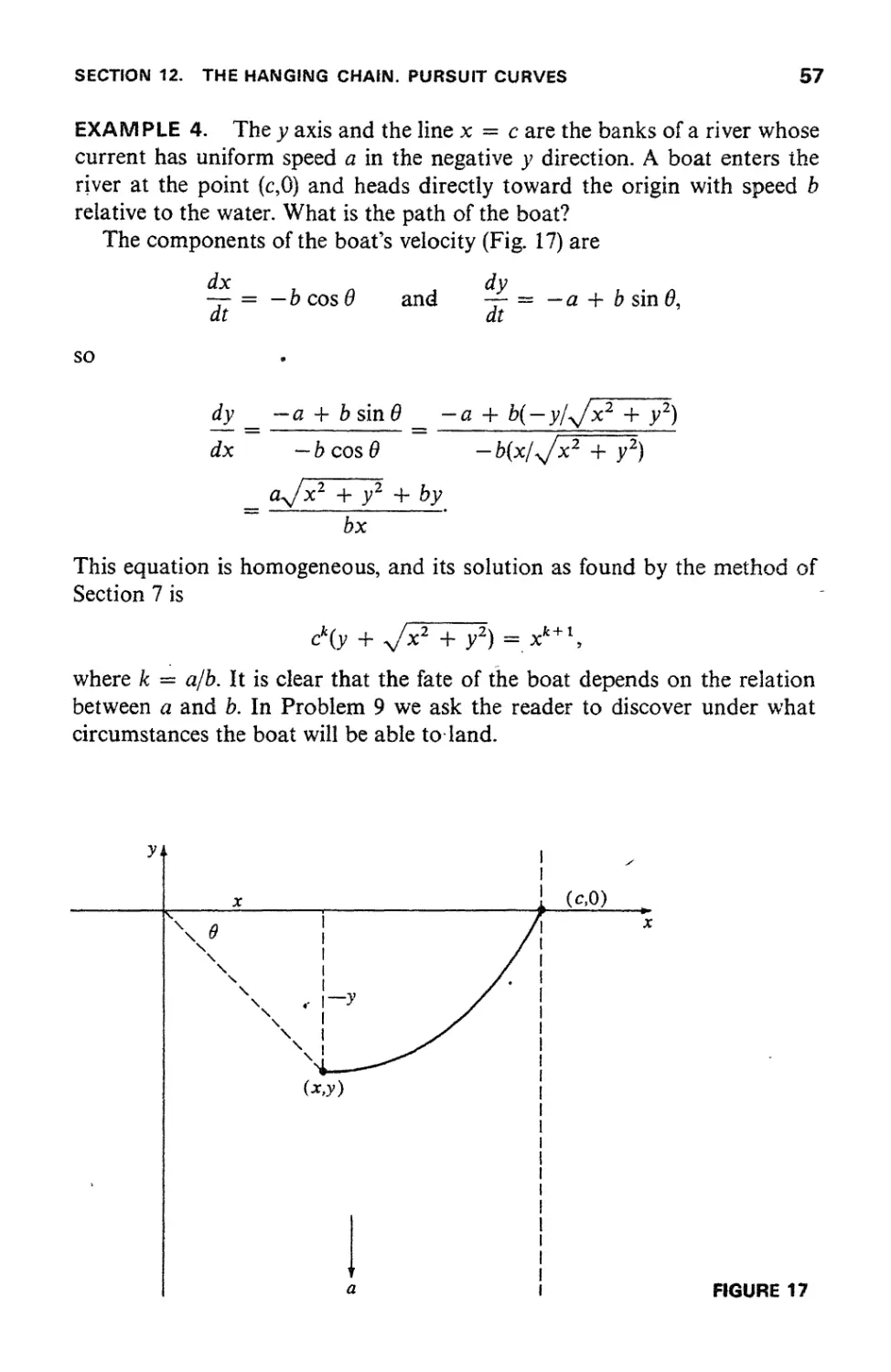
Text
                    The sole aim of science is the honor of the human mind,
and from this point of view
a question about numbers
is as important
as a question about the system of the world.
—C.G.J. Jacobi
GEORGE F. SIMMONS Professor of Mathematics, Colorado College
DIFFERENTIAL EQUATIONS
WITH APPLICATIONS AND HISTORICAL NOTES
m
TATA McGRAW-HILL PUBLISHING COMPANY LTD.
New Delhi

DIFFERENTIAL EQUATIONS
WITH APPLICATIONS AND HISTORICAL NOTES
Copyright © 1972 by McGraw-Hill, Inc.
All Rights Reserved.
No part of this publication may be reproduced, stored in a
retrieval system, or transmitted, in any form or by any means,
electronic, mechanical, photocopying, recording, or otherwise,
without the prior written permission of the publisher.
Τ Μ Η Edition 1974
Reprinted 1978
Reprinted 1979
Reprinted in India by arrangement with McGraw-Hill, Inc. New York.
This edition can be exported from India only by the Publishers,
Tata McGraw-Hill Publishing Company Ltd.
Published by Tata McGraw-Hill Publishing Company Limited and
Printed by Mohan Makhijani at Rekha Printers Pvt Ltd., New Dethi-HOOtt.

FOR HOPE AND NANCY
my wife and daughter
who make it all worthwhile

PREFACE
To be worthy of serious attention, a new textbook on an old subject should
embody a definite and reasonable point of view which is not represented
by books already in print. Such a point of view inevitably reflects the
experience, taste, and biases of the author, and should therefore be clearly
stated at the beginning so that those who disagree can seek nourishment
elsewhere. The structure and contents of this book express my personal
opinions in a variety of ways, as follows.
The place of differential equations io mathematics. Analysis has been
the dominant branch of mathematics for 300 years, and differential equations
is the heart of analysis. This subject is the natural goal of elementary
calculus and the most important part of mathematics for understanding the
physical sciences. Also, in the deeper questions it generates, it is the source
of most of the ideas and theories whiQh constitute higher analysis. Power
series, Fourier series, the gamma function and other special functions,
integral equations, existence theorems, the need for rigorous justifications
of many analytic processes—all these themes arise in our work in their most
natural context. And at a later stage they provide the principal motivation
behind complex analysis, the theory of Fourier series and more general
orthogonal expansions, Lebesgue integration, metric spaces and Hubert
spaces, and a host of other beautiful topics in modern mathematics. I
vti

VIII
PREFACE
would argue, for example, that one of the main ideas of complex analysis
is the liberation of power series from the confining environment of the
real number system; and this motive is most clearly felt by those who have
tried to use real power series to solve differential equations. In botany, it is
obvious that no one can fully appreciate the blossoms of flowering plants
without a reasonable understanding of the roots, stems, and leaves which
nourish and support them. The same principle is true in mathematics,
but is often neglected or forgotten.
Fads are as common in mathematics as in any other human activity,
and it is always difficult to separate the enduring from the ephemeral in the
achievements of one's own time. At present there is a strong current of
abstraction flowing through our graduate schools of mathematics. This
current has scoured away many of the individual features of the landscape
and replaced them with the smooth, rounded boulders of general theories.
When taken in moderation, these general theories are both useful and
satisfying; but one unfortunate effect of their predominance is that if a
student doesn't learn a little while he is an undergraduate about such colorful
and worthwhile topics as the wave equation, Gauss's hypergeometric
function, the gamma function, and the basic problems of the calculus of
variations—among many others—then he is unlikely to do so later. The
natural place for an informal acquaintance with such ideas is a leisurely
introductory course on differential equations. Some of our current books
on this subject remind me of a sightseeing bus whose driver is so obsessed
with speeding along to meet a schedule that his passengers have little or no
opportunity to enjoy the scenery. Let us be late occasionally, and take
greater pleasure in the journey.
Applications. It is a truism that nothing is permanent except change; and
the primary purpose of differential equations is to serve as a tool for the
study of change in the physical world. A general book on the subject without
a reasonable account of its scientific applications would therefore be as
futile and pointless as a treatise on eggs that did not mention their
reproductive purpose. This book is constructed so that each chapter except the
last has at least one major "payoff—and often several—in the form of a
classic scientific problem which the methods of that chapter render accessible.
These applications include
the brachistochrone problem;
the Einstein formula Ε = тс1;
Newton's law of gravitation;
the wave equation for the vibrating string;
the harmonic oscillator in quantum mechanics;
potential theory;

PREFACE
IX
the wave equation for the vibrating membrane;
the prey-predator equations;
nonlinear mechanics;
Hamilton's principle; and
Abel's mechanical problem.
I consider the mathematical treatment of these problems to be among
the chief glories of Western civilization, and I hope the reader will agree.
The problem of mathematical rigor. On the heights of pure
mathematics, any argument that purports to be a proof must be capable of
withstanding the severest criticisms of skeptical experts. This is one of the rules
of the game, and if you wish to play you must abide by the rules. But this is
not the only game in town.
There are some parts of mathematics—perhaps number theory and
abstract algebra—in which high standards of rigorous proof may be
appropriate at all levels. But in elementary differential equations a narrow
insistence on doctrinaire exactitude tends to squeeze the juice out of the subject,
so that only the dry husk remains. My main purpose in this book is to help
the student grasp the nature and significance of differential equations;
and to this end, I much prefer being occasionally imprecise but
understandable to being completely accurate but incomprehensible. I am not
at all interested in building a logically impeccable mathematical structure,
in which definitions, theorems, and rigorous proofs are welded together
into a formidable barrier which the reader is challenged to penetrate.
In spite of these disclaimers, I do attempt a fairly rigorous discussion
from time to time, notably in Chapter 11 and Appendices A in Chapters
4 and 5, and В in Chapter 8. I am not saying that the rest of this book is
nonrigorous, but only that it leans toward the activist school of
mathematics, whose primary aim is to develop methods for solving scientific
problems—in contrast to the contemplative school, which analyzes and
organizes the ideas and tools generated by the activists.
Some will think that a mathematical argument either is a proof or is
not a proof. In the context of elementary analysis I disagree, and believe
instead that the proper role of a proof is to carry reasonable conviction to
one's intended audience. It seems to me that mathematical rigor is like
clothing: in its style it ought to suit the occasion, and it diminishes comfort
and restricts freedom of movement if it is either too loose or too tight.
History and biography. There is an old Armenian saying, "He who lacks
a sense of the past is condemned to live in the narrow darkness of his own
generation." Mathematics without history is mathematics stripped of its
greatness; for, like the other arts—and mathematics is one of the supreme

χ
PREFACE
arts of civilization—it derives its grandeur from the fact of being a human
creation.
In an age increasingly dominated by mass culture and bureaucratic
impersonality, I take great pleasure in knowing that the vital ideas of
mathematics were not printed out by a computer or voted through by a
committee, but instead were created by the solitary labor and individual
genius of a few remarkable men. The many biographical notes in this book
reflect my desire to convey something of the achievements and personal
qualities of these astonishing human beings. Most of the longer notes are
placed in the appendices, but each is linked directly to a specific contribution
discussed in the text. These notes have as their subjects all but a few of the
greatest mathematicians of the past three centuries: Fermat, Newton, the
Bernoullis, Euler, Lagrange, Laplace, Gauss, Abel, Hamilton, Liouville,
Chebyshev, Hermite, Riemann, and Poincare. As T. S. Eliot wrote in
one of his essays, "Someone said: 'The dead writers are remote from us
because we know so much more than they did.' Precisely, and they are that
which we know."
History and biography are very complex, and Ϊ am painfully aware that
scarcely anything in my notes is actually quite as simple as it may appear.
I must also apologize for the many excessively brief allusions to
mathematical ideas most student readers have not yet encountered. But with the
aid of a good library, a sufficiently interested student should be able to
unravel most of them for himself. At the very least, such efforts may help
to impart a feeling for 4he immense diversity of classical mathematics—
an aspect of the subject that is almost invisible in the average undergraduate
curriculum.
GEORGE F. SIMMONS

SUGGESTIONS FOR THE INSTRUCTOR
The following diagram gives the logical dependence of the chapters and
suggests a variety of ways this book can be used, depending on the tastes
of the instructor and the backgrounds and purposes of his students.
4. Oscillation
Theory and
Boundary
Value Problems
1. The Nature of
Differential
Equations
2. First Order
Equations
3. Second Order
Linear
Equations
5. Power Series
Solutions and
Special
Functions
6. Some Special
Functions of
Mathematical
Physics
9. The Calculus
of Variations
7. Systems of
First Order
Equations
10. Laplace
Transforms
8. Nonlinear
Equations
11. The Existence
and
Uniqueness
of Solutions
Chapters 1, 2, and 9 are relatively straightforward, and much of the
material in the first two of these is often given in calculus courses. Chapter 3
is the cornerstone of the structure. Chapters 4, 5, and 6 deal with the more
advanced theory of second order linear equations and with series solutions,
and 10 provides a supplementary approach. Chapters 7 and 8 are aimed
at second order nonlinear equations, and 8 and 11 are the closest in spirit
to the mathematical interests of our own times. A word of warning: the
material covered in Sections 28 to 35 is rather formidable in places, and the
instructor giving a short course should perhaps consider reserving these
sections'for Jiis most ambitious students.

The scientist does not study nature because it is useful; he studies it because he delights
in it, and he delights in it because it is beautiful. If nature were not beautiful, it would
not be worth knowing, and if nature were not worth knowing, life would not be worth
living. Of course I do not here speak of that beauty that strikes the senses, the beauty of
qualities and appearances; not that I undervalue such beauty, far from it, but it has
nothing to do with science; I mean that profounder beauty which comes from the
harmonious order of the parts, and which a pure intelligence can grasp.
—Henri Poincare
As a mathematical discipline travels far from its empirical source, or still more, if it is
a second or third generation only indirectly inspired by ideas coming from "reality,"
it is beset with very grave dangers. It becomes more and more purely aestheticizing,
more and more purely Tart pour Fart. This need not be bad, if the field is surrounded by
correlated subjects, which still have closer empirical connections, or if the discipline is
under the influence of men with an exceptionally well-developed taste. But there is a grave
danger that the subject will develop along the line of least resistance, thai the stream,
so far from its source, will separate into a multitude of insignificant branches, and that the
discipline will become a disorganized mass of details and complexities. In other words,
at a great distance from its empirical source, or after much "abstract" inbreeding, a
mathematical subject is in danger of degeneration.
—John von Neumann
Just as deduction should be supplemented by intuition, so the impulse to progressive
generalization must be tempered and balanced by respect and love for colorful detail.
The individual problem should not be degraded to the rank of special illustration of lofty
general theories. In fact, general theories emerge from consideration of the specific, and
they are meaningless if they do not serve to clarify and order the more particularized
substance below. The interplay between generality and individuality, deduction and
construction, logic and imagination—this is the profound essence of live mathematics.
Any one or another of these aspects of mathematics can be at the center of a given
achievement. In a far-reaching development all of them will be involved. Generally speaking,
such a development will start from the "concrete" ground, then discard ballast by
abstraction and rise to the lofty layers of thin air where navigation and observation are easy;
after this flight comes the crucial test of landing and reaching specific goals in the newly
surveyed low plains of individual "reality." In brief the flight into abstract generality
must start from and return to the concrete and specific.
— Richard Courant

CONTENTS
Preface
Suggestions for the Instructor
THE NATURE OF DIFFERENTIAL EQUATIONS 1
1. Introduction 1
2. General remarks on solutions 3
3. Families of curves. Orthogonal trajectories 8
4. Growth, decay, and chemical reactions 14
5. Falling bodies and other rate problems 19
6. The brachistochrone. Fermat and the Bernoullis 25
FIRST ORDER EQUATIONS 35
'7. Homogeneous equations |3~
8. Exact equations 38
9. Integrating factors <&
10. Linear equations 47
A1. Reduction of order " 49
12. The hanging chain. Pursuit curves 52
13. Simple electric circuits 58
Appendix A. Numerical methods 65

SECOND ORDER LINEAR EQUATIONS 72
14. Introduction 72
15. The general solution of the homogeneous equation 76
16. The use of a known solution to find another 81
J 7. The homogeneous equation with constant coefficients 83
18. The method of undetermined coefficients 87
719. The method of variation of parameters 90
20. Vibrations in mechanical systems 93
21. Newton's law of gravitation and the motion of the planets 100
Appendix A. Euler 107
Appendix B. Newton 111
OSCILLATION THEORY AND
BOUNDARY VALUE PROBLEMS 115
22. Qualitative properties of solutions 115
23. The Sturm comparison theorem 121
24. Eigenvalues, eigenfunctions, and the vibrating string 124
Appendix A. Regular Sturm-Liouville problems 133
POWER SERIES SOLUTIONS AND
SPECIAL FUNCTIONS 140
25. Introduction. A review of power series 140
26. Series solutions of first order equations 147
~ 27. Second order linear equations. Ordinary points 151
28. Regular singular points 159
29. Regular singular points (continued) 167
30. Gauss's hypergeometric equation 174
31. The point at infinity 180
Appendix A. Two convergence proofs 183
Appendix B. Hermite polynomials and quantum mechanics 187
Appendix C. Gauss · 196
Appendix D. Chebyshev polynomials and the minimax property 204
Appendix Ε. Riemanns equation 211
SOME SPECIAL FUNCTIONS OF
MATHEMATICAL PHYSICS 219
32. Legendre polynomials 219
33. Properties of Legendre polynomials 226
34. Bessel functions. The gamma function 232
35. Properties of Bessel functions 242
Appendix A. Legendre polynomials and potential theory 249
Appendix B. Bessel functions and the vibrating membrane 255
Appendix С'. Additional properties of Bessel functions 261

7 SYSTEMS OF FIRST ORDER EQUATIONS 265
3$. General remarks on systems 265
37. Linear systems 268
3&. Homogeneous linear systems with constant coefficients 276
39. Nonlinear systems. Volterra's prey-predator equations 284
8 NONLINEAR EQUATIONS 290
40. Autonomous systems. The phase plane and its phenomena 290
41. Types of critical points. Stability 296
42. Critical points and stability for linear systems 305
43. Stability by Liapunov's direct method 316
44. Simple critical points of nonlinear systems 323
45. Nonlinear mechanics. Conservative systems 332
46. Periodic solutions. The Poincare-Bendixson theorem 338
Appendix 4. Poincare 346
Appendix B. Proof of Lienard's theorem 349
9 THE CALCULUS OF VARIATIONS 353
47. Introduction. Some typical problems of the subject 353
48. Euler's differential equation for an extremal ~ 356
49. Isoperimetric problems 366
Appendix A. Lagrange 376
Appendix B. Hamilton's principle and its implications 377
10 LAPLACE TRANSFORMS 388
50. introduction 388
51. A few remarks on the theory 392
52. Applications to differential equations 397
53. Derivatives and integrals of Laplace transforms 402
" 54. Convolutions and Abel's mechanical problem 407
Appendix A. Laplace 413
Appendix B. Abel 415
1 1 THE EXISTENCE AND UNIQUENESS OF SOLUTIONS 418
55. The method of successive approximations 418
56. Picard's theorem 422
57. Systems. The second order linear equation 433
Answers
Index
436

1
THE NATURE OF
DIFFERENTIAL EQUATIONS
1. INTRODUCTION
An equation involving one dependent variable and its derivatives with
respect to one or more independent variables is called a differential equation.
Many of the general laws of nature—in physics, chemistry, biology, and
astronomy—find their most natural expression in the language of differential
equations. Applications also aboundi in mathematics itself, especially in
geometry, and in engineering, economics, and many other fields of applied
science.
It is easy to understand the reason behind this broad utility of differential
equations. The reader will recall that if у = f(x) is a given function, then its
derivative dy/dx can be interpreted as the rate of change of у with respect to x.
In any natural process, the variables involved and their rates of change are
connected with one another by means of the basic scientific principles that
govern the process. When this connection is expressed in mathematical
symbols, the result is often a differential equation.
The following example may illuminate these remarks. According to
Newton's second law of motion, the acceleration α of a body of mass m is
proportional to the total force F acting on it, with 1/m as the constant of
proportionality, so that a = F/m or
ma = F. (1)
1

2
CHAPTER 1. THE NATURE OF DIFFERENTIAL EQUATIONS
Suppose, for instance, that a body of mass m falls freely under the influence
of gravity alone, in this case the only force acting on it is mg, where g is the
acceleration due to gravity.1 if у is the distance down to the body from some
fixed height, then its acceleration is d2y/dt2, and (1) becomes
d*y
dt
or
dy
dt
т~1л = т$
2 = 9· (2)
if we alter the situation by assuming that air exerts a resisting force
proportional to the velocity, then the total force acting on the body is mg —
k(dyldt\ and (1) becomes
d2y dy
*^mg~kTt
m-uf=m9-k-u' (3)
Equations (2) and (3) are the differential equations that express the essential
attributes of the physical processes under consideration.
As further examples of differential equations, we list the following:
!--*; (4)
d2y
dx
m"5?= ~ky; (5)
+ 2xy = e'*2; (6)
dt2
dy
dx2 dx
„L-5_£ + 6y = 0; (7)
(1_x2)i?"2xS + p(p + 1)3' = 0; (8)
^ + χε + ^-^-α (9)
The dependent variable in each of these equations is y, and the independent
variable is either t or x. The letters /c, m, and ρ represent constants. An
ordinary differential equation is one in which there is only one independent
variable, so that all the derivatives occurring in it are ordinary derivatives.
Each of these equations is ordinary. The order of a differential equation is
lg can be considered constant on the surface of the earth in most applications, and is
approximately 32 feet per second per second: (or 980 centimeters per second per second).

SECTION 2. GENERAL REMARKS ON SOLUTIONS
3
the order of the highest derivative present Equations (4) and (6) are first
order equations, and the others are second order. Equations (8) and (9) are
classical, and jare called Legendre's equation and Bessefs equation,
respectively. Each has a vast literature and a history reaching back hundreds of
years. We shall study all of these equations in detail later.
A partial differential equation is one involving more than one independent
variable, so that the derivatives occurring in it are partial derivatives. For
example, if w = f(x,y,z,t) is a function of time and the three rectangular
coordinates of a point in space, then the following are partial differential
equations of the second order:
d2w d2w d2w
a? + W + a? = ;
2 fd2w d2w d2w\ dw
a \ώ? + If + a?J = ~дГ;
2fd2w d2w d2w\ d2w
a v^ + ^ + ^2; Ж
These equations are also classical, and are called Laplace's equation, the
heat equation, ( and the wave equation, respectively. Each is profoundly
significant in theoretical physics, and their study has stimulated the
development of many important mathematical ideas. In general, partial differential
equations arise in the physics of continuous media—in problems involving
electric fields, fluid dynamics, diffusion, and wave motion. Their theory is
very different from that of ordinary differential equations, and is much more
difficult in almost every respect. For some time to come, we shall confine our
attention exclusively to ordinary differential equations.
2. GENERAL REMARKS ON SOLUTIONS
The general ordinary differential equation of the nth order is
/ dy d2y d»y\
Γ\?*ΈΈ?-'''!*) = * (1)
or, using the prime notation for derivatives,
F(x,v,/,/,..-,yn)) = 0.
Any adequate theoretical discussion of this equation would have to be based
on a careful study of explicitly assumed properties of the function F. However,
undue emphasis on the fine points of theory often tends to obscure what is
really going on. We will therefore try to avoid being overly fussy about such
matters—at least for the present.

4
CHAPTER 1. THE NATURE OF DIFFERENTIAL EQUATIONS
It is normally a simple task to verify that a given function у = y(x) is a
solution of an equation like (1). All that is necessary is to compute the
derivatives of y(x) and to show that y(x) and these derivatives, when
substituted in the equation, reduce it to an identity in x. In this way we see that
у = e2x and у = e3x
are both solutions of the second order equation
y" - 5/ + 6y = 0; (2)
and, more generally, that
y^cxe2x + c2eZx (3)
is also a solution for every choice of the constants cx and c2. Solutions of
differential equations often arise in the form of functions defined implicitly,
and sometimes it is difficult or impossible to express the dependent variable
explicitly in terms of the independent variable. For instance,
xy = log у -f с (4)
is a solution of
dy y2
dx 1 — xy
(5)
for every value of the constant c, as we can readily verify by differentiating
(4) and rearranging the result. These examples also illustrate the fact that a
solution of a differential equation usually contains one or more arbitrary
constants, equal in number to the order of the equation.
In most cases procedures of this kind are easy to apply to a suspected
solution of a given differential equation. The problem of starting with a
differential equation and finding a solution is naturally much more difficult
In due course we shall develop systematic methods for solving equations
like (2) and (5). For the present, however, we limit ourselves to a few remarks
on some of the general aspects of solutions.
The simplest of all differential equations is
g=/(*), (6)
and we solve it by writing
y= if(x)dx + c. (7)
In some cases the indefinite integral in (7) can be worked out by the methods

SECTION 2. GENERAL REMARKS ON SOLUTIONS
5
of calculus. In other cases it may be difficult or impossible to find a formula for
this integral. It is known, for instance, that
\e χ1 dx and
dx
cannot be expressed in terms of a finite number of elementary functions.1 If
we recall, however, that
J·
f(x) dx
is merely a symbol for a function (any function) with derivative/(x), then we
can almost always give (7) a valid meaning by writing it in the form
JXQ
+ с. (8)
The crux of the matter is that this definite integral is a function of the upper
limit χ (the г under the integral sign is only a dummy variable) which aiwayfc
exists when the integrand is continuous over the range of integration, and
that its derivative is f(x)·2
The general first order equation is the special case of (I) which corresponds
to taking л =* 1:
FH£)-a (9)
We normally expect that an equation like this will have a solution, and that
this solution will contain one arbitrary constant. However,
I)1—·
has no real-valued solutions at all, and
has only the single solution у = 0 (which contains no arbitrary constants).
Situations of this kind raise difficult theoretical questions about the existence
and nature of solutions of differential equations. We cannot enter here into a
1 Any reader who is curious about the reasons for this should consult D. G. Mead, Integration,
Am. Math. Monthly, vol. 68, pp. 152-156, 1961. For additional details, see G. H. Hardy, "the
Integration of Functions of a Single Variable," Cambridge University Press, London, 1916; or
J. F. Ritt, "Integration in Finite Terms," Columbia University Press, New York, 1948.
2This statement is one form of the fundamental theorem of calculus.

6
CHAPTER 1. THE NATURE OF DIFFERENTIAL EQUATIONS
full discussion of these questions, but it may clarify matters if we give an
intuitive description of a few of the basic facts.
For the sake of simplicity, let us assume that (9) can be solved for dy/dx:
%-fM (10)
We also assume that f(x,y) is a continuous function throughout some
rectangle R in the xy plane. The geometric meaning of a solution of (10) can best
be understood as follows (Fig. 1). If P0 = (x0,y0) is apoint in R, then the
number
(ε)λ-■"■*»>
determines a direction at PQ. Now let Pl = (xuyi) be a point near F0 in
this direction, and use
(4 -№-"'
to determine a new direction at Px. Next, let P2 = {хг*Уг) be a point near
Pi in this new direction, and use the number
to determine yet another direction at P2. if we continue this process, we
obtain a broken line with points scattered along it like beads; if we now
imagine that these successive points move closer to one another and become
more numerous, then the broken line approaches a smooth curve through
the initial point P0. This curve is a solution у = у(х) of equation (10); for at
each point (x,y) on it, the slope is given by/(x, y)—precisely the condition
required by the differential equation, if we start with a different initial point,
then in general we obtain a different curve (or solution). Thus the solutions
of (10) form a family of curves, called integral curves.1 Furthermore, it
appears to be a reasonable guess that through each point in R there passes
just one integral curve of (10). This discussion is intended only to lend
plausibility to the following precise statement.
THEOREM A. (PICARD'S THEOREM.) Ifj(x,y) and df/ду are
continuous functions on a closed rectangle R, then through each point (х0,Уо) in the
interior of R there passes a unique integral curve of the equation dy/dx =
Жу).
1 Solutions of a differential equation are sometimes called integrals of the equation because the
problem of finding them is more or less an extension of the ordinary problem of integration.

SECTION 2. GENERAL REMARKS ON SOLUTIONS
>4
FIGURE 1
If we consider a fixed value of x0 in this theorem, then the integral curve
that passes through (х0,Уо) is fully determined by the choice of y0. In {his
way we see that the integral curves of (10) constitute what is called a one-
parameter family of curves. The equation of this family can be written in
the form
у = >'(*, с),
(И)
where different choices of the parameter с yield different curves in the family.
The integral curve that passes through (х0,Уо) corresponds to the value of с
for which v0 = y(xoicY ^ we denote this number by cQ, then (11) is called
the general solution of (10), and
y = y(x,c0)
is called the particular solution that satisfies the initial condition
У = У о
when
Χ — -^o*
The essential feature of the general solution (11) is that the constant с in it
can be chosen so that an integral curve passes through any given point of
the rectangle under consideration.
Picard's theorem is proved in Chapter 11. This proof is quite complicated,
and is probably best postponed until the reader has had considerable
experience with the more straightforward parts of the subject. The theorem

8
CHAPTER 1. THE NATURE OF DIFFERENTIAL EQUATIONS
itself can be strengthened in various directions by weakening its hypotheses;
it can also be generalized to refer to nth order equations solvable for the
nth order derivative. Detailed descriptions of these results would be out of
place in the present context, and we content ourselves for the time being with
this informal discussion of the main ideas. In the rest of this chapter we
explore some of the ways in which differential equations arise in scientific
applications.
PROBLEMS
1. Verify that the following functions (explicit or implicit) are solutions of
the corresponding differential equations:
a. у = χ2 -l· с у' = 2x;
b. у — ex2 ■ xy = 2y;
c. у1 = e2x + с уу' = e2x;
d. у = cekx yr — ky;
e. у — ci sin 2x 4 c2 cos 2x y" 4- Ay = 0;
f. у — cle2x 4 c2e~2x y" — Ay = 0;
g. у = cl sinh 2x 4- c2 cosh 2x y"' — Ay = 0;
h. у = sin"l xy xy' -f у = у у/1 — χ2у2;
i. у = χ tan x xy' - у + χ2 -f у2;
■> г> -у л , ХУ
у x2 = 2y2logy у = х2 + у2>
к. у2 = х2 - сх 2хуу = х2 4- у2]
1. у = с2 -4- с/х у + χ/ = λ'4(у')2;
т. у = сву/х у' = у2/(ху ~ х2);
п. у 4- sin у = χ (у cos у — sin у 4 х)у' = у;
о. χ + у = tan ~2 у i 4- у2 4 у2у' = 0.
2. Find the general solution of each of the following differential equations:
a. y' = e3x — x; с. у = хех ;
b. xy' = 1; d. у = sin"1 x.
3. For each of the following differential equations, find the particular
solution that satisfies the given initial condition:
a. у = xex, у = 3 when χ = 1;
b. у' = 2 sin χ cos x, у = 1 when χ = 0;
c. у = log χ, у = 0 when x = е.
3. FAMILIES OF CURVES. ORTHOGONAL TRAJECTORIES
We have seen that the general solution of a first order differential equation
normally contains one arbitrary constant, called a parameter. When this
parameter is assigned various values,, we obtain a one-parameter family of

SECTION 3. FAMILIES OF CURVES 9
curves. Each of these curves is a particular solution, or integral curve, of
the given differential equation, and all of them together constitute its general
solution.
Conversely, as we might expect, the curves of any one-parameter family
are integral curves of some first order differential equation. If the family is
/(-W) = 0,
(1)
then its differential equation can be found by the following steps. First,
differentiate (1) implicitly with respect to χ to get a relation of the form
Next, eliminate the parameter с from (1) and (2) to obtain
(2)
(3)
F(x.y,gJ-0
as the desired differential equation. For example,
x2 + v2 = c2
is the equation of the family of all circles with centers at the origin (Fig. 2).
(4)
FIGURE 2

10
CHAPTER 1. THE NATURE OF DIFFERENTIAL EQUATIONS
On differentiation with respect to χ this becomes
dv
2x + 2y-f- = 0;
ax
and since с is already absent, there is no need to eliminate it and
dy r.
(5)
is the differential equation of the given family of circles. Similarly,
X2 + у* = 2CX (6)
is the equation of the family of all circles tangent to the у axis at the origin
(Fig. 3). When we differentiate this with respect to x, we obtain
2x + 2y -/ = 2c
dx
or
dy
Х + УТх = С-
(7)
FIGURE 3

SECTION 3. FAMILIES OF CURVES
11
The parameter с is still present, so it is necessary to eliminate it by combining
(6) and (7). This yields
dy
dx
2xy
(8)
as the differential equation of the family (6).
As an interesting application of these procedures, we consider the problem
of finding orthogonal trajectories. To explain what this problem is, we
observe that the family of circles represented by (4) and the family у = тх of
straight lines through the origin (the dotted lines in Fig. 2) have the following
property: each curve in either family is orthogonal (i.e., perpendicular) to
every curve in the other family. Whenever two families of curves are related
in this way, each is said to be a family of orthogonal trajectories of the other.
Orthogonal trajectories are of interest in the geometry of plane curves, and
also in certain parts of applied mathematics. For instance, if an electric
current is flowing in a plane sheet of conducting material, then the lines of
equal potential are the orthogonal trajectories of the lines of current flow.
In the example of the circles centered on the origin, it is geometrically
obvious that the orthogonal trajectories are the straight lines through the
origin, and conversely. In order to cope with more complicated situations,
however, we need an analytic method for finding orthogonal trajectories.
Suppose that
dy
dx
-f(x,y)
(9)
is the differential equation of the family of solid curves in Fig. 4. These curves
-slope = — l/f(x,y)
FIGURE 4

12
CHAPTER 1. THE NATURE OF DIFFERENTIAL EQUATIONS
are characterized by the fact that at any point (x9y) on any one of them the
slope is given byj(x,y). The dotted orthogonal trajectory through the same
point, being orthogonal to the first curve, has as its slope the negative
reciprocal of the first. Thus, along any orthogonal trajectory, we have
dy/dx = - l/f(x,y) or
~-/<*,Λ (Ю)
dy
Our method of finding the orthogonal trajectories of a given family of curves
is therefore as follows: first, find the differential equation of the family;
next, replace dy/dx by — dx/dy to obtain the differential equation of the
orthogonal trajectories; and, finally, solve this new differential equation.
If we apply this method to the family of circles (4), we get
or
dx χ
(11)
as the differential equation of the orthogonal trajectories. We can now
separate the variables in (11) to obtain
dy dx
у χ'
which on direct integration yields
log у = log χ + log с
or
у = ex
as the equation of the orthogonal trajectories.
It is often convenient to express the given family of curves in terms of
polar coordinates. In this case we use the fact that if φ is the angle from the
radius to the tangent, then tan ψ = rdBjdr (Fig. 5). By the above discussion,
we replace this expression in the differential equation of the given family by
its negative reciprocal, -dr/rdO, to obtain the differential equation of the
orthogonal trajectories. As an illustration of the value of this technique, we
find the orthogonal trajectories of the family of circles (6). If we use
rectangular coordinates, it follows from (8) that the differential equation of the
orthogonal trajectories is
dy 2xy
dx x2 — у
2 л,2
(12)

SECTION 3. FAMILIES OF CURVES
FIGURE 5
Unfortunately, the variables in (12) cannot be separated,-so without
additional techniques for solving differential equations we can go no further in
this direction. However, if we use polar coordinates, the equation of our
family can be written as
r = 2c cos Θ.
From this we find that
(13)
dr
άθ
= — 2c sin 0,
(14)
and after eliminating с from (13) and (14) we arrive at
rdQ __ cos_0
dr sin θ
as the differential equation of the given family. Accordingly,
rdO _ sinfl
dr cos θ
is the differential equation of the orthogonal trajectories, in this case the
variables can be separated, yielding
dr _ co$ed6
r sin Θ

14
CHAPTER 1. THE NATURE OF DIFFERENTIAL EQUATIONS
and after integration this becomes
log r = log (sin Θ) -f log 2c,
so that
r = 2csin0 (15)
is the equation of the orthogonal trajectories. It will be noted that (15) is
the equation of the family of all circles tangent to the χ axis at the origin (see
the dotted curves in Fig. 3).
in Chapter 2 we develop a number of more elaborate procedures for
solving first order equations. Since our present attention is directed more at
applications than formal techniques, all the problems given in this chapter
are solvable by the method of separation of variables illustrated above.
PROBLEMS
1. Sketch each of the following families of curves, find the orthogonal
trajectories, and add them to the sketch:
a. xy = с; с. г = c{\ 4- cos#);
b. у — ex2; d. у = cex.
2. Sketch the family y2 = 4c(x 4- c) of all parabolas with axis the χ axis
and focus at the origin, and find the differential equation for the family.
Show that this differential equation is unaltered when dy/dx is replaced
by — dx/dy. What conclusion can be drawn from this fact?
3. Find the curves that satisfy each of the following geometric conditions:
a. the part of the tangent cut off by the axes is bisected by the point of
tangency;
b. the projection on the χ axis of the part of the normal between (x, v)
and the χ axis has length 1;
c. the projection on the χ axis of the part of the tangent between (x,y)
and the χ axis has length 1;
d. the polar angle θ equals the angle ψ from the radius to the tangent;
e. the angle φ from the radius to the tangent is constant.
4. A curve rises from the origin in the xy plane into the first quadrant. The
area under the curve from (0,0) to (x,y) is one-third the area of the
rectangle with these points as opposite vertices. Find the equation of
the curve.
4. GROWTH, DECAY, AND CHEMICAL REACTIONS
If a molecule has a tendency to decompose spontaneously into smaller
molecules at a rate unaffected by the presence of other substances, then it is

SECTION 4. GROWTH, DECAY. AND CHEMICAL REACTIONS 15
natural to expect that the number of molecules of this kind that will
decompose in a unit of time will be proportional to the total number present.
A chemical reaction of this type is called z. first-order reaction.
Suppose, for example, that x0 grams of matter are present initially, and
decompose in a first-order reaction. If χ is the number of grams present at a
later time f, then the principle stated above yields the following differential
equation:
dx
'dt
kxy k> 0.
(1)
[Since dx/dt is the rate of growth of x, —dx/dt is its rate of decay, and (1)
says that the rate of decay of χ is proportional to x.] If we separate the
variables in (1), we obtain
dx
= -kdu
which after integration becomes
log χ = — kl -f c.
The initial condition
χ = x0 when t = 0 (2)
gives с = log x0, so log χ = — kt 4- log x0, log (x/x0) = — fer, x/x0 = e~k\
and
χ = x0e~kt- (3)
This function is therefore the solution of the differential equation (i) that
satisfies the initial condition (2). its graph is given in Fig. 6. The positive
constant к is called the rate constant, for its value is clearly a measure of the
rate at which the reaction proceeds.
Very few first-order chemical reactions are known, and by far the most
FIGURE 6

16
CHAPTER 1. THE NATURE OF DIFFERENTIAL EQUATIONS
important of these is radioactive decay. It is convenient to express the rate of
decay of a radioactive element in terms of its half-life, which is the time
required for a given quantity of the element to diminish by a factor of one-
half. If we replace χ by x0/2 in formula (3), then we get the equation
У = *o*
for the half-life T, so
kT= log 2.
If either к or Τ is known from observation or experiment, this equation
enables us to find the other.
These ideas are the basis for a scientific tool of fairly recent development
which has been of great significance for geology and archaeology. In essence,
radioactive elements occurring in nature (with known half-lives) can be used
to assign dates to events that took place from a few thousand to a few billion
years ago. For example, the common isotope of uranium decays through
several stages into helium and an isotope of lead, with a half-life of 4.5
billion years. When rock containing uranium is in a molten state, as in lava
flowing from the mouth of a volcano, the lead created by this decay process
is dispersed by currents in the lava; but after the rock solidifies, the lead is
locked in place and steadily accumulates alongside the parent uranium. A
piece of granite can be analyzed to determine the ratio of lead to uranium,
and this ratio permits an estimate of the time that has elapsed since the critical
moment when the granite crystallized. Several methods of age determination
involving the decay of thorium and the isotopes of uranium into the various
isotopes of lead are in current use. Another method depends on the decay of
potassium into argon, with a half-life of 1.3 billion years; and yet another,
preferred for dating the oldest rocks, is based on the decay of rubidium into
strontium, with a half-life of 50 billion years. These studies are complex and
susceptible to errors of many kinds; but they can often be checked against
one another, and are capable of yielding reliable dates for many events in
geological history linked to the formation of igneous rocks. Rocks tens of
millions of years old are quite young, ages ranging into hundreds of millions
of years are common, and the oldest rocks yet discovered are upwards of
3 billion years old. This of course is a lower limit for the age of the earth's
crust, and so for the age of the earth itself. Other investigations, using various
types of astronomical data, age determinations for minerals in meteorites,
and so on, have suggested a probable age for the earth of about 4.5 billion
years.l
1 For a full discussion of these matters, as well as many other methods and results of the science
of geochronology, see F. E. Zeuner, "Dating the Past," 4th ed., Methuen, London, J 958.

SECTION 4. GROWTH, DECAY, AND CHEMICAL REACTIONS
17
The radioactive elements mentioned above decay so slowly that the
methods of age determination based on them are not suitable for dating
events that took place relatively recently. This gap was filled by Willard
Libby's discovery in the late 1940s of radiocarbon, a radioactive isotope of
carbon with a half-life of about 5600 years. By 1950 Libby and his associates
had developed the technique of radiocarbon dating, which added a second
hand to the slow-moving geological clocks described above and made it
possible to date events in the later stages of the Ice Age and some of the
movements and activities of prehistoric man. The contributions of this
technique to late Pleistocene geology and archaeology have been spectacular.
in brief outline, the facts and principles involved are these. Radiocarbon
is produced in the upper atmosphere by the action of cosmic ray neutrons on
nitrogen. This radiocarbon is oxidized to carbon dioxide, which in turn is
mixed by the winds with the nonradioactive carbon dioxide already present.
Since radiocarbon is constantly being formed and constantly decomposing
back into nitrogen, its proportion to ordinary carbon in the atmosphere has
long since reached an equilibrium state. All air-breathing plants incorporate
this proportion of radiocarbon into their tissues, as do the animals that eat
these plants. This proportion remains constant as long as a plant or animal
lives; but when it dies it ceases to absorb new radiocarbon, while the supply
it has at the time of death continues the steady process of decay. Thus, if a
piece of old wood has half the radioactivity of a living tree, it lived about
5600 years ago, and if it has only a fourth this radioactivity, it lived about
11,200 years ago. This principle provides a method for dating any a"ncient
object of organic origin, for instance, wood, charcoal, vegetable fiber, flesh,
skin, bone, or horn. The reliability of the method has been verified by
applying it to the heartwood of giant sequoia trees whose growth rings
record 3000 to 4000 years of life, and to furniture from Egyptian tombs whose
age is also known independently. There are technical difficulties, but the
method is now felt to be capable of reasonable accuracy as long as the periods
of time involved are not too great (up to about 50,000 years).
Radiocarbon dating has been applied to thousands of samples, and
laboratories for carrying on this work number in the dozens. Among the
more interesting age estimates are these: linen wrappings from the Dead
Sea scrolls of the Book of Isaiah, recently found in a cave in Palestine and
thought to be first or second century B.C., 1917 ± 200 years; charcoal from
the Lascaux cave in southern France, site of the remarkable prehistoric
paintings, 15,516 ± 900 years; charcoal from the prehistoric monument at
Stonehenge, in southern England, 3798 ± 275 years; charcoal from a tree
burned ai the time of the volcanic explosion that formed Crater Lake in
Oregon, 6453 ± 250 years. Campsites of ancient man throughout the
Western Hemisphere have been dated by using pieces of charcoal, fiber
sandals, fragments of burned bison bone, and the like. The results suggest

1$ CHAPTER 1. THE NATURE OF DIFFERENTIAL EQUATIONS
that man did not arrive in the New World until about the period of the last
Ice Age, some 11,500 years ago, when the level of the water in the oceans was
substantially lower than it now is and he could have walked across the
Bering Straits from Siberia to Alaska.1
These ideas may seem rather far removed from the subject of differential
equations, but actually they rest on the mathematical foundation provided
by equation (1) and its solution as given in formula (3). In the following
problems we ask the reader to apply similar techniques to questions arising
in chemistry, biology, and physics.
PROBLEMS
1. Suppose that two chemical substances in solution react together to form
a compound. If the reaction occurs by means of the collision and
interaction of the molecules of the substances, we expect the rate of
formation of the compound to be proportional to the number of collisions
per imit time, which in turn is jointly proportional to the amounts of the
substances that are untransformed. A chemical reaction that proceeds
in this manner is called a second-order reaction, and this law of reaction is
often referred to as the law of mass action. Consider a second-order
reaction in which χ grams of the compound contain ax grams of the
first substance and bx grams of the second, where a + b » 1. If there
are a A grams of the first substance present initially, and bB grams of the
second, and if χ = 0 when t « 0, find χ as a function of the time t.>
2. Suppose that x0 bacteria are placed in a nutrient solution at time f = 0,
and that χ is the population of the colony at a later time t If food and
living space are unlimited, and if, as a consequence, the population at
any moment is increasing at a rate proportional to the population at that
* moment, find χ as a function of t.
3. It in Problem 2, space is limited and food is supplied at a constant rate,
then competition for food and space will act in such a way that ultimately
the population will stabilize at a constant level xx. Assume that under
these conditions the population grows at a rate jointly proportional to χ
and to the difference xx — x, and find χ as a function of t.
4. Assume that the air pressure ρ at an altitude ft above sea level is
proportional to the mass of the column of air above a horizontal unit area at
that altitude, and also that the product of the volume of a given mass of
air and the pressure on it remains constant at all altitudes. If ρ = p0 at
sea level, find ρ as a function of h.
1 Libby won the I960 Nobel Prize for chemistry as a consequence of the work described above.
His own account of the method, with its pitfalls and conclusions, can be found in his book
"Radiocarbon Dating»" 3(i ed„ University of Chicago Press, 1955. See also G. С Baldwin,
"America's Buried Past,- Putnam, New York, 1962.

SECTION 5. FALLING BODSES AND OTHER RATE PROBLEMS
19
5. Assume that the rate at which a hot bod}' cools is proportional to the
difference in temperature between it and its surroundings (Newton's law
of cooling1). A body is heated to 110°C and placed in air at 10°C After
ί hour its temperature is 60°C How much additional time is required for
it to cool to 30° C?
6. According to Lambert's law of absorption, the percentage of incident
light absorbed by a thin layer of translucent material is proportional to
the thickness of the layer.2 if sunlight falling vertically on ocean water is
reduced to one-half its initial intensity at a depth of 10 fest, at what
depth is it reduced to one-sixteenth its initial intensity? Solve this problem
by merely thinking about it, and also by setting up and solving a suitable
differential equation.
5./FALLING BODIES AND OTHER RATE PROBLEMS
In this section we study the dynamical problem of determining the motion
of a particle along a given path under the action of given forces. We consider
only two simple cases: a vertical path, in which the particle is falling either
freely under the influence of gravity alone, or with air resistance taken into
account; and a circular path, typified by the motion of the bob of a pendulum.
Free fall· The problem of a freely falling body was discussed in Section 1,
and we arrived at the differential equation
d2y
Ί?-' (1)
for this motion, where у is the distance down to the body from some fixed
height. One integration yields the velocity,
dy
V " ~It = 0t + °1' (2)
Since the constant cx is clearly the value of ν when t = 0, it is the initial
velocity t70, and (2) becomes
dy
ν = -~ = gt + v0. (3)
1 Newton himself applied this rule to estimate the temperature of a red-hot iron ball So little
was known about the laws of heat transfer at that time that his result was only a crude
approximation, but it was certainly better than nothing.
2Johann Heinrich Lambert (1728-1777) was a Swiss-German astronomer, .mathematician,
physicist, and man of learning. He was mainly self-educated, and published works on the orbits
of comets, the theory of light, and the construction of maps. The Lambert equal-area projection
is well known to all cartographers. He is remembered among mathematicians for having given
the first proof of the fact that π L· irrational.

20 CHAPTER 1. THE NATURE OF DEFERENTIAL EQUATIONS
On integrating again we get
1 2
The constant c2 is the value of у when t = 0, or the initial position y0, so we
finally have
y = —gt2 + i>0r + Уо (4)
as the general solution of (1). if the body falls from rest starting at у = 0,
so that i?0 = y0 = 0, then (3) and (4) reduce to
υ = gt and у = у #r2.
On eliminating f we have the useful equation
ν = j2fy (5)
. i
for the velocity attained in terms of the distance fallen. This result can also
be obtained from the principle of conservation of energy, which can be stated
in the form
kinetic energy + potential energy = a constant
Since our body falls from rest starting at у = 0, the fact that its gain in
kinetic energy equals its loss in potential energy gives
Г 2
Ymv =.т9У>
and (5) follows at once.
Retarded fall. If we assume that air exerts a resisting force proportional
to the velocity of our falling body, then the differential equation of the motion
is
d2y dy
2=0-<"f· (6)
where с — k/m [see equation l-(3)]. If dy/dt is replaced by i\ this becomes
%-Я-co. (7)
On separating variables and integrating, we get
dv
dt
g - cv

SECTION 5. FALLING BODIES AND OTHER RATE PROBLEMS
21
and
■log fe - cu) = t + cu
so
g — cv = c2e .
The initial condition υ = 0 when t = 0 gives c2 = Q-, so
i? = — (1 - έΓβ).
с
(8)
Since с is positive, ι; -> g/c as ί -» со. This limiting value of ν is called the
terminal velocity. If we wish, we can now replace ν by dy/dt in (8) and perform
another integration to find у as a function of t.
The motion of a pendulum. Consider a pendulum consisting of a bob
of mass m at the end of a rod of negligible mass and length a. If the bob is
pulled to one side through an angle α and released (Fig. 7), then by the
principle of conservation of energy we have
— mv2 = mg(a cos θ — a cos a).
Since s = αθ and ν = ds/dt = a (d9/dt\ this equation gives
= ga(cos6 — cos a);
2a \dt
(9)
(10)
FIGURE 7

22 CHAPTER 1. THE NATURE OF DIFFERENTIAL EQUATIONS
and on solving for at and taking into account the fact that θ decreases as t
increases (for small t), we get
2g ^/cos^ ~ cos α
If Τ is the period, that is, the time required for one complete oscillation, then
τ /7 f ° άθ
.-lit·.
V2.I.
τ-4νέΓ-=^— (,,)
4 V 2g Ja. л/cos θ - cos α
or
άθ
*/οο$θ — cos α
The value of Τ in this formula depends on a, which is the reason why
pendulum clocks vary in their rate of keeping time as the bob swings through a
greater or lesser angle. This formula for the period can be expressed more
satisfactorily as follows. Since
·> θ
cos θ = 1 — 2 sin2 —
2
and
we have
cos α = 1 — 2 sur —
2
V g Jo V sin2(a/2) - sir
sin2(0/2)
= 2
J0 , . a
, , , =» /c"=sm— (12)
о v7* - sin2(0/2) 2
We now change the variable from θ to φ by putting sin (0/2) = & sin φ, so
that 0 increases from 0 to π/2 as θ increases from 0 to a, and
— cos — άθ = к cos φ άφ
or
2k cos φ # _ 2y/k2 -$ίη2(θ/2)άφ
cos (0/2) " 71 -fc2sin2<£

SECTION 5. FALLING BODIES AND OTHER RATE PROBLEMS
23
This enables us to write (12) in the form
Γ-4/ΙΓ , άΦ =4ilF(k^\ (13)
where
Г+ άφ
Ρ{Κφ) =
i φ called
elliptic integral of the second kind,
0 y/1 - к2 sin2 φ
is a function of к and φ called the elliptic integral of the first kind.1 The
Е(к,ф) =
о
Vl -к2ьт2фаф,
arises in connection with the problem of finding the circumference of an
ellipse (see Problem 5). These elliptic integrals cannot be evaluated in terms
of elementary functions. Since they occur quite frequently in engineering
applications, their values as numerical functions of к and φ are often given
in mathematical tables.
Our discussion of the pendulum problem up to this point has focused on
the first order equation (10). For some purposes it is more convenient to
deal with the second order equation obtained by differentiating (10) with
respect to t:
а1л'=1 -0sm0. (14)
dt
If we now recall that sin θ is approximately equal to θ for small values of 0,
then (14) becomes (approximately)
dt2 ' a
._ +.2-0 = 0. (15)
2 + k2y - 0
it will be seen later that the general solution of the important second order
equation
d^y
dx2
is
' у - cx sin kx + c2 cos be,
so (15) yields
θ = Ci sin —t 4- c2 cos /— L (16>
1 It is customary in the case of elliptic integrals to violate ordinary usage by allowing the same
letter to appear as the upper limit and as the dummy variable of integration.

24
CHAPTER 1. THE NATURE OF DIFFERENTIAL EQUATIONS
The requirement that θ = α and άθ/dt = 0 when t = Ό implies that ct = 0
and c2 = a, so (16) reduces to
θ = a cos /— t. (17)
The period of this approximate solution of (14) is 2n^[a[g. It is interesting
to note that this is precisely the value of Τ obtained from (13) when к = 0,
which is approximately true when the pendulum oscillates through very
small angles.
PROBLEMS
1. if the air resistance acting on a falling body of mass m exerts a retarding
force proportional to the square of the velocity, then equation (7)
becomes
dv 9
where с = k/m. If ν = 0 when t = 0, find г; as a function of t. What is
the terminal velocity in this case?
2. A torpedo is traveling at a speed of 60 miles/hour at the moment it runs
out of fuel. If the water resists its motion with a force proportional to the
speed, and if 1 mile of travel reduces its speed to 30 miles/hour, how far
will it coast?1
3. The force that gravity exerts on a body of mass m at the surface of the
earth is mg. In space, however, Newton's law of gravitation asserts
that this force varies inversely as the square of the distance to the earth's
center. If a projectile fired upward from the surface is to keep traveling
indefinitely, show that its initial velocity must be at least -^IgR, where
R is the radius of the earth (about 4000 miles). This escape velocity is
approximately 7 miles/second or 25,000 miles/hour. (Hint: If χ is the
distance from the center of the earth to the projectile, and υ — dx/dt is
its velocity, then
d2x dv _ dv dx _ dv
dt1 ~~ at" dx dt ~ Ь dx
4. Inside the earth, the force of gravity is proportional to the distance from
the center. If a hole is drilled through the earth from pole to pole, and a
rock is dropped in the hole, with what velocity will it reach the center?
1 In the treatment of dynamical problems by means of vectors, the words velocity and speed are
sharply distinguished from one another. However, in the relatively simple situations we
consider, it is permissible (and customary) to use them more or less interchangeably.

SECTION 6. THE BRACHSSTOCHRONE
25
5. Show thai the circumference of the ellipse χ = a cos Θ, у — b sin 0, with
a < b, is given by 4bE{e,n/2\ where e is the eccentricity.
6. Show that the length of one arch of у = sin χ is 2^β E(*J2/2,n/2).
7. Show that the total length of the lemniscate r2 = a2 cos 2Θ is
4aF(j2,n/4).
6. THE BRACHISTOCHROME. FERMAT AND THE BERSSSOULLiS
Imagine that a point A is joined by a straight wire to a lower point В in
Fig. 8, and that a bead is allowed to slide without friction down the wire
from A to B. We can also consider the case in which the wire is bent into an
arc of a circle, so that the motion of the bead is the same as that of the
descending bob of a pendulum. Which descent takes the least time, that along
the straight path, or that along the circular path? Galileo believed that the
bead would descend more quickly along the circular path, and probably
most people would agree with him. Many years later, in 1696, Johann
Bernoulli posed a more general problem. He imagined the wire bent into the
shape of an arbitrary curve, and asked which curve among the infinitely
many possibilities will give the shortest possible time of descent. This curve
is called the brachistochrone (from the Greek brachistos, shortest, -f chronos,
time). Our purpose in this section is to understand Bernoulli's marvelous
solution of this beautiful problem.
We begin by considering an apparently unrelated problem in optics.
Figure 9a illustrates a situation in which a ray of light travels from A to Ρ
with velocity vx and then, entering a denser medium, travels from Ρ to В with
A
В
FIGURE 8

26 CHAPTER 1. THE MATURE OF DIFFERENTIAL EQUATiONS
FIGURE 9
a smaller velocity i?2. In terms of the notation in the figure, the total time Τ
required for the journey is given by
If we assume that this ray of light is able to select its path fr.>m 4 to В in such
a way as to minimize T, then dT/dx = 0 and by the methods of elementary
calculus we find that
χ с — χ

SECTION 6. THE BRACHISTOCHRONE
27
or
sin cCi sin cl2
υ1 ν2
This is SneWs law of refraction, which was originally discovered
experimentally in the less illuminating form sino^/sino^ = a constant1 The
assumption that light travels from one point to another along the path
requiring the shortest time is called Fermafs principle of least time. This
principle not only provides a rationai basis for SnelFs law, but can also be
applied to find the path of a ray of light through a medium of variable
density, where in general light will travel along curves instead of straight
lines. In Fig. 9b we have a stratified optical medium. In the individual layers
the velocity of light is constant, but the velocity decreases from each layer
to the one below it. As the descending ray of light passes from layer to layer,
it is refracted more and more toward the vertical, and when SnelFs law is
applied to the boundaries between the layers, we obtain
sin olx sin a2 sin a3 sin a4
Vi V2 V3 V4
If we next allow these layers to grow thinner and more numerous, then in the
limit the velocity of light decreases continuously as the ray descends and we
conclude that
sin a
— a constant.
ν
This situation is indicated in Fig. 9c, and is approximately what happens to a
ray of sunlight falling on the earth as it slows in descending through
atmosphere of increasing density.
Returning now to Bernoulli's problem, we introduce a coordinate system
as in Fig. 10 and imagine that the bead (like the ray of light) is capable of
selecting the path down which it will slide from Λ to В in the shortest possible
time. The argument given above yields
sin α
= a constant. (1)
By the principle of conservation of energy, the velocity attained by the bead at
a given level is determined solely by its loss of potential energy in reaching
that level, and not at all by the path that brought it there. As in the preceding
section, this gives
'Willebrord Snell (1591-1626) was a Dutch astronomer and mathematician. At the age of
twenty-two he succeeded his father as professor of mathematics at Leiden. His fame resrs
mainly on his discovery in 1621 of the law of refraction, which played a significant role in the
development of both calculus and the wave theory of light.

28
CHAPTER 1. THE MATURE OF DIFFERENTIAL EQUATIONS
αΪ j χ
\ i y
vs.
FIGURE 10
v = ^/2gy.
From the geometry of the situation we also have
1 1
sin α = cos/?
sec
β ^Τ+ίζη2β Jl + (Я2
(2)
(3)
On combining equations (1), (2), and (3)—obtained frox&^ptics, mechanics,
and calculus—we get
y[l + (/)*] = с (4)
as the differential equation of the brachistochrone.
We now complete our discussion, and discover what curve the
brachistochrone actually is, by solving (4). When y' is replaced by dy/dx and the
variables are separated, (4) becomes
dx
с - ν*
dy.
At this point we introduce a new variable φ by putting
tan 0,
\c - У.
(5)
so that у — с sin2 φ, dy = 2c sin φ cos φ άφ, and
dx = tan φ dy
— 2c sin2 φ άφ
— c{\ — cos2o)d<b.

SECTION 6. THE BRACHiSTOCHROftfE
29
integration now yields
χ = — (20 — sin 20) -f cx.
Our curve is to pass through the origin, so by (5) we have χ — у = 0 when
0 = 0, and consequently с χ = 0. Thus
с
χ = — (20 — sin 20) (6)
and
с
у = с sin2 φ = — (1 — cos 20). (7)
If we now put a = c/2 and # — 20, then (6) and (7) become
χ = α(θ - sin θ) and у = a(i - cos£). (8)
These are the standard parametric equations of the cycloid shown in Fig. 11,
which is generated by a point on the circumference of a circle of radius a
rolling along the χ axis. We note that there is a single value of α that makes the
first arch of this cycloid pass through the point В in Fig. 10; for if a is allowed
to increase from 0 to oo, then the arch inflates, sweeps over the first quadrant
of the plane, and clearly passes through В when a is suitably chosen.
Some of the geometric properties of the cycloid are perhaps familiar to the
reader from elementary calculus. For example, the length of one arch is 4
times the diameter of the generating circle, and the area under one arch is
3 times the area of this circle. This remarkable curve has many other
interesting properties, both geometric and physical, and some of these are described
in the problems below.
We hope that the necessary details have not obscured the wonderful
imaginative qualities in Bernoulli's solution of his problem, for it is a work of
/
/
_ ■■ . ..-a»
X ,
FIGURE 11

30
CHAPTER 1. THE NATURE OF DIFFERENTIAL EQUATIONS
art of a very high order, in addition to its intrinsic interest, the brachisto-
chrone problem has a larger significance: it was the historical source of the
calculus of variations—a powerful branch of analysis that in modern times has
penetrated deeply into the hidden simplicities at the heart of the physical
world. We shall discuss this subject in Chapter 9, and develop a general
method for obtaining equation (4) which is applicable to a wide variety of
similar problems.
NOTE ON FERMAT. Pierre de Fermat (1601-1665) was the greatest mathematician of the
seventeenth century, but his influence was limited by his lack of interest in publishing his
discoveries, which are known mainly from letters to friends and marginal notes in the books he
read. By profession he was a jurist and the king's parliamentary counselor in the French
provincial town of Toulouse. However, his hobby and private passion was mathematics. In
1629 he invented analytic geometry, but most of the credit went to Descartes, who hurried into
print with his own similar ideas in 1637. At this time—13 years before Newton was born—
Fermat also discovered a method for drawing tangents to curves and finding maxima and
minima, which amounted to the elements of differential calculus. Newton acknowledged, in a
letter that became known only in 1934, that some of his own early ideas on this subject came
directly from Fermat. In a series of letters written in 1654, Fermat and Pascal jointly developed
the fundamental concepts of the theory of probability. His discovery in 1657 of the principle of
least time, and its connection with the refraction of light, was the first step ever taken in the
direction of a coherent theory of optics. It was in the theory of numbers, however, that Fermafs
genius shone most brilliantly, for it is doubtful whether his insight into the properties of the
familiar but mysterious positive integers has ever been equaled. We mention a few of his many
discoveries in this field.
1. Fermafs two squares theorem: Every prime number of the form An + 1 can be written as the
sum of two squares in one and only one way.
2. Fermafs theorem: If ρ is any prime number and η is any positive integer, then ρ divides
np - n.
3. Fermafs last theorem: If η > 2, then x" + y" = z" cannot be satisfied by any positive integers
-v, .V, r.
He wrote this last statement in the margin of one of his books, in connection with a passage
dealing with the fact that x2 + y2 = z2 has many integer solutions. He then added the*tantalizing
remark, "I have found a truly wonderful proof which this margin is too narrow to contain."
Unfortunately no proof has ever been discovered by anyone else, and Fermafs last theorem
remains to this day one of the most baffling unsolved problems of mathematics. Finding a proof
would confer instant immortality on the finder, but the ambitious student should be warned
that able mathematicians have tried in vain for hundreds of years.
NOTE ON THE BERNOULLI FAMILY. Most people are aware that Johann Sebastian
Bach was one of the greatest composers of all time. However, it is less well known that his prolific
family was so consistently talented in this direction that several dozen Bachs were eminent
musicians from the sixteenth to the nineteenth centuries. In fact, there were parts of Germany
where the very word bach meant a musician. What the Bach clan was to music, the Bernoullis
were to mathematics and science. In three generations this remarkable Swiss family produced
eight mathematicians—three of them outstanding—who in turn had a swarm of descendants who
distinguished themselves in many fields.
Jakob Bernoulli (1654-1705) studied theology at the insistence of his father, but abandoned
it as soon as possible in favor of his love for science. He taught himself the new calculus of
Newton and Leibniz, and was professor of mathematics at Basel from 1687 until his death. He

MISCELLANEOUS PROBLEMS
31
wrote on infinite series, studied many special curves, invented polar coordinates, and introduced
the Bernoulli numbers that appear in the power series expansion of the function tan x. in his book
Ars Conjectandi he formulated the basic principle in the theory of probability known as Bernoulli" s
theorem or the law of large numbers: if the probability of a certain event is p, and if л independent
trials are made with к successes, then kfn -*■ ρ as η -+ χ. At first sight this statement may seem to
be a triviality, but beneath its surface lies a tangled thicket of philosophical (and mathematical)
problems that have been a source of controversy from Bernoulli's time to the present day.
Jakob's younger brother Johann Bernoulli (l667-1748) also made a false start in his career,
by studying medicine and taking a doctor's degree at Basel in 1694 with a thesis on muscle
contraction. However, he also became fascinated by calculus, quickly mastered it, and applied
it to many problems in geometry, differential equations, and mechanics. In 1695 he was appointed
professor of mathematics and physics at Groningen in Holland, and on Jakob's death he
succeeded his brother in the professorship at Basel. The Bernoulli brothers sometimes worked on
the same problems, which was unfortunate in view of their jealous and touchy dispositions. On
occasion the friction between them flared up into a bitter and abusive public feud, as it did over
the brachistochrone problem. In 1696 Johann proposed the problem as a challenge to the
mathematicians of Europe. It aroused great interest, and was solved by Newton and Leibniz as
well as by the two Bernoullis. Johann's solution (which we have seen) was the more elegant,
while Jakob's — though rather clumsy and laborious—was more general. This situation started
an acrimonious quarrel that dragged on for several years and was often conducted in rough
language more suited to a street brawl than a scientific discussion. Johann appears to have
been the more cantankerous of the two; for much later, in a fit of jealous rage, he threw his own
son out of the house for winning a prize from the French Academy that he coveted for himself.
This son, Daniel Bernoulli (1700- 1782), studied medicine like his father and took a degree
with a thesis on the action of the lungs; and like his father he soon gave way to his inborn talent
and became a professor of mathematics at St. Petersburg. In 1733 he returned to Basel and
was successively professor of botany, anatomy, and physics. He won 10 prizes from the French
Academy, including the one that infuriated his father, and over the years published many works
on physics, probability, calculus, and differential equations. In his famous book Hydrodynamka
he discussed fluid mechanics and gave the earliest treatment of the kinetic theory of gases. He
is considered by many to have been the first genuine mathematical physicist.
PROBLEMS
1. Consider a wire bent into the shape of the cycloid (8), and invert it
as in Fig. 10. If a bead is released at the origin and slides down the
wire without friction, show that nj~a/g is the time it takes to reach
the point (πα,ΐα) at the bottom.
2. Show that n^fajg of Problem 1 is also the time the bead takes in sliding
to the bottom from any intermediate point, so that the bead will reach
the bottom in the same time no matter where it is released. This is known
as the tautochrone property of the cycloid (from the Greek tauto, the
same, 4- chronos, time).
MISCELLANEOUS PROBLEMS FOR CHAPTER 1
1. It began to snow on a certain morning, and the snow continued to fall
steadily throughout the day. At noon a snowplow started to clear a

32
CHAPTER 1. THE NATURE OF DIFFERENTIAL EQUATIONS
road at a constant rate in terms of the volume of snow removed per
hour. The snowplow cleared 2 miles by 2 p.m. and 1 more mile by 4 р.м.
When did it start snowing?
2. A mothball whose radius was originally % inch is found to have a
radius of % inch after ί month. Assuming that it evaporates at a rate
proportional to its surface, find the radius as a function of time. After
how many more months will it disappear altogether?
3. A tank contains 100 gallons of pure water. Beginning at time t = 0,
brine containing 1 pound salt/gallon runs in at the rate of 1 gallon/-
minute, and the mixture (which is kept uniform by stirring) flows out at
the same rate. When will there be 50 pounds of dissolved salt in the
tank?
4. A large tank contains 100 gallons of brine in which 200 pounds of salt
are dissolved. Beginning at time t = 0, pure water runs in at the rate of
3 gallons/minute, and the mixture (which is kept uniform by stirring)
flows out at the rate of 2 gallons/minute. How long will it take to reduce
the amount of salt in the tank to 100 pounds?
5. A smooth football having the shape of a prolate spheroid 12 inches long
and 6 inches thick is lying outdoors in a rainstorm. Find the paths along
which water will run down its sides.
6. If с is a positive constant and a is a positive parameter, then
a2 a2 — c2
is the equation of the family of all ellipses (a > c) and hyperbolas
(a < c) with foci at the points (±c,0). Show that this family ofconfocal
conies is self-orthogonal (see Problem 3-2).
7. According to TorricelWs law, water in an open tank will flow out through
a small hole in the bottom with the speed it would acquire in falling
freely from the water level to the hole.1 A hemispherical bowl of radius
Ris initially full of water, and a small circular hole of radius r is punched
in the bottom at time t = 0. How long will the bowl take to empty
itself?
8. The clepsydra, or ancient water clock, was a bowl from which water
was allowed to escape through a small hole in the bottom, it was often
*Evangelista Torricelli (1608-1647) was an Italian physicist and mathematician and a disciple
of Galileo, whom he served as secretary. In addition to formulating the principle stated above,
he advanced the first correct ideas—which were narrowly missed by Galileo—about
atmospheric pressure and the nature of vacuums, and invented the barometer as an application of his
theories. See James B. Conant, "Science and Common Sense," pp. 63-71, Yale University
Press, New Haven, Conn., 1951.

MISCELLANEOUS PROBLEMS
33
used in Greek and Roman courts to time the speeches of lawyers, in
order to keep them from talking too much. Find the shape it should have
if the water level is to fail at a constant rate.
9. Two open tanks with identical small holes in the bottom drain in the
same time. One is a cylinder with vertical axis and the other is a cone
with vertex down, if they have equal bases and the height of the cylinder
is /г, what is the height of the cone?
10. A cylindrical can partly filled with water is rotated about its axis with
constant angular velocity ω. Show that the surface of the water assumes
the shape of a paraboloid of revolution. (Hint: The centripetal force
acting on a particle of water of mass m at the free surface is τηχω2 where
χ is its distance from the axis, and this is the resultant of the downward
gravitational force mg and the normal reaction force R due to other
nearby particles of water.)
11. Consider a bead at the highest point of a circle in a vertical plane, and
let that point be joined to any lower point on the circle by a straight
wire. If the bead slides down the wire without friction, show that it will
reach the circle in the same time regardless of the position of the lower
point.
12. A chain 4 feet long starts with 1 foot hanging over the edge of a table.
Neglect friction, and find the time required for the chain to slide off
the table.
13. Experience tells us that a man holding one end of a rope wound around
a wooden post can restrain with a small force a much greater force at the
other end. Quantitatively, it is not difficult to see that if Γ and Τ 4* AT
are the tensions in the rope at angles 0 and 0 -f Δ0 in Fig. 12, then a
normal force of approximately Τ Δ0 is exerted by the rope on the post
in the region between 0 and θ -f Αθ. It follows from this that if μ is
the coefficient of friction between the rope and the post, then Δ Τ is
approximately μΤ ΑΘ. Use this statement to formulate the differential
equation relating Γ and 0, and solve this equation to find Τ as a function
of 0, u, and the force T0 exerted by the man.
14. A load L is supported by a tapered circular column whose material has
density a. if the radius of the top of the column is r0, find the radius r at a
distance χ below the top if the areas of the horizontal cross sections are
proportional to the total loads they bear.
15. The President and the Prime Minister order coffee and receive cups of
equal temperature at the same time. The President adds a small amount
of cool cream immediately, but does not drink his coffee until 10
minutes later. The Prime Minister waits 10 minutes, and then adds the
same amount of cool cream and begins to drink. Who drinks the hotter
coffee?

34 CHAPTER 1. THE MATURE OF DIFFERENTIAL EQUATIONS
16. A destroyer is hunting a submarine in a dense fog. The fog lifts for a
moment, discloses the submarine on the surface 3 miles away, and
immediately descends. The speed of the destroyer is twice that of the
submarine, and it is known that the latter will at once dive and depart
at full speed in a straight course of unknown direction. What path
should the destroyer follow to be certain of passing directly over the
submarine? Hint: Establish a polar coordinate system with the origin
at the point where the submarine was sighted.
17. Four bugs sit at the corners of a square table of side a. At the same
instant they all begin to walk with the same speed, each moving steadily
toward the bug on its right, if a polar coordinate system is established
on the table, with the origin at the center and the polar axis along a
diagonal, find the path of the bug that starts on the polar axis and the
total distance it walks before all bugs meet at the center.

2
FIRST ORDER EQUATIONS
7. HOMOGENEOUS EQUATIONS
Generally speaking, it is very difficult to solve first order differential
equations. Even the apparently simple equation
dv
cannot be solved in general, in the sense that no formulas exist for obtaining
its solution in all cases. On the other hand, there are certain standard types
of first order equations for which routine methods of solution are available.
In this chapter we shall briefly discuss a few of the types that have many
applications. Since our main purpose is to acquire technical facility, we shall
completely disregard questions of continuity, differentiability, the possible
vanishing of divisors, and so on. The relevant problems of a purely
mathematical nature will be dealt with later, when some of the necessary
background has been developed.
The simplest of the standard types is that in which the variables are
separable:
(ty = £(x)
dx h(y)
35

38 CHAPTER 2. FIRST ORDER EQUATIONS
To solve this, we have only to write it in the form h(y)dy = g{x)dx and
integrate:
h(y) dy =
g(x) dx -f- c.
We have seen many examples of this procedure in the preceding chapter.
At the next level of complexity is the homogeneous equation. A function
f{x,y) is called homogeneous of degree η if
f(tx,ty)=-ff(x,y)
for all suitably restricted x, y, and L Thus x2 + xy\ Jx2 + y2, and sin (x/y)
are homogeneous of degrees 2, 1, and 0. The differential equation
M(x,y) dx + N(x, y) dy = 0
is said to be homogeneous if Μ and N are homogeneous functions of the
same degree. This equation can then be written in the form
dy -,
/х=Л*Л (i)
where f(x,y) = — M(x,y)/N(x,y) is clearly homogeneous of degree 0. The
procedure for solving (1) rests on the fact that it can be changed into an
-equation with separable variables by means of the substitution ζ - y/x. To
see this, we note that the relation
ffaty) = t°f(x9y) = f(x,y)
permits us to set t = l/x and obtain
/(x,j;)=/(i,v/x)-/(l,z).
Then since у — zx and
dy _ dz
equation (1) becomes
4χ-ζ+ΧΈ (2)
z + x— =/(l,z),
αχ
and the variables can be separated:
dz dx
f(Uz) -z~T
We now complete the solution by integrating and replacing ζ by y/x.

SECTION 7. HOMOGENEOUS EQUATIONS 37
EXAMPLE 1. Solve (x -f y)dx ~ (x - jy) dy = 0.
We begin by writing the equation in the form suggested by the above
discussion:
dy __ χ -f- у
dx χ — у
Since the function on the right is dearly homogeneous of degree 0, we know
that it can be expressed as a function of ζ = yjx. This is easily accomplished
by dividing numerator and denominator by χ: ι , ^
o/*z ^ dy _ 1 + y/x _ 1 + z ομτ " ^ л'л' ~ *
^X ~ ~ \'v dx "~ 1 - y/x " 1 - ζ ^ (№ _ */
We next introduce equation (2) and separate the variables, which gives
"y (1 — z)dz dx
i + z2 ~~ χ
On integration this yields
tan"1 ζ - —log(1 + z2) = log χ + c;
and when ζ is replaced by y/x, we obtain
tan J — = log Jx2 + v2 + с
χ
as the desired solution.
PROBLEMS
1. Verify that the following equations are homogeneous, and solve them:
f. (x2 - 2y2)dx + xydy = 0;
45. x2/ - 3xy - ly2 = 0;
с χ2/ = 3(x2 + y2) tan""1 — + xy;
. У dy . у
(Kxsm г = у sm h x;
χ αχ χ
4. xy = у -f 2xe~y,x.
2. Use rectangular coordinates to find the orthogonal trajectories of the
family of all circles tangent to the у axis at the origin.

38 CHAPTER 2. FIRST ORDER EQUATJONS
3. Show that the substitution ζ = ax -f by 4- с changes
/ = f(ax + by + c)
into an equation with separable variables, and apply this method to
solve the following equations:
a. y' = (χ + y)2;
b. / = sin2 (x — у -f 1).
4. a. if ae Φ bd, show that constants h and & can be chosen in such a way
that the substitutions χ — z — h, y = w — к reduce
'+ by + c\
dx \dx -
+ ey + /;
to a homogeneous equation,
b. if ae = bd, discover a substitution that reduces the equation in (a)
to one in which the variables are separable.
5. Solve the following equations:
dy χ 4- у + 4
a.
b.
dx
dy =
dx
x — у — 6'
x + У + 4
χ -f у — 6
8. EXACT EQUATIONS
If we start with a family of curves f(x,y) = c, then its differential equation
can be written in the form df = 0 or
f Л 4- f ^ = 0.
ox dy
For example, the family xzy3 = с has 2xy3 dx -f 3x2y2 dy = 0 as its
differential equation. Suppose we turn this situation around, and begin with
the differential equation
M(x9y)dx + N(x,y)dy = 0. (1)
If there happens to exist a function f(x9y) such that
J^ = M and f—N, (2)
3x dy
then (1) can be written in the form
$Ldx + fdy = 0 or df = 0,
ox dy

SECTION 8. EXACT EQUATIONS
39
and its general solution is
f(x,y) = с
in this case the expression Μ dx -f N dy is said to be an exact differential,
and (1) is called an exact differential equation.
it is sometimes possible to determine exactness and find the function/ by
mere inspection. Thus the left sides of
1 χ
ydx + xdy = 0 and — dx =■ d у — 0
У У
are recognizable as the differentials of xy and x/y, respectively, so the
general solutions of these equations are xy = с and x/y = c. in all but the
simplest cases, however, this technique of "solution by insight" is clearly
impractical. What is needed is a test for exactness and a method for finding
the function/ We develop this test and method as follows.
Suppose that (1) is exact, so that there exists a function / satisfying
equations (2). We know from elementary calculus that the mixed second
partial derivatives of/are equal:
d2f d2f
dy dx dx dy
This yields
BM _ dN
dy dx'
(3)
(4)
so (4) is a necessary condition for the exactness of (1). We shall prove that it is
also sufficient by showing that (4) enables us to construct a function/ that
satisfies equations (2). We begin by integrating the first of equations (2) with
respect to x:
ί
f=\Mdx+g(y). (5)
The "constant of integration" occurring here is an arbitrary function of у since
it must disappear under differentiation with respect to x. This reduces our
problem to that of finding a function g{y) with the property that/as given
lThe reader should be aware that equation (3) is true whenever both sides exist and are
continuous, and that these conditions are satisfied by almost all functions that are likely to arise
in practice. Our blanket hypothesis throughout this chapter (see the first paragraph in Section
7) is that all the functions we discuss are sufficiently continuous and differentiable to guarantee
the validity of the operations we perform on them.

40
CHAPTER 2. FIRST ORDER EQUATIONS
by (5) satisfies the second of equations (2). On differentiating (5) with respect
to у and equating the result to N, we get
d__
Μ dx + g'(y) = N,
so
g'(y) = N -y \Mdx.
This yields
0(У) =
N~-|M^)^,
(6)
provided the integrand here is a function only of y. This will be true if the
derivative of the integrand with respect to χ is 0; and since the derivative in
question is
dN d2
ox\ dy
Mdx\ =
dx
dN
dx
dN
dx '
dxdy
d2
dydx
dM
~"3y"
Mdx
ί
Mdx
an appeal to our assumption (4) completes the argument.
In summary, we have proved the following statement: equation (1) is
exact if and only if dM/ду = dN/dx; and in this case, its general solution is
f(x*y) = c* where f is given by (5) and (6). Two points deserve emphasis:
it is the equation f(x,y) = c, and not merely the function f which is the
general solution of (1); and it is the method embodied in (5) and (6), not the
formulas themselves, which should be learned.
EXAMPLE 1. Test the equation ey dx + (xey + 2y)dy = 0 for exactness,
and solve it if it is exact.
Here we have
so
Μ = ey and N = xey + 2y,
dM , dN
— = ey and — = ey.
dy dx

SECTION 8. EXACT EQUATIONS
41
Thus condition (4) is satisfied, and the equation is exact. This tells us that there
exists a function /(x,y) such that
df df
ir = ey and ■/- = xey + 2y.
dx dy
Integrating the first of these equations with respect to χ gives
f=\e>dx + g(y) = xe> + giy)9
so
df
Since this partial derivative must also equal xey -f 2y, we have g'(y) — 2y,
so g{y) = y2 and/ = xey + y2. All that remains is to note that
xey -f у2 = с
is the desired solution of the given differential equation.
PROBLEMS
Determine which of the following equations are exact, and solve the ones that
are.
j, χ ^ ) dy -f у dx — 0.
2. (sin χ tan у -f 1) dx + cos χ sec2 у dy = 0.
/. {y - x3)dx + (x + y3)dy = 0.
4. (2y2 - 4x + 5) Ac = (4 - 2y + 4xy) dy.
jif (y -f у cos xy) dx -f (x -f x cos xy) dy = 0.
6. cos χ cos2 у dx -f 2 sin χ sin у cos у dy = 0.
/ (sin χ sin у — xey) dy = (ey -f- cos χ cos y) dx.
1 χ xx
8 sin — dx Η—=■ sin — dy = 0.
У У У У
f. (1 +y)dx + (1 - x)~dy = 0.
10. (2xy3 + ycosx)dx 4- (3x2y2 + sin x)dy = 0.
ν χ
f1 J dx = =-x dx + 5~2 ^·
7 1 - x2y2 1 - x2y

42 CHAPTER 2. FIRST ORDER EQUATIONS
9. INTEGRATING FACTORS
The reader has probably noticed that exact differential equations are
comparatively rare, for exactness depends on a precise balance in the jprm
of the equation and is easily destroyed by minor changes in this form.^ f his
being the case, he may have doubts that exact equations are worth discussing
at all. In the present section we shall try to answer these doubts.
The equation
ydx + (x2y - x)dy = 0 (1)
is easily seen to be nonexact, for дМ/ду — 1 and dN/дх = 2xy — i.
However, if we multiply through by the factor I/x2, the equation becomes
L2dx + (y-.iyy = 0,
which is exact. To what extent can other nonexact equations be made exact
in this way? in other words, if
M(x,y)dx + N(x,y)dy = 0 (2)
is not exact, under what conditions can a function μ{χ,γ) be found with the
property that
μ(Μάχ + Ndy) = 0
is exact? Any function μ that acts in this way is called an integrating factor
for (2). Thus 1/x2 is an integrating factor for (1). We shall prove that (2)
always has an integrating factor if it has a general solution.
Assume then that (2) has a general solution
(3)
·/(
and eliminate с by differentiating:
d±d.
dx
It follows from (2) and (3) that
dy
dx
x,y) = c,
dy
Μ
'n ~
5
= 0.
Sf/δχ
df/dy
so
Μ Ν ' /
If we denote the common ratio in (4) by /*(x,y), then
(4)

SECTION S. INTEGRATING FACTORS
43
— = μΜ and — = uN.
дх dy
On multiplying (2) by μ, it becomes
μΜ dx -f μΝ dy — 0
or
4~dx 4- /^ = 0,
which is exact. This argument shows that if (2) has a general solution, then
it has at least one integrating factor μ. Actually it has infinitely many
integrating factors; for if F{f) is any function of/, then
μ¥ΰ)(Μ dx + N dy) = Fif) df = d
Ftf)df
so /iF(/*) is also an integrating factor for (2).
Our discussion so far has not considered the practical problem of rinding
integrating factors, in general this is quite difficult. There are a few cases,
however, in which formal procedures are available. To see how these
procedures arise, we consider the condition that μ be an integrating factor
for(2):
δ(μΜ) __ δ(μΝ)
ду дх
If we write this out, we obtain
dM Λδμ δΝ Χ7δμ
μ—- + M-f = μ— + Αί/
ду ду дх дх
or
L(N?E _ м?А = дЛ„<Е. (5)
μ \ дх ду) ду дх
It appears that we have "reduced" the problem of solving the ordinary
differential equation (2) to the much more difficult problem of solving the
partial differential equation (5). On the other hand, we have no need for the
general solution of (5) since any particular solution will serve our purpose.
And from this point of view, (5) is more fruitful than it looks. Suppose, for
instance, that (2) has an integrating factor μ which is a function of χ alone.
Then δμ/дх = άμ/dx and δμ/ду = 0, so (5) can be written in the form
1 άμ дМ/ду - dN/дх
— = _ (6)
μ dx Ν

44 CHAPTER 2. RRST ORDER EQUATIONS
Since the left side of this is a function only of x, the right side is also, if we put
дМ/ду - dN/dx
N
= #(*)>
then (6) becomes
or
so
\ άμ
μ ax
a**-«*
= f зм
log μ = 0(x) rfx
and
?\gix)dx (J)
This reasoning is obviously reversible: if the expression on the right side of
(6) is a function only of x, say g(x\ then (7) yields a function μ that depends
only on χ and satisfies equation (5), and is therefore an integrating factor for
(2).
EXAMPLE 1. In the case of equation (ί) we have
dM/cy - dN/dx _ 1 - (2xy - 1) _ -2{xy - 1) _ _2_
N x2y — χ x(xy - I) x'
which is a function only of x. Accordingly,
η = ei~(Vx)dx = £-21ogx _ χ-2
is an integrating factor for (1), as we have already seen.
Similar reasoning gives the following related procedure, which is
applicable whenever (2) has an integrating factor depending only on y: if the
expression
дМ/ду - dN/dx
_ (8)
is a function of у alone, say h{y\ then
μ = e!h{yydy (9)

SECTION 9. INTEGRATING FACTORS
45
is also a function only of у which satisfies equation (5), and is consequently an
integrating factor for (2).
There is another useful technique for converting simple nonexact
equations into exact ones. To illustrate it, we again consider equation (1),
rearranged as follows:
x2ydy - (xdy - ydx) = 0. (10)
The quantity in parentheses should remind the reader of the differential
formula
which suggests dividing (10) through by x2. This transforms the equation
into ydy — d(y/x) = 0, so its general solution is evidently
1 2 У
in effect, we have found an integrating factor for (1) by noticing in it the
combination xdy — ydx and using (11) to exploit this observation. The
following are some other differential formulas that are often useful in
similar circumstances:
d(f) = ydx-xdy; (12)
d(xy) = xdy + ydx; (13)
d(x2 +y2) = 2(xa + ydy); (14)
x\ ydx-xdy
1 2 '
у J xz -f yl
d(logA = yJ^z^± (16)
V у J ху
We see from these formulas that the very simple differential equation
ydx - xdy = 0 has 1/x2,1/y2, l/(x2 + y2), and l/xy as integrating factors,
and thus can be solved in this manner in a variety of ways.
EXAMPLE 2. Find the shape of a curved mirror such that light from a
source at the origin will be reflected in a beam of rays parallel to the χ axis.
The mirror will have the shape of a surface of revolution generated by
revolving a curve APB (Fig. 13) about the χ axis, it follows from the law of
reflection that α = β. By the geometry of the situation, φ = β and θ =
α + φ — 2β. Since tan θ = у/χ and

46
CHAPTER 2. FIRST ORDER EQUATIONS
FIGURE 13
tan θ = tan 2β
2 tan/?
1 - tan2/?'
we have
2 dy/dx
χ 1 - (dy/dx)2
Solving this quadratic equation for dy/dx gives
dy _ —x ± yjx1 + y2
dx у
or
xdx -f ydy = ±-v/x2 -f- j>2<ix.
By using (14), we get
±dix:.+y2\=*,
"27^+"
so
±s/x2 + У2 = χ + с
On simplification this yields
j;2 = 2cx 4- c2,
which is the equation of the family of all parabolas with focus at the origin
and axis the χ axis. It is often shown in elementary calculus that all parabolas
have this so-called focal property. The conclusion of this example is the
converse: parabolas are the only curves with this property.

SECTION 10. LINEAR EQUATIONS
47
PROBLEMS
1. Show that if (дМ/ду - dN/dx)/(Ny - Mx) is a function g(z) of the
product ζ = xy, then
μ = e№z)dz
is an integrating factor for equation (2).
2. Solve each of the following equations by finding an integrating factor:
a. (3x2 — y2)dy — Ixydx = 0;
b. (xy - l)dx + (x2 - xy)dy = 0;
с x^/y -f yifx + 3x3y4dy — 0.
3. Under what circumstances will equation (2) have an integrating factor
that is a function of the sum ζ = χ + у?
4. Solve each of the following equations:.
a. xdy — у dx = (1 -f y2)dy;
b. у dx — xdy = xy3 dy;
c. xdy = (x5 -f x3y2 -f y)dx;
d. (y -f x)dy = (у — x)dx;
e. χ dy = (y 4- x2 4- 9y2) dx.
10. LINEAR EQUATIONS
The most important type of differential equation is the linear equation, in
which the derivative of highest order is a linear function of the lower order
derivatives. Thus the general first order linear equation is
dy
— = p(x)y + q(x\
the general second order linear equation is
d2y , .dy
αΨ = ρ{χ)Τχ
ι =pMz t Ф)у + Φλ
and so on. It is understood that the coefficients on the right in these
expressions, namely, p(x), q(x), r(x), etc., are functions of χ alone.
Our present concern is with the general first order linear equation, which
we write in the standard form
^ + P(x)y = Q(x). (1)
The simplest method of solving this depends on the observation that
4-(elpdxy) - e!pdx $ + yPefPdx = el*<*№ + Py\ (2)
dx dx \dx J

48
CHAPTER 2. FIRST ORDER EQUATIONS
Accordingly, if (1) is multiplied through by e$Pdx, it becomes
2^{e!Fdx y) = Qelpdx. (3)
integration now yields
eSpdxy = \Qelpdxdx + c,
so
-!p*(lQefFdxdx + c\ (4)
is the general solution of (1).
EXAMPLE 1. Solve-^ + — У = Ъх.
αχ χ
This equation is obviously linear with Ρ = 1/x, so we have
\pdx = —ax = logx and
efPdx = ^logx = χ
On multiplying through by χ and remembering (3), we obtain
so
xy = x3 + с or у = χ2 + ex i.
As the method of this example indicates, one should not try to learn the
complicated formula (4) and apply it mechanically in solving linear equations.
Instead, it is much better to remember and use the procedure by which (4)
was derived: multiply by e^Pdx and integrate. One drawback to the above
discussion is that everything hinges on noticing the fact stated in (2). in other
words, the integrating factor e$Pdx seems to have been plucked mysteriously
out of thin air. In Problem 1 below we ask the reader to discover it for himself
by the methods of Section 9.
PROBLEMS
1. Write equation (1) in the fonti^M dx + N dy = 0 and use the ideas of
Section 9 to show that this equation has an itttegrafmg facton и that is a

SECTION 11. REDUCTION OF ORDER
49
A.
function of χ alone. Find μ and obtain (4) by solving μΜ dx -f μΝ dy = 0
as an exact equation.
2. Solve the following as linear equations:
f x-£ - 3y = x4; fi. / + у = 2х<Г* +
Уу' +y = ττ^·; X^ + j; cot * = 2x csc x;
pf. (1 + x2)dy + 2xj/dx = cot jc dfx; / (2j/ — x3)dx = xdy.
2Г The equation
g + p(x)y = ew/,
which is known as Bernoulli's equation, is linear when и = 0 or 1. Show
that it can be reduced to a linear equation for any other value of η by the
change of variable ζ = yl~n, and apply this method to solve the following
equations:
a. xy' + у = χ4 у3;
b. xy2y' -f- y3 = χ cos x.
4. The usual notation dy/dx implies that χ is the independent variable and
у is the dependent variable. In trying to solve a differential equation,
it is sometimes helpful to replace χ by у and у by χ and work on the
resulting equation. Apply this method to the following equations:
a. (е* - 2xy)y' = y2;
b. у — xy' = y'y2ey.
5. Find the orthogonal trajectories of the family у = χ + ce~x.
6. We know from (4) that the general solution of a first order linear equation
is a family of curves of the form
у = cf(x) + g(x).
Show, conversely, that the differentia! equation of any such family is
linear.
11. REDUCTION OF ORDER
As we .have seen, the general second order differential equation has the
form
In this section we consider two special types of second order equations that
can be solved by first order methods.

50 CHAPTER 2. FIRST ORDER EQUATIONS
Dependent variable missing. If у is not explicitly present, our equation
can be written
АъУУ) = 0. (i)
in this case we. introduce a new dependent variable ρ by putting
/ = p and y" = fx (2)
tbis substitution transforms (1) into the first order equation
/(«*)-α m
If we can find a solution for (3), we can replace ρ in this solution by dy/dx
and attempt to solve the result. This procedure reduces the problem of
solving the second order equation (1) to that of solving two first order
equations in succession.
EXAMPLE 1. Solve xy" - y' = 3x?.
The variable у is missing from this equation, so (2) reduces it to
dP « _ ^2
or
x ρ = 3x
ax
dp 1 ,
ρ = 3x,
αχ χ
which is linear. On solving this by the method of Section 10, we obtain
dy „ 7
ρ = — = 3χ^ + Clx,
dx
so
У = +YCl + C2
is the desired solution.
independent variabfe missing, if χ is not explicitly present, our second
order equation can be written
дШУ) = 0. (4)
Here we introduce our new dependent variable ρ in the same way, but this
time we express /' in terms of a derivative with respect to y:

SECTION 11. REDUCTION OF ORDER
51
, „ dp dp dy dp
y=P and /=_ = _- = ρ-£ (5)
This enables us to write (4) in the form
4^1)=o; (6)
and from this point on we proceed as above, solving two first order equations
in succession.
EXAMPLE 2. Solve y" + k2y = 0.
With the aid of (5), we can write this in the form
P~r + k2y = 0 or ρ dp 4- k2ydy - 0.
Integration yields '*/ ~**<*к-~и ~ ^
•p2 + ^2 = ^2^
SO
or
dy
Ρ-$-±*ν^Γ7
= +kdx.
·,/<? -y2 -
A second integration gives
ч/?^7
sin
"J — = ±kx + b,
so
у = я sin (±bc 4- b) or у — A sin (/ex 4- Л).
This general solution can also be written as
у = С! sin be + с2 cos /ex, (7)
by expanding sin (kx + B) and changing the form of the constants.
The equation solved in Example 2 occurs quite often in applications (see
Section 5), It is linear, and its solution (7) will be fitted into the general
theory of second order linear equations in the next chapter.

52 CHAPTER 2. FIRST ORDER EGUATSONS
PROBLEMS
1. Solve the following equations:
a. yy" + (j/)2 = 0; с. у" - к2у = 0;
b. Xf = у' + (j/)3; d. χ2/ = 2xyf + (/)2.
2. Find the specified particular solution of each of the following equations:
a. (x2 + 2y')y" 4 2xy' = 0, у = 1 and y' = 0 when χ = 0;
b- 37" = yV 4- (У)2> у = — i and y' = 1 when χ = 0.
3. Solve y" = 1 4- iy')2 by both methods of this section, and reconcile the
results.
4. Consider a wire bent into the shape of the cycloid whose parametric
equations are χ = α(Θ — sin θ) and у = я(1 — cos 0), and invert it as in
Fig. 10. if a bead is released on the wire and slides without friction and
under the influence of gravity alone, show that its velocity ν satisfies
the equation
4av2 = g(s02 - s2),
where s0 and 5 are the arc lengths from the lowest point to the bead's
initial position and its position at any later time, respectively. By
differentiation obtain the equation
d2s q
— + ~$ = 0,
dt2 4a
and from this find s as a function of t and determine the period of the
motion. Note that these results establish the tautochrone property of
the cycloid discussed in Problem 6-2.
12. THE HANGING CHAIN. PURSUIT CURVES
We now discuss several applications leading to differential equations that
can be solved by the methods of this chapter.
EXAMPLE 1. Find the shape assumed by a flexible chain suspended
between two points and hanging under its own weight.
Let the у axis pass through the lowest point of the chain (Fig. 14), let s be
the arc length from this point to a variable point (x,y), and let w(s) be the
linear density of the chain. We obtain the equation of the curve from the fact
that the portion of the chain between the lowest point and (x,y) is in
equilibrium under the action of three forces: the horizontal tension TQ at the lowest
point; the variable tension Г at (x,y), which acts along the tangent because
of the flexibility of the chain; and a downward force equal to the weight of

SECTION 12. THE HANGING CHAIN. PURSUIT CURVES
53
FIGURE 14
the chain between these two points. Equating the horizontal component of
Τ to T0 and the vertical component of Τ to the weight of the chain gives
Τ cos Θ
and Tsin0
-Г
w(s) ds.
It follows from the first of these equations that
dv
Τ sin θ = Totan0 = Τσ~>
dx
so
T0 У = w(s)ds.
We eliminate the integral here by differentiating with respect to x:
d Cs d fs
dx Jo ds Jo
Thus
J fs ds
w(s) ds = — I w(s) ds —
ds л dx
T0f = w(s)Vl + (/)2
(1)

54
CHAPTER 2. FIRST ORDER EQUATIONS
&tfee differential equation of the desired curve, and the curve itself is found
by solving this equation. To proceed further, we must have definite
information about the function w(s). We shall solve (1) for the case in which
w(s) is a constant w0, so that
w0
У" = ay/I + (y')2, a = ψ. (2)
On substituting y' = ρ and y" = dp/dx, as in Section 11, equation (2)
reduces to
dp
= a ax. (3)
We now integrate (3) and use the fact that ρ — 0 when χ = 0 to obtain
log (ρ + ν71 + Ρ2) = <**·
Solving for ρ yields
If we place the χ axis at the proper height, so that у = \ja when χ = 0,
we get
3> = -~(eflX 4- в"л;с) == —coshαχ
2a a
as the equation of the curve assumed by a uniform flexible chain hanging
under its own weight. This curve is called a catenary, from the Latin word
for chain, catena. Catenaries also arise in other interesting problems. For
instance, it will be shown in Chapter 9 that if an arc joining two given points
and lying above the χ axis is revolved about this axis, then the area of the
resulting surface of revolution is smallest when the arc is part of a catenary.
EXAMPLE 2. A point Ρ is dragged along the xj/ plane by a string PT of
length a. If Τ starts at the origin and moves along the positive у axis, and if
Ρ starts at (α,Ο), what is the path of P? This curve -is called a tractrix (from
the Latin tractum, meaning drag).
It is easy to see from Fig. 15 that the differential equation of the path is
dy __ ^/a2 — x2
dx χ
On separating variables &nd integrating, and using the fact that у ~ 0
when χ = a, we find that
(a + >/я2 - *2\ л 1
у = a log I -* I - ^/a2 - x2

SECTION 12. THE HANGING CHAIN. PURSUIT CURVES
55
FIGURE 15
is the equation of the tractrix. This curve is of considerable importance, for
the surface obtained by revolving it about the у axis is a model for Loba-
chevsky's version of non-Euclidean geometry.
EXAMPLE 3. A rabbit starts at the origin and runs up the у axis with
speed a. At the same time a dog, running with speed h, starts at the point
(c,0) and pursues the rabbit. What is the path of the dog?
At time r, measured from the instant both start, the rabbit will be at the
point jR = (0,at) and the dog at D = (x,y) (Fig. 16). Since the line DR is
tangent to the path, we have
dy
dx
at
or
xy
-at
(4)
To eliminate r, we begin by differentiating (4) with respect to x, which gives
dt
xy
dx
Since ds/
dt = b, we have
dt dt ds
dx ds dx
^-s/^W)\
(5)
(6)

CHAPTER 2. FIRST ORDER EQUATIONS
FIGURE 16
where the minus sign appears because 5 increases as χ decreases. «When (5)
and (6) are combined, we obtain the differential equation of the path:
xf = ky/l + {y)\ к = у
The substitution y' — ρ and y" = dp/dx reduces (7) to
(7)
dp
yrr
= к
dx
and on integrating and using the initial condition ρ = 0 when χ = с, we
find that
log (p + V1 + P2)
This can readily be solved for p, yielding
P ~ dx ~ 2
log(|)·
In order to continue and find у as a function of x, we must have further
information about k. We ask the reader to explore some of the possibilities
in Problem 8.

SECTION 12. THE HANGING CHAIN. PURSUIT CURVES
57
EXAMPLE 4. The у axis and the line χ — с are the banks of a river whose
current has uniform speed a in the negative у direction. A boat enters the
river at the point (c,0) and heads directly toward the origin with speed b
relative to the water. What is the path of the boat?
The components of the boat's velocity (Fig. 17) are
dx
~dt
dy
= —h cos θ and —- = — a -f b sin 0,
dt
so
dy
dx
+ bsin0 _ -a + H-y/y/x2 + y2
— b cos θ
а-чА2 + у2 -f by
bx
-b(x/y/x
У2)
This equation is homogeneous, and its solution as found by the method of
Section 7 is
ck(y + V*2 + y2) = xk+\
where к = a/b. It is clear that the fate of the boat depends on the relation
between a and b. In Problem 9 we ask the reader to discover under what
circumstances the boat will be able to land.
FIGURE 17

58
CHAPTER 2. FIRST ORDER EQUATIONS
PROBLEMS
1. In Example 1, show that the tension Tat an arbitrary point (x,y) on the
chain is given by w0y.
2. If the chain in Example 1 supports a load of horizontal density L(x),
what differential equation should be used in place of (1)?
3. What is the shape of a cable of negligible density [so that xv($) = 0] that
supports a bridge of constant horizontal density given by L(x) = L0?
4. If the length of any small portion of an elastic cable of uniform density is
proportional to the tension in it, show that it assumes the shape of a
parabola when hanging under its own weight.
5. A curtain is made by hanging thin rods from a cord of negligible density.
If the rods are close together and equally spaced horizontally, and if the
bottom of the curtain is trimmed to be horizontal, what is the shape of
the cord?
6. What curve lying above the χ axis has the property that the length of the
arc joining any two points on it is proportional to the area under that
arc?
7. Show that the tractrix in Example 2 is orthogonal to the family of
circles with radius a and centers on the у axis.
8. a. In Example 3, assume that a < b (so that к < 1) and find у as a
function of x. How far does the rabbit run before the dog catches him?
b. Assume that a = b and find у as a function of x. How close does the
dog come to the rabbit?
9. In Example 4, solve the equation of the path for у and determine
conditions on a and b that will allow the boat to reach the opposite bank.
Where will it land?
13. SIMPLE ELECTRIC CIRCUITS
In the present section we consider the linear differential equations that
govern the flow of electricity in the simple circuit shown in Fig. 18. This
circuit consists of four elements whose action can be understood quite
easily without any special knowledge of electricity.
A. A source of electromotive force (emf) E—perhaps a battery or generator
—which drives electric charge and produces a current /. Depending on the
nature of the source, Ε may be a constant or a function of time.
B. A resistor of resistance R, which opposes the current by producing a
drop in emf of magnitude
ER = RL

SECTION 13. SIMPLE ELECTRIC CIRCUITS
59
ΑΛΑ
R
FIGURE 18
This equation is called Ohm's law.1
C. An inductor of inductance L, which opposes any change in the current
by producing a drop in emf of magnitude
D. A capacitor (or condenser) of capacitance C, which stores the charge
Q. The charge accumulated by the capacitor resists the inflow of additional
charge, and the drop in emf arising in this way is
Furthermore, since the current is the rate of flow of charge, and hence the
rate at which charge builds up on the capacitor, we have
/ =
dQ
dt'
*Georg Simon Ohm (1787-1854) was a German physicist whose only significant contribution
to science was his discovery of the law stated above. When he announced it in 1827 it seemed too
good to be true, and was not believed. Ohm was considered unreliable because of this, and was
so badly treated that he resigned bis professorship at Cologne and lived for several years in
obscurity and poverty before it was recognized that he was right. One of his pupils in Cologne
was Peter Dirichlet, who later became one of the most eminent German mathematicians of the
nineteenth century.

60
CHAPTER 2. FIRST ORDER EQUATIONS
These circuit elements act together in accordance with Kirchhojfs law,
which states that the algebraic sum of the electromotive forces around a
closed circuit is zero.1 This principle yields
Ε — ER — EL — Ec = 0
or
which we rewrite in the form
dl 1
L~+*/ + -Q = £. (1)
Depending on the circumstances, we may wish to regard either / or Q as the
dependent variable. In the first case, we eliminate Q by diiferenTiaiing (1)
with respect to t and replacing dQ/dt by /:
d2I ndl I r dE
,—y 4- R-— + —/=—·
dt2 dt С dt
^ + *£ + ·^-^ (2)
in the second case, we simply replace I by dQ/dt:
d2Q dO 1
We shall consider these second order linear equations in more detail later.
Our concern in this section is primarily with the first order linear equation
L^- + RI = E (4)
dt
obtained from (1) when no capacitor is present.
EXAMPLE 1. Solve equation (4) for the case in which an initial current
/0 is flowing and a constant emf E0 is impressed on the circuit at time t = 0.
For ί > 0. our eauation is
For t > 0, our .equation is
'dt
L~ + RI = E0.
"Gustav Robert Кirchhoff (1824-1887) was another German scientist whose work on electric
circuits is familiar to every student of elementary physics. He also established the principles of
spectrum analysis and paved the way for the applications of spectroscopy in determining the
chemical constitution of the stars.

MISCELLANEOUS PROBLEMS
61
The variables can be separated, yielding
dl 1 ,
= — dt.
E0 - Rl L
On integrating and using the initial condition I = I0 when f = 0, we get
log (£0 - RI) = ~ t + log (£0 - Я/0), .
\ ,. Л
SO
' - £+('· - l)«-M-
Note that the current / consists of a steady-state part £0/Я and a transient
part (70 — E0/R)e~Rl!L that approaches zero as r increases. Consequently,
Ohm's law £0 = RI is nearly true for large t. We also observe that \ΐ /0 = 0.
then
andif£0 = 0-then/ - V~*"L.
PROBLEMS
1. Solve equation (4) for the case in which the circuit has an initial current
I0 and the ernf impressed at time t = 0 is given by
a. £ = E0e~kt; b. £ = £0 sin ωί.
2. Consider a circuit described by equation (4), and show
a. that Ohm's law is satisfied whenever the current is at a maximum or
minimum;
b. that the emf is increasing when the current is at a minimum and
decreasing when it is at a maximum.
MISCELLANEOUS PROBLEMS FOR CHAPTER 2
Among the following 25 differential equations are representatives of all the
types discussed in this chapter. Solve them.
1. v/' = (y')2.
2. (I - xy)y' = y2.
3. (2x + 3v + \)dx + (2y - 3.v + 5)</.v = 0.
4. xy = /χ- -f ν .

62
CHAPTER 2. FIRST ORDER EQUATIONS
5. y2 dx = (x3 - xy) iiy.
6. (x2y3 + y)dx = (x3y2 - x)dy.
7. yy"+ (y')2 - 2yy'= 0.
8. χ dy 4 у dx = χ cos χ dx.
9. xy <iy = x2 dy 4 y2 dx.
10. (e* - 3x2y2)y' 4- yex = 2xy3.
11. y" + 2x(y')2 = 0.
12. (x2 4- у)й?Х = xdy.
13. xy' 4- у = χ2 cosx.
14. (6x 4- 4y 4 3) dx 4 (3x 4 2y + 2) <y = 0.
15. cos (x 4 y) dx — χ sin (x 4- y) dbc -f χ sin (x 4- y) rfy.
16. x2y" + xy' = 1.
17. (y2exy 4- cosx)dx 4- (e*y -f xyexy\dy = 0.
18. y' log (x - y) = 1 4· log (x - y).
19. y' 4- 2xy = e-*2.
20. (у2 — Зху — 2x2)dx = (χ2 — xy)dy.
21. (14 x2)y' 4 2xy = 4x3.
22. ex sin ydx + ex cos у dy = у sin xy dx 4-х sin xy dy.
23. (14 x2)y" + xy' = 0.
24. (хе* 4 у - x2)dy = (2xy - ^ - x) dx.
25. e*(l 4- x)dx = (xe* - ye*')^·
26. Suppose that a given radioactive element A decomposes into a second
radioactive element B, and that В in turn decomposes into a third
element C. if the amount of A present initially is x0, if the amounts of
A and В present at a later time t are χ and y, respectively, and iik1 and
k2 are the rate constants of these two reactions, find у as a function of t.
27. A tank contains 50 gallons of brine in which 25 pounds of salt are
dissolved. Beginning at time t = 0, water runs into this tank at the rate
of 2 gallons/minute, and the mixture flows out at the same rate through
a second tank initially containing 50 gallons of pure water. When will
the second tank contain the greatest amount of salt?
28. A natural extension of the first order linear equation
y' = p(x) 4 q(x)y
is the Riccati equation1
1 Count Jacopo Francesco Riccati (1676-1754) was an Italian savant who wrote on mathematics,
physics, and philosophy. He was chiefly responsible for introducing the ideas of Newton tc

MISCELLANEOUS PROBLEMS
63
У = *>(*) + Я{х)У + r(x)y2.
In general, this equation cannot be solved by elementary methods.
However, if a particular solution yl(x) is known, then the general
solution has the form
y(x) = ^(x) 4- z(x)
where z(x) is the general solution of the Bernoulli equation
ζ — (q 4- 2ryx)z = rz2.
Prove this, and find the general solution of the equation
/ = — + xV - *5>
which has yx(x) = χ as an obvious particular solution.
Dynamical problems with variable mass. In the preceding pages, we
have considered many applications of Newton's second law of motion in the
form given in Section 1:
F = ma,
where F is the force acting on a body of mass m whose acceleration is a. It
should be realized, however, that this formulation applies only to situations
in which the mass is constant. Newton's law is actually somewhat more
general, and states that when a force F acts on a body of mass m, it produces
momentum (mv, where ν is the velocity) at a rate equal to the force:
F = ±(m).
This equation reduces to F = ma when m is constant. In applying this form
of the law to a moving body with variable mass, it is necessary to distinguish
momentum produced by F from momentum produced by mass joining the
body from an outside source. Thus, if mass with velocity ν -f w (so that
Italy. At one point he was offered the presidency of the St. Petersburg Academy of Sciences,
but understandably he preferred the leisure and comfort of his aristocratic life in Italy to
administrative responsibilities in Russia. Though widely known in scientific circles of his
time, he now survives only through the differential equation bearing his name. Even this was
an accident of history, for Riccati merely discussed special cases of this equation without
offering any solutions, and most of these special cases were successfully treated by various
members of the Bernoulli family. The details of this complex story can be found in G. N.
Watson, "A Treatise on the Theory of Bessel Functions," 2d ed., pp. 1-3, Cambridge, London,
1944. The special Riccati equation y' + by2 = cxm is known to be solvable in finite terms if
and only if the exponent m is -2 or of the form —4k/(2k + 1) for some integer к (see Problem
35-8 below).

64
CHAPTER 2. FIRST ORDER EQUATIONS
w is its velocity relative to m) is being added to m at the rate dm/dt, the
effect of F in increasing momentum must be supplemented by (r -f \v) dm/dt,
giving
which simplifies to
dm d
dm dv
dt dt
We note that dm/dt is positive or negative according as the body is gaining
or losing mass, and that w is positive or negative depending on the motion of
the mass gained or lost relative to m. The following problems provide several
illustrations of these ideas.
29. A rocket of structural mass ml contains fuel of initial mass m2. it is
fired straight up from the surface of the earth by burning fuel at a
constant rate a (so that dm/dt = — a where m is the variable total
mass of the rocket) and expelling the exhaust products backward at a
constant velocity b relative to the rocket. Neglecting all external
forces except' a gravitational force rag, where g is assumed constant,
find the velocity and height attained at the moment when the fuel is
exhausted (the burnout velocity and burnout height).
30. A spherical raindrop, starting from rest, falls under the influence of
gravity, if it gathers in water vapor (assumed at rest) at a rate
proportional to its surface, and if its initial radius is 0, show that it falls
with constant acceleration g/4.
31. A spherical raindrop, starting from rest, falls through a uniform mist.
If it gathers in water droplets (assumed at rest) as it moves, and if its
initial radius is 0, show that it falls with constant acceleration g/1.
32. Einstein's special theory of relativity asserts that the mass m of a particle
moving with velocity ν is given by the formula
m
s/l-v*/c>
where с is the velocity of light and m0 is the rest mass.
a. If the particle starts from rest in empty space and moves for a long
time under the influence of a constant gravitational field, find ν as a
function of time by taking w = -1\ and show that г -* с as t -* χ.l
1 Enrico Fermi has suggested that the phenomenon described here, transferred to the case of
charged particles of interstellar dust accelerated by the magnetic fields of stars, can account
in part for the origin of primary cosmic rays.

APPENDIX A. NUMERICAL METHODS
65
b. Let Μ = m — m0 be the increase in the mass of the particle. If the
corresponding increase Ε in its energy is taken to be the work done
on it by the prevailing force F, so that
Ε =
Fdx =
о
— (mv)dx —
о dt
vd (mr),
о
verify that
с Deduce (*) from (**).
Mc2. (**)
APPENDIX A. NUMERICAL METHODS
In this chapter we have developed several techniques for solving certain
types of first order equations by means of formulas. Unfortunately, these
techniques are not always applicable to differentia! equations that arise
in practical work. What can be done in such a case? The reader is perhaps
acquainted with Simpson's rule, which makes it possible to calculate the
numerical value of a definite integral as accurately as may be wished. This
rule does not depend on finding a formal expression for the corresponding
indefinite integral. Similarly, there are methods- for computing to any
desired degree of accuracy the numerical solution of almost any first order
differential equation with a given initial condition, and these methods can
be applied regardless of whether the equation is formally solvable in terms
of familiar elementary functions. The study of such methods is part of the
branch of mathematics known as numerical analysis, whose aim is the
approximate calculation in decimal form of numerical answers to
mathematical problems.
In order to understand what is meant by a numerical solution of a
differential equation, we consider the simple initial value problem
У = y} y(0) = 1. (1)
This problem has the obvious solution у = ех, and for most theoretical
purposes this is enough. However, in a practical application it might be
necessary to know the value of this solution when χ = 0.5, and the decimal
1.649 is likely to be more useful than the symbol e0'5. In contrast to the
theoretical solution of (1) given by the formula у = ex, a numerical solution
is provided by a table of values for e*.
In this appendix we describe several methods of calculating an
approximate numerical solution for an initial value problem of the form
/=/C*»)0, y(x0) = J>o· (2)
We shall assume that this problem has a unique solution denoted by y(x).

66
CHAPTER 2. FIRST ORDER EQUATIONS
Our methods consist of computational procedures based solely on the
information given by (2), and are completely independent of whether a
formula for y(x) is known or not. These numerical methods and others like
them are therefore the court of last resort for those initial value problems
that cannot be solved exactly, and also for those having exact formal solutions
that are such jumbles of implicit functions that they are almost useless for
practical purposes.
Let us be a little more specific about the nature of these methods. We shall
not approximate the exact solution y(x) for all values of χ in some interval,
but only for a discrete sequence of points beginning at x0, say
Xq9 Χι == Xq τ* Λ, Χ2 = -^i "г f2,. . - ,
where h is a positive number. This means that we want an approximation
yx to the exact value y{xx\ an approximation y2 to the exact value y(x2%
and so on. Each numerical method we describe will be a rule for using yn to
compute yn+i· Since we know the initial value y(x0) = j;0 (this is exact),
we can apply the rule with η = 0 to obtain yu with η = 1 to obtain yb etc.
Our general purpose is to present enough of the details of each method to
enable the reader to apply it himself if the need should ever arise.1
We shall illustrate our methods by applying them to the very simple
problem
/ = x + У* У(0) = 1, (3)
which we call our test problem. The differential equation in (3) is clearly
linear, and the exact solution of the problem is easily found to be
у = 26х - χ - 1. (4)
We have chosen (3) as our test problem for two reasons. First, it is so simple
that a numerical method can be applied to it without obscuring the main
steps by a morass of computations. Second, the exact solution (4) can easily
be evaluated for various x's with the aid of a table of values for e*, so we
have a means of judging the accuracy of the approximate solutions produced
by our numerical methods.
The Euler method. If we integrate the differential equation in (2) from
x0 to Xi = Xq + h and use the initial condition y(x0) = y0, then we obtain
у{Хг) - y(xQ)
f(x,y) dx
xFor additional discussions, with careful treatments of the difficult problems of error and
accuracy, see J. B. Scarborough, "Numerical Mathematical Analysis," 5th ed., Johns Hopkins,
Baltimore, 1962; or W. Jennings, "First Course in Numerical Methods," Macmillan, New
York, 1964.

APPENDIX A. NUMERICAL METHODS
67
or
rt*i) = Уо + f(x,y)dx.
f
(5)
Since the unknown function у = y(x) occurs under the integral sign in (5),
we can go no further without some kind of approximation for this integral,
and each type of approximation determines a method of numerically
solving (2).
The Euler method is very simple but rather crude. It is worth considering
because it paves the way for an understanding of other more accurate but
also more complicated methods. The idea is to obtain yl— our
approximation to y(xi)—by assuming that the integrand f{x,y) in (5) varies so little
over the interval x0 < χ < xx that only a small error is made by replacing
it by its value f(x0,y0) at the left endpoint:
f*1
У\ = Уо +
Дхо,Уо)Лх = Уо +/(*ο>)ΌΧχι ~ *o)
= Уо + hf(x0,y0). (6)
We now continue and obtain y2 from yx in the same way, by the formula
У2 — У\+ hf(xl,y1); and in general we have
Ун+i = У η + hf(xn9y„).
(7)
The geometric meaning of these formulas is shown in Fig. 19, where the
smooth curve is the unknown exact solution of (2) which is being approxi-
RGURE19

68
CHAPTER 2. FIRST ORDER EQUATIONS
mated by the broken line. To understand this figure, remember that/(x0,y0)
is the slope of the tangent line to the curve at the initial point (x0,y0).
We illustrate the Euier method by applying it to the test problem (3).
We approximate the solution at the points xn = 0.2, 0.4, 0.6, 0.8, and 1.0 by
using intervals of length h = 0.2. it is convenient to arrange the calculations
as shown in Table 1. In the first line of this table, the initial condition у = !
when χ — 0 determines a slope у — χ -f у = 1.00. Since h — 0.2 and yx =
y0 + hf(x0yy0), the next value yx is given by 1.00 + 0.2(1.00) = 1.20. This
TABLE 1
x„
0.0
0.2
0.4
0.6
0.8
1.0
y«
1.00
1.20
1.48
1.86
2.35
2.98
Slope = x„ -\- y„
1.00
1.40
1.88
2.46
3.15
y„ + 0.2 (slope) = y„+1
1.00 + 0.2(1.00)= 1.20
1.20 + 0.2(1.40) = 1.48
1.48 + 0.2(1.88) = 1.86
1.86 + 0.2(2.46) = 2.35
2.35 + 0.2(3.15) = 2.98
approximation is then shifted to the yn column in the second line and the
process is repeated to find y2> which turns out to be 1.48. We have kept two
figures after the decimal point, and the resulting approximate value of y(l)
is 2.98. The exact value found from (4) is 3.43656, so the error is about 14
percent, if we carry out similar calculations with h = 0.1, then the resulting
approximation for y(l) is 3.18, and the error is reduced to about 8 percent.
We can therefore improve the accuracy of the method by taking smaller
values of /i, but at the expense of more computational work.
An improved Euler method. Errors of this magnitude (14 and 8 percent)
are obviously unsatisfactory. They can.be reduced considerably by using
much smaller values of h, but a better approach is to develop more accurate
methods. For example, we can expect an improvement if we approximate
the integrand in (5) by the average of its values at the left and right endpoints
of the interval, that is, by Hf(x0,y0) + Α*ι,3>(*ι))]· This amounts to using
the trapezoidal rule for approximating the definite integral in (5), and in
place of (6) we get
У ι = Уо + yI/(xoO>o) +/(*i.)<*i))l· (8)
The difficulty with (8) is that у[хг) is unknown. However, if we replace у(хг)
by its approximate value as found by the simple Eider method, which we
denote here by zx = y0 + hf(x09y0\ then (8) assumes the usable form
h
.Vt = Уо + у |/(*oO>o) +Д*1ЛЯ·

APPENDIX A. NUMERICAL METHODS
69
More generally,
h
Уп+ι = У η + у [f(xn,yn) +/(Xn+i^B+i)l·
where
in the case of our test problem (3) with intervals of length h
formulas become
z« + i = У η + 0.2(хи -f у J
and
Уп+i = }'« + 0.1 [(xB + y„) 4- (xn+1 + zB+1)].
To begin the calculation, we set η = 0 and use the initial values xQ = 0.0
and y0 — 1.000 (this time we keep three figures after the decimal point) to
write
zx = 1.000 4- 0.2(0.0 +-1.000) = 1.200
and
yx = 1.000·+ 0.1 [(0.0 + 1.000).+ (0.2 + 1.200)] - 1.240.
Table 2 shows the approximate values of the solution obtained at the points
xn = 0.2, 0.4, 0.6, 0.8, and 1.0 by continuing this process. The resulting
approximate value for ;>(1) is.3.406. The error with this method is therefore
about 1 percent, which is a substantial improvement.
TABLE 2
xn
0.0
0.2
0.4
0.6
0.8
1.0
y\
1.000
1.240
1.577
2.032
2.631
3.4.06
zn+ 1
1.200
1.528
Ϊ.973
2.558
3^17
У η + I
1.240
1.577
2.032
2.631
3.406
The Runge-Ku*ta method.1 This powerful method is capable of giving
accurate results without taking h so small that coi-ipubi onal labor becomes
'Carl Rimge (1856-1927) was professor of applied mathematics at Gottingen from 1904 to
1925. He is kno-vn for his work on the Zeeman effect and for his discovery of a theorem that
foreshadowed the famous Thue-Siegel-Roth theorem in Diophantme equations. He also taught
Hubert to ski. M. W. Kutta (1867-1944), another German applied mathematician, is
remembered for his contribution to the Kutta-Joukowski theory of airfoil lift in aerodynamics.
(9)
(10)
= 0.2, these

70
CHAPTER 2. FIRST ORDER EQUATIONS
excessive. We will not derive the method, but only describe its use.1 In order
to find yn+l in terms of xn and yn, we begin by calculating in order the four
numbers
Щ = hf(xn,yH),
tJ h тЛ
m2 = hflxn + —>yn + — l·
,si h mi\
тъ = hf\xn + —*yn -f —y
™* = A/(xB + Kyn + m3).
The. number v„+ j is then given by
J>B+i = З^п + -j (Щ + 2w2 + 2m3 + m4). (11)
The efficiency of this method is suggested by the fact that for η = 0 the
method is equivalent to using Simpson's rule to approximate the integral
in (5) in those cases where the integrand f(x,y) depends only on x.2
We now apply (11) to approximate y(l) in our test problem (3). With
h = 1, so that only a single step is required, we have
mi = 1(0 + 1) = 1,
m2 = 1(0 + 0.5 + 1 + 0.5) = 2,
m3 = 1(0 + 0.5 + 1 -f 1) = 2.5,
m4 = 1(0 ц- 1 + 1 + 2.5) = 4.5,
so
Уг = 1 + 4-(l + 4 + 5 + 4.5) = 3.417.
о
This approximation is even better than that given by the improved Euler
method with h = 0.2. In Table 3 we show the result of applying the Runge-
Kutta method to our test problem with h = 0.2. It will be observed that our
approximate value for y(l) is 3.436, which agrees with the exact value to
three figures aft^r the decimal point.
It is customary to make a few remarks at this stage about the uses of
high-speed digital computers in applying these methods. However, the
present writer prefers to heed the advice of the great art historian who said,
"A fool he who gives more than he has."
^or a derivation, see W. Jennings, "First Course in Numerical Methods," pp. 143-147,
MacmiHan, New York, 1964.
2 See Scarborough, pp. 357-358.

APPENDIX A. NUMERICAL METHODS
TABLE 3
xn
0.0
0.2
0.4
0.6
0.8
1.0
Уп
1.000
1.243
1.584
2.044
2.651
3.436
тг
0.200
0.289
0.397
0.529
0.690
Щ
0.240
0.337
0.4-56
0.002
0.779
m3
0.244
0.342
0.462
0.609
0.788
тг
0.289
0.397
0.529
0.691
0.888
Уп+1
1.243
1.584
2.044
2.651
3.436

3
SECOND ORDER
LINEAR EQUATIONS
14. INTRODUCTION
In the preceding chapters we studied a few restricted types of differential
equations that can be solved in terms of familiar elementary functions. The
methods we developed require considerable skill in the techniques of
integration, and their.many interesting applications have a tasty flavor of
practicality. Unfortunately, however, it must be admitted that this part of
the subject tends to be a miscellaneous bag of tricks, and conveys little
insight into the general nature of differential equations and their solutions. In
the present chapter we discuss an important class of equations with a rich
and far-reaching theory. We shall see that this theory can be given a coherent
and satisfying structure based on a few simple principles. *
The general second order linear differential equation is
g + P(x)|+6(*)^*(x),
or, more simply,
/ + P(x)y' + Q(x)y « R(x). (1)
As the notation indicates, it is understood that P(x), Q{x), and R(x) are
functions of χ alone (or perhaps constants). It is clear that no loss of generality
results from taking the coefficient of y" to be 1 since this can always be
72

SECTION 14. INTRODUCTION
73
accomplished by division. Equations of this kind are of great significance in
physics, especially in connection with vibrations in mechanics and the
theory of electric circuits. In addition-—as we shall see in later chapter—
many profound and beautiful ideas in pure mathematics have grown out of
the study of these equations.
We should not be misled by the fact that first order linear equations are
easily solved by means of formulas. In general, (1) cannot be solved explicitly
in terms of known elementary functions, or even in terms of indicated
integrations. To find solutions, it is commonly necessary to resort to infinite
processes of one kind or another, usually infinite series. Many special
equations of particular importance in applications, for instance those of
Legendre and Bessel mentioned in Section 1, have been studied at great
length; and the theory of a single such equation has often been found so
complicated as to constitute by itself an entire department of analysis. We
shall discuss these matters in Chapters 5 and 6.
in this chapter our detailed consideration of actual methods for solving
(1) will be restricted, for the most part, to the special case in which the
coefficients P(x) and Q(x) are constants, it should also be emphasized that
most of the ideas and procedures we discuss can be generalized at once to
linear equations of higher order, with no change in the underlying principles
but only an increasing complexity in the surrounding details. By limiting
ourselves to second order equations, we attain as much simplicity as possible
without distorting the main ideas, and yet we still have enough generality
to include almost all the linear equations of greatest interest in mathematics
and physics.
Since in general it is not possible to produce an explicit solution of (1)
for inspection, our first order of business is to assure ourselves that this
equation really has a solution. The following existence and uniqueness
theorem is proved in Chapter 11.
THEOREM A. Let P(x\ Q(x), and R(x) be continuous functions on a closed
interval \_а,Ь].1 If xQ is any point in [я,Ь], and if yQ and y0' are any numbers
whatever, then equation (1) has one and only one solution y(x) on the interval
such that y(x0) = y0 and y'(x0) = y0'.
Thus, under these hypotheses, at any point x0 in [a,b] we can arbitrarily
prescribe the values of y(x) and y'(x), and there will then exist precisely one
solution of (1) on [a,b] that assumes the prescribed values at the given point;
or, more geometrically, (1) has a unique solution on [a,6] that passes through
1К a and b are real numbers such that a < b. then the symbol [σ,6] denotes the interval consisting
of all real numbers χ that satisfy the inequalities a < χ < b. This interval is called closed
because it contains its endpoints. The open interval resulting from the exclusion of the end-
points is denoted by (л, h) and is defined by the inequalities a < χ < b<

74
CHAPTER 3. SECOND ORDER LINEAR EQUATIONS
a specified point (x0,y0) with a specified slope y0'. In our general discussions
through the remainder of this chapter, we shall always assume (without
necessarily saying so explicitly) that the hypotheses of Theorem A are
satisfied.
The term R{x) in equation (1) is isolated from the others and written on
the right because it does not contain the dependent variable у or any of its
derivatives. If R(x) is identically zero, then (1) reduces to the homogeneous
equation
y" + P(x)y' + Q(x)y = 0. (2)
(This traditional use of the word homogeneous should not be confused with
the equally traditional but totally different use given in Section 7.) If R(x) is
not identically zero, then (1) is said to be nonhomogeneous. In studying the
nonhomogeneous equation (i) it is necessary to consider along with it the
homogeneous equation (2) obtained from (1) by replacing R(x) by 0. The
reason for this is easily seen. Suppose that in some way we know that
j>g(x,Ci,c2) is the general solution of (2)—we expect it to contain two arbitrary
constants since the equation is of the second order—and that yp(x) is a
fixed particular solution of (1). If y(x) is any solution whatever of (1), then an
easy calculation shows that y(x) — yp(x) is a solution of (2):
(У - yP)" + P(xb - УрУ + Qixfo ~ УР)
= if + P{xW + Q{x)y]
- О/' + P(x)yP' + Q(x)yP]
= R(x) - R(x) = 0. (3)
Since yg(x,ci,c2) is the general solution of (2), it follows that y(x) — yp(x) =
Уд(^сис2) or
Ax) = Уд(х*сис2) + yp{x)
for a suitable choice of the constants c1 and c2. This argument proves the
following theorem:
-THEOREM B. // yg is the general solution of equation (2) and yp is any
particular solution of equation (1), then yg + yp is the general solution of (I).
We shall see in Section 19 that if y9 is known, then a formal procedure is
available for finding >y This shows that the central problem in the theory
of linear equations is that of solving the homogeneous equation. Accordingly,
most of our attention will be devoted to studying the structure of yg and
investigating, various ways of determining its explicit form—none of which is
effective in all cases.

SECTION 14. INTRODUCTION
75
The first thing we should notice about the homogeneous equation (2)
is that the function y(x) which is identically zero—that is, y(x) = 0 for ail
x—is always a solution. This is called the trivial solution, and is usually of
no interest. The basic structural fact about solutions of (2) is given in the
following theorem.
THEOREM C. If yx{x) and y2(x) are any two solutions of (2), then
Ciyt(x) + c2y2(x) (4)
is also a solution for any constants cx and c2.
PROOF. The statement follows immediately from the fact that
(с\Ух + c2y2)" + P{x){clyl 4- с2у2У + 6M(ciJ>i + С2У2)
= (С1У1" + c2y2") + Р{х)(с1У1' + c2y2)
+ Q(*)(ciyi + c2y2)
= с,ЬГ + P(x)yi' + Q(x)yi]
+ cibi + д%2' + ewy2]
= c1-0 + c2-0 = 0, (5)
where the coefficients of ct and c2 are zero because, by assumption, yt and
y2 are solutions of (2).
For reasons connected with the elementary algebra of vectors, the
solution (4) is commonly called a linear combination of the solutions yt(x)
and y2(x). If we use this terminology, Theorem С can be restated as foliows:
any linear combination of two solutions of the homogeneous equation (2) is also
a solution.
Suppose that by some means or other we have managed to· find two
solutions of equation (2). Then this theorem provides us with another which
involves two arbitrary constants, and which therefore may be the general
solution of (2). There is one difficulty: if either yx or y2 is a constant multiple
of the other, say y\ = ky2, then
С1У1 + С2У2 = сгку2 + c2y2 = (cxk + c2)y2 = cy29
and only one essential constant is present. On this basis we have reasonable
grounds for hoping that if neither yx nor y2 is a constant multiple of the
other, then
c^j(x) + c2y2(x)
will be the general solution of (2). We shall prove this in the next section.
It is worth remarking at this pouit that a large part of the theory of linear

76
CHAPTER 3. SECOND ORDER LINEAR EQUATIONS
equations rests on the fundamental properties stated in Theorems В and C.
An inspection of the calculations (3) and (5) will show at once that these
properties in turn depend on the linearity of differentiation, that is, on the
fact that
[*Άχ) + βθ(χ)1'.= *Τ(χ) + βΰ'(χ)
for all constants α and β and all differentiable functions Дх) and g(x).
PROBLEMS
1. By inspection, find the general solution of y" = ex.
2. Find a particular solution for each of the following equations:
a. x3y" -i- x2y H- xy = 1;
b. y" - 2/ = 6;
α у" — 2y = sin x.
3. By eliminating the constants ci and c2, find the differential equation of
each of the following families df curves:
a. у — cYx -f c2x2;
b. у = cx£* 4- c2e~kx;
c. у = Cj sin /ex -f c2 cos /ex.
4. Verify that у = clx~1 -f c2x5 is a solution of
x2/' - 3x/ - 5y = 0
on any interval [a,b] that does not contain zero. If x0 Φ 0, and if y0
and y0' are arbitrary, show that cl and c2 can be chosen in one and only
one way so tha:t y(x0) = y0 and j/(x0) = Уо'-
5. Show that у = χ2 sin χ and у — 0 are both solutions of
χ V - 4xy' + (x2 + 6)y = 0,
and that both satisfy the conditions y(0) = 0 and /(0) —, 0. Does this
contradict Theorem A? If not, why not?
6. If a solution of equation (2) on an interval [a,b] is tangent to the χ axis
at any point of this interval, then it must be identically zero. Why?
7. If у j (x) and j;2(x) are two solutions of equation (2) on an interval [a,&],
and have a common zero in this interval, show that one is a constant
multiple of the other. [Recall that a point x0 is said to be a zero of a
function/(x) if/(x0) = 0.]
15. THE GENERAL SOLUTION OF THE HOMOGENEOUS EQUATION
If two functions/(x) and #(x) are defined on an interval [a,b] and have the
property that one is a constant multiple of the other, then they are said to be

SECTION 15. GENERAL SOLUTION, HOMOGENEOUS EQUATION
77
linearly dependent on [я,Ь]. Otherwise-— that is, if neither is a constant
multiple of the other—they are called linearly independent. It is worth
noting that if/(x) is identically zero, then/(x) and g(x) are linearly dependent
for every function g(x), since/(x) = Og(x).
Our purpose in this section is to prove the following theorem.
THEOREM A. Let yx(x) and y2(x) be linearly independent solutions of the
homogeneous equation
у» + P{x)y> + Q(x)y = 0 (1)
on the interval [a,b]. Then
СгУЛх) + с2у2(х) (2)
is the general solution of equation (1) on [a,b], in the sense that every solution
of (1) on this interval can be obtained from (2) by a suitable choice of the
arbitrary constants cx and c2.
The proof will be given in stages, by means of several lemmas and auxiliary
ideas.
Let y(x) be any solution of (1) on \a,b~]. We must show that constants cx
and c2 can be found so that
y(x) = cjiW + c2y2(x)
for all χ in [a,b]. By Theorem 14-A, a solution of (1) over all of [a,b] is
completely determined by its value and the value of its derivative at a single
point. Consequently, since c^iCx) + c2y2(x) and y(x) are both solutions of
(1) on [д,Ь], it suffices to show that for some point x0 in [я,Ь] we can find
cx and c2 so that
С1Уг(х0) + c2y2(x0) = y(*o)
and
Wi(x0) + c2y2f{xQ) « У(х0).
For this system to be solvable for ct and c2, it suffices that the determinant
Уг(хо) У2(хо)
Ух(хо) У2(*о)
= УЛхо)У2(хо) - У2(хо)У1'(хо)
have a value different from zero. This leads us to investigate the function of
χ defined by
ЩУиУг) = УхУ2 - У2Уг\

78
CHAPTER 3. SECOND ORDER LINEAR EQUATIONS
which is known as the Wronskian1 of j^ and y2, with special reference to
whether it vanishes at x0- °ur first lemma simplifies this problem by showing
that the location of the point x0 is of no consequence.
LEM Μ A 1. lfy1 (x) and y2(x) are any two solutions of equation (1) on [я,Ь],
then their Wronskian W = W(yuy2) is either identically zero or never zero
on [a,ft].
PROOF. We begin by observing that
W' = У1У2" + УхУг - УгУх' ~ УгУх
= УхУг - УгУх"·
Next, since yx and y2 are both solutions of (1), we have
Ух" + РУг + йУг = 0
and
У2" + *>У2' 4- 6y2 - 0.
On multiplying the first of these equations by y2 and the second by yl9 and
subtracting the first from the second, we obtain
{УхУг ~ У2Ух") + Р(УхУг ~ УгУх) = 0
or
dW nt„ л
_ + PW = 0.
αχ . . τ
The general solution of this first order equation is
W= ce~!pdx;
and since the exponential factor is never zero, the proof is complete.
This result reduces our overall task of proving the theorem to that of
showing that the Wronskian of any two linearly independent solutions of
(1) is not identically zero. We accomplish this in our next lemma, which
actually yields a bit more than is needed.
LEMMA 2. If y\{x) and y2{x) are two solutions of equation (1) on [д,Ь],
then they are linearly dependent on this interval if and only if their Wronskian
ЩУх,Уг) = УхУг — УгУх Is identically zero.
lHoene Wronski (1778-1853) was an impecunious Pole of erratic personality who spent most
of his life in France. The Wronskian determinant mentioned above was his sole contribution
to mathematics. He was the only Polish mathematician of the nineteenth century whose name
is remembered today, which is a little surprising in view of the many eminent men in this field
whom Poland has given to the twentieth century.

SECTION 1S. GENERAL SOLUTSOM. HOMOGENEOUS EQUATION
79
PROOF. We begin by assuming that yx and y2 are linearly dependent,
and we show as a consequence of this that yxy2' - y2V\ = 0· First, if
either function is identically zero on [a,ft], then the conclusion is clear. We
may therefore assume, without loss of generality, that neither is identically
zero; and it follows from this and their linear dependence that each is a
constant multiple of the other. Accordingly we have y2 — cy\ for some
constant c, so y2 = cyx. On eliminating с from these equations, we obtain
У1У2 ~~ У2У1 ~ 0» which proves this half of the lemma.
We now assume that the Wronskian is identically zero and prove linear
dependence. If yx is identically zero on [a,b\ then (as we remarked at the
beginning of the section) the functions are linearly dependent. We may
therefore assume that y\ does not vanish identically on [a,fc], from which it
follows by continuity that yx does not vanish at all on some subinterval
[c,d] of [a,b]. Since the Wronskian is identically zero on [д,Ь], we can divide
it by yx2 to get
УгУ2' -УгУг' = Q
УГ
on [cbd~\. This can be written in the form {у2/У\У — 0, and by integrating
we obtain y2jy\ = к or y2(x) = ky\{x) for some constant к and all χ in
[c9d]. Finally, since y2(x) and kyx(x) have equal values in [c,d], they have
equal derivatives there as well; and Theorem 14-A allows us to infer that
y2(x) = ky\{x)
for all χ in [fl9b], which concludes the argument.
With this lemma, the proof of Theorem A is complete.
Ordinarily, the simplest way of showing that two solutions of (1) are
linearly independent over an interval is to show that their ratio is not
constant there, and in most cases this is easily determined by inspection. On
occasion, however, it is convenient to employ the formal test embodied in
Lemma 2: compute the Wronskian, and show that it does not vanish. Both
procedures are illustrated in the following example.
EXAMPLE 1. Show that j; = cx sin χ -f c2 cos χ is the general solution
of y" -f у = 0 on any interval, and find the particular solution for which
y(0) - 2 and j/(0) = 3.
The fact that yx = sin χ and y2 = cos χ are solutions is easily verified by
substitution. Their linear independence on any interval \a,b~\ follows from
the observation that ух/у2 = tan χ is not constant, and also from the fact
that their Wronskian never vanishes:
W{yuy2) =
sin χ cos χ
cos χ — sin χ
— sin2x — cos2x = — 1.

80
CHAPTER 3. SECOND ORDER LINEAR EQUATIONS
Since P(x) = 0 and Q(x) = i are continuous on [tf,ft], it now follows from
Theorem A that у = cx sin χ + c2 cos χ is the general solution of the given
equation on [a,b]. Furthermore, since the interval [я,6] can be expanded
indefinitely without introducing points at which P(x) or Q(x) is discontinuous,
this general solution is valid for all x. To find the required particular solution,
we solve the system
cx sinO -f c2 cosO = 2,
cx cosO — c2 sinO = 3. p
This yields c2 = 2 and C! = 3, so у = 3 sin χ -f 2 cos χ is the particular
solution that satisfies the given conditions.
The concepts of linear dependence and independence are significant in
a much wider context than appears here. As the reader is perhaps already
aware, the important branch of mathematics known as linear algebra is in
essence little more than an abstract treatment of these concepts, with many
applications.
PROBLEMS
In Problems 1 to 4, use Wronskians to establish linear independence.
1. Show that ex and e~x are linearly independent solutions of/' - у = 0
on any interval.
2. Show that у = cxx + c2x2 is the general solution of
x2y" — 2xy' -f 2y = 0
on any interval not containing 0, and find the particular solution for
which y(3) = 3and/(l) - 5.
3. Show that у = сгех -f c2e2x is the general solution of
/' _ зу и- 2у = 0
on any interval, and find the particular solution for which y(0) = — 1
and/(0) = 1.
4. Show that у = cle2x -f c2xe2x is.the general solution of
у _ 4V' + Ay = 0
on any interval.
5. Consider the two functions fix) = x3 and g(x) = x2\x\ on the interval
[-1.1]-
a. Show that their Wronskian W(f,g) vanishes identically.
b. Show that / and g are not linearly dependent.
с Do (a) and (b) contradict Lemma 2? if not, why not?

SECTION 16. USE OF A KNOWN SOLUTION
81
6. It is clear that sin x, cos χ and sin x, sin χ — cos χ are two distinct pairs
of linearly independent solutions of y" +y = 0. Thus, if yx and y2
are linearly independent solutions of the homogeneous equation
y" + iW + Q(x)y = 0,
we see that yx and y2 are not uniquely determined by the equation,
a. Show that
and
m = УгУг" ~ УгУх
W(ylty2)
so that the equation is uniquely determined by any given pair of
linearly independent solutions,
b. Use (a) to reconstruct the equation у" + у = 0 from each of the two
pairs of linearly independent solutions mentioned above,
с Use (a) to reconstruct the equation in Problem 4 from the pair of
linearly independent solutions e2x, xe2x.
16. THE UM OF A KNOWN SOLUTION TO FIND ANOTHER
As we have seen, it is easy to write down the general solution "of the
homogeneous equation
y" + P(x)/ + Q(x)y =-0 (1)
whenever we know two linearly independent solutions yx(x) and y2(x). But
how do we find yx and y2? Unfortunately there is no general method for
doing this. However, there does exist a standard procedure for determining
у2 when yx is known. This is of considerable importance, for in many cases
a single solution of (1) can be found by inspection or some other device.
To develop this procedure, - we assume that У\{х) is a known nonzero
solution of (1), so that cyx{x) is also a solution for any constant c. The basic
idea is to replace the constant с by an unknown function t?(x)} and then to
attempt to determine ν in such a manner that y2 = vyt will be a solution of
(1). It isn't at all clear in advance that this approach will work, but it does.
To see how we might think of trying it, recall that the linear independence
of the two solutions yx and y2 requires that the ratio y2/yx must be a non-
constant function of x, say υ; and if we can find i?9 then since we know yx we
have y2 and our problem is solved.
We assume, then, that y2 — vyx is a solution of (1), so that
Уг' + РУ2 + йУг = °> (2)

82 CHAPTER 3. SECOND ORDER LINEAR EQUATIONS
and we try to'discover the unknown function v(x). On substituting y2 = vy1
and the expressions
У г = Wi + ν'У ι Άηά Уг = ^У\ + 2υ' Уг + ν" У ι
into (2) and rearranging, we get
»(УГ + *V + Qyi) + ^i + »'(2yi' + ^i) = 0.
Since у ι is a solution of (1), this reduces to
v"yi + *(2Уг + ^i) = 0
or
t; yt
An integration now gives
l0gy' = -2\ogyx - \Pdx,
so
v' = Λ WPd*
and
-J*
o~iPdx
Лс. (3)
All that remains is to show that yt and y2 = vyu where ι? is given by (3),
actually are linearly independent as claimed; and this we leave to the reader
in Problem 1.
EXAMPLE 1. yx = χ is a solution of x2y" + xy' - у = 0 which is simple
cnmp/to be discovered by inspection. Find the general solution.
We begin by writing the given equation in the form of (1):
„1,1
y" + —у - ~y - 0.
X X^
Since P(x) =s 1/x, a second linearly independent solution is given by y2 =
17у1э where
-2
This yields y2 = (— l/2)x_1, so the general solution is у = CjX + c2x~l.
χ

SECTION 17. HOMOGENEOUS EQUATION, CONSTANT COEFFICIENTS
83
PROBLEMS
1. If yt is a nonzero solution of equation (1) and v2 = vyl9 where ν is
given by formula (3), is the second solution found in the text, show by
computing the Wronskian that yt and y2 are linearly independent.
2. Use the method of this section to find the general solution of each of the
following equations from the given solution yx:
a. y" 4- у = 0, yx = sin x;
b. y" - у = 0, yx = e*.
3. The equation xy" 4- 3/ = 0 has the obvious solution yx — 1. Find
the general solution.
4. Verify that y\ = x2 is one solution of x2y" 4- xy' — 4j/ = 0, and find
the general solution.
${. The equation (1 — x2)y" — 2x/ 4- 2>' = 0 is the special case of
Legendre's equation
(1 - x2)y" - 2xy' -f p(p + l)y = 0
corresponding to ρ = 1. It has у x ~ χ as an obvious solution. Find the
general solution.
6. The equation x2y" 4- xy' 4- (x2 — %)y = 0 is the special case of
BessePs equation
x2y" 4- xy' 4 (x2 — p2)>' = 0
corresponding to ρ = %. Verify that yx = x"x/l sin χ is one solution
over any interval including only positive values of x, and find the
general solution.
7. Use the fact that y\ = χ is an obvious solution of each of the following
equations to find thejr general solutions:
x > l
*>y -—iy+—iy-0;
b, x2y" 4- 2xy' — 2y = 0. -
8. Find the general solution of y" — xf{x)y' -f f{x)y = 0.
9. Verify that one solution of xy" — (2x 4- 1)/ 4- (x 4- l)y = 0 is given
by У\ = ех, and find the general solution.
10. Find the general solution of/' — f(x)yr 4- [/(*) — l]j> = 0.
17. THE HOMOGENEOUS EQUATION
WITH CONSTANT COEFFICIENTS
We are now in a position to give a complete discussion of the homogeneous
equation /' 4- P{x)y' 4- Q(x)y = 0 for the special case in which P(x) and

84
CHAPTER 3. SECOND ORDER LINEAR EQUATIONS
Q(x) are constants ρ and q:
У + РУ' + qy = 0. (1)
Our starting point is the fact that the exponential function emx has the
property that its derivatives are all constant multiples of the function itself.
This leads us to consider
у = emx (2)
as a possible solution for (1) if the constant m is suitably chosen. Since / =
memx and y" — m2emx, substitution in (1) yields
(m2 + pm + q)emx = 0; (3)
and since emx is never zero, (3) holds if and only if m satisfies the auxiliary
equation
m1 + pm + q = 0. (4).
The two roots m{ and w2 of this equation, that is, the values of m for which
(2) is absolution of (1), are given by the quadratic formula:
-P± χ/Ρ" ~Ч /4ГЧ
ml4m2 = ^ P)
Further development of this situation requires separate treatment of the
three possibilities inherent in (5).
Distinct real roots. It is clear that the roots mx and m2 are distinct real
numbers if and only if p2 - 4q > 0. In this case we get the two solutions
emiX and em2X.
Since the ratio
„ e(mi ~m2)x
^т2х
is not constant, these solutions are linearly independent and
у = cxem'x + с2етгх (6)
is the general solution of (1).
Distinct .complex roots.1 The roots ml and m2 are distinct complex
numbers if and only if p2 - 4q < 0. In this case ml and m2 can be written
in the form a ± ib\ and by Eulers formula
1 We take it for granted that the reader is acquainted with the elementary algebra of complex
numbers. Euler's formula (7) is— at ought to be—a standard part of any reasonably
satisfactory course in calculus.

SECTION 17. HOMOGENEOUS EQUATION, CONSTANT COEFFICIENTS 85
ei0 = cos θ + i sin Θ, (7)
our two solutions of (1) are
emx = eia + ib)x = eaxeibx = g«*(cos fo + / sjn ^) (g)
and
em2x = е(а-«*)дс = g«e-ito = ^(CQS ftx _ f sin bx) (9j
Since we are interested only in solutions that are real-valued functions, we
can add (8) and (9) and divide by 2, and subtract and divide by 2i, to obtain
έ?" cos fee and eaxsinbx. (10)
These solutions are linearly independent, so the general solution of (1) in
this case is
у = eax(cx cos bx 4- c2 sin bx). (11)
We can look at this matter from another point of view. A complex-valued
function w(x) — u(x) -f iv(x) satisfies equation (1), in which ρ and q are
real numbers, if and only if u(x) and v(x) satisfy (1) separately. Accordingly,
a complex solution of (1) always contains two real solutions, and (8) yields
the two solutions (10) at once.
Equal real roots. It is evident thai the roots mt and m2 are equal real
numbers if and only if p2 — Aq = 0. Here we obtain only one solution
у = emx with m = —p/2. However, we can easily find a second linearly
independent solution by the method of the preceding section: if we take
Ух = e('p/2)-\ then
v = ^e~^dx~^~e-t>*dx = x
and у2 — vyi = xemx. In this case (1) has
у = Ciemx + с2хвтх (12)
as its general solution.
In summary, we have three possible forms—given by formulas (6), (11),
and (12)—for the general solution of the homogeneous equation (1) with
constant coefficients, depending on the nature of the roots mx and m2 of
the auxiliary equation (4). It is clear that the qualitative nature of this general
°^lution is fully determined by the signs and relative magnitudes of the
coe.licients ρ and q, and can be radically changed by altering their numencal
values. This matter is important for physicists concerned with the detailed
analysis of mechanical systems or electric circuits described by equations of
the form (1). For instance, if p2 <c 4q, the graph of the solution is a wave

86
CHAPTER 3. SECOND ORDER LIMEAR EQUATIONS
whose amplitude increases or decreases exponentially according as ρ is
negative or positive. This statement and others like it are obvious con-
sequences of the above discussion, and are given exnaustive treatment in
books dealing more fully with the elementary physical applications of
differential equations.
The ideas of this section are primarily due to Euler. A brief sketch of a
few of the many achievements of this great scientific genius is given in
Appendix A.
PROBIEMS
1. Find the general solution of each of the following equations:
a. y" + y' - 6y = 0; * e. y" - 4y' + Ay = 0;
b. y» + 2/ 4- у = 0; f. y" - 9/ + 20y = 0;
-ъ у" + 8y = 0; g. If + 2y' + 3y - 0.
d. If - Ay + 8)> = 0;
2. Show that the general solution of equation (1) approaches 0 as χ -> со
if and only if ρ and # are both positive.
3. Without using the formulas obtained in this section, show that the
derivative of any solution of equation (1) is also a solution.
4. The equation
x2f + pxy' -r qy = 0,
where ρ and q are constants, is called Euler's equidimensional equation.1
Show that the change of independent variable given by χ = ez
transforms it into an equation with constant coefficients, and apply this
technique to find the general solution of each of the following equations:
a. x2f + Ъху' -f 10j; = 0;
b. 2x2f + lOxy' + 8y - 0;
с x2f 4- 2xyf - \2y = 0.
5. In Problem 4 certain homogeneous equations with variable coefficients
were transformed into equations with constant coefficients by changing
the independent variable from χ to ζ = log χ. Consider the general
homogeneous equation
f + P(x)y' + Q(x)y = 0, (*)
and change the independent variable from xtoz = z(x), where z(x)
is an unspecified function of x. Show that equation (*) can be transformed
4t is also known as Cauchy's equidimensional equation. Euler's researches were so extensive
that many mathematicians try to avoid confusion by naming equations, formulas, theorems,
etc., for the person who first studied them after Euler.

SECTION 18. UNDETERMINED COEFFICIENTS 87
in this way into an equation with constant coefficients if and only if
{Q + 2PQ)/Q% is constant, in which case 2 = J y]Q(x) dx wiii effect the
desired result.
18. THE METHOD OF UNDETERMINED COEFFICIENTS
In the preceding two sections we considered several ways of finding the
general solution of the homogeneous equation
/ + P{x)y' + Q(x)y = 0. (1)
As we saw, these methods are effective in only a few special cases: when the
coefficients P(x) and Q(x) are constants, and when they are not constants
but are still simple enough to enable us to discover one nonzero solution by
inspection. Fortunately these categories are sufficiently broad to cover a
number of significant applications. However, it should be clearly understood
that many homogeneous equations of great importance in mathematics
and physics are beyond the reach of these procedures, and can only be solved
by the method of power series developed in Chapter 5.
In this and the next section we turn to the problem of solving the non-
homogeneous equation
y" + P{x)y' + 6Цх)у = R(x) (2)
for those cases in which the general solution yg(x) of the corresponding
homogeneous equation (1) is already known. By Theorem 14-B, if yp(x) is
any particular solution of (2), then ,-;., . y
is the general solution of (2). But how do we find >'p?"This is the practical
problem that we now consider.
The method of undetermined coefficients is a procedure for finding yp
when (2) has the form
/ + РУ' + qy = Я(х), (3)
where ρ and q are constants and R(x) is an exponential, a sine or cosine, a
polynomial, or some combination of such functions. As an example, we
study the equation
y" + py' + qy ~ e?* (4)
Since differentiating an exponential such as eax merely reproduces the
function with a possible change in the numerical coefficient, it is natural to guess
that
У, = Aeax
(5)

88
CHAPTER 3. SECOND ORDER LINEAR EQUATIONS
might be a particular solution of (4). Here A is the undetermined coefficient
that we want to determine in such a way that (5) will actually satisfy (4). On
substituting (5) into (4), we get
A(a2 + pa + q)eax = eax,
so
A = —2 · (6)
a2 + pa + q
This value of Л will make (5) a solution of (4) except when the denominator on
the right of (6) is zero. The source of this difficulty is easy to understand, for
the exception arises when α is a root of the auxiliary equation
m2 + pm + 0 = 0, (7)
and in this case we know that (5) reduces the left side of (4) to zero and cannot
possibly satisfy (4) as it stands, with the right side different from zero.
What can be done to continue the procedure in this exceptional case?
We saw in the previous section that when the auxiliary equation has a double
root, the second linearly independent solution of the homogeneous equation
is obtained by multiplying by x. With this as a hint, we take
yp = Axeax (8)
as a substitute trial solution. On inserting (8) into (4), we get
A(a2 + pa + q)xeax + A(2a + p)eax = eax.
The first expression in parentheses is zero because of our assumption that a
is a root of (7), so
• ' (9)
2a + ρ
This gives a valid coefficient for (8) except when a = —p/2, that is, except
when a is a double root of (7). in this case we hopefully continue the successful
pattern indicated above and try
jy= Ax2eax. (10)
Substitution of (10) into (4) yields
A(a2 + pa + q)x2eax + 2A(2a + p)xeax + 2Aeax = eax.
Since a is now assumed to Se a double root of (7), both expressions in
parentheses are zero and
•4 = у (11)

SECTION 18: UNDETERMINED COEFFICIENTS
89
To summarize: if α is not a root of the auxiliary equation (7), then (4) has a
particular solution of the form Aeax; if α is a simple root of (7), then (4) has
no solution of the form Aeax but does have one of the form Axeax\ and if
α is a double root, then (4) has no solution of the form Axeax but does have
one of the form Ax2eax. in each case we have given a formula for A, but
only for the purpose of clarifying the reasons behind the events, in practice
it is easier to find A by direct substitution in the equation at hand.
Another important case where the method of undetermined coefficients
can be applied is that in which the right side of equation (4) is replaced by
sin hx:
y" 4- py' + qy = sin bx. (12)
Since the derivatives of sin bx are constant multiples of sin bx and cos bx, we
take a trial solution of the form
yp — A sin bx + В cos bx. (13)
The undetermined coefficients A and В can now be computed by substituting
(13) into (12) and equating the resulting coefficients of sin bx and cos bx
on the left and right. These steps work just as well if the right side of equation
(12) is replaced by cos bx or any linear combination of sin bx and cos bx, that
is, any function of the form α sin bx -f β cos bx. As before, the method
breaks down if (13) satisfies the homogeneous equation corresponding to
(12). When this happens, the procedure can be carried through by using
yp = x(A sin bx -f В cos bx) (14)
as our trial solution instead of (13).
Finally, we consider the case in which the right side of equation (4) is
replaced by a polynomial:
У" + РУ + ЧУ = «ο + βι* + * * * + anxn. (15)
Since the derivative of a polynomial is again a polynomial, we are led to
seek a particular solution of the form
yp - A0 + Atx + · · < + Anxn. (16)
When (16) is substituted into (15), we have only to equate the coefficients of
like powers of χ to find the values of the undetermined coefficients A0,
Au ..., An. If the constant q happens to be zero, then this procedure gives
xn~l as the highest power of χ on the left of (15), so in this case we take our
trial solution in the form
yp = x(A0 + Axx + · · · 4- Anxn)
= A0x + Atx2 + · · · + Лпхп+1 . (17)
If ρ and q are both zero, then (15) сад be aolvectat once by direct integration

90
CHAPTER 3. SECOND ORDER LINEAR EQUATIONS
The above discussions show that the form of a particular solution of
equation (3) can often be inferred from the form of the right-hand member
R(x). In general this is true whenever R(x) is a function with only a finite
number of essentially different derivatives. We have seen how this works
ifor exponentials, sines and cosines, and polynomials. In Problem 3 we
indicate a course of action for the case in which R(x) is a sum of such functions.
It is also possible to develop slightly more elaborate techniques for handling
various products of these elementary functions, but for most practical
purposes this is unnecessary. In essence, the whole matter is simply a question
of intelligent guesswork involving a sufficient number of undetermined
coefficients that can be tailored to fit the circumstances.
PROBLEMS
1. Find the general solution of each of the following equations:
a. /' + 3/ - Юу = 6eAx;
b. /' + 4y = 3 sinx;
с / 4- 10/ + 25y = 14e~5x;
A /' - 2/ + 5y = 25x2 + 12;
e. /' - / - 6y = 20έΤ2*;
f. /' - 3/ + 2y = 14 sin 2x - 18 cos 2jc;
g. /4 у = 2 cos x;
h. /' ~ 2/ = 12x - 10.
2. If к and b are positive constants, find the general solution of
/'.+ k2y = sin bx.
3. If У\ {х) and y2{x) are solutions of
/' + P{x)y' + Q(x)y = R^x)
and
/' + P(x)yr + Q(x)y = R2(x),
show that ><x) = y^x) + y2(x) is a solution of
/ + P{x)yf + Q(x)y - ^(x) + Д2(х).
Use this principle to find the general solution of
y" + Ay = 4 cos 2x + 6 cos χ + 8x2 - 4x.
19. THE METHOD OF VARIATION OF PARAMETERS
The technique described in Section 18 for determining a particular solution
of the nonhomogeneous equation
f + F(x)/ + <2(x)y = R(X) (1)

SECTION 19. VARIATION OF PARAMETERS 91
has two severe limitations: it can be used only when the coefficients P(x)
and Q(x) are constants, and even then it works only when the right-hand
term R(x) has a particularly simple form. Within these limitations, however,
this procedure is usually the easiest to apply.
We now develop a more powerful method that always works—regardless
of the nature of Ρ, β, and Д—provided only that the general solution of the
corresponding homogeneous equation
f + p{x)y> + Q(x)y = 0 (2)
is already known. We assume, then, that in some way the general solution
y(x) = clyl(x) + c2y2(x) (3)
of (2) has been found. The method is similar to that discussed in Section 16;
that is, we replace the constants c^ and c2 by unknown functions vl(x) and
v2{x\ and attempt to determine vl and v2 in such a manner that
у = viyi -f v2y2 (4)
will be a solution of (l).1 With two unknown functions to find, it will be
necessary to have two equations relating these functions. We obtain one of
these by requiring that (4) be a solution of (1). It will soon be clear what the
second equation should be. We begin by computing the derivative of (4),
arranged as follows:
/ = fayi + v2y2) 4- {vl,yl + v2y2). (5)
Another differentiation will introduce second derivatives of the unknowns
v1 and v2. We avoid this complication by requiring the second expression in
parentheses to vanish:
»1>1 + ν2>'2 = 0. (6)
This gives
y' = Viyi' -f v2y2\ (7)
so
y" = t^jV' + ό^ι + v2y2" + v2'y2. (8)
On substituting (4), (7), and (8) into (1), and rearranging, we get
ΚιΟΊ" + РУг + β^ι) + »2(У2" + ?Уг + <1Уг)
+ Vi'yi + *гУг = Л(х). (9)
Since yx and y2 are solutions of (2), the two expressions in parentheses are
equal to 0, and (9) collapses to
*V)V + ЪгУг = κ(χ1 (Щ
lThis is the source of the name variation of parameters: we vary the parameters cx and c2.

92
CHAPTER 3. SECOND ORDER LINEAR EQUATIONS
Taking (6) and (10) together, we haye two equations in the two unknowns
ι?/ and v2:
vl'yl 4- ^2^2 = 0,
^ι>/ -Ь v2'y2' = JR(a:).
These can be solved at once, giving
u, =
-y2R(x)
and
iV
УхЩх)
(11)
It should be noted that these formulas are legitimate, for the Wronskian in
the denominators is nonzero by the linear independence of yl and y2. All
that remains is to integrate formulas (11) to find v\ and v2:
vi =
-yiRix)
dx
and
ЩУиУ2)
We can now put everything together and assert that
ЩУиУг)
dx.
*ί
-УгЧх)
ЩУиУ2)
dx + y2
_ yiR(x)
ЩУиУ2)
dx
(12)
(13)
is the particular solution of (1) we are seeking.
The reader will see that this method has disadvantages of its own. In
particular, the integrals in (12) may be difficult or impossible to work out.
Also, of course, it is necessary to know the general solution of (2) before the
process can even be started; but this objection is really immaterial because
we are unlikely to care about finding a particular solution of (1) unless the
general solution of (2) is already at hand.
EXAMPLE 1. Find a particular solution of/' -f у — esc χ.
The corresponding homogeneous equation y" -f у = 0 has y(x) = cx
sin* + c2 cosx as its general solution, so yt = sinx, yx' = cosx, y,2 =
cos x, and у 2 = — sin x. The Wronskian of у х and y2 is
ЩУпУг) = У\Уг
so by (12) we have
л — cos χ esc χ
УгУх = -sin2* - cos2x = -1,
-1
dx
f cosx
= ~ dx =
J smx
log (sin x)
and
Sill X CSC X
dx = -x.

SECTION 20. VIBRATIONS IN MECHANICAL SYSTEMS
93
Accordingly,
yz= sin χ log (sin x) — χ cos χ
is the desired particular solution.
PROBLEMS
1. Find a particular solution of
y" — 2y -f у = 2x,
first by inspection and then by variation of parameters.
2. Find a particular solution of
/' - / - by = e~x,
first by undetermined coefficients and then by variation of parameters.
3. Find a particular solution of each of the following equations:
a. /' -4- Ay = tan 2x;
b. y" -f 2/ 4- у = e~*logx;
с /' — 2/ — Ъу = 64x£~x;
d. у + 2y' + 5y = e~x sec2x.
4. Find the general solution of each of the following equations:
a. (x2 - \)y" - 2xye + 2y = (x2 - l)2;
b. (x2 + x)y" + (2 - x2)/ - (2 4- x)y = x(x + l)2.
20. VIBRATIOMS IN MECHAMICAL SYSTEMS
Generally speaking, vibrations occur whenever a physical system in stable
equilibrium is disturbed, for then it is subject to forces tending to restore its
equilibrium. In the present section we shall see how situations of this kind
can lead to differential equations of the form
d2x dx
-^ + p- + qx = R{t),
and elso how the study of these equations sheds light on the physical
oirdumsfances.
Undamped simple harmonic vibrations. As a continuing example, we
consider a cart of mass Μ attached to a nearby wall by means of a spring
(Fig. 20). The spring exerts no force when the cart is at its equilibrium
position χ = 0. If the cart is displaced by a distance x, then the spring exerts
a restoring force Fs = —/ex, where к is a positive constant whose niagmtucie
is a measure of the stiffness of the spring. By Newton's second law of motion,

94
CHAPTER 3. SECOND ORDER LINEAR EQUATIONS
Μ
ΤΓΎΎ
FIGURE 20
which says that the mass of the cart times its acceleration equals the total
force acting on it, we have
or
dt1
d2x к
;X = 0,
dt2 ' M'
It will be convenient tp write tms equation of motion in the form
d2x
dt2
H- a2x
0,
(1)
(2)
(3)
where a
IkJM, and its general solution can be written down at once:
χ = Cj sin at H- с2 cos at. (4)
If the cart is pulled aside to the position χ = x0 and released without any
initial velocity at time t = 0, so that our initial conditions are
Χ — Xn
and
dx
!?te — = 0
dt
when t = 0,
(5)
then it is easily seen that cx == 0 and c2 = x0, so (4) becomes
χ = x0 cos at. [6)
The graph of (6) is shown in Fig. 21. The amplitude of this simple harmonic
vibration is x0; and since its period Τ is the time required for one complete
cycle, we have aT = 2π and
IM
(7)
Its frequency f is the number of cycles per unit time, so/Τ = 1 and

SECTION 20. VIBRATIONS IN MECHANICAL SYSTEMS
95
FIGURE 21
it is clear from (8) that the frequency of this vibration increases if the stiffness
of the spring is increased or if the mass of the cart is decreased, as our common
sense would have led us to predict.
Damped vibrations. As our next step in developing this physical problem,
we consider the additional effect of a damping force Fd due to the viscosity of
the medium through which the cart moves (air, water, oil, etc.). We make the
specific assumption that this force opposes the motion and has magnitude
proportional to the velocity, that is, that Fd = ~-c(dx/dt), where с is a
positive constant measuring the resistance of the medium. Equation (1) now
becomes
d2x
М-Г2= Fs + Fd,
(9)
so
d2x с dx к
It2 + Μ ~dt + M'
Again for the sake of convenience, we write this in the form
d2x _ dx , _
—T + 2b — 4- a2x = 0,
dt2 dt
where b = c/2M and a = ^jk/M. The auxiliary equation is
m2 + 2bm + a2 = 0,
and its roots ml and m2 are given by
m1,m2
-2b ± Ч/4Ь2 - 4a2
-b ± 4^~- a1
(10)
(11)
(12)
(13)
The general solution of (11) is of course determined by the nature of the
numbers ml and m2. As we know, there are three cases, which we consider
separately.

96
CHAPTER 3. SECOND ORDER LINEAR EQUATIONS
CASE A. b2 — a2 > 0 or b > a. In loose terms this amounts to assuming
that the factional force due to the viscosity is large compared to the stiffness
of the spring. It follows that mx and m2 are distinct negative numbers, and
the general solution of (11) is
x = Clemxt + c2em2t. (14)
if we apply the initial conditions (5) to evaluate cx and c2, (14) becomes
x = Ξ° (miem2t - m2emii)· (15)
m1 - m2
The graph of this function is given in Fig. 22. It is clear that no vibration
occurs, and that the cart merely subsides to its equilibrium position. This
type of motion is called overdamped. We now imagine that the viscosity is
decreased until we reach the condition of the next case.
CASE B. b2 - a2 = 0 or b — a. Here we have ml = m2 = — b = —a,
and the general solution of (11) is
x = Cie'at 4- c2te~at (16)
When the initial conditions (5) are imposed, we obtain
χ = x0e'at(l + at). (17)
This function has a graph similar to that of (15), and again we have no
vibration. Any motion of this kind is said to be critically damped. If the
viscosity is now decreased by any amount, however small, then the motion
becomes vibratory, and is called underdamped. This is the really interesting
situation, which we discuss as follows.
FIGURE 22

SECTION 20. VIBRATIONS IN MECHANICAL SYSTEMS
97
CASE С b2 — a2 < 0 or h < a. Here mx and m2 are conjugate complex
numbers — b ± ioc, where
and the general solution of (11) is
χ = e~bt{ci.cos at -f c2 sin at).
(18)
When cx and c2 are evaluated in accordance with the initial conditions (5),
this becomes
χ = —e bt (a cos at + b sin at).
a
(19)
If we introduce θ = tan 1 (b/a), then (19) can be expressed in the more
revealing form
' xQJa2 + b2 _bt
- V e 01 C(>s ^αί _ Qy
(20)
This function oscillates with an amplitude that fails off exponentially, as
Fig. 23 shows. It is not periodic in the strict sense, but its graph crosses the
equilibrium position χ = 0 at regular intervals. If we consider its "period"
Τ as the time required for one complete "cycle," then aT = 2π and
2π
2π
2π
л/α2 - b2 у/к/Μ -с2/4М~2
Also, its "frequency"/ is given by
1
1
/.τ_ νβ2_*._
2π V Μ 4Μ2
(21)
(22)
FIGURE 23

98
CHAPTER 3. SECOND ORDER LINEAR EQUATIONS
This number is usually called the natural frequency of the system. When the
viscosity vanishes, so that с = 0, it is clear that (21) and (22) reduce to (7)
and (8). Furthermore, on comparing (8) and (22) we see that the frequency
of the vibration is decreased by damping, as we might expect.
Forced vibrations. The vibrations discussed above are known as free
vibrations because all the forces acting on the system are internal to the
system itself. We now extend our analysis to cover the case in which an
impressed external force Fe =/(r) acts on the cart. Such a force might
arise in many ways: for example, from vibrations of the wall to which the
spring is attached, or from the effect on the cart of an external magnetic
field (if the cart is made of iron), in place of (9) we now have
so
,d2x dx
IF* °Tt
M^2+c~ + kx=f(t). (24)
The most important case is that in which the impressed force is periodic and
has the form/(r) = F0 cos ωί, so that (24) becomes
d χ dx
Μ ~rr + с — 4- kx = F0 cos cot. (25)
dt2 dt
We have already solved the corresponding homogeneous equation (10), so
in seeking the general solution of (25) all that remains is to find a particular
solution. This is most readily accomplished by the method of undetermined
coefficients. Accordingly, we take χ = A sin ωί 4- В cos ωί as a trial solution.
On substituting this into (25), we obtain the following pair of equations for
A&ndB:
ok A + (fc - ω2Μ)Β = F0,
(k - co2M)A - шсВ = 0.
The solution of this system is
cocFq . D (k'-co2M)F0
A _ mzb т~=г and, Β =
(к - ω2 Μ)2 + ω2с2 """' " (к - ω2 Mi)2 + ω2 с2
Our desired particular solution is therefore
F
X = (k - ω2~Μ)2 + tuV iWC Sm Ш + ik ~ ω2Μ) C0S ω*Ί· {26)

SECTION 20. VIBRATIONS IN MECHANICAL SYSTEMS
99
By introducing φ = tan l \coc/{k - ω2Μ)\ we can write (26) in the more
useful form
*= in 2I2 T!cos{ωΐ -φ)' (27)
у/(к - ω2Μ)2 Η- (о2с2
If we now assume that we are dealing with the underdamped motion
discussed above, then the general solution of (25) is
χ = e"bt(cl cos at -f c2 sin at)
+ F° cos (ωί - φ). (28)
У(& - ω2Μ)2 + ω2α2
The first term here is clearly transient in the sense that it approaches 0 as
t -+ oo. As a matter of fact, this is true whether the motion is underdamped
or not, as long as some degree of damping is present (see Problem 17-2).
Therefore, as time goes on, the motion assumes the character of the second
term, the steady-state part. On this basis, we can neglect the transient part
of (28) and assert that for large t the general solution of (25) is essentially
equal to the particular solution (27). The frequency of this forced vibration
equals the impressed frequency ω/2π, and its amplitude is the coefficient
F° _· (29)
V(/c - ω2Μ)2 + ω2 с2
This expression for the amplitude holds some interesting secrets, for it
depends not only on ω and F0 but also on ft, с, and M. As an example, we note
that if с is very small and ω is close to ^Jk/M (fco that к — ω2Μ is very small),
which means that the motion is lightly damped and the impressed frequency
ω/2π is close to the natural frequency
i к
ΙπλίΜ AM2
then the amplitude is very large. This phenomenon is known as resonance.
A classic example is provided by the forced vibration of a bridge under the
impact of the feet of marching columns of men whose pace corresponds
closely to the natural frequency of the bridge.
Finally, we mention briefly certain links between the mechanical problem
treated above and the electrical problem discussed in Section 13. It was shown
in that section that(Tfarperiodic electromotive force Ε — EQ cos ωί acts in a
simple circuit containing a resistor, an inductor, and a capacitor, then
the charge Q on the capacitor is governed by the differential equation
d2Q dO 1
^ + R-f + ZQ = E0coScot.

100
CHAPTER 3. SECOND ORDER LINEAR EQUATIONS
This equation is strikingly similar to (25). In particular, the following
correspondences suggest themselves:
mass Μ «-* inductance L;
viscosity с *-* resistance R;
stiffness of spring к <-* reciprocal of capacitance —;
displacement χ «-» charge Q on capacitor.
This analogy between the mechanical and electrical systems renders identical
the mathematics of the two systems, and enables us to carry over at once all
mathematical conclusions from the first to the second. In the given electric
circuit we therefore have a critical resistance below which the free behavior
of the circuit will be vibratory with a certain natural frequency, a forced
steady-state vibration of the charge g, and resonance phenomena that
appear when the circumstances are favorable.
PROBLEMS
1. Consider the forced vibration (27) in the underdamped case, and find
the impressed frequency for which the amplitude (29) attains a maximum.
Will such an impressed frequency necessarily exist? This value of the
impressed frequency (when it exists) is called the resonance frequency.
Show that it is always less than the natural frequency.
2. Consider the underdamped free vibration described by formula (20).
Show that χ assumes maximum values for t = 0, Τ, 2Τ, ..., where Τ
is the "period" as given in formula (21). If χ ι and x2 are any two
successive maximum values of x9 show that xxlx2 = ebT. The logarithm
of this quantity, bl] is known as the logarithmic decrement of the vibration.
3. A spherical buoy of radius r floats half submerged in water. If it is
depressed slightly, a restoring force equal to the weight of the displaced
water presses it upward; and if it is then released, it will bob up and down.
Find the period of oscillation if the friction of the water is neglected.
4. Suppose that a straight tunnel is drilled through the earth between any
two points on the surface. If tracks ire laid, then—neglecting friction—a
train placed in the tunnel at one end will roll through the earth under its
own weight, stop at the other end, and return. Show that the time required
for a complete round trip is the same for all such tunnels, and estimate its
value.
21. NEWTON'S LAW OF GRAVITATfON
AND THE MOTION OF THE PLANETS
The inverse square law of attraction underlies so many natural phenomena—
the orbits of the planets around the sun, the motion of the moon and artificial

SECTION 21. NEWTON'S LAW OF GRAVITATION
101
satellites aDout the earth, the paths described by charged particles in atomic
physics, etc.— that every person educated in science ought to know something
about its consequences. Our purpose in this section is to deduce Kepler's
laws of planetary motion from Newton's law of universal gravitation, and
to this end we discuss the motion of a small particle of mass m (a planet) under
the attraction of a fixed large particle of mass Μ (the sun).
For problems involving a moving particle in which the force acting on it is
always directed along the line from the particle to a fixed point, it is usually
simplest to resolve the velocity, acceleration, and force into components
along and perpendicular to this line. We therefore place the fixed particle
Μ at the origin of a polar coordinate system (Fig. 24) and express the radius
vector from the origin to the moving particle m in the form
r = rnr, (1)
where ur is the unit vector in the direction of r.1 it is clear that
ur — i cos θ + j sin 0, (2)
and also that the corresponding unit vector u0, perpendicular to ur in the
direction of increasing 0, is given by
щ — — i sin Θ 4· j cos 0. (3)
The simple relations
dur du0
Ίθ=»° and Ж=-""
obtained by differentiating (2) and (3), respectively, are essential for com-
FIGURE 24
1 We here adopt the usual convention of signifying vectors by boldface type.

102
CHAPTER 3. SECOND. ORDER LINEAR EQUATIONS
puting the velocity and acceleration vectors ν and a. Direct calculation
from (1) now yields
dr dnr
dr
dnr d&
dr
άθ
dr
n'Tt = rTeTt+a'Jt = rJt^ + Ttxl'
(4)
and
dv
d2Q „ dr άθ\
r-r-τ- + 2— — |ue 4-
u„.
(5)
dt2 ~ dt dt
If the force F acting on m is written in the form
F = Feue + Fru„ (6)
then from (5) and (6) and Newton's second law of motion ma = F, we get
, d2e „ dr άθ
m\ r-— + 2—- —
dt2 dt dt
= Fe
and
m
dt2
= Fr. (7)
These differential equations govern the motion of the particle m, and are
valid regardless of the nature of the force. Our next task is to extract
information from them by making certain assumptions about the direction and
magnitude of F.
Central forces. F is called a central force if it has no component
perpendicular to r, that is, if Fe = 0. Under this assumption the first of equations
(7) becomes
d20 „ dr άθ
dt2 dt dt
0.
On multiplying through by r, we obtain
,d2d
at2
+ lr—
dr άθ
dt dt
or
d_
dt
*$-*
r>o
■— = h
dt
(8)
for some constant h. We shall assume that h is positive, which evidently
means that m is moving in a counterclockwise direction. If A = A(t) is the

SECTION 21. NEWTON'S LAW OF GRAVITATION
103
area swept out by r from some fixed position of reference, so that dA =
r2 άθ/2, then (8) implies that
^-тЮл = тлл·- (9)
On integrating (9) from tx to i2, we get
A(t2)-A(tl) = jh(t2 ~t{). (10)
This yields Kepler s second law: the radius vector г from the sun to a planet
sweeps out equal areas in equal intervals of time.1
Central gravitational forces. We now specialize even further, and assume
that F is a central attractive force whose magnitude—according to Newton's
law of gravitation—is directly proportional to the product of the two masses
and inversely proportional to the square of the distance between them:
F,--G**. (11)
The letter G represents the gravitational constant, which is one of the universal
constants of nature. If we write (11) in the slightly simpler form
F - km
where к = GM, then the second of equations (7) becomes
d*r__ fcW\2 к
dt2 r\dt
(12)
It turns out that this equation assumes a familiar form if we introduce a
new variable ζ = 1/r and use θ instead of t as the independent variable.
To effect this transformation, we must first compute
dt~ dt\z)~ z2 dt ~ z2 ТВ It ~ _? dO r2 ~ d§
and
dt2 ~ dt\de) ~ ' d0\de) dt ~ d&2 r2 " Z d02'
'When the Danish astronomer Tycho Brahe died in 1601, his assistant Johannes Kepler
(1571-1630) inherited great masses of raw data on the positions of the planets at various times.
Kepler worked incessantly on this material for 20 years, and at last succeeded in distilling from
it his three beautifully simple laws of planetary motion —which were the climax of thousands
of years of purely observational astronomy.

104
CHAPTER 3. SECOND ORDER LINEAR EQUATIONS
When the latter expression is inserted in (12), and r and dB/dt are replaced
by 1/z and hz2, respectively, we get
d2? 1
_fcV—■ - — h2z4 = -Ъ2
П Δ d92 ζ h Z k~
or
d2z к
W + 2 = ¥' (13)
The general solution of this equation can be written down at once:
к
ζ = A sin θ 4- В cos θ 4- тг (14)
For the sake of simplicity, we shift the direction of the polar axis in such a
way that r is minimal (that is, m is closest to the origin) when θ = 0. This
means that ζ is to be maximal in this direction, so
dz Λ , d2z
- = 0 and ^<0
when 0 = 0. These conditions imply that A = 0 and В > 0. If we now
replace ζ by 1/r, then (14) can be written
1 h2/k
k/h2 + В cos θ 1 + (Bh2/k) cos 0'
and if we put e = Bh2/k, then our equation for the orbit becomes
h2/k
1 4- e cos Θ'
(15)
where г is a positive constant.
At this point we recall (Fig. 25) that the locus defined by PF/PD = e is
the conic section with focus F, directrix d, and eccentricity e. When this
condition is expressed in terms of r and 0, it is easy to see that
1 -f e cos I
is the polar equation of our conic section, which is an ellipse, a parabola,
or an hyperbola according as e < 1, e - 1, or e > 1. These remarks show
that the orbit (15) is a conic section with eccentricity e = Bh2/k; and
since the planets remain in the solar system and ;faerefore move in closed
orbits, we nave Kepler's first law: the orbit of each planet is an ellipse with
the sun at one focus.

SECTION 21. NEWTON'S LAW OF GRAVITATION
105
FIGURE 25
The physical meaning of the eccentricity. It follows from equation (4)
that the kinetic energy of m is
1 1 Γ . fdff\2 idA
■mv
•m
άθ\2
dt
(16)
The potential energy of the system is the negative of the work required to
move m to infinity (where the potential energy is zero), and is therefore
km km
km
r
(17)
If Ε is the total energy of the system, which is constant by the principle of
conservation of energy, then (16) and (17) yield
1
§y
km
= E.
(18)
At the instant when θ = 0, (15) and (18) give
r —
h2/k
1 +e
and
km
= E.
It is easy to eliminate r from these equations; and when the result is solved
for e, we find that
e= /1 + Ε
2h2
mk2

106
CHAPTER 3. SECOND ORDER LINEAR EQUATIONS
This enables us to write equation (15) for the orbit in the form
h2/k
1 + 4/l + E(2h2/mk2) cos 0 ■
It is evident from (19) that the orbit is an ellipse, a parabola, or an hyperbola
according as Ε < 0, Ε = 0, or Ε > 0. it is therefore clear that the nature of
the orbit of m is completely determined by its total energy E. Thus the planets
in the solar system have negative energies and move in ellipses, and bodies
passing through the solar system at high speeds have positive energies and
travel along hyperbolic paths. It is interesting to realize that ιΐ a planet like
the earth could be given a push from behind, sufficiently strong to speed it up
and lift its total energy above zero, it would enter into a hyperbolic orbit
and leave the solar system permanently.
The periods of revolution of the planets. We now restrict our attention
to the case in which m has an elliptic orbit (Fig. 26) whose polar and
rectangular equations are (15) and
It is well known from elementary analytic geometry that e = c/a and c2 =
a2 — b2, so e2 = {a2 - b2)/a2 and
b2 = a2(l - <r). (20)
FIGURE 26

APPENDIX A. EULER
107
The mean distance a of m from the focus F is one-half the sum of the least
and greatest values of r, so (15) and (20) give
_ 1 fh2/k h2/k \_h2 _ h2a2
a " 2 \l + e + 1 - e) " k(\ - e2) ~ kb2 '
and we have
b2 = ^· (21)
к
if Τ is the period of m (that is, the time required for one complete revolution
in its orbit), then since the area of the ellipse is nab it follows from (10) that
nab = hT/2. In view of (21), this yields
_ 4n2a2b2 /4π2\ ,
та--р--Ыв" m
In the present idealized treatment, the constant к = GM depends on the
central mass Μ but not on w, so (22) holds for all the planets in our solar
system and we have Kepler's third law: the squares of the periods of revolution
of the planets are proportional to the cubes of their mean distances.
The ideas of this section are of course due primarily to Newton (Appendix
B). However, the arguments given here are quite different from those of his
original discussion, for he made no explicit use of the methods of calculus.
PROBLEMS
1. Show that Kepler's first two laws in the form of equations (8) and (15)
imply that m is attracted toward the origin with a force whose magnitude
is inversely proportional to the square of r. This was Newton's
fundamental discovery, for it caused him to propound his law of gravitation and
investigate its consequences.
2. Show that the speed ι* of a planet at any point of its orbit is given by
3. Suppose that the earth explodes into fragments which fly off at the same
speed (relative to the sun) in different directions into orbits of their own.
Show that all fragments that do not fall into the sun or escape from the
solar system will reunite later at the same point.
APPENDIX A. EULER
Leonhard Euler (1707-1783) was Switzerland's foremost scientist and one
of the three greatest mathematicians of modern times (the other two being

108
CHAPTER 3. SECOND ORDER LINEAR EQUATIONS
Gauss and Riemann). He was perhaps the most prolific author of ail time in
any field. The publication of his collected works was started in 1911, and it is
estimated that more than 100 large volumes will ultimately be required for
the completion of the project. His writings are models of relaxed clarity. He
never condensed, and reveled in the rich abundance of his ideas and the vast
scope of his interests. The French physicist Arago, in speaking of Euler's
incomparable mathematical facility, remarked that "He calculated without
apparent effort, as men breathe, or as eagles sustain themselves in the wind."
He suffered total blindness during the last 17 years of his life; but with the aid
of his powerful memory and fertile imagination, and with helpers to write
his books and scientific papers, from dictation, he actually increased his
already prodigious output of work.
Euler was a native of Basel and a student of Johann Bernoulli at the
University, but he soon outstripped his teacher. His working life was spent
as a member of the Academies of Science at Berlin and St. Petersburg. He
was a man of broad culture, well versed in the classical languages and
literatures (he knew the Aeneid by heart), many modern languages,
physiology, medicine, botany, geography, and the entire body of physical science
as it was known in his time. However, he had little talent for metaphysics or
disputation, and came out second best in many good-natured verbal
encounters with Voltaire at the court of Frederick the Great. His personal life
was as placid and uneventful as is possible for a man with 13 children.
• Though he was not himself a teacher, Euler has had a deeper influence on
the teaching of mathematics than any other man. This came about chiefly
through his three great treatises: Introductio in Analysin Infinitorum (1748);
Institutiones Calculi Differentialis (1755); and Institutiones Calculi Integraiis
(1768-1794). There is considerable truth in the old saying that all elementary
and advanced calculus textbooks since 1748 are essentially copies of Euler
or copies of copies of Euler.1 These works summed up and codified the
discoveries of his predecessors, and are full of Euler's own ideas. He extended
and perfected plane and solid analytic geometry, introduced the analytic
approach to trigonometry, and was responsible for the modern treatment of
the functions log χ and ex. He created a consistent theory of logarithms of
negative and imaginary numbers, and discovered that log χ has an infinite
number of values. It was through his work that the symbols e, π, and i
became common currency for all mathematicians, and it was he who linked
them together m the astonishing relation eni + 1=0. This is a special case
of his famous formula ё1в = cos Θ -f i sin 0, which connects the exponential
and trigonometric functions. Among his other contributions to standard
mathematical notations were sin xy cos x, the use of f(x) for an unspecified
1See С В. Boyer, The Foremost Textbook of Modern Times, Am. Math. Montkly, vol. 58, pp.
223-226, 1951.

APPENDIX A. EULER
109
function, and the use of Σ for summation.1 He was the first and greatest
master of infinite series, infinite products, and continued fractions, and his
works are crammed with striking discoveries in these fields. He preferred
concrete special problems to the general theories in vogue today, and his
unique insight into the connections between apparently unrelated formulas
blazed many trails into new areas of analysis which he left to his successors
to cultivate.2
He contributed many important ideas to differential equations: the
various methods of reduction of order, the notion of an integrating factor
(often called an Elder multiplier), substantial parts of the theory of second
order linear equations as given in this chapter, power series solutions—all
these are due to Euler.3 in addition, he gave the first systematic discussion of
the calculus of variations (founded on his basic differential equation for a
minimizing curve), discovered the Eulerian integrals defining the gamma
and beta functions, and introduced the Euler constant
у = lim ( 1 + — + 4- + ' ' ' + log η j = 0.5772 ...,
И->*Л 2 3 η J
which is the most important special number in mathematics after к and e.4
He also worked with Fourier series, encountered the Bessel functions in his
study of the vibrations of a stretched circular membrane, and applied
Laplace transforms to solve differential equations—all before Fourier,
Bessel, and Laplace were born. The origins of topology—-one of the dominant
forces in modern mathematics-—lie in his solution of the Konigsberg bridge
problem and his formula V — Ε -f F = 2 connecting the numbers of
vertices, edges, and faces of a simple polyhedron.
In number theory, he gave the first published proofs of both Fermat's
theorem and Fermat's two squares theorem (see Section 6). He later
generalized the first of these classic results by introducing the Euler φ function; his
proof of the second cost him 7 years of intermittent effort. In addition, he
proved that every positive integer is a sum of four squares, investigated the
law of quadratic reciprocity, and initiated the theory of partitions, which
deals with such problems as that of determining the number of ways in which
a given positive integer can be expressed as a sum of positive integers.
Some of his most interesting work was connected with the sequence of
1 F. Cajori, "A Historj of Mathematical Notations," Open Court, La Salle, III., 1929.
" For the reader who wishes to experience some of Eulcr's thought at first hand, we recommend
chap. VI in the first volume of G. Polya's remarkable book, '"Mathematics and Plausible
Reasoning,"' Princeton University Press, Princeton, N.J., 1954.
3See the historical survey given by E. L. ince on pp. 533-536 of his "Ordinary Differential
Equations/* Dover, New York, 1956.
4See Philip J. Davis, Leonhard Euler's integral: A Historic Profile of the Gamma Function,
Am. Math. Monthly* vol. 66, pp. 849-869, 1959.

110
CHAPTER 3. SECOND ORDER LINEAR EQUATIONS
prime numbers, that is, with those integers ρ > I whose only positive
divisors are 1 and p. His use of the divergence of the harmonic series 1 -f
i + i + * " ' to Prove Euclid's theorem that there are infinitely many
primes is so simple and ingenious that we venture to give it here. Suppose
that there are only N primes, say Pi,p2,- · -*Рл'· Then each integer η > 1
is uniquely expressible in the form η = P\a'xPi2· · · pNax. If a is the largest of
these exponents, then it is easy to see that
11 1/11 1
— + — + ·■·+ — <1+ — + — + ···+ —
2 3 η \ Pi ρ/ pxl
/, 1 1 1 \ / 1 1 1 \
(1+ — + — + ·■·+—}···1+ — + ^ + ···+ — Ь
V Pi Pi Pi J \ Pn Pn Pn J
by multiplying out the factors on the right. But the simple formula 1 н-
.x + x2 + · · · = 1/(1 - χ), which is valid for |x| < 1, shows that the
factors in the above product are less than the numbers
1 1 1
1 - 1/Pl 1 - l/p2 1 - \/pN
so
1+1 + 1 + ...+ l - Pl P2 Pn
2 3 η p1 — 1 p2 — 1 pN — 1
for every n. This contradicts the divergence of the harmonic series and shows
that there cannot exist only a finite number of primes. He also proved that
the series
1111111
of the reciprocals of the primes diverges, and discovered the following
wonderful identity: if s > 1, then
x 1 1
where the expression on the right denotes the product of the numbers
(1 - p"*)"1 for all primes p. We shall return to this identity later, in our
note on Riemann in Appendix Ε in Chapter 5.
The distinction between pure and applied mathematics did not exist in
Euler's day, and for him the physical universe was a convenient object that
offered scope for his methods of analysis. The foundations of classical
mechanics had been laid down by Newton, but Euler was the principal
architect. In his treatise of 1736 he was the first to explicitly introduce the
concept of a mass-point or particle, and he was also the first to study the

APPENDIX B. NEWTON
111
acceleration of a particle moving along any curve and to use the notion of a
vector in connection with velocity and acceleration. His continued successes
in mathematical physics were so numerous, and his influence was so
pervasive, that most of his discoveries are not credited to him at all and are
taken for granted by physicists as part of the natural order of things. However,
we do have Euler's equations of motion for the rotation of a rigid body,
Euler's hydrodynamical equation for the flow of an ideal incompressible
fluid, Euler's law for the bending of elastic beams, and Euler's critical load
in the theory of the buckling of columns. On several occasions the thread of
his scientific thought ha him to ideas his contemporaries were not ready to
assimilate. For example, he foresaw the phenomenon of radiation pressure,
which is crucial for the modern theory of the stability of stars, more than a
century before Maxwell rediscovered it in his own work on electromagnet ism.
Euler was the Shakespeare of mathematics—universal, richly detailed,
and inexhaustible.
APPENDIX B. WEWTOM
Most people are acquainted in some degree with the name and reputation of
Isaac Newton (1642—1727), for his universal fame as the discoverer of the law
of gravitation has continued undiminished over the two and a half centuries
since his death, it is less well known, however, that in the immense sweep
of his vast achievements he virtually created modern physical science, and
in consequence has had a deeper influence on the direction of civilized life
than the rise and fall of nations. Those in a position to judge have been
unanimous in considering him one of the very few supreme intellects that the
human race has produced.
Newton was born to a farm family in the village of Woolsthorpe in
England. Little is known of his early years, and his undergraduate life at
Cambridge seems to have been outwardly undistinguished, in 1665 an
outbreak of the plague caused the universities to close, and Newton returned
to his home in the country, where he remained until 1667. There, in 2 years
of rustic solitude—age twenty-two to twenty-four—his creative genius
burst forth in a flood of discoveries unsurpassed in the history of human
thought: the binomial series for negative and fractional exponents; the
differential and integral calculus; universal gravitation as the key to the
mechanism of the solar system; and the resolution of sunlight into the visual
spectrum by means of a prism, with its implications for understanding the
colors of the rainbow and the nature of light in general, in his old age he
reminisced as follows about this miraculous period of his youth: "In those
days I was in the prime of my age for invention and minded Mathematicks
and Philosophy [i.e., science] more than at any time since."
Newton was always an inward and secretive man, and for the most part

112
CHAPTER 3. SECOND ORDER LINEAR EQUATIONS
kept his monumental discoveries to himself. He had no itch to publish, and
most of his great works had to be dragged out of him by the cajolery and
persistence of his friends. Nevertheless, his unique ability was so evident to
his teacher, Isaac Barrow, that in 1669 Barrow resigned his professorship
in favor of his pupil (an unheard-of event in academic life!) and Newton
settled down at Cambridge for the next 27 years. His mathematical
discoveries were never really published in connected form, and became known
in a limited way almost\ by accident, through conversations and replies to
questions put to him in correspondence. He seems to have regarded his
mathematics mainly as a fruitful tool for the study of scientific problems, and
of comparatively little interest in itself. Meanwhile, Leibniz in Germany had
also invented calculus independently; and by his active correspondence with
the Bernoullis, and the later work of Euler, leadership in the new analysis
passed to the Continent, where it remained for 200 years.1
Not much is known about Newton's life at Cambridge in the early years
of his professorship, but it is certain that optics and the construction of
telescopes were among his main interests. He experimented with many
techniques for grinding lenses (using tools he made himself), and about
1670 built the first reflecting telescope, the ancestor of the great instruments
in use today at Mount Palomar and throughout the world. The pertinence
and simplicity of/his prismatic analysis of sunlight have always marked this
early work as one of the timeless classics of experimental science. But this
was only the beginning, for he went further and further in penetrating the
mysteries of light, and all his efforts in this direction continued to display
experimental genius of the highest order. He published some of his
discoveries, but they were greeted with such contentious stupidity by the leading
scientists of the day that he retired back into his shell with a strengthened
resolve to work thereafter for his own satisfaction alone. Twenty years later
he unburdened himself to Leibniz in the following words: "As for the
phenomena of colours... I conceive myself to have discovered the surest explanation,
but Ϊ refrain from publishing books for fear that disputes and controversies
may be raised against me by ignoramuses."2
in the late 1670s Newton lapsed into one of his periodic fits of distaste for
science, and directed his energies into other channels. As yet he had published
nothing about dynamics or gravity, and the many discoveries he had already
made in these areas lay unheeded in his desk. At last, however, aroused and
4t is interesting to read Newton's correspondence with Leibniz (via Oldenburg) in 1676 and
1677 (see H. W. Turnbull, ed„ "The Correspondence of Isaac Newton," Cambridge, New York,
1959-1961). In Items 165, 172,188, and 209, Newton discusses his binomial series but conceals
in anagrams his ideas about calculus and differential equations, while Leibniz freely reveals his
own version of the calculus, item 190 is also of considerable interest, for in it Newton records
what is probably the earliest statement and proof of the fundamental theorem of calculus.
^'Correspondence," item 427.

APPENDIX B. NEWTON
113
angered by the claims and criticism of Robert Hooke, and diplomatically
soothed by Edmund Halley (of Halley's Comet), he turned his mind once
again to these problems and began to write his greatest work, the Principia.
In his scientific efforts Newton somewhat resembled a live volcano, with long
periods of quiescence punctuated from time to time by massive eruptions of
almost superhuman activity. The Principia was written in 18 incredible
months of total concentration, and when it was published in 1687 it was
immediately recognized as one of the supreme achievements of the human
mind. In it he laid down the basic principles of theoretical mechanics and
fluid dynamics; gave the first mathematical treatment of wave motion;
deduced Kepler's laws from the inverse square law of gravitation, and
explained the orbits of comets; calculated the masses of the earth, the sun,
and the planets with satellites; accounted for the flattened shape of the earth,
and used this to explain the precession of the equinoxes; and founded the
theory of tides. These are only a few of the splendors of this prodigious work.
The Principia has always been a difficult book to read, for the style has an
inhuman quality of icy remoteness, which perhaps is appropriate to the
grandeur of the theme. Also, the densely packed mathematics consists
almost entirely of classical geometry, which was little cultivated then and is
less so now.1 In his dynamics and celestial mechanics Newton achieved the
victory for which Copernicus, Kepler, and Galileo had prepared the way.
This victory was so complete that the work of the greatest scientists in these
fields over the next two centuries amounted to little more than footnotes to
his colossal synthesis. It is also worth remembering in this context that the
science of spectroscopy, which more than any other has been responsible for
extending astronomical knowledge beyond the solar system to the universe at
large, had its origin in Newton's spectral analysis of sunlight.
After the mighty surge of genius that went into the creation of the Principia,
Newton again turned away from science. In 1696 he left Cambridge for
London to become Warden (and later Master) of the Mint, and during the
remainder of his long life he entered a little into society and even began to
enjoy his unique position at the pinnacle of scientific fame. These changes in
his interests and surroundings did not reflect any decrease in his unrivalled
intellectual powers. For example, late one afternoon at the end of a hard day
at the Mint, he learned of Johann Bernoulli's brachistochrone problem-
posed as a challenge "to the most acute mathematicians of the entire world"—
and solved it that evening before going to bed.
Of much greater significance for science was the publication of his
Opticks in 1704. In this book he drew together and extended his early work
'An additional difficulty is that this "geometry" is often a translation of calculus reasoning ίηιο
geometric language, which must have made it almost impossible for contemporary readers to
understand. See Newton and the Attraction of a Sphere, in J. Ε Littlewood, "A Mathematician's
Miscellany," pp. 94-99, Methuen, London, 1963.

114
CHAPTER 3. SECOND ORDER LINEAR EQUATORS
on light and color. As an appendix he added his famous Queries, or
speculations on areas of science that lay beyond his grasp in the future. In part ХЫ
Queries relate to his lifelong preoccupation with chemistry (or alchemy, as it
was then called). He formed many tentative but exceedingly careful
conclusions—always founded on experiment—about the probable nature of
matter; and though the testing of his speculations about atoms (and even
nuclei) had to await the refined experimental work of the late nineteenth
and early twentieth centuries, he has been proven absolutely correct in the
main outlines of his ideas.1 So, in this field of science too, the prodigious
reach and accuracy of his scientific intuition passed far beyond not only his
contemporaries but also many generations of his successors. In addition,
we quote two astonishing remarks from Queries 1 and 30 respectively:
"Do not Bodies act upon* Light at a distance, and by their action bend its
Rays?" and "Are not gross Bodies and Light convertible into one another?"
It seems as clear as words can be that Newton is here conjecturing the
gravitational bending of light and the equivalence of mass and energy—
which are prime consequences of the theory of relativity. On other occasions
as well as he seems to have known, in some mysterious intuitive way, far
more than he was ever willing or able to justify, as in this cryptic sentence in
a letter to a friend: "It's plain to me by the fountain I draw it from, though I
will not undertake to prove it to others."2 Whatever the nature of this
"fountain" may have been, it undoubtedly depended on his extraordinary
powers of concentration. When asked how he made his discoveries, he said,
"I keep the subject constantly before me and wait till the first dawnings open
little by little into the full light." This sounds simple enough, but everyone with
experience in science or mathematics knows how very difficult it is to hold
a problem continuously in mind for more than a few seconds or a few
minutes» One's attention flags; the problem repeatedly slips away and
repeatedly has to be dragged back by an effort of will. From the accounts
of witnesses, Newton seems to have been capable of almost effortless sustained
concentration on his problems for hours and days and weeks, with even the
need for occasional food and sleep scarcely interrupting the steady squeezing
grip of his mind.
Newtoa has often been considered and described as the ultimate
rationalist, as the embodiment of the Age of Reason. It is perhaps more accurate
to think of him in medieval terms—as a consecrated, solitary, intuitive mystic
for whom science and mathematics were means of reading the riddle of the
universe.
1 See S. I. Vavilov, Newton and the Atomic Theory, in "Newton Tercentenary Celebrations,"
Cambridge University Press, New York, 1947.
2 "Correspondence," Item 193.

4
OSCILLATION THEORY AMD
BOUNDARY VALUE PROBLEMS
22. QUAUTATIVE PROPERTIES OF SOLUTIONS
it is natural to feel that a differential equation should be solved, and one of
the main aims of our work in Chapter 3 was to develop ways of finding
explicit solutions of
y» + p(x)y> + Q{x)y ? 0. (1)
Unfortunately, however—as we have tried to emphasize—it is rarely possible
to solve this equation in terms of familiar elementary functions. This situation
leads us to seek wider vistas by formulating the problem at a higher level,
and to recognize that our real goal is to understand the nature and properties
of the solutions of (1). if this goal can be attained by means of elementary
formulas for these solutions, well and good, if not, then we try to open up
other paths to the same destination. In this chapter we turn our attention to
the problem of learning what we can about the essential characteristics
of the solutions of (1) by direct analysis of the equation itself, in the absence of
formal expressions for these solutions. It is surprising how much interesting
and useful information can be gained in this way.
As an illustration of the idea that many properties of the solutions of a
differential equation can be discovered by studying the equation itself,
without solving it in any traditional sense, we discuss the familiar equation
/ + у = 0. (2)
115

116
CHAPTER 4. OSCILLATION THEORY
We know perfectly well that yx(x) = sin χ and y2(x) = cos χ are two
linearly independent solutions of (2); that they are fully determined by the
initial conditions y^O) = 0, ^'(O) = 1 and y2{0) = 1, y2'(0) = 0; and that
the general solution is y(x) = Ci)>i(x) + c2y2{x). Normally we regard (2)
as completely solved by these observations, for the functions sin χ and cos χ
are old friends and we know a great deal about them. However, our
knowledge of sin χ and cos χ can be thought of as an accident of history; and for
the sake of emphasizing our present point of view, w^ now pretend total
ignorance of these familiar functions. Our purpose is to see how their
properties can be squeezed out of (2) and the initial conditions they satisfy. The
only tools we shall use are qualitative arguments and the general principles
described in Sections 14 and 15.
Accordingly, let у — s(x) be defined as the solution of (2) determined by
the initial conditions 5(0) = 0 and s'(0) = 1. If we try to sketch the graph
of s(x) by letting χ increase from 0, the initial conditions tell us to start the
curve at the origin and let it rise with slope beginning at 1 (Fig. 27). From the
equation itself we have s"(x) = — s(x), so when the curve is above the χ axis,
s"(x) is a negative number that decreases as the curve rises. Since s"(x) is
the rate of change of the slope s'(x), this slope decreases at an increasing
rate as the curve lifts, and it must reach 0 at some point χ = m. As χ continues
to increase, the curve falls toward the χ axis, s'(x) decreases at a decreasing
rate, and the curve crosses the χ axis at a point we can define to be π. Since
s"(x) depends only on s(x), we see that the graph between χ = 0 and χ = π
is symmetric about the line χ = m, so m = π/2 and s'(n) = —LA similar
argument shows that the next portion of the curve is an inverted replica
of the first arch, and so on indefinitely.
In order to make further progress, it is convenient at this stage to introduce
у = c(x) as the solution of (2) determined by the initial conditions c(0) = 1
and c'(0) = 0. These conditions tell us (Fig. 27) tha^ the graph of c(x) starts at
the point (0,1) and moves to the right with slope beginning at 0. Since by
equation (2) we know that c"(x) = — c(x), the same reasoning as before shows
that the curve bends down and crosses the χ axis. It is natural to conjecture
FIGURE 27

SECTION 22. QUALITATIVE PROPERTIES OF SOLUTIONS
117
that the height of the first arch of s(x) is 1, that the first zero of c(x) is π/2, etc.;
but to establish these guesses as facts, we begin by showing that
s'(x) = c(x) and c'(x) = —s(x). (3)
To prove the first statement, we start by observing that (2) yields/" -f y' = 0
or (y')" 4- у' = 0, so the derivative of any solution of (2) is again a sblution
(see Problem 17-3). Thus s'(x) and c(x) are both* solutions of (2), and by
Theorem 14-A it suffices to show that they have the same values and the same
derivatives at χ — 0. This follows at once from s'(0) = 1, c(0) = 1 and
s"(0) = — s(0) = 0, c'(0) = 0. The second formula in (3) is an immediate
consequence of the first, for c'(x) — s"(x) = — s(x). We now use (3) to prove
s(x)2 + c(x)2 = 1. (4)
Since the derivative of the left side of (4) is
2s(x)c(x) — 2c(x)s(x),
which is 0, we see that s(x)2 -f c(x)2 equals a constant, and this constant
must be ί because s(0)2 4- c(0)2 = 1. It follows at once from (4) that the
height of the first arch of s{x) is 1 and that the first zero of c(x) is π/2. This
result also enables us to show that s(x) and c(x) are linearly independent, for
their Wronskian is
Ж[>(х),с(х)] = s{x)c'(x) - c{x)s'(x)
= -s(x)2 - c(x)2 = -1.
In much the same way, we can continue and establish the following additional
facts:
s(x 4- a)'= s(x)c(a) + c(x)s(a); (5)
c(x -f a) = c(x)c(a) — s(x)s(a); (6)
s(2x) = 2s{x)c(x); (7)
c(2x) = c(x)2 - s(x)2; (8)
s(x + 2π) = s(x); (9)
c(x + 2%) = c{x). (10)
The proofs are not difficult, and we leave them to the reader-.(see Problem
1). Among other things, it is easy to see from the above results that the positive
zeros of s(x) and c(x) are, respectively, π, 2π, 3π, . . . and π/2, π/2 -f π,
π/2 + 2π,. . . .
There are two main points to be made about the above discussion. First,
we have extracted almost every significant property of the functions sin χ
and cos χ from equation (2) by the methods of differential equations alone,

118
CHAPTER 4. OSCILLATION THEORY
without using any prior knowledge of trigonometry. Second, the tools we
did use consisted* chiefly of convexity arguments (involving the sign and
magnitude of the second derivative) and the basic properties of linear
equations set forth in Sections 14 and 15.
it goes without saying that most of the above properties of sin χ and cos χ
are peculiar to these functions alone. Nevertheless, the central feature of
their behavior—the fact that they oscillate in such a manner that their zeros
are distinct and occur alternately—can be generalised far beyond these
particular functions. The following result in this direction is called the
Sturm separation theorem.1
THEOREM A. If y\(x) and y2(x) are two linearly independent solutions of
y" + P(x)y* 4- Q(x)y = 0, '
then the zeros of these functions are distinct and occur alternately—in the
sense that \\{x) vanishes exactly once between any two successive zeros of
v2(x), and conversely.
PROOF. The argument rests primarily on the fact (see the lemmas in
Section 15) that since yx and y2 are linearly independent, their Wronskian
ЩУиУг) = УЛх)У2'(х) ~ hWj'i'W
does not vanish, and therefore—since it is continuous—must have constant
sign. First, it is easy to see that yx and y2 cannot have a common zero; for
if they do, then the Wronskian will vanish at that point, which is impossible.
We now assume that xx and x2 are successive zeros of y2 and show that y\
vanishes between these points. The Wronskian clearly reduces to у\{х)у2(х)
at xt and x2,s0 k°tn factors >ί(χ) and y2'{x) are Φ 0 at each of these points.
Furthermore, y2{xx) and у 2(^2) must ^ave opposite signs, because if y2 is
increasing at χχ it must be decreasing at x2, and vice versa. Since the
Wronskian has constant sign, yx{xi) and Ух&г) must also have opposite
signs, and therefore, by continuity, ух(х) must vanish at some point between
xx and x2. Note that уг cannot vanish more than once between xx and x2;
for if it does, then the same argument shows that y2 must vanish between
these zeros of yl9 which contradicts the original assumption that Xi and x2
2ltq successive zeros of у2 ♦
The convexity arguments given above in connection with the equation
Jacques Charles Frangois Sturm (1803-1855) was a Swiss mathematician who spent most of
his life in Paris. For a time he was tutor to the de Broglie family, and after holding several
other positions he at last succeeded Poisson in the Chair of Mechanics at the Sorboniie. His
main work was done in what is now called the Sturm-Liouville theory of differential equations,
which has been of steadily increasing importance ever since in both pure mathematics and
mathematical physics.

SECTION 221 QUALITATIVE PROPERTIES OF SOLUTIONS
119
у" + у = 0 make it clear that in discussing the oscillation of solutions it is
convenient to deal with equations in which the first derivative term is missing.
We now s#iow that any equation of the form
y" + P(x)y' -l· Q(x)y = 0 (II)
can be written as
u" + q(x)u = 0 (12)
by a simple change of the dependent variable, it is customary to refer to
(1!) as the standard form, and to (12) as the normal form, of a homogeneous
second order linear equation. To write (11) in normal form, we put y(x) =
u(x)v(x), so that у = uvr 4- u'v and y" = uv" 4- lu'v' 4- u"v. When these
expressions are substituted in (11), we obtain
ш" + (2i/ + Pv)u' 4- {υ" 4- Pv' 4- Qu)w = 0. (13)
On setting the coefficient of u' equal to zero and solving, we find that
ν = έΓ± ίΡίί* (14)
reduces (13) to the normal form (12) with
q(x) = Q(x) - 1 P(x)2 - у Р'(х). (15)
Since v(x) as given by (14) never vanishes, the above transformation of (11)
into (12) has no effect whatever on the zeros of solutions, and therefore leaves
unaltered the oscillation phenomena which are the objects of our present
interest.
We next show that ifq(x) in (12) is a negative function, then the solutions
of this equation do not oscillate at all.
THEOREM B. Ifq(x) < 0, and u(x) is a nontrivial solution of u" 4- q(x)u =
0, then u{x) has at most one zero.
PROOF. Let x0 be a zero of u{x% so that u(x0) = 0. Since u(x) is nontrivial
(i.e., is not identically zero), Theorem 14-A implies that м'(х0) ф- 0. For the
sake of concreteness, we now assume that u'(x0) > 0, so that u(x) is positive
over some interval to the right of x0. Since q(x) < 0, u"(x) = — q(x)u(x) is
a positive function on the same interval This implies that the slope ti'(x)
is an increasing function, so u(x) cannot have a zero to the right of x0? and
in the same way it has none to the left of x0. A similar argument holds when
u'(x0) < 0, so u(x) has either no zeros at all or only one, and the proof is
complete.

120
CHAPTER 4. QSCJLLATION THEORY
Since our interest is in the oscillation of solutions, this result leads us to
confine our study of (12) to the special case in which q(x) is a positive function.
Even in this case, however, it is not necessarily true that solutions will
oscillate. To get an idea of what is involved, let u(x) be a nontrivial solution
of (12) with q(x) > 0. if we consider a portion of the graph above the χ axis
(Fig, 28), then u"(x) = -q(x)u(x) is negative, so the slope u'{x) is decreasing.
If this slope ever becomes negative, then the curve plainly crosses the χ axis
somewhere to the right and we get a zero for u(x). We know that this happens
when q(x) is constant. The alternative is that although u'(x) decreases, it
never reaches zero and the curve continues to rise, as in the upper part of
Fig. 28. it is reasonably clear from these remarks that u(x) will haye zeros
as χ increases whenever q{x) does not decrease too rapidly. This leads us to
the next theorem.
THEOREM С Let u(x) be any nontrivial solution ofu" -f q(x)u = 0, where
q(x) > Ofor all χ > 0. If
Γ
q(x)dx = со, (16)
then u(x) has infinitely many zeros on the positive χ axis.
PROOF. Assume the contrary, namely, that u(x) vanishes at most a finite
number of times for 0 < χ < oo, so that a point x0 > 1 exists with the
property that u(x) Φ 0 for all χ > x0. We may clearly suppose, without any loss
of generality, that u(x) > 0 for all χ > xQ, since u(x) can be replaced by its
negative if necessary. Our purpose is to contradict the assumption by
«-£—·—
-tf-
--— —«.
v.
N.
\
\
\
FIGURE 28

SECTION 23. STURM COMPARISON THEOREM
121
showing that u'(x) is negative somewhere to the right of x0—for, by the above
remarks, this will imply that u(x) has a zero to the right of x0. if we put
v(x) = гт-
u(x)
for χ > x0, then
υ'{χ) = #(x) -f фс)2;
and on integrating this from x0 to x, where χ > χ0, we get
ϋ(χ) — фс0) = q(x)dx -f y(x)2 dx.
We now use (16) to conclude that υ(χ) is positive if χ is taken large enough.
This shows that u(x) and u'(x) have opposite signs if χ is sufficiently large,
so u'(x) is negative and the proof is complete.
PROBLEMS
1. Prove formulas (5) to (10) by arguments consistent with the spirit of the
preceding discussion.
2. Show that the zeros of the functions a sin χ -f b cos χ and с sin χ + d
cos χ are distinct and occur alternately whenever ad — be Φ 0.
3. Find the normal form of Bessel's equation
x2y" + xy' + (x2 - p2)y = 0,
and use it to show that every nontrivial solution has infinitely many
positive zeros.
4. The hypothesis of Theorem С is false for the equation /' -f (k/x2)y = 0,
but the conclusion is sometimes true and sometimes false, depending
on the magnitude of the positive constant k. Show that every nontrivial
solution has an infinite number of positive zeros if к > 1/4, and only a
finite number if к < 1/4.
23. THE 8ТШШ COMPARISON THEOREM
In this section we continue our study of the oscillation behavior of nontrivial
solutions of the differential equation
/ + <Лх)У = 0, (1)
where фс) is a positive function. We begin with a theorem that rules out the
possibility erf infinitely many oscillations on closed intervals.

122
CHAPTER 4. OSCILLATION THEORY
THEOREM A. Let y{x) be a nontrivial solution of equation (1) on a closed
interval \а>Ъ\ Then y(x) has at most a finite number of zeros in this interval.
PROOF. We assume the contrary, namely, that y(x) has an infinite number of
zeros in [a,ft], it follows from this that there exist in [a,ft] a point x0 and a
sequence of zeros xn φ x0 such that xn -> Xq.1 Since y(x) is continuous and
differentiable at x0, we have
><x0) = lim y(xn) = 0
+ XQ
and
/(* ) - lim ^tlJ^o) = 0
By Theorem 14-A, these! Statements imply that y(x) is the trivial solution of
(1), and this contradiction completes the proof.
We now recall that the Sturm separation theorem tells us that the zeros
of any two (nontrivial) solutions of (1) either coincide or occur alternately,
depending on whether these solutions are linearly dependent or independent.
Thus, all solutions of (ί) oscillate with essentially the same rapidity, in the
sense that on a given interval the number of zeros of any solution cannot
differ by more than one from the number of zeros of any other solution. On
the other hand, it is clear that solutions of
/ + 4y = 0 (2)
oscillate more rapidly—that is, have more zeros—than solutions of
/ + у = 0; (3)
for the zeros of a solution of (2) such as у = sin 2x are only half as far apart
as the zeros of a solution у = sin χ of (3). The following result, which is known
as the Sturm comparison theorem, shows that this behavior is typical in the
sense that the solutions of (1) oscillate more rapidly when q(x) is increased.
THEOREM B. Let y{x) and z(x) be nontrivial solutions of
y" + q(x)y - 0
and
z" H- r(x)z = 0,
where q(x) and r(x) are positive functions such that q(x) > r(x). Then y(x)
vanishes at least once between any two successive zeros ofz{x).
1 in this inference we use the Bohano-Weierstrass theorem of advanced calculus, which expresses
one of the basic topological properties of the real number system.

SECTION 23. STURM COMPARISON THEOREM
123
PROOF. Let Xj and x2 be successive zeros of z(x), so thai z(xx) = z(x2) = 0
and z{x) does not vanish on the open interval (x1?x2). We assume that >'(x)
does not vanish on {xux2), and prove the theorem by deducing a
contradiction, it is clear that no loss of generality is involved in supposing that both
y(x) and z(x) are positive on (x1,x2\ for either function can be replaced by
its negative if necessary, if we emphasize that the Wronskian
Щу,г) = y(x)z(x) - z(x)y'(x)
is a function of χ by writing it W(x\ then
dW(x) „
~dx~ = У2 - 2У
= ){-rz) - z(-qy)
= (q - r)yz > 0
on (.χΐ9χ2). We now integrate both sides of this inequality from Xj to x2 and
obtain
W{x2) - W(xy) > 0 or W(x2) > W(xx).
However, the Wronskian reduces to y{x)z'{x) at xx and x2, so
^(χ!)>0 and W(x2) < 0,
which is the desired contradiction.
It follows from this theorem that if we have q(x) > к2 > О in equation (ί),
then any solution must vanish between any two successive zeros of a solution
y(x) = sin k(x — x0) of the equation y" -f k2y = 0, and therefore must
vanish in any interval of length π/k. For example, if we consider Bessel's
equation
x2/ + x/ + (x2 - p2)y = 0
in normal form
and compare this with u" -f и = 0, then we at once have the next theorem.
THEOREM С Let yp(x) be a nontrivial solution ofBesseVs equation on the
positive χ axis. If 0 < ρ < 1/2, then every interval of length π contains at
least one zero ofyp(x); ifp= 1/2, then the distance between successive zeros
°fyP(x)is exactly π; and if ρ > 1/2, then every interval of length π contains at
most one zero ofyp(x).

124
CHAPTER 4. OSCILLATION THEORY
PROBLEMS
1. Let Xi and x2 be successive positive zeros of a nontrivial solution yp(x)
of BesseFs equation.
a. If 0 < ρ < 1/2, show that x2 — Xi is less than π and approaches π
as Xj -+ oo.
b. if ρ > 1/2, show that x2 - xt is greater than π and approaches π
as x1 -> oo.
2. If у(х) is a nontrivial solution of y" + <?(x)y = 0, show that y(x) has an
infinite number of positive zeros if q(x) > k/x2 for some к > 1/4, and
only a finite number if q(x) < l/4x2.
3. Every nontrivial solution of / 4- (sin2 χ + \)y = 0 has an infinite
number of positive zeros. Formulate and prove a theorem that includes
this statement as a special case.
24. EIGENVALUES, EIGENFUNCTIONS,
AND THE VIBRATING STRING
Our work on oscillations has prepared the way for a brief study of some ideas
that have been of major importancevin analysis from the middle of the
eighteenth century down to the present day.
We begin by seeking a nontrivial solution y(x) of the equation
f + Aj; = 0 (1)
that satisfies the boundary condition's
уф) = 0 and' y(n) = 0. - (2)
The parameter λ in (1) is free to assume any real value whatever, and part of
our task is to discover the A's for which the problem can be solved. In our
previous work we have considered only initial value problems, in which the
solution of a second order equation is sought that satisfies two conditions
at a single value of the independent variable. Here we have an entirely
different situation, for we wish to satisfy one condition at each of two
distinct values of x. Problems of this kind are called boundary value problems,
and in general they are more difficult and far reaching—in both theory and
practice—than initial value problems.
In the problem posed by (1) and (2), however, there are no difficulties.
If λ is negative, then Theorem 22-B tells us that only the trivial solution of
(1) can satisfy (2); and if A = 0, then the general solution of(l) is y(x) = Clx +
c2, and we have the same conclusion. We are thus restricted to the case in
which A is positive, where the general solution of (1) is
y{x) = cx sin у^х + с2 cos yJJx;

SECTION 24. THE VIBRATING STRfNG
125
and since y(0) must be 0, this reduces to
y(x) — с γ sin^/Ix G)
Thus, if our problem has a solution, it must be of the form (3). For the second
boundary condition у(к) = О to be satisfied, it is clear that ^Jht must equal
пк for some positive integer w, so λ = η1, in other words, λ must equal one of
the numbers 1,4,9, These values of λ are called'the eigenvalues of the
problem, and corresponding solutions
sin x, sin 2x, sin 3x,. .. (4)
are called eigenfunctions. It is clear that the eigenvalues are uniquely
determined by the problem, but that the eigenfunctions are not; for any nonzero
constant multiples of (4), say al sin x, a2 sin 2x, аъ sin 3x,..., will serve just
as well and are also eigenfunctions. We notice two facts: the eigenvalues
form an increasing sequence of positive numbers that approaches oo;
and the wth eigenfunction, sin их, vanishes at the endpoints of the interval
[Ο,π] and has exactly η — 1 zeros inside this interval.
We now examine one of the classical problems of mathematical physics—
that of the vibrating string. Our purpose is to understand haw eigenvalues
and eigenfunctions arise. Suppose that a flexible string is pulled taut on the
χ axis and fastened at two points that for convenience we take to be χ = 0
and χ = π. The string is then drawn aside into a certain curve у = f(x) in
the xy plane (Fig. 29) and released. In order to obtain the equation of motion,
we make several simplifying assumptions, the first of which is that the
subsequent vibration is entirely transverse. This means that each point of the
string has constant χ coordinate, so that its у coordinate depends only on χ
and the time r. Accordingly, the displacement of the string from its
equilibrium position is given by some function у = y(x,t\ and the time derivatives
ду/dt and d2y/dt2 represent the string's velocity and acceleration. We
consider the motion of a small piece which in its equilibrium position has
length Δχ. If the linear mass density of the string is m = w(x), so that the
RGUR£ 29

126-
CHA^TER 4. OSCILLATION THEORY
mass of the piece is m Δχ, then by Newton's second law of motion the
transverse force F acting on it is given by
F = mAx-
d2y
dt2
(5)
Since the string is flexible, the tension Τ = Τ (χ) at any point is directed
along the tangent (see Fig. 29) and has Τ sin θ as its у component. We next
assume that the motion of the string is due solely to the tension in it. As a
consequence, F is the difference between the values of Τ sin Θ at the ends of
our piece, namely, A(Tsin Θ), so (5) becomes
d^y
' dt2
A(T sin Θ) = mAx ~^·
(6)
If the vibrations are relatively small, so that θ is small and sin θ is
approximately equal to tan θ = ду/дх, then (6) yields
А(Тду/дх) _ d2yt
Ax ~~Ш dt2'
and when Δχ is allowed to approach 0, we obtain
dx V dx
= m
d^y_
dt2'
(7)
Our present interest in this equation is confined to the case in which b^oth
m and Τ are constant, so that
dx2
d2i
dt2
(8)
with a = *jT/m. For reasons that will emerge in the problems, equation (8)
is called the one-dimensional wave equation. We seek a solution y(x,t) that
satisfies the boundary conditions
and
and the initial conditions
y(0,t) = 0
У fat) = 0,
(9)
(10)
8i\
8t\
= 0
(П)
and
y(x,0)=/(x).
(12)

SECTION 24. THE VIBRATING STRING
127
Conditions (9) and (10) express the assumption that the ends of the string are
permanently fixed at the points χ = 0 and χ = π; and (11) and (12) assert
that the string is motionless when it is released and that у = f(x) is its shape
at that moment. We note explicitly, however, that none of these conditions
are in any way connected with the derivation of (7) and (8).
We shall give a formal solution of (8) by the method of separation of
variables. This amounts to looking for solutions of the form
y(xj) = u(x)v(t), (13)
which are factorable into a product of functions each of which depends on
only one of the independent variables. When (13) is substituted into (8),
we get
a2u"{x)v(t) = u{x)v"(t)
or
u"{x) 1 υ" it)
—_ — Li. и a\
u(x) a2 v{t) { }
Since the left side is a function of χ and the right side is a function of i, equation
(14) can hold only if both sides are constant. If we denote this constant by
—λ, then (14) splits into two ordinary differential equations for u(x) and
v(t):
и" + Ли = 0 (15)
and
υ" + λα2 ν = 0. (16)
It is possible to satisfy (9) and (10) by solving (15) with the boundary
conditions w(0) = u{n) = 0. We have already seen that this problem has a
nontrivial solution if and only if λ = η2 for some positive integer и, and that
corresponding solutions (the eigenfunctions) are
un(x) = sin nx.
Similarly, for these A's (the eigenvalues) the general solution of (16) is
v(t) = Cj sin not -V c2 cos nat\
and if we impose the requirement that v'(0) - 0, so that (11) is satisfied,
then Cj = 0 and we have solutions
vn(t) — cos nat.
The corresponding products of the form (13) are therefore
yn(x,t) = sin nx cos nat.

128
CHAPTER 4. OSCILLATION THEORY
Each of these functions, for η = 1Д..., satisfies equation (8) and conditions
(9), (10), and (11); and it is easily verified that the same is true for any finite
sum of constant multiples of the j/w's:
ax sin χ cos at 4- a2 sin 2x cos 2at + · · · 4- an sin nx cos not.
If we proceed formally—that is, ignoring all questions of convergence,
term-by-term differentiability, and the like—then any infinite series of the
form
oo
y(x,t) = ]T) an s*n nx cos nat — я ι sin χ cos at
4- a2 sin 2x cos 2at 4- · · · 4- an sin nx cos nat 4- · · · (17)
is also a solution that satisfies (9), (10), and (11). This brings us to the final
condition (12), namely, that for t = 0 our solution (17) should yield the
initial shape of the string:
f(x) = ax sin χ 4- a2 sin 2x + · · · 4- an sin nx 4- · · · . (18)
In 1755, when these formulas were developed by Daniel Bernoulli, it
seemed to many mathematicians that (18) ought to be impossible unless
f(x) were a function of some very special type. During the next century it
became clear that this opinion was mistaken, and that in reality expressions
of the form (18) are valid for very wide classes of functions/(x) that vanish
at 0 and π. Assuming that this is true, the problem remains of finding the
coefficients an when the function f(x) is given. This problem was solved by
Euler in 1777, and his solution launched the vast subject of Fourier series.
We shall find these coefficients by methods that fit into a broader pattern
of ideas.
The eigenfunctions um{x) and w„(x), that is, sin mx and sin nx, satisfy the
equations
uw" = ~m2um and мв" = ~-n2un.
If the first equation is multiplied by un and the second by um then the difference
of the resulting equations is
or
(»n< - Ц»«»)' = fa2 - ™2)umun. (19)
On integrating both sides of (19) from 0 to π and using the fact that um(x) =
sin mx and un{x) = sin nx both vanish at 0 and π, we obtain
(n2 - m2) um(x)ua{x)dx = «n(x)ww'(x) - um(x)un'{x)
= 0,
о

SECTJOfVS 24. THE VIBRATING STRING
129
SO
sin mx sin nx dx = 0 when m Φ n. (20)
Jo
This result suggests multiplying (18) through by sin nx and integrating the
result term by term from 0 to π. When these operations are carried out,
(20) produces a wholesale disappearance of terms, leaving only
f(x) sin nx dx = an \ sin2 nx dx;
о
and since
о
an sir
sin2 nxdx = — | (1 — co$,2nx)dx = —<
we have
an = — j f(x) sin nx dx. (2ί)
These «n's are called the Fourier coefficients of/(x), and (21) is known as
Eulefs formula. With these coefficients, (18) is the Fourier sine series of/(x)
or the eigenfunction expansion of f(x) in terms of the eigenfunctions sin nx
and (17) is called Bernoulli's solution of the wave equation.
The above "solution" of the wave equation is clearly riddled with doubtful
procedures and unanswered questions, so much so, indeed, that from a
strictly rigorous point of view it cannot be regarded as having more than a
suggestive value. But even this much is well worth the effort, for some of the
questions that arise—especially those about the meaning and validity of
(18)—are exceedingly fruitful. For instance, if the an"s are computed by
means of (21) and used to form the series on the right of (18), under what
circumstances will this series converge? And if it converges at a point x,
does it necessarily converge to/(x)? These questions-and their answers form
the main theme pf the theory of Fourier series.1
We give a brief statement of one answer to the above questions and posi-
1 Joseph Fourier (1768-1830), an excellent mathematical physicist, was a friend of Napoleon
and accompanied his master to Egypt in 179S. On his return he became prefect of the district
of Isere in southeastern France, and in this capacity built the first real road from Grenoble to
Turin. He also befriended the boy Champoliion, who later deciphered the Rosetta stone.
During these years he worked on the theory of the conduction of heat, and in 1822 published
his famous Theorie Analytique de la Chaleur, in which he made extensive use of the series that
now bear his name. However, he contributed nothing whatever to the mathematical theory of
these series; which were well known much earlier to Euler, Daniel Bernoulli, Lagrange, and
others. Fourier held the curious opinion that desert heat is the ideal environment for a healthy
life, and accordingly swathed himself like a mummy and lived in overheated rooms.

130
CHAPTER 4. OSCILLATION THEORY
poae a detailed examination of this rich branch of analysis to a later volume
€ff this series.
The function/(x) under consideration is defined on the interval [Ο,π] and
vanishes at the endpoints. Suppose that f(x) is continuous on the entire
interval, and also that its derivative is continuous with the possible exception
of a finite number oijump discontinuities, where the derivative approaches
finite but different limits from the left and from the right. In geometric
language, the graph of such a function is a continuous curve with the property
that the direction of the tangent changes continuously as it moves along the
curve, except possibly at a finite number of "corners" where its direction
changes abruptly. Under these hypotheses the expansion (18) is valid; that
is, if the a„'s are defined by (21), then the series on the right converges at
every point to the value of the function at that point. This statement is a
restricted form of a more general theorem sometimes called the Fourier
expansion theorem. The need for a carefully constructed theory can be seen
from the fact that if f(x) is merely assumed to be continuous, and nothing
is said about its derivative, then it is known to be possible for the series on
the right of (18) to diverge at some points.
Another line of investigation considers the possibility of eigenfunction
expansions like (18) for other boundary value problems. If we put aside the
issue of the validity of such expansions, then the main problem becomes
that of showing in other cases that we have an adequate supply of suitable
building materials, i.e., a sequence of eigenvalues with corresponding
eigenfunctions that satisfy some condition similar to (20).
Suppose, for instance, we consider the vibrating string studied above with
one significant difference: the string is nonhomogeneous, in the sense that
its density m = m(x) may vary from point to point. In this situation, (8) is
replaced by
dx2~~ τ dt2' {ZZ)
If we again seek a solution of the form (13), then (22) becomes
u"(x) __ j_ */'(*).
m(x)u(x) ~ Τ ν(ή '
and, as before, we are led to the following boundary value problem:
u" + λπι(χ)η = 0, м(0) = u(n) = 0. (23;
What are the eigenvalues and eigenfunctions in this case? Needless to say,
we cannot give precise answers without knowing something definite about
the density function m(x\ But at least we can show that these eigenvalues
and eigenfunctions exist. The details of this argument are given in Appendix
A.

SECTION 24. THE VIBRATING STRING
131
PROBLEMS
1. Find the eigenvalues λη and eigenfunciions yn(x) for the equation y" +
Xy = 0 in each of the following cases:
а. до) = o,j; = (π/2) «0;
Ъ.у(0) = 0,у(2п) = 0;
c.y(0) = 0,y(l) = 0;
d. >'(0) = 0, y(L) = 0 when L > 0;
e. y(-L) = 0, y(L) = 0 when L > 0;
f. j;(<2) = o, )>(b) = 0 when a < b.
Solve the following two problems formally, i.e., without considering such
purely mathematical issues as the differentiability of functions and the
convergence of series.
2. if у — F(x) is an arbitrary function, then у = F(x + at) represents a
wave of fixed shape that moves to the left along the χ axis with velocity
a (Fig. 30). Similarly, if у = G(x) is another arbitrary function, then
у — G(x — at) is a wave moving to the right, and the most general
one-dimensional wave with velocity a is
y(x,t) = F(x 4- at) + G(x - at).
a. Show that (*) satisfies the wave equation (8).
(*)
У4
at
y = F(x)
FIGURE 30
b. it is easy to see that the constant a in equation (8) has the dimensions
of velocity. Also, it is intuitively clear that if a stretched string is
disturbed, then waves will move in both directions away from the
source of the disturbance. These considerations suggest introducing
the new variables α = χ + at and β = χ - at. Show that with these
independent variables, equation (8) becomes
еле β
о,

132
CHAPTER 4. OSCULATION THEORY
and from this derive (*) by integration. Formula (*) is called
d'Alemberfs solution of the wave equation.1 It was also obtained
by Euler, independently of d'Alembert but slightly later (both
discovered it in 1747).
3. Consider an infinite string stretched taut on the χ axis from ~-oo to oo.
Let the string be drawn aside into a curve у = f(x) and released, and
assume that its subsequent motion is described by the wave equation (8).
a. Use (*) to show that the string's displacement is given by d'Alemberfs
formula
y(x,t) = у [f(x + at) + f(x - at)l (**)
Hint: Remember the initial conditions (11) and (12).
b. Assume further that the string remains motionless at the points
χ = 0 and χ = π (such points are called nodes), so that y(0,t) =
y(n,t) = 0, and use (**) to show that/(x) is an odd function that is
periodic with period In [that is,/(—x) = —/(x) and/(x + 2%) =
/Ml·
с Show that since/(x) is odd and periodic with period ·2π, it necessarily
vanishes at 0 and π.
d. Show that Bernoulli's solution (17) can be written in the form of (**).
Hint: 2 sin nx cos nat = sin [n(x + a0] -f sin [n(x — at)],
4. Consider a uniform flexible chain of constant mass density m0 hanging
freely from one end. If a coordinate system is established as in Fig. 31,
then the lateral vibrations of the chain, when it is disturbed, are governed
by equation (7). In this case the tension Τ at any point is the weight of
the chain below that point, and is therefore given by Τ = m0xg, where
g is the acceleration due to gravity. When m0 is canceled, (7) becomes
дх\дхдх)~~ dt2'
a. Assume that this partial differential equation has a solution of the
form y(x,i) = u(x)v(t\ and show as a consequence that u(x) satisfies
the following ordinary differential equation:
Чеап le Rond d'Alembert (1717-1783) was a French physicist, mathematician, and man of
letters. In science he is remembered for d'Alemhert's principle in mechanics and his solution of
the wave equation. The main work of his life was his collaboration with Diderot in preparing
the latter's famous Encychpedie, which played a major role in the French Enlightenment by
emphasising science and literature and attacking the forces of reaction in church aad state.
He wu ш fitted of Euler, Lagrange, and Laplace.

APPENDIX A. REGULAR STURM-LIOUVILLE PROBLEMS
133
FIGURE 31
b. If the independent variable is changed from χ to ζ = l^/Xx/g, show
that equation (***) becomes
d2u du
2 "tt ■+■ ~r + zu
dzz dz
0,
which (apart from notation) is Bessel's equation l-(9) for the special
case in which ρ = 0.
APPENDIX A. REGULAR STURM-LIOUVILLE PROBLEMS
The general theory of eigenvalues, eigenfunctions, and eigenfunction
expansions is one of the deepest and richest parts of modern mathematics.
In this appendix we confine our attention to a small but significant fragment
of this broad subject. Our primary purpose is to prove that any boundary
value problem of the form 24-(23)—which arose in connection with the
nonhomogeneous vibrating string—has eigenvalues and eigenfunctions with
properties similar to those encountered in Section 24. Once this is
accomplished, we will find that a simple change of variable allows us to extend this
result to a considerably more general class of problems.

134
CHAPTER 4. OSCILLATION THEORY
We begin with several easy consequences of the Sturm comparison
theorem.
LEMMA 1. Let y(x) and z(x) be nontrivial solutions of
y" + q(x)y - 0
and
z" -f r(x)z = 0,
where q{x) and r(x) are positive continuous functions such that q(x) > r(x).1
Suppose that y(x) and z(x) both vanish at a point b0, and that z(x) has a finite
or infinite number of successive zeros bu b2, . . ., bn, . .. to the right of b0.
Then y{x) has at least as many zeros as z(x) on every closed interval [^0^n] \an^
if the successive zeros of y(x) to the right ofbQ are au a2, . . ., an,. . . , then
an < bnfor every n.
PROOF. By the Sturm comparison theorem (Theorem 23-B), y(x) has at
least one zero in each of the open intervals (Ь0,ЬД (bub2), . . ., (bn„ubn\
and both statements follow at once from this.
LEMMA 2. Let q(x) be a positive continuous function that satisfies the
inequalities
0 < m2 < q(x) < M2
on a closed interval \_a,b~\. If y(x) is a nontrivial solution of y" -f q(x)y = 0
on this interval, and ifx1 and x2 are successive zeros ofy(x), then
— <x2-xl< — (1)
Μ m
Furthermore, if y(x) vanishes at a and b, and at η — 1 points in the open
interval {a,b\ then
m(b - a) M(b~ a)
< η < . (2)
η к
PROOF. To prove (1), we begin by comparing the given equation with
z" + m2z = 0. A nontrivial solution of this that vanishes at x{ is z(x) =
sin m(x - x{). Since the next zero of z(x) is xt + π/m, and Theorem 23-B
tells us that x2 must occur before this, we have x2 < xx + п/тотх2 — xx <
π/m. A similar argument gives the other inequality in (1).
To prove (2), we first observe that there are η subintervals between the
и + 1 zeros, so by (1) we have b — a = the sum of the lengths of the η
1 The continuity of all coefficient functions has been tacitly assumed up to this point. We now
make this assumption explicit since the proof of Lemma 3 rests on the visible use of certain
properties of positive continuous functions on closed intervals.

APPENDIX A. REGULAR STURIVf-LIOUViLLE PROBLEMS
135
subiniervals < n(n/m), and therefore m(b — a)/n < n. In the same way we
see that b — a > η(π/Μ), so η < M(b — α)/π.
Our main preliminary result is the next lemma.
LEMIVIA 3. Let q(x) be a positive continuous function and consider the
differential equation
y" + ?ф:)у = 0 (3)
on a closed interval [я, ft]. For each λ, let νλ(χ) be the unique solution of equation
(3) which satisfies the initial conditions γλ(α) = 0 and y}'(a) = 1. Tfien there
exists an increasing sequence of positive numbers
λ, < λ2 < · · · < ;.„ < ■ ■ ■
that approaches со and has the property that y}m(b) = 0 if and only if λ equals
one of the λ„\ Furthermore, the function V; Jx) has exactly η -- 1 zeros in the
open interval (a, ft).
PROOF. It is clear by Theorem 22-B that γλ(χ) has no zeros to the right of
a when λ < 0. Our plan is to watch the oscillation behavior of j-;(x) as λ
increases from 0. We begin with the observation that by the continuity of
q(x) there exist positive numbers m and Μ such that on [a, ft] we have
0 < m2 < q(x) < M2. Thus, in the sense made precise in Section 23, νλ(χ)
oscillates more rapidly on \_a,b~\ than solutions of
y" + km2 у = 0,
and less rapidly than solutions of
/' + ?M2y = 0.
By Lemma 2, when λ is positive and small (so small that π/^/λΜ > b — a)
the function yx(x) has no zeros in [л, ft] to the right of β; and when λ increases
to the point where щ\р.т < b — a, then y(x) has at least one such zero.
Similarly, as λ increases to oo, the number of zeros of y;{x) in [o,ft] tends
toward oo. it follows from Lemma 1 that the nth zero of y;(x) to the right of
a moves to the left as λ increases, and we shall take it for granted (it can be
proved) that this zero moves continuously. Consequently, as λ starts at 0
and increases to со, there are infinitely many values ль /2, ...,/.„,... for
which a zero of yx(x) reaches b and subsequently enters the interval, so that
}'λη(χ) vanishes at a and b and has η — 1 zeros in (a,ft). To show that the
sequence Ab λ2, ...,/„,... approaches oo, we appeal to the inequalities
(2), which in this case become
Jkn m(b - a) V-'X M(b - a)
π π

136
CHAPTER 4. OSCILLATION THEORY
or
M2(b - a)2 < n < m2(b - a)2'
Equation (3) is the special case of the Sturm-Liouville equation
d
dx
*4
+ Xq(x)y = 0 (4)
and
C* dt
]a />«'
dy dy dw
dx dw dx
1 dy
p(x) dw
in which p{x) = 1. We assume here that p(x) and q(x) are positive continuous
functions on [a,b], and also that p{x) has a continuous derivative on this
interval. If we change the independent variable in (4) from χ to a new variable
w defined by
w(x)
so that
dw __ 1
dx p(x)
then (4) takes the form
^+*4iMy = 0, (5)
where <?i(w) is positive and continuous on the transformed interval 0 <
w < с — w(b). On applying Lemma 3 to equation (5), we immediately
obtain the following statement about (4).
THEOREM A. Consider the boundary value problem
+ Xq{x)y = 0, y(a) = y(b) = 0, (6)
d Γ, Μ
where p(x) and q(x) satisfy the conditions stated above. Then there exists an
increasing sequence of positive numbers
λχ < λ2 < · ♦ · < λη < - · ·
that approaches oo and has the property that (6) has a nontrivial solution if
and only if λ equals one of the A„'s. The solution corresponding to λ = λη is
unique except for an arbitrary constant factor, and has exactly η ~ \ zeros in
the open interval (a,b).
The numbers A„ are the eigenvalues of the problem (6), and corresponding
solutions yn(x) are eigenfunctions. We therefore have

APPENDIX A. REGULAR STURM-LIOUVILLE PROBLEMS
137
dx
and
dx L dx
+ ЛтЧУт = 0
+ Kwn = o.
If these equations are multiplied by yn and ym, respectively, and subtracted,
we obtain
d_
dx
K*£ - >■
dx
+ ft» - ЮЧУтУп = 0.
which after integration from a to b becomes
['(*£"
dyn
1 dx
+ (λη
~ К) <1Ут
yndx = 0.
Since ym(x) and yn(x) both vanish at a and b, the first term on the left is zero
and we conclude that
f
qymyndx = 0 Ίϊτηφη.
These calculations establish the next theorem.
(7)
THEOREM B. The eigenfunctions of the boundary value problem (6) satisfy
the relation (7).
The content of this theorem is usually expressed by saying that the
eigenfunctions }>i(x), y2(x\ · · · 5 Уп(х% · · · are orthogonal on the interval [а,Ь]
with respect to the weight function q(x). In particular, as we saw in Section 24,
the functions
sin x, sin 2x,..., sin nx,...
(8)
are eigenfunctions of the problem y" -f λγ = 0, y(0) — у(к) = 0, and are
therefore orthogonal on the interval [0,π] with respect to the weight function
1.
Just as the functions (8) are the basis for the Fourier sine series of a
function that vanishes at 0 and π, the eigenfunctions of (6) can be used to
obtain the eigenfunction expansion of a function f(x) for which f(a) —
f(b) = 0:
f(x) = a1yl(x) + a2y2(x) + · · · + a„y„(x) +
(9)

138
CHAPTER 4. OSCILLATION THEORY
If we multiply this by q{x)y„(x) and formally integrate term by term from a
to b, then by using (7) we find that the nth coefficient is
Cb
an =
q(x)yn(x)fM dx, where an
q{x)yn{x)\dx. (10)
Expansions of the form (9), with their coefficients given by (10), are often
called Sturm-Liouville expansions. They are valid for broad classes of
functions, but a careful study of such problems is beyond the scope of this book.
One final remark is in order. We usually refer to (6) as a regular Sturm-
Liouville problem because the interval is finite and the functions p(x) and
q(x) are positive and continuous on the entire interval. Singular problems
arise when the interval is infinite, or when it is finite and p(x) or q(x) vanishes
or is discontinuous at one or both endpoints. These problems are
considerably more difficult, and of course are not covered by our discussion in this
appendix. Unfortunately, many of the most interesting differential equations
are singular in this sense. We mention Legendre's equation
dx
(i - χ2)
dy
dx
+ ky = 0,
Chebyshev's equation
d_
dx
(1 - x2f
±ay
dx
+ A(l - x2)"
•1 < x < 1;
-1 < χ < 1;
Hermiteys equation
dx dx
4- ke x у = 0, — со < χ < oo;
and Laguerre's equation
dx
xe
:dy
dx
+ ke x у = 0, 0 < χ < oo.
These equations will appear again in Chapter 5, where they are studied from
an entirely different point of view.
NOTE ON LIOUV1LLE. Joseph Liouville (1809-1882) was a highly respected professor at the
Coilege de France in Paris and the founder and editor of the Journal cles Mathematiques Pures
et Appliquees. a famous periodical that played an important role in French mathematical life
throughout the nineteenth century. For some reason, however, his own remarkable
achievements as a creative mathematician have not received the appreciation they deserve. The fact
that his collected works have never been published is an unfortunate and rather surprising
oversight on the part of his countrymen.
He was the first ю solve a boundary value problem by solving an equivalent integral equation,
a method developed by FredhoJm and Hubert in the early 1900s into one of the major fields of
modern analysis. His ingenious theory of fractional differentiation answered the long-standif^

APPENDIX A. REGULAR STURM-L1CUVILLE PROBLEMS
139
question of what reasonable meaning can be assigned to the symbol d"y/dx" when n is not a
positive integer. He discovered the fundamental result in complex analysis now known as
Liouville's theorem—that a bounded entire function is necessarily a constant—and used it as
the basis for his own theory of elliptic functions. There is also a well-known Liouville theorem
in Hamiltonian mechanics, which states that volume integrals are time-invariant in phase
space. His theory of the integrals of elementary functions was perhaps the most original of all
his achievements, for in it he proved that such integrals as
J J χ J * J Jog*
as well as the elliptic integrals of the first and second kinds, cannot be expressed in terms of a
finite number of elementary functions.1
The fascinating and difficult theory of transcendental numbers is another important branch
of mathematics that originated in Liouville's work. The irrationality of π and e—that is, the
fact that these numbers are not roots of any linear equation ax + b = 0 whose coefficients are
integers—had been proved in the eighteenth century by Lambert and Euler. In 1844 Liouville
showed that e is also not a root of any quadratic equation with integral coefficients. This led him
to conjecture that e is transcendental, which means that it does not satisfy any polynomial
equation
anx* + d„_1.xn""1 + · · · + β,* + a0 — 0
with integral coefficients. His efforts to prove this failed, but his ideas contributed to Hermite's
success in 1873 and then to Lindemann's 1882 proof that π is also transcendental. Lindemann's
result showed at last that the age-old problem of squaring the circle by a ruler-and-compass
construction is impossible. One of the great mathematical achievements of modern times was
Gelfond's 1929 proof that e" is transcendental, but nothing is yet known about the nature of
any of the numbers π + e,ne or π*. Liouville also discovered a sufficient condition for transcen-
dance and used it in 1844 to produce the first examples of real numbers that are provably
transcendental. One of these is
γ * = _L + _L + _l + .. . = o.iioooioo....
fz\ 10"! 10l 102 106
His methods here have also led to extensive further research in the twentieth century.2
*See D. G. Mead, Integration, Am. Math. Monthly, vol. 68, pp. 152-156, 1961. For additional
details, see G. H. Hardy, "The integration of Functions of a Single Variable," Cambridge,
London, 1916; or J. F. Ritt, "integration in Finite Terms," Columbia, New York, 1948.
2 An impression of the depth and complexity of this subject can be gained by looking into A. O.
Gelfond, "Transcendental and Algebraic Numbers," Dover, New York, i960.

5
POWER SERIES SOLUTIONS
AND SPECIAL FUNCTIONS
25. INTRODUCTION. A REVIEW OF POWER SERIES
Most of the specific functions encountered in elementary analysis belong to
a class known as the elementary functions. In order to describe this class,
we begin by recalling that an algebraic function is a polynomial, a rational
function, or more generally any function у = f(x) that satisfies an equation
of the form
Pn(x)f + Рп^(х)уп~1 + · · · + Ρ My + P0(x) = 0,
where each Ρ((χ) is a polynomial. The elementary functions consist of the
algebraic functions; the elementary transcendental (or nonalgebraic)
functions occurring in calculus—i.e., the trigonometric, inverse trigonometric,
exponential, and logarithmic functions; and all others that can be constructed
from these by adding, subtracting, multiplying, dividing, or forming a
function of a function. Thus,
у = tan
xe1/x + tan-1(l + x2)
L sin χ cos 2x — >/logx J
is an elementary function.
Beyond the elementary functions lie the higher transcendental functions,
or, as they are often called, the special functions. Since the beginning of the
140

SECTION 25. REVIEW OF POWER SERIES
141
eighteenth century, many hundreds of special functions have been considered
sufficiently interesting or important to merit some degree of study. Most of
these are almost completely forgotten, but some, such as the gamma function,
the Riemann zeta function, the elliptic functions, and those that continue to
be useful in mathematical physics, have generated extensive theories. And
among these, a few are so rich in meaning and influence that the mere
history of any one of them would fill a large book.1
The field of special functions was cultivated with enthusiastic devotion by
many of the greatest mathematicians of the eighteenth and nineteenth
centuries—by Euler, Gauss, Abel, Jacobi, Weierstrass, Riemann, Hermite,
and Poincare, among others. But tastes change with the times, and today
most mathematicians prefer to study large classes of functions (continuous
functions, integrable functions, etc.) instead of outstanding individuals.
Nevertheless, there are still* many who favor biography over sociology, and
a balanced treatment of analysis cannot neglect either view.
Special functions vary rather widely with respect to their origin, nature,
and applications. However, one large group with a considerable degree of
unity consists of those that arise as solutions of second order linear
differential equations. Many of these find applications in connection with the partial
differential equations of mathematical physics. They are also important,
through the theory of orthogonal expansions, as the main historical source
of linear analysis, which has played a central role in shaping much of modern
pure mathematics.
Let us try to understand in a general way how these functions arise, it will
be recalled that if we wish to solve the simple equation
f + У = 0, (1)
then the familiar functions у — sin χ and у — cos χ are already available
for this purpose from elementary calculus. The situation with respect to the
equation
xy" 4- У + xy = 0 (2)
is quite different, for this equation cannot be solved in terms of elementary
functionsl As a matter of fact, there is no known type of second order linear
equation—apart from those with constant coefficients, and equations
reducible to these by changes of the independent variable—which can be
solved in terms of elementary functions./In Chapter 4 we found that certain
general properties of the solutions of such an equation can often be
established without solving the equation at all. But if a particular equation of
this kind seems important enough to demand some sort of explicit solution,
lThe reader who wishes to form an impression of the extent of this part of analysis would do well
to look through the three volumes of "Higher Transcendental Functions," A. Erdelyi (ed.),
McGraw-Hill, New York, 1953-1955.

142
CHAPTER 5. POWER SERIES SOLUTSGMS
what can we do? The approach we develop in this chapter is to solve it in
c terms of power series and to use these series to define new special functions.
vWe then investigate the properties of these functions by means of their series
expansions.)If we succeed in learning enough about them, then they attain
the status of "familiar functions" arid can be used as tools for studying the
problem that gave rise to the original differential equation. Needless to say,
this program is easier to describe than to carry out, and is worthwhile only in
the case of functions with a variety of significant applications.
It is clear from the above remarks that we will be using power series
extensively throughout this chapter. We take it for granted that most readers
are reasonably well acquainted with these series from an earlier course in
calculus. Nevertheless, for the benefit of those whooe familiarity with this
topic may have faded slightly, we present a brief review of the main facts.
A. An infinite series of the form
CO
]T anxn = a0 4- axx 4- a2x2 -f * · · (3)
is called a power series in x. The series
00
2] an(x - x0)n = a0 4- ax(x - x0) 4- a2(x - x0)2 + · · - (4)
« = o
is a power series in χ — x0, and is somewhat more general than (3). However,
(4) can always be reduced to (3) by replacing χ — xG by x—which is merely a
translation of the coordinate systenj—so for the most part we shall confine
our discussion to power series of ttie form (3).
B. | The series (3) is said to converge at a point χ if the limit
m
ι™ Σ αη*η
m-*co η = 0
exists, and in this case the sum of the series is the value of this limitj it is
obvious that (3) always converges at the point χ = 0. With respect то the
arrangement of their points of convergence, all power series in χ fall into one
or another of three major categories. These are typified by the following
examples:
CO
Σ n\xn = 1 + x + 2!x2 + 3!x3 + · · ·; (5)
n="0
qo χη 2 3 ^-
Σ x" = 1 + χ + jc2 + x3 + · · ·. (7)
л
'~П

SECTION 25. REVIEW OF POWER SERIES
143
The first of these series diverges (i.e., fails to converge) for all χ Φ 0\ the
second converges for all x; and the third converges for jx j < ! and diverges
for |x| > l| Some power series in χ behave like (5), and converge only for
χ = 0. Thefe are of no interest to us. Some, like (6), converge for all x. These
are the easiest to work with. All others are roughly similar to (7). This means
that to each series of this kind there corresponds a positive real number Λ,
called the radius of convergence, with the property that the series converges
if jx| < R and diverges if |x| > R [R = 1 in the case of (7)].
It is customary tofput R equal to 0 when the ^ries converges only for
χ = 0,jand equal to do when it converges for all xJThis convention allows
us to cover all possibilities in a single statement: each power series in χ
has a radius of convergence R, where 0 < R < oo, with the property that
the series converges if |x| < R and diverges if |x| > R. It should be noted
that if R = 0 then no χ satisfies Ixl < R, and if R = oo then no χ satisfies
|*| > R.
In many important cases the value of R can be found as follows. Let
Σ Un = M0 + M! + M2 + · · ·
n = Q
be a series of nonzero constants. We recall from elementary calculus that) if
the limit
lirn
Π-+Ο0
= L
exists, then the ratio test asserts that the series converges if L < I and
diverges if L > ί Jin the case of our power series (3), this tells us that if each
a„ Φ 0, and if for a fixed point x^Owe have
lim
n-*oo
cue
= lim
П-+-Х)
и
then (3) converges if L < 1 and diverges iiL> 1. These considerations yield
the formula
R = lim
Л-КЭС
if this limit exists (we put jR = oo if \ajan+1 \ -» oo). Regardless of whether
this formula can be used or not, it is known that R always exists; and if R
is finite and nonzero, then it determines an interval of convergence — R <
χ < R such that inside the interval the series converges and outside the
interval it diverges/ A power series may or may not converge at either
endpoint of its interval of convergence.)

144
CHAPTER 5. POWER SERIES SOLUTIONS
C. Suppose that (3) converges for |x| < R with R > 0, and denote its
sum byf(x):
f(x) = Σ й«х" = ao + αι* + й2*2 + · · · . (8)
Then /(x) is automatically continuous and has derivatives of all orders for
|x| < RJAlso,the series can be differentiated termwise in the sense that
OO
f'(x) = Σ rc^x""1 = αγ 4- 2a2x 4- Зя3х2 4- · · ·,
f"(x) = f) φ - 1)йяхп~2 = 2я2 + 3·2α3χ + · · · ,
and so on, and each of the resulting series converges for J χ | < R. These
successive differentiated series yield the following basic formula linking
the an's to/(x) and its derivatives:
/(n)(0)
an = -^- (9)
Furthermore, it is often useful to know that the series (8) can be integrated
termwise provided the limits of integration lie inside the interval of
convergence.
if we have a second power series in χ that converges to a function g(x)
for |xj < Д, so that
00
g(x) = Σ Κ*η = b0 + bxx + b2x2 + · · ·, (10)
n = 0
then (8) and (10) can be added or subtracted termwise:
f(x) ± g(x) = Σ ("η ± K)xn = (fl0 ± b0) + (a, ± b,)x + · · · .
л = 0
They can also be multiplied as if they were polynomials, in the sense that
00
f(x)g(x) = Σ cnxn
n = 0
where cn = а0Ьи 4- a1bn_l + · · · -f ^^o·1 If it happens that both series
converge to the same function, so that/(x) = g(x) for |x| < R, then formula
(9) implies that they must have the same coefficients: aQ - b0, ax = bl4
in particular, iff(x) = 0 for |x| < #, then a0 = 0, ax = 0,
4t will be useful later to notice that c„ can be written in two equivalent forms:
cn = £ «A_* and c„ = £ a„-A-

SECTION 25. REVIEW OF POWER SERIES 145
D. Let f(x) be a continuous function that has derivatives of all orders for
|xj < R with R > 0. Can f(x) be represented by a power series? If we use
(9) to define the an\ then it is natural to hope that the expansion
x f{n)(0) f"(Q)
„ = ο ηι ι-
will hold throughout the interval. This is often true, but unfortunately it is
sometimes false. One way of investigating the validity of this expansion
for a specific point χ in the interval is to use Taylor's formula:
k = 0 Ki
where the remainder Rn(x) is given by
R (X) = I ~1χη+ι
n[X) (n + 1)!
t
for some point χ between 0 and x.jTo verify (11), it suffices to show that
Rn(x) -► 0 as η -+ co\; By means of tffrs procedure, it is quite easy to obtain
the following familiar expansions, which are valid for all x:
„=o "'· 2! 3!
< "η*-.?.(-1Γ№ΓΤ1)ϊ-χ-ΙΪ + 5!-···: (13)
00 х2и x2 x4
' C°S;C = „?o(-1)"^)! = 1-2T + 4T-···· (14)
if a specific convergent power series is given to us, how can we recognize the
function that is its sum? In general it is impossible to do this, for very few
power series have sums that are familiar elementary functions.
E. A function f(x) with the property that a power series expansion of the
form
fix) = Σ an(x ~ *o)" (15)
и = 0
is valid in some neighborhood of the point x0 is said to be analytic at x0.
In this case the a^s are necessarily given by
fW(xo)
** = —*-
and (15) is called the Taylor series of f(x) at x0. Thus, (12), (13), and (14)
tell us that e*, sin x, and cos χ are analytic at x0 = 0, and the given series are

146 CHAPTER 5. POWER SERIES SOLUTIONS
the Taylor series of these functions at this point. Most questions about
analyticity can be answered by means of the following facts:
1. Polynomials and the functions ex, sin x, and cos χ are analytic at all points.
i. If/(x) and g(x) are analytic at x0, then/(x) -f g(x),f{x)g(x\ and/(χ)/$(χ)
[if g(x0) φ 0] are also analytic at x0.
3. If Дх) is analytic at x0 and/-1(x) is a continuous inverse, then/-1(x)
is analytic at/(x0) if/'(x0) φ 0.
4. If g(x) is analytic at x0 and/(x) is analytic at g(x0\ then f(g(x)) is analytic
at x0.
5. The sum of a power series is analytic at all points inside the interval of
convergence.
Some of these statements are quite easy to prove by elementary methods,
but others are not. Generally speaking, the behavior of analytic functions
can be fully understood only in the broader context of the theory of functions
of a complex variable.
PROBLEMS
1. Use the ratio test to verify that R — 0, jR = со, and R = 1 for the series
(5),(6)5and(7).
2. lip is not zero or a positive integer,vshow that the series
" ρ(ρ-1)(ρ-2)···{ρ-η.+ 1)χ,
converges for |x| < 1 and diverges for |x| > 1.
3. Show that R - oo for the series on the right sides of expansions.(13)
and (14).
4. Use Taylor's formula to establish the validity of the expansions (12),
(13), and (14) for all x. Hint: <f/n\ -* 0 for every constant a (why?).
5. It is well known from elementary algebra that
1 — xn+l
1 + χ + x2 + · · · + хи = — if χ Φ 1.
1-х
Use this to show that the expansions
= 1 + χ + x2 + x3 -f · · ·
1-х
and
7-— =l-x + x2-x3 + ···

SECT8CM 26. SERIES SOLUTIONS OF FIRST ORDER EQUATIONS
147
are valid_for |x| < 1. Apply the latter to show that
X2 X3 X"
log(l + x) = x-y + y- —+
and
x1
tan * χ = χ —^"^"ё— "tT +
for \x\ < 1.
6. Use the first expansion given in Problem 5 to find the power series for
1/(1 - x)2
a. by squaring;
b. by differentiating.
7. a. Show that the series for cos x,
, x2 x4 x6
y 1-2 1-2-3-4 1·2·3·4·5·6
has the property that y" = — y9 and is therefore a solution of equation
(1)·
b. Show that the series
_ x^ _x^ x6
У 22 +22·42 22·42·62 + * ' *
converges for all x, and verify that it is a solution of equation (2).
[Observe that this series can be obtained from the one in (a) by
replacing each odd factor in the denominators by the next greater
even number. The sum of this series is a useful special function denoted
by J0(x) and called the Bessel function of order 0; it will be studied in
detail in the next chapter.]
26. SERIES SOLUTIONS OF FIRST ORDER EQUATIONS
We have repeatedly emphasized that many interesting and important
differential equations cannot be solved by any of the methods discussed in
earlier chapters, and also that solutions for equations of this kind can often
be found in terms of power series. Our purpose in this section is to explain
the procedure by showing how it works in the case of first order equations
that are easy to solve by elementary methods.
As our first example, we consider the equation
/ - * ' (1)

14Ь
CHAPTER 5. POWER SERIES SOLUTIONS
We assume that this equation has a power series solution of the form
у = aQ -f avx + a2x2 + · · · + anxn + · · · (2)
that converges for |x| < R with R > 0; |hat is, we assume that (1) has a
solution that is analytic at the origin^ A power series can be differentiated
term by term in its interval of convergence, so
У = ax + 2a2x + 3a3x2 + ··· + (« + 1К+1хл + · · ·. (3)
Since У = у, the series (2) and (3) must have the Same coefficients:
ax = a0, 2a2 = fll9 3fl3 = a2,.. .,(и + 1)ал+1 = α„,. .. .
These equations enable us to express each an in terms of a0:
at a0 a2 a0 a0
а, = а0, «2=y = T α3=τ = —,...,αη=-,..-.
When these coefficients are inserted in (2), we obtain our power series solution
(x2 x3 xn \
1 + X + 2! + 3! + " ■ + ^! + ' " ') (4)
where no condition is imposed on a0. It is essential to understand that so far
this solution is only tentative, for we have no guarantee that (1) actually has
a power series solution of the form (2). The above argument shows only that if
(1) has such a solution, then that solution must be (4). However, it follows at
once from the ratio test that the series in (4) converges for all x, so the term-
by-term differentiation is valid and (4) really is a solution of (1). In this case
we can easily recognize the series in (4) as the power series expansion of ex,
so (4) can be written as
у = floe*.
Needless to say, we can get this solution directly from (1) by separating
variables and integrating. Nevertheless, it is important to realize that (4)
would still be a perfectly respectable solution even if (1) were unsolvable by
elementary methods and the series in (4) could not be recognized as the
expansion of a familiar function.
This example suggests a useful method for obtaining the power series
expansion of a given function: find the differential equation satisfied by the
function, and then solve this equation by pov/er series.
As an illustration we consider the function
У = (1 + x)p, (5)
where ρ is an arbitrary constant. It is easy to see that (5) is the indicated

SECTION 26. SERIES SOLUTIONS OF FIRST ORDER EQUATIONS 149
particular solution of the following differential equation:
(1 + x)y = py, У(0) = 1. (6)
As before, we assume that (6) has a power series solution *
у = a0 4- axx 4- a2x2 + - · · + anxn 4- · · · (7)
with positive radius of convergence, it follows from this that
y' = ax 4- 2a2x 4- 3a3x2 4- · · · -f (и 4- l)an+lx" 4- · · ·,
xy' = axx 4- 2<32x2 4- · · · 4- nanxn 4- · · ·,
РУ = Pao + paxx + pa2x2 4- · · · 4- panxn 4- · · ·.
By equation (6), the sum of the first two series must equal the third, so
equating the coefficients of successive powers of χ gives
a1 = pa0, 2a2 4- al = pa{, 3a3 4- 2я2 = Раг, ■ · ·»
(π + 1)аи + 1 + ляи = рап,
The initial condition in (6) implies that aQ = 1, so
*i = A «a = J = —у—>
= a2(p - 2) = p(p - l)(p - 2)
йъ 3 2-3 ' "''
pfr- ί)(ρ-2)···(ρ-"+ ί)
д = ■ >
л!
With these coefficients, (7) becomes
+ P(P-W-2)...(P-n + l)x„^
η I
i To conclude that (8) actually is the desired solution, it suffices to observe that
this series converges for |x| < l)(see Problem 25-2). On'comparing the two
solutions (5) and (8), and using tne fact that (6) has only one solution, we have
+ р(р-1)...(р-п41)/ + |„ (9)

1Б0
CHAPTER Б. POWER SERIES SOLUTIONS
for \x\ < 1. This result is called the binomial series, and generalizes the
binomial theorem to the case of an arbitrary exponent.1
PROBLEMS
1. Consider the following differential equations:
a. / — 2xy:
b. У + у « 1.
in each case, find a power series solution of the. form Σ αηχ?9 try to
recognize the resulting series as the expansion of a familiar function,
and verify your conclusion by solving the equation directly.
2. Consider the following differential equations:
a. xy' = y\
b. x2y' - y.
In each case, find a power series solution of the form Σ anx\ solve the
equation directly, and explain any discrepancies that arise.
3. Express sin""1 χ in the form of a power series Σα/ by solving y' =
(I — x2)"1/2 in two ways. (Hint: Remember the binomial series.) Use
this result to obtain the formula
π 1 1 1 1-3 1 1-3-5 1
6 2 2 3·23 2-4 5·25 2·4·6 7·27 '
The differential equations considered in the text and preceding problems
are all linear. The equation
У = 1 + У2 . (*)
is nonlinear, and it is easy to see directly that у = tan χ is the particular
solution for which у (0) = 0. Show that
tan χ = χ + — χά 4- — χ5 +
1 , 2
Ύχ +Ϊ5-
1 As the reader will recall from elementary algebra, the binomial theorem states that if η is a
positive integer, then
n(n - 1) , n(n - 1) · · · (n - к + 1) .
(1 + хУ = 1 + их + V + ■ · · + —τ) '* + · ' · + *"·
More concisely,
where the binomial coefficient I , J is defined by
(n\_ *? _ή(η-1)··-(η -к 4- 1)
Л!

SECTION 27. ORDINARY POINTS
151
by assuming a solution for equation (*) in the form of a power series
Σ α,,χ" and finding the a„'s
a. by the method of the examples in the text (note particularly how the
noniinearity of the equation complicates the formulas);
b. by differentiating equation (*) repeatedly to obtain
/ = 2yy\ y" = 2yy" + 2(v')2,. . .,
and using the formula an = fin)(0)/nl
5. Solve the equation
j; = χ - y, y(0) = о
by each of the methods suggested in Problem 4. What familiar function
does the resulting series represent? Verify your conclusion by solving
the equation directly as a first order linear equation.
27. SECOND ORDER LINEAR EQUATIONS. ORDINARY POINTS
We now turn our attention to the general homogeneous second order
linear equation
f + P(x)y' + Q(x)y = 0. (1)
As we know, it is occasionally possible to solve such an equation in terms of
familiar elementary functions. This is true, for instance, when P(x) and Q(x)
are constants, and in a few other cases as well. For the most part, however,
the equations of this type having the greatest significance in both pure and
applied mathematics are beyond the reach of elementary methods, and can
only be solved by means of power series. *
The central fact about equation (i) is thattjhe behavior of its solutions
near a point x0 depends on the behavior of its coefficient functions P(x)
and Q(x) near this point) in this section we confine ourselves to the case in
whichuPix) and Q(x) are "well behaved" in the sense of being analytic at x0,
which means that each has a power series expansion valid in some
neighborhood of this point|In this case x0 is called an ordinary point of equation (1),
and it turns out tiiat every solution of the equation is also analytic at this
poinu In other words, the analyticity of thQ coefficients of (1) at a certain
point implies that its solutions are also analytic there.(Any point that is not
an ordinary point of (1) is called a singular point)
We shall prove the statement made in the above paragraph, but first we
consider some illustrative examples.
In the case of the familiar equation
У + уш 0, (2)

152 CHAPTER 5. POWER SERIES SOLUTIONS
the coefficient functions are P(x) = 0 and Q(x) = 1. These functions are
analytic at all points, so we seek a solution of the form
у = a0 -f axx -f a2x2 + * * * + a„x" + · · ·. (3)
Differentiating (3) yields
у =z ax 4- 2a2x + 3a3x2 + · · · + (w + 1Κ+ιΧη + · · · (4)
and
y" = 2a2 + 2-3a3x + 3-4я4х2 + · · ·
+ (и + 1)(и + 2Κ+2χ" + · · ·. (5)
If we substitute (5) and (3) into (2) and add the two series term by term, we
get
(2a2 + a0) + (2-Зя3 + ax)x + (3-4я4 + a2)x2 + (4-5a5 + a3)x3
+ - · - + [(и + 1)(и + 2)an+2 + fljx" + · · - = 0;
and equating to zero the coefficients of successive powers of χ gives
2a2 + a0 = 0, 2*3a3 + at = 0, 3·4α4 + a2 = 0,
4·5α5 + α3 = 0,..., (л + № + 2)απ+2 + an = 0,....
By means of these equations we can express an in terms of a0 or ax according
as η is even or odd:
a0 _ _ a! _ я2 _ 0q
a2 « -y> «a - 2T *4 " ~~34 ~ 2T7
5 4-5 2-3-4-5'""'
With these coefficients, (3) becomes
-Ч1"^+^"'")+в1(х"^+й-·') (б)
Let ^(х) апс* УгМ denote the two series in parentheses. We have shown
formally that (6) satisfies (2) for any two constants a0 and ax. In particular,
by choosing a0 — 1 and ^ = G we see that j^ satisfies this equation, and
the choice a0 = 0 and ax = 1 shows that y2 also satisfies the equation.
Just as in the examples 4)f the previous section/the only remaining issue
concerns the convergence of the two series defining yx and jO But the ratio
test shows at once that each of these series—and therefore the series (6)—

SECTION 27. ORDINARY POINTS
153
converges for all χ (see Problem 25-3). It follows that all the operations
performed on (3) are legitimate, so (6) is a valid solution of (2) as opposed
to a merely formal solution. Furthermore,^ and y2 are linearly independent
since it is obvious that neither series is a constant multiple of the other) We
therefore see that (6) is the general solution of (2), and that any particular
solution is obtained by specifying the values of y(0) = a0 and /(0) = ax.
In the above example the two series in parentheses are easily recognizable
as the expansions of cos χ and sin x, so (6) can be written in the form
у = a0 cos χ + ax sin x.
Naturally, this conclusion could have been foreseen in the beginning, since
(2) is a very simple equation whose solutions are perfectly familiar to us.
However, this result should be regarded as only a lucky accident, for most
series solutions found in this way are quite impossible to identify and
represent previously unknown functions.
As an illustration of this remark, we use the same procedure to solve
Legendre's equation
(1 - x2)y" - 2xy' +p(p + l)y = 0, (7)
where ρ is a constant. It is clear that the coefficient functions
JW-Ϊ^ and Q(x) = f^ (8)
are analytic at the origin. The origin is therefore an ordinary point, and we
expect a solution of the form у — Σαηχη. Since у' = Σ (η -f l)an+lxn, we
get the following expansions for the individual terms on the left side of
equation (7):
/ =Σ(* + 1)(π + 2)αη+2χΛ,
-*V = Σ -0» - 1)иа.*",
-2xy' = Σ -2ηαηχη,
pip + % = Σ pip + ita,*"·
By equation (7), the sum of these series is required to be zero, so the coefficient
of x" must be zero for every n:
(n + l)(w + 2)an+2 - (n - \)nan - 2nan + p(p + l)an = 0.
With a little manipulation, this becomes
(p - n)(p + η + 1) ^
«-« - " (я+1Хя + 2) °" (9)
and

154
CHAPTER 5. POWER SERIES SOLUTIONS
Just as in the previous example, this recursion formula enables us to express
an m tferms of a0otax according as η is even or odd:
PJP + 1) „
®2 = j^2— °'
(p - l)(p 4- 2)
<ь = —
2-3
a1?
(P - 2Xp + 3) p(p - 2)(p + ΐχρ + 3)
β* = ^4 a* β 4^ *°*
(ρ -JXp + 4) (р-1Хр-ЗХр + 2Χρ + 4)
α5 = ΤΊ аъ - "Τι *1»
α6 = -
4-5
(Ρ - 4Χρ + 5)
5!
я? =
5-6
(ρ - 4ρ + 6)
6-7
Ρ(Ρ - 2)(ρ - 4)(ρ 4- ί)(ρ + 3)(ρ + 5)
6!
-%,
^5
= (Ρ - 1ΧΡ -'\3ΧΡ - 5)(ρ + 2Χρ + 4)(ρ + 6)
7!
αί9
and so on. By inserting these coefficients into the assumed solution у «
ΣαΛχ", we obtain
y = a0
1 /»(Р+Цмз , iKP-2)(p+ 1)H 3) 4
2!
4!
+
Γ <p
pip - 2Xp - 4)(p + l)(p + 3)(p + 5) 6
6! —* + ' ' ·_
- 1XP + 2) 3 , (p - 1KP ~ 3)(p + 2Xp + 4) ,
3! X + 5! X
(p - l)(p - 3Xp - 5Xp + 2Xp + 4)(p + 6) 7
_ —— x7 +
(10)
our formal solution of (7).
When ρ is not an integer, each series in brackets has radius of convergence
R — l.)This is most easily seen by using the recursion formula (9): for the
first series, this formula (with η replaced by 2n) yields
a2n + 2x
2n + 2
α-,,χ"
(ρ - 2я)(р + 2n + 1)
(2л + 1)(2и + 2)
Ι*Ι2-ΗχΙ2
as n -* со, aad similarly for the second series. As before, the fact that each

SECTION 27. ORDINARY POINTS .
155
series has positive radius of convergence justifies the operations we have
performed and shows that (10) is a valid solution of (7) for every choice of the
constants a0 and ax. Each bracketed series is a particular solution;1 and since
it is clear that the functions defined by these series are linearly independent,
(10) is the general solution of (7) on the interval \x\ < 1.
The functions defined by (10) are called Legendre functions, and in general
they are not elementary. However, when ρ is a non-negative integer, one of
the series terminates and is thus a polynomial—the first series if ρ is even
and the second series if ρ is odd—while the other does not and remains an
infinite series. This observation leads to the particular solutions of (7) known
as Legendre polynomials, whose properties and applications we discuss in
Chapter 6.
We now apply the method of these examples to establish the following
general theorem about the nature of solutions near ordinary points.
THEOREIV1 A. Let x0 he an ordinary point of the differential equation
y" 4- P(x)y' + Q(x)y = 0, (11)
and let a0 and a1 he arbitrary constants. Then there exists a unique function
y(x) that is analytic at x0, is a solution of equation {li)ina certain neighborhood
of this poinU and satisfies the initial conditions y(x0) = a0 and y'{x0) = ax.
Furthermore, if the power series expansions of P(x) and Q(x) are valid on an
interval \x — x0| < R, R > 0, then the power series expansion of this solution
is also valid on the same interval
PROOF. For the sake of convenience, we restrict our argument to the case in
which x0 = 0. This permits us to work with power series in χ rather than
x - x0, and involves no real loss of generality. With this slight simplification,
the hypothesis of the theorem is that P(x) and Q(x) are analytic at the origin
and therefore have power series expansions
00
Pix) = Σ PX = Po + Pix + Pi*2 + ''· ' (12)
n = 0
and
OO
Ш = Σ <?«*" = *o + Si* + 42*2 + · · ' (13)
n = 0
that converge on an interval |x| < R for some R > 0. Keeping in mind the
specified initial conditions, we try to find a solution for (11) in the form of a
power series
У = Σ α«χΚ = a0 + alX + α2χ1 + * * * (14)

156 CHAPTER 5. POWER SERIES SOLUTIONS
with radius of convergence at least R. Differentiation of (14) yields
00
У = Σ (и + 1)аи+1х" = ах -f 2д2х + Зя3*2 + · · ■ (15)
я = 0
and
У = Σ (η + IK» + 2К+2х"
η = 0
= 2я2 4- 2-Ъаъх + 3·4α4χ2 + · · ·.
It now follows from the rule for multiplying power series that
(16)
my = Σ Pn*n
n = 0
Σ(η + l)an+1xn
= Σ
n = 0
Σ P*-k(k + IK+i
.* = 0
(17)
and
Q(x)y = (ς inA(i, *ηχ?
\n = 0 /\n = 0
Σ Σ 4п-*д*К·
(18)
On substituting (16), (17), and (18) into (11) and adding the series term by
term, we obtain
η η ~\
(w + l)(n + 2)an+2 + Σ Рп-к(к + l)fl*+i + Σ <1п-к<*к U" = О,
fc = 0 k = 0 J
so we have the following recursion formula for the an'$:
(n -f l)(n + 2)яи + 2 = -Σ Κ* + 1)Ρη-***+ι + ^-k^fc].
fc = 0
For и = 0,1,2,— this formula becomes
2a2 = -(Po*i + 4oaoX
2-3^3 = -(p1al + 2p0a2 + ^^o 4- q0ax\
3·4β4 = -(ρ2^ι + 2Pi<t2 + Зро^з + <?2^ο + iifli + 4ο^2),
(19)
These formulas determine д2,д3,... in terms of a0 and au so the resulting
series (14), which formally satisfies (11) and the given initial conditions, is
uniquely determined by these requirements.
Suppose now that we can prove that the series (14), with its coefficients

SECTION 27. ORDINARY POINTS
157
defined by formula (19), actually converges for |x| < R. Then by the general
theory of power series it will follow that the formal operations by which (14)
was made to satisfy (11)—termwise differentiation, multiplication, and term-
by-term addition—are justified, and the proof will be complete. This
argument is not easy. We give the details in Appendix A, where they can be
omitted conveniently by the reader who wishes to do so.
A few final remarks are in order. In our examples we encountered only
what are known as two-term recursion formulas for the coefficients of the
unknown series solutions. The simplicity of these formulas makes it fairly
easy to determine the general terms of the resulting series and to obtain
precise information about their radii of convergence. However, it is apparent
from formula (19) that this simplicity is not to be expected in general. In
most cases the best we can do is to find the radii of convergence of the series
expansions of P(x) and Q(x) and to conclude from the theorem that the
radius for the series solution must be at least as large as the smaller of these
numbers. Thus, for Legendre's equation it is clear from (8) and the familiar
expansion
-_L_ = ι + x2 + x4 + . . . , R = i9
I — x1
thrt R = 1 for both P(x) and Q(x). We therefore know at once, without
further calculation, that any solution of the form у = Σαηχ" must be valid
at least on the interval |x| < 1.
PROBLEMS
1. Find the general solution of (1 + x2)y" 4- 2x/ — 2y = 0 in terms of
power series in x. Can you express this solution by means of elementary
functions?
if Consider the equation y" + xy -f у = 0.
a. Find its general solution у = Σαηχη in the form у — α0}\(χ) +
а\Уг(х)-> where y\(x) and y2{x) are power series.
b. Use the ratio test to verify that the two series y{ (x) and y2(x) converge
for all x, as Theorem A asserts.
с Show that уг{х) is the series expansion of e~x2'2, use this fact to find
a second independent solution by the method of Section 16, and
convince yourself that this second solution is the function y2(x) found
in (a).
3. Verify that the equation y" -f y' - xy = 0 has a three-term recursion
formula, and find its series solutions yi(x) and }'2(x) such that
a. yi(0) = 1, >V(0) = 0;
b. .v2(0) = 0, y2'(0) = 1.

168
CHAPTER 5. POWER SERIES SOLUTIONS
Theorem A guarantees that both series converge for all x. Notice how
difficult this would be to prove by working with the series themselves.
4. The equation /' + (p + i — \x2)y = 0, where ρ is a constant, certainly
has a series solution of the form у = Σα„χ".
a. Show that the coefficients an are related by the three-term recursion
formula
/ 1\ 1
(и + \){n + 2K+2 + Ι ρ + у К ~ j^-2 = 0.
b. if the dependent variable is changed from у to w by means of у =
we~x2/4r, show that the equation is transformed into w" - xw' -f
pw == 0.
с Verify that the equation in (b) has a two-term recursion formula and
find its general solution.
5. Solutions of Airy's equation y" + xy = 0 are called Airy functions, and
have applications to the theory of diffraction.1
a. Apply the theorems of Section 22 to verify that every nontrivial
Airy function has infinitely many positive zeros and at most one
■negative zero.
b. Find the Airy functions in the form of power series, and verify directly
that these series converge for^ail x.
c. Use the results of (b) to write down the general solution of/ — xy —
0 without calculation.
6. Chebyshev's equation is
(1 - x2)y" - xy' + p2y = 0,
where ρ is a constant.
a. Find two linearly independent series solutions valid for |x| < I.
b. Show that if ρ *= η where η is an integer > 0, then there is a
polynomial solution of degree n. When these are multiplied by suitable
constants, they are called the Chebyshev polynomials. We shall return
to this topic in the problems of Section 30 and in Appendix D.
1. Hermite^s equation is
y" — 2xyr + 2p>' = 0,
where ρ is a constant.
'Sir George Biddeli Airy (1801-1892), astronomer royal of England for many years, was a
hard-working, systematic plodder whose sense of decorum almost deprived· John Couch
Adams of credit for discovering the planet Neptune. As a boy Airy was notorious for his skill
in designing peashooters; but in spite of this promising start and some early work in the theory
of light—in connection with which he was the first to draw attention to the defect of vision
known as astigmatism—he developed into the excessively practical type of scientist who is
obsessed by elaborate numerical computations and has little use for general scientific ideas.

SECTION 28. REGULAR SINGULAR POINTS
159
a. Show that its general solution is y{x) = α0>Ί (χ) + aly2(x), where
2p_2 , 22p(p-2)^ 23p(p-2)
2! + 4! X 6!
л(х) - ! - %* + B!f%zi>x< _ 2¥^-2)(,-4)χ6 +
and
23(p-l)(p-3)(p-5)^7 ,
By Theorem A, both series converge for all x. Verify this directly,
b. If ρ is a non-negative integer, then one of these series terminates and
is thus a polynomial— уι(χ) if ρ is even, and y2(x) if ρ is odd—while
the other remains an infinite series. Verify that for ρ = 0, ί, 2, 3, 4, 5,
these polynomials are ί, χ, 1 — 2x2, χ — fχ3, 1 — 4x2 -f §x4,
X — -jX -f- jjX .
с It is clear that the only polynomial solutions of Hermite's equation
are constant multiples of the polynomials described in (b). Those
constant multiples with the property that the terms containing the
highest powers of χ are of the form 2"хл are denoted by Hn(x) and
called the >Hermite polynommls. Verify that H0(x) = 1, Ht(x) ~ 2x,
H2(x) « 4x2 - 2, H3(x) = 8x3 - 12x, tf4(x) = 16x4 - 48x2 + 12,
and#5(x) = 32x5 - i60x3 + 120x.
d. Verify that the polynomials listed in (c) are given by the general
formula -
in Appendix В we show how the formula in (d) can be deduced from the
series in (a), we prove several of the most useful properties of the Hermite
polynomials, and we show briefly how these polynomials arise in a
fundamental problem of quantum mechanics.
28. REGULAR SINGULAR POINTS
*We recall that a point x0 is a singular point of the differential equation
y" + P(x)y' + Q(x)y = 0 (1)
if one or the other (or both) of the coefficient functions P(x) and Q(x) fails
to be analytic at χ<Λϊη this case the theorem and methods of the previous
section do not apply, and new ideas are necessary if we wish to study the
solutions of (1) near x0. This is a matter of considerable practical importance;
for many differential equations that arise in physical problems have singular

160
CHAPTER 5. POWER SERIES SOLUTIONS
points, and the choice of physically appropriate solutions is often determined
by their behavior near these points. Thus, while we might want to avoid the
singular points of a differential equation, it is precisely these points that
usually demand particular attention. (As a simple example, the origin is
clearly a singular point of
Χ X
It is easy to verify that yx = χ and y2 = x""2 are independent solutions for
χ > 0, so у = cxx + c2x~2 is the general solution on this interval. If we
happen to be interested only in solutions that are bounded near the origin,
then it is evident from this general solution that these are obtained by putting
^2 = 0. )
In general, there is very little that can be said about the solutions of (1)
near the singular point x0. Fortunately, however, in most of the applications
the singular points are rather "weak," in the sense that the coefficient functions
are only mildly nonanalytic, and simple modifications of our previous
methods yield satisfactory solutions. These are the regular singular points,
which are defined as follows. A singular point x0 of equation (1) is said to be
regular if the functions (x — x0)P(x) and (x - x0)2Q(x) are analytic, and
irregular otherwise.1 Roughly speaking, this means that the singularity in
P{x) cannot be worse than l/(x - x0), and that in Q{x) cannot be worse than
l/(x - x0)2.
If we consider Legendre's equation 27-(7) in the form
2x p(p + 1)
1-х2" 1-х2
it is clear that χ = 1 and χ = -1 are.singular points. The first is regular
because
(X_1)PW * and fr-l)»ft*)--(x-1)yi+1)
x + 1 χ + 1
are analytic at χ = 1, and the second is also regular for similar reasons. As
another example, we mention BesseVs equation of order p, where ρ is a
non-negative constant:
x2/ ■+· xy' + (x2 - p2)y = 0. (2)
If this is written in the form
1 , x2 — p2
f + ~у + —-^-y = o,
lThis terminology follows a time-honored tradition in mathematics, according to which
situations that elude simple analysis are dismissed by such pejorative terms as "improper,"
"inadmissible," "degenerate," "irregular," and so on.

SECTION 28. REGULAR SINGULAR POINTS
161
it is apparent that the origin is a regular singular point because
xP(x) = 1 and x2Q(x) = x2 - p2
are analytic at χ = 0. In the remainder of this chapter we will often use
BesseFs equation as an illustrative example, and in Chapter 6 its solutions
and their applications will be examined in considerable detail.
Now let us try to understand the reasons behind the definition of a regular
singular point. To simplify matters, we may assume that the singular point
x0 is located at the origin; for if it is not, then we can always move it to the
origin by changing the independent variable from χ to χ — x0. Our starting
point is the fact that the general form of a function analytic at χ = 0 is
a0 4- axx 4- a2x2 4- · · · . As a consequence, the origin will certainly be a
singular point of(l) if
P(x) = · · ■ + —^ + —^ + b0 + bxx + b2x2 + · · ·
XL X
and
Q(x) = - · - + ^- + -~J-'+ c0 4- cxx 4- c2x2 + ■ · · ,
and at least one of the coefficients with negative subscripts is nonzero. The
type of solution we are aiming at for (1), for reasons that will appear below,
is a "quasi power series" of the form
у = хт(а0 4- axx + a2x2 + ■ · ·)
= a0xm + alxm+l + a2xm + 2 + · · ·, (3)
where the exponent m may be a negative integer, a fraction, or even an
irrational real number. We will see in Problems 6 and 7 that two independent
solutions of this kind are possible only if the above expressions for P(x)
and Q(x) do not contain, respectively, more than the first term or more than
the first two terms to the left of the constant terms b0 and с0Г An equivalent
statement is that xP{x) and x2Q(x) must be analytic at the origin; and
according to the definition, this is precisely what is meant by saying that the singular
point χ = 0 is regular.N
The next question we attempt to answer is: where do we get the idea that
series of the form (3) might be suitable solutions for equation (1) near the
regular singular point χ = 0? At this stage, the only second order linear
equation we can solve completely near a singular point is the Euler equation
discussed in Problem 17-4:
x2y" 4- pxy' + qy = 0. (4)
If this is written in the form
/ + —У +—2У = Ъ .(5)
χ χ1

162
CHAPTER i. POWER SERIES SOLUTI0US
so that P(x) = pfx and Q(x) = q/x2, then it is clear that the origin is a
regular singular point whenever the constants ρ and q are not both zero.
The solutions of this equation provide a very suggestive bridge to the general
case, so we briefly recall the details. The key to finding these solutions is the
fact that changing the independent variable from χ to ζ = log χ transforms
(4) into an equation with constant coefficients. To carry out this process,
we assume that χ > 0 (so that ζ is a real variable) and write
dy dy dz dy 1
dx dz dx dz
aad
dx2 dx\dxj dz\ x2) x dxydz^
1 dy J_ _i_ /dy\ dz I d2y 1 dy
~ x2 dz χ dz \dz) dx x2 dz2 x2 dz
When these expressions are inserted in (4), the transformed equation is
clearly
d2y , ^dy
1?- + {р-г)т2
2 +(p- i)~ + ^y = o, (6)
whose auxiliary equation is
Μ2 + (ρ-ί)ΐίΐ + ρΟ. (7)
If the roots of (7) are m1 and m2, then we know that (6) has the following
independent solutions:
emiZ and em2Z \im2 φ mx\
^lZ and zemz if m2 = m^ φξ
Since e2 = x, the corresponding pairs of solutions for (4) are
xmi and xmi ifm2 φ mx\
xmi and xmi logx ifw2 = Щ. J±
if we seek solutions valid on the interval χ < 0, we have only to change the
variable to t = — χ and solve the resulting equation for t > 0. J
We have presented this discussion of Euler's equation and its solutions for
two reasons. First, we point out that the most general differential equation
with a regular singular point at the origin is simply equation (5) with the
constant numerators ρ and q replaced by power series:

SECTION 28. REGULAR SINGULAR POINTS
103
" + (p° + Ρϊχ + Ρ2χ2 + " '
X2
y = 0. (9)
Second, if the transition from (5) to (9) is accomplished by replacing constants
by power series, then it is natural to guess that the corresponding transition
from (8} to the solutions of (9) might be accomplished by replacing power
fractions xm by series of the form (3). We therefore expect that (9) will have
two independent solutions of the form (3), or perhaps one of this form and
one of the form
у = xm log χ (a0 + axx -f a2x2 +···), (10)
where we assume that χ > 0. The next section will show that these are very
g$od guesses.
"■'Юпе final remark is necessary before we leave these generalities. Notice
tnat if a0 = 0 in expressions like (3) and (10), then some positive integral
power of χ can be factored out of the power series part and combined with
χ1". We therefore always assume that a0 Φ 0 in such expressions; and this
assumption means only that the highest possible power of χ is understood
to be factored out before any calculations are performed. Series of the form (3)
are called Frohenius series, and the procedure described below for finding
solutions of this type is known as the method of Frohenius.1 Frobenius
series evidently include power series as special cases, whenever m is zero or a
positive integer. &
To illustrate the above ideas, we consider the equation
2x2/' + x(2x + l)y - у - 0. (11)
If this is written in the more revealing form
„ 1/2 4- χ , -1/2
/ + J——-y + —Т-У = °5 <i2)
X X
then we see at once that xP(x) = \ + χ and x2Q(x) = —^ so χ = 0 is
a regular singular poipt. We now introduce our assumed Frobenius series
solution
у = x?"(a0 + axx + a2x2 + · · ·)
= a0xm + a^™*1 + a2xm+2 + · · ·, (13)
Ferdinand Georg Frobenius (1849-1917) taught in Berlin and Zurich. He made several
valuable contributions to the theory of elliptic functions and differential equations. However,
his most influential work was in the field of algebra» where he invented and applied the important
concept of group characters and psoved а £ат©ш theorem about possible «ismi@m of the
complex number system.

164
CHAPTER B. POWER SERIES SOLUTIONS
and its derivatives
У = a0mxm~l 4- ax(m 4- l)xm 4- a2(m 4- 2)xm+1 4- · · ·
and
y" = a0m(m - l)xm~2 4- ax(m + l)mxm_1 + a2(m 4- 2)(m 4- l)xm + · · ·.
To find the coefficients in (13), we proceed in essentially the same way as in the
case of an ordinary point, with the significant difference that now we must
also find the appropriate value (or values) of the exponent m. When the three
series above are inserted in (12), and the common factor xm~2 is canceled,
the result is
a0m(m — 1) -f ax{m 4- l)mx -f a2(m + 2)(w 4- l)x2 4- · · ·
4- ί — 4- x 1 [aQm 4- ax(m + l)x + a2{m + 2)x2 + · · ·]
_ -^-(ao + αιχ + α2χ2 4- ■ ■ ·) = 0.
By inspection, we combine corresponding powers of χ and equate the
coefficient of each power of χ to zero. This yields the following system of
equations:
До
m(m - 1) 4- —m - —
ax
(m+ \)m +y(m -f 1) - —
a2
(m + 2)(m 4- 1) 4- у (m 4- 2) - —
-0,
4- й0^ = 0, (14)
4- Лх(т + 1) = 0,
As we explained above, it is understood that a0 φ 0. It therefore follows
from the first of these equations that
^ m(m - 1) 4-у т-~ = 0.
(15)
is is called the indicial equation of the differential equation (IlkIts roots
are
Ж
and υπί — —
and these are the only possible values for the exponent m in (13). For each of

SECTION 28. REGULAR SINGULAR POINTS
165
these values of m, we now use the remaining equations of (14) to calculate
alf a2i. .. in terms of a0. For ml — 1, we obtain
a0 2
ai = ~~—r—t=~*°'
2-1 +—-2 - —
2 2
2ax 2 4
αι = ", , ι ,—Γ = "У*' = 35a°'
3-2 + —-3 - —
2 2
And for m2 = ——> we obtain
ya°
v ι/ η, ι ι
2 V 2/2 2
1
У*1
3 1 13 1
2'2+ 2'2 2
— -j — До>
-у
1 1
= __αι=_αο
о-г =-
We therefore have the following two Frobenius series solutions, in each of
which we have put a0 = 1:
*-*(i-f * + £** + ■·} (i6)
y2 = ^%(l -*+yX2 +· ' ·\ (17)
These solutions are clearly independent for χ > 0, so the general solution
^of (11) on this interval is
у = qx 1 -yx + —x2 + · · -J + c2x"%i 1 - χ + уx2 + ··■!)
The problem of determining the interval of convergence for the two power
series in parentheses will be discussed in the next section.
If we look closely at the way in which (15) arises from (12), it is easy to see
that the indicial equation of the more general differential equation (9) is
m(m - 1) + mp0 + q0 = 0. (18)

1ββ
CHAPTER 5. POWER SERIES S0LUTI0WS
In our example, the indicial equation had two distinct real roots leading to
the two independent series solutions (16) and (171 It is natural to expect such
a result whenever the indicial equation (18) has distinct real roots mx and
m2.'This turns out to be true if the difference between mx and*w2 is not an
mteger^If, however, this difference is an integer, then it often (but not always)
happens that one of the two expected series solutions does not exist. In this
case it is necessary—just as in the case ml = m2—to find a second
independent solution by other methods. In the next section we investigate these
difficulties in greater detail.
PROBLEMS
1. For each of the following differential equations, locate and classify its
singular points on the χ axis:
a. x3(x - 1)/' - 2(x - 1)/ + 3xy = 0;
b. x2(x2 ~ iff - x(l - х)У + 2y - 0;
с x2f + (2 - x)y' = 0;
d. (3x + \)xf - (x 4 1)/ -f 2y = 0.
2. Determine the nature of the point χ = 0 for each of the following
equations:
a. f 4- (sin x)y = 0; d. x3f 4 (sin x)y = 0;
b. xf 4- (sin x)y = 0; e. x4y" 4- (sin x)y = 0.
с x-V' 4· (sitix)y = 0;
3. Find the indicial equation and its roots for each of the following differ-,
ential equations:
a. x3f 4- (cos 2x — l)yf 4- 2xy = 0;
b. 4x2f + (2x4 - 5x)f + (3x2 + 2)y = 0.
4. For each of the following equations, verify that the origin is a regular
singular point and calculate two independent Frobenius series solutions:
a. 4xy" 4- 2/ + у = 0;
b. 2xy" 4- (3 - х)У - J> = 0;
с 2x/ 4- (x 4-' 1)У 4- 3y = 0;
d. 2x2y" 4- хУ - (χ 4 l)y = 0.
5. When ρ = 0, Bessel's equation (2) becomes
х2У 4- *У 4- x2j = 0.
Show that its indicia! equation has only one root, and use the method
of this section to deduce that
is the corresponding Frobenius series solution (see Problem 25-7b).

SECTION 29. REGULAR SINGULAR POINTS (CONTINUED)
167
6. Consider the differential equation
„1,1
a. Show that χ = 0 is an irregular singular point.
b. Use the fact that yx = χ is a solution to find a second independent
solution y2 by the method of Section 16.
с Show that the second solution y2 found in (b) cannot be expressed as
a Frobenius series.
7. Consider the differential equation
Ρ , 4
where ρ and q are nonzero real numbers and b and с are positive integers.
It is clear that χ = 0 is an irregular singular point if b > 1 or с > 2.
a.· If b = 2 and с = 3, show that there is only one possible value of m
for which there might exist a Frobenius series solution.
b. Show similarly that m satisfies a quadratic equation—and hence we
can hope for two Frobenius series solutions, corresponding to the
roots of this equation—if and only if b — 1 and с < 2. Observe that
these are exactly the conditions that characterize χ = 0 as a "weak"
or regular singular point as opposed to a "strong" or irregular
singular point.
8. The differential equation
x2y" + (3.x - 1)/ + у = 0
has χ = 0 as an irregular singular point, if (3) is inserted in this equation,
show that m = 0 and the corresponding Frobenius series "solution"
is the power series
00
У = Σ и!χ",
л = 0
which converges only at χ = 0. This demonstrates that even when a
Frobenius series formally satisfies such an equation, it is not necessarily
a valid solution.
29. REGULAR SINGULAR POINTS (CONTINUED)
Our work in the previous section was mainly directed at motivation and
technique. We now confront the theoretical side of the problem of solving
the general second order linear equation
/' 4- P(x)y' 4- Q(x)y = 0
(1)

168
CHAPTER 5. POWER SERIES SOLUTIONS
near the regular singular point χ = 0. The ideas developed above suggest
that we attempt, a formal calculation of any solutions of (1) that have the
Frobenius form
у = xm(a0 + aYx + a2x2 + ···)> (2)
where a0 Φ 0 and m is a number to be determined. Our hope is that any
formal solution that arises in this way can be legitimized by a proof and
established as a valid solution. The generality of this approach will also
serve to illuminate the circumstances under which equation (I) has only one
solution of the form (2).1 For reasons already explained, we confine our
attention to the interval χ > 0. The behavior of solutions on the interval
χ < 0 can be studied by changing the variable to t = — χ and solving the
resulting equation for t > 0.
Our hypothesis is that xP(x) and x2Q{x) are analytic at χ = 0, and
therefore have power series expansions
xP(x) = Σ ρηχη and χ2β(χ) = Σ qnxn (3)
which are valid on an interval | χ | < R for some R > 0. Just as in the example
of the previous section, we must find the possible values of m in (2); and then,
for each acceptable m, we must calculate the corresponding coefficients
a0, au я2» · · · · ^ we write (2) in the form
CC 00
у = χ"1 Σ αηχ" = Σ an*m+\
n=0 n~0
then differentiation yields
У = Σ <*Μ + n)xm+n~l
п = 0
and
у" = Σ ап(т + п)(т +п — *)*'
,т + η - 2
= χΜ"2 Σ fl«(m + и)(т + и - 1)хи.
п = 0
The terms P{x)y' and Q(x)^ in (1) can now be written as
Σ fln(m + n)xwl+n"1
X \я = 0 /I
1 When we say that (1) has "only one" solution of the form (2), we mean that a second
independent solution of this form does not exist.

SECTION 29. REGULAR SINGULAR POINTS (CONTINUED)
169
= ^"2 Σρ/
n = 0
Σ an(m + n)xn
= xm'2 Σ
n = 0 Lk = 0
"и-1
Σ рп-л(™ + fc)
_ vOT ~ ^
xm~2 ς
Σ Vn-b<*№ + fc) + Po^n(^ + И)
and
„ = o Lfc = o
X \n = 0 /\h = 0
= ^2Σν" Σ^
= Χ""2 Σ (Σ Чп-каЛх"
п=0 \fc=0 /
= *m~2 Σ (Σ ««-kfl* + 4ο<*η)χη·
и = 0 \к = 0 /
When these expressions for y'\ P(x)y\ and Q(x)y are inserted in (1) and the
common factor xm~2 is canceled, then the differential equation becomes
Σ \cin[(m + n)(m 4- η - 1) + (m + n)/?0 + <?0]
+ Σ fl*[(w + k)pn„k + <?„-*] >x" = 0;
fc = 0 J
and equating to zero the coefficient of xn yields the following recursion
formula for the an*$:
an[(m + n){m + η - 1) + (m + «)p0 + <?0]
n- 1
+ Σ aki(m + *)P„-* + Sir-*] 77 0. (4)
fc = 0
On writing this out for the successive values of w, we get
a0[m(m - 1) + mp0 4- <?0] = 0,
fli[(w + l)m + (m + l)p0 -f q0~\ + a0(mpl + qx) = 0,
л2[(т + 2)(m + 1) + (m + 2)p0 4- <?o]
+ a0(mp2 + g2) + aiKm 4- l)Pi 4- <?i] = 0,

ίΐύ
CHAPTER δ. POWER SERIES SOLUTIONS
an{(m + n)(m 4- η - 1) + (от + ф0 + $0]
+ a0(mpn + qn) + — · + a„-i[(m + и - 1)^ + qt] = 0,
if we put f(m) = m(m - 1) + mp0 + #0> inen these equations become
«о/И = 0,
aj{m + 1) + а0И>1 + ^i) = 0,
a2f(m + 2) + 0o(mp2 + q2) + ax[(m 4- l)pt + qx~] == 0,
яй/(т + и) + а0(трй + 9я) + . . - + а^Дот + и - 1)рх 4- 4ι] « 0,
Since я0 ¥= 0> we conclude from the first of these equations that/(m) = 0
or, equivalently, that
m(m — 1) + mpo + 4o = 0. (5)
This is the indicial equation, and its roots m1 and т2-~which are possible
values for m in our assumed solution (2)—are called the exponents of the
differential equation (1) at the regular singular point χ = 0. The following
equations give ax in terms of a0, a2 in terms of a0 and au and so on. The
an'$ are therefore determined in terms of я0 for each choice of m unless
f(m + w) — 0 for some positive integer w, in which case the process breaks
off. Thus, if mt = m2 + η for some integer я > 1, the choice m = m1 gives
a formal solution but in general m = m2 does not—since /(m2 4- n) =
/(wij) = 01 if От! = m2 we also obtain only one formal solutiori?)in all other
cases where ml and m2 are real numbers, this procedure yields two
independent formal solutions. It is possible, of course, for mx and w2 to be
conjugate complex numbers, but we do not discuss this case because an
adequate treatment would lead us too far into complex analysis. The specific
difficulty here is that if the ot's are allowed to be complex, then the a„'s will
also be complex, and we do not assume that the reader is familiar with
power series having complex coefficients.
These ideas are formulated more precisely in the following theorem.
THEOREM A. Assume that χ = Oisa regular singular point of the
differential equation (1) and that the power series expansions (3) ofxP(x) and x2Q(x)
are valid on an interval \x\ <R with R > 0. Let the indicial equation (5)
have real roots ml and m2 with m2 < mt. Then equation (1) has at least one
solution
oo
У1 - *"" Σ я»*" («о Ф 0) (6)
и = 0

SECTION 29. REGULAR LINGULAR POINTS (CONTINUED)
171
on the interval 0 < χ < R, where the a„s are determined in terms of aQ by
the recursion formula (4) with m replaced bymx, and the series Σαηχ? converges
for \x\ < R. Furthermore, ifm1 — m2 is not zero or a positive integer, then
equation (1) has a second independent solution
У2 = *m2 Σ "η*" (flo Φ 0) (7)
и = 0
on the same interval, where in this case the a„s are determined in terms of a0
by formula (4) with m replaced by m2, and again the series Σαηχη converges
for\x\ < R.
In view of what we have already done, the proof of this theorem can be
completed by showing that in each case the series Σαηχ" converges on the
interval |xj < R. The reader who is interested in the details of this argument
will find them in Appendix A. We emphasize that in a specific problem it is
much simpler to substitute the general Frobenius series (2) directly into the
differential equation than to use the recursion formula (4) to calculate the
coefficients. This recursion formula finds its main application in the delicate
convergence proof given in Appendix A.
Theorem A unfortunately fails to answer the question of how to find a
second solution when the difference тг — m2 is zero or a positive integer.
In order to convey an idea of the possibilities here, we distinguish three cases.
CASE A. If m x = m2, there cannot exist a second Frobenius series solution.
The other two cases, in both of which mx — m2 is a positive integer, will
be easier to grasp if we insert m = m2 in the recursion formula (4) and write it
as
*«/(w2 + n) = ~a0(m2pn + qn) - · - ·
-*„-i[(m2 + η - l)Pi -f ft]. (8)
As we know, the difficulty in calculating the a„'s arises because f(m2 + n) = 0
for a certain positive integer и. The next two cases deal with this problem.
CASE B. If the right side of (8) is not zero when/(m2 -f n) = 0, then there
is no possible way of continuing the calculation of the coefficients and there
cannot exist a second Frobenius series solution.
CASE Cv If the right side of (8) happens to be zero when/(m2 + n) = 0,
then On is\unrestricted and can be assigned any value whatever. In particular,
we can put an = 0 and continue to compute the coefficients without any
further difficulties. Hence in this case there does exist a second Frobenius
series solution.

172
CHAPTER 5. POWER SERIES SOLUTIONS
The problems below will demonstrate that each of these three possibilities
actually occurs.
The following calculations enable us to discover what form the second
solution takes when ml — m2 is zero or a positive integer. We begin by
defining a positive integer к by к = ml — m2-fl. The indicial equation
(5) can b^ written as
(m — тх){т — m2) = m2 — (ml 4- m2)m 4- mlm2 = 0,
so equating the coefficients of m yields p0 — 1 = — (т{ 4- m2) or m2 =
1 — Po — m\-> and we have к = 2m! 4- p0. By using the method of Section
16, we can find a second solution y2 from the known solution y1 = xmi(^o +
^x + · ♦ ·) by writing у2 = vyl9 where
Ό' = —e-iP(x)dx
Ух2
1 f/Po
x2mi{a0 + axx 4- · · ·)
1
x2mi(a0 + aix + * ' О2
J(*+ „+.·■>
gi-Pologx-ΡϊΧ )
1 , ! / ч
хк(я0 4 дхх 4- · · ·)2 **
The function g(x) defined by the last equality is clearly analytic at χ = 0,
with g{0) = l/a02, so in some interval about the origin we have
g(x) = b0 + b,x 4- b2x2 + · · ·, b0 ф 0. (9)
It follows that
so
and
t/ = b0x~k + bxx~k+1 4- · · · 4- bfc_jx 1 4- bk 4-
о = °. , , + , , - + · · · + Vi bgx + bkx +
— fc 4- 1 —fc + 2
J>2 =.?ι» = ?i( ^k + t + · · · 4- bfe_j logx + bfcx 4
b0x
-k+l
= b^^i logx 4- xmi(a0 + flix + · · *)(, + 1 + *
if we factor x"k+I out of the series last written, use mx — к + 1 = m2, and
multiply the two remaining power series, then we obtain

SECTION 29. REGULAR SINGULAR POINTS (CONTINUED)
173
У2 = b*-iJ>i logx + xm2 Σ cnxn (10)
n = 0
as our second solution.
Formula (10) has only limited value as a practical tool," but it does yield
several grains of information. First, if the exponents m1 and m2 are equal,
then к = 1 and bk.1 = bQ Φ 0; so in this case—which is Case A above—the
term containing logx is definitely present in the second solution (10).
However, if ml - m2 = к — 1 is a positive integer, then sometimes bk_x Φ 0
and the logarithmic term is present (Case B), and sometimes bfc_x = 0 and
there is no logarithmic term (Case C). The practical difficulty here is that we
cannot readily find bk_ x because we have no direct means of calculating the
coefficients in (9). In any event, we at least know that in Cases A and B,
when bk„x Φ 0 and the method of Frobenius is only partly successful, the
general form of a second solution is
y2 = л logx + x"» Σ V" (")
« = 0
where the c^s are certain unknown constants that can be determined by
substituting (11) directly into the differential equation. Notice that this
expression is similar to formula 28-(10) but somewhat more complicated.
PROBLEMS
1. The equation
x2y" - 3xy' + (4x + % = 0
has only one Frobenius series solution. Find it.
2. The equation
4.x2/' - 8x2/ + (Ax1 + \)y = 0
has only one Frobenius series solution. Find the general solution.
3. Find two independent Frobenius series solutions of each of the following
equations:
a. xy" + 2/ + xy = 0;
b. x2y" - x;/ 4- (x2 - 2)v = 0;
с xy" — yr + 4л'3)' = 0.
4. BesseFs equation of order ρ = 1 is
x2y" + xy' + (x2 - l)у = 0.
Show that m, — m2 = 2 and that the equation has only one Frobenius
series solution. Then find it.

174
CHAPTER 5. POWER SERIES SOLUTIONS
5. Bessel's equation of order ρ ~ — is
x2y" + xy' 4- I x2 - — ρ = 0.
Show that m1 — m2 = 1, but that nevertheless the equation has two
independent Frobenius series solutions. Then find them.
β. The only Frobenius series solution of Bessel's equation of order ρ = 0 is
given in Problem 28-5. By taking this as yx, and substituting formula (11)
into the differential equation, obtain the second independent solution
22и(л!)2Г + 2 +" ' '+ η
}>2 = j^logx-f Σ о2*/,пИ1 + — + ■■■ +
30. GAUSS'S HYPERGEOSV1ETB8C EQUATIONS
This famous differential equation is
x(l - x)y" + [c - {a -f b + l)x]/ - flby = 0, (1)
where a, fe, and с are constants. The coefficients of (1) may look rather strange,
but we shall find that they are perfectly adapted to the use of its solutions in a
wide variety of situations. The best way to understand this is to solve the
equation for ourselves and see what happens.
We have
с - (a + b + l)x -лЬ
P(x) = and Q{x) =
x(l — x) x(l — x)
so χ = 0 and χ = 1 are the only singular points on the χ axis. Also,
„. ч с — {a -f b 4- l)x r . , чч τ/, ? ν
xP(x) = 1— i- « [c - (a + b + l)x](l + x + x2 4- · · ·)
= c + [c-(« + * + l)]x + · · ·
and
- — abx ,
x*g(x) = —— = -abx(l + χ + χ2 + · · ·)
= — abx — abx2 — · - ·,
so χ =-Otand similarly χ = 1) is a regular singular point. These expansions
show that p0 — с and q0 = 0, so the indicial equation is
m(m — 1) + mc = 0 or m\m — (1 — c)] = 0

SECTION 30. GAUSS'S HYPERGEOMETRiC EQUATSOIM
175
and the exponents are ml = 0 and m2 — 1 — c. If 1 — с is not a positive
integer, that is, if с is not zero or a negative integer, then Theorem 29-A
guarantees that (1) has a solution of the form
x° Σ anx" = ao + aix + ^г*2 +
(2)
where a0 is a nonzero constant. On substituting this into (1) and equating to
zero the coefficient of xn, we obtain the following recursion formula for the
a 's:
Ди+1 =
(α + n)(h + η)
{η 4- l)(c + η) "
We now set a0 = 1 and calculate the other an*$ in succession:
(3)
ah
he'
a7 =
a(a + l)b(b + 1)
l-2c(c + 1)
_ a(a + l)(g + 2)b(b + l)(b + 2)
йз ~ l-2-3c(c + l)(c + 2)
With these coefficients, (2) becomes
1 ^
a(a + l)fe(b + 1) ^
l-2c(c + 1) :
a(a + l)(g + 2)ft(b + l)(b -f 2) 3
_|_ .—_ _ _ .—__ . __ χ _μ
= ι + Σ
l-2-3c(c + l)(c + 2)
α(α 4- i) · · · {a 4- η - l)b(b + 1) · · · (b + η
1)
и!с(с + 1)··· (с + л - 1)
χ". (4)
This is known as the hypergeometric series, and is denoted by the symbol
F(a9b,c,x). It is called this because it generalizes the familiar geometric series
as follows: when a = 1 and с = Ь, we obtain
F(l9b,b,x) =1+χ + γ + ··· =
1
1
If a or b is zero or a negative integer, the series (4) breaks off and is a
polynomial; otherwise the ratio test shows that it converges for |x| < 1, since
(3) gives
α»χ"
(a +'n)(b + n)
tin + l)(c + n)
as η
00.
This convergence behavior could also have been predicted from the fact that
the singular poinTcldsest to the origin is χ = 1. Accordingly, when с is not

176 CHAPTER 5. POWER SERIES SOLUTIONS
zero or a negative integer, F(a,b,c,x) is an analytic function—called the hyper-
geometric function—on the interval |x| < 1. It is the simplest particular
solution of the hyper geometric equation. The hypergeometric function has a great
many properties, of which the most obvious is that it is unaltered when a and b
are interchanged: F(a,b,c,x) = F{b,a,c,x)}
If 1 — с is not zero or a negative integer—which means that с is not a
positive integer—then Theorem 29-A also tells us that there is a second
independent solution of (1) near χ = 0 with exponent m2 = 1 — c. This solution
can be found directly, by substituting
у = χ1 ~c(a0 + axx + a2x2 -f · * ·)
into (1) and calculating the coefficients, it is more instructive, however, to
change the dependent variable in (1) from у to ζ by writing
y = xl~ez.
When the necessary computations are performed—the reader should do this
work himself—equation (1) becomes
x(l - x)z" + [(2 - c) - ([a - с + 1] + [Ь - с + 1] + ί)χ]ζ'
-{a-c + 1)(Ь - с + l)z = 0, (5)
which is the hypergeometric equation with the constants a, b, and с replaced
Ьуд — c-fl, b — c + 1, and 2-е. We already know that (5) has the power
series solution
ζ = F(a - с 4- 1,6 - с + 1,2 - c,x)
near the origin, so our desired second solution is
у = xl-cF(a - с + 1,6 - с + 1,2 - c,x).
Accordingly, when с is not an integer, we have
у = cxF(a,b,c,x) -h c2xl~cF(a — с 4- 1,6 — с -f 1,2 - c,x) (6)
as the general solution of the hypergeometric equation near the singular
point χ = 0.
In general, the above solution is only valid near the origin. We now solve
*(i) near the singular point χ = 1. The simplest procedure is to obtain this
solution from the one already found, by introducing a new independent
variable t = 1 — x. This makes χ = 1 correspond to t = 0 and transforms
(l)into
r(l - t)y" + [(a + b - с + 1) - {a + b + l)i]/ - aby = 0,
1A summary of some of its other properties can be found in A. Erdelyi (ed.), "Higher
Transcendental Functions" vol. I, pp. 56-119, McGraw-Hill, New York, 1953.

SECTION 30. GAUSS'S HYPERGEOMETRIC EQUATION
177
where the primes signify derivatives with respect to t. Since this is a hyper-
geometric equation, its general solution near t = 0 can be written down at
once from (6), by replacing χ by t and с by a -f ft - с + I; and when t is
replaced by 1 — x, we see that the general solution of (1) near χ = 1 is
у — cxF{aJj,a -f b — с + 1,1 — χ)
+ c2(\ - x)c"fl"bF(c - ft,с - ачс - я - ft + 1,1 - .χ). (7)
In this case it is necessary to assume that с — a — J? is not an integer.
Formulas (6) and (7) show that the adaptability of the constants in
equation (1) makes it possible to express the general solution of this equation near
each of its singular points in terms of the single function F. Much more than
this is true, for these ideas are applicable to a wide class of differential
equations. The key is to notice the following general features of the hypergeometric
equation: that the coefficients of v", y\ and у are polynomials of degrees
2, 1, and 0, and also that the first of these polynomials has distinct real zeros.
Any differential equation with these characteristics can be brought into the
hypergeometric form by a linear change of the independent variable, and
hence can be solved near its singular points in terms of the hypergeometric
function.
To make these remarks somewhat more concrete, we briefly consider the
general equation of this type,
(x - A)(x - B)y" + (C + Dx)y' + Ey = 0, (8)
where Α Φ В. If we change the independent variable from χ to t by means of
χ - A
thenx = A corresponds to t = (Xand.x = Blot = 1. With a little calculation,
equation (8) assumes the form
r(l - My" + (F + Gt)y' + Ну - О,
where F, G, and Η are certain combinations of the constants in (8) and the
primes indicate derivatives with respect to t. This is a hypergeometric
equation with я, ft, and с defined by
F = c, G = -{a + ft + 1), Я - -я/\
and can therefore be solved near t = 0 and i — 1 in terms of the
hypergeometric function. But this means that (8) can be solved in terms of the same function
near χ - A and χ — В.
The above ideas suggest the protean versatility of the hypergeometric
function F(fl,ft,c\x) in the field of differential equations. We will also see (in
Problem 1) that the flexibility afforded by the three constants a, ft, and с

178
CHAPTER S. POWER SERIES SOLUTIONS
allows the hypergeometric function to include as special cases most of the
familiar functions of elementary analysis. This function was known to Euler,
who discovered a number of its properties; but it was first studied
systematically in the context of the hypergeometric equation by Gauss, who in this
connection gave the earliest satisfactory treatment of the convergence of an
infinite series. Gauss's work was of great historical importance because it
initiated far-reaching developments in many branches of analysis—not only
in infinite series, but also in the general theories of linear differential equations
and functions of a complex variable. The hypergeometric function has
retained its significance in modern mathematics because of its powerful
unifying influence, since many of the principal special functions of higher
analysis are also related to it.1
PROBLEMS
1. Verify each of the following by examining the series expansions of the
functions on |he left sides:
a. (1 + x)p = F(-p9b,b9-x);
b. log(l + x) = xF(l,l,2,-x);
c. sin lx = xF
1.12
2' 2 2
α
13
d. tan lx = xF{ —>!,—> — x2
It is also true that
e. ex = lim F a9b,a,
f. sin χ = χ
g. cos χ = lim F a9a,
lim F ( aya9
1
3 -x2
2 4a2
2 4a2
Satisfy yourself of the validity of these statements without attempting to
justify the limit processes involved.
2. Find the general solution of each of the following differential equations
near the indicated singular point:
a. x(l — x)y" -f
-2x)/
+ 2j> = 0, χ = 0;
1A brief account of Gauss and his scientific work is given in Appendix C.

SECTIQfy 30. GAUSS'S HYPERGEOMETRIC EQUATION 179
b. (2x2 -f 2x)y" + (1 + 5x)y' + у = 0, χ = 0;
c. (χ2 - Ι)/ + (5χ + 4)У 4- 4у = 0, χ = -1;
d. (χ2 - χ - в)у" + (5 + Зх)У + у = 0, χ = 3.
3. In Problem 27-6 we discussed Chebyshev's equation
(2 - x2)y" - xy + p2j> = 0,
where ρ is a non-negative constant. Transform it into a hypergeometric
equation by replacing χ by t = — (1 — x), and show that its general
solution near χ = 1 is
1 1 - χ
У = CiF{P,-P>
Л - AKi * ι 3 ι - χ
4. Consider the differential equation
x(l - x)y" + [p - (p + 2)x]y - py = 0,
where ρ is a constant.
a. If ρ is not an integer, find the general solution near χ = 0 in terms of
hypergeometric functions.
b. Write the general solution found in (a) in terms of elementary functions.
c. When ρ = 1, the differential equation becomes
x(l - x)y" + (1 - Зх)У - у = 0,
and the solution in (b) is no longer the general solution. Find the
general solution in this case by the method of Section 16.
5. Some differential equations are of the hypergeometric type even though
they may not appear to be so. Find the general solution of
(1 - e*)y" + —у + еху = 0
near the singular point χ = 0 by changing the independent variable to
t = ?.
ah
6. a. Show that F'(oAcx) = — F(a + l,b + he + l,x).
с
b. By applying the differentiation formula in (a) to the result of
Problem 3, show that the only solutions of Chebyshev's equation whose
derivatives are bounded near χ = 1 are у = C|Ft p,—p,—'——-~ )·

180
CHAPTER 5. POWER SERIES SOLUT80NS
Conclude that the only polynomial solutions of Chebyshev's equation
are constant multiples of FI n, — н,—-,——- \ where η is a non-negative
integer
The Chebyshev polynomial of degree η is denoted by Tn(x) and defined by
Tn(x) = Fl n,-n,~->—;"~)·1 An interesting application of these
polynomials to the theory of approximation is discussed in Appendix D.
31. THE POIWT AT SISiFiMITY
It is often desirable, in both physics and pure mathematics, to study the
solutions of
y" + P(x)y' + Q(x)y = 0 (1)
for large values of the independent variabi o. For instance, if the variable is
time, we may want to know how the physical system described by (1) behaves
in the distant future, when transient disturbances have faded away.
We can adapt our previous ideas to this broader purpose by studying
solutions near the point at infinity. The procedure is quite simple, for if we
change the independent variable from χ to
1
t = -, (2)
χ
then large x's correspond to small fs. Consequently, if we apply (2) to (1),
solve the transformed equation near f — 0, and then replace t by l/x in these
solutions, we have solutions of (1) that are valid for large values of x. To
carry out this program, we need the formulas
, _ dy __ dy dt _ dy ( 1 \ 2dy
У ~"ώ<~ It dx = A V 1?) = ~t It (3)
and
d fd\:\ d (dy\ dt ( ,d2y ^ dy\ ,
>'=Tx{t) -*{£)*- {-'~ϊ? ~ 2t*rt]- (4)
When these expressions are inserted in (1), and primes are used to denote
derivatives with respect to r, then (1) becomes
ν +
2 PjU)
t t2
f + mr-o. m
'The notation TH\x) is used because Chebyshev's name was formerly transliterated as
Tchebychev, Tchebycheff, or behebychefT.

SECTION 31. THE POINT AT INFINITY
181
We say that equation (!) has χ - oo as an ordinary point, a regular singular
point with exponents m, and m2, or an irregular singular point, if the point
t = 0 has the corresponding character for the transformed equation (5).
As a simple illustration, consider the Euler equation
4 2
y" + — У + — ν = 0. (6)
A comparison of (6) with (5) shows that the transformed equation is
y" - Ay + -|У = 0. (7)
It is clear that t = 0 is a regular singular point for (7), with indicia! equation
m(m — 1) — 2m + 2 = 0
and exponents w, = 2 and m2 = 1. This means that (6) has χ = χ as a
regular singular point with exponents 2 and 1.
Our main example is the hypergeometric equation
x(l -- x)y" + [c - {a + b + 1)х]У - aby = 0. (8)
We already know that (8) has two finite regular singular points: χ = 0 with
exponents 0 and 1-е; and χ = 1 with exponents 0 and с — a — b. To
determine the nature of the point χ = x>, we substitute (3) and (4) directly
into (8). After a little rearrangement, we find that the transformed equation is
У" +
"(1 - д - b) - (2 - c)f\ , ab
υ Η r
id - 0 J t2(\ - t)
y> + у = о. (9)
This equation has t = 0 as a regular singular point with indicial equation
m(m - 1) + (1 — a - b)m + яб = 0
or
(m — ut)(w — b) = 0.
This shows that the exponents of equation (9) at t = 0 are a and 6, so
equation (8) has χ = со as a regular singular point with exponents a and b. We
conclude that the hypergeometric equation (8) has precisely three regular
singular points: 0, 1, and oc with corresponding exponents 0 and 1-е,
0 and с - a — b, and a and b. in Appendix Ε we demonstrate that the form
of the hypergeometric equation is completely determined by the specification
of these three regular singular points together with the added requirement
that at least one exponent must be zero at each of the points χ = 0 and
χ = 1.
Another classical differential equation of considerable importance is the
confluent hypergeometric equation

182
CHAPTER 5. POWER SERIES SOLUTIONS
xy" 4- (c - x)y' - ay = 0. (10)
To understand where this equation comes from and why it bears this name,
we consider the ordinary hypergeometric equation (8) in the form
s(l - s& +[c-{a + b+ l)s]$- - aby = 0. (11)
as ds
If the independent variable is changed from s to χ = bs, then we have
cfy _ dy_ dx _ dy_ d2y hi^Z
ds dx ds dx ds2 dx2'
and (11) becomes
xfl - ■
ί 1 - —\f + I (с - χ) W -ау = 0,
(12)
where the primes denote derivatives with respect to x. Equation (12) has
regular singular points at χ = 0, χ = b, and χ = oo; it differs from (11) in that
the singular point χ = b is now mobile. If we let b -+ oo, then (12) becomes
(10). The singular point at b has evidently coalesced with the one at oo, and
this confluence of two regular singular points at oo is easily seen to produce an
irregular singular point there (Problem 3).
PROBLEMS
1. Use (3) and (4) to determine the nature of the point χ = oo for
a. Legendre's equation (1 - x2)y" — 2xy' + p(p -f \)y = 0;
b. Bessel's equation x2y" -f xy 4- {x2 — p2)y = 0.
2. Show that the change of dependent variable defined by у = taw
transforms equation (9) into the hypergeometric equation
i(l - t)W + {(1 -f a - b) - [a + (1 + a - c) + \]t}W
— a(\ + a - c)w = 0.
If α and b are not equal and do not differ by an integer, conclude that the
hypergeometric equation (8) has the following independent solutions for
large values of x:
3>i = — Μ <U + a - c,l + a - b,—
x \ χ
and
Уг
^р(ьЛ+Ь-сЛ + Ь~а9±\

APPENDIX A. TWO CONVERGENCE PROOFS
183
3. Verify that the confluent hypergeometric equation (Ю) has χ = со as an
irregular singular point.
4. Verify that the confluent hypergeometric equation (10) has χ = 0 as a
regular singular point with exponents 0 and 1 — c. If с is not zero or a
negative integer, show that the Frobenius series solution corresponding
to the exponent 0 is
+ £?1П\с(с+ 1)---(с + л- 1)Х*
The function defined by this series is known as the confluent
hypergeometric function, and is often denoted by the symbol F(a,c,x).
5. Laguerre" s equation is
xy" + (1 - x)y' + ρ у = 0,
where ρ is a constant.1 Use Problem 4 to show that the only solutions
bounded near the origin are constant multiples of F( — p,\,x\ and also
that these solutions are polynomials if ρ is a non-negative integer. The
functions Ln(x) — F( —л, \4x), where η = 0, 1, 2,. . . , are called Laguerre
polynomials', they have important applications in the quantum mechanics
of the hydrogen atom.
APPENDIX A. TWO CONVERGENCE PROOFS
Proof of Theorem 27-A (conclusion). Our assumption is that the series
PM = Σ Ρ»*" and Q(x) = Σ Чп*п 0)
converge for |x| < R, R > 0. We must prove that the series
У = Σ ««*" (2)
/1 = 0
converges at least on the same interval if a0 and ax are arbitrary and if an + 2
is defined recursively for η > 0 by
η
(η + 1)(л + 2)an + 2 =~E[(U 1)Р„-кЯ*+1 + <?„-*<**]. (3)
Let r be a positive number such that r < R. Since the series (1) converge for
1 Edmond Laguerre (1834-1886) was a professor at the College de France in Paris, and worked
primarily in geometry and the theory of equations. He was one of the first to point out thr t a
"reasonable" distance function (metric) can be imposed on the coordinate plane of analytic
geometry in more than one way.

184
CHAPTER 5. POWER SERIES SOLUTIONS
χ — i\ and the terms of a convergent series approach zero and are therefore
bounded, there exists a constant Μ > 0 such that
\pn\r" < Μ and \qn\r" ^ Μ
for all /2. Using these inequalities in (3), we find that
Μ "
(η + 1)(л + 2)|яя + 2| < - Σ Uk + l)k + i| + ЫУ
r k = 0
Μ "
ζ- Σ №+ 1)К+,| + к*|У + м|а.+ 1|г,
where the term M\an+X\r is inserted because it will be needed below. We
now define bQ - |a0|, 6, = \ax |, and bn + 2 (for η > 0) by
Μ "
(η + l)(n 4- 2)bn,2 = — Σ Ρ* + Obfc+i + 6fc]rfc + Мйи+1г. (4)
} л = о
It is clear that 0 < |яи| < ft„ for every n. We now try to learn something
about the values of л* for which -the series
Σ Vv" (5)
и = 0
converges, and for this we need information about the behavior of the
ratio bn+i/bn as η -> χ. We acquire this information as follows. Replacing
η in (4) first by η - 1 and then by η — 2 yields
Μ "~'
n(n + 1)/7,1+I = ~ Σ [(* + l)*fc+i + fcft]r* + Af*nr
' л = υ
and
Μ "~2
(n - \)nbn = -^τ Σ [<* + 1)6*+ι + Mr* 4- Mb^^.
' k = o
By multiplying the first of these equations by r and using the second, we
obtain
Μ "~2
m(n + l)bn + 1 = —τ Σ [(* + l)bfc+i + №
+ гМ(лЬя + Ья-,) + А№яг2
= (и - 1)н&й - /U^-,γ + гМ(лЬи + йя-1) + МЪпг2
= [(и - 1)л + гМл + М/'2]ЬП,
so
bn+i _ (и - 1)и + rMn + Mr2
£п г«(л + 1)

APPENDIX A. TWO CONVERGENCE PROOFS
185
This tells us that
bn+lx
b„x"
%L|X|-Iil
b ' ' r
The series (5) therefore converges for |x| < r, so by the inequality |яи| < bn
and the comparison test, the series (2) also converges for |xj < r. Since r
was an arbitrary positive number smaller than jR, we conclude that (2)
converges for |x| < R, and the proof is complete.
Proof of Theorem 29-A (conclusion). The argument is similar to that
just given for Theorem 27-A, but is sufficiently different in its details to merit
separate consideration. We assume that the series
xPM = Σ PnX" and x2Q(x) = Σ «η** (θ)
л=0 п=0
converge for |x| < R, R > 0. The indicial equation is
f(m) = m(m - 1) + mp0 4- q0 = 0, (7)
and we consider only the case in which (7) has two real roots mx and m2
with m2 < w,. The series whose convergence behavior we must examine is
Σ α-ν". (8)
/1 = 0
where a0 is an arbitrary nonzero constant and the other a^s are defined
recursively in terms of a0 by
n- 1
f(m 4- n)a„ = ~Σ akl(m + *)Pn-* + qn„k~\. (9)
Our task is to prove that the series (8) converges for |x| < R if m = wij,
and also if w = w2 and m, - w2 is not a positive integer.
We begin by observing that f(m) can be written in the form
f(m) = (m — w^Xm - ш2) = ш2 - (iiij + m2)m + mlm2.
With a little calculation, this enables us to write
f(ml + n) = л(и 4- mx - m2)
and
/(/w2 + n) = n(n + m2 - mi);
and consequently
|/(«i + «)|> Φ - |«! - m2\) (10)

186
CHAPTER 5. POWER SERIES SOLUTIONS
and
\f(m2 + и)| > n(n - \m2 - mij). (II)
Let r be a positive number such that r < R. Since the series (6) converge
for χ = r, there exists a constant Μ > 0 with the property that
\pn\rn < Μ and \qn\rn < Μ (12)
for all n. if we put m = и*! in (9) and use (10) and (12), we obtain
n(n - К - m2|)|fle| < Μ Σ Ы(Ы + к + 1).
we now define a sequence (6„} by writing
b„ = \an\ for 0 < η < \mx - m2\
and
n(n - \тг - m2\)bn = Μ Σ ~^г(Ы + * + 1) 03)
for и > \ml — m2\. It is clear that 0 < \an\ < bn for every n. We shall prove
that the series
Σ Ь.х" (14)
я = 0
converges for |x| < r, and to achieve this we seek a convenient expression
for the ratio bn+ Jbn. By replacing η by η -f 1 in (13), multiplying by r, and
using (13) to simplify the result, we obtain
фг + 1)(л + 1 - К - т2|)Ья + 1
= п(п - |тх - w2|)b„ -j- Mb^m^ + л + 1),
so
b„+1 _ φ - \mi - m2\) H- Mfl/wJ + и + 1)
bn ~~ r(n 4- l)(n + 1 — |тх — m2|)
This tells us that
frn+1x Ьи+1, , |x]
__j — — x ^ ,
M"
so (14) converges for |jc| < r. It now follows from 0 < \an\ < bn that (8)
also converges for \x\ < r; and since r was taken to be an arbitrary positive
number smaller than R, we conclude that (8) converges for Jjc| < JR. If JWi
is everywhere replaced by m2 and (11) is used instead of (10), then the same
calculations prove that in this case the series (8) also converges for Ι χ I < R—

APPENDIX В. HERMITE POLYNOMIALS AND QUANTUM MECHANICS 187
assuming, of course, that mx - m2 is not a positive integer so that the series
(8) is well defined.
APPENDIX B. HERMITE POLYNOMIALS AND
QUANTUM MECHANICS
The most important single application of the Hermite polynomials is to the
theory of the linear harmonic oscillator in quantum mechanics. A differential
equation that arises in this theory and is closely related to Hermite's equation
(Problem 27-7) is
j£ + (2p + 1 - x> = 0, (1)
where ρ is a constant. For reasons discussed at the end of this appendix,
physicists are interested only in solutions of (1) that approach zero as
|x| -» oo. If we try to solve (1) directly by power series, we get a three-term
recursion formula for the coefficients, and this is too inconvenient to merit
further consideration. To simplify the problem, we introduce a new dependent
variable у by means of
ye'**'2. (2)
This transforms (1) into
d2v dv
^-2*-2 + 2р, = 0, (3)
which is Hermite's equation. The desired solutions of (1) therefore correspond
to the solutions of (3) that grow in magnitude (as |x| -» oo) less rapidly than
exZ/2, and we shall see that these are essentially the Hermite polynomials.
Physicists motivate the transformation (2) by the following ingenious
argument. When χ is large, the constant 2p -f 1 in equation (1) is negligible
compared with x2, so (1) is approximately
d2w
τ? = x w-
It is not too outrageous to guess that the functions w = e±x2/2 might be
solutions of this equation. We now observe that
w' - ±xe±x212 and W = x2e±x2{1 ± e±x2/2;
and since for large χ the second term of w" can be neglected compared with
the first, it appears that w = ex2/2 and w = e'**12 are indeed "approximate
solutions" of (ί). The first of these is now discarded because it does not
approach zero as |x| -* oo. It is therefore reasonable to suppose that the

188
CHAPTER 5. POWER SERIES SOLUTIONS
exact solution of (1) has the form (2), where we hope that the function y(x)
has a simpler structure than w(x).
Whatever one thinks of this reasoning, it works. For we have seen in
Problem 27-7 that Hermite's equation (3) has a two-term recursion formula
2(P - n) „ ш
^2=-(.+ 1)(п + 2Л (4)
and also that this formula generates two independent series solutions
2p 2 22p(p - 2) A 2'pjp - 2
VX +—4T~X 6!
^■.-Ь,^-^-^?-^.- (5)
and
Up-\) 2\p - l)(p - 3)
y2(x) = x —x3 + jj x
_2'(ρ-ΐΧΡ7-3Κ,-5)χ7 + ... (6)
that converge for all x.
We now compare the rates of growth of the functions y^x) and ex2/2.
Our purpose is to prove that
-~rjY -> 0 as |x| -» oo
if and only if the series for yx(x) breaks off and is a polynomial, that is, if and
only if the parameter ρ has one of the values 0,2,4,. . . . The "if part is clear
by PHospitaFs rule. To prove the "only if part, we assume that ρ φ 0,2,4,...,
and show that in this case the above quotient does not approach zero. To
do this, we use the fact that yx(x) has the form yx{x) = Σα2ηχ2η with its
coefficients determined by (4) and the condition a0 = 1, and also that
e*2/2 has the series expansion ex2>2 = Zb2nx2n where b2n = \/{2nn\), so
yx{x) a0 + a2x2 + д4х4 -f · · · + a2nx2n + · · ·
e
:2/2 b0 + b2x2 + b4x4 + · · · + b2nx2n + ·
Formula (4) tells us that all coefficients in the numerator with sufficiently
large subscripts have the same sign, so without loss of generality these
coefficients may be assumed to be positive. To prove that our quotient does
not approach zero as \x\ -* oo, it therefore suffices to show that a2n > b2n
if η is large enough. To establish this, we begin by observing that
Up - 2ή) _Λ b2n+2 1
and
a2n (In + lX2n + 2) b2n 2(n + 1)
so

APPENDIX B. HERMITE POLYNOMIALS AND QUANTUM MECHANICS 189
ain + ilain = 2(p - 2n)2(n + 1)
b2n + 2lbln (2n + \)(2n + 2)
This implies that
22n+2 2-
2 h2n
for all sufficiently large ns. UN is any one of these /i's, then repeated
application of this inequality shows that
a2N + 2k (_\ UlN > 1
"2N + 2k \ 2 / b>2N
for all sufficiently large k\ so а2п/Ь2п > 1 or a2n > bln if π is large enough.
The above argument proves that yl(x)e~x2'2 -> 0 as |x| -> со if and only if
the parameter ρ has one of the values 0,2,4,. ... Similar reasoning yields the
same conclusion for y2(x)e~x2/2 (with ρ — 1,3,5,. ..), so the desired solutions
of Hermite's equation are constant multiples of the Hermite polynomials
Я()(л-), Я,(л·), Я2(х),... defined in Problem 27-7.
The generating function and Rodrigues' formula. We have seen how
the Hermite polynomials arise, and we now turn to a consideration of their
most useful properties. The significance of these properties will become clear
at the end of this appendix.
These polynomials are often defined by means of the following power
series expansion:
e^-.' = £ Ш? = Hq(x) + Hi(x)t + !Шг2 + .... (7)
The function e2xt~t2 is called the generating function of the Hermite
polynomials. This definition has the advantage of efficiency for deducing
properties of the Hn(x)\ and the obvious weakness of being totally unmotivated.
We shall therefore derive (7) from the series solutions (5) and (6).
All polynomial solutions of (3) are obtained from these series by replacing
ρ by an integer η > 0 and multiplying by an arbitrary constant. They all
have the form
hn(x) = · · · + ап-ьх*-* + </и_4.*я"4 + <'«-2*""2 + "ι.*"
= anx" + an-2xn~2 + «n_4x"~ + + </„-(1л'"~6 + · ■ ■ ,
where the sum last written ends with a0 or a{ χ according as η is even or odd
and its coefficients are related by
2(n - k)
a»> = " (ГТЖТ2) "'■ (8)

190
CHAPTER 5. POWER SERIES SOLUTIONS
We shall find aB_2, a„_4,... in terms of an, and to this end we replace к in
(8) by к — 2 and get
2(л - k + 2)
я* = —
or
Д*-? = —;
(к - 1)к
к(к - 1)
"k-l
2(и - fc -f 2)
Letting к be w, π - 2, и - 4, etc., yields
φ - 1)
я*.
an
a„-
<V
-2
-4
-fi
=
=
_il
и(и -
_ίϋ
2^"
- 2)(n -
2-4
- l)(n -
-3K
a„-
2Хи-
22·2·4
- 4Xn -
-5)
-2
3)
-4
<*ю
2-6
»(n - l)(n - 2){n - 3)(n - 4)(n - 5)
23·2·4·6
a„,
and so on, so
й„(х) = a,
,» ^-^^-a , Φ-1ΧΗ-2Χ/.-3)
λ 2·2 + 22·2·4
«(« - ΐχ« - 2Хд - ЗХн - 4)(η - 5) „
23·2·4·6
χ" ° +
+ (-Ι)'
η(η- 1) · · · (η - 2k + 1)
2*·2·4···(2Λ)
хп-2к + .
This expression can be written in the form
t»/21
Κ(χ) = α.Σ(-ιϊτπ
~п~2к
fcf0 22*/с!(и - 2k)!
where [и/2] is the standard notation for the greatest integer < и/2. То get
the nth Hermite polynomial Ha(x\ we put an = 2" and obtain
W2]
η ι
ίΞο к\{п-2к)\
(2x)n~2k.
(9)

APPENDIX B. HERMITE POLYNOMIALS AND QUANTUM MECHANICS
191
This choice for the value of an is purely a matter of convenience; it has the
effect of simplifying the formulas expressing the various properties of the
Hermite polynomials.
in order to make the transition from (9) to (7), we digress briefly. The
defining formula for the product of two power series,
'■)(: , ν
is awkward to use when the first series contains only even powers of t:
Σ<μ" Σ ьх = Σ Σ«Α-α l·"
Σ ν2" EV =?
What we want to do here is gather together the nth powers of t from all
possible products akt2kbjt\ so 2k + j = η and the terms we consider are
c-kt2khn,2ktn~2k.The restrictions are к > Oandn - 2k > 0,so0 < к < и/2;
and for each η > 0 we see that к varies from 0 to the greatest integer < nil.
This yields the product formula
oo \ / χ \ oo /[nil] \
Σ^2η Σ b„f =Σ (Σ«Α-»)«".
\n = Q /\n = Q J и = 0 \k = 0 J
If we now insert (9) into the right side of (7) and use (10), we obtain
(Ю)
00 Η (χ) °°
Ίψ (-l)t(2x)"-^'
f
Σ Ч1'2"
^ ΠΙ
n = 0
i ^V
!L« = 0
ill
(~t2T
(2xtf
e e = e
2xt-t*
which establishes (7).
As an application of (7) we prove Rodrigues* formula for the Hermite
polynomials:
tfn(x) = (-l)V2^-
(11)
in view of formula 25-(9) for the coefficients of a power series, (7) yields
Я-МЧ^'2*"'3
= er
or
if we introduce a new variable ζ = χ - t and use the fact that didt =

192 CHAPTER 5. POWER SERIES SOLUTIONS
— (£/dz), then since t =.0 corresponds to ζ = χ, the expression last written
becomes
Σ-Χ
and the proof is complete.
Orthogonality. We know that for each non-negative integer η the function
wn(x) = e-*llHJLx\ (12)
cailed the Η ermite function of order w, approaches zero as |x| -> oo and is a
solution of the differential equation
w„" + {2n -f 1 - x2K = 0. (13)
An important property of these functions is the fact that
wmwndx ~ e~x2Hm(x)Hn(x)dx - 0 if/и =£ и. (14)
This relation is often expressed by saying that the Hermite functions are
orthogonal on the interval (- oo, oo).
To prove (14) we begin by writing down the equation satisfied by wm(x),
wm" + (2m + 1 - x2)wm = 0. (15)
Now, multiplying (13) by wm and (15) by wn and subtracting, we obtain
^«ww - wm'wn) + 2(и - m)wmwn = 0.
If we integrate this equation from — oc to oo and use the fact that w„'wm —
wm'wn vanishes at both limits, we see that
2(и ~ m)
wmwndx = 0,
which implies (14).
We will abo need to know that the value of the integral in (14) when
m = η is
e-x\H„(x)]2dx = 2"п!,/я. (16)
To establish this, we use Rodrigues' formula (11) and integrate
i:
е-*Х(х)Я„(х) Лс = (-1)" | Я„(х) ^ г"-2 dx

APPENDIX B. HERMITE POLYNOMIALS AND QUANTUM MECHANICS 193
by parts, with
и = Hn(x\
dn
dv — -— e~x2 dx,
dxn
du — Hn'(x)dx,
d-1 __2
V =
dx"
Since uv is the product of e χ2 and a polynomial, it vanishes at both limits
and
e-*2[H„(x)]2dx = (-\r+i
"n'(x)£^e~*2dx
(-1Γ2 Γ Η'
= (-02
d"~2
(χ)-—ζ~Ίβ-χ2άχ
dx "
Hnw(x)e~x2dx.
Now the term containing the highest power of χ in Hn(x) is 2nx", so H„{n)(x) =
2nn\ and the last integral is
2nn\
ldx = (2nn\)2 e'x2dx = 2nnlx^
which is the desired result.1
These orthogonality properties can be used to expand an "arbitrary"
function f(x) in a Hermite series:
f(x) = £ αηΗη(χ).
(17)
If we proceed formally, the coefficients an can be found by multiplying (17)
by e~x2Hm(x) and integrating term by term from — oo to oo. By (14) and (16)
this gives
e-x2HJx)f(x)dx= ][>„
χ я = 0
so (replacing m by n)
e x2Hm(x)Hn(x)dx = am2mm\ 4/π,
an =
2nn\ V π
*-*X(x)/(x)ix.
(18)
This formal procedure suggests the mathematical problem of determining
conditions on the function/(x) thai guarantee that (17) is valid when the a^s
are defined by (18). Problems of this kind are part of the general theory of
The fact that the integral of e~*2 from 0 to oc is φι/2 is often proved in elementary calculus.
See Problem 34-3.

194
CHAPTER 5. POWER SERIES SOLUTIONS
orthogonal functions. Some direct physical applications of orthogonal
expansions like (17) are discussed in Appendices A and В of Chapter 6.
The harmonic oscillator. As we stated at the beginning, the mathematical
ideas developed above have their main application in quantum mechanics.
An adequate discussion of the underlying physical concepts is clearly beyond
the scope of this appendix. Nevertheless, it is quite easy to understand the
role played by the Hermite polynomials Hn{x) and the corresponding
Hermite functions e~x2l2Hn(x).
in Section 20 we analyzed the classical harmonic oscillator, which can be
thought of as a particle of mass m constrained to move along the χ axis and
bound to the equilibrium position χ = 0 by a restoring force - /ex. The
equation of motion is
dt2
m—rr = —kx;
and with suitable initial conditions, we found that its solution is the harmonic
oscillation
fk
χ = x0cos / — i,
V m
where x0 jsjhe amplitude. We also recall that the period Τ is given by
Τ = 2π y/m/k; and since the vibrational frequency ν is the reciprocal of the
period, we have к = 4n2mv2. Furthermore, since the kinetic energy is
^m(dx/dt)2 and the potential energy is \kx2, an easy calculation shows that
the total energy of the system is Ε = jkx02, a constant. This total energy
may clearly take any positive value whatever.
in quantum mechanics, the Schrodinger wave equation for the harmonic
oscillator described above is
аЦ U2m( 1
dx2 + ~ΊτΓΓ ~T
+ —j-[E--kx2 U = 0, (19)
where Ε is again the total energy, h is Planck's constant, and satisfactory
solutions φ(χ) are known as Schrodinger wave functions.1 If we use the
equation к = 4n2mv2 to eliminate the force constant fc, then (19) can be
written in the form
dhf/ t 8tc2w
dx
2 + -Tr№ - 2π2ίην2χ2)ψ = 0. (20)
^rwin Schrodinger (1887-1961) was an Austrian theoretical physicist who shared the 1933
Nobel Prize with Dirac. His scientific work can be appreciated only by experts, but he was a
man of broad cultural interests and was a brilliant and lucid writer in the tradition of Poincare.
He liked to write pregnant little books on big themes: What Is Life?, Science and Humanism,
Nature and the Greeks, Cambridge University Press, New York, 1944, 1952,1954, respectively.

APPENDIX B. HERMITE POLYNOMIALS AND QUANTUM MECHANICS
195
The physically admissible (or "civilized") solutions of this equation are those
satisfying the conditions
φ -> 0 as | χ I -*· oo
and
Γ \φ\2άχ = 1.
J - oo
(21)
These solutions—the Schrodinger wave functions—are also called the eigen-
functions of the problem, and we shall see that they exist only when Ε has
certain special values called eigenvalues.
If we change the independent variable to
и = 2π
then (20) becomes
ά2φ
du2
IE
hv
tj + h~ - "2 Φ = о
and conditions (21) become
ψ -> Oas \u
00
and
i:
2du = 2π /—-
(22)
(23)
(24)
Except for notation, equation (23) has exactly the form of equation (1), so we
know that it has solutions satisfying the first condition of (24) if and only if
2E/hv = In + 1 or
Ε = hv [n ■+
1
(25)
for some non-negative integer n. We also know that in this case these solutions
of (23) have the form
φ - се~и2/2Нп(и)
where с is a constant. If we now impose the second condition of (24) and use
(16), then it follows that
4nvm
22n{n\)2h_
The eigenfunction cprresponding to the eigenvalue (25) is therefore
4nvm
Φ
22n(nl)2h
^e-"2'2Hn(u\
(26)
where (22) gives и in terms of x.
Physicists have a deep professional interest in the detailed properties of
these eigenfunctions. For us, however, the problem is only an illustration of

196
CHAPTER 5. POWER SERIES SOLUTIONS
the occurrence of the Hermite polynomials, so we will not pursue the matter
any further—beyond pointing out that formula (25) yields the so-called
quantized energy levels of the harmonic oscillator. This means that the
energy Ε may assume only these discrete values, which of course is very
different from the corresponding classical situation described above. The
simplest concrete application of these ideas, is to the vibrational motion of
~the atoms in a diatomic molecule. When this phenomenon is studied
experimentally, the observed energies are found to be precisely in accord
with (25).
NOTE ON HERMITE. Charles Hermite (1822-1901), one of the most eminent French
mathematicians of the nineteenth century, was particularly distinguished for the elegance and
high artistic quality of his work. As a student, he courted disaster by neglecting his routine
assigned work to study the classic masters of mathematics; and though he nearly failed his
examinations, he became a first-rate creative mathematician himself while still in his early
twenties. In 1870 he was appointed to a professorship at the Sorbonne, where he trained a whole
generation of well-known French mathematicians, including Picard, Borel, and Poincare.
The unusual character of his mind is suggested by the following remark of Poincare: "Talk
with M. Hermite. He never evokes a concrete image, yet you soon perceive that the most abstract
entities are to him like living creatures." He disliked geometry, but was strongly attracted to
number theory and analysis, and his favorite subject was elliptic functions, where these two
fields touch in many remarkable ways. The reader may be aware that Abel had proved many
years before that the general polynomial equation of the fifth degree cannot be solved by
functions involving only rational operations and root extractions. One of Hermite's most
surprising achievements (in 1858) was to show that this equation can be solved by elliptic
functions. His 1873 proof of the transcendence of e was another high point of his career.
Several of his purely mathematical discoveries had unexpected applications many years
later to mathematical physics. For example, the Hermitian forms and matrices he invented in
connection with certain problems of number theory turned out to be crucial for Heisenberg's
1925 formulation of quantum mechanics, and we have seen that Hermite polynomials and
Hermite functions are useful in solving Schrodinger's wave equation. The reason is not clear,
but it seems to be true that mathematicians do some of their most valuable practical work
when thinking about problems that appear to have nothing whatever to do with physical
reality.
APPENDIX C. GAUSS
Carl Friedrich Gauss (1777-1855) was the greatest of all mathematicians and
perhaps the most richly gifted genius of whom there is any record. This
gigantic figure, towering at the beginning of the nineteenth century, separates
the modern eraWn mathematics from all that went before. His visionary
insight and originality, the extraordinary range and depth of his achievements,
his repeated demonstrations of almost superhuman power and tenacity—all
these qualities combined in a single individual present an enigma as baffling
to us as it was to his contemporaries.
Gauss was born in the city of Brunswick in northern Germany. His
exceptional skill with numbers was clear at a very early age, and in later life he

APPENDIX C. GAUSS
197
joked that he knew how to count before he could talk. It is said that Goethe
wrote and directed little plays for a puppet theater when he was six, and that
Mozart composed his first childish minuets when he was five, but Gauss
corrected an error in his father's payroll accounts at the age of three.1 His
father was a gardener and bricklayer without either the means or the
inclination to help develop the talents of his son. Fortunately, however, Gauss's
remarkable abilities in mental computation attracted the interest of several
influential men in the community, and eventually brought him to the
attention of the Duke of Brunswick. The Duke was impressed with the boy and
undertook to support his further education, first at the Caroline College in
Brunswick (1792-1795) and later at the University of Gottingen (1795-1798).
At the Caroline College, Gauss completed his mastery of the classical
languages and explored the works of Newton, Euler, and Lagrange. Early in
this.period—perhaps at the age of fourteen or fifteen—he discovered the
prime number theorem, which was finally proved in 1896 after great efforts
by many mathematicians (see our notes on Chebyshev and Riemann). He
also invented the method of least squares for minimizing the errors inherent in
observational data, and conceived the Gaussian (or normal) law of
distribution in the theory of probability.
At the university, Gauss was attracted by philology but repelled by the
mathematics courses, and for a time the direction of his future was uncertain.
However, at the age of eighteen he made a wonderful geometric discovery that
caused him to decide in favor of mathematics and gave him great pleasure to
the end of hjs. life. The ancient Greeks had known ruler-and-compass
constructions for regular polygons of 3, 4, 5, and 15 sides, and for all others
obtainable from these by bisecting angles. But this was all, and there the
matter rested for 2000 years, until Gauss solved the problem completely.
He proved that a regular polygon with η sides is constructible if and only
if η is the product of a power of 2 and distinct prime numbers of the form
pk = 22k 4- 1. In particular, when к = 0,1,2,3, we see that each of the cor-
respynding numbers pk = 3,5,17,257 is prime, so regular polygons with these
numbers of sides are constructible.2
During these years Gauss was almost overwhelmed by the torrent of ideas
which flooded his mind. He began the brief notes of his scientific diary in an
effort to record his discoveries, since there were far too many to work out in
detail at that time. The first entry, dated March 30, 1796, states the con-
structibility of the regular polygon with 17 sides, but even earlier than this
he was penetrating deeply into several unexplored continents in the theory
[See W. Sartorius von Waltershausen, "Gauss zum Gedachtniss." These personal recollections
appeared in 1856, and a translation by Helen W. Gauss (the mathematician's
great-granddaughter) was privately printed in Colorado Springs in 1966.
2 Details of some of these constructions are given in H. Tietze, "Famous Problems of
Mathematics," chap. IX, Graylock, Baltimore, 1965.

198
CHAPTER 5. POWER SERIES SOLUTIONS
of numbers. In 1795 he discovered the law of quadratic reciprocity, and as he
later wrote, "For a whole year this theorem tormented me and absorbed my
greatest efforts, until at last I found a proof."1 At that time Gauss was
unaware that the theorem had already been imperfectly stated without proof
by Euler, and correctly stated with an incorrect proof by Legendre. It is the
core of the central part of his famous treatise Disquisitiones Arithmeticae,
which was published in 1801 although completed in 1798.2 Apart from a few
fragmentary results of earlier mathematicians, this great work was wholly
original. It is usually considered to mark the true beginning of modern
number theory, to which it is related in much the same way as Newton's Principia
is to physics and astronomy. In the introductory pages Gauss develops his
method of congruences for the study of divisibility problems and gives the
first proof of the fundamental theorem of arithmetic (also called the unique
factorization theorem), which asserts that every integer η > 1 can be
expressed uniquely as a product of primes. The central part is devoted mainly
to quadratic congruences, forms, and residues. The last section presents his
complete theory of the cyclotomic (circle-dividing) equation, with its
applications to the constructibility of regular polygons. The entire work was a
gargantuan feast of pure mathematics, which his successors were able to
digest only slowly and with difficulty.
In his Disquisitiones Gauss also created the modern rigorous approach to
mathematics. He had become thoroughly impatient with the loose writing
and sloppy proofs of his predecessors, and resolved that his own works would
be beyond criticism in this respect. As he wrote to a friend, "I mean the word
proof not in the sense of the lawyers, who set two half proofs equal to a whole
one, but in the sense of the mathematician, where 1/2 proof = 0 and it is
demanded for proof that every doubt becomes impossible." The Disquisitiones
was composed in this spirit and in Gauss's mature style, which is terse,
rigorous, devoid of motivation, and in many places so carefully polished that
it is almost unintelligible. In another letter he said, "You know that I write
slowly. This is chiefly because I am never satisfied until I have said as much
as possible in a few words, and writing briefly takes far more time than
writing at length." One of the effects of this habit is that his publications
concealed almost as much as they revealed, for he worked very hard at removing
every trace of the train of thought that led him to his discoveries. Abel
remarked, "He is like the fox, who effaces his tracks in the sand with his tail"
Gauss replied to such criticisms by saying that no self-respecting architect
leaves the scaffolding in place after completing his building. Nevertheless, the
difficulty of reading his works greatly hindered the diffusion of his ideas.
'See D. E. Smith, "A Source Book in Mathematics," pp. 112-118, McGraw-Hill, New York,
1929, This selection includes a statement of the theorem and the fifth of eight proofs that
Gauss found over a period of many years. There are probably more than 50 known today.
2There is a translation by Arthur A. Clarke (Yale University Press, New Haven, Conn., 1966).

APPENDIX C GAUSS
199
Gauss's doctoral dissertation (1799) was another- milestone m the history
of mathematics. After several abortive attempts by earlier mathematicians—
d'Alembert, Euler, Lagrange, Laplace—the fundamental theorem of algebra
was here given its first satisfactory proof This theorem asserts the existence
of a real or complex root for any polynomial equation with real or complex
coefficients. Gauss's success inaugurated the age of existence proofs, which
ever since have played an important part in pure mathematics. Furthermore,
in this first proof (he gave four altogether) Gauss appears as the earliest
mathematician to use complex numbers and the geometry of the complex
plane with complete confidence.1
The next period of Gauss's life was heavily weighted toward applied
mathematics, and with a few exceptions the great wealth of ideas in his diary and
notebooks lay in suspended animation.
In the last decades of the eighteenth century, many astronomers were
searching for a new planet between the orbits of Mars and Jupiter, where
Bode's law (1772) suggested that there ought to be one. The first and largest of
the numerous minor planets known as asteroids was discovered in that region
in 1801, and was named Ceres, This discovery ironically coincided with an
astonishing publication by the philosopher Hegel, who jeered at astronomers
for ignoring philosophy: this science (he said) could have saved them from
wasting their efforts by demonstrating that no new planet could possibly
exist.2 Hegel continued his career m a similar vein, and later rose to even
greater heights of clumsy obfuscation. Unfortunately the tiny new planet was
difficult to see under the best of circumstances, and it was soon lost in the'
light of the sky near the sun. The sparse observational data posed the problem "
of calculating the orbit with sufficient accuracy to locate Ceres again after
it had moved away from the sun. The astronomers of Europe attempted this
task without success for many months. Finally, Gauss wasattracted by the
challenge; and with the aid of his method of least squares and his unparalleled
skill at numerical computation he determined the orbit, told the astronomers
where to look with their telescopes, and there it was. He had succeeded in
rediscovering Ceres after all the experts had failed.
This achievement brought him fame, an increase in his pension from the
Duke, and in 1807 an appointment as professor of astronomy and first
director of the new observatory at Gottingen. He carried out his duties with his
customary thoroughness, but as it turned out, he disliked administrative
chores, committee meetings, and all the tedious red tape involved in the
business of being a professor. He also had little enthusiasm for teaching,
which he regarded as a waste of his time and as essentially useless (for dif-
1The idea of this proof is very clearly explained by F. Klein, "Elementary Mathematics from an
Advanced Standpoint," pp. 101-104, Dover, New York, 1945.
2 See the last few pages of "De Orbitis Planetarum," vol. I of Georg Wilheim Hegel's "Samtliche
Werke," Frommann Verlag, Stuttgart, 1965.

200
CHAPTER 5. POWER SERIES SOLUTIONS
ferent reasons) for both talented and untalented students. However, when
teaching was unavoidable he apparently did it superbly. One of his students
was the eminent algebraist Richard Dedekind, for whom Gauss's lectures
after the passage of 50 years remained "unforgettable in memory as among the
finest which I have ever heard."1 Gauss had many opportunities to leave
Gottingen, but he refused all offers and remained there for the rest of his
life, living quietly and simply, traveling rarely, and working with immense
energy on a wide variety of problems in mathematics and its applications.
Apart from science and his family—-he had two wives and six children, two
of whom emigrated to America—his main interests were history and world
literature, international politics, and public finance. He owned a large
library of about 6000 volumes in many languages, including Greek, Latin,
English, French, Russian, Danish, and of course German. His acuteness in
handling his own financial affairs is shown by the fact that although he
started with virtually nothing, he left an estate over a hundred times as great
as his average annual income during the last half of his life.
In the first two decades of the nineteenth century Gauss produced a steady
stream of works on astronomical subjects, of which the most important was
the treatise Theoria Motus Corporum CoeJestium (1809). This remained the
bible of planetary astronomers for over a century. Its methods for dealing
with perturbations later led to the discovery of Neptune. Gauss thought of
astronomy as his profession and pure mathematics as his recreation, and
from time to time he published a few of the fruits of his private research. His
great work on the hypergeometric series (1812) belongs to this period. This
was a typical Gaussian effort, packed with new ideas in analysis that have
kept mathematicians busy ever since.
Around 1820 he was asked by the government of Hanover to supervise a
geodetic survey of the kingdom, and various aspects of this task—including
extensive field work and many tedious triangulations—occupied him for a
number of years. It is natural to suppose that a mind like his would have
been wasted on such an assignment, but the great ideas of science are born
in many strange ways. These apparently unrewarding labors resulted in one
of his deepest and most far-reaching contributions to pure mathematics,
without which Einstein's general theory of relativity would have been quite
impossible.
Gauss's geodetic work was concerned with the precise measurement of
large triangles on the earth's surface. This provided the stimulus that led
him to the ideas of his paper Disquisitiones generates circa superficies curvas
(1827), in which he founded the intrinsic differential geometry of general
1 Dedekind's detailed recollections of this course are given in G. Waldo Dunnington, "Carl
Friedrich Gauss: Titan of Science," pp. 259-261, Hafner, New York, 1955. This book is useful
mainly for its many quotations, its bibliography of Gauss's publications, and its list of the
courses he offered (but often did not teach) from 1S08 to 1854.

APPENDIX C. GAUSS
201
curved surfaces.1 in this work he introduced curvilinear coordinates и and ν
on a surface; he obtained the fundamental quadratic differential form
ds2 = Edu2 -f IFdudv 4- G dv2 for the element of arc length ds, which makes
it possible to determine geodesic curves; and he formulated the concepts of
Gaussian curvature and integral curvature.2 His main specific results were
the famous theorema egregium, which states that the Gaussian curvature
depends only on £, JF, and G, and is therefore invariant under bending; and
the Gauss-Bonnet theorem on integral curvature for the case of a geodesic
triangle, which in its general form is the central fact of modern differential
geometry in the large. Apart from his detailed discoveries, the crux of Gauss's
insight lies in the word intrinsic, for he showed how to study ihe geometry
of a surface by operating only on the surface itself and paving no attention
to the surrounding space in which it lies. To make this more concrete, Ы us
imagine an intelligent two-dimensional creature who inhabits a surface but
has no awareness of a third dimension or of anything not on the surface,
if this creature is capable of moving about, measuring distances along the
surface, and determining the shortest path (geodesic) from one point to
another, then he is also capable of measuring the Gaussian curvature at any
point and of creating a rich geometry on the surface—and this geometry will
be Euclidean (fiat) if and only if the Gaussian curvature is everywhere zero.
When these conceptions are generalized to more than two dimensions, then
they open the door to Riemannian geometry, tensor analysis, and the ideas
of Einstein.
Another great work of this period was his 1831 paper on biquadratic
residues. Here he extended some of his early discoveries in number theory
with the aid of a new method, his purely algebraic approach to complex
numbers. He defined these numbers as ordered pairs of real numbers with
suitable definitions for the algebraic operations, and in so doing laid to rest
the confusion that still surrounded the subject and prepared the way for the
later algebra and geometry of «-dimensional spaces. But this was only
incidental to his main purpose, which was to broaden the ideas of number
theory into the complex domain. He defined complex integers (now called
Gaussian integers) as qomplex numbers a 4- ib with a and b ordinary integers;
he introduced a new concept of prime numbers, in which 3 remains prime
but 5 = (1 4- 2/)(l — 2Ϊ) does not; and he proved the unique factorization
theorem for these integers and primes. The ideas of this paper inaugurated
algebraic number theory, which has grown steadily from that day to this.3
1 A. translation by A. Hiltebeitei and J. Morehead was publisbed under the title "General
Investigations of Curved Surfaces" by the Raven Press, Hewlett, New York, in 1965.
2These ideas are explained in nontechnical language in C. Lanczos, "Albert Einstein and the
Cosmic World Order," chap. 4, Interscience-Wiley, New York, 1965.
See Ε. Τ. Bell, Gauss and the Early Development of Algebraic Numbers, National Math.
Mug., vol. 18, pp. 188-204, 219-233, 1944.

202
CHAPTER 5. POWER SERIES SOLUTIONS
From the 1830s on, Gauss was increasingly occupied with physics, and he
enriched every branch of the subject he touched. In the theory of surface
tension, he developed the fundamental idea of conservation of energy and
solved the earliest problem in the calculus of variations involving a double
integral with variable limits, in optics, he introduced the concept of the focal
length of a system of lenses and invented the Gauss wide-angle lens (which
is relatively free of chromatic aberration) ior telescope and camera objectives.
He virtually created the science of geomagnetism, and in collaboration with
his friend and colleague Wilhelm Weber he built and operated an iron-free
magnetic observatory, founded the Magnetic Union for collecting and
publishing observations from many places in the world, and invented the
electromagnetic telegraph and the bifilar magnetometer. There are many references
to his work in James Clerk Maxwell's famous Treatise on Electricity and
Magnetism (1873). In his preface, Maxwell says that Gauss "brought his
powerful intellect to bear on the theory of magnetism and on the methods
of observing it, and he not only added greatly to our knowledge of the theory
of attractions, but reconstructed the whole of magnetic science as regards
the instruments used, the methods of observation, and the calculation of
results, so that his memoirs on Terrestrial Magnetism may be taken as models
of physical research by all those who are engaged in the measurement of any
of the forces in nature." in 1839 Gauss published his fundamental paper on
the general theory of inverse square forces, which established potential theory
as a coherent branch of mathematics.1 As usual, he had been thinking
about these matters for many years; and among his discoveries were the
divergence theorem (also called Gauss's theorem) of modern vector analysis,
the basic mean value theorem for harmonic functions, and the very powerful
statement which later became known as "Dirichlet's principle" and was
finally proved by Hubert in 1899.
We have discussed the published portion of Gauss's total achievement,
but the unpublished and private part was almost equally impressive. Much
of this came to light only after his death, when a great quantity ofonaterial
from his notebooks and scientific correspondence was carefully analyzed and
included in his collected works. His scientific diary has already been
mentioned. This little booklet of 19 pages, one of the most precious documents
in the history of mathematics, was unknown until 1898, when it was found
among family papers in the possession of one of Gauss's grandsons. It extends
from 1796 to 1814 and consists of 146 very concise statements of the results
of his investigations, which often occupied him for weeks or months.2 All of
this material makes it abundantly clear that the ideas Gauss conceived and
1 George Green's "Essay on the Application of Mathematical Analysis to the Theories of
Electricity and Magnetism" (1828) was neglected and almost completely unknown until it
was reprinted in 1846.
2See Gauss's "Werke," vol. X, pp. 483-574,1917.

APPENDIX C. GAUSS
203
worked out in considerable detail, but kept ίο himself, would have made Mm
the greatest mathematician of his time if he had published them and done
nothing else.
For example, the theory of functions of a complex variable was one of the
major accomplishments of nineteenth century mathematics, and the central
facts of this discipline are Cauchy's integral theorem (1827) and the Taylor
and Laurent expansions of an analytic function (1831, 1843). In a letter
written to his friend Bessel in 1811, Gauss explicitly states Cauchy's theorem
and then remarks, "This is a very beautiful theorem whose fairly simple proof
1 will give on a suitable occasion, it is connected with other beautiful truths
which are concerned with series expansions."1 Thus, many years in advance
of those officially credited with these important discoveries, he knew Cauchy's
theorem and probably knew both series expansions. However, for some
reason the "suitable occasion" for publication did not arise. A possible
explanation for this is suggested by his comments in a letter to Wolfgang
Bolyai, a close friend from his university years with whom he maintained a
lifelong correspondence: "It is not knowledge but the act of learning, not
possession but the act of getting there, which grants the greatest enjoyment.
When I have clarified and exhausted a subject, then I turn away from it in
order to go into darkness again." His was the temperament of an explorer,
who is reluctant to take the time to write an account of his last expedition
when he could be starting another. As it was, Gauss wrote a great deal; but to
publish every fundamental discovery he made in a form satisfactory to
himself would have required several long lifetimes.
Another prime example is non-Euclidean geometry, which has been
compared with the Copernican revolution in astronomy for its impact on the
minds of civilized men. From the time of Euclid to the boyhood of Gauss,
the postulates of Euclidean geometry were universally regarded as necessities
of thought. Yet there was a flaw in the Euclidean structure that had long
been a focus of attention: the so-called parallel postulate, stating that through
a point not on a line there exists a single line parallel to the given line. This
postulate was thought not to be independent of the others, and many had
tried without success to prove it as a theorem. We now know that Gauss
joined in these efforts at the age of fifteen, and he also failed. But he failed
with a difference, for he soon came to the shattering conclusion—which had
escaped ail his predecessors—that the Euclidean form of geometry is not
the only one possible. He worked intermittently on these ideas for many
years, and by 1820 he was hrfull possession of the main theorems of non-
Euclidean geometry (the name is due to him).2 But he did not reveal his
conclusions, and in 1829 and 1832 Lobachevsky and Johann Bolyai (son of
laWerke," vol. VIII, p. 91, 1900.
2 Everything he is known to have written about the foundations of geometry was published щ
his "Werke," vol. VIII, pp. 159-268, 1900.

204
CHAPTER 5. POWER SERIES SOLUTIONS
Wolfgang) published their own independent work on the subject. One reason
for Gauss's silence in this case is quite simple. The intellectual climate of the
time in Germany was totally dominated by the philosophy of Kant, and one
of the basic tenets of his system was the idea that Euclidean geometry is the
only possible way of thinking about space. Gauss knew that this idea was
totally false and that the Kantian system was a structure built on sand.
However, he valued his privacy and quiet life, and held his peace in order to avoid
wasting his time on disputes with the philosophers, in 1829 he wrote as
follows to Bessel: 'Ί shall probably not put my very extensive investigations
on this subject [the foundations of geometry] into publishable form for a
long time, perhaps not in my lifetime, for 1 dread the shrieks we would hear
from the Boeotians if I were to express myself fully on this matter."1
The same thing happened again in the theory of elliptic functions, a very
rich field of analysis that was launched primarily by Abel in 1827 and also
by Jacobi in 1828-1829. Gauss had published nothing on this subject, and
claimed nothing, so the mathematical world was filled with astonishment
when it gradually became known that he had found many of the results of
Abel and Jacobi before these men were born. Abel was spared this devastating
knowledge by his early death in 1829, at the age of twenty-six, but Jacobi was
compelled to swallow his disappointment and go on with his work. The
facts became known partly through Jacobi himself. His attention was caught
by a cryptic passage in the Disquisitiones (Article 335), whose meaning can
only be understood if one knows something about elliptic functions. He
visited Gauss on several occasions to verify his suspicions and tell him abput
his own most recent discoveries, and each time Gauss pulled 30-year-old
manuscripts out of his desk and showed Jacobi what Jacobi had just shown
him. The depth of Jacobi's chagrin can readily be imagined. At this point in
his life Gauss was indifferent to fame and was actually pleased to be relieved
of the burden of preparing the treatise on the subject which he had long
planned. After a week's visit with Gauss in 1840, Jacobi wrote to his brother,
"Mathematics would be in a very different position if practical astronomy had
not diverted this colossal genius from his glorious career."
Such was Gauss, the supreme mathematician. He surpassed the levels of
achievement possible for ordinary men of genius in so many ways that one
sometimes has the eerie feeling that he belonged to a higher species.
APPENDIX D. CHEBYSHEV POLYNOMIALS
AND THE MINIMAX PROPERTY
In Problem 30-6 we defined the Chebyshev polynomials Tn(x) in terms of the
hypergeometric function by Tn(x) = f( h, - и, — * —— ), where η = 0,1,2,....
1 "Werke," vol. VIII, p. 200. The Boeotians were a dull-witted tribe of the ancient Greeks.

APPENDIX D. CHEBYSHEV POLYNOMIALS
205
Needless to say, this definition by itself tells us practically nothing, for the
question that matters is-; what purpose do these polynomials serve? We will
now try to answer this question.
It is convenient to begin by adopting a different definition for the
polynomials Tn(x). We will see later that the two definitions agree. Our starting
point is the fact that if и is a non-negative integer, then de Moivre's formula
from the theory of complex numbers gives
cos?20 4- isinn0 = (cos θ -f /sin0)n
= cos"0 4- ncosB"10(/sin0)
4- -r^-^cosn-2e(isine)2 + ■ ■ ■ + (isinfly, (1)
so cos ηθ is the real part of the sum on the right. Now the real terms in this
sum are precisely those that contain even powers of /sin0; and since
sin2 0=1 — cos2 0, it is apparent that cos ηθ is a polynomial function of
cos Θ. We use this as the definition of the nth Chebyshev polynomial: 7^(x) is
that polynomial for which
cos ηθ = Tn(cos0). (2)
Since 7^(x) is a polynomial, it is defined for all values of x. However, if χ is
restricted to lie in the interval — 1 < χ < 1 and we write χ = cos 0 where
0 < θ < π, then (2) yields
TJx) = cos (и cos "* x). (3)
With the same restrictions, we can obtain another curious expression for
T„(x). For on adding the two formulas
cos ηθ ± i sin ηθ = (cos θ ± i sin 0)",
we get
coswfl = — [(cos0 4- isinfl)" + (cos0 - isinfl)"]
= — [(cos0 4- i Vl - cos20)" + (cos0 - / ^T^ cos20)M]
= y[(cos0 + 7cos20 - \f + (cos0 - v/cos20 -™l)n],
so
Tn(x) = у [(x + Jx1^)*1 + {x- V*2 - I)"]- (4)

206 CHAPTER 5. TOWER SERIES SOLUTIONS
Another explicit expression for Tn(x) can be found by using the binomial
formula to write (1) as
cosw0 + isuiHfl = έ I H |cosn~w0(*sin0)m.
w=о W
We have remarked that the real terms in this sum correspond to the even
values of m, that is, to m = 2k where к = 0,1,2, ..., [и/2].1 Since
(isinflT = (isinfl)2* = (~l)fe(l - cos20)* = (cos2 Θ - 1)*,
we have
[n/2] / \
cosn0 = Σ U/ cos"-2/c0(cos20 - If,
and therefore
N2] „f
T"(X) = go(2/c)!(n"-2fc)!^2t(x2-1)fc (5)
It is clear from (4) that T0,(x) = 1 and 7i(x) = x; but for higher values of
n, Tn(x) is most easily computed from a recursion formula. If we write
cos ηθ - cos [0 + (n - 1)0] = cos 0 cos (n - 1)0 - sin 0 sin (n - 1)0
and
cos (n - 2)0 = cos [-0 + {n - 1)0]
= cos 0 cos (n — 1)0 -f sin 0 sin (и — 1)0,
then it follows that
cos ηθ -f cos {n — 2)0 = 2 cos 0 cos (w - 1)0.
If we use (2) and replace cos θ by x, then this trigonometric identity gives the
desired recursion formula:
Tn(x) + Tn_2(x) = 2xTn.l(x). (6)
By starting with T0(x) = 1 and Tt(x) — x, we find from (6) that Γ2(χ) =
2x2 - 1, T3(x) = 4x3 - 3x, T4(x) = 8x4 - 8x2 4- 1, and so on.
Tfoe-hypergeometric form. To establish a connection between Cheby-
shev^s diiferential equation and the Chebyshev polynomials as we have
just defined them, we use the fact that the polynomial у = 7^(x) becomes
the function у = cos ηθ when the variable is changed from χ to 0 by meansj
1The symbol [n/2] is the standard notation for the greatest integer < n/2·

APPENDIX 0. CHEBYSHEV POLYNOMIALS 207
of x = cos Θ. Now the function у = cos ηθ is clearly a solution of the
differential equation
and an easy calculation shows that changing the variable from θ back to χ
transforms (7) into Chebyshev's equation
d2y dy
dx2 dx
(l-x2)-r^-x-^ + n2y^0. (8)
We therefore know that у = Tn(x) is a polynomial solution of (8). But
Problem 30-6 tells us that the only polynomial solutions of (8) have the form
cFI n, — w5— >—-— J; and since (4) implies that Tn(l) = 1 for every n, and
cfI n, — и, —> —-— J = c, we conclude that
ад^к-й,у1^\ (9)
Orthogonality. One of the most important properties of the functions
yn(9) = cos ηθ for different values of η is their orthogonality on the interval
0 < θ < π, that is, the fact that
j/m)>n <i0 — cos ηιθ cos ηθ άθ ~ 0 if m ^ и.
Jo Jo
(10)
To prove this, we write down the differential equations satisfied by ym =
cos m9 and yn = cos ηθ:
- JC + ™2Уж = 0 and yn" + n2yn = 0. t
On multiplying the first of these equations by yn and the second by ym9
and subtracting, we obtain
а§(УтУп ~ УпУт) + fa2 ~ п2)утун = 0;
and (10) follows at once by integrating each term of this equation from 0
to π, since ym' and yn' both vanish at the endpoints and m2 -~ η2 Φ 0.
When the variable in (10) is changed from θ to χ = cos Θ, (10) becomes
ί
TJx)Tn{x) dx = Q i{m ^ n (11)
-i уД-х-
This fact is usually expressed by saying that the Chebyshev polynomials are

208 CHAPTER 5. POWER SERIES SOLUTIONS
orthogonal on the interval — 1 < χ < 1 with respect to the weight function
(1 — x2)_i. When m = η in (11), we have
№Я2 .ac=Jt for"^a
for η = 0.
-. ..^/F^, U f«r-.n (12)
These additional statements follow from
for η φ 0,
for η — 0,
which are easy to establish by direct integration.
Just as in the case of the Hermite polynomials discussed in Appendix B,
the orthogonality properties (11) and (12) can be used to expand an
"arbitrary" function/(x) in a Chebyshev series:
/Μ = Σ *ηΤη{χ). (Π)
п = 0
The same formal procedure as before yields the coefficients
1
a0= —
π
and
2
π J
ι
f(x)
-. vA"
-dx (14)
T-W/W ^ (15)
>/Γ-χ
2
for « > 0. And again the true mathematical issue is the problem of finding
conditions under which the series (13)—with the an's defined by (14) and
(15)—actually converges to/(x).
The mini max property. The Chebyshev problem we now consider is to
see how closely the function x" can be approximated on the interval — 1 <
χ < 1 by polynomials α,,-^χ"""1 + · · ■ -f axx + aQ of degree η — 1; that
is, to see how small the number
max |x" — an_lxn~l — · - · - axx — a0\
can be made by an appropriate choice of the coefficients. This in turn is
equivalent to the following problem: among all polynomials P(x) = x" 4-

APPENDIX D. CHEBYSHEV POLYNOMIALS
20S
fln4x" l + · · · 4- axx + a0 of degree η with leading coefficient ί, to
minimize the number
max |P(x)|,
- 1 < χ < 1
and if possible to find a polynomial that attains this minimum value.
it is clear from Ti(x) = χ and the recursion formula (6) that when η > 0
the coefficient of xtl in Tn(x) is 2й"1, so 21~nTn(x) has leading coefficient 1.
These polynomials completely solve Chebyshev's problem, in the sense that
they have the remarkable
j
MINIMAX PROPERTY. Among all polynomials P(x) of degree η > 0 with
leading coefficient 1, 21_и7^(х) deviates least from zero in the interval
-1 < x < 1:
max \P(x)\ > max |21"п7;,(х)| = 2X'\ (16)
- 1<x<1 - 1<x< 1
PROOF. First, the equality in (16) follows at once from
max |Tn(x)| = max |cosn0j = 1.
- 1<x<1 ' 0<θ<π
To complete the argument, we assume that P(x) is a polynomial of the stated
type for which
max \P(x)\ < 2X~\ (17)
- 1 <д:< 1
and we deduce a contradiction from this hypothesis. We begin by noticing
that the polynomial 21-nT„(x) = 21"л cos ηθ has the alternately positive
and negative values 21"", ~21_и, 2l~n,. . . , ±2l~n at the η + 1 points χ
that correspond to θ = 0, π/π, 2я/л, . . . , ππ/π = π. By assumption (17),
Q(x) = 2!~пГи(х) - J°(x) has the same sign as 21_"Ги(х) at these points,
and must therefore have at least η zeros in the interval — 1 < χ < 1. But
this is impossible since Q(x) is a polynomial of degree at most η — I which
is not identically zero.
In this very brief treatment the minimax property unfortunately seems to
appear out of nowhere, with no motivation and no hint as to why the
Chebyshev polynomials behave in this extraordinary way. We hope the
reader will accept our assurance that in the broader context of Chebyshev's
original ideas this surprising property is really quite natural.1 For those who
'Those readers who are blessed with indomitable skepticism, and rightly refuse to accept
assurances of this kind without personal investigation, are invited to consult Ν. Ϊ. ,.chieser,
"Theory of Approximation," Ungar. New York, 1956; E. W. Cheney, "introduction to
Approximation Theory," McGraw-Hill. New York, 1966; or G. G. Lorentz, "Approximation of
Functions," Holt, New York, 1966.

210
CHAPTER 5. POWER SERIES SOLUTIONS
like their mathematics to have concrete applications, it should be added
that the minimax property is closely related to the important place Chebyshev
polynomials occupy in contemporary numerical analysis.
NOTE ON CHEBYSHEV. Pafnuty Lvovich Chebyshev (1821-1894) was the most eminent
Russian mathematician of the nineteenth century. He was a contemporary οι the famous
geometer Lobachevsky (1793-1856), but his work had a much deeper influence throughout
Western Europe and he is considered the founder of the great school of mathematics that has
been flourishing in Russia for the past century.
As a boy he was fascinated by mechanical toys, and apparently was first attracted to
mathematics when he saw the importance of geometry for understanding machines. After his student
years in Moscow, he became professor of mathematics at the University of St. Petersburg, a
position he held until his retirement. His father was a member of the Russian nobility, but after
the famine of 1840 the family estates were so diminished that for the rest of his life Chebyshev
was forced to live very frugally and he never married. He spent much of his small income on
mechanical models and occasional journeys to Western Europe, where he particularly enjoyed
seeing windmills, steam engines, and the like.
Chebyshev was a remarkably versatile mathematician with a rare talent for solving difficult
problems by using elementary methods. Most of his effort went into pure mathematics, but he
also valued practical applications of his subject, as the following remark suggests: "To isolate
mathematics from the practical demands of the sciences is to invite the sterility of a cow shut
away from the bulls." He worked in many fields, but his most important achievements were in
probability, the theory of numbers, and the approximation of functions (to which he was led by
his interest in mechanisms).
In probability, he introduced the concepts of mathematical expectation and variance, gave
a beautifully simple proof of the law of large numbers based on what is now known as
Chebyshev's inequality, and worked extensively on the central limit theorem. He is regarded as
the intellectual father of a long series of well-known Russian scientists who contributed to the
mathematical theory of probability, including A. A. Markov, S. N. Bernstein, A. N. Kolmogorov,
A. Y. Khinchin, and others.
In the late 1840s Chebyshev helped to prepare an edition of some of the works of Euler. It
appears that this task caused him to turn his attention to the theory of numbeis, particularly
to the very difficult problem of the distribution of primes. As the reader probably knows, a
prime number is an integer ρ > 1 that has no positive divisors except 1 and p. The first few are
easily seen to be 2,3, 5,7, 11, 13, 17, 19, 23, 29, 31, 37, 41,43,· It is clear that the primes are
distributed among all the positive integers in a rather irregular way; for as we move out, they
seem to occur less and less frequently, and yet there are many adjoining pairs separated by a
single even number. The problem of discovering the law governing their occurrence—and of
understanding the reasons for it—is one that has challenged the curiosity of men for hundreds
of years. In 1751 Euler expressed his own bafflement in these words: "Mathematicians have tried
in vain to this day to discover some order in the sequence of prime numbers, and we have
reason to believe that it is a mystery into which the human mind will never penetrate."
Many attempts have been made to find simple formulas for the nth prime and for the exact
number of primes among the first η positive integers. All such efforts have failed, and real
progress was achieved only when mathematicians started instead to look for information about
the average distribution of the primes among the positive integers. It is customary to denote by
π(χ) the number of primes less than or equal to a positive number x. Thus π(1) = 0, π(2) = 1,
π(3) = 2, π(π) = 2, π(4) = 2, and so on. In his early youth Gauss studied π{χ) empirically, with
the aim of finding a simple function that seems to approximate it with a small relative error for
large x. On the basis of his observations he conjectured (perhaps at the age of fourteen or fifteen)
that xflog χ is a good approximating function, in the sense that

APPENDIX E. RIEMANN'S EQUATION
211
π(χ)
lim ~ 1. (18)
χ„% x/logx
This statement is the famous prime number theorem; and as far as anyone knows, Gauss was
never able to support his guess with even a fragment of proof.
Chebyshev, unaware of Gauss's conjecture, was the first mathematician to establish any
firm conclusions about this question. In 1848 and 1850 he proved that
n{x)
0.9213... < —— < 1.1055.. . (19)
x/log χ
for ail sufficiently large x, and also that if the limit in (18) exists, then its value must be l.1 As
a by-product of this work, he also proved Bertrand's postulate: for every integer η > 1 there
is a prime ρ such that η < ρ < In. Chebyshev's efforts did not bring him to a final proof of the
prime number theorem (this came in 1896), but they did stimulate many other mathematicians
to continue working on the problem. We shall return to this subject in Appendix E, in our note
on Riemann.
APPENDIX E. RIEMANN'S EQUATION
Our purpose in this appendix is to understand the structure of Gauss's
hypergeomeiric equation
x(l - x)f + \_c - (a + b -f l)x]/ - aby = 0. (1)
In Sections 30 and 31 we saw that this equation has exactly three regular
singular points χ = 0, χ = 1, andx = со, and also that at least one exponent
has the value 0 at each of the points χ = 0 and χ = 1. We shall prove that
(1) is fully determined by these properties, in the sense that if we make these
assumptions about the general equation
f + P(x)y* + Q(x)y - 0, (2)
then (2) necessarily has the form (1).
We begin by recalling from Section 31 that if the independent variable in
(2) is changed from χ to t = 1/x, then (2) becomes
У" +
2 Р{Щ
t t2
у + Щ±у-о, т
wrlere the primes denote derivatives with respect to t. it is clear from (3)
that the point χ = oo is a regular singular point of (2) if it is not an ordinary
point and the functions
are both analytic at t — 0.
6
!The number on the left side of (19) is A = log 2*3*5*30""■"·, and that on the right is Л\

212 CHAPTER 5. POWER SERIES SOLUTIONS
We now explicitly assume that (2) has χ = 0, χ = 1, and χ = со as
regular singular points and that all other points are ordinary, it follows that
xP(x) is analytic at χ - 0, that (x - l)P(x) is analytic at χ = L and that
x(x — l)P(x) is analytic for all finite values of x:
x(x - l)P(x) = Σ αηχη. (4)
и = 0
if we substitute χ = 1/f, then (4) becomes
Ητ-'ΚτΚ!>θ)"
so
Ит)"т^£^-гЬ(—■*?-
Since λ* = χ is a regular singular point of (2), this function must be analytic
at / = 0. We conclude that a2 = a3 = · · · = 0, so (4) yields
P(x) . SiL + fii = 1 + * (5)
x(x — 1) χ χ - 1
for certain constants A and B. Similarly, x2(x — l)2<2(x) is analytic for all
finite values of x, so
x2(x - \)2Q(x) = Σ M"<
л = 0
Mr -Ю -s4tf
and
^\J (ΐ-ί)2?ο'ν
= (i~7Fr°r2 + bli + bl + ^ + ' ''} (6)
As before, the assumption that χ = oc is a regular singular point of (2)
implies that (6) must be analytic at t = 0, so b$ = b4 = · · · = 0 and
^ ч b0 + bjx + b,x2 С D Ε F
Q(x) = V 77^— = — + -- + + - -^ (7
x~(x - 1)- χ χ" χ - 1 (x - 1)-
Now the fact that (6) is bounded near t = 0 means that x2Q(x) is bounded
for large x, so

APPENDIX E. RIEMANN'S EQUATION
'С Е
213
+
χ- 1
= хл
(С + Е)х - С
х(х ~ 1)
is also bounded and С -f Ε — 0. This enables us to write (7) as
Q(x) =
D
:2 + (x
С
ί)2
χίχ
1)
and in view of (5) and (8), equation (2) takes the form
D F С
У +
A В
— +
χ χ —
У +
с2 + (χ - Ι)2
Φ - 1)
у = 0.
(8)
(9)
Let the exponents belonging to the regular singular points 0, 1, and oo be
denoted by ax and a2, /?t and /?2, >Ί and y2, respectively. These numbers are
the roots of the indicial equations at these three points:
m(m - 1) + Am -f D = 0,
m(m — 1) 4- Вт + F = 0,
w(m -l) + (2-A-J?)w + (D + F-C) = 0.
The first two of these equations can be written down directly by inspecting
(9), but the third requires a little calculation based on (3). If we write these
equations as
m2 + (A - \)m + D = 0,
m2 -f (B - l)m + F = 0,
m2 4- (1 - Л - B)m + (D + F - C) - 0,
then by the well-known relations connecting the roots of a quadratic
equation with its coefficients, we obtain
(10)
tti 4- a2 = 1 — -4, axa2 = Д
βχ + β2 = 1 - В, β,β2 = F,
У. + 72 = Λ + В - 1, y,y2 = ί) + F
It is clear from the first column that
«ι +a2 + /J, +j?2 +y, +y2 = 1;
and by using (10), we can write (9) in the form
\ χ χ — 1 /
+
<Xi<*2 JM2 У1У2 ~ 04α2 -
__ χ2 (χ - l)2 x(x - 1)
(Π)

214
CHAPTER 5- POWER SERIES SOLUTIONS
This is called Riemann's equation, and (11) is known as Riemanrfs identity.
The qualitative content of this remarkable conclusion can be expressed
as foirows: the precise form of (2) is completely determined by requiring
that it have only three regular singular points χ = 0, χ = 1, and χ = oo
and by specifying the values of its exponents at each.of these points. ^
Let us now impose the additional condition that at least one exponent
must have the value Oat each of the points χ = Oandx = ^sayo^ = βγ = 0.
Then with a little simplification and the aid of (11), Riemann's equation
reduces to
x(\ - x)y" 4- [(1 - a2) - (7i + y2 + 1)х]У ~ У1У2У = 0,
which clearly becomes Gauss's equation (1) if we introduce the customary
notation a = yu b = γ2; с = 1 — α2. For this reason, equation (12) is
sometimes called the generalized hypergeometric equation.
These results are merely the first few steps in a far-reaching theory of
differential equations initiated by Riemann. One of the aims of this theory
is to characterize in as simple a manner as possible all differential equations
whose solutions are expressible in terms of Gauss's hypergeometric function.
Another is to achieve a systematic classification of all differential equations
with rational coefficients according to the number and nature of their singular
points. One surprising fact that emerges from this classification is that
virtually all such equations arising in mathematical physics can be generated
by confluence from a single equation with five regular singular points in
which the difference between the exponents at each point is 1/2.l
NOTE ON RIEMANN. No great mind of the past has exerted a deeper influence on the
mathematics of the twentieth century than Bernhard Riemann (1826-1866), the son of a poor
country minister in northern Germany. He studied the works of Euler and Legendre while he
was still in secondary school, and it is said that he mastered Legendre's treatise on the theory
of numbers in less than a week. But he was shy and modest, with little awareness of his own
extraordinary abilities, so at the age of nineteen he went to the University of Gottingen with the
aim of pleasing his father by studying theology and becoming a minister himself. Fortunately
this worthy purpose soon stuck in his throat, and with his father's willing permission he switched
to mathematics.
The presence of the legendary Gauss automatically made Gottingen the center of the
mathematical world. -But Gauss was remote and unapproachable—particularly to beginning
students—and after only a year Riemann left this unsatisfying environment and went to the
University of Berlin. There he attracted the friendly interest of Dirichlet and Jacobi, and learned
a great deal from both men. Two years later he returned to Gottingen, where he obtained his
doctor's degree in 185L During the next eight years he endured debilitating poverty and created
his greatest works. In 1854 he was appointed Privatdozent (unpaid lecturer), which at that time
1A full understanding of these further developments requires a grasp of the main principles of
complex analysis. Nevertheless, a reader without this equipment can glean a few useful
impressions from Ε. Τ. Whittaker and G. N. Watson, "Modern Analysis," pp. 203-208, Cambridge,
London, 1935; or E. D. Ra-inville, "Intermediate Differential Equations," chap. 6, Macmillan,
New York, 1964.

APPENDIX E. RIEMANN'S EQUATION
215
was the necessary first step on the academic ladder. Gauss died in 1855. and Dirichiet was
called to Gottingen as his successor. Dirichiet helped Riemann in every way he could, first with
a small salary (about one-tenth of that paid to a full professor) and then with a promotion to an
assistant professorship. In 1859 he also died, and Riemann was appointed as a full professor to
replace him. Riemann's years of poverty were over, but his health was broken. At the age of
thirty-nine he died of tuberculosis in Italy, on the last of several trips he undertook in order to
escape the cold, wet climate of northern Germany. Riemann had a short life and published
comparatively little, but his works permanently altered the course of mathematics in analysis,
geometry, and number theory.1
His first published paper was his celebrated dissertation of 1851 on the general theory of
functions of a complex variable." Riemann's fundamental aim here was to free the concept of an
analytic function from any dependence on explicit expressions such as power series, and to
concentrate instead on general principles and geometric ideas. He founded his theory on what
are now called the Cauchy-Riemann equations, created the ingenious device of Riemann
surfaces for clarifying the nature of multiple-valued functions, and was led to the Riemann
mapping theorem. Gauss was rarely enthusiastic about the mathematical achievements of his
contemporaries, but in his official report to the faculty he warmly praised Riemann's work*
"The dissertation submitted by Herr Riemann offers convincing evidence of the author's
thorough and penetrating investigations in those parts of the subject treated in the dissertation,
of a creative, active, truly mathematical mind, and of a gloriously fertile originality."
Riemann later applied these ideas to the study of hypergeometric and Abelian functions. In
his work on Abelian functions he relied on a remarkable combination of geometric reasoning
and physical insight, the latter in the form of Dirichlet's principle from potential theory. He used
Riemann surfaces to build a bridge between analysis and geometry which made it possible :o
give geometric expression to the deepest analytic properties of functions. His powerful intuition
often enabled him to discover such properties—for instance, his version of the Riemann-Roch
theorem—by simply thinking about possible configurations of closed surfaces and performing
imaginary physical experiments on these surfaces. Riemann's geometric methods in complex
analysis constituted the true beginning of topology, a rich field of geometry concerned with
those properties of figures that are unchanged by continuous deformations.
In 1854 he was required to submit a probationary essay in order to be admitted to the
position of Privatdozent, and his response was another pregnant work whose influence is
indelibly stamped on the mathematics of our own time.3 The problem he set himself was to
analyze Dirichlefs conditions (1829) for the representability of a function by its Fourier series.
One of these conditions was that the function must be integrable. But what does this mean?
Dirichiet had used Cauchy's definition of integrability, which applies only to functions that are
continuous or have at most a finite number of points of discontinuity. Certain functions that
arise in number theory suggested to Riemann that this definition should be broadened. He
developed the concept of the Riemann integral as it now appears in most textbooks on calculus,
established necessary and sufficient conditions for the existence of such an integral, and
generalized Dirichlet's criteria for the validity of Fourier expansions. Cantor's famous theory of
sets was directly inspired by a problem raised in this paper, and these ideas led in turn to the
concept of the Lebesgue integral and even more general types of integration. Riemann's pioncer-
1 His "Gesammelte Mathematische Werke" (reprinted by Dover in 1953) occupy only a single
volume, of which two-thirds consists of posthumously published material. Of the nine papers
Riemann published himself, only five deal with pure mathematics.
"Grundlagen fur eine allgemeine Theorie der Functionen einr veranderlichen complexen
Grosse, in "Werke," pp. 3-43.
Ueber die Darstellbarkeit einer Function durch eine trigonometrischc Reihe, in "Werke,"
pp. 227-264.

216
CHAPTER 5. POWER SERIES SOIUT10NS
ing investigations were therefore the first steps in another new branch of mathematics, the theory
of functions of a real variable.
The Riemann rearrangement theorem in the theory of infinite series was an incidental result
in the paper just described. He was familiar with Dirichlet's example showing that the sum of
a conditionally convergent series can be changed by altering the order of its terms:
1111111 , η
t_T + T__ + T_T + _-_ + ... = log2, (13)
1+т-т + т + т-т + --- = т,0ё2· (14)
It is apparent that these two series have different sums but the same terms; for in (14) the first
two positive terms in (13) are followed by the first negative term, then the next two positive
terms are followed by the second negative term, and so on. Riemann proved that it is possible
to rearrange the terms of any conditionally convergent series in such a manner that the new-
series will converge to an arbitrary preassigned sum, or diverge to oo or — oo.
In addition to his probationary essay, Riemann was also required to present a trial lecture
to the faculty before he could be appointed to his unpaid lectureship. It was the custom for the
candidate to offer three titles, and the head of his department usually accepted the first. However,
Riemann rashly listed as his third tepic the foundations of geometry, a profound subject on
which he was unprepared but which Gauss had been turning over in his mind for 60 years.
Naturally, Gauss was curious to see how this paf ticular candidate's "gloriously fertile originality"
would cope with such a challenge, and to Riemann's dhiway he designated this as the subject
of the lecture. Riemann quickly tore himself away from his other interests at the time—"my
investigations of the connection between electricity, magnetism, light, and gravitation"—and
wrote his lecture in the next two months. The result was one of the great classical masterpieces
of mathematics, and probably the most important scientific lecture ever given.1 It is recorded
that even Gauss was surprised and enthusiastic.
Riemann's lecture presented in nontechnical language a vast generalization of all known
geometries, both Euclidean and non-Euclidean. This field is now called Riemannian geometry;
and apart from its great importance in pure mathematics, it turned out 60 years later to be
exactly the right framework for Einstein's general theory of relativity. Like most of the great
ideas of science, Riemannian geometry is quite easy to understand if we set aside the technical
details and concentrate on its essential features. Let us recall the intrinsic differential geometry
of curved surfaces which Gauss had discovered 25 years earlier. If a surface imbedded in three-
dimensional space is defined parametrically by three functions χ — x{u,v), у = y(u,v\ and
ζ — z(w.u), then и and г can be interpreted as the coordinates of points on the surface. The
distance ds along the surface between two nearby points (м,г) and (н -f du,v -f dv) is given by
Gauss's quadratic differential form
ds2 = Ε du2 + IF du dv + G dv2,
where E> F, and G are certain functions of и and v. This differential form makes it possible to
calculate the lengths of curves on the surface, to find the geodesic (or shortest) curves, and to
compute the Gaussian curvature of the surface at any point—all in total disregard of the
surrounding space. Riemann generalized this by discarding the idea of a surrounding Euclidean
space and introducing the concept of a continuous η-dimensional manifold of points
Ueber die Hypothesen, welche der Geometrie zu Grunde liegen, in "Werke," pp. 272-286.
There is a translation in D. E. Smith, "A Source Book in Mathematics," McGraw-Hill, New
York, 1929.

APPENDIX E. RSEMANN'S EQUATION
217
{xl4x2 x„)· He then imposed an arbitrarily given distance (or metric) as between nearby
points
(Xj,x2 хя) anc* (χι + dxl4x2 + dx2*. ■ . ,x„ -г dxn)
by means of a quadratic differential form
ds2 = Σ QijdXidx^ (15)
ij = 1
where the gtJ*s are suitable functions οϊχι,χ2,. . . ,xH and different systems ofg^s define different
Riemannian geometries on the manifold under discussion. His next steps were to examine the
idea of curvature for these Riemannian manifolds and to investigate the special ease of constant
curvature. All of this depends on massive computational machinery, which Riemann mercifully
omitted from his lecture but included in a posthumous paper on heat conduction. In that paper
he explicitly introduced the Riemann curvature tensor, which reduces to the Gaussian curvature
when η = 2 and whose vanishing he showed to be necessary and sufficient for the given quadratic
metric to be equivalent to a Euclidean metric. From this point of view, the curvature tensor
measures the deviation of the Riemannian geometry defined by formula (15) from Euclidean
geometry. Einstein has summarized these ideas in a single statement: "Ricmann's geometry
of an ^-dimensional space bears the same relation to Euclidean geometry of an «-dimensional
space as the general geometry of curved surfaces bears to the geometry of the plane."
The physical significance of geodesies appears in its simplest form as the following
consequence of Hamilton's principle in the calculus of variations: if a particle is constrained to
move on a curved surface, and if no force acts on it, then it glides along a geodesic.1 A direct
extension of this idea is the heart of the general theory of relativity, which is essentially a theory
of gravitation. Einstein conceived the geometry of space as a Riemannian geometry in which the
curvature and geodesies are determined by the distribution of matter: in this curved space,
planets move in their orbits around the sun by simply coasting along geodesies instead of being
pulled into curved paths by a mysterious force of gravity whose nature no one has ever really
understood.
in 1859 Riemann published his only work on the theory of numbers, a brief but exceedingly
profound paper of less than 10 pages devoted to the prime number theorem.2 This mighty
effort started tidal waves in several branches of pure mathematics, and its influence will probably
still be (sh a thousand years from now. His starting point was a remarkable identity discovered
by Euler over a century earlier: if s is a real number greater than i, then
where the expression on the right denotes the product of the numbers (1 - p~Λ)"' for all primes
p. To understand how this identity arises, \u· note that 1/(1 - x) = 1 + λ + χ2 -Η ■ · · for
j.vj < 1, so for each ρ we have
1_ = j J_ J_ .
1 - (1/У) + p4 + P2i + ' " ' "
On multiplying these series for all primes ρ and recalling that each integer η > 1 is uniquely
'This is proved in Appendix В of Chapter 9.
2Ueber die Anzahl der Primzahlen unter einer gegebenen Grosse, in "Werke," pp. 145-153.
See the statement of the prime number theorem in our note on Chebyshev in Appendix D.

213
CHAPTER 5. POWER SERIES SOLUTIONS
c.vpiedible as a product of poweis of different primes, we see that
l l l
r= J + 4- + ■ ■ ■ + s I- ■ ■
Τ 3s /f
which ϊν the identity (16}. The sum of the series on the left of 116} is evidently a function of the
real variable s > 1. and the identity establishes a connection between the behavior of this
function and properties of the primes. Huler himself exploited this connection in several ways,
hut Rieinann perceived that access to the deeper features of the distribution of primes can onl>
be gamed by allowing ч to be a complex variable. He denoted the resulting function b> J(.s·).
and ii has since been known as the Riemann /eta function:
1 1
~{y) = 1 + -f ^ 4- · - · , s = σ 4- ii.
in his paper he proved several important properties of this function, and in a sovereign way
simply stated a number of others without proof. During the century since his death, many of the
lineal iTuivhematiCians m the worid have exerted their strongest efforts and created rich new
h'anche- οι analysis in attempts to prove these statements. The first success was achieved m
1>1>3 by .3. Hadamard. and with one exception every statement has since been settled in the sense
Riemann e\pec*.ed.' This exception is the famous Riemann hypothesis: that all the zeros of J(.s)
it: the strip !» < с < 1 He on the central line a = ! :. it stands today as the most important
unsolved problem of mathematics, and is probably the most difficult problem that the mind of
man has ever conceived In a fragmentary note found among his posthumous papers, Riemann
wrote that these theorems "follow from an expression for the function C(.s) which \ have not yet
simplified enough to publish."2 Writing about this fragment in 1944, Hadamard remarked with
justified e\a:»peratioii. " We still have not the slightest idea of what the expression could be."3
He adds the further comment: "In general, Riemann's intuition is highly geometrical; but this
is not the case for hi» memoir on prime numbers, the one in which that intuition is the most
powerful and nivstcnous."
'· Hadamard's \\ .irk led him to his ί 896 proof of the prime number theorem. See E. C. Titehmarsh,
"The Theory of the Riemann Zeta Function," chap. 3, Oxford University Press, London, 1951.
'{ his treatise has a bibliography of 326 items.
:"Werke/" p. 154
uTho Psychology of Invention in the Mathematical Field," p. 118, Dover, New York, 1954.

6
SOME SPECIAL FUNCTIONS
OF MATHEMATICAL PHYSICS
32. LEGENDRE POLYNOMIALS
This section and the next are entirely devoted to the technical task of defining
the Legendre polynomials and establishing a number of their special
properties, it is natural to wonder about the purpose of this elaborate machinery,
and more generally, why we care about Legendre polynomials at all The
simplest answer is that the Legendre polynomials have many important
applications to mathematical physics, and these applications depend on
this machinery. For the benefit of the reader who wishes to see for himself, the
physical background and several typical applications are discussed in
Appendix A. There is another answer, however, which is less utilitarian and
applies equally to our subsequent treatment of Bessel functions. It is that the
study of specific functions and their individual properties provides a healthy
counterpoise to the abstract ideas that sometimes seem to dominate
mathematics. In addition, we mention several items that arise naturally in the
context of this chapter which we hope will be of interest to all students of
mathematics: the gamma function and the formula ( — τ)! = */π; Lamberfs
continued fraction for the tangent,
1
tan χ = -- '
"*~ 3 1 ~
χ 5
χ
219

220 CHAPTER 6. SPECIAL FUNCTIONS OF MATHEMATICAL PHYSICS
and the famous series
06 1 π2 °° 1 я4"
S?-T and £^ = 90'
whose sums were discovered by Euler in the early eighteenth century and
which appear again in a surprising way in connection with the zeros of
Bessel functions.
Now for the Legendre polynomials themselves, which we approach by
way of the hypergeometric equation.1
In Section 27 we used Legendre's equation to illustrate the technique of
finding power series solutions at ordinary points. For reasons explained in
Appendix A, we now write this equation in the form
(1 - x2)y" - 2xy' + n(n + \)y = 0, (1)
where η is understood to be a non-negative integer. The reader will recall
that ail the solutions of (1) found in Section 27 are analytic on the interval
— 1 < χ < 1. However, the solutions most useful in the applications are
those bounded near χ = 1, and for convenience in singling these out we
change the independent variable from χ to t = — (1 — x). This makes χ = 1
correspond to t = 0 and transforms (1) into
i(l - t)f + (1 - 2t)y* + n(n 4- \)y = 0, (2)
where the primes signify derivatives with respect to r. This is a hypergeometric
equation with a = — n, b = η -f 1, and с = 1, so it has the following
polynomial solution near t = 0:
yx =F(-n,n + 1,1, t). (3)
Since the exponents of (2) at the origin are both zero (mx — 0 and m2 = 1 —
с = 0), we seek a second solution by the method of Section 16. This second
solution is у2 = vyi, where
3>i Pi
^drien Marie Legendre (1752-1833) encountered his polynomials in his research on the
gravitational attraction of ellipsoids. He was a very good French mathematician who had the
misfortune of seeing most of his best work—in elliptic integrals, number theory, and the method
of least squares—superseded by the achievements of younger and abler men. For instance,
he devoted 40 years to his research on elliptic integrals, and his two-volume treatise on the
subject had scarcely appeared in print when the discoveries of Abel and Jacobi revolutionized
the field completely. He was very remarkable for the generous spirit with which he repeatedly
w Scorned newer and better work that made his own obsolete.

SECTION 32. LEGENDRE POLYNOMIALS
221
1
1
yl2t{\ -1) t
1
;>Γ(ί - 0.
by an elementary integration. Since yx2 is a polynomial with constant term
1, the bracketed expression on the right is an analytic function of the form
1 + axt -f a2t2 -f · · ·, and we have
v' = — 4- ax + a-yt -f · · ·.
r
This yields у = log r + a^i + · · ·, so
Уг = 3;i0ogi + <V + · · ·)
and the general solution of (2) near the origin is
У = Ci>;i + c2y2. (4)
Because of the presence of the term log t in y2, it is clear that (4) is bounded
near t = 0 if and only if c2 - 0. If we replace t in (3) by - -(Д - x), it follows
that the solutions of (1) bounded near χ = 1 are precisely constant multiples
of the polynomial F[ —л, л 4- 1,1, —(1 — χ)].
This brings us to the fundamental definition. The nth Legendre polynomial
is denoted by Pn(x) and defined by
Pn(x) = F
-n,n 4- U.ytt - x)
- 1 +
(~n)(n 4- 1)/Ί - χ
^ (_и)(-л + 1)(п+ lXw + 2)fl-x> +
+
(2!)2 V 2
(-иХ-л + 1) · · · [-л + (и - 1)](л 4- 1Хл + 2) · · - (2л) /1 - х\л
(πί)2
(i!)22
(2!)222
+
•+w^(x-1)n· (5)
We know from our work in Section 27 that Pn(x) is a polynomial of degree л
that contains only even or only odd powers of χ according as л is even or odd.
It can therefore be written in the form
Pn(x) = a„x" + a„_2x"-2 + a„_4xn"4 +
(6)

222
CHAPTER 6. SPECIAL FUNCTIONS OF MATHEMATICAL PHYSICS
where this sum ends with a0 if η is even and αγχ if η is odd. It is clear from
(5)thatPn(l) = 1 for every л, and in view of (6) we also have P„(-l) = (-1)".
As it stands, formula (5) is a very inconvenient tool to use in studying
P„(x), so we look for something simpler. We could expand each term in (5),
collect like powers of x, and arrange the result in the form (6), but this would
be unnecessarily laborious. What we shall do is notice from (5) that an =
(2n)!/(/2!)22;1 and calculate яи_2,яи..4,... recursively in terms of an. What is
needed here is formula 27-(9) with ρ replaced by η and л by к — 2:
(n-k + 2)(n + k-l)
ak^ _____ йк_2
or
k(k - 1)
When к = я, и - 2,..., this yields
С1к~2 (л - к + 2)(η 4- к - Ι)**'
η(η - 1)
2(2л - 1)"
αη-2 = -χ^ ~αη
•(л - 2)(η - 3)
"л~4 " ~ 4(2* - 3) *""2
2-4(2л.- 1)(2л- 3)
and so on, so (6) becomes
n{ ' (n])22n
»(»-!)„„-a + и(и-1)(н-2)01-3)^,, +
2(2л-1)' 2·4(2η-1)(2η-3)
(7)
4.i ,* »(»-l)---(n-2fc + l) - a
2*fc!(2w - 1)(2л - 3) · · - (2n - 2k +-1)
Since
n(n - 1) · ■ · (л - 2fc + 1) =
(n - 21k)!
and
(2л - 2k + 1)(2л - 2ifc + 3) · · · (2?i - 3)(2w - 1)
- (2n ~ 2fc + 1)(2л - 2k -f 2)(2n - 2/c 4- 3) - · - {2n - 3)(2и - 2)(2и - 1)2л
(2л - 2k 4- 2) · · · (2и - 2)2л
(2л)! 1 (2л)!(л - /с)!
(2л - 2fc)! 2k(n - к + 1) · · - (л - 1)л (2л - 2/с)!2ки!

SECTION 32. LEGEINJDRE POLYNOMIALS
223
the coefficient of x" ~k in (7) is
k fil_ (In ~2k)l2knl (nl)2(2n - 2k)l
2kkl(n - 2k)\ (2n)\(n - k)\ k\{2n)\(n - k)l(n - 2k)I
This enables us to write (7) as
[tlf2] On — JkV
ρ (χ) = У (-if \fH ~-}- X»~2k, (8)
n{ } £0 } Tk\(n~ k)!(n - 2k)\ ' K
where [и/2] is the usual symbol for the greatest integer < и/2. We continue
toward an even more concise form by observing that
Ρ ix) = ψ ("3>* (*i-2*)! „
пУ' ' k^02nkl(n - k)l (n - 2fc)! *
_ V^ * *' u 2n-2k
to2nk\(n - k)\ dxn''
] d" {n''2] л'
2nn\ dxn lf=Ok\(n - k)\ l ;
If we extend the range of this sum by letting λ' vary from 0 to n—which changes
nothing since the new terms are of degree < η and their nth derivatives are
zero—then we get
and the binomial formula yields
1 dn
p (x) = —- — (x2 - D". (9)
'n[) 2nn\ dxA ' ™
This expression for Pn(x) is called Rodriguez1 formula.1 it provides a relatively
easy method for computing the successive Legendre polynomials, of which the
first few (Fig. 32) are
PoM=l PiW = x* {10)
P2M = 4(3χ2_ ll Рз(х) = Τ(5χ3 " 3χ)·
'Olinde Rodrigues (1794-1851) was a French banker who came to the aid of Claude Henri
Saint-Simon (the founder of socialism) in his destitute old age, supported h'Ti during the last
years of his life, and became one of his earliest disciples. He discovered the above formula in
1816, but soon thereafter became interested in the scientific organization of society and never
returned to mathematics. The term "Rodrigues4 formula" is often applied by transference to
similar expressions for other classical polynomials of which Rodrigues himself knew nothing.

224
CHAPTER 6. SPECIAL FUNCTIONS OF MATHEMATICAL PHYSICS
P0(x)
1 \ ΡΛχ)
~~ι V \ / /
A
ΡΛΧ)/β
Vk{x)/ ///
\ \ / / i l
P,(x)
-it
FIGURE 32
An even easier procedure is suggested in Problem 2, and a more significant
application of (9) will appear in the next section.
PROBLEMS
1. The function on the left side of
1
Jl - 2xt + t2
= P0(x) + P,(x)i + P2(x)t2 + · · · + Ρ„(χ)ί» +
is called the generating function of the Legendre polynomials. Assume
that this relation is true, and use it
a. to verify that P„(l) = 1 and Pn{- Ϊ) = (-1)";
b. to show that P2n+1(0) = 0 and P2„(0) = (-1)'
1-3 --{In - 1)
Tn\
2. Consider the generating relation
1
= Σ p.Mf"·
у/\ - 2xt + i2 ~0 '
a. By differentiating both sides with respect to i, show that
(* - 0 Σ Р*М'" = (* ~ 2xt + ί2) Σ ΛΡ^ίί""1.

SECTION 32. LEGENDRE POLYNOMIALS 225
b. Equate the coefficients of tn in (a) to obtain the recursion formula
(n + 1)Ря+1(х) = (2n + l)xPn(x) - nPH^(x).
с Assume that P0(x) = 1 and Ρι(χ) = χ are known, and use the
recursion formula in (b) to calculate P2(x), Рз{х\ ΡΛχ\ and P5{x).
3. Establish the generating relation of Problems 1 and 2 by the following
steps:
a. Use the binomial series to write
1 1«3
[1 - t(2x - i)]~* = 1 + yi(2x - f) + 222[f2(2x " t)2 + * ' *
1-3 · · · (2n — 3) „ ,,„ .„_,
+ г-Чп-iy.1 i2x-t]
1-3 •••(2и- 1) ш/#ч
b. It is clear that tn can occur only in terms out to and including the last
term written in (a). By expanding the various powers of 2x — r, show
that the total coefficient of tn is
ii^<*nJW - 't;;(2"-3) i^w->
2"и! v 7 2B_1(n-l)! 1!
1·3···(2β-5) (№-2)(η ,„„
ЬЗ---(2п-5) (и-2)(и-3)^чи_4
2""2(??-2)! 2!
с. Show that the sum in (b) is Pn(x) as given by (8).
4. This problem constitutes a direct verification that if Pn(x) is defined by
formula (9), then it satisfies Legendre's equation (1) and has the property
that Pn(l) = 1. Consider the polynomials of degree η defined by
y(x) = £(*2 - ir.
a. If w = (x2 - 1)", then (x2 - l)w' — 2nxw = 0. By differentiating this
equation к + 1 times, show that
(x2 - l)w(* + 2) + 2(fc + l)xw<fc+1) + (Л + l)fcw(k)
-2nxw(*+1) - 2{k + l)nw{k) = 0,
and conclude that у = w{n) is a solution of equation (1).
b. Put и = (χ — l)n and υ = (χ 4- 1)" and use the formula
to show that y(l) = n\T.

226
CHAPTER 6. SPECIAL FUNCTIONS OF MATHEMATICAL PHYSICS
33. PROPERTIES OF LEGENDRE POLYNOMIALS
In the previous section we defined the sequence of Legendre polynomials
Ρ0(χ),Ρι(χ),Ρ2(χ),..-,Ρη(χ),..·. U)
The reader is aware that these polynomials have a number of applications,
which range from mathematical physics to the theory of approximation. We
now discuss the fundamental ideas on which some of these applications
depend.
Orthogonality. The most important property of the Legendre polynomials
is the fact that
0 if m ψ и,
PJx)Pn(x)dx
In + 1
ifm == n.
(2)
This is often expressed by saying that (1) is a sequence oforthogonal functions
on the interval - 1 < χ < 1. We shall explain the significance of this property
after we prove it.
Let f(x) be any function with at least η continuous derivatives on the
interval -1 < χ < 1, and consider the integral
/ =
f(x)Pn(x)dx.
Rodrigues' formula enables us to write this as
1
/
2nnl
'dx?y
and an integration by parts gives
/ =
1
2nn\
/we^·2"1)Л
/'W^r(x2 ™ Ifdx.
The expression in brackets vanishes at both limits, so
/ =
1
2nn\
fix)
dxil
l)ndx-
dnd by continuing to integrate by parts, we obtain
/ =
(-1)" Π
2nnl
f(n)(x)(x2 - l)ndx.
iif{x) = Pm(x) with m < «, then/(n)(x) = 0 and consequently / = 0, which

SECTION 33. PROPERTIES OF LEGENDRE POLYNOMIALS
227
proves the first part of (2). To establish the second part, we put/(.v) = Pn(x).
Since Pn{n)(x) = (2n)l/2"nl it follows that
/ =
(2/i)l
22и(и!)2
2(2n)!
22я(л!)2
(1 - x2fdx
(1 - x2)ndx.
(3)
If we criange the variable by writing χ = sin Θ, and recall the formula (proved
by an integration by parts)
1 2/7
cosln+l OdO - -cos2n0sinO + -z——
2/2 4-1 2/7 + 1
then the definite integral in (3) becomes
co$2n+l0dO = ~-—
о 2/7 + 1
in In
cos2"" l0d04 (4)
cos2""1 OdO
2/? + 12/2-1
2nn\
cos OdO
22n(nl)2
1-3·· -(2/2 - \){2n + 1) (2>z)!(2n + 1)
We conclude that in this case / = 2/(2/7 + 1), and the proof of (2) is complete.
Legend re series. As we illustrate in Appendix A, many problems of
potential theory depend on the possibility of expanding a given function in a
series of Legendre polynomials. It is easy to see that this can always be done
when the given function is itself a polynomial. For example, formulas 32-( 10)
tell us that
1 = P0(x), л- = Ρ,{χ),
х^4 + 4ад-4зд + |р^
χ3 = -у .ν + ~ρ,(χ) = у рг(х) + уР3(*);
and it follows that any third-degree polynomial p(x) = b0 + b{x + b2x2
+ b3x3 can be written as
p(x) = bnPQ(x) + b{P{(x) + b2
yF0(x) + ~P2(x)
ь3|-тр>^+ i^M

228
CHAPTER 6. SPECIAL FUNCTIONS OF MATHEMATICAL PHYSICS
^nM , /, , 3^ D ^ , 2b2 D /л t 2b3
= \b0 + -^ \P0(x) + (^ + γ P,(x) + ^Р2(х) + γΡ3Μ
«=0
More generally, since Pn(x) is a polynomial of degree η for every positive
integer л, a simple extension of this procedure shows that xn can always be
expressed as a linear combination of P0(x), РДх),..., P„(x), so any
polynomial p(x) of degree & has an expansion of the form
k
P(x) = Σ fl»W
An obvious problem that arises from these remarks—and also from the
demands of the applications—is that of expanding an "arbitrary" function
f(x) in a so-called Legendre series:
fix) = Σ аяРн(х). (5)
n=0
It is clear that a new procedure is needed for calculating the coefficients a„
in (5), and the key lies in formulas (2).
If we throw mathematical caution to the winds, and multiply (5) by Pm(x)
and integrate term by term from — 1 to 1, then the result is
f(x)Pm(x)dx -£«, PJx)P„(x)dx;
and in view of (2), this collapses to
f(x)PJx)dx =
I
2a„
/_! 2m + 1
We therefore have the following formula for the a„s in (5):
t)j:
η + t f(x)Pn(x)dx. (6)
These manipulations are easy to justify iff{x) is known in advance to have a
series expansion of the form (5) and this series is integrable term by term on
the interval — l<x< 1. Both conditions are obviously satisfied when f(x) is
a polynomial; but in the case of other types of functions we have no way of
knowing this, and our conclusion that the coefficients a„ in (5) are given by
(6) is of doubtful validity. Nevertheless, these formal procedures are highly
suggestive, and can lead to legitimate mathematics if we'ask the following
question. If the an's are defined by formula (6) and then used to form the
series (5), for what kinds of functions/!*) will these a„"$ exist and the expansion

SECTION 33. PROPERTIES OF LEGENDRE POLYNOMIALS
229
(5) be valid? The reader will recall that a similar question arose in connection
with our remarks about Fourier series in Section 24. A similar answer is
available here, but this is not the place to go into details.1
The possibility of expansions of the form (5) obviously depends in a crucial
way on the orthogonality property (2) of the Legendre polynomials. This is an
instance of the following general phenomenon, which is often encountered
in the theory of special functions, if a sequence of functions фг(х\ φ2(χ\
..., φη(χ\ ... defined on an interval a < χ < b has the property that
b , / ч ι / . t fO Urn Φ n,
фт(х)фп(х)ах = i , л ., (7)
α„ ψ 0 if m = и,
then the <£„'s are said to be orthogonal functions on this interval. Just as above,
the general problem that arises in connection with a sequence of this kind
is that of representing "arbitrary" functions j\x) by expansions of the form
00
f(x) = £ а„фп(х),
n=l
and a formal use of (7) suggests that the coefficients an ought to be given by
1 Cb
an = — Лх)ф„(х)ах.
"ή J a
Additional examples occur in Appendices В and D of Chapter 5, where the
orthogonality (with respect to suitable weight functions) of the Hermite
polynomials and Chebyshev polynomials are briefly mentioned. The
satisfactory solution of this group of problems was one of the main achievements
of pure mathematics in the nineteenth and early twentieth centuries, and will
be studied in a later volume of this series.
Least squares approximation. Let/(x) be a function defined on the
interval — 1 < χ < 1, and consider the problem of approximating f(x) as
closely as possible in the sense of least squares by polynomials p(x) of
lThe answer we refer to—often called the Legendre expansion theorem—is easy to understand,
but its proof depends on many properties of the Legendre polynomials that we have not
mentioned. This theorem makes the following statement: if both/(x) and/'(.χ) have at most
a finite number of jump discontinuities on the interval - 1 < χ < 1, and if f{x —) and /(x + )
denote the limits of f(x) from the left and from the right at a point x, then the aB's exist and
the Legendre series converges to
γ[/(*-)+/(χ + )]
for-1 < χ < l,to/(~l+)atx = — l,andto/(l— )atx = 1—and in particular, it converges
to f{x) at every point of continuity. See N. N. Lebedev, "Special Functions and Their
Applications," pp. 53-58, Prentice-Hall, Englewood Cliffs, N.J., 1965.

230
CHAPTER 6. SPECIAL FUNCTIONS OF MATHEMATICAL PHYSICS
degree < n. if we think of the integral
/ =
[f(x)-p(x)]2dx
(8)
as representing the sum of the squares of the deviations of p(x) from /(x),
then the problem is to minimize the value of this integral by a suitable choice
of p(x). It turns out that the minimizing polynomial is precisely the sum of the
first η -f 1 terms of the Legendre series (5),
p(x) - a0P0(x) + · · · + anPn(x),
where the coefficients are given by (6).
To prove this, we use the fact that all polynomials of degree < η are
expressible in the form bQP0(x) + - · · -f bnPn(x). The integral (8) can therefore
be written as
/ =
/to - Σ ькрк(х)
* = o
dx
2Σ^
f(x)Pk(x)dx
2Σ^ т/ГТТ
Rxfdx + Σ ^Г
■ι /t = oi/c
№* " ak)2 - Σ
-я*
*Го 2* + 1
Since the afc's are fixed and the bks are at our disposal, it is clear that / assumes
its minimum value when bk — ak for к = 0,..., п. The only hypothesis
required by this argument is that f(x) and f(x)2 must be integrable. if the-
function f(x) is sufficiently well behaved to have a power series expansion
on the interval — 1 < χ < 1, then most students assume that the "best"
polynomial approximations to f(x) are given by the partial sums of this
power series. The result we have established here shows that this is false ιΐ
our criterion is approximation in the sense of least squares.
PROBLEMS
1. Verify formula (4).
2. Legendre's equation can also be written in the form
d
dx
[(1 - x2)/] + n(n + l)у = 0,

SECTION 33. PROPERTIES OF LEGENDRE POLYNOMIALS 231
so that
~[(l-x2)Pm']+m(m + l)Pm = 0
and
^[(1 -x2)P„'] +n(« + l)P„ = 0.
Use these two equations to give a proof of the first part of formula (2)
that does not depend on the specific form of the Legendre polynomials.
Hint: Multiply the first equation by P„ and the second by Pm, subtract,
and integrate from — 1 to 1.
3. If the generating relation given in Problems 1 and 2 of Section 32 is
squared and integrated from jc= -1 tox=l, then the first part of
(2) implies that
Establish the second part of (2) by showing that the integral on the left
has the value
CO "S
У ——12\
„tb 2» + 1
4. Find the first three terms ofThe Legendre series of
... fO if-l<x<0,
a-/(x) = |x ifO<*<l;
b. f{x) = e*.
5. If p(x) is a polynomial of degree η > 1 such that
f
x*p(x)ifx = 0 for к = 0, 1,..., η
ι
show that p(x) = cPn(x) for some constant с
6. If Pn(x) is multiplied by the reciprocal r of the coefficient of Xя, then the
resulting polynomial rPn{x) has leading coefficient 1. Show that this
polynomial has the following minimum property: among all
polynomials of degree η with leading coefficient 1, rPn(x) deviates least from
zero on the interval -1 < χ < 1 in the sense of least squares.

232
CHAPTER 6. SPECIAL FUNCTIONS OF MATHEMATICAL PHYSICS
34. BESSEL FUNCTIONS. THE GAMMA FUNCTION
The differential equation
x2y" 4- xy' + {x2 - P2)y = 0, (1)
where ρ is a non-negative constant, is called BesseVs equation, and its solutions
are known as Вesselfunctions. These functions first arose in Daniel Bernoulli's
investigation of the oscillations of a hanging chain (Problem 24-4), and
appeared again in Euler's theory of the vibrations of a circular membrane
and Bessel's studies of planetary motion.1 More recently, Bessel functions
have turned out to have very diverse applications in physics and engineering,
in connection with the propagation of waves, elasticity, fluid motion, and
especially in many problems of potential theory and diffusion involving
cylindrical symmetry. They even occur in some interesting problems of pure
mathematics. We present a few applications in Appendix B, but first it is
necessary to define the more important Bessel functions and obtain some of
their simpler properties.2
The definition of the function Jp{x). We begin our stujiy of the solutions
of (1) by noticing that after division by x2 the coefficients of y' and у are
P(x) = l/x and Q(x) = (x2 - p2)/x\ so xP(x) = 1 and x2Q(x) = -p2 + x2.
The origin is therefore a regular singular point, the indicial equation 29-(5)
is m2 — p2 = 0, and the exponents are ml = ρ and m2 = —p- it follows from
Theorem 29-A that equation (1) has a solution of the form
у = χρΣαηχη =Σ<*ηχη+ρ, (2)
where a0 ψ 0 and the power series Σ a„xn converges for all x. To find this
solution, we write
У-Σ (n + p)anxn+>~1
and
/Friedrich Wilhelm Bessel (1784-1846) was a famous German astronomer and an intimate
friend of Gauss, with whom he corresponded for many years. He was the first man to determine
the distance of a fixed star: his parallax measurement of 1838 yielded a distance for the star
61 Cygni of 11 light-years or about 360,000 times the diameter of the earth's orbit. In 1844 he
discovered that Sirius, the brightest star in the sky, has a traveling companion and is therefore
what is now known as a binary star. This Companion of Sirius, with the size of a planet but
the mass of a star, and consequently a density many thousands of times the density of water,
is one of the most interesting objects in the universe. It was the first dead star to be discovered,
and occupies a special place in modern theories of stellar evolution.
2The entire subject is treated on a vast scale in G. N. Watson, "A Treatise on the Theory of
Bessel Functions," 2d ed., Cambridge University Press, London, 1944. This is a gargantuan
work of 752 pages, with a 36-page bibliography of 791 items. What we shall discuss amounts to
little more than the froth on a heaving ocean of scientific effort extending over nearly three
centuries.

SECTION 34. BESSEL FUNCTIONS. THE GAMMA FUNCTION 233
У =Σ (n + p- l)(n^p)anxn+^\
These formulas enable us to express the terms on the left side of equation
(1) in the form
*V =Σ (я + Ρ ~ 1Хи + р)апхп + р,
ху' =Σ (п + Р)апхп+Р,
-р2>' - Σ -рЧ*п+р.
if we add these series and equate to zero the coefficient of xn+p, then after a
little simplification we obtain the following recursion formula for thr a„V.
n(2p + n)an + an_2 = 0 (3)
or
л(2р 4- и)
(4)
We know that a0 is nonzero and arbitrary. Since a_j =0, (4) tells us that
α χ = 0; and repeated application of (4) yields the fact that an = 0 for every
odd subscript и. The nonzero coefficients of our solution (2) are therefore
a0 a2 a0
fl*.=
2(2p + 2) * 4(2p + 4) 2 · 4 (2p + 2)(2p + 4)
% До
6(2p + 6) 2-4-6 (2p + 2)(2p + 4X2p 4- 6)
and the solution itself is
у = a0xp
A
ι -„„ . ., +
22(P + 1) 242!(p + ΐχρ + 2)
x^
263!(P+ lXp + 2Xp + 3) + ' -
= α0χ"Σ(-1)"2η *' .· (5)
„=o 22nn!(p + 1)···(ρ + и)
The Bessel function of the first kind of order p, denoted by Jp(x), is defined by
putting a0 = l/2pp ! in (5), so that
J'W = ¥ρΊ „?o(~1)Л22°nl(p+l)---(p + n)
" '(x/2)2"+p

234
CHAPTER 6. SPECIAL FUNCTIONS OF MATHEMATICAL PHYSICS
The most useful Bessel functions are those of order 0 and 1, which are
Jo(x)=t (-WjL·
11 = 0 \nl)
22+ 2M2
22·42·6'
+ · · ·
(7)
and
'Μ-Σΐ-ντΰ-πμν
X
2
1
1!2!
+
1
2!3!
(8)
Their graphs are shown in Fig. 33. These graphs display several interesting
properties of the functions J0(x) and J^x): each has a damped oscillatory
behavior producing an infinite number of positive zeros; and these zeros
occur alternately, in a manner suggesting the functions cos χ and sin x. This
loose analogy is strengthened by the relation J0'(x) — —Ji(x\ which we
ask the reader to prove and apply in Problems 1 and 2.
We hope the reader has noticed the following flaw in this discussion—
that Jp(x) as defined by (6) is meaningless unless the non-negative, real
number ρ is an integer, since only in this case has any meaning been assigned
to the factors (p 4- w)! in the denominators. We next turn our attention to
the problem of overcoming this difficulty.
The gamma function. The purpose of this digression is to give a
reasonable and useful meaning to pi [and more generally to {p -f n)\ for η =
0, 1, 2, . ..] when the non-negative real number ρ is not an integer. We
accomplish this by introducing the gamma function T{p\ defined by
T(p)
f
гр-1е'гаи р>0.
(9)
FIGURE 33

SECTION 34. BESSEL FUNCTIONS. THE GAMMA FUNCTION
235
The factor e~l -» 0 so rapidly as t -> со that this improper integral converges
at the upper limit regardless of the value of p. However, at the lower limit
we have e~l -► 1, and the factor tp~x -* со whenever ρ < 1. The restriction
that ρ must be positive is necessary in order to guarantee convergence at
the lower limit.
It is easy to see that
Г(р +-1) = РГ(р); (10)
for integration by parts yields
Г(р + 1) = lim
b-oo JO
tpe-'dt
lim (-
b-oo \
pi Hni
\b-oo .
ip<Tr
fb
0
+ ρ Ι tp'xe-ldt
о
e"'di = 1,
Г(3) = 2Г(2) =
1) = и!
= 2-1, Г(4) =
(И)
= ЗГ(3) =
(12)
'dt\ = PT(pl
since b'/^ -+ 0 as b -* oo. If we use the fact that
rm - Г
then (10) yields Г(2) = 1Г(1) - 1,
3-2-1, and in general
Г(п +
for any integer η > 0.
- We began our discussion of the gamma function under the assumption
that ρ is non-negative, and we mentioned at the outset that the integral (9)
does not exist if ρ = 0. However, we can define Γ(ρ) for many negative p's
without the aid of this integral if we write (10) in the form
m - ^ (.3)
This extension of the definition is necessary for the applications, and it
begins as follows: if — 1 < ρ < 0, then 0 < ρ + 1 < 1, so the right side
of equation (13) has a value and the left side of (13) is defined to have the
value given by the right side. The next step is to notice that if—2<p<—1,
then — 1 < ρ + 1 < 0, so we can use (13) again to define Γ(ρ) on the interval
— 2<p< —1 in terms of the values of Г(р + 1) already defined in the
previous step. It is clear that this process can be continued indefinitely.
Furthermore, it is easy to see from (11) that
lim Г(р) = lim Г(р + l) = ±oo
p-0 p-0 Ρ

236
CHAPTER 6. SPECIAL FUNCTIONS OF MATHEMATICAL PHYSICS
FIGURE 34
according as ρ -» 0 from the right or left. The function T(p) behaves in a
similar way near all negative integers, and therefore its graph has the general
appearance shown in Fig. 34. We will also need to know the curious fact that
-Ш
(14)
This is indicated in the figure, and its proof is left to the reader (in Problem
3). Since Γ(ρ) never vanishes, the function 1/F(p) will be defined and well
behaved for all values of ρ if we agree that i/F(p) = 0 for ρ = 0, -1, -2,
These ideas enable us to define ρ I by
p! = UP + 1)
for all values of ρ except negative integers, and by formula (12) this function
has its usual meaning when ρ is a non-negative integer, its reciprocal,
1/p! = 1/F(p -f 1), is defined for all p's and has the value 0 whenever ρ
is a negative integer.

SECTION 34. BESSEL FUNCTIONS. THE GAMMA FUNCTION
237
The gamma function is a deeply interesting function in its own right, and
we shall give a much fuller account of its properties and applications in a
later volume of this series. Our purpose in introducing it here is solely to
guarantee that the function Jp(x) as defined by formula (6) has a meaning
for every ρ > 0. We point out that even more has been achieved—since
\/(p 4- n)\ now has a meaning for every ρ -f л, (6) defines a perfectly
respectable function of χ for all values of p, without exception.
The general solution of Bessel's equation. Our present position is this:
we have found a particular solution of (1) corresponding to the exponent
mi = p, namely, Jp(x). in order to find the general solution, we must now
construct a second independent solution—that is, one that is not a constant
multiple of Jp{x). Any such solution is called a Bessel function of the second
kind. The natural procedure is to try the other exponent, m2 = —p. But in
doing so, we expect to encounter difficulties whenever the difference raL —
m2 = 2p is zero or a positive integer, that is, whenever the non-negative
constant ρ is an integer or half an odd integer. It turns out that the expected
difficulties are serious only in the first case.
We therefore begin by assuming that ρ is not an integer. In this case we
replace ρ by — ρ in our previous treatment, and it is easy to see that the
discussion goes through almost without change. The only exception is that
(3) becomes
n{~2p + n)an + a„_2 = 0;
and if it happens that ρ = 1/2, then by letting η = 1 we see that there is no
compulsion to choose a1 = 0. However, since all we want is a particular
solution, it is certainly permissible to put ax — 0. The same problem arises
when ρ — 3/2 and η = 3, and so on; and we solve it by putting av —
ά3 = · · · = 0 in all cases. Everything else goes as before, and we obtain a
second solution
00 (x/2)2n~p
'-·«-.?.<-,1Г^т* ,15>
The first term of this series is
' χ
(-pV-\2
so J-P(x) is unbounded near χ — 0. Since Jp{x\ ^ bounded near χ = 0,
these two solutions are independent and
У = ίΊ^Μ + C2J-P(xh Ρ not an integer, (16)
is the general solution of (1).

238 CHAPTER 6. SPECIAL FUNCTIONS OF MATHEMATICAL PHYSICS
The situation is entirely different when ρ is an integer m > 0. Formula
(15) now becomes
oo (уП\2п~т
(x/2)2n_m
= Σ(-υη
n\(-m + л)!
since the factors l/(-m -f- n)\ are zero when и = 0, 1, . . ., m - 1. On
replacing the dummy variable η by η -f- m and compensating by beginning
the summation at fi = 0, we obtain
oo (Yfy\2(n + m)-m
J-J*)=E(-i)"+"—
= (-ΐΓΣ(-ί)'
(и + m)!w!
(x/2)2*+m
nl(m + и)!
' =(-irjOT(x).
This shows that J _ш(х) is not independent of Jm(x), so in this case
У = ct Jm(x) + c2J_m(x)
is not the general solution of (1), and the search continues.
At this point the story becomes rather complicated, and we sketch it
very briefly. One possible approach is to use the method of Section 16,
which is easily seen to yield
J mix)
. xJM(x)2
as a second solution independent of Jm(x). It is customary, however, to
proceed somewhat differently, as follows. When ρ is not an integer, any
function of the form (16) with c2 Φ 0 is a Bessel function of the second kind,
including J-P(x) itself. The standard Bessel function of the second kind is
defined by
Yp(x) . Wospn-J_„(X)
p sin pn
This seemingly eccentric choice is made for good reasons, which we describe
in a moment. First, however, the reader should notice that (Щ can certainly
be written in the equivalent form
У = CiJp(x) + c2 Yp(x\ ρ not an integer. (18)
We still have the problem of what to do when ρ is an integer m, for (17) is

SECTION 34. BESSEL FUNCTIONS. THE GAMMA FUNCTION 239
meaningless in this case. it turns out after detailed analysis that the function
defined by
YJx) = lim Yp(x) (19)
p~*m
exists and is a Bessel function of the second kind; and it follows that
y = ClJp{x) + c2Yp{x) (20)
is the general solution of BessePs equation in all cases,, whether ρ is an
integer or not. The graph of Y0(x) is shown by the dashed curve in Fig. 33.
This graph illustrates the important fact that for every ρ > 0, the function
Yp(x) is unbounded near the origin. Accordingly, if we are interested only in
solutions of BesseFs equation that are bounded near χ — 0, and this is often
the case in the applications, then we must take c2 = 0 in (20).
Now for the promised explanation of the surprising form of (17). We have
pointed out that there are many ways of defining Bessei functions of the
second kind. The definitions (17) and (19) are particularly convenient for
two reasons. First, the form of (17) makes it fairly easy to show that the limit
(19) exists (see Problem 9). And second, these definitions imply thai the
behavior of Yp(x), for large values of x, is matched in a natural way to the
behavior of Jp(x). To understand what is meant by this statement, we recall
from Problem 22-3 that introducing a new dependent variable u(x) =
y/xy(x) transforms BesseFs equation (1) into
"'' + (l+^)" = 0. (21)
When χ is very large, equation (21) closely approximates the familiar
differential equation и" + и = 0, which has independent solutions u^x) =
cos χ and u2{x) = sin x4We therefore expect that for large values of x, any
Bessel function y(x) will behave like some linear combination of
1 l ·
cos χ and —== sin x.
This expectation is supported by the/act that
[Y ( π ρπ\ гг(х)
,r, * ,2 . / π ρπ\ r2{x)
and
pW V πχ V 4 2 / χ
where rt(x) and r2(x) are bounded as χ -+ со.1
*See Watson, chap. VII; or R. Courant and D, Hubert, "Methods of Mathematical Physics,'*
vol. i, pp. 331-334, 526, Interscience-Wiley, New York, 1953.

240
CHAPTER 6. SPECIAL FUNCTIONS OF MATHEMATICAL PHYSICS
PROBLEMS
1. Use (7) and (8) to show that
a. ^JoW = ~Ji(x)l
b. ^[xJtM] = xJ0(x)·
2. Use Problem 1 and Rolle's theorem to show that
a. between any two positive zeros of J0(x) there is a zero of Ji(x);
b. between any two positive zeros of Ji(x) there is a zero of J0(x).
3. According to the definition (9),
и
r*e-'dt.
a. Show that the change of variable t = s2 leads to
in:
' ds.
b. Since s in (a) is a dummy variable, we can write
dx
dy
e-(x2+y2)dxdy.
о Jo
By changing this double integral to polar coordinates, show that
/ ι \2 Λπ/2 Λοο
г(т)-4 J. ·"'"'**-"■
4. Since ρ! = Г(р + 1) whenever p is not a negative integer, (14) says that
(—|)! = ^/π. Calculate (5)! and (f)!. More generally, show that
1 V (2и + 1)! г
and
Μι (2")! ,
for any non-negative integer п.

SECTION 34. BESSEL FUNCTIONS. THE GAMMA FUNCTION
241
5. When ρ = 1/2, equation (21) shows that the general solution of BesseFs
equation is expressible in either of the equivalent forms
У =
1
(cj cos χ -f с2 sin χ)
and
у = с^±(х) + c2J_i(x).
It therefore must be true that
yjx J±{x) = a cos χ -f fe sin χ
and
д/х J-i(x) = с cos χ -f d sin χ
for certain constants a, b, c, and d. By evaluating these constants, show
that
and
A(x) = J —sin χ
πχ
J-jl(x) = / COSX.
6. Establish the formulas in Problem 5 by direct manipulation of the series
expansions of J±(x) and J-±(x).
7. Many differential equations are really BesseFs equation in disguised
form, and are therefore solvable by means of Bessel functions. For
example, let BesseFs equation be written as
„i2w
dz2
+ z— + (z2 - p2)w = 0,
dz
and show that the change of variables defined by ζ = axb and w = yxc
(where a, b, and с are constants) transforms it into
x2^| + (2c + l)x^ + [a2b2x2b + (с2 -УЬ2)]у - О.
Write the general solution of this equation in terms of Bessel functions.
8. Use the result of Problem 7 to show that the general solution of Airy's
equation y" -f xy = 0 (see Problem 27-5) is
у = χ*
ι·Μτχ* + °2J-
x2
3" ; ' —Нз
9. Apply l'Hospital's rule to the limit (19) to show that
1
Ym(x) =
|iPW-(-ir|i-P(x)

242
CHAPTER 8. SPECIAL FUNCTIONS OF MATHEMATICAL PHYSICS
35. PROPERTIES OF BESSEL FUNCTIONS
The Bessel function Jp(x) has been defined for any real number ρ by
x (rP)2n + p
JpW= L(-Dn „* „■ (i)
p n=0 n\(p + n)!
In this section we develop several properties of these functions that are useful
in their applications.
Identities and the functions Jm + x(x). We begin by considering the
formulas
A
dxl
and
d__
dxl
;[WpW] = xVrl(x)· (2)
;[x-pJp(x)]= ~X-Vp+1(x). (3)
To establish (2), we simply multiply the series (1) by xp and differentiate:
A A * (_n"v2n+2p
<ixL pWJ Лс^г^+'иКр + и)!
ос / ι\ηγ2η+2ρ~1
η^ο22π+ρ-1„!(ρ+η_ ц,
ю ί*/'^2', + ί'-1
-J".?o'-lr^'(/-1^)|-i"-'--w
The verification of (3) is similar, and we leave the details to the reader in
Problem 1 below. If the differentiations in (2) and (3) are carried out, and the
results are divided by x±p, then the formulas become
Jp\x) + -^Jp{x) = Jp-l{x) (4)
and
Jp'(x)-^Jp(x)= -Jp+i(x). (5)
if (4) and (5) are first added and then subtracted, the results are
2J/(x) = Jp_1(x)- Jp+l(x) (6)
arid
^JpM^/p-tM + Jp+iix). (7)

SECTION 3S. PROPERTIES OF BESSEL FUfyCTIOIMS
243
These formulas enable us to express Bessel functions and their derivatives
in terms of other Bessel functions.
An interesting application of (7) begins with the formulas
[2 [2
J Ax) = /—sinx and J-Ax) = /—cosx,
T V πχ τ V πχ
which were established in Problem 34-5. it now follows from (7) that
Ji(x) = i-J*(x) - J-,(x) = J^~ - cos*
and
Also,
and
r ( \ 3 τ ( \ r r \ / 2 /3 sin χ 3 cos χ . . »
J-&) = ~J-*(x) - J*M = ^(~ - smx)
r ( \ 3 /Y/3cosx 3sinx \
jr_#W = --·/_*(*) - J.,(x) = ^-(j-p- + — - cosxj.
It is clear that calculations of this kind can be continued indefinitely, and
therefore every Bessel function Jm+i(x) (where m is an integer) is elementary.
It has been proved by Liouville that these are the only cases in which Jp(x) is
elementary.1
Another application of formula (7) is given at the end of Appendix C,
where we show how it yields Lambert's continued fraction for tan x. This
continued fraction is of great historical interest, for it led to the first proof
of the fact that π is not a rational number.
When the differentiation formulas (2) and (3) are written in the form
l·
xpJp-x(x)dx = xpJp(x) + с (8)
and
ί
x'pJu+l(x)dx = -x~pJp(x) + c, (9)
*The details of this remarkable achievement can be found in Watson, chap. IV, and in J. F. Ritt,
"Integration in Finite Terms," Columbia University Press, New York, 1948. The functions
Jm + i(x) are often called spherical Bessel functions because they arise in solving the wave
equation in spherical coordinates.

244
CHAPTER 6. SPECIAL FUNCTIONS OF MATHEMATICAL PHYSICS
then they serve for the integration of many simple expressions containing
Bessel functions. For example, when ρ = 1, (8) yields
/»
xJ0{x)dx = xJx(x) + с (10)
J
In the case of more complicated integrals, where the exponent does not match
the order of the Bessel function as it docs in (8) and (9), integration by parts
is usually necessary as a supplementary tool.
Zeros and Bessel series. It follows from Problem 22-3 that for every value
of p, the function Jp(x) has an infinite number of positive zeros. This is true
in particular of J0(x). The zeros of this function are known to a high degree
of accuracy, and their values are given in many volumes of mathematical
tables. The first five are approximately 2.4048, 5.5201, 8.6537, 11.7915, and
14.9309; their successive differences are 3.1153, 3.1336, 3.1378, and 3.1394.
The corresponding positive zeros and differences for J^x) are 3.8317, 7.0156,
10.1735,13.3237, and 16.4706; and 3.1839, 3.1579, 3.1502, and 3.1469. Notice
how these differences confirm the guarantees given in Problem 23-1.
What is the purpose of this concern with the zeros of Jp(x)l It is often
necessary in mathematical physics to expand a givm function in terms of
Bessel functions, where the particular type of expansion depends on the
problem at hand. The simplest and most useful expansions of this kind are
series of the form
f(x) = Σ «nJpttnX) = aiJp&i*) + a2Jp(k2x) + · · · , (11)
n-l
where/(x) is defined on the interval 0 < χ < 1 and the A„'s are the positive
zeros of some fixed Bessel function Jp(x) with ρ > 0. We have chosen the
interval 0 < χ < 1 only for the sake of simplicity, and all the formulas given
below can be adapted by a simple change of variable to the case of a function
defined on an interval of the form 0 < χ < a. The role of such expansions in
physical problems is similar to that of Fourier and Legendre series as
illustrated in Section 24 and Appendix A, where the problems considered involve
a vibrating string and temperatures in a sphere. In Appendix В we
demonstrate the use of (11) in solving the two-dimensional wave equation for a
vibrating circular membrane.
In the light of our previous experience with Fourier and Legendre series,
we expect the determination of the coefficients in (11) to depend on certain
integral properties of the functions Jp(X„x). What we need here is the fact that
Ρ ί° ifm*n' (17)
xJp(Xmx)J (Xnx)dx = \ 1
Jo hjJp+iiK) if m = n.

SECTION 35. PROPERTIES OF BESSEL FUNCTIONS
245
In terms of the ideas introduced in Section 33, these formulas say that the
functions yfic Jp{Xnx) are orthogonal on the interval 0 < χ < 1. We shall
prove them at the end of this section, but first we demonstrate their use.
If an expansion of the form (11) is assumed to be possible, then multiplying
through by xJp{Xmx\ formally integrating term by term from 0 to 1, and
using (12) yields
xf(x)jpttmx)dx = ^jp+lvm)2;
and on replacing m by η we obtain the following formula for a„:
2
a„ =
J p+l\KY
f
xf(x)Jp(X„x)dx.
(13)
The series (11), with its coefficients calculated by (13), is called the Bessel
series— or sometimes the Fourier-Bessel series—of the function/(x). As usual,
we state without proof a rather deep theorem that gives conditions under
which this series actually converges and has the sum/Xx).1
THEOREM A. (BESSEL EXPANSION THEOREM.) Assume that f(x)
andf'(x) have at most a finite number of jump discontinuities on the interval
0 < χ < 1. //0 < χ < 1, then the Bessel series (11) converges tof(x) when χ
is a point of continuity of this function, and converges to %[f(x — ) +/(x +)]
when χ is a point of discontinuity.
It is natural to wonder what happens at the endpoints of the interval. At
χ = 1, the series converges to zero regardless of the nature of the function
because every Jp(Xn) is zero. The series also converges at χ = 0, to zero if
p>0andtof(0-f)ifp = 0.
As an illustration, we compute the Bessel series of the function f(x) = 1
for the interval 0 < χ < 1 in terms of the functions J0(A„x), where it is
understood that the A„'s are the positive zeros of J0(x). in this case, (13) is
a„ =
Ji(K)2
xJ0(Xnx)dx.
By (10), we see that
xJQ{Xnx)dx —
1
xJ^x)
Jx(Xn)
so
Κ^ίχλη)
lFor the proof, see Watson, chap. XVIIL

246
CHAPTER 6. SPECIAL FUNCTIONS OF MATHEMATICAL PHYSICS
It follows that
n=l AnJl\An)
is the desired Bessel series.
Proofs of the orthogonality properties. To establish (12), we begin with
the fact that у = Jp(x) is a solution of
if a and b are distinct positive constants, it follows that the functions
u(x) = Jp(ax) and v(x) = Jp(bx) satisfy the equations
u" + — u' + (a2 - Ом = 0 (14)
-,2
υ" + — ι/ + (b2 — ^д J » « 0- (15)
and
We now multiply these equations by ν and u, and subtract the results, to
obtain
— (u'v — v'u) Λ (и'υ — ν и) = φ2 — a2)uv;
αχ χ
and after multiplication by χ, this becomes
— [x(u'v - v'u)~] = (b2 — a2)xuv. (16)
When (16) is integrated from χ = 0 to χ = 1, we get
(fc2 — a2) xuvdx — [x{u'v — и'м)]£.
Jo
The expression in brackets clearly vanishes at χ = 0, and at the other end
of the interval we have w(l) = Jp(a) and v(l) = /p(b). It therefore follows that
the integral on. the left is zero if a and b are distinct positive zeros Xm and λη
o{Jp(x); that is, we have
•i
xJp{Xmx)Jp{Xnx)dx = 0, (17)
о
which is the first, part of (12).

SECTION 35. PROPERTIES OF BESSEL FUNCTIONS
247
Our final task is to evaluate the integral in (17) when m = n. If (14). is
multiplied by 2x2u\ it becomes
2x2u'u" + 2xu'2 + 2a2x2uu' - 2p2uu' = 0
or
~{x2u'2) + ~{a2x2u2) - 2a2xu2 - -^(p2u2) = 0,
ax ax ax
so on integrating from χ = 0 to χ = 1, we obtain
2a2
xu2dx = [xV2 + (a2x2 - p2)M2]J.
(18)
When χ = 0, the expression in brackets vanishes; and since w'(l) = aJp\a\
(18) yields
L
1 1 1 / D2
xJ„(ax)4x = -j;{af + — / l - ^
lo 2
We now put a = λη and get
hW
I
1 xjp(xnxfdx = -Ь/ω2 = -tjp+i^)2·
jo 2~pv"n/ 2
where the last step makes use of (5), and the proof of (12) is complete.
PROBLEMS
1. Verify formula (3).
2. Prove that the positive zeros of Jp(x) and Jp+l(x) occur alternately, in the
sense that between each pair of consecutive positive zeros of either there
is exactly one zero of the other.
3. Express J2(x\ Jz(x)> and </4(x) in terms of J0(x) and Ji(x).
4. If/(x) is defined by
/(*) =
0 < χ < к
x - ι
X — 2>
\ < x < 1,
show that
* J, (Ли/2)
where the An's are the positive zeros of Ja(x).

248 CHAPTER 6. SPECIAL FUNCTIONS OF MATHEMATICAL PHYSICS
5. lff(x) = xp for the interval 0 < χ < Γ, show^hat its Bessel series in the
functions Jp(Xnx\ where the An's are the positive zeros of Jp(x\ is
η-I AnJ ρ+1\Λη)
6. Use the notation of Problem 5 to show formally that if g{x) is a well-
behaved function on the interval 0 < χ < 1, then
■i Π xp+1g(x)dx - Σ ΤΤ^Τπ Г х<?Шр(Кх)*х.
* JO л=3 AnJp+UAn) JO
By taking #(x) = x^ and xp+2, deduce that
£ 1 1 - 1 1
ί=Ί К2 ЧР + 1) ~" „^ V 1б(р + 1)2(р + 2)
7. The positive zeros of sin χ are π, 2π, 3π, Use the result of Problem 6
(and Problem 34-5) to show that
£1,11 π2,
n~ η2 4 9 6
and
£1,11 π4
ntTi п4 16 81 90
8. Show that the change of dependent variable defined by
1 du
By^~ —
и dx
transforms the special Ricatti equation
■+- By2 = Cxm
аУ · o„2
dx
into
^ - BCxmu - 0.
dxz
If w Φ —2, use Problem 34-7 to show that this equation is solvable in
terms of elementary functions if and only if m = —4k/(2k + 1) for some
integer &. (When w = -2, the substitution j/ = y/x transforms Ricatti's
equation into an equation with separable variables that has an elementary
solution.)

APPENDIX A. LEGENDRE POLYNOMIALS AND POTENTIAL THEORY 249
9. Show that the general solution of
can be written as
APPENDIX A. LEGENDRE POLYNOMIALS AND POTENTIAL THEORY
If a number of particles of masses mu m2,..., mn, attracting according to the
inverse square law of gravitation, are placed at points Pl9 P2> · · ·»Pfo then the
potential due to these particles at any point Ρ (that is, the work done against
their attractive forces in moving a unit mass from Ρ to an infinite distance) is
PP, PP2 PP„ У '
where G is the gravitational constant.1 If the points P,PUP2,...,P„ have
rectangular coordinates(x,y,z),(x1,y1,z1),(x2,y2,z2),■■■,(*я,Уп,г„),so that
PPi = V(* - *i)2 + (У- Уг)2 +(z~ Zi)2>
with similar expressions for the other distances, then it is easy to verify by
partial differentiation that the potential U satisfies Laplace's equation:
d2U d2U d2U n
^Г+-^Г + ^Г = 0. (2)
This partial differential equation does not involve either the particular masses
or the coordinates of the points at which they are located, so it is satisfied
by the potential produced in empty space by an arbitrary discrete or
continuous distribution of particles. It is often written in the form
V2I7 = 0, (3)
where the symbol V2 (del squared) is simply a concise notation for the
differential operator
Jll il ii
дх2 + ду2 + dz2'
lSce equation 21 -(17).

250
CHAPTER 6. SPECIAL FUNCTIONS OF MATHEMATICAL PHYSICS
The function U is called a gravitational potential. If we work instead with
charged particles of charges qi,q2>---*qnitnen tneu* electrostatic potential has
the same form as (1) with the m's replaced by <?'s and G by Coulomb's constant,
so it also satisfies Laplace's equation. This equation has such a wide variety
of applications that its study is a branch of analysis in its own right, known
as potential theory. The related equation
«'V'17-f. (4)
called the heat equation, occurs in problems of heat conduction, where U is
now a function of the time t as well as the space coordinates. The wave equation
*W = ^ (5)
is connected with vibratory phenomena.
We add a few brief comments on the physical meaning of these equations.
Equation (5) is simply the three-dimensional counterpart of the one-
dimensional wave equation 24-(8), which we have already discussed quite
fully. Turning to Laplace's equation (3), we see that it makes the same sort of
statement about the function U as the one-dimensional equation d 2y/dx2 = 0
makes about a function y(x) of the single variable x. But the latter equation
implies that y(x) has the linear form у = mx + b; and every such function
has the property that its value at the center of an interval equals the average
of its values at the endpoints. It is clear from (1) that solutions of Laplace's
equation need not be linear functions of x, y, and z; in fact, they can be very
complicated indeed. Nevertheless, it can be proved (and was discovered by
Gauss) that any solution of (3) has the very remarkable property that its
value at the center of a sphere equals the average of its values on the surface
of that sphere. More generally, the function V2 U can be thought of as a rough
measure of the difference between the average value of U on the surface of a
small sphere and its exact value at the center. Thus, for example, if U
represents the temperature at an arbitrary point Ρ in a solid body, and V2U is
positive at a certain point P0, then the value of U at P0 is in general lower
than its values at nearby points. We therefore expect heat to flow toward P0,
raising the temperature there; and since the temperature U is rising, dU/dt is
positive at P0. This is essentially what the heat equation (4) says: that
dU/dt is proportional to V2C/ and has the same sign. If the temperature U
reaches a steady state throughout the body, so that dU/dt = 0 at all points,
then V2 U = 0 and we are back to the case of Laplace's equation.
We shall have occasion to use the formulas for V2U in cylindrical
coordinates (ν,θ,ζ) and spherical coordinates (ρ,θ,φ), as shown in Fig. 35.

APPENDIX A. LEGENDRE POLYNOMIALS AND POTENTIAL THEORY 251
FIGURE 35
These coordinates are related to rectangular coordinates by the equations
χ = r cos Θ, у = r sin Θ, ζ = ζ,
and
χ = ρ sin φ cos Θ, у = .ρ sin φ sin 0, ζ = ρ cos φ.
By tedious but straightforward calculations one can show that in cylindrical
coordinates,
V2l/
d2U 1 SIT 1 d2!7,_ d2U
dr2
+ —
r
dr
+
<902
+
dz2
(6)
and in spherical coordinates,
V2i/ =
ι δ
au
p2 dp \ dp
1 д / dU
+ 2 ■ jl TT Sin Φ ЧТ
ρ1 sm φ οφ\ дф
+
1
δ2(/
p2sin20 d02
(7)
Every student of mathematics should carry out the necessary calculations
at least once in his life, but perhaps once is enough!
Steady-state temperatures in a sphere. Our purpose in this example is
to illustrate as simply as possible the role of Legendre polynomials in solving
certain boundary value problems of mathematical physics.1
Let a solid sphere of radius 1 be placed in a spherical coordinate system
with its center at the origin. Let the surface be held at a specified temperature
1 Many problems of greater complexity are discussed in Lebedev, chap. 8.

252
CHAPTER 6. SPECIAL FUNCTIONS OF MATHEMATICAL PHYSICS
/(φ), which is assumed to be independent of θ for the sake of simplicity,
until the flow of heat produces a steady state for the temperature Τ(ρ,φ)
within the sphere. The problem is to find an explicit representation for the
temperature function Τ(ρ,φ).
The steady-state temperature Τ satisfies Laplace's equation in spherical
coordinates; and since Τ does not depend on 0, (7) allows us to write this
equation in the form
д ( Ίδτ\ ι г Л .гг\ л
Тр\гъ) + Жф1ф\тфъг*· (8)
То solve (8) subject to the given boundary condition
Т(19ф) = Ml (9)
we use the method of separation of variables introduced in Section 24;
that is, we seek a solution of (8) of the form Τ(ρ,φ) — η(ρ)ν(φ). When this
expression is inserted in (8) and the variables are separated, we obtain
1 d ( ,du\ 1 d Λ ± dv\
и dp\ dp) νβιηφ άφ \ άφ/
The crucial step in the method is the following observation: since the left
side of equation (10) is a function of ρ alone and the right side is a function
of φ alone, each side must be constant. If this constant—called the separation
constant—is denoted by λ, then (10) splits into the two ordinary differential
equations
- d2u ^ du . л /4,.
ριρ + 2ρτΡ-λη=:0 (11)
and
-άφΊφ(5ίηφ^) + λν = °- (12)
Equation (11) is an Euler equation with ρ = 2 and q = — Я, so its indicial
equation is
m(m - 1) + 2m - λ = 0 or m2 + m - A = 0.
The exponents are therefore |(-1 ± yjl 4- 4Я), and the general solution of
(11) is
и - С1р"*+^Т + c2p~*-S^ (13)
or
и = c2p~* + c4p~Mogp.
To guarantee that и is single-valued and bounded near ρ = 0, we discard the
second possibility altogether, and in (13) put c2 = Oand —\ + y/λ -f- £ = η

APPENDIX A. LEGENDRE POLYNOMIALS AND POTENTIAL THEORY 253
where и is a non-negative integer. It follows that λ = n(n + 1), so (13)
reduces to
и = cxpn (14)
and (12) becomes
d2v cos φ dv
+ —r-j- -jr + n(n + l)v = 0.
^ sin φ άφ
if the independent variable is changed from φ to χ = cos 0, then this
equation is transformed into
- d2v dv
(1 - x2) —Ί - 2x — + и(и + l)i; = 0, (15)
dxz dx
which is precisely Legendre's equation. By the physics of the problem,
the function ν must be bounded for 0 < φ < π, or equivalently for — 1 <
χ < 1; and we know from Section 32 that the only solutions of (15) with this
property are constant multiples of the Legendre polynomials P„(x). if this
result is combined with (14), then it follows that for each η = 0, 1, 2, ...,
we have particular solutions of (8) of the form
anpnPn(cos φ\ (16)
where the tf„'s are arbitrary constants. We cannot hope to satisfy the boundary
condition (9) by using these solutions individually. However, Laplace's
equation is linear and sums of solutions are also solutions, so it is natural
to put the particular solutions (16) together into an infinite series and hope
that Τ(ρ,φ) can be expressed in the form
Τ(Ρ,Φ)= Σ апр»Рп(со*ф). (17)
я = 0
The boundary condition (9) now requires that
№ = Σ «nPn(<*s Φ\
n=0
or equivalently that
/(cos~1x)= Σ аяРя(х). (18)
п = 0
We know from Section 33 that if the function/(cos"l x) is sufficiently well
behaved, then it can be expanded into a Legendre series of the form (18)
where the coefficients an are given by
1\ f1
f(cos'1 x)Pn(x)dx. (19)
1
fl" = |n+2
With these coefficients, (17) is the desired solution of our problem.

254
CHAPTER 6. SPECIAL FUNCTIONS OF MATHEMATICAL PHYSICS
FIGURE 36
—q a 0 a q
We have found the solution (17) by rather formal procedures, and it
should be pointed out that there are difficult questions of pure mathematics
involved here that.we have not touched on at all. To a physicist, it may seem
obvious that a solid body whose surface temperature is specified will actually
attain a definite and unique steady-state temperature at every interior point,
but mathematicians are unhappily aware that the obvious is often false.1
The so-called Dirichlet problem of potential theory requires a rigorous
proof of the existence and uniqueness of a potential function throughout a
region that assumes given values on the boundary. This problem was solved
in the early twentieth century by the great German mathematician Hubert,
for very general but precisely defined types of boundaries and boundary
functions.
The electrostatic dipole potential. The generating relation
(1 - 2xt + t2)~± = Σ Pn(x)tn (20)
for the Legendre polynomials is discussed in Problems 32-1, 32-2, and 32-3.
As a direct physical illustration of its value, we use it to find the potential
due to two point charges of equal magnitude q but opposite sign. If these
charges are placed in a polar coordinate system (Fig. 36), then with suitable
units of measurement the potential at Ρ is
l/-i--^-. (21)
where
rt = yjr2 + a2 — 2ar cos Θ and r2 = ^Jr2 -f a2 4- 2ar cos θ
^orae fairly simple examples in which the statement just made is false are given in O. D
Kellogg, "Foundations of Potential Theory," p. 2S5, Springer, New York, 1929. Einstein a
great maker of aphorisms, said: "The rarest and most valuable of all intellectual traits «fthe
capacity to doubt the obvious."

APPENDIX B. BESSEL FUNCTIONS AND THE ViBRATSNG MEMBRANE 255
by the law of cosines. When r > a, we can use (20) to write
1 1 1
1 °° / a V
rt r y/l - 2 cos θ (a/r) + (a/r)2 , n = 0
and similarly
'- = -! ' = 1 £ F„(-cos 0)^Y.
r2 r Vl + 2 cos θ {a/r) + (a/r)2 г ~0 \rj.
Formula (21) can now be written
U = - Σ [Pnioos θ) - F„(-cos θ)] (-Y. (22)
1 «=0 \ГJ
We know that the nth Legendre polynomial Pn(x) is even if π is even and odd
iin is odd. The bracketed expression therefore equals 0 or 2P„(cos Θ) according
as η is even or odd, and (22) becomes
U =
2q
r
2q
r
χ / \2n-fl
Z^2»+i(cos0) -
л = 0 \ Г /
P^cos^i—j + P3(cos
•®"-l
(23)
If we now assume that all terms except the first can be neglected when r is large
compared with a, and recall that Р{(х) = χ, then (23) yields
This is the approximation used by physicists for the dipole potential.
APPENDIX B. BESSEL FUNCTIONS AMD
THE VIBRATING MEMBRANE
One of the simplest physical applications of Bessel functions occurs in
Euler's theory of the vibrations of a circular membrane. In this context a
membrane is understood to be a uniform thin sheet of flexible material pulled
taut into a state of uniform tension and clamped along a given closed curve
in the xy plane. When this membrane is slightly displaced from its
equilibrium position and then released, the restoring forces due to the deformation
cause it to vibrate. Our problem is to analyze this vibrational motion.
The equation of motion. Our discussion is similar to that given in
Section 24 for the vibrating string; that is, we make several simplifying

256 CHAPTER 6. SPECIAL FUNCTIONS OF MATHEMATICAL PHYSICS
у
FIGURE 37
assumptions that enable us to formulate a partial differential equation, and
we hope that this equation describes the motion with a reasonable degree
of accuracy- These assumptions can be summarized in a single statement:
we consider only small oscillations of a freely vibrating membrane. The
various ways in which this is used will appear as we proceed.
First, we assume that the vibrations are so small that each point of the
membrane moves only in the ζ direction, with displacement at time t given
by some function ζ = z(x,y,t). We consider a small piece of the membrane
(Fig. 37) bounded by vertical planes through the following points in the
xy plane: (x,y\ (x -f Ax,y), (x + Axyy -f Ay), and (x,y -f Ay), if m is the
constant mass per unit area, then the mass of this piece is mAxAy, and by
Newton's second law of motion we see that
a * d2z
F = mAxAy yy (!)
is the force acting on it in the ζ direction.
When the membrane is in its equilibrium position, the constant tension
Γ has the following physical meaning; along any line segment of length As,
the material on one side exerts a force, normal to the segment and of
magnitude Τ As, on the material on the other side, in this case the forces on opposite
edges of our small piece are parallel to the xy plane and cancel one another.
When the membrane is curved, as in the frozen instant of motion shown in
Fig. 37, we assume that the deformation is so small that the tension is still Τ
but now acts parallel to the tangent plane, and therefore has an appreciable
vertical component. It is the curvature of our piece which produces different
magnitudes for these vertical components on opposite edges, and this in
turn is the source of the restoring forces that cause the motion.
We analyze these forces by assuming that the piece of the membrane
denoted by ABCD is only slightly tilted. This makes it possible to replace
the sines of certain small angles by their tangents, as follows. Along the edges

APPENDIX В. BESSEL FUNCTIONS AND THE VIBRATING MEMBRANE 257
DC and AB, the forces are perpendicular to the χ axis and almost parallel
to the у axis, with small ζ components approximately equal to
TAx(^) and -TAx(~),
\дУ/у+Ау \cyJy
so their sum is approximately
-(-)]■
y + Ay \Wj
The subscripts on these partial derivatives indicate their values at the points
(хлу -f Ay) and (x,y). By working in the same way on the edges ВС and AD,
we find that the total force in the ζ direction (neglecting all external forces)
is approximately
so (1) can be written
T(dz/dx)x+&x - (dz/dx)x + T(Bz/dy)y+Ay - (3z/dy)y = J^l
Ax Ay dt2
if we now put a2 = T/m and let Ax -> 0 and Ay -* 0, this becomes
2/d2z d2z\ o2z
*\*? + i?rw (2)
which is the two-dimensional wave equation.
The reader may be somewhat skeptical about the argument leading to
equation (2). if so, he has plenty of company; for the question of what
constitutes a satisfactory derivation of the differential equation describing a
given physical system is never easy, and is particularly baffling in the case of
the wave equation. To give a more refined treatment of the limits involved
would get us nowhere, since the membrane is ultimately atomic and not
continuous at all. Perhaps the most reasonable attitude is to accept our
discussion as a plausibility argument that suggests the wave equation as a
mathematical model. We can then adopt this equation as an axiom of
rational mechanics describing an "ideal membrane" whose mathematical
behavior may or may not match the actual behavior of real membranes.1
The circular membrane. We now specialize to the case of a circular
membrane, in which it is natural to use polar coordinates with the origin
located at the center. Formula (6) of Appendix A shows that in this case
1 On the question, "What is rational mechanics?," we recommend the illuminating remarks of
С Truesdell, "Essays in the History of Mechanics," pp. 334-340, Springer, New York, 1968.
TAxl
+ TAx\
dz\
dy)y+Ay
— 11
pyJyS

258
CHAPTER 6. SPECIAL FUNCTIONS OF MATHEMATICAL PHYSICS
the wave equation (2) takes the form
d2z 1 dz 1 d2z\ δ2ζ
а2\д^+ г дг + г2 δθ2)~ dt2' (3)
where ζ = z(r,6,t) is a function of the polar coordinates and the time. For
convenience we assume that the membrane has radius 1, and is therefore
clamped to its plane of equilibrium along the circle r = 1. Accordingly, our
boundary condition is
z(l,0,i) - 0. (4)
The problem is to find a solution of (3) that satisfies this boundary condition
and certain initial conditions to be specified later.
in applying the standard method of separation of variables, we begin*
with a search for particular solutions of the form
z{rAt) = u(r)v(0)w(t). (5)
When (5) is inserted in (3) and the result is rearranged, we get
n"(r) 1 u(r) Ι ν»(θ) = 1 w"(t)
u(r) r u{r) r2 ν(θ) a2 w(t) { j
Since the left side of equation (6) is a function only of r and Θ, and the right
side is a function only of t, both sides must equal a constant. For the
membrane to vibrate, w(t) must be periodic; and the right side of (6) shows that
in order to guarantee this, the separation constant must be negative. We
therefore equate each side of (6) to — λ2 with λ >0, and obtain the two
equations
w"(t) + λ2α2χν(ή = 0 (7)
and
u"(r) 1 u'{r) 1 υ"{θ)
u(r) r u(r) r2 ν(θ) ' [Ъ}
It is clear that (7) has
w(t) = q cos Xat + с2 sin Xat (9)
as its general solution, and (8) can be written as
r
u"{r) u'(r) 12 2 υ"{θ)
In (10) we have a function of r on the left and a function of θ on the right,
so again both sides must equal a constant. We now recall that the polar
angle θ of a point in the plane is determined only up to an integral multiple

APPENDIX B. BESSEL FUNCTIONS AND THE VIBRATING MEMBRANE 259
of 2π; and by the nature of our problem, the value of ν at any point must be
independent of the value of θ used to describe that point. This requires that
υ must be either a constant or else nonconstant and periodic with period In.
An inspection of the right side of equation (10) shows that these possibilities
are covered by writing the separation constant in the form n2 where η =
0,1,2,..., and then (10) splits into
υ"{Θ) + η2υ(θ) = 0 (11)
and
r2u"{r) + ru\r) + {λ2τ2 - пг)и(г) = 0. (12)
By recalling that υ is either a constant or else nonconstant and periodic with
period 2π, we see that (11) implies that
ν(θ) = dx cos ηθ + d2 sin ηθ (13)
for each и, regardless of the fact that (13) is not the general solution of (11)
when η = 0. Next, it is clear from Problem 34-7 that (12) is a slightly
disguised form of Bessel's equation of order n, with a bounded solution J„(/ir)
and an independent unbounded solution Υη{λτ). Since u(r) is necessarily
bounded near r — 0, we discard the second solution and write
u(r) = k Jn{Xr\ (14)
The boundary condition (4) can now be satisfied by requiring that u(\) = 0
or
JnW = 0. (15)
Thus the permissible values of λ are the positive zeros of the function Jn(x),
and we know from Section 35 that Jn(x) has an infinite number of such
zeros. We therefore conclude that the particular solutions (5) yielded by
this analysis are constant multiples of the doubly infinite array of functions
Jn(Xr)(d1 cos ηθ + d2 sin ηθ^Ογ cos λαί + c2 sin λαί), (16)
where η = 0,1,2,..., and for each η the corresponding A's are the positive
roots of (15).
Special initial conditions. The above discussion is intended to show how
Bessel functions of integral order arise in physical problems. It also
demonstrates the significance of the positive zeros of these functions. For the sake
of simplicity, we confine our further treatment to the following special cg.se:
the membrane is displaced into a shape ζ — f(r) independent of the variable
Θ, and then released from rest at the instant t = 0. This means that we impose
the initial conditions
z(rA0)=f(r)
(17)

260
CHAPTER 6. SPECIAL FUNCTIONS OF MATHEMATICAL PHYSICS
and
%\ =0· (18)
The problem is to determine the shape z(r,0,i) at any subsequent time
t> 0.
Our strategy is to adapt the particular solutions already found to the
given initial conditions. First, the part of (17) that says that the initial shape'
is independent of θ implies that υ(θ) is constant, so <ДЗ) tells us that η = 0
If the positive zeros of J0(x) are denoted by Xi9 A2, ..., Xn, ..., then this
remark reduces the array of functions (16) to
J0(Xnr)(cl cos Xnat -f c2 sin Xnat), η — 1,2,
Next, (18) implies that c2 — 0, and this leaves us with constant multiples ol
the functions
J0(Xnr) cos Xnatf η — 1,2,
Up to this point we have not used the fact that sums of solutions of (3) are
also solutions. Accordingly, the most general formal solutions now available
to us are the infinite series
00
z = Σ αη Л>(Л/) cos Xnat. (19)
Our final step is to try to satisfy (17) by putting t = 0 in (19) and equating
the result to f(r):
f(r)= Σ OnJofor).
The Bessel expansion theorem of Section 35 guarantees that this
representation is valid whenever f(r) is sufficiently well behaved, if the coefficients
are defined by
Qn JlVn)2 Jo
rf(r)J0(Xnr)dr.
With these coefficients, (19) is a formal solution of (3) that satisfies the
given boundary condition and initial conditions, and this concludes our
discussion.1
1 Many additional applications of Bessel functions can be found in Lebedev, chap. 6. See also
A. Gray and G. B. Mathews, "A Treatise on Bessel Functions and Their Applications to
Physics," Macmilian, New York, 1952.

APPENDIX C. ADDITIONAL PROPERTIES OF BESSEL FUNCTIONS
261
APPENDIX C. ADDITIONAL PROPERTIES
OF BESSEL FUNCTIONS
In Sections 34 and 35, we had no space for several remarkable properties
of Bessel functions that shoukTnot go unmentioned, so we present them
here. Unfortunately, a full justification of our procedures requires several
theorems from more advanced parts of analysis, but this does not detract
from the validity of the results themselves.
The generating function. The Bessel functions Jn{x) of integral order are
linked together by the fact that
^ωα-ι/ο = jo(x) + £ Jn{x)itn + (_!)-,-«]. (1)
Since J-n(x) = (- \)nJn{x\ this is often written in the form
pim-rn^ j* jnWr«. (2)
n= — oo
To establish (1), we formally multiply the two series
e*"2 = Σ fr fr' and β-"'» - Σ Цг F'"* (3)
j=0 J- * fc = 0 Kl L
The result is a so-called double series, whose terms are all possible products
of a term from the first series and a term from the second. The fact that each
of the series (3) is absolutely convergent permits us to conclude that this
double series converges to the proper sum regardless of the order of its terms.
For each fixed integer η > 0, we obtain a term of the double series containing
tn precisely when; = η + к; and when all possible values of к are accounted
for, the total coefficient of tn is
to (n + k)\ 2'+k k\ 2* to 'k](n + k)\ n()-
Similarly, a term containing С (и > 1) arises precisely when к = η + j,
so the total coefficient of t-" is
у ι χ* (-D"+J *n+i , lv,f., ■ (x/2)2j+n
tojl * (n+j)\ 2"+' { 'to ' j\(n+j)l
= (-l)"J„(x),
and the proof of (1) is complete.
A simple consequence of (2) is the addition formula
Ux + y)= Σ Л-*МЛ(у)· (4)
fc= - со

262
CHAPTER 6. SPECIAL FUNCTIONS OF MATHEMATICAL PHYSICS
To prove this, we notice first that
00
e(x/2)(t-llt)e(yl2)(t-ljt) = ei(x + y)/2](t-l/t) _ y* J^χ + y^n
n= — oo
However, the product of the two exponentials on the left is also
Γ" °° ~~ΙΓ °° ~1 oo г* oo
Σ JjW Σ ΛϋΟί* = Σ Σ Jn-MJi
Li = - χ» _][_£ = - oo J n--co\_k- - oc
(У)
t,
and (4) follows at once on equating the coefficients of f in these expressions.
When η = 0, (4) can be written as
00
Л)(* + у) = Σ J-kMJk(y)
k= - oo
со со
= JoWoM + Σ J^ixWkM + Σ Jt(x)J-k(y)
k=l lc=l
= JoWoiy) + Σ (-i)Vk(x)Jk(y) + ЛМЛ(У>]
or
= ых)ш+ Σ(-ΐ)*2ΛΜΛω
ft = 1
Joi* + ν) = J0(x)Jo(y) - 2J1(x)J1(y) + 2J2(x)J2(y)
• · · (5)
If we replace у by -x and use the fact that Jn(x) is even or odd according as
η is even or odd, then (5) yields the remarkable identity
1 - J0(x)2 + 2J1(x)2 4- 2J2(x)2 + · · ·, (6)
which shows that |J0(*)| ^ 1 and \Jn(x)\ < 1Д/2 for π = 1,2,
Bessel's integral formula. When t = ew, the exponent on the left side
of (2) becomes
e" - e
= ix sin v,
and (2) itself assumes the form
eixsin° = f) Jn(x)eM.
(7)
Since efa8ine = cos(x sin0) + i sin(x sin0) and еыв да cosn# + ζ sinrcfl,
equating real and imaginary parts in (7) yields

APPENDIX C. ADDITIONAL PROPERTIES OF BESSEL FUNCTIONS 263
CO
cos(x sin 0) = Σ ΛΜ cos n@ β)
n= — со
and
CO
sin(x sin 0) = ]T J„(x) sin «ft (9)
й= — CO
If we now use the relations J-n(x) = (~l)nJn(x), со$(-пв) = cos n0, and
sin( — ηθ) = —sin ив, then (8) and (9) become
CO
cos(x sin 0) = J0(x) + 2 £ J2„(x) cos 2n0 (10)
and
CO
sin(x sin 0) - 2 Σ J2„- x(x) sin (2л - 1)0. (11)
n=l
As a special case of (10), we note that 0 = 0 yields the interesting series
1 = J0(x) + 2J2(x) 4- 2J4(x) 4- · · ·.
Also, on putting 0 = π/2 in (10) and (11), we obtain the formulas
cosx = JQ(x) — 2J2(x) + 2J4(x) — · · ·
and
sinx = 2Jt(x) — 2J3(x) 4- 2J5(x) — · · ·,
which demonstrate once again the close ties between the Bessel functions and
J;he trigonometric functions.
The most important application of (8) and (9) is to the proof of BesseVs
integral formula ·
ι Γπ
jn(x) = — \ cos {ηθ - χ sin 0) άθ. (12)
71 Jo
To establish this, we multiply (8) by cos w0, (9) by sin m0, and add:
CO
cos (m0 - χ sin 0).== ]T Jn(x) cos (m — n)6.
n= — со
When both sides of this are integrated from 0 = 0 to θ = π, the right side
reduces to nJm(x\ and replacing m<by η yields formula (12). In his
astronomical work, Bessel encountered the functions J„(x) in the form of these
integrals, and on this basis developed many of their properties.1
xFor a description of Besael's original problem, see Gray and Mathews, pp. 4-7.

264 CHAPTER 6. SPECIAL FUNCTIONS OF MATHEMATICAL PHYSICS
Some continued fractions. If we write the identity 35-(7) in the form
2p
Jp-i(x) = —Jpix) ~ ■'p+iM»
then dividing by Jp(x) yields
Jp-ifr) = 2P __ *
JP{X) X JpW/Jp+dx)
When this formula is itself applied to the second denominator on the right,
with ρ replaced by ρ 4- 1, and this process is continued indefinitely, we
obtain
Jp-iW = 2p J
JPW x 2p + 2 1
χ 2p + 4
χ
This is an infinite continued fraction expansion of the ratio Jp-i(x)/Jp{x).
We cannot investigate the theory of such expansions here. Nevertheless, it
may be of interest to point out that when ρ = 1/2, it follows from Problem
34-5 that J_±(x)/J±(x) = cot x, so
1
χ A 1
_ -y—
X
This continued fraction was discovered in 1761 by Lambert, who used it to
prove that π is irrational. He reasoned as follows: if χ is a nonzero rational
number, then the form of this continued fraction implies that tan χ cannot
be rational; but tan π/4 = 1, so neither π/4 nor π is «rational Several minor
flaws in Lambert's argument were patched up by Legendre about 30 years
later.

7
SYSTEMS OF FIRST
0RDER EQUATfOWS
36. GENERAL REMARKS ON SYSTEMS
One of the fundamental concepts of analysis is that of a system of η
simultaneous first order differential equations. If yi(x\ y2(x\ ···> Уп(х) are
unknown functions of a single independent variable x, then the most general
system of interest to us is one in which their derivatives y\\ y2\ ..., >',/ are
explicitly given as functions of χ and >'1? y2,..., yn:
)V =Мх,УиУ2*--->У«)
У ι = к{х,У\,У1,.--.У^
(1)
Systems of differential equations arise quite naturally in many scientific
problems. In the example below we shall see how they occur in connection
with dynamical systems having several degrees of freedom, and in Section
39 we will use them to analyze a simple biological community composed of
different species of animals interacting with one another.
An important mathematical reason for studying systems is that the single
nth order equation
ут=Кх,у>у\--.^-1)) (2)
265

266 CHAPTER 7. SYSTEMS OF FIRST ORDER EQUATIONS
can always be regarded as a special case of (1). To see this, we put
)>i = У> Уг = У, ··■> Уп = У{п'1]
and observe that (2) is equivalent to the system
Ух = Уг
Уг = Уъ
Уп = Кх>УиУг>--">Уп\
which is clearly a special case of (1). The statement that (2) and (4) are
equivalent is understood to mean the following: if y(x) is a solution of equation
(2), then the functions у{{х\ y2(x\ . . - , yn(x) defined by (3) satisfy (4); and
conversely, if y^x), y2(x),. ., y„M satisfy (4), then y(x) = y^x) is a solution
of (2).
This reduction of an nth order equation to a system of η first order
equations has several advantages. We illustrate by considering the relation
between the basic existence and uniqueness theorems for the system (1)
and for equation (2).
If a fixed point χ = x0 is chosen and the values of the unknown functions
J>i(*o) = au У2М = <*2, · · ·, yn(xo) = an (5)
are assigned arbitrarily in such a way that the functions fuf2, · · · Jn a^e
defined, then (1) gives the values of the derivatives yi(x0), У2(хо\ ··■>
Уп(хо)- The similarity between this situation and that discussed in Section
2'suggests the following analog of Picard's theorem.
THEOREM A. Let the functions fu f2, ...,/„ and the partial derivatives
dfi/dyu ..., dfjdyn9 \.., dfjdyu ..., dfjdyn be continuous in a region R
°f {х>УиУ2> -->Уп) space. If (x0,a1,a2i..., an) is an interior point of R, then
the system (1) has a unique solution yi(x), y2(xX · · · > Уп(х) which satisfies the
initial conditions (5).
We will not prove this theorem, but instead remark that when the ground
has been properly prepared, its proof is identical with that of Picard's
theorem as given in Chapter 11. Furthermore, by virtue of the above
reduction, Theorem A includes as a special case the following corresponding
theorem for equation (2).
THEOREM B. Let the function f and the partial derivatives df/ду df/dy\
. .., df/eyin~l) be continuous in a region R of (x,y,y'... >Уп-1)) space. If
(χ0,αΐ5α2,...,αη) is an interior point of R, then equation (2) has a unique
(3)
(4)

SECTION 36. GENERAL REMARKS ON SYSTEMS
267
solution y(x) which satisfies the initial conditions v(x0) — au y'(x0) = a2,
As a further illustration of the value of reducing higher order equations to
systems of first order equations, we consider the famous η-body problem of
classical mechanics.
Let η particles with masses mf be located at points (х^у^г^ and assume
that they attract one another according to Newton's law of gravitation. If
rl7 is the distance between mt- and mp and if θ is the angle from the positive
χ axis to the segment joining them (Fig. 38), then the χ component of the
force exerted on mf by rn-} is
Gm^m: GmfmJXj — xt·)
■— cos υ = -—i >
Y·· Y·.
1 Ч 11 j
where G is the gravitational constant. Since the sum of these components
for allj Φ i equals m^d2 xjdt2), we have η second order differential equations
d2Xj _ r v mjjxj - Xj)
, 2 - °" L·, 3
at jfi ri}
and similarly
and
d2yi _ ^ ntjiyj - yj)
, 2 — u ^ r 3
ai j^i τ{]
at1
Q j2 mfa ~Ζί)
Ζί
m
Ц,у,,г()
i ^χ
9~yt
/
/
FIGURE 38

268
CHAPTER 7. SYSTEMS OF FIRST ORDER EQUATIONS
if we put vx. = dxjdt, vy. = dyjdt, and vz. — dzjdi, and apply the above
reduction, then we obtain a system of 6и equations of the form (1) in the
unknown functions Xi,vXl,..., xn,vXn, yi,vyii..., y„,vyn, zl9vZl,..., zn,vSn. If
we now make use of the fact that
V = [(x, - xj)2 + fo - yj)2 + (zf - ζ,)2]*,
then Theorem A yields the following conclusion: if the initial positions and
initial velocities of the particles, i.e., the values of the unknown functions at
a certain instant t = t0, are given, and if the particles do not collide in the
sense that the rf/s do not vanish, then their subsequent positions and
velocities are uniquely determined. This conclusion underlies tne once popular
philosophy of mechanistic determinism, according to which the universe is
nothing more than a gigantic machine whose future is inexorably fixed by
its state at any given moment.1
PROBLEMS
1. Replace each of the following differential equations by an equivalent
system of first order equations:
a. /' — x2y' — xy = 0;
b. /" = f - x2(/)2-
2. if a particle of mass m moves in the xy plane, its equations of motion are
d2x ,, ч , d2y
m-p- = /(t,x,j;) and m —^ = g(t,x,y),
where / and g represent the χ and у components, respectively, of the
force acting on the particle. Replace this system of two second order
equations by an equivalent system of four first order equations of the
form (1).
37. LINEAR SYSTEMS
For the sake of convenience and clarity, we restrict our attention through
the rest of this chapter to systems of only two first order equations in two
1 It also led Sir James Jeans to define the universe as "a self-solving system of 6N simultaneous
differential equations, where N is Eddington's number." Sir Arthur Eddington asserted (with
more poetry than truth) that
N = — χ 136 χ 2256
2
is the total number of particles of matter in the universe. See Jeans, "The Astronomical
Horizon," Oxford University Press, London, 1945; or Eddington, "The Expanding Universe,"
Cambridge University Press, London, 1952.

SECTION 37. LINEAR SYSTEMS
269
unknown functions, of the form
Tt = Ht,x,y)
dy
(1)
= G(i,x,y).
The brace notation is used to emphasize the fact that the equations are
linked together, and the choice of the letter t for the independent variable
and χ and у for the dependent variables is customary in this case for reasons
that will appear later.
In this and the next section we specialize even further, to linear systems, of
the form
dx
at
dy_
I dt
a,{t)x + МФ+Л(0
= a2(t)x + b2(t)y +/2(i).
(2)
We shall assume in the present discussion, and in the theorems stated below,
that the functions af(r), b^i), and^-(i), i — 1, 2, are continuous on a certain
closed interval [a,b] of the t axis. If/i(i) and/2W &ж identically zero, then
the system (2) is called homogeneous; otherwise it is said to be nonhomo-
geneous. A solution of (2) on [я,Ь] is of course a pair of functions x(i) and
y(t) that satisfy both equations of (2) throughout this interval. We shall
write such a solution in the form
χ = x(t)
у - y(t).
Thus, it is easy to verify that the homogeneous linear system (with constant
coefficients)
dx
dt
= Ax - у
(3)
has both
У = е
and
χ = e"
у - 2e2t
(4)
as solutions on any closed interval.
We now give a brief sketch of the general theory of the linear system (2).

270
CHAPTER 7. SYSTEMS OF FIRST ORDER EQUATIONS
It will be observed that this theory is very similar to that of the second order
linear equation as described in Sections 14 and 15. We begin by stating the
following fundamental existence and uniqueness theorem, whose proof is
given in Chapter 11.
THEOREM A. If t0 is any point of the interval [a,b], and if x0 and yQ are
any numbers whatever, then (2) has one and only one solution
= x(t)
valid throughout [я,Ь], such that x(t0) = x0 and y(t0) = y0.
Our next step is to study the structure of the solutions of the homogeneous
system obtained from (2) by removing the terms /i(f) and/2(i):
'-£ = аг(1)х + bt{t)y
d ®
2- = α2(ήχ + b2(t)y.
It is obvious that (5) is satisfied by the so-called trivial solution, in which
x(t) and y(t) are both identically zero. Our main tool in constructing more
useful solutions is the next theorem.
THEOREM B. If the homogeneous system (5) has two solutions
X = Xj(£) Г X = X2(t)
on [a,b\ then
у-УгЮ md Ь = У2(0 (6)
x = Cixdt) + c2x2(t)
У = ^i^iW + c2y2(t)
is also a solution on [a,b] for any constants cx and c2.
PROOF. The proof is a routine verification, and is left to the reader.
The solution (7) is obtained from the pair of solutions (6) by multiplying the
first by cu the second by c2, and adding; (7) is therefore called a linear
combination of the solutions (6). With this terminology, we can restate
Theorem В as follows: any linear combination of two solutions of the
homogeneous system (5) is also a solution: Accordingly, (3) has

SECTION 37. LINEAR SYSTEMS
271
» Г. P3t
x = cxe*z H- c2ez
у = cxe3t + 2c2e2r
(8)
as a solution for every choice of the constants сл and c2-
The next question we must settle is that of whether (7) contains all solutions
of (5) on [a,fe], that is, whether it is the general solution of (5) on [я,Ь]. By
Theorem A, (7) will be the general solution if the constants cx and c2 can be
chosen so as to satisfy arbitrary conditions x(i0) = x0 and y(tQ) =-yQ at
an arbitrary point t0 in [o,b], or equivalently, if the system of linear algebraic
equations
^ι^ι(ίο) + ^Jbfa)) = Уо
in the unknowns cx and c2 can be solved for each t0 in [a,b~\ and every pair of
numbers x0 and y0. By the elementary theory of determinants, this is possible
whenever the determinant of the coefficients,
W(t) =
*i(0
yi(t)
y2(t)
does not vanish on the interval [a,b~\. This determinant is called the
Wronskian of the two solutions (6) (see Problem 4), and the above remarks
prove the next theorem.
THEOREM C. If the two solutions (6) of the homogeneous system (5) have a
Wronskian W(t) that does not vanish on [a,b\ then (7) is the general solution
of (5) on this interval
it follows from this theorem that (8) is the general solution of (3) on any
closed interval, for the Wronskian of the two solutions (4) is
W(t)
e2t
2e2t
= e
which never vanishes. It is useful to know, as this example suggests, that the
vanishing or nonvanishing of the Wronskian W(t) of two solutions does not
depend on the choice of t. To state it formally, we have
THEOREM D. If W(t) is the Wronskian of the two solutions (6) of the
homogeneous system (5), then W(t) is either identically zero or nowhere zero
on [a,ft].
PRt8>Ft A simaie edtodafyn ;sh@ws that W(t) satisfies the first order

272
CHAPTER 7. SYSTEMS OF FIRST ORDER EQUATIONS
differential equation
dW
^ = ыо + мда (9)
from which it follows that
W{t) = с eilai(i)+b2it)]dt (10)
for some constant с The conclusion of the theorem is now evident from the
fact that the exponential factor in (10) never vanishes on [я,&].
Theorem С provides an adequate means of verifying that (7) is the general
solution of (5): show that the Wronskian W(t) of the two solutions (6) does
not vanish. We now develop an equivalent test that is often more direct jind
convenient.
The two solutions (6) are called linearly dependent on [я,Ь] if one is a
constant multiple of the other in the sense that
*i(t) = kx2(t) x2(t) = kxM
or
yi(i) = ky2(t) y2(t) = kyi(t)
for some constant к and all t in [a,b], and linearly independent if neither is a
constant multiple of the other. It is clear that linear dependence is equivalent
to the condition that there exist two constants cx and c2, at least one of which
is not zero, such that
c1xl(t) + c2x2{t) = 0
ciydt) + c2y2(t) = 0 (11)
for all t in'[fl,b]. We now have the next theorem.
THEOREM Ε. If the two solutions (6) of the homogeneous system (5) are
linearly independent on [α,Ζ?], then (7) is the general solution of (5) on this
interval.
PROOF, in view of Theorems С and D, it suffices to show that the solutions
(6) are linearly dependent if and only if their Wronskian W(t) is identically
zero. We begin by assuming that they are linearly dependent, so that, say,
Then
W{t) =
XiW = kx2(t)
yi(t) = ky2(t).
xdt) x2(*)
У Μ У2О)
(12)
kx2(t) x2(t)
ky2(t) y2(t)

SECTION 37. LINEAR SYSTEMS 273
= kx2(t)y2(t) - kx2(t)y2(t) = 0
for all t in [д,Ь]. The same argument works equally well if the constant к is
on the other side of equations (12). We now assume that W(t) is identically
zero, and show that the solutions (6) are .linearly dependent in the sense of
equations (11). Let t0 be a fixed point in \a,b~\. Since И^о) = 0, the system
of linear algebraic equations
CiXi(t0) + c2x2(t0) = 0
Ciyiih) + c2y2{t0) = 0
has a solution cl9 c2 in which these numbers are not both zero. Thus, the
solution of (5) given by
X = C^W + C2X2(t)
У = ciyi(t) + c2y2(t) (ί3)·
equals the trivial solution at i0. It now follows from the uniqueness part of
Theorem A that (13) must equal the trivial solution throughout the interval
[я,Ь], so (11) holds and the proof is complete.
The value of this test is that in specific problems it is usually a simple matter of
inspection to decide whether two solutions of (5) are linearly independent or
not.
We now return to the nonhomogeneous system (2) and conclude our
discussion with
THEOREM F. If the two solutions (6) of the homogeneous system (5) are
linearly independent on \a,b\ and if
X = Xp(t)
. У = УP(t)
is any particular solution of (2) on this interval, then
χ = c.x^t) + c2x2{t) + xp(t)
У = Ci>'iW + c2y2(t) + yp(t) (14)
is the general solution of (2) on [a,b].
PROOF. It suffices to show that if
fx = x(f)
\y = y(t)
is an arbitrary solution of (2), then

274
CHAPTER 7. SYSTEMS OF RRST ORDER EQUATIONS
' x = x(t) - xp(t)
у = y(r) - yp(t)
is a solution of (5), and this we leave to the reader.
The above treatment of the linear system (2) shows how its general solution
(14) can be built up out of simpler pieces. But how do we find these pieces?
Unfortunately—as in the case of second order linear equations—there does
not exist any general method that always works, in the next section we
discuss an important special case in which this problem can be solved:
that in which the coefficients ax{t) and b.{t\ i = 1,2, are constants.
PROBLEMS
1. Prove Theorem B.
2. Finish the proof of Theorem F.
3. Verify equation (9).
4. Let the second order linear equation
d2x л, ч dx
be reduced to the system
Г dx
2 +P(t)^ + Q(t)x = 0 (·)
Tt=y
Л=~Q(t)x ~p{t)y-
(**)
If xx{t) and x2(t) are solutions of equation (*), and if
X = Xj(i) fX = X2(t)
3>~Λ(ί) and \y = y2(t)
are the corresponding solutions of (**), show that the Wronskian of
the former in the sense of Section 15 is precisely the Wronskian of the
latter in the sense of this section.
5. a. Show that
(x = e*1 Cx^e~lt
\y = e*< and \y=-e-
.У
«
are solutions of the homogeneous system

SECTION 37. LINEAR SYSTEMS
275
6.
7.
( dx
dt
dy
dt
= χ 4- 3y
= Зх + y.
b Show in two ways that the given solutions of the system in (a) are
linearly independent on every closed interval, and write the general
solution of this system.
с Find the particular solution
' χ = x(t)
. У = y(t)
of this system for which x(0) = 5 and y(0) = 1.
a. Show that
χ = 2e4i Г χ = e~l
- M and \ _r
у = Ъем l у = -е *
are solutions of the homogeneous system
Г dx
dt
= χ + 2 у
— = Зх + 2y.
dt
b. Show in two ways that the given solutions of the system in (a) are
linearly independent on every closed interval, and write the general
solution of this system.
c. Show that
χ = 3i - 2
.y = -It + 3
is a particular solution of the nonhomogeneous system
— = χ + 2y + t - 1
-Г = 3x + 2y - 5t - 2,
at
and write the general solution of this system.
Obtain the given solutions of the homogeneous system in Problem 6
a. by differentiating the first equation with respect to t and eliminating у;

276
6HAPTER 7. SYSTEMS OF FIRST ORDER EQUATIONS
b. by differentiating the second equation with respect to t and
eliminating x.
8. Use a method suggested by Problem 7 to find the general solution of the
system
Γ dx
dt
χ + у
dy
I dt
= У-
9. a. Find the general solution of the system
' dx
dt
dy
Idt
= χ
= У-
Show that any second order equation obtained from the system in (a)
is not equivalent to this system, in the sense that it has solutions that
are not part of any solution of the system. Thus, although higher
order equations are equivalent to systems, the reverse is not true,
and systems are more general.
38. HOMOGENEOUS LINEAR SYSTEMS
WITH CONSTANT COEFFICIENTS
We are now in a position to give a complete explicit solution of the simple
system
dx
= fljX 4- Ьгу
— a2x -f b2y,
(1)
where al,hl, a2, and b2 are given constants. Some of the problems at the
end of the previous section illustrate a procedure that can often be applied
to this case: differentiate one equation, eliminate one of the dependent
variables, and solve the resulting second order linear equation. The method
we now describe is based instead on constructing a pair of linearly
independent solutions directly from the given system.
If we recall that the exponential function has the property that its
derivatives are constant multiples of the function itself, then (just as in Section 17)
it is natural to seek solutions of (1) having the form

SECTION 38. LINEAR SYSTEMS, CONSTANT COEFFICIENTS
277
χ = Aemt
(2)
у = Bemt.
If we substitute (2) into (1) we get
Amemt = axAem + bxBemt
Bmemt = a2Aemt + b2Bemt;
and dividing by emt yields the linear algebraic system
(a1 - m)A + bxB = 0
(3)
a2A + (b2 - m)B = 0
in the unknowns A and £. It is clear that (3) has the trivial solution A — В = 0,
which makes (2) the trivial solution of (1). Since we are looking for nontrivial
solutions of (1), this is no help at all. However, we know that (3) has non-
trivial solutions whenever the determinant of the coefficients vanishes, i.e.,
whenever
m b1
b2 — m
= 0.
When this determinant is expanded, we get the quadratic equation
m2 - (ax + b2)m -f (axb2 - a2bx) = 0 -(4)
for the unknown m. By analogy with our previous work, we call this the
auxiliary equation of the system (1). Let ml and m2 be the roots of (4). If we
replace m in (3) by wl5 then we know that the resulting equations have a
nontrivial solution AuBl9so
χ = Axem^
у = Вхет1{
is a nontrivial solution of the system (1). By proceeding similarly with tn2,
we find another nontrivial solution
x = A2em2i
(6)
у = B2emit.
In order to make sure that we obtain two linearly independent solutions—
and hence the general solution—it is necessary to examine in detail each of
the three possibilities for mx and m2.
Distinct real roots. When mx and m2 are distinct real numbers, then (5)

278 CHAPTER 7. SYSTEMS OF FIRST ORDER EQUATIONS
and (6) are easily seen to be linearly independent (why?) and
(x = c^A^eT'1 + c2A2em2t
[у = с1В1еШ1Г + с2В2ет21
is the general solution of (1).
(7)
EXAMPLE 1. In the case of the system
' dx
It
dy
(3)is
Έ = χ + *
dt=4x-2y,
(8)
(9)
(1 - m)A + В = 0
4A + (-2 - m)B - 0.
The auxiliary equation here is
m2 + m - 6 = 0 or (jn + 3)(m - 2) = 0,
so mt and m2 are —3 and 2. With m = — 3, (9) becomes
4Л + В = 0
4Л + В = 0.
A simple nontrivial solution of this system is A = 1, В = — 4, so we have
{, - -«.-« <io)
as a nontrivial solution of (8). With m = 2, (9) becomes
-Л + £ = 0
4Л - 4B = 0,
and a simple nontrivial solution is Л = 1, В = 1. This yields
у = e2t
as another solution of (8); and since it is clear that (10) and (11) are linearly
independent,

SECTION 38. LINEAR SYSTEMS, CONSTANT COEFFICIENTS
27S
X " Cie~3' + С2е" (12)
У = -4Cle-3t + c2e2'
is the general solution of (8).
Distinct complex roots. if m1 and m2 are distinct complex numbers,
then they can be written in the form a ± ib where a and b are real numbers
and b Φ 0. in this case we expect the A's and B's obtained from (3) to be
complex numbers, and we have two linearly independent solutions
f χ = A^eia+ib)t (x = A2*e{a~ib)t
\y = B^e{a+ib)t and \y = B2*e{a~ib)i (13)
However, these are complex-valued solutions, and to extract real-valued
solutions we proceed as follows. If we express the numbers At* and Bx* in
the standard form At* = Ax -f L42 and Б,* = B} l- Ш2, and use Euler's
formula 17-(7), then the first of the solutions (13) can be written as
' χ = (Ai -f iA2)eat(cos bt -f ί sin fa)
. у = (Bj + iB2)eat(cos bt + f sin fa)
or
χ = eat[(Al cos bt - Л2 sin bt) + i(Ax sin bt -f A2 cos fa)]
[y = eat[(B1 cos fa - B2 sin fa) + i(Bx sin fa -f #2 cos fa)].
(14)
it is easy to see that if a pair of complex-valued functions is a solution of (1),
in which the coefficients are real constants, then their two real parts and their
two imaginary parts are real-valued solutions. It follows from this that (14)
yields the two real-valued solutions
χ = eat(Ai cos bt ~ A2 sin fa)
.y = eat(B{ cos bt - B2 sin bt) (15)
and
' χ — eat(Al sin bt 4- A 2 cos bt)
у = еш(В1 sin bt + B2 cos bt). (16)
It can be shown that these solutions are linearly independent (we ask the
reader to prove this in Problem 3), so the general solution in this case is
f χ = eat[ci(A1 cos bt — A2 sin bt) -f c2(Ax sin bt -f Л2 cos fa)]
{y = easlc1(B1 cos fa - Б2 sin fa) + c2(Bx sin bt + #2 cos fa)]. * '

280
CHAPTER 7. SYSTEMS OF FIRST ORDER EQUATIONS
Since we have already found the general solution, it is not necessary to
consider the second of the two solutions (13).
Equai real roots. When mx and m2 have the same value w, then (5) and
(6) are not linearly independent and we essentially have only one solution
' χ = Aemt
у = Bemt. (18)
Our experience in Section 17 would lead us to expect a second linearly
independent solution of the form
χ = Atemi
у = Btem.
Unfortunately the matter is not quite as simple as this, and we must actually
look for a second solution of the form
χ = {Ax + A2t)em
.y = (Bl +B2t)eT9 (19)
so that the general solution is
'x = cxAemt + c2{Al 4- A2t)em
у = ClBem + c2(Bl + B2t)em! (20)
The constants Au Аъ Ви and B2 are found by substituting (19) into the
system (1). Instead of trying to carry this through in the general case, we
illustrate the method by showing how it works in a simple example.
EXAMPLE 2.
Intr
ie case of
the system
dx
- = 3*-4y
dy
(21)
!The only exception to this statement occurs when ax — b2 — a and a2 = bx — 0, so that the
auxiliary equation is m1 - lam -f a2 ~ 0, m = a, and the constants A and В in (18) are
completely unrestricted. In this case the general solution of (1) is obviously
χ = cxeM
У = c2emt,
and the system is said to be uncoupled (since each equation can be solved indepemkalfy of the
other).

SECTION 38. LINEAR SYSTEMS, CONSTANT COEFFICIENTS 281
(3)is
(3 - m)A - 4B = 0
A + (-1 - m)B = 0.
The auxiliary equation is
m2 - lm + 1 = 0 or (m - l)2 = 0,
which has equal real roots 1 and 1. With m = 1, (22) becomes
2Л - AB = 0
Λ - 2£ = 0.
A simple nontriviai solution of this system is A = 2, В = 3, so
χ = 2ё
(22)
(23)
is a nontriviai solution of (21). We now seek a second linearly independent
solution of the form
(24)
χ = (Ai + A2t)ef
,y = (Bl +B2t)er.
When this is substituted into (21), we obtain
(A, + A2t + А2)ё = 3(A1 + Л2гУ - 4(Bl + £2г)ег
(Bi + B2t + B2y = (Л1 + X2i)er - (B, + B2t)e\
which reduces at once to
(2Л2 - 4B2)t + (2^ - Л2 - ABX) = 0
(Л2 - 2B2)r + (A, - 2BX - B2) = 0.
Since these are to be identities in the variable i, we must have
2Л2 - 4£2 = 0 2AX - A2- 4Bt=Q
A2 - 2B2 = 0, A1 - 2BX - B2 = 0.
The two equations on the left have A2 = 2, B2 = 1 as a simple nontriviai
solution. With this, the two equations on the right become
2AX -4B,=2
A, - 2BX = 1,
so m may take Ax = 1, J?x =0. We now insert these numbers into (24) and
«bt&in

282
CHAPTER 7. SYSTEMS OF FIRST ORDEH EQUATIONS
(25)
χ = (1 + 2t)el
у = ιέ
as our second solution, it is obvious that (23) and (25) are linearly
independent, so
x= 2cxef + c2(l + 2t)e?
[y — c^ex 4- c2i^
is the general solution of the system (21).
PROBLEMS
1. Use the methods described in this section to find the general solution of
each of the following systems:
a.
b.
Γ Ac
j dt ~
[dt
(dx
\~dt =
<
I dt
(dx
It =
<
)dy_
I dt
~3x + Ay
-2x + 3y;
Ax - 2y
5x + 2y;
5x -ι- Ay
—x 4- y;
It
= 2x
ι*-*
f dx
dt
— Ax — у
- = 7x + 6y
2.
3.
d. f dx
7ί
= Αχ - Зу
Lf=8x-6y;
h. f dx
dt
dy
dt
= χ — 2y
= 4x + 5y.
Show that the condition a2bx > 0 is sufficient, but not necessary, for
the system (1) to have two real-valued linearly independent solutions
of the form (2).
Show that the Wronskian of the two solutions (15) and (16) is given by

SECTION 38. LINEAR SYSTEMS, CONSTANT COEFFICIENTS
283,
5.
W(t) = (A1B2- АгВх)ега,
and prove that AtB2 - A2Bt Φ 0.
Show that in formula (20) the constants A2 and B2 satisfy the same linear
algebraic system as the constants A and B, and that consequently we may
put A2 = A and B2 = В without any loss of generality.
Consider the nonhomogeneous linear system
'dx
dt
dy
\.dt
= al(t)x + bMy+Mt)
a2(t)x + b2(t)y + f2(t)
and the corresponding homogeneous system
dy
[dt
= a2(t)x + b2(t)y.
a. If
(*)
(**\
X = X1(t) Γχ = χ2(ή
.y = yat) and Ь = л(0
are linearly independent solutions of (**), so that
χ = cxxx(t) + c2x2(t)
[y = Clyx(t) + C2y2(t)
is its general solution, show that
fx = ^iWxiW + v2(t)x2{t)
ly = v^y^t) + v2(t)y2{t)
will be a particular solution of (*) if the functions v^t) and v2{t)
satisfy the system
vllxl + u2'*2 = /i
vl'yl + v2y2 =f2.
This technique for finding particular solutions of nonhomogeneous
linear systems is called the method of variation of parameters.

284
CHAPTER 7. SYSTEMS OF FIRST ORDER EQUATIONS
b. Apply the method outlined in (a) to find a particular solution of the
nonhomogeneous system
1 dt
4' = 4x - 2y - St - 8,
dt
whose corresponding homogeneous system is solved in Example 1.
39. NONLINEAR SYSTEMS. VOLTERRA'S
PREY-PREDATOR EQUATIONS
Everyone knows that there is a constant struggle for survival among different
species of animals living in the same environment. One kind of animal
survives by eating another; a second, by developing methods of evasion to
avoid being eaten; and so on.
As a simple example of this universal conflict between the predator and
its prey, let us imagine an island inhabited by foxes and rabbits. The foxes
eat rabbits, and the rabbits eat clover. We assume that there is so much clover
that the rabbits always have an ample supply of food. When the rabbits are
abundant, then the foxes flourish and their population grows. When the
foxes become too numerous and eat too many rabbits, they enter a period
of famine and their population begins to decline. As the foxes decrease, the
rabbits become relatively safe and their population starts to increase again.
This triggers a new increase in the fox population, and as time goes on we see
an endlessly repeated cycle of interrelated increases and decreases in the
populations of the two species. These fluctuations are represented graphically
in Fig. 39, where the sizes of the populations are plotted against time.
FIGURE 39

SECTION 39. VOLTERRA'S PREY-PREDATOR EQUATIONS
285
Problems of this kind have been studied by both mathematicians and
biologists, and it is quite interesting to see how the mathematical conclusions
we shall develop confirm and extend the intuitive ideas arrived at in the
preceding paragraph, in discussing the interaction between the foxes and the
rabbits, we shall follow the approach of Volterra, who initiated the
quantitative treatment of such problems.1
if χ is the number of rabbits at time t, then we should have
<**
-7- = ax, a > 0,
dt
as a consequence of the unlimited supply of clover, if the number у of foxes
is zero, it is natural to assume that the number of encounters per unit time
between rabbits and foxes is jointly proportional to χ and y. If we further
assume that a certain proportion of these encounters result in a rabbit being
eaten, then we have
In the same way
dx
—- = ax — bxy,
dt
dy
-=-cy + dxy,
a and b > 0.
с and d > 0
for in the absence of rabbits the foxes die out, and their increase depends on
the number of their encounters with rabbits. We therefore have the following
nonlinear system describing the interaction of these two species:
— = X(a - by)
lit = ~y<<c ~~ dx^'
Equations (1) are called Volterra's prey-predator equations. Unfortunately
this system cannot be solved in terms of elementary functions. On the other
1 Vito Volterra (1860-1940) was an eminent Italian mathematician. His early work on integral
equations (together with that of Fredholm and Hubert) began the full-scale development of
linear analysis that dominated so much of mathematics during the first half of the twentieth
century. His vigorous excursions in later life into mathematical biology enriched both
mathematics and biology. For further details, see his "Legons sur la theorie mathematique de la
lutte pour la vie" (Gauthier-Villars, Paris, 1931); or A. J. Lotka, "Elements of Mathematical
Biology," pp. 88-94, Dover, New York, 1956. A modern discussion, with the Hudson's Bay
Company data on the numbers of lynx and hares in Canada from 1847 to 1903, can be found in
E. R. Leigh, The Ecological Role of Volterra's Equations, in "Some Mathematical Proble·"
in Biology," American Mathematical Society, Providence, R.I., 1968.

286
CHAPTER 7. SYSTEMS OF FIRST ORDER EQUATIONS
hand, if we think of its unknown solution
χ = x(f)
У = y(t)
as constituting the parametric equations of a curve in the xy plane, then we
can find the rectangular equation of this curve. On eliminating t in (1) by
division, and separating the variables, we obtain
(a - by)dy __ (c — dx)dx
У *
integration now yields
a log у — by = — с log χ + rfx -f log К
or
/бГ* = Kx~cedx, (2)
where the constant К is given by
in terms of the initial values of χ and y.
Although we cannot solve (2) for either χ or y, we can determine points
on the curve by an ingenious method due to Volterra. To do this, we equate
the left and right sides of (2) to neW variables ζ and w, and then plot the
graphs Ct and C2 of the functions
2 = fe~hy and w = JbrV* (3)
as shown in Fig. 40. Since ζ = w, we are confined in the third quadrant to the
dotted line L. To the maximum value of ζ given by the point AonCl9 there
corresponds one у and—via Μ on L and the corresponding points A' and
A" on C2—two x's, and these determine the bounds between which χ may
vary. Similarly, the minimum value of w given by В on C2 leads to N on L and
hence to B' and #" on Cu and these points determine the bounds for y.
In this way we find the points PUP2 and Qi9Q2 on the desired curve C3.
Additional points are easily found by starting on L at a point R anywhere
between Μ and N and projecting up to Cx and over to C3, and then over to
С2 and up to C3, as'indicated in Fig. 40. It is clear that changing the value of
К raises or lowers the point Д and this expands or contracts the curve C3.
Accordingly, when К is given various values, we obtain a family of ovals
about the point S, which is all there is of C3 when the minimum value of w
equals the maximum value of z.
We next show that as t increases, the corresponding point (x,y) on C3
moves around the curve in a counterclockwise direction. To see this, we
begin by noting that equations (1) give the horizontal and vertical compo-

SECTION 39. VOLTERRA'S PREY-PREDATOR EQUATIONS
287
FIGURE 40
nents of the velocfty of this point. A simple calculation based on formulas
(3) shows that the point S has coordinates χ — c/d, у - a/b. When χ < c/d,
it follows from the second equation of (1) that dy/dt is negative, so our point
on C3 moves down as it traverses the arc Q2PiQi- Similarly, it moves up
along the arc QiP2Q2> s0 me assertion is proved.
Finally, we use the fox-rabbit problem to illustrate the important method
of linearization. First, we observe that if the rabbit and fox populations are
χ = — and
a
y~T
(4)
then the system (1) is satisfied and we have dx/dt = 0 and dy/dt = 0, so
there are no increases or decreases in χ or y. The populations (4) are called
equilibrium populations, for χ and у can maintain themselves indefinitely at
these constant levels. It is obvious that this is the special case in which the
minimum of w equals the maximum of z, so that the oval C3 reduces to the
point S. If we now return to the general case and pMt
x =-- + X
a
and

288
CHAPTER 7. SYSTEMS OF FIRST ORDER EQUATIONS
then X and У can be thought of as the deviations of χ and у from their
equilibrium values. An easy calculation shows that if χ and у in (1) are
replaced by X and У [which amounts to translating the point (c/d,a/b) to
the origin] then (1) becomes
dt d
tl^^x + dxr.
dt b
(5)
We now "linearize" by assuming that if X and У are small, then the XY
terms in (5) can be discarded without serious error. This assumption amounts
to little more than a hope, but it does simplify (5) to a linear system
dt d
dY adv (6)
It is easy to find the general solution of (6), but it is even easier to eliminate t
by division and obtain
dY ·_ ad2 X
Jx ~~ ~ΨΙ Ύ
whose solution is immediately seen to be
ad2X2 + b2cY2 « C2.
This is a family of ellipses surrounding the origin in the XY plane. Since
ellipses are qualitatively similar to the ovals of Fig. 40, we have reasonable
grounds for hoping that (6) is an acceptable approximation to (5).
We trust that the reader agrees that the fox-rabbit problem is interesting
for its own sake. Beyond this, however, we have come to appreciate the fact
that nonlinear systems present us with problems of a different nature than
those we have considered before. In studying a system like (1), we have
learned to direct our attention to the behavior of solutions near points in the
xy plane at which the right sides both vanish; we have seen why periodic
solutions (i.e., those that yield simple closed curves like C3 in Fig. 40) are
important and desirable; and we have a hint of a method for studying
nonlinear systems by means of linear systems that approximate them. In the next
chapter we shall study nonlinear systems more fully, and each of these
themes will be worked out in greater detail and generality.

SECTION 39. VOLTERRA'S PREY-PREDATOR EQUATIONS
289
PROBLEMS
1. Eliminate у from the system (1) and obtain the nonlinear second order
equation satisfied by the function x(t).
2. Show that d2y/dt2 > 0 whenever dx/dt > 0. What is the meaning of this
result in terms of Fig. 39?

8
NONLINEAR EQUATIONS
40. AUTONOMOUS SYSTEMS.
THE PHASE PLANE AND ITS PHENOMENA
There have been two major trends in the historical development of differential
equations. The first and oldest is characterized by attempts to find explicit
solutions, either in closed form—which is rarely possible—or in terms of
power series, in the second, one abandons all hope of solving equations in
any traditional sense, and instead concentrates on a search for qualitative
information about the general behavior of solutions. We applied this
point of view to linear equations in Chapter 4. The qualitative theory of
nonlinear equations is totally different. It was founded by Poincare around
1880, in connection with his work in celestial mechanics, and since that time
has been the object of steadily increasing interest on the part of both pure
and applied mathematicians.1
The theory of linear differential equations has been studied deeply and
extensively for the past 200 years, and is a fairly complete and well-rouaded
body of knowledge. However,-very little of a general nature is known about
nonlinear equations. Our purpose in this chapter is to survey some of the
central ideas and methods of this subject, and also to demonstrate that it
presents a wide variety of interesting and distinctive new phenomena that
1 See Appendix A for a general account of Poincare's work in mathematics and science.
290

SECTION 40. THE PHASE PLANE AND ITS PHENOMENA
2S1
do not appear in the linear theory. The reader will be surprised to find that
most of these phenomena can be treated quite easily without the aid of
sophisticated mathematical machinery, and in fact require little more than
elementary differential equations and two-dimensional vector algebra.
Why should one be interested in nonlinear differential equations? The
basic reason is that many physical systems—and the equations that describe
them—are simply nonlinear from the outset. The usual linearizations are
approximating devices that are partly confessions of defeat in the face of the
original nonlinear problems and partly expressions of the practical view that
half a loaf is better than none, it should be added at once that there are many
physical situations in which a linear approximation is valuable and adequate
for most purposes. This does not alter the fact that, in many other situations
linearization is unjustified.1
it is quite easy to give simple examples of problems that are essentially
nonlinear. For instance, if χ is the angle of deviation of an undamped
pendulum of length a whose bob has mass m, then we saw in Section 5 that
its equation of motion is
dt2 + a
2 -f —sin χ = 0; (1)
and if there is present a damping force proportional to the velocity of the
bob, then the equation becomes
d2x с dx a .
-ту + — -г + — sm χ = 0. (2)
dt2 m dt a
In the usual linearization we replace sin χ by x, which is reasonable for small
oscillations but amounts to a gross distortion when χ is large. An example
of a different type can be found in the theory of the vacuum tube, which leads
to the important van der Pol equation
d2x , . dx
1? + μ{χΐ-1)Έ + χ = 0. (3)
It will be seen later that each of these nonlinear equations has interesting
properties not shared by the others.
Throughout this chapter we shall be concerned with second order
nonlinear equations of the form
d2x J dx
* =/lx'*> (4)
1 It has even been suggested by Einstein that since the basic equations of physics are nonlinear,
all of mathematical physics will have to be done over again. If his crystal ball was clear on the
day he said this, the mathematics of the future will certainly be very different from that of the
past and present.

292
CHAPTER 8. NONUNEAR EQUATIONS
which includes equations (1), (2), and (3) as special cases, if we imagine a
simple dynamical system consisting of a particle of unit mass moving on the
χ axis, and if /(x, dx/dt) is the force acting on it, then (4) is the equation of
motion. The Values of χ (position) anavx/dt (velocity), which at each instant
characterize the state of the system, are called its phases, and the plane of the
variables χ and dx/dt is called the phase plane. If we introduce the variable
у = dx/dt, then (4) can be replaced by the equivalent system
dx
It
dy
Idt
(5)
= /(xj*
We shall see that a good deal can be learned about the solutions of (4) by
studying the solutions of (5). When t is regarded as a parameter, then in
general a solution of (5) is a pair of functions x(i) and y(t) defining a curve in
the xy plane, which is simply the phase plane mentioned above. We shall be
interested in the total picture formed by these curves in the phase plane.
More generally, we study systems of the form
dx
Tt
dy
It
= F(x,y)
= G(x,y\
(6)
where F and G are continuous and have continuous first partial derivatives
throughout the plane. A system of this kind, in which the independent
variable t does not appear in the functions F and G on the right, is said to be
autonomous. We now turn to a closer examination of the solutions of such a
system.
It follows from our assumptions and Theorem 36-A that if r0 is any number
and (х0,Уо) is any point in the phase plane, then there exists a unique solution
(x = x(t)
Ъ = y(t)
(7)
of (6) such that x(t0) = x0 and y(t0) =' yQ. If x(r) and y(t) are not both
constant functions, then (7) defines a curve in the phase plane called a path
of the system.1 It is clear that if (7) is a solution of (6), then
χ = x(i 4- c)
у = y(t + c)
(8)
1 The terms trajectory and characteristic are used by some writers.

SECTION 40. THE PHASE PLANE AND ITS PHENOMENA
293
is also a solution for any constant с Thus each path is represented by many
solutions, which differ from one another only by a translation of the
parameter. Also, it is quite easy to prove (see Problem 2) that any path through
the point (xoJ'o) must correspond to a solution of the form (8). it follows
from this that at most one path passes through each point of the phase
plane. Furthermore, the direction of increasing t along a given path is the
same for all solutions representing the path. A path is therefore a directed
curve, and in our figures we shall use arrows to indicate the direction in which
the path is traced out as t increases.
The above remarks show that in general the paths of (6) cover the entire
phase plane and do not intersect one another. The only exceptions to this
statement occur at points (x0 J'o) where both F and G vanish:
Р(хо>Уо) = 0 and G(x0,y0) = 0.
These points are called critical points, and at such a point the unique solution
guaranteed by Theorem 36-A is the constant solution χ = x0 and у = v0.
A constant solution does not define a path, and therefore no path goes
through a critical point. In our work we will always assume that each critical
point (x0,y0) is isolated, in the sense that there exists a circle centered on
(хо>Уо) that contains no other critical point.
in order to obtain a physical interpretation of critical points, let us consider
the special autonomous system (5) arising from the dynamical equation (4).
In this case a critical point is a point (x0,0) at which у = 0 and/(x0,0) = 0;
that is, it corresponds to a state of the particle's motion in which both the
velocity dx/dt and the acceleration dy/dt = d2x/dt2 vanish. This means that
the particle is at rest with no force acting on it, and is therefore in a state of
equilibrium.1 It is obvious that the states of equilibrium of a physical system
are among its most important features, and this accounts in part for our
interest in critical points.
The general autonomous system (6) does not necessarily arise from any
dynamical equation of the form (4). What sort of physical meaning can be
attached to the paths and critical points in this case? Here it is convenient to
consider Fig. 41 and the two-dimensional vector field defined by
V(x,y) = F(x,y)i + G(x,y)l
which at a typical point Ρ = (x,y) has horizontal component F(x,y) and
vertical component G{x,y). Since dx/dt = F and dy/dt = G, this vector is
tangent to the path at F and points in the direction of increasing t. If we think
of ί as time, then V can be interpreted as the velocity vector of a particle
moving along the path. We can also imagine that the entire phase plane is
filled with particles, and that each path is the trail of a moving particle
tineceded and followed by тару others orUfacLsame patb and accompanied
1 For this reason, some writers use the term equilibrium point instead of critical point.

294 CHAPTER 8. NOMSJNEAR EQUATIONS
FIGURE 41
by yet others on nearby paths. This situation can be described as a two-
dimensional fluid motion; and since the system (6) is autonomous, which
means that the vector V(x,y) at a fixed point (x,.y) does not change with time,
the fluid motion is stationary. The paths are the trajectories of the moving
particles, and the critical points β, R, and £ are points of zero velocity where
the particles are at rest (i.e., stagnation points of the fluid motion).
The most striking features of the fluid motion illustrated in Fig. 41 are:
a. the critical points;
b. the arrangement of the paths near critical points;
с the stability or instability of critical points, that is, whether a particle
near such a point remains near or wanders off into another part of the
plane;
d. closed paths (like С in the figure), which correspond to periodic solutions.
These features constitute a major part of the phase portrait (or overall picture
of the paths) of the system (6). Since in general nonlinear equations and
systems cannot be solved explicitly, the purpose of the qualitative theory
discussed in this chapter is to discover as much as possible about the phase
portrait directly from the functions F and G. To gain some insight into the
sort of information we might hope to obtain, observe that if x(t) is a periodic
solution of the dynamical equation (4), then its derivative y(t) = dx/dt is
also periodic and the corresponding path of the system (5) is therefore
closed. Conversely, if any path of (5) is closed, then (4) has a periodic solution.
As a concrete example of the application of this idea, we point out that the
van der Pol equation—which cannot be solved—can nevertheless be shown

SECTION 40. THE PHASE PLANE AND ITS PHENOMENA
295
to have a unique periodic solution (if μ > 0) by showing that its equivalent
autonomous system has a unique closed path.
PROBLEMS
1
2.
3.
5.
6.
Derive equation (2) by applying Newton's second law of motion to the
bob of the pendulum.
Let (х0,Уо) be a point in the phase plane. If x^i), y^t) and x2(0> У2М
are solutions of (6) such that Xi(tt) = x0, yi(h) = Уо and x2{t2) = *o>
У2(^2) =* Уо f°r suitable tx and i2, show that there exists a constant с
such that
Xl(t + c) = x2(i) and yx{t + c) = j>2(i).
Describe the relation between the phase portraits of the systems
{dx
Έ = F(x'y)
dy
dt
and
= G(x,y)
dt
dy
Idt
= -F(xoO
= -G(x,y).
4. Describe the phase portrait of each of the following systems:
a.
\dx η
I*
£-*
Их
— = χ
\dt
Idt
с
<
d.
<
(dx
Tt = l
'dx
dt ~
£--,.
ΙΛ '
The critical points and paths of equation (4) are by definition those of the
equivalent system (5). Find the critical points of equations (1), (2), and
(3).
Find the critical points of
d2x dx t ,
+ x2 - 2x) = 0;
b. (dx
Έ
= y2 - Sx + 6
\dy
~dt
x-y.

296
CHAPTER 8. NONLINEAR EQUATIONS
7. Find all solutions of the nonautonomdus system
(dx
dt
dy
Idt
= χ -f e\
and sketch (in the xy plane) some of the curves defined by these solutions.
41. TYPES OF CRITICAL POINTS. STABILITY
Consider an autonomous system
f!-™
dy
dt
(1)
G{xyy).
We assume, as usual, that the functions F and G are continuous and have
continuous first partial derivatives throughout the xy plane. The critical
points of (1) can be found, at least in principle, by solving the simultaneous
equations F(x,y) — 0 and G(x9y) = 0. There are four simple types of critical
points that occur quite frequently, and our purpose in this section is to
describe them in terms of the configurations of nearby paths. First, however,
we need two definitions.
Let (x0J;o) be an isolated critical point of (1). If С — J[x(t\y(t)'] is a
path of (ί), then we say that С approaches (x0,y0) as t ~> со if
lim x(r) = x0 and lim y(t)
JO-
(2)
Geometrically, this means that if Ρ — {x,y) is a point that traces out С in
accordance with the equations χ = x(t) and у = y(t\ then Ρ -* (xo^o) as
t -* oo. if it is also true that
lim
y(i) - Уо
t-*oo X\4 ~~ *0
(3)
exists, or if the quotient in (3) becomes either positively or negatively infinite
as t -* со, then we say that С enters the critical point (χο,^ο) as ί -^· со. The
quotient in (3) is the slope of the line joining (x0,>'o) and the point Ρ with
coordinates x(t) and y(t), so the additional requirement means that this
line approaches a definite direction as t -+ со. In the above definitions, we
1 It can be proved that if (2) is true for some solution x(r), j;(i), then (х0'Уо) »s necessarily a critical
point. See F. G. Tricomi, "Differential Equations," p. 47, Blackie, Glasgow, 1961.

SECTION 41. TYPES OF CRITICAL POINTS. STABILITY
297
may also consider limits as t -» - oo. It is clear that these properties are
properties of the path C, and do not depend on which solution is used to
represent this path.
It is sometimes possible to find explicit solutions of the system (1), and these
solutions can then be used to determine the paths. In most cases, however,
to find the paths it is necessary to eliminate t between the two equations of the
system, which yields
dx F(x,y) K }
This first order equation gives the slope of the tangent to the path of (1)
that passes through the point (x,y), provided that the functions F and G
are not both zero at this point. In this case, of course, the point is a critical
point and no path passes through it. The paths of (1) therefore coincide with
the one-parameter family of integral curves of (4), and this family can often
be obtained by the methods of Chapter 2. It should be noted, however, that
while the paths of (1) are directed curves, the integral curves of (4) have no
direction associated with them. Each of these techniques for determining
the paths will be illustrated in the examples below.
We now give geometric descriptions of the four main types of critical
points. In each case we assume that the critical point under discussion is the
origin О = (0,0).
Nodes. A critical point like that in Fig. 42 is called a node. Such a point is
FIGURE 42

298
CHAPTER 8. NONUNEAR EQUATIONS
approached and also entered by each path as t -» oo (or as t -*· — oo). For
the node shown in Fig. 42, there are four half-line paths, АО, ВО, CO, and DO,
which together with the origin make up the lines AB and CD. All other paths
resemble parts of parabolas, and as each of these paths approaches О its
slope approaches that of the line AB.
EXAMPLE 1.
Consider the system
(dx
dt
Idt
— χ
(5)
= —x -f 2y.
It is clear that the origin is the only critical point, and the general solution can
be found quite easily by the methods of Section 38:
ex = c1et
\y β Cl<f + Clft (6)
When сγ = 0, we have χ = 0 and у — c2e2t. in this case the path (Fig. 43) is
the positive у axis when c2 > 0, and the negative у axis when c2 < 0, and
each path approaches and enters the origin as t ~> — oo. When c2 — 0, we
have χ = cxi and у = схё. This path is the half-line у = χ, χ > 0, when
сг > 0, and the half-line у = χ, χ < 0, when c1 < 0, and again both paths
approach and enter the origin as t -> — oo. When both ct and c2 are ^ 0,
У4
FiGURE 43

SECTION 41. TYPES OF CRITICAL POINTS. STABILITY
299
the paths lie on the parabolas у = χ + {c2/ci2)x2, which go through the
origin with slope 1. it should be understood that each of these paths consists
of only part of a parabola, the part with χ > 0 if c} > 0, and the part with
χ < 0 if cx < 0. Each of these paths also approaches and enters the origin
as t -» — oo; this can be seen at once from (6). If we proceed directly from (5)
to the differential equation
dx χ ' [)
giving the slope of the tangent to the path through (x,y) [provided (x,y) Φ
(0,0)], then on solving (7) as a homogeneous equation, we find that у = χ -f
cx2. This procedure yields the curves on which the paths lie (except those on
the у axis), but gives no information about the manner in which the paths are
traced out. it is clear from this discussion that the critical point (0,0) of the
system (5) is a node.
Saddle points. A critical point like that in Fig. 44 is called a saddle point.
it is approached and entered by two half-line paths АО and BO as t -> oo,
and these two paths lie on a line AB. It is also approached and entered by
two half-line paths CO and DO as t -► — oo, and these two paths lie on
another line CD. Between the four half-line paths there are four regions,
and each contains a family of paths resembling hyperbolas. These paths do
FIGURE 44

300
CHAPTER 8. NONLINEAR EQUATIONS
not approach 0 as t -» oo or as t -* — oo, but instead are asymptotic to
one or another of the half-line paths as t -* со and as t -* — со.
Centers. A center (sometimes called a vortex) is a critical point that is
surrounded by a family of closed paths, it is not approached by any path as
t -» oo or as t -» — oo.
EXAMPLE 2. The system
= -У
dx
It
dy
Idt
has the origin as its only critical point, and its general solution is
(x = —Cj sin i + c2 cos t
[y = cx cos i + c2 sin t.
The solution satisfying the conditions x(0) = ί and y(0) — 0 is clearly
Cx = cos t
\y = sin i;
and the solution determined by x(0) = 0 and y(0) = — 1 is
(8)
(9)
(10)
fx = sin ί = cosi t
[y = — cos ί = sin Ι ί
(H)
These two different solutions define the same path С (Fig. 45), which is
evidently the circle x2 -f y2 = 1. Both (10) and (11) show that, this path is
traced out in the counterclockwise direction. If we eliminate t between the
equations of the system, we get
dy * χ
dx у
whose general solution x2 -f y2 = c2 yields all the paths (but without their
directions). It is obvious that the critical point (0,0) of the system (8) is a center.
Spirals. A critical point like that in Fig. 46 is called a spiral (or sometimes
a focus). Such a point is approached in a spiral-like manner by a family of
paths that wind around it an infinite number of times as t -* oo (or as

SECTION 41. TYPES OF CRITICAL POINTS. STABILITY
301
FIGURE 45
t -» — oo). Note particularly that^while the paths approach 0, they do not
enter it. That is, a point Ρ moving along such a path approaches 0 as
t -► oo (or as t -► — oo), but the line OP does not approach any definite
direction.
ЖЮШ4$

302
CHAPTER 8. NONLINEAR EQUATIONS
EXAMPLE 3. If α is an arbitrary constant, then the system
dx
- = αχ - у
(12)
dy
has the origin as its only critical point (why?). The differential equation of
the paths,
dy χ -f ay
-j- = -> (13)
dx ax — у
is most easily solved by introducing polar coordinates r and θ defined by
χ = r cos Θ and у = r sin θ. Since
r2 = x2 + j>2 and 0 = tan"1 —
χ
we see that
dr dy t Ί άθ dy
r -γ- = χ 4- у — and rz —- = χ у.
dx ax dx dx
With the aid of these equations, (13) can easily be written in the very simple
form
dr
so
r = сё" (14)
is the polar equation of the paths. The two possible spiral configurations are
shown in Fig. 47, and the direction in which these paths are traversed can
be seen from the fact that dx/dt = —y when χ = 0. if a = 0, then (12)
collapses to (8) and (14) becomes r = c, which is the polar equation of the
family x2 -f y2 = c2 of all circles centered on the origin. This example
therefore generalizes Example 2; and since the center shown in Fig. 45 stands
on the borderline between the spirals of Fig. 47, a critical point that is a
center is often called a borderline case. We will encounter other borderline
cases in the next section.
We now introduce the concept of stability as it applies to the critical
points of the system (1).
It was pointed out in the previous section that one of the most important
questions in the study of a physkau system is that of its steady states. However,

SECTION 41. TYPES OF CRITICAL FOiWTS. STABILITY 303
У
(
i
J
a>0
FIGURE 47
a steady state has little physical significance unless it has a reasonable
degree of permanence, i.e., unless it is stable. As a simple example, consider
the pendulum of Fig. 48. There are two steady states possible here: when the
bob is at rest at the highest point, and when the bob is at rest at the lowest
point. The first state is clearly unstable, and the second is stable. We now
recall that a steady state of a simple physical system corresponds to an
equilibrium point (or critical point) in the phase plane. These considerations
suggest in a general way that a small disturbance at an unstable equilibrium
point leads to a larger and larger departure from this point, while the opposite
is true at a stable equilibrium point.
We now formulate these intuitive ideas in a more precise way. Consider an
isolated critical point ofthe system (i), and assume for the sake of convenience
that this point is located at the origin О = (0,0) of the phase plane. This
critical point is said to be stable if for each positive number R there exists
f
1»*
FIGURE 48

304
CHAPTER 8. NONLINEAR EQUATIONS
FIGURE 49
a positive number r < R such that every path which is inside the circle
x2 -f y2 = r2 for some t = t0 remains inside the circle x2 -f y2 = R2 for all
t > t0 (Fig. 49). Loosely speaking, a critical point is stable if all paths that
get sufficiently close to the point stay close to the point. Further, our critical
point is said to be asymptotically stable if it is stable and there exists a circle
x2 4. y2 = r02 such that every path which is inside this circle for some
t = t0 approaches the origin as t -> oo. Finally, if our critical point is not
stable, then it is called unstable.
As examples of these concepts, we point out that the node in Fig. 43, the
saddle point in Fig. 44, and the spiral on the left in Fig. 47 are unstable,
while the center in Fig. 45 is stable but not asymptotically stable. The node
in Fig. 42, the spiral in Fig. 46, and the spiral on the right in Fig. 47 are
asymptotically stable.
PROBLEMS
1. For each of the following nonlinear systems: (i) find the critical points;
(ii) find the differential equation of the paths; (iii) solve this equation to
find the paths; and (iv) sketch a few of the paths and show the direction
of increasing i.
a.
fdx
dt
- y(x2 + 1)
b.
&-**
dx
Tt
dy
dt
= >'(*2 + 1)
= -x(x2 + 1);

SECTION 42. CRITICAL POINTS FOR LINEAR SYSTEMS
305
с
(dx
\dt
]dy
Idt
d.
= e
= ey cosx;
(dx
Ydt
\dy
Idt
= —x
- 2x2y2.
Each of the following linear systems has the origin as an isolated critical
point, (i) Find the general solution, (ii) Find the differential equation of
the paths, (iii) Solve the equation found in (ii) and sketch a few of the
paths, showing the direction of increasting t. (iv) Discuss the stability
of the critical point.
a.
b.
{dx
Έ
dly
Idt
(dx
dt
*:
Idt
= χ
= -У\
dx
~dt
dy
Idt
= 4y
= ~2y;
Sketch the phase portrait of the equation d2x/dt2 = 2x3, and show that
it has an unst^le isolated critical point at the origin.
42. CRITICAL POINTS AND STABILITY FOR LINEAR SYSTEMS
Our goal in this chapter is to learn as much as we can about nonlinear
differential equations by studying the phase portraits of nonlinear
autonomous systems of the form
(dx
It
dy
dt
= Ffry)
G(x,y).
One aspect of this is the problem of classifying the critical' points of such a
system with respect to their nature and stability, it will be seen in Section 44
that under suitable conditions this problem can be solved for a given
nonlinear system by studying a related linear system. We therefore devote this
section to a complete analysis of the critical points of linear autonomous
systems.

306
CHAPTER 8. NONLINEAR EQUATIONS
We consider the system
(dx .
_ = axx + bxy
at
A (1)
dy t
-L = a2x + b2y,
<.at
which has the origin (0,0) as an obvious critical point. We assume throughout
this section that
a2 b
2 u2
φ 0, (2)
so that (0,0) is the only critical point, it was proved in Section 38 that (i).has
a nontrivial solution of the form
χ = Aemi
= Bemt
whenever m is a root of the quadratic equation
m2 - (ax + b2)m 4- (alb1 - а^Ь^) = 0, (3)
which is called the auxiliary equation of the system. Observe that condition
(2) implies that zero cannot be a root of (3).
Let mx and m2 be the roots of (3). We shall prove that the nature of the
critical point (0,0) of the system (1) is determined by the nature of the
numbers m1 and w2. It is reasonable to expect that three possibilities will
occur, according as ml and m2 are real and distinct, real and equal, or
conjugate complex. Unfortunately the situation is a little more complicated
than this, and it is necessary to consider five cases, subdivided as follows.
major cases:
Case A. The roots ml and m2 are real, distinct, and of the same sign (node);
Case B. The roots ml and m2 are real, distinct, and of opposite signs
(saddle point);
Case C. The roots m1 and m2 are conjugate complex but not pure imaginary
(spiral).
BORDERLINE CASES:
Case D. The roots ml and m2 are real and equal (node);
Case E. The roots m1 and m2 are pure imaginary (center).
The reason for the distinction between the major cases and the borderline
cases will become clear in Section 44. For the present it suffices to remark that

SECTION 42. CRITICAL POINTS FOR LINEAR' SYSTEMS
307
while the borderline cases are of mathematical interest they have little
significance for applications, because the circumstances defining them are
unlikely to arise in physical problems. We now turn to the proofs of the
assertions in parentheses.
CASE A. If the roots m1 and m2 are real, distinct, and of the same sign,
then the critical point (0,0) is a node.
PROOF. We begin by assuming that ml and m2 are both negative, and we
choose the notation so that тг < m2 < 0. By Section 38, the general
solution of (1) in this case is
χ = clA1emit 4- c2A2em2t
у = схВх^1 + c2B2em2\ (4)
where the A's and B's are definite constants such that Βι/Αί ψ B2/A2,
and where the c's are arbitrary constants. When c2 — 0, we obtain the
solutions
χ = clAlemit
(5)
[y = схВхеШ1\
and when cx = 0, we obtain the solutions
x = c2A2emit
у =* c2B2em2t
2C
(6)
2C ·
For any с ι > 0, the solution (5) represents a path consisting of half of the line
А\У — &ix w^tn sl°Pe ^ιΜιί anc* &>г any cx < 0, it represents a path
consisting of the other half of this line (the half on the other side of the origin).
Since ml < 0, both of these half-line paths approach (0,0) as t -* oo; and
since y/x = Bx/Al9 both enter (0,0) with slope BJA1 (Fig. 50). In exactly
the same way, the solutions (6) represent two half-line paths lying on the line
А-гУ = &2X with slope B2/A2. These two paths also approach (0,0) as t -» oo,
and enter it with slope BJji^.
If cl ψ 0 and c2 ^ 0, the general solution (4) represents curved paths.
Since rnx < 0 and m2 < 0, these paths also approach (0,0) as t -+ oo.
Furthermore, since mx — m2 < 0 and*
у с&еГ* + c2B2em2' (c1#1/c2)e(w'-m2)i + J32
χ с^е""' + c2A2em2t (c1^I/c2)e(",1""m2)' + Л
2
it is clear that y/x -> В2/Л2 as f -+ oo, so all of these paths enter (0,0) with
slope B2/A2. Figure 50 presents a qualitative picture of the situation. It is
evident that our critical point is a node, and that it is asymptotically stable.
If mt and m2 are both positive, and if we choose the notation so that

308
CHAPTER 8. NONLINEAR EQUATIONS
I FIGURE 50
m% > m2 > 0, then the situation is exactly the same except that all the paths
now approach and enter (0,0) as t -> — oo. The picture of the paths given in
Fig. 50 is unchanged except that the arrows showing their directions are all
reversed. We still have a node, but now it is unstable.
CASE B. If the roots ml and m2 are real, distinct, and of opposite signs,
then the critical point (0,0) is a saddle point.
PROOF. We may choose the notation so that mx < 0 < m2. The general
solution of (1) can still be written in the form (4), and again we have particular
solutions of the forms (5) and (6). The two half-line paths represented by (5)
still approach and enter (0,0) as t -» oo, but this time the two half-line paths
represented by (6) approach and enter (0,0) as t -* — oo. Ifcj. Φ 0andc2 φ 0,
the general solution (4) still represents curved paths, but since ml < 0 < m2,
none of these paths approaches (0,0) as r -> oo or as ί -> — oo. instead, as
t -> oo, each of these paths is asymptotic to one of the half-line paths
represented by (6); and as t -> — oo, each is asymptotic to one of the half-
line paths represented by (5). Figure 51 gives a qualitative picture of this
behavior. In this case the critical point is a saddle point, and it is obviously
unstable.
CASE C. If the roots mL and m2 are conjugate complex but not pure
imaginary, then the critical point (0,0) is a spiral.
PROOF. In this case we can write 1Щ and m2 in the form a ± ih where

SECTION 42. CRITICAL POINTS
FOR LINEAR SYSTEMS
309
I FIGURE 51
a and b are nonzero real numbers. Also, for later use, we observe that the
discriminant D of equation (3) is negative:
£ = (dl + b2)2 - 4(aib2 - а2Ьг)
= («ι - b2)2 + 4a2bx < 0. (7)
By Section 38, the general solution of (1) in this case is
x = eat[cl(Ai cos bt - A2 sin bt) 4- c2(Al sin fei -f Л2 cos btj]
у = eat[cl{Bl cos bt - B2 sin bt) + c2(#! sin bf + B2 cos bi)], * '
where the Л's and B's are definite constants and the c's are arbitrary constants.
Let us first assume that a < 0. Then it is clear from formulas (8) that
χ -* 0 and у -> 0 as ί -> oo, so all the paths approach (0,0) as ί -> oo. We
now prove that the paths do not enter the point (0,0) as t -* oo, but instead
wind around it in a spiral-like manner. To accomplish this we introduce the
polar coordinate θ and show that, along any path, άθ/dt is either positive for
all t or negative for all t. We begin with the fact that θ = t&n~l(y/x\ so
άθ χ ay I at — у dx/dt^
It = x2 + у2 ;
and by using equations (1) we obtain
— - α2χ2 + (Z>2 ~ a^xy "" ^ (Q\
> J*. — 2,2 * v"/

310
CHAPTER 8. NONLINEAR EQUATIONS
Since we are interested only in solutions that represent paths, we assume that
x2 4. y2 φ 0. Now (7) implies that a2 and bx have opposite signs. We
consider the case in which a2 > 0 and bx < 0. When у — 0, (9) yields
άθ/dt = a2 > 0. If J' φ 0, άθ/dt cannot be 0; for if it were, then (9) would
imply that
or
a2x2 + (b2 - ax)xy — Ьху2
0
+ (b2 ~ fli) bx
(10)
for some real number x/y—and this cannot be true because the discriminant
of the quadratic equation (10) is Д which is negative by (7). This shows that
d9/dt is always positive when a2 > 0, and in the same way we see that it is
always negative when a2 < 0. Since by (8), χ and у change sign infinitely
often as t -► oo, all paths must spiral in to the origin (counterclockwise or
clockwise according as a2 > 0 or a2 < 0). The critical point in this case is
therefore a spiral, and it is asymptotically stable.
if a > 0, the situation is the same except that the paths approach (0,0)
as f-► — oo and the critical point is unstable. Figure 47 illustrates the
arrangement of the paths when a2 > 0.
CASE D. If the roots mx and m2 are real and equal, then the critical point
(0,0) is a node.
PROOF. We begin by assuming that ml — m2 = m < 0. There are two
subcases that require separate discussion: (i) ax = b2 Φ 0anda2 = bx = 0;
(ii) all other possibilities leading to a double root of equation (3).
We first consider the subcase (i), which is the situation described in the
footnote on page 280. If a denotes the common value of at and b2, then
equation (3) becomes rn2 — lam + a2 = 0 and rn = a. The system (ί) is
thus
[dx
Tt
= ax
and its general solution is
dy
X = C^1
у = с2еГ\
(Π)

SECTION 42. CRITICAL POINTS FOR LINEAR SViTEMS
311
FIGURE 52
where cx and c2 are arbitrary constants. The paths defined by (11) are half-
lines of all possible slopes (Fig. 52), and since m < 0 we see that each path
approaches and enters (0,0) as t -* oo. The critical point is therefore a
node, and it is asymptotically stable. If m > 0, we have the same situation
except that the paths enter (0,0) as t -+ — oo, the arrows in Fig. 52 are
reversed, and (0,0) is unstable.
We now discuss'subcase (ii). By formulas 38-(20) and Problem 38-4, the
general solution of (1) can be written in the form
χ = cYAem -f c2(A1 + At)emt
у = ClBemt + c2{Bl -f Bt)em\
(12)
where the ^'s and Fs are definite constants and the cs are arbitrary constants.
When c2 = 0, we obtain the solutions
χ = схАеп
у - с1Вет
(13)
We know that these solutions represent two half-line paths lying on the line-
Ay = Bx with slope B/A9 and since m < 0 both paths approach (0,0) as
ί -► oo (Fig. 53). Also, since y/x = B/A, both paths enter (0,0) with slope B/A.

ai2 CHAPTERS. NONLINEAR EQUATIONS
I FIGURE 53
If c2 φ 0, the solutions (12) represent curved paths, and since m < 0 it is
clear from (12) that these paths approach (0,0) as t -* oo. Furthermore, it
follows from
x ~ сдЛетг + c2(Al + ,4f)<?mi ~ cYA/c2 + At + At
that y/x -» B/A as i4-* oo, so these curved paths all enter (0,0) with slope
B/A. We also observe that y/x -* B/A as £ -> — oo. Figure 53 gives a
qualitative picture of the arrangement of these paths. It is clear that (0,0) is a node
that is asymptotically stable. If m > 0, the situation is unchanged except that
the directions of the paths are reversed and the critical point is unstable.
CASE E. If the roots ml and m2 are pure imaginary, then the critical
point (0,0) is a center.
PROOF. It suffices here to refer bacfe to the discussion of Case C, for now
ml and m2 are of the form a ± ib with a = 0 and b φ 0. The general solution
of (1) is therefore given by (8) with the exponential factor missing, so x(t)
arid y(t) are periodic and each path is a closed curve surrounding the origin.
As Fig. 54 suggests, these curves are actually ellipses; this can be proved
(see Problem 5) by solving the differential equation of the paths,

SECTION 42. CRITICAL POINTS
FOR LINEAR SYSTEMS
313
FIGURE 54
dy
dx
a2x 4- b2y
axx -f bxy
(14)
Our critical point (0,0) is evidently a center that is stable but not
asymptotically stable.
In the above discussions we have made a number of statements about
stability. It will be convenient to summarize this information as follows.
THEOREM A. The critical point (0,0) of the linear system (1) is stable if
ana only if both roots of the auxiliary equation (3) have nonpositive real
parts, and it is asymptotically stable if and only if both roots have negative
real parts.
If we now write equation (3) in the form
(m~— mx)(m — m2) = m2 -f pm + q = 0,
(15)
so that ρ = —(тх -f m2)andg = m1m2, then our five cases can be described
just as readily in terms of the coefficients ρ and q as in terms of the roots mt
and m2. In fact, if we Interpret these cases in the pq plane, then we arrive at a
striking diagram (Fig. 55) that displays at a glance the nature and stability

314
CHAPTER 8. NONLINEAR EQUATIONS
UNSTABLE
I ASYMPTOTICALLY
STABLE STABLE
FIGURE 55
properties of the critical point (0,0). The first thing to notice is that the ρ
axis q = 0 is excluded, since by condition (2) we know that mlm2 φ 0. in
the light of what we have learned about our five cases, all of the information
contained in the diagram follows directly from the fact that
mum2
„, -Ρ ± y/p2 - 4<?
Thus, above the parabola p2 — 4q = 0, we have p2 — 4q < 0, so mi and
m2 are conjugate complex numbers that are pure imaginary if and only if
ρ = 0; these are Cases С and Ε comprising the spirals and centers. Below
the ρ axis we have q < 0, which means that mx and m2 are real, distinct, and
have opposite signs; this yields the saddle points of Case B. And finally,
the zone between these two regions (including the parabola but excluding
the ρ axis) is characterized by the relations p2 — Aq > 0 and q > 0, so mx
and m2 are real and of the same sign; here we have the nodes of Cases A
and D. Furthermore, it is clear that there is precisely one region of asymptotic
stability: the first quadrant. We state this formally as follows.-
THEOREM B. The critical point (0,0) of the linear system (1) is
asymptotically stable if and only if the coefficients ρ = —(ax + b2) and q = ахЪг —
a2bx of the auxiliary equation (3) are both positive.
Finally, it should be emphasized that we have studied the paths of our

SECTION 42. CRITICAL POINTS FOR LINEAR SYSTEMS
315
linear system near a critical point by analyzing explicit solutions of the
system. In the next two sections we enter more fully into the spirit of the
subject by investigating similar problems for nonlinear systems, which in
general cannot be solved explicitly.
PROBLEMS
1
Determine the nature and stability properties of the critical point (0,0)
for each of the following linear autonomous systems:
a.
(dx
— = 2x
dt
b.
dy_
Idt
(dx
dt
dy
Idt
(dx
It
dy
= 3j;;
= —x — 2y
= 4x - 5y;
= -3x + 4y
= -2x + 3y;
dx
It
dy
Idt
(dx
dt
*y
Idt
(dx
It
dy
dt
— —Ax — у
= x - 2y;
= 4x - 3y
= 8x - 6y;
= 4x - 2y
= 5x -f 2y.
d.
'dx c „
- = 5x + 2 у
= -\lx - 5y;
2. If axb2 — a2bl = 0, show that the system (1) has infinitely many critical
points, none of which is isolated.
3. a. If alb2 — a2bl Φ 0, show that the system
(dx
Ydt
]*!
Idt
<*1χ + bxV -f Ci
= a2x + b2y + c2
has a single isolated critical point (xo^o)-
b. Show that the system in (a) can be written in the form of (1) by means
of the change of variables χ = χ — x0 and у — у — y0.

316
CHAPTER 8. NONLINEAR EQUATIONS
c. Find the critical point of the system
(dx
dt
dy
Idt
= 2x ~Лу + 10
- Их - 8v + 49,
write the system in the form of (1) by changing the variables, and
detersJiie the nature and stability properties of the critical point.
in Section 20 we studied the free vibrations of a mass attached to a spring
by solving the equation
d2x ΛΙ dx -
--г + 2b — + a2 x
at2 dt
0,
where b ^ 0 and a > 0 are constants representing the viscosity of the
medium and the stiffness of the spring, respectively. Consider the
equivalent autonomous system
(dx
Tt
dy
dt
= У
= —a* x
(*)
2by9
which has (0,0) as its only critical point.
a. Find the auxiliary equation of (*). What are ρ and g?
b. For each of the following four cases, describe the nature and stability
properties of the critical point, and give a brief physical interpretation
of the corresponding motion of the mass:
i. b ~ 0; iii. b = a;
il 0 < b < a; iv. b > a.
Solve equation (14) under the hypotheses of Case E, and show that the
result is a one-parameter family of ellipses surrounding the origin.
Hint: Recall that if Ax2 -f- Bxy + Cy2 = D is the equation of a real
curve, then the curve is an ellipse if and only if the discriminant B2 —
4AC is negative.
4-3. STABfLITY BY LIAPUNOV'S DiRECT METHOD
It is intuitively clear that if the total energy of a physical system has a local
minimum at a certain equilibrium point, then that point is stable. This idea

SECTION 43. STABILITY BY LIAPUNOV'S DIRECT METHOD
317
was generalized by Liapunov* into a simple but powerful method for studying
stability problems in a broader context. We shall discuss Liapunov's method
and some of its applications in this and the next section.
Consider an autonomous system
& « F(x, v)
dt
dy
dt
(1)
= G(x,y\
and assume that this system has an isolated critical point, which as usual
we take to be the origin (0,0).2 Let С = [x(t),y(t)] be a path of (1), and
consider a function E(x,y) that is continuous and has continuous first
partial derivatives in a region containing this path. If a point (x,y) moves
along the path in accordance with the equations χ = x(t) and у = >*(£),
then £(x,y) can be regarded as a function of t along С [we denote this function
by E(t)~] and its rate of change is
dE дЕ ах дЕ dy
dt ox at dy dt
дЕ дЕ
This formula is at the heart of Liapunov's ideas, and in order to exploit it we
need several definitions that specify the kinds of functions we shall be
interested in.
Suppose that E(x,y) is continuous and has continuous first partial
derivatives in some region containing the origin. If Ε vanishes at the origin,
so that £(0,0) — 0, then it is said to be positive definite if E(xfy) > 0 for
(x,y) φ (0,0), and negative definite if E{x,y) < 0 for (x,y) φ (0,0). Similarly,
Ε is called positive semidefinite if £(0,0) = 0and£(x,y) > 0for(x,j;) ф (0,0),
and negative semidefinite if £(0,0) = 0 and E{x,y) < 0 for (x,>') Φ (0,0).
It is clear that functions of the form ax2m 4- by2n, where a and b are positive
constants and m and η are positive integers, are positive definite. Since
1 Alexander Mikhailovich Liapunov (1857-1918) was a Russian mathematician and mechanical
engineer. He had the very rare merit of producing a doctoral dissertation of lasting value. This
classic work was originally published in 1892 in Russian, but is now available in an English
translation, "Stability of Motion," Academic, New York, 1966. Liapunov died by violence in
Odessa, which cannot be considered a surprising fate for a middle-class intellectual in the
chaotic aftermath of the Russian Revolution.
"A critical point (х0.Уо) c&n always be moved to the origin by a simple translation of coordinates
χ = χ — x0 and у = >' — y0, so there is no loss of generality in assuming that it lies at the
origin in the first place.

318
CHAPTER 8. NONLINEAR EQUATIONS
FIGURE 56
£(x,y) is negative definite if and only if ~~E(x,y) is positive definite, functions
of the form ax2m + by2n with a < 0 and b < 0 are negative definite. The
functions x2m, y2m, and (x - y)2m are not positive definite, but are
nevertheless positive semidefinite. If £(x,y) is positive definite, then ζ = E(x,j>) can be
interpreted as the equation of a surface (Fig. 56) that resembles a paraboloid
opening upward and tangent to the xy plane at the origin.
A positive definite function £(x,y) with the property that
dE BE
δχ ду
(3)
is negative semidefinite is called a Liapunov function for the system (1). By
formula (2), the requirement that (3) be negative semidefinite means that
dE/dt < 0—and therefore Ε is nonincreasing—along the paths of (1) near
the origin. These functions generalize the concept of the total energy of a
physical system. Their relevance for stability problems is made clear in the
following theorem, which is Liapunov's basic discovery.
THEOREM A. If there exists a Liapunov function E(x,y)for the system (1),
then the critical point (0,0) is stable. Furthermore, if this function has the
additional property that the function (3) is negative definite, then the critical
point (0,0) is asymptotically stable.

SECTION 43. STABILITY BY LIAPUNOV'S DIRECT METHOD
319
FIGURE 57
PROOF. Let Cx be a circle uf radius R > 0 centered on the origin (Fig. 57),
and assume also that Cx is stpall enough to lie entirely in the domain of
definition of the function E. Sini$e E(x,y) is continuous and positive definite,
it has a positive minimum m on L Next, E(x,y) is continuous at the origin
and vanishes there, so we can fiftd a positive number r < R such that
E{x,y) < rn whenever (x,y) is inside the circle C2 of radius r. Now let С =
[x{t\y{t)~] be any path which is inside C2 fori = t0.ThenE(t0) < m, and since
(3) is negative semidefinite we have dE/dt < 0, which implies that E{t) <
E(t0) < m for all t > t0. It follows that the path С can never reach the circle
Cx for any t > i0, so we have stability.
To prove the second part of the theorem, it suffices to show that under the
additional hypothesis we also have E(t) -> 0, for since E(x,y) is positive
definite this will imply that the path С approaches the critical point (0,0).
We begin by observing that since dE/dt < 0, it follows that E(t) is a decreasing
function; and since by hypothesis E(t) is bounded below by 0, we conclude
that E(t) approaches some limit L > 0 as t -* oo. To prove that E(t) -» 0 it
suffices to show that L = 0, so we assume that L > 0 and deduce a
contradiction. Choose a positive number f < r with the property that E(x,y) < L
whenever (x,y) is inside the circle C3 with radius r. Since the function (3)
is continuous and negative definite, it has a negative maximum ~/c in the
ring consisting of the circles Cl and C3 and the region between them. This

320 CHAPTER 8. NONLINEAR EQUATIONS
ring contains the entire path С for ί > t0>s0 tne equation
f dE ,
ЖО-ВД + J^*
yields the inequality
£(i) < E(t0) - k(t - t0) (4)
for all t > t0. However, the right side of (4) becomes negatively infinite as
t -+ oo, so E(t) -» - oo as t -+ oo. This contradicts the fact that E(x$y) > 0,
so we conclude that L == 0 and the proof is complete.
EXAMPLE 1. Consider the equation of motion of a mass m attached to a
spring:
d χ dx
it1 dt
Here с > 0 is a constant representing the viscosity of the medium through
which the mass moves, and к > 0 is the spring constant. The autonomous
system equivalent to (5) is
[dx
= У
(6)
тгу
dy к с
χ у,
Idt m m
and its only critical point is (0,0). The kinetic energy of the mass is my2/2,
and the potential energy (or the energy stored in the spring) is
i
kx dx = —kx2.
Jo
Thus the total energy of the system is
E(x,y)=*—my2 + jkx2. (7)
it is easy to see that (7) is positive definite; and since
dE π ^ дЕ г ь j. ( k c
-τ— F + -г- G = kxy 4- my\ χ у
dx су \ m m
= -cy2 < 0,
(7) is a Liapunov function for (6) and the critical point (0,0) is stable. We know
from Problem 42-4 that when с > 0 this critical point is asymptotically

SECTION 43. STABILITY BY LtAPUNOV'S DIRECT METHOD
321
stable, but the particular Liapunov function discussed here is not capable
of detecting this fact.1
EXAMPLE 2. The system
(dx
dt
*:
Ut
— —2xy
x2 - y3
(8)
has (0,0) as an isolated critical point. Let us try to prove stability by
constructing a Liapunov function of the form E(x9y) = ax2m 4- by2n. it is clear that
^F + ~G = 2max2m-1(-2xy) + 2nby2n~\x2 - y3)
ox oy
= (-4max2my + 2nbx2y2n'1) - 2nby2n+2.
We wish to make the expression in parentheses vanish, and inspection shows
that this can be done by choosing m = 1,и = Ι,α = l,andb = 2. With these
choices we have E(x,y) = x2 -f 2y2 (which is positive definite) and
(dE/dx)F 4- (dE/dy)G = — 4>'4 (which is negative semidefmite). The critical
point (0,0) of the system (8) is therefore stable.
it is clear from this example that in complicated situations it may be very
difficult indeed to construct suitable Liapunov functions. The following
result is sometimes helpful in this connection.
THEOREM B. The function E(x,y) = ax2 + bxy 4- cy2 is positive definite
if and only if a > 0 and b2 — 4ac < 0, and is negative definite if and only if
a < 0 and b2 — Aac < 0.
PROOF. If у = 0, we have E(x,0) = αχ2, so E(x,0) > 0 for χ Φ 0 if and
only if a > 0. If у Φ 0, we have
Ajf+b(j]+c
E(x,y) = y2 I
and when a > 0 the bracketed polynomial in x/y (which is positive for large
1 It is known that both stability and asymptotic stability can always be detected by suitable
Liapunov functions, but knowing in principle that such a function exists is a very different
matter from actually finding one. For references on this point, see L. Cesari, "Asymptotic
Behavior and Stability Problems in Ordinary Differential Equations/' p. Ill, Academic,
New York, 1963; or G. San^onfc and*R: Qontv"Non-Linear Differential Equations," p. 481,
Macmillan, New York, 1964.

322
CHAPTER 8. NONLINEAR EQUATIONS
x/y) is positive for all x/y if and only if b2 - Aac < 0. This proves the first
part of the theorem, and the second part follows at once by considering the
function -E{x,y).
2.
PROBLEMS
1. Determine whether each of the following functions is positive definite,
negative definite, or neither:
a. x2 - xy - y2\ с. -2х2 + Ъху - у2;
b. 2x2 - 3xy rt- 3y2; d. -x2 - 4xj> - 5y2.
Show that a function of the form ахъ 4- 6x2y -f cxy2 4- dy2 cannot be
either positive definite or negative definite.
Show that (0,0) is an asymptotically stable critical point for each of the
following systems:
a.
dx
Tt
- -~3x3 -y
Kdt
dx
Tt
dy
dt
;3
= — 2x -f xy
= — x2y2 — jA
Prove that the critical point (0,0) of the system (1) is unstable if there
exists a function E(x,y) with the following properties:
a. E(x,y) is continuous and has continuous first partial derivatives in
some region containing the origin;
b. £(0,0) = 0;
с every circle centered on (0,0) contains at least one point where
E(x,y) is positive;
d. (dE/dx)F -f (dE/dy)G is positive definite.
Show that (0,0) is an unstable critical point for the system
(dx ,
-=2xy + x>
dy
Ut
— —x"
6. Assume that f(x) is a function such that /(0) = 0 and xf(x) > 0 for
χ ψ 0 [that is,/(x) > 0 when χ > 0 and f(x) < 0 when χ < 0].
a. Show that
E(x,y) = -yj>2 +
f(x)dx
is positive definite.

SECTION 44. SIMPLE CRITICAL POINTS OF NONLINEAR SYSTEMS 323
b. Show that the equation
d2x
It
2 +/M-0
has χ — 0, у = dx/dt = 0 as a stable critical point.
с If g(x) > 0 in some neighborhood of the origin, show that the
equation
d2x , . dx
^ + ,(χ)-+/(χ) = 0·
has χ = 0, у = dx/dt = 0 as a stable critical point.
44. SIMPLE CRITICAL POINTS OF NONLINEAR SYSTEMS
Consider an autonomous system
(dx
dt
Idt
= F{x9y)
= G(x,y)
(1)
with an isolated critical point at (0,0). If F(x,y) and G(x,y) can be expanded
in power series in χ and y, then (1) takes the form
dx
Tt
dy
dt
= αλχ + bxy + cxx2 -f dxxy 4- ely2 + ·
— a2x -f b2y -f- c2xz -f d2xy + e2y2 -f "
(2)
When |л?| and, |v| are small—that is, when (x,)>) is close to the origin-
trie terms of second degree and higher are very small It is therefore natural to
discard ihese. nonlinear terms and conjecture that the qualitative behavior
of the paths of (2) near the critical point (0,0) is similar to that of the paths of
the related linear system
dx
Tt
dy
Idt
= atx 4- bxy
= a2x + b2y.
(3)
We shall see that ίή general this is actually the case. The process of replacing
(2) by the linear system (3) is usually called linearization.

324
CHAPTER 8. NONLINEAR EQUATIONS
More generally, we shall consider systems of the form
dx , rt
— = axx + Ь*у + /(x,y)
.-£ = a2x -f fc2y 4- g{x,y).
(4)
It will be assumed that
ax b1
&2 b2
Φ0,
(5)
so that the related linear system (3) has (0,0) as an isolated critical point;
that f(xj) and g(x9y) are continuous and have continuous first partial
derivatives for all (x,y); and that as (x,y) -+ (0,0) we have
lim
«J*2 + f
= 0 and lim
g(*j)
= o.
(6)
Observe that conditions (6) imply that/(0,0) = 0 and #(0,0) = 0, so (0,0) is
a critical point of (4); also, it is not difficult to prove that this critical point is
isolated (see Problem 1). With the restrictions listed above, (0,0) is'said to be a
simple critical point of the system (4).
EXAMPLE 1. In the case of the system
(dx
dt
d±
Ut
~2x ■+· 3y + xy
-x + у - 2xy2
(7)
we have
= 1^0,
J ax bx I 1-2 3
I a2 b2 j J —1 1
so (5) is satisfied. Furthermore, by using polar coordinates we see that
1/(x,j01 _ \r2 sin0 cos 0|
s/X2 + V2
< r
and
\9(х>У)\ = |2r3sin2gcos<9| 2
Ух2 -f y2 r ~"

SECTION 44. SIMPLE CRITICAL POINTS OF NONLINEAR SYSTEMS 325
sof(x,y)/r and g(x,y)/r ~-> 0 as (x,y) -> (0,0) (or as r -* 0). This shows that
conditions (6) are also satisfied, so (0,0) is a simple critical point of the system (7).
The main facts about the nature of simple critical points are given in the
following theorem of Poincare, which we state without proof.1
THEOREM A. Let (0,0) be a simple critical point of the nonlinear system
(4), and consider the related linear system (3). J/ the critical point (0,0) of
(3) falls under any one of the three major cases described in Section 42, then the
critical point (0,0) of (4) is of the same type.
As an illustration, we examine the nonlinear system (7) of Example 1,
whose related linear system is
fix
dt
ay
Idt
= -2x + 3y
(8)
= — χ 4- y.
The auxiliary equation of (8) is m2 -f m -f 1 = 0, with roots
-1 ±Jli
ml9m2 = γ*—
Since these roots are conjugate complex but not pure imaginary, we have
Case С and the critical point (0,0) of the linear system (8) is a spiral. By
Theorem A, the critical point (0,0) of the nonlinear system (7) is also a spiral.
It should be understood that while the type of the critical point (0,0) is
the same for (4) as it is for (3) in the cases covered by the theorem, the actual
appearance of the paths may be somewhat different. For example, Fig. 51
shows a typical saddle point for a linear system, whereas Fig. 58 suggests
how a nonlinear saddle point might look. A certain amount of distortion is
clearly present in the latter, but nevertheless the qualitative features of the
two configurations are the same.
It is natural to wonder about the two borderline cases, which are not
mentioned in Theorem A. The facts are these: if the related linear system (3)
has a borderline node at the origin (Case D), then the nonlinear system (4)
can have either a node or a spiral; and if (3) has a center at the origin (Case E),
then (4) can have either a center or a spiral. For example, (0,0) is a critical
detailed treatments can be found in W. Hurewicz, "Lectures on Ordinary Differential
Equations," pp. 86-98, MIT, Cambridge, Mass., 1958; L. Cesari, "Asymptotic Behavior and
Stability Problems in Ordinary Differential Equations," pp. 157-163, Academic, New York,
1963; or F. G. Tricomi, "Differential Equations," pp. 53-72, Blackie, Glasgow, 1961.

326
CHAPTER 8. NONLINEAR EQUATIONS
FIGURE 58
point for each of the nonlinear systems
(dx 2
\dy
and
Ut
= χ
(dx
Έ
dy
Jt
= -У
= x.
(9)
In each, case the related linear system is
(dx
| dt
Uy
= -~y
(10)
Ut
= x.
It is easy to see that (0,0) is a center for (10). However, it can be shown that
while (0,0) is a center for the first system of (9), it is a spiral for the second.1
We have already encountered a considerable variety of configurations at
critical points of linear systems, and the above remarks show that no new
phenomena appear at simple critical points of nonlinear systems. What about
critical points that are not simple? The possibilities here can best be
appreciated by examining a nonlinear system of the form (2). if the linear
terms in (2) do not determine the pattern of the paths near the origin, then
we must consider the second degree terms; if these fail to determine the
!See Hurewicz, p. 99.

SECTION 44. SIMPLE CRITICAL POINTS OF NO&UNEAR SYSTEMS 327
FIGURE 59
pattern, then the third degree terms must be taken into account, and so on.
This suggests that in addition to the linear configurations, a great many
others can arise, of infinite variety and staggering complexity. Several are
shown in Fig. 59. it is perhaps surprising to realize that such involved
patterns as these can occur in connection with systems of rather simple
appearance. For example, the three figures in the upper row show the arrangement
of the paths of
(dx
μ
]dy
Ut
= 2xy
= y2 - χ2,
(dx
Tt
x3 — 2xy2
аУ -, 2
ι Έ = 2xy
dx
Tt
dy
Idt
χ - Ay y/\xy\
•У +-4x4/|xy|·
In the first case, this can be seen at once by looking at Fig. 3 and equation
3.(8).
We now discuss the question of stability for a simple critical point. The
main result here is due to Liapunov: if (3) is asymptotically stable at the
origin, then (4) is also. We state this formally as follows.
THEOREM B. Let (0,0) he a simple critical point of the nonlinear system
(4), and consider the related linear system (3). // the critical point (0,0) of

328 CHAPTER 8. NONLINEAR EQUATIONS
(3) is asymptotically stable, then the critical point (0,0) of {A) is also
asymptotically stable.
PROOF. By Theorem 43-A, it suffices to construct a suitable Liapunov
function for the system (4), and this is what we do.
Theorem 42-B tells us that the coefficients of the linear system (3) satisfy
the conditions
ρ = -{ax 4- b2) > 0 and q = axb2 - a2bx > 0. (Π)
Now define
E(x,y) = у {ax2 4- 2bxy + cy2)
by putting
a =
a22 4- b22 4- {axb2 - a2bx)
b = -
and
where
# = V4 = -(«i + b2)(axb2 - fl2b!).
By (11), we see that D > 0 and α > 0. Also, an easy calculation shows that
D2(ac - b2) = (a22 + b22)(ax2 + V)
+ (<*22 + b22 + ax2 + i>i2)(flib2 - а2Ьх) 4- (a^ - a2bl)2 - (a^ + bxb2)2
= (л22 + b22 + fll2 + VXa^, - a2bx) 4 2(^62 - я2Ьх)2
>0,
so b2 — дс < 0. Thus, by Theorem 43-B, we know that the function E(x,y)
is positive definite. Furthermore, another calculation (whose details we leave
to the reader) yields
dE cE
--(ape + bxy) 4- j-(a2x + ьгУ) = ~(x2 + Г)· (12)
This function is clearly negative definite, so £(x,y) is a Liapunov function
for the linear system (3).1
JThe reason for the definitions of д, b, and с can now be understood: we want (12) to be true

SECTION 44. SIMPLE CRITICAL POINTS OF NONLINEAR SYSTEMS 329
We next prove that E(x,y) is also a Liapunov function for the nonlinear
system (4). If F and G are defined by
F(x,y) = агх 4- Ьгу +f(x,y)
and
G(x,y) = a2x + b2y + g(x,y),
then since Ε is known to be positive definite, it suffices to show that
ψΓ + ψα (Π)
ox oy
is negative definite. If we use (12), then (13) becomes
-(x2 + y2) 4- (ax 4- by)f{x,y) 4- (foe + cy)g(x,y);
and by introducing polar coordinates we can write this as
— r2 + r[{a cos Θ 4- bsin0)/(x,)O + (bcos# 4- csin0)g(x,>')].
Denote the largest of the numbers |a|, |b|, |c| by X. Our assumption (6) now
implies that
ν
\f(x>y)\ < g]£ and
for all sufficiently small r > 0, so
— F -f — G < -r2 +
OX 0^
for these r's. Thus E(x,.y) is a positive definite function with the property
that (13) is negative definite. Theorem 43-A now implies that (0,0) is an
asymptotically stable critical point of (4), and the proof is complete.
To illustrate this theorem, we again consider the nonlinear system (7) of
Example 1, whose related linear system is (8). For (8) we have ρ = 1 > 0 and
q = 1 > 0, so the critical point (0,0) is asymptotically stable, both for the
linear system (8) and for the nonlinear system (7).
EXAMPLE 2. We know from Section 40 that the equation of motion for
the damped vibrations of a pendulum is
d2x с dx
at2 m at ' sa
\g(x
4Kr2 _
.y)\
■■ —
<
r1
3
r
6X
<0
2 + ~ ~ + r~sm x ~ 0,
where с is a positive constant The equivalent nonlinear system is

330
CHAPTER 8. NONLINEAR EQUATIONS
(dx
At
Let us now write (14) in the form
(dx
я . c
— sinx y.
a m
(14)
dy
Idt
(15)
it is easy to see that
— χ у +
a m
x-smx
-(x — sinx).
as(x,.y)
v/?T7
(0,0), for if χ ψ 0, we have
χ — smx χ — sinx
< J ι
smx
0;
J χ2 + y2 \x\
and since (0,0) is evidently an isolated critical point of the related linear
system
(dx
Tt=y
Idt a
(16)
С
— У,
m
it follows that (0,0) is a simple critical point of (15). inspection shows
{p = c/m > 0 and q = g/a > 0) that (0,0) is an asymptotically stable critical
point of (16), so by Theorem В it is also an asymptotically stable critical point
of (15). This reflects the obvious physical fact that if the pendulum is slightly
disturbed, then the resulting motion will die out with the passage of time.
PROBLEMS
1. Prove that if (0,0) is a simple critical point of (4), then it is necessarily
isolated. Hint: Write conditions (6) in the form f(x,y)/r = ex -► 0 and
g{x,y)/r = e2 -* 0, and in the light of (5) use polar coordinates to deduce
a contradiction from the assumption that the right sides of (4) both
vanish at points arbitrarily close to the origin but different from it.
2. Sketch the family of curves whose polar equation is r = a sin 20 (see

SECTION 44. SIMPLE CRITICAL POINTS OF NONLINEAR SYSTEMS 331
Fig. 59), and express the differential equation of this family ill the form
dy/dx = G{x,y)/F{x,y).
3. If (0,0) is a simple critical point of (4) and q = αφ2 — a2bl < 0, then
Theorem A implies that (0,0) is a saddle point of (4) and i$ therefore
unstable. Prove that if ρ = — {аг -f b2) < Oandq = axb2 — a2bx > 0,
then (0,0) is an unstable critical point of (4). Hint: Adapt the proof of
Theorem В to show that there exists a positive definite function E(x,y)
such that
dE i и ч дЕ
(a2x + b2y) = x2 + y2,
and apply Problem 43-4. (Observe that these facts together with Theorem
В demonstrate that all the information in Fig. 55 about asymptotic
stability and instability carries over directly to nonlinear systems with
simple critical points from their related linear systems.)
Show that (0,0) is an asymptotically stable critical point of
(dx
dy
Idt
= χ
y\
but is an unstable critical point of
\dx ,
\dy_
At
= x 4- jr.
5.
How are these facts related to the parenthetical remark in Problem 3?
Verify that (0,0) is a simple critical point for each of the following
systems, and determine its nature and stability properties:
a. (dx
It
= χ + у — 2xy
b.
6. The van der Pol equation
d2x
-p+.^-Dji + x-O
'dx 2
dy
-r- = — 2x — 4y + у sin x.
.dt
dx

332
CHAPTER 8. NONLINEAR EQUATIONS
is equivalent to the system
(dx
*! = _x _ μ(χ* _ i)y.
Lai
investigate the stability properties of the critical point (0,0) for the cases
μ > 0 and μ < 0.
45. NONLINEAR MECHANICS. CONSERVATIVE SYSTEMS
it is well known that energy is dissipated in the action of any real dynamical
system, usually through some form of friction. However, in certain situations
this dissipation is so slow that it can be neglected over relatively short
periods of time. In such cases we assume the law of conservation of energy,
namely, that the sum of the kinetic energy and the potential energy is constant.
A system of this kind is said to be conservative. Thus the rotating earth can
be considered a conservative system over short intervals of time involving
only a few centuries, but if we want to study its behavior throughout millions
of years we must take into account the dissipation of energy by tidal friction.
The simplest conservative system consists of a mass m attached to a spring
and moving in a straight line through a vacuum, if χ denotes the displacement
of m from its equilibrium position, and the restoring force exerted on m by
the spring is —kx where к > 0, then we know that the equation of motion is
d2x
m-^r + kx = 0.
dt2
A spring of this kind is called a linear spring because the restoring force is a
linear function of x. if m moves through a resisting medium, and the resistance
(or damping force) exerted on m is —c(dx/dt) where с > 0, then the equation
of motion of this nonconservative system is
d2x dx
m —5- + с — -f kx = 0.
dt2 dt
Here we have linear damping because the damping force is a linear function
of dx/dt. By analogy, if/ and д are arbitrary functions with the property
that/(0) == 0 and д(0) = 0, then the more general equation
*e + '(f)+/(x,-° (1)
can be interpreted as the equation of motion of a mass m under the action of

SECTION 45. NONLINEAR MECHANICS. CONSERVATIVE SYSTEMS
333
a restoring force —f(x) and a damping force —g(dx/dt). In general these forces
are nonlinear, and equation (1) can be regarded as the basic equation of
nonlinear mechanics. In this section we shall briefly consider the special case
of a nonlinear conservative system described by the equation
m
dt2
+ fix) = 05
(2)
in which the damping force is zero and there is consequently no dissipation
of energy.1
Equation (2) is equivalent to the autonomous system
(dx
dt
dy
dt
m
(3)
If we eliminate dt, we obtain the differential equation of the paths of (3) in the
phase plane,
dy
dx
fix)
my
(4)
arid this can be written in the form
my dy = —fix) dx. (5)
If χ = x0 and у = y0 when r = i0? then integrating (5) from t0 to t yields
1
-my
,2 _
1
■туо
-\X f{x)dx
Jxo
or
t*"! + I
f(x)dx = —my02 +
f(x)dx.
(6)
To interpret this result, we observe that {my2 = jm(dx/dt)2 is the kinetic
energy of the dynamical system and
V(x)
■Г
f(x)dx
(7)
1 Extensive discussions of *(1), with applications to a variety of physical problems, can be found in
J. J. Stoker, "Nonlinear Vibrations," interscience-Wiley, New York, 1950; ami ш A. A.
Andronow and C. Ε. Chaikin, "Theory of Oscillations," Princeton University Press, Princeton,
N.J., 1949.

334
CHAPTER 8. NONLINEAR EQUATIONS
is its potential energy. Equation (6) therefore expresses the law of conservation
of energy,
±-my2 + V(x) = £, (8)
where Ε = jmy02 -f V(x0) is the constant total energy of the system. It is
clear that (8) is the equation of the paths of (3), since we obtained it by solving
(4). The particular path determined by specifying a value of £ is a curve of
constant energy in the phase plane. The critical points of the system (3) are
the points (xc,0) where the x/s are the roots of the equation f(x) = 0. As
we pointed out in Section 40, these are the equilibrium points of the dynamical
system described by (2), it is evident from (4) that the paths cross the χ axis
at right angles and are horizontal when they cross the lines χ = xc. Equation
(8) also shows that the paths are symmetric with respect to the χ axis.
If we write (8) in the form
у = ±J2-IE-V{x)l (9)
then the paths can be constructed by the following easy steps. First, establish
an xz plane with the ζ axis on the same vertical line as the ν axis of the phase
plane (Fig. 60). Next, draw the graph of ζ = V{x) and several horizontal
lines ζ = Ε in the xz plane (one such line is shown in the figure), and observe
the geometric meaning of the difference Ε - V(x). Finally, for each x,
multiply Ε — V(x) as obtained in the preceding step by 2/m and use formula
(9) to plot the corresponding values of у in the phase plane directly below.
Note that since dx/dt = v, the positive direction along any path is to the
right above the χ axis and to the left below this axis.
EXAMPLE 1. We saw in Section 40 that the equation of motion of an
undamped pendulum is
—ί + * sin χ = 0, (10)
at
where к is a positive constant. Since this equation is of the form (2), it can
be interpreted as describing the undamped rectilinear motion of a unit mass
under the influence of a nonlinear spring whose restoring force is —A: sin x.
The autonomous system equivalent to (10) is
(dx
\Tt=y
\dy <")
— - -rk sin x,

SECTION 45. NONLINEAR MECHANICS. CONSERVATIVE SYSTEMS
335
FIGURE 60
and its critical points are (0,0), (± π,Ο), (± 2π,0), The differential equation
of the paths is
dy __ к sih χ
dx у
and by separating variables and integrating, we see that the equation of the
family of paths is
у У2 + (к - к cos x) « £

336
E—V(x)
CHAPTER 8. NONLINEAR EQUATIONS
z= V(x) =k—kcosx
FIGURE 61
,This is evidently of the form (8), where m = 1 and
V(x) =
f(x) dx = к — к cos χ
is the potential energy. We now construct the paths by first drawing the
graph of ζ = V(x) and several lines ζ = £ in the xz plane (Fig. 61, where
2 s £ = 2/c is the only line shown). From this we read off the values Ε — V(x)
and sketch the paths in the phase plane directly below by using у =
±у/2[Е — K(x)]. It is clear from this phase portrait that if the total energy
Ε is between 0 and 2/c, then the corresponding paths are closed and equation
(10) has periodic solutions. On the other hand, if Ε > 2k, then the path is
not closed and the corresponding solution of (10) is not periodic. The value
Ε = 2/c separates the two types of motion, and for this reason a path
corresponding to Ε = 2/c is called a separatrix. The wavy paths outside the
separatrices correspond to whirling motions of the pendulum, and the
closed paths inside to oscillatory motions. It is evident that the critical
points are alternately unstable saddle points and stable but not asymptot-

SECTION 45. NONLINEAR MECHANICS. CONSERVATIVE SYSTEMS
337
ically stable centers. For the sake of contrast, it is interesting to consider the
effect of transforming this conservative dynamical system into a nonconser-
vative system by introducing a linear damping force. The equation of motion
then takes the form
d2x
dx
__ .f c — 4- к sin χ = 0, с > 0,
at2 at
and the configuration of the paths is suggested in Fig. 62. We find that the
centers in Fig. 61 become asymptotically stable spirals, and also that every
path—except the separatrices entering the saddle points as ί -» oo-~~
ultimately winds into one of these spirals.
PROBLEMS
1. If/(0) = 0 and xf(x) > 0 for χ φ 0, show that the paths of
dzx
dt2
+ /(x) = 0
are closed curves surrounding the origin in the phase plane; that is,
show that the critical point χ = 0, у = dx/dt = 0 is a stable but not
asymptotically stable center. Describe this critical point with respect
to its nature and stability if/(0) = 0 and xf (x) < 0 for χ Φ 0.
Most actual springs are not linear. A nonlinear spring is called hard or
soft according as the magnitude of the restoring force increases more
rapidly or less rapidly than a linear function of the displacement. The
equation
d2x
—y + kx + αχ3 = 0, к > 0,
at
FIGURE &Z

338
CHAPTER 8. NONLINEAR EQUATIONS
describes the motion of a hard spring if α > 0 and a soft spring if a < G.
Sketch the paths in each case.
3. Find the equation of the paths of
d2x - г л
-r-r-, - χ + 2x3 = 0,
and sketch these paths in the phase plane. Locate the critical points and
determine the nature of each.
4. Since by equation (7) we have dV/dx = Дх), the critical points of
(3) are the points on the χ axis in the phase plane at which V'ty) = 0.
In terms of the curve ζ = V(x)—if this curve is smooth and well
behaved—there are three possibilities: maxima, minima, and points of
inflection. Sketch all three possibilities, and determine the type of
critical point associated with each (a critical point of the third type is
called a cusp).
46. PEPODIC SOLUTIONS.
THE POINCARE-BENDIXSON THEOREM
Consider a nonlinear autonomous system
h = F{x'y)
• (i = G(^
in which the functions F(x,y) and G(x,y) are continuous and have continuous
first partial derivatives throughout the phase plane. Our work so far has told
us practically nothing about the paths of (1) except in the neighborhood
of certain types of critical points. However, in many problems we are much
more interested in the global properties of paths than we are in these local
properties. Global properties of paths are those that describe their behavior
over large regions of the phase plane, and in general they are very difficult
to establish.
The central problem of the global theory is that of determining whether
(1) has closed paths. As we remarked in Section 40, this problem is important
because of its close connection with the issue of whether (1) has periodic*
solutions. A solution x(t) and y(t) of (1) is said to be periodic if neither function
is constant, if both are defined for all t, and if there exists a number Τ > 0
such that x(t + T) = x(t) and y{t + T) = y{t) for all t The smallest Τ with
this property is called the period of the solution.1 It is evident that each
1 Every periodic solution has a period in this sense. Why?

SECTION 46. PERIODIC SOLUTIONS
339
periodic solution of (1) defines a closed path that is traversed once as t
increases from t0 to t0 + Τ for any f0. Conversely, it is easy to see that if
С = [x(t%y(ty\ is a closed path of (1), then x(f), y(t) is a periodic solution.
Accordingly, the search for periodic solutions of (1) reduces to a search for
closed paths.
We know from Section 42 that a linear system has closed paths if and only
if the roots of the auxiliary equation are pure imaginary, and in this case every
path is closed. Thus, for a linear system, either every path is closed or else no
path is closed. On the other hand, a nonlinear system can perfectly well have
a closed path that is isolated, in the sense that no other closed paths are near
to it. The following is a well-known example of such a system:
-y + x(l - x2 - y2)
(dx
dt
Q = χ + y(l - x2 - y2).
(2)
To solve this system we introduce polar coordinates r and Θ, where χ = r
cos θ and у = r sin Θ. If we differentiate the relations x2 + yz = r2 and
θ = tan"'(y/x), we obtain the useful formulas
dx dy dr
x—r + y— = r— and
dt
dt
dt
dy
dt
dx
,άθ
У dt Г dt
(3)
On multiplying the first equation of (2) by χ and the second by y, and adding,
we find that
r% = r2(l - r2).
dt
(4)
Similarly, if we multiply the second by χ and the first by y, and subtract, we
get
,άθ
dt
(5)
The system (2) has a single critical point at r = 0. Since we are concerned only
with finding the paths, we may assume that r > 0. In this case, (4) and (5)
show that (2) becomes
ri-·*'-">
(6)
= 1.
These equations are easy to solve separately, and the general solution of the

340
CHAPTER 8. NONLINEAR EQUATIONS
system (6) is found to be
(7)
The corresponding general solution of (2) is
_ cos (t -f i0)
= у/\ \ce~2t
sin (t -f i0)
(δ)
V 1 +
се
Let us analyze (7) geometrically (Fig. 63). If с = 0, we have the solutions
r — 1 and Θ = t + i0, which trace out the closed circular path x2 -f j;2 = 1
in the counterclockwise direction. If с < 0, it is clear that r > 1 and that
r ~> 1 as ί -> oo. Also, if с > 0, we see that r < 1, and again r -> 1 as ί -+ ос.
These observations show that there exists a single closed path (r = 1) which
all other paths approach spirally from the outside or the inside as t -► со.
In the above discussion we have shown that the system (2) has a closed
path by actually finding such a path. In general, of course, we cannot hope
FIGURE 63

SECTION 46. PERIODIC SOLUTIONS
341
to be able to do this. What we need are tests that make it possible for us to
conclude that certain regions of the phase plane do or do not contain closed
paths. Our first test is given in the following theorem of Poincare. A proof is
sketched in Problem l.
THEOREM A. A closed path of the system (1) necessarily surrounds at
least one critical point of this system.
This result gives a negative criterion of rather limited value: a system
without critical points in a given region cannot have closed paths in that
region.
Our next theorem provides another negative criterion, and is due to
Bendixson.1
THEOREM B. // dF/дх -f dG/ду is always positive or always negative in
a certain region of the phase plane, then the system (1) cannot have closed
paths in that region.
PROOF. Assume that the region contains a closed path С = [x(r),y(r)]
with interior R. Then Green's theorem and our hypothesis yield
(Fdy - Gdx) =
% fdF dG\ л л , Λ
However, along С we have dx — F dt and dy = G dt, so
-i
(Fdy - Gdx) =1 (FG - GF)dt = 0.
This contradiction shows that our initial assumption is false, so the region
under consideration cannot contain any closed path.
These theorems are sometimes useful, but what we really want are positive
criteria giving sufficient conditions for the existence of closed paths of (1).
One of the few general theorems of this kind is the classical Poincare-
Bendixson theorem, which we now state without proof.2
THEOREM C. Let R be a hounded region of the phase plane together with
its boundary, and assume that R does not contain any critical points of the system
(1). If С = [x(t),y(t)] is a path of (1) that lies in Rfor some t0 and remains in
lIvar Otto Bendixson (1861-1935) was a Swedish mathematician who published one important
memoir in 1901 supplementing some of Poincare's earlier work. He served as professor (and
later as president) at the University of Stockholm, and was an energetic long-time member of
the Stockholm City Council.
2 For details, see Hurewicz, pp. 102-111, or Cesari, pp. 163-167.

342
CHAPTER 8. NONLINEAR EQUATIONS
jR for all t > i0, then С is either itself a closed path or it spirals toward a
closed path as t -> oo. Thus in either case the system (1) has a closed path in R.
In order to understand this statement, let us consider the situation suggested
in Fig. 64. Here jR consists of the two dashed curves together with the ring-
shaped region between them. Suppose that the vector
V(x,jO = F(x,y)i + G(x,y)i
points into R at every boundary point. Then every path С through a boundary
point (at t = t0y must enter jR and can never leave it, and under these
circumstances the theorem asserts that С must spiral toward a closed path
C0. We have chosen a ring-shaped region R to illustrate the theorem because
a closed path like C0 must surround a critical point (P in the figure) and R
must exclude all critical points.
The system (2) provides a simple application of these ideas. It is clear that
(2) has a critical point at (0,0), and also that the region R between the circles
r — \ and r = 2 contains no critical points. In our earlier analysis we found
that
dr
— = r(l - r2) for r > 0.
dt
This shows that dr/dt > 0 on the. inner circle and dr/dt < 0 on the outer
circle, so the vector V points into R at all boundary points. Thus any path
through a boundary'point will enter R and remain in R as t ~> oo, and by

SECTION 46. PERIODIC SOLUTIONS
343
the Poincare-Bendixson theorem we know that R contains a closed path
C(). We have already seen that the circle r = 1 is the closed path whose
existence is guaranteed in this way.
The Poincare-Bendixson theorem is quite satisfying from a theoretic;»!
point of view, but in general it is rather difficult to apply. A more practical
criterion has been developed that assures the existence of closed paths for
equations of the for»"
^+/(x)^ + i/(x)-0, (9)
which is called Lienors equation.1 When we speak of a closed path for such
an equation, we of course mean a closed path of the equivalent system
\± - >
xdt
and as we know, a closed path of (10) corresponds to a periodic solution oi
(9). The fundamental statement about the closed paths of (9) is the following
theorem.
THEOREM* D. (UENARD'S THEOREM.) Let the junctions j\x) and g(x)
satisfy the following conditions: (i) both are continuous and have continuous
derivatives for all x; (ii) g(x) is an odd function such that g(x) > 0 for χ > 0,
and f(x) is an even function; and (iii) the odd function F(x) = jof(x)dx has
exactly one positive zero at χ = a, is negative for 0 < χ < a, is positive and
nondecreasing for χ > a, and F(x) -» oo as χ -* x>. Then equation (9) has a
unique closed path surrounding the origin in the phase plane, and this path is
approached spirally by every other path as t -* cc.
For the benefit of the skeptical and tenacious reader who is rightly
reluctant to accept unsupported assertions, a proof of this theorem is given in
Appendix B. An intuitive understanding of the role of the hypotheses can be
gained by thinking of (9) in terms of the ideas of the previous section. From
this point of view, equation (9) is the equation of motion of a unit mass
attached to a spr *ig and subject to the dual influence of a restoring force
1 Alfred Liencrd (18 9-1958) was a French scientist who spent most of his career teaching
applied physics at the School of Mines in Paris, of which he became director in 1929. Hh
physical research was mainly in the areas of electricity and magnetism, elasticity, and hydro*
dynamics. From time to time he worked on mathematical problems arising from his otht?r
scientific investigations, and in 1933 was elected president of the French Mathematical Society.
He was an unassuming bachelor whose life was devoted entirely to his work and his students.

344
CHAPTER 8. NONLINEAR EQUATIONS
- g(x) and a damping force -f(x) dx/dt. The assumption about g(x) amounts
to saying that the spring acts as we would expect, and tends to diminish the
magnitude of any displacement. On the other hand, the assumptions about
fix)—roughly, that/(x) is negative for small |x| and positive for large
|x| —mean that the motion is intensified for small |x| and retarded for large
|x|, and therefore tends to settle down into a steady oscillation. This rather
peculiar behavior of/(x) can also be expressed by saying that the physical
system absorbs energy when |x| is small and dissipates it when |x| is large.
The main application of Lienard's theorem is to the van der Pol1 equation
§ + /^-d£ + * = o, (11)
where μ is assumed to be a positive constant for physical reasons. Here
f(x) = μ(χ2 — 1) and g(x) = x, so condition (i) is clearly satisfied, it is
equally clear that condition (ii) is true. Since
F(x) - μί ух3 - x) = у μχ(χ2 - 3),
we see that F(x) has a single positive zero at χ = л/3, is negative for 0 <
χ < v 3, is positive for χ > ^/3, and that F(x) -* x· as x-> oo. Finally,
F'(x) = μ(χ2 — ί) is positive for χ > 1, so F(x) is certainly nondecreasing (in
fact, increasing) for χ > v/f3. Accordingly, all the conditions of the theorem
are met, and we conclude that equation (11) has a unique closed path (periodic
solution) that is approached spirally (asymptotically) by every other path
(nontrivial solution).
PROBLEMS
1. A proof of Theorem A can be built on the following geometric ideas
(Fig. 65). Let С be a simple closed curve (not necessarily a path) in the
phase plane, and assume that С does not pass through any critical point
of the system (1). if Ρ = (χ, у) is a point on C, then
V(x,>') = F(x,3>)i + G(x,y)j
is a nonzero vector, and therefore has a definite direction given by the
angle 0. U Ρ moves once around С in the counterclockwise direction,
the angle θ changes by an amount Δ# = 2πη, where η is a positive
integer, zero, or a negative integer. This integer η is called the index of C.
If С shrinks continuously to a smaller simple closed curve C0 without
1 Baithasar \an der Pol (1889- ), a Dutch scientist specializing in the theoretical aspects of
radioengineering, initiated the study of equation (11) in the 1920s, and thereby stimulated
Lienard and others to investigate the mathematical theory of self-sustained oscillations in
nonlinear mechanics.

SECTION 46. PERIODIC SOLUTIONS
345
FIGURE 65
passing over any critical point, then its index varies continuously; and
since the index is an integer, it cannot change.
a. If С is a path of (1), show that its index is 1.
b. If С is a path of (1) that contains no critical points, show that a
small C0 has index 0, and from this infer Theorem A.
Consider the nonlinear autonomous system
dx
Tt
dy
= Ax -f- Ay — x(x2 -f y2)
— = ~4x 4- 4y - y(x2 -f y2).
a. Transform the system into polar coordinate form.
b. Apply the Poincare-Bendixson theorem to show that there is a
closed path between the circles r = 1 and r = 3.
Find the general nonconstant solution χ = x(t) and у = y(t) of the
original system, and use this to find a periodic solution corresponding
to the closed path whose existence was established in (b).
d. Sketch the closed path and at least two other paths in the phase plane.
3 Show that the nonlinear autonomous system
с
[dx
dt
dy
Idt
= 3x — у — xex2+y2
= χ +■ Ъу — №х2+л'2
has a periodic solution.

346
CHAPTER 8. NONLINEAR EQUATIONS
4. In each of the following cases use a theorem of this section to determine
whether or not the given differential equation has a periodic solution:
a. ί!| + (5χ*-9χ2)— + x>=0;
dr dt
с £ - (£)' - „ + Л - θ;
d2x . dx , c/x
е. —Γ -f xb ~- - χ2 — 4- x = 0.
dt2 at dt
5. Show that any differential equation of the form
a~ + &(.x2 - 1)^ + ex = 0 (fl,b,c > 0)
ar яг
can be transformed into the van der Pol equation by a change of the
independent variable.
APPENDIX A. POINCARE
Jules Henri Poincare(1854-1912) was universally recognized at the beginning
of the twentieth century as the greatest mathematician of his generation.
He began his academic career at Caen in 1879, but only 2 years later he was
appointed to a professorship at the Sorbonne. He remained there for the rest
of his life, lecturing on ъ. different subject each year. In his lectures—which
were edited and published by his students—he treated with great originality
and mastery of technique virtually all known fields of pure and applied
mathematics, and many that were not known until he discovered them.
Altogether he produced more than 30 technical books on mathematical
physics and celestial mechanics, half a dozen books of a more popular
nature, and almost 500 research papers on mathematics. He was a quick,
powerful, and restless thinker, not given to lingering over details, and was
described by one of his contemporaries as "a conquerer, not а соЬшз^' Не
also had the advantage of a prodigious memory, and habitually did his
mathematics in his head as he paced back and forth in his study, writing h
down on \y after it was complete in his mind. He was elected to the Academy of
Sciences at the very early age of thirty-two. The academician who proposed
him Ϊοϊ membership said that "his work is above ordinary praise, and rcm».ndi

APPE UDIX A. POIMCARE
347
us inevitably of what Jacobi wrote of Abel—that he had settled questions
which, before him, were unimagined."
Poincare's first great achievement in mathematics was in analysis. He
generalized the idea of the periodicity of a function by creating his theory of
automorphic functions. The elementary trigonometric and exponential
functions are singly periodic, and the elliptic functions are doubly periodic.
Poincare's automorphic functions constitute a vast generalization of these,
for they are invariant under a countably infinite group of linear fractional
transformations and include the rich theory of elliptic functions as a detail.
He applied them to solve lineai differential equations with algebraic
coefficients, and also showed how they can be used to uniformize algebraic curves,
that is, to express the coordinates of any point on such a curve by means of
single-valued functions x(t) and y(t) of a single parameter t. in the 1880s
and 1890s automorphic functions developed into an extensive branch of
mathematics, involving (in addition to analysis) group theory, number
theory, algebraic geometry, and non-Euclidean geometry.
Another focal point of his thought can be found in his researches into
celestial mechanics {Les Μ in hades NouveUe de la Месапкще Celeste, three
volumes, 1892-1899). In the course of this work he developed his theory of
asymptotic expansions (which kindled interest in divergent series), studied
the stability of orbits, and initiated the qualitative theory of nonlinear
differential equations. His celebrated investigations into the evolution o"
celestial bodies led him to study the equilibrium shapes of a rotating mass of
fluid held together by gravitational attraction, and he discovered the pear-
shaped figures that played an important role in the later work of Sir G. H.
Darwin (Charles4 son).1 In Poincare's summary of these discoveries, he
writes: "Let us imagine a rotating fluid body contracting by cooling, but
slowly enough to remain homogeneous and for the rotation to be the same
in all its parts. At first very approximately a sphere, the figure of this mass will
become an ellipsoid of revolution which will flatten more and more, then,
at a certain moment, it will be transformed into an ellipsoid with three
unequal axes. Later, the figure will cease to be an ellipsoid and will become
pear-shaped until at last the mass, hollowing out more and more at its
'waist,' will separate into two distinct and unequal bodies." These ideas have
gained additional interest in our own time; for with the aid οι artificial
satellites, geophysicists have recently found that the earth itself is slightly
pear shaped.
Many of the problems he encountered in this period were the seeds of
new ways of thinking, which have grown and nourished in twentieth century
mathematics. We have already mentioned divergent .series and nonlinear
differential equations, in addition, his attempts to master the qualitative
:Sl\ (i. H. Darwin, 'The Tides.- chap. XVIII, Houghton Mifflin. Boston, 1899.

348
CHAPTER 8. NONLINEAR EQUATtONS
nature of curves and surfaces in higher dimensional spaces resulted in his
famous memoir Analysis situs (1895), which most experts agree marks the
beginning of the modern era in algebraic topology. Also, in his study of
periodic orbits he founded the subject of topological (or qualitative)
dynamics. The type of mathematical problem that arises here is illustrated by a
theorem he conjectured in 1912 but did not live to prove: if a one-to-one
continuous transformation carries the ring bounded by two concentric
circles into itself in such a way as to preserve areas and to move the points
of the inner circle clockwise and those of the outer circle counterclockwise,
then at least two points must remain fixed. This theorem has important
applications to the classical problem of three bodies (and also to the motion
of a billiard ball on a convex billiard table). A proof was found in 1913 by
Birkhoff, a young American mathematician.1 Another remarkable discovery
in this field, now known as the Poincare recurrence theorem, relates to the
long-range behavior of conservative dynamical systems. This result seemed
to demonstrate the futility of contemporary efforts to deduce the second law
of thermodynamics from classical mechanics, and the ensuing controversy
was the historical source of modern ergodic theory.
One of the most striking of Poincare's many contributions to
mathematical physics was his famous paper of 1906 on the dynamics of the electron.
He had been thinking about the foundations of physics for many years, and
independently of Einstein had obtained many of the results of the special
theory of relativity.2 The main difference was that Einstein's treatment was
based on elemental ideas relating to light signals, while Poincare's was
founded on the theory of electromagnetism and was therefore limited in its
applicability to phenomena associated with this theory. Poincare had a high
regard for Einstein's abilities, and in 1911 recommended him for his first
academic position.3
In 1902 he turned as a side interest to writing and lecturing for a wider
public, in an effort to share with nonspecialists his enthusiasm for the meaning
and human importance of mathematics and science. These lighter works
have been collected ю four books, La Science et rHypothese (1903), La
Valeur de la Science (1904), Science et Methode (1908), and Dernieres Pensees
(1913).4 They are clear, witty, profound, and altogether delightful, and show
him to be a master of French prose at its best. In the most famous of these
essays, the one on mathematical discovery, he looked into himself and
1 See G. D. Birkhoff, "Dynamical Systems," chap. VI, American Mathematical Society
Colloquium Publications, vol. IX, Providence, R.I., 1927.
2 A discussion of the historical background is given by Charles ScribneT, Jr., Henri Poincare and
the Principle of Relativity, Am. J. Phys., vol. 32, p. 672, 1964.
3See M. Lincoln Schuster (ed.), W*A Treasury of the World's Great Letters," p. 4SX Simon and
Schuster, New York, 1940.
*A11 have been published in English translation by Dover Publications, New York.

APPENDIX B. PROOF OF LIENARD'S THEOREM
349
analyzed his own menial processes, and in so doing provided the rest of us
with some rare glimpses into the mind of a genius at work. As Jourdain
wrote in his obituary, "One of the many reasons for which he will live is that
he made it possible for us to understand him as well as to admire him.M
At the present time mathematical knowledge is said to be doubling every
10 years or so, though some remain skeptical about the permanent value of
this accumulation. It is generally believed to be impossible now for any human
being to understand thoroughly more than one or two of the four main
subdivisions of mathematics—analysis, algebra, geometry, and number
theory—to say nothing of mathematical physics as well. Poincare had
creative command of the whole of mathematics as it existed in his day, and
he was probably the last man who will eyer be in this position.
APPENDIX B. PROOF OF LIENARD'S THEOREM
Consider Lienard's equation
d2x ,, dx
(Π
and assume that/(x) and g(x) satisfy the following conditions: (i)/(x) and
g(x) are continuous and have continuous derivatives; (ii) g(x) is an odd
function such that g(x) > 0 for χ > 0, and f(x) is an even function; and
(iii) the odd function F(x) = §of(x)dx has exactly one positive zero at
χ = я, is negative for 0 < χ < a, is positive and nondecreasing for χ > a,
and F(x) -> oo as χ -» со. We shall prove that equation (1) has a unique
closed path surrounding the origin in the phase plane, and that this path is
approached spirally by every other path as r -^ oo.
The system equivalent to (1) in the phase plane is
dx
Έ
Idt
= у
= -g(x) -fix)y.
(2)
By condition (i), the basic theorem on the existence and uniqueness οϊ
solutions holds. It follows from condition (ii) that g(U) - 0 and g\x) =*= 0 for
χ Φ 0, so the origin is the only critical point. Also, we know that any closed
path must surround the origin. The fact that
d2x „ dx d
_+/(.X)_ = _
rff* dt dt
dx
It
+
f(x\dx
dt
[ ν + F(.v)]

350
CHAPTER 8. NONLINEAR EQUATIONS
suggests introducing a new variable,
г = у + Fix).
With (his notation, equation (1) is equivalent to the system
frf.v
lit
tiz
Fix) ■
■ - (3)
In the xz plane. Again we see that the existence and uniqueness theorem
holds, thai the origin h the only critical point, and that any closed path must
surround the origin. The one-to-one correspondence (л\у)«-> (χ,ζ) between
the points of the two planes is continuous both ways, so closed paths
correspond to closed paths and the configurations of the paths in the two planes
и re qualkaiivcl} similar. The differential equation of the paths of (3) is
dx ζ - F{x\
Ί hese paths are easier to analyze than their corresponding paths in the phase
plane. for the following reasons.
First, since both cj{x\ and F(xj are odd. equations (3) and (4) are unchanged
'\hw\ χ and ζ are replaced by — χ and — z. This means that any curve
symmetric to a path with respect to the origin is also a path. Thus if we know the
paths m (he right half-plane (.v > 0), those in the left half-plane (x < 0) can
be obtained a<: once by reflection through the origin.
Second, equation (4) shows that the paths become horizontal only as they
..'•obs the ζ axis, and become vertical only as they cross the curve ζ =- Fix).
Λί>ο. an inspection of the signs of the right sides of equations (3) shows that
■л·.: paths are directed to the right above the curve ζ = F(x) and to the kit
belosv this curve, and mo\e downward or upward according as χ > 0 or
ν < U, These remarks mean that the curve ζ — F(x), the ζ axis, and the
■vertical line through any point Q on the right half of the curve ζ = F{x) can
be crossed on\\ hi the directions indicated by the arrows In Fig. 66. Suppose
:hat the solution of (3) defining the path С through Q is so chosen that the
-. hit О corresponds to the value t — 0 of the parameter. Then as / increases
i;u *· ρ jsi:i· e \ allies, a point on С with coordinates x(t} and y{t) moves down
c'vj to the kh until il crosses the ζ axis at a point jR; and as t decreases into
n.native \ahics. the point on С rises to the left until it crosses the ζ axis at a
ρ -pa P. li will be convenient to kt b be the abscissa of β and to denote the
p<:*h С by C\.
l\ *■- eas\ to see from the symmetry property that when the path Ch is
co!i:iiiued be\ond Ρ and R into the left half of the plane, the result will be a

APPENDIX B. PROOF OF LIENARD'S THEOREM
351
FIGURE 66
closed path if and only if the distances OP and OR are equal. To show thai
there is a unique closed path, it therefore suffices to show that there is a
unique value of/) with the property that OP = OR.
To pro\e this, we introduce
Gix) -
cjix)dx
and consider the function
E(x.z) -
G(xl
•л'Ысп reduces to z1 2 on the г axis. Along any path we have
dz
eft
dE dx
at eh
t ,- τ dz dz
- F(.v)
J;"

352
CHAPTER 8. NONLINEAR EQUATIONS
If we compete the line integral off dz along the path Cb from Ρ to R, we obtain
1(b) =
Fdz
dE = ER- EP = -j(OR2 - 0P2\
so it suffices to show that there is a unique b such that 1(b) = 0.
lfh<a, then F and dz are negative, so 1(h) > 0 and Cb cannot be closed.
Suppose now that h > a, as in Fig. 66. We split 1(b) into two parts,
I i(b)
so that
Fdz 4- Fdz and /2(ft) =
/(b) = I,(b) + /2(b).
jFJz,
Since F and dz are negative as Cb is traversed from Ρ to S and from Τ to #,
it is clear that J, (6) > 0. On the other hand, if we go from S to Γ along
Cb we have F > 0 and dz < 0, so I2(b) < 0. Our immediate purpose is
to show that 1(b) is a decreasing function of b by separately considering
Ix(b) and /2(b). First, we note that equation (4) enables us to write
γα vdz A -Q(*)F(x) ,
F dz = F — dx — ^7~r~dx.
dx ζ — F(x)
The effect of increasing b is to raise the arc PS and to lower the arc TR, which
decreases the magnitude of [ — g(x)F(x)]/[z — F(x)] for a given χ between
0 and a. Since the limits of integration for I{(b) are fixed, the result is a
decrease in I{(b). Furthermore, since F(x) is positive and nondecreasing to
the right of a, we see that an increase in b gives rise to an increase in the
positive number -l2(h), and hence to a decrease in I2(b). Thus 1(b) = lx(b)
+ l2(b) is a decreasing function for b > a. We now show that I2(b) -* — oo
as b -> oo. If L in Fig. 66 is fixed and К is to the right of L, then
12(b)
Fdz <
J ST
Fdz < -(LM)-(LN);
and since LN -> χ: as b -» oc, we have /2(^) -+ - °c-
Accordingly, 7(6) is a decreasing continuous function of fr for b > a,
1(a) > 0, and 1(b) -* - oo as b -> oc. It follows that /(/?) = 0 for one and only
one h — b0, so there is one and only one closed path Cho.
Finally, we observe that OR > OP for b < /?0;-and from this and the
symmetry we conclude that paths inside Cho spiral out to Cho. Similarly, the
fact that OR < OP for b > b0 implies that paths outside Cbo spiral in to Cbo.

9
THE CALCULUS
OF VARIATIONS
47. INTRODUCTION.
SOME TYPICAL PROBLEMS OF THE SUBJECT
The calculus of variations has been one of the major branches of analysis for
more than two centuries. It is a tool of great power that can be applied to a
wide variety of problems in pure mathematics. It can also be used to express
the basic principles of mathematical physics in forms of the utmost simplicity
and elegance.
The flavor of the subject is easy to grasp by considering a few of its typical
problems. Suppose that two points Ρ and Q are given in a plane (Fig. 67).
There are infinitely many curves joining these points, and we can ask which
of these curves is the shortest. The intuitive answer is of course a straight line.
We can also ask which curve will generate the surface of revolution of
smallest area when revolved about the χ axis, and in this case the answer is far
from clear, if we think of a typical curve as a frictionless wire in a vertical
plane, then another nontrivial problem is that of finding the curve down
which a bead will slide from Ρ to Q in the shortest time. This is the famous
brachistochrone problem of Johann Bernoulli, which we discussed in
Section 6. Intuitive answers to such questions are quite rare, and the calculus
of variations provides a uniform analytical method for dealing with situations
of this kind.
353

354
CHAPTER 9. THE CALCULUS OF VARIATIONS
у ι
Q
FIGURE 67
Every student of elementary calculus is familiar with the problem of
rinding points at which a function of a single variable has maximum or
minimum values. The above problems show that in the calculus of variations
we consider some quantity (arc length, surface area, time of descent) that
depends on an entire curve, and we seek that curve that minimizes the quantity
in question. The calculus of variations also deals with minimum problems
depending on surfaces. For example, if a circular wire is bent in any manner
and dipped into a soap solution, then the soap film spanning the wire will
assume the shape of the surface of smallest area bounded by the wire. The
mathematical problem is to find the surface from this minimum property and
the known shape of the wire.
In addition, the calculus of variations has played an important role as a
unifying influence in mechanics and as a guide in the mathematical
interpretation of many physical phenomena. For instance, it has been found that
if the configuration of a system of moving particles is governed by their
mutual gravitational attractions, then their actual paths will be minimizing
curves for the integral, with respect to time, of the difference between the
kinetic and potential energies of the system. This far-reaching statement of
classical mechanics is known as Hamilton's principle after its discoverer. Also,
in modern physics, Einstein made extensive use of the calculus of variations
in his work on general relativity, and Schrodinger used it to discover his
famous wave equation, which is one of the cornerstones of quantum
mechanics.
A few of the problems of the calculus of variations are very old, and were
considered and partly solved by the ancient Greeks. The invention of ordinary
calculus by Newton and Leibniz stimulated the study of a number of
variational problems, and some of these were solved by ingenious special methods.

SECTION 47. TYPICAL PROBLEMS OF THE SUBJECT
355
However, the subject was launched as a coherent branch of analysis by
Euler in 1744, with his discovery of the basic differential equation for a
minimizing curve.
We shall discuss Euler's equation in the next section, but first we observe
that each of the problems described in the second paragraph of this section
is a special case of the following more general problem. Let Ρ and Q have
coordinates (xi,yx) and (x2,y2), anc* consider the family of functions
'y = y(x) (1)
that satisfy the boundary conditions y(xx) = у χ and y(x2) = >'2—that is, the
graph of (1) must join Ρ and Q. Then we wish to find the function in this
family that minimizes an integral of the form
/(У) =
f(x,y,y')dx. (2)
To see that this problem indeed contains the others, we note that the length
of the curve (1) is
ν
Ί + (y'Ydx, (3)
and that the area of the surface of revolution obtained by revolving it about
the χ axis is
2πν V1 + (y'fdx. (4)
In the case of the curve of quickest descent, it is convenient to invert the
coordinate system and take the point Ρ at the origin, as in Fig. 68. Since the
velocity r = ds/dt is given by ν = yjlgy, the total time of descent is the
integral ofds/v and the integral to be minimized is
'"ЛЩ.^ (5)
J2gy
Accordingly, the function f(x, у, у') occurring in (2) has the respective forms
VΊ + (У)2, 2ку у/Т~+ (уУ and Ji + (yY/yJ2gy in our three problems.
It is necessary to be somewhat more precise in formulating the basic
problem of minimizing the integral (2). First, we will always assume that the
function/(x,}',/) has continuous partial derivatives of the second order with
respect to x, y, and y'. The next question is, What types of functions (1) are to
be allowed? The integral (2) is a well-defined real number whenever the.
integrand is continuous as a function of x, and for this it suffices to assume
that y'{x) is continuous. However, in order to guarantee the validity of the
operations we will want to perform, it is convenient to restrict ourselves once

356
CHAPTER 9. THE CALCULUS OF VARIATIONS
e=(*„y,)
FIGURE 68
and for all to considering only unknown functions y(x) that have continuous
second derivatives and satisfy the given boundary conditions у(хг) = yx and
y(x2) = y2. Functions of this kind will be called admissible. We can imagine
a competition which only admissible functions are allowed to enter, and the
problem is to select from this family the function or functions that yield the
smallest value for /.
In spite of these remarks, we will not be seriously concerned with issues of
mathematical rigor. Our point of view is deliberately naive, and our sole
purpose is to reach the interesting applications as quickly and simply as
possible. The reader who wishes to explore the very extensive theory of the
subject can readily do so in the systematic treatises.1
48. EULER'S DIFFERENTIAL EQUATION FOR AN EXTREMAL
Assuming that there exists an admissible function y(x) that minimizes the
integral
Jxi
(1)
how do we find this function? We shall obtain a differential equation for
y(x) by comparing the values of/ that correspond to neighboring admissible
functions. The central idea is that since y(x) gives a minimum value to /,
/ will increase if we "disturb" y(x) slightly. These disturbed functions are
constructed as follows.
Lei η(χ) be any function with the properties that η"(χ) is continuous and
η(Χι) = Φι) = 0. (2)
"'See, for example, I. M. Gelfand and S. V. Fomin, "Calculus of Variations," Prentice-Hall,
Englewood Cliffs, N. J., 1963; G. M. Ewing, "Calculus of Variations with Applications;'
Norton, New York, 1969; or C. Caratheodory, "Calculus of Variations and Partial Differential
Equations of the First Order, Part II: Calculus of Variations," Holden-Day, San Francisco,
1967.

SECTION 48. EULER'S DIFFERENTIAL EQUATION
357
y(x)=y(x)+ar}(<x)
(х*,У*)
If α is a small parameter, then
y(x) = y(x) + αη(χ)
FIGURE 69
(3)
represents a one-parameter family of admissible functions. The vertical
deviation of a curve in this family from the minimizing curve y(x) is αη(χ\
as shown in Fig. 69.1 The significance of (3) lies in the fact thai for each family
of this type, that is, for each choice of the function η(χ), the minimizing
function y(x) belongs to the family and corresponds to the value of the
parameter α — 0.
Now, with η(χ) fixed, we substitute y(x) = y(x) + щ{х) and y(x) =
>·'(*) 4- χη'(χ) into the integral (1), and get a function of a,
m =
f(xj\9')dx
f[x4y(x) 4- a*7(x),v'(.v) + a}f(x)]dx.
(4)
When a .= 0, formula (3) yields y{x) = y(x)\ and since y(x) minimizes the
integral, we know that /(a) must have a minimum when α = 0. By elementary
calculus, a necessary condition for this is the vanishing of the derivative
/'(a) when a = 0: /'(0) = 0. The derivative !'(<x) can be computed by
differentiating (4) under the integral sign, that is,
^he difference ν — у — щ is called the variation of the function у and is denoted by t)y. This
notation can be developed into a useful formalism {which we do nol discuss) and is the source οι
the name calculus of variations.

358
CHAPTER 9. THE CALCULUS OF VARIATIONS
/'(a)
Гх- Я
J*. δα'
--f(x,y,y')dx.
(5)
By the chain rule for differentiating functions of several variables, we have
~даПХ'У,У' ex cot dy δα By' da.
so (5) can be written as
/'(«) =
ду су
5Ф{Х) + Ιίη'(Χ\
dx.
(6)
dx = 0.
Now /'(0) = 0, so putting α = 0 in (6) yields
ду су
In this equation the derivative η'(χ) appears along with the function η(χ).
We can eliminate tf{x) by integrating the second term by parts, which gives
f
JXl
(7)
X2 fif
.— n\x)dx =
Χχ СУ
M*L
χι η{χ)Τχ{-87Γ
η(χ)ί{ν)άχ
by virtue of (2). We can therefore write (7) in the form
dy dx\dyr;
η(χ)
dx = 0.
(8)
Our reasoning up to this point is based on a fixed choice of the function η(χ).
However, since the integral in (8) must vanish for every such function, we at
once conclude that the expression in brackets must also vanish. This yields
dx\cy') dy
0,
(9)
which is Eider's equation.1
4n more detail, the indirect argument leading to (9) is as follows. Assume that the bracketed
fuiinion in {8) is not zero (say, positive) at some point л: - a in the interval. Since this function
is continuous, it will be positive throughout some.buoiruerval about .\· = a. Choose an η{κ)
thw is positive inside tht subinterval and zero outside. For thi» η(χ), the integral ir i$) will be
positive-wnich is a contradiction. "Vhen this argument is formalized, the resulting statement
\5 known as the fundamental lemma of the calculus of'vuaaror.K.

SECTION 48. EULER'S DIFFERENTIAL EQUATION
359
It is important to have a clear understanding of the exact nature of our
conclusion: namely, if y(x) is an admissible function that minimizes the
integral (1), then у satisfies Euler's equation. Suppose an admissible function у
can be found that satisfies this equation. Does this mean that у minimizes II
Not necessarily. The situation is similar to that in elementary calculus, where
a function g(x) whose derivative^ zero at a point x0 may have a maximum,
a minimum, or a point of inflection at x0. When no distinctions are made,
these cases are often called stationary values of g(x\ and the points xQ at
which they occur are stationary points. In the same way, the condition
/'(0) = 0 can perfectly well indicate a maximum or point of inflection for I (at)
at α = 0, instead of a minimum. Thus it is customary to call any admissible
solution of Euler's equation a stationary function or stationary curve, and to
refer to the corresponding value of the integral (1) as a stationary value of this
integral—without committing ourselves as to which of the several possibilities
actually occurs. Furthermore, solutions of Euler's equation which are
unrestricted by the boundary conditions are called extremals.
in calculus we use the second derivative to give sufficient conditions
distinguishing one type of stationary value from another. Similar sufficient
conditions are available in the calculus· of variations, but since these are
quite complicated, we will not consider them here. In actual practice, the
geometry or physics of the problem under discussion often makes it possible
to determine whether a particular stationary function maximizes or
minimizes the integral (or neither). The reader who is interested in sufficient
conditions and other theoretical problems will find adequate discussions in
the books mentioned in Section 47.
As it stands, Euler's equation (9) is not very illuminating. In order to
interpret it and convert it into a useful tool, we begin by emphasizing that
the partial derivatives df/ду and df/ёу' are computed by treating x, y, and j/
as independent variables. In general, however, df/ду is a function of χ
explicitly, and also implicitly through у and y\ so the first term in (9) can be
written in the expanded form
dx \ dy' J dy\ dy' J dx dy \ dy ) dx
Accordingly, Euler's equation is
£y §+/•,£ +(/,·,-/,) = <>. (10)
This equation is of the second order unless fy-y· = 0, so in general the
extremals—its solutions—constitute a two-parameter family of curves; and
among these, the stationary functions are those in which the two parameters
are chosen to fit the given boundary conditions. A second order nonlinear

360 CHAPTER 9. THE CALCULUS OF VARIATIONS
equation like (10) is usually impossible to solve, but fortunately many
applications lead to special cases that can be solved.
CASE A. if χ and у are missing from the function/, then Euler's equation
reduces to
' dx2
Jy'y' JV2 U'
and ftfyy φ 0, we have d2y/dx2 = 0 and у = c{x + c2i so the extremals are
all straight lines.
CASE B. If у is missing from the function/ then Euler's equation becomes
dx \ dy'J
and this can be integrated at once to yield the first order equation
df
w~c>
for the extremals.
CASE C. If χ is missing from the function/ then Euler's equation can be
integrated to
df , ,
-г-,У -J = cv
dy
This follows from the identity
df
dx\dy,y J) yldx\dye) dy_
dx
since df/дх — 0 and the expression in brackets on the right is zero by Euler's
equation.
We now apply this machinery to the three problems formulated in
Section 47.
EXAMPLE 1. To find the shortest curve joining two points (x^yi) and
(х2^Уг)-~which we know intuitively to be a straight line—we must minimize
the arc length integral

SECTION 48. EULER'S DIFFERENTIAL EQUATION
361
The variables χ and у are missing from/(/) = >/l + {/)29 so this problem
falls under Case A. Since
Λ> s/2 [ι + (/)2]* ψ '
Case A tells us that the extremals are the two-parameter family of straight
lines у = cyx + c2- The boundary conditions yield
У _ yi = Z?_Z2i(x _ Xl) (И)
X2 — Χι
as the stationary curve, and this is of course the straight line joining the two
points. It should be noted that this analysis shows only that if / has a
stationary value, then the corresponding stationary curve must be the straight
line (11). However, it is clear from the geometry that / has no maximizing
curve but does have a minimizing curve, so we conclude in this way that (11)
actually is the shortest curve joining our two points.
In this example we arrived at an obvious conclusion by analytical means.
A much more difficult and interesting problem is that of finding the shortest
curve joining two fixed points on a given surface and lying entirely on that
surface. These curves are called geodesies, and the study of their properties
is one of the focal points of the branch of mathematics known as differential
geometry.
EXAMPLE 2. To find the curve joining the points (xi9yx) and {x2,yi) that
yields a surface of revolution of minimum area when revolved about the
χ axis, we must minimize
f*2
/ =
Iny^/l +(γψάχ. (12)
The variable χ is missing from/(у,/) = Iny^/l + (j/)2, so Case С tells us
that Euler's equation becomes
which simplifies to
С\У' = s/y1 - c,2.
On separating variables and integrating, we get

362
CHAPTER S. THE CALCULUS OF VAfMTIONS
and solving for у gives
:t coshf -\
\ ct J
(13)
The extremals are therefore catenaries, and the required minimal surface—
if it exists—must be obtained by revolving a catenary. The next problem is
that of seeing whether the parameters сл and c2 can indeed be chosen so that
the curve (13) joins the points (xl5yi) and (x2,y2).
The choosing of these parameters turns out to be curiously complicated.
If the curve (13) is made to pass through the first point (χχ^γ\ then one
parameter is left free. Two members of this one-parameter family are shown
in Fig. 70. it can be proved that all such curves are tangent to the dashed
curve C, so no curve in the family crosses С Thus, when the second point
(x2,j>2) is below C, as in Fig. 70, there is no catenary through both points
and no stationary function exists. In this case it is found that smaller and
smaller surfaces are generated by curves that approach the dashed line from
{хиух) to (xls0) to (x2,0) to (x2>y2\ so no admissible curve can generate a
minimal surface. When the second point lies above C, there are two catenaries
through the points, and hence two stationary functions, but only the upper
catenary generates a minimal surface. Finally, when the second point is on C,
FIGURE 70

SECTION 48. EULER'S DIFFERENTIAL EQUATION 363
there is only one stationary function but the surface it generates is not
minimal1
EXAMPLE 3." To find the curve of quickest descent in Fig. 68, we must
minimize
Again the variable χ is missing from the function/^, y') = y/l + (у12/\/^9У>
so by Case C, Euler's equation becomes
со2 _Vi + (/)2 = c
This reduces to
y[l + (У)2] = c,
which is precisely the differential equation 6-(4) arrived at in our earlier
discussion of this famous problem. Its solution is given in Section 6. The
resulting stationary curve is the cycloid
x — α{θ — sin θ) and у = a(l — cos0) (14)
generated by a circle of radius a rolling under the χ axis, where a is chosen
so that the first inverted arch passes through the point (х29Уг) *n Fig. 68.
As before, this argument shows only that if J has a minimum, then the
corresponding stationary curve must be the cycloid (14). However, it is
reasonably clear from physical considerations that / has no maximizing
curve but does have a minimizing curve, so this cycloid actually minimizes
the time of descent.
We conclude this section with an easy but important extension of our
treatment of the integral (1). This integral represents variational problems
of the simplest type because it involves only one unknown function. However,
some of the situations we will encounter below are not quite so simple, for
they lead to integrals depending on two or more unknown functions.
For example, suppose we want to find conditions necessarily satisfied by
two functions y(x) and z(x) that give a stationary value to the integral
/= Γ V(x,y,z,/,z')ix, (15)
lA full discussion of these statements, with proofs, can be found in G. A. Bliss, "Calculus of
Variations,** chap. IV, Carus Monograph no. 1, Mathematical Association of America, 1925.

304
CHAPTER 9 THE CALCULUS OF VARIATIONS
where the boundary values у(хД 2(*i) and y(x2), z{x2) are specified in
advance. Just as before, we introduce functions ηχ{χ) and η2{χ) that have
continuous second derivatives and vanish at the endpoints. From these we
form the neighboring functions y(x) « y(x) + щх(х) and z{x) = z(x) +
αη2{χ), and then consider the function of α defined by
(α) = Γ]
Hoc) = f(x,y 4- aih,z 4- α^2>/ + Щ\^ + αη2)άχ. (16)
Again, if y(x) and z{X) are stationary functions we must have /'(0) = 0,
so by computing the derivative of (16) and putting a = 0we get
f
Jx
or, if the terms involving ηχ* and η2' are integrated by parts,
Finally, since (17) must hold for all choices of the functions η^χ) and η2(χ),
we are led at once to Euler's equations
!(£И- - έ(#)-Ι- <■-
Thus, to find the extremals of our problem, we must solve the system, (18).
Needless to say, a system of intractable equations is harder to solve than
only one; but if (18) can be solved, then the stationary functions are
determined by fitting the resulting solutions to the given boundary conditions.
Similar considerations apply without any essential change to integrals like
(15) which involve more than two unknown functions.
PROBLEMS
1. Find the extremals for the integral (1) if the integrand is
a
b.
Vi
f-
+ (y)2.
У
- (у')2.
2. Find the stationary function of
Ixy'- (y')2]dx
Jo-
which is determined by the boundary conditions y(0) = 0 and y(4) = 3.
Г

SECTION 48. EULER'S DIFFERENTIAL EQUATION
365
3. When the integrand in (1) is of the form
a(x){y')2 + 2b(x)yy' 4- c(x)y2,
show that Euler's equation is a second order linear differential equation.
4. If Ρ and Q are two points in a plane, then in terms of polar coordinates,
the length of a curve from Ρ ίο Q is
J · ds = Γ Jdr2 + r2 J02.
Find the polar equation of a straight line by minimizing this integral
a. with θ as the independent variable;
b. with r as the independent variable.
5. Consider two points Ρ and Q on the surface of the sphere x2 -f y2 +
z2 = a2, and coordinatize this surface by means of the spherical
coordinates Θ and φ, where χ — a sin φ cos θ, у = α sin </> sin 0, and ζ =
я cos 0. Let Θ = F(<£) be a curve lying on the surface and joining Ρ and
Q. Show that the shortest such curve (a geodesic) is an arc of a great
circle, that is, that it lies on a plane through the center. Hint: Express the
length of the curve in the form
CQ CQ
ds = \ yjdx2 + dy2 + dz2
Jp л JP
solve the corresponding Euler equation for θ, and convert the result
back into rectangular coordinates.
β. Prove that any geodesic on the right circular cone z2 = a2(x2~+ y2\
ζ > 0, has the following property: if the cone is cut along a generator
and flattened into a plane, then the geodesic becomes a straight line.
Hint: Represent the cone parametrically by means of the equations
_ rcosi^yi + a2) _ rsm(0y/l + a2) _ ar
show that the parameters r and Θ represent ordinary polar coordinates
on the flattened cone; and show that a geodesic r = r(0) is a straight line
in these polar coordinates.
7. If the curve у = g(z) is revolved about the ζ axis, then the resulting surface
of revolution has x2 + yi- = g(z)2 as its equation. A convenient
parametric representation of this surface is given by
χ — g(z) cos θ, у = g(z) sin θ, ζ = ζ,

366
CHAPTER 9. THE CALCULUS OF VARIATIONS
where θ is the polar angle in the xy plane. Show that a geodesic θ = θ(ζ)
on this surface has
= Cx
^±yw_^dz + C2
g(z)y/g(z)2 - ci2
as its equation.
8. If the surface of revolution in Problem 7 is a right circular cylinder, show
that every geodesic of the form θ = θ{ζ) is a helix or a generator.
49. ISOPERIMETRIC PROBLEMS
The ancient Greeks proposed the problem of finding the closed plane curve
of given length that encloses the largest area. They called this the isoperimetric
problem, and were able to show in a more or less rigorous manner that the
obvious answer—a circle—is correct.l If the curve is expressed parametrically
by χ = x(t) and у = y(t\ and is traversed once counterclockwise as t
increases from tx to t2, then the enclosed area is known to be
which is an integral depending on two unknown functions.2 Since the length
of the curve is
m
'♦©"*
the problem is to maximize (1) subject to the side condition that (2) must have
a constant value. The term isoperimetric problem is usually extended to
include the general case of finding extremals for one integral subject to any
constraint requiring a second integral to take on a prescribed value.
We will also consider finite side conditions, which do not involve integrals
or derivatives. For example, if
G(x,y,z) = 0 (3)
is a given surface, then a curve on this surface is determined parametrically
by three functions χ = x(t\ у = y(t\ and ζ = z(t) that satisfy equation (3),
^ee B. L. van der Waerden, "Science Awakening," pp. 268-269, Oxford University Press,
London, 1961; also, G. Polya, "Induction and Analogy in Mathematics," chap. 10, Princeton
University Press, Princeton, N.J., 1954.
2FormuIa (1) is a special case of Green's theorem. Also, see Problem 1.

SECTiON 49, SSOPERIMETRiC PROBLEMS
367
and the problem of finding geodesies amounts to the problem of minimizing
the arc length integral
....'§)'♦(£'+'-·*
ΙΗ0*
subject to the side condition (3).
Lagrange multipliers. It is necessary to begin by considering some
problems in elementary calculus that are quite similar to isoperimetric
problems. For example, suppose we want to find the points (x,y) that yield
stationary values for a function ζ = f(x,y% where, however, the variables
χ and у are not independent but are constrained by a side condition
g(x,y) --- 0. (5)
The usual procedure is to arbitrarily designate one of the variables χ and у
in (5) as independent, say x, and the other as dependent on it, so that dy/dx
can be computed from
$g , dg dy
ax cy ax
We next use the fact that since ζ is now a function of χ alone, dz/dx = 0
is a necessary condition for ζ to have a stationary value, so
dx dx dy dx
or
df df дд/дх
dx dy dg/dy
= 0. (6)
On solving (5) and (6) simultaneously, we obtain the required points (x,y)}
One drawback to this approach is that the variables χ and у occur
symmetrically but are treated tmsymmetrically. it is possible to solve the
same problem by a different and more elegant method that also has many
practical advantages. We form the function
F(x,y,A) =f(xj) + Xg{x,y)
and investigate its unconstrained stationary values by means of the necessary
conditions
'In very simple cases, of course, we can solve (5) for у as a function of χ and insert this in
ζ — /(x,y), which gives 2 as an explicit function of x; and all that remains is to compute dz/dx,
solve the equation dz/dx = 0, and find the corresponding /s.

368
CHAPTER 9. THE CALCULUS OF VARIATIONS
дх дх dx
ду ду ду
dF
ж = g(w) = o.
If A is eliminated from the first two of these equations, then the system
clearly reduces to
df df дд/дх л , ч л
ex cy og/vy
and this is the system obtained in the above paragraph. It should be observed
that this technique (solving the system (7) for χ and y) solves the given problem
in a way that has two major features important for theoretical work: it does
not disturb the symmetry of the problem by making an arbitrary choice of
the independent variable; and it removes the side condition at the small
expense of introducing A as another variable. The parameter A is called a
Lagrange multiplier, and this method is known as the method of Lagrange
multipliers.1 This discussion extends in an obvious manner to problems
involving functions of more than two variables with several side conditions.
Integral side conditions. Here we want to find the differential equation
that must be satisfied by a function y(x) that gives a stationary value to the
integral
f(x,y,y') dx, (8)
}Xl
I =
where у is subject to the side condition
"*2
g(x,y,y') dx = с (9)
χι
and assumes prescribed values y(xi) — у ι and y(x2) = y2 at the endpoints.
As before, we assume that y{x) is the actual stationary function and disturb
it slightly to find the desired analytic condition. However, this problem
cannot be attacked by our earlier method of considering neighboring
functions of the form y(x) = y(x) + αη(χ\ for in general these will not
maintain the second integral J at the constant value с instead, we consider
a two-parameter family of neighboring functions
y{x) = y(x) + a1?h(x) + α2η2(χ\ (10)
lA brief account of Lagrange is given in Appendix A.

SECTION 49. ISOPERIMETRiC PROBLEMS
369
where η^χ) and η2(χ) have continuous second derivatives and vanish at the
endpoints. The parameters ot\ and a2 are not independent, but are related by
the condition that
J(otua2) = g(x,y,y')dx =
(Π)
Our problem is then reduced to that of finding necessary conditions for the
function
I(auoc2) =
f(x,y,y')dx
(12)
to have a stationary value at at = a2 = 0, where at and a2 satisfy (11).
This situation is made to order for the method of Lagrange multipliers. We
therefore introduce the function
Κ(αΐ9α2,λ) = /(аьа2) + Μ(*ΧΑ2)
F(x,y,y')dx,
(13)
where
F-f+Лд,
and investigate its unconstrained stationary value at ax = а2 = 0 by means
of the necessary conditions
dK _ dK _ a
За j, da2
when o^ = a2 = 0.
(14)
If we differentiate (13) under the integral sign and use (10), we get
dK
dF , ч dF ., s"
da, Κ.\-6ΤηΛΧ) + ψη'{Χ)
dx
fori = 1,2;
and setting olx = a2 = 0 yields
by virtue of (14). After the second term is integrated by parts, this becomes
Since ηγ(χ) and η2(χ) are both arbitrary, the two conditions embodied in (15)
amount to only one condition, and as usual wfe-conclude that the stationary
function y(x) must satisfy Euler's equation

370
CHAPTER 9. THE CALCULUS OF VARIATIONS
№)-%-*
The solutions of this equation (the extremals of our problem) involve three
undetermined parameters: two constants of integration, and the Lagrange
multiplier A. The stationary function is then selected from these extremals by
imposing the two boundary conditions and giving the integral J its prescribed
value с
in the case of integrals that depend on two or more functions, this result
can be extended in the same way as in the previous section. For example, if
fX2
J = f(x,y9z,y',z')dx
has a stationary value subject to the side condition
J =
g(x,y,z,y\z') dx = c,
then the stationary functions y(x) and z(x) must satisfy the system of equations
d (dF\ dF . d (dF\ dF .
sIvJt"0 and 4^h"&*a (17)
where F = /4- Xg. The reasoning is similar to that already given, and we
omit the details.
EXAMPLE 1. We shall find the curve of fixed length L that joins the points
(0,0) and (1,0), lies above the χ axis, and encloses the maximum area between
itself and the χ axis. This is a restricted version of the original isoperimetric
problem in which part of the curve surrounding the area to be maximized is
required to be a line segment of length 1. Our problem is to maximize β у dx
subject to the side condition
i
V 1 + (У)2 dx = L
and the boundary conditions y(0) = 0 and y(l) = 0. Here we have F =
у + Xy/1 + (/)2, so Euler's equation is
A/
dxKJl +(/)2".
or, after carrying out the differentiation,
-1=0, (18)
[l+(/)2]*~ λ' (19)

SECTION 49. ISOPERIMETRIC PROBLEMS 371
in this case no integration is necessary, since (19) tells us at once that the
curvature is constant and equals ί Д. It follows that the required maximizing
curve is an arc of a circle (as might have been expected) with radius X. As an
alternate procedure, we can integrate (18) to get
n/1 +(У')2 *
On solving this for f and integrating again, we obtain
(x - Cl)2 + (y - c2)2 = X\ (20)
which of course is the equation of a circle with radius X.
EXAMPLE 2. in Example 1 it is clearly necessary to have L > 1. Also, if
L > π/2, the circular arc determined by (20) will not define у > 0 as a single-
valued function of x. We can avoid these artificial issues by considering curves
in parametric form χ = χ(ή and у = y(t) and by turning our attention
to the original isoperimetric problem of maximizing
Я
'2
(xy - yx) dt
(where χ = dx/dt and у = dy/dt) with the side condition
f'2
y/x2 + y2 dt = L.
Here we ha ν
so the Euler
and
e
F
-j(xy
equations (17) are
-(
4
dt\
1
- yx) + λ
λχ
J^~+T
,2 JFTfJ
•Jx2 + У2,
)-±,..
-f — χ = 0.
2
These equations can be integrated directly, which yields
λχ , Xy
—у Л , = —Ci and χ 4-
If we solve for χ — c2 and у — с,, square, and add, then the result is
i* - c2)2 + (у - с,)2 = Λ2,

372
CHAPTER 9. THE CALCULUS OF VARIATIONS
so the maximizing curve is a circle. This result can be expressed in the
following way: if L is the length of a closed plane curve that encloses an
area A, then A < ί?/4π, with equality if and only if the curve is a circle. A
relation of this kind is called an isoperimetric inequality.1
Finite side conditions. At the beginning of this section we formulated the
problem of rinding geodesies on a given surface
G(x,y,z) = 0. (21)
We now consider the slightly more general problem of finding a space curve
χ - x(t\ у = y(t\ ζ '= z(t) that gives a stationary value to an integral of the
form
f'Viw)*, (22)
where the curve is required to lie on the surface (21).
Our strategy is to eliminate the side condition (21), and to do this we
proceed as follows. There is no loss of generality in assuming that the curve
lies on a part of the surface where Gz Φ 0. On this part of the surface we can
solve (21) for z, which gives ζ = g(x,y) and
δα δα
When (23) is inserted in (22), our problem is reduced to that of finding
unconstrained stationary functions for the integral
IX
л**!*-g»i*
We know from the previous section that the Euler equations 48-( 18) for this
problem are
d fdf df dg\ df δζ Λ
and
dt \дх dz дх dz дх
^/^4^^~ = о
dt \ду δζ dyj δζ δγ
It follows from (23) that
£Л(¥) and * <(*
δχ dt \δχ/ δν dt \ду
1 Students of physics may be interested in the ideas discussed infG. Polya and G. Szego,
"Isoperimetric Inequalities in Mathematical Physics," Princeton University Press, Princeton, N.J.,
1951.

SECTION 49. ISOPERIMETRIC PROBLEMS 373
so the Euler equations can be written in the form
d (df\ dg d (df\ d (df\ dg d (df\
If we now define a function λ(ί) by
А(|) = ДИС„ (M,
and use the relations дд/дх = -GJGZ and dg/ду = —Gy/G29 then Euler's
equations become
Mi)=im*> (25)
and
Цд1
dt \dy
= λ{№Γ (26)
Thus a necessary condition for a stationary value is the existence of a
function λ(ή satisfying equations (24), (25), and (26). On eliminating Λ(ί), we
obtain the symmetric equations
(d/dt)(df/dx) = (d/dt) (df/ду) = {d/dt){dfldz)
Gx Gy Gz
which together with (21) determine the extremals of the problem. It is worth
remarking that equations (24), (25), and (26) can be regarded as the Euler
equations for the problem of finding unconstrained stationary functions for
the integral
[/(χ,Λζ) + X(t)G(x9y9zf]dt
This is very similar to our conclusion for integral side conditions, except that
here the multiplier is an undetermined function of t instead of an
undetermined constant.
When we specialize this result to the problem of finding geodesies on the
surface (21), we have
/ = У*2 + f + ^2·
The equations (27) become
(d/dt) (x/f) (d/dt) (у/f) (d/dt) (z/f)
Ox Gy Gz
(28)
and the problem is to extract information from this system.

374
CHAPTER 9. THE CALCULUS OF VARIATIONS
EXAMPLE 3. If we choose the surface (21) to be the sphere x2 + y2 + z2
= a2, then G(x,.v,z) = x2 + y2 + z2 - a2 and (28) is
fx - xf = fy - yf = fz - z/
2x/2 23/2 2z/2 '
which can be rewritten in the form
xy - У* = /_ = yi' " z)7,
xj> - yx f yi - zy
if we ignore the middle term, this is
(d/dt){xy - yx) = (d/dt)(yi - zj)
xy — yx yi — zy
One integration gives x>> — yx = cx(yz - zy) or
χ -f cxz _ у
χ + c^ у
and a second yields χ + c\z = c2 y. This is the equation of a plane through the
origin, so the geodesies on a sphere are arcs of great circles. A different method
of arriving at this conclusion is given in Problem 48-5.
in this example we were able to solve equations (28) quite easily, but in
general this task is extremely difficult! The main significance of these
equations lies in their connection with the following very important result in
mathematical physics: if a particle glides along a surface, free from the action
of any external force, then its path is a geodesic. We shall prove this dynamical
theorem in Appendix B. For the purpose of this argument it will be
convenient to assume that the parameter t is the arc length s measured along the
curve, so that / = 1 and equations (28) become
d2x/ds2 d2V/ds2 d2z/ds2
—-—-—· <29)
PROBLEMS
1. Convince yourself of the validity of formula (1) for a closed convex
curve like that shown in Fig. 71. Hint: What is the geometric meaning of
ydx + I ydx,
J? JQ
where the first integral is taken from right to left along the upper part of
the curve and the second from left to right along the lower part?

SECTION 49. ISOPERIMETRIC PROBLEMS
375
У4
FIGURE 71
2. Verify formula (1) for the circle whose parametric equations are χ =
a cos t and у — a sin t, 0 < t < 2π.
3. Solve the following problems by the method of Lagrange multipliers.
a. Find the point on the plane ax 4- by -f cz = d that is nearest the
origin. Hint: Minimize w — x2 + y2 4- z2 with the side condition
αχ 4- by -f cz — <i = 0.
b. Show that the triangle with greatest area Λ for a given perim-
eter is equilateral. Hint: If x, y, and ζ are the sides, then Λ =
^Jsis - x)(s — y)(s — z) where s = (x+ji + z)/2.
с If the sum of η positive numbers χ u x2,..., хл has a fixed value s, prove
that their product xxx2 · · · xn has sn/rf as its maximum value, and
conclude from this that the geometric mean of η positive numbers
can never exceed their arithmetic mean:
y-
XiX?
Xi + X2 + ·
4. A curve in the first quadrant joins (0,0) and (1,0) and has a given area
beneath it. Show that the shortest such curve is an arc of a circle.
5. A uniform flexible chain of given length hangs between two points. Find
its shape if it hangs in such a way as to minimize its potential energy.
6. Solve the original isoperimetric problem (Example 2) by using polar
coordinates. Hint: Choose the origin to be any point on the curve and
the polar axis to be the tangent line at that point; then maximize
2 Jo
r2d0

376
CHAPTER 9. THE CALCULUS OF VARiATfOfys
with the side condition that
must be constant.
7. Show that the geodesies on any cylinder of the form g{x,z) = 0 make a
constant angle with the у axis.
APPENDIX A. LAGRANGE
Joseph Louis Lagrange (1736-1813) detested geometry but made outstanding
discoveries in the calculus of variations and analytical mechanics. He also
contributed to number theory and algebra, and fed the stream of thought
that later nourished Gauss and Abel. His mathematical career can be viewed
as a natural extension of the work of his older and greater contemporary,
Euler, which in many respects he carried forward and refined.
Lagrange was born in Turin of mixed French-Italian ancestry. As a boy,
his tastes were more classical than scientific; but his interest m mathematics
was kindled while he was still in school by reading a paper by Edmund
Halley on the uses of algebra in optics. He then began a course of independent
study, and progressed so rapidly that at the age of nineteen he was appointed
professor of mathematics at the Royal Artillery School in Turin.1
Lagrange's contributions to the calculus of variations were among his
earliest and most important works, in 1755 he communicated to Euler his
method of multipliers for solving isoperimetric problems. These problems
had baffled Euler for years, since they lay beyond the reach of his own semi-
geometrical techniques. Euler was immediately able to answer many
questions he had long contemplated; but he replied to Lagrange with admirable
kindness and generosity, and withheld his own work from publication "so
as not to deprive you of any part of the glory which is your due." Lagrange
continued working for a number of years on his analytic version of the
calculus of variations, and both he and Euler applied it to many new types
of problems, especially in mechanics.
In 1766, when Euler left Berlin for St. Petersburg, he suggested to
Frederick the Great that Lagrange be invited to take his place. Lagrange
accepted and lived in Berlin for 20 years until Frederick's death in 1786.
During this period he worked extensively in algebra and number theory and
wrote his masterpiece, the treatise Mecanique Analytique (1788), in which he
unified general mechanics and made of it, as Hamilton later said, "a kind of
scientific poem." Among the enduring legacies of this work are Lagrange's
!See George Sarton's valuable essay, Lagrange's Personality, Proc. Am. Phil. Soc, vol. 88,
pp. 457-496, 1944.

APPENDIX A. LAGRANGE
377
equations of motion, generalized coordinates, and the concept of potential
energy (which are all discussed in Appendix B).1
Men of science found the atmosphere of the Prussian court rather
uncongenial after the death of Frederick, so Lagrange accepted an invitation
from Louis XVI to move to Paris, where he was given apartments in the
Louvre. Lagrange was extremely modest and undogmatic for a man of his
great gifts; and though he was a friend of aristocrats—and indeed an
aristocrat himself—he was respected and held in affection by all parties throughout
the turmoil of the French Revolution. His most important work during these
years was his leading part in establishing the metric system of weights and
measures. In mathematics, he tried to provide a satisfactory foundation for
the basic processes of analysis, but these efforts were largely abortive. Toward
the end of his life, Lagrange felt that mathematics had reached a dead end,
and that chemistry, physics, biology, and other sciences would attract the
ablest minds of the future. His pessimism might have been relieved if he had
been able to forsee the coming of Gauss and his successors, who made the
nineteenth century the richest in the long history of mathematics.
APPENDIX B. HAMILTON'S PRINCIPLE
AMD ITS IMPLICATIONS
One purpose of the mathematicians of the eighteenth century was to discover
a general principle from which Newtonian mechanics could be deduced,
in searching for clues, they noted a number of curious facts in elementary
physics: for example, that a ray of light follows the quickest path through an
optical medium; that the equilibrium shape of a hanging chain minimizes
its potential energy; and that soap bubbles assume a shape having the least
surface area for a given volume. These facts and others suggested to Euler
that nature pursues its diverse ends by the most efficient and economical
means, and that hidden simplicities underlie the apparent chaos of
phenomena It was this metaphysical idea that led him to create the calculus of
variations as a tool for investigating such questions. Euler's dream was
realized almost a century later by Hamilton.
Hamilton's principle. Consider a particle of mass m moving through space
under the influence of a force
F = Fx\ 4- F2j 4- F3k,
and assume that this force is conservative in the sense that the work it does
in moving the particle from one point to another is independent of the path.
*For some interesting views on Lagrangian mechanics (and many other subjects)» see S.
Bochner, "The Roie of Mathematics in the Rise of Science," pp. 199-207, Princeton University
Press, Princeton, N.J., 1966.

m
CHAPTER 9. THE CALCULUS OF VARIATIONS
It is easy to show that there exists a scalar function U(x,y,z) such that
dU/дх = Fu dU/ду = F2, and 6U/dz = F3.1 The function K = - U is called
the potential energy of the particle, since the change in its value from one
point to another is the work done against F in moving the particle from .the
first point to the second. Furthermore, if r(l) = x{t)i + >'(f)j 4- z(t)k is the
position vector of the particle, so that
dx. dy. dz. A IfdxY _, fdyV (dz\
are its velocity and speed, respectively, then Τ = mv2/2 is its kinetic energy.
If the particle is at points Px and P2 at times rt and i2, then we are interested
in the path it traverses in moving from Px to P2. The action (or Hamilton's
integral) is defined as
Л =
(Г- V)du
and in general its value depends on the path along which the particle moves
in passing from Px to P2. We will show that the actual path of the particle
is one that yields a stationary value for the action A.
The function L = Τ — F is called the Lagrangian, and in the case under
consideration it is given by
L = —m
2
dx\2 fdy\2 fdz^2
dt! + [dt) + \dt
V(x,y,z). _
The integrand of the action is therefore a function of the form f(x,y,z,dx/dt,
dy/dt,dz/dt), and if the action has a stationary value, then Euler's equations
must be satisfied. These equations are
d2x dV л d2y dV л d2z bV
i-jt + -r— == 0, т-тт + -т- = 0, m—^ + —-
if2 dx dt2 dy dt2 cz
and can be written in the form
d2x dV. dV. dV'
m——- = --τ—ι —— j — k = F.
dr ex cy cz
This is precisely Newton's second law of motion. Thus Newton's law is a
necessary condition for the action of the particle to have a stationary value.
Since Newton's law governs the motion of the particle, we have the following
conclusion.
BAMILTOM'S PRINCIPLE. // a particle moves from a point P, to a point
Ρ2 in a time interval t{ < t < i2, then the actual path it follows is one for
which the action assumes a stationary value.
1 In the language of vector analysis, F is the gradient of V.

АРРЕМШХ В. HAMILTON'S PRINCIPLE
379
It is quite easy to give simple examples in which the actual path of a particle
maximizes the action. However, if the time interval is sufficiently short,
then it can be shown that the action is necessarily a minimum, in this form,
Hamilton's principle is sometimes called the principle of least action, and
can be loosely interpreted as saying that nature tends to equalize the kinetic
and potential energies throughout the motion.
In the above discussion we assumed Newton's law and deduced Hamilton's
principle as a consequence. The same argument shows that Newton's law
follows from Hamilton's principle, so these two approaches to the dynamics
of a particle—the vectorial and the variational—are equivalent to one
another. This result emphasizes the essential characteristic of variational
principles in physics: they express the pertinent physical laws in terms of
energy alone, without reference to any coordinate system.
The argument we have given extends at once to a system of η particles of
masses mh with position vectors rf(f) = xf-(r)i -f _y;(i)j -f г((г)к, which are
moving under the influence of conservative forces Ff = Fni 4- Fi2] -f Fi3k.
Here the potential energy of the system is a function V(x1,yl,z1,..., xn,yn,zn)
such that
the kinetic energy is
and the action over a time interval t1 < t < t2 is
A = | (Г- V)dt.
in just the same way as above, we see that Newton's equations of motion for
the system,
are a necessary condition for the action toJhave a stationary value. Hamilton's
principle therefore holds for any finite system of particles in which the forces
are-conservative. It applies equally well to more general dynamical systems
involving constraints and rigid bodies, and also to continuous media.
In addition, Hamilton's principle can be made to yield the basic laws of
electricity and magnetism, quantum theory, and relativity. Its influence is so
profound and far reaching that many scientists regard it as the most powerful
single principle in mathematical physics and place it at the pinnacle of
physical science. Max Planck, the founder of quantum theory, expressed

380
CHAPTER 9. THE CALCULUS OF VARIATIONS
this view as follows: 'The highest and most coveted aim of physical science
is to condense all natural phenomena which have been observed and are
stil! to be observed into one simple principle .... Amid the more or less
general laws which mark the achievements of physical science during the
course of the last centuries, the principle of least action is perhaps that which,
as regards form and content, may claim to come nearest to this ideal final
aim of theoretical research."
EXAMPLE 1. if a particle of mass m is constrained to move on a given
surface G(x,y,z) = 0, and if no force acts on it, then it glides along a geodesic.
To establish this, we begin by observing that since no force is present we
have V = 0, so the Lagrangian L = Τ — К reduces to Τ where
* 1
Τ = —m
Lv!HSHi)j
We now apply Hamilton's principle, and require that the action
J Ldt = | Tdt
be stationary subject to the side condition G(x,y,z) = 0. By Section 49,
this is equivalent to requiring that the integral
t2 [T + A(i)G(x,y,z)] dt
be stationary with no side condition, where λ(ή is an undetermined function
of t. Euler's equations for this unconstrained variational problem are
d2x d2v d2z
m-TT - XGX = 0, m —^ - XGV = 0, m—ψ- AG, = 0.
dt2 * dt2 > dt2
When m and λ are eliminated, these equations become
d2x/dt2 _ d2y/dt2 _ d2z/dt2
Gx ~ Gy ~~δΓ'
Now the total energy Τ 4- V = Τ of the particle is constant (we prove this
below), so its speed is also constant, and therefore s = kt for some constant
к if the arc length 5 is measured from a suitable point. This enables us to
write our equations in the form
d2x/ds2 d2y/ds2 d2z/ds2
<?,
These are precisely equations 49-(29), So the oath of the particle is a
on the surface, as .stated.

APPENDIX B. HAMILTON'S PRINCIPLE
381
Lagrange's equations. In classical mechanics, Hamilton's principle can
be viewed as the source of Lagrange's equations of motion, which occupy a
dominantposition in this subject, in order to trace the connection, we must
first understand what is meant by degrees of freedom and generalized
coordinates.
A single particle moving freely in three-dimensional space is said to have
three degrees of freedom, since its position can be specified by three
independent coordinates x, y, and z. By constraining it to move on a surface
G(x,y,z) = 0, we reduce its degrees of freedom to two, since one of its
coordinates can be expressed in terms of the other two. Similarly, an
unconstrained system of η particles has Ъп degrees of freedom,; and the effect of
introducing constraints is to reduce the number of independent coordinates
needed to describe the configurations of the system. If the rectangular
coordinates of the particles are xi9 yh and zt (i = 1,2,..., w), and if the
constraints are described by к consistent and independent equations of the
form
Gj(xuyuzl9.. .,xH,yH9zn) = 0, j = 1,2,... ,/c,
then the number of degrees of freedom is m = Ъп — к. In principle these
equations can be used to reduce the number of coordinates from Ъп to m
by expressing the Ъп numbers xb yh and z·. (i = 1,2,..., n) in terms of m
of these numbers. It is more convenient, however, to introduce Lagrange's
generalized coordinates ql9 q2, ·.., qm, which are any m independent
coordinates whatever whose values determine the configurations of the
system. This allows us full freedom to choose any coordinate system adapted
to the· problem at hand—rectangular, cylindrical, spherical, or any other—
and renders our analysis independent of any particular coordinate system.
We now express the rectangular coordinates of the particles in terms of
these generalized coordinates and note that the resulting formulas
automatically include the constraints: x( = Xi(ql9..., qm\ yt = yAqu ■ · ·»<?m)>
and zi = zi(qu ..., qm\ where i = 1,2,..., n.
If m£ is the mass of the ith particle, then the kinetic energy of the system is
and in terms of the generalized coordinates this can be written as
„ 1 " Г/ - dxt . Υ /" ду, Υ /" dz, VI
where qi = dq^dt For later use, we point out that Τ is a homogeneous
function of degree 2 in the q/s. The potential energy V of the system is
assumed to be a function of the q/s alone, so the Lagrangian L - Τ — К is

382 CHAPTER 9. THE CALCULUS OF VARIATIONS
a function of the form
L = L(ql,q2,...,qm4uq2^^,qml
Hamilton's principle tells us that the motion proceeds in such a way that the
action J· J L at is stationary over any interval of time tx < t < i2, so Euler's
equations must be satisfied. In this case these are
d (dL\ dL л . л ^
which are called Lagrange's equations. They constitute a system of m second
order differential equations whose solution yields the qjs as functions of t.
We shall draw only one general deduction from Lagrange's equations,
namely, the law of conservation of energy.
The first step in the reasoning is to note the following identity, which
holds for any function L of the variables f, qx, q2,... ,qm, qx, q2,..., qn
d[".dL 1 - . Yd (dL\ dL
dL
or (3)
Since the Lagrangian L of our system satisfies equations (2) and does not
explicitly depend on r, the right side of (3) vanishes and we have
™ dL
S^-L = £ (4)
for some constant E. We next observe that dV/dqj = 0, so dL/dqj = dT/dqj.
As we have already remarked, formula (1) shows that Τ is a homogeneous
function of degree 2 in the <j/s, so
" . dL A . dT
by Euler's theorem on homogeneous functions.1 With this result, equation
(4) becomes 2T - L = Ε or IT - (T - V) = £, so
Τ + К = £,
which states that during the motion, the sum of the kinetic and potential
energies is constant.
In the following example we illustrate the way in which Lagrange's
equations can be used in specific dynamical problems.
Recall that a function f(x,y) is homogeneous of degree η in χ and у if f(kx,ky) — knf(x,y). If
both sides of this are differentiated with respect to к and then к is set equal to 1, we obtain
df df
ox су
which is Euler's theorem for this function. The same result holds for a homogeneous function
of more than two variables.

APPENDIX B. HAMILTON'S PRINCIPLE
383
EXAMPLE 2. If a particle of mass m moves in a plane under the influence
of a gravitational force of magnitude km/r2 directed toward the origin, then
it is natural to choose polar coordinates as the generalized coordinates:
ql = r and q2 = Θ. It is easy to see that Τ = (m/2)(r2 + r2U2) and V =
-km/r, so the Lagrangian is
2 r
and Lagrange's equations are
d fdL\ dL л
^Ы-17 = 0' (5)
d (dL\ dL л
Since L does not depend explicitly on #, equation (6) shows that dL/δό =
mr20 is constant, so
for some constant h assumed to be positive. We next observe that (5) can
easily be written in the form
d2r /άθ\2 к
dt2 r\dtJ ~ «2
This is precisely equation 21-(12), which we solved in Section 21 to obtain
the conclusion that the path of the particle is a conic section.
Variational problems for double integrals. Our general method of
finding necessary conditions for an integral to be stationary can be applied equally
well to multiple integrals. For example, consider a region R in the xy plane
bounded by a closed curve С (Fig. 72). Let ζ = z{x,y) be a function that is
defined in R and assumes prescribed boundary values on C5 but is otherwise
arbitrary (except for the usual differentiability conditions). This function
can be thought of as defining a variable surface fixed along its boundary in
space. An integral of the form
I(z) = fix, У, z, zx,zy) dx dy
(8)
R
will have values that depend on the choice of z, and we can pose the problem
of finding a function ζ (a stationary function) that gives a stationary value
to this integral.
Our reasoning follows a familiar pattern. Assume that z(x,y) is the desired

384
CHAPTER 9. THE CALCULUS OF VARIATIONS
*4
z = z(*oO
х*(У)
FIGURE 72
stationary function and form the varied function z(x,y) = z(xby) + щ(х,у\
where щ(х,у) vanishes on C. When f is substituted into the integral (8), we
obtain a function /(a) of the parameter a, and just as before, the necessary
condition /'(0) = 0 yields
И
df df
й' + аГ*
+ ^)dxdy
o.
(9)
To simplify the task of eliminating ηχ and t\r we now assume that the curve
С has the property that each line in the xy plane parallel to an axis intersects
С in at most two points.1 Then, regarding the double integral of the second
term in parentheses in (9) as a repeated integral (see Fig. 72), we get
f
df A A ^
— tlxdxdy =
vX2(y)
Х1(У)
8zr
nxdxdy;
and since
'« df df
ηχάχ = η
dzr
dzr
хг а (ж.
χι dx\dzx
η — \-7τ-]άχ
Г2 1Ш
}χιηδχ\δζχ)
= -Ι η — \-tt-Ux
'{This restriction is unnecessary, and can be avoided if .we are willing to use Green's theorem.

APPENDIX B. HAMILTON'S PRINCIPLE
385
because η vanishes on C, it follows that
8f
dz.
1x dx dy =
's(£i**
The term containing η}, can be transformed by a similar procedure, and (9)
becomes
_dz dx\dzxJ dy\dzyjy
l·
dx dy = 0.
(10)
We now conclude from the arbitrary nature of η that the bracketed expression
in (10) must vanish, so
д f df\ д ( of
ex \ cz
dv \cz.
-f=0
(11)
is Euler's equation for an extremal in this case. As before, a stationary
function (if one exists) is an extremal that satisfies the given boundary
conditions.
EXAMPLE 3. in its simplest form, the problem of minimal surfaces was first
proposed by Euler as follows: to find the surface of smallest area bounded
by a given closed curve in space. If we assume that this curve projects down
to a closed curve С surrounding a region R in the xy plane, and also that the
surface is expressible in the form ζ — z(x,y\ then the problem is to minimize
the surface area integral
v/l -f- zx2 + zy2 dx dy
subject to the boundary condition that z(x,y) must assume prescribed
values on C. Euler's equation (11) for this integral is
* ( zx
dx VI + zx2 + zy2J ' dy \y/l + z2 + z/
which can be written in the form
= 0,
Zxxd +
- 2zxzyzxy + zyy(l + zx2) = 0.
(12)
This partial differential equation was discovered by Lagrange. Euler showed
that every minimal surface not part of a plane must be saddle-shaped, and
also that its mean curvature must be zero at every point.1 The mathematical
lThc mam curvature of a surface at a point is defined as follows. Consider the normal line to the
surface at the point, and a plane containing this normal line. As this plane rotates about the
ling, the curvature of the curve in which it intersects the surface varies» and the mean curvature
is one-half the sum of its maximum and minimum values.

386
CHAPTER 9. THE CALCULUS OF VARIATIONS
problem of proving that minimal surfaces exist, i.e., that (12) has a solution
satisfying suitable boundary conditions, is extremely difficult. A complete
solution was attained only in 1930 and 1931 by the independent work of
T. Rado (Hungarian, 1895-1965) and J. Douglas (American, 1897-1965).
An experimental method of finding minimal surfaces was devised by the
blind Belgian physicist J. Plateau (1801-1883), who described it in his 1873
treatise on molecular forces in liquids. The essence of the matter is that if a
piece of wire is bent into a closed curve and dipped in a soap solution, then
the resulting soap film spanning the wire will assume the shape of a minimal
surface in order to minimize the potential energy due to surface tension.
Plateau performed many striking experiments of this kind, and since his
time the problem of minimal surfaces has been known as Plateau's problem}
EXAMPLE 4. in Section 24 we obtained the one-dimensional wave
equation from Newton's second law of motion, in this example we deduce it
from Hamilton's principle with the aid of equation (11). Assume the following:
a string of constant linear mass density m is stretched with a tension Τ and
fastened to the χ axis at the points χ = Oandx = π; it is plucked and allowed
to vibrate in the xy plane; and its displacements y(x,i) are relatively small, so
that the tension remains essentially constant and powers of the slope higher
than the second can be neglected. When the string is displaced, an element of
length dx is stretched to a length ds, where
ds =V1 +Ух2Лх £ Π + у у*2 J
dx.
This approximation results from expanding y/1 -f y2 — (1 4- yx2f in the
binomial series 1 4- yx2/2 -f * · · and discarding all powers of yx higher than
the second. The work done on the element is T(ds — dx) = \Tyx2 dx, so
the potential energy of the whole string is
2
Ух dx*
The element has mass m dx and velocity yt, so its kinetic energy is jmy2 dx,
and for the whole string we have
τ l
T=Tm
y2dx.
.0
The Lagrangian is therefore
1 The standard mathematical work on this subject is R. Courant, "Dirichlet's Principle,
Conformal Mapping, and Minimal Surfaces," Interscience-Wiley, New York, 1950.

APPENDIX B. HAMILTON'S PRINCIPLE
387
and the action, which must be stationary by Hamilton's principle, is
1 (my~ - Tyx2)dxdt.
2 ^
in this case equation (1 i) becomes
τ'
which we recognize as the wave equation 24-(8).
NOTE ON HAMILTON. The Irish mathematician and mathematical physicist William
Rowan Hamilton (1805-1865) was a classic child prodigy. He was educated by an eccentric
but learned clerical uncle. At the age of three he could read English; at four he began Greek,
Latin, and Hebrew; at eight he added italian and French; at ten he learned Sanskrit and Arabic;
and at thirteen he is said to have mastered one language for each year he had lived. This forced
flowering of linguistic futility was broken off at the age of fourteen, when he turned to
mathematics, astronomy, and optics. At eighteen he published a paper correcting a mistake in Laplace's
Mecanique Celeste; and while still an undergraduate at Trinity College in Dublin, he was
appointed professor of astronomy at that institution and automatically became Astronomer
Royal of Ireland.
His first important work was in geometrical optics. He became famous at twenty-seven as a
result of his mathematical prediction of conical refraction. Even more significant was his
demonstration that all optical problems can be solved by a single method that includes Fermat's
principle of least time as a special case. He th^n extended this method to problems in mechanics,
and by the age of thirty had arrived at a single principle (now called Hamilton's principle) that
exhibits optics and mechanics as merely two aspects of the calculus of variations.
In 1835 he turned his attention to algebra, and constructed a rigorous theory of complex
numbers based on the idea that a complex number is an ordered pair of real numbers. This work
was done independently of Gauss, who had already published the same ideas in 1831, but with
emphasis on the interpretation of complex numbers as points in the complex plane. Hamilton
subsequently tried to extend the algebraic structure of the complex numbers, which can be
thought of as vectors in a plane, to vectors in three-dimensional space. This project failed,
but in 1843 his efforts led him to the discovery of quaternions. These are four-dimensional
vectors that include the complex numbers as a subsystem; in modern terminology, they constitute·
the simplest noncommutative linear algebra in which division is possible.1 The remainder of
Hamilton's life was devoted to the detailed elaboration of the theory and applications of
quaternions, and to the production of massive-indigestible treatises on the subject. This work had
little effect on physics and geometry, and was supplanted by the more practical vector analysis
of Willard Gibbs and the multilinear algebra of Grassmann and E. Cartan. The significant
residue of Hamilton's labors on quaternions was the demonstrated existence of a consistent
number system in which the commutative law of multiplication does not hold. This liberate^
algebra from some of the preconceptions that had paralyzed it, and encouraged other
mathematicians of the late nineteenth and twentieth centuries to undertake broad investigations of
linear algebras of all types.
Hamilton was also a bad poet and a friend of Wordsworth and Coleridge, with whom he
corresponded voluminously on science, literature, and philosophy.
fortunately Hamilton never learned-that Gauss had discovered quaternions in 1819 but kept
his ideas to himself. See Gauss, "Werke," vol. VIII, pp. 357-362.

10
LAPLACE TRANSFORMS
50. INTRODUCTION
In recent years there has been a considerable growth of interest in the use
of Laplace transforms as an efficient method for solving certain types of
differential and integral equations. In addition to such applications, Laplace
transforms also have a number of close connections with important parts of
pure mathematics. We shall try to give the reader an adequate idea of some
of these matters without dwelling too much on the analytic fine points and
computational techniques that would be appropriate in a more extensive
treatment.
Before entering into the details, we offer a few general remarks aimed at
placing the ideas of this chapter in their proper context. We begin by noting
that the operation of differentiation transforms a function f(x) into another
function, its derivative/'(x). If the letter D is used to denote differentiation.
then this transformation can be written ;
£[/(*)] =/'(4 (D
Another important transformation of functions is that of integration:
'[/(*)]« \f(t)dt. (2)

SECTION 50. INTRODUCTION
389
An even simpler transformation is the operation of multiplying all functions
by a specific function g(x):
Mg[f(x)] = g(x)f(x). (3)
The basic feature these examples have in common is that each transformation
operates on functions to produce other functions, it is clear that in most cases
some restriction must be placed on the functions f(x) to which a given
transformation is applied. Thus, in (l)/(x) must be differentiable, and in (2)
it must be integrable. In each of our examples, the function on the right is
called the transform off(x) under the corresponding transformation.
A general transformation Τ of functions is said to be linear if the relation
T[af{x) + fig(xi] = <xT[/(*)] + fiT{jg{xf] (4)
holds for all admissible functions f(x) and g(x) and all constants a and /?.
Verbally, equation (4) says that the transform of any linear combination of
two functions is the same linear combination of their transforms, it is worth
observing that (4) reduces to
T[f(x) + g(xi] = T[/(x)] + TOM]
and
T[a/(x)] = aT[/(x)]
when a = β = 1 and when β = 0. it is easy to see that the transformations
defined by (1), (2), and (3) are all linear.
A class of linear transformations of particular importance is that of the
integral transformations. To get an idea of what these are, we consider
fimctions/(x) defined on a finite or infinite interval a < χ < h, and we choose
a fixed function K(p,x) of the variable χ and a parameter p. Then the general
integral transformation is given by
n/w] =
η
K(p9x)f(x)dx = F{p). (5)
The function K(p,x) is called the kernel of the transformation 7^ and it is
clear that Τ is linear regardless of the nature of K. The concept of a linear
integral transformation, in generalized form, has been the source of some of
the most fruitful ideas in modern analysis. Also, in classical analysis* various
special cases of (5) have been minutely studied, and have led to specific
transformations useful in handling particular types of problems.
When a = 0, b = oo, and K(p,x) = e'px, we obtain the special case of
(5) that concerns us—the Laplace transformation L, defined by
-£
ЦЯ*)]-· «-"yWMbf-FCrt

390
CHAPTER 10. LAPLACE TRANSFORMS
Thus the Laplace transformation L acts on any function/(x) for which this
integral exists, and produces its Laplace transform L[/(x)] = F(p), a function
of the parameter p.1 We remind the reader that the improper integral in (6)
is defined to be the following limit, and exists only when this limit exists:
e ~ pxf(x) dx = lim e ~ pxf(x) dx.
Ь-σο JO
(7)
When the limit on the right exists, the improper integral on the left is said to
converge.
The following Laplace transforms are quite easy to compute:
fix) = l,
f(x) = x,
f(x) = x",
fix) = <?\
fix) = sin ал
F(p) =
1
e~p*dx = —;
ο Ρ
f00 1
F(j>)= e-v*xdx = -i;
Jo Ρ
m-
e"pxxnix = ~ττ;
Jo Ρ
*»-£■
, F(P) = i
f(x) = cos ax, F(p) =
«
0-px αχ ΛΎ _ .
i к. (ЛЛ —- ,
p — a
*0C
с Mil UA Мл — г-
о Ρ
[ с V^Liis ιίλ ил — ;
о
Ρα
т^;
Ρ
+ а2'
(8)
(9)
(10)
(11)
(12)
(13)
The integral in (11) converges for ρ > α, and all the others converge for ρ > 0.
The reader should perform the necessary calculations himself, so that the
source of these restrictions on ρ is perfectly clear (see Problem 1). As an
illustration, we provide the details for (10), in which η is assumed to be a
positive integer:
L[xn] = e'pxxndx =
xne
4-
— f *
Ρ Jo
e'pxxn'idx
Ρ Ρ \ Ρ J "
p"4iJ p»+l
1 As this remark suggests, \ye shall consistently use small letters to denote functions of χ and the
•fcerrespondmg capital letters to denote the transforms of these functions.

SECTION 50. INTRODUCTION 391
It will be noted that we have made essential use here of the fact that
xn
iim -— = 0 for ρ > 0.
χ-+00 c
The above formulas will be found in Table 1 in Section 52. Additional
simple transforms can readily be determined without integration by using
the linearity of L, as in
L[2x + 3] = 2L[x] + 3L[1] = ^ + у
in later sections we shall develop methods for finding Laplace transforms of
more complicated functions.
As we stated above, the Laplace transformation h сад* be regщ^dMa£ϋl&,
sg&cial case, nf the gmemLiolegra! iransfflmiatiQO, (5) QhMn^dMLl^khxg
^= Q. h = oo. and ffip.x) = g"py. Why do we choose these limits and this
particular kernel? In order ίο see why this might be a fruitful choice, it is
useful to consider a suggestive analogy with power series.
if we write a power series in the form
π = 0
then its natural analog is the improper integral
a{t)xl at.
I
We now change the notation slightly by writing χ = e p, and this integral
becomes
Γ
e~pta(t)dt,
which is precisely the Laplace transform of the function a(t). Laplace
transforms are therefore the continuous analogs of power series: and since
the sums nf power яепел яге Important in analysis цге have геаъппаЫе
grounds for expecting that Laplace transforms will also be important.
A short account of Laplace is given in Appendix A.
PROBLEMS
Д. Evaluate the integrals in (8), (9), (11), (12), and (13).
2: Without integrating, show that
a. L[sinh ax] — —* τ, ρ >
ρ — a2

392
CHAPTER 10. LAPLACE TRANSFORMS
b. L[coshax] = 2 _ 2, ρ > |α|.
3. Find L[sin2 ax] and L[cos2 αχ] without integrating. How are these two
transforms related to one another?
4. Use the formulas given in the text to find the transform of each of the
following functions:
a. 10; d. 4 sin χ cos χ + 2e~x\
b. x5 4- cos 2л; е. x6 sin2 3x -f x6 cos2 3x.
c. 2еЪх — sin 5x;
5. Find a function/(x) whose transform is
30
,7;
ρ 4- 3
4
6
Ρ2 + Ρ
1
V + P2
" ρ3 ρ2 + 4'
6. Give a reasonable definition of \!.
51. A FEW REMARKS OM THE THEORY
Before proceeding to the applications, it is desirable to consider more
carefully the circumstances under which a function has a Laplace transform.
A detailed and rigorous treatment of this problem would require familiarity
with the general theory of improper integrals, which we do not assume.
On the other hand, it is customary to give a brief introduction to this subject
in elementary calculus, and a grasp of the following simple statements will
suffice for our purposes.
First, the integral
is said to converge if the limit
lim
b-+oc
f(x)dx (1)
f(x) dx
exists, and in this case the value of (1) is by definition the value of this limit:
f(x)dx= lim I f(x)dx.
JO b-oo Jo

SECTION 51. REMARKS ON THE THEORY
393
Next, (1) converges whenever the integral
\f(x)\dx
i:
converges, and in this case (1) is said to converge absolutely. And finally,
(1) converges absolutely—and therefore converges—if there exists a function
g{x) such that |/(x)| < g(x) and
Λοο
g(x) dx
Jo
converges (this is known as the comparison test).
Accordingly, if/(x) is a given function defined for χ > 0, the convergence
of (1) requires first of all that the integral \b0 f(x) dx must exist for each
finite b > 0. To guarantee this, it suffices to assume that f(x) is continuous,
or at least is piecemse continuous. By the latter we mean that/(x) is continuous
over every finite interval 0 < χ < b, except possibly at a finite number of
points where there are jump discontinuities, at which the function approaches
different limits from the left and right. Figure 73 illustrates the appearance
of a typical piecewise continuous function; its integral from 0 to b is the sum
of the integrals of its continuous parts over the corresponding subintervals.
This class of functions contains virtually all that are likely to arise in practice.
In particular, it includes the discontinuous step functions and sawtooth
functions expressing the sudden application or removal of forces and voltages
in problems of physics and engineering.
FIGURE 73

394
CHAPTER 10. LAPLACE TRANSFORMS
lff(x) is piecewise continuous for χ > 0, then the only remaining threat to
the existence of its Laplace transform
F(p) =
e-pxf{x)dx
о
is the behavior of the integrand e~pxf{x) for large x. in order to make sure
that this integrand diminishes rapidly enough for convergence—or that
f(x) does not grow too rapidly—we shall further assume that f(x) is of
exponential order. This means that there exist constants Μ and с such that
|/(x)| < Mefx (2)
Thus, although/(x) may become infinitely large as χ -» со, it must grow less
rapidly than a multiple of some exponential function ecx. It is clear that any
bounded function is of exponential order with с = 0. As further examples,
we mention eax (with с - a) and xn (with с any positive number). On the
other hand, e*2 is not of exponential order. If/(x) satisfies (2), then we have
\e'pxf(x)\ < Me~{p-C)x;
and since the integral of the function on the right converges for ρ > с,
the Laplace transform of f{x) converges absolutely for ρ > с. In addition,
we note that
№1 = Ι Π e'^f(x)dx\ < Г \e~pxf(x)\ dx
Jo Jo
f00 Μ
<M\ e~{p-c)xdx = > ρ > с,
Jo Ρ - с
so
F(p) -► 0 as ρ -► со. (3)
Actually, it can be shown that (3) is true whenever F(p) exists, regardless of
whether or not/(x) is piecewise continuous and of exponential order. Thus,
if φ(ρ) is a function of ρ with the property that its limit as ρ -> со does not
exist or is not equal to zero, then it cannot be the Laplace transform of any
f(x). In particular, polynomials in p, sin p, cos p, ep, and log ρ cannot be
Laplace transforms. On the other hand, a rational function is a Laplace
transform if the degree of the numerator is less than that of the denominator.
The above remarks show that any piecewise continuous function of
exponential order has a Laplace transform, so these conditions are sufficient
for the existence of L\_f(x)\ However, they are not necessary, as the example
f(x) « x""* shows. This function has an infinite discontinuity at χ = 0, so
it is not piecewise continuous, but nevertheless its integral from 0 to b exists;

SECTION 51. REMARKS OfSJ THE THEORY
396
and since it is bounded for large x, its Laplace transform exists. Indeed, for
ρ > 0, we have
and the change of variable px = t gives
I[x-*] = p~± Γ e-*r*dt.
Another change of variable, t = s2, leads to
L[x-*] - 2jT* i°Vs24s. (4)
in most treatments of elementary calculus it is shown that the last-written
integral has the value y/πβ (see Problem 1), so we have
*-*]-#
(5)
This result will be useful in Ά later section.
In the remainder of this chapter we shall concentrate on the uses of
Laplace transforms, and will not attempt to study the purely mathematical
theory behind our procedures. Naturally these procedures need justification,
and the reader who is impatient with formalism can find what he wants in
more extensive discussions of the subject.
PROBLEMS
1. If 1 denotes the integral in (4), then (5 being a dummy variable) we can
write
!* = { Γ e~x2 dxΥ Г е~У2 dy\ = P° f°° e~^^dxdy.
Evaluate this double integral by changing to polar coordinates, and
show that J = *Jn/2.
2. in each of the following cases, graph the function and find its Laplace
transform:
a. f(x) = u(x — a) where а к a positive number and w(x) is the unit step
function defined by
(0 if χ < 0
u(x) = \
U ifx>0;

396
CHAPTER 10. LAPLACE TRANSFORMS
b. f{x) = [x] where [x] denotes the greatest integer < x;
с f(x) = χ - [χ];
fsin χ if 0 < χ < π
(.0 ή χ > π.
3. Show explicitly that l\ex2~\ does not exist. Hint: x2 - px = (x - p/2)2
- P2/4.
4. Show explicitly thai L[x"l] does not exist.
•5. Let £ be a positive number and consider the function/Дх) defined by
?/€ if 0 < χ < ε
№
о
if χ > с
The graph of this function is shown in Fig. 74. It is clear that for every
£ > 0 we have $* f£(x) dx = 1. Show that
L[ft(*)l
pc
and
lim L[/e(x)] = 1.
£-0
Strictly speaking, lim/ix) does not exist as a function, so L[lim £(x)]
is not defined; but if we throw caution to the winds, then
<5(x) = lim/£(x)
l/г
PfOURi 74

SECTION 52. APPLICATIONS TO DIFFERENTIAL EQUATIONS
397
is seen to be some kind of quasi-function that is infinite at χ = 0 and
zero for χ > 0, and has the properties
3(x)dx== 1 and L[S(xf] = 1.
This quasi-function δ(χ) is called the Dirac delta function or unit impulse
function.i
52. APPLICATIONS TO DIFFERENTIAL EQUATIONS
Suppose we wish to find the particular solution of the differential equation
f + ay' + by=f(x) (1)
that satisfies the initial conditions y(0) = y0 and /(0) = y0'. It is clear that
we could try to apply the methods of Chapter 3 to find the general solution
and then evaluate the arbitrary constants in accordance with the given
initial conditions. However, the use of Laplace transforms provides an
alternate way of attacking this problem that has several advantages.
To see how this method works, let us apply the Laplace transformation L
to both sides of(l):
L[f + ay' + by] = L[f(x)l
By the linearity of L, this can be written as
L\_y"-\ + aL\_y'] + bL\_y~\ = L[/(x)]. (2)
Our next step is to express L[/] and L[/'] in terms of L[y]. First, an
integration by parts gives
L[/] = e-pxy'dx
= ye
о
-px
i
ρ e~pxydx
so
= -y(0) + pL[yl
L[y'1 = pL[y-] - y(0). (3)
1 P. A. M. Dirac (1902- ) is an English theoretical physicist who won the Nobel Prize at the
age of thirty-one for his work in quantum theory. There are several interesting ways of making
good mathematical sense out of his delta function. See, for example, I. Halperin, "Introduction
to the Theory of Distributions," University of Toronto Press, Toronto, 1952; or A. Erdefyi».
"Operational Calculus and Generalized Functions,'* Holt, New York, 1962.

398
CHAPTER 10. LAPLACE TRAWSFORMS
Next,
Li/1 = l[(j01 - pL[/] - /(0),
so
Ь[Л = Р2ВД ~ PJ>(0) - У(0). (4)
If we now insert the given initial conditions in (3) and (4), and substitute these
expressions in (2), we obtain an algebraic equation for L[y\,
Р2Ц.У] ~ РУо ~ Уо + apL[y] - ay0 4- bL[y\ = L[/(x)];
and solving for L[y] yields
= ![/&] + (p + fl)y0 + y0\
1 J p2 4- ap + fc w
The function/(x) is known, so its Laplace transform L[/(x)] is a specific
function of p; and since a, b, y0, and j>0' are known constants, L[y] is com*
pletely known as a function of p. if we can now find which function y(x) has
the right side of equation (5) as its Laplace transform, then this function will
be the solution of our problem—initial conditions and all. These procedures
are particularly suited to solving equations of the form (1) in which the
function/(x) is discontinuous, for in this case the methods of Chapter 3 may
be difficult to apply.
There is an obvious flaw in this discussion: in order for (2) to have any
meaning, the functions/(x), )>, /, and y" must have Laplace transforms. This
difficulty can be remedied by simply assuming that f(x) is piecewise
continuous and of exponential order. Once this assumption is made, then it can
be shown (we omit the proof) that y, y\ and y" necessarily have the same
properties, so they also have Laplace transforms. Another difficulty is that
in obtaining (3) and (4) we took it for granted that
lim ye'px = 0 and lim y'e~px = 0.
χ-*· cc jc-+ac·
However, since у and у are automatically of exponential order, these
statements are valid for all sufficiently large values of p.
EXAM PLE 1. Find the solution of
/' + Ay = 4x (6)
that satisfies the initial conditions y(Q) = 1 and y'(0) = 5.
When L is applied to both sides of (6), we get
ЦЛ + 4L[y] - 4L[xl (7)

SECTION S2. APPLICATIONS TO DIFFERENTIAL EQUATIONS 399
If we recall that Цх) = 1/p2, and use (4) and the initial conditions, then (7)
becomes
p2L[>] -P-5 + 4L[>] = i-
or
so
(p2 + 4)L[y] = ρ 4- 5 + -у,
Ρ
вд
Ρ
р2.+ 4
Ρ
~ ρ2 + 4
ρ2 +4
+
+
+
Ρ2
Ρ2
Ρ2"
5
+ 4
5
+ 4
4
Τ~4
+
+
+
4
Ρ2(Ρ2 +
1
Ρ2 Ρ2
1
4)
1
+
4
(8)
On referring to the transforms obtained in Section 50, we see that (8) can be
written
*0] = L[cos2x] + L[2sin2x] + L[x]
= L[cos2x 4- 2sin2x 4- x],
so
у = cos2x 4- 2sin2x 4- x
is the desired solution. We can easily check this result, for the general solution
of (6) is seen by inspection to be
у = C!C0s2x 4- c2sin2x 4- x,
and the initial conditions imply at once that cx = 1 and c2 = 2.
The validity of this procedure clearly rests on the assumption that only
one function y(x) has the right side of equation (8) as its Laplace transform.
This is true if we restrict ourselves to continuous j;(x)V-and any solution
of a differential equation is necessarily continuous. When/(x) is continuous,
the equation L[/(x)] = F(p) is often written in the form
L-llF(Py]=f(x).
It is customary to-call 17l the inverse Laplace transformation, and to refer
to/(χ) &s the inverse Laplace transform of F(p). Since L is linear, it is evident

400
CHAPTER 10. LAPLACE TRANSFORMS
that L~l is also linear. In Example 1 we made use of the following inverse
transforms:
L"1
Ρ + 4
= cos2x,
p2 +4^
= sin2x,
■M-
x.
This example also illustrates the value of decomposition into partial fractions
as a method of finding inverse transforms.
For the convenience of the reader, we give a short list of useful transform
pairs in Table 1 below. Much more extensive tables are available for the use
of those who find it desirable to apply Laplace transforms frequently in
their work.
TABLE 1 Simple transform pairs
fix) F(p) = L[f(x)]
1
I —
Ρ
eax
sin ax
cos ax
sinh ax
cosh ax
p«+i
1
ρ - a
a
p2 + a2
Ρ
ρ2 + α2
a
p2 -a2
Ρ
ρ2 - a2
We shall consider a number of general properties of Laplace transforms
that greatly increase the flexibility of Table 1. The first of Jhese is the shifting
formula:
L[e°*f(x)l= F(p - a).
To establish this, it suffices to observe that
(9)

SECTION 52. APPLICATIONS TO DIFFERENTIAL EQUATIONS
401
L[eaxf(x)] = e~pxeaxf(x)dx
e-(p'a)xf(x)dx
= F(p - a).
Formula (9) can be used to find transforms of products of the form eaxf(x)
when F(p) is known, and also to find inverse transforms of functions of the
form F(p — a) when/(x) is known:
EXAMPLE 2.
so
L[sinbx] =
p2 + b2
L[eaxsinbx]
(p - a)2 + b2
EXAMPLE 3.
so
L'1
= x,
1/7 - a)'
The methods of this section can be applied to systems of linear differential
equations with constant coefficients, and also to certain types of partial
differential equations. Discussions of these further applications can be found in
more extended works on Laplace transforms.1
PROBLEMS
■ 1. Find the Laplace transforms of
a. xse~2x; c. e3A'cos2x.
b. (1 - x2)e~*\
1 For example, see R. V. Churchill, "Operational Mathematics," 2d. ed, McGraw-Hill, New
York, 1958.

402
CHAPTER 10. LAPLACE TRANSFORMS
3.
4.
5.
Find the inverse Laplace transforms of
a.
b.
P + 3
(p 4 2)2 + 9'
12
p2 + 2p 4 5
(P + 3)4>
Solve each of the following differential equations by the method of
Laplace transforms:
a. / 4 у = 3e2\ y(0) = 0;
b. f - Ay' 4 4y = 0, y(0) = 0 and /(0) = 3;
c. у" 4 2/ 4 2y = 2, }>(0) = 0 and yr(0) = 1;
d. у + / = Зх2, у(0) = 0 and /(0) = 1;
e. у" 4 2/ 4 5у = Зе~х sin χ, >'(0) = 0 and /(0) = 3.
Find the solution of у" - lay' 4- д2}> = 0 in which the initial conditions
j'(0) = y0 and y'(0) = y0' are left unrestricted. (This provides an
additional derivation of our earlier solution, in Section 17, for the case in
which the auxiliary equation has a double root.)
Apply (3) to establish the formula for the Laplace transform of an
integral,
f(x)dx
F(p)
Ρ
and verify this by finding
in two ways.
1
pip + 1).
53. DERIVATIVES AND INTEGRALS OF LAPLACE TRANSFORMS
Consider the general Laplace transform formula
F(p) =
e-?xf(x)dx.
The differentiation of this with respect to ρ under the integral sign can be
justified, and yields
Пр) - I e->*{-x)f(x)dx
or
L[-xf(x)J ш F'(p).
(1)
m

SECTION 53. DERIVATIVES AND INTEGRALS 403
By differentiating (1), we find that
L[x2/«] - F"(P), (3)
and, more generally, that
L[(-lJ"xy(x)] = Fin)(P) (4)
for any positive integer n. These formulas can be used to find transforms of
functions of the form xnf(x) when F(p) is known.
EXAMPLE 1. Since L[sinax] = a/(p2 + a2\ we have
* ( a \
L\x sm ax\ = — — —~ ? =
dp \P2 + a2J
lap
(P2 + a2)2
EXAMPLE 2. We know from Section 51 that L[x_i] = ^/π/ρ, so
If we apply (2) to a function y{x) and its derivatives—and remember
formulas 52-(3) and 52-(4)—then we get
Чч-]--£ч>]--£ «я
and
= ~j-piPZY - руШ (7)
These formulas can sometimes be used to solve linear differential equations
whose coefficients are first degree polynomials in the independent variable.
EXAMPLE 3. Bessel's equation of order zero is
xy" + y' + xy = 0. (8)
It is known to have a single solution y(x) with the property that y(0) = 1.
To find this solution, we apply L to (8) and use (5) and (7), which gives
-£&>τ·-,] + ,γ-ι-£-ο

404
CHAPTER 10. LAPLACE TRANSFORMS
or
(p2 + l)^=-pY. (9)
If we separate the variables in (9) and integrate, we get
с
ч/Р2 + 1
Φ2 + 1)"
= 7(1+Й" (10)
On expanding the last factor by the binomial series
. a(a - 1) , a(a - \){a - 2) ,
(i + zf = 1 + az + Л-2Г2*2 + £ 2 +
a(a - 1)· · -(a - η + 1) и
4- - ~ -zn + ·
(10) becomes
y--i
L _L J_JL:L_L_-L-L2-JL.L
"T'p + ϊΓΤ'Τ'ρ* ~ If' 2 ' 2 ' 2.'ρ6 +
1·3·5···(2β- 1) (-1)"
Tn\ p2"
V (2n)! (-1)"
C-„tO 22"(n!)2 p2"+1'
If we now proceed formally, and compute the inverse transform of this series
term by term, then we find that
y(x) = с Σ
(-1)" .л*
„=o 22и(п!)2
Cfl 22+22·42 22-42·62+'
Since )>(0) = 1, it follows that с = 1, and our solution is
Y2 Y4" Y6
This series defines the important Bessel function J0(x\ whose Laplace
transform we have found to be l/^/p2 + 1. Chapter 6 contains a detailed
study of the function J0(x) from a totally different point of view, and it is
interesting to see how easily it can be obtained by Laplace transform methods.

SECTION 53. DERIVATIVES AND INTEGRALS
40§
We now turn to the problem of integrating transforms, and our main
result is
ьр^] = |%(р)Ф- (ii)
To establish this, we put L[/(x)/x] = G{p). An application of (2) yields
*L = l["(-x)M] = -£[/(*)] = -F(p),
dp L x J
so
G(p) = -
F(p)dp
for some a. Since we want to make G(p) -> 0 as ρ -> oo, we put α = oo
and get
G(p)
-i
F(p)dp,
which is (11). This formula is useful in finding transforms of functions of
the form/(x)/x when F(p) is known. Furthermore, if we write (11) as
Γ e~p*£M_dx= Γ F(p)dp
JO X Jp
and let ρ -+ 0, we obtain
i;
/w
6?X
F(p) dp,
(12)
which is valid whenever the integral on the left exists. This formula can
sometimes be used to evaluate integrals that are difficult to handle by other
methods.
EXAMPLE 4. Since L[sin x] = l/(p2 4- 1), (12) gives
sin χ
dx =
dp
о Г + 1
- tan"1
π
Τ
For easy reference, we list the main general properties of Laplace
transforms in the following table. It will be noted that the last item in the list is
new. We shall discuss this formula and its applications in the next section.

406
CHAPTER 10. LAPLACE TRANSFORMS
TABLE 2 General properties of ![/(*)] = F(P)
L[pf(x) + fttfx)] = *F(p) + /?G(p)
L[e«/W] « F(p - β)
ЦЛх)]-Р^(р)-/(0);
ЦГМ]-Р2ад-дГ(0)-Л0)
,[)>,] .a
if]-:'»*
L[jj(x ~ t)g(t)dt^ = F(p)G(p)
PROBLEMS
1. Show that
2.
3.
4.
L\ χ cos ax = 7-= 575'
(P + a2)2
and use this result to find
1 1
.(P2 + a2)2]
Find each of the following transforms:
a. L[x2 sin ax];
b. L[x*].
Solve each of the following differential equations:
a. xy" + (3x - i)j/ - (4x + 9)y = 0, y(0) - 0;
b. xy" + (2x + 3)/ + (x + 3)y = Зе", у(0) = 0.
If j(x) satisfies the differential equation
y" + x2j; = 0,
where y(0) = j0 and /(0) = y0\ show that its transform Y(p) satisfies
the equation
Y" + P2Y = pyQ + y0'.
Observe that the second equation is of the same type as the first, so that
no progress has been made. The method of Example 3 is advantageous
only when the coefficients are first degree polynomials.

SECTION 54. ABEL'S MECHANICAL PROBLEM 407
5. if α and b are positive constants, evaluate the following integrals:
— e
-dx;
'· sin bx
dx.
6. Show formally that
a. J0(x)dx = 1;
b. J0(x) =
cos(x cos i) dt.
7. If χ > 0, show formally that
a. /(x) = £°
sm χί , π
dt = —;
f 2
b./(x) =
00 cos xt , π
о 1 + r2 2
8. a. If/(x) is periodic with period a9 so that/(x + a) = /(a), show that
F(p) = y^~^ Γ «""^/W ^χ·
b. Find F(p) lff(x) = 1 in the intervals from 0 to 1, 2 to 3, 4 to 5, etc.,
and/(x) = 0 in the remaining intervals.
54. CONVOLUTIONS AND ABEL'S MECHANICAL PROBLEM
If L[/(x)] = F(p) and L[g(xJ\ — G(p), what is the inverse transform of
F(p)G(pV
To answer this question formally, we use dummy variables s and t in the
integrals defining the transforms and write
F(p)G(p)
e-psf(s)ds
l·"
g(t)dt
■[£
С00 С°°
jo Jo
l)f(s)g(t)dsdt
where the integration is extended over the first quadrant (s > 0, t > 0) in

408
CHAPTER 10. LAPLACE TRANSFORMS
the st plane. We now introduce a new variable χ in the inner integral of the
last expression by putting s = χ - t, so that s + t = x and (t being fixed
during this integration) ds = dx. This enables us to write
F(p)G(p)
0 Ji
έΓ*7(χ - t)dx
g(t)dt
e~pxf(x~ t)g(t)dxdt.
This integration is extended over the first half of the first quadrant (x — t > 0)
in the xt plane, and reversing the order as suggested in Fig. 75, we get
F(p)Gip) =
e'pxf(x-t)g(t)dt
I
f(x - t)g(t) dt
dx
dx
i:
f{x - t)g{t)dt
The integral in the last expression is a function of the upper limit x, and
provides the answer to our question. This integral is called the convolution
of the functions f(x) and g(x). It can be regarded as. a "generalized product"
of these functions.
FIGURE 75

SECTION 54. ABELS MECHANICAL PROBLEM
409
Convolutions can be used to find inverse transforms. For instance, since
L[x] = l/p2 and L[sin x] = l/(p2 + 1), we have
L"1
1
p\pl + l)_
= V
1
1
Ρ + 1
Г f
= (x - t) sin tat - -λ<*τ\?^
= χ — sin x,
as can easily be verified by partial fractions. A more interesting class of
applications arises as follows. If f{x) and k(x) are given functions, then the
equation
f(x)
= y(x) + Γ
k(x - t)y(t)dt,
(1)
in which the unknown function y(x) appears under the integral sign, is called
an integral equation. Because of its special form, in which the integral is the
convolution cf the two functions k(x) and y(x\ this equation lends itself to
solution by means of Laplace transforms. In fact, if we apply L to both
sides of equation (1), we get
*№)] = L[y(x)] + L[fc(x)]L[y(x)],
L[f(x)~]
so
b[y(x)] =
1 + L[fc(x)]
(2)
The right side of (2) is presumably known as a function of p; and if this
function is a recognizable transform, then we have our solution y(x).
EXAMPLE 1. The integral equation
y(x) = χ3 + sin(x - t)y(t) dt
(3)
is of this type, and by applying L we get
L[y(x)-} = L[x3] + L[sin x]Lj>(*)l·
Solving for L[y{x)] yields
L[x3] 3!/p*
L[y(xi] =
1 - L[sin x] 1 - l/(p2 + 1)
2 j_ A 3?
3| /У + 1
„4
= -^ +
3!
ТУ

410
CHAPTER 10. LAPLACE TRANSFORMS
SO
y(X) = X3 + _ χ5
is the solution of (3).
As a further illustration of this technique, we analyze a classical problem
in mechanics that leads to an integral equation of the above type. Consider a
wire bent into a smooth curve (Fig. 76) and let a bead of mass m start from
rest and slide without friction down the wire to the origin under the action
of its own weight. Suppose that (x,y) is the starting point and (u,v) is any
intermediate point, if the shape of the wire is given by a function у = у(х\
then the total time of descent will be a definite function T(y) of the initial
height y. AbeVs mechanical problem is the converse: specify the function
T(y) in advance, and then find the shape of the wire that yields this T(y) as
the total time of descent.
To formulate this problem mathematically, we start with the principle of
conservation of energy:
Τm \ Tt) ~ y or ~ Έ = ч g^ ~~u)'
which can be written as
ds
dt = -
y/2g(y - υ)
On integrating this from ν = у to ν = 0, we get
T{y) = dt=\ = -= -μ===. (4)
Jv=y Jo v/2^(3; - v) V 2# Jo \/У ~ ν
figure is

SECTION 54. ABEL'S MECHANICAL PROBLEM
411
Now
Jo V* ' \dy)
is known whenever the curve у =? у(х) is known, so its derivative
^)=!\/i + i~T^
/(y)-^(y)-Jl+(g)a (5)
is also known. If we insert (5) in (4), then we see that
1
T{y) =
~/2gjo y/y - ν
f(v)dv (6)
and this enables us to calculate T(y) whenever the curve is given. In Abel's
problem we want to find the curve when T(y) is given; and from this point of
view, the function/(y) in equation (6) is the unknown and (6) itself is called
Abel's integral equation. Note that the integral in (6) is the convolution of
the functions y~* and f(y\ so on applying the Laplace transformation L
we get
L[r(y)]=-1=L|>-*]L[/O0l·
J2g
If we now recall that L[y *] = y/π/ρ, then this yields
(?)
When T(y) is given, the right side of equation (7) is known as a function of p,
so hopefully we can find f(y) by taking the inverse transform. Once f(y) is
known, the curve itself can be found by solving the differential equation (5).
As a concrete example, v/e now specialize our discussion to the case in
which T(y) is a constant T0. This assumption means that the time of descent
is to be independent of the starting point. The curve defined by this property-
is called the tautochrone, so our problem is that of finding the tautochrone.
in this case, (7) becomes
LU№ - ^P*L[T0] = Wp^ = b» £
Λ/ π ν π Ρ ν Ρ
•2/w2
where b = 2gT02/n2. The inverse transform of ^ π/ρ is у *, so

412
CHAPTER 10. LAPLACE TRANSFORMS
With this/(>■). (5) now yields
, (dxY b
1 + У =7
as the differential equation of the curve, so
χ =
b-y
dy.
On substituting у = b sin2 ф9 this becomes
χ = 2b
cos2 φ άφ = b
(1 + cos 2φ) άφ
= — (2φ 4- sin 2φ) 4- с,
so
χ = — \2φ -f sin 2φ) + с
and
y = -(\ -сов2ф). (9)
The curve must pass through the origin (0,0), so с = 0; and if we put a = b/2
and θ = 2фУ then (9) takes the simpler form
x = α(θ + sin 0) and у = a(l — cos 0)
These are the parametric equations of the cycloid shown in Fig. 77, which
is generated by a fixed point on a circle of radius a rolling under the horizontal
dashed line у = 2a. Since 2a = b = 2gT02/n2, the diameter of the generating
circle is determined by the constant time of descent.
Accordingly, the tautochrone is a cycloid, in Problems 6-2 and 11-4 we
verified this property of cycloids by other methods. Our present discussion
J4
—л—
/\
/ \
/
FIGURE 77

APPENDS A. LAPLACE
413
has the advantage of enabling us to find the tautochrone without knowing in
advance whaMhe answer will be.
PROBLEMS
1. Find 17l [l/(p2 + a2)2] by evolution. (See Problem 53-1.)
2. Solve each of the following integral equations:
a. y(x) = 1
b. y(x)
I +
с. е~х = y(x) + 2
- (x - t)y(t)dt;
e-*y(t)dt\;
cos(x — t)y(t)dt;
(x - t)y(t) at.
d. 3 sin 2x = y(x) 4-
3. Deduce
/w.^Sif то*.
π dy Jo V У - l
from equation (7), and use this to verify (8) when T(y) is a constant T0.
4. Find the equation of the curve of descent if T{y) = kyfy for some
constant k.
5. Show that the differential equation
f + a2y=f(x), y(0) =/(0) = 0,
has
y(x) =
1
f(t) sin a(x — t) dt
as its solution.
APPENDIX A. LAPLACE
Pierre Simon de Laplace (1749-1827) was a French mathematician and
theoretical astronomer who was so famous in his own time that he was
known as the Newton of France. His main interests throughout his life were
celestial mechanics, the theory vof probability, and personal advancement.
At the age of twenty-four he was already deeply engaged in the detailed
application of Newton's law of gravitation to the solar system as a wholefk

414
CHAPTER 10. LAPLACE TRANSFORMS
which the planets and their satellites are not governed by the sun alone but
interact with one another in a bewildering variety of ways. Even Newton had
been of the opinion that divine intervention would occasionally be needed
to prevent this complex mechanism from degenerating into chaos. Laplace
decided to seek reassurance elsewhere, and succeeded in proving that the
ideal solar system of mathematics is a stabie dynamical system that will
endure unchanged for all time. This achievement was only one of the long
series of triumphs recorded in his monumental treatise Mecanique Celeste
(published in five volumes from 1799 to 1825), which summed up the work
on gravitation of several generations of illustrious mathematicians.
Unfortunately for his later reputation, he omitted all reference to the discoveries
of his predecessors and contemporaries, and left it to be inferred that the
ideas were entirely his own. Many anecdotes are associated with this work.
One of the best known describes the occasion on which Napoleon tried to
get a rise out of Laplace by protesting that he had written a huge book on the
system of the world without once mentioning God as the author of the
universe. Laplace is supposed to have replied, "Sire, I had no need of that
hypothesis." The principal legacy of the Mecanique Celeste to later
generations lay in Laplace's wholesale development of potential theory, with its
far-reaching implications for a dozen different branches of physical science
ranging from gravitation and fluid mechanics to electromagnetism and
atomic physics. Even though he lifted the idea of the potential from Lagrange
without acknowledgment, he exploited it so extensively that ever since his
time the fundamental differential equation of potential theory has been
known as Laplace's equation.
His other masterpiece was the treatise Theorie Analytique des Probabilites
(1812), in which he incorporated his own discoveries in probability from the
preceding 40 years. Again he failed to acknowledge the many ideas of others
he mixed in with his own; but even discounting this, his book is generally
agreed to be the greatest contribution to this part of mathematics by any
one man. In the introduction he says: "At bottom, the theory of probability
is only common sense reduced to calculation." This may be so, but the
following 700 pages of intricate analysis—in which he freely used Laplace
transforms, generating functions, and many other highly nontrivial tools—has
been said by some to surpass in complexity even the Mecanique Celeste.
After the French Revolution Laplace's political talents and greed for
position came to full flower. His countrymen speak ironically of his
"suppleness" and "versatility" as a politician. What this really means is that each
time there was a change of regime (and there were many), Laplace smoothly
adapted himself by changing his principles—back and forth between fervent
republicanism and fawning royalism—and each time he emerged with a
better job and grander titles. He has been aptly compared with the apocryphal
Vicar of Bray in English literature, who was twice a Catholic and twice a

APPENDIX В. ABEL
415
Protestant. The Vicar is said to have replied as follows to the charge of being
a turncoat: "Not so, neither, for if! changed my religion, Ϊ am sure Ϊ kept true
to my principle, which is to live and die the Vicar of Bray."
To balance his faults, Laplace was always generous in giving assistance
and encouragement to younger scientists. From time to time he helped
forward in their careers such men as the chemist Gay-Lussac, the traveler and
naturalist Humboldt, the physicist Poisson, and—appropriately—the young
Cauchy, who was destined to become one of the chief architects of nineteenth
century mathematics.
APPENDIX B. ABEL
Niels Henrik Abel (1802-1829) was one of the foremost mathematicians of
the nineteenth century and probably the greatest genius produced by the
Scandinavian countries. Along with his contemporaries Gauss and Cauchy,
Abel was one of the pioneers in the development of modern mathematics,
which is characterized by its insistence on rigorous proof. His career was a
poignant blend of good-humored optimism under the strains 9/ poverty and
neglect, modest satisfaction in the many towering achievements of his brief
maturity, and patient resignation in the face of an early death.
Abel was one of six children in the family of a poor Norwegian country
minister. His great abilities were recognized and encouraged by one of his
teachers when he was only sixteen, and soon he was reading and digesting
the works of Newton, Euler, and Lagrange. As a comment on this experience,
he inserted the following marginal remark in one of his later mathematical
notebooks: "it appears to me that if one wants to make progress in
mathematics, one should study the masters and not the pupils." When Abel was
only eighteen his father died and left the family destitute. They subsisted by
the aid of friends and neighbors, and somehow the boy, helped by
contributions from several professors, managed to enter the University of Oslo in
1821. His earliest researches were published in 1823, and included his
solution of the classic tautochrone problem by means of the integral equation
discussed in Section 54. This was the first solution of an equation of this kind,
and foreshadowed the extensive development of integral equations in the
lafe nineteenth and early twentieth centuries. He also proved that the general
fifth degree equation ax5 4- bxA -f ex3 + dx2 4- ex + f = 0 cannot be
solved in terms of radicals, as is possible for equations of lower degree, and
thus disposed of a problem that had baffled mathematicians for 300 years.
He published his proof in a small pamphlet at his own expense.
In his scientific development Abel soon outgrew Norway, and longed to
visit France and Germany. With the backing of his friends and professors
he applied to the government, and after the usual red tape and delays, he
received a fellowship for a mathematical grand tour of the Continent. He

416
CHAPTER 10. LAPLACE TRANSFORMS
spent most of his first year abroad in Berlin. Here he had the great good
fortune to make the acquaintance of August Leopold Crelle, an enthusiastic
mathematical amateur who became his close friend, advisor, and protector,
in turn, Abel inspired Crelle to launch his famous Journal fur die Reine una
Angewandte Mathematik, which was the world's first periodical devoted
wholly to mathematical research. The first three volumes contained 22
contributions by Abel.
Abel's early mathematical training had been exclusively in the older formal
tradition of the eighteenth century, as typified by Euler. in Berlin he came
under the influence of the new school of thought led by Gauss and Cauchy,
which emphasized rigorous deduction as opposed to formal calculation.
Except for Gauss's great work on the hypergeometric series, there were
hardly any proofs in analysis that would be accepted as valid today. As Abel
expressed it in a letter to a friend: "if you disregard the very simplest cases,
there is in all of mathematics not a single infinite series whose sum has been
rigorously determined. In other words, the most important parts of
mathematics stand without a foundation." In this period he wrote his classic study
of the binomial series, in which he founded the general theory of convergence
and gave the first satisfactory proof of the validity of this series expansion.
Abel had sent to Gauss in Gottingen his pamphlet on the fifth degree
equation, hoping that it would serve as a kind of scientific passport. However,
for some reason Gauss put it aside without looking at it, for it was found
uncut among his papers after his death 30 years later. Unfortunately for
both men, Abel felt that he had been snubbed, and decided to go on to Paris
without visiting Gauss.
In Paris he met Cauchy, Legendre, Dirichlet, and others, but these
meetings were perfunctory and he was not recognized for what he was. He
had already published a number of important articles in Crelle's Journal,
but the French were hardly aware yet of the existence of this new periodical
and Abel was much too shy to speak of his own work to people he scarcely
knew. Soon after his arrival he finished his great Memoire sur une Propriete
Generale dune Classe Tres Etendue des Functions Transcendantes, which he
regarded as his masterpiece. This work contains the discovery about integrals
of algebraic functions now known as Abel's theorem, and is the foundation
for the later theory of Abelian integrals, Abelian functions, and much of
algebraic geometry. Decades later, Hermite is said to have remarked of this
Memoire: "Abel has left mathematicians enough to keep them busy for 500
years." Jacobi described Abel's theorem as the greatest discovery in integral
calculus of the nineteenth century. Abel submitted his manuscript to the
French Academy. He hoped that it would bring him to the notice of the
French mathematicians, but he waited in vain until his purse was empty and
he was forced to return to Berlin. What happened was this: the manuscript
was given to Cauchy and Legendre for examination; Cauchy took it home,

APPENDIX B. ABEL
417
mislaid it, and forgot all about it; and it was not published until 1841, when
again the manuscript was lost before the proof sheets were read. The original
finally turned up in Florence in 1952.1 In Berlin, Abel finished his first
revolutionary article on elliptic functions, a subject he had been working on
for several years, and then went back to Norway, deeply in debt.
He had expected on his return to be appointed to a professorship at the
university, but once again his hopes were dashed. He lived by tutoring, and
for a brief time held a substitute teaching position. During this period he
worked incessantly, mainly on the theory of the elliptic functions that he had
discovered as the inverses of elliptic integrals. This theory quickly took its
place as one of the major fields of nineteenth century analysis, with many
applications to number theory, mathematical physics, and algebraic
geometry. Meanwhile, Abel's fame had spread to all the mathematical centers of
Europe and he stood among the elite of the world's mathematicians, but in
his isolation he was unaware of it. By early 1829 the tuberculosis he contracted
on his journey had progressed to the point where he was unable to work,
and in the spring of that year he died, at the age of twenty-six. As an ironic
postcript, shortly after his death Crelle wrote that his efforts had been
successful, and that Abel would be appointed to the chair of mathematics in
Berlin.
Crelle eulogized Abel in his Journal as follows: "All of Abel's works carry
the imprint of an ingenuity and force of thought which is amazing. One may
say thai ле was able to penetrate all obstacles down to the very foundation of
the problem, with a force which appeared irresistible .... He distinguished
himself equally by the purity and nobility of his character and by a rare
modesty which made his person cherished to the same unusual degree as
was his genius." Mathematicians, however, have their own ways of
remembering their great men, and so we speak of Abel's integral equation, Abelian
integrals and functions, Abelian groups, Abel's series, Abel's partial,
summation formula, Abel's limit theorem in the theory of power series, and
Abel summability. Few have had their names linked to so many, concepts
and theorems in modern mathematics, and what he might have accomplished
in a normal lifetime is beyond conjecture.
*For the details of this astonishing story, see the fine book by O. Ore, "Niels Henrik Abel:
Mathematician Extraordinary;' University of Minnesota Press, Minneapolis, 1957.

11
THE EXISTENCE AND
UNIQUENESS OF SOLUTIONS
55. THE METHOD OF SUCCESSIVE APPROXIMATIONS
One of the main recurring themes of this book has been the idea that only
a few simple types of differential equations can be solved explicitly in terms
of known elementary functions. Some of these types are described in the
first three chapters, and Chapter 5 provides a detailed account of second
order linear equations whose solutions are expressible in terms of power
series. However, many differential equations fall outside these categories,
and nothing we have done so far suggests a procedure that might work in
such cases.
We begin by examining the initial value problem described in Section 2:
У'=ЯЪУ), У(хо) = Уо, Ш
where f(x,y) is an arbitrary function defined and continuous in some
neighborhood of the point (x0,}?o)· *n geometric language, our*purpose is to
devise a method for constructing a function у = y{x) whose graph passes
through the point (x0,y0) and that satisfies the differential equation y' =
f(x,y) in some neighborhood of xQ (Fig. 78). We are prepared for the idea
that elementary procedures will not work and that in general some type of
infinite process will be required.
The method we describe furnishes a line of attack for solving differential
418

SECTION 55. METHOD OF SUCCESSIVE APPROXIMATIONS
419
34
(x„y,)^^ y=y(x)
X,
FIGURE 78
equations which is quite different from any the reader has encountered before.
The key to this method lies in replacing the initial value problem (1) by the
equivalent integral equation
Г
У(х) = Уо + /!>,>'(')] dt.
(2)
This is called an integral equation because the unknown function occurs
under the integral sign. To see that (1) and (2) are indeed equivalent, suppose
that y(x) is a solution of (1). Then y(x) is automatically continuous and the
right side of
v'(x) = f[x,y(x)l
is a continuous function of x; and when we integrate this from x0 to χ and
use y(x0) = y0, the result is (2). As usual, the dummy variable t is used in (2)
to avoid confusion with the variable upper limit χ on the integral Thus any
solution of (1) is a continuous solution of (2). Conversely, if y(x) is a
continuous solution of (2), then y(x0) = y0 because the integral vanishes when
χ » хл. and by differentiation of (2) we recover the differential equation
y'(x) as /[x,y(x)]. These simple arguments show that (1) and (2) are
equivalent in the sense that the solutions of (1)—if any exist—are precisely the
continuous solutions of (2). in particular, we automatically obtain a solution
for (ί) if we can construct a continuous solution for (2).
We now turn our attention to the problem of solving (2) by a process of
iteration. That is, we begin with a crude approximation to a solution and
improve it step by step by applying a repeatable operation which we hope will

420
CHAPTER 11. EXISTENCE AND UNIQUENESS OF SOLUTIONS
bring us as close as we please to an exact solution. The primary advantage that
(2) has over (1) is that the integral equation provides a convenient mechanism
for carrying out this process, as we now see.
A rough approximation to a solution is given by the constant function
y0{x) = >'0, which is simply a horizontal straight line through the point
(*о>Уо)· We insert this approximation in the right side of equation (2) in
order to obtain a new and perhaps better approximation y\(x) as follows:
J>iM = >'o + I f(t,y0)dt.
Jxo
The next step is to use ух(х) to generate another and perhaps even better
approximation y2(x) in the same way:
У2(х) = Уо + fiUyMdt
Jxo
At the nth stage of the process we have
Уп(*) = Уа + I f&yn-i(t)]dt. (3)
Jxo
This procedure is called PicarcTs method of successive approximations} We
show how it works by means of a few examples.
The simple initial value problem
y' = y, y(0) = l
has the obvious solution y(x) = ex. The equivalent integral equation is
y(t)dt,
о
y(x) = 1 +
and (3) becomes
yn(x) = 1 + \yn-x(f)dt.
With y0(x) = 1, it is easy to see that
УЛх) = 1 +
dt = 1 + χ.
lEmile Picard (1856-1941), one of the most eminent French mathematicians of the past
century, made two outstanding contributions to analysis: his method of successive
approximations, which enabled him to perfect the theory of differential equations that Cauchy had
initiated in the 1820s; and his famous theorem (called Picard's Great Theorem) about the values
assumed by a complex analytic function near an essential singularity, which has stimulated
much important research down to the present day. Like a true Frenchman, he was a connoisseur
of fine food and was particularly fond of bouillabaisse.

SECTION 55. METHOD OF SUCCESSIVE APPROXIMATIONS
421
y2(x) = 1 +
(1 + t)dt = 1 + χ 4-
/:(■
y3(x) =1+1 ( 1 + f + yjdr = 1 + χ + у 4- -^y
and in general
x2 x3
yn(x) =l+x+- + - +
+
ni
in this case it is very dear that the successive approximations do in fact
converge to the exact solution, for these approximations are the partial
sums of the power series expansion of ex.
Let us now consider the problem
у = χ + у,
y(0) = 1.
(4)
This is a first order linear equation, and the solution satisfying the given
initial condition is easily found to be y(x) = 2ex — χ — ί. The equivalent
integral equation is
y(x)=l + P[r + y(t)]A,
and (3) is
лМ = ι +
With y0(x) = 1, Picard's method yields
(*x 2
ytlx) = 1 + (t + I) at = 1 + χ + |y
[ί + Λ-ι(0]Λ·
j/2(x) = 1 + ί 1 + It + — I it = 1 + χ + x2 + ?->
2!
3!
j/3(x) = 1 +
С
1 +2t + t2 +^-)it
= I + χ -\r x2 + '— + —
3 ' 4!
1 + 2r + t2 + ^- +
t3 i4
A
= l+x + x2 + — +
3-4 + 5!

422
CHAPTER 11. EXISTENCE AND UNIQUENESS OF SOLUTIONS
and in general
/x2 x3 xn\ xn+l
This evidently converges to
1 + χ + 2(ex - χ - 1) + 0 - 2ex - χ - 1,
so again we have the exact solution.
in spite of these examples, the reader may not be entirely convinced of the
practical value of Picard's method. What are we to do, for instance, if the
successive integrations are very complicated, or not possible at all except
in principle? This skepticism is justified, for the real power of Picard's
method lies mainly in the theory of differential equations—not in actually
finding solutions, but in proving under very general conditions that an initial
value problem has a solution and that this solution is unique. Theorems
that make precise assertions of this kind are called existence and uniqueness
theorems. We shall state and prove several of these theorems in the next two
sections.
PROBLEMS
1. Find the exact solution of the initial value problem
У' = У\ УФ) = I-
Starting with yQ{x) = 1, apply Picard's method to calculate yx(x),
v2U), Уз(х\ an<3 compare these results with the exact solution.
2. Find the exact solution of the initial value problem
У = 2x(l + y), y(0) = 0.
Starting with y0(x) = 0, calculate yt(x), у2М, УзМ» УЛ*\ and compare
these results with the exact solution.
3. It is instructive to see how Picard's method works with a choice of the
initial approximation other than the constant function y0(x) = y0.
Apply the method to the initial value problem (4) with
a. y0(x) = ex; с y0(x) = cos x.
b. y0(x) = 1 + -x;
56. PICARD'S THEOREM
As we pointed out at the end of the last section, the principal value of Picard's
method of successive approximations lies in the contribution it makes to the
theory of differential equations. This contribution is most clearly illustrated
in the proof of the following basic theorem.

SECTION 56. PICARD'S THEOREM
FIGURE 79
THEOREM A. (PICARD'S THEOREM.) Let f(x,y) and df/ду be
continuous functions ofx and у on a closed rectangle R with sides parallel to the
axes {Fig. 79). 1/(х0,Уо) is any interior point of R, then there exists a number
h > 0 with the property that the initial value problem
У = f(x,y), y(x0) = Уо (l)
has one and only one solution у = y{x) on the interval | χ — x01 < A.
PROOF. The argument is fairly long and intricate, and is best absorbed in
easy stages.
First, we know that every solution of (1) is also a continuous solution of
the integral equation
Γ
У(х) = Уо + /ftrtO] dt.
(2)
and conversely. This enables us to conclude that (1) has a unique solution on
an interval \x — x0\ < A if and only if (2) has a unique continuous solution
on the same interval In Section 55 we presented some evidence suggesting
that the sequence of functions yn(x) defined by
Уо(х)
Уг(х) = Уо +
Уо,
/['οό(0]λ,
У2(х)"Уо + flbyiWftdt,
(3)
Уп(х) = Уо +
fit,y.-i
Jxo
(0]л,

424
CHAPTER 11. EXISTENCE AND UNIQUENESS OF SOLUTIONS
converges to a solution of (2). We next observe that yn(x) is the nth partial
sum of the series of functions
ОС
Уо(х) + Σ [>'»(*) - Уп-i(x)l = УоМ + I>iW ~ УоЫ]
η- 1
+ bib) - viM] + · · · + Ых) - л-iW] + ■ · ·> W
so the convergence of the sequence (3) is equivalent to the convergence of
this series, in order to complete the proof, we produce a number h > 0 that
defines the interval \x - x0\ < A, and then we show that on this interval
the following statements are true: (i) the series (4) converges to a function
y(x); (ii) y(x) is a continuous solution of (2); (iii) y{x) is the only continuous
solution of (2).
The hypotheses of the theorem are used to produce the positive number A,
as follows. We have assumed that/(xjO and df/ду are continuous functions
on the rectangle R. But R is closed (in the sense that it includes its boundary)
and bounded, so each of these functions is necessarily bounded on R. This
means that there exist constants Μ and К such that
|/(x,v)|<M (5)
and
д
Зу***
<K (6)
for all points (x,y) in R. We next observe that {((x'.y^ and (x,y2) are distinct
points in R with the same χ coordinate, then the mean value theorem
guarantees that
|/(^i)-/(x.y2)| =
if(x,y*)
cy
\Ух-Уг\ V)
for some number y* between yx and y2. It is clear from (6) and (7) that
|/(^i)-/(^2)|^^bi -Уг\ (δ)
for any points (χ,;·,) and (x,y2) in jR (distinct or not) that lie on the same
vertical line. We now choose A to be any positive number such that
Kh < \ (9)
and the rectangle R' defined by the inequalities \x - x0| < A and
| J' - Jo | й, Mh is contained in R. Since (x0J?o) is an interior point of #,
there is no difficulty in seeing that such an A exists. The reasons for these
apparently bizarre requirements will of course emerge as the proof continues.
From this point on, we confine our attention to the interval | χ - x0 j < A.
in order to prove (i), it suffices to show that the series

SECTION 56. PiCARDS THEOREM
425
boWl + biW - Уо(х)\ + \у2(х) - УЛх)\
+ · · · + Ы*)- Jb-iMl +· · * (Ю)
converges; and to accomplish this, we estimate the terms \yn(x) — y„_ i(x)|-
It is first necessary to observe that each of the functions yn(x) has a graph
that lies in R' and hence in JR. This is obvious for y0(x) = y0, so the points
[f,j;o(0] are in R\ (5) yields | f[t,y0(t)] \ < M, and
biW - Уо\ =
/[г,Уо(0] dt
< ML·
which proves the statement for }ί{χ). it follows in turn from this inequality
that the points [t,3^i(i)] are in R\ so |/[i,Vi(0]| ^ Μ and
Γχ I
/ΟοΊίΟ]* < ML·
Iv
Similarly,
У2(х) - J>o
|з>зМ - .vol =
/[WiW] dt
< MK
and so on. Now for the estimates mentioned above. Since a continuou
function on a closed interval has a maximum, and уг(х) is continuous, w<
can define a constant α by я = maxj Vi(x) — >'0| and write
biM ~ J>oM| ^ я.
Next, the points [f,yi(0] and [i,_yo(0] ^e m R\ so (8) yields
\flt,ydt)] -/[iJ'oWll < K\yx(t) - y0(t)\ < Ka
and we have
Ы*) - >'iW| =
(/[^iW]-/[6oW])A
Similarly,
< Kflh = a(K/z).
№j>2«] ~/frj>iW3i < x|y2W - 3Ί(0| < ^2^
so
Ы*) - y2W| =
Ρ(/[ί,Λ(0]-/[ί^ιίί)])Λ
< (K2ah)h = а(КЙ)2.
By continuing in this manner, we find that
Ы*)-Уп-Ах)\<а{Щп-1

426 CHAPTER 11. EXISTENCE AND UNIQUENESS OF SOLUTIONS
for every η - .1,2, Each term of the series (10) is therefore less than or
equal to the corresponding term of the series of constants
|j;0| + β + a(Kh) + a\Kh)2 + · ■ ■ + a(Kh)"~l + · · ·.
But (9) guarantees that this series converges, so (10) converges by the
comparison test, (4) converges to a sum which we denote by y(x\ and yn(x) -+ y(x).
Since the graph of each y„(x) lies in R\ it is evident that the graph of y(x)
also has this property.
Now for the proof of (ii). The above argument shows not only that yn{x)
converges to y(x) in the interval, but also that this convergence is uniform.
This means that by choosing η to be sufficiently large, we can make yn(x)
as close as we please to y{x) for all χ in the interval; or more precisely, if
ε > 0 is given, then there exists a positive integer n0 such that if η > n0
we have | y(x) — yn(x) | < ε for all χ in the interval. Since each yn(x) is clearly
continuous, this uniformity of the convergence implies that the limit function
y{x) is also continuous.1 To prove that y(x) is actually a solution of (2), we
must show that
У(х)-Уо- fV[i,J>M]* = 0. (11)
Jxo
But we know that
У*(х)-Уо- Γ/[^-ι(0]Λ = 0, (12)
Jxq
so subtracting the left side of (12) from the left side of (11) gives
У(х) - JO - ίΙ*Μ*ϊ\&
Jxo
= У(х) - УЛх) + j (/[ί,Λ-ι(Γ)] -f\t,y(t)\)dt,
Jxo
and we obtain
У(х) -Уо- fiUy(t)~]dt
Jxo
< \y(x) - y„(x)| +
f (f[t,yn-At)~fit,y(t)])di
Jxo
1 We will not discuss this in detail, but the reasoning is quite simple and rests on the inequality
Ы*) - y(x)\ - \[y(x) - yMl + |>.W - y,(x)l + Шх) - y(xf]\
£ \y{x) - уЛх)\ + \yn(x) - yn(x)\ + Шх) ~ ν(χ)|.

SECTION 56. PICARD'S THEOREM
427
Since the graph of y(x) lies in R' and hence in R, (8) yields
У(х) ~ JO
f
f[t,y(ii] it
< \y(x) - yn(x)\ + Kb max |yB.-iM - y(x)\. (13)
The uniformity of the convergence of y„(x) to y(x) now implies that the right
side of (13) can be made as small as we please by taking η large enough. The
left side of (13) must therefore equal zero, and the proof of (11) is complete,
in order to prove (iii), we assume that y(x) is also a continuous solution
of (2) on the interval |x — x0j $. h, and we show that y(x) — y(x) for every
χ in the interval For the argument we give, it ;s necessary to know that the
graph of y(x) lies in R' and hence in R, so our first step is to establish this
fact. Let us suppose that the graph of y(x) leaves R' (Fig. 80). Then the
properties of this function [continuity and the fact that y(x0) = Уо] imply
that there exists an Xj such that \xt — x0\ < h, |jj(*i) ~ Уо\ = Mh9 and
\y(x) — Уо| < Mh if jx - x0| < jxx — x0|. It follows that
\y(xi) - Уо\ _ Mh Mh
= M.
ΙΛι
X, - Xa
However, by the mean value theorem there exists a number x* between x0
and xl such that
^-¥ = |Ях*)|-|/[х*,Ях*)]|
\χι ~- -X-ol
< M,
since the point [_x*,y(x*j] lies in R'. This contradiction shows that no point
with the properties of xx can exist, so the graph of y(x) lies in R\ To complete
.адш#

428
CHAPTER 11. EXISTENCE AND UNIQUENESS OF SOLUTJONS
the proof of (iii), we use the fact that y(x) and y(x) are both solutions of (2)
to write
\y{x) - yix)\ =
\x uvjin'j-jVMtmdt
JXQ
Since the graphs ofy(x) and y(x) both lie in R\ (8) yields
j.f(x) - y(x)\ < Kh max]у(x) - y(x)\.
so
max \y(x) - y(x)\ < Kh max \y(x) - y(x)\.
This implies that max \y(x) - y(x)\ - 0, for otherwise we would have
I < Kh in contradiction to (9). It follows that y(x) — y(x) for every χ in the
interval \x - x0 j < К and Picard's theorem is fully proved.
REMARK 1. This theorem can be strengthened in various ways by
weakening its hypotheses. For instance, our assumption that df/ду is continuous
on R is stronger than the proof requires, and is used only to obtain the
inequality (8). We can therefore introduce this inequality into the theorem
as an assumption that replaces the one about df/ду. In this way we arrive at
a stronger form of the theorem since there are many functions that lack a
continuous partial derivative but nevertheless satisfy (8) for some constant
K. This inequality, which says that the difference quotient
f(x>yi)-f(x,y2)
Vi - y2
is bounded on jR, is called a Lipschitz1 condition in the variable y.
REMARK 2. If we drop the Lipschitz condition, and assume only that
/(x,v) is continuous on R, then it is still possible to prove that the initial
value problem (1) has a solution. This result is known as Peano's theorem,2
1 Rudolf Lipschitz (1832-1903) was a professor at Bonn for most of his life. He is remembered
chiefly for his role in simplifying and clarifying Cauchy's original theory of the existence and
uniqueness of solutions of differential equations. However, he also extended Dirichlet's theorem
on the representability of a function by its Fourier series, obtained the formula for the number
of ways a positive integer can be expressed as a sum of four squares as a consequence of his own
theory of the factorization of integral quaternions, and made useful contributions to theoretical
mechanics, the calculus of variations, Bessel functions, quadratic differential forms, and the
theory of viscous fluids.
2Guiseppe Peano (1858-1932), Italian logician and mathematician, strongly influenced Hubert's
axiomatic treatment of plane geometry and the work of Whitehead and Russell on mathematical
logic. His postulates for the positive integers have led generations of students to wonder whether
all of modern algebra is some kind of conspiracy to render the obvious obscure (it is not!).
In 1890 he astounded the mathematical world with his remarkable construction of a con-

SECTION 56. PICARD'S THEOREM
429
The only known proofs depend on more sophisticated arguments than those
we have used above.3 Furthermore, the solution whose existence this
theorem guarantees is not necessarily unique. As an example, consider the
problem
У' = Ъу\ У(0) = 0, (14)
and let R be the rectangle jxj < 1, \y\ < 1. Here/(x,y) = 3y* is plainly
continuous on jR. Also, ух(х) = χ3 and y2(x) = 0 are two different solutions
valid for all x, so (14) certainly has a solution that is not unique. The
explanation for this nonuniqueness lies in the fact that f(x,y) does not satisfy a
Lipschitz condi ion on the rectangle R9 since the difference quotient
ту)-то) =зу» = 3
у - 0 у У*
is unbounded in every neighborhood of the origin.
REMARK 3. Theorem A is called a local existence and uniqueness theorem
because it guarantees the existence of a unique solution only on some
interval j χ — xQ \ < h where h may be very small. There are several important
cases in which this restriction can be removed. Let us consider, for example,
the first order linear equation
y' + P(x)y - β(χ),
where P(x) and Q(x) are defined and continuous on an interval a < χ < b.
Here we have
Дх,у)= -Р(х)у + Q(x);
and if К — max \P(x)\ for a < χ < bt it is clear that
\f(x,yi) -f(x,y2)\ = \~Р(х)(Уг - Уг)\ ^ «bi " Уг\-
The function/(x,j;) is therefore continuous and satisfies a Lipschitz condition
on the infinite vertical strip defined by a < χ < b and — oo < у < oo.
Under these circumstances, the initial value problem
/ + P(x)y = Q(x\ y{x0) = y0
has a unique solution on the entire interval a < χ < b. Furthermore, the
point (x0^o)can be any point of the strip, interior or not. This statement is a
special case of the next theorem.
tinuous curve in the plane that completely fills the square 0 <x< 1,0 < у <, 1. Unfortunately
for a man who valued logic so highly, his 1886 proof of the above existence theorem for solutions
of / = f(x>y) was inadequate, and a satisfactory proof was not found until many years later.
3See, for example, A. N. Kolmogorov and S. V. Fomiji, "Elements of the Theory of Fimct ns
and Functional Analysis,** vol, 1, p. 56, Graylock, Baltimore, 1957.

430
CHAPTER 11. EXISTENCE AND UNIQUENESS OF SOLUTIONS
THEOREM B. Let f(x,y) be a continuous function that satisfies a Lipschitz
condition
\Дх,У1)-Ях,Уг)\*К\У1
Уг\
on a strip defined by a < χ < b and — oo < у < ос. If(x0,y0) is any point
of the strip, then the initial value problem
y'=f(x>y\ У(хо) = У о (15)
has one and only one solution у = y(x) on the interval a < χ < b.
PROOF. The argument is similar to that given for Theorem A, with certain
simplifications permitted by the fact that the region under discussion is not
bounded above or below. In particular, we start the proof in the same way
and show that the series (4)—and therefore the sequence (3)—is uniformly
convergent on the whole interval a < χ < b. We accomplish this by using a
somewhat different method of estimating the terms of the series (10).
First, we define M0, Ml9 and Μ by
M0 = |}'o|> Mx =/*riax \yt(x)\9 Μ = M0 + Ml9
and we notice that \y0{x)\ < Μ and \уг(х) — yO(x)\ < M. Next, if x0 :<
χ < b, it follows that
\y2(x) - Уг(х)\ =
Γ{/[ί^ι(0]-/[ί,3Ό(ί)]}Λ
Jxo
< (x\fit,yi<m-fit,yo(t)\dt
Jxo
<c К \yi(t) - y0(t)\dt
Jxo
< KM(x - x0\
I Уз М ~ Уг(х)\ =
{fit,y2(t)-}~fit,yi(t)]}dt
f
JXQ
^K Г \y2(t) - yi(t)\dt
^ K2M j (t- x0)dt = К
Jxo
>Μ{χ-χ°)2,
and in general
lynW-y.-iMU^-'M
(Χ-ΧοΓ1

SECTION 56. PSCARD'S THEOREM
431
The same argument is also valid for a < χ < x0, provided only that χ — x0
is replaced by jx — xQ\, so we have
In- 1
\ye(x)-y,-i(x)\^K"'lM
x0\
< Kn~lM
(n - Dl
(b - a)"-1
- Ш
(n- 1)
for, every χ in the interval and η = 1,2,.... We conclude that each term of
the series (10) is less than or equal to the corresponding term of the convergent
series of constants
Μ + Μ + KM(b - a) + K2M^—~-
+ КЪМХ -f ·
so (3) converges uniformly on the interval a < χ < b to a limit function y(x).
Just as before, the uniformity of the convergence implies that y(x) is a
solution of (15) on the whole interval, and all that remains is to show that it
is the only such solution. We assume that y(x) is also a solution of (15) on the
interval. Our strategy is to snow that yn(x) -» y(x) for each χ as η -* oo; and
since we also have y„(x) -» y[x), it will follow that y{x) = y(x). We begin by
observing that y(x) is continuous and satisfies the equation
y(x) = Уо + flt,y(t)] dt.
if A = max \y(x) — y0\, then for x0 < χ < b we see that
f
\y(x) - ^(x)] =
< к
{/['.Κ«)]-/[ί,Λ(ί)]}Λ
|/[i,Kt)]-/[t,JOW]|*
I И*) - >ό|*
< ΚΑ(χ - χ0),
\у(х) - у2(х)\
{/fcyW]-/[^i(i)]}A
Jxo
К2 А Г (ί
yi(t)\dt
Xo)dt^K2A^-^-°t

432
CHAPTER 11. EXISTENCE AND UNIQUENESS OF SOLUTIONS
and in general
\№-Уп(х)\<кпА{х~п*оТ-
A similar result holds for a < χ < x0, so for any χ in the interval we have
\m - УМ < К"A li^ < K"A <*^£.
Since the right side of this approaches zero as η -> oo, we conclude that
y(x) = y(x) for every χ in the interval, and the proof is complete.
PROBLEMS
1. Let (x0,}>o) be an arbitrary point in the plane and consider the initial
value problem
/ = У2, У М = }'ο·
Explain why Theorem A guarantees that this problem has a unique
solution on some interval |x — x0| < h. Since f(x,y) — y2 and df/ду =
2y are continuous on the entire plane, it is tempting to conclude that this
solution is valid for all x. By considering the solutions through the
points (0,0) and (0Д), show that this conclusion is sometimes true and
sometimes false, and that therefore the inference is not legitimate.
2. Show that /(x,y) = y*
a. does not satisfy a Lipschitz condition on the rectangle jx| < 1 and
0<y < 1;
b. does satisfy a Lipschitz condition on the rectangle |x| < 1 and
с < у < d, where 0 < с < d.
3. Show that/(x,y) = хг\у | satisfies a Lipschitz condition on the rectangle
|x| < 1 and \y\ < 1 but that df/ду fails to exist at many points of this
rectangle.
4. Show that/(x,y) = xy2
a. satisfies a Lipschitz condition on any rectangle a < χ < h and
с < у < d;
b. does not satisfy a Lipschitz condition on any strip a < χ < b and
— oo < у < со.
5. Show that/(x,y) = xy
a. satisfies a Lipschitz condition on any rectangle a < χ < b and
с < у < d;
b. satisfies a Lipschitz condition on any strip a < χ < b and — oo <
у < oo;
с does not satisfy a Lipschitz condition on the entire plane.

SECTION 57. SYSTEMS. THE SECOND ORDER LINEAR EQUATION 433
6. Consider the initial value problem
/ = \у\, У(*о) = Уо·
a. For what points (х0,Уо) does Theorem A imply that this problem has
a unique solution on some interval \x — x0\ < h?
b. For what points (х0,Уо) does this problem actually have a unique
solution on some interval |x — x0| < hi
7. For what points (x0,y0) does Theorem A imply that the initial value
problem
У = у\у\, y(x0) = Уо
has a unique solution on some interval | χ — x0 \ < Kl
57. systems; the second order linear equation
Picard's method of successive approximations can also be applied to systems
of first order equations. Let us consider, for example, the initial value problem
consisting of the following pair of first order equations and initial conditions:
dy
— = f(x,y,z\ y(x0) <= Уо,
\dx
\dz_
Idx
= g{x,y,z), z(xQ) = z0,
where the right sides are continuous functions in some region of xyz space
that contains the point (χ0,^ο»ζο)· We use the differential notation here in
order to emphasize that χ is the independent variable. A solution of such a
system is of course a pair of functions у = у (χ) and ζ = z(x) which together
satisfy the conditions imposed by (1) on some interval containing the point
x0. As in the case of a single first order equation, it is apparent that the
system (1) is equivalent to the system of integral equations
\y(x) = Уо +
z(x) = z0 +
f[tMt)Mt)]dt,
r* (2)
0[f,j;(i),z(i)] at,
JXO
in the sense that the solutions of (1)—if any exist—are precisely the
continuous solutions of (2). If we attempt to solve (2) by successive approximations
beginning with the constant functions
Уо(х) ~ Уо and z0(x) = z0,
then the Picard method proceeds exactly as before. At the first stage we have

434
CHAPTER 11. EXISTENCE AMD UNIQUENESS OF SOLUTIONS
У1М = Уо + /|>,Уо(0»*о(*)] Л,
2iW
ί
Jjcc
i[i,y0(i),zoW] A;
at the second stage we have
f
y2(X) = y0 +
<
[z2(x) = zo +
/[ίΟΊ(0.*ι(ί)]Λ,
*0
^[^ι(ί^ι(ί)]Λ;
and so on. This procedure generates two sequences of functions yn(x) and
zn(x); and under suitable hypotheses, the arguments of Theorem 56-A can
easily be adapted to prove that these sequences converge to a solution of (1)
which exists and is unique on some interval \x — x0\ < h.
We now specialize to a linear system, in which the functions f(x,y,z) and
g{x>y,z) in (1) are linear functions of у and z. That is, we consider an initial
value problem of the form
(dy
dx
dz_
Ux
= Pi My + qt(x)z + ^М, у(*о) = Уо>
= Р2МУ + QiW2 + ^(4 z(x0) = z0,
(3)
where the six functions pf(x), ^(x), and гДх) are continuous on an interval
a £ χ < b and x0 is a point in this interval. Since each of these functions is
bounded for a < χ < Ь, there exists a constant К such that \р((х)\ < К
and |ς,·Μ| ^ Κ for i = 1,2. It is now easy to see that the functions on the
right sides of the differential equations in (3) satisfy Lipschitz conditions of
the form
and
|/(x,ylszi) -/(х,У2^2)| ^ к(\Уг ~ Уг| + \Σι - ζι\)
bMyi^i) ~ 0(*>У2>*2)| ^Д(|У1 ~ У2| + \ζι - ζ2\).
Just as in the proof of Theorem 56-B, these conditions can be used to show
that (3) has a unique solution on the whole interval a < χ < b. Again we
spare the reader the details.
These remarks about systems make it possible to give a simple proof of
the following basic theorem, which we stated at the beginning of Chapter 3
and which has played an unobtrusive but crucial role in all of our work on
second order linear equations..

SECTION 57. SYSTEMS. THE SECOM0 ORDER LIMEAR EQUATION
435
THEOREM A. Let P(x\ Q(x\ and R(x) be continuous functions on an
interval a < χ < b. If x0 is any point in this interval, and y0 and y0' are any
numbers whatever, then the initial value problem
#y
Jy
άχ2 + P(x)-£ + Q{x)y = R(x\ У(*о) = Уо and y'(x0) = y0', (4)
has one and only one solution у = y(x) on the interval a < χ < b.
PROOF. If we introduce the variable ζ = dy/dx, then it is clear that every
solution of (4) yields a solution of the? linear system
dx
dz_
Idx
— z>
У Μ = JO,
(5)
= ~P{x)z - Q(x)y + R{x), z(x0) = y0\
and conversely. We have seen that (5) has a unique solution on the interval
a < χ < b, so the same is true of (4).
PROBLEM
1. Solve the following initial value problem by Picard's method, and
compare the result with the exact solution:
dx
"fk _ _
Idx ~ y'
У(0) = 1,
z(0) = 0.

ANSWERS
SECTION 2
2. а. у = ?e3x - |x2 + с; с. у = \е?г 4- с;
b. у = log x 4- с; d. j; = χ sin"* χ -f «Jl — x2 4~ c.
3. а. у = xe* — ex + 3; с j; = χ log χ — χ.
2
b. у = sin2 χ + 1;
SECTION
1.
a.
b.
X2
x2
3
—
+
y2-
2y2
= c;
= c2
с r — c{\ — cos 0);
d. y2 — —2x 4- c.
2-у2-2хуа£ + у2(тх
the family is self-orthogonal in the sense that when a curve in the family
intersects another curve in the family, it is orthogonal to it.
a. xy - c; d. θ = (У or r = с sin 0;
b. y2 = ±2x + c; e. θ = 0O or r = a?*0.
с. у = ce±x;
у = ex2.
436

ANSWERS
437
SECTION 4
kA2abt
1. KB = A.thtnx =
kAaht 4- Γ
AB{1 — £-*(л-в)яыч
and if В < A, then χ = ^ _ Bg-,u-^t -
2. X = X0^'·
XqXj
3. χ =
x0 + (xx - x0)e *Xl'
Ρ
log 5
4. ρ = p0e-ch,
' log 2
6. 40 feet.
SECTION 5
1 hours.
. · the terminal velocity is /—
2. 2 miles.
4. >/##, which is approximately 5 miles/second.
MISCELLANEOUS PROBLEMS FOR CHAPTER 1
1. (yft — 1) hours before noon.
2. r = (2 — t)/8; one more month.
3. After 100 log 2 minutes.
4. 100(72 - 1) minutes.
5. The intersections of the cylinders χ — су* with 4x2 4- y2 4- 4z2 = 36.
14Д*
/.
8.
9.
12.
13.
14.
lSr2^^"^'
The shape of the surface obtained by revolving у =
у axis.
25/i.
/Τ
γι— log (4 4- J15) seconds.
V g
^ = μΤ;Τ= T0e*°.
r = г р^го2лх/2Ь
ex4 about the

438
ANSWERS
15. The President.
16. Go 2 miles toward the origin and then move outward along one of the
spirals r - £±e,'v3.
17. r = —~e~°\ total distance = a.
SECTION 7
1. a. y2 = x2 4- ex4"; d. cos -—l· log ex = 0;
b. у = cx2(x 4- y)\
c. у = χ tan ex3; e· *"* = log ex2.
2. x2 4- y1 = O'·
3. a. x 4- у = tan (χ 4- с);
b. tan (x — у 4- 1) = χ 4- c.
4. b. z = Лс 4- ey.
5. a. tan-1 ^ _ 1 = logv/(x - Ί)2 4- (y 4- 5)2" 4- c;
b, у - x = 5 log (x 4- у - 1) 4- с.
SECTION 8
1. xy 4- log y2 = c.
2. Not exact.
3. 4xy — x4 4- y4 = c.
4. Not exact.
5. xy 4- sin xy = c.
6. Not exact.
7. xe* 4- sin χ cos у = c.
8.
9.
10.
11.
X
cos — — с
У
Not exact.
x2y3 4- у sin χ
icgfi^-
1 — xy
SECTION 9
2.
1 x2
У у3
or
= c.
2x =
1
X
У
с.
c\

ANSWERS
439
1 1 l 2
b. μ « — ·> xy - log χ - — yz = c;
с μ
1
1
x3y3 2x2y2 2
+ — y^ = c.
(2 ι / *s χ γ \
-τ -τ— ]/(N — M) is a function #(z) of ζ = χ 4- у.
4. a. =
У
4- у -f с;
Ъ. log— ^ —уъ + с\
ά. log У*2 4- у2 = tan l — 4- с;
-Ι Зу
е. tan — = Зх -f с.
χ
с. tan"
-χ4 + с;
SECTION 10
2. а. у = х4 4- сх3;
b. у = e~*tan~
c. у = (1 4· х2)""1 log(sin χ) + с(1 4- χ2)"1;
d. у = χ2έ?~* 4- χ2 - 2χ + 2 4· се~х;
e. у = χ2 esc χ 4- с esc x;
f. y =
-χ3 + сх2.
4.
5.
a. -=■ = — χ* 4- сх ,
b. у3 = 3 sinx + 9Х"1 cosx - 18х~2 sin x -18x~3cosx 4- сх"
a. xy2 = ey 4· c;
χ = у - 2 4- ce~y.
b. χ = yey 4- cy.
SECTION 11
1. a. y2 = ctx 4- c2;
b. x2 + (y - c2)2 = C!2;
с. у
4^-
c^e1* 4- с2е
1 ,
•г — схх
Ci2log(x - С!) 4- с2.
2. а. у = 1 or Зу 4- х3 = 3;
Ь. 2у - 3 = 8уе3*/2. _
3Г-у = -log [cos (χ 4- cj] + c2.
4. s = s0 cos ^/#/40 i, period = 4π ^/o/gr.

440
ANSWERS
SECTION 12
2. V = w(s)vTTWu(4
3. A parabola.
5. у = c(e°* 4- e~flJC), where the bottom of the curtain is on the χ axis and
the lowest point of the cord is on the у axis.
6. A horizontal straight line or a catenary.
y~ 2 \_1 + *U/ * ~* W
so the distance the rabbit runs is ck/(l — k2).
1 [x2 -c1 f x]
clog7J
8. a.
+
1-&2
b. y =
2c
and the dog can get closer than — 4- ε for any € > 0 but not as close
as c/2.
Э. У = у
x*"
If a > b (k > 1), then у -> — oo as χ ~> Ο and the boat will never land.
If a = b(/c = 1), then у -» -c/2 as χ -* 0 and the boat will land at
(0, -c/2). If a < h (k < 1), then у -* 0 as χ -+ 0 and the boat will land
at the origin.
SECTION
1.
a. I =
b. / =
13
£o
~ R-kLC
E0
7FTT
where tan α =
-*· + (
2ω2
Ιω/Д.
?°"
ι(ωί
£o \
Я -JfcL/
- «) + (/„
?-*'№
' Я*
E0La>
+ Βω2.
MISCELLANEOUS PROBLEMS FOR CHAPTER 2
1. у — c2eClX.
2. xy = log у 4- с.
3. 3 tan"1 -^±1 = log [(y + I)2 + (* - l)2] + с
4. Ул/х2 4- у2 4- x2 log (у 4- Ух2 4- у2) + у2 - Зх2 log χ 4- ex2.
δ. Зу = 2χ2 + сх2 у*.

ANSWERS
441
2x^?==1°gT
« -ЯГ^72 = 1о§— + c'
7. У2 =F C2£2* + ^1-
8. xy = χ sin x -f cos χ 4- с
9. у = x log у 4- ex.
10. yex ~ x2y3 = c.
11. cx tan"1 CjX = у 4- c2.
12. у = x2 4- ex.
13. у = χ sin χ 4- 2 cos χ — 2x_1 sin χ 4- ex""1.
14. (3x + 2y) 4· log(3x 4- 2y)2 4- x = с
15. xcos(x 4- y) = c.
16. у = γ (log χ)2 + Cj logx + c2.
17. ye*y + sin χ — с
18. (x - у) log (x - У) = с - у.
19. у — хе х ·¥ се .
20. х2у2 — 2х3у — х4 = с.
21. у = χ4(1 +Χ2)"1 +с(1 + х2)""1.
22. е* sin у 4- cos xy = с.
23. у = сх log (χ 4- «У1 4- χ2) 4- c2.
24. 2x<?y + x2 + у2 - 2х2у = с.
25. 2хехе~у 4- у2 = с.
26. lfk2 φ киу = *'^° (g-*" - e-fc2f);andif^2 = kl9y = ^Хо^Ч
/c2 /Cj
27. When t = 25.
28. ce{2/5)xS = ^^·
у + χ
29. Burnout velocity = b log ( 1 +
, . л —дгпу2 bm2 . to τ «
burnout height =* - 2 ~H ~ 4- -— log -
2a2 a a mi 4- m2
32. a. If the constant acceleration due to the constant gravitational field
/ ι - e~\Atlc\
is denoted by A, then ν = c\

442
ANSWERS
SECTION 14
1. у = сгх 4 c2 4- ex.
2. а. у = £;
b. у = — Зх;
3. a. x2y" - 2xv 4 2y = 0;
b. / - fc2y = 0;
с. у — -ysm x.
с у" 4 &2*' = 0.
SECTION 15
2. у = χ 4 2x2.
3. у = -3ex 4- 2e2x.
SECTION 16
2. а. у = Cj sin χ 4- c2 cos x;
b. у = Cjex 4- c2e~x.
3. у *= a + c2x~2.
4. у = C1X2 4- C2x"~2.
5. у = ^x 4- c2
χ , /1 4 χ
TIoglr^
ι
6. у = <ΓιΧ * sin χ 4 c2x *
cos x.
7. а. у = ctx 4- c2ex; b. у = cxx 4- c2x~
8. y = Clx + c2xJx-2ei^x)dxiix.
9. у = c^e* 4 c2x2e*.
10. y = cxex + c2exlel~2x+Sfix)dxldx.
SECTION 17
,Λχ
a. у = c^** 4 c2e_,3X;
b. у = c^"* 4 c2xe~x;
c. у = cx cos 2^/2 χ 4· c2 sin 2,^2 x;
d. у = ex(cj cos ^/3 χ 4- c2 sin л/3 х);
e. у — cvelx + c2xe2jc;
f. у = c2e5x 4- c2€"
g. у = e л/2
(«
л/5 - >/5
cos ■—- x + ci sm —r- χ
2 2 2
)
4. а. у t= x~* [c! cos (log x3) + c2 sin (log x3)];
b. у = CjX""2 4· c2x~2 log x;
С. у = CjX3 4" C2X~4.

ANSWERS
443
SECTION 18
1. а. у - cxe2x + c2e~5x 4- ^e*x\
b. у = сг sin 2x 4- c2 cos 2x + sin x;
c. у = c1e"5jc -f- c2xe~5x + 7x2e~5x;
ά. у = ex(c1 cos 2x 4- c2 sin 2x) 4- 2 4- 4x 4- 5x2;
е-У = ^i^3x + c2e~2x — 4x£~2*;
f. у = ctex + c2e2x 4- 2 sin 2x 4- 3 cos 2x;
g. у = q sin χ 4- c2 cos χ 4- χ sin x;
h. у = ct 4- c2*?2* -f 2x — 3x2.
2. у = cx sin /ex 4- c2 cos /ex 4- ^ ту un*e$s Ь = /с, in which case у =
/с t?
. , . χ cos kx
cx sin /ex 4- c2 cos /ex —
Z.K
3. у — cx sin 2x 4- c2 cos 2x 4- χ sin 2x 4- 2 cos χ — 1 — χ 4- 2x2.
SECTION 19
yp = 2x + 4.
Τ
2· JV = - — e~
3. a. yp= -j cos 2x log (sec 2x 4- tan 2x);
1 2 -x, 3
yx2e *logx - —
с yp = -έΓχ(8χϊ 4· 4x 4· 1);
b. yp = yx2£T*logx - — xV
— xe x sin 2x '4- —
2 4
d. yp = — xe x sin 2x '4- — e x cos 2x log (cos 2x).
4. а. у = cxx 4--c2(x2 4- 1) 4- — x4 - -r-x2;
о 1
b. у = c1ex 4- c2x_1 — χ — ί —Τχ2-
SECTION 20
1 [к с2 к с2
1. The frequency is — /— - —77 when — - —-τ is positive, which is
4 y 2% V Μ 2Μ2 Μ 2Μ2 F
fe с2
more restrictive than the condition that — — -—~~ > 0.
Μ 4Μ2

444
ANSWERS
3. 2π y/2r/3g seconds.
4. The round trip time is 2πΛ/Κ/# seconds, where R is the radius of the
earth; this is approximately 90 minutes.
SECTION 22
SECTION 23
3. If/(x) ^ 0 an<3 к > 0, then every solution of the equation y" -f [/(*) +
k]y = 0 has an infinite number of positive zeros.
SECTION 24
1. a. λη = 4n2, yn(x) = sin 2nx;
b. A„ =
с. A„ =
d. A„ =
e. 1„ =
f. A„ =
SECTION 25
β. £ «χ-
я=1
SECTION 26
и2
Τ*
η2π2,
η2π2
Η2π2
41? '
η2π
(^
1
»Μ«
Уп(х)
Л(*)
Уп(х)
2
арул
. nx
smy;
= sin ηπχ;
. ηπχ
. ηπ(χ
= Sin ;
+
(χ) = sm ——
b -
- a
±
κ1 f!
2! + 3! ' 4!
1. а. у = α0( 1 + χ2 + fL + :L + ί, + · . ·) = ^
b. j = «„ - (β0 - 1)л· + ^ϋχ2 - ί^Ζ_1)χ3
2! '" 3! л +
= 1 + (во - D^l -x + _-_ + --.J = l+(eo- ΐ)β-.
2. а. у = αj χ, no discrepancies;
b. у « 0, у - «>-*/* the latter being analytic at χ = 0 only when с = 0.

ANSWERS
445
. -, , A 1-3··.(2и - 1) x2n+l
3. sin χ = χ + λ —— -
~ι 2·4·-.(2л) 2и + 1
_ χ2 χ3 χ4
δ· *~2Ϊ~3ί + 4ί~""'
( χ χ χ4
= η _* + ___ + _ ] + x_1 = e-, + x_L
SECTION 27
1. y = a0(l + *2 "J*4 +y*6 ~Υχ8 +
= α0(1 4- χ tan-1 χ) + αχχ.
■. . . χ2 я* χ6
2. ^.M^-y + ^4-2^4-···'
+ fltX
УгУ } 3 3-5 3-5-7
+
3. ап + 2 = -
(и + 1)ая+1 - Ав.1
(и + 1)(и + 2) '
а. ух{х) = 1 4?
χ4 χ5
+
2-3 2·3·4 2-3-4-5
4 4х5
χ2 χ3
Ь.Л(х)-х-Т + 23+2^- 2.3.4-5
+ · ·
4. С. Я„ + 2 =
ρ - η
(η + 1)(и + 2)
w(x) = я0
1_^χ2 + ρ(^2)^
2!
4!
у (Р-1)хз | (Ρ - 1)(Ρ - 3)
[οο / IV1 ν3" "^
1 + .ζ 2·5·8·,··(3η-ΐΜ
Γ ν (-ΐ)"χ3"+1 "j
+ "'f + £ 4-7-10- · -(3η + 1)3"η!_Γ
1 + .?1.2Г5.8..-(Зв-1)У»!]
4. Γ- - V 1
L * »=ι 4·?·ίο· · -(Зи + i)3"«.'J'

446
ANSWERS
, (ρ - 1)(ρ - 3)(ρ + 1)(ρ Η- 3) 5
SECT! Ο Μ 28
1. a. χ = 0 irregular, χ = 1 regular;
b. χ — 0 and χ = 1 regular, χ = - 3 irregular;
c. χ = 0 irregular;
d. χ = 0 and χ = — —- regular.
2. a, ordinary point;
b. ordinary point;
с regular singular point;
d. regular singular point;
e. irregular singular point.
3. a. m(m - 1) - 2m + 2 = 0, m1 = 2, m2 = 1;
^ , « 5 1 1
b. m(m — lj - ~~m + -— = 0, m1 = 2, w2 = —.
/ χ χ2 \
4. a. >',(x) = .y±M - — + — - < · · j = sin yfx,
-2
y2(x) = i - _ + ___... = cos Vx;
b- }Ί(χ) = Σ
.to 1·3·5···(2η + 1)
с >',(x) = xi(l-]-x + |x2 +···),
j>2(x) = 1 _ Зх + 2х2 +
1 1
7х + 7о
& У^Х) = χ( 1 + — X + — χ2
Уг{х) = х-*(\ -х-~х2 + ■ ■ \
6. Ь. у2(х) = -хе11х.

ANSWERS 447
SECTION 29
1. У - *2(i - 4x 4- 4x2 -f · · ·).
2. у = CjX^e^ 4- с2х*ех log x.
X X^
3. a. )Ί = 1 - — + jj - · · · = x~l sin x,
y2 - χ ι ι - — -f- — - · . ■ ι = χ cos x;
с yia-x^l-- + _ J = sin χ2,
J2 = 1 - — + — -···= COS X2.
4- уя*Μ -ΛΓΠ- +
222! 242!3!
x2 x4
5. j! = x*( 1 - — + — -···) = χ * sin x,
x2 x4
y2 = χ * (1 - — + — - · · · ) = χ * cos x.
SECTION 30
\. а. у = с^(2,-1,у,х| 4- c2x-*Fiy> -yyx
= Cl(l-yx) + c2x-*F(l,-l,l,x);
b- У - Wy, l,y> -xj + c2(-x)±F (l,y>y> -xj
= ^(rb) + C2[n^}
r/, 1 x + l\ /x + l\* /5 5 3 x + 1^
с y = ClF 2,2,-,—- + c2 Hr- F -,-
2' 2 / П 2 / \2 2 2 2
г./ , , 14 3-х
d. у = clF\ 1,1, у,—у

448 ANSWERS
4. а. у = cxF(p,l,p,x) + c2x'-pF(l,2 - p,2 - p,x);
*■>''*[τ=τΙ+ cAi
-}■
1 \ / log χ
с-У = ^\-ГГх) + С\1-х
5. y = cxF(u-l, -1 1 - e») + c2(l - «*)*F^1,1,-1,1 - Л
SECTION 31
1. a. A regular singular point with exponents ρ + 1 and —p.
b. An irregular singular point.
SECTION 32
2. c. P2(x) = ~(3x2 - 1), P3(x) = у (5x3 - 3x),
***(*) = -τ(35χ4 - 30χ2 + 3)-
О
Ps(x) = -ί-(63χ5 - 70x3 + 15x).
SECTION 33
4. a. /(x) = lp0(x) + lp,(x) + if2(x) +
b./(x) = y(e - e-l)P0(x) + 3e~1P1(x)
+ — (5e - 35e-l)P2(x) +
SECTION 34
7. у = x_i[c, Jp(axh) + c2J-p(axb)] if ρ is not an integer;
у - х~с[е^р(ахь) + c2 Yp{axb)1 in all cases.
SECTION 35
2
3. J2(x) = —J,(x)-J0(x);
J3(x) = ^-lV,(x)-^J0(x);
^-(?4Η-(?-Ή

ANSWERS
SECTION
1. a. dy
dx
36
= z
b. </>>
d~x = Z
dz Ί dz
— = xv + x2z; —
dx ' dx
dw
—— = VV — X^Z .
αχ
2.
tfx
л"
dvx
dt
dy
dt
dvy
7/7
=
=
SECTION
5.
b.
с
r*
h>
f*
ь<
^x
f(t,x,y)
m
vy
g(t,x,y).
m
37
= Cje*' + c2*>~
= с, β41 -
= Зе4' +
= Зе4' -
- с2е~
2е~2'
2е~2'.
■It
2ι.
Ь. (х = 2c{e4t + с2е~!
Ъ^ЗсУ ~с2е~1;
fx - 2с1е4' + с2е~1 + Зг - 2
[v = Ъсхем - с2е~1 - 2ί + 3.
8. fx = с^' + t'2te'
\у = сгё.
9. a. jx — clet
\у = с2ё,
SECTION 38
1. a. fx = 2схе~1 + с2ё
\у = схе~1 4- с2е';
b. fx = e*l(2c1 cos 3ί + 2с2 sin 3r)
\у = e3r[c!(cos Зг + 3 sin Зг) + c2(sin Зг — 3 cos

450
ANSWERS
x = ~1схеъх + c2(l + 2t)e3t
у = Cle3t - c2ie3i;
χ = 3c, + c2^~2f
у = 4d 4- 2c2e'2';
e. fx = c^2r
Ь = сге*\
f. fx = c^-3' + c2(l -i)*"3'
у = -c^"3' + c2re~3';
χ = 2cIe,°'+ 3c2e3r
Lv = ClelQl - 2c2e3i;
h. С χ = eZt(cx cos 2i 4- с2 sin 2r)
[v = e3,[c,(sin It - cos 2i) - c2(sin It 4- cos 2f)].
b. fx = 3r 4- 2
Ь = 2r - 1.
SECTION 39
d2x Ί dx , , , ,4 /rfx\2
2. The fox curve is concave up whenever the rabbit curve is rising.
SECTION 40
2. Put с = tx — t2 and use uniqueness.
3. They are the same except that the directions of all paths are reversed in
passing from one to the other.
4. a. Every point is a critical point, and there are no paths.
b. Every point on the у axis is a critical point, and the paths are horizontal
half-lines directed out to the left and right from the у axis.
с There are no critical points, and the paths are straight lines with slope
2 directed up to the right.
d. The point (0,0) is the only critical point, and the paths are half-lines of
all possible slopes directed in toward the origin.
5. For equations (l) and (2), they are (0,0) (±π,0), (·±2π,0), (±3π,0), . . .;
and for equation (3), (0,0) is the only critical point.
6. a. (-.2,0), (0,0), (1,0); Ы (272)," (2,3).

ANSWERS 451
7. jx = схё
[у = схё + ё 4- с2.
SECTION 41
1. a. (i) The critical points are the points on the χ axis;
(ii) dy/dx = 2xy/(x2 + 1);
(iii) j; = c{x2 -f 1).
b. (i) (0,0); (iii) χ2 + j;2 = c\
(ii) dy/dx = — x/y\
c. (i) There are no critical points;
(ii) dy/dx = cos x;
(iii) у = sin χ -f с
d. (i) The critical points are the points on the у axis;
(ii) dy/dx — —2xy2;
(iii) у = l/(x2 + c) and у = 0.
2. a. (i) fx = схё (iii) xy = c;
(ii) dy/dx = -y/x\
b. (i) fx = c^e-'
Ъ = c2e-*;
(ii) rf^/rfx = 2j;/x;
с (i) Jx = 2c j cos 2i 4-
|y = — cx sin 2i +
αχ 4y
(iv) unstable.
(iii) j; = ex2;
(iv) asymptot
2c2 sin 2f
c2 cos 2i;
x2 v2
4c2 c2
(iv) stable but not asymptotically stable.
SECTION 42
1. a. Unstable node;
b. Asymptotically stable spiral;
с Unstable saddle point;.
d. Stable but not asymptotically stable center;
e. Asymptotically stable node;
f. The critical point is not isolated;
g. Unstable spiral.

452
AfVSSWERS
3. с. The critical point is (-3,2), the transformed system is
'<& „- .-
— =» 2x — 2y
at
and the critical point is an asymptotically stable node.
4. a. m2 + 2bm + a2 = 0; ρ = 2fe, 4 = я2.
b. (i) A stable but not asymptotically stable center; the mass oscillates;
the displacement χ and velocity у — dx/dt are periodic functions
of time,
(ii) An asymptotically stable spiral; the mass executes damped
oscillations; χ and dx/dt -> 0 through smaller and smaller
oscillations,
(iii) An asymptotically stable node; the mass does not oscillate;
χ and dx/dt -» 0 without oscillating,
(iv) The same as (iii).
5. a2xz — 2axxy — bly2 = c.
SECTION 43
1. a. Neither; c. Neither;
b. Positive definite; d. Negative definite.
SECTION 44
2. fk = 2x2y ~~ y2.
dx x3 — 2xy2
3. PutD = — pq - {ax 4- b2){alb2 - a2bl) > 0.
4. No conclusion can be drawn about the stability properties of the
nonlinear system (4) at (0,0) when the related linear system (3) has a center
at (0,0).
5. a. Unstable spiral; b. Asymptotically stable node.
6. The critical point (0,0) is unstable if μ > 0 and asymptotically stable if
μ < 0.
SECTION 45
1. If /(0) = 0 and xf(x) < 0 for χ ψ 0, the critical point is an unstable
saddle point.
3. y2 - x2 -f x4 = 2£; (-,/2/2,0) is a center; (0,0) is a saddle point; and
(^/2/2,0) is a center.

ANSWERS
453
4. When ζ = F(x) has a maximum, the critical point is a saddle point;
when it has a minimum, the critical point is a center; and when it has a
point of inflection, the critical point is a cusp.
SECTION 46
2. a.
с
<
il - * - '2)
.A
2 cos 4(£ + t0)
-2sin4(i 4- t0)
f χ = 2 cos 4/
|з> = —2 sin 4i
a. A periodic solution (Lienard's theorem);
b. No periodic solution (Theorem B);
с No periodic solution (Theorem A);
d. No periodic solution (Theorem B);
e. A periodic solution (Lienard's theorem).
SECTION 48
г.
2.
4.
a.
b.
У
a.
У = <Ί
1 , .
xY + У2
sin (x —
>--x).
Cj = Г COS (Θ —
SECTION 49
3
a.
X ~~ 2
ar
7 .—
ad
+ b2 +
cd
= с
c2).
c2);
c2'
b. Same as (a).
Ы
b2 + c2
" ' a2 + b2 + c2
5. The catenary у + λ — cl cosh
SECTION 50
χ — c-
3. L[sin2 αχ] =
1
о2 + Aa2
and
rr 2 1 1 fl Ρ \
L[cos^ ax] — — — 4- -4 -pr l·
L J 2 \p p2 + Aa2)
the sum of these transforms is the transform of 1 (= \/p).

454
10 4^2
4. a. —; d. -5—7 +
Ρ
ρ2 + 4 p+ 1'
t 5! Ρ 6r
b. —r Η—5 τ; ε. -у.
ρ6 ρ2 + 4' ρ7
2 5
ρ-3 ρ2 + 25'
5. а. 5χ3; ά. 1 - е~"х\
b, 2е~Ъх; * е. χ — sin x.
c. 2х2 -f 3 sin 2х;
SECTION 51
ί ep - 1 - ρ
2. a. —-г: с.
ре"' ' ρ V - 1) *
' р(ер - 1); ' р2 + 1 '
SECTION 52
5! р-3
1. а. -—-—г; с.
Ь.
(р + 2)6' ~ (ρ - З)2 + 4
1 2!
р+1 (р+1)3'
2. а. 2е~2х sin Зх; с. £~* cos 2х + е~х sin
b. 2е~3хх3;
3. а. у(х) = ~~е~х 4- е2х;
b. у(х) = Зхе2х;
c. >f(x) = 1 - е~х cos x;
d. у(х) = -5 + 6х - Зх2 + х3 + 5е"х;
e. у(-х) = е~х sin 2х -f е~х sin x
4. >>(*) = у0еах 4- (уо# - ау0)хеах.
5. 1 - *-*. '
SECTION 53
- г-1Г ^ 1 1 /sin αχ \
2. a. *£Ll2£ b J. &
(p2--a2f> b'4p2 У ρ
3, а. у (χ) * cxV; b. ,y(x) = χ,?"*.

ANSWERS
455
, b -ι b
5. a. log—; b. tan —
a a
8. b.
1
p(l + e~p)
SECTION 54
2. a. y(x) = cos x;
b. y(x) = e2x;
4. у = CX.
с y(x) = *-*(* - l)2;
d. y(x) = — 2 sin χ 4- 4 sin 2x.
SECTION 55
1. у = =1+χ + χ2+-··,χ<1;
1-х ' '
У1(х) = 1 + χ,
J^M = 1 -f χ -f x2 4- yx3,
.Уз Μ = 1 + x + χ2 + χ3 + — χ4 + — χ5 + — χ6 + — χ7.
63"
2. y = e*2 - 1;
УЛх) = *2>
y2(X) = χ2 + —,
y3(x) - χ2 + — 4-
2 2-3
j;4(X) β x2 + + +
2 2-3 2-3-4
3. а. Ул(^) = _ + — + --· + (^ΪΠ[)Τ
4- e* -» (e* - χ - 1) 4- ex\
b. yn{x) = 1 + χ + 2
-» 1 + χ + 2(ex - χ - 1);
1 j f-
2! 3! 4!
(n+ 1)!
с y^x) = (sin x — x) + l+x + '—
2!
y2W = - cos.x - 1 4- — + 1 4- x +(x2) + —
3!
y3(x) - -( sin χ - χ 4- — ) + 1 4- x 4- (x24-
4!

456 ANSWERS
χ2 χ4
j,4(x)= cosx- 1 +1τί~7τ) + 1 +χ
2! 4!y
+ ( χ2 V ~ +
3-4У 5!
SECTION 56
6. a. AH points (x0,.Fo) ™**Ь 3>o ^ 0;
b. All points {x0Joh sincef(x,y) — \y\ satisfies a Lipschitz condition on
every rectangle.
7. All points (х09уо).
SECTION 57
1. [y = cos χ
-sin x.

INDEX
Abel, Ν. Η., 196, 204, 220η, 347,
415-417
quoted on Gauss, 198
Abel's integral equation, 411
Abel's mechanical problem, 410
Absolute convergence, improper integral,
393
Achieser, N. I., 209«
Action, 378
Adams, J. C, 158/1
Admissible function, 356
Airy, G. В., 158л
Airy functions, 158
Airy's equation, 158, 241
Analytic function, 145
Andronow, Α. Α., 333 л
Arago, F., 108
Asymptotically stable critical point, 704
Autonomous system, 292
Auxiliary equation, 84
of a system, 277, 306
Baldwin, G. С, 18л
Barrow, Isaac, 112
Bell, E. Т., 201л
Bendixson, I. O., 341
Bernoulli, Daniel, 31, 128, 232
Bernoulli, Jakob, 30
Bernoulli, Johann, 25, 31, 108, 113, 353
Bernoulli's equation, 49
Bernoulli's solution, wave equation, 129
Bertrand's postulate, 211
Bessel, F. W., 232, 263
Gauss's letters to, 203, 204
Bessel expansion theorem, 245
Bessel functions, 232
first kind, 233
generating function, 261
integral formula, 263
integrals of, 243
order 0, 147, 166,234,404
graph, 234
order Vb, 83, 174,241
order 1, 173, 234
graph, 234
* orthogonality, 244
oscillation, 121, 123,124
457

458
INDEX
Bessel functions (cont'd):
second kind, 174, 237-239
spherical, 243л
vibrating membrane, 259-260
zeros, 123, 124, 244, 247
Bessel series, 245
Bessel's equation, 3, 160, 232
general solution, 237-239
generalization, 241
normal form, 121, 123
/7 = 0, solution, 147, 166, 234,403
second solution, 174
ρ = i/2, solution, 83,174,241
ρ - 1, solution, 173,234
point at infinity, 182
vibrating chain, 133
vibrating membrane, 259
BessePs integra1 formula, 263
Binomial coefficient, 150/z
Binomial series, 150
Binomial theorem, 150/z
Birkhoff, G. D., 348
Bliss, G. Α., 363η
Bochner, S., 377л
Bolyai, J., 203
Bolyai, W., 203
Boundary conditions, 124
Boundary value problems, 124
Boyer, С. В., 108л
Brachistochrone problem, 25, 113, 353,
363
Brahe, Tycho, 103л
Cajori, F., 109л
Cantor, G., 215
CaratheOdory, C, 356/2
Cartan, E.f 387
Catenary, 54, 362
Cauchy, A. L.,416
Cauchy's equidimensional equation, 86/z
Center, 300
Central force, 102
Central gravitational force, 103
Cesari, JL, 321/?, 325/z, 341 л
Chaikin, С. Е., 333/z
Chebyshev, P. L„ 210-211
Chebyshev polynomials, 158, 180,
204-210
orthogonality, 208
Chebyshev problem, 208
Chebyshev series, 208
Chebyshev's equation, 138, 1 j8, 179, 207
Cheney, E. W., 209л
Churchill, R. V., 401/2
Circular membrane, 257
Closed interval, 73n
Coleridge, S. Т., 387
Comparison test, improper integral, 393
Comparison theorem, Sturm, 122
Conant, J. В., 32/z
Confluent hypergeometric equation, 181,
183
Confluent hypergeometric function, 183
Confocal conies, 32
Conservation of energy, 20, 382
Conservative force, 377
Conti, R., 321n
Continued fractions, 264
Convergence, improper integral, 392
Convolution, 408
Cooling, Newton's law of, 19
Coordinates, generalized, 381
Copernicus, N., 113
Courant, R., 239/2, 386/2
Crelle, A. L., 416-417
Critical point, 293
asymptotically stable, 304
isolated, 293
simple, 324
stable, 303
unstable, 304
Critically damped vibration, 96
Curve, stationary, 359
Curves:
integral, 6
one-parameter family of, 7
Cycloid, 29, 31,52,363,412
d'Alembert, Jean le Rond, 132/z
d'Alembert's formula, 132
d'Alembert's solution, wave equation,
132
Damped vibration, 95
Damping force, 95, 332-333
Darwin, G. R, 347
Dating, radiocarbon, 17-18
Davis, P. J., 109/2
Dedekind, R., 200
Degrees of freedom, 381
Descartes, R„ 30

INDEX
459
Differential equation, 1
linear, 47, 72
normal form, 119
order, 2
ordinary, 2
ordinary point, 151
partial, 3
singular point, 151, 159
irregular, 160
regular, 160
standard form, 119
(See also Equation)
Dirac, P. Α. Μ., 397л
Dirac delta function, 397
Dirichlet, P. G. L., 59л, 214-216
Dirichlet problem, 254
Douglas, J., 386
Dunnington, G. W., 200л
Dynamical problems, variable mass, 63
Eccentricity, physical meaning, 105
Eddington, Α., 268л
Eigenfunction, 125, 136, 195
Eigenfunction expansion, 129, 137
Eigenvalue, 125, 136, 195
Einstein, Α.:
on doubting the obvious, 254л
on future of mathematical physics,
291л
and Poincare, 348
relativity impossible without Gauss,
200-201
on Riemannian geometry, 217
use of calculus of variations, 354
variable mass and Ε = тс2, 64
Electrostatic dipole potential, 254
Electrostatic potential, 250
Elliptic integral:
first kind, 23
second kind, 23
Energy:
conservation of, 20, 382
kinetic, 20, 105, 320, 378
potential, 20, 105, 320, 378
Equation (s):
Airy's, 158,241
Bernoulli's, 49
Bessel's (see Bessel's equation)
Chebyshev's, 138, 158, 179, 207
differential (see Differential equation)
Equation(s) (cont'd):
equidimensional:
Cauchy's, 86n
Euler's, 86, 161
Euler's, calculus of variations, 358
exact, 39
heat, 3, 250
Hermite's, 138, 158, 187
homogeneous, 36, 74
hypergeometric:
confluent, 181, 183
Gauss's, 174, 181,211
generalized, 214
integral (see Integral equation)
Lagrange's, 382
Laguerre's, 138, 183
Laplace's, 3, 249
Legendre's, 3, 83, 138,153,160, 182,
220, 253
Lienard's, 343, 349
linear differential, 47, 72
nonhomogeneous, 74
prey-predator, 285
Riccati (see Riccati equation)
Riemann's, 214
Sturm-Liouville, 136
van der Pol, 291, 294, 331, 344, 346
wave (see Wave equation)
Equidimensional equation:
Cauchy's, S6n
Euler's, 86, 161
Erd&yi, Α., 141л, 176л, 397л
Escape velocity, 24
Euclid's theorem, 110
Euler, L., 86, 107-111,112
calculus of variations, 355, 358, 377
Fourier coefficients, 128-129
hypergeometric function, 178
identity for primes, 110, 217-218
irrationality of e, 139
and Lagrange, 376
law of quadratic reciprocity, 198
minimal surfaces, 385
on sequence of primes, 210
sums of series, 220
vibrating membrane, 232, 255
Euler method, 66
improved, 68
Euler's equation, calculus of variations,
358
Euler's equidimensional equation, 86,161

460
INDEX
Euler's formula, 84
for Fourier coefficients, 129
Euler's identity for primes, 110,
. 217-218
Euler's theorem, homogeneous functions,
382
Ewing, G. Μ., 356л
Exact differential, 39
Exact equation, 39
Expansion theorem:
Bessel, 245
Fourier, 130
Legendre, 229л
Exponential order, function of, 394
Exponents, 170
Extremal, 359
Fermat, P., 30,109
Fermat's principle of least time, 27,
387
Fermi, E., 64n
First-order reaction, 15
Focal property, parabolas, 46
Fomin, S. V., 356л, 429л
Force:
central, 102
conservative, 377
damping, 95, 332-333 ·
gravitational, 103
Forced vibration, 98
Fourier, J., 129л
Fourier-Bessel series, 245
Fourier expansion theorem, 130
Fourier sine series, 129
Fredholm,L, 138,285я
Free vibration, 98
Frobenius, F. G., 163 л
method of, 163
Frobenius series, 163
Function (s):
admissible, 356
Airy, 15$
algebraic, 140
analytic, 145
Bessei (see Bessel functions)
Dirac delta, 397
elementary, 140
exponential order, 394
gamma, 234
Hermite. 192. 194
Function (s) (confd);
homogeneous, 36
Euler's theorem, 382
hypergeometric, 176
confluent, 183
Legendre, 155
Liapunov, 318
negative definite, 317
negative semidefinite, 317
orthcgonal, 137,229
piecewise continuous, 393
positive definite, 317
positive semidefinite, 317
special, 140
spherical Bessel, 243л
stationary, 359
transcendental:
elementary, 140
higher, 140
unit impulse, 397
Fundamental lemma, calculus of
variations, 358л
Fundamental theorem of calculus, 5n
Galileo, 25, 32л, 113
Gamma function, 234
Gauss, C. F., 108, 196-204, 214
and Abel, 416
complex numbers and quaternions, 387
hypergeometric function, 178
potential theory, 250
prime number theorem, 210-211
Riemannian geometry, 216
on Riemann's dissertation, 215
Gauss, Helen W.> 197л
Gauss's hypergeometric equation, 174,
181,211
Gelfand, I. M., 356л
Gelfond, A. O., 139
General solution, 7, 271
Generalized coordinates, 381
Generalized hypergeometric equation, 214
Generating function:
Bessel functions, 261
Hermite polynomials, 189
Legendre polynomials, 224
Geodesies, 361, 367, 373
on cone, 365
on cylinder, 366, 376
in nhveire 1ЯС\

INDEX
461
Geodesies (cont'd):
on sphere, Зф, 374
Gibbs,W., 387
Grassmann, H., 387
Gravitation, Newton's law of, 24, 103,
267, 413
Gravitational force, 103
Gravitational potential, 250
Gray, Α., 260л, 263л
Green, G., 202л
Hadamard, J., 218
Half-life, 16
Halley,E., 113,376
Halperin, I., 397л
Hamilton, W. R., 376, 387
Hamilton's principle, 354, 378
Hardy, G. И., 5л, 139л
Harmonic oscillator, 194
Heat equation, 3, 250
Hegel, G. W., 199
Hermite, C, 139,196,416
Hermite functions, 192,194
orthogonality, 192
Hermite polynomials, 159, 187-196
generating function, 189
Rodrigues' formula, 191
Hermite series, 193
Hermite's equation, 138, 158,187
Higher transcendental functions, 140
Hubert, D., 69л, 138, 202, 239л, 254,
285л
Homogeneous equation, 36, 74
Homogeneous function, 36
Euler's theorem, 382
Homogeneous linear system, 269
Hooke, R., 113
Hurewicz, W., 325л, 326л, 341 л
Hypergeometric equation:
confluent, 181, 183
Gauss's, 174, 181,211
generalized, 214
Hypergeometric function, 176
confluent, 183
Hypergeometric series, 175
Improper integral:
absolute convergence, 393
comparison test, 393
Improper integral (contay:
convergence, 392
Improved Euler method, 68
Ince, E. L., 109л
Indicial equation, 164,165,170
Initial condition, 7
Initial value problems, 124
Integral curves, 6
Integral equation, 409, 419
Abel's, 411
Integral transformation, 389
Integrating factor, 42
Interval:
closed, 73л
of convergence, 143
open, 73л
Inverse Laplace transform, 399
Inverse Laplace transformation, 399
Irregular singular point, 160
Isolated critical point, 293
Isoperimetric inequality, 372
Isoperimetric problem, 366, 370, 371,375
Jacobi, С G. J., 214,220л
on Abel, 347, 416
and Gauss, 204
Jeans, J., 268я
Jennings, W., 66л," 70л
Jump discontinuities, 130
Kant, I., 204
Kellogg, O. D., 254л
Kepler, J., 103л, 113
Kepler's law:
first, 104
second, 103
third, 107
Kernel, integral transformation, 389
Kinetic energy, 20, 105, 320, 378
Kirchhoff, G. R., 60л
KirchhofFs law, 60
Klein, F., 199л
Kolmogorov, A. N., 429л
Kutta, M. W., 69л
Lagrange, J. L., 376-377, 385, 414
Lagrange multiplier, 368
Lagrange's equations, 382

462
INDEX
Lagrangian, 378
Laguerre, E., 183л
Laguerre polynomials, 183
Laguerre's equation, 138,183
Lambert, J. H., 19/i, 139, 219, 264
Lambert's law of absorption, 19
Lanczos, C, 201 л
Laplace, P. S., 387, 413-415
Laplace transform, 390
inverse, 399
Laplace transformation, 389
inverse, 399
Laplace's equation, 3, 249
Law of conservation of energy, 20, 382
Law of gravitation, Newton's, 24, 103,
267, 413
Law of mass action, 18
Lawyers, 33, 198
Least action, principle of, 379
Least squares approximation, 229
Least time, Fermat's principle of, 27, 387
Lebedev, Ν. Ν., 229л, 251л, 260л
Legendre, A. M., 198, 220л, 264, 416
Legendre expansion theorem, 229/i
Legendre functions, 155
Legendre polynomials, 155, 221
applications, 253-255
generating function, 224, 254
orthogonality, 226,230-231
Rodrigues' formula, 223
Legendre series, 228
Legendre's equation, 3, 83,138, 153,
160,182,220,253
Leibniz, G.W., 31,112
Leigh, E. R., 285л
Liapunov, A. M., 317, 318, 327
Liapunov function, 318
Libby,W., 17, 18л
Li&iard, Α., 343л
Lie*nard's equation, 343, 349
Lienard's theorem, 343, 349
Lindemann, F., 139
Linear combination, 75
Linear differential equation, 47, 72
Linear system:
homogeneous, 269
nonhomogeneous, 269
uncoupled, 280л
Linear transformation, 389
Linearization, 288, 323
Linearly dependent, 77, 272
Linearly independent, 77, 272
LiouvilIe,J., 138-139,243
Lipschitz, R., 428л
Lipschitz condition, 428
Littlewood, J. E., 113л
Lobachevsky, N. I., 55,203
Lorentz, G. G., 209л
Lotka, A. J., 285л
Mass action, law of, 18
Mathews, G. В., 260л, 263л
Maxwell, J. С, 111,202
Mead, D. G., 5л, 139л
Mechanistic determinism, 268
Method of Frobenius, 163
Method of separation of variables, 127,
252, 258
Minimal surfaces, 385
Minimax property, 209
Motion, Newton's second law of, 1, 63,
93,102, 126, 256, 378
л-body problem, 267
Negative definite function, 317
Negative semidefinite function, 317
Newton, Isaac, 19л, 30, 31, 110,111-114.
414
Newton's law of cooling, 19
Newton's law of gravitation, 24,103, 267,
413
Newton's second law of motion, 1, 63,
93, 102, 126, 256, 378
Node, 297
Nonhomogeneous equation, 74
Nonhomogeneous linear system, 269
Normal form, differential equation, 119
Ohm, G. S., 59n
Ohm's law, 59
One-dimensional wave, 131
One-dimensional wave equation, 126, 386
One-parameter family of curves, 7
Open interval, 73л
Order, differential equation, 2
Ordinary differential equation, 2
Ordinary point, 151
Ore, О., 417л
Orthogonal functions, 137, 229

INDEX
463
Orthogonal trajectories, 11
Orthogonality:
Bessel functions, 244
Chebyshev polynomials, 208
Hermite functions, 192
Legendre polynomials, 226, 230-231
Overdamped vibration, 96
Parabolas, focal property, 46
Partial differential equation, 3
{See also Heat equation; Laplace's
equation; Wave equation)
Particular solution, 7
Pascal, В., 30
Peano, G., 428л
Peano's theorem, 428
Pendulum, 21, 2?1, 329, 334-337
Periods of revolution of planets, 106
Phase plane, 292
Phase portrait, 294
Philosophers, 199, 204
Picard, E., 420/z
Picard's method of successive
approximations, 420
Picard's theorem, 6,266,423
Piecewise continuous function, 393
Planck, M., 379
Planets, periods of revolution of, 106
Plateau, J., 386
Plateau's problem, 386
Poincare, H., 196, 290, 325, 341, 346-349
Poincare*-Bendixson theorem, 341
Point:
critical, 293 .
asymptotically stable, 304
isolated, 293
simple, 324
stable, 303
unstable, 304
at infinity, 180
ordinary, 151
singular, 151,159
irregular, 160
regular, 160
Polya, G., 109л, 366/1, 372/1
Polynomials:
Chebyshev, 158, 180, 204-210
Hermite, 159,187-196
Laguerre, 183
Legendre {see Legendre polynomials)
Positive definite function, 317
Positive semidefinite function, 317
Potential, 249
electrostatic, 250
electrostatic dipole, 254
gravitational, 250
Potential energy, 20, 105, 320, 378
Potential theory, 250
Power series, 142
interval of convergence, 143
radius of convergence, 143
Prey-predator equations, 285
Prime number theorem, 211
Principle of least action, 379
Problem:
Abel's mechanical, 410
air pressure, 18
bacteria, 18
bead on circle, 33
brachistochrone, 25, 113, 353, 363
brine, 32, 62
bugs on table, 34
buoy, 100
chain on table, 33
chemical reaction, 18
clepsydra, 32
confocal conies, 32
destroyer hunting submarine, 34
dog-rabbit, 55, 58
earth explodes, 107
escape velocity, 24
falling raindrop, 64
football, 32
geodesies:
on cone, 365
on cylinder, 366
on sphere, 365, 374
hanging chain, 52, 375
hole drilled through earth, 24
isoperimetric, 366, 370, 371, 375
Lambert's law of absorption, 19
minimal surface of revolution, 54,361
mirror, 45
mothball, 32
«-body, 267
Newton's law of cooling, 19
one-dimensional wave, 131
path of boat, 57,58
Plateau's, 386
President and Prime Minister, 33
radioactive decay, 62

464
INDEX
Problem (cont'd):
relativity, 64
rocket, 64
rope wound around post, 33
rotating can of water, 33
snowplow, 31
tank, 33
tapered column, 33
tautochrone, 31, 52,411
Torricelli's law, 32, 33
tractrix, 54
tunnel through earth, 100
vibrating chain, 132
Quantized energy levels, 196
Radioactive decay, 16,62
Radiocarbon, 17
Radiocarbon datug, 17-18
Radius of convergence, 143
Rado, Т., 386
Rainville, E. D., 214л
Ratio test, 143
Reaction:
first-order, 15
second-order, 18
Recursion formula, 154
three-term, 157, 158
two-term, 157
Refraction, Sneil's law of, 27
Regular singular point, 160
Regular Sturm-Liouville problem, 138
Resonance, 99
Riccati, L F., 62л
Riccati equation, 62
special, 63л, 248
Riemann, В., 108,214-218
Riemann's equation, 214
Riemann's identity, 214
Ritt, J. F., 5л, 139л, 243л
Rodrigues, О., 223л
Rodrigues' formula:
Hermite polynomials, 191
Legendre polynomials, 223
Runge, С, 69л
Runge-Kutta method, 69
Saddle point, 299
Sansone, G., 321л
Sarton, G., 376n
Scarborough, J. В., 66л, 70л
SchrSdinger, Ε., 194л, 354
Schrodinger wave equation, 194
Schrodinger wave functions, 194
Schuster, M. Ь,*348л
Scribner, C, Jr., 348л
Second-order reaction, 18
Separation of variables, method of, 127,
252, 258
Separation constant, 252
Separation theorem, Sturm, 118
Series:
Bessel, 245
binomial, 150
Chebyshev, 208
Fourier-Bessel, 245
Fourier sine, 129
Frobenius, 163
Hermite, 193
hyper geometric, 175
Legendre, 228
power, 142
Taylor, 145
Simple critical point, 324
Singular point, 151,159
irregular, 160
regular, 160
Singular Sturm-Liouville problem, 138
Smith, D.E., 198 л, 216л
Snell, W., 27л
Snell's law of refraction, 27
Solution:
general, 7,271
particular, 7
trivial, 75
Special functions, 140
Special Riccatti equation, 63n, 248
Spherical Bessel functions, 243л-
Spiral, 300
Stable critical point, 303
Standard form, differential equation, 119
Stationary curve, 359
Stationary function, 359
Stationary value, 359
Stoker, J. J,, 333л
Sturm, J. C. F., 118л
Sturm comparison theorem, 122
Sturm-Liouville equation, 136
Sturm-Liouville expansion, 138

INDEX
46$
Sturm-Liouville problem:
regular, 138
singular, 138
Sturm separation theorem, 118
System:
autonomous, 292
auxiliary equation of, 277, 306
linear homogeneous, 269
linear nonhomogeneous,, 269
SzegorO., 372л
Tautochrone problem, 31, $2,411
Taylor series, 145
Taylor's formula, 145
Terminal velocity, 21
Tietze H., 197л
Titchmarsh, E. C.K 218л
Torricelli, E., 32чл
Torricelli's law, 32
Tractrix, 54,-58
Transcendental functions, higher,
140
Transcendental numbers, 139
Transform:
inverse Laplace, 399
Laplace, 390
Transformation:
integral, 389
inverse Laplace, 399
Laplace, 389
linear, 389
Tricomi, F. G., 296л, 325л
Trivial solution, 75
Truesdell, С, 257л
Turnbull, Η. W., 112/2
Two-dimensio**aI wave equation, 257
Uncoupled linear system, 280л
Undamped vibration, 93
Underdamped vibration, 96
Undetermined coefficient, 88
Unit impulse function, 397
Universe:
Euler's use of, 110
Jeans' definition of, 268л
Unstable critical point, 304
van der Pol,\ В., 344л
van der Pol equation, 291, 294, 331, 3*4
346
van der Waerden, B. L., 366л
Variable mass, 63
Variation of parameters:
for linear equations, 90
for linear systems, 283
Vavilov, S. L, 114«
Velocity:
escape, 24
terminal, 21
Vibration:
critically damped, 95
damped, 96
forced, 98
free, 98
undamped, 93
underdamped, 96
Vicar of Bray, 414
Voltaire, 108
Volterra, V., 285л
Volterra's prey-predator equations, 285
Waltershausen, W. Sartorius von, 197л
Watson, G. N., 63л, 214л, 232л, 239л,
243л, 245л
Wave equation, 3,250
one-dimensional, 126, 386
Bernoulli's solution, 129
d'Alembert's solution, 132
Schrodinger, 194
two-dimensional, 257
Weber, W., 202
Whittaker, E. Т., 214л
Wordsworth, W., 387
Wronski, H., 78л
Wronskian, 78, 271
Zero of a function, 76
Zeros of Bessel functions, 244
Zeuner,F. E., 16л