Introduction to Mathematical Finance
Discrete Time Models
Stanley R. Pliska

Copyright © Stanley R. Pliska 1997
The right of Stanley R. Pliska to be identified as author of this work has been
asserted in accordance with the Copyright, Designs and Patents Act 1988.
First published 1997
Reprinted 1997, 1998, 1999, 2000 (twice), 2001
Blackwell Publishers Inc
350 Main Street, Maiden, Massachusetts 02148, USA
Blackwell Publishers Ltd
108 Cowley Road, Oxford OX4 1JF, UK
All rights reserved. Except for the quotation of short passages for the purposes
of criticism and review, no part of this publication may be reproduced, stored
in a retrieval system, or transmitted, in any form or by any means, electronic,
mechanical, photocopying, recording or otherwise, without the prior permission
of the publisher.
Except in the United States of AmeFica, this book is sold subject to the condition
that it shall not, by way of trade or otherwise, be lent, re-sold, hired out, or
otherwise circulated without the publisher's prior consent in any form of binding
or cover other than that in which itis published and without a similar condition
including this condition being imposed on the subsequent purchaser.
Library of Congress Cataloging in Publication Datahzs been applied for
British Library Cataloguing in Publication Data
A CIP catalogue record for this book is available from the British Library
ISBN 1-55786-945-6
Commissioning Editor: Rolf Janke
Desk Editor: Linda Auld
Production Manager/Controller: Lisa Parker
Text Designer Lisa Parker
Typeset in Times on 10/11.5 pt.
by Pure Tech India Ltd., Pondicherry, India
Printed and bound in Great Britain
by MPG Books Ltd, Bodmin, Cornwall
This book is printed on acid-free paper.

Contents
Preface v
Acknowledgments x
1 Single Period Securities Markets 1
1.1 Model Specifications 1
1.2 Arbitrage and Other Economic Considerations 4
1.3 Risk Neutral Probability Measures 11
1.4 Valuation of Contingent Claims 16
1.5 Complete and Incomplete Markets 21
1.6 Risk and Return 28
2 Single Period Consumption and Investment 33
2.1 Optimal Portfolios and Viability 33
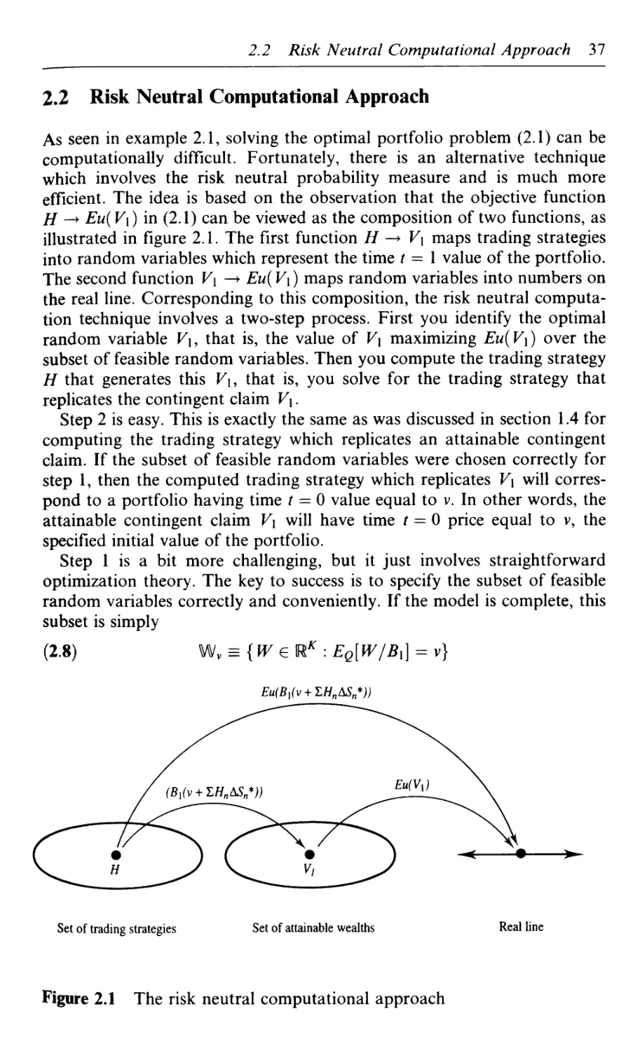
2.2 Risk Neutral Computational Approach 37
2.3 Consumption Investment Problems 40
2.4 Mean-Variance Portfolio Analysis 47
2.5 Portfolio Management with Short Sales Restrictions and
Similar Constraints 52
2.6 Optimal Portfolios in Incomplete Markets 58
2.7 Equilibrium Models 64
3 Multiperiod Securities Markets 72
3.1 Model Specifications, Filtrations, and Stochastic Processes 72
3.2 Return and Dividend Processes 84
3.3 Conditional Expectation and Martingales 88
3.4 Economic Considerations 92
3.5 The Binomial Model 100
3.6 Markov Models 106
4 Options, Futures, and Other Derivatives 112
4.1 Contingent Claims 112
4.2 European Options Under the Binomial Model 120

iv Contents
4.3 American Options 124
4.4 Complete and Incomplete Markets 133
4.5 Forward Prices and Cash Stream Valuation 136
4.6 Futures 140
5 Optimal Consumption and Investment Problems 149
5.1 Optimal Portfolios and Dynamic Programming 149
5.2 Optimal Portfolios and Martingale Methods 156
5.3 Consumption-Investment and Dynamic Programming 162
5.4 Consumption-Investment and Martingale Methods 168
5.5 Maximum Utility from Consumption and Terminal Wealth 173
5.6 Optimal Portfolios with Constraints 178
5.7 Optimal Consumption-Investment with Constraints 184
5.8 Portfolio Optimization in Incomplete Markets 193
6 Bonds and Interest Rate Derivatives 200
6.1 The Basic Term Structure Model 200
6.2 Lattice, Markov Chain Models 208
6.3 Yield Curve Models 217
6.4 Forward Risk Adjusted Probability Measures 222
6.5 Coupon Bonds and Bond Options 227
6.6 Swaps and Swaptions 229
6.7 Caps and Floors 234
7 Models with Infinite Sample Spaces 238
7.1 Finite Horizon Models 238
7.2 Infinite Horizon Models 243
Appendix: Linear Programming 250
Bibliography 254
Index 257

Preface
Aims and Audience
This book, which has grown out of research conducted by the author with
J. Michael Harrison in 1981, is designed to serve as a textbook for advanced
undergraduate and beginning graduate students who seek a rigorous yet
accessible introduction to the modern financial theory of security markets.
This is a subject that is taught in both business schools and mathematical
science departments, and it is also a subject that is widely and extensively
utilized in the financial industry. The derivatives industry has roughly $20
trillion in notional principal outstanding as this book goes to press, and the
portfolio management industry is probably even bigger. Mathematics play
crucial roles in both these areas. Consequently, financial practitioners (espe-
(especially 'rocket scientists,' quants, financial engineers, etc.) may find this book
useful for their theoretical background.
The full theory of security markets requires knowledge of continuous time
stochastic process models, measure theory, mathematical economics, and
similar prerequisites which are generally not learned before the advanced
graduate level. Hence a proper study of the complete theory of security
markets requires several years of graduate study (or equivalent, sink or
swim, experience). However, by restricting attention to discrete time models
of security prices it is possible to acquire an introduction without making a
big investment in the advanced mathematics. In fact, while living in a
discrete time world it is possible to learn virtually all of the important
financial concepts. The purpose of this book is to provide such an intro-
introductory study.
There is still a lot of mathematics in this book. The reader should be
comfortable with calculus, linear algebra, and probability theory that is
based on calculus (but not necessarily measure theory). Random variables
and expected values will be playing important roles. The book will develop
important notions concerning discrete time stochastic processes; prior
knowledge here will be useful but is not required. Presumably the reader
will be interested in finance and thus will come with some rudimentary
knowledge of stocks, bonds, options, and financial decision making. The
last topic involves utility theory, of course; hopefully the reader will be

vi Preface
familiar with this and related topics of introductory microeconomic theory.
Some exposure to linear programming would be advantageous, but those
lacking this knowledge can make do with the appendix and independent
study.
The aim of this book is to provide a rigorous treatment of the financial
theory while maintaining a casual style. There is an emphasis on computa-
computational examples, and exercises are provided to check understanding and
provide supplemental information. Readers seeking institutional knowledge
about securities, derivatives, and portfolio management should look
elsewhere, but those seeking a careful introduction to financial engineering
will find that this is a useful and comprehensive introduction to the subject.
Brief Summary of This Book
This book consists of seven chapters, each divided into a number of sections.
Important equations, fundamental statements, examples, and exercises are
labeled with numbers by chapter. For example, equation 2.1 is the first
equation in chapter 2.
This summary will point out which subjects are most important, and why
(usually because I think something is of fundamental importance rather than
a narrow result of limited or temporary consequence). It will also indicate
topics that are new, at least in their treatment. Arguably, there are no new
results in this book, but, like Monday morning quarterbacking, we can look
backwards and see better ways to say and do things. Hopefully, the book
will successfully do this, thereby conveying a clear understanding of some
fundamental ideas about security markets.
The first two chapters are devoted to single period models. Most of
the important concepts in this book are introduced here, making sections
1.1.-1.5 and 2.1-2.3 especially important. Section 2.4 is a modern treatment
of the important mean-variance portfolio analysis. Sections 1.6 and 2.5-2.7
are extensions and ventures into significant topics that are a bit out of this
book's mainstream.
The rest of this book is devoted to multiperiod models. This builds on the
single period results, emphasizing what is new and different. The redundant
material is kept concise in order to spare the patience of the stronger reader
(but such readers will still find it worthwhile to refer to the first two
chapters). Chapter 3 describes the basic elements of securities market models
and introduces important notions such as dividend processes and the bino-
binomial model. Chapter 4 is devoted to derivatives, including forwards and
futures; all the sections here are of fundamental interest. Chapter 5 attends
to optimal consumption and investment problems. Sections 5.2 and 5.4 are
the most important ones here (of course I might be biased, for the ideas
originated from my research in 1982 and 1986), because they deal with the
risk neutral computational approach. Sections 5.5-5.8 are extensions and
special cases.

Preface vii
Interest rate derivatives have become extremely important in recent years.
Chapter 6 is devoted to this subject, covering examples of key derivatives
,ucn as caps and swaptions and explaining how discrete time interest rate
models are used for derivative valuation.
Chapter 7 provides a brief look at models with infinite sample spaces. This
seemingly innocuous extension leads to significant mathematical complica-
complications and technicalities, and so this chapter will be most appealing to readers
whose interests lean in the direction of abstract mathematics.
Suggested Readings
The aim here is to provide some suggestions for further study, not to give an
account of which researchers are responsible for specific results. Most of the
references that will be mentioned are books, and some of these have very
comprehensive bibliographies of old research. This discussion is for the
reader who wishes to learn more mathematical finance, not history.
I will begin with the prerequisites, starting with basic probability theory.
Feller A968, 1971) is a classic still worth reading. I used Olkin, Gleser, and
Derman A980) for teaching probability courses in the 1970s and 80s. More
recent texts on basic probability theory include Ross A997a), Karr A993),
and Pitman A993). All these texts assume the reader knows some calculus,
but measure theory is not needed.
This book uses a lot of linear algebra and matrix theory, another subject
where the newer books are no better than a classic, namely, Gantmacher
A959). Nevertheless, here are some newer books: Brown A991), Roman
A992), Lay and Guardino A997), and Riess et al. A997).
Growing out of linear algebra is the subject of linear programming, the
problem of maximizing or minimizing a linear objective function subject to
some linear constraints. The appendix provides a quick overview of this
subject as well as a list of good references. A closely related subject, quad-
quadratic programming, involves similar optimization problems, differing only in
that the objective function is a quadratic function. Even more general are
convex optimization problems, also called nonlinear programming pro-
problems, where the objective function is not necessarily quadratic. Such
problems arise in finance when a portfolio manager seeks to maximize
expected utility. Some good references include Jeter A986), Hayhurst
A987), Bazaraa A993), and Rockafellar A997).
One subject of mathematics that should not be ignored is introductory
analysis. This has to do with things like convergence, open and closed sets,
functions, and limits. The books by Bartle and Sherbert A992), Mikusinski
and Mikusinski A993), Berbenan A994), and Browder et al. A996) are
Popular texts for this area.
Many of the preceding mathematical topics are covered in the intro-
introductions to the mathematics that are useful in economics by Klein
A973), Chiang A974), and Ostaszewski A993). These books are highly

viii Preface
recommended, because while giving primary emphasis to the mathematical
tools, they also explain how the math is used in economics, thereby provid-
providing some economic background for the study of financial markets. In this
same category, but focusing more narrowly on the application of optimiza-
optimization theory to economics, is the book by Dixit A990).
So much for the prerequisites. It is not necessary to be an expert in any of
the preceding areas, but you should be familiar with them.
I now turn to three areas that are developed in this book and that the
reader may wish to investigate further. For discrete time stochastic processes
(random walks, Bernoulli processes, Markov chains, martingales, etc.) there
are several introductory books to choose from: Hoel, Port, and Stone A972),
Cinlar A975), Karlin and Taylor A975, 1981), Taylor and Karlin A984),
Ross A995), A997b), Kijima A997) and Norris A998). At a more advanced
level (some measure theory may be used) one should be aware of the classics
by Doob A953), Neveu A975) and Revuz A984) as well as the more recent
books by Durrett A991) and Williams A991).
Another mathematical topic that is developed in this book is dynamic
programming. This has to do with the optimal control of a stochastic
process. In the common situation where the process is Markovian, this
topic is called Markov decision theory. Here one can do no better than
look at the work by Bertsekas A976), Denardo A982), Whittle A982, 1983),
and Puterman A994).
Finally I come to financial economics. Until recently, most of the books
on the theory of security markets were written by finance professors and
thus tended to emphasize economic theory at the expense of probability
modeling. Markowitz A990) is the definitive reference on single period
portfolio management. Ingersoll A987) and Duffie A992) provide good,
broad treatments of both discrete and continuous time models. Other
books containing some general treatments of discrete time models, but
presented in an older fashion, are Jarrow A988), Huang and Litzenberger
A988), and Eatwell, Milgate, and Newman A989). Meanwhile, three excel-
excellent books with a narrower focus, namely, on discrete and continuous time
models of derivatives, are by Cox and Rubenstein A985), Hull A993), and
Jarrow and Turnbull A996). Also worth looking at is the book by Wilmott,
Dewynne, and Howison A993), which studies option pricing from the
partial differential equation perspective, and the one by Dixit and Pindyck
A994), which studies capital investment decisions by firms and thus covers
some of the same ground as one would when investing in securities.
In the last few years a variety of finance books have been written by
mathematicians. These tend to emphasize probabilistic rather than economic
arguments. Luenberger A998) and Panjer et al. A998) take very broad,
introductory perspectives. Baxter and Rennie A996), Lamberton and
Lapeyre A996), Elliott and Kopp A998), and Mikosch A998) provide
good introductions to the continuous time theory after first developing
some discrete time theory. All of these might be sensible for a first year
graduate course.

Preface ix
At a more advanced, research level, one can find comprehensive treat-
treatments by Duffie A988), Dothan A990), Merton A990), Musiela and
Rutkowski A997), Bingham and Kiesel A998), and Bjork A998). Korn
tl997) and Karatzas and Shreve A998) provide advanced studies of optimal
consumption/investment problems. Rebonato A998) focuses on models of
interest rate derivatives.
Final Remarks
The first two printings of this book had a number of typographical errors.
These are listed on my web page: www.uic.edu/~srpliska. If you discover any
errors in this printing, please bring them to my attention by contacting me
at: srpliska@uic.edu.
A solutions manual for all the exercises in this book has been prepared for
instructors who adopt this book for classroom use. Instructors should con-
contact me about this, and I will mail a copy free of charge.
Stanley R. Pliska

Acknowledgments
This book grew out of lecture notes, first organized in a careful fashion for a
1991 PhD class in Japan, while I was a Yamaichi Visiting Professor of
Finance at Tsukuba University. I am indebted to Masaaki Kijima for mak-
making this experience possible. The work continued in 1992 while I was a
Distinguished Visiting Fellow at the London School of Economics (thank
you Michael J. P. Selby) and a Visiting Scholar at the University of Warwick
(thank you Stewart Hodges).
A preliminary version of the book was tried out in a 1994 PhD class at the
University of Illinois at Chicago. The reaction of the students was very
useful, especially the feedback from Bill Francis and Rashida Dahodwala.
In January, 1995, I took a close-to-final version to the Program on
Financial Mathematics at the Isaac Newton Institute for Mathematical
Sciences, University of Cambridge (I am indebted to Chris Rogers for
making this rewarding experience possible). There, parts of the book were
used for a course, and copies of the whole book were made available to
visiting researchers. The feedback I received and the hospitality of the
Institute while I was there for six months as a Prudential Distinguished
Visiting Fellow were important factors in the final stages of book prepara-
preparation. In particular, careful comments by Abel Cadenillas and Peter Lakner,
two visiting researchers who took copies for 1995-96 courses at their respec-
respective universities, were especially helpful. Also, Ruediger Kiesel provided
some useful feedback.
I am very grateful to Andriy L. Turinskiy, a graduate mathematics student
at my university, for helping me prepare the solutions manual. I also owe
thanks to various people, especially Tomasz Bielecki, John Fuqua, and
Edward Kao, for pointing out some typographical errors in the first two
printings of this book.

1 Single Period Securities Markets
7. \ Model Specifications
7 2 Arbitrage and Other Economic Considerations
13 Risk Neutral Probability Measures
IA Valuation of Contingent Claims
1.5 Complete and Incomplete Markets
1.6 Risk and Return
1.1 Model Specifications
Single period models are obviously unrealistic representations of complex,
time-varying, random phenomena such as stock and bond prices. But they
have the virtues of being mathematically simple as well as being able to
illustrate many of the important economic principles associated with even
the most complex, continuous time models. Hence single period models are
worth studying for introductory purposes.
The following elements of the basic, single period model are specified as
data:
• Initial date t = 0 and terminal date / = 1, with trading and consumption
possible at these two dates.
• A finite sample space ft with K < oo elements:
ft = {©i,GJ,..
Here each co e ft should be thought of as a possible state of the world, the
value of which is unknown at time t = 0 but which becomes apparent to
the investors at time t=\.
• A probability measure P on ft, with />(©) > 0 for all co e ft.
• A bank account process B = {Bt : t = 0,1}, where Bo = 1 and B\ is a
random variable. The bank account process will be distinguished from
the other securities because its time t = 1 price B\ (co) will be assumed to
be strictly positive for all co e ft. Usually, in fact, B\ ^ 1, in which case B\
should be thought of as the time / = 1 value of the bank account when $1
is deposited at time t = 0 and r = B\ - 1 ^ 0 should be thought of as the
interest rate. For many applications the quantities r and i?i are taken
to be deterministic scalars. If necessary for a particular application,

2 Single Period Securities Markets
however, B\ can be a positive random variable with r violating the
constraint r ^ 0.
• A price process S = {St : t = 0,1}, where St = (Si(f), S2{t)...,
SN(t)),N < oo, and ?„(*) is the time t price of security n. For many
applications these TV risky securities are stocks. The time t = 0 prices
are positive scalars that are known to the investors, whereas the time
t = 1 prices are non-negative random variables whose values become
known to the investors only at time t = 1. When N = 1, it is convenient
to simply write St for the time t price.
Having specified all the data describing the model, the next step is to
define several quantities of interest. A trading strategy H = (Hq,H\,
...,//#) describes an investor's portfolio as carried forward from time
/ = 0 to time t — 1. In particular, the scalar Ho is the number of dollars
invested in the savings account, and for n ^ 1 the scalar Hn is the number of
units of security n (for example, shares of stock) held between times 0 and 1.
In general, Hn can be positive or negative (negative means borrowing or
selling short), but sometimes there are constraints specified for the trading
strategies to be admissible (for example, Hn ^ 0 for n ^ 1; that is, no short
selling of the risky securities).
The value process V — { Vt : t = 0,1} describes the total value of the
portfolio at each point in time. By simple bookkeeping this is
Note that the value process depends on the choice of the trading strategy H
and that V\ is a random variable.
The gains process G is a random variable that describes the total profit or
loss generated by the portfolio between times 0 and 1. Since Hn{Sn{\)-
Sn{0)) is the net profit due to investment in the n\h security (similarly for the
bank account), the gains process is
where, by standard notation, ASn = Sn(\) — Sn@).
A simple calculation verifies that
A.1) K^Ko + G
Hence equation A.1) says that any change in the value of the portfolio must
be due to a profit or loss in the investment and not, for example, due to the
addition of funds from an outside source.
The movement of the security prices relative to each other will be impor-
important to study, so it is convenient to normalize the prices in such a way that
the bank account becomes constant. In other words, we are going to make
the bank account the numeraire. We do this by defining the discounted price
process S* = {S; : / = 0,1} by setting S* = (S\(t),..., S*N(t)) and

/./ Model Specifications 3
the discounted value process V* = { V* : t = 0,1} by
n=\
and the discounted gains process G* by the random variable
<? = ?//„ as;
where, as one should guess, AS* = 5*A) - S*@). With some more elemen-
elementary bookkeeping, one eventually obtains
A.2) K = Vt/Bt, t = 0,1
as well as the discounted counterpart of equation A.1), namely,
A.3) v; = vs + cr
Example 1.1 Suppose K = 2, N = 1, r = 1/9, So = 5, Si(©i) = 20/3
and 5i(co2) = 40/9. Then Bx = 1 + r = 10/9, SJ(coi) = 6, and
5j(co2)=4. For an arbitrary trading strategy H we have
Ko = r0* = Ho + 5//! as well as
G = (l/9)//0 4- HX{SX -5) G* = HX(S*X - 5)
Hence in state coi
Vx = (\0/9)H0 + B0/3) tf, V\ = Ho 4- 6tf,
G = (l/9)H0 4- E/3)//i G* = //i
whereas in state a>2
Vx = A0/9)//0 4- D0/9)//, Kf = //0 + 4HX
G=(\/9)H0-E/9)Hx G* = -Hx
It is easy to verify that equations A.1) to A.3) hold for both co e ft.
Example 1.2 With everything else the same as in example 1.1, take
K == 3 and set 5i((o3) = 30/9, so that Sf(co3) = 3. The other quantities
of interest are left to the reader. Although this was a simple modifica-
modification, it will be shown later that we have substantially changed the
character of this model.
Example 1.3 For a simple model featuring two risky securities, sup-
suppose K = 3, r = 1/9 and the price process is as follows:

4 Single Period Securities Markets
n
1
2
Sfl@)
5
10
discounted
n
1
2
S*n@)
5
10
COi
60/9
40/3
price
0I
6
12
Sn(l)
0J
60/9
80/9
process is
S,*(!)
0J
6
8
0K
40/9
80/9
given
0K
4
8
The other quantities of interest are left to the reader.
Example 1.4 Again, and as will be shown later, a small modification
will create a model having substantially different character. With
everything else the same as in example 1.3, we take K = 4 and set the
prices in state (o4 to be S\{\) = 20/9 and S2{\) = 120/9. Now the
discounted price process is:
1
2
sm
5
10
0I
6
12
0J
6
8
0K
4
8
0L
2
12
Exercise 1.1 Verify A.2).
Exercise 1.2 Verify A.3).
Exercise 1.3 Specify V, V\ G and G* for
(a) Example 1.2
(b) Example 1.3
(c) Example 1.4
1.2 Arbitrage and other Economic Considerations
In order for the single period model to be reasonable from the economic
standpoint, it must satisfy various criteria. For example, the model would
be unreasonable if the investors were certain to be able to make a profit on a
transaction, without any risk of losing money or even of failing to make a
gain. Such would be the case if there existed a dominant trading strategy.
A trading strategy H is said to be dominant if there exists another trading
strategy, say //, such that Ko = Vo and V\ (go) > V\ (co) for all o) G ?1 In

1.2 Arbitrage 5
other words, both trading strategies start with the same amount of money,
but the dominant one is certain to end up with more.
If H is a trading strategy satisfying Vo = 0 and V\ (co) > 0 for all co € ft,
then H is dominant because it dominates the strategy which starts with zero
money and does no investment at all. Conversely, if the trading strategy H
dominates the trading strategy H, then by defining a new trading strategy
H = H - H it follows by the linearity in the definition of V that
Vo = Vo - VQ = 0 and Ki(co) = Ki(co) - V\((o) > 0 for all cd e ft. In other
words, the following is true:
A.4) There exists a dominant trading strategy if and only if there exists a
trading strategy satisfying Vo = 0 and V\ (co) > 0 for all co € ft.
Note that the condition in A.4) is unreasonable from the economic
standpoint; an investor starting with zero money should not have a guaran-
guaranteed way of ending up with a positive amount of money. Hence a securities
market model having a dominant trading strategy cannot be a realistic
one.
Not surprisingly, if there exists a dominant trading strategy, then there
exists a trading strategy which can transform a strictly negative initial wealth
into a non-negative wealth. To see this, suppose H satisfies the condition in
A.4). Then by A.2) and the fact that Bt > 0, one has Fo* = 0 and F,*(co) > 0
for all cd € ft. So by A.3), (HU-. -,HN) must be such that <7*(co) > 0 for all
co € ft. Now define a new strategy H by setting Hn — Hn for n — 1,..., N
and
N
where
8 = minG*(co) >0
CO
It follows from the definition of Vf that V* = -5 < 0 and Kf (co) = Fo* +
G*(co) = -8 + G*(co) ^ 0 for all co e ft. Hence by A.2), again, H is as
desired.
Conversely, suppose there is a trading strategy such as H. Then by rever-
reversing the preceding argument one sees that (H\,...,HN) is such that
G*(co) > 0 for all co € ft. Hence upon setting Hn = Hn for n = 1,..., N and
it follows that the new trading strategy H satisfies Vo — 0 and V\ (co) > 0 for
all co g Q. In view of A.4), this means there is another equivalent condition:
A.5) There exists a dominant trading strategy if and only if there exists a
trading strategy satisfying Vq < 0 and Fi(co) ^ 0 for all co € ft.
The existence of a dominant trading strategy is unsatisfactory from an-
another standpoint: it leads to illogical pricing. For reasons which will soon

6 Single Period Securities Markets
become clear, it is often useful to interpret V\ (co) as the time / = 1 payoff of
a contract or claim when state co pertains, in which case Ko can be inter-
interpreted as the time t = 0 price of this claim. But if the trading strategy H
dominates H, then the contingent claims V and V have the same prices even
though the former claim has a strictly greater payoff in every state co. This is
not consistent with reality.
The pricing of claims will be logically consistent if there is a linear pricing
measure, that is, a non-negative vector n = (tc(coi), ..., 7t(coa:)) such that for
every trading strategy H you have
Now the illogical pricing associated with dominant trading strategies no
longer exists; each claim has a unique price, and a claim that pays more
than another in every state will have a higher time t — 0 price.
If there is a linear pricing measure n9 then by its definition and that of V*
one has
n=\
Taking H\ = ... = HN — 0, it can be seen that the linear pricing measure
must satisfy 7i(coj) + ... + k(g)k) = 1; thus one can interpret n as a prob-
probability measure on the sample space Q. Taking for arbitrary i e {1,..., N}
a trading strategy with Hn = 0 for all n ^ /, one sees that this equation
implies
A.7) S;@) = ?>(a))S;(l)(a)), n = l,...,N
CD
Conversely, suppose n is a probability measure on Q, satisfying A.7). Then
A.6) is satisfied, and it follows that:
A.8) The vector n is a linear pricing measure if and only if it is a probability
measure on Q satisfying A.7).
Since a linear pricing measure n can be taken to be a probability measure,
A.7) says that the initial price of each security is equal to the expectation2
under n of the final discounted price. Similarly, by the original definition of
7i, the initial value Vo of any portfolio is equal to the expectation under n of
the final discounted value of the portfolio.
It turns out there exists a close relationship between the concepts of
dominant trading strategies and linear pricing measures:
A.9) There exists a linear pricing measure if and only if there are no domi-
dominant trading strategies.
This important principle can be verified with linear programming duality
theory.3 In particular, let n G RK be a column vector, let Z € RN+[ denote
the column vector

1.2 Arbitrage 7
/ SUO) \
Z =
and let Z denote the (N + 1) x K matrix
Z =
l, co,)... S*N(l,
1 ... 1
/
Then by A.8) the existence of a linear pricing measure implies the existence
of a solution to the linear program
A.10)
maximize
subject to
it
0.
By duality theory there must exist a solution h— (h\,.
linear program
to the dual
minimize
subject to
hZ
0
and the two optimal objective values must coincide (in which case they
obviously equal zero). Now interpret the solution h of A.11) as a trading
strategy, with the last component of h corresponding to Hq. The objective
function in A.11) says that Fo* = 0, whereas the constraint says that
^7(co) ^ 0 for all co e ft. Since the minimizing strategy h has an objective
value equal to zero, there cannot be any trading strategies with Fo < 0 and
Fi(co) ^ 0 for all © e ft. Hence by A.5) the existence of a linear pricing
measure implies there cannot be any dominant trading strategies.
Conversely, if there are no dominant trading strategies, then A.11) has a
solution, namely, h = 0. It follows by duality theory that A.10) has a solu-
solution 7c which, as explained above, can be taken as the linear pricing measure.
To summarize matters up to this point, securities market models that
permit dominant trading strategies are unreasonable from the economic
point of view. Moreover, models without dominant strategies are reason-
reasonable, it would seem, because they are accompanied by linear pricing mea-
measures. Hence it makes sense to concentrate attention on the latter kind of
model. But before agreeing to drop from consideration all models with
dominant trading strategies, it is worth mentioning that one can have an
even less reasonable securities market model.
It is said that the law of one price holds for a securities market model if
there do not exist two trading strategies, say H and //, such that

8 Single Period Securities Markets
j/j (co) = V\ (co) for all co € ft but Vq > Vo. In other words, if the law of one
price holds, then there is no ambiguity about the time t = 0 price of any
claim. On the other hand, the law of one price does not hold if there are two
different trading strategies that yield the same time / = 1 payoff but the
initial values of the two corresponding portfolios are different. This notion
was mentioned above, just following principle A.5).
Notice that if there do not exist two distinct trading strategies yielding
the same payoff at time 1, then automatically the law of one price holds.
On the other hand, if H and H are as in the preceding paragraph, then
V* = V* and KJ > Fo* which, in turn, imply G*(g>) < G*(co) for all co e ft.
Defining a new trading strategy H by taking Hn = Hn - Hn for
w = 1,... ,7V yields G*(co) > 0 for all co e ft. Finally, taking Ho = - ?
HnS*{0) leads to VO = 0 and V\((o) > 0 for all co e ft. Hence by A.4) the
following is true:
A.12) If there are no dominant trading strategies, then the law of one price
holds. The converse, however, is not necessarily true.
In other words, if the law of one price fails to hold, then there will exist a
dominant trading strategy. The converse is not necessarily true, because, as
will be illustrated in example 1.5 that follows, you can have a dominant
trading strategy for a model that satisfies the law of one price. Thus failure
of the law of one price is, in a sense, worse than having dominant trading
strategies.
Example 1.5 For a trivial example where the law of one price fails to
hold, suppose K = 2, TV = 1, r = 1, So = 10, and Si(coi) = ?1@02)
= 12. Hence V\ is constant on ft, and for any scalar A, there is an
infinite number of trading strategies with V\ — X, each of which has a
different value of Vo.
Now suppose S\ (©2) is changed to the value 8. For any X eU2 there
is a unique H (and thus a unique time t = 0 price) such that V\ = X, so
the law of one price must hold. However, the trading strategy
H = A0, -1) satisfies Ko = 0 and V\ = (8,12), so it must be a domin-
dominant trading strategy.
Returning to the category of models that are without dominant trading
strategies, it is clear that such models cannot have trading strategies that
start with zero wealth and are certain to have a strictly positive amount of
wealth at time t = 1. But what about trading strategies that start with zero
wealth, cannot lose any money, and end up with a strictly positive amount of
wealth at time t = 1 in at least one of the states co, but not all? In other
words, investors would have the possibility of being able to make a profit on
a transaction without being exposed to the risk of incurring a loss. Such an
investment opportunity is called an arbitrage opportunity, and it is unreas-
unreasonable from the economic standpoint.
Formally, an arbitrage opportunity is some trading strategy H such that

1.2 Arbitrage 9
(a) VQ = 0.
(b) Vi ^ 0, and
(c) EVl > 0.
Note that an arbitrage opportunity is a riskless way of making money: you
start with nothing and, without any chance of going into debt, there is a
chance of ending up with a positive amount of money. If such a situation
were to exist, then everybody would 'jump in' with this trading strategy,
affecting the prices of the securities. This economic model would not be in
equilibrium. Hence for our single period model to be sensible from the
economic standpoint, there cannot exist any arbitrage opportunities.
The following principle is true by A.4) and example 1.6, which follows.
A.13) If there exists a dominant trading strategy, then there exists an arbit-
arbitrage opportunity, but the converse is not necessarily true.
Example 1.6 Suppose K = 2, N=l, r = 0, So = 10, Si(coi) = 12,
and S\((o2) = 10 (with one stock, the subscript denotes time). The
trading strategy H =(-10,1) is an arbitrage opportunity, because
Vo = 0 and V\ =B,0). However, there are no dominant trading
strategies, because n = @,1) is a linear pricing measure.
From A.2) and the fact that Bt > 0 for all / and co, it follows easily that H
is an arbitrage opportunity if and only if
(a) V*=0,
(b) V{ > 0, and
(c) EV{ > 0.
In fact, there is still another equivalent condition:
A.14) H is an arbitrage opportunity if and only if
(a) G* ^ 0, and
(b) EG* > 0.
To see this, suppose H is an arbitrage opportunity. By A.3),
G* = V{ - Fo*, so by the preceding remark G* ^ 0 and EG* = EV\-
EVq = EV\ > 0. Conversely, suppose (a) and (b) in A.14) are satisfied by
some trading strategy H. Then consider the strategy H = (Hq,H\,. ..)
where
n=\
Under H one has V* = 0. Moreover, by A.3) one has V\ = V* + G* = G*.
Hence (a) and (b) in A.14) imply V\ ^ 0 and EV\ > 0, in which case H is an
arbitrage opportunity by the preceding remark.
In summary, and as illustrated in figure 1.1, all single period securities
market models can be classified into four categories: A) there are no arbit-
arbitrage opportunities, B) there are arbitrage opportunities but no dominant

10 Single Period Securities Markets
Law of one price
does not hold
Figure 1.1 Classification of securities market models
trading strategies, C) there are dominant trading strategies but the law of
one price holds, and D) the law of one price does not hold. And only the first
category is reasonable from the economic point of view.
Unfortunately, it is not so easy to check directly whether a model has any
arbitrage opportunities, at least when there are two or more risky securities.
But there is an important necessary and sufficient condition for the model to
be free of arbitrage opportunities. This condition involves the discounted
price process and something called a risk neutral probability measure, which
is a special kind of linear pricing measure. It will be the subject of the next
section.
Exercise 1.4 Consider the model with K = 3, N = 2, r = 0, and the follow-
following security prices:
n Sn@)
S«A)(cd2) SB
4
7
10
3
4
Show that there exist dominant trading strategies and that the law of one
price holds.
Exercise 1.5 Show for example 1.3 that there are no dominant trading
strategies but there exists an arbitrage opportunity.

1.3 Risk Neutral Probability Measures 11
1.3 Risk Neutral Probability Measures
In the preceding section it was explained that if there exists a linear pricing
measure, then there cannot be any dominant trading strategies, although
there can still be arbitrage opportunities. In order to rule out arbitrage
opportunities, we need a little bit more: there must exist a linear pricing
measure which gives strictly positive mass to every state co € ft.
A probability measure Q on ft is said to be a risk neutral probability
measure if
(a) Q(co) > 0, all co e ft, and
(b) EQ[AS*n]=0,n=l,2,...,N.
Here the notation Eq[X] means the expected value of the random variable X
under the probability measure Q. Note that
eq[as:) = eq[s;(\) - s;(o)] = Ee[srn(i)] - s;(o),
so Eq[AS*] = 0 is equivalent to
A.15) ?fiK(i)] = m * = i,2,...,jv
This is essentially the same as A.7) and says that under the indicated
probability measure the expected time t — 1 discounted price of each risky
security is equal to its initial price. Hence a risk neutral probability measure
is just a linear pricing measure giving strictly positive mass to every co e ft.
We now come to a very important result.
A.16) There are no arbitrage opportunities if and only if there exists a risk
neutral probability measure Q.
Before proving this result, it is worthwhile to look at some examples and
provide some intuition.
Example 1.1 (continued) We want to find strictly positive numbers
g(coi) and Q((o2) so that A.15) is satisfied, that is,
Also Q must be a probability measure, so it must satisfy
It is easy to see that Q((O\) = 2(c°2) = 1/2 satisfies both equations, so
this is a risk neutral probability measure, and by A.16) there cannot be
any arbitrage opportunities.
Of course, with this simple example it is easy to see from the discounted
price process that there cannot be any arbitrage opportunities. Indeed,
principle A.16) is easy to understand in the case where there is a single
risky security (i.e., N = I). From the definition, there is an arbitrage oppor-
opportunity if and only if one can take a position H\ in the discounted price
process S* that will possibly gain but cannot lose. This means that either

12 Single Period Securities Markets
AS* ^ 0 with A5*(©) > 0 for at least one co e ft or AS* ^ 0 with
AS*(co) < 0 for at least one co e ft. Clearly, in both cases it is impossible
to find a strictly positive probability measure satisfying A.15). On the other
hand, if neither of these two cases applies, then one can find a risk neutral
probability measure and there are no arbitrage opportunities.
Example 1.2 (continued) The system of equations to be solved,
namely,
0(co3)
involves three unknowns but only two equations, so we will solve for
two of the unknowns in terms of the third, say C(toi). Thus this system
will be satisfied for an arbitrary real number Q((O\) if
G(a>2) = 2-3e(<oi) and g(co3) = -1 +20(co,)
Now for Q to be a strictly positive probability measure we must have
Q{(Oi) > 0 for all /. Using the preceding two equations, this leads to
three inequalities for Q(o>\), including Q(<0\) > 0. In view of its equa-
equation, g(co2) > 0 if and only if g(a>i) < 2/3. Similarly, 0(co3) > 0 if and
only if Q((O\) > 1/2. Hence our solution will be a strictly positive
probability measure if and only if 1/2 < g(a>i) < 2/3. In other
words, Q = (X, 2- 3A,, -1 + Ik) is a risk neutral probability measure
for each value of the scalar X satisfying 1/2 < X < 2/3, and there are
no arbitrage opportunities.
Example 1.3 (continued) We seek a solution of
6G(co2)+40(gK)
1 = 2@H+ g(©2)+ fi@3)
There exists a unique solution to these equations, namely, Q((O\) =
g(oK) = 1/2, 2@J) =0. This is a linear pricing measure, but this
solution is not strictly positive, so there does not exist a risk neutral
probability measure. By A.16), therefore, there must exist an arbitrage
opportunity. It takes a bit of work to find one; we will come back to
this example later.
Example 1.3 illustrates why the intuition which worked for the case of a
single risky security does not work when there are two or more risky
securities. Looking at the discounted price process for the first security, it
is clear that we can find a strictly positive probability measure Q satisfying
2sg[Si(l)] = 5. Similarly for the second risky security. The problem, how-
however, is that we cannot find a single strictly positive probability measure that
will simultaneously work for both securities. The interactions between these
two securities permit arbitrage opportunities even though, taken individu-

1.3 Risk Neutral Probability Measures 13
ally, the securities seem acceptable. And it is these kinds of interactions
which make the intuitive understanding of principle A.16) much more
difficult when there are two or more risky securities.
These three examples illustrate the three kinds of situations that can arise:
either A) there is a unique risk neutral probability measure, B) there are
infinitely many risk neutral probability measures, or C) there are no risk
neutral probability measures.
We now return to the explanation of A.16) for the case where N ^ 2. For
a general, single period model, consider the set
W = {X e Rk' : X = (Tfor some trading strategy H}
One should think of W as a set of random variables, and because of A.3) one
should think of each X e W as a possible time t = 1 discounted wealth when
the initial value of the investment is zero. Note that W is actually a linear
subspace of RK, that is, for any X, X eW and any scalars a and b one also
has aX + bX e W.
Next, consider the set
This is just the non-negative orthant of RK. In view of A.14) it is apparent
that there exists an arbitrage opportunity if and only if W Pi A ^ 0, that is, if
and only if the subspace W intersects with the non-negative orthant of RK.
Hence to find an arbitrage opportunity in a model for which there is no risk
neutral probability measure, one can use linear algebra to characterize W
quantitatively and then compute a vector in its intersection with A.
Now corresponding to the subspace W is the orthogonal subspace
WJ- = { Y G RK : X ¦ Y = 0 for all X e W}
where X • Y = X{(&\)Y{<n\) + ... + X(g>k) Y(g>k) denotes the inner product
of X and Y. If you consider the geometric picture for the case K = 2 (see
figure 1.2) or even the case K = 3, it should be easy to believe that
W n A = 0 implies the existence of a ray in W1 along which every compo-
component of every point not at the origin is strictly positive.4 In particular, along
this ray there will exist one point whose components sum to one, in which
case this point can be interpreted as a probability measure. In other words,
denoting
the geometry suggests that W n A = 0 if and only if W1 n P} / 0.
Since AS* e W for all n, it follows that any element of the set WL n (P+ is
actually a risk neutral probability measure. Conversely, if Q is any risk
neutral probability measure, then for any G* e W (with corresponding
trading strategy H) we have
A.17) EQG* = EQ
W=l I #1=1

14 Single Period Securities Markets
Figure 1.2 Geometric interpretation of the risk neutral probability measures
so Q G W1 n P(. Thus if we let M denote the set of all risk neutral prob-
probability measures, we have that
M = W1 n P+
Moreover, by the geometric intuition used above we conjecture that
W n A — 0 if and only if M ^ 0. This conjecture, of course, is the same as
principle A.16).
In order to make this argument more rigorous and apply it to the case of
general K, it is convenient to use a version of the Hahn-Banach theorem
called the separating hyperplane theorem. Consider the set
/\+ = {X e/\:EX ^ 1}
This is a closed and convex5 subset of RK, and the absence of arbitrage
opportunities implies W and A+ are disjoint. Hence by the separating
hyperplane theorem there exists some Y e W1 such that X ¦ Y > 0 for all
X € A1". For each k — \,..,K we can find a vector X in A whose
&th component is positive and other components are zeros, so every
component of Y must be strictly positive. By setting (?((*>*) =
Y(d}k)/[Y((O\) + ... + Y((oK)]9 it is clear that Q is a probability measure
with Q e W1. Since AS* G W for all n, we conclude that Q is a risk neutral
probability measure.
What about the converse of A.16)? This is easy. If Q is a risk neutral
probability measure, then, as explained above, for an arbitrary trading
strategy H we have equation A.17), which shows that G* cannot satisfy

1.3 Risk Neutral Probability Measures 15
both G* ^ 0 and EG* > 0. Hence by A.14) there cannot be any arbitrage
opportunities, and so our conjecture and principle A.16) are verified.
Example 1.3 (continued) We want to compute WflA, which we know
is non-empty. Knowing S*n, one computes AS* to be as follows:
1 1 1 \
2 2 -2-2
It follows that
W = {X e R3 : X
= (Hi + 2H2, H{ - 2H2, -Hi - 2H2) for some HuH2e R}
Notice that Xx + X3 = 0 for all leW. Conversely, given any vector X
with Xi + X-± = 0, one can readily find a unique trading strategy H
with G* = X. Hence
W = {X € R3 : ^i + X3 = 0}
that is,
W1 = {7 € R3 : r = (X,0, A.)for some AeR}
Now comparing W and A we see that
jjreiR3 -xx =Xi = o,x2>o}
So starting with any positive number X2, we compute the trading
strategy H which gives rise to the time t = 1 portfolio value @, X2,0).
This will be the solution of
Hx
Hi - 2H2 = X2
namely, Hi = X2/2 and H2 — -X2/4. Finally, upon setting
Ho = -HiS;@) - H2S*2@) = -(X2/2)E) - (-JT2/4)A0),
one obtains Hq = 0. It is apparent that H = @, X2/2, -X2/4) is an
arbitrage opportunity for every X2 > 0.
Exercise 1.6 Show that W and W1 are linear subspaces.
Exercise 1.7 Specify W and W1 in the case of
(a) Example 1.1.
(b) Example 1.2.
(c) Example 1.4.

16 Single Period Securities Markets
Exercise 1.8 Determine either all the risk neutral probability measures or
all the arbitrage opportunities in the case of example 1.4.
Exercise 1.9 Suppose K = 2, TV = 1, and the interest rate is a scalar para-
parameter r ^ 0. Also, suppose So = 1, Si(coi) = u ('up'), and Si(co2) = d
('down'), where the parameters u and d satisfy u> d > 0. For what values
of r, w, and d does there exist a risk neutral probability measure? Say
what this measure is. For the complementary values of these parameters,
say what all the arbitrage opportunities are.
Exercise 1.10 Let A denote the (K + 1) x (K + 2N) matrix
0 0 0 .-¦ 0 1 1 •¦• 1
ASJ(o>,) -ASJ(©i) AS*(co,) ... -AS^(a>,) _i o ••¦ 0
AS*(co2) -AS*(co2) AS2*(co2) ••¦ -A^(co2) 0 -1 •¦¦ 0
0 0 ... -
and let b denote the (K + l)-component column vector A,0,..., 0)'. Show
that
Ax = b, x ^ 0, xe UK+2N
has a solution if and only if there exists an arbitrage opportunity.
Exercise 1.11 Farkas's Lemma, a variation of the separating hyperplane
theorem, says that given an m x n matrix A and an m-dimensional column
vector b, either
Ax = b, x ^ 0, xe Un
has a solution or
yA ^ 0, yb>0, ye Um
has a solution, but not both. Use this and the results of exercise 1.10 to show
that if there are no arbitrage opportunities, then there exists a risk neutral
probability measure.
1.4 Valuation of Contingent Claims
A contingent claim is a random variable X representing a payoff at time
t = \. You can think of a contingent claim as part of a contract that a buyer
and a seller make at time t = 0. The seller promises to pay the buyer the
amount A"(go) at time / = 1 if co e ft turns out to be the true state of the

1.4 Valuation of Contingent Claims 17
world. Hence, when viewed at time t = 0, the payoff X is a random variable,
and so the problem of interest is to determine the time t = 0 value of this
payoff. In other words, what is the fair price that the buyer should pay the
seller at time t = 0 in order for the two parties to be happy with their
contract?
Now one might suppose that the value of a contingent claim would
depend on the risk preferences and utility functions of the buyer and seller,
but in a great many cases this is not so. It turns out that by the arguments of
arbitrage pricing theory there is often a unique, correct, time t = 0 value for
the contingent claim, a value that does not depend on the risk preferences of
the parties who buy and sell this claim.
Here is the argument. A contingent claim X is said to be attainable
or marketable if there exists some trading strategy H, called the
replicating portfolio, such that V\ = X. In this case one says that H gener-
generates X. Now suppose the time t = 0 price p of X is such that p > Vq.
Then an astute individual would sell the contingent claim for p at
time / = 0, follow the trading strategy H at a time t = 0 cost of Vq, and
pocket the difference p — Vq. This individual has made a riskless
profit, because at time t = 1 the value V\ of the portfolio corresponding
to H is exactly equal to the obligation X of the contingent claim in
every state of the world. In other words, if p%> Vq, then this astute
individual could lock in a profit of p - Vq by investing in a portfolio that
provides exactly the right value to settle the obligation on the contingent
claim.
Similarly, if p < Vq, then an astute individual would follow the trading
strategy -H, thereby collecting the amount Vq at time t = 0, and purchasing
the contingent claim for the amount p, thereby locking in a risk free
profit of Vq - p. At time t = 1 the amount collected X is exactly what is
needed to settle the obligation V\ associated with the trading strategy —H.
Again, if p < Vq, then this astute individual could lock in a riskless profit
ofVo-p.
Up = Vq, then apparently we cannot use H to create a riskless profit. So
does this mean that Vq is the correct value of XI Not necessarily, for
suppose there is a second trading strategy, say H, such that V\ = X but
Vq ^ Vq. Then even if p — Vq, one could use H and the argument above to
lock in a riskless profit, thereby implying the different price Vq. The problem
here, of course, is that the law of one price does not hold. So for Vq to be the
unique, logical, time / = 0 price of X, it is necessary to assume that the law of
one price does indeed hold. In this case we say that Vq is the price of X as
implied by arbitrage pricing theory.
As explained in section 1.2, if there are no arbitrage opportunities, then
there are no dominant trading strategies, and if there are no dominant
trading strategies, then the law of one price holds. Thus by A.16) the
existence of a risk neutral probability measure implies the law of one price.
Alternatively, we can see this directly from the following, very important
calculation:

18 Single Period Securities Markets
A.18) If Q is any risk neutral probability measure, then for every trading
strategy H one has
K0 = VS = EQ VI = Ee[ V\ - G*] = EQ V; -fjf Hn AS'n
= EqV\ - J2HnEQ[AS'n} = EQV;-0 = EqV; = EQ[Vt/Bi)
n=l
In other words, under Q the expected, discounted, time / = 1 value of any
portfolio is equal to its initial value. So if there is a positive probability that
the portfolio will go up in value, then there also must be a positive prob-
probability of going down in value, and vice versa. Moreover, there is no way you
can have two trading strategies H and H with both V\ = V\ and V$ ^ Vo, so
the law of one price must hold.
Notice for future reference that the calculation in A.18) does not depend
on the choice of Q, because V\ is the time / — 1 discounted value of the
portfolio under some trading strategy. In other words, for a model where
there are two or more risk neutral probability measures, Eq V\ is constant
with respect to such Q.
Returning to the contingent claim X, by the arguments near the beginning
of this section we have the following important valuation concept:
A.19) If the law of one price holds, then the time / = 0 value of an attainable
contingent claim A' is Vo = H0BQ + ]T^=i HnSn(Q), where H is the
trading strategy that generates X.
If we have the stronger condition that the model is free of arbitrage
opportunities, then we have the following, sensational result:
A.20) Risk neutral valuation principle: If the single period model is free of
arbitrage opportunities, then the time / = 0 value of an attainable
contingent claim A" is Eq[X/B\\, where Q is any risk neutral probabil-
probability measure.
This follows immediately from A.2), A.18), A.19), and the fact that B0=l.
We now turn to several examples.
Example 1.1 (continued) Suppose r — 1/9, A"(o>i) = 7, and ^@J) = 2.
Then the time t — 0 value of X is
EQ[X/Bi] = (l/2)(9/10O + (l/2)(9/10J = 4.05
providing A'is attainable. How do we check this? One way is to try to
compute the trading strategy H that generates X. This can be done by
solving
X/B\ = V\ = V* + G* = 4.05 + HiAS\
There is one unknown, H\, and two equations, one for each co, but
both equations give the same solution, namely, H\ = 2.25. To deter-
determine Hq one can solve

/. 4 Valuation of Contingent Claims 19
4.05 = Ko = #o + HXSX = Ho + B.25)E)
to obtain i/0 = -7.2.
In summary, the contingent claim Zis indeed attainable. To generate
it you start with 4.05, you borrow 7.2 at the riskless interest rate r — 1/9,
and you use the sum 4.05 + 7.2 = 11.25 to purchase 11.25 -=- 5 = 2.25
shares of the risky asset. At time t = 1 you must pay G.2) A0/9) = 8 to
settle the loan. The amount of money remaining in the portfolio will
depend on co: in state coi this will be V\ — B.25)B0/3) — 8 = 7, whereas
in state co2 this will be Vx = B.25) D0/9) -8 = 2. If the time t = 0 value
of this contingent claim were different from 4.05, then you could use this
trading strategy in the manner discussed at the beginning of this section
to lock in a riskless profit.
Example 1.7 For a general securities model, taking
co ^ co
for some (?> ? ft leads to the time / = 0 price (if X is attainable)
EQ[X/Bi] = ?fi(a>)Jf (©)/*, (co) = 0(d>)/*,F)
For this reason Q((b)/B\ (cb) is sometimes called the state price for state
co E ft. Thus the time / = 0 price of an attainable contingent claim is
simply the weighted sum across the states of the payoffs under X, with
the weights being the state prices.
Example 1.8 - Call Options Suppose iV = 1 and X has the form
+ 0,S! - e}
where e is a specified number called the exercise price or the strike price.
Hence Xis the contingent claim corresponding to the right to purchase
the risky security at time t = 1 for the amount e. If it turns out that
Si ^ e, then at time / = 1 this right will be worth the difference S\ - e,
and so the option should be exercised. On the other hand, if S\ ^ e, then
at time t = 1 this right will be worth nothing, and so the option should
not be exercised. If A'is attainable, then its time / = 0 price is
where ft' = {co e ft : Si(co) ^ e}.
Example 1.1 (continued) With r = 1/9 and e = 5, the time t — 1 value
of the call option is

20 Single Period Securities Markets
*(co) {
v > y 0, CO = 0J
Hence if * is attainable, then its time t = 0 value is
EQ[X/B{] = (l/2)(9/\0)E/3) =0.75
To check whether * is attainable, we shall try to compute a trading
strategy that generates X. We solve the system of two equations (one
for each state)
Vx =//o?i+#iSi =X
for the two unknowns and obtain //, = 0.75 and Hq — -3. So, indeed,
Vo = Ho + H{Sq = -3 + @.75)E) = 0.75 is the time t = 0 price of X.
Example 1.9 - Put options Suppose N = 1 and X has the form
Then *is the contingent claim that gives the owner the right to sell the
risky security at time / = 1 for the amount e. This option should be
exercised if and only if S\ < e.
Example 1.2 (continued) Consider an arbitrary contingent claim
* = (*i,*2,*3). This claim is marketable if and only if V\ —
HqB\ + H\S\ — X for some pair of numbers Ho and H\, that is,
there exists a solution to the system of equations
co, : A0/9)//0-f B0/3)//! = X\
co2 : (lO/9)//o + D0/9)//, = X2
co3:
Since there are three equations with only two unknowns, perhaps there
is no solution. Let's see. Using the third equation to substitute for //0
in the first two gives
Hx = C*1 — 3JT3)/1O and //, = (9X2 - 9*3)/10
Hence the contingent claim is attainable if and only if these two values
of Hx are the same, that is, if and only if
A.21) Xx - 3*2 + 2*3 =0
This example illustrates the general principle that not all the contingent
claims are attainable whenever the underlying model has multiple risk
neutral probability measures, a principle that will be developed in the
next section.

1.5 Complete and Incomplete Markets 21
Exercise 1.12 For example 1.1 with r — 1/9, what is the price of a put
option with exercise price e = 5? What trading strategy generates this con-
contingent claim?
Exercise 1.13 - Put-Call parity Suppose the interest rate r is a scalar, and let
c and/? denote the prices of a call and put, respectively, both having the same
exercise price e. Show that either both are marketable or neither is market-
marketable. Use risk neutral valuation to show that in the former case one has
c-p = S0-e/{l+r)
1.5 Complete and Incomplete Markets
Just because, as will be assumed throughout this section, there exists a risk
neutral probability measure, it does not necessarily follow that one can use
the risk neutral valuation principle to determine the time t = 0 price of a
contingent claim. The problem, of course, is that the contingent claim might
not be marketable, in which case it is not clear what its time t — 0 price
should be. In particular, there is no reason to be sure that Eq[X/B\] is the
correct value. We therefore need a convenient method for checking whether
a contingent claim is indeed marketable. One method, as illustrated with
example 1.1 in the preceding section, is to try to compute a generating
trading strategy by solving a system of linear equations. A solution to such
a system will exist if and only if the contingent claim is marketable. But there
exist alternative methods.
The model is said to be complete if every contingent claim X can be
generated by some trading strategy. Otherwise, the model is said to be
incomplete. It turns out there are simple ways to check whether a model is
complete. One way is to understand when the system of linear equations
mentioned just above will always have a solution.
A.22) Suppose there are no arbitrage opportunities. Then the model is com-
complete if and only if the number of states in ft equals the number of
independent vectors in {B\, S\ A),..., SnA)}¦
To see this, define the K x (N + 1) matrix A by
A =
SN(l)((oK)_
and consider column vectors H = Bf0, #1, , HN)' and X = (X{,..., XK).
Then the model is complete if and only if the system AH = X has a solution

22 Single Period Securities Markets
H for every X. By linear algebra, this last fact will be true if and only if the
matrix A has rank K, that is, this matrix has K independent columns.
Example 1.1 (continued) The matrix
[10/9 20/3]
[10/9 40/9 J
has two independent rows, so this model is complete
Example 1.10 Suppose we take example 1.1 and add a second risky
security with S2@) = 54, S2(l)(a>i) = 70, and 5r2(l)(co2) = 50. Note
that Q = A/2,1/2) is still a risk neutral probability measure because
54 = (l/2)(9/10O0 + (l/2)(9/10M0. Now
[
10/9 20/3 70
10/9 40/9 50
but this still has rank two. Hence this augmented model is still com-
complete, although the risky securities are redundant.
Example 1.2 (continued) The matrix
0/9 20/3"
A = 10/9 40/9
10/9 10/3_
has rank two, whereas K = 3, so this model is incomplete. Now we saw
earlier that the risk neutral probability measures are of the form
Q = (X, 2 — 3 A., — 1 -f 2X.), where X is any scalar satisfying
1/2 < X < 2/3. Suppose we take any such Q and then use the formula
from the risk neutral valuation principle A.20):
EQ[X/B\) = A,(9/10)JTi + B - 3^(9/10)^2 + (-1 + 2A,)(9/10)JT3
If X is marketable, then this value will be the same for all X because it
must coincide with Fo under the generating trading strategy. Note that
this value is the same if and only if equation A.21) holds. Moreover,
recall from the discussion of A.21) that a contingent claim is market-
marketable if and only if A.21) holds. Putting this together, we see that a
contingent claim in this model is marketable if and only if Eq[X/B\) is
the same value under every risk neutral probability measure. It turns
out that this necessary and sufficient condition holds in general.
As stated earlier, throughout this section it will be assumed that M / 0,
where M is the set of all risk neutral probability measures. Now if the
contingent claim X is attainable, then Eq[X/B\] is constant with respect to
all Q g ML This is because, as already discussed in connection with A.18),

1.5 Complete and Incomplete Markets 23
one has Vq = EQ[X/B{} for all QeM, where Vo is the initial value of the
replicating portfolio.
To show the converse, it suffices to suppose that the contingent claim X is
not attainable and then demonstrate that Eq[X/B\] does not take the same
value for all Q e M. Consider the K x (N + 1) matrix A, the (N + 1)-
dimensional column vector //, and the /^-dimensional column vector X as
described above in connection with A22). If X is not attainable, then there is
no solution H to the system AH = X. By a slightly modified version of
Farkas's Lemma (see exercise 1.11), it follows that there must exist a row
vector n = (n\,..., nK) satisfying
nA = 0, nX > 0.
Let Q G IU be arbitrary, and let the scalar X > 0 be small enough so that
Q(a>k) = ?(©*) + XnkBx (©*) > 0, all k = 1,..., K.
Since n times the 'zeroth' column of A is zero, it follows that the quantity Q
which was just defined is actually a probability measure giving positive
probability to each state co e ft. Moreover, for any discounted price process
S* we have
where we used the fact that n times the '«th' column of A is zero. But Q e M,
so Y, Q(®k)S*{l)(<Qk) = S*@), in which case we realize that QzM.
It remains to show that the expected value of X jB\ under Q is different
from the expected value under Q. Denote 5 = kX and note that 5 > 0. Then
EQ[X/BX) = Y^Q(®k)X(<ok)/[B{(®k)]
^ fi()*()/[i* ()] +
In other words, Eq[X/B\] ^ ^[X/^i] since Xis not attainable. In summary,
therefore, we have the following important result.
A.23) The contingent claim X is attainable if and only if Eq[X/B\] takes the
same value for every Q e M.
Notice that if M is a singleton and Xis an arbitrary contingent claim, then
trivially Eq[X/B\] takes the same value for all Q e M, in which case Zmust
be attainable and the model must be complete. On the other hand, suppose
every contingent claim X is attainable but M contains two distinct risk
neutral probability measures, say Q and Q. In this case there must exist
some state co^ with Q((dk) / G(g>/0, so take the contingent claim Xdefined by

24 Single Period Securities Markets
\, otherwise
Then
EQ[X/BX) = q
But this contradicts A.23), which says that if X\s attainable, then Eq[X/B\\
takes the same value for all Q e M. Hence if the model is complete, then M
cannot have more than one element. We can combine these observations as
follows.
A.24) The model is complete if and only if M consists of exactly one risk
neutral probability measure.
To summarize matters, if the model is complete then we know how to
price all the contingent claims. Moreover, if the model is not complete then
we know how to price some of the contingent claims, namely, all the attain-
attainable ones. But what about the claims that are not attainable in an incomplete
model? For such a claim we cannot pinpoint its time t = 0 price, but it turns
out that at least we can identify an interval within which a fair, reasonable
value for the time t = 0 price must fall.
For the rest of this section we shall be considering an incomplete model
and we shall focus on an arbitrary contingent claim X that is not attainable.
Consider the quantity
V+{X) = inf{EQ[Y/Bi] : Y > X, Y is attainable}
and refer to figure 1.3 throughout this discussion. The choice of Q e M here
does not really matter since it is only being used to compute the price of
attainable contingent claims. Note that XB\ is an attainable contingent claim
for all values of the scalar X and that XB\ ^ X for all large enough values of
X; hence V+(X) is well defined and finite. Notice also that V+(X) is bounded
below by sup {EQ[X / Bx] : QeM}.
The quantity V+(X) is important because it is a good upper bound on the
fair price of X. This follows from an arbitrage argument that is similar to the
one discussed in the preceding section. If X could be sold for a greater
amount, say p > V+(X), then one should make use of the trading strategy
that replicates Y, which is any attainable contingent claim satisfying Y ^ X
and/? > Eq[Y/B\] ^ V+(X). In particular, one should sell Xat time t = 0,
use part of the proceeds to purchase for the amount Eq[Y/B\] the portfolio
which replicates Y, and pocket the difference p - EQ[Y/B\] as a riskless
profit. At time / = 1 the value of the portfolio Y will always be enough to
cover the obligation X of the contingent claim. Hence V+(X) is the price of
the cheapest portfolio that can be used to hedge a short position in the
contingent claim X.
The unattainable contingent claim X cannot trade at a price higher than
V+(X), or else there will exist an arbitrage opportunity. Similarly, this
contingent claim cannot trade at a price lower than K_(A"), where

1.5 Complete and Incomplete Markets 25
X(co2)
solution of A.25) _
solution of A.26)
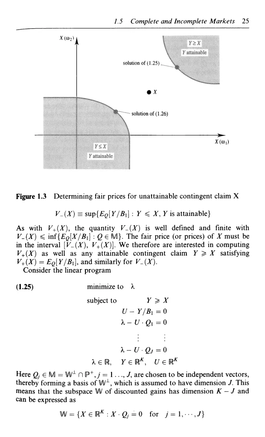
Figure 1.3 Determining fair prices for unattainable contingent claim X
V.(X) = sup{EQ[Y/Bi] : Y ^ X, Y is attainable}
As with V+(X), the quantity V-(X) is well defined and finite with
V-(X) < inf{EQ[X/Bi] : g € M}. The fair price (or prices) of X must be
in the interval [F_(JF), V+(X)]. We therefore are interested in computing
V+(X) as well as any attainable contingent claim Y ^ X satisfying
V+(X) = EQ[Y/Bi], and similarly for V.{X).
Consider the linear program
A.25)
minimize to k
subject to
Y > X
U - Y/Bi = 0
X-U>Qx=0
X - U Qj = 0
x € R, reU^, c/ g R*
Here 0 ? M = W1 nP+,;= 1...,/, are chosen to be independent vectors,
thereby forming a basis of W1, which is assumed to have dimension /. This
means that the subspace W of discounted gains has dimension K - J and
can be expressed as
= {X
X Qj =
for

26 Single Period Securities Markets
Now suppose Y is an attainable contingent claim with time t = 0 price X,
and set U = Y/B\. Because Vf — KJ -f G\ this statement is equivalent to
the statement that U - Xe e W and U = F/2?i, where <? here is a row vector
of l's. But e • Qj = I for ally, so this statement, in turn, is equivalent to the
statement that U = Y/B\ and U ¦ Q, - X = 0 for j = 1, ¦ • • J. Hence the
feasible region in the linear program A.25) can be interpreted as being the
set of all attainable contingent claims Fwith Y ^ X. It follows that if X and
Y are part of an optimal solution of this linear program, then V+{X) — X
and Y is an attainable contingent claim with Y ^ X and time / = 0 price
equal to V+(X). Note that an optimal solution always exists to this linear
program because the feasible region is nonempty and the objective function
is bounded below.
Similarly, if you solve the linear program
A.26) maximize X
subject to Y ^ X
U - Y/Bx = 0
X- UQ} =0
X - U • Qj = 0
XeU, Y e (RA\ u e UK
and obtain an optimal solution (X, Y, ?/), then V-(X) and Yis an attainable
contingent claim with Y ^ X and time / = 0 price equal to V-(X).
It turns out that not only does linear programming enable us to comple-
completely solve for the quantities of interest, but it gives us something extra as a
bonus. Consider another linear program:
A.27) maximize
A = l
subjet to Gi + •• • + Qj = 1
\\f eUK QeUJ \|/ s* 0
If (v|/, 0) is an arbitrary feasible solution, then
V|/ = 0101 +0202 + ••¦ + 0/0/,
which is non-negative. Moreover, with e a row vector of Vs we have
e • \|/ = Q\e ¦ Q\ + • • • + dje ¦ Qj = Q{ + • • • + 0y = 1

1.5 Complete and Incomplete Markets 27
since each Qj is a probability measure, so v|/ can be interpreted as a prob-
probability measure too. For any discounted price process S* we have
E^[AS*n] = Q& • AS*n + • •. + djQj AS*=0
since each Qj eM. Hence \|/ can be interpreted as a linear pricing measure
(but not, necessarily, as a risk neutral probability measure). In other words
the feasible region can be interpreted as the closure of M. It follows that the
optimal value of the objective function in linear program A.27) is precisely
equal to s\xp{EQ[X/B\] : Q e M}.
Now here comes a startling result of fundamental importance. By linear
programming theory the linear programs A.25) and A.27) are duals of each
other. Both programs are feasible, so by linear programming duality theory,
their optimal objective values are equal to each other. Analogous results
hold for linear program A.26), of course, so all these results can be summar-
summarized as follows:
A.28) If M ^ 0, then for any contingent claim X one has
V+(X) = sup{EQ[X/Bi] : Q € M} and
V.(X) = mf{EQ[X/Bi] : Q € M}.
Of course, if X is attainable, then V+(X) = V-(X) is its usual time / = 0
price.
Example 1.2 (continued) Consider the contingent claim X = C0,20,
10). This is not attainable, because it does not satisfy equation A.21).
Recalling that M consists of all probability measures of the form
Q = (q,2 - 3q, -1 + 2q) where 1/2 < q < 2/3, it is straightforward
to compute (making a slight and obvious change of notation for this
particular example) Eq[X/B\] =21 - 9q. Hence
V+(X) = supEq[X/Bx] = sup {27 - 9q} = 21 - 9A/2) = 22 1/2
q q
and
= in(Eq[X/B{] = inf {27 - 9q} =21 - 9B/3) = 21
q q
Upon solving the linear program A.25) one obtains the attainable
contingent claim corresponding to V+(X); this is Y = C0,20,15), as
can be verified by checking equation A.21) and checking that the time
t = 0 price of Y is indeed 22 1/2. Similarly, the attainable contingent
claim corresponding to V-(X) is verified to be Y = C0, 50/3,10).
Exercise 1.14 Explain why the model in example 1.4 is not complete.
Characterize the set of all the attainable contingent claims. Compute
V+(X) and V_{X) for X = D0,30,20,10).

28 Single Period Securities Markets
Exercise 1.15 Use A.23) to verify whether there are any values of the
exercise price e such that the call option is attainable for the model in
example 1.2. Similarly, specify which put options are attainable. Assume
r= 1/9.
Exercise 1.16 Just after linear program A.25) it was asserted that one
can choose Q}¦ e M = W1 n P+, y = 1, •••,/, to be independent vectors,
thereby forming a basis of Wx, which is assumed to have dimension J.
Use linear algebra to carefully verify this assertion. Compute Qj vectors
for example 1.4.
1.6 Risk and Return
With Q a risk neutral probability measure and co e fi, recall that
g((o)/Z?i(@) is sometimes called the state price of co. For this reason, the
random variable
is called the state price vector or the state price density. The main result to be
shown in this section is that the risk premium of an arbitrary portfolio is
proportional to the covariance6 between a return corresponding to the state
price density and the return for the portfolio, a result that resembles a
principal finding of the capital asset pricing model.
Assuming the time t = 0 price Sn@) is strictly positive, the return Rn for
risky security n is defined to be the random variable
_ 5,A)-5,@)
Rn- Sn{0) , n-\, ¦ ,N
Similarly, the return corresponding to the bank account is defined by
The returns are useful quantities for a variety of purposes, one of which is
that if you know the time t = 0 prices and the returns, then you can compute
time / = 1 prices. Since prices are non-negative one has Rn ^ - 1, with
equality if and only if Sn{\) = 0. It is left as an exercise to verify that the
gain for a portfolio can be written as
N
A.29) G = HQB0R0 + ? HnSn@)Rn
Hence the gain for a portfolio is a weighted combination of the underlying
returns, each weight being the amount of money invested at time / = 0 in the
corresponding security.

1.6 Risk and Return 29
The returns can also be used to compute risk neutral probability measures.
Since
Rn}S,,@) - [1 + Rq]Sr@)
it follows from A.15) that
A.30) If Q is a probability measure with g(co) > 0 for all coefi, then Q is a
risk neutral probability measure if and only if
—
Notice that when the interest rate Rq = r is deterministic, the equation in
A.30) becomes simply
EQ[Rn]=r, n=h...,N
This is one example of many situations where, under the assumption of a
deterministic interest rate, one has a nice, and often important, relationship
involving returns. Therefore, this assumption will be in force for the balance
of this section, as will be the assumption that there exists a risk neutral
probability measure Q.
The mean return for security «, denoted Rn — E[Rn], often plays an
important role. For example, it is easy to see that cov(/?,,,L) = E[RnL] —
E[Rn]E[L] = EQ[Rn] - E[Rn] = r - Rn. In other words,
A.31) Rn-r= -cov(RfU L), n = 1, ¦ • ¦ ,7V
The difference Rn - r here is called the risk premium for the security; nor-
normally this is positive because investors usually insist that the expected
returns of risky securities be higher than the riskless return r. Thus A.31)
says that the risk premium of a security is related to the correlation7 between
the security's return and the state price density.
Consider the return R of a portfolio corresponding to an arbitrary trading
strategy H = (Hq,H\,...,Hn). Assuming Vo > 0, this is
Using Sn(l) = 5n@)[l + Rn] and the definition of Vt one obtains
A.32) R = ^r

30 Single Period Securities Markets
If you interpret Ho/Vo as the fraction of money invested in the savings
account (recall Bo = 1) and HnSn(O)/Vo as the fraction of money invested in
the nth security, then A.32) says that the return on the portfolio is a convex
combination of the returns of the individual securities. Using A.31), A32),
and some basic properties of the covariance, it is straightforward to verify
that
A.33) R-r=-cov{R,L)
where, of course, R = E[R].
Now fix two scalars a and b with b ^ 0, and assume the contingent claim
a + bL is attainable, that is, suppose there exists some trading strategy H'
such that V[=a + bL. Since FJA +K)=a + bL (here V and R' denote
the value and return processes, respectively, corresponding to //')> one can
substitute for L and use the properties of the covariance relationship to
verify that
cov(J?,L)=-^ cov(R,Rf)
b
(R still corresponds to an arbitrary trading strategy). Hence A.33) can be
rewritten as
A.34) R-r=-^ co\{R,Rf)
b
In particular, in the special case where you choose H = Hf, A.34) says
that
R' - r = - -^ cov(#, R1) = - -^ var(/0
b b
Using this to substitute for V^/b in A.34), where now we are back to an
arbitrary trading strategy H, we obtain the following:
A.35) Suppose for scalars a and b the contingent claim a + bL is generated by
some portfolio having return R' and suppose the interest rate r is
deterministic. Let R be the return of an arbitrary portfolio. Then
= cov(*,*')
var(fl') v ;
The ratio cov(R, R')/v&v(R') is called the beta of the trading strategy H
with respect to the trading strategy H'. This result says that the risk premium
of H is proportional to the risk premium of H'', with the proportionality
constant being this beta. Or from a slightly different perspective, A.35)
says that the risk premium is proportional to its beta with respect to a
linear transformation of the state price density. This result resembles the
traditional capital asset pricing model, only here Hf corresponds to a linear
transformation of the state price density instead of the market portfolio.
Notice that with a deterministic interest rate r and with arbitrary scalars a
and b (b ^ 0), the contingent claim a + bL is attainable if and only if the

/. 6 Risk and Return 31
state price density L is. This is because 7/o(l + r) + JZ//„?„( 1) = a + bL if
and only if
Exercise 1.17 Verify equation A.29), both in general and by applying it to
example 1.1.
Exercise 1.18 Assuming the time t = 0 price is strictly positive, the dis-
discounted return R*n is defined by R*n = [S*(l) - S*n{0)]/S*@) for n = 1,..., N.
Show that
(a)
n=l
(c) The strictly positive probability measure Q is a risk neutral probability
measure if and only if EQ[R*n] = 0 for n = 1,..., N.
Exercise 1.19 Analyze the risk and return properties of example 1.1 assum-
assuming P(@\) = p for a general parameter 0 < p < 1.
(a) What are Rx and Rtf
(b) What is L?
(c) Verify A.31) forn = 0 and 1.
From now on suppose H = (Ho,H\) = A,3).
(d) What are R and W.
(e) Verify A.32).
(f) Verify A.33).
(g) What are H1\ V^ and R"?
(h) Verify A.34).
(i) Verify A.35).
NOTES
1 If A" is a random variable, this means A' is a real-valued function on the sample space
n. In other words, we know the value X(u>) for each state of the world co e 17.
2 The expected value (also called the mean or average) of the random variable X is
denoted EX or E[X] and defined to be

32 Single Period Securities Markets
More generally, if/is a real-valued function on the real line,
In particular, for scalars a and b, E[aX + b] = aEX -f b.
3 See the appendix on linear programming.
4 In other words, for some Y € WL whose components are all strictly positive, the
ray is of the form {Y e UN : Y = XY, X > 0, X e U}.
5 Closed means that if {X\} is a sequence of points in A4 that converges to some
X eUK, then X e /\+; convex means that for any I, J G A1 and any scalar X with
0 < X < 1, then XX + A - X)X e A\
6 For two random variables X and 7, the covariance cov(Ar, Y) is defined to be
E[XY] - E[X]E[Y}. Note that cov(X - ?[*], Y) = cov(JT, 7). Moreover, given
three random variables X, Y, and Z and two scalars a and 6, one has
cox{aX + 6Z, F) = a cov(^, 7) + b cov(Z, F).
7 The variance, denoted var(Ar), of a random variable A" is defined by var(X)
= ?[^2] - (E[X}J = E\(X - EfJIT]J]. The standard deviation of JT is ox =
y/vsLr(X). The correlation between the random variables X and Y (assuming
gx > 0 and a>- > 0) is defined by p(X, Y) = cov(X, Y)/(gxoy). Hence the risk
premium for security n equals -p(Rn,L)oRn<jL.

2 Single Period Consumption and
Investment
2.1 Optimal Portfolios and Viability
2.2 Risk Neutral Computational Approach
2.3 Consumption Investment Problems
2.4 Mean-Variance Portfolio Analysis
2.5 Portfolio Management with Short Sales Restrictions and Similar
Constraints
2.6 Optimal Portfolios in Incomplete Markets
2.7 Equilibrium Models
2.1 Optimal Portfolios and Viability
This chapter is concerned with the problem of choosing the best trading
strategy for the purpose of transforming wealth invested at time t — 0 into
time t = 1 wealth. With some variations of this problem that will be con-
considered in later sections, a portion of the wealth is consumed at time t = 0.
The problem is to compute an optimal trading strategy, and for this a
measure of performance is needed.
The measure of performance that will be used here is that of expected
utility. In particular, suppose u :U x ft —> M is a function such that
w —> w(w, 0) is differentiate, concave, and strictly increasing for each
co G 0. If w is the value of the portfolio at time t = 1 and co is the state,
then w(w, co) will represent the utility of the amount w. Hence our measure of
performance will be the expected utility of terminal wealth, that is,
Note that the utility function u can depend explicitly on both the terminal
wealth w and the state co. However, for many applications it suffices for u to
depend only on the wealth, in which case u is simply a concave, strictly
increasing function with a single argument.
Let H denote the set of all trading strategies, that is, H = RN+\ the linear
space of all vectors of the form (//0, H\,...,HN). Let v e U be a specified
scalar representing the initial, time t = 0 wealth. We are interested in the
following optimal portfolio problem:

34 Single Period Consumption and Investment
B.1) maximize Eu(V\)
HeH
subject to Vo = v
Since V\ = Bx V* and V\ = FJ + G\ this is the same as
B.2) maximize E[u(Bx{v + Hx AS* 4-... + fl^AS^})]
Notice that if there exists an arbitrage opportunity, then there cannot exist
a solution to B.1). In other words, if H is a solution and H is an arbitrage
opportunity, then setting H — H + H gives
v + ]T HnAS*n = v + ? HnAS: + J2 HnAS'n >v + J2 HnAS;
n=\ n=\ n=\ n=\
where the inequality follows because H is an arbitrage opportunity. In fact,
this inequality is actually strict for at least one co G ft. Since u is strictly
increasing in wealth and since P(co) > 0 for all co 6 Q,, this means the
objective value in B.2) is strictly greater under H than under H. This
contradicts the assertion that H is an optimal solution of B.2), in which
case the following must be true:
B.3) If there exists an optimal solution of the portfolio problem B.1) or B.2),
then there are no arbitrage opportunities.
In other words, B.3) says that if there exists an optimal solution to B.1) or
B.2), then there exists a risk neutral probability measure. By a result that is
somewhat surprising, there exists an explicit relationship between any such
solution and the risk neutral probability measures. This relationship can be
derived from the first order conditions necessary for optimality. To see this,
rewrite the objective function in B.2) as
P(g>)u(Bx (co){v
so that the first order necessary condition can be expressed as
B4) Q_T
©){v + Hx AS7(co) + ... + HNAS^(co)}, co)?,(co
= E[Blu'(V{)AS*n], /i=l,...,JV
where u1 denotes the partial derivative of u with respect to the first argument.
Hence if (H, V) is a solution of B.2), then it must satisfy this system of N
equations. But recall the condition which a risk neutral probability measure
must satisfy:
B.5) 0 = EQ[AS*n} = J2 G(«)AS», n = 1,..., TV

2. / Optimal Portfolios and Viability 35
Comparing B.4) and B.5) it is apparent that upon setting Q(co) =
/>(co)J9i(co)w/(Fi(co),co) one has obtained a measure satisfying B.5). Note
that 2(co) > 0 for all co since u is strictly increasing. However,
Q((O\) + ... + Q{<ok) is not necessarily equal to one, so Q is only a prob-
probability measure up to a constant. It is easy to see what this constant should
be, and so we have the following:
B.6) If (Hy V) is a solution of the optimal portfolio problem B.1) or B.2), then
defines a risk neutral probability measure.
Rewriting B.6) slightly in the case where B\ = 1 + r is constant, we obtain
L(co) = Q((o)/P(<a) = m/(K,(co),co)/?'[m/(F1)]. In other words, when the in-
interest rate is deterministic, the state price density is proportional to the
marginal utility of terminal wealth.
What about the converse? If there exists a risk neutral probability measure
Q, then does the optimal portfolio problem B.1) have a solution? Not
necessarily, for some u and v may be such that no solution H exists. How-
However, one can always find some u and v such that a solution H does
exist. Formalizing this idea, we will say that the model is viable if there
exists a function u : R x ft —» R and an initial wealth v such that
w —> u(w, co) is concave and strictly increasing for each co e ft and such
that the corresponding optimal portfolio problem B.1) has an optimal
solution H.
B.7) The securities market model is viable if and only if there exists a risk
neutral probability measure Q.
In view of B.6), to verify this principle it suffices to assume the existence of
a risk neutral probability measure, cleverly select u and v, and then demon-
demonstrate the existence of a solution of B.2). The choice of u will be
w(w,co) = w D, rc
while v will be arbitrary. Now for an arbitrary (H\,..., H^) we have
E[u(Bi{v + HiAS\ + ... + HNAS*N},<i>)}
M1(co){v + HlAS*l+...
= v + H\EQ[AS\] + ... + HNEQ[AS*N} = v
so every vector (H\,... ,//#) gives rise to the same objective value in B.2).
Equivalently, every trading strategy with initial wealth v gives rise to the
same objective value in B.1), which means that all such trading strategies are
optimal. Hence B.7) is true by this clever choice of utility function.

36 Single Period Consumption and Investment
The optimal portfolio problem B.1) or B.2) is a standard convex optimi-
optimization problem, so one can use standard techniques to compute a solution.
One such approach is to work with the necessary equations B.4), a
system of N equations and N unknowns. Unfortunately, as seen in the
following example, these equations can be nonlinear in H and thus difficult
to solve.
Example 2.1 Suppose N = 2, K = 3, r = 1/9, and the discounted
price process is as follows:
n
1
2
s;(<>)
6
10
0I
6
13
s;(i)
OJ
8
9
0K
4
8
Note that there exists a unique risk neutral probability measure, be-
because Q = A/3,1/3,1/3) is the unique solution of the following sys-
system of equations:
10=
With the exponential utility function u(w) = -exp{-w}, the mar-
marginal utility function is w'(vv) = exp{-w}. Hence the necessary condi-
conditions B.4) are:
0 = P(cdi) exp{-A0/9)(v + 0//, + 3//2)}A0/9)@)
4- J>(g>2) exp{-A0/9)(v + 27/, - #2)}A0/9)B)
+ P(©3) exp{-A0/9)(v - 2//, - 2i
0 = JP(co1)exp{-A0/9)(v + 0/f,
+ P(cG2)exp{-A0/9)(v
+ P(co3) exp{-A0/9)(v - 27/, -
Needless to say, these are not so easy to solve for //, and //2.
Exercise 2.1 Suppose TV = 1, K = 2, So = 5, Si (co,) = 20/3, and Si (co2) =
40/9. Solve B.1) in the case of r = 1/9 and general scalar parameters for
the initial wealth v ^ 0 and the probability P(a>i) =p under the utility
functions
(a) u(w) = Inw
(b) u(w) = — exp(—w)
(c) u(w) — y^7, where -oo < y < 1, y ^ 0.

2.2 Risk Neutral Computational Approach 37
2.2 Risk Neutral Computational Approach
As seen in example 2.1, solving the optimal portfolio problem B.1) can be
computationally difficult. Fortunately, there is an alternative technique
which involves the risk neutral probability measure and is much more
efficient. The idea is based on the observation that the objective function
H —¦ Eu{ V\) in B.1) can be viewed as the composition of two functions, as
illustrated in figure 2.1. The first function H —> V\ maps trading strategies
into random variables which represent the time / = 1 value of the portfolio.
The second function V\ —> Eu{ V\) maps random variables into numbers on
the real line. Corresponding to this composition, the risk neutral computa-
computation technique involves a two-step process. First you identify the optimal
random variable V\, that is, the value of V\ maximizing Eu(V\) over the
subset of feasible random variables. Then you compute the trading strategy
H that generates this V\, that is, you solve for the trading strategy that
replicates the contingent claim V\.
Step 2 is easy. This is exactly the same as was discussed in section 1.4 for
computing the trading strategy which replicates an attainable contingent
claim. If the subset of feasible random variables were chosen correctly for
step 1, then the computed trading strategy which replicates V\ will corres-
correspond to a portfolio having time / = 0 value equal to v. In other words, the
attainable contingent claim V\ will have time t = 0 price equal to v, the
specified initial value of the portfolio.
Step 1 is a bit more challenging, but it just involves straightforward
optimization theory. The key to success is to specify the subset of feasible
random variables correctly and conveniently. If the model is complete, this
subset is simply
B.8) Wv = {W 6 UK : EQ[W/Bi] = v}
Set of trading strategies
Set of attainable wealths
Real line
Figure 2.1 The risk neutral computational approach

38 Single Period Consumption and Investment
(the specification of Wv for incomplete models is more complex and will be
discussed below). To see this, note that under any trading strategy H with
Vo = v one has Eq[V\/B\] = v by the risk neutral valuation principle. Con-
Conversely, for any contingent claim W e Wv there exists, again by the risk
neutral valuation principle, a trading strategy H such that Vo — v and
Vx — W. In the context of optimal portfolio problems, the subset Wv (actu-
(actually, an affine subspace) is called the set of attainable wealths.
The first step in the risk neutral computation technique is to solve the
subproblem:
B.9) maximize Eu{ W)
subject to W eWv
When the model is complete, this problem can be conveniently solved with a
Lagrange multiplier. In view of B.8), problem B.9) is equivalent to
B.10) maximize Eu{W) - XEQ[W/BX]
where the Lagrange multiplier X is chosen so that the solution in B.10) satisfies
B.11) EQ[W/BX) = v
Introducing the state price density L = Q/P, the objective function in B.10)
can be rewritten as
Eu(W) - XE[LW/BX] = E[u{W) - XLW/BX]
= ^>(co)[w(l^(co)) -XL((o)W((o)/B] (co)]
@
If W maximizes this expression, then the necessary conditions must be
satisfied, giving rise to one equation for each co € ?1:
u'(W{(d)) = AZ(G))/fli(©), all co e n
Note that this equation is exactly the same as the one in B.6); in fact, since
W = V\ one can deduce that X is equal to E[B\u\W)}, where W is the
optimal solution. To compute Wwe solve the preceding displayed equation
for IV((o) giving
B.12) W((o) = l[XL{(D)/Bl((o)]
where I denotes the inverse function corresponding to u1.
Hence B.12) gives the optimal solution of B.9) when X takes the correct
value. But what is the correct value? It is simply the value such that B.11) is
satisfied when B.12) is substituted for W, that is,
B.13) EQ[l(XL/Bl)/Bl] = v
The inverse function I is decreasing, and its range will normally include
@, oo), so normally a solution X to B.11) will exist for v > 0.
Example 2.2 Suppose u(w) = -exp(-w), so that u'{w) = exp(-w).
Then i/(w) = / if and only if w = - ln(/), so /(/) = - ln(i). Hence the
optimal solution of B.9) is of the form

2.2 Risk Neutral Computational Approach 39
W =- \n(XL/B{) = - ln(Jt) - \n(L/B{)
and B.13) becomes
v = -EQ[B-XX \n{XL/Bx)} = -ln(X)EQBil - EQ[\n{L/Bx)/Bx
Hence the correct value of X is given by
r-v
x-expi
so
Substituting this into -exp (-W) gives
u(W) = -exn \
I
EQB-XX J
= -XL/BX
so the optimal value of the objective function in B.9) is
Eu(W) = -\E[L/BX] = -XEQB\X
This example illustrates a general pattern: general formulas for the opti-
optimal wealth W and so forth are obtained which depend on the underlying
securities market model only via the probability measures P and Q. In other
words, P and Q comprise what can be thought of as a sufficient statistic for
the optimal portfolio subproblem B.9). After deriving the formulas like
those in example 2.2 for a particular utility function, one can quickly analyse
any complete securities market model having the same utility function.
Examples 2.1 and 2.2 (continued) Suppose P(o)i) = 1/2 and jP(co2) =
P(co3) = 1/4 so the state price density L is given by L(coi) = 2/3 and
L(co2) = L(co3) = 4/3. With r = 1/9 and #i = 10/9 we compute
.^ +21n E^)] =-0.04873
so the optimal attainable wealth is
W = v(l + r) + EQ[ln(L/Bx)] - ln(L/Bx)
"vA0/9) + 0.46209, co = co,
vA0/9)-0.23105, co = co2, (o3
Note that EQ[W/Bx] = v, as desired. Now X = exp{-A0/9)v+
0.04873}, so the optimal value of the objective function is

40 Single Period Consumption and Investment
Notice that, consistent with B.6), X — E[B\u!(V\)\. Also, having
computed the optimal attainable wealth W, we can now easily compute
the optimal trading strategy H by solving W/B\ = v + G*. In state coi
the discounted terminal wealth W(@\)/B\ equals
v + (9/10) @.46209) = v + 0.41588, whereas the initial wealth plus the
discounted gain v + G*(g>i) equals v + H\ F - 6) + #2A3 - 10)
= v -f 3//2- Similarly, equations are obtained corresponding to states
C02 and 003, yielding the following system of three equations:
co, : 0.41590= Otf, + 3H2
(o2 : -0.20795 = 2H{ - H2
co3 : -0.20795 = -2HX - 2H2
These equations are redundant and there exists a unique solution,
which is Hi = -0.03466 and H2 = 0.13863. Using v = Ko = Ho+
6H\ + 10i/2 to solve for Ho yields HQ = v - 1.17834. Finally, notice
that, as desired, this trading strategy satisfies the necessary conditions
B.4) (see example 2.1 above).
Exercise 2.2 (tog utility) Suppose u(w) = \n(w). Show that the inverse
function /(/) = i~\ the Lagrange multiplier X = v, the optimal attainable
wealth is W = vL~]B\, and the optimal objective value is ln(v)—?[ln
(L/B\)]. Compute these expressions and solve for the optimal trading strat-
strategy in the case where N = \, K = 2, r = 1/9, So = 5, S\((O\) = 20/3,
Si (©2) = 40/9, and />(©i) = 3/5.
Exercise 2.3 (isoelastic utility) Suppose u(w) = y~lwy, where —00 < y < 1
and y 7^ 0. Show that the inverse function /(/) =/~1/A~y)j the Lagrange
multiplier
the optimal attainable wealth
and the optimal objective value E[u( W)] = Xv/y. Compute these expressions
and solve for the optimal trading strategy in the case where the underlying
model is as in exercise 2.2.
2.3 Consumption Investment Problems
A consumption process C = (Go, Ci) consists of a non-negative scalar Co and
a non-negative random variable C\. A consumption-investment plan consists

2.3 Consumption Investment Problems 41
of a pair (C, //), where C is a consumption process and H is a trading
strategy. A consumption-investment plan is said to be admissible if A)
Co + Fo = v, the money available at time t — 0, and B) Ci = Ki. We always
assume v ^ 0.
The quantity Ct should be interpreted as the amount consumed by the
investor at time t. Since Co equals time zero consumption and since
y0 = Ho + Y, HnSn@) is the amount invested at time / = 0, the amount of
money v available at time zero must be at least Co + Vo. Since
V\ — HqB\ + 5^//wSw(l) is the amount of money available at time / = 1, it
must be that C\ ^ V\. Now a sensible investor who can consume only at
times t = 0 and t — 1 would not leave money 'lying on the table' at either
time, so this investor would probably not want to adopt a consumption-
investment plan unless it is admissible.
A question that naturally arises is, given a consumption-investment plan
(C, H) and an initial amount of funds v, how do you check whether (C, H) is
admissible? Of course one way is to compute Vt and then check whether both
Co + Vo = v and C\ — V\. Notice that if (C, H) is indeed admissible, then C\
is an attainable contingent claim with
EQ[Q/Bl]=EQ[Vl/Bx]= Vo
for every risk neutral probability measure Q, in which case
B.14) Eq[Co + Q/Bi] = v
Now here is a harder question: given some v ^ 0 and some consump-
consumption process C, how do you know whether there exists some trading
strategy H such that (C, H) is admissible? Well, if C\ is an attainable
contingent claim, then there exists some trading strategy H such that
d = V\ = H0B{+ Y,HnSn. If, moreover, B.14) is satisfied for some g,
then Co + Fo = v, in which case (C, H) is admissible. Notice that
Eq[Co + C\/B\] is constant with respect to all risk neutral probability mea-
measures if and only if C\ is attainable. Hence we can summarize all these
findings as follows:
B.15) Let the initial amount of money v ^ 0 and the consumption process C
be fixed. There exists a trading strategy H such that the consumption-
investment plan (C, H) is admissible if and only if
for every risk neutral probability measure Q.
Example 2.1 (continued) This model is complete with Q = A/3,
1/3,1/3). In order for the consumption process (Co, Ci) to be part of
an admissible consumption-investment plan we must have, of course,
0 ^ Co ^ v and C\ ^ 0. In addition, we must have by B.15)
v - Co = ^EQCX = ^ [C,(co,) + d(co2) + C,(a>3)]

42 Single Period Consumption and Investment
Suppose an investor starts with initial wealth v and wants to choose an
admissible consumption-investment plan so as to maximize the expected
value of the utility of consumption at both times 0 and 1. Here the utility
function u : U+ —> U is assumed to be concave, differentiable, and strictly
increasing. Mathematically this problem is:
maximize w(Co) + E[u(C\)]
N
subject to Co + H0B0 + XH»s»(°) = v
N
rt=i
Co^U Cj^U /i€lHi
As with the optimal portfolio problem, this consumption-investment pro-
problem can be solved either with standard optimization theory or with a risk
neutral computational approach. To illustrate the former, consider the
following:
Example 2.1 (continued) Suppose u(c) = ln(c). Since ln(c) —> — oo as
c \ 0, we can drop the explicit non-negativity constraints in B.16).
With P(coi) = 1/2 and />(co2) = ^(©3) - 1/4 and r = 1/9, the optimi-
optimization problem becomes
maximize ln(C0) +^ln(C,(coi)) +|ln(C,(co2)) +|ln(d(co3))
subject to Cq = v-H0- 6H{ - 10//2
K) 60 130
:9 o+9 i+9 2
This simplifies to become
maximize ln(v - Ho - 6H\ - IO//2)
60 130
+ -Hi+—
1, (\Q „ 80 „ 90 Tr
l{Ho + -Hl+-H
rr 40,, 80

2.3 Consumption Investment Problems 43
Computing the partial derivatives with respect to the Hn and then
setting them equal to zero, we obtain the necessary conditions:
— 1 1 10 1 1 10 1 1 10 1
^ ' Co+2'T' d(co) +4'"9"'c1(co2)+4'"9"'c,(co3) "
-6 1 60 1 1 80 1 1 40 1
C^ + 2'"9"'d(co,) +4"~9~'c1(co2)~f4"T' C,(©3) ~
-10 \_ B0 1 1_ 90 1 J, 80 1
Co + l' 9 "Ci(co1)+4* 9 'c,(co2)+4' 9 *Ci(co3) ~
Here the four equations in B.17) were used in order to be concise, so
actually the three equations in B.18) involve just the three unknowns
Ho, H\, and Hi. Hence, although it is not particularly easy to do so,
these three equations can be solved for the optimal trading strategy //,
and then finally the four equations in B.17) can be used to obtain the
optimal consumption process C.
A general consumption investment problem B.16) can be solved in a
manner similar to that just used for example 2.1. The N + 1 first order
necessary conditions are, in general:
B.19) u\Co)=E[Blu'(Cl)]
B.20) t/(Co)Sn(O)=E[i/(d)Sn(l)], n=l,...,tf
Using the constraints in B.16) to substitute for Co and C\ gives rise to TV + 1
equations which, in principle, can be solved for the N + 1 unknowns
Hq,H\,...,Hn. Substituting these values into the constraints of B.16)
gives the values of Co and C\. This procedure yields a solution of B.16)
provided Co and C\ are both non-negative (suitable assumptions about the
utility function, such as u'(c) —> oo as c \ 0, will guarantee the success of
this procedure).
For some utility functions it is possible that one or more of the non-
negativity constraints will be binding, in which case the procedure just
described would be unsuccessful. Standard methods can be used to cope
with such complications, but they will not be described here.
Notice that equation B.20) is similar to the condition that must be
satisfied by a risk neutral probability measure. Not surprisingly, therefore,
we have the following counterpart to B.6):
B.21) If C is part of a solution to the optimal consumption investment
problem B.16) with Co > 0 and Ci(co) > 0 for all co, then
defines a risk neutral probability measure.

44 Single Period Consumption and Investment
To see this, simply note that
"'(Co) L v 1; nK n
Meanwhile, if Co > 0 and Cx (co) > 0 for all co e ft, then the first order
necessary condition B.20) must hold. In this case it follows that
E[t/{C\)Sn(l)]/i/(C0) and thus EQ[Sn{\)/Bx] equal Sn@). Finally, using
B.19) it is easy to show that J2 2(C0) — 1> and so> indeed, Q as defined in
B.21) is a risk neutral probability measure.
We now turn to the risk neutral computational approach for solving the
consumption-investment problem B.16) in the case of a complete model.
The idea is to first use principle B.15) to rewrite B.16) as follows:
B.22) maximize u(C0) + E[u(C\)]
subject to Co 4- EQ[C\/B\] = v
Co > 0 d ^ 0
The optimization problems B.16) and B.22) are essentially the same, be-
because if the pair (C, H) is feasible for B.16), then C is feasible for B.22);
conversely, if C is feasible for B.22), then there exists some H such that (C,
H) is feasible for B.16).
Notice the trading strategy H does not appear at all in B.22), so the first
step with the risk neutral computational approach, solving B.22), is much
easier than solving B.16). This leaves for the second and final step the
computation of the trading strategy H that generates the contingent claim
C\, where C\ is time / = 1 consumption under the solution of subproblem
B.22). Analogous to the optimal portfolio problem, these two steps can be
readily solved with standard methods.
To solve B.22) with a Lagrange multiplier, one first analyses the uncon-
unconstrained problem
B.23) maximize n(C0) + E[u(Cx)} - X{C0 + E[CXL/BX}}
(recall E[C\L/B\] = EQ[C\/B\\). With suitable assumptions about the utility
function u to ensure the optimal solution of B.22) will feature strictly
positive consumption values, the following first order necessary conditions
must be satisfied:
w'(Co) - X and w'(Ci(co)) = XL/BX
Hence
B.24) Co = I{X) and C{ (co) = I{XL/BX)

2.3 Consumption Investment Problems 45
where /(•) is the inverse of the marginal utility function t/(-). Of course, the
Lagrange multiplier X must take the correct value, namely, the value such
that the constraint in B.22) is satisfied. This is
B.25) I(X) + EQ[I(XL/B[)/Bl] = v
As is the case with B.13), the inverse function I is decreasing so this equation
will normally have a solution X. If the corresponding values of Q and C\, as
given by B.24), are non-negative, then they must be an optimal solution
of B.22).
If this procedure yields a consumption value that is not non-negative, then
a more complicated algorithm must be used to derive the solution of B.22).
Such algorithms are standard, although they will not be discussed here.
Suffice it to say that in this case it is still much easier to solve B.22) than
B.16).
Example 2.3 Suppose u(c) = ln(c), so that i/(c) = \/c and the inverse
function /(/) = \/i. Equations B.24) and B.25) become
Co = 1A and d(co) = \/{XL/B\)
and
so X = 2/v, Co = v/2, and Ci(co) = vB\(a)P((o)/[2Q((o)]. Notice that
these are non-negative as long as v ^ 0. Substituting these values gives
the maximum value of the objective function in B.22) to be 2 ln(v/2)+
E[\n(B{/L)}.
Example 2.1 and 2.3 (continued) With L(coi) = 2/3, L(co2) = L(co3)
= 4/3, and r — 1/9 as before, we have
-v, co = coi
6
Note that the equation in B.15) as well as the necessary conditions
B.18) are satisfied, as desired. We compute the optimal H\ and Hi by
solving the system C\/B\ = v/2 + G\ that is,
-v = -v + 0//i +3//2
4 2
-27/2

46 Single Period Consumption and Investment
Although there are three equations and two unknowns, the solution is
unique: H{ = -v/48 and H2 = v/12. Since v/2 = Ho + 6H\ + 10i/2, it
follows that Ho = -E/24)v.
In summary, principle B.15) greatly simplifies the solution of the optimal
consumption investment problem because it allows one to decompose the
original problem into two simpler subproblems: in the first you solve for the
optimal consumption process without worrying about the trading strategy,
and in the second you derive the trading strategy that corresponds to the
solution of the first subproblem.
The basic consumption investment problem B.16) can be generalized in
several directions. For example, the objective function can be written as
B.26) ii(Co)
where the scalar P satisfies 0 < P ^ 1. The idea here is to model the time-
value of when consumption occurs by regarding the specified parameter p as
a discount factor.
A second generalization of B.16) is to allow the consumer to have income
or endowment E at time t = 1, where E is a specified random variable. The
optimization problem thus is:
B.27) maximize w(C0) + E[u(C\)}
N
subject to Co + H030 + ]P HnSn{0) = v
n=\
N
Co ^ 0 Q ^ 0 He
The pair (v, E) is sometimes called the endowment process for the consumer.
Exercise 2.4 Derive formulas for X, Co, and C\ for the consumption
investment problem in the case where the utility function is:
(a) u(c) = -exp{-c}.
(b) u(c) = Y~V, where -oo < y < 1 and y / 0.
Exercise 2.5 Show that if the objective function for the consumption
investment problem is as in B.26), then the equation in B.21) should be
generalized to:
Exercise 2.6 For the consumption investment problem B.27) with an en-
endowment, show that the equation in B.15) generalizes to
Co+EQ[(Ci-k)/Bx] = v

2.4 Mean-Variance Portfolio Analysis 47
Exercise 2.7 For example 1.4, suppose the initial wealth v = 100. Charac-
Characterize the set of all consumption processes C such that there is a trading
strategy H making the consumption-investment plan (C, H) admissible.
2.4 Mean-Variance Portfolio Analysis
Throughout this section it will be assumed that the interest rate r is determi-
deterministic, there are no arbitrage opportunities, and there exists some portfolio
with E[R] ^ r. A classical problem in this case is to solve the mean-variance
portfolio problem:
B.28) minimize var(R)
subject to E[R] = p
R is a portfolio return
where p is a specified scalar. Notice that for each value of p ^ r, the feasible
region in B.28) is non-empty (to see this, just take a suitable linear combina-
combination of the riskless portfolio and a specific one with E[R] ^ r), and so the
solution of B.28) is well defined. In particular, the optimal value of the
objective function equals zero if and only if p = r; otherwise, it will be a
finite, positive number.
Recalling that the return for a portfolio can be expressed as
it follows that R is the return for a portfolio if and only if it can be written in
the form R = (\ - F\ — ... — FN)r + ^ FnRn, where Fn can be interpreted as
the fraction of time t = 0 wealth that is invested in security n. Hence B.28)
can be rewritten as
B.29) minimize FCF'
subject to (l-Fi-...-FN)r + '?fFnRn = p
where C is the N x TV matrix of the covariances for the returns (its z/th
element is cov(jR,-, Rj)9 Rn = ERn, and F = (F\,..., Fn). This is a quadratic
programming problem, a well-known kind of problem in the area of opti-
optimization theory, and it has been the subject of extensive study by financial
researchers and mathematical programmers.
In this section, problem B.28) will be solved with a different approach,
one that relies on the modern theory developed in section 2.2. Consider the
following problem:
B.30) minimize var( V\)
subject to E[V\] = v(l + p)

48 Single Period Consumption and Investment
Here the constraints identify the set of all time t = 1 portfolio values that can
be achieved starting with initial wealth v and which have mean v(l -f p),
where p ^ r is as in B.28) and v > 0 is a specified scalar. Notice that if V\ is a
solution of B.30), then R = (V\- v)/v satisfies the constraints in B.28).
Moreover, if R is any other return that is feasible for B.28), then
V\ = v(l + R) satisfies E{V\) = v(l 4- p), which means V\ is feasible for
B.30). Hence
var(?) =^var(ri) ^ ^var(Ki) = var(i?)
which means R is a solution of B.28). Conversely, a solution of B.28) gives
just as easily a solution of B.30), so really B.28) and B.30) are equivalent
problems. In other words,
B.31) The relationship V\ — v(l + R) establishes a one-to-one correspon-
correspondence between feasible solution of B.28) and B.30).
You can see where we are headed: we want to reformulate B.28) so we can
apply the results of section 2.2, and B.30) is a step in this direction. For the
next step, consider how to solve B.30) with a Lagrange multiplier. Introdu-
Introducing the scalar P, one is interested in minimizing the objective function
var(Fi) - P?[Fi], subject to the constraint VQ = v. But var(Fj) = E[Vf}-
(EV\) , so, as will be verified later, this objective function can be written as
E[^ V\ — PKj]. In other words, with the Lagrange multiplier approach we
are interested in solving
B.32) maximize E[-^Vf
subject to Vq = v.
Problem B.32) is in the form studied in section 2.2, so applying the results
there one concludes the optimal solution, denoted V, is given by (this is left
as an exercise)
B.33) v = A^(EQL-L) + v{\+r)-±-
in which case E[V] = $(EQL - \)/EQL + v(l + r)/EQL (recall L = Q/P is
the state price density). Now assuming Q and P are not identical, one has
EqL > 1 (this is also left as an exercise). Hence E[V] = v(l + p) if and only if
B.34) v[(l
EqL — 1
Substituting this into B.33) means that V is feasible for B.30). If Fis any
other random variable that is feasible for B.30), then the facts that
E[V] = E[V] and that E[-\ V2 -f CK] 2* E[-\ V2 + PK] imply var(K) <
var(K). Hence V is an optimal solution of B.30).
Conversely, suppose V is a solution of B.30) with p as in B.34). If Kis any
other random variable that is feasible for B.30), then E[-\V2 + $V] ^
E[-\V2 + PF]. We saw above that any solution of B.32) must be feasible

2.4 Mean-Variance Portfolio Analysis 49
for B.30), so we conclude that V must be an optimal solution of B.32). The
relationship between B.30) and B.32) is summarized as follows:
B.35) Portfolio problems B.30) and B.32) are equivalent provided p and p
are related according to B.34).
Notice according to B.34) that P is a strictly increasing function of p
which equals v(l + r) when p = r. Moreover, when p = r, the optimal solu-
solution B.33) is V = v(l + r). This is a constant, as anticipated.
Problem B.32) has the standard form of sections 2.1 and 2.2 if the
investor's utility function is taken to be the quadratic function u(w) =
-vt>2/2 + Pw. Although quadratic utility functions are dubious because
they are not non-decreasing with respect to wealth (this function is concave
but attains its maximum value at w = P < oo), they are accepted for various
applications. In particular, principle B.31) implies there is a one-to-one
correspondence between solutions of the quadratic utility portfolio problem
B.32) and solutions of the mean-variance portfolio problem B.28).
This correspondence has a fundamental consequence. Looking at B.33)
we see that the solution of B.28) must be an affine1 function of the state
price density. Indeed, substituting B.34) in B.33) we compute that the return
R corresponding to V is
pEQL -r p - r
B.36) R =
EnL - 1 EnL - 1
Hence we conclude (this also could have been worked out using B.12) for the
case of a quadratic utility function):
B.37) The optimal solution R of the mean-variance portfolio problem B.28)
is an affine function of the state price density L.
A further consequence is realized if you tie this together with result A.35)
concerning the relationship between the risk premium of an arbitrary port-
portfolio and its beta with respect to a portfolio whose return is an affine
function of the state price density. It is apparent that we have established
the famous security market line result of the capital asset pricing model
(CAPM) theory:
B.38) CAPM: If R' is a solution of the mean-variance portfolio problem
B.28) for p ^ r and if R is the return of an arbitrary portfolio, then
This relationship is quite important, because in a world of mean-variance
investors there is often a portfolio (for example, a stock index) which can be
assumed to be a solution of B.28) and whose mean return can be estimated,
thereby giving via B.38) estimates of the mean return of arbitrary portfolios.
Principle B.37) has another important consequence. Fix some arbitrary
p > r and consider the corresponding return R as given by B.36). Think of R

50 Single Period Consumption and Investment
as corresponding to some portfolio or mutual fund that is available for
investment. Suppose an investor puts the fraction X of his money in the
riskless security and the balance 1 — X in this mutual fund, where X =
(p - p)/(p - r) and p ^ r (X < 0 corresponds to borrowing at the riskless
rate). Since this portfolio's return R = Xr+(\ -X)R, one can do some
tedious algebra to verify that, in fact, R is given precisely by B.36),
only with p instead of p on the right hand side. Hence to achieve any
solution of the mean-variance portfolio problem B.28) it is not necessary
to trade the individual securities, provided there is a mutual fund
available which corresponds to one solution. It is just a question of
dividing up the invested funds between the riskless security and the
mutual fund. Since all the risky securities are in the mutual fund, it
must mean that the relative proportions invested in the risky securities
(that is, the money invested in security n divided by the money invested in
the mutual fund) are constants with respect to p. This all can be summarized
as follows:
B.39) Mutual fund principle: Suppose you fix a portfolio whose return is a
solution of the mean-variance portfolio problem B.28) corresponding
to some mean return p > r. Then the solution of B.28) can be achieved
for any other mean return by a portfolio consisting of investments in
just the riskless security and the fixed portfolio.
Hence a world of mean-variance investors is quite nice; it enjoys many
nice properties. However, it should be stressed that many of these nice
properties may disappear in the presence of investors whose decisions are
not consistent with quadratic utility functions. For example, as seen in
section 2.2, log utility investors will want to choose portfolios whose time
t = 1 values are proportional to the inverse of the state price density. In this
case the time t — 1 wealth cannot, in general, be expressed as an affine
function of the state price density, and the security market line result will
not hold with respect to any portfolio in which the log utility investor would
desire to invest his or her money.
Indeed, it is almost a lucky accident that the CAPM security market
line result holds for a reasonable class of utility functions. With most
utility functions the return of the optimal portfolio will not be an affine
function of the state price density and thus cannot play the role of Rf in
A.35). Result A.35) is more fundamental in the sense that it applies to
any single period securities market provided its general hypotheses
are satisfied, whereas the CAPM result B.38) is a special case or corollary.
But the general version is not particularly useful unless you can identify
R' with an economically meaningful portfolio. In the mean-variance
world you can do this, and that is why the CAPM result B.38) is so
important.
Example 2.4 Suppose N = 2, K = 3, and the return processes Rn and
the probability measure P are as indicated in table 2.1.

2.4 Mean-Variance Portfolio Analysis 51
Table 2.1
*2(C0)
/>(©)
g(©) 0.
?(©) 0.
Data
CO,
0.2
0.15
1/3
l+r
0.15-r
l+r
258 +
774 +
for example 2.4
©2
-0.2
0
1/3
-0.2-r
l+r
T+7
4.52r 0.355 - 1.3r
13.56r 1.065 - 3.9r
©3
0.05
-0.1
1/3
0.05-r
l+r
-o-i-'
l+r
0.387 - 3.22r
1.161-9.66r
Solving ^^* = 0 for the risk neutral probability measure Q, it is
apparent that this exists, provided r < 0.387/3.22 = 0.12. These quan-
quantities along with the resulting state price density L are displayed in
table 2.1.
To solve the classical mean-variance problem B.29), we first com-
compute ?7*i = ER2 = 1/60, var(JR1) = 0.02722, var(J?2) = 0.01056, and
cov(jRi, R2) = 0.00805. Assuming (for simplicity) from now on that
r = 0, this leads to the solution F\ = 6.95p and F2 = 53.05p. Hence,
for example, if p = 1 percent, then 6.95 percent of the funds should be
invested in the first risky security, 53.05 percent in the second risky
security, and 40 percent in the riskless security. Moreover, the return of
the resulting portfolio is
0.0936, © = ©1
R = F1R1 + F2R2 = < - 0.0140, co = ©2
- 0.0496, © = ©3
Alternatively, using formulas B.33) and B.34) one computes EqL =
1.027, p = v[l + 38.04p], F = v[l+38.04p-37.04pL], and R =
38.04p-37.04pL. To get F\ and F2, you solve R = FiR{+F2R2-
Hence, for example, if p = 1 percent, then you get the values already
presented above.
Exercise 2.8 With Q a risk neutral probability measure, P the original
probability measure, and L the corresponding state price density, show
that EqL^I, with equality if and only if Q = P (hint: minimize
2 Q2(co^)//>(co/t) subject to suitable constraints).
Exercise 2.9 Verify equation B.33).
Exercise 2.10 Verify the assertion made in connection with the mutual
fund principle B.39): R = Xr+(l- X)R satisfies B.36), where X = (p - p)
/(p-r).

52 Single Period Consumption and Investment
2.5 Portfolio Management with Short Sales Restrictions and
Similar Constraints
The basic optimal portfolio problem studied in earlier sections may be
inappropriate for many practical situations because important constraints
are ignored. For example, the investor might be prohibited by stock ex-
exchange rules from selling stocks short or from financing the purchase of
stocks by borrowing money. Consequently, it is important to be able to solve
versions of problem B.1) where constraints are imposed on the admissible
trading strategies.
In actual situations it is usually more natural to express the constraints in
terms of the fractions Fn = HnSn(O)/Vo of money invested in security
n,n = \,... ,N, rather than in terms of the number Hn of shares invested in
security n. For example, no short selling of security nisFn^ 0, no borrowing
from the bank account is F\ + ... -f Fn ^ 1, and a stipulation that no more
than 4 percent of the wealth can be invested in security n is Fn ^ 0.04. In
general, therefore, the constraints of interest will be expressed by stipulating
that F = (Fj,... ,Fn) e K, where K c UN is a specified subset that is as-
assumed to be closed and convex. In order to simplify the presentation later in
this section, it will also be assumed that the strategy 0 e IK, that is, it is always
feasible to invest all the funds in the bank account. For example, IK is equal
to {F e UN : Fn ^ 0}, {F e UN : F{ + ... + FN ^ 1}, and {FeUN :Fn^
0.04}, respectively, in the three cases mentioned just above.
With the trading strategy expressed in the form F, it is convenient to
express the time t = 1 wealth V\ = Fo(l + R) in terms of R, the return
process for the portfolio. In view of A.32) this is
(
) n=\
where Rn is the return process for security n. Hence the optimal portfolio
problem can be written as
N
B.40) maximize Eu(v(\ + r + ^Fn(Rn - r)))
F e K n=\
where v = Vo is the initial value of the portfolio.
It is straightforward to solve this kind of problem with traditional meth-
methods, similar to those used in section 2.1 for the unconstrained problem. This
is best explained by considering a simple example.
Example 2.5 The security processes are the same as in example 2.4,
but now r = 0, ^(coi) = 0.26, P(co2) = ^(©3) = 0.37, and the utility
function is the log function. Thus the objective function is
0.26 ln[l +0.2Fi +0.15F2]+0.37 1n[l -0.2Fx}
+ 0.371n[l +0.05/M -0.1F2]

2.5 Short Sales Restrictions 53
and the corresponding partial derivatives are
a 0.052 0.074 0.0185
dFi 1 + 0.2Fi + 0A5F2 1 - 0.2F, 1 + 0.05F, - O.\F2
and
a 0.039 0.037
dF2 1 + 0.2F{ + 0.15F2 1 + 0.05^1 - 0.1F2
Hence the optimal solution for the unconstrained problem, obtained by
setting these partials equal to zero, is F\ = -0.21333 and F2 = 0.33467.
Now suppose that short sales of the risky securities are prohibited,
that is, IK = {F e R2 : F\ ^ 0 and F2 ^ 0}. In this case the uncon-
unconstrained optimal solution is not feasible, and so we must do some
more work. It is apparent that the new optimal solution must be on
the boundary of IK at a point where the directional derivative is normal
to IK. In view of the unconstrained optimal solution, we conjecture the
new optimal solution satisfies F\ = 0 and F2 > 0. We therefore look
for a point satisfying F\ — 0, F2 > 0, d/6F2 = 0, and d/dF\ < 0. Using
the above expressions for the partials, we readily compute the optimal
solution for the constrained problem to be F\ = 0 and F2 — 0.21164.
Note that the optimal attainable wealth is
r 1.03175v co = co,
W = v[l + FiRi + FiR2] = < v, co = co2
( 0.97884v, co = co3
and the optimal objective value is
ElnW = lnv + 0.261n( 1.03175) + 0.371n@.97884) = In v + 0.00021
To summarize the traditional method for solving problem B.40), first
obtain the unconstrained optimal solution and check to see if it is feasible;
if not, then look for a point on the boundary of IK where the directional
derivative is normal to IK, using the partial derivatives throughout. While
this method was easy to apply in the case of example 2.5, the computations
could become formidable in a case where there are many securities and/or
there is a different kind of utility function. Furthermore, these computa-
computational difficulties are compounded when dealing with multiperiod models.
We therefore are interested in an alternative method, a risk neutral compu-
computational approach.
The risk neutral computational approach for constrained portfolio pro-
problems is roughly as follows. For each value of a parameter k contained in a
certain subset IK c UN define a modified securities market denoted J/k{k = 0
corresponds to the original market). Then consider the unconstrained
problem for the market J/K. In particular, using the formulas developed in
section 2.2 focus on the optimal objective value, denoted JK(v), for each
keK Then solve the dual problem:

54 Single Period Consumption and Investment
B.41) minimize JK(v)
KG IK
If k denotes the optimal solution of B.41), then the optimal solution for the
unconstrained problem in the market M* will turn out to be the optimal
solution for the constrained problem in the original market dt§. Moreover,
the corresponding optimal objective values will coincide.
Although the risk neutral computational approach still requires one to
solve a constrained optimization problem with traditional methods, it turns
out that solving B.41) is often easier than solving B.40).
Turning to some details, the set IK is simply
K = {k g UN : 8(k) < oo}
where the function 5 : UN -* U U {+00} is defined by
5(k)= sup (-/V)
FeK
and k' denotes the transpose of the row vector k. The function 5 is convex
and is called the support function of -IK. Notice that 5 is non-negative,
because 0 e IK. It will be assumed that IK is such that 5 is continuous on IK.
The set IK, called the effective domain of 5, is a convex cone that contains the
point k = 0. For example, ifK={FeUN:Fn^0,n=l,..., N}, then
B.42) 8(k) = < .*,
v ' v ' \ 00, k 0 IK
and IK = IK. For another example, if IK = {F G UN : F\ + ... + FN ^ 1}, then
(<% a<>\ s/ N i -^ K! = ... = K^ = A.^0
B.43) 8(k) = <^
I 00, otherwise
and IK = {k G R^ : Kj = ... = Kn ^ 0}.
To define the auxiliary market MK for each k g IK, we simply modify the
return processes for the bank account and the risky securities according to
r->r + 5(K)
Rn ->/?/i + 8(k) + k,i, n= \,...,N
In other words, in the market MK the bank's interest rate is replaced by the
original rate plus the non-negative quantity 5(k), and so forth. Notice that
the case k = 0 does indeed coincide with the original market.
In order to solve the unconstrained problem in the market J(K, we will
need to use the corresponding risk neutral probability measure, which is
denoted QK. Throughout this section it will be assumed that the risk neutral
probability measure Q = Qo for the original market exists and is unique.
Since Qo is the unique probability measure satisfying
O, -I N

2.5 Short Sales Restrictions 55
it follows for other k g K that QK must be a probability measure satisfying
for Q = Qk
It is not clear whether QK will exist for all k g IK, but a unique QK will exist
and the function k -^ QK will be continuous at least for all k g K in some
open neighborhood of k = 0, by the assumed continuity of 8().
In the market MK the state price density and the bank account process are
denoted respectively by
= ^ and
B\ = 1 + r + 5(k)
Moreover, given any trading strategy F, the time t = 1 value of the portfolio
in the market JiK is given by
B.45)
= v{\+RK) =
1 + r 4- 8(k) +
n + k* - r)
n=\
= V
N
8(k)
= F° + v[5(k) + Fk'}
It is important to note that if F G IK, then by the definition of 5() one has
8(k) + Fk' > 0, in which case V* > F,°. On the other hand, if F k K then
possibly 8(k) + F\cf < 0, in which case Vf < V® and Eu(Vf) < Eu{ F,°). This
is the reason why it is possible to have the optimal objective values satisfy
A-(v) < 70(v).
We are now in a position to illustrate how the risk neutral computational
approach works.
Example 2.5 (continued) With K = {F G R2 : F\ ^ 0, F2 > 0}, we have
(K = IK and S(-) as in B.42) above. With r = 5(k) = 0 for k g IK, B.44)
reduces to
O.150K((o,) -O.ieK(co3) =-k2
Solving this system along with Eqk[1] = 1 leads to
{[8-40ki - 100k2]/31, co = co,
[11 + IOOki - 60k2]/31, co = co2
[12-60kj + 160k2]/31, © = ©3
These probabilities are strictly positive, and thus QK is a valid risk
neutral probability measure for the market JfK, as long as k g IK and
100k2 < 8.

56 Single Period Consumption and Investment
The next step is to solve the unconstrained optimization problem for
the market J/K. Letting WK denote the corresponding optimal attain-
attainable wealth, we have by exercise 2.2 in section 2.2
B.46) WK = vB\/LK = vP/QK
Moreover, the optimal value of the objective function is
B.47) JK(v) = ln(v) - E\n{LK/BKx) = ln(v) + ElnP - ElnQK
= ln(v) + [0.261n@.26) + 2@.37) ln@.37)]
- [0.26ln(8 -40ki - 100k2) + 0.371n(ll - IOOkj - 60k2)
+ 0.371nA2 - 60K] + 160k2) -
The next step is to minimize /K(v) with respect to k G IK. In view of
the preceding expression, this is the same as solving
maximize 0.261n(8 - 40k i - 100k2) + 0.371n(l 1 - IOOki - 60k2)
+ 0.371nA2-60K,+ 160k2)
subject to Ki ^ 0, k2 ^ 0
Using partial derivatives in the standard way, the optimal solution is
computed to be Ki = 0.0047 and ic2 = 0. Substituting these values in
B.46) and B.47) yields the same values for the optimal attainable
wealth and the optimal objective value as were obtained earlier with
the traditional approach.
Why does this risk neutral approach work? The key is expression B.45)
for the attainable wealths in the market JtK as well as the observations made
immediately thereafter. By the same considerations, the optimal objective
value for the constrained problem in the original market J?o, which we
denote by 7(v), must be less than or equal to the optimal objective value
for the constrained problem in the market JtK for any k g IK. And the latter,
of course, must be less than or equal to the optimal objective value for the
unconstrained problem in the market JtK. Hence we must have
B.48) /(v)</K(v), all K€lK
Apparently this inequality can be an equality for the k that minimizes the
right hand side of B.48), as explained in the following.
B.49) Suppose for some k e K that F, the optimal trading strategy for the
unconstrained portfolio problem in the market M^, satisfies
(a) FeK
(b) 5(k) + Fk' = 0.
Then F is optimal for the constrained problem in the original market
J(o, and J(v) = Jk(v) < JK(v) for all k e K

2.5 Short Sales Restrictions 57
To see this, note by B.45) that (b) implies W, the attainable wealth under
fin the market M^ satisfies
which means that W is also the attainable wealth under F in the original
market J?q. Since F is feasible for the constrained problem, it follows
that Eu(W)^J(v). But Eu(W) = /*(v), so by B.48) we must have
Eu{W) = / (v) = /*(v) ^ /K(v) for all k e IK.
In summary, the obvious candidate for the k in B.49) is the solution of the
dual problem B.41). Having computed this ic, you then verify whether F9 the
optimal trading strategy for the unconstrained optimal portfolio problem in
the market Ji^ satisfies F e K and 5(ic) + Fkf = 0 (there is no guarantee
that both these conditions will be satisfied, but in a wide variety of cases they
will both automatically hold). If so, then F will be optimal for the con-
constrained problem in the original market J{q.
This section concludes with another example.
Example 2.6 The security processes are the same as in examples 2.4
and 2.5, but now r = 0, P(o>i) = P(co2) = P(co3) = 1/3, the utility
function is the log function, and borrowing funds from the bank
is prohibited. Thus IK = {F e U2 : F\ + F2 ^ 1}, K = {k e U2 : Kj =
k2 ^ 0}, and
~, , I -K K! = K2 = X< 0
I oo, otherwise,
and so for ease of exposition we will identify the vector k € IK with the
scalar X < 0.
The interest rate for the bank account in the market MK will be —X,
but the return processes for the risky securities in the market J(K will
be the same as in the original market J(§. Hence by B.44) the risk
neutral probability measure QK can be obtained by solving the system
0.2fiK(coi) - 0.2Qk(g>2) + 0.05eK(o>3) = -X
0.15Gc(fl>i) -0.1fiK(ffl3) =~X
This leads to
{[8-140XJ/31, o = ffli
[11+40XJ/31, (d = (o2
[12-hlOOX]/31, co = co3
These probabilities are all strictly positive and thus QK is a legitimate
risk neutral probability measure if —0.12 < X < 0.

58 Single Period Consumption and Investment
With Z?f = (l—A.), the optimal objective value for the uncon-
unconstrained problem in the market JtK is given by
yK(v) = \n{v)-E\n(LK/BK{) = ln(v) - E\nQK + E\nP + ln(l -X)
Hence dual problem B.41) amounts to the same thing as
maximize \ ln(8 - 140^) + ^ln(l 1 + 40A.)
-0.12 < X^O 3 3
+ ^lnA2+100A,)-ln(l -X)
Although this objective function is not concave on the real line, the
solution of this constrained problem is easily found to be approxi-
approximately X = -0.00711, that is, k = (-0.00711,-0.00711).
The next step is to compute the optimal trading strategy F for the
unconstrained problem in the market M^. The corresponding optimal
attainable wealth is
{1.157v, 0) = coi
0.972v, co = co2
0.921v, co = cg3
so F can be computed by solving B.45), that is,
W*(g>) - v[l.00711 +Fi(/?i(cd) -0.00711) +F2(/?2(co) -0.00711)]
This yields F = @.14,0.86). Clearly F e K and 5(k) + Fk' = 0, so by
B.49) F must be the optimal solution for the constrained problem.
Substituting k = -0.00711 in the above expression for JK{v) gives the
optimal objective value equal to lnv + 0.01171.
Exercise 2.11 Solve example 2.6 assuming P((&\) — 0.5, P(($2) = 0.3, and
P(aK) = 0.2.
2.6 Optimal Portfolios in Incomplete Markets
Throughout this chapter up to this point it has been assumed that the model
is complete, a crucial assumption for the risk neutral computational ap-
approach. Under this assumption the set of attainable wealths is easy to
identify and characterize, and so after using convex optimization theory to
identify the optimal attainable wealth, one is assured of finding the trading
strategy which generates this wealth. In the case of incomplete markets the
principles are the same, but more work must be done to properly identify the
set of attainable wealths. Having done so, one computes the optimal attain-

2.6 Optimal Portfolios in Incomplete Markets 59
able wealth and finally the trading strategy which generates this wealth, the
same as before.
Of course, one could always revert to the standard approach, working
with the first order necessary conditions and so forth, exactly the same as
described in section 2.1. The standard approach is no more difficult with
incomplete than with complete models, so the relative advantages of the risk
neutral computational approach are diminished in the case of incomplete
models. However, the risk neutral approach is still preferred when dealing
with certain utility functions and, as will be seen later, when analyzing
multiperiod models.
It turns out there is even a third approach for solving optimal portfolio
problems in incomplete markets. This approach relies on the constrained
optimization methods presented in the preceding section, and so it lends
itself well to the introduction of short sales restrictions and/or similar con-
constraints. The idea is to introduce fictitious securities to the market in such a
way as to make the model complete, and then use constraints to prohibit any
positions in these fictitious securities. This fictitious security approach will be
described later in this section, after examining the risk neutral computational
approach.
A key to the identification of the set of attainable wealths is principle
A.23), which says that a contingent claim (i.e., wealth) Wis attainable if and
only if Eq[W/B\] takes the same value for every risk neutral probability
measure Q e M. Thus Wv, the set of wealths that can be generated starting
with initial capital v, is given by Wv = {W e UK : Eq[W/B\) = v, all
QeM}. But this characterization of Wv is not practical, because with
incomplete models the set M of risk neutral probability measures contains
an infinite number of elements. This difficulty is resolved with the help of
relationship A.17), which says that M is the intersection of a linear subspace
and the set of strictly positive probability measures. In particular, there
exists a finite number of independent vectors in M (the closure of M), say
2A), 2B),..., Q(J), such that each element of M can be expressed as a
linear combination of these / vectors (see the linear program A.25)), where
the weights, some of which can be zero or negative, add up to one. Hence
Eq[W/Bx] = v for all Q e M if and only if EQ(j)[W/Bx] = v for; = 1,...,/,
and so
Wv = {WeRK :EQU)[W/Bl] = v for y=l,...,/}
It follows that the optimal portfolio problem B.1) (or B.9)) can be written as
maximize Eu( W)
subject to EQU)[W/Bi] = v, j=l,...,J
As in section 2.2, problem B.50) can be solved by introducing / Lagrange
multipliers as well as /corresponding state price densities L7 = Q(j)/P:
j
B.51) maximize Eu{ W) - ]T XjE[Lj W/Bx)

60 Single Period Consumption and Investment
The first order necessary conditions, one for each ©GO, are:
j
u'{W{(o)) = ^^(coV^co), all co e ft
or
j
B.52) W{a>)=I
all co e
L y=i
where /(•) is the inverse function of vl. This gives the solution of B.51) as a
function of the J Lagrange multipliers. Substituting this expression into the J
constraints of B.50) enables one to solve for the values of the Lagrange
multipliers which provide the solution of B.50). In other words, substituting
the values of the Lagrange multipliers satisfying
B.53) E[LjI(XxLx/Bx + ... + XjLj/Bx)/Bx] = v, j = 1,..., /
into B.52) provides the optimal solution of B.50). From this solution, the
optimal attainable wealth, one finally computes the optimal trading strategy
in the usual way.
The system B.53) will normally have a unique, non-negative solution,
depending upon the properties of the utility function. If the utility function
is strictly concave, then the solution of B.50) will be unique. This computa-
computational procedure will now be illustrated with an example.
Example 2.7 The securities model is the same as in example 1.2,
namely, K = 3,N=l,r= 1/9, So = 5, and
co iSi(co) 57 (co) />(©)
co! 20/3 6 1/3
co2 40/9 4 1/3
co3 30/9 3 1/3
In chapter 1 it was established that this model is incomplete with M
consisting of all probability measures of the form
Q = @,2 - 39, -1 + 20), where \ < 0 < \
and with a contingent claim X — (Jfi, A2, A3) being attainable if and
only if
B.54) Xx- 3X2 +2^3=0
In this case a 'basis' for M can be obtained by taking any two distinct
elements of M. In fact, one can take the two endpoints, corresponding
to 0 = 1/2 and 0 = 2/3, and this is what we will do:
= A/2,1/2,0) gB) = B/3,0,1/3)
= C/2,3/2,0) L2 = B,0,1)

2.6 Optimal Portfolios in Incomplete Markets 61
Talcing u(w) = ln(vv) one has w'(vv) = \/w and /(/) = 1//, so system
B.53) becomes, after a little algebra,
J J__
The unique, non-negative solution is found to be
A,, = 0.46482 V X2 = 0.53519 v
Substituting these values into B.52) yields
0.46482(9/10)L,(co)+0.53519(9/10)L2(co)
0.62860 v, co = co,
= { 1.59360v, co = co2
2.07611v, co = co3
for the optimal attainable wealth. Notice, as verification, that W
satisfies equation B.54). Solving Ho + 6H\ = (9/10)@.6286)v and
Ho + 4H\ = (9/10)A.5936)v for the optimal trading strategy yields
#o = 3.17124v and 7^ =-0.43425 v
The optimal objective value is 0.24409 -f lnv.
In summary, the risk neutral computational approach for incomplete
models is essentially the same as for complete models, but the computational
difficulties are increased due to the need to first specify and then cope with
the additional constraints in B.50).
We now turn to an alternative computational approach that features
fictitious securities. The idea is to add one or more securities to the model
in such a way as to make it complete (without, of course, creating any
arbitrage opportunities). Then one solves, using the methods of the preced-
preceding section, the optimal portfolio problem with the constraint that no
position can be taken in any of the added, fictitious securities. Since this
optimization problem is done for a complete market, the computations may
be simpler than with the two alternative approaches, even with the con-
constraints.
While this concept is simple, a key step is to properly specify the added,
fictitious securities. A good way to do this is to work with the K x N matrix
A of chapter 1:

62 Single Period Consumption and Investment
B\(<x>\)
5,(l)(ffl2) ...
A =
This matrix has rank less than K, since the market is incomplete. We need to
add some fictitious securities, that is, column vectors of non-negative num-
numbers to A, so that the rank of A becomes equal to K. When selecting column
vectors one must be careful to avoid adding arbitrage opportunities. A little
linear algebra will ensure a successful result, as illustrated in the following
example.
Example 2.7 (continued) It suffices to add one fictitious security, so
that the matrix A has the form
A =
10/9 60/9 52(l)(oi)
10/9 40/9 52(l)(oJ)
[10/9 30/9 S2A)(g>3)
Taking, for instance, 52A) = E0/9,20/9,70/9), it is easy to verify that
the matrix A will have full rank 3. Since all the risk neutral probabil-
probabilities in the original market satisfy Q = @,2 — 36, -1 4- 20) for
1/2 < 0 < 2/3, it follows that the unique risk neutral probability mea-
measure in the new market must be of this form as well. Taking,
for instance, 6 = 7/13 gives Q = G/13,5/13,1/13) as well as
S2@)=EQ[(9/\0)S2(\)}=4.
It remains to solve the optimal portfolio problem in the new market
with the constraint that positions in security #2 are prohibited. Taking
the approach described in the preceding section, this means that IK =
{F eU2 :F2 = 0},
8(k)= sup
F e K
sup
F, G R
0, Kj = 0
oo otherwise
and IK = {k e R2 : K\ = 0}. The return processes in the market JiK are
CO!
^i(co) 1/3
R2((o) 7/18 H
UK2
co2
-1/9
-4/9 +
¦K2
CO3
-1/3
17/18 + k2
and the corresponding risk neutral probability measure is computed
to be
7/13-A8/65)k2, co = co!
= { 5/13 + E4/65)k2, co = co2
1/13-C6/65)k2, co-co3

2.6 Optimal Portfolios in Incomplete Markets 63
Notice that these probabilities are strictly positive as long as
-25/54 < k2 < 5/36. Since B^ = 10/9 and we are still using log utility,
the optimal objective value for the unconstrained problem in the
market J(K is 7K(v) = lnv - ln(9/10) - E\nQK + ElnP. The dual pro-
problem is therefore the same as maximizing E\nQK over IK, that is, with
respect to k2 over the interval (—25/54,5/36). Some simple calculus
provides the optimal solution: k = @, —0.18321).
The corresponding optimal attainable wealth is
{0.62860 v © = ©i
1.59360v, (o = G>2
2.07611 v, @ = 0K
which is seen to be generated by the trading strategy
F = (-2.17125,0). Since F € IK and 8(k) +Fk' = 0, it follows that
this is also the optimal solution for the constrained problem as well
as for the original unconstrained problem in the incomplete market.
A virtue of the fictitious securities approach is that it readily lends itself to
problems which have short sales restrictions or similar constraints on the
real securities. One proceeds in exactly the same way, only choosing the
constraint set IK so as to capture the explicit constraints on the real securities
as well as the prohibition from taking a position in the fictitious securities. A
return to the same example will illustrate this.
Example 2.7 (continued) Suppose we prohibit short sales, so the
solution obtained earlier is now infeasible. With the fictitious security
the same as before, take IK = {F e R2 : F\ ^ 0, F2 = 0}, so that
6(k)= sup (-Fk')= sup (-F1k1) | /.
F € IK Fx ^ 0 { °° otherwise
and IK = {kgIR2:ki^0}. The return processes in the market JtK are
(Oi C02 CO3
*i(©) 1/3 + k, -1/9+ ki -1/3 + ki
R2((o) 7/18 4-k2 -4/9 + k2 17/18+ k2
and the corresponding risk neutral probability measure is
{7/13 - D5/26)ki - A8/65)k2, © = ©1
5/13 + (9/13)ki +E4/65)k2, © = ©2
1/13 + B7/26)ki - C6/65)k2, © = co3
Note these probabilities are strictly positive on the triangular subset
of U2 where k2 < -B5/4)ki 4-35/18, k2 > -E/6)ki -25/54, and

64 Single Period Consumption and Investment
K2 < A5/8)ki+5/36. The optimal objective value for the
unconstrained problem in the market JiK has the same form as before,
so the dual problem comes down to maximizing E\nQK on the inter-
intersection of this triangular subset with the half-plane where K\ ^ 0.
Using the first order conditions, it is easy to verify that
k = D/27, -5/27) is the optimal solution. Corresponding to this are
g* = 0/3,1/3,1/3) and Wk = 10v/B7&) = A0v/9)(l, 1,1), both
constants on Q. The trading strategy that generates W* is easily com-
computed to be F — @,0), that is, invest all the money in the bank
account. Clearly FgIK and 5(ic) + Fkf = 0, so F is also the optimal
trading strategy for the original constrained optimal portfolio pro-
problem, which is what we suspected from the start. The optimal objective
value is lnv + lnA0/9).
Exercise 2.12 Solve example 2.7 with P(g>\) = 0.5, P((o2) = 03, and
P{<oi) = 0.2, assuming
(a) short sales are allowed,
(b) short sales are prohibited.
2.7 Equilibrium Models
Until now, the specification of the security price processes Si, S2,..., S#, has
been part of the data, external to the model. But it is important to under-
understand prices, and so financial economists develop and study models where
the price processes are internal, that is, endogenous.
An important category of models of this type is the class of equilibrium
models. Sometimes the prices at both time / = 0 and time t — 1 are internal.
Other times, and this is the kind of equilibrium model that will be looked at
in this section, the prices at time t = 1 are specified and only the prices at
time t = 0 are internal.
The data for the one-period equilibrium model will consist of the sample
space ft, the probability measure P, the bank account process B, and the N
random variables Si(l), ?2A),..., S#(l) representing the time t = 1 prices
of the risky securities. In addition, there are / investors (or traders or
consumers), numbered /= 1,2,...,/. Corresponding to each trader is a
utility function m, (differentiable, concave, strictly increasing) and an endow-
endowment process (vj,Ej).
Internal to the model are three kinds of variables: the time t = 0 security
prices S\ @), S2@),..., SN@); a consumption process C = (Cj, Cj) for each
investor; and a trading strategy Hl = (//j, H\\,... H'N) for each investor. The
equilibrium solution concept involves finding values of all these variables such
that a set of internally consistent conditions is satisfied. In particular,

2.7 Equilibrium Models 65
The variables 5n@), n = 1,..., N, and {C, #'}>i = 1»• • •»A are said to be an
equilibrium solution if for each / the consumption investment plan (O, Hl) is
optimal for investor /, that is, (C, //') is a solution of
B.55) maximize w,(CJ) + ?[w/(CJ)]
subject to Cj + flj5o + ]T ^^@) = v,
n=\
//'" € UN+i
and the security market clears, that is, the aggregate demand for each security
is zero, that is
B.56) YlH"=0 for * = <U,...,#
Note that B.55) does not include any explicit constraints requiring the
consumption to be non-negative; if negative consumption is a problem, then
one could specify utility functions that would force the consumption to be
non-negative. It is possible to add explicit non-negativity constraints, but
doing so would make the analysis of the equilibrium model more compli-
complicated. The requirement B.56) that aggregate demand be zero does not make
much sense for securities such as stocks and bonds, but it does hold perfectly
well for things like futures contracts. Alternatively, one can imagine that
some individuals act as firms, raising capital by selling stocks and bonds, and
investing in the technologies that produce returns. These individuals are
short the securities while everybody else is long. In the aggregate, the net
positions in the securities are zero, and real aggregate wealth is equal to the
total investment in the fundamental technologies.
Since the traders have strictly increasing utility functions, if there exists a
solution to the equilibrium problem, then by B.21) there must exist a risk
neutral probability measure, say Q. It follows, therefore, that the time t = 0
prices must satisfy
5n@) = EQ[Sn{\)/Bx\
Hence if we can derive the equilibrium consumption processes, then every-
everything else will fall into place: B.21) and the preceding equation will provide
time zero prices, and investor f s trading strategy Hl will be the one which
generates the contingent claim Cj - Et (assuming C\ - Et is attainable for
all i, which will be the case if the model is complete).
Unfortunately, it is rather difficult to compute equilibrium consumption
processes. In fact, an equilibrium solution does not necessarily exist, in
general, so we shall not attempt to compute one. We shall need to be content

66 Single Period Consumption and Investment
with a study of the relationship between the equilibrium solution and some-
something called Pareto efficiency.
But first notice that if you add up the time t = 0 budget constraint in
B.55) across / and rearrange terms you get
In view of B.56), if this is an equilibrium solution, then the left hand side
equals zero, in which case the same can be said for the right hand side. One
obtains a similar conclusion from the time t = 1 budget constraint in B.55),
and so
B.57) If the consumption processes C\ / = 1,...,/, are part of an equili-
equilibrium solution, then
?co = ±v, and ±C[=±Ei
A collection of consumption processes satisfying these two equations is
said to be feasible. In other words, the aggregate consumption equals the
aggregate endowment, which is a kind of budget constraint.
The collection {C1, C2,..., C7} of consumption processes is said to be
Pareto efficient if they are feasible (as in B.57)) and there is no other
collection {C1, C2,..., C7} of feasible consumption processes such that
B.58) Ui(C0) + Eui(C\) > Ui(Cl0) + ?«,•(?(), i = 1,..., /
with this inequality being strict for at least one /.
The condition for Pareto efficiency says that there is no feasible collection
of consumption processes such that all of the investors are just as happy as
they would be under the feasible collection {C1, C2,... C7}, with at least one
being strictly happier. Hence one might conjecture that a necessary and
sufficient condition for {C1, C2,..., C1} to be part of an equilibrium solu-
solution is that it be Pareto efficient. While this is not exactly right, we do have
the following:
B.59) If the model is complete and { C1, C2,..., C1} is part of an equilibrium
solution, then {C1, C2,..., C1} is Pareto efficient.
To see why this is true, suppose {C1, C2,..., C7} is part of an equilibrium
solution, but there exists a feasible collection {C1, C2,..., C7} of consump-
consumption processes as in B.58), with at least one inequality being strict. I will
show this leads to a contradiction. Since the model is complete, for each
investor / there exists a trading strategy H' satisfying
B.60) Hfa +Y/HinSn(l) = C\ - Ei

2.7 Equilibrium Models 67
In view of B.56), this means that
/ r #
n=\
So defining a new trading strategy H by
vn, « = o,i,...,tv
we see that the time t — 1 value of the portfolio corresponding to H is
identical to zero. Since there are no arbitrage opportunities (recall that
there must exist a risk neutral probability measure), by the law of one
price the time t = 0 value of this portfolio must be zero, that is,
N / /
B.61) 0 = H0B0 +
This equation will be used in a moment. Meanwhile, define the scalars
B.62) ^ = Ci-v;
Think of Cq — \|/, as time t = 0 consumption for investor /. The consumption
process {C'o -\|//? CJ} is attainable by B.60) and B.62). If v|/, < 0, then
investor i strictly prefers the consumption process {Cq - v|/,, CJ} to the
consumption process {Cq, CJ}. Moreover, {Cq - \|/,, Cj} satisfies the budget
constraints in investor /'s optimization problem B.55), and {Cq,CJ} is
preferred to {Cj, Cj} by inequality B.58). Hence \|/, < 0 would imply {Cq,
CJ} is strictly preferred to {Q, Cj}, thereby contradicting the fact that the
latter is an optimal solution of B.55). It must be that v)/,- ^ 0 for all
By almost the same logic, if inequality B.58) for investor / is strict, then
i|/, = 0 leads to a contradiction, and so this same v)/, must be strictly positive.
Since at least one inequality in B.58) is supposed to be strict, if we sum
equation B.62) across i, we see that both sides of the resulting equation must
be strictly positive. Using B.61), we see that the right hand side is simply
i=\ /=1
But this contradicts the supposition that {C1, C2,..., C1} satisfy the feasi-
feasibility requirement B.57); we conclude the collection {C1, C2,..., C7} must
be Pareto efficient.
In summary, if the market is complete, then a necessary condition for a
collection of consumption processes to be part of an equilibrium solution is
that the collection be Pareto efficient. Hence to compute an equilibrium
solution, a reasonable approach might be first to identify all the Pareto

68 Single Period Consumption and Investment
efficient collections of consumption processes and then to search among
these for one that is part of an equilibrium solution. Unfortunately, this
approach is easier said than done, in general, and so this idea will not be
pursued any further. Instead, we will study a variation of the equilibrium
problem for which it is easier to compute equilibrium solutions.
Suppose we simplify the basic equilibrium problem by stipulating that
Co = 0 and Ei — 0 for every investor / = 1,...,/ and ignoring the utility of
time / = 0 consumption, so that B.55) for each investor is simply a standard
optimal portfolio problem. Furthermore, condition B.56) for an equilibrium
solution is replaced by
B.63) YlHn=s»> for "=h...,N
i=i
where sn > 0 represents the total supply or number of units or shares of
security n that are present in the market. The equilibrium problem can now
be thought of as a market where all the investors share common beliefs
about the time / = 1 prices in each of the states, and the question is, 'What
are the appropriate time / = 0 prices?' Or perhaps N companies are making
initial public offerings of their securities, they can assess the correct time
t = 1 prices of their securities in each of the states, and they want to set the
time / = 0 offering prices properly. In any event, the equilibrium solution
will now consist of time t = 0 prices and a trading strategy for each in-
investor such that the optimal portfolio problem B.55) is satisfied for each
investor and the market clearing condition B.63) is satisfied.
To solve this kind of problem, a good approach is first to compute
H'{So) = {H\(S0),..., //jy(Sb)}, the optimal solution of the portfolio pro-
problem B.55) as a function of the specified time t = 0 prices So = {S\ @),...,
SV@)}. Thus So —> Hln(So) should be thought of as investor fs demand
'curve' or demand function for security n. Knowing these demand functions
for all / and «, it remains to substitute them in B.63) and solve for a time
t = 0 price vector So such that the market clearing condition B.63) is
satisfied.
We know something about the demand functions right away: they are
finite at the point So if and only if there exists a risk neutral probability
measure at the point So. This is because if there is no risk neutral pro-
probability measure, then there is some arbitrage opportunity, in which case
the investors would find it desirable to buy long or sell short an infinite
quantity of one or more of the securities. It follows that the region where the
demand functions are all finite, which will be denoted S, is a subset of the n~
dimensional interval
N
X [min{S;(l)(©) : co e Jl}, max{SJ(l)(ffl) :(oefl}]
If JV = 1, then this interval coincides with S. With TV ^ 2, S can either
coincide with the ^-dimensional interval or be a proper subset of its interior.

2.7 Equilibrium Models 69
Consideration of this interval helps to organize the computation of the
demand functions.
If the utility functions are suitably smooth with w'() taking all the non-
negative values on the real line, then the demand functions So —> H1(Sq) are
continuous on S. This is because the first order necessary conditions B.4)
are satisfied for each investor /, namely,
B.64) 0 = ?[2?iW'(v,- + H[{S\(l) - Sx@)} + ... + H'H{S*H(l)
(recall Sn@) = S*@)). These equations are satisfied by some Hl for each So
in S, and with modest assumptions the solution Hl(So) will vary in a
continuous fashion with respect to Sq by what is called the implicit function
theorem.2 Moreover, the absolute value of one or more components of the
demand functions will become arbitrarily large as So approaches the bound-
boundary of S. For example, in the case N = 1 the function H\(So) becomes
arbitrarily large (small) as So approaches the lower (respectively, upper)
endpoint of the interval §.
As stated above, to compute an equilibrium solution the recommended
approach is first to compute the demand functions and then to substitute
them in the market clearing condition B.63) to solve for So. But one should
be warned that this recipe will usually entail some nasty calculations; in fact,
this approach is not guaranteed to be successful. It is instructive to now look
at an example.
Example 2.8 Suppose N = 2, K = 3, P= A/3,1/3,1/3), r = con-
constant, and there are / identical investors with w,(w) = ln(vv) and
v,- = v. The time t = 1 discounted prices are:
n
1
2
©I
6
13
srH(i)
0J
8
9
0K
4
8
Recalling the matrix A that was studied in chapter 1, it is apparent that
if there is a risk neutral probability measure, then this market must be
complete. To compute the risk neutral probability measure as a func-
function of the still unknown time t — 0 prices, one solves the usual system
of equations and obtains
-28-S,@)+4S2@)
18
-4 + 5Si@)-2S2@)
18
50 -4Si@) -252@)
18 '
CO = 0I
CO = 0J
CO = CO3

70 Single Period Consumption and Investment
The region where these three fractions are all strictly positive coincides
with the region § where the demand functions are finite; some simple
algebra reveals this to be the interior of the triangle with vertices at
D,8), F,13), and (8,9). With log utility the optimal attainable wealth is
of the form W — vP(l -f r)/Q (see exercise 2.2), so solving the system
/70(l+r)+ H\S\(v)) + //2S2(co) = W((o), one obtains the demand
functions
D/3)v
-28-5, @) + 452@) 50 - 4S, @) - 2S2@)
(V3)v
H'2(S0) =
-4 + 5S,@)-2S2@)
D/3)v B/3)v
-28 - S\ @) + 4S2@) 50 - 45i @) - 2S2@)
B/3)v
-4 + 5S,@)-2S2@)
Hence knowing the values s\, s2, /, and v, one can substitute these two
functions in the two market clearing equations B.63) and solve for the
two unknown time t = 0 prices. For example, if there are / = 2 inves-
investors each having v = $6000 to invest, and if there are available
s} = 4000 and s2 = 2000 shares of securities 1 and 2, respectively,
then system B.63) yields Si@) = 5 and S2@) = 9. Substituting these
values back into the demand functions gives H\ = 2000 and
H'2 = 1000, numbers which are as anticipated, since with / identical
investors the equilibrium trading strategies will necessarily satisfy
Hln = sn/I. Note that Ho = v - //iS,@) - H2S2@) = -13,000, so
each investor will borrow $13,000 in order to finance these tran-
transactions.
Exercise 2.13 Suppose N = I, K = 2, r = constant, Si(coi) = 6, ?1@02) =
4, and P(coi) = 2/3. There are /identical investors, each with initial capital v
and with log utility preferences.
(a) Show that the risk neutral probability measure must be of the form
fi(co,) - [S0(l + r) - 4]/2 with S - D/A + r), 6/A + r)).
(b) Show that the demand function is
v(l+r){3S0(l+r)-16}
=
3{4-So(l+r)}{6-S0(l+r)}
and is strictly decreasing on S.
(c) Derive a formula for the equilibrium price So in terms of general
parameters /, v, s\, and r. What is the equilibrium price when 7 = 3,
v = si = 1000, and r = 0?

2.7 Equilibrium Models 71
NOTES
1 An affine function is equal to a constant plus a linear function.
2 For the situation here, suppose the N partial derivatives of the right hand side of
B.64) with respect to each Hln as well as to each Sn@) is a continuous function.
Moreover, suppose the determinant of the N x AT matrix of the partial derivatives
of the right hand side of B.64) with respect to each Hln,n= 1,..., N (this is called a
Jacobian), is non-zero at some point So where B.64) is satisfied. Then the implicit
function theorem says there exist continuous functions H\(So),... ,HlN(So) such
that, when substituted in B.64), this equation is satisfied for all So in some
neighborhood of So.

3 Multiperiod Securities Markets
3.1 Model Specifications, Filiations, and Stochastic Processes
3.1.1 Information Structures
3.1.2 Stochastic Process Models of Security Prices
3.1.3 Trading Strategies
3.1.4 Value Processes and Gains Processes
3.1.5 Self-Financing Trading Strategies
3.1.6 Discounted Prices
3.2 Return and Dividend Processes
3.2.1 Returns for discoun ted price processes
3.2.2 Returns for the value and gains processes
3.2.3 Dividend processes
3.3 Conditional Expectation and Martingales
3.4 Economic Considerations
3.5 The Binomial Model
3.6 Markov Models
3.1 Model Specifications, Filtrations, and Stochastic Processes
Multiperiod models of securities markets are much more realistic than single
period models. In fact, they are extensively used for practical purposes in the
financial industry.
The following elements of the basic, multiperiod model are specified as data:
• T + 1 trading dates: t = 0,1,..., T.
• A finite sample space ft with K < oo elements:
A probability measure Ponfl with P((o) > 0 for all co e ft.
A filtration F = {J%; t = 0,1,..., T}, which is a submodel describing
how the information about the security prices is revealed to the investors.
A bank account process B = {Bt) t = 0,1,..., T}, where B is a stochastic
process with Bo = 1 and with 2?, (co) > 0 for all t and co. Here Bt should be
thought of as the time t value of a savings account when $1 is deposited at
time 0. Usually B is a non-decreasing process, and the (possibly random)
quantity rt = (Bt - Bt-\)/Bt-\ ^ 0, t = 1,..., T, should be thought of as
the interest rate pertaining to the time interval (t — 1, t).

3.1 Model Specifications and Filtrations 73
• TV risky security processes Sn = {Sn(t)\ t = 0,1,... T}, where Sn is a non-
negative stochastic process for each n = 1,2,... iV. Here Sn(t) should be
thought of as the time t price of risky security n, for example, the price of
one share of common stock of a particular corporation.
Note the multiperiod securities market model has two new features not
shared with single period models: the information submodel and stochastic
process submodels of prices. These will now be described.
3.LI Information Structures
It is important to have a clear idea about how information concerning the
security prices is revealed to the investors. This is done in terms of subsets of
the sample space ft.
Consider that at time t = 0 every state co e ft is possible. Some states may
be more likely than others, but none is ruled out. Meanwhile, at time t = T (it
will always be assumed) the investors learn the true state G) of the world (and
thus the true value of every random variable). This is because as time evolves
the investors will be able to deduce the true state by observing the informa-
information as it unfolds, since it will be assumed there exists a one-to-one corre-
correspondence between each possible sequence of information and each state.
What about the information at intermediate times, namely, when
0 < t < T ? How do we model the way the information evolves? Well, the
new information observed over one time period enables the investors to rule
out certain states as being impossible. Hence one can view the evolution of
information as a random sequence {At} of subsets of ft, where Aq = ft,
AT = {co} for some co e ft and Aq 2 A\ 2 • • • 2 Aj-x 3 At- The investors
know at time t that for some subset At the true state is some co e Au but they
are not sure which one it is. Some states co e At may be more likely than
others, but none is ruled out. On the other hand, every state co € Act (the
complement of At) is ruled out by the investors at time t. The investors know
the true state of the world is not outside At. Logically, one period later the
relevant subset At+\ describing investor information must be, in turn, a
subset of At. Thus the sequence {At} of subsets that unfolds for the investors
must satisfy At+\ C At for all t.
Notice there exist K possible information sequences {At} of subsets. At
time t = 0 the investors are aware of all these sequences, but they do not
know which one is going to unfold. Arbitrarily select one such sequence {At}
and some time s < T, and consider the collection of all the sequences {At}
which coincide with {At} up through time s along with {At} itself. In
particular, consider all the time s + 1 subsets As+\ from the sequences in
this collection. If co € As, then there must exist at least one subset As+\
containing co (if none of the sequences coinciding with {At} through time s
ends up in state co, then co should not have been in As to begin with). Hence
the union of all the subsets As+\ that can possibly follow As must be equal to
As. Moreover, this collection {As+\} of subsets must be mutually exclusive

74 Multiperiod Securities Markets
(if co, say, were contained in two distinct subsets, then there would exist
two or more distinct sequences {At} corresponding to state co, a contra-
contradiction). Hence the collection {As+\} of subsets that can possibly follow As
forms a partition of As, that is, a collection of disjoint subsets whose union
equals As.
In particular, taking s = 0, we see that the collection {A\} of all possible
time / = 1 subsets forms a partition of ?2. This partition is denoted &\.
Moreover, the collection {^2} of all possible time t = 2 subsets also forms
a partition, denoted &>2, of fi; it has the property that each A e 0>\ is equal to
the union of one or more of the elements of <^2- It follows, therefore, that the
information structure is fully described by a sequence ^0,^1, •• -&t of
partitions of ft, with ^0 = {^}, &t = {{©1 }, • • •» {©#}}> and satisfying the
property that each A 6 ^/ is equal to the union of some elements in 0*t+\ f°r
every t < T. This sequence {^f} of partitions is uniquely constructed from
the collection of possible information sequences {At}. Conversely, given a
sequence {^J of partitions as above, there is a unique, corresponding
collection of possible information sequences {At}.
There are several good ways to visualize the information structure. The
sequence of partitions can, of course, be described with a sequence of
pictures of the sample space, one picture for each point in time showing
the corresponding partition. Alternatively, the sequence of partitions can be
described with a network diagram known as a tree, where each node corres-
corresponds to one element At of the time t partition, and there is one arc going
from this node to each node corresponding to some At+\ C At. There will
thus be one path from the time t = 0 node (i.e., A$ = Q) to each / = T node
(i.e., At = co for each state co), and each such path will indicate a possible
information sequence {At}.
Example 3.1 With K = 8 and T = 3, suppose the time t = 1 partition
is
9\ = {{©1,@2,@3,@4}, {CO5,CO6,©
Then for the time t = 2 partition we could take
&2 = {{a>i,©2}, {co3,co4}, {©5,0M}, {©7,©s}}
or
^2 = {{©l}, {©2, ©3, ©4}, {©5, ©6, ©7, ©8}}
for example, but we could not take
^2 = {{C0i, C02, CO3}, {CO3,©4}, {©5, ©6}, {©7, ©8}}
for example, because two of the subsets are not disjoint, nor could we
take
^2 = {{©1,@2}, {©3, ©4, ©5}, {©6,©7,©s}}

3.1 Model Specifications and Filtrations 75
because no union of any of these subsets equals {co5,co6,co7,@8}.
Adopting the first suggestion for the time t = 2 partition, this example
can be conveniently described by the sequence of pictures shown in
figure 3.1 or by the tree diagram in figure 3.2.
In summary, the submodel of information structure can be organized as a
sequence of partitions, with each successive partition becoming finer. Or it
can be organized as a tree. There is still another way to specify the submodel.
A collection 3F of subsets of ft is called an algebra on ft if
(a) fte^
(b) Fg/ =* Fc = ft\F e &
(c) F and G e & => F U G e &.
Note that the empty set 4> = ftc, so if 3* is an algebra, then it must contain
the empty set. Note also that FnG= (FCU Gc)\ so if & is an algebra
containing F and G, then & must contain the intersection F Pi G of F and
G. Hence an algebra on ft is a family of subsets of ft that is stable under
finitely many set operations.
Given an algebra on ft, denoted 3Fu you can always find a unique
collection {Fn} of subsets Fn such that
(a) eachFnei^,
(b) the subsets {Fn} are disjoint, and
(c) the union of the subsets {Fn} equals Q.
In other words, corresponding to the algebra 3Ft is a partition of ft, which is
unique.
©3 0L C07 0)8
t=l
0J
0L
©5
t = 2
Figure 3.1 Partitions corresponding to information submodel for
example 3.1

76 Multiperiod Securities Markets
CO,
co2
©5
0N
0O
/=/
Figure 3.2 Information tree submodel for example 3.1
Conversely, given a partition you can perform a variety of elementary set
operations (taking complements, intersections, unions, and so forth), gen-
generating as many new subsets as possible. You thereby end up with an
algebra, which is unique.
Hence there is a one-to-one correspondence between partitions of ft and
algebras on ft, and so the submodel of the information structure can be
organized as a sequence {^t] of algebras. We write F = {^t;
t = 0,1,..., T} and call F a filtration. Note that J^o = {<t>,^} and &T
consists of all the subsets of ft. Since each subset in the time t partition
equals the union of some subsets in the time (t + 1) partition, we must have
&t Q «^7fi> that is, each subset of 3Ft must be an element of ^t+\- One thus
can say that our filtration is a nested sequence of algebras.
Example 3.1 (continued) Corresponding to the time t = 1 partition is
the algebra
&\ = {4>,ft, {0I,0J,0K,0L}, {0M, oN,0O, co8}}
Corresponding to the time t = 2 partition we adopted is the algebra
^2 = {((), ft, {CO,., 0J}, {0K, 0L}, {@5, 0N}, {CO7, 0)8}, {CO], 0J, 0K, 0L},
{(O5, 0N, 0O, 0)8}, {0)i, 0J, C05, @6}, {0I, 0J, 0O, COg}, {0K, 0L, 0M, 0N},
{0K, OL, 0O, 0)g}, {0)!, 0J, 0K, 0L, 0M, 0N}, {(Oi, 0J, 0K, 0L, 0O, 0)8},
{«i, 0J, ©5, G>6, W7, COg}, {(O3, 0L, C05, 0N, ©7,

3.1 Model Specifications and Filtrations 11
3.L2 Stochastic Process Models of Security Prices
A stochastic process Sn is a real-valued function Sn(t,<o) of both t and co.
Hence the domain is {0,1,..., T} x ft. For each fixed co G ft, the
function t —> Sn(t, co) is called the sample path. For each fixed f, the function
co —> Sn(t, co) is a random variable.
For modeling purposes, we want our stochastic process model of the
security prices to be consistent with the information structure. In particular,
we want the information available to the investors at any point in time to
include knowledge of the present and past security prices. This is accom-
accomplished by introducing the concept of measurability of random variables.
The random variable Xis said to be measurable with respect to the algebra
3F if the function co —> X(g)) is constant on any subset in the partition
corresponding to 3F. Equivalently, for every real number jc, the subset
{co € ft : A"(co) = x} is an element of the algebra &'.
Example 3.2 With fF\ = {(t>,ft, {coi,gJ,g>3,co4}, {co5,co6,oO,co8}} as
in Example 3.1, suppose
[6, co = coi,co2,co3, orco4
[8, co = co5,co6,co7, or co8
and
Y( ) - { ll (O = G)i'GK,co5, orco7
[0, co = co2,co4,co6, orco8
Then Zis measurable with respect to 3F\^ but Yis not.
A stochastic process Sn = {Sn(t); t — 0,1,..., T} is said to be adapted to
the filtration F = {#',; t = 0,1, T} if the random variable Sn(t) is mea-
measurable with respect to &'t for every / = 0,..., 7\ It will be assumed in all
that follows that the price of the «th risky security is an adapted stochastic
process Sn for n = 1,..., N, and the same for the bank account process B.
So how does the requirement that the stochastic processes be adapted
ensure that each investor has full knowledge of the past and present prices?
The investors know at time t that the true state co is contained in a particular
subset in the time t partition $Pt. The time t price Sn(t) of each security must
be constant on this subset, so the investors can work out what the time t
values of the securities must actually be. Moreover, since the partitions form
a nested sequence, the investors can infer the observed subsets in earlier
partitions and thereby deduce the actual security prices at earlier times.
In summary, our securities market model will consist of security processes
that are adapted to the filtration, so the investors will have full knowledge of
the past and present prices. While the information and security submodels
can be specified simultaneously, in practice the filtration is often specified
only after first specifying the stochastic process submodel of the securities.

78 Multiperiod Securities Markets
But starting with a specification of the stochastic processes, it is usually
possible to specify two or more filtrations such that the security prices will be
adapted. Some of these filtrations may be unacceptable, however, because
they may be consistent with allowing the investors to look into the future.
For example, if time t + 1 prices are 3Ft measurable, then the investors know
at time t what the prices will be at time t+\. Nevertheless, there is always
one filtration that corresponds to learning about the prices as time goes on,
but learning nothing more. The derivation of this kind of filtration is illu-
illustrated in the following example.
Example 3.3 Consider an investor who watches a security and knows
that it is going to evolve as follows:
co* t = 0 t=\ t = 2
©i So = 5 Si = 8 S2 = 9
©2 So = 5 Si = 8 S2 = 6
co3 So = 5 Si = 4 S2 = 6
co4 So - 5 S, = 4 S2 = 3
Here N = \, and we are using the convention that when N = 1 the
subscript can denote the time index instead of the identification of the
risky security. Moreover, T = 2 and K = 4, so the stochastic process S
has been specified for every (/,©).
Now at time t = 0 all the investor observes is So = 5; in other words,
the investor does not have a clue about the true state, so J^o = {<(>, 0}.
But at time t = 1 the investor observes either Si = 8 or Si = 4. In the
former case the investor infers the true state must be either coi or 0J; in
the latter case it must be either co3 or co4. Hence the relevant partition is
{©1,@2} U {0K,0L}, and the corresponding algebra is
&x = {<|>,fi,{a>i,©2}, {co3,©4}}
At time t = 2 the investor observes S2 and thereby deduces the true
state © (the investor distinguishes ©2 from ©3 by remembering Si).
Hence the relevant partition is ©1 U ©2 U ©3 U ©4 and J^2 is the collec-
collection of all subsets of fi. The resulting information structure can be
described as the tree in figure 3.3. Note that, indeed, the stochastic
process S is adapted to the filtration.
A filtration constructed in the manner illustrated in example 3.3 is said to
be generated by the stochastic process. The resulting filtration is the coarsest
one possible, that is, the various algebras have the fewest possible subsets
such that the stochastic process under discussion is adapted.
But there is another useful way to construct the securities market model.
You can start with a filtration submodel, based upon, perhaps, a variety of
information reports. Then you add stochastic process models of security

3.1 Model Specifications and Filtrations 79
C02
QK
C04
t = 0
t=J
Figure 3.3 Information structure and risky security for example 3.3
prices, making sure the processes are adapted to ensure appropriate investor
knowledge of past and present prices. This is illustrated in the following
example.
Example 3.4 Suppose, with K = 4, N = 1, and T = 2, that at time
/ = 1 a marketing survey will be conducted that will be either favorable
(corresponding to the subset {coi, 003}) or unfavorable {©2, 004}, re-
respectively). Morever, in either case the risky security will possibly take
one of two distinct values. Hence the relevant partition at time / = 1 is
coi U ©2 U 0K U ©4 and the corresponding algebra &\ is the collection
of all subsets of ft. Note that the risky process defined in example 3.3
is adapted to this filtration and thus consistent with the informa-
information submodel. But since the investors can distinguish ©1 from CO2 as
well as ©3 from C04 at time t = 1 by observing the marketing report,
they learn more information than by only observing the price
process. In fact, the investors can now look into the future, for
they know at time / = 1 what the prices will be at time t = 2. The
filtrations in examples 3.3 and 3.4 are different, although the price
processes are the same. This modeling flexibility is one reason why we
go to the trouble of having filtration submodels of the information
structure.

80 Multiperiod Securities Markets
3.1.3 Trading Strategies
A trading strategy H = (//0, H\, • • •, Hn) is a vector of stochastic processes
Hn = {Hn{t); t = 1, 2, • • •, r}, * = 0, 1, • ¦ •, N. Note that //„(()) is not
specified; this is because, for n^ 1, Hn(t) should be interpreted as the
number of units (e.g., shares of stock) that the investor owns (i.e., carries
forward) from time t - 1 to time t, whereas Ho(t)Bt-\ equals the amount of
money invested in the bank account at time t - 1. Note also that Hn(t) can
be negative; this corresponds to borrowing money from the bank (in the case
n = 0) or selling short security n (in the cases n ^ 1).
It may seem odd to model an investor's trading strategy as a stochastic
process, but upon recalling that a stochastic process is little more than a real-
valued function of time and the state, this begins to make sense. A trading
strategy should be a rule (i.e., a function) that specifies the investor's posi-
position in each security at each point in time and in each state of the world.
Moreover, this rule should allow the investor to choose a position in the
securities based on all the available information, but it should not allow, for
example, the investor to 'look into the future.' Hence the trading strategies
must be related to the filtration submodel of the information structure in just
the right way so that the investor can base the trading position on the
available information, but nothing more. This is done by introducing the
concept of predictibility.
A stochastic process Hn is said to be predictable with respect to the
filtration F if each random variable Hn{t) is measurable with respect to
&*t-\ for all t — 1, 2, • •, T. Since tFt-\ ^ ^/> this means that all predict-
predictable stochastic processes are adapted.
It will be assumed in all that follows that each component of a trading
strategy // is a predictable stochastic process. Since the trading position
Hn(t) established by the investor at time / — 1 is constant on the subset
that is observed in the time /- 1 partition &t-\, the investor can take
into account all of the information available at that time, but nothing
more.
Example 3.1 (continued) Since Hn{\) e J^o, the position in security n
carried forward from time / = 0 to time t = 1 must be the same for all
co G ft. At time t = 1 the trader can adjust this position based on the
information which becomes available, that is, on the observation as to
whether the true state co G {coj, ©2, C03, ©4}. Consequently, the inves-
investor can choose one value for HnB, co) if co e {coi, C02, C03, 034} and a
second value for HnB, co) if co ^ {coi, C02, CO3, C04}. In other words, the
investor's new position at time t = 1 can be according to any rule
HnB) with HnB) G!F\. Finally, and in a similar fashion, at time
t — 2 the investor learns the information corresponding to ^i\
the investor can take a new position according to any rule HnC)
with HnC) € J*2; and this rule will have the property that
//,,C, co!) = Hn C, ©2), • ¦ •, and #,,C, co7) = //wC, co8).

3.1 Model Specifications and Filtrations 81
3.1.4 Value Processes and Gains Processes
The value process V = { V,; t = 0, 1, ¦ ¦, T} is a stochastic process defined
by
Hence Ko is the initial value of the portfolio and, for t ^ 1, Vt is the time-f
value of the portfolio before any transactions are made at that same time.
Note that V is an adapted stochastic process (if you know the subset in dPu
then you know H(t), Bh and Sn(t), in which case you know Vt).
Denote
ASn(t) = Sn(t) - Sn(t - I)
for the change in the value of the stochastic process Sn between times t — 1
and t. Then Hn(t)ASn(t) represents the one-period gain or loss due to the
ownership of Hn{i) units of security n between times t — 1 and t. Similarly,
Hn(u) ASn(u)
U=\
represents the cumulative gain or loss through time t due to the investment in
security n. This sum is an example of what is called a (discrete time)
stochastic integral, being the weighted sum of the values of one stochastic
process (Hn)9 where the weights are given by the one-period changes of
another stochastic process . Finally,
G, =
w=l n=\ u=\
defines the gains process and represents the cumulative gain or loss
through time t of the portfolio. Thus G is the stochastic integral of
the trading strategy with respect to the price process. Note that
G = [Gt] t = 1,..., T} is an adapted stochastic process.
Example 3.3 (continued) Suppose Bt = A + r)\ where r^O is a con-
constant. Then for the value process we have Vq = HqA) + 5H\(l),
¦{:
and
Vi= \ (l+rJi/0B)
(l+rJH0B)
CO
CO
CO
CO
CO
= 0I,
= 0K,
= 0I,
= 0J,
= CO4
C02
C04
CO3

82 Multiperiod Securities Markets
The gains process is given by
= fr#b(l) + 37/i(l), co = co,,co2
1 \rHo(\)-Hx{\), co - co3,co4
and
+r(l+r)//oB) + //1B), co = a>!
+ r(l+r)//0B)-2//1B), co = co2
r(l-|-r)//oB) + 2//lB), co = ©3
r(l+r)H0B)-HxB), co = co4
3.1.5 Self-Financing Trading Strategies
As mentioned earlier, for /^ 1 the quantity Vt represents the time t value of
the portfolio just before any transactions (that is, any changes of ownership
positions) take place at that time. Meanwhile,
represents the time t value of the portfolio just after any time t transactions,
that is, just before the portfolio is carried forward to time t + 1. In general,
these two portfolio values can be different, which means that at time / some
money is either added to or withdrawn from the portfolio. However, for
many applications money cannot be added to or withdrawn from the port-
portfolio at times other than t — 0 and t — T, and so this leads to the concept of
self-financing trading strategies.
A trading strategy H is said to be self-financing if
N
C.1) Vt = H0(t + \)Bt + Y,Hn{* + 1)^@, * = 1, ¦ - •, T - 1.
n=l
In other words, the time t values of the portfolio just before and just after
any time t transactions are equal. Intuitively, if no money is added to or
withdrawn from the portfolio between times t = 0 and t = T, then any
change in the portfolio's value must be due to a gain or loss in the invest-
investments. Note this concept is not relevant to single period models. Moreover,
one can show by some simple bookkeeping calculations that:
C.2) A trading strategy H is self-financing if and only if
Vt = Vo + Gt, t= 1,2,...,7\
Example 3.3 (continued) For the trading strategy H to be self-finan-
self-financing, one must have at time t = 1
K, = A + r)//0(l) + 8//,(l) = A + r)//0B) + 8//,B)

3.1 Model Specifications and Filtrations 83
in states coj and oc>2 and
Vx = A + r)tfo(l) + 4ff,(l) = A + r)H0B) +4//,B)
in states 0K and co4. Equivalently, using Vt = Vq + G, for f = 1 and
f = 2 gives V\ = V2 - [G2 - G\]. Computing this for coj yields
Vx = A + rJi/0B) + 9if,B) - [r(l + r)#0B) + #,B)]
which is the same as the self-financing equation C.1). Similarly for 0J.
For ©3 one computes
Vx=(l+ rJH0B) + 6//, B) - [r(l + r)#0B) + 2//, B)]
which is also the same as earlier.
3.1.6 Discounted Prices
It is convenient to introduce discounted versions of some of the price
processes that have been introduced above. For much of the financial theory
that will be developed, what matters is the behavior of the security prices
relative to each other, rather than their absolute behavior. Hence we will be
interested in normalized versions of the security prices, obtained by dividing
the prices of the various securities by the price of one of them. For this
purpose it is convenient to select the bank account as the divisor, that is, as
the numeraire.
The discounted price process S* = {S*(t)\ t = 0,1,..., T} is defined by
The discounted value process V* = { V*\ t = 0,1,..., T} is defined by
y* = ) n=l
\H0(t) +
Finally, the discounted gains process G* — {G*; t = 1,2,..., T} is defined by
n=\ u=\
where the notation A5*(w) means S*(u) - S*(u - 1), as should be guessed
from the earlier definition of the (undiscounted) gains process. All of these
are adapted, stochastic processes.
By carrying out some bookkeeping calculations it is straightforward to
verify that

84 Multiperiod Securities Markets
C.3) v;
and that
C.4) A trading strategy H is self-financing if and only if
V; = J^ + G;, fort=l,2,...,T
Exercise 3.1 Verify C.2).
Exercise 3.2 Verify C.3).
Exercise 3.3 Verify C.4).
3.2 Return and Dividend Processes
Given a price process Sn,n = 1,..., N, suppose one defines a new process
Rn = {Rn{t); t = 0,1,..., T} by setting Rn@) = 0 and, for all t = 1,..., 7\
.. (ASn(t)/Sn(t-l), Sn(t-\)>0
C.5) ARn(t) = {0 Sn(t-l)=0
This process /?„ is called the return process corresponding to the price process
Sn. The return process Rq is defined in terms of the bank account process B
in a similar manner, giving ARo(t) = rt. These and other kinds of return
processes are often useful for making various kinds of calculations.
Note that ARn(t)^ - 1, because the prices are non-negative. Moreover,
ARn(t) > -1 for all t if and only if the price process Sn is strictly positive.
The equation defining Rn is the same as
C.6) ASn(t) = Sn(t - l)A^@, t = 1,..., T
which, in turn, is the same as
C.7) Sn(t) = Sn@) + J2sn(u - 1) ARn(u), t = 1,..., T
Still another equivalent equation is
C.8) Sn(t) = Sn@)f[(\ + ARn(u)), t= 1,..., T
u=\
These last two equations show that starting with a return process Rn satisfy-
satisfying ARn > -1 together with an initial price Sn@), one can define a strictly
positive price process . Hence there is a one-to-one correspondence between
positive price processes and pairs consisting of a positive initial price to-
together with a return process having jumps bigger than minus one. This is a
useful fact, because it is often easier to set up a securities market model by

3.2 Return and Dividend Processes 85
first specifying the return processes rather than by directly specifying the
price processes.
3.2.1 Returns for Discounted Price Processes
The return processes corresponding to value processes, discounted price
processes, and so forth can be defined in exactly the same way. Since
S*(t) — Sn(t)/Bt for t = 1,..., T, one may wonder how R*n, which denotes
the return process corresponding to S*, relates to Rn, the return process
corresponding to the undiscounted price process. To find out, we can
compute
As:(t) = s:(t) - s;(t - i) = sn(t)/B, - s;(t -1)
= Sn(t-\)[l+ARn(t)}
) J
Since AS*(t) = S*(t - \)AR*n{t) by definition, this implies
ARn(t)-ARo(t)
t)= l+AR0(t)
This is consistent with
J
3.2.2 Returns for the Value and Gains Processes
Since Hn(t)ASn(t) = Hn(t)Sn(t - \)ARn(t), it follows that the gains process
satisfies
/ N t
G, = ^//o(«) 5U_,A/?O(") + X) Z)
u=\ n=\ u=\
= ?mo(u) AR0(u) + J2 EM»("
u=\ n=\ u=\
where the quantity
M(A=(H0(t)Bt-U n = 0
Mn(t)-\Hn(t)Sn{t-l), n=l,2,...,N
can be interpreted as the money invested in security n beginning at time
t~\. In other words, M = {M0,Mi,... ,MN) is an alternative way to

86 Multiperiod Securities Markets
specify the trading strategy, and the preceding expression for G says that the
gains process is equal to the stochastic integral of the trading strategy M
with respect to the return process of the securities. Note that
Mn = \Mn(t)\ t = 1,2,..., T} is a predictable stochastic process.
Next, consider the return process, denoted R, corresponding to the value
process V. Since
N
V, = V,-i + H0(t)AB, + J2Hn
n=\
N
= K,_, + M0(t)ARo(t) + ^
it follows that
n=0
where
represents the fraction of the investor's wealth invested in security n at time
t - 1 and about to be carried forward to time /. The equation for R expresses
the return process for the value process in terms of the return processes for
the individual securities. Note that Fn = {Fn(t); t — 1,2,..., T) is a predict-
predictable stochastic process. The quantity Fn{t) can be negative for some n, t, and
co, but one always has Fo(t) = 1 - F\ (t) - ... - FN(t). Hence F =
{F\,..., FN} is still another form of the trading strategy.
In summary, the trading strategy can be expressed in three ways: as the
number of units, Hn, invested in security n; as the amount of money, A/w,
invested in security n\ or as the fraction of wealth, Fn, invested in security
n. In the latter case, if you also know the return process for each security,
then you have a convenient, alternative expression for the value process,
namely,
u=] u=\ n=0
So, starting with a trading strategy in the fractional form F = {Fi, ...,/>}
together with the individual return processes {Rn} and the initial value Ko,
one can compute Vt as well as the trading strategy in the monetary form
M = {Mo,Mi,... ,MiV}. Knowing, in addition, the initial prices 2?o and
Sw@), one can compute the price processes as well as, finally, the trading
strategy in unit form H = {//q, H\,..., //#}.

3.2 Return and Dividend Processes 87
With R* = {R*(t); t = 0,1,..., T) denoting the return process corres-
corresponding to the discounted value process V*, it follows from the above results
that
Hence
which is consistent with the fact that V* = V/B.
3.2.3 Dividend Processes
Various kinds of securities, such as dividend-paying stocks, issue cash pay-
payments to the owners on a periodic basis. Up to this point, this feature has
been ignored. It is of no interest for the single period model, because Sn(l)
represents the time / = 1 value of one unit of the security for the investor
who made the purchase at time / = 0, and how this is divided up between a
cash dividend and the time t = 1 value of a stock certificate, say, is of no
consequence. For multiperiod models, however, it is often important to
explicitly model any dividend payments. For example, the investor holding
a stock over several periods may receive a cash dividend, and it is necessary
to carefully model whether the investor reinvests the cash in the same stock,
deposits the cash in the bank account, or uses the cash in another way.
There are two ways to incorporate dividend payments: implicitly and
explicitly. With the implicit approach, Sn(t) should be interpreted as the
value of the investment where one unit of the security is purchased at time
/ = 0 and held indefinitely, and any dividends received are reinvested in the
same security. For example, if a $1 dividend is received at time t = 1, then
the ex-dividend price at that time is 5WA) - 1, which means the $1 dividend
was used to purchase En(l) - I) additional units of the security. But as
time evolves further the bookkeeping becomes rather messy, as one tries to
keep track of the true security price, the true position in the security, and so
forth. Nevertheless, this implicit approach is sometimes convenient for
addressing issues where the return process is what matters, because two
securities having the same return process are (at least for some purposes)
equivalent, even though one pays dividends and the other does not. In other
words, the implicit approach is really one where you can work exclusively
with return processes rather than a price process; in effect, each dividend-
paying security is replaced by a security that does not pay any dividends but
has exactly the same return process.
To see what the return process is for a dividend-paying security, and to
describe the explicit approach, we call Dn = {Dn(t) : t = 0,..., T} the divi-
dividend process for security n, n = 1,..., N9 where Dn@) = 0 and ADn(t)
represents the dividend per security unit paid at time /. Thus Dn(t) represents

88 Multiperiod Securities Markets
the cumulative dividend payments associated with one unit of the security.
Moreover, Sn{t) represents the ex-dividend price of the security, that is,
the price after any time t dividend payment. It will always be assumed that
the dividend process is an adapted process. For securities paying dividends,
the dividend processes should be specified as part of the data.
Now an investor owning one unit of security n at time / - 1 will earn a
profit of ASn(t) + ADn(t) over the ensuing period, so the corresponding
one-period return is (assuming Sn(t - 1) > 0)
1,-! I-..-. -V
Thus knowing the price and dividend processes for a security, one can
deduce the security's return process (of course, Rn@) = 0), but not conver-
conversely. For a given return process, it is clear that there can exist an infinite
number of price-dividend process pairs all having this same return process,
with one of these pairs satisfying Dn = 0.
The discounted return process R*n for a dividend-paying security is defined
by taking R*n@) = 0 and
It is not difficult to verify that the earlier expression AR*}(t) —
[ARn(t) - ARo(t)]/[l + ARo(t)], derived for the case of no dividends, still
holds.
In all that follows, a dividend-paying security will have its dividends
modeled in this explicit fashion. Thus if no dividend process is specified,
then it should be assumed the security does not pay any dividends.
Exercise 3.4 Show that in example 3.3 one has i?i(l,coi) = 7?i A, C02) = 0.6,
#i(l,co3) - i?i(l,co4) = -0.2, *iB,a>i) = 0.725, /*iB,©2) = 0.35,
R\ B, co3) = 0.3 and R] B, co4) = -0.45. What is the return process R* corre-
corresponding to S\ in the case where the interest rate is the constant r > 0?
Exercise 3.5 Show that C.5), C.6), C.7), and C.8) are all equivalent when
Sn is strictly positive. What if Sn can be zero?
Exercise 3.6 Verify relationship C.9) in two different ways.
3.3 Conditional Expectation and Martingales
Just as with single period models, the multiperiod securities market model
will have no arbitrage opportunities if and only if there exists a risk
neutral probability measure. However, in the multiperiod situation the risk
neutral probability measures are defined in terms of things called martin-
martingales, and these, in turn, are defined with conditional expectations. The

3.3 Conditional Expectation and Martingales 89
purpose of this section will therefore be to introduce these two concepts from
the world of probability theory.
In elementary probability theory, where, as we are assuming, the sample
space Qs is finite, the conditional expectation of the discrete random variable
Y given the event A is denoted ?[y|^4] and defined in terms of the condi-
conditional probability distribution P{ Y = y\A} by
y
Since P{ Y = y\A} = P{ Y = y,A}/P{A} by Bayes's Law, it follows that
E[Y\A] = Yj P{Y(a)=y}A}/P{A} = ^7 (co) P{®}/P{A}
y we A
Hence in example 3.3, for instance, where P{(?>} = 1/4, for all co ? 0, one
has P{S2 = 9|Si = 8} = P{S2 = 6|5i = 8} = (l/4)/(l/4 + 1/4) = 1/2, in
which case ?[S2|Si = 8] = 7.5. Similarly, E[S2\S\ =4}= 4.5.
When working with stochastic processes defined on a filtered probability
space, it is often convenient to use E\Y\^\ as a summary of all the condi-
conditional expectations of the form ?[7|v4] as the event A runs through the
algebra SF. The idea is that E\Y\3F\ is defined by
E\Y\!F\\a=E\Y\A\,*SlKz&
where & is the partition of Q that corresponds to 3F. Thus E\Y\fF\ will be a
random variable that is measurable with respect to !F. In the case of example
3.3, for instance,
coj and ©2
0K and ©4
Since E\Y\&*\ is a perfectly good random variable, we can compute its
expectation:
E[Y\A]
A slight generalization of this is the following.
C.10) If #-, c #, then e[e[Y|JF2] |
In example 3.3, for instance, E[E[S2\^\]\ = 7.5/2 + 4.5/2 = 6 = ES2-
If the random variable lef, then one can write
C.11) X

90 Multiperiod Securities Markets
where xA is a scalar and & is the partition corresponding to !F. Hence
E[XY\&\ = J2ElXY\A] 1a = ^E[xAY\A] IA
In a similar fashion one can verify the following generalization.
C.12) Given random variables X\,Xi, Yn and Yi with X\,Xi G J*\ one has
E[XY r, + X2 Y2\^} = XxE[Yx\&] 4-
If Yis a constant, then clearly E\Y\&\ = Y. Taking Y = 1 and using C.12),
it follows that
C.13) If X e & then E[X|JF] = X
In the case of example 3.3, for instance, ?'[5i52|J5'i] = Siis^l^i] and
Taking A e^ implies \A G.f, so E\Y\A\&\ = \AE[Y\&\ by C.12).
Hence by C.10) one has
It turns out this equation provides an alternative definition of E[Y\^], one
that generalizes to probability spaces where ft is not finite. In particular,
suppose X e 3? satisfies
C.14) E[\AX) = E[YlA], all A e &
Taking X as in C.11), it follows that E[\AX] = xAP{A) when A e @, the
partition corresponding to #\ Meanwhile, taking the same A € & one has
E[Y\A] = Y, Y(<o)P{a>} = P{A}J2y(<»)P{<»}/P{A} = P{A}E[Y\A]
meA meA
Hence C.14) implies
xA=E[Y\A], allAe0>
which means X = E\Y\!F\. This characterization of E\Y\fF\ is summarized
in the following.
C.15) Given an arbitrary random variable 7, the conditional expectation
E\Y\!F\ is the unique random variable such that
(a)
(b) E[E[Y\&]\A]=E[Y1A], 2\\Ae^
We now turn to the topic of martingales. We are given a filtered prob-
probability space together with an adapted stochastic process
Z = {Z,; t = 0,1,..., T}. The process Z is said to be a martingale if
E[Zt+s\&t] =Z,,

3.3 Conditional Expectation and Martingales 91
Example 3.4 Consider a coin with P(heads) = /?, where 0 < p < 1. Let
Nt = number of heads after t independent coin flips,
Z, =Nt- pt, and
&t = algebra corresponding to the observations of the first t coin flips.
It is easy to see that E[Nt] = pt. Moreover, Z is a martingale, because
E[Zt+s\Pt] = E[Nt+s -p(t +
= E[Nt+s - Nt\Pt) + E[Nt\Pt] -pt-ps
= E[Ns]+Nt-pt-ps
= N,-pt = Zt
Here we used the self-evident fact that coin flips f + 1, f + 2,...,/ + .s
are independent of the first t flips, in which case the expected number
of heads observed during flips t + 1, t + 2,..., t + s, conditioned on
the observations of the first t flips, is equal to the expected number of
heads observed during s flips.
Martingales are often used as models of fair gambling games, where Z,
represents the gambler's stake after / plays of the game.
I conclude by mentioning two kinds of processes that are closely related to
martingales. An adapted stochastic process Z = {Z,; t = 0,1,..., T} is said
to be a supermartingale if
E[Zt+s\&t]^Z, ,alls,t>0
Thus a supermartingale resembles a martingale, except that the conditional
expectation of the future value can be less than as well as equal to the current
value. All martingales are supermartingales, but not vice versa.
Finally, an adapted stochastic process Z = {Zt\ t = 0,1,..., T} is said to
be a submartingale if
Thus Z is a submartingale if and only if -Z is a supermartingale. Also, Z is a
martingale if and only if it is both a submartingale and a supermartingale.
Exercise 3.7 Verify C.10).
Exercise 3.8 Verify C.12).
Exercise 3.9 With X = {Xt\ t = 0,1,..., T} an adapted stochastic process,
show that the following are equivalent:
(a) X is a martingale.
(b) Xt

92 Multiperiod Securities Markets
3.4 Economic Considerations
I now return to our securities market model and develop a relationship that
is analogous to the one for single period models: there are no arbitrage
opportunities if and only if there exists a risk neutral probability measure.
This and most other economic concepts developed for single period models
hold in a rather similar fashion for multiperiod models; really only the
details are different.
An arbitrage opportunity in the case of a multiperiod securities market is
some trading strategy H such that
(a) V& = 0,
(b) Vr^0,
(c) EVT > 0, and
(d) H is self-financing.
As with single period models, the existence of an arbitrage opportunity is not
consistent with economic equilibrium. The presence of a possibility of turn-
turning zero dollars into a positive amount of dollars without any risk of losing
money would beckon market forces that would disrupt the underlying
structure of security prices.
In view of C.3), it is immediate that
C.16) The self-financing trading strategy H is an arbitrage opportunity if and
only if
(a) K0*=0,
(b) Ff^O, and
(c) ?Kf>0.
And thanks to C.4), we also have that
C.17) The self-financing trading stragegy H is an arbitrage opportunity if
and only if
(a)G^O, and
(b) EG*T > 0.
Example 3.3 (continued) If Bt = 1 for t = 0, 1, and 2, then there are
no arbitrage opportunities. If the investor has any position at all in the
risky asset at time t = 1, then there is always the possibility that the
price will move in a losing direction. If any position is taken in the risky
asset at time t = 0, then there is the possibility of 'being in the red' at
time t = 1 with no guaranteed way of recovering in the next period.
On the other hand, suppose Bt = A + r)' with the scalar r^ 12.5 per
cent. Consider the trading strategy where you start with zero dollars
and do nothing at time t = 0 or at time / = 1 if S\ = 4, but if Si =8
then at time t = 1 you sell short one share of the risky asset (i.e.,
H\B) = — 1) and invest the $8 proceeds in the bank account (i.e.,
//0B) = 8/A+ r)). Then at time / = 2 the value of the portfolio is

3.4 Economic Considerations 93
CO = COi
A + r)zHoB) + 6//,B) = 8A + r) - 6^0, co = co2
Hence this trading strategy is an arbitrage opportunity.
It turns out that, as with single period models, there are no arbitrage
opportunities if and only if there exists a risk neutral probability measure.
But while risk neutral probabilities are defined in terms of ordinary expecta-
expectations for single period models, they are defined in terms of martingales for
multiperiod models.
A risk neutral probability measure (also called a martingale measure) is a
probability measure Q such that
1 Q(co) > 0 for all co G ft, and
2 The discounted price process 5* is a martingale under Q for every
n = 1,2,. ..,7V.
In other words, in view of the definition of martingales, a risk neutral
probability measure Q must satisfy
that is,
C.18)
Example 3.3 (continued) Suppose Bt = A + r)! where r^O is a con-
constant. We want to compute a martingale measure, if there is one. To do
this, we can use C.18) for different values of s and t, giving the
following equations:
= 0, s = 2 : 5A + rf = 9Q{^) + 60(co2) + 6B(co3) + 3B(co4)
=ljJ=l: 8A+r) =[9Q(coi) + 6c2(co2)]/[B(co,)
= 1,5=1: 4A +r) = [6g(co3) + 3c2(co4)]/[e(co3)
Taking any three of these equations together with the equation
+ ... + (9(c°4) — 1 allows one to solve for the four unknowns:
+ 5A/2 + 8A n, , /1 + 5A/1-8
2@L) =
Note these are all strictly positive, and thus we have a valid probability
measure, if O^r < 1/8. On the other hand, if r^ 1/8 then 2(^2) is not
strictly positive, in which case there is no martingale measure.
If r < 1/8, then you cannot find any situation (that is, any time and
state) where the discounted price next period can be strictly higher

94 Multiperiod Securities Markets
than the current discounted price unless there is a chance the dis-
discounted price next period is strictly lower. Nor can you find any
situation where the discounted price next period can be strictly lower
than the current discounted price unless there is a chance the dis-
discounted price next period is strictly higher. Hence in every situation
there is a risk that a non-zero position in the risky security will lose
money over the next period, and so there are no arbitrage opportun-
opportunities.
On the other hand, if r^ 1/8, then if Si = 8 at time / = 1 (which
means the state is co or CO2), then SJ(coi) ^SJ"(©1) and S^t&i) < SJ(a>2).
Here is a situation where the discounted price next period can be
strictly lower than the present price without there being any risk that
the discounted price next period can be strictly higher. Of course, now
there is an arbitrage opportunity, as was described earlier.
We now come to the principal result of this section.
C.19) There are no arbitrage opportunities if and only if there exists a
martingale measure Q.
A proof of this is similar to our proof of the analogous result for single
period models. In order to explain one direction, namely why the existence
of a martingale measure implies there are no arbitrage opportunities, we will
first provide a useful result that is in general terms:
C.20) If Z is a martingale and H is a predictable process, then
is also a martingale.
This follows from some straightforward calculations using some proper-
properties of conditional expectations. Let s, />0 be arbitrary. Then
E[Gt+,\Pt] = E[GI+S -G, +
= E[H,+lAZ,+l + ... + H,+SAZ,+S\^,\ + G,
+ E[E[Hl+2AZ1+2\&l+]}\ 3?,} + ...
+ E[E[Hl+sAZl+s\^t+s-i} I y,\ + G,
+ E[Hl+2E[AZt+2\tFl+i}\ &,} + ...
+ E{Hl+sE[AZl+s\^l+s^ I P,\ + G,
E[Ht+i -0| J%] + ... + E[HI+S ¦ 0\&,] + G,
G,

3.4 Economic Considerations 95
where the next to last equality follows from the fact that Z is a martingale.
Hence G is a martingale too.
It follows directly from C.4) and C.20) that we have the following result,
which is of considerable practical importance:
C.21) If Q is a martingale measure and H is a self-financing trading strategy,
then V*, the discounted value process corresponding to //, is a
martingale under Q.
We can use C.21) to quickly show that the existence of a martingale
measure Q implies there cannot be any arbitrage opportunities. Suppose H
is an arbitrary self-financing trading strategy with Ff ^0 and EVj > 0. This
implies EqVj > 0. Since by C.21) V* is a martingale under Q9 it follows that
V* — EqVj> 0. Hence by C.16) Hcannot be an arbitrage opportunity, nor
can any other trading strategies be arbitrage opportunities, by the arbitrary
choice of H.
One can show the converse of C.19) in several ways, such as by using an
extension of the separating hyperplane theorem argument that was used for
the case of single period models. However, it is much easier to build on what
we already know for single period models, namely, the single-period result
analogous to C.19). In particular, knowing there are no arbitrage opportun-
opportunities for the multiperiod model, one can construct one-period conditional
probabilities that are compatible with risk neutrality. The martingale mea-
measure Q can then be computed from these conditional probabilities by multi-
multiplying them together in accordance with the information structure of the
multiperiod model. In other words, the martingale measure for the multi-
period model is constructed by 'pasting together' various single period
models.
To be more precise, there is one underlying single period model corres-
corresponding to each non-terminal node of the tree structure of the information
submodel, that is, to each A e ?Pt (the minimal partition corresponding to
&t) for each t < T. The single period 'time 0' discounted price of risky
security n is S*(t, co),co ? A, which is constant on A. The corresponding
single period 'sample space' consists of one state for each cell A' C A that
is a member of the partition ^t+\ (that is, one state for each branch coming
out of the node in the tree structure of the information submodel). Finally,
the 'time 1' discounted prices for this single period model are given by the
values of S*(t + 1, co) for co e A.
If any underlying single period model has an arbitrage opportunity in
the single period sense, then the multiperiod model must have an arbitrage
opportunity in the multiperiod sense. To see this, suppose there exists
an arbitrage opportunity H for the single period model corresponding
to some A ? ??t fox t < T. This means that the discounted gain
HiAS\(t + 1) + ... + /f/vAS^(f + 1) is non-negative and not identical to
zero on the event A. Now construct a multiperiod trading strategy H by
taking

96 Multiperiod Securities Markets
{Hn, s - t+1, co e A, n - 1,...,N
-HlS*l(t)-...-HNS*»(t),
HASKt+l) + + HA
0, otherwise
Thus, as can be verified with a little work, H is the self-financing trading
strategy which starts with zero money and does nothing unless the event
A occurs at time t9 in which case at time t the position Hn is taken in the
nth risky security, while the position in the bank account is chosen in a
self-financing manner. Subsequently, no position is taken in any of the
risky securities; any non-zero value of the portfolio is reflected by a
position in the bank account. If H is an arbitrage opportunity for the
single period model, then this subsequent position in the bank account
will, in fact, be non-negative for all co e ft and strictly positive for at
least one co e A. In particular, under H one will have Fo* =0, Kf^O,
and Ff(co) >0 for at least one coeQ, that is, H will be an arbitrage
opportunity.
In other words, we see that
C.22) If the multiperiod model does not have any arbitrage opportunities,
then none of the underlying single period models has any arbitrage
opportunities in the single period sense.
Consequently, in view of what we know for single period models, corres-
corresponding to each underlying single period model is a risk neutral probability
measure. For example, corresponding to each A e SPt for t < T is a prob-
probability measure, denoted Q(t9 A), on the single period sample space. This
probability measure gives positive mass to each cell A1 C A in the partition
&t+\, it sums to one over such cells, and it satisfies Eq^ A)AS*(t + 1) = 0 for
Notice that Q(t, A) gives rise to a probability for each branch in the
information tree that emerges from the node corresponding to (t, A).
These probabilities should be thought of as conditional risk neutral prob-
probabilities, given the event A at time t. Hence starting with a collection of risk
neutral probability measures Q(t, A) for all A e !Ft and t < T, one can
construct a probability measure Q for the whole multiperiod model by
proceeding in an obvious manner: <2(co) is set equal to the product of the
conditional probabilities along the path from the node at t = 0 to the node
corresponding to (T, co). Clearly X^n^co) = 1. Moreover, Q((o) > 0 for
every co e ?1, because all the conditional risk neutral probabilities are strictly
positive.
It remains to explain why the probability measure Q that has been con-
constructed is actually a martingale measure. Since Eg(tiA)AS*(t + 1) = 0 for
n=\,...,N,Ae&t and / < T, it follows that
C.23) EQ[AS*(t+ \)\&t] =0forn= l,...,Nandt<T

3.4 Economic Considerations 97
Mow take arbitrary s, t, ^0 and n:
= ?e[A5;(/
= EQ[EQ[AS:(t + j)|^"/+j-i] |^,] -f ...
where the next to last equality follows from C.23) (note this calculation
demonstrates that, in general, an expression like C.23) is equivalent to that
used in the definition of a martingale). Hence S* is a martingale under Q,
and so Q is a risk neutral probability measure.
The preceding explanation of the fundamental principle C.19) may be a
bit abstract, but it becomes transparent if you look at the picture of an
information tree for a simple multiperiod model.
Example 3.3 (continued) Suppose Bt = (I +r)' with r a constant, as
before. Looking at the node corresponding to / = 0 (which has two
branches emerging, corresponding to {co,, 002} and {0K,004}, respec-
respectively), one sees that the conditional probability measure Q@, Q.) can
be obtained by solving 5 = pS/(\ + r) + A -pL/(\ + r). Thusp, the
conditional probability associated with the {co,,co2} branch, is
A + 5r)/4, in which case the conditional probability associated with
the other branch is C - 5r)/4. In a similar fashion, one analyzes the
A, {coj,co2}) node and finally the A, {0K,004}) node to obtain
B + 8r)/3, A - 8r)/3, A + 4r)/3, and B - 4r)/3 for the conditional
probabilities associated with the branches leading into the B,ooi),
B,002), B,003), and B,0L) nodes, respectively. Notice that all of
these conditional probabilities are strictly positive when 0 <; r < 1/8,
in accordance with our earlier observation that arbitrage opportunities
will exist when r ^ 1/8. Moreover, notice these conditional probabil-
probabilities are unique, that is, no other choices will yield risk neutral prob-
probabilities for the underlying single period models. Hence multiplying the
conditional probabilities along the four paths leading to the four states
in Q, we quickly obtain the same martingale measure Q that was
derived earlier in a different way. Indeed, we now recognize the earlier
expressions for g(co) as being simply the products of the appropriate
conditional probabilities.
The martingale measures can be defined in terms of return processes
instead of price processes. We saw above that a strictly positive probability
measure Q is a martingale measure if and only if C.23) is satisfied. Since
AS*n{t + 1) = S*(t)AR*n(t+ 1), C.23) is true if and only if S*(t)EQ{AR;
(r + 1) \&t] = 0 for all n and t < T. But S*(t) = 0 implies AR*n(t + 1) = 0 by
the definition of the return process, so this last statement is true if and only if:
C.24) EQ[AR*n(t f 1)|^,] = 0, all n and t < T

98 Multiperiod Securities Markets
that is, if and only if R*n is a martingale under Q for all n. In summary, we
have
C.25) The strictly positive probability measure Q is a martingale measure if
and only if R* is a martingale under Q for n — 1,..., N.
The corresponding requirement in terms of the (undiscounted) return
process Rn is not so nice. It is not difficult to verify that
i+AR0(t+l)
so if all the price processes are strictly positive, then C.23) is the same as
Of course, we could have known immediately that this is equivalent to C.24),
in view of the expression in section 3.2 for AR*n in terms of ARn.
Now suppose some of the securities pay a dividend. To check whether
there are any arbitrage opportunities, what really matters are the return
processes of the securities, so principle C.25) remains true. In other words,
there are no arbitrage opportunities if and only if C.24) (or C.26)) holds,
where now the return processes are defined in terms of dividend processes as
in section 3.2: ARn(t + 1) = [ASn(t + 1) + ADn(t + l)]/Sn(t) and AR*n(t+
1) = [AS*(t + 1) + ADn(t + l)/B,+\]/S*n(t). Thus C.24) can be rewritten as
C.27) EQ[STn(t + 1) + ADn(t + \)/B(+l\ft) = S*n(t), alln and t < T
This makes sense: if the investor purchases one unit of security n at time t,
then the expected discounted value of this investment next period is equal to
the discounted value of the time t position.
Using C.27) and a fundamental property of conditional expectations, it is
easy to see that
EQ[S*n(t + 2) + ADn(t + 2)/Bt+2 + ADn(t
= EQ[EQ[S*n(t + 2) + ADn(t
= EQ[STH(t + 1) + ADn(t + \)/Bt+] \Pt]
By a generalization of this argument, we therefore have:
C.28) If Q is a risk neutral probability measure, then for each risky security
and every /, s ^ 0
STH(t) = EQ[ADn(t + \)/Bt+l + ... + ADn(t + s)/Bt+s + S*n(t + s) \&t]
Thus the time t discounted price equals the conditional expected value of the
discounted dividend payments up through time / + s plus the time t + s
discounted price.

3.4 Economic Considerations 99
Turning to another topic which is analogous to a notion introduced for
single period models, a linear pricing measure is a non-negative vector tt =
(tti ,..., 7Tk) such that for every self-financing trading strategy H you have
Vo = ]TV(co) F* (co)
@
If g is a risk neutral probability measure, then clearly it is also a linear
pricing measure. Conversely, any strictly positive linear pricing measure n
must be a risk neutral probability measure. To see this, first take any trading
strategy with H\ = ... = H^ = 0 to conclude tti + ... + 7r* = 1. Next, fix
arbitrary n,t < T, and some event A G 3Ft = 1, and consider the self-finan-
self-financing trading strategy which starts at time t — 0 with $1 in the bank account
and does no transactions unless event A occurs at time /, in which case all the
money is transferred into a long position in security n for one period, after
which it is immediately transferred back into the bank account, where it
remains until time T. The bank account equals Bt at time t, so with security n
having value Sn(t)lA (here \a denotes the indicator function of the event A,
that is, I,* (co) = 1 if co ? A, whereas l^(co) = 0 if co ^ A), this strategy entails
a time t purchase of Bt/Sn{i) = l/S*(t) units of security n if event A occurs.
Since all the money is transferred back to the bank account at time / + 1, the
discounted gain under this trading strategy will be
GTT = (lA/S:(t)) AS*n(t+l) = lA AR*n(t+l)
Now the trading strategy is self-financing, so C.4) holds. Thus if n is a linear
pricing measure, it follows that
5>(a>)<rr(a>) = 0
CO
This is true for every A ? & u so taking Q(($) = tt(co) we conclude by C.24),
C.25), and our expression for G*T that Q is a risk neutral probability
measure.
In summary, a vector n is a linear pricing measure if and only if it is a
probability measure on Q under which all the discounted price processes are
martingales. This is the multiperiod generalization of principle A.8).
As with single period models, the law of one price holds for a multiperiod
model if there do not exist two trading strategies, say H and H, such that
VT((o) = VT((?>) for all co € ?1 but Vq ^ Fo. Clearly the existence of a linear
pricing measure implies that the law of one price will hold.
Denote
W = {X e UK : X = G* for some trading strategy H}
W1 = { Y e UK : X - Y = 0 for all X € W}
/\={XeUK :X^0, X^O}
P = {X € RK : X\ + ... + XK = 1, X^O} and

100 Multiperiod Securities Markets
Then just as with single period models, P D W1 is the set of all the linear
pricing measures and Ml = P+ n W1 is the set of all risk neutral probability
measures. Moreover, fundamental principle C.19) is the same thing as
saying W n A = 0 if and only if Ml ^ 0. Notice that M is a convex set
whose closure equals P n Wx.
Exercise 3.10 Consider a 2-period problem with Q = {coi ,...,0M}, r — 0,
and one risky security:
@
CO]
@2
C03
CO4
0M
Sq((o)
6
6
6
6
6
5,@))
5
5
5
7
7
52(co)
3
4
8
6
8
The filtration is the one generated by this risky security. Show that the set of
all the martingale measures is
M = {Q G U5 : QX = q/2, Q2 = C - 5*)/8, Q3 = A + ?)/8,
G4 = Gs = 1/4,0 <?< 3/5}
Show that PnW1, the set of all the linear pricing measures, is equal to
M U {@,3/8,1/8,1/4,1/4)} U {3/10,0,1/5,1/4,1/4)}.
Exercise 3.11 Let Q be a probability measure, such as a risk neutral
probability measure, that is equivalent to P, set A>(co) = Q(<o)/P((o), and
let Xt = E[XT\&t) for t = 0,1,..., T - 1. Show that X is strictly positive
with Xq = 1. Let {7/; / = 0,1,..., T} be a stochastic process. Show that Yis
a martingale under Q if and only if the process {XtYt\ t — 0,1,..., T} is a
martingale under P. (Hint: use the abstract definition of conditional expec-
expectations).
Exercise 3.12 Use exercise 3.11 to show that if there exists a martingale
measure, then there must exist a strictly positive, adapted, real-valued
process Z = {Z,; / = 0,1,..., T} satisfying Zo = 1 and such that
BtZt, S\(t)Zt,..., and 5^(/)Z/ are all martingales under P. Conversely,
show that if there exists a process Z as indicated, then there must exist a
martingale measure Q. Moreover, show how to compute Q from a specified
Z. (Note: such a process Z is called a state-price deflator.)
3.5 The Binomial Model
The 'binomial model' is a simple yet very important model for the price of a
single risky security. It is commonly used by practitioners, for example, to
determine the price of various kinds of stock options.

3.5 The Binomial Model 101
Each period there are two possibilities: the security price either goes up by
the factor u (w > 1) or it goes down by the factor d @ < d < 1). The prob-
probability of an up move during a period is equal to the parameter /?, and the
moves over time are independent of each other. Hence the binomial model is
related to the process Nt (introduced in example 3.4) representing the num-
number of heads after t independent coin flips. The process Nu in turn, is based
upon what is called a Bernoulli process.
The stochastic process {Xt\ t = 1,2,...} is said to be a Bernoulli process
with parameter p if the random variables X\, Xi,... are independent and
p(Xt = 1) = 1 - P(Xt = 0)=p for all t. Hence one should think of a se-
sequence of coin flips where the event {Xt = 1} means that the outcome of flip
number Ms a 'head.' The underlying sample space ft consists of all the
sequences of the form
© = @,1,0,0,1,1,...)
with each co € ft providing, in an obvious manner, a record of a possible
sequence of flips.
Strictly speaking, the Bernoulli process features an infinite number of
coinflips, so the vector co has an infinite number of components and the
sample space ft has an infinite number of states. However, our securities
market model features just a finite number T of periods, so for our purposes
it suffices to consider a 'modified' Bernoulli process corresponding to only T
coin flips. Now each state co will have T components, each being either a 0 or
a 1. There are 2T vectors like this, and the sample space for our modified
Bernoulli process will have exactly one of each. Whether standard or mod-
modified, Xt((o) will take the value 1 or 0 as the tth component of co G ft is 1 or 0,
respectively. Moreover, <P't will be the algebra corresponding to the observa-
observations of the first t coin flips, that is, 0>t will be the partition consisting of 2X
cells, one for each possible sequence of t coin flips. And the probability
measure is given by jP(oo) = p (\ -p)T~", where co G ft is any state corre-
corresponding to n 'heads' and T-n 'tails.'
The process {Nt\ t = 1,2,...} is defined in terms of the Bernoulli process
(or the modified Bernoulli process) by setting
Nt(<n) = Xx(<o) + ... + X,(<d)
Hence the random variable Nt should be thought of as the number of heads
in the first t coin flips (or as the number of up moves by the security during
the first t periods). Since E[Xt] = p and var(Xt) = p( 1 - p), it follows that, for
anyr,
E[Nt] = tp
and
var (Nt) = tp(l -p)
Moreover, it is not difficult to show that
C.29) For all/= 1, 2,...
Q/>)'""> 1 = 0,1,...,/.

102 Multiperiod Securities Markets
This is called the binomial probability distribution, and
t\
0-:
n\{t-n)\
is called a binomial coefficient.
We are now ready to define the binomial security price model. This model
features four parameters: /?, d, u, and So, where 0 < p < \,0 < d < 1 < u9
and, of course, So > 0. The time t price of the security is given simply by
S, = S0 *"'</'A r=l,2,...,r
Hence, as advertised, each period there are two possibilities: either with
probability p the coin flip is heads and the price goes up by the factor u, or
with probability 1 — p it is tails and the price goes down by the factor d.
Moreover, in view of C.29), the probability distribution of St is given by
C.30) P(S, = S0ifd'-n) = Q pn{\ -p)'-\ /i = 0,1,..,,/
With 2T elements in the underlying sample space, the information tree
terminates with 2T nodes, as illustrated in figure 3.4. In particular, there are
2T possible sample paths for the security price process. However, it is
convenient to use a more compact diagram to illustrate the various possible
sample paths. The event {S,(co) = SowV1} occurs if and only if exactly n
out of the first t moves are 'up' moves; the order of these / moves does not
matter. For example, {^(co) = Soud} if either the first move is an 'up' and
t=0 t=l t=2
Figure 3.4 Information tree for the binomial model (K = 2T)

3.5 The Binomial Model 103
the second is a 'down,' or vice versa. As you can see from C.30), at time t the
price process St can take one of only t + 1 possible values, although there are
2' possible sample paths of length t. Figure 3.5 shows a network where there
is one node corresponding to each event of the form {S,(co) = S^tPd*'"}.
Note that the number of ways this event can occur is equal to the number of
paths to this event from the beginning node, and this is equal to Q. While
the kind of network shown in figure 3.5 is convenient for many purposes,
it should not be confused with the information structure network as in
figure 3.4.
A desirable feature of the binomial security price model is that its return
process is given simply by
C.31)
-l, t= 1,2,..., T
In other words, either AR\ = u — 1 with probability/? or AR\ = d - 1 with
probability 1 - p. In particular, the value of the return process is indepen-
independent of the current price of the security, a feature that is often desirable when
modeling securities such as common stocks.
What about the martingale measure? Assuming the interest rate is con-
constant so that ARo(t) = r for all /, by C.26) and C.31) we must have
u-l-r
1+r
d-l-r
1+r
SqU
t = 2
Figure 3.5 Lattice showing price process for the binomial model (T = 5)

104 Mult (period Securities Markets
where q is the conditional probability the next move is an 'up' move given
the information $Ft at any time /. Hence
1+r-rf
for all <Ft and t. Since we need q < 1, we realize that there will exist a
martingale measure if and only if u > 1 + r. In this case the martingale
measure is given by
where co e fi is any state corresponding to n 'ups' and r - n 'downs.' It
follows that the probability distribution of St under the risk neutral prob-
probability measure is given for all t by
C.32)
Q(St = Sou"d'-n) =
- q)'-\ n = 0,1,..., t
The binomial model lends itself to some useful computations, such as the
probability distribution for the maximum value achieved by the security
process during the T periods. We will derive this for the special case where
thereby leading to the simplification St = Sou1Nt~l. Define
= u~\
level Sou'
Figure 3.6 The reflection principle

3.5 The Binomial Model 105
YT = max{S, : t = 0,1,..., T}, and note this random variable takes the
T + 1 values Sb, Squ, ... Sou7. Our aim is to compute P{YT^Sou'} for
i=l,2,...,7\
Fix / and notice that St > Squ' if and only if 2N, -t^i, so P{ YT ^ Sow'} is
the same as P{2N{ — t^i for some /}. We shall compute this latter prob-
probability with something called the reflection principle, as illustrated in figure
3.6. The idea is to define the first passage time r, = mm{t: 27V, - / = /},
where r = oo if 2N, - t < i for all / ^ T, and consider all the sample paths for
which Tj ^ T. There are three mutually exclusive events. If / equals one of the
values T, T - 2, T - 4,..., then it is possible to have 2NT - T = /, in
which case, of course, r, ^ T. Secondly, you can have 77 < T and
2A^r - T > i. Thirdly, you can have 77 < T and 27Vr — T < i. Hence
P{ YT ^Sow'} = P{2Nt - t^i for some t}
= P{event 1} + P{event 2} + P{event 3}
This first probability is
P {event 1} = P{NT = {T + i)/2} = [^}jp(T+m{\ -p)(T-i)/2
when T + i is an even number, whereas P{event 1} = 0, otherwise. The
second probability is easy, because if 27VY - T > /, then automatically
Tj < T. Thus
/>{event 2} = P{NT > (T
where n* denotes the smallest integer strictly greater than (T + z)/2 (this sum
is taken to be zero if n* > T).
Computing the third probability is more difficult, and this is where we use
the reflection principle. The idea is that each sample path in event 2 is paired
with a unique sample path in event 3, as illustrated in figure 3.6. The sample
paths coincide up to time 77, and then each is the mirror image of the other
across the level /. Hence the number of sample paths in the two events are
equal, although the probabilities of the two events are not equal unless
p=\/2.
To finish the computation of Pjevent 3} we need to do some book-
bookkeeping. Consider an arbitrary sample path from event 2, and suppose it is
such that NT = n(^n*). This sample path occurs with probability
//'(I -p)T~n and there are (^) sample paths with NT = n. Now upon look-
looking at figure 3.6 it becomes apparent that the 'partner' of this sample path
terminates with Nt = T + i - n, a symmetric distance below the level
(r-f 0/2. The probability of this 'partner' sample path ispT+i~n(l -p)"~''.
Since there are (^) sample paths in event 3 with NT — T + / - n, it
follows that
P{{event 3} n {NT - T + / - n}} = (T) pT'l'n{\ -p)""'

106 Multiperiod Securities Markets
in which case
n=n*
Hence we finally have
P{event 3} = ? (T) pT^-n{\ -pf
C.33) />{ Kr > So«'} = f^,V r+')/2( 1 - p)
(T'm
?
where the first term on the right hand side is zero when T + i is an odd
number and where n* denotes the smallest integer strictly greater than
(T + i)/2.
We now have, in principle, the probability distribution for the maximum
security price during the T periods. More generally, these formulas can also
be used for the maximum security price during the first / periods when t < T.
Since the event {Yt^Sou1} is the same as the event {7^/}, we also have
the probability distribution for the first passage time to security price level
Soul.
Similar formulas can be derived for the probability distributions of
the minimum security price and the first passage times to price levels
below So-
Exercise 3.13 Derive C.29).
Exercise 3.14 For the case T = 4 and d — 1/w, compute the probability
distributions of YT and ti.
3.6 Markov Models
This section will introduce a class of stochastic processes that share what is
called the 'Markov property:' the future is independent of the past, given the
present values of the process. Markov processes are important models of
security prices, because they are often realistic representations of true prices
and yet the Markov property leads to simplified computations.
Throughout this section the filtration F = {#',; / = 0,1,..., T} is gener-
generated by a stochastic process X = {Xt\ t = 0,1,..., T}. This process takes
values in some finite set E, called the state space. If Xt =j e E, we shall say
'the process is in statey' at time /.' The most common situation is for the state
to be a scalar, but frequently it is more convenient for the state to be a
vector. As usual, there is a sample space $1 and a probability measure P on it,
and the information &'t should be thought of as the history of the present
and past values of the process X.

3.6 Markov Models 107
The stochastic process X is said to be a Markov chain if
for ally € E and all t. By elementary probability calculations, it follows that
C.34) P{Xt+s =j\Pt} = P{Xt+s =j\Xt}, all s> 1
Thus a Markov chain is a stochastic process where the only information
useful for predicting future values is the current state; in other words, given
the history of the process, the past values can be ignored as long as you know
the present state.
The Markov chain X is said to be stationary or time-homogeneous if the
conditional probabilities P{Xt+\ =j\?rt} do not depend on time t. In this
case it is convenient to define the transition probabilities
and to organize them into a transition matrix
P =
Note this is a square matrix with the number of rows equal to the number of
elements in the state space E. Moreover, the sum of the elements in each row
of P equals one. It should be clear from the context whether P denotes the
probability measure, a transition probability, or the transition matrix.
If the Markov chain is not stationary, then one can still talk about the
transition probabilities, only now they depend on time: Pt(iJ) = P{Xt+\ =
j\Xt = /}. In this more general case there is a distinct transition matrix for
each point in time:
Pt = [Pi(iJ)]
Example 3.5 The process N = {Nt; t— 1,..., T} studied in section
3.5 and representing the number of heads in t flips of a coin that lands
'head' with probability p is an example of a stationary Markov chain.
For the state space it is convenient to take {0,1,..., T}, in which case
the transition matrix is
P =
(\-p p 0 ... 0\
0 1 -p p ... 0
\
0 0 0 ... 1/
Since this Markov chain starts in state 0, it can only reach state T at
the final time period T, and so the transition probabilities from state
T do not really matter, except that they must add up to one. We
arbitrarily took P(T,T) = l9 meaning that the Markov chain
would remain in state T forever, even if it were to keep operating
after time T.

108 Multiperiod Securities Markets
A useful property of Markov chains is provided by the following:
C.35) If Y =f(Xt, AW.., XT) for some function/, then
This says the future and the past are conditionally independent, given the
present.
Now suppose we have a securities market model where the discounted
price process is a Markov chain. This means that P{S*+l =j\&t} =
P{S*+\ =j\S*} for ally e E and t. It is natural to wonder whether anything
special can be said about the martingale measure, if there is one. In parti-
particular, one should ask whether the discounted security prices are Markov
chains under the martingale measure. This is a non-trivial question, because
a stochastic process may lose its Markov property when you change from
one probability measure to an equivalent one. For example, you can make
the third coin flip depend on the first coin flip just by changing the
probability measure associated with the heads counting process Nt in
example 3.5.
It turns out, however, that our question can be answered in the affirma-
affirmative:
C.36) If there are no arbitrage opportunities, if the discounted price process
S* is a Markov chain under P, and if the filtration F is the one
generated by S*, then there exists a martingale measure Q under
which S* is a Markov chain.
To see this, suppose the Markov chain (under P) is stationary, and consider
the construction of the martingale measure as developed in section 3.4.
In particular, consider the conditional probabilities associated with the
'single period model' associated with an individual node of the information
tree. If the corresponding, current state of the discounted price process 5*
is s, then the conditional, risk neutral probabilities must be, of course,
such that the expected value of S* at the end of the period is equal to s.
But there is a one-to-one correspondence between each branch leading
out of this node and each transition probability P(s, j) from state s that
is strictly positive. In other words, P{sJ) > 0 if and only if j is a possible
state for S* at the end of the period. Hence choosing the risk neutral
conditional probabilities for this node amounts to suitably choosing
new transition probabilities Q(s, j) from state s, making sure Q(s, j) > 0
if and only if P(s, j) > 0 for ally. By hypothesis, we know this choice can be
made.
Now there may be many other nodes in the information tree where the
corresponding, current state of S* is s, but the same situation will exist. The
single period models will all be identical, and so you can choose the same set
of risk neutral transition probabilities Q(s, j) for all these nodes.
In a similar manner, one chooses the risk neutral transition
probabilities for all the other nodes in the information tree, making sure

3.6 Markov Models 109
the probabilities are the same for all the nodes that share the same value for
the current state of the discounted price process. Hence not only does this
lead to the risk neutral probability measure Q as was derived in section 3.4,
but these transition probabilities form a Markov transition matrix under
which S* is a Markov chain. Hence C.36) is true when S* is a stationary
Markov chain under P9 and this argument can be easily extended to cover
the case where S* is a Markov chain that is not stationary.
It follows from C.35) and C.36) that EQ[S%(t + s)\&t] = EQ[S*n(t + s)\S;].
Hence the standard relationship for Q to be a martingale measure can be
written as
Srn(t) = EQ[S*n{t + s)\Srt], all/i, f, and*
If the original price process St is a Markov chain under P and the bank
account Bt is deterministic, then the discounted price process S* = St/Bt will
also be a Markov chain. However, if the bank account process is stochastic,
even a Markov chain, then the discounted price process will not necessarily
be a Markov chain. In this case all is not lost; it might still be possible to take
advantage of the Markov properties of the model.
One way to proceed when Bt is stochastic is to set up the securities market
model with an underlying stochastic process X that is a stationary Markov
chain under P and with the filtration being generated by this process. For
example, Xt could be a vector of the current prices of all the relevant
securities. In doing this, one would normally fix the initial state Xq — iq
and then let the sample space ft be the set of all the possible sample paths
of X. Then if co ? ft corresponds to the sample path (*o, *i, 12, • • •, h\ one
would take the probability measure to be such that P{(o} = P(io,i\)P(i\,i2)
...P(iV-i,i"r).
Next, suppose for each t that/, is a real valued function on the state space
E such that the bank account process satisfies Bt =ft(Xt). If the risky
security price processes are defined in a similar manner, then the discounted
price processes can also be expressed as functions of the underlying Markov
chain X, being the ratio of two such functions. Now none of these price
process is necessarily a Markov chain; for example, the function/may give
rise to the same price for two distinct states in E. However, we may re-do the
argument for C.36) and recover a useful result.
Again, we look at the single period model associated with each node of the
information tree, only now associated with each node is the current state of
the Markov chain X. We construct the conditional probabilities g(i, j) and
the martingale measure Q as before, only now X will turn out to be a
Markov chain under Q. Hence by C.35) we will have for the resulting Q
that EQ[S*n(t + s)\&t] = EQ[S%(t + s)\Xt]9 in which case the standard rela-
relationship for Q to be a martingale measure can be written as
S*n(t) = EQ[S*n{t + s)\Xt], all, «, r, and*
Example 3.5 (continued) Taking ft(x) = Soi4xdt~x we have for the
binomial security price model of section 3.5 St=ft(Nt), where the

110 Multiperiod Securities Markets
head counting process Nt is a Markov chain, as discussed earlier.
Actually, St is also a stationary Markov chain, even though/, depends
on /, because the future changes in the price process depend only on the
future 'coin flips,' which are independent of time. If ^ is the state where
St = s, then the transition probability P{sJ) =pifj = su,
P(sJ) = 1 —p ifj — sd, and P(sj') = 0, otherwise. For general para-
parameters m and d the state space is rather messy, as it can contain up to
(T + l)(T -h 2)/2 distinct values, that is, the number of nodes in the
network such as figure 3.4. However, in the important special case
where d = u~\ the state space has only IT + 1 distinct values, as can
be seen by studying figure 3.5.
To demonstrate the preceding equations which the martingale mea-
measure Q must satisfy, we have S* = SotiNtdt~Nt/(l + r)' and
Similarly, one verifies EQ[S*+l\Nt] = S*.
A virtue of Markov chains is that it is straightforward to compute condi-
conditional probability distributions for the state of the Markov chain at a
specified number of periods in the future. For example,
P{X2 =j\Xo = 1} = $>{*2 =J\ Xi = k\X0 = i]
keE
= ^P{X2 =j\ X\ = k, Xo = i}P{Xx = k\X0 = i}
keE
= ^2P{X2 =j\Xx = k}P{Xx = k\X0 = i)
keE
keE
We recognize this last expression as the result of matrix multiplication. In
other words, P{Xt+2 =j\Xt = i} will be equal to the i/th element of the
matrix product PtPt+\- This pattern extends to any number of periods:
P{Xt+s =j\Xt = i} will be equal to the ijth element of the matrix product
PtPt+\ ...Pt+s-\. Of course, in the stationary case one simply has
Example 3.6 Consider the binomial security process model with
d = w~ *; the price process St is a Markov chain with state space

3.6 Markov Models 111
E= {Sou-T,Sou-T+l,...,Sou-\So,Sou1...,SouT-\SouT}. But sup-
suppose the conditional probability of an 'up' move varies with the
state. In particular, suppose P{St+\ = Sow'^, = Sow'} = 1 — p{ and
P{Sl+\ = SowHl|S, = Sow'} = pi for IT - 1 parameters />/,/ = -T+
1,..., -1,0,1,..., T - 1. (For example, the model builder could give
price level So a measure of stability by setting p, > 1/2 for / < 0 and
Pi < 1/2 for / > 0). Thus the transition matrix is
1 0 0
1 -p-T+\ 0 P-T+\
\-p-i 0 />_,
1 - po 0 po
1 - p\ 0 p\
1 -pT-\ 0 pT-\
0 0 1
and, for example, P{S^ = Sow} = A -po)p-\Po +/>o(l -P\)po +Po
P\(\ -Pi)-
Exercise 3.15 Derive C.35).
Exercise 3.16 Derive C.34). (Hint: Use C.35))
Exercise 3.17 Prove by mathematical induction for a stationary Markov
chain X with transition matrix P that P{Xi+s =j\X, + /} is equal to the j/th
element of the s- fold matrix product of P.

4 Options, Futures, and Other
Derivatives
4.1 Contingent Claims
4.2 European Options Under the Binomial Model
4.3 American Options
4.4 Complete and Incomplete Markets
4.5 Forward Prices and Cash Stream Valuation
4.6 Futures
4.1 Contingent Claims
A contingent claim is a random variable X that represents the time T payoff
from a 'seller' to a 'buyer.' This definition is essentially the same as for single
period models, and it turns out that the basic ideas are very similar as well.
However, much more can be said, primarily because the multiperiod setting
leads to a number of rich examples, many of which see practical use in the
financial industry.
In most instances the random variable .Yean be taken to be some function
of an underlying security price, and so contingent claims are examples of
what are called derivative securities. With a single period model, contingent
claims are about the only kind of derivative security you can think of. But
with several periods to work with it is possible to consider other kinds of
derivative securities, that is, securities whose values depend on underlying
securities but which cannot be modeled as a time T payoff X. Other kinds of
derivatives will be discussed later in this chapter.
As with single period models, a contingent claim is like a contract or
agreement between two parties. Since one party (the seller) promises to pay
the other party (the buyer) the amount X at time T, the buyer will normally
pay some money to the seller when they make their agreement, say at time
t < T. The fundamental question to be addressed is: what is the appropriate
value for this time t payment? In other words, what is the time t value of this
contingent claim?
In general, the time T payoff X can be strictly negative for some states of
the world co e ft. This amounts to a payment by the buyer to the seller. In
contrast, of considerable importance is the case where the buyer has the
option at time T to proceed with the payment at that time. In this case, called

4.1 Contingent Claims 113
a European option, the payment will naturally take place if and only if it
is positive. Consequently, European options are the same things as non-
negative contingent claims.
Example 4.1 Consider the simple model with T = 2 and K = 4 that
was introduced as example 3.3 in chapter 3. The single risky security is
as follows:
co^ t = 0 t = 1 t = 2
coi So = 5 S\ = 8 S2 = 9
co2 So = 5 Si = 8 S2 = 6
co3 So = 5 Si = 4 S2 = 6
C04 So = 5 Si = 4 S2 = 3
If X = S2 - 5, the net profit at time T = 2 for purchasing one unit of
the security for the price 5, then the payoff is negative in state 0L. But
if this is a European option, then one should take X = max
{S2 - 5, 0}, so X((o) takes the values 4, 1, 1, and 0 in states
coi, @2, ©3, and 0L, respectively. This European option is called a
call option with exercise price 5. Similarly, X = max {e — S2,0} is a
put option with exercise price e9 that is, X is the option to sell one unit
of the security for the price e at time T = 2.
Example 4.2 Suppose for the same securities market model as in
example 4.1 that X = max {[So + Si + S2 ]/ 3 - 5, 0}, so that X (co)
takes the values 7/3, 4/3, 0, and 0 in states coi, co2, 0K, and 0L, respec-
respectively. Now X is an example of what is called an Asian or averaging
option. Options like this are used to hedge against rising prices for
parties who need to buy fixed quantities of the security every period.
Unlike put and call options, where the value of X depends only on the
final value of the security, here the value of X depends on the whole
history of the security.
Throughout this chapter it will be assumed that the securities market
model is economically reasonable, that is, there exists a risk neutral prob-
probability measure Q. A contingent claim is said to be marketable or attainable if
there exists a self-financing trading strategy such that Kr(co) = X((o) for all
co ? Q. The corresponding portfolio or trading strategy H is said to replicate
or generate X. In the case of single period models, the time t = 0 value of a
contingent claim was seen to be the expectation under a risk neutral prob-
probability measure of the discounted value of the claim. In the multiperiod case
this conclusion generalizes slightly to:
D.1) Risk neutral valuation principle: The time / value of a marketable con-
contingent claim X is equal to F,, the time t value of the portfolio which
replicates X. Moreover,
v; = vt/B( = EQ[x/BT\^ll / = o,i,...,r
for all risk neutral probability measures Q.

114 Options, Futures, and Other Derivatives
The first statement in D.1) is a consequence of the law of one price. Indeed
(as will be discussed more fully below), if X could be purchased or sold at
time / for an amount other than Vt, then one could exploit an arbitrage
opportunity by taking suitable positions in this contingent claim and the
other securities. Since Vt = X if and only if Vj — X/Bt, the equation in
D.1) follows from the fact that V* is a martingale under Q (see C.21)).
Example 4.1 (continued) Suppose r = 0 (see example 3.3) so Q = A/6,
1/12, 1/4, 1/2). If the call option with exercise price e = 5 is attain-
attainable, then its time t = 0 value must be
D) +
In states coj and oJ we have
while in states 033 and @4 we have
K, =
Similarly, the put with exercise price e — 5 pays off the amounts 0, 0, 0,
and 2 in states coj to 004, respectively, so Vo = 1, V\ = 0 in states coi
and 0J, and V\ =4/3 in states 0K and 0L.
It is important to be able to compute the trading strategy which generates
a particular contingent claim. For one thing, this verifies that the contingent
claim is indeed attainable. Moreover, even if you know the contingent claim
is attainable, you may want to use the replicating trading strategy, perhaps
to hedge a position in the contingent claim.
There are several good methods for computing replicating trading strate-
strategies. For the first method you already know the value process V for the
replicating portfolio, and so you solve for the trading strategy H using the
linear equations (one for each state ) in the definition of the value process
and keeping in mind that H is predictable. This is illustrated in the following
example:
Example 4.1 (continued) For t = 2 we have
K2(a>,) = 4 = //oB)(co,)l + #,B)(a>,)9
K2(co2) = 1 =//0B)(co2)l + J/iB)(a>2N
K2(co3) = 1 = //0B)(co3)l 4- //iB)(co3N
F2(co4) = 0 = //0B)(co4)l + H\ B)(co4K

4.1 Contingent Claims 115
Since H is predictable we also have
= H0B)((o4)
= #iB)(co4)
Solving these equations yields HqB) = -5 and H\B) = 1 in states coi
and co2, whereas H0B) = -1 and H\B) = 1/3 in states ©3 and ©4.
Meanwhile, for t = 1 we have
F,(©) = 3 = //OA)(©I + #l(l)(©)8, © = ©!,©2
Ki(©) = I = i/o(l)(©)l + #i(l)(©L, © = ©3,©4
= //0A)(C02) =
Solving these gives Ho(\) = -7/3 and H\(l) = 2/3 for all ©.
For the second method for computing a replicating trading strategy,
suppose all you know is X. You then work backwards in time, deriving V
and H simultaneously. Since Vj = X, you first solve
N
X = H0(T)BT + Y,Hn(T)Sn(T)
n=\
for H(T) as in the first method. Since H is self-financing, it follows that
VT.X = H0(T)BT-i + ? Hn(T)Sn(T - 1)
Al=l
so now you know Vj-\.
Next you solve
Fr_! =H0(T- \)BT-x
n=\
for H(T - 1) as in the first method, and then you compute Vt-i- You repeat
this cycle working backwards in time until, finally, you compute Vo.
Example 4.1 (continued) Using this second method we first compute
HoB) = -5 and H\B) = 1 for states ©1 and ©2, so V\ = -5A)+
1(8) = 3 in these same two states. Similarly, //oB) = — 1 and
Hx{2) = 1/3 in states ©3 and ©4, so V\ = -1A) + (l/3)D) = 1/3 in
these same two states. Next we use these values of V\ to compute
#o(l) = -7/3 and #i(l) = 2/3 for all ©. Finally, we see that
Vo = (_7/3)(l) + B/3)E) = 1 for all ©.
Still another method for computing a replicating strategy involves
working with the discounted prices and the discounted value process. The
self-financing equation Fo* + G* = V* is the same thing as

116 Options, Futures, and Other Derivatives
So if you know V*, then you can use this system of equations together with
the predictability requirement to solve for V*_{ along with the positions
H\(i) ...,HN(t). Hence you begin with t = T and Kf = X/BT and you
work backwards in time, computing the discounted value process V* of
the replicating portfolio as well as the replicating trading strategy's positions
in all the risky securities. This gives V = V*B. Finally, using the definition of
either For F*, you compute Ho, the positions in the bank account. This is
illustrated in the following example.
Example 4.2 (continued) Assuming r — 0, the equations are
V;
and
in states coi and ce>2, respectively. Hence V\ = 2 and H\B) = 1/3 in
these same states. Similarly, the equations
and
give V\ — 0 and H\ B) = 0 in states CO3 and 0L.
For the second iteration we have
K0*(ffl)-hJy1(l)((D)C)=2, @ = ©!, C02
F0*(co)+i/1(l)(co)(-l)=0, co-033, C04
Hence Fo* = 1/2 and Hx{\) = 1/2 for all co.
It remains to compute H$. Using Hq(\) — V? — H\A)Sq we get
//o(l) = -2. Similarly, we get Hq{2) = —2/3 in states coi and 002, and
we get HqB) = 0 in states 0K and co4. Note that EQ[X] = A/6)
G/3) -h (l/12)D/3) = 1/2, the same as the value of V* that was
already computed.
We now return to the earlier discussion of arbitrage pricing. If the actual
traded price of a contingent claim differs from the value of the replicating
portfolio, then one can find an arbitrage opportunity. To see this, let Pt
denote the actual time / price of the contingent claim.
First suppose Pt> Vt. Then sell the contingent claim for Pt, collecting this
amount. Simultaneously, begin the replicating trading strategy with an ini-
initial amount of capital equal to Vt. Invest the difference, Pt - Vu at the bank

4.1 Contingent Claims 117
account rate. At time T your liability on the contingent claim will be
PT = X, but this will coincide exactly with your replicating portfolio. One
will precisely offset the other. Meanwhile, the investment in the bank ac-
account has become (Pt - Vt)BT/Bt > 0, a sure profit.
On the other hand, if Pt < Vt9 then you do the opposite of these transac-
transactions. You buy the contingent claim, follow the negative of the replicating
trading strategy (thereby collecting Vt dollars), and invest the difference
Vt - Pt in the bank account. At time T your liability VT is exactly offset
by the value Pt = X of the contingent claim. Meanwhile, you now have
(Vt - Pt)BT/Bt > 0 in the bank.
Turning to another topic, if the bank account process B is deterministic
(see exercise 4.3) then a call option on a security is marketable if and only if
the put option on the same security with the same exercise price is market-
marketable. If they are both marketable, then one has the put-call parity re-
relationship:
D.2) p = c + eEQ{l/BT}-S0
where c and p are the time / = 0 prices of the call and put options, respec-
respectively, both having the common exercise price e and the underlying security
S. This is one in a number of examples where the price of the option of
interest (in this case the put) can be expressed as a linear combination of the
prices of one or more conventional calls, the price of the underlying security,
and the 'forward' price Eq[\/Bt\. Here is another example.
Example 4.3 Suppose the buyer acquires at time 0 an option which
provides the right to choose at fixed time t, where 0 < t < T, between a
call option and a put option, both having the same exercise price e and
expiring at time T. This is called a chooser option. If Ct and Pt denote
their respective time t prices, then the option buyer will choose the call
if and only if Ct ^ Pu in which case the time T payoff will be
(ST - e)+\{Ct>Pt} + (e - ST)+l
{cl<Pt}
where 1^, the indicator function of the event A, equals one if event
A occurs and equals zero if it does not. We are interested in
computing the time 0 value of this option with the risk neutral valua-
valuation principle D.1).
Now by adding and subtracting the term (St — e)+\{Ct<p,}, it fol-
follows that the time T payoff of the chooser option is equal to
(ST-e)+ + (e-ST)l{Ct<Pl}
Hence by risk neutral valuation, if this chooser option is marketable,
then its time 0 price is equal to the price of the ordinary call option
(St — e)+ plus the quantity
D.3) EQ[(e-ST)\{Ct<Pt]/BT)

118 Options, Futures, and Other Derivatives
Assuming the interest rate r is constant and the call option (St - e)+ is
marketable, expression D.3) has a simple form. The put-call parity
relationship D.2) applies at time t, so the event Ct < Pt is the same as
the event St < e(\ + r)l~T. Hence
= EQ[\{Ci<Pi}EQ[(e - ST)/(l + r)T\?Ft\\
= EQ[l{c,<Pi](l + r)~'{e(l + r)'~T - EQ[ST{\
= EQ[\{Ci<Pi]{\+ry'{e{\+r)'-T -S,}}
where the next to last equality uses the fact that the discounted price
process S* = S/B is a martingale under Q. We recognize the final
expression to be the time 0 price of an ordinary put option that has
exercise price e{\ + r){~T and expires at time /. Hence under the in-
indicated assumptions the time 0 price of the chooser option equals the
price of a certain ordinary call plus the price of a certain ordinary put,
with the latter expressable in terms of another call by the put-call
parity relationship.
Example 4.1 (continued) With interest rate r — 0 and exercise price
e = 5, consider the chooser option where the buyer chooses between
the put and call at time t = 1. By our earlier calculations for the
ordinary put and call, the chooser option buyer will choose the call if
S\ = 8 and will choose the put if ^i = 4. Hence the chooser option will
pay off the amounts 4, 1,0, and 2 in states coi to 004, respectively, at
time 2. The time 0 price of this chooser option is
Meanwhile, the put with exercise price 5 that expires at time 1 will pay
off the amount 0 if S\ = 8 and the amount 1 if Si = 4, so its time 0
price is |@) + \ A) = |. The time 0 price of the call that expires at time
2 was calculated earlier and found to be 1, so this illustrates that the
price of the chooser option equals the price of this put plus the price of
this call.
Of course, options can be defined in terms of two or more underlying
securities. For example, given a function g : R^ —> U+ one can take
X = g(S\(T),..., Syv(r)). Then if you know the joint probability distribution
of the random variables S\(T),.. .SN(T) under the martingale measure, it is
easy to compute the time 0 value of this contingent claim. In particular, with
g(s\ ,...,sN) = {a\S\+...+ aNsN - e)+

4.1 Contingent Claims 119
for positive scalars a\,... a^ you could have a call option on a stock index.
Or with
..,sN) = max {su...,sNle}
you would have a contingent claim delivering the best of N securities and the
cash amount e.
Example 4.4 Suppose K = 9, N = 2, 7 = 2, r = 0, and the price
processes and information structure are as displayed in figure 4.1.
There is a unique risk neutral probability measure Q for this model;
it is also displayed in figure 4.1. Now consider a call option with
exercise price e = 13 on the time T = 2 value of the stock index
S\(t) + S2(t). In other words, this contingent claim X = (S\B)+
52B) - 13) and is displayed in figure 4.1. As will be explained in
section 4.4, X is marketable. Hence its time 0 price is easily computed
to be EQX = 19/18.
Exercise 4.1 Consider the usual two-period model as in example 4.1 with
r = 0. Compute the time t = 0 values and the replicating trading strategies
for the following European options:
(a) A call option with exercise price 7.
(b) A put option with exercise price 7.
(c) An Asian put option with exercise price 7.
(d) A chooser option with exercise price 7 and decision time 1.
1/9
1/9
1/9
1/6
1/12
1/12
1/12
1/6
1/12
1
1
0
1
2
4
0
0
2
Figure 4.1 Data for example 4.4

120 Options, Futures, and Other Derivatives
Exercise 4.2 A look-back option is one where the payoff is based on the
maximum (or perhaps the minimum) price of the underlying security during
a recent time interval. Compute the time / = 0 value and the replicating
strategy for the following look-back call option: A" = max {0, So - 7,
Si - 7, Si - 7}. As usual, work with the two period model of example 4.1
with r = 0.
Exercise 4.3 Consider a European put and a European call option on the
same security S, where they have the same expiration date T and the same
exercise price e.
(a) Show that D.2) holds if both the put and call are marketable (Hint: use
(ST - e)+ - (e - ST)+ = ST - e to show that the claim with time T
payment equal to the constant e is also marketable).
(b) Show that if the bank account process B is deterministic, then the call
option is marketable if and only if the corresponding put option is
marketable (Hint: specify the trading strategy which replicates the
constant payment e).
(c) Show that if the bank account process B is predictable but not deter-
deterministic, then it is possible for a call to be marketable even though the
corresponding put as well as the claim with time T payment equal to the
constant e are not marketable. Do this by considering the model with
7 = 2, K = 6, N = 1, 9>\ = {{(Oi,(O2}, {©3,@4}, {(O5,co6}}, So =40,
options expiring at T = 2 with e = 43-j^, and prices as follows:
(o B
@i
@?
0K
@4
@5 1
co6 J
i(o>)
1.10
1.10
1.10
1.10
1.10
1.10
S,((o)
45
45
40
40
35
35
B2(<o)
1.232
1.232
1.21
1.21
1.188
1.188
S2((o)
55
40
50
35
40
30
Exercise 4.4 For the model in example 4.4, compute the time 0 price and
the replicating portfolio for the following options:
(a) Call with e = 13 on the time 2 value of the index Si + S2 (hint: we
already know the price is 19/18).
(b) Put with e = 13 on the time 2 value of the index Si + S2.
(c) An option to acquire the maximum of Si B) and S:B).
(d) A call with e = 6 on max {5iB),S2B)}.
(e) An Asian (i.e., averaging) call option with e = 13 on the index Si + S2.
4.2 European Options Under the Binomial Model
The binomial model was introduced in section 3.4. It consists of a single
risky security satisfying

4.2 Binomial Model Options 121
St = SouNld'-N<, r=l,2,...,r
where 0 < d < 1 < u and N = {Nt; t = 1,..., T} is a binomial process with
parameter p, 0 < p < \. Assuming the interest rate r is constant with
u > 1 + r, there exists a martingale measure; it is given by
u - d
where oo e ft is any state corresponding to n 'up moves' and T — n 'down
moves' by the risky security.
The probability distribution of St under the martingale measure is given
by C.32). Hence if a contingent claim is of the form
for a specified real-valued function g, then the time t = 0 value of Xis given by
D.4) Vo = A + r)~T EQ g(ST)
n=0
The binomial model is a good illustration of a useful principle: if the
underlying securities are Markov chains, then you probably can work out
explicitly the probability distribution for the time T values of the securities
under the martingale measure, in which case you can compute explicit
formulas for the values of contingent claims which are of the form
Example 4.5 For a call option with exercise price e we have
Hence the time t = 0 price is
Vo = A +rrr\^ f )qn A -q)T~n max{0, S^dT~n - e}
Note that
S^dT~n - e > 0 <* {u/d)n > e/(SodT)
& n log(u/d) > log(e/(S0dT))
log(e/(S0dT))
log(u/d)
We define h to be the smallest non-negative integer n such that this
strict inequality is satisfied.
Now if h > T, then Soifd7'" < e for all n ^ 7\ in which case Fo = 0.
On the other hand, if 0 ^ h ^ T, then there is a chance the call option
will finish in the money, in which case Ko > 0. In particular,

122 Options, Futures, and Other Derivatives
n=0
(l) T-" - e]
where q = qu/{\ -h r). It is left to the reader to use elementary algebra
to verify that 1 - q = A - q)d/(\ + r) and 0 < q < 1. Hence both
terms in the formula for Vo involve the sum of T - h + 1 binomial
probabilities.
Example 4.6 Consider a look-back call option X = (Yj — e)+, where
Yt = max {S/ : f = 0,1,..., T}, as introduced in section 3.4. Assume
d = u~\ so that Yt will take one of the T + 1 values So, Sow,..., or
Sowr. Under the martingale measure, the probability P{ Yt > Sou1} is
given for / = 1,..., T by formula C.33), only with parameter q in place
of/?. Hence in principle we have the probability distribution of YT, and
so it is straightforward to compute a formula for the time t = 0 price
A -f r)~TEq{ Yt — e)^. Similar approaches will work for the look-back
put option X = (e - Yt)+ as well as look-back puts and calls based on
the minimum security price level reached before time T.
Example 4.7 Knockout options are ones which expire worthless if the
price level ever hits a specified level, say k. For example, suppose
So < k, e < k, X = (St — e)+ if the maximum price Yt < k, and
X = 0 if Yt ^ k. The ideas developed in section 3.4 and applied in
example 4.6 can be used to value this option.
Suppose d = u~l and / is such that Sow' = k. As explained in section
3.4, we know, at least in principle, the probability distribution under
the martingale measure of 77, the first passage time to security price
level k. Note that 77 takes one of the values 1, 2,..., T> or, if the

4.2 Binomial Model Options 123
security price never reaches the level k, infinity. Moreover, we know
the conditional probability Q{ST = Sow7 177 = t} is the same as the
conditional probability Q{ST-t = SouJ'^So = k}, where integer
j < i. In other words, this conditional probability is the same as the
probability that the price process which is at level k at time t will find
itself exactly / —j price levels lower after the remaining T — t periods.
Under the martingale measure, this conditional probability is
Q{ST = SoJfr = r}
provided n = (T - t +7 - i)/2 is an integer (here n is the number of
'up moves' during the last T - t periods so that the price moves from
level k to level Sou7). Hence we can compute the joint probability
distribution
Q{ST = Sot/,77 = /} = Q{ST = Sou*\Ti = t}Q {77 = t}
for j < i and t = 1,..., T. Next we easily compute for j < i
T
Q{ST = Sot/, 77 = 00} = Q{ST = Sow7) - ^ Q{ST = Sou>\ 77 = /}
t=\
All these probabilities, of course, are under the martingale measure Q.
Finally, we compute the price A 4- r)~TEqX of the knockout option
by using A 4- r)'TYtj<i Q{$t = Sow7", 77 = oo}(S0W - e)+.
The option in example 4.7 is also called an up-and-out call. You could also
have a down-and-out call (k < So,k < e), an up-and-out put (So < k,e < k),
and a down-and-out put (k < So,k < e). With all these options you can
compute the time 0 price with a similar approach, that is, by deriving the
joint probability distribution under the martingale measure Q{St = Sow7,
Tj = OO}.
Paired with each of these four knockout options are options that become
activated if and only if the price level k is ever reached. For example, an up-
and-in call (So < k, e < k) expires worthless if the maximum price remains
strictly less than k, whereas the expiration value is (S^ — e)+ if the maximum
security price during [0, 7] is greater than or equal to k. You also have down-
and-in calls, up-and-in puts, and down-and-in puts. All eight of these options
are called barrier options. Again, you can compute time 0 prices of these four
'in' options by deriving the joint probability distribution Q{St = Sow7,
77 < 00}. Or, if you already know the price of the paired knockout option,
then you can use the fact that the time 0 price of an ordinary call (or put) is
equal to the sum of the prices of the barrier options in a pairing. For
example, the price of the up-and-in call option with parameters k and e is
equal to the price of the European call option with exercise price e less the
price of the up-and-out call option with parameters k and e. This is because

124 Options, Futures, and Other Derivatives
the expiration value of the call option is equal to the expiration value of the
up-and-in call plus the expiration value of the up-and-out call.
Exercise 4.5 Consider the European call option under the binomial model
with T = 2, e= 1000, u = 1.1, d = 0.9, and r = 1/100. Compute the option
price as a function of the initial stock price So and draw a precise graph of
this function.
Exercise 4.6 Suppose So = 80, T = 3, u = 1.5, d — 0.5, and r = 0.1 are the
parameters for the binomial model, and consider a call option with exercise
price e = 80.
(a) Draw a lattice (i.e., recombining network) for the model and label the
nodes with the security's price St.
(b) Compute q and q.
(c) Label each node with the corresponding option value.
(d) Determine the replicating portfolio.
Exercise 4.7 Suppose So = 36, T = 2, u = 1.5, d = 2/3, and r = 0 are the
parameters for the binomial model. Compute the prices of the following
barrier options by deriving the joint probability distribution Q{St,t},
where r is the first passage time to the barrier k.
(a) Up-and-in call with k — 54 and e = 24.
(b) Up-and-out call with k = 54 and e = 24.
(c) Up-and-in put with k = 54 and e = 40.
(d) Up-and-out put with k = 54 and e = 40.
(e) Down-and-in call with A: = 24 and e = 30.
@ Down-and-out call with k = 24 and e = 30.
(g) Down-and-in put with k = 24 and e = 54.
(h) Down-and-out put with k = 24 and e = 54.
4.3 American Options
With European options, that is, with contingent claims, the payoff X can
only occur at a specified date T, the expiration date. American options are
similar, only now the payoff can occur at any time r on or before the
specified expiration date T.
As with European options, you should think of an American option as a
contract between two parties, a buyer and a seller. Specified as data is a non-
negative, adapted stochastic process Y = { Yt\ t = 0,1 ..., T}. If they make
an agreement at time /, then at that time the buyer pays the seller an amount
Z, equal to the time t value of this option. The buyer then has the right to
exercise this option at any time r, where t ^ r < T. If the option is ex-
exercised at time r, then the seller pays YT to the buyer. An American option

4.3 American Options 125
can only be exercised once. If it is never exercised, then no payoff occurs.
The key problem, of course, is to determine the time t value Z{ of this option,
that is, the value process Z = {Z,; t = 0,1,..., T} for this American option
Y.
Example 4.8 Setting Y{ = {Sn(t) — e)+ gives rise to an American call
option with exercise price e. Hence the buyer has the right to purchase
one unit of security n for the amount e at any time on or before date T.
Similarly, setting Yt = (e — Sn(t))* leads to an American put which
gives the option buyer the right to sell one unit of the security on or
before time T for the price e.
If you buy an American option, then you can always postpone the exercise
decision until time T, so the value Z( of the American option Y is at least as
large as the value Vt of the European option that has payoff X — Yj. In
addition, the possibility of being able to collect a desirable payoff at an
earlier time tends to make American options more valuable than their
European counterparts. Surprisingly, however, there are important situ-
situations where the two values coincide.
D.5) Consider an American option Y = { Yf\ t = 0,1,..., T} and the corre-
corresponding European option with time T payoff X = Yj. Let Vt denote
the time / value of this European option. If V, ^ Yt for all / and cg e ft,
then, for all /, Vt is equal to Z,, the time t value of the American option,
and it is optimal to wait until time T to exercise.
The reasoning is quite simple: if you bought the American option and
Vt ^ Yt, then exercising at time t would be foolish, because you can always
guarantee yourself a time / payoff of Vt. For example, you could turn
around and sell the corresponding European option for Vt, or you could
go short the portfolio which replicates the corresponding European option.
Since it is optimal to wait until time T to decide whether to exercise, the
values of the two options must be the same.
Example 4.1 (continued) Suppose Yf = (St - 5) + , where S, is the
price process in example 4.1. Recall r = 0 and T = 2. The value process
Vt for the corresponding European option X — max {0,S2 - 5} was
derived in section 4.1. Figure 4.2 displays on the information tree for
this model the price process, the value process V, and the payoff
process Y. Since Vt ^ Yt for all t, V is equal to the value process Z
for the American option.
Alternatively, suppose the American option's payoff Y is as dis-
displayed in figure 4.3. The time 2 payoffs are the same as in the figure
4.2 example, but now the time 0 and 1 payoffs Yt are greater (e.g.,
think of the American call option with e = 4, and suppose the stock
pays a $1 dividend between times 1 and 2). Hence the value process Vt
for the European option X = Y^ will be the same as in the figure 4.2

126 Options, Futures, and Other Derivatives
Figure 4.2 Values of American and European options are the same for
example 4.1
example, but now the payoff process will not satisfy V ^ Y. In parti-
particular, Y\ > V\ when aSi = 8, and now there is no reason to suppose
5, = 4, y, = 0,
V, = 1/3, Z, = 1/3
Figure 4.3 Values of American and European options are different for
example 4.1

4.3 American Options 127
the American option's value is given by V. The value process Z for
this American option is displayed in figure 4.3 and will be derived
later.
In order to evaluate American options, it is necessary to introduce a new
kind of stochastic process. The adapted stochastic process Z = {Z,;
/ = 0,1,..., T} is said to be a supermaningale (see section 3.3) if
E[Z, | &s] ^Zs all 0 < s ^ t ^ T
Thus a supermartingale resembles a martingale, except that the conditional
expected future value can be less than, instead of identical to, the current
value. All martingales are supermartingales, but not vice versa. We know
that the discounted value of a European option is a martingale under the risk
neutral probability measure. It turns out that the discounted value of an
American option is a supermartingale under the same measure.
It is necessary to introduce a second topic from the theory of stochastic
processes. A stopping time is a random variable r taking values in the set
{0,1,..., T, oo} such that each event of the form {r = t},t < T, is an
element of the algebra 3Ft. Thus you can evaluate whether the event
{r = /} occurs simply by examining <Fu the information available at time
t. For example, for a security with So = 10, t\ = min{/: St ^ 20} is a
stopping time, because you learn the event {t\ = t} by time t. However,
the random variable ti = max{r: St ^ 20} is not a stopping time, because
you may not learn whether {ti = t} until time T. Stopping times are allowed
to take a value such as oo in order to provide for the possibility that the event
of interest never occurs. For example, r\ = oo if the event {St ^ 20} does not
occur by time T.
There are many stopping times associated with our security model's
filtration. It is convenient to classify these stopping times by letting ((s, t)
denote the set of (random variables which are) stopping times that take finite
values in the closed interval [s,t].
The process Z in what follows will turn out to be the value process for the
American option Y.
D.6) Suppose there exists a risk neutral probability measure Q and define the
adapted stochastic process Z = {Z,; t = 0,..., T} by
D7) Z, - maXreavEQiYrBt/BrlP,].
Then the process Z/B is the smallest Q- supermartingale satisfying
D.8) Z, ^ Yh a///,©.
Moreover, the stopping time
D.9) r(t) = min{s ^ t : Z, = Ys}
maximizes the right hand side of D.7) for t = 0,1,..., T.

128 Options, Futures, and Other Derivatives
In order to explain these principles, we will first describe a method for
computing the process Z, a topic of importance in its own right. The com-
computations will be done with dynamic programming, an algorithmic method
of wide applicability. The idea in the case of American options is to work
backwards in time, computing as you go the process Z. Note that D.8) is
clearly true for / = T, that is, Zj = Yj- Moreover, D.9) holds for t = T.
Now the first iteration is to compute Zj-\ by taking
D.10) Zr_! =max{rr_l,?e[Z7'5r-i/5r|ir7--i]}
noting for future reference that it will be optimal to take r = T - 1 if and
only if Zj-\ = IV-1- Now D.7) can be rewritten for t = T - 1 as
ZT-i =max{YT-uEQ[YTBT-i/BT\&rT-i]}
so comparing this with D.10) we realize that ZT-\ given by D.10) satisfies
D.7) for t = T — 1. Moreover, the stopping time that is spelled out in D.9) for
T - 1 is the one which maximizes the right hand side of D.7) for t = T - 1.
Now suppose you have computed Zt and you know that this satisfies D.7)
and that D.9) for time / gives a stopping time which maximizes the right
hand side of D.7) for time t. Then Z,_i, as given by
D.11) Z,_, = max{Yl.uEQ[ZtBl.l/Bt\^l.x]}
will satisfy D.7) for t - 1. To see this, note that D.7) holds for time f, so with
Z/_i as has been computed we have
D.12) Z,_, =max{rf_i,?e[max
r e C(r, T)
for all t e ((t,T). Hence Z,_i as has been computed is greater than or equal
to the right hand side of D.7) for time t - 1. On the other hand, taking the
stopping time in D.9) for time t - 1 we see that D.12) becomes an equality. It
follows that Zt-\ as has been computed satisfies D.7) for time t and that the
stopping time given by D.9) for time / — 1 is the one which maximizes the
right hand side of D.7) for time t — \.
Hence by a mathematical induction argument we have described an
algorithm for computing a process Z which satisfies D.7), and we have
verified that D.9) gives the stopping times which achieve the maximum on
the right hand side of D.7). This algorithm is based on dynamic program-
programming, which is simply the idea that if the optimal exercise strategy starting at
time t - 1 calls for continuing at least one more period, then next period you
will use the optimal exercise strategy starting at time /.
Example 4.1 (continued) Starting with Z2 = Yi we compute for states
coi and ocb
EQ[Z2\PX] = EQ[Y2\&x] = 1D) +1A) = 3

4.3 American Options 129
Hence Z\ = max{YuEQ[Z2\^\]} = max{4,3} = 4 in these same
states. Similarly, in states C03 and co4 we have Eq[Z2\^\] = 1/3
andZi = max{0,1/3} = 1/3.
For the next dynamic programming iteration, that is, for time 0, we
have
EQ\ZX\P*\ = EQZX = 1D) +^A/3) = 1.25
in which case Zo = max{Y0,EQZ\} = max{l, 1.25} = 1.25. Note Z is
displayed in figure 4.3.
Looking at D.11) it is easy to see that Z ^ Y and that
Z, ^ EQlZt+iBt/Bt+il&t] for t = 0, 1, ..., T-\. It follows from this
inequality that Z/B is a g-supermartingale. Note that the value process Z
= Z/B (recall B = 1) in figure 4.3 for example 4.1 is indeed a g-super-
martingale.
Now suppose U is another process satisfying U ^ Y and such that U/B is
a (?-supermartingale. Then
D.13) Ut-X > m^{Yt-UEQ[UtBt-X/Bt\3?t-X]}, f=l,...,r
In particular, Ut^ Yj = ZT, so taking D.13) for t = T we realize from
D.11) that Ut-\ > Z,_i. We can repeat this argument, working backwards
in time, until we eventually obtain the conclusion that Uq ^ Zo. We thus
conclude that Z/B is the smallest g-supermartingale such that Z ^ Y. This
completes the verification of principle D.6).
Recall that the time / price of a European option X is given by
EglXBt/Brl^t] provided X is marketable, whereas we are unable to pin
down the price of X if it is not marketable. A similar situation exists for
American options. If an American option Y is marketable (to be defined
shortly), then its time t price is given by Zu as developed in D.6). On the
other hand, if Y is not marketable, then we are unable to specify its price.
The American option Y will be marketable or attainable if for each stop-
stopping time r ^ T there exists a self-financing trading strategy such that the
corresponding portfolio value V satisfies VT — YT. In other words, Fwill be
marketable if one can replicate claims of the form YT9 and the trading
strategy that corresponds to Vz = Yx is called a replicating or hedging trading
strategy. This definition of marketability is stronger than necessary, since we
really only need to worry about stopping times of the form D.9).
However, the approach taken here is simpler, and it is a property that can
be checked without having to first compute the American option's value
process Z.
Example 4.1 (continued) For the American option in figure 4.3 we
will only check the stopping times of the form D.9), that is
2, co = (O3,co4

130 Options, Futures, and Other Derivatives
and tB)(co) = 2, all co G fi. Now YT{2) — Yi is the same as the European
call option Xthat we have been studying; we know X\s marketable, so
there exists a trading strategy such that VT^ — rr(/) holds for / = 2.
For r = r@) = r(l) we have
{4, CO = (Oi,C02
1, CO = CO3
0, co = C04
To see if there is a trading strategy such that VT^ = YT(t) is satisfied for
t = 0 and 1, we work backwards in time, trying to compute the requi-
requisite trading strategy, beginning with the largest value of r:
H0B) + 6 HxB) =
The solution exists and is HoB) = -1 and H\B) = 1/3 in states coi
and CO2. Since the trading strategy must be self-financing, this implies
V] = 1/3 in the same states.
The values of HoB) and H\B) for states 033 and C04 do not really
matter, since r = 1 in these states. All that remains is to see if there are
values of 7/o(l) and H\(l) satisfying
H0(l) + 4 7/,(l) = K,(co3) - Vi(m) = 1/3
The solution exists and is Ho(\) = -10/3 and 7/,(l) = 11/12. Thus
there exists a trading strategy satisfying Fr(/) = yr(/) for / equal to 0
and 1, in which case Y is a marketable American option. Notice that
the time 0 value of the portfolio we just derived is —10/3 +
5 A1/12) = 5/4, which is the same as the value of Zo for this American
option that was computed earlier.
D.14) Suppose there exists a risk neutral probability measure Qy the process
Z is as in D.7), and the American option Yis marketable. Then Z is the
value or price process for F, and the optimal early exercise strategy
r@) is given by D.9).
To see that Z is the price process for Y, one can use an arbitrage argument
similar to what was used for European options. Briefly, let/? denote the time
0 price of Y, and suppose/? > Zo. Then one can sell the option for/? dollars,
undertake the trading strategy that replicates YT^) at a cost of Zo, and invest
the difference p - Zo in the bank account. Later, if the buyer exercises the
option at time /^r@), you liquidate the portfolio, collecting Zt dollars and
paying the option buyer Y{. Since Z,^Yt, these transactions at the exercise
time will only add to your profit, thereby guaranteeing yourself a strictly
positive profit overall.
On the other hand, suppose the option buyer does not exercise by time
t = r@), where r@) < T. Then you repeat this process, undertaking the

4.3 American Options 131
trading strategy that replicates Yr{t) at a cost of EQ[Z(+]Bt/Bh] \ \&t], which
is less than or equal to Z, = Y, by the dynamic programming relationship
D.11). As before, if the option buyer exercises at some time s ^ r(r), then
the value of the portfolio will be enough to cover the payoff Ys. If the buyer
still has not exercised by time r(t), then you repeat this process yet again,
and so forth. The bottom line: you will always have enough money in your
portfolio to cover the payoff, and your overall profit will be at least
p-Z0>Q.
For the opposite case, suppose the time 0 price of the option satisfies
p < Zq. Then you buy the option for/? dollars, you undertake the negative of
the replicating trading strategy, thereby collecting Zo dollars, and you invest
the difference Z$—p in the bank account. Later you exercise the option at
time t@), and you liquidate the replicating portfolio at the same time. Since
Kr@) = yr@)> tne amount you collect from the option seller is exactly equal
to your liability on the portfolio. Meanwhile, you have (Zo - p)BT^ > 0
dollars in the bank account.
Hence if p ^ Zo there will exist an arbitrage opportunity, so Zo must be
the time 0 price of the American option Y. Moreover, an optimal exercise
strategy for the option buyer is given by D.9), because any other
strategy runs the risk of exercising when Z,(co) > Yt((o), which means
the option's buyer would foolishly sacrifice the amount Z,(oo) - Yt((o) > 0.
A similar argument will verify that Z, is the time t price of this option and
that D.9) also gives the optimal exercise strategy starting at time t when
We now turn to a new question: under what circumstances should the
buyer of an American option never exercise early? Principle D.5) gives one
sufficient condition for r = T to be the optimal exercise strategy. An
adapted stochastic process Z = {Zt\ t = 0,1,..., T} is said to be a submar-
tingale (see section 3.3) if
E[Zt\Ps] > Zs, allO ^s ^ t ^ T,
that is, if -Z is a supermartingale. This definition permits one to state
another sufficient condition.
D.15) If Y is a marketable American option and Y/B is a g-submartingale,
then r = T is always an optimal exercise strategy, and the price of this
American option coincides with the price of the European option
X= YT.
To understand this, we need something called the optional sampling theo-
theorem, which says that if Y/B is a B-submartingale, then Eq[Yt/Bt
^ Eq[Yt/Bt] for all stopping times r ^ T. Hence by D.7) with / = 0 we
have Zo = Eq[Yt/Bt], which we recognize as the price of the European
option X = Yt-
Principle D.15) provides a condition that is sometimes convenient for
checking whether the American and European options' values coincide.
For example, we have the following.

132 Options, Futures, and Other Derivatives
D.16) In a world of non-negative interest rates and no dividends, an Amer-
American call option written on an individual risky security should not be
exercised early.
To see this it suffices to verify that (S, - e) + /Bt = (S,/Bt - e/Bt)+ is a Q-
submartingale by showing for arbitrary s, t ^ 0 that
(S,/B, - e/Bt)v < EQ[ (St+S/BHS - e/Bt+s) + \Pt]
To begin with, we have
EQ[ (St+S/Bt+S - e/B,+s) + \&t] > EQ[ (St+S/Bt+S -
= EQ[St+s/Bt+s\&t] - eEQ[l/Btu\Pt] = St/Bt -
where the last equality is because SIB is a Q-m2ivtmga\e. But BtrS ^ Bt, so
\/Bt > \/Bl+s and thus
EQ[ (Sl+S/Bt+S - e/Bt+s) + \Pt] > St/Bt - eEQ[l/Bt\Pt] = St/Bt - e/Bt
Finally, since EQ[ (S,+S/Bns - e/Bt+s) + \^t] > 0, it follows that EQ[ (St+S/
Bt+s-e/Bt+s) + \^t] ^ max{0, St/Bt - e/Bt), which is exactly what we
wanted to show.
It should be emphasized that a crucial part of this verification of D.16) is
the requirement that the discounted security price SIB is a g-martingale. If
the risky security pays a dividend, then the discounted, ex-dividend price of
this security is not necessarily a g-martingale, in which case the American
call option based on the ex-dividend price might be worth strictly more than
the corresponding European option.
Exercise 4.8 For the model in example 4.1 with r = 0, what is the time 0
price of an American put that has exercise price e = 6? Is it optimal to
exercise early? If so, when? And how do you hedge this option if you sell it
at time 0?
Exercise 4.9 Consider the binomial stock price model with T = 4, So = 20,
u = 1.2214, and d = 0.8187 - u~K The interest rate is r = 3.82%. What is
the time 0 price of an American put that has exercise price e = 18? Is it
optimal to exercise early? If so, when?
Exercise 4.10 Show that if M = {Mt\ t = 0,..., T} is a supermartingale,
then E[MT\!Ft] ^ Mt for all stopping times r with t ^ r ^ T.
Exercise 4.11 Suppose the American option Yt = g{St), where g is a con-
convex function with g@) = 0. Let the interest rate be constant with r ^ 0.
Show that r = T is an optimal exercise strategy. (Hint: use D.15) together
with Jensen's inequality, which says that g(?'[Ar|«^']) ^ ?[g(^)|«^'] for any
convex function g, any random variable X, and any algebra J^.)
Exercise 4.12 Suppose b is a positive constant and the interest rates are
non-negative. Show that —b/Bt is a g-submartingale. If Mi (/), • • •, Mj(t) are

4.4 Complete and Incomplete Markets 133
0-submartingales and mi,..., my are positive scalars, then show
m\M\ + ... + mjMj is a B-submartingale. Hence show for American
options of the form
Yt = m0S, + /w,($ - ei)+ + ... + mj(St - ej)+ - b
where m\ ^ 0..., mj > 0, and b > 0 (but m0 can be negative), that it is
optimal to not exercise early.
4.4 Complete and Incomplete Markets
In order to price a contingent claim Zyou need to worry about whether it is
marketable, that is, whether there exists a self-financing trading strategy
such that VT = X. In this regard, the situation is virtually the same as with
single period models. This section will explain how the single period results
generalize to multiperiod models and give special attention to the new issue
of marketable American options. Throughout this section, of course, it will
be assumed that there exists a risk neutral probability measure Q.
The model is said to be complete if every contingent claim is marketable;
otherwise, the model is said to be incomplete. For single period models, we
saw there were two characterizations of completeness: either A.22), the
number of independent vectors in a certain matrix, denoted A, equals the
number of states, or A.24), the risk neutral probability measure is unique.
Both characterizations generalize to multiperiod models, as can be seen by
decomposing the multiperiod model into a network of single period models,
as was done in section 3.3. In particular, think of the information tree
corresponding to the multiperiod model, with one underlying single period
model at each node of this network.
If the multiperiod model is complete, then for an arbitrary contingent
claim Xyou can always work backwards in time, as was explained in section
4.1, to compute the trading strategy that generates X. This means the matrix
A for each underlying single period model must have the requisite number of
independent columns, or the computational procedure may fail. Thus every
underlying single period model must be complete. Conversely, if every
underlying single period model is complete, then the computational
procedure for the multiperiod model will always succeed, and we have the
following.
D.17) The multiperiod model is complete if and only if every underlying
single period model is complete.
In particular, the multiperiod model is complete if and only if the ^-matrix
corresponding to every underlying single period model has the requisite
number of independent columns. Now this generalization of A.22) is a rather
ugly and impractical characterization, so it will not be highlighted.

134 Options, Futures, and Other Derivatives
On the other hand, the generalization of A.24) is rather nice. Every
underlying single period model is complete if and only if each underlying
single period model has a unique risk neutral 'conditional' probability
measure. In view of the construction that was developed in section 3.3 of
the risk neutral probability measure for the multiperiod model, every under-
underlying single period model has a unique risk neutral 'conditional' probability
measure if and only if the risk neutral probability measure for the multi-
period model is unique. Hence we have the following.
D.18) The multiperiod model is complete if and only if the risk neutral
probability measure Q is unique.
Example 4.1 (continued) This model is complete, because the risk
neutral probability measure is unique.
Example 4.4 (continued) This model is complete, because the risk
neutral probability measure is unique.
Example 4.9 (continued) The binomial model studied in section 4.2 is
complete, because the risk neutral probability measure is unique.
In an incomplete model, therefore, there will exist at least two, and thus
many, risk neutral probability measures. If X is an attainable contingent
claim in an incomplete model, then its time 0 price will equal V$ for the
trading strategy which generates X. Since Vo — Eq[X/Bt] for every risk
neutral probability measure Q, we realize that for marketable contingent
claims the quantity Eq[X/Bt] is constant over the risk neutral probability
measures, that is, over all Q e M.
To show the converse, it suffices to suppose the contingent claim X is not
attainable and then demonstrate that Eq[X/Bt) does not take the same
value for all Q EM. The argument will only be sketched. Again, think of
the network of underlying single period models, and suppose you are trying
to compute the replicating trading strategy by working backwards in time.
This procedure will break down at some single period model. As seen in
section 1.5, this means there will exist at least two sets of risk neutral
'conditional' probabilities for this single period model giving different con-
conditional expectations to X/Bt- It follows that there will exist at least two
martingale measures Q giving different values to Eq[X/Bt}.
In summary, we have the following generalization of A.23), true for both
complete and incomplete models.
D.19) The contingent claim X is attainable if and only if Eq[X/Bt] takes the
same value for every Q e M.
Turning to American options, fortunately there is the following.
D.20) If the model is complete, then every American option is marketable.

4.4 Complete and Incomplete Markets 135
To see this it suffices to take an arbitrary non-negative adapted process Y
and an arbitrary stopping time r and show that there exists a self-
financing trading strategy such that VT = YT. To do this we use a trick:
we consider a trading strategy, say H, which starts at time r with the
YT dollars, all of which is put into and kept in the bank account until time
T. Under such a strategy there will be YTBT/BT dollars at time
T. Meanwhile, since the model is complete, we know there exists a
trading strategy, say H, which starts at time 0 and satisfies VT = YtBt/Bt.
Since the time T values of the two portfolios are the same, we realize that
the time r values of the portfolios under H and H must coincide, that is,
VT = Vr = YT. Hence H is the strategy we were seeking.
If the market is incomplete, then an arbitrary American option may or
may not be marketable. In view of D.19) and the preceding paragraph, we
have the following.
D.21) The American option Y is attainable if and only if, for each stopping
time r in D.9), EQ[YT/Br] takes the same value for all QeM.
Unfortunately, this condition is not so easy to check in particular cases.
Example 4.10 Suppose K = 5, N = 1, T = 2, r = 0, the filtration &t
is generated by the price process S, and S is as shown:
CO Sq •S'l ^2
COi
©2
CO3
CO4
CO5
5
5
5
5
5
8
8
8
4
4
9
7
6
6
3
B
B<
?/4
- 3^)/4
?~ l)/4
1/4
1/2
The martingale measure Q was computed and is displayed in this table;
here q is any scalar satisfying 1/2 < q < 2/3. This model is not com-
complete, because the martingale measure is not unique.
The contingent claim X is marketable if and only if
EqX = [qXx + B - 3q)X2 + Bq - l)X3 + X4 + 2X5]/4
= q[Xx - 3JT2 + 2Z3]/4 + A2/2 - X3/4 + A4/4 + Xs/2
is constant with respect to q, where here X\ denotes A^co,). Hence the
contingent claim X is marketable if and only if
Xx - 3X2 + 2X3 = 0
To check whether the American option Y is marketable, we certainly
need to check whether this equation is satisfied with X = Y2. In addi-
addition, we need to check whether, for relevant stopping times r, Eq YT is
constant with respect to q. There are only two stopping times of

136 Options, Futures, and Other Derivatives
interest: either ra = l{iSi=8} + 2 • 1{5|=4} or rh = 2 • l{s,=8}+ l{s,=4}.
Applying D.21), we compute
EqYTa = 7,@H/4+ 72(co4)/4 + 72(co5)/2
(recall 7 is adapted, so Fi(ooi) = 71@02) = 71@03)). This is clearly
constant with respect to q. Similarly, we compute
EqYn = Y2(a>\)q/4 + 72(co2)B - 3q)/4 + 72(co3)B<7 - l)/4 + 37!(co4)/4
= |[72(co1)-372(co2)+272(co3)]+72(co2)/2-72(co3)/4+371(co4)/4
The condition that this be constant with respect to q leads to the same
requirement as before: the American option 7 is marketable if and
only if X\ - 7>Xi + 2X3 = 0 is satisfied with X = 72, that is, if and only
if the European option X — 7? is marketable.
Exercise 4.13 Consider the model in example 4.10. For what values of the
exercise price e is the call option marketable? For what values of e is the put
option marketable?
4.5 Forward Prices and Cash Stream Valuation
Suppose you agree at time t to acquire a security at time r, paying for it at
time r with an amount you negotiated at time /. Or suppose you want to
purchase a cash stream of future receipts in exchange for your payment at
time /. As will be discussed in this section, the prices of these derivative
securities can be evaluated with arbitrage pricing theory.
Actually, these derivative securities can only be evaluated if they can be
replicated with trading strategies, so for ease of exposition it will be assumed
throughout this section that the securities market model is complete.
First consider a cash stream which consists of ADS dollars received at time
s, where t < s ^ T. This is just a time s contingent claim, so its time t value is
EQ[ADsBt/Bs\^t]. If ADS is deterministic (or even is <Ft measurable), then
this simplifies to ADsEQ[Bt/BS\!F,]. If, in addition, the interest rate r ^ 0 is
constant, then this simplifies further to ADS{\ + r)'~v. All these expressions
are often called the time t present value of ADS.
Next consider a cash stream AD,+i, • • •, ADT. For example, these receipts
may be the dividends associated with one unit of a security S. In view of the
preceding paragraph, the time t present value of this cash stream is simply
EQ[ADsBt/Bs\&(}.
s=t+\
In the special case where this cash stream comes from the dividend process D
associated with the security S, it follows from C.28) that the time t present
value of this cash stream is

4.5 Forwards and Cash Stream Valuation 137
St-EQ[STBt/BT\fFt).
These present value expressions are of fundamental importance in finance,
especially when the interest rate is constant.
Sometimes two parties may each have a cash stream which, although
featuring different receipts at various future times, have identical time t
present values. In such a case, these two parties may find it advantageous
to trade their cash streams. Such a transaction is called a swap. Swaps are
also made when the time t present values of the two cash streams are
different, simply by having one party pay the other at time t an amount
equal to the difference between the two time / present values.
Turning to the subject of forward prices, suppose at time / you agree to
purchase one unit of security S from a broker. No money or security
units are exchanged at time t, but the agreement you made at time t
stipulates that at the future time r,t < t^T, you will receive one unit of
security S and you will pay your broker Ot dollars (note: the notation '0/
comes from fOrward). The question is: is there a correct value for the
forward price Op
It should not come as a surprise to learn that the answer to this question is
yes. The idea is to realize that holding the forward agreement plus Ot dollars
at time r is equivalent to holding one unit of security S at the same time. To
be specific, in the first strategy you enter the forward agreement at time t, at
the same time you replicate the contingent claim which pays Ot dollars at
time r, and at time r you fulfill the forward agreement by paying Ot dollars
and receiving the security. The time t cost of replicating Ot is simply the
present value of Ot, that is,
EQ[0tBt/BT\Pt] = 0tEQ[Bt/BT\Pt].
The second strategy is worth ST at time r, and its time t present value is
simply St (by the definition of the martingale measure Q). But the first
strategy is also worth ST at time r, so by the law of one price the time t
values of the two strategies must be equal, that is, St = OtEQ[Bt/BT\^t]' In
other words, we have the following.
D.22) The time / forward price Ot of security S, which is received and paid
for at time r > t and which pays no dividends, is
It is worth pointing out that this expression for the forward price is not
necessarily true if the security S pays dividends. This is because D.22) was
derived by assuming SIB is a Q-martingale, an assumption that is false when
the security pays a dividend. However, principle D.22) can easily be general-
generalized to the case of a dividend-paying security.
To derive a generalization, we need to concoct and then price the
trading strategy which replicates the time r contingent claim equal to ST.
Here it is:

138 Options, Futures, and Other Derivatives
At time / purchase one unit of the security by paying St.
At time / borrow EQ[ADt+\Bt/ Bt+\\JF t] dollars by undertaking the ne-
negative of the trading strategy that replicates the time t -f 1 receipt AD,+i.
Then at time t + 1 use the dividend payment ADt+\ to settle the liability
under this strategy.
• At time t borrow EQ[ADTBt/BT\^t] dollars by undertaking the negative
of the trading strategy that replicates the time r receipt ADT. Then at
time r use the dividend payment ADT to settle the liability under this
strategy.
The time / value of this replicating portfolio must be
EQ[ADsBt/Bs\Ft]
s=t+\
Equating this with the time t present value of the time r receipt Ot, we obtain
the following conclusion.
D.23) The time t forward price Ot of security S, which is received and paid
for at time r > t, and which has the dividend process D, is
EQ[Bt/BT\!Ft} ^
Sometimes forward prices are associated with assets which cannot be
classified as securities because it is impossible to sell them short. For exam-
example, most agricultural commodities, such as live hogs, bushels of corn, and
bales of cotton, cannot be sold short, perhaps because there is no market to
borrow these physical goods from the farmers. Consequently, the usual
arbitrage arguments break down, and one cannot be sure whether the
discounted cash (or spot) prices of these assets are martingales under any
probability measure.
For many such assets it is perfectly feasible to purchase them, provided
you are willing to pay a carrying cost of c dollars per unit per period (perhaps
this is an inventory storage charge). This is like a security that pays a
dividend, only the dividend process satisfies ADt — -c for all t.
Let At denote the time / cash price of this asset, t = 0,1,... T. An arbitrage
opportunity associated with this asset can be defined just as with a security,
except that one must add the stipulation that the position H\ in this asset
must be non-negative. Recalling the economic principles associated with
ordinary securities, we realize that an arbitrage opportunity will exist with
this asset if we can find some time t and some event E e 3Ft such that
At((B)/Bt{<x>) ^ 04,+i(©) - <:)//?,+, (©), all co e E
with this inequality being strict for at least one (oe? If event E occurs, then
we buy the asset with money borrowed from the bank, and next period we

4.5 Forwards and Cash Stream Valuation 139
cash out with a net profit that is non-negative in all go e E and strictly
positive for at least one such co. It follows that if there exists a strictly positive
probability measure Q such that
D.24) AtjBt > EQ[(At+l - c)/Bt+x \&t], t = 0,1,..., T - 1.
then this kind of arbitrage opportunity cannot arise.
On the other hand, there is no economic mechanism to prevent inequality
D.24) from being strict for some co and some t. If this asset A = {At\
T = 0,1..., T} is actually a security, then a strict inequality by every strictly
positive probability measure would signal an arbitrage opportunity, with the
associated trading strategy entailing a short position in the security. But for
our asset which cannot be sold short, a strict inequality in D.24) is of no
consequence, because a trading strategy involving a short position is inad-
inadmissible and thus not an arbitrage opportunity. Hence I have sketched out
an explanation of the following.
D.25) If the market model includes an asset with cash price
A = {A,; T = 0,..., T} which cannot be sold short and which has
carrying cost c per unit per period, then there are no arbitrage oppor-
opportunities if and only if there exists a strictly positive probability measure
Q such that all the discounted securities are g-martingales and such
that D.24) is satisfied.
Now suppose there is a forward price Ot for this asset A, based upon payment
at time r. If this asset is actually a security, then by D.23) we would have
(din n = At . r V
^'^> Ut EQ[Bt/BT\^yCs^
However, if this asset cannot be sold short, then the law of one price does not
hold. In particular, if the forward price Ot is strictly less than the right hand
side of D.26), then it would be desirable to buy the asset for time r delivery
at the forward price Ot while simultaneously following the negative of the
trading strategy that replicates AT. But this cannot be done, because it is
not possible to sell this asset short. There is no economic mechanism to
prevent the forward price Ot from being strictly less than the right hand
side of D.26).
On the other hand, if the forward price Ot is strictly greater than the right
hand side of D.26), then it would be desirable to sell the asset for time r
delivery at the forward price Ot while simultaneously following the trading
strategy that replicates AT. This can be done, so this is an arbitrage oppor-
opportunity. This can be summarized as follows.
D.27) Suppose there is an asset with cash price A = {At\ t = 0,1..., T}
which cannot be sold short and which has carrying cost c per unit
per period. The time / forward price Ot of this asset, which is received
and paid for at time r > /, satisfies
n
EQ{B,/BT\.<F,

140 Options, Futures, and Other Derivatives
Exercise 4.14 Consider a two-period model with S7 = {coj,..., 04} and an
asset with time 0 price Ao = 100.
(a) If the bank account process is deterministic according to Bt — A.05)/
for t — 0,1,2 and if the asset can be sold short, then what is the time 0
forward price Oo of the asset for delivery at time 2?
(b) If the bank account process is random with B\ = A.05),
B2{(O\) = #2@J) = 112 and ^(co3) = B2((o4) = 1.10 and if the asset
can be sold short, then what is the time 0 forward price Oo for time 2
delivery of the asset? Provide an expression in terms of Q({(&\, C02}).
(c) If the bank account process is random as in part (b) and if the asset
cannot be sold short, then what is the largest value for the time 0 price
Oo of the asset for time 2 delivery that is consistent with no-arbitrage?
(d) Same as part (c), only now the asset has a carrying cost of $5 per
period.
4.6 Futures
Futures prices closely resemble forward prices in that they both are based on
the cash price of a security or asset at a fixed, future point in time. In
particular, at time r both the forward and futures prices for time r delivery
will equal the underlying cash price. However, there are subtle differences
which can cause the two prices to be different.
Futures prices are associated with futures contracts which are traded on
organized exchanges. For example, a speculator can purchase a contract for
the delivery of 5000 bushels of wheat in July. The price is established at the
time of the transaction, and then, as additional transactions occur between
other buyers and sellers, the value of the speculator's purchased contract will
fluctuate in accordance with the ensueing transaction prices. Moreover, the
speculator can close out the position at any time before delivery by doing a
reverse transaction at the exchange, thereby yielding a net profit based on
the difference between the futures prices at the two transaction times. Hence,
in the case of futures contracts, there may be arbitrage opportunities which
can be 'cashed out' well before the scheduled delivery time.
In contrast, positions in forward contracts must be held until the time of
actual delivery. This is because forward contracts are made between two
specific individuals or parties, and the position held by one of these parties
cannot be closed out before the delivery time by selling the position to a third
party. Hence the only arbitrage opportunities that can be present are ones
which, once a forward position is established, are held in constant fashion
until the delivery time.
Just as with forwards, for every buyer of a futures contract there is a seller,
that is, an individual who 'promises to deliver a specified quantity of the
asset at a specified future point in time.' This phrase is in quotes, because
usually the seller will close out his or her position before the delivery time,

4.6 Futures 141
and some futures contracts are simply tied to the underlying cash price at the
'delivery' time, with no possibility for an actual delivery to occur.
An important feature of futures contracts is that buyers and sellers must
deposit margin or collateral with the exchange. This is to make sure the
buyer or seller does not walk away from a losing position. The amount of
funds in the trader's margin account will fluctuate continuously in
accordance with the fluctuations of subsequent futures prices. For
example, if the futures price of a 5000 bushel July wheat contract goes
down ten cents a bushel, then a buyer of this contract will have $500
removed from his or her margin account. In this fashion, cumulative net
profits from futures transactions are continuously reflected until the posi-
positions are closed out.
Futures traders cannot borrow money and then put the resulting funds in
their margin account in order to trade futures contracts. And the exchange
will either ask for more funds or close out the trader's futures positions if the
margin account becomes depleted. Hence futures traders always have posi-
positive wealth, and individuals with zero or negative wealth cannot trade
futures contracts.
Futures traders may use securities as collateral in the margin account. For
example, a trader could pledge funds earning interest in a bank account.
Hence an individual with a security portfolio that has positive wealth can
trade futures simply by using part or all of this portfolio as collateral for the
margin requirement. This trader is thereby able to trade futures contracts
without using any extra funds that are dedicated to the futures contracts. To
buy a security you must come up with some cash, but you can buy a futures
contract for free!
In order to make these ideas more precise and to see their consequences,
we take our usual securities market model and superimpose one or more
futures price processes. Let Ut (or Uj(t), j — 1,...,/) denote (the notation
'?/' comes from futures) the time t futures price for a security or asset that is
delivered at time r ^ T (or tj, respectively). It may be appropriate to
stipulate Uj(tj) = Sj(tj) forj = 1,...,/, but in some cases the futures mar-
market model may contain one or more futures price processes that are not tied
to specific securities in this manner. For example, the securities could be
stocks and Ut could be the futures price of May corn.
In addition to the usual strategies for trading the securities, let the pre-
predictable process Ht (or ///(/)) represent the position in the futures contract U
(or Uj, respectively) held from time t - 1 to time /. Naturally, if the futures
contract Uj expires at time r, < T, then Hj{t) = 0 is required for all f > 77.
The overall trading strategy will be a predictable, vector-valued process of
At time /, just after any time t transactions, the value of a portfolio is the
same as before when there are no futures contracts, namely,
N
H0(t+ \)Bt + ]?#„(*+ \)Sn(t)

142 Options, Futures, and Other Derivatives
V, = H0(t)Bt + Y,Hn(t)Sn(t) + ^i/yWAt/yM, t > 0
However, the portfolio's value Vt just before any time t transactions will be
different, for it will equal the money in the bank account and the securities
(as with no futures) plus the net profit over the last period due to the futures
trades. In other words,
We let
n=\
denote the usual time 0 value of the portfolio.
A trading strategy (//, H) in our futures market model will be called self-
financing if no money is consumed or added to the portfolio from an
exogenous source between times 0 and T, that is, if
N
V, = H0(t + \)Bt + ?#„(* + 1M,@, t = 1,..., T - 1
Our aim is to derive an explicit relationship for the futures price in terms
of its underlying security. We can do this if it is assumed there are no
arbitrage opportunities. Since futures traders must have positive wealth,
we cannot proceed as with ordinary securities market models and define
an arbitrage opportunity as a trading strategy that starts with Ko = 0. But
the idea will be the same; we will just shift the starting point to a positive
level of initial wealth. A self-financing trading strategy in our futures market
model will be called an arbitrage opportunity if
(a) Kr(co) ^ Ko^r(co), all co
(b) Kr(co) > V0BT {(?>), some co
Thus an arbitrage opportunity will do no worse than putting all your money
in the bank account, and there is the possibility that it will do strictly better.
Just as for ordinary securities market models, we can decompose the
multiperiod futures market model into a network of single period models,
with one single period model corresponding to each node in the information
tree submodel of the filtration. It follows that an arbitrage opportunity will
exist for the multiperiod model if and only if there exists an arbitrage
opportunity for one or more of the underlying single period models. Hence
we can learn about multiperiod futures markets by first studying single
period futures markets.
We begin by comparing V\ with Vq(B\/Bo):
Vx > V0(Bl/B0)
Ho(l)Bx

4.6 Futures 143
N
n=\ J
N J N
n=\ j=\ n=\
n=\ j=\ n=\
D.28)
n=\ j=\
Note the first inequality is strict for one or more states co if and only if
inequality D.28) is strict. Thus (if, H) is an arbitrage opportunity for this
single period model if and only if D.28) holds, with the inequality being strict
for one or more co e ft.
Looking at D.28) we see that the quantity AUj(l)/B\ plays the same kind
of role as the quantity AS*A). Knowing what we do for conventional single
period models, we conclude the following.
D.29) There are no arbitrage opportunities in the single period futures mar-
market model if and only if there exists a strictly positive probability
measure Q such that S*{0) = EQ [S*(l)], n = 1,... ,N and that
Uj@) = EQ[Uj(l)/Bl)/EQ [l/^,],y=l,...,7. If the interest rate
r = (B\ - Bq)/Bo is constant, then this last equation simplifies to
Uj@) = EQUj(\).
Now D.29) can be viewed as a requirement for the risk neutral probability
measure. Given the bank account, security, and futures prices, it gives the
requirement which Q must satisfy for there to be no arbitrage opportunities.
Notice the requirement that Uj(tj) = Sj(tj) for some time 7} was not used;
we only used the futures exchange's trading rules. Hence D.29) can be
applied to situations where expiration times r exceed one (or even to situa-
situations where a futures price is based on an asset that is not a security or on a
security that is not part of the securities model).
Alternatively, one could start with an arbitrage free securities market
model and wish to add futures prices based on these securities. In the case
of the single period model, one would know Q (this comes from the original
securities market model) and the fact that Uj(l) = Sj(\), and so one would
use D.29) and the fact that Sj@) = Eq[SjA)/B\] to conclude
D.30) Uj{0)= Sj<°^
Eq[\/Bx]
Example 4.11 Consider the single period model with TV = 1, K = 2,
So = 5, Si(a>i) = ?/i(g>i) = 8, Si(©2) = U{((o2) = 4, and the interest

144 Options, Futures, and Other Derivatives
rate constant with O^r < 3/5. The risk neutral probability measure is
computed from EQ[AS*] = 0 to be Q(<0\) = A + 5r)/4 and
(?(co2) = C - 5r)/4. Hence by D.29) the futures market model
is arbitrage free if and only if Uq = Eq[S\] = 5A + r) = 5B\.
Of course, this is the same as D.30) and is consistent with the fact
that
D.31) Vi = HOBX + HiSx + HAU = (Vo - 5Hl)Bl + HxSi + HAU
_ f VoBi(<oi) + Hx(&-5Bi(®i)) + HAU(a>i), co = coi
F5() + //D55()) ^Ai7() co = co2
© = ©i
1 K0(l+r) + tf,(-l-5r)+//(-l-5r), co - co2
The rjoint here is that with Uq = 5A + r) there is no way to choose //i
and // so as to make V\ ^ K0(l + r) and V\ ^ K0(l -f r). On the other
hand, with C/o taking any other value, the vector At/ will not be a
scalar multiple of the vector S\ - SoB\9 and one can choose H\ and H
so as to be an arbitrage opportunity.
More generally, if U\ is arbitrary instead of being equal to S\, then
D.29) implies Uo = ?/i(©i)(l + 5r)/4+ ?/i(©2)C - 5r)/4. A little
algebra verifies that the vector AU\ is a scalar multiple of the vector
S\ — SqB\ , which is consistent with no arbitrage.
Now return to the case where U\ = S\ and suppose the interest rate r
is random. The formula Uo = Eq[S\] in D.29) will not apply, and
instead we must use the more general Uo = Eq[S\/B\]/Eq[\/B\] or
D.30). For example, with r(coi) = 1/16 and r(co2) = 1/8, the risk neu-
neutral probability measure is computed to be (?(oe>i) = 221/608 and
0(co2) = 387/608. It follows from D.30) that Uo = 5 35/69, which is
different than EQS\ = 5 69/152. With Uo = 5 35/69 one has
A?/(©i) = 172/69 and At/(©2) = -104/69, so the first part of D.31)
implies
Some more algebra verifies that the vector A U is a scalar multiple of
S\ — SqB\, so there is no way of choosing H\ and H so as to be an
arbitrage opportunity. Similar results hold when B\ is random and
In the preceding example, when U\ = S\ the futures price Uo came out
equal to the forward price Oo = So/Eq[\/B\]. Looking at D.30) one sees that
this will hold in all single period models, even if B\ is random, when U\ = S\.
This is not surprising, since in a single period model the trading strategies
available for replicating mispriced forwards and futures are identical. But in

4.6 Futures 145
a multiperiod setting only 'buy-and-hold' and 'short-and-hold' strategies can
be used to replicate mispriced forwards, and so, as we shall see, the futures
and forward prices can be different.
We are now ready to analyze the multiperiod futures market model.
Consider the single period model associated with an arbitrary time t and
event A in &u the cell in the partition corresponding to 3F t. As stated earlier,
the multiperiod futures market model has no arbitrage opportunities if and
only if none of the underlying single period models has any arbitrage
opportunities. Our arbitrary single period model has an arbitrage opportu-
opportunity if and only if trading positions can be taken at time t such that
Vt+\lA^lAVtBt+\/Bt, with this inequality being strict for at least one
co e A. Proceeding in an analogous fashion through the implications that
led to D.28), we see that the single period model has an arbitrage opportu-
opportunity if and only if
jjl > 0, all co e A
n=\ j=\
with this inequality being strict for at least one co e A. It follows as in D.29)
that this single period model has no arbitrage opportunities if and only if
there is a conditional risk neutral probability measure Q(t,A) > 0 such that
E9{t,A)[AS*n(t + 1)] = 0 for all n and EQ{t,A)[AUj(t + \)/Bt+l] = 0 for ally.
Finally, and just as with conventional, multiperiod securities markets models
(see section 3.4), we can paste all the single period models together and
conclude that the multiperiod futures market model has no arbitrage oppor-
opportunities if and only if there exists a strictly positive probability measure Q
such that each S* is a Q-martingale and
D.32) EQ[AUj(t+l)/Bt+l\^t} = 0, all t>0 and./ = 1,... ,7
There is just one problem: condition D.32) is rather distasteful, being
unattractive and somewhat difficult to work with. It turns out that little
will be lost and considerable simplification will be gained if it is assumed that
the bank account process B is predictable (in the single period model, this is
the same as requiring B\ to be a constant), for then D.32) reduces to the
much nicer requirement that each (undiscounted) futures process is a mar-
martingale under Q. This is the approach we will take; the results are summar-
summarized in the following.
D.33) Suppose the bank account process is predictable. Then there are no
arbitrage opportunities in the multiperiod futures market model if
and only if there exists a strictly positive probability measure Q such
that each S*, n = 1,..., N, and each ?/,-, j = 1,..., Jy is a martingale
under Q.
Now suppose U is the price of a futures contract based on the delivery of
security S at time r, so UT = ST. Then D.33) implies Ut = EQ[Sr\&'t\ for all
t = 0,..., r. Meanwhile, consider the forward price Ot for delivery of the

146 Options, Futures, and Other Derivatives
same security S at the same time r. If this security pays no dividend, then
D.22) says
St EQ[SrBt/BT\&t] = EQ[Sr/BT\^t}
' EQ[Bt/BT\Pt] EQ[Bt/BT\Pt] EQ[l/BT\Pt]
Comparing this with Ut = Eq\St\^^, we realize the following.
D.34) When the bank account process B is deterministic, the forward and
futures prices for time r delivery of the same security coincide, whereas
if B is random (and predictable), then these forward and futures price
processes can be different.
This same conclusion holds when the underlying security pays a dividend, as
can be verified by using D.23) and C.28).
Example 4.1 (continued) Suppose B\ = 1 and
t 00 = 0K,0L
The unique probability measure such that S* is a martingale is easily
computed to be g(©i) = 5/24, 0(co2) = 1/24, and g(©3) = Q(co4) =
3/8. Hence for the futures price process U satisfying U2 = S2 one has
Ul=EQ[S2\*ri] = {
Meanwhile, the time 0 forward price for time 2 delivery of this security
is given by O0 = S0/EQ[l/B2} = 5/D6/51) - 525/46.
Now turn to the topic of options on futures. For example, suppose
contingent claim X is defined by X = g(Us) for some expiration date s
satisfying 0 < s < r. More generally, X is an 3Fs measurable random vari-
variable with s smaller than all the delivery times of the various futures contracts
associated with the model. The objectives are to determine the price of this
European option and to derive a trading strategy which replicates this
option, that is, a self- financing trading strategy (//, H) satisfying Vs = X,
where, as above,
Vt = H0(t)Bt + J2Hn(t)Sn(t) + Y/Hj(t)AUj(t), t > 0
As usual, an option X will be called attainable or marketable if it can
be replicated. And if X can be replicated by the trading strategy (H,H),
then the corresponding portfolio value Vt must be the time t price of X for all
In order to obtain nice results, from now on it will be assumed that the
bank account process B is predictable and that there exists a risk neutral

4.6 Futures 147
probability measure Q for this futures market model. It follows from this
assumption and D.33) that:
D.35) The discounted value process V* = V/B is a g-martingale.
Now X'\s attainable if and only ifX/Bs — V* for some self-financing trading
strategy, so just as with ordinary security market models D.35) implies
D.36) If X e 3* s is an attainable contingent claim in the futures market
model, then its time / price is Vt = EQ[XBt/Bs\!Ft] for all
It is worth pointing out that results like D.35) and D.36) hold even if the
bank account process B is not predictable, but you must be careful what you
mean by the risk neutral probability measure in such a case.
This valuation formula for options on futures looks exactly the same as
ordinary European options on securities, but there is a subtle difference. In
practical applications it is common to work with a model consisting of the
bank account and just one risky price process (chosen to be, of course, the
price underlying the option). If this underlying risky price is a security, then
the martingale measure Q will be such that the discounted risky price process
is a martingale. On the other hand, if the underlying risky price is a futures
price, then the martingale measure Q must be such that the undiscounted
risky price process is a martingale. Thus starting with the same model for the
risky price process, you can get two different prices for the same option on
this price process, depending on whether it is a security or a futures price.
Example 4.12 Consider a futures market model that consists of a
single risky security, namely, a futures price process U that is governed
by the binomial model of section 3.5. In particular, for parameters
0 < d < 1 < u and 0 < p < 1 and initial price t/o,
where TV is a binomial process with parameter/?. As usual, the interest
rate r^O is constant.
The risk neutral probability measure is easy to obtain. We want Uio
be a martingale, so this is simply the same as before, only with the
interest rate r = 0. In particular, the probability q of an 'up' move
should be taken to be
1 -d
Everything else should be the same as before, even if the true interest
rate r is strictly positive. In particular, formula C.32) still holds for
the probability distribution of Ut, except that we now use the new
value of q.
Now consider the European call option X = (Us - e)+. To compute
its time 0 price we proceed in exactly the same way as in section 4.2,

148 Options, Futures, and Other Derivatives
only using the new value of q. In particular, we define h to be the
smallest non-negative integer n such that
log(e/(Uod'))
log(u/d)
If h > s, then U§ is so far out of the money that there is no chance of
finishing in the money (that is, with Us > e)), in which case the time 0
price of the option is Vo — 0. On the other hand, if n^s, then
where q = A - d)/(u - d) and q = qu/{\ + r) = A - d)u/[{u - d)
A -h r)]. This formula has exactly the same form as for a call option
on a security, only now q ^ A 4- r - d)/(u - d).
Exercise 4.15 Verify that D.34) holds when the underlying security pays a
dividend.

5 Optimal Consumption and Investment
Problems
5.1 Optimal Portfolios and Dynamic Programming
5.2 Optimal Portfolios and Martingale Methods
5.3 Consumption-Investment and Dynamic Programming
5.4 Consumption-Investment and Martingale Methods
5.5 Maximum Utility from Consumption and Terminal Wealth
5.6 Optimal Portfolios with Constraints
5.7 Optimal Consumption-Investment with Constraints
5.8 Portfolio Optimization in Incomplete Markets
5.1 Optimal Portfolios and Dynamic Programming
The purpose of this chapter is to study the multiperiod generalizations of the
single period consumption and investment problems that were introduced in
chapter 2. I begin by investigating the basic optimal portfolio problem,
where the objective is to maximize the expected utility of time T wealth
and where there is no consumption before time T.
A utility function u : R x ft —> R is specified, with w(w, co) representing the
utility of wealth w at time T when co e fi is the state of the world. It will be
assumed that w —> m(h>,go) is differentiate, concave, and strictly increasing
for each co e ft. Usually u will be independent of co.
An initial wealth v is specified. The investor can choose any self-financing
trading strategy H consistent with this initial wealth. The measure of
performance of any such H will be the expected utility of terminal wealth,
that is,
Eu{VT) =
The investor is therefore interested in solving the following optimal portfolio
problem:
E.1) maximize Eu(Vt)
subject to Vq = v
H eU
where H denotes the set of all self-financing trading strategies.

150 Optimal Consumption and Investment Problems
Keeping in mind that trading strategies must be predictable, we see that
E.1) actually involves three kinds of constraints. But two of these three
kinds can easily be set aside. Since VT = BTVj and Vj = Ko* + G*T, it
follows that E.1) is equivalent to
E.2) maximize Eu(BT{v + G*T})
subject to (HU...,HN) e Mp
where Hp denotes the set of all predictable processes that take values in UN.
Thus if (H\,... ,Hn) is a solution of E.2), then it is a simple matter to
choose Ho so that H = (//o,#i,... ,Hn) is self-financing and Vo = v,
thereby giving an optimal solution of E.1).
Problem E.2) can be solved with several approaches. One is to use standard
calculus and optimization theory, keeping in mind the predictability constraint.
Example 5.1 Suppose T = 2, K = 4, TV = 1, the interest rate r is a
constant satisfying O^r < 0.125, the filtration is the one generated
by the risky security, and the price process for the risky security and
the probability measure are as follows:
CO
COi
CO?
Oh
CO4
So(co)
5
5
5
5
Si (co)
8
8
4
4
S2(co)
9
6
6
3
1/4
1/4
1/4
1/4
In addition, suppose the investor has an exponential utility function:
u(w) = 1 — exp{—w}. In view of the predictability requirement, the
strategy H\ for trading the risky security entails the specification of
three scalar values: the position, denoted H5, carried forward from
time 0 when the price So = 5, the position, denoted 7/8, carried for-
forward from time 1 when the price S\ = 8, and the position, denoted H4,
carried forward from time 1 when the price S\ = 4. Hence the objective
function in E.2) can be written as
Eu(B2{v + G*}) = 1 - E exp{-(l + rJ[v + HX{\)AS*
= l-Mexp|-(l+rJ
l+r

5.1 Optimal Portfolios and Dynamic Programming 151
Setting the partial derivative with respect to each of the three variables
equal to zero leads to the following three equations:
Taking logs, one obtains a system of three linear equations; from this
the final solution is easily obtained:
s 3 lnC - 5r) + B - 4r) lnB - 4r) + A + Ar) ln( 1 + 4r)
12A+r)
3ln(l + 5r) + B + 8r) lnB + 8r) + A - 8r) ln(l - 8r)
T20T7)
It remains to compute Ho, the strategy for trading the bank account.
Clearly HqA) = v — 5H5. In states ©i and 0J the value of the portfolio
will be Vx = (v-5#5)(l+r) + 8#5, so setting this equal to
//0B)(l+r) + 8i78 gives H0B) = (v - 5H5) -h S(H5 - //8)/(l -f r).
Similarly, one computes #0B) = (v - 5^5) + 8(//5 - H4)/{\ + r) for
states 0K and 04.
As seen in the case of single period models, if there exists an arbitrage
opportunity, then there cannot exist an optimal solution to portfolio pro-
problems E.1) or E.2). In other words, if E.1) or E.2) has a solution, then there
are no arbitrage opportunities, in which case there must exist a risk neutral
probability measure. Indeed, principle B.6) for single period models gener-
generalizes to the following:

152 Optimal Consumption and Investment Problems
E.4) If (H,V) is a solution of the optimal portfolio problem E.1) or E.2),
then a risk neutral probability measure is defined by
2(C0)= E[Bru'(VT)] ' tt€n
where vi denotes the partial derivative with respect to the first argument.
To see this, consider an arbitrary time /, arbitrary security «, and arbitrary
event A in ^t-\, the partition corresponding to tFt-\- Corresponding to A is
Hn(t)lA, the position in security n that is carried forward from time t - 1
when event A occurs. The first order necessary condition corresponding to
this scalar-valued variable is
P(®W(Bt{<»){v + G*r(co)}, co)^(co) ASTn(t, co) = 0
This is true for all A e &t-\, so
E[i/(BT{v + G*T})BTAS:(t)\^t^\ = 0
Hence EQ[AS*(t)\&rt-i]=0 if Q is defined as in E.4), since VT =
BT{v+G*T}.
Example 5.1 (continued) The three equations in E.3) correspond
respectively to
Hence E.4) implies
Conventional methods verify that this is the unique risk neutral prob-
probability measure.
It should be apparent that the approach illustrated in example 5.1 for
computing the optimal trading strategy may be impractical for large prob-
problems. With TV equations and TV variables for each node of the underlying
information tree, the resulting system of equations may be too large to solve.

5.1 Optimal Portfolios and Dynamic Programming 153
But an alternative approach called dynamic programming may reduce these
computational difficulties.
The dynamic programming idea was already introduced in connection
with computing the value of American options. The idea is to realize that
when faced with a sequence of decisions, the optimal decision to make now
should be consistent with the intention to act optimally in all future periods.
In other words, if you know the optimal strategy starting at time t + 1, then
the determination of the optimal strategy starting at time t can be reduced to
one or more one-period problems. It follows that a multiperiod decision
problem can be solved by solving a sequence of one-period problems. You
work backwards in time, first computing the optimal decisions with one
period to go, then computing the optimal decisions with two periods to go,
and so forth.
In order to implement this procedure in the case of our optimal portfolio
problem, it is necessary to keep track of the optimal value process
Ut(w), t = 0,..., T. Here Ut(w) equals the maximum (over all self-financing
trading strategies) expected utility of time T wealth given it is now time f, the
time t wealth is w, and the time t history is 3Ft, Hence Ut(w) will be an <Ft
measurable random variable.
The value of Ut(w) when t = T is clear: it coincides with the utility
function, that is,
Ut(w) — w(w, co)
It turns out that for t < T the value of Ut(w) satisfies the important dynamic
programming functional equation:
E.5) Ut(w) = max E[UM{Bt+x{w/Bt + H • AS,*+1})|^,]
H €&t
Here //, the decision variable for period f, is an TV-dimensional random
variable that is required to be &'t measurable. The value of H that maximizes
this expression will turn out to be the vector of optimal positions in the risky
securities carried forward from time t, given the history 3Ft. The notation
H ¦ A5;+1 represents the inner product, that is, H • AS*+1 = H{AS\(t + 1)
-h... + HxAS*N(t + 1). This equals the discounted gain from time t to time
t + 1. Notice that the argument of Ut+\ in E.5) equals the time t + 1 wealth if
the time t wealth is w, H gives the positions in the risky securities, and
Ho(t+ 1), the position in the bank account, is chosen in a self-financing
manner.
The dynamic programming equation E.5) can be used to compute an
optimal solution to the portfolio problem E.1) or E.2) by computing the
optimal value functions Ut(w) in a recursive manner. First compute
UT_i(w), then compute Ur-iiw), and so forth. Along the way keep track
of the maximizing values of //, for these will form the components of
the optimal trading strategy. When completed, U0(w) will equal the
optimal value of the objective function in E.1) or E.2) given w = v.
Thus the dynamic programming method provides a bonus: you have a

154 Optimal Consumption and Investment Problems
solution for all possible values of the initial wealth w = v, not just a specific
value.
Example 5.1 (continued) Taking t = 1 and either coi or ©2, the right
hand side of E.5) becomes
max E[i _ exp(-(l + rJ{w/(\ + r) + /zAS*})|S, = 8]
= max(i — _exp{ —(lH-r)w—A — 8r)/i} --exp{-(l + r)w+B-
h 2 2
The decision variable h here is a scalar. Computing the derivative of
this argument with respect to h and setting this equal to zero soon leads
to the maximizing value of h, namely,
h = -l In
3 V1 -
Substituting this back into the right hand side of E.5) yields
~B+8r)/3
= 1 _ ^ B + 8r)"B+8f)/3(l - 8r)-A-8r)/3exp{-(l + r)w}
for 001 and a>2.
In a similar fashion, taking t = 1 and either @3 or 004, the right hand
side of E.5) becomes
max?[l - exp (-A + rf{w/{\ + r) + h&S*2})\S\ = 4]
h
= max(l-Iexp{-(l +r)w-B - 4r)h}-\exp{-(l +r)w + {\ +4r)h})
2 2
so ln[B — 4r)/(l + 4r)]/3 is the maximizing value of h and
1 [ f2 - 4r\A+4r)/3 /2-4A-Br)/3
= 1 - 2B - 4r)-B-4'l/!(l + 4r)-|1+4')/3exp{-(l + r)w)
for 033 and 0L.
We are now ready to do the dynamic programming iteration and
compute Uo(w). Denote

5.1 Optimal Portfolios and Dynamic Programming 155
/(r, a
so U\(w)
Equation
U0(w)
can be written
Ui{w)
E.5) becomes
= max?[j -j
h
= max(i_L
h
concisely
= 1 -/(',
^co,)exF
A+1)-^
as
to)exp{-(l
:-d+r)[(l
" , (O = CO3,CO4
+ r)w)
+ r){w + hAS\}}}}
- i/(r, co3)exp{-(l + rJw + A + r)(l + 5r)A})
Setting the derivative with respect to h equal to zero, one is eventually
led to the maximizing value of A:
3 In C - Sr) + B - 4r) In B - 4r) + A + Ar) In A + 4r)
12A +r)
3 In A + 5r) + B + 8r) In B + 8r) + A - 8r) In A - 8r)
Substituting this back into the right hand side of E.5) enables one to
obtain an expression for Uq(w). However, the algebraic details are
excessive, so an actual formula will not be provided.
In summary, the dynamic programming approach can, in principle, be used
to solve the optimal portfolio problem. It provides solutions for many cases
where a conventional approach, based on the first-order necessary condi-
conditions, is inadequate. On the other hand, there are many practical situations
where the computational difficulties are formidable, if not unsurmountable.
Fortunately, the risk neutral computational approach, which is the subject of
the next section, can often overcome these computational difficulties.
Exercise 5.1 Use dynamic programming to compute the optimal trading
strategy as a function of the initial wealth v for the securities market in
example 5.1. Use log utility, that is, u(w) = ln(w), and assume the interest
rate r is an arbitrary constant. Compute the optimal objective value as a
function of the parameters r and v. (Hints: try the special case r = 0 first;
show the optimal time 0 position in the risky security is A + r)(l — 5r)v/
Exercise 5.2 Use dynamic programming to show that with exponential
utility (that is, u(w) = a — F/c)exp{-cw}, where a, b > 0 and c > 0 are

156 Optimal Consumption and Investment Problems
scalar parameters), with a general securities model, and with a predictable
bank account process, that the optimal position in the securities is always
independent of the current wealth. What happens if you drop the predict-
predictability requirement? Give a proof or use the security in example 5.1 to
provide a counter-example.
Exercise 5.3 Suppose there is a single risky security that follows the bino-
binomial model with parameters 0 < d < \ + r < u and 0 < p < 1. The interest
rate r ^ 0 is constant. The initial price So, the initial wealth v, and the time
horizon T are arbitrary. Use dynamic programming to compute the optimal
trading strategy for the following utility functions:
(a) u(w) = 1 -exp{-w} (Hint: show by induction that Ut(w)) is of the
form 1 — kt exp{ —A + r) ~'w}9 where kt is a constant.)
(b) u(w) = ln(vv) (Hint: show by induction that Ut(w) is of the form
ln(vv) + ku where kt is a constant.)
Exercise 5.4 For the model in example 5.1 with constant interest rate r = 0,
compute the optimal trading strategy for the indicated utility function, using
both the standard optimization approach (i.e., set the three partials equal to
zero) and dynamic programming. Verify that your answers are the same.
(a) u(w) = -w~l (isoelastic utility)
(b) u(w) = fiw - i w2 (quadratic utility).
5.2 Optimal Portfolios and Martingale Methods
The risk neutral computational approach for solving multiperiod optimal
portfolio problems is pretty much the same as for solving single period
problems. Given problem E.1) or E.2), the first step is to identify Wv, the
set of all the attainable wealths. This is Wv = {w e RK : W = VT for some
self-financing H with Vq = v}, the set of all the time T contingent claims that
can be generated by some self-financing trading strategy starting with initial
wealth v. If the model is complete, this set is simply
E.6) Wv = { W e UK : EQ[W/BT] = v}
If the model is not complete, then the specification of Wv is more complex
and will be discussed in a later section.
The second step is to solve the subproblem:
E.7) maximize Eu( W)
subject to W eWv
If the model is complete, then this problem can be solved with a Lagrange
multiplier technique, as will be explained in a moment. Finally, having
obtained the optimal solution W9 say, the third step is to compute the

5.2 Optimal Portfolios and Martingale Methods 157
trading strategy H which generates W, doing this exactly as one would
compute the trading strategy that replicates a contingent claim.
Throughout this section it will be assumed that the model is complete, so
the only step requiring explanation is the second: solving subproblem E.7).
An efficient procedure will now be described, and examples will be provided.
Actually, the second step is very little different from what was done for
single period models. In view of E.6), we want to solve E.7) by introducing
the Lagrange multiplier X and then solving
E.8) maximize Eu( W) - XEQ[W/BT]
This is an unconstrained problem with the variable W eRK. Introducing the
state price density L = Q/P, the objective function in E.8) can be rewritten as
E[u(W) - XLW/BT} = 2^P(a)[u{W(a)) - LL(co
If W maximizes this expression, then the necessary conditions must be
satisfied, giving rise to one equation for each co € ft:
i/(W(<q)) = XL((o)/BT{(Q), all co e ft
(it is now being assumed that the utility function u : R —> R is a function only
of wealth, independent of the state co € ft). This is equivalent to
E.9) W((x>) = I(XL(g>)/Bt((o)), all co e fi
where /denotes the inverse function corresponding to w7.
All that remains is to determine the correct value of X. This is simply the
value such that v = Eq[W/Bt] is satisfied when E.9) is substituted for W. In
other words, X should be chosen to satisfy
E.10) EQ[I(XL/BT)/BT] = v
The inverse function / is normally decreasing with a range that includes
@, oo), so normally a solution X to E.10) will exist for any v > 0. Hence the
solution of subproblem E.7) is really no different from what it was for single
period models, except that now we discount by Bt rather than B\. In view of
the single period results in section 2.2, we immediately have the following
examples.
Example 5.2 (exponential utility) The exponential utility function of
example 2.2 can easily be generalized to be of the form u(w) = a
-be exp{-w/c}, where a, 6, and c are scalar parameters with b > 0
and c > 0. This gives the optimal attainable wealth
L[L/Bt\
and the optimal objective value
¦-v/c-E[(L/BT)\n(L/BT)}
Eu{ W)=a- bcE[L/BT] exp I -
E[L/BT)

158 Optimal Consumption and Investment Problems
Example 5.3 (tog utility) If w(w>) = ln(w), then the optimal attainable
wealth is
W = vBt/L
and the optimal objective value is
Eu{W) = \n(v) - E[ln(L/BT)}
Example 5.4 (isoelastic utility) If u(w) = y~lwy, where — oo < y < 1
and y ?" 0, then the optimal attainable wealth is
and the optimal objective value is
Example 5.5 (quadratic utility) This example builds on the results in
section 2.4. If u(w) = Pw - w2/2 for parameter P > 0, then /(/) =
P - z. Equation E.9) becomes W = P - XL/Bt- Solving equation
E.10) for X and then substituting gives
for the optimal attainable wealth. Substituting this into the objective
function eventually leads to
for the optimal objective value.
Example 5.1 and 5.2 (continued) The risk neutral probability measure
and the state price vector are easily computed to be as follows:
@ g(@) L(@) = G(<D)/P(©)
@, (l+5r)B + 8r)/12 A + 5r)B + 8r)/3
@2 (l+5r)(l-8r)/12 A + 5r)(l - 8r)/3
@3 C-5r)(l+4r)/12 C-5r)(l+4r)/3
@4 C-5r)B-4r)/12 C - 5r)B-4r)/3
We first compute E[L/B2] = EQ\{\ + r)~2} = A + r),
= A + r)-2EQ[\n{L)\ - 2A + r)-2ln(l + r)

5.2 Optimal Portfolios and Martingale Methods 159
and
EQ[\n{L)] = ^( - 121nCL-3A + 5r)ln(l + 5r) + 3C - 5r)lnC - 5r)
+ A 4- 5r)B + 8r) In B + 8r) + A + 5r)(l - 8r) In A - 8r)
+ C - 5r)(l + 4r) In A + 4r) + C - 5r)B - 4r) In B - 4r))
Hence the optimal attainable wealth is
Solving the system
yields
and
rf
lnC)
5r) - lnB + 8r), co = o>i
5r) - ln(l - 8r), co = a>2
- lnC - 5r) - ln(l + 4r), co = co3
- lnC - 5r) - lnB - 4r), co = a>4
21nB + 8r) - ln(l + 5r) - 31n(l - 8r)
in states coi and o>2. Similarly, solving the system
rJH0B)
yields
2-

160 Optimal Consumption and Investment Problems
and
#oB) =
?fi[ln(L)]+lnC)
¦4r)-lnC-5r)-21nB-4r)
0+'J
in states 0K and 0J4.
Next, solving the system
+r)H0(l)
+r)H0(l)
= K,(co3) = A +r)//0B,a>3) + 4//,B,co3)
yields the values of Ho(l) and //i(l) (see the calculations in section
5.1). Finally,
Eu{W) = 1 - A +r)-2exp{-v(l +rJ - EQ[\n{L)\
is the optimal objective value.
r)}
Example 5.6 Suppose there is a single risky security that is governed
by the binomial model with general parameters r, p, u, and d, and
suppose u(w) = ln(w). In view of section 3.5,
L(co) =
where q = A + r - rf)/(w - rf) and « is the number of "up" moves by
the risky security corresponding to state co. Recall that Nt, the number
of up moves during the T periods, is a binomial random variable
having parameters T and p. With log utility, it follows from example
5.3 that
NT /I «\ T-NT
1
is the optimal attainable wealth. Moreover, since ENt —pT, the opti-
optimal objective value is
Eu{ W) = ln(v) + ln(l + r)T - E\n{L)
= \n(v) + T\n(\+r)-E
-E
In
T-NT
Lzi
\-P
\_-q_
1-P.
Now for arbitrary n < T, suppose Nr-\ — n and consider the opti-
optimal positions in the bank account and risky security that should be
carried forward from time T — 1. These are obtained by solving
^J -A -p)T\n

5.2 Optimal Portfolios and Martingale Methods 161
v(l + r)T(p/q)n+l({l -
T-idH](T) = v(l + r)T{p/q)n{{\ -
thereby yielding
H IT) ^y(l +O
ST-x(u-d)q(l-q)
and
Ho(T) =
Since Kr_i = A 4- r)T~lH0{T) + ST-\H\(T), it follows with some al-
algebra that
j^V-i = v(i + r) {p/q)n{{! — p}/{1 ~ #})
Now consider the fraction of money that is invested at time T - 1 in
the risky security. This is
/C11N ST-\H{{T) _ (l+r)(p-q)
Vt-x -(u-d)q(l-q)
Notice this is independent of n and T. Moreover, notice that Vj-\ has
the same form as VT = W, so an induction argument can be used to
show that the optimal trading strategy has a very simple form: at each
time and in each state simply invest the fraction E.11) of one's wealth
in the risky asset.
Exercise 5.5 For the model in example 5.1 with constant interest rate r
equal to a general parameter O^r < 0.125 and with log utility u(w) = ln(vv),
compute the optimal attainable wealth, the optimal objective value, and the
optimal trading strategy using the risk neutral computational approach.
Exercise 5.6 In the specific case of example 5.1 with r — 0, compute the
optimal attainable wealth, the optimal objective value, and the optimal
trading strategy under the utility function
(a) u(w) = —w~l
(b) u(w) = pw - w2/2.
Exercise 5.7 Suppose there is a single risky security that is governed by the
binomial model over Tperiods with constant interest rate r^O and general
values for the parameters So, p, w, and d. Compute the optimal attainable
wealth, the optimal objective value, and the optimal trading strategy under
the exponential utility function u(w) = -exp(-w). In particular, show that if
time / node entails n "ups" and t - n "downs," then under the optimal
strategy the corresponding value of the portfolio is

162 Optimal Consumption and Investment Problems
, [qt - n] \n{q/p) + [(\-q)t+(n- Q] ln((l - <?)/(! -p))
(l+rf-'
Exercise 5.8 For the binomial model as in exercise 5.7 and with the quad-
quadratic utility function u(w) = |3w - w2/2, show that the optimal attainable
wealth is
where n is the number of "up" moves in the corresponding sample path.
Moreover, show that the optimal objective value is
2[qyp + (l-q)z/(l-p)}'
Hint:
Exercise 5.9 For the binomial model as in exercises 5.7 and 5.8 and with
the isoelastic utility function u(w) — y~lwy, show that the optimal attainable
wealth is
and the optimal objective value is
//7\
I)
Hint: see exercise 5.8.
5.3 Consumption-Investment and Dynamic Programming
A consumption process C — {Ct\ t = 0,..., T) is a non-negative, adapted
stochastic process with C{ representing the amount of funds consumed by
the investor at time t. A consumption-investment plan consists of a pair (C,
H), where C is a consumption process and H is a trading strategy. A utility
will be earned for the amount that is consumed in each period; naturally, the
higher the consumption, the higher the utility. The investor seeks to choose

5.3 Consumption—Investment and Dynamic Programming 163
the consumption-investment plan that maximizes the expected utility over
the T periods. In particular, the investor faces a trade-off between consump-
consumption and investment, especially in the early periods. This section will explain
how to solve this problem with dynamic programming.
Given the investor's initial wealth v, the consumption-investment plan (C,
H) will be called self-financing if no money is added to or withdrawn from
the portfolio between times 0 and T, other than the amounts that are
consumed. As usual,
N
E.12) Vt
n=\
represents the value of the portfolio before any time / transactions. It will be
assumed for / 3* 1 that Vt is also the value of the portfolio before any time t
consumption. We let Vo = v denote the initial wealth. Thus to say (C, H) is
self-financing means that
N
E.13) Vt = Ct + H0(t + l)tf, + ?HH(t + l)Sn(t), t = 0,..., T - 1
Given initial wealth v, the self-financing consumption-investment plan (C,
H) is said to be admissible if Ct ^ VT. Since C is a non-negative process, this
implies Vt ^ 0.
The investor's consumption-investment problem is
r t
E.14) maximize ?mTVw(C,)
L/=o
subject to: v = initial wealth
(C, H) is admissible
Here u : R —> [—oo, oo] is a specified concave increasing utility function and
a is a specified scalar parameter satisfying 0 < a ^ 1. Since the consumption
process is required to be non-negative, without loss of generality it will be
assumed that u(w) = -oo for all w < 0 (whereas, of course, u(w) > -oo for
all w > 0).
To solve this problem with dynamic programming we will compute,
working backwards in time in a recursive manner, the value function
ut(w). This represents the maximum expected utility of consumption
through time T, starting with wealth w and consumption at time / and
given the time t history ^t.
The value of wj is easy to specify. Since the utility function u is increasing,
the investor will want to consume all the wealth that is available in the final
period. Thus ut = u.
Starting at time T — 1 with wealth w, the investor is faced with a problem
that is essentially equivalent to a series of the single period problems of
section 2.3:

164 Optimal Consumption and Investment Problems
E.15) maximize u(CT-\) + E[olut{W)\^t-\]
N
subject to: w = CT-\ -f Ho(T)BT-\ + ^2Hn(T)Sn{T - 1)
yv
W = Ho{I )?>T ~l~ / v "n[I )bn{I )
n=\
Hfi(T) e PT-\ for n = 0,..., TV; Cr_, € FT-\
Notice the assumption that u(w) = —oo for all w < 0 will force the solution
of E.15) to satisfy CT-\ > 0 and W > 0.
Using the first constraint to solve for Hq(T) and then substituting this in
the second constraint, one eventually obtains
N
Jt = (w — Ct-\ )?>t/ ?>T-\ "+" / Iin\I )[^n(I ) — "T^n{I — 1)/"t-\\
«=1
Hence E.15) can be rewritten as
max u(Ct-\)+olE
i
subject to: Hn{T) e ^t-\ for « = 1,..., TV and Cj-\ G &t-\
We now set m/-_i(w) equal to this optimal objective value.
In general, having computed ut(w), the value function ut-\(w) is computed
from the dynamic programming functional equation
E.16) w,-i(w) = max^K(C,_i)+
where the maximum is over all //„(/) G f ,_i for w=l,...,N and
Q_i € «^r-i- The value function wo(v) will then be the optimal objective
value for the original problem E.14) or E.15), and the maximizing values of
Ct~\ and Hn{i) will be part of the optimal consumption-investment plan.
The final component, Ho, will come from the self-financing equation.
Example 5.7 Consider the security model of example 5.1 with interest
rate the constant r ^ 0 and utility function u(w) = ui{w) = ln(vv). The
dynamic programming functional equation for t = 2 and for states coi
and co-) is

5.5 Consumption—Investment and Dynamic Programming 165
E.17) m(w) = max{ln(c) +| ln[(w - c)(l + r)
Computing the partial derivatives of the argument with respect to c
and h and then setting these equal to zero gives two equations; the
solution is eventually found to be
w , , 1 <x(l+r)(l + 16#>
c = - and h = ---
2(l+a)B + 8r)(l-8r)
Note this means that if S\ =8 and the wealth at time 1 is w, then it is
optimal to consume w/(l -hoc) right away and invest the balance by
taking the (short) position h in the risky security and the (self-finan-
(self-financing) position
qW/(l+a)-8ft
B)= n^J
in the bank account. Substituting these values of c and h back into the
dynamic programming equation E.17) eventually results in the time 1
value function for states ©i and ©2:
where f% (a, r) is a new function defined for convenience by
Similarly, if S\ = 4, then one computes the optimal time 1 consump-
consumption to be c = w/(l + a), the optimal position in the risky security:
. 1 a(l+r)(l-8r)w
n = —
2 (l+a)B-4r)(l+4r)
and the time 1 value function for states ©3 and 004:
«i(w) = A +a)ln(w) +/4(a, r)
where fa (a, r) is a new function defined for convenience by
a , (\ + 4r
-2ln(^
To summarize matters at this point,
/ x _ f A+a) In (w)+/s(a,r), © = ©1,0J
Ul[W) " \ A + a) In (w) +/4(a,r), © = ©3,©4

166 Optimal Consumption and Investment Problems
and we are now in a position to use the dynamic programming equa-
equation E.16) to recursively compute uq:
iio(w) = max (in (c) + J A + a) ln[(w - c)(\ + r) + C - 5r)A]
Computing the partial derivatives and so forth eventually leads to
w , ,
c — =¦ ana n =
1+oc + a2 (l+a + a2)C-5r)(l+5r)
in which case
2)ln(w) In A + a + a2) 4 (l + ) I p^1 +
uo(w) =A + a + or)ln(w) - In A + a + a2) + a(l + a) In i ¦
- ?A + a)ln[(l + 5r)C - Sr)] +^/8(a,r) +^/4(«,r)
If you relax the assumption that u(c) = -oo for all c^O, then the dynamic
programming method can still be utilized to compute optimal consumption-
investment plans, provided you explicitly worry about the constraint that the
consumption process be non-negative. This may entail considerable extra
work, as can be seen in the following example.
Example 5.8 Consider the security model of examples 5.1 and 5.7
with interest rate r — 0, ot=l, and exponential utility function
u(c) = —exp(-c). Since m'@) = 1, in order to guard against negative
consumption levels it is necessary to explicitly impose in the dynamic
programming functional equation not only the constraint that the
decision variable c ^ 0, but also constraints which guarantee that next
period's wealth will be non-negative. For example, for states <x>i and C02
and time t — 1 the dynamic programming equation should be
( 1 11
u\ (w) = max < —e~c - - e~w+c~h - - e-w+c+2h K
These three constraints define the feasible region, a triangular subset of
U2 with vertices at (c,h) = @, -w), @, w/2), and (w,0).
We compute the maximizing values of the decision variables c and h
by examining the partial derivatives. The partial derivative of the
argument with respect to h is equal to zero if and only if h = - \ In2.
The partial derivative with respect to c is equal to zero if and only if

5.5 Consumption—Investment and Dynamic Programming 167
c =X-{w + ln2 -\n[e~h + e2*]}
Substituting A = -^In2 = — 0.231, we see that the point
(e, A) = @.0283+ w/2,-0.231) maximizes the argument over R2.
This point will fall in the feasible region if and only if w^ 0.5186, in
which case, we see by substitution, u\(w) = -1.9442 e~w/2.
If w = 0.5186, then the solution just discussed will make the con-
constraint w - c + A>0 tight. We therefore realize that the solution (c, A)
must satisfy c = vv + A for all w^ 0.5186. Substituting this equation,
the objective function becomes -e~w~h - \ - \elh. The derivative of
this equals zero if and only if A = —vv/4 - 0.1014, in which case
c = 3w/4- 0.1014. But note that this gives c^0 if and only if
w ^ 0.1352. We therefore conclude that the optimal solution for all w
satisfying 0.1352^w^0.5186 is (c,A) = Cw/4 - 0.1014,-w/4-
0.1014), in which case, we see by substitution, wi(vv) = —1.4756
e-^4-\.
For vv = 0.1352 this solution gives c = 0. We therefore realize that
for all vv satisfying O^w^O.1352 the optimal solution must be at the
vertex of the triangle where c = 0 and A = -vv, in which case
ux(w) = -\-\e-^.
Needless to say, the computation of u\(w) for states ©3 and @4 will
be equally difficult (see exercise 5.13). Moreover, with the messy nature
of Mi(vv), the computation of wo(vv) will be even more difficult. Without
taking this example further, it should be clear that the computational
difficulties can become formidable when you relax the assumption that
i/@) = 00.
Exercise 5.10 For the security model of example 5.1 with constant interest
rate r = 0, utility parameter a=l, and isoelastic utility function
u(c) = -l/c, use dynamic programming to compute the optimal consump-
consumption process and the optimal trading strategy.
Exercise 5.11 For a single security governed by the binomial model with
parameters/?, w, d, r, and T, with utility parameter <x< 1, and with log utility
u(c) = \n(c), use dynamic programming to show that the optimal amount to
consume at time t is
c,=
1 + a + ... + ar"'
where Wt is the wealth available at that same time. Moreover, show that at
every time t the optimal fraction of the invested funds which are put in the
risky security is
StHx(t + 1) = A + r)\pu + A -p)d - A + r)]
Wt-Ct (l+r-d)(u-\-r)

168 Optimal Consumption and Investment Problems
Finally, show that the time t value function is of the form ut(w) =
A + a + ... + aT~{)ln(w) plus a constant.
Exercise 5.12 For a single security governed by the binomial model with
parameters p, u, d, r, and T9 with utility parameter a^ 1, and with isoelastic
utility u(c) = cY/y, use dynamic programming and an induction argument to
show that the optimal amount to consume at time Ms Ct = kt Wu where kt is
a positive constant that depends on t but is independent of the state co. Show
that at every time t the optimal fraction of the invested funds which are put
in the risky security is
wt-ct
A ) [A f^\\ + r -
r) [A -
-A -p)l^y~l\\ +r_rf)Y/(Y-D+/,l/(Y-l)(M_ 1 _r)Y/(Y-D
Finally, show that the time t value function is of the form ut(w) = y,wY,
where yt is a constant that depends on t but is independent of the state co.
Exercise 5.13 For the situation in example 5.8, compute u\(w) and the
corresponding maximizing values of c and h for states 0K and 004 and for
all
5.4 Consumption-Investment and Martingale Methods
As an alternative to dynamic programming, the risk neutral probability
measure can be exploited to provide an efficient method for solving the
consumption-investment problem E.14), an approach that is a natural
generalization of the one taken for single period models. Throughout this
section it will be assumed that there exists a unique martingale measure Q9 so
the model is complete. A consumption process C will be called attainable if
there exists a trading strategy H such that (C, H) is an admissible consump-
consumption-investment plan satisfying Cj = VT (implicit is a specified initial wealth
V). In this case one says that H replicates or generates C.
The first step in the risk neutral computational approach is to characterize
the set of all attainable consumption processes. The second step is to find the
element of this set that maximizes expected utility, that is, the objective
function in E.14). Finally, one derives the self-financing trading strategy H
that generates this optimal C.
We begin by observing the following:
E.18) Given an initial wealth v^O, a consumption process C, and a self-
financing trading strategy //, one has
r-l
V./B, = v + Gt,-YdCJBu, t =],...,T
u=0

5.4 Consumption—Investment and Martingale Methods 169
One can see this by an induction argument. The reader can use E.13) to
verify this is true for t = 1. For the induction step, suppose this equation
holds for t = s. Now E.13) implies
H0(s+l) = Vs/Bs - Cs/Bs -?//„(*+ 1)S»
so substituting this in E.12) with t = s + 1 after dividing by Bs+\ yields
*W*,+i = Vs/B5 + ?#„(* + \)AS*n(s + 1) - Cs/Bs
n=\
The induction assumption that E.18) holds for t = s therefore finishes the
argument that E.18) holds for t = s + 1.
Relationship E.18) will enable us to characterize the attainable consump-
consumption processes. If we define Mt = v + G*n then M is a martingale under the
risk neutral probability measure Q satisfying Mo = v. Hence if E.18) applies,
then M, = Vt/Bt + Co/Bo + ... + Ct-\/Bt-\ and
v = EQ[Vt/Bt + Co/Bo + ... + C,_i/tf,_,], r = 1,..., T
If, in addition, Cj = Vt, then
E.19) v = EQ[Co/Bo + ... + Cr/*r]
In other words, equation E.19) is a necessary condition for the consumption
process C to be attainable. It turns out that E.19) is also a sufficient
condition, that is,
E.20) Given the initial wealth v ^ 0, the consumption process C is attainable
if and only if E.19) holds. If Vo is the value of the portfolio which
replicates C, then F0^0.
To see why equation E.19) is sufficient, observe that X = Bt[Co/Bo + ...
+Ct/Bt] is an attainable contingent claim. Actually, X should be viewed as
the composition of T + 1 attainable contingent claims, where the tth claim is
the receipt of Ct dollars at time /, which are then deposited and held in the
bank account until time T. Thus there are T self-financing trading strategies
H\ ...,HT that replicate the T contingent claims Q,..., Ct, respectively.
Taking H = Hl + ... + HT, it follows that H is a self-financing trading
strategy such that (C, H) is an admissible consumption-investment plan
with CT = VT.
For the second part of E.20), we see from E.18) that
t-\ r
K,/2?, + ? Cu/Bu = EQ VtIBt +
w=0 L M=o
is a martingale under Q with time T value equal to
u=0

170 Optimal Consumption and Investment Problems
Thus
Vt/Bt = EQ
must be non-negative for all t.
Assuming the utility function satisfies u(c) = — oo for all c < 0, then by
E.20) the optimal consumption-investment problem E.14) is equivalent to
the following:
r t
E.21) maximize
[t=o
subject to Eq[C0/B0 + ... + CT/BT] = v
C is an adapted process
The assumption about the utility function will guarantee that the optimal
solution is a non-negative stochastic process. In view of E.20), the optimal
solution will be an attainable consumption process whose objective value is
greater than or equal to that for every other attainable consumption process.
Hence with a solution C of E.21), all that remains to obtain the solution of
E.14) is to derive the trading strategy that replicates C.
Problem E.21) can be solved with a Lagrange multiplier in a fashion similar
to the optimal portfolio problem of section 5.2. However, the situation here is
a little more tricky because the decision variable is an adapted process, not just
a random variable. The following result will play a crucial role.
E.22)
G/BA =
QN
/=0
where N is the adapted stochastic process defined for all / by Nt =
E[L\&,]/Bt.
Since L = Q/P, this result follows from a simple calculation:
T
= E L
t=o
T
As a consequence, problem E.21) can be rewritten as follows:
T
E.23) maximize E
subject to E
t=0
T
f=0
C is an adapted process.

5.4 Consumption—Investment and Martingale Methods 171
Introducing a Lagrange multiplier X, we now want to solve:
E.24) maximize E ?Vw(C,) - X^ C<N'\
J
\
/=o /=o J
With suitable assumptions about the utility function u to ensure the optimal
solution C will feature strictly positive consumption values (e.g., it suffices to
require that the marginal utility i/(c) converges to oo as c approaches 0 from
above and that i/(c) converges to 0 as c increases to oo), the following first
order necessary condition must be satisfied:
E.25) atuf(Ct) = XNh all co € Q, / = 0,...,T
Equivalently, if/(•) is the inverse of the marginal utility function t/(), then
we must have
E.26) C, = 7(AJV,/a'), all co e ft, / = 0,...,T
All that remains is to establish the correct value of the Lagrange multiplier X;
this is simply the value such that the constraint in E.23) is satisfied when
E.26) is substituted, that is, the correct value of X is the unique solution of
E.27)
t=o
Example 5.9 With u(c) = ln(c) we have i/(c) = c~l and /(/) = i, in
which case
= <x7(AJV,). Equation E.27) becomes
t=0
Thus
It follows from E.26) that the optimal solution is
_0 T
-u,...,i
Thus, for instance, when a = 1 the optimal objective value is (T + 1)
In {v/{T + 1)} - ? In (No) - ... - ? In (JVr).
Examples 5.1 and 5.9 (continued) For the security model of example
5.1 with a constant interest rate r^O, the stochastic process N is as
follows:

172 Optimal Consumption and Investment Problems
CO
CO]
co2
co3
co4
;:
L((D)
3
3
C-5r)B-4r)
3
;
2{l+r)
N2
A+rJ
(X+rf
The optimal consumption process is C, = a/v/[(l + a + a2OV/], so, in
particular,
Now by considering how to replicate the contingent claim V2, we must
have, in states coi and 0J, respectively,
'"lv';"(l+« + a2)L((o,)
and
Solving for //0B) and #,B) yields
oc2v(l+rJ(l
A + a + a2)(l + 5r)B + 8r)(l - 8r)
and
12a2v(l + lOr)
Hence the value of the portfolio just after time 1 consumption is
Adding Ci to this gives
2av(l+r)(l+a)
for the value of the portfolio just before time 1 consumption in states
coi and @2.

5.5 Maximizing Consumption and Terminal Wealth 173
In a similar fashion we compute
w^_ a2v(l+rJ(l-8r)
H0B)=-
•a + a2)C-5r)(l+4r)B-4r)
36a2 vr
¦a + a2)C-5r)(l+4r)B-4r)
2av(l+/•)(! +a)
in states C03 and 04.
Finally, we compute the trading strategy that will replicate V\y
giving
(l+a + a2)(l+5r)C-5r)
and
Notice that Co 4- Ho(l) + 5//i(l) = v, as required.
Exercise 5.14 Use the martingale approach to show that with the isoelastic
utility function u(c) = cY/y, y < 1, y ^ 0, the optimal consumption process is
given by
C,a
and the optimal objective value is given by vYA1~Y/y, where
t=0
Exercise 5.15 For the security model of example 5.1 with a^l, initial
wealth v, constant interest rate r^O, and isoelastic utility function
u(c) = cY/y, use the risk neutral computational approach to write algebraic
formulas for the optimal consumption process C. Compute numerical values
for this process as well as the optimal trading strategy in the special case
y = -1, a = 1, and r = 0.
5.5 Maximum Utility From Consumption and Terminal Wealth
This section investigates the problem where utility is gained from both the
consumption each period as well as the amount of money that is dedicated at
time T for subsequent use. This is a modest generalization of the ordinary

174 Optimal Consumption and Investment Problems
consumption-investment problem, where now only a portion Ct of the time
T wealth Vt is consumed, leaving Vt - Cj for future investment. This new
situation is equivalent to the ordinary consumption-investment problem,
except that the utility function for period T consumption is allowed to be
different from the utility function for the other periods. Not surprisingly, it is
easy to solve this generalized consumption-investment problem, using slight
generalizations of either the dynamic programming or the risk neutral
computational approaches.
Throughout this section it will be assumed that there exists a unique risk
neutral probability measure Q, so the model is complete. Let s#v denote the
set of all the admissible consumption-investment plans with initial wealth
Vo = v, so each (C, H)es/V is self-financing with C a non-negative,
adapted process satisfying Ct ^ Vt.
For the generalized consumption-investment problem, two concave, in-
increasing utility functions are specified: uc measures the utility of consump-
consumption each period and satisfies uc(c) = — oo for all c < 0 (for computational
convenience we shall usually assume, in addition, u'c(c) —> oo as c \ 0),
while up measures the utility of the funds that are reserved at time T for
the future, as in an ordinary optimal portfolio problem. The problem is to
choose the {C,H) G $4V which maximizes the expected total utility, which is
We are also interested in the corresponding value function, which keeps
track of the optimal objective value as a function of the initial wealth v. This
is denoted J(v) and is given by
E.28) J(v) = max E V"a'wc(C,) + <xTup( VT - CT)
{C,H)es/v |?o J
With the dynamic programming approach we use E.16), exactly the same
recursive functional equation as with the ordinary consumption-investment
problem, for t = 1,..., T, namely
= max I uc(C) + a?(wr((w - C)Bt/Bt.x
C,H^ V V
n=\
where the maximum is taken over all Hn e ^t-\ for n — 1,..., TV and over
all C G &*t-\- As usual, the function ut(w) is to be interpreted as the max-
maximum expected discounted utility beginning at time t with wealth w, and so
Mo(vv) = J(w). Moreover, after recursively computing the ut functions, one
obtains the optimal consumption-investment plan by taking the maximizing
values of H and C, beginning with t = 1.

5.5 Maximizing Consumption and Terminal Wealth 175
A crucial difference between the dynamic programming approach for
the ordinary consumption-investment problem and the one here is the
specification of the terminal utility function uj. In the former case one
simply takes ut(w) = uc(w), because with wealth w at time T the obvious
thing to do is to consume everything. But now in this situation one needs to
optimally divide the wealth between immediate consumption and terminal
investment, which means one should take
«r(w) = max {uc(c) + up(w - c)}
Hence the dynamic programming approach for a problem featuring both
consumption and terminal wealth is essentially the same as for an ordinary
consumption-investment problem, except that the utility associated with
time T consumption should be as in E.29) instead of uc.
Example 5.10 Suppose uc(c) — ln(c) and up(w) = wy/y with y < 1
and y ^ 0, so ut(w) = max{ln(c) -f (w — c)y/y}. A little calculus
shows the maximizing c is a root of the equation c = (w — c){~y. For
instance, if y = -1, then
c = w + 1/2 - VWl/4 = [y/w+l/4 - 1/2]2
in which case
uT(w) = 21n(>/w+l/4 - 1/2) - ¦
= 2uc{g{w)) + up(g(w))
where g is the concave, increasing function g(w) =
with domain [0, oo).
Turning to the risk neutral computational approach, in view of E.19) and
E.20) it should be clear that the following holds:
E.30) Given the initial wealth v ^ 0 and the admissible consumption-invest-
consumption-investment plan (C, H), one has
v = EQ[C0/B0 + ... + CT.Y/BT-i + Vt/Bt}
Conversely, if this equation holds and if C is a consumption process
with CT < VT, then there exists a trading strategy H such that (C, H) is
an admissible consumption-investment plan with v ^ 0.
It follows that our optimization problem can be formulated as follows:
" t
maximize E ^^qr
.f=0
subject to v = Eq[Co/Bo + ... + CT-\/BT-\ + Vt/Bt)
C is an adapted process

176 Optimal Consumption and Investment Problems
Our assumption that i/c(c) —> oo as c \ 0 will guarantee that the maximizing
consumption process will satisfy Ct > 0 for all t. We will assume in addition
that u'p(w) —> oo as w \ 0, so that the constraint Vt > Ct will automatically
be satisfied by the optimal solution. In other words, with these assumptions
about the utility functions it suffices to work with the following formulation
of the optimization problem:
r t
E.31) maximize E J2 ^uc{Ct) + uTup{ VT - CT)
L'=o
subject to v = Eq[Co/Bq + ... + CT-\/BT-\ + VT/BT]
C is an adapted process
The optimal solution will immediately give a consumption process with
Ct > 0 for all / and with CT < VT. It follows from E.30) that there exists
a trading strategy H making (C, H) an admissible consumption-investment
plan which must be the solution of the original optimization problem.
Problem E.31) is solved with the same approach as was used with problem
E.21). We introduce the Lagrange multiplier X and the adapted process TV
defined by Nt = E[L\^t]/Bt, thereby allowing us to rewrite E.31) as
r t
maximize E ]TVwc(C/) + oltup(Vt - CT) -
L
T-\
r=o t=o
where the maximum is over stochastic processes C and random variables Vj.
Differentiating with respect to each Ct and then VT, we see that the follow-
following first order necessary conditions must be satisfied:
oltup(Vt-Ct) =
Introducing 7C(), the inverse of the marginal utility function uc(-), as well as
Ip(-), the inverse of the marginal utility function up(-), it follows that the
optimal solution must satisfy
Ct Ic(Nt/*% f = O,...,J\
( " } V
for some positive value of the scalar X. The correct value of X is the one
which satisfies the constraint in E.31) upon substitution of E.32), namely,
E.33)
Ip(\Nt/olt)Nt
t=o
= V

5.5 Maximizing Consumption and Terminal Wealth 111
With this value of X the optimal objective value is thus
J(v) = E\22 OL'uc(Ic(XN,/a')) + aTup(Ip(XNT/(xT))
Example 5.10 (continued) Suppose uc{c) = ln(c) and up(w) = -1/w,
so Ic(i) = \/i and Ip(i) = \/\fi. Hence E.33) becomes
and so the correct value of X can be obtained by solving a simple
quadratic equation.
We can sharpen these results if the utility functions are sufficiently differ-
entiable. Define/ : @, oo) —> @, oo) by
f(X) =
MN, + Ip(XNT/aT)NT
J
t=o
so equation E.33) is the same thing as/(A,) = v. With minor assumptions
about the utility functions, the function / will be continuous and strictly
decreasing, in which case it will have an inverse function, which will be
denoted g. Thus/(A,) = v if and only if X = g(v). In particular, the expres-
expressions in E.32) for the optimal solution become
VT = Ic{g(v)NT/*T) + Ip(g(v)NT/oiT)
and the optimal objective value J(v) = K(g(v)), where we have introduced
the function
But
so
K(X) = E\y a'uc(Ic(XN,/a')) + aTup(IJXNT/aT))
f'(X) = E\J21'c(XN,/*<)N?/a' + I'p(XNT/aT)N2T/aJ
\t=0
K'(X) = E
JKd
t=0
d
)lxi

178 Optimal Consumption and Investment Problems
= E
t=0
T
¦aiT(XNT/aiTJi;(\NT/aLT)\
= E
j=0
= Xf'(X)
It follows that
/(v)=g(v)
because by standard rules of differential calculus
J\v) = K'(g(v))g'(v)=g(v)f'(g(v))g(v)=g(v)
Notice that the g function will be positive and strictly decreasing, so we
conclude from these calculations that the value function / is strictly increas-
increasing and strictly concave.
Exercise 5.16 For a simple single period model with one security with
ft = {001,0J}, So = 4, Si(cgi) = 5, ?1@02) = 3, a = 1 and constant interest
rate r = 0, suppose the utility functions are as in example 5.10 with y = -1.
Moreover, suppose P((&\) = 2/3. Compute the optimal consumption
process and trading strategy for the generalized consumption-investment
problem of this section using:
(a) the dynamic programming approach,
(b) the risk neutral computational approach.
Exercise 5.17 Show that the g(v) functions corresponding to the isoelastic
utility function u(w) = y~lwy for general values of the parameter y, where
-00 < y < 1 and y ^ 0, are given by
gc(v) =
l-y
and
1-7
for the ordinary consumption-investment and the ordinary optimal portfo-
portfolio problems, respectively.
Exercise 5.18 Show that if up(w) = ln(vv), then g(v) = 1/v for an ordinary
optimal portfolio problem with uc — 0.
5.6 Optimal Portfolios With Constraints
The ideas in this section are, for the most part, straightforward general-
generalizations of the single period concepts in section 2.5. A non-empty, closed,

5.6 Optimal Portfolios With Constraints 179
convex subset IK of RN is specified, and the trading strategy, when expressed
as the N-vector representing the fractions of the wealth held in the risky
securities, is required to be an element of IK at each time t. Examples of (K are
given in section 2.5. This constrained, multiperiod problem can be solved
with either dynamic programming or a risk neutral computational approach,
as will now be discussed.
To be precise, trading strategies will be of the form F = (F\,... ,Fn),
where each Fn = {Fn(t); t = 1,..., T} is a predictable stochastic process
with Fn{t) = Hn(t)Sn(t - l)/Vt-\ representing the fraction of the time t - 1
wealth that is invested at that time in security n and held until time t.
Assuming the trading strategy is self-financing, it follows that
1 - F\ (/) — ... — Ftf(t) is the fraction of time t - 1 wealth that is invested
in the bank account. In general, the value Fn(t) can be less than zero or
greater than one. However, with the specification of the constraint set IK, for
a trading strategy to be admissible it is necessary that F(t) € K for
t = 1,..., T. Let st denote the set of all such admissible trading strategies.
According to section 3.2, the time T value Vt of the portfolio can be
expressed as
where v is the initial wealth, rt = (Bt - Bt-\)/Bt-\ is the interest rate asso-
associated with the interval [/ — 1, /]» and ARn(t) = Rn(t) - Rn(t - 1) is the
change in the return process associated with security n. With the specifica-
specification of the utility function u and the initial wealth v, the constrained optimal
portfolio problem is:
E.34) maximize Eu( VT)
subject to Fes/, Vo = v
The corresponding value function is
J{v) = sup Eu{VT)
F€*/
This problem can be solved with dynamic programming by using recur-
recursively the dynamic programming functional equation:
w,_i (w) = max E
FeK
L ( w\ 1 + rt + V F{ARn(t) - rt \ )
for t = 1,2,..., T together with the boundary condition ut{w) = u(w). Thus
ut(w) represents the maximum expected utility of terminal wealth when you
start with initial wealth w at time t and the information available is 3Ft. In
particular, J{y) = «o(v). The dynamic programming approach is illustrated
in the following example.
Example 5.11 Consider the two-period, single security model in ex-
example 5.1 with the interest rate r, = 0. Some relevant data are:

180 Optimal Consumption and Investment Problems
CO
CO!
C02
CO3
CO4
/»(©)
1/4
1/4
1/4
1/4
A/?,(co)
3/5
3/5
-1/5
-1/5
Ai?2(co)
1/8
-2/8
2/4
-1/4
Suppose the utility function u(w) = ln(vv) and short selling of the risky
security is prohibited, so IK = [0,00). The dynamic programming equa-
equation for t = 2 and co = coi, CO2 is
u\{W) = max ?[ln(w{l + FAR2}\S\ = 8]
F0
= max (ilnKl +F/8)] +^ln[w(l -F/4)}}
0l2 2
The argument is a concave function with respect to F, and its derivative
at F = 0 is negative, so the argument is maximized on [0,00) at F = 0.
Substituting this value gives wi(vv) = ln(w) for coi and C02.
The dynamic programming equation for t = 2 and co = CO3, C04 is
= max
(iln[w(l +F/2)] + Jln[w(l -F/4)}
I2 2
The argument here is concave with respect to F, but the derivative at
F = 0 is positive, so the argument is maximized on [0,00) where the
derivative equals 0. This is easily computed to be F = 1, giving by
substitution
for C03 and C04.
The dynamic programming equation for t = 1 is
wo(w) = max E[u\(w{\ + FAR\}]
(\ 1
= max < - ln[w(l + 3F/5)] + -
The maximizing value of F is found, as above, to be F = 5/3, and
substitution gives the value function
wo(v) = J(v) = ln(v) + — In B)
4
In summary, the optimal strategy is to invest 5v/3 dollars in the
risky security at time 0 (since So = 5, this means one should buy v/3
units or shares), borrowing 2v/3 dollars from the bank. If S\ = 8, then
at time 1 the portfolio will be worth 2v dollars; all of this should be
held in the bank account until time 2, ending up with 2v dollars in both
states coi and C02. If S\ — 4, then at time 1 the portfolio will be worth

5.6 Optimal Portfolios With Constraints 181
2v/3 dollars. In this case it is optimal to invest exactly this sum in the
risky security (that is, go long v/6 units), taking no position with the
bank. Hence one will end up with v and v/2 dollars in states 0K and 004,
respectively.
The risk neutral computational approach for the constrained, multiperiod
problem is very similar to the approach for the single period problem, with
one important exception: the scalar parameter v will now be a predictable
stochastic process. As before, the support function 6(x) : RN —> R U {+00} of
IK is convex and defined by
8(x) = sup {-Fx)
FeK
The effective domain of 5 is the convex cone IK = {x G RN : 6{x) < 00}. It
will be assumed that IK is such that 8 is continuous on IK. In addition, it will
be assumed 0 e K so 8 ^ 0. Examples of 8 and IK are given in section 2.5.
We now introduce a predictable stochastic process K = {ic(/);f=l,
..., T} which is required to satisfy k(j) € K for all t^ 1. Thus ic(f, co) will
be an TV-vector; its nth component will correspond to the nth risky security,
as will be shown in a moment. Let jV denote the set of all such processes k.
We next define an auxiliary market JtK for each k g Jf by modifying the
return processes for the bank account and the risky securities according to
rt —> rt + 8(ic(f)), t ^ 1
ARn{t) - ARn(t) + 5(k@) + Kn(t), n = 1,..., JV; t> 1
For each such market, let QK denote a corresponding risk neutral probability
measure, if one exists. Notice that the market M§ with k = 0 is the same as
the original market, since 8@) = 0. It will usually be the case that QK exists
and is unique, in which case a unique QK will also exist for all k g Jf in some
neighborhood of k = 0, by the assumed continuity of 8().
For the market M^ and any trading strategy F, whether it is admissible or
not, the time T value of the portfolio is
T
E.35) V} = v]\
t=\
T
n(t) - rt) + 8(k?) + F(t)Kt
where the scalar F(t)Kt denotes the inner product of the row vector F(t) with
the column vector Kr
For each kg/ we shall be interested in the unconstrained optimal
portfolio problem:
maximize Eu(V^)
subject to Vo = v
In other words, this is the ordinary optimal portfolio problem for the market
JtK. Let /K(v) denote the corresponding optimal objective value.

182 Optimal Consumption and Investment Problems
Consider an arbitrary market MK with k ^ 0. As with the single period
case, if F(t) e IK for all t, then by the definition of 5() one has
8(k,) + F(t)Kt^0 for all co and /, in which case by E.35) V^V% for all
co e ft. On the other hand, if F(t) & K for some t, then 8(k,) + F(t)Kt ^ 0
might not hold for all co and /, in which case one might have Vj < V\ for
some co e ft. In particular, if F(t) ? K for some /, then it is possible to have
Eu(Vj) < Eu(V^). For this reason, it is possible to have JK(v) < J0(v) for
some k e /, that is, the optimal objective value for the unconstrained
problem in some of the auxiliary markets may be strictly less than the optimal
objective value for the unconstrained problem in the original market.
Now for an arbitrary market MK with k ^ 0, it is clear that JK(v), the
optimal objective value for the unconstrained problem, is greater than or
equal to the optimal objective value for the constrained problem (because if
you add constraints, then the optimal objective value, which is being max-
maximized, will not increase).
Meanwhile, suppose F(t) denotes the optimal trading strategy for the
original constrained problem, which has optimal objective value J(v). By
E.35) we have V\ < Vf, in which case J(v) = Eu{V$) ^ Eu{V}). But the
right hand side of this inequality will be less than or equal to the optimal
objective value for the constrained problem in the market MK.
Putting together the inequalities of the two preceding paragraphs, we
thus have
E.36) 7(v)^JK(v), all kg/
If this is an equality for some k e /, then the optimal F corresponding to
the right hand side is a candidate as the solution of the original constrained
problem, because of the following generalization of principle B.49):
E.37) Suppose for some k e / that F, the optimal trading strategy for the
unconstrained portfolio problem in the market J(^ satisfies
(a) Fej/(i.
(b) 8(k(/))+F@k@ = 0, all/^1
Then F is optimal for the constrained problem in the original market
J?o and J(v) = Jk(v) ^JK(v) for all kg/.
To see this, note by expression E.35) for Vj that W, the attainable wealth
under F in the market M^, is also the attainable wealth under F in the
original market J?q. Since F is feasible for the constrained problem, it
follows that Eu(w) ^ J(v). But Eu(w) = 7k(v), so by E.36) we must have
Eu(w) = J{v) = Jt{v)^JK(v) for all kg/.
In summary, with the risk neutral computational approach you first solve
the dual problem
minimize JK(V)
KG/
If k denotes the optimal solution, then the optimal trading strategy for the
unconstrained problem in the market M^ will be the candidate for the

5.6 Optimal Portfolios With Constraints 183
solution of the constrained problem in the original market M§. All that
remains is to verify that this strategy satisfies the two conditions in E.37).
Perhaps surprisingly, this procedure is usually efficient and successful; an
explanation of why this is so is rather difficult and will not be given here.
Example 5.11 (continued) For this single risky security, two-period
model with the no short selling constraint K = [0, oo), one has
oo, x < 0
and IK = [0, oo). The set Jf of admissible predictable processes will be
all k of the form
/ = 2, CO = COi, OJ
t = 2, CO = (O3, CO4
where k5, k8 and k4 are non-negative scalars. Since 8(x) =0 for all
x € IK, the interest rate process in the market JiK is the same as the
interest rate process in the market J/o, which is taken to be r\ = ri = 0.
Hence the bank account process B* = 1 for all t and all k g JT.
The return process R* for the risky security will vary with k € Jf.
This is shown below, along with the risk neutral probability measure
QK and the state price density LK:
co Ai^l
0)! 3/5 4
co2 3/5 4
co3 1/5
co4 1/5-
f \
K5
fK5
fK5
1/8 + K8 •
1/4+ k8 :
1/2+ K4 ¦
1/4+ K4 •
&(«>)
[1-5k5)B-8ks]
3
C+5^B^
12
Lk(co)
i A-5k5)B-8k8)
3
A-5k5)A+8k8)
3
C+5k5)B+4k4)
3
The optimal attainable wealth and the value function for the un-
unconstrained problem in the market J?K are given respectively by
3v
*
3v
C+5k5)B+4k8)

184 Optimal Consumption and Investment Problems
and
/K(v) = ln(v) - ?ln(LK)
+ 5k5)A-4k4)\ _ \_ fC + 5k5)B + 4k4)
3 ) 4
Hence the dual problem is:
maximize 2 In A - 5k5) + 2 In C + 5k5) + In B - 8k8)
+ In A + 8k8) + In A - 4k4) + In B + 4k4)
subject to k5 Ss 0, k8 ^ 0, k4 > 0
The optimal solution of this is easily found to be
K5 = 0, K8=-^-, K4 = 0
16
Substituting these values in the above expressions for WK and JK(v)
gives
{2v, CO = CO], 0J
v, co = co3
v/2, co = co4
and 7K(v) = ln(v) + lnB)/4 (Note these are the same values that were
obtained with dynamic programming). The replicating trading strategy
is F\ = 5/3; Fi = 0 if co = coi,02; and F2 = 1 if co = C03, ©4. The two
conditions in E.36) are clearly satisfied, so this must be the optimal
strategy for the constrained problem.
Exercise 5.19 For the security model in example 5.11 with r = 0 and log
utility, suppose short selling is allowed but you cannot borrow money from
the bank. Solve this optimal portfolio problem with:
(a) dynamic programming (Hint: show wo(v) = ln(v) -f lnF/5))
(b) the risk neutral computational approach (Hint: show the optimal solu-
solution of the dual problem is kA) = - -^ and kB) = 0).
5.7 Optimal Consumption-Investment With Constraints
It is straightforward to take the optimal consumption/investment model of
sections 5.3 and 5.4, add constraints on the admissible trading strategies, and

5.7 Consumption—Investment With Constraints 185
solve the resulting problem with either dynamic programming or a risk
neutral computational approach. Indeed, there is no problem extending
these ideas to the model studied in section 5.5, where multiperiod consump-
consumption/investment is combined with terminal wealth. All this will be explained
in this section.
As in section 5.6, the trading strategies are predictable and of the form
F = (F\,... ,Fn), with Fn(t) representing the fraction of the time t-\
wealth that is invested at that time in security n and held until time t. A
non-empty, closed, convex subset IK of UN is specified, and it is required that
F(t) e K for t = 1,..., T. A consumption process C = {C,; t = 0,..., T} is
an adapted, non-negative stochastic process with Ct representing the amount
of funds consumed by the investor at time /. A consumption-investment plan
consists of a pair (C, F), where Cis a consumption process and Fis a trading
strategy.
As usual, the consumption-investment plan (C, F) will be called self-
financing if no money is added to or withdrawn from the portfolio between
times 0 and T, other than the amounts that are consumed. With Vt denoting
the value of the portfolio just before any time t transactions or consumption,
for self-financing plans it means that
E.38) Vt =
for / = 1,..., r, where rt = (Bt - Bt-\)/Bt-\ is the interest rate associated
with the interval (r — 1,0 and &Rn{t) = ^@ - R»(f ~ 1) is the change in
the return process for security n. A consumption-investment plan will be
called admissible if it is self-financing and Vj^Cj- Since consumption
processes are non-negative, this implies Vt^O. Let stv denote the set of
all admissible consumption-investment plans with initial wealth v.
With the specification of the initial wealth v, the discount parameter
satisfying 0 < a ^ 1, and the concave, increasing utility function u, the in-
investor's consumption-investment problem is:
E.39) maximize E \ y afu
\_t=o
subject to: (C, F) €
The corresponding value function is
J(v) = sup
(C,F)
Note that E.39) is the same as problem formulation E.14) in section 5.3,
except that implicit is the added requirement that F(t) € K for all /.
This problem can be solved by using recursively the dynamic program-
programming functional equation

186 Optimal Consumption and Investment Problems
ut-\{w) =
max < u(c) + aE\ut l(w - c)< 1 +rt 4- ^2Fn(t){ARn(t) - rt}
F e K I I V I n=\
fort= 1,2,..., T together with the boundary condition ut{w) = u{w). Thus
ut{w) represents the maximum expected utility of consumption from time t
onwards when you start with initial wealth w at time t and the information
available is &t. Moreover, J(v) = uq(v). With the common assumption that
w'@) = oo, the explicit constraint 0^ C can be eliminated, thereby simplify-
simplifying the computations. The dynamic programming approach is illustrated in
the following example.
Example 5.12 Consider the two-period, single security model in ex-
example 5.1 with interest rate rt — 0, the same situation as in example
5.11. Suppose the utility function u(c) — -c~x and short selling of the
risky security is prohibited, so IK = [0, oo). With />(coi) = ...=
/>(co4) = 1/4, the dynamic programming equation for t — 2 and
co = coi, ol>2 is
0 ^c^
= max
ax <
^O ^ c
2{w-c)(\-F/4)j
0 < c ^ w
Computing the partial derivative of the argument with respect to Fand
setting this equal to zero gives
But this violates the short-selling constraint, so take F = 0 and sub-
substitute this into the above dynamic programming equation, giving
u\(w) = max
i I
l c w-c>
Setting the derivative of the argument with respect to c equal to zero,
one easily obtains C = w/(l + y/oi) for the optimal consumption quan-
quantity and
(B2

5.7 Consumption—Investment With Constraints 187
for the maximum expected utility.
For / = 2 and oo = co3, co4 the dynamic programming equation is
ux(w)= max /_! ? ? X
0 ^ c^ w
Setting to zero the partial derivative with respect to F leads to
which satisfies the short-selling constraint. Substituting this into the
dynamic programming equation yields
Hence the optimal consumption quantity is C = w/(l + v^i) and the
maximum expected utility is
CO = 0K,@4
w
where for convenience the new parameter
ct(l + v5J
6
has been introduced.
For / = 1 the dynamic programming equation is
wo(w)= max {_! «(l + >/5J *(l + Jitf 1
ir^o \ c 2(w-c)(l+3F/5) 2{w-c)(l-F/5)j
w
Setting the partial derivative of the argument with respect to F equal to
zero leads to
This is easily verified to be positive, so the short-selling constraint is
satisfied. Substituting this back into the dynamic programming equa-
equation gives
= max < >
O^c^l c w~ci

188 Optimal Consumption and Investment Problems
where for convenience the new parameter
has been introduced. Hence C = w/(\ + v^o) *s tne optimal time-0
consumption quantity and
is the value function for the original problem.
The risk neutral computational approach for the multiperiod consump-
consumption-investment problem is essentially the same as for the multiperiod
optimal portfolio problem. The support function 8(x) : RN —> R U {+00} of
—IK is defined by
5(x) = sup {—Fx)
FeK
the effective domain of which is the convex cone IK = {x G UN : 8(x) < 00}.
It will be assumed that IK is such that 8 is continuous on IK with 0 € IK.
Let Jf denote the set of all predictable stochastic processes
K = {k@ : / = 1,..., T] satisfying k(j) G K for all t. For each k g Jf one
defines an auxiliary market MK by modifying the return processes for the
bank account and the risky securities according to
ARn(t) -+ ARn(t) + 5(k(/)) + Kn(t) n = 1,..., N; t> 1
For each such market, let QK denote a corresponding risk neutral probability
measure. It will usually be the case that Q — Qq exists and is unique, in which
case a unique QK will also exist for all k g Jf in some neighbourhood of
K = 0.
For the market JiK and any self-financing consumption plan (C, F),
whether it is admissible or not, the self-financing equation E.38) becomes
E.40)
Vt =
- rT) + 5(Kf) + F(t)Kt
n=\
where the scalar F(f)ic'(f) denotes the inner product of the row vector F(t)
with the column vector k (t) = Kr Notice that the market Jt§ with k = 0 is
the same as the original market.
For each KG/we shall be interested in the unconstrained consumption-
investment problem:

5.7 Consumption—Investment With Constraints 189
T
E.41) maximize E
subject to : Vo = v, VT ^ Cr
F, C, F satisfy E.40) for t ^ 1
In other words, this is the ordinary consumption-investment problem for the
market J(K9 with no special constraints on the values of F. Let JK(v) denote
the corresponding optimal objective value.
As we saw for constrained optimal portfolio problems in section 5.6,
E.42) /(v)<;K(v), allKG^T
that is, the optimal objective value for the original constrained problem is
less than or equal to the optimal objective value for the unconstrained
problem in market JtKi provided k g Jf. This is because if (C, F) is feasible
for E.39), then E.40) together with 8(k,) + F(t)Kt > 0 imply (C, F) is also
feasible for E.41). Hence if E.42) is an equality for some k € */T, then the
optimal (C, F) corresponding to this v is a candidate for the solution of the
original constrained problem, because of the following counterpart of E.37)
(which is true by exactly the same kind of logic):
E.43) Suppose for some k € Jf that (C, F\ the optimal consumption-in-
consumption-investment plan for the unconstrained consumption-investment pro-
problem in the market Ji^ satisfies
(a) (C, F) € s*K
(b) 5(ic,) + F(t)Kt > 0, all t > 1
Then (C, F) is optimal for the original constrained consumption-
investment problem, and J(y) = /k(v) ^ ^k(v) for all k € ^.
In summary, to solve the constrained consumption-investment problem
with the risk neutral computational approach, you first solve the dual
problem of minimizing the right hand side of E.42) over k € jV. This will
be illustrated in the following example.
Example 5.12 (continued) Since IK = [0, oo) and the original markets
are the same, the auxiliary markets JiK will be the same as in example
5.11. In particular, the set Jf, the notation for the processes k, the
return processes RK, and the risk neutral probability measures QK are
given in section 5.6.
In order to solve the unconstrained problem E.41) for each k € jV,
it is necessary to introduce for each k the process A^ corresponding to
TV of E.22); this is given below (recall Bf = 1 for all t):

190 Optimal Consumption and Investment Problems
co AT0y((o) AT,"
co, 1 A-5k5)/2 A-5k5)B-8k8)/3
co2 1 A - 5k5)/2 A - 5k5)A + 8k8)/3
co3 1 C + 5k5)/2 C + 5k5)A - 4k4)/3
co4 1 C + 5k5)/2 C + 5k5)B + 4k4)/3
By exercise 5.14, the optimal objective value for the unconstrained
problem E.41) is given by
J(v)-- —
V
where
Hence the dual problem amounts to maximizing A2 over all k e Jf,
that is, over all non-negative, predictable k. With a little bit of work,
the solution is found to be
K5=0, K8=—, K8 = 0
16
giving the corresponding value
Note that this value of A gives, after a little algebra,
J%(v) — -A + \^olqJ/v, the same as the optimal objective value for
the original constrained consumption-investment problem, as com-
computed earlier with dynamic programming.
Since A^CcoO = Nf((o2) = 1/2, 7V7(co3) = A^(co4) = 3/2, N${<Qi) =
AfJ(a>2) = 1/2, ^(@3) = 1 and ^VJ(©4) = 2, exercise 5.14 also gives
Ci((Di) = C,(g>2) = vv^S/A, d(co3) - C,(co4) = vV/2S73/A, C2(co,)
= C2(co2) = vocV2/A, C2(co3) = va/A, and C2(go4) = va/(Av/2).
To compute the replicating trading strategy, we begin by noting that
C2(a>i) = C2(co2) implies F2(cdi) = F2(co2) = 0 for the optimal fraction
of the available funds that are invested in the risky security at time 1. It
follows that
V\ (co) = C\ (co) + C2(co) = ^- \clV2 4- >/2a|, co = ©1, gJ
Next, solving

5.7 Consumption—Investment With Constraints 191
gives
and
= F2(a>4) =
4(^2-1)
aB + y/2) Via
+ ¦
Finally, solving
(Vo - C0)(l + 3F/5) = ^ [aV5 + >/2a]
gives the same value for F\ as was obtained with dynamic program-
programming.
Needless to say, the preceding ideas can be combined with the ideas of
section 5.6 to solve the section 5.5 kind of problem where there is utility from
both consumption and terminal wealth. In particular, you can use either
dynamic programming (see exercise 5.20) or the risk neutral computational
approach that will now be explained.
With «a/v the set of admissible consumption-investment plans with initial
wealth v and F satisfying the constraint IK, we are interested in the value
function
T
J(v) = max E Voc'i
(C, F) ? s*v |?o
where uc and up are two specified utility functions, as in section 5.5. This is
the same as E.28), and this corresponds to exactly the same optimization
problem as in section 5.5, only now the constraint F (t) ? K is implicit.
We now define the auxiliary markets JtK exactly the same as for the
constrained optimal portfolio problem of section 5.6 and as the constrained
consumption-investment problem studied earlier in this section. The set Jf
of predictable processes k, the modified return processes, and so forth will
depend on IK and the original security model, but they will be independent of
the utility functions and whether uc or up equals zero.
Next, for each KG/we wish to consider the "unconstrained" optimiza-
optimization problem:
maximize E
t=o
subject to : Vo = v, VT > CT
V, C, F satisfy E.40) for t

192 Optimal Consumption and Investment Problems
This is the same as E.41), only now there is the additional term associated
with the utility of terminal wealth. In particular, this is the same as the
optimization problem of section 5.5 for the market JiK, with no special
constraints on the values of F. Thus /K(v), the corresponding optimal
objective value, can be computed with the methods of that section.
Finally, we solve the dual problem of minimizing JK(v) over kg/. If
ic G c/T is the minimizing value and (C, F) is the corresponding optimal
consumption-investment plan, then it only remains to check the two condi-
conditions in E.43) in order to conclude that (C, F) is also the optimal solution
for the original constrained optimization problem.
Example 5.13 Consider the two-period, single security model in ex-
example 5.1 with interest rate rt — 0. This is the same situation as in
examples 5.11 and 5.12, except now it is assumed that uc(c) = ln(c) and
up(w) =\n(w). The auxiliary markets JtK, including the processes NK,
are the same as in example 5.12.
In view of section 5.5, the optimal solution for the unconstrained
problem is of the form Ct = OL'/(XNf) and V2 = 2oL2/(Xiq), where the
process N* depends on the underlying market J?K. Since/(X) = A
+a + 2a2)/X, it follows that X = g(v) = A + a + 2a2)/v and
c _ tt'v v = 2a2v
' ~ A + a + 2u?)Nf 2 " A-f a + 2a2)A^2K
Moreover, since
K(X) = -A +a + 2a2)ln>,+ (a + 4a2)ln2
it follows from /K(v) = K(g(v)) that
7K(v) = A -f a + 2a2) In (—^——) + (a + 4a2) In a
Now upon substituting NK (see example 5.12), it is apparent the dual
problem amounts to maximizing
(a/2 + a2) [In A - 5k5) + In C + 5k5)] - a lnB) - 2a2 In C)
a2
—
a2
+ — [In B - 8k8) + In A + 8k8) + In A - 4k4) + In B + 4k4)]
over non-negative values of the scalars k4, k5 and k8. The optimal
solution is easily found to be k4 = k5 = 0, k8 = 1/16. The correspond-
corresponding process A^K is

5.8 Optimal Portfolios in Incomplete Markets 193
in which case Co = v/(l + a + 2a2),
2a2v
2av
/ \ _ ) i -r u, -r ^.ur ^r /_N j a V
1 + a + 2a2
1 + a + 2a2
a2v/2
1 + a + 2a2
©1,@2
C03
CO4
and V2 = 2C2. After computing the replicating trading strategy F, one
verifies that the two conditions in E.43) are satisfied, which means this
consumption-investment plan must be optimal for the constrained
problem. The optimal objective value J(v) is
A + a + 2a2) In (- V—^) + (a + 4a2)lna + (a + a2/2) In 2 - J In3
\1 + a -h 2az/ 2
Exercise 5.20 Use dynamic programming to compute the optimal trading
strategy F for the problem in example 5.13. Show that F\ — 5/3, Fifa) — 0
when co = (Oi,g>2, an^ F2((o) = 1 when co = @3,0L. Verify that you get the
same value for J(v) as in example 5.13.
5.8 Portfolio Optimization in Incomplete Markets
In view of section 2.6 and the themes of this chapter, there are three principal
approaches to solving optimal portfolio and consumption-investment
problems when the underlying securities market is incomplete: dynamic
programming, the convex optimization approach using Lagrange multipliers
as in sections 5.2 and 5.4, only with multiple constraints and multiple risk
neutral probability measures, and an approach featuring augmented ficti-
fictitious securities coupled with constraints on the trading strategies. These
three approaches are straightforward extensions of principles studied earlier
in this chapter, so the emphasis will be on the presentation of an example,
with redundant explanations kept to a minimum.
The dynamic programming approach for incomplete markets is exactly
the same as for complete markets. The computational requirements depend
primarily on the number of periods, the number of nodes in the information
tree, and the number of securities, but not on whether the market is com-
complete. It is largely a matter of taste whether one chooses the trading strategy
in terms of the units held of each security (i.e., H) or in terms of the fractions
of wealth allocated among the securities (i.e., F).
Example 5.14 The incomplete securities market model is the same as
example 4.10, namely, K = 5, N = 1, r = 0, the filtration 3Ft is gener-
generated by the price process S, and the specifications of 5, the underlying

CO]
co2
CO3
0L
5
5
5
5
8
8
8
4
9
7
6
6
3/5
3/5
3/5
-1/
194 Optimal Consumption and Investment Problems
probability measure P, and the family of risk neutral probability
measures Q are:
co Sp S\ S2 Afl(l) AflB) P Q
1/8 1/5 q/4
-1/8 1/5 {2-3q)/4
-1/4 1/5 Bq-\)/4
1/2 1/5 1/4
cos 5 4 3 -1/5 -1/4 1/5 1/2
The parameter q here is any scalar satisfying 1/2 < q < 2/3. The
objective will be to maximize expected utility of terminal wealth
given the log utility function u(w) = ln(vv).
With trading strategies expressed as the fraction F of wealth held in
the risky security, the dynamic programming functional equation is:
ut{w) = max E[ut+\(w{l+FAR(t+l)})\Ft]
F
Taking U2(w) = ln(vv) when / = 1 and co = coj, ©2 or 0K this is
ut(w) = max I [ In (w{ 1+F/8}) + In (w{ 1 -F/8}) + In (w{ 1 - F/4})]
F 3
Notice this utility function forces the time t = 2 wealth to be positive,
so one has the implicit constraint -8 < F < 4. Computing the deriva-
derivative of the argument with respect to F, the necessary condition leads to
the quadratic equation 3F2 - 8F - 64 = 0. This equation has two
roots, but only one falls in the interval (-8,4), so
F = ^(\ -vf3) ^ -3.4741
Substituting this back into the dynamic programming equation even-
eventually leads to u\(w) = ln(w) +&8, where for convenience I have in-
introduced the scalar
&8 = I In IY7 - V\3) E + VT3) D + 2VT3)| - In 6 ^ 0.0703
In a similar fashion one computes for t = 1 and co = C04 or C05 the
optimal fraction F = 1 and u\(w) = In (w) + ?4, where k* is another
new scalar given by k4 = lnC) - C/2) In B) ^ 0.0589.
Turning to the dynamic programming equation for t = 0, one has
uo(w) = max \\[ In (w{l + 3F/5}) + *8] +?[ In (w{l - F/5})+kA
It follows in the usual manner that the optimal fraction is F = 7/3 and
that the optimal value function J(v) = wo(v) = ln(v) + k5 where

5.8 Optimal Portfolios in Incomplete Markets 195
k5 = ±lnC) + y lnB) - lnE) + |*8 + |*4 - 0.3397
Starting with v dollars and implementing the optimal values of F that
were just computed, one ends up with the terminal wealth
2vG-
2vE-
4vB +
4v/5,
k 2v/5,
vT3)/5,
yi3)/5,
vT3)/5,
CO=C0i
C0=C02
co=a>3
C0=C04
C0=C05
The second computational approach, which for convenience will be called
the Lagrange multiplier approach, is essentially the same as for single period
models (see section 2.6). One starts with the standard convex optimization
problem B.50), which now features two or more constraints. Each con-
constraint corresponds to a risk neutral probability measure, and there are
enough such risk neutral probability measures to form a "basis" for the
set of all risk neutral probability measures. Since there will be one Lagrange
multiplier corresponding to each constraint, the amount of computational
work will go up, compared to a model for complete markets. This is because
a system of equations (one equation for each constraint) will need to be
solved to compute the correct value of these Lagrange multipliers.
Example 5.14 (continued) Two risk neutral probability measures suf-
suffice to comprise a basis for the set of risk neutral probability measures.
Indeed, one can take, as I shall, the extreme points of the closure of this
set, corresponding to the parameter values q = 1/2 and q = 2/3:
GO) = A/8, 1/8, 0, 1/4, 1/2) GB) = A/6, 0, 1/12, 1/4 ,1/2)
The corresponding state price vectors are:
L, - E/8, 5/8, 0, 5/4, 5/2) L2 = E/6, 0, 5/12, 5/4, 5/2)
The optimization problem we need to solve is:
maximize E[ln( W))
subject to ?g(i)[W] = v
Em[W] = v
Proceeding in the usual way, we introduce the Lagrange multipliers X\
and A,2 and use the inverse of the marginal utility function to derive the
following expression for the terminal (time t = 2) wealth:

196 Optimal Consumption and Investment Problems
The correct values of the Lagrange multipliers are obtained by solving
the system:
"BA)
1
X\L\ -j- X2L2
= V
= V
The solution is:
vE + VT3) vB -
Substitution in the above expression for W(a>) gives the same values as
were computed earlier with dynamic programming.
The basic idea of the third approach is the same as with the single period
model of section 2.6: first add one or more fictitious securities in such a way
as to make the risk neutral probability measure unique. Then solve the
portfolio optimization problem with the constraint that precludes trading
in the fictitious securities.
To add the fictitious securities, a good approach is to work with return
processes and the information tree, constructing the fictitious securities by
proceeding from one node to the next. If the conditional risk neutral prob-
probabilities at a node are not unique, then add one or more (one-period)
fictitious securities to that node so as to make these conditional probabilities
unique. The analysis at any one node is equivalent to that for a single period
problem.
As one proceeds through the tree, it may turn out that different nodes
require the addition of different numbers of fictitious securities. In fact,
some nodes may not require any. So after the initial pass through the net-
network, note the maximum number of additional fictitious securities that are
required. This becomes the number needed to add to the overall multiperiod
problem. It is then necessary to go back to the nodes where less than this
maximum number were defined and add some more (one-period) fictitious
securities, as necessary, so as to bring the total number up to the maximum.
In order to preserve the arbitrage-free property of the securities market,
these additional (one-period) securities will need to be 'locally redundant,'
that is, linear combinations of the (one-period) securities that are already
specified at that same node. For convenience, these additional (one-period)
securities that are defined in this 'topping-up' phase should be linear combi-
combinations of the original securities but not of any fictitious (one-period)
securities that may have been defined during the initial pass through the
information tree.
At this stage the same number of (one-period) fictitious securities will have
been defined, in terms of their return processes, at each node of the informa-
information tree. There will also be a unique risk neutral conditional probability

5.8 Optimal Portfolios in Incomplete Markets 197
measure at each node. By specifying their time t = 0 values, the full specifi-
specifications of all the (multiperiod) fictitious securities can now be synthesized.
And the unique risk neutral probability measure for the overall multiperiod
model can readily be computed.
Suppose there is a total of N securities, with the original ones indexed
n = 1, 2,..., h and the fictitious ones indexed n = h+\,. ..,N. I would now
like to introduce a constraint of the form
K = {F e UN : FM = ... = FN = 0}
In view of section 5.6, this would imply taking
/ 17 ' \ J '
~ r _V, ^ X ' ~ \ oo,
**¦" = . . . — Xfi = 0
otherwise
IK = {x g R^ : xi = ... = Xn = 0}, and Jf the set of all predictable pro-
processes k satisfying k(j) g IK for all f. Moreover, the return processes for the
interest rate and original securities would remain unchanged in the auxiliary
market MKi while the return processes for the fictitious securities would be
given by ARn(t) + Kn(t), where Rn is its return process in the original market.
However, this may lead to a complication. If you look at a node of the
information tree where there are "locally redundant" fictitious securities,
you may find that there does not exist a conditional risk neutral probability
measure for that node in the auxiliary market J?K, because for non-zero k
the securities have ceased to be locally redundant. Indeed, arbitrage oppor-
opportunities may now exist in every auxiliary market, which means the risk
neutral computational procedure for solving the constrained optimization
problem breaks down.
The way around this difficulty is to realize that there is no harm in trading
a fictitious security if at a particular moment in time it is "locally redundant."
In other words, if corresponding to a particular node in the information tree
the one-period return for a fictitious security is a linear combination of the
returns for the original securities, then we can relax the constraint which
precludes trading in that security in that (one-period) circumstance. Hence
the sets IK and IK should be defined for each node in the information tree, as
these may vary across the network. The set IK at a node should stipulate that
Fn = 0 if and only if security n is fictitious but it is not "locally redundant" at
that node. It follows that for Jf one should take all predictable processes k
such that k(j, to) is an element of the set IK which corresponds to (f, co).
As usual, an auxiliary market JiK will be defined for each k € jV. The
return processes for the interest rate and the original securities will remain
the same, but in the auxiliary market M* the return process for fictitious
security n will be given by ARn(t) +Kn(t), where Rn is its original return
process. Now if fictitious security n is locally redundant at a node in the
information tree, the corresponding value of Kn(t) will be zero, a unique
conditional risk neutral probability measure will exist at that node, and the
risk neutral computational approach for solving this constrained optimiza-

198 Optimal Consumption and Investment Problems
tion problem can proceed without difficulty. This all will be illustrated in the
following example.
Example 5.14 (continued) We now need to let S\ denote the original
risky security. The conditional risk neutral probability measures for
the nodes where Si@) = 5 and S\(\) = 4 are unique, but this is not
true for the node where S\ A) = 8. There we need to add one fictitious
security, which we denote security n = 2 and take Ai?2B, «i) = 1/16,
AjR2B, co2) = 0, and A/?2B, ©3) = -3/16. This results in the condi-
conditional risk neutral probability measure @.6, 0.2, 0.2), which is a special
case of what exists with the original incomplete model. We take
AR2 = AR\ at the other two nodes, so choosing S2@) = 10, the full
specifications of fictitious security S2 are listed below. The unique risk
neutral probability measure Q is also provided.
@
@,
C03
@4
@5
S2@)
10
10
10
10
10
52A)
16
16
16
8
8
52B)
17
16
13
12
6
AJ?2A)
3/5
3/5
3/5
-1/5
-1/5
AR2B)
1/16
0
-3/16
1/2
-1/4
Q
0.15
0.05
0.05
0.25
0.50
There are no constraints at the nodes where Si @) = 5 and
S,(l) = 4, so there we take IK = {x e U2} and IK = {@, 0)}. At the
node where Si A) = 8 we want to preclude trading in fictitious
security S2 so there we have IK = {x e U2 : F2 = 0} and K = {x e
R2 : x\ =0}. Hence jV consists of all the predictable processes k of
the form
M',«;- |@ q^ otherwise
where ic is a scalar.
The next step is to compute the risk neutral probability measure for
the market Ji^. We have
{1/16 + ic, co= coi
K, C0= C02
-3/16 -hie, co= 0K
whereas AiifB) = Ai?2B) for all kg/. Thus using the two equa-
equations EQk[AR*B)\S\A) = 8] for n = 1 and 2 we solve for and obtain
the conditional risk neutral probability measure at the node where
16ic 1 -48ic l+32ic

5.8 Optimal Portfolios in Incomplete Markets 199
The conditional risk neutral probability measures at the other two
nodes are the same as for the original market J%o, so the risk neutral
probability measure for the market JiK must be:
+ 16ic 1 -48ic 1 + 32ic 1 1
20 ' 20 ' 20 ' 4' 2
The next step is to solve the dual problem of minimizing JK(v) over
k e Jf. Since with log utility for unconstrained problems /K(v) =
ln(v) - E ln@K) -f E ln(P), this amounts to maximizing E ln(gK)
over ic e U. Writing this out and differentiating leads to the necessary
condition:
16 48 32
+ 0
3+16ic l-48ic l + 32ic
The solution is found to be
V~16G-\/l3)
With log utility for unconstrained problems the optimal terminal
wealth is VJ = vP/QK, so substituting ic one obtains the final result.
This optimal terminal wealth for the constrained problem is equal to
the optimal terminal wealth for the original incomplete market model,
a terminal wealth that we computed earlier with two other approaches.
It should be clear that multiperiod consumption - investment problems
for incomplete markets can also be solved with the same three approaches.
The applications of these approaches are so similar to what has already been
done that the details will be left to the reader.
Exercise 5.21 Solve the consumption - investment problem for the model
in example 5.14, assuming log utility (i.e., u(c) = ln(c)) and a discount
parameter a taking a general non-negative value less than or equal to one.
Derive the optimal trading strategy, the optimal consumption process, and
the optimal value function J(v). In particular, show that the optimal con-
consumption quantity at time t = 2 is 2a2vAr(co)/[5(l + a + a^)], where the
random variable X is equal to 7 - V\3, 5 + \/l3, 4 + 2\/T3, 2, and 1 in
states coi, o>2, @3,004, and 0M, respectively.
(a) Use the dynamic programming approach.
(b) Use the Lagrange multiplier approach.
(c) Use the fictitious securities approach.

6 Bonds and Interest Rate Derivatives
6.1 The Basic Term Structure Model
6.2 Lattice, Markov Chain Models
6.3 Yield Curve Models
6.4 Forward Risk Adjusted Probability Measures
6.5 Coupon Bonds and Bond Options
6.6 Swaps and Swaptions
6.7 Caps and Floors
6.1 The Basic Term Structure Model
Although the securities market models discussed in the preceding chapters
are very general in terms of the kinds of securities that can be modeled, the
securities being modeled were usually thought of as equities such as common
stocks. However, the case where fixed income securities such as bonds are
included among the risky securities is so important that it will be the subject
of this entire chapter. The securities market model for this situation is called
a term structure model.
For a securities market model to be a term structure model, three things
are required. First, it must be a multiperiod model. Second, the interest rate r
must be a strictly positive, predictable process, so that the interest rate rt for
borrowing and lending over the period (t — 1, t] is known at time t — 1. As
usual, Bo = 1 and rt = (Bt - Bt-\)/Bt-\ for t = 1,..., T so the assumption
rt > 0 means that the bank account B is strictly increasing in time. Since the
term structure model will feature several interest rates, r will be called the
spot interest rate as well as (although this is misleading, since r can be
random) the riskless interest rate.
Thirdly, and most important, included among the risky securities is a
collection of what are called zero coupon or discount bonds. Defined for
each x such that 1 ^ t ^ T, the zero coupon bond with maturity x is the
security whose price at time t is certain to be one. Its time-/ price will
be denoted Z,T, so ZT = {Z,T; 0 ^ t ^ x} is an adapted process with Z\ = 1.
The price of ZT is not defined for t > x.
The term structure model includes a zero coupon bond ZT for every
t satisfying x = 1,..., T. Hence at each time t there is a collection
{Z{+1, Zf+2,..., Zf} of zero coupon bond prices. This collection is called
the term structure of zero coupon bond prices.

6.1 The Basic Term Structure Model 201
The term structure model must be free of arbitrage opportunities, so there
must exist a risk neutral probability measure Q under which the discounted
prices of the zero coupon bonds are martingales. In other words, there must
exist some probability measure Q with Q (co) > 0 for all co e Q such that, for
every x,
F.1) Z] = EQ[BsZ]lBt\Psl Q^s^t^x
But Z\ = 1 and Bt/Bs = A + rs+\)... A + r,), so taking / = iwe see that
zero coupon bonds must satisfy the important relationship
F.2) Z,T = EQ[BS/BX\^S] = EQ[\/{A + rs+l)... A + rx)}\Ps], O^s^x
given any risk neutral probability measure Q. Since rt > 0, this implies, for
each fixed s and co, that x —> Z/(co) is a strictly decreasing function with
Zf (co) < 1. Note that taking x = s + 1 in F.2) gives
F.3) rJ+, + l = l/Zf\ j = 0,1,...,J-1
With most kinds of securities market models it is customary to start with a
probability space (Q, J^, P, F) and then define the spot interest rate r and the
risky securities with respect to the "real-world" probability measure P; this is
because the future values of the risky securities are uncertain. Subsequently, a
risk neutral probability measure Q is determined from these data. But with a
term structure model, where future values of some key securities (i.e., the zero
coupon bonds) are known with certainty, it is possible to take a different
approach: first specify a probability space (Q, J^, Q, F), letting Q be the risk
neutral probability measure from the start, then specify the spot interest rate
r, giving its probabilistic behavior with respect to Q, and finally use F.2) to
provide the specification of the zero coupon bond prices. Thus it is possible to
construct a perfectly satisfactory term structure model without worrying
about the probabilistic behavior of the spot interest rate and the zero coupon
bond prices under a real-world probability measure.
Although this is a common approach, the reader should keep in mind that
it is not immediately obvious whether there will exist a subjective probability
measure P under which r and the zero coupon bond prices behave in a
realistic or desirable manner. And it may be difficult to determine such a P9
even if one is known to exist. This approach is illustrated in example 6.2,
after first illustrating an alternative approach.
Example 6.1 With T = 3 and Q = {a>i, 0J, ...,a>6} suppose the
time-1 partition is &\ = {coi, gJ}u{oK, a>4}U{co5, a>6} and the
time-2 and time-3 partitions are ^2 = ^3 = {a>i} U ... U {co6}. The
"real-world" probability measure P can be specified, but its values
are not important. For the spot interest rate, let r\ = 0.06,
co = ©1, CO2
r2(co) = ^ 0.06, co = ©3, C04
co = C05, co6

202 Bonds and Interest Rate Derivatives
and
r3(co) =
0.10,
0.08,
0.07,
0.05,
0.04,
0.02,
CO = COi
CO = 0J
CO = CO3
CO = CO4
CO = CO5
CO = CO6
Next is the specification of the zero coupon bond price processes
Z1, Z2, and Z3. For this you cannot take arbitrary stochastic pro-
processes with Z,T < 1 for t < x and with ZTT = 1; you must carefully
respect equation F.1) in order to preclude the introduction of arbitrage
opportunities. Indeed, by equation F.3) there is no flexibility in the
choice of Z*_{ for x = 1,2, and 3; these values are presented in table
6.1.
Next, consider the specification of Z3(coi) = Z3(a>2). Taking
/ = s + 1 in F.1) we have
F.4)
; = EQ{(\ +
- A +
Now we have flexibility in the choice of Z] for s < x — 1, coming from
the freedom to choose the conditional, risk neutral probabilities. In
particular, with two possibilities for the value of Z\{&) given the
information at time 1, Z3(co) can be chosen to be any value such that
A +r2)Zj*(co) is strictly between the maximum and minimum values
that the zero coupon price can become next period. For example, since
Z|(coi) = (l.l) = 0.9091 and Z^(co2) = A.08) = 0.9259, it suffices
for Zj*(coi) and Z3(a>2) to satisfy the constraints
0.9091 < 1.09Z^(coi) - 1.09Z3(co2) < 0.9259
We shall take Z3(oc>i) — Z\(©2) = 0.840. In a similar fashion, we must
have
Z3(co3) = 0.9346
1.06Z3(co3) = 1.06Zj*(co4)
- 0.9524
and
Z3(co5) = 0.9615 < 1.03Z3(co5) = 1.03Z?(©6) < Z|(©6) = 0.9804
so we shall take Z3(co3) = Z3(co4) = 0.890 and Z3(co5) = Zj*(co6) =
0.940.
Turning to the specification of Z\ and Zjj, we see that the situation is
somewhat more complicated because each zero coupon bond can
become one of three instead of just two distinct values. Equation
F.4) must be satisfied by both Z2 and Z3:

6.1 The Basic Term Structure Model 203
\.06Zl = 0.9174/? + 0.9434? + 0.9709A -p - q)
\.06Zl = 0.84/? + 0.89? + 0.94A - p - q)
where p = 6(C0i) + 6@J) and q = 6@K) + 6@L)- These equations
coupled with the constraints p > 0, ? > 0, and /> + ? < 1 give rise to
three constraints on the pair (Zj, Z\). We shall simply take
p = q = 0.3, thereby giving Z^ = 0.893 and Z\ = 0.844.
This completes the specification of the zero coupon bond processes
and thus of the model; the details are presented in the table 6.1. Notice
that Z3 is not an increasing process.
Table 6.1 Data for example 6.1
©1
©3
0>4
COs
co6
A
0.9434
0.9434
0.9434
0.9434
0.9434
0.9434
zo
0.893
0.893
0.893
0.893
0.893
0.893
A
0.9174
0.9174
0.9434
0.9434
0.9709
0.9709
A
0.844
0.844
0.844
0.844
0.844
0.844
Z3
0.84
0.84
0.89
0.89
0.94
0.94
A
0.9091
0.9259
0.9346
0.9524
0.9615
0.9804
G(«»)
0.1839
0.1161
0.1517
0.1483
0.2582
0.1418
It remains to compute a risk neutral probability measure Q. This will
be done by first computing the conditional risk neutral probabilities,
using equation F.4). We already have these for the first period:
6(©i) + 6(^2) = 6@33) + 6@L) = 0.3 and Q(<o5) + 6K>) = 0.4.
For the second period, equation F.4) with s = 1, x = 3, and co = 0I
or co2 gives 1.09@.84) = ?@.9091) + A - q) @.9259), so q = 6(^2 =
0.9091 \Z\ = 0.84) = 0.6131. In a similar fashion, equation F.4) gives
Q(Z\ = 0.9346|Zj> = 0.89) = 0.5056 and 6(^2 = 0.9615|Zj> = 0.94) =
0.6455. Taking appropriate products of these conditional probabilities
yields the risk neutral probability measure, which is displayed in table
6.1. Note this is the unique risk neutral probability measure associated
with this specification of the zero coupon bonds, so this model is
complete.
Example 6.2 With T = 3, the sample space Q, the filtration F, and the
spot interest rate r all the same as in example 6.1, we can jump directly
to the specification of the risk neutral probability measure Q. Any
strictly positive probability measure will do. We shall illustrate this by
simply taking Q(<8\) = ... = 6((°6) = 1/6.
This completes the specification of the model (unless you also want
the real-world probability measure P). It remains to derive the zero
coupon bond price processes by using equation F.2) or F.4).
The values of Z\_x for x = 1,2, and 3 will, of course, be the same as
in example 6.1. Equation F.4) with 5=1, t = 3, and co = coi or co2 is

204 Bonds and Interest Rate Derivatives
Similarly, Zj(co3) = Z\{an) = 0.8901 and Zj(«o5) = Z\(co6) = 0.9427.
Equation F.4) with s = 0 and x = 3 is
Finally, equation F.4) with s = 0 and x = 2 is
2_ 1 0.9174 1 0.9434 1 0.9709 _
Z° " 3 T06" + 3 T06" + 3 T06~~
The details for this model are summarized as follows:
(Oi
(O2
0K
0L
0M
0N
0.9434
0.9434
0.9434
0.9434
0.9434
0.9434
0.8905
0.8905
0.8905
0.8905
0.8905
0.8905
0.9174
0.9174
0.9434
0.9434
0.9709
0.9709
0.8410
0.8410
0.8410
0.8410
0.8410
0.8410
0.8417
0.8417
0.8901
0.8901
0.9427
0.9427
0.9091
0.9259
0.9346
0.9524
0.9615
0.9804
0.1667
0.1667
0.1667
0.1667
0.1667
0.1667
Notice that here, in contrast with example 6.1, all the zero coupon
bond price processes are increasing.
The approaches used to specify the models in examples 6.1 and 6.2 are easy
to implement, but there is no direct control over all the prices and interest rates
that are observable at time t = 0. For practical purposes, it is often important
to have a model where these time t = 0 values are equal to prescribed
quantities. This is feasible to achieve, simply by starting with these values
and then using equations F.1) to F.4) to introduce arbitrage-free future
values of the interest rates and zero coupon bond prices. The risk neutral
probability measure is introduced simultaneously, as will now be illustrated.
Example 6.3 With T = 3, the sample space ft, and the filtration F all
the same as in examples 6.1 and 6.2, suppose the values r\ =0.06,
Z\ = 0.9434, Z\ = 0.89, and Z\ = 0.84 are observed at time t = 0. To
introduce future values of r and of the prices of these zero coupon
bonds, it suffices to use equations F.3) and F.4), moving forward one
period at a time; the risk neutral conditional probabilities will be
introduced simultaneously.
Starting with the arbitrary values Z?(a>i) = 0.91, Z\(co3) = 0.94,
Zj(@5) = 0.97, and Q{Z\ = 0.91) = 0.3, it follows from equation
F.4) with s = 0 and x = 2 that Q{Z\ = 0.94) = 0.2867 and
Q(Z\ = 0.97) = 0.4133. Equation F.3) thus implies that r2 takes the
values 0.0989, 0.0638, and 0.0309 in states coi, co3 and co5, respectively.

6.1 The Basic Term Structure Model 205
Turning next to the specification of Z\, we see that we can choose
arbitrary values for two of the three possible values, say Z](<s?,) = 0.89
and Z\{(ds) = 0.94. This choice implies Zj(coi) = 0.8223, since equa-
equation F.4) must be satisfied with s = 0 and x = 3.
The next step is to choose the values of Z\9 making sure equation
F.4) with s = 1 and x = 3 is satisfied for suitable values of the con-
conditional, risk neutral probabilities. For instance, with Zl((O\) = 0.90
and Z3(©2) = 0.92, equation F.4) gives Q{Z\ = 0.90|Z3 = 0.8223)
= 0.8187. Similarly, the choice of Z|(co3) = 0.94, Z^(co4) = 0.95,
Z^(©5) = 0.96, and Z|(©6) = 0.98 implies Q{Z\ = 0.94\Z\ = 0.89) -
0.32 and Q(Z\ = 0.96|Z? = 0.94) = 0.55. Equation F.3) stipulates the
values of r^. This model is summarized as follows:
CO
COi
©2
C03
CO4
©5
©6
A
0.91
0.91
0.94
0.94
0.97
0.97
A
0.8223
0.8223
0.89
0.89
0.94
0.94
z3
z,2
0.90
0.92
0.94
0.95
0.96
0.98
0.0989
0.0989
0.0638
0.0638
0.0309
0.0309
0.1111
0.0870
0.0638
0.0526
0.0417
0.0204
Q
0.2456
0.0544
0.0917
0.1950
0.2273
0.1860
It remains to compute the risk neutral probability measure Q. This
follows immediately from the conditional probabilities which have
already been computed; the values of g(©) are shown above.
We now turn to a new topic, the yield to maturity. This is an adapted
stochastic process, denoted Yx = { Y,T; t = 0,..., x — 1}, that is uniquely
associated with each zero coupon bond. The value YJ is defined to be the
one-period interest rate such that a sum of money equal to the current price
of the zero coupon bond, namely Z,1, will become exactly ZTT = 1 at time x
when invested and compounded at this constant rate. In other words,
which is the same as
F.5) Z; =
as well as
F.6) YJ =
Notice that Y/+1 = rt+\, the current spot interest rate.
At each time t there is a collection { y/+1,..., Yf} of yields that is called
the term structure of interest rates or the yield curve. In view of equations
F.5) and F.6), knowledge of the term structure of interest rates is equivalent
to knowledge of the term structure of zero coupon bond prices

206 Bonds and Interest Rate Derivatives
Example 6.1 (
continued) Using equation F.6), we quickly derive the
following yields
0)
0I
0J
0K
CO4
@5
0N
yl
0.06
0.06
0.06
0.06
0.06
0.06
Yo
0.0582
0.0582
0.0582
0.0582
0.0582
0.0582
yQ3
0.0582
0.0582
0.0582
0.0582
0.0582
0.0582
Y\
0.09
0.09
0.06
0.06
0.03
0.03
Y\
0.0911
0.0911
0.0600
0.0600
0.0314
0.0314
Yl
0.10
0.08
0.07
0.05
0.04
0.02
Notice the various kinds of term structures. The time / = 0 term
structure is decreasing with respect to maturity, two of the time / = 1
term structures are increasing, and the third time / = 1 term structure
is constant.
Another important concept pertaining to term structure models is that of
forward interest rates. Suppose it is time s, and consider the forward price O
of the x-maturity zero coupon bond, delivered at time /, where s ^ t ^ x. In
view of principle D.22) and equation F.2), this must be
s
This equation makes economic sense, since there are no arbitrage
opportunities. In one case you buy the x-maturity discount bond at time s
and hold it until time x. In the other case you make at time s a forward
contract to take delivery of this same bond at time / and then hold it until it
matures at time x, financing the time t payment Os by investing at time s
exactly OSZ'S dollars in the /-maturity discount bond. In both cases you are
sure to have $1 at time x, so the time s expenditures must be the same by the
law of one price.
For the special case where x = t + 1,
F.7) °* ?r
must be the time-s forward price of a zero coupon bond that is delivered at
time t and matures one period later. The yield, denoted/^, t\ corresponding
to forward price F.7) must be
F-8) f(s, 0 = J?
because ZJ/^ dollars invested at time t at the interest rate f(s,t) will
become one dollar at time / + 1. Note that f(s, t) > 0, because, as pointed
out earlier, t —¦ Z[ is a strictly decreasing function. Since the yield f(s,t) is
associated with a single period, it will be called the forward spot interest rate
or, simply, the forward interest rate.

6.1 The Basic Term Structure Model 207
Taking t = s in F.8), we see from F.3) that
f{s,s) =
This is logically consistent, because if delivery occurs right away, then the
forward and spot interest rates coincide. We also see from F.8) that/(j, t) is
an 3Fs— measurable random variable for each t^s. Hence, for each fixed
t, s —> f(s, t) is an adapted stochastic process.
The collection {f(s, j),... J{s, T - 1)} is called the time-s term structure
of forward interest rates. In view of equation F.8), knowledge of the
term structure of zero coupon bond prices gives you the term structure of
forward interest rates. The converse is true, because Zss = \ and so you
can use F.8) to work out the remaining zero coupon bond prices
in a recursive manner. Hence all three kinds of term structures are equiva-
equivalent.
A useful relationship between the forward rates and the price of a discount
bond is obtained from the identity
z; =
t-s+\
Substituting F.8) yields
F.9) z; = n t
t=s+\
Compare this with equation F.2).
Example 6.1 (continued) Using equation F.8), we quickly derive the
following forward interest rates.
©
©1
©2
©3
©4
©5
©6
/@,0)
0.06
0.06
0.06
0.06
0.06
0.06
/@,D
0.0564
0.0564
0.0564
0.0564
0.0564
0.0564
/@,2)
0.0581
0.0581
0.0581
0.0581
0.0581
0.0581
This is consistent with equation F.9),
Z2
1
/(U)
0.09
0.09
0.06
0.06
0.03
0.03
/(U)
0.0921
0.0921
0.0600
0.0600
0.0329
0.0329
/B,2)
0.10
0.08
0.07
0.05
0.04
0.02
because, for example,
— n
0 A.06) A.0564) "
i.893
Exercise 6.1 For a term structure model with T = 5, suppose the time t = 0
term structure is as indicated below. Derive the other two kinds of term
structures.

208 Bonds and Interest Rate Derivatives
(a) The term structure of zero coupon bond prices is Z\ = 0.96,
Z\ = 0.915, Z\ = 0.88, Z\ = 0.837, and Z\ = 0.80.
(b) The term structure of yields is Y? = 4%, 702 = 5%, Fo3 = 6%, Y* =
7%, and 705 = 6.5%.
(c) The term structure of forward interest rates is /@,0) = 4%,
/@,1) = 6%,/@,2) = 5.5%,/(O,3) = 5%, and/@,4) = 5%.
Exercise 6.2 For the same model as in example 6.2 except that Q((Oi) =
//21 for i = 1,..., 6, compute all the zero coupon bond, yield, and forward
rate processes. (Hint: show Z\ = 0.8604)
6.2 Lattice, Markov Chain Models
Given an arbitrary filtration F, it is usually difficult to specify the spot
interest rate process r and other elements of the model so that the various
interest rate and price processes will be realistic under a subjective prob-
probability measure P and, moreover, their time-0 values will be consistent with
an arbitrary time-0 term structure. It is desirable to develop a class of simple
models where these objectives are met.
An obvious candidate that comes to mind is an interest rate version of the
binomial model studied in section 3.5. The idea would be to model the spot
interest rate r just like the risky security in the binomial model, selecting a
value q for the risk neutral conditional probability, and then the zero coupon
bond prices would follow from equation F.2). However, due to the fact this
model involves only four parameters (namely, r\, u, d, and q), there is
no reason to expect the computed zero coupon bond prices to match an
arbitrary term structure. This kind of model is too simple.
But all is not lost with the binomial model approach. A modest general-
generalization will do the job. One retains the same submodel of the information
structure as for the binomial model, namely, as portrayed in figure 3.4.
But the spot interest rate process r will be generalized to the extent of
being a Markov chain, along the lines of the risky security of example 3.6
in section 3.6. To be precise, let X denote a Markov chain with initial value
Xo = 0, with state space E = {0,1,..., T}, and with transition probabilities
satisfying
P{Xt+{ =j\Xt = n} > 0, j = n+l or; = /i,
P{Xt+\ =j\Xt = n) = 0, otherwise
for t = 0,1,..., T - 1. Hence Xt can be thought of as the cumulative number
of heads after t tosses of a coin, but unlike the binomial process Nt studied in
sections 3.5 and 3.6, the various coin flips are not necessarily independent or
identically distributed. Instead, the probability that coin flip number t + 1 is
a head depends, in general, on both / and the current value Xt.
Figure 6.1 shows a network with the nodes representing the states which X
can possibly reach at each time / starting with Xq. The branches correspond

6.2 Lattice, Markov Chain Models 209
n= 1
t=\
Figure 6.1. State space for the Markov chain X
to positive transition probabilities. Needless to say, this picture is essentially
the same as the lattice in figure 3.5 for the binomial model.
The Markov chain A"is not stationary, because the transition probabilities
can vary with respect to t. However, upon defining a new stochastic process
by setting Xt = (Xt, t)9 it is apparent that X is also a Markov chain that is, in
fact, stationary. Indeed, the nodes in figure 6.1 correspond to its
possible states, each of the form (n, t), and the branches correspond to its
positive Markov transition probabilities. This "stationary" perspective will
be more convenient for the term structure model that is being developed.
Now suppose there are functions p, : {0,1,..., t} —> @, oo) for
t = 0,1,..., T — 1. Usually, each such function is strictly increasing on its
domain, but this is not crucial. We can define the spot interest rate process r
by setting
The Markov chain X can be interpreted as an exogenous "factor" with the
property that knowledge of it implies knowledge of the spot interest rate r.
Knowing that Xt = n at time f, say, you not only know that rt+\ = pt(n)9 but
you also know that at time t+1 the spot interest rate rr+2 will be either
P/+i(w) or Pr+i(w + !)• ^n particular, if each function pr is strictly increasing
on its domain, then knowledge of rr+i is equivalent to knowledge of Xt, and
the spot interest rate process is itself a Markov chain. This is the usual case.
Of course, explicit knowledge of the functions p, is not necessary; they
were introduced primarily as a device to link this term structure model with
the discussion in section 3.6 about Markov chains, especially example 3.5.
To develop the term structure model one can proceed directly from the state
space representation as displayed in figure 6.1 to the specification of the
spot interest rate process ru simply by specifying its value at each node of
the lattice. Let rt+\{ri) denote the value associated with state (n,t) for
n = 0,1..., / and / = 0,1,... T - 1. Even if r,+i(«i) = rt+\(n2), say, the

210 Bonds and Interest Rate Derivatives
understanding is that at time t the agents in this securities market know the
underlying state Xt = («,/).
To complete the specification of the term structure model it suffices to
specify the conditional risk neutral transition probabilities for the process X.
Since only two kinds of transitions from state Xt = (w, /) are possible,
namely, to either state («+ l,f + 1) or state (w, f + 1), it is convenient to
introduce the notation
q{n,t) = Q{XnX = («+ l,f + 1)| Xt = („,/)}
for n = 0,1,..., t and t = 0,1,..., T - 1. Note, for example, that
Q{rt+2 = r,+2(/i) | Xt = («, /)} = 1 - q(n, t)
The complete specification of the Markov chain term structure model can
now be neatly displayed with the lattice diagram shown in figure 6.2. With T
time periods, there are 1 + 2 + ... + T = T(T + l)/2 nodes in this lattice,
not counting the terminal nodes at time T. Thus there is a total of T(T + 1)
parameters to be specified in this model, one value of r and one value of q for
each node.
What about the prices of the zero coupon bonds? In view of equation F.2)
and the Markov property, we have that
In words, the price of a zero coupon bond depends on the state of the
underlying factor Xt, but otherwise it is independent of the history of prices
and interest rates. As with the spot interest rate, the value of Z,T can be
expressed as some function of Xt. Equivalently, the process ZT is fully
/=o t=\ t=2 r=3
Figure 6.2 The Markov chain term structure model

6.2 Lattice, Markov Chain Models 211
specified by knowing its value at each node of the lattice in figure 6.2. We
shall take this latter approach and let Z,T(w) denote the value of Z,T at the
node corresponding to Xt = n.
It is useful to have a formula for Z,T(«) in terms of the spot interest rate
and conditional risk neutral probabilities. We can derive one from equation
F.4), which now can be rewritten as
F.10) Z,»= l
i -f- rt+\ \n)
Denote
and
so that F.10) can be simplified to become
/=0
Since Z\ = 1, a backwards induction argument on f can be used with this
equation to show for t — 0,..., x and n = 0,..., t that
F.11) Z]{n)=Y^ §(*>Mi) ^ 8 (« + /i,/+l,i2)...
/i=0 /2=0
1
5 (/I + li -h . . . -|- «T_f_i,T — 1, It- 1 )
In particular, the time-0 prices of the zero coupon bonds are given by
F.12) ZS= i 6@,0,i,) ?5(/,,U2)...
/,=0 /2=0
1
... Y^ 8(li+... + «T-l,T- l,l't)
it=0
As mentioned at the beginning of this section, it is desirable for the term
structure model to be consistent with the observed, time-0 term structure of
zero coupon bond prices. In principle, equation F.12) can be used to choose
the parameters of the model in a consistent manner. But there are two
problems with this. First, equation F.12) is difficult to work with for the
purpose of solving for parameters on the right hand side. Secondly, our
general Markov term structure model entails T(T + 1) parameters, whereas
the observed time-0 term structure together with F.12) give only T equations
in the T(T + 1) unknowns. We still have a great many degrees of freedom in
the choice of the parameters.
This matter will be resolved by making further simplifications in the
model. The idea is to reduce the effective number of parameters by making

212 Bonds and Interest Rate Derivatives
assumptions about the spot interest rate and/or the conditional risk neutral
probabilities. The aim is to obtain a system of equations which is feasible to
solve for unique values of the parameters.
The usual simplification is to make some assumption about the "volati-
"volatilities," which are taken to be either the ratios rt+\(n + l)/f/+i(n) or the ratios
[1 +/*/+i(w+ 1)]/[1 +r/+i(w)]. These two approaches are examined in the
following two examples.
Example 6.4 Assume the conditional risk neutral probabilities are
independent of «, that is,
q(n,t)=q(t), 0 < n ^ t< T
These T numbers #@),... ,q{T - 1), and thus all the conditional risk
neutral probabilities, are specified. In addition, T numbers
c@),..., c(T - 1) are also specified, and it is required that (the first
equality here is just F.3))
The number c(t) can be interpreted as a measure of the volatility of the
time-/ spot interest rate, a measure which is independent of n. Using
F.13) recursively gives
F.14) Z^tw + O-Z^Wc'fx-l), 0</i^/H-i<T-l<r
In particular,
F.15) ZTT_,@ = ZliiOWXx - 1), 0 ^ i ^ I - 1< T
Since Z\_x(ri) = 1/[1 +rT(«)], this says that knowing r,@) you can
deduce rt{n) for all n ^ 1. Hence this model will be fully specified if
we can choose the T numbers ro(O),... ,r^_i@) (equivalently,
Z<J@), Z?@),...,Zf_1@)) to be consistent with the T observed
zero coupon bond prices Zq,. .., Zq*.
To show how to do this, use will be made of the following equation:
f
F.16) Z» = f[g(j, I - 1)Z>+I (*), /i = 0,1,..., r
where g(^, 5) = 1 and
g(/, j) = 1 - q(j) + ?(/>(/ -hi)... c(j), 7 = 0,1,..., j - 1
Equation F.16) can be verified with a backwards induction argument
on /, beginning with f = t — 1, for which it is clearly true. Assuming
F.16) is true for t + 1, equation F.10) gives

6.2 Lattice, Markov Chain Models 213
rt(n) = Z\+\n)[q{t)rt+l{n+ 1) + [1
= Z;+1(«) [?(/) n g(;,x - 1) ZJ+1 (n + 1)
+ 0-<?(>)} fl g(A:,t-l)Z*
Z\+\n) \q{t) f[ g(j,x-
where the last equality uses F.14). Hence
i n gu
j=t+\
= Z;+\n)g{t,x- 1) [I ^(/.t - 1) Zjj+\n)
j=t+\
and equation F.16) is verified.
It follows from F.16) that
=
zo(°) nji^o; r - i)zf '(o) njdUa * - o
where the second equality uses g(t, t) = g(t - 1, t - 1) = 1. Hence this
and F.15) give the key result for 0 < n ^ t < T:
F17)
F.17)
The right hand side of F.17) is completely known, coming from either
the specified numbers q{i) and c{t) or the time-0 term structure of
zero coupon bond prices. Hence rt+\(ri) = \/ZttirX{n) - 1 is known
for all n and t.
The numbers c(t) are normally in the vicinity of 1, which means the
spot interest rate does not change too much from one period to the
next. Indeed, these numbers must be selected with care in order to keep
the interest rates from becoming negative or unreasonably large. If, for
instance, c{t) = 1, then by F.14) Zr/+1(«) is independent of n. This also
implies g(j,t)=g(j,t-l), so F.17) becomes Z\+X(n) = Zj+1@)/
Zq@), that is, one period zero coupon bond prices at time t do not
depend on the state n but only on the initial term structure.

214 Bonds and Interest Rate Derivatives
This model can be generalized to allow the risk neutral conditional
probabilities q(t) to depend on the state n. In the opposite direction, an
important special case is obtained by taking q(t) = q and c(t) = \/k
for all t, where q and k are specified positive scalars with q < 1. Then
fory < s the function g becomes
where the new function h is defined in an obvious manner. In this case
F.17) becomes simply Zj+l(«) = Z^]@)k~nh(t)/Zt0@).
Example 6.5 Assume q(n, t) — 0.5 for all n and t, so
8(/i, /, 1) = 8(n, t, 0) = °'5 = 0.5Z;+1 (n)
l+r,+i(/i)
Equation F.12) simplifies to become
/|\T-1 1 1
F.18) Zo = I-I Z0(UJ2_^^i^i
V2/ i,=0
l
h-1=0
It remains to specify the T(T + l)/2 values of the spot interest rate.
They will be chosen to be consistent with the T time-0 zero coupon
bond prices as well as T(T - l)/2 specified spot rate volatilities, giving
a total of T(T + l)/2 constraints.
The spot rate volatility is defined to be
Thus if you know rn\ or ZJ+1 (n) for one value of «, you know both for
all n = 0,..., r, just like example 6.4. For instance,
rt+2(n + 1) = r,+2@)exp {2[a,@) + ... + <r,(/i)]}. Using this idea,
equation F.18), and the time 0 term structure, you can work out all
the values of the spot interest rate by moving forward in time in a
recursive manner. Beginning with r = 2 in F.18) and t = 0 in F.19),
you solve for the two unknowns ri(Q) and r2(l). In general, knowing
Z\_x{n) and rr(n) for all 0^« < t < r, you use r — 1 versions of F.19)
with t = r - 2 together with F.18) to solve for the r unknowns
rr@),...,rr(T-l).
An alternative perspective is to view the spot interest rate process r as
being governed by the stochastic difference equation
F.20) Ar,+ i = /u(r, r,) + <r(f, r,)W,,

6.2 Lattice, Markov Chain Models 215
where /i : R2 -> R and a : R2 —> R+ are specified functions, {JV,} is a se-
sequence of independent and identically distributed random variables
with Q{Nt = 1) = Q(Nt = -1) = 0.5, and, as usual, Art+\ = rt+\ - rt. This
stochastic difference equation formulation is appealing, because under the
risk neutral probability measure Q the conditional expected change in the
spot rate is fi(t} rt) and the conditional variance of the change in the spot rate
iso2(/,r/).
Given a spot interest rate process r defined on a binary lattice, it is easy to
come up with consistent functions for \i and a. For example, knowing
r,(w), rt+\(ri)9 and rt+\(n + 1), the stochastic difference equation gives
r,+i (n + 1) - r,(#i) = /i(/, r,(n)) + a{t, rt{n))
and
O+iW - rt{n) = fi(t,rt(n)) - <j(t,rt{n))
in which case one must have
and
More useful is to start with a stochastic difference equation for r and then
derive a binomial lattice formulation. For example, suppose
F.21) Art+{=<f>(t)-art + a(t)Nh
where a is a scalar satisfying 0 < a < 1 and <j> and a are positive functions
with domain R. This formulation is appealing, because it says the interest
rate tends to decrease if rt > <f>(t)/a9 otherwise the interest rate tends to
increase. However, the function a must satisfy a certain constraint in order
for this process to be consistent with a binomial lattice formulation. In
particular, an up-down move (that is, Nt = 1 and Nt+\ = — 1) must arrive
at the same value for the spot interest rate as a down-up move (that is,
Nt = — 1 and Nt+\ = 1). In other words, we must have
r,+2 = </>(' + 1) + A - a)<j>{t) + A - afrt 4- A - a)a{t) - a(t + 1)
= 4>(t + 1) + A - a)<t>{t) 4- A - afrt - A - a)a{t) + a(t + 1)
for all t. A necessary and sufficient (assuming a > 0) condition for this to be
true is that a(t + 1) = A - fl)<r(r) = A - tf)V(l). Hence the adaptation of
this stochastic difference equation formulation to a binomial lattice leads to
a severe restriction on the "volatility" functions a.
This restriction on the volatility function can be ameliorated by working
with a trinomial lattice. The idea here is that from one period to the next the
spot interest rate moves to one of three possible values: "up," "middle," or
"down." Moreover, various paths recombine: up-down = middle-middle =
down-up, up-middle = middle-up, and middle-down = down-middle. Thus

216 Bonds and Interest Rate Derivatives
there will be three nodes after one period, five nodes after two periods, and,
in general, It + 1 nodes after t periods.
The stochastic difference equation for r has the same form as F.20), only
now the random variables {Nt} are independent but satisfy Q(Nt = 1) =
Q(Nt =-I) = q(t) and Q{Nt = 0) = I-2q(t), where 0<q(t)<l/2.
Hence (see exercise 6.7) the conditional mean and variance of the change
in the spot interest rate are n{t,r{) and 2q(t)a2(t,rt), respectively.
Now consider again the special case F.21), only with {Nt} as in the
preceding paragraph. This formulation is compatible with a trinomial lattice
if and only if (see exercise 6.8) a(t + 1) = A - a)a(t) = A - a)'a(l), the
same condition as before. In this case, the conditional variance of the change
of the spot interest rate is 2q(i){\ - aJt~2a(\). Hence flexibility in the choice
of the probabilities q{t) give the model builder some room to match the
conditional variances with desired values. For instance, these variances can
be made constant by taking q(t) = 0.5A - aJ', provided these probabil-
probabilities satisfy 0 < q(t) < 1/2.
Exercise 6.3 Show for example 6.4 that if m~l ^ [c@]' ^mt f°r some num-
number mt > 1, then
m,Z'0@) - ' ^ - Z'0@)
Use this fact to show how the c's can be selected to ensure the spot interest
rate remains between specified upper and lower bounds.
Exercise 6.4 Show for the special case of example 6.4 with q{i) = q and
c(t) = \/k that starting with arbitrary values of q, k, and the initial term
structure, it is possible to obtain negative interest rates.
Exercise 6.5 For the model in example 6.4, show that.
(a) Z](ri)
(c) /(f,r,a) = [Z5(O)/Z5+I(O)]
where f(t, r,n) denotes the forward spot rate corresponding to state n at
time /.
Exercise 6.6 Example 6.5 can be generalized to allow for arbitrary condi-
conditional probabilities with 0 < q(n,t) < 1, in which case the volatilities are
defined by
at(n) = In {r,+2(« + l)/rt+2{n)}y/q(n,t)[l - q{n,t)\
For an arbitrary term structure of discount bond prices with
Zq > Z\ > ... > Zq and for arbitrary volatilities with at(n) > 0, show by
induction that there exists a unique and strictly positive spot interest rate

6.3 Yield Curve Models 217
process r such that the model is consistent with these quantities and free of
arbitrage.
Exercise 6.7 Suppose the spot interest rate r is governed by the stochastic
difference equation F.20) with Q(Nt = 1) = Q{Nt = -1) = q(t) and
Q(Nt = 0) = 1 - 2q(t)9 where 0 < q(t) < 1/2. Verify that the conditional
mean and variance of the change in the spot interest rate are /z(f, rt) and
2#(/)<r2(/,r,), respectively.
Exercise 6.8 Suppose the spot interest rate r is governed by the stochastic
difference equation F.21) with Q(Nt = 1) = Q(Nt = -1) = q(t) and
Q(Nt = 0) = 1 - 2q(t)9 where 0 < q[t) < 1/2. Assuming o(t) > 0, verify
that this formulation is compatible with a trinomial lattice if and only if
a{t+\) = {\-a)a{t) = {\-a)'a{\).
Exercise 6.9 Suppose the spot interest rate is governed by stochastic dif-
difference equation F.20) with the volatility function of the form
<j(/, r) = y/r a(t) for some positive function a on R. Under what restrictions
on /i and a will this formulation be compatible with:
(a) a binomial lattice?
(b) a trinomial lattice?
6.3 Yield Curve Models
In the preceding two sections, the construction of term structure models
emphasized the role of the spot interest rate process r = {rt\ t ^ 1}. The idea
was to first specify the probability space and the filtration, to then specify
the process r (usually it is taken to be a Markov chain), and to finally use
equations like F.2) to specify the zero coupon bond processes. This is an
easy approach to implement, providing a variety of arbitrage-free term
structure models. However, this approach has a disadvantage: it is difficult
to model the behavior of yields and zero coupon bond prices at different
maturities. For example, the model builder may be concerned with the
volatility of the zero coupon bond that matures in period 10. Or the model
builder may be particularly interested in the spread between short and long
term interest rates. Features like these cannot be modeled explicitly with the
spot interest rate approach.
An alternative approach, called the yield curve or whole yield approach, is
to build the model by regarding the whole term structure as the state of a
stochastic process. After specifying the probability space and the
filtration submodel of the information flow, you directly specify how the
whole term structure evolves in time. This can be done by working with
either the term structure of yields, the term structure of zero coupon bond
prices, or the term structure of forward spot rates. Whatever the choice, after
one term structure process is specified, the other two as well as the spot
interest rate processes follow from the equations in section 6.1. Moreover,

218 Bonds and Interest Rate Derivatives
the term structure process is usually taken to be a Markov chain, and one
can work with either the real-world or the risk neutral probability measure.
A disadvantage of the yield curve approach is that worrying about arbit-
arbitrage opportunities can make its development and implementation more
difficult than with the spot interest rate approach. Combining equations
F.3) and F.4) gives
F.22) ZJ = Zs
For the absence of arbitrage opportunities, it is necessary and sufficient that
there exists a probability measure Q (the risk neutral probability measure)
such that this equation is satisfied for all indicated s and r. But as illustrated
in the following example, an arbitrary selection of the term structure process
may not satisfy F.22) for any probability measure.
Example 6.6 Suppose T — 3, K = 8, and the information submodel
is a binomial tree (but not a lattice). The time 0 zero coupon bond
prices are taken to be Z\ = 0.95, Z\ = 0.90, and Z\ = 0.85. In the case
of an "up" move, the time 1 discount bond prices are taken to be
Z\ = 0.94 and Z\ = 0.89, whereas in the case of a "down" move the
time 1 discount bond prices are taken to be Z\ = 0.96 and Z\ = 0.91.
Let q denote the risk neutral conditional probability of an "up" move
between times 0 and 1. Equation F.22) for r = 2 implies q = 0.6316,
whereas equation F.22) for r = 3 implies q = 0.7632. But there is no
probability measure Q under which F.22) is satisfied for both r = 2
and r = 3. Hence there must exist an arbitrage opportunity.
To produce an arbitrage opportunity, let Ht denote the units pur-
purchased at time 0 of the zero coupon bond that matures after / periods,
i = l,2, and 3. The initial cost of this portfolio is Ko = 0.95H\ + 0.9
H2 + 0.85Z/3; for an arbitrage opportunity we want Vo = 0, implying,
for instance, H2 = -A9/18) Hx - A7/18) H3. After an up move the
time 1 value of the portfolio will be
V\ = H\ + 0.94 H2 + 0.89 H3 = 0.0078 Hx + 0.0022 H3
whereas after a down move the value will be
Vx = Hx + 0.96 H2 + 0.91 H3 = - 0.0133 Hx + 0.0033 H3
Thus any trading strategy which makes the right hand sides of both
values of V\ strictly positive will be an arbitrage opportunity. For
instance, one could take H\ — 0 and //3 = 18, in which case H2 = -17.
The problem illustrated by example 6.6 was that the model was over-
specified, making it impossible for F.22) to be satisfied. To circumvent
this difficulty, the trick is to specify just enough of the risk neutral prob-
probability measure Q and the term structure process values so that F.22) (or
one of its equivalents) can be used to uniquely specify the balance of the

6.3 Yield Curve Models 219
model. This will be illustrated by working with a binary tree submodel of
the information, where the risk neutral conditional probability of an "up"
move from a node will always be denoted by q (the actual value can possibly
vary from one node to another). The objective here is to explain how to
achieve a satisfactory specification of the term structure process of zero
coupon bond prices. Later, an alternative, more efficient approach will be
presented, where the constructed process is the term structure of forward
spot rates.
Suppose the term structure {Z;J+1,Z^+2,... ,Zf} of zero coupon bond
prices at a time s node of the information tree has been specified. This can
be any collection of T — s numbers satisfying 1 > Zss+l > Zss+2 > ... >
Zj > 0. The objective, to be carried out in two steps, is to specify the time
s + 1 values of these zero coupon bond prices at the two "downstream"
nodes. This two-step process can be replicated at the other nodes in the
information tree, thereby completing the specification of the term structure
process.
The first step is to set the time s + 1 zero coupon bond prices in the event
of an up move. These will be T — s - 1 arbitrary numbers denoted
Z?i(u) Z?\(u)...Zj+l(u) and satisfying
F.23) 1 > Z??(«) > Z»\(u) >.> Zf+1 («) > 0
It is here that the model builder can incorporate desirable features, such as
the manner in which the term structure shifts from one time period to the
next.
The second and final step is to use equation F.22) to specify the T - s - 1
zero coupon bond prices, denoted Z*+](d), Zss^]{d),... ,Zj+l(d), in the
event of a "down" move. Solving for ZTs+{(d), F.22) gives
F.24) z;+1(J)=ZJ/Zr|~^l("),r = , + 2,...,r
Hence this completes the specification of the term structure process at the
two downstream nodes, except for one possible problem: there is no guar-
guarantee that the term structure of zero coupon bond prices will be "legiti-
"legitimate," satisfying the inequalities
F.25) 1 > Z??(</) > Z??(rf) > ... > Zsr+1 (d) > 0
In view of F.24), it is not sufficient for the zero prices after an up move to
merely satisfy the inequalities in F.23); they must satisfy some additional
constraints.
Equation F.24) says that Zj+] (d) > 0 if and only if
F-26) 4(«)<^|t
This is easy to satisfy, since the right hand side is sure to be strictly positive.

220 Bonds and Interest Rate Derivatives
Equation F.24) says that 1 > Zss^2x(d) if and only if
F-27) Z^i(w)>-f^-~
This also is easy to satisfy, since an easy computation shows that the right
hand side is sure to be strictly less than one.
Finally, the remaining inequalities in F.25) are
Equation F.24) says that these inequalities are satisfied if and only if
F.28) ZJ+1(w) - Z^l(u) <Z'~5^P , t = s + 2,...,T-1
Given arbitrary values of #,ZJll,.--> and Zj with #€@,1) and 1
> Zf > ... > Zj > 0, it is possible to choose Z^(m), ..., Zj+](u) so as
to satisfy F.28) as well as F.23), F.26), and F.27) (see exercise 6.10).
Similarly, given arbitrary values of Zssvl,..., and Zj with 1 > ZfM > ...
> ZTS > 0 and arbitrary values of Zs^\(u),..., Zf+] (u) satisfying F.23), it is
possible to choose # close enough to 0 so that F.28) will be satisfied. Hence
with a little bit of flexibility, it is always possible to specify legitimate term
structures of zero coupon bond prices at both downstream nodes. Moreover,
since equation F.22) was utilized, the absence of arbitrage opportunities is
ensured.
Example 6.7 Suppose Z"s+i = 8l and ZH\+i(u) = 0l for z = 1,2,...
and two numbers 6,0 € @,1). The numbers 6 and T are fixed; there is
some flexibility in the choice of q and 0. Inequality F.26) is the same as
F.29) q0T's~l <8T-S-1
whereas inequality F.27) is the same as
F.30) 1 - q + q 0 > 8
Moreover, the inequalities in F.28) are the same as
Now suppose 0 = 8 + e for some e > 0. Inequality F.29) will be true
provided q < (8/0) ~s~ , so reasonable values of q can be accommo-
accommodated if e is small enough. Inequality F.30) is automatically true,
because 1 - q + qO > 1 -# + #?> A — q)8 + q8 = 8. Inequality F.31)
is true for all r ^ T - 1 if and only if it is true for r = T - 1, so our
final requirement on q and e is
(\-8) (8 \T-s-2

6.3 Yield Curve Models 221
a requirement that is usually easy to achieve with reasonable values of
q and e.
Constructing the term structures of zero coupon bond prices at each node
of a binary tree can be tricky, because you need to worry about constraints
of the form F.25). It is often easier to work with term structures of forward
spot rates, because instead of constraints like F.25) you only need to make
sure the forward spot rates at each node are positive (of course, in both cases
you must also worry about the no-arbitrage conditions).
To see how to construct a forward spot rate yield curve model, suppose a
term structure {f (s, s),..., f (s, T - 1)} of (non-negative) forward spot rates
has been specified at a time s node of the binary information tree. Let q be
the conditional risk neutral probability of an "up" move to the time (s + 1)
node where the term structure {fu(s + 1, s + 1),... ,fu(s + 1,7"— 1)} has also
been specified. The objective is to use the no-arbitrage conditions to produce
the term structure {fd(s + \,s + 1),... Jd(s + 1, T - 1)} at the time (s + 1)
"down" node.
Using equation F.9) to substitute for Z in equation F.22), one obtains the
no-arbitrage condition
F.32) f[[l+f(s,t-l)}-]
t=s+2
= EC
We can use these T - s - 1 equations to solve for the T - s - 1 variables
Ms + l,s+l),... Ms + 1, T - 1).Denoted, t) = [1 +f(s, t)]-\gu(s, t) =
[1 +fu(s, t)] \ and gd(s, t) = [1 +fd(s, t)] '. Then F.32) can be rewritten as
t=s+2 l=s+2 l=s+2
in which case
F.33) gd(s+l,T-l)
I! g(s,t-l)-q U gu{s+l,t-\) T = s + 2 T
_ t=s+2 t=s+2 ' '' *'
r
t=s+2
Hence the g/s can be computed recursively, starting with t = s + 2 (the
denominator is just 1 - q in this case), then r = s + 3, and so forth. Given
arbitrary values of q, the/'s, and the/w's, there is no guarantee that all the
//s will turn out positive. However, given arbitrary values of the /'s and
some flexibility in the choice of q and the/M's, it is always possible to obtain
non-negative f/s.

222 Bonds and Interest Rate Derivatives
Exercise 6.10 Verify the statement made just after F.28): given arbitrary
values of q, Zs+X,..., and ZTS with q e @,1) and 1 > ZJ+1 > ... > Zj > 0,
it is possible to choose Zssf\(u),... ,ZTsJrX so as to satisfy F.28) as well as
F.23), F.26), and F.27).
Exercise 6.11 In example 6.7, suppose s = 0, 6 = 0.95, and T = 8. What
values of 9 > 0.95 are admissible if q = 0.5? What values of q are admissible
if 0 = 0.96? Compute Z[(rf), r = 2,..., 7\ for the case where q = 0.5 and
6 = 0.96.
Exercise 6.12 Suppose s = 0,q = 0.5, T = 5,/@,0) = 0.05,/@,1) = 0.06,
/@,2) = 0.07, /@,3) = 0.06, and /@,4) = 0.05. Moreover, suppose
/M(l,0 =/@,0 + 0.01 for all t^\. Use F.33) to verify that fd(\, 1) =
0.0502, //A,2) = 0.0603, //A,3) = 0.0505, and//A,4) = 0.0407.
Exercise 6.13 Suppose positive values of f(s,s),... ,/($, 71 — 1) are fixed.
For the cases listed below, explain whether it is always possible to produce
positive values of fd(s + l,j + 1),... ,fd(s + 1,7-1) satisfying F.33). If
yes, give a proof. If no, give a counter-example.
(a) q e @,1) and positive values offu(s + 1, s + 1),... Ju(s + 1, 71 - 1) are
all fixed, arbitrary numbers.
(b) q G @,1) is a fixed number, but there is flexibility in the choice of the
positive numbers fu(s+ 1, j+ 1),... ,fu{s+ \,T — 1).
(c) The positive numbers fu(s + 1, ? + 1),... ,fu(s + 1, T - 1) are fixed, but
there is flexibility in the choice of q e @,1).
6.4 Forward Risk Adjusted Probability Measures
In order to facilitate computations for interest rate derivatives this section
will introduce and describe the properties of a new probability rieasure. In
particular, a new and quite useful formula will be developed for the price of a
contingent claim. First, however, are some preliminary results from prob-
probability theory.
Throughout this section fix the time r < T and consider a strictly positive
random variable MT e &'T satisfying Eq[Mt] = 1. For the time being, Q here
is an arbitrary probability measure, although shortly we shall take Q to be
the risk neutral probability measure.
Define a new probability measure, denoted PT, by setting
Pr(a>) = Afr(co)g(cG), all co G O
Note that PT is indeed a legitimate probability measure, because /^(cg) > 0
for all co and the assumption Eq[Mt] = 1 implies PT{Vt) = 1. Let Ex denote
the expectation operator corresponding to Px.
Next, define a martingale M = {Mt\ t = 0,..., x} by setting

6.4 Forward Risk Adjusted Measures 223
Notice that Mq = Eq[Mx] = 1 and that M is a martingale with respect to Q
but not necessarily with respect to Px. This martingale plays a role in the
following technical result, which relates conditional expectation under the
two probability measures.
F.34) If JTis a random variable, then Ex[MtX\Pt] = EQ\MxX\&t] for t = 0,
1,...,T.
Clearly F.34) is true for X € 3FU for then the equation is simply
MtX = XEq[Mx\!Ft}. It is also easily seen to be true for t = 0, for then
Afo = 1 and we have
EX[X) =
For the general case, it suffices to consider arbitrary A € &t, an event in the
partition of fi corresponding to 3FU and show that
F.35) EX[M,X\A] = EQ[MXX\A]
For the left hand side we have
? jr(co)Mr(co)/\(co) ? JT(«>)Af,(cD)Jlft(<»)fi(a>)
E,[MtX\A] = SSA = MA
? Pt(co) E
©Gv4 @6/4
But Mr is constant on A and given by
M,(co) = ?e[Mr|^] = ^ JlfTF)e(©)/fi(^), all co
so substituting this in the expression for EX[M,X\A] yields
Ez\MtX\A] =^ ^ = EQ[MXX\A)
This completes the verification of F.35) and thus F.34).
We are now in a position to explain a fundamental relationship in prob-
probability theory:
F.36) The stochastic process YM = {YtMt\t = 0,... ,x} is a martingale
under Q if and only if the stochastic process Y — {Yt\t = 0,... ,x} is
a martingale under Px.
To see this, note that YM is a martingale under Q if and only if
YtMt = EQ[YxMx\3Ft] for all t. Now using F.34) with X = rx, we see the
latter is true if and only if YtMt = Ex[MtYx\^t] for all t. But
Ex[MtYx\^t) = MtEx\Yx\&^ so the latter is the same as Yt = Ex[Yx\3?t]
for all t, that is, Y is a martingale under PT.
With these preliminaries out of the way, we are ready to return to our term
structure model. Let the stochastic process n = {7r, : 0 ^ t ^ s} represent the
price of an asset such as a stock, a zero coupon bond, or a contingent claim,
where t ^ s ^ T. Set Yt = n;t/Z] and recall from principle D.22) that Yt

224 Bonds and Interest Rate Derivatives
represents the time-t forward price for delivery of the asset at time t. Using
our standard notation for forward prices, we therefore will sometimes write
Ot for Yt = -Kt/Z].
Next, let Q be the risk neutral probability measure and set Mx = [BXZ?] 1.
Note that MT(co) > 0 and EQ[MX) = (\/Z*)EQ[\/Bx] = 1 (because Zox =
Eq[\/Bt]). Hence we can proceed as above and define the g-martingale
Mt = ^ ^L
where the last equality follows from the risk neutral formula F.1) for Z\. We
also define the forward risk adjusted probability measure (also called the x
forward probability measure):
Now observe that YtMt = OtMt = Grt/ZJ)(Zj/[Z^Bt]) = 7r,/[ZJ5,], so
the process YM represents the discounted price of the asset divided by the
constant Zg. This is a martingale under the risk neutral probability measure
Q, so by F.36) we have the following important result:
F.37) Under the forward risk adjusted probability measure Px, the time-/
forward price Ot for delivery of an asset at time x is a martingale.
Principle F.37) is important because it leads to a new and useful formula
for the price of a derivative security. Let nx e 2FX be the time - x price of a
security; for instance, ttt is the time - x payoff of a contingent claim. But the
time - x forward price Ox for time - x delivery of this security is Ox = irx, so
F.37) implies
Ot = tt,/z; = Ex[Ox\^t] = Ex[Kx\&t], t ^ x
Multiplying through by Z] yields the following:
F.38) If 7T/ is the time-f price of a security, then
The traditional risk neutral formula irt = B(Eq[kx/Bx\^\) is convenient
when the spot interest rate is constant or deterministic, for then the time—x
value Bx of the bank account process is deterministic and this formula
simplifies to tt, = (Bt/Bx)Eq[kx\!Ft\. Hence for derivative pricing all you
need is the conditional distribution of ttx under the risk neutral probability
measure. But for interest rate models and other situations where the spot
interest rate r is stochastic, the bank account value Bx does not factor outside
the conditional expectation, and so to apply the traditional formula you
need the conditional joint distribution of {irx,Bx) under the risk neutral
probability measure. In practice, this may be difficult to obtain. On the
other hand, even with stochastic interest rates, to apply the formula in
F.38), all you need is the conditional distribution of ttt under the forward
risk adjusted probability measure corresponding to time-x.

6.4 Forward Risk Adjusted Measures 225
Example 6.1 (continued) For i = 3 we first compute M}((x>) =
[ZlBi(a)}-] = [0.844{l +r,(co)}{l +r2(co)}{l +r3(co)}]-1. Then using
the risk neutral probabilities we compute the forward risk adjusted
probability measure /^(cg) = Af 3 (©)??(©). These numbers are given
below, along with the earlier values of the martingale M, which are
computed using M, =
CO
COi
©2
C03 1
CO4
CO5 1
0N 1
B,
1.2709
1.2478
1.2023
1.1798
1.1355
1.1136
Mo
1.0
1.0
1.0
1.0
1.0
1.0
Mi
0.939
0.939
0.995
0.995
1.051
1.051
M2
0.9323
0.9495
0.9855
1.0043
1.0434
1.0640
M3
0.9323
0.9495
0.9855
1.0043
1.0434
1.0640
P3
0.1714
0.1102
0.1495
0.1489
0.2694
0.1509
To illustrate the application of formula F.38), consider the contin-
contingent claim X with time-3 payoff X((?>j) = /, / = 1,..., 6. The computa-
computation of 7T2 is easy, because tt2 = Z\Ei\X\$F-^ = Z\X. Thus
7r2(co6) = Z^(oN)Ar(co6) = 0.9804F) = 5.8824, and similarly 7r2(co,) =
0.9091,1.8518,2.8038,3.8096 and 4.8075 for i = 1,..., 5, respectively.
For tt\ — Z\Ei\X\3F)\ we need the conditional probability distribu-
distribution, but this is easily computed from P3. For example,
= 0.6087 + 2@.3913) = 1.3913
so nx((oi) = 7ti(q>2) = Zf(coi)?3[^|{oI,oJ}] = 0.84A.3913) = 1.1687.
Similarly, 71-1@K) = 7Ti(co4) = 3.1141 and tti(co5) = 7ri(co6) = 5.0375.
To complete the computation of the process n, we have
7ro = Z\E-i\X\^{^ — 0.8442s3[Jf], so we simply use the probability mea-
measure P3 itself and compute tto = 3.113.
Finally, using Ot = 7rt/Z* we immediately have the forward price
process: O0 = 3.6884, Oi(coi) = Oi(co2) = 1.3913, 0i(a>3) = Oi(a>4) =
3.4990, 0i (©5) = Oi (©6) = 5.3590, and 02(©/) = 03(©/) = i for / =
1,..., 6. Using ot = ?3 [03^,] and the conditional probabilities corre-
corresponding to P3, it is straightforward to verify that the process O is
indeed a martingale under P3.
Example 6.2 (continued) In order to prepare for the computation of
some derivatives having known time-2 payoffs, we are interested in the
corresponding forward risk adjusted probability measure Pi. With
M2 = [ZlB2)~x = [0.8905A + ri)(l + r?)] and g(co) = 1/6 for all a>,
the quantities of interest are:

226 Bonds and Interest Rate Derivatives
CO
CO,
co2
0K
CO4
CO5
co6
B2
1.1554
1.1554
1.1236
1.1236
1.0918
1.0918
M2
0.9719
0.9719
0.9994
0.9994
1.0285
1.0285
Pi
0.1620
0.1620
0.1666
0.1666
0.1714
0.1714
Computing forward risk adjusted probability measures for lattice-type
interest rate models is not much easier than it is for general models. This is
because although the spot interest rate process r is a path-independent
Markov chain, with each node of the lattice corresponding to a value of
the spot rate at a point in time, the bank account process B is not path-
independent. The different paths leading up to a node will correspond to
different sequences of spot rates and thus to different bank account values.
In general, for a binomial lattice, Bt will take one of 2/-1 values, whereas
there will only be t + 1 nodes for time t. Hence when computing the forward
risk adjusted probability measure, the lattice loses most of its simplifying
advantages. The computations required for a lattice model are not much
easier than for a general model having about the same number of states co. In
particular, there are no simple formulas for the forward risk adjusted prob-
probability measures associated with the binomial lattice models of section 6.2.
Exercise 6.14 For example 6.1, verify with detailed calculations that:
(a) M is a martingale under Q with Eq[M-$] = 1.
(b) The computed price process tt satisfies F.38) for all t and co.
(c) The computed price process n satisfies the traditional risk neutral
valuation formula for all t and co.
(d) The computed forward price process O is a martingale under P3.
Exercise 6.15 For example 6.1, suppose a derivative security has time-3
price 7r3(co/) = max {/ - 3,0}, / = 1,..., 6. Compute the time-0 price ttq.
Exercise 6.16 For example 6.2, suppose there is an asset with time-2 prices
7T2(C0i) = 7T2(CO2) = 7, ^2@K) = ^2@L) = 9, and 7T2(CO5) = 7^@N ) = ~ 1-
Show that tto = 4.3848, and compute n\.
Exercise 6.17 For example 6.2, specify the Q-martingale M and the for-
forward risk adjusted probability measure Pt, corresponding to x = 3.
Exercise 6.18 With the process M as in F.36), show that the process
X = {Xt\ t = 0,... ,t} is a martingale under Px, where Xt((o) = 1/Mr(co),
all co and t.
Exercise 6.19 If X = \A is the time-x payoff of a contingent claim, where
A ? 3Fx, then show its time-0 price is ttq =

6.5 Coupon Bonds and Bond Options 227
6.5 Coupon Bonds and Bond Options
Consider a European call option on the zero coupon bond Zs having time-x
payoff:
Our aim is to compute the time-/ price nt of X for t < x. Using F.38), this is
given by
F.39) 7rt
where ET denotes expectation with respect to the forward risk adjusted
probability measure PT. Hence we first need the conditional probability
distribution of Z\ under Px, and then we can compute the conditional
expectation.
Alternatively, of course, we can use the customary risk neutral valuation
formula:
F.40) nt = BtEQ[(Z'x-K)+/Bx\Ft], t^x
The specific circumstances will dictate which approach will be the easiest
from the computational standpoint.
Example 6.2 (continued) For a general model such as this, the for-
forward risk adjusted approach is often the best, especially if one is
planning to value more than one derivative having the same payoff
time. Suppose K = 0.95, t = 0, x = 2, and s = 3. Then F.39) gives
7T0 = 0.S905E2[(Zl -0.95)+]
= 0.8905@.1666@.0024) + 0.1714@.0115) + 0.1714@.0304)}
= 0.0068
Alternatively, using F.40) we have
^o = EQ[(Z\ - 0.95)+/B2]
= 0.1667@.0024)/1.1236 + 0.1667@.0115)/1.0918
+ 0.1667@.0304)/1.0918
= 0.0068
It was remarked at the end of section 6.4 that lattice models of interest
rates offer no simple formulas for forward risk adjusted probability mea-
measures because the bank account process is path dependent. For the same
reason, the same remark holds true in regard to the use of the risk neutral
formula F.40): there are no simple formulas for the price of contingent
claims such as our call option on a bond when the underlying model is a
lattice model as in section 6.2.

228 Bonds and Interest Rate Derivatives
A coupon bond is just a linear combination of zero coupon bonds. To see
this, suppose a coupon bond is scheduled to pay Cn dollars at time tn for
n = 1,..., N, where t < t\ < ... < tN. By either the risk neutral valuation
formula F.1) or the forward risk adjusted formula F.38), the time-/ price of
the contingent claim which pays Cn at time tn is precisely Z\nCn. Moreover,
the price of the cash flow is just the sum of the price of each component, so
with Ct denoting the time-/ price of this bond, we have
In words, the price of the coupon bond is equal to the expected discounted
value of the cash flow, where expectation is with respect to the risk neutral
probability measure.
Example 6.1 (continued) Suppose C\ —1, t\— 2, Ci — 107, and
t2 = 3. Then #> = 1Z\ + \01Z30 = 96.559 and
96.302, co = coi,a>2
? = 4 101.834, co = co3,co4
107.376, @ = 0M,0N
Now suppose we have a European call option on this coupon bond. The
time-x payoff, where t < x < t\, is, as usual, X = (EX — K)+. For the time-/
price, we can use F.1), giving
F.41) 7T, = B,EQ[(?z\'Cn -
Or we can use F.38), giving
F.42) tt, = rtEx [( Y, A" Cn-K) + \!?\
There are rarely any computational shortcuts with either the forward risk
adjusted or the risk neutral approach.
Example 6.1 (continued) Suppose we have a call option on the cou-
coupon bond with exercise price AT = 100 and exercise date r = 1. Equa-
Equation F.41) gives for the time-0 price
tto = @.1517+ 0.1483)A.834/1.06) + @.2582 + 0.1418)G.376/1.06)
= 3.3025
Exercise 6.20 Let c and p denote the time-0 prices of a European call and a
put, respectively, both having the same exercise date t, the same exercise
price K, and the same underlying, namely, a zero coupon bond with maturity

6.6 Swaps and Swaptions 229
date s > t. Show that the following put-call parity relationship holds:
c - p = Zq - KZ\. Compute p in the case of example 6.2 when K = 0.95,
x = 2, and ^ = 3. Verify the put-call parity relationship for this particular put
and the corresponding call.
Exercise 6.21 For example 6.1, compute the time-0 prices of the European
put and call having exercise price K = 0.95, exercise date x = 2, and under-
underlying Z3. Verify the corresponding put-call parity relationship.
Exercise 6.22 For example 6.2, compute the time-0 and time-l prices of the
coupon bond which pays 8 dollars at time 2 and 108 dollars at time 3.
Compute the time-0 prices of the European put and call on this bond,
where the exercise price is K = 102 and the exercise date is x = 1.
6.6 Swaps and Swaptions
Swaps are agreements between two parties where the first pays a floating rate
to the second, while the second pays a fixed rate to the first, with both
payments being based on a common principal amount. The payments are
made each period during an interval of time. The floating rate payment is
based on the spot rate r, with the value actually used being either the one for
the period just ended (the swap is settled in arrears) or the one for the period
about to begin (the swap is settled in advance).
With ordinary swaps the initial floating rate payment is based on the spot
rate when the agreement is made; this is true whether it is settled in arrears or
in advance. There are also forward start swaps where the initial payments are
based on a spot rate that is subsequent to the one which exists when the
agreement is reached.
The value of a swap is just the expected present value of the net cash flow,
so the value to one party is the negative of the value to the opposite party.
With a payer swap the value is from the perspective of the party who
pays the fixed rate and receives the floating rate. A receiver swap is the
opposite.
This section will focus on a payer forward start swap on principal 1 settled
each period in arrears, leaving other cases for the reader. The fixed interest
rate is denoted K. With the initial floating rate payment based on rT, the
party will pay ^dollars and receive rx dollars at time x. Similar payments will
occur each period through time-s, so the time-f value of this payer forward
start swap is
F.43) 7t, = EQ
t < I
It turns out there is a simple and useful formula for 7r,. Since
Zuu_x = A 4- ru)~\ this value equals

230 Bonds and Interest Rate Derivatives
¦K, = Er
= EQ
where the last equality uses equation F.2). Now using Zuu_x = A + ru)~l
Bu-\/Bu again, one obtains
where the cash flow variables Cu = K for u = t, ..., s - 1 and C5 = 1 + K
have been introduced. Thus the price of the forward swap is given by a
simple present value calculation. In particular, in the case of an ordinary
swap, for which x = t + 1, the time-f price is
F.44)
tt, = 1 - ? CuZ»t
u=t+\
This should be interpreted as one minus the time-/ price of a coupon paying
bond, a bond having face value one and coupon rate K.
The forward swap rate k is that value of the fixed rate K which makes the
time-/ value of the forward swap zero, that is,
Z1 — Zs
The (ordinary) swap rate is simply the special case when x = t + 1, that is,
Example 6.1 (continued) With # = 0.06, t = 0, x = 1, and s = 3, the
time-0 price of the payer swap is
tto = Zq — A^Zq — A^Zq — A + AT)Z0
= 1 - 0.06@.9434) - 0.06@.893) - 1.06@.844)
= -0.0049

6.6 Swaps and Swap (ions 231
in which case the price of the receiver swap is 0.0049. The swap rate is
Z*-Zl 1 - 0.844
K =
Z\ + Zl + Z3 " 0.9434 + 0.893 + 0.844
= 0.0582
A payer swaption is like a European call on the time x - 1 value of the
corresponding payer forward start swap, where the exercise date is x — 1 and
the exercise price is zero. A receiver swaption is defined in a similar manner
with respect to the receiver swap. The payer and receiver swaptions thus
have respective time-f prices (t < x)
and
Note the payer swaption price minus the receiver swaption price equals
' B, ,
Bx-\\
B,
s
. Qvhi
t-i/
" J
-K)
l^ (v i^\
U=X U
= EQ
which is the time-f price of a forward start swap. Thus the following parity
relationship holds:
F.45) payer swaption - receiver swaption = forward swap
In view of equation F.44), the time-(x — 1) price of the payer swap is given
by
S
7TT_i = 1 - 2^ CUZ%_X
u=x
so another expression for the time-/ price of the payer swaption is
F \ Bt
Q ~B~
This provides another interpretation:
F.46) A payer swaption is the same as a put option on a coupon bond, where
the exercise date is x - 1 and the exercise price is one. This coupon
bond has face value one and coupon rate K.

232 Bonds and Interest Rate Derivatives
Similarly, receiver swaptions can be interpreted as call options on coupon
bonds.
Still another interpretation can be obtained:
F.47) A payer (receiver) swaption is like a portfolio of call (respectively, put)
options on the swap rate «(t — 1,t, j).
To be precise, suppose for each time u = x, x -I- 1,..., s, there is a call option
with time-w payoff [k(t — 1,t,j) - K)^. To see that this portfolio is like a
payer swaption, consider its time-(x - 1) value, namely
It follows that the time-/ value of this portfolio is
T-l
But «(x - l,x, j)[ZJ_! H-... + Z^_j] = ZJi{ - Z^_! by the definition of the
swap rate, so substituting this in the preceding expression yields
\-Zs
T-l
which is recognized to be the time-f price of the payer swaption by F.46).
Example 6.4 With K = 0.06, t = 1, x = 2, and s = 3, the time-/ price
of the payer swap is
TTi = 1 -KZ\-(\ +K)Z\
{1 - 0.06@.9174) - 1.06@.8417) = 0.0528, co = ©,,©2
1 - 0.06@.9434) - 1.06@.8901) = -0.0001, co = co3,co4
1 - 0.06@.9709) - 1.06@.9427) = -0.0576, co = co5, co6
The time-0 price of the payer swaption is
Eq\t

6.6 Swaps and Sw apt ions 233
The time-0 price of the receiver swaption is
EQ
= 2@.1667)^ + 2@.1667)^
1.06
1.06
Note that the time-0 price of the forward start swap is
0.1667 + 0.1667
1.06
[0.0528 - 0.0001 - 0.0576] = -0.0015
so, indeed, the parity relationship F.45) is satisfied.
To verify interpretation F.47), note that we have
? = °-09' © =
= 006> »-
SO
\K
@ = C0i,0>2
otherwise
The portfolio of interest has two options, one paying off at time t = 2,
the other paying off at t = 3. Each pays 0.03 dollars in the event
A = {©1,0J} but pays zero otherwise. The time-0 present value of
this cash flow is
0.03
2@.1667)@.03) 0.1667@.03) 0.1667@.03)
1.06A.09) + 1.06A.09)(l.l) + 1.06A.09)A.08)
~ '
which equals the time-0 price of the payer swaption, in accordance
with F.47).
Exercise 6.23 For the model in example 6.2 with K = 0.06, x = 1, and
s = 3, compute the time-0 prices of the payer and receiver swaps, and
compute the swap rate at t = 0.
Exercise 6.24 For the model in example 6.1 with K = 0.06, x = 2, and
(a) Compute the time-1 prices of the payer swap.
(b) Compute the time-0 price of the payer forward start swap.
(c) Compute the time-0 price of the payer swaption.

234 Bonds and Interest Rate Derivatives
(d) Compute the time-0 price of the receiver swaption, and verify parity
relationship F.45).
(e) Compute the swap rate «A,2,3).
(f) Verify F.47) by specifying the appropriate option portfolio and com-
computing its time-0 value.
Exercise 6.25 Show that the time-f price of a payer forward start swap
settled in advance is
7T/ = Eq
r« ~ K)
, t <
6.7 Caps and Floors
A caplet is a European call option on the spot interest rate r at a fixed point
in time. As with swaps, caplets can be settled in arrears or in advance. In the
former case, the time-x payoff of a caplet is simply (rT - K)+, where Kis the
specified strike or exercise price. For /<x the time-f price of this caplet is
tt, = BtEQ[(rz - K)+/BT\^t] = FtEx[{rx - K)+\^t]
A cap is a strip of caplets, all having a common exercise price and with one
for each time period in an interval of time. In general, some caplets in the cap
will pay off and others will not, depending on whether the spot rate exceeds
the strike. As with swaps, there are both ordinary and forward start caps,
depending on whether the initial caplet corresponds to the current spot rate.
The time-/ price of a forward start cap settled in arrears is
F.48) 7Tt =
The time-/ price of an ordinary cap is given by the same formula with
l
Example 6.1 (continued) Suppose the exercise price K = 0.06 and
consider an ordinary cap settled in arrears. The payoff of the x = 1
caplet is identical to zero, so its time-0 price is zero. The payoff of the
x = 2 caplet is
otherwise
so its time-0 price is
EQ[{r2 - 0.06)+/*2] = @.1839 + 0.1161)
= 0.0078

6.7 Caps and Floors 235
The payoff of the x = 3 caplet is
0.04, co = CO!
0.02, co = CO2
0.01, co = CO3
. 0, otherwise
so its time-0 price is
0.1839@.04) 0.1161@.02)
+
EQ[(ri-0.06)
01517@01)
1.06A.06)A.07)
Thus the time-0 price of the corresponding cap with x = 1 and s = 3 is
0.0078 4-0.0091 =0.0169.
Floorlets are defined in the same manner as caplets, only they are put
options on the spot rate. Similarly, floors are strips of floorlets and thus are
analogous to caps. In particular, the time-/ price of a forward start floor
settled in arrears is
F.49) 7T, = B^EqKK - ru)^/Bu\^t], t <x^s^T
u=x
Comparing this with F.43) and F.48) immediately gives the following parity
relationship:
F.50) The price of a cap minus the price of a floor equals the price of a swap.
Example 6.1 (continued) Consider the floor that is settled in arrears
with K = 0.06, x = 1, and s = 3. Since r\ = 0.06, the x = 1 floorlet has
time-0 price equal to zero. The x = 2 floorlet has time-0 price
?e[@.06 - r2)+/B2) = @.2582 + 0.1418) n ™* ^ = 0.011
The x = 3 floorlet has time-0 price
O.1483(.O1) O.2582(.O2)
1.06A.06)A.05) + 1.06A.03)A.04) + 1.06A.03)A.02)
Thus the time-0 price of the floor is 0.011 + 0.0108 = 0.0218. Note this
is consistent with parity relationship F.50), because the price of the
corresponding cap is 0.0169, whereas (see section 6.6) -0.0049 is the
price of the corresponding swap.
A caption is a put or call option whose underlying security is a
forward cap. A floortion is a put or call option whose underlying security

236 Bonds and Interest Rate Derivatives
is a forward floor. These are examples of what are called compound options,
that is, options whose underlying securities are themselves options.
Normally the exercise date of the caption or floortion is prior to the time
associated with the initial caplet or floorlet in the underlying. Moreover, the
strike of the caption or floortion is generally not the same as the strike of the
cap or floor.
The computation of the price of a caption or floortion is best viewed as a
two-step procedure. First you compute the probability distribution of the
caption or floortion payoff under either the risk neutral or the forward risk
adjusted probability measure. In other words, you first compute the prob-
probability distribution of the contingent claim. Then you compute in a standard
way the price of this contingent claim. This is illustrated in the following
example.
Example 6.1 (continued) First consider a forward start cap with
K — 0.06, i = 2 and s = 3. The x = 2 caplet has time-1 price
- ok)-/*!*,! - { if °mm - °'0275' ™!
The i = 3 caplet has time-1 price
= 0.0271, co = co,,co2
CO = CO3,CO4
0
where 0.613 equals the conditional probability Q((d\\{<d\,GJ}), and so
forth. Thus the time-1 price of this forward start cap is
{0.0275 + 0.0271 = 0.0546, co = coj, co2
0.0045, co = 0K,0L
0, CO = 0M,0N
Notice that the time-0 price of this cap is
, . 0.3@.0546) 0.3@.0045)
^ = 00168
as was computed earlier in a different manner.
Now consider a caption, in particular, a put on this cap with strike
0.02 and exercise date x = 1. Its time-1 payoff is
{0, CO = C0i,0J
0.0155, co = 0K,0L
0.02, 0) = 0M,0N

6.7 Caps and Floors 237
in which case the time-0 price of the caption is
Similarly, the time-0 price of the caption which is a call having the
same strike and exercise date is
0.0098
Exercise 6.26 Consider the model in example 6.2.
(a) Compute the time-0 and time-1 prices of the forward start cap that is
settled in arrears with K = 0.06, x = 2, and s = 3.
(b) Compute the time-0 and time-1 prices of the forward start floor that is
settled in arrears with the same parameters.
(c) Verify that the time-0 prices in (a) and (b) satisfy the parity relationship
F.50).
(d) Compute the time-0 prices of the put and call captions, where the
underlying is as in (a), the strike is 0.01, and the exercise date is x = 1.
(e) Compute the time-0 prices of the put and call floortions, where the
underlying is as in (b), the strike is 0.01, and the exercise date is x = 1.

7 Models With Infinite Sample Spaces
7.1 Finite Horizon Models
7.2 Infinite Horizon Models
7.1 Finite Horizon Models
The fundamental theorem of asset pricing says that there are no arbitrage
opportunities if and only if there exists a risk neutral probability measure. In
earlier chapters this principle was shown true for single and multiperiod
models under the critical assumption that the underlying sample space ft has
a finite number of elements. This assumption is crucial, because it enables
one to apply simple results of linear programming or, more generally, to use
simple versions of the separating hyperplane theorem for problems posed in
terms of finite dimensional spaces. But when the sample space ft has a
countably infinite or an uncountably infinite number of elements, the
space of random variables representing terminal wealth will be a space of
infinite dimension. There are certainly separating hyperplane theorems for
these infinite dimensional settings, but a straightforward application of such
a theorem will break down owing to technical complications. A more
delicate analysis is required.
It turns out the fundamental theorem of asset pricing remains true in the
case of infinite sample spaces ft provided the number T of trading periods is
finite. The purpose of this section is to establish this result. As will be seen in
the following section, however, the theorem breaks down when the number
T of trading periods is infinite.
Some results in this chapter are more technical than much of the earlier
chapters. To begin with, in progressing to an infinite sample space it is
necessary to generalize the concept of the filtration that is used as the
information submodel. Recall that a collection 3F of subsets of ft is called
an algebra on ft if
1 ft? &
2 Fe^=> Fc =
3
The collection <F is called a ^-algebra on ft if, in addition

7.1 Finite Horizon Models 239
In words, D) says that countable unions of subsets in !F are also in 3F. If fi is
finite, then D) is superfluous, because ft has only finitely many subsets. But
if ft has infinitely many subsets then C) does not imply D). Condition D) is
necessary for what needs to be done.
Our aim is to use a-albegras as models for the information that is known
to the investors at the various points in time. Recall that algebras were used
for this purpose in the finite sample space context. Moreover, recall that
when ft is finite, algebras on ft are equivalent to partitions of ft, and this led
to a very intuitive interpretation of algebras as models of the information
known to the investors. Unfortunately, the analogous result does not hold
for a-algebras on ft when ft has an infinite number of elements. Recall from
chapter 3 that for A c ft to be an element of the partition 9 corresponding
to &, one must have A e & as well as {B e &, A / B, and B c A}
=> B = 0. But applying this requirement to infinite sample spaces produces
silly, worthless results. For instance, if ft = [0,1] and SF includes all the
open intervals of the form (a, b), where a and b are rational numbers, then
this requirement implies the corresponding partition includes all the rational
numbers of the unit interval as distinct elements.
Nevertheless, we will use a-algebras to model the information known to
the economic agents at individual points in time. The economic intuition to
justify this approach is dubious, since the partition interpretation was aban-
abandoned. We must soldier on, being content with the view that a-algebras are
natural extensions of the concept that made good sense when ft was finite.
As with the case of a finite sample space, the information flow in the
securities market will be modeled by a filtration F = {^t\ f = 0,1,... T},
where {^t) is an increasing sequence of a-albegras. In particular,
&t-\ C <Ft for t = 1,..., T, because the investors learn as time goes on.
The probability measure P is such that the probability P(A) is well defined
for each A € &T-
The random variable X is said to be measurable with respect to the a-
algebra & if, for every real number x, the subset {co e ft: X (co) ^x} is an
element of the a-algebra 9'. In this case one writes lef. The stochastic
process X = {Xt\ t = 0,..., T} is said to be adapted ifXte^t for all t. The
stochastic process H = {Ht\ t = 1,..., T} is said to be predictable if
Ht e 3?t-\ for all u
At this point it is convenient to introduce a new and rather
technical concept. When speaking about equations, inequalities, and the
like involving random variables, it is often appropriate to include the phrase
almost surely. This means that the equation or whatever holds for all co e ft
except, possibly, for some co G A, where A is some event in <FT such that
P(A) = 0. In other words, although the relationship in question might not
hold for all co € ft, the only exceptions are inconsequential and can be
ignored. Almost surely is often abbreviated a.s.
The rest of the securities market model is largely the same as before.
There is a bank account process B = {Bt\t = 0,1,..., T}, an adapted,
non-decreasing stochastic process with Bo = \. There are N risky security

240 Models With Infinite Sample Spaces
processes Sn = {Sn(t); t = 0,1,..., T}, where Sn is a non-negative, adapted
stochastic process for each n = 1, 2,..., N. And there are Ndiscounted price
processes 5* = {S*(t)\ t = 0,1,..., T}, where S*(t) = Sn(t)/Bt for all t.
We are now ready to tackle the fundamental theorem of asset pricing. This
will be done after first presenting a preliminary result which is so technical
that its explanation will be omitted.1 Here Y and Z are each random
variables taking values in RN, \\ Y \\ denotes the Euclidean norm of the
vector Y, and Z • Y denotes the inner product of the vectors Y and Z.
G.1) Suppose <3 and jf are two a-algebras with # C jf C &T. Let Ye J^ be
such that
G.2) {Z € ^ and Z • r ^ 0 a.s.} => {Z • Y = 0 a.s.}
Then there exists a scalar-valued random variable D e Jtf such that:
G.3) 0 < ZK l,a.s.
G.4) ? [/) || Y ||] < oo, and
G.5) E[YD\&]=0
In words, G.2) says that the only random variables Z € ^ satisfying the
inequality actually satisfy the equality. Shortly it will be seen that this is the
same as saying there are no one-period arbitrage opportunities. The random
variable D will play the role of a state price density and will be used in the
construction of the risk neutral probability measure.
The trading strategy H, the value process V, the discounted value process
F*, and the discounted gains process G* are defined in exactly the same
manner as in the case of a finite sample space fJ (see section 3.1). Moreover,
arbitrage opportunities are also defined the same way: the self-financing
trading strategy H is an arbitrage opportunity if A) Vo — 0, B) Vj ^ 0, and
C) E[VT) > 0. Just as with C.17), an equivalent condition for H to be an
arbitrage opportunity is for the discounted gains process to satisfy G*T ^ 0
and E[G*T] > 0.
In view of this latter characterization of arbitrage opportunities, it is not
surprising that the absence of arbitrage opportunities implies a condi-
condition that resembles G.2). To prepare for this, let S* = {S*; t = 0,..., T}
denote the R^-valued process whose nth component is S*, the
discounted price process for the nth risky security, n = 1,..., N. There
should not be any confusion about whether the subscripts here represent
time t or security n. It is convenient to denote AS* = S* - S*_{9 a R^-valued
random variable.
G.6) If there are no arbitrage opportunities, then for all / 6 {1,2,..., T} and
all UN -valued random variables Z,
G.7) {Z € &t-\ and Z ¦ AS,* ^ 0 a.s.} => {Z • AS,* = 0 a.s.}

7.1 Finite Horizon Models 241
Principle G.6) can be verified by contradiction, because if there exists
some t and some Z = (Z\,..., ZN) 6 & t-\ such that Z • AS* ^0 a.s. and
P(Z • AS* > 0) > 0, then one can construct an arbitrage opportunity, as will
now be shown.
Let A e J*,_i denote the set {© eft : P(Z • AS* > 0|J2rr_i)(co) > 0}, and
note that P(A) > 0 by assumption. The arbitrage opportunity H is obtained
by taking Hn (s) (co) = 0 for all s < t, all co e O, and n = 0,1,..., N; by taking
{Z,,(cg), ©€^,w=1,...,JV
-Z-S^g)), coG^,« = 0
0, C0€^C
and by taking
, otherwise
for s = t + 1,..., T. Clearly i/ is predictable and Vo = 0. It is left for the
reader to verify that H is self-financing (exercise 7.1). This strategy takes the
time-/ wealth Vt and holds it in the bank account, so VT^0 if F,^0. But
Kr(co) = Z • A5*(co)^O if co € A, whereas F,(co) = 0, otherwise, so indeed
Fr^0. Moreover, E[VT) > 0 if E[Vt] > 0. But
E[Vt] = E[1AZ • AS?] = E[1AE[Z ¦ AS,*|^,_,]] > 0
so all this implies H is an arbitrage opportunity, which is a contradiction.
Principles G.1) and G.6) can now be used to show that the absence of
arbitrage opportunities implies the existence of a risk neutral probability
measure. A risk neutral probability measure is defined in the same way as in
the case of a finite sample space; it is a probability measure Q, equivalent to
i\ under which the discounted price of each risky security is a martingale. By
equivalent, one means that for each event A e ^t the probability P{A) = 0
if and only if Q(A) = 0. In words, there is agreement between the two
probability measures about which events can and cannot happen.
To see why no arbitrage implies the existence of a risk neutral probability
measure Q, I will indicate how to construct this measure. Begin by setting
J^r+1 = &T,Sj>+{ = S*T,DT+i = 1, and YT+\ = 0. The scalar-valued ran-
random variables D\,..., Dj and the R^-valued random variables Y\,...,Yt
are now defined recursively, backwards in time. For example, suppose
Dr+i,..., DT and Yt+\,.. -, YT have been defined such that
G.8) Dk is ^k measurable, t + 1 ^ k ^ T + 1
G.9) Yk = AS*kE[Dk+l ... DT+X \Fk] a.s., t+\^k^T
G.10) 0 < Dk ^ 1 a.s., t+\^k^T +\
G.11) E [DK\\ Yk\\] < oo, t + 1 ^ k ^ 7\ and
G.12) E [YkDd&k-x] = 0 a.s., t+\^k^T

242 Models With Infinite Sample Spaces
Now use principle G.1) with # = #",_i, ^ = &t, and y = Yt9 where F, is as
in G.9) with k = t. Note that Yt G J*,. Moreover, because of G.6), property
G.2) holds. Thus by G.1) there exists a scalar-valued random variable Dt
such that equations G.8), G.10), G.11), and G.12) all hold with k = t.
Having specified D\,... ,Dt, the next step is to define a few more items.
Set
Do= and D =
1 + IPoll
Note that 0 < D^ 1 a.s. In addition, define what will turn out to be the risk
neutral probability measure by taking
G(^)=4m^T> all events ,4 €
that is,
eq\x\ = ir/M » a11 random variables X Gfr
?[?>J
Clearly g is a probability measure that is equivalent to P. It remains to
show that the discounted risky security prices are martingales under Q.
There are two parts to this. The first is to show the usual conditional
expected value relationship. The other is to show that the discounted risky
price process is integrable under Q, that is, to show that various expected
values of this process are well-defined and finite.
To verify g-integrability, we have
D\\So\\\ =
Jb[U\ i " V11J E[D]
We also have
t? Inc* c* in p Inn?* ?*
[do...d,\\s; -s;_,
But this last expression is finite by G.11), so S* is Q-integrable.

7.2 Infinite Horizon Models 243
It remains to show EQ[S*\^t-\]= S*_{ for all t, that is, to show
EQ[AS*\& t-\] = 0 for all t. We have
1 E[D0 ... A-i
But this last expression equals 0 by G.12), so S* is indeed a martingale
under Q.
In summary, if there are no arbitrage opportunities, then there exists a risk
neutral probability measure. The converse is immediate, by the same argu-
argument as used for the finite sample space case. Hence we have established that
the following is true even if the sample space fi has infinitely many elements:
G.13) Fundamental Theorem of Asset Pricing Suppose the number of trading
periods T is finite. Then there are no arbitrage opportunities if and
only if there exists a risk neutral probability measure.
Exercise 7.1 The statement was made that the arbitrage opportunity con-
constructed in the explanation of G.6) is a self-financing trading strategy. Verify
this assertion.
Exercise 7.2 Suppose there is a single security S with ASt = exp {aWt + /x},
where { Wt] is a sequence of independent standard normal random variables
and where fj, and a are positive constants. In addition, suppose the spot
interest rate is the constant r ^ 0. Derive a risk neutral probability measure,
first for the case T = 1, then for the general case T < oo.
7.2 Infinite Horizon Models
Finite horizon models with infinite sample spaces are not much different
from finite horizon models with finite sample spaces, because the funda-
fundamental theorem of asset pricing holds in both cases. But this theorem is not
quite true when there is an infinite number of trading periods, and there are
also significant modeling issues associated with admissibility of trading
strategies. This section will examine these and related matters.
First of all, what is meant by an infinite horizon model? For finite horizon
models it was tacitly assumed that the time index / keeps track of both the
number of periods as well as the elapsed time by some unit of measure such

244 Models With Infinite Sample Spaces
as months or years. This implies the time periods are of equal durations,
such as one year. Retaining this set-up for an infinite horizon problem leads
to the choice T = oo, meaning there is a (countably) infinite number of
trading periods, all with the same length.
There is an alternative approach, however, that is useful for some pur-
purposes: there is a finite planning horizon, but there is also a (countably)
infinite number of trading periods before the planning horizon. Here, of
course, the various periods have different lengths, as measured by clock
time. For instance, with a planning horizon of one year, period t would
last for A/2)' years, / = 1,2,... Either way (and, admittedly, the termino-
terminology is not entirely consistent), the defining feature of infinite horizon models
is the (countably) infinite number of trading periods; whether the planning
horizon measured in clock time is finite and whether all the periods are of the
same length of clock time are unimportant issues for the purposes of this
section. Throughout, one should think of t as the counter for the number of
periods, thereby suggesting T = oo.
Building the security price processes for the infinite horizon model pre-
presents no great difficulties. Needless to say, the sample space ft will necessa-
necessarily be infinite. With the specification of the probability space (ft, #\ P), the
filtration model of the information, F = {^t; t = 0,1,...}, will be a collec-
collection of cr-algebras with <P't C lFt+\ C ... C $F for all /. The security price
processes will then be, as usual, non-negative, adapted stochastic processes.
When it comes to the specification of the trading strategies, however, we
quickly encounter a complication. As usual, we will want to require the
trading strategies to be predictable stochastic processes, for this will enable
the investors to use all the past and present available information without
being able to look into the future. But without additional restrictions, the
opportunity to trade infinitely many times will allow investors to make
arbitrage profits, even with perfectly reasonable stock price models. This
will be illustrated in the following example, which deals with the very simple
binomial stock price model.
Example 7.1 Consider a simple binomial stock price model where the
"up" factor u = 1.1,, the "down" factor d = 0.9, and the riskless
interest rate r = 0. The objective here is to describe an arbitrage
opportunity where you start with zero dollars and you are certain to
end up with $1. The probability of an up-move is strictly between 0 and
1; the exact value is unimportant. But note there is a risk neutral
probability measure for this model; it is the one consistent with equal
conditional probabilities for up and down moves over one period.
The idea will be to use a 'doubling' strategy where you start out at
time t = 0 borrowing $10, say, investing all of this in the stock. If the
stock goes up in the first period, then your investment becomes $11, so
you repay your $10 loan and you take the remaining $1 and run. On
the other hand, if the stock goes down, then your stock investment
becomes worth $9; since you owe $10, this puts you $1 in debt. You

7.2 Infinite Horizon Models 245
can "recover" by borrowing enough money to double the initial $10
investment in the stock. In particular, you borrow an additional $11,
raising the total loan to $21 and making the total investment in the
stock equal to $20. If the stock goes up over the second period, then
your stock investment becomes $22, so you repay your $21 loan
and you take the remaining $1 and run. But if the stock goes down,
then your stock investment becomes $18, leaving you $3 in debt,
requiring you to "double-up" at least one more time.
In general, if there is at least one up move during the first / periods,
then you will have realized your desired $1 profit and you will have
terminated all borrowing and trading by time /. On the other hand, if
the stock goes down each of the first t periods, then after / periods you
will be 1 - 2' in debt, you will owe 11 B)' - 1 on your loan, and your
current investment in the stock will be worth 9B)'~* (check: 1 - 2' =
9B)f - [11B)'~1 - 1]). In this latter case then at time t you will
borrow an additional 11B)'"* dollars to increase your stock invest-
investment to 10B)' dollars and keep on going.
Now if there is only a finite number T of periods, then with a
positive probability the stock will have gone down every period and
you will have ended up 1 - 2T dollars in debt, in which case this would
not be an arbitrage opportunity. But with an infinite number of trad-
trading periods, the probability of always going down and thus ending up
in debt is equal to zero. In other words, under the doubling strategy the
probability of ending up with $1 as your final wealth is equal to one.
This is an arbitrage opportunity.
So what is the problem? Is our notion of an arbitrage opportunity im-
improper for the case of an infinite horizon model? It is questionable to talk
about being sure of having a positive wealth infinitely far out in the future
when you run the risk of being in debt at every finite time, but keep in mind
that the infinite horizon model can be associated with a planning horizon of
finite clock time, with an infinite number of trading periods of varying
length. With this latter perspective we would be referring to a positive wealth
at a finite distance in the future. Our notion of arbitrage opportunities is not
the problem.
The problem with example 7.1 is that the specified trading strategy is
unrealistic. In the first place, there is no lower bound on the amount the
investor could be in debt (this could be 1 - 2l after t periods), nor is there an
upper bound on the amount (which could be llB)r~1 - 1 dollars after t
periods) of the loan. Furthermore, there is no upper bound on the shares of
stock that the investor might need to own (the dollars invested grow without
bound as the price per share drops, so the number of shares owned will grow
without bound as well). These situations are unrealistic from the modeling
and economic points of view.
It is reasonable to make an assumption that would rule out these unrea-
unrealistic situations. For example, one could stipulate that the trading strategies

246 Models With Infinite Sample Spaces
(i.e., the number of shares long or short) are bounded. Or one could stipulate
that there is a lower bound on the wealth of the investor. Assumptions like
these will rule out the doubling strategies that produce arbitrage opportu-
opportunities. This is the approach I will take.
I now return to the fundamental theorem of asset pricing, which says there
exists a risk neutral probability measure if and only if there are no arbitrage
opportunities. In order to discuss this, and in view of the preceding discus-
discussion, it is necessary to give a careful definition about arbitrage opportunities
in the case of an infinite horizon model (the definition of the risk neutral
probability measure is no different than in the finite horizon case). A pre-
predictable trading strategy H will be said to be admissible if there exists a scalar
m < oo such that the time-f wealth Vt ^ - m for all t (this inequality holds
with probability one; note admissibility rules out doubling strategies). The
admissible, self-financing trading strategy H is said to be an arbitrage
opportunity if (recall V* = Vt/Bt is the time-/ discounted value of the port-
portfolio):
1 Ko = Fo* = 0
2 There exists a random variable V* ? 3F such that V* —> V* as / —> oo
(that is, P(V; -> V*) = 1)
3 V*^0
4 E[V*]>0
Thus A), C), and D) are the same as in the finite horizon case, except that
here they involve the discounted wealth V* after an infinite number of
trading periods, with V* given in B).
It is now easy to explain the following:
G.14) If there exists a risk neutral probability measure g, then there are no
arbitrage opportunities.
To see this, suppose H is an admissible trading strategy with V* as in B) and
with Vq = 0. Then just as in the finite horizon case, t —> V* is a martingale
under Q, so Eq[V*) = V? = 0 for all t. It follows from Fatou's Lemma (a
technical convergence theorem for sequences of random variables) that
Eq[V*] ^ 0, so V* cannot satisfy both C) and D). Thus H cannot be an
arbitrage opportunity.
Unfortunately, the converse of G.14), which together with G.14) would
comprise the Fundamental Theorem of Asset Pricing, is not true for general
infinite horizon models. This will be illustrated with the following example.
Example 7.2 Consider a securities market model with one risky
security S, r = 0, and a countable sample space ft = {1,2...}. Set
So = 1 and, for all t > 1 and all co e 0, set
S fort-/0/2)' ' <"

7.2 Infinite Horizon Models 247
This means that in state co the price falls by 50 per cent per period for
co - 1 consecutive periods, from time co - 1 to time co the price in-
increases by (co2 + 2co)(l/2)co, and from then on the price is constant. In
other words,
f
AS,(a>) = S,(co) - S,_i(co) = < (co2 + 2co)(l/2)°\ t = co
[ 0, t > co
Let Ht denote the number of shares of the risky security held from
time t — 1 to time t. Given the nature of the price process, nothing is
lost by restricting attention to trading strategies where {//,} is a
sequence of real numbers. In order to avoid doubling strategies, it
will also be assumed that the sequences {//,} are bounded. Of course,
the trading strategies must be self-financing. Hence the admissible
trading strategies are fully described by the initial wealth Vq and the
bounded sequence {H{} of real numbers.
If t < co, then during period t the portfolio loses A/2)'//, in value,
whereas if t = co, then the portfolio gains (co2 + 2co)(l/2)co//,. Of
course, if t > co, then the portfolio remains constant in value, even
though the value of Ht might be non-zero. Hence the time t value of the
portfolio under admissible trading strategy (Fo, {///}) is
/). ( )(/r/w, t> co
It is easy to verify that the value process Fis bounded below, since the
sequence Ht is required to be bounded.
The absence of arbitrage in this market follows from three factors:
the date of the price increase is unpredictable; the price will be
arbitrarily low even after the increase if co is sufficiently large;
and only bounded trading strategies are allowed. Recall the defini-
definition of an arbitrage opportunity as well as the fact that Vt — V* since
r = 0. If Vo = 0 and {Ht} is such that Vt -> V with F(co) ^0 for all co,
then
co-l
G.15) -^2(l/2)'Ht + (co2 + 2co)(l/2)CD//(o > 0, all co € fi
Now suppose for some integer k and some e > 0 that
G.16) ?(l/2)'#, > ?
It follows easily by induction, using G.15), that

248 Models With Infinite Sample Spaces
(co2 + 2co)(l/2)CD//(O > 8, all co > k
But this cannot be true because {Ht} is bounded, so there does not
exist any integer k and 8 > 0 such that G.16) is true. In other words, it
must be that
k
G.17) ^(l/2)'#,^0, all k^ 1
Taking co = 1 in G.15) and k = 1 in G.17), it follows that Hx = 0.
More generally, if H{ = H2 = •. - = Hk-{ = 0, then G.15) and G.17)
imply Hk = 0. Thus, by induction, our candidate for an arbitrage
opportunity satisfies Ht = 0 for all t. There cannot exist any arbitrage
opportunities.
To show there cannot exist any risk neutral probability measures Q,
consider what the risk neutral conditional probabilities must be. Let
qt-\ denote the risk neutral conditional probability of an "up" move
from time / — 1 to time t. The corresponding conditional expectation
of AS, must be zero, that is,
qt-xtf + 2r)(l/2)' + A - ?,_,)[-(l/2)'] - 0. all t^ 1
This implies
G.18) fl,_, = (r+l)-2, allt^l
Another induction argument shows that the unconditional risk neutral
probability Q((o^t) must therefore equal (f+l)/B0, which, it
should be noted, converges to 1/2 as t —> oo. But for this to be a
valid probability measure, it must be that
limQ(co^ t) =0
t—*oo
whereas here this limit equals 1/2. Thus there are no probability
measures under which the price process S is a martingale.
While example 7.2 is a discouraging result, it is not the end of the world. In
the first place, while some might argue that the security model is a reason-
reasonable one from the economic point of view, others would argue that it is
not. Modest variations on the definition of an arbitrage opportunity could
lead to the identification of undesirable trading strategies.2 These variations
can become very technical, so they will not be pursued here. In the second
place, we had to work quite hard to come up with an example like this. Such
examples are rare. In practice, risk neutral probability measures invariably
exist for realistic models of securities markets, even if there is an infinite
number of trading periods.
Exercise 7.3 Show in detail that G.15) and G.16) imply (co2 + 2co) {\/2f
//w > 8 for all co > k.

7.2 Infinite Horizon Models 249
Exercise 7.4 Show in detail that G.15) and G.17) imply Ht = 0 for all
Exercise 7.5 Show in detail that G.18) implies Q(a ^ t) = (/ + l)/Bf).
NOTES
1 This result and much of the subsequent development is based on Dalang, Morton
and Willinger A990). See also Schachermayer A992).
2 See Schachermayer A994) for a comprehensive, advanced study of this subject.

Appendix:
Linear Programming
Linear programs are optimization problems where there is a linear
objective function in one or more variables and there is also a number of
linear constraints. Linear programs have many useful applications, such as
the scheduling of transportation systems, the control of production
and inventory systems, and the optimal allocation of scarce resources.
The study of linear programs is a primary topic in the subject of
operations research. Many useful books have been written on the
subject, ranging from the classical book by Dantzig A998), through
the excellent treatments by Murty A976) and Chvatal A980), and up to
the recent texts by Sierksma A996) and Vanderbei A998). The purpose
of this appendix is to briefly summarize the aspects of linear program-
programming that are utilized for the theory of securities markets in this
book.
A typical linear program is of the form
(A.I) minimize c X
subject to AX ^ b
where the decision variables comprise the non-negative column vector
X eUn and the data consist of the column vector c ? W\ the column vector
b e Um, and the m x n matrix A = (ay). The feasible region, that is
{X e Un : AX ^ b, X ^ 0}, is either empty or a convex subset of Un, being
the intersection of m x n half-spaces. Moreover, the feasible region, if it is
non-empty, will have a number of corners, vertices, or extreme points, that is,
feasible points which cannot be expressed as convex combinations of other
feasible points. Since the objective function is linear, if an optimal solution
exists, then at least one extreme point will be optimal.
Linear programs are solved by using one of two kinds of algorithms. The
simplex algorithm and its variations proceed from one extreme point to
another in a systematic fashion until the optimal extreme point is reached.
The ellipsoid methodignores the extreme points but rather focuses on solving
a certain system of inequalities; it enjoys the theoretical property of having a
computational time that is bounded above by a fixed polynomial in the size
of the data. Both kinds of algorithms are readily available in the form of
commercial computer code.

7.2 Infinite Horizon Models 251
There are several variations to the form in (A.I): the objective function
can be maximized, some of the m constraints can be equalities and/or reverse
inequalities, and some of the variables can be unrestricted in sign. However,
all such variations can be transformed to the standard form (A.I). For
instance, maximizing c'x is the same as minimizing -c'x, and the constraint
^\aijXj^bi is the same as J2j(~av) % ^ - bj. Also, the constraint
^ ciijXj = bi is the same as the pair of constraints Yli aU^j ^ */ anc*
YLiai)X) ^ bj. Finally, if the variable A} is unrestricted in sign, then it is
equivalent to replace it everywhere in the problem by the difference, say
Uj — Vj, of two non-negative variables.
Every linear program (LP) is paired with its dual. For instance, the dual of
the LP in standard form (A.I) is
(A.2) maximize Y'b
subject to A'Y^c
where Y e Um is a column vector of variables. Using the transformations in
the preceding paragraph, it is straightforward to show that the dual of (A.2)
is the original LP (A.I) (see exercise A.I). This principle is true for any of the
variations discussed in the preceding paragraph; in general, with the con-
convention of calling the original LP the primal, one says that 'the dual of the
dual is the primal.'
It is worthwhile spending a minute considering the duals of the different
variations discussed above. First note that the m primal constraints are in
one-to-one correspondence with the dual variables. Similarly, the n primal
variables are in one-to-one correspondence with the dual constraints. To
establish the dual of an arbitrary LP, one begins by making sure that if the
primal objective function is to be minimized, then there are no "less than or
equal to" (that is, u^") constraints. Similarly, if the primal objective func-
function is to be maximized, then there must not be any "greater than or equal
to" (that is, ">") constraints.
Next, as in going between (A.I) and (A.2), if the primal is "maximization"
then the dual is "minimization," and vice versa. The data in the primal
objective function becomes the data in the dual right hand side, and vice
versa. If the data in the left hand side of the primal constraints is organized
in the matrix A, then the corresponding dual matrix becomes the transpose
A' (keep in mind that {AX)' — X'A'). Moreover, if a primal variable is
required to be non-negative, then the corresponding dual constraint is an
inequality ("<" if the dual objective function is to be maximized; "^"
otherwise). Furthermore, if a primal constraint is an inequality, then the
corresponding dual variable is required to be non-negative.
Now for the variations. If a primal variable is unrestricted in sign, then the
corresponding dual constraint is an equality (see exercise A.2). And if a
primal constraint is an equality, then the corresponding dual variable is
unrestricted in sign (see exercise A.3).

252 Appendix: Linear Programming
Every linear program can be classified into one of three categories, as
indicated in the following:
(A.3) Given an arbitrary linear program, either
(a) it has a finite optimal solution,
(b) the optimal solution is unbounded, or
(c) the feasible region is empty.
For example, minimizing X\ with respect to the non-negative variables X\
and Xi is an example of (a), whereas changing this to a maximization
problem gives an example of (b). Adding the constraint X\ + Xi^ —1
gives an example of (c).
There is a logical relationship between the category for a linear program
and the category of its dual. Suppose Xis feasible for (A.I) and Y\s feasible
for (A.2). Multiplying the primal constraints on the left by the row vector Y'
gives Y'AX ^ Y'b. Meanwhile, the dual constraints are the same as
Y'A ^ d, so multiplying this on the right by the column vector X gives
TAX < dX. Combining these inequalities give dX > Y'b. Since X and Y
are arbitrary feasible points, some logical conclusions are:
(A.4) If a linear program is in category (A.3a), then its dual cannot be in
category (A.3b). Moreover, if a linear program is in category (A.3b),
then its dual must be in category (A.3c).
If a linear program is in category (A.3a), then can its dual be in (A.3c)?
The answer is no:
(A.5) If a linear program is in category (A.3a), then so is its dual.
Before proving this result, it should be mentioned that it is possible for a
linear program as well as its dual to both be in category (A. 3c) (see exercise
A.4). Thus if a linear program is in category (A.3c), it follows that its dual is
in either category (A.3b) or (A.3c), but it cannot be in (A.3a).
In order to verify (A.5), use will be made of Farkas's Lemma, which is
derived from the separating hyperplane theorem. Although this lemma was
already stated for exercise 1.11, it will be repeated here for convenience:
(A.6) Given the matrix D and the row vector d, either there exists a column
vector v such that Dv ^ 0 and the scalar dv is strictly positive or there
exists a non- negative row vector w such that wD = d, but not both.
To apply this lemma, take for D the matrix consisting of n + m rows and
m + 1 columns with (Af, c) comprising the first n rows and (—/,0) compris-
comprising the last m rows, where / is the m x m identity matrix. Set d equal to the
m -f 1-dimensional row vector @,..., 0, -1). It is left to the reader (exercise
A.5) to show that (A.2) is feasible if and only if there exists some v such that
Dv ^ 0 and dv is strictly positive.
We now prove (A.5) by assuming linear program (A.I) is in category
(A.3a) while LP (A.2) is in category (A.3c) and then deriving a contradiction.

Appendix: Linear Programming 253
By the preceding paragraph and (A.6), if LP (A.2) is in category (A.3c), then
there exists a non-negative row vector w = (w\, w2) such that wD = d, where
w\ has n components and w2 has m components. Writing this equation
explicitly yields two equations, one of which is w\c — —1. The other equa-
equation is w\A' - w2 = 0, which is really the same as Aw\ ^ 0. So the infeasi-
bility of (A.2) implies the existence of a w\ such that Aw\ ^ 0 and w\c = — 1.
Now let Xbe a feasible solution to the primal LP (A.I) and consider the
point X + \w\ , where A is any non-negative scalar. Clearly X + Xw\ is non-
negative for all non-negative values of A. Moreover, A(X + Xw\) ^ b, so, in
fact, X + \w\ is primal feasible for all non-negative A. The objective function
is c(X + \w\) = cX - A, so letting A increase to infinity it is apparent that
the objective function decreases to minus infinity. This contradicts our
assumption that the primal LP (A.I) is in category (A.3a).
It turns out that the conclusion of (A. 5) can be strengthened. The proof of
the following result is similar to the proof of (A. 5), and so it will be left to the
reader (see exercise A.6).
(A.7) The duality theorem: If a linear program is in category (A.3a), then so
is its dual, and the respective optimal values of the objective functions
are equal to each other.
Exercise A.I Use the transformations 'maximizing cX is the same as mini-
minimizing —cX' and so forth to prove that (A.I) is the dual of the dual of (A.I).
Exercise A.2 Use the aforementioned transformations and the duality
between (A.I) and (A.2) to show that if a primal variable is unrestricted in
sign, then the corresponding dual constraint is an equality.
Exercise A.3 Use the aforementioned transformations and the duality
between (A.I) and (A.2) to show that if a primal constraint is an equality,
then the corresponding dual variable is unrestricted in sign.
Exercise A.4 Show that neither the linear program
minimize X\ — 2^2
subject to X\ - X2^ -\
-X]+X2^2
X\ > 0, X2 ^ 0
nor its dual have feasible solutions.
Exercise A.5 With D and d defined as in the proof of (A.5), show that there
is no v such that Dv^O and that dv is strictly positive if and only if LP (A.2)
is infeasible. In other words, show there exists some v such that Dv^O and dv
is strictly positive if and only if LP (A.2) is feasible.
Exercise A.6 Prove the duality theorem (A.7). Hint: if it is false, then there
cannot be any solutions to AX ^ b, Y'A < c, X ^ 0, Y > 0, and c'X < Y'b.

Bibliography
Bartle, Robert G. and Sherbert, Donald R. 1992: Introduction to Real Analysis,
Wiley, New York.
Baxter, Martin and Rennie, Andrew 1996: Financial Calculus, Cambridge University
Press, Cambridge.
Bazaraa, M. S. 1993: Nonlinear Programming, Wiley, New York.
Berberian, Sterling K. 1994: A First Course in Real Analysis, Springer-Verlag, New
York.
Bertsekas, Dimitri P. 1976: Dynamic Programming and Stochastic Control, Academic
Press, New York.
Bingham, N. H. and Kiesel, Riidiger 1998: Risk Neutral Valuation, Springer-Verlag,
New York.
Bjork, Tomas 1998: Arbitrage Theory in Continuous Time, Oxford University Press,
Oxford.
Browder, Andrew, Halmos, P. R. and Axler, S. 1996: Mathematical Analysis: An
Introduction, Springer Verlag, New York.
Brown, William C. 1991: Matrices and Vector Spaces, Marcel Dekker, New York.
Chiang, Alpha C. 1974: Fundamental Methods of Mathematical Economics, McGraw
Hill, New York.
Chvatal, V. 1980: Linear Programming, W.H. Freeman & Co., New York.
Cinlar, Erhan, 1975: Introduction to Stochastic Processes, Prentice-Hall, Englewood
Cliffs, NJ.
Cox, John C. and Rubenstein, Mark 1985: Options Markets, Prentice-Hall, Engle-
Englewood Cliffs, NJ.
Dalang, R., Morton, A. and Willinger, W., 1990: "Equivalent martingale measures
and no-arbitrage in stochastic securities market models", Stochastics and Stochas-
Stochastic Reports, 29, pp. 185-201.
Dantzig, G. B. 1998: Linear Programming and Extensions, Princeton University
Press, Princeton, NJ.
Denardo, Eric V. 1982: Dynamic Programming: Models and Applications, Prentice-
Hall, Englewood Cliffs, NJ.
Dixit, Avinash K. 1990: Optimization in Economic Theory, Oxford University Press,
Oxford.
Dixit, Avinash K. and Pindyck, Robert S. 1994: Investment Under Uncertainty,
Princeton University Press, Princeton, NJ.
Doob, J. L. 1953: Stochastic Processes, Wiley, New York.
Dothan, Michael U. 1990: Prices in Financial Markets, Oxford University Press,
Oxford.
Duffie, Darrell 1988: Security Markets: Stochastic Models\ Academic Press, New York.
1992: Dynamic Asset Pricing Theory, Princeton University Press, Princeton, NJ.
Durrett, Richard 1991: Probability: Theory and Examples, Wadsworth & Brooks,
Pacific Grove, CA.

Bibliography 255
Eatwell, John, Milgate, Murray and Newman, Peter 1989: The New Palgrave:
Finance, W. W. Norton, New York.
Elliott, Robert J. and Kopp, P. Ekkehard 1998: Mathematics of Financial Markets,
Springer-Verlag, New York.
Feller, William 1968: An Introduction to Probability Theory and Its Applications,
Vol.1, 3rd edn., Wiley, New York.
1971: An Introduction to Probability Theory and Its Applications, Vol. 2, 2nd
edn. Wiley, New York.
Gantmacher, F. R. 1959: The Theory of Matrices, 2 vols, Chelsea, New York.
Harrison, J. Michael and Pliska, Stanley, R. 1981: "Martingales and stochastic
integrals in the theory of continuous trading," Stochastic Processes and Their
Applications, 11, pp. 215-60.
Hayhurst, George 1987: Mathematical Programming Applications, Macmillan, New
York.
Hoel, P., Port, S. and Stone, C. 1972: Introduction to Stochastic Processes, Houghton
Mifflin, Boston.
Huang, Chi-fu and Litzenberger, Robert H. 1988: Foundations for Financial Econom-
Economics, North-Holland, New York.
Hull, John 1997: Options, Futures, and Other Derivative Securities, Prentice Hall,
Englewood Cliffs, NJ.
Ingersoll, Jr., Jonathan E. 1987: Theory of Financial Decision Making, Rowman &
Littlefield, Totowa, NJ.
Jarrow, Robert A. 1988: Finance Theory, Prentice-Hall, Englewood Cliffs, NJ.
Jarrow, Robert and Turnbull, Stuart 1996: Derivative Securities, South-Western
College Publishing, Cincinnati.
Jeter, Melvyn W. 1986: Mathematical Programming: An Introduction to Optimization,
Marcel Dekker, New York.
Karatzas, Ioannis and Shreve, Steven E. 1998: Methods of Mathematical Finance,
Springer-Verlag, New York.
Karlin, Samuel and Taylor, Howard M. 1975: A First Course in Stochastic Processes,
Academic Press, New York.
1981: A Second Course in Stochastic Processes, Academic Press, New York.
Karr, Alan F. 1993: Probability, Springer-Verlag, New York.
Kijima, Masaaki 1997: Markov Processes for Stochastic Modeling, Chapman & Hall,
London.
Klein, E. 1973: Mathematical Methods in Theoretical Economics, Academic Press,
New York.
Korn, Ralf 1997: Optimal Portfolios, World Scientific Publishing Co., Singapore.
Lamberton, Damien and Lapeyre, Bernard 1996: Introduction to Stochastic Calculus
Applied to Finance, Chapman & Hall, London.
Lay, David C. and Guardino, Karen 1997: Linear Algebra and Its Applications,
Addison-Wesley, Harlow, Essex.
Luenberger, David G. 1998: Investment Science, Oxford University Press, Oxford.
Markowitz, Harry 1990: Mean-Variance Analysis in Portfolio Choice and Capital
Markets, Blackwell, Oxford.
Merton, Robert C. 1990: Continuous-Time Finance, Blackwell, Oxford.
Mikosch, Thomas 1998: Elementary Stochastic Calculus with Finance in View, World
Scientific Publishing Co., Singapore.
Mikusinski, Jan and Mikusinski, Piotr 1993: An Introduction to Real Analysis: From
Number to Integral, Wiley, New York.
Murty, Katta G. 1976: Linear and Combinatorial Programming, Wiley, New York.

256 Bibliography
Musiela, Marek and Rutkowski, Marek 1997: Martingale Methods in Financial
Modeling, Springer-Verlag, New York.
Neveu, J. 1975: Discrete-parameter Martingales, North-Holland, Amsterdam.
Norris, J. 1998: Markov Chains, Cambridge University Press, Cambridge.
Olkin, Ingram, Gleser, Leon J. and Derman, Cyrus 1980: Probability Models and
Applications, Macmillan, New York.
Ostaszewski, Adam 1993: Mathematics in Economics: Models and Methods, Black-
well, Oxford.
Panjer, Harry et al. 1998: Financial Economics, With Applications to Investments,
Insurance and Pensions, The Actuarial Foundation, Schaumburg, Illinois.
Pitman, Jim 1993: Probability, Springer-Verlag, New York.
Pliska, Stanley R. 1982: "A discrete time stochastic decision model," in Advances in
Filtering and Optimal Stochastic Control, (edited by W. H. Fleming and
L. G. Gorostiza; Lecture Notes in Control and Information Sciences, 42),
Springer-Verlag, New York, pp. 290-304.
1986: "A stochastic calculus model of continuous trading: optimal portfolios,"
Math. Operations Research, 11, pp. 371-84.
Puterman, Martin L. 1994: Markov Decision Processes: Discrete Stochastic Dynamic
Programming, Wiley, New York.
Rebonato, Riccardo 1998: Interest Rate Option Models: Understanding, Analyzing
and Using Models for Exotic Interest-Rate Options, John Wiley, Chichester.
Revuz, D. 1984: Markov Chains, North-Holland, Amsterdam.
Riess, R. Dean, Johnson, Lee W. and Arnold, Thomas A. 1997: Introduction to
Linear Algebra, Addison-Wesley, Harlow, Essex.
Rockafellar, R. Tyrrell 1997: Convex Analysis, Princeton University Press, Princeton,
NJ.
Roman, Steven 1992: Advanced Linear Algebra, Springer-Verlag, New York.
Ross, Sheldon M. 1995: Stochastic Processes, John Wiley, Chichester.
1997a: A First Course in Probability, Prentice-Hall, Englewood Cliffs, NJ.
1997b: Introduction to Probability Models, Academic Press, New York.
Schachermayer, W., 1992: "A Hilbert space proof of the fundamental theorem of
asset pricing in finite discrete time", Insurance: Mathematics and Economics, 11,
pp. 1-9.
1994: "Martingale measures for discrete-time processes with infinite horizon",
Mathematical Finance, 4, pp. 25-56.
Sierksma, Gerard 1996: Linear and Integer Programming: Theory and Practice,
Marcel Dekker, New York.
Taylor, Howard M. and Karlin, Samuel 1984: An Introduction to Stochastic Model-
Modeling, Academic Press, New York.
Vanderbei, Robert J. 1998: Linear Programming: Foundations and Extensions,
Kluwer Academic Press, Kingston-upon-Thomes, Surrey.
Whittle, Peter 1982: Optimization Over Time: Dynamic Programming and Stochastic
Control Vol. 1, Wiley, New York.
1983: Optimization Over Time: Dynamic Programming and Stochastic Control,
Vol. 2, Wiley, New York.
Williams, David 1991: Probability with Martingales, Cambridge University Press,
Cambridge.
Wilmott, Paul, Dewynne, Jeff and Howison, Sam 1993: Option Pricing: Mathem-
Mathematical Models and Computation, Oxford Financial Press, Oxford.

Index
admissible consumption-investment
plans, 41, 185
affine function, 71
'almost surely', 239
American options, 124-33,153
arbitrage free securities market
model, 143 4
arbitrage opportunities
bonds and interest rate derivatives, 201,
218
contingent claims, 116
finite horizon models, 238, 240-1, 243
forward prices and cash stream
valuation, 138^40
futures, 140, 142-3
infinite horizon models, 245, 246, 248
multiperiod securities markets, 92, 96
optimal portfolios, 151-2
single period consumption and
investment, 34
single period securities markets, 8-10,
11 13, 17,24
arbitrage pricing, 116
arbitrage pricing theory, 17
asset pricing, fundamental theorem of see
fundamental theorem of asset pricing
attainable American options, 129
attainable consumption processes, 168
attainable contingent claims, 17, 113
attainable wealths, 38
bank account process
contingent claims, 117
finite horizon models, 239
futures, 145-6
multiperiod securities markets, 72
single period securities markets, 1
barrier options, 123
Bernoulli processes, 101
binomial coefficients, 102
binomial model
European options, 120-4
interest rate version, 208
multiperiod securities markets, 100-6
binomial probability distribution, 102
bond options, 227-9
bonds and interest rate derivatives
arbitrage opportunities, 201, 218
binomial model, interest rate version,
208
bond options, 227-9
caplets, 234-5
caps, 234-5
captions, 235-7
compound options, 236
contingent claims, 222
coupon bonds, 227-9
derivative pricing, 224
filtration, 203^, 208
floorlets, 235
floors, 235
floortions, 235-7
forward interest rates, 206
forward risk adjusted probability
measures, 222-6
forward spot interest rates, 206
forward start swaps, 229
lattice, Markov chain models, 208-17
lattice-type interest rate models, 226
Markov chain models, 208-17,226
martingales, 201, 223, 224
payer swaps, 229
payer swaptions, 231-4
receiver swaps, 229
receiver swaptions, 231-4
risk neutral probability measures, 201,
203-5, 218, 224
riskless interest rate, 200
spot interest rate, 200, 210-12, 215-17
swaps and swaptions, 229-34
term structure model, 200-8, 223
term structure of forward interest rates,
207
term structure of interest rates, 205-6
term structure of zero coupon bond
prices, 200, 219-22
volatilities, 212-17
whole yield approach, 217
yield curve, 205-6; models, 217-22
yield to maturity, 205

258 Index
bonds (contd)
zero coupon bonds, 200; prices, 201-3,
208-13
call options, 117
capital asset pricing model (CAPM)
theory, 49-50
caplets, 234-5
caps, 234-5
captions, 235-7
carrying cost, 138
cash stream valuation, 136-40
chooser options, 117-18
collateral, 141
complete markets
derivatives, 133-4
single period consumption and
investment, 33-58
single period securities markets, 21-24
compound options, 236
conditional expectation and
martingales, 88-91
consumption and terminal wealth,
maximum utility from, 173-8
consumption-investment
dynamic programming, 162-8
martingale methods, 168-73
optimal, with constraints, 184-8; risk
neutral computational approach,
188-93
problems, 40-7
risk neutral probability measure, 168-73
see also single period consumption and
investment
consumption-investment plans, 40-1,
162-3, 185
consumption processes, 40-1,162,168,185
contingent claims
derivatives see derivatives
options, 117-20
price formula, 222
single period securities markets see single
period securities markets
coupon bonds, 227-9
demand functions, 68
derivative pricing, 224
derivatives
binomial model: European
options, 120-4; Markov chains, 121;
martingale measures, 121
complete and incomplete markets,
133; complete , 133-4; contingent
claims, 134; incomplete, 134-6;
multiperiod models , 133; risk neutral
'conditional' probability
measures, 134; stopping time , 135
contingent claims; arbitrage
opportunity, 116; arbitrage
pricing, 116; attainable, 113; bank
account process, 117; call
options, 117; chooser options,
117-18; definition, 112; law of one
price, 114; look-back options, 120;
marketable, 113; martingale
measures, 118; options, 117-20;
put-call parity, 117; put options, 117;
replicating trading strategy, 114-16;
risk neutral valuation principle, 113;
trading strategy, 114
forward prices and cash stream
valuation, 136-8; arbitrage
opportunities, 138-40; carrying cost,
138
futures: arbitrage free securities market
model, 143-4; arbitrage
opportunities, 140, 142-3; bank
account process, 145-6; discounted
risky price process, 147; forward
prices compared, 140-1; margin or
collateral, 141; martingales, 147;
options, 146-8; risk neutral
probability measures, 143; self-
financing, 142; undiscounted risky
price process, 147
options: American, 124-33; attainable
American, 129; barrier options, 123;
call, 117; chooser, 117-18; contingent
claims, 117-20; down-and-in calls,
123; down-and-in puts, 123;
down-and-out calls, 123;
down-and-out puts, 123;
European, 113, 120-4; futures,
146—8; hedging trading strategy, 129;
knockout, 122-3;
look-back, 120; marketable
American, 129; optional sampling
theorem, 131; put, 117; replicating
trading strategy, 129; stopping
time, 127; submartingales, 131, 132;
supermartingales, 127, 129; up-and-in
calls, 123; up-and-in puts, 123; up-
and-out calls, 123; up-and-out
puts, 123; value process, 125
swaps, 137
discount bonds see zero coupon bonds
discounted gains process
finite horizon models, 240
multiperiod securities markets, 83
single period securities markets, 3

Index 259
discounted price process
finite horizon models, 240
Markov models, 108
multiperiod securities markets, 83
returns for: multiperiod securities
markets, 85
single period securities markets, 2-3
discounted prices, 83-4
discounted risky price process, 147
discounted value process
finite horizon models, 240
multiperiod securities markets, 83
single period securities markets, 3
dividend processes, 87-8
dominant trading strategy, 4—10, 17
down-and-in calls, 123
down-and-in puts, 123
down-and-out calls, 123
down-and-out puts, 123
dynamic programming
consumption-investment, 162-8
optimal portfolios, 153-6
portfolio optimization in incomplete
markets, 193-5
economic considerations
multiperiod securities markets, 92-100
ellipsoid method
linear program solving, 250
equilibrium models, 64-70
European options, 113, 120-4, 231, 234
fictitious security approach
portfolio optimization in incomplete
markets, 196-9
single period consumption and
investment, 59-64
filtration
bond and interest rate derivatives,
203-4, 208
multiperiod securities markets, 77-9
finite horizon models, 238-43
floorlets, 235
floors, 235
floortions, 235-7
forward interest rates, 206
forward prices, 136-40,140-1
forward risk adjusted probability
measures, 222-6
forward spot interest rates, 206
forward start swaps, 229
fundamental theorem of asset pricing
finite horizon models, 238, 240-3
infinite horizon models, 246-8
futures see derivatives
gains process
multiperiod securities markets, 81-2;
returns for, 85-7
single period securities markets, 2
Hahn-Banach theorem, 14
hedging trading strategy, 129
incomplete markets
derivatives, 134-6
portfolio optimization in, 193-9
single period consumption and
investment, 58-64
single period securities markets, 24-8
infinite horizon models, 243-9
infinite sample spaces models
arbitrage opportunities, 238, 240-1, 243,
245, 246, 248
bank account process, 239
discounted gains process, 240
discounted price process, 240
discounted value process, 240
finite horizon models, 238-43
fundamental theorem of asset pricing,
238, 240-3, 246-8
infinite horizon models, 243-9
linear programming, 238
martingales, 241
risk neutral probability measure, 238,
241,243,246
separating hyperplane theorem, 238
trading strategies, 244
value process, 240
information structures, 73-6
interest rates
binomial model, 208
forward, 206; term structure, 207
lattice-type models, 226
multiperiod securities markets, 72
riskless, 200
single period securities markets, 1
spot, 200,210-12,215-17
term structure, 205-6
knockout options, 122-3
Lagrange multiplier approach
portfolio optimization in incomplete
markets, 195-6
lattice, Markov chain models, 208-17
lattice-type interest rate models, 226
law of one price
contingent claims, 114
multiperiod securities markets, 99
single period securities markets, 7-8, 10,
17

260 Index
linear pricing measure
multiperiod securities markets, 99-100
single period securities markets, 6-7
linear programming, 250-3
finite horizon models, 238
linear programming duality theory
single period securities markets, 6-7, 27
look-back options, 120
margin
futures, 141
marginal utility of terminal wealth, 35
marketable American options, 129
marketable contingent claims, 17, 113
Markov chains, 121
discounted price process, 108
models, 208-17,226
stationary, 107, 108-11
time-homogeneous, 107
transition probabilities, 107-8
Markov models
multiperiod securities markets, 106-11
martingale measures
contingent claims, 118
European options, 121
multiperiod securities markets, 93, 97
martingale methods
consumption-investment, 168-73
optimal portfolios, 156-62
martingales
bonds and interest rate derivatives, 201,
223, 224
finite horizon models, 241
futures, 147
multiperiod securities markets, 88-91,
94-5, 98
maximum utility from consumption and
terminal wealth, 173-8
mean-variance portfolio analysis, 47-51
model specifications, filtrations, and
stochastic processes see multiperiod
securities markets
multiperiod models
derivatives, 133
multiperiod securities markets
arbitrage opportunities, 92, 96
bank account processes, 72
Bernoulli processes, 101
binomial coefficients, 102
binomial model, 100-6
binomial probability distribution, 102
conditional expectation and
martingales, 88-91
economic considerations, 92-100
interest rates, 72
law of one price, 99
linear pricing measures, 99-100
Markov models, 106-11
martingale measures, 93, 97
martingales, 88-91,94-5,98
model specifications, filtrations, and
stochastic processes, 72-3; discounted
gains processes, 83; discounted price
processes, 83; discounted prices,
83^; discounted value processes, 83;
filtration, 77-9; information
structures, 73-6; self-financing
trading strategies, 82-3; stochastic
integrals, 81; stochastic process
models of security prices, 77-9;
trading strategies, 80; value processes
and gains processes, 81-2
reflection principle, 105
return and dividend processes, 84—5;
dividend processes, 87-8; returns for
discounted price processes, 85;
returns for value and gains
processes, 85-7; trading strategy, 86
risk neutral probability measures, 93,
99
risky security processes, 73
state-price deflator, 100
state space, 106
stationary Markov chain, 107
submartingales, 91
supermartingales, 91
time-homogeneous Markov chain, 107
transition matrices, 107
mutual fund principle, 50
optimal consumption and investment
problems
consumption-investment, 162-73; with
constraints, 184-93
maximum utility from consumption and
terminal wealth, 173-8
optimal portfolios, 149-62,178-84
portfolio optimization in incomplete
markets, 193-9
optimal portfolios, 149-51
arbitrage opportunities, 151-2
with constraints, 178-81; risk neutral
computational approach,
dynamic programming, 153-6
in incomplete markets, 58-64
martingale methods, 156-62
risk neutral computational
approach, 156-62
and viability, 33-6
optimal value process, 153

Index 261
optional sampling theorem, 131
options see bonds and interest rate
derivatives; derivatives
Pareto efficiency, 66-8
payer swaps, 229
payer swaptions, 231-4
portfolio management with short sales
restrictions and similar constraints,
52-8
portfolio optimization in incomplete
markets, 193
dynamic programming, 193-5
fictitious securities, 196-9
Lagrange multiplier approach, 195-6
price process, 2
see also discounted price process
put-call parity, 117
put options, 117
receiver swaps, 229
receiver swaptions, 231-4
reflection principle, 105
replicating portfolio, 17
replicating trading strategy, 114-16, 129
return and dividend processes, 84-8
returns for discounted price processes,
85
returns for value and gains processes,
85-7
risk and return, 28-31
risk neutral computational approach
maximum utility from consumption and
terminal wealth, 175
optimal consumption-investment with
constraints, 188-93
optimal portfolios, 156-62; with
constraints, 181-4
single period consumption and
investment, 37-40, 44-6, 53-8, 61
risk neutral 'conditional' probability
measures, 134
risk neutral probability measure
bonds and interest rate derivatives, 201,
203-5, 218, 224
consumption-investment, 168-73
defined in terms of martingales, 88
finite horizon models, 238, 241
futures, 143
infinite horizon models, 243, 246
maximum utility from consumption and
terminal wealth, 174
multiperiod securities markets, 93, 99
single period consumption and
investment, 34, 35-6, 43, 65, 67
single period securities markets, 10,
11-16,21^,28
risk neutral valuation principle
contingent claims, 18,113
risk premiums, 29
riskless interest rate, 200
risky price process, discounted and
undiscounted, 147
risky security processes, 73
securities markets see complete markets;
incomplete markets; multiperiod
securities markets; single period
securities markets
self-financing consumption-investment
plans, 163
self-financing futures, 142
self-financing trading strategies, 82-3
separating hyperplane theorem, 14, 238
simplex algorithm
linear program solving, 250
single period consumption and investment
admissible consumption-investment
plans, 41
arbitrage opportunities, 34
attainable wealths, 38
capital asset pricing model (CAPM)
theory, 49-50
complete markets, 33-58
consumption-investment plans, 40-1
consumption investment problems, 40-7
consumption processes, 40-1
demand functions, 68
equilibrium models, 64-70
fictitious security approach, 59-64
incomplete markets, 58-64
marginal utility of terminal wealth, 35
mean-variance portfolio analysis, 47-51
mutual fund principle, 50
optimal portfolios and viability, 33-6
optimal portfolios in incomplete
markets, 58-64
Pareto efficiency, 66-8
portfolio management with short sales
restrictions and similar
constraints, 52-8
risk neutral computational
approach, 37^0, 44-6, 53-8, 61
risk neutral probability measures, 34,
35-6, 43, 65, 67
state price density, 35
single period securities markets
arbitrage opportunities, 8-10, 11-13, 17,
24
arbitrage pricing theory, 17

262 Index
single period securities markets (contd)
bank account process, 1
classification, 9-10
complete markets, 21-24
contingent claims; attainable, 17;
complete markets, 24; incomplete
markets, 24; marketable, 17;
meaning, 16-17; risk neutral
valuation principle, 18;
unattainable, 24; valuation, 16-21
discounted gains process, 3
discounted price process, 2-3
discounted value process, 3
dominant trading strategy, 4-10, 17
gains process, 2
incomplete markets, 24-8
interest rate, 1
law of one price, 7-8, 10, 17
linear pricing measure, 6-7
linear programming duality theory, 6-7,
27
model specifications, 1-4
price movement, 2
price process, 2
replicating portfolio, 17
risk and return, 28-31
risk neutral probability measures, 10,
11-16,21-4,28
risk premiums, 29
separating hyperplane theorem, 14
state price density, 28
state price vector, 28
trading strategy, 2
value process, 2
spot interest rate, 200, 210-12, 215-17
state-price deflator, 100
state price density, 28, 35
state price vector, 28
state space, 106
stationary Markov chain, 107,108-11
stochastic integrals, 81
stochastic process models of security
prices, 77-9
stopping time
derivatives, 135
options, 127
submartingales
multiperiod securities markets, 91
options, 131, 132
supermartingales
multiperiod securities markets, 91
options, 127, 129
swaps, 137, 229-34
swaptions, 231-34
term structure model
bonds and interest rate derivatives,
200-8, 223
forward interest rates, 207
interest rates, 205-6
zero coupon bond prices, 200, 219-22
terminal wealth, maximum utility from
consumption and, 173-8
time-homogeneous Markov chain, 107
trading strategies
contingent claims, 114
dominant, 4-10, 17
hedging, 129
infinite horizon models, 244
multiperiod securities markets, 80, 86
optimal portfolios with constraints, 179
replicating, 114-16, 129
self-financing, 82-3
single period securities markets, 2
transition matrices, 107
transition probabilities, 107-8
unattainable contingent claims, 24
undiscounted risky price process, 147
up-and-in calls, 123
up-and-in puts, 123
up-and-out calls, 123
up-and-out puts, 123
value process
American options, 125
finite horizon models, 240
multiperiod securities markets, 81-2;
returns for, 85-7
optimal, 153
options, 125
single period securities markets, 2
volatilities, 212-17
whole yield approach
bonds and interest rate derivatives, 217
yield curve, 205-6
models, 217-22
yield to maturity, 205
zero coupon bonds, 200
prices, 201-3, 208-13; term structure,
219-22