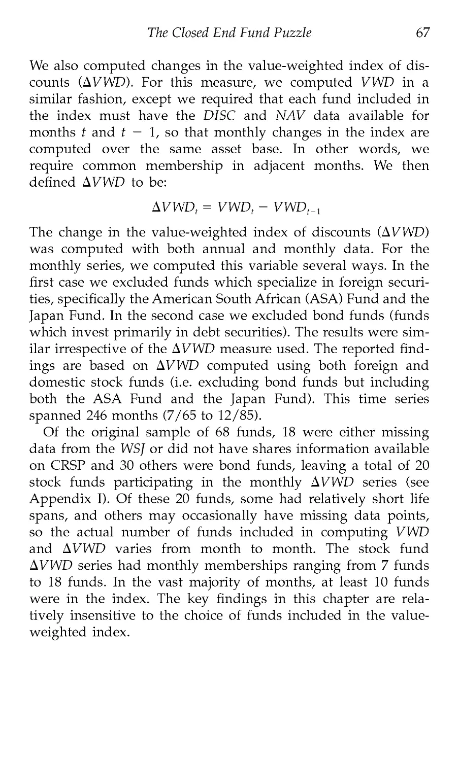
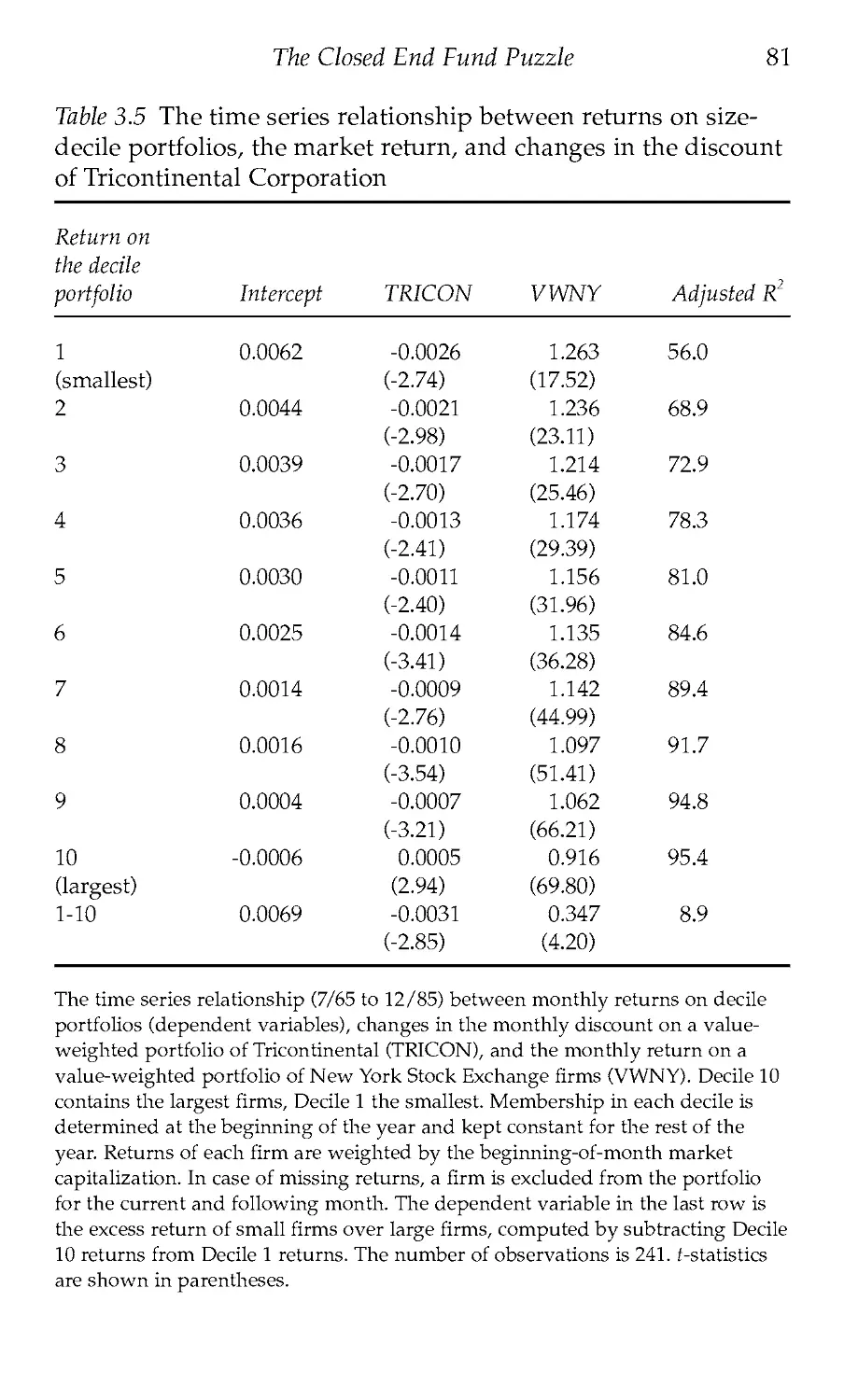
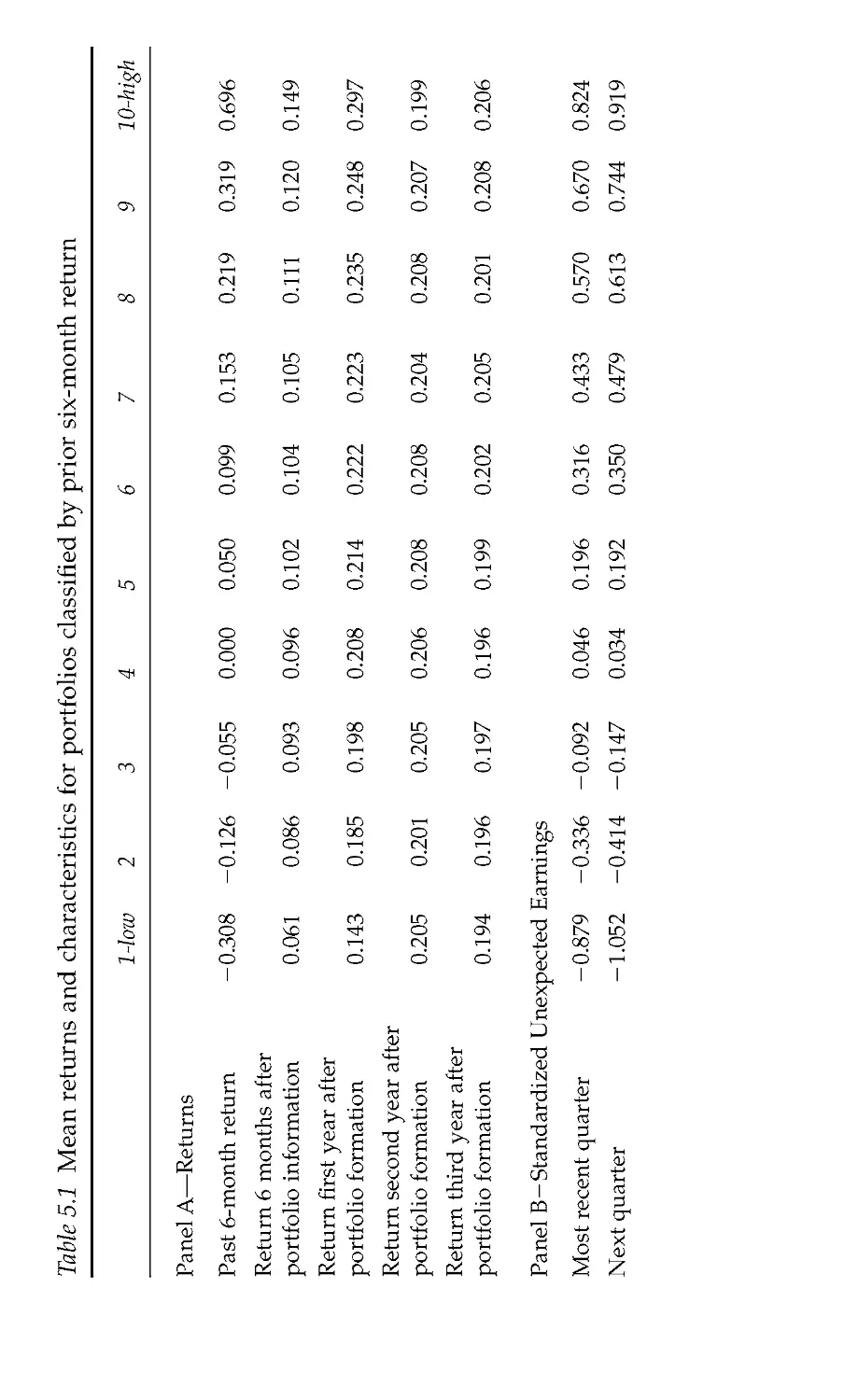
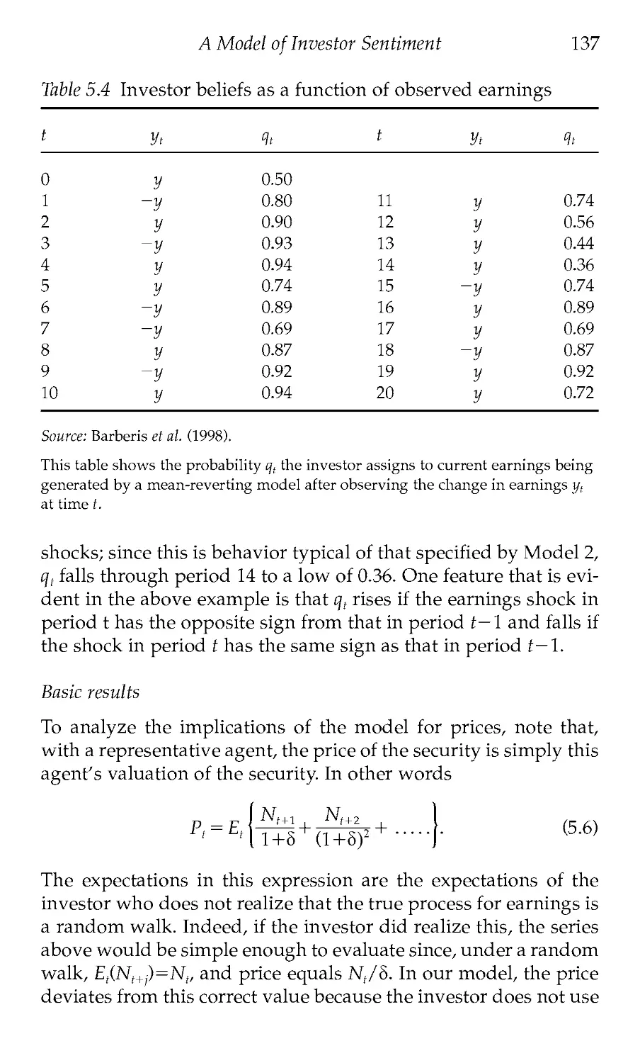
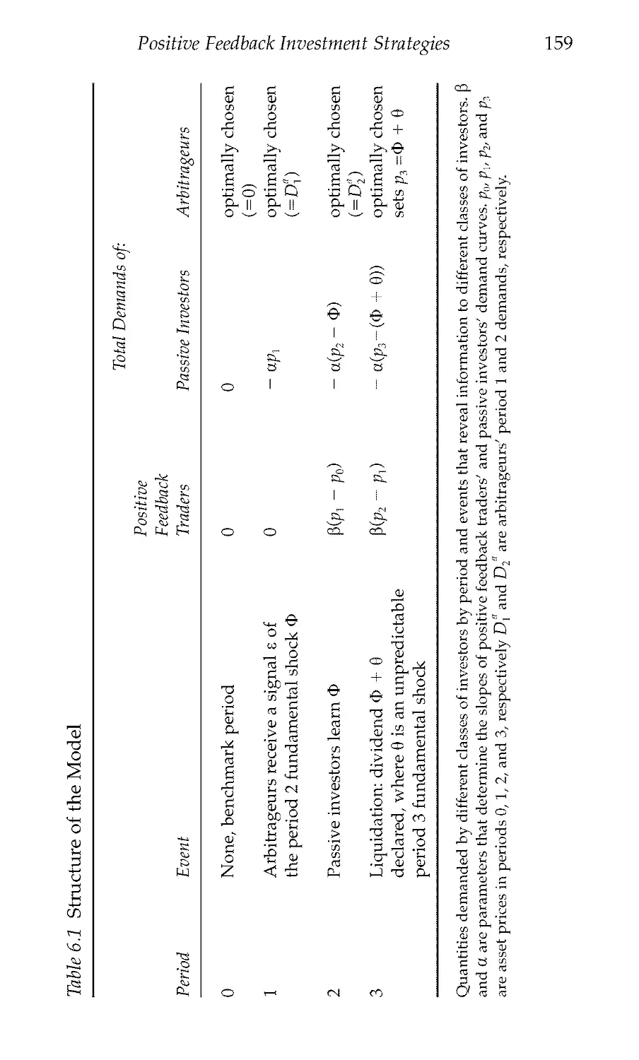
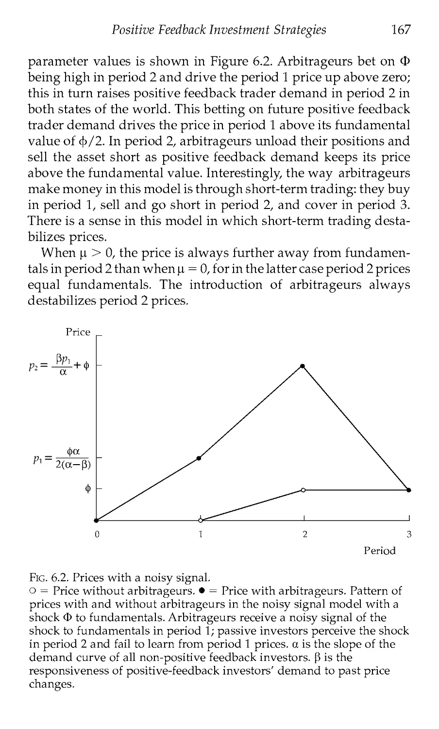
/


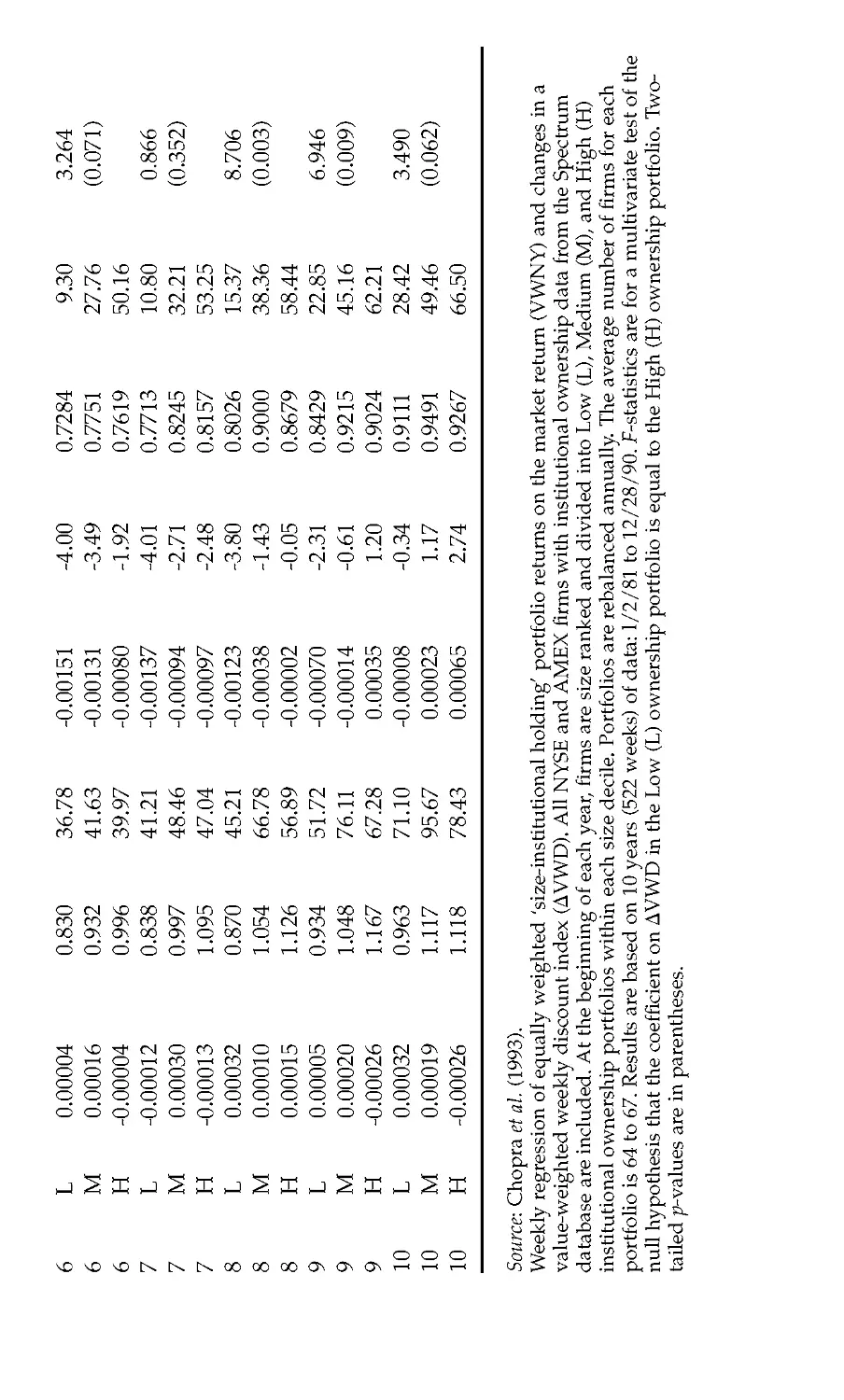


Text
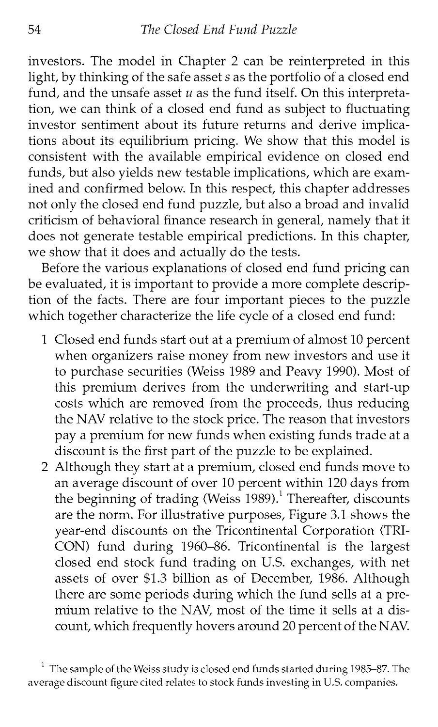
Clarendon Lectures in Economics
Andrei Shleifer
INEFFICIENT
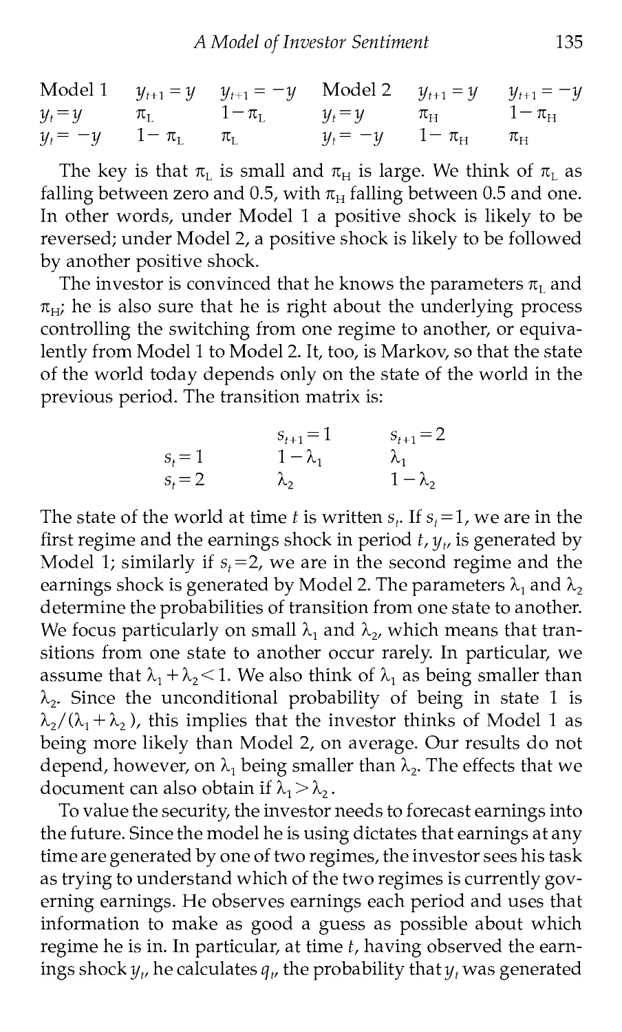
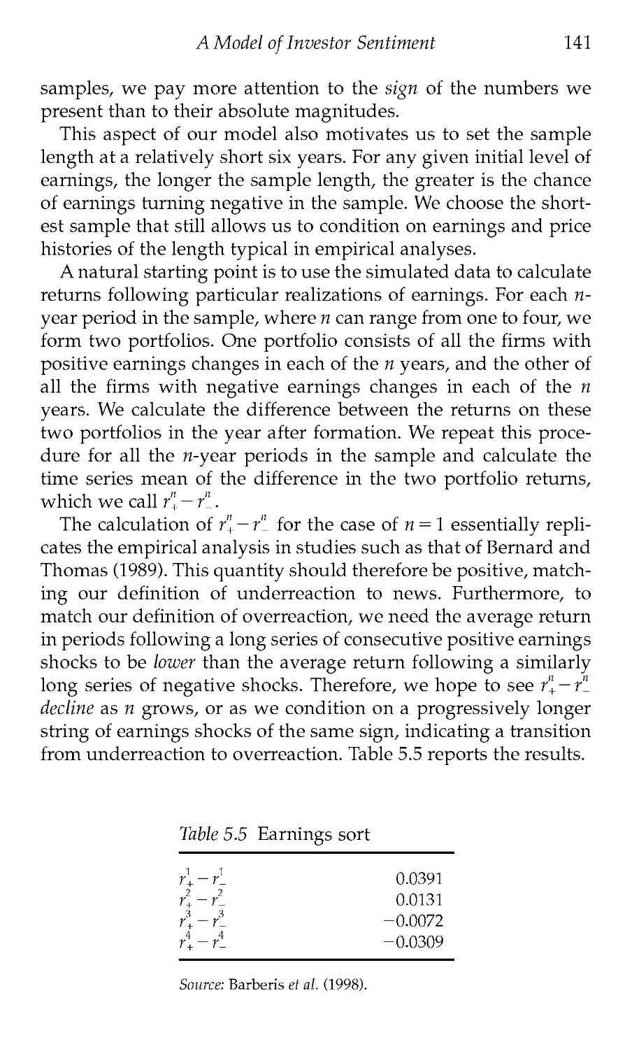
MARKETS
Inefficient Markets
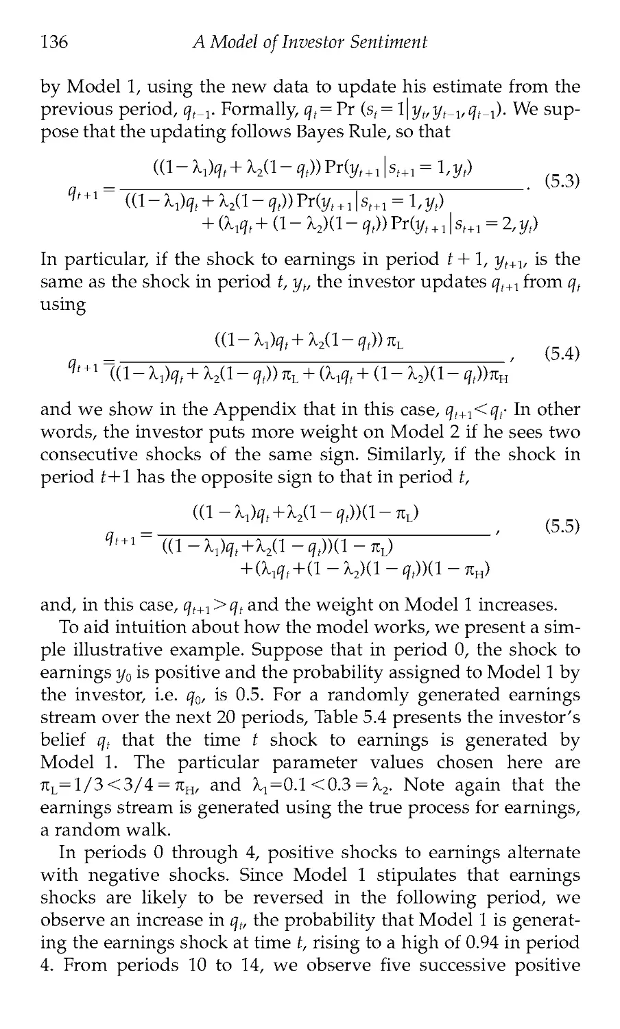
An Introduction to Behavioral Finance
ANDREI SHLEIFER
OXFORD
UNIVERSITY PRESS
This book has been printed digitally and produced in a standard specification
in order to ensure its continuing availability
OXFORD
UNIVERSITY PRESS
Great Clarendon Street, Oxford 0X2 6DP
Oxford University Press is a department of the University of Oxford.
It furthers the University’s objective of excellence in research, scholarship,
and education by publishing worldwide in
Oxford New York
Auckland Bangkok Buenos Aires Cape Town Chennai
Dar es Salaam Delhi Hong Kong Istanbul Karachi Kolkata
Kuala Lumpur Madrid Melbourne Mexico City Mumbai Nairobi
Sao Paulo Shanghai Taipei Tokyo Toronto
Oxford is a registered trade mark of Oxford University Press
in the UK and in certain other countries
Published in the United States
by Oxford University Press Inc., New York
© Andrei Shleifer 2000
The moral rights of the author have been asserted
Database right Oxford University Press (maker)
Reprinted 2004
All rights reserved. No part of this publication may be reproduced,
stored in a retrieval system, or transmitted, in any form or by any means,
without the prior permission in writing of Oxford University Press,
or as expressly permitted by law, or under terms agreed with the appropriate
reprographics rights organization. Enquiries concerning reproduction
outside the scope of the above should be sent to the Rights Department,
Oxford University Press, at the address above
You must not circulate this book in any other binding or cover
And you must impose this same condition on any acquirer
ISBN 0-19-829228-7
For Nancy
Contents
Acknowledgments vii
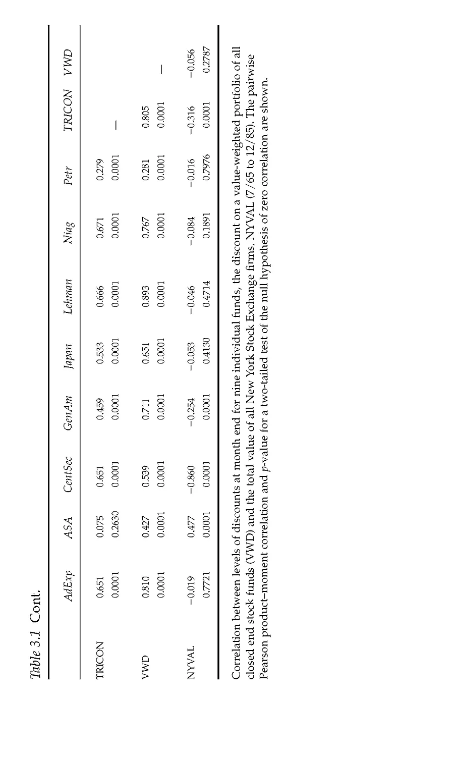
1. Are Financial Markets Efficient? 1
2. Noise Trader Risk in Financial Markets 28
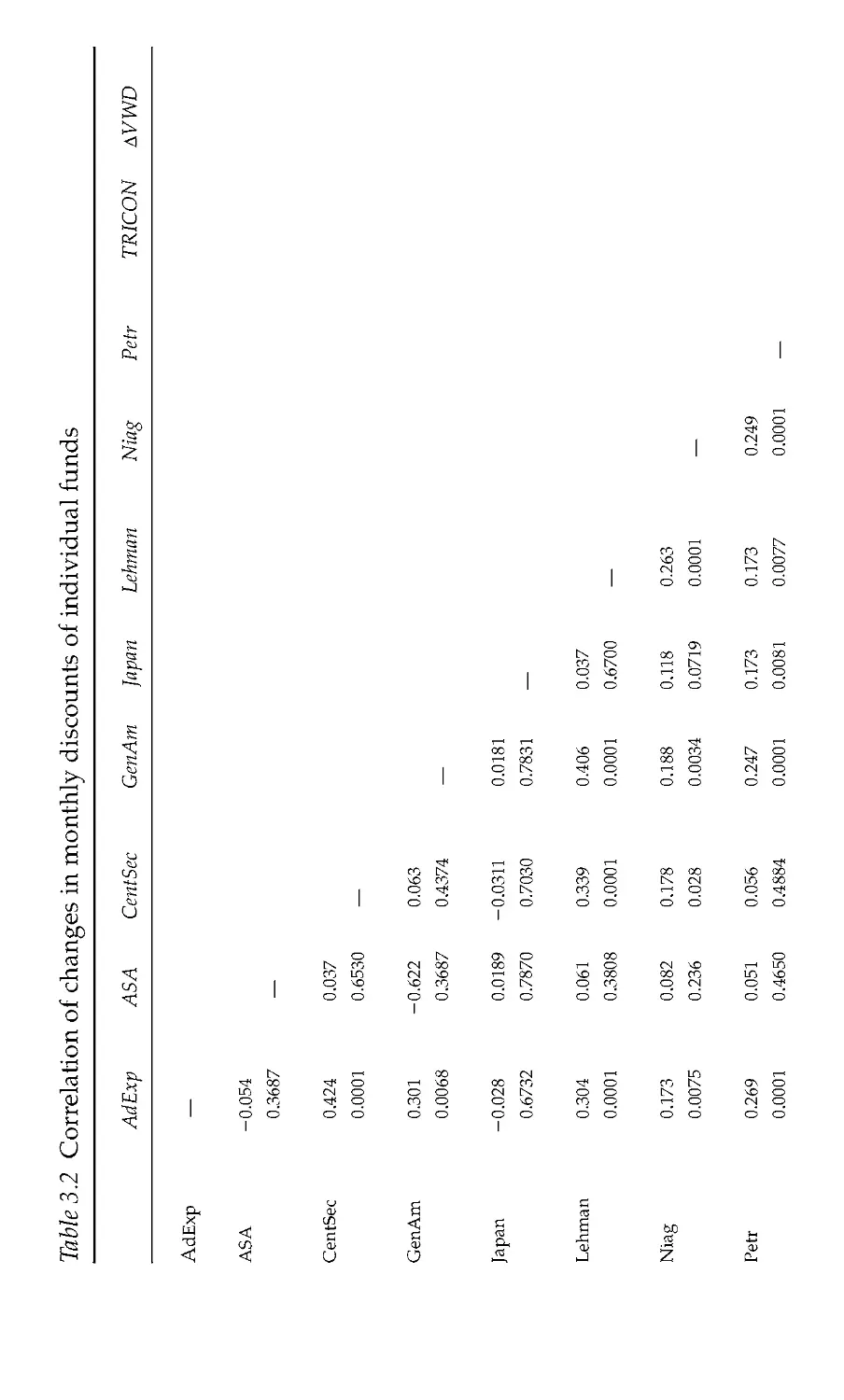
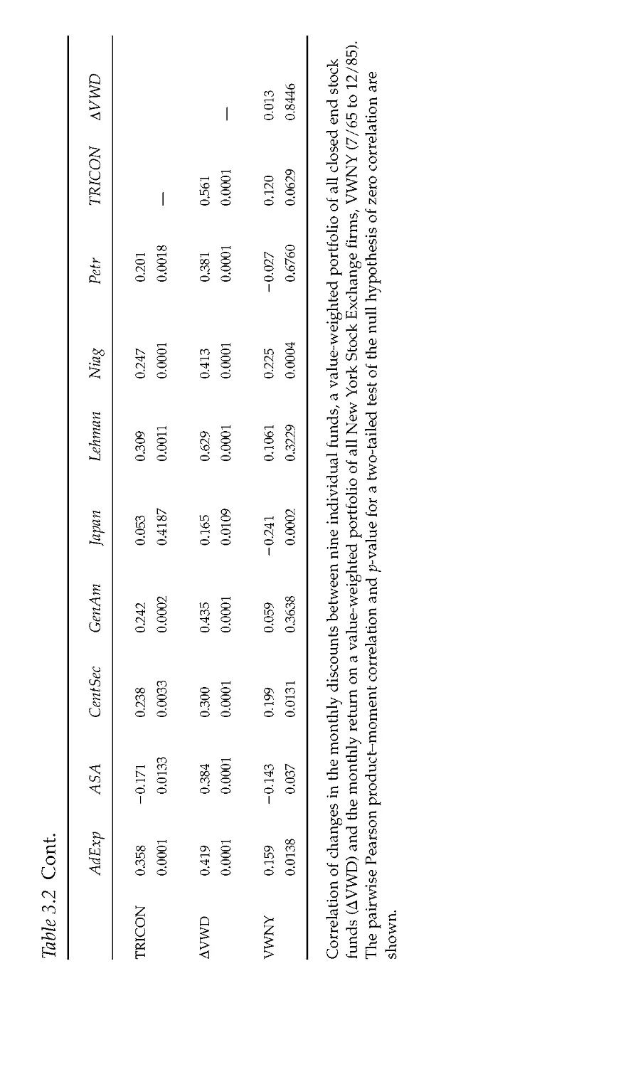
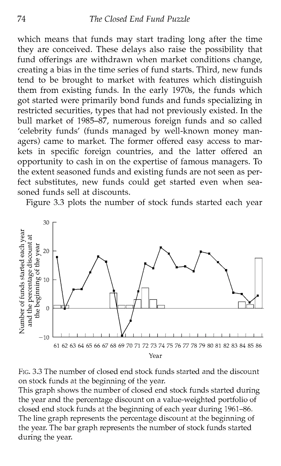
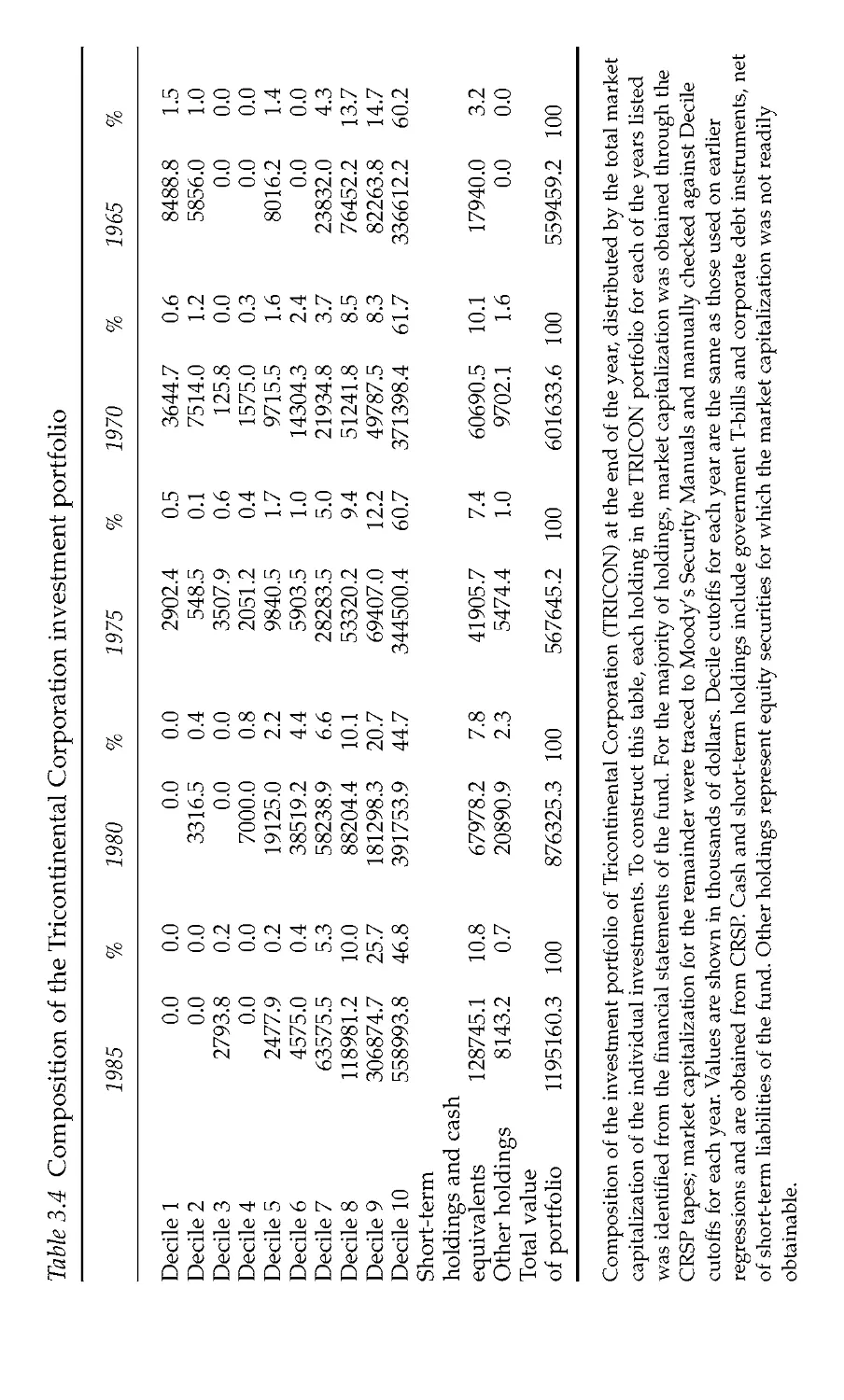
3. The Closed End Fund Puzzle 53
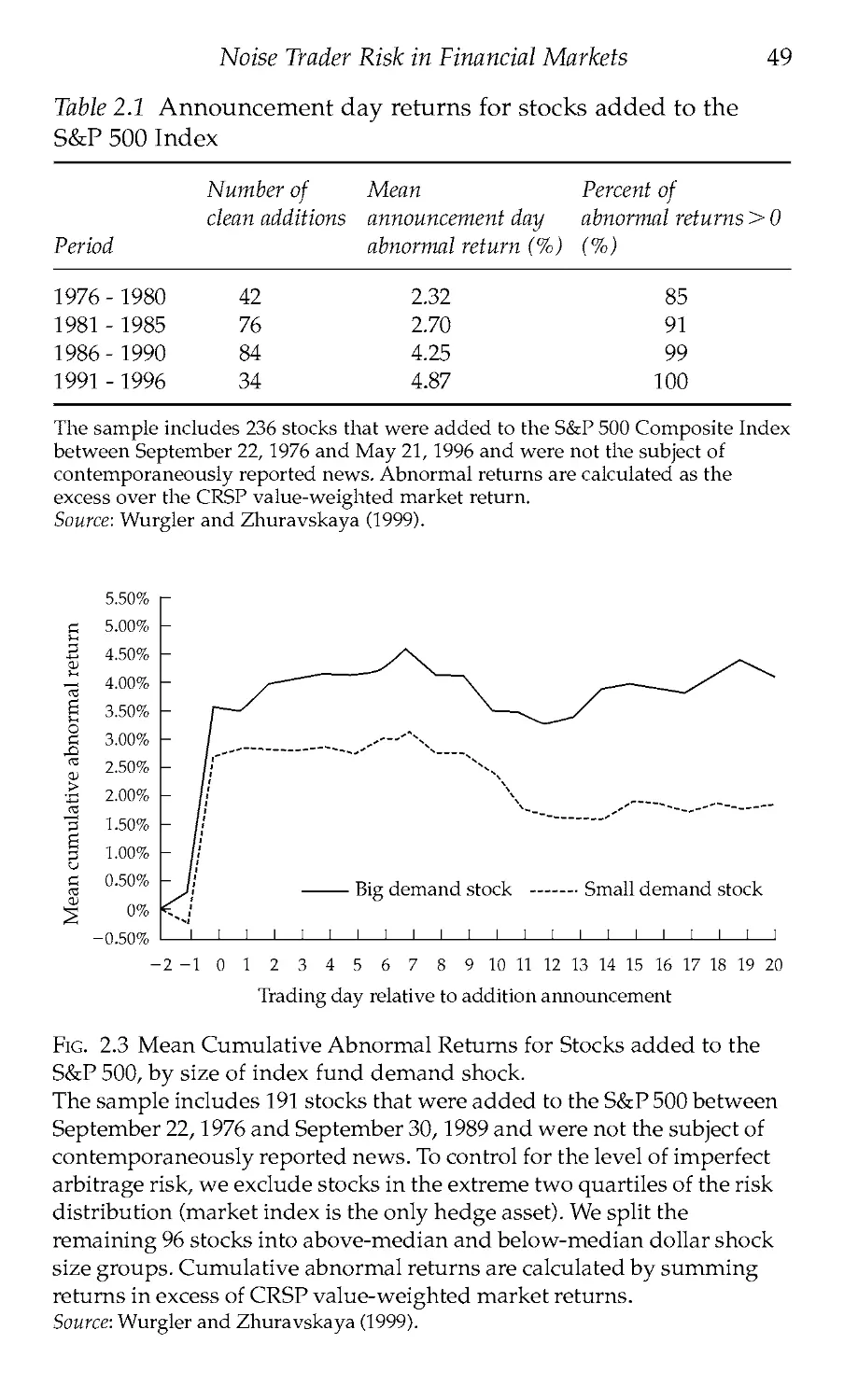
4. Professional Arbitrage 89
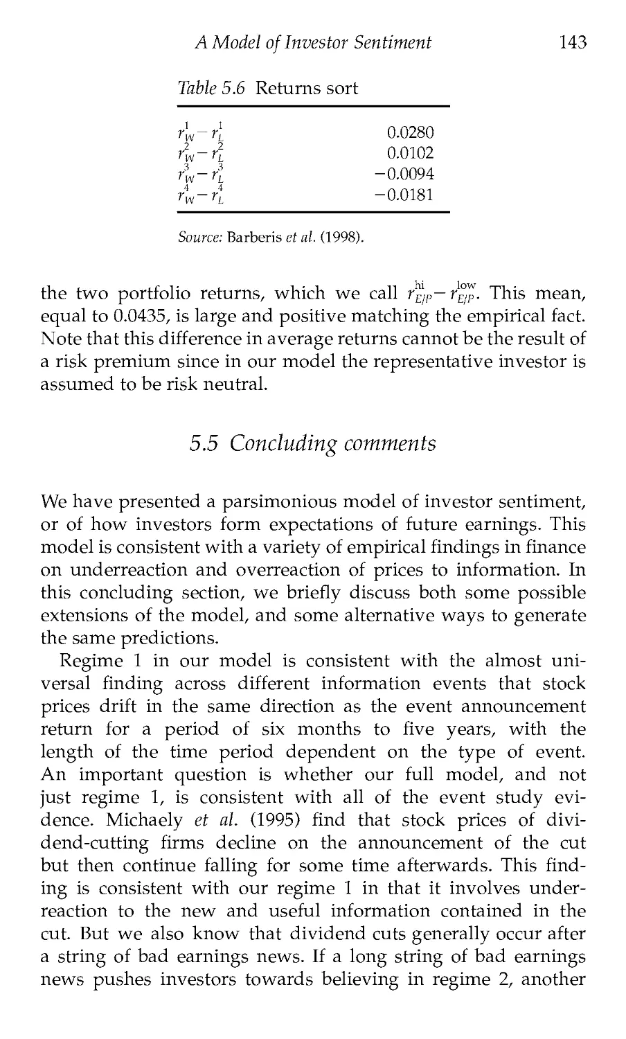
5. A Model of Investor Sentiment 112
6. Positive Feedback Investment Strategies 154
7. Open Problems 175
Bibliography 198
Index 211
Acknowledgmen is
This book grows out of the Clarendon Lectures given at Oxford in
the Spring of 1996. I appreciate the hospitality of Oxford
University Press and its economics editor, Andrew Schuller.
I started working on the efficiency of financial markets as a
graduate student in the mid-1980s. At the time, there were only a
handful of academic papers in behavioral finance, written by
people like Robert Shiller, Larry Summers, and Richard Thaler.
The assessment by financial economists of this research was not
especially generous. Nonetheless, the area seemed to me to be
incredibly exciting. During graduate school, I wrote a paper on
stock inclusions into the S&P 500 Index and started on a series of
theoretical projects with Brad De Long, Larry Summers, and
Robert Waldmann. Behavioral finance experienced an upsurge of
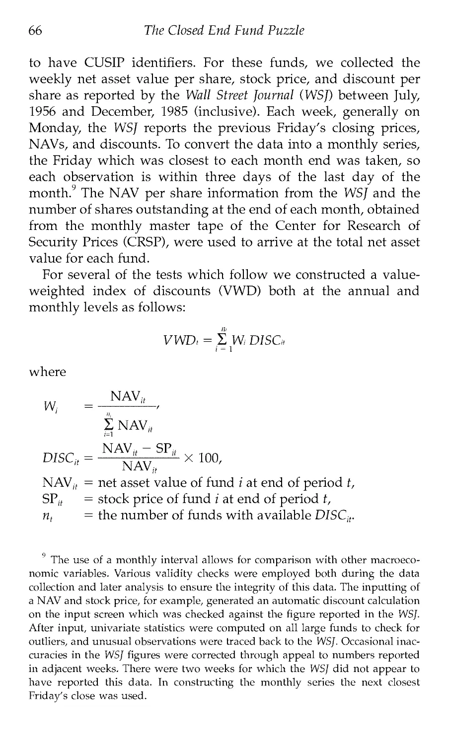
research in the late 1980s. I had intended to write a book about it
while visiting the Russell Sage Foundation in 1992, but that plan
did not materialize. In some ways, this is fortunate, since much
work has been done in this area since then. I am still very grate-
ful to the Russell Sage Foundation for getting me started.
During the 1990s, I have worked on a number of projects with
Josef Lakonishok and Robert Vishny, both of whom have greatly
contributed to the material presented in this book. I also learned
a lot about arbitrage from Gabe Sunshine and Nancy
Zimmerman, who introduced me to some fascinating analytical
issues which arise from a more practical understanding of mar-
kets. The invitation to give the Clarendon Lectures came at a per-
fect moment and allowed me to write this book. I am finally
finishing it during a sabbatical year at the Massachusetts Institute
of Technology, which both kindly hosted me and encouraged
me to present some chapters as Independent Activities Period
lectures.
Many of the chapters draw heavily on my joint research with
a number of colleagues. Chapter 2 draws on 'Noise Trader Risk
in Financial Markets,' written with Brad De Long, Lawrence
viii
Acknow ledgmen ts
Summers, and Robert Waldmann and published in the Journal of
Political Economy in 1990. Chapter 3 is based on 'Investor
Sentiment and the Closed End Fund Puzzle/ written with
Charles Lee and Richard Thaler and published in the Journal of
Finance in 1991. Chapter 4 borrows heavily from 'The Limits of
Arbitrage/ written with Robert Vishny and published in the
Journal of Finance in 1997. Chapter 5 follows 'A Model of Investor
Sentiment/ written with Nicholas Barberis and Robert Vishny
and published in the Journal of Financial Economics in 1998.
Chapter 6 uses material from 'Positive Feedback Investment
Strategies and Destabilizing Rational Speculation/ written with
Brad De Long, Lawrence Summers, and Robert Waldmann and
published in the Journal of Finance in 1990. While I have borrowed
liberally from these articles, I have equally liberally added and
subtracted material. I am grateful to all my co-authors for years of
collaboration.
I was fortunate to receive many extremely perceptive com-
ments on this book from Nicholas Barberis, Olivier Blanchard,
John Campbell, Edward Glaeser, Paul Gompers, Oliver Hart,
Simon Johnson, Daniel Kahneman, David Laibson, Rafael La
Porta, Florencio Lopez-de-Silanes, Andrew Metrick, Sendhil
Mullainathan, Michael Rashes, Lawrence Summers, Richard
Thaler, Daniel Wolfenzon, and Jeff Wurgler. Their comments had
a significant impact on the final draft. Nicholas Barberis and
David Laibson were particularly helpful. I am also very grateful
to Clare MacLean, who worked tirelessly to get this book out the
door, and to Malcolm Baker for preparing the index.
My two greatest debts, however, are to Larry Summers and
Nancy Zimmerman. Larry got me started as an economist and
introduced me to behavioral finance. He has been a shining
example in many ways. Nancy's insight into financial markets is
always inspiring. This book is dedicated to her.
1
Are Financial Markets Efficient?
The efficient markets hypothesis (EMH) has been the central
proposition of finance for nearly thirty years. In his classic state-
ment of this hypothesis, Fama (1970) defined an efficient financial
market as one in which security prices always fully reflect the
available information. The efficient markets hypothesis then states
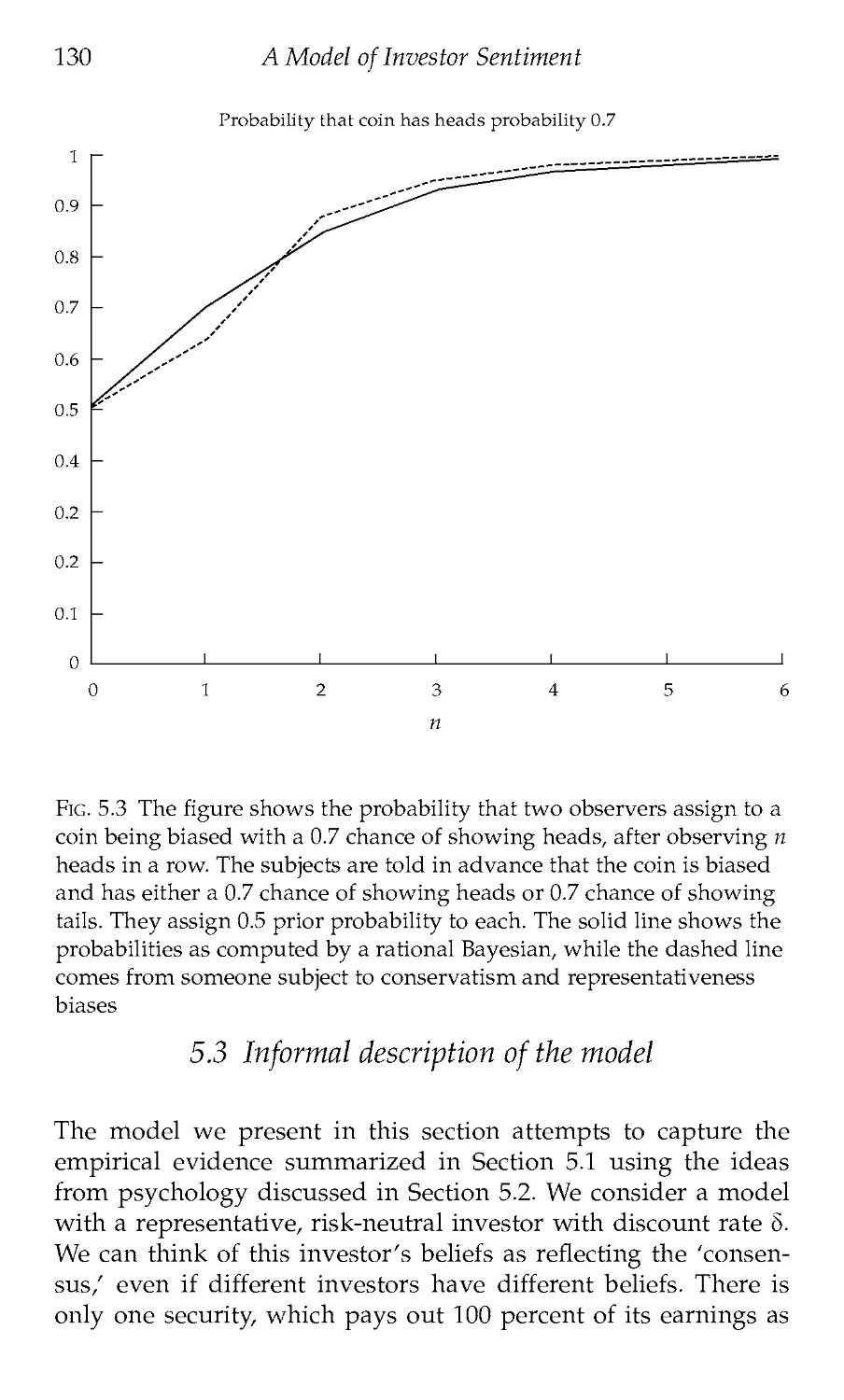
that real-world financial markets, such as the U.S. bond or stock
market, are actually efficient according to this definition. The
power of this statement is dazzling. Perhaps most radically, the
EMH 'rules out the possibility of trading systems based only on
currently available information that have expected profits or
returns in excess of equilibrium expected profit or return' (Fama
1970). In plain English, an average investor—whether an individ-
ual, a pension fund, or a mutual fund—cannot hope to consistently
beat the market, and the vast resources that such investors dedi-
cate to analyzing, picking, and trading securities are wasted. Better
to passively hold the market portfolio, and to forget active money
management altogether. If the EMH holds, the market truly knows
best.
In the first decade after its conception in the 1960s, the EMH
turned into an enormous theoretical and empirical success.
Academics developed powerful theoretical reasons why the
hypothesis should hold. More impressively, a vast array of empiri-
cal findings quickly emerged—nearly all of them supporting the
hypothesis. Indeed, the field of academic finance in general, and
security analysis in particular, was created on the basis of the EMH
and its applications. The University of Chicago, where the EMH
was invented, justly became the world's center of academic finance.
In 1978, Michael Jensen—a Chicago graduate and one of the cre-
ators of the EMH—declared that 'there is no other proposition in
economics which has more solid empirical evidence supporting it
than the Efficient Markets Hypothesis' (Jensen 1978, p. 95).
Such strong statements portend reversals, and the EMH is no
exception. In the last twenty years, both the theoretical foundations
1
Are Financial Markets Efficient?
of the EMH and the empirical evidence purporting to support it
have been challenged. The key forces by which markets are sup-
posed to attain efficiency, such as arbitrage, are likely to be much
weaker and more limited than the efficient markets theorists have
supposed. Moreover, new studies of security prices have reversed
some of the earlier evidence favoring the EMH. With the new theory
and evidence, behavioral finance has emerged as an alternative
view of financial markets. In this view, economic theory does not
lead us to expect financial markets to be efficient. Rather, systematic
and significant deviations from efficiency are expected to persist for
long periods of time. Empirically, behavioral finance both explains
the evidence that appears anomalous from the efficient markets
perspective, and generates new predictions that have been con-
firmed in the data.
This book introduces the research in behavioral finance. In this
opening chapter, we describe both the theoretical and the empir-
ical foundations of the EMH, as well as some of the cracks that
have emerged in these foundations.
The theoretical foundations of the EMH
The basic theoretical case for the EMH rests on three arguments
which rely on progressively weaker assumptions. First, investors
are assumed to be rational and hence to value securities ratio-
nally. Second, to the extent that some investors are not rational,
their trades are random and therefore cancel each other out with-
out affecting prices. Third, to the extent that investors are irra-
tional in similar ways, they are met in the market by rational
arbitrageurs who eliminate their influence on prices.
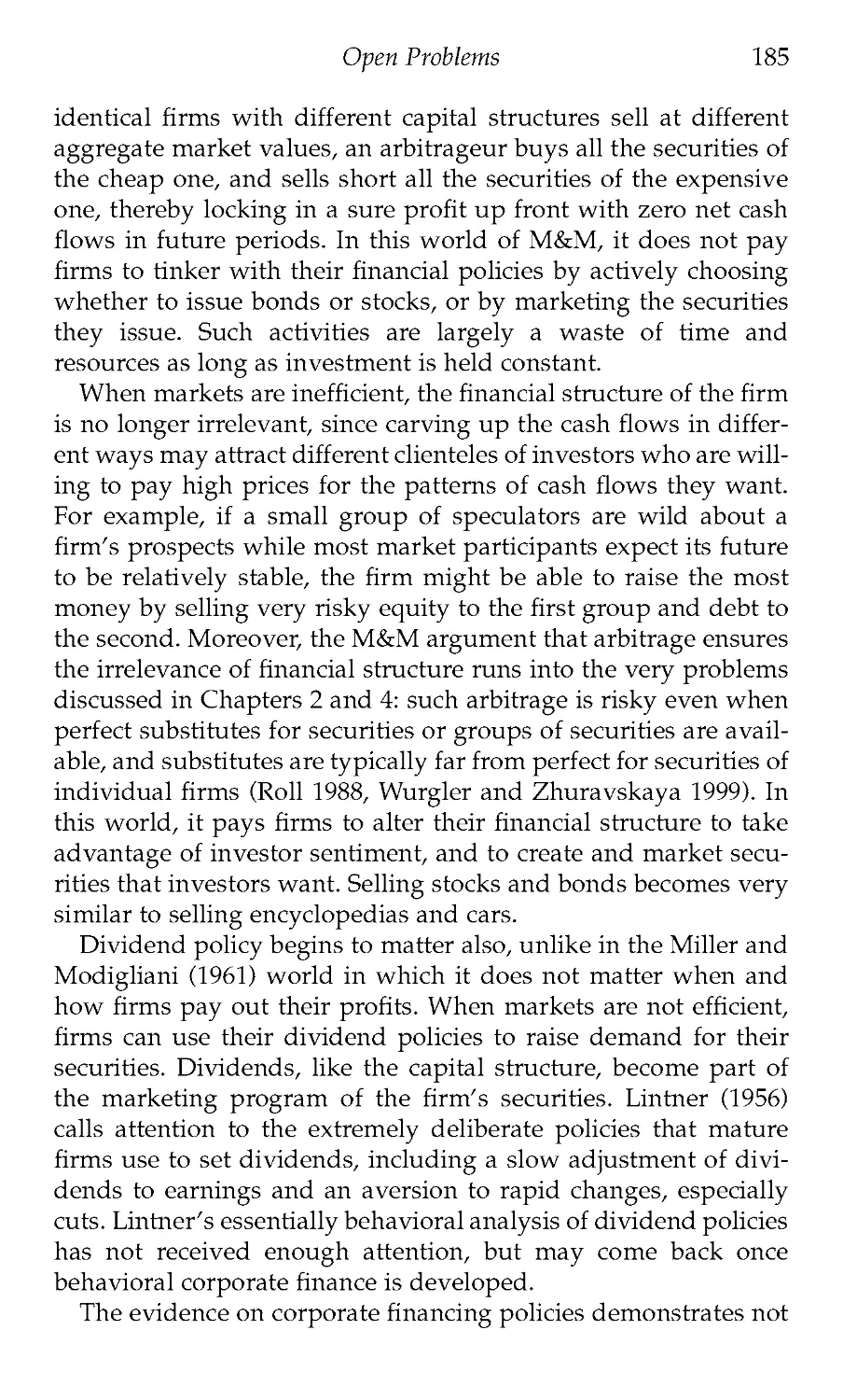
When investors are rational, they value each security for its
fundamental value: the net present value of its future cash flows,
discounted using their risk characteristics. When investors learn
something about fundamental values of securities, they quickly
respond to the new information by bidding up prices when the
news is good and bidding them down when the news is bad. As
a consequence, security prices incorporate all the available infor-
mation almost immediately and prices adjust to new levels corre-
sponding to the new net present values of cash flows. Samuelson
(1965) and Mandelbrot (1966) proved some of the first theorems
showing how, in competitive markets with rational risk-neutral
Are Financial Markets Efficient?
3
investors, returns are unpredictable—security values and prices
follow random walks. Since then, economists have characterized
efficient securities prices for risk-averse investors, with both vary-
ing levels of risk over time and varying tolerances toward risk. In
these more complicated models security prices are no longer pre-
dicted to follow random walks. Still, investor rationality implies
the impossibility of earning superior risk-adjusted returns, just as
Fama wrote in 1970. The EMH is thus first and foremost a conse-
quence of equilibrium in competitive markets with fully rational
investors.
But remarkably, the EMH does not live or die by investor ratio-
nality. In many scenarios where some investors are not fully ratio-
nal, markets are still predicted to be efficient. In one commonly
discussed case, the irrational investors in the market trade ran-
domly. When there are large numbers of such investors, and
when their trading strategies are uncorrelated, their trades are
likely to cancel each other out. In such a market, there will be sub-
stantial trading volume as the irrational investors exchange secu-
rities with each other, but the prices are nonetheless close to
fundamental values. This argument relies crucially on the lack of
correlation in the strategies of the irrational investors, and, for
that reason, is quite limited. The case for the EMH, however, can
be made even in situations where the trading strategies of
investors are correlated.
This case, as made by Milton Friedman (1953) and Fama (1965),
is based on arbitrage. It is one of the most intuitively appealing
and plausible arguments in all of economics. A textbook defini-
tion (Sharpe and Alexander 1990) defines arbitrage as 'the simul-
taneous purchase and sale of the same, or essentially similar,
security in two different markets at advantageously different
prices.' Suppose that some security, say a stock, becomes over-
priced in a market relative to its fundamental value as a result of
correlated purchases by unsophisticated, or irrational, investors.
This security now represents a bad buy, since its price exceeds
the properly risk adjusted net present value of its cash flows or
dividends. Noting this overpricing, smart investors, or arbi-
trageurs, would sell or even sell short this expensive security and
simultaneously purchase other, 'essentially similar/ securities to
hedge their risks. If such substitute securities are available and
arbitrageurs are able to trade them, they can earn a profit, since
4
Are Financial Markets Efficient?
they are short expensive securities and long the same, or very
similar, but cheaper securities. The effect of this selling by arbi-
trageurs is to bring the price of the overpriced security down to
its fundamental value. In fact, if arbitrage is quick and effective
enough because substitute securities are readily available and the
arbitrageurs are competing with each other to earn profits, the
price of a security can never get far away from its fundamental
value, and indeed arbitrageurs themselves are unable to earn
much of an abnormal return. A similar argument applies to an
undervalued security To earn a profit, arbitrageurs would
buy underpriced securities and sell short essentially similar secu-
rities to hedge their risk, thereby preventing the underpricing
from being either substantial or very long-lasting. The process of
arbitrage brings security prices in line with their fundamental
values even when some investors are not fully rational and
their demands are correlated, as long as securities have close
substitutes.
Arbitrage has a further implication. To the extent that the secu-
rities that the irrational investors are buying are overpriced and
the securities they are getting rid of are underpriced, such
investors earn lower returns than either passive investors or arbi-
trageurs. Relative to their peers, irrational investors lose money.
As Friedman (1953) points out, they cannot lose money forever:
they must become much less wealthy and eventually disappear
from the market. If arbitrage does not eliminate their influence on
asset prices instantaneously, market forces eliminate their wealth.
In the long run, market efficiency prevails because of competitive
selection and arbitrage.
It is difficult not to be impressed with the full range and power
of the theoretical arguments for efficient markets. When people
are rational, markets are efficient by definition. When some
people are irrational, much or all of their trading is with each
other, and hence has only a limited influence on prices even with-
out countervailing trading by the rational investors. But such
countervailing trading does exist and works to bring prices closer
to fundamental values. Competition between arbitrageurs for
superior returns ensures that the adjustment of prices to funda-
mental values is very quick. Finally, to the extent that the irra-
tional investors do manage to transact at prices that are different
from fundamental values, they only hurt themselves and bring
Are Financial Markets Efficient?
5
about their own demise. Not only investor rationality, but market
forces themselves bring about the efficiency of financial markets.
The empirical foundations of the EMH
Strong as the theoretical case for the EMH may seem, the empiri-
cal evidence that appeared in the 1960s and the 1970s was even
more overwhelming. At the most general level, the empirical pre-
dictions of the EMH can be divided into two broad categories.
First, when news about the value of a security hits the market, its
price should react and incorporate this news both quickly and
correctly. The 'quickly' part means that those who receive the
news late—for instance by reading it in the newspapers or in
company reports—should not be able to profit from this informa-
tion. The 'correctly' part means that the price adjustment in
response to the news should be accurate on average: the prices
should neither underreact nor overreact to particular news
announcements. There should be neither price trends nor price
reversals following the initial impact of the news. Second, since a
security's price must be equal to its value, prices should not move
without any news about the value of the security. That is, prices
should not react to changes in demand or supply of a security
that are not accompanied by news about its fundamental value.
The quick and accurate reaction of security prices to information,
as well as the non-reaction to non-information, are the two broad
predictions of the efficient markets hypothesis.
The principal hypothesis following from quick and accurate
reaction of prices to new information is that stale information is
of no value in making money, as Fama (1970) points out. To eval-
uate this hypothesis empirically, researchers needed to define
'stale information' and 'making money.' The first definition turns
out to be relatively straightforward. Defining 'making money/ in
contrast, is enormously controversial. The reason is that 'making
money' in finance means making a superior return after an
adjustment for risk. Showing that a particular strategy based on
exploiting stale information on average earns a positive cash flow
over some period of time is not, therefore, by itself evidence of
market inefficiency. To earn this profit, an investor may have to
bear risk and his profit may just be a fair market compensation for
risk-bearing. The trouble is that measuring the risk of a particular
6 Are Financial Markets Efficient?
investment strategy is both difficult and controversial, and
requires a model of the fair relationship between risk and return.
One widely-accepted model is the Capital Asset Pricing Model
(Sharpe 1964), but it is not the only possibility. The dependence of
most tests of market efficiency on a model of risk and expected
return is Fama's (1970) deepest insight, which has pervaded the
debates in empirical finance ever since. Whenever researchers
have found a money-making opportunity resulting from trading
on stale information, critics have been quick to suggest a model
of risk—convincing or otherwise—that would reduce these prof-
its to a fair compensation for risk-taking.
The definition of stale information is far less controversial.
Fama distinguishes between three types of stale information, giv-
ing rise to three forms of the EMH. For the so-called weak form
efficiency, the relevant stale information is past prices and
returns. The weak form EMH posits that it is impossible to earn
superior risk-adjusted profits based on the knowledge of past
prices and returns. Under the assumption of risk neutrality, this
version of the EMH reduces to the random walk hypothesis, the
statement that stock returns are entirely unpredictable based on
past returns (Fama 1965).
Past returns are not the only stale information that investors
have. The semi-strong form of the EMH states that investors cannot
earn superior risk-adjusted returns using any publicly available
information. Put differently, as soon as information becomes pub-
lic, it is immediately incorporated into prices, and hence an
investor cannot gain by using this information to predict returns.
A semi-strong form efficient market is obviously weak form effi-
cient as well, since past prices and returns are a proper subset of
the publicly available information about a security
It is still possible that while an investor cannot profit from trad-
ing on publicly available information, he can still earn abnormal
risk-adjusted profits by trading on information that is not yet
known to market participants, sometimes described as inside
information. The strong form of the EMH states that even these
profits are impossible because the insiders' information quickly
leaks out and is incorporated into prices. To be fair, most evalua-
tions of the EMH have focused on weak and semi-strong form
efficiency, and have not taken the extreme position that there is no
such thing as profitable insider trading, as would be required if
Are Financial Markets Efficient?
7
the strong form EMH were to hold. Indeed, the insider traders
occupying minimum security prisons for making illegal profits
themselves represent some evidence against the strong form
EMH. But there is more systematic evidence as well that insiders
earn some abnormal returns even when they trade completely
legally (Seyhun 1998, Jeng et al. 1999).
When economists have set out to test these predictions, their
evidence was broadly supportive of the EMH. With respect to
weak form efficiency, Fama (1965) finds that stock prices indeed
approximately follow random walks. He finds no systematic evi-
dence of profitability of 'technical' trading strategies, such as buy-
ing stocks when their prices just went up or selling them when
their prices just went down. On a given day, the price of a stock
is as likely to rise after a previous day's increase as after a previ-
ous day's decline. Early tests of more complicated trading rules
have yielded similar failures to earn profits on average by pre-
dicting returns based on past returns, consistent with the weak
form EMH.
The initial tests corroborated semi-strong form efficiency as
well. One testing strategy is to look at particular news events
pertaining to individual companies and to ask whether prices
adjusted to this news immediately or over a period of a few
days. These so-called event studies, pioneered by Fama et al.
(1969), became the principal methodology of empirical finance,
as multitudes of important corporate news events, such as
earnings and dividend announcements, takeovers and divesti-
tures, share issues and repurchases, changes in management
compensation, and so on, came to be evaluated empirically
through the effects of these news events on share prices. As an
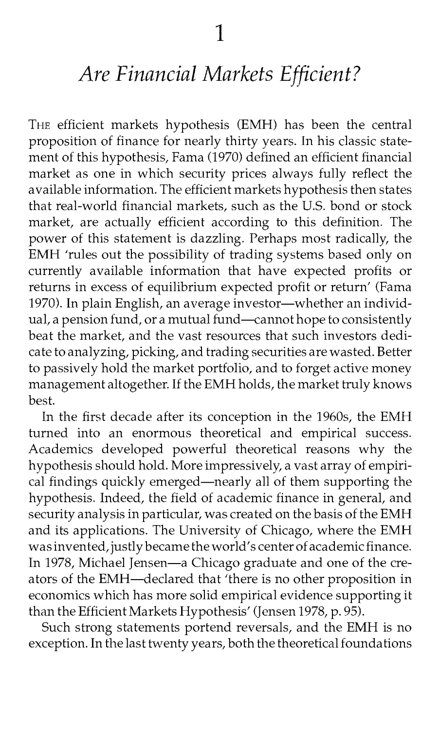
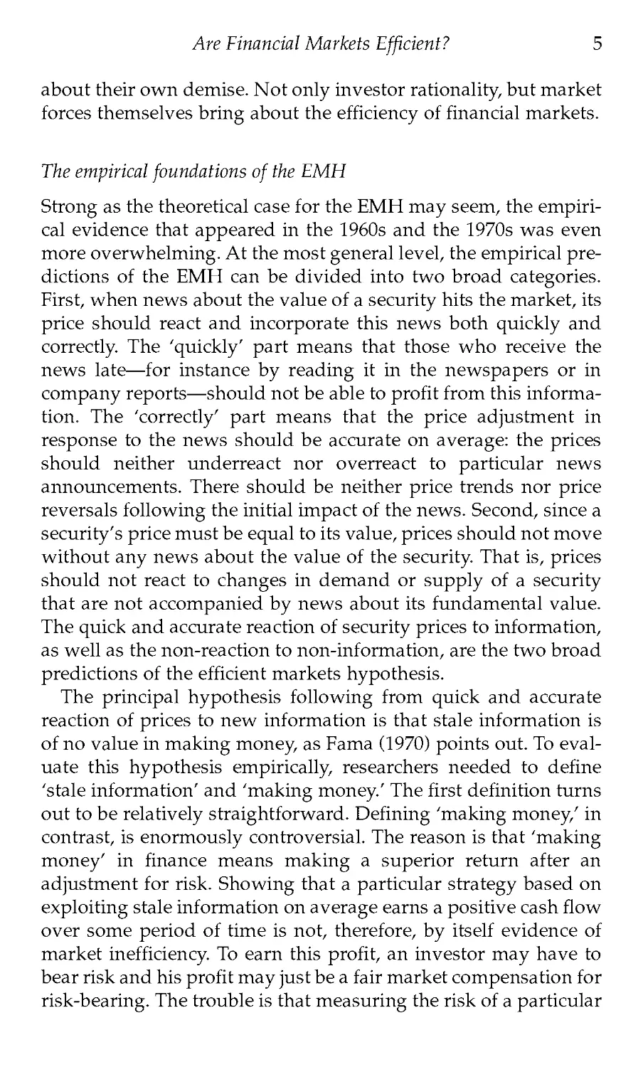
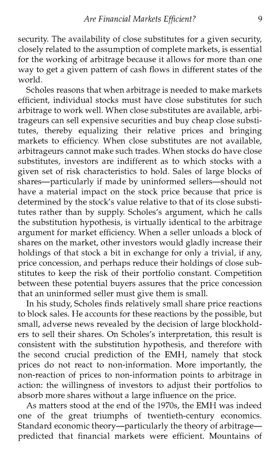
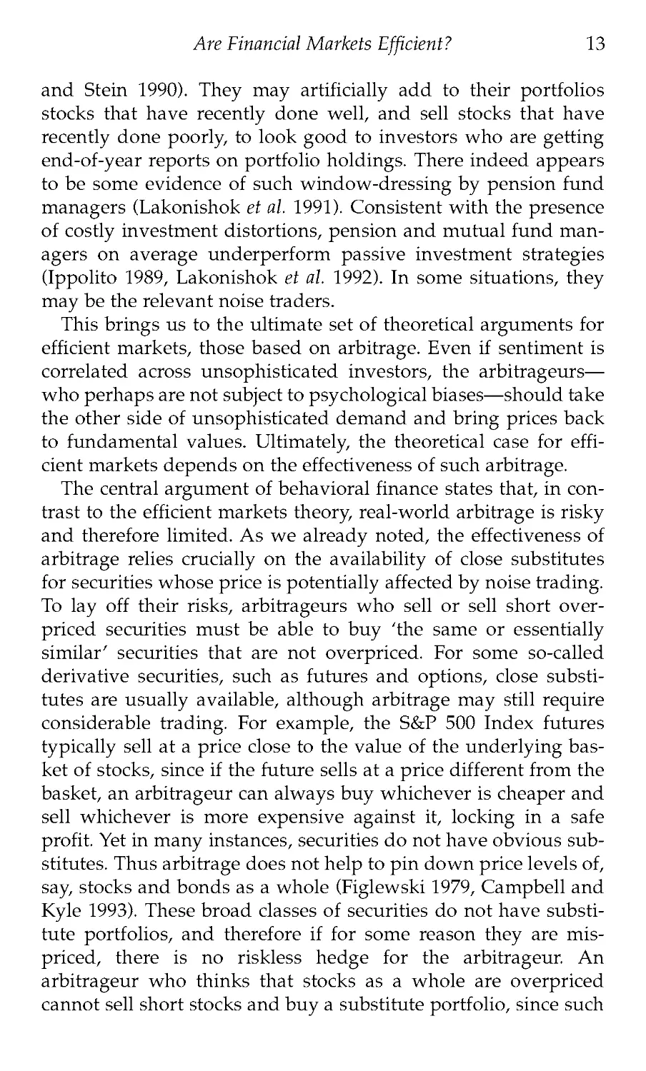
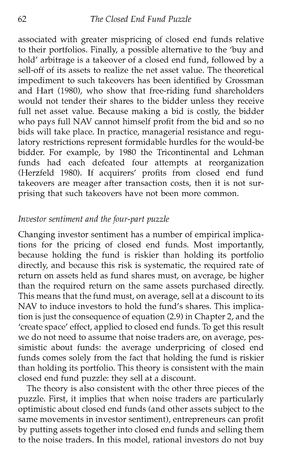
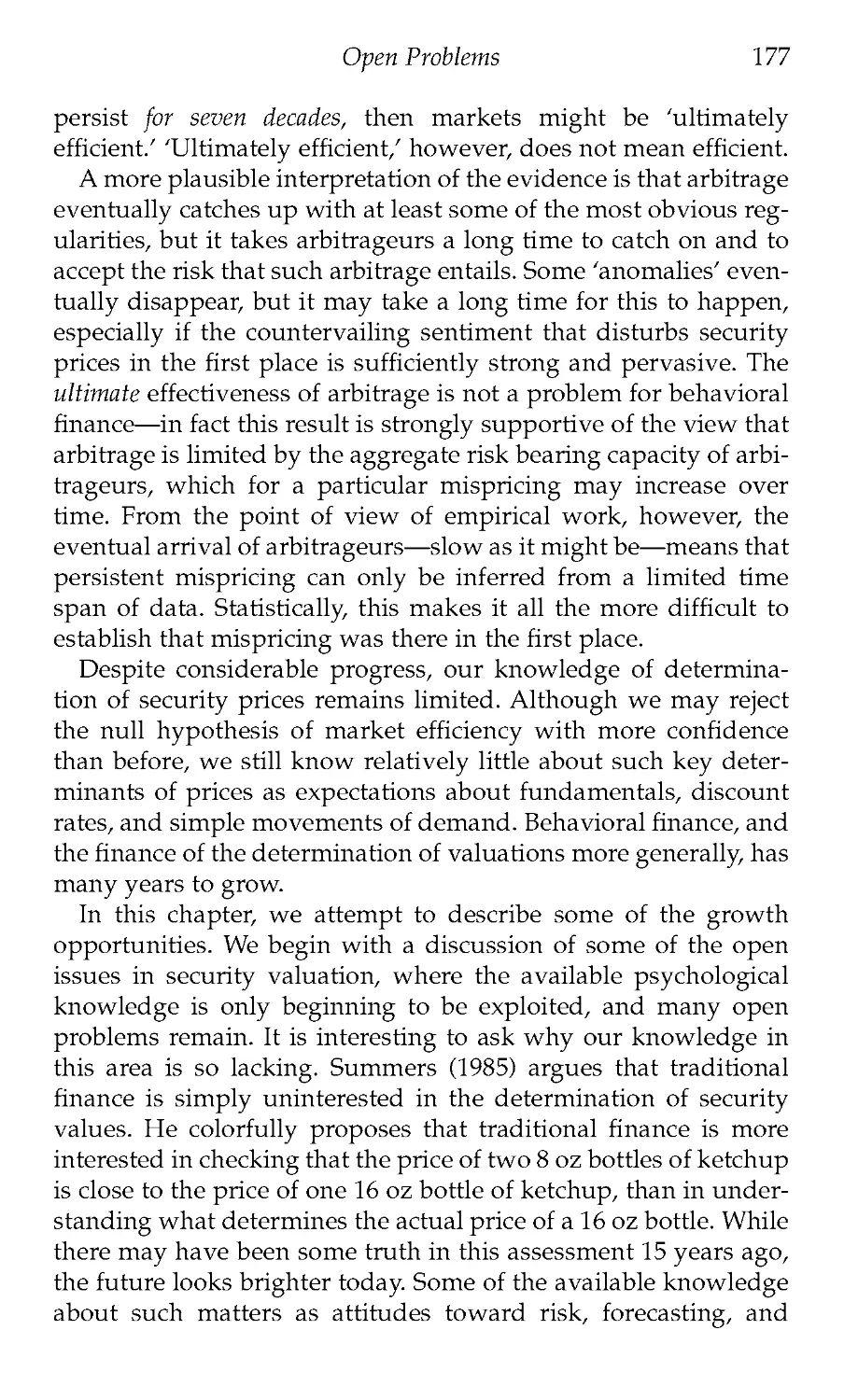
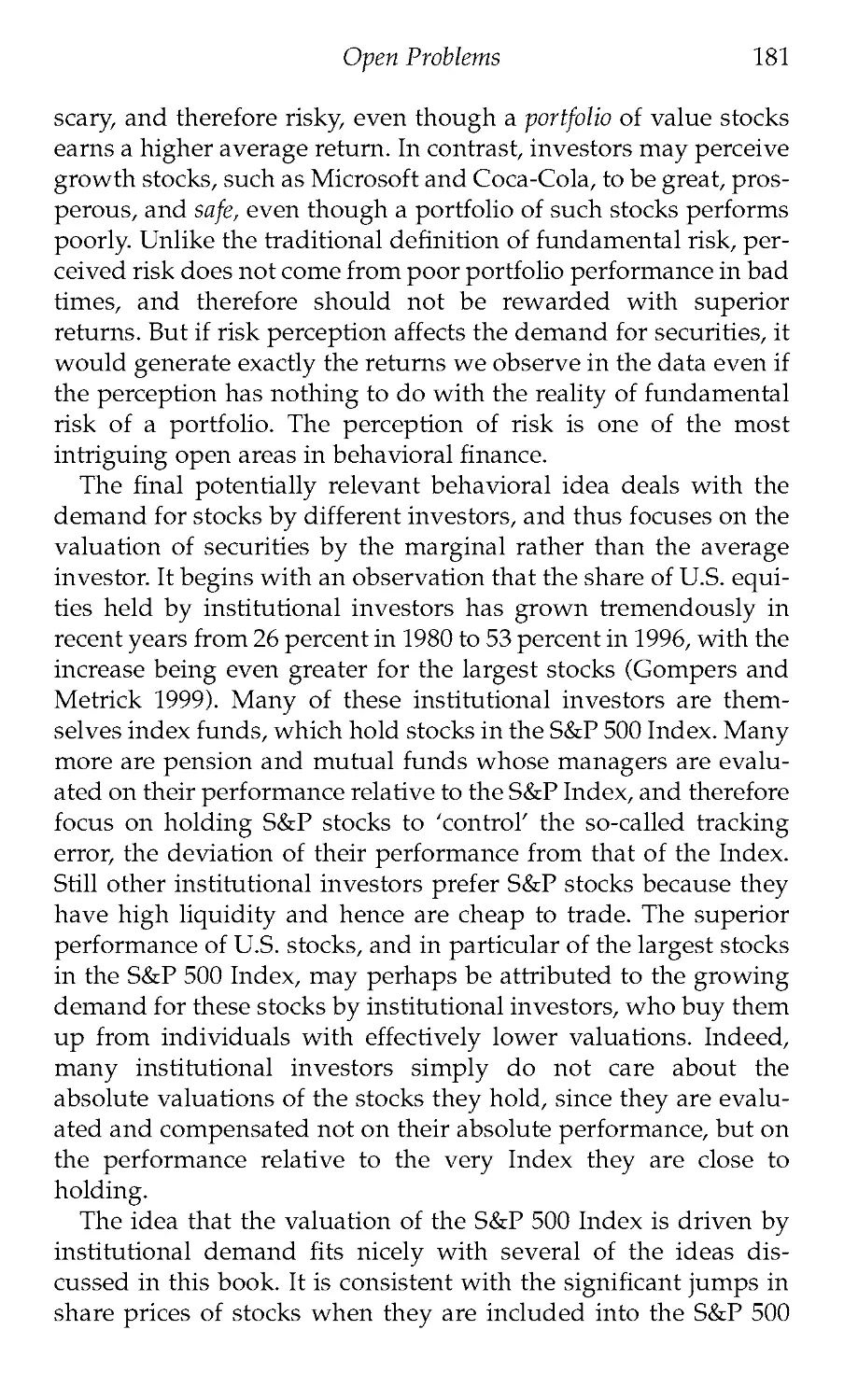
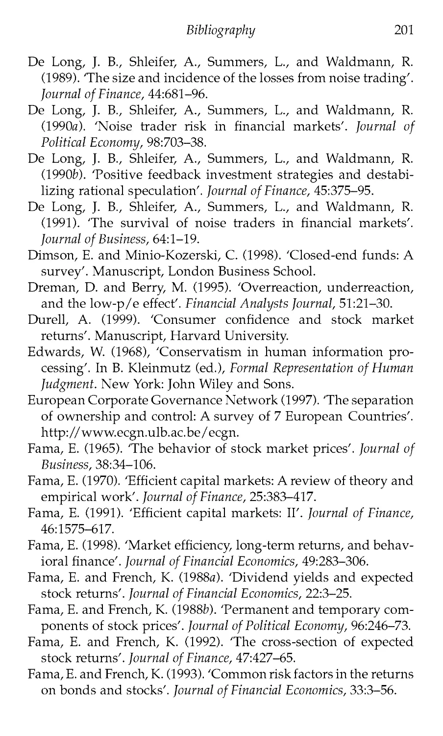
illustration, consider the study by Keown and Pinkerton (1981)
of returns to targets of takeover bids around the announcement
of the bid. The results for returns of an average target, adjusted
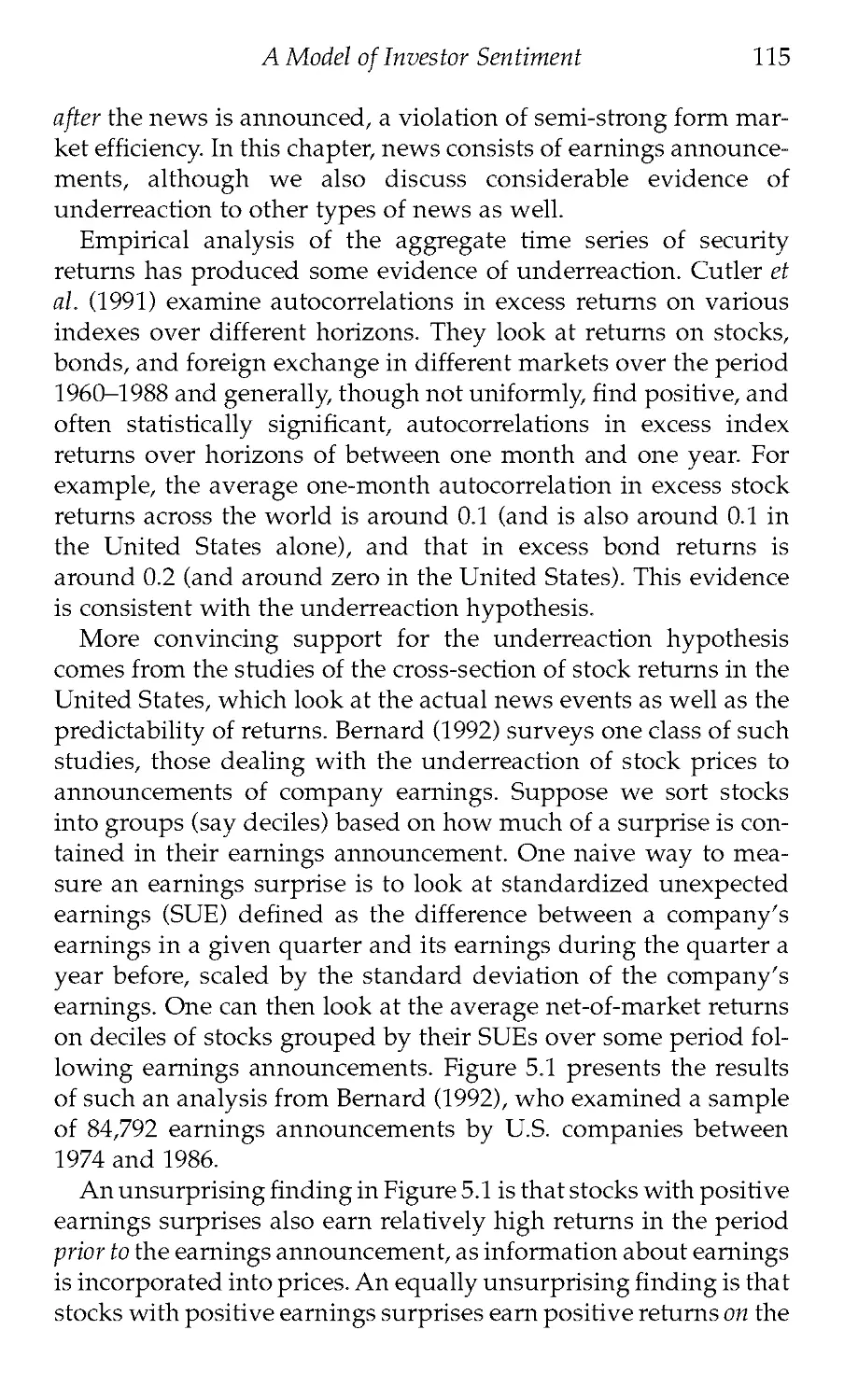
for market movements, are reproduced in Figure 1.1. They
show that share prices of targets begin to rise prior to the
announcement of the bid as the news of a possible bid is incor-
porated into prices, and then jump on the date of the public
announcement to reflect the takeover premium offered to target
firm shareholders. But the jump in share prices on the
announcement is not followed by a continued trend up or a
reversal down, indicating that prices of takeover targets adjust
8
Are Financial Markets Efficient?
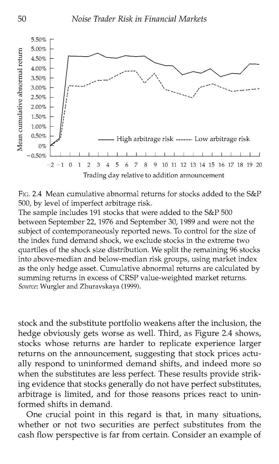
Fig. 1.1 Cumulative abnormal returns to shareholders of targets of
takeover attempts around the announcement date.
Source: Keown and Pinkerton (1981).
to the public news of the bid instantaneously, consistent with
the semi-strong form EMH.
Taken together, the early evidence on weak and semi-strong
form market efficiency was almost entirely supportive. The same
was also the case with the other implication of the EMH, namely
that prices do not react to non-information. In the principal early
empirical study of this proposition, Scholes (1972) uses the event
study methodology to evaluate share price reactions to sales of
large blocks of shares in individual companies by substantial
stockholders. Scholes's work is particularly important because it
deals directly with the issue central to the arbitrage arguments in
the efficient markets theory: the availability of close substitutes
for individual securities. An exact substitute for a given security
is another security (or portfolio of securities) with identical cash
flows in all states of the world. A close substitute is a security (or
portfolio) with very similar cash flows in all states of the world,
and therefore with similar risk characteristics to those of a given
Are Financial Markets Efficient?
9
security. The availability of close substitutes for a given security,
closely related to the assumption of complete markets, is essential
for the working of arbitrage because it allows for more than one
way to get a given pattern of cash flows in different states of the
world.
Scholes reasons that when arbitrage is needed to make markets
efficient, individual stocks must have close substitutes for such
arbitrage to work well. When close substitutes are available, arbi-
trageurs can sell expensive securities and buy cheap close substi-
tutes, thereby equalizing their relative prices and bringing
markets to efficiency When close substitutes are not available,
arbitrageurs cannot make such trades. When stocks do have close
substitutes, investors are indifferent as to which stocks with a
given set of risk characteristics to hold. Sales of large blocks of
shares—particularly if made by uninformed sellers—should not
have a material impact on the stock price because that price is
determined by the stock's value relative to that of its close substi-
tutes rather than by supply Scholes's argument, which he calls
the substitution hypothesis, is virtually identical to the arbitrage
argument for market efficiency. When a seller unloads a block of
shares on the market, other investors would gladly increase their
holdings of that stock a bit in exchange for only a trivial, if any,
price concession, and perhaps reduce their holdings of close sub-
stitutes to keep the risk of their portfolio constant. Competition
between these potential buyers assures that the price concession
that an uninformed seller must give them is small.
In his study, Scholes finds relatively small share price reactions
to block sales. He accounts for these reactions by the possible, but
small, adverse news revealed by the decision of large blockhold-
ers to sell their shares. On Scholes's interpretation, this result is
consistent with the substitution hypothesis, and therefore with
the second crucial prediction of the EMH, namely that stock
prices do not react to non-information. More importantly, the
non-reaction of prices to non-information points to arbitrage in
action: the willingness of investors to adjust their portfolios to
absorb more shares without a large influence on the price.
As matters stood at the end of the 1970s, the EMH was indeed
one of the great triumphs of twentieth-century economics.
Standard economic theory—particularly the theory of arbitrage—
predicted that financial markets were efficient. Mountains of
10
Are Financial Markets Efficient?
empirical evidence based on some of the most extensive data
available in economics, that on security prices, almost universally
confirmed the predictions of the theory Whenever researchers
found small money-making opportunities, they could be easily
explained away by a variety of arguments, the most pervasive of
which was the failure to adjust properly for risk. At the time,
Jensen's claim about the best established fact in economics was
not all that outrageous.
Theoretical challenges to the EMH
Shortly after Jensen's pronouncement, the EMH was challenged
on both theoretical and empirical grounds. Although the initial
challenges were primarily empirical, it is easier to begin by
reviewing some potential difficulties with the theoretical case for
the EMH and then turn to the evidence. This chapter only high-
lights the principal challenges. They are developed in the rest of
the book.
To begin, it is difficult to sustain the case that people in general,
and investors in particular, are fully rational. At the superficial
level, many investors react to irrelevant information in forming
their demand for securities; as Fischer Black (1986) put it, they
trade on noise rather than information. Investors follow the
advice of financial gurus, fail to diversify, actively trade stocks
and churn their portfolios, sell winning stocks and hold on to los-
ing stocks thereby increasing their tax liabilities, buy and sell
actively and expensively managed mutual funds, follow stock
price patterns and other popular models. In short, investors
hardly pursue the passive strategies expected of uninformed
market participants by the efficient markets theory
This evidence of what investors actually do is only the tip of the
iceberg. Investors' deviations from the maxims of economic ratio-
nality turn out to be highly pervasive and systematic. As summa-
rized by Kahneman and Riepe (1998), people deviate from the
standard decision making model in a number of fundamental
areas. We can group these areas, somewhat simplistically, into
three broad categories: attitudes toward risk, non-Bayesian
expectation formation, and sensitivity of decision making to the
framing of problems.
First, individuals do not assess risky gambles following the
Are Financial Markets Efficient?
11
precepts of von Neumann-Morgenstern rationality. Rather, in
assessing such gambles, people look not at the levels of final
wealth they can attain but at gains and losses relative to some ref-
erence point, which may vary from situation to situation, and dis-
play loss aversion—a loss function that is steeper than a gain
function. Such preferences—first described and modeled by
Kahneman and Tversky (1979) in their 'Prospect Theory'—are
helpful for thinking about a number of problems in finance. One
of them is the notorious reluctance of investors to sell stocks that
lose value, which comes out of loss aversion (Odean 1998).
Another is investors' aversion to holding stocks more generally,
known as the equity premium puzzle (Mehra and Prescott 1985,
Benartzi and Thaler 1995).
Second, individuals systematically violate Bayes rule and other
maxims of probability theory in their predictions of uncertain
outcomes (Kahneman and Tversky 1973). For example, people
often predict future uncertain events by taking a short history of
data and asking what broader picture this history is representa-
tive of. In focusing on such representativeness, they often do not
pay enough attention to the possibility that the recent history is
generated by chance rather than by the 'model' they are con-
structing. Such heuristics are useful in many life situations—they
help people to identify patterns in the data as well as to save on
computation—but they may lead investors seriously astray. For
example, investors may extrapolate short past histories of rapid
earnings growth of some companies too far into the future and
therefore overprice these glamorous companies without a recog-
nition that, statistically speaking, trees do not grow to the sky
Such overreaction lowers future returns as past growth rates fail to
repeat themselves and prices adjust to more plausible valuations.
Perhaps most radically, individuals make different choices
depending on how a given problem is presented to them, so that
framing influences decisions. In choosing investments, for
example, investors allocate more of their wealth to stocks rather
than bonds when they see a very impressive history of long-term
stock returns relative to those on bonds, than if they only see the
volatile short-term stock returns (Benartzi and Thaler 1995).
A number of terms have been used to describe investors whose
preferences and beliefs conform to the psychological evidence
rather than the normative economic model. Beliefs based on
12
Are Financial Markets Efficient?
heuristics rather than Bayesian rationality are sometimes called
'investor sentiment.' Less kindly, the investors whose conduct is
not rational according to the normative model are described as
'unsophisticated' or, following Kyle (1985) and Black (1986), as
'noise traders.'
If the theory of efficient markets relied entirely on the rationality
of individual investors, then the psychological evidence would by
itself present an extremely serious, perhaps fatal, problem for the
theory. But of course it does not. Recall that the second line of
defense of the efficient markets theory is that the irrational
investors, while they may exist, trade randomly, and hence their
trades cancel each other out. It is this argument that the Kahneman
and Tversky theories dispose of entirely. The psychological evi-
dence shows precisely that people do not deviate from rationality
randomly, but rather most deviate in the same way. To the extent
that unsophisticated investors form their demands for securities
based on their own beliefs, buying and selling would be highly cor-
related across investors. Investors would not trade randomly with
each other, but rather many of them would try to buy the same secu-
rities or to sell the same securities at roughly the same time. This
problem only becomes more severe when the noise traders behave
socially and follow each others' mistakes by listening to rumors or
imitating their neighbors (Shiller 1984). Investor sentiment reflects
the common judgment errors made by a substantial number of
investors, rather than uncorrelated random mistakes.
Individuals are not the only investors whose trading strategies
are difficult to reconcile with rationality. Much of the money in
financial markets is allocated by professional managers of pen-
sion and mutual funds on behalf of individual investors and cor-
porations. Professional money managers are of course themselves
people, and as such are subject to the same biases as individual
investors. But they are also agents who manage other people's
money, and this delegation introduces further distortions into
their decisions relative to what fully-informed sponsors might
wish (Lakonishok et al. 1992). For example, professional man-
agers may choose portfolios that are excessively close to the
benchmark that they are evaluated against, such as the S&P 500
Index, so as to minimize the risk of underperforming this bench-
mark. They may also herd and select stocks that other managers
select, again to avoid falling behind and looking bad (Scharfstein
Are Financial Markets Efficient?
13
and Stein 1990). They may artificially add to their portfolios
stocks that have recently done well, and sell stocks that have
recently done poorly, to look good to investors who are getting
end-of-year reports on portfolio holdings. There indeed appears
to be some evidence of such window-dressing by pension fund
managers (Lakonishok et al. 1991). Consistent with the presence
of costly investment distortions, pension and mutual fund man-
agers on average underperform passive investment strategies
(Ippolito 1989, Lakonishok et al. 1992). In some situations, they
may be the relevant noise traders.
This brings us to the ultimate set of theoretical arguments for
efficient markets, those based on arbitrage. Even if sentiment is
correlated across unsophisticated investors, the arbitrageurs—
who perhaps are not subject to psychological biases—should take
the other side of unsophisticated demand and bring prices back
to fundamental values. Ultimately, the theoretical case for effi-
cient markets depends on the effectiveness of such arbitrage.
The central argument of behavioral finance states that, in con-
trast to the efficient markets theory, real-world arbitrage is risky
and therefore limited. As we already noted, the effectiveness of
arbitrage relies crucially on the availability of close substitutes
for securities whose price is potentially affected by noise trading.
To lay off their risks, arbitrageurs who sell or sell short over-
priced securities must be able to buy 'the same or essentially
similar' securities that are not overpriced. For some so-called
derivative securities, such as futures and options, close substi-
tutes are usually available, although arbitrage may still require
considerable trading. For example, the S&P 500 Index futures
typically sell at a price close to the value of the underlying bas-
ket of stocks, since if the future sells at a price different from the
basket, an arbitrageur can always buy whichever is cheaper and
sell whichever is more expensive against it, locking in a safe
profit. Yet in many instances, securities do not have obvious sub-
stitutes. Thus arbitrage does not help to pin down price levels of,
say, stocks and bonds as a whole (Figlewski 1979, Campbell and
Kyle 1993). These broad classes of securities do not have substi-
tute portfolios, and therefore if for some reason they are mis-
priced, there is no riskless hedge for the arbitrageur. An
arbitrageur who thinks that stocks as a whole are overpriced
cannot sell short stocks and buy a substitute portfolio, since such
14
Are Financial Markets Efficient?
a portfolio does not exist. The arbitrageur can instead simply sell
or reduce exposure to stocks in the hope of an above-market
return, but this arbitrage is no longer even approximately risk-
less, especially since the average expected return on stocks is
high and positive (Siegel 1998). If the arbitrageur is risk-averse,
his interest in such arbitrage will be limited. With a finite risk-
bearing capacity of arbitrageurs as a group, their aggregate abil-
ity to bring prices of broad groups of securities into line is
limited as well.
Even when individual securities have better substitutes than
does the market as a whole, fundamental risk remains a signifi-
cant deterrent to arbitrage. First, such substitutes may not be per-
fect, even for individual stocks. An arbitrageur taking bets on
relative price movements then bears idiosyncratic risk that the
news about the securities he is short will be surprisingly good, or
the news about the securities he is long will be surprisingly bad.
Suppose, for example, that the arbitrageur is convinced that the
shares of Ford are expensive relative to those of General Motors
and Chrysler. If he sells short Ford and loads up on some combi-
nation of GM and Chrysler, he may be able to lay off the general
risk of the automobile industry, but he remains exposed to the
possibility that Ford does surprisingly well and GM or Chrysler
do surprisingly poorly, leading to arbitrage losses. With imperfect
substitutes, arbitrage becomes risky. Such trading is commonly
referred to as 'risk arbitrage/ because it focuses on the statistical
likelihood, as opposed to the certainty, of convergence of relative
prices.
There is a further important source of risk for an arbitrageur,
which he faces even when securities do have perfect substitutes.
This risk comes from the unpredictability of the future resale
price or, put differently, from the possibility that mispricing
becomes worse before it disappears. Even with two securities that
are fundamentally identical, the expensive security may become
even more expensive and the cheap security may become even
cheaper. Even if the prices of the two securities ultimately con-
verge with probability one, the trade may lead to temporary
losses for an arbitrageur. If the arbitrageur can maintain his posi-
tions through such losses, he can still count on a positive return
from his trade. But sometimes he cannot maintain his position
through the losses. In the cases where arbitrageurs need to worry
Are Financial Markets Efficient?
15
about financing and maintaining their position when price diver-
gence can become worse before it gets better, arbitrage is again
limited. This type of risk, which De Long et al. (1990a) dubbed
'noise trader risk/ shows that even an arbitrage that looks nearly
perfect from the outside is in reality quite risky and therefore
likely to be limited. As a consequence, the arbitrage-based theo-
retical case for efficient markets is limited as well—even for
securities that do have fundamentally close substitutes.
An example may help illustrate the idea of risky and limited
arbitrage. Consider the case of American stocks, particularly the
large capitalization stocks, in the late 1990s. At the end of 1998,
large American corporations were trading at some of their histor-
ically highest market values relative to most measures of their
profitability. For example, the ratio of the market value of the S&P
500 basket of stocks to the aggregate earnings of the underlying
companies stood at around 32, compared to the post-war average
of 15. Both distinguished financial economists, such as Campbell
and Shiller (1998) and leading policy makers such as Federal
Reserve Chairman Alan Greenspan, called attention to these pos-
sibly excessive valuations of large capitalization American stocks
as early as 1996. But their warnings are contradicted by the
assessments of the new financial gurus, such as Abby Joseph
Cohen of Goldman Sachs, who argue that large American com-
panies are operating in a new world of faster growth and lower
risk and hence rationally warrant higher valuations. In 1929,
Irving Fisher similarly argued that 'stock prices have reached a
new and higher plateau/ just before the market tanked and the
economy plunged into the Great Depression.
But what is an arbitrageur to do? If he sold short the S&P 500
Index at the beginning of 1998, when the price earnings multiple
on the Index was at an already high level of 24, he would have
suffered a loss of 28.6 percent by year end. In fact, if he sold
short early on when the experts got worried, at the beginning of
1997, he would have lost 33.4 percent that year before losing
another 28.6 percent the next. If he followed a more sophisti-
cated strategy of selling short the S&P 500 at the beginning of
1998 and buying the Russell 2000 Index of smaller companies as
a hedge on the theory that their valuations by historical stan-
dards were not nearly as extreme, he would have lost 30.8 per-
cent by the end of the year. Because the S&P 500 Index does not
16
Are Financial Markets Efficient?
have good substitutes and relative prices of imperfect substitutes
can move even further out of line, arbitrage of the Index is
extremely risky. An arbitrageur who tried to exploit this appar-
ent mispricing is unlikely still to be in business. Not surpris-
ingly, very few arbitrageurs or even speculators have put on
such trades. In the meantime, the puzzle of the overvaluation of
large stocks as well as the market as a whole has only deepened.
Once it is recognized that arbitrage is risky, Friedman's selec-
tion arguments become questionable. When both noise traders
and arbitrageurs are bearing risk, the expected returns of the dif-
ferent types depend on the amount of risk they bear and on the
compensation for the risk that the market offers. Moreover, even
if the average returns of the arbitrageurs exceed those of the noise
traders, the former are not necessarily the ones more likely to get
rich, and the latter impoverished, in the long run. Consider two
illustrations. First, if the misjudgments of the noise traders cause
them to take on more risk, and if risk taking is on average
rewarded with higher average returns, then the noise traders may
earn even higher average returns despite their portfolio selection
errors. Second, there is an 'optimal' amount of risk taking for
long-run survival. A risk-neutral investor, for example, may earn
very high expected returns, but end up bankrupt with near cer-
tainty (Merton and Samuelson 1974). Some types of noise traders
may have as good as or better chances of maintaining their
wealth above a certain level in the long run as the arbitrageurs,
simply because they bear the superior amount of risk from the
perspective of survival. The point here is not to make descriptive
statements, but rather to point out that the theoretical case for
the irrelevance of irrationality for financial markets is far from
watertight.
The bottom line of this work is that theory by itself does not
inevitably lead a researcher to a presumption of market efficiency.
At the very least, theory leaves a researcher with an open mind on
the crucial issues.
Empirical challenges to the EMH
Chronologically, the empirical challenges to the EMH have pre-
ceded the theoretical ones. An early and historically important
challenge is Shiller's (1981) work on stock market volatility,
Are Financial Markets Efficient? 17
which showed that stock market prices are far more volatile than
could be justified by a simple model in which these prices are equal
to the expected net present value of future dividends. Shiller com-
puted this net present value using a constant discount rate and
some specific assumptions about the dividend process, and his
work became a target of objections that he misspecified the funda-
mental value (e.g., Merton 1987b). Nonetheless, Shiller's work has
pointed the way to a whole new area of research.
Consider first the weak form EMH: the proposition that an
investor cannot make excess profits using past price information.
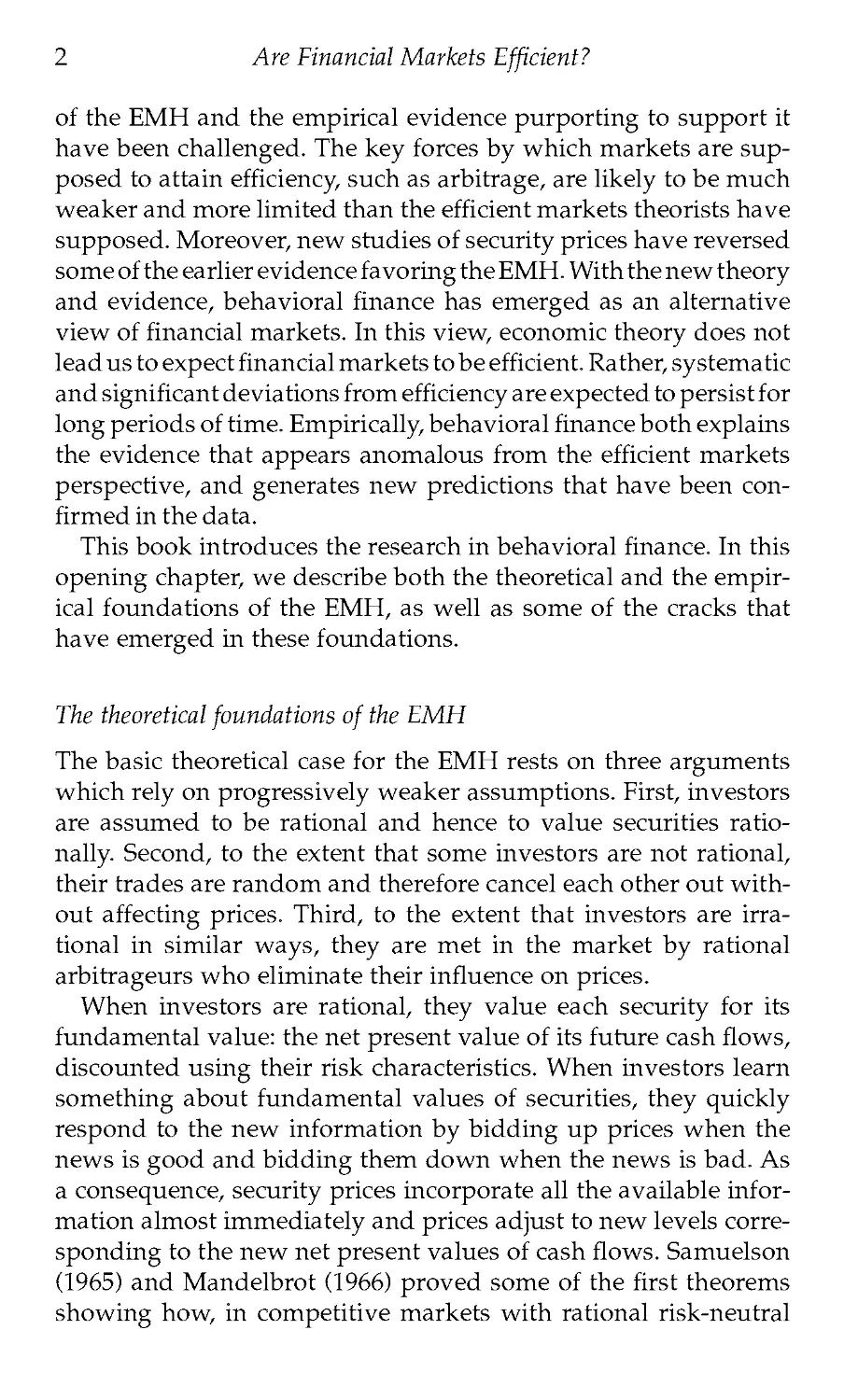
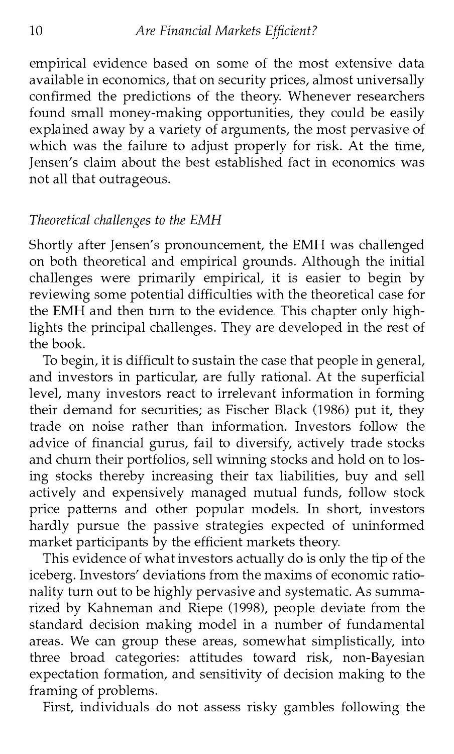
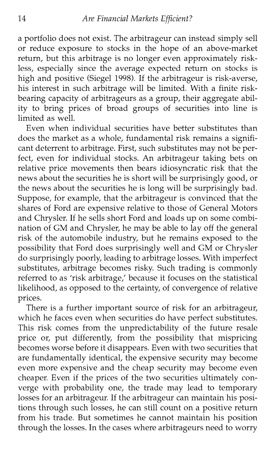
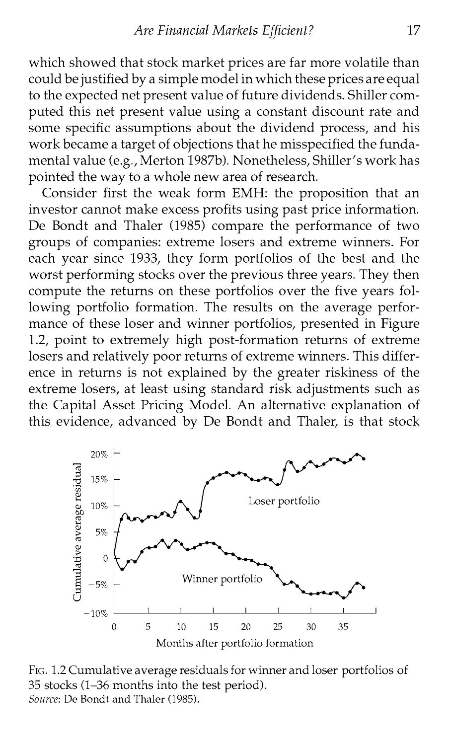
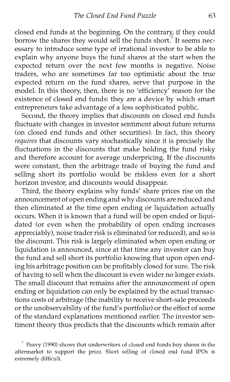
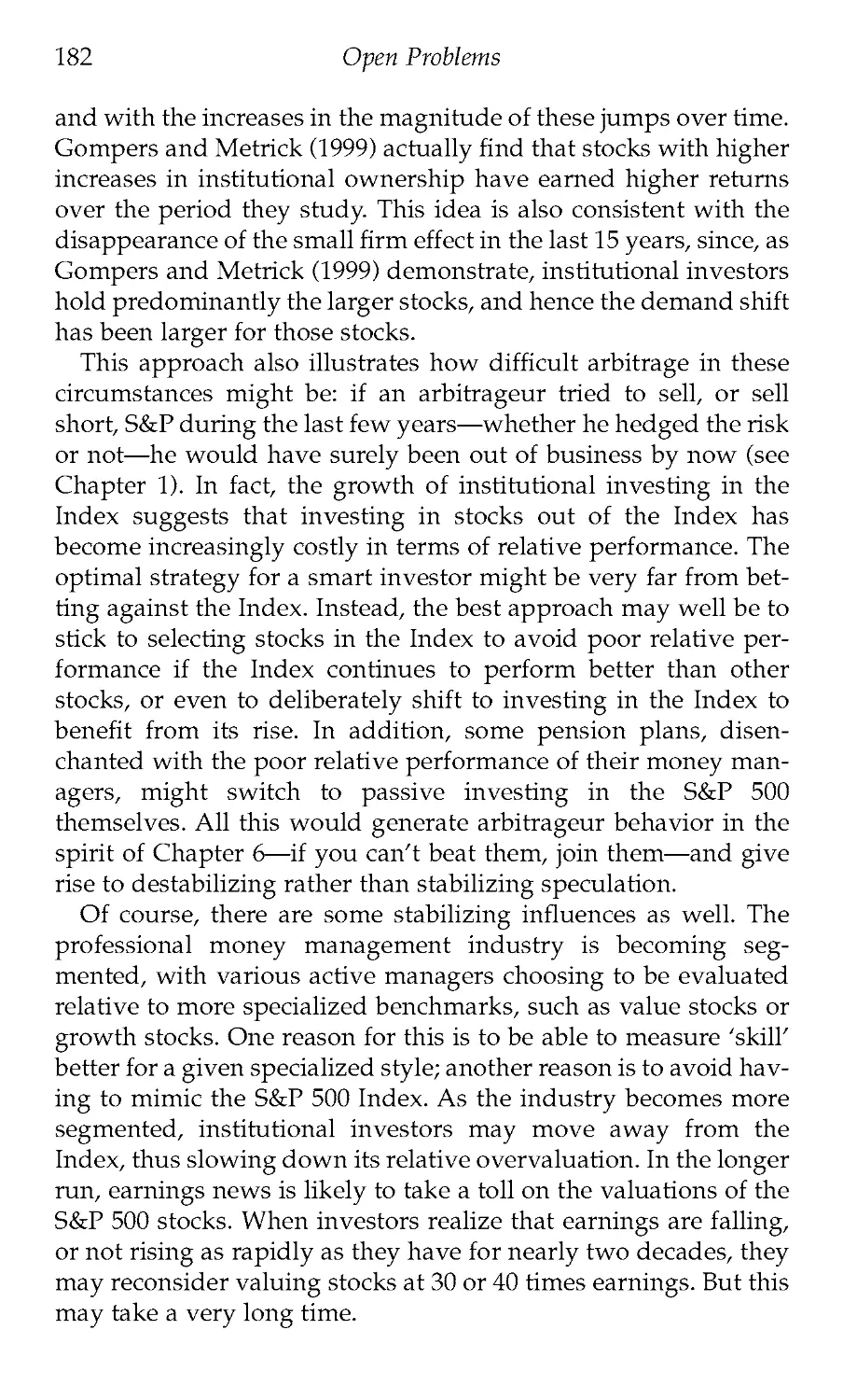
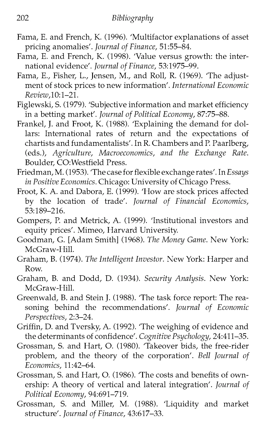
De Bondt and Thaler (1985) compare the performance of two
groups of companies: extreme losers and extreme winners. For
each year since 1933, they form portfolios of the best and the
worst performing stocks over the previous three years. They then
compute the returns on these portfolios over the five years fol-
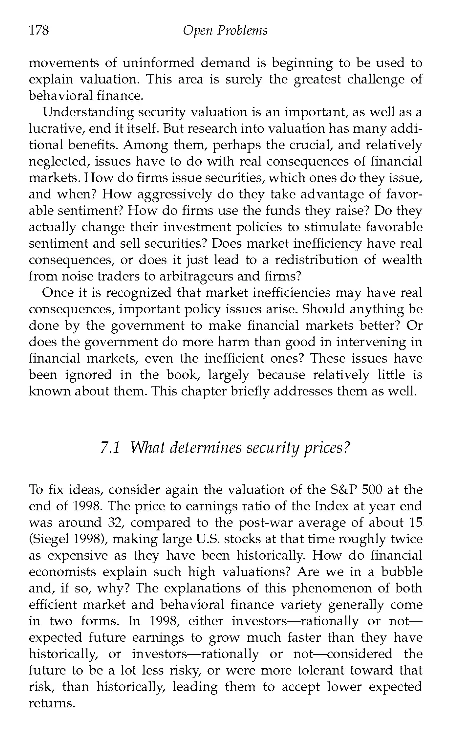
lowing portfolio formation. The results on the average perfor-
mance of these loser and winner portfolios, presented in Figure
1.2, point to extremely high post-formation returns of extreme
losers and relatively poor returns of extreme winners. This differ-
ence in returns is not explained by the greater riskiness of the
extreme losers, at least using standard risk adjustments such as
the Capital Asset Pricing Model. An alternative explanation of
this evidence, advanced by De Bondt and Thaler, is that stock
Fig. 1.2 Cumulative average residuals for winner and loser portfolios of
35 stocks (1-36 months into the test period).
Source: De Bondt and Thaler (1985).
18
Are Financial Markets Efficient?
prices overreact: the extreme losers have become too cheap and
bounce back, on average, over the post-formation period,
whereas the extreme winners have become too expensive and
earn lower subsequent returns. This explanation fits well with
psychological theory: the extreme losers are typically companies
with several years of poor news, which investors are likely to
extrapolate into the future, thereby undervaluing these firms, and
the extreme winners are typically companies with several years of
good news, inviting overvaluation.
Subsequent to De Bondt and Thaler's findings, researchers
have identified more ways to successfully predict security
returns, particularly those of stocks, based on past returns.
Among these findings, perhaps the most important is that of
momentum (Jegadeesh and Titman 1993), which shows that
movements in individual stock prices over the period of six to
twelve months tend to predict future movements in the same
direction. That is, unlike the long-term trends identified by De
Bondt and Thaler, which tend to reverse themselves, relatively
short-term trends continue. Some of these results are discussed in
Chapter 5, but for now suffice it to say that even the weak form
efficient markets hypothesis has faced significant empirical chal-
lenges in recent years. Even Fama (1991) admits that stock returns
are predictable from past returns and that this represents a depar-
ture from the conclusions reached in the earlier studies.
The semi-strong form efficient markets hypothesis has not
fared better. Perhaps the best known deviation is that, historically,
small stocks have earned higher returns than large stocks.
Between 1926 and 1996, for example, the compounded annual
return on the largest decile of the New York Stock Exchange
stocks has been 9.84 percent, compared to 13.83 percent on the
smallest decile of stocks (Siegel 1998, p. 93). Moreover, the supe-
rior return to small stocks has been concentrated in January of
each year, when the portfolio of the smallest decile of stocks out-
performed that of the largest decile by an average of 4.8 percent.
There is no evidence that, using standard measures of risk, small
stocks are that much riskier in January. Since both a company's
size and the coming of the month of January is information
known to the market, this evidence points to excess returns based
on stale information, in contrast to semi-strong form market effi-
ciency. Interestingly for the purposes of this book, both the small
Are Financial Markets Efficient? 19
firm effect and the January effect seem to have disappeared in the
last 15 years.
More recent research uncovered other variables that predict
future returns. Suppose that an investor selects his portfolio using
the ratio of the market value of a company's equity to the
accounting book value of its assets. The market to book ratio can
be loosely thought of as a measure of the cheapness of a stock.
Companies with the highest market to book ratios are relatively
the most expensive 'growth' firms, whereas those with the lowest
ratios are relatively the cheapest 'value' firms. For this reason,
investing in low market to book companies is sometimes called
value investing. Following De Bondt and Thaler's logic, the high
market to book ratios may reflect the excessive market optimism
about the future profitability of companies resulting from overre-
action to past good news. Consistent with overreaction, De Bondt
and Thaler (1987), Fama and French (1992), and Lakonishok et al.
(1994) find that, historically, portfolios of companies with high
market to book ratios have earned sharply lower returns than
those with low ratios. Moreover, high market to book portfolios
appear to have higher market risk than do low market to book
portfolios, and perform particularly poorly in extreme down
markets and in recessions (Lakonishok et al. 1994).
The size and market to book evidence, on the face of it, presents
a serious challenge to the EMH, because stale information obvi-
ously helps predict returns, and the superior returns on value
strategies are not due to higher risk as conventionally measured.
Yet this evidence again has been subjected to a radical version of
the Fama critique. Fama and French (1993, 1996) ingeniously
interpret both a company's market capitalization and its market
to book ratio as measures of fundamental riskiness of a stock in a
so-called three-factor model. According to this model, stocks of
smaller firms or of firms with low market to book ratios must
earn higher average returns precisely because they are funda-
mentally riskier as measured by their higher exposure to size and
market to book 'factors.' Conversely, large stocks earn lower
returns because they are safer, and growth stocks with high mar-
ket to book ratios also earn lower average returns because they
represent hedges against this market to book risk.
It is not entirely obvious from the Fama and French analysis
how either size or the market to book ratio, whose economic
20
Are Financial Markets Efficient?
interpretations are rather dubious in the first place, have emerged
as heretofore unnoticed but critical indicators of fundamental
risk, more important than the market risk itself. Fama and French
speculate that perhaps the low size and market to book ratio
proxy for different aspects of the 'distress risk/ but up to now
there has been no direct evidence in support of this interpretation,
and indeed Lakonishok et al. (1994) find no evidence of poor per-
formance of value strategies in extremely bad times. The fact that
the small firm effect has disappeared in the last 15 years, and
before that was concentrated in January, also presents a problem
for the risk interpretation. And even Fama and French do not
offer a risk interpretation of the momentum evidence. Chapter 5
revisits some of this evidence and related controversies, and
offers a behavioral analysis.
Finally, what about the basic proposition that stock prices do
not react to non-information? Here again there has been much
work, but three types of findings stand out. Perhaps the most
salient piece of evidence bearing on this prediction is the crash of
1987. On Monday, October 19, the Dow Jones Industrial Average
fell by 22.6 percent—the largest one day percentage drop in his-
tory—without any apparent news. Although the event caused an
aggressive search for the news that may have caused it, no per-
suasive culprit could be identified. In fact, many sharp moves in
stock prices do not appear to accompany significant news. Cutler
et al. (1991) examine the 50 largest one day stock price movements
in the United States after World War II, and find that many of
them came on days of no major announcements. This evidence is,
of course, broadly consistent with Shiller's earlier finding of
excess volatility of stock returns. More than news seems to move
stock prices.
A similar conclusion has been reached in two striking studies
by Richard Roll (1984,1988). In the first, Roll (1984) examines the
influence of news about weather on the price of orange juice
futures. Roll argues that because the production of oranges for
juice in the United States is extremely geographically concen-
trated and tastes for orange juice are very stable, news about
weather should account for most of the variation in futures
prices. He finds that, although news about weather help deter-
mine futures price movements, they account for a relatively small
share of these movements. Roll (1988) extends this idea to indi-
Are Financial Markets Efficient?
21
vidual stocks. He calculates the share of variation in the returns
of large stocks explained by aggregate economic influences, the
contemporaneous returns on other stocks in the same industry,
and public firm-specific news events. He finds the average
adjusted R2s to be only .35 with monthly data and .2 with daily
data, suggesting that movements in prices of individual stocks
are largely unaccounted for by public news or by movements in
potential substitutes. In both of Roll's studies, shocks other than
news appear to move security prices, in contrast to the efficient
markets analysis.
Roll's second study is also important because, at least in prin-
ciple, his R2s are good indicators of the closeness of available sub-
stitute portfolios for a given stock. If a stock had perfect
substitutes, which presumably are other stocks in the same indus-
try, Roll's R2s should be close to one, especially after he controls for
firm-specific news events. In reality, the R2s he finds are far below
one, no matter how hard he works to raise them. The natural inter-
pretation of this evidence is that the available substitutes are far
from perfect.
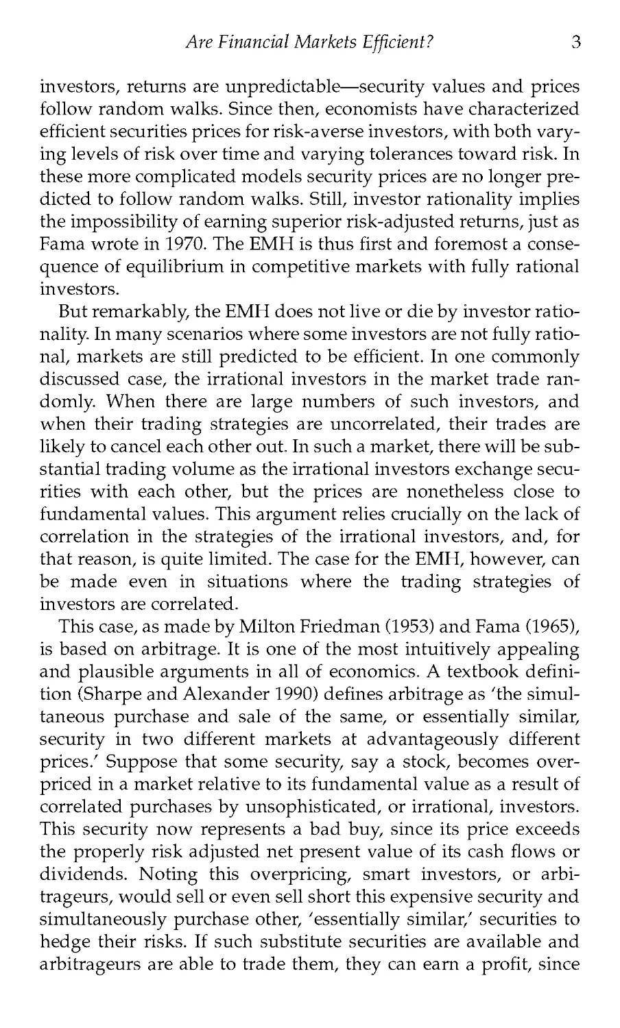
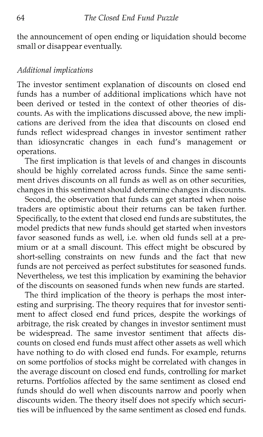
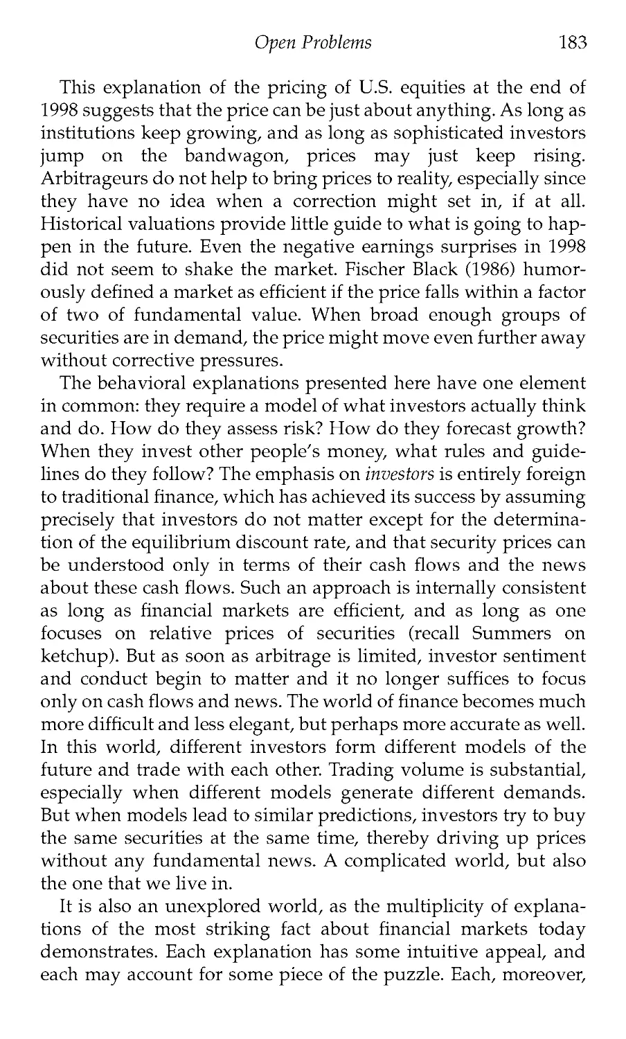
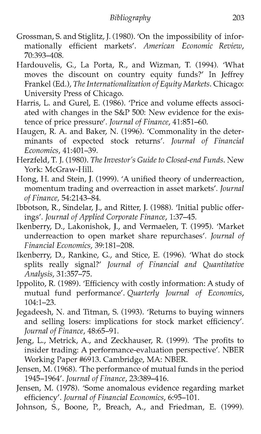
Other, seemingly unrelated, results that show that prices react
to uninformed demand shifts are those on inclusion of stocks into
the Standard and Poor's 500 Index. The S&P 500 Index consists of
500 large U.S. companies, and is designed in part to include the
largest firms, but also to be representative of the American econ-
omy. Every year, a few stocks are withdrawn from the Index,
most often because these companies are taken over. These stocks
are then replaced by the Standard and Poor's Corporation with
other stocks, largely with the goal of maintaining the representa-
tiveness of the Index. Inclusion into the Index is an interesting
event to study because it is unlikely to convey any information
about the company, but at the same time entails substantial buy-
ing of shares. When a company is included in the Index, a signif-
icant number of its shares is acquired by so-called index funds,
which hold passive portfolios replicating the Index, as well as by
other professional money managers whose portfolios are suppos-
edly kept close to the Index. The inclusion thus generates a sub-
stantial uninformed demand for the shares of the company.
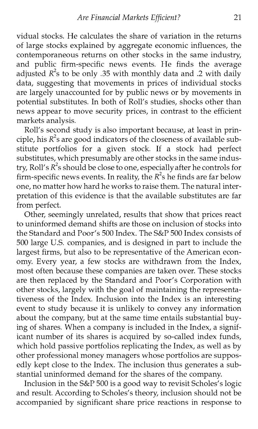
Inclusion in the S&P 500 is a good way to revisit Scholes's logic
and result. According to Scholes's theory, inclusion should not be
accompanied by significant share price reactions in response to
22
Are Financial Markets Efficient?
-2 -1 0 1 2 3 4 5 6 7 8 9 10 11 12 13 14 15 16 17 18 19 20
Trading day relative to addition announcement
Fig. 1.3 Mean cumulative abnormal returns for stocks added to the S&P
500.
The sample includes 236 stocks that were added to the S&P 500
between September 22,1976 and May 21,1996 and were not the subject
of contemporaneously reported news. Cumulative abnormal returns are
calculated by summing returns in excess of CRSP value-weighted
market returns. The standard error of the series is approximately 0.20
percent at day 0 and 0.45 percent at day +20.
Source: Wurgler and Zhuravskaya (1999).
new demand because the initial holders of included stocks
should be pleased to sell and to move into substitutes. According
to the view that securities do not have perfect substitutes, in con-
trast, the buying following the inclusion should be accompanied
by share price increases since buyers need to get the shares from
inframarginal sellers. Harris and Gurel (1986) and Shleifer (1986)
examine this experiment. As Figure 1.3 taken from a recent study
by Wurgler and Zhuravskaya (1999) illustrates, inclusion
between 1976 and 1996 is actually accompanied by average share
price increases of 3.5 percent. These increases are relatively per-
manent and have become larger as the relative share of the mar-
ket held in index funds has increased (see Chapter 2). In
December 1998, America Online—one of the glamourous Internet
stocks of the late 1990s—rose 18 percent on the news of its inclu-
sion in the Index. This evidence casts doubt on a basic implication
Are Financial Markets Efficient?
23
of the EMH: the non-reaction of prices to non-information.
Moreover, it is consistent with Roll's analysis in suggesting that
demand shifts move security prices, and that arbitrage does not
eliminate the influence of these shifts on prices because securities
do not have good substitutes.
Many of the results described here have been challenged on a
variety of grounds, including data snooping, trading costs, sam-
ple selection biases, and most centrally improper risk adjustment.
Nonetheless, it is difficult to deny that the thrust of this evidence
is very different from what researchers found in the 1960s and the
1970s, and is much less favorable to the EMH. An interesting
question is why have researchers failed to report much evidence
challenging market efficiency until 1980? One possible explana-
tion is the professional dominance of the EMH supporters, and
the difficulty of publishing rejections of the EMH in academic
journals. This explanation is not entirely satisfactory, since there
are many competing journals in finance and economics aiming to
publish novel findings. A more plausible, and scientifically more
satisfactory, account of the failure to find contradictory evidence
is provided by Summers (1986). Summers argues that many tests
of market efficiency have low power in discriminating against
plausible forms of inefficiency. He illustrates this observation by
showing that it is often difficult to tell empirically whether some
time series, such as the value of a stock index, follows a random
walk or alternatively a mean-reverting process that might come
from a persistent fad. It takes a lot of data, and perhaps a better
theoretical idea of what to look for, before researchers can find
persuasive evidence. Whatever the reason why it took so long in
practice, the cumulative impact of both the theory and the evi-
dence has been to undermine the hegemony of the EMH and to
create a new area of research—behavioral finance. This book
describes some of the theoretical and empirical foundations of
this research.
Organization of the book
At the most general level, behavioral finance is the study of human
fallibility in competitive markets. It does not simply deal with an
observation that some people are stupid, confused, or biased.
This observation is uncontroversial, although understanding the
24
Are Financial Markets Efficient?
precise nature of biases and confusions is an enormously difficult
task. Behavioral finance goes beyond this uncontroversial obser-
vation by placing the biased, the stupid, and the confused into
competitive financial markets, in which at least some arbitrageurs
are fully rational. It then examines what happens to prices and
other dimensions of market performance when the different types
of investors trade with each other. The answer is that many inter-
esting things do happen. In particular, financial markets in most
scenarios are not expected to be efficient. Market efficiency only
emerges as an extreme special case, unlikely to hold under plausi-
ble circumstances.
As a study of human fallibility in competitive markets, behav-
ioral finance theory rests on two major foundations. The first is
limited arbitrage. This set of arguments suggests that arbitrage in
real-world securities markets is far from perfect. Many securities
do not have perfect or even good substitutes, making arbitrage
fundamentally risky and, even when good substitutes are avail-
able, arbitrage remains risky and limited because prices do not
converge to fundamental values instantaneously. The fact that
arbitrage is limited helps explain why prices do not necessarily
react to information by the right amount and why prices may
react to non-information expressed in uninformed changes in
demand. Limited arbitrage thus explains why markets may
remain inefficient when perturbed by noise trader demands, but
it does not tell us much about the exact form that inefficiency
might take. For that, we need the second foundation of behavioral
finance, namely investor sentiment: the theory of how real-world
investors actually form their beliefs and valuations, and more
generally their demands for securities. Combined with limited
arbitrage, a theory of investor sentiment may help generate pre-
cise predictions about the behavior of security prices and returns.
Both of these elements of behavioral theory are necessary. If
arbitrage is unlimited, then arbitrageurs accommodate the unin-
formed shifts in demand as well as make sure that news is incor-
porated into prices quickly and correctly. Markets then remain
efficient even when many investors are irrational. Without
investor sentiment, there are no disturbances to efficient prices in
the first place, and so prices do not deviate from efficiency. A
behavioral theory thus requires both an irrational disturbance
and limited arbitrage which does not counter it.
Are Financial Markets Efficient?
25
Both the theory of limited arbitrage and the theory of investor
sentiment allow researchers to make predictions about security
prices. Some of these predictions can be made from the recogni-
tion of limited arbitrage alone: an exact model of investor senti-
ment is not required (Chapter 3). But the finer predictions tend to
require a specification of how investors form beliefs, that is, a
model of investor sentiment (Chapter 5).
As this book is being written, our state of understanding of the
two ingredient theories of behavioral finance is very different. We
understand a lot more about the limits of arbitrage than we do
about investor sentiment. Part of the reason for that is that the
theory of limited arbitrage is based on the behavior of rational
actors, namely arbitrageurs, and economics is better at modeling
and understanding such behavior. Another part of the reason is
that psychological evidence on judgment errors has not been
developed with an eye toward the interests of financial econo-
mists. There is a lot of psychology that might be relevant for
the formation of investor sentiment, and no obvious way of
deciding which psychological biases are the most important. As a
consequence, the research on investor sentiment has been more
tentative.
The goal of this book is to present some of the central ideas of
behavioral finance, organized around the themes of limited arbi-
trage and investor sentiment. At various points, the book touches
on many findings and results in behavioral finance. But it is not a
survey. Rather, it is a presentation of a set of themes—and a selec-
tive presentation at that since all the main chapters originate in
articles which the author of this book participated in writing. One
further clarification is in order. There is no single unifying model
in behavioral finance. Each theoretical chapter presented here con-
tains its own model, suited for the points the chapter is trying to
make. This state of affairs is not as satisfactory as a unified model,
but it is quite similar to that prevailing in other fields of economics
that develop theoretical models attempting to capture reality. Thus
modern macroeconomics, trade theory, development theory,
theory of industrial organization, and theory of corporate
finance—to name a few—are all organized around a number of
small models each focusing on a potentially important economic
mechanism.
As a central organizing principle, the next three chapters of this
26 Are Financial Markets Efficient?
book deal with limited arbitrage and its consequences and the fol-
lowing two focus on investor sentiment. Chapter 2 develops the
concept of noise trader risk and examines how it limits arbitrage.
This chapter also discusses in more detail the research related to
the availability of close substitutes for stocks. Chapter 3 examines
a particularly famous and important example of limited arbi-
trage, the closed end fund puzzle. This puzzle refers to the fact
that closed end mutual funds—the funds that hold portfolios of
other securities and have a fixed number of shares that are them-
selves traded in the market—often sell at prices different from the
market values of the portfolios they hold. Chapter 3 shows that
the closed end fund puzzle can be fruitfully analyzed in terms of
the model of noise trader risk presented in Chapter 2. Chapter 4
considers noise trader risk in the agency context of arbitrage
activity. When arbitrage is conducted by specialists using other
people's money, arbitrageurs are affected by the inability of their
investors to separate luck from skill. Because such arbitrage is
even more limited and unstable than when arbitrageurs invest
their own money, as they do in Chapter 2, Chapter 4 sheds further
doubt on the effectiveness of arbitrage in achieving market effi-
ciency. Chapter 4 also briefly discusses the turbulence of financial
markets in the summer of 1998, which vividly illustrated the lim-
its of arbitrage.
Chapters 2 through 4 reach two crucial conclusions. First, plau-
sible theories of arbitrage do not lead to the prediction that mar-
kets are efficient—quite the opposite. Second, the recognition that
arbitrage is limited, even without specific assumptions about
investor sentiment, generates new empirically testable predic-
tions, some of which have been confirmed in the data.
The two subsequent chapters focus on investor sentiment.
Chapter 5 begins with an overview of some of the empirical vio-
lations of weak and semi-strong form market efficiency that
recent models of investor sentiment try to address. It then pre-
sents one such model motivated by the idea that, in forecasting
future earnings, investors interpret the data on recent past earn-
ings using the representativeness heuristic. The simple model is
consistent with both psychological evidence and the evidence
from security prices. Chapter 6 presents another approach of
overreaction based on the idea that some investors extrapolate
past trends in prices. This chapter also describes the interaction of
Are Financial Markets Efficient? 27
noise traders and arbitrageurs and shows that in cases where
arbitrageurs trade in anticipation of noise trader demand they
move prices away from rather than toward fundamental values.
In addition to perhaps shedding further light on overreaction of
security prices, this chapter continues and expands the themes of
Chapters 2 and 4 by showing that rational arbitrage not only may
be limited in bringing about market efficiency, but may actually
in some circumstances move prices away from fundamentals and
make markets less efficient. Chapters 5 and 6 reveal the benefits
of modeling investor sentiment explicitly and of considering the
interactions of noise traders and arbitrageurs in the same market.
The field of behavioral finance is still in its infancy. Yet it has
presented financial economics with a new body of theory, a new
set of explanations of empirical regularities, as well as a new set
of predictions. The concluding chapter summarizes some of the
successes of behavioral finance, and shows how this field can
inform the analysis of broader questions in economics, including
the study of real consequences of financial markets and of public
policies toward them. In addition, Chapter 7 discusses some of
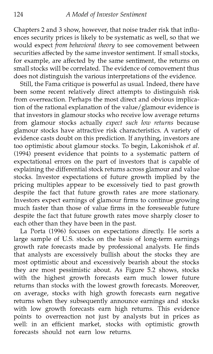
the many problems that remain open.
2
Noise Trader Risk in Financial Markets
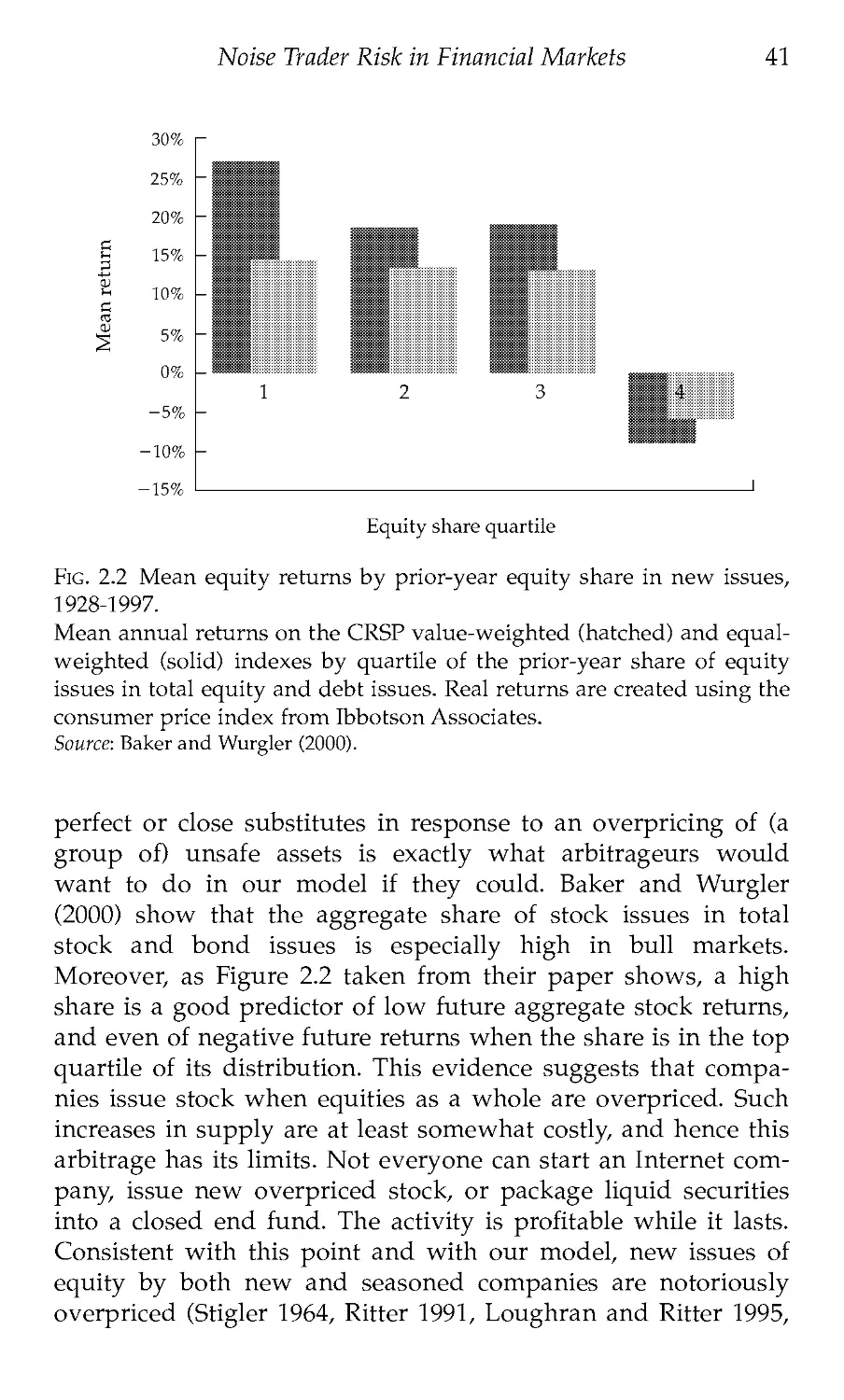
One of the fundamental concepts in finance is arbitrage, defined
as 'the simultaneous purchase and sale of the same, or essentially
similar, security in two different markets for advantageously dif-
ferent prices' (Sharpe and Alexander 1990). Theoretically
speaking, such arbitrage requires no capital and entails no risk.
When an arbitrageur buys a cheaper security and sells a more
expensive one, his net future cash flows are zero for sure and he
gets his profits up front. Arbitrage plays a critical role in the
analysis of securities markets, because its effect is to bring prices
to fundamental values and to keep markets efficient. For this rea-
son, it is important to understand how well this textbook descrip-
tion of arbitrage approximates reality. This chapter argues that
the textbook description does not describe realistic arbitrage
trades. Moreover, we can gain a deeper understanding of market
efficiency by focusing explicitly on some of the deviations of real-
world arbitrage from the textbook model.
In this chapter, we explore some of the basic risks associated
with arbitraging two fundamentally identical assets—the near
textbook case. We thus abstract away from the additional risks
arising from arbitrage of nearly, but not completely, perfect
substitutes as well as from transaction costs, both of which would
limit arbitrage even further. The risk we focus on is that of mis-
pricing deepening in the short run. Such risk is extremely
important for relatively short horizon investors engaged in arbi-
trage against noise traders: the risk that noise traders' beliefs
become even more extreme before they revert to the mean.
If noise traders today are pessimistic about an asset and have
driven down its price, an arbitrageur buying this asset must
recognize that in the near future noise traders might become even
more pessimistic and drive the price down even further. If the
arbitrageur has to liquidate before the price recovers, he suffers a
loss. Fear of this loss should limit his original arbitrage position.
Conversely, an arbitrageur selling an asset short when bullish
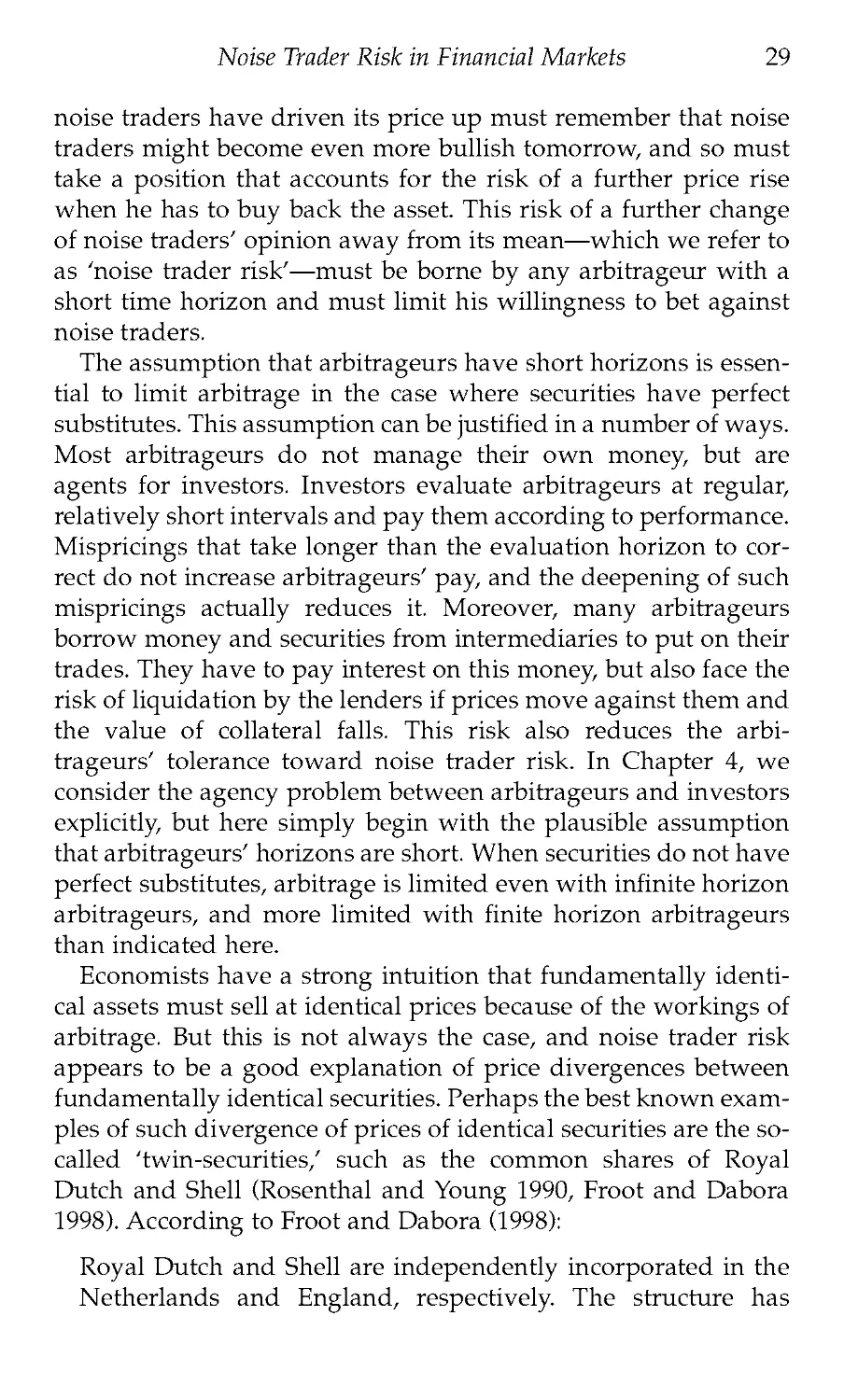
Noise Trader Risk in Financial Markets 29
noise traders have driven its price up must remember that noise
traders might become even more bullish tomorrow, and so must
take a position that accounts for the risk of a further price rise
when he has to buy back the asset. This risk of a further change
of noise traders' opinion away from its mean—which we refer to
as 'noise trader risk'—must be borne by any arbitrageur with a
short time horizon and must limit his willingness to bet against
noise traders.
The assumption that arbitrageurs have short horizons is essen-
tial to limit arbitrage in the case where securities have perfect
substitutes. This assumption can be justified in a number of ways.
Most arbitrageurs do not manage their own money, but are
agents for investors. Investors evaluate arbitrageurs at regular,
relatively short intervals and pay them according to performance.
Mispricings that take longer than the evaluation horizon to cor-
rect do not increase arbitrageurs' pay, and the deepening of such
mispricings actually reduces it. Moreover, many arbitrageurs
borrow money and securities from intermediaries to put on their
trades. They have to pay interest on this money, but also face the
risk of liquidation by the lenders if prices move against them and
the value of collateral falls. This risk also reduces the arbi-
trageurs' tolerance toward noise trader risk. In Chapter 4, we
consider the agency problem between arbitrageurs and investors
explicitly, but here simply begin with the plausible assumption
that arbitrageurs' horizons are short. When securities do not have
perfect substitutes, arbitrage is limited even with infinite horizon
arbitrageurs, and more limited with finite horizon arbitrageurs
than indicated here.
Economists have a strong intuition that fundamentally identi-
cal assets must sell at identical prices because of the workings of
arbitrage. But this is not always the case, and noise trader risk
appears to be a good explanation of price divergences between
fundamentally identical securities. Perhaps the best known exam-
ples of such divergence of prices of identical securities are the so-
called 'twin-securities/ such as the common shares of Royal
Dutch and Shell (Rosenthal and Young 1990, Froot and Dabora
1998). According to Froot and Dabora (1998):
Royal Dutch and Shell are independently incorporated in the
Netherlands and England, respectively. The structure has
30
Noise Trader Risk in Financial Markets
grown out of 1907 alliance between Royal Dutch and Shell
Transport by which the two companies agreed to merge their
interests on a 60:40 basis while remaining separate and distinct
entities. All sets of cash flows, adjusting for corporate tax con-
siderations and control rights, are effectively split in these pro-
portions. Information clarifying the linkages between the two
companies is widely available. Royal Dutch and Shell trade on
nine exchanges in Europe and the U.S., but Royal Dutch trades
primarily in the U.S. and the Netherlands (it is in the S&P 500
and virtually every index of Dutch shares), and Shell trades
predominantly in the UK (it is in the Financial Times Allshare
Index, or FTSE). In sum, if the market values of securities were
equal to the net present values of future cash flows, the value
of Royal Dutch equity should be equal to 1.5 times the value of
Shell equity. This, however, is far from the case.
Figure 2.1 presents the percentage deviation from the 60:40
ratio in the market values of equity of Royal Dutch and Shell
between September 1980 and September 1995. It shows enormous
deviations from parity, ranging from the relative underpricing of
Royal Dutch by 35 percent to relative overpricing by 10 percent.
There is no structural explanation of these deviations that we are
Stock price of Royal Dutch relative to Shell
Fig. 2.1 Log deviations from Royal Dutch/Shell parity.
Source: Froot and Dabora (1998).
Noise Trader Risk in Financial Markets
31
aware of, and indeed one might be especially difficult to find in
light of the fact that sometimes one of the securities trades at a
discount, and sometimes the other. Such deviations cannot exist
in a market where arbitrageurs have infinite time horizon and
face no transaction (including short-selling) costs, for an arbi-
trageur can simply buy the cheap shares, sell the same number of
expensive shares, put the net proceeds in his pocket, and hold the
hedged position forever.1
This evidence presents a deep challenge to the efficient markets
hypothesis. This is not a case of high returns on a particular class
of securities, where one can debate whether these returns are
anomalous or simply a compensation for risk. Rather, here two
fundamentally identical securities sell at different prices—a most
basic contradiction to the claim that price equals value. There is
no story in which the cash flows of one stock are subjected to a
different fundamental risk than the cash flows of the other. The
Fama critique is irrelevant. Moreover, the Royal Dutch/Shell
example is not unique. There are other companies for which sim-
ilar differences are observed. There are cases where ADRs
(American Depositary Receipts) trade at different prices in the
United States than identical shares sell at in local markets. Similar
mispricings are common in the bond market. But perhaps the
most celebrated illustration of the related phenomenon is closed
end funds, which trade in the United States and elsewhere at
market prices different from the market values of portfolios they
hold. Although in the case of closed end funds there are alterna-
tive 'structural' explanations of the observed valuations, we show
in Chapter 3 that the arguments presented in this chapter shed
considerable light on the closed end fund puzzle as well.
An examination of Figure 2.1 points to a crucial cost of arbi-
trage in Royal Dutch and Shell: the risk that mispricing becomes
more extreme. An arbitrageur who bought the relatively cheap
Royal Dutch shares, and sold the corresponding number of the
relatively expensive Shell shares in mid 1983, when the discount
was 10 percent, experienced a severe deterioration of his position
1 Actually, the optimal arbitrage strategy is not obviously to buy and sell the
same amount of cheap and expensive shares, respectively. Rashes (1998b) works
out the optimal arbitrage strategy, and applies it to a number of examples, includ-
ing Royal Dutch/Shell arbitrage.
32
Noise Trader Risk in Financial Markets
as the discount widened to nearly 25 percent six months later. If
this arbitrageur was leveraged or if he had to explain his losses to
investors (see Chapter 4), he might have failed to survive through
these losses, and might have been forced to liquidate this
position. To him, noise trader risk is very important.
Equally interesting, Figure 2.1 reveals that it takes about four
years for the 30 percent mispricing of Royal Dutch and Shell preva-
lent in September of 1980 to go away. In return for bearing this
noise trader risk, the arbitrageur earns about 7 percent per year.
Note that this 7 percent comes from a period where we know ex
post that the mispricing has corrected; it could of course have
widened and led to a loss. In principle, the arbitrageur could have
leveraged his position to earn a higher average return, but then he
had to take into account the costs of leverage, as well as the possi-
ble risk of unfavorable liquidation as the mispricing widens. These
calculations suggest that perhaps the arbitrage of Royal Dutch ver-
sus Shell was not ex ante especially attractive in September of 1980,
when the mispricing was 30 percent, and these are fundamentally
identical securities! The converse point is that, when mispricing
can take a while to correct, enormous inefficiencies can be sus-
tained without aggressive arbitrage activity coming in to correct
them. From the point of view of the EMH, this observation is cru-
cial, for it shows that—even for securities with perfect substi-
tutes—large deviations of prices from fundamental values can be
explained by somewhat risky arbitrage that takes time to correct.
In this chapter, we present a theory of arbitrage limited by
noise trader risk, just as in the case of Royal Dutch and Shell. We
study financial markets in which the mere unpredictability of
investor sentiment—of future noise trader demand for assets—
becomes an important source of risk and a deterrent to arbitrage.
We derive equilibrium security prices, and show that—because
arbitrage is risky and limited—financial markets are not efficient.
We then examine Friedman's evolutionary argument in such a
market and find that the conclusion that the unsophisticated
investors earn lower average returns than the arbitrageurs is
unwarranted. Finally, we discuss the costs of arbitrage activity
more generally than we do in the formal model. In particular, we
focus on a number of costs that the model does not include, as
well as on the important case where mispriced securities do not
have perfect substitutes.
Noise Trader Risk in Financial Markets
33
2.1 Noise trading as a source of risk
A model
The model contains noise traders and arbitrageurs. Noise traders
form erroneous beliefs about the future distribution of returns on
a risky asset. In this chapter, it does not matter exactly why noise
traders form erroneous beliefs. They may be subject to one of the
behavioral biases in processing information and forecasting
returns. Alternatively, they may incorrectly perceive the riskiness
of returns, perhaps because they are overconfident. Noise traders
select their portfolios on the basis of such incorrect beliefs. In
response, it is optimal for arbitrageurs to exploit noise traders'
misperceptions. Their investment strategies push prices toward
fundamentals, but not all the way.
The basic model is a stripped-down overlapping generations
model with two-period-lived agents (Samuelson 1958). For sim-
plicity, there is no first-period consumption, no labor supply
decision, and no bequest. As a result, the resources agents have to
invest are exogenous. The only decision agents make is to choose
a portfolio when young.
The economy contains two assets that pay identical dividends.
One of the assets, the safe asset s, pays a fixed real dividend r per
period. Asset s is in perfectly elastic supply: a unit of it can be cre-
ated out of, and a unit of it turned back into, a unit of the con-
sumption good in any period. With consumption each period
taken as numeraire, the price of the safe asset is always fixed at
one. The dividend r paid on asset s is thus the riskless rate. The
other asset, the unsafe asset u, always pays the same fixed real
dividend r as asset s. But и is not in elastic supply: it is in fixed
and unchangeable quantity, normalized at one unit. The price of
и in period t is denoted pt. If the price of each asset were equal to
the net present value of its future dividends, then assets и and s
would be perfect substitutes and would sell for the same price of
one in all periods. But this is not how the price of и is determined
in the presence of noise traders.
The analysis below relies on a limited risk bearing capacity of
arbitrageurs as a whole. There are two ways to justify this assump-
tion. First, we can assume that noise trader risk is market-wide
rather than idiosyncratic. For example, it can be a risk affecting the
34
Noise Trader Risk in Financial Markets
stock market as a whole, or a large group of stocks. In the Royal
Dutch and Shell example, Froot and Dabora (1998) document that
Royal Dutch shares comove with the Dutch market, whereas Shell
shares comove with the British market—exposing an arbitrageur
to price movements in both markets. Alternatively, we can assume
as we do in Chapter 4 that the market in question requires special-
ized arbitrage resources, and that such resources dedicated to that
market are limited. For example, arbitrage trades in emerging mar-
kets are often limited by the fact that access to these markets is
restricted, and therefore only a few experts who set up specialized
operations can engage in arbitrage. Still another way to proceed is
to assume that there is a cost of learning about the valuation of a
particular security or class of securities, which limits the entry of
arbitrageurs (Merton 1987«).
Without one of these assumptions, there are too many possibil-
ities for arbitrageurs to diversify, and hence their trading is more
aggressive. For example, if noise traders' misperceptions of the
returns to individual assets are uncorrelated and if each asset is
small relative to the market, a large number of tiny arbitrageurs
eliminate any possible mispricing for the same reasons that idio-
syncratic risk is not priced in the standard capital asset pricing
model. Such Ross-style arbitrage (Ross 1976) by a huge number of
diversified arbitrageurs is what drives market efficiency in
standard finance models, but it does not work when sentiment is
correlated across investors or when markets are segmented. The
model here is that of correlated sentiment and of the limited risk-
bearing capacity of the arbitrageurs.
There are two types of agents: arbitrageurs (denoted я) who
have rational expectations and noise traders (denoted n). We
assume that noise traders are present in the model in measure Li,
that arbitrageurs are present in measure 1 — Li, and that all agents
of a given type are identical. Both types of agents choose their
portfolios when young to maximize perceived expected utility
given their own beliefs about the ex ante mean of the distribution
of the price of и at t + 1. The representative arbitrageur young in
period t accurately perceives the distribution of returns from
holding the risky asset, and so maximizes expected utility given
that distribution. The representative noise trader young in period
t misperceives the expected price of the risky asset by an inde-
pendent and identically distributed normal random variable pf:
Noise Trader Risk in Financial Markets
35
pf~N(p*,np. (2.1)
The mean misperception p* is a measure of the average 'bullish-
ness' of the noise traders, and is the variance of noise traders'
misperceptions of the expected return per unit of the risky asset.2
The results we derive below depend critically on the unpre-
dictability of future investor sentiment; the exact form of this sen-
timent is not essential for our findings. Noise traders thus
maximize their own expectation of utility given the next-period
dividend, the one-period variance of pM, and their false belief
that the distribution of the price of и next period has mean pf
above its true value. Each agent's utility is a constant absolute risk
aversion function of wealth when old:
U = -e(2'l)w, (2.2)
where у is the coefficient of absolute risk aversion and w is
wealth when old. Given their beliefs, all young agents divide
their portfolios between и and s. When old, agents convert their
holdings of s into the consumption good, sell their holdings of и
for price p/+1 to the new young, and consume all their wealth.
With normally distributed returns to holding a unit of the risky
asset, maximizing the expected value of (2.2) generates demands
for the risky asset proportional to perceived expected returns and
inversely proportional to the perceived variance of returns.
Denote by X" the amount of the risky asset и held by an arbi-
trageur, by X" amount held by a noise trader, and define fpf+!
to be the rationally expected at time t price of и at time
t + 1, and
- Ef (?7f +7)]2} (2.3)
to be the one-period-ahead variance of pt + v The quantities X"and
X" of the risky asset purchased are functions of its current price p„
its expected price and its variance, and of noise traders' misper-
ception pt. The exact demands are given by:
2 The assumption that noise traders misperceive the expected price hides the
fact that the expected price is itself a function of the parameters p* and cdp. Thus
we are implicitly assuming that noise traders know how to factor the effect of
future price volatility into their calculations of values. This assumption is made
for simplicity.
36
Noise Trader Risk in Financial Markets
, a = r+tpt + 1 - (1 + r)pt z (2 4)
„ = r + tpt + A - (1 + r)pt p, . (2.5)
2Y42f + 1) 2?4+р
We allow noise traders' and arbitrageurs' demands to be nega-
tive; they can take short positions at will. Even if investors hold
only positive amounts of both assets, the fact that returns are
unbounded allows each investor to have negative final wealth.
We use a standard specification of returns at the cost of allowing
consumption to be negative with positive probability.3
The demands for the risky asset are proportional to its per-
ceived excess return and inversely proportional to its perceived
variance. The additional term in the demand function of noise
traders comes from their misperception of the expected return.
When noise traders overestimate expected returns, they demand
more of the risky asset than arbitrageurs; when they underesti-
mate the expected return, they demand less. Arbitrageurs exert a
stabilizing influence in this model since they offset the volatile
positions of the noise traders.
The variance of prices appearing in the denominators of the
demand functions is derived solely from noise trader risk. Both
noise traders and arbitrageurs limit their demand for asset и
because the price at which they can sell it when old depends on
the uncertain beliefs of the next period's young noise traders.
This uncertainty about the price for which asset и can be sold
afflicts all investors, no matter what their beliefs about expected
returns and so limits the extent to which they are willing to bet
against each other. If the price next period were certain, then
noise traders and arbitrageurs would hold different beliefs about
expected returns with certainty; they would therefore try to take
infinite bets against each other. An equilibrium would not exist.
Noise trader risk limits all investors' positions and in particular
keeps arbitrageurs from driving prices all the way to fun-
damental values.
3 An appendix of De Long et al. (1987) presents an example in which asset
prices and consumption are always positive.
Noise Trader Risk in Financial Markets
37
The pricing function
To calculate equilibrium prices, observe that the old sell their
holdings and so the demands of the young must sum to one in
equilibrium. Equations (2.4) and (2.5) imply that
Pt = [r + f +1 ~“2'V(X + ? + HPJ- (2.6)
Equation (2.6) expresses the risky asset's price in period t as a
function of period t's misperception by noise traders (pt), of the
technological (r) and behavioral (y) parameters of the model, and
of the moments of the one-period-ahead distribution of pt + v We
consider only steady-state equilibria by imposing the require-
ment that the unconditional distribution of pt + j be identical to the
distribution of pt. The endogenous one-period-ahead distribution
of the price of asset и can then be eliminated from (2.6) by solving
recursively:
т , P(Pf - P*) , PP* 2y 2
pt = 1 + —y—------+------------(fo„ )• (2.7)
r r 1+r Г Г + 1
Inspection of (2.7) reveals that only the second term is variable,
for y, p*, and r are all constants, and the one-step-ahead variance
of pt is a simple unchanging function of the constant variance of a
generation of noise traders' misperception pf.
2 2
2 _ 2 _ P
f<4 + l “ Ch + 1 “ (1 + r)2 '
(2.8)
The final form of the price of u, which depends only on exoge-
nous parameters of the model and on public information about
present and future misperception by noise traders, is
, , p(pf - P*) , PP* 4 pVP
p--1+ i + r +ТН2’’ю7?
(2.9)
Interpretation
The last three terms that appear in (2.9) show the impact of noise
traders on the price of asset u. As the distribution of pf converges
to a point mass at zero, the equilibrium pricing function (2.9) con-
verges to its fundamental value of one.
38
Noise Trader Risk in Financial Markets
The second term in (2.9) captures the fluctuations in the price of
the risky asset и due to the variation of noise traders' mispercep-
tions. Even though asset и is not subject to any fundamental
uncertainty and is known to be so by a large class of investors, its
price varies substantially as noise traders' opinions shift. When a
generation of noise traders is more bullish than the average gen-
eration, they bid up the price of u. When they are more bearish
than average, they bid down the price. When they hold their
average misperception—when pt = p*—the term is zero. As one
would expect, the more numerous noise traders are relative to
arbitrageurs, the more volatile are asset prices.
The third term in (2.9) captures the deviations of pt from its fun-
damental value due to the fact that the average misperception by
noise traders is not zero. If noise traders are bullish on average, this
'price pressure' effect makes the price of the risky asset higher than
it would otherwise be. Optimistic noise traders bear a greater than
average share of price risk. Since arbitrageurs bear a smaller share
of price risk when p* is higher, they require a lower expected excess
return and so are willing to pay a higher price for asset u.
The final term in (2.9) is the heart of the model. Arbitrageurs
would not hold the risky asset unless compensated for bearing the
risk that noise traders become bearish and the price of the risky
asset falls. Both noise traders and sophisticated investors present
in period t believe that asset и is mispriced, but because pt + 1 is
uncertain, neither group is willing to bet too much on this mis-
pricing. At the margin, the return from enlarging one's position in
an asset that everyone agrees is mispriced (but different investors
think is mispriced in different directions) is offset by the additional
price risk that must be borne. Noise traders thus 'create their own
space': the uncertainty over what next period's noise traders will
believe makes the otherwise riskless asset и risky and drives its
price down and its return up. This is so despite the fact that both
arbitrageurs and noise traders always hold portfolios that possess
the same amount of fundamental risk: zero. For the economy as a
whole, there is no risk to be borne.
These results depend on three fundamental assumptions of the
model: the overlapping generations structure, the fixed supply of
the unsafe asset, and the systematic nature of noise trader risk. All
three assumptions have significant economic content, and war-
rant some discussion.
Noise Trader Risk in Financial Markets
39
The overlapping generations structure of the model plays two
roles. In the model, equilibrium exists as long as the returns to
holding the risky asset are always uncertain. In the overlapping
generations structure, this is assured by the absence of a last
period. For if there is a last period in which the risky asset pays a
nonstochastic dividend and is liquidated, then both noise traders
and arbitrageurs will seek to exploit what they see as riskless
arbitrage. If, say, the liquidation value of the risky asset is 1 + r,
previous-period arbitrageurs will try to trade arbitrarily large
amounts of asset и at any price other than one, and noise traders
will try to trade arbitrarily large amounts at any price other than
Pf = i+TT7' (2.10)
The excess demand function for the risky asset will be undefined.
But in a model with fundamental dividend risk on asset u, the
assumption that there is no last period is not necessary because и
and s are no longer perfect substitutes (Campbell and Kyle 1993).
In this case, no agent is ever subjectively certain what the return
on the risky asset will be, and so the qualitative properties of
equilibrium are preserved even with a known terminal date. The
overlapping generations structure is not needed when the two
assets are not perfect substitutes.
The overlapping generations structure plays another function:
it assures that each agent's horizon is short. No agent has any
opportunity to wait until the price of the risky asset recovers
before selling. Such a structure may be a fruitful way of modeling
the effects on prices of a number of institutional features, such as
frequent evaluations of money managers' performance, that may
lead rational, long-lived market participants to care about short-
term rather than long-term performance (see Chapter 4).
In our model, the horizons of arbitrageurs are important. If
their horizons are long relative to the duration of noise traders'
optimism or pessimism toward risky assets, then they can buy
low, confident of being able to sell high when prices revert to the
mean. Noise trader risk is an important deterrent to arbitrage
only when the duration of noise traders' misperceptions is of the
same order of magnitude as or longer than the horizon of the
arbitrageurs.
40
Noise Trader Risk in Financial Markets
In general, the longer the horizons of the arbitrageurs, the more
aggressively they trade, and the more efficient are the markets.
Although arbitrage is not riskless for long but finite-lived agents,
their asset demands are more responsive to price movements
than those of two-period-lived agents. There are two reasons for
this. First, even if an и > 2 period-lived arbitrageur can liquidate
his position in asset и only in the last period of his life, he bears
the same amount of resale price risk as his two-period-lived
counterpart, but gets some insurance from dividends. If, for
example, he buys an undervalued asset u, he receives a high div-
idend yield for several periods before he sells. Because as the
horizon expands so does the share of dividends in expected
returns, agents with longer horizons buy more at the start.
Second, a long-lived arbitrageur has many periods to liquidate
his position. Since he makes money on arbitrage if the price
reverts to the mean at any time before his death, having several
opportunities to liquidate reduces his risk. For these two reasons,
raising arbitrageurs' horizons makes them more aggressive and
brings the price of и closer to fundamentals.
The assumption of the fixed supply of the unsafe asset prevents
arbitrageurs from pursuing other money making strategies, such
as the conversion of the safe asset into unsafe asset when the lat-
ter is overpriced, and vice versa when it is underpriced. If this
assumption were completely removed, the opportunities for arbi-
trage would expand so as to restore market efficiency. In many
instances, this assumption is completely realistic: the Royal Dutch
and Shell shares indeed exist in fixed proportions and an arbi-
trageur could not convert the relatively cheap Royal Dutch shares
into the relatively expensive Shell shares in the 1980s. In other
instances, arbitrageurs may actually increase the supply of the
expensive unsafe asset. Thus arbitrageurs create companies in
overpriced industries and take them public, whether these are
companies in hot industries such as biotechnology companies in
the 1980s (Lerner 1994) or the Internet stocks in the late 1990s, or
closed end mutual funds in the 1920s, 1960s, and 1980s (De Long
and Shleifer 1991 and Chapter 3). Increases in the supply of secu-
rities during price bubbles have also been extremely important
historically (see Kindleberger 1978 and Chapter 6).
Companies themselves can and do issue securities when they
believe that these securities are overpriced. Such creation of
Noise Trader Risk in Financial Markets
41
Equity share quartile
Fig. 2.2 Mean equity returns by prior-year equity share in new issues,
1928-1997.
Mean annual returns on the CRSP value-weighted (hatched) and equal-
weighted (solid) indexes by quartile of the prior-year share of equity
issues in total equity and debt issues. Real returns are created using the
consumer price index from Ibbotson Associates.
Source: Baker and Wurgler (2000).
perfect or close substitutes in response to an overpricing of (a
group of) unsafe assets is exactly what arbitrageurs would
want to do in our model if they could. Baker and Wurgler
(2000) show that the aggregate share of stock issues in total
stock and bond issues is especially high in bull markets.
Moreover, as Figure 2.2 taken from their paper shows, a high
share is a good predictor of low future aggregate stock returns,
and even of negative future returns when the share is in the top
quartile of its distribution. This evidence suggests that compa-
nies issue stock when equities as a whole are overpriced. Such
increases in supply are at least somewhat costly, and hence this
arbitrage has its limits. Not everyone can start an Internet com-
pany, issue new overpriced stock, or package liquid securities
into a closed end fund. The activity is profitable while it lasts.
Consistent with this point and with our model, new issues of
equity by both new and seasoned companies are notoriously
overpriced (Stigler 1964, Ritter 1991, Loughran and Ritter 1995,
42
Noise Trader Risk in Financial Markets
Brav and Gompers 1997, and Brav, et al. 1999), and earn low
returns subsequent to issuance.4 Just as arbitrageurs take advan-
tage of noise traders and earn profits by selling short expensive
securities and buying cheap substitutes, firms and entrepre-
neurs make money by issuing overpriced securities to new
buyers. As we discuss in Chapter 7, it remains an open ques-
tion whether taking advantage of overpricing is a minor or a
major driving force behind security issues.
The third major assumption we make is that noise trader risk
is systematic: it affects either the market as a whole or a signifi-
cant segment of traded securities. If noise trader risk on each
asset were purely idiosyncratic, it would not be priced in equi-
librium. The necessity of noise trader risk being systematic for it
to be priced implies that the securities influenced by noise trader
sentiment must have correlated returns. This would be the case
even if these securities were fundamentally uncorrelated, and
the only common influence on their prices was noise trader
demand. This observation generates a very sharp prediction:
fundamentally unrelated securities subject to the same noise
trader sentiment must observably move together. In the next
chapter, we apply this observation to the study of closed end
funds.
The converse implication of systematic noise trader risk is also
important. Authors such as Fama and French (1993) have inter-
preted the evidence that particular groups of securities move
together as pointing to a common fundamental risk to which their
holders are exposed. The analysis in this chapter suggests that
comovement may indeed be evidence of a common risk expo-
sure, but shows that such risk does not have to be fundamental.
Noise trader risk not only can, but must be systematic to be
priced in equilibrium and hence the comovement of different
securities can be pointing to their exposure to common noise
trader risk rather than fundamental risk. In fact, the comove-
ment of securities which can be shown to be fundamentally
unrelated can be taken as strong evidence of the influence of
investor sentiment on security prices.
We come back to the various interpretations of these low returns in Chapters
5 and 7.
Noise Trader Risk in Financial Markets
43
2.2 Relative returns of noise traders and arbitrageurs
We have demonstrated that noise traders can affect prices even
though there is no uncertainty about fundamentals. Friedman
(1953) and Fama (1965) argue that noise traders who affect prices
earn lower returns than the arbitrageurs they trade with, and so
economic selection works to weed them out. In our model, it need
not be the case that noise traders earn lower returns. Noise
traders' collective shifts of opinion increase the riskiness of
returns to assets. If noise traders' portfolios are concentrated in
assets subject to noise trader risk, noise traders can earn a higher
average rate of return on their portfolios than the arbitrageurs.
The conditions under which noise traders earn higher expected
returns than arbitrageurs are easily laid out. All agents earn a cer-
tain net return of r on their investments in asset s. The difference
between noise traders' and arbitrageurs' total returns, given
equal initial wealth, is the difference in their holdings of the risky
asset и times the excess return paid by a unit of that asset. Call
this difference in returns to the two types of agents:
AR„ _ a = Of - X")[r + Pt +, - pf(l + r)]. (2.11)
Some calculations show that the expected value of this difference
is given by:
E(AR„_„) = p*
(1 + r)2(p*)2 + (1 + r)2o2.
(2?)ро2
(2.12)
Equation (2.12) makes obvious the requirement that for noise
traders to earn higher expected returns, the mean misperception
p* of returns on the risky asset must be positive. The first p* on the
right-hand side of (2.12) increases noise traders' expected returns
through what might be called the 'hold more' effect. Noise
traders' expected returns relative to those of arbitrageurs are
increased when noise traders on average hold more of the risky
asset and earn a larger share of the rewards of risk bearing. When
p* is negative, noise traders' changing misperceptions still make
the fundamentally riskless asset и risky and still push up the
expected return on asset u, but the rewards to risk bearing accrue
disproportionately to arbitrageurs, who on average hold more of
the risky asset than the noise traders do. Interestingly, the case of
44
Noise Trader Risk in Financial Markets
a positive p* corresponds to excessive noise trader optimism,
which Kahneman and Riepe (1998) describe as a common bias in
judgment. As interestingly, if noise traders are overconfident—
another common bias—they will also overinvest in the unsafe
asset u.
The first term in the numerator in (2.12) incorporates the 'price
pressure' effect. As noise traders become more bullish, they
demand more of the risky asset on average and drive up its price.
They thus reduce the return to risk bearing and, hence, the differ-
ential between their returns and those of arbitrageurs.
The second term in the numerator incorporates the buy high-
sell low or 'Friedman' effect. Because noise traders' mispercep-
tions are stochastic, they have the worst possible market timing.
They buy the most of the risky asset и just when other noise
traders are buying it, which is when they are most likely to suffer
a capital loss. The more variable noise traders' beliefs are, the
more damage their poor market timing does to their returns.
The denominator incorporates the 'create space' effect central
to this model. As the variability of noise traders' beliefs increases,
so does price risk. To take advantage of noise traders' mispercep-
tions, arbitrageurs must bear this greater risk. Since arbitrageurs
are risk averse, they reduce the extent to which they bet against
noise traders' in response to this increased risk. If the 'create
space' effect is large, then the 'price pressure' and 'buy high-sell
low' effects inflict less damage on noise traders' average returns
relative to arbitrageurs' returns.
Two effects—'hold more' and 'create space'—tend to raise
noise traders' relative expected returns. Two effects—'Friedman'
and 'price pressure'—tend to lower noise traders' relative
expected returns. Neither pair clearly dominates. Noise traders
cannot earn higher average returns if they are on average bearish,
for if p* does not exceed zero, there is no hold more effect and
(2.12) must be negative. Nor can noise traders earn higher aver-
age returns if they are too bullish, for as p* gets large the price
pressure effect, which increases with (p*)2, dominates. For inter-
mediate degrees of average bullishness, noise traders earn higher
expected returns. And it is clear from (2.12) that the larger у is,
that is, the more risk-averse agents are, the larger is the range of
p* over which noise traders earn higher average returns.
The fact that bullish noise traders can earn higher returns in the
Noise Trader Risk in Financial Markets
45
market than arbitrageurs implies that Friedman's simple 'market
selection' argument is incomplete. The key difference from
Friedman's (1953) model is that here the demand curve of arbi-
trageurs shifts in response to the addition of noise traders and the
resulting increase in risk. Because of this shift, arbitrageurs'
expected returns may fall relative to the returns of the noise
traders even though their expected utility rises relative to that of
the noise traders. Since noise traders' wealth can increase faster
than arbitrageurs', it is not possible to make any blanket state-
ment that noise traders lose money and eventually become
unimportant.
One should not overinterpret our result, however, for two rea-
sons. First, although they may earn a higher average return, noise
traders always receive a lower average utility. Still, wealth rather
than utility is relevant for financial influence, so the noise traders
might well be influential in the market, though not so happy, on
average, because of the volatility of returns.
Second, and much more important, expected returns are not
the same as long run survival. The greater variance of noise
traders' returns might give them in the long run a high probabil-
ity of having low wealth and a low probability of having very
high wealth. Market selection might work against such traders
even if their expected value of wealth is high since they would be
almost surely poor. A more appropriate selection criterion would
take this into account. This turns out to be difficult, since it
requires modeling long-lived agents.
A preliminary effort to deal with some of the relevant issues
was made by De Long et al. (1991), who show in a model where
noise traders have no effect on prices that they might, in some
circumstances, have higher survival chances. As shown by
Merton and Samuelson (1974), long run survival in financial
markets relies on a delicate tradeoff of risk and expected return.
Among rational investors with different utility functions, those
with logarithmic preferences over wealth have the highest prob-
ability of keeping their wealth above a given level in the long
run. From this perspective, some types of noise traders might
end up with more attractive portfolios than the arbitrageurs who
simply have preferences that are not best suited for survival. For
example, if both noise traders and arbitrageurs have preferences
that are more risk-averse than logarithmic, and noise traders are
46
Noise Trader Risk in Financial Markets
overconfident, they may choose portfolios closer to those of
rational investors with logarithmic preferences. As a conse-
quence, they would have better long run survival chances than
the rational, but more risk-averse, arbitrageurs (De Long et al.
1991).
Many other issues enter the survival arguments. If noise
traders are on average bullish, they might under some conditions
consume less and save more, thereby enhancing their long run
wealth. This effect is not present in this model, but that does not
mean that it is empirically unimportant. Moreover, when there is
a variety of noise traders, some of them might get lucky and do
well, thereby attracting imitators at least over some period of
time. Such recruitment will also increase noise traders' influence
on prices. And even if noise traders lose wealth, they may keep
coming back into the market because they keep earning
investable labor income themselves, and, besides, there is a noise
trader born every minute (period). In the relatively long run,
these surely are extremely important factors. In sum, while the
empirical relevance of these various effects is hard to assess, any
blanket statements that irrationality will be driven out of the
market are surely false.
2.3 Further aspects of limited arbitrage
Perhaps the most immediate implication of the model is that even
when securities are fundamentally perfect substitutes, i.e. pay
identical dividends in all states of the world, they need not be
perfect substitutes from the point of view of an arbitrageur who
cannot literally convert one security into another. An arbitrageur
taking a bet against the relative mispricing of the two securities
bears the risk that mispricing widens, and that he might have to
liquidate his position at that time. When an arbitrageur is risk-
averse, his willingness to bet against the mispricing of funda-
mentally identical securities is limited and hence their prices can
diverge from each other. The example of Royal Dutch and Shell at
the beginning of this chapter is a striking illustration of this
phenomenon.
For several reasons, the view of the effectiveness of arbitrage
Noise Trader Risk in Financial Markets
47
presented in this chapter is in all likelihood excessively opti-
mistic, even for fundamentally identical securities. First, in real
markets, an extremely important potential cost of this type of
arbitrage has to do with the mechanics of short selling. To sell
short a security, an arbitrageur must borrow it from a broker or
some other intermediary and then sell it on the market. In many
markets, short selling is prohibited, or at least restricted, by law.
Even when it is not, it is often difficult for arbitrageurs to find
securities that they can borrow and sell. And even in the
extremely developed markets where a security can be borrowed
and sold short, such loans are only good as long as the broker
retains a long position in the security in its own or a customer's
account. If the customer chooses to sell the security or with-
draws it from the brokerage account, the broker recalls the loan
and the arbitrageur must immediately buy back the security he
is short in the market 'to cover his short.' If the market for a
security is not perfectly liquid or if there are large holders of this
security who try to 'squeeze' the short-sellers, the premium that
an arbitrageur might have to pay to buy back the security can
be very large. This would be a further cost of arbitrage, which
can prevent the short-selling of overpriced securities and,
indirectly—to the extent that arbitrageurs wish to lay off funda-
mental risk—the buying of underpriced securities as well. In
many emerging markets, this fear of short squeezes is a crucial
deterrent of arbitrage activity.
Second, the arbitrageur here knows the model for investor sen-
timent and is only uncertain about the stochastic realization of
noise trader beliefs. Often, arbitrageurs, like the economists who
study security prices, are far less certain about the form of
investor sentiment. As Black (1986) and Summers (1986) make
clear, we know very little about noise. In this situation,
arbitrageurs are likely to be less effective in leaning against noise
trading than they are in our model, even when the securities they
trade are fundamentally identical.
Third, arbitrageurs here face no transaction costs. Some of these
costs, such as the trading costs per se, are probably not terribly
large in liquid markets, although the price impact of trades can
become very large in less than perfectly liquid markets. Other
transaction costs, such as the costs associated with the possible
need to cover a short position in an illiquid market discussed
48
Noise Trader Risk in Financial Markets
above, can be substantial and hence can significantly limit
arbitrage.
The above discussion explains why the prices of fundamentally
identical securities can diverge from each other. Of course, when
securities only have fundamentally close rather than fundamen-
tally perfect substitutes, arbitrage becomes that much more risky
because the relative prices of close substitutes can diverge for fun-
damental and not just for reasons of sentiment. This point might
explain the anomalous S&P 500 inclusion evidence described in
Chapter 1. When a stock is included in the Index and indexers
and quasi-indexers begin buying the shares, arbitrageurs do not
have a riskless trade. If they sell or sell short the stock and buy the
substitute portfolio, they run the risks that (1) the included stock
keeps going up in price relative to the substitute portfolio because
the indexers keep buying it (noise trader risk), and (2) the substi-
tute portfolio is an imperfect substitute, and hence its price dete-
riorates relative to that of the included stock for purely
fundamental reasons. In light of these two sources of risk, it is not
surprising that arbitrage of the S&P anomaly is limited, and the
inclusion is accompanied by a share price increase without any
fundamental good news about the company.
In a recent paper, Wurgler and Zhuravskaya (1999) explicitly
examine the determinants of the reaction of share prices to inclu-
sion into the S&P 500 Index. They measure the size of the demand
shock by looking at the weight of each company in the Index, and
considering the fraction of a company's equity likely to be
acquired by index funds. They measure the availability of substi-
tutes explicitly by asking, in the spirit of Roll (1988), how much of
a past return on an included stock can be replicated by a potential
substitute portfolio. Their paper presents a number of interesting
findings. First, as Table 2.1 shows, stock price increases on the
news of the inclusion in the Index have grown sharply over time
as index funds grew, reaching an average announcement day
appreciation of nearly 5 percent. Moreover, as Figure 2.3 shows,
stocks that experience larger demand shocks as a consequence of
inclusion also experience larger returns on the announcement,
inconsistent with perfect arbitrage. Second, like Roll (1988), the
paper shows that, even using historical data, it is difficult to con-
struct portfolios that share more than 25 percent of the variance
with a given included stock. If the comovement between that
Noise Trader Risk in Financial Markets
49
Table 2.1 Announcement day returns for stocks added to the
S&P 500 Index
Period Number of clean additions Mean announcement day abnormal return (%) Percent of abnormal returns > 0 (%)
1976- 1980 42 2.32 85
1981 - 1985 76 2.70 91
1986- 1990 84 4.25 99
1991 -1996 34 4.87 too
The sample includes 236 stocks that were added to the S&P 500 Composite Index
between September 22, 1976 and May 21, 1996 and were not the subject of
contemporaneously reported news. Abnormal returns are calculated as the
excess over the CRSP value-weighted market return.
Source: Wurgler and Zhuravskaya (1999).
Trading day relative to addition announcement
Fig. 2.3 Mean Cumulative Abnormal Returns for Stocks added to the
S&P 500, by size of index fund demand shock.
The sample includes 191 stocks that were added to the S&P 500 between
September 22,1976 and September 30,1989 and were not the subject of
contemporaneously reported news. To control for the level of imperfect
arbitrage risk, we exclude stocks in the extreme two quartiles of the risk
distribution (market index is the only hedge asset). We split the
remaining 96 stocks into above-median and below-median dollar shock
size groups. Cumulative abnormal returns are calculated by summing
returns in excess of CRSP value-weighted market returns.
Source: Wurgler and Zhuravskaya (1999).
50
Noise Trader Risk in Financial Markets
-2 -1 0 1 2 3 4 5 6 7 8 9 10 11 12 13 14 15 16 17 18 19 20
Trading day relative to addition announcement
Fig. 2.4 Mean cumulative abnormal returns for stocks added to the S&P
500, by level of imperfect arbitrage risk.
The sample includes 191 stocks that were added to the S&P 500
between September 22,1976 and September 30,1989 and were not the
subject of contemporaneously reported news. To control for the size of
the index fund demand shock, we exclude stocks in the extreme two
quartiles of the shock size distribution. We split the remaining 96 stocks
into above-median and below-median risk groups, using market index
as the only hedge asset. Cumulative abnormal returns are calculated by
summing returns in excess of CRSP value-weighted market returns.
Source: Wurgler and Zhuravskaya (1999).
stock and the substitute portfolio weakens after the inclusion, the
hedge obviously gets worse as well. Third, as Figure 2.4 shows,
stocks whose returns are harder to replicate experience larger
returns on the announcement, suggesting that stock prices actu-
ally respond to uninformed demand shifts, and indeed more so
when the substitutes are less perfect. These results provide strik-
ing evidence that stocks generally do not have perfect substitutes,
arbitrage is limited, and for those reasons prices react to unin-
formed shifts in demand.
One crucial point in this regard is that, in many situations,
whether or not two securities are perfect substitutes from the
cash flow perspective is far from certain. Consider an example of
Noise Trader Risk in Financial Markets
51
sovereign debt, where it sometimes happens that two debt issues
of the same sovereign in different currencies but with identical
cash flows once the exchange rate risk is laid off, trade at differ-
ent prices. The arbitrage opportunity here is nearly perfect, but
the arbitrageur still needs to answer some questions. First, can
there be a selective default on one debt issue without a default
on the other, in which case of course the two debt issues are not
perfect substitutes? Second, how good are the currency hedges
and in particular might the counterparties default? While there
are many legal rules that evidently protect investors from selec-
tive defaults, the Russian domestic debt default of August 1998
has shown both that such defaults are possible and that currency
hedges are themselves subject to counterparty default.
This discussion shows that arbitrage of fundamentally identical
securities is risky, and that when securities do not have perfect
substitutes, it may be riskier still. Of course, when we get into the
realm of quasi-arbitrage, where the relative prices of broad
groups of securities seem to be out of whack, the risks become
even more substantial. As an illustration, consider the anomalies
discussed in Chapter 1, such as the superior average returns of
stocks with poor past performance or of stocks with low ratios of
market values to book values. Why doesn't 'arbitrage' eliminate
such potential mispricing? An arbitrageur buying value stocks
and hedging them with any other portfolio (an index fund or
growth stocks), bears not only the risk that mispricing deepens,
but also the risk that value continues to underperform because of
bad fundamental news. Overall, noise trader risk is only the
beginning of the long story of the costs of what traditional finance
has come to call 'arbitrage.'
2.4 Conclusion
Risk created by the unpredictability of investor sentiment signifi-
cantly reduces the attractiveness of arbitrage. As long as arbi-
trageurs have short horizons and so must worry about liquidating
their investment in a mispriced asset, their aggressiveness will be
limited even in the absence of fundamental risk. In this case noise
trading can lead to a large divergence between market prices and
52
Noise Trader Risk in Financial Markets
fundamental values. Moreover, noise traders may be compensated
for bearing the risk that they themselves create and so earn higher
returns than arbitrageurs even though they distort prices. This
result calls for a closer scrutiny of the standard argument that noise
traders will not persist in the market.
The essential assumption behind these results is that the opin-
ions of noise traders are to some extent unpredictable and arbi-
trage requires bearing the risk that their misperceptions become
even more extreme tomorrow than they are today. Since 'unpre-
dictability' seems to be a general property of the behavior of
irrational investors, our conclusions are not simply a conse-
quence of a particular parameterization of noise trader actions.
Indeed, this chapter demonstrates that something can be learned
about financial markets simply by looking at the effect of unpre-
dictability of investor sentiment on the opportunities available to
arbitrageurs.
Crucial for the argument in this book, this chapter has shown
that arbitrage is extremely limited even in an environment that
is very close to a textbook model. In more complicated environ-
ments, it is more limited still. The theoretical presumption for
market efficiency based on arbitrage simply does not exist once
the realities of real-world arbitrage begin to be modeled seri-
ously. In some ways, the model of this chapter and even the dis-
cussion of the results underestimate the potential costs of
arbitrage. In Chapter 4, we return to these costs and examine the
constraints imposed by the agency relationship in which arbi-
trageurs function.
3
The Closed End Fund Puzzle
Few problems in finance are as perplexing as the closed end fund
puzzle. A closed end fund, like the more popular open end fund,
is a mutual fund which typically holds other publicly traded
securities. Unlike an open end fund, however, a closed end fund
issues a fixed number of shares that are traded on the stock mar-
ket. To liquidate a holding in a fund, investors must sell their
shares to other investors rather than redeem them with the fund
itself for the net asset value (NAV) per share as they would with
an open end fund. The closed end fund puzzle is the empirical
finding that closed end fund shares typically sell at prices not
equal to the per share market value of assets the fund holds.
Although funds sometimes sell at premia to their net asset values,
in recent years discounts of 10 to 20 percent have been the norm.
Several studies have attempted to solve the puzzle by pointing
out that the methods used to value the securities in the portfolio
might overstate the true value of the assets. Three factors are
often cited as potential explanations: agency costs, tax liabilities,
and illiquidity of assets. The agency costs theory states that man-
agement expenses incurred in running the fund are too high
and/or the potential for subpar managerial performance reduces
asset value. The tax explanation argues that capital gains tax lia-
bilities on unrealized appreciations (at the fund level) are not cap-
tured by the standard calculation of NAV. Finally, because some
funds hold restricted or letter securities which have trading
restrictions, the argument has been made that such assets are
overvalued in the calculation of NAV. While each of these expla-
nations is logical and may explain some portion of the observed
discounts, we show below that even collectively these factors fail
to account for much of the existing evidence.
This chapter evaluates empirically an alternative explanation
for the closed end fund puzzle suggested by the analysis in
Chapter 2 and by Zweig (1973). Zweig (1973) suggests that dis-
counts on closed end funds reflect expectations of individual
54
The Closed End Fund Puzzle
investors. The model in Chapter 2 can be reinterpreted in this
light, by thinking of the safe asset s as the portfolio of a closed end
fund, and the unsafe asset и as the fund itself. On this interpreta-
tion, we can think of a closed end fund as subject to fluctuating
investor sentiment about its future returns and derive implica-
tions about its equilibrium pricing. We show that this model is
consistent with the available empirical evidence on closed end
funds, but also yields new testable implications, which are exam-
ined and confirmed below. In this respect, this chapter addresses
not only the closed end fund puzzle, but also a broad and invalid
criticism of behavioral finance research in general, namely that it
does not generate testable empirical predictions. In this chapter,
we show that it does and actually do the tests.
Before the various explanations of closed end fund pricing can
be evaluated, it is important to provide a more complete descrip-
tion of the facts. There are four important pieces to the puzzle
which together characterize the life cycle of a closed end fund:
1 Closed end funds start out at a premium of almost 10 percent
when organizers raise money from new investors and use it
to purchase securities (Weiss 1989 and Peavy 1990). Most of
this premium derives from the underwriting and start-up
costs which are removed from the proceeds, thus reducing
the NAV relative to the stock price. The reason that investors
pay a premium for new funds when existing funds trade at a
discount is the first part of the puzzle to be explained.
2 Although they start at a premium, closed end funds move to
an average discount of over 10 percent within 120 days from
the beginning of trading (Weiss 1989).1 Thereafter, discounts
are the norm. For illustrative purposes, Figure 3.1 shows the
year-end discounts on the Tricontinental Corporation (TRI-
CON) fund during 1960-86. Tricontinental is the largest
closed end stock fund trading on U.S. exchanges, with net
assets of over $1.3 billion as of December, 1986. Although
there are some periods during which the fund sells at a pre-
mium relative to the NAV, most of the time it sells at a dis-
count, which frequently hovers around 20 percent of the NAV.
The sample of the Weiss study is closed end funds started during 1985-87. The
average discount figure cited relates to stock funds investing in U.S. companies.
The Closed End Fund Puzzle
55
Fig. 3.1 Percentage discount or premium of Tricontinental Corporation
at the end of each year during 1960-86.
The percentage discount is computed as 100 X (NAV — SP)/ NAV;
where NAV is the per share net asset value and SP is the share price of
the fund. The mean (median) of the percentage discount or premium is
14.43 (15.0). The maximum (minimum) value is 25.0 (- 2.5) and the
standard deviation is 8.56-
3 As Figure 3.1 illustrates for TRICON, discounts on closed
end funds are subject to wide fluctuations over time.
During 1960-86, у ear-end discounts for TRICON ranged
from 25 percent to a premium of 2.5 percent. It is by no
means the case that the discount is a constant fraction of
net asset value (or a constant dollar amount). The fluctua-
tions in the discounts appear to be mean reverting (Sharpe
and Sosin 1975). Thompson (1978), Richards et al. (1980),
Herzfeld (1980), Anderson (1986), and Brauer (1988) all
document significant positive abnormal returns from
assuming long positions on funds with large discounts.
4 When closed end funds are terminated through either a
liquidation or an open ending, fund share prices rise and dis-
counts shrink (Brauer 1984, Brickley and Schallheim 1985).
Most of the positive returns to shareholders accrue when
discounts narrow around the announcement of termination. A
small discount persists, however, until final termination or
open ending.
56
The Closed End Fund Puzzle
Our purpose is to understand this four-piece puzzle. We first
argue that standard explanations of the puzzle cannot, separately
or together, explain all four pieces of the puzzle. We then present
an explanation of the puzzle based on the model in Chapter 2,
discuss some implications of this explanation, and finally test
them using data on U.S. closed end funds. The data are largely
supportive of the investor sentiment explanation of the closed
end fund puzzles.
3.1 Standard explanation of the closed end fund puzzle
Agency costs, illiquidity of assets, and tax liabilities have all been
proposed as potential explanations of closed end fund discounts.
These arguments, even when considered together, do not explain all
four pieces of the closed end fund puzzle. This section explains why.
Agency costs
Agency costs could create discounts for closed end funds if man-
agement fees are too high or if future portfolio management is
expected to be subpar (Boudreaux 1973). There are several prob-
lems with agency costs as a theory of closed end fund pricing.
First, neither current nor future agency costs can account for the
wide fluctuations in the discounts. Management fees are typically
a fixed percentage of NAV and certainly do not fluctuate as much
as do discounts. The present value of future management fees can
in principle fluctuate with interest rates. Changes in discounts,
however, are not significantly correlated with interest rate
changes. Second, agency costs cannot explain why rational
investors buy into closed end funds initially at a premium, since
they should expect the funds to sell at a discount eventually.
Third, agency costs do not seem to explain much of the cross-
sectional variation in discounts (Malkiel 1977).
Illiquidity of assets
Two other theories posit that the NAV published by the funds
exaggerates the true asset value. The first theory, the restricted
The Closed End Fund Puzzle
57
stock hypothesis, says that funds hold substantial amounts of let-
ter stock, the market value of which is lower than its unrestricted
counterpart, and that such holdings are overvalued in the calcu-
lation of NAV.2 This idea can be ruled out immediately as a gen-
eral explanation of discounts since many of the largest funds that
trade at discounts hold only liquid publicly traded securities. For
example, TRICON does not have any significant restricted hold-
ings. An examination of the annual financial statements of TRI-
CON reveals that for the years during the period studied, the
assets which either required Board of Directors' valuation or were
marked as 'unidentified' common stocks are always less than 0.5
percent of the total NAV of the fund.
The effect of holding restricted stocks is also mitigated by
regulation, which requires the funds to discount such securities in
computing NAV to an amount which their Boards of Directors
have determined (and publicly attest) is a fair market value
equivalent. Nevertheless, there is a small but significant relation-
ship in the cross section between the level of restricted holdings
and the level of discounts (Malkiel 1977). Apparently, the market
does not believe the funds have adequately discounted these
securities. Restricted stock holdings can thus explain a portion of
the discount on certain specialized funds, but offer no explana-
tion for the substantial discounts of large, diversified funds.
Another version of the illiquidity argument, the block discount
hypothesis, is based on the observation that reported NAVs are
computed using the trading price of a marginal share. Since
closed end funds sometimes hold substantial blocks of individual
securities, the realizable proceeds from a liquidation could be
lower than the reported NAV especially if demand curves for
stocks have significant downward slopes (Chapter 2). Like the
restricted stock hypothesis, this argument runs obviously counter
to the evidence that large abnormal positive returns are realized
when closed end funds are open ended (Brauer 1984, Brickley
2 Letter, or restricted, stock refers to securities of a corporation which may not
be publicly traded without registration under the Securities Act of 1933 because
they have not been previously registered. A fund acquires these securities through
private placement and agrees to a 'letter' contract restricting their resale to the
public within a specified time period. These securities can be resold privately with
the letter attached.
58
The Closed End Fund Puzzle
and Schallheim 1985). Also, neither theory makes any contribu-
tion to explaining the other parts of the puzzle.
Capital gains tax liabilities
The reported NAV of a closed end fund does not reflect the capi-
tal gains tax that must be paid by the fund if the assets in the fund
are sold.3 The tax liability associated with assets which have
appreciated in value would reduce the liquidation value of the
fund's assets. This theory runs into a serious problem with the
already mentioned evidence that, on open ending, closed end
fund prices move up to net asset values rather than the net asset
values falling down to the fund share prices, as would be the case
if the measured net asset values were too high. Also, Malkiel
(1977) demonstrates that, under fairly generous assumptions, the
tax liabilities can account for a discount of no more than 6 per-
cent.4 * 6 Finally, the tax theory suggests that discounts should widen
when the market rises (since unrealized appreciation tends to
increase in a bull market), contrary to the evidence presented
below.
To summarize, standard explanations have been marginally
successful (for some funds) in explaining part two of the four-
part puzzle—the existence of discounts. However, the existing
theories do not provide satisfactory explanations for the other
parts of the puzzle: why funds get started, why the discounts
fluctuate over time, and why large positive abnormal returns are
realized when the fund is open ended. Perhaps most important,
3 The fund has a choice of retaining or distributing its net realized capital gains.
If the fund distributes these gains, owners of the fund's shares must pay tax on the
distributions according to their own personal tax status. If the fund retains a por-
tion of its net realized capital gains, it is required to pay taxes in accordance with
the highest marginal personal tax rate. A tax receipt is then issued to the share-
holders which is deductible from personal income taxes.
The key assumptions in this calculation are the percentage of unrealized
appreciation in the assets, the period of time before the asset is sold by the fund,
and the holding period of the investor after the sale. Malkiel (1977) assumed the
unrealized appreciation was 25 percent of the fund's assets and, in the worst case
the asset was sold immediately by the fund and the shares were sold immediately
thereafter by the investor (which would maximize his tax liability) to arrive at the
6 percent amount. A more probable estimate, given the 25 percent unrealized
appreciation, would be around 2 percent.
The Closed End Fund Puzzle
59
each of these explanations deals with the puzzle of closed end
funds selling at discounts and fails to explain why funds some-
times sell at premia, particularly when they are started. Even
taken collectively, these explanations cannot account for all the
evidence.
3.2 Investor sentiment
The model applied to closed end funds
Consider the model in Chapter 2, and assume that the safe asset s
is the portfolio of a closed end fund, and the unsafe asset и is the
fund itself. This modeling assumption is particularly appropriate
because the crucial feature of a closed end fund is that the supply
of shares is fixed, as of course is the supply of the unsafe asset in
the model in Chapter 2. Suppose further that noise traders' beliefs
about the return on и relative to the return on s are subject to fluc-
tuating sentiment. Some of the time noise traders are optimistic
about returns on closed end funds and drive up their prices rela-
tive to fundamental values; other times they are pessimistic and
drive down the price of и relative to that of s. For securities where
fundamental values are hard to observe, the effects of this fluctu-
ating sentiment will be hard to identify. But in the case of closed
end funds, investor optimism will result in funds selling at premia
or at smaller discounts, whereas their pessimism will result in
wider discounts. In this way, stochastic changes in demand for
closed end funds by investors with unpredictably changing expec-
tations of returns cause stochastic fluctuations in the discounts.
In this model, the risk from holding a closed end fund (and any
other security subject to the same stochastic sentiment) consists of
two parts: the risk of holding the fund's portfolio and the risk that
noise trader sentiment about the funds changes. In particular, any
investor holding a closed end fund bears the risk that the dis-
count widens in the future if noise traders become relatively more
pessimistic about closed end funds. If this risk from the unpre-
dictability of future investor sentiment affects many securities at
the same time, it will be priced in equilibrium, just like the noise
trader risk in Chapter 2's model.
60
The Closed End Fund Puzzle
What is this differential sentiment that might affect the prices
of closed end funds relative to those of their underlying portfo-
lios? In this chapter, we conjecture that the discount movements
reflect the differential sentiment of individual investors, since in
the United States these investors hold and trade a preponder-
ance of closed end fund shares but are not as important an own-
ership group in the assets of the funds' investment portfolios.
There is ample evidence that in the United States closed end
funds are owned and traded primarily by individual
investors.5 For example, Weiss (1989) found that three calendar
quarters after the initial offering of new closed end funds,
institutions held less than 5 percent of the shares in compari-
son to 23 percent of the shares of a control sample of Initial
Public Offerings (IPOs) for operating companies. Similarly, the
average institutional ownership in the closed end funds in this
chapter's sample (Appendix I) at the beginning of 1988 is just
6.6 percent (median 6.2 percent). For the sake of comparison,
at that point in time, average institutional ownership for a ran-
dom sample of the smallest 10 percent of NYSE stocks is 26.5
percent (median 23.9 percent) and 52.1 percent (median 54.0
percent) for the largest 10 percent of NYSE stocks. Intraday
trading data show that, in 1987, 64 percent of the trades in
closed end funds were smaller than $10,000. This number is 79
percent for the smallest 10 percent of NYSE stocks and only 28
percent for the largest 10 percent of NYSE stocks.6 Collectively,
the evidence strongly indicates that closed end funds are both
held and traded primarily by individual investors.
5 This is not true everywhere in the world. For example, in the United
Kingdom, closed end funds are primarily held by institutions, and so we would
not predict that small investor sentiment matters for closed end fund pricing in
the UK.
6 Decile membership is based on total market capitalization at the beginning of
each year. Firms are sorted by CUSIP, and every third firm is selected to form the ran-
dom sample. Inclusion in the final sample is subject to availability of data. There were
44-48 firms in each decile portfolio of the final sample. Percentage institutional own-
ership isbased on the first issue of the Standard and Poor's Stock Report in each year
after adjusting for known closely-held shares and block holdings. That is, the values
reported are percentages of institutional holdings, divided by (100 percent of closely-
held orblock shares). The intraday trading data is from the Institute for the Study of
Security Markets (ISSM) based at Memphis State University.
The Closed End Fund Puzzle
61
This evidence suggests a conjecture that the sentiment that
affects closed end fund discounts should also affect other
securities that are held and traded predominantly by individ-
ual investors. As the evidence above shows, one set of such
securities is small firms. If smaller capitalization stocks are
subject to the same individual investor sentiment as closed
end funds, then fluctuations in the discounts on closed end
funds should be correlated with the returns on smaller stocks.
When enough stocks in addition to closed end funds are
affected by the same investor sentiment, risk from this senti-
ment cannot be diversified and is therefore priced.
The noise trader approach to the closed end fund puzzle
explains why fund mispricing relative to its portfolio is not elim-
inated by arbitrage. The hedge in which an arbitrageur buys an
underpriced closed end fund, and sells short its underlying port-
folio, even if feasible and costless, is not a pure arbitrage oppor-
tunity unless the arbitrageurs have an infinite time horizon and
are never forced to liquidate their positions. If, in contrast, an
arbitrageur might need to liquidate at some finite time, then he
faces the risk that the discount widens since the time the arbitrage
trade was put on. If the discount widens, the arbitrage trade obvi-
ously results in a loss. Arbitrageurs would never need to liquidate
their positions if they received the full proceeds from the initial
short sales, since the initial investment would have been negative,
and all future cash flows would be zero. But, since arbitrageurs
do not get full proceeds, they might need to liquidate to obtain
funds. In such cases, bearing noise trader risk is unavoidable. As
long as arbitrageurs do not have infinite horizons, arbitrage
against noise traders is not riskless because the discount can
widen. Because of this risk, arbitrageurs take only limited posi-
tions, and mispricing can persist. Mispricing is thus the logical
consequence of arbitrage limited by noise trader risk.
Although the risk of widening discounts is the essential build-
ing block of this model, there are other costs that in reality also
limit arbitrage and thus allow mispricing to persist. These
include, for example, the risk resulting from the difficulty of
exactly replicating the closed end fund portfolio in an arbitrage
trade and the interest that needs to be paid on borrowed securi-
ties. Pontiff (1996) presents evidence that, in a cross-section of
closed end funds, higher levels of these costs are generally
62 The Closed End Fund Puzzle
associated with greater mispricing of closed end funds relative
to their portfolios. Finally, a possible alternative to the 'buy and
hold' arbitrage is a takeover of a closed end fund, followed by a
sell-off of its assets to realize the net asset value. The theoretical
impediment to such takeovers has been identified by Grossman
and Hart (1980), who show that free-riding fund shareholders
would not tender their shares to the bidder unless they receive
full net asset value. Because making a bid is costly, the bidder
who pays full NAV cannot himself profit from the bid and so no
bids will take place. In practice, managerial resistance and regu-
latory restrictions represent formidable hurdles for the would-be
bidder. For example, by 1980 the Tricontinental and Lehman
funds had each defeated four attempts at reorganization
(Herzfeld 1980). If acquirers' profits from closed end fund
takeovers are meager after transaction costs, then it is not sur-
prising that such takeovers have not been more common.
Investor sentiment and the four-part puzzle
Changing investor sentiment has a number of empirical implica-
tions for the pricing of closed end funds. Most importantly,
because holding the fund is riskier than holding its portfolio
directly, and because this risk is systematic, the required rate of
return on assets held as fund shares must, on average, be higher
than the required return on the same assets purchased directly.
This means that the fund must, on average, sell at a discount to its
NAV to induce investors to hold the fund's shares. This implica-
tion is just the consequence of equation (2.9) in Chapter 2, and the
'create space' effect, applied to closed end funds. To get this result
we do not need to assume that noise traders are, on average, pes-
simistic about funds: the average underpricing of closed end
funds comes solely from the fact that holding the fund is riskier
than holding its portfolio. This theory is consistent with the main
closed end fund puzzle: they sell at a discount.
The theory is also consistent with the other three pieces of the
puzzle. First, it implies that when noise traders are particularly
optimistic about closed end funds (and other assets subject to the
same movements in investor sentiment), entrepreneurs can profit
by putting assets together into closed end funds and selling them
to the noise traders. In this model, rational investors do not buy
The Closed End Fund Puzzle
63
closed end funds at the beginning. On the contrary, if they could
borrow the shares they would sell the funds short.7 It seems nec-
essary to introduce some type of irrational investor to be able to
explain why anyone buys the fund shares at the start when the
expected return over the next few months is negative. Noise
traders, who are sometimes far too optimistic about the true
expected return on the fund shares, serve that purpose in the
model. In this theory, then, there is no 'efficiency' reason for the
existence of closed end funds: they are a device by which smart
entrepreneurs take advantage of a less sophisticated public.
Second, the theory implies that discounts on closed end funds
fluctuate with changes in investor sentiment about future returns
(on closed end funds and other securities). In fact, this theory
requires that discounts vary stochastically since it is precisely the
fluctuations in the discounts that make holding the fund risky
and therefore account for average underpricing. If the discounts
were constant, then the arbitrage trade of buying the fund and
selling short its portfolio would be riskless even for a short
horizon investor, and discounts would disappear.
Third, the theory explains why funds' share prices rise on the
announcement of open ending and why discounts are reduced and
then eliminated at the time open ending or liquidation actually
occurs. When it is known that a fund will be open ended or liqui-
dated (or even when the probability of open ending increases
appreciably), noise trader risk is eliminated (or reduced), and so is
the discount. This risk is largely eliminated when open ending or
liquidation is announced, since at that time any investor can buy
the fund and sell short its portfolio knowing that upon open end-
ing his arbitrage position can be profitably closed for sure. The risk
of having to sell when the discount is even wider no longer exists.
The small discount that remains after the announcement of open
ending or liquidation can only be explained by the actual transac-
tions costs of arbitrage (the inability to receive short-sale proceeds
or the unobservability of the fund's portfolio) or the effect of some
of the standard explanations mentioned earlier. The investor sen-
timent theory thus predicts that the discounts which remain after
7 Peavy (1990) shows that underwriters of closed end funds buy shares in the
aftermarket to support the price. Short selling of closed end fund IPOs is
extremely difficult.
64
The Closed End Fund Puzzle
the announcement of open ending or liquidation should become
small or disappear eventually.
Additional implications
The investor sentiment explanation of discounts on closed end
funds has a number of additional implications which have not
been derived or tested in the context of other theories of dis-
counts. As with the implications discussed above, the new impli-
cations are derived from the idea that discounts on closed end
funds reflect widespread changes in investor sentiment rather
than idiosyncratic changes in each fund's management or
operations.
The first implication is that levels of and changes in discounts
should be highly correlated across funds. Since the same senti-
ment drives discounts on all funds as well as on other securities,
changes in this sentiment should determine changes in discounts.
Second, the observation that funds can get started when noise
traders are optimistic about their returns can be taken further.
Specifically, to the extent that closed end funds are substitutes, the
model predicts that new funds should get started when investors
favor seasoned funds as well, i.e. when old funds sell at a pre-
mium or at a small discount. This effect might be obscured by
short-selling constraints on new funds and the fact that new
funds are not perceived as perfect substitutes for seasoned funds.
Nevertheless, we test this implication by examining the behavior
of the discounts on seasoned funds when new funds are started.
The third implication of the theory is perhaps the most inter-
esting and surprising. The theory requires that for investor senti-
ment to affect closed end fund prices, despite the workings of
arbitrage, the risk created by changes in investor sentiment must
be widespread. The same investor sentiment that affects dis-
counts on closed end funds must affect other assets as well which
have nothing to do with closed end funds. For example, returns
on some portfolios of stocks might be correlated with changes in
the average discount on closed end funds, controlling for market
returns. Portfolios affected by the same sentiment as closed end
funds should do well when discounts narrow and poorly when
discounts widen. The theory itself does not specify which securi-
ties will be influenced by the same sentiment as closed end funds.
The Closed End Fund Puzzle
65
As we argued above, however, in the United States, smaller
capitalization stocks, as well as other stocks held and traded
predominantly by individual investors, are likely to be influenced
by the same sentiment.
The last implication is, conceptually, the most important as well
as the most general one. The reason is that it suggests that, con-
trary to be basic notion of efficient markets, there will be a
comovement in the prices of securities that are fundamentally
unrelated to each other solely because they are traded by similar
investors and therefore influenced by similar sentiment. The pre-
diction of such comovement is essential because it can, in princi-
ple, be detected in the data. The detection of such comovement
contradicts the basic principle of efficient markets that security
prices should not move when there is no news, since comove-
ment represents a response to demand changes that are unlikely
to be related to fundamental news for fundamentally unrelated
securities. Methodologically, this is a crucial implication of noise
trader theory.
Other models of closed end fund discounts are either silent
about these three new predictions, or else they yield the opposite
results. The evidence we present below, then, is either orthogonal
to alternative theories, or else enables us to differentiate between
them and the investor sentiment explanation of discounts.
3.3 . Data and variable description for the basic analysis8
Closed end fund data were collected from two main sources.
Information on annual discounts and net asset values, as well as
background information on each fund, was obtained from the
1960-87 editions of Wiesenberger's Investment Companies
Services annual survey of mutual funds. We were also able to
obtain the year that each fund started from these sources. A total
of 87 funds were initially identified through this source, of which
68 were selected for monthly analysis because they were known
8 The empirical work described in this chapter was initially reported in Lee et al.
(1991), and has not been updated. Recent research on the closed end funds is sur-
veyed by Dimson and Minio-Kozerski (1998).
66
The Closed End Fund Puzzle
to have CUSIP identifiers. For these funds, we collected the
weekly net asset value per share, stock price, and discount per
share as reported by the Wall Street Journal (WSJ) between July,
1956 and December, 1985 (inclusive). Each week, generally on
Monday, the WSJ reports the previous Friday's closing prices,
NAVs, and discounts. To convert the data into a monthly series,
the Friday which was closest to each month end was taken, so
each observation is within three days of the last day of the
month.9 The NAV per share information from the WSJ and the
number of shares outstanding at the end of each month, obtained
from the monthly master tape of the Center for Research of
Security Prices (CRSP), were used to arrive at the total net asset
value for each fund.
For several of the tests which follow we constructed a value-
weighted index of discounts (VWD) both at the annual and
monthly levels as follows:
VWD, = £ W, DISC,,
i = 1
where
nav,7
S NAV,f
IN/iV Ц
NAV,f = net asset value of fund i at end of period t,
SPjf = stock price of fund i at end of period t,
nt = the number of funds with available DISCit.
9 The use of a monthly interval allows for comparison with other macroeco-
nomic variables. Various validity checks were employed both during the data
collection and later analysis to ensure the integrity of this data. The inputting of
a NAV and stock price, for example, generated an automatic discount calculation
on the input screen which was checked against the figure reported in the WSJ.
After input, univariate statistics were computed on all large funds to check for
outliers, and unusual observations were traced back to the WSJ. Occasional inac-
curacies in the WSJ figures were corrected through appeal to numbers reported
in adjacent weeks. There were two weeks for which the WSJ did not appear to
have reported this data. In constructing the monthly series the next closest
Friday's close was used.
The Closed End Fund Puzzle
67
We also computed changes in the value-weighted index of dis-
counts (AVWD). For this measure, we computed VWD in a
similar fashion, except we required that each fund included in
the index must have the DISC and NAV data available for
months t and t — 1, so that monthly changes in the index are
computed over the same asset base. In other words, we
require common membership in adjacent months. We then
defined AVWD to be:
AVWDf = VWDt - VWDt_,
The change in the value-weighted index of discounts (AVWD)
was computed with both annual and monthly data. For the
monthly series, we computed this variable several ways. In the
first case we excluded funds which specialize in foreign securi-
ties, specifically the American South African (ASA) Fund and the
Japan Fund. In the second case we excluded bond funds (funds
which invest primarily in debt securities). The results were sim-
ilar irrespective of the AVWD measure used. The reported find-
ings are based on AVWD computed using both foreign and
domestic stock funds (i.e. excluding bond funds but including
both the ASA Fund and the Japan Fund). This time series
spanned 246 months (7/65 to 12/85).
Of the original sample of 68 funds, 18 were either missing
data from the WSJ or did not have shares information available
on CRSP and 30 others were bond funds, leaving a total of 20
stock funds participating in the monthly AVWD series (see
Appendix I). Of these 20 funds, some had relatively short life
spans, and others may occasionally have missing data points,
so the actual number of funds included in computing VWD
and A VWD varies from month to month. The stock fund
AVWD series had monthly memberships ranging from 7 funds
to 18 funds. In the vast majority of months, at least 10 funds
were in the index. The key findings in this chapter are rela-
tively insensitive to the choice of funds included in the value-
weighted index.
68
The Closed End Fund Puzzle
3.4 Evidence
Comovements in discounts of different funds
The investor sentiment model predicts that both the levels and
the changes in the discounts on closed end funds should be
correlated. Figure 3.2 shows the levels of discounts for all
closed end stock funds at the end of each year during 1960-86.
The clear impression is that discounts on individual funds are
highly correlated. In fact, the average pairwise correlation of
year-end discounts for domestic funds is 0.497 (0.607 for diver-
sified domestic funds). Individual pairwise correlations range
from insignificant with specialized funds to above 0.8 for some
diversified domestic funds. The average pairwise correlation of
annual changes in discounts among domestic stock funds is
0.389.
The same conclusion emerges from an examination of monthly
pairwise correlations. Tables 3.1 and 3.2 present the monthly cor-
relations of both levels and changes in discounts for several major
Fig. 3.2. Percentage discount or premium at the end of the year for all
closed end stock funds during 1960-86.
The percentage discount is computed as 100 X (NAV — SP)/NAV; where
NAV is the per share net asset value and SP is the share price of the fund.
The sample includes all 46 stock funds reported in the Wiesenberger
Investment Companies Services Annual survey during this period. The
discount on a value-weighted portfolio of these funds is represented by
the solid line.
Table 3.1 Correlation of monthly discounts of individual funds
AdExp ASA CentSec GenAm Japan Lehman Niag Petr TRICON VWD
AdExp —
ASA 0.266
0.0001 —
CentSec 0.654 -0.286
0.0001 0.0003 —
GenAm 0.737 0.065 0.596
0.0001 0.3279 0.0001 —
Japan 0.430 0.235 0.512 0.395
0.0001 0.0004 0.0001 0.0001 —
Lehman 0.830 0.303 0.693 0.785 0.643
0.0001 0.0001 0.0001 0.0001 0.0001 —
Niag 0.596 0.106 0.266 0.633 0.533 0.753
0.0001 0.1104 0.0007 0.0001 0.0001 0.0001 —
Petr 0.378 0.165 0.159 0.254 -0.084 0.230 0.198
0.0001 0.0129 0.0447 0.0001 0.1947 0.0002 0.0019 —
Table 3.1 Cont.
AdExp ASA CentSec GenAm Japan Lehman Niag Petr TRICON VWD
TRICON 0.651 0.075 0.651 0.459 0.533 0.666 0.671 0.279
0.0001 0.2630 0.0001 0.0001 0.0001 0.0001 0.0001 0.0001 —
VWD 0.810 0.427 0.539 0.711 0.651 0.893 0.767 0.281 0.805
0.0001 0.0001 0.0001 0.0001 0.0001 0.0001 0.0001 0.0001 0.0001 —
NYVAL -0.019 0.477 -0.860 -0.254 -0.053 -0.046 -0.084 -0.016 -0.316 -0.056
0.7721 0.0001 0.0001 0.0001 0.4130 0.4714 0.1891 0.7976 0.0001 0.2787
Correlation between levels of discounts at month end for nine individual funds, the discount on a value-weighted portfolio of all
closed end stock funds (VWD) and the total value of all New York Stock Exchange firms, NYVAL (7/65 to 12/85). The pairwise
Pearson product-moment correlation and p-value for a two-tailed test of the null hypothesis of zero correlation are shown.
Table 3.2 Correlation of changes in monthly discounts of individual funds
AdExp ASA CentSec GenAm japan Lehman Niag Petr TRICON NVWD
AdExp —
ASA -0.054
0.3687 —
CentSec 0.424 0.037
0.0001 0.6530 —
GenAm 0.301 -0.622 0.063
0.0068 0.3687 0.4374 —
Japan -0.028 0.0189 -0.0311 0.0181
0.6732 0.7870 0.7030 0.7831 —
Lehman 0.304 0.061 0.339 0.406 0.037
0.0001 0.3808 0.0001 0.0001 0.6700 —
Niag 0.173 0.082 0.178 0.188 0.118 0.263
0.0075 0.236 0.028 0.0034 0.0719 0.0001 —
Petr 0.269 0.051 0.056 0.247 0.173 0.173 0.249
0.0001 0.4650 0.4884 0.0001 0.0081 0.0077 0.0001 —
Table 3.2 Cont.
AdExp ASA CentSec GenAm Japan Lehman Niag Petr TRICON AVWD
TRICON 0.358 -0.171 0.238 0.242 0.053 0.309 0.247 0.201
0.0001 0.0133 0.0033 0.0002 0.4187 0.0011 0.0001 0.0018 —
A VWD 0.419 0.384 0.300 0.435 0.165 0.629 0.413 0.381 0.561
0.0001 0.0001 0.0001 0.0001 0.0109 0.0001 0.0001 0.0001 0.0001 —
VWNY 0.159 -0.143 0.199 0.059 -0.241 0.1061 0.225 -0.027 0.120 0.013
0.0138 0.037 0.0131 0.3638 0.0002 0.3229 0.0004 0.6760 0.0629 0.8446
Correlation of changes in the monthly discounts between nine individual funds, a value-weighted portfolio of all closed end stock
funds (ДVWD) and the monthly return on a value-weighted portfolio of all New York Stock Exchange firms, VWNY (7/65 to 12/85).
The pairwise Pearson product-moment correlation and p-value for a two-tailed test of the null hypothesis of zero correlation are
shown.
The Closed End Fund Puzzle
73
funds. The ten funds in these tables have the highest number of
available observations over the study period. With the notable
exceptions of ASA Fund and the Japan Fund (two foreign funds),
and perhaps Petroleum Resources (a fund specializing in oil and
gas stocks), the levels of discounts on different funds show a high
level of correlation. The average pairwise correlation of month-
end discounts for domestic funds is 0.530 (0.643 for diversified
domestic funds). The average pairwise correlation of monthly
changes in discounts among domestic stock funds is 0.248 (0.267
for diversified domestic funds). That this comovement is cap-
tured by the VWD variable is seen in the strong correlation of this
variable to the discounts of each individual fund. This is true
even for the two foreign funds.
It seems clear from Tables 3.1 and 3.2 that discounts of different
domestic funds tend to move together. In fact, these high correla-
tions between discounts justify the construction of the value-
weighted discount. The positive correlations are consistent with
the hypothesis that discounts on different funds are driven by the
same investor sentiment. Tables 3.1 and 3.2 also illustrate the
point that neither the levels nor the changes in discounts on
closed end funds are related very strongly to levels of stock prices
or stock returns. The correlation between the returns on the
value-weighted market index (VWNY) and the changes in the
value-weighted discount index (AVWD) is not significantly dif-
ferent from zero. A similar result was obtained by Sharpe and
Sosin (1975). Thus, if discounts are driven by movements in
investor sentiment, this sentiment is not strongly correlated with
the aggregate stock market returns. As we argued above, these
movements in the United States reflect the differential sentiment
of individual investors.
When do funds get started?
The investor sentiment model predicts that new funds get
started when old funds sell at premiums or at small discounts.
Testing this hypothesis presents several problems. First, over
most of the period we examine, very few funds get started.
Although this fact makes sense given that funds almost always
trade at a discount during this period, it makes testing more dif-
ficult. Second, it takes time to organize and register a fund,
74
The Closed End Fund Puzzle
which means that funds may start trading long after the time
they are conceived. These delays also raise the possibility that
fund offerings are withdrawn when market conditions change,
creating a bias in the time series of fund starts. Third, new funds
tend to be brought to market with features which distinguish
them from existing funds. In the early 1970s, the funds which
got started were primarily bond funds and funds specializing in
restricted securities, types that had not previously existed. In the
bull market of 1985-87, numerous foreign funds and so called
'celebrity funds' (funds managed by well-known money man-
agers) came to market. The former offered easy access to mar-
kets in specific foreign countries, and the latter offered an
opportunity to cash in on the expertise of famous managers. To
the extent seasoned funds and existing funds are not seen as per-
fect substitutes, new funds could get started even when sea-
soned funds sell at discounts.
Figure 3.3 plots the number of stock funds started each year
Year
Fig. 3.3 The number of closed end stock funds started and the discount
on stock funds at the beginning of the year.
This graph shows the number of closed end stock funds started during
the year and the percentage discount on a value-weighted portfolio of
closed end stock funds at the beginning of each year during 1961-86.
The line graph represents the percentage discount at the beginning of
the year. The bar graph represents the number of stock funds started
during the year.
The Closed End Fund Puzzle
75
against the VWD at the beginning of the year. Fund starts tend
to be clustered through time. Periods when many funds start
roughly coincide with periods when discounts are relatively
low. We can compare the value-weighted discounts on sea-
soned funds in years when one or more new stock funds begin
trading and in years where no stock funds begin trading.
Between 1961 and 1986, there are 12 years in which one or
more stock funds get started and 14 years in which no stock
funds start.
The average beginning-of-year discount in the former sub-
set of years is 6.40 percent, and the average beginning-of-year
discount in the latter subset of years is 13.64 percent. The dif-
ference between the average discounts in the two subsamples
of years is significant at the 1 percent level. This result lends
some support to the argument that new funds get started
when discounts on old funds are lower, though the discounts
are nontrivial even in the years with new start-ups. Given the
caveats discussed above, the evidence on start-up of new
funds is at least consistent with the investor sentiment
hypothesis.
Discount movements and returns on small firms
In this subsection, we present evidence on perhaps the least
obvious prediction of the theory, namely that changes in the
discounts on closed end funds should be correlated with
returns on baskets of stocks that may have nothing to do with the
funds themselves. In particular, we look at portfolios of firms
with different capitalizations, under the theory that the indi-
vidual investors are significant holders and traders of smaller
stocks, and so changes in their sentiment should affect both
closed end funds and smaller stocks. Since we have estab-
lished that discounts on different funds move together, we use
the change in the value weighted discount (AVWD) as a proxy
for discount changes. Our measure of market returns are
returns on the value weighted index of NYSE stocks. Finally,
the portfolios of stocks we consider are ten size-ranked port-
folios. The first portfolio (Decile 1) are the 10 percent of all
stocks that have the smallest equity value on NYSE, and the
76
The Closed End Fund Puzzle
tenth portfolio (Decile 10) are the 10 percent with the largest
equity value.10 11
Table 3.3 presents the results of time series regressions of
returns of decile portfolios on market returns and on changes in
VWD. As in previous studies, we find that all portfolios have
market betas in the neighborhood of 1, with the smallest firms
having a beta of 1.3 and largest firms having a beta of 0.93. Beta
estimates are almost identical when these regressions are run
without the VWD variable. For all portfolios, we also find evi-
dence of a correlation between returns and changes in the VWD
holding market returns constant. For Decile 10, the largest firms,
we find that stock prices do poorly when discounts narrow. For
the other nine portfolios, stocks do well when discounts shrink.
As predicted, when individual investors become optimistic about
closed end funds and smaller stocks, these stocks do well and dis-
counts narrow. When individual investors become pessimistic
about closed end funds and smaller stocks, smaller stocks do
badly and discounts widen.11
For Decile 1, a drop of 1 percent in the monthly value weighted
discount index is accompanied by an extra return of 0.67 percent
10 The portfolio rebalancing algorithm used to compute decile portfolio returns
follows Chen et al. (1986). Membership of each decile was determined at the begin-
ning of each year and kept constant for the rest of the year. The returns of each
firm in the decile were weighted by its beginning-of-month market capitalization.
In case of missing returns, a firm was excluded from the portfolio for the current
and following month. Since discounts are reported as of each Friday's close, the
use of full monthly returns introduces a potential timing problem. We correct for
this by computing the monthly market returns and the returns of the decile port-
folios using the exact dates on which the discounts are computed. Slightly weaker
results than those of Table 3.3 obtain if full monthly returns are used, although the
coefficient on AVWD is still significant in all deciles at the 1 percent level (two-
tailed), except for Decile 9, which is significant at the 2 percent level. We thank
Raymond Kan for suggesting this improvement.
11 The evidence presented thus far is inconsistent with the unmeasured capi-
tal gains tax liability hypothesis of discounts. This theory predicts that when
stocks do well, closed end funds should accrue unrealized capital gains, and dis-
counts should in general widen, holding the turnover rates on fund assets con-
stant. However, Table 3.2 shows that the correlation between returns on the
market and changes in discounts is about zero (the statistically insignificant cor-
relation is negative which goes against the tax theory). Table 3.3 also indicates
that discounts narrow when small stocks do well which is also inconsistent with
the tax explanation.
The Closed End Fund Puzzle
77
Table 3.3 The time-series relationship between returns on size-
decile portfolios, the market return, and changes in closed end
fund discounts
Return on the decile portfolio Intercept AVWD VWNY Adjusted R2
1 (smallest) 0.0062 -0.0067 (-4.94) 1.238 (18.06) 58.7
2 0.0042 -0.0049 (-4.83) 1.217 (23.66) 70.3
3 0.0036 -0.0039 (-4.20) 1.202 (26.09) 74.0
4 0.0033 -0.0038 (-5.07) 1.163 (30.64) 79.7
5 0.0027 -0.0029 (-4.12) 1.148 (32.90) 81.8
6 0.0024 -0.0028 (-4.65) 1.124 (37.08) 85.1
7 0.0013 -0.0015 (-3.03) 1.134 (45.30) 89.4
8 0.0015 -0.0015 (-3.45) 1.088 (51.32) 91.5
9 0.0003 -0.0010 (-3.14) 1.057 (66.93) 94.8
10 (largest) -0.0005 0.0010 (3.84) 0.919 (71.34) 95.4
1-10 0.0067 -0.0077 (-4.93) 0.319 (4.05) 13.5
The time series relationship (7/65 to 12/85) between monthly returns on decile
portfolios (dependent variables), changes in the monthly discount on a value-
weighted portfolio of closed end stock funds (AVWD), and the monthly return
on a value-weighted portfolio of New York Stock Exchange firms (VWNY).
Decile 10 contains the largest firms, Decile 1 the smallest. Membership in each
decile is determined at the beginning of year and kept constant for the rest of the
year. Returns of each firm are weighted by the beginning-of-month market
capitalization. In case of missing returns, a firm is excluded from the portfolio
for the current and following month. The dependent variable in the last row is
the excess return of small firms over large firms, computed by subtracting Decile
10 returns from Decile 1 returns. The number of observations is 245. f-statistics
are shown in parentheses.
78
The Closed End Fund Puzzle
per month. Since the median absolute change in the monthly dis-
count index over our study period is 1.40, this means in a typical
month the discount factor is associated with a monthly fluctuation
of 0.94 percent in the Decile 1 returns. The median monthly
absolute return for Decile 1 firms over this period is 3.91 percent.
Thus, in a typical month, approximately 24 percent of the monthly
small firm returns is accountable by discount changes, even after
controlling for general market movements. For Deciles 2 through
9, the effect is in the same direction but weaker. The effect on the
returns of Decile 10 firms, while statistically significant, is of a dif-
ferent sign and much smaller: in a typical month, about five per-
cent of the total return is accountable by discount changes.12
The coefficients on the change in VWD are monotonic in
portfolio size. For the smallest stocks, which typically have the
highest individual ownership, the comovement with closed end
funds is the greatest. For larger capitalization stocks, which have
lower individual ownership, this comovement is weaker. Finally,
the largest stocks, which by the end of this period had over 50
percent institutional ownership, seem to move in the opposite
direction from the discounts.
A final piece of evidence germane to this analysis comes from
the seasonal pattern of discounts. Brauer and Chang (1990) pre-
sent the striking result that prices of closed end funds exhibit a
January effect even though prices of the funds' portfolios do not.
We confirmed this result in our data: the mean January AVWD is
significantly negative, meaning discounts shrink in January.
Interestingly, Ritter (1988) documents that 40 percent of the year-
to-year variation in the turn-of-the-year effect is explained by the
buy-sell activities of individual investors. These findings, of
course, accord well with the notion that closed end fund prices
are affected by individual investor trading, some of which occurs
at the end of the year, and not just by fundamentals. To ensure
that the Table 3.3 results are not restricted to the turn-of-the-year,
we performed the same regressions with January and December
observations removed. The coefficients on A VWD remained sig-
nificant for all ten deciles at the 1 percent level and the
monotonicity is preserved.
,2Based on (1.40 x 0.10)/2.534, where 2.534 is the median absolute return on
the Decile 10 portfolio.
The Closed End Fund Puzzle
79
To summarize, the evidence suggests that discounts on closed
end funds narrow when smaller stocks do well. This correlation
is the stronger, the smaller are the stocks. These results are con-
sistent with the hypothesis that, in the United States, individual
investor sentiment is particularly important for the prices of
smaller stocks and of closed end funds.
Before moving on, we need to consider a suggestion that this
crucial finding is spurious.
Suppose that closed end funds holdings are concentrated in
smaller stocks which are thinly traded. Then prices used in the cal-
culation of net asset value are often stale, whereas closed end fund
prices are relatively fresh. This means that when smaller stocks do
well, closed end funds that hold these stocks appreciate, but the
net asset value does not rise by as much as it should because some
of the smaller stock prices used to compute the NAV are stale.
Reported NAVs could also be stale if closed end funds report
changes in NAV sluggishly. The effect would be the same as if
assets were infrequently traded. In their case, the discount narrows
(i.e. the stock price of the fund moves up relative to its NAV) pre-
cisely when smaller stocks do well. The key finding of Table 3.3
could then result from the mismeasurement of the net asset value.
This objection relies on the critical assumption that closed end
funds invest in smaller stocks (so their stock prices move together
with the prices of smaller firms). This assumption is suspect in
light of Brauer and Chang's (1990) finding that the portfolio hold-
ings of closed end funds do not exhibit a January effect. To evaluate
this assumption more directly, we examine the portfolio of TRI-
CON. Table 3.4 describes TRICON's holdings, distributed by decile,
every five years starting in 1965. The table shows that TRICON's
holdings are concentrated in stocks in the largest two deciles, which,
together with short-term holdings and cash equivalents, represent
about 80 percent of the fund's holdings. Short-term holdings and
stocks in the top five deciles typically represent over 90 percent of
the fund's earning assets. In contrast, the fund typically holds less
than 4 percent of its assets in stocks from the bottom five deciles.
Since the stocks in the top two deciles are virtually never mis-
priced because of nontrading, and since the stocks in the top five
deciles are rarely mispriced, it is hard to believe that TRICON's
portfolio is subject to large mistakes in the calculation of net asset
value because of nontrading or sluggish reporting.
Table 3.4 Composition of the Tricontinental Corporation investment portfolio
1985 % 1980 % 1975 % 1970 % 1965 %
Decile 1 0.0 0.0 0.0 0.0 2902.4 0.5 3644.7 0.6 8488.8 1.5
Decile 2 0.0 0.0 3316.5 0.4 548.5 0.1 7514.0 1.2 5856.0 1.0
Decile 3 2793.8 0.2 0.0 0.0 3507.9 0.6 125.8 0.0 0.0 0.0
Decile 4 0.0 0.0 7000.0 0.8 2051.2 0.4 1575.0 0.3 0.0 0.0
Decile 5 2477.9 0.2 19125.0 2.2 9840.5 1.7 9715.5 1.6 8016.2 1.4
Decile 6 4575.0 0.4 38519.2 4.4 5903.5 1.0 14304.3 2.4 0.0 0.0
Decile 7 63575.5 5.3 58238.9 6.6 28283.5 5.0 21934.8 3.7 23832.0 4.3
Decile 8 118981.2 10.0 88204.4 10.1 53320.2 9.4 51241.8 8.5 76452.2 13.7
Decile 9 306874.7 25.7 181298.3 20.7 69407.0 12.2 49787.5 8.3 82263.8 14.7
Decile 10 Short-term holdings and cash 558993.8 46.8 391753.9 44.7 344500.4 60.7 371398.4 61.7 336612.2 60.2
equivalents 128745.1 10.8 67978.2 7.8 41905.7 7.4 60690.5 10.1 17940.0 3.2
Other holdings Total value 8143.2 0.7 20890.9 2.3 5474.4 1.0 9702.1 1.6 0.0 0.0
of portfolio 1195160.3 100 876325.3 100 567645.2 100 601633.6 100 559459.2 100
Composition of the investment portfolio of Tricontinental Corporation (TRICON) at the end of the year, distributed by the total market
capitalization of the individual investments. To construct this table, each holding in the TRICON portfolio for each of the years listed
was identified from the financial statements of the fund. For the majority of holdings, market capitalization was obtained through the
CRSP tapes; market capitalization for the remainder were traced to Moody's Security Manuals and manually checked against Decile
cutoffs for each year. Values are shown in thousands of dollars. Decile cutoffs for each year are the same as those used on earlier
regressions and are obtained from CRSP. Cash and short-term holdings include government T-bills and corporate debt instruments, net
of short-term liabilities of the fund. Other holdings represent equity securities for which the market capitalization was not readily
obtainable.
The Closed End Fund Puzzle
81
Table 3.5 The time series relationship between returns on size-
decile portfolios, the market return, and changes in the discount
of Tricontinental Corporation
Return on the decile portfolio Intercept TRICON VWNY Adjusted R2
1 (smallest) 0.0062 -0.0026 (-2.74) 1.263 (17.52) 56.0
2 0.0044 -0.0021 (-2.98) 1.236 (23.11) 68.9
3 0.0039 -0.0017 (-2.70) 1.214 (25.46) 72.9
4 0.0036 -0.0013 (-2.41) 1.174 (29.39) 78.3
5 0.0030 -0.0011 (-2.40) 1.156 (31.96) 81.0
6 0.0025 -0.0014 (-3.41) 1.135 (36.28) 84.6
7 0.0014 -0.0009 (-2.76) 1.142 (44.99) 89.4
8 0.0016 -0.0010 (-3.54) 1.097 (51.41) 91.7
9 0.0004 -0.0007 (-3.21) 1.062 (66.21) 94.8
10 (largest) -0.0006 0.0005 (2.94) 0.916 (69.80) 95.4
1-10 0.0069 -0.0031 (-2.85) 0.347 (4.20) 8.9
The time series relationship (7/65 to 12/85) between monthly returns on decile
portfolios (dependent variables), changes in the monthly discount on a value-
weighted portfolio of Tricontinental (TRICON), and the monthly return on a
value-weighted portfolio of New York Stock Exchange firms (VWNY). Decile 10
contains the largest firms, Decile 1 the smallest. Membership in each decile is
determined at the beginning of the year and kept constant for the rest of the
year. Returns of each firm are weighted by the beginning-of-month market
capitalization. In case of missing returns, a firm is excluded from the portfolio
for the current and following month. The dependent variable in the last row is
the excess return of small firms over large firms, computed by subtracting Decile
10 returns from Decile 1 returns. The number of observations is 241. {-statistics
are shown in parentheses.
82
The Closed End Fund Puzzle
We can now evaluate the validity of the objection by regress-
ing decile returns on VWNY and changes in discounts as in
Table 3.3, but this time using changes in TRICON's discount
instead of the changes in the value-weighted discount. The
results, reported in Table 3.5, are very similar to those in Table
3.3, although parameter estimates are closer to zero, presumably
because of a larger idiosyncratic component to TRICON's dis-
counts. Thus smaller stocks do well when TRICON's discount
narrows even though TRICON is holding virtually no small
stocks. This finding is inconsistent with the hypothesis that our
results can be explained by nontrading or delayed reporting.13
Incidentally, TRICON itself is a Decile 8 stock, and its comove-
ment with small stocks cannot be explained by the size of its
own market capitalization.
Discount movements and returns on firms held by individuals
An alternative, and perhaps more direct, way to look at comove-
ment is by focusing on the ownership structure of firms directly
and asking whether closed end funds move together with other
firms with low institutional (and therefore presumably high indi-
vidual) ownership. To do this correctly, we have to sort firms by
ownership and size separately since, as we have already pointed
out, smaller firms also have higher individual ownership.
Unfortunately, the ownership data are only available since 1980
and hence we need to change the frequency of observations to
weekly rather than monthly data. We have compiled a database
using Spectrum data on 13-F SEC filings of institutional holdings
in all NYSE firms between 1981 and 1990. At the beginning of
each year, we divided all the firms in this sample into size decile
13 We also regressed the difference between the small and large firm returns
(Decile 1 returns minus Decile 10 returns) against market movements and the
change in discounts for each of ten major funds. For all ten funds, the coefficient
on the discount variable was negative, significantly so for eight of the funds. Thus
the relationship between small firm excess returns and discount changes is rela-
tively insensitive to the choice of the fund. However, the f-statistics on ^DISC, for
individual funds are lower than the f-statistic on AVWD in Table 3.3, suggesting
that the portfolio approach removes idiosyncratic variations in the individual
fund discounts.
The Closed End Fund Puzzle
83
portfolios by market capitalization. We then ranked the firms
within each decile by institutional ownership, and formed for
each decile three equal groups with high, medium, and low insti-
tutional holdings. This procedure yielded 30 size-institutional
ownership portfolios that are rebalanced annually. With these
data, we can directly examine the relationship between returns
and changes in discounts by institutional ownership within each
size decile.
Table 3.6 reports the results of weekly regressions using these
data. Table 3.6 shows very clearly that, within every size decile
but the first, low institutional ownership firms comove more
strongly with changes in discounts than medium and high
institutional ownership firms. The difference in coefficients on
change in the value weighted discount between 'high' and
'low' institutional ownership groups is significant in the 6th,
8th, 9th, and 10th size deciles. For all ten size deciles put
together, the F-statistic of the hypothesis that the coefficient for
low and high institutional ownership firms are the same has
the value of 22.70 and a p-value of 0.0001. This result is broadly
consistent with the previous finding that what is important
about the comovement of small firms and closed end funds is
their common structure of predominantly individual owner-
ship. Indeed, the likely reason that we do not see much differ-
ence within the first decile in comovement between discounts
and the three ownership portfolios is the fact that, during this
time period, there was hardly any institutional ownership of
first decile stocks (see Chopra et al. 1993). Even this evidence,
then, is consistent with the view that, in the United States, dis-
counts on closed end funds reflect individual investor sentiment.
Table 3.6 The weekly time series relations between size-institutional ownership portfolio returns, market
returns and changes in closed end fund discounts over 1/2/81 to 12/28/90
Mean
Institutional ^-statistic
Size Inst. Intercept VWNY t-statistic AVWD t-statistic A/'.R2 Ownership (%) on AVWD (H0:L=H)
1 L 0.00105 0.718 16.57 -0.00206 -2.85 0.3507 0.99 0.018
1 M 0.00031 0.711 17.31 -0.00233 -3.39 0.3712 5.05 (0.892)
1 H 0.00031 0.671 16.79 -0.00216 -3.22 0.3570 16.83
2 L -0.00044 0.712 20.98 -0.00249 -4.38 0.4653 2.73 1.550
2 M 0.00021 0.811 25.30 -0.00166 -3.08 0.5586 8.60 (0.214)
2 H 0.00002 0.802 24.79 -0.00192 -3.54 0.5481 23.64
3 L -0.00001 0.825 26.42 -0.00228 -4.35 0.5794 3.64 1.340
3 M -0.00068 0.878 29.28 -0.00186 -3.71 0.6290 12.21 (0.248)
3 H -0.00024 0.892 30.84 -0.00179 -3.70 0.6531 30.41
4 L -0.00082 0.808 29.26 -0.00212 -4.58 0.6285 4.82 1.177
4 M -0.00070 0.910 34.71 -0.00199 -4.54 0.7045 16.82 (0.279)
4 H -0.00006 0.966 33.95 -0.00164 -3.44 0.6957 36.06
5 L -0.00035 0.814 32.09 -0.00176 -4.15 0.6707 6.64 1.123
5 M -0.00015 0.899 35.86 -0.00105 -2.50 0.7193 21.73 (0.290)
5 H -0.00005 0.968 36.05 -0.00132 -2.93 0.7210 42.89
6 L 0.00004 0.830 36.78 -0.00151 -4.00 0.7284 9.30 3.264
6 M 0.00016 0.932 41.63 -0.00131 -3.49 0.7751 27.76 (0.071)
6 H -0.00004 0.996 39.97 -0.00080 -1.92 0.7619 50.16
7 L -0.00012 0.838 41.21 -0.00137 -4.01 0.7713 10.80 0.866
7 M 0.00030 0.997 48.46 -0.00094 -2.71 0.8245 32.21 (0.352)
7 H -0.00013 1.095 47.04 -0.00097 -2.48 0.8157 53.25
8 L 0.00032 0.870 45.21 -0.00123 -3.80 0.8026 15.37 8.706
8 M 0.00010 1.054 66.78 -0.00038 -1.43 0.9000 38.36 (0.003)
8 H 0.00015 1.126 56.89 -0.00002 -0.05 0.8679 58.44
9 L 0.00005 0.934 51.72 -0.00070 -2.31 0.8429 22.85 6.946
9 M 0.00020 1.048 76.11 -0.00014 -0.61 0.9215 45.16 (0.009)
9 H -0.00026 1.167 67.28 0.00035 1.20 0.9024 62.21
10 L 0.00032 0.963 71.10 -0.00008 -0.34 0.9111 28.42 3.490
10 M 0.00019 1.117 95.67 0.00023 1.17 0.9491 49.46 (0.062)
10 H -0.00026 1.118 78.43 0.00065 2.74 0.9267 66.50
Source: Chopra et al. (1993).
Weekly regression of equally weighted 'size-institutional holding' portfolio returns on the market return (VWNY) and changes in a
value-weighted weekly discount index (AVWD). All NYSE and AMEX firms with institutional ownership data from the Spectrum
database are included. At the beginning of each year, firms are size ranked and divided into Low (L), Medium (M), and High (H)
institutional ownership portfolios within each size decile. Portfolios are rebalanced annually. The average number of firms for each
portfolio is 64 to 67. Results are based on 10 years (522 weeks) of data: 1/2/81 to 12/28/90. f-statistics are for a multivariate test of the
null hypothesis that the coefficient on YVWD in the Low (L) ownership portfolio is equal to the High (H) ownership portfolio. Two-
tailed p-values are in parentheses.
86
The Closed End Fund Puzzle
3.5 Further evidence
The previous section has found empirical support for all of the
new predictions of the investor sentiment explanation of the
closed end fund puzzles. There is, however, further evidence
bearing on this hypothesis. In this subsection, we briefly review
some of this evidence.
One possible, though not necessarily plausible, argument is
that fluctuations in discounts do reflect an additional risk from
holding a fund rather than its portfolio, but that this risk is not
noise trader risk of Chapter 2, but rather some sort of fundamen-
tal risk. For example, if discounts comove with small stocks, as
we have shown they do, perhaps closed end funds are affected by
the same allegedly 'fundamental' risk factor as the small firms.
This explanation is tenuous since, as the analysis of the TRICON
portfolio has shown, this fund holds large stocks, is an 8th decile
stock itself, and yet it comoves with smaller stocks. If 'fundamen-
tals' refer to the actual cash flow characteristics of TRICON, its
fundamentals are those of a large, not a small stock, and hence on
the fundamental risk theory it should trade like a large stock. The
fact that it does not presents a serious challenge to this
explanation.
Lee et al. (1991) pursue the fundamental risk story further by
looking at the relationship between the value-weighted discount
and the fundamental 'risk' factors identified by Chen et al. (1986).
If the discounts are highly correlated with measures of funda-
mental risk, then the investor sentiment interpretation may be
suspect. Chen et al. (1986) present a number of macroeconomic
variables that affect stock returns in time series regressions. They
interpret the variables to be risk factors. The variables include
'innovations' in: industrial production, risk premia on bonds, the
term structure of interest rates, and expected inflation. Lee et al.
(1991) find that changes in discounts are not correlated with
changes in 'fundamental' factors, except for a weak and not obvi-
ously interpretable correlation with changes in the expected infla-
tion rate. The 'fundamental risk' theory thus does not appear to
explain the data.
But there is some further evidence consistent with the investor
sentiment interpretation. Malkiel (1977) found that discounts on
The Closed End Fund Puzzle
87
closed end funds narrow when purchases of open end funds out-
strip redemptions. His interpretation of this finding is that simi-
lar shifts in investor demand drive open fund purchases and
closed end fund appreciation. Lee et al. (1991) confirm Malkiel's
findings during their sample period. The evidence suggests that
the investors whose sentiment changes are also investors in open
end funds. These tend to be individual rather than institutional
investors.
As indicated earlier, conceptually the most important evidence
in favor of investor sentiment theory is the comovement of funda-
mentally unrelated securities (or, alternatively, of comovement
after the 'fundamentals' are controlled for). Some of the strongest
evidence along these lines has come from examining closed end
country funds, which are funds traded in the United States that
hold securities traded in specific countries' markets outside the
United States. For example, there are funds holding German,
Mexican, or Korean securities. Bodurtha et al. (1993) and
Hardouvelis et al. (1994) present striking evidence that the prices
of closed end funds traded in the United States are 'excessively
sensitive' to U.S. stock returns. That is, the fact that the funds trade
in the United States imparts a U.S.-component to their returns
unrelated to the returns on their portfolios. For example, the price
of German fund shares rises when the U.S. market rises, even
when the German market does not. This result again suggests that
factors unrelated to fundamentals, such as sentiment, influence
returns. It cannot be easily explained by a fully rational model, but
is broadly consistent with the analysis of this chapter.
3.6 Conclusion
In this chapter, we applied the theory developed in Chapter 2 to the
pricing of closed end funds in the United States, and found sub-
stantial evidence that investor sentiment, and particularly individ-
ual investor sentiment, influences the prices of these securities. The
analysis is perhaps a useful illustration of how the theory works, but
it also has two broader implications. First, it stresses a crucial—and
testable—idea of comovement of fundamentally unrelated securi-
ties as a manifestation of investor sentiment influencing prices in
88
The Closed End Fund Puzzle
the world of limited arbitrage. Evidence of such comovement—in
both closed end fund and other markets—turns out to be very diffi-
cult to reconcile with market efficiency. Second, and at an even
broader level, this analysis illustrates the all-important proposition
that the theory of inefficient markets can and does produce new
empirical hypotheses that can be brought to the data. The research
on which Chapter 2 was based came several years before the tests
discussed in this chapter were performed. While this is certainly not
the only case of behavioral finance theory generating predictions
that are subsequently tested empirically, it should put to rest the
contention that behavioral finance theories are untestable.
Appendix I
This appendix comprises a list of the twenty closed end stock
funds used in constructing the monthly changes in the value-
weighted index of discounts (earlier name in parentheses).
ASA Ltd. (American South African)
Abacus Fund, Inc.
Adams Express Co.
Advance Investors Corp.
American International Corp.
Carriers and General Corp.
Dominick Fund, Inc.
Eurofund International, Inc. (Eurofund, Inc.)
General American Investors, Inc.
MA Hanna Co.
International Holdings Corp.
Japan Fund, Inc.
Lehman Corp.
Madison Resources, Inc. (Madison Fund, Inc.)
Niagara Shares Corp.
Petroleum and Resources Corp. (Petroleum Corp, of America)
Surveyor Fund, Inc. (General Public Service Corp.)
Tricontinental Corp.
United Corp.
United States and Foreign Securities Corp.
4
Professional Arbitrage
In Chapter 2, we considered arbitrageurs who used their own
wealth to trade, and were limited only by their own risk aversion.
More commonly, arbitrage is conducted by relatively few
professional, highly specialized investors who combine their
knowledge with resources of outside investors to take large posi-
tions. The fundamental feature of such arbitrage is that brains
and resources are separated by an agency relationship. For
example, mutual and pension funds manage money for millions
of individual investors. Hedge funds take money from wealthy
individuals, banks, endowments, and other investors with only a
limited knowledge of individual markets and invest it using
highly specialized knowledge. In this chapter, we examine such
arbitrage and its effectiveness in achieving market efficiency.
The implications of the fact that arbitrage requires capital
become extremely important in the agency context. In models
without agency problems, such as that in Chapter 2, arbitrageurs
become more aggressive when prices move further away from
fundamental values. When, in contrast, the arbitrageur manages
other people's money, and his investors do not know or under-
stand exactly what he is doing, they only observe him losing
money when prices move further out of line. They may infer from
this loss that the arbitrageur is not as competent as they
previously thought, refuse to provide him with more capital, and
even withdraw some of the capital although the expected return
from the trade has increased.
We refer to the phenomenon of responsiveness of funds under
management to past returns as performance based arbitrage.
Unlike the arbitrageurs investing their own money, who allocate
funds based on expected returns from trades, investors may ratio-
nally allocate money based on past returns of arbitrageurs, and
withdraw funds after poor past performance. This problem is
even more extreme for lenders to an arbitrageur, who typically
call their loans when the value of securities used as collateral
90
Professional Arbitrage
declines, as it does after poor performance. Poor performance can
thus erode both the equity base and the borrowing capacity of an
arbitrageur, regardless of the attractiveness of arbitrage
opportunities he faces.
As a consequence, when arbitrage requires debt or equity cap-
ital, arbitrageurs can become most constrained precisely when
they have the best opportunities, i.e., when the mispricing they
have bet against widens. The fear of such a scenario would make
arbitrageurs more cautious when they put on their initial trades,
and hence less aggressive in betting against the mispricing. This
chapter argues that this feature of arbitrage can limit its effective-
ness in achieving market efficiency well beyond the limitations
noted in Chapter 2. We show that performance-based arbitrage is
particularly ineffective in extreme circumstances, when prices are
significantly out of line and arbitrageurs are fully invested. In
such panics, arbitrageurs might bail out of the market—voluntar-
ily or not—when their participation is most needed. Performance
based arbitrage brings about the deepening of financial panics
rather than an amelioration of price collapses.
We begin with a very simple model that illustrates the mechan-
ics of performance based arbitrage. The model has a much simpler
dynamic structure than the one in Chapter 2, but focuses explicitly
on the agency relationship between arbitrageurs and their
financiers. For simplicity, we examine the case where mispricing
may deepen in the short run, even though there is no long run fun-
damental risk in the trade. We then demonstrate the
ineffectiveness of arbitrage when prices move very far from
fundamentals. The remainder of the chapter discusses the rele-
vance of the model to financial markets, particularly in times of
crisis.
4.1 An agency model of limited arbitrage
We focus on the market for a specific asset with three types of par-
ticipants: noise traders, arbitrageurs, and investors in arbitrage
funds who do not trade on their own. Arbitrageurs specialize in
trading only in this market, whereas investors allocate funds
between arbitrageurs operating in both this and many other mar-
Professional Arbitrage
91
kets. The fundamental value of the asset is U, which arbitrageurs,
but not their investors, know. There are three time periods: 1, 2,
and 3. At time 3, the value V becomes known to arbitrageurs and
noise traders, and hence the price is equal to that value. Since the
price is equal to V at t = 3 for sure, there is no long run funda-
mental risk in this trade (this is not risk arbitrage). For t = 1, 2, the
price of the asset at time t is pt. For concreteness, we only consider
pessimistic noise traders. Unlike in Chapter 2, we do not formally
model their beliefs, but rather consider a reduced form demand
function. In each of periods 1 and 2, noise traders may experience
a pessimism shock S(, which generates for them, in the aggregate,
the demand for the asset given by:
QW) = [V - S,] /p, (4.1)
At time t = 1, the first period noise trader shock Sj is known
to arbitrageurs, but the second period noise trader shock is
uncertain. In particular, there is some chance that S2 > Slz i.e. that
noise trader misperceptions deepen before they correct at t = 3.
Chapter 2 stressed the role of such noise trader risk for the
analysis of arbitrage.
Both arbitrageurs and their investors are fully rational.
Risk-neutral arbitrageurs take positions against the mispricing
generated by the noise traders. Each period, arbitrageurs have
cumulative resources under management (including their bor-
rowing capacity) given by Ft. These resources are limited, for
reasons we describe below. We assume that F} is exogenously
given, and specify the determination of F2 below. The
assumption of limited arbitrage resources distinguishes this
model from that in Chapter 2, where arbitrageurs could
invest all they wanted in the risky asset subject only to their
own risk tolerance.
At time t = 2, the price of the asset either recovers to V, or does
not. If it recovers, arbitrageurs invest in cash. If noise traders con-
tinue to be confused, then arbitrageurs want to invest all of P2 in
the underpriced asset, since its price rises to V at t = 3 for sure. In
this case, the arbitrageurs' demand for the asset QA(2) = F2/p2
and, since the aggregate demand for the asset must equal the unit
supply, the price is given by:
p2 — V — S2 + F2.
(4.2)
92
Professional Arbitrage
We assume that P2 < S2, so the arbitrage resources are not suffi-
cient to bring the period 2 price to fundamental value, unless of
course noise trader misperceptions have corrected anyway.
In period 1, arbitrageurs do not necessarily want to invest all of
in the asset. They might want to keep some of the money in
cash in case the asset becomes even more underpriced at t = 2, so
they could invest more in that asset. Accordingly, denote by D,
the amount that arbitrageurs invest in the asset at t = 1. In this
case, QA(1) = DJpir and
p, = V~ S.+ Dv (4.3)
We again assume that, in the range of parameter values we are
focusing on, arbitrage resources are not sufficient to bring prices
all the way to fundamental values, i.e. F} < S}.
To complete the model, we need to specify the organization of
the arbitrage industry and the relationship between arbitrageurs
and their investors, which determines F2. Recall that we are focus-
ing on a particular narrow market segment in which a given set
of arbitrageurs specialize. A 'segment' here should be interpreted
as a particular arbitrage strategy. We assume that there are many
such segments and that within each segment there are many arbi-
trageurs, so that no arbitrageur can affect asset prices in a seg-
ment. For simplicity, we can think of T investors each with one
dollar available for investment with arbitrageurs. We are con-
cerned with the aggregate amount F2 « T that is invested with
the arbitrageurs in a particular segment.
Arbitrageurs compete in the price they charge for their ser-
vices. For simplicity, we assume constant marginal cost per dol-
lar invested, such that all arbitrageurs in all segments have the
same marginal cost. We also assume that each arbitrageur has at
least one competitor who is viewed as a perfect substitute, so
that Bertrand competition drives price to marginal cost. Each of
the T risk-neutral investors allocates his $1 investment to maxi-
mize expected consumer surplus, i.e. the difference between the
expected return on his dollar and the price charged by the arbi-
trageur. Investors are Bayesians and have prior beliefs about the
expected return of each arbitrageur. Since prices are equal, an
investor gives his dollar to the arbitrageur with the highest
expected return according to his beliefs. Different investors hold
different beliefs about various arbitrageurs' abilities, so one
Professional Arbitrage
93
arbitrageur does not end up with all the funds. The market share
of each arbitrageur is just the total fraction of investors who
believe that he has the highest expected return. The total share
of money allocated to a given segment is just the sum of these
market shares across all arbitrageurs in the segment.
Importantly, we assume that arbitrageurs across many segments
have, on average, earned high enough returns to convince
investors to invest with them rather than to pursue passive
indexing strategies.
The key remaining question is how investors update their
beliefs about the future expected returns of an arbitrageur. We
assume that investors have no information about the structure
of the model determining asset prices in any segment. In par-
ticular, they do not know the trading strategy employed by any
arbitrageur. This assumption is meant to capture the idea that
arbitrage strategies are difficult to understand, and a lot of spe-
cialized knowledge is needed for investors to evaluate them. In
part, this is because arbitrageurs do not share all their knowl-
edge with investors, and cultivate secrecy to protect their
knowledge from imitation. Even if the investors were told more
about what arbitrageurs were doing, they would have a diffi-
cult time deciding whether what they heard was true.
Implicitly, we are assuming that the underlying structural
model is sufficiently nonstationary and high dimensional that
investors are unable to infer the underlying structure of the
model from past returns data. As a result, they only use simple
updating rules based on past performance. In particular,
investors are assumed to form posterior beliefs about future
returns of the arbitrageur based only on their prior and any
observations of his arbitrage returns.
Under these informational assumptions, individual arbi-
trageurs who experience relatively poor returns in a given
period lose market share to those with better returns. Moreover,
since all arbitrageurs in a given segment are taking the same
positions, they all attract or lose investors simultaneously,
depending on the performance of their common arbitrage strat-
egy. Specifically, investors' aggregate supply of funds to the arbi-
trageurs in a particular segment at time 2 is an increasing
function of arbitrageurs' gross return between time 1 and time 2
(call this performance-based-arbitrage or PBA). Denoting this
94 Professional Arbitrage
function by G, and recognizing that the return on the asset is
given by p2/Piz the arbitrageurs' supply of funds at t = 2 is given
by:
F2 = Г, * G[(.Da/P\) * (p2/P1) + (F\ - DJ/FJ, (4.4)
with G(l) = 1, G' > 1, G" < 0.
If arbitrageurs do as well as some benchmark given by per-
formance of arbitrageurs in other markets, which for simplic-
ity we assume to be zero return, they neither gain nor lose
funds under management. They gain (lose) funds if they out-
perform (underperform) that benchmark. Because of the poor
quality of investors' information, past performance of arbi-
trageurs completely determines the resources they get to man-
age, regardless of the actual opportunities available in their
market.
The responsiveness of funds under management to past
performance (as measured by G') is the solution to a signal
extraction problem in which investors are trying to ascribe an
arbitrageur's poor performance to one of three causes: (1) a ran-
dom error, (2) a deepening of noise trader sentiment (bad luck),
or (3) inferior ability. High cross-sectional variation in ability
across arbitrageurs will tend to increase the responsiveness of
invested funds to past performance. High variance of the noise
trader sentiment relative to the variation in (unobserved) ability
will tend to decrease the responsiveness to past performance. In
the limit, if ability is known or does not vary across arbitrageurs,
poor performance could be ascribed only to a deepening of the
noise trader shock (or a pure noise term), which would only
increase the investor's estimate of the arbitrageur's future
return. The seemingly perverse behavior of taking money away
from an arbitrageur after noise trader sentiment deepens, i.e.
precisely when his expected return is the highest, is a rational
response to the problem of trying to infer the arbitrageur's
(unobserved) ability and future opportunities jointly from past
returns.
Since our results do not rely on the concavity of the G function,
we focus on a linear G, given by
G(x) = ax + 1 - a, with a > 1, (4.5)
Professional Arbitrage
95
where x is the arbitrageur's gross return. In this case, period 2
funds under management become:
F2 = a {Dfy^/pJ + (Fj - Dj)} + (1 - a)F}=F} -aDfl -p2/pj.
(4.6)
With this functional form, if p2 = рг so the arbitrageur earns a
zero net return, he neither gains nor loses funds under manage-
ment. If p2 > plf he gains funds and if p2 < pv he loses funds. The
higher is a, the more sensitive are the resources under manage-
ment to past performance. The case of a = 1 corresponds to the
arbitrageur not getting any more money when he loses some,
whereas if a > 1, funds are actually withdrawn in response to poor
performance.
More complicated incentive contracts would in principle allow
arbitrageurs to signal their opportunities or abilities and attract
funds based not just on past performance. For example, arbi-
trageurs who feel that they have superior investment opportuni-
ties might try to offer contracts to investors that pay arbitrageurs
a fixed price below marginal cost and a share of the upside. That
is, if at a particular point of time arbitrageurs believe that they can
earn extremely high returns with a high probability (as happens
artificially at t = 2 in our model), they can try to attract investors
by partially insuring them against further losses. We do not con-
sider such 'separating' contracts in our model, since they are
unlikely to emerge in equilibrium under plausible circumstances.
First, with limited liability, arbitrageurs might be unwilling or
unable after mispricing worsens to completely retain (or increase)
funds under management by insuring the investor against losses,
or pricing below marginal cost. Second, these contracts are less
attractive when the risk-averse arbitrageur himself is highly
uncertain about his own ability to produce a superior return. We
could model this more realistically by adding some noise into the
third period return. In sum, under plausible conditions, the use of
incentive contracts does not eliminate the influence of past per-
formance on the market shares of arbitrageurs.
Empirically, most money managers in the pension and mutual
fund industries work for fees proportional to assets under man-
agement and rarely get a percentage of the upside. One exception
is hedge fund managers, who typically do get a large incentive
component in their compensation. We are not aware of increases
96
Professional Arbitrage
in that component and cuts in fees to avert withdrawal of funds
from the hedge funds. For mutual funds, Ippolito (1989) and
Warther (1995) find that managers lose funds under management
when they perform poorly. Warther (1995) also shows that fund
flows in and out of mutual funds affect contemporaneous returns
of securities these funds hold, consistent with the results estab-
lished below.
PBA is critical to our model. In conventional arbitrage, capital
is allocated to arbitrageurs based on expected returns from their
trades. Under PBA, in contrast, capital is allocated based on past
returns, which in the model are low precisely when expected
returns are high. At that time, arbitrageurs face fund with-
drawals, and are not very effective in betting against the mispric-
ing. Breaking the link between greater mispricing and higher
expected returns perceived by those allocating capital drives our
main results.
To complete the model, we need to set up an arbitrageur's opti-
mization problem. For simplicity, we assume that the arbitrageur
maximizes expected time 3 profits. Since arbitrageurs are price-
takers in the market for investment services and marginal cost is
constant, maximizing expected time 3 profit is equivalent to max-
imizing expected time 3 funds under management. For concrete-
ness, we examine a specific form of uncertainty about S2. We
assume that, with probability q, S2 = S > Sj—noise trader mis-
perceptions deepen. With a complementary probability 1 — q,
noise traders recognize the true value of the asset at t = 2, so S2 =
0 and p2 = V. When S2 = 0, arbitrageurs liquidate their position at
a gain at t = 2 and hold cash until t = 3. In this case, W = a{DA *
U/P1 + F, - DJ + (1 - alFp
When S2 = S, in contrast, arbitrageurs' third period funds are
given by W = (V/p2) * [«{Di * p2/P1 + Fj - DJ + (1 - a)FJ.
Arbitrageurs then maximize:
f / D. * V \ ]
EW = (1 - я) a —5----------+ Fj - Dj + (1 - a)Fj
I \ Pi / J
, . , , . , (4.7)
/ V \ / D, * p2 \
+ q HF * fl v + F, - D, + (1 - а)Г, .
\ Pz / I \ Pl / J
Professional Arbitrage 97
4.2 Performance-based arbitrage and market efficiency
Before analyzing the pattern of prices in our model, we specify
some benchmarks. The first benchmark is efficient markets, in
which arbitrageurs have access to all the capital they want. In this
case, noise trader shocks are fully counteracted by arbitrageurs
and Pi = p2 = V. An alternative benchmark is one in which arbi-
trageurs resources are limited, but PBA is inoperative, so arbi-
trageurs can always raise Ft. Even if they lose money, they can
replenish their capital up to Ft. In this case, pi = V — Sj + Fj and
p2 = V — S + Fs. Prices fall one for one with noise trader shocks in
each period. This case corresponds most closely to that in Chapter
2. One final interesting benchmark is a = 1. In this case, arbi-
trageurs cannot replenish the funds they have lost, but do not suf-
fer withdrawals beyond what they have lost.
The first order condition to the arbitrageur's optimization
problem is given by:
( V \ t Pi \ V
(1-^) --1 + ->0, (4.8)
\ Pl / \ Pl / P2
with strict inequality holding if and only if D, = Flz and equal-
ity holding if D, < Fr The first term of equation (4.8) is an
incremental benefit to arbitrageurs from an extra dollar of
investment if the market recovers at t = 2. The second term is
the incremental loss if the price falls at t = 2 before recovering
at t = 3, and so they have forgone the option of being able to
invest more in that case. Condition (4.8) holds with a strict
equality if the risk of price deterioration is high enough, and
this deterioration is severe enough, that arbitrageurs choose to
hold back some funds for the option to invest more at time 2.
On the other hand, condition (4.8) holds with a strict inequality
if q is low, if pA is low relative to V (Sj is large), if p2 is not too
low relative to p: (S not too large relative to Sj). That is to say,
the initial displacement must be very large and prices should
be expected to recover with a high probability rather than fall
further. If they do fall, it cannot be by too much. Under these
circumstances, arbitrageurs choose to be fully invested at t = 1
rather than hold spare reserves for t = 2. We describe the case
in which mispricing is so severe at t = 1 that arbitrageurs
98
Professional Arbitrage
choose to be fully invested as 'extreme circumstances/ and
discuss it at some length.
This discussion can be summarized more formally in:
Proposition 1: For a given V, Slz S, Flz and a, there is a q*
such that, for q > q*, D, < F}, and for q < q*, DA = Fv
If equation (4.8) holds with equality, the equilibrium is given by
equations (4.2), (4.3), (4.6), and (4.8). If equation (4.8) holds with
inequality, then equilibrium is given by D, = Flz рг = V — Sj + Flz
as well as equations (4.2) and (4.6). To illustrate the fact that both
types of equilibria are quite plausible, consider a numerical
example. Let V = 1, Тг = 0.2, a = 1.2, Sj = 0.3, S2 = 0.4. For this
example, q* = 0.35. If q < 0.35, then arbitrageurs are fully invested
and Dj = Fj = 0.2, so that the first period price is 0.9. In this case,
regardless of the exact value of q, we have f2 = 0.1636 and p2 =
0.7636 if noise trader sentiment deepens, and f2 = 0.227 and p2 =
V = 1 if noise trader sentiment recovers. On the other hand, if q
> 0.35, then arbitrageurs hold back some of the funds at time 1,
with the result that pA is lower than it would be with full invest-
ment. For example, if q = 0.5, then D, = 0.1743 and pA = 0.8743
(arbitrage is less aggressive at t = 1). If noise trader shock deep-
ens, then P2 = 0.1766 and p2 = 0.7766 (arbitrageurs have pre-
served more funds to invest at t = 2), whereas if noise trader
sentiment recovers then F2 = 0.23 and price returns to V = 1. This
example illustrates that both the corner solution and the interior
equilibrium are quite plausible. In fact, both occur for most para-
meters we have tried.
In this simple model, we can show that the larger are the
shocks, the further are the prices from fundamental values (the
proof of this proposition is tedious and is omitted).
Proposition 2: At the corner solution (D. = Ff), dp^/dS^ 0,
dp2/dS < 0, and dp^/dS = 0. At the interior solution, dp^ /dS^ <
0, dpjdS < 0, and dp,/dS < 0.
This proposition captures the simple intuition, common to all
noise trader models, that arbitrageurs' ability to bear against mis-
pricing is limited, and larger noise trader shocks lead to less effi-
cient pricing. At the interior solution, arbitrageurs spread out the
effect of a deeper period 2 shock by holding more cash at t = 1
and thus allowing prices to fall more at t = 1. As a result, they
Professional Arbitrage
99
have more funds at t = 2 to counter mispricing at that time. The
interior solution bears some resemblance to the model in Chapter
2, in which arbitrageurs limit their betting against the mispricing
because they are risk-averse. Here the reason for holding back is
not risk aversion but rather the option to invest more in the future
if mispricing deepens. The agency problem can thus be an alter-
native to risk aversion for explaining why arbitrage is limited in
normal circumstances. The most interesting results of the model
in this Chapter are for the case where arbitrageurs are fully
invested at time 1, which we call extreme circumstances.
We can say more about the effectiveness of arbitrage under
such circumstances. In particular, we can analyze whether arbi-
trageurs become more aggressive when mispricing worsens.
There are two ways to measure this. One is to ask whether arbi-
trageurs invest more total dollars in the asset at t = 2 than at t =
1, i.e., is D, < F27 The second is whether arbitrageurs actually
hold proportionally more of the asset at t = 2, i.e., is D^/p^ <
P2/p2? In principle, it is possible that because p2 < рг arbitrageurs
hold more of the asset at t = 2 even though they spend less on it.
Perhaps the clearest case of less aggressive arbitrage at t = 2
would occur if arbitrageurs actually hold fewer shares at t = 2,
and are liquidating their holdings, even though prices have fallen
from t = 1. In the rest of this section, we focus on these liquidation
problems.
We focus on a sufficient condition for liquidation at t = 2 when
the noise trader shock deepens, namely, that arbitrageurs are fully
invested at t = 1. Specifically, we have:
Proposition 3: If arbitrageurs are fully invested at t = 1, and
noise trader misperceptions deepen at t = 2, then for a > 1
we have P2 < D, and P2 /p2 < D^/px.
Proposition 3 describes the extreme circumstances in our model,
in which fully invested arbitrageurs experience an adverse price
shock, face equity withdrawals, and so liquidate their holdings of
the extremely underpriced asset. Arbitrageurs bail out of the mar-
ket when opportunities are the best.
Before analyzing this case in more detail, we note that full
investment at t = 1 is a sufficient, but not a necessary condition for
liquidation at t = 2. In general, for q's in the neighborhood above
q*, where Fx — D. is positive but small, investors still liquidate
100
Professional Arbitrage
some of their holdings when a > 1. The reason is that their cash
holdings are not high enough to maintain their holdings of the
asset despite equity withdrawals. The cash holdings ameliorate
but do not eliminate these withdrawals. For higher q's, however,
D, is high enough thatP2/p2 > D^/p^.
We can illustrate this with our previous numerical example,
with V = 1, Sj = 0.3, S2 = 0.4, F2 = 0.2, and a = 1.2. In this
example, we had q* = 0.35. One can show that asset liquidations
occur for q < 0.39, i.e. when arbitrageurs are fully invested as well
as in a small region where they are not. For q > 0.39, arbitrageurs
increase their holdings of the asset at t = 2.
For concreteness, it is easier to focus on the case of Proposition
3, when arbitrageurs are fully invested. In this case, we have
that:
p2=[V- S-aF,+ FJ/[1 - aF, /pj, (4.9)
as long as aF^ < px. The condition that aFx < p, is a simple sta-
bility condition in this model, which basically says that arbi-
trageurs do not lose so much money that in equilibrium they bail
out of the market completely. If aFx > plz then at t = 2 the only
equilibrium price is p2 = V — S, and arbitrageurs bail out of the
market completely. In the stable equilibrium, arbitrageurs lose
funds under management as prices fall, and hence liquidate some
holdings, but they still stay in the market. For this equilibrium,
simple differentiation yields the following result:
Proposition 4: At the fully invested equilibrium, dp2/dS <
— 1 and d2p2/ (dS)2 < 0.
This proposition shows that when arbitrageurs are fully invested
at time 1, prices fall more than one for one with the noise trader
shock at time 2. Precisely when prices are furthest from funda-
mental values, arbitrageurs take the smallest positions. Moreover,
as PBA intensifies, i.e. as a rises, the price decline per unit increase
in S gets greater. If we think of dp2/dS as a measure of the
resiliency of the market (equal to zero for an efficient market and
to — 1 when a = 0 and there is no PBA), then Proposition 4 says
that a market driven by PBA loses its resiliency in extreme cir-
cumstances. The analysis thus shows that the arbitrage process
can be quite ineffective in bringing prices back to fundamental
values in extreme circumstances.
Professional Arbitrage
101
This result contrasts with those in Chapter 2, where arbi-
trageurs are most aggressive when prices are furthest away from
fundamentals. This point relates to Friedman's (1953) observation
that 'to say that arbitrage is destabilizing is equivalent to saying
that arbitrageurs lose money on average/ which is implausible.
The model here is consistent with Friedman in that on average
arbitrageurs make money and move prices toward fundamentals.
The fact that they make money on average does not however
mean that they make money always. The model shows that the
times when they lose money are precisely the times when prices
are far away from fundamentals, and in those times the trading
by arbitrageurs has the weakest stabilizing effect.
These results are intimately related to the recent studies of fire
sales (Shleifer and Vishny 1992, Stein 1996, Pulvino 1998). As in
these studies, an asset here is liquidated involuntarily at a time
when the best potential buyers — other arbitrageurs of this asset
— have limited funds and external capital is not easily forthcom-
ing. As a result of such fire sales, the price falls even further below
fundamental value holding the noise trader shock constant. The
implication of limited resiliency is that arbitrage does not bring
prices close to fundamental values in panics.
This discussion raises an obvious question: are there markets
that arbitrageurs would prefer and markets that they will avoid
because of these risks of involuntary liquidation? Casual
empiricism suggests that a great deal of professional arbitrage
activity, such as that by hedge funds, is concentrated in a few
markets, such as the bond market and the foreign exchange mar-
ket. These also tend to be the markets where extreme leverage,
short selling, and performance-based fees are common. In con-
trast, such activity is less evident in the stock market, either in the
United States or abroad. Why is that so? Which markets attract
arbitrage?
Part of the answer is the ability of arbitrageurs to ascertain value
with confidence and to realize it quickly. In the bond market, calcu-
lations of relative values of different fixed income instruments are
manageable, since future cash flows of securities are almost certain
and can usually be replicated with other securities. As a conse-
quence, there is little fundamental risk in arbitrage. In foreign
exchange markets, calculations of relative values are more
difficult, and arbitrage becomes riskier. Arbitrageurs put on their
102 Professional Arbitrage
largest trades, however, and appear to make the most money,
when central banks attempt to maintain nonmarket exchange
rates, so it is possible to bet that prices are not equal to funda-
mental values and to profit quickly. In stock markets, in contrast,
both the absolute and the relative values of different securities are
harder to calculate, and as we know from Roll (1988) and Wurgler
and Zhuravskaya (1999) substitute portfolios are far from perfect.
As a consequence, arbitrage opportunities are harder both to
identify and to benefit from in stock markets than in bond and
foreign exchange markets. One example of this is the value/growth
anomaly discussed in Chapter 1. Although value stocks have out-
performed growth stocks by a significant amount on average,
they have historically shown superior returns only about two
thirds of the time, and there is no way to construct a riskless arbi-
trage portfolio. Such risky arbitrage is not attractive to specialized
arbitrageurs. They can find lower-hanging fruit in bond and for-
eign exchange markets.
In addition, unlike the well-diversified arbitrageurs of Chapter
2, the specialized arbitrageurs here might avoid extremely
volatile markets. Although highly volatile markets sometimes
offer better arbitrage opportunities, the odds of extreme adverse
events in these markets are also higher. If the costs of such events
to arbitrageurs are enormous, these markets will be avoided.
Although diversification alleviates this problem to some extent,
arbitrageurs may not be able to diversify too much if their knowl-
edge is specialized. Moreover, as we discuss below, the correla-
tions in returns between different asset classes that arbitrageurs
are interested in might rise sharply during crises, rendering
diversification an inadequate protection against liquidation. All
this suggests that arbitrageurs will choose to swim in relatively
calm markets, and that volatility deters arbitrage even when it
comes with significant opportunities.
4.3 Discussion of performance-based arbitrage
In our model performance-based arbitrage (PBA) delinks the
arbitrageurs' demand for an asset from its expected return, and is
consequently very limited. Even if PBA plays some role in the
Professional Arbitrage
103
world, are its consequences as significant as our model suggests?
In fact, one can raise a number of objections to the potential
empirical importance of PBA. First, even if funds under manage-
ment decline in response to poor performance, they do so with a
lag. For most price moves, arbitrageurs might be able to hold out
and not liquidate until the price recovers. Second, if arbitrageurs
are at least somewhat diversified, not all of their holdings lose
money at the same time, suggesting again that they might be able
to avoid forced liquidations. Third, arbitrageurs with relatively
long and successful track records might be able to avoid equity
withdrawals by investors. Perhaps they can step in and stabilize
prices even as other arbitrageurs are liquidating their holdings.
Each of these objections has merit. Yet despite them, the case for
the quantitative importance of PBA remains strong. First, the lag
on fund withdrawals in reality is often short. In many arbitrage
funds, investors have the option to withdraw at least some of
their funds at will and are likely to do so quite rapidly if perfor-
mance is poor. To some extent, this problem is mitigated by con-
tractual restrictions on withdrawals, which are either temporary
(as in the case of hedge funds that do not allow investors to take
the money out for one to three years) or permanent (as in the case
of closed end funds). Because these restrictions expose investors
to being stuck with a bad fund manager for a long time, they are
relatively uncommon. Most hedge funds, for example, allow
investors to withdraw their funds with only a few weeks' notice.
Moreover, there may be an agency problem inside an arbitrage
organization. If the boss is unsure of the ability of the subordinate
taking a position, and the position loses money, the boss may
force a liquidation of the position before the uncertainty works
itself out.
A further factor that shortens the lags is voluntary liquidations.
The model shows how arbitrageurs might be forced to liquidate
their positions when prices move against them. One effect that
the model does not capture is that risk-averse arbitrageurs might
choose to liquidate in this situation even when they do not have to,
for fear that a possible further adverse price move will cause a
really dramatic outflow of funds later on, or a forced liquidation
by creditors. Such risk aversion by arbitrageurs, which is not
modeled here, would make them likely to liquidate rather than
double up when prices move further away from fundamentals,
104
Professional Arbitrage
making the problem we are identifying even worse. In this way,
the fear of future withdrawals might have a similar effect to with-
drawals themselves. Even when arbitrageurs are not fully
invested in a particular arbitrage strategy, significant losses in
that strategy may induce a voluntary liquidation in extreme cir-
cumstances that look very much like the involuntary liquidation
in the model.
Perhaps the most important reason why poor performance
leads to quick asset sales is liquidation by creditors. Creditors
usually demand immediate repayment, or else liquidate the col-
lateral, when the value of this collateral gets near the debt level.
Unlike the equity investors in funds, who may either have to or
choose to wait to withdraw their capital, creditors have every
incentive to rush to get their money back ahead of the equity
investors. This phenomenon is a source of considerable instabil-
ity, for arbitrageurs need to come up with cash to satisfy their
creditors and avoid liquidation precisely when they are fully
invested and do not have any spare cash. If the arbitrageurs can-
not come up with the cash, the securities in the fund are
liquidated, often in fire sales that fetch extremely low prices, with
the result that the markets become still less efficient, and the posi-
tion of an arbitrageur still more precarious. Moreover, such liqui-
dations often spill over across markets as funds attempt to
liquidate their positions in other markets to meet the lenders' call
for funds and avoid liquidations of the most illiquid securities.
Creditors are far more important than equity investors in
precipitating liquidations.
There are several further problems associated with liquidations
by creditors. First, if the creditors have the right to liquidate col-
lateral themselves but the amount owed to them is lower than the
value of this collateral, they do not care at what price they liqui-
date, since the difference belongs to the borrower. Suppose, for
example, that a hedge fund borrows $80 from a bank, collateral-
ized by $100 of securities for which the fund must put up 20 per-
cent, or $20, of its own equity capital. Suppose the market value
of securities drops to $90, on which the bank is still only willing
to lend 80 percent, or $72, and so it demands an immediate repay-
ment of $8. If the fund does not have the necessary cash, the bank,
which has control of the securities, has the right to sell them to
pay itself back. The key point is that the bank has no incentive to
Professional Arbitrage
105
sell for any price above $80, since the difference belongs to the
fund. And while the bank does have some obligation to solicit
multiple bids, it can often get them from other investors it does
business with, and to whom it may well wish to sell the securities
at lower—rather than higher—prices. The outcome of such a liq-
uidation might be to push the transaction value of the securities
all the way down to $80, causing the fund to lose its full equity
investment in these securities. This is another way in which
forced liquidation puts downward pressure on prices.
A further potential moral hazard on the part of the creditors is
front running. If the bank in question knows what some of the
holdings of the fund are, and knows in advance that the fund
might be liquidating these holdings involuntarily, it has an incen-
tive to sell short the securities owned by the fund only to buy
them back at lower prices when the fund is actually liquidating,
possibly from the fund itself. The result of such short-selling is to
put downward pressure on prices and to accelerate liquidation. It
is not known how important this problem is empirically, but the
theoretical potential for significant collapses in prices of less than
perfectly liquid securities is clearly present. In this and other
ways, creditors might precipitate price collapses in extreme cir-
cumstances regardless of the lags on withdrawals by arbitrage
fund investors.
Moral hazard problems on the part of the creditors raise some
interesting contractual and policy questions, which we can only
briefly mention. For example, it is often said that transparency
and disclosure on the part of arbitrageurs is a good idea. Who can
be against transparency and disclosure? But disclosure by arbi-
trageurs who have sparse cash and borrowing capacity might
only precipitate front running and premature liquidation of these
arbitrageurs' positions. Disclosure can make markets less stable,
especially near a panic.
What about the role of diversification by arbitrageurs in pre-
venting crises? If a panic is restricted to a market that represents
a small share of the total, diversification is a good safeguard
against liquidations. Arbitrageurs would just sell their most liq-
uid securities to meet cash demands by their creditors, and equi-
librium would be restored. Note, however, that as this happens
there is downward pressure on the prices of all the securities that
arbitrageurs are liquidating to meet the calls for cash.
106
Professional Arbitrage
Liquidations in one market may then turn into liquidations in
other markets. The panic might spill over across markets, partic-
ularly if shocks are large enough to stimulate substantial volun-
tary as well as involuntary liquidations. At the extremes, all
securities move down together, and diversification does not solve
the problem, especially when arbitrageurs are highly leveraged.
This model points to a possibility of financial contagion without
any fundamental reason why different markets should move
together.
Finally, our model assumes that all arbitrageurs have the same
sensitivity of funds under management to performance, and that
all invest in the mispriced asset from the beginning. In fact, arbi-
trageurs differ. Some may have access to resources independent
of past performance, and as a result might be able to invest more
when prices diverge further from fundamentals. A substantial
number of such arbitrageurs can undo the effects of performance
based liquidations. If the new arbitrageurs reverse the price
decline, the already invested arbitrageurs make money and hence
no longer need to liquidate their holdings. After a large noise
trader shock that we have in the model, however, most arbi-
trageurs operating in a market are likely to find themselves fully
committed. Even if some of them have held back initially, at some
point most of them entered and even accumulated substantial
debts to bet against the mispricing. As the mispricing gets deeper
withdrawals and feared future withdrawals cause them to liqui-
date. Admittedly, the total amount of capital available for arbi-
trage is huge, and perhaps outsiders can come in when insiders
liquidate. But in practice, arbitrage markets are specialized and
arbitrageurs typically lack the experience and reputations to
engage in arbitrage across multiple markets with other people's
money. In the extreme circumstances, the few specialist arbi-
trageurs whose resources are relatively insensitive to past perfor-
mance are unlikely to stabilize the market.
This discussion has one further implication. The sensitivity to
past returns of funds under management must be higher for
young, unseasoned arbitrage (hedge) funds than for older, more
established funds, with a long reputation for performance. As a
result, the established funds will be able to earn higher returns in
the long run, since they have more funds available when prices
have moved way out of line, which is when the returns to arbitrage
Professional Arbitrage
107
are the greatest. In contrast, new arbitrageurs lose their funds pre-
cisely when the potential returns are the highest, and hence their
average returns would be lower than those of the older funds.
To summarize, this analysis has established that performance
based arbitrage leads to potential instability of financial markets,
particularly in extreme circumstances. This instability comes from
both voluntary and involuntary liquidations of money-losing
positions by arbitrageurs and their creditors, even when these
positions have positive risk-adjusted expected returns. This insta-
bility manifests itself in substantial deviations of security prices
from fundamental values in times of crisis, but also in large losses
of the arbitrageurs, their counterparties, and other financial mar-
ket participants. Although lags in liquidations, diversification,
and the presence of arbitrageurs whose resources are not respon-
sive to past performance ameliorate this problem, they are
unlikely to do so completely, especially in a crisis.
While we have not modeled the economic consequences of such
large losses, it is easy to see how they lead to chains of liquidations,
and to financial distress of many market participants. When these
market participants are financial intermediaries, they may curtail
their lending to firms, thereby engendering a recession. When
firms hold financial or other assets whose collateral value
declines, they might have to cut down their borrowing, invest-
ment, and production. Financial panics can thus have severe real
consequences. This model, then, provides a potential justification
for the Central Bank or another institution becoming the lender of
last resort that can step in at the time of crisis and stop the chain
of liquidations (Bagehot 1872, Kindleberger 1978). In this model,
such intervention would improve the efficiency of financial mar-
kets. In a more general model, it can perhaps preserve the
integrity of the financial system as well, and even prevent an eco-
nomic rather than just a financial meltdown.
4.4 A postscript on Long Term Capital Management
On August 16, 1998—a year and a half after the article on which
this chapter is based was published—Russia defaulted on most
of its ruble-denominated debt and sharply devalued the ruble.
108
Professional Arbitrage
In addition, it imposed a moratorium that froze Western
investors' accounts in which these ruble-denominated bonds
were held, as well as disabled Russian banks from paying off
their private debts to Western creditors. Russia did not, however,
default on its foreign debt. The consequences of these actions
were manifold. The International Monetary Fund (IMF) sus-
pended its program in Russia. Nearly all the reformers who
were a substantial presence in the Russian government since
1992 were fired and replaced by Gorbachev-era 'moderates.'
More germane to the subject of this book, world capital markets
were severely shaken.
A substantial fraction of Russia's ruble-denominated debt at the
time was held by Western hedge funds and other investors
involved in emerging markets, and attracted by high yields on that
debt. Many of the hedge funds anticipated the likelihood of
Russian default on this debt and hedged their risks by selling short
Russia's foreign debt (on the theory that Russia is unlikely to
default on domestic debt without defaulting on foreign debt), as
well as selling the rubles (forward) to Russian banks (on the theory
that if Russia devalues, they can at least benefit from their short
position in the ruble). The fact that Russia did not default on its for-
eign debt and imposed a moratorium on payments by its banks
meant that neither of these hedges worked. As a consequence,
most hedge funds investing in Russia suffered severe losses.
Some of the hedge funds leveraged their Russian positions and
many used non-Russian securities as collateral. Following the
default, these funds had to come up with cash to pay off their
debts and meet their collateral requirements or else face the
seizure and liquidation of collateral. Many of them, therefore,
started liquidating other emerging markets positions, or even had
these positions liquidated for them. In the meantime, the bad
news from Russia and the concerns about the capability of the
IMF to deal with emerging markets crises reduced the valuation
of emerging markets securities, quite aside from the fact that the
positions in these securities were being liquidated in fire sales.
Moreover, the liquidations, both voluntary and involuntary,
spread to other markets where arbitrageurs were active, such as
mortgage backed securities. A bona fide fire sale liquidation of
hedge fund portfolios by creditors had begun.
Perhaps the best known hedge fund caught in this wave of
Professional Arbitrage
109
liquidations was Long Term Capital Management (LTCM), a fund
known for its large size, extreme use of leverage, and extraordi-
nary talent it employed. According to reports, the fund lost nearly
half of its $3-4 billion in equity in August 1998. The fund was left
with virtually no cash, vast losses on its portfolio, and enormous
demands by creditors for cash or additional collateral. As a con-
sequence, its many creditors began to seize and liquidate its port-
folio. On September 23,1998, following several failed attempts to
raise cash from new or old investors, LTCM was rescued by a
group of its creditors, who injected $3.6 billion into the portfolio,
took 90 percent of the equity and the control of the fund, and
wiped out the existing shareholders other than LTCM's partners.
This rescue was conducted under the auspices of the Federal
Reserve Bank and has evidently slowed down the liquidation of
LTCM's portfolio.
Other hedge funds were not so lucky. Under the pressure on
prices resulting both from bad fundamental news and security
sales by other funds, many smaller hedge funds suffered
enormous losses and were liquidated. The ones that survived
were the ones that were more diversified, less leveraged, and bet-
ter positioned vis-a-vis the creditors. The panic appeared to
subside only in November, as better fundamental news (includ-
ing the IMF's rescue of Brazil) and significant interest rate cuts by
the Federal Reserve brought new liquidity to the markets.
From the economic perspective, it made a lot of sense for the
LTCM to be rescued by a committee of its creditors. After all, by
liquidating LTCM's portfolio at fire-sale prices, the creditors were
only reducing the value of their collateral and thus suffering huge
losses on their loans to LTCM. Indeed, many of the largest com-
mercial and investment banks reported poor profits for the third
quarter of 1998 stemming from their losses on loans to the hedge
funds. The committee of creditors could thus address the central
problem arising in any liquidation: the uncoordinated efforts by
separate creditors to grab and liquidate their collateral, which
results in large losses to all of them. Whether the oversight by the
Federal Reserve was essential for the achievement of this
coordinated outcome remains an open question.
In his testimony to the U.S. House of Representatives on the
LTCM rescue, the Federal Reserve Chairman Alan Greenspan
analyzed the situation as follows:
110
Professional Arbitrage
Had the failure of LTCM triggered the seizing up of markets,
substantial damage would have been inflicted on many market
participants, including some not directly involved with the
firm, and could have potentially impaired the economies of
many nations, including our own. With credit spreads already
elevated and the market prices of risky assets under consider-
able downward pressure, Federal Reserve officials moved more
quickly to provide their good offices to help resolve the affairs
of LTCM than would have been the case in more normal times.
In effect, the threshold of action was lowered by the knowledge
that markets had recently become fragile. Moreover, our sense
was that the consequences of a fire sale triggered by
cross-default clauses, should LTCM fail on some of its obliga-
tions, risked a severe drying up of market liquidity. The plight
of LTCM might scarcely have caused a ripple in financial mar-
kets or among Federal regulators 18 months ago—but in current
circumstances it was judged to warrant attention...
Quickly unwinding a complicated portfolio that contains expo-
sure to all manner of risks, such as that of LTCM, in such mar-
ket conditions amounts to conducting a fire sale. The prices
received in a time of stress do not reflect longer term potential,
adding to the losses incurred. Of course, a fire sale that trans-
fers wealth from one set of sophisticated market players to
another, without any impact on the financial system over all,
should not be a concern for the central bank. Moreover, credi-
tors should reasonably be expected to put some weight on the
possibility of a large market swing when making their risk
assessments. Indeed, when we examine banks we expect them
to have systems in place that take account of outsized market
moves. However, a fire sale may be sufficiently intense and
widespread that it seriously distorts markets and elevates
uncertainty enough to impair the overall functioning of the
economy. Sophisticated economic systems cannot thrive in
such an atmosphere.
During the fall of 1998, the LTCM rescue appeared to be a suc-
cessful investment for the creditors as the fund earned substantial
positive returns (consistent with the prediction of the model that,
in a crisis, arbitrageurs' positions are liquidated even though they
Professional Arbitrage
111
have a positive expected return). It remains uncertain whether the
relative calm of emerging markets in late 1998 will be sustained
through the possible withdrawal of investments in hedge funds
by their shareholders, and whether the system has already expe-
rienced all the shocks of this crisis. It is far more certain that arbi-
trage in these particular circumstances was extremely limited.
5
A Model of Investor Sentiment
Previous chapters have focused on the limits of arbitrage. They
concluded that financial markets should not in general be pre-
sumed to be efficient. Moreover, some predictions could be made
about the actual behavior of security prices, such as closed end
funds, solely from an understanding of the limits of arbitrage. Yet
the models in these chapters did not allow strong predictions
about stock returns. For that, as we argued in Chapter 1, we need
a more elaborate model of investor sentiment—of how investors
form beliefs. This chapter presents one such model that is consis-
tent with both the available evidence on stock returns and some
of the most robust psychological theories of belief formation.
As a first step in this argument, this chapter briefly reviews
some recent empirical research in finance. This research has iden-
tified two families of pervasive regularities apparently inconsis-
tent with weak and semi-strong form market efficiency. These
regularities, already mentioned in Chapter 1, are conveniently
called underreaction and overreaction. The underreaction evi-
dence shows that security prices underreact to news such as earn-
ings announcements. If the news is good, prices keep trending up
after the initial positive reaction; if the news is bad, prices keep
trending down after the initial negative reaction. Put differently,
current news has power in predicting not just the returns on the
announcement of these news, but also returns in the future, when
the news is already stale. The momentum evidence briefly
described in Chapter 1 is closely related to underreaction, since
the positive autocorrelations of returns over relatively short hori-
zons may reflect slow incorporation of news into stock prices.
The overreaction evidence shows that over longer horizons of
perhaps three to five years, security prices overreact to consistent
patterns of news pointing in the same direction. That is, securities
that have had a long record of good news tend to become over-
priced and have low average returns afterwards. Securities with
strings of good performance, however measured, receive
A Model of Investor Sentiment
113
extremely high valuations, and these valuations, on average,
return to the mean.1
In Chapter 1, we have already mentioned some research in this
area, such as the reversals in returns of extreme winners and
losers documented by De Bondt and Thaler (1985), and the
predictability of returns from accounting ratios such as book to
market.
In this chapter we propose a model of investor sentiment con-
sistent with this evidence. The model is motivated by experimen-
tal psychological evidence on failures of individual judgment
under uncertainty. Our specification is motivated by the results of
Tversky and Kahneman (1974) on the important behavioral
heuristic known as representativeness, or the tendency of experi-
mental subjects to view events as typical or representative of
some specific class and to ignore the laws of probability in the
process. An important manifestation of the representativeness
heuristic is that people think that they see patterns in truly ran-
dom sequences. Our model also relates to another phenomenon
documented in psychology, conservatism, defined as the slow
updating of models in the face of new evidence (Edwards 1968).
We consider both representativeness and conservatism in the
context of investors' interpretation of the news about corporate
earnings.
At an intuitive level, our model works as follows. Investors
have some prior views about the company in question. When
they receive earnings news about this company, they tend not to
react to this news in revaluing the company as much as Bayesian
statistics warrants, because they exhibit conservatism. This
behavior gives rise to underreaction of prices to earnings
announcements, and to short horizon trends. At the same time,
when investors are hit over the head repeatedly with similar
news—such as good earnings surprises—they not only give up
their old model but, because of representativeness, attach them-
selves to a new model, in which earnings trend. In doing so, they
1 There is also evidence of non zero return autocorrelations at very short hori-
zons such as a day (Lehmann 1990). We do not believe that it is essential for a
behavioral model to confront this evidence because it can be plausibly explained
by market microstructure considerations such as the fluctuation of recorded prices
between the bid and the ask.
114
A Model of Investor Sentiment
underestimate the likelihood that the past few positive surprises
are the result of chance rather than of a new regime. This gives
rise to overreaction. The model presented below incorporates
these two elements into a formal story.
The next section summarizes the empirical findings that we try
to explain. We then discuss the psychological evidence that moti-
vates the model that follows. The empirical evidence seems to be
broadly consistent with the predictions of that model.
5.1 The evidence
The volume of statistical evidence of underreaction and overreac-
tion in security returns is enormous. We devote only minor atten-
tion to the behavior of aggregate stock and bond returns because
these data often do not provide enough information to reject the
hypothesis of efficient markets. Most of the anomalous evidence
that our model tries to explain comes from the cross-section of
stock returns. Much of this evidence is from the United States,
although some recent research has found similar patterns in other
countries.
Statistical evidence of underreaction
To begin, we need to define underreaction to news announce-
ments. Suppose that in each time period, the investor hears news
about a particular company. We denote the news he hears in
period t by zt. This news can be either good or bad, i.e. zf = G or zt
= B. By underreaction we mean that the average return on the
company's stock in the period following an announcement of
good news (i.e. after the initial price reaction to the news) is higher
than the average return in the period following bad news:
E(rf+1|zf = G)>E(rf+1|zf = B) (5.1)
In other words, the stock underreacts to the announcement of
news, a mistake which is at least partly corrected in the following
period, spreading the impact of the announcement on the price
over time. Because the stock underreacts to the actual announce-
ment, profits can potentially be earned by trading in the stock
A Model of Investor Sentiment
115
after the news is announced, a violation of semi-strong form mar-
ket efficiency. In this chapter, news consists of earnings announce-
ments, although we also discuss considerable evidence of
underreaction to other types of news as well.
Empirical analysis of the aggregate time series of security
returns has produced some evidence of underreaction. Cutler et
al. (1991) examine autocorrelations in excess returns on various
indexes over different horizons. They look at returns on stocks,
bonds, and foreign exchange in different markets over the period
1960-1988 and generally, though not uniformly, find positive, and
often statistically significant, autocorrelations in excess index
returns over horizons of between one month and one year. For
example, the average one-month autocorrelation in excess stock
returns across the world is around 0.1 (and is also around 0.1 in
the United States alone), and that in excess bond returns is
around 0.2 (and around zero in the United States). This evidence
is consistent with the underreaction hypothesis.
More convincing support for the underreaction hypothesis
comes from the studies of the cross-section of stock returns in the
United States, which look at the actual news events as well as the
predictability of returns. Bernard (1992) surveys one class of such
studies, those dealing with the underreaction of stock prices to
announcements of company earnings. Suppose we sort stocks
into groups (say deciles) based on how much of a surprise is con-
tained in their earnings announcement. One naive way to mea-
sure an earnings surprise is to look at standardized unexpected
earnings (SUE) defined as the difference between a company's
earnings in a given quarter and its earnings during the quarter a
year before, scaled by the standard deviation of the company's
earnings. One can then look at the average net-of-market returns
on deciles of stocks grouped by their SUEs over some period fol-
lowing earnings announcements. Figure 5.1 presents the results
of such an analysis from Bernard (1992), who examined a sample
of 84,792 earnings announcements by U.S. companies between
1974 and 1986.
An unsurprising finding in Figure 5.1 is that stocks with positive
earnings surprises also earn relatively high returns in the period
prior to the earnings announcement, as information about earnings
is incorporated into prices. An equally unsurprising finding is that
stocks with positive earnings surprises earn positive returns on the
116
A Model of Investor Sentiment
Event time in trading days relative to earnings announcement day
Fig. 5.1 Cumulative abnormal returns (CAR) for SUE portfolios (84,792
earnings announcements, 1974-86).
Source. Bernard (1992).
announcement as some news is incorporated into prices. The sur-
prising finding is that stocks with higher earnings surprises also
earn higher returns in the period after the announcement and
therefore after the portfolios are actually formed: the market
underreacts to the earnings announcement in revising a com-
pany's stock price. Over the 60 trading days after portfolio forma-
tion, stocks with the highest SUE earn a 4.2 percent higher
cumulative risk-adjusted return than do stocks with the lowest
SUE. Stale information, namely the SUE or the past earnings
announcement return, has predictive power for future risk-
A Model of Investor Sentiment 117
adjusted returns. Put differently, information about earnings is
only slowly incorporated into stock prices.
Bernard also summarizes some evidence on the actual proper-
ties of the time series of earnings and provides an interpretation
for his findings. The relevant series is changes in a company's
earnings in a given quarter relative to the same calendar quarter
in the previous year. Over the period 1974-86, using a sample of
2,626 firms, Bernard and Thomas (1990) find that these series
exhibit an autocorrelation of about 0.34 at a lag of one quarter,
0.19 at two quarters, 0.06 at three quarters, and —0.24 at four
quarters. Earnings changes exhibit a slight trend at one-, two-,
and three-quarter horizons and a slight reversal after a year. In
interpreting the evidence, Bernard conjectures that market partici-
pants do not recognize the positive autocorrelations in earnings
changes, and in fact believe that earnings follow a random walk.
This belief causes them to underreact to earnings announcements.
Our model uses a related idea for generating under reaction: we
suppose that earnings follow a random walk but that investors
typically assume that earnings are mean-reverting. The key idea
that generates underreaction, which Bernard's and our analyses
share, is that investors typically (but not always) believe that
earnings are more stationary than they really are. As we show
below, this idea is consistent with psychological evidence.
Further evidence of underreaction comes from Jegadeesh and
Titman (1993), who examine a cross-section of U.S. stock returns
and find reliable evidence that over a six-month horizon stock
returns are positively autocorrelated. Similar to the earnings
drift evidence, they interpret their finding of the 'momentum' in
stock returns as pointing to underreaction to information and
slow incorporation of information into prices. Chan et al. (1996)
extend this evidence to a large sample of U.S. stocks between
1977 and 1993. Table 5.1 presents a sampling of their results.
Chan et al. (1996) find that, during their sample period, the
decile portfolio of worst performing stocks over a previous six-
month period underperforms on average the decile portfolio of
best performing stocks in the future. For example, in the six
months after portfolio formation, the past six-month loser port-
folio underperforms the past six-month winner portfolio by
nearly nine percent. Chan et al. (1996) also show that stocks in
the loser portfolio on average had negative earnings surprises
Table 5.1 Mean returns and characteristics for portfolios classified by prior six-month return
1-low 2 3 4 5 6 7 8 9 10-high
Panel A—Returns Past 6-month return -0.308 -0.126 -0.055 0.000 0.050 0.099 0.153 0.219 0.319 0.696
Return 6 months after portfolio information 0.061 0.086 0.093 0.096 0.102 0.104 0.105 0.111 0.120 0.149
Return first year after portfolio formation 0.143 0.185 0.198 0.208 0.214 0.222 0.223 0.235 0.248 0.297
Return second year after portfolio formation 0.205 0.201 0.205 0.206 0.208 0.208 0.204 0.208 0.207 0.199
Return third year after portfolio formation 0.194 0.196 0.197 0.196 0.199 0.202 0.205 0.201 0.208 0.206
Panel В-Standardized Unexpected Earnings
Most recent quarter -0.879 -0.336 -0.092 0.046 0.196 0.316 0.433 0.570 0.670 0.824
Next quarter -1.052 -0.414 -0.147 0.034 0.192 0.350 0.479 0.613 0.744 0.919
Panel C—Abnormal Return around earnings announcements
Most recent announcement -0.027 -0.013 -0.007 -0.003 0.000 0.004 0.007 0.012 0.018 0.035
First announcement after portfolio formation -0.011 -0.004 -0.001 0.000 0.002 0.003 0.004 0.006 0.009 0.015
Second announcement after portfolio formation -0.002 0.000 0.000 0.001 0.001 0.003 0.003 0.003 0.005 0.008
Third announcement after portfolio formation 0.002 0.001 0.002 0.001 0.002 0.001 0.003 0.003 0.003 0.005
Fourth announcement after portfolio formation 0.003 0.001 0.002 0.001 0.001 0.000 0.001 0.002 0.001 0.001
Source: Chan et al. (1996).
At the beginning of every month from January 1977 to January 1993, all stocks are ranked by their compound return over the prior six
months and assigned to one of ten portfolios. The assignment uses breakpoints based on New York Stock Exchange (NYSE) issues only.
All stocks are equally weighted in a portfolio. The sample includes all NYSE, American Stock Exchange (AMEX), and Nasdaq domestic
primary issues with coverage on the Center for Research in Security Prices (CRSP) and COMPUSTAT. Panel A reports the average past
six-month return for each portfolio, and buy-and-hold returns over periods following portfolio formation (in the following six months
and in the first, second, and third subsequent years). Panel В reports each portfolio's most recent past and subsequent values of
quarterly standardized unexpected earnings (the change in quarterly earnings per share from its value four quarters ago, divided by
the standard deviation of unexpected earnings over the last eight quarters). Panel C reports abnormal returns around earnings
announcements dates. Abnormal returns are relative to the equally-weighted market index and are cumulated from two days before to
one day after the beginning date of earnings announcement.
120
A Model of Investor Sentiment
prior to portfolio formation and, more impressively, on average
have negative earnings surprises following portfolio formation.
This evidence suggests that the momentum results are closely
related to earnings announcements evidence in that both reflect
underreaction of stock prices to new information. More recent
work by Rouwenhorst (1997) documents the presence of
momentum in international equity markets as well.
In addition to the evidence of stock price underreaction to earn-
ings announcements and the related evidence of momentum in
stock prices, there is also a body of closely related evidence on
stock price drift following other announcements and events. For
example, Ikenberry et al. (1995) find that stock prices rise on the
announcement of share repurchases but then continue to drift in
the same direction over the next few years. Michaely et al. (1995)
find similar evidence of drift following dividend initiations and
omissions, while Ikenberry et al. (1996) document such a drift fol-
lowing stock splits. Finally, Loughran and Ritter (1995) and Spiess
and Affleck-Graves (1995) find evidence of a drift following sea-
soned equity offerings. A theory of investor sentiment should
presumably come to grips with this pervasive evidence of
underreaction.
Statistical evidence of overreaction
Analogous to the definition of underreaction at the start of the
previous subsection, we define overreaction as occurring when
the average return following not one but a series of announce-
ments of good news is lower than the average return following a
series of bad news announcements. Using the same notation as
before,
E(rf+11 zf = G, zM = G,..., zM = G)
(5.2)
<E(rf+1 |zf = B,zt_1 = B,..., zH = B),
where j is at least one and probably higher. The idea here is that
after a series of announcements of good news, the investor
becomes overly optimistic that future news announcements will
also be good and hence overreacts, sending the stock price to
unduly high levels. Subsequent news is likely to contradict his
A Model of Investor Sentiment
121
optimism, leading to lower returns. Again, the idea is that trading
on stale information, in this case a series of good or bad news, can
earn superior returns.
Empirical studies of predictability of aggregate index returns
over long horizons are extremely numerous. Early papers include
Fama and French (1988) and Poterba and Summers (1988); Cutler
et al. (1991) examine some of this evidence for a variety of markets.
The thrust of the evidence is that, over horizons of three to five
years, there is a relatively slight negative autocorrelation in stock
returns in many markets. Moreover, over similar horizons, some
measures of stock valuation, such as the aggregate dividend yield
or the aggregate book to market ratio, have predictive power for
returns in a similar direction: a low dividend yield or book to mar-
ket ratio tend to predict a low subsequent return (Campbell and
Shiller 1988; Pontiff and Schall 1998; Kothari and Shanken 1997).
As before, the more convincing evidence comes from the
cross-section of stock returns. In an early paper, mentioned in
Chapter 1, De Bondt and Thaler (1985) discover from looking
at U.S. data dating back to 1933 that portfolios of stocks with
extremely poor returns over the previous three years dramati-
cally outperform portfolios of stocks with extremely high
returns, even after making the standard risk adjustments. De
Bondt and Thaler's findings are corroborated by later work
(e.g. Chopra et al. 1992). In the case of earnings, Zarowin
(1989) finds that firms that have had a sequence of bad earn-
ings realizations subsequently outperform firms with a
sequence of good earnings. This evidence suggests that stocks
with a consistent record of good news, and hence extremely
high past returns, are overvalued, and that an investor can
therefore earn abnormal returns by betting against this overre-
action to consistent patterns of news. Similarly, stocks with a
consistent record of bad news become undervalued and subse-
quently earn superior returns.
Subsequent work has changed the focus from past returns to
other measures of valuation, such as the ratio of market value to
book value of assets (De Bondt and Thaler, 1987; Fama and
French, 1992), market value to cash flow (Lakonishok et al. 1994),
and other accounting measures. All this evidence points in the
same direction. Stocks with very high valuations relative to their
assets or earnings (growth or glamour stocks), which tend to be
122
A Model of Investor Sentiment
stocks of companies with extremely high earnings growth over
the previous several years, earn relatively low risk-adjusted
returns in the future, whereas stocks with low valuations (value
stocks) earn relatively high returns. Table 5.2 presents some evi-
dence from Lakonishok et al. who look at the U.S. stocks between
1968 and 1990, and consider a number of risk-adjustments in cal-
culating abnormal returns, as well as control for size. As an
example, Lakonishok et al. find spreads of 8-10 percent per year
between returns of the extreme value and glamour deciles mea-
sured by either book to market ratio or cash flow to price ratio.
Moreover, their study finds that the glamour portfolios typically
have prolonged prior records of high earnings growth, whereas
value portfolios have records of consistent poor earnings growth.
This evidence points to overreaction by investors to a prolonged
record of extreme company performance, whether good or bad:
the prices of stocks with such extreme performance tend to be too
extreme relative to what these stocks are worth and relative to
what the subsequent returns actually deliver. Recent research
extends the evidence on value stocks to other countries, including
those in Europe, Japan, and emerging economies (Fama and
French 1998; Haugen and Baker 1996).
Fama and French (1993, 1996) propose to interpret this evi-
dence as pointing to the higher risk from investing in high book
to market and small stocks. In effect, they define the glamour
stocks as less risky, and the value stocks as more risky, thereby
denying that the superior average returns from investing in value
stocks are actually superior on the risk-adjusted basis. Fama and
French also take the position that the risk that a high book to mar-
ket ratio proxies for is 'distress' risk, although direct evidence of
this conjecture has not yet been provided. This research repre-
sents the Fama (1970) critique of the tests of market efficiency,
because it argues that profits from value investing are not supe-
rior on the risk-adjusted basis for no other reason than that value
investing is riskier by definition.
An important piece of evidence taken by Fama and French
(1993) as supporting the risk explanation is the comovement
between securities of similar size or book to market ratio. This
comovement points to systematic influences on broad groups of
securities with similar characteristics, which Fama and French
interpret as evidence of common fundamental risk. The results of
A Model of Investor Sentiment
123
Table 5.2 Decile returns based on book to market and cashflow
to price
Decile returns based on book to market
BM Growth 1 2 5 6 9 Value 10
R1 0.110 0.117 0.131 0.154 0.183 0.173
R2 0.079 0.107 0.153 0.156 0.182 0.188
R3 0.107 0.132 0.165 0.172 0.196 0.204
R4 0.081 0.133 0.170 0.169 0.213 0.207
R5 0.088 0.137 0.171 0.176 0.206 0.215
AR 0.093 0.125 0.158 0.166 0.196 0.198
CR5 0.560 0.802 1.082 1.152 1.449 1.462
SAAR -0.043 -0.020 0.006 0.012 0.033 0.035
Decile returns based on cash flow to price
BM Growth 1 2 5 6 9 Value 10
R1 0.084 0.124 0.153 0.148 0.183 0.183
R2 0.067 0.108 0.156 0.170 0.183 0.190
R3 0.096 0.133 0.170 0.191 0.193 0.204
R4 0.098 0.111 0.166 0.172 0.223 0.218
R5 0.108 0.134 0.187 0.177 0.212 0.208
AR 0.091 0.122 0.166 0.171 0.199 0.201
CR5 0.543 0.779 1.158 1.206 1.476 1.494
SAAR -0.049 -0.025 0.013 0.019 0.037 0.039
Using the universe of stocks from the New York Stock Exchange and
the American Stock Exchange, at the end of each April between 1968
and 1989, 10 decile portfolios are formed in ascending order based on
B/M and C/P. B/M for each stock is the ratio of book value of equity
to market value of equity; C/P is the ratio of cash flow to market value
of equity. The returns presented in the table are averages over all
formation periods. Rt is the average return in year t after formation,
t~l, .. .,5. AR is the average annual return over 5 post-formation years.
CR5 is the compounded 5-year return assuming annual rebalancing.
SAAR is the average annual size-adjusted return computed over 5 post-
formation years. The growth portfolio refers to the decile portfolio
containing stocks ranking lowest on B/M and C/P, respectively. The
value portfolio refers to the decile portfolio containing stocks ranking
highest on B/M and C/P, respectively.
Source: Lakonishok et al. (1994).
124
A Model of Investor Sentiment
Chapters 2 and 3 show, however, that noise trader risk that influ-
ences security prices is likely to be systematic as well, so that we
would expect from behavioral theory to see comovement between
securities affected by the same investor sentiment. If small stocks,
for example, are affected by the same sentiment, the returns on
small stocks will be correlated. The evidence of comovement thus
does not distinguish the various interpretations of the evidence.
Still, the Fama critique is powerful as usual. Indeed, there have
been some recent relatively direct attempts to distinguish risk
from overreaction. Perhaps the most direct and obvious implica-
tion of the rational explanation of the value/glamour evidence is
that investors in glamour stocks who receive low average returns
from glamour stocks actually expect such low returns because
glamour stocks have attractive risk characteristics. A variety of
evidence casts doubt on this prediction. If anything, investors are
too optimistic about glamour stocks. To begin, Lakonishok et al.
(1994) present evidence that points to a systematic pattern of
expectational errors on the part of investors that is capable of
explaining the differential stock returns across glamour and value
stocks. Investor expectations of future growth implied by the
pricing multiples appear to be excessively tied to past growth
despite the fact that future growth rates are more stationary.
Investors expect earnings of glamour firms to continue growing
much faster than those of value firms in the foreseeable future
despite the fact that future growth rates move sharply closer to
each other than they have been in the past.
La Porta (1996) focuses on expectations directly. He sorts a
large sample of U.S. stocks on the basis of long-term earnings
growth rate forecasts made by professional analysts. He finds
that analysts are excessively bullish about the stocks they are
most optimistic about and excessively bearish about the stocks
they are most pessimistic about. As Figure 5.2 shows, stocks
with the highest growth forecasts earn much lower future
returns than stocks with the lowest growth forecasts. Moreover,
on average, stocks with high growth forecasts earn negative
returns when they subsequently announce earnings and stocks
with low growth forecasts earn high returns. This evidence
points to overreaction not just by analysts but in prices as
well: in an efficient market, stocks with optimistic growth
forecasts should not earn low returns.
A Model of Investor Sentiment
125
Fig. 5.2 Portfolios formed on analysts' expected earnings growth
(1982-91).
Source-. La Porta (1996).
Table 5.3 Annual cumulative earnings announcement returns on value and glamour portfolios classified by
book-to-market ratios, 1971-1992 (full sample)
BM Glamour 1 2 9 Value 10 Mean difference 10-1 t-stat for mean difference 10-1
Event Returns
Q01-Q04 -0.00472 0.00772 0.03200 0.03532 0.04004 5.65
Q04-Q08 -0.00428 0.00688 0.02828 0.03012 0.03440 7.14
Q09-Q12 0.00312 0.00796 0.02492 0.03136 0.02824 5.12
Q13-Q16 0.00804 0.00812 0.02176 0.02644 0.01840 3.67
Q17-Q20 0.00424 0.01024 0.01368 0.02432 0.02008 4.49
Source: La Porta et al. (1997).
At the end of each June between 1971 and 1992, 10 decile portfolios are formed in ascending order based on the ratio of the book
value of equity to market value of equity (BM). The glamour portfolio refers to the decile portfolio containing stocks ranking lowest
on BM. The returns presented in the table are averages over all formation periods. It contains (equally-weighted) earnings
announcement returns for each portfolio. These are measured quarterly over a 3-day window (t—1, t+1) around the Wall Street Journal
publication date and then summed up over the four quarters in each of the first five post-formation years (Q01-Q04, ..., Q17-Q20).
A Model of Investor Sentiment
A Model of Investor Sentiment
127
Finally, La Porta et al. (1997) find direct evidence of over-
reaction in glamour and value stocks defined using account-
ing variables. Specifically, glamour stocks earn negative
returns on the days of their future earnings announcements
and value stocks earn positive returns (Table 5.3). The market
learns when earnings are announced that its valuations
have been too extreme. It is very difficult to reconcile this evi-
dence with a risk story in which expectations are by definition
rational, and hence earnings announcements should be on average
unsurprising. Moreover, as Fama (1998, p. 283) himself points
out, the event study evidence is particularly compelling since the
Fama critique has little bite: 'because daily returns are close to
zero, the model of expected returns does not have a big effect on
inferences about abnormal returns.'
In sum, the cross-sectional overreaction evidence, like the
cross-sectional underreaction evidence, presents rather reliable
regularities. These regularities taken in their entirety are difficult
to reconcile with the efficient markets hypothesis. In the case of
overreaction, there is considerable evidence inconsistent with the
fundamental risk explanation and no direct evidence to support
it. In the case of underreaction, an efficient markets explanation
has not even been proposed. The two regularities challenge
behavioral finance to provide a model of how investors form
beliefs that can account for the empirical evidence.
5.2 Some psychological evidence
Our model is motivated by two important phenomena docu-
mented by psychologists: conservatism and the representativeness
heuristic.
Edwards (1968) identifies a phenomenon known as conser-
vatism. Conservatism states that individuals are slow to change
their beliefs in the face of new evidence. Edwards benchmarks
a subject's reaction to new evidence against that of an idealized
rational Bayesian in experiments in which the true normative
value of a piece of evidence is well defined. In his experiments,
individuals update their posteriors in the right direction, but
128
A Model of Investor Sentiment
by too little in magnitude relative to the rational Bayesian
benchmark. This finding of conservatism is actually more pro-
nounced the more objectively useful is the new evidence. In
Edwards' own words: 'It turns out that opinion change is very
orderly, and usually proportional to numbers calculated from the
Bayes Theorem—but it is insufficient in amount. A conventional
first approximation to the data would say that it takes anywhere
from two to five observations to do one observation's worth of
work in inducing a subject to change his opinions (Edwards 1968,
p. 359).'
Conservatism is extremely suggestive of the underreaction
evidence described above. Individuals subject to conservatism
might disregard the full information content of an earnings
(or some other public) announcement, perhaps because they
believe that this number contains a large temporary compo-
nent and still cling at least partially to their prior estimates of
earnings. As a consequence, they might adjust their valuation
of shares only partially in response to the announcement.
Edwards would describe such behavior in Bayesian terms as
a failure to properly aggregate the information in the new
earnings number with investors' own prior information to
form a new posterior earnings estimate. In particular, individ-
uals tend to underweight useful statistical evidence relative to
the less useful evidence used to form their priors.
A second important phenomenon documented by psycho-
logists is the representativeness heuristic (Tversky and
Kahneman 1974): 'A person who follows this heuristic evaluates
the probability of an uncertain event, or a sample, by the degree
to which it is (i) similar in its essential properties to the parent
population, (ii) reflects the salient features of the process by
which it is generated' (p. 33). For example, if a detailed descrip-
tion of an individual's personality matches up well with the sub-
ject's experiences with people of a particular profession, the
subject tends to significantly overestimate the actual probability
that the given individual belongs to that profession. In over-
weighting the representative description, the subject under-
weights the statistical base rate evidence of the small fraction of
the population belonging to that profession.
An important manifestation of the representativeness heuris-
tic, discussed in detail by Tversky and Kahneman, is that
A Model of Investor Sentiment
129
people think they see patterns in truly random sequences. This
aspect of the representativeness heuristic is suggestive of the
overreaction evidence described above. When a company has a
consistent history of earnings growth over several years, accom-
panied as it may be by salient and enthusiastic descriptions of its
products and management, investors might conclude that the
past history is representative of an underlying earnings growth
potential. While a consistent pattern of high growth may be noth-
ing more than a random draw for a few lucky firms, investors see
'order in chaos' and infer from the in-sample growth path that the
firm belongs to a small and distinct population of firms whose
earnings just keep growing. As a consequence, investors using
the representativeness heuristic might disregard the reality that a
history of high earnings growth is unlikely to repeat itself, over-
value the company, and become disappointed in the future when
the forecasted earnings growth fails to materialize. This, of
course, is what overreaction is all about.
To illustrate the general interplay of conservatism and repre-
sentativeness, consider an individual who observes the out-
comes of consecutive tosses of an unfair coin, one toss at a
time. Suppose that, in reality, the coin comes out heads 70 per-
cent of the time. The individual knows that the coin is unfair,
but he begins with a prior that it is equally likely to be a 70
percent-heads coin or a 70 percent-tails coin. Consider what
happens after n trials in which the coin always comes up heads.
Figure 5.3 shows how a true Bayesian would update his beliefs,
as well as how a person whose conduct is consistent with
experimental evidence, called a subject, would update. It por-
trays the probability that each type would attach to the coin
being 70 percent-heads as a function of n heads in a row. The
solid line shows the Bayesian updating. The dotted line
shows that, relative to a Bayesian, a subject first does not
update his probability enough (conservatism), but having seen
a few heads in a row, jumps to a conclusion that the coin is
even more likely to be 70 percent-heads than it really is
because the string of heads is 'representative' of what would
come from such a coin. This series of trials, consistent with
experimental evidence, shows a subject underreacting to individ-
ual pieces of information, but overreacting to conspicuous
patterns.
130
A Model of Investor Sentiment
Fig. 5.3 The figure shows the probability that two observers assign to a
coin being biased with a 0.7 chance of showing heads, after observing и
heads in a row. The subjects are told in advance that the coin is biased
and has either a 0.7 chance of showing heads or 0.7 chance of showing
tails. They assign 0.5 prior probability to each. The solid line shows the
probabilities as computed by a rational Bayesian, while the dashed line
comes from someone subject to conservatism and representativeness
biases
5.3 Informal description of the model
The model we present in this section attempts to capture the
empirical evidence summarized in Section 5.1 using the ideas
from psychology discussed in Section 5.2. We consider a model
with a representative, risk-neutral investor with discount rate 5.
We can think of this investor's beliefs as reflecting the 'consen-
sus/ even if different investors have different beliefs. There is
only one security, which pays out 100 percent of its earnings as
A Model of Investor Sentiment
131
dividends; in this context, the equilibrium price of the security is
equal to the net present value of future earnings, as forecasted by
the representative investor. In contrast to models with het-
erogeneous agents, there is no information in prices over
and above the information already contained in earnings.
Given the assumptions of risk-neutrality and a constant dis-
count rate, returns are unpredictable if the investor knows the
correct process followed by the earnings stream (Samuelson
1965). If our model is to generate the kind of predictability in
returns documented in the empirical studies, the investor must be
using the wrong model to form expectations.
We suppose that the earnings stream follows a random walk.
This assumption is not entirely accurate, as we discussed above,
since earnings growth rates at one- to three-quarter horizons are
slightly positively autocorrelated (Bernard and Thomas 1990). We
make this assumption only for concreteness: all that is essential
for the results is that investors sometimes believe that earnings
are more stationary than they really are—the idea stressed by
Bernard and captured in the model below. This relative misper-
ception is the key to underreaction.
The investor in our model does not realize that earnings follow
a random walk. He thinks that the world moves between two
'states' or 'regimes' and that there is a different model governing
earnings in each regime. When the world is in regime 1, Model 1
determines earnings; in regime 2, Model 2 determines them.
Neither of the two models is a random walk. Rather, under Model
1, earnings are mean-reverting; in Model 2, they trend. For sim-
plicity, we specify these models as Markov processes: that is, in
each model the change in earnings in period f depends only on
the change in earnings in period f — 1. The only difference
between the two models lies in the transition probabilities. Under
Model 1, earnings shocks are likely to be reversed in the follow-
ing period, so that a positive shock to earnings is more likely to
be followed in the next period by a negative shock than by
another positive shock. Under Model 2, shocks are more likely to
be followed by another shock of the same sign.
The idea that the investor believes that the world is governed by
one of the two incorrect models is a crude way of capturing the
psychological phenomena of the previous section. An investor
using Model 1 to forecast earnings reacts too little to an individual
132
A Model of Investor Sentiment
earnings announcement, as would an investor exhibiting conser-
vatism. In contrast, the investor who believes in Model 2 behaves
as if he is subject to the representativeness heuristic, as he takes
past earnings growth to be representative of the future as well.
After a string of positive or negative earnings changes, the investor
uses Model 2 to forecast future earnings, extrapolating past per-
formance too far into the future.
The investor also believes that there is an underlying regime-
switching process that determines which regime the world is in at
any time. We specify this underlying process as a Markov process
as well, so that whether the current regime is Model 1 or Model 2
depends only on what the regime was last period. We focus atten-
tion on cases in which regime switches are relatively rare. That is,
if Model 1 determines the change in earnings in period t, it is
likely that it determines earnings in period t + 1 also. The same
applies to Model 2. With some small probability, though, the
regime changes, and the other model begins generating earnings.
For reasons that will become apparent, we often require the
regime-switching probabilities to be such that the investor thinks
that the world is in the mean-reverting regime of Model 1 more
often than he believes it to be in the trending regime of Model 2.
The transition probabilities associated with Models 1 and 2 and
with the underlying regime-switching process are fixed in the
investor's mind. In order to value the security, the investor needs
to forecast future earnings. To do this, he uses the earnings stream
he has observed to update his beliefs about which regime is gen-
erating earnings. Once this is done, he uses the regime-switching
model to forecast future earnings. The investor updates in a
Bayesian fashion even though his model of earnings is incorrect.
For instance, if he observes two consecutive earnings shocks of
the same sign, he believes more strongly that he is in the trending
earnings regime of Model 2. If the earnings shock this period is of
the opposite sign to last period's earnings shock, he puts more
weight on Model 1, the mean-reverting regime.
Unlike in a typical learning setup, the investor here never
changes the model he is using to forecast earnings, but rather uses
the same regime-switching model, with the same regimes and
transition probabilities throughout. Even after observing a very
long stream of earnings data, he does not change his model to
something more like a random walk, the true earnings process.
A Model of Investor Sentiment
133
His only task is to figure out which of the two regimes of his
model is currently generating earnings. This is the only sense in
which he is learning from the data.2
A model of such an investor facing a random walk process
for earnings can generate the empirical phenomena discussed
earlier, including both underreaction to earnings announce-
ments and long-run overreaction. A natural way of capturing
overreaction is to say that the average realized return following
a string of positive shocks to earnings is lower than the average
realized return following a string of negative shocks to earn-
ings. Indeed, after our investor sees a series of positive earnings
shocks, he puts a high probability on Model 2 generating cur-
rent earnings. Since he believes regime switches to be rare, this
means that Model 2 is also likely to generate earnings in the
next period. The investor then expects the shock to earnings
next period to be positive again. Earnings, however, follow a
random walk: next period's earnings are equally likely to go up
or down. If they go up, the return will not be large, as the
investor is expecting exactly such a rise in earnings. If they fall,
however, the return is large and negative as the investor is
taken by surprise by the negative announcement.3 The average
realized return after a string of positive shocks is therefore neg-
ative; symmetrically, the average return after a string of nega-
tive earnings shocks is positive. The negative difference
between the average returns in the two cases is consistent with
the observed overreaction.
Following our earlier discussion, underreaction refers to the
fact that the average realized return following a positive shock
to earnings is greater than the average realized return following
a negative shock to earnings. Underreaction obtains in our
model as long as the investor places more weight on Model 1
2 From a mathematical perspective, the investor would eventually learn the
true random walk model for earnings if it were included in the support of his
prior; from the viewpoint of psychology, though, there is much evidence that
people learn slowly and find it difficult to shake off pervasive biases such as con-
servatism and representativeness.
This is exactly the empirical finding of Dreman and Berry (1995). They find
that glamour stocks earn small positive event returns on positive earnings sur-
prises and large negative event returns on negative earnings surprises. The con-
verse holds for value stocks.
134 A Model of Investor Sentiment
than on Model 2, on average. Consider the realized return fol-
lowing a positive earnings shock. Since, by assumption, the
investor on average believes Model 1, he on average believes
that this positive earnings shock will be partly reversed in the
next period. In reality, however, a positive shock is as likely to be
followed by a positive as by a negative shock. If the shock is
negative, the realized return is not large, since this is the earn-
ings realization expected by the investor. If the shock is positive,
the realized return is large and positive, since this shock is unex-
pected. Similarly, the average realized return following a nega-
tive earnings shock is negative, and hence the difference in the
average realized returns is indeed positive, consistent with the
evidence of post-earnings announcement drift and short-term
momentum.
The empirical studies indicate that underreaction is a broader
phenomenon than simply the delayed reaction to earnings news.
Although we formulate the model in terms of earnings news,
delayed reaction to announcements of dividends and share
repurchases can be understood just as easily in our framework.
Just as the investor displays conservatism when adjusting his
beliefs in the face of a new earnings announcement, so he may
also underweight the information in the announcement of a divi-
dend cut or a share repurchase.
5.4 A model of investor sentiment
A formal model
Suppose that earnings at time t are Nt = + yt, where yt is the
shock to earnings at time t, which can take one of two values, +y
or — y. Assume that all earnings are paid out as dividends. The
investor believes that the value of yt is determined by one of two
models, Model 1 or Model 2, depending on the 'state' or 'regime'
of the economy. Models 1 and 2 have the same structure: they are
both Markov processes, in the sense that the value taken by yt
depends only on the value taken by yt_A. The essential difference
between the two processes lies in the transition probabilities. To
be precise, the transition matrices for the two models are:
A Model of Investor Sentiment
135
Model 1
yt=y
yt= -y
Ум = У
1- nL
Уж = -y
l-nL
Model 2
yt=y
yt= -y
Ум = у
ян
1— ян
yf+i = ~У
1— ян
ян
The key is that nL is small and ян is large. We think of nL as
falling between zero and 0.5, with ян falling between 0.5 and one.
In other words, under Model 1 a positive shock is likely to be
reversed; under Model 2, a positive shock is likely to be followed
by another positive shock.
The investor is convinced that he knows the parameters nL and
nH; he is also sure that he is right about the underlying process
controlling the switching from one regime to another, or equiva-
lently from Model 1 to Model 2. It, too, is Markov, so that the state
of the world today depends only on the state of the world in the
previous period. The transition matrix is:
Sf=l
sf = 2
st+i = 1
1-X,
k2
sf+i = 2
1-X2
The state of the world at time t is written sf. If sf = l, we are in the
first regime and the earnings shock in period t, yt, is generated by
Model 1; similarly if sf=2, we are in the second regime and the
earnings shock is generated by Model 2. The parameters and X2
determine the probabilities of transition from one state to another.
We focus particularly on small Xj and X2, which means that tran-
sitions from one state to another occur rarely. In particular, we
assume that Xj + /.,< 1. We also think of Xj as being smaller than
X2. Since the unconditional probability of being in state 1 is
X2/(Xj + X2), this implies that the investor thinks of Model 1 as
being more likely than Model 2, on average. Our results do not
depend, however, on Xj being smaller than X2. The effects that we
document can also obtain if Xj > X2.
To value the security, the investor needs to forecast earnings into
the future. Since the model he is using dictates that earnings at any
time are generated by one of two regimes, the investor sees his task
as trying to understand which of the two regimes is currently gov-
erning earnings. He observes earnings each period and uses that
information to make as good a guess as possible about which
regime he is in. In particular, at time t, having observed the earn-
ings shock yt, he calculates qt, the probability that yt was generated
136
A Model of Investor Sentiment
by Model 1, using the new data to update his estimate from the
previous period, qt_v Formally, qt = Pr (sf = 1|i/f,q^). We sup-
pose that the updating follows Bayes Rule, so that
((l-X1)(jf+X2(l-<?f))Pr(i/f + 1|sf+1 = l,yf)
„ =____________________________________________________(5.3)
^f + 1 ((1 - X.ilq'f + k2(l - qff) Pr(yf + 21 sf+1 = 1, yf)
+ (X.^ + (1 - X2)(l - qf)) Pr(yf + ] | sf+1 = 2, yf)
In particular, if the shock to earnings in period t + 1, y(+1, is the
same as the shock in period t, yt, the investor updates qf+1 from qt
using
a =-------------------------------------------------' (5.4)
'r +1 ((1 - Xj)qf + X2(l - qf)) nL + (X^ + (1 - X2)( 1 - qt))лн
and we show in the Appendix that in this case, qf+i<qf- In other
words, the investor puts more weight on Model 2 if he sees two
consecutive shocks of the same sign. Similarly, if the shock in
period t+1 has the opposite sign to that in period t,
((l-X^+X^l-qPXl-^)
a =, (5-5)
+ (k^f+(l - X2)(l - qf))(l - лн)
and, in this case, qt+1 > qt and the weight on Model 1 increases.
To aid intuition about how the model works, we present a sim-
ple illustrative example. Suppose that in period 0, the shock to
earnings y0 is positive and the probability assigned to Model 1 by
the investor, i.e. q0, is 0.5. For a randomly generated earnings
stream over the next 20 periods, Table 5.4 presents the investor's
belief qt that the time t shock to earnings is generated by
Model 1. The particular parameter values chosen here are
nL=l/3<3/4 = nH, and X^O.l <0.3 = X2. Note again that the
earnings stream is generated using the true process for earnings,
a random walk.
In periods 0 through 4, positive shocks to earnings alternate
with negative shocks. Since Model 1 stipulates that earnings
shocks are likely to be reversed in the following period, we
observe an increase in qt, the probability that Model 1 is generat-
ing the earnings shock at time t, rising to a high of 0.94 in period
4. From periods 10 to 14, we observe five successive positive
A Model of Investor Sentiment
137
Table 5.4 Investor beliefs as a function of observed earnings
t У: т t У: т
0 У 0.50
1 -у 0.80 11 У 0.74
2 У 0.90 12 У 0.56
3 -у 0.93 13 У 0.44
4 У 0.94 14 У 0.36
5 У 0.74 15 -у 0.74
6 -у 0.89 16 У 0.89
7 -у 0.69 17 У 0.69
8 У 0.87 18 -у 0.87
9 -у 0.92 19 У 0.92
10 У 0.94 20 У 0.72
Source: Barberis et al. (1998).
This table shows the probability qf the investor assigns to current earnings being
generated by a mean-reverting model after observing the change in earnings y,
at time t.
shocks; since this is behavior typical of that specified by Model 2,
qt falls through period 14 to a low of 0.36. One feature that is evi-
dent in the above example is that qt rises if the earnings shock in
period t has the opposite sign from that in period t— 1 and falls if
the shock in period t has the same sign as that in period t— 1.
Basic results
To analyze the implications of the model for prices, note that,
with a representative agent, the price of the security is simply this
agent's valuation of the security. In other words
p = F + _L2±2_
f Ц1+5 (1+5)2
(5.6)
The expectations in this expression are the expectations of the
investor who does not realize that the true process for earnings is
a random walk. Indeed, if the investor did realize this, the series
above would be simple enough to evaluate since, under a random
walk, Et(Nt+f)=Nt, and price equals Nt/8. In our model, the price
deviates from this correct value because the investor does not use
138
A Model of Investor Sentiment
the random walk model to forecast earnings, but rather some
combination of Models 1 and 2, neither of which is a random
walk. The following proposition, proved in the Appendix, sum-
marizes the behavior of prices in this context, and shows that they
depend on the state variables in a particularly simple way.
Proposition 1: If the investor believes that earnings are gen-
erated by the regime-switching model described above, then
prices satisfy
Nt
where рг and p2 are constants that depend on nL, ян, and 12.
The full expressions for p} and p2 are given in the Appendix.4
The formula for Pt has a very simple interpretation. The first
term, Nt/8, is the price that would obtain if the investor used the
true random walk process to forecast earnings. The second term,
yfyA—Pitft), gives the deviation of price from this fundamental
value.
Proposition 2 below gives sufficient conditions on рг and p2 to
ensure that this price function exhibits the empirical phenomena
we are after. As a first step, we try to build intuition for those con-
ditions. First, note that if the price function Pt is to exhibit under-
reaction to earnings news, on average, then рг cannot be too large
in relation to p2. Suppose the latest earnings shock yt is positive.
Underreaction means that, on average, the stock price does not
react sufficiently to this shock, leaving the price below funda-
mental value. This means that, on average, yt(.pi~ p2qt), the devia-
tion from fundamental value, must be negative. If (javg denotes an
average value of qt, this implies that we must have Pi<p2qavg- This
is the sense in which рг cannot be too large in relation to p2.
On the other hand, if Pt is also to display overreaction to
sequences of similar earnings news, then рг cannot be too small in
relation to p2. Suppose that the investor has just observed a series
of good earnings shocks. Overreaction would require that price
now to be above fundamental value. Moreover, we know that
4 It is difficult to prove general results about p, and p2, although numerical com-
putations show that p, and p2 are both positive over most of the range of values of
tcl, tch, and л2 we are interested in.
A Model of Investor Sentiment
139
after a series of shocks of the same sign, qt is normally low, indi-
cating a low weight on Model 1 and a high weight on Model 2. If
we write qlow to represent a typical low value of qt, overreaction
then requires that i/Q^—p2(?low) t° be positive, or that Pi>p2<?iow
This is the sense in which рг cannot be too small in relation to p2.
Putting the two conditions together, we obtain p2qiow<Pi< РгЧ^-
In Proposition 2, we provide sufficient conditions on рг and p2
for prices to exhibit both underreaction and overreaction, and
their form is very similar to what we have just obtained. In fact,
the argument in Proposition 2 is essentially the one we have just
made, although some effort is required to make the reasoning
rigorous.
Recall that overreaction means that the expected return follow-
ing a sufficiently large number of positive shocks should be lower
than the expected return following the same number of succes-
sive negative shocks. In other words, there exists some number
J > 1, such that for all j > J,
Ef(Pf+1 -Pt\yt = yt-i= = yM = y)
(5.7)
-Ef(Pf+1 - Pt | yt = yt_i = • • • = yt_t = —y) < 0.
Underreaction means that the expected return following a posi-
tive shock should exceed the expected return following a nega-
tive shock. In other words,
Ef(Pf+1 - Pt | yt = +y) ~Et(PM - Pt | yt = -y) > 0. (5.8)
Proposition 2 provides sufficient conditions on nL, ян, X.lz and z.2
for these two inequalities to hold.5
Proposition 2: If the underlying parameters nL, ян, X.lz and z.2
satisfy
5 For the purposes of Proposition 2, we have made two simplifications in our
mathematical formulation of under- and overreaction. First, we examine the
absolute price change P(ll— Pt rather than the return. Second, the good news is
presumed here to be the event y, = +y, i.e. a positive change in earnings, rather
than better-than-expected earnings. Since the expected change in earnings E,(yf ।,)
always lies between — у and +y , a positive earnings change is in fact a positive
surprise. Therefore, the results are qualitatively the same in the two cases. In the
simulations below, we calculate returns in the usual way, and condition on earn-
ings surprises as well as raw earnings changes.
140
A Model of Investor Sentiment
кр2<р,<кр2г
p2>0,
then the price function in Proposition 1 exhibits both under-
reaction and overreaction to earnings; к and к are positive
constants that depend on nL, ян, Xlz and k2 (the full expres-
sions are given in the Appendix).
Barberis et al. (1998) evaluate the conditions in Proposition 2
numerically for a large range of parameter values. They find that,
for most reasonable parameter values, both conditions of
Proposition 2 are satisfied, implying that the model can easily
generate both underreaction and overreaction.
Some simulation experiments
One way of evaluating our model is to try to replicate the empir-
ical evidence using artificial data sets of earnings and prices sim-
ulated from our model. First, we fix parameter values, setting the
regime-switching parameters to )ч=0.1 and /.,= 0.3. We set
nL=l/3 and ян=3/4: these parameters comfortably satisfy the
conditions of Proposition 2.
To simulate earnings, prices, and returns for a large number of
firms over time, we choose an initial level of earnings and use
the true random walk model to simulate 2,000 independent earn-
ings sequences, each one starting at Each sequence represents
a different firm and contains six earnings realizations. We think of
a period in our model as corresponding roughly to a year, so that
our simulated data set covers six years. For the parameter values
chosen, we then apply the formula derived above to compute
prices and returns.
The random walk model we use for earnings imposes a con-
stant volatility for the earnings shock yt, rather than making this
volatility proportional to the level of earnings Nf. While this
makes our model tractable enough to calculate the price function
in closed form, it also allows earnings, and hence prices, to turn
negative. In the simulations, we choose the absolute value of the
earnings change у to be small relative to the initial earnings level
so as to avoid generating negative earnings. Since this choice
has the effect of reducing the volatility of returns in our simulated
A Model of Investor Sentiment 141
samples, we pay more attention to the sign of the numbers we
present than to their absolute magnitudes.
This aspect of our model also motivates us to set the sample
length at a relatively short six years. For any given initial level of
earnings, the longer the sample length, the greater is the chance
of earnings turning negative in the sample. We choose the short-
est sample that still allows us to condition on earnings and price
histories of the length typical in empirical analyses.
A natural starting point is to use the simulated data to calculate
returns following particular realizations of earnings. For each n-
year period in the sample, where n can range from one to four, we
form two portfolios. One portfolio consists of all the firms with
positive earnings changes in each of the n years, and the other of
all the firms with negative earnings changes in each of the n
years. We calculate the difference between the returns on these
two portfolios in the year after formation. We repeat this proce-
dure for all the и-year periods in the sample and calculate the
time series mean of the difference in the two portfolio returns,
which we call r" — r".
The calculation of r" — r" for the case of и = 1 essentially repli-
cates the empirical analysis in studies such as that of Bernard and
Thomas (1989). This quantity should therefore be positive, match-
ing our definition of underreaction to news. Furthermore, to
match our definition of overreaction, we need the average return
in periods following a long series of consecutive positive earnings
shocks to be lower than the average return following a similarly
long series of negative shocks. Therefore, we hope to see r" — rn_
decline as n grows, or as we condition on a progressively longer
string of earnings shocks of the same sign, indicating a transition
from underreaction to overreaction. Table 5.5 reports the results.
Table 5.5 Earnings sort
0.0391
0.0131
-0.0072
-0.0309
Source: Barberis et al. (1998).
142
A Model of Investor Sentiment
The results display the pattern we expect. The average return
following a positive earnings shock is greater than the average
return following a negative shock, consistent with underreaction.
As the number of shocks of the same sign increases, the difference
in average returns turns negative, consistent with overreaction.
While the magnitudes of the numbers in the table are quite rea-
sonable, their absolute values are smaller than those found in the
empirical literature. This is a direct consequence of the low
volatility of earnings changes imposed to prevent earnings from
turning negative in our simulations. Moreover, we report only
point estimates and do not try to address the issue of statistical
significance. Doing so would require more structure than we
have imposed so far, such as assumptions about the cross-
sectional covariance properties of earnings changes.
An alternative computation to the one reported in Table 5.5 is
to condition not on raw earnings but on the size of the surprise in
the earnings announcement, measured relative to the investor's
forecast. This calculation yields very similar results.
Jegadeesh and Titman (1993) and De Bondt and Thaler (1985)
calculate returns conditional not on previous earnings realiza-
tions but on previous realizations of returns. To replicate these
studies, for each и-year period in our simulated sample, where n
again ranges from one to four, we group the 2,000 firms into
deciles based on their cumulative return over the n years and
compute the difference between the return of the best- and the
worst-performing deciles for the year after portfolio formation.
We repeat this for all the и-year periods in our sample, and com-
pute the time series mean of the difference in the two portfolio
returns, rnw- rnL. We hope to find that rnw- rnL decreases with n, with
rw~rl positive just as in Jegadeesh and Titman and r4w- r{ nega-
tive as in De Bondt and Thaler. The results, shown in Table 5.6, are
precisely these.
Finally, we can also use our simulated data to try to replicate
one more widely reported empirical finding, namely the predic-
tive power of earnings-price (E/P) ratios for the cross-section of
returns. Each year, we group the 2,000 stocks into deciles based
on their E/P ratio and compute the difference between the return
on the highest E/P decile and the return on the lowest E/P decile
in the year after formation. We repeat this for each of the years in
our sample and compute the time series mean of the difference in
A Model of Investor Sentiment
Table 5.6 Returns sort
143
r„-rL 0.0280
rw -r2L 0.0102
rw -r[ -0.0094
r„-rL -0.0181
Source: Barberis et al. (1998).
the two portfolio returns, which we call rf/P—rPff. This mean,
equal to 0.0435, is large and positive matching the empirical fact.
Note that this difference in average returns cannot be the result of
a risk premium since in our model the representative investor is
assumed to be risk neutral.
5.5 Concluding comments
We have presented a parsimonious model of investor sentiment,
or of how investors form expectations of future earnings. This
model is consistent with a variety of empirical findings in finance
on underreaction and overreaction of prices to information. In
this concluding section, we briefly discuss both some possible
extensions of the model, and some alternative ways to generate
the same predictions.
Regime 1 in our model is consistent with the almost uni-
versal finding across different information events that stock
prices drift in the same direction as the event announcement
return for a period of six months to five years, with the
length of the time period dependent on the type of event.
An important question is whether our full model, and not
just regime 1, is consistent with all of the event study evi-
dence. Michaely et al. (1995) find that stock prices of divi-
dend-cutting firms decline on the announcement of the cut
but then continue falling for some time afterwards. This find-
ing is consistent with our regime 1 in that it involves under-
reaction to the new and useful information contained in the
cut. But we also know that dividend cuts generally occur after
a string of bad earnings news. If a long string of bad earnings
news pushes investors towards believing in regime 2, another
144
A Model of Investor Sentiment
piece of bad news such as a dividend cut would perhaps
cause an overreaction rather than an underreaction in our
model.6
To explain such findings, it would be useful to extend the model
to consider different kinds of news. Our model predicts an overre-
action when the new information is part of a long string of similar
numbers, such as earnings or sales figures. An isolated informa-
tion event such as a dividend cut, an insider sale of stock, or a pri-
mary stock issue by the firm may not constitute part of the string,
even though it could superficially be classified as good news or
bad news like the earnings numbers that preceded it. Investors
need not simply classify all information events, whatever their
nature, as either good or bad news and then claim to see a trend on
this basis. Instead, they may form forecasts of earnings or sales
using the time series for those variables and extrapolate past
trends too far into the future. A model with different types of news
may well be consistent with an overreaction to a long string of bad
earnings news and the underweighting of informative bad news of
a different type which arrives shortly afterwards.
Another important extension is to add risk-averse arbitrageurs
to this model. It is quite obvious that such arbitrageurs would not
eliminate market inefficiency because arbitrage here is risky. It is
risky both because the fundamental value is unpredictable and
because investor sentiment can get further out of line, as it does
when an investor overpricing the asset gets another positive
surprise. Arbitrage in this model raises interesting questions. For
example, suppose that arbitrageurs know 'the model/ i.e. exactly
the form of behavior that the noise traders follow, and trade with the
noise traders to take advantage of their misperceptions. Would such
arbitrageurs bring the price of an asset closer to its fundamental
value? At least in principle, it is possible that in some situations it
pays arbitrageurs to anticipate future noise trader demand, and to
'jump on the bandwagon' when prices are high rather than sell the
asset. In Chapter 6, we illustrate this idea in a much simpler
6 A similar puzzle is presented by Ikenberry et al. (1996), who find that the pos-
itive price reaction to the announcement of a stock split is followed by a substan-
tial drift in the same direction over the next few years. The split is also often
preceded by a persistent run-up in the stock price, suggesting an overreaction that
should ultimately be reversed.
A Model of Investor Sentiment 145
model, but here only note that the effects of arbitrage in this
chapter's model are not entirely straightforward.
Although we take our approach to modeling beliefs to be
extremely plausible, ours is not the only way to model investor
behavior that generates both underreaction and overreaction.
Daniel et al. (1998) present a model in which noise traders are
overconfident and also suffer from biased self-attribution in their
evaluation of their own performance. Hong and Stein (1999) con-
sider a market in which different classes of investors pay atten-
tion to different information: some only look at fundamental
news while others only look at past price trends. Earlier models
by Frankel and Froot (1988), Cutler, Poterba, and Summers (1991),
and De Long et al. (1990a) focus on the interaction between trend-
chasing noise traders and arbitrageurs, and derive predictions
similar to those examined here. The next chapter in fact focuses
on a model taken from the last of these papers, which offers
another perspective on the evidence.
Appendix 5.1
Proposition 1: If the investor believes that earnings are gen-
erated by the regime-switching model described in Section 4,
then prices satisfy
where рг and p2 are given by the following expressions:
Pi = у (Yod + 5Ж1 + 5)-Q] 1QY1),
p2 = - y(Y',(I +6)|/(I +o)-Q| 'Q72),
where
y^ = (1,-1,1,-1),
Y; = (o, o, i, o),
Y'=(l,0, -1,0),
146
A Model of Investor Sentiment
Q =
! (1—(1 — XqXl — nL) z.2Tt| X.2(l — nL) '
(1 — XqXl — nL) (1—X.2(l — nL) X2nL
X-! ян X./1 - ян) (1 - X.2) ян (1 - X.2)(l - ян)
\ Х./1-Ян) (1 - X.2)(l - ян) (1-Х2)ян /
Proof of Proposition 1: The price will simply equal the
value as gauged by the uniformed investors which we can
calculate from the present value formula:
p = e 1—— +
11 l i x ;
lvt+2
(1+5)2
Since
Ef(Nf+1) = Nf + Ef(yf+1),
Ef(Nf+2) = Nt + Ef(yf+1)+ Ef(yf+2), and so on,
we have
p,4|n,+e,w+^+^+.J.
So the key is to calculate Ef(yf+;). Define
where
q{+’ =Pr(sf+; = l,yf+;. = у(|Ф(),
q‘2+’ =Pr(sf+; = l,yf+;. = -yt |Ф(),
'' =Pr(sf+; = 2,yt+j = yt |ф(),
qff’ =Pr(sf+/ = 2,yf+/ = -yt |Ф(),
where Ф, is the investor's information set at time t consisting
of the observed earnings series (y0, ylz ..yf), which can be
summarized as (yt,qf).
Note that
Pr(yf+/ = yt | Ф() = q\+1 + q3+1 = Yq‘+>
/ = (1, 0, 1,0).
A Model of Investor Sentiment
147
The key insight is that
where Q is the transpose of the transition matrix for the
states (sf+y, yt+f), i.e.
Q' =
(1) (2) (3) (4)
(1) (1 -XqXl -KL) kj 7TH Vl-Ян)
(2) (1 -XjXl -nL) X-Xl-Ян) Мн
(3) k2nL k2(l-nL) (1-к2)ян (1 — X.2)(l — ян)
(4) k2(l-nL) k2nL (1 - k2)(l - ян) (1-к2)ян
where, for example,
Pr(sf+; = 2,yf+; = yf |sf+M = = yt) = к^н.
Therefore,
ч‘+' = Q’q = Q’
0
1~4tl
\o I
(Note the distinction between qt and if). Hence,
and
Ef(yf+;|Ф() =yt (f'Qfif) + (-pX/OV),
y' = (0,1,0, 1).
Substituting this into the original formula for price gives:
Pi = у (Yo(l + 5XK1 + 8) - QP1 QT1),
p2 = - у (Yo(l + 8)[I(1 +8)-Q]-1Qy2)/
y^ = (l, -1, 1, -1),
y( = (0, 0, 1, 0),
Y2 = (l,0, -1,0),
148
A Model of Investor Sentiment
Proposition 2: Suppose the underlying parameters nL, ян, X.lz
and z.2 satisfy
kp2 < p, < kp2,
p2>0,
where
к = q_+?A(q),
к = £+Kci + c2q*),
_ A(q)q - A(q)q_
ci —--------------/
4 -4
_ A(q) - A(q_)
C2 ~----------z
4-4
qe if c2< 0,
qe if c2 > 0,
where qe and qe are bounds on the unconditional mean of the
random variable qt. Then the conditions for both underreaction
and overreaction given in Section 5.1 are satisfied. (Functions
and variables not yet introduced will be defined in the proof.)
Proof of Proposition 2: Before we enter the main argument of
the proof, we present a short discussion of the behavior of qt,
the probability assigned by the investor at time t to being in
regime 1. Suppose that the earnings shock at time t + 1 is of
the opposite sign to the shock in period t. Let the function
A(q'f) denote the increase in the probability assigned to being
in regime 1, i.e.
W =<?f+i qt=q
_ ((1 - Xf)q +X2(1 - ij))(1 - nL)
" ((1 - +X2(l-<?))(!-яь)
+(1^ +(1 - k2)(l - ij))(1 - лн)
A Model of Investor Sentiment
149
Similarly, the function AG?) measures the size of the fall in qt
if the period t + 1 earnings shock should be the same sign as
that in period t, as follows:
__________________((1 <j))nL_________
((1 - kftq +X2(1 - q))nL + (X^ +(1 — X2)(l
By checking the sign of the second derivative, it is easy to see
that both AG?) and AG?) are concave. More important, though,
is the sign of these functions over the interval [0,1]. Under
the conditions nL < ян and Xj + X2<1, it is not hard to show
that AG?)>0 over an interval [0,q], and that A(/?)>0 over
[q, 1], where q and q satisfy 0 <q < q < 1.
The implication of this is that over the range [q, q], the fol-
lowing is true: if the time t earnings shock has the same sign
as the time t+1 earnings shock, then qt+1 < qt, or the prob-
ability assigned to regime 2 rises. If the shocks are of differ-
ent signs, however, then qM > qt, and regime 1 will be seen
as more likely.
Note that if qt G [q, q], then qT G [q, q], for V т > t. In other
words, the investor's belief will always remain within this
interval. If the investor sees a very long series of earnings
shocks, all of which have the same sign, qt will fall every
period, tending towards a limit of q. From the updating for-
mulas, this means that q satisfies
n_ ((1-Х1)д'+Х2(1-д'))яь
- ((1 - k1)q_ +X2(1 - ^))nL + (X^+(l - X2)(l -<р)ян
Similarly, suppose that positive shocks alternate with
negative ones for a long period of time. In this situation, z?f
will rise every period, tending to the upper limit q, which
satisfies
_ _ (d - X^ +X2(1 - q))(l - nL)
'?"((l-X1)^+X2d-^))d-nL)
^+±-s+(?v.]^ +(1 — X2)(l — <?))d — ян)
In the case of the parameters used for Table 5.2, q = 0.28 and
q = 0.95.
150
A Model of Investor Sentiment
There is no loss of generality in restricting the support of qt
to the interval [q, q]. Certainly, an investor can have prior
beliefs that lie outside this interval, but with probability one,
qt will eventually belong to this interval, and will then stay
within the interval forever.
We are now ready to begin the main argument of the proof.
Underreaction means that the expected return following a
positive shock should exceed the expected return following
a negative shock. In other words,
Ef(Pf+1 —Pt\yt = +y) —Ef(Pf+1 ~Pt\yt = ~y) >0.
Overreaction means that the expected return following a
series of positive shocks is smaller than the expected return
following a series of negative shocks. In other words, there
exists some number J > 1, such that for all j > J,
P/Pt+i ~Pt | yt = yt-x = • • • = yH = y)
-Ef(Pf+1 -Pt\yt=yM = --- = yM = - y) < 0.
Proposition 2 provides sufficient conditions on рг and p2 so
that these two inequalities hold. A useful function for the
purposes of our analyis is:
flq) = Et(Pt+1 -Pf | yt = +y, qt = q)
-Ef(Pf+1-Pf|yf = -y, qt = q).
The function f(q) is the difference between the expected
return following a positive shock and that following a nega-
tive shock, where we also condition on qt equaling a specific
value q. It is simple enough to write down an explicit expres-
sion for this function. Since
we find
Ef(Pf+1 - Pt | yt = Ay, qt = q) = Ц-| + yp2 A (q)j
+s(--g- 21/^ ~p2q) ~yp2Mq) + 2yp2,\(q)
= y(p2q ~pf)+lyp2(A (q) + Aft/))
A Model of Investor Sentiment 151
Further, it is easily checked that
Ef(Pf+1 -Pt|yt = +y, qt=q) = -Ef(Pf+1 ~Pt|yt = -y, qt = q)
and hence that
f(q) = 2.y(p2q - pj) + yp2(A(/j) + A (</)).
First, we show that a sufficient condition for overreaction is
f(q)<0.
If this condition holds, it implies
Ef(Pf+i ~Pt |yf = +y, qt = q) <Ef(Pf+1 -Pt | yt = -y, qt = q).
Now as j CO f
ЕДЛ+1-Л|у( = у(-1=---
= yt-j =yX —Pt\yt = + y,qt = q)
and
Ef(P;+i — Pt|j/f— J/f-i ' ~yt-j ~ ~yl
Ef(Pf+1 -Pt | yt_i = - y, qt = q).
Therefore, for sufficiently large, it must be true that
Ef(Pf+1 - Pt | yt = yt_i = • • • = yt_t = y)
< Ef(Pf+1-Pf | yt = yt_i = • • • = yH = ~y\
which is nothing other than our original definition of overre-
action.
Rewriting the condition f (q) < 0 as:
2y(p2^ - pj + yp2(Mq) + A (47)) < 0,
we obtain
which is one of the sufficient conditions given in the
Proposition.
We now turn to a sufficient condition for underreaction.
The definition of underreaction can also be succinctly stated
in terms of f(q) as:
E,W)>0,
152
A Model of Investor Sentiment
where E, denotes an expectation taken over the uncondi-
tional distribution of q.
Rewriting this, we obtain:
2yp2E(q) - 2yp- yp2Eq(&(q) + A(q)) > 0,
and hence,
/ ЕД(?) + А(?))\
Pi < Pi -----2-------/ '
Unfortunately, we are not yet finished because we do not
have closed form formulas for the expectations in this
expression. To provide sufficient conditions, we need to
bound these quantities. In the remainder of the proof, we
construct a number к where
This makes рг < p2k a sufficient condition for A.2. Of course,
this assumes that p2 > 0, and so we impose this as an addi-
tional constraint to be satisfied. In practice, we find that for
the ranges of ttl, tth, X.1z and л2 allowed by the model, p2 is
always positive. However, we do not attempt a proof of this.
_The first step in bounding the expression EGp+jE,
(A(q) + A(qf) is to bound E(q). To do this, note that:
E(<?f) = E(tjf+1) =E,,(E(<jf+11 q,))
= Eqi(l(qt+ &(qt)) + l(q- Mqt)))
Consider the function g(q) defined on [q, q]. The idea is to
bound this function above and below over this interval by
straight lines, parallel to the line passing through the end-
points of g(q), namely (q,g(q)) and (q,g(q)). In other words,
suppose that we bound g(q) above by gfq) = a + bq. The slope
of this line is:
_ (q--q)-lA(q) + 'Uq)}
and a will be such that
A Model of Investor Sentiment
153
inf (я + bq - g(qY) = 0.
4s lq_,q]
Given that
E„W~<?) = 0,
we must have
or
Е(я + bq — > 0
й
since b < 1. This gives us an upper bound on E(q), which we
will call qe. A similar argument produces a lower bound q’.
The final step before completing the argument is to note
that since A(<?) and A(cf) are both concave, A(<j)+A(<j)is also
concave, so that
(A + A)(4?) > (-2—‘L-) A(q) + (1——) A(<j),
\q-q /- \q— q/ 1
= Cj + c2q
where
_ A(q)q- A(q)q_
Cl------=-------/
i
_ Mq)-A(q_)
C2------=-------•
q-q_
Therefore,
E(q) + |E(A(<j) + A (9)) > q_e + sEfq + c2q) >q_e + Kg + c2q*),
where
qe if c2<0,
q = .
* q if c2 > 0,
This completes the proof of the Proposition.
6
Positive Feedback Investment Strategies
The previous chapter has focused on underreaction to news as a
source of momentum in stock returns. While underreaction to
news is well documented empirically, it may not describe some
important instances of momentum. These are the so-called price
bubbles, in which prices go up and up without much news just
because noise traders are chasing the trend. Noise traders in price
bubbles react to past price changes, as opposed to particular news.
Amost immediate example of such an apparent bubble is Internet
stocks in 1998. Companies providing services related to the
Internet, such as Yahoo!, Ebay, and Amazon.com, often have few
assets, little market power, and negative earnings, yet during 1998
they kept rising in price and acquired market capitalizations in the
tens of billions of dollars. In early 1999 market capitalization of
Amazon.com reached $30 billion, increasing 20-fold since the
beginning of 1998. To put this in perspective, this ca pitalization was
seven times the combined market values of the two largest book-
sellers in the United States, Barnes and Noble and Borders, and 200
times their combined earnings. Amazon.com, which sold about
$250 million worth of books per quarter over the Internet and lost
about $90 million in 1998 had become an object of intense discus-
sions in Internet chatrooms, where anxious investors advanced
arguments as to why the price should just keep rising. Ebay, whose
market capitalization reached $12 billion, runs online auctions of
such objects as Beanie-babies, for which it collects small fees. It too
had not yet made money. It is conceivable that, over the next decade,
Internet commerce will grow so fast and so profitably as to justify
the enormous current valuations of the industry as a whole. Even
so, it is virtually inconceivable that the Internet companies traded
today, as opposed to the new entrants, will represent most of the
value of that industry. Such price bubbles, which exhibit positive
return autocorrelations until the crash, are not well described by
underreaction to news about fundamentals.
A better description of noise trader behavior in such bubbles is
Positive Feedback Investment Strategies
155
positive feedback trading. Positive feedback investors buy securi-
ties after prices rise and sell after prices fall. Many forms of behav-
ior common in financial markets can be described as positive
feedback trading. It can result from extrapolative expectations
about prices, or trend chasing. It can also result from stop-loss
orders, which prompt selling in response to price declines.
Another form of positive feedback trading is the liquidation of the
positions of investors unable to meet margin calls, described in
Chapter 4. Positive feedback trading is also exhibited by buyers of
portfolio insurance, a popular investment strategy until the mar-
ket crash of 1987 whereby institutional investors attempted to
increase their exposure to stocks slowly as prices rose, and to
diminish it as prices fell. Investors might engage in this practice
because their willingness to bear risk rises sharply with wealth
(Black 1988), which effectively amounts to positive feedback
trading.
Many surveys point to the prevalence of extrapolative expecta-
tions that could underlie positive feedback trading. Case and
Shiller (1988) find that home buyers in cities where house prices
have risen rapidly in the past anticipate much greater future price
appreciation than home buyers in cities where prices have been
stagnant or have fallen. Shiller (1988) surveys investors in the
wake of the 1987 market crash and finds that most sellers of shares
cite price declines as the reason that they have sold—presumably
because they anticipate further price declines.
Perhaps the most interesting survey evidence on extrapolative
expectations of prices is presented in Frankel and Froot's (1988)
work on the dollar exchange rate in the 1980s. Frankel and Froot
evaluate the forecasts and recommendations of a number of
exchange rate forecasting services during the period in the mid-
1980s when the dollar had been rising for some time without a
widening in the U.S.-rest of world interest rate differentials and
with a rising U.S. trade deficit. Frankel and Froot find that during
this period the typical forecaster expected the dollar to continue to
appreciate over the next month but also to depreciate within a year
in accordance with underlying fundamentals. Consistent with
these expectations, forecasting services were issuing buy recom-
mendations while maintaining that the dollar was overpriced rel-
ative to its fundamental value. Such trend-chasing short run
expectations, combined with a belief in a long run return to
156
Positive Feedback Investment Strategies
fundamentals, are hard to reconcile with a fully rational model.
In addition to possibly shedding light on price bubbles, positive
feedback trading raises another issue crucial to the analysis in this
book, namely that of the stabilizing powers of arbitrage. Generally
in this book, we have taken the position that arbitrageurs lean
against noise trader demands and therefore stabilize prices,
though sometimes imperfectly. The one exception, analyzed in
Chapter 4, is the case of price collapses where arbitrageurs effec-
tively lose control over their positions and have to liquidate their
holdings. A key reason for this generally benign view of arbitrage
is that arbitrageurs do not have any superior information about
future noise trader demand. If arbitrageurs can anticipate noise
trader demand, the analysis changes drastically. Specifically, in the
presence of positive feedback traders, arbitrage can be destabiliz-
ing. When arbitrageurs receive good news, they recognize that the
initial price increase will stimulate buying by positive feedback
traders tomorrow. In anticipation of these purchases, informed
arbitrageurs buy more today, and so drive prices up today higher
than fundamental news warrants. Tomorrow, positive feedback
traders buy in response to today's price increase and so keep prices
above fundamentals even as arbitrageurs are selling out and stabi-
lizing prices. Although part of the price rise is rational, part of it
results from arbitrageurs' anticipatory trades and from positive
feedback traders' reaction to such trades. Trading by arbitrageurs
destabilizes prices because it triggers positive feedback trading.
An extensive literary tradition describes positive feedback trad-
ing and destabilizing arbitrage along these lines. George Soros
(1987,1998) describes his own trading in similar terms. Soros has
apparently been successful over the past three decades by betting
not on fundamentals but, he claims, on future crowd behavior.
Soros finds clear examples of the trading opportunities he seeks in
the 1960's conglomerate and the 1970's Real Estate Investment
Trust (REIT) booms.1 In his view, the 1960s saw a number of poorly
informed investors become excited about rises in the reported
annual earnings of conglomerates. The truly informed investment
strategy in this case, says Soros, was not to sell short in anticipation
of the eventual collapse of conglomerate shares (which did not
happen until 1970) but instead to buy in anticipation of further
1 For similar accounts, see Tobias (1971) and Goodman (1968).
Positive Feedback Investment Strategies 157
buying by uninformed investors. The initial price rise in conglom-
erate stocks, caused in part by purchases by speculators like Soros,
stimulated the appetites of uninformed investors since it created a
trend of increasing prices and allowed conglomerates to report
earnings increases through acquisitions. As uninformed investors
bought more, prices rose further. Eventually price increases
stopped, conglomerates failed to perform up to uninformed
investors' expectations, and stock prices collapsed. Although in
the end disinvestment and perhaps short sales by arbitrageurs
brought the prices of conglomerate stocks down to fundamentals
(or even below), the initial buying by smart money, by raising the
expectations of noise traders about future returns, may have
amplified the total move of prices away from fundamentals.
Soros's analysis of REITs tells the same story.
Soros's view of self-feeding bubbles has a distinguished history,
dating back at least to Bagehot (1872). According to Bagehot,
'owners of savings... rush into anything that promises speciously,
and when they find that these specious investments can be
disposed of at a high profit, they rush into them more and more.
The first taste is for high interest [i.e. large fundamental returns],
but that taste soon becomes secondary. There is a second appetite
for large gains to be made by selling the principal which is to yield
the interest. So long as such sales can be effected the mania contin-
ues.' Kindleberger (1978) also sees speculative price movements as
involving 'insiders [who] destabilize by driving the price up and
up, selling out at the top to the outsiders who buy at the top and
sell out at the bottom.... The professional insiders initially desta-
bilize by exaggerating the upswings and the falls, while the out-
sider amateurs who buy high and sell low are ... the victims of
euphoria, which infects them late in the day.' More recently, John
Train (1987) in his profiles of successful U.S. investors refers to the
activity of one of his protagonists as 'pumping up the tulips.'
Investment pools (common earlier in this century) that were
explicitly designed to excite positive feedback traders are yet
another example.
The next section of this chapter presents a model that combines
arbitrageurs' trading in anticipation of noise demand with posi-
tive feedback strategies to show that the addition of rational spec-
ulators can destabilize prices. We then briefly present a history of
some of the famous price bubbles and argue that our model
158
Positive Feedback Investment Strategies
describes all the events occurring during such bubbles more accu-
rately than do the models of rational price bubbles, which focus
exclusively on price increases and crashes (Blanchard and Watson
1982, Tirole 1982).
6.1 A model
Assumptions
We consider a model with four periods—0, 1, 2, and 3—and two
assets, cash and stock. Cash is in perfectly elastic supply and pays
no net return. Stock is in zero net supply: it should be thought of as
side bets that investors make against one another. Stock is
liquidated and pays a risky dividend equal to Ф + 0 in period 3,
which is when investors consume all their wealth. 0 is distributed
normally with mean zero and variance o-д. No information about 0
is released at any time before period 3. Ф has mean zero and can
take on three possible values: ф, 0, and — ф. The value of Ф
becomes public in period 2, and a signal about Ф is released in
period 1.
The model includes three types of investors: positive feedback
traders, present in a measure of one, denoted arbitrageurs who
maximize utility as a function of period 3 consumption, present in
a measure of jr, denoted 'a'; and passive investors whose demand
in all periods depends only on the price relative to its fundamental
value, who are present in a measure of 1 — jr and who are denoted
'z7 We keep the total of the last two types of investors constant to
derive comparative statics results on the effect of changes in the
number of arbitrageurs holding constant the risk-bearing capacity
of the market.
It is easiest to describe the structure of the model and the behav-
ior of investors from period 3 backwards. Table 6.1 summarizes the
assumptions.
Table 6.1 Structure of the Model
Period Event Positive Feedback Traders Total Demands of:
Passive Investors Arbitrageurs
0 None, benchmark period 0 0 optimally chosen (=0)
1 Arbitrageurs receive a signal s of the period 2 fundamental shock Ф 0 - «Pi optimally chosen (=D?)
2 Passive investors learn Ф P<Pi - Po) - a(p2 - Ф) optimally chosen (=D")
3 Liquidation: dividend Ф + 9 declared, where 0 is an unpredictable period 3 fundamental shock ₽(p2 - Pi) ---- а(р3-~(Ф + 9)) optimally chosen sets p3 =Ф + 0
Quantities demanded by different classes of investors by period and events that reveal information to different classes of investors. P
and a are parameters that determine the slopes of positive feedback traders' and passive investors' demand curves. p,„ p2, and
are asset prices in periods 0,1, 2, and 3, respectively D " and Df are arbitrageurs' period 1 and 2 demands, respectively.
Positive Feedback Investment Strategies 159
160
Positive Feedback Investment Strategies
Period 3
In period 3, there is no trading. Investors pay each other according to
the positions they hold in the stock and the publicly known di vidend
Ф+0. Since the dividend is known for certain in period 3, arbitrageurs
pin the stock price down to its fundamental value of Ф + 0.
Period 2
In period 2, the value of Ф is revealed to both arbitrageurs and
passive investors. We require that the realized value of Ф be
sufficiently small so as not to upset the mean-variance
approximation used in deriving arbitrageurs' demands.2
Positive feedback traders' demand for stock in period 2 is given
by
D/2 = ₽(p1-po)=₽(Pi)z (6.1)
where pA is the price in period 1, p0 is the price in period 0 (which is
set equal to 0), and p is the positive feedback coefficient. Positive
feedback traders' period 2 demands respond to the price change
between periods 0 and 1: if the price had risen they buy; if the price
had fallen they sell. Importantly, positive feedback traders place a
market order today in response to a past price change. This formu-
lation does not allow investors to respond instantaneously to price
movements; they do not place market orders based on price
changes between periods 1 and 2. One way to describe this
assumption is that investors react to a past history of capital gains
by raising their estimate of the mean rate of return and thus
increasing their demand.
In this model, no arbitrageur would follow a positive-feedback
trading strategy. Since rational investors know the expected period
3 value of the stock, no rational investor would hold a positive quan-
tity of stocks in period 2 if p2 > Ф because such a portfolio is exposed
to risk and has a negative expected return. In contrast, positive feed-
back traders' purchases are invariant to the period 2 price.
2 In our setup, period 2 news is about the fundamental value of stocks. Our
conclusions also hold if Ф represents a 'noise' shock—a temporary shock to noise
traders' demand but not to the fundamental value of stocks.
Positive Feedback Investment Strategies
161
Arbitrageurs choose their period 2 demand Da2 to maximize a
mean-variance utility function with risk aversion coefficient y. In
period 2, the aggressiveness of arbitrageurs in betting on reversion
to fundamentals is limited only by period 3 dividend risk. The
demand of an arbitrageur is given by
D“ = = а(ф _ рг)/ (6.2)
2y <r0
1
where we set а = --------5- for notational convenience.
2y <js
A passive investor's period 2 demand is also negatively related
to price:
D2' = а(Ф - p2), (6.3)
where we assume that a is the same as in equation (6.2). We
make the slope of passive investors' demands and arbitrageurs'
period 2 demands equal and set the numbers of arbitrageurs and
passive investors equal to jr and 1 — ji, respectively. This allows
us to examine the consequences of introducing arbitrageurs
without changing the risk-bearing capacity of the market, since
changes in jr keep the risk-bearing capacity of the economy con-
stant. In the absence of passive investors, an increase in the
number of arbitrageurs has two opposite effects: it destabilizes
prices because it enhances the stimulus of arbitrageurs' pur-
chases to positive-feedback trading, and it stabilizes prices
because it increases the risk-bearing capacity of the market (as in
Chapter 2). In this chapter, however, we abstract from this effect
and to this end include passive investors in the model.3 If we
perform the experiment of simply adding arbitrageurs, there are
still cases in which the risk-sharing stabilizing effect is less
important than the destabilizing effect of anticipatory purchases.
For the model to have stable solutions, we require that a > p.
Passive investors are not simply uninformed arbitrageurs. Since the price in
period 1 reveals what arbitrageurs have learned, any rational investor can infer
the period 1 signal from prices. Such a rational investor would then want to get
into the speculative game as well. Passive investors, by contrast, neither receive
the period 1 signal nor infer this signal from prices.
162 Positive Feedback Investment Strategies
Because arbitrage makes period 1 prices rise one-for-one with
expected period 2 prices, unless a>p the model has no stable
equilibrium: for high correctly anticipated values of p2, demand
exceeds supply.
Period 1
In period 1, arbitrageurs receive a signal s e { — ф, 0, ф} about period
2 fundamental news Ф. We consider two different assumptions
about the signal s. First, the signal could be noiseless: s = Ф.
Second, the signal could be noisy and satisfy:
Prob (s = ф, Ф = ф) = .25, Prob (s = ф, Ф = 0) = .25,
(6.4)
Prob (e = -ф, Ф = -ф) = .25, Prob (e = -ф, Ф = 0) = .25.
In the case of a noisy signal, when the arbitrageurs' signal 8 is ф,
the expectation of the subsequent value of Ф is ф/2; when the arbi-
trageurs' signal 8 is — ф, the expectation of the subsequent value of
Ф is —ф/2. In period 1, arbitrageurs choose their demand D/ to
maximize the same mean-variance utility function as in period 2
over the distribution they face as of period 1 of their certain-
equivalent wealth in period 2.4
Passive investors' demand in period 1 takes the same form as in
period 2. They buy low and sell high, and their demand is given by:
Di=-apr (6.5)
Positive feedback traders' demand in period 1 is equal to zero:
D(=0- (6.6)
Since the form of positive feedback behavior we study reacts to
past price movements but not to current price changes, positive
feedback traders do not trade in period 1.
Period 0
Period 0 is a reference period. No signals are received. As a result,
the price is set at its initial fundamental value of zero, and there is
no trading. Period 0 provides a benchmark against which the pos-
4 These preferences are time consistent up to the approximation error from
using the mean variance formulation.
Positive Feedback Investment Strategies
163
itive feedback traders can measure the appreciation or deprecia-
tion of stock from period 0 to periods 1 and 2 and so form their pos-
itive feedback demands in periods 1 and 2.
Since there is no trading in periods 0 or 3, the market clearing
conditions are automatically satisfied in those periods. For periods
1 and 2, since there are jr arbitrageurs and 1 — jr passive investors,
the market clearing conditions are, respectively,
0 = D(+ ц D“ + (1 - [i)D; (6.7)
0 = d/ + [1 D2“ + (1 - p)D2 (6.8)
Solution with a noiseless signal
We consider the case of a positive demand shock, Ф = + ф. The
argument is symmetric in the case of a negative demand shock. If
the arbitrageurs' signal e is perfectly correlated with the period 2
demand shock Ф, then from their point of view there is no uncer-
tainty in period 1 about the period 2 stock price. As long as arbi-
trageurs are present in positive measure (jr > 0), their trades
guarantee the equality of prices in periods 1 and 2. If no arbi-
trageurs are present (jr = 0), then the period 1 price equals zero, for
no one has information about the period 3 value of Ф + 0.
Pi = p2 if ii > 0
K (6.9)
Pi = 0 if jr = 0.
Imposing market clearing in period 2, and substituting in the
period 2 demands (6.1), (6.2), and (6.3) into (6.8), yields the period
2 equilibrium condition:
0 = Ppj + а(ф - p2) (6.10)
Combining (6.9) and (6.10), we obtain
P! = p2 = аФо if Ц > 0, (6.11)
г г а - p
Pi = 0, p2 = ф if [i = 0. (6.12)
If P > a/2, then the price is strictly further away from fundamen-
tals in all periods when arbitrageurs are present than when they are
absent. In the case of a noiseless signal, therefore, the addition of
arbitrageurs can push prices away from fundamentals.
164 Positive Feedback Investment Strategies
The path of prices in the case of a noiseless signal is discontinu-
ous: ji = 0 and 0 < jr« 1 are not nearly equivalent. Moreover, once
ji A 0, the path of prices is invariant to changes in jr (Figure 6.1).
These peculiarities arise from the fact that the period 1 signal of Ф
is noiseless. For an arbitrageur, the round-trip trade involving a
purchase in period 1 and a sale in period 2 carries no risk since no
uncertainty is resolved in period 2. Even a small measure jr of arbi-
trageurs is consequently willing to put on an arbitrarily large posi-
tion. To make holding stocks between periods 1 and 2 risky, we
next consider the case in which arbitrageurs' signal e of Ф is
imperfect.
Fig. 6.1 Prices with a noiseless signal.
3 = Price without arbitrageurs. • = Price with arbitrageurs. Pattern of
prices with and without arbitrageurs in the noiseless signal model with
a shock Ф to fundamentals. Arbitrageurs perceive the shock in period 1;
passive investors perceive the shock in period 2 and fail to learn from
period 1 prices, a is the slope of the demand curve of all non-positive
feedback investors. P is the responsiveness of positive feedback
investors' demand to past price changes.
Positive Feedback Investment Strategies
165
Solution with an imperfectly informative signal
Suppose that arbitrageurs receive a noisy signal. Once again we
consider the case of a (possible) positive shock to fundamentals: e
= ф, which implies that Ф = +ф with probability 1/2 and that Ф =
0 with probability 1/2. The symmetric case obtains when e = — ф.
We call the first resolution of uncertainty state 2a and the second
resolution state 2b.
There are now two market clearing conditions for period 2, which
together replace equation (6.10) for states 2a and 2b, respectively:
o = ₽Pj + а(ф - p^), (6.13)
0 = ₽Pi-<W- (6.14)
The market clearing condition for period 1 is simply
0 = jrD“ - a(l - [r)plz
(6.15)
with arbitrageurs' period 1 demand Df still to be determined.
The expected value of the investment opportunities open to
arbitrageurs in period 2 is such as to provide them, for given pur-
chases Df in period 1, with certain-equivalent wealth as of period
2 in the two states a and b equal to:
TA, _ rvv \ “Qba - Ф )2_ rvL . ₽-a PVi
- pf) +-----2-----“ ^ЦФ + —й—Pi/ + —2oT'
(6.16)
mz _ rft \ . aP2b _ rW ₽ “ a \ . ₽2Pi
D/Pa, Pi) + 2 ^i^ a Py+ 2a
(6.17)
Maximization of mean-variance utility over the distribution of
period 2 certain equivalent wealth yields arbitrageurs' period 1
demand:
na = (Pit, + Ргь) ~ 2pi .
1 Y<P2fl - p2i,)2
(6.18)
166
Positive Feedback Investment Strategies
Arbitrageurs' period 2 demands are simply expected returns
divided by the next period's risk; they are proportional to the
expected return Ф — p2 and inversely proportional to the funda-
mental risk o-g borne by holding stocks from period 2 to period 3.
Period 1 demands also have a simple return/risk interpretation.
Since p2a is equal to p2b + ф, and since the expected fundamental
value of stocks in period 2 is higher by ф in state 2a than in state 2b,
the profit opportunities open in period 2 to arbitrageurs are invari-
ant to realized returns from period 1 to period 2. The arbitrageur's
two-period decision problem can accordingly be treated as a
sequence of one-period decision problems. Period 1 demand is just
the expected one-period return divided by 2y times the risk.
Equations (6.13), (6.14), (6.15), and (6.18) form a system in four
unknowns, the three prices plz p2, and p2b and arbitrageurs' period
1 demand D“. The solution for the period 1 price is:
фа 1
Pi = v -----r------v-2----------;-----(6.19)
2 а — p ф _ а _ 1 — Ц
4<jg а - p jr
In the special cases where jr is equal to 1 or to 0, this expression
reduces to
ф / a \
if [i = 1,
(6.20)
p1=Oif// = O. (6.21)
When no passive investors are present (jr = 1) in period 1, arbi-
trageurs' period 1 holdings are zero—there is no one from whom
they can buy. For arbitrageurs' period 1 holdings to be zero, there
must be no expected profit opportunity from buying in period 1
and selling in period 2. Hence, in (6.20) the period 1 price is sim-
ply equal to the expected period 2 price. When no arbitrageurs
are present (jr = 0), no one in period 1 foresees the period 2 shock
to fundamentals. Hence, in (6.21) the period 1 price is zero.
Rewriting (6.13) and (6.14) makes it obvious that the period 2
deviation of prices from their fundamental value of Ф is
monotonically increasing in the period 1 price as long as p > 0:
Pin = Pl + Ф, (6.22)
P
P2b = ~^ Pl- (6-23)
The effect of arbitrage on the pattern of prices for one set of
Positive Feedback Investment Strategies
167
parameter values is shown in Figure 6.2. Arbitrageurs bet on Ф
being high in period 2 and drive the period 1 price up above zero;
this in turn raises positive feedback trader demand in period 2 in
both states of the world. This betting on future positive feedback
trader demand drives the price in period 1 above its fundamental
value of ф/2. In period 2, arbitrageurs unload their positions and
sell the asset short as positive feedback demand keeps its price
above the fundamental value. Interestingly, the way arbitrageurs
make money in this model is through short-term trading: they buy
in period 1, sell and go short in period 2, and cover in period 3.
There is a sense in this model in which short-term trading desta-
bilizes prices.
When jr > 0, the price is always further away from fundamen-
tals in period 2 than when jr = 0, for in the latter case period 2 prices
equal fundamentals. The introduction of arbitrageurs always
destabilizes period 2 prices.
Fig. 6.2. Prices with a noisy signal.
о = Price without arbitrageurs. • = Price with arbitrageurs. Pattern of
prices with and without arbitrageurs in the noisy signal model with a
shock Ф to fundamentals. Arbitrageurs receive a noisy signal of the
shock to fundamentals in period 1; passive investors perceive the shock
in period 2 and fail to learn from period 1 prices, a is the slope of the
demand curve of all non-positive feedback investors. P is the
responsiveness of positive-feedback investors' demand to past price
changes.
168 Positive Feedback Investment Strategies
The period 1 price is further away from fundamentals when jr
> 0 than when pi = 0 if
1 — ц 2oy f / a — В \ 1
------<------1 1-2 --------- . (6.24)
ji Ф I \ a /J
When a small number of arbitrageurs is introduced into this econ-
omy, they always bring the period 1 price closer to its fundamen-
tal value. However, as long as p > a/2, there will always be a ji*
< 1 such that the introduction of more than ji* arbitrageurs
moves the period 1 price further from fundamentals than it
would be with ji = 0. The value ji* is lower when the positive
feedback coefficient p is higher and when uncertainty about 0 is
high relative to uncertainty about Ф. When enough arbitrageurs
are trading, both period 1 and period 2 prices are destabilized.
With a noisy period 1 signal, the period 1 price reflects uncer-
tainty about period 2 demand. When arbitrageurs are risk-
averse, the period 1 price is lower than the average period 2
price. Short-run price movements from period 0 to period 1 on
average continue from period 1 to period 2. Returns are there-
fore positively correlated at short horizons, even though at long
horizons—in period 3 in this model—prices come back to fun-
damental values and two-period returns are negatively corre-
lated. This pattern is consistent with the evidence of a positive
serial correlation of returns over the horizon of several months
and mean reversion over several years described in Chapter 5,
but of course there is no sense in which prices underreact to
news in this model. As importantly, the negative correlation of
returns over longer horizons here comes simply from the fact
that time ends and prices have to return to fundamentals, rather
than from a more basic model of how reality sets in.5 Despite
these reservations, the model does produce a pattern of returns
and expectations that appears to be highly relevant in at least
some situations.
5 Positive feedback trading would lead to the observed pattern of returns even
without the working of the arbitrageurs. The point here is that the arbitrageurs
accentuate these price movements away from fundamental values, rather than
counter them through their trades.
Positive Feedback Investment Strategies
169
6.2 Anatomy of a price bubble6
The combination of positive return correlation at short horizons
and eventual reversion to the mean corresponds to a conventional
view of a price bubble, as Figure 6.2 illustrates. Our version of
such a bubble relies on the positive feedback investment strate-
gies of a significant number of investors, aggravated by
arbitrageurs' anticipatory pumping up of the bubble. This
description of price bubbles is not new. For example, Goodman
(1968) refers to an 'informal theorem of chartism' that classifies
phases of price movements in terms of categories—accumulation,
distribution, and liquidation—that correspond one-to-one to the
periods in our model. Accumulation involves purchases by
informed investors in anticipation of a future price rise and
reveals itself through increased volume and upward price pres-
sure; distribution involves 'the smart people who bought it early
selling to the dumb people who bought it late'; and liquidation
involves the return of prices to fundamental values.
Although the basic structure of a price bubble is similar to the
structure of our model, narrative histories of famous price bub-
bles—presented brilliantly by Kindleberger (1978)—suggest a
more elaborate, and interesting, story. In Table 6.2, we summarize
the stories of ten world-famous price bubbles and organize them
along a number of elements that elaborate Kindleberger's descrip-
tion. The evidence points to important new elements of both noise
trading and smart money response in the course of most bubbles.
To begin, just as in the model, most price bubbles start with ini-
tial good news, called 'displacement' by Kindleberger, which gen-
erate substantial profits for some investors in an asset. In the case
of the Dutch Tulipmania, mosaic viruses produced interesting look-
ing tulips which connoisseurs paid high prices for. The Mississippi
Bubble was stimulated by expanding trade with the New World.
The first British Railway boom arose out of excitement about the
new means of transportation. The U.S. stock market boomed in the
1920s as the economy and even more so the industry grew for sev-
eral years at a remarkable pace. The examples can be continued
(see Table 6.2) but the role of the initial major good news is
indisputable.
6 This section is based on some old unpublished research with Brad De Long.
Bubble Initial displacement Smart-money response Sustaining the bubble Authoritative blessing Crash Political reaction
Dutch Tulipmania (1630s) Mosaic viruses produce interesting looking tulips; prosperity of Holland Selective breeding of tulips; purchase by 'insiders' of broken tulips that can only reproduce slowly and asexually Development of tulip speculation contracts, which can be signed before notaries; appearance of trading 77 1637 77
South Sea Profits from conversion Insiders buy up debt Development of Government approval; 1720 ex post facto punishing
Bubble (1710-20) of government debt- supposed monopoly on trade with Spanish ruled parts of America in advance of the conversion scheme, then profit by presenting debt for full conversion coffee house network for speculation; new subscriptions royal involvement directors; restrictions on use of the corporate form
Mississippi Rapidly growing trade with Law's plan to make Government support; Official government 1720 Fall of Law; end of
Bubble the New World; Law's money and acquire large expansion of support. Duke of efforts to reform French
(1717-20) success as a financial organizer power by securitizing the French debt credit by Law's bank to support further purchases Orleans imprisons critics of Law — the president of the Parlement de Paris and others finances until 1787
British first End of depression; Many new railroad Ponzi schemes by Parliamentary bills No crash, gradual Reform of accounting
railway boom (1845-6) excitement over the new means of transportation projects George Hudson (i.e. use this railroad's capital to pay the last railroads dividends) passed for every railroad suggesting government approval; close links between George Hudson and London Society decline standards; requirement that dividends be paid only out of earnings, not out of capital
U.S. 1873 End of the Civil War; Construction of Additional railroad Henry Varnum Poor 1873 — Bankruptcy ??
railway boom settlement of the American government subsidized charters; expectation and Charles Frances of Jay Cooke & Co.,
Argentine loans (1880s) Strong demand on world markets for the staple products of Argentinian agriculture; large profits made by early investors Investment flows from Britain to Argentina; expansion of railway network; construction of of social overhead capital New issues on the Foreign investors London exchange; 'grossly misled ... by creation of joint-stock Argentinian president' companies to speculate Barings' express in Argentinian land optimism that the situation might improve (hoping to avoid bankruptcy) Baring Bros, bankruptcy November 1890 Coup d'etat in Argentina; laws discriminating against foreign investment
1920s Florida land boom Great winter climate; closeness to centers of American population; prosperity of the 1920s Building of railroads; development of Miami; land development projects Subdivisions; creation of a network of real estate offices selling Florida land William Jennings Bryan boosts Florida land; close connections between mayors and developers 1926 Fraud prosecutions
1920s U.S. Stock Market boom Decade of fast growth in the 1920s; end of fears of post WWI deflation; rapid expansion of mass production Expansion of supply of shares; creation of new closed end funds Regional exchanges; growth of margin accounts and brokers' loans Blessings from Coolidge, Hoover, Mellon and Irving Fisher October 1929 and following Glass-Steagall Act; creation of SEC; public utility holding company act; election of FDR
1920s U.S. utility stocks boom Expansion of demand for power; economies of scale High leverage; expansion of scale to capture economies Creation of public utility holding companies with cascades of control ?? October 1929 and following Breakup of large utilities, TVA a byproduct; substantial government regulation of utility industries
1960s conglomerate mergers in the US Two decades of a rising stock market during which investing in growth stocks had been profitable Emergence of professional conglomerates; Harold Geneen's ITT, Textron, Teledyne, etc. Stock swaps to create apparent earnings growth Harvard endowment takes large positions in National Student Marketing; McGeorge Bundy urges institutions to invest aggresively 1970-1971 Reform of accounting practices; Williams Act
172 Positive Feedback Investment Strategies
In response to the initial increases in asset prices, smart money
(arbitrageurs) begins by increasing the supply of both the desir-
able physical assets and the claims to them. To increase the supply
of actual assets that are the subjects of excitement, smart money
reproduce tulips, build railroads, develop land, organize holding
companies and conglomerates, and so on. But smart money also
create financial assets to take advantage of noise traders, particu-
larly in the later stages of the bubble as they try to sustain noise
trader enthusiasm. In the case of Tulipmania, they developed new
speculative contracts; in the case of the Mississippi Bubble,
issuance of new securities to replace national debt was accelerated;
in the case of the Argentine Loans, Barings floated new issues on
the London exchange; in the case of the U.S. stock market boom of
the 1920s, new stock issues, including closed end funds and utili-
ties holding companies, were floated to meet the public demand
(De Long and Shleifer 1991). In the 1960s, of course, new
conglomerates rapidly increased their supply of shares through
acquisitions for stock. This form of arbitrage—through meeting
noise trader demand by increasing supply—appears to be the crit-
ical element of just about every bubble.
Of course, smart investors also take positions in the desirable
securities early on, and even make an effort for organized front-
running in bubbly markets, just as our model predicts. This
happened with John Law and friends in both the South Sea and the
Mississippi Bubble, with various political friends of developers in
the Florida Land boom, and with railroad speculators in the
United States. Perhaps as interestingly, smart investors stimulate
positive feedback trading not just by buying the securities
themselves, but also by facilitating noise trader speculation. In
Tulipmania, futures contracts on tulips were developed. In the
South Sea Bubble, a coffee house network of speculation was
created. In the Mississippi Bubble, John Law's bank greatly
expanded credit to finance purchases of French debt. In the U.S.
stock price bubble of the 1920s, closed-end funds were created to
provide investors with access to baskets of hot stocks. The oppor-
tunities for 'pumping up the tulips' in reality are far more
extensive than arbitrageurs just 'jumping on the bandwagon' as
they do in the model.
At the very top, something more is perhaps needed to sustain the
bubble, and this something in many cases is an authoritative
Positive Feedback Investment Strategies
173
blessing. The Mississippi Bubble received official government
support, and in fact some of Law's critics were imprisoned. The
U.S. railway boom of 1873 was endorsed and justified by Henry
Varnum Poor (of the later Standard and Poor's fame). Florida Land
in the 1920s was pumped up by William Jennings Bryan (of the ear-
lier cross of gold fame). The boom in U.S. equities in the 1920s was
justified by many people, including at least two U.S. Presidents.
Irving Fisher famously declared in the summer of 1929 that 'the
stock prices have reached a new and higher plateau.' In the 1960s,
McGeorge Bundy encouraged U.S. institutional investors to take
positions in growth stocks, and Harvard University took a large
position in National Student Marketing. Who could argue against
that?
Inevitably, these bubbles have been followed by crashes, with
vast losses for the noise traders who have held on to their securi-
ties, again pretty much as our model suggests. The crash of a bub-
ble has often been accompanied by a severe financial crisis and a
depression, more along the lines of the discussion in Chapter 4.
For example, the crash of the U.S. railway boom of 1873 and the
Great Crash of 1929 were both followed by severe depressions,
which might have been caused by the severe disruption of the
financial system. These elements are not captured by the model
presented here.
One final twist here is that many of the bubbles were followed
by an extremely adverse political response aimed at both the spec-
ulators and the organizers of the scheme. The South Sea Bubble in
England was followed by an over-century-long prohibition on the
formation of joint stock companies without an explicit permission
by Parliament, the collapse of the Argentine Loans bubble brought
about a coup d'etat, not to mention severe restrictions on foreign
investment, and the Crash of 1929 resulted in the Glass-Steagall
Act, the Public Utility Holding Company Act, the formation of the
SEC and many other new regulations of the financial markets. The
bubbles clearly have economic repercussions considerably more
extensive than allowed for in the model.
These histories suggest that our model is incomplete, but that it
gets at some of the crucial aspects of real-world bubbles. It cap-
tures some elements of reality for which the alternative of rational
price bubbles, where nothing but the growth of prices takes place,
leaves no room. This is not a place to argue with these models, but
174 Positive Feedback Investment Strategies
rather to suggest quite the opposite, namely that a full model of
economics and politics of bubbles remains to be built.
6.3 Conclusion
This short chapter has attempted to do three things. First, it pre-
sented an alternative view of price patterns observed in the data on
security returns, one based on positive feedback trading. Rather
than take the view that one theory is right and the other is wrong,
it is probably more accurate to say that each applies in somewhat
different circumstances. Second, the chapter has argued that, in the
presence of positive feedback trading, rational arbitrage can desta-
bilize security prices. Rather than bucking the trends, smart
investors might rationally choose to jump on the bandwagon. This
aspect of arbitrage, like many others we presented in earlier chap-
ters, is inconsistent with a strong faith in its effectiveness in bring-
ing prices to fundamental values. Finally, the chapter has argued
that the particular interaction between positive feedback traders
and arbitrageurs modeled here is germane to the study of price
bubbles. In this area in particular, much can be learned about what
arbitrageurs really do when there is a lot of money to be taken from
the noise traders.
7
Open Problems
The last 20 years have been very exciting for academic finance—
perhaps almost as exciting as they were for financial markets. We
have learned a lot, and what we think we know now is quite a bit
different from what we thought we knew in 1978. Among the
many changes of views, the increased skepticism about market
efficiency stands out. This skepticism derives from many sources,
including the recognition of the limitations of arbitrage, the accu-
mulation of evidence on predictability of security returns, the
observation of identical securities trading at different prices in
different markets, and the salient but unexplained movements in
stock market prices, such as the crash of 1987. Of course, the
theories, the evidence, and even the unexplained movements
have all been subject to much debate. But the cumulative effect
has been to put the new discipline—behavioral finance—on the
map.
Behavioral finance has provided both theory and evidence
which suggest what the deviations of security prices from funda-
mental values are likely to be, and why they persist over time
without being eliminated by arbitrage. In many cases, behavioral
theories have also met the 'scientific' standard of issuing new
testable predictions that are subsequently confirmed. Two exam-
ples discussed in this book illustrate this crucial point. First, the
analysis of limited arbitrage predicted that discounts on different
closed end funds should reflect systematic investor sentiment
and therefore should move together. Subsequent research, dis-
cussed in Chapter 3, confirmed this finding. Second, behavioral
theories arguing that high valuation companies are inefficiently
overvalued predicted that their subsequent earnings announce-
ments should, on average, disappoint investors. A number of
studies discussed in Chapter 5 confirmed this prediction as well.
Through this interplay of new theory and evidence, finance has
moved from so-called 'anomalies,' a favorite term of efficient
market theorists for empirical regularities they have trouble
176 Open Problems
explaining, to 'behavioral explanations' of these, as well as many
new, regularities.
Despite these successes, debates over market efficiency con-
tinue, and usually take a highly predictable form. First, price pre-
dictability is hard to establish with statistical confidence
(Summers 1986). By its nature it is imperfect—remember that
residual risk must remain for price predictability not to be elimi-
nated by arbitrage. For instance, while value stocks have outper-
formed growth stocks by a substantial margin on average, there
are many individual years and even longer periods in which
growth has outperformed value. Second, once predictability is
established, the data-snooping discussion inevitably ensues: does
this predictability reflect a real economic phenomenon or a
chance occurrence (Merton 1987b, Black 1993, Fama 1998)?
Although many of the findings discussed in Chapter 5 have been
replicated out of sample, using both historical and international
data, such replication never entirely eliminates the concerns about
data-snooping. Third, even the regularities established with sta-
tistical confidence both in and out of sample are subject to the
Fama critique and the ex post rationalizations of the new evi-
dence as reflecting fundamental risk. This critique can be
addressed in part by looking at the event studies, as we did in
Chapter 5, but it never dies. Even the Fama critique, however,
does not explain why identical securities sell at different prices in
different markets (Chapter 2).
Finally, in a number of instances price predictability eventually
disappears, either permanently or for a while, as more arbi-
trageurs learn about it and more resources are brought to bear
against it. In the last 15 years, this happened to the superior
returns on small firms in January, which have previously per-
sisted in the United States for seven decades. Such disappearance
is very informative. If permanent, it is a huge embarrassment to
the view that size is a permanent proxy for fundamental risk,
since the higher risk demands the no-longer-available higher
average returns. The disappearance surely undermines the view
that size is somehow a 'risk factor.' Still, the efficient markets
theorists often greet the disappearance of small firm and similar
effects as proof that markets are ultimately efficient. If ultimately
means that totally obvious regularities, such as a portfolio of
small firms earning an extra 5 percent during each January, can
Open Problems
177
persist for seven decades, then markets might be 'ultimately
efficient.' 'Ultimately efficient/ however, does not mean efficient.
A more plausible interpretation of the evidence is that arbitrage
eventually catches up with at least some of the most obvious reg-
ularities, but it takes arbitrageurs a long time to catch on and to
accept the risk that such arbitrage entails. Some 'anomalies' even-
tually disappear, but it may take a long time for this to happen,
especially if the countervailing sentiment that disturbs security
prices in the first place is sufficiently strong and pervasive. The
ultimate effectiveness of arbitrage is not a problem for behavioral
finance—in fact this result is strongly supportive of the view that
arbitrage is limited by the aggregate risk bearing capacity of arbi-
trageurs, which for a particular mispricing may increase over
time. From the point of view of empirical work, however, the
eventual arrival of arbitrageurs—slow as it might be—means that
persistent mispricing can only be inferred from a limited time
span of data. Statistically, this makes it all the more difficult to
establish that mispricing was there in the first place.
Despite considerable progress, our knowledge of determina-
tion of security prices remains limited. Although we may reject
the null hypothesis of market efficiency with more confidence
than before, we still know relatively little about such key deter-
minants of prices as expectations about fundamentals, discount
rates, and simple movements of demand. Behavioral finance, and
the finance of the determination of valuations more generally, has
many years to grow.
In this chapter, we attempt to describe some of the growth
opportunities. We begin with a discussion of some of the open
issues in security valuation, where the available psychological
knowledge is only beginning to be exploited, and many open
problems remain. It is interesting to ask why our knowledge in
this area is so lacking. Summers (1985) argues that traditional
finance is simply uninterested in the determination of security
values. He colorfully proposes that traditional finance is more
interested in checking that the price of two 8 oz bottles of ketchup
is close to the price of one 16 oz bottle of ketchup, than in under-
standing what determines the actual price of a 16 oz bottle. While
there may have been some truth in this assessment 15 years ago,
the future looks brighter today. Some of the available knowledge
about such matters as attitudes toward risk, forecasting, and
178
Open Problems
movements of uninformed demand is beginning to be used to
explain valuation. This area is surely the greatest challenge of
behavioral finance.
Understanding security valuation is an important, as well as a
lucrative, end it itself. But research into valuation has many addi-
tional benefits. Among them, perhaps the crucial, and relatively
neglected, issues have to do with real consequences of financial
markets. How do firms issue securities, which ones do they issue,
and when? How aggressively do they take advantage of favor-
able sentiment? How do firms use the funds they raise? Do they
actually change their investment policies to stimulate favorable
sentiment and sell securities? Does market inefficiency have real
consequences, or does it just lead to a redistribution of wealth
from noise traders to arbitrageurs and firms?
Once it is recognized that market inefficiencies may have real
consequences, important policy issues arise. Should anything be
done by the government to make financial markets better? Or
does the government do more harm than good in intervening in
financial markets, even the inefficient ones? These issues have
been ignored in the book, largely because relatively little is
known about them. This chapter briefly addresses them as well.
7.1 What determines security prices?
To fix ideas, consider again the valuation of the S&P 500 at the
end of 1998. The price to earnings ratio of the Index at year end
was around 32, compared to the post-war average of about 15
(Siegel 1998), making large U.S. stocks at that time roughly twice
as expensive as they have been historically. How do financial
economists explain such high valuations? Are we in a bubble
and, if so, why? The explanations of this phenomenon of both
efficient market and behavioral finance variety generally come
in two forms. In 1998, either investors—rationally or not—
expected future earnings to grow much faster than they have
historically, or investors—rationally or not—considered the
future to be a lot less risky, or were more tolerant toward that
risk, than historically, leading them to accept lower expected
returns.
Open Problems
179
Begin with the rational explanations. It is possible that the earn-
ings of American corporations will grow in the next decade much
faster than they have historically, perhaps as a result of improve-
ments in information technology But such rapid earnings
growth, especially on the tails of already huge increases in earn-
ings in the last 15 years, appears unlikely Campbell and Shiller
(1998) report that earnings growth rates implied by extreme mar-
ket valuations have never materialized in U.S. history, and it is
the stock prices that adjust down rather than earnings that adjust
up. It is also possible that the U.S. economy is now less volatile
than it has been during most of the post-war period, although the
recent volatility of the economies outside the United States does
not raise confidence in this hypothesis. Instead, recent research
has focused on a different idea, namely that after a period of very
good times such as the 1980s and the 1990s investors have an
extraordinarily high tolerance for risk, and so accept a relatively
low expected return to hold stocks (Campbell and Cochrane
1999). This hypothesis is intuitively appealing, and in fact has an
even more appealing behavioral counterpart discussed below.
Unfortunately, this hypothesis also has a less plausible empiri-
cal prediction that investors expect low stock returns in bull mar-
kets such as 1998. In contrast to this prediction, survey evidence
on investor expectations shows that in good times, when stock
prices are high, investors actually expect high returns on stocks,
and not low returns that they supposedly accept because they are
especially risk-tolerant (Durell 1999). Similar evidence has also
been obtained for the 'hot' housing markets, in which investors
expect further rapid appreciation rather than low returns (Case
and Shiller 1988). Prices are high because investors expect them to
go even higher, not because they are ready for prices to go down.
Behavioral finance also offers explanations of the pricing of
stocks at the end of 1998 dealing with expected growth of earn-
ings and the discount rates. Barsky and De Long (1993) and
Chapter 5 suggest that, when earnings grow rapidly, investors
extrapolate past growth rates of earnings into the long run future.
The earnings of U.S. corporations have indeed grown much faster
than the long run trend over the past 15 years, and hence the con-
version to such beliefs by many investors is plausible. Although
such an expectation is unlikely to be rational since earnings do
not usually grow at a permanently much faster rate (Campbell
180
Open Problems
and Shiller 1998), it is consistent with investor surveys (Durell
1999, Case and Shiller 1988).
Another idea focuses on the way in which investors assess risk.
This explanation, due to Barberis et al. (1999), combines the
Prospect Theory of Kahneman and Tversky (1979) with the idea
that investors' willingness to gamble rises with their stock market
winnings (Thaler and Johnson 1990). The theory holds that many
investors in the United States are now sitting on considerable cap-
ital gains in their stock portfolios. Because they are so much
ahead of what they paid for their investments, their willingness
to bear risk is extremely high. As a consequence, they drive stock
prices further up. Like Campbell and Cochrane (1999), this expla-
nation focuses on the movements in tolerance toward risk, but
derives them from psychology rather than from the variations in
the marginal utility of consumption. The theory can also explain
the equity premium puzzle, the historical 7 percent per year dif-
ference in returns on stocks and bonds in the U.S. and other mar-
kets (Mehra and Prescott 1985). Although investors can become
tolerant of stock market risk in very good times, they are on aver-
age loss-averse and hence avoid equities (see also Benartzi and
Thaler 1995). On the other hand, like Campbell and Cochrane
(1999), this theory has trouble explaining high returns on stocks
actually expected by investors in boom times.
Another possible view of low discount rates is worth mention-
ing even though it does not have as distinguished a psychologi-
cal pedigree, namely that investors perceive the world to have
become less risky, and hence require a lower rate of return on
their stocks. Unlike Prospect Theory, which has to do with the tol-
erance of a given level of risk, this explanation focuses on the pos-
sibly inaccurate evaluation of how risky holding stocks actually
is. The false sense of security about the stock market in 1998 may
have come from the investors' good fortune with stocks in the last
two decades, or from some theory of how the world of global cap-
italism is safe for corporations. This perception would justify a
low required return and hence a high valuation.
Risk perception comes up in other instances in security valua-
tion, such as the value/growth puzzle already discussed in
Chapter 5. The underpricing of value stocks may come from the
fact that investors perceive individual value stocks—whose past
performance after all has been terrible—as likely to go bankrupt,
Open Problems
181
scary, and therefore risky, even though a portfolio of value stocks
earns a higher average return. In contrast, investors may perceive
growth stocks, such as Microsoft and Coca-Cola, to be great, pros-
perous, and safe, even though a portfolio of such stocks performs
poorly Unlike the traditional definition of fundamental risk, per-
ceived risk does not come from poor portfolio performance in bad
times, and therefore should not be rewarded with superior
returns. But if risk perception affects the demand for securities, it
would generate exactly the returns we observe in the data even if
the perception has nothing to do with the reality of fundamental
risk of a portfolio. The perception of risk is one of the most
intriguing open areas in behavioral finance.
The final potentially relevant behavioral idea deals with the
demand for stocks by different investors, and thus focuses on the
valuation of securities by the marginal rather than the average
investor. It begins with an observation that the share of U.S. equi-
ties held by institutional investors has grown tremendously in
recent years from 26 percent in 1980 to 53 percent in 1996, with the
increase being even greater for the largest stocks (Gompers and
Metrick 1999). Many of these institutional investors are them-
selves index funds, which hold stocks in the S&P 500 Index. Many
more are pension and mutual funds whose managers are evalu-
ated on their performance relative to the S&P Index, and therefore
focus on holding S&P stocks to 'control' the so-called tracking
error, the deviation of their performance from that of the Index.
Still other institutional investors prefer S&P stocks because they
have high liquidity and hence are cheap to trade. The superior
performance of U.S. stocks, and in particular of the largest stocks
in the S&P 500 Index, may perhaps be attributed to the growing
demand for these stocks by institutional investors, who buy them
up from individuals with effectively lower valuations. Indeed,
many institutional investors simply do not care about the
absolute valuations of the stocks they hold, since they are evalu-
ated and compensated not on their absolute performance, but on
the performance relative to the very Index they are close to
holding.
The idea that the valuation of the S&P 500 Index is driven by
institutional demand fits nicely with several of the ideas dis-
cussed in this book. It is consistent with the significant jumps in
share prices of stocks when they are included into the S&P 500
182
Open Problems
and with the increases in the magnitude of these jumps over time.
Gompers and Metrick (1999) actually find that stocks with higher
increases in institutional ownership have earned higher returns
over the period they study This idea is also consistent with the
disappearance of the small firm effect in the last 15 years, since, as
Gompers and Metrick (1999) demonstrate, institutional investors
hold predominantly the larger stocks, and hence the demand shift
has been larger for those stocks.
This approach also illustrates how difficult arbitrage in these
circumstances might be: if an arbitrageur tried to sell, or sell
short, S&P during the last few years—whether he hedged the risk
or not—he would have surely been out of business by now (see
Chapter 1). In fact, the growth of institutional investing in the
Index suggests that investing in stocks out of the Index has
become increasingly costly in terms of relative performance. The
optimal strategy for a smart investor might be very far from bet-
ting against the Index. Instead, the best approach may well be to
stick to selecting stocks in the Index to avoid poor relative per-
formance if the Index continues to perform better than other
stocks, or even to deliberately shift to investing in the Index to
benefit from its rise. In addition, some pension plans, disen-
chanted with the poor relative performance of their money man-
agers, might switch to passive investing in the S&P 500
themselves. All this would generate arbitrageur behavior in the
spirit of Chapter 6—if you can't beat them, join them—and give
rise to destabilizing rather than stabilizing speculation.
Of course, there are some stabilizing influences as well. The
professional money management industry is becoming seg-
mented, with various active managers choosing to be evaluated
relative to more specialized benchmarks, such as value stocks or
growth stocks. One reason for this is to be able to measure 'skill'
better for a given specialized style; another reason is to avoid hav-
ing to mimic the S&P 500 Index. As the industry becomes more
segmented, institutional investors may move away from the
Index, thus slowing down its relative overvaluation. In the longer
run, earnings news is likely to take a toll on the valuations of the
S&P 500 stocks. When investors realize that earnings are falling,
or not rising as rapidly as they have for nearly two decades, they
may reconsider valuing stocks at 30 or 40 times earnings. But this
may take a very long time.
Open Problems
183
This explanation of the pricing of U.S. equities at the end of
1998 suggests that the price can be just about anything. As long as
institutions keep growing, and as long as sophisticated investors
jump on the bandwagon, prices may just keep rising.
Arbitrageurs do not help to bring prices to reality, especially since
they have no idea when a correction might set in, if at all.
Historical valuations provide little guide to what is going to hap-
pen in the future. Even the negative earnings surprises in 1998
did not seem to shake the market. Fischer Black (1986) humor-
ously defined a market as efficient if the price falls within a factor
of two of fundamental value. When broad enough groups of
securities are in demand, the price might move even further away
without corrective pressures.
The behavioral explanations presented here have one element
in common: they require a model of what investors actually think
and do. How do they assess risk? How do they forecast growth?
When they invest other people's money, what rules and guide-
lines do they follow? The emphasis on investors is entirely foreign
to traditional finance, which has achieved its success by assuming
precisely that investors do not matter except for the determina-
tion of the equilibrium discount rate, and that security prices can
be understood only in terms of their cash flows and the news
about these cash flows. Such an approach is internally consistent
as long as financial markets are efficient, and as long as one
focuses on relative prices of securities (recall Summers on
ketchup). But as soon as arbitrage is limited, investor sentiment
and conduct begin to matter and it no longer suffices to focus
only on cash flows and news. The world of finance becomes much
more difficult and less elegant, but perhaps more accurate as well.
In this world, different investors form different models of the
future and trade with each other. Trading volume is substantial,
especially when different models generate different demands.
But when models lead to similar predictions, investors try to buy
the same securities at the same time, thereby driving up prices
without any fundamental news. A complicated world, but also
the one that we live in.
It is also an unexplored world, as the multiplicity of explana-
tions of the most striking fact about financial markets today
demonstrates. Each explanation has some intuitive appeal, and
each may account for some piece of the puzzle. Each, moreover,
184
Open Problems
has some support from the lab or from other market data. Yet we
still do not know which one of them is driving U.S. stock prices
today, or which will drive them in the future. In fact, we do not
even know that we have the right theory on the list.
7.2 Does it matter?
Does inefficiency of financial markets have real consequences?
Note first that, even if it does not, and the trading between noise
traders and arbitrageurs results merely in a redistribution of
wealth from the former to the latter, many thorny issues come up.
For example, if individuals are on average poor investors and sig-
nificantly underperform the market, as they appear to do, then
allowing individuals to manage their Social Security savings
might be a bad idea. Individual retirement accounts contem-
plated in some discussions of Social Security reform in the United
States may lead to publicly unacceptable wealth losses by poor
investors. Here we largely ignore these issues—important as they
are—and focus on 'real' consequences.
The channels of influence of financial markets—efficient or oth-
erwise—on 'real life' are extremely numerous: stock values enter
aggregate wealth, they help firms and other economic agents
forecast the future, they influence financing and investment, and
so on. For concreteness, this section takes a more narrow 'corpo-
rate finance' view, and asks whether market inefficiency has
implications for corporate financing and investment decisions.
An analysis of financial markets is incomplete without at least
some attention being paid to this issue.
If the world of efficient markets, the central proposition of cor-
porate finance is the Modigliani-Miller (M&M) Theorem
(Williams 1938, Modigliani and Miller 1958). It states that the
market value of the firm, holding its investment policy constant,
is independent of the firm's capital structure. The proof of this
proposition is straightforward: if securities are correctly valued for
their cash flows, then the combined market value of all the secu-
rities that the firm issues is equal to the present value of this
firm's profits regardless of which securities are issued. Riskless
arbitrage also works to render capital structure irrelevant: if two
Open Problems
185
identical firms with different capital structures sell at different
aggregate market values, an arbitrageur buys all the securities of
the cheap one, and sells short all the securities of the expensive
one, thereby locking in a sure profit up front with zero net cash
flows in future periods. In this world of M&M, it does not pay
firms to tinker with their financial policies by actively choosing
whether to issue bonds or stocks, or by marketing the securities
they issue. Such activities are largely a waste of time and
resources as long as investment is held constant.
When markets are inefficient, the financial structure of the firm
is no longer irrelevant, since carving up the cash flows in differ-
ent ways may attract different clienteles of investors who are will-
ing to pay high prices for the patterns of cash flows they want.
For example, if a small group of speculators are wild about a
firm's prospects while most market participants expect its future
to be relatively stable, the firm might be able to raise the most
money by selling very risky equity to the first group and debt to
the second. Moreover, the M&M argument that arbitrage ensures
the irrelevance of financial structure runs into the very problems
discussed in Chapters 2 and 4: such arbitrage is risky even when
perfect substitutes for securities or groups of securities are avail-
able, and substitutes are typically far from perfect for securities of
individual firms (Roll 1988, Wurgler and Zhuravskaya 1999). In
this world, it pays firms to alter their financial structure to take
advantage of investor sentiment, and to create and market secu-
rities that investors want. Selling stocks and bonds becomes very
similar to selling encyclopedias and cars.
Dividend policy begins to matter also, unlike in the Miller and
Modigliani (1961) world in which it does not matter when and
how firms pay out their profits. When markets are not efficient,
firms can use their dividend policies to raise demand for their
securities. Dividends, like the capital structure, become part of
the marketing program of the firm's securities. Lintner (1956)
calls attention to the extremely deliberate policies that mature
firms use to set dividends, including a slow adjustment of divi-
dends to earnings and an aversion to rapid changes, especially
cuts. Lintner's essentially behavioral analysis of dividend policies
has not received enough attention, but may come back once
behavioral corporate finance is developed.
The evidence on corporate financing policies demonstrates not
186
Open Problems
only that market inefficiency matters, but that it matters in a way
suggested by the model in Chapter 2: firms take part in arbitrage
by issuing securities in high valuation markets. Such activities as
initial and secondary equity offerings, mergers (particularly with
stock as a means of payment), and the formation of closed end
funds (see Chapter 3) are all heavily concentrated in 'hot' markets
about to go down (Baker and Wurgler 2000). Overvaluation of new
security issues is made more convincing by the fact that such
securities themselves—whether of new firms, seasoned firms, or
new closed end funds—earn low returns after issuance (Stigler
1964, Ritter 1991, Loughran and Ritter 1995, Brav and Gompers
1997, Brav et al. 1999).
Figure 7.1 presents the data on the performance of an average
IPO issued between 1975 and 1992 and compares it to the S&P 500
Index benchmark as well as a benchmark of firms of comparable
Months since IPO
S&P 500 —•—IPOs ‘ Size and Book-to-Market Benchmark
Fig. 7.1 The long run performance after initial public offerings relative
to size and book-to-market matched benchmarks and the S&P 500.
The sample is all IPOs from 1975 through 1992. Buy and hold returns
are calculated from the offering date through five years after the
offering. The buy and hold return on benchmarks matched on the basis
of size and book-to-market as well as the S&P 500 are also plotted over
the same period.
Source: Brav and Gompers (1997).
Open Problems
187
size and market to book ratio. The figure shows how far the IPOs
have fallen behind the S&P 500 index during this period, but also
that they are not bad investments relative to matched small
growth firms (Brav and Gompers 1997). Similar findings obtain
for seasoned equity offerings (Brav et al. 1999).
What can we make of these findings? The authors of these stud-
ies note that since both the equity offerings and small growth
firms are bad investments during this period relative to the S&P
500, the returns on both types of investments may be appropriate
once fundamental risk is properly measured. The view that small
growth firms and IPOs are expected by the investors who buy
them to earn low returns because they are especially good hedges
against risk strains credulity, and runs into the many problems of
treating size and market to book ratio as proxies for fundamental
risk. It is more likely that small growth firms and new issues are
both on average overpriced.
Much supplementary evidence points to such overpricing. Not
only do firms issue securities when the valuations are unusually
high, and not only do these securities earn low returns after the
issuance, but firms actively manipulate their accounts to raise
valuations prior to selling stock by creating trends of growing
earnings (Teoh et al. 1998a, 1998b). Such manipulation appears to
work: analysts are excessively optimistic about the earnings
potential of recent IPOs and their growth prospects (Rajan and
Servaes 1996). And the poor stock performance following both
initial and secondary equity offerings is accompanied by
announcements of disappointing earnings (Loughran and Ritter
1997). The earnings evidence matches the timing, the expecta-
tions, and the returns evidence to suggest that companies both
promote and take advantage of overvaluation of their stock to
raise capital.
Comparable evidence suggests that firms buy back shares
when they feel that these shares are underpriced in the market.
Ikenberry et al. (1995) find that firms buy back shares when val-
uations are low, and that firms earn superior returns on both the
announcement of a share buyback, and during the period when
shares are actually repurchased. Moreover, low valuation firms
earn higher returns as a result of the repurchases than high val-
uation firms. Again, the evidence points to firms engaging in
arbitrage in their own shares.
188
Open Problems
Although the results just described represent some of the
most persuasive evidence that corporate financial policies are
responsive to market inefficiencies, they have not become a cen-
tral part of corporate finance thinking. We still, as a conse-
quence, do not know whether taking advantage of market
inefficiencies is a small part of how firms raise external funds,
or whether it is a central, or even the dominant, aspect of their
financing policies. Would many firms choose to raise external
equity, or merge for stock, were it not for temporary overpric-
ing of their equity? An interesting question, but one for which
the answer is unavailable.
The fact that firms time the market in security issues does not
by itself imply that such timing influences their investment. After
all, firms may simply issue overpriced securities and invest the
proceeds in cash or fairly priced securities, and benefit their exist-
ing shareholders and managers without committing more funds
to real investment. Conversely, firms may buy back underpriced
shares and reduce dividends, thereby benefitting their sharehold-
ers without cutting investment. Morck, Shleifer and Vishny (1990)
and Stein (1996) suggest that firms should engage in such finan-
cial arbitrage while setting real investment without regard for
market valuations. On the other hand, De Long et al. (1989) pre-
sent a model in which firms must commit to their investment
plans in advance and it is rational for firms to let stock market
inefficiencies influence their investment. Which of these theoreti-
cal possibilities better describes reality is rather poorly
understood at the moment.
Even if market inefficiencies influence investment, as they are
likely to in some circumstances, there is an important question of
whether this is good or bad for efficiency. In some cases, firms
wishing to continue issuing overpriced securities must invest
some of the proceeds to convince future buyers that they actually
do have good opportunities. To do so, they may have to invest in
bad projects. Take the case of price bubbles discussed in Chapter
6, such as the Florida Land Bubble. The evidence shows that this
was not a purely financial set of transactions: entrepreneurs
invested substantial funds into developing and selling Florida
land as part of attracting outside funds. Likewise, railroad
builders actually had to build railroads, often too many of them,
to raise external finance. In these and other cases, 'pumping up
Open Problems
189
the tulips' requires a distortion in real investment and not just
financial arbitrage by firms.
Alternatively, overvaluation may enable firms to finance prof-
itable projects that they could not finance otherwise because of
imperfections in the capital markets. When capital markets are
not sufficiently developed to enable the financing of all privately
profitable projects, bubbles play an extremely positive social
role. This benefit only becomes greater when the social return on
investment exceeds the private return. Keynes (1931) has
pointed this out in his defense of the stock market boom of the
1920s when he wrote: 'While some part of the investment which
was going on ... was doubtless ill judged and unfruitful, there
can, I think, be no doubt that the world was enormously
enriched by the constructions of the quinquennium from 1925 to
1929; its wealth expanded in those five years by as much as in
any other ten or twenty years in its history. ... A few more quin-
quennia of equal activity might, indeed, have brought us near to
the economic Eldorado where all our reasonable economic needs
would be satisfied.' Comparable arguments can perhaps be
made about Latin American and Asian economies in the 1980s
and the 1990s. And even a believer that the pricing of Internet
stocks in recent years is a bubble would recognize that a large
number of creative entrepreneurs have moved into this line of
activity as a result, which may well be efficient in light of the
possibly significant external benefits from innovation in this
area.
The other side of stock market booms is stock market panics
(see Chapters 4 and 6). Historically, many of these have been fol-
lowed by prolonged depressions and severe cuts in real invest-
ment. In the United States, the Great Depression following the
Crash of 1929, which itself followed the decade of growth of both
security prices and economic activity, is the most disturbing
example of this problem, but Kindleberger (1978) presents many
other equally compelling examples from around the world.
Although the stock market crash of 1929 did not overreact to
what was to come, and stock prices continued falling for several
years, it may have exacerbated the collapse of investment and
real activity, and therefore worsened the Depression. More gener-
ally, collapses of security prices lead to collapses of collateral
values of assets and entail possibly hugely inefficient liquidations
190
Open Problems
and investment collapses. The recent Asian crisis illustrates this
problem all too vividly. This too is a largely unexplored subject,
but the evidence does point to a potentially large cost of market
inefficiency.
The overall state of understanding at this writing seems to be
that market inefficiency almost surely matters for corporate
finance and is likely to matter for real investment, especially in
extreme situations. Finding out how it matters, and how much, is
an exciting area of inquiry.
7.3 Is there a role for authorities?
When the inefficiency of any market, including the stock market,
is mentioned, economists often have one of the two opposite reac-
tions. Some of them, particularly those who spend time in
Washington, get the itch to intervene to correct 'market failures.'
In their view, government intervention is nearly always benign
and typically effective. Other economists, particularly those who
spend time in Chicago, respond to the possibility of government
intervention by denying the existence of a market inefficiency in
the first place. To them, government intervention is almost never
benign and even less often effective. It should be resisted at all
costs, perhaps even the cost of denying the reality of market inef-
ficiency in the first place.
It may be better to adopt a more judicious perspective than the
two extremes: markets are sometimes inefficient, and some poli-
cies may help improve efficiency, but government intervention
often makes matters worse and therefore should be viewed with
considerable skepticism (Stigler 1964, Shleifer and Vishny 1998).
From this perspective, it is possible to say a few things about at
least some government interventions in financial markets. Here
we briefly consider just three policies where market efficiency
considerations enter the discussions: investor protection, lender
of last resort, and curbs on trading. In all these debates, market
efficiency is only one of several relevant matters, and hence the
discussion here is extremely tentative.
One area where the authorities play a crucial role in financial
markets is the protection of investors from theft and expropria-
Open Problems
191
tion by corporate insiders. When insiders are not prevented from
stealing from the firm (i.e. from the outside investors) by law or
regulation, they often do so in a variety of ways, including exces-
sive compensation, transfer pricing, and asset diversion to related
companies controlled by insiders, and simple theft. These prob-
lems take a relatively mild form in the U.K. and the United States,
a more extreme form in Continental Europe, and become the cen-
tral reality of financial markets in some Asian countries and
Russia. The protection of investors from expropriation requires
government intervention in the form of legal rules, such as dis-
closure requirements, legal recourse against abuse and expropri-
ation by directors, and bankruptcy procedures advantageous to
creditors. Effective protection also requires good enforcement of
these rules, such as functioning and relatively uncorrupt courts
and regulatory agencies. Without investor protection, financial
markets simply disintegrate.
In fact, recent research documents significant adverse conse-
quences of the failure of a legal regime to protect investors.
Countries with strong legal protections of minority shareholders
and creditors have bigger and broader capital markets, larger
firms, more initial public offerings, and more dispersed corporate
ownership even controlling for firm size (ECGN 1997, La Porta
et al. 1997,1998; La Porta et al. 1999). They also have more efficient
markets, in which prices more accurately reflect the fundamentals
of individual companies (Morck et al. 2000). The evidence also
shows that, when investor protection is poor, investment funds
are not allocated efficiently across activities (Wurgler 2000), since
entrepreneurs with profitable projects need not be the ones with
access to funds and investors do not entrust their funds to entre-
preneurs. These failures of markets to work well have significant
real consequences. Levine and Zervos (2000) and Rajan and
Zingales (1998) show that poor investor protection policies,
through their adverse effects on capital market development,
retard economic growth. And Johnson et al. (1999) find that, dur-
ing the financial crisis of 1997-98, countries with bad investor
protection have experienced greater declines in their financial
markets than did the countries with good protection.
In the area of investor protection, more activist governments—
such as those in the United States and the U.K.—have done a lot
more for the development of financial markets than the less
192
Open Problems
activist governments in Continental Europe, Latin America, and
East Asia. This, perhaps, has been the clearest case of advantageous
government regulation of financial markets. This is not to say that
financial regulations and regulators have been perfect in the United
States: Stigler (1964) and Miller (1997) offer stinging criticisms of the
Securities and Exchange Commission's interventionism. While the
U.S. regulators may be overly zealous, the fact remains that the U.S.
(and British) capital markets are tremendously broad and liquid,
attract tens of millions of investors, and remain the ultimate place
where companies seeking equity funds seek to be listed. The heavy
disclosure requirements, and the broad shareholder powers
including the right to sue directors, do not deter these firms. It
remains an open question whether financial markets in other
countries will converge to this model, or whether political and his-
torical obstacles will prevent convergence (Coffee 1999).
Another area where the case for government intervention is
fairly strong, though more controversial, is the lender of last resort.
This case makes little sense when financial markets are efficient,
since in such markets security prices are always at efficient levels
and are unaffected by liquidations. In contrast, the model in
Chapter 4 shows that financial panics can lead to failures of arbi-
trage and market inefficiencies. Such inefficiencies may well
undermine the financial system as well as the real economy: as col-
lateral values of firms' assets decline, so does their ability to bor-
row, invest, and produce. The lender of last resort—such as the
Bank of England or the Federal Reserve—can inject liquidity into
financial institutions that are subject to bank runs or other forms of
liquidation, thereby preventing the inefficient collapse of security
prices, further liquidations, and a real recession (see Bagehot 1872
and Kindleberger 1978). Here, as well, there is a positive role for
government intervention in securities markets, although the risks
of governments becoming too soft in their rescue policies are defi-
nitely present.
There is an intimate and largely ignored relationship between
the quality of investor protection, the susceptibility of financial
markets to a crisis, and the need for the lender of last resort. When
investor protection works well, creditors can repossess and sell
collateral or reschedule their loans to the borrowers, and share-
holders can attempt to restructure the company or its manage-
ment without the fear that the insiders will steal whatever assets
Open Problems
193
remain before the creditors show up. When financial shocks can
be worked out privately, or with minimum government interven-
tion, the likelihood of systemic collapses and the need for major
bailouts is lower. The Long Term Capital Management (LTCM)
example in Chapter 4 illustrates this point extremely well: the
creditors were able to take control of an extremely complex com-
pany with only a minor intervention from the Federal Reserve
and with no public money. When corporate governance mecha-
nisms work effectively, the demands on the lender of last resort
are that much smaller. In contrast, when corporate governance
mechanisms do not function well, as was the case in Asia in 1998,
the financial system itself cannot work out the shocks, and is
therefore much more susceptible to a collapse. This, of course, is
exactly what Johnson et al. (1999) find in their study of the Asian
crisis: countries with the best corporate governance experienced
the mildest crises.
Perhaps the most controversial area of government interven-
tion in securities markets is policies aimed to stabilize, or even fix,
securities prices. The best known example of such policies is fix-
ing the exchange rates, but there are many others. These include
government purchases of equities to prevent price collapses, as
was done by the Ministry of Finance in Japan in the 1990s and by
the Hong Kong Monetary Authority in 1998; trading halts and cir-
cuit breakers to prevent panics (Greenwald and Stein 1988); trans-
action taxes to prevent excess volatility, as practiced in some
European countries and advocated by Summers and Summers
(1988); and perhaps other measures as well. Relatedly, one can
wonder whether opening up new markets improves risk sharing
opportunities and arbitrage, or only facilitates speculation.
Generally speaking, advocates of restrictions on trading make
two types of argument. The first is alleviation of a panic and
financial distress. The second is discouragement of speculation. It
is difficult to believe that fixing prices, whether of currencies or
equities, or preventing them from falling, is a good way to pre-
vent a panic. Government price stabilization only invites specu-
lation against the government, which often leads to eventual
price collapses after the expenditure of enormous funds on price
stabilization, as the many currency crises in the 1990s have
shown. More direct lender of last resort policies may achieve the
same goal without subsidizing the arbitrageurs. Consistent with
194
Open Problems
this skepticism, Roll (1989) examines the magnitude of the 1987
stock market crash in a number of countries, and finds no evi-
dence that countries that had stock market rules limiting price
movements experienced smaller crashes.
Policies restricting market trading are extremely controversial.
Whether they are desirable depends to some extent on whether
they primarily discourage noise traders or arbitrageurs. Even if
they primarily discourage the noise traders, such policies may
not be desirable. For example, by limiting participation in finan-
cial markets, such policies keep stock prices down even when
high stock prices encourage both privately and socially desirable
investment. The Internet bubble of the late 1990s might be wel-
fare-enhancing. Even aside from the effect of noise traders on
prices, discouraging people from investing when they enjoy
doing it and there are no clear negative externalities is not an obvi-
ously good thing for the state to do.
If restrictions on trading primarily discourage arbitrageurs,
they may make markets more volatile, and make inefficiencies
associated with panics more extreme. If anything, the theoretical
presumption is that restrictions on trading do discourage arbi-
trageurs. As we have shown in Chapters 2 and 4, the aggres-
siveness of arbitrageurs in countering mispricing depends on
how well they can hedge their risks. Continuous trading, low
cost trading, and the availability of derivative instruments such
as futures and options all facilitate hedging by arbitrageurs and
therefore make them more aggressive in betting against the
noise traders. Opening up markets makes arbitrage cheaper and
more effective, shutting them down keeps arbitrageurs out or
even sends them away to other markets, reducing market effi-
ciency. Indeed, the rapid development of financial markets
around the world, including the creation of new derivatives and
other markets, has been accompanied by significant capital flows
to poorer countries, in part because investors could better hedge
their risks. Finally, as Keynes (1936) was early to recognize, poli-
cies that make trading more expensive reduce market liquidity,
and therefore are likely to discourage all investors from partici-
pation in markets, raising the cost of capital and discouraging
real investment in the first place. In general, security price stabi-
lization by the government appears to be a highly dubious
proposition.
195
Open Problems
7.4 Open problems
Much of this chapter has presented opinions about issues in
financial economics that are only beginning to be understood. In
conclusion, it seems useful to briefly summarize some of the open
problems. The list presented below is highly subjective, and
includes without discussion many problems that have been men-
tioned elsewhere in the book. The goal is to highlight some of the
areas of intellectual excitement rather than to point to any
solutions.
Twenty broad problems in behavioral finance
Investors
1 How do investors perceive risk? How are perceptions related
to the actual fundamental risk, and how are they shaped by
investors' own successes and failures and the framing of the
investment problem?
2 How do investors evaluate risk? Why do they sometimes
gamble, e.g. by investing in Internet stocks, and sometimes
reveal extreme caution, e.g. by avoiding equities? Do they
have different mental accounts for different investments
(Poker Chips and Nest Eggs)?
3 What are the catalysts that prompt people to form an extrap-
olative (trend-chasing) model of returns on some security, or
a group of securities? How do bubbles get started?
4 What are the important psychological phenomena shaping
investor demand for stocks, and what, in contrast, are the
'just-so' stories?
5 Why do different investors have such different models of
what are good investments? Why do they trade so much
with each other?
Markets
1 Why do the mechanisms of borrowing securities and selling
them short appear so underdeveloped? Why are some cru-
cial securities that arbitrageurs need missing altogether?
196
Open Problems
2 How long does it take arbitrage to eliminate a money-mak-
ing regularity, and what does this depend on? Why do some
'anomalies' persist so much longer than others?
3 What is the life cycle of an investment style? How does it
originate, become more popular, and disappear? Is it better
to be a lone arbitrageur in a market because the opportuni-
ties are the best, or is there strength in numbers because
prices converge faster to fundamental values?
4 Where do indexing and quasi-indexing lead us? How big can
the index premium get? What, if anything, will eliminate it?
5 How do 'corrections' set in? Do earnings or other news act as
a catalyst? Or is there a big self-fulfilling element, whereby
small news reveal large amounts of information?
Real consequences
1 How central is investor sentiment for security issuance?
What do firms do to market their securities? How are
dividends and earnings 'managed' to improve sentiment?
2 What, if any, are the investment distortions arising from mar-
ket inefficiencies? Do bubbles help finance good investment
projects that would not be financed otherwise, or encourage
the undertaking of wasteful projects?
3 Does opening markets, or facilitating trading more generally,
only increase speculation or does it primarily improve arbi-
trage? When does it do more harm, more good?
4 What are the benefits of portfolio investment in a country,
and what are the costs?
5 What are the consequences of investors doing badly in finan-
cial markets—because of unwise investment choices or even
ripoffs—for their willingness to participate in the future?
Policy
1 When should the government intervene to 'stabilize' security
prices (e.g. fix exchange rates, buy securities, stop trading,
etc.)? How can governments be encouraged to intervene
when they should and not when they should not?
2 How can noise trading be discouraged (assuming that it
should be) without discouraging arbitrage? Who should reg-
ulate securities markets and how?
Open Problems
197
3 Should disclosure by money managers be improved? Is con-
tinuous marking portfolios to market desirable, or does it
cause trigger-happy front-running and liquidations by cred-
itors, and consequent crashes? Is transparency of intermedi-
aries always good, or does it encourage panics?
4 Who, if anyone, should be rescued in distress, and by whom?
5 Can investor education overcome psychological biases, and
if so, how? Why aren't there private 'de-biasing' services?
Many of these problems remain poorly understood. In fact, most
of them have trivial answers if financial markets are efficient, and
extremely complex answers if they are not. But progress is in
sight. We now understand that arbitrage is a costly activity lim-
ited by risk aversion and severe agency problems. Viewed as an
economic activity itself, arbitrage does not automatically, or even
readily, lead to market efficiency even when arbitrageurs fiercely
compete with each other for profits. We also understand that
investor sentiment influences security prices, and recognize some
of the ways in which this sentiment is formed. In particular, when
sentiment is correlated across investors and is therefore system-
atic, its effect on security prices is likely to be large. The evidence
and the theory in behavioral finance tell the same story: financial
markets are inefficient, just as an economist would expect. Moreover,
once we begin to see financial markets as places where these dif-
ferent types of investors—some rational, some not—trade, and
understand the forces that shape their demands for securities, we
can begin to think about many new problems. Tremendous
opportunities for both research and intelligent discussions of how
to make markets more efficient open up.
Bibliography
Alpert, M. and Raiffa, H. (1982). 'A progress report on the train-
ing of probability assessors'. Judgment under Uncertainty:
Heuristics and Biases. In Daniel Kahneman, Paul Slovic, and
Amos Tversky (eds.) Cambridge: Cambridge University Press.
Anderson, S. (1986). 'Closed-end funds versus market efficiency'.
Journal of Portfolio Management, 13:63-7.
Bagehot, W. (1872). Lombard Street. London: Smith, Elder.
Baker, M. and Wurgler, J. (2000). 'The equity share in new issues
and aggregate stock returns'. Journal of Finance, forthcoming.
Barberis, N., Huang, M., and Santos, T. (1999) 'Prospect theory
and asset prices'. Mimeo, University of Chicago.
Barberis, N., Shleifer, A., and Vishny, R. (1998). 'A model of
investor sentiment'. Journal of Financial Economics, 49:307-43.
Barsky, R., and De Long, J. B. (1993). 'Why does the stock market
fluctuate?' Quarterly Journal of Economics, 108:291-311.
Benartzi, S. and Thaler, R. (1995). 'Myopic loss aversion and the
equity premium puzzle'. Quarterly Journal of Economics,
110:73-92.
Bernard, V. (1992). 'Stock price reactions to earnings announce-
ments'. In R. Thaler, (ed.), Advances in Behavioral Finance. New
York: Russell Sage Foundation.
Bernard, V., and Thomas, J. K. (1989). 'Post-earnings announce-
ment drift: delayed price response or risk premium?' Journal of
Accounting Research, Supplement 27:1-36.
Bernard, V. and Thomas, J. K. (1990). 'Evidence that stock prices
do not fully reflect the implications of current earnings for
future earnings'. Journal of Accounting and Economics, 13:305-41.
Black, F. (1986). 'Noise'. Journal of Finance, 41:529-43.
Black, F. (1988). 'An equilibrium model of the crash'. NBER
Macroeconomics Annual, 269-76.
Black, F. (1993). 'Beta and return'. Journal of Portfolio Management,
20:8-18.
Blanchard, O. and Watson, M. (1982). 'Bubbles, rational expecta-
Bibliography
199
tions, and financial markets'. In P. Wachtel (ed.) Crises in the
Economic and Financial Structure. Lexington, MA: Lexington
Books.
Bodurtha, J., Kim, D., and Lee, С. M. (1993). 'Closed-end country
funds and U.S. market sentiment'. Review of Financial Studies,
8:879-918.
Boudreaux, K. J. (1973). 'Discounts and premium on closed-end
mutual funds: A study in valuation'. Journal of Finance,
28:515-22.
Brauer, G. A. (1984). 'Open-ending closed-end funds'. Journal of
Financial Economics, 13:491-507.
Brauer, G. A. (1988). 'Closed-end fund shares' abnormal returns
and the information content of discounts and premiums'.
Journal of Finance, 43:113-28.
Brauer, G. A. and Chang, E. (1990). 'Return seasonality in stocks
and their underlying assets: Tax loss selling versus information
explanations'. Review of Financial Studies, 3:257-80.
Brav, A. and Gompers, P. (1997). 'Myth or Reality? The long-run
underperformance of initial public offerings: Evidence from
venture and nonventure capital-backed companies'. Journal of
Finance, 52:1791-1821.
Brav, A., Geczy, C., and Gompers, P. (1999). 'Is the abnormal
return following equity issuances anomalous?' Mimeo, Duke
University.
Brickley, J. A. and Schallheim, J. S. (1985). 'Lifting the lid on
closed-end investment companies: A case of abnormal returns'.
Journal of Financial and Quantitative Analysis, 20:107-17.
Campbell, J. Y. and Cochrane, J. (1999). 'By force of habit: A con-
sumption-based explanation of aggregate stock market
behavior'. Journal of Political Economy, 107:205-51 .
Campbell, J. Y. and Kyle, A. (1993). 'Smart money, noise trading,
and stock price behavior'. Review of Economic Studies, 60:1-34.
Campbell, J. Y. and Shiller, R. (1988). 'Stock prices, earnings, and
expected dividends'. Journal of Finance, 43:661-76.
Campbell, J. Y, and Shiller, R. (1998). 'Valuation ratios and the
long-run stock market outlook'. Journal of Portfolio Management,
24:11-26.
Campbell, J. Y., Grossman, S., and Wang, J. (1993). 'Trading vol-
ume and serial correlation in stock returns'. Quarterly Journal of
Economics, 108:905-39.
200
Bibliography
Case, К., and Shiller, R. (1988). 'The behavior of home buyers in
boom and post boom markets'. In R. Shiller (1989), Market
Volatility. Cambridge, MA:MIT Press.
Chan, L., Jegadeesh, N., and Lakonishok, J. (1996). 'Momentum
strategies'. Journal of Finance, 51:1681-713.
Chen, N., Roll, R., and Ross, S. (1986). 'Economic forces and the
stock market'. Journal of Business, 59:383-403.
Chevalier, J. and Ellison, G. (1997). 'Risk taking by mutual funds
as a response to incentives'. Journal of Political Economy,
105:1167-200.
Chopra, N., Lakonishok, J., and Ritter, J. (1992). 'Measuring
abnormal performance: Do stocks overreact?' Journal of
Financial Economics, 31:235-68.
Chopra, N., Lee, С. M., Shleifer, A., and Thaler, R. (1993). 'Yes, dis-
counts on closed-end funds are a sentiment index'. Journal of
Finance, 48:801-08.
Coffee, J. (1999). 'The future as history: The prospects for global
convergence in corporate governance and its implications',
Northwestern Law Review, 93:631-707.
Cutler, D., Poterba, J., and Summers, L. (1991). 'Speculative
dynamics'. Review of Economic Studies, 58:529-46.
Daniel, K., Hirshleifer, D., and Subrahmanyam, A. (1998).
'Investor psychology and security market under- and overreac-
tions'. Journal of Finance, 53:1839-85.
De Bondt, W. F. M. (1993). 'Betting on trends: Intuitive forecasts of
financial risk and return'. International Journal of Forecasting,
9:355-71.
De Bondt, W. F. M. and Thaler, R. (1985). 'Does the stock market
overreact?' Journal of Finance, 40:793-805.
De Bondt, W. F. M., and Thaler, R. (1987). 'Further evidence on
investor overreaction and stock market seasonality'. Journal of
Finance, 42:557-81.
De Long, J. B. and Shleifer, A. (1991). 'The stock market bubble of
1929: Evidence from closed-end mutual funds'. Journal of
Economic History, 51:675-700.
De Long, J. B., and Shleifer, A. (1993). 'Anatomy of a price bubble'.
Mimeo, Harvard University.
De Long, J. B., Shleifer, A., Summers, L., and Waldmann, R.
(1987). 'Noise trader risk in financial markets'. NBER Working
Paper no. 2395. Cambridge, MA:NBER.
Bibliography
201
De Long, J. B., Shleifer, A., Summers, L., and Waldmann, R.
(1989). 'The size and incidence of the losses from noise trading'.
Journal of Finance, 44:681-96.
De Long, J. B., Shleifer, A., Summers, L., and Waldmann, R.
(1990a). 'Noise trader risk in financial markets'. Journal of
Political Economy, 98:703-38.
De Long, J. B., Shleifer, A., Summers, L., and Waldmann, R.
(1990b). 'Positive feedback investment strategies and destabi-
lizing rational speculation'. Journal of Finance, 45:375-95.
De Long, J. B., Shleifer, A., Summers, L., and Waldmann, R.
(1991). 'The survival of noise traders in financial markets'.
Journal of Business, 64:1-19.
Dimson, E. and Minio-Kozerski, C. (1998). 'Closed-end funds: A
survey'. Manuscript, London Business School.
Dreman, D. and Berry, M. (1995). 'Overreaction, underreaction,
and the low-p/e effect'. Financial Analysts Journal, 51:21-30.
Durell, A. (1999). 'Consumer confidence and stock market
returns'. Manuscript, Harvard University.
Edwards, W. (1968), 'Conservatism in human information pro-
cessing'. In B. Kleinmutz (ed.), Formal Representation of Human
Judgment. New York: John Wiley and Sons.
European Corporate Governance Network (1997). 'The separation
of ownership and control: A survey of 7 European Countries',
http:// www.ecgn.ulb.ac.be/ecgn.
Fama, E. (1965). 'The behavior of stock market prices'. Journal of
Business, 38:34-106.
Fama, E. (1970). 'Efficient capital markets: A review of theory and
empirical work'. Journal of Finance, 25:383-417.
Fama, E. (1991). 'Efficient capital markets: II'. Journal of Finance,
46:1575-617.
Fama, E. (1998). 'Market efficiency, long-term returns, and behav-
ioral finance'. Journal of Financial Economics, 49:283-306.
Fama, E. and French, К. (1988«). 'Dividend yields and expected
stock returns'. Journal of Financial Economics, 22:3-25.
Fama, E. and French, K. (1988b). 'Permanent and temporary com-
ponents of stock prices'. Journal of Political Economy, 96:246-73.
Fama, E. and French, K. (1992). 'The cross-section of expected
stock returns'. Journal of Finance, 47:427-65.
Fama, E. and French, K. (1993). 'Common risk factors in the returns
on bonds and stocks'. Journal of Financial Economics, 33:3-56.
202
Bibliography
Fama, E. and French, K. (1996). 'Multifactor explanations of asset
pricing anomalies'. Journal of Finance, 51:55-84.
Fama, E. and French, K. (1998). 'Value versus growth: the inter-
national evidence'. Journal of Finance, 53:1975-99.
Fama, E., Fisher, L., Jensen, M., and Roll, R. (1969). 'The adjust-
ment of stock prices to new information'. International Economic
Review, 10:1-21.
Figlewski, S. (1979). 'Subjective information and market efficiency
in a betting market'. Journal of Political Economy, 87:75-88.
Frankel, J. and Froot, K. (1988). 'Explaining the demand for dol-
lars: International rates of return and the expectations of
chartists and fundamentalists'. In R. Chambers and P. Paarlberg,
(eds.), Agriculture, Macroeconomics, and the Exchange Rate.
Boulder, CO:Westfield Press.
Friedman, M. (1953). 'The case for flexible exchange rates'. In Essays
in Positive Economics. Chicago: University of Chicago Press.
Froot, K. A. and Dabora, E. (1999). 'How are stock prices affected
by the location of trade'. Journal of Financial Economics,
53:189-216.
Gompers, P. and Metrick, A. (1999). 'Institutional investors and
equity prices'. Mimeo, Harvard University.
Goodman, G. [Adam Smith] (1968). The Money Game. New York:
McGraw-Hill.
Graham, B. (1974). The Intelligent Investor. New York: Harper and
Row.
Graham, B. and Dodd, D. (1934). Security Analysis. New York:
McGraw-Hill.
Greenwald, B. and Stein J. (1988). 'The task force report: The rea-
soning behind the recommendations'. Journal of Economic
Perspectives, 2:3-24.
Griffin, D. and Tversky, A. (1992). 'The weighing of evidence and
the determinants of confidence'. Cognitive Psychology, 24:411-35.
Grossman, S. and Hart, O. (1980). 'Takeover bids, the free-rider
problem, and the theory of the corporation'. Bell Journal of
Economics, 11:42-64.
Grossman, S. and Hart, O. (1986). 'The costs and benefits of own-
ership: A theory of vertical and lateral integration'. Journal of
Political Economy, 94:691-719.
Grossman, S. and Miller, M. (1988). 'Liquidity and market
structure'. Journal of Finance, 43:617-33.
Bibliography
203
Grossman, S. and Stiglitz, J. (1980). 'On the impossibility of infor-
mationally efficient markets'. American Economic Review,
70:393-408.
Hardouvelis, G., La Porta, R., and Wizman, T. (1994). 'What
moves the discount on country equity funds?' In Jeffrey
Frankel (Ed.), The Internationalization of Equity Markets. Chicago:
University Press of Chicago.
Harris, L. and Gurel, E. (1986). 'Price and volume effects associ-
ated with changes in the S&P 500: New evidence for the exis-
tence of price pressure'. Journal of Finance, 41:851-60.
Haugen, R. A. and Baker, N. (1996). 'Commonality in the deter-
minants of expected stock returns'. Journal of Financial
Economics, 41:401-39.
Herzfeld, T. J. (1980). The Investor's Guide to Closed-end Funds. New
York: McGraw-Hill.
Hong, H. and Stein, J. (1999). 'A unified theory of underreaction,
momentum trading and overreaction in asset markets'. Journal
of Finance, 54:2143-84.
Ibbotson, R., Sindelar, J., and Ritter, J. (1988). 'Initial public offer-
ings'. Journal of Applied Corporate Finance, 1:37-45.
Ikenberry, D., Lakonishok, J., and Vermaelen, T. (1995). 'Market
underreaction to open market share repurchases'. Journal of
Financial Economics, 39:181-208.
Ikenberry, D., Rankine, G., and Stice, E. (1996). 'What do stock
splits really signal?' Journal of Financial and Quantitative
Analysis, 31:357-75.
Ippolito, R. (1989). 'Efficiency with costly information: A study of
mutual fund performance'. Quarterly Journal of Economics,
104:1-23.
Jegadeesh, N. and Titman, S. (1993). 'Returns to buying winners
and selling losers: implications for stock market efficiency'.
Journal of Finance, 48:65-91.
Jeng, L., Metrick, A., and Zeckhauser, R. (1999). 'The profits to
insider trading: A performance-evaluation perspective'. NBER
Working Paper #6913. Cambridge, MA: NBER.
Jensen, M. (1968). 'The performance of mutual funds in the period
1945-1964'. Journal of Finance, 23:389-416.
Jensen, M. (1978). 'Some anomalous evidence regarding market
efficiency'. Journal of Financial Economics, 6:95-101.
Johnson, S., Boone, P., Breach, A., and Friedman, E. (1999).
204 Bibliography
'Corporate governance in the Asian financial crisis, 1997-98'.
Mimeo, MIT.
Kahneman, D. and Riepe, M. (1998). 'Aspects of investor psy-
chology'. Journal of Portfolio Management, 24:52-65.
Kahneman, D. and Tversky, A. (1973). 'On the Psychology of
Prediction'. Psychological Review, 80:237-51.
Kahneman, D. and Tversky, A. (1979). 'Prospect theory: An analy-
sis of decision under risk'. Econometrica, 47:263-91.
Keown, A. and Pinkerton, J. (1981). 'Merger announcements and
insider trading activity: An empirical investigation'. Journal of
Finance, 36:855-69.
Keynes, J. (1931). 'An economic analysis of unemployment'. In
Collected Writings, Volume XII. London: Macmillan.
Keynes, J. (1936). The General Theory of Employment, Interest, and
Money. London: Macmillan.
Kindleberger, C. (1978). Manias, Panics, and Crashes. New York:
Basic Books.
Kothari, S. and Shanken, J. (1997). 'Book-to-market, dividend
yield, and expected market returns: A time series analysis'.
Journal of Financial Economics, 46:169-203.
Kyle, A. (1985). 'Continuous auctions and insider trading'.
Econometrica, 47:1315-36.
La Porta, R. (1996). 'Expectations and the cross-section of stock
returns'. Journal of Finance, 51:1715-42.
La Porta, R., Lakonishok, J., Shleifer, A., and Vishny, R. (1997)
'Good news for value stocks: further evidence on market effi-
ciency'. Journal of Finance, 52:859-74.
La Porta, R., Lopez-de-Silanes, F., and Shleifer, A. (1999). 'Corpor-
ate ownership around the world'. Journal of Finance, 54:471-517.
La Porta, R., Lopez-de-Silanes, E, Shleifer, A., and Vishny, R.
(1997). 'Legal determinants of external finance'. Journal of
Finance, 52:1131-50.
La Porta, R., Lopez-de-Silanes, E, Shleifer, A., and Vishny, R. (1998).
'La w and finance'. Journal of Pol itical Economy, 106:1113-55.
Lakonishok, J., Shleifer, A., Thaler, R., and Vishny, R. (1991).
'Window dressing by pension fund managers'. American
Economic Review Papers and Proceedings, 81:227-31.
Lakonishok, J., Shleifer, A., and Vishny, R. (1992). 'The structure
and performance of the money management industry'.
Brookings Papers on Economic Activity Microeconomics, 339-91.
Bibliography
205
LakonishokJ., Shleifer, A., and Vishny,R. (1994). 'Contrarian invest-
ment, extrapolation, and risk'. Journal of Finance, 49:1541-78.
Lee, С. M., Shleifer, A., and Thaler, R. (1991). 'Investor sentiment
and the closed-end fund puzzle'. Journal of Finance, 46:75-110.
Lehmann, B. (1990). 'Fads, martingales, and market efficiency'.
Quarterly Journal of Economics, 105:1-28.
Leland, H., and Rubinstein, M. (1988). 'Comments on the market
crash: Six months after'. Journal of Economic Perspectives, 2:45-50.
Lerner, J. (1994). 'Venture capitalists and the decision to go pub-
lic'. Journal of Financial Economics, 35:293-316.
Levine, R. and Zervos, S. (1998). 'Stock markets, banks, and eco-
nomic growth'. The American Economic Review, 88:537-58.
Lintner, J. (1956). 'Distribution of incomes of corporations among
dividends, retained earnings, and taxes'. American Economic
Review, 46:97-113.
Loughran, T. and Ritter, J. (1995) 'The new issues puzzle'. Journal
of Finance, 50:23-51.
Loughran, T. and Ritter, J. (1997). 'The operating performance of
firms conducting seasoned equity offerings/ Journal of Finance,
52:1823-50.
Malkiel, B. (1977). 'The valuation of closed-end investment com-
pany shares'. Journal of Finance, 32:847-59.
Mandelbrot, B. (1966). 'Forecasts of future prices, unbiased
markets, and martingale models'. Journal of Business, 39:242-55.
Mehra, R. and Prescott, E. (1985). 'The equity premium: A puzzle'.
Journal of Monetary Economics, 15:145-61.
Merton, R. (1987«). 'A simple model of capital market equilibrium
with incomplete information'. Journal of Finance, 42:483-510.
Merton, R. (1987b). 'On the current state of the stock market ratio-
nality hypothesis'. In R. Dornbusch, S. Fischer, and J. Bossons
(eds) Macroeconomics and Finance: Essays in Honor of Franco
Modigliani. Cambridge, MA: MIT Press.
Merton, R. and Samuelson, P. (1974). 'Fallacy of the log-normal
approximation to optimal portfolio decision-making over
many periods'. Journal of Financial Economics, 1:67-94.
Michaely, R., Thaler, R., and Womack, K. (1995) 'Price reactions
to dividend initiations and omissions: Overreaction or drift?'
Journal of Finance, 50:573-608.
Miller, M. (1997). Merton Miller on Derivatives. New York: John
Wiley & Sons.
206
Bibliography
Miller, M. and Modigliani, F. (1961). 'Dividend policy, growth,
and the valuation of shares/ Journal of Business, 34:411-33.
Modigliani, F. and Miller, M. (1958). 'The cost of capital, corpora-
tion finance, and the theory of investment'. American Economic
Review, 48:655-69.
Morck, R., Shleifer, A., and Vishny, R. (1990). 'The stock market
and investment: Is the stock market a sideshow', Brookings
Papers on Economic Activity, 2:157-215.
Morck, R., Yeung, B., and Yu, W. (2000) 'The information content
of stock markets: Why do emerging markets have synchro-
nous stock price movements?' Journal of Financial Economics,
forthcoming.
Odean, T. (1998). 'Are investors reluctant to realize their losses?'
Journal of Finance, 53:1775-98.
Peavy, J. (1990). 'Returns on initial public offerings of closed-end
funds'. Review of Financial Studies, 3:695-708.
Pontiff, J. (1996). 'Costly arbitrage: Evidence from closed-end
funds'. Quarterly Journal of Economics, 111:1135-52.
Pontiff, J. and Schall, J. (1998). 'Book-to-market ratios as predic-
tors of market returns'. Journal of Financial Economics, 49:141-60.
Poterba, J. and Summers, L. (1988). 'Mean reversion in stock
returns: Evidence and implications'. Journal of Financial
Economics, 22:27-59.
Pul vino, T. (1998) 'Do asset fire sales exist: An empirical investiga-
tion of commercial aircraft transactions'. Journal of Finance,
53:939-78.
Rabin, M. (1998). 'Psychology and economics'. Journal of Economic
Literature, 36:11-46.
Rajan, R. and Servaes, H. (1996). 'Analyst following of initial
public offerings'. Mimeo, University of Chicago.
Rajan, R. and Zingales, L. (1998). 'Financial dependence and
growth'. American Economic Review, 88:559-86.
Rashes, M. (1998a). 'Optimal hedging of noise trader risk'.
Mimeo, Harvard University.
Rashes, M. (1998b). 'Massively confused investors making
conspicuously ignorant choices (MCI-MCIC)'. Mimeo, Harvard
University.
Richards, R. M., Fraser, D., and Groth, J. (1980). 'Winning strate-
gies for closed-end funds'. Journal of Portfolio Management,
7(l):50-5.
Bibliography
207
Ritter, J. (1988). 'The buying and selling behavior of individual
investors at the turn of the year'. Journal of Finance, 43:701-17.
Ritter, J. (1991). 'The long-run performance of initial public
offerings'. Journal of Finance, 42:365-94.
Roenfeldt, R. and Tuttle, D. (1973). 'An examination of the
discounts and premiums of closed-end investment companies'.
Journal of Business Research, 1:129-40.
Roll, R. (1984). 'Orange juice and weather'. American Economic
Review, 74:861-80.
Roll, R. (1988). 'R2'. Journal of Finance, 43:541-66.
Roll, R. (1989). 'The international crash of 1987'. In R. Kamphuis, R.
Kormendi, and J. W. Watson (eds), Black Monday and the Future of
Financial Markets. Homewood, IL:Dow Jones-Irwin, Inc.
Rosenthal, L. and Young, C. (1990). 'The seemingly anomalous
price behavior of Royal Dutch Shell and Unilever nv/plc'.
Journal of Financial Economics, 26:123-41.
Ross, S. (1976). 'The arbitrage theory of capital asset pricing'.
Journal of Economic Theory, 13:341-60.
Ross, S., Jaffe, J., and Westerfield, R. (1992). Corporate Finance, 3rd
edition. Burr Ridge, IL: Irwin.
Rouwenhorst, G. (1997). 'International momentum strategies'.
Journal of Finance, 53:267-84.
Russell, T. and Thaler, R. (1985). 'The relevance of quasi rationality
in competitive markets'. American Economic Review, 75:1071-82.
Samuelson, P. (1958). 'An exact consumption loan model of inter-
est with or without the social contrivance of money'. Journal of
Political Economy, 66:467-82.
Samuelson, P. (1965). 'Proof that properly anticipated prices fluc-
tuate randomly'. Industrial Management Review, 6:41-49.
Scharfstein, D. and Stein, J. (1990). 'Herd behavior and invest-
ment'. American Economic Review, 80:465-89.
Scholes, M. (1972). 'The market for securities: Substitution versus
price pressure and effects of information on share prices'.
Journal of Business, 45:179-211.
Seyhun, H. N. (1998). Investment Intelligence From Insider Trading.
Cambridge: MIT Press.
Sharpe, W. (1964). 'Capital asset prices: A theory of market equi-
librium under conditions of risk'. Journal of Finance, 19:425-42.
Sharpe, W. and Alexander, G. (1990). Investments, 4th edition.
Englewood, NJ: Prentice Hall.
208
Bibliography
Sharpe, W. and Sosin, H. (1975). 'Closed-end investment compa-
nies in the United States: Risk and return'. In B. Jacquillat (ed.),
European Finance Association 1974 Proceedings. Amsterdam:
North-Holland, 37-63.
Shiller, R. (1981). 'Do stock prices move too much to be justified
by subsequent changes in dividends'. American Economic
Review, 71:421-36.
Shiller, R. (1984). 'Stock prices and social dynamics'. Brookings
Papers on Economic Activity, 2:457-98.
Shiller, R. (1988). 'Portfolio insurance and other investor fash-
ions as factors in the 1987 stock market crash'. NBER
Macroeconomics Annual 1988, 287-96.
Shiller, R. (1989). Market Volatility. Cambridge, MA:MIT Press.
Shleifer, A. (1986). 'Do demand curves for stocks slope down?'
Journal of Finance, 41:579-90.
Shleifer, A. and Summers, L. (1990). 'The noise trader approach to
finance'. Journal of Economic Perspectives, 4:19-33.
Shleifer, A. and Vishny, R. (1990). 'Equilibrium short horizons of
investors and firms'. American Economic Review Papers and
Proceedings, 80:148-53.
Shleifer, A. and Vishny, R. (1992). 'Liquidation values and debt
capacity—a market equilibrium approach'. Journal of Finance,
47:1343-66.
Shleifer, A. and Vishny, R. (1997). 'The limits of arbitrage'. Journal
of Finance, 52:35-55.
Shleifer, A. and Vishny, R. (1998). The Grabbing Hand: Government
Pathologies and their Cures. Cambridge:Harvard University Press.
Siegel, J. (1998). Stocks for the Long Run. New York: McGraw Hill.
Smith, V, Suchanek, G., and Williams, A. (1998). 'Bubbles,
crashes, and endogenous expectations in experimental spot
asset markets'. Econometrica, 56:1119-53.
Soros, G. (1987). The Alchemy of Finance. New York: Simon and
Schuster.
Soros, G. (1998). The Crisis of Global Capitalism. New York: Public
Affairs.
Spiess, D. K. and Affleck-Graves, J. (1995). 'Underperformance in
long-run stock returns following seasoned equity offerings'.
Journal of Financial Economics, 38:243-67.
Stein, J. (1987). 'Informational externalities and welfare-reducing
speculation'. Journal of Political Economy, 95:1123-45.
Bibliography
209
Stein, J. (1995). 'Prices and trading volume in the housing market:
A model with downpayment effects'. Quarterly Journal of
Economics, 110:379-406.
Stein, J. (1996). 'Rational capital budgeting in an irrational world'.
Journal of Business, 69:429-55.
Stigler, G. (1964). 'Public regulation of the securities market'.
Journal of Business, 37:117-42.
Summers, L. (1985). 'On economics and finance'. Journal of
Finance, 40:633-35.
Summers, L. (1986). 'Does the stock market rationally reflect fun-
damental values?' Journal of Finance, 41:591-601.
Summers, L. and Summers, V. (1989). 'When financial markets
work too well: A cautious case for a securities transactions tax'.
Journal of Financial Services Research, 3:261-86.
Teoh, S. W., Welch, I., and Wong, T . J. (1998«). Earnings manage-
ment and the long-run market performance of initial public
offerings'. Journal of Finance, 53:1935-74.
Teoh, S. W., Welch, I., and Wong, T . J. (1998b). 'Earnings manage-
ment and the post-issue under performance in seasoned equity
offerings', Journal of Financial Economics, 50:63-99.
Thaler, R. and Johnson, E. (1990) 'Gambling with the house
money and trying to break even: The effect of prior outcomes
on risky choice'. Management Science, 36:643-60.
Thompson, R. (1978). 'The information content of discounts and
premiums on closed-end fund shares'. Journal of Financial
Economics, 6:151-86.
Tirole, J. (1982). 'On the possibility of speculation under rational
expectations'. Econometrica 50:1163-82.
Tobias, A. (1971). TheFunnyMoneyGame. Chicago, IL:Playboy Press.
Train, J. (1979). 'Pumping up the tulips'. Forbes (October 1).
Reprinted and expanded in Train, 1987.
Train, J. (1987). The Money Masters. New York: Harper and Row.
Tversky, A. and Kahneman, D. (1974). 'Judgement under uncer-
tainty: Heuristics and biases'. Science, 185:1124-31.
Warther, V. (1995). 'Aggregate mutual fund flows and security
returns'. Journal of Financial Economics, 39:209-36.
Weiss, K. (1989). 'The post-offering price performance of closed-
end funds'. Financial Management, 57-67.
Wiesenberger, A. (1960-1986), Investment Companies Services,
annual surveys. New York, NY: Warren, Gorham, and Lamont.
210 Bibliography
Williams, J. B. (1938). The Theory of Investment Value. Cambridge:
Harvard University Press.
Wurgler, J. (2000). 'Financial markets and the allocation of capital'.
Journal of Financial Economics, forthcoming.
Wurgler, J. and Zhuravskaya, E. (1999). 'Does arbitrage flatten
demand curves for stocks?'. Mimeo, Harvard University.
Zarowin, P. (1989). 'Does the stock market overreact to corporate
earnings information?' Journal of Finance, 44:1385-400.
Zweig, M. (1973). 'An investor expectations stock price predictive
model using closed-end fund premiums'. Journal of Finance,
28:67-87.
Index
Affleck-Graves, J., 120
agency costs, 53, 56. See also arbitrage,
closed end fund puzzle
Alexander, G., 3, 28
Amazon.com, 154
America Online, 22
American Depositary Receipt (ADR),
31
American South African (ASA) Fund,
67, 73
Anderson, S., 55
arbitrage:
agency model of limited arbitrage,
"90-96
Chrysler, Ford, General Motors, 14
close substitutes, 4, 8-9,13,15, 21,
26, 28, 41, 48, 102
destabilizing arbitrage, 101,156,
161, 182
diversification, 105
infinite time horizon, 31, 61
involuntary liquidation, 101,
104-105, 108
ketchup, 177, 183
limited arbitrage, 15, 24-26, 88, 91,
175
market efficiency, 97-102
perfect substitutes, 14, 21-22, 29,
32-33, 39,46, 48, 50-51, 64, 74,185
performance-based arbitrage, 89-90,
93, 96, 97,100,102-103,107
risk arbitrage and quasi-arbitrage,
14, 51
Ross-style arbitrage, 34
short horizons, 28-29, 51,
63
transparency and disclosure, 105,
197
voluntary liquidation, 104, 108
Argentine Loans, 172,173
Asian crisis, 190, 193
Bagehot, W„ 107, 157, 192
Baker, M., 41, 186
Baker, N„ 122
Bank of England, 192
Barberis, N„ 140, 180
Barings, 172
Barnes and Noble, 154
Barsky, R., 179
Bayes rule, 11
behavioral biases, 33
attitudes toward risk, 10, 177
biased self-attribution, 145
conservatism, 113, 127-134
decision making and framing,
10-11, 195
heuristics, 11-12, 26,113,127-132
non-Bayesian expectation
formation, 10
overconfidence, 33, 44, 46, 145
Prospect Theory, 11,180
psychological evidence, 127-129
representativeness, 11, 21, 26,113,
127-133
behavioral finance, 2, 13, 23-25, 27, 54,
88,127, 175,177-178, 181, 197
Benartzi, S., 11,180
Bernard, V., 115,117, 131, 141
Berry, M., 133n
Bertrand competition, 92
biotechnology, 40
Black, E, 10,12, 47, 155, 176, 183
block holdings, 57, 60n. See also
liquidity
block trades, 8, 9. See also liquidity
Bodurtha, J., 87
book to market ratio. See returns
(cross-section), returns (time
series)
Borders, 154
Boudreaux, K. J., 56
Brauer, G. A., 55, 57, 78, 79
Brav, A., 42, 186, 187
Brickley, J. A., 55, 57
British railway boom, 169
Bryan, W. J., 173
bubbles, 40,154, 156-158,169,
173-174,188-189,195-196. See also
crash of 1929, crash of 1987,
panics, positive feedback trading
authoritative blessing, 172
212
Index
Bubbles (cont.):
displacement, 169
Bundy, M., 173
Campbell, J., 13, 15, 39, 121,179, 180
Capital Asset Pricing Model, 6,
17
capital gains. See tax liabilities
capital structure. See financial
structure
Case, K., 155, 179,180
Center for Research of Security Prices
(CRSP), 66, 67
Chan, L., 117
Chang, E., 78, 79
Chen, N., 76n, 86
Chicago, University of, 1, 190
Chopra, N, 83, 121
Chrysler. See arbitrage
circuit breakers, 193
closed end fund puzzle, 26, 31, 53-54,
56, 61-62
agency cost explanation, 56
basic empirical facts, 54-55
comovement of discounts, 68-73
illiquidity of assets explanation,
56-58
individual ownership, 82-84
investor sentiment, 59-65
small firms, 75-82
standard explanations, 56-59
starts, 73-75
unrealized capital gains
explanation, 58-59
closed end mutual funds, 26, 31,
40-42, 53-88, 103, 112, 172, 175,
186
celebrity funds, 74
country funds, 87
data. See Wiesenberger Investment
Companies Services
net asset value (NAV), 53-58, 62,
66-67, 79
open ending, 55, 57-58, 63-64
value-weighed index of discounts
(VWD), 66-67, 73, 75-76, 78, 82
Coca-Cola, 181
Cochrane, J., 179, 180
Coffee, J., 192
Cohen, A., 15
comovement, 34, 42, 48, 65, 68, 73, 78,
82-83, 86-88. See also closed end
fund puzzle
conglomerates, 156-157. See also
bubbles
conservatism. See behavioral biases
contagion, 106
corporate governance, 193
convergence, 192
crash of 1929,189. See also bubbles,
panics
crash of 1987, 20, 155,175. See also
bubbles, panics
credit spreads, 110
Cutler, D., 20, 115, 121, 145
Dabora, E., 29, 34
Daniel, K., 145
data snooping, 23, 176
De Bondt, W. F. M., 17, 18, 19,113,121,
142
De Long, B., 15, 36n, 40, 45, 46, 145,
169n, 172, 179, 188
Dimson, E., 65n
disclosure. See arbitrage
distress risk. See returns (cross-section)
divestitures, 7
dividend announcements, 7
dividend policy, 185
dividend yield. See returns (time
series)
Dow Jones Industrial Average, 20
Dreman, D., 133n
Durrell, A., 179, 180
Dutch Tulipmania, 169, 172
earnings announcements. See
underreaction
Ebay, 154
Edwards, W., 113, 127,128
efficient markets hypothesis (EMH),
1-23, 31-32, 127
definition of making money and
Fama critique, 5, 19, 31, 122,124,
127, 176
empirical challenges, 16-23
empirical foundations, 5-10
semi-strong form efficiency, 6-8, 18,
26, 112, 115
stale information, 5-6,18-19,116,121
strong form efficiency, 6-7
theoretical challenges, 10-16
theoretical foundations, 2-5
ultimately efficient, 176-177
weak form efficiency, 6-7, 17-18,
26, 112
Index
213
emerging markets, 34, 47, 108,
111
equity premium puzzle, 11, 180
European Corporate Governance
Network (ECGN), 191
event studies, 7, 176
excess volatility, 16, 17
exchange rates, 102, 193, 196
fads, 23
Fama, E., 1, 3, 5, 6, 7, 18,19, 20, 31, 42,
43, 121, 122, 124, 127, 176
Fama critique. See efficient markets
hypothesis (EMH)
Fama-French three-factor model, 19.
See also returns (cross-section)
Federal Reserve Bank, 15,109-110,
192-193
Figlewski, S., 13
financial structure, 185. See also
Modigliani-Miller Theorem
Financial Times Allshare Index (FTSE),
30
fire sales, 108, 110. See also liquidity
Fisher, I., 15, 173
Florida Land boom, 172-173, 188. See
also bubbles
Ford. See arbitrage
framing. See behavioral biases
Frankel, J., 145, 155
French, K., 19, 20, 42,121, 122
Friedman, M., 3, 4, 16, 32, 43, 44, 45,
101
front running, 105, 172, 197
Froot, K., 29, 34,145, 155
General Motors. See arbitrage
Glass-Steagall Act, 173
Goldman Sachs, 15
Gompers, B, 42, 181, 182, 186, 187
Goodman, G., 156n, 169
government purchases of equities, 193
Great Depression, 15, 189
Greenspan, A., 15, 109
Greenwald, B., 193
Grossman, S., 62
Gurel, E., 22
Hardouvelis, G., 87
Harris, L., 22
Hart, O., 62
Harvard University, 173
Haugen, R. A., 122
hedge funds. See professional money
managers
Herzfeld, T. J., 55, 62
heuristics. See behavioral biases
Hong, H., 145
Hong Kong Monetary Authority, 193
Ikenberry, D., 120, 144n, 187
illiquidity. See liquidity
index funds, 21-22, 48, 181. See S&P
500 Index
individual ownership. See closed end
fund puzzle
insider trading, 6, 144
Institute for the Study of Security
Markets (ISSM), 60n
institutional investors, 87, 155,173,
181-182
institutional ownership, 60, 78, 82-83,
182
Spectrum data, 82
International Monetary Fund (IMF),
108-109
Internet stocks, 22, 40-41, 154, 189, 195
investment pools, 157
investor protection, 190-192. See also
public policy and finance
investor sentiment, 12, 24-27, 32, 35,
42, 47, 51-52, 54, 56, 59-68, 73, 75,
79, 83, 86, 87, 112-145, 175, 183,
185, 196,197. See also closed end
fund puzzle
correlated sentiment, 34. See also
closed end fund puzzle,
comovement
description of the model, 130-134
model, 134—143
Ippolito, R., 13, 96
January effect, 19, 78, 79, 176
Japan Fund, 67, 73
Jegadeesh, N., 18, 117, 142
Jeng, L., 7
Jensen, M., 1, 10
Johnson, E., 180
Johnson, S., 191, 193
Kahneman,D., 10,11,12,44,113,128,180
Kan, R., 76n
Keown, A., 7
Keynes, J. M., 189, 194
Kindleberger, C., 40, 107, 157, 169, 189,
192
214
Index
Kothari, S. R, 121
Kyle, A., 12, 13, 39
La Porta, R., 127, 191
Lakonishok, J., 12,13,19, 20, 121,122,
124
Law, J., 172
Lee, C, 65n, 86, 87
Lehmann, B., 113n
Lehman Fund, 62, 88
lender of last resort, 107, 190,192-193.
See also public policy and finance
Lerner, J., 40
letter stock. See liquidity
Levine, R., 191
limited arbitrage. See arbitrage
Lintner, J., 185
liquidation. See arbitrage
liquidity, 41, 47, 56-57, 104-105, 192.
See also arbitrage, block holdings,
closed end fund puzzle, fire sales
letter stock, 57n
nontrading, 79, 82
restricted securities, 57, 74
logarithmic preferences. See
preferences
Long Term Capital Management
(LTCM), 107-111,193. See also
arbitrage
loss aversion, 11, 180
Loughran, T., 41,120, 186,187
Malkiel, B., 56, 57, 58n, 86, 87
Mandelbrot, B., 2
margin calls, 155
market efficiency. See arbitrage,
efficient markets hypothesis
(EMH)
market microstructure, 113n
market to book. See returns (cross-
section)
Mehra, R., 11, 180
Merton, R., 16, 17, 34, 45,176
Metrick, A., 181, 182
Michaely, R., 120, 143
Microsoft, 181
Miller, M., 184, 185,192
Minio-Kozerski, C., 65n
Ministry of Finance, Japan, 193
Mississippi Bubble, 169, 172. See also
bubbles
Modigliani, E, 184—185
Modigliani-Miller Theorem, 184,185
momentum. See returns (cross-section)
Morck, R., 188, 191
mutual funds. See closed end mutual
funds, open end mutual funds,
professional money managers
National Student Marketing, 173
net asset value (NAV). See closed end
mutual fund
net present value, 2-3, 17, 33, 131
new issues, 7, 41-42,144, 172,186-187,
196
initial public offerings, 60,186-187,
191
New York Stock Exchange (NYSE), 18,
60, 75, 82
noise traders, 12-16, 24, 26-27, 28-65,
86, 90-101, 106, 124, 144-145, 154,
156-157, 160,172-174, 178,184,
194
create space effect, 38, 44, 62
Friedman effect, 44
hold more effect, 43-44
model of noise trader risk, 33-42
noise traders and limited arbitrage,
46-51
overlapping generations model, 33,
38,39
price pressure effect, 38, 44,169
relative returns of noise traders and
arbitrageurs, 43-46
nontrading. See liquidity
Odean, T., 11
open end mutual funds, 53, 87. See also
closed end mutual funds
orange juice futures, 20
out-of-sample tests, 176
overconfidence. See behavioral biases
overlapping generations model. See
arbitrage (short horizons), noise
traders
overreaction, 18, 19, 26-27, 112,114,
120-127, 129, 133, 138-145
statistical evidence, 120-127
panics, 189. See also bubbles, crash of
1929, crash of 1987
Parliament, 173
Peavy, J., 54, 63n
pension funds. See professional money
managers
pension plans, 182
Index
215
performance based arbitrage (PBA).
See arbitrage
Petroleum Resources, 73
Pinkerton, J., 7
Pontiff, J., 61, 121
Poor, H. V., 173
portfolio insurance, 155
positive feedback trading, 155-156,
172, 174
connection to bubbles, 169-173
model, 158-168
Poterba, J., 121, 145
preferences:
habit formation, 179
logarithmic, 45-46
von Neumann-Morgenstern utility,
11
Prescott, E., 11, 180
professional money managers:
hedge funds, 89, 96, 101, 103,
108-111
mutual funds, 1, 10, 12-13, 65, 89,
95, 96,181
pension funds, 1, 12-13, 89, 95,181
window dressing, 13
Prospect Theory. See behavioral biases
public policy and finance, 27,190-194,
196. See also investor protection,
lender of last resort, trading
(curbs on)
Public Utility Holding Company Act,
173
Pulvino, T., 101
Rajan, R., 187, 191
random walk. See returns (time series)
Rashes, M., 31 n
rationality. See behavioral biases,
preferences
real consequences of financial
markets, 27, 107,178, 184-190,
191, 196
Real Estate Investment Trust (REIT),
156, 157
representativeness. See behavioral
biases
repurchases, 7, 120,134, 187
restricted securities. See liquidity
returns (cross-section):
distress risk, 20, 122
momentum, 18, 20,112, 117,120,
134, 154
size and market to book, 19, 20, 187.
See also Fama critique,
Fama-French three-factor model
returns (time series):
book to market, 121
dividend yield, 121
random walk, 3, 6, 7, 23
Richards, R. M., 55
Riepe, M., 10, 44
Ritter, J., 41, 78,120, 121,186, 187
Roll, R., 20, 21, 23, 48, 102, 185, 194
Rosenthal, L., 29
Ross, S., 34
Rouwenhorst, G., 120
Royal Dutch and Shell, 29-32, 34, 40,
46
Russell 2000 Index, 15
Russia, default, 51,107-108
S&P 500 Index, 12-13, 15, 21, 30, 48,
178,181-182,186-187
futures, 13
inclusions, 21-22, 48, 50,181
sample selection bias, 23
Samuelson, P, 2,16, 33, 45, 131
Schalheim, J. S., 55
Schall, J., 121
Scharfstein, D., 12
Scholes, M., 8, 9, 21
Securities Act of 1933, 57n
Securities and Exchange
Commission (SEC), 82, 173,192
self-attribution. See behavioral biases
Servaes, H., 187
Seyhun, N., 7
Shanken, J., 121
Sharpe, W., 3, 6, 28, 55, 73
Shell. See Royal Dutch and Shell
Shiller, R., 12, 15, 16, 17, 20, 121, 155,
179, 180
Shleifer, A., 22, 40, 101,172, 188,190
short selling, 3-4, 13, 31, 47-48, 61,
63-64,101, 105,156-157,182
squeeze, 47
Siegel, J., 14, 18, 178
small firm effect, 20,182. See also
closed end fund puzzle, returns
(cross-section)
Soros, G., 156, 157
Sosin, H., 55, 73
South Sea Bubble, 172, 173. See also
bubbles
sovereign debt, 51
216
Index
Spectrum data. See institutional
ownership
Spiess, D. K., 120
Standard and Poor's Stock Report, 60n
standardized unexpected earnings
(SUE), 115, 116
Stein, J., 13, 101,145, 188,193
Stigler, G., 41, 186, 190, 192
stock split, 144n
stop-loss orders, 155
Summers, L., 23, 47,121, 145,176, 177,
183, 193
Summers, V., 193
takeovers, 7, 62
free riding and closed end funds, 62
tax liabilities, 10, 53, 56, 58
capital gains, 53, 58, 76n, 160, 180.
See also closed end fund puzzle
technical trading strategies, 7
Teoh, S. W, 187
Thaler, R., 11, 17, 18, 19, 113, 121, 142,
180
Thomas, J. K., 117, 131, 141
Thompson, R., 55
Titman, S., 18, 117, 142
Tobias, A., 156n
tracking error, 181
trading (curbs on), 190. See also public
policy and finance
trading halts, 193
Train, J., 157
transaction costs, 23, 28, 47, 62
transparency. See arbitrage
Tricontinental Corporation (TRICON),
54-55, 57, 62, 79, 82, 86
Tversky, A., 11, 12, 113, 128, 180
twin securities, 29
underreaction, 112-120,127-128,131,
133-134, 138-145, 154
earnings announcements, 115-117
statistical evidence, 114—120
United Kingdom, 60n
U.S. railway boom of 1873, 173
valuation of securities, 177-84
value investing, 19,122
Vishny, R., 101, 188, 190
Wall Street Journal (WSJ), 66, 67
Warther, V., 96
Weiss, K., 54, 54n, 60
Wiesenberger Investment Companies
Services, 65
Williams, J. B., 184
Wurgler, J., 22, 41, 48,102,185,186,191
Yahoo!, 154
Young, C, 29
Za rowin, R, 121
Zervos, S., 191
Zhuravskaya, K., 22, 48,102,
185
Zingales, L., 191