A Complete Introduction t»
V*
Spectrosc* p
Mi
A

A COMPLETE INTRODUCTION TO
MODERN NMR SPECTROSCOPY
ROGER S. MACOMBER
University of Cincinnati and
Pepperdine University
A Wiley-Interscience Publication
JOHN WILEY & SONS, INC.
New York • Chichester • Weinheim • Brisbane • Singapore • Toronto

Permission for the publication herein of Sadtler Standard Spectra® has been granted, and all rights are reserved,
by Sadtler Research Laboratories, Division of Bio-Rad Laboratories, Inc.
This book is printed on acid-free paper.®
Copyright © 1998 by John Wiley & Sons, Inc. All rights reserved.
Published simultaneously in Canada.
No part of this publication may be reproduced, stored in a retrieval system or transmitted in any form or by any
means, electronic, mechanical, photocopying, recording, scanning or otherwise, except as permitted under Sec-
Sections 107 or 108 of the 1976 United States Copyright Act, without either the prior written permission of the Pub-
Publisher, or authorization through payment of the appropriate per-copy fee to the Copyright Clearance Center, 222
Rosewood Drive, Danvers, MA 01923, E08) 750-8400, fax E08) 750-4744. Requests to the Publisher for per-
permission should be addressed to the Permissions Department, John Wiley & Sons, Inc., 605 Third Avenue, New
York, NY 10158-0012, B12) 850-6011, fax B12) 850-6008, E-Mail: PERMREQ@WILEY.COM.
Library of Congress Cataloging-in-Publication Data:
Macomber, Roger S.
A complete introduction to modern NMR spectroscopy / Roger S.
Macomber.
p. cm.
"A Wiley-Interscience publication."
Includes bibliographical references and index.
ISBN 0-471-15736-8 (alk. paper)
1. Nuclear magnetic resonance spectroscopy. I. Title.
QD96.N8M3 1997
543'.0877-dc21 97-17106
Printed in the United States of America.
1098765

Dedication
First, to those closest to me: my parents, Roxanne, Barbara, Dan, and Juliann. And
second, to the memory of Thomas L. Jacobs of UCLA, the person who inspired my
life-long interest in organic chemistry. Without all of you, this book would never have
come into being.

CONTENTS
Preface
Acknowledgments
Frequently Used Symbols and Abbreviations
Chapter 1 SPECTROSCOPY: SOME PRELIMINARY CONSIDERATIONS
1.1 What is NMR Spectroscopy?
1.2 Properties of Electromagnetic Radiation
1.3 Interaction of Radiation with Matter: The Classical Picture
1.4 Uncertainty and the Question of Time Scale
Chapter Summary
Review Problems
MAGNETIC PROPERTIES OF NUCLEI
2.1 The Structure of an Atom
2.2 The Nucleus in a Magnetic Field
2.3 Nuclear Energy Levels and Relaxation Times
2.4 The Rotating Frame of Reference
2.5 Relaxation Mechanisms and Correlation Times
Chapter Summary
Additional Resources
Review Problems
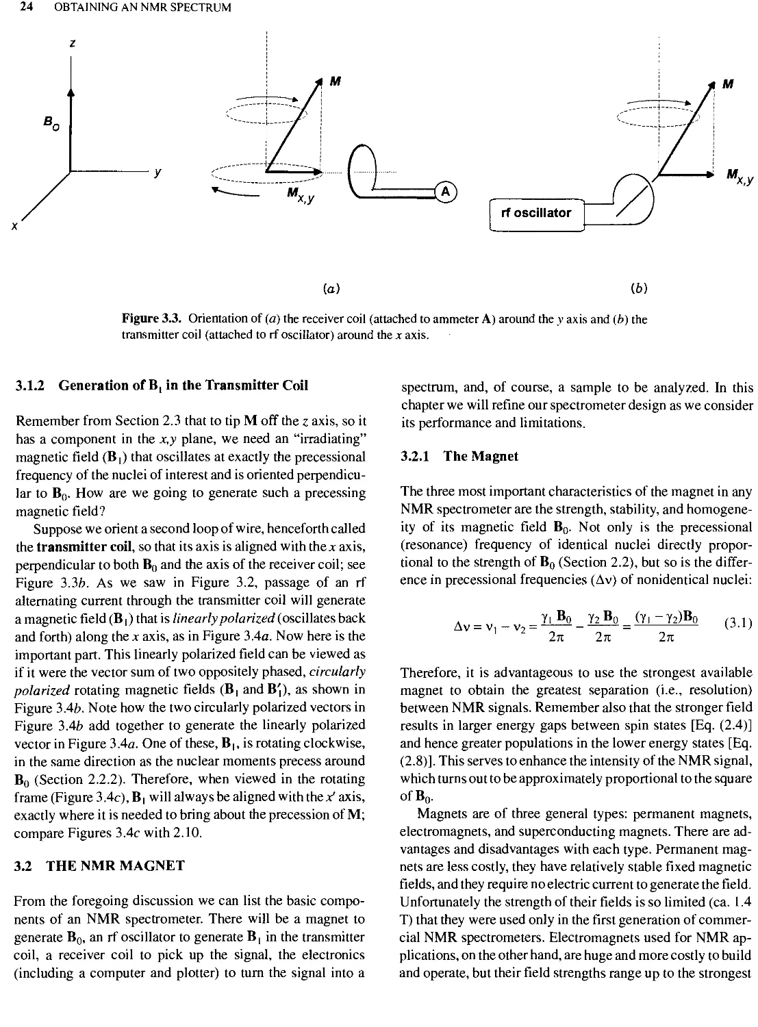
OBTAINING AN NMR SPECTRUM
3.1 Electricity and Magnetism
3.2 The NMR Magnet
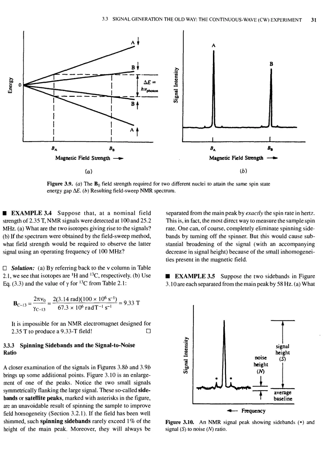
3.3 Signal Generation the Old Way: The Continuous-Wave (CW) Experiment
3.4 The Modern Pulsed Mode for Signal Acquisition
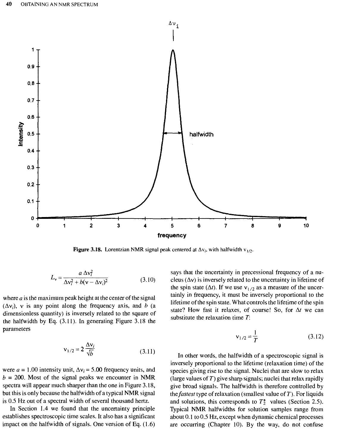
3.5 Line Widths, Lineshape, and Sampling Considerations
3.6 Measurement of Relaxation Times
Chapter Summary
XI
XIII
xv
1
1
3
4
5
5
6
9
12
15
18
20
20
20
22
22
24
28
32
39
41
46

vi CONTENTS
Additional Resources
Review Problems
Chapter 4 A LITTLE BIT OF SYMMETRY
4.1 Symmetry Operations and Distinguishability
4.2 Conformations and Their Symmetry
4.3 Homotopic, Enantiotopic, and Diastereotopic Nuclei
4.4 Accidental Equivalence
Chapter Summary
Additional Resources
Review Problems
Chapter 5 THE *H AND 13C NMR SPECTRA OF TOLUENE
5.1
5.2
5.3
5.4
5.5
The 'H NMR Spectrum of Toluene at 80 MHz
The Chemical Shift Scale
The 250- and 400-MHz 'H NMR Spectra of Toluene
The I3C NMR Spectrum of Toluene at 20.1, 62.9, and 100.6 MHz
Data Acquisition Parameters
Chapter Summary
Review Problems
48
51
53
54
54
54
54
56
56
59
60
62
64
67
67
Chapter 6 CORRELATING PROTON CHEMICAL SHIFTS WITH MOLECULAR STRUCTURE
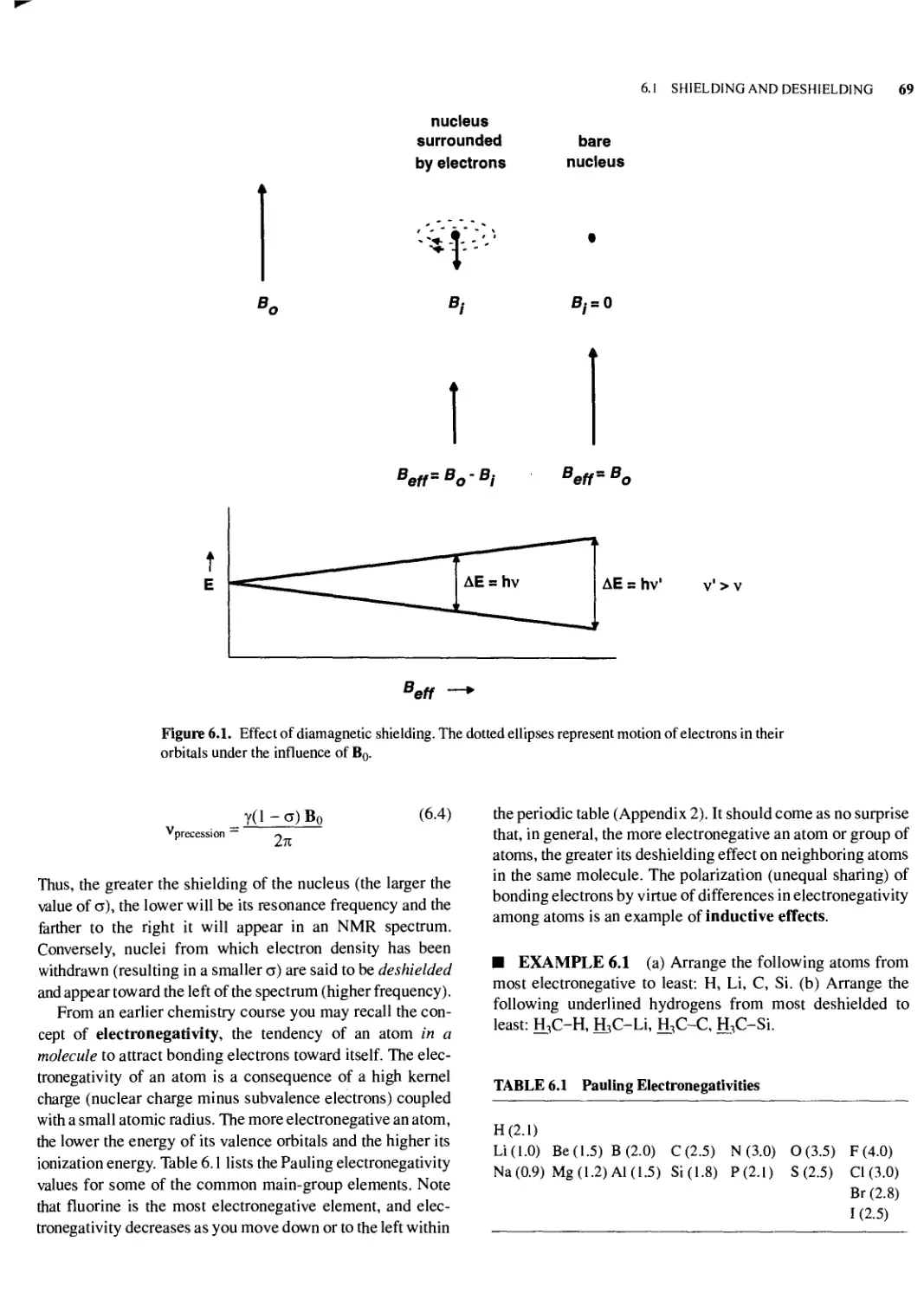
6.1 Shielding and Deshielding
6.2 Chemical Shifts of Hydrogens Attached to Tetrahedral Carbon
6.3 Vinyl and Formyl Hydrogen Chemical Shifts
6.4 Magnetic Anisotropy
6.5 Aromatic Hydrogen Chemical Shift Correlations
6.6 Hydrogen Attached to Elements Other than Carbon
Chapter Summary
References
Additional Resources
Review Problems
Chapter 7 CHEMICAL SHIFT CORRELATIONS FOR 13C AND OTHER ELEMENTS
7.1 I3C Chemical Shifts Revisited
7.2 Tetrahedral (sp2 Hybridized) Carbons
7.3 Heterocyclic Structures
7.4 Trigonal Carbons
7.5 Triply Bonded Carbons
7.6 Carbonyl Carbons
7.7 Miscellaneous Unsaturated Carbons
7.8 Summary of I3C Chemical Shifts
7.9 Chemical Shifts of Other Elements
Chapter Summary
References
Review Problems
68
68
70
74
77
78
81
85
86
86
87
88
91
92
96
96
97
99
101
102
102
103
SELF-TEST I
106
Chapter 8 FIRST-ORDER (WEAK) SPIN-SPIN COUPLING
8.1 Unexpected Lines in an NMR Spectrum
110
110

CONTENTS vii
8.2 The 'H Spectrum of Diethyl Ether 110
8.3 Homonuclear 'H Coupling: The Simplified Picture 112
8.4 The Spin-Spin Coupling Checklist 113
8.5 Then+ 1 Rule 1J4
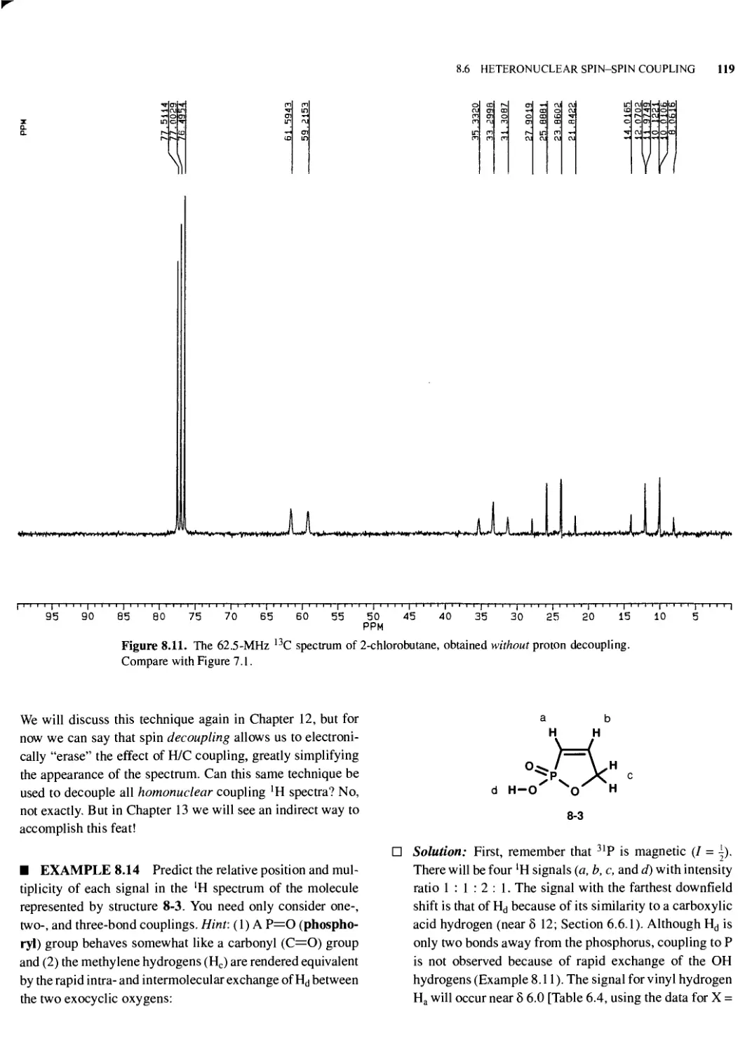
8.6 Heteronuclear Spin-Spin Coupling 117
8.7 Review Examples 122
Chapter Summary 125
Review Problems 125
Chapter 9 FACTORS THAT INFLUENCE THE SIGN AND MAGNITUDE OF /:
SECOND-ORDER (STRONG) COUPLING EFFECTS 132
9.1 Nuclear Spin Energy Diagrams and the Sign of J 132
9.2 Factors that Influence J: Preliminary Considerations 135
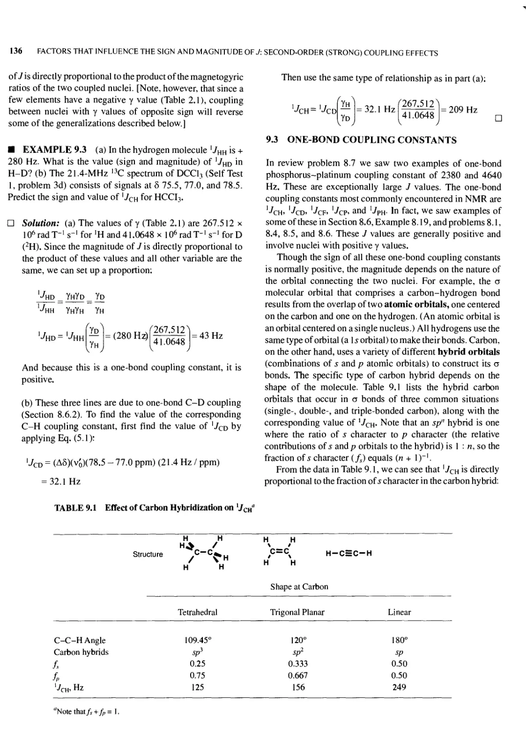
9.3 One-Bond Coupling Constants 136
9.4 Two-Bond (Geminal) Coupling Constants 138
9.5 Three-Bond (Vicinal) Coupling Constants 138
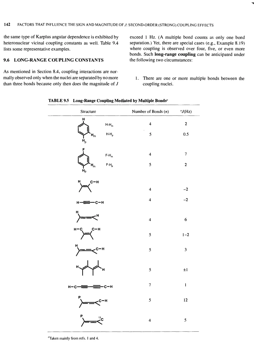
9.6 Long-Range Coupling Constants 142
9.7 Magnetic Equivalence 143
9.8 Pople Spin System Notation 144
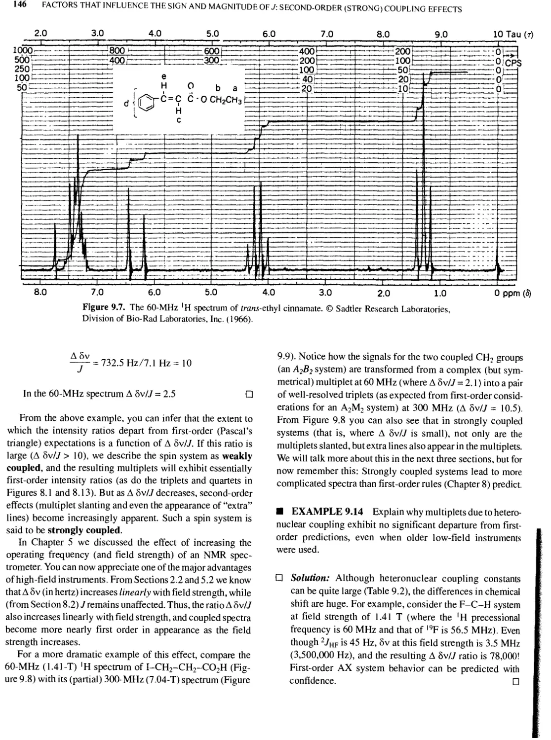
9.9 Slanting Multiplets and Second-Order (Strong Coupling) Effects 145
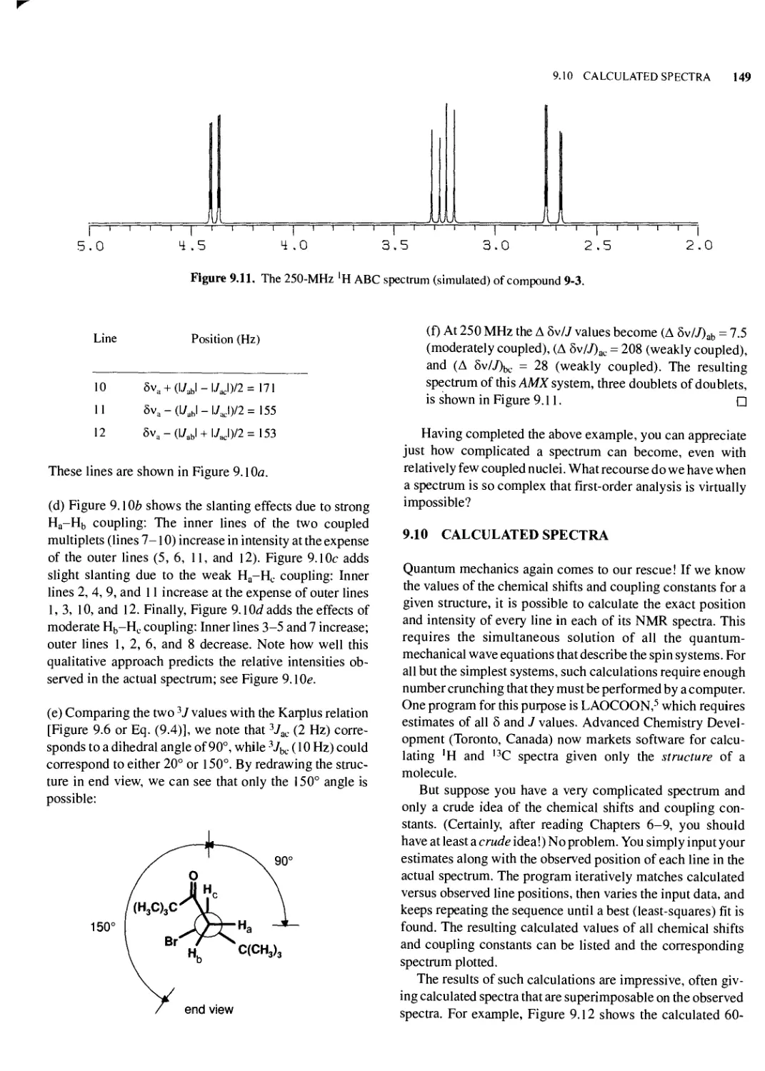
9.10 Calculated Spectra 149
9.11 The AX -> AB -> A2 Continuum 151
9.12 More About the ABX System: Deceptive Simplicity and Virtual Coupling 154
Chapter Summary 155
References 155
Review Problems 156
Chapter 10 THE STUDY OF DYNAMIC PROCESSES BY NMR 158
10.1 Reversible and Irreversible Dynamic Processes 158
10.2 Reversible Intramolecular Processes Involving Rotation Around Bonds 159
10.3 Simple Two-Site Intramolecular Exchange 159
10.4 Reversible Intramolecular Chemical Processes 163
10.5 Reversible Intermolecular Chemical Processes 164
10.6 Reversible Intermolecular Complexation 165
10.7 Other Examples of Reversible Complexation: Chemical Shift Reagents 168
Chapter Summary 171
References 172
Review Problems 172
Chapter 11 ELECTRON PARAMAGNETIC RESONANCE SPECTROSCOPY AND
CHEMICALLY INDUCED DYNAMIC NUCLEAR POLARIZATION 176
11.1 Electron Paramagnetic Resonance 176
11.2 Free Radicals 176
11.3 The g Factor 177
11.4 Sensitivity Considerations 179
11.5 Hyperfine Coupling and the a Value 179
11.6 A Typical EPR Spectrum 181
11.7 CIDNP: Mysterious Behavior of NMR Spectrometers 182
11.8 The Net Effect \ 182
11.9 The Multiplet Effect 183
11.10 The Radical-Pair Theory of The Net Effect 185
11.11 The Radical-Pair Theory of the Multiplet Effect 187

viii CONTENTS
11.12 A Few Final Words about CIDNP 188
Chapter Summary 189
References 189
Review Problems 189
Chapter 12 DOUBLE-RESONANCE TECHNIQUES AND COMPLEX PULSE SEQUENCES 191
12.1 What is Double Resonance? 19]
12.2 Heteronuclear Spin Decoupling 192
12.3 Polarization Transfer and the Nuclear Overhauser Effect 193
12.4 Gated and Inverse Gated Decoupling 196
12.5 Off-Resonance Decoupling 196
12.6 Homonuclear Spin Decoupling 198
12.7 Homonuclear Difference NOE: The Test for Proximity 198
12.8 Other Homonuclear Double-Resonance Techniques 200
12.9 Complex Pulse Sequences 201
12.10 The /-Modulated Spin Echo and the APT Experiment 203
12.11 More About Polarization Transfer 205
12.12 Distortionless Enhancement by Polarization Transfer 210
Chapter Summary 210
References 211
Additional Resources 211
Review Problems 211
Chapter 13 TWO-DIMENSIONAL NUCLEAR MAGNETIC RESONANCE 215
13.1 What is 2D NMR Spectroscopy? 215
13.2 2D Heteroscalar Shift-Correlated Spectra 218
13.3 2D Homonuclear Shift-Correlated Spectra 222
13.4 NOE Spectroscopy (NOESY) 228
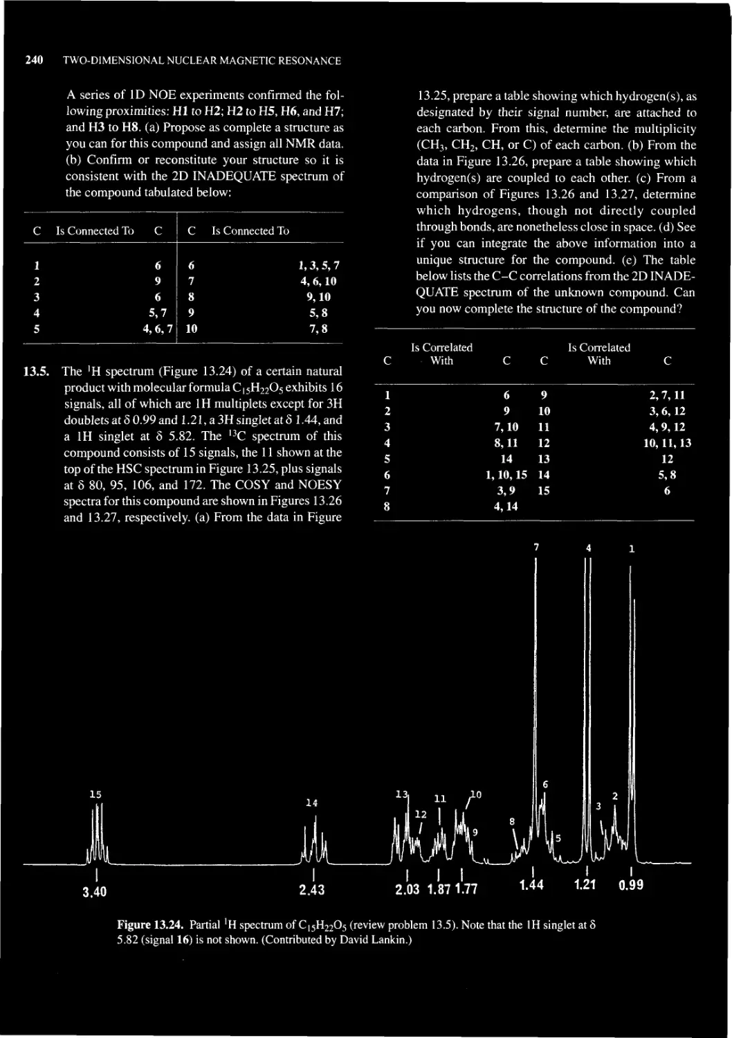
13.5 Hetero- and Homonuclear 2D /-Resolved Spectra 229
13.6 ID and 2D INADEQUATE 230
13.7 2D NMR Spectra of Systems Undergoing Exchange 236
Chapter Summary 236
References 236
Additional Resources 236
Review Problems 236
SELF-TEST II 244
Chapter 14 NMR STUDIES OF BIOLOGICALLY IMPORTANT MOLECULES 252
14.1 Introduction 252
14.2 NMR Line Widths of Biopolymers 252
14.3 Exchangeable and Nonexchangeable Protons 253
14.4 Chemical Exchange 254
14.5 The Effects of pH on the NMR Spectra of Biomolecules 256
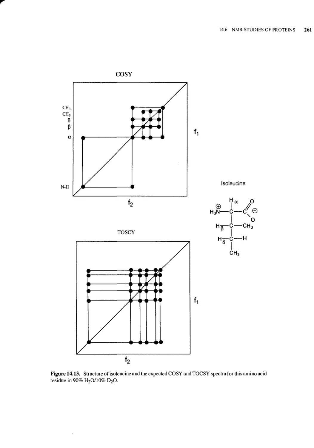
14.6 NMR Studies of Proteins 256
14.7 NMR Studies of Nucleic Acids 263
14.8 Lipids and Biological Membranes 270
14.9 Carbohydrates 275
Chapter Summary 277
References 277

CONTENTS ix
Additional Resources
Review Problems
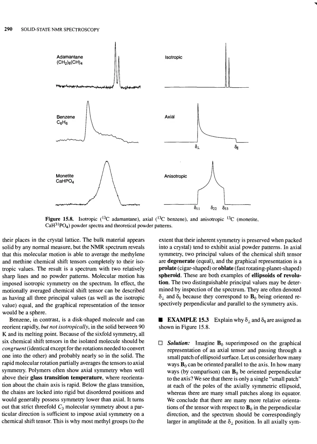
Chapter 15 SOLID-STATE NMR SPECTROSCOPY
15.1 Why Study Materials in the Solid State?
15.2 Why is NMR of Solids Different from NMR of Fluids?
15.3 Chemical Shifts in Solids
15.4 Spin-Spin Coupling
15.5 Quadrupole Coupling
15.6 Overcoming Long 7"i: Cross Polarization
Chapter Summary
Additional Resources
Review Problems
Chapter 16 NMR IN MEDICINE AND BIOLOGY: NMR IMAGING
16.1 A Window into Anatomy and Physiology
16.2 Biomedical NMR
16.3 Pictures with NMR: Magnetic Resonance Imaging
16.4 Image Contrast
16.5 Higher Dimensional Imaging
16.6 Chemical Shift Imaging
16.7 NMR Movies: Echo Planar Imaging
16.8 NMR Microscopy
16.9 In Vivo NMR Spectroscopy
16.10 Nonmedical Applications of MRI
Chapter Summary
Additional Resources
Appendix 1 ANSWERS TO REVIEW PROBLEMS
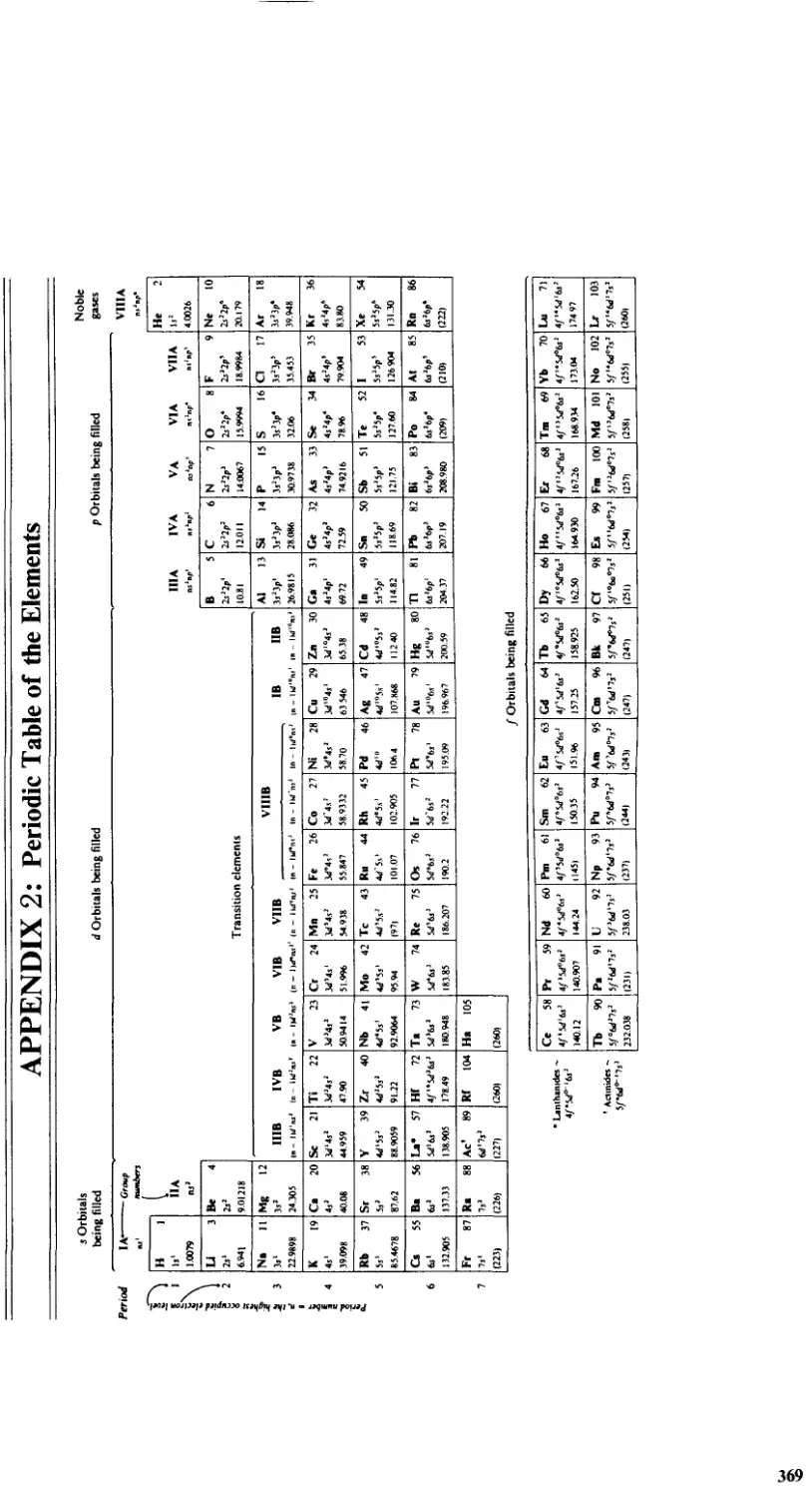
Appendix 2 PERIODIC TABLE
SUBJECT INDEX
CHEMICAL COMPOUNDS INDEX
277
277
283
283
284
286
294
297
299
304
304
304
306
306
306
309
317
322
323
325
325
326
329
333
333
334
369
370
379

PREFACE
In the decade since the first version of this book was written,
the field of nuclear magnetic resonance (NMR) spectroscopy
has made, quite literally, quantum leaps. Computer-controlled
NMR spectrometers with high-field superconducting mag-
magnets, once available only to the most well-funded institutions,
are now commonplace. Two-dimensional NMR techniques,
in their infancy a decade ago, have blossomed into an indis-
indispensable array of tools to elucidate the molecular structure of
compounds as complex as proteins. And who is unaware of
the growing importance of NMR to medical diagnosis
through the technique of magnetic resonance imaging (MRI)?
Nuclear magnetic resonance has become ubiquitous in
such divergent fields as chemistry, physics, material science,
biology, medicine, and forensic science, among others. In
writing this book it has been my goal to provide a monograph
aimed at anyone, not just chemists, with an interest in learning
about NMR. Medical students, whose interest lie not so much
in molecular structure as it does in the three-dimensional
distribution of magnetic nuclei such as hydrogen, will find
what they are looking for in the beginning three chapters,
which discuss the physics of NMR signal generation, and
Chapter 16, which describes MRI. If your interests are in
biochemistry, Chapter 14 will be very useful to you. The
majority of you will use NMR to elucidate molecular struc-
structures, so in Chapters 4-131 have tried to give you everything
you will need to get that job done efficiently.
A first-year college chemistry course is the only scientific
background I have assumed the reader has. All the necessary
details are developed from the most basic level. The approach
is relatively nonmathematical, with only a few simple equa-
equations. But do not let this fool you. By the end of the book you
will be well prepared to solve any molecular structure prob-
problem given a complete set of NMR data. And you will be able
to proceed confidently to any advanced treatise on NMR.
Above all, I have tried to make the text clear, logical, and
interesting to read. There are hundreds of figures and actual
spectra to illustrate the many topics. The vast majority of
spectra were obtained on modern high-field spectrometers.
Because of the way I structured the book, I recommend that
you proceed through it chapter by chapter, rather than skip-
skipping around. Nonetheless, I have tried to help those readers
who skip around by adding liberal references to earlier sec-
sections that have supporting information on each topic.
Soon after starting Chapter 1 you will note that I have
adopted a semiprogrammed approach. That is, there are fre-
frequent example problems (with solutions) to test your mastery
of the topic at hand. To get the most from your reading, try to
work each problem as you encounter it. They often contain
important additional information about the material just cov-
covered. Then, at the end of each chapter there is a chapter
summary and several review problems to see if you have
mastered the concepts in that chapter. There are also two
self-tests (after Chapters 7 and 13) that will help you assess
your overall mastery of the subject. The answers to these
review and self-test problems appear in Appendix 1.
I hope you enjoy this book and that it inspires you to learn
all you can about modern NMR methods. I would also appre-
appreciate greatly any feedback you would like to offer.
Malibu, California
Roger S. Macomber

ACKNOWLEDGMENTS
Many individuals have contributed mightily to this book, and
without their help I could not have gone forward with the
project.
About two years ago Jeff Holtmeier, a consulting editor at
John Wiley, approached me to see if I had any interest in
writing an updated edition of my earlier book on NMR
spectroscopy, published in early 1988. When I said yes, he set
about getting the original edition reviewed by a half-dozen
experts in the field. With these in hand, he single-handedly
promoted the project through the appropriate Wiley channels,
resulting in a contract in late 1995.
As the prospectus for the new edition was being developed,
several of my colleagues agreed to contribute chapters in their
particular areas of expertise. George Kreishman and Elwood
Brooks (UC's staff NMR spectroscopist) collaborated to write
Chapter 14, dealing with the applications of NMR to bio-
biochemistry. Jerry Ackerman, a one-time colleague of mine at
the University of Cincinnati and now director of NMR spec-
spectroscopy at Massachusetts General Hospital and assistant
professor of radiology at the Harvard Medical School, offered
to contribute Chapters 15 and 16 on solid-state NMR and
magnetic resonance imaging.
Fortuitously, at that time I signed the contract, I was just
beginning a previously arranged two-quarter sabbatical leave,
during which I planned to make major progress on the new
edition. My first stop was the Chemistry Department at the
University of Hawaii, hosted by my friend and colleague, Karl
Seff. Here I spent a most enjoyable month writing drafts of
several chapters, delivering and attending seminars, surfing,
and biking. Then, after six weeks back in Cincinnati, I headed
to the University of Utah, where I was hosted by my friends
Pete Stang and Wes Bentrude. Before I arrived, the winter in
Utah had been exceptionally mild, with absolutely no snow
on the slopes, so I expected to get a lot of writing done. Before
I left Utah, over 120 inches of fresh powder had fallen. Need
I say more?
While at Utah a number of individuals offered to contribute
example spectra for inclusion in the book. I have mentioned
the source of each contributed spectrum in the text or figure
legend, but let me introduce them here, as well: Bobby L.
Williamson (with Peter Stang's group), Alan Sopchik (with
Wes Bentrude's group), Dhileepkumar Krishnamurthy and
Stan McHardy (with Gary Keek's group), and John Bender
and Soren Giese (with Fred West's group). I also wish to thank
Steve Fetherston and Rosemary Laufer, able staff members
who made my visit even more productive and enjoyable.
Back again in Cincinnati, Elwood Brooks, Marshall Wil-
Wilson, and graduate students Pat Hutchins, Mark Guttaduaro,
and Sheela Venkitachalam contributed additional spectra for
the book, as did David Watt of the University of Kentucky.
But there are two major contributors of example spectra who
deserve special thanks. Sadtler Research Laboratories (Divi-
(Division of Bio-Rad Laboratories, Inc.), through staff scientist
Marie Scandone, provided many of the one-dimensional 'H
and I3C spectra. And David Lankin, a graduate of this depart-
department and currently a research scientist and NMR expert at
Searle, provided the bulk of the special 2D and related spectra
in Chapters 12 and 13, with the help of Geoffrey Cordell of
the University of Illinois School of Pharmacy.
Finally, three more of my faculty colleagues at UC deserve
special thanks. Albert Bobst advised me on the EPR section
of Chapter 11, Frank Meeks provided mathematical advice,
and Allan Pinhas helped edit the entire set of proofs. To all
these individuals, I give a sincere thank you!
Roger S. Macomber
xiii

FREQUENTLY USED SYMBOLS AND ABBREVIATIONS
•, an unpaired electron
T or -I, possible orientations (with respect to Bo) of the
magnetic moment of an electron or an / = ^ nucleus
[ ], concentration in moles per liter
{ }, indicates the nucleus being irradiated in a double-
resonance experiment
2D, NMR spectrum where signal intensity is a function of
two frequencies
A, A) mass number of a nucleus; B) net CIDNP absorption
a, hyperfine coupling constant in an EPR spectrum
a, A) one possible orientation (with respect to Bq) of the
magnetic moment of an electron or an / = ^ nucleus;
B) the flip angle in a pulsed NMR experiment
AA'BB', Pople designation for a coupled four-spin system
consisting of two chemically but not magnetically
equivalent nuclei in each of two sets
A/E, absorption-emission CIDNP net effect
APT, attached proton test
Bq, external (applied) magnetic field vector
B!, oscillating magnetic field vector of the observing chan-
channel
B2, oscillating magnetic field vector of the "irradiating"
channel
C, possible orientation (with respect to Bo) of the magnetic
moment of an electron or an / = , nucleus
e> Bohr magneton
Cn, n-fold axis of symmetry
C(A)T, computed (axial) tomography
COSY, 2D correlation spectroscopy
CSR, chemical shift reagent
d, doublet (signal multiplicity)
D, deuterium BH)
A, a change (e.g., A£, a change in energy)
8, chemical shift signal position (ppm)
S11, 822, 833, chemical shift tensors
A8x, substituent shielding parameter
Av, frequency difference (Hz) between the signal of inter-
interest and the operating frequency of the spectrometer;
also used for electric quadrupole interaction
Avq, frequency difference (Hz) between two sites at the
slow exchange limit
8v, frequency difference (Hz) between the signal of inter-
interest and the frequency of the internal standard signal;
also a measure of spectral resolution
&x, spatial resolution along x axis
A,, field of view along x axis
DEPT, distortionless enhancement by polarization transfer
DMF, dimethylformamide
E, A) energy; B) net CIDNP emission
XV

xvi FREQUENTLY USED SYMBOLS AND ABBREVIATIONS
E/A, emission-absorption CIDNP net effect
EPI, echo planar imaging
EPR, electron paramagnetic resonance
ESR, electron spin resonance (same as EPR)
exp, exponentiation on the base e
Fh the FT of the evolution/mixing time parameter in a 2D
NMR experiment
F2, the FT of the detection time parameter in a 2D NMR
experiment
FID, free induction decay time-domain signal
FOV, field of view
fp, fraction of p-orbital character
/,, fraction of s-orbital character
FT, Fourier transformation
g (factor), signal position parameter in an EPR spectrum
G°, standard-state free energy
y, magnetogyric ratio of a nucleus
Tn, the type of CIDNP net effect
Tm, the type of CIDNP multiplet effect
G^, magnetic field gradient
GHz, gigahertz A09 Hz)
h, Planck's constant
r\, signal intensity enhancement due to NOE
HSC, 2D heteroscalar shift-correlated NMR spectrum
HET2DJ, 2D heteronuclear /-resolved experiment
HETCOR, same as HSC
HOM2DJ, 2D homonuclear ./-resolved experiment
HSC, 2D heteronuclear shift correlation
Hz, unit of frequency (cycles per second)
/, magnetic spin of a nucleus
INADEQUATE, 1D and 2D NMR experiments to demon-
demonstrate direct C-C connectivity
INEPT, insensitive nuclei enhanced by polarization trans-
transfer
IOU, index of unsaturation
J, joules, a unit of energy
J, internuclear coupling constant (Hz)
Jn residual internuclear coupling constant (Hz) observed
in an off-resonance decoupled spectrum
k, rate constant for exchange
kc, rate constant at coalescence
K, equilibrium constant
L, number of lines (multiplicity) of a signal
m, magnetic spin quantum number of a nucleus
ms, magnetic spin quantum number of an electron
M, net (macroscopic) magnetization vector
Mo, net (macroscopic) magnetization vector at time zero
M,, net (macroscopic) magnetization vector at time /
M xy, component of the net (macroscopic) magnetization
vector in the x, y plane
H, A) magnetic moment of a nucleus; B) parameter used
to calculate the CIDNP net effect
MHz, megahertz A06 Hz)
MRI, magnetic resonance imaging
n, A) number of nuclei in an equivalent set; B) mixing
coefficient of an sji1 hybrid orbital
N, number of neutrons in a nucleus
v, frequency (Hz)
vav, average position (Hz) of two or more signals undergo-
undergoing exchange
v0, operating frequency (Hz) of an NMR spectrometer
Vq, operating frequency (MHz) of an NMR spectrometer
V|, observing frequency in a double-resonance experiment
v2, "irradiating" frequency in a double-resonance experi-
experiment
V|/2, signal halfwidth
v?/2> signal halfwidth at the fast exchange limit
NMR, nuclear magnetic resonance
NOE, nuclear Overhauser effect
NOESY, a 2D COSY spectrum showing NOE interactions
co, angular frequency (rad s~')
P, population of a given state or energy level

FREQUENTLY USED SYMBOLS AND ABBREVIATIONS xvii
ppm, parts per million
Pro-/?, configuration of an atom about a prochiral center
Pro-5, configuration of an atom about a prochiral center
PSR, paramagnetic shift reagent
nx, B | pulse causing a 180° rotation around the x' axis
(ji/2)r, B, pulse causing a 90° rotation around the x' axis
q, quartet (signal multiplicity)
q, electric quadrupole
r, internuclear distance
/?, A) exchange ratio, k/Av0, B) absolute configuration at
a chiral center; C) spectroscopic resolution; D) ideal
gas constant
ROI, region of interest
s, singlet (signal multiplicity)
s, A) same as ms, B) an atomic orbital
S, absolute configuration at a chiral center
a, A) representing a plane of symmetry; B) shielding
constant; C) parameter used in describing the CIDNP
multiplet effect; D) cylindrically symmetric bond or
molecular orbital
S/N, signal-to-noise ratio
SPI, selective population inversion
sp", hybridized atomic orbital with mixing coefficient n
SW, sweep (or spectral) width (Hz)
tacq, acquisition time
TE, echo time
td, dwell time (s)
tp, duration ([is) of a pulse
TR, repetition time
tw, delay time
T (Tesla), unit of magnetic field strength
T, absolute temperature (K)
Tp, absolute rotating frame temperature
7",, spin-lattice (longitudinal) relaxation time of a nucleus
T[p, rotating-frame spin-lattice relaxation time
T2, spin-spin (transverse) relaxation time of a nucleus
T2p, rotating-frame spin-spin relaxation time
7*2, effective spin-spin (transverse) relaxation time of a
. nucleus
TCP, cross-polarization time constant
t, A) old chemical shift scale; B) lifetime (s)
tc, correlation time of a nucleus
0, A) angle between the internuclear vector and Bo, B)
dihedral (torsional) angle
TMS, tetramethylsilane (internal standard)
TOCSY, total correlation 2D NMR spectroscopy
W, watt (measure of rf power)
X, mole fraction
x,y,z, Cartesian coordinate system in the laboratory frame
of reference
x',y',z, Cartesian coordinate system in the rotating frame
of reference
t, time (s)
t, triplet (signal multiplicity)
z axis, the axis of Bo, the external (applied) magnetic field
Z, atomic number

1
SPECTROSCOPY: SOME PRELIMINARY
CONSIDERATIONS
1.1 WHAT IS NMR SPECTROSCOPY?
Nuclear magnetic resonance (NMR) spectroscopy is the
study of molecular structure through measurement of the
interaction of an oscillating radio-frequency electromag-
electromagnetic field with a collection of nuclei immersed in a strong
external magnetic field. These nuclei are parts of atoms that,
in turn, are assembled into molecules. An NMR spectrum,
therefore, can provide detailed information about molecular
structure and dynamics, information that would be difficult,
if not impossible, to obtain by any other method.
It was in 1902 that physicist P. Zeeman shared a Nobel
Prize for discovering that the nuclei of certain atoms behave
strangely when subjected to a strong external magnetic field.
And it was exactly 50 years later that physicists F. Bloch and
E. Purcell shared a Nobel Prize for putting the so-called
nuclear Zeeman effect to practical use by constructing the
first crude NMR spectrometer. It would be an understatement
to say that, during the succeeding years, NMR has completely
revolutionized the study of chemistry and biochemistry, not
to mention having a significant impact on a host of other areas.
Nuclear magnetic resonance has become arguably the single
most widely used technique for elucidation of molecular
structure. But before we can begin our foray into NMR, we
need to review a few fundamental principles from physics.
1.2 PROPERTIES OF ELECTROMAGNETIC
RADIATION
All spectroscopic techniques involve the interaction of matter
with electromagnetic radiation, so we should begin with a
description of the properties of such radiation. The light rays
that allow our eyes to see this page constitute electromagnetic
radiation in the visible region of the electromagnetic spec-
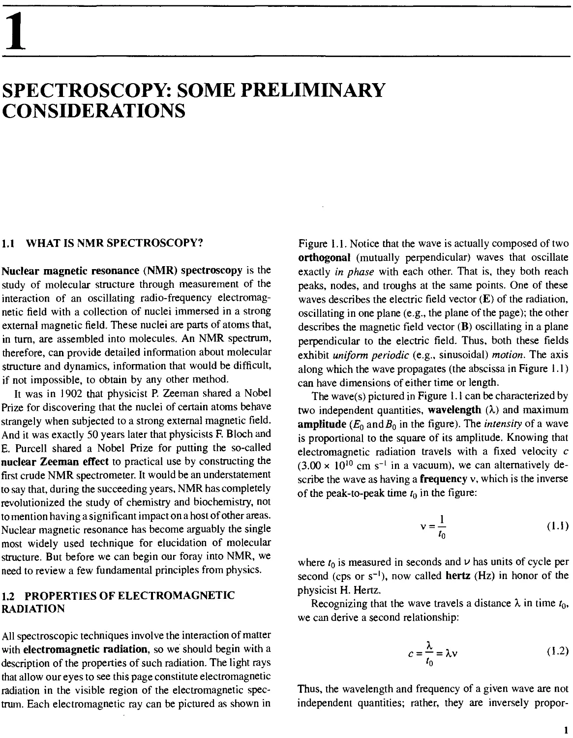
spectrum. Each electromagnetic ray can be pictured as shown in
Figure 1.1. Notice that the wave is actually composed of two
orthogonal (mutually perpendicular) waves that oscillate
exactly in phase with each other. That is, they both reach
peaks, nodes, and troughs at the same points. One of these
waves describes the electric field vector (E) of the radiation,
oscillating in one plane (e.g., the plane of the page); the other
describes the magnetic field vector (B) oscillating in a plane
perpendicular to the electric field. Thus, both these fields
exhibit uniform periodic (e.g., sinusoidal) motion. The axis
along which the wave propagates (the abscissa in Figure 1.1)
can have dimensions of either time or length.
The wave(s) pictured in Figure 1.1 can be characterized by
two independent quantities, wavelength (X) and maximum
amplitude (£0 andfi0 'n the figure). The intensity of a wave
is proportional to the square of its amplitude. Knowing that
electromagnetic radiation travels with a fixed velocity c
C.00 x 10'° cm s~' in a vacuum), we can alternatively de-
describe the wave as having a frequency v, which is the inverse
of the peak-to-peak time t0 in the figure:
v = —
'o
A-1)
where t0 is measured in seconds and v has units of cycle per
second (cps or s), now called hertz (Hz) in honor of the
physicist H. Hertz.
Recognizing that the wave travels a distance X in time t0,
we can derive a second relationship:
c = — = Xv
'o
A.2)
Thus, the wavelength and frequency of a given wave are not
independent quantities; rather, they are inversely propor-
1

2 SPECTROSCOPY: SOME PRELIMINARY CONSIDERATIONS
if abscissa scale is time
if abscissa scale is length
trough
Figure 1.1. Electromagnetic wave with electric vector E and magnetic vector B.
tional. Radiation of high frequency has a short wavelength,
while radiation of low frequency has a long wavelength.
The known electromagnetic spectrum (Table I.I) ranges
from cosmic rays of extremely high frequency (and short
wavelength) to rf (radio-frequency) radiation of low fre-
frequency (and long wavelength). The narrow visible region in
the middle of the electromagnetic spectrum corresponds to
radiation of wavelength 380-780 nm A nm= 10"9 m = 10
cm) and frequency 4 x 1014—8 x 1014 Hz. Our optic nerves do
not respond to electromagnetic radiation outside this region.
In addition to its wave properties, electromagnetic radia-
radiation also exhibits certain behavior characteristic of particles.
A particle, or quantum, of radiation is called a photon. For
our purposes the most important particlelike property of a
photon is its energy (£). Each photon possesses a discrete
amount of energy that is directly proportional to its frequency
(if we regard it as a wave). This relationship can be written
E = hv
A.3)
where h, Planck's constant, has values of 6.63 x 104 J s per
photon. Alternatively, h can be expressed on aper-mole basis
through multiplication by Avogadro's number F.02 x 1023
mol-') and division by 103 J(kJ) to give h = 3.99 x 103 kJ
s mol. (A mole of photons is referred to as an Einstein.)
Since the strength of a chemical bond is typically around 400
kJ mol, radiation above the visible region in Table 1.1 has
sufficient energy to photodissociate (break) chemical bonds,
while radiation below the visible region does not (see Table
1.1). Of particular interest to us for NMR purposes is rf
radiation, the same frequency range that carries communica-
communication signals to our radios and televisions. We will normally be
using radiation with frequencies of 200-750 MHz A MHz =
106 Hz), at the low end of the energy scale in Table 1.1. This,
it will turn out, is exactly the amount of energy we will need
to perform NMR experiments.
To summarize, if two photons possess the same energy,
they correspond to waves (or wavelets) of the same frequency
and the same maximum amplitude. The total intensity of an
electromagnetic beam is therefore the number of photons
delivered per second.
■ EXAMPLE 1.1 Derive the relationship between the
energy of a photon and its wavelength.
□ Solution: We can rearrange Eq. A.2) to v = c/X. Substi-
Substituting for v in Eq. A.3) gives
E= hv = —
A.
□

1.3 INTERACTION OF RADIATION WITH MATTER: THE CLASSICAL PICTURE
TABLE 1.1 Electromagnetic Spectrum
Radiation
Cosmic rays
Gamma rays
X-rays
Far ultraviolet
Ultraviolet
Visible
Infrared
Far infrared
Microwaves
Radio frequency
Wavelength, A. (nm)
<10
10'-10-3
10-10
200-10
380-200
780-380
3 x 104-780
3x 105-3x 104
3x 107-3x 105
10"-3x 107
Frequency, v (Hz)
>3x 1020
3x 10'8-3x 1020
3xlO16-3x 1018
1.5xl015-3xl016
8x 1014-1.5x 1015
4x 1014-8x 1014
10l3-4x 1014
IO'2-IO13
1010-1012
106-1010
Energy (kJ mol ')
>1.2x 108
1.2 x 106-1.2x 108
1.2 x 104-1.2x 106
6x 102-1.2x 104
3.2 x 102-6x 102
1.6 x 102-3.2x 102
4-1.6 x 102
0.4-4
4x 10-0.4
4x 10-4x 10
It is perhaps worthwhile to mention that the velocity (v) of
electromagnetic radiation decreases as it passes through a
condensed medium (e.g., a liquid or solution). The ratio of its
speed in a vacuum (c) to its velocity in the medium is called
the index of refraction (n) of the medium:
c
n = —
v
A.4)
The magnitude of n for a given medium varies inversely with
the wavelength of radiation, but it is always greater than unity.
The energy of a photon (unless it is absorbed) is unaffected
by passage through the medium, so its frequency must also be
unchanged [Eq. A.3)]. Therefore, its wavelength must have
decreased (to A,') in order to preserve the relationship in Eq.
A.2):
■ = A/v
where A.' = "k/n = A,v/c.
1.3 INTERACTION OF RADIATION WITH
MATTER: THE CLASSICAL PICTURE
Now that we know something about electromagnetic radia-
radiation, let us turn to the question of what factors control the
interaction of such radiation with particles of matter. The three
main types of interactions of interest to spectroscopists are
absorption, emission, and scattering. When absorption oc-
occurs, the photon disappears and its entire energy is transferred
to the particle that absorbed it. The resulting particle with this
excess energy is said to be in an excited state. It can relax
back to its ground state by emitting a photon, which carries
off the excess energy.
Radiation is scattered when the direction of propagation
of the photon is shifted by some angle, the result of passing
close to a perturbing particle. If the frequency of the radiation
is unchanged, the scattering is described as elastic. However,
if the frequency has changed (inelastic scattering), this indi-
indicates that there was a partial exchange of energy between the
photon and the particle.
In the case of NMR spectroscopy we will be concerned
only with absorption and emission of rf radiation. Quantum
mechanics, the field of physics that deals with energy at the
microscopic (atomic) level, allows us to define selection rules
that describe the probability for a photon to be absorbed or
emitted under a given set of circumstances. But even classical
(i.e., pre-quantum-mechanical) physics tells us there is one
requirement shared by all forms of absorption and emission
spectroscopy: For a particle to absorb (or emit) a photon, the
particle itself must first be in some sort of uniform periodic
motion with a characteristic fixed frequency. Most important,
the frequency of that motion must exactly match the frequency
of the absorbed (or emitted) photon:
^motion photon
A.5)
This fact, which at first glance might appear to be an incred-
incredible coincidence, is actually quite logical. If a photon is to be
absorbed, its energy, which is originally in the form of the
oscillating electric and magnetic fields, must be transformed
into energy of the particle's motion. This transfer of energy
can take place only if the oscillations of the electric and/or
magnetic fields of the photon can constructively interfere with
the "oscillations" (uniform periodic motion) of the particle's
electric and/or magnetic fields. When such a condition exists,
the system is said to be in resonance, and only then can the
act of absorption take place. By the way, do not confuse the
term resonance in this context with the concept of resonance
(conjugation) of electrons used to describe the structure of
molecules.

4 SPECTROSCOPY: SOME PRELIMINARY CONSIDERATIONS
■ EXAMPLE 1.2 The C—O bond in formaldehyde vi-
vibrates (stretches, then contracts) with a frequency of 5.13 x
1013 Hz. (a) What frequency of radiation could be absorbed
by this vibrating bond? (b) How much energy would each
photon deliver? (c) To which region of the electromagnetic
spectrum does this radiation belong? (d) Are photons of this
region capable of breaking bonds?
□ Solution: (a) From Eq. A.5) we know the frequencies
must match; therefore, vphoton = 5.13 x 1013 Hz. (b) From
E3
photon = hv = F.63 x 10-34Js)E.13 x 1013 s)
= 3.40x 10-20J = 20.5kJmol-'
(c) From Table 1.1 we see that radiation of this frequency
and energy falls in the infrared region, (d) No. This
amount of energy is less than half that required to break
even the weakest chemical bond. However, absorption of
such a photon does create a vibrationally excited bond,
which is more likely to undergo certain chemical reactions
than is the same bond in its ground state. □
At this point you might think that the frequency-matching
requirement places a heavy constraint on the types of absorp-
absorption processes that can occur. After all, how many kinds of
periodic motion can a particle have? The answer is that even
a small molecule is constantly undergoing many types of
periodic motion. Each of its bonds is constantly vibrating; the
molecule as a whole and some of its individual parts are
rotating in all three dimensions; the electrons are circulating
through their orbitals. And each of these processes has its own
characteristic frequency and its own set of selection rules
governing absorption!
All of the above forms of microscopic motion are what we
might describe as intrinsic. That is, the motion takes place all
by itself, without intervention by any external agent. How-
However, it is possible under certain circumstances to induce
particles to engage in additional forms of periodic motion.
Still, to achieve resonance, we need to match the frequency of
this induced motion with that of the incident radiation [Eq. A.5)].
For example, an ion (or any charged particle, for that
matter) follows a curved path as it moves through a magnetic
field. If we carefully adjust the strength of the magnetic field,
the ion will follow a perfectly circular path, with a charac-
characteristic fixed frequency that depends on its mass, charge,
velocity, and strength of the magnetic field. Matching this
characteristic cyclotron frequency with incident electromag-
electromagnetic radiation of the same frequency can lead to absorption,
and this is the basis of a technique known as ion cyclotron
resonance (ICR) spectroscopy. We will discover in Chapter
2 that a strong magnetic field can also be used to induce
certain nuclei to move with uniform periodic motion of a
different type.
1.4 UNCERTAINTY AND THE QUESTION OF
TIME SCALE
If you have ever tried to take a photograph of a moving object,
you know that the shutter speed of the camera must be
adjusted to avoid blurring the image. And, of course, the faster
the object is moving, the shorter must be the exposure time to
"freeze" the motion. We have very similar considerations in
spectroscopy.
Suppose you owned a collection of very extraordinary
chameleons that were able to change colors instantaneously
from white to black or black to white every 1 s. If you took a
picture of them with a shutter speed of 10 s, each of the little
critters would appear to be gray. But if you decreased the
exposure time to 0.01 s, the photograph would show black
ones and white ones in roughly equal numbers but no gray
ones! Thus, to capture the individual colors, your exposure
time must be significantly shorter than the lifetimes of the
species, in this case the 1-s lifetime of each colored form.
There are many types of molecular chameleons, that is,
molecules that constantly undergo some sort of reversible
reorganization of their structures. If absorption of the photon
is fast enough, we will detect both the "black" and "white"
forms of the molecule. But if the absorption process is slower
than the interconversion, we will detect only some sort of
time-averaged structure. The situation therefore boils down
to the question: How long does it take for a particle to absorb
a photon? Unfortunately, such a question is impossible to
answer with complete precision.
In 1927, W Heisenberg, a pioneer of quantum mechanics,
stated his uncertainty principle: There will always be a limit
to the precision with which we can simultaneously determine
the energy and time scale of an event. Stated mathematically,
the product of the uncertainties of energy (A£) and time (At)
can never be less than h (our old friend, Planck's constant):
AEAt>h
A.6)
Thus, if we know the energy of a given photon to a high order
of precision, we would be unable to measure precisely how
long it takes for the photon to be absorbed. Nonetheless, there
is a useful generalization we can make. Using Eq. A.3), we
can substitute h Av for the AE in Eq. A.6), giving
At>-
Av
where Av is the uncertainty in frequency. As a result, the time
required for a photon to be absorbed (At) must be approxi-
approximately as long as it takes one "cycle" of the wave to pass the

REVIEW PROBLEMS (Answers in Appendix I)
particle. That length of time, Iq in Figure 1.1, is nothing more
than 1/v. This result stands to reason if we consider that the
particle would have to wait through at least one cycle before
it could sense what the radiation frequency was. At least we
now have an order-of-magnitude idea of how fast our shutter
speed must be in order to "freeze" a given molecular event.
We will encounter the uncertainty principle at several points
along our voyage through NMR spectroscopy.
■ EXAMPLE 1.3 Suppose our NMR experiment re-
required the use of rf radiation with a frequency of 250 MHz to
examine formaldehyde (see Example 1.2). Will this NMR
experiment enable us to see the various individual lengths of
the C=O bond as it vibrates, or will we detect only a time-av-
time-averaged bond length?
□ Solution: The vibrational time scale A /v = 1 /E.13 x 1013
Hz) = 1.9 x 104 s) is much shorter (faster) than the NMR
time scale [1/v = 1/B.5 x 108 Hz) = 4 x 10"9 s].
Therefore, NMR can only detect a time-averaged C=O
bond length. □
Equipped with this knowledge about electromagnetic ra-
radiation, periodic motion, resonance, and time scale, we are
now ready to enter the intriguing world of the atomic nucleus.
CHAPTER SUMMARY
1. Nuclear magnetic resonance spectroscopy involves
the interaction of certain nuclei with radio-frequency
(rf) electromagnetic radiation when the nuclei are im-
immersed in a strong magnetic field.
2. Electromagnetic radiation is characterized by its fre-
frequency (v) or wavelength (A.), which are inversely
proportional [Eq. A.2)]. Radio-frequency radiation
used in NMR spectroscopy typically has frequencies
on the order of 200-750 MHz.
3. The energy of a photon (a quantum of radiation) is
directly proportional to its frequency [Eq. A.3)].
4. For radiation to be absorbed by a particle, the fre-
frequency of the radiation must equal the frequency of the
particle's periodic motion.
5. The Heisenberg uncertainty principle [Eq. A.6)] de-
defines the time scale of radiation absorption event as
inversely proportional to the radiation's frequency.
Processes that occur faster than the spectroscopic time
scale are time averaged during the absorption process.
REVIEW PROBLEMS (Answers in Appendix 1)
1.1. The linear HCN molecule rotates around an imaginary
axis through its center of mass and perpendicular to the
molecular axis. The frequency of this rotation is
4.431598 x 1010 Hz. (a) What frequency of radiation
could be absorbed by this rotating molecule? (b) To
which region of the electromagnetic spectrum does
such radiation belong?
1.2. When laser light with X = 1064 nm impinges on a
sample of formaldehyde (Example 1.2), most of the
light is scattered elastically. But a small number of
scattered photons emerge with X = 1301 nm. Account
for this exact wavelength. (This is an example of Raman
spectroscopy.)
1.3. What is the shortest lifetime a species could have and
still be detectable with visible light having X = 500 nm?

2
MAGNETIC PROPERTIES OF NUCLEI
2.1. THE STRUCTURE OF AN ATOM
The compounds we examine by NMR are composed of mole-
molecules, which are themselves aggregates of atoms. Each atom
has some number of negatively charged electrons whizzing
around a tiny, dense bit of positively charged matter called the
nucleus. The size of an atom is the volume of space that the
electron cloud occupies. However, >99.9% of the mass of an
atom is concentrated in its nucleus, though the nucleus occu-
occupies only one trillionthA0~12) of the atom's volume. Even the
nucleus can be further dissected into other fundamental par-
particles, including protons and neutrons, not to mention a host
of other subnuclear particles that help hold the nucleus to-
together and give nuclear physicists something to wonder about.
2.1.1 The Composition of the Nucleus
It is the number of protons in an atom's nucleus (Z, the atomic
number) that determines both the atom's identity and the
charge on its nucleus. In the periodic table of the elements
(Appendix 2) the atomic number of each element is shown to
the right of its chemical symbol. Every nucleus with just one
proton is a hydrogen nucleus, every nucleus with six protons
is a carbon nucleus, and so on. Yet, if we carefully examine a
large sample of hydrogen atoms, we find that not all their
nuclei are identical. It is true that all have just one proton, but
they differ in the number of neutrons. Most hydrogen atoms
in nature (99.985%, to be exact) have no neutrons (N = 0), but
a small fraction @.015%) have one neutron (A^= 1) in addition
to the proton. These two forms are the naturally occurring
stable isotopes of hydrogen, and they are given the symbols
'H and 2H, respectively. The leading superscript is the mass
number (A) of the isotope, which is the integer sum of Z and
N:
A=Z+N B.1)
The isotope 2H is usually referred to as deuterium (D), or
heavy hydrogen, but most isotopes of other elements are
identified simply by their mass number. The atomic mass
listed for each element in the periodic table is a weighted
average, the fractional abundance of each isotope times its
exact mass, summed over all naturally occurring isotopes.
■ EXAMPLE 2.1 Tritium, 3H, is a radioactive (unstable)
isotope of hydrogen. What is the composition of its nucleus?
□ Solution: Since the atom is an isotope of hydrogen, Z =
1. The mass number A is 3 and therefore, from Eq. B.1),
N = 2. Thus, the nucleus consists of one proton and two
neutrons. □
■ EXAMPLE 2.2 Natural chlorine (Z = 17) is composed
of two isotopes, 35C1 and 37C1. The atomic mass listed for
chlorine in the periodic table is 35.5. (a) What is the compo-
composition of each nucleus? (b) What is the natural abundance of
each isotope? (You may assume for the purposes of this
question that the exact mass of each isotope is exactly equal
to its mass number, though in general this is not the case.)
□ Solution: (a) Chlorine-35 has Z = 17A7 protons), A =
35, and N = 18 A8 neutrons); 37C1 hasZ= 17, A = 37, and
N = 20. (b) Since the atomic mass of 35.5 is a weighted
average of a mixture of 35C1 and 37C1, we can use a little
algebra to calculate the fraction (/) of each isotope:
and since only the two isotopes are present,

2.1. THE STRUCTURE OF AN ATOM
/35+/37=i.oo
Therefore,
(/„ -35) + A.00 -/35)C7) = 35.5
/35 = 0.75G5%) and /37 = 0.25B5%)
□
2.1.2 Electron Spin
Before we delve further into the properties of the nucleus, let
us momentarily shift our attention back to one of the electrons
zooming around the nucleus. Just like photons, electrons
exhibit both wave and particle properties. Each electron wave
in an atom is characterized by four quantum numbers. The
first three of these numbers can be taken as the electron's
address and describe the energy, shape, and orientation of the
volume the electron occupies in the atom. This volume is
called an orbital. The fourth quantum number is the electron
spin quantum number s, which can assume only two values,
+i or -i. (Why ± j was selected rather than, say, ±1 will be
described a little later.) The Pauli exclusion principle tells us
that no two electrons in an atom can have exactly the same set
of four quantum numbers. Therefore, if two electrons occupy
the same orbital (and thus possess the same first three quan-
quantum numbers), they must have different spin quantum num-
numbers. Therefore, no orbital can possess more than two
electrons, and then only if their spins are paired (opposite).
Is there any other significance to the spin quantum num-
number? Yes, indeed! Because the electron can be regarded as a
particle spinning on its axis, it has a property called spin
angular momentum. Further, because the electron is a
charged particle (Z = -1), this spinning gives rise to a mag-
magnetic moment (symbol |i) represented by the boldface vector
arrows in Figure 2.1. We describe such a species as having a
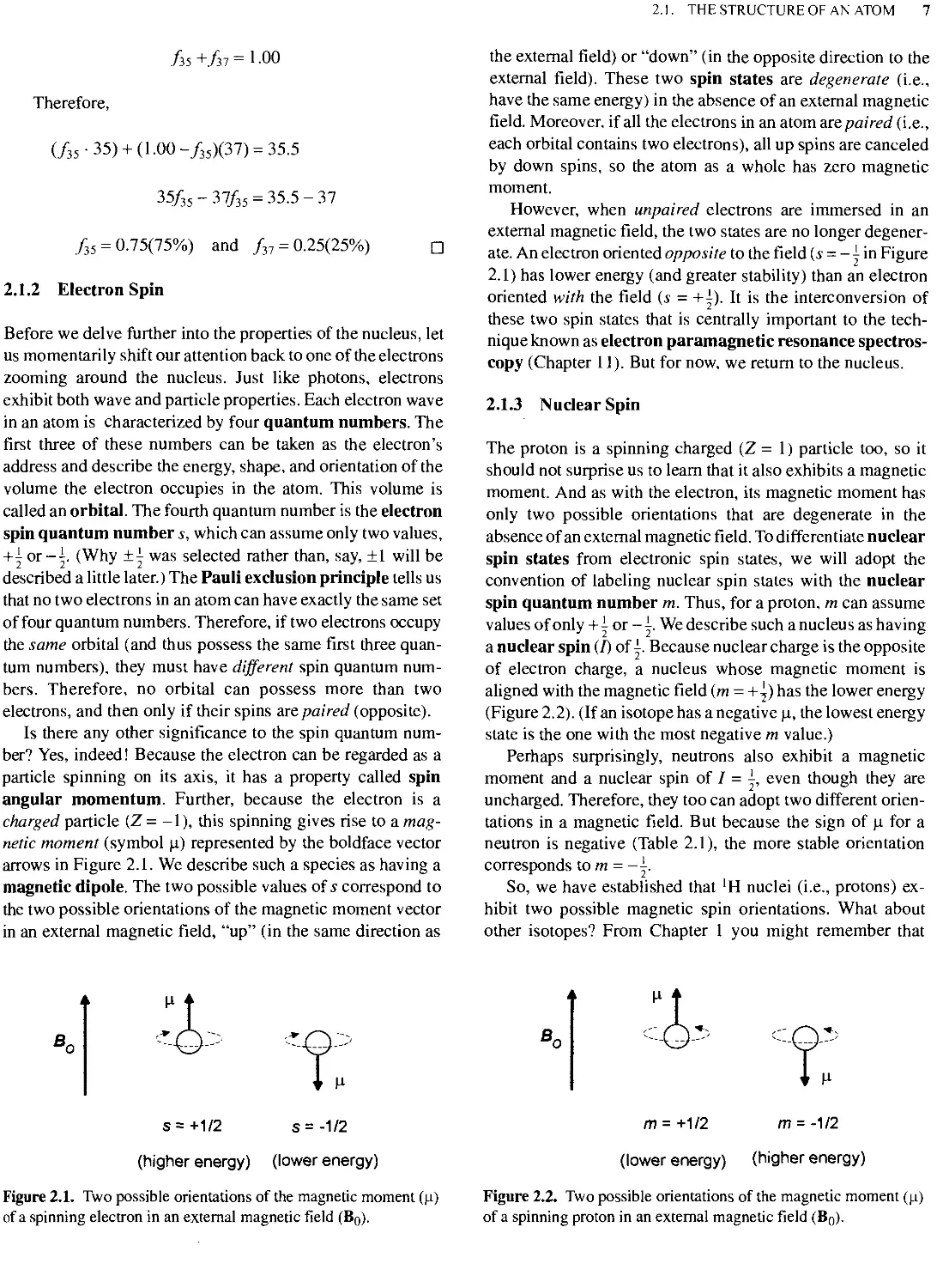
magnetic dipole. The two possible values of s correspond to
the two possible orientations of the magnetic moment vector
in an external magnetic field, "up" (in the same direction as
the external field) or "down" (in the opposite direction to the
external field). These two spin states are degenerate (i.e.,
have the same energy) in the absence of an external magnetic
field. Moreover, if all the electrons in an atom ^repaired (i.e.,
each orbital contains two electrons), all up spins are canceled
by down spins, so the atom as a whole has zero magnetic
moment.
However, when unpaired electrons are immersed in an
external magnetic field, the two states are no longer degener-
degenerate. An electron oriented opposite to the field (s = - ^ in Figure
2.1) has lower energy (and greater stability) than an electron
oriented with the field (s - +^). It is the interconversion of
these two spin states that is centrally important to the tech-
technique known as electron paramagnetic resonance spectros-
copy (Chapter 11). But for now, we return to the nucleus.
2.1.3 Nuclear Spin
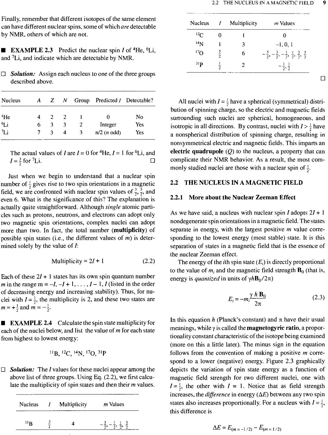
The proton is a spinning charged (Z = 1) particle too, so it
should not surprise us to learn that it also exhibits a magnetic
moment. And as with the electron, its magnetic moment has
only two possible orientations that are degenerate in the
absence of an external magnetic field. To differentiate nuclear
spin states from electronic spin states, we will adopt the
convention of labeling nuclear spin states with the nuclear
spin quantum number m. Thus, for a proton, m can assume
values of only +i or -|. We describe such a nucleus as having
a nuclear spin (/) of j. Because nuclear charge is the opposite
of electron charge, a nucleus whose magnetic moment is
aligned with the magnetic field (m = +^) has the lower energy
(Figure 2.2). (If an isotope has a negative ji, the lowest energy
state is the one with the most negative m value.)
Perhaps surprisingly, neutrons also exhibit a magnetic
moment and a nuclear spin of / = ±, even though they are
uncharged. Therefore, they too can adopt two different orien-
orientations in a magnetic field. But because the sign of |i for a
neutron is negative (Table 2.1), the more stable orientation
corresponds to m = -|.
So, we have established that 'H nuclei (i.e., protons) ex-
exhibit two possible magnetic spin orientations. What about
other isotopes? From Chapter 1 you might remember that
s=+1/2 s=-1/2
(higher energy) (lower energy)
Figure 2.1. Two possible orientations of the magnetic moment (|i)
of a spinning electron in an external magnetic field (Bo).
m=+M2
(lower energy)
m = -1/2
(higher energy)
Figure 2.2. Two possible orientations of the magnetic moment
of a spinning proton in an external magnetic field (Bo).

8 MAGNETIC PROPERTIES OF NUCLEI
TABLE 2.1 Magnetic Properties of Selected Particles"
Isotope
n
'H
2H
7Li
I0g
"B
13C
I4N
15N
I7O
19F
23Na
27A1
29Si
3lp
33S
35C1
37C1
%h
—
99.985
0.015
92.58
19.58
80.42
1.108
99.63
0.37
0.037
100
100
100
4.70
100
0.76
75.53
24.47
"Abstracted in Dart from Th
Z
0
1
1
3
5
5
6
7
7
8
9
11
13
14
15
16
17
17
e 64th CRC
N
1
0
1
4
5
6
7
7
8
9
10
12
14
15
16
17
18
20
Handbook oi
A
1
1
2
7
10
11
13
14
15
17
19
23
27
29
31
33
35
37
" Chemistry an
I
i
2
1
2
l
3
2
3
3
2
1
2
1
2
5
2
1
2
3
2
5
2
1
1
2
3
3
2
3
2
d Physics,
yc
-183.26
267.512
41.0648
103.96
28.748
85.828
67.2640
19.325
-27.107
-36.27
251.667
70.761
69.706
-53.142
108.29
20.517
26.212
21.82
CRC Press, Boca
v"
29.167
42.5759
6.53566
16.546
4.5754
13.660
10.7054
3.0756
4.3142
5.772
40.0541
11.262
11.094
8.4578
17.235
3.2654
4.1717
3.472
Raton, FL,
H'
-1.91315
2.79268
0.857387
3.2560
1.8007
2.6880
0.702199
0.40347
-0.28298
-1.8930
2.62727
2.2161
3.6385
-0.55477
1.1305
0.64257
0.82091
0.6833
1984.
Qf
0
0
2.73 x 10-3
-3x lO-2
7.4 x lO-2
3.55 x lO-2
0
1.6 x lO-2
0
-2.6 x lO-2
0
0.14
0.149
0
0
-6.4 x lO-2
-7.89 x lO-2
-6.21 x lO-2
S*
0.322
1.00
9.65 x
0.293
1.99 x
0.165
1.59 x
1.01 x
1.04 x
2.91 x
0.833
9.25 x
0.206
7.84 x
6.63 x
2.26 x
4.70 x
2.71 x
lO-3
io2
lO
lO-3
lO-3
io-2
lO-2
10-3
lO-2
lO-3
lO-3
10-3
Natural abundance.
cMagnetogyric ratio in units of 10 radT" s.
^Resonance frequency in megahertz in a 1-T field.
'Magnetic moment in nuclear magnetons.
^Electric quadrupole moment in barns.
^Sensitivity (relative to proton) for equal numbers of nuclei at constant field;
S = 7.652 x 10n3(/+ I)//2.
Zeeman found only certain isotopes give rise to multiple
nuclear spin states when immersed in an external magnetic
field. This is because only isotopes with an odd number of
protons (odd Z) and/or an odd number of neutrons (odd N)
possess nonzero nuclear spin. Nuclei with zero nuclear spin
(those with an even Zand even AO have zero nuclear magnetic
moment and cannot be detected by NMR methods.
Here is the reason that the parity (odd or even number) of
protons and neutrons is so important: A proton spin can only
pair with (cancel) another proton spin, but not a neutron spin,
and vice versa. This rule allows us to assign every isotope to
one of three groups.
Group 1: Nuclei with Both Z and N even (and Therefore
A Even).
In such nuclei all proton spins are paired and all neutron spins
are paired, resulting in a net nuclear spin of zero (/ = 0). Such
nuclei are invisible to NMR. Some examples include the
abundant isotopes I2C, I6O, I8O, and 32S.
Group 2: Nuclei with Both Z and N Odd (and Therefore
A Even).
Such nuclei must have an odd number of unpaired proton
(/ = I) spins, and an odd number of unpaired neutron (/ = ^)
spins, so the net magnetic spin must be a nonzero integer [i.e.,
an integer multiple of 2(±)]. Such nuclei are detectable by
NMR. A few common examples are 2H G=1), IOB (/ = 3),
l4N(/=l),and50V(/ = 6).
Group 3: Nuclei with Even Z and Odd N, or Odd Z and
Even N (In Either Case Odd A).
These nuclei must have an even number of proton spins (all
paired) and an odd number of unpaired neutron spins, or vice
versa. Therefore, the net magnetic spin is an odd integer
multiple of ^, and these nuclei can be detected by NMR. Here
are some examples: 'H (/ = ±), "B (/ = §), 13C (I = \), I5N
(/ = I), "O (I = f), 19F (/ = 1), 29Si (/ = I), 3'P (/ = I).

2.2 THE NUCLEUS IN A MAGNETIC FIELD
Finally, remember that different isotopes of the same element
can have different nuclear spins, some of which are detectable
by NMR, others of which are not.
■ EXAMPLE 2.3 Predict the nuclear spin / of 4He, 6Li,
and 7Li, and indicate which are detectable by NMR.
□ Solution: Assign each nucleus to one of the three groups
described above.
Nucleus
I2C
I7O
3lp
/
0
1
5
2
1
2
Multiplicity
1
3
6
2
5
2'
m Values
0
-1,0, 1
3 113 5
2' 2' *>' 2' 2
1 1
V 2
□
Nucleus
A Z N Group Predicted/ Detectable?
4He
6Li
7Li
4
6
7
2
3
3
2
3
4
1
2
3
0
Integer
n/2 (n odd)
No
Yes
Yes
The actual values of / are / = 0 for 4He, / = 1 for 6Li, and
7 = |for7Li. □
Just when we begin to understand that a nuclear spin
number of ± gives rise to two spin orientations in a magnetic
field, we are confronted with nuclear spin values of \, |, and
even 6. What is the significance of this? The explanation is
actually quite straightforward. Although single atomic parti-
particles such as protons, neutrons, and electrons can adopt only
two magnetic spin orientations, complex nuclei can adopt
more than two. In fact, the total number (multiplicity) of
possible spin states (i.e., the different values of m) is deter-
determined solely by the value of /:
Multiplicity = 2/+ 1
B.2)
Each of these 2/ + 1 states has its own spin quantum number
m in the range m = -/,-/+ 1,...,/- 1,/ (listed in the order
of decreasing energy and increasing stability). Thus, for nu-
nuclei with I = \, the multiplicity is 2, and these two states are
m = +y and m = —i.
■ EXAMPLE 2.4 Calculate the spin state multiplicity for
each of the nuclei below, and list the value of m for each state
from highest to lowest energy:
"B, I2C, I4N, I7O,31P
□ Solution: The / values for these nuclei appear among the
above list of three groups. Using Eq. B.2), we first calcu-
calculate the multiplicity of spin states and then their m values.
Nucleus / Multiplicity m Values
All nuclei with I = j have a spherical (symmetrical) distri-
distribution of spinning charge, so the electric and magnetic fields
surrounding such nuclei are spherical, homogeneous, and
isotropic in all directions. By contrast, nuclei with / > - have
a nonspherical distribution of spinning charge, resulting in
nonsymmetrical electric and magnetic fields. This imparts an
electric quadrupole (Q) to the nucleus, a property that can
complicate their NMR behavior. As a result, the most com-
commonly studied nuclei are those with a nuclear spin of j.
2.2 THE NUCLEUS IN A MAGNETIC FIELD
2.2.1 More about the Nuclear Zeeman Effect
As we have said, a nucleus with nuclear spin / adopts 2/ + 1
nondegenerate spin orientations in a magnetic field. The states
separate in energy, with the largest positive m value corre-
corresponding to the lowest energy (most stable) state. It is this
separation of states in a magnetic field that is the essence of
the nuclear Zeeman effect.
The energy of the /th spin state (£,) is directly proportional
to the value of /n, and the magnetic field strength Bo (that is,
energy is quantized in units of y/iB0/27i)
£, = -mr
2ti
B.3)
In this equation h (Planck's constant) and n have their usual
meanings, while y is called the magnetogyric ratio, a propor-
proportionality constant characteristic of the isotope being examined
(more on this a little later). The minus sign in the equation
follows from the convention of making a positive m corre-
correspond to a lower (negative) energy. Figure 2.3 graphically
depicts the variation of spin state energy as a function of
magnetic field strength for two different nuclei, one with
/ = i, the other with / = 1. Notice that as field strength
increases, the difference in energy (A£) between any two spin
states also increases proportionally. For a nucleus with / = j,
this difference is
.1-111
'2» 2' 2' 2

10 MAGNETIC PROPERTIES OF NUCLEI
m = -1/2
t
£
= +1/2
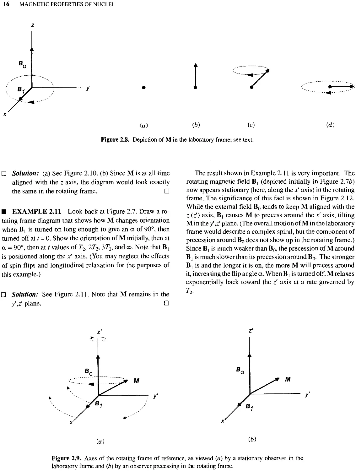
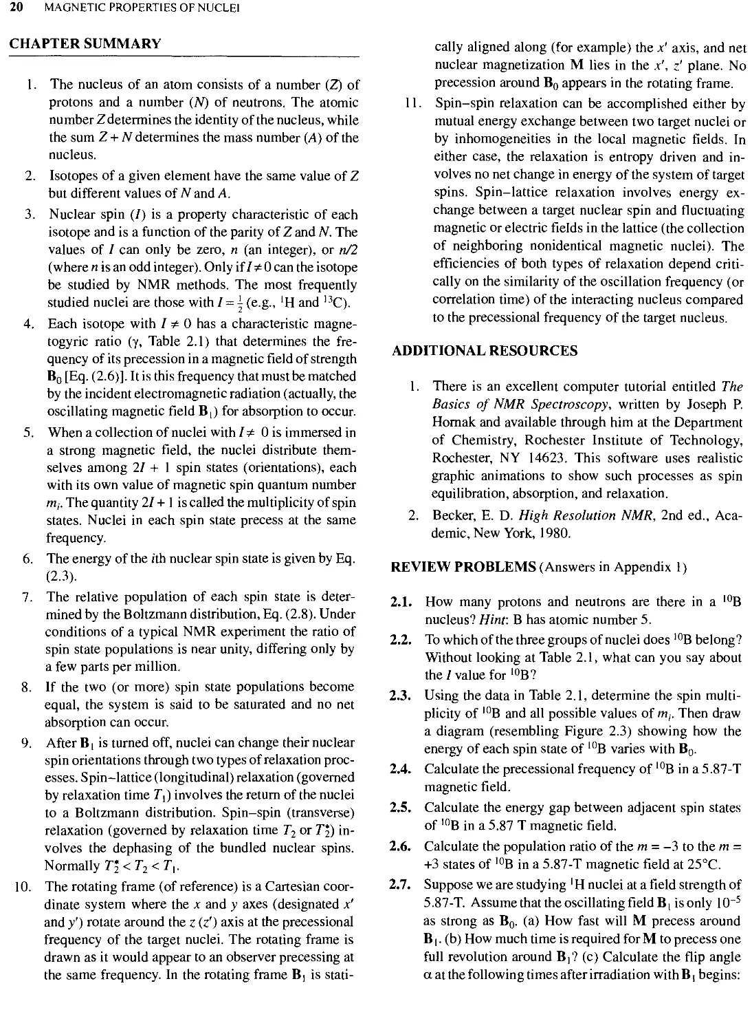
Figure 2.3. Nuclear Zeeman effect, (a) A nucleus with / = I. (fc) A nucleus with / = 1. The arrow
beside each spin state line indicates the orientation of the magnetic moment in a vertical magnetic
field.
B.4)
271
And now you realize why values of ±| were picked for m
(and 5 too, for that matter). It is so that the difference in energy
between two neighboring spin states will always be an integer
multiple of y h Bq/271.
The magnetogyric ratio y describes how much the spin
state energies of a given nucleus vary with changes in the
external magnetic field. Each isotope with nonzero nuclear
spin has its own unique value of y, though the magnitude of y
depends on the units selected for Bo. We will use the unit tesla
(T) for magnetic field strength so that y has units of radians
per tesla per second Btc radians in one cycle of 360°). As we
will see in Chapter 3, modern commercial NMR spectrome-
spectrometers are equipped with magnets that generate fields ranging
from ca. 5 to 16 T. For comparison, the earth's magnetic field is
a mere 6 x 10~5 T. {Note: Earlier books on NMR used the gauss
or kilogauss for magnetic field strength; 1 T = 104 G = 10 kG.)
In Table 2.1 are listed many of the common isotopes
examined by NMR techniques, together with their nuclear
constants. Notice that a bare proton has the largest y value of
any nuclear particle, while heavier nuclei, surrounded by
many subvalence electrons, tend toward lower values. This
will become significant later. Relative sensitivity is the
strength of the NMR signal that is generated by a fixed
number of nuclei of a given isotope relative to the signal
obtained from an equal number of 'H nuclei. If we compare
the data on natural abundance and sensitivity, we see why
historically the most easily studied nuclei were 'H, I9F, and
3'P. Indeed, prior to the 1970s these three were the only nuclei
routinely studied with commercially available instrumenta-
instrumentation. More recently, however, instruments have become avail-
available that can routinely examine a wide variety of other
ubiquitous elements, including I3C (which is of immense
importance to organic chemists), I5N, 23Na, and 29Si, to men-
mention just a few.
■ EXAMPLE 2.5 (a) What is the energy difference be-
between the two spin states of 'H in a magnetic field of 5.87 T?
(b) Of 13C?
□ Solution: (a) Use Eq. B.4) and the y values in Table 2.1.
yhB0
AE = -
2k
B67.512x 106radT-'s-')F.63x 1Q-34 J s)E.87 T)
2C.14rad)
= 1.66x 105J

2.2 THE NUCLEUS IN A MAGNETIC FIELD
11
(b) For I3C, y = 67.2640 x 106, so AE = 4.18 x 106 J,
about one-fourth the difference for 'H. □
2.2.2 Precession and the Larmor Frequency
We now know that nuclei with 7*0, when immersed in a
magnetic field, adopt 27 + 1 spin orientations, each with a
different energy. But before these nuclei can absorb photons,
they must be oscillating in some sort of uniform periodic
motion (Section 1.3). Fortunately, quantum mechanics re-
requires that the magnetic moments are actually not statically
aligned exactly parallel or antiparallel to the external mag-
magnetic field, as Figure 2.2 implied. Instead, they are forced to
remain at a certain angle to Bo, and this causes them to
"wobble" around the axis of the field at a fixed frequency.
Why is this so?
If you have ever played with a spinning top, you may know
that it is the spin angular momentum of the top that prevents
it from falling over and also causes it to wobble in addition to
spinning. This periodic wobbling motion that the top assumes
in a gravitational field is called precession. The earth pre-
cesses on its axis in much the same way, though much more
slowly. In an exactly analogous way, the magnetic moment
vector of a nucleus in a magnetic field also precesses with a
characteristic angular frequency called the Larmor fre-
frequency (go), which is a function solely of y and Bo:
go = y Bo B.5)
The angular Larmor frequency, in units of radians per second,
can be transformed into linear frequency v (in reciprocal
seconds or hertz) by division by 2n:
quency is independent of m, so that all spin orientations of a
given nucleus precess at the same frequency in a fixed mag-
magnetic field.
■ EXAMPLE 2.6 (a) At 5.87 T, what is the precession
frequency v of a 'H nucleus? A I3C nucleus? (b) In what
region of the electromagnetic spectrum does radiation of these
frequencies occur?
□ Solution: (a) For'H, using they value from Table2.1, we
find
yB0 B67.512 x
' 2tt ~
T)
2C.14 rad)
= 2.50 x 108s-'= 250 MHz
Similarly, for I3C, v = 62.9 MHz.
After you have completed these calculations the "long"
way, using Bo andy values from Table 2.1, try this easier
way. In Table 2.1, the data in the column labeled v are the
precession frequencies (in megahertz) of each nucleus in
a 1.00-T magnetic field. Simply multiplying these num-
numbers by the actual field strength (in tesla), directly gives
the value of v at any other field strength. Thus, for 'H,
v = D2.5759 MHz T-')E.87 T) = 250 MHz
(b) From Table 1.1 we note that these frequencies fall in
the rf region. □
v precession '
CO
271
2tc
B.6)
This precessional motion causes the tip of the magnetic mo-
moment vectors (either up or down) to trace out a circular path,
as shown in Figure 2.4. Note also that the precession fre-
m = +1/2
m = -1/2
Figure 2.4. Precession of the magnetic moment in each of the two
possible spin states of an/ = ^ nucleus in external magnetic field Bq.
■ EXAMPLE 2.7 At what magnetic field strength do pro-
protons ('H nuclei) precess at a frequency of 300 MHz?
□ Solution: Rearranging Eq. B.6), we find
_ 27TV
Y
2C.14rad)C00x 106s-')
267.512 x 106radT-'s-'
= 7.04 T
□
We are almost ready to perform our NMR experiment. We
have immersed the collection of nuclei in a magnetic field;
each nucleus is precessing with a characteristic frequency. To
observe resonance, all we have to do is irradiate them with
electromagnetic radiation of the appropriate frequency, right?
Well, almost!

12 MAGNETIC PROPERTIES OF NUCLEI
2.3 NUCLEAR ENERGY LEVELS AND
RELAXATION TIMES
2.3.1 Boltzmann Distribution and Saturation
In Chapter 1 we hinted that once a particle absorbs a photon,
the energy originally associated with the electromagnetic
radiation appears somehow in the particle's motion. Where
does the energy go in the case of precessing 'H nuclei?
Because there are only two spin states possible, the energy
goes into a spin flip. That is, the photon's energy is absorbed
by a nucleus in the lower energy spin state (m = +~), and the
nucleus is flipped into its higher energy spin state (m = ~).
This situation is depicted in Figure 2.5. And remember that
this spin flip does not change the precessional frequency of
the nucleus.
We have already calculated the energy gap between these
two spin states [Eq. B.4)], and this must equal the energy of
the absorbed photon [Eq. A.3)]. Combining these with Eq.
B.6) gives us
AE =
^
= "^precession = ^photon = "vphoton
B.7)
Thus, as we expected from Chapter 1, for resonance to occur,
the radiation frequency must exactly match the precessional
frequency.
But there is a fly in the ointment. Quantum mechanics tells
us that, for net absorption of radiation to occur, there must be
more particles in the lower energy state than in the higher one.
If the two populations happen to be equal, Einstein predicted
theoretically that transition from the upper (m = -±) state to
the lower (m = +j) state (a process called stimulated emis-
emission) is exactly as likely to occur as absorption. In such a case,
no net absorption is possible, a condition called saturation.
Is there any reason to expect that there will be an excess of
nuclei in the lower spin state? The answer is a qualified yes.
For any system of energy levels at thermal equilibrium, there
will always be more particles in the lower state(s) than in the
upper state(s). However, there will always be some particles
in the upper state(s). What we really need is an equation
relating the energy gap (AE) between the states to the relative
populations of (numbers of particles in) each of those states.
This time, quantum mechanics comes to our rescue in the
form of the Boltzmann distribution:
P(m =
(m = I /2)
f-AE
= exp[Tr
B.8)
where P is the population (or fraction of the particles) in each
state, T. is the absolute temperature in Kelvin (not to be
confused with nonitalicized T for Tesla), and k (the Boltzmann
constant) has a value of 1.381 x 103 J K.
■ EXAMPLE 2.8 At 25°C B98 K) what fraction of 'H
nuclei in 5.87 T field are in the upper and lower states? See
Example 2.5 for the value of AE.
□ Solution: Use Eq. B.8) and the results of Example 2.5:
AE
kT
= exP -
1.66 x 105 J
1.381 x 10-23JK-' x298K
= 0.99996
t
E
= -M2
= +M2
Figure 2.5. Relative energy of both spin states of an / = i nucleus as a function of the strength of the
external magnetic field Bo.

2.3 NUCLEAR ENERGY LEVELS AND RELAXATION TIMES 13
Since there are only two spin states, P
I-/W1/2), so/>(m = _1/2) = 0.49999 and
0.50001
□
As you can see from the above example, the difference in
populations of the two 'H spin states is exceedingly small, on
the order of 20 ppm. And the difference for other elements is
even smaller because of their smaller y values. But do not
despair. This difference is sufficient to allow an NMR signal
to be detected. It is this small difference, however, that ac-
accounts in part for the relatively low sensitivity of NMR
spectroscopy compared to other absorption techniques such
as infrared and ultraviolet spectroscopy. Remember, factors
such as a stronger magnetic field (Bo), a larger magnetogyric
ratio, or a lower temperature all contribute to a larger popula-
population difference, reduce the likelihood of saturation, and lead
to a more intense NMR signal.
2.3.2 Relaxation Processes
Our NMR theory is almost complete, but there is one more
thing to consider before we set about designing a spectrome-
spectrometer. We indicated previously that at equilibrium in the absence
of an external magnetic field, all nuclear spin states are
degenerate and, therefore, of equal probability and popula-
population. Then, when immersed in a magnetic field, the spin states
establish a new (Boltzmann) equilibrium distribution with a
slight excess of nuclei in the lower energy state.
A relevant question is this: How long after immersion in
the external field does it take for a collection of nuclei to
reequilibrate? This process is not infinitely fast. In fact, the
rate at which the new equilibrium is established is governed
by a quantity called the spin-lattice (or longitudinal) relaxa-
relaxation time, T\. The exact relation involves exponential decay.
P — P
r eq 't
B.9)
where P^ — P, is the difference between the equilibrium
population of a given state (for example, the m = +^ state) and
the population after time t and the subscript zero refers to t =
0. (Peq is thus the population at t = oo.)
■ EXAMPLE 2.9 (a) Suppose that for a certain set of' H
nuclei at 25°C, the value of 7, is 0.20 s. How long after
immersion in a 5.87-T magnetic field will it take for an
initially equal distribution of 'H spin states to progress 95%
of the way toward equilibrium? (b) What would happen if the
magnet were turned off at this point?
□ Solution: (a) From Example 2.8, we know that the final
equilibrium population of the m = +j state will be
0.50001. At 95% of equilibrium Peq-P,
0.05(/'eq - Po). Use Eq. B.9) and solve for t:
0.05(Peq-P0)
0.05 = exp -
Taking the natural logarithm (In) of both sides of the
equation, we find
-3.00 = ~ or r=3.00r,
11
Since T{ = 0.20 s, t = 3@.20 s) = 0.60 s.
(b) When the field strength returns to zero, the collection
of nuclei will decay exponentially toward the original
equal populations of spin states at a rate still governed by
the same value of T,. □
Figure 2.6 graphically depicts the situation in Example 2.9.
The arrows in the three diagrams below the graph represent
the distribution of individual precessing 'H magnetic mo-
moments, either up or down. Initially there are equal numbers of
nuclei in each spin state. But at equilibrium in the magnetic
field, there is a 20 ppm excess of up spins (exaggerated in the
middle diagram). When the magnetic field is turned off, the
collection decays back to the original equal distribution.
The values of T\ range broadly, depending on the particular
type of nucleus, the location of the nucleus (atom) within a
molecule, the size of the molecule, the physical state of the
sample (solid or liquid), and the temperature. For liquids or
solutions, values of 10~2-102 s are typical, though some
quadrupolar nuclei have (faster) relaxation times of the order
of 10 s. For crystalline solids, Tt values are much longer
(Section 2.5). For now, just remember that the larger the value
of Th the longer it takes for a collection of nuclei to reach (or
return to) equilibrium.
There is another reason why the magnitude of T\ is impor-
important. Suppose we have a Boltzmann distribution of nuclei
precessing in a magnetic field, and we irradiate the collection
with photons of precisely the correct frequency (and energy)
to cause transitions (spin flips) between the lower (m = +\)
level and the upper (m = —~) states. Because there is initially
such a small difference between the populations of the two
states, it will not be long before the populations are equalized
through the absorption of the photons! This, of course, means
the spin system has become saturated and no further net
absorption is possible. However, if we turn off the source of
rf radiation, the system can relax back to the Boltzmann
distribution (at a rate controlled by T\) and absorption can

14 MAGNETIC PROPERTIES OF NUCLEI
(a)
F)
■) T
0.9 -
°r 0.7
S" 0.6 -
S0.5-
S. 0.4-
g" 0.3 -
t0.2-
0.1 -
0 -
^—
/
/
- /
-/
I I I I I
magnet turned off
\
X.
^••^^^
1 1 1 1 II I ^^
spin distribution
(exaggerated)
3 4
time (units of T1)
5 up, 5 down
6 up, 4 down
5 up, 5 down
Figure 2.6. (a) Graphical depiction of the approach of a collection of magnetic nuclei toward
equilibrium when the external field is turned on (f = 0, ... 37",), then turned off. (b) Exaggerated
pictorial depiction of the spin state distribution at t = 0, 3Th <x>.
resume. This fact presents us with a paradox. The spin system
must absorb enough photons for us to be able to detect the
signal instrumentally, but not so much as to cause saturation.
This brings us to the question (to be covered more fully in
Section 3.1) of how an NMR signal is actually generated.
Figure 2.7 depicts a collection of / = ± nuclei at equilibrium,
in a magnetic field aligned with the +z axis. (By convention,
the static magnetic field, Bo, always defines the z axis.) Before
irradiation begins (Figure 2.7a), the nuclei in both spin states
are precessing with the characteristic frequency, but they are
completely out of phase, that is, randomly oriented around the
z axis. The net nuclear magnetization M is the vector sum of
all the individual nuclear magnetic moments, and its magni-
magnitude is determined by the excess of up spins over down spins.
Here, M is aligned parallel to Bo; it has no precessional motion
and no component in the x,y plane.
Now suppose there were a way to produce another mag-
magnetic field perpendicular to Bo. However, this new field (B|)
will be much weaker than Bo, and it will precess in the x,y
plane, oscillating at exactly the same frequency as the nuclear
magnetic moments (Figure 2.7b). (In Section 3.1 we will
describe how to generate such an oscillating magnetic field,
but it should not surprise you to learn that it involves electro-
magnetic radiation of the same frequency.) At any rate, a
rather strange thing happens when this irradiation by B]
begins: All of the individual nuclear magnetic moments be-
become phase coherent. That is, they focus, tracking the oscil-
oscillating magnetic field, and form a precessing "bundle" as
shown in Figure 2.7c. Provided we have not saturated the
system by absorbing too may photons, this phase coherence
also requires that M tip away from the z axis and begin to
precess around the z axis, again with the characteristic Larmor
frequency. As such, M now has a component in the x,y plane
(M^y) oscillating with the same frequency. The flip angle a
that M makes with the z axis controls the magnitude of M,>v,
by the relation
y = M sin a
B.10)
The angle a is, in turn, determined by the power and duration
of the irradiation by B,. Ultimately, the actual NMR signal

2.4 THE ROTATING FRAME OF REFERENCE 15
a1
V
(a)
(b)
(c)
Figure 2.7. Precession of a collection of / = | nuclei around external magnetic field Bq. Here, M
represents the net nuclear magnetization, the vector sum of all the individual nuclear magnetic
moments, (a) Before irradiation by B|. (£>)The orientation of the rotating magnetic field Bj. (c) During
irradiation by B|.
will be generated from the oscillation of M^v (Section 3.1),
so the maximum signal intensity will occur when a equals
90° (Why?).
There is one other type of relaxation process that must be
mentioned at this point. After irradiation ceases and B, disap-
disappears, not only do the populations of the m = +^ and m = -i
states revert to the Boltzmann distribution, but also the indi-
individual nuclear magnetic moments begin to lose their phase
coherence and return to a random arrangement around the z
axis (Figure 2.7a). This latter process, called spin-spin (or
transverse) relaxation, causes decay of M,_y at a rate control-
controlled by the spin-spin relaxation time T2. Normally, T2 is
much shorter than 7",. A little thought should convince you
that if T2 < Th then spin-spin (dephasing) relaxation takes
place much faster than spin-lattice (Boltzmann distribution)
relaxation.
2.4 THE ROTATING FRAME OF REFERENCE
Frequently in this book we will want to depict nuclear spin
orientations like those shown in Figure 2.7. More often than
not, we will focus our attention on the net nuclear magnetic
moment (M) rather than on the individual nuclear spins.
Because M will sometimes precess around Bo (i.e., the z
axis), we need a more convenient way than the dashed ellipses
used so far to depict M as it precesses and changes orientation.
Henceforth we will use another convention to represent this
precessional motion of M, the rotating frame of reference,
which is designed to show the effects of B, on M.
In Figure 2.8 are shown four representations of M in the
"old" way, the so-called laboratory frame of reference, the
normal x,y,z coordinate system as viewed by a stationary
observer in the lab. In part (a) of the figure Bo and B, are off,
so the populations of individual up and down nuclear spins
are equal, and the magnitude of M is zero. In (b) the equilib-
equilibrium distribution of spins with Bo on has been achieved and
M is aligned along the z axis, even though the individual
nuclear magnetic moments still precess around the z axis. Part
(c) shows M tipped to an a of 45° through its interaction with
B[, and the resulting precession of M describes a cone. Finally
in (d) the flip angle is 90° so the precession of M describes a
disc in the x,y plane.
Instead, suppose the x and y axes were themselves precess-
ing clockwise (when viewed from above) around the z axis at
the same frequency the nuclear spins are precessing. Further
suppose we, the observers, were precessing around the z axis
at the same frequency. To differentiate this rotating coordinate
system from the fixed (i.e., laboratory frame) system, we will
use labels x',y\ and z' to represent the three rotating axes (the
z' axis is coincident on and equivalent to the z axis). To us
rotating observers, the rotating axes and Bj appear stationary,
and M will rotate in the plane perpendicular to B|. These
relationships are shown in Figure 2.9.
Clearly, viewing the motion of M in the rotating frame
simplifies our drawings. Still, it is important to remember this
about rotating-frame diagrams: Whenever M is anywhere
except directly along the z' axis, it has a component oscillating
in the x,y plane (laboratory frame), and this is what gives rise
to an NMR signal.
■ EXAMPLE 2.10 (a) Look back at Figure 2.6. Draw a
laboratory frame diagram that shows M at
t = 0, T\, 2T\,..., 6Ty. (b) How would the diagram change
in the rotating frame?

16 MAGNETIC PROPERTIES OF NUCLEI
1
(a) F) (c)
Figure 2.8. Depiction of M in the laboratory frame; see text.
id)
□ Solution: (a) See Figure 2.10. (b) Since M is at all time
aligned with the z axis, the diagram would look exactly
the same in the rotating frame. □
■ EXAMPLE2.il Look back at Figure 2.7. Draw a ro-
rotating frame diagram that shows how M changes orientation
when B, is turned on long enough to give an a of 90°, then
turned off at t = 0. Show the orientation of M initially, then at
a = 90°, then at t values of T2, 2T2, 3T2, and oo. Note that B,
is positioned along the x' axis. (You may neglect the effects
of spin flips and longitudinal relaxation for the purposes of
this example.)
□ Solution: See Figure 2.11. Note that M remains in the
y',z' plane. □
The result shown in Example 2.11 is very important. The
rotating magnetic field B, (depicted initially in Figure 2.7b)
now appears stationary (here, along the x' axis) in the rotating
frame. The significance of this fact is shown in Figure 2.12.
While the external field Bo tends to keep M aligned with the
z (z1) axis, B, causes M to precess around the x' axis, tilting
M in the y',z' plane. (The overall motion of M in the laboratory
frame would describe a complex spiral, but the component of
precession around Bo does not show up in the rotating frame.)
Since B, is much weaker than Bo, the precession of M around
B! is much slower than its precession around Bo. The stronger
B| is and the longer it is on, the more M will precess around
it, increasing the flip angle a. WhenB, is turned off, M relaxes
exponentially back toward the z' axis at a rate governed by
i
Bo
7<
^> M
z'
M
y"
(a)
ib)
Figure 2.9. Axes of the rotating frame of reference, as viewed (a) by a stationary observer in the
laboratory frame and (b) by an observer precessing in the rotating frame.

2.4 THE ROTATING FRAME OF REFERENCE 17
magnet turned off
0 12 3 4
t (units of T1)
Figure 2.10. Pictorial solution to Example 2.10. Compare with Figure 2.6a.
z'
B,
M
t= 0
B1 on
-»[« B1 off
2T2 3T2
00
Figure 2.11. Pictorial solution to Example 2.11.
M
a =90°
a =180°
Figure 2.12. Precession of M around B| in the rotating frame.

18 MAGNETIC PROPERTIES OF NUCLEI
2.5 RELAXATION MECHANISMS AND
CORRELATION TIMES
The complete microscopic details of how longitudinal (spin-
lattice, 7",) and transverse (spin-spin, T2) relaxation occur is
beyond the scope of this book. But a little further discussion
might be profitable in order to provide us with at least a
qualitative understanding of the subject.
Look again at Figure 2.7c. What causes the individual up
and down nuclear spins in a "bundled" set of identical target
(observed) nuclei to randomize their phasing (defocus) after
B, is turned off? One mechanism for spin-spin relaxation can
be pictured as follows. Suppose that one of the up spins and
one of the down spins instantaneously exchange energy. In
this way, the up spin is converted to a higher energy down
spin, and vice versa, with no net change in energy. However,
although the orientations (up or down) have exchanged, the
exact phasing has not, as shown in Figure 2.13. Repetition of
this process with other pairs of up/down spins will have the
ultimate effect of randomizing their phasing, driving M.x y to
zero and with it the NMR signal.
Spin-spin relaxation can also occur when other nearby
oscillating magnetic or electric fields interfere with the exter-
external field Bq, causing some of the nuclei to experience a
slightly augmented magnetic field while others experience a
slightly diminished one. Those nuclei in the region of the
augmented field will precess slightly faster, while those ex-
experiencing the diminished field will precess slightly slower
(Figure 2.14). This will result in the "fanning out" of individ-
individual spin vectors again with no net energy change.
As we will see in Section 3.2, there is also a limit to the
homogeneity of Bo itself. Even the finest magnets produce a
field strength that varies ever so slightly around the region
containing the sample. And this small range in field strength
causes nuclei in one part of the sample to precess at very
slightly different frequencies, again leading to dephasing of
the nuclear spins once B, is turned off. This mechanism for
spin-spin relaxation is usually the dominant one and gives
rise to an effective spin-spin relaxation time known as T\,
where T2 < T2 (the "natural" spin-spin relaxation time). All
three types of spin-spin relaxation are driven by the second
law of thermodynamics: In the absence of other forces, a
system will tend spontaneously to attain that arrangement
with maximum entropy (disorder).
Thermodynamics also tells us that systems tend spontane-
spontaneously toward equilibrium, which is characterized by a mini-
minimum energy (or free energy, to be exact). One component of
free energy is the entropy mentioned above. Normally the
dominant component of free energy is enthalpy (heat con-
content). Within a magnetic field, the equilibrium (Boltzmann)
distribution of nuclear spins is the one with minimum en-
enthalpy (and maximum entropy). Any other distribution will
have higher enthalpy (and free energy). For such a higher
enthalpy distribution to relax back to equilibrium, it must
dissipate its excess energy to the surroundings. In the context
of NMR, these surroundings (the lattice) comprise other
nearby nonidentical magnetic nuclei that can, but need not
necessarily, be part of the same molecule as the nuclei of
interest. The lattice can also be regarded as an infinite heat
(energy) sink to or from which energy can be transferred
without changing its temperature.
The most important mechanism for spin-lattice relaxation
involves a direct (through space) interaction between the
magnetic dipole of a target nucleus and that of lattice nuclei.
Since lattice nuclei are undergoing constant periodic motion
(e.g., rotation and translation), the local magnetic fields due
to their magnetic moments will also be oscillating at the same
frequencies. When the frequency of this motion is comparable
to the frequency of precession of the target nucleus (e.g., 250
MHz), there can be a mutual spin flip. But since these nuclei
are nonidentical, there will be a net change in energy accom-
accompanying the exchange. That is, energy will either be passed to
B,
previously "down" spin
previously "up" spin
Figure 2.13. Result of one spin-spin exchange, shown in the laboratory frame. Compare with Figure
2.7c. Here, M is not shown.

2.5 RELAXATION MECHANISMS AND CORRELATION TIMES
19
1T,
2T,
3To
Figure 2.14. Laboratory frame diagram of "effective" spin-spin relaxation. Here, M is not shown.
the lattice nucleus (if the target nucleus drops to a lower
energy level) or energy will be absorbed from the lattice
nucleus (if the target nucleus is promoted to a higher energy
level). These exchanges continue at a rate governed by Ti until
equilibrium is reestablished.
The above dipole-dipole mechanism for spin-lattice re-
relaxation depends on the interaction of the target nucleus with
the magnetic field B; of a lattice nucleus with magnetic
moment |i;. The magnitude of B; is governed by the equation
B,=
C cos2G - 1)
?■
B.11)
where 0 is the angle between the external field Bo and a line
of length r connecting the two nuclei. This equation shows
that the effectiveness of spin-lattice relaxation (as measured
by how short 7", is) is increased by the lattice nucleus having
a large \i and being as close to the target nucleus as possible
to (i.e., in the same molecule or in high concentration in the
bulk medium).
In addition to the direct interaction of magnetic dipoles,
spin-lattice relaxation can proceed by way of interactions
between the magnetic dipole of the target nucleus and fluctu-
fluctuating electric fields in the lattice. This is why neighboring
quadrupolar nuclei (those with / > 5, Section 2.1) can bring
about very efficient spin-lattice relaxation (short 7", values).
As mentioned above, the frequency of rotational or trans-
lational motion of magnetic and electric fields in the lattice
nuclei is critical to the effectiveness of spin-lattice relaxation.
It cannot be too fast or too slow. It is common to express the
frequencies of these types of molecular motion in terms of a
so-called correlation time xc. If the angular rotation fre-
frequency is 00 (in radians per second), the rotational correlation
time is l/oo, the time required for a molecule (or part of a
molecule) to rotate 1 rad. Similarly, the translational correla-
correlation time can be equated to the time required for a molecule
to move a distance equal to one molecular diameter. In both
cases tc is an average measure of how long the two nuclear
magnetic dipoles remain in the appropriate relative orienta-
orientation to interact. Furthermore, it can be shown that
1
Btiv0tcJ
B.12)
where v0 is the precessional frequency of the target nucleus.
This equations tells us that for very fast molecular motion (i.e.,
when 1 /ic » 27tv0), 1 /7"] is proportional to t,. G", is inversely
proportional to xc). That is, as correlation time increases
(molecular motion slows), relaxation time decreases (the rate
of relaxation increases). Conversely, for slow molecular mo-
motion (i.e., when 1/tc « 27iv0), 7", is directly proportional to
tc; they both increase together. The minimum in T{ (ca. 10~3
s), and hence the most efficient spin-lattice relaxation, occurs
As we will see later, the magnitudes of relaxation and
correlation times are influenced by many factors, such as
temperature, viscosity of the medium, and size of the mole-
molecules involved. For example, in crystalline solids where all
translational and rotational motion has ceased, Tt values are
exceptionally large while T2 values are exceptionally small.
A major problem that results from inefficient spin-lattice
relaxation is that the target nuclei are much more easily
saturated (Section 2.3), making it difficult to obtain the de-
desired NMR signal. And, as we will see in Section 3.5, highly
efficient spin-spin relaxation gives rise to very broad signal
peaks. On the other hand, by measuring relaxation times and
correlation times, we are able to obtain detailed information
about how the giant molecules (e.g., polymers and proteins)
actually move (see Chapter 14).

20 MAGNETIC PROPERTIES OF NUCLEI
CHAPTER SUMMARY
1. The nucleus of an atom consists of a number (Z) of
protons and a number (AO of neutrons. The atomic
number Zdetermines the identity of the nucleus, while
the sum Z + N determines the mass number (A) of the
nucleus.
2. Isotopes of a given element have the same value of Z
but different values of N and A.
3. Nuclear spin (/) is a property characteristic of each
isotope and is a function of the parity of Z and N. The
values of / can only be zero, n (an integer), or n/2
(where n is an odd integer). Only if /* 0 can the isotope
be studied by NMR methods. The most frequently
studied nuclei are those with / = i (e.g., 'H and I3C).
4. Each isotope with / * 0 has a characteristic magne-
togyric ratio (y, Table 2.1) that determines the fre-
frequency of its precession in a magnetic field of strength
Bo [Eq. B.6)]. It is this frequency that must be matched
by the incident electromagnetic radiation (actually, the
oscillating magnetic field B,) for absorption to occur.
5. When a collection of nuclei with/ * 0 is immersed in
a strong magnetic field, the nuclei distribute them-
themselves among II + 1 spin states (orientations), each
with its own value of magnetic spin quantum number
m,. The quantity 11 + 1 is called the multiplicity of spin
states. Nuclei in each spin state precess at the same
frequency.
6. The energy of the zth nuclear spin state is given by Eq.
B.3).
7. The relative population of each spin state is deter-
determined by the Boltzmann distribution, Eq. B.8). Under
conditions of a typical NMR experiment the ratio of
spin state populations is near unity, differing only by
a few parts per million.
8. If the two (or more) spin state populations become
equal, the system is said to be saturated and no net
absorption can occur.
9. After B, is turned off, nuclei can change their nuclear
spin orientations through two types of relaxation proc-
processes. Spin-lattice (longitudinal) relaxation (governed
by relaxation time 7",) involves the return of the nuclei
to a Boltzmann distribution. Spin-spin (transverse)
relaxation (governed by relaxation time T2 or Tj) in-
involves the dephasing of the bundled nuclear spins.
Normally T2<T1<T].
10. The rotating frame (of reference) is a Cartesian coor-
coordinate system where the x and y axes (designated x'
and y') rotate around the z (zf) axis at the precessional
frequency of the target nuclei. The rotating frame is
drawn as it would appear to an observer precessing at
the same frequency. In the rotating frame B, is stati-
statically aligned along (for example) the x' axis, and net
nuclear magnetization M lies in the x', z' plane. No
precession around Bo appears in the rotating frame.
11. Spin-spin relaxation can be accomplished either by
mutual energy exchange between two target nuclei or
by inhomogeneities in the local magnetic fields. In
either case, the relaxation is entropy driven and in-
involves no net change in energy of the system of target
spins. Spin-lattice relaxation involves energy ex-
exchange between a target nuclear spin and fluctuating
magnetic or electric fields in the lattice (the collection
of neighboring nonidentical magnetic nuclei). The
efficiencies of both types of relaxation depend criti-
critically on the similarity of the oscillation frequency (or
correlation time) of the interacting nucleus compared
to the precessional frequency of the target nucleus.
ADDITIONAL RESOURCES
1. There is an excellent computer tutorial entitled The
Basics of NMR Spectroscopy, written by Joseph P.
Hornak and available through him at the Department
of Chemistry, Rochester Institute of Technology,
Rochester, NY 14623. This software uses realistic
graphic animations to show such processes as spin
equilibration, absorption, and relaxation.
2. Becker, E. D. High Resolution NMR, 2nd ed., Aca-
Academic, New York, 1980.
REVIEW PROBLEMS (Answers in Appendix 1)
2.1. How many protons and neutrons are there in a IOB
nucleus? Hint: B has atomic number 5.
2.2. To which of the three groups of nuclei does IOB belong?
Without looking at Table 2.1, what can you say about
the/value for IOB?
2.3. Using the data in Table 2.1, determine the spin multi-
multiplicity of IOB and all possible values of m,. Then draw
a diagram (resembling Figure 2.3) showing how the
energy of each spin state of IOB varies with Bo.
2.4. Calculate the precessional frequency of IOB in a 5.87-T
magnetic field.
2.5. Calculate the energy gap between adjacent spin states
of IOB in a 5.87 T magnetic field.
2.6. Calculate the population ratio of the m = -3 to the m =
+3 states of IOB in a 5.87-T magnetic field at 25°C.
2.7. Suppose we are studying ' H nuclei at a field strength of
5.87-T. Assume that the oscillating field B| is only 10~5
as strong as Bo. (a) How fast will M precess around
B |. (b) How much time is required for M to precess one
full revolution around B,? (c) Calculate the flip angle
a at the following times after irradiation with B, begins:

2.5 RELAXATION MECHANISMS AND CORRELATION TIMES 21
0, 0.10, and 0.20 ms A ms = 10 s). (d) Draw a
rotating-frame diagram that shows M at each of the
above times, (e) Suppose B, is turned off 0.20 ms after
it was turned on. Describe what happens to M in terms
of r, and T2 using a rotating-frame diagram.
2.8. A collection of 'H nuclei is irradiated by B, to give a
flip angle of 60°, during which about a fourth of the
excess up spins absorb photons and flip to down spins.
Then B, is turned off. (a) At this point, what is the
magnitude (length) of the M vector, compared to its
initial equilibrium magnitude? (b) Use a rotating-frame
diagram to show what happens to M after B, is turned
off.
2.9. Explain what effect dissolved oxygen (O2) might have
on longitudinal relaxation of 'H nuclei. Hint: The oxy-
oxygen molecule has two unpaired electrons with the same
s value.

3
OBTAINING AN NMR SPECTRUM
3.1 ELECTRICITY AND MAGNETISM
From a physics course in your past you are probably aware
that there is an intimate connection between electricity and
magnetism. Let us review a few of the relevant physical
principles.
3.1.1 Faraday Induction in the Receiver Coil
When a steady direct current of electricity (electrons) passes
through a loop of wire [by attaching the ends of the wire to a
battery or other source of direct-current (dc) voltage], a steady
magnetic field is established along the axis of the loop (a line
perpendicular to the loop and through its center); see Figure
3.1. The higher the current (amperes), the greater is the
strength of the resulting magnetic field. The field is also
strengthened by using a coil of wire made up of several loops
or by coiling the wire around an iron bar. These principles are
used in the construction of all electromagnets and supercon-
superconducting magnets (Section 3.2).
If the direction of current flow in the coil is reversed, so is
the direction of the magnetic field. And if the current is
oscillating (i.e., alternating current), the resulting linearly
polarized magnetic field will oscillate (change directions) at
the same frequency (Figure 3.2).
Now let us take the same loop of wire and replace the
voltage source with an ammeter. Initially, of course, no cur-
current registers in the ammeter. However, if we pass a bar
magnet down into the coil, the needle of the ammeter deflects,
indicating a current as long as the bar magnet is moving.
Change the direction of the magnet's movement and you will
see that the direction of the current reverses. This effect is
called Faraday induction: A current is induced in the wire
by the movement of the magnetic field near the wire.
Suppose that instead of a bar magnet we use the preces-
sional motion of M (the net nuclear magnetization vector;
Section 2.3) to induce an oscillating current [i.e.. a radio-fre-
radio-frequency alternating-current (ac) signal] in a coil of wire. We
will orient the coil so that its axis lies anywhere in the x,y
plane, for example, along the y axis and perpendicular to
Bo, as in Figure 3.3a. Henceforth, any time there is a compo-
component of M oscillating in the x,y plane (M, v[ Figure 2.7]), an
alternating current of the same frequency will be induced in
the coil's circuitry. We will label this loop the receiver coil,
for it is here that the NMR signal is generated.
B
T
Figure 3.1. Magnetic field B along the axis of a loop of wire
carrying direct current. The dotted lines indicate a few of the lines
of magnetic flux.
22

B = O
time
Figure 3.2. Orientation and magnitude of a linearly polarized magnetic field B as a function of the ac
voltage in the loop of wire. The voltage follows the cosine curve shown below.

24 OBTAINING AN NMR SPECTRUM
(a)
[b)
Figure 3.3. Orientation of (a) the receiver coil (attached to ammeter A) around the .y axis and (b) the
transmitter coil (attached to rf oscillator) around the x axis.
3.1.2 Generation of B, in the Transmitter Coil
Remember from Section 2.3 that to tip M off the z axis, so it
has a component in the x,y plane, we need an "irradiating"
magnetic field (B,) that oscillates at exactly the precessional
frequency of the nuclei of interest and is oriented perpendicu-
perpendicular to Bo. How are we going to generate such a precessing
magnetic field?
Suppose we orient a second loop of wire, henceforth called
the transmitter coil, so that its axis is aligned with the x axis,
perpendicular to both Bo and the axis of the receiver coil; see
Figure 3.3b. As we saw in Figure 3.2, passage of an rf
alternating current through the transmitter coil will generate
a magnetic field (B,) that is linearly polarized (oscillates back
and forth) along the x axis, as in Figure 3.4a. Now here is the
important part. This linearly polarized field can be viewed as
if it were the vector sum of two oppositely phased, circularly
polarized rotating magnetic fields (B, and B',), as shown in
Figure 3.4b. Note how the two circularly polarized vectors in
Figure 3.4b add together to generate the linearly polarized
vector in Figure 3.4a. One of these, B,, is rotating clockwise,
in the same direction as the nuclear moments precess around
Bo (Section 2.2.2). Therefore, when viewed in the rotating
frame (Figure 3.4c), B| will always be aligned with thex' axis,
exactly where it is needed to bring about the precession of M;
compare Figures 3.4c with 2.10.
3.2 THE NMR MAGNET
From the foregoing discussion we can list the basic compo-
components of an NMR spectrometer. There will be a magnet to
generate Bo, an rf oscillator to generate B, in the transmitter
coil, a receiver coil to pick up the signal, the electronics
(including a computer and plotter) to turn the signal into a
spectrum, and, of course, a sample to be analyzed. In this
chapter we will refine our spectrometer design as we consider
its performance and limitations.
3.2.1 The Magnet
The three most important characteristics of the magnet in any
NMR spectrometer are the strength, stability, and homogene-
homogeneity of its magnetic field Bo. Not only is the precessional
(resonance) frequency of identical nuclei directly propor-
proportional to the strength of Bo (Section 2.2), but so is the differ-
difference in precessional frequencies (Av) of nonidentical nuclei:
Av = V| — V2 =
Yi
(Yi ~
2ti
271
Therefore, it is advantageous to use the strongest available
magnet to obtain the greatest separation (i.e., resolution)
between NMR signals. Remember also that the stronger field
results in larger energy gaps between spin states [Eq. B.4)]
and hence greater populations in the lower energy states [Eq.
B.8)]. This serves to enhance the intensity of the NMR signal,
which turns out to be approximately proportional to the square
of Bq.
Magnets are of three general types: permanent magnets,
electromagnets, and superconducting magnets. There are ad-
advantages and disadvantages with each type. Permanent mag-
magnets are less costly, they have relatively stable fixed magnetic
fields, and they require no electric current to generate the field.
Unfortunately the strength of their fields is so limited (ca. 1.4
T) that they were used only in the first generation of commer-
commercial NMR spectrometers. Electromagnets used for NMR ap-
applications, on the other hand, are huge and more costly to build
and operate, but their field strengths range up to the strongest

3.2 THE NMR MAGNET 25
(a)
B1 (linear)
V
I!
B1 8,'
(c)
i
Figure 3.4. (a) Linearly polarized magnetic field B, (linear) oscillating along the x axis of the
laboratory frame; compare with Figure 3.2. (b) Resolution of Bj (linear) into oppositely rotating
circularly polarized magnetic fields, B, and B|' both oscillating at v0. (c) Orientation of B{ in the
rotating frame.
ever achieved, in excess of 34 T (which corresponds to a 'H
resonance frequency of 1.45 GHz, where 1 GHz = 109 Hz).
However, electrical resistance to the high current necessary to
generate strong magnetic fields generates considerable heat
that must be efficiently dissipated to assure a stable field.
The superconducting magnets used in NMR spectrometers
constitute a special subcategory of electromagnets. Each su-
superconducting magnet is designed to provide a specific nomi-
nominal field strength, currently in the range of ca. 6-18 T,
corresponding to 'H operating frequencies in the range of
250-750 MHz. The cylindrical solenoid through which the
large direct current flows is made of a unique niobium-tin
alloy that becomes superconducting (that is, develops zero
electrical resistance) when cooled to 4 K D degrees above
absolute zero) by immersion into liquid helium in a cryostat
that includes an outer jacket filled with liquid nitrogen. Figure
3.5a shows a complete Bruker DMX-500 NMR spectrometer.
The internal configuration of the magnet and probe region is
detailed in the cutaway diagram of Figure 3.5b.
The appropriate current is initially established in the
cooled solenoid with the aid of a high-voltage dc source. Then
the two ends of the solenoid loop are "short circuited," remov-
removing the dc source. However, because the solenoid circuit has
zero resistance, the large direct current continues coursing
through the solenoid indefinitely (as long as the helium holds
out!), thereby generating a very strong and stable magnetic
field.
As strong and stable as the magnetic field is, it is still
necessary to provide some mechanism by which the stability
of the field is monitored and controlled. This can be achieved
through an electronic feedback technique known as locking.
We first select a substance with nuclei that give rise to a strong
NMR signal (the lock signal) at a different frequency from
those of the nuclei of interest. If the lock substance is kept
physically apart from (but close to!) the sample, it is referred
to as an external lock. More commonly, the lock substance
is used as the solvent for the sample and is termed an internal
lock. In either case, the frequency of the lock signal is con-
continuously monitored and electronically compared to a fixed

1 I
I
26 OBTAINING AN NMR SPECTRUM
reference frequency rf oscillator. Any difference between the
lock and reference frequencies causes a direct microcurrent
to pass through a secondary coil (known as the Z° gradient
coil, aligned with and inside the solenoid). This results in a
small secondary magnetic field to be generated, aligned either
with Bo (increasing its magnitude slightly) or against Bo
(decreasing its magnitude slightly) until the lock frequency
once again matches the reference frequency. At this point the
magnet is said to be "locked."
The most common lock systems monitor the signal from
deuterium BH, /= 1), so it is common in NMR to use deute-
riated solvents such as D2O or CDC1-, (deuteriated chloro-
chloroform). Many such deuteriated solvents are readily available.
■ EXAMPLE 3.1 If the spectrometer's magnetic field
varied by +0.00001 T (that is, about 2 ppm), what magnitude
of change would be iniroduced in the resonance frequency of
'H nuclei at 5.87 T?
□ Solution: We can use a simple proportion:
0.00001 T Av
5.87 T 50 MHz
Av = 0.000430 MHz = 430 Hz
As we will see later, this ~2 ppm shift would be a very
large shift indeed! □
■ EXAMPLE 3.2 Suppose the lock signal frequency is
found to be slightly less than the constant reference frequency
of the rf oscillator. Should the magnetic field be increased or
decreased to bring it back to the nominal value?
□ Solution: Remember |Eq. C.1)] that the frequency of
any signal increases in direct proportion to the field
strength. Thus, to increase the lock signal frequency, we
need to increase ihe field strength. □
Once a .stable field is established, the question remains as
to whether that field is completely homogeneous (uniform)
throughout the region of the sample. The level of homogene-
homogeneity required for a given NMR experiment depends on the
desired level of resolution, which in turn controls the preci-
precision of the measurement. In the case of 'H nuclei at 5.87 T,
for example. Example 3.1 suggests that to achieve a precision
of ±1 Hz at a frequency of 250 MHz. (four parts per billion!),
the field must be homogeneous to the extent of 2.35 * 10~sT!
Such phenomenal uniformity can be achieved by means of
two additional instrumental techniques. First, the sample
vessel (normally a precisely constructed glass tube) is posi-
positioned along the center (r axis) of the solenoid in a region
called the probe (Figure 3.5/?) that is separated from the
region cooled by liquid helium and whose temperature can
therefore be independently controlled. The tube is spun
around its axis at ca. 100 Hz by means of an air stream that
turns a small plastic turbine attached to the top of the tube.
(a)
Figure 3.5. (a) Bruker model DMX-500 NMR speciromeier. The magnet cryosiat is located on the
lefi.

3.2 THE NMR MAGNET 27
liquid nitrogen
liquid helium
superconducting
solonoid
rotor
turbine
sample tube
transmitter / receiver coil
magnet shim coils
probe shim coils
probe head
rf
transmitter
filter
commutator
relay
pre-
preamplifier
(b)
receiver
Figure 3.5. (b) Cutaway diagram of the cryoslat, showing the essential parts of ihe magnet and probe.
(Courtesy of Bruker Instruments. Inc.)
This spinning helps to "average out" any slight inhomogenei-
lies of the field in the sample region.
Second, the contour (shape) of the field itself can be varied
(within very narrow limits) by passing extremely small cur-
currents through a complex series of shim coils located around
the probe cavity. The resulting small fields in these coils can
be adjusted to further improve the homogeneity of the field.
This process, called shimming or tuning the magnet, is ac-
accomplished by adjustment of a dizzying series of shim con-
controls (labeled by the field axis most affected, e.g.,

28 OBTAINING AN NMR SPECTRUM
Z2, Z\ X, Y, XZ, YZ, XY, X2, -Y1, etc.) before each spectrum
is taken. With the advent of microprocessor-controlled spec-
spectrometers, the bulk of these adjustments are now accom-
accomplished automatically.
We are left with a paradox. To get an acceptable signal, we
need to have as many nuclei as possible in the sample region
(remember the minute difference between spin state popula-
populations?). But we must restrict our sample to the smallest
possible volume in the interest of precision and resolution.
The eventual compromise results in a sample cavity of -0.05
cm3 for instruments that accommodate narrow-bore E-mm-
o.d.) tubes to -1.0 cm3 for instruments using wide-bore
A0-20-mm-o.d.) tubes. [However, for medical use, some
low-resolution NMR instruments have been constructed that
accommodate entire human bodies! (See Chapter 16)] Typi-
Typically, 'H and I3C spectra require ca. 5 and 15 mg of sample,
respectively.
■ EXAMPLE 3.3 A typical thin-wall narrow-bore NMR
tube has an outside diameter of 5.00 mm @.500 cm) and an
inside diameter of 4.20 mm. It is usually filled to a height of
-1 in. B.5 cm), (a) What is the wall thickness of the glass
tube? (b) If the total volume of the sample cavity (including
the tube) is 0.050 cm3, what are the dimensions (radius r,
height h, and volume) of the space that is actually occupied
by sample? [Hint: The volume of the cylinder is nr^h,]
□ Solution: Refer to Figure 3.6.
(a) Wall thickness = E.00 mm - 4.20 mm)/2 = 0.40 mm.
(b) The diameter of the sample is the same as the inside
00 mm
20 mm
bottom
section of
tube
diameter of the tube, 0.42 cm. The height of the sample
cavity is given by
sample cavity
h =
n 'f
fotai
0.050 cm3
cmJ
= 0.255 cm
Since rsamp,e = 0.42 cm/2 = 0.21 cm,
Figure 3.6. Bottom section of an NMR sample tube and the sample
cavity where the NMR signal is generated.
'sample ~ 7T. 'sample
h = 7i@.21 cmJ@.255 cm) = 0.035 cm3 = 35 \xh
Thus, only 70% of the sample cavity is filled with sample
in this case. Clearly, the thinner the wall of the tube, the
more sample actually gets into the sample cavity. Further-
Furthermore, for samples in very limited supply (<1 mg), pre-
precisely machined Teflon inserts for the tubes are available
to both reduce the amount of dead volume in the tube
below the sample cavity and prevent formation of vortices
(whirlpools) of the solution within the tube when it is
spun. □
There is one more thing you should know about the pow-
powerful magnets used in today's NMR spectrometers. If you get
too close to the magnet itself, you run the risk of demagnet-
demagnetizing anything on your person, such as credit cards, magnetic
tapes, and computer diskettes. (This fact was central to the
plot of a recent novel by Joseph Wambaugh.) But no need to
worry; it will not affect your magnetic personality!
3.2.2 Assembling the Pieces
We are now ready. The magnetic field is locked at 5.87 T and
a sample containing a substance with 'H nuclei, dissolved in
a deuterium-containing solvent, is spinning in the probe. We
activate the rf oscillator in the transmitter coil, producing a
B i field oscillating at 250 MHz radiation, and... yes! A weak
signal is detected in the receiver circuit! But let us not cele-
celebrate yet. What has this told us, except that we have 'H in the
sample, precessing at 250 MHz? Certainly, we would like to
be able to adjust parameters to test for nuclei precessing at
other frequencies as well. How can we accomplish that?
3.3 SIGNAL GENERATION THE OLD WAY: THE
CONTINUOUS-WAVE (CW) EXPERIMENT
Recall from Chapter 2 that, at a given field strength, each
magnetic isotope (/ * 0) precesses at a unique frequency
governed by its magnetogyric ratio [Eq. B.6)]; see Figure 3.7.
Thus, if we intend to use our spectrometer to observe nuclei
other than 'H, there must be a way to vary either the operating
(B,) frequency or the magnetic field strength.

},} SIGNAL GENERATION THE OLD WAY: THE CONTINUOUS-WAVE (CW) EXPERIMENT
u
225 200
175 150 125 100 75
Resonance Frequency (MHz) at 5.87 T
Figure 3.7. Resonance frequencies and relative sensitivities of several common isotopes at 5.87 T;
compare with Table 2.1.
From the discussion in Section 3.2, it is clear that the field
strength of any type of electromagnet can only be varied
within an extremely narrow range. This means that the nomi-
nominal operating frequency for, say, 'H nuclei is also fixed. (In
fact, the model number of most commercial NMR spectrome-
spectrometers is the same as the 'H operating frequency in megahertz.)
Since, for a given instrument, we cannot change Bo, the only
way to investigate nuclei other than 'H is to switch to a
different rf oscillator (B, source) with a frequency appropriate
for the specific nucleus of interest (e.g., I3C or-"P). In the old
days, switching oscillator circuits could be a rather tedious
process, but these days it requires little more than pushing a
few buttons or typing a few commands into the computer that
controls the instrument.
However, as we will see in Chapter 5, the real value of
NMR does not come from generating one signal for each
isotope present in the sample (e.g., one signal each for 'H,
L'C, or 3lP). Rather, we will find that even the individual
nuclei of the same isotope in different molecular environ-
environments can precess at slightly different frequencies (on the
order of parts per million), and these small differences can tell
us much about the details of the molecular structure involved.
Thus, we normally examine only one isotope (e.g., 'H) in each
NMR spectrum; that is, each spectrum is homonuclear. Since
we are examining only one isotope at a time, we only have to
vary the magnetic field (field sweep) or rf frequency (fre-
(frequency sweep) over narrow limits to see all of the nuclei of
that specific target isotope. All older NMR spectrometers,
equipped with conventional electromagnets, used either field-
or frequency-sweep technology. Because both involved con-
continuous operation of the rf (B|) oscillator, they were both
referred to as continuous-wave (cw) techniques.
3.3.1 Frequency-Sweep Mode
In the case of a frequency-sweep cw experiment, the magnetic
field strength (Bo) was fixed. Suppose our sample contained
two different nuclei (A and B) characterized by slightly
different resonance frequencies, with vA > vB. The spin state
energies of these two nuclei are depicted in Figure 3.8a. In
order for nuclei A and B to generate resonance signals, Eq.
B.7) requires they be irradiated with B| frequencies given
by

30 OBTAINING AN NMR SPECTRUM
CO
cm
S5
Bo
Magnetic Field Strength
(a)
Frequency
(b)
Figure 3.8. (a) Spin state energy gaps (AE) for two different nuclei at field strength Bo. (b) Resulting
frequency-sweep NMR spectrum.
Thus, it was necessary to sweep the operating frequency over
the range vA to vB (or vice versa) using a variable-frequency
if transmitter. This range of frequencies (va-vb) is called the
spectral width (or sweep width), SW, of the spectrum and
was limited to about 2000 Hz. Beginning at a frequency a little
less than vB, the frequency of the continuous if radiation was
gradually increased to a value above vA while the receiver
circuit was constantly monitored for a signal. As the fre-
frequency passed first through vB, then through vA, two separate
signals were detected. A plot of the intensity of these signals
versus frequency (Figure 3.8b) is our first frequency-domain
NMR spectrum, with frequency increasing from right to left
(as is the convention).
3.3.2 Field-Sweep Mode
Although some early NMR spectrometers did employ the
frequency-sweep (at constant field) technique, it turned out to
be electronically simpler to maintain the constant B, oscilla-
oscillator frequency appropriate for the target isotope and sweep
(vary) the magnetic field to achieve resonance for the nuclei
in the sample. By passing a slowly increasing direct current
though sweep coils, the magnetic field Bo could be varied
through a limited range while maintaining its homogeneity in
the sample area. Let us investigate how this change affected
the spectrum.
Because the operating radio frequency (v0) was now con-
constant, only photons of energy hv0 were available in the experi-
experiment [see Eq. A.3)]. Thus, the energy gap [AE, Eq. B.4)] for
each nucleus had to be adjusted by varying the magnetic field
strength Bo. By rearranging Eq. B.7), we can solve for the
field strength at which nuclei A and B entered resonance:
BA =
Br =
Ya
Yb
C.3a)
C.3b)
Figure 3.9a depicts the situation graphically. This time, in-
instead of varying the Bt frequency until it matched the preces-
siona! frequencies of nuclei A and B, we varied the
processional frequencies (by varying the field strength) until
they matched the B, frequency. Most importantly, the result-
resulting spectrum (Figure 3.%) was indistinguishable from the
frequency-sweep spectrum, except that the abscissa was cali-
calibrated in magnetic field units increasing from left to right.
Comparing Figure 3.8/? with Figure 3.9b reveals that nu-
nucleus A enters resonance at a higher frequency (at constant
field) or at a lower field (at constant frequency) than does
nucleus B. For this reason, the right-hand (low-frequency)
side of an NMR spectrum is often referred to as the high-field
(or upfield) side, while the left-hand (high-frequency) side is
called the low-field (or downfield) side.

3.3 SIGNAL GENERATION THE OLD WAY: THE CONTINUOUS-WAVE (CW) EXPERIMENT 31
So-
SoI
I
Magnetic Field Strength
(a)
Magnetic Field Strength
(b)
Figure 3.9. (a) The Bo field strength required for two different nuclei to attain the same spin state
energy gap AE. (b) Resulting field-sweep NMR spectrum.
■ EXAMPLE 3.4 Suppose that, at a nominal field
strength of 2.35 T, NMR signals were detected at 100 and 25.2
MHz. (a) What are the two isotopes giving rise to the signals?
(b) If the spectrum were obtained by the field-sweep method,
what field strength would be required to observe the latter
signal using an operating frequency of 100 MHz?
□ Solution: (a) By referring back to the v column in Table
2.1, we see that isotopes are 'H and I3C, respectively, (b) Use
Eq. C.3) and the value of y for I3C from Table 2.1:
_ 2tiv0 _ 2C.14 radXIOO x 106 sr') _ 9 33 T
C"'3 Yc-13 67.3x 106radT-'s-'
It is impossible for an NMR electromagnet designed for
2.35 T to produce a 9.33-T field! □
3.3.3 Spinning Sidebands and the Signal-to-Noise
Ratio
A closer examination of the signals in Figures 3.Sb and 3.9b
brings up some additional points. Figure 3.10 is an enlarge-
enlargement of one of the peaks. Notice the two small signals
symmetrically flanking the large signal. These so-called side-
sidebands or satellite peaks, marked with asterisks in the figure,
are an unavoidable result of spinning the sample to improve
field homogeneity (Section 3.2.1). If the field has been well
shimmed, such spinning sidebands rarely exceed 1 % of the
height of the main peak. Moreover, they will always be
separated from the main peak by exactly the spin rate in hertz.
This is, in fact, the most direct way to measure the sample spin
rate. One can, of course, completely eliminate spinning side-
sidebands by turning off the spinner. But this would cause sub-
substantial broadening of the signal (with an accompanying
decrease in signal height) because of the small inhomogenei-
ties present in the magnetic field.
■ EXAMPLE 3.5 Suppose the two sidebands in Figure
3.10 are each separated from the main peak by 58 Hz. (a) What
;nsity
H
S3
C
eo
55
sig
lal
1 height
noise (j)
height
(AO
I average
• baseline
■*— Frequency
Figure 3.10. An NMR signal peak showing sidebands (*) and
signal (S) to noise (N) ratio.

32 OBTAINING AN NMR SPECTRUM
is the spin rate of the sample tube? (b) How could you confirm
that these peaks were indeed spinning sidebands and not due
to something else?
□ Solution: (a) Because the frequency separation of a side-
sideband from the main peak is equal to the spin rate, the latter
must also be 58 Hz. (b) Varying the spin rate (by adjusting
an air flow directed at the spinner paddle) causes spinning
sidebands to shift position accordingly. If the peaks do
not shift position, they are not spinning sidebands.
There are other types of satellite peaks that we will
encounter later. □
You will also notice in Figure 3.10 that the signal baseline
is not perfectly flat. Instead, there is perceptible random
background noise causing a continuous wiggle in the base-
baseline. Even in the most carefully built and tuned spectrometers
there will always be some electronic noise generated by the
various circuits within the instrument, and the way the signal
data are processed. Normally, this does not present a problem,
provided the sample gives signals strong enough to be easily
differentiated from the noise. But what about really weak
signals? For example, a sample of natural hydrogen (Table
2.1) contains 99.985% 'H with a relative sensitivity of 1.00,
while a sample of natural carbon contains only 1.1% I3C,
which has a relative sensitivity of 1.59 x 10~2. These two
factors, low natural abundance and low relative sensitivity,
combine to make the carbon signal only about 2 x 10~4 times
as intense as a hydrogen signal for equal numbers of atoms of
each element. Thus, a I3C signal is much harder to distinguish
from noise than is a 'H signal.
To deal with this problem, we define a quantity called
signal-to-noise ratio (S/N), where S and N are approximated
by their respective peak heights, as shown in Figure 3.10.
■ EXAMPLE 3.6
3.10.
Using a ruler, estimate S/N in Figure
D Solution: The exact values of S and N will depend on the
scale of your ruler. But the ratio of the two numbers, S/N,
should be about 20. D
The goal in an NMR experiment is to maximize S/N, and
this can be achieved in several ways. One method is to use
higher rf power and a series of rf filters to remove some of the
noise. While this technique results in some improvement, care
must be taken to avoid saturation problems (see Section 2.3).
A far better improvement can be obtained by relying on a
result of the central limit theorem from information theory.
This theorem tells us that if the spectrum is scanned n times
and the resulting data are added together, signal intensity will
increase directly with n while noise (being random) will only
increase by ~Jn:
C.4)
where (S/N)] is the ratio after a single scan. Thus, S/N
improves linearly with ^n.
To make use of this multiple-scan technique, we first need
an extremely stable field. Then we need a computer to collect
the signal data (digitally) from each scan, add the data to-
together, and then divide the sum by n. The technique is known
as signal averaging or CAT (computer-averaged transients,
not to be confused with the diagnostic X-ray technique called
computer-aided axial tomography). Because each scan of an
older cw instrument could require 10 or more minutes, this
process used to take hours, during which time the magnetic
field had to be kept as perfectly stable and homogeneous as
possible. A momentary flicker in the building power during
an overnight experiment could cause all the data to be useless.
■ EXAMPLE 3.7 A single 10-min cw NMR scan of a
certain highly dilute sample exhibited S/N of 1.9. How much
time would be required to generate a spectrum with S/N of
19?
□ Solution: We can rearrange Eq. C.4) to calculate the
required number of scans:
D
(^ = J9 ,
(S/N)y 1.9
n=\& = 100
The time required for 100 scans is
t = A00 scans)A0 min per scan)
= 1000min= 16 h 40 min
No sleep tonight!
3.4 THE MODERN PULSED MODE FOR SIGNAL
ACQUISITION
Further improvement in S/N had to await the development of
faster computer microprocessors, which was exactly what
happened during the 1980s. Armed with very fast and efficient
microcomputers with large memories, chemists discovered
they could now generate NMR signals in an entirely new way.
Have you ever been sitting in a quiet room when suddenly
a fixed pitch noise (sound waves) causes a nearby object to
vibrate in sympathy? This is an example of acoustic reso-
resonance, in which the frequency of the sound waves exactly
matches the frequency with which the object naturally vi-
vibrates. If the pitch of the sound changes, the resonance ceases.

3.4 THE MODERN PULSED MODE FOR SIGNAL ACQUISITION 33
This is because only when the two frequencies match can the
sound waves constructively interfere (reinforce) the motion
of the object. At any other frequency the interaction will be
one of destructive interference and the net result will be no
vibration by the object. This is exactly analogous to the
continuous-wave NMR experiment. But have you not also
heard how a single loud sound such as a sonic boom can set
many different objects vibrating for a long period after the
boom is over? This occurs because the brief sound pulse acts
as though it is a mixture of all audible frequencies. Might it
also be possible to generate NMR signals this way?
In a pulsed-mode NMR experiment, which is performed
at both constant magnetic field and constant rf frequency, rf
radiation is supplied by a brief but powerful computer-con-
computer-controlled pulse of rf current through the transmitter coil. This
"monochromatic" (single-frequency) pulse, centered at the
operating frequency v0, is characterized by a power (measured
in watts and controlling the magnitude of B|) and a pulse
width (tp), the duration of the pulse measured in microsec-
microseconds. However, as a direct consequence of the uncertainty
principle [Eq. A.6)], this brief pulse acts as if it covers a range
of frequencies from v0 - Av to v0 + Av (Figure 3.11), where
Av is nothing more than the inverse of tp (Section 1.4). Thus,
the shorter the pulse, the greater the range of frequencies
covered.
The exact value of v0 is designed to be slightly offset from
the range of nuclear precession frequencies to be examined
(the spectral width, SW, in hertz). Therefore, the SW can be
no greater (and preferably less) than Av, leading to the rela-
relationship
SW < (*.)-'
or r.<(SW)-
i-i
C.5)
The power of the pulse must be sufficient to cause all sets of
nuclei precessing at frequencies within the SW to become
phase coherent, each set tipping their M vectors toward the
x',y' plane (Section 2.3). The nearer a nucleus's precession
frequency is to v0, the more excitation energy the nucleus
receives from the pulse, and the greater its flip angle a.
However, the closer a is to 90°, the stronger will be the signal
generated by a set of nuclei (Section 2.3). At the powers
normally used, a pulse as long as 1/SW causes flip angles to
Av
Vo
Av
frequency
Figure 3.11. Frequency distribution profile for an rf pulse of duration (pulse width) tp. The frequencies
range from v0 - Av to vq + Av, where Av equals \ltp. The sweep width can be either half of the curve.

34 OBTAINING AN NMR SPECTRUM
exceed 90°, so tp is generally set to approximately one-fourth
of (SW). This also avoids using the outer "tails" of the pulse
profile (Figure 3.11). The ultimate result of the pulse is a
complex signal in the receiver circuit that is the superposition
of the precession frequencies of all nuclei within the SW.
■ EXAMPLE 3.8 At 5.87 T the required 'H spectral
width is normally on the order of 5000 Hz. (a) At what
frequency should v0 be positioned? (b) What should be the
value of tpl
□ Solution: (a) At a field strength of 5.87 T, the nominal 'H
resonance frequency is 250 MHz, though the exact value
of v0 should be slightly offset from all nuclei of interest,
(b) tp « D SW)-1 = D x 5000 Hz) = 5 x 10 s = 50 (is.D
The next step in a pulsed-mode experiment is to monitor
the induced ac signal (voltage or current) in the receiver coil
as a function of time. In order to carry out signal averaging,
the data must be collected digitally. Thus, the computer in-
instantaneously measures the voltage in the receiver coil at
regular intervals (called dwell time td). A typical set of such
data might look something like Figure 3.12. The pattern
described by these 100 points is not obvious because data
points have not been collected often enough, at least for our
eyes to recognize it. The experiment can be repeated with the
dwell time reduced by a factor of 5, thus affording 500 data
points in the same total time. Figure 3.13 shows the result: a
more detailed wave function, made even more recognizable
by connecting sequential dots (Figure 3.14).
Take a moment to look carefully at the wave function in
Figure 3.14. You will see that the pattern is made up of two
superimposed cosine waves, a lower frequency wave (which
goes through 5 complete cycles during one "time unit") and
a higher frequency wave (which goes through 25 complete
cycles during one time unit). If the time unit were seconds,
the two frequencies would be 5 and 25 Hz, respectively.
Furthermore, the lower frequency component is about twice
as intense as the higher frequency one. It turns out that, rather
than measuring actual precessional frequencies (v,-), it is
electronically easier and more precise to measure the differ-
difference between v, and the operating frequency
v0 (Av, = v,- - v0) for each signal.
So, one important lesson is that the receiver circuit must
be sampled often enough to make the pattern recognizable.
The Nyquist theorem tells us that in order for a computer to
determine the frequency (Av,-) of each component of the wave
function by this method, it must acquire at least two points
1.5 ♦
1 ■-.
0.5-■
@
O)
5
-0.5 - ■
-1 ■•
-1.5
0.1
0.2
0.3
0.4
0.5
time
0.6
0.7
0.8
0.9
Figure 3.12. The ac signal (voltage or current) in the receiver coil, collected digitally as a function of
time.

3.4 THE MODERN PULSED MODE FOR SIGNAL ACQUISITION 35
1.5 <
1 ■
0.5-
0 ■
0.5-
-1 ■
1.5-
i
i
#
■ •
• *
•• #
•
I
I
•
•
•
•
#
•
•• #
<
•
# ••
•
p
ft
# #
• •
t •
f \
—\—
•
r
•
* ••
v;-
• <
• a
••
<
i
*• •
•V
1
t
•
1
•
»
ft
w
# #
• •
• •
•
•
<
^
»
•
• ••
• •
• •
ft
••
• •
# #
•• ••
* •• *• *
• f
1 %
1
• •
—•—
•
•
#
••
# ••
•
•
r
1—
0.1
0.2
0.3
0.4
0.5
time
0.6
0.7
0.8
Figure 3.13. Same signal as in Figure 3.12, except the dwell time has been reduced by a factor of 5.
0.9
-0.5 - -
-1.5
0.9
Figure 3.14. Same data as in Figure 3.13, except the dots are connected to make visualization easier.

36 OBTAINING AN NMR SPECTRUM
per cycle for each contributing wave. Therefore, so that fre-
frequencies of Av,- from 0 to SW hertz can be determined, the
computer must collect 2x SW data points per second, which is
equivalent to a dwell time no larger than the inverse of twice S W:
C.6)
Actually, the spectroscopic data would more closely re-
resemble the pattern in Figure 3.15, which is the same as the
wave in Figure 3.14, except that the overall intensity of the
signal decays exponentially with time. (Note that the decay
does not affect the frequencies.) Such a pattern is called the
modulated free induction decay (FID) signal (or time-do-
time-domain spectrum). The decay is the result of spin-spin relaxa-
relaxation (Section 2.3.2), which reduces the net magnetization in
the x, y plane. The envelope (see Section 3.6.2) of the damped
wave is described by an exponential decay function whose
decay time is T\, the effective spin-spin relaxation time.
Most molecules examined by NMR have more than just
two sets of nuclei, each set with a different frequency (Av,).
Furthermore, each set has its own relaxation times
G*! and T2), and usually there are different numbers of nuclei
within each set. These factors combine to give complex digital
FID curves consisting of n data points (usually in the thou-
thousands), numbered from 0 to n - 1.
For example, Figure 3.16 shows the 'H FID curve for
toluene C-1):
H H
3-1
From the FID data the computer determines the frequency
(Av,) and intensity of each component wave. How does it
accomplish this magic? The computer performs a Fourier
transformation (FT) of the FID data according to the equation
n-l
k=0
iKijk
n
foiy =
C.7)
where Tk represents the &th point of the time-domain (FID)
data and Fj represents they'th point in the resulting frequency-
domain spectrum. Thus, each Fj point (from 0 to n - 1)
requires a summation over all n points in the FID curve, and
the total calculation involves n2 multiplications and additions.
Figure 3.15. Simulated FID signal. The same data as in Figure 3.14, with exponential decay of the
signal added.

3.4 THE MODERN PULSED MODE FOR SIGNAL ACQUISITION 37
Figure 3.16. Actual 'H FID curve for toluene C-1).
An algorithm developed by Cooley and Tukey simplified this
extremely time-consuming calculation, bringing it within the
capability of modern microcomputers. Today, the transforma-
transformation takes only a few seconds, after which the frequency-do-
frequency-domain spectrum Fj can be plotted. (The frequency-domain
spectrum corresponding to Figure 3.16 will be discussed in
Chapter 5.)
During the FT of the FID data the computer will perform
a series of additional manipulations on the time- and fre-
frequency-domain data in order to present the most accurate peak
shape and spectrum appearance, including such computa-
computational techniques as zero filling and apodization. Zero filling
is a process for retrieving the maximum resolution present in
the FID data without increasing the RAM requirement of the
computer. Apodization eliminates sinusoidal wiggles in the
baseline around a frequency-domain signal peak caused by
truncating the FID acquisition too soon (using a racq that is too
short). Further details of these techniques are beyond the
scope of this book, but the interested reader may wish to
consult the Additional Resources section at the end of this
chapter. With input from the operator, adjustments can also be
made to the phasing of each signal, ensuring that the baseline
on both sides is symmetrically horizontal.
In experiments with either dilute samples or insensitive
nuclei (such as I3C), one pulse usually does not give a suffi-
sufficiently high S/N to allow the determination of the component
frequencies and intensities accurately. The S/N can be im-
improved by repeating the pulse-data acquisition sequence, then
adding the new FID data to the previously acquired data, as
in a CAT experiment. The required number of pulse sequences
(scans) is determined by the desired S/N. But there is an
additional consideration: To avoid saturation, one must allow
enough time between pulses for the nuclei to return (or nearly
return) to their original equilibrium (Boltzmann) distribution.
The required delay time (tw) is a function of the 7", values for
each set of nuclei of interest (Sections 2.3 and 2.5).
As a typical example of the pulse-data acquisition-delay
sequence (hereafter referred to as the pulse sequence), we
consider the parameters necessary when generating a typical
pulsed-mode 250-MHz 'H NMR spectrum. First, we select a
spectral width that covers all the nuclei of interest, usually
around 4000 Hz. Remember that the SW determines the pulse
width [tp « D SW)], which in this case would have to be
62.5 us. Since the frequency (Av,) of each component wave
can be uniquely determined by two points per cycle and our
spectral width might include frequencies anywhere from 0 to
4000 Hz, we must sample points twice that fast, or 8000 Hz
(a dwell time tj of 125 jas), to ensure collecting all relevant
frequencies [Eq. C.6)]. Moreover, we are limited by our
computer's memory capacity. Generating 8000 points per
second will fill up 32K C2,768 locations) of the computer's
RAM in 4.1 s. This fact determines the maximum acquisition
time (racq), the length of time a given FID signal is actually
monitored. Moreover, resolution (R), the ability to distin-
distinguish two nearby signals, is inversely proportional to acqui-
acquisition time:

Time
•■a,
■etc.
Figure 3.17. Pictorial representation of the complete pulse-acquisition-delay sequence (including
parameters tp, ?acq, and tw), repeated twice.

3.5 LINE WIDTHS, L1NESHAPE, AND SAMPLING CONSIDERATIONS 39
R = (tacqT[ C.8)
Thus, the 4.1 s acquisition time would provide a resolution of
D.1 s) = 0.24 Hz. If we require a resolution better (smaller)
than 0.24 Hz, either we need more computer RAM to accom-
accommodate a longer acquisition time or we have to decrease our
spectral width window.
Because the FID signal decays due to spin-spin relaxation,
there is a time limit beyond which further monitoring of the
FID provides more noise than signal. The usual compromise
is to have a short enough dwell time to cover the spectral width
and a long enough acquisition time to provide the desired
resolution, consistent with computer memory limitations.
After collecting data from one pulse, we must wait for the
nuclei to relax to equilibrium. A total of at least 2>TX is usually
adequate, but part of this is spent as acquisition time. Thus,
the additional pulse delay time (tw), the time between the end
of data acquisition and the next pulse, is given by
tw =3T\-t.
acq
C.9)
Since 'H nuclei normally exhibit T\ values on the order of 1
s, we need essentially no additional delay after 4 s acquisition
time. For I3C and other slow-to-relax nuclei, however, sub-
substantial delay times are sometimes required. Following the
pulse delay, the sample is irradiated with another pulse, and
the data acquisition sequence begins anew.
Figure 3.17 depicts this sequence. After some number of
pulse sequences (depending on sample concentration and
isotope being studied), the data are subjected to a Fourier
transformation, and the S/N of the resulting frequency-do-
frequency-domain spectrum is ascertained. If it is not yet adequate, the
pulse sequence is resumed until the desired S/N is attained.
To summarize, a pulsed-mode NMR experiment encom-
encompasses two steps: A) the collection of FID data by a pulse-
data acquisition-delay sequence, repeated enough times to
yield a time-averaged signal possessing the desired S/N, and
B) a FT of the FID data followed by plotting of signal
intensity as a function of frequency. The main thing to remem-
remember is that the frequency-domain spectrum generated in a
pulsed-mode/Fourier transform experiment contains all the
same information as the spectrum obtained in a cw experiment
(e.g., Figure 3.8), but in principle all the relevant spectro-
scopic information can be generated in just a few seconds
from a single rf pulse (S/N limitations notwithstanding). And
there is one further incidental advantage to the pulse-mode
technique. Because the receiver coil is off during the pulse
and the transmitter coil is off during data acquisition, we can
use just one coil to do both jobs (Figure 3.5Z?)!
■ EXAMPLE 3.9 Suppose we are about to acquire a
62.5-MHz I3C NMR spectrum. The desired spectral width
window is 15,000 Hz. The nuclei have 7", values up to 3 s and
the computer RAM has a capacity of 64K F5,536 locations).
The desired resolution is 0.5 Hz. (a) Using Figure 3.17 as a
guide, suggest values for the various data acquisition parame-
parameters, (b) How many data points can be collected from one
pulse sequence with these values? (c) If 1000 pulse sequence
repetitions (scans) are required for the desired S/N, how long
will the total experiment take?
□ Solution: (a) Use Eqs. C.5), C.6), C.8), and C.9):
tp * D SW)-1 = D x 15,000 Hz)'1 = 17|is
rJ = BSW)-|=C0,000Hzrl
= 33 [is C0,000 data points per second)
racq = /?-| = @.5Hz)=2s
b) Acquiring 30,000 data points per second for 2 s results
in 60,000 points for each pulse, well within the computer's
RAM limits, (c) Since the pulse time is negligible, the total
pulse sequence time is essentially equal to
'acq + tw (= 37^); thus, each pulse sequence requires 6 s. If
we need 1000 scans, the total time required for the experi-
experiment is 6000 s A h 40 min). Although this may seem like
a long time, remember from Example 3.7 that just 100 cw
scans required nearly 17 h! □
Lest you worry that you will have to supply each parameter
in every pulse sequence each time you take an NMR spectrum,
you can relax. Modern spectrometers are menu driven. For
most common nuclei all you have to do is select the nucleus
and the computer assigns the appropriate pulse sequence
parameters for most normal cases. However, when you are
dealing with an unusual structure or an uncommon nucleus,
you may have to do some experimenting with the parameters
to get the best spectroscopic data.
3.5 LINE WIDTHS, LINESHAPE, AND SAMPLING
CONSIDERATIONS
3.5.1 Line Widths and Peak Shape
A typical signal peak in a frequency-domain NMR spectrum
is characterized by several features. Most important are its
frequency (its position in the spectrum, Av,) and intensity
(peak height, or more accurately, the area under the peak). B ut
it is also characterized by a shape and a halfwidth. The
halfwidth (V|/2) of a signal is the width (in hertz) of the peak
at half height (Figure 3.18). The shape, which is determined
during the FT process, is described as Lorentzian (as opposed
to, say, Gaussian; see review problem 3.3). A Lorentzian
signal peak (Lv) conforms to the lineshape equation

40 OBTAINING AN NMR SPECTRUM
Av.
1 -r
2 3 4 5 6
frequency
Figure 3.18. Lorentzian NMR signal peak centered at Av,-, with halfwidth vi/2.
a Av2
Av2 + b(v - Av,J
C.10)
where a is the maximum peak height at the center of the signal
(Av,), v is any point along the frequency axis, and b (a
dimensionless quantity) is inversely related to the square of
the halfwidth by Eq. C.11). In generating Figure 3.18 the
parameters
C.11)
were a - 1.00 intensity unit, Av,- = 5.00 frequency units, and
b = 200. Most of the signal peaks we encounter in NMR
spectra will appear much sharper than the one in Figure 3.18,
but this is only because the halfwidth of a typical NMR signal
is 0.5 Hz out of a spectral width of several thousand hertz.
In Section 1.4 we found that the uncertainty principle
establishes spectroscopic time scales. It also has a significant
impact on the halfwidth of signals. One version of Eq. A.6)
says that the uncertainty in precessional frequency of a nu-
nucleus (Av) is inversely related to the uncertainty in lifetime of
the spin state (At). If we use v,/2 as a measure of the uncer-
uncertainly in frequency, it must be inversely proportional to the
lifetime of the spin state. What controls the lifetime of the spin
state? How fast it relaxes, of course! So, for At we can
substitute the relaxation time T:
T
C.12)
In other words, the halfwidth of a spectroscopic signal is
inversely proportional to the lifetime (relaxation time) of the
species giving rise to the signal. Nuclei that are slow to relax
(large values of T) give sharp signals; nuclei that relax rapidly
give broad signals. The halfwidth is therefore controlled by
the fastest type of relaxation (smallest value of T). For liquids
and solutions, this corresponds to T\ values (Section 2.5).
Typical NMR halfwidths for solution samples range from
about 0.1 to 0.5 Hz, except when dynamic chemical processes
are occurring (Chapter 10). By the way, do not confuse

3.6 MEASUREMENT OF RELAXATION TIMES 41
halfwidth, which is controlled by the rate of spin-spin relaxa-
relaxation, with signal intensity. In a pulsed-mode spectrum, inten-
intensity increases as spin-lattice relaxation time (T\) decreases.
3.5.2 Sampling Considerations
As we saw in Section 3.2, the intensity of an NMR signal is
determined in part by the number of nuclei giving rise to the
signal. We normally use solution samples to obtain reasonable
relaxation times and halfwidths. It is typical to dissolve ap-
approximately 5-10 mg of a substance of average molecular
weight (say, 200 daltons) in 0.4 mL of deuteriated solvent.
Using special microtechniques, it is possible in some cases to
obtain 'H spectra on as little as 10 fig of sample!
When picking a solvent there are several considerations.
First, and most obvious, the solvent must be inert, and it must
dissolve the sample! Of course, if your sample is sparingly
soluble or if there is only a fraction of a milligram of sample
available, you can usually resort to signal-averaging tech-
techniques to obtain the desired S/N. Besides that, it is best if the
solvent does not contain any nuclei of the isotope to be
examined.
Make sure you use thoroughly cleaned and dried NMR
tubes, and never assume that a new tube, fresh out of the box,
is clean to NMR standards.
3.6 MEASUREMENT OF RELAXATION TIMES
At this point it would be useful to review many of the
important topics covered in the first three chapters by discuss-
discussing a few of the actual techniques used to measure relaxation
times.
3.6.1 Review of Exponential Decay
Take a moment to look back at Figure 2.10. It shows how the
magnitude of the z-component net magnetization vector M,
when displaced from its Boltzmann equilibrium value, always
recovers exponentially back to this equilibrium value at a rate
determined by T\, the spin-lattice (longitudinal) relaxation
time. In this case, we will label this value Mo, the equilibrium
magnitude of M in the magnetic field. Since the magnitude of
M at any time (M,) is solely dependent on the difference
between the populations of the up and down spin states, we
can recast Eq. B.9) in the form
C.13a)
which is exactly the equation for the first half of the curve in
Figure 2.10, with Mxj = Mg. Alternatively, this equation can
be expressed in natural logarithmic form as
-ln(Mo - M,) = T ~ ln(Mo)
C.13b)
which shows that a plot of -ln(M<) - M,) versus time will be
linear with slope \/T\.
In an analogous manner, the decay toward zero of an NMR
signal (i.e., thex,y component of M) by spin-spin (transverse)
relaxation follows the equation
C.14a)
where Mq is now the magnitude of Mv,. the instant B, is turned
off. This equation describes a curve identical to the second
half of Figure 2.10. And it too can be recast in logarithmic
form:
C.14b)
showing that a plot of ln(Mg/]VL) versus time will be linear
with slope 1 /T2. (Here, M^ = 0.)
3.6.2 Measurement of T\
We have already hinted at two ways to measure T\- In cases
where the observed line width is due solely to effective (field-
inhomogeneity-caused) spin-spin relaxation, the reciprocal
of the halfwidth of the peak is T\ [Eq. C.12)]. Also, in
Section 3.4 we noted that the envelope of the FID signal
follows exponential decay governed by T\. In principle, we
could measure the amount of time (r| /2) required for the FID
signal to decay to exactly half its initial magnitude
(M, = \ Mg), at which point Eq. C.14b) gives
1 In 2 0.693
In Figure 3.19 the envelope of the FID is shown by the dashed
lines, and tl/2 occurs at 0.33 time units.
3.6.3 Measuring T2 by the Spin Echo Technique
In the usual case where T\ is less than T2, the latter value
cannot be determined from normal FID data. However, there
is a way to measure "true" (as opposed to effective) T2 values,
and it involves a frequently encountered technique known as
the spin echo.
Let us review what happens to Mg while and after it is
irradiated by a B, pulse. First, we set the power and pulse
duration (pulse width tp) to result in a flip angle a of 90° (nil
rad). Since in the present case B, is oriented along the y! axis
of the rotating frame, we will refer to this as a 90v' pulse.
Figure 3.20a shows the initial orientation of M and Figure

42 OBTAINING AN NMR SPECTRUM
1.5
1 --I
0.5 •■
@
O)
'5
o
-0.5-
0.9
Figure 3.19. Data in Figure 3.15, with the signal envelope shown by the dashed lines. The half-life
of the signal is r1/2, about 0.33 time units.
3.20b the result of a 90x. pulse: M has rotated (precessed)
clockwise around the x' axis (as viewed along the x' axis
toward the origin) and now lies along the +/ axis.
At this point, with Bt off, the individual nuclear magnetic
moments that comprise M begin to dephase (relax trans-
transversely) because inhomogeneities in the magnetic field Bq
cause some of the nuclei to begin precessing slightly faster
than v0, while others precess slightly slower (Figure 2.4). In
the rotating frame, nuclei precessing faster than v0 will begin
to move clockwise (when viewed from above), while the
slower ones will move counterclockwise. We will depict this
by a "fanning out" of M in the x',y' plane, as shown in Figure
(a)
z'
(c)
z1
■*—y'
z'
(e)
z'
180x,
Figure 3.20. Pulse sequence and resulting behavior of M in a spin echo experiment; see text.

3.6 MEASUREMENT OF RELAXATION TIMES 43
exp(-f/T2)
M-H*-
acquire FID
90x.
180x.
Figure 3.21. Behavior of the receiver (FID) signal during a spin echo experiment. Only the envelope
of the FID is shown.
3.20c, where the "+" side of the "fan" indicates the faster
moving nuclear moments and the "-" the slower ones.
We will let this fanning out evolve for a period x, at which
point we will deliver a 180,.. pulse. This second pulse will have
the effect of rotating the entire fan 180° clockwise around the
x' axis, leaving it centered on the -y axis, as depicted in Figure
3.2Od. Now think about what will occur next. The "+" nuclear
moments will continue to move clockwise, the "-" ones
counterclockwise, and if we again wait a period exactly equal
to x, all the individual nuclear moments will refocus on the -y
axis (Figure 3.2O<?), undoing all the effects of local inhomo-
geneities! This regeneration of M (and the corresponding FID
signal) is termed the spin echo, and since M now lies in the
x',y' plane, it generates an FID curve (Figure 3.21) that under-
undergoes relaxation [Eq. C.14b)] governed by the "true" spin-
spin relaxation time Ti-
The spin echo technique, which has many uses in NMR
spectroscopy, has introduced us to our first example of a
multipulse sequence: 90^-1-180y-x-acquire. We will see
another example below and many more examples in Chapters
12 and 13.
3.6.4 Phase-Sensitive Detection and Spin
Inversion—Recovery
Because of the way the FID signal is electronically sensed,
there is information buried in the FID data other than simply
the frequency, intensity, and relaxation time of the nuclei. The
detector circuit also detects the phase of the signal. Back in
Figure 1.1 we showed that the magnetic and electric vectors
of an electromagnetic wave are "in phase," both reaching
peaks and valleys at the same instant. Two waves are exactly
out of phase when one reaches a peak at the same instant the
other reaches a valley. The phase of an FID signal is always
compared to the phase of v0, which is taken to define the +y'
axis of the rotating frame. Thus, whenever M has a component
on the +y' axis, the resulting signal is said to have a positive
phase (with respect to v0). Fourier transformation of such a
signal results in a normal (upward) Lorentzian peak. If, in-
instead, M is aligned with the -y' axis, it is exactly 180° out of
phase with v0. The FT of this FID will lead to a negative
(downward) peak.
Take a moment to look at review problem 2.7 and Figures
A.2 and A.3 in Appendix 1. In this problem the 0.20-ms pulse
resulted in an inversion of M (a flip angle of 180° resulting
from a 180t. pulse). Then M decayed exponentially back to
Mq as described by the equation
l-2exp-
C.15)
The extra 2 in this equation, compared to Eq. C.13a), arises
from the fact that, when fully inverted, M must relax from
-Mq, through zero, to +Mq, or a total of 2Mq. If we could
measure the exact time (tz) required for M to reach zero (the
asterisk in Figure A.3), we could then calculate 7, by recasting
Eq. C.15) in the form
T - -
1 In 2 0.693
C.16)
There is a problem, however. Since M is located along the z
axis at all times in this experiment, it cannot generate an FID
signal! So how can we tell when M reaches t.l Take a moment
to see if you can come up with a way.
Suppose that after the 180v pulse we allow M to begin to
relax [by Eq. C.15)] for a period t that is less than t~; then we
apply a 90y pulse. This will rotate the residual M onto the -y

z'
FID
1
FT
FID
1
FT
FID
1
FT
frequency
domain
signal
S
5!
>
z
z
2
73
2
Figure 3.22. Behavior of M, and the resulting frequency-domain signal, during a spin inversion/
recovery experiment.

3.6 MEASUREMENT OF RELAXATION TIMES 45
T (Sec)
40
20
10
5
2.5
1.25
0.625
0.313
0.156
0.0781
0.0391
0.0195
Figure 3.23. Spin inversion/recovery ' H NMR spectrum of artimisinin as a function of delay time (x).
(Courtesy of David Lankin.)
axis, resulting in an FID signal whose FT is a negative
frequency-domain peak (Figure 3.22a). If, on the other hand,
t is greater than tz, M will have become positive during the
delay, and the subsequent 90y pulse will put it on the +y axis,
leading ultimately to a positive peak (Figure 3.22c). However,
if we happen to hit it just right and set x equal to tz, M will
have vanished and the 90^. pulse will have nothing to rotate—
no FID, no peak (Figure 3.22b).
In practice this inversion-recovery experiment is done by
programming the computer to carry out the following se-
sequence of events automatically:
1. Set the value of x to zero.
2. Carry out the pulse sequence 180^.-x-90^.-FID acqui-
sition-FT (save the spectrum).
3. Increment the value of x by Ax («tz) and repeat step 2.
4. Repeat step 3 until x has been incremented through
about 3tz.
When the frequency-domain data are plotted out, each peak
in the spectrum will reach a minimum (flat line) when
x = 0.6937, for the nuclei giving rise to that signal. Provided
you have picked a small enough value for Ax, you will be able
to determine the T, value for each set of nuclei in the molecule
of interest in just this one experiment.
■ EXAMPLE 3.10 In the complex molecule artemisinin
(the structure of which can be seen in Chapter 13) each
hydrogen exhibits its own signal. Figure 3.23 shows the 'H
spectrum of this compound, obtained by the inversion-recov-
inversion-recovery pulse sequence. Estimate the value of T{ for each signal.
□ Solution:Most of the signals go through zero intensity at
a xz value of approximately 0.625 s. From Eq. C.16), this
corresponds to a r, value of 0.625/0.693 = 0.90 s. The
two-line signal furthest to the right-hand side of the spec-
spectrum relaxes slightly faster (becomes positive at a smaller
value of xz), while the left most signal relaxes more slowly
(Tl = 1.25/0.693 = 1.80 s). □
The above multipulse inversion-recovery sequence is our
first example of a 2D NMR spectrum. That is, it is a plot of
signal intensity versus both the frequency of the signal (Av,)

46 OBTAINING AN NMR SPECTRUM
and the length of the delay (x). We will see many other
examples of 2D pulse sequences in Chapter 13.
Before we can venture much further into the subject of
NMR, we must be able to look at any molecular structure and
decide how many signals of each type we can expect. To do
this, we will need a little training in symmetry, and that is our
next topic.
CHAPTER SUMMARY
1. A modern NMR spectrometer consists of the follow-
following components:
a. A superconducting magnet capable of sustaining
a strong, stable, homogeneous magnetic field. The
nominal field strength of the magnet is maintained
by electronic locking, and homogeneity is main-
maintained by shimming.
b. A probe within the magnetic field made up of a
sample cavity, a transmitter coil (in which the
oscillating magnetic field Bi is generated), and a
receiver coil (in which the NMR signal is gener-
generated by Faraday induction). In modern pulsed-
mode spectrometers, one coil serves both
purposes.
c. Appropriate electronic circuitry, a computer, and
peripheral devices to detect, process, and display
the NMR signals.
2. Older continuous wave (c w) NMR spectrometers were
designed to operate in one of two modes:
a. Frequency sweep, where the magnetic field
strength was fixed and the Bi irradiation fre-
frequency was varied (swept).
b. Field sweep, where the irradiation frequency was
fixed and the field strength was varied by means
of sweep coils.
In either case, only one isotope at a time can be
examined.
3. The signal-to-noise ratio (S/N) of an NMR signal
improves with Vn, where n is the number of times
(scans) the signal is measured and averaged [Eq.
C.4)].
4. The pulsed-mode technique for acquiring an NMR
spectrum involves the following steps once the sample
is immersed in the magnetic field:
a. Irradiation of the sample with a short but powerful
B, pulse of rf radiation. The pulse width (tp)
determines the range of frequencies covered [Eq.
C.5)].
b. Digital acquisition of the free induction decay
(FID) signal induced in the receiver coil as a
function of time. The length of time between
acquisition of each data point is called dwell time
[td, Eq. C.6)]. The total length of time that the FID
signal is monitored is called the acquisition time
(racq), which is inversely related to the spectro-
scopic resolution [Eq. C.8)].
c. If signal-to-noise considerations require FID sig-
signal averaging, multiple pulse sequences are car-
carried out. There is a delay (tw) within each pulse
sequence to allow the nuclei to relax back to spin
equilibrium (at a rate governed by 7"!).
d. Fourier transformation of the FID (time-domain)
signal into a frequency-domain spectrum [Eq.
C.7)], including certain curve-smoothing proce-
procedures.
5. The NMR signal peaks are Lorentzian in shape. The
halfwidth (v1/2) of the peak is normally a function of
72, the effective spin-spin relaxation time, which in
turn is mainly dependent on inhomogeneities in the
magnetic field.
6. An NMR spectrometer can only be configured to
examine one isotope at a time, resulting in a homonu-
clear spectrum. Because the magnetic field strength
Bo is fixed, each different isotope requires a different
Bi oscillator (operating) frequency v0.
7. When preparing solution samples for NMR, care
should be taken in the choice of a solvent. It is best if
the solvent is deuteriated, inert, and lacks any nuclei
of the target isotope.
8. The spin echo technique is a multipulse sequence used
(among other things) to measure true T2 values. The
spin inversion-recovery techniques is a multipulse 2D
technique for measuring 7", values.
ADDITIONAL RESOURCES
1. Derome, A. E., Modern NMR Techniques/or Chemical
Research, Pergamon, Oxford, 1987.
2. King, R. W., and Williams, K. R., "The Fourier Trans-
Transform in Chemistry," a four-part series in the Journal
of Chemical Education: Part 1, 66, A213 A989); Part
2, 66, A243 A989); Part 3 (which also includes a
useful glossary of terms), 67, A93 A990); Part 4, 67,
A125 A990).
REVIEW PROBLEMS (Answers in Appendix 1)
3.1. From memory, draw a cutaway diagram of a supercon-
superconducting magnet assembly (including the probe). De-
Describe the purpose of each part of the assembly.
3.2. You are using a superconducting NMR spectrometer
that has a proton operating frequency of 250 MHz and
a computer with 64K of RAM to examine the 3IP
spectrum of a compound. Based on prior experience,

REVIEW PROBLEMS (Answers in Appendix I) 47
you know that all the frequency-domain 3IP signals
(Av,) fall within a spectral width of 32,350 Hz, and you
require a resolution of 1 Hz. You may assume that the
various relaxation times of 31P resemble those of 'H.
(a) What is the3 'P operating frequency of this instru-
instrument? (b) What values of the data acquisition
parameters tp, td, and racq would be appropriate?
(c) The frequency-domain spectrum from the
initial FID exhibits a S/N of 2.4, but you require
a value of at least 15 to see the detail you need.
How many scans (repetitions) of the pulse se-
sequence must be signal averaged to attain this? (d)
What will be the total time required for data
acquisition?
3.3. A Gaussian lineshape (Gv) has the appearance of the
curve in Figure 3.11, and conforms to the equation
Gv = a ex
-(v ~ voJ
b2
C.17)
where a is the maximum peak height at v0 and v is any
point along the frequency axis. Derive the relationship
between b and \m.

4
A LITTLE BIT OF SYMMETRY
4.1 SYMMETRY OPERATIONS AND
DISTINGUISHABILITY
Before we can begin to predict the appearance of NMR
spectra, we must be able to recognize when the nuclei (i.e.,
atoms) in a given structure will be distinguishable and when
they will not. The test of distinguishability is based on sym-
symmetry relations among the nuclei, and it is these we will now
explore.
Perhaps the best one-word synonym for symmetry is bal-
balance, but our use of the term requires a more detailed analysis.
A symmetry operation is defined as some actual or imagined
manipulation of an object that leaves it completely indistin-
indistinguishable from the original object in all ways, including
orientation. Doing nothing to an object leaves it indistinguish-
indistinguishable, but we will not consider this trivial identity operation
further. Symmetrical objects are said to possess symmetry
elements, which are centers (points), axes, or planes that help
describe symmetry operations. An object that possesses no
symmetry elements is labeled asymmetric.
Imagine a perfect glass sphere. Assuming that we leave its
center of mass unmoved, how might we manipulate it and still
leave it indistinguishable? For one thing, we could rotate it
around any imagined axis passing through its center, and the
sphere would appear unchanged. Not only that, but we could
also rotate it any number of degrees around such an axis, and
it would still be unchanged. Such a symmetry element is
called a CK rotational axis, for reasons that will become clear
shortly. Moreover, there is an infinite number of such axes
passing through the center of the sphere.
Here is another manipulation we could perform. Suppose
we were to pass an imaginary mirror directly through the
center of the sphere. Certainly the mirror image of the left half
would be indistinguishable from the actual right half, and vice
versa. Thus, a sphere is said to have a plane of symmetry
(symbol a) because one half of the object is the mirror image
of the other half. In fact, the sphere has an infinite number of
such mirror planes.
No other objects are as perfectly symmetrical as a sphere.
Still, many objects, and most molecules, have at least some
symmetry. Let's discuss a few examples.
Chloromethane, structure 4-1, has a nearly tetrahedral
structure, where the chlorine and hydrogen atoms form the
corners of a pyramid (tetrahedron) with carbon at its center.
ci
4-1
This molecule possesses several types of symmetry. Consider
Figure 4.1. If you rotate the molecule around an imaginary
axis passing through the carbon and chlorine atoms (colinear
with the C-Cl bond), you'll notice that every 120° rotation
brings each hydrogen to a position previously occupied by
another hydrogen, leaving the structure as a whole indistin-
indistinguishable from the original. These hydrogens are said to be
related by this operation and are therefore indistinguishable
from one another. Of course, after the third 120° rotation, we
would return to where we started. And that is why this axis is
called a C3 axis: The object becomes indistinguishable from
the original three times during one complete revolution
C60°). To generalize, an object with a Cn axis becomes
indistinguishable n times during one 360° rotation (once
every 360°/n degrees).
Notice also that if we were to rotate 4-1 by any angle other
than an integer multiple of 120°, the molecule would be
distinguishable from the original. For example, rotation of the
48

Side View
Top View
120* rotation
120* rotation
a
I"
120* rotation
Figure 4.1. The Cj axis of chloromethane. The circle represents the
centra] carbon atom. One hydrogen is starred to follow its position
during rotation. It is actually indistinguishable from either of the
other hydrogens.
top structure in Figure 4.1 around its C3 axis by 60° or 180°
would give structures 4-1' and 4-1", respectively. Do you see
how these differ in orientation from the original structure,
while all the structures in Figure 4.1 are indistinguishable?
ci
H* H
side view
CI
I
4-1'
side view
top view
4.1 SYMMETRY OPERATIONS AND D1STINGUISHABILITY 49
■ EXAMPLE 4.1 A certain object has a C6 axis, (a) How
many times does it become indistinguishable from the origi-
original during one full rotation around the axis? (b) How many
degrees of rotation bring it to an indistinguishable orienta-
orientation?
□ Solution: (a) From the definition of a Cn axis, this object
becomes indistinguishable six times during one 360° ro-
rotation around the axis, (b) 360°/6 = 60°. Now you see why
the rotational axes of a sphere are Cx. The sphere becomes
indistinguishable an infinite number of times during one
complete rotation. □
Reflection in a mirror plane is also a symmetry operation.
You may have realized that chloromethane also has three
planes of symmetry, one for each C-H bond (and each con-
containing the chlorine atom), as shown in Figure 4.2. Reflection
in any of these planes relates one of the remaining (out-of-
plane) hydrogens to the other, so mirror symmetry (like the
Ct, axis) tells us that the three hydrogens are indistinguishable.
Here is the most important thing to remember. Atoms (i.e.,
nuclei) that are related by virtue of a symmetry operation are
said to be symmetry (or chemically) equivalent. As such, they
are indistinguishable in all respects, and they are isochro-
isochronous; that is, they precess at exactly the same frequency. Thus,
symmetry-equivalent nuclei cannot be distinguished by
NMR. Returning to the case of chloromethane, the three
hydrogens are symmetry equivalent by virtue of both the C3
axis and the symmetry planes and therefore give rise to only
one signal in the 'H NMR spectrum of the compound.
Next, consider the three isomers (molecules with the same
molecular formula but somehow a different structure) of
dichloroethylene, structures 4-2,4-3, and 4-4:
CI CI CI
H CI
H
4-1"
>=<>=<>=<
H H H CI CI H
4-2 4-3 4-4
Each of these structures is planar; that is, all six atoms in
each molecule lie in the same plane, called the molecular
plane. What symmetry relationships can you find in these
structures? Figure 4.3 shows that, in all three cases, the pairs
of hydrogens and chlorines are symmetry equivalent by virtue
of C2 axes and/or a planes. Note also that for each of these
three planar structures, the molecular plane itself constitutes
a plane of symmetry. But this symmetry element does not
relate any of the atoms to each other because all the atoms lie
in this plane.
■ EXAMPLE 4.2 How many 'H, I3C, and 35C1 signals
would you expect from each of the isomers in Figure 4.3?

50 A LITTLE BIT OF SYMMETRY
Figure 4.2. Mirror planes of chloromethane. The asterisk indicates which atoms lie in the o plane;
the remaining hydrogens are related by the o plane.
□ Solution: In each case the two hydrogens are symmetry
equivalent, as are the two chlorines. Therefore, each iso-
mer would exhibit a single 'H signal and a single 35C1
signal. In both 4-2 and 4-3 the two carbons are also
equivalent, giving one I3C signal in each case. However,
in 4-4 the carbons are not related by any symmetry
element, so this molecule would give rise to two I3C
signals. □
a
4-2
h
4-3
4-4
S X
Side View
Figure 4.3. Symmetry elements of the dichloroethylenes.

4.2 CONFORMATIONS AND THEIR SYMMETRY 51
■ Example 4.3 (a) What symmetry elements can you dis-
discover for the planar molecule benzene, structure 4-5? (b) How
many 'H and 13C NMR signals would you predict for ben-
benzene?
H
4-5
□ Solution: (a) All six hydrogens, as well as all six carbons,
are symmetry equivalent by virtue of a Q axis perpen-
perpendicular to the ring and passing through its center. Addi-
Additionally, the molecule has six C2 axes in the plane of the
ring, six a planes perpendicular to the ring, and one more
a in the plane of the ring. Some of these are shown in
Figure 4.4. Can you find the rest? (b) Because of the
equivalencies, benzene exhibits one 'H signal and one I3C
signal. □
There is another type of symmetry element that, though
less common than simple planes and axes, is nonetheless
useful. If a molecule has a center of symmetry (symbol i,
located at its center of mass), every atom in the structure has
an indistinguishable companion atom located the same dis-
distance from the center, along a line through the center connect-
connecting the atoms. Though it lacks any planes or axes of symmetry,
structure 4-6 has a center of symmetry. Do you see how each
pair of companion atoms (carbons, hydrogens, chlorines, and
bromines) are equivalent by virtue of the i?
Cl
Cl H
side view
4-6
■ EXAMPLE 4.4 Which other molecules (if any) de-
described previously in this chapter possess a center of symme-
symmetry?
D Solution: Structures 4-3 and 4-5 each possess a center of
symmetry. D
4.2 CONFORMATIONS AND THEIR SYMMETRY
In Chapter 5 we will discuss the 'H and I3C NMR spectra of
toluene C-1, Section 3.4). Examine the two structures of
toluene shown in Figure 4.5. These are referred to as confor-
mational structures (or conformations, for short) because
they are related by rotation around a single bond (in this case
the ring-to-CH3 bond), a process that is very facile. There is
actually an infinite number of such conformations, differing
only in the angle of rotation around this bond.
There is a significant difference in symmetry between
these two conformations of toluene. In structure B, one of the
methyl (CH3) hydrogens (H*) is in the symmetry plane con-
containing the benzene (or phenyl) ring, while in structure A, H*
is in a symmetry plane exactly perpendicular to the ring.
Careful inspection will reveal that the a plane in structure A
makes the two unstarred methyl hydrogens equivalent to each
other, the two ortho ring hydrogens (Ho) and carbons equiva-
equivalent to each other, and the two meta ring hydrogens (Hm) and
carbons equivalent to each other. On this basis, we would
Figure 4.4. Some symmetry elements of benzene.

52 A LITTLE BIT OF SYMMETRY
c — *_
H?—C (J C —
,H
C—iH*
/ \
Hm H
H
Top View
Side View
Figure 4.5. Symmetry elements of two conformations of toluene. The symbol H* indicates the hydrogen in the o plane; o, m, and p indicate
the ortho, meta, and para positions.
expect structure A to exhibit five carbon signals (the methyl
carbon and the four sets of phenyl ring carbons) and five
hydrogen signals (two types of methyl hydrogens and three
sets of ring hydrogens). Note that toluene lacks the Q axis
present in benzene (Example 4.3).
■ EXAMPLE 4.5 (a) What symmetry element(s) can you
find in structure B, Figure 4.5? (b) How many 'H and I3C
NMR signals do you predict for this conformation?
□ Solution: (a) There is a a plane containing all six ring
carbons, the five ring hydrogens, the methyl carbon, and
one methyl hydrogen (H*). The two remaining methyl
hydrogens are related by this plane and are thus equiva-
equivalent, (b) Because of the location of H*, all seven carbons
and all ring hydrogens are nonequivalent. Therefore, there
will be six carbon signals and seven hydrogen signals. D
It will turn out in Chapter 5 that the actual 'H and I3C NMR
spectra of toluene match quite closely our expectations for
structure A, with one important exception. We find that the
three methyl hydrogens always prove to be equivalent. Why
is this so? The answer lies in the rate at which the ring-methyl
bond rotates. Because this process is extremely rapid on the
NMR time scale (Section 1.4), the methyl group behaves as
if it had a local C3 axis, rendering all three hydrogens sym-
symmetry equivalent on the time average (i.e., dynamically
equivalent):
"local" C, axis
Thus, the methyl group can be treated as if it has threefold
symmetry, without regard to the rest of the molecule. But
remember, this is true only because of the high rate of rotation.
If this rate of interconversion between the conformations were
slow on the NMR time scale, we would indeed expect to see
multiple 'H signals from the methyl group hydrogens.
To summarize, different conformations of a molecule can
exhibit different NMR spectroscopic properties. However, if
the conformations interconvert rapidly (as they normally do),
they generate a time-averaged spectrum that reflects the most
symmetrical conformation of the molecule. In order to ob-
observe spectra of the separate conformations, it would be
necessary to slow down the rotation of some of the single
bonds in the molecule, and this can sometimes be done by
cooling the sample to a very low temperature. There will be
more about these dynamic processes in Chapter 10.

4.3 HOMOTOPIC, ENANTIOTOPIC, AND DIASTEREOTOPIC NUCLEI 53
4.3 HOMOTOPIC, ENANTIOTOPIC, AND
DIASTEREOTOPIC NUCLEI
^Nuclei that are equivalent by virtue of any C,, axis (n > 1) are
said to be homotopic. The hydrogens in 4-1 through 4-5 all
fall into this category. A set of homotopic nuclei gives rise to
only one NMR signal.
Consider now the structure of bromochloromethane, struc-
structure 4-7. Careful inspection will reveal the presence of a a
plane containing the bromine, carbon, and chlorine atoms and
bisecting the H-C-H angle:
Structures 4-8 and 4-9 are more challenging examples:
Cl
4-7
Therefore, these two hydrogens are symmetry equivalent (and
isochronous) since they are related by reflection in the mirror
plane. But because they are not related by any axis of symme-
symmetry, they are not homotopic. They are instead referred to as
enantiotopic hydrogens, ones related only by a symmetry
plane.
If you have difficulty deciding whether two nuclei are
related by a mirror plane, there is another test for whether or
not two atoms are enantiotopically related; it is called the
isotope substitution test. To make the test, mentally substi-
substitute first one, then the other, suspected atom with a different
isotope, and compare the two resulting structures. If the two
structures are enantiomers (i.e., non-superimposable mirror
images, as are your left and right hands), the two suspected
nuclei are said to be enantiotopically related. In the case of
structure 4-7 the two substituted structures would be 4-7A and
4-7B:
\Z.HD B'\Z!il _ dIx^
ci
4-7A
Cl
Cl
4-7B
These two structures are, in fact, non-superimposable mirror
images, though you may wish to verify this by constructing
molecular models of each one. We can summarize by saying
that all enantiotopic nuclei are symmetry equivalent (by virtue
of a a plane) but not all symmetry-equivalent nuclei are
enantiotopic. To prove this, carry out the isotope substitution
test on the equivalent nuclei in structures 4-1 through 4-5 and
confirm that no two are enantiotopic.
ci
H)
n)
H3C Cl
4-8
Cl
H Cl
4-9
Are the two circled hydrogens in each structure equivalent or
not? For structure 4-8 (in the conformation shown) there is a
a plane (can you find it?) that relates the two circled hydro-
hydrogens. Application of the isotope substitution rule should also
convince you that they are enantiotopic. But that same a plane
is absent in structure 4-9 because the carbon bearing the
asterisk has four different substituents attached to it (H, Cl,
CH3, and CH2C1). In structure 4-8 the analogous carbon has
only three different groups (the two methyls, like the two
circled hydrogens, are enantiotopic and therefore equivalent).
A tetrahedral atom with four different attached groups is
called a chiral (or asymmetric) center. Applying the isotope
substitution test to structure 4-9, we generate structures 4-9A
and 4-9B, which are not enantiomers, but rather are dias-
tereomers (stereoisomers that are not enantiomers):
Cl
Cl
Cl
4-9A
4-9B
Therefore, the two circled hydrogens in 4-9 are said to be
diastereotopically related, or simply diastereotopic. They are
not equivalent. And this relationship persists even though
rotation of the C*-C bond is fast on the NMR time scale. Here
is the all-important bottom line: While NMR normally cannot
distinguish between enantiotopic nuclei (but see Section
10.7.3), NMR can distinguish between diastereotopic nuclei
(at least in principle).
■ EXAMPLE 4.6 (a) Indicate all homotopic nuclei, en-
enantiotopic nuclei, and diastereotopic nuclei in structure 4-10.
You may assume rapid rotation of all bonds, (b) How many
'H and I3C NMR signals would you predict for the com-
compound?
Br
CH,
CO2H
4-10
□
Solution: (a) First, notice that the carbon marked with an
asterisk is a chiral center, so the molecule as a whole is
asymmetric. In each methyl group the three hydrogens are

54 A LITTLE BIT OF SYMMETRY
equivalent by virtue of the rapid rotation of the C-C bonds
(local C3 axes). However, the two methyl groups attached
to the same carbon are diastereotopic (and therefore dis-
distinguishable), and each is also distinguishable from the
third methyl group. The remaining nuclei are all unique
and therefore distinguishable.
(b) Each of the three methyl groups will exhibit its own
'H and I3C signal. In addition, the three remaining
carbons and two remaining hydrogens will each give a
separate signal, for a total of six carbon and five hydro-
hydrogen signals. □
4.4 ACCIDENTAL EQUIVALENCE
In Chapter 3 we intimated that the true value of NMR comes
from its ability to distinguish identical nuclei (e.g., 'H) that
have nonidentical molecular environments. And, as stated in
the previous section, we can in many cases even distinguish
two hydrogens attached to the same carbon if they are dias-
diastereotopic. However, it occasionally happens (especially in
older low-field 'H spectra) that two nuclei that are not sym-
symmetry equivalent in any way accidentally precess at exactly
the same frequency and, hence, give rise to a single NMR
signal. Such nuclei are said to exhibit accidental equivalence.
The two classic examples of this are propyne D-11) and
cyclopentanone D-12). Both compounds would be expected
to exhibit two hydrogen signals, yet both (at 60 MHz) display
only one!
4-11
H H
4-12
■ EXAMPLE 4.7 (a) Verify that structure 4-12 would be
expected to show only two hydrogen signals, (b) How many
carbon signals are expected?
□ Solution: (a) The four hydrogens closer to the C=O
form a symmetry-equivalent set by virtue of two a planes
and a C2 axis. (Can you find these symmetry elements?)
The same is true of the two carbons to which these
hydrogens are attached. The four remaining hydrogens
form a second set of equivalent hydrogens, and the car-
carbons to which they are attached form a second set of
equivalent carbons. Thus, there are only two hydrogen
signals expected, (b) The two sets of carbons, plus the
C=O carbon, give rise to three carbon signals. □
Now that we have an idea of what to expect, we can
proceed to the next chapter and examine some actual NMR
spectra.
CHAPTER SUMMARY
1. A symmetry operation is the manipulation (e.g., rota-
rotation or reflection) of an object in such a way that it is
left indistinguishable in all respects from the original
object. There are three principal types of symmetry
elements: centers, axes, and planes.
2. An n-fold axis of symmetry (designated Cn) is an
imaginary axis passing through the center of the ob-
object. Rotation around this axis by 360°/n leaves the
object indistinguishable from the original.
3. A plane of symmetry (designated a) is an imaginary
(mirror) plane through the center of an object. The half
of the object on one side of the plane is the mirror
image of the half on the other side.
4. A molecule has a center of symmetry (symbol i) when
every atom in the structure has an indistinguishable
companion atom located the same distance from the
center, along a line through the center connecting the
atoms.
5. Conformations of a molecule are the instantaneous
arrangements of the atoms in the molecule that inter-
convert by rotation around its single bonds.
6. Nuclei that are related by one or more symmetry
elements are indistinguishable by NMR methods.
They are said to be symmetry or chemically equivalent
and precess at identical frequencies.
7. Nuclei that are related by an axis of symmetry are
called homotopic.
8. Nuclei that are related only by a plane of symmetry
are termed enantiotopic.
9. Nuclei that are not symmetry equivalent but nonethe-
nonetheless precess at the same frequency are described as
accidentally equivalent.
ADDITIONAL RESOURCES
1. Mislow, K., Introduction to Stereochemistry, W. A.
Benjamin, New York, 1966.
2. Orchin, M., and Jaffe, H. H., Symmetry, Orbitals, and
Spectra, Wiley Interscience, New York, 1971.
REVIEW PROBLEMS (Answers in Appendix 1)
4.1. Are the hydrogens in toluene C-1) homotopic or enan-
enantiotopic, assuming rapid rotation of the ring-methyl
bond?

4.4 ACCIDENTAL EQUIVALENCE 55
4.2. Describe the type and location of symmetry elements
in each of the cyclopropane derivatives below. Indicate
which nuclei are equivalent, and specify how many 'H
and I3C NMR signals each structure will exhibit.
F
H
H
—T—-
T
H
A
F
u
\
H
F
H
H
—T—
T
H
B
H
F
many 'H NMR signals would you expect for this struc-
structure?
(b) Redraw the molecule in its most symmetrical
conformation. How many 'H NMR signals would
you now expect for this compound?
H
H
F F
side view
At-
H / F
end view
4.3. (a) What symmetry, if any, can you find in the confor-
conformation of 1,1,2-trifluoroethane shown below? How
4.4. Are the hydrogens in structure 4-6 (page 51) enantio-
topic?

5
THE XH AND 13C NMR SPECTRA OF TOLUENE
5.1 THE 'H NMR SPECTRUM OF TOLUENE AT 80
MHz
The ultimate value of any type of spectroscopy depends on
our ability to interpret accurately the spectroscopic data we
acquire. These data are usually plotted as a spectrum, which
is nothing more than a graph of intensity versus frequency
(also called position) for each signal. In this chapter we will
examine and interpret the actual 'H and l3C NMR spectra of
toluene.
From our discussion in Chapter 4 of its symmetry proper-
properties, we decided that toluene (structure 3-1) should exhibit
four 'H signals: one for the three equivalent methyl hydro-
hydrogens, one for the two equivalent ortho hydrogens (Ho), one
for the two equivalent meta hydrogens (Hm), and one for the
para hydrogen (Up):
Hm
Ho
C—C
c—c
/ \
Hm Ho
3-1
Figure 5.1 shows the actual 'H frequency-domain NMR
spectrum of toluene generated using pulse-mode technology
on an instrument with a conventional electromagnet (field
strength of 1.88 T) and an operating frequency of 80 MHz.
The sample solution consisted of 25.5 mg of toluene and 0.40
mL of CDC13 solvent (containing 0.2% TMS, see below) in a
5-mm tube.
Not only does this spectrum show three signals instead of
four, but the signal at "zero" is actually from another source
to be discussed later. Thus, toluene itself exhibits only two 'H
signals at 80 MHz, one at 188 Hz downfield (to the left) of
zero and another at 573 Hz. The hertz scale is shown at the
top of the spectrum. The ratio S/N (Section 3.3.3) exceeds 40,
and the spinning sidebands are too small to be observed.
Recall from Section 3.2 that although it is virtually impos-
impossible to measure absolute frequencies with the high degree of
precision and reproducibility necessary in NMR, it is possible
to measure frequency differences very precisely. This is the
reason that NMR signal (precession) frequencies are actually
measured as the difference (Av,) between the precession
frequency and the instrument's oscillator (operating) fre-
frequency: Av,- = V,- - v0.
Recognizing that there is a slight unavoidable drift in
absolute frequencies but a constancy of frequency differences,
how might we devise a reproducible scale for the position
(frequency) axis of an NMR spectrum? A little thought should
suggest the answer. We dissolve in each sample solution a
small amount (<1% by volume) of a standard internal refer-
reference compound that gives rise to a sharp signal somewhat
apart from the other signals of interest. Although the reference
signal will drift along with the other signals from the sample,
the difference in frequency between the reference signal and
any other signal is always constant. We will arbitrarily assign
the reference signal the frequency value zero and measure
frequency differences in hertz downfield or upfield (to the
right) of the reference signal. To differentiate the instrumen-
tally measured signal frequency (Av,) from the signal position
relative to the reference signal, we will use the symbol
8v; (= Av, - Avref) for the latter.
Because we can only examine one isotope at a time (Sec-
(Section 3.3), the reference signal must come from the same
isotope as the nuclei of interest, e.g., a 'H reference signal for
'H spectra, a I3C reference signal for I3C spectra, and so on.
56

Hz Downfield from TMS
I 1 I I , | , . . ■ I . i l I » I I J_L I 1 I I I I -L-J- I I I I I I « I
7.0
6.0
5.0
4.0
3.0 2.0
1.0
8 (ppm)
Figure 5.1. The 80-MHz 'H spectrum of toluene.

58
THE 'HAND I3CNMR SPECTRA OF TOLUENE
The reference compound should be chemically inert, soluble
in a variety of solvents, and readily removable if the sample
is to be reclaimed. A perfect candidate in the case of 'H, I3C,
and 29Si spectroscopy is tetramethylsilane (TMS, structure
5-1) in which all 12 hydrogens are symmetry equivalent
(why?), as are the 4 carbons. The use of TMS as reference is
so widespread that you may assume its signal defines zero
frequency in all 'H and I3C spectra. TMS is responsible for
the upfield zero marker signal in Figure 5.1. Unfortunately,
TMS is not water soluble, so for samples requiring an aqueous
(D2O) medium, a water-soluble analog of TMS known as DSS
(or SDDSS), compound 5-2, is available. In this case the 'H
or I3C signal of the (CH3KSi group serves as reference (see
review problem 5.1):
TABLE 5.1 NMR Reference Compounds"
-CH,
"Si
TMS E-1)
(H3CKSiCH2CH2CH2SO3 Na*
DSS E-2)
In some cases, notably 3IP NMR, the chosen reference
compound is not inert toward most samples. One way around
this problem is to put the reference compound in a small
capillary tube, which itself is carefully centered within the
sample tube. Such a reference compound is referred to as
external, that is, not dissolved in the sample solution.
Reference compounds for other nuclei are more varied,
and some of these are listed in Table 5.1. It is always good
practice to verify what the reference compound is before
attempting to interpret an NMR spectrum.
Perhaps this discussion of reference compounds may re-
remind you of the lock substances mentioned in Section 3.2.
Indeed, in some older cw spectrometers, the reference signal
was used as the lock signal. There were two major problems
with this, however. First, it required large amounts of the
reference compound to be dissolved in the sample, and sec-
second, it was very difficult to observe signals located near the
lock signal because of electronic interference between them.
In modern spectrometers this problem is avoided by using a
heteronuclear lock, that is, a lock substance containing none
of the isotope that generates the signals of interest. Thus, a
deuterium BH) lock is used in most cases.
Now that we have agreed on a position scale (hertz down-
field or upfield from TMS, in the case of 'H and I3C spectra),
we consider the.scale for intensity. In Figure 5.1 the signals
at 188 and 578 Hz seem to have about the same peak height,
but signal height alone is not the best measure of intensity.
Look at the three signals in Figure 5.2. Although each one has
a different height, the actual intensities of the signals are
equal. This is because signal intensity is best measured by the
area under the curve, which is roughly equal to the peak height
times halfwidth (Section 3.5.1).
Nucleus
'H
2H(D)
I3C
15N
19p
31p
Reference Compound
(CH3LSi (TMS)"
(CH3K(CDH2)Sir
(CH3LSi (TMS)''
(CH3LN+I-, NH3, or CH3NO2
CCljF
85% H3PO4 (external)
"The signal of the underlined atom(s) is used as reference.
*DSS [(H3CKSiCH2CH2CH2SO3-Na+] is used for aque-
aqueous samples.
'Natural abundance 0.2% in normal TMS.
rfDSS [(H3CKSiCH2CH2CH2SO3-Na+] is used for aque-
aqueous samples.
■ EXAMPLE 5.1 Using a ruler, measure the peak height
and halfwidth of each signal in Figure 5.2 and confirm that
all three are equally intense.
□ Solution: Measure the halfwidth of each peak and mul-
multiply this by the height of the peak. The exact numbers you
calculate will depend on the scale of your ruler, but the
three products should be essentially identical. □
Look again at Figure 5.1. Can you measure halfwidths
accurately enough to decide if the downfield signal is really
more intense? In general, this is difficult to do, especially for
sharp signals. But do not despair! All NMR spectrometers can
electronically integrate (i.e., find the relative area under) any
Figure 5.2. Three signal peaks of different height and halfwidth but
equal area.

peak in the spectrum. This integral can be displayed numeri-
numerically or shown by an S-shaped line like those beside each
signal in Figures 5.1 and 5.2. The vertical displacement of the
"integral" line is proportional to signal area and, hence, inten-
intensity.
The integrals in Figure 5.1 tell us that the ratio of intensity
of the downfield signal to that of the upfield signal is 4.9: 3.0.
This is very significant, because (all other things being equal)
the intensity of an NMR signal is directly proportional to the
number of nuclei giving rise to that signal.
Since the closest integer ratio of the integrals for toluene
is 5 : 3 and there are eight hydrogens in the molecule, we can
infer that the downfield signal represents five hydrogens and
the upfield signal three. But which hydrogens go with which
signals?
Because toluene exhibits fewer 'H signals than we ex-
expected on the basis of symmetry considerations (Chapter 4),
there must be accidental equivalence (Section 4.4) of some of
the nuclei. Which ones would you expect to have the most
similar molecular environments? Judging from the structure
of toluene and the integral ratios, it would be a reasonable
guess (and is indeed correct!) to assign the downfield signal
to the five accidentally equivalent hydrogens attached to the
phenyl ring and the upfield signal to the three equivalent
methyl hydrogens.
5.2 THE CHEMICAL SHIFT SCALE
A new problem now emerges. Even though we all agree to use
TMS as our reference signal, the spectroscopic data, when
expressed as 5v (hertz downfield from TMS), will vary from
one spectrometer to another if their operating frequency (and
magnetic field) are different. This is again because preces-
sional frequencies, and any differences between them, are
directly proportional to field strength [Eq. C.1)]. Is there a
system we could all adopt that would give the same numerical
position scale regardless of the spectrometer's field strength
or operating frequency? Indeed, there is! We'll define a new
quantity called the chemical shift of nucleus i E,) by the
equation
v0
v0
where v0 and Vq are the operating frequencies in hertz and
megahertz, respectively. The 5 scale is actually dimensionless,
but its "dimension" is often expressed as ppm (parts per
million) as a consequence of the factor of 106 in Eq. E.1).
5.2 THE CHEMICAL SHIFT SCALE 59
□ Solution: (a) For the upfield signal at 80-MHz
5v 188 Hz „„„
5v 578 Hz
5downf,e,d -
(b) Exactly the same! The 5 scale is field and operating
frequency independent. □
■ EXAMPLE 5.3 The 250-MHz 'H NMR spectrum of
methyllithium (CH3Li) shows a signal at 525 Hz upfield of
TMS. What is its chemical shift?
□ Solution: A signal upfield of TMS has a negative 5v;
(because 5vref > 5v,), so its 5 value will also have a nega-
negative value:
5 (CH3L0 = — = -
525 Hz
250 MHz
= -2.10ppm
□
As Example 5.3 shows, signals downfield from the refer-
reference signal have positive chemical shifts, and those upfield of
the reference signal have negative chemical shifts. In the older
literature there was some confusion about whether the upfield
or downfield signals should carry positive chemical shifts, but
the above convention has since been universally adopted.
Look back at Figure 5.1. In addition to the hertz scale, the
5 scale is shown along the bottom axis. And here is something
important to remember: Eq.E.1) also requires that 1 5 unit
equals 80 Hz at 80 MHz, 250 Hz at 250 MHz, and so on. For
this reason, you can think of the units of v'o as hertz per parts
per million.
At one time an alternate 'H chemical shift scale called the
tau (z) scale was used, defined by the relationship
t/= 10-5,-= 10-—^
E.2)
Although the x scale is not used much any more, you may
occasionally run across it in older literature. So beware!
■ EXAMPLE 5.4 Calculate the chemical shifts in x units
for the signals in Examples 5.2 and 5.3.
■ EXAMPLE 5.2 (a) Calculate the chemical shifts of the
two toluene signals using the 80-MHz data, (b) What would
have been the chemical shift of each signal if a 250-MHz
instrument had been used?
□ Solution: Substitute the 5 values from Examples 5.2 and
5.3 into Eq. E.2). For toluene
T upfield
= 10 -S
upfieid
= 10-2.35 = 7.65

60 THE'HAND I3CNMR SPECTRA OF TOLUENE
= 10 - 5downfieid= 10 - 7.23 = 2.77
For methyllithium
t (CH3Li) = 10 - 6(CH3Li) = 10 - (-2.10) = 12.10 □
5.3 THE 250- AND 400-MHZ 'H NMR SPECTRA OF
TOLUENE
By using a newer instrument equipped with a supercon-
superconducting magnet and the same toluene sample as before, we
can generate the 250-MHz !H spectrum of toluene shown in
Figure 5.3. In this figure, only the 5 scale is shown.
■ EXAMPLE 5.5 (a) What field strength is needed to
generate a 250-MHz 'H spectrum? (b) What is the chemical
shift of the methyl signal in Figure 5.3? (c) What is the
position of the methyl signal in hertz downfield of TMS Ev)?
(d) The tiny spinning side bands for the methyl signal are
marked with asterisks. Estimate the spinning rate.
□ Solution: (a) 5.87 T (see Table 2.1). (b) Even before we
look at Figure 5.3 we know the methyl signal should have
a chemical shift of 5 2.35 (Example 5.2). Although we
probably cannot interpolate the 5 scale quite that pre-
precisely, notice that the exact 5 value is written numerically
at the top of the peak B.34679, but usually reported only
to three decimal places). Such a numerical presentation of
chemical shifts is called peak picking, (c) Using a rear-
rearranged version of Eq. E.1):
5v25o MHz = 8 B50 Hz/ppm) = 2.347 B50) = 586.75 Hz
(d) At 250 MHz, each 5 unit equals 250 Hz, so each tick
on the position axis equals 25 Hz. The spacing between
1 t ■ ■ ■ ■ i ' ■ ■ ■ i ■ ' ■ • i i ■ ■ • i ■ ' ■ ' i ■ ' ■ ■ i ■ * ■ ■ i • ■ ■ ■ i * ■ ■ ■ r ■ r ■ ■ i ■ ■ ■ ■ i • ■ i ■ i ■ ■ ■ ■ i ■ ■ ■ * i ■ '
7.5 7.0 6.5 6.0 5.5 5.0 4.5 4.0 3.5 3.0 2.5 2.0 1.5 1.0 .5 0.0
PPM
Figure 5.3. The 250-MHz 'H spectrum of toluene.

E
O
o
o
o
ppm
Figure 5.4. The 400-MHz H spectrum of toluene.

62
THE ' H AND I3CNMR SPECTRA OF TOLUENE
each sideband and main peak is therefore approximately
65 Hz, and this equals the spin rate (see Example 3.5). □
The integral in this spectrum is shown both numerically
and with the S-shaped curve. The numerical integration indi-
indicates a 4.58 : 3.00 ratio of phenyl ring hydrogens to methyl
hydrogens, acceptably close to 5 : 3, the error due mainly to
differences in relaxation times. But do you notice anything
else different about this spectrum, compared to the 80-MHz
spectrum? Certainly the signal-to-noise ratio is much im-
improved, now exceeding 200. But even more important, the
ring hydrogen signal is now split into six lines, rather than
being a single peak as in Figure 5.1. This is because we are
operating at such a high field strength that signals previously
accidentally equivalent are now capable of being resolved.
Two of these lines are separated by as little as 0.0129 ppm
C.2 Hz), and this is why the level of spectroscopic resolution
[Eq. C.8)] is so important.
Figure 5.4 shows the 400-MHz 'H spectrum of toluene
obtained on an instrument with a 9.39-T superconducting
magnet using the same sample solution as before but this time
in a 10-mm tube. It looks quite similar to the 250-MHz
spectrum; the chemical shift of the methyl group is within
0.002 ppm @.8 Hz) of the previous value, the integral ratio is
5.0 : 3.3, and S/N exceeds 100. Notice that the complex
downfield signal has separated even further into two separate
multiline signals. And the small signal at 5 1.46 is due to a
trace of moisture (water) in the sample.
The lesson to be gained from comparisons between Fig-
Figures 5.1, 5.3, and 5.4 is that for a given sample the higher the
field (and operating frequency) of an NMR spectrometer, the
higher is S/N and the better resolution it provides.
If you are wondering why there are more lines for the ring
hydrogen signals than the three we expected on the basis of
symmetry, you will find out in Chapter 8!
5.4 THE I3C NMR SPECTRUM OF TOLUENE AT
20.1, 62.9, AND 100.6 MHZ
5.4.1 The 20-MHz I3C Spectrum
Figure 5.5 is the I3C NMR spectrum of toluene, obtained with
the same sample and same instrument (same magnetic field
strength) that provided the 80-MHz 'H spectrum in Figure
5.1.
■ EXAMPLE 5.6 (a) What operating frequency was used
to obtain the 20-MHz I3C spectrum? (b) How many hertz
correspond to each 5 unit?
□ Solution: (a) The field strength that generated a 'H fre-
frequency of 80-MHz is 1.88 T [from Section 5.1 or by
solving Eq. B.6) for Bo]. From this value, we calculate an
actual operating frequency of 20.1 MHz. (b) At 20.1 MHz,
each 5 unit equals 20.1 Hz. □
Once again, TMS (its carbon signal) is used to define
"zero" on the chemical shift scale. Furthermore, the three
small signals near 5 77 ppm arise from the carbon atom in
solvent (C_DC13), which also provides the deuterium for the
lock signal. (The reason CDC13 exhibits three carbon signals,
rather than just one, will be explained in Section 8.6.2.)
Besides those peaks, there are five others exactly in accord
with our expectations (Section 4.2). The exact positions of
these signals, obtained by peak picking because visual inter-
interpolation is too imprecise, are 5 21.4, 125.6, 128.5,129.2, and
137.6.
■ EXAMPLE 5.7 What is the position Ev,) of each I3C
toluene signal in hertz downfield from TMS?
□ Solution: Multiply the chemical shift of each signal by
20.1 Hz, to give 430, 2525, 2583, 2597, and 2766 Hz,
respectively. □
Because of the similarity in relative position of the signals
in this spectrum to those in the previously discussed 'H
spectra, it seems reasonable (and is indeed correct!) to assign
the upfield signal to the methyl carbon and the four relatively
close signals to the four nonequivalent phenyl ring carbons.
But wait! If the above assignments are correct, should the
intensity ratios of these five signals not be (from right to left)
1:2:2:1: 1? The answer is yes, and no.
It turns out there are several factors that control the relative
intensity of NMR signals generated by the pulsed-mode tech-
technique. Besides the relative numbers of nuclei giving rise to
the signal, the most important of these are relative T] relaxa-
relaxation times and the nuclear Overhauser effect (NOE). The
dependence on spin-lattice relaxation time is far more signifi-
significant with the pulsed-mode method than with the continuous-
wave method. When using signal-averaging procedures,
rapidly relaxing nuclei give stronger signals than slow-relax-
slow-relaxing ones. This is because rapidly relaxing nuclei return more
quickly to a Boltzmann distribution (Section 2.3) and are thus
less likely to approach saturation. In the case of 'H nuclei, the
difference in relaxation times is fairly small, and therefore the
relaxation factor is roughly the same for all 'H nuclei in a
molecule. With I3C nuclei, however, there can be large differ-
differences in relaxation times and thus a significant span of inten-
intensities for equal numbers of nonequivalent carbons. One way
to circumvent the relaxation problem is to provide long delay
times (Section 3.4) between pulses, but because of time
constraints, this is not always practical.
The nuclear Overhauser effect is the enhancement of in-
intensity of an NMR signal generated by one nucleus when it
is near another nonequivalent nucleus being simultaneously
irradiated. We will discuss this effect in more detail later

JUUL
I
I
I
140 130 120 110 100 90 80 70 60
8 (ppm)
50
40
30
20
10
Figure 5.5. The 20.1-MHz C spectrum of toluene.

64
THE'HAND I3CNMR SPECTRA OF TOLUENE
(Chapter 12), but for now, here is its most significant result:
Among carbons with otherwise similar molecular environ-
environments (e.g., tetrahedral), the more hydrogens directly attached
to a given carbon, the more intense will be its signal. This fact
helps us assign the phenyl ring carbon signals to the various
positions in toluene. The weakest signal (at 5 137.6) must
correspond to the carbon lacking hydrogens, the one bearing
the methyl group. Each of the remaining ring carbons has a
single hydrogen attached, but there are two equivalent ortho
carbons, two equivalent meta carbons, and only one para
carbon. The second weakest signal at 125.6 ppm can therefore
be assigned to the para carbon. The remaining two signals are
harder to assign, especially since their relative intensity de-
depends on the exact parameters of the pulse sequence (see Table
5.2). We will learn more in Chapter 7 about assigning such
signals, but it turns out that the 5 128.5 signal results from the
meta carbons, while the 5 129.2 signal is due to the ortho
carbons. Empirically, we notice that the closer a ring carbon
is to the methyl group, the farther downfield its signal occurs.
Finally, notice that the signal for the methyl carbon, with
three hydrogens directly attached, is slightly less intense than
the signal for the para carbon (with one hydrogen attached).
This is because the molecular environment of the methyl
carbons involves sp* hybridization (four single bonds), while
the phenyl ring carbons are all sp2 hybridized (two single
bonds and one aromatic double bond). These differences in
bonding environment (and the associated changes in relaxa-
relaxation times) more than offset the Overhauser enhancement
factor.
■ EXAMPLE 5.8 (a) How many signals do you expect to
see in the I3C NMR spectrum of cyclohexanone, structure
5-3? (b) Based on NOE considerations, which signal should
be the least intense?
5-3
□ Solution: (a) Symmetry considerations (Chapter 4) lead
us to conclude that there are four sets of carbons:
c3-c,
/c'=0
(b) Of the four signals, the carbonyl (C=O) signal will be
weakest, for the carbonyl carbon lacks any hydrogens
attached directly to it (see problem 6 in Self-Test I). □
There is another very significant difference between the 'H
spectra we saw previously and this I3C spectrum. Did you
notice it? The 'H signals of toluene differ in chemical shift by
only about 5 ppm, which would correspond to 100 Hz at 20
MHz. The I3C signals, on the other hand, occupy a span of
nearly 120 ppm B400 Hz)! In fact, the 'H signals of most
known compounds show up in a fairly narrow range of
chemical shift, about 5 -5-15 ppm E000 Hz at 250 MHz),
while '3C signals span a range of 250 ppm A5715 Hz at 62.9
MHz). These spans, in fact, determine the spectral width
discussed in Section 3.4. For this reason, the chance of acci-
accidental equivalence is far smaller in the case of' 3C spectra than
with lH spectra.
5.4.2 The 62.9- and 110.6-MHz 13C Spectra of Toluene
Before looking at Figures 5.6 and 5.7, try to predict the effect
on the I3C spectrum of toluene of increasing the field strength
by factors of 3.125 and 5.0 using the same instruments and
samples that provided the 250- and 400-MHz 'H spectra.
Although the signal positions will spread out (when meas-
measured in hertz), the chemical shifts E) should remain unaf-
unaffected. Relative intensities might vary a little because of
different pulse parameters. But, by and large, the spectra
should not change significantly, since there are no accidental
equivalencies to resolve.
Now look at the 62.9-MHz 13C spectrum in Figure 5.6. You
are right! Except for the relatively larger signals for the
solvent E 76.5-77.5), there are no significant changes! The
chemical shifts of the toluene signals, now determined with a
higher degree of both precision and accuracy, are all within a
small fraction of a 5 unit of the previous values. The relative
intensities of the ring carbon signals have changed little, and
we would have no difficulty in recognizing these to be I3C
spectra of toluene.
Figure 5.7 shows the 100.6-MHz I3C spectrum. Again it is
superimposable on the 62.9-MHz spectrum, except for one
thing: See review problem 5.4.
5.5 DATA ACQUISITION PARAMETERS
As mentioned in Section 3.4, the success of the pulsed-mode
NMR technique depends on the careful selection of data
acquisition parameters. These data for the six spectra dis-
discussed in this chapter appear in Table 5.2. The same sample
was used for all the spectra.
Notice the following trends. First, as expected, it takes
many more scans to generate an adequate I3C spectrum than
a 'H spectrum because of the lower sensitivity of the carbon
nuclei (Table 2.1). On the other hand, the higher the field and
operating frequency, the fewer scans needed to produce the
desired S/N. Because the carbon spectral width is substan-
substantially larger than that of hydrogen at the same field strength,
the dwell time is shorter for carbon, and since this fills the

5.5 DATA ACQUISITION PARAMETERS 65
TABLE 5.2 Data Acquisition Parameters for NMR Spectra of Toluene"
Figure
Nucleus
Vo(MHz)
SW (Hz)
Scans
facq (S)
Us)
S/N
5.1
'H
80
1200
8
5.0
3.0
367
3.0
>40
5.3
'H
250
5000
8
6.0
0.819
100.0
3.0
>200
5.4
'H
400
4200
4
20.0
1.95
119.0
1.0
>100
5.5
I3C
20.1
5000
2000
6.0
0.77
94
15
>100
5.6
I3C
62.9
21739
512
2.0
0.377
23.0
3.0
>30
5.7
13C
110.6
17857
64
15.0
0.917
28.0
1.00
>140
"Refer to Figure 3.17.
T^^r'f'WIW'r'
140
120
100
80
60
40
PPM
Figure 5.6. The 62.9-MHz I3C spectrum of toluene.
20

e
a.
a
m
o
en
OJ
T OJ
oj m
cd m
OJ OJ
o
o
pom
i
120
I
100
I
80
I
60
I
40
I
20
Figure 5.7. The 100.6-MHz C spectrum of toluene.

5.5 DATA ACQUISITION PARAMETERS 67
microprocessor's memory faster, acquisition times are gener-
generally shorter for carbon than for hydrogen.
Before we leave the discussion of these I3C spectra, there
is one more qualifier to add. All three I3C spectra discussed
in this chapter (and all subsequent ones we will encounter,
unless specifically noted to the contrary) involve simultane-
simultaneous irradiation of the hydrogens as well as the carbons, a
technique known as 'H-spin decoupling. (It is this simulta-
simultaneous, or "double," irradiation that gives rise to the NOE
mentioned in Section 5.4.1.) A 'H-spin-decoupled I3C spec-
spectrum is labeled I3C {'H}. Spin decoupling will be described
more fully in Chapter 12, but for now, suffice it to say that if
we had not made use of this decoupling, these spectra would
have looked far more complicated, and all intensity differ-
differences due to NOE would be absent.
So now we have seen and interpreted several actual 'H and
13C NMR spectra over a large span of frequency and field
strength. We have made some empirical observations about
factors that influence the position and intensity of the various
signals. For example, there appears to be a rough correlation
between the relative chemical shifts of 'H nuclei and the
relative chemical shifts of the carbons to which they are
attached. In the next two chapters, our goal is to systematize
a very large body of chemical shift data in order to be able to
assign NMR signals to specific nuclei within any molecule
and to predict where such signals might occur even before
seeing the spectrum!
CHAPTER SUMMARY
1. Positions of NMR signals (Av,-) are actually measured
in hertz from the operating frequency (Av, = v, - v0).
The signal position is then recast as 5v,-, the frequency
difference (in hertz) between Av; and the signal of a
reference compound Ev, = Av; - Avref). The reference
signal comes from a standard reference compound
added to the sample. For 'H and 13C NMR, the refer-
reference compound is tetramethylsilane (TMS). Finally,
the signal position is quoted in field- and operating-
frequency-independent 5 (ppm) units: 5, = 5v/vo,
where Vo is the operating frequency in megahertz.
2. The intensity of an NMR signal is directly propor-
proportional to the area (rather than peak height) of the signal.
This area is measured by electronically integrating the
signal. The intensity of 'H NMR signals is directly
proportional to the number of hydrogens giving rise to
each signal. The intensity of I3C signals is normally
not directly proportional to the number of carbons
giving rise to the signal. This is because different
carbons usually have a greater range of relaxation
times and because of NOE enhancements.
3. The higher the operating frequency (and field) of an
NMR spectrometer, the better the signal-to-noise ratio
and the resolution it provides in NMR spectra.
REVIEW PROBLEMS (Answers in Appendix 1)
5.1. How many 'H and I3C signals will DSS (structure 5-2)
exhibit? What will be the relative intensity (integral) of
the proton signals?
5.2. How many 'H signals will cyclohexanone (structure
5-3, Example 5.8) exhibit, assuming that the ring is flat
on the NMR time average? What will be the relative
intensity (integral) of these signals?
5.3. Suppose that the3'P spectrum acquired in review prob-
problem 3.2 exhibits two signals, one at 6396 Hz downfield
from the reference compound and the other at 3937 Hz
upfield from the reference compound, (a) What is the
reference compound? (b) What is the chemical shift in
ppm for each of the above signals?
5.4. (a) Deuteriochloroform (CDC13), the common NMR
solvent, is usually 99.9% deuteriated. The 'H NMR
spectrum of this solvent shows a very weak signal at 5
7.24. To what do you attribute this signal? (b) You may
have noticed that although the chemical shift of the
middle line of the I3C signal for deuteriochloroform
was the same in Figures 5.5,5.6, and 5.7, the two outer
lines had different chemical shifts in each spectrum.
What are the separations in hertz between the outer lines
and the middle line in Figures 5.6 and 5.7? What is the
significance of these differences?
5.5. The following questions pertain to the data in Table 5.2
for Figure 5.6. (a) How many 5 units are covered by the
sweep width? (b) How many data points were acquired
in each scan for the spectrum? (c) What is the resolution
in the spectrum?

6
CORRELATING PROTON CHEMICAL SHIFTS WITH
MOLECULAR STRUCTURE
6.1 SHIELDING AND DESHIELDING
From our discussion in Chapter 5, we can begin to appreciate
the ability of NMR spectroscopy to act as a sensitive probe of
molecular structure. We saw that the 'H NMR spectrum of
toluene readily distinguishes the methyl hydrogens from the
ring hydrogens (and even the individual ring hydrogens from
one another at sufficiently high field) and how the I3C spec-
spectrum distinguishes all the carbons from one another. In this
chapter we will explore semiquantitative relationships be-
between the chemical shift of a given 'H nucleus and its molecu-
molecular environment.
Let us return for a moment to the 80-MHz 'H NMR
spectrum of toluene (Figure 5.1). In it we saw three signals:
TMS (reference) hydrogens at 5 0.00 ppm, methyl hydrogens
at 2.35 ppm, and ring hydrogens at 7.23 ppm. Suppose you
were asked to indicate which of these hydrogens precesses
with the highest frequency at a given field strength. Recall
from Section 3.3 that frequency increases from right to left in
a typical spectrum. Therefore, the TMS hydrogens precess
slowest, while the ring hydrogens precess fastest at a given
field strength. Conversely, we could say that at constant
frequency the TMS hydrogen signals occur at the highest field
(i.e., the TMS hydrogens require the highest field to enter
resonance), while the ring hydrogen signals occur at the
lowest field. If we could obtain an NMR signal for a "bare"
'H nucleus (a proton free of all electrons and other molecular
entanglements), its signal would appear downfield (higher
frequency) than even the toluene ring hydrogens. Why does
a bare proton precess at such a high frequency, while' H nuclei
within molecules (and surrounded by electrons) precess more
slowly?
The answer lies in a very simple fact: The electron cloud
surrounding each nucleus in a molecule serves to shield that
nucleus from the external magnetic field. Let us see how this
happens. Figure 6.1 depicts a comparison between a bare
proton and one shielded by an electron cloud. Recall from
Section 3.1.1 that an electric current moving through a wire
generates a magnetic field. In an analogous way, the external
magnetic field (Bo in Figure 6.1) causes each electron pair
surrounding the nucleus to circulate through its orbital in such
a way as to generate an induced magnetic field (B,) opposed
to the external field. As a result, while a bare proton experi-
experiences the full magnitude of the external field, the shielded
nucleus experiences an effective field (Beff) that is equal to the
external field minus the induced field:
efl"= Bo ~ B,
F.1)
Because the strength of the induced field is directly pro-
proportional to that of the external field, we can define a shield-
shielding constant a (not to be confused with a a bond) that is a
function of the exact molecular (i.e., electronic) environment
of the nucleus:
B, = aB0
F.2)
The value of a (ca. 10~5 for 'H, larger for heavier atoms with
many electrons) is dimensionless and field independent.
Many advanced texts on NMR tabulate signal positions in
terms of a rather than in terms of 8 (chemical shift). See
Example 6.4.
Using Eq. F.2), Eq. F.1) can be recast in the form
Beff=(l-a)B0
Substituting this result into Eq. B.6) gives
F.3)
68

6.1 SHIELDINGAND DESHIELDING 69
B,
nucleus
surrounded
by electrons
bare
nucleus
= 0
Beff=Bo'Bi
f= Bo
t
E
AE = hv1 v' > v
°eff —>
Figure 6.1. Effect of diamagnetic shielding. The dotted ellipses represent motion of electrons in their
orbitals under the influence of Bo.
v(i-a)B0
^precession ~ ~
F.4)
Thus, the greater the shielding of the nucleus (the larger the
value of a), the lower will be its resonance frequency and the
farther to the right it will appear in an NMR spectrum.
Conversely, nuclei from which electron density has been
withdrawn (resulting in a smaller a) are said to be deshielded
and appear toward the left of the spectrum (higher frequency).
From an earlier chemistry course you may recall the con-
concept of electronegativity, the tendency of an atom in a
molecule to attract bonding electrons toward itself. The elec-
electronegativity of an atom is a consequence of a high kernel
charge (nuclear charge minus subvalence electrons) coupled
with a small atomic radius. The more electronegative an atom,
the lower the energy of its valence orbitals and the higher its
ionization energy. Table 6.1 lists the Pauling electronegativity
values for some of the common main-group elements. Note
that fluorine is the most electronegative element, and elec-
electronegativity decreases as you move down or to the left within
the periodic table (Appendix 2). It should come as no surprise
that, in general, the more electronegative an atom or group of
atoms, the greater its deshielding effect on neighboring atoms
in the same molecule. The polarization (unequal sharing) of
bonding electrons by virtue of differences in electronegativity
among atoms is an example of inductive effects.
■ EXAMPLE 6.1 (a) Arrange the following atoms from
most electronegative to least: H, Li, C, Si. (b) Arrange the
following underlined hydrogens from most deshielded to
least: HjC-H, H3C-Li, H3C-C, H3C-Si.
TABLE 6.1 Pauling Electronegativities
Li A.0) Be A.5) B B.0) C B.5)
Na@.9) MgA.2)AlA.5) Si A.8)
N C.0)
PB.1)
0C.5) FD.0)
S B.5) Cl C.0)
BrB.8)
I B.5)

70 CORRELATING PROTON CHEMICAL SHIFTS WITH MOLECULAR STRUCTURE
□ Solution: (a) C B.5) > H B.1) > Si A.8) > Li A.0). (b)
H3C-C > H3OH > H3C-Si > HjC-Li. □
The type of shielding and deshielding we have been dis-
discussing so far is a consequence of the isotropic (spherically
symmetric) distribution of paired (Section 2.1.2) electrons
and is referred to as diamagnetic shielding. In the case of
heavier atoms there can also be a nonsymmetrical (anisot-
ropic) distribution of valence electrons, and circulation of
these electrons in a magnetic field gives rise to an induced
field aligned with the external field. This is called paramag-
paramagnetic shielding. Thus, the net a value for an atom includes
both terms, adiamagnetjc - cr,
electron density around the nucleus.
paramagnetic
proportional to the
■ EXAMPLE 6.2 Does paramagnetic shielding cause a
nucleus to precess at higher or lower frequency?
□ Solution: Referring to Figure 6.1, we note that if B, is
aligned with Bo, then Beff will equal Bo + B,. This larger
net field will cause the nucleus to precess at a higher
frequency. Thus, paramagnetic "shielding," in a sense,
deshields nearby nuclei, that is, causes them to precess at
a higher frequency. □
In the case of hydrogen (which has its electrons in spheri-
spherically symmetric orbitals), diamagnetic shielding is the pre-
predominant term. But for other nuclei (e.g., carbon, fluorine,
and phosphorus) paramagnetic shielding (which has the op-
opposite effect) becomes increasingly important. It is possible,
by means of molecular orbital calculations, to estimate the
electron distribution around each atom in a molecule and
thereby to make quantitative estimates of shielding at each
nucleus. However, we will adopt a semiempirical approach,
trying to discern from large amounts of chemical shift data
the likely position of signals for nuclei in a variety of molecu-
molecular environments.
6.2 CHEMICAL SHIFTS OF HYDROGENS
ATTACHED TO TETRAHEDRAL CARBON
6.2.1 Methyl Hydrogens
A carbon atom that is singly (i.e., a) bonded to four other
atoms is called aliphatic, saturated, or tetrahedral because
the four attached atoms lie approximately at the corners of a
tetrahedron (Section 4.1). Such a carbon is nominally sp3
hybridized. The simplest molecule containing a tetrahedral
carbon is methane, CH4. If one of the hydrogens in methane
is substituted by a different atom or group (X), the resulting
molecule, CH3X, is still tetrahedral at carbon and consists of
a methyl group attached to X. Sequential substitution of two
more hydrogens leads first to XCH2Y (a methylene group
with two substituents) and then to XCH( Y)Z (a methine group
with three substituents), both still tetrahedral at carbon.
So far we have discussed the 'H chemical shifts of the
methyl groups in toluene (8 2.35 ppm), TMS @.00 ppm), and
CH3Li (-2.10 ppm; Example 5.3) as well as the ring hydro-
hydrogens of toluene (ca. 7.23 ppm). In Figure 6.2, the relative
positions of these signals are depicted graphically. Of these,
the CH3Li has the most shielded hydrogens and the most
upfield chemical shift, owing to the low electronegativity and
resulting electron-donating effect of the lithium atom (Exam-
(Example 6.1). The methyl hydrogens in TMS are the next most
shielded, due to the nearby electron-rich silicon atom. The
methyl group in toluene is somewhat less shielded (or more
deshielded), and the ring hydrogens are the most deshielded
of all, for reasons we will explain in Section 6.5. One way to
begin to organize such data, at least for the methyl groups, is
to regard each of these compounds as a derivative (CH3X) of
methane whose 'H signal occurs at 8 0.23 ppm. Next, we can
define a substituent parameter (A8X) for substituent X by
the equation
A5X = S(CH3X) - 5(CH4) = 5(CH3X) - 0.23 F.5a)
phenyl ring
hydrogens
CH3Ph
CH,
TMS
CH3Li
I
7
I
4
-1
I
-2
Chemical Shift (S, ppm)
high frequency
low field
increased shielding
•« increased deshielding
Figure 6.2. Partial 'H chemical shift range.
low frequency
high field

6.2 CHEMICAL SHIFTS OF HYDROGENS ATTACHED TO TETRAHEDRAL CARBON 71
■ EXAMPLE 6.3 Calculate A8X for the following X
groups: Li, Si(CH3K, H, and phenyl (C6H5).
□ Solution: Using Eq. F.5a),
A8Li = 5(CH3Li) - 5(CH4) =-2.10- 0.23 = -2.33
In like manner, the A8X values for Si(CH3K, H, and phenyl
are -0.23,0.00, and 2.12, respectively, the same order we
saw in Example 6.1. □
Notice from Example 6.3 that a positive value of A8X
corresponds to a downfield shift in signal position (resulting
from deshielding of the nucleus by the substituent) and a
negative value corresponds to an upfield shift (shielding of the
nucleus by the substituent), relative to the effect of X = H.
■ EXAMPLE 6.4 Derive the relationship between the
shielding constant a [Eqs. F.2)-F.4)] and the substituent
parameter A8X. [Hint: You will need to remember Eq. E.1).]
□ Solution: From Eq. F.5a)
A8X = 5(CH3X)-5(CH4)
Using Eq. E.1), we can recast this equation as
[Av(CH3X) - Av(TMS)] Av(CH4) - Av(TMS)
ASy=-
Vo
Av(CH3X) - Av(CH4)]
Applying Eq. F.4) gives us
[(l-Ox)-(l-oH)]YBo [(aH-ax)]yB0
A8y=-
2nv'o
Thus, a substituent (X) that is more strongly shielding
than H (ax > aH) has a negative value of A8X (correspond-
(corresponding to an upfield shift), while a deshielding substituent (ax
< aH) has a positive A8X (corresponding to a downfield
shift). □
When 'H NMR spectroscopy was in its infancy, J. W.
Shoolery began analyzing the spectra of literally thousands of
compounds in an attempt to extract average values of A8X for
a wide variety of common substituents in a number of differ-
different molecular environments. Over the years these values have
been refined by him and others, and the concept has been
extended to I3C chemical shifts as well as to those of many
other common nuclei (Chapter 7). With these values in hand,
it is possible to predict the chemical shift of a given hydrogen
by using a rearranged version of Eq. F.5a):
Scale = base value + Y. (A8X)
F.5b)
where the base value is the chemical shift of the appropriate
unsubstituted molecule (e.g., 8 0.23 for methane) and Z (AS)
is the sum of A8X values for all contributing substituents.
Table 6.2 lists some of the most commonly encountered
substituent groups and their average substituent parameters
when attached to tetrahedral carbon. The values labeled A8a_x
are to be used when X is directly attached to the methyl group,
while the values labeled A8p_x are used when a methylene
group separated the methyl from the X (CH3CH2X). When
using one or more A8p_x values in a calculation, be sure to
add 0.62 for the deshielding effect of the intervening CH2
group.
Notice in Table 6.2 that the deshielding ability of substi-
substituents increases as you go down the table. Note also that the
A8a_x value phenyl B.00) is slightly different from the value
we calculated in Example 6.3 B.12). This is because the latter
value comes from a specific compound (toluene) while the
former value represents an average value from many phenyl-
containing molecules.
■ EXAMPLE 6.5 Using the data in Table 6.2 together
with Eq. F.5b), estimate the chemical shift of the methyl
hydrogens in the following compounds:
(a) H3C-l
(b)
o
(c)
□ Solution: (a) We will use the base value of 8 0.23 (CH4)
and the AS value for X = I A.94) from Table 6.2.
8(CH3X) = 0.23 + AS, = 0.23 + 1.94 = 2.17 ppm
The actual value from the spectrum of CH3I is 2.15
ppm.2
(b) By symmetry (Chapter 4), both methyl groups in this
molecule are equivalent. The A8a_x for C(=O)R is 1.87,
leading to a predicted chemical shift of 8 2.10 A.87 +
0.23) for both methyl groups. The observed value is 8
2.17.2
(c) The two methyl groups in this structure are not equiva-
equivalent; one is attached to an oxygen atom, the other to a
carbonyl carbon atom. The chemical shift of the former is
calculated from the ASa _ x value for the -OC(=O)R
group C.40) while the latter requires the value for the
-C(=O)OR group A.77):

72 CORRELATING PROTON CHEMICAL SHIFTS WITH MOLECULAR STRUCTURE
TABLE 6.2 H
Group X*
-R
-CF3
-CH=C(R/HJ
-C=C(R/H)
-C(=O)OR
-C(=O)N(R/HJ
-C(=O)OH
-S(R/H)
-C(=O)R
-C=N
-I
-C(=O)H
-NR2
-Ph
-PR2,-P(=O)R2
-C(=O)Ph
-SSR
-NH2
Substituent Parameters
0.62
1.2
1.37
1.50
1.77
1.77
1.87
1.87
1.87
1.92
1.94
1.97
2.00
2.00
2.00
2.17
2.17
2.27
(A5X, ppm) for Substituents on Tetrahedral
A5p^
0.01
0.15
0.35
0.33
0.25
0.33
0.43
0.20
0.43
0.90
0.25
0.20
0.33
0.33
Group X*
-SPh
_S(=OI2R
-Br
-SC=N
-N=CR2
-N+(R/HK
-NHC(=O)R
-SO3(R/H)
-Cl
-O(R/H)
-P+Clj
_N=C=S
Carbons"
A5a_x
2.27
2.37
2.47
2.47
2.67
2.72
2.72
2.77
2.80
2.97
3.07
3.17
-OC(=O)(R/H) 3.40
-OSO2R
-OPh
-OC(=O)Ph
-NO2
_p
3.47
3.60
3.60
3.82
4.00
AW
0.95
0.55
0.25
0.70
0.35
0.45
0.45
0.80
0.75
0.70
"Compiled from data in ref. 1. All numerical data in ppm. When calculating the chemical shift of a methylene group (X-CH2-Y), decrease by 10% the value
calculated from Eq. F.6a) [see Eq. F.6b)].
*R represents any alkyl group; R/H represents either alkyl or hydrogen; Ph represents phenyl.
"^When using these values to calculate the methyl chemical shift of CH3CH2X, be sure to add 0.62 ppm for the effect of the CH2 group.
calculated
observed
2.00
2.09
3.63
3.71
■ EXAMPLE 6.6 Estimate the chemical shift of the
methyl hydrogens in CH3CH2NO2.
□ Solution:ln this case the NO2 group is P to the CH3
(separated by a CH2), so we will use a base value of 8 0.23,
the A8p_x for NO2 @.75), and add 0.62 for the effect of
the CH2 group, leading to a predicted chemical shift of 8
1.60. □
■ EXAMPLE 6.7 A certain compound has molecular
formula C2H3N but its structure is unknown. The compound
exhibits a single peak in its 'H NMR spectrum at 8 2.05.3
Propose a structure for the molecule.
□ Solution: Because there is only one peak, all three of the
hydrogens are equivalent, probably occurring as a methyl
group. This would leave one carbon and one nitrogen as
"X" to account for the observed chemical shift. Notice in
Table 6.2 that a -C=N group has a A8a_x value of 1.92,
so a methyl attached to a CN group should occur near 8
1.92 + 0.23 = 2.15. Indeed, CH3CN is the unknown
compound. □
In most cases the use of the substituent parameters in Table
6.2 gives a reasonable estimate (± 0.2 ppm) of the expected
chemical shift of a given methyl hydrogen. Once you have
tentatively identified the compound from its spectrum, you
can in many cases look up the actual spectrum of the assigned
structure in references (such as those listed at the end of this
chapter) to confirm the identification.
6.2.2 Acyclic Methylene and Methine Hydrogens
Suppose a methylene group were connected to two of the
substituent groups from Table 6.2. Could you predict the
chemical shift of the methylene hydrogens? If the two substi-
substituents (X and Y) exert their (de)shielding effects inde-
independently, then perhaps the chemical shift of the methylene
group could be calculated by simply adding the substituent
parameters of both substituents to the chemical shift of methane:
S(XCH2Y) = 0.23 + ASa_x + ASa_Y
F.6a)

6.2 CHEMICAL SHIFTS OF HYDROGENS ATTACHED TO TETRAHEDRAL CARBON 73
Let us see how well the additivity principle implied in Eq.
F.6a) really works.
■ EXAMPLE 6.8 Predict the chemical shift of the
methylene hydrogens in (a) C1-CH2-C1, (b) Br-CH2-
C(=O)Ph, (c) Ph-CH2-C(=O)CH3.
□ Solution: (a) By substituting the substituent parameter
for Cl B.80) into Eq. F.6a) for both X and Y, we calculate
a chemical shift of 8 5.83. The observed 'H chemical shift
of this compound is 8 5.30.2 (b) In this case the relevant
ASa_x values are 2.47 for Br and 2.17 for C(=O)Ph,
leading to a predicted chemical shift of 8 4.87. The ob-
observed value is 8 4.44.3 (c) Remember, we are after the
methylene chemical shift, so we will use the A8a_x values
for Ph B.00) and C(=O)R A.87), giving a predicted
chemical shift of 8 4.10. The actual value is 8 3.67.3 □
We note from the above example that the additivity prin-
principle works reasonably well when X = R, but it consistently
overestimates the chemical shift by ca. 10%. Applying this
10% correction, Eq. F.6b) yields quite good results when X
and Y * R:
H H
S(XCH2Y) = 0.90 @.23 +
F.6b)
You might wonder if such an approach can be extended to
methine groups. Unfortunately, in such cases the three sub-
substituent groups tend to interfere significantly with each other
so that their (de)shielding effects are not simply additive.
■ EXAMPLE 6.9 Predict the chemical shift of the
methine hydrogen in H-C(OCH2CH3K.
□ Solution: The A8a_x value for the OR group is 2.97.
Adding three of these to 8 0.23 gives a predicted chemical
shift of 8 9.14. The value actually observed is 8 5.16,3 so
the additivity principle [Eq. F.6a)] greatly overestimates
the chemical shift of methine hydrogens. □
6.2.3 Methylene and Methine Groups That Are Part of
Rings
Many chemical compounds contain rings formed by the cy-
cyclic connection of three or more atoms. Toluene (Chapters
3-5), for example, possesses a ring composed of six carbons.
Let us see if we can use the approach developed so far to
estimate the chemical shifts of some cyclic compounds whose
rings are composed solely of tetrahedral carbons.
■ EXAMPLE 6.10 Predict the chemical shift of the hy-
hydrogens in the cycloalkanes below. For the purposes of this
problem you may assume that the rings are planar, though
actually they are not:
(a)
(b)
H H
H X. H
y\^r ^^-/ II
H H
cyclopentane
H H
cyclohexane
□ Solution: (a) By symmetry (a C5 axis), all five of the
methylene groups are equivalent. We can estimate their
chemical shift by treating them as R-CH2-R groups,
where A8a _R is 0.62. Using Eq. F.6a), we calculate a
chemical shift of 8 1.47; the observed value is 8 1.51.3
(b) Using the same reasoning, we predict that all six
equivalent methylenes in cyclohexane should appear at
the same chemical shift, 8 1.47. In actuality, the signal
occurs at 8 1.43.2 □
Example 6.10 tempts us to predict that all simple cyclic
structures composed of methylenes should exhibit 'H NMR
signals at about the same position. Although this is true for
rings with five or more methylenes, the smaller rings show
significant variations (see Table 6.3). The reason for the
anomalous behavior of the small rings (n = 3, 4) will be
described in Section 6.4. But more important for the present
purpose is that we can use the chemical shifts in Table 6.3,
rather than the value 8 0.23 (methane), as base values when
estimating the chemical shifts of methylene and methine
hydrogens in cyclic compounds.
■ EXAMPLE 6.11 Estimate the chemical shift of the un-
underlined hydrogen in chlorocyclohexane:
H Cl
H*
1
H' H1
TABLE 6.3 H Chemical Shifts of Unsubstituted
Cycloalkanes"
Name
Cyclopropane
Cyclobutane
Cyclopentane
Cyclohexane
Cycloheptane
Cyclooctane
Cyclodecane
Ring Size
3
4
5
6
7
8
10
8 (ppm)
0.22
1.96
1.51
1.43
1.53
1.57
1.51
"Data from refs. 1 and 3.

74 CORRELATING PROTON CHEMICAL SHIFTS WITH MOLECULAR STRUCTURE
□ Solution: Using a base value of 8 1.51 for a CH2 group
in cyclopentane (Table 6.3) and the ASa_a value of 2.80
(Table 6.2), we predict a chemical shift of 8 4.31. The
observed value is 8 431? □
By comparing the ASa and ASp for substituents in Table
6.2, you have probably noted that the (de)shielding effect of
a substituent normally decreases as the number of intervening
bonds increases. The chlorine is separated from the under-
underlined hydrogen in Example 6.11 by two bonds; this is called
a geminal relationship, and here the effect is greatest (A8a_a
= 2.80). The hydrogens (H*) three bonds away from the
chlorine (called a vicinal relationship) are deshielded only
slightly (A8p_ci = 0.70), while the deshielding effect on those
hydrogens (H') separated by four bonds is negligible.
Before we proceed any further, there is something else that
might be troubling you. Why do we need all these correlations
and tables if we can simply look up the actual spectra of so
many compounds? There are two answers to this question.
First, in trying to identify an unknown compound, we need to
start somewhere, and acquiring its NMR spectrum is the best
place. With only that information, we can usually (if it is not
too complicated a molecule) make a decent guess about its
structure, then go to the literature for confirmation. But what
if the spectrum of our compound has never been reported
before? In that case our main evidence for its structure may
be how well its NMR spectrum matches expectations based
on the above correlations.
6.2.4 Index of Unsaturation and the Nitrogen Rule
In the course of this book we are going to be solving many
problems like the one in Example 6.7. Here is a little "trick"
to make the process a little easier. Whenever you encounter a
molecular formula CclihNnOoXx (where X represents halo-
halogen: F, Cl, Br, or I), begin by calculating its index of unsatu-
unsaturation (IOU) from the equation
F.7)
This equation derives from the normal valences of (number
of bonds to) atoms of carbon, nitrogen, hydrogen, and halogen
D, 3, 1, and 1, respectively) in molecules where all valences
are satisfied (divalent atoms such as oxygen and sulfur do not
appear in the equation). The IOU tells us how many rings plus
7i bonds there must be in any legitimate isomer with that
molecular formula. Recall that a double bond is usually
pictured as one cylindrically symmetric a bond and one n
bond between two parallel p orbitals. A triple bonds consists
of one a bond and two n bonds. The IOU, therefore, is very
useful in quickly eliminating from consideration any struc-
structures that do not possess the correct number of rings plus n
bonds. Thus, the IOU of C2H3N (Example 6.7) is [2B) + 2 +
1 - 3]/2 = 2, so the correct structure must have either two rings
or one ring and one n bond (i.e., one double bond) or two ti
bonds (two double bonds or one triple bond). The CH,C=N
molecule fits in the last category.
The "nitrogen rule" applies to molecules made up of
carbon, hydrogen, nitrogen, oxygen, sulfur, and halogen.
When the number of nitrogens in the molecular formula is
even, the number of hydrogens plus halogens, as well as the
nominal molecular mass, must both be even. When the num-
number of nitrogens is odd, the number of hydrogens plus halo-
halogens, as well as the nominal molecular mass, must both be
odd (zero is considered even in this context). This rule can be
useful in making guesses about an unknown molecular for-
formula, when the number of hydrogens plus halogens is known
(e.g., from NMR data).
■ EXAMPLE 6.12 Deduce the structure of the com-
compound whose 250-MHz 'H NMR spectrum is reproduced in
Figure 6.3, given only that its molecular formula is C6H]2O.
□ Solution: Begin by calculating the IOU: [2F) + 2 - 121/2
= 1. The molecule must therefore possess one ring or one
n (that is, double) bond. We note immediately that there
are 12 hydrogens, and therefore an even number (zero) of
nitrogens. These 12 are divided into 9 equivalent hydro-
hydrogens at 8 1.15 and 3 other equivalent ones at 8 2.14.
Whenever you encounter a 9-proton signal near 8 1.0, it
is probably due to 3 equivalent methyl groups, such as
those in a tertiary butyl group [(CH3KC-1. Note how all
3 of the methyls in such a group are equivalent, just as the
3 hydrogens in a methyl group are equivalent (Section
4.2). The 8 2.14 signal fits well for a methyl group
connected directly to a C(=O)R group (see Table 6.2 and
Example 6.5). The correct structure, therefore, is pina-
colone C,3-dimethyl-2-butanone):
CH,

H3C CH3
□
6.3 VINYL AND FORMYL HYDROGEN
CHEMICAL SHIFTS
Two carbons connected by a double (i.e., a + tc) bond are
called vinyl or oleflnic carbons. Each vinyl carbon is nomi-
nominally sp2 hybridized and attached to three atoms (one of which
is the other vinyl carbon). These three atoms describe an
approximately equilateral triangle, which is why vinyl car-
carbons are also described as trigonal. Hydrogens attached
directly to vinyl carbons are called vinyl (or olefinic) hydro-
hydrogens.

6.3 VINYL AND FORMYL HYDROGEN CHEMICAL SHIFTS 75
■ I ' ' ' ' I ' ' ' ' I ' ' ' ' I ' ' ' ' I ' ' ' ' I ' ' ' ' I ' ' ' ' I ' ' ' ' I ' ' ' ■ I ' ' ' ' I ' ' ' ' I ' ' ' ' I ' ' ' ' I ' ' ■ ' I ' ' ' ' I ' ■ '
7.5 7.0 6.5 6.0 5.5 5.0 4.5 4.0 3.5 3.0 2.5 2.0 15 10 5 0 0
PPM
Figure 6.3. The 250-MHz 'H NMR spectrum of C6H12O.
■ EXAMPLE 6.13 (a) Circle the vinyl hydrogens in
structure 6-1. (b) What is the IOU of 6-1?
□ Solution: (a)
H H
6-1
HH
H H
HH
(b) Hopefully you did not go to the trouble of first gener-
generating the molecular formula, then using Eq. F.7). Just
look at the structure. There are two n bonds and one ring;
IOU =3. □
The sp2 orbitals with which a vinyl carbon forms a bonds
are somewhat more electronegative than the sp3 orbitals that
tetrahedral carbons use. This is because an sp2 hybrid has
greater 5 orbital character than an sp* hybrid C3.3 vs. 25%),
and since 5 orbitals are lower in energy than the corresponding
p orbitals used to create the hybrids, sp2 hybrids are lower
energy than sp3 hybrids. The lower the energy of a valence
orbital, the more it tends to attract bonding electrons toward
itself. Vinyl hydrogens, therefore, have less electron density
around them than do hydrogens attached to tetrahedral car-
carbons. As a direct result (see Section 6.1), vinyl hydrogens are
deshielded, and their signals appear downfield of hydrogens
attached to tetrahedral carbons. For example, the simplest

76 CORRELATING PROTON CHEMICAL SHIFTS WITH MOLECULAR STRUCTURE
alkene, ethylene F-2), exhibits one 'H signal (all four hydro-
hydrogens are equivalent, right?) at 8 5.28:
H H
H
H H
6-2
Vinyl hydrogens typically appear in the 8 4.5-7.0 region
of the 'H spectrum. We can establish a list of substituent
parameters for vinyl substituents (Table 6.4) similar to the one
we had for methyl substituents (Table 6.2). Notice that the
magnitude of a substituent's (de)shielding effect is strongly
dependent on its location relative to the vinyl hydrogen of
interest. In our calculations of vinyl hydrogen chemical shifts,
we will use 8 5.28 (the chemical shift of ethylene) as our base
value in Eq. F.5b).
■ EXAMPLE 6.14 Predict the chemical shift of each of
the three vinyl hydrogens in styrene F-3):
cis
6-3
TABLE 6.4 Substituent Parameters (ASX, ppm) for Vinyl Hydrogen Chemical
Shifts"
-X
-C=N
-R (alkyl)
-C=CR
-CH2SR
-CH2NR2
-CH2OR
-CH2I
-NR2
-Cycloalkenyl*
-CH2C1
-CH2Br
-C(=O)OR
-CH=CH2
-C(=O)OH
-Cl
-SR
-C(=O)H
-Br
-C(=O)R
-C(=O)C1
-OR
-Ph
-C(=O)NR2
-SO2R
-OC(=O)R
X H
H
gem H H
A5gem
0.23
0.44
0.50
0.53
0.66
0.67
0.67
0.69 B.30)
0.71
0.72
0.72
0.84 @.68)
0.98A.26)
1.00@.69)
1.00
1.00
1.03
1.04
1.10A.06)
1.10
1.18A.14)
1.35
1.37
1.58
2.09
cis
trans
A5cis
0.78
-0.26
0.35
-0.15
-0.05
-0.02
-0.02
-1.19 (-0.73)
-0.33
0.12
0.12
1.15A.02)
-0.04 @.08)
1.35@.97)
0.19
-0.24
0.97
0.40
1.13A.01)
1.41
-1.06 (-0.65)
0.37
0.93
1.15
-0.40
A5trans
0.58
-0.29
0.10
-0.15
-0.23
-0.07
-0.07
-1.31 (-0.81)
-0.30
0.07
0.07
0.56 @.33)
-0.21 (-0.01)
0.74 @.39)
0.03
-0.04
1.21
0.55
0.81 @.95)
0.99
-1.28 (-1.05)
-0.10
0.35
0.95
-0.67
"Data (in ppm) from Pascual, C, Meier, J., and Simon, W., Helv. Chim. Ada, 49, 164 A966),
as quoted in ref. I. Recall that a negative value of A5 corresponds to an upfield shift. The data
in parentheses are to be used if either the X group or the C=C is further conjugated.
*The double bond is endocyclic to a ring.

6.4 MAGNETIC ANISOTROPY 77
□ Solution: For each hydrogen, add the appropriate value
of A8 for a Ph group to the base value of 8 5.28:
5gem = 5.28 + 1.35 = 6.63 (observed: S6.662)
8cis = 5.28 + 0.37 = 5.65 (observed: 8 5.642)
S,ranS = 5.28 + (-0.10) = 5.18 (observed: 8 5.182)
The close agreement of these numbers is no accident.
Styrene was the model compound used to generate the
A5 values for a phenyl substituent! Now, let us try a more
challenging example. □
■ EXAMPLE 6.15 Deduce the structure of a compound
whose molecular formula is C5H8O2 and that exhibits 'H
NMR signals at 8 6.13 AH), 5.59 AH), 3.79 CH), and 1.98
CH); the number in parentheses is the relative integration of
each signal.
□ Solution: This problem requires us to use everything we
have learned so far in this chapter. First, the IOU is [2E) +
2 - 8]/2 = 2; two rings plus n bonds. From the chemical
shifts and integrals it looks as though this molecule pos-
possesses two nonequivalent vinyl hydrogens and two non-
equivalent methyl groups. From Table 6.2, the methyl
group at 8 3.79 could be connected to a -OC(=O)R group
@.23 + 3.40 = 3.66), suggesting the partial H3C-O-
C(=O)-R, where R must consist of the remaining three
carbons and five hydrogens. Furthermore, the methyl
group at 8 1.98 must be attached to a vinyl carbon. Here
are several possible structures:
H,CO
H*
H,CO
-4 h.
A
H3CO
H1 CH3
B
H1
H*
How should we decide among the three structures? Right!
We'll use the data in Table 6.4 to calculate the expected
chemical shifts of the two vinyl hydrogens in each struc-
structure. In A, H* is cis to the CO2CH3 group and trans to the
CH3 group, so we predict a chemical shift of 8 6.14 E.28
+ 1.15 - 0.29). Similarly, H' should occur near 8 5.59
E.28 + 0.56 - 0.26). For structure B the calculated chemi-
chemicals shifts are H*S6.87 E.28+ 1.15 + 0.44) and H'8 5.86
E.28 + 0.84 - 0.26). For structure C the calculated
chemicals shifts are H* 8 6.28 E.28 + 0.56 + 0.44) and
H' 8 5.83 E.28 + 0.84 - 0.29). Clearly structure A fits the
observed data best, and this result supports our extending
the additivity principle to vinyl hydrogens. □
There is another type of hydrogen that, at first glance,
appears quite similar to a vinyl hydrogen. It is called a formyl
(or aldehydic) hydrogen and is directly bonded to a carbonyl
(i.e., C=O) carbon:
A.
H
aldehydes
6 9.5 -10.2
O
I
H/NZ (Z = OH, OR, NR2)
formate derivatives
5 8.0
The carbonyl group has a strong deshielding effect (see Tables
6.2 and 6.4) by virtue of the highly electronegative oxygen.
For this reason, formyl hydrogens are significantly more
deshielded than even vinyl hydrogens. They are found in a
rather remote region of the 'H spectrum, around 8 8-10.5,
where little else appears.
6.4 MAGNETIC ANISOTROPY
Knowing that a vinyl hydrogen is quite a bit more deshielded
than typical methyl or methylene hydrogens, what would you
predict about the properties of a hydrogen (called an acety-
acetylenic hydrogen) directly attached to a triply bonded carbon
(H-C=C-)? We might predict such a hydrogen to be even
more deshielded than a vinyl hydrogen, because the sp orbital
carbon uses to form the a bond with the hydrogen is more
electronegative than an sp2 orbital (Why?). In fact, acetylenic
hydrogens normally appear in the region around 8 2.0-3.0,
significantly upfield of their vinyl cousins. Why is this so?
The explanation for this apparent anomaly involves the
special way in which the "cylinder" of electrons in the triple
bond behaves when immersed in a magnetic field. Recall
(Section 6.1) that when electrons are subjected to a strong
external magnetic field, they circulate in such a way as to
induce a smaller magnetic field that opposes the external field.
An external magnetic field causes the electrons in the triple
bond to circulate around the intemuclear (bond) axis, thereby
inducing a field along the intemuclear axis in opposition to
the external field. This is depicted in Figure 6.4, where the
lines of magnetic flux are shown as dotted lines. Note that in
the cone-shaped regions around the intemuclear axis the
induced field, being opposed to the external field, will shield
nuclei situated there. A hydrogen attached to a triply bonded
carbon lies along this axis and therefore experiences a sub-
substantial upfield shift in the position of its NMR signal.
Notice also that in the regions outside the cones (i.e.,
perpendicular to the triple-bond axis) the induced field is

78 CORRELATING PROTON CHEMICAL SHIFTS WITH MOLECULAR STRUCTURE
shielding cone
deshielding • i
region
. . . deshielding
C \ .' ' ' re9'on
shielding cone
Figure 6.4 Anisotropic-induced magnetic field (dotted lines) in the proximity of a triple bond.
aligned with the external field. Because the direction and
magnitude of the induced field vary as a function of position,
we say the induced field is anisotropic. Similar anisotropic
induced fields in the regions around double bonds and
strained a bonds in small rings account for the anomalous
chemical shifts of nearby nuclei (e.g., cyclopropane; Table
6.3).
■ EXAMPLE 6.16 In cyclooctyne would you expect the
H* hydrogens to be shielded or deshielded by the induced
field of the triple bond? Explain.
V*
□ Solution: The induced field in the region of the H*
hydrogens is aligned with the external field (see Figure
6.4), so the effective field (Section 6.1) experienced by the
H* hydrogens is greater than the external field alone. This
causes the signal to move downfield (to higher fre-
frequency), the result of apparent deshielding. However, this
deshielding effect would be smaller than the shielding
effect on acetylenic hydrogens because the H* hydrogens
are farther away from the triple bond. □
It should be noted that molecules like acetylene in Figure
6.4 are not, as the figure might suggest, statically aligned
parallel to the external field. Instead, they are constantly
tumbling around in solution millions of times per second
(Section 2.5). However, during the times when they are ap-
approximately parallel to the field, the anisotropic-induced field
will be operative. When the molecules are approximately
perpendicular to the field, there will be little or no anisotropic-
induced field. The overall field surrounding the triple bond
will be the time average of all possible orientations.
6.5 AROMATIC HYDROGEN CHEMICAL SHIFT
CORRELATIONS
Recall from Chapter 5 that in toluene the five hydrogens
attached to the phenyl ring appear at ca. 8 7.23, somewhat
more deshielded than typical vinyl hydrogens. These hydro-
hydrogens belong to a special subclass of vinyl hydrogens called
aromatic hydrogens. You probably remember from an earlier
organic chemistry course that molecules possessing a planar
ring composed of sp2 hybridized atoms and containing An +
2k electrons (e.g., 2,6,10,14) have very special chemical and
physical properties. Compounds with such rings are referred
to as aromatic, referring to the unique resonance charac-
characteristics of such a cyclic network of alternating double and
single bonds.
The fact that aromatic hydrogens are deshielded compared
to their vinyl cousins is a direct consequence of the magnetic
anisotropy of the aromatic n system. Below is a depiction of
the toluene molecule showing how the three n bonds (six n
electrons) are conjugated, that is, all the p orbitals (one on
each sp2 ring carbon) are parallel. This makes all C-C bonds
in the ring equivalent, halfway between single and double

6.5 AROMATIC HYDROGEN CHEMICAL SHIFT CORRELATIONS 79
bonds in character. This cyclic array of six ji electrons can be
viewed as forming "donuts" of electron density above and
below the ring:
(This is the reason that structures of aromatic compounds are
often shown with circles inside the ring; see Section 3.4 and
Examples 4.3 and 4.5.) When immersed in an external mag-
magnetic field, these ji electrons begin to circulate just as the
electrons in a triple bond did in Figure 6.4. This circulation,
called a ring current in the context of aromatic molecules,
generates an analogous induced field whose lines of magnetic
flux are shown by the dashed lines in Figure 6.5. Look
carefully at the direction of the induced field. Above and
below the center of the ring, the induced field is opposed to
the external field, giving rise to a shielding effect on nuclei
located in that region. However, in the donut-shaped region
outside the periphery of the ring where aromatic hydrogens
are located, the induced field is aligned with the external field,
causing deshielding of nuclei in that region. Thus, aromatic
hydrogens experience a deshielding effect due to the ring
current of the aromatic ji electrons.
Aromatic hydrogens typically occur in the 8 6.5-8.0
chemical shift range. And just as for vinyl hydrogens, corre-
correlation tables of substituent parameters have been developed
for aromatic substituents. In this case we will use the chemical
shift of benzene (8 7.27) as our base value in the calculations.
Table 6.5 lists many common aromatic substituent parame-
parameters.
■ EXAMPLE 6.17 Predict the chemical shift of the aro-
aromatic hydrogens in the compound whose structure is shown
below:
H
□ Solution: First, we recognize from symmetry considera-
considerations that all four aromatic hydrogens are equivalent
whenever there are two equivalent functional groups para
to each other (see review problem 6.2). Further, each of
these hydrogens is both ortho and meta to a C(=O)R
group. Therefore, using the data in Table 6.5,
8=7.27 + 0.64 + 0.09 = 8.00
The value actually observed is 8 8.08.3
□
■ EXAMPLE 6.18 Identify the compound C8H6 that ex-
exhibits signals at 8 7.40 EH) and 3.09 AH) in its 'H NMR
spectrum.
□ Solution: The IOU is [2(8) + 2 - 6]/2 = 6. Clearly this
compound must have a monosubstituted benzene ring,
shielding cone
deshielding
region
deshielding
1 f region
/
/
shielding cone
Figure 6.5. Anisotropic-induced magnetic field (dotted lines) in the proximity of an aromatic ring.
The ellipses above and below the ring represent the ring current of n electrons.

80 CORRELATING PROTON CHEMICAL SHIFTS WITH MOLECULAR STRUCTURE
TABLE 6.5 Aromatic Substituent Parameters (A8X, ppm)"
X
-CH3
-CH2CH3
-CH(CH3J
-C(CH3K
-CH=CH2
-C=CH
-Ph
-CF3
-CH2C1
-CHC12
-CC13
-CH2OH
-CH2OR
-CH2NH2
-SR
-F
-Cl
-Br
"ortho
-0.17
-0.15
-0.14
0.01
0
0.20
0.18
0.25
0
0.10
0.8
-0.10
0
0.0
-0.03
-0.30
0.02
0.22
Hmela
-0.09
-0.06
-0.09
-0.10
0
0
0
0.25
0.01
0.06
0.2
-0.10
0
0.0
0
-0.02
-0.06
-0.13
T_T
npara
-0.18
-0.18
-0.18
-0.24
0
0
0.08
0.25
0
0.10
0.2
-0.10
0
0.0
0
-0.22
-0.04
-0.03
X
-I
-OH
-OR
-OC(=O)R
-OSO2Ar
-C(=O)H
-C(=O)R
-C(=O)OH
-C(=O)OR
-C(=O)C1
-C=N
-NH2
-NR2
-NHC(=O)R
-N+H3
-NO2
_N=C=O
Honho
0.40
-0.50
-0.27
-0.22
-0.26
0.58
0.64
0.8
0.74
0.83
0.27
-0.75
-0.60
0.23
0.63
0.95
-0.20
It
nmeta
-0.26
-0.14
-0.08
0
-0.05
0.21
0.09
0.14
0.07
0.16
0.11
-0.24
-0.10
0.25
0.17
-0.20
Hpara
-0.03
-0.4
-0.27
0
0
0.27
0.3
0.20
0.20
0.3
0.3
-0.63
-0.62
0.25
0.33
-0.20
"Data abstracted from refs. 1 and 4.
judging from the five equivalent aromatic hydrogens.
Since these five hydrogens cannot be symmetry equiva-
equivalent, the lone substituent must have nearly the same effect
on ortho, meta, and para hydrogens. The only reasonable
structure is phenylacetylene:
Yet, is the 8 3.09 value a reasonable chemical shift for the
acetylenic hydrogen? In Section 6.4 we saw that such
hydrogens usually fall in the region 8 2-3 ppm. The
observed signal in this case is at the deshielded end of this
range, probably because the acetylenic hydrogen lies in
the deshielded region of the aromatic ring. □
■ EXAMPLE 6.19 Identify the compound with molecu-
molecular formula C8H6O2 whose 'H NMR spectrum exhibits signals
at 8 8.06 DH) and 10.15 BH).
□ Solution: The IOU is 6. The ratio of hydrogens and the
signal at 8 8.09 suggest an aromatic ring with two equiva-
equivalent deshielding substituents para to each other. But what
kind of hydrogens occur at 8 10? Look back at Section
6.3. Aldehydic hydrogens! The spectrum belongs to the
dialdehyde below:

6.6 HYDROGEN ATTACHED TO ELEMENTS OTHER THAN CARBON 81
The predicted chemical shift of these aromatic hydrogens
is 8 7.27 + 0.58 + 0.21 = 8.06. Note the close similarity
of its spectrum to the one described in Example 6.17. □
■ EXAMPLE 6.20 Explain why the two equivalent
methyl groups in structure 6-4 appear at 8 -4.25,5 far upfield
ofTMS:
,CH3
top view
side view
6-4
□ Solution: The alternating single and double bonds
around the periphery of the 14-membered ring give rise
to an aromatic 14 n electron cloud, with its associated ring
current. The methyl groups lie directly above and below
the plane of the ring, in the strongly shielding region of
the induced field. □
Not all cyclic molecules with alternating single and double
bonds are aromatic, only those with An + 2n electrons. Fur-
Furthermore, not all aromatic rings are six membered (benzenoid
aromatics); some are five membered with a n system that
includes an unshared pair of electrons donated by a heteroa-
tom (an atom other than carbon). For example, the structures
6-5 through 6-9 all exhibit aromatic properties, and hydrogens
attached to the rings fall in the aromatic region. The chemical
shift of each set of equivalent hydrogens is given in parenthe-
parentheses. Compounds such as 6-5, 6-6, and 6-7 are called het-
H G.36)
H F.99)
H (8.50)
6-5
pyridine
eroaroniatic compounds because their rings contain atoms
other than carbon. Compounds 6-8 and 6-9 are examples of
polycyclic aromatic hydrocarbons (PAH):
6.6 HYDROGEN ATTACHED TO ELEMENTS
OTHER THAN CARBON
With more than 100 elements besides carbon in the periodic
table (Appendix 2), you might fear that the number of 'H
chemical shift correlations is endless. However, except for a
few specialized applications, the most important heteroatoms
to which hydrogen finds itself bonded are oxygen and nitro-
nitrogen. But before we discuss these two specific cases, here is a
useful generalization: As the electronegativity (Table 6.1) of
X increases, both the acidity and chemical shift of a hydrogen
bonded directly to X increase.
6.6.1 Hydrogens Attached to Oxygen
A hydrogen attached to an oxygen (O-H) constitutes a hy-
droxyl group. Hydroxyl groups appear in several classes of
organic molecules, including alcohols (where the carbon
bearing the O-H is tetrahedral), enols (where the O-H group
is directly bonded to a vinyl carbon), phenols (where the O-H
group is bonded directly to an aromatic ring), and carboxylic
acids (where the O-H group is directly bonded to a carbonyl
carbon):
R
R-
R
alcohol
H
' OH
enol
OH
phenol carboxylic acid
The order of acidity of these four classes of compounds is
alcohols < enols < phenols < carboxylic acids. Therefore, it
H F.06)
H F.28)
F.53)
V S^H G-36)
H
6-6
pyrrole
6-7
furan
H G.78)
H G42>
6-8
naphthalene
H G-39>
6-9
anthracene

82 CORRELATING PROTON CHEMICAL SHIFTS WITH MOLECULAR STRUCTURE
should not surprise us that the chemical shifts (in CDC13
solvent) follow pretty much the same order: alcohols (8 1-4)
< phenols (8 4.0-7.5) < enols (8 6-7 for enols of cyclic
a-diketones, 8 14.5-16.5 for enols of P-dicarbonyls) < car-
boxylic acids (8 10-14). In fact, carboxylic acid hydrogens
and p-dicarbonyl enol hydrogens are among the most
deshielded of all hydrogens, thereby defining the high-fre-
high-frequency (low-field) limit of the 'H spectral width.
However, hydroxyl proton NMR signals have several ad-
additional characteristics of which you should be aware. To
describe these, we need to know a little about an important
property of acidic hydrogens. Unlike most hydrogens at-
attached to carbon, those attached to oxygen and nitrogen are
subject to hydrogen bonding and exchange. Hydrogen
bonding is a special type of charge dipole-dipole interaction
involving a relatively acidic, partially positively charged hy-
hydrogen still bonded to X (X-H^) but also attracted to another
electronegative atom, Y5~ (8+ and 8- represent partial
charges). This is usually written X-H-Y or X--H--Y. Thus,
two hydrogen-bonded alcohol molecules might look some-
something like this:
H H
T I
OH OH
6-10
CH3
CH3
(a) Give the chemical shift and integration of each signal, (b)
Assign each signal to specific hydrogens in the molecule, and
compare the observed chemicals shifts with predicted values,
(c) Account for the halfwidth of the signal at 8 4.29.
□ Solution: (a) 8 1.32 A2H), 1.72 BH), and 4.29 BH). (b)
The 12H signal must be due to the four equivalent methyl
groups, whose predicted chemical shift is 8 1.22 [0.23 +
0.62 (a-R) + 2 @.01,0-R) + 0.35 @-OH)]. The methylene
hydrogens are predicted to appear at 8 1.99 {0.9[0.23 +
2@.62) + 4@.01) + 2@.35)]}, and this corresponds to the
signal observed at 8 1.72. The alcoholic OH signal should
appear in the range 8 1-4, consistent with the signal
observed at 8 4.29. (c) This signal, being due to the OH
groups, is broadened by hydrogen bonding and ex-
exchange. □
5H R
R H
6+
Under certain conditions (such as the presence of a small
amount of acid or base catalyst), the hydrogens can actually
be traded (i.e., exchanged) between the two hydroxyl groups.
Such exchange processes can be very rapid, occurring at rates
comparable to the NMR time scale (Section 1.4). The results
of hydrogen bonding and exchange are that hydroxyl proton
signals are often broader (larger halfwidth, Section 3.5.1) than
C-H proton signals, and their chemical shifts are quite de-
dependent on temperature, concentration, and the nature of the
solvent (Section 3.5.2) because all three of these variables
affect the rate of hydrogen exchange and the strength of the
hydrogen bonds. The upshot of all this is that hydroxyl proton
chemical shifts are quite variable, and it is difficult to be as
accurate in our predictions of their chemical shifts as we were
with hydrogens attached to carbon.
Finally, it is important to recognize that hydrogen bonding
can be either mtermolecular (X-H and Y are part of separate
molecules) or intramolecular (X-H and Y are part of the same
molecule).
■ EXAMPLE 6.21 Examine the 250-MHz 'H NMR
spectrum (Figure 6.6) of 2,4-dimethyl-2,4-pentanediol, 6-10:
■ EXAMPLE 6.22 A dilute solution of CH3OH in CDC13
exhibits its O-H signal at 8 1.43 ppm. When a slight excess
of D2O (deuterated water) is added to the sample, the hy-
hydroxyl signal disappears and is replaced by a signal at 8 4.75.'
Explain.
□ Solution: Remember that deuterium BH, Table 2.1) does
not show up in a 'H spectrum. But chemically deuterium
acts just like hydrogen. So there is exchange between the
OH hydrogens of the alcohol and the deuteria of D2O,
thereby generating CH3OD (which exhibits only a methyl
signal) and H-O-D. The latter gives rise to the 8 4.75
signal. This deuterium exchange technique is a useful
way of confirming the presence of a readily exchangeable
hydrogen. □
6.6.2 Hydrogens Attached to Nitrogen
Hydrogens directly bonded to nitrogen occurs in several
classes of compounds, as shown in structures 6-11 through
6-15. Compare these structures with those of alcohols, enols,
phenols, and acids:
H
N-H >=
6-11 6-12 6-13
(amine) (imine) (aryl amine)

6.6 HYDROGEN ATTACHED TO ELEMENTS OTHER THAN CARBON 83
2, 4-DIMETHYL-2. 4-PENTANEDIOL
9.0
8.0
7.0
6.0
5.0
PPM
4.0
3.0
2.0
1.0
0.0
Figure 6.6. The 250-MHz 'H NMR spectrum of 2,4-dimethyl-2,4-pentanediol.
0
NH2
6-14
(amide)
R
R —N-H
/
R
6-15
(ammonium ion)
Because nitrogen is somewhat less electronegative than
oxygen (why?), N-H hydrogen signals tend to be less
deshielded and appear at higher field (lower frequency) than
their O-H counterparts. The normal chemical shift ranges are
amines (8 0.5-3.0) < aryl amine (8 3-5) < amides (8 4-7) <
ammonium salts (8 6.0-8.5) < imines (8 5-11), again paral-
paralleling the acidity of these hydrogens. As in the case of O-H
hydrogens, N-H signals are also affected by hydrogen bond-
bonding and exchange and are therefore also dependent on tem-
temperature, concentration, and solvent. And there is one further
complication. Nitrogen (I4N) has a nuclear spin of 1 and is
therefore a quadrupolar nucleus (Section 2.1). For this reason,
nitrogen nuclei undergo rapid spin-lattice relaxation (Section
2.5), and this facilitates similar fast relaxation of the attached
hydrogens. In addition, as we will see in Chapter 8, nitrogen
exhibits "spin coupling" with the attached hydrogens. These
factors combine to make the NMR signals of protons attached
to nitrogen exceptionally broad, so broad, in fact, that they are
sometimes difficult to differentiate from baseline noise (Sec-
(Section 3.3.3).
■ EXAMPLE 6.23 Identify the compound C2H5NO
whose 250-MHz 'H spectrum is shown in Figure 6.7. Also
account for the small signal at 8 7.27.
□ Solution: The IOU in this case is 1. The three-hydrogen
signal at 8 2.01 is exactly where we would expect a methyl
group bonded directly to an amide carbonyl @.23 + 1.77;
Table 6.2). Moreover, the two remaining hydrogens give

84 CORRELATING PROTON CHEMICAL SHIFTS WITH MOLECULAR STRUCTURE
' I ' ' ' ■ I ' ' ' ' I ' ' ' ' I ' ''' '■ I ■ ' ' ' I ' ' ' ' I ' ' ' ' I ' ' ' ' I ' ' ' ' I ' ■ ' ' I ' ' ' '' l' ' ' ' ' I ' ' ' ' I ' ' ' ' I ' ' ' ' I ' ■ ' ■
7.5 7.0 6.5 6.0 5.5 5.0 4.5 4.0 3.5 3.0 2.5 2.0 1.5 1.0 .5 0.0
PPM
Figure 6.7. The 250-MHz 'H NMR spectrum of C2H5NO.
rise to an exceptionally broad signal centered at 5 5.6, in
the middle of the amide hydrogen region. The large
halfwidth is due mainly to the quadrupolar effects of
nitrogen as well as to hydrogen bonding and exchange
effects. The compound is acetamide, and the small signal
at 5 7.27 is due to the small amount of CHC13 in the CDC13
solvent [see review problem 5.4(a)]:
NH2
We will learn in Chapter 10 that there is one additional
complication in the NMR spectra of amides: the two
amide hydrogens are not equivalent because rotation of
the C-N bond is often slow on the NMR time scale! D
In this chapter we have developed a familiarity with the
factors that influence the NMR chemical shift of hydrogens,
principally their molecular environments. Figure 6.8 reviews
graphically what we have learned. We have also begun to use
our knowledge to assign structures to unknown compounds.
Let us finish this chapter with one final example to see how
well you have mastered the material.
■ EXAMPLE 6.24 Identify the compound C2H8N2
whose 250-MHz 'H NMR spectrum is shown in Figure 6.9.
Assign both signals to specific hydrogens in your structure
and show that their chemical shifts are within expected limits.
D Solution: The fact that there are only two signals, each
resulting from four equivalent hydrogens, suggests a high
degree of symmetry in the structure. The signal at 5 1.33,
while equal in intensity to the one at 5 2.75, is nonetheless
very broad. This may be due to nitrogen quadrupolar
effects, suggesting the signal is due to hydrogens directly

6.6 HYDROGEN ATTACHED TO ELEMENTS OTHER THAN CARBON 85
R2C=N-H
R3N+-H
RC(=O)NH2
R2N-H
R2C=C-OH
RC(=O)OH
-C-OH
O=C-H
RO-C-H
I
R2C=C-H
RC=C-H
I
— R2N-C-H
— Ar-CH,
O=C-CH3
R2C=C-CH3
R-CH2-R
X-C-CH,
metal-C-H •
I
I
16
I
14
I
12
10
8
I
6
I
-2
Hydrogen Chemical Shift (S, ppm)
Figure 6.8. Complete 'H chemical shift range.
bonded to nitrogen. Also, the 5 1.38 chemical shift is
squarely in the range for amine N-H. Moreover, the 5 2.75
signal is correct for the equivalent methylene hydrogens
in a structure of the type R2N-CH2-CH2-NR2 [5 =
0.9@.23 + 2.20 + 0.62 + 0.20) = 2.93]. Putting all of
this together in one structure leads to H2N-CH2-CH2-
NH,
CHAPTER SUMMARY
□
Although all nuclei of a given isotope have exactly the
same magnetogyric ratio, they may precess at slightly
different frequencies (and hence give rise to separate
NMR signals) because of differences in their molecu-
molecular (electronic) environments. In general, the greater
the electron density around a nucleus, the more it is
shielded from the effects of the external magnetic field.
The more shielded a nucleus is, the lower will be the
frequency of its NMR signal.
2. Hydrogen nuclei attached to carbon are divided among
the following groups: aliphatic (methyl, methylene,
methine), vinyl (olefinic), acetylenic, aromatic, and
formyl.
3. The chemical shift of a hydrogen attached to carbon
can be predicted quite accurately from a version of Eq.
F.5b), with the appropriate base value and substituent
parameter(s) from Tables 6.2-6.5.
4. Certain types of functional groups, most notably carb-
carbon-carbon triple bonds and aromatic rings, give rise
to pronounced anisotropic-induced magnetic fields.
As a result, acetylenic hydrogens are unusually
shielded, while aromatic hydrogens are unusually
deshielded.

CORRELATING PROTON CHEMICAL SHIFTS WITH MOLECULAR STRUCTURE
■ I ' ' ' ' I ' ' ' ' I ' ' ' ' I ' ' ' ' I ' ' ' ' I ' ' ' ' I ' ' ' ' I ' ' ' ' I ' ' ' ' I ' ' ' ' I ' ' ' ' I ' ' ' ' I1'1' i i | i ■ i i | i i i i | i
7.5 7.0 6.5 6.0 5.5 5.0 4.5 4.0 3.5 3.0 2.5 2.0 1.5 1.0 5 0.0
PPM
Figure 6.9. The 250-MHz 'H NMR spectrum of C2H8N2.
5. Hydrogens attached to oxygen or nitrogen give NMR
signals whose positions are highly dependent on con-
concentration, temperature, and solvent. This is because
such hydrogens undergo hydrogen bonding and ex-
exchange. Often, such signals are quite broad, especially
when subject to the quadrupolar effects of nitrogen.
6. The IOU of a molecular formula [Eq. F.7)] is the sum
of rings plus n bonds in the structure. The nitrogen rule
says that the parity (odd or even) of the number of
nitrogens in the molecular formula must match the
parity of the nominal molecular mass and the number
of hydrogens plus halogens.
REFERENCES
'Silverstein, R. M., Bassler, G. C, and. Morrill, T. C,
Spectrometric Identification of Organic Compounds, 5 th
ed., Wiley, New York, 1991.
2Bhacca, S., Hollis, D. P., Johnson, L. E, and Pier, E. A.,
High Resolution NMR Spectra Catalog, Varian Associ-
Associates, Palo Alto, C A, 1963.
3Pouchert, C. J., The Aldrich Library of NMR Spectra, 2nd
ed., Aldrich Chemical Company, Milwaukee, 1983.
4Gunther, H., NMR Spectroscopy, An Introduction, Wiley,
New York, 1973.
5Boekelheide, V., and Phillips, J. B., J. Am. Chem. Soc. 89,
1695 A967).
ADDITIONAL RESOURCES
If you need to review the relevant basics of organic chemistry,
you might take a look at: Macomber, R. S., Organic Chemis-
Chemistry, Vols. I and II, University Science Books, Sausalito, CA,
1996.
Other 'H NMR spectral compilations, in addition to the
references cited above, include:

ADDITIONAL RESOURCES 87
1. The Sadtler Standard NMR Spectra, Sadtler Research
Laboratories, Philadelphia, 1972.
2. Handbook of Proton NMR Spectra and Data, Asahi
Research Center, Academic, Orlando, 1985.
REVIEW PROBLEMS (Answers in Appendix 1)
6.1. (a) Differentiate the quantities Av, 5v, and A5. (b) What
is the A5 value for hydrogen?
6.2. How many 'H NMR signals would you predict for each
structure below when X = Y? When X * Y?
6.3.
6.4.
Explain why the circled CH2 hydrogens appear at 5 0.8
while the benzylic CH2 groups (those directly bonded
to the aromatic ring) have a chemical shift of 5 2.6.
,CH
Identify each compound below from its molecular for-
formula and 'H NMR spectrum. Assign all signals to
specific hydrogens in your structure, and show that the
observed chemical shifts are in accord with your struc-
structure: (a) C5H10O2; 5 1.26 (9H), 12.05 AH, broad); (b)
C2H2C12; 5 6.40; (c) C12H18; 5 2.20; (d) C12H18; 5 1.08
FH),1.60A2H);(e)C15H24O;51.47A8H),2.29CH),
4.99 AH, broad), 7.00 BH).

7
CHEMICAL SHIFT CORRELATIONS FOR 13C AND OTHER
ELEMENTS
7.1 I3C CHEMICAL SHIFTS REVISITED
In Chapter 6 we developed an understanding of the rela-
relationships between the molecular environment of a hydrogen
atom and the chemical shift of its nucleus. Now let us see if
the same approach of base values plus substituent parameters
[Eq. F.5b)] will allow us to predict I3C chemical shifts. Recall
from Sections 2.1 and 2.2 that I3C (like 'H) has a nuclear spin
of j but undergoes resonance at a much lower frequency than
'H because of the lower magnetogyric ratio of I3C. Also, the
low natural abundance and low relative sensitivity of |3C
(Table 2.1) require that the signal-averaged pulsed-mode
technique (Section 3.4) be used for data collection. Remem-
Remember that TMS (its carbon signal now) still defines the zero
point of our chemical shift scale and that I3C chemical shifts
span a range of about 250 ppm. And finally, unless otherwise
noted, all I3C spectra discussed in this chapter are proton
decoupled (Section 5.5).
7.2 TETRAHEDRAL (sp3 HYBRIDIZED) CARBONS
Take a moment to review the I3C spectra of toluene in Section
5.4. How would you go about predicting the I3C chemical
shift of the methyl group in toluene? The logical base value
is the I3C chemical shift of methane (which, it turns out, is 5
-2.3, Table 7.1), to which we add the I3C substituent parame-
parameter of a phenyl ring connected directly to the methyl carbon
(A5 = 23, Table 7.2). The predicted valued, therefore, is 5 20.7,
in excellent agreement with the observed value of 5 21.4.
Table 7.1 lists I3C chemical shifts for a number of common
alkanes and cycloalkanes, to be used as base values. Table 7.2
gives the substituent parameters for many common substi-
substituent groups as a function of their proximity to the carbon of
interest (a = one-bond separation, p = two-bond separation,
y = three-bond separation). Notice once again that the
(de)shielding effect of a substituent tends to decrease as the
number of intervening bonds increases. In fact, most groups
exert a modest shielding effect (shown by the negative value
of A5) on the y carbon.
■ EXAMPLE 7.1 Why does butane (Table 7.1) exhibit
only two I3C signals rather than four?
□ Solution: By symmetry, the two methyl groups are equiva-
equivalent E 13.4), as are the two methylenes E 25.2). □
TABLE 7.1 13C Chemical Shifts for Common Alkanes and
Cycloalkanes"
Name
Methane
Ethane
Propane
Butane
Pentane
Hexane
Cyclopropane
Cyclobutane
Cyclopentane
Cyclohexane
Cycloheptane
Cyclooctane
Structure
CH4
CH3CH3
CH3CH2CH3
CH3CH2CH2CH3
CH3CH2CH2CH2CH3
CH3CH2CH2CH2CH2CH
Cyclo-(CH2K
Cyclo-(CH2L
Cyclo-(CH2M
Cyclo-(CH2N
Cyclo-(CH2O
Cyclo-(CH2)8
Cl''
-2.3
5.7
15.8
13.4
13.9
314.1
-3.5
22.4
25.6
26.9
28.4
26.9
C2 C3
16.3
25.2
22.8 34.7
23.1 32.2
"Data from ref. 1.
''Numbering starts at a terminal carbon.
88

7.2 TETRAHEDRAL(sp HYBRIDIZED) CARBONS
TABLE 7.2 13C Substituent Parameters (AS, ppm)'
X
-F
-NO2
-OR
-OC(=O)R
-OH
-NR2
-NHR
-C(=O)C1
-Cl
-C(=O)H
-C(=O)R
-NH2
-N+H3
-C(=O)O"
-Phenyl
-C(=O)NH2
-C(=O)OH
-CH=CH2
-C(=O)OR
-Br
-SR
-SH
-CH,
-C=C-H
-C=N
_j
a
68
63
58
51
48
42
37
33
31
30
29
26
25
23
22
21
20
20
20
20
11
9
4.5
4
-6
Terminal X
X-Ca-Cp-Cy
P
9
4
8
6
10
6
8
—
11
31
1
11
8
5
9
—
3
6
3
11
7
12
10
5.5
3
11
Y
-4
—
-4
_3
_5
-3
_4
—
-4
_2
_2
_5
-5
-2
-2
-0.5
-2
-0.5
-2
-3
-3
-4
-2
-3.5
-3
-1
a
63
57
51
45
41
31
28
32
0
24
24
24
20
17
2.5
16
17
25
11
6
1
4
Internal X
Cr-Cp-Ca(X)-Cp-Cr
p
6
4
5
5
8
6
2
10
—
1
10
6
3
7
—
2
2
10
11
8
3
12
Y
-1
-4
-3
-5
-4
-4
-2
-2
_5
-5
-2
-2
-0.5
-2
-2
-3
-4
-2
-3
-1
"Data from Wehrli, F.W., and Wirthlin, T., Interpretation ofCarbon-13 NMR Spectra, 2nd Ed., Heyden, London,1983, as quoted in ref. 1.
■ EXAMPLE 7.2 Predict the chemical shift of each carb-
carbon in cyclopentanol (the C-H hydrogens are not shown in the
structure below):
□ Solution: Using as a base value the chemical shift of
cyclopentane E 25.6, Table 7.1) and the internal substi-
substituent parameters for the -OH group, we calculate:
= 25.6
=66.6
5P = 25.6 + 8 = 33.6
5y = 25.6 + (-5) = 20.6
These are in reasonable agreement with the observed
values of 5 73.3, 35.0, and 23.4.' □
■ EXAMPLE 7.3 The I3C spectrum of 2-chlorobutane
(Figure 7.1) exhibits signals at 5 11.01, 24.85, 33.33, and
60.38. Assign each signal to a specific carbon in the structure
by correlating the observed chemical shifts with the predicted
values:
Cl
,CH
4
H3C
CH,

90 CHEMICAL SHIFT CORRELATIONS FOR I3C AND OTHER ELEMENTS
1/
V*
95
90
85 80
75
70
65
60
55
50
PPM
45
40
35
30
25
1 i '
20
15
10
Figure 7.1. The 62,5 MHz 13C spectrum of 2-chlorobutane.
□ Solution: For carbon 1 we use the Cl base value for
butane E 13.4 ppm, Table 7.1) and add the A5 value for
an internal P chlorine A0 ppm, Table 7.2). Thus,
Similarly,
5, = 13.4+ 10 = 23.4 ppm
52 = 25.2 + 32 = 57.2 ppm
53 = 25.2+ 10 = 35.2 ppm
54 = 13.4 + (-4) = 9.4 ppm
Clearly, 5, corresponds to the peak at 5 24.85, 52 to the
peak at 60.38, 53 to the peak at 33.33, and 54 to the peak
at 11.01. Note that I3C chemical shifts can be ascertained
only to +1 ppm when determined visually from a plotted
spectrum. These more precise values come from peak
picking (the number plotted above each signal) or a com-
computer listing that accompanies the spectrum. □
Did you notice the relative intensities of the lines in Figure
7.1? From Section 5.4 we know that I3C signal intensities are
not necessarily proportional to the numbers of carbons giving
rise to the signal (as they are in the case of hydrogen signals)
because of differences in relaxation times and NOE enhance-
enhancements. Nonetheless, as is usually the case, the relative inten-
intensities of the four tetrahedral carbon signals in the spectrum of
2-chlorobutane vary according to the number of hydrogens
directly attached to each carbon, that is, methyl > methylene
> methine.
■ EXAMPLE 7.4 Now let us try to identify an unknown.
Suggest a structure forC5H-,N, whose I3C spectrum2 exhibits

signals at 5 10.4,30.4, and 54,4. Assign each signal to acarbon
in your structure; then calculate the expected chemical shift
of each carbon in your structure.
□ Solution: The IOU for this molecular formula is zero;
therefore, it is saturated, with no rings or multiple bonds.
The fact that there are only three signals for the five
carbons indicates that the structure has some symmetry.
The only substituent groups with a single nitrogen that
give a signal in the 5 50-60 region are primary A°),
secondary B°), or tertiary C°) amines (structures 7-1
through 7-3):
RyR
H
7-2 B°)
R-NH2
7-1 A°)
RyR
R
7-3 C°)
The signal at 5 54.4 represents either one carbon or two or
three equivalent carbons attached directly to nitrogen. A little
thought should convince you that there is no way to distribute
five carbons among two or three equivalent R groups to yield
a secondary or tertiary amine unless there were two different
signals in the 5 50-60 range. Therefore, we must be dealing
with a primary amine with just one carbon attached to nitro-
nitrogen. The four remaining carbons must be divided into two sets
of two to account for the two remaining signals. The only
structure that fulfills these criteria is 3-aminopentane:
To confirm our assignment, let us calculate the predicted
chemical shifts using the base values for pentane (Table 7.1)
and the A5 values for an NH2 substituent (Table 7.2):
5, = 13.9+ (-5) = 8.9
52 = 22.8 +10 = 32.8
53 = 34.7 + 24 = 58.7
Once again, the agreement with the observed values is close
enough to give us confidence in our structural assignment. □
7.3 HETEROCYCLIC STRUCTURES 91
7.3 HETEROCYCLIC STRUCTURES
A cyclic molecule in which one or more of the ring atoms is
a heteroatom is referred to as a heterocyclic molecule.
■ EXAMPLE 7.5 Predict the chemical shift of the car-
carbons in the heterocyclic molecule below, known as dioxane:
H2C
CH,
□ Solution: First, we recognize by symmetry that all four
carbons are equivalent. We can think of the molecule as a
derivative of ethane:
H2C'
*OR
Thus, each carbon is a to one and p to another (equivalent)
O-R group. Using the data in Tables 7.1 and 7.2, we
calculate
5 = 6(ethane) + A5 (OR, a) + A6 (OR, P)
= 5.7 + 58 + 8 = 71.7
The observed value is 66.5.'
□
When predicting chemical shifts for substituted heterocy-
cles, you will find it preferable to use the chemical shifts of
the parent heterocycle as base values. The |3C chemical shifts
for a few typical examples are shown in structures 7-4 through
7.9 1.3,4 Consult the references listed at the end of this chapter
for additional examples:
or
tetrahydrofuran G-4)
j^°N. 68.6
\^27 2
24.2
tetrahydropyran G-7)
H
O:;
pyrrol id ine G-5)
H
c y*
25.9
piperidine G-8)
S
' 31.2
thiacyclopentane G-6)
CT
^^> 27.8
26.6
thiacyclohexane G-9)
■ EXAMPLE 7.6 Predict the chemical shift of each carb-
carbon in the structure below:

92
CHEMICAL SHIFT CORRELATIONS FOR I3C ANDOTHER ELEMENTS
3 2
H3C—\^_/-"
D Solution: Using the base values in structure 7-8 and the
substituent parameters for an internal CH3 group (Table
7.2), we predict the following for the ring carbons:
52 = 6(piperidine, C2) + A6 (CH3( y) = 47.9 + (-2) = 45.9
53 = 6(piperidine, C3) + A6(CH3, p) = 27.8 + 8 = 35.8
64 = 5(piperidine, C4) + A5 (CH3, a) = 25.9 + 6 = 31.9
We can calculate the chemical shift of the methyl carbon
by viewing the molecule as a substituted derivative of
ethane (Table 7.2):
7.4 TRIGONAL CARBONS
You remember that the aromatic carbons of toluene (Section
5.4) appear far downfield of the methyl carbon. Just as with
vinyl and aromatic hydrogens (Sections 6.3 and 6.5), sp2
hybridized vinyl and aromatic carbons are deshielded in com-
comparison to their sp3 hybridized tetrahedral counterparts. For this
reason, their signals usually fall in the region of 5 100-165.
7.4.1 Vinyl Carbons
We will treat molecules with vinyl carbons as derivatives of
ethylene (H2C=CH2, Section 6.3), whose l3C signal appears
at 5 123.3.' To this base value, we will apply A5 corrections
(Table 7.3) for substituents according to their location with
respect to the carbon of interest.
■ EXAMPLE 7.7 Predict the chemical shift of the two
vinyl carbons in fran.s-2-pentene:
6, = 5(ethane) + 2[A8(CH3, p)] = 5.7 + 2A0) = 25.7
These turn out to be very close to the observed values of
6 46.8, 35.7, 31.3, and 22.5, respectively.3 □
H3C
CH2CH3
□ Solution: Carbon 2 has alkyl carbon substituents at po-
positions a, a, and b. Therefore, 52 = 5(C2H4) + A5(R, a) +
TABLE 7.3 Vinyl Carbon Substituent Parameters (AS, ppmf-*
\
p a
\ /
C=C
*'\
X
-R
-OR
-OC(=O)R
-C(=O)R
-Phenyl
-C(=O)OR
-C(=O)OH
-OH
-Cl
-Br
-C=N
-I
a
10.6
29
18
15
12
6
4
—
3
-8
-16
-38
P
7.2
2
—
—
—
—
—
6
-1
0
—
this carbon
y a
-1.5 -7.9
— -39
— -27
— 6
— -11
— 7
— 9
— —
— -6
— -1
— 15
— 7
-1
-1
-1
2
2
-1.5
"Data from refs. I and 4, R = alkyl,
"When a group is in the b (or p) position, X,, (or Xa) is assumed to be carbon; when a group is in the c (ory) position, both X,, and Xb (or Xa and Xp) are assumed
to be carbon.

A5(R, a) + A5(R, b) = 123.3 + 10.6 + (-7.9) + (-1.8) =
124.2
Similarly,
53 = 5(C2H4) + A5(R, a) + A5(R, a) + A5(R, P)
= 123.3 + 10.6+ (-1.8) + 7.2 = 133.2
The observed values are 5 123.7 and 133.3, respec-
respectively. □
Table 7.3 includes substituent parameters for several het-
eroatom-containing substituents. Notice that there is a very
large difference between the A5 value for a group located at
the a position and the value for the same group at the a
position. This is because the n electrons in the carbon-carbon
double bond interact directly through resonance with many
of these substituents, causing substantial shielding when at
the a position and deshielding when at the a position, or vice
versa.
For example, an atom X with an unshared pair of electrons
(e.g., X = OR, NR2, S, or halogen) can donate the pair to (i.e.,
share it with) the 7i system, as shown in the resonance struc-
structures below. This interaction increases the electron density at
carbon 2 (thereby shielding it), while decreasing the electron
density on carbon 1 and X (deshielding them):
:X
k
+C
/I
/
C:"
2\
Conversely, if atom X has an empty p-type valence orbital
(e.g., X = C=O, C=N, NO2), it can withdraw a pair of
electrons from the ti bond, significantly deshielding carbon 2
while shielding X:
Thus, the net effect of any such polar substituent is the sum
of its resonance effects and its inductive (electronegativity)
effects.
■ EXAMPLE 7.8 Predict the chemical shifts for the vinyl
carbons in the molecule below; then draw a resonance struc-
structure of the molecule that shows why one vinyl carbon is
exceptionally shielded while the other is deshielded:
H3C-O H
H H
7.4 TRIGONAL CARBONS 93
□ Solution: Using the data in Table 7.3,
5, = 5(ethylene) + A6(OR, a) = 123.3 + 29 = 152.3
52 = 5(ethylene) + A5(OR, a) = 123.3 + (-39) = 84.3
Recall that a divalent oxygen has two unshared electron
pairs, either of which can be donated to the n system:
H,C-0
w
/7~A
H H
H,C-O+
/1 2\
The observed signals occur at 5 153.2 and 84.2, respec-
respectively.' Notice that carbon 1 is deshielded by the electro-
electronegative oxygen directly connected to it, while carbon 2
is shielded by resonance between the n bond and the
unshared pair on oxygen.
Because of such resonance interactions, the best policy to
follow when you are predicting chemical shifts of vinyl
carbons with polar substituents directly connected is to
find a model compound as similar in structure as possible
to serve as the source of base values. □
In organometallic complexes of alkenes, where a transition
metal uses an empty d orbital to coordinate to the n bond of
the alkene, the vinyl carbons move upfield to the range of 5
7-110, varying widely and depending on the exact structure
of the complex.5 The reasons for this upfield shift include both
shielding by the electron-rich electropositive metal, and a
change in hybridization of the vinyl carbons toward less s
character (i.e., more sp* like).
7.4.2 Aromatic Carbons
In the case of aromatic carbons, we will use as our base value
the I3C chemical shift of benzene (Example 4,3), 5 128.5.
Notice that aromatic carbons appear slightly downfield of
vinyl carbons, just as aromatic hydrogens appear downfield
of vinyl hydrogens (Sections 6.3 and 6.5). Table 7.4 lists
substituent parameters for a number of aromatic substituents
as a function of proximity to a given carbon. Observe how, for
many of these groups, their effect alternates back and forth
from deshielding to shielding as the number of intervening
bonds increases. This is a consequence of the changing bal-
balance between competing inductive and resonance effects of
the substituent as a function of location.
■ EXAMPLE 7.9 Predict the chemical shifts of each aro-
aromatic carbon in /?ara-nitroaniline:

94 CHEMICAL SHIFT CORRELATIONS FOR I3C AND OTHER ELEMENTS
TABLE 7.4 Aromatic Substituent Parameters (A5, ppm)"
o (Ortho)
m (Meta)
p (Para)
-F
-OCH3
-OPh
-OH
-OC(=O)CH3
-N(CH3J
-C(CH3K
-CH(CH3J
-NO2
-NH2
-CH,CH3
-S(OJNH2
-Si(CH3K
-CH2OH
-phenyl
-NHC(=O)CH3
-SCH3
-CH3
-CH=CH2
-C(=O)Ph
-C(=O)H
-C(=O)CH3
-CH2OC(=O)CH3
-Cl
_N=C=O
-C(=O)C1
-C(=O)OH
-CF3
-SH
-C(=O)OCH3
-Br
-C(=O)CF3
-C=CH
-C=N
-I
35.1
31.4
29.0
26.6
22.4
22.4
22.2
20.1
19.6
19.2
15.6
15.3
13.4
13.3
12.1
11.1
10.2
9.3
9.1
9.1
8.2
7.8
7.7
6.4
5.7
4.6
2.9
2.6
2.3
2.0
-5.4
-5.6
-5.8
-16.0
-32.2
-14.3
-14.4
-9.4
-12.7
-7.1
-15.7
-3.4
-2.0
-5.3
-12.4
-0.5
-2.9
4.4
-0.8
-1.8
-9.9
-1.8
0.7
-2.4
1.5
1.2
-0.4
0
0.2
-3.6
2.9
1.3
-3.1
0.6
1.2
3.4
1.8
6.9
3.6
9.9
0.9
1.0
1.6
1.6
-0.4
0.8
-0.4
0
0.9
1.3
0.0
0.4
-1.1
-0.6
-0.1
0.2
0.4
-0.1
0.2
-0.2
0.6
-0.4
0
1.0
1.2
0.6
0.4
0.4
0.2
-0.1
2.2
0.7
0.1
0.6
2.6
-4.5
-7.7
-5.3
-7.3
-3.2
-11.8
-3.1
-2.5
6.0
-9.5
-2.6
3.3
-1.1
-0.4
-1.6
-5.6
-3.6
-2.9
-0.5
3.8
5.8
2.8
0
-2.0
-2.8
7.0
4.3
3.4
-3.3
4.8
-1.0
6.7
0.4
4.3
-7.3
"Data abstracted from ref. 1.

7.4 TRIGONAL CARBONS 95
□ Solution: By symmetry, the aromatic carbons are divided
into four sets in the ratio of 1 : 2 : 2 : 1. Carbon 1 is a to
an NH2 group, and para to an NO2 group. Therefore,
6, = 6(benzene) + A5(NH2, a) + A5(NO2,/>)
= 128.5+ 19.2 + 6.0= 153.7
Likewise,
62 = 6(benzene) + A5(NH2, o) + A6(NO2, m)
= 128.5+ (-12.4)+ 0.9 =117.0
63 = 6(benzene) + A6(NH2, m) + A5(NO2, o)
= 128.5+ 1.3 +(-5.3)= 124.5
64 = 6(benzene) + A6(NH2,/>) + A5(NO2, a)
= 128.5+ (-9.5)+19.6 =138.6
These predictions agree quite nicely with the observed
values of 5 155.1, 112.8, 126.3, and 136.9, respectively.
Notice how carbons 1 and 4 are deshielded (the former
quite strongly) while carbons 2 and 3 are shielded, relative
to benzene. □
■ EXAMPLE 7.10 Which of the three isomers of xylene
gives a I3C spectrum with signals at 5 137.7, 130.0, 128.2,
126.2, and 21.3? To confirm your choice, predict the chemical
shift of each carbon in your structure:
ortho
meta
□ Solution: If you took more than 1 minute to pick out the
correct answer, you have forgotten what you learned about
symmetry in Chapter 4. In each of these three structures
the two methyl groups are equivalent. But the number of
aromatic carbon signals would vary: The ortho isomer
would show three, the meta four, and the para only two.
Since the first four l3C signals are squarely in the aromatic
region, only the meta isomer fits the observed spectrum.
To confirm our identification, let us predict chemical
shifts:
5, = 5(benzene) + A5(CH3, a) + A5(CH3, m)
= 128.5+ 9.3 +(-0.1)= 137.7
52 = 5(benzene) + 2[A5(CH3, o)]
= 128.5 + 2@.7)= 129.9
53 = 5(benzene) + A6(CH3, o) + A5(CH3,/>)
= 128.5+ 0.7 +(-2.9)= 126.3
54 = 5(benzene) + 2[A5(CH3, m)]
= 128.5+ 2(-0.1)= 128.3
The observed chemical shift of the methyl groups E 21.3)
could have been predicted from the data for toluene in
Section 7.2. □
As we saw with metal complexed vinyl carbons, or-
ganometallic complexes of aromatic compounds exhibit l3C
chemical shifts upfield of the uncomplexed compound. For
example, metal-coordinated benzene carbons are found in the
range 5 74-111, depending on the exact structure of the
complex. Similarly, metal-coordinated cyclopentadienide
(C5H5-, abbreviated Cp~) appears in the range 5 75-123.
7.4.3 Heteroaromatic Compounds
As was true for the hydrogens attached to heteroaromatic
rings and polycyclic aromatic hydrocarbons (Section 6.5), the
carbons of such rings also appear in the aromatic region. Some
examples are given below,' and these can be used as base
values when calculating chemical shifts for substituted de-
derivatives of these compounds:
135.9
0
pyridlne
123.9
150.2
108.0
118.4
H
pyrrole

96 CHEMICAL SHIFT CORRELATIONS FOR '3C AND OTHER ELEMENTS
o
furan
109.6
142.7
128.1
125.9
132.6 130.1
.132.2.
125.4
naphthalene
anthracene
7.5 TRIPLY BONDED CARBONS
Recall (Section 6.4) that hydrogens attached to triply bonded
carbons (acetylenic hydrogens) are unusually shielded be-
because of the magnetic field anisotropy in the region of the
triple bond. Exactly the same is true of acetylenic carbons
themselves. Triply bonded E/7-hybridized) carbons usually
appear in the 5 70-90 region, significantly upfield of typical
vinyl and aromatic carbons. This is a region of the spectrum
where relatively few other types of carbons are found. Acety-
Acetylenic carbons are classified as either terminal (if they have a
hydrogen directly attached) or internal (if they have a carbon
attached). Signals for internal acetylenic carbons are usually
downfield of and less intense than the signals for terminal
ones. This is because of the deshielding effect of the carbon
substituent (Table 7.2) and the absence of the intensity-in-
intensity-increasing NOE (Section 5.4.1) due to the attached hydrogen.
■ EXAMPLE 7.11 Propose a structure for the compound
C8H6 whose I3C spectrum exhibits signals at 5 77.4,83.8 (the
latter being only 20% as intense as the former), 122.4,128.3,
128.7, and 132.2. Assign all signals by calculating expected
chemical shifts.
□ Solution: The IOU is 6. We note immediately that there
are four signals in the aromatic region and two in the
acetylenic region. Thus, a likely candidate would be a
monosubstituted aromatic ring with one acetylenic sub-
substituent:
\\ /r^'
Carbons 1 and 2 can be assigned on the basis of relative
position and intensity (remember the NOE: fewer at-
attached hydrogens, weaker signal) to the signals at 5 77.4
and 83.8, respectively. To assign the aromatic signals, let
us predict where each should appear, with observed val-
values:
63 = 6(benzene) + A5 (-C=CH, a)
= 128.5 +(-5.8)= 122.7
54 = 5(benzene) + A6(-C=CH, 6)
= 128.5 + 6.9= 135.4
65 = 5(benzene) + A6(-C=CH, m)
= 128.5 + 0.1 = 128.6
56 = 5(benzene) + A6(-C=CH, p)
= 128.5 + 0.4= 128.9
The signals for carbons 5 (of which there are two) and 6
(of which there is one) are so close that assignments based
on calculated chemical shifts alone are not likely to be
100% reliable. But notice that relative signal intensity is
also consistent with the above assignment.
Look back at Example 6.18. Notice once again how the
relative chemical shifts of the hydrogens parallel the
relative chemical shifts of the carbons to which they are
bonded. □
Another important triply bonded carbon is the one in a
cyano group (-C=N). Because of the higher electronegativ-
ity (and hence deshielding effect) of the nitrogen, cyano
carbons occur downfield of acetylenic carbons, usually
around 5 115-120. And remember: With no hydrogens at-
attached, they usually give fairly weak signals.
Finally, in the quite unusual -C=P group, the carbon is
deshielded to 5 185, while metal carbyne complexes (M=C-
R) are even further deshielded into the region 5 230-365. This
indicates not only less shielding by the magnetic anisotropy
of the CP triple bond (suggesting that there is less efficient
circulation of the C=P triple bond electrons around the
internuclear axis) but also paramagnetic deshielding by the
phosphorus or metal atom.
7.6 CARBONYL CARBONS
Among the most deshielded carbon atoms are those that are
doubly bonded to oxygen (C=O). Because of the high elec-
tronegativity of oxygen, carbonyl carbons generally appear in
the 5 165-220 range. The carbonyl group occurs in many
types of organic and organometallic compounds, and its I3C
chemical shift varies accordingly, as shown in Table 7.5.
Because the regions characteristic of each functional group
tend to overlap, one must usually consider the chemical shifts

7.7 MISCELLANEOUS UNSATURATED CARBONS 97
TABLE 7.5 13C Chemical Shift Ranges of Carbonyl Compounds
Compound class
Ketone
Aldehyde
Carboxylic acid
Carboxylate ester
Anhydride
Amide
Acid halide
Metal-coordinated CO
Carbon monoxide
Carbon dioxide
Ketene
Structure
R_C(=O)-R
R_C(=O)-H
R-C(=O)-OH
R-C(=O)-OR
R-C(=O)-O-C(=O)-R
r_C(=O)-NR2
R_C(=O)-X(X = Cl, Br, I)
M-C=O
CO
CO2
R2C=C=O
5 (ppm)
195-220
190-200
170-185
165-175
165-175
160-170
160-170
150-285
183.4"
124.8"
See Table 7.6
"CO terminally coordinated to a metal in an organometallic complex (M-C=O) is usually
deshielded and appears in the range 8 180-250 (ref. 5).
*CO2-saturated CDCb.
of the other carbons in order to suggest a unique structure for
an unknown compound.
In addition to their characteristic downfield positions, car-
carbonyl carbons can also be recognized by their relatively low
intensity. Except in the case of a formyl carbonyl [one at-
attached directly to a hydrogen, -C(=O)H], there are no hy-
hydrogens attached to carbonyl carbons, so their signal cannot
benefit from NOE enhancement. Carbonyl carbons also tend
to have longer T{ relaxation times than many other carbons,
another cause of lower intensities in a signal-averaged pulsed-
mode spectrum (Section 5.4.1).
■ EXAMPLE 7.12 Which of the isomeric structures be-
below has a I3C spectrum consisting of signals at 5 190.6,135.2,
132.3, 130.8, and 129.4? Assign all signals by correlating
them with predicted chemical shifts:
3 2
H H
H H
H H
H H
□ Solution: It is easy to pick out the carbonyl signal; it is
the one at 5 190.6. From Table 7.5 we can see that this
signal is within the normal range for aldehydic carbons
but too far downfield for an acid halide carbonyl. So, we
pick the structure on the right:
5, = 5(benzene) + A5[-C(=O)H, a) + Ad(Br,p)
= 128.5+ 8.2 +(-1.0)= 135.7
52 = 5(benzene) + A5[-C(=O)H, o) + A5(Br, m)
= 128.5+ 1.2 + 2.2= 131.9
53 = 5(benzene) + A6[-C(=O)H, m) + A6(Br, 6)
= 128.5+0.6 + 3.4= 132.5
54 = 6(benzene) + A5[-C(=O)H, p) + A6(Br, a)
= 128.5+ 5.8 +(-5.4)= 128.9 □
7.7 MISCELLANEOUS UNSATURATED CARBONS
There is a host of less common functional groups that involve
unsaturated (i.e., multiply bonded) carbon and appear in the
same downfield region of the I3C spectrum as carbonyls, for
example, the central (sp hybridized) carbon of an allene
linkage (C=C=C). Such carbons give very weak signals

CHEMICAL SHIFT CORRELATIONS FOR '3C AND OTHER ELEMENTS
TABLE 7.6 I3C Chemical Shifts of Other Functional Groups
Functional Group Structure
Oxime
Isocyanate
Isothiocyanate
Metallo-carbene
Carbenium ions
Acylium ions
Carbon disulfide
Ketenes"
Ketenes"
"See ref. 6.
carboxylic acid
ketone
aldehyde
ester
amide
5(ppm)
R2C=N-OH
R-N=C=O
R_N=C=S
M=CR2
R3C+
R-C+=O
s=c=s
Z2Cp=Ca=O
Z2Cp=Ca=O
145-170
110-135
120-140
180-400
212-320
145-155
192.3
Z = H, alkyl, aryl: a, 194-206; p, 2.5-48
Z = heteroatom: a, 161-183; p, -20-125
C=0 (carbonyl carbons)
\
C
R2C=NR
\
C=C
\
RC=N
heteroaromatics
- o
RO-C— (alkoxy carbons)
R2N—C— (amino carbons)
X-C— (halogenated carbons)
-3°
R-C—
I
carbons) <
I
25
>■
TMS 1
T
225
200
175
150
125
100
75
50
Carbon Chemical Shift (S, ppm)
Figure 7.2. Pictorial representation of the I3C chemical shift ranges for various classes of carbons.

7.8 SUMMARY OF 13C CHEMICAL SHIFTS 99
(why?) in the 5 200-215 region. The two outer carbons, by
contrast, are more shielded than typical vinyl carbons (Section
7.4) and appear in the 5 75-95 range. Table 7.6 lists some
additional examples.
7.8 SUMMARY OF "C CHEMICAL SHIFTS
The range of 13C chemical shifts is shown graphically in
Figure 7.2. This is a useful place to start when trying to
identify an unknown compound from its I3C spectrum. But
remember that these ranges represent only generalizations and
that certain combinations of substituents will cause a carbon
signal to show up outside the confines of its "normal" region.
Notice the similarity of Figure 7.2 with the corresponding
one for hydrogen chemical shifts (Figure 6.8). This parallel
behavior is because in general (there are exceptions) a carbon
and the hydrogens attached directly to it both experience
similar shielding and deshielding effects of neighboring sub-
substituents. To demonstrate the validity of this assertion, Figure
7.3 shows a plot of !H chemical shifts for 335 different
hydrogens versus the I3C chemical shifts of the carbons to which
they are directly bonded.7 The linear relationship, expressed by
Eqs. G.1a) and G.1b), exhibit a correlation coefficient of 0.995
over a wide variety of molecular environments:
5H = 0.04795c + 0.472
G.1a)
E
<o
sz
o
c
o
£
All hydrogens
, CC - .95
M - 4.785 t-BZ
B - .472
21B 192 172 158 138 UB 92
Carbon chemical shift
IB
38
18
-18
Figure 7.3. Graphical comparison of 'H chemical shifts of C-H hydrogens versus the I3C chemical
shift of the attached carbon. [From "Proton-Carbon Chemical Shift Correlations," by R. S. Macomber,
Journal of Chemical Education, 68, 284-285 A991). Reprinted with permission.]

100 CHEMICAL SHIFT CORRELATIONS FOR I3C AND OTHER ELEMENTS
= 20.95H-9.85
G.1b)
Thus, armed with only the 'H spectrum of a molecule, one
can estimate the chemical shift of the attached carbons (or vice
versa) with a fair level of confidence.
■ EXAMPLE 7.13 Suggest a structure for C8H5NO,
whose I3C spectrum exhibits signals at 5 112.9,129.6,130.3,
133.4, 136.9, and 167.8. Assign all signals by calculating the
expected chemical shift of each carbon in your suggested
structure.
□ Solution: The IOU for this compound is 7. There are six
signals in this spectrum, indicative of some symmetry
equivalences in the molecule. The four signals at 5 129.6,
130.3, 133.4, and 136.9 fall squarely in the aromatic
carbon region, indicating either a monosubstituted ben-
benzene ring or one with two dissimilar groups para to each
other. The signal at 5 167.8 is likely to be some sort of
carbonyl carbon. But what kind of nitrogen-containing
group would appear at 5 112.9? A cyano group! Now, see
if you can put all this information into some tentative
isomeric structures:
H H
H H
The structure on the left has a functional group we have
not encountered previously, one with a cyano group at-
attached directly to a carbonyl. It is somewhat like a ketone,
whose carbonyls usually appear around 5 195-220, not 5
168. Similarly, the one on the right is an aldehyde, so its
carbonyl carbon should appear around 5 190. For some
reason our carbonyl signal must be unusually shielded.
Perhaps the triple bond of the CN group can give rise to
anisotropic shielding just like a carbon-carbon triple
bond. Let us see how close the aromatic carbons in the
left-hand structure come to our expectations, by treating
the -C(=O)CN group as the closest analog to be found
in Table 7.4, a -C(=O)CH3 group:
3 2
H H
H H
5, = 5(benzene) + A6[-C(=O)CH3, a)
= 128.5 + 7.8=136.3
52 = 5(benzene) + A6[-C(=O)CH3, o)
= 128.5 + (-0.4) = 128.1
53 = 6(benzene) + A6[-C(=O)CH3, m)
TABLE 7.7 Representative I9F Chemical Shifts"
Compound
5, ppmft
Compound
5, ppm''
C1F
CH3F
HF
lrans-FHC=CUF
SiF4
Os-FHC=CHF
CH2F2
F2C=CF2
BF3
CH3CHF2
Ph-F
O=PF3
C2F6
H2C=CF2
CFC12H
-441.5
-275.4
-214.4
-186
-167.6
-165
-143.5
-135.1
-131.6
-110.8
-106.3
-92.6
-87.4
-83.4
-80.7
CF3H
CF2C1H
CF4
CF3CN
CF3C1
CF3Br
CF2C12
CF3I
CFC13
C1O2F
F2
XeF4
FNO
XeF6
FOOF
-78.5
-71.8
-63.4
-56.5
-28.8
-18.2
-7.0
-4.0
0
332.1
428.4
446.6
485.6
552.6
871.6
"From ref. 8.
"All chemical shifts referenced to CFCh.

7.9 CHEMICAL SHIFTS OF OTHER ELEMENTS 101
= 128.5 +(-0.4)= 128.1
54 = 5(benzene) + A5[-C(=O)CH3,/>)
= 128.5+2.8= 131.3
Although the signal observed at 5 136.9 is assignable to
Cl, the remaining signals are difficult, if not impossible,
to assign unambiguously among C2, C3, and C4. In
Chapter 13 we will find ways to make more definite
assignments. Just to set your mind at ease, the cyano-ke-
tone structure above is the correct answer. This example
demonstrates that in many real-life situations we have to
use all the data at our disposal and still make some
educated judgments. That, after all, is what makes life
interesting! □
7.9 CHEMICAL SHIFT S OF OTHER ELEMENT S
As stated in Chapters 2 and 5, the applications of NMR extend
well beyond just hydrogen and carbon, although these two are
arguably among the most commonly studied. Other nuclei
subjected to routine NMR examination include 2H, I4N, I9F,
and3 'P; scores of others are studied somewhat less routinely.
For several of these nuclei, semiempirical chemical shift
correlations of the type we have seen for 'H and I3C have been
generated. In addition, there are several computer software
packages now available that use these types of correlations to
estimate the hydrogen and carbon chemical shifts for virtually
any structure input to the program.
Table 7.7 lists the I9F chemical shifts for a variety of
fluorine-containing compounds; notice that these values span
a range of 1300 ppm! Figures 7.4 and 7.5 show, respectively,
the chemical shift ranges for 3IP (data from ref. 9) and I4N
Z-P=P-Z
Z2N-P=NR
ArP=C=PAr
i ArP=C=CAr,
ArP=C=O • } ArP=C=Z2
X-P(Y)-Z
P(TMSK ' ' PCI3 - P(ORK PAr3. . (H3CKP
Z = R2, halogen ———————«-
PH3
Z=SiR3 i
Z= R
Z=R
R3P-R'
!'}Z3P
Z=F. Z-C^P
R2P-PR2
Z= OR
Z = R, (ORJ
Z = Cl, (ORJ —
Z = Cl2, R
Z3P=O
Z = R2, (ORK
Z= OR
Z=R4,H
R2P' M+
600
500
400
300
200
100
-100
-200
-300
Phosphorus Chemical Shift (S, ppm)
Figure 7.4. Pictorial representation of the 3 'P chemical shift ranges for various classes of phosphorus
atoms. Chemical shifts are referred to 85% H3PO4.

102 CHEMICAL SHIFT CORRELATIONS FOR '3C AND OTHER ELEMENTS
nitroso compounds
nitrites
azo compounds
nitrosamines
nitro compounds
nitrates —
nitramines —
imines, oximes
^— azoxy compounds
nitrones —
azine N-oxides
azinium ions
azines
azoles (N:)
azoles (N-R) -
nitriles
nitrile N-oxide ^—
thiocyanate — —— cyanate
— azides — —
isothiocyanate
carbodiimides
— cyanamides
amides
urea
amine N-oxides
arylamines, hydrazines
ammonium ions —
alkyl amines —
CH3NO2 C32.5) I CH3CN A95.5) 1
isocyanate
(CH3LN+r
1NH3 (-48)
300
800
700
600
500
400
200
100
-100
Nitrogen Chemical Shift (S, ppm)
Figure 7.5. Pictorial representation of the I4N chemical shift ranges for venous classes of nitrogen
atoms. Chemical shifts are referred to
(data from ref. 10); both span ranges of more than 900 ppm.
Compare these chemicals shift ranges with those for 'H B0
ppm) and I3C (less than 400 ppm).
CHAPTER SUMMARY
1. Carbon atoms in molecules are classified, as are
hydrogens, on the basis of the structural unit of
which they are a part: tetrahedral (methyl,
methylene, methine, or quaternary), trigonal (e.g.,
vinyl, aromatic, or carbonyl), and triply bonded
(e.g., acetylenic).
2. Because of the low natural abundance and low sensi-
sensitivity of I3C, the acquisition of carbon NMR spectra
requires the use of signal-averaged pulsed-mode meth-
methods. Further simplification is afforded by applying 'H
decoupling.
3. The chemical shift of each carbon in a molecule can
be predicted accurately by the same type of correla-
correlations used for hydrogens, namely, an appropriate base
value plus substituent parameters [Eq. F.5b)].
4. There is a consistent parallel between the relative order
of hydrogen chemical shifts and the order of chemical
shifts of the carbons to which they're attached.
REFERENCES
'Silverstein, R. M., Bassler, G. C, and Morrill, T. C,
Spectrometric Identification of Organic Compounds, 5th
ed., Wiley, New York, 1991.

REVIEW PROBLEMS (Answers in Appendix I) 103
2Simons, W. W.( Ed., The Sadtler Guide to Carbon-13
NMR Spectra, Sadtler Research Laboratories, Division
of Bio-Rad Laboratories, Philadelphia, 1983.
3Johnson, L. E, and Jankowski, W. C, Carbon-13 NMR
Spectra, Krieger, Huntington, NY, 1978.
4Cooper, J. W., Spectroscopic Techniques for Organic
Chemists, Wiley, New York, 1980.
5Kegley, S. E., and Pinhas, A. R., Problems and Solutions
in Organometallic Chemistry, University Science Books,
Mill Valley, CA, 1986.
^Tidwell, T. T., Ketenes, Wiley, New York, 1995.
7Macomber, R. S., J. Chem. Educ, 68, 284 A991).
8Mason, J., Ed., Multinuclear NMR, Plenum, New York,
1987.
9Verkade, J. G., and Quin, L. D., Ed., Phosphorus-31 NMR
Spectroscopy in Stereochemical Analysis. Organic Com-
Compounds and Metal Complexes, VCH Publishers, New
York, 1987.
l0Witanowski, M, and Webb, G. A., Ed., Nitrogen NMR,
Plenum, New York, 1973.
REVIEW PROBLEMS (Answers in Appendix 1)
7.1. Why are aromatic carbons only slightly more
deshielded than vinyl carbons, whereas aromatic hydro-
hydrogens are considerably more deshielded than vinyl hy-
hydrogens.
r
20
I
240
I'"'"
220
I
200
180
I
160
140
120
PPM
100
80
60
""I"
40
Figure 7.6. The 62.5-MHz 13C spectrum of C6H,2O [Review Problem 7.6(a)].

104 CHEMICAL SHIFT CORRELATIONS FOR I3C AND OTHER ELEMENTS
i
100
PPM
80
180
160
140
120
"T"
60
40
T
20
Figure 7.7. The 62.5-MHz I3C spectrum of C7H,6O2 [Review Problem 7.6(b)].
7.2. Draw one or more resonance structures of pyrrole (Sec- 7.4.
tion 7.4.3) that show why the carbon chemical shifts
have the relative order they exhibit.
7.3. How many carbon signals will each of the structures
below exhibit if X * Y? Repeat your analysis for the 7.5.
situation where X = Y.
What would be the I4N chemical shift of acetonitrile
(H3CCN) if, instead of (CH3LN+I', nitromethane
(CH3NO2) were used as internal standard? (See Figure
7.5.)
One of the carbenium ions below exhibits a I3C signal
at 5 320.6 for the charged carbon, while the other's
occurs at 5 250.3. Which chemical- shift goes with
which structure and why?
ortho
meta
para
H3C,
C-H
C —OH
H3C
7.6. Identify each compound below based solely on its
molecular formula and I3C spectroscopic data. Then
assign each I3C signal by calculating the expected

5000
4500
4000
3500
3000
2500
2000
REVIEW PROBLEMS (Answers in Appendix 1)
1500
105
1000 500 0 Hz
1111. ri i~ i ■ 1111111 i"i 1111 ■ 11111.
CO
o
8
<c
c
o
i t . | i ■ i i | i t ■ i | i i i i J i n i j t i i i | i i i i j i i i i | i t i t | ■ i i ■ | i i i i | i i I I | i I i ipi i i [ I I i ij i n i | i i i i | I I I I J I I I I | I I I I | I I I
200 190 180 170 160 150 140 130 120 110 100 90 80 70 60 50 40 30 20 10 0 ppm
Figure 7.8. The 20-MHz 13C spectrum of C, |H,5N0. © Sadtler Research Laboratories, Division of
Bio-Rad Laboratories, Inc. A983).
7.7.
7.8.
chemical shift: (a) C6Hi20; its 13C spectrum appears in
Figure 7.6 (page 103); (b) C7H16O2; its 13C spectrum
appears in Figure 7.7; (c) C9H10; 8 19.6, 19.7, 30.6,
85.2,92.0; and (d) Ci0H8O4Cr; 8 55.6,78.3, 85.6,95.2,
143.4, 233.3. (Hint: The chromium is coordinated to
three equivalent carbon monoxide molecules and to the
six 7i electrons of an aromatic ring.)
What compound gives rise to the three signals at 8 76.9,
77.4, and 77.9 in Figures 7.1, 7.7, and 7.8?
Identify each compound below based on its molecular
formula and NMR spectroscopic data. Be prepared to
support your structure by assigning all signals and
demonstrating that their chemical shifts are within ap-
appropriate ranges: (a) C5H9P; 'H 8 1.15; 13C 8 31.3,36.4,
184.8; 31P 8 -69.2; (b) C2H,N; 'H 8 1.95; 13C 8 1.7,
117.9; 14N 8 195.5; (c) C6H4C1F; I3C 8 116.7, 121.2,
125.0, 128.3, 130.9, 158.5; 19FS-109.
7.9. Suggest a structure for CnHi5NO whose 13C {'H)
spectrum (shown in Figure 7.8) exhibits signals at 8
12.5, 44.5, 110.7, 124.9, 132.0, 152.2, and 189.2 . Be
prepared to support your structure by assigning all
signals and demonstrating that their chemical shifts are
within appropriate ranges.

SELF-TEST I
At this point it is time to demonstrate that you can really apply
the things you have learned so far from this book by solving
some problems. Refer back as necessary to the previous
chapters to get values for physical constants, AS values, and
so on. If you can solve these problems without looking at the
answers in Appendix 1, you are ready to proceed to the next
topics. If not, perhaps you should review the relevant sections
of the first seven chapters.
1.
2.
3.
What is the significance of the 00" in the model
number of the Bruker DMX 500 NMR spectrometer
shown in Figure 3.5a?
Consider the 250-MHz 'H NMR spectrum of C6H,2O2
shown in Figure ST1.1. (a) In this spectrum, 0.0-8.0
ppm on the 8 scale corresponds to how many hertz? In
what part of the electromagnetic spectrum does 250-
MHz radiation appear? What is the energy of a photon
of this frequency? (b) At what magnetic field strength
was this spectrum obtained? How many spin states are
available to a 'H nucleus in such a field? How fast do
'H nuclei precess when immersed in a field of this
magnitude? (c) What is the source of the signals at 8
0.00 and 7.27? (d) What is the chemical shift and
relative intensity (expressed as the number of hydro-
hydrogens represented) of the other signals in the spectrum?
(e) What is the IOU of C6Hi2O2? Suggest a structure
consistent with the spectrum, (f) Assign all signals to
hydrogens in your structure and show that the ob-
observed chemical shifts match expected values.
Consider the 13C NMR spectrum of C9Hi0O2 shown
inFigureST1.2(a) A I3C nucleus possesses how many
protons? Neutrons? (b) At what nominal frequency
was this spectrum obtained? (c) What is the nuclear
spin of a 13C nucleus and what is the importance of this
number? (d) To what are the signals at 8 0.0 and 75-80
due? (e) What is the chemical shift of each signal
[other than those mentioned in part (d)]? What is the
separation in hertz between the two most downfield
signals? (f) Suggest a structure consistent with the
spectrum, (g) Assign the signals in part (e) to carbons
in your structure and show that the observed chemical
shifts match expected values.
4. The 'H NMR spectrum for a certain compound with
molecular weight 116 shows two sharp signals, one at
8 1.41 and the other at 8 1.90, with intensity ratio 3 :
1, respectively. The 13C NMR spectrum of the same
compound is shown in Figure ST1.3.
(a) Without being given the molecular formula, sug-
suggest a structure consistent with both spectra.
(b) Assign each NMR signal to appropriate nuclei in
your structure and correlate observed chemical
shifts with expected values.
5. For each set of spectroscopic data below, suggest a
structure consistent with the data. Assign each NMR
signal to the appropriate nucleus.
(a)
(b)
(c)
(d)
(e)
@
(g)
(h)
Molecular
Formula
C7H8O
CjHjCIj
C14H12O
C14H12O
C|oH2o
C5H12O
C7H7CI
C6H4CI2
Nucleus
•H
•H
•H
•H
'H
'H
•H
•H
Signal Position (Relative
Intensity)
5 2.43 AH); 4.58 BH); 7.28
(m, 5H)"
8 2.20 CH); 4.02 BH)"
53.88 BH); 7.38 (m, 10H)"
8 4.37 BH); 7.20 (m, I0H)"
5 0.98A8H);5.37BH)
5 0.93(9H); 1.74 AH, broad);
3.34 BH)
8 4.50 BH); 7.23 (m, 5H)
8 7.20
106

REVIEW PROBLEMS (Answers in Appendix 1) 107
u u
7.5 7.0 6.5 6.0 5.5 5.0 4.5 4.0 3.5 3.0 2.5 2.0
PPM
1.5 1.0
.5 0.0
Figure ST1.1. The 250-MHz 'H spectrum of C6Hi202, problem 2.

108 SELF-TEST 1
5000 45PO
4000
3500
500
0 Hz
200 190 180 170 160 lbO 140 130 120 110 100 90 80 70 60 50 40 30 20 lU 0 ppm
Figure ST1.2. The I3C spectrum of C9H|0O2, problem 3. © Sadtler Research Laboratories, Division
of Bio-Rad Laboratories, Inc. A983).
4000
3600
3200
2800
240D
2000
1600
1200
800
400
OhU
I . : i i I :
1 I 1 1 1 ! 1 1
200 190 180 170 160 lbO 140 130 120 110 100 90 80 70 60 50 40 30 20 10 0 ppm
Figure ST1.3. The I3C spectrum of the compound in Problem 4. © Sadtler Research Laboratories.
Division of Bio-Rad Laboratories, Inc. A983).

REVIEW PROBLEMS (Answers in Appendix 1) 109
(•)
(j)
(k)
A)
(m)
(n)
(o)
(P)
Molecular
Formula
C18H30
Ci6H16
C10H14O
C5H7N
C7H12O2
C3H,O3P
C3H,N
C4H,O2N
Nucleus
'H
'H
13C
13C
13C
•H
13C
31p
>H
13C
•4N
'H
•4N
Signal Position (Relative
Intensity)
5 1.19A8H); 1.21 A2H)
5 3.09 (8H); 6.52 (8H)
5 31.5 (86); 33.7 A0); 114.9
E5); 125.9 C6); 141.6 G);
154.7G)*
5 35.6A8); 108.3 (88);121.6
E8)"
5 25.5 F0); 25.9 G0); 29.0
F6); 43.1 C8); 183.0B5)*
5 3.34
561.9
5 137.7
52.18
5 45.7
5-30
5 1.59
5 522
" From High Resolution NMR Spectra Catalog, Varian Instruments,
Palo Alto, CA, 1963. The symbol m indicates a multiplet, several
close lines that are not completely resolved.
''From The Sadtler Guide to Carbon-li NMR Spectra, Sadtler
Research Laboratories, Division of Bio-Rad Laboratories, Philadel-
Philadelphia, 1983.
6. Explain why the compound below exhibits only two
'H signals 8 2.99 and 9.28.
7. Explain why the indicated hydrogens in phenanthrene
appear at 8 8.93, while in the ethynyl derivative on the
right H appears at 8 10.64:
H H
phenanthrene

8
FIRST-ORDER (WEAK) SPIN-SPIN COUPLING
8.1 UNEXPECTED LINES IN AN NMR SPECTRUM
Alas, things are not as simple as they may have appeared.
From the discussions in Chapters 6 and 7 you might be under
the impression that typical 'H NMR spectra exhibit just one
sharp signal line for each 'H nucleus (or each set of equivalent
'H nuclei) and that the same thing is true for I3C spectra as
well as for spectra of any other isotope. Actually, this is not
usually the case. Instead, the individual signals expected on
the basis of the molecule's symmetry are themselves often
split into symmetrical patterns (multiplets) consisting of two
or more lines. While these extra lines do make a spectrum
appear more complex, they also offer valuable structural
information that complements the chemical shift data. This
chapter explains the source of these extra lines and shows how
useful they can be for confirming the structures of molecules.
Take a moment to look back at the 250- and 400-MHz 'H
spectra of toluene in Figures 5.3 and 5.4. Do you recall that
there were more lines (at least six) for the aromatic hydrogens
than the three we predicted from symmetry considerations?
And do you recall from our discussions in Chapters 5 and 7
that all of the I3C spectra involved a technique called proton
spin decoupling? These phenomena are related.
8.2 THE 'H SPECTRUM OF DIETHYL ETHER
Before looking at Figure 8.1, try to predict the appearance of
the 'H spectrum of diethyl ether, CH3CH2-O-CH2CH3. By
using symmetry and the data in Table 6.2, we would predict
two signals: one near 8 1.2 for the six equivalent methyl
hydrogens and one near 8 3.4 for the four equivalent
methylene hydrogens. Now look at the actual 250-MHz 'H
spectrum in Figure 8.1. There are two signals, a three-line
pattern centered at 8 1.21 and a four-line pattern centered at
8 3.48. The ratio of the total areas of these two multiplets is 6
: 4, respectively. Let us examine these signals a little more
closely.
The three-line signal for the methyl hydrogens is a triplet.
The multiplicity of a signal is the number of lines in the
signal, so a triplet has multiplicity 3. The three lines that
constitute the triplet have an intensity ratio of 1 : 2: 1, and the
spacings between neighboring lines are equal. From the exact
position of each line (expressed in hertz at the top of the
spectrum), the magnitude of these spacings (both 6.9 Hz in
this case) can be determined. The chemical shift of a multiplet
is measured at its center, which in the case of a triplet corre-
corresponds to the middle line.
The four-line pattern for the methylene hydrogens is a
quartet and has multiplicity 4. Its chemical shift is midway
between the second and third lines. Again, the three spacings
between neighboring lines are all equal to the spacings in the
triplet F.9 Hz). However, in a quartet the relative intensity of
the lines is 1 : 3 : 3 : 1. These intensity ratios, and the fact that
the spacings in both multiplets are equal, are no accident.
■ EXAMPLE 8.1 How many lines constitute each of the
following multiplets: doublet, quintet, sextet, septet?
□ Solution: Two, five, six, and seven, respectively. Note: A
signal with only one line is a singlet.
■ EXAMPLE 8.2 (a) What is the separation in hertz be-
between the triplet and the quartet in Figure 8.1 ? (b) What would
be the separation if the spectrum were run at 400 MHz?
□ Solution: (a) You can either measure the center-to-center
spacing using the hertz scale at the top of the spectrum
(869.83 - 301.97 = 567.86 Hz) or calculate it from the
difference in chemical shifts. From Eq. E.1)
110

8.2 THE'H SPECTRUM OF DIETHYL ETHER
HI
DIETHYL ETHER
J_
u
u
4.5
1 I '
4.0
3.5 3.0 2.5 2.0 1.5
PPM
Figure 8.1. The 250-MHz 'H spectrum of diethyl ether.
1 i ■
1.0
.5
0.0
Av = E, - 52)Vq
= C.48- 1.21 ppm) B50 Hz/ppm)
= 568 Hz
(b) Use a proportion of the type described in Section 5.2:
Av,
Of course, the separation expressed in 5 (ppm) would be
unchanged, 2.27 ppm. □
In Example 8.2, you found that the separation between the
multiplets would increase from 568 to 909 Hz if the spec-
spectrometer's operating frequency were increased from 250 to
400 MHz. That is nothing new. But here is the surprise. Even
at 400 MHz, the spacings between the lines within each
multiplet of diethyl ether is still 6.9 Hz! This spacing between
the lines of a multiplet is called the (spin-spin) coupling
constant and is given the symbol J. Do not forget: While
multiplet positions (and their differences) in hertz vary di-
directly with the operating frequency and field strength of the
instrument, coupling constants (in hertz) are independent of
these instrumental parameters.
When reporting NMR data in condensed format, you list
the chemical shift in 5 (ppm) of each multiplet, followed in
parentheses by the type of multiplet (often abbreviated), cou-
coupling constant (in hertz), and, in the case of 'H spectra, relative
signal area (intensity). By the way, the magnitude of J must

112 FIRST-ORDER (WEAK) SPIN-SPIN COUPLING
usually exceed 1 Hz for the individual lines within a multiplet
to be resolved. Values of 7 less than 1 Hz normally render the
signal a somewhat broadened singlet.
■ EXAMPLE 8.3 Describe in condensed format the data
from the spectrum in Figure 8.1.
□ Solution: 6 1.21 (triplet, J = 6.9 Hz, 6H), 3.48 (quartet,
7= 6.9 Hz, 4H); or 5 1.21 (t, J = 6.9,6H), 3.48 (q, J = 6.9,
4H). □
8.3 HOMONUCLEAR !H COUPLING: THE
SIMPLIFIED PICTURE
I hope that by now your interest has been piqued. Why do
equivalent hydrogens give rise to singlets in some cases and
multiplets in others? To understand the phenomenon of spin
coupling, recall how the magnitude of the effective magnetic
field experienced by a nucleus determines its precessional
frequency and thereby its chemical shift. If that is not second
nature to you by now, perhaps you should review Section 6.1
before proceeding further.
Let us examine the two equivalent hydrogen nuclei in one
of the methylene groups of diethyl ether. Each of these hydro-
hydrogens has two possible spin states (orientations, Section 2.1.3):
up (aligned with the Bo external field, m = \) or down (opposed
to the field, m = -j). These two spin states are essentially
equally populated (Section 2.3), and nuclei in each state
precess at the same frequency (Section 2.2). Since n equiva-
equivalent nuclei can exist in any one of B/ + 1)" spin combinations,
the two hydrogens together can adopt four possible spin
combinations: both up, both down, or one of each, as shown
in Figure 8.2. We can label each resulting spin state by its M
value, where M, the total magnetization, is the sum of the
individual m values:
M=
(8.1)
11
It II
It
M= -1
M=\
Figure 8.2. Pictorial representation of the spin states of two hydro-
hydrogens (or other / = j) nuclei.
The number of different spin states (M values) that n equiva-
equivalent nuclei can adopt is 2nl + 1. Notice that there is only one
way to have both up (M = \ + \ = 1) and one way for both to
be down (M =~j~j = ~l) ^ut two combinations where one
is up and one is down (M = j - \ = 0). Thus, two equivalent
hydrogens together give rise to three spin states (M = 1,0, -1)
with population ratio of 1 : 2 : 1. Does this ratio ring a bell?
For a moment, consider the methyl hydrogens. Just three
bonds away are the two methylene hydrogens, which can be
in any one of the three possible spin states. Suppose the
methylene hydrogens happen to be in the (slightly) more
stable M = 1 state. Since their spins are aligned with the
external field, is it not reasonable to expect that the effective
field the methyl hydrogens experience is slightly increasedby
the "both up" methylene hydrogens? If so, the methyl hydro-
hydrogens will precess at a somewhat greater frequency, and their
signal will be correspondingly shifted downfield. Alterna-
Alternatively, suppose the two methylene hydrogens were in the M -
-1 state. Their spins, being opposed to the external field,
would slightly diminish the effective field experienced by the
methyl hydrogens, causing them to precess more slowly and
their signal to move upfield.
■ EXAMPLE 8.4 If the methylene hydrogens were in the
M = 0 state, what effect would they have on the precession
rate of the methyl hydrogens?
□ Solution: None! When M = 0 the two methylene hydro-
hydrogens are in opposite spin states, so their effects on the
effective magnetic field cancel each other. □
Consider the implications of this. In a collection of diethyl
ether molecules, the methyl hydrogens are next to methylene
hydrogens that can be in any one of three spin states with
relative probability 1 :2 : 1. As a result, the methyl signal will
be split into three lines with intensity ratio 1 :2: 1, as depicted
in Figure 8.3. This phenomenon is therefore termed spin-
spin coupling (or splitting). It is further described as ho-
monuclear coupling because the coupling takes place
between nuclei of the same isotope (here, 'H).
■ EXAMPLE 8.5 Describe what happens to the
methylene signal as a consequence of the three neighboring
(separated by three bonds) methyl hydrogens, (a) How many
spin states can three equivalent hydrogens adopt? Draw all
possible combinations and group them by M value, (b) What
multiplicity do you predict for the methylene signal? What
will be the intensity ratio of the lines? (c) Draw a diagram
similar to Figure 8.3 for the methylene signal.
□ Solution: (a) The three methyl hydrogens together can
adopt eight B3) possible spin combinations distributed
among four [2C)(i) + 1] spin states. Of these, one has all
three up (M = f), three have two up and one down (M = \),

8.4 THE SPIN-SPIN COUPLING CHECKLIST 113
methylene I A A I II
hydrogen ff \\ \\ \\
SpnSt3t
Figure 8.3. Methyl signal, split into a triplet by the methylene
hydrogens.
three have one up and two down (M = ~), and one has all
three down (M = - f); see Figure 8.4. (b) Quartet (four
lines) in the ratio 1 : 3 : 3 : 1. (c) See Figure 8.4.
□
Remember this: If nucleus A is coupled to nucleus B, then
nucleus B is also coupled to nucleus A, and the coupling
ttt m ut ui
methyl 4 14 14 1
hydrogen ' f ' T ' "
spin states Ail All
M = % M - Vi M = - !/j M = -3/j
Figure 8.4. Methylene signal, split into a quartet by the methyl
hydrogens.
constant (/) will have the same magnitude in the multiplets of
both A and B.
8.4 THE SPIN-SPIN COUPLING CHECKLIST
By now it should be apparent to you that the multiplicity of a
given signal is related to the number of neighboring nuclei,
not to the number of nuclei in the set giving rise to the signal.
Let us review what we know so far.
1. For two nuclei to engage in spin coupling, both must
have nonzero nuclear spin {/ * 0, Section 2.1). If the neigh-
neighboring nucleus had / = 0, it could adopt only one orientation
in a magnetic field and therefore could not split the signal of
the other nucleus.
2. To produce the multiplet characteristic of spin cou-
coupling, the coupling nuclei must be nonequivalent. We have
already decided (from symmetry considerations) that all four
methylene hydrogens are equivalent, as are the six methyl
hydrogens. Why is it that the three hydrogens within each
methyl group do not couple with each other? The answer is
they do! But, for reasons we will discuss in the next chapter,
we normally cannot see the effects of this coupling because
the three methyl hydrogens are all equivalent to each other.
3. Finally, you might wonder why the methyl hydrogens
are coupled only to the two nearest (three bonds away)
methylene hydrogens and not to the other two located five
bonds away. Here is the reason. The interaction between
nuclear spins takes place predominantly through the interven-
intervening bonds (electrons). In the next chapter we will discuss the
factors that influence the magnitude of 7, but for now we can
generalize by saying that, normally, coupling is observed only
when the nuclei are separated by no more than three bonds.
To summarize, here is our spin-coupling checklist:
1. Are both (sets of) nuclei magnetic (/ * 0)?
2. Are they nonequivalent?
3. Are they separated by three or fewer bonds?
■ EXAMPLE 8.6 Which hydrogens in structure 8-1 are
expected to exhibit coupling with each other?
Br I Cl Hd
I I I I
I I I I
Ha Hb Hc Hd
8-1
□ Solution: By symmetry (or the lack of it!), <, _• see that
Ha, Hb, and Hc are all nonequivalent, but the three methyl
hydrogens (Hj) are equivalent. We would therefore expect
four signals. Recalling that all 'H nuclei have / = , and
counting the bonds separating them, we can complete our
checklist:

114 FIRST-ORDER (WEAK) SPIN-SPIN COUPLING
Interaction Separation (bonds) Coupling Observable?
TABLE 8.1 Pascal's Triangle (Coefficients of the Binomial
Distribution)
Ha-Hb
Ha-Hc
Ha-Hd
Hb-Hc
Hb-Hd
Hc-Hd
Hd-Hd
3
4
5
3
4
3
2
Yes
No
No
Yes
No
Yes
No (equivalent!)
Thus, the homonuclear couplings we will observe are
Ha-Hb, Hb-Hc, and Hc-Hd. □
8.5 THE n + 1 RULE
Let us attack the general problem. How do we predict the
number of lines and their relative intensity in a given multiplet
once we know the number of neighboring nuclei? We know
that if there are two equivalent neighboring hydrogens, a
triplet results (Figure 8.3), while if there are three equivalent
neighboring hydrogens, a quartet results (Figure 8.4). A little
inductive reasoning should convince you that if a nucleus has
n equivalent neighboring hydrogens, its signal will be split
into n + 1 lines. This is because n neighboring hydrogens (or
other nuclei with / = 3) can generate only n + 1 different spin
states (M values) from 2" spin combinations.
■ EXAMPLE 8.7 (a) Diagram all possible spin combina-
combinations of four equivalent hydrogens. Arrange them into spin
states by their value of M. (b) If another hydrogen were
coupled to these four hydrogens, how many lines would
comprise its multiplet and what would be their relative inten-
intensities?
□ Solution: (a) There are 16 B4) combinations distributed
among 5 D + 1) spin states:
M
Multiplicity
-2 iiii 1
-1 uit un ini nu 4
0 ttu nn itu mt utt tut 6
1 tm tut utt j/rrr 4
2 tm 1
(b) Five lines (a quintet) with intensity ratio 1:4:6:
4:1. □
Review the intensity ratios we have encountered so far:
triplet, 1:2:1; quartet, 1 : 3 : 3 : 1; and quintet, 1:4:6:4:
1. Do these ratios sound familiar? Actually, they are the
coefficients of the binomial distribution. There is a cute
n
0
1
2
3
4
5
n+\
1
2
3
4
5
6
Intensity Ratio
1
1 1
1 2 1
13 3 1
14 6 4 1
1 5 10 10 5 1
Multiplicity
1
2
3
4
5
6
Multiplet
Singlet
Doublet
Triplet
Quartet
Quintet
Sextet
mnemonic device called Pascal's triangle that will enable
you to generate these ratios in short order. A portion of it is
shown in Table 8.1 (the triangle can be extended downward
as far as you wish to go). Note how each number in the triangle
is the sum of the two numbers diagonally above it. For
example, each 10 in the last line is the sum of the 6 and 4
above it.
■ EXAMPLE 8.8
septet?
What is the ratio of intensities in a
□ Solution: Generate the next line of Pascal's triangle to
get 1 :6: 15:20: 15:6: 1. □
We should reemphasize at this point that these ratios apply
only to nuclei with 1 = ^. Coupling to nuclei with 1>\ will be
covered in the next section.
Let us return to our discussion of the 'H spectrum of
structure 8.1 in Example 8.6. The signal for Ha will be split
into a doublet by its one neighbor, Hb. Similarly, the methyl
(Hj) signal will be split into a doublet by Hc. But what about
Hb? Its signal will be split by both Ha and Hc, but how? The
answer depends on the relative magnitudes of 37ab versus V^
(where the superscript 3 indicates the number of intervening
bonds). Suppose for the moment that 37ab > Vbc. The signal
for Ub would first be split into a doublet by Ha (with line
separation 37ab), and each of the resulting lines would be
further split into a doublet by Hc (with line separation -V^).
The resulting pattern, a doublet of doublets, is shown in
Figure 8.5. Note that the intensity ratio of the lines is 1 : 1 : 1
: 1. If 37bc were larger than 37ab, the pattern would look the
same, except that the two coupling constants would be inter-
interchanged.
■ EXAMPLE 8.9 How would you describe the appear-
appearance of Figure 8.5 if the two coupling constants (Vab an
were accidentally equal?

8.5 THEn+lRULE 115
Figure 8.5. Signal for Hb of structure 8-1, split into a doublet of
doublets with Jab > Jbc.
D Solution: The two middle lines would be superimposed
to give a triplet with line intensities 1:2:1 (see Figure
8.6). □
You can infer from Example 8.9 that a triplet is really a
doublet of doublets with both coupling constants are equal.
Similarly, a quartet can be seen to be a doublet of doublets of
doublets, with all three coupling constants equal.
But what about the signal for Hc? It will be split by both
Hb as well as the three methyl hydrogens. Suppose that 37bc >
37C(j. Each line of the doublet due to coupling with Hb will be
split further into a quartet by the three methyl hydrogens, as
in Figure 8.7. This multiplet is called a doublet of quartets,
and the line intensity ratio is 1 : 3 : 3 : 1 : 1 : 3 : 3 : 1.
Figure 8.7. Signal for Hc of structure 8-1, split into a doublet of
quartets with 7bc > 7c(j.
■ EXAMPLE 8.10 How would Figure 8.7 appear if (a)
37bc were less than 37cd or (b) 37bc = 37cd?
□ Solution: (a) A quartet of doublets with intensity ratio
1 : 1 : 3 : 3 : 3 : 3 : 1 : 1, as shown in Figure 8.8a. (b) A
quintet with intensity ratio 1 : 4 : 6 : 4 : 1, as shown in
Figure 8.8b. □
We can generalize as follows:
1.
2.
If a nucleus is coupled to n other I = ~ nuclei and all
coupling constants are equal, the signal for the nucleus
will be split into n + 1 lines whose intensity ratio can
be predicted from Pascal's triangle.
If a nucleus is coupled to several sets of / = | nuclei (na
of nucleus a, nb of nucleus b, etc.), the total multiplicity
(L) of the signal (assuming no overlap of any lines) is
given by the product
(g.2)
= IT («, + 1) (/ = 5 nuclei only)
where the FI indicates a product of i terms. Thus, in
the case of Hc in structure 8.1 (with nb = 1 and nd = 3)
there will be A+1)C+1) = 8 lines (barring accidental
equivalence and overlap). The intensity ratio of the lines
will depend on the relative magnitudes of the two cou-
coupling constants (compare Figures 8.7, 8.8a, and 8,8b).
Figure 8.6. Signal for Hb of structure 8-1, collapsed to a triplet
because 7ab = 7bc.
■ EXAMPLE8.il (a) Predict in detail the appearance of
the 250-MHz 'H spectrum of isobutyl alcohol (8-2), given the

116 FIRST-ORDER (WEAK) SPIN-SPIN COUPLING
(a) (b)
Figure 8.8. (a) Signal for Hc of structure 8-1, split into a quartet of doublets with J^ < 7C(j; (Jb) the
same signal collapsed to a quintet with 7bc = 7c(j.
spectroscopic parameters below. Draw the spectrum on graph
paper with the x axis scaled to 0.01-ppm divisions:
(Ha, 6 0.915)
(H,, 8 1.76) H,
H3C
H H
(Hc, 6 3.40)
H (Hdl
6 1.98)
3Jbc
3Jcc
= 6.7 Hz
- 6.6 Hz
i - 5.6 Hz
8-2
(b) Describe the resulting spectrum in condensed format.
□
Solution: (a) Let us begin by transforming the J values
into ppm downfield from TMS by dividing each by 250
Hz/ppm (Section 5.1). Thus, the 37ab is 0.027 ppm, 37bc is
0.026 ppm, and 37cd is 0.022 ppm. Note also that all three
coupling constants are within about 1 Hz. (As we will see
in Chapter 9, 6.5 Hz is a typical value for 37HH in a freely
rotating system.)
The six equivalent methyl hydrogens (Ha) are coupled
only to Hb (why?). The Ha signal therefore appears as a
doublet with a separation between the lines of 0.027 ppm
F.7 Hz, 37ab). Draw two equally intense lines A:1 ratio,
right?), one at 6 0.915 - @.027/2) = 0.90; the other at 5
0.915 + @.027/2) = 0.93. Remember that the total area of
this doublet is six hydrogens, so each of these lines
represents three hydrogens.
Let us shift our attention to Hj. It is coupled to the two
equivalent Hc's with a 7 value C7cd) of 5.6 Hz @.022 ppm).
Therefore, the Hd signal will appear as a 1 : 2 : 1 triplet,
with lines at 6 1.96,1.98, and 2.00. The total area (height)
of this triplet is ± of the total height of the doublet, so each
outer line of the triplet is -^ as tall as the lines in the Ha
doublet. [It should be noted that because OH hydrogens
undergo rapid exchange if there is even a trace of acidic
or basic impurities present (Section 6.6.1), they do not
exhibit the effects of spin coupling unless the sample has
been rigorously purified to prevent exchange.]
Since 37bc and 37C(j are within 1 Hz of the same value, Hc
will think it is essentially coupled to two equivalent hy-
hydrogens with an average J value of 6 Hz @.024 ppm), so
its signal will be split into a triplet. Draw three lines, each
twice as intense as the Hj signal (since there are two Hc's),
at 5 3.38, 3.40, and 3.42.

8.6 HETERONUCLEAR SPIN-SPIN COUPLING 117
ISOBUTYL ALCOHOL
If//
A a
KKJ
3.5
3.0
2.5
2.0
PPM
1.5
1.0
.5
0.0
Figure 8.9. The 250-MHz 'H spectrum of highly purified isobutyl alcohol.
Last but not least is Hb. Since it is coupled to two Hc's and
six Ha's, will it appear as a triplet of septets B1 lines) or
a septet of triplets? Answer: Neither! Because both cou-
coupling constants (Vab and 37bc) are essentially equal F.6 Hz
or 0.026 ppm), Hb will think it is coupled to eight equiva-
equivalent nuclei. Therefore, its signal will be split into a nine-
line (8+1) multiplet (nonet) with intensity ratio 1 : 8 : 28
: 56 : 70 : 56: 28 : 8 : 1. Furthermore, the total area of this
multiplet will equal one hydrogen. Try to draw this on
your diagram!
The actual spectrum of this compound is shown in Figure
8.9. How does it compare with your drawing? Notice how
the nonet has to be amplified to show all the lines.
8.6 HETERONUCLEAR SPIN-SPIN COUPLING
Spin-coupling interactions are not limited to hydrogens. Any
magnetic (/ #■ 0) nuclei within three bonds can split a signal.
Let us divide our discussion into heteronuclei with / = ^, and
then all others.
8.6.1 Heteronuclear Coupling to / = ± Nuclei
From Chapter 2 we know that the common / = ^ nuclei are 'H,
13C, 19F, and 3IP. Consider the molecule H2CF2 (di-
fluoromethane), and assume that the carbon is I2C (/ = 0):
(b) 5 0.915 G= 6.7,6H), 1.76 G= 6.6,1H), 1.98 G= 5.6,
1H), 3.40G=6.0, 2H). □

118 FIRST-ORDER (WEAK) SPIN-SPIN COUPLING
The two hydrogens are equivalent, as are the two fluorines.
Since we can only examine the NMR spectrum of one isotope
at a time, can you predict the appearance of the 'H spectrum
of this compound? Because there are two neighboring flour-
ines (i.e., within three bonds), the hydrogen signal is split into
a triplet (intensity ratio 1:2:1), and the spacing between the
lines will be 2Jhf- This is an example of two-bond heteronu-
clear coupling because it occurs between different isotopes
or different elements.
■ EXAMPLE 8.12 Predict the appearance of the 19F
spectrum of difluoromethane.
□ Solution: The I9F signal is also split into a triplet (inten-
(intensity ratio 1 : 2 : 1) by the two equivalent hydrogens, with
the same line spacing B7hf) as in the 'H spectrum. □
But then, why have we not seen couplings between 'H and
I3C in all the 'H spectra we have examined so far? The answer
is that the natural abundance of I3C is only 1% of all carbon
(Table 2.1). So only 1% of the hydrogens bonded to carbon
are attached to a I3C nucleus, and this small fraction of
coupled hydrogens can normally be neglected. Nonetheless,
in some cases you can see the effect of 13C-H coupling in 'H
spectra. Look at the highly amplified singlet in the 'H spec-
spectrum of TMS (Figure 8.10) or any other sharp 'H singlet for
that matter. The two small satellite peaks (sidebands) flanking
the singlet (each integrating to 0.5% of the main singlet) are
not spinning sidebands (Section 3.3.3) because changing the
sample spinning rate does not affect their position. In fact, the
satellites are due to one-bond 13C-H coupling. One percent
of the methyl groups in a collection of TMS molecules
possesses a I3C atom. This atom splits the methyl hydrogen
signal (the one we use as our reference signal) into a doublet,
0.0 6
Figure 8.10. The I3C satellite peaks flanking a greatly amplified
TMS singlet.
with line spacing lJCH. Of course, you will see these satellites
only if you greatly increase the signal amplification (gain).
But they are there, and the magnitude of '7CH is approximately
125 Hz, independent of sample spin rate or instrument oper-
operating frequency .
■ EXAMPLE 8.13 From your knowledge of heteronu-
clear coupling, predict which I3C-'H couplings should be
observed in the 13C spectrum of 2-chlorobutane:
H3C
CH2
c
□ Solution: Let us prepare a coupling checklist (the J val-
values are from Chapter 9):
Coupling
Ca-Ha
Ca~Hb
Ca-Hc
Ca-Hd
Cb-Ha
Cb-Hb
Cb-Hc
Cb-Hd
Cc-Ha
Cc-Hb
Cc-Hc
Cc-Hd
Cd-Ha
Cd~Hb
Cd-Hc
Cd-Hd
Bonds
1
2
3
4
2
1
2
3
3
2
1
2
4
3
2
1
Observable?
Yes
Yes
Yes
No
Yes
Yes
Yes
Yes
Yes
Yes
Yes
Yes
No
Yes
Yes
Yes
7, Hz
125
5-6
3-5
5-6
125
5-6
3-5
3-5
5-6
125
5-6
3-5
5-6
125
□
Figure 8.11 shows the actual undecoupled 62.5-MHz l3C
spectrum of 2-chlorobutane. The signal for Cd E 11.0) is split
into a quartet (by Hd,7= 125 Hz) of barely discernable triplets
(by Hc, J = 6 Hz); coupling to Hb is too small to observe. The
remaining signals clearly exhibit multiplets due to one-bond
H/C coupling (Ca, 5 24.9, q; Cc, 5 33.3, t; Cb, 5 60.4, d); the
two- and three-bond couplings in these three signals are too
small to be resolved. Compare this spectrum with the one in
Figure 7.1. Why is the latter spectrum so simple, showing only
a singlet for each carbon? If you look carefully in Chapters 5
and 7, you will see the proviso that all I3C spectra were
obtained using a technique called proton spin decoupling.

8.6 HETERONUCLEAR SPIN-SPIN COUPLING
119
2998
m
m
30 B7
m
9019
cv
BBBl
IT.
CM
BfiO?
R4?P
2
C
CV
o
c
a
Ol
Ol
Y
a
a.
o
o
o
Oblb
O3
1
JUL
~rT~r
95
"T1"
90
1 ' l ' '
50
PPM
~rTr
40
"I1
35
1 I ' ' '
15
85
80
75
70 65
60
55
45
~rT~r
30
25
T1"
20
10
Figure 8.11. The 62.5-MHz 13C spectrum of 2-chlorobutane, obtained without proton decoupling.
Compare with Figure 7.1.
We will discuss this technique again in Chapter 12, but for
now we can say that spin decoupling allows us to electroni-
electronically "erase" the effect of H/C coupling, greatly simplifying
the appearance of the spectrum. Can this same technique be
used to decouple all homonuclear coupling 'H spectra? No,
not exactly. But in Chapter 13 we will see an indirect way to
accomplish this feat!
■ EXAMPLE 8.14 Predict the relative position and mul-
multiplicity of each signal in the 'H spectrum of the molecule
represented by structure 8-3. You need only consider one-,
two-, and three-bond couplings. Hint: A) A P=O (phospho-
ryl) group behaves somewhat like a carbonyl (C=O) group
and B) the methylene hydrogens (Hc) are rendered equivalent
by the rapid intra- and intermolecular exchange of Hd between
the two exocyclic oxygens:
d H-0
8-3
□ Solution: First, remember that 31P is magnetic (/ = i).
There will be four 'H signals (a, b, c, and d) with intensity
ratio 1:1:2:1. The signal with the farthest downfield
shift is that of Hd because of its similarity to a carboxylic
acid hydrogen (near 5 12; Section 6.6.1). Although Hd is
only two bonds away from the phosphorus, coupling to P
is not observed because of rapid exchange of the OH
hydrogens (Example 8.11). The signal for vinyl hydrogen
Ha will occur near 5 6.0 [Table 6.4, using the data for X =

120 FIRST-ORDER (WEAK) SPIN-SPIN COUPLING
C(=O)OR and CH2OR] and will be split into a doublet
(by phosphorus) of doublets (by Hb), but it is not coupled
to Hd (why?). The signal for Hc will appear near 5 4.7
(Table 6.2) and is split into a doublet (by phosphorus) of
doublets (by Hb). The signal for Hb (near 5 6.5; Table 6.4)
will be split into a doublet (by phosphorus) of doublets
(by Ha) of triplets (by the two He's), fora total of 12 lines!
We will discuss this spectrum again in Section 9.10. □
8.6.2 Heteronuclear Coupling Involving
Nuclei with / > j
In Section 5.4 (and Self-Test I, problem 3d) we saw that
CDC13, a very common NMR solvent, gives rise to three lines
in its I3C spectrum. Why is this so? Recall that D represents
2H (deuterium), an isotope of hydrogen with /= 1, which can
therefore adopt three Bnl +1=2x1x1 + 1 = 3) spin states
(M = m = -1, 0, 1) with essentially equal populations in a
magnetic field (Section 2.2). Thus, the carbon signal of CDC13
will be split into three equally intense lines, a 1 : 1 : 1 triplet,
with line spacing '7CD.
Next, consider the molecule D2CH2. Each of the two D
nuclei can adopt three orientations. Therefore, two D nuclei
can adopt nine [B1 + 1 J] spin combinations corresponding
to five Bnl + 1) spin states (M = 2, 1, 0, -1, -2). These are
shown in Figure 8.12. Notice that the 1:2:3:2:1 population
ratio of these states (which is the same as the relative intensity
of the multiplet lines coupled to them) is different from that
predicted by Pascal's triangle, which only applies to / = 5
nuclei. At any rate, the 'H spectrum of D2CH2 shows a
five-line pattern, with intensity ratio 1:2:3:2:1 and line
spacing 27HD.
EXAMPLE 8.15 Predict the appearance of the deuterium
BH) spectrum of D2CH2.
□ Solution: The (only) deuterium signal will be split into
a triplet A : 2 : 1) by the two equivalent hydrogens. The
line spacing 27HD will be the same as in the 'H spectrum.
EXAMPLE 8.16 Fully deuteriated acetone (acetone-D6)
is often used as a proton-free NMR solvent. However, it
usually contains a small amount of acetone-D5. (a) Predict
the appearance of the 'H spectrum of acetone-D5. (b) Predict
the appearance of the I3C spectrum of acetone-D6:
D D "
acetone-D.
"A
acetone-D-
□ Solution: (a) There are two deuterium nuclei two bonds
away and three others four bonds away from the hydro-
hydrogen. Only the former ones will couple with the hydrogen.
Therefore, the 'H spectrum will exhibit a five-line pattern
centered at 5 2.05, with intensity ratio 1:2:3:2:1, and
line spacing 27hd- (b) The carbonyl carbon signal appears
at 5 206 (Table 7.5) and is split by the six equivalent
deuterium nuclei (two bonds away) into 2x6x1 + 1 =
13 lines, with line spacing 2Jqd- However, this coupling
constant is much smaller than 1 Hz, so the individual lines
are not resolved, and the signal appears as a slightly
broadened singlet. The two equivalent methyl carbons
will appear at 5 20.8 (Tables 7.1 and 7.2). The signal is
split by a one-bond coupling to the nearest three deuteri-
deuteriums and by a much smaller (< 1 Hz) three-bond coupling
to the three more remote deuteriums. The latter coupling
is too small to observe. Thus, the total multiplicity of this
signal is 2x3x1 + 1=7 lines, with line spacing '7CD.
(See problem 4a in Self-Test II.) □
T M=-l
M=0
M= 1
M= -2
M=-\
It ^
t!
two2H
M= 1
M = 2
one2H
Figure 8.12. Possible spin states of one and two 2H (or other / = 1) nuclei.

8.6 HETERONUCLEAR SPIN-SPIN COUPLING 121
We can now modify Eq. (8.2) into a more general form.
Since the number of different spin states (different M values)
available to n nuclei with nuclear spin / is Inl + 1, the total
multiplicity L is given by
= Bna/a+l)Bnb/b+l)
(8.3)
assuming there are no overlaps of lines. Notice how Eq. (8.3)
reduces to Eq. (8.2) if we substitute a value of ^ for /.
■ EXAMPLE 8.17 Predict the chemical shift and multi-
multiplicity of the 'H and I9F NMR signals and the multiplicity of
the D BH) signal for CHDF2. Assume that the carbon is I2C
(/= 0) and that the deuterium can be treated as a hydrogen in
chemical shift estimations.
□ Solution: Let us summarize the properties of each mag-
magnetic nucleus:
Nucleus
H
D
F
n,
1
1
2
I,
i
1
1
i
1
Iriflj + 1
2
3
3
The 'H chemical shift should be 5 7.4 (Table 6.2), and the
signal will be split into a total of 3 x 3 = 9 [Eq. (8.3)] lines,
a 1 : 2 : 1 triplet due to coupling with the two fluorines
(with line spacing 2./hf)> with each of these three lines
being further split into a 1 : 1 : 1 triplet by the deuterium
(line spacing 2JHD).
The I9F signal appears at 5 -143.5 (Table 7.7) and will be
split into 2x3=6 lines, a 1:1 doublet due to the hydrogen
(with line spacing 27hf)> with each line further split into a
1:1:1 triplet by the deuterium (line spacing 27df)-
Table 8.2 !H and 13C Data for Common NMR Solvents"
Compound
Acetic acid-D4
Acetone-D6
Acetonitrile-D3
Benzene-D6
Carbon tetrachloride
Chloroform-D
Cyclohexane-D,2
Diethylether-D,0
Dimethyl formamide-D7
Dimethyl sulfoxide-D6
Dioxane-D8
Ethanol-D6
Hexamethyl phos-
phoramide-D,8
Methanol-D4
Methylene chloride-D2
Nitromethane-D3
Pyridine-D5
Tetrahydrofuran-D8
Toluene-D8
Trifluoroacetic acid-D
Water-D2
Structure
H3CCO2H
D3CC(=O)CD3
D3CCN
Example 4.3f
CC14
CDC13
Example 6.10*
C2D5-O-C2D5
DC(=O)N(CD3J
D3CS(=O)CD3
Example 7.5''
D3CCD2OD
O=P[N(CD3J]3
D3COD
CD2C12
D3CNO2
Section 6.5f
Section 7.3f
Section 3.4f
F3CCO2D
D2O
•H5*
2.03 E), 11.59
2.05 E)
1.94E)
7.15
7.24
1.38
1.07 (m), 3.34 (m)
2.74E), 2.91 E), 8.02
2.50 E)
3.53 (m)
1.1 (br), 3.55 (br), 5.26
2.53 B x 5)
3.30 E), 4.84
5.31C)
4.33 E)
7.20, 7.57, 8.73
1.72 (br), 3.57 (br)
2.08 E), 6.97 (m), 7.01
(m), 7.09 (m)
11.50
4.82
I3C5
20.0G), 178.4
20.8 G), 206.2
1.24G), 118.1
128.0C)
97
77.0 C)
26.4 E)
13.4G), 64.3E)
30.1 G), 35.2 G), 162.7C)
39.4 G)
66.5 E)
17.2 G), 56.8 E)
35.8 G x 2)
59.05 G)
53.8E)
62.8 G)
123.4<3), 135.4C),
149.8C)
25.3 E), 67.4 E)
20.4G), 125.1C),
149.8C) 128.9C), 137.5
121 D), 164
—
'H5(H2O)'
11.59''
2.85
2.16
0.5
1.54
3.48
3.32
2.43
5.26''
4.84''
1.52
4.96
2.23
4.96
11.50''
4.82''
" Number in parentheses is multiplicity, if > 1; br = broad, m = unresolved multiple!.
b Residual monoprotonated compound (one D replaced by H).
c Signal for adventitious water.
i Exchange with the OD of solvent.
' Refer to this section for the structure of the undeuteriated compound.

122 FIRST-ORDER (WEAK) SPIN-SPIN COUPLING
The 2H signal appears as 2 x 3 = 6 lines, a 1 : 1 doublet
due to coupling with the hydrogen (with line spacing
27DH), with each line further split into a 1 : 1 : 1 triplet by
the deuterium (line spacing 27df)- n
Now that we know when to expect homo- and heteronu-
clear couplings, you might want to look at the NMR data for
the most common solvents used in NMR, shown in Table 8.2.
See if you can account for the multiplicity of each signal.
8.7 REVIEW EXAMPLES
Let us look at two more examples that review the concepts we
have seen in the preceding sections.
■ EXAMPLE 8.18 Consider the 250-MHz 'H spectrum
of C||H|2O2, which is shown in Figure 8.13. (a) From the
spectrum determine the value (in hertz) of each H/H coupling
constant except those in the aromatic multiplets. (b) Suggest
a structure for the molecule, given that its I3C spectrum (not
shown) exhibits, among others, a signal at 5 170. Be sure your
structure accounts for all the observed multiplicities in the 'H
spectrum.
□ Solution: (a) First, we notice a triplet centered at 5 1.34,
a quartet at 5 4.27, two doublets E 6.44 and 7.69), and
two complex aromatic multiplets at 5 7.38 and 7.52. The
coupling constants in each of the first four multiplets,
obtained by multiplying the line spacing (in ppm) by 250
Hz/ppm, are 7.2,7.1,16.1, and 16.0 Hz, respectively. This
shows that the triplet and quartet are coupled to each other
(as in a CH3CH2 group), as are the two doublets (as in an
Ha-C-C-Hb group or an Ha-C-Hb group). In accord
with these partial assignments, the integral (intensity) of
each multiplet indicates 3H, 2H, 1H, and 1H, respectively,
with 5H in the aromatic multiplets.
r
V
4.5 4.0
PPM
I ' ' ' ' I
.5 0.0
Figure 8.13. The 250-MHz 'H spectrum of C||H,2O2.

8.7 REVIEW EXAMPLES 123
(b) From the similarity of the triplet and quartet to those
in Figure 8.1, we can assign them to an ethoxy
(OCH2CH3) group, probably part of an ester group judg-
judging from the I3C signal at 5 170. The five aromatic
hydrogens suggest a monosubstituted aromatic ring. From
their quite different chemical shifts, the two doublets are
most likely due to vinyl hydrogens at opposite ends of a
polarized double bond. We might propose two structures,
the ethyl esters of cis- or trans-cinnamic acid (A and B),
respectively:
The predicted chemical shifts of vinyl hydrogens Hc and
Hd (Table 6.3) are 5 6.02 and 7.19, respectively, for A, and
5 6.49 and 7.78, respectively, for B. Structure B is a much
better fit. As we will see in Chapter 9, the magnitude of
37c(j is also very informative with regard to selecting the
correct stereoisomer. The coupling constant 37C(j for trans
alkenes is uniformly larger A6-18 Hz) than for cis
alkenes A0-12 Hz), so the observed value of 16 Hz
further supports the trans isomer.
You already know that the five aromatic hydrogens are
divided into three sets (two ortho, two meta, and one para;
Section 5.1) that occur at nearly the same chemical shift.
If each signal were completely resolved from the other
two, the ortho hydrogen signals would be split into a
doublet by the meta hydrogen three bonds away. The meta
hydrogens are coupled to both the ortho and para hydro-
hydrogens three bonds away, so the signal should be split into
a doublet of doublets (or a triplet, if the two J values are
comparable). The para hydrogen will be coupled into a
triplet by the two equivalent meta hydrogens. Chemical
shift predictions (Table 6.5, with X = CO2R) suggest that
the downfield 2H multiplet is the ortho hydrogen signal,
while the upfield 3H signal (a triplet) is due to the acci-
accidentally equivalent meta and para hydrogens. The reason
the ortho signal is not simply a doublet is due to additional
long-range (more than three-bond) coupling, to be dis-
discussed in Chapter 9. It is difficult to measure all these
coupling constants directly from this spectrum, though
there are alternative techniques for doing so, to be dis-
discussed later. □
■ EXAMPLE 8.19 The 'H of an unknown compound
with molecular formula C6H4FNO2 consists of signals at 5
7.19 [doublet of doublet (dd), J= 9 and 8 Hz, 2H], 8.20 (dd,
J = 9 and 5 Hz, 2H). The proton-decoupled 20-MHz 13C
spectrum for the compound is shown in Figure 8.14 and
consists of lines at 5 116.0, 117.2,126.3,126.9,144.9, 160.3,
and 173.1. (a) Suggest a structure for the compound. Account
for the multiplicity of each signal in both spectra. Note: you
need not worry about coupling with nitrogen; the J value is
too small, (b) Determine the magnitude of any couplings in
the I3C spectrum.
□ Solution: (a) Remember: With fluorine (/ = i) present
there are going to be extra coupling interactions! The two
doublets of doublets in the 'H spectrum are in the aromatic
region, with two of the four hydrogens in each. The I3C
spectrum has seven lines for six carbons; the extra line(s)
must be due to coupling(s) between carbon and fluorine.
The four lines from 5 116 to 127 suggest a monosubsti-
monosubstituted or para-disubstituted aromatic ring. Yet, if there are
only six carbons in the structure, all of them must be part
of the aromatic ring. This requires that the signals in the
region 5 145-173 also represent aromatic carbons, ones
that are highly deshielded by substituent groups. A quick
review of Table 7.4 shows that two of the most deshielding
groups are F and NO2. On the basis of the analysis so far
we can suggest three isomeric structures:
The table below shows the predicted number of signals
(before couplings are considered) for each structure:
para
Structure
Ortho
Meta
Para
'H
4
4
2
I3C
6
6
4

124 FIRST-ORDER (WEAK) SPIN-SPIN COUPLING
4000
200 190 180 170 160 150 140 130 120 110 100 90 80 70 60 50 40 30 20 10 0 ppm
Figure 8.14. The 20-MHz I3C spectrum of C6H4FNO2. © Sadtler Research Laboratories, Division
of Bio-Rad Laboratories, Inc. A983).
When you include both homonuclear and heteronuclear
couplings, you can quickly see how the ortho and meta
structures would give much more complicated 'H and 13C
spectra than those actually observed.
Let us focus our attention on the para isomer. The signal
for Ha should occur (Table 6.5) at 5 7.14 and should be
split into a doublet (by F) of doublets (by Hb). The reason
that Ha is split by only the Hb ortho to it (and not the Hb
para to it) is because of the number of intervening bonds.
Similarly, the Hb signal is predicted to appear at 5 8.20,
split into a doublet by Ha. The fact that the actual signal
appears as a doublet of doublets shows that there is also a
long-range (four-bond) coupling between Hb and F (see
Chapter 9).
Using the data in Table 7.4, we can compute the predicted
chemical shifts of each carbon in the para isomer:
5, = 128.5 + 35.1 +6.0= 169.6
52= 128.5-14.3 + 0.9= 115.1
53= 128.5 + 0.9-5.3= 124.1
54= 128.5-4.5+ 19.6= 143.6
From these calculated values we must conclude that the
two signals near 5 116 are actually the two lines of a
doublet for C2, centered at 5 116.6. The same is true of the
two lines centered at 5 126.6 for C3. The weak singlet at
5 144.9 must correspond to C4, not coupled to F. This
leaves the last two lines, which must constitute a doublet
centered at 5 166.7 for C,.
(b) The I3C-F coupling constants can be estimated by
computing the line spacings in ppm, then multiplying by
20 Hz/ppm. The values l7(C,-F) = 256 Hz, 27(C2-F) =
24 Hz, and 37(C3-F) = 12 Hz. Note how the magnitude of
the coupling constant decreases as the number of inter-
intervening bonds increases. More on this in Chapter 9.
In like manner, the H-H and H-F coupling constants can
be determined as follows. Remembering that 37ab must
equal Vba, we look in the two multiplets for the coupling
constant that is common to both. That value, 9 Hz, must
be the three-bond Ha-Hb coupling constant. The remain-
remaining spacings are the H-F coupling constants. From the
lower field multiplet we extract a value of 47(Hb-F) = 5
Hz; from the upfield one, 37(Ha-F) = 8 Hz. □
In the next chapter we will discuss the various factors that
determine the magnitude of typical homo- and heteronuclear
coupling constants.

REVIEW PROBLEMS (Answers in Appendix 1) 125
CHAPTER SUMMARY
1. If two nuclei in a molecule meet the criteria of the
spin-coupling checklist (below), the NMR signal for
each nucleus will be split into multiple lines, a. Are
both nuclei magnetic (/ ^ 0)? b. Are they nonequiva-
lent? c. Are they separated by no more than three
bonds?
2. The maximum multiplicity (number of lines, L) in a
given NMR signal is determined by the number (n) of
neighboring coupled nuclei according the Eq. (8.3), L
3. In the case of coupling to n equivalent hydrogens (or
other / = j nuclei), Eq. (8.3) reduces to L = n + 1.
4. The NMR signals consisting of multiple lines are
characterized by the number of lines: doublet (two),
triplet (three), quartet (four), and so on. A signal with
just one line is a singlet. A signal with an unspecified
number of lines is a multiplet.
5. The relative intensity of lines within a multiplet can be
predicted from consideration of the various possible
spin combinations among the spin states of the neigh-
neighboring nuclei. In the case of coupling to n equivalent
hydrogens (or other /=j nuclei), the relative intensities
of the n + 1 lines are given by Pascal's triangle.
6. The separation between neighboring lines of a multi-
multiplet is called the coupling constant J and is measured
in hertz. The value of 7 is dependent on the type of and
structural relationship between the nuclei; it is not
affected by the field strength or operating frequency of
the spectrometer. Here, 37ab indicates a three-bond
coupling between nuclei a and b. Note also that 7ab =
■4a-
REVIEW PROBLEMS (Answers in Appendix 1)
8.1. (a) Predict the multiplicity of the I3C signal of CD3OD,
assuming that only one-bond C-D coupling is observ-
observable, (b) Draw a diagram similar to Figure 8.12 showing
all possible spin orientations for three deuterium nuclei
grouped by M values. From this, give the relative inten-
intensity of the lines predicted in part (a).
8.2. Predict the multiplicity of each 'H signal for cw-l,2-di-
methylcyclopropane:
8.3.
(a) Figure 8.15 shows the 60-MHz 'H spectrum of
C4H6BrF3O. Determine the structure of the molecule
and assign each signal, (b) Report the NMR data in
condensed format.
2.0
3.0
10 Tau (t)
1000 r
CPS
0 ppm E)
Figure 8.15. The 60-MHz 'H spectrum of C4H6BrF3O. © Sadtler Research Laboratories, Division
of Bio-Rad Laboratories, Inc. A970).

126 FIRST-ORDER (WEAK) SPIN-SPIN COUPLING
4000 3600 3200 2800 2400
2000
1600
1200
800
400
OHz
200 190 180 170 160 150 140 130 120 110 100 90 80 70 60 50 40 30 20 10 0 ppm
Figure 8.16. The 20-MHz 13C spectrum of C6H4F2. © Sadtler Research Laboratories, Division of
Bio-Rad Laboratories, Inc. A983).
4000
3600
3200
2800
2400
2000
1600
1200
R00
400
OHz
8
Ji
t 1 1 1 1 t 1
1 1 1 1 1 1 1 1
200 190 180 170 160 150 140 130 120 110 100 90 80 70 60 50 40 30 20 10 0 ppm
Figure 8.17. The 20-MHz 13C spectrum of C18H|5P. © Sadtler Research Laboratories, Division of
Bio-Rad Laboratories, Inc. A983).

8.4.
8.5.
8.6.
8.7.
(a) Figure 8.16 shows the 20-MHz 13C spectrum of
C6H4F2, with lines at 5 103.0, 104.3, 105.6, 110.9,
112.1, 130.5, 131.0, 131.5, 158.4, 159.0, 170.8, and
172.4. Determine the structure of the molecule and
assign each signal, (b) Determine the value of each C-F
coupling constant.
(a) Figure 8.17 shows the 20-MHz 13C spectrum of
C18H15P, with lines at5 128.4,128.8 (two superimposed
lines), 133.1,134.1,136.9, and 137.5. The 31P spectrum
of the compound exhibits one signal at 5 -8. Determine
the structure of the molecule and assign each signal, (b)
Determine the value of each C-P coupling constant.
Peter Stang and co-workers at the University of Utah
have synthesized a family of alkynyliodonium triflate
salts with the generic structure
In Figures 8.18a and b are shown the 300-MHz 'H and
75-MHz 13C spectra for one such compound (A) with
molecular formula CUH8F3IO5S. In Figures 8.19a and
b are shown the !H and l3C spectra for another member
of the class (B) with molecular formula
C10H7ClF3IO3S. (a) To obtain the NMR spectra, one of
the above compounds was dissolved in CDC13. What
solvent was used to dissolve the other compound? (b)
Both l3C spectra exhibit a quartet centered at approxi-
approximately 5 120. What species is giving rise to this signal?
(c) Each of the 'H spectra exhibit three signals in the
range 5 7.5-8.2, with integrals of 2H, 1H, and 2H. What
is the multiplicity of each signal and why? (d) Suggest
structures for A and B. Assign the remaining signals in
both spectra and account for any anomalous chemical
shifts.
Figures 8.20a and b show, respectively, the proton-de-
proton-decoupled 121.4-MHz 31P and partial 300-MHz 'H spec-
spectra (also contributed by Stang) of the novel
8.8.
REVl EW PROBLEMS (Answers in Appendix 1) 127
organometallic complex shown below:
PPh3
CF3SO;
Note that platinum is composed of six different isotopes
but all are nonmagnetic (/ = 0) except 195Pt (I=\), which
has a natural abundance of 33.8%. (Iridium, though
composed of two / = | isotopes, does not give rise to
observable coupling.) (a) As best you can, assign all the
signals in the 31P spectrum. Account for the multiplicity
of each signal, and estimate the magnitude of each
platinum-phosphorus coupling constant, (b) Figure
8.17b shows the 300-MHz 'H signal for the bridging
hydrido hydrogen, a complex multiplet centered at 5
-11.55 that is highly shielded by the two nearby metal
atoms. Account for the multiplicity of the signal, and
estimate the magnitude of all phosphorus and platinum
coupling constants to this hydrogen.
Consider the structure of the bicyclic diol below:
H H
(a) How many 'H signals do you expect for this struc-
structure and what should be the multiplicity of each signal?
(b) The 300-MHz 'H spectrum (contributed by John
Bender and Soren Giese of Fred West's group at the
University of Utah) of a highly purified sample of the
diol is shown in Figure 8.21. Noting the chemical shift
and multiplicity of each signal, assign as many as you
can to the hydrogens in the structure.

128 FIRST-ORDER (WEAK) SPIN-SPIN COUPLING
10
11 '
3
r | i i fttt i i i | i ■■ i
1 0 ppm
i' | i i I I | i i I i | i i i I | i I I i | i i i i | i i i i | i i i i | i i i I | i i i i | i i i i | i i i i | i i i i | i i i i | i ill | i Mi | i ill | ii
160 140 120 100 80 60 40 20 ppm 0
Figure 8.18 (a) The 300-MHz 'H spectrum of A, problem 8.6. (b) The 75-MHz I3C spectrum of A,
problem 8.6.

REVIEW PROBLEMS (Answers in Appendix 1) 129
>|1111111111111111111111 11 111 111111111111[ 111 r1111111111111111111111 n 1111 1111111111111111111111111111 i
10 98 7654321 ppm 0
(a)
r| i i i i I i i i i I i i i i I i i i i I i i i i I i i i i I i i i i I i i i i | i i i i I i i i i I i i i i I i i i i | i i i i | i i i i | i i i i | i i i i i i i
160 140 120 100 80 60 40 20 ppm 0
Figure 8.19 (a) The 300-MHz 'H spectrum of B, problem 8.6. (b) The 75-MHz I3C spectrum of B,
problem 8.6.

130 FIRST-ORDER (WEAK) SPIN-SPIN COUPLING
i i I i i i i I i i i i I i i i i I i i i i I t i i i r t i i i I i i i i i i i i i i i i
35 30 25 20 15 10 5 0 -5 PPM
(o)
-10.5
i i i i r i i i i i
-11.0 -11.5
i i | i i i i | i i i
-12.0 -12.5 PPM
Figure 8.20. (a) The 121.4-MHz 3IP spectrum of the organometallic complex in problem 8.7. (/?)
Partial 300-MHz 'H spectrum of the organometallic complex in problem 8.7.

-i—i—I—i—i—i—I—
4.9 4.8
_A
4.0 3.9 3.8
C\J C\j
C\j C\i
O i-
|
2.30 2.25 2.20
1 1 1 1 1 1 1 1 1 1 1 1 1 1 1 1 1 1 1 1 1 1 1 1 1 1 1 1 1 1 1 !—
4.0 3.5 3.0 2.5 2.0 1.5 ppm
4.5
3.03
3.08 3.13
2.97 3.12 3.10 6.65 3.15 8.58 8.69 2.9C
Figure 8.21. The 300-MHz !H spectrum of the bicyclic diol in problem 8.8.

9
FACTORS THAT INFLUENCE THE SIGN AND MAGNITUDE
OF /: SECOND-ORDER (STRONG) COUPLING EFFECTS
9.1 NUCLEAR SPIN ENERGY DIAGRAMS AND
THE SIGN OF J
Most numbers have three parts: a magnitude, a sign (positive
or negative), and units (dimensions). In Chapter 8 we found
that coupling constants have widely varying magnitude, and
they have units (hertz). Now we are going to discover that they
also have signs.
Consider the situation where we have two nonequivalent
hydrogens in a molecule, Ha (with chemical shift 5a) and Hb
(with chemical shift 5b). For the sake of this discussion, we
will assume that 5a > 5b and that the two nuclei are not spin
coupled to each other. Each of the 'H nuclei can exist in either
of two spin orientations (or spin states), and transitions be-
between these spin states give rise to their NMR signals (Section
2.3). Figure 9.1 shows the relative energies of the two states
for Ha, the two states for Hb, as well as the four spin states
(numbered from the bottom up) that result from a combination
of Ha and Hb. Recall that, since 5a > 5b, Ha has the higher
precessional frequency (va) and the larger energy gap (/iva)
between its two spin states.
If asked how many transitions are possible among the four
spin states, you might be tempted to list all of the following:
l->2, l->3, l->4, 2->3, 2->4, and 3->4. But there is a
selection rule that controls the probability (and hence inten-
intensity) of each transition: An allowed transition involves only
the flip of one nuclear spin; all transitions involving more than
one flip are forbidden. From the list of transitions we can
therefore delete l->4 and 2->3, because these involve the
simultaneous flip of both spins. Transitions 1 ->2 and 3->4
result from the flip of only the Hb spin and are thus allowed
and responsible for the Hb signal. Likewise, transitions l->3
and 2-»4 result from the flip of only the Ha spin and give rise
to the Ha signal. Further, notice (from symmetry) that transi-
transitions l->2 and 3->4 are degenerate (involve an identical
energy gap hvb), as are transitions 1 ->3 and 2->4 (energy gap
*va).
In Figure 9.2b are the same four (uncoupled) spin states
we saw in Figure 9.1. In this diagram, however, we have
numbered the allowed transitions rather than the spin states
themselves. So, transition 1 ->2 has become transition 1,1 ->3
becomes transition 2, 2->4 becomes 3, and 3->4 becomes 4.
The two-singlet spectrum that would result from these transi-
transitions is shown below the spin state diagram. Note how tran-
transitions 2 and 3 (which are degenerate) define 5a, while
transitions 1 and 4 define 5b.
Now, let us complicate the picture by including a coupling
interaction between Ha and Hb. This interaction will have one
of two effects. Either the parallel spin states A and 4) will be
raised in energy (by an amount A) and the antiparallel states
B and 3) lowered by the same amount or vice versa. This is
easier to show in a diagram. Figure 9.2a shows the spin state
energies after the parallel states are raised by an amount A
and the antiparallel ones are lowered by A. In Figure 9.2c it
is the parallel states that are lowered (by A) and the antiparallel
ones that are raised (by A). Inspection of the gaps between the
energy levels in the two coupled cases reveals that transitions
1 and 4 are no longer degenerate, nor are transitions 2 and 3,
as they were in the uncoupled case. In Figure 9.2a, transitions
3 and 4 have increased in energy gap (and hence frequency)
by 2A while transitions 1 and 2 have decreased by 2A. There-
Therefore, the lines resulting from transitions 1 and 2 move slightly
upfield, while the lines corresponding to transitions 3 and 4
move an equal amount downfield. The resulting spectrum
(shown below the spin state diagram) consists of two dou-
doublets, one centered at 5a, the other at 5b, with coupling constant
J separating the two lines of each doublet.
132

9.1 NUCLEAR SPIN ENERGY DIAGRAMS AND THE SIGN OF J 133
hv.
kv.
l<
a b
hv.
it
a b
a b
a b
H.
H. + Hb
combinations
Hb
Figure 9.1. Nuclear spin states of two ' H nuclei. Ha (on the left), Hb (on the right), and Ha + Hb (center,
with J = 0).
■ EXAMPLE 9.1 What is the relationship between A
(expressed in hertz) and 7?
□ Solution: Because the separation between lines 2 and 3
in the coupled case is 7 hertz, each line must have moved
7/2 hertz away from 5a. Line 2 involves a transition
between spin state 1 (which was raised by A) to spin state
3 (which was lowered by A). Therefore, 7/2 must equal
2A, or 7 = 4A. □
Next, compare Figure 9.2c with 9.2b. Because this time
the antiparallel states are raised (by A) and the parallel ones
lowered, the positions of lines 2 and 3 have been reversed, as
have the positions of lines 1 and 4. But the resulting spectrum
itself is indistinguishable from the one in Figure 9.2a.
If the (a) and (c) (coupled) spectra are identical (except for
the ordering of lines), what difference, if any, is there between
the two cases? The answer is the sign of the coupling constant.
A positive value G > 0) implies that antiparallel spin states are
lowered and parallel ones raised, while a negative value G <
0) implies the converse. Thus, while a coupling constant
possesses a sign as well as a magnitude, the sign (whether
positive or negative) normally has no effect on the appearance
of the spectrum. But the relationship between the signs of the
coupling constants in a molecule (i.e., whether the signs are
like or unlike) can sometimes have an effect when second-or-

134 FACTORS THAT INFLUENCE THE SIGN AND MAGNITUDE OF J: SECOND-ORDER (STRONG) COUPLING EFFECTS
y<o
2 + 3 1+4
3 2 4 1
It II
I I
2 3 14
I I
(a)
F)
(c)
Figure 9.2. Effects of spin coupling on the Ha + Hb spin state diagram in Figure 9.1: (a) J>0;
= 0,(c)J<0.

9.2 FACTORS THAT INFLUENCE J: PRELIMINARY CONSIDERATIONS 135
der coupling (Section 9.9) is involved. Furthermore, when
measuring J values from a spectrum, we can get only the
magnitude of J, not its sign.
9.2 FACTORS THAT INFLUENCE J:
PRELIMINARY CONSIDERATIONS
9.2.1 Factors Influencing the Sign of J
From Chapter 8 we know that coupling constants have a
magnitude that is somehow related to the number of interven-
intervening bonds. Furthermore, in the previous section we learned
that each coupling constant has a sign that indicates whether
antiparallel spin states are lowered as a result of coupling (J
> 0) or parallel states are lowered (J < 0). The sign of J, it turns
out, is also affected by the number of intervening bonds.
Theoretical chemists have a relatively complete under-
understanding of the factors that control the sign and magnitude of
J. In fact, they have derived some impressive equations that
describe the spin-coupling interaction. We will try our best to
steer clear of the high-powered math and take a more qualita-
qualitative approach.
Recall from Section 8.4 that the information about a nu-
nucleus's spin state is communicated to other nearby nuclei
predominantly through the intervening bonding electrons.
Thus, it comes as no surprise that, in general, the magnitude
of J tends to decrease as the number of intervening bonds
increases. A chemical bond consists of a pair of electrons
occupying a molecular orbital, a region of space around two
(or more) nuclei. Electrons, like protons, have magnetic spin
(s = + j, Section 2.1.2), and in order for two electrons to
occupy the same orbital, their spins must be paired (antipar-
(antiparallel, one with s - + i, the other with s= - ±). The simplest case
of coupling between two hydrogen nuclei is the one-bond
coupling in the hydrogen (H2) molecule depicted in Figure
9.3. Suppose that the preferred (more stable, lower energy)
orientation of a nuclear spin is opposite to the spin of the
nearest electron. Since the electron spins are paired, the two
nuclear spins would also prefer to be paired (antiparallel). And
orbital
more stable
less stable
Figure 9.3. Nuclear and electronic spin orientations in the H2
molecule. Boldface arrows represent nuclear spins, while regular
arrows represent the electronic spins. The more stable arrangement
is the one with nuclear spins paired (opposite).
this is exactly the definition of a positive coupling constant.
Thus, the coupling constant between two nuclei is positive if
the spins of the coupled nuclei prefer to be paired (antiparal-
(antiparallel).
■ EXAMPLE 9.2 Using the spin-pairing model above,
predict the sign of the two-bond coupling constant B7HH) in
H-13C-H.
□ Solution: Building an extra bond onto the more stable
sequence in Figure 9.3 gives a preferred parallel orienta-
orientation of the two 'H nuclei (Figure 9.4). Therefore, we
predict that 2Jhh should be negative. □
Although this model is somewhat naive, it does help us
rationalize why one- and three-bond H-H, C-H, and C-C
coupling constants are usually positive, while two-bond cou-
coupling constants are usually negative.
9.2.2 Factors Influencing the Magnitude of J
So much for the sign of J. In general, the magnitude (absolute
value) of a coupling constant between nuclei a and b A7ab |)
is determined by the generalized equation.
«Y.Yb/,/b jangle) (9.1)
where y is the magnetogyric ratio (Section 2.2),/is the fraction
of ^-orbital character in the atomic orbital used to create the
molecular orbital, F(angle) is a functional dependence on the
angle between interacting molecular orbitals (in the case of
multibond couplings), and oc indicates "proportional to."
Thus, for example, all other things being equal, the magnitude
less stable
Figure 9.4. Nuclear and electronic spin orientations in an H-13C-H
unit. Boldface arrows represent nuclear spins, while regular arrows
represent the electronic spins. The more stable arrangement is the
one with 'H nuclear spins parallel (unpaired).

136 FACTORS THAT INFLUENCE THE SIGN AND MAGNITUDE OF J: SECOND-ORDER (STRONG) COUPLING EFFECTS
of J is directly proportional to the product of the magnetogyric
ratios of the two coupled nuclei. [Note, however, that since a
few elements have a negative y value (Table 2.1), coupling
between nuclei with y values of opposite sign will reverse
some of the generalizations described below.]
■ EXAMPLE 9.3 (a) In the hydrogen molecule '7HH is +
280 Hz. What is the value (sign and magnitude) of lJHD in
H-D? (b) The 21.4-MHz 13C spectrum of DCC13 (Self Test
1, problem 3d) consists of signals at 5 75.5, 77.0, and 78.5.
Predict the sign and value of '7CH for HCCI3.
D Solution: (a) The values of y (Table 2.1) are 267.512 x
106radT-' s for 'H and41.0648 x l06radT-' s forD
BH). Since the magnitude of J is directly proportional to
the product of these values and all other variable are the
same, we can set up a proportion:
%d YhYd Yd
Then use the same type of relationship as in part (a):
YhYh Yh
'CH =
I Yd I 141.0648
9.3 ONE-BOND COUPLING CONSTANTS
a
And because this is a one-bond coupling constant, it is
positive.
(b) These three lines are due to one-bond C-D coupling
(Section 8.6.2). To find the value of the corresponding
C-H coupling constant, first find the value of '7cd by
applying Eq. E.1):
1JCD = (A5)(vq)G8.5 - 77.0 ppm) B1.4 Hz / ppm)
= 32.1 Hz
TABLE 9.1 Effect of Carbon Hybridization on 1/CHa
In review problem 8.7 we saw two examples of one-bond
phosphorus-platinum coupling constant of 2380 and 4640
Hz. These are exceptionally large J values. The one-bond
coupling constants most commonly encountered in NMR are
lJCH, '7CD, 'yCF, 'yCP, and lJPH. In fact, we saw examples of
some of these in Section 8.6, Example 8.19, and problems 8.1,
8.4, 8.5, and 8.6. These J values are generally positive and
involve nuclei with positive y values.
Though the sign of all these one-bond coupling constants
is normally positive, the magnitude depends on the nature of
the orbital connecting the two nuclei. For example, the a
molecular orbital that comprises a carbon-hydrogen bond
results from the overlap of two atomic orbitals, one centered
on the carbon and one on the hydrogen. (An atomic orbital is
an orbital centered on a single nucleus.) All hydrogens use the
same type of orbital (a Is orbital) to make their bonds. Carbon,
on the other hand, uses a variety of different hybrid orbitals
(combinations of s and p atomic orbitals) to construct its a
bonds. The specific type of carbon hybrid depends on the
shape of the molecule. Table 9.1 lists the hybrid carbon
orbitals that occur in a bonds of three common situations
(single-, double-, and triple-bonded carbon), along with the
corresponding value of '^ch- Note that an sp" hybrid is one
where the ratio of s character to p character (the relative
contributions of s and p orbitals to the hybrid) is 1 : n, so the
fraction of s character (fs) equals (n + I).
From the data in Table 9.1, we can see that '7CH is directly
proportional to the fraction of s character in the carbon hybrid:
C-C-H Angle
Carbon hybrids
f,
'SCH, Hz
"Note that/,+/,,= I.
Structure
H H
HA /
H H
Tetrahedral
109.45°
0.25
0.75
125
H\ /H
,C=C% H-CSC-H
H H
Shape at Carbon
Trigonal Planar
120°
sp2
0.333
0.667
156
Linear
180°
sp
0.50
0.50
249

9.3 ONE-BOND COUPLING CONSTANTS 137
1JCH = E00 Hz) (/,)
(9.2)
The reason for this effect is that s orbitals interact more
directly (i.e., have more "contact") with the nucleus than do
p orbitals. So, the greater an orbital's s character, the more
nuclear spin information it communicates between neighbor-
neighboring nuclei.
■ EXAMPLE 9.4 What type of carbon hybrid is involved
in each of the eight equivalent C-H bonds (only one is
explicitly shown) of the cubane, the structure below? Hint:
The value of ]JCH is 160 Hz.
□ Solution: Solving Eq. (9.2) for/, we find
*JCh 160 Hz
Js 500 Hz 500 Hz
Since, for any sip hybrid,/ +fp = 1,
fp=\-fs= 1-0.32 = 0.68
n =fp/fs =0.68/ 0.32 = 2.13
Therefore, the hybrid orbital is .sp2-13. D
Many other homonuclear and heteronuclear one-bond cou-
coupling constants are known; ranges of J values for some of the
most common ones are listed in Table 9.2.
■ EXAMPLE 9.5 From the value of 'JA3C=13C) listed
in Table 9.2, devise a relationship to predict the values of
iy(i3C=i3c)andlJ(l3C-l3C).
D Solution: Because 'Jcc is sensitive to the fraction of s
character (/j) in both carbon orbitals of the a bond, a
relationship similar to Eq. (9.2) should prove valid for
carbon-carbon coupling. The a component of a triple
bond is formed in part by the overlap of two sp orbitals.
that of a double bond involves overlap of two sp2 orbitals,
and a single bond results from overlap of two sp* orbitals.
Thus, the desired relationship should include the product
of both/values:
=c = (const)(/;J
(9.3)
To evaluate the constant, we enter the data for the triple
bond:
'Jc=c = 170 Hz = (const)@.50J
const = 170 Hz/@.50J = 680 Hz
Using this constant for '7C_C and '7c=c gives
'Jc-c = F80 Hz)@.25J = 42.5 Hz
iJc=c = F80 Hz)@.33J = 75 Hz
These are in quite good agreement with the observed
values in Table 9.2. □
TABLE 9.2
Type
'H-'H
'H-13C
'H-3IP
'H-31P=O
13C-13C
I3C=I3C
I3C=I3C
I3C-I5N
I3C=I5N
Some Representative One-Bond
'V(Hz)
280
110-270
140-1115
500-700
35
70
170
-4-18*
-17"
Coupling Constants"
Type
13C_19p
l3C(sp3)-31P
13C(sp2)-P31
13C=3'P
13C=3IP
15N-15N
i"F-31P=O
31p_31p
'y (Hz)
-165 to-350'
48-56
P73-159
50-95
150-200
14
1000
-100 to-500'
"Most data quoted from ref. 1.
'"Negative sign due to negative y value for 15N.
'Negative sign due to the effect of the unshared pair on the heteroatom.

138 FACTORS THAT INFLUENCE THE SIGN AND MAGNITUDE OF J: SECOND-ORDER (STRONG) COUPLING EFFECTS
9.4 TWO-BOND (GEMINAL) COUPLING
CONSTANTS
The most important two-bond coupling constants are H-H,
H-F, and H-P. In general, two-bond (geminal) coupling
constants have a smaller magnitude than one-bond coupling
constants and often (but not always) have negative signs
(Section 9.2.1). Geminal coupling constants are sensitive not
only to magnetogyric ratios and ^-character effects but also to
the angle between the two bonding molecular orbitals (i.e.,
the bond angle).
As Table 9.3 shows, two-bond hydrogen-hydrogen cou-
coupling constants (as in H-C-H) usually fall in the range -9 to
-15 Hz. In the cyclic molecules the value of 2JHH becomes
less negative (i.e., more positive) as the ring gets smaller (and
hence, the H-C-H angle gets larger). This is because the
fraction of s character (/) in the carbon orbitals increases with
the angle between them.
Recall that two nuclei attached to the same atom can be
nonequivalent [as required to produce observable coupling
between them (Section 8.4)] if they are diastereotopic (Sec-
(Section 4.3). Even if the two nuclei are equivalent, there is a way
to measure the coupling constant between them. For example,
if two hydrogens are equivalent, one can (in principle, at least)
substitute a deuterium for one of them, measure 27HD, then use
an equation like the one in Example 9.3(a) to calculate 2Jm.
Nonetheless, it is true that geminal nuclei often are equivalent,
so that coupling between them is not observed in the spectrum.
9.5 THREE-BOND (VICINAL) COUPLING
CONSTANTS
Of all the types of coupling, vicinal (three-bond) coupling
constants (which are normally positive) can tell us the most
about the three-dimensional arrangement of the atoms within
a molecule. To understand why this is so, we will be making
reference to dihedral angles, the angle between two planes.
If you open this book and lay it on your desk, the angle
between the facing pages is 180°; if you close the book, the
angle between the facing pages is 0° (Figure 9.5). In an
analogous way, vicinal bonds describe a dihedral angle, as
also shown in Figure 9.5. The angle of interest is the one
between the Ha-C-C plane and the C-C-Hb plane. In actual
molecular structures, this dihedral angle can vary continu-
continuously (and rapidly) from 0° to 360° by rotation around the
C-C single bond. Certain conformations (Section 4.2), how-
however, are more stable (and more prevalent) than others, and
each one has its own specific dihedral angle. For example.
TABLE 9.3 Some Representative Two-Bond Coupling Constants"
Structure
2JHH (Hz)
Structure
2J (Hz)
h2c;
)n c;
n = 5
n = 4
n = 3
L n = 2
K
' H
H
H
H
SH
I9F-C(.V3)-19F
I9F-C(.sp2)-I9F
-12.4
-13
-10.5
-9
-4.3
"C(sp)-C(sp)-H
-5-6
-2.4-27
49-61
44-81''
+ 2.5
+ 2.8
+ 15.3
155-225
28-87
<9F-C(sp2)-H
3IP-C(^3)-H
3IP-C(.sp2)-H
i3C-C-3lP=O
I3C=C-3IP=O
C=I3C=C-3IP=O
3IP(V)-CW)-F
70-80
7-14
33
10-15
7-40
0
6-190
" Data from ref. 1-4.
* Absolute values.

9.5 THREE-BOND (VICINAL) COUPLING CONSTANTS 139
180°-.
side view
H
end view
H.
Figure 9.5. Representations of dihedral angles.
dihedral angles of 180° and 60°, called and and staggered,
respectively, are more stable than 0° or 120° (eclipsed) be-
because there is less electronic and steric repulsion with the
former angles.
The important fact is that the magnitude of 37ab (e.g.,
between Ha and Hb in Figure 9.5) is (in addition to its depend-
dependence on y values and ^-character effects) a function of the
dihedral angle @) between the nuclei. The Karplus equation
(named for the discoverer of the relationship) for vicinal H-H
coupling has the form
3/HH = G - cos 0 + 5 cos 20) Hz
(9.4)
Figure 9.6 is a graph of this equation. Notice how J reaches
its maximum values at 0° (J = 11 Hz) and 180° A3 Hz) and
its minimum value at 90° B Hz). This is because the
stereoelectronic interaction between" the two vicinal molecu-
molecular orbitals (bonds) is at its maximum when the orbitals are
parallel (dihedral angles of 0° or 180°) and decreases to nearly
zero when the orbitals are perpendicular (a dihedral angle of
90°). This is quite analogous to the requirement for/? orbitals
to be parallel to form a n bond.
■ EXAMPLE 9.6 Cyclohexane and its derivatives usu-
usually exist mainly in a nonplanar conformation called a chair
form, with the attached substituents occupying sites that are
either axial (a) or equatorial (e):
Predict the values of -V for H,-HP and Ht-Hfl and 2J for
Ha-H,.
□ Solution: From the structural diagrams it is clear that the
Hx-He dihedral angle is 60°, while the Hv-Hfl angle is
180°. Using Eq. (9.4) or Figure 9.6.
V« = 7 - cos 60° + 5 cos 120° = 4 Hz
V™ = 7 - cos 180° + 5 cos 360° = 13 Hz

140 FACTORS THAT INFLUENCE THE SIGN AND MAGNITUDE OF J: SECOND-ORDER (STRONG) COUPLING EFFECTS
16
14
12
N
c3
0°
30°
60"
90°
Dihedral Angle
120°
150"
180°
Figure 9.6. Graphical depiction of Eq. (9.4); the Karplus relationship for vicinal (three-bond) H-H
coupling.
To get the value of 2Jae (a geminal coupling constant),
refer back to Table 9.3; the value of 27HH for cyclohexane
is -13 Hz. Note: Cyclohexane is another example of a
molecule in which two hydrogens attached to the same
carbon (He and Hfl) are nonequivalent. □
As mentioned above, most single bonds that are not part
of a ring rotate constantly and rapidly (on the NMR time
scale), interconverting all possible conformations and dihe-
dihedral angles. Since each conformation has a different value of
each vicinal coupling constant, the observed values of 37
represent a weighted average over all conformations. Such
coupling constants can also show a dependence on tempera-
temperature, because the ratio of the various conformations (of differ-
different energy) can vary with temperature [the Boltzmann
distribution; Eq. B.8)].
■ EXAMPLE 9.7 Suppose a molecule were limited to
just two conformations, A (where 37HH = 13 Hz) and B (VHH
= 4 Hz). Furthermore, suppose there is rapid interconversion
between these two conformations and that the observed value
of 37HH is 7 Hz (a typical value in freely rotating systems).
Calculate the average fraction of the population in each con-
conformation.
□ Solution: Let/A equal the fraction of conformation A.
Therefore, fB = 1 - fA . Since the observed coupling
constant is the weighted average over both conformations,
Vobs = 7 Hz =/A A3 Hz) +/B D Hz)
=/aA3Hz) + A-/a)DHz)
Thus,/A = 0.33 and/B = 0.67. □
Vicinal coupling across double bonds (a + ji) shows a
similar variation with stereochemistry. But the presence of the
double bond has two important consequences. First, the dou-

9.5 THREE-BOND (VICINAL) COUPLING CONSTANTS 141
ble bond (owing to the presence of the rc-bond component)
does not allow rotation and therefore limits vicinal relation-
relationships to either 0° (cis) or 180° (trans):
■ EXAMPLE 9.8 Refer back to the solution of Example
8.18. From the observed value of -Vcd A6 Hz), which stereoi-
somer (A or B) better fits the data?
H
\ /
cis
> /
/C=c
H
trans
Second, because of the extra intervening (n) bond, there are
more electrons communicating spin information between the
nuclei, and 37HH is about 20% greater than in the case of all
single bonds. Thus, cis 37HH values across a double bond are
typically 10-12 Hz (8 Hz for ortho hydrogens on an aromatic
ring), while the corresponding trans values are 16-18 Hz.
□ Solution: The H-C=C-H dihedral angle is 0° (cis) in A
and 180° (trans) in B. The 16-Hz coupling constant is
further evidence for structure B. □
It may seem somewhat anomalous that the value of VHH
in the linear molecule acetylene (H-C=C-H) is only 9 Hz,
because both the presence of the triple bond (a + 2 ji) and
^-character effects might have led us to predict a larger value.
The problem here is that the two C-H molecular orbitals are
collinear (and face opposite directions), so there is no dihedral
angle.
So far in this section we have dealt only with homonuclear
(HH) vicinal coupling. But it should come as no surprise that
TABLE 9.4 Typical Heteronuclear Vicinal Coupling Constants"
Structure
«c'c^c'H
F-V
F H
X
F'C^C'F
F F
H
V(HZ)
3-5
0-30
2-20
30-50
-3 to -20
20-58
-95 to -120
X = H:6-10
X = F: 20
Structure
p'<Vh
P H
H
P-%-H
P Y
H
p'c"c'P
V(Hz)
12-14
30-55
50
5-15
-5-30
7-11
18-26
24-44
"Abstracted mainly from refs. 1 and 3.

142 FACTORS THAT INFLUENCE THE SIGN AND MAGNITUDE OF J: SECOND-ORDER (STRONG) COUPLING EFFECTS
the same type of Karplus angular dependence is exhibited by
heteronuclear vicinal coupling constants as well. Table 9.4
lists some representative examples.
9.6 LONG-RANGE COUPLING CONSTANTS
As mentioned in Section 8.4, coupling interactions are nor-
normally observed only when the nuclei are separated by no more
than three bonds because only then does the magnitude of J
exceed 1 Hz. (A multiple bond counts as only one bond
separation.) Yet, there are special cases (e.g., Example 8.19)
where coupling is observed over four, five, or even more
bonds. Such long-range coupling can be anticipated under
the following two circumstances:
1. There are one or more multiple bonds between the
coupling nuclei.
TABLE 9.5 Long-Range Coupling Mediated by Multiple Bonds"
Structure
Number of Bonds («)
"/(Hz)
H-Hm
H-H,
4
5
4
5
2
0.5
7
2
H-
H
-C-H
-2
-2
H-C C-H
1-2
+ 1
H-C-
-C-H
C-H
12
"Taken mainly from refs. I and 4.

9.7 MAGNETIC EQUIVALENCE 143
2. The molecule is rigid and the two nuclei are part of a
W geometrical relationship.
Electron pairs involved in the n component of multiple
(i.e., double or triple) bonds behave somewhat differently
from those in single (a) bonds (Section 7.4.1). Not only are
there differences in geometry, hybridization, and s character
(Section 9.3), but rc-bond electrons interact with (delocalize
into) neighboring a molecular orbitals in the molecule (hy-
perconjugation). Because of this delocalization, rc-bond
electrons can communicate nuclear spin information over
distances further than three bonds. Several examples of this
type of long-range coupling are listed in Table 9.5.
The other situation where long-range coupling can be
expected is when the orbitals connecting the two coupling
nuclei (X and Y) are forced by a rigid molecular architecture
to adopt a W relationship:
In such a structure the nuclear spin information is communi-
communicated between nuclei X and Y by overlap of the "tails" of the
C-X and C-Y a molecular orbitals. This overlap "short
circuits" or sidesteps the other two intervening C-C bonds,
making this type of four-bond interaction resemble a three-
bond coupling. But, again, the molecular structure must con-
constrain these bonds into this W relationship for long-range
coupling of this sort to be significant. For example, compare
the value of the four-bond H^-H^ (W relationship) coupling
constant in cyclohexane (Table 9.6) with the negligibly small
values of the four-bond He-Ha- and Hn-Hn. (not W) coupling
constants.
The bottom line is that observable long-range coupling
(over more than three bonds) is possible, but only under
limited circumstances. And even then, it usually involves
relatively small coupling constants.
9.7 MAGNETIC EQUIVALENCE
In Chapter 4 we encountered the concept of equivalence. If
two (or more) nuclei are related by virtue of an axis, center,
or plane of symmetry, they are said to be symmetry (or
chemically) equivalent. Furthermore, chemically equivalent
nuclei precess at exactly the same frequency and hence give
rise to one NMR signal (coupling notwithstanding).
There is another kind of equivalence we need to introduce
at this point. Let us examine the structure discussed in Exam-
Example 8.19, p-fluoronitrobenzene:
9-1
The two Ha's are chemically equivalent, being related by both
a plane of symmetry and a Ci axis; so are the two Hb's. Yet,
as we found in Example 8.19, a given Ha couples only with
TABLE 9-6 Long-Range Coupling Mediated by W-Type Overlap
Structure
Coupling
V(Hz)
ee'
ea'(= ae')
aa'
1.8 (W)
-0.4 (not W)
-0.9 (not W)
exo-exo

144 FACTORS THAT INFLUENCE THE SIGN AND MAGNITUDE OF J: SECOND-ORDER (STRONG) COUPLING EFFECTS
the Hb ortho to it (three bonds away) and not to the other Hb
(five bonds away). Thus, as far as either Ha is concerned, the
two Hb's are not equivalent, even though we know they are
equivalent by symmetry. How can we resolve this paradox?
We describe this situation by saying that the two Hb's are
chemically equivalent (i.e., they are symmetry equivalent and
occur at the same chemical shift), but they are not magneti-
magnetically equivalent. For two (or more) nuclei to be magnetically
equivalent, they must not only be chemically equivalent but
also be equally coupled to any other nucleus. Thus, all mag-
magnetically equivalent nuclei are also chemically equivalent, but
not all chemically equivalent nuclei are magnetically equiva-
equivalent. We will use the same letter with a prime to indicate when
one nucleus is chemically but not magnetically equivalent to
another. So, we can relabel structure 9-1 as follows:
9-1
■ EXAMPLE 9.9 Use letter subscripts in the following
structures to indicate which nuclei are chemically equivalent
(by symmetry). Then use primes to indicate which are chemi-
chemically equivalent nuclei but not magnetically equivalent. Con-
Consider only H-H and H-F couplings.
H CI
1 I
□ Solution:
Cl Cl
Hb Cl
Hb
Hb
Ha Fj,
>=<
Ha' Fb
B
In A, the Hb's are magnetically equivalent (no prime)
because their couplings to Hc are equal (ca. 8 Hz) and their
couplings to Ha (<1 Hz) are equal. In B, the Ha's are not
magnetically equivalent, nor are the Hb's, because ortho
(three-bond) coupling between Ha and Hb is different from
the meta (four-bond) coupling between Ha and Hb. (or Hb
and Ha0. And in C, the hydrogens are not magnetically
equivalent, nor are the fluorines, because VIrans is greater
than Vcis. □
The situation becomes more complicated when we con-
consider molecules with multiple conformations. For example,
look carefully at the structure of 1,1,1-trifluoroethane:
H
F H
side view
F H
end view
9-2
If this molecule were "frozen" in the conformation shown, the
hydrogens would not be magnetically equivalent because
their couplings to the three fluorines would involve three
different dihedral angles and hence three different values of
37Hf- Thus, we would label them H, H', H", F, F, and F".
However, just as we saw with the methyl group of toluene
(Section 4.2), there is rapid rotation around the C-C single
bond, which averages all the H-F couplings (see Example
9.7). Thus, all three hydrogens are rendered magnetically
equivalent on the time average, as are the three fluorines. But
if this rotation were slowed or stopped, the effects of their
magnetic nonequivalence would reemerge.
9.8 POPLE SPIN SYSTEM NOTATION
We are now ready to introduce a shorthand method developed
by Pople for labeling spin-coupled systems. These labels will
help us recognize some of the more common coupled multi-
plet patterns. Here is how it works. Assign a capital letter to
each magnetic nucleus involved in the coupled system. Select
letters whose alphabetic relationship reflects the relative
chemical shifts of the various nuclei. Thus, for two nuclei of
very different chemical shift (or different isotopes), pick A
and X; for nuclei that have very similar (but not identical)
chemical shifts, use A and B. For three nuclei of moderately
different chemical shifts, use A, M, and X. (Just how much of
a difference constitutes "very different" or "very similar" is
discussed in the next section.) If two (or more) nuclei are
chemically equivalent, give them the same letter. Finally, if
two (or more) chemically equivalent nuclei are not also mag-
magnetically equivalent, distinguish them by adding a prime (or
multiple primes).
Refer back to the structure of 1,1,1-trifluoroethane (9-2).
Assuming rapid bond rotation, we would designate it as an

9.9 SLANTING MULTIPLETS AND SECOND-ORDER (STRONG COUPLING) EFFECTS 145
A3X3 spin system, where A3 represents the three magnetically
equivalent hydrogens and X3 the three magnetically equiva-
equivalent fluorines. Of course, if bond rotation were stopped, the
system would become an AA'A"XX'X" system, because the
magnetic equivalence would have been lost.
■ EXAMPLE 9.10 Label the H/F spin system (neglect-
(neglecting carbon coupling) for structures A, B, and C in Example
9.9.
□ Solution: A: AB2C (all chemical shifts are similar); B:
AA'BB'; C: AA'XX'. □
■ EXAMPLE 9.11 Label the H/F spin system (neglect-
(neglecting carbon coupling) in p-fluoronitrobenzene (9-1).
□ Solution: The completely correct answer is AA'BB'X.
But since para (five-bond) couplings (A-B' and A'-B) are
essentially zero, we can regard the spin system as two
equivalent (and superimposed) ABX systems. □
But why go to the trouble of labeling spin systems? The
answer is that spin systems with identical labels give spectra
that are very similar in appearance. We can learn to recognize
these recurring patterns and realize immediately what aspects
of molecular structure generates them. For example, an
ethoxy group (CH3-CH2-O-) is an example of an A3X2 spin
system and always gives the familiar triplet (for three A nuclei
split by two X nuclei) and quartet (for two X nuclei split by
three A nuclei), as we saw in Section 8.1 and Example 8.18.
See also Sections 9.11 and 9.12.
■ EXAMPLE 9.12 What type of spectra would you ex-
expect from the following spin systems: (a) AX; (b) AA'XX';
(c) AM2X? (Assume all letters represent nuclei of the same
isotope.)
□ Solution: (a) Two doublets, one for A (split by X) and
one for X (split by A), (b) The A signal will be split into
a doublet of doublets by X and X'; the X signal will also
be split into a doublet of doublets by A and A'.
(c) The A signal will be split into a triplet (by the two M
nuclei) of doublets (by X); the M signal will be split into
a doublet (by A) of doublets (by X), while the X signal
will be split into a triplet (by the two M nuclei) of doublets
(by A). □
9.9 SLANTING MULTIPLETS AND
SECOND-ORDER (STRONG COUPLING) EFFECTS
All of the coupling and multiplets we described in Chapter 8
result from what is called first order (or weak) coupling.
Now we will introduce a complication.
Take a moment to compare the 250-MHz 'H spectrum of
ethyl cinnamate (Figure 8.13) with the 60-MHz spectrum of
the same compound, shown in Figure 9.7. What differences
do you see?
We expect the quartet lines in each spectrum to exhibit
(from Pascal's triangle) an intensity ratio of 1 : 3 : 3 : 1, while
the triplet lines should have a ratio of 1 : 2 : 1. Although the
observed ratios match these expectations in Figure 8.13, there
is an unmistakable trend in Figure 9.7. The higher field lines
of the quartet are slightly more intense than the corresponding
lower field lines, while the lowest field line of the triplet is
slightly more intense than the highest field line. Another way
of saying this is that the inner lines of both multiplets (those
lines closer to the other coupled multiplet) are more intense
than the outer lines. This asymmetry of the multiplets, some-
sometimes referred to as slanting, canting, or leaning of the mul-
multiplets, is the result of perturbations in spin state populations
caused by second-order effects. Such effects can either help
or hinder the interpretation of complex spectra.
Here is one way that multiplet slanting can be helpful.
Notice how, in Figure 9.7, the inner lines of the two vinyl
hydrogen doublets are larger than the outer lines (though the
inner line of the downfield doublet is partially obscured by
the aromatic hydrogen signals). The two doublets are slanted
toward each other, helping us to know where to look for the
other multiplet(s) that are coupled to the multiplet of interest.
Why is the asymmetry very slight in the higher field
spectrum and much more pronounced in the lower field
spectrum? To answer that question, we need to examine the
quantity A 5v/7, where A 5v is the difference in chemical shift
(measured in hertz; Section 5.1) between the two multiplets
and J (in hertz) is the absolute value (magnitude without sign)
of the coupling constant they share.
■ EXAMPLE 9.13 Referring again to Figures 8.13 and
9.7, calculate A 8v/J for (a) the pair of doublets and (b) the
quartet/triplet.
□ Solution: (a) From the solution to Example 8.18, we
know that the two doublets are centered at 5 6.44 and 7.69
ppm and that they share a V value of 16 Hz. The spectrum
was run at 250 MHz; therefore,
A 5v = G.69 - 6.44) ppm B50 Hz/ppm) = 312.5 Hz
A5v
J
= 312.5 Hz/16 Hz= 19.5
In the 60-MHz spectrum A 5v/7= 4.7. (b) Again using the
data from Example 8.18,
A 5v = D.27 - 1.34) ppmB50 Hz/ppm) = 732.5 Hz

146 FACTORS THAT INFLUENCE THE SIGN AND MAGNITUDE OF J: SECOND-ORDER (STRONG) COUPLING EFFECTS
2.0 3.0 4.0 5.0 6.0 7.0 8.0 9.0
10 Tau (t)
4.0
7.0 6.0 5.0
Figure 9.7. The 60-MHz 'H spectrum of trans-ethyl cinnamate.
Division of Bio-Rad Laboratories, Inc. A966).
3.0 2.0 1.0
Sadtler Research Laboratories,
0 ppm E)
A5v
= 732.5 Hz/7.1 Hz= 10
In the 60-MHz spectrum A 5v/7 = 2.5
□
From the above example, you can infer that the extent to
which the intensity ratios depart from first-order (Pascal's
triangle) expectations is a function of A 5v/7. If this ratio is
large (A 5v/7 > 10), we describe the spin system as weakly
coupled, and the resulting multiplets will exhibit essentially
first-order intensity ratios (as do the triplets and quartets in
Figures 8.1 and 8.13). But as A 5v/7 decreases, second-order
effects (multiplet slanting and even the appearance of "extra"
lines) become increasingly apparent. Such a spin system is
said to be strongly coupled.
In Chapter 5 we discussed the effect of increasing the
operating frequency (and field strength) of an NMR spec-
spectrometer. You can now appreciate one of the major advantages
of high-field instruments. From Sections 2.2 and 5.2 we know
that A 5v (in hertz) increases linearly with field strength, while
(from Section 8.2) J remains unaffected. Thus, the ratio A 5v/7
also increases linearly with field strength, and coupled spectra
become more nearly first order in appearance as the field
strength increases.
For a more dramatic example of this effect, compare the
60-MHz A.41-T) 'H spectrum of I-CH2-CH2-CO2H (Fig-
(Figure 9.8) with its (partial) 300-MHz G.04-T) spectrum (Figure
9.9). Notice how the signals for the two coupled CH2 groups
(an A2B2 system) are transformed from a complex (but sym-
symmetrical) multiplet at 60 MHz (where A 5v/7 = 2.1) into a pair
of well-resolved triplets (as expected from first-order consid-
considerations for an A2M2 system) at 300 MHz (A 5v/7 = 10.5).
From Figure 9.8 you can also see that in strongly coupled
systems (that is, where A 5v/7 is small), not only are the
multiplets slanted, but extra lines also appear in the multiplets.
We will talk more about this in the next three sections, but for
now remember this: Strongly coupled systems lead to more
complicated spectra than first-order rules (Chapter 8) predict.
■ EXAMPLE 9.14 Explain why multiplets due to hetero-
nuclear coupling exhibit no significant departure from first-
order predictions, even when older low-field instruments
were used.
□ Solution: Although heteronuclear coupling constants
can be quite large (Table 9.2), the differences in chemical
shift are huge. For example, consider the F-C-H system
at field strength of 1.41 T (where the 'H precessional
frequency is 60 MHz and that of I9F is 56.5 MHz). Even
though 27HF is 45 Hz, 5v at this field strength is 3.5 MHz
C,500,000 Hz), and the resulting A 8v/7 ratio is 78,000!
First-order AX system behavior can be predicted with
confidence. □

3.0
9.9 SLANTING MULTIPLETS AND SECOND-ORDER (STRONG COUPLING) EFFECTS 147
4.0 5.0 6.0 7.0 8.0 9.0 10 Tau (t)
8.0
0 ppm (<5)
Figure 9.8. The 60-MHz 'H spectrum of 3-iodopropionic acid. © Sadtler Research Laboratories.
Division of Bio-Rad Laboratories, Inc. A973).
■ EXAMPLE 9.15 Consider the molecular structure of
compound 9-3:
H3C. Ha Hh CH^
II C
Hc Br °
9-3
The 60-MHz 'H spectrum of this compound shows, in addi-
addition to the two 9-hydrogen singlets for the (CH3KC- groups,
a set of signals for Ha, Hb, and Hc. Their chemical shifts Ev,
in hertz downfield from TMS) and coupling constants (in
hertz) are 5va,163; 5vb, 195; 5vc, 263; 27ab, -18; Vac, 2; and
37bc, 10. Here are the questions: (a) Why are Ha and Hb
nonequivalent? (b) Calculate A 5v/7 for each coupling inter-
interaction. What type of spin system do these three nuclei consti-
constitute? (c) Using graph paper, draw the predicted first-order
spectrum for the three hydrogens, (d) By successively "turn-
"turning on" the slanting due to a-b, a-c, then b-c coupling,
predict the final appearance of the spectrum, including all
appropriate multiplet slanting, (e) What do the magnitudes of
37ac and 37bc indicate about the molecule's preferred confor-
conformation? (f) What would this spectrum look like at 250 MHz?
i—i—I—i—i—i—i—I—i—i—i
3.6 3.5
3.4
t—|—i—i—i—i—]—i—i—i—i—I i i—i—i—i—i—i—i—i—I—i—i—r
3.3 3.2 3.1 3.0 2.9 PPM
Figure 9.9. Partial 300-MHz 'H spectrum of 3-iodopropionic acid (simulated), showing the two
triplets characteristic of an A2M2 spectrum.

148 FACTORS THAT INFLUENCE THE SIGN AND MAGNITUDE OF J: SECOND-ORDER (STRONG) COUPLING EFFECTS
Solution: (a) Here, Ha and Hb are rendered diastereotopic
(and hence nonequivalent) by the neighboring asymmet-
asymmetric center (the carbon bearing Hc; Section 4.3).
(b) (A 5vA/)ab = A95 - 163) Hz/18 Hz = 1.8 (strongly
coupled); (A 5v//)ac = B63 - 163) Hz/2 Hz = 50 (weakly
coupled); and (A 5vA/)bc = B63 - 195) Hz/10 Hz = 6.8
(moderately coupled). Thus, we would designate this
system either ABM or ABX.
(c) Under first-order conditions each of the hydrogens
would give rise to a doublet of doublets. The position of
each of the 12 equally intense lines can be predicted from
the values of 5v and J, as in Example 8.11. (The term 171
indicates the absolute value of J; the first four lines are
due to Hc, the next four to Hb, and the last four to Ha.)
Line
Position (Hz)
5vc + (L/bcl + L/atl)/2 = 269
5vc + (I7bcl - L/acl)/2 = 267
5vc - (L/fcl - L/acl)/2 = 259
5vc - (L/,,.1 + \J.J)/2 = 257
5vb + (L/J + 14,0/2 = 209
5vb + (J.J-UJ)/2= 199
5vb-(iyj-iybcl)/2=191
2
3
4
5
6
7
8
9
5va + (L/abl + L/acl)/2 = 173
(a)
Hc
II II
Hb
I I 1 I II II
12 3 4
5 6 7 8 910 1112
(b)
II
(c)
111
(d)
Jl
J I
J I
I I I
J I
250
200
150
Figure 9.10. Predicted and observed 60-MHz 'H ABC spectra of compound 9-3. (a) Predicted first
order spectrum; (b)-(d) multiplet slanting due to second-order effects; (e) observed spectrum [From
"Prediction of the Appearance of Non-First-Order Proton NMR Spectra," by R. S. Macomber, Journal
of Chemical Education, 60, 525 A983). Reprinted by permission.

9.10 CALCULATED SPECTRA
149
5.0
4.5
4.0
i—|—i—i—i—i—|—
3.5 3.0
2.5
Figure 9.11. The 250-MHz 'H ABC spectrum (simulated) of compound 9-3.
i |
2.0
Line
Position (Hz)
10 5va + (L/abl - L/J)/2 = 171
11 5va-(L/abl-L/acl)/2=155
12 5va-(L/ttbl + l/J)/2=153
These lines are shown in Figure 9.10a.
(d) Figure 9.1 Ob shows the slanting effects due to strong
Ha-Hb coupling: The inner lines of the two coupled
multiplets (lines 7-10) increase in intensity at the expense
of the outer lines E, 6, 11, and 12). Figure 9.10c adds
slight slanting due to the weak Ha-Hc coupling: Inner
lines 2, 4, 9, and 11 increase at the expense of outer lines
1, 3, 10, and 12. Finally, Figure 9.lOJadds the effects of
moderate Hb-Hc coupling: Inner lines 3-5 and 7 increase;
outer lines 1, 2, 6, and 8 decrease. Note how well this
qualitative approach predicts the relative intensities ob-
observed in the actual spectrum; see Figure 9.10e.
(e) Comparing the two 37 values with the Karplus relation
[Figure 9.6 or Eq. (9.4)], we note that 37ac B Hz) corre-
corresponds to a dihedral angle of 90°, while -Vbc A0 Hz) could
correspond to either 20° or 150°. By redrawing the struc-
structure in end view, we can see that only the 150° angle is
possible:
90°
150°
end view
(f) At 250 MHz the A 5v/7 values become (A 5v//)ab = 7.5
(moderately coupled), (A 5v//)ac. = 208 (weakly coupled),
and (A 5vA/)bc = 28 (weakly coupled). The resulting
spectrum of this AMX system, three doublets of doublets,
is shown in Figure 9.11. □
Having completed the above example, you can appreciate
just how complicated a spectrum can become, even with
relatively few coupled nuclei. What recourse do we have when
a spectrum is so complex that first-order analysis is virtually
impossible?
9.10 CALCULATED SPECTRA
Quantum mechanics again comes to our rescue! If we know
the values of the chemical shifts and coupling constants for a
given structure, it is possible to calculate the exact position
and intensity of every line in each of its NMR spectra. This
requires the simultaneous solution of all the quantum-
mechanical wave equations that describe the spin systems. For
all but the simplest systems, such calculations require enough
number crunching that they must be performed by a computer.
One program for this purpose is LAOCOON,5 which requires
estimates of all 5 and J values. Advanced Chemistry Devel-
Development (Toronto, Canada) now markets software for calcu-
calculating 'H and I3C spectra given only the structure of a
molecule.
But suppose you have a very complicated spectrum and
only a crude idea of the chemical shifts and coupling con-
constants. (Certainly, after reading Chapters 6-9, you should
have at least a crude idea!) No problem. You simply input your
estimates along with the observed position of each line in the
actual spectrum. The program iteratively matches calculated
versus observed line positions, then varies the input data, and
keeps repeating the sequence until a best (least-squares) fit is
found. The resulting calculated values of all chemical shifts
and coupling constants can be listed and the corresponding
spectrum plotted.
The results of such calculations are impressive, often giv-
giving calculated spectra that are superimposable on the observed
spectra. For example, Figure 9.12 shows the calculated 60-

150 FACTORS THAT INFLUENCE THE SIGN AND MAGNITUDE OF J: SECOND-ORDER (STRONG) COUPLING EFFECTS
I—i—i—r ' i—I—i—i—t—i—i—~i—i—i—i—I—i—i—i—i | i—i i i | r
5.0 4.5 4.0 3.5 3.0 2.5
Figure 9.12. Computer-simulated 60-MHz 'H ABC spectrum of compound 9-3.
2.0
MHz 'H spectrum of compound 9-3 in Example 9.15. Figures
9.13a and b show, respectively, the computer-generated 60-
and 250-MHz 'H spectra of structure 8-3 (Example 8.14),
resulting from these input data:
wH
d H-0
8-3
H
5v (Hz)
J values (Hz)
a
b
c
d
368
399
294
720 (not shown)
P-Htt, 33; Ha-Hb, 8.5
P-H,,. 49; Hb-Hc, 0
P-Hc, 5.5;Hb-Hc, 2
(All couplings to Hd are prevented by exchange processes.)
The chemical shift of the phosphorus (which would not be
1 1 1 1 1 1 1 1 1 1 1 1 1 1——r
6.5 6.0 5.5
(a)
7.5
7.0
5.0
4 .5
j 1 1 r"~~\ 1 1 1 1 i |
7.5 7.0 6.5
6.0
(b)
—] 1-—T 1 1 1 T 1 1 1 1
5.5 5.0 4.5
Figure 9.13. Computer-simulated 'H spectrum of compound 8-3 at (a) 60 MHz and (b) 250 MHz.

9.11 THE AX ->AB->A2 CONTINUUM 151
part of the 'H spectrum) can be set to any off-scale value.
However, you must enter some value for 5vP (e.g., 2000 Hz);
otherwise the program will not include P-H couplings in its
calculations. Notice once again that the 250-MHz spectrum
shows all the signals as first-order multiplets (an A2MX
system), while in the 60-MHz spectrum many of the multi-
multiplets overlap and are unrecognizable (an A2BC system).
9.11 THE AX -> AB -> A2 CONTINUUM
A detailed examination of the calculated spectra for a host
of common Pople spin systems has been published.6 Still, it
is instructive to examine certain aspects of the simplest cou-
coupled systems, those of two and three spins.
Let us start by considering a molecule with two coupled
nuclei (A andB) of the same isotope (e.g., 'H). There are three
independent variables that describe the system completely,
the chemical shifts E or 5v) of A and B and their homonuclear
coupling constant 7. The exact appearance of the NMR spec-
spectrum for this system, that is, the position and intensity of each
line, can be calculated from the values of these three variables
(and the operating frequency of the instrument if 5 values are
used). The general solution for the two-spin system is a
four-line spectrum, with each line having the position and
intensity listed below:
Line 5v (Hz downfield of TMS)
Relative Intensity
1
2
3
4
where vav =
Vav
Vav
Vav
Vav
EvA-
+ C+ G/2)
+ C - G/2)
- C + G/2)
-C-G/2)
f5vB)/2;z
1 - G/2C)
1 + G/2Q
1 + G/2C)
1 - G/2C)
= 5vA - 5vB; and C = A /2)[(A
5vJ+72]1/2
A graphical representation of the general solution for the
AB system is shown in Figure 9.14b. The most significant
features to remember are A) the AB spectrum is symmetrical
around its midpoint (vav), with the inner lines larger and the
outer lines smaller; B) the doublets are centered not at 5A and
5vB but rather at vav ± C The latter feature is what makes the
measurement of exact chemical shifts difficult in spectra that
show second-order effects.
7/2C into the general solution gives a spectrum described
by the following:
Line 5v (Hz downfield of TMS) Relative Intensity
vav + A 5v/2 + G/2)
vav + A 5v/2 - G/2)
vav - A 5v/2 + G/2)
vav - A 5v/2 - G/2)
This result, shown in Figure 9.14a, is exactly the two
doublets we would have expected from the first-order (n
+ l)rule.
(b) If A 5v = 0, nuclei A and B have the same chemical
shift and so are chemically equivalent, making this an A2
spin system. In this case, C = (l/2)[72]'n = 7/2, and 7/2C
= 1. Notice how these values affect the position and
especially the intensity of each line:
Line
5v (Hz downfield of TMS) Relative Intensity
vav + 7
vav-7
This result, shown in Figure 9.14c, has lines 2 and 3
superimposed at vav (= 5vA = 8vB), while outer lines 1 and
4 have zero intensity. Now you see why coupling between
equivalent nuclei, though it does occur, is not observed in
the spectrum (Section 8.4). □
■ EXAMPLE 9.17 Suppose there were an AB spectrum
in which the spacing between lines 2 and 3 was accidentally
equal to 7. (a) What would be the position and intensity of
each line? (b) What would be the value of A 5v IJl (c) How
would this spectrum compare with a first-order quartet?
■ EXAMPLE 9.16 Consider two extremes of the two-
spin system. Predict the appearance of the spectrum (a) when
A 5v » 7 and (b) when A 5v = 0.
□ Solution: (a) Because A 5v » J, A 5v IJ is very large.
This is the weakly coupled limit, an example of an AX
spectrum. In this case C « A/2)[(A 5vJ ]l/2 = A 5v/2,
and 7/2C = //A 5v « 0. Substituting these values for C and
□ Solution: (a) From either Figure 9.14b or the general
equations for the two-spin system, we can see that the
separation between lines 2 and 3 is 2C - 7. But in this case
we have arbitrarily set this separation equal to 7. There-
Therefore, 2C - 7 = 7, or C = 7. Using this relation, we can
calculate the position and intensity of each line:

152 FACTORS THAT INFLUENCE THE SIGN AND MAGNITUDE OF J: SECOND-ORDER (STRONG) COUPLING EFFECTS
(a)
L
! \-
U, I
I I
6".
ASv
-2C-7-
A'V
J I
i i
4 j r
av
(b)
■2C-7-
I I
I
6".
av
ASv -
(c)
vav =
Figure 9.14. The AB spectrum as a function of A 5vAA (a) A 5vA/ > 10, an AX system;
{b) 0 < A 5vA/ < 10, an AB spectrum; (c) A 5vA/ = 0, an A2 spectrum.

9.11 THEAX->AB->A2 CONTINUUM 153
Line 5v (Hz downfield of TMS) Relative Intensity
1
2
3
4
vav + 37/2
vav + 7/2
Vav - V/2
vav - 37/2
i
2
3
2
3
2
1
2
(b) From part (a), we know that C = J. Therefore,
11/2
(c) The result in (a), shown in Figure 9.15, is identical to
a first-order quartet with the intensity ratios predicted by
Pascal's triangle. Are you wondering how to tell the
difference between a quartet and an AB quartet? There
are two ways. If it is a "real" quartet, there are three other
equivalent I = j nuclei somewhere in the molecule respon-
responsible for the coupling; try to find them. If they do not
appear in the spectrum at hand (they may be heteroatoms
such as F, P, etc.), try regenerating the spectrum at higher
field strength. A real quartet will be unaffected, whereas
in an AB quartet the spacing (in hertz) between lines 2 and
3 will increase while the spacing (in hertz) between lines
1 and 2 and between lines 3 and 4 (J) will remain constant
(Section 9.9). □
= [(A5vJ+J2
ASv
J
= V3
■ EXAMPLE 9.18 The values of how many parameters
are needed to calculate the appearance of an AA'BB' spec-
spectrum?
I
V
av
A6v
Figure 9.15. An AB quartet with A 5v/7 = VI.

154 FACTORS THAT INFLUENCE THE SIGN AND MAGNITUDE OF J: SECOND-ORDER (STRONG) COUPLING EFFECTS
□ Solution:Two chemical shifts, for A (=A') and B (=B'),
and four coupling constants, 7A_B, 7A'_B', A'-b. and 7A-B'-
Often, fewer coupling constants are needed, either be-
because 7A_B = 7A'_b' and Ja'-b = Ja-w or because 7A._B =
A-b- = 0. D
9.12 MORE ABOUT THE ABX SYSTEM:
DECEPTIVE SIMPLICITY AND VIRTUAL
COUPLING
Before we leave the topic of second-order effects, we revisit
the three-spin system previously introduced in Example 9.15.
There we established that if the chemical shifts of the three
nuclei in a structure such as 9-3 are sufficiently different (i.e.,
an AMX system), the spectrum will consist of 12 lines: 3
(first-order) doublets of doublets, each one centered at the
appropriate chemical shift and exhibiting line spacings equal
to the appropriate coupling constants.
Let us now consider the consequences of changing some
of the relationships between the nuclei. Suppose we were to
make two of the nuclei magnetically equivalent to give an A2X
system. The resulting spectrum is determined by just three
parameters: the chemical shifts of nuclei A and X and the
coupling constant between them GAX); any coupling between
the two equivalent A nuclei would not affect the appearance
of the spectrum (Section 8.4). The spectrum would exhibit
just two signals, a doublet (integral = 2) for the A nuclei and
a triplet (integral = 1) for the X nucleus, both with line
spacings equal to 7AX.
Suppose we now make the two A nuclei magnetically
nonequivalent but still chemically equivalent, giving an AA'X
system. We still have just two chemical shifts, but there are
now two coupling constants, 7AX and 7A'X . We might there-
therefore expect the X signal to be split into a doublet of doublets,
but computer simulation shows that the X signal is still a
triplet. More importantly, the line spacings in this triplet (the
apparent J value) are neither 7AX nor 7A.X, but in fact the
average of the two. If you encountered such a spectrum
without knowing the actual structure of the compound, you
would likely be misled into thinking it represented a simple
A2X system. Such a spectrum is described as deceptively
simple, and this averaging of coupling constants is another
manifestation of second-order effects.
Now let the two A nuclei become very slightly nonequiva-
nonequivalent, to give an ABX system. We will assume A and B are
strongly coupled to each other, but only A is coupled to X.
That is, 7BX is zero- Our first-order expectation is that the X
signal should now be a doublet, with line spacing 7AX. But
once again the computer simulation shows otherwise. The X
signal is still a doublet of doublets, with one larger "apparent"
TABLE 9.7 Simulated Spectra for Two ABX Spectra Differing Only in the Sign of One J Value"
yAX = +3 Hz
= -3 Hz
Position (Hz)
Intensity
Apparent J
Position (Hz)
Intensity
Apparent J
286.1
292.5
301.1
307.5
308.8
312.4
323.8
327.4
595.0
598.7
601.4
605.0
0.33
0.25
1.63
1.79
1.64
1.78
0.34
0.24
1.03
1.00
0.99
0.97
15.0,6.4
15.0,3.6
6.4, 3.6
286.5
292.0
301.5
307.0
310.0
311.5
325.0
326.5
578.5
596.5
598.0
602.0
603.5
621.6
0.38
0.18
1.58
1.85
1.83
1.60
0.16
0.41
0.03
1.00
1.01
0.99
0.95
0.02
15.0,5.5
15.0,1.5
5.5,1.5
"8a= 1.00,8b= 1.05, 8c = 2.00,/ab= 15 Hz,/Bx = 7 Hz.

REFERENCES 155
coupling constant (just slightly smaller than 7AX), and a
smaller apparent coupling constant, seemingly indicative of
weak coupling between B and X. The sum of these two
apparent coupling constants equals the true magnitude of 7AX.
Actually, the extra splitting, called virtual coupling, is not
due to any direct interaction between nuclei B and X, but
rather to the second order effect that nucleus B has on the spin
states of nucleus A, which lifts the degeneracy of lines that
were previously superimposed.
It was stated in Section 9.1 that although the absolute sign
of a coupling constant does not affect the appearance of an
NMR multiplet, the relative signs of two coupling constants
that are part of the same spin system can have an observable
effect. In Table 9.7a and b are listed the position and intensity
of each line in two closely related 300-MHz ABX spectra,
differing only in the sign of the smallest of the three coupling
constants. The input data are 5A = 1.00, 5B = 1.05, 5C = 2.00,
JAB = 15 Hz, 7BX = 7 Hz, and 7AX = ±3 Hz. Take a moment to
compare the two sets of line positions, intensities, and appar-
apparent J values.
Notice that when 7AX and 7BX have the same sign, there are
twelve lines but the apparent J values differ significantly from
the "true" (i.e., input) values. When 7AX and 7BX have opposite
signs, all positions, intensities, and apparent J values change,
and there are even some new (but very weak) lines shown in
boldface. The message is to be aware of these potential pitfalls
whenever you are dealing with signals where the ratio A 5v/7
is small.
Now that we have spent two chapters describing spin-spin
coupling, we will find in Chapter 12 ways to get rid of the
effects of coupling!
CHAPTER SUMMARY
1. Nuclear spin coupling constants (J values) are either
positive or negative. If the value of J is positive, the
antiparallel arrangement of nuclear spins of the cou-
coupled nuclei is lower in energy than the parallel arrange-
arrangement; if the value of J is negative, the parallel
arrangement is lower in energy than the antiparallel
arrangement.
2. In general, the signs of HH, CH, and CC coupling
constants are a function of the number of intervening
bonds: positive if the number of bonds is odd, negative
if the number of bonds is even. In the case of coupling
to atoms with unshared pairs, the sign of J is often
reversed from expectations based on number of inter-
intervening bonds.
3. Normally, the sign of a coupling constant has no effect
on the appearance of the NMR spectrum.
4. The magnitude of coupling constants is dependent on
many factors [Eq. (9.1)]:
a. the number of intervening bonds (J normally de-
decreases as the number of bonds increases);
b. the product of the magnetogyric ratios of the
coupled nuclei;
c. the fraction of s character (/) of the hybrid orbi-
tals connecting the nuclei;
d. for geminal (two-bond) coupling constants, the
internuclear angle: J increases (becomes more
positive) as the angle increases;
e. for vicinal (three-bond) coupling constants, the
dihedral angle [Eq. (9-4)]; and
f. for long-range coupling constants (over more than
three bonds), the number of intervening multiple
bonds and the geometric relationship between the
orbitals involved.
5. Two or more nuclei are magnetically equivalent if they
are chemically equivalent (i.e., possess the same
chemical shift) and are equally coupled to any other
nucleus.
6. Spin systems (collections of interacting nuclei) are
often labeled (Pople notation) by assigning a letter
from the alphabet to each set of magnetically equiva-
equivalent nuclei. Nuclei that are close (but not identical) in
chemical shift are given letters that are close in the
alphabet (e.g., AB). Two nuclei that are chemically
equivalent but not magnetically equivalent are as-
assigned the same letter but one letter is primed (e.g.,
AA').
7. As the ratio of A 5v (the difference in chemical shift
between two coupled nuclei) to J decreases, the rela-
relative intensities of the lines in a multiplet deviate further
from first-order (e.g., Pascal triangle) ratios. Inner
lines (those facing the coupled multiplet) increase in
intensity, while outer lines lose intensity. This slanting
of the multiplets is one type of second-order effect. At
very small values of A 5v/7, not only may extra lines
appear in the multiplets but also apparent line positions
and spacings may not equate with true chemical shifts
and coupling constants (e.g., deceptive simplicity and
virtual coupling).
8. Computer software exists that can calculate the exact
position and intensity of each line in an NMR spectrum
for which all 5 and J values are known (or can be
estimated). Such programs can also extract exact 5 and
J values from an observed spectrum by iterative data
fitting.
REFERENCES
'Becker, E. D., High Resolution NMR, 2nd ed., Academic,
New York, 1980.

156 FACTORS THAT INFLUENCE THE SIGN AND MAGNITUDE OF J: SECOND-ORDER (STRONG) COUPLING EFFECTS
2Lazlo, P., and Stang, P. J., Organic Spectroscopy, Harper
& Row, New York, 1971.
3J. G. and Quin, L. D., Ed., Phosphorus-31 NMR Spectros-
Spectroscopy in Stereochemical Analysis. Organic Compounds
and Metal Complexes, Verkade, VCH Publishers, Deer-
field Beach, FL, 1987.
4Silverstein, R. M, Bassler, G. C, and Morrill, T. C,
Spectrometric Identification of Organic Compounds, 5th
ed., Wiley, New York, 1991.
5S. Castellano and A. A. Bothner-By, available from the
Quantum Chemistry Program Exchange at Indiana Uni-
University, Bloomington, IN 47401.
6Wiberg, K. B., and Nist, B. J., Identification of NMR
Spectra, Benjamin, New York, 1962.
REVIEW PROBLEMS (Answers in Appendix 1)
9.1 Use Pople notation to identify the types of spin systems
that give rise to the spectra shown in Figures 8.20a and
b (review problem 8.7).
9.2 Use Pople notation to identify the type of hydro-
hydrogen/phosphorus spin system in the structure below:
3.0
4.0
ppm (r) 6.0
7.0
8.0
9.0
400
300
20C
100
6H
1H
7.0
6.0
5.0 ppm E) 4.0
3.0
2.0
Figure 9.16. The 60-MHz 'H spectrum of C5H7C12OP (review problem 9.4). [From "Phosphorus
Coupling in I3C and ]H NMR," by R. S. Macomber, Journal of Chemical Education, 56, 109 A979).
Reprinted by permission.
1.0

REVIEW PROBLEMS (Answers in Appendix 1) 157
9.3 Referring to review problem 8.8, explain why the cyclo-
propyl hydrogen (Hc) appears as a doublet rather than
a triplet or doublet of doublets.
9.4 (a) From its 60-MHz' H spectrum (Figure 9.16), identify
the compound whose molecular formula is C5H7CI2OP.
Hint: The3 'P chemical shift is consistent with a dichlo-
rophosphonyl (O=PC12) group, (b) Account for the
chemical shift and multiplicity of each signal, and re-
report the value of each coupling constant, (c) Predict the
multiplicity of the 3IP signal.
9.5 (a) From the 20-MHz I3C spectroscopic data below,
identify the compound whose molecular formula is
C6Hi|O3P. Hint: The 3IP chemical shift is consistent
with a phosphonate [O=P(ORJ] group:
Line
1
2
3
4
5
5 (ppm)
26.6
27.4
52.7
52.9
85.0
Intensity
70
72
12
14
7
Line
6
7
8
9
10
5 (ppm)
85.5
110.5
118.5
156.4
157.2
Intensity
9
24
20
40
30
(b) Account for the chemical shift and multiplicity of
each signal, and report the value of each coupling
constant, (c) Predict the multiplicity of the 3IP signal.

10
THE STUDY OF DYNAMIC PROCESSES BY NMR
10.1 REVERSIBLE AND IRREVERSIBLE
DYNAMIC PROCESSES
In chemistry the term dynamic implies changing with time.
Dynamic physical and chemical processes are of two basic
types, irreversible and reversible.
Irreversible processes are normally encountered in the
context of chemical reactions. When the free energy (G°) of
the product(s) of a reaction is sufficiently lower than the free
energy of the reactant(s), the final (equilibrium) reaction
mixture will comprise essentially all product(s) and no reac-
tant(s). For example, a free-energy difference as little as 5
kcal/mol (ca. 21 kJ/mol) means the equilibrium mixture will
consist of >99.97% products at 25°C [Eq. B.8)]. In such
cases, we can regard the reaction as essentially irreversible,
that is, going in only one direction, or "going to completion."
If the rate of an irreversible reaction is slow enough that
there is no significant change in the composition of the
reaction mixture during the time it takes to acquire a spectrum,
the reaction can be monitored by NMR, collecting spectra at
regular intervals. It is essential that the temperature of the
reaction mixture be held constant (±0.1°C) to generate precise
kinetic data. Subsequent Fourier transformation followed by
integration of the appropriate signals allows us to follow
either the disappearance of reactant(s) or the appearance of
product(s) as a function of time. Such composition-versus-
time data can then be fit to appropriate rate laws to determine
rate constants, half-lives, and activation parameters for reac-
reaction. Because collection of suitable FID data requires a minute
or so for a typical 'H spectrum, the half-life of an irreversible
reaction should be at least on the order of several minutes to
be monitored by NMR techniques.
When studying irreversible reactions by NMR, it is often
useful to include an internal standard, an inert substance
added to the reaction mixture at the beginning of the reaction,
that generates a signal whose intensity is constant during the
reaction. The intensity of a reactant (or product) signal can
then be expressed as a ratio of that signal's integral to the
integral of the internal standard signal. This ratio technique
assures that any changes in signal intensity are due to de-
decreases (or increases) in the amount of reactant (or product)
and not to some inadvertent experimental variable (e.g., a
change in sample volume or the instability of a reactant or
product). It is even possible to use the reference signal (e.g.,
TMS) as an internal standard, provided that the sample tube
is well sealed.
In Chapter 11 we will discuss a special class of irreversible
reactions that involve radical-pair intermediates. Such reac-
reactions give rise to some very odd-looking NMR spectra.
A reversible process is one in which a molecule (or set of
molecules) changes back and forth between two (or more)
different structures (e.g., different conformations, different
stereoisomers, even different structural isomers), forming an
equilibrium mixture of both (or all) the structures. Recall that
although the concentration of each component of an equilib-
equilibrium mixture does not change with time, equilibrium is none-
nonetheless dynamic because interconversion between the
components continues at rates that preserve the composition
of the mixture.
Virtually all of the molecular structures we have encoun-
encountered in this book have dynamic aspects to their structures in
the sense that there is rapid interconversion between all pos-
possible conformations (Section 4.2) of each molecule. As we
shall see in the next few sections, many types of both physical
and chemical processes occur reversibly, at rates that range
from much slower than the NMR time scale (Section 1.4) to
much faster. These processes are often ideally suited to study
by NMR methods.
158

10.2 REVERSIBLE INTRAMOLECULAR PROCESSES INVOLVING ROTATION AROUND BONDS 159
10.2 REVERSIBLE INTRAMOLECULAR
PROCESSES INVOLVING ROTATION AROUND
BONDS
Molecules are constantly undergoing many types of motion.
One type is translation, motion in which the molecule as a
whole (including its center of mass) changes position. In
addition, there is rotation of the entire molecule around its
center of mass and vibration (alternate stretching and com-
compression) of each bond. There is also internal rotation (or
torsion), rotation around individual single bonds that con-
converts one conformation into another. (Double bonds cannot
rotate without breaking the n bond, a prohibitively costly
process energetically.) These types of motion are considered
physical processes because they do not involve making or
breaking chemical bonds or a change in the sequence (con-
(connectivity) of atoms in the molecule. For the most part, these
processes are much faster than the NMR time scale, so an
NMR spectrum normally exhibits signals with chemical shifts
and coupling constants that are averaged over all possible
conformations. We previously discussed the manifestations
of this averaging in Section 4.2 when we examined the hydro-
hydrogens of a methyl group attached to a benzene ring.
However, there are many molecules where rotation around
a particular single bond is restricted, that is, prevented from
rotating freely. If rotation is much slower than the NMR time
scale, the molecule is essentially "locked" in one conformation.
One example of such a compound is AyV-dimethylformamide
(DMF, 10-1), whose NMR data are given in Table 8.1:
C-N:
/ \
H CH,
C-N rotation
CH,
trans
= 0
W /
C-N:
H CH
By the time DMF reaches 130°C, rotation becomes fast on the
NMR time scale (the fast-exchange limit) and the two methyl
signals are "averaged" to give one sharp signal midway be-
between the two slow-exchange signals ('H 5 2.825, 13C 5
32.65).'
10.3 SIMPLE TWO-SITE INTRAMOLECULAR
EXCHANGE
Just as we can calculate the appearance of an NMR spectrum
if all the chemical shifts and coupling constants are known
(Section 9.10), we can accurately predict the appearance of a
spectrum of a molecule undergoing dynamic reversible ex-
exchange if we know the following:
1. the chemical shifts and coupling constants for each of
the exchanging structures at the slow-exchange limit
and, from this, the difference in resonance frequency
(Av0 = vA - vB) of the exchanging signals;
2. the populations (relative amounts) of the exchanging
structures (or sites); and
3. the rate constants (k) for interconversion of the vari-
various structures.
0 ru
H CH,
"V /CH3
H CH3
10-1
Because of resonance (Section 7.4) between the unshared
electron pair on nitrogen and the C=O bond, there is some
"double-bond character" to the formally single C-N bond. At
room temperature there is not enough average thermal energy
available to overcome the double-bond character. For this
reason, rotation around the bond is restricted, and the two
methyl groups are rendered nonequivalent: one is cis to the
oxygen, the other is trans. At this slow-exchange limit each
methyl group exhibits its own signal ('H 5 2.74 and 2.91, I3C
6 30.1 and 35.2).
As the temperature of a collection of molecules increases,
the molecules acquire more thermal energy, and the rates of
physical processes such as translation, rotation, and torsion
increase. At sufficiently high temperature, the rate of rotation
of the C-N bond in DMF becomes significant, bringing about
reversible exchange of the two methyl groups: The cis
methyl exchanges position with the trans:
For exchange between two equally populated sites (as with
the methyl groups in DMF; Section 10.2), the lineshape
equation [Eq. A0.1)] that describes NMR signal intensity
[/(v)] at each point along the frequency (v) axis2 is:
A0.1)
- VJ + 47T2(VA - VJ(VB " VJ
where vav = (vA + vB)/2 and the scaling constant C has units
of hertz. Equation A0.1) neglects the contribution of effective
transverse relaxation G^; Section 3.5.1) to the linewidth of
each signal: vol/2= 1 /T\ ? The individual rate constants k for
exchange from one site to another are inversely related to the
lifetime (x) of each site (the average time that a specific
nucleus occupies that site):
• - m-1
where k =
; + ftn
A0.2)
If the two sites are equally populated, both individual rate
constants are equal, as are both lifetimes, and the total lifetime

160 THE STUDY OF DYNAMIC PROCESSES BY NMR
(x) is one-half of xA (or xB). Notice also that slow processes
are ones with small rate constants and long lifetimes.
At this point we can be more explicit about what we mean
by "NMR time scale." We will define the dimensionless
exchange ratio (/?) as the total rate constant (k, in reciprocal
seconds) divided by the difference in frequency between two
exchanging signals (Avq, in hertz):
R =
A0.3)
Avn
A large value of R (k » Avo) indicates/arf exchange, while
a small value (k « Av0) indicates slow exchange.
Let us investigate what happens to the NMR spectrum of
DMF as we increase the exchange ratio from the slow-ex-
slow-exchange limit to the fast-exchange limit.
1. When R is less than ~0.1, the system is essentially
"frozen" at the slow-exchange limit, and Eq. A0.1)
predicts two sharp signals, one at vA, the other at Vb
(Figure 10.1, R = 0.10). The halfwidth of these signals
(vj/2 is the inverse of the effective spin-spin relaxation
time.
2. As the value of/? increases (by increasing the tempera-
temperature to increase k), the signals broaden and move closer
together (Figure 10.1; R = 2.66). The separation (Av)
between these broadened signals during slow ex-
exchange is given by
(b) At 250 MHz, Av0 = B.91 - 2.74 ppm) B50 Hz/ppm)
= 42.5 Hz. Using Eq. A0.5)
k = tW2[D2.5J - C4.0J] = 113 Hz = 113 s
From Eq. A0.3)
= 2.66
Av0 42.5
□
3. At a higher value of R, the two peaks coalesce into a
single peak centered at vav (Figure 10.1, R = 4.44).
However, this peak is sometimes so broad that it can
be difficult to distinguish from background noise.
■ EXAMPLE 10.2 (a) In terms of Av0, calculate the values
of k and R at coalescence, (b) At what value of k will the
methyl signals in the 250-MHz 'H spectrum of DMF coa-
coalesce?
□ Solution:(a) By the definition of coalescence, Av must
equal zero. Substituting this value into Eq. A0.5), we find
that kc (the value of k at coalescence) is given by
A0.6)
and therefore
A0.4)
■ EXAMPLE 10.1 (a) Rearrange Eq. A0.4) to express
the slow-exchange rate constant k as a function of Av and Avo
(b) What is the value of Av0 for the 250-MHz 'H spectrum of
DMF? (c) At a certain temperature the 250-MHz 'H spectrum
of DMF exhibits two broad signals with a separation of 34.0
Hz. Calculate the values of k and R at this temperature.
□ Solution: (a)
Av = .
2;r2Avg
A0.4')
k2
2;r2Av2
=1-
' Av ^ Av^ - Av2
(Av0
Av2
k = 7rV2(Av§ - Av2)
A0.5)
kc 4.44 A v0
= 4.44
/?c = =
Av0 Av0
(b) Using Eq. A0.6)
kc = 4.44 D2.5 Hz) = 189 s
□
4. As R increases further, the single peak at vav sharpens
(Figure 10.1, R = 8.90). The halfwidth (vl/2) at mod-
moderately fast exchange is
o (nAvo)
V,/2=V|/2+ £
A0.7)
where v°l/2 is the line width due to spin-spin relaxation
(usually taken to be equal to the halfwidth of the signal
at the fast-exchange limit) and rcAv^/fc is the addi-
additional broadening due to exchange.
■ EXAMPLE 10.3 (a) Solve Eq. A0.7) for the/tat mod-
moderately fast exchange, (b) Calculate the values of k and R for
the methyl exchange of DMF if v1/2 = 16 Hz and v°l/2 = 1-0
Hz.

10.3 SIMPLE TWO-SITE INTRAMOLECULAR EXCHANGE 161
0.5 1
R = 50
Frequency (Hz)
Figure 10.1. The NMR lineshape for exchange between two equally populated sites [Eq. A0.1)] as
a function of exchange ratio R. The following conditions are shown: the slow-exchange limit (R -
0.10), moderately slow exchange (R = 2.66), coalescence (R = 4.44), moderately fast exchange (R =
8.90), and approaching the fast-exchange limit (R = 50).

162 THE STUDY OF DYNAMIC PROCESSES BY NMR
□ Solution: (a)
k = -
V,/2-V?/2
A0.8)
(b) Applying Eq. A0.8)
*-£-»■">
n
5. Finally, when R is greater than ~50, the system is
essentially at the fast-exchange limit, and the spectrum
consists of one sharp signal at vav (Figure 10.1, R =
50). At higher values of R the halfwidth of this signal
approaches v°W2-
The curves in Figure 10.1 were generated from Eq. A0.1)
using the above values of £ and the following data: vA = 727.5
Hz and vB = 685 Hz, vav = 706.3 Hz, Av0 = 42.5 Hz, and C =
lHz.
Whenever an NMR spectrum exhibits reversible changes
as the sample temperature is varied, we should suspect that
dynamic processes are at work. In a full investigation of a
10
9
8
7
1
J5
s 4
0.000967
0.000130
1
0.32000
0.053687.
0.007206
140
130
120
110 100 90 80 70
Frequency downfield from TMS (Hz)
60
50
Figure 10.2. Stacked plot rendering of computer-simulated spectra for an AB <=> A'B' exchanging
system. [From "A Simple Three Dimensional Perspective Plotting Program," by R. S. Macomber,
Journal of Chemical Education, S3, 279 A976). Reprinted by permission.]

10.4 REVERSIBLE INTRAMOLECULAR CHEMICAL PROCESSES 163
dynamic process by NMR, the first step is to determine the
values of Va and vb and the fractions of the molecular popu-
population in each structure or site at the slow exchange limit. Next,
spectra are recorded at various higher temperatures, including
at coalescence and into the fast-exchange region. The value
of v°l/2 is measured at the fast-exchange limit. Finally, the
sample is cooled back to the slow-exchange limit to insure
that no irreversible processes have occurred at the higher
temperatures.
The rate constant corresponding to each spectrum can be
calculated using equations similar to Eq. A0.1)—A0.8). For
systems involving more complex exchange processes than
simple two-site exchange, such calculations require computer
simulation, and programs for this purpose (such as DNMR3L
are available. The practice of matching an actual spectrum
with a computer-generated spectrum is called complete line-
shape analysis.
Figure 10.2 is a computer-simulated 60-MHz 'H spectrum
of a coupled AB spin system (Section 9.11) undergoing
exchange. An example of such a system is the "ring flipping"
(a series of connected rotations of the C-C bonds) of cyclo-
hexane derivative 10-2 from one chair conformation to the
other. Notice how this process exchanges the sites (environ-
(environments) of the two indicated hydrogens from axial (a) to
equatorial (e), though the two structures i and ii are otherwise
equivalent:
H axial
ring
H equatorial
10-2i
flip
10-2H
Values used in creating Figure 10.2 were va = 120 Hz, ve - 60
Hz, 2Jae = 10 Hz, and v°w2 = 2 Hz. The spectra are plotted as
a function of X;, the lifetime of structure 10-2i (x; = l/k^a).
■ EXAMPLE 10.4 From the data used to generate Figure
10.2, calculate Av0 and Xj at coalescence.
□ Solution
Av0 = vfl - ve = A20 - 60 Hz) = 60 Hz
Next, substitute the value of the total rate constant kc at
coalescence [4.44 Av0, from Eq. A0.6)] into Eq. A0.2):
i 2 2
T. = 2x = - =
1
k 4.44Av0 D.44)F0 Hz)
= 0.0075 s
Note in Figure 10.2 that at this value of X; the spectrum
consists of one very broad signal. □
■ EXAMPLE 10.5 Suppose you are using a 400-MHz
instrument to investigate the dynamic behavior of an ex-
exchange process involving the two methyl groups in DMF. (a)
At what value ofk will the 'H signals coalesce? Will this occur
at a higher or lower temperature than coalescence at 250
MHz? (b) At what value of k will the I3C signals coalesce?
Will this occur at a higher or lower temperature than coales-
coalescence of the 'H signals?
□ Solution: (a) In going from 250 to 400 MHz, Av0 for the
'H signals will increase from 42.5 to 68 Hz. This means
that that kc increases from 189 to 302 s. This larger rate
constant will require a higher temperature, (b) A 400-
MHz instrument will function at 100 MHz for 13C. The
chemical shift difference for the carbon signals C5.2 -
30.1 = 5.1 ppm) thus corresponds to a Avo of 510 Hz.
Coalescence of the carbon signals therefore occurs at a k
value of 4.44 E10 Hz) = 2260 s^1, requiring a much higher
temperature than coalescence of the 'H signals at 400
MHz. □
10.4 REVERSIBLE INTRAMOLECULAR
CHEMICAL PROCESSES
Many molecules undergo reversible chemical changes, that is,
reorganization of bonds and changes in the sequence of atoms.
Such chemical changes can be either intramolecular or inter-
molecular. Molecules that undergo reversible intramolecular
chemical changes are called fluxional, and two (or more)
structures that are interconverted by this type of reorganiza-
reorganization are called valence isomers. As with dynamic physical
processes, such dynamic chemical processes are also particu-
particularly amenable to study by NMR.
One classic example of valence isomerization is bullva-
lene5:
Ha'
This unique structure has a C3 axis (Section 4.1), and its
hydrogens (as well as its carbons) constitute an AA'A"B-
B'B"CC'C"D spin system. At low temperature (< -85°C)
nothing extraordinary occurs, and the 100-MHz 'H spectrum
shows four complex multiplets centered at 5 2.07 (Ha), 2.13
(Hd), 5.62 (Hb), and 5.70 (Hc). But as the temperature of the
sample is raised, these multiplets broaden and move together.
At 15CC the spectrum coalesces to one extremely broad

164 THE STUDY OF DYNAMIC PROCESSES BY NMR
unsymmetrical signal (v1/2 = 150 Hz). And at 120°C there is
but one sharp singlet!
The way in which all 10 hydrogens (or carbons) in bullva-
lene become equivalent involves a series of degenerate (i.e.,
leading to an equivalent structure) isomerizations known as
Cope rearrangements (or [3.3] sigmatropic shifts). One
such rearrangement is shown below (the dot is there to keep
track of Cd):
Note how this particular bond reorganization of two n bonds
and one cyclopropane bond interconverts three pairs of hy-
hydrogens (and the attached carbons): Ha with Hc, Ha" with Hc",
and Ha. with Hd. Repetition of this rearrangement with other
sets of n and cyclopropane bonds ultimately renders all 10
hydrogens (and carbons) equivalent.
■ EXAMPLE 10.6 Predict the chemical shift of bullva-
lene at the fast-exchange limit.
□ Solution: Remember that this signal is the weighted av-
average of all exchanging signals. The spectrum of bullva-
lene at the slow-exchange limit has a 3H multiplet at 5
2.07, 1H at 5 2.13, 3H at 5 5.62, and 3H at 5 5.70. Thus,
the average chemical shift of all 10 hydrogens is [ 3B.07)
+ 1B.13) + 3E.62) + 3E.70)]/10 = 5 4.23, exactly as
observed! □
■ EXAMPLE 10.7 The 25-MHz proton-decoupled I3C
spectrum of bullvalene consists of singlets at 5 21.0 (Ca), 31.0
(Cd), 128.3 (Cd), and 128.5 (Cc). (a) Which will coalesce at
the higher temperature, the 100-MHz 'H spectrum or the
25-MHz I3C spectrum? (b) Predict the I3C chemical shift of
the fast-exchange spectrum.
□ Solution: (a) The maximum A50 in the 'H spectrum is
E.70 - 2.07 ppm)A00 Hz/ppm) = 363 Hz. In the I3C
spectrum the largest A50 value is A28.5 - 21.0 ppm)B5
Hz/ppm) = 2690 Hz. Thus, the I3C spectrum will coalesce
at a higher temperature (observed at 40°C). (b) 5 =
[3B1.0) + C1.0) + 3A28.3) + 3A28.5)]/10 = 86.4. □
Many examples of this type of fluxional behavior are now
known. But had it not been for NMR, most would never have
been discovered!
10.5 REVERSIBLE INTERMOLECULAR
CHEMICAL PROCESSES
One of the most ubiquitous reactions in chemistry is intermo-
lecular proton (H+) transfer, that is, the reaction between a
Bronsted acid and base. Examples include all reactions that
are acid or base catalyzed. In general, proton transfers are
among the fastest reactions known, occurring in the fast (or
very fast) exchange region of the NMR time scale. This is the
reason that hydrogens (such as those in O-H groups) under-
undergoing intermolecular exchange often give rise to broadened
signals with concentration-dependent chemical shifts (Sec-
(Section 6.6.1). However, in some cases proton transfer can be
accompanied by a rearrangement that slows the overall reac-
reaction.
■ EXAMPLE 10.8 Enols, compounds with an OH group
directly bonded to a vinyl carbon, are normally less stable than
the corresponding carbonyl ("keto") isomer. [A few enols
(e.g., phenols) exist predominantly or exclusively in the enol
form.] Though the uncatalyzed equilibration of enols with
their keto isomers is usually slow, the rate of isomerization
increases dramatically in the presence of a small amount of
acid (HA) or base (B):
O-H
O-H
+ HA
-HA
fast
enol
keto
HB
HB*
+ B
fast
+ B
-B
fast
The room temperature 'H NMR spectrum of symmetrical
diketone 10-4,
H H
10-4
exhibits the following sharp signals3:5 2.0 (s, 6H), 2.2 (s, IH),
3.7(s,0.l6H),5.7(s, lH), 15.3 (broads, IH). As the tempera-
temperature is raised (or if an acid catalysts is added in increasing

10.6 REVERSIBLE INTERMOLECULAR COMPLEXATION 165
amount), the signals at 5 2.0 and 2.2 approach coalescence, as
do the signals at 5 3.7, 5.7, and 15.3. Explain.
□ Solution: The dynamic behavior, the unexpected number
of signals in the spectrum, and the enolic OH signal at 5
15.3 (Section 6.6.1) all suggest that we are dealing with
keto-enol equilibration of the C-diketone. The signals at
5 2.2 and 3.7 are in the correct positions (Chapter 6) and
ratio F:1) for compound 10-4. The signals at 5 2.0,5.7,
and 15.3 belong to enol 10-5, rendered symmetrical by a
combination of resonance and intramolecular hydrogen
bonding:
O
I
H,C
c
H
CH,
H3C
*C
H
'CH,
10-5
From the signal integrations it is clear that the enol form
constitutes 86% of the equilibrium mixture. Furthermore,
at room temperature the rate of equilibration must be
much slower than the NMR time scale to observe both sets
of sharp signals. □
10.6 REVERSIBLE INTERMOLECULAR
COMPLEXATION
One of the most active areas in modern chemical research
involves molecular recognition, the formation of so-called
host-guest (or H-G) complexes (C) that arise when two
molecules "fit" perfectly together, held in place predomi-
predominantly by hydrogen bonding:
K =
Xr
Xr
A0.9)
XH[G]
where the brackets indicate molar concentration at equilib-
equilibrium, XH is the mole fraction of uncomplexed host, and Xc is
the mole fraction of complexed host.
10.6.1 Determining K Under Slow-Exchange
Conditions
To use NMR methods to study such complexation pheno-
phenomena, at least one nucleus in the uncomplexed host (or guest)
molecule must give rise to a signal whose chemical shift 5h
is significantly different from the same nucleus in the com-
complexed host (or guest) molecule EC). The magnitude of this
difference (A5 = 5H - 5C) often gives information about the
structure of the complex and may be as large as several ppm.
With this information, we can determine the value of K
under slow-exchange conditions by first rewriting Eq. A0.9)
as
K =
[C]
A0.10)
where [H]o and [G]o are the formal (i.e., precomplexation)
concentrations of host and guest; [C]o = 0). The relative signal
integrals at 5H (/H) and 5C (/c) give Xc by the relationship
X
A0.11)
Moreover, since [C] =XC [H]o, Eq. A0.10) can be rewritten
in the form
A0.12)
H + G
Such complexes are sometimes called supramolecules. The
choice of which molecule is the host and which is the guest is
somewhat arbitrary, but the larger molecule is usually deemed
the host. Enzyme-substrate complexes are a prime biochemi-
biochemical example of such interactions. Cram, Pedersen, and Lehn
shared the 1987 Nobel Prize in chemistry for their pioneering
work in the area of molecular recognition and supramolecular
chemistry. The recent chemical literature is replete with ex-
examples in which NMR has been used to study such complexa-
complexation.6
Of particular interest is the strength of the complexation,
as measured by equilibrium constant K:
[H\0(\-Xc)(r-Xc)
where r is the ratio [G]o/[H]O.
10.6.2 Determining K under Fast-Exchange Conditions
Under fast-exchange conditions the observed chemical shift
E) of the nucleus of interest will be the population average of
5n and 5^:
A0.13)
5 - XH 5H ■
This leads to the relationship
Xr =
sH-s
A5
A0.14)

166 THE STUDY OF DYNAMIC PROCESSES BY NMR
Now we can use the observed fast-exchange chemical shift 5,
together with 5H and 5C from slow-exchange measurements
and the known values of [H]o and [G]o, to evaluate K using
Eq. A0.12).
The observed chemical shift under fast-exchange condi-
conditions is a complicated function of [H]o, [G]o, 5H, 5C, and K;
A0.15)
where b = 1 + r + (K [H]o)~"' (see review problem 10.4).
Equation A0.15) describes the complexation-induced
shift (CIS) of an NMR signal. The systematic variation of 5
with changing values of r (= [G]o/[H]O) forms the basis of a
general technique known as NMR titration for the determi-
determination of K values for complexation.
Figure 10.3 is a plot of Eq. A0.15) that shows graphically
how 5 varies with r for several values of K. In all cases 5
asymptotically approaches 5c as r increases. As we might
expect, values of K greater than 50 (curves F and G in Figure
10.3) lead to rapid "saturation" of the host sites at relatively
low values of r and consequent rapid changes in 5. By con-
contrast, when K = 0.10 (curve A), the observed chemical shift
changes by only 9% of A5 when r = 10 and by only 50% when
r- 100 (see Figure 10.4).
For convenience, it is usually easiest to carry out an NMR-
CIS experiment by preparing just one solution of known [H]o
and [G]o, then diluting it successively and measuring 5 as a
function of the dilution. In this case, Eq. A0.15) takes the form
2 3 4 5
[G]o/[H]O
Figure 10.4. Plots of lines A, B, and C from Figure 10.3, extended
to larger values of r. [From 'An Introduction to NMR Titration for
Studying Rapid Reversible Complexation," by R. S. Macomber,
Journal of Chemical Education, 69, 375-378 A992). Reprinted by
permission.]
= 5H-
AS
2[H]0
A0.16)
where B = [H]o + [G]o + K~l.
When using Eq. A0.16) it is necessary to recalculate values
for [H]o and [G]o for each dilution. The CIS titration curve
can be plotted as 5 versus [G]o (Figure 10.5). It is also possible

u
■O
J3
O
0 1
2 3 4 5 6 7
[Glo/lHJo
Figure 10.3. Plots of Eq. A0.15) relating 5 tor (= [G]o/[H]O). The
values of K are (a) 0.1; (b) 0.5; (c) 1.0; (d) 5; (e) 10; (/) 50; (g) 100
XT'. For each line, [H]o = 0.10 M, 5H = 0 Hz, and 5C = 10 Hz. [From
"An Introduction to NMR Titration for Studying Rapid Reversible
Complexation," by R. S. Macomber, Journal of Chemical Educa-
Education, 69, 375-378 A992). Reprinted by permission.]
1 23456789 10
10*[G]0(=10*[H]0)
Figure 10.5. Plot of Eq. A0.16), the effect on 5 of successively
diluting a solution with initial concentration [H]q = [G]o = 1.0 M.
Additional input parameters include Af= 10 /V/~', 5n = 0 Hz, and 5^
= 10 Hz. [From "An Introduction to NMR Titration for Studying
Rapid Reversible Complexation," by R. S. Macomber, Journal of
Chemical Education, 69, 375-378 A992). Reprinted by permis-
permission.]

10.6 REVERSIBLE INTERMOLECULAR COMPLEXATION 167
0 1
8 9 10
Figure 10.6. Plot of 5 versus Xc using the data in Figure 10.5.
(review problem 10.7).
to plot 5 against Xc [Eq. A0.13)], yielding a straight line with
y intercept 5h (Figure 10.6).
Alas, there is a fly in the ointment. Equations A0.14)-
A0.16) all require that both 5H and 5C be known. Although
the former is easily determined by direct measurement in the
absence of a guest, the latter cannot usually be determined
directly for two reasons. First, the rate constants for com-
plexation and decomplexation [ft, and fc_1; Eq. A0.9)] are
often very large, making it impossible to reach the slow-ex-
slow-exchange limit. Second, unless the value of K is substantially
greater than 10, it may be difficult to approach the 5C limit of
5 at any readily attainable ratio of [G]o to [H]o (see Figure
10.3, lines A, B, and Q. So, we are left with one equation [Eq.
A0.15) or A0.16)] with two unknown parameters, 5C and K.
But all is not lost. It is possible to use iterative nonlinear
curve fitting to determine which values of K and of 5C best
simulate an experimental set of 5-versus-r (or 5-vs-[G]0) data.
Programs for doing this are described in ref. 6. The input data
include the experimental point-by-point values of 5-versus-
[G]o, the values of [H]o and 5H, and an estimate of K. One
approach is to use the 5-versus-[G]0 data point with the largest
[G]o value, together with the estimate of K, to calculate a value
for 5C using Eq. A0.16). With these estimates of 5C and K, the
program calculates a predicted value of 5 Eca)c) for each
experimental value of [G]o using Eq. A0.16). Then it com-
computes the difference E0bs - 5calc) for each point. If the sum of
these differences is positive, the value of K is incremented; if
the sum is negative, K is decremented. The entire process is
repeated iteratvely with the updated lvalue until convergence
is achieved.
This curve-fitting approach for the determination of K is
most accurate when the experimental data cover a range of r
values that is broad enough to allow a significant degree of
host saturation. In fact, it can be shown6 that the optimum
conditions for data collection are [H]o = 0A0/K. with [G]o
spanning the range 0.10/K to 10/K. In such a case, the result-
resulting titration curve will resemble line C in Figure 10.4. (An-
(Another approach to evaluating K is given in review problem
10.6.)
It is important to be aware of certain assumptions that are
implicit in the derivation of the above equations. Most impor-
importantly, it is assumed that 5C and 5H are themselves independent
of concentration and temperature effects. While this can often
be experimentally verified for 5H, it is generally impossible
to verify for 5C unless the slow-exchange limit can be attained.
Another potential error is the failure to include activity coef-
coefficients in the equilibrium expressions, even though concen-
concentrations often exceed 1 M. Since iterative nonlinear curve
fitting often involves locating a relatively shallow minimum,
effects such as these can lead to significant error in derived K.
The bottom line is this: When an NMR spectrum exhibits
a shift in 5 as a function of the changing concentration of other
potential interacting species, this is probably due to com-
plexation-induced shifts under fast-exchange conditions.
■ EXAMPLE 10.9 Investigators7 were attempting to use
NMR methods to measure the rate for the irreversible reaction
of compound 10-6 with trifluoroethanol, forming ether A0-7)
and trifluoroacetic acid (TFA):
CF3CH2OH
OC(=O)CF,
10-6
OCH2CF3
CF3CO2H
TFA
10-7
Their initial plan was to follow the rate of disappearance of
10-6 or the rate of appearance of 10-7 by monitoring the
methyl signal of each compound as a function of time. To
prevented unwanted side reactions catalyzed by TFA, they
included in the reaction mixture one equivalent of buffering
base 2,6-dimethylpyridine (DMP), to neutralize the acid:
CF,CO,H +
DMP
...jQ-
+ CF3CO2-
CH,
H
DMPH*

168 THE STUDY OF DYNAMIC PROCESSES BY NMR
As the reaction proceeded, they noticed something odd. The
position of the methyl signal of DMP (initially at 5 2.504)
shifted steadily downfield, reaching 5 2.651 at completion.
Explain the reason for this shift and how the position of the
DMP methyl signal could be used to measure the rate of the
conversion of 10-6 to 10-7.
□ Solution: We are observing the dynamics of a complexa-
tion (host-guest) reaction between DMP and H+ (donated
by TFA), forming the complex DMPH+. Because K is
large, virtually all the H+ becomes complexed to DMP as
soon as it is formed. But there is also rapid proton transfer
from one DMP to another: DMPH+ + DMP -» DMP +
DMPH+. Thus, once the reaction begins, the DMP methyl
signal will be a population average of the signal for DMP
E 2.504) and that of DMPH+ E 2.651, downfield of DMP
owing to the deshielding effect of the positively charged
nitrogen). The exact relationship is given by Eq. A0.13)
with H = DMP and C = DMPH+. Moreover, Eq. A0.14)
and the observed chemical shift of the signal can be used
to give the mole fraction of DMPH+ at any point during
the reaction. Since the mole fraction of DMPH+ must
stoichiometrically equal the mole fraction of product 10-7
at any point in the reaction, the rate constant for disap-
disappearance of 10-6 (or formation of 10-7) can be determined
by simply monitoring the DMP signal position as a func-
function of time.7 □
10.7 OTHER EXAMPLES OF REVERSIBLE
COMPLEXATION: CHEMICAL SHIFT REAGENTS
10.7.1 Chemical Shift Reagents
In Section 9.9 we discussed how the appearance of a spin-cou-
spin-coupled NMR spectrum is determined by the ratio of Av (the
difference in chemical shifts between the coupling nuclei) to
J (the coupling constant they share). For the spectrum to
exhibit first-order multiplet intensities (Pascal's triangle; Sec-
Section 8.5), the value of AvA/has to be at least 10. Smaller values
of Av/7 lead to progressively greater complications due to
second-order effects.
Although it is possible, in principle, to analyze a second-
order spectrum through computer simulation (Section 9.10),
it would be easier to interpret such a spectrum if we could
somehow "force" it into a first-order appearance. Since the
magnitude of J is determined solely by the molecule's struc-
structure (and is field independent; Section 8.2), the only way we
can increase Av/7 is to increase Av. One way to accomplish
this is to use a spectrometer with a higher field strength and
operating frequency (Section 9.9), but such an instrument
may not be readily accessible to us when we need it. In many
cases there is a relatively simple way to accomplish the same
thing!
There is a family of compounds that, when added to a
solution under NMR examination, can lead to large changes
in the chemical shifts of the sample's nuclei. These param-
paramagnetic (or chemical) shift reagents8 (PSRs or CSRs) are
coordination complexes of paramagnetic metal ions of the
lanthanide group, such as europium (Eu3+) and praseodym-
praseodymium (Pr3+). One commercially available shift reagent, abbre-
abbreviated Eu(fodK A0-8), has an Eu3+ ion coordinated to three
equivalent P-diketone enolates. This compound is also avail-
available in a deuterated version, in which all 30 hydrogens have
been replaced with deuterium:
When a PSR is added to a solution containing the sample
(i.e., the host) of interest, there is rapid reversible complexa-
tion between the PSR (the guest) and the sample molecules.
The sample molecules in the complex are held in relatively
close proximity to the metal ion and experience the strong
paramagnetic field of the metal ion. As a result, nuclei in the
sample molecule usually experience substantial deshielding,
causing a downfield shift EC - 5H > 0) in the position of their
signals (Section 6.1). The sample nuclei nearest to the metal
ion exhibit the greatest shift. This pseudocontact shift inter-
interaction operates directly through space (as opposed to through
bond), and its magnitude is inversely proportional to the cube
of the average distance from the metal ion to the nucleus of
interest.
Because of the rapid reversible nature of this complexa-
tion, the magnitude of PSR-induced shifts is also a function
of the equilibrium constant for complexation as well as the
mole ratio of PSR to sample (Section 10.6). But since K is
normally greater than 1, 5 rapidly approaches 5C (as in curve
G of Figure 10.3) as the ratio of PSR to sample approaches 1
: 1. Beyond that ratio, each sample molecule already has its
"own" PSR, so additional PSR normally has little effect.
An example of PSR-induced shifts can be seen in the
80-MHz 'H spectrum of dibutyl ether:
d
H3C-
'CH,
-CH,,
-CH,,
-CH,
*CH,
10-9
In the uncomplexed spectrum (Figure 10.7a) the signal for the
four Ha nuclei appears as the expected triplet E 3.40 ppm),
the Hd "triplet" E 0.91 ppm) is very distorted by second-order

I
6
4
PPM
(a)
p
8
r—I—r-?"i—i—i—n—r—r|—i—i—t—t—t—i—i—i—i—r—i—r—t—i—i—i—i—i—r~r~T—i—r~i—i—i—i—i—i—j—i—i i r i—i—r—i—i—i—r~»—i—r r i i—i—r~"i~
7 6 5 4 3 2 1
PPM
(b)
Figure 10.7. (a) The 80-MHz 'H spectrum of dibutyl ether A0-9) in CDC13. (b) Same sample after
addition of 0.72 equivalents of Eu(fodK.
T
0
169

170 THE STUDY OF DYNAMIC PROCESSES BY NMR
effects, while the complex Hb and Hc multiplets E 1.8 ppm)
are not resolved. Addition of deuterated Eu(fodK causes the
signals of all four sets of hydrogens to shift downfield to
varying degrees, with the most downfield signal (Ha) exhib-
exhibiting the greatest shift (Figure 10.7fr). When the ratio of
Eu(fodK to 10-9 reaches 0.72, the four signals are fully
resolved, with chemical shifts 5a 5.46 (triplet), 5b 2.73 (quin-
(quintet), 5C 1.91 (sextet with some additional structure), and 5d
1.11 (triplet). Note how the multiplicity of each signal is now
in accord with first-order expectations.
■ EXAMPLE 10.10(a) Calculate the magnitude (in ppm)
of the PS R-induced shift for each hydrogen in 10-9. (b) Where
in the structure of 10-9 is the metal ion most likely com-
plexed?
□ Solution: (a)
H
a
b
c
d
PSR-Induced Shift (ppm)
5.46-
2.73-
1.91 -
1.11-
- 3.40 = 2.06
- 1.45" = 1.28
. 1.45" = 0.46
-0.91 =0.20
" Estimated as the center of the multiplet.
(b) Because the PSR-induced shifts follow the order Ha >
Hb > Hc > Hd, complexation of the metal ion must be
nearest to Ha, and furthest from Hd. Complexation there-
therefore must involve sharing of a nonbonding electron pair
on the oxygen atom with an empty d orbital on europium.
Paramagnetic shift reagent complexation takes place at
the most electron-rich site of the sample molecule. This
site is usually a heteroatom such as oxygen, nitrogen, or
halogen.
10.7.2 Solvents as Chemical Shift Reagents
Recall that the chemical shift of a given nucleus is determined
by the strength of the external magnetic field as modified by
the neighboring electrons and nuclei through shielding and
deshielding effects (Section 6.1). These neighboring electrons
and nuclei include not only those in the same molecule as the
nucleus of interest but also those in nearby molecules, includ-
including host molecules and even solvent molecules. It is not
uncommon for the chemical shift of one or more hydrogens
in a molecule to change by a few tenths of a ppm by simply
changing the composition of the solvent. In this case the
solvent itself is acting as a chemical shift reagent, or a host
for the guest solute, because solvation is one more type of
rapid reversible complexation (though perhaps weaker than
the types we have discussed heretofore).
For example, the 60-MHz 'H spectrum of cyclopropane
derivative 10-10 dissolved in carbon tetrachloride exhibits
only one sharp signal at 5 1.45 ppm,9 indicating that the two
sets of hydrogens (six methyl and two methylene) are acci-
accidentally equivalent (Section 4.4):
By contrast, when the benzene is used as solvent, two singlets
appear [5 1.11 BH); 1.17 FH)], as expected on the basis of
symmetry. This effect, known as the solvent-induced shift
(SIS), is due to the anisotropic-induced field around the
benzene molecules (Section 6.6). Because of the particular
way solute molecules are solvated by benzene molecules, all
eight hydrogens in 10-10 experience extra shielding by sol-
solvent, but the CH2 hydrogens are shielded more than the CH3
hydrogens.
Thus, when confronted with a case of accidental equiva-
equivalence, it is worthwhile to see if changing the solvent resolves
the signals. If not, try a lanthanide shift reagent.
10.7.3 Chiral Shift Reagents
In Section 4.3 we mentioned two important stereochemical
terms, enantiomers and enantiotopic nuclei. Enantiomers are
structures related as the left hand is related to the right:
nonsuperimposable mirror images. Any chiral (dissymmetric)
molecule can exist in two (and only two) enantiomeric forms.
For example, chiral alcohol 10-11 has two enantiomeric con-
configurations, labeled/? andS.10Enantiotopic nuclei are those
related by a plane of symmetry. The methylene hydrogens of
benzyl alcohol A0-12) are enantiotopic and are labeled pro-R
and pro-S10:
=v OH
\
H /
F3C
-f
r
=\_
J~
OH
\H pro-S
H pro-R
10-12
10-11
Here is the most important thing to remember about enan-
enantiotopic nuclei: They have identical physical, chemical, and
spectroscopic properties and are therefore indistinguishable
by NMR under normal conditions. Likewise, enantiomers
have identical physical, chemical, and spectroscopic proper-
properties and are indistinguishable by NMR under normal condi-
conditions. (Enantiomers can be distinguished by a technique

10.7 OTHER EXAMPLES OF REVERSIBLE COMPLEXATION: CHEMICAL SHIFT REAGENTS 171
known as polarimetry, which depends on their different
absorptivity toward circularly polarized light.10) Thus, the
two enantiomers of 10-11 exhibit identical NMR spectra, and
the methylene hydrogens in 10-12 are magnetically equiva-
equivalent.
The above proviso, "under normal conditions," is the
hedge. In general, enantiomers (as well as enantiotopic nu-
nuclei) can be differentiated, provided we place the molecules
in an asymmetric environment. One way to accomplish this is
to use a PSR with ligands that are themselves single enantiom-
enantiomers. The PSR containing ligands with only the R configuration
will complex differently with the R enantiomer of the solute
than with the S enantiomer. This usually results in greater
signal shifts for one of the solute enantiomers. The analogy is
this: To differentiate between left hands and right hands, throw
in left-handed gloves!
The PSR 10-13, known as Pr(hfcK, makes use of three
identical ligands related to enantiomerically pure camphor":
CHAPTER SUMMARY
10-13
In the presence of this compound the enantiotopic methylene
hydrogens of alcohol 10-12 are no longer equivalent, exhib-
exhibiting a chemical shift difference up to 0.8 ppm at 100 MHz.
Since these hydrogens are no longer equivalent, the coupling
constant between them can be measured directly: 2J = 13 Hz.
Compare this approach with the method discussed in Section
9.4.
Just as solvents can serve as CSRs, it is possible to use
enantiomerically pure solvents to provide the asymmetric
environment necessary to differentiate enantiomers. This then
allows us to determine the relative amount of two enantiomers
in a mixture of them, something that is otherwise difficult to
accomplish without resorting to polarimetry. Enantiomeri-
Enantiomerically pure alcohol (R)-10-11 has been used as a solvent to
differentiate the enantiomers of aminoester 10-1412:
2.8
2.3
A
13
H CO2CH3
10-14
The numbers above the three sets of hydrogens indicate the
differences (in hertz) between the enantiomeric signals.
1. There are two basic types of chemical processes: re-
reversible (leading to, and maintaining, an equilibrium
mixture) and irreversible (proceeding in one direction,
i.e., to completion). NMR methods can be used to
study both types of processes. A common example of
an irreversible process is a chemical reaction with a
free energy more negative than ca. 20 kJ/mol. Revers-
Reversible processes include interconversions of conforma-
conformations by rotations around single bonds,
interconversions of fluxional molecules and valence
isomers, and proton transfers, to name a few.
2. To be studied by NMR, a reversible reaction must
bring about the exchange in site (molecular environ-
environment) of one or more nuclei. The appearance of a
spectrum for a compound undergoing exchange de-
depends on the relative magnitude of the exchange rate
constant fc compared to the difference in chemical shift
between the sites (Av). When k « Av (very slow
exchange), the spectrum consists of sharp signals for
each site in each of the interconverting structures.
When k » Av (very fast exchange) each set of ex-
exchanging nuclei gives rise to one sharp signal whose
chemical shift is the average of all the interconverting
sites. When k « Av, each set of exchanging nuclei gives
rise to one very broad signal, a condition known as
coalescence. The exact lineshapes (equations describ-
describing the appearance of an exchanging spectrum) are
known. Complete lineshape analysis involves a com-
computer analysis of the spectrum over a wide range in k
values.
3. Many rapid reversible chemical reactions involve for-
formation of guest-host complexes between two or more
molecules. If a nucleus in the guest molecule exhibits
a difference in chemical shift between the complexed
and uncomplexed state (A5), the observed chemical
shift E) under fast-exchange conditions is related to
the magnitude of the equilibrium constant (K) for
formation of the complex.
4. Chemical shift reagents are compounds that form
complexes with samples of interest, causing changes
in the chemical shifts of the sample. Shift reagents that
involve paramagnetic lanthanide ions bring about par-
particularly dramatic changes in chemical shifts, but even
changing solvent molecules can bring significant
changes in chemical shifts.
5. Enantiomers and enantiotopic nuclei normally exhibit
identical NMR spectra. However,: if such molecules
are immersed in an asymmetric medium (e.g., a chiral
shift reagent or chiral solvent), the signals for each
enantiomer (or each enantiotopic nucleus) will be re-
resolved.

172 THE STUDY OF DYNAMIC PROCESSES BY NMR
REFERENCES
'Rabinowitz, M., and Sievers, R. E.,7. Am. Chem. Soc, 93,
1522A971).
2Becker, E. D., High Resolution NMR, 2nd ed., Academic,
New York, 1980.
3For a more detailed treatment of two site exchange, see
Gunther, H., NMR Spectroscopy, An Introduction, Wiley,
New York, 1973.
4Kleier, D. A., and Binsch, G. and available from the
Quantum Chemistry Program Exchange at Indiana Uni-
University, Bloomington, IN.
5Oth, J. F. M., Mullen, K., Gilles, J., and Schroder, G., Helv.
Chim. Acta, 57, 1415A974).
6Macomber, R. J. Chem. Educ, 69, 375 A992).
7Creary, X., and Jiang, Z., J. Org. Chem., 59, 5106A994).
8Martin, M. L., Delpuech, J. -J., and Martin, G. J., Practi-
Practical NMR Spectroscopy, Heyden & Sons, Philadelphia,
1980.
9Lilje, K. C, andMacomber, R. S.,7. Org. Chem., 39,3600
A974).
10The R/S and pro-R/S nomenclature systems are described
in Eliel, E. L., Wilen, S. H., Stereochemistry of Organic
Compounds, Wiley, New York, 1994, as well as in most
organic chemistry textbooks.
1 'Fraser, R. R., Petit, M. A., and Miskow, M., J. Am. Chem.
Soc, 94, 3253A972).
l2Pirkle, W. H., and Beare, S. D., J. Am. Chem. Soc, 91,
5150A969).
REVIEW PROBLEMS (Answers in Appendix 1)
10.1 Stan McHardy (with Gary Keek's group at the Uni-
University of Utah) found that the 500-MHz 'H NMR
spectrum of compound 10-15 exhibits temperature
dependence, as shown in Figure 10.8:
-C(CH3K
10-15
By assigning each of the signals in the room tempera-
temperature and 12O°C spectra, explain the cause of this
temperature dependence.
10.2 The monodeutero derivative of alcohol 10-12 shown
below is chiral:
10-12D
The 500-MHz 'H spectrum of a racemic (equal)
mixture of the R and S enantiomers exhibits a singlet
for the benzylic hydrogen, slightly broadened by two-
bond H-D coupling. Esterification of this (racemic)
alcohol with enantiomerically pure (/?)-10-16 gave
ester 10-17, which exhibited two equally intense (and
slightly broadened) singlets for the the benzylic hy-
hydrogen.
rac-10-12 +
10.3
10.4
10.5
10-17
Explain. (This example was contributed by Dhileep-
kumar Krishnamurthy, also with Keek's group.)
Alan Sopchik (with Wesley Bentrude's group at the
University of Utah) has found that the proton-decou-
proton-decoupled 125-MHz 13C spectrum of phosphorane 10-18 is
temperature dependent, as shown in Figures 10.9a
and b:
39.0 52.1(d)
H3C OCH3
48.9
25.3
} 56.15(d)
59.7(d)
10-18
(The numbers surrounding the structure are the carb-
carbon chemical shifts at -90°C; a "d" indicates a doublet
due to C-P coupling.) Account for the changes in the
spectrum as the temperature is raised from -90 to
20.4°C.
Derive Eq. A0.15) from Eq. A0.12) and A0.13).
The 60-MHz 'H NMR spectrum of 1-phenylethyl-
amine 10-19 consists of the following signals: 5 1.29
(d, CH3), 1.47 (s, NH2), 4.01 (q, C-H), and 7.21 (m,
ring hydrogens):

REVIEW PROBLEMS (Answers in Appendix 1) 173
I2O°C
100 °C
90 °C
i I
A_A_J_
80 °C
60 °C
40 °C
v A IWV
Room Temp.
987654321 0; PPM
Figure 10.8. The 500-MHz 'H spectrum of compound 10-15 (review problem 10.1) as a function of
temperature.

J = 11.86 Hz
J = 9.41 Hz
a?
sis
o
i-H
J = 8.99 Hz
i '
58
i i i i i i i '
55 54
(a)
J = 11.29 Hz
u
-i—1—r
53
61
60
cvi
8
59
57
56
52
51
■i-p-r
50
49
48 ppm
J = 9.68 Hz
Si:
J = 3.77 Hz
61 60 59 58 57 56 55 54 53 52 51 50 49 48 ppm
(b)
Figure 10.9. (a) Partial 125-MHz I3C spectrum of phosphorane 10-18 (review problem 10.3) at
-90°C. (b) Same spectrum, obtained at 20.4°C.
174

REVIEW PROBLEMS (Answers in Appendix 1) 175
10.6
10-19
Addition of 0.5 equivalents of 10-20 not only causes
all five multiplets to shift downfield [CH3 -» 5 10.9,
C-H -» 5 16.9, ortho-U -> 5 13. l(d), meta-H -» 5
9.1 (t), and para-H —» 5 8.8(t)], but also causes each
multiplet to separate into two essentially identical
multiplets. Explain these observations [See
Whitesides, G. M., and Lewis, D. W., J. Am. Chem.
Soc, 92, 6979A970).]
Compound 10-21 exhibits some interesting proper-
properties. For example, when 10-21 is added to a 0.010 M
solution of resorcinol A0-22), the circled hydrogen
of resorcinol shifts upfield from 5 6.50, approaching
5 3.80 as the ratio [1O-21]o/[1O-22]o approaches 3.0:
(a) Explain specifically what this behavior indicates.
10.7.
(b) The chemical shift for the circled hydrogen is 5
5.15 when the ratio [10-2iy[10-22]0 is 0.538. Cal-
, culate the value of K. [See Sijbesma, R. P., Kentgens,
A. P. M., and Nolte, R. J. M., J. Org. Chem., 56, 3199
A991).]
Verify Eq. A0.4).

11
ELECTRON PARAMAGNETIC RESONANCE
SPECTROSCOPY AND CHEMICALLY INDUCED DYNAMIC
NUCLEAR POLARIZATION
11.1 ELECTRON PARAMAGNETIC RESONANCE
From Section 2.1.2 you will recall that individual electrons,
like protons, have magnetic spin (/ = i) and can therefore
adopt either of two precessing spin orientations,
ms = +^ or - i (differing slightly in energy), when immersed
in an external magnetic field (Figure 2.1). Thus, in a molecule
with an unpaired electron, it should be possible to induce
transitions between these electronic spin energy levels by
subjecting the electrons to electromagnetic radiation equal in
frequency to their precessional frequency. This fact is the
basis of electron paramagnetic resonance (EPR) spectros-
spectroscopy,1-2 also known as electron spin resonance (ESR) spec-
spectroscopy, a technique that traces its origin to experiments by
Zavoisky in 1945.
The magnetogyric ratio of a free electron is approximately
657 times that of a proton. Modern EPR spectrometers use a
microwave generator (klystron) as the source of electromag-
electromagnetic radiation (i.e., the oscillating magnetic field), with op-
operating frequencies in the range 1-100 GHz A GHz = 103
MHz = 109 Hz); 9.5 GHz (the so-called X-band) is perhaps
the most common.
■ EXAMPLE 11.1 What magnetic field strength would
be appropriate for a 9.500-GHz EPR spectrometer? For a
35.00-GHz (g-band) spectrometer?
field strength of 1.25 T. Thus, typical EPR spectrometers
operate at 20-100 times the frequency of NMR spec-
□
Solution: From Table 2.1 we know that for a proton the
ratio of resonance frequency (in megahertz) to magnetic
field strength (in tesla) is 42.576. For an electron, there-
therefore, the ratio is 657D2.576) = 28.0 GHz/T. Therefore, a
9.500-GHz instrument requires a magnetic field of
9.500/28.0 = 0.339 T. The 35-GHz spectrometer needs a
operate ai zu-100 times the frequency of NMR spec-
spectrometers using conventional magnets that are about
1/1 Oth as strong. □
The design of EPR spectrometers resembles that of a
field-sweep NMR instrument (Section 3.3.2), though pulsed-
mode (Fourier transform; Section 3.4) EPR spectrometers are
now available. Many of the considerations (such as field
stability, lineshape, saturation, relaxation, etc.) that were dis-
discussed in Chapters 2 and 3 for NMR are also important in
EPR,1 but there are some significant differences.
11.2 FREE RADICALS
There is a fly in the ointment. EPR spectroscopy can detect
only molecules that possess one or more unpaired (Sections
2.1.2 and 9.2.1) electrons. Such species are described as
paramagnetic because their electronic magnetic moments
interact strongly with an external magnetic field and they are
attracted into the field. Some inorganic ions and organomet-
allic complexes are paramagnetic by virtue of unpaired elec-
electrons in the d orbitals of certain transition metals; such
compounds can be studied by EPR techniques. However,
almost without exception, all stable organic molecules (those
composed of main-group nonmetallic elements) have an even
number of electrons arranged in pairs and are therefore dia-
magnetic (Section 6.1); they are weakly repelled by an exter-
external magnetic field. Electron paramagnetic resonance
spectroscopy is of no use for studying diamagnetic com-
compounds.
The few organic molecules that do possess an unpaired
electron and are paramagnetic are called free radicals. They
176

11.3 THE g FACTOR 177
are normally short-lived because of the tendency for pairs of
radicals to recombine, that is, "pair up" their unpaired elec-
electrons, thereby creating a new chemical bond (which, after all,
is nothing more than a shared pair of electrons). Free radicals
are usually encountered as intermediates that are formed and
then consumed during chemical reactions. These radicals are
generated by homolytic cleavage of a chemical bond, requir-
requiring an amount of energy termed the bond dissociation en-
energy. This process leaves one unpaired electron (indicated
either by a dot or an arrow) on each fragment radical:
r R dissociation □ □
recombination
A free radical (with just one unpaired electron) is described
as an electronic doublet because, in an external magnetic
field, the electron can only exist in one of two possible spin
states ("up" or "down"). By contrast, a pair or radicals, or a
biradical (a species with two unpaired electrons in the same
molecule) can exist in either of two electronic states: singlet
or triplet. In the singlet state the electrons are paired (opposite
spin); a singlet radical pair (or biradical) is thus diamagnetic
(Ms=]--\ = 0) and not observable by EPR. The radical pair
above is shown in the singlet state.
In the triplet state the electrons are not paired, so there are
three spin combinations: both up {Ms = i + i = 1), both down
(Ms = _i _ 1 = _ i), or one of each (Ms = \-\ = 0). But wait!
How is the Ms = 0 combination of the triplet different from a
singlet? The answer lies in the precessional phase of the two
electrons. As shown in Figure 11. la, the singlet state has zero
net magnetization because the two electron magnetic mo-
moments are precessing 180° out of phase, completely canceling
each other. By contrast, in all three arrangements of the triplet
state (Figure 11.1 b) the electron magnetic moments are pre-
precessing exactly in phase, leading to a nonzero vector sum,
even in the Ms = 0 state. Thus, a triplet radical pair (or
biradical) is paramagnetic and can be studied by EPR.
11.3 THE g FACTOR
The precessional frequency (v) of an unpaired electron is
directly proportional to the applied magnetic field strength
(B) and can be expressed by the equation
h
h
A1.1)
where P, is the Bohr magneton (9.2740 x 104 Joule T)
and h is Planck's constant (Section 1.2), so $e/h = 1.3996 x
10'° Hz T. The parameter g is a dimensionless proportion-
proportionality constant called the electron Zeeman factor, org factor,
for short. Compare Eq. A1.1) with Eq. B.6), which deals with
the precession of magnetic nuclei. There is a close parallel
between g$e/h and the magnetogyric ratio y. Just as the value
of y determines the precessional frequency of a magnetic
nucleus in a given magnetic field, the value of g$e/h deter-
determines the precessional frequency of an unpaired electron in a
given magnetic field. The value of g for a free electron (ge) is
one of the most accurately known of all physical constants,
2.002319304386 + 0.000000000020.
(a)
(b)
/
Ms=0
singlet
Ms=-1
v
triplet
Figure 11.1. (a) Singlet and (b) tripletelectronic states of a radical pair or biradical. Boldface (vertical)
arrow indicates the direction of Bo; dashed arrows represent the net magnetic vector of the electrons.

178 ELECTRON PARAMAGNETIC RESONANCE SPECTROSCOPY AND CHEMICALLY INDUCED DYNAMIC NUCLEAR POLARIZATION
Recalling that subtle changes in molecular environment
and shielding can cause nuclei to precess at slightly different
frequencies (Section 6.1), it should come as no surprise that
similar environmental effects can bring about small but meas-
measurable changes in precessional (and hence, resonance) fre-
frequencies of unpaired electrons. So, we will adopt the g factor
[g = v/( 1.3996 x 1010) B] as the signal position parameter
("chemical shift," if you will) in EPR spectroscopy. If a
field-sweep instrument is being used, v will be constant and
B in Eq. A1.1) will be the value of the magnetic field at the
center of the signal. In an FT instrument, B will be fixed, and
the value of v for each signal will be used to calculate the g
factor. Moreover, since most of the species we will be study-
studying by EPR have just one unpaired electron, there will only
be one signal!
Table 11.1 lists the g factors for a variety of different free
radicals, listed in the order of increasing g factor (decreasing
shielding). At first glance, it might seem that all the values
appear to be quite similar. But, as Example 11.2 shows, these
"small" differences in g actually correspond to large and
easily measured differences in field strength or frequency.
■ EXAMPLE 11.2 (a) Assume we are using a 9.41756-
GHz instrument. The signal of interest occurs at a field
strength of 157.27 mT A mT = 10 T). Evaluate the g factor
of this signal, (b) Assume we are using a 0.3400-T FT instru-
instrument. Calculate the difference in precessional frequencies
between a trichloromethyl radical and an alkylperoxy radical.
TABLE 11.1 Values for g Factors of Several Common
Organic Radicals"
Radical
Hydrogen (atom)
Vinyl
Free electron
Anthracene cation
Allyl
Methyl
Perylene cation
Ethyl
Perylene anion
Naphthalene anion
Benzene anion
DPPHfr
p-Benzoquinone anion
Triphenylphosphine cation
Alkylcarboxy
Trichloromethyl
Alkylperoxy
g Factor
2.0022
2.00220
2.00232
2.00249
2.00254
2.00255
2.002569
2.00260
2.002657
2.002743
2.00276
2.00354
2.004665
2.00554
2.0058
2.0091
2.0155
□ Solution: (a) g = v/( 1.3996 x 1010) B = 9.41756 x
1O9/[A.3996 x 1010) @.15727)] = 4.2785. (b) We can
recast Eq. A1.1) into the form Av = Ag B ($e/h), where
A represents the "difference." From Table 11.1, Ag =
2.0155 - 2.0091 = 0.0064. Therefore, Av = @.0064)
@.3400) A.3996 x 1010) = 3.0 x 107 Hz = 30 MHz (or
about 3000 ppm). □
Because of the huge (compared to NMR) frequency (or
field) differences between EPR signals, concerns about reso-
resolution, line widths, field homogeneity, and field stability are
less worrisome than they were in NMR. Lock signals are not
needed; the instrument can be readily calibrated with any of
a number of paramagnetic radicals. Therefore, it is not neces-
necessary that the sample be dissolved in solution or that it be spun
in the probe. Indeed, a large fraction of EPR spectra are run
on solid-state samples, either crystalline or in a glassy matrix
at very low temperature (to help stabilize the radicals). The g
factors listed in Table 11.1 are for solution phase samples, and
since these radicals are tumbling freely through the medium,
their g factors are averaged over all environments and orien-
orientations. Such values are referred to as isotropic g factors.
When radicals are confined to the crystalline state, such
averaging does not take place, so the g factor is anisotropic,
varying in each of the three Cartesian directions. For the
purposes of this chapter, we will confine ourselves to the
isotropic g factors.
There are some organic free radicals that are sufficiently
stable to last indefinitely, even at room temperature. Such
persistent radicals owe their greatly increased stability to one
or more of the following structural features: The unpaired
electron is formally located on a heteroatom (e.g., oxygen or
nitrogen) such that the bond resulting from recombination
would be weak (e.g., O-O); the unpaired electron is delocal-
ized over a highly conjugated n system; and/or the molecular
structure in the immediate vicinity of the unpaired electron is
sterically highly congested, inhibiting recombination. A few
examples of such radicals are shown below:
NPh2
DPPH
11-1
H,CO.
"Data from refs. I and 2.
A2,2-Diphenyl- I-picrylhydrazyl.

11.4 SENSITIVITY CONSIDERATIONS 179
Especially notable are nitroxide radicals such as 11-1. Mole-
Molecules of this class are sufficiently stable to survive a variety
of chemical reactions, allowing them to be covalently bonded
to other molecules (e.g., biopolymers such as proteins and
nucleic acids). They can then serve as spin labels, transmit-
transmitting information (via their EPR spectra) about the molecules
to which they are attached.
11.4 SENSITIVITY CONSIDERATIONS
In EPR, like 'H NMR, signal intensity is directly proportional
to the number of unpaired electrons giving rise to the signal.
However, we learned in Chapter 2 that different isotopes have
different inherent sensitivity toward generating an NMR sig-
signal (Table 2.1). In addition, we saw how the intensity of an
NMR signal is very sensitive to saturation effects because of
the small differences in spin state populations. Do you expect
saturation problems to be as important a consideration in
EPR?
■ EXAMPLE 11.3 (a) What is the energy gap (in joules)
between the two spin states of a free electron at 0.34 T? (b)
What is the equilibrium population ratio of these states at
room temperature?
D Solution: (a) Recall from Section 2.3.1 that the energy
gap between two spin states is proportional to the preces-
precession frequency, which must be matched by the irradiation
frequency:
AE = hv = F.63 x 10-34 J s)(9.50 x 109 s~')
= 6.30x 104 J
(b) Use the Boltzmann distribution [Eq. B.8)]:
= exp
kT
= exp [-F.30 x 104J)/
A.38 x 1O3J K-') B98 K)] = 0.998486
This ratio indicates that at equilibrium 50.0379% of the
electrons are in the lower (ms = -±) state, while
49.9621 % are in the upper state. Or, to put it another way,
of one million electrons, there are 758 more in the lower
state than in the upper state. Although this may seem like
a very small difference, it is 38 times greater than the
difference in proton spin state populations, a difference of
only 20 nuclei per million at 2.35 T (Example 2.8)! □
The fact that the population difference between spin states
is greater for electrons than for nuclei means that EPR spec-
troscopy is much more sensitive than NMR. Thus, while
modern NMR methods (Section 3.3) still require sample
concentrations of at least 0.01 M(moles per liter), EPR signals
can be detected from radicals in as low a concentration as 10~8
M at room temperature A0~12 mol in a sample volume of
0.1-0.2 mL).
In Chapter 1 we discussed the concept of spectroscopic
time scale. Because EPR involves frequencies on the order of
109 Hz (and a resulting time scale of 1O~9 s), it takes a much
faster "snapshot" of dynamic systems than does NMR. As a
result, EPR can generate information about chemical proc-
processes that are too fast to study by NMR.
You will notice one other difference between an EPR
spectrum and an NMR spectrum. All the Lorentzian-shaped
NMR signals (Section 3.5.1) encountered so far in this book
are displayed in the absorption mode (see Figure 3.18). By
contrast, EPR signals are usually detected and displayed in
the dispersion mode (Figure 11.2). You might recognize a
dispersion signal as essentially the first derivative (slope) of
the corresponding absorption signal (see review problem
11.5). The position (Avj or g) of a dispersion mode signal is
the point where the signal line crosses the baseline.
11.5 HYPERFINE COUPLING AND THE a VALUE
Just as the NMR signal of one nucleus can be split into a
multiplet by other neighboring magnetic nuclei (Chapters 8
and 9), the EPR signal of the unpaired electron in a radical
can be split by magnetic nuclei within the radical. This cou-
coupling follows exactly the same first-order (Pascal's triangle)
coupling rules we saw in Section 8.8. Thus, the number of
lines in an EPR multiplet is governed by Eq. (8.3). The only
differences are that the separation between the lines of a
multiplet in an EPR spectrum is called the hyperfine cou-
coupling, is given the symbol a (rather than J), and is expressed
in the unit of magnetic field strength [millitesla A0~3 T = 10
G) rather than hertz].
■ EXAMPLE 11.4 Predict the position and multiplicity
of the EPR signals of (a) a hydrogen atom and (b) a methyl
radical (H3C»).
□ Solution: (a) The signal will be centered at a g value of
2.0022 (Table 11.1) and will be split into a 1 : 1 doublet
by the neighboring hydrogen nucleus, (b) The signal will
be centered at a g value of 2.00255 (Table 11.1) and will
be split into a quartet (intensity ratio 1 : 3 : 3 : 1) by the
three equivalent neighboring hydrogen nuclei. □
As was true for the sign and magnitude of coupling con-
constant J (Chapter 9), the sign and magnitude of a given a value
depends on the "proximity" of the unpaired electron to the

180 ELECTRON PARAMAGNETIC RESONANCE SPECTROSCOPY AND CHEMICALLY INDUCED DYNAMIC NUCLEAR POLARIZATION
1.5-■
1 - -
0.5-■
CO
I
-0.5 - •
-1 ■■
-1.5 ■■
10
frequency
Figure 11.2. Dispersion mode (first-derivative) Lorentzian signal. The position of a dispersion mode
signal is where the line crosses its baseline; the halfwidth is the horizontal distance between the
maximum and the minimum of the signal curve. Compare this signal with the absorption mode
Lorentzian signal in Figure 3.18; both were plotted using the same parameter values (see review
problem 11.5).
coupling nuclei. But the word proximity is harder to define
for an electron than for a nucleus. Actually, the unpaired
electron is to some extent delocalized through the entire
molecule by resonance (Sections 7.4 and 9.6), spending a (not
necessarily equal) portion of its time near each nucleus. The
fraction of time it spends near a given nucleus is called the
electron spin density (p) at that nucleus, and the magnitude
of the a value for coupling to that nucleus is directly propor-
proportional to p at that nucleus. In fact, the value of a is the best
experimental measure of how the unpaired electron density is
distributed in a radical (see review problems 11.1 and 11.2).
For example, the magnitude of the a values for the hydrogen
atom and the methyl radical (Example 11.4) are 51 and 2.30
mT, respectively. This is because the electron in a hydrogen
atom is localized in an orbital centered on the hydrogen
nucleus, while the unpaired electron in the methyl radical is
formally located in an orbital centered on the carbon nucleus,
one bond away from the hydrogen nuclei. Similarly, the
magnitudes (in millitesla) of the a values for the propyl radical
(structure 11-3) are aa = 2.21, ap = 3.32, and ay = 0.04}
indicating that the unpaired electron has a higher spin density
at the Hp's than at the Ha's:
H H
H'l
I
Ha
11-3

11.6 A TYPICAL EPR SPECTRUM 181
It may surprise you that «p is larger than aa, but this fact is
consistent with the way the unpaired electron is delocalized
through the molecule. In particular, another contributing "no-
bond" (hyperconjugative) resonance structure for the propyl
radical is written with the unpaired electron directly on Hp:
P
H H»
v HI
Y H
I
Ha
There is no valid resonance structure that places the electron
directly on Ha or Hy.
■ EXAMPLE 11.5 How many lines would you expect to
find in the EPR spectrum of the propyl radical and where
would the signal be centered?
D Solution: Because of its similarity to the ethyl radical
(Table 11.1), we predict that the signal should occur near
g = 2.00260. It will be split into a triplet (by the two Hp's)
of triplets (by the two Ha's) of quartets (by the three H^'s),
a total of 36 lines! Alternatively, we could have used Eq.
(8.3):
L = Bx2xi+ I)Bx2xl+ I)Bx3xl+ 1) = 36
Just as we did for 'H NMR, we can neglect hyperfine
coupling to the carbons because of the low natural abun-
abundance of I3C (Table 2.1). □
■ EXAMPLE 11.6 An a value of 3.32 mT at 0.34 T and
9.5 GHz is equivalent to what value in hertz?
D Solution: We can set up a simple proportion:
3.32 mT x
340mT~9.5x 109Hz
x = 9.3x lO7Hz=93MHz
Compare this 93 MHz to typical 'H-'H coupling con-
constants of ca. 10 Hz! □
As with homo- and heteronuclear coupling constants (Sec-
(Section 9.2), a values have signs. A useful generalization (though
not without exceptions) is that the sign of a is a function of
the number of bonds separating the unpaired electron from
the coupling nucleus. If the separation is zero or an even
number of bonds, a will be positive; if the separation is an odd
number of bonds, a will be negative. Note that this pattern is
exactly the reverse of what we saw for nuclear coupling
constants and is due to the negative charge of the electron.
■ EXAMPLE 11.7 Predict the sign of the a values of the
hydrogen atom, the methyl radical, and the propyl radical.
□ Solution: For H» (zero-bond separation) the a value is
positive; for H3O (one-bond separation) the a value is
negative, and for the propyl radical, aa (one-bond separa-
separation) is negative while ap (two-bond separation) is posi-
positive. □
Although the sign of a has no effect on the appearance of
an EPR spectrum [just as the sign of J has no effect on an
NMR spectrum (Section 9.1)], it does have an effect on
CIDNP behavior (Section 11.7).
11.6 A TYPICAL EPR SPECTRUM
Because resonance interactions play such an important role in
determining electron spin density and, therefore, the appear-
appearance of EPR spectra, let us consider another example of such
effects. The compound 11-4, BHT (review problem 6.4e), is
a common antioxidant that owes its chemical properties to the
ease with which it donates a hydrogen atom to an attacking
radical (R»), thereby forming phenoxy radical 11-5. This
radical exists as a hybrid of five principal resonance struc-
structures, ll-5a-e. From these structures it is apparent that 11-5
has a vertical plane of symmetry (as well as a Ci axis), relating
its left and right halves. The electron spin density is concen-
concentrated mainly on the oxygen (in a), on the ortho carbons (b
and c), on the para carbon (d), and the methyl hydrogens (e):
11-4
[t-Bu = -C(CH3).j]
11-5a
11-5b
t-Bu t-Bu
11-5e
11 -5d
11-5c

182 ELECTRON PARAMAGNETIC RESONANCE SPECTROSCOPY AND CHEMICALLY INDUCED DYNAMIC NUCLEAR POLARIZATION
g = 2.004
0.00 5 mT
Figure 11.3. The EPR spectrum of phenoxy radical 11.5.
■ EXAMPLE 11.8 Predict the appearance of the EPR
spectrum of phenoxy radical 11-5.
□ Solution: The signal should be centered at the position
of resonance-stabilized oxygen radicals (with a g factor
in the range 2.0036-2.0058; Table 11.1). It will be split
into a quartet by the three methyl hydrogens, and each line
of the quartet will be further split into a triplet by the two
equivalent aromatic hydrogens. The a value for the
former coupling (zero-bond separation) should be
larger than that for the latter coupling (two-bond sepa-
separation). Further splitting by the 18 equivalent tert-buty\
hydrogens should be negligible (three-bond separa-
separation), and there will be no splitting by oxygen (i6O is
nonmagnetic; Table 2.1).
The actual EPR spectrum of 11-5 is shown in Figure 11.3.
The quartet of triplets is centered at g = 2.0040, with a
values of +1.13 and +0.15 G, in complete agreement with
our expectations. □
11.7 CIDNP: MYSTERIOUS BEHAVIOR OF NMR
SPECTROMETERS
Back in 1967 two groups of chemists, working independently,
were using NMR spectroscopy to monitor certain chemical
reactions as they were occurring. They became quite con-
concerned when the signals portrayed on their spectra seemed to
make no sense. Some of the signals were much more intense
than they should have been, while other signals were negative
(upside down). And in some cases multiplets were composed
of both positive and negative signals! Only after the NMR
repairman assured them that their instruments were in perfect
working order did it become apparent that a new effect had
been discovered. This effect has come to be known as chemi-
chemically induced dynamic nuclear polarization, or CIDNP
(sometimes pronounced "kidnap")-3
11.8 THE NET EFFECT
In order to understand these unexpected observations, we
need to review the importance of nuclear spin state popula-
populations on NMR signal intensity. As first discussed in Section
2.3 (and again in Section 11.4), the intensity of an NMR signal
depends on the ability of the spin system to absorb photons
of electromagnetic radiation. The two requirements for this to
happen are (a) the frequency of the electromagnetic irradia-
irradiation must match the nuclear precessional frequency and (b)
there mustbe an excess of nuclei in the lowerenergy spin state.
Because at equilibrium the difference in nuclear spin state
populations is very small (about 20 ppm; Example 2.8), any
factor that affects the relative populations of the two states
even slightly can have a profound effect on signal intensity.
For example, increasing relaxation rates (Section 2.3), in-
increasing magnetic field strength, or decreasing the tempera-
temperature of the sample all serve to increase the equilibrium

(a)
(b)
(c)
11.9 THE MULT1PLET EFFECT
(d)
183
spin state
populations
resulting
signal
L_L
Figure 11.4. Effect of spin state populations (indicated by the relative thickness of the lines) on NMR
signal intensity, («) Larger than normal excess in lower state, giving enhanced absorption; (h) normal
slight excess in lower state, giving normal signal intensity; (c) saturation, giving zero signal: and (d)
inverted population (excess in upper state), giving net emission.
population of the lower state and increase signal intensity.
Conversely, if relaxation is slow, the system can become
saturated (equal populations in both states; Section 2.3) so that
no net absorption is possible. It turns out that certain chemical
reactions in which free radicals are involved can form prod-
products whose nuclei have non-Boltzmann spin state populations,
and these reactions can give rise to the dramatic CIDNP
effects. We describe a spin system with nonequilibrium spin
state populations as polarized.
Suppose, for example, a reaction product is formed in
which the nuclei have a polarized spin state distribution, with
larger than Boltzmann population in the lower state. This
would make the absorption process more favorable, and the
resulting signal intensity would be greater than normal. This
situation is referred to as enhanced absorption, or an A net
effect. On the other hand, suppose for some reason the spin
state distribution were polarized in the opposite way, with
more nuclei in the upper state. Now, not only is absorption
disfavored, but net emission of radiation (at the precessional
frequency) takes place as the molecules attempt to reestablish
equilibrium. This emission of radiation, called an E net effect,
results in a negative NMR signal. These effects are depicted
in Figure 11.4.
11.9 THE MULTIPLET EFFECT
As mentioned in Section 11.7, the most baffling aspect of
NMR spectra showing CIDNP effects was the occurrence of
both positive and negative signals within the same multiplet.
Sometimes the left half of the multiplet was positive and the
right half negative (an AIE multiplet effect), while sometimes
the reverse was observed (an El A multiplet effect). These are
shown in Figure 11.5.
As with the net E and A effects, the multiplet effects can
also be rationalized on the basis of nonequilibrium spin state
populations. Recall the AB spin system we discussed in

184 ELECTRON PARAMAGNETIC RESONANCE SPECTROSCOPY AND CHEMICALLY INDUCED DYNAMIC NUCLEAR POLARIZATION
ME EIA
doublet
triplet
missing lines
quartet
Figure 11.5. Multiplet effects in a doublet, triplet, and quartet. Note how the middle line of the triplet
vanishes.
Section 9.1. Consider Figure 11.6, which is derived from
Figure 9.2. Suppose a chemical reaction generated a product
containing an AB spin system (with J > 0), where the polari-
polarization increased the populations of the parallel spin states
(Figure 11.6a). Lines 1 and 2 would exhibit an A effect, while
lines 3 and 4 would exhibit an E effect, resulting in EIA
multiplet effects in both doublets. Alternatively, if the anti-
parallel states were favored (Figure 11.6c), an A/E multiplet
effect would be observed in both doublets.
■ EXAMPLE 11.9 How would a negative value of J af-
affect the type of multiplet effects in the CIDNP spectra of an
AB system?
□ Solution: You may remember that changing the sign of
J changes the ordering of the lines of each multiplet
(Figure 9.2c). If the system were now polarized in favor
of the parallel states, we would observe A/E multiplet
effects, while antiparallel polarization would result in EIA

11.10 THE RADICAL-PAIR THEORY OF THE NET EFFECT 185
4
i
2
I
1
I
1
3
—
il
if
II
EIA EIA normal AIE A/E
3 2 4 1
u a
(a) (b) (c)
Figure 11.6. Way in which spin state populations give rise to multiplet effects in an AB spin system.
plet effects. Thus, the sign of J is one factor that governs
whether the multiplet effect is A/E or EIA. □
11.10 THE RADICAL-PAIR THEORY OF THE NET
EFFECT
Early explanations of CIDNP were based solely on Over-
hauser effects between an unpaired electron and a nucleus
(Section 12.3, Example 12.4), but these early theories failed
to account for several important aspects of CIDNP, such as
multiplet effects. Nearly two years passed before a satisfac-
satisfactory theory explaining CIDNP emerged. It is now believed
that chemical reactions involving pairs of interacting free
radicals are responsible for all CIDNP effects.
When the unpaired electrons of two radicals interact within
a magnetic field, there are four possible combinations of their
precessing spins: the singlet and the three components of the
triplet (Section 11.2). If both electrons are equivalent (having

186 ELECTRON PARAMAGNETIC RESONANCE SPECTROSCOPY AND CHEMICALLY INDUCED DYNAMIC NUCLEAR POLARIZATION
the same g factor), their phase relationship will remain con-
constant. That is, a singlet will remain a singlet and a triplet will
remain a triplet. But, if the two electrons precess at slightly
different frequencies (because their g factors are slightly
different), their relative phasing will change with time. Al-
Although this constantly changing phase relationship will have
no significant effect on the Ms = ±1 components of the triplet
radical pair, it will cause the Ms = 0 component of the triplet
state (Figure 11.1 b) to change periodically into the singlet
state (Figure 11.1a), then change back again. The rate of this
singlet-triplet mixing will increase as the difference in
precessional frequencies between the two unpaired electrons
increases. Therefore, any factor (such as hyperfine coupling
to a nearby nucleus) that affects the precessional frequency
(by splitting it into several values) will also influence the rate
of dephasing and rephasing.
When a radical pair is formed in solution as the result of
homolytic bond cleavage, the two radicals remain close to-
together for a short time, held in place by a "cage" of solvent
molecules. In order for the radicals to recombine (Section
11.2), the two electrons must be paired, that is, in the singlet
state. If the radical pair is in the triplet state, the radicals must
stay together long enough for the Ms = 0 triplet to mix into
the singlet. If this mixing takes too long, the radicals may
escape the solvent cage before rephasing (and recombination)
occurs. Radicals thatescape the cage are unlikely toencounter
other radicals (because of their exceedingly low concentra-
concentration), forming instead other types of so-called escape prod-
products. Thus, recombination products will be formed from
radical pairs with nuclear spins that favor the singlet elec-
electronic state, while escape products will be formed from radical
pairs whose nuclear spins favor the triplet electronic state.
This effect has been called nuclear spin sorting.
The direction of polarization, and hence the type of net
CIDNP effect (A or E), can be predicted if you know the signs
of four variables:
1. |i, the original spin state of the radical pair at its "birth"
(+ for triplet, - for singlet);
2. s, the type of reaction leading to the observed product
(+ for cage recombination, - for escape);
3. Ag = g[ - g2, the difference in g factors between the
two radicals, where gt refers to the radical with the
nucleus being observed; and
4. a, the hyperfine coupling between the electron and the
nucleus being observed.
The type of net effect, given the symbol Tn, is determined by
the sign of the product of the four variables listed above:
In the above equation (attributed to Kaptein) a positive Fn
corresponds to an A net effect; a negative Fn corresponds to
an E net effect. The magnitude of the net effect is highly
variable and depends on several factors. However, the maxi-
maximum A net effect can result in an intensity enhancement by a
factor of several hundred (see Section 12.3).
■ EXAMPLE 11.10 Can a net effect be observed with a
pair of identical radicals?
□ Solution: No! Because Ag = 0, there will be no dephasing
or rephasing of the spins. Thus, in order to generate a net
effect, two radicals must have different g factors. □
■ EXAMPLE 11.11 When the peroxide with structure
11-6 is heated in the presence of iodine, four major products
are formed: carbon dioxide and compounds 11-7, 11-8, and
11-9. When the reaction is monitored by 'H NMR, the signal
for 11-7 E 2.1) exhibits a strong A net effect, while the signal
for 11-9 E 2.7) shows a strong E net effect:
heat
0 Y
0
11-6
H,C-
11-7
11-8
H.C-CCI,
11-9
(a) Rationalize these CIDNP results, (b) Why is it that 11-8
does not show a net effect?
□ Solution: (a) Heating 11-6 causes the relatively weak
0-0 bond to break, leading (after expulsion of two CO2
molecules) to a pair of radicals (H3C» and "CCl;,). The
horizontal bars in the reaction scheme below indicate a
radical pair formed within a solvent cage:
H3C
H,C- -CCI3
I,
H3C-CCI,
11-9
recombination escape
+ 2CO2
•H3C-I + 1-CCI3
11-7 "-a
n = |ie Ag a
A12)
Either the radical pair can undergo cage recombination to
form 11-9 or the individual radicals can escape and react
with I2 to form 11-7 and 11-8.
The signal for recombination product 11-9 shows net
emission, so Tn must be negative. What does this tell us

II.II THE RADICAL-PAIR THEORY OF THE MULTIPLET EFFECT 187
about |i, the original spin state of the radical pair? We
know the g factors for both radicals (Table 11.1), and
therefore Ag = 2.0025 - 2.0091, which is negative. The
value of a for H3C» is negative (Example 11.7), and s is
positive for a recombination product. Thus, expressing
each variable in Eq. A1.2) by its sign, we have
This equation can be true only if |i is also negative,
indicating that the radical pair was initially formed in the
singlet state. This is eminently reasonable when you con-
consider that precursor 11-6 had all its electrons paired. This
result is consistent with the notion that thermal fragmen-
fragmentation of a chemical bond preserves the spin state of the
electrons, normally the singlet. Many photochemical frag-
fragmentations, on the other hand, proceed by way of elec-
electronically excited triplet states and produce triplet radical
pairs.
Using the negative value of |i deduced above, let us predict
the type of net effect for escape product 11-7. Everything
is the same as before, except that s is now negative (for an
escape product). Thus,
rn = he Ag * = (-)(-) (-)(-) = (+)
So, net enhanced absorption is predicted, in agreement
with experimental observation.
(b) This is a trick question! Since ICC13 has no hydro-
hydrogens, it produces no 'H NMR signal! However, it might
show CIDNP effects in its I3C spectrum (see Example
11.13). □
From Example 11.11 you can infer that the greatest values
of CIDNP are its ability to confirm the involvement of radical
pairs in reactions, to determine the spin state of the radical
pair precursor at its "birth," and to distinguish between prod-
products that arise via recombination and those that arise from
escape.
11.11 THE RADICAL-PAIR THEORY OF THE
MULTIPLET EFFECT
We saw in Section 11.9 how multiplet effects result from
coupled spin states that become polarized. The type of multi-
multiplet effect (ElA or AIE) can be predicted in much the same
way as the net effect [Eq. A1.2)], except that more parameters
must be considered. The multiplet effect (Fm) is given by the
sign of the product:
A1.3)
where |i and s have the same meaning as before, a{ and a-} are
the hyperfine couplings of the electron to nuclei i and j, and
7ij is the coupling constant they share. The sign of a is positive
if nuclei i and j are in the same radical, negative if they are in
separate radicals. A positive Tm indicates an El A multiplet
effect; a negative Tm corresponds to an AIE effect (Figure
11.5). Note that rm does not involve g factors, so even if the
two radicals in the pair are identical, they can still generate a
multiplet effect.
■ EXAMPLE 11.12 When symmetrical peroxide 11-10
is thermally decomposed in a chlorinated solvent (abbreviated
S-Cl), the major products, beside CO2, are compounds 11-11
and 11-125:
CHjCH
A«
11-10
rCHlC
0
2CO2
... heat
S-CI
t H3CCH2CH2CH3
11-11
+ CH3CH2CI
11-12
Predict the type of 'H multiplet effect expected for products
11-11 and 11-12.
□ Solution: From our discussion in Example 11.11, we can
assume that the product-determining radical pair A1-13)
is "born" in the singlet state. Furthermore, it is reasonable
to expect that 11-11 arises from recombination within the
cage, while 11-12 is an escape product:
11-10
ch,chAt
CH3CH2T J,CH2CH3
11-13
-2 CO,
recombination
S-CI
escape
11-11
CH3CH2CI
11-12

188 ELECTRON PARAMAGNETIC RESONANCE SPECTROSCOPY AND CHEMICALLY INDUCED DYNAMIC NUCLEAR POLARIZATION
The 'H spectrum of escape product 11-12 consists of the
familiar (Chapter 8) quartet and triplet. With regard to the
precursor ethyl radical, we know (from Section 11.5) that
aa is negative and ap is positive, while (from Section 9.2)
7ap is positive:
H
a
H
a
Since both Ha and Hp occur in the same radical, a is
positive. Thus, for the CH2 quartet we predict
Tm = iiEapjIiP = (") (") (") (+) (+) (+) = (")
for an AIE multiplet effect. For the CH3 triplet,
rm = (-) (-) (+) (-) (+) (+) = (-)
and again an AIE multiplet effect is predicted. In perfect
agreement with our expectations, both multiplets of 11-12
exhibit AIE multiplet effects.5 In the case of recombina-
recombination product 11-11, the only difference is that s is now
positive. Therefore, both multiplets are predicted to show
El A multiplet effects, and they do! □
11.12 A FEW FINAL WORDS ABOUT CIDNP
In many cases an NMR spectrum exhibits both net and
multiplet CIDNP effects. In many of these cases the net E or
A effect is superimposed on the multiplet effect of a given
signal. For example, when singlet radical pair 11-14 under-
undergoes recombination to 11-15, the 'H spectrum of the CH2
group in the product shows an El A multiplet effect superim-
superimposed on an E net effect3:
o
1
PIT Of i CH2CH3
11-14
CO2 + PhCH2CH3
11-15
The E net effect can be rationalized by Eq. A1.2). Recall-
Recalling that the g factor for ethyl radical is less than that of an
alkyl carboxy radical (Table 11.1), we calculate for the CH2
quartet
Tn = he Aga = (_)(+X-)(-) = (-)
for a net E effect. The El A multiplet effect in the quartet c
be predicted from Eq. A1.3):
an
for an El A multiplet effect.
And finally, as hinted in Example 11.11b, CIDNP effects
are not limited to 'H spectra. Below is an example involving
I3C NMR.
■ EXAMPLE 11.13 The photolytic (light-induced, des-
designated hv) decomposition of compound 11-16 in solvent
CC14 is believed to involve singlet carbene (a divalent carbon
with two unshared electrons) intermediate 11-17. This car-
carbene abstracts a chlorine atom from solvent to give singlet
radical pair 11-18, which ultimately undergoes cage recom-
recombination to product 11-19:
\ + -
C = N = N
11-16
CT4- N2
-N,
CCL,
CT4- CI-CCI,
C-CI TCCI,
H
11-18
RO2Cv2 CI
A3
H CCI3
11-19
A net effect (E or A) was observed in each I3C signal of
product 11-19. Predict the type of net effect for each carbon.
□
Solution: To calculate Tn for each carbon signal, we need
to know (a) the sign of Ag (g factors: »CC13, 2.0091;
RO2C-C(»)HC1,2.003) and (b) the signs of the hyperfine
couplings to the carbons (a, negative, a2 positive, a3
positive). With these data and the fact that we are dealing
with cage recombination (s = +) of a singlet radical pair
(|i = -), we predict the following net effects:
Carbon
Tn = |ae Ag a
Net Effect
1
2
3
(-)(+)(-)(-) = (-)
(-)(+)(-)(+) = (+)
(-)(+)(+)(+) = (-)
E
A
E
Believe it or not, this is exactly what was observed!7 □
The main thing to remember from this discussion is that
CIDNP effects are seen in the NMR spectra of the products
as they are being formed from reactions involving radical
pairs. You do not observe the radicals themselves, as you do
with EPR spectroscopy. So, the next time your NMR spec-

REFERENCES 189
trometer shows peaks that are either too big, negative, or
strangely constructed, do not automatically assume your in-
instrument is on the blink. Perhaps the spectrum is trying to tell
you something!
There is a related effect seen in the EPR spectra of products
arising from radical pair reactions. This effect is known as
chemically induced dynamic electron polarization, or
CIDER A discussion of CIDEP is beyond the scope of this
book, but interested readers can consult ref. 6.
CHAPTER SUMMARY
1. Molecules or molecular fragments that possess one (or
more) unpaired electrons are called free radicals. Free
radicals are usually formed through homolytic cleav-
cleavage of a chemical bond; recombination is the process
of two free radicals combining to re-form the bond.
2. An unpaired electron, like a proton, can adopt either
of two spin orientations when immersed in a magnetic
field. An electron in either orientation will precess at
a frequency given by Eq. A1.1). The g factor is similar
in some respects to the magnetogyric ratio (y) used in
NMR spectroscopy. The value of g, used as the posi-
position parameter in EPR spectroscopy, depends on the
exact structure of the free radical possessing the un-
unpaired electron.
3. An unpaired electron precesses about 657 times faster
than a proton at the same magnetic field strength. The
energy gap between the two electronic spin states is
therefore 657 times larger than that for protons, which
translates into a difference in populations of the two
spin states much greater than in NMR.
4. An EPR (or ESR) signal is generated when an un-
unpaired electron in the lower energy spin state absorbs
a photon at vprec and is elevated to the higher energy
spin state. The EPR signals are usually displayed in the
dispersion (first-derivative) mode.
5. The EPR signals, like NMR signals, can be split into
multiplets by coupling between the unpaired electron
and neighboring magnetic nuclei. Such splitting is
governed by the same type of first-order coupling rules
(e.g., the n + 1 rule) that govern internuclear spin
coupling, except that the hyperfine coupling constant
(a value) is expressed in millitesla rather than in hertz.
6. A radical pair (two interacting radicals) can exist in
either the singlet state (electronic spins paired) or
triplet state (with electronic spins parallel).
7. The NMR spectra of compounds being formed from
reactions involving radical pairs often exhibit anoma-
anomalous signals as the result of chemically induced dy-
dynamic nuclear polarization (CIDNP). While EPR
signals are due to radicals themselves, CIDNP signals
are due to the products arising from radical-pair reac-
reactions. These products can be formed with nuclei in
polarized (nonequilibrium) spin state distributions.
8. The CIDNP signals are of two basic types: (a) those
exhibiting a net effect, that is, highly intense positive
(net absorption, or A) signals or intense negative (up-
(upside-down, net emission, or E) signals, and (b) those
exhibiting a multiplet effect, that is, both positive and
negative signals in the same multiplet. Multiplet ef-
effects are designated AIE or El A.
9. The direction (positive or negative) of the net effect
(Fn) is determined by the sign of the product of the four
spectroscopic parameters shown in Eq. A1.2).
10. The type of multiplet effect (AIE or El A) is determined
by the sign of the product of the six spectroscopic
parameters shown in Eq. A1.3).
11. The principal value of CIDNP spectra is that they
supply information about the spin state (singlet or
triplet) of the radical pair at its birth, \i in Eqs. A1.2)
and A1.3).
REFERENCES
'Weil, J. A., Bolton, J. R., and Wertz, J. E., Electron
Paramagnetic Resonance, Wiley Interscience, New York,
1994.
2Pasto, D. J., and Johnson, C. R., Organic Structure Deter-
Determination, Prentice-Hall, New York, 1969.
3Ward, H. R., Ace. Chem. Res., 5, 18 A972).
4Lawler, R. G., Ace. Chem. Res., 5, 25 A972).
5Pine, S. H., J. Chem. Educ, 49, 664 A972).
6Lepley, A. R., and Closs, G. L., Ed., Chemically Induced
Magnetic Polarization, Wiley, New York, 1973.
7Iwamura, H., Imahashi, Y, and Kushida, K.,7. Am. Chem.
Soc, 96, 921 A974).
REVIEW PROBLEMS (Answers in Appendix 1)
11.1. One resonance structure of the benzyl radical
(PhCH2») is shown below:
(a) Draw three additional resonance structures that
show how the unpaired electron is delocalized into the
aromatic ring, (b) Predict the multiplicity of the EPR
spectrum and the sign of each a value. (You need
consider only those couplings to hydrogen.) (c) The

190 ELECTRON PARAMAGNETIC RESONANCE SPECTROSCOPY AND CHEMICALLY INDUCED DYNAMIC NUCLEAR POLARIZATION
magnitude of the observed a values (in millitesla) are
a, 1.5; ortho, 0.49; meta, 0.15; and para, 0.61. What
fraction of the unpaired electron density is at the meta
carbon? Is your answer consistent with the resonance
structures in part (a)?
The 7t molecular orbital (n MO) system of 1,3-butadi-
ene consists of four four-center n, MO's (yi - y4):
H
1,3-butadiene
The four n electrons in the system reside as pairs in
\|/i and \j/2> as shown below. In each n MO the shading
represents orbital phase, while the size of each com-
component/? atomic orbital represents its relative contri-
contribution to that MO:
Energy
T-l
n
(a) When an additional electron is added to butadiene,
the resulting species is a butadiene radical anion.
Where does the extra electron reside? (b) Predict the
multiplicity of the EPR spectrum of this radical anion.
(c) The observed EPR spectrum exhibits two a values,
0.76 and 0.28 mT. Which a value corresponds to
which coupling interaction?
11.3. Thiophenol (PhSH) is a reagent capable of intercept-
intercepting radicals (R») by the reaction
R» + PhSH -► -► R-SPh + H»
When peroxide 11-10 (Example 11.12) is ther-
molyzed in the presence of PhSH (rather than S-Cl),
one of the products is PhS-CH2CHv Predict the type
of CIDNP effect(s) in the 'H spectrum of both the
quartet and triplet of its ethyl group.
11.4. When ethyllithium (CH,CH2Li) and ethyl iodide
(CH3CH2I) are combined in an NMR spectrometer
cavity, the 'H spectrum exhibits a strong A/Emultiplet
effect (but no net effect) for both the triplet and quartet
of the ethyl iodide (see ref. 3). Explain why.
11.5. Using the equation for a Lorentzian absorption signal
[Eq. C.10)], derive the equation of the dispersion
curve shown in Figure 11.2.

12
DOUBLE-RESONANCE TECHNIQUES AND COMPLEX
PULSE SEQUENCES
12.1 WHAT IS DOUBLE RESONANCE?
In Chapters 2 and 3 we described the basic components of an
NMR spectrometer and how an NMR signal is generated.
Before proceeding further you might want to review the
relevant parts of Sections 2.3-2.5 and 3.4-3.6. To briefly
summarize these sections, we can describe the key steps in
signal generation as follows:
nal is amplified and collected digitally as a function of
time.
5. Fourier transformation of the FID signal produces the
conventional frequency-domain spectrum, a plot of
signal intensity versus frequency, with a line for each
contributing precessional frequency of the observed
nuclei.
1. The external magnetic field Bo, aligned along the z
axis, causes all magnetic nuclei in the sample to as-
assume an equilibrium distribution among spin states
precessing around Bo, giving rise to a net nuclear
magnetization (M) aligned along the +z axis (parallel
to Bo), as in Figure 2.7a.
2. Passage of a brief but powerful pulse of rf current
through the transmitter coil (whose axis lies in the xy
plane) gives rise to a secondary oscillating magnetic
field (B,) perpendicular to and precessing around Bo.
The frequency of Bi is set to match the precessional
frequency of the specific isotope (e.g., I3C) to be
observed.
3. When viewed in the rotating frame of reference [Fig-
[Figure 2.9b], B, (statically aligned with, for example, the
+x' axis) causes M for the observed nuclei to precess
by an angle a in the y'z' plane (Figure 2.12). The
magnitude of a depends on the strength of B|, which
in turn depends on the power and duration of the pulse.
4. After B \ is turned off, each nonzero component of M
in the x'y' plane (that is, precessing in the xy plane)
gives rise to an induced rf signal (which is a summation
of all contributing precessional frequencies) in the
receiver circuit. This exponentially decaying FID sig-
We will now make a significant addition to our spectrome-
spectrometer: a second transmitter coil that, like the first one, has its axis
in the x,y plane. The purpose of the second transmitter coil is
to enable us to irradiate a second set of nuclei (e.g., 'H) while
still observing the original nuclei (e.g., I3C). Because these
two sets of nuclei undergo resonance simultaneously (though
at different frequencies, by virtue of their different y or 5
values), we refer to such experiments as double-resonance
techniques. To distinguish between the two precessing mag-
magnetic fields, we will henceforth refer to the original one as the
observing field (B,, with frequency V|) because it is the one
that generates the NMR signal of interest. The other one will
be called the irradiating field (B2, with frequency v2), even
though both rf fields actually irradiate the sample. Both v, and
V2 are normally generated independently by two separately
tunable rf oscillators.
When the two sets of nuclei are of different isotopes (e.g.,
I3C and 'H), the experiment is described as heteronuclear
double resonance. When we observe the signal from nuclei of
isotope A while irradiating nuclei of isotope B, we label the
resulting spectrum with the shorthand designation A {B}.
When the two sets of nuclei belong to the same isotope (e.g.,
both 'H), the technique is described as homonuclear double
resonance.
191

192 DOUBLE-RESONANCE TECHNIQUES AND COMPLEX PULSE SEQUENCES
■ EXAMPLE 12.1 Suppose we were to observe the 'H
spectrum of CH2F2 (Section 8.6.1) at a field strength of 5.87
T, while simultaneously irradiating the fluorines, (a) Does this
experiment involve homo- or heteronuclear double reso-
resonance? (b) What are the values of v,, v2, and the difference
(Av) between them?
□ Solution: (a) Heteronuclear, because 'H and 19Fare dif-
different elements. We would designate the resulting spec-
spectrum with the label 'H {I9F(. (b) The 'H frequency (v,)
would be 250 MHz (Example 2.6), while the I9F fre-
frequency (v2) would be 235 MHz, as calculated from Eq.
B.6) and the y value for I9F in Table 2.1. Therefore, Av =
250 MHz - 235 MHz = 15 MHz = 15,000,000 Hz. D
■ EXAMPLE 12.2 Suppose we were to reexamine the
250-MHz 'H spectrum of diethyl ether (Section 8.2 and
Figure 8.1). But this time we will observe the methyl triplet
while we irradiate the methylene quartet, (a) Does this experi-
experiment involve homo- or heteronuclear double resonance? (b)
What is the value of Av in this case?
□ Solution: (a) Homonuclear, because both sets of nuclei
are 'H. (b) From Figure 8.1 (or Example 8.2), we can see
that the triplet is separated from the quartet by 568 Hz.D
These two examples show that Av is very much smaller
for homonuclear double resonance, suggesting a simple way
to generate v2. Instead of using a separate rf oscillator, we can
use part of the output from the v, channel electronically
modulated with an audio-frequency signal to generate output
at v2. This technique makes it easier to control the exact value
of Av and to focus V| and v2 exactly where we want them.
The family of double-resonance techniques has many
members, and in this chapter we will examine some of the
most common. We will discover that the different effects of
double resonance depend primarily on the exact frequency,
timing, duration, phasing, and power of the irradiating field.
Furthermore, by careful tuning of the observing transmitter
coil, one can send both v | and v2 through it, obviating the need
for the second transmitter coil. It is even possible to add
additional irradiating fields, but these higher order multiple-
resonance techniques are beyond the scope of this book.
You might wonder what would happen if v, and v2 acci-
accidentally took on exactly the same value. For example, what
would happen to the 'H quartet of diethyl ether (Figure 8.1)
if v2 were set at its center (870 Hz downfield from TMS)?
Under pulse-mode conditions, the Fourier transformation of
the multiplet being irradiated normally generates either a beat
pattern (Figure 12.1) from the interference between two
closely similar frequencies, a broad nonsymmetrical negative
peak, or a negative multiplet with sharp lines, depending on
the type of experiment employed.
Figure 12.1. Beat pattern resulting from interference between two
similar frequencies.
12.2 HETERONUCLEAR SPIN DECOUPLING
When we discussed heteronuclear 13C-H spin coupling (Sec-
(Section 8.6.1), we noted that all the I3C spectra presented in
Chapters 5 and 7 had been proton decoupled, because in the
absence of such decoupling the spectra would have been
considerably more complex. Now we are ready to see how the
effects of I3C-H spin coupling can be erased when acquiring
a I3C spectrum.
Suppose we first generate the undecoupled I3C spectrum
of chloroform, HCC13. We know that, in the absence of
decoupling, the carbon magnetization (Mc) will be split into
two components (a doublet) by coupling to the "up" and
"down" spin states of the lone hydrogen with coupling con-
constant '7CH (Figure 12.2a). We first deliver a 90^ B, pulse at
the precessional frequency of I3C (v|) to rotate both compo-
components of Mc onto the +y' axis (Figure \2.2b). Next, with B,
turned off, one of the Mc vectors will precess faster than V|
(by 7/2), while the other half precesses slower (by 7/2). In the
rotating frame (which itself is processing at v,), these two new
vectors will precess, respectively, at frequencies of +7/2
(clockwise) and -7/2 (counterclockwise), as shown in Figure
12.2c. During this time we collect the FID signal (observing
at v,), perform the FT, and generate the frequency-domain
spectrum with two equally intense lines, one at V| + 7/2, the
other at V] - 7/2. Note that the spacing between these lines
is 7.
Now let us generate the proton-decoupled spectrum of
chloroform. Everything is the same as before, until we get
ready to collect the FID signal. Just before we start the data
acquisition, we begin irradiating the sample with a powerful
continuous (as opposed to pulsed) B2 field centered at the
average precessional frequency of 'H nuclei (v2) and com-
composed of all the frequencies in the 'H region. This broadband
irradiation of the 'H nuclei causes the net magnetization of
the protons (MH) to precess continuously around B2 (Figure
I2.2d). The individual 'H nuclei are no longer distributed

12.3 POLARIZATION TRANSFER AND THE NUCLEAR OVERHAUSER EFFECT 193
F)
Z1
(O
z'
(e)
z'
-JI2
+JI2
y'
-JI2
y'
x'
+JI2
90x,
time
B,
W)
Figure 12.2. Rotating frame depictions of the doublet components of Mc (a) before and (b) after the
9(k' pulse, (c) divergence of the two components when (d) B2 is off, and (e) freezing the components
(now shown without boldface) when B2 is on. The resulting vector sum (boldface) is aligned on the
+y axis and leads to a positive signal.
essentially equally between up (+z) and down (-z) spin ori-
orientations, as required for spin coupling to occur (Section 8.3).
Instead, as MH continuously precesses around B2, the individ-
individual 'H nuclei are rapidly changing spin from up to down and
vice versa. Thus, we have saturated the 'H spin states! Since
the 'H nuclei are no longer aligned solely with and against Bo,
they can no longer augment and diminish the magnetic field
experienced by the carbon. So the two components of Mc no
longer precess at different frequencies; they both precess at
V(, frozen in the rotating frame, with their vector sum along
the +/ axis (Figure I2.2e). While B2 is on, the FID data are
collected, and the FT yields a frequency-domain spectrum
with just one signal at v,. The net result of this technique is
that all I3C-H coupling interactions disappear, and each I3C
multiplet collapses to a singlet! The important thing is that,
for decoupling to occur, B2 must be on during acquisition of
the FID data.
Example 8.13 described the appearance of the I3C spec-
spectrum of 2-chlorobutane in the absence of f'H} decoupling.
Figure 7.1 showed the proton-decoupled 13C spectrum of this
compound, with one sharp line for each carbon. Clearly, the
main virtue of heteronuclearspin decoupling is its simplifying
effect on the appearance of the spectrum, making the task of
measuring chemical shifts and assigning signals much easier.
But there is an additional benefit as well, an improvement in
the signal-to-noise ratio (Section 3.3.3). One reason for this
is that the various lines of each multiplet are now collected
into a single line with the same total intensity. But there is
another, more subtle, intensity-increasing factor, and this is
the subject of the next section.
12.3 POLARIZATION TRANSFER AND THE
NUCLEAR OVERHAUSER EFFECT
In Section 11.8 we saw how polarization (departure from the
equilibrium distribution) of nuclear spin state populations by
a nearby unpaired electron can have a profound effect on
NMR signal intensity. It turns out that in a I3C {'H} experi-

194 DOUBLE-RESONANCE TECHNIQUES AND COMPLEX PULSE SEQUENCES
ment, irradiation of the hydrogen nuclei can affect the carbon
nuclear spin state populations in such a way as to increase the
intensity of the I3C signals. This nuclear Overhauser effect
(NOE) was first mentioned in Section 5.4.1. Below is a
simplified description of how this special example of a di-
pole-dipole relaxation process arises.
The NOE interaction between two proton magnetic di-
poles takes place predominantly directly through space rather
than through bonds (as is the case in normal spin coupling).
This through-space interaction is very sensitive to the distance
(r) between the interacting nuclei, being inversely propor-
proportional to r6. Thus, for two protons to exhibit an NOE, they
must be in quite close proximity in the molecular structure.
They need not be spin coupled, but the NOE is not precluded
if they are.
Consider a molecule that possesses a I3C atom and a
nearby (though not necessarily spin-coupled) 'H atom. The
combinations of spin states for this two-spin system, shown
in Figure 12.3, are quite similar to the spin states of two 'H
nuclei (Figure 9.1), except that AE for the 'H nuclei is four
at equilibrium
"c
!♦
t*
H C
after *H saturation
and relaxation (Ar)
State
Population
Population
Difference
Population
Population
Difference
-AH - Ac
-AH + Ac
+AH - Ac
+AH + Ac
2AC
2AC
-Ac - Ar
+AC
-Ac
2AC + Ar
Figure 12.3. Spin state populations that result in the nuclear Overhauser effect.

12.3 POLARIZATION TRANSFER AND THE NUCLEAR OVERHAUSER EFFECT 195
times that for the I3C nuclei (Example 2.5). As we did in
Chapter 11, we will depict relative spin state populations by
the relative thickness of the spin state line. Recall from
Section 2.3.1 that at equilibrium there will be a slight prefer-
preference for / = j nuclei to be in the lower energy spin state (up,
parallel to Bo), with slightly fewer in the down state. We will
call this population difference 2AC for the carbon and 2Ah for
the hydrogen, and AH is four times as large as Ac (Section 2.3).
Therefore, the population of state 1 is augmented by AH + A,-,
state 2 by AH - Ac, and so on.
The 13C signal results from transitions between states 1 and
2 and between states 3 and 4. Its intensity is a function of the
difference in populations between states 1 and 2 and between
states 3 and 4. At equilibrium, this population difference is
2A,- in both cases. Now, if the 'H states were saturated in a
double-resonance experiment, AH would become zero. This
would mean that states 1 and 3 would become equally popu-
populated, as would states 2 and 4. At first glance it would seem
that the population difference between states 1 and 2 and
between states 3 and 4 would still be 2AC, but another factor
intervenes. Notice that the populations of states 1 and 4 are
now polarized. At equilibrium before saturation, the differ-
difference between them was 2AH + 2AC, but at saturation it is only
2Aq. In an attempt to restore equilibrium, a number (Ar) of
nuclei in state 4 relax to state 1, provided that we allow enough
time for this relaxation to evolve. Thus, the population of state
1 will increase (by Ar), while that of state 4 will decrease (by
Ar), so the intensity of both 13C transitions A -> 2 and 3 ->
4) will increase in proportion.1
The NOE is an example of polarization transfer (or cross
polarization), because polarization of one set of nuclear spin
states (here, saturation of the 'H nuclei) results in the polari-
polarization of another set (here, the 13C nuclear spin states). The
maximum Overhauser signal enhancement (r\) is given by
T| =
(JobsJ
A2.1)
where yirr and yobs are the magnetogyric ratios of the irradiated
(here, 'H) and observed nuclei (here, 13C), respectively, and
these can be found in Table 2.1. Notice that an r\ value of 1.0
indicates a 100% enhancement, to give a signal twice what it
was in the absence of the NOE.
■ EXAMPLE 12.3 Calculate the maximum NOE signal
enhancement in a 13C {'H( experiment.
□ Solution: Using Eq. A2.1) and the y values for 13C and
'H in Table 2.1, we find
Thus, the signal of a 13C nucleus with a neighboring 'H
nucleus can be enhanced by nearly 200%, to give a signal
three times as intense as one lacking the NOE, that is, a
13C nucleus with no nearby hydrogens. □
The total NOE enhancement for a given carbon signal
tends to increase with the number of nearby hydrogens
(though not in direct proportion). This is why we saw in
Sections 5.4.1 and 7.2 that proton-decoupled I3C signal inten-
intensities often follow the order methyl (CH3) > methylene (CH2)
> methine (CH) > quaternary carbon (C). However, CH3
signals are frequently less intense than expected (owing to an
efficient spin-rotation contribution to relaxation) while qua-
quaternary carbon signals can be more intense than expected if
there are enough nearby hydrogen nuclei. Also remember that
the enhancement calculated in Eq. A2.1) is the maximum
NOE; the observed effect falls off with the sixth power of the
internuclear distance.
To summarize, the NOE can serve two purposes. First, it
provides an added bonus when we generate a proton-decou-
proton-decoupled 13C spectrum. By polarization transfer, NOE helps com-
compensate for the low natural abundance and low sensitivity of
I3C (Table 2.1). Second, and even more important, NOE can
provide a measure of the through-space proximity of one
nucleus to another.
Such NOE experiments work best when the more abun-
abundant (or sensitive) nucleus (e.g., 'H) is irradiated while the
effect is observed on the less abundant (or sensitive) nucleus
(e.g., I3C). It would be fruitless (as well as unnecessary) to
carry out the reverse experiment, 'H {I3C(, and expect to see
any enhancement of the hydrogen signal. Furthermore, re-
remember that the NOE requires time to evolve. This is why,
during a typical 13C {'H( decoupling experiment, the v2
channel is left on not only during FID acquisition but before-
beforehand as well (during the presaturation or preequilibration
delay).
We will discuss homonuclear NOE in Section 12.7, but
before we leave the topic of heteronuclear NOE, try the
example below.
■ EXAMPLE 12.4 Calculate the maximum signal en-
enhancement due to the Overhauser effect between an unpaired
electron and a 'H nucleus, as takes place in a CIDNP experi-
experiment (Section 11.8).
□ Solution: From Section 11.1 we know that the ratio Ye/yH
is 657. Therefore,
1 \
r|=-
2
I in"
Yobs
=-F57) = 329
2
f267.5
r1-9
This is in part why CIDNP-enhanced absorptions and
emissions can be so intense. □

196 DOUBLE-RESONANCE TECHNIQUES AND COMPLEX PULSE SEQUENCES
12.4 GATED AND INVERSE GATED DECOUPLING
It is useful at this point to introduce a simple pictorial repre-
representation of what is occurring with both the observing channel
(v,) and the irradiating channel (v2) during the experiments
described above. The normal pulse-FID acquisition-delay
sequence will be shown as in Figure 12.4a; compare this with
Figure 3.17. A representation of the pulse sequence for a
typical proton-decoupled 13C spectrum is shown in Figure
12.4b. Note how the decoupler (v2) is left on during both FID
acquisition (to effect heteronuclear decoupling) and the prior
presaturation delay (to generate the NOE).
One relatively simple pulse sequence alteration, called
gated decoupling, is depicted in Figure 12.5a. Because the
NOE requires time for the critical relaxation to evolve (build-
(building up or decaying as an exponential function of T{, Section
12.3), its magnitude depends on the length of time v2 is on.
Conversely, the decoupling effect of v2 requires only that v2
be on during FID acquisition. Therefore, if v2 is on during the
presaturation delay but off during FID acquisition, most of the
NOE enhancement would be preserved but all decoupling
would be lost. The net result is a coupled spectrum with
improved signal-to-noise ratio.
Inverse gated decoupling (Figure 12.5b) involves turning
v2 on during data acquisition but off during the presaturation
delay. In this case the decoupling effect is preserved, but
essentially all of the NOE enhancement is lost. As we will see
later, both of these techniques can be used to our advantage
in a variety of related applications.
12.5 OFF-RESONANCE DECOUPLING
Every silver lining has a cloud! Although an 'H-decoupled
13C spectrum has the advantages of simplicity and improved
time
90 i pulse
~l
(a)
pre-saturation or
re-equilibration
delay
FID acquisition (detection)
repetition for adequate S/N
> FT
F)
on
V2 J off
Figure 12.4. Pictorial depiction of two common pulse sequences: (a) a normal detection pulse
sequence and (b) detection with decoupling.

12.5 OFF-RESONANCE DECOUPLING 197
(a)
F)
Figure 12.5. Pulse sequences for (a) gated decoupling and (b) inverse gated decoupling.
signal-to-noise ratio, something has been lost. That "some-
"something" is the information coupling provides about the struc-
structure of the sample molecules. For example, in a coupled 13C
spectrum (considering only one-bond I3C-H couplings),
methyl carbons appear as quartets, methylenes as triplets, and
so on, making them easier to assign (see, e.g., Figure 8.11).
In fully decoupled I3C spectra, all the signals appear as
singlets. As we saw in Chapter 7, chemical shift calculations
and NOE enhancements do not always allow us to differenti-
differentiate unambiguously between carbon signals, especially when
we study complex molecules. It would be useful if we could
turn off all proton-carbon coupling except between hydro-
hydrogens directly attached (one-bond couplings) to carbons.
One way to do this involves a technique called off-reso-
off-resonance decoupling. As the term implies, we do not set v2 at
the center of the 'H resonance frequencies, but instead shift it
ca. 1000-3000 Hz away. While this is still close enough to
preserve most of the NOE enhancement of the I3C signals, all
coupling constants (/) are reduced in magnitude according to
the equation
2nJAv
YhB2
A2.2)
where Jr is the reduced (observed, or residual) coupling
constant, Av is the difference between v2 and vpreeession of the
coupling 'H nucleus, and B2 is the strength of the irradiating
rf field (typically 2 x 10 T). Notice that if v2 = vprecession (and
B2 is sufficiently strong), all I3C-H coupling constants are
reduced to zero (complete decoupling).

198 DOUBLE-RESONANCE TECHNIQUES AND COMPLEX PULSE SEQUENCES
■ EXAMPLE 12.5 Typical I3C-H coupling constants for
tetrahedral carbons (Sections 9.3-9.5) are lJ, 125 Hz; 2J, 5
Hz; and 37,5 Hz. Calculate the reduced coupling constants in
an off-resonance decoupled spectrum when Av averages 2000
HzandB2 = 2x 1OT.
□ Solution: Apply Eq. A2.2):
, . 2nJAv
YhB2
27tA25Hz)B000Hz)
B67.5 x 106 rad T Hz) B x 10 T)
= 29 Hz
In like manner, 2Jr = 3Jr = 1 Hz, which is negligibly small.
So, only one-bond C-H couplings are preserved in an
off-resonance decoupled 13C spectrum. □
■ EXAMPLE 12.6 Predict the appearance of the off-
resonance-decoupled I3C spectrum of 2-chlorobutane (Exam-
(Examples 7.3 and 8.13) that would result using the parameters given
in Example 12.5:
H3C
Cl
b
CH2
□
Solution: Deleting all but one-bond I3C-H couplings
leaves Ca-Ha, Cb-Hb, Cc-Hc, and Cd-Hd as the only
couplings. Using the chemical shift data in Example 7.3,
we therefore predict a quartet at 5 24.85 for methyl carbon
Ca, a doublet at 5 60.38 for methine carbon Cb, a triplet at
5 33.33 for methylene carbon Cc, and a quartet at 5 11.01
for methyl carbon Cd. Each multiplet would exhibit a lJr
value of ca. 29 Hz. The appearance of this spectrum would
be quite similar to that in Figure 8.11, except that the
separations between the lines in each of the multiplets
would be only one-fourth as large. □
As useful as off-resonance decoupling once was, there is
an even better way to get the same type of information, as we
will see later in this chapter and in Chapter 13.
12.6 HOMONUCLEAR SPIN DECOUPLING
It would be useful if we could use a double-resonance ap-
approach to generate 'H spectra free of all homonuclear H-H
coupling, so that each set of equivalent hydrogens gave rise
to a singlet, as we see in proton-decoupled I3C spectra.
However, if we were to subject all the hydrogens to broadband
irradiation while simultaneously observing the 'H signals, v,
would equal v2 and a horrendous mush of overlapping broad
negative peaks and beat patterns would result. (However, in
Chapter 13 we will see a way to accomplish this feat using a
2D NMR technique.)
Nonetheless, we can carry out partial homonuclear de-
decoupling by focusing v2 on one particular 'H signal while
observing the resulting effects on the rest of the ' H spectrum.
This technique results in partial simplification of the spectrum
and confirms which nuclei are coupled to which others. The
pulse sequence for this experiment is basically the same as
inverse gated sequence shown in Figure 12.5£>, though in
some cases the v2 channel output is produced as a rapid series
of pulses rather than continuous irradiation.
Take a moment to review the 'H spectrum of structure 8-2
(Example 8.11). What would be the effect of irradiating the
Hb multiplet at 5 1.76? Saturating spin states of Hb by irradia-
irradiation at that frequency would cause all H-H spin couplings
involving that nucleus to disappear. As a result, the doublet
centered at 5 0.915 would collapse to a singlet, and the triplet
at 5 3.40 would collapse to a doublet.
There are, however, certain operational problems with this
technique. First, it can be quite tedious and time consuming
to locate v2 at exactly the desired frequency, then adjust its
power to saturate only that signal without disturbing any
nearby signals. Second, toconfirm all couplings in a molecule
with n sets of mutually coupled nuclei, it would be necessary
to generate at least n - 1 separate decoupled spectra. Fortu-
Fortunately, there are easier ways to confirm which sets of nuclei
are coupled, and we will discuss these in Chapter 13.
12.7 HOMONUCLEAR DIFFERENCE NOE: THE
TEST FOR PROXIMITY
Just as saturation of 'H spin states leads to both proton
decoupling and enhancement of signals for nearby 13C nuclei
(through NOE cross polarization), homonuclear double reso-
resonance can also affect signal intensities as well as multiplici-
multiplicities. As before, the effects are significant only if the nuclei are
relatively close in space, as the following examples demon-
demonstrate. Furthermore, the magnitude of the effect depends in
part on the exact relaxation mechanisms operating, for exam-
example, whether or not the nuclei are spin coupled (through
bonds). If they are not spin coupled, a signal enhancementcan
occur; if they are spin coupled, the signal can be modestly
diminished by the NOE. (Interested readers can consult
Derome's excellent book listed in the Additional Resources
section at the end of this chapter for a more detailed discus-
discussion.)
■ EXAMPLE 12.7 What is the maximum NOE signal
enhancement expected in a homonuclear NOE experiment?
□ Solution: Because both y values are equal, Eq. A2.1)
reduces to a maximum enhancement of r\ = 0.5 E0%). Of

12.7 HOMONUCLEAR DIFFERENCE NOE: THE TEST FOR PROXIMITY 199
course, the further apart the nuclei are, the less will be the
enhancement. □
The pulse sequence for difference-NOE experiments is
similar to the gated decoupling sequence in Figure \2.5a and
generates the NOE without decoupling. (Note: The power
level used in difference-NOE experiments is much lower than
in homonuclear decoupling experiments.) There are, however,
two additional wrinkles. First, the sample tube is not spun
during the experiment, in order that artifact signals due to
second order spinning sidebands (Section 3.3.3) can be
avoided. Second, we will initially perform the experiment
with v? set exactly on the signal we wish to irradiate, repeating
the sequence until the FID has the desired signal-to-noise
ratio. (As stated before, if we are testing for proximity be-
between two specific sets of nuclei, we normally irradiate the
set comprising the greater number of nuclei.) Then we will
repeat the experiment an equal number of times with v2 set
far away from the frequency of all signals in the spectrum.
The FID data for the latter experiment are subtracted from the
former, and the remainder FID is Fourier transformed. The
resulting difference-NOE spectrum will show a negative sig-
signal for the irradiated multiplet and positive signals only for
nuclei that experienced NOE enhancements (r| > 0). Custom-
Customarily the integral of the irradiated signal is set to -100%, so
that the integral of all other signals in the difference spectrum
are direct measures of the NOE enhancement r|.
Figure 12.6 shows a difference-NOE spectrum of the pic-
pictured coumarin derivative. Irradiation of the methyl signal at
5 2.23 results in NOE enhancements for only 2 of the 12
hydrogens in the molecule, the circled aromatic hydrogen at
5 6.85 (r| = 4.9%) and the circled vinyl hydrogen at 5 5.85 (r|
= 4.8%). None of the 10 more remote methylene hydrogens
(which are not explicitly shown in the structure) exhibit any
enhancement.
■ EXAMPLE 12.8 At room temperature the ' H spectrum
of DMF (Table 8.1 and Section 10.2) consists of two methyl
singlets E 2.74 and 2.91) and the remaining formyl hydrogen
singlet at 5 8.02:
:o.
as
r\
CH3 trans
DMF
NOE Difference Spectroscopv
4.9%
4.8%
Irradiation of methyl resonance
at 2.23 ppm
4.9 4.8
i n i [iiii ji \\ t [
i i i | i i i iiii i
0(PPM)
Figure 12.6. Difference-NOE 'H spectrum of the coumarin derivative pictured, resulting from
irradiation of the methyl signal. (Contributed by David Lankin.)

200 DOUBLE-RESONANCE TECHNIQUES AND COMPLEX PULSE SEQUENCES
There is no observable spin coupling between any of the
hydrogens. (The reason the two methyl groups are not ren-
rendered equivalent by rotation around the C-N bond was dis-
discussed in Section 10.2.) The question is this: Which signal
belongs to which methyl group?
□ Solution:To carry out this experiment, the NOE enhance-
enhancement of the formyl hydrogen signal can be observed while
first one, then the other, methyl signal is irradiated. When
the signal at 5 2.74 is irradiated, the formyl signal is
essentially unaffected. By contrast, irradiation of the sig-
signal at 5 2.91 leads to an 18% enhancement of the formyl
signal.2 This result indicates that the signal at 5 2.91
belongs to the methyl group closer to the formyl hydro-
hydrogen, the one that is cis to the formyl hydrogen (and trans
to the oxygen). □
12.8 OTHER HOMONUCLEAR
DOUBLE-RESONANCE TECHNIQUES
Most other homonuclear double-resonance techniques, with
names such as spin tickling and selective decoupling, pro-
provide information about the arrangement of spin states and the
relationships between spin transitions. A comprehensive dis-
discussion of all these techniques is beyond the scope of this
book, but we will examine one of them in some detail.
In Section 9.1 we noted that each coupling constant has a
sign related to the ordering of spin states and spectroscopic
lines. The signs of coupling constants usually have no effect
on the appearance of a typical NMR spectrum, and the sign
cannot be determined from a typical spectrum. (For an excep-
exception, see Section 9.12.) However, the parity of the signs
(whether they are the same or opposite) can often be deter-
determined by the selective decoupling technique. In this method
only part of a given multiplet is saturated, and decoupling is
observed only in the "connected" part of each coupled multi-
multiplet.
To understand how this works, consider a three-spin AMX
system characterized by three chemical shifts EA, 5M, and 5X)
and three coupling constants GAM, 7AX, and 7Mx)-3 The first-
order (Section 8.5) spectrum of this system consists of three
doublets of doublets, as shown in Figure 12.7. Each line of
the A multiplet corresponds to a specific spin orientation of
nuclei M and X; each line of the M multiplet corresponds to
a specific spin orientation of nuclei A and X; and so on. The
A
M
A,
12 3 4
tttl
till
h
JllLJLJl
12 3 4
ft U
U ft
■AC)
JLUUL
1 2 3 4
spin state of X
if all J positive
if
mx negative
Figure 12.7. Connected multiplets in a three-spin AMX system.

12.9 COMPLEX PULSE SEQUENCES 201
specific spin orientations that correspond to a certain line are
determined by the signs of the coupling constants.
Assume for the moment that all three coupling constants
in our AMX system are positive, and focus your attention on
the A and M multiplets. Lines A, and A2 correspond to the
"up" orientation of nucleus X, while lines A3 and A4 corre-
correspond to the "down" orientation of X. Similarly, lines M, and
M2 correspond to the up orientation of nucleus X, while lines
M3 and M4 correspond to the down orientation. We describe
this situation by saying that the A,-A2 doublet is connected
(via the similar spin state of nucleus X) with the M,-M2
doublet, and the A3-A4 doublet is connected with the M3-M4
doublet. These connections are shown below the spectrum. If
we simultaneously saturate only lines A, and A2 (by focusing
v2 between them and carefully adjusting its power), only the
connected lines (doublet M,-M2) will collapse to a singlet.
Lines M3 and M4 would remain intact.
Suppose instead that 7MX is negative but the other two
coupling constants remain positive. In this case, lines Mi and
M2 correspond to the down orientation of X, while lines M3
and M4 correspond to the up orientation. Now doublet A,-A2
is connected with the M3-M4 doublet, and the A3-A4 doublet
is connected with the M|-M2 doublet. This time, irradiation
of doublet A|-A2 results in the collapse of lines M3 and M4
to a singlet. Thus, depending on which part of the M multiplet
collapses when the A,-A2 doublet is irradiated, we can deter-
determine which pairs of lines are connected, and from this we can
tell whether 7MX and 7AX have like or unlike signs.
Through a similar series of experiments, we can determine
the relative sign of the third coupling constant. Notice that
selective decoupling does not establish the absolute sign (plus
or minus) of the coupling constants, only the relationship
between their signs (same or opposite). Usually, however, we
can make an educated guess about the absolute sign of at least
one of the coupling constants (Chapter 9) and use that to
determine the absolute signs of the remaining ones.
■ EXAMPLE 12.9 Suppose 7MX and 7AX have unlike
signs, while 7AM and 7AX have like signs, (a) What is the
sign relationship between 7AM and 7MX? (b) If 7MX is a
one-bond C-H coupling constant, predict the absolute
sign of all three J values.
□ Solution: (a) Opposite signs, (b) Since one-bond C-H
coupling constants are positive (Section 9.3), 7MX is posi-
positive, while 7AM and 7AX are both negative. □
12.9 COMPLEX PULSE SEQUENCES
Without doubt the biggest advances in NMR technology over
the past decade have involved the advent of higher field
pulse-mode spectrometers together and the realization that,
by careful manipulation of the v, and v2 pulse sequences, the
net magnetization vector M can be redirected at will to
provide an almost infinite variety of interesting spectroscopic
effects. For example, by adjusting the phase of the V| pulse
relative to the detector phase, B| can be made to appear not
only on the x' axis of the rotating frame but anywhere in the
x'y' plane. Also recall (Figure 3.22 in Section 3.6.3) that a
component of M precessing on the +y' axis is ultimately
detected as a positive signal, a component along the +x' or -x'
axis gives zero signal, while a component precessing on the
-y' axis leads to a negative signal. Before proceeding further,
try the example below.
■ EXAMPLE 12.10 Recall that M will precess around B,
clockwise (as viewed along the Bi axis toward the origin)
through an angle determined by the duration and power of the
pulse. Complete the table below by showing the final orien-
orientation of M (Mf) resulting from irradiation of M (initial
alignment M,) with the indicated pulse.
+z
-y
-x'
+y
M,
+z
+z
+z
+z
+z
+z
Pulse
90,.
90y
90_,.
ISO,
180y
180_,.
Mr
+/
M,
+/
+y
+y
+y
+x'
Pulse
90,.
90,
90.,.
180,.
180y
O Solution:
M,
+z
+z
+z
+z
+z
+z
Pulse
90,.
90,
90_,
180,.
180y
180_,.
+y
-x1
~y
-z
-z
-z
M,
+/
+y
+y
+y
+X1
Pulse
90,.
90y
90_,.
180,,
180y
M,
-z
+y
+z
-y
-x'
There are two things to note at this point. First, the 180^
pulse inverts M (rotates it 180° around the x' axis) to the
-z axis, giving an excess of spins.in the higher energy spin
state (a population inversion). The l80y. pulse inverts M
around the / axis. Such a pulse will become important in
the next section. □

202 DOUBLE-RESONANCE TECHNIQUES AND COMPLEX PULSE SEQUENCES
(a)
on
x'
i(sec)
F)
180.
(c)
V2 on,
evolve for t
(d)
v2 on, ,
FID, FT |
(e)
1
off
1
1/B J)
3/DJ)
I I I I
T
MJ
I I I I I
I I I
T

12.10 THE ./-MODULATED SPIN ECHO AND THE APT EXPERIMENT 203
12.10 THE /-MODULATED SPIN ECHO AND THE
APT EXPERIMENT
The majority of pulse sequence variations focus on the events
that precede detection (FID acquisition). The interval preced-
preceding detection is divided into a preparation time (which may
include delays for preequilibration or presaturation), the initi-
initiating pulse, an evolution time (x), followed by one or more
additional Vj pulses and evolution times. During this entire
period, plus the subsequent FID collection, the v2 (irradiating)
channel may also be activated at various times.
Let us investigate what happens when we alter the normal
I3C f'H} experiment in Figure 12.2 by using the /-modu-
/-modulated spin echo pulse sequence shown in Figure 12.8a. This
pulse sequence is closely related to the spin echo technique
described in Section 3.6.3.
We begin with a presaturation delay (v2 on to produce the
NOE), followed by the usual 90y pulse of V|, which rotates
Mc onto the +y' axis. Next, with the decoupling (v2) channel
off, the two Mc components of the doublet begin to diverge
("modulated" by 7), one moving clockwise with frequency
+7/2 (in the rotating frame), the other counterclockwise with
frequency -7/2 (Figure 12.2). Note that a frequency of 7/2
hertz means that one complete revolution of each vector
requires 2/7 seconds, and one-half of a revolution requires 1 IJ
seconds. Figure 12.8b shows the location of both Mc compo-
components in the x'y' plane as a function of time (seconds) from 0
to 1/7.
After the desired evolution time (x) has elapsed, a 180y
pulse (Example 12.10) is delivered, reflecting each compo-
component of M through the y'z plane; Figure 12.8c shows the result
for each of the times shown in (b). Next, the decoupler is
turned back on, causing all of the components to "freeze" in
the rotating frame as well as generating additional NOE
enhancement. After a second evolution time (x) exactly equal
to the first (needed to refocus the spin echo; Section 3.6.3),
the resulting Mc vector sum for each of the times is shown in
Figure 12.8rf. With the decoupler still on (so that there is
complete proton decoupling and NOE), we collect the FID
and carry out the FT, leading to the frequency-domain I3C
signals shown in Figure 12.8e.
Figure 12.8. (a) Pulse sequence for the ./-modulated spin echo
experiment. Both x values (typically a few milliseconds) are equal
and are a thousandfold greater than the pulse widths (typically a few
microseconds), (b) Position of each doublet component (viewed in
the x'y' plane) as a function of evolution time x (from zero to \IJ
seconds), (c) Effect of a 180/ pulse on each of the times in part (a).
Note how the clockwise vector are rotated from bottom to top, while
counterclockwise vectors are rotated from top to bottom, (d) Effect
of resuming decoupling: Each component of the doublet is frozen in
the rotating frame (no longer shown boldface), giving a vector sum
(boldface) along the +/ axis, (e) Frequency-domain signal resulting
from each boldface vector in part (d).
Note how the sign and intensity of this I3C-H signal is a
function of which evolution time x is selected. An evolution
time x = 0 leads to a normal positive signal for the CH carbon,
x = 1/7 leads to a perfectly inverted signal, and so on.
■ EXAMPLE 12.11 How will the appearance of a qua-
quaternary carbon signal obtained using the 7-modulated spin
echo technique vary with x?
□ Solution: Because a quaternary carbon is not coupled to
any hydrogens, there will be only one component of Mc.
The 90^. pulse will rotate it onto the +y' axis. Since there
is no 7 modulation of the signal, it will remain there
regardless of the length of x, and it will be unaffected by
the 180y pulse. Subsequent FID acquisition and FT lead
to a normal positive signal regardless of the value of x. □
The reason this pulse sequence is so useful is that 13C
signals of different multiplicities (e.g., singlets for quaternary
carbons, doublets for CH carbons, triplets for CH2 carbons,
and quartets for CH3 carbons) have predictably different
responses to the evolution time, as shown in the equations
below:
CH: 7=cosGi7x)
CH,
CH3:
= i[l +cosBtl/x)
A2.3a)
A2.3b)
A2.3c)
These equations are plotted graphically in Figure 12.9. Note
how the quaternary carbon signal is always positive through
the range x = 0 to x = 1/7, the CH signal varies from +1 to -1
[compare with Figure 12.8(e)], the CH2 signal varies from +1
through a minimum at zero and back to +1, and the CH3 signal
goes from +1 through an inflection at zero and on to -1.
Suppose we have a decoupled I3C spectrum consisting of
one signal for each carbon but, because of the close proximity
of the signals, we are unable to make unambiguous assign-
assignments. If all the one-bond C-H coupling constants are ap-
approximately equal in magnitude (e.g., '7 = 125 Hz if all the
carbons have sp3 hybridization), the 7-modulated spin echo
spectrum with x = 1/7 [e.g., x = 1/A25 Hz) = 8 ms] will have
all signals from quaternary and CH2 carbons positive, while
all signals from CH and CH3 carbons will be negative. This
experiment is thus known as the attached proton test, or
APT. Put simply, the APT experiment determines the parity
(odd or even) of the number of hydrogens attached to a given
carbon.

204 DOUBLE-RESONANCE TECHNIQUES AND COMPLEX PULSE SEQUENCES
1
0.8-
0.6-
0.4-
o 0.2
re
<75
I -0.2 H
-0.4
-0.6
-0.8 H
-1
0.25
0.50
tau (in units of 1/J)
0.75
1.00
Figure 12.9. APT signal intensity as a function of signal multiplicity and evolution time x.
■ EXAMPLE 12.12 Draw the 7-modulated spin echo 13C
spectrum of 2-chlorobutane (Example 12.6) that results from
using x = 8 ms.
□ Solution: The 8-ms evolution time correspond to 1/7 for
the 125-Hz one-bond C-H couplings expected for the
four tetrahedral carbons in this molecule. According to
Figure 12.9, the APT spectrum would exhibit negative
peaks at 5 11.01 (CH3), 24.85 (CH3), and 60.38 (CH), and
a positive peak at 5 33.33 (CH2). The resulting simulated
spectrum is shown in Figure 12.10; compare this to the
normal I3C spectrum in Figure 7.1. Note that the signal
for TMS (CH3) is negative, while the triplet for solvent
CDC13 is positive, since C-D coupling is unaffected by
this experiment. □
■ EXAMPLE 12.13 Consider the structure of compound
12-1, in which all 13 carbons are sp2 hybridized. Ten of the
carbons have a hydrogen attached, the other three (shown with
dots) are nonprotonated:
12-1
(a) Predict the number of signals in the normal 13C {'H)
spectrum of this compound. In what range of chemical shifts
do you expect to find these signals? (b) What is the average
value of '7CH for the protonated carbons in this compound?
(c) Predict the appearance of the APT spectrum for this
compound using x = 6.4 ms.
□ Solution: (a) Of the 13 vinyl and aromatic carbons in the
molecule, there are two sets of 2 (the ortho and meta
aromatic hydrogens on the phenyl ring) and 9 additional
unique carbons, for a total of 11 signals. From the data in
Section 7.4, we expect to find these signals in the 5
100-150 range, (b) From Table 9.1, all the '7Ch values

12.11 MORE ABOUT POLARIZATION TRANSFER 205
C,CH2
I
I
CH, CH3
70
10
90
80
60
50
PPM
40
30
20
Figure 12.10. Simulated APT 13C spectrum of 2-chlorobutane.
should be approximately 156 Hz. (c) Conveniently, a x
value of 6.4 ms corresponds to 1/156, that is, 1/7. There-
Therefore, we expect the three nonprotonated carbons to appear
as positive peaks, while all the CH signals will be nega-
negative. Figure 12.11a is the normal proton-decoupled 13C
spectrum of 12-1. Notice that only 10 lines are apparent.
This is because the signal at 5 145.5 is actually 2 very
closely spaced lines. The APT spectrum, shown in Figure
12. llb,has the unprotonated carbons at5 145.5 and 133.8
positive and all the remaining CH carbons negative. □
Although the APT experiment readily differentiates CH
and CH3 signals from C and CH2 signals, it is difficult to
differentiate CH signals from CH3 signals and quaternary C
signals from CH2 signals unless we run a number of experi-
experiments with differing x values. It also requires that all '7CH
values are approximately equal. Fortunately, there is a simpler
way to differentiate all four classes of carbons using the DEPT
technique, to be described a little later.
12.11 MORE ABOUT POLARIZATION TRANSFER
We began our discussion of internuclear polarization transfer
in the context of the NOE in Section 12.3. There, by saturating
all the hydrogens by broadband irradiation, we noted en-
enhancement of ' 3C signal intensity for those carbons attached
directly to one or more hydrogens. Then (in Section 12.7) we
found that with difference-NOE spectra only signals that arise
from polarization transfer are observed. For the remaining
techniques described in this chapter, as well as many of the
experiments to be discussed in Chapter 13, the spectra exhibit
only those signals that arise by polarization transfer.
12.11.1 Selective Population Inversion
Instead of broadband irradiation of all the hydrogens, let us
see what happens to the ' 3C spectrum of chloroform when we
selectively irradiate just one specific hydrogen transition. This
experiment resembles selective decoupling (Section 12.8)
except that, instead of observing the effect of continuously
irradiating (saturating) one signal, we will observe the effects
on the 13C spectrum caused by a pulsed inversion of just one
specific hydrogen signal.
Figure 12.12a depicts the coupled C-H spin system of
HCC13, a composite of Figures 12.3 and 9.2a. There are two
13C transitions (vci < Vc2), each with intensity proportional
to population difference 2Ac, and two 'H transitions (Vhi <
vH2), each with intensity proportional to population difference
2AH (AH = 4AC). In the selective population inversion (SPI)
experiment, we will irradiate only one specific hydrogen

206 DOUBLE-RESONANCE TECHNIQUES AND COMPLEX PULSE SEQUENCES
F)
(a)
J 1 1 I I | I I I I | I I I I | I I I 1 | I I I I | I 1 I I j I I I I | I—TT~1—|—I 1 I I—|
150 145 140 135 130 125 120 115 110 PPM 105
Figure 12.11. (a) Normal 13C ('H) spectrum of compound 12-1 and (b) APT 13C spectrum of the
same compound. (Contributed by David Lankin.)
transition (for example, vH1) with a 180y pulse. This has the
immediate effect of exchanging the populations of the first
and third spin states (Figure 12.12b). Although the frequency
of each transition remains the same, the intensities vary dra-
dramatically. The signal at vc2 now has an intensity proportional
to 2AH + 2AC, six times as large as its original intensity, while
the signal at vcl is now inverted with intensity -2AH + 2Ac
(about 60% of the vc2 signal). The signal at vH2 is unaffected,
but the signal at vHi is inverted. The most important result is
that both I3C signals have their absolute intensities increased
(one positively, one negatively) approximately by the ratio
Yh/Yc = 4.
Although the SPI experiment is not too useful by itself, we
will discover that the technique of polarization by population
inversion is central to many of the more advanced pulse
sequence experiments.
■ EXAMPLE 12.14 Describe the result of repeating the
above experiment but irradiating at vH2 instead of vHl.
□ Solution: The second and fourth spin states would ex-
exchange so that now vC\ would be positive and vC2 inverted
while vHi is unaffected and vH2 is inverted. □
12.11.2 Insensitive Nuclei Enhanced by Polarization
Transfer
Now let us take the SPI experiment one step further. Instead
of irradiating just one hydrogen transition we will, in effect,
invert all of them simultaneously. This feat is accomplished
by the pulse sequence known as Insensitive Nuclei Enhanced
by Polarization Transfer (INEPT) depicted in Figure 12.13a,
which, for a doublet signal results in a spectrum like the one
at the bottom of Figure \2.\2b. The difference in intensity of
the two lines BAH + 2AC vs. -2AH + 2AC; Section 12.11.1)
can be eliminated by repeating the INEPT pulse sequence
using a 90_v. 'H pulse instead of the 90v. pulse, then subtract-
subtracting the latter data from the normal INEPT data to give the
spectrum in Figure 12.13b. It is also possible to "refocus"

12.11 MORE ABOUT POLARIZATION TRANSFER 207
(a)
F)
2AL
VC2
"C2
2AH+2AC
2AC
Vh2 180.. at
C1
VH1
"H2
-2At
2A.
-2AH+2AC
VH2 VH1
C2
"H2
"C2
"H1
"C1
Figure 12.12. (a) Equilibrium spin state population for a coupled 'H-13C spin system and the two
resulting doublets, (b) Effect on spin state populations of selective inversion of the vH i transition and
the resulting two doublets.

(a)
pulse sequence
180 x'
n
9(v
I" x»1/DJ)  x = 1/DJ) [I
JbzzihzziiL
90.
F)
18(V
w
90
y
90.
resulting spectaim
(c) Same as in F) to the 90± .pulse; than add
..JLJl
90 180
90^. 180
jfgtzzd
90
±y/
180
id) Same as in (c), except broadband decoupling is added.
v2_._J
Figure 12.13. Pulse sequences and resulting spectra for (a) simple INEPT, (b) INEPT with elimination
of intensity differences due to natural component BAC) of Mc, (c) refocused INEPT (the evolution
time A must be adjusted for multiplicities other than doublet), and (d) refocused INEPT with
decoupling.
208

12.11 MORE ABOUT POLARIZATION TRANSFER 209
middle line
of triplet
vanished
70
60
I
50
I
40
I
30
20
10
PPM
Figure 12.14. Simulated INEPT 13C spectrum of 2-chlorobutane. Compare with Figure 8.11.
(invert) the negative line by the more complicated pulse
sequence in Figure 12.13c. The resulting doublet resembles
the normal one at the bottom of Figure 12.12a, except that it
is four times as intense. Finally, one can add broadband
decoupling (Figure 12.13d), resulting in a decoupled singlet
that is 33% more intense than one enhanced by a maximum
NOE. It should be noted that the evolution time x must be
adjusted somewhat to accommodate multiplets with signifi-
significantly different multiplicities or J values.4
The simulated INEPT 13C spectrum of 2-chlorobutane is
shown in Figure 12.14. By comparing this to the correspond-
corresponding undecoupled 13C spectrum (Figure 8.11), note how each
multiplet is both intensified and divided at its center into
positive and negative lines that no longer show the same
relative intensities as in the undisturbed multiplet. The appear-
appearance of these multiplets is quite similar to the multiplet effect
CIDNP spectra we saw in Section 11.9, and as was true there,
the middle leg of a multiplet with an odd number of lines
vanishes.
A3C)
v2AH)
x = 1/BJ)
90x.
180
broadband
decoupling
90.
180..
Figure 12.15. Pictorial depiction of the DEPT pulse sequence.

210 DOUBLE-RESONANCE TECHNIQUES AND COMPLEX PULSE SEQUENCES
12.12 DISTORTIONLESS ENHANCEMENT BY
POLARIZATION TRANSFER
Now we are prepared to combine the APT (Section 12.10) and
INEPT (Section 12.11.2) experiments into one of the most
useful experiments in modern NMR. Like an APT spectrum,
a DEPT (distortionless enhancement by population transfer)
13C spectrum is designed to display separate subspectra for
CH, CH2, and CH3 carbon signals. And like an INEPT spec-
spectrum, signal intensity (i.e., sensitivity) arises by polarization
transfer.
The DEPT pulse sequence is depicted in Figure 12.15. The
key addition is the inclusion of a 'H pulse ©y with a variable
tip angle that controls the relative intensity of carbon signals
of different multiplicity according to the equations
CH:
r=N
sin©
A2.4a)
CH,
/= I— sin 2©
(YcJ
A2.4b)
CH,
4Yc
These equations are plotted graphically in Figure 12.16. Note
that with © set to 90° [a DEPT (90) subspectrum] the intensity
of the CH signal is at a maximum, while CH2 and CH3 signals
are zero. Compare these equations with those for the APT
experiment [Eq. A2.3) and Figure 12.8].
■ EXAMPLE 12.15 What subspectrum would result
from (a) subtracting the DEPT A35) data from the DEPT D5)
data? (b) DEPT D5) + DEPT A35) - 0.707 DEPT (90)?
□ Solution: (a) The DEPT D5) gives maximum CH2 signal
intensity and near-maximum CH3 signal intensity, while
a DEPT A35) gives minimum CH2 signal intensity and
near-maximum CH3 signal intensity. Therefore, a DEPT
D5) - DEPT A35) subspectrum exhibits only the CH2
signals, (b) This subspectrum exhibits only the CH3 sig-
signals. □
This process for separating the various DEPT subspectra
by arithmetic manipulation of data resulting from different ©
values is referred to as editing. The edited DEPT spectra of
the molecule below (artemisinin) are shown in Figure 12.17:
The bottom spectrum is the normal decoupled ' 3C spectrum
consisting of 15 signals. The top three subspectra reveal,
respectively, which are the CH3, CH2, and CH signals. The
fourth subspectrum is the sum of the first three; any signals
not present in this subspectrum but present in the normal 13C
spectrum must belong to nonprotonated carbons.
CHAPTER SUMMARY
1. Double-resonance NMR techniques involve simulta-
simultaneous irradiation of the sample with two oscillating
magnetic fields (B[ and B2) of frequencies V| and v2.
This allows us to determine the effect of irradiating one
set of nuclei (at v2) while observing the NMR signal
of another set of nuclei (at V[).
2. Homonuclear double resonance indicates that both v,
and v2 are focused on nuclei of the same isotope, while
heteronuclear double resonance indicates that the vi
and v2 are focused on different isotopes or elements.
3. Depending on the power and exact location of v2, a
variety of useful effects can be generated during dou-
double-resonance experiments. Some of the more com-
common are the following:
a. Decoupling: Irradiation of nuclei in set B during
observation of the signal from those in set A can
"erase" the effects of any A-B coupling. For
example, irradiation of all 'H nuclei during acqui-
acquisition of a 13C spectrum (denoted I3C {'H}) re-
results in a greatly simplified 13C spectrum free of
all C-H couplings. Both homonuclear and hetero-
heteronuclear decoupling are possible.
b. Nuclear Overhauser effect: Irradiation of nuclei
in set B can have an effect on the spin state
populations of other nearby nuclei, causing a
change in intensity of the signals of the nearby
nuclei (usually an increase in intensity. Thus, in a
13C {'HJ experiment, not only is the spectrum
simplified by decoupling but also the intensity of
most signals is increased by the NOE [Eq.
A2.1)].). The magnitude of the NOE enhance-
enhancement is highly sensitive to, and therefore a probe
of, internuclear distance.
c. Off-resonance decoupling: When v2 is focused
somewhat apart from the resonance frequency of

1.5 i
1 -
>• 0.5
55
1
5
S. -0.5
-1.5
CH
CH2
CH3
45
90
135
180
Figure 12.16. DEPT signal intensity as a function of signal multiplicity and the tip angle of variable pulse 0.
CH3
CH2
CH
[CHN]
Waltz-16 Decoupled
Carbon-13 NMR Spectrum
10
I
12a
' ■ I " " I ' ' '! | ' ' ' ' I ' ' ' ' | ' ' ■ ' I ' I ■ ■ | I I ■ ■ | I
160 140 120 100 80
3-CH,
,.CH
5a
8a
60
40
20 (PPM)
ZOO 180
Figure 12.17. Edited DEPT 13C spectrum of artemisinin. (Contributed by David Lankin and Geoffrey Cordell).

212 DOUBLE-RESONANCE TECHNIQUES AND COMPLEX PULSE SEQUENCES
set B nuclei while the spectrum of set A nuclei is
observed, A-B coupling constants are reduced in
magnitude but not eliminated completely. The
reduced coupling constant (Jr) is given by Eq.
A2.2).
d. Selective decoupling: By carefully adjusting the
power and frequency of v2, it is possible to decou-
decouple only parts of multiplets and thereby generate
information that helps determine the relative signs
of coupling constants.
4. Modern pulse-mode NMR spectrometers allow the
details of the Vi and v2 pulse sequence to be altered in
an infinite variety of ways to yield useful information
about molecular structure. Such pulse sequence vari-
variations include the following:
a. Gated decoupling: If v2 is turned on during the
presaturation delay but off during FID acquisi-
acquisition, much of the NOE signal enhancement is
preserved, though there is no decoupling.
b. Inverse gated decoupling: If v2 is off during the
presaturation delay but on during acquisition, the
result is a spectrum where there is little NOE but
decoupling is preserved.
c. APT: A' 3C pulse sequence by which CH and CH3
signals can be differentiated from C and CH2
signals.
5. There is a large and growing class of complex pulse
sequences that involve polarization transfer from a set
of more sensitive nuclei (e.g., 'H) to a set of less
sensitive nuclei (e.g., 13C), greatly increasing the sig-
signal intensity of the latter set. Examples include the
following:
a. SPI, where one particular transition is inverted by
a pulse sequence on the v2 channel, causing half
of the coupled multiplet to be inverted in the
observed spectrum;
b. INEPT, where all 'H signals are inverted by a
pulse sequence on the v2 channel and half of all
connected multiplets are inverted in the observed
spectrum; and
c. DEPT, where the normal 13C spectrum is sepa-
separated into individual subspectra for CH, CH2, and
CH3 signals.
REFERENCES
'Cooper, J. W., Spectroscopic Techniques for Organic
Chemists, Wiley, New York, 1980.
2Anet, F. A. L., and Bourn, A. J. R., J. Am. Chem. Soc, 87,
5250 A965).
3Becker, E., High Resolution NMR, 2nd ed., Academic,
New York, 1980.
4Shoolery, J. N., J. Nat. Prod., 47, 226 A984).
ADDITIONAL RESOURCES
1. Derome, A. E., Modern NMR Techniques for Chemis-
Chemistry Research, Pergamon, New York, 1987.
2. Benn, R., and Gunther, H., Angew. Chem. Int. Ed.
Engi, 22, 350A983).
3. Kessler, H., Gehrke, M., and Griesinger, C, Angew.
Chem. Int. Ed. Engi, 27, 490 A988).
4. Nakanishi, K., Ed., One-Dimensional and Two-Di-
Two-Dimensional NMR Spectra by Modern Pulse Techniques,
University Science Books, Sausalito, 1990.
5. Duddeck, H., and Dietrich, W., Structure Elucidation
by Modern NMR, A Workbook, Springer-Verlag, New
York, 1989.
REVIEW PROBLEMS (Answers in Appendix 1)
12.1. The 'H spectrum of 2,2,6,6-tetramethyl-4-heptyn-3-ol
(below) consists of two nine-hydrogen singlets E
0.96 and 1.20) and two one-hydrogen singlets (O-H
at 5 2.25 and C-H at 5 3.94):
H
P-i
,CH3
C=C O
/ \
H H
While the intensity of the C-H signal was observed,
each terr-butyl signal was (separately) irradiated. Ir-
Irradiation of the signal at 5 1.20 produced no signifi-
significant change, but irradiation at 5 0.96 gave an 11%
increase in the intensity of the signal at 5 3.94. What
can you infer from these results?
12.2. Verify Eq. A2.3 b).
12.3. Vinyl acetate, the structure of which is shown below,
undergoes addition polymerization to form polyvinyl
acetate (PVA), used in paints and adhesives:
C,
CH/
Figure 12.18 shows the edited DEPT 13C spectrum E
0-80) of a sample of PVA dissolved in fully deuter-
ated dimethyl sulfoxide. (a) Account for the seven-
line pattern (highlighted with dots) near 5 40. Explain
why it does not show up in any of the upper four
subspectra. (b) Propose a structure for PVA consistent
with the DEPT data, and assign all signals in the
spectra.

12.4. Figure 12.19 shows the 300-MHz 'H spectrum of the
ester of 3-phenyl-l-propanol shown below:
OCH
REVIEW PROBLEMS (Answers in Appendix 1) 213
(a) Assign all signals in the spectrum, and account for
their multiplicity. Hint: see review problem 10.2. (b)
Predict the effect on the spectrum of irradiating the
multiplet centered at 5 2.04.
Poly(vinylacetate) / DMSO-d6 @ - 80 ppm region)
Carbon-13 and Edited DEPT Spectra with Waltz-16 Decoupling
CH3
CH2
CH
[CHN]
Waltz-16 Decoupled
Carbon-13 NMR Spectrum
I IT I |
i
80
70
60
i
50
i
40
30
20
10 PPM
Figure 12.18. Edited DEPT 13C spectrum of poly vinyl acetate. (Contributed by David Lankin.)

214 DOUBLE-RESONANCE TECHNIQUES AND COMPLEX PULSE SEQUENCES
M"ii|iiii|iiii|iiii|i'i'|iiii|iiii|in 111■ >11■ j■ ■ 11.i.|.i..[..,.|
4.40 4.38 4.36 4.34 4.32 4.30 4.26
4
i
-\ 1 1 1 r
7
PPM
Figure 12.19. The 300-MHz 'H spectrum of the MTPA ester of 3-phenyl- 1-propanol. (Contributed
by Dhileepkumar Krishnamurthy, of Gary Keek's group at the University of Utah.)

TWO-DIMENSIONAL NUCLEAR MAGNETIC RESONANCE
13.1 WHAT IS 2D NMR SPECTROSCOPY?
By now you have gained an appreciation for the great power
of NMR to convey highly detailed information about the
structure of molecules and the dynamic processes they un-
undergo. The chemical shift of a nucleus is indicative of its
electronic and magnetic environment in a molecule; coupling
constants show through-bond proximity between nuclei, dif-
ference-NOE spectra provide stereochemical (through-space)
information about the arrangement of atoms, and dynamic
NMR spectra provide rates of conformational interconver-
sions and other types of fluxional behavior. The problem is
that as we graduate to ever more complex molecular struc-
structures, their NMR spectra become progressively more difficult
to disentangle. The recent advent of 2D NMR techniques now
allows us to acquire direct structural information such as
connectivity and proximity more efficiently and unambigu-
unambiguously than ever before.
The term 2D NMR, which stands for two-dimensional
NMR, is something of a misnomer. All the NMR spectra we
have discussed so far in this book are two dimensional in the
sense that they are plots of signal intensity versus frequency
(or its Fourier equivalent, signal intensity versus time). By
contrast, 2D NMR refers to spectroscopic data that are col-
collected as a function of two time scales, t\ (evolution and
mixing) and t2 (detection). The resulting data set is then
subjected to separate Fourier transformations of each time
domain to give a frequency-domain 2D NMR spectrum of
signal intensity versus two frequencies, Fx (the Fourier trans-
transform of the tx time domain) and F2 (the Fourier transform of
the t2 time domain). Thus, a 2D NMR spectrum is actually a
three-dimensional data set!
The F2 frequency normally corresponds to a chemical shift
axis, for example, 'H or I3C. When the F, axis also corre-
corresponds to a chemical shift scale, we describe the result as a
2D shift-correlated spectrum. When the F, axis corresponds
to a coupling constant scale (e.g., 'H-'H or 'H-i3C), we
generate a 2D /-resolved spectrum.
A typical 2D NMR spectrum is actually composed of a
large number of spectra (often several hundred) collected
automatically, each with a uniformly incremented value of?,.
For example, consider an unedited DEPT (Section 12.12)
experiment on 2-chlorobutane:
2-chlorobutane
The 13C spectrum of 2-chlorobutane, first encountered in
Figure 7.1, consists of signals at 5 60.4 (CH), 33.3 (CH2), 24.8
(CH3), and 11.0 (CH3). In our experiment, we will first collect
the 13C DEPT spectrum (using the pulse sequence in Figure
12.15), with the variable ®y> pulse width set to zero degrees.
The process is then repeated 18 more times, with ©v- incre-
incremented by 10° each time. Finally, the data are subjected to
Fourier transformation to give a frequency-domain data set
with the F2 axis corresponding to 13C chemical shift and the
F\ axis to 0y.
The resulting 2D NMR data can be plotted in either a
stacked plot or a contour plot. The simulated stacked plot
(Figure 13.1) portrays all three dimensions in a perspective
view, with positive signal intensity in the upward dimension.
(Another example of a stacked plot can be seen in Figure
10.2.) The contour plot (Figure 13.2) represents a horizontal
cross section of the stacked plot, taken at some selected
intensity value above, on, or below the Fy-F2 plane. In Figure
13.2 the cross section is taken in the Fx-F2 plane. The size of
the circles represents the relative intensity of each signal;
closed circles represent positive signals, while open circles

13.1 WHAT IS 2D NMR SPECTROSCOPY? 217
Figure 13.3. Stacked plot of a typical 2D NMR spectrum. (Contributed by R. Marshall Wilson.)
5.0 h
Figure 13.4. Contour plot of a typical 2D hydrogen COSY spectrum. (Contributed by R. Marshall
Wilson.)

218 TWO-DIMENSIONAL NUCLEAR MAGNETIC RESONANCE
correspond to negative signals. Compare the two plots; note
how the sign and magnitude of each of the four I3C signals
vary with ©v-, in accord with the dependence shown graphi-
graphically in Figure 12.16.
An actual stacked 2D NMR spectrum is shown in Figure
13.3. Compare this with an actual contour 2D spectrum (of a
different compound) in Figure 13.4. In most cases it is easier
to derive the desired information from a contour plot than
from a stacked plot.
As with the advanced one-dimensional techniques dis-
discussed in Chapter 12, there is a large and growing family of
2D NMR pulse sequences.1 In this chapter we will examine
some of the most widely used ones, focusing our attention on
the information contained in each type of 2D spectrum. How-
However, we will not describe in any detail the pulse sequences
that give rise to each spectrum. Readers interested in these
details should consult the references.
13.2 2D HETEROSCALAR SHiFf-CORRELATED
SPECTRA
When attempting to unravel the complex structure of an
unknown molecule from its I3C and 'H spectra, it is often
quite helpful to determine which hydrogens are connected to
which carbons. In the parlance of 2D NMR, we wish to find
out which 'H signals are correlated (associated via one-bond
C-H coupling) with which I3C signals. The technique we will
use involves heteronuclear (e.g., carbon vs. hydrogen) chemi-
55 50 45 40 35 30 25 20
PPM
Figure 13.5. The 2D C,H-HSC spectrum of 2-chlorobutane.

cal shift correlation (HSC). The technique is also known as
CH-HETCOR, or C,H-COSY for carbon-hydrogen corre-
correlation spectroscopy.
The contour plot of the C.H-HSC spectrum of 2-chlorobu-
tane is shown in Figure 13.5, where the F{ (vertical) axis
corresponds to 'H chemical shift and the F2 axis to 13C
chemical shift. Note that the normal 'H spectrum [5 1.01 (t,
3H), 1.52(d,3H), 1.72,m,2H),3.96(m, 1H)] is plotted vertically
along the left side of the 2D spectrum, while the proton-decou-
proton-decoupled 13C spectrum is plotted horizontally along the top.
The vertically elongated 2D signals in Figure 13.5 reveal
the hydrogen signal(s) to which each carbon signal is corre-
correlated by a one-bond coupling constant of ca. 125 Hz. As
shown in Figure 13.6, the carbon signals at 8 11.0 (signal 1,
13.2 2D HETEROSCALAR SHIFT-CORRELATED SPECTRA 219
CH3), 24.8 (signal 2, CH3), 33.3 (signal 3, CH2), and 60.4
(signal 4, CH) correlate, respectively, with the hydrogen
multiplets at 5 1.01 (signal 1), 1.52 (signal 2), 1.72 (signal 3),
and 3.96 (signal 4). Note that this roughly diagonal relation-
relationship between signals is expected based on our discussion in
Section 7.8 (Figure 7.3).
When generating the HSC spectrum of an unknown com-
compound, one with a wide range of one-bond C-H J values and
signal multiplicities, it is usually necessary to vary some of
the pulse sequence parameters in order to acquire all the
desired correlation signals. Another problem involves differ-
differentiating weak artifact signals from true correlation signals.
These are two aspects of the "art" of 2D NMR, and one
becomes an artist only through much practice and experience.
i ;
60 55 50
30 25
Figure 13.6. Figure 13.5 including signal labels and dashed lines to show correlations.

220 TWO-DIMENSIONAL NUCLEAR MAGNETIC RESONANCE
(PPM)
145 140 135 130 125 120 115 110 105 100
F2 (PPM)
Figure 13.7. The 2D C.H-HSC spectrum of compound 12-1. (Contributed by David Lankin.)
I EXAMPLE 13.1 Figure 13.7 shows the C,H-HSC
spectrum of the compound 12-1, previously encountered in
Example 12.13:
hydrogens comprise 8 sets because the 2 ortho phenyl hydro-
hydrogens are equivalent, as are the 2 meta hydrogens. The 8
hydrogen multiplets are numbered consecutively (in the order
of increasing chemical shift), as are the 10 carbon signals.
Using these numbers, indicate all H-C correlations.
Recall that there are 11 sets of carbons but only 10 signals (the
signal at 5 145.5 is composed of 2 unresolved lines). The
□ Solution: Hydrogen signal number 1 E 6.80) correlates
with carbon signals number 2 E 113), and so on. A
complete list of the correlations is tabulated below:

13.2 2D HETEROSCALAR SHIFT-CORRELATED SPECTRA 221
Hydrogen Carbon Hydrogen Carbon
Note that carbon signals 9 and 10 give no correlation
signals, so they must correspond to the three unprotonated
carbons, a fact that might have been guessed from the low
intensity of these signals. Notice also that the roughly
diagonal relationship seen in Figure 13.6 is absent here,
mainly because the carbon and hydrogen chemical shift
ranges (ca. 20 and 1.4 ppm, respectively) are relatively
small. □
4.0 3.5
2.5 2.0
PPM
Figure 13.8. The 2D hydrogen COSY spectrum of 2-chlorobutane.

222 TWO-DIMENSIONAL NUCLEAR MAGNETIC RESONANCE
Although the CH-HSC spectrum indicates all one-bond
C-H connectivities, it does not give us any direct information
about the more important C-C connectivities. And when
complex molecular structures are involved, the HSC spectrum
may not help too much in assigning all signals to specific
carbons and hydrogens. One approach to resolve this problem
is to adjust the HSC pulse sequence to test for longer range
C-H couplings. A technique for accomplishing this is known
as COLOC (correlation spectroscopy via long-range cou-
couplings). By comparing a COLOC spectrum with a conven-
conventional HSC for the same compound, it is possible (though
often with some difficulty) to map out two- and even three-
bond C-H coupling interactions. This information can often
help in elucidating the carbon-carbon connectivities in the
molecule.
Another approach to deduce carbon connectivity patterns
from HSC data is to determine which hydrogen signals are
coupled together, and that is our goal in the next section.
13.3 2D HOMONUCLEAR SHIFT-CORRELATED
SPECTRA
The 2D HSC spectrum in Figure 13.7 indicates, among other
correlations, that carbon signals 6 and 8 correlate, respec-
respectively, with hydrogen signals 8 and 4. Suppose you know from
a homonuclear decoupling experiment (Section 12.6) that
hydrogen signals 8 and 4 are themselves correlated by a
three-bond H-H coupling constant. What does this tell you?
As shown below, carbon signals 6 and 8 must belong to
carbons that are directly bonded to each other!
off-diagonal signals (so-called cross peaks) that provide the
information we need. Since the magnitude of both two- and
three-bond H-H coupling constants generally fall in the range
0-20 Hz (Chapter 9), we set the pulse sequence parameters
to detect such J values. Thus, in general, each cross peak
represents a correlation due to either two- or three-bond H-H
coupling. In the case of 2-chlorobutane, all geminally (two-
bond) related hydrogens are equivalent, so no two-bond cou-
couplings are observed (Section 8.4). Therefore, each cross peak
in Figure 13.8 indicates a vicinal (three-bond) relationship.
We again begin by labeling the hydrogen multiplets 1-4
(in order of increasing chemical shift), as shown in Figure
13.9. Then we proceed down the diagonal from the upper
right. Signal 1 has a cross peak with signal 3, signal 2 with
signal 4, and so on. Taken in order, the observed cross peaks
indicate the following correlations: 1-3,2-4, and 3-1 (which
is the same as 1-3); 3-4, and 4-3 (the same as 3-4); and 4-2
(the same as 2-4).
Suppose we did not know the structure of 2-chlorobutane,
just its molecular formula (C4H9C1). Could we have deduced
its structure from the HSC and COSY correlations in Figures
13.6 and 13.9?
Let us begin by tabulating all the known signal correlations
as follows:
Is Connected Which Is
Carbon To Hydrogen Coupled To Hydrogen(s)
bond
From these data we can put together a map of C-C connec-
connectivity:
Although we might be able to get all the H-H coupling
information through a long series of homonuclear decoupling
experiments, there is a much simpler way: the 2D NMR
technique known as homonuclear shift correlation spectros-
spectroscopy, or COSY.
Let us take a look at a contour plot of the lH COSY
spectrum of 2-chlorobutane in Figure 13.8. Note first that the
normal ID 'H spectrum is plotted along both axes, since both
axes correspond to 'H chemical shift. Notice also that the
actual 2D contour signals form a pattern that is perfectly
symmetrical about the diagonal, so we get the same informa-
information from the upper left triangle as we do from the lower right
triangle.
In a homonuclear hydrogen COSY spectrum the signals
along the diagonal reflect the normal !H spectrum. It is the
All that remains is to use chemical shift and 'H integration
data to put the chlorine on carbon 4 and fill in the hydrogens;
voilal
■ EXAMPLE 13.2 The hydrogen COSY for compound
12-1 (Example 13.1) is shown in Figure 13.10. (a) Using the
same hydrogen signal labels as in Figure 13.7, list all H-H
correlations. Arrange these, along with all C-H correlations,
in a table like the one above, (b) Draw a map of carbon
connectivity like the one above, (c) Assign as many 'H and
13C signals to specific nuclei in the molecule as you can.

2-CHL0R0BUTANE
13.3 2D HOMONUCLEAR SHIFT-CORRELATED SPECTRA 223
4.5 4.0 3.5 3.0 2.5 2.0
PPM
1.5 1.0
Figure 13.9. Figure 13.8, including signal labels and dashed lines to show correlations.

224 TWO-DIMENSIONAL NUCLEAR MAGNETIC RESONANCE
F2 (PPM)
7.4 7.
7.0 6.B 6.6 6.4
Fl (PPM)
Figure 13.10. The 2D hydrogen COSY spectrum of compound 12-1. (Contributed by David Lankin.)
D Solution: (a)
Is Connected Which Is
Carbon To Hydrogen" Coupled To Hydrogen(s)fc
Is Connected Which Is
Carbon To Hydrogen" Coupled To Hydrogen(s)''
"From Example 13.1.
A(w) indicates very weak (long-range) coupling.
3(w),4
4,8(w)
(b) It is generally easiest to start with a carbon whose
hydrogen is coupled to only one other hydrogen. Thus,

F2 (PPM)
13.3 2D HOMONUCLEAR SHIFT-CORRELATED SPECTRA 225
—I 1 1 1 1 1 1
3.4 3.2 3.0 2.8 2.6 2.4 2.2 2.0 1.8 1.6 1.4 1.2 1.0 0.8 0.6
Fl (PPM)
Figure 13.11. Absolute-value hydrogen COSY spectrum of menthol. (Contributed by David Lankin).
hydrogen 7 (attached to carbon 5) is coupled to hydrogen
1 (attached to carbon 2); hydrogen 1 is also coupled to
hydrogen 2 (attached to carbon 4); and so on. From this
type of reasoning we can generate three pieces of the
overall map:
The remaining three nonprotonated carbons (recall that
signal 10 represents two accidentally equivalent carbons)
must be the connecting links between these three pieces.

226 TWO-DIMENSIONAL NUCLEAR MAGNETIC RESONANCE
(c) Knowing that there are two equivalent hydrogens for
carbon signals 4 and 8, it is logical to assign the three
carbon piece to the phenyl group. We can also assign
carbon 6 and hydrogen 1:
But without making some guesses about chemical shift,
we cannot yet be sure which end of the four-carbon
fragment belongs where, and we cannot assign carbon
signals 9 and 10 unambiguously. But be patient; we will
soon have the answer! I
As is true for many of the advanced 2D NMR techniques,
there are several variations of the basic COSY pulse sequence,
each of which serves to improve the resolution and signal-to-
noise ratio of the 2D signals, remove long-range couplings,
F2 (PPM)
i i i i i i i i i i i i i i i
3.4 3.2 3.0 2.B 2.6 2.4 2.2 2.0 1.8 1.6 1.4 1.2 1.0 0.8 0.6
Fl (PPM)
Figure 13.12. Double quantum filtered hydrogen COSY spectrum of menthol. (Contributed by David
Lankin.)

:.3 2D HOMONUCLEAR SHIFT-CORRELATED SPECTRA 227
or otherwise simplify and improve the quality of the spectrum.
For example, Figures 13.11, 13.12, and 13.13 compare three
types of hydrogen COSY experiments on menthol, whose 'H
spectrum shows all 14 nonequivalent sets of protons: A) 5
0.80 (d, 3H); B) 0.83 (td, 1H); C) 0.90 (d, 3H); D) 0.92 (d,
3H); E) 0.94 (m, 1H); F) 0.96 (m, H); G) 1.10 (m, 1H); (8)
1.41 (m, 1H); (9) 1.48 (s, 1H); A0) 1.60 (dq, 1H); A1) 1.65
(dquintuplet, 1H);A2) 1.95 (m, 1H); A3) 2.16 (septet d, 1H);
A4) 3.39 (ddd, 1H).
menthol
F2 (PPM)
3.4 3.2 3.0 2.8 2.6 2.4 2.2 2.0 1.8 1.6 1.4 1.2 1.0 0.8 0.6
Fl (PPM)
Figure 13.13. Primitive edited hydrogen COSY spectrum of menthol. (Contributed by David Lankin.)

228 TWO-DIMENSIONAL NUCLEAR MAGNETIC RESONANCE
Figure 13.11 shows the "normal" absolute value COSY.
Figure 13,12 is the double-quantum-filtered (DQF) phase-
sensitive COSY, which removes all uncoupled signals (e.g.,
the singlet at 8 1.48) from the diagonal. And Figure 13.13
shows the primitive-edited (PE) phase-sensitive COSY, which
attenuates long-range couplings (those beyond three bonds).
In the phase-sensitive spectra, positive signals are shown as
filled contours while negative signals are shown as open
contours (as we saw in Figure 13.2). The relative phase of
signals can provide information about the relative signs of
coupling constants involved (Section 9.12).
Because signal 7 is further coupled to 6, which in turn is
coupled strongly to 10 and weakly to 2, we can complete
the assignments:
| HO
7H 9
EXAMPLE 13.3(a) Using the numerical labels given in
Figure 13.13 for the menthol signals, prepare a table showing
all H-H correlations, (b) Assign as many signals as you can
to hydrogens in menthol.
□ Solution: (a) With a spectrum this complex, the process
requires patience and a good set of plastic triangles!
Below are the observed correlations; entries in parentheses
indicate weak cross peaks. Note that cross peaks involving
signals 5 and 6 are somewhat difficult to differentiate.
Is Coupled To Is Coupled To
Hydrogen Hydrogen(s) Hydrogen Hydrogen(s)
JO
F), (8), A0), 11
(8), 12,14
B), G), 10
F), 14
B), 3, E)
5,14
1,4
5, 7,12
(b) Recall that the strongest H-H coupling are the geminal
(two-bond) ones and the vicinal (three-bond) ones with
anti geometry (i.e., trans diaxial, Example 9.6). We can
readily assign doublets 1 and 4 to the methyls of the
isopropyl group, since they are both coupled only to
multiplet 13. Similarly, doublet 3 is the lone methyl,
coupled only to multiplet 8. Signal 8 is further (weakly)
coupled to 2 and 5, so these must belong to the two axial
hydrogens trans to it. Singlet 9 must be the hydroxyl
hydrogen, and multiplet 14 (the most downfield signal)
must belong to the hydrogen on the same carbon. Since
signal 14 is also coupled to signals 5, 7, and 12, we can
so far assign all these signals:
13.4 NOE SPECTROSCOPY (NOESY)
By altering the COSY pulse sequence slightly, we can gener-
generate a 2D spectrum where the cross peaks reflect homonuclear
Overhauser effects (direct through-space polarization trans-
transfer, Section 12.7), rather than through-bond coupling. The
advantage of a NOESY spectrum over the previously encoun-
encountered difference-NOE spectrum is that, instead of probing just
one set of interactions at a time in search of NOE enhance-
enhancements, we can now probe all possible NOE interactions at
once. (Note: The actual experimental details of the steady
state difference-NOE are quite different from those of the
dynamic NOESY experiment, so that the results of the two
experiments are sometimes not comparable.)
The NOESY spectrum usually exhibits most or all of the
peaks observed in the corresponding COSY spectrum, plus
additional cross peaks from nuclei that are close within the
molecule but not directly coupled. It is therefore preferable to
compare the COSY and NOESY side by side when making
NOESY signal assignments.
To illustrate the complementary value of a NOESY spec-
spectrum, compare the NOESY (Figure 13.14) of compound 12-1
(Examples 13.1 and 13.2) with the corresponding COSY
(Figure 13.10). The table below lists all cross peaks in the
NOESY spectrum, with cross peaks not seen in the COSY
shown in boldface:
Hydrogen exhibits NOE with Hydrogen
3,8
2, 6 (w)
5 (w), 7,8
1,6, 8 (w)
4, 6,7 (w)
I HO
7H 9
In Example 13.2 we were unable to complete the carbon
skeleton of the molecule because we had no information about

13.5 HETERO-AND HOMONUCLEAR 2D7-RESOLVED SPECTRA 229
F2 (PPM)
7.9 7.7 7.5 7.3 7.1 6.9 6.7 6.5
Fl (PPM)
Figure 13.14. The 2D NOESY spectrum of compound 12-1. (Contributed by David Lankin.)
how the four-, three-, and one-carbon subunits were con-
connected by the remaining three carbons. Now we have the
necessary information. Although hydrogen 6 is not directly
coupled to any other hydrogens, it is close to hydrogens 7 and
8 (the cross peak with 5 is weak, indicating a longer range
interaction). This allows us to assign the sequence of all
protonated carbons:
The only assignments that remain are those of carbon signals
9 and 10.
13.5 HETERO- AND HOMONUCLEAR 2D
/-RESOLVED SPECTRA
In Section 12.6 we hinted that there was a way to effect
complete homonuclear decoupling in a 'H spectrum so that
each signal was reduced to a singlet. This would greatly
facilitate signal resolution and chemical shift determinations
in complex spectra. However, there would be a price for
removing all the coupling: All information about through-
bond connectivity would be lost.

230 TWO-DIMENSIONAL NUCLEAR MAGNETIC RESONANCE
Fortunately, there is now a 2D technique that accomplishes
complete homonuclear decoupling while retaining all the
coupling information! It is called the homonuclear J-re-
solved 2D spectrum, or HOM2DJ for short. Here, the F2 axis
is the proton chemical shift, while the F\ axis is the separation
(in hertz) of the component lines of each multiplet. In effect,
the HOM2DJ pulse sequence takes the normal 'H spectrum
and rotates each multiplet perpendicular to the chemical shift
axis. Thus, all the components of a given multiplet are pro-
projected onto a single line along the F2 axis, but these same
components are resolved and displayed along the Fj axis.
Take a moment to review the rather complex 'H spectrum
of menthol described in Section 13.3 and shown at the top of
Figure 13.13. Compare that to the HOM2DJ spectrum of
menthol shown in Figure 13.15. Each of the 14 signals long
the F2 axis now appears as a broadened singlet. The multiplic-
multiplicity of each signal is fully resolved in contours along the F\
axis. For example, symmetrical multiplet signals 7A2 lines
centered at 5 1.10) and 14 (8 lines centered at 8 3.39) of the
normal 'H spectrum (expanded on the right side of Figure
13.15) now appear as the appropriate number of contours A2
and 8, respectively) along the F\ axis. The magnitude of each
coupling constant can be determined from the center-to-cen-
center-to-center spacing between these contours.
There is also a heteronuclear version of the /-resolved
experiment, known as HET2DJ. The most common exam-
examples involve the 13C spectrum displayed as decoupled singlets
along the F2 axis, with the proton coupling (principally the
one-bond C-H couplings) displayed along the F\ axis. Figure
13.16 shows the simulated HET2DJ spectrum of 2-chlorobu-
tane. Note the quartets for methyl signals 1 and 2, the triplet
for methylene signal 3, and the doublet for methine signal 4.
The magnitude of the one-bond C-H coupling constants can
also be ascertained; here all the spacings are approximately
125 Hz. For a complex undecoupled 13C spectrum where the
multiplets overlap, the HET2DJ spectrum can confirm the
multiplicity (number of attached hydrogens) of each carbon
signal, the same information available from an edited DEPT
experiment (Section 12.12).
13.6 ID AND 2D INADEQUATE
So far we have discussed homonuclear 2D H,H-shift correla-
correlation spectroscopy (H.H-COSY) as well as heteronuclear 2D
C,H-shift correlation spectroscopy (CH-COSY, or C,H-
HSC). Let us now consider homonuclear 2D C,C-shift corre-
correlation spectroscopy.
F2(ppm)
-2.8W
-3,0 -J
-5 -10 -15 -20 -25
F1 (Hz)
Figure 13.15. The HOM2DJ spectrum of menthol. (Contributed by David Lankin.)

1.6 ID AND 2D INADEQUATE 231
F2E1JC)
Figure 13.16. Simulated HET2DJ spectrum of 2-chlorobutane.

232 TWO-DIMENSIONAL NUCLEAR MAGNETIC RESONANCE
Suppose we could devise a 2D NMR technique to map out
all one-bond C-C couplings. What would be the value of such
data? A moment's reflection should convince you that this
information would provide the carbon-carbon connectivity
(the carbon backbone) of the entire molecule! This is the
single most useful piece of information in the elucidation of
organic structure. But how can we accomplish it?
Recall how we could use the small 13C satellites present in
a 'H spectrum to determine the magnitude of one-bond C-H
coupling constants (Section 8.6.1). Now we will need to use
13C satellites in the proton-decoupled 13C spectrum to map
out all KC-I3C one-bond couplings! This will not be easy,
however, because the probability of having two 13C nuclei
bonded together in a molecule is 1% of 1%, or 1 in 10,000.
There is a ID NMR technique, not mentioned in Chapter
12, that begins to get at this problem. Known as ID-INADE-
ID-INADEQUATE (incredible natural abundance double-quantum
transfer experiment), this spectrum shows only the one-bond
13C satellites of each carbon signal. The main peaks them-
themselves, except for signals due to isolated carbons (those not
connected to other carbons), are suppressed by the pulse
sequence. Thus, for example, the methine carbon of 2-chlo-
robutane A3C signal 4) would appear as two overlapping
doublets, one due to coupling with the methylene carbon
(signal 3) and one due to coupling with the methyl carbon of
signal 2. Notice that the signal is not a doublet of doublets
because we are only viewing one pair of 13C nuclei at a time.
That is, we see the 4-3 coupling separately from the 4-2
coupling. Figure 13.17fr shows the simulated ID INADE-
INADEQUATE multiplet corresponding to signal 4 in the 13C spec-
spectrum of 2-chlorobutane. Because the two one-bond coupling
constants are nearly equal (ca. 35 Hz between tetrahedral
carbons; Section 9.3), the two doublets are barely resolved,
appearing instead as one doublet at lower resolution.
If all the individual one-bond JC-c values in a compound
could be determined, and the multiplets thereby correlated,
we would have the precious C-C connectivity information we
are seeking. Unfortunately, for all but the most simple struc-
structures, this has proven impossible because of the close similar-
similarity in the J values. But do not despair! There is a 2D version
of INADEQUATE that provides exactly the correlations we
seek, even when all the J values are too close to resolve!
The simulated double-quantum coherence 2D INADE-
INADEQUATE spectrum of 2-chlorobutane is shown in Figure
13.18. The normal 13C spectrum is plotted along the top. Only
the cross peaks appear in the contour plot, and each cross peak
appears as a doublet (a pair of dots) at this level of resolution.
The separation between these dots, about 35 Hz in this case,
is 1Jqc- Each pair of correlated (by one-bond coupling) cross
peaks is indicated by a separate dotted horizontal line, with
the midpoint of each line on the diagonal. The F\ axis is the
double-quantum frequency, essentially the sum of the 5v
values of the two coupled nuclei.
Thus, the 2D INADEQUATE spectrum of 2-chlorobutane
confirms that the carbon of signal 1 is connected to the carbon
of signal 3,3 is connected to 4, and 4 is connected to 2. Since
the DEFT spectrum (or HET2DJ) of 2-chlorobutane already
identified signals 1 and 2 as methyls, 3 as a methylene, and 4
Figure 13.17. (a) Simulated expansion of signal 4 of the proton-decoupled 13C spectrum of 2-chlo-
2-chlorobutane. {b) Simulated ID INADEQUATE spectrum of the same signal.

13.6 ID AND 2D INADEQUATE 233
F2E13C)
Figure 13.18. Simulated 2D INADEQUATE spectrum of 2-chlorobutane.
as a methine, the structure is unambiguously determined by
just these two spectra!
3 2
CH2 4 ^CH,
Cl
Perhaps the main lesson in this chapter is that a 2D IN-
INADEQUATE spectrum combines the information of an H,H-
COSY and a C,H-HSC. With only an edited DEPT spectrum
and a 2D INADEQUATE spectrum the atomic sequence
(structure without stereochemistry) of most molecules can be
determined. However, there is a down side: the time and effort
required to generate the 2D INADEQUATE spectrum. Be-
Because we are looking at very weak sidebands of weak signals,
it can take days of pulse sequence repetitions to generate the
desired information. Moreover, the recycle delay between
pulses must be carefully set to exceed (by 1.5- to 3-fold) the
longest carbon Tx value in the molecule. Also, the experiment

234 TWO-DIMENSIONAL NUCLEAR MAGNETIC RESONANCE
requires high sample concentrations, careful temperature con-
control, and a nonspinning sample. And most important, one can
only probe a limited range of lJcc values in a given experi-
experiment. If a molecule has C=C bonds ('7Cc = 70 Hz) or C=C
bonds ('7CC = 170 Hz) in addition to C-C bonds, several
INADEQUATE spectra, covering the appropriate range of
lJcc values, may have to be collected to acquire a complete
carbon-carbon connectivity map.
EXAMPLE 13.4 Describe the appearance of a ID and
2D INADEQUATE signal for a methoxy carbon, OCH3.
D Solution: The ID INADEQUATE will exhibit a singlet
for such a carbon. Since there are no 13C satellites, its
signal will not appear in the 2D INADEQUATE spec-
■ EXAMPLE 13.5 A certain compound with molecular
formula Ci0H20O exhibits a proton-decoupled I3C spectrum
with signals at 5 16.1,21.0,22.2, 23.2,25.8, 31.7, 34.6,45.1,
50.1, and 71.3. Figure 13.19 shows the 2D INADEQUATE
spectrum of this compound. Numbering the carbon signals
from 1 (highest field) to 10, list the carbon connectivity in the
molecule. Then propose a structure for the compound.
Fl (HZ)
100(H
70 65 60 55 50 45 40 35 30 25 20 15
F2 (PPM)
Figure 13.19. The 2D INADEQUATE spectrum of C10H20O, Example 13.5. (Contributed by David
Lankin.)

13.6 ID AND 2D INADEQUATE 235
□ Solution: The/Oi/forthiscompoundis 1. All lOcarbons
are distinguishable. The table below lists the C-C corre-
correlations in the INADEQUATE spectrum.
From the data in this table we can map out the C-C
connectivities:
C Is Connected To C C Is Connected To C
5
5
6
7,9
1,2,9
6
7
8
9
10
3,7,8
4,6
6,10
4,5,10
8,9
The ring accounts for the IOU value of 1, so the oxygen
must be present as OH, and it must be connected to the
lowest field signal A0). Thus, the structure of the mole-
molecule is
(ppm)H
58 57 56 55 54 53 52 51
Fl (ppm)
Figure 13.20. Contour plot of the 2D I3C exchange spectrum of compound 10-18. (Contributed by
Alan Sopchik of Wes Bentrude's group at the University of Utah.)

TWO-DIMENSIONAL NUCLEAR MAGNETIC RESONANCE
2. Two-dimensional NMR techniques in general provide
direct information about various types of correlations
between nuclei in a molecule. The 2D techniques
described in this chapter are characterized in the table
below:
All that remains is to establish the relative stereochemistry
of the three substituents, which could be accomplished by
NOESY. The compound is our old friend menthol. □
13.7 2D NMR SPECTRA OF SYSTEMS
UNDERGOING EXCHANGE
There are many other 2D and higher multidimensional NMR
techniques being developed. The common thread of all of
them is to show correlations between certain nuclear proper-
properties: chemical shifts, couplings, NOE, and so on. We will close
our discussion of 2D techniques by mentioning just one more.
Recall how dynamic exchange processes can affect the
lineshape of an NMR spectrum (Section 10.3). There is a
homonuclear 2D method where the signals of the exchanging
system are displayed along the diagonal and the off-diagonal
cross peaks indicate which signals are correlated by ex-
exchange.6
Take a moment to look back at review problem 10.3. The
I3C spectrum of compound 10-18 is temperature dependent
because of a series of pseudorotations that exchange the
equatorial and apical methoxy groups:
52.1 (apical)
H,C OCH,
3 \ I
N_pp»OCH. i
y l>nr>u } 56.15(equatorial)
The relevant part of the 2D 13C exchange spectrum of this
molecule (at -90°C in toluene-d8) is shown in the contour plot
of Figure 13.20. Note how the symmetrically placed cross
peaks indicate that the signals at 5 52.1 and 56.15 are corre-
correlated by exchange at -90°C, even though this exchange is not
apparent in the ID spectrum until the temperature is raised
much higher.
CHAPTER SUMMARY
1. The term two-dimensional BD) NMR spectrum refers
to a data set where signal intensity is a function of two
frequency domains (F] and F2). The corresponding
FID data are collected as a function of two time do-
domains (detection and evolution/mixing) and then
Fourier transformed in each dimension. The resulting
data are most commonly displayed in a contour for-
Acronym F, F2 Type of Information Conveyed
CH-HSC S'H 513C Direct C-H connectivity
(H,H-)COSY S'H 5'H Two-or three-bond
homonuclear H-H coupling
NOESY 8'H 8'H Proximity of hydrogens through
space or through bond
HOM2DJ JH_H 5 'H H-H multiplets perpendicular
to chemical shift axis
HET2DJ JC_H 5 13C C-H multiplets perpendicular
to chemical shift axis
INADEQUATE 8 I3C 8 13C Direct C-C connectivity
REFERENCES
'Derome, A. E., Modern NMR Techniques for Chemistry
Research, Pergamon, New York, 1987.
2Benn, R., and Gunther, H., Angew. Chem. Int. Ed. Engl.,
22,350A983).
3Kessler, H., Gehrke, M., and Griesinger, C, Angew.
Chem. Int. Ed. Engl, 27, 490 A988).
4Nakanishi, K., Ed., One-Dimensional and Two-Dimen-
Two-Dimensional NMR Spectra by Modern Pulse Techniques, Uni-
University Science Books, Sausalito, 1990.
5Duddeck, H., and Dietrich, W., Structure Elucidation by
Modern NMR, A Workbook, Springer-Verlag, New York,
1989.
6Ernst, R. R., Bodenhausen, G., and Wokaum, A., Princi-
Principles of Nuclear Magnetic Resonance in One- and Two-
Dimensions, Oxford University Press, London, 1987,
Chapter 9.
REVIEW PROBLEMS (Answers in Appendix 1)
13.1. Figure 13.21 is a stacked plot corresponding to one of
the contour plots encountered earlier in this chapter.
To which figure does it correspond?
13.2. (a) Predict the number of 'H signals in the spectrum
of alkaloid 13-1:

REVIEW PROBLEMS (Answers in Appendix 1) 237
Figure 13.21. Stacked plot for review problem 13.1. (Contributed by Alan Sopchik of Wes Bentrude's
group at the University of Utah.)
(b) The 300-MHz >H spectrum of 13-1 consists of the
following 17 signals: 5 1.28 (d, 3H), 1.67 (br. s, 1H),
1.76 (br. m, 2H), and a series of 1H signals at 2.13
(dt), 2.47 (td), 2.62 (q), 2.78 (dd), 2.92 (d), 3.48 (td),
3.73 (d), 4.29 (q), 5.56 (br. s), 6.89 (d), 7.03 (t), 7.20
(t), 7.39 (d), and 8.15 (s). A D2O exchange experiment
indicates that the signals at 5 1.67 and 8.15 can be
assigned respectively to the O-H and N-H hydro-
hydrogens. Numbering the remaining signals from 1 to 15,
prepare a table of H-H COSY correlations, given that
Figure 13.4 is the 'H COSY of 13-1 (with the chemi-
chemical shift scales increasing from left to right).
(c) Assign as many of the signals in the 'H spectrum
of 13-1 as you can.
The 'H spectrum of 9-benzylanthracene consists of the
following six signals: 8 5.35 (s, 2H), 7.50 (m, 5H), 7.80
(m, 4H), 8.38 (m, 2H), 8.57 (m, 2H), and 8.78 (s, 1H).
The 2D COSY and NOESY spectra for this molecule
9-benzylanthracene
are reproduced in Figures 13.22 and 13.23. Assign all
'H signals to hydrogens in the molecule.
13.4. A natural product with molecular formula Ci0H|4O
exhibited the following spectroscopic data (abstracted
from ref. 5):
'H: 8 0.72 (s, 3H), 1.22 (s, 3H), 1.74 (d, J = 1 Hz, 3H),
1.77 (d, 1H), 2.16 (m, 1H), 2.35 (m, 1H), 2.53 (m,
1H), 5.42 (q, 7=1 Hz, 1H).
13C (DEPT multiplicity): 8 21.8 (CH3), 23.3 (CH3),
26.3 (CH3), 40.5 (CH2), 49.4 (CH), 53.6 (C), 57.3
(CH), 120.8 (CH), 169.9 (C), 203.3 (C).
The H,H-COSY and CH-HSC correlations for
this compound are summarized below:
Is Connected To H Which Is Coupled To H(s)

240 TWO-DIMENSIONAL NUCLEAR MAGNETIC RESONANCE
A series of ID NOE experiments confirmed the fol-
following proximities: HI to H2; H2 to H5, H6, and H7;
and H3 to H8. (a) Propose as complete a structure as
you can for this compound and assign all NMR data,
(b) Confirm or reconstitute your structure so it is
consistent with the 2D INADEQUATE spectrum of
the compound tabulated below:
C Is Connected To C C Is Connected To
5,7 9
4, 6, 7 10
1,3,5,7
4, 6,10
9,10
5,8
7,8
13.5. The 'H spectrum (Figure 13.24) of a certain natural
product with molecular formula C15H22O5 exhibits 16
signals, all of which are 1H multiplets except for 3H
doublets at 5 0.99 and 1.21, a 3H singlet at 8 1.44, and
a 1H singlet at 8 5.82. The 13C spectrum of this
compound consists of 15 signals, the 11 shown at the
top of the HSC spectrum in Figure 13.25, plus signals
at 8 80, 95, 106, and 172. The COSY and NOESY
spectra for this compound are shown in Figures 13.26
and 13.27, respectively, (a) From the data in Figure
13.25, prepare a table showing which hydrogen(s), as
designated by their signal number, are attached to
each carbon. From this, determine the multiplicity
(CH3, CH2, CH, or C) of each carbon, (b) From the
data in Figure 13.26, prepare a table showing which
hydrogen(s) are coupled to each other, (c) From a
comparison of Figures 13.26 and 13.27, determine
which hydrogens, though not directly coupled
through bonds, are nonetheless close in space, (d) See
if you can integrate the above information into a
unique structure for the compound, (e) The table
below lists the C-C correlations from the 2D INADE-
INADEQUATE spectrum of the unknown compound. Can
you now complete the structure of the compound?
Is Correlated
C With
C C
Is Correlated
With C
9 10
7,10 11
2, 7,11
3, 6,12
4, 9,12
10,11,13
1,10,15 14
3,9 15
4,14
2.03 1.871.77 1-44 1-21 0.99
Figure 13.24. Partial 'H spectrum of Ci5H22O5 (review problem 13.5). Note that the 1H singlet at 5
5.82 (signal 16) is not shown. (Contributed by David Lankin.)

REVIEW PROBLEMS (Answers in Appendix 1) 241
10
F2 (PPM)
Figure 13.25. Partial 2D H.C-HSC spectrum of C15H22O5 (review problem 13.5). Note that the
correlation between carbon signal 13 and hydrogen signal 16 is not shown. (Contributed by David
Lankin and Geoffrey Cordel.)

242 TWO-DIMENSIONAL NUCLEAR MAGNETIC RESONANCE
lfa kh\J*J\ .
3.4 3.2 3.0 2.8 2.6 2.4 2.2 2.0 1.8 1.6 1.4 1.2 1.0 0.8
F2(PPM)
Figure 13.26. The COSY spectrum of C15H22O5, review problem 13.5 (Contributed by David Lankin
and Geoffrey Cordel.)

REVIEW PROBLEMS (Answers in Appendix I) 243
F2 (PPM)
Figure 13.27. The NOESY spectrum of Q5H22O5, review problem 13.5. (Contributed by David
Lankin and Geoffrey Cordell.)

SELF-TEST II
The following questions range in difficulty from relatively
straightforward to quite difficult; the answers are in Appendix
1. Each of the first three problems consists of a molecular
formula, a 'H spectrum, and a 13C {'H} spectrum of an
unknown compound. For each of these three sets of spectra:
(a) Propose a molecular structure consistent with both
spectra; then assign all signals in both spectra to nuclei
in your structure by calculating the expected position
of each resonance.
(b) Answer any additional questions posed in each prob-
problem.
Predict the position and intensity of each line in the
coupled 13C spectra of (a) acetone-D6 [D3C-C(=O)-
CD3]and(b)F-13CH3.
Cyclooctatetraene exhibits only one signal in its 'H
spectrum, at 8 5.75. Compare this value to the chemi-
chemical shift of benzene (Section 6.5) and discuss its sig-
significance:
1. (a) Molecular formula C9H8; 'H: 5 1.99 (s, 3H), 7.30
(m, 5H); 13C: 8 4.1, 80.1, 85.9, 124.4, 127.6, 128.3,
131.7.' (b) Predict the appearance of the off-resonance
decoupled I3C spectrum of this compound, with v2 set
at 2000 Hz away from the average 'H chemical shift
and B2 equal to 2 x 10T.
2. (a) Molecular formula C7Hi402; 'H: 8 0.95 (t, 7=7,
3H), 1.22 (d, 7=7, 6H), 2.18 (t, 7 = 7, 2H), 4.92 (m,
7=7, 1H); 13C: 8 13.7, 18.7, 22.0, 36.6, 67.1, 172.7.'
(b) Predict the appearance of the APT I3C spectrum of
this compound with x set to 8 ms.
3. (a) Molecular formula C7H6C1NO2; 'H: 84.63 (s,2H),
7.56(d,7= 11,2H), 8.19(d,7= 11,2H); 13C:844.6,
123.8, 129.8, 144.9, 147.5.' (b) By drawing a contour
plot similar to Figure 13.6, predict the appearance of
the C,H-HSC spectrum of this compound. You may
assume that '7Ch values of ca. 125-160 Hz can be
detected.
cyclooctatetraene
benzene
6. (a) Predict the appearance of the first-order 'H spec-
spectrum of compound A2:
C(CH3),
(b) The actual 60-MHz 'H spectrum of A is shown in
Figure ST2.1. Account for any differences between it
and your predictions. What are the small signals flank-
flanking the singlet at 8 1.03?
(c) Next, consider the related molecule B.3 By label-
labeling each hydrogen, indicate which, if any, are symme-
symmetry equivalent. You may assume free rotation around
all single bonds.

SELF-TEST II 245
sweep width 250 Hz
S(ppm)
Figure ST2.1. The 60-MHz 'H spectrum of compound A, problem 6(a).
;c=c=c
(d) How many 5 and J values would be needed to
generate an accurate computer simulation of the 'H
spectrum of B? Estimate the magnitude of each of
these quantities.
(e) Figure ST2.2 is the 90-MHz 'H spectrum of B.
Assign all signals. According to first-order rules, what
is the maximum number of lines in the multiplet at 5
2.3?
(f) Predict the result on the rest of the spectrum in
Figure ST2.2 of irradiating the signal at 5 2.3.
(g) What is unique about the 13C signal from the
middle carbon in a C=C=C linkage?
(h) Section 6.6 states that O-H and N-H resonances
are broadened and decoupled by exchange processes.
Explain how this exchange broadens the signals.
7. Consider structures C and D. The 'H spectrum of C is
independent of temperature, showing (among other
signals) two singlets for the OCH3 groups [5 4.04 FH),
4.10 CH)]. By contrast, the 'H spectrum of D is
reversibly temperature dependent. At +38°C there are
two OCH3 singlets [5 3.44 FH), 3.79 CH)], at -23°C
only one is observed (8 3.79), and at -67°C there are
three [5 2.76 CH), 3.79 CH), and 4.13 CH)].4 Account
for these observations:
In Example 2.2 (and Table 2.1) we encountered the
two isotopes of chlorine. Each of these isotopes has an
/ value of I and a substantial y value as well as an

246 SELF-TEST II
S(ppm)
Figure ST2.2. The 90-MHz 'H spectrum of compound B, problem 6(c).
electric quadrupole moment. Yet in all the NMR spec-
spectra of chlorine-containing compounds we have dis-
discussed there has never been any evidence of coupling
between the chlorine and the other hydrogens and
carbons in the molecules. In contrast, hyperfine cou-
coupling between the chlorine and the unpaired electron
is commonly observed in EPR spectra of chlorine-con-
chlorine-containing radicals. Why is coupling to chlorine observed
in EPR spectra but not in NMR spectra?
(a) Figure ST2.3 is the 500-MHz 'H spectrum (in
CDCI3) of a highly purified compound with molecular
formula CuH^O. Deduce its structure and assign all
signals. Hints: The J values in the doublets at 8 2.13
(which disappears in D2O) and 2.44 are matched in the
triplet of doublets at 8 4.82. Furthermore, the "singlet"
at 8 1.80 is very weakly coupled to the singlets at 8
4.86 and 4.93. (b) Figure ST2.4 shows the effect of
adding Eu(hfcK (the Eu analog of compound 10-13;
Section 10.7.3) to the solution. The signals in the
ranges 8 < 2.0 and 8 > 10 are due to the hfc ligand (see
structure 10.13). Explain the changes in the spectrum.
(These spectra were contributed by Dhileepkumar
Krishnamurthy with Gary Keek's group at the Univer-
University of Utah.)
10. A novel marine natural product with molecular for-
formula C28H39O4CI was recently isolated and charac-
characterized by 2D NMR.5 The I3C, DEPT, and C,H-HSC
data for this compound are tabulated below (signals
are numbered in the order of increasing chemical
shift).
C 8 DEPT C,H-HSC with H(s)
1
2
3
4
5
6
7
8
9
10
11
12
11.5
17.7
20.9
21.7
21.8
23.4
27.7
27.8
28.9
31.0
34.0
34.4
CH3
CH3
CH2
CH3
CH3
CH2
CH,
CH
CH2
CH2
CH2
CH,
1
9
11,12
3
4
8,15
10,19
25
21,27
6,18
22
16.20

SELF-TEST II 247
6.0 5.5 5.0 4.5 4.0 3.5
2.0 ppm
Figure ST2.3. The 500-MHz 'H spectrum of C, ,H14O, problem 9(a).
DEPT CH-HSC with H(s)
13 35.1
14 36.8
15 40.9
16 41.4
17 42.1
18 42.2
19 52.1
20 53.9
21 55.3
22 121.6
23 127.2
24 154.9
25 164.8
CH
CH
CH
C
CH
C
CH
CH
CH
CH:
C
C
C
The 'H and COSY data for the compound are tabulated
below.
5 (m, #H) COSY with H(s)
0.86 (s, 3)
0.95 (td, 1)
0.99 (d, 3)"
0.99 (d, 3)"
1.02 (mj)
1.05 (m, 1)
1.08 (m, 1)
1.17 (m, 1)
1.22 (s, 3)
1.31 (m, 1)
1.40 (qd, 1)
1.55 (m, 1)
1.57 (m, 1)
1.60 (q, 1)
11,12,13
25
8,13,15
13,18, 21,27
11,12,17
5,10,15,19
8,14,15,19
2,7,12,17
2,7,11,17
2,5, 6,18
10,19, 23

248 SELF-TEST II
Figure ST2.4. Spectrum from Figure ST2-3, after addition of Eu(hfcK.
8 (m, #H) COSY with H(s)
1.66 (m, 1)
1.68 (td, 1)
1.89 (m, 1)
1.90 (m, 1)
1.91 (m, 1)
2.01 (dt, 1)
2.17 (td, 1)
2.55 (m, 2)
2.76 (td, 1)
2.85 (dd, 1)
2.85 (sept, 1)
3.08 (dd, 1)
3.23 (ddd, 1)
5.71 (d, 1)
5.96 (d, 1)
ll.Ofexch, 1)
5,8,10,19
20,22
7,11,12
6,13,21,27
8,10,14,15
16,22
6,18,27
16,20
14,24,26
23,26
3,4
23,24
6,18,21
29
28
a Signals with the same chemical shift could be differ-
differentiated in 2D spectra.
Finally, a 2D COLOQ experiment showed the follow-
following long range C-H correlations:
1
14
24,26
3,4
28,29
9
14,18,19,21
7,17,18,26
24,28
8,24
8,24, 28
12,16,20,25
Using these data establish the structure of the com-
compound and assign all NMR signals.
11. Another steroidal natural product has molecular for-
formula C30H54. The C.H-HSC and COSY spectra (con-
(contributed by David S. Watt at the University of
Kentucky) are shown in Figures ST2.5 and ST2.6,
respectively; asterisks indicate signals with the same
chemical shift that were differentiated in the 2D spec-
spectra. To help identify the individual signals, the 'H and

SELF-TEST II 249
Fl (ppiti)
Figure ST2.5. The CH-HSC spectrum of C30H54, problem 11. [From Stoilov, I., Smith, S. L., Watt,
D. S., Carlson, R. M. K, Fago, F. J., and Moldowan, J. M., Mag. Res. Chem., 32, 101 A994). Copyright
1994 by John Wiley & Sons.
13C spectra for this compound are tabulated below;6
Identify the structure of this compound, and assign all
resonances.
31.3
32.3
34.6
35.1
35.9
36.4
36.6
38.9
40.2
40.6
42.6
44.0
53.5
54.8
56.6
57.9
CH
CH2
CH
CH
CH
C
CH2
CH2
CH2
CH,
c
CH
CH
CH
CH
CH

250 SELF-TEST II
Fl (ppm)
Figure ST2.6. The COSY spectrum of C30H54, problem 11. [From Stoilov, I., Smith, S. L., Watt, D.
S., Carlson, R. M. K., Fago, F. J., and Moldowan, J. M, Mag. Res. Chem., 32, 101 A994). Copyright
1994 by John Wiley & Sons. Reprinted by permission.
1
2
3
4
5
6
7
8
9
10
11
12
13
14
15
16
17
18
0.60
0.62
0.64
0.65
0.76
0.79*
0.79*
0.79*
0.79*
0.87*
0.87*
0.89*
0.89*
0.92
0.94
0.99
1.03*
1.03*
19
20
21
22
23
24
25
26
27
28
29
30
31
32
33
34
35
36
37
1.08
1.10
1.22
1.25
1.30
1.30
1.32
1.34
1.46
1.49
1.53
1.55
1.62
1.64
1.65
1.67
1.67
1.86
1.97

SELF-TEST II 251
(b) The idealized 2D INADEQUATE data for this
compound are tabulated below. Can you now complete
the structure?
C is bonded to C
is bonded to
2, 23, 29, 30
1,14,17
12,15, 20
8,18, 20
11.18, 25
13.19, 25
REFERENCES
13,29
16,27
11,30
4,10,26
7,21,27
12,18
5,24,26
16,28,29
6,24,30
3, 22, 27, 28
9,15
9,20
8,25
17,19
'The 'H data are abstracted from The Sadtler Standard
NMR Spectra, Sadtler Research Laboratories, Division of
Bio-Rad Laboratories, Philadelphia, 1972. The 13C data
are abstracted from The Sadtler Guide to Carbon-13 NMR
Spectra, Simons, W. W., Ed., Sadtler Research Laborato-
Laboratories, Division of Bio-Rad Laboratories, Philadelphia,
1983.
2Macomber, R. S., and Lilje, K. C, J. Org. Chem., 39,3600
A974).
3Macomber, R. S., J. Org. Chem., 36, 999 A971).
4Schmidt, J. C, Benson, H. D., Macomber, R. S., Weiner,
B., and Zimmer, H., J. Org. Chem., 42, 2003 A977).
5Carney, J. R., Scheuer, P. J., and Kelly-Borges, M., J. Org.
Chem.,58, 3460 A993).
6Stoilov, I., Smith, S. L., Watt, D. S., Carlson, R. M. K.,
Fago, F. J., and Moldowan, J. M., Mag. Res. in Chem., 32,
101 A994).

14
NMR STUDIES OF BIOLOGICALLY IMPORTANT
MOLECULES
14.1 INTRODUCTION
The utilization of NMR spectroscopic techniques to study
biologically important molecules began in the 1960s. Bio-
Biochemists realized that the same methods being used to deter-
determine the structure of small organic molecules could also be
applied to much larger biomolecules. NMR techniques could
be used to determine A) the structures of unknown molecules,
B) the absolute stereochemical configuration of known mole-
molecules, C) the modes of interaction of small molecules with
larger ones, D) the kinetics and thermodynamics of such
interactions, and E) the dynamics of molecules in supra-
molecular assemblies.
Due to their larger size, biomolecules do present problems
that are not encountered in the structural analysis of smaller
organic molecules. Biomolecules are polymers comprising a
large number of monomers with similar structures, resulting
in considerable overlap of individual resonances. Therefore,
unambiguous assignment of these resonances to individual
atoms becomes more difficult. Additionally, as these mole-
molecules increase in size, their relaxation times decrease, leading
to increasingly broad peaks. These difficulties are being over-
overcome with the development of higher field instruments and
more sophisticated hardware and software.
14.2 NMR LINE WIDTHS OF BIOPOLYMERS
As we saw in Section 3.5, the line width (peak width at half
height) of a Lorentzian line is determined by the reciprocal of
the effective spin-spin relaxation time (T%). For small organic
Contributed by George P. Kreishman and Elwood Brooks.
molecules, T2 is long and the intrinsic line width is small, on
the order of a few hertz or less. For spherical molecules
undergoing isotropic motion, increasing molecular weight
causes a decrease in molecular motions and averaging of field
inhomogeneities and a consequent broadening of lines. This
effect is reflected in the dependence of 7*2 on the motional
correlation time, xc, which is the time required for a molecule
to rotate through 1 rad (Section 2.5). This relationship is
shown in Figure 14.1. The line width can range from a few
hertz for small oligopeptides (n = ~10) to tens of hertz for
proteins with up to -100 amino acids. For large proteins with
molecular weight (MW) > 50,000 daltons, the line widths are
very large and the signals are usually broadened beyond
detection.
Not all large molecules are spherical; they can also be long
random coils with a certain degree of flexibility along the
chain. If the chain is flexible, there are rapid local fluctuations
between monomers and the dipole-dipole interactions are
effectively averaged. An example of this is polyuridylic acid
(poly U), which has a molecular weight of 100,000 daltons
but is nonetheless very flexible. The line widths for poly U as
a random coil are only a few hertz. If the chain is incorporated
into a rigid double or triple helix, these local motions are lost
and the resonances are broadened beyond detection (see Sec-
Section 14.7.2).
Many small molecules have a tendency to form large
aggregates in solution. It is no longer the molecular weight of
an individual monomer that determines the line width but the
overall mobility of the molecule in the aggregate. An extreme
example of this phenomenon is lipid molecules in membranes
(Section 14.8).
252

14.3 EXCHANGEABLE AND NONEXCHANGEABLE PROTONS 253
105-
T2 or1
10
1 _
10-3-
proteins
organic
molecules
10"'
I
10"'
- 1000
-1.0
N
1
9
LJJ
0.1 cl
10
,-7
10
,-3
Figure 14.1. Dependence of the spin-spin relaxation time (T2) and spin-lattice relaxation time (Ti)
on the motional correlation time xc. Approximate values of the expected line widths for small organic
molecules, proteins, and lipids in a bilayer are indicated.
14.3 EXCHANGEABLE AND
NONEXCHANGEABLE PROTONS
The spectra of small biomolecules can be obtained in organic
solvents such as DMSO-d6. The 'H spectra of adenosine in
DMSO-d6 and D2O are shown in Figures 14.2 (page 254) and
14.3 (page 255), respectively. In DMSO-d6, all of the protons
are observed. The base protons appear at ~5 8, the NH2
protons at 5 7.4, Hr of the sugar at 5 5.9, the hydroxyl protons
between 5 5.5 and 4.5, and the remaining ribose protons
between 5 4.3 and 3.0. In D2O, the amine and hydroxyl
protons have been exchanged with deuterons and no longer
appear in the 'H spectrum. Comparison of the two spectra
facilitates the assignment, but this comparison is limited to
small monomers and oligomers of biomolecules.
With larger biopolymers, the solvent of choice is an aque-
aqueous medium since, in most cases, water is required to maintain
the native conformation in solution. In addition, the exchange-
exchangeable protons are of importance because they are involved in
such things as hydrogen bonding and salt bridges, which are
critical in stabilizing the native structure. The total spectrum
of the native conformation of a biomolecule can be obtained
in 90%/10% H2O/D2O solutions. The small amount of D2O
is used for the lock signal. Since the majority of the solvent
is H2O, the exchangeable protons will not be significantly
deuterated and can be observed in the spectrum. To eliminate
the extremely large solvent peak, a pulse sequence called
presaturation (Figure 14.4, page 255) can be used. Prior to
excitation, a "soft" pulse is applied at the solvent's chemical
shift. This pulse saturates the solvent peak before the excita-
excitation (observing) pulse, and therefore it does not contribute to
the spectrum. Because of the low amplitude and long pulse
length (several seconds), only a small spectral region (usually
a few hertz) is saturated. When the "hard" excitation pulse of
short duration (several microseconds) and high amplitude is
applied, all of the remaining protons except for the solvent
protons are excited. With this pulse sequence, the spectrum of
both the exchangeable and nonexchangeable can be obtained.
A portion of the presaturated spectrum of horse heart cyto-
chrome c in 90%/10% H2O/D2O and the spectrum in 99.9%
D2O are compared in Figure 14.5 (page 256). As can be seen,
the resonances for the exchangeable amide protons can be

254 NMR STUDIES OF BIOLOGICALLY IMPORTANT MOLECULES
ADENOSINE/DMS
"I I"
5.0 4.0
PPM
1 ' I ■ '
1.0
8.0
7.0
6.0
3.0
2.0
Figure 14.2. The 250-MHz 'H spectrum of adenosine in DMSO-c^.
observed in the H2O sample but do not appear in the D2O
sample.
14.4 CHEMICAL EXCHANGE
In the earlier discussion of the effects of dynamic processes
on NMR spectra of small molecules (Chapter 10), the NMR
time scale for the exchange process was determined by the
relationship between the preexchange lifetimes (or the inverse
rate constants) and the chemical shift difference between the
two states (or sites). This is also true for many systems of
biological importance when the line widths of the resonances
are small and observable. However, it is not the case for
biological systems where one component is very large and the
72 values of the protons are extremely short. In the last case,
the NMR time scale is determined by the relationship between
the preexchange lifetime and T$ of the bound state. An exam-
example of this is the binding of a substrate to a large enzyme. If
the preexchange lifetime is long compared to T$ of the large
molecule, the magnetization of the small molecule will have
relaxed before departing the large molecule and no signal will
be observed. If, however, the preexchange lifetime in the
bound state is short compared to 73, the observed spectrum
will be a weighted average of the individual free and bound

ADEN0SINE/D20
VJ
8.0
■ ■ i ■ ■
7.0
i ■••
6.0
5.0 4.0
PPM
3.0 2.0
Figure 14.3. The 250-MHz 'H spectrum of adenosine in D2O.
1.0
High Power
Excitation Pulse
Switching Time
Low Power Selective Presaturation Pulse
Relaxation
Acquisition
Figure 14.4. Pulse sequence of a solvent suppression experiment.
255

256 NMR STUDIES OF BIOLOGICALLY IMPORTANT MOLECULES
\J
Hor-sie
y
Heo
■J
8(
Ai
H20
2C
D20
\r
15.0
14.0
J3. 0
J2.0
J J .0
10.0
Figure 14.5. The 400-MHz 'H spectrum of horse heart cytochrome c in 80% H2O/20% D2O and in
99.9% D2O.
states, characteristic of a fast-exchange process (Section 10).
Thus, even though the resonance of a small molecule bound
to a large molecule cannot be detected directly, the chemical
shift can be deduced from the weighted average spectrum as
compared to that in the free state.
14.5 THE EFFECTS OF pH ON THE NMR
SPECTRA OF BIOMOLECULES
The acid and base groups found in biomolecules can be
protonated or deprotonated depending on the pH of the me-
medium and the pK value for that group. Since the electron
density around a nucleus will change as the charge on the
molecule changes, the chemical shift will also be influenced.
The chemical shift of the H2 resonances of two histidine
residues of ribonuclease are shown in Figure 14.6.1 With
increasing pH, the resonances are shifted upfield as the ring
is deprotonated. The point of maximum inflection is the pKa
value for that specific group in a given environment. Titration
curves are useful in assigning resonances to particular amino
acids because of the characteristic pKa values. In the native
protein both histidine residues are exposed to the solvent and
their pH dependencies are approximately the same. Upon
addition of an inhibitor that binds to the active site of the
protein, the titration curve for His-12 is markedly shifted
because it is being shielded from the solvent by the inhibitor
molecule. This simple experiment confirmed that His-12 is in
the active site of the protein.
Examples of NMR studies of the four classes of bio-
biomolecules (proteins, nucleic acids, lipids, and carbohydrates)
are described in the next sections. Each class has unique
characteristics, so they will be discussed separately.
14.6 NMR STUDIES OF PROTEINS
Proteins constitute a diverse class of polymers made up of 20
amino acids linked by peptide bonds. They range in size from
small oligomers to large molecules with molecular weights in
the millions of daltons. The primary structure (the sequence
of amino acids) of a protein also determines its secondary and
tertiary structure. The general structure of the peptide back-
backbone is shown in Figure 14.7, and the structures of the R side
chains of the individual amino acids are shown in Figure 14.8
(page 258). The approximate chemical shifts (in D2O) of the

14.6 NMR STUDIES OF PROTEINS 257
940-
80
pH
Figure 14.6. The pH dependence of the chemical shift of the H2
resonances of several histidine residues in ribonuclease: ( ) in
the absence of inhibitor; ( ) in the presence of inhibitor. (From
ref. 1. Copyright 1969 by Academic Press. Reprinted by permis-
permission.)
various protons in these isolated amino acid are also indicated
in Figure 14.8. These chemical shifts will be affected by the
local environments of the amino acids in the native protein.
As an example, consider the 'H spectrum of ribonuclease,
a small protein of 124 amino acids (MW = 12,000 daltons).
This protein can be reversibly denatured either by the addition
of denaturants such as urea or guanadinium hydrochloride or
by high temperatures. Upon denaturation, the protein unfolds
from its tertiary structure to a random coil with four disulfide
bridges. These disulfide bridges can be cleaved with the
addition of p-mercaptoethanol and the protein becomes a
completely random coil,2 as depicted in Figure 14.9. There
are four histidine residues in the protein. In the native state,
each of the four occupies a unique environment, and the NMR
spectrum consists of four resolved resonances for the H2
protons (Figure 14.10, page 260).3 With the addition of in-
increasing amounts of guanadinium hydrochloride, the protein
begins to unfold and the four resonances for the H2 protons
R1 0
R2 0
R3 0
© i ii i ii i ii r /
H3N-C—C—N—C—C—N—C—C—N—C—C 0
I II II I I \
H HH HH HHU
Figure 14.7. Generalized structure of the backbone of a protein.
coalesce into a single resonance. The NMR spectrum of the
native protein does reflect the unique structure of the protein,
and this demonstrates how powerful NMR is as a tool for
studying tertiary structures of proteins.
14.6.1 Strategies For Assigning Individual Resonances
The complete assignment of individual resonances for a pro-
protein can, in principle, be achieved by using multidimensional
NMR spectroscopic techniques. For simplicity, the following
three 2D NMR 'H techniques will be discussed. They are
COSY (Section 13.3), NOESY (Section 13.4), and TOCSY.
These techniques allow for the identification of resonances
for nuclei that are connected through bonds, those that are in
close proximity in space, and those that are within a given spin
system, respectively.
The initial assignment begins with the resonances of the
protons in the peptide backbone. In Figure 14.11 (page 260),
a generalized peptide backbone is illustrated. Beginning with
the amino protons on residue 1 (Hi), this proton is spin
coupled to the alpha proton on the same residue (Hai) and
would exhibit a cross peak in the COSY spectrum. The Hal
is in close proximity to the amide proton of the second residue
(H2), and a cross peak for these protons would be exhibited in
the NOESY spectrum. The H2 is spin-spin coupled to Ha2
and would show a cross peak in the COSY spectrum. This
pattern of alternating COSY-NOESY correlations continues
down the chain. In the assignment process for the backbone
protons, it is customary to combine a COSY spectrum and a
NOESY spectrum into a single spectrum where the upper left
half is the NOESY spectrum and the lower right half is the
COSY spectrum. A simulated spectrum for the backbone
described above is shown in Figure 14.12 (page 260). Some
characteristic information about the starting amino or alpha
proton must be ascertained independently. This could be the
unique shift of the terminal amino group as compared to the
amide proton of the peptide bond or some correlation with a
unique side-chain group that will be discussed later. Starting
with the unique amino proton, one looks for a correlation with
the alpha proton in the COSY spectrum. This defines the
chemical shift of the first alpha proton. Next, correlation with
an amino proton is found in the NOESY spectrum, and the
chemical shift of the second amide proton is assigned. The
second alpha proton connectivity sequence is found in the
COSY spectrum. Its proximity to the third amide proton is
found in the NOESY spectrum, and so on. This process can
be continued sequentially down the chain as long as the
individual cross peaks can be resolved. In practice, this is
usually limited to about 30 residues; thereafter, ambiguities
may arise.
With the backbone assigned, it is necessary to continue
with the assignment of the side-chain protons. Commonly,
another 2D spectroscopic technique, TOCSY (total correla-
correlation spectroscopy), is employed in addition to COSY. This

258 NMR STUDIES OF BIOLOGICALLY IMPORTANT MOLECULES
H 3.73
+H3N-C-COCT
CH2 1.87
I
CH2 1.70
CH2 1.46
CH2 3.02
NH3+
Lysine (Lys)(K)
H 3.74
+H3N-C-COO"
CH2 1.87
CH2 1.67
CH2 3.22
N-H
C=NH2+
NH2
Arginine (Arg)(R)
H 3.64
+H3N-C-COO"
H 3.51
H 3.72
CH21.24, 1.45
CH3
0.99
Isoleucine (lleu)(l)
+H3N-C-COO' +H3N-C-COO'
4.22 H-C-OH
CH3 1.31
Threonine (Thr)(T)
H 3.97
+H3N-C-COO"
CH2 2.91
k
O NH2
Asparagine (Asn)(N)
H 3.73
+H3N-C-COO"
CH2 2.10
I
CH2 2.43
k
O NH2
Glutamjne (Glu)(Q)
H 3.95
1.95 H-C-CH3 0.92 +H3N-CCOO
H
4.11
+H2N-C-COO-
CH2 -CH9
3.34 Nc 232
' 2.01
H2
Praline (Pro)(P)
H 3.85
+H3N-C-COO"
H-C-H 3.93
I
OH
Serine (Ser)(S)
CH2 3.05
SH
Cysteine (Cys)(C)
H 3.98
+H3N-C-COO'
I H
3.18 H2C I 708
c-K
+ I NH
HN*c'
I 7.84
H
Histidine (His)(H)
H 3.85
+H3N-CCOO"
CH2 2.70
Aspartic Acid (Asp)(D)
CH,
2.06
CH2 2.33
Glutamic Acid (Glu)(E)
H 3.83
+H3N-CCOO"
CH2 2.12
CH2 2.64
S
CH3 2.12
Methionine (Met)(M)
H
1
3.52
+H3N-CCOO"
H
Glycine (Gly)(G)
H
1
3.76
+H3N-c-cocr
CH3 1.46
Alanine (Ala)(A)
H 3.59
+H3N-CCOO-
CH 2.25
CH3 NCH3
0.97 1.02
Valine (Val)(V)
H
3.70
+H3N-CCOO-
CH2 1.70
CH 1.70
CH3 CH3
0.96 0.96
Leucine (Leu)(L)
H 3.98
+H3N-C-COO
7.40
Phenylalanine (Phe)(F)
H 4.28
+H3N-C-COO"
' 2.97
Tryptophan (Trp)(W)
Figure 14.8. Structures of the side chains of the amino acids and their characteristic chemical shifts
in D2O.

14.6 NMR STUDIES OF PROTEINS 259
denaturation with
urea and RSH
■4
renaturation
-urea, -RSH
Native active
ribonuclease
Figure 14.9. Pictorial depiction of the native and denatured structures of ribonuclease.
technique is similar to a COSY spectrum, but the cross peaks
arise from all of the connectivities within the spin system, not
only those through three bonds. The pattern of these connec-
connectivities is unique for protons within a given spin system.
Taking isoleucine as an example, its structure, COSY spec-
spectrum, and TOCSY spectrum are shown in Figure 14.13 (page
261). From the previously assigned connectivities of the alpha
protons, the individual side-chain protons can be assigned.
The TOCSY pattern can be used initially to assign an alpha
proton of a unique amino acid residue, and this can then be
used to assign sequentially the remaining backbone protons.
One of the first total assignments of a protein spectrum
using these techniques was for the DNA binding domain (or
head piece) of the Escherichia coli lac repressor. This protein
fragment contains 51 amino acid residues (MW 5,500 dal-
tons).4 As can be seen in Figure 14.14 (page 262), the 2D
spectrum for even such a small protein is quite complex.
Using only 2D techniques, complete assignment can be
achieved for proteins with molecular weights below -10,000
daltons. With the application of 3D and higher dimensional
techniques, as well as superhigh magnetic fields (800 MHz),
the upper limit for molecular weights is now -40,000 daltons.
In addition to the use of NOESY spectra for the assignment
of individual resonances, they can also be used for the deter-
determination of the three-dimensional structure of the protein in
solution. Up to now we have only dealt with the connectivities
along the backbone between protons that are close to each
other because of chemical bonding. There are also correla-
correlations between amino acids that are far apart in the primary
structure but are in close proximity because of the folding
found in the tertiary structure. For example, a portion of the
chain near the amino terminus can be near the carboxy termi-
terminus. These correlation patterns can be used to determine the
overall structure of the protein.
14.6.2 Binding of Small Molecules to Proteins
In a classic study utilizing NMR titration techniques (Section
10.6.2), the mode of interaction of an inhibitor, 5'-cytidine-
monophosphate E'-CMP) with ribonuclease (RNAase) was
ascertained.' In RNAase, the individual resonances for the H2
resonances of the four histidines can be resolved and have
been assigned. Of the four histidines, two are in the active site.
Upon addition of 5'-CMP, two of the histidine resonances are
shifted downfield with increasing inhibitor concentration
(Figure 14.15, page 262). In addition to the histidine reso-
resonances, a resonance from a phenylalanine group of the protein
is shifted upfield with increasing 5'-CMP concentration (Fig-
(Figure 14.16, page 262). The aromatic resonances of the cytosine
base of 5'-CMP are shifted downfield compared to their
chemical shifts at low concentrations in the absence of
RNAase (Figure 14.16).
These data can be interpreted as follows. Since the chemi-
chemical shifts of both resonances from the protein and the inhibitor
are concentration dependent, the exchange rate between the
free and bound states is fast on the NMR time scale. The
observed chemical shifts are a weighted average of the two
states [Eq. A0.13)]. For the protein resonances, the fraction
bound increases with increasing inhibitor concentration. At
zero concentration of the inhibitor, the observed chemical
shift is that of the unbound state, while at concentrations
above -0.06 M inhibitor, the observed chemical shift is that
of the bound state. For the inhibitor, the highest fraction
bound occurs at the lower concentrations of the inhibitor and
the lowest fraction bound at the higher concentrations. There-

260 NMR STUDIES OF BIOLOGICALLY IMPORTANT MOLECULES
R1 O
I II
R2 O
R3
I
2.5 M
2.3 M
2.1 M
520 460
Hz from Dioxane
440
Figure 14.10. The H2 resonances of the histidines of ribonuclease
as a function of added guanadinium hydrochloride. (From ref. 3.
Reprinted with permission of Elsevier Science-NL, Sara Burgerhart-
straat 25, 1055 KV Amsterdam, The Netherlands.)
©
I II I II I /
H2N—C—C—N—C—C—N C—C' ©
V
HA) Ha, HB) Ha2 HC) Ha3
y COSY
NOESY NOESY
COSYV y COSYN ' COSY
Figure 14.11. Peptide backbone of a protein with the expected
correlations from a COSY and NOESY experiments.
Figure 14.12. Simulated combined COSY/NOESY spectrum of a
peptide backbone.

14.6 NMR STUDIES OF PROTEINS 261
COSY
CH3
CH3
5
P
a
N-H
/
i
\:
y,
§ %
f
¥ V
lsoleucine
©
/
TOSCY
H3N C C ©
Ho C CH3
HF"C—H
5
\
(
1
/
f '
w i
y,
r %
Y%
x
/
Figure 14.13. Structure of isoleucine and the expected COSY and TOCSY spectra for this amino acid
residue in 90% H2O/10% D2O.

262 NMR STUDIES OF BIOLOGICALLY IMPORTANT MOLECULES
co2 (ppm)
9.0 8.0 7.0
_i I I
- 0
. : • v
». *
, . t< .1, ... .
- 2
»?;■
- 4
E
Q.
Q.
- 6
- 8
Figure 14.14. The 500-MHz 'H 2D NOESY spectrum of the lac
repressor headpiece in H2O. (From ref. 4. Copyright 1985 by John
Wiley & Sons, Inc. Reprinted by permission.)
fore, the histidine resonances of the protein are shifted down-
field and the phenylalanine resonances are shifted upfield in
the bound state. For the inhibitor, the aromatic resonances are
shifted downfield in the bound state. These observed shifts
are in agreement with the proposed configuration of 5'-CMP
in the active site (Figure 14.17). The downfield shift of the
histidines results from the deshielding effects of the nearby
negatively charged phosphate group. The upfield shift of the
phenylalanine resonances arises from their close proximity to
the shielding region of the cytosine ring. The cytidine ring
resonances are shifted downfield because they are in the
deshielding region of the phenylalanine ring.
NMR techniques can thus be used to ascertain the nature
of the binding of small molecules to large proteins. Although
initial studies involved the simplest of systems, similar analy-
J
880
860
84G
820
7S0
- ^^
/ '
/ 10S "
I '
C_. . ios
1 1 1 1 1 1 1 I
0-020
0040 0-060
[S'-CMP]
0080
Figure 14.15. Chemical shifts of the H2 resonances of ribonuclease
as a function of 5'-CMP concentration at pH 7.0. [RNAase] = 0.0065
M. (From ref. 1. Copyright 1969 by Academic Press. Reprinted by
permission.)
840
820
t 680
E
1
U
660
640
S'-CMP CF)-H
RNase aromatic
S'-CMP C(S)-H
■s^cmp ciin:H"
0020
0-040 O060
[S'-CMP]
0-080
Figure 14.16. Chemical shifts of the aromatic resonance of ribonu-
clease and the Hr, H5, and H6 resonances of ribonuclease as a
function of 5'-CMP concentration at pH 5.5 [RNAse] = 0.0065 M.
The dotted lines indicate the chemical shifts of the 5'-CMP reso-
resonances in the absence of RNAase. (Copyright 1969 by Academic
Press. Reprinted by permission.)

14.7 NMR STUDIES OF NUCLEIC ACIDS 263
NH
HISriOINC 119
Figure 14.17. Schematic drawing of the 5'-CMP/RNAase complex as seen from the back of the active
site cleft. (Copyright 1969 by Academic Press. Reprinted by permission.)
ses have since been applied to a wide variety of more complex
systems.
14.7 NMR STUDIES OF NUCLEIC ACIDS
Nucleic acids, ihe molecules that transmit ail hereditary infor-
information, are polymers comprised of nucleosides and phospho-
phosphoric acid. Each nucleoside consists of a nitrogenous base and
a sugar. The structures and 'H spectra of several nucleosides
are shown in Figures 14. \Sa-d (pages 264-265). The sugar
resonances are found at ~5 3-4 for the H2-, H3., H4., H5- and
Hy protons and at ~5 5 for the Hr proton. Since all of the
nucleosides contain the same sugar group, even small oligom-
ers (/i < 5) exhibit considerable signal overlap, so this region
of the spectrum can be very complex. The base protons of ihe
pyrimidine and purine rings are downfield at ~5 5-9 and do
not exhibil as much overlap as the sugar resonances.
As with proteins, 2D techniques can be applied to elucidate
assignments and structure for nucleic acids. Since there is no
spin coupling between sugar protons and ring protons, COSY
spectra are not normally used, but NOESY spectra are still
useful. For a single nucleoside such as uridine, there are
distinct NOE interactions between the sugar protons and the
ring protons (Figure 14.19, page 266):
The most prominent cross peak is that between the Hv of the
sugar and H6 of the base. In solution, uridine must be in a
conformation where Hr is in close proximity to H6. Such a
conformation is shown in Figure 14.20 (page 266).
14.7.1 Conformation of a Dinucleotide in Solution
The relative conformation of the bases in a dinucleotide such
as adenylyl 3'—»5' adenosine (ApA) can be ascertained from
the differential shifts of the aromatic protons of the purine
ring.5 For ApA, the downfield region of the 'H spectrum
consists of two resonances for the nonequivalent H2 protons
and two resonances for the nonequivalent H8 protons (Figure
14.21, page 267). The Hs proton resonances can be differen-

264 NMR STUDIES OF BIOLOGICALLY IMPORTANT MOLECULES
H,
Ppn
11
10
-NH,
(a)
H,
OH's
J\ / V_/V
H2.H3. H4H5H5.
HO OH
Crtidln*
H,
OH's
ppn
11
10
F)
Figure 14.18. Structures and 250-MHz 'H spectra of (a) adenosine, (b) cytidine, (c) guanosine, and
(d) uridine in DMSO-d^

14.7 NMR STUDIES OF NUCLEIC ACIDS 265
NH
H,
-NH2
OH's
H2. H3. H4.
ny H5-
UL
ppn
11
10
NH
(e)
H,.
H.
OH1 H2H3. H4.H5.H5-
ppn
11
10
(d)
Figure 14.18. (Continued)

266 NMR STUDIES OF BIOLOGICALLY IMPORTANT MOLECULES
Uridine in DMSO-d6
NOESY spectrum
500 msec mixing time
ii * a
■
to «
*
it
1
M
N
H6-
■
• m
* -
"
H2-
- 3
- 5
- 6
ppm
ppm 7 6 5 4
Figure 14.19. The 400-MHz NOESY spectrum of uridine in DMSO-c^.
Figure 14.20. Conformation of uridine in DMSO-d^
tiated from the H2 proton resonances by elevating the tem-
temperature of the sample in D2O to ~90°C for an hour; the H8
protons will exchange with the deuterated solvent and disap-
disappear. In the conformation of ApA in solution (Figure 14.22),
the H2C') proton is in close proximity to the shielding region
of the neighboring adenine base and is shifted up field relative
to H2E'). Due to its close proximity to the negatively charged
phosphate group of the backbone, H8E') is deshielded relative
to H8C>
14.7.2 Helix Formation
Nucleic acid polymers are known to undergo transitions be-
between single strands and double and triple helices. These
transitions are readily detected by NMR because of the large
differences in the line widths of a flexible random coil com-
compared to a rigid helix. A mixture of adenosine, a mononu-
cleoside, and poly U, a large single-stranded polymer, is
known to form a triple helix at low temperatures.6 The down-

14.7 NMR STUDIES OF NUCLEIC ACIDS 267
ppm
7.0
T
7.7
I
7.6
r
7.5
i
7.4
r
7.3
Figure 14.21. The 400-MHz 'H spectrum of ApA in the aromatic region.
OH
H
OH OH
NH2
N
2C')
Figure 14.22. Structure of ApA. From ref. 5. (Copyright 1969 by
the American Chemical Society. Reprinted with permission.)
field region of the 'H spectrum for a 1 : 2 base ratio of a
mixture of adenosine and poly U is shown in Figure 14.23,
where the H2 and H8 proton resonances of the adenosine ring
and the H6 proton resonance of the uridine ring are observed.
At room temperature, there is no significant interaction be-
between the adenosine and poly U. The line widths of all of the
resonances are fairly sharp because adenosine is a small
molecule and poly U is a flexible single strand (Section 14.2).
As the temperature is lowered, broadening in all of the reso-
resonances is observed. This is indicative of interaction between
the adenosine and the poly U, which results in partial immo-
immobilization of the aromatic bases. Below ~20°C, the resonances
are broadened beyond detection. At these temperatures, the
adenosine and poly U form a rigid helix with little flexibility.
This results in very short T2 values and extremely broad lines.
Since all of the resonances are broadened beyond detection,
the ratio of the bases must be one adenosine to two uridine in
a triple helix.
14.7.3 Structural Analysis of Small Helices
The structure of small helices of 10 base pairs or less can be
obtained from their NOES Y spectra and subsequent computer

268 NMR STUDIES OF BIOLOGICALLY IMPORTANT MOLECULES
(a) 26'C.
-8689ppm
A-H-
-8.54lppm
A-H,
8.298ppm
U-He
F) 24°C.
-8.651
-8.480
-8.286
(c) ?
-8.599
-8 406 -8.291
(ef
25cps
-* H,
Figure 14.23. The 100-MHz 'H spectrum of a 1 : 2 mixture of adenosine/poly U at
temperatures. (From ref. 6. Reprinted with permission of S. I. Chan.)
various
analysis. The self-complimentary decanucleotide,
CATAGCTATG, forms a double helix at room temperature.7
In addition, it forms a complex with cisplaten, a popular
antitumor drug. The expected NOESY correlations of H6 of
the pyrimidines and H8 of the purines with H y of the deoxyri-
bose sugars are depicted in Figure 14.24, where the backbone
of the helix is depicted. Each Hr proton is in close proximity
to the Hg or H8 proton of a base on its own nucleotide, as well
as the one on the base of its neighbor. The actual NOESY
correlations can be seen in Figure 14.25. For the complimen-
complimentary decanucleotide, the assignment of resonances begins
with H6 of cytidine-1 at 5 7.4, which gives rise to across peak
with the H i. signal at 5 5.3. This H,. exhibits a cross peak with
the H8 signal of the neighboring adenosine at 5 8.2, which in
turn shows a cross peak with the H,. signal 5 6.0, and this
correlates with the H6 signal of the neighboring thymidine at
5 6.8. Continuing in this manner, the entire chain can be
assigned sequentially. With the assignment of the base protons
and Hr protons complete, the H2< and H2>. protons can be made
from correlations made with the Hr protons.
The chemical shift and cross-peak intensities are very
sensitive to the secondary structure of the helix. Each of the

14.7 NMR STUDIES OF NUCLEIC ACIDS 269
N—H
NOESY
NOESY
Figure 14.24. Illustration of the expected NOESY correlations
along the polynucleotide backbone.
known types of helices, the A form, the B form, and the Z
form, yield a distinctive pattern. From the analysis of the data
it can be ascertained that the maj ority of the bases, four at each
end, are in a B-type helix. The interior G and C bases are not
in the helix but are complexed with the cisplatin or turned out.
Using the distance constraints from the NOE measurements
and those from covalent linkages, computer analysis gener-
generated the three-dimensional structure of the complex shown in
Figure 14.26.
14.7.4 Hydrogen Bonding between Nucleosides
In nonaqueous solvents such as DMSO-d6, complementary
nucleosides will form Watson-Crick base pairs that can be
monitored by NMR. The spectra of guanosine and cytidine,
both separately and together, are shown in Figure 14.27. For
guanosine, the observed resonances include H8 at 5 8.6, NH2
at 5 7.2, and the Hr at 5 6.4. For cytidine, the observed
resonances are H6 at 5 8.5, NH2 at 5 7.8, H,, at 5 6.5, and H5
at 5 6.45. In a 1 : 1 mixture, the resonances for the amine
protons of both the guanosine and cytidine bases are shifted
downfield due to hydrogen bond formation. In addition, the
5.0
Figure 14.25. The NOESY spectrum of CATAGCTATG in the
region where correlations between the Hr protons of the deoxyri-
bose sugar and the H6 and Hg protons of the nitrogenous bases are
observed. (From ref. 7. Copyright 1995 by the American Association
for the Advancement of Science. Excerpted with permission.)
Figure 14.26. Three-dimensional structure of the decanucleotide-
cisplatin complex. The cisplatin is shown in CPK format and the
turned-out cytidines are shown in black. The coordinates were
supplied by B. P. Hoskins. (From ref. 7. Copyright 1995 by the
American Association for the Advancement of Science. Excerpted
with permission.)

270 NMR STUDIES OF BIOLOGICALLY IMPORTANT MOLECULES
guanosi
guanos i
8.4 8.1 7.8 7.5 7.2 6.9 6.6
ppm
Figure 14.27. Downfield region of the 400-MHz 'H spectra of guanosine, guanosine plus cytidine,
and cytidine in DMSO-dg.
H5 and Hg resonances are shifted downfield because each
proton lies in the deshielding region of the neighboring
guanosine base, and the two bases are in the same plane when
they are hydrogen bonded.
14.8 LIPIDS AND BIOLOGICAL MEMBRANES
The two major components of biological membranes are
lipids and cholesterol. One major class of lipids are the
phospholipids. The 'H spectrum of one such phospholipid,
dipalmitoylphosphatidylcholine (DPPC), in chloroform is
shown in Figure 14.28. The 'H spectrum of cholesterol in
chloroform is shown in Figure 14.29 (page 272).
In nonaqueous solvents such as chloroform, such mole-
molecules do not aggregate and their intrinsic line width of several
hertz is controlled primarily by their molecular weight. The
spectrum of DPPC consists of the resonances for the choline
head group at 3.3 ppm, those for the ethyl group and glycerol
group in the region 5 4-5.3, the methylene groups from 5 2.3
for C2 to 5 1.2 for the others, and the terminal methyl group
at 5 0.8. The spectrum of cholesterol consists of the vinyl
proton at5 5.3, the methine hydrogen onthehydroxyl-bearing
carbon at 5 3.5, the various ring protons from 5 0.7 to 2.4, and
the three singlets for the methyl groups near 5 0.7.
In aqueous solutions, lipids form huge supramolecular
aggregates, the major one being the bilayer structure shown
in Figure 14.30 (page 272). This is a sheet that is only two
molecules thick but extends large distances in a two-dimen-
two-dimensional plane. The bilayer structure can undergo a phase tran-
transition from gel to liquid crystalline, the former being almost
solid and the latter exhibiting liquidlike diffusion in a con-
constrained manner. In the gel phase, the motions of the lipids are
so constrained that the intrinsic line widths of the protons are
thousands of hertz, broadened beyond detection. Above the
phase transition temperature, the lipids are more mobile and
an NMR spectrum can be detected (Figure 14.30). The motion
of the lipid molecules is anisotropic. There is rapid rotation
around the long axis of the molecule and slower lateral
diffusion within the plane of the bilayer. In addition, the
mobility of the fatty acid residues increases toward the termi-
terminal methyl group. There is very little motion in the glycerol
backbone. Due to this asymmetry of motion of the lipid
molecules, the line widths of the various components vary
markedly. The terminal methyl group at ~5 1.0 and some of

14.8 LIPIDS AND BIOLOGICAL MEMBRANES 271
CH2-
O
CH—CH2
CH,
O P—O—CH2CH2—N—CH3
O0 CH3
C=0
(CH2I4
CH3
C=O
(CH2)i4
5.5 5.0 4.5 4.0 3.5 3.0 2.5 2.0
PPM
1.5
1.0
.5
Figure 14.28. Structure and 250-MHz 'H spectrum of DPPC in CDC13.

CH, H
H C C—~C—~C—— C—CH3
• H2 H2 H2 I
CH3
5. *5
1—I—1
2.5
1—1—1
1. 
5.0 4.  4.0 3. 3.0 2.5 2.0 1.  1.0
PPM
Figure 14.29. Structure and 250-MHz 'H spectrum of cholesterol in CDC13.
.5
DPPC Liposomes
D2O at 321.1 oK
+
(CH3KN-
■CH2-
■CH3
6.0
4.0
0.0
ppm
Figure 14.30. Pictorial depiction of the bilayer arrangement of DPPC molecules in aqueous solution
and the 400-MHz 'H spectrum of DPPC at 45°C.
272

glucose in DMS0"d6
glucose in DMS0~d6
plus D20
HOCH2
OH
HO
H
OH H
H OH
6.0
5.4
4.8
A.2
3.6
3.0
ppm
Figure 14.31. Structure and 400-MHz H spectrum of glucose in DMSO-d6 and in D2O.

sucrose in DMS0"d6
sucrose in DMS0~d6
plus 020
HOC H2
H OH
CHjOH
OH H
6.4
5.6
4.8
4.0
ppm
3.2
2.4
Figure 14.32. Structure and 400-MHz !H spectrum of sucrose in DMSO-d6 and D2O.
! .6

14.9 CARBOHYDRATES 275
OH
guluronic acid
Oil II
mannuronic acid
G2
184.0
I 76.0
104.0
96.0
88.0
80.0
72.0
ppm
Figure 14.33. Structures of guluronic acid and mannuronic acid and the 100-MHz 13C spectrum of
alginic acid. (From ref. 8. Reprinted with permission of Elsevier Science S.A.)
the nearby methylene groups at ~5 1.5 are reasonably sharp
(-50-200 Hz). The same is true for the methyl groups of the
choline head group at ~5 3.5. The remaining protons form a
very broad (> 1000 Hz) non-Lorentzian line centered at
approximately 5 2.5. The analysis of the line widths and
lineshapes is complex but can be used to ascertain the dy-
dynamic properties of lipid molecules in the bilayer. Similarly,
the effects of cholesterol on the mobilities of various portions
of the lipid molecule can be analyzed.
14.9 CARBOHYDRATES
Carbohydrates have the general formula (C^O),,, where n =
3,..., 8. Because of the presence of stereoisomers, there are
literally hundreds of monosacchandes. The monosacchandes
can combine to form disaccharides and higher polymers.
There is a high heterogeneity of carbohydrates in nature. The
'H spectra of two common carbohydrates, D-glucose and
sucrose (in DMSO-d6), are shown in Figures 14.31 (page 273)
H
Figure 14.34. Structure of alginic acid. (From ref. 8. Reprinted with permission of Elsevier Science
S.A.)

^^^
>#JIVvl^
.0 96.0 88.0 80.0 72.0 ppm
Figure 14.35. The 100-MHz l3C spectrum of alginic acid with the addition of Ca2+ ion. (From ref.
8. Reprinted with permission of Elsevier Science S.A.)
O31
O41
O3'
O4'
Figure 14.36. Proposed structure of Ca2+/alginic acid complex. (From ref. 8. Reprinted with permis-
permission of Elsevier Science S.A.)
276

REFERENCES 277
and 14.32 (page 274), respectively. The spectra consist of the
anomeric proton at 8 5-6, the hydroxyl protons at 8 4-5, and
the other protons at 8 3-4. The hydroxyl protons can be
identified by exchange in D2O.
In contrast to 'H spectra, where there is considerable
overlap of resonances, 13C spectra of carbohydrates show
greater chemical shift dispersion. The' 3C spectrum for alginic
acid is shown in Figure 14.33 (page 275).8 Alginic acid is a
naturally occurring linear, binary copolymer of 1,4-linked
a-L-guluronic acid and P-D-mannuronic acid found in brown
algae (Figure 14.34, page 275). The sequence of residues is
random, which leads to three types of blocks: homopolymeric
sequences of mannurate (MM blocks) and guluronate resi-
residues (GG blocks) and a region where the two residues alter-
alternate (MG blocks). In solution, alginates behave like flexible
coils, as evidenced by the relatively sharp lines. Some divalent
cations such as Ca2+ ions are known to bind to the carboxylic
acid groups of mannuronic acid. Titration of alginic acid with
Ca2+ is shown in Figure 14.35 (page 276). With increasing
Ca2+, there is a decrease in the intensities of the mannuronic
acid resonances. For these groups, there are two states, free
and bound. In the bound state, it is postulated that the man-
mannuronic acid residues form a chelatelike structure around the
Ca2+ (Figure 14.36, page 276). The binding of the ions immo-
immobilizes these residues, and the effective averaging of the
dipole-dipole interactions is lost. These resonances are
broadened beyond detection. Since exchange between the free
and bound states is slow on the NMR time scale, only the
resonances from the free state are observed. Integration of the
intensities of these resonances can be used in determining the
fraction bound.
CHAPTER SUMMARY
1. Nuclear magnetic resonance spectroscopy can be ap-
applied to the study of biomolecules for structural and
conformational elucidation, the modes of interaction
between and within molecules, and the dynamics in
supramolecular complexes.
2. The NMR line widths are affected by the molecular
weight of biomolecules, their flexibility, and the de-
degree of association of the molecules.
3. Exchangeable (hence, hydrogen-bonding) protons are
important in biomolecules, and special techniques
may be used for their observation.
4. Dynamic processes between molecules of biological
importance can be characterized by NMR studies.
5. The NMR parameters of certain groups in bio-
biomolecules are sensitive to the pH of the medium and
the presence of other complexing agents.
6. The NMR studies of proteins lead to information about
their primary, secondary, and tertiary structure as well
as information about their interactions with substrates.
7. The NMR studies of nucleic acids can yield informa-
information about base sequences, conformations in solution,
helix formation, and hydrogen bonding between base
pairs.
8. The NMR studies of lipids can be used to probe the
structure and function of biological membranes.
9. The NMR studies of carbohydrates provides informa-
information about structure, conformation, and complexation
with small molecules and ions.
REFERENCES
'Meadows, D. H., Roberts, G. C. K., and Jardetzky, O., J.
Mol. BioL, 45, 491 A969).
2Zubay, G. L., Parson, W. W., and Vance, D. E., Principles
of Biochemistry, Wm. C. Brown: Dubuque, IA, 1995.
3Bebz, F. W., and Roberts, G. C. K., FEBS Lett., 29, 263
A973).
4Zuiderweg, E. R. P., Scheek, R. M., and Kaptein, R.,
Biopolymers, 24, 2257 A985).
5Chan, S. I., and Nelson, J. H., J. Am. Chem. Soc, 91, 168
A969).
6Bamgerter, B. W., and Chan, S. I., Proc. Natl. Acad. Sci.,
U.S.A.,60, 1144A968).
7Huang, H., Zhu, L., Reid, B. R., Drobny, G. P., and
Hopkins, P. B., Science, 270, 1842 A995).
8DeRamos, C. M., Irwin, A. E., Nauss, J. L., and Stout, B.
E., Inorg. Chim. Acta, 256, 69 A997).
ADDITIONAL RESOURCES
1. James, T. L., Nuclear Magnetic Resonance in Bio-
Biochemistry: Principles and Applications, Academic,
New York, 1975.
2. Schraml, J., and Bellama, J. M., Two-Dimensional
NMR Spectroscopy, Wiley, New York, 1988.
3. Yarger, J. L., Nieman, R. A., and Bieber, A. L., J.
Chem. Educ.,74, 243 A997).
REVIEW PROBLEMS (Answers in Appendix 1)
14.1. Draw the structure of arginine. Predict the appearance
of its 'H spectrum. Number these signals in order of
increasing chemical shift, then use the numbers to list
all the correlations expected in the 'H COSY spec-
spectrum of arginine. Draw the COSY spectrum.
14.2. Gramicidin S is a cyclic decapeptide antibiotic with
the following sequence:
D-Phe - L-Leu - L-Orn - L-Val- L-Pro
L-Pro- L-Val - L-Orn - L-Leu - D-Phe

278 NMR STUDIES OF BIOLOGICALLY IMPORTANT MOLECULES
JLJULLj
iJ
8
-■ 1 ■ 1 ■ r
6 4 2
Figure 14.37. The 'H spectrum of gramicidin-S in DMSO-dg.
ppm
L-Orn is ornithine, an amino acid found in metabolic
pathways and is one methylene shorter than lysine.
(a) Draw the structure of gramicidin S. Is there an axis
of symmetry? Are the pairs of like amino acids
equivalent? (b) Figure 14.37 shows the 'H spectrum
of gramicidin-S. The full COSY spectrum is shown
in Figure 14.38, and expansions of the upfield and
downfield halves are shown in Figures 14.39 and
14.40. The combined NOESY/COSY spectrum of the
correlations between the amino and a protons is
shown in Figure 14.41. How many amino proton
signals are expected and where do they appear in the
COSY spectrum? (c) The resonance at 8 8.1 is the
amino group of the L-Orn side chain. Beginning
there, map the correlations in the COSY spectrum of
L-Orn to its backbone amino group. Locate the other
COSY correlations for the other side chains. Map the
remaining COSY-NOESY correlations along the
backbone of the entire peptide.
Figure 14.42 (page 281) shows the temperature-de-
temperature-dependent 'H spectrum of a 1 : 1 mixture of adenosine
and Poly U. At 30°C, the spectrum is identical to that
14.4.
of the separate components. With decreasing tem-
temperature, broadening of all the signals is observed.
Below 21 °C, the H6 resonance of Poly U is broadened
beyond detection. The H2 and H8 resonances of
adenosine are half as intense as they were at higher
temperatures, and sharpen with decreasing tempera-
temperature. Account for this behavior.
Benzaldehyde dehydrogenase (BDH), a hypothetical
enzyme, catalyzes the oxidation of benzaldehyde to
benzoic acid. The enzyme has a flavin prosthetic
group that accepts electrons from the substrate upon
oxidation:
flavin

REVIEW PROBLEMS (ANSWERS IN APPENDIX I) 279
- 2
- 4
- 6
- 8
ppm
ppm 8 6 4 2
Figure 14.38. Full 'H COSY spectrum of gramicidin-S in DMSO-d6.
- 1
- 2
- 3
- 4
- 5
ppm
ppm 4 3 2 1
Figure 14.39. Upfield region E 6.0 to 0.5) of the 'H COSY spectrum of gramicidin-S in DMSO-d6

280 NMR STUDIES OF BIOLOGICALLY IMPORTANT MOLECULES
- 5
- 6
- 7
- 8
- 9
ppm
ppm 9
8
Figure 14.40. Downfield region E 9.5 to 4.0) of the ' H COSY spectrum of gramicidin-S in DMSO-d6.
NOESY
- b
- 6
- 7
- a
- 9
ppm
ppm 9 8 7 6 5
Figure 14.41. Downfield region E 9.5 to 4.0) of the combined 'H NOESY/COSY spectrum of
gramicidin-S in DMSO-d6.

REVIEW PROBLEMS (ANSWERS IN APPENDIX 1) 281
(a) 30°C. .
F) 2I°C.
(c) 13-C.
(d) 4*C.
(e) -3"C.
I
-8 673ppm
A-H8
-8.503ppm
A-H-
-8.633
-8.633
-8.616
25cps
-8 295ppm
U-Hc
-8.418
-8.399
-8.357
Hr
Figure 14.42. Downfield region of the temperature-dependent 'H spectrum of a 1 : 1 mixture of
adenosine and poly U. The Hg and H2 resonances of adenosine and the H6 resonance of uridine are
visible in this region. (From ref. 6. Reprinted with permission of S. I. Chan.)

282 NMR STUDIES OF BIOLOGICALLY IMPORTANT MOLECULES
-1
-2
< *■
-5
-7
0.00 mM
0.50 mM
1.0 mM
1.5 mM
2.0 mM
Concentration
Figure 14.43. Concentration dependence of the benzaldehyde resonances in the presence of BDH.
[BDH] is constant. Chemical shifts are given relative to benzaldehyde resonances at the same
concentration in the absence of BDH.
The concentration dependence of the resonances of
benzaldehyde are shown in Figure 14.43, where the
BDH concentration is kept constant. Is exchange fast
or slow on the NMR time scale? If positive A 8v is
downfield, is the plane of benzaldehyde ring parallel
or perpendicular to the flavin ring?

15
SOLID-STATE NMR SPECTROSCOPY
15.1 WHY STUDY MATERIALS IN THE SOLID
STATE?
Most NMR spectroscopy is performed on fluid samples,
typically solutions. But there are materials for which requiring
a fluid sample to analyze in the spectrometer just will not do.
(Have you ever tried ordering a 2.0 M solution of Illinois No.
6 coal?) The word "material" is used here in the very specific
sense employed by materials scientists: A material is an
aggregation of matter that might consist of many compounds
and in which things such as phase (solid, liquid, gas), micro-
structure (crystallinity, grain size, fiber orientation), and mo-
molecular motions (diffusion, entangling of polymer chains,
exchange of a small molecule between the gas phase and the
adsorbed state on a silica gel surface) all figure importantly
in the properties of the material. In such cases, it would make
no sense to dissolve the material for the purpose of NMR
analysis because the properties of interest may then be de-
destroyed. Nuclear magnetic resonance is one of a group of
analytical techniques called nondestructive, and the use of
these analytical methods in the characterization of materials
is known in the materials science community as nondestruc-
nondestructive testing (NDT) or nondestructive evaluation (NDE).
Examples of destructive techniques include atomic absorp-
absorption spectrophotometry (the sample is dissolved and burned)
and wet chemical analysis (the sample is dissolved and altered
chemically).
How NMR spectroscopy can work on solid samples with-
without dissolution (sometimes even without grinding to a pow-
powder)—and how it differs from the fluid phase NMR with
which most chemists are familiar—is the subject of the next
*Contributed by Jerome L. Ackerman
section. Here we can list some materials that are commonly
studied with solid state NMR spectroscopy.
An early impetus for the development of solid-state NMR
was the study of polymers. The NMR of polymer solutions
was (and still is!) an important means of characterizing the
chemical structure of the monomer segments, their stereo-
stereochemistry (for a polymer, this includes the monomer sequenc-
sequencing along the polymer chain), the branch points in polymer
chains, and so forth. However, many polymers are highly
crosslinked (the chains are covalently bonded together into a
tight network) and may be filled (contain dispersions of small
particles for added strength). Even pure polymer melts may
have many of their properties, such as viscosity, determined
by the extent of molecular entanglements (compare swim-
swimming through a bowl of soup versus a bowl of spaghetti).
Dissolving the polymer would require destroying the
crosslinks, leaving the fillers behind, and making the entan-
entanglement effects disappear. You would not be studying the
material you had presumed to analyze.
The other early driving force for the development of solid-
state NMR techniques was the study of fossil fuels such as
coal. Coal represents the fossil remains of thick beds of
decaying plant matter, such as that produced in bogs. It
consists of an agglomeration of innumerable organic mole-
molecules, many of which are highly crosslinked, and often con-
contains various minerals and elemental carbon. Dissolving coal
requires breaking chemical bonds and therefore amounts to
destroying the material. Solid-state NMR has proved invalu-
invaluable for quantitative analysis of the aromatic and aliphatic
content of coals.
Solid-state NMR is used in the analysis of ceramics (they
are neither soluble nor meltable), biological cell membranes,
wood, cellulose and other plant materials, bone, and even
gemstones (any volunteers for solution NMR spectroscopy of
283

284 SOLID-STATE NMR SPECTROSCOPY
your diamond ring?). One can even study highly reactive
intermediates such as free radicals if they are isolated and
frozen solid in an inert matrix (such as argon) at very low
temperature. In all these cases, fluid-state NMR would be
inappropriate.
Another application of solid-state NMR is in the study of
solid-state conformation. In solution molecules tumble rap-
rapidly, and rotations about single bonds are fast; recall that in
solution spectra the three methyl protons are normally equiva-
equivalent (Section 4.2). In the solid state many of these motions are
restricted or suppressed entirely, and many of the chemical
shift degeneracies to which we have become accustomed are
now split. For example, para-dimethoxybenzene, structure
15-1, exhibits a solution I3C spectrum in which the two
methoxy carbons are equivalent to each other, as are the two
substituted aromatic carbons, and each set gives rise to a
single resonance:
The four unsubstituted aromatic carbons also are equivalent
and yield a single resonance. In the solid, crystal packing
forces (the crystal field) create slightly different microenvi-
ronments for each carbon in the molecule, so crystalline 15-1
gives rise to eight distinct I3C signals. Often, for many com-
compounds, packing effects create different environments for
molecules that are otherwise identical but occur in different
orientations or positions in the unit cell of the crystal struc-
structure. (The unit cell of a crystal is the smallest part of a crystal
that can be used to construct the entire crystal by successive
replications along the unit cell axes.) The result is a spectrum
with separate resonances for each environment.
Lastly, molecular motion affects solid-state spectra just as
chemical exchange does in solution (Chapter 10 and Section
14.2). Nuclear magnetic resonance provided the proof that
benzene molecules, structure 15-2, rotate in place about their
sixfold axes (Example 4.3) in the crystal above 90 K (Kelvins
absolute temperature; 0°C = 273 K):
15-2
Below that temperature this thermally activated motion is
frozen out. There is a characteristic change in the solid-state
lineshape that clearly demonstrates the effect. Nuclear mag-
magnetic resonance can in such cases provide important informa-
information about molecular structure and dynamics in solids.
15.2 WHY IS NMR OF SOLIDS DIFFERENT FROM
NMR OF FLUIDS?
For nuclear spins, the difference between a solid and a fluid
depends on the extent and type of molecular motion and how
the motion affects the various interactions experienced by the
spin. Let us clarify this by looking at motions and interactions
in more detail. By now we are familiar with the J coupling
interaction, which is a magnetic interaction between pairs of
spins that is transmitted through the covalent chemical bond-
bonding network of a molecule (Chapters 8 and 9). But that is only
a small part of the entire story. The maximum coupling that
can exist between a pair of protons can be on the order of 50
kHz E0,000 Hz) or greater, far larger than the few hertz found
in solution spectra. Why is it that we never see such an
enormous coupling in solution?
Figure 15.1 shows a pair of protons in the magnetic field
Bo. Because each spin possesses a magnetic moment, each is
surrounded by a magnetic field that is experienced by the
other. This is the direct, or through-space, dipole-dipole (or
dipolar) coupling. The equation that describes the direct
splitting Av (in hertz) in the spectrum is
A5.1)
Notice two things about this equation. First, the splitting
depends very strongly upon the distance r between the nuclei,
varying as the inverse third power. Second, the splitting also
depends upon the angle 0 the internuclear vector makes with
the static field Bo. This is both a blessing and a curse. By
measuring the splitting caused by the direct dipole-dipole
coupling, we can in principle measure internuclear distances
Figure 15.1. Dipole-dipole spin pair.

15.2 WHY IS NMR OF SOLIDS DIFFERENT FROM NMR OF FLUIDS? 285
with great accuracy. However, this measurement is compli-
complicated by its anisotropic nature: It is dependent upon the
orientation of the spin pair.
■ EXAMPLE 15.1 At what orientation is the dipolar cou-
coupling at its maximum? Its minimum? Exactly zero? What is
the maximum splitting for two protons separated by 1 A A0~8
cm)?
□ Solution: The orientation is given by the angle 0. The
function 3 cos2 0 - 1 is equal to 2 (maximum splitting)
when 0 = 0° (cos 0=1), which corresponds to the spin
pair aligned along the static field. The function equals -1
when 0 equals n/2 (90°; cos 0 = 0), which corresponds to
the spin pair lying in the plane perpendicular to the static
field. And it equals zero at the so-called magic angle,
which can be found as follows:
3 cos2 0-1=0
0 = 54.74° = 54°44'
To compute the size of the maximum splitting for r = 1 A,
we need the magnetic moment of the proton, 1.41 x 10~23
erg/G, and we will use 0 = 0 in Equation A5.1):
~
3A.41 x
F.63 x 107 erg s)A0"8 cmK
= 180 kHz!
(Do not worry about making the units come out, or about
doing the calculation in MKS units; electromagnetic units
can be very complicated and are beyond the scope of this
book.) □
That is a rather large splitting, far larger than the entire
chemical shift range for protons at any reasonable field
strength. For an isolated spin pair, this size and variability in
the splitting would be quite manageable. But now consider
the approximately 1021 spins in a millimole-sized crystal.
Each pair of spins (there are 1042 possible pairs!) experiences
the direct dipole-dipole interaction. For each pair there is a
particular distance and angle, giving a huge number of possi-
possible splittings spanning the continuum between the minimum
splitting and the maximum. What is actually observed in the
proton spectrum of a solid (if no special experimental tech-
technique is employed) is a featureless broad line (since this many
splittings could never be separately resolved), typically ap-
approximating a Gaussian (review problem 3.3) shape, with a
width at half height on the order of half of the splitting given
by Equation A5.1) evaluated for the nearest-neighbor inter-
proton distance. Because the width of solid-state proton lines
is so large compared with the chemical shift range, resolving
and measuring chemical shifts in this situation is hopeless
without special techniques. You are more familiar with the
magic angle than you may realize at this point. It is actually
one-half the tetrahedral angle, of course familiar to chemists.
Additional—and equally familiar—geometric interpreta-
interpretations will show up later.
10"' r
Fluid state
Fast motion
Extreme narrowing
I iii mill i i i n
Solid state
Slow motion
Full line broadening
10'11 10'9 10 10
Tc, sec
Figure 15.2. Relationships between T\ and T2 versus xc.

286 SOLID-STATE NMR SPECTROSCOPY
Let us reexamine the relationship between the correlation
time xc and the relaxation times T{ and T2 introduced in
Section 2.5. Remember that xc is a characteristic time for
molecular motion: The shorter the value of xc, the faster the
motion. The precise definition of xc depends upon the details
of the specific type of motion being discussed, but for our
purposes, we may again regard it as characterizing the average
time it takes for a nuclear spin pair (say, the protons in a
methylene group) to become completely randomized in ori-
orientation with respect to any given starting time. (Correlation
times are statistical quantities because molecular motions are
random and do not actually occur as, for example, simple,
smooth rotations.)
We may plot Equation B.12), which approximately de-
describes T,, and also plot a similar relation for T2 in Figure 15.2.
The axes are both logarithmic because the variables cover
large dynamic ranges. On the left side of the graph, xc. is short,
and therefore this side represents fast molecular tumbling and
low-viscosity fluids (extreme narrowing of the dipole-
dipole interaction that underlies this relaxation mechanism).
On the right side of the graph, xc is long, which corresponds
to slow motions and high viscosity. We may therefore regard
the right-hand side of the plot as the limit of a fluid of very
high viscosity: essentially a solid with no free molecular
tumbling.
We notice two features of the graph. First, in the limit of
low viscosity and fast motion, T{ and T2 are equal and vary
inversely with xc. Second, in the limit of high viscosity and
restricted motion T2 becomes much shorter than Th with T{
varying directly with xc and T2 approaching a very small and
constant value, the rigid-lattice limit. We therefore expect
T, in solids to be very long and T2 to be very short. The T{
minimum discussed in Chapter 2 is quite apparent from
Figure 15.2. The minimum occurs when the correlation time
is equal to the inverse of the Larmor frequency in radians per
second and is about where Tx and T2 diverge. This theory was
expounded in a famous 1948 paper by Nikolaas Bloembergen,
Edward Purcell, and Robert Pound (the former are two of the
seven Nobel Prize winners who have influenced NMR
greatly) and is known affectionately as BPP theory.
These relaxation time effects usually are bad news for the
spectroscopist attempting to analyze solid materials. Since the
T, is long, the delay time tw between rf pulses must be long
to allow the spins to repolarize. This reduces the signal-to-
noise ratio that can be accumulated in a given time. Because
T2 is short, the resonance is spread over a large spectral
bandwidth (range of frequencies), which reduces the peak
amplitude of the line with respect to the noise. Another way
of understanding this effect is to realize that the noise power
acquired is proportional to the spectral bandwidth of the
measurement. Measuring a signal that occupies a larger band-
bandwidth necessitates acquiring more noise along with the signal.
Finally, the broad lineshapes reduce the spectral resolution.
It is worth including a final note on molecular motions in
systems other than simple fluids or fully rigid solids. Some
compounds may appear solid macroscopically but may expe-
experience substantial motion at the molecular level. For example,
the hydrocarbon adamantane and the molecule camphor are
both roughly spherical in shape:
adamantane
camphor
At room temperature, these molecules occupy well-defined
locations in their respective crystal lattices. However, they
tumble freely and isotropically (equally in all directions) in
place at-their lattice positions. As a result, their solid phase
NMR spectra show features highly reminiscent of liquids. We
will see an illustration of this point shortly. Other molecules
may reorient anisotropically (as in solid benzene). Polymer
segmental motions in the melt may cause rapid reorientation
about the chain axis but only relatively slow reorientation of
the chain axes themselves. Large molecular aggregates in
solution (such as surfactant micelles or protein complexes or
nucleic acids) may appear to have solidlike spectra if their
tumbling rates are sufficiently slow. There are numerous other
instances in which our macroscopic motions of solid and
liquid may be at odds with the molecular dynamics. Nuclear
magnetic resonance is one of the foremost ways of investigat-
investigating these situations.
To summarize the features of solid-state NMR spectros-
copy, spin-lattice relaxation is generally inefficient (long
7Vs), spin-spin relaxation is extremely efficient (short
T2s), and spectral lines are quite broad due to the anisotropic
nature of the interactions.
15.3 CHEMICAL SHIFTS IN SOLIDS
15.3.1 Revisiting the Origin of the Chemical Shift
We learned in Section 6.1 that the chemical shift effect results
from shielding of the nucleus by the electron cloud of the
molecule. Imagine the simplest case, for example, a helium
atom CHe has a spin of ± and gives a strong NMR signal,
although its natural abundance is zero; it is obtained as a
byproduct of tritium production). This is a perfectly spherical
atom, and when placed in a magnetic field, the electrons in
the atomic orbitals circulate about the field in a direction so
as to produce diamagnetic shielding; thus, the Larmor fre-
frequency is slightly lower than it would be if only a bare 3He
nucleus were present. The spherical atomic symmetry assures
that no matter how the atom is reoriented in the magnetic field,
only a single well-defined chemical shift value is observed.

15.3 CHEMICAL SHIFTS IN SOLIDS 287
Figure 15.3. Electronic circulation in the nonspherical molecular
orbitals of a methyl group give rise to an anisotropic chemical shift.
There is probably not a great demand or future for 3He
NMR spectroscopy, so let us examine a slightly more inter-
interesting situation: the I3C resonance of a methyl group, dia-
diagrammed in Figure 15.3. At room temperature, the methyl
protons reorient rapidly about the local C3 axis, imposing
axial symmetry C^ (continuous rotational symmetry about an
axis). Picture the electron cloud of the carbon atom and how
the Bo field might drive the electronic circulation. If the local
Ct, axis is parallel to Bo, we might expect the electrons to
follow circular paths about the field direction, just as in the
isolated spherical atom. But suppose the methyl group axis is
tipped away from Bo by some angle. The paths of electronic
circulation can no longer be circular; in any case it is clear that
the shielding effect must be altered in some way and that the
value of the chemical shift may depend upon the orientation
of the molecule with respect to the magnetic field. This effect
is known as chemical shift anisotropy. Just like the direct
dipole-dipole interaction, chemical shielding is anisotropic.
15.3.2 Chemical Shift Anisotropy: The Chemical Shift
Tensor
This anisotropy is just what is observed when we obtain
spectra from molecules in specific orientations, for example,
in a single crystal of a compound or salt. There are normally
just a few discrete possible molecular orientations in a crystal,
and if the spectrum of the compound is not too complicated,
it is possible to see resonances for all the molecular orienta-
orientations. The salt calcium formate, structure 15-3, contains 16
different formate ions in the unit cell of its crystal structure:
15-3
Remember that the entire crystal may be built up by replicat-
replicating the unit cell of a crystal structure via translation along all
three crystal axes. This is an example of a space symmetry,
225 200 175
PPM from TMS
150
Figure 15.4. The '-'C spectra of a single crystal of calcium formate
in two orientations with respect to Bo. In the top spectrum the crystal
is oriented such that all eight distinguishable chemical shift tensors
give different chemical shift values. In the lower spectrum the crystal
is oriented such that Bq lies in a symmetry plane of the crystal
structure, causing pairwise degeneracies of the chemical shift values.
as opposed to the point symmetries discussed in Chapter 4.
The calcium formate unit cell contains a center of inversion
(a point symmetry) that relates eight of the formate ions to the
other eight. Nuclear magnetic resonance spectroscopy cannot
CO
O
CD
6
20 40 60 80 100 120 140 160 180
Rotation angle, (%)
Figure 15.5. Rotation pattern of a single crystal of calcium for-
formate, showing the 13C resonance positions as a function of orienta-
orientation. The three arrows at top indicate orientations at which B() lies in
a symmetry plane, causing pairwise chemical shift degeneracies as
in the lower spectrum of Figure 15.4.

288 SOLID-STATE NMR SPECTROSCOPY
distinguish structures related by an inversion, and so there can
in principle be up to eight lines in the I3C spectrum. Figure
15.4 shows two such spectra of a crystal of calcium formate
in two arbitrary orientations. In the top spectrum, all eight
magnetically distinct formate resonances are resolved. In the
bottom spectrum, the crystal is turned such that pairs of ions
occupy similar orientations with respect to Bo, and only four
(degenerate) lines are resolved. This can occur if Bo lies within
a mirror plane (point) symmetry element in the unit cell.
Figure 15.5 plots the resonance positions as spectra are ob-
obtained at successive angles of rotation of the crystal about a
particular axis. All eight resonances are now apparent. We are
used to ascribing a single chemical shift value to a nucleus (or
a set of equivalent nuclei) in any given compound. How are
we now to describe this complex situation of orientation-de-
orientation-dependent chemical shifts? The answer is provided by the
mathematics of tensors, the details of which are beyond the
scope of this book. However, the principles are easily under-
understood if we refer to Figure 15.6. The figure shows a formate
H »
Figure 15.6. Graphical representation of the I3C chemical shift
tensor in calcium formate; views from above and from within the
OCO plane. (Reprinted with permission from Ackerman JL, Tegen-
feldt J, Waugh JS. I3C chemical shielding anisotropies in single
crystal calcium formate. J Amer Chem Soc. 1974; 96: 6843-6845.
Copyright 1974 American Chemical Society.)
ion in two views, one in the molecular plane and one from
above. The I3C chemical shift tensor is represented by an
ellipsoidal surface. If we were to draw the direction of Bo
passing through the center of the ellipsoid representing the
chemical shift tensor, the "radius" from the center to where
Bo intersects the surface is a measure of the chemical shift for
that particular orientation of the molecule with respect to
Bo. We see that there are three special directions, the major
axes, or principal directions, or eigenvectors, of the ellip-
ellipsoid (and of the chemical shift tensor), with corresponding
principal values, or eigenvalues. The principal values are
usually labeled in order of increasing shielding as
8n <522<533. (The double-subscript notation comes from
tensor algebra.) We see also that the chemical shift tensor is
not aligned exactly along the symmetry axes of the formate
ion. With some reflection, this should not be surprising,
because we are not observing an isolated gas phase ion but
rather one that is packed into a crystal lattice. Crystal field
effects "push" the electron density around, distorting the
molecular orbitals from the shapes they would have if the ion
were free of packing forces.
We can interpret the principal values of the chemical
shift tensor in similar ways to the use of liquid-state chemi-
chemical shifts and make use of the directional information the
tensor provides. In the formate ion, the most shielded
direction lies approximately perpendicular to the O-C-0
plane, and the least shielded direction lies approximately
along the a bond. This turns out to be a general trend for
carboxylate I3C tensors.
What is the relationship between the chemical shift tensor
and the shifts measured in liquids? The average, or isotropic,
chemical shift of the tensor, that is, the mean chemical shift
of a large collection of crystals distributed in all orientations
in space, is given simply by the average of the three principal
values:
8, = 8 = } (8,,+822 + 833)
A5.2)
The isotropic shift is the equivalent to the shift we might
observe if the sample were truly liquid. In the case of calcium
formate, we could dissolve the crystal in water and measure
the I3C spectrum again. Rapid and isotropic molecular tum-
tumbling in solution would create an averaging, precisely in the
same manner as does chemical exchange (Chapter 10) be-
between sites, yielding the isotropic average of the tensor. In the
case of calcium formate, there are two slightly, but measur-
measurably, different tensors, corresponding to the two ions in the
asymmetric unit (the smallest possible part of the structure
that can be related to the rest of the crystal by all the symmetry
operations of the space group of the crystal structure; the
asymmetric unit is always part of or equal to the unit cell).
There is no requirement that the two ions of the asymmetric
unit be superimposable. The principal values for

15.3 CHEMICAL SHIFTS IN SOLIDS 289
Si i, 522, and 833 are respectively 8 234, 189, and 104 ppm for
tensor 1 and 8 239, 185, and 104 ppm for tensor 2.
■ EXAMPLE 15.2 Compute the isotropic chemical
shifts for solid calcium formate.
□ Solution: Use Eq. A5.2).
For tensor 1: 8, = ±B34 + 189 + 104) = 176 ppm
For tensor 2: 8, = ^B39 + 185 + 104) = 176 ppm
Since the two ions are essentially the same chemically but
merely differ slightly in how they pack into the crystal, it
is not surprising the average shifts do not differ signifi-
significantly. For comparison, the chemical shift of a 1 M solu-
solution of calcium formate is 8 172 ppm. Again, we expect
similarity, but not identity, with respect to the isotropic
solid-state shift. In the solution case the ion is surrounded
by a solvation sphere, whereas in the crystal, the "solvent"
is other ions. It is not unreasonable to expect a moderate
shift due to that effect. It is also very often the case that
principal values are individually more sensitive to intra-
and intermolecular effects than are isotropic shifts. □
It is important to take note of the large 135-ppm span in
chemical shift that occurs in the spectra of just this single
compound. This span is more than half of the typical range of
liquid shifts for all carbon compounds! Such large chemical
shift anisotropies are the norm in solids!
15.3.3 The Powder Pattern
The most common applications of solid-state NMR do not
involve simple single crystals. What does a spectrum of a
powder or other disordered solid look like? Let us grind up
our crystal of calcium formate and observe the spectrum. (Do
not worry, calcium formate crystals are relatively easy to grow
from water solution!) If we have done a thorough job of
grinding, the powder will contain numerous tiny crystallites,
and all possible orientations will be equally represented. Each
crystal will exhibit its own spectrum similar to those in Figure
15.4, but with the resonance positions determined by the
orientation of the chemical shift tensor with respect to Bo.
Since the number of crystals is large, and the resonance lines
are not particularly narrow, we will not be able to resolve the
spectra of individual crystals. Instead we see a powder pat-
pattern, a broad line with a characteristic shape (Figure 15.7).
Despite our lack of knowledge about the orientation of any
one of the crystallites, we can still read from the spectrum the
three principal chemical shifts, which correspond to the upper
and lower limits and the peak of the powder pattern.
Calcium formate
13,
C powder patterns
5n
Theoretical
633
Theoretical with
30 ppm line
broadening
Experimental
at 24 MHz
250
100
200 150
PPM from TMS
Figure 15.7. The I3C powder pattern spectrum of calcium formate.
Each spectral position in the powder pattern arises from
crystals with a particular orientation or family of orientations.
The characteristic shape of the pattern arises from the mathe-
mathematics of tensors and is entirely predictable. Although we
need not be concerned with the exact mathematical details,
we can use the shapes to learn about the symmetry environ-
environment of molecular fragments, simply by inspection of the
spectra. Figure 15.8 presents I3C spectra of adamantane and
frozen benzene and the 3IP spectrum of monetite, CaHPO4,
along with the theoretical powder patterns.
Adamantane, as noted previously, has a diamondlike struc-
structure but overall is spherical in shape. At room temperature
adamantane molecules reorient rapidly and isotropically in

290 SOLID-STATE NMR SPECTROSCOPY
Adamantane
(CH2N(CHL
Isotropic
Benzene
C6H6
Axial
Monetite
CaHPO4
Anisotropic
Figure 15.8. Isotropic (I3C adamantane), axial A3C benzene), and anisotropic I3C (monetite,
CaH3lPO4) powder spectra and theoretical powder patterns.
their places in the crystal lattice. The bulk material appears
solid by any normal measure, but the NMR spectrum reveals
that this molecular motion is able to average the methylene
and methine chemical shift tensors completely to their iso-
isotropic values. The result is a spectrum with two relatively
sharp lines and no powder patterns. Molecular motion has
imposed isotropic symmetry on the spectrum. In effect, the
motionally averaged chemical shift tensor can be described
as having all three principal values (as well as the isotropic
value) equal, and the graphical representation of the tensor
would be a sphere.
Benzene, in contrast, is a disk-shaped molecule and can
reorient rapidly, but not isotropically, in the solid between 90
K and its melting point. Because of the sixfold symmetry, all
six chemical shift tensors in the isolated molecule should be
congruent (identical except for the rotations needed to convert
one into the other) and probably nearly so in the solid. The
rapid molecular rotation partially averages the tensors to axial
symmetry. Polymers often show axial symmetry when well
above their glass transition temperature, where reorienta-
tion about the chain axis is rapid. Below the glass transition,
the chains are locked into rigid but disordered positions and
would generally possess symmetry lower than axial. It turns
out that strict threefold C3 molecular symmetry about a par-
particular direction is sufficient to impose axial symmetry on a
chemical shift tensor. This is why most methyl groups (to the
extent that their inherent symmetry is preserved when packed
into a crystal) tend to exhibit axial powder patterns. In axial
symmetry, two principal values of the chemical shift tensor
are degenerate (equal), and the graphical representation is a
prolate (cigar-shaped) or oblate (fast rotating-planet-shaped)
spheroid. These are both examples of ellipsoids of revolu-
revolution. The two distinguishable principal values may be deter-
determined by inspection of the spectrum. They are often denoted
8± and 8n because they correspond to Bo being oriented re-
respectively perpendicular and parallel to the symmetry axis.
■ EXAMPLE 15.3 Explain why 8± and 8n are assigned as
shown in Figure 15.8.
□ Solution: Imagine Bo superimposed on the graphical
representation of an axial tensor and passing through a
small patch of ellipsoid surface. Let us consider how many
ways Bo can be oriented parallel to the axis. In how many
ways (by comparison) can Bo be oriented perpendicular
to the axis? We see that there is only a single "small patch"
at each of the poles of the axially symmetric ellipsoid,
whereas there are many small patches along its equator.
We conclude that there are many more relative orienta-
orientations of the tensor with respect to Bq in the perpendicular
direction, and the spectrum should be correspondingly
larger in amplitude at the 8± position. In all axially sym-

15.3 CHEMICAL SHIFTS IN SOLIDS 291
metric powder patterns, the taller feature is therefore 81.
Whether 8± is upfield or downfield with respect to 8n
depends of course upon which orientation is more
shielded. □
In analogy to the well-established empirical rules for iso-
tropic chemical shift correlations with molecular structure,
there is a series of generalized empirical rules for predicting
the relative magnitudes of the principal values of the chemical
shift. The least shielded direction generally is found to be
perpendicular to the ring for aromatic carbons, parallel to the
C3 axis for methyl carbons, and perpendicular to the sp2 plane
for carbonyls and carboxylates. The intermediate principal
direction is typically tangent to the ring for aromatic carbons,
perpendicular to the C3 axis for methyl carbons (and in the
mirror plane if the methyl does not rotate), and in the sp2 plane
but perpendicular to the C-C bond for carboxylates. The most
shielded direction is typically in the plane of the ring and
oriented radially for aromatic carbons, perpendicular to the
C3 axis for methyl carbons (and perpendicular to the mirror
plane if the methyl does not rotate), and upright in the sp1
plane for carbonyls and carboxylates. Methyl groups nor-
normally have rather small chemical shift anisotropies (8, [-833)
of about 20-50 ppm, methylenes about 30-60 ppm, aromatics
about 170-230 ppm, carboxylates about 130-160 ppm, and
carbonyls about 150-200 ppm. Carbon monoxide has an
anisotropy around 400 ppm.
15.3.4 Eliminating Powder Patterns: Magic Angle
Spinning
The information provided by the solid-state spectra we have
seen so far can be enormously useful for understanding mo-
molecular structure and dynamics in systems that are chemically
relatively simple. What if we wish to study a molecule with
10,20, or 30 different types of carbons? In any but the simplest
compounds there will be a sizable number of powder patterns
that will mostly overlap, leading to complex, broad, feature-
featureless, and largely uninterpretable spectra. What is needed is a
means to convert our spectra to something akin to those of
fluids, namely spectra containing sharp resonances with one
resonance per distinguishable nuclear site. In 1959 two re-
research groups independently came up with the same trick to
accomplish this. One group was led by Irving Lowe at the
University of Pittsburgh and the other by E. Raymond Andrew
at the University of Cambridge in the United Kingdom. The
solid sample was placed in a small container, which formed
the rotor of a very high speed gas turbine. A jet of compressed
gas impinging on flutes in the rotor caused the sample to spin.
When the spinning axis was rotated so that it made an angle
of 54.74° with Bo, the broad powder patterns "magically"
scaled to narrow lines!
Magic angle spinning, or MAS, relies on the very fortu-
fortunate mathematical and physical equivalence between the iso-
tropic averaging of tensor interactions such as the chemical
shift performed by Brownian motion in liquids and the aver-
averaging performed by mechanical spinning about an axis.
Rather than delve into the mathematics, the principles may be
understood with reference to Figure 15.9. As chemists, we are
quite familiar with atomic orbitals and with the concept that
particular orbitals (electron wavefunctions) may be repre-
represented as linear combinations of other orbitals. A simple
example is the representation of sp3 hybrid orbitals in terms
of linear combinations of the s andp atomic orbitals (the basis
set). The entire collection of s,p, d,f,... orbitals has particular
significance for any function of orientation: They form a
complete basis set. This means that any function that is solely
dependent upon orientation variables (for instance, the angles
0 and (() of a spherical polar coordinate system) may be
expanded in terms of a series of the functions (known as the
spherical harmonics) that describe the s, p,d,f, ... orbitals.
This is in rough analogy to the use of the Fourier transforma-
transformation to represent a function of time as an expansion in terms
of the linear harmonic functions (sines and cosines).
Since the anisotropic chemical shift depends on orienta-
orientation, it is a good candidate for expansion in terms of orbitals,
or spherical harmonics. It turns out that this approach yields
a particularly simple expansion. We know from our graphical
representation of chemical shift tensors that they are invariant
under inversion, which eliminates/? (and/, h,...) orbitals from
the expansion. Furthermore, it can be shown that only terms
to second order need be retained, which means that we need
go no higher than d orbitals. As shown in the top half of Figure
15.9, the orientation dependence of any chemical shift tensor
may be expanded in terms of the s and the five d orbitals.
Another way of viewing this picture is to say that the angular
dependence of the chemical shift tensor is represented as the
angular dependence of a function made up of these six orbitals
in combination, each multiplied by an appropriate coefficient,
or mixing contribution. The s contribution represents the
isotropic shift (it does not vary with orientation), while the d
contributions express the anisotropic part (with the expected
invariance under inversion).
How does magic angle spinning affect this picture? Rapid
spinning imposes motional averaging, just as nature might
through the random motions of individual molecules. In the
MAS case, we as experimenters average every tensor in the
sample to an axial tensor, with every tensor axis now being
aligned with the spinner axis. Which orbitals can survive this
averaging process? There are now only two: s and dp, as
indicated in the lower half of the figure. Thcsorbital still carries
the isotropic part, while the entire anisotropy (which is now
purely axial) is represented by the dp term. At this point we
consult our favorite textbook on atomic orbitals to discover that
the functional form of the dp- orbital is given by (lo and behold!)
A5.3)

292 SOLID-STATE NMR SPECTROSCOPY
General 2nd rank tensor
Bo
Figure 15.9. Chemical shift tensor expansion in spherical harmonics (atomic orbitals); top: second-
rank tensor with no special symmetry; bottom: axially symmetric tensor.
All tensor interactions in the sample are scaled down by this
factor di @), where 0 is the angle between the spinning axis and
the field. For 9 = 0°, d2 @) = 1; for 0 = 90°, d2 @) = - \\ and
for 0 = 54.74° (our old friend, the magic angle), d2 @) = 0.
Therefore, if the spinning axis is tilted at 54.74° relative to Bo,
all tensor interactions are scaled to zero: The powder patterns
narrow to sharp liquidlike lines. A diagram of one type of
magic angle spinner appears in Figure 15.10.
Figure 15.11 shows I3C spectra of hexamethylbenzene
(structure 15-4),
Cap
Drive air
Stator
(air bearing
and RF coil)
Figure 15.10. Diagram of a magic angle spinner.

6 kHz
aromatic
centerband
I
15.3 CHEMICAL SHIFTS IN SOLIDS 293
CH3
"TV*-*
5 kHz
4 kHz
A A.
3 kHz
2 kHz
1 kHz
static (powder patterns)
300
200 100
PPM from TMS
Figure 15.11. Hexamethylbenzene I3C spectra at various spinning speeds. The rotation of the
molecule about its sixfold axis imposes axial symmetry on its chemical shift tensors. The double
rotation of the methyl group (first about its own C3 axis and then about the molecular Dg axis) averages
its chemical shift anisotropy to an exceedingly small value.
H3C
CH,
15-5
nonspinning, and spinning at several different speeds at the
magic angle. The aromatic and methyl resonances are readily
apparent. Magic angle spinning makes a dramatic difference
in spectral resolution!
How fast should one spin the sample to achieve line
narrowing? Just as with chemical exchange narrowing, the
criterion for motion to narrow the spectrum is that the rate of
motion—the inverse of the correlation time in the case of
molecular motion, the spinning speed in the case of MAS—
must be greater than the width (in the corresponding fre-
frequency units) of the spectral feature to be narrowed. That may
turn out to be a rather fast spinning speed. On a 200-MHz
spectrometer, I3C nuclei resonate at about 50 MHz. An anisot-
anisotropy of 100 ppm will span 5 kHz of spectral bandwidth. To
get a better feel for this number, multiply by 60 s min~' to get
rpm: E000 s"')F0 s min) = 300,000 rpm. The acceleration
at the inner wall of a 5-mm-inside-diameter rotor at this speed
is about one-quarter of a million times the force of gravity!
Nevertheless, modern MAS probes work well at these speeds
and in some cases can go much higher. The sample must be
carefully prepared and packed into the rotor so that it is
mechanically balanced in order to reach the required speed.

294 SOLID-STATE NMR SPECTROSCOPY
It turns out that the requirement of the spinning rate being
greater than the anisotropy can be relaxed to a fair extent,
making life on very high field spectrometers and with large
anisotropies somewhat easier. If we examine the spectra in
Figure 15.11, we find that the effect of MAS is not merely to
collapse the powder pattern to a single sharp line but rather to
produce a series of spinning sidebands. These spinning
sidebands are analogous to those produced by spinning a
liquid sample in a standard NMR tube when the field is not
fully shimmed. There is a centerband at the isotropic shift
position that is flanked by spinning sidebands spaced at the
spinning frequency. The envelope of the spinning sideband
pattern approximately traces out the shape of the nonspinning
powder pattern. For a relatively slow spinning rate, there are
many sidebands, and as the spinning rate increases, the side-
sideband separation increases, yielding a reduced number of
sidebands. Because each sideband is relatively sharp, MAS is
still quite useful even if the "fast spinning" criterion cannot
be fully met. Sideband patterns from overlapping powder
patterns may overlap, but it is often the case that the center-
bands (peaks at the isotropic shift positions) can still be
resolved and identified to permit analysis of the spectrum. If
the centerbands cannot be unambiguously identified by in-
inspection, the spectrum can be acquired again at a slightly
different spinning rate. Only the sidebands will move, and the
centerbands will remain at the same spectral positions.
We might note in passing that there is a 2D NMR MAS
technique known as variable angle spinning (VAS) in which
spectra are obtained as a function of spinning angle. Many
other variations on MAS (including spinning at two angles
simultaneously: double rotation, or DOR) are possible.
■ EXAMPLE 15.4 A sample of brushite, CaPO4-2H2O,
with a 3IP anisotropy of 121 ppm yields sidebands of 2 ppm
width when spun at 2.5 kHz on a 400-MHz (proton frequency)
spectrometer. Estimate the effective increase in the signal-to-
noise ratio.
□ Solution: From Table 2.1, we find that the 3lPLarmor
frequency on this spectrometer is D00 MHz)( 17.235)/
D2.5759) = 161.92 MHz. The powder anisotropy there-
therefore covers A61.92 MHz)A21 ppm) = 19.6 kHz. At a
spinning rate of 2.5 kHz, there will be approximately
A9.6)/B.5) = 7.8 » 8 sidebands within the span of the
powder pattern. The total signal intensity (area under the
powder pattern) will be distributed among eight sidebands
of about 2 ppm width each, or a total of about 16 ppm,
when the spinner is running. This reduction in signal
bandwidth of 121/16 = 7.6 will result in an increase in the
height of the resonance by the same factor of 7.6 (the total
area under the resonance is preserved). If no other changes
are made, the signal-to-noise ratio will increase by 7.6,
which is equivalent to a factor of 58 in signal averaging
time. □
15.4 SPIN^SPIN COUPLING
We discussed direct dipole-dipole coupling in fair detail in
Section 15.2. In this section we will explore ways of reducing
its effects on solid state spectra, so that chemical shifts may
be resolved. Spin-spin couplings fall into two broad classifi-
classifications: homonuclear (between like spins, for instance proton-
proton) and heteronuclear (between unlike spins, for instance
proton-carbon). We are already familiar with ways to elimi-
eliminate the effects of heteronuclear couplings: To obtain a I3C
spectrum free of the effects of proton couplings, we may apply
strong continuous rf at the proton resonance frequency (pro-
(proton decoupling; Section 12.2). This is particularly important
in solid-state spectroscopy because direct heteronuclear cou-
couplings can be very strong, on the order of 50 kHz for
methylene groups. This would totally obscure any chemical
shift information if proton decoupling were not employed.
The couplings would not occur in discrete multiplet patterns
as they do in liquids. Rather, the couplings would be manifest
as extreme line broadening, since in the solid the couplings
are anisotropic (giving powder patterns) and have both inter-
and intramolecular contributions. The rf power level required
for solid-state proton decoupling is much higher than for
liquids because the interactions to be averaged are much
stronger (compare 150 Hz J couplings in liquids with 50 kHz
through space couplings in solids). Because of this, solid-state
proton decoupling is always performed in the gated mode
(just during the sampling of the FID; Section 12.4) and is
never applied continuously. Continuous application of proton
rf power of this magnitude would quickly destroy the sample
and the probe. Since motions in solids are highly restricted,
nuclear Overhauser enhancements are extremely weak or
nonexistent, and so there is no point to keeping the decoupler
running continuously anyway. (It is these strong direct cou-
couplings, which are made time dependent by molecular tum-
tumbling and are averaged out of the liquid spectrum, that provide
the relaxation pathway necessary for NOEs to work in liquid
spectroscopy.) To differentiate the two types of decoupling,
the terms dipolar decoupling (for solid-state interactions)
and scalar decoupling (for liquid-state interactions) are
sometimes used. Figure 15.12 shows agated decoupling pulse
sequence.
The familiar liquid-state J couplings also play a role in the
solid state. Unlike direct through-space coupling, the elec-
electron-mediated J coupling has a nonzero mean that survives
motional averaging in the liquid state. It is this isotropic, or
scalar, part of the J coupling interaction that gives rise to the
familiar multiplet patterns in liquid-state spectroscopy. The J
coupling interaction has an anisotropic part that is manifest in
solids and cannot in fact be easily distinguished from the
through-space coupling, because both follow the same tenso-
rial behavior with respect to rotations. However, the J cou-
coupling is normally much smaller than the through-space
coupling for the most commonly studied nuclei. For nuclei in

15.4 SPIN-SPIN COUPLING 295
Decouple
Observe
Signal
fl
Figure 15.12. Gated decoupling pulse sequence.
the lower rows of the periodic table, where the very large
atomic polarizabilities lead to very large J interactions A-10
kHz in some cases) and the large atomic radii reduce the
through-space interactions, it is possible for the anisotropic J
coupling to dominate.
In 1965 a unique experiment was reported by the physicists
Lee and Goldberg. They applied continuous rf power to a
solid-state proton system and found that the normally ex-
extremely short T2 became longer during the pulse. In fact, the
spin-spin relaxation rate followed the relation
^ICcos29-1)
A5.4)
In this equation, 0 is the effective field angle (the angle
between the effective magnetic field and the z axis) in the
rotating frame (Section 2.4) and is set by adjusting the
strength of the rf and its resonance offset. This was the first
indication that homonuclear spin-spin couplings could be
manipulated with rf pulses in a manner that might be useful
for chemical shift spectroscopy in solids. (This report was also
the first to use the term "magic angle.") At the magic angle,
the solid-state FID, dominated by the direct spin-spin cou-
coupling, was lengthened by about a factor of 10. The key to the
potential usefulness of the experiment was that resonance
offsets, chemical shifts in particular, were scaled by
8 oc cos 9
A5.5)
At the magic angle, chemical shifts were scaled by
cosE4.74°) = 0.577.
In the Lee-Goldberg experiment, spin-spin couplings
were scaled nominally to zero, while chemical shifts were
reduced only by about half, suggesting that this might be a
means to eventually see solid-state chemical shift spectra in
the presence of attenuated spin-spin couplings. As it turns
out, various higher order effects combined with the difficulty
of assuring that the magic angle condition was met throughout
the entire sample volume (because of the inhomogeneity of
the field produced by the rf coil) prevented this experiment
from allowing practical spectroscopy, but it pointed out the
way forward. As opposed to the use of mechanical motion
(magic angle spinning) to achieve scaling of an interaction
(the anisotropic part of the chemical shift) in real space, the
Lee-Goldberg experiment is an example of averaging in spin
space, that is, by manipulating the spins in the rotating frame
with rf pulses.
Shortly afterward, in 1968, a now famous experiment by
Waugh, Huber, and Haeberlen, the WAHUHA multiple-
pulse sequence, was published. It built on the Lee-Goldberg
concept of scaling the dipolar coupling as close to zero as
possible while retaining the chemical shift. Instead of using
continuous rf, it employed a rapid but precisely timed se-
quenceof 90° pulses, which provided two critical advantages.
First, the FID could be sampled during the pulse sequence, in
"windows" between pulses. The use of continuous rf in the
Lee-Goldberg experiment meant that only a single point of
the FID could be sampled (at the end of the pulse) in any single
repetition. Second, small adjustments of the timing, phase,
and amplitude of the rf pulses in the WAHUHA sequence
could compensate for various experimental errors and ineffi-
inefficiencies, leading to much superior performance. This was the
first practical sequence for performing high-resolution NMR
spectroscopy in homonuclear dipolar broadened solids.
A full analysis of this pulse sequence requires the use of
quantum theory, but the general idea follows easily by extend-
extending our now well developed notions of averaging and scaling
to the rotating frame. In the Lee-Goldberg experiment the
effective rf magnetic field is placed at the magic angle in the
rotating frame, which scales both chemical shift and dipolar
interactions by the formulas above. Another way of achieving
the same effect is to place the effective field successively and
rapidly along each of the coordinate axes x, y, and z in the
rotating frame. If done properly and with careful attention to
the quantum mechanical analysis (beyond our scope here), a
much more accurate and robust scaling of the dipolar coupling
can be achieved. This brings up yet another interpretation of
the magic angle: It is the angle between the edge and the body
WAHUHA
z
M
M
Figure 15.13. Rotating-frame diagrams for the Lee-Goldberg and
WAHUHA pulse sequences.

296 SOLID-STATE NMR SPECTROSCOPY
Digitize one FID point
I
90°x 90°-y 90°y 90°-x
2x
2x
-Cycle time-
Figure 15.14. WAHUHA pulse sequence.
diagonal of a cube or between the z axis and the 111 direction
of the rotating frame. Figure 15.13 shows the rotating-frame
diagram for the Lee-Goldberg and WAHUHA pulse se-
sequences. It is clear how WAHUHA, on average, accomplishes
the equivalent averaging as Lee-Goldberg. The pulse se-
sequence timing diagram for WAHUHA is shown in Figure
15.14.
A flurry of improved multiple-pulse sequences, compen-
compensating for various higher order effects and experimental er-
errors, followed the introduction of WAHUHA. The improved
sequences are built up of successively nested cycles and
subcycles of rf pulses, in some cases amounting to as many
as 128 pulses per sampled FID point, and thousands of rf
pulses per FID. The most popular sequence became known as
MREV-8 (Mansfield-Rhim-Ellman-Vaughan eight-pulse
cycle). Magic angle spinning was added to narrow the proton
powder patterns in a technique that is known as CRAMPS
(combined rotation and multiple-pulse spectroscopy). This
achieves averaging in spin and real space simultaneously. In
exceptional cases, dipolar broadening can be narrowed by
about four orders of magnitude, down to a few tens of hertz.
Most typically, however, no more than about a 1-2 ppm
limiting line width can be achieved routinely. Because the
isotropic chemical shift range for protons is only about 10
ppm, this achievable spectral resolution may not always be
useful. Multiple-pulse spectroscopy remains difficult because
of the need to produce long, tediously adjusted, and excep-
exceptionally stable trains of very high power rf pulses, and not all
spectrometers are properly equipped to perform the measure-
measurement. Nevertheless, multiple-pulse spectroscopy can be a
powerful tool for studying solid-state chemistry.
A special case occurs if the solid contains nuclear spin
pairs that are sufficiently far apart from each other such that
intrapair coupling dominates interpair coupling. In this situ-
situation, instead of a featureless broad lineshape, we observe a
well-defined powder pattern known as a Pake doublet (Fig-
(Figure 15.15). Since the dipolar coupling between two nuclei
depends upon the same function of orientation as does the
axial chemical shift tensor [compare Eqs. A5.1) and A5.3)],
it would not be surprising to observe an axial powder pattern
for each component of the dipolar splitting doublet. The Pake
doublet is simply two back-to-back axial powder patterns.
The separation of the "horns" may be used to determine the
internuclear separation directly from Eq. A5.1) evaluated
with 9 = 90°. (Exercise: Why 90°?)
The very first application of NMR to a problem in chem-
chemistry was just this measurement. As a physics graduate student
working in the Harvard laboratory of Edward Purcell (one of
the codiscoverers of NMR who shared the 1952 Nobel Prize
in physics with Felix Bloch for this achievement), George
Pake measured the proton spectrum of gypsum, CaSO4-2H2O,
in 1948. The separation between the peaks in the Pake doublet
(he probably was not the one who named it the Pake doublet)
gave a value of 1.58 A for the interproton distance in the
waters of crystallization. Chemists immediately began to take
notice of this new physical phenomenon called NMR. Hydro-
Hydrogens are notoriously difficult to locate in crystals by means of
X-ray diffraction, because their very low electron density
yields negligible X-ray scattering. They suspected that NMR
might be useful in determining hydrogen positions in corn-
Figure 15.15. Pake doublet quadrupole powder pattern.

15.5 QUADRUPOLE COUPLING 297
pounds, and indeed that has turned out to be the case. Pake
later went on to become a vice president of research at Xerox
Corporation.
As a final note, it may already have occurred to you that
the homonuclear dipolar interaction may be averaged to zero
by means of magic angle spinning alone. That is in principle
true, except that the typical safe upper limit of the order of 5
kHz spinning speed is usually insufficient to give narrowing
in most organic compounds of interest. Unlike the anisotropic
chemical shift, "slow" spinning does not produce sharply
resolved spinning sidebands in homonuclear dipolar broad-
broadened systems. However, there are now advanced "supersonic"
MAS probe technologies that enable spinning speeds of
around 20 kHz A.2 million RPM) or higher to be reached
routinely. The design of MAS probes revolves around the
same high-speed aerodynamic technology used in designing
modern aircraft. The extremely high spinning speeds require
that the rotor be suspended on a bearing film of compressed
gas, usually air; liquid lubrication would introduce unaccept-
unacceptable frictional losses and prevent reaching high speed. The
rotational velocity is normally limited to that at which the
linear surface speed equals the speed of sound in the bearing
gas. This is the same limitation imposed by ideal gas thermo-
thermodynamics for aircraft reaching the sound barrier: The gas flow
no longer conserves entropy, a "shock" front is created, and
the drive energy requirements rise drastically.
15.5 QUADRUPOLE COUPLING
An interaction that is never directly seen in liquid spectra but
that, if present, always dominates solid-state spectra is the
quadrupole interaction. In Figure 15.16 we see the energy
level scheme for a spin / = 1 nucleus, such as deuterium, 2H.
Recall that a system with an angular momentum / has 2/ + 1
levels, and in the absence of other effects these levels will be
equally spaced. Nuclei with I>~ behave as if their electric
charge distribution is nonspherical. In effect, we may regard
these nuclei as being shaped like oblate or prolate spheroids
(again, the respective fast-spinning planet or cigar shapes).
Atomic nuclei, as well as the electrons, are subject to enor-
enormous electrostatic forces. These forces give atoms and mole-
molecules their shapes and keep nuclei in their nominal positions.
The nuclear positions are the places where the net electrostatic
forces on nuclei are balanced; otherwise any net nonzero
forces would displace the nuclei elsewhere. However, in most
locations in space occupied by matter there exist electrostatic
field gradients, which are simply regions of varying electro-
electrostatic field. Although a given atomic nucleus may reside at a
balance (null) point with respect to the net electric field (or
force), that point in most cases will experience an electric field
gradient. This simply means that if the nucleus were to be
displaced in either direction along the gradient, there would
be a restoring force pushing it back.
Nuclei with / = 0, j do not care about electric field gradi-
gradients: Their charge distribution is spherical. But nuclei with
higher spin do care, as the figure shows. The prolate nuclear
charge distribution is seen immersed in an electrostatic field
with a nonzero gradient. For some orientations, the extended
reaches of the nuclear charge distribution are slightly closer
to the higher potential regions, whereas for other orientations,
the nuclear charge distribution is a bit closer to regions of
negative potential. Note that the net force on this nucleus
remains zero, so there is no tendency for the nucleus to be
displaced. However, the nucleus is certainly "happier" in
certain orientations than in others; in other words, there is an
electrostatic energy associated with varying nuclear orienta-
orientation. As NMR spectroscopists, we are in the business of
reorienting nuclei. Therefore, when we deal with quadrupolar
ucleus
^Electric
High energy: mz = ±1
-1-
Low energy: mz = 0
charges 0.
mz = +1 ■
v0 + Av/2
v0 - Av/2
-Av-
No quadrupole With quadrupole
interaction interaction
Figure 15.16. Nuclear electric quadrupole coupling.

298 SOLID-STATE NMR SPECTROSCOPY
20
-20
kHz
Figure 15.17. Deuterium quadrupole spectra static (top) and magic angle spinning at 1 kHz (bottom).
nuclei (and this includes most nuclei in the periodic table,
since only a few have / = ±) we can expect there to be electric
quadrupole interactions.
Nuclei with / > ^ have an electric quadrupole moment q
that is a measure of the deviation of the nuclear charge
distribution from spherical symmetry. The intensity of the
electrostatic field gradient is given the symbol Q, and the
electric quadrupole interaction is given by
4WB/-
- C cos29 - 1)
A5.6)
In this equation e is the charge on the electron, / is the spin
quantum number of the nucleus, and Av is the separation
between adjacent lines of the 2/-component multiplet. This
spectrum arises because the quadrupolar interaction pushes
some energy levels up and some down; the transitions be-
between adjacent energy levels (recall that the only allowed
transitions are between adjacent levels) are shifted by
amounts proportional to mz. The center of gravity of the
spectrum is not affected to first order. Equation A5.6) applies
only to axially symmetric electric field gradient tensors, such
as those experienced by 2H in a typical C-D bond. The

15.6 OVERCOMING LONG T\: CROSS POLARIZATION 299
expression for nonaxial electric field gradient tensors is far
more complicated, but the general ideas remain the same.
Figure 15.17 shows 2H spectra of powdered hexamethyl-
benzene-D18. Since we are dealing with a powder, we expect
powder patterns, and the back-to-back superimposition of a
pair of asymmetric powder lineshapes is clearly seen. Quad-
rupolar interactions can get quite large, and in most cases they
will dominate the chemical shift spectrum. For deuterium,
which has a rather tiny quadrupole moment, the quadrupolar
interaction varies from about 25 kHz in hexamethylbenzene-
D,8 to about 200 kHz in carboxylate deuterons. In the heavier
nuclei, such as I27I, the quadrupolar interaction can reach
2000 MHz! No one is ever likely to observe a spectrum that
wide.
There is a redeeming instance that often makes partial
spectra of quadrupolar nuclei observable. For odd-half inte-
integral nuclei, such as 23Na (/ = |), the mz = ~tomz = - j transi-
transition is not affected by the quadrupolar interaction to first order
and remains relatively sharp, while the satellite transitions,
such as mz = | to mz = j and mz = -± to mz = -^, are broad-
broadened by the powder distribution. There is a substantial sec-
second-order effect of the quadrupole coupling that broadens
even the central transition, but this broadening is often only a
few kilohertz to a few tens of kilohertz—large but much
smaller than Megahertz.
Another special case occurs if the nucleus is at a site of
cubic point symmetry (actually tetrahedral symmetry or
higher will do). If this condition holds, the electric field
gradient must by symmetry disappear, and the quadrupole
coupling vanishes. Common examples are tetrahedral ions
such as SO^", MoOjf, TcOj, and simple salts, such as NaCl,
in which the ions reside in sites of cubic symmetry. Unfortu-
Unfortunately, this situation almost never occurs for the quadrupolar
nuclei, such as I7O, I4N, and 35C1, that one might wish to study
in organic compounds. The only possible exceptions are
symmetrically tetrasubstituted ammonium salts.
Of course, in single crystals the spectrum consists of
discrete lines whose frequencies move with crystal orienta-
orientation. In some cases involving large couplings it is possible to
track the positions of these discrete lines as the crystals are
rotated by retuning the spectrometer and probe at each crystal
orientation. In that manner a spectral width of several mega-
megahertz may be covered in smaller, more practical pieces of
bandwidth. This method has been used to determine the
sequence and tertiary structure of crystalline proteins by
observing the I4N resonances of the amide backbones.
Magic angle spinning can be used on quadrupole couplings
as well as on the other interactions. It works only to first order
for the quadrupole coupling, but that is often good enough to
achieve satisfactory spectral resolution. The catch with using
magic angle spinning has to do with the size of the interaction
to be scaled. A 1° error in the angle setting makes the scaling
factor about 2.5% [try comparing 0 = 55.74° with 0 = 54.74°
in Eq. A5.3) for the scaling factor]. If a 10-kHz powder width
is being studied, this gives a residual line width of 250 Hz. If
we are attempting to narrow a 1 -MHz powder width, the same
angle error gives a line width of 25 kHz, not narrow at all. For
good deuteron solid-state spectroscopy (the chemical shifts
are the same as for protons) extreme accuracy and stability
(within hundredths of a degree) of the angle setting are
essential.
15.6 OVERCOMING LONG 7,: CROSS
POLARIZATION
Until the early 1970s solid-state NMR was the province of
physicists. The phenomenal power of NMR spectroscopy to
reveal molecular structure to chemists was primarily depend-
dependent upon the high spectral resolution afforded by liquid-state
spectroscopy. In 1962 Sven Hartmann and Erwin Hahn (the
inventor of the spin echo and the first to perform pulsed NMR
routinely) published an experiment in which they transferred
the magnetization of one spin system—an abundant spin
species that was concentrated and gave a strong signal—to
another, rare spin species, one that would be extremely
difficult to observe because of low signal-to-noise ratio. The
sample they used was calcium fluoride, CaF2, sometimes
known in NMR circles as the physicists' crystal, since this salt
was used in many early solid-state NMR experiments. Fluorine-
19 is 100% abundant and gives signals almost as strong as
protons. On the other hand, 43Ca is a total loser in terms of its
NMR visibility: Larmor frequency only 6.7% that of the
proton, 0.143% natural abundance, / = ^ (fortunately its quad-
quadrupole moment is unusually small). Flourine-19 is easy to
detect with NMR, while 43Ca is extraordinarily difficult.
To understand cross polarization and its many variants,
we need several new concepts. These concepts include spin-
locking (one element of this double-resonance pulse se-
sequence), rotating-frame relaxation times, spin tempera-
temperature and Curie's law, and finally, establishing contact, or
mixing, between spin systems by means of applied rf.
Spinlocking is best understood by reference to the rotating
frame (Figure 15.18). Following a 90° pulse, the rf phase is
shifted by 90°, bringing the magnetization of the sample into
alignment with the applied rf field. Recall that there is an
y
v90° pulse
M
B,
M
90° phase shift
Figure 15.18. Spinlocking in the rotating frame.

300 SOLID-STATE NMR SPECTROSCOPY
energy E associated with the interaction of a magnetic mo-
moment M and an applied magnetic field B given by
E = -M B = -MB cos 9
A5.7)
In general, the magnetic moment M and the magnetic field B
are vector quantities, since they have both magnitude and
direction. Equation A5.7) states that the energy is given by
the dot product of the two vectors, which is equal to the
product of the magnitudes times a factor that depends upon
how the vectors are aligned. If the two vectors are parallel
(and pointed in the same direction), cos 0=1, and the energy
is at a minimum, the most stable situation. If the two vectors
are antiparallel (parallel but pointed in opposite directions),
cos 0 = -1, and the energy is at a maximum, the most unstable
situation. The energy varies smoothly between these limits as
the vectors are rotated relative to each other from one extreme
to the other. If the vectors are at right angles, cos 0 = 0, and
the energy is zero.
In the laboratory frame of reference, then, any component
of magnetization along Bo is associated with an energy. We
also know that this longitudinal component relaxes back to its
equilibrium value Mo with a time constant T\. Spin-lattice
relaxation, which changes the magnitude of the component of
magnetization along the field, requires a change in the energy
of the spin system; that energy is exchanged with the lattice,
and this process can be a bottleneck (it may be slow). On the
other hand, any component of magnetization perpendicular to
Bo has no energy of interaction with the field, and we are
familiar with the fact that this transverse component relaxes
back to its equilibrium value of zero with a time constant
T2. Spin-spin relaxation, which does not change the magni-
magnitude of the component of magnetization along the field,
requires no exchange of energy with the lattice.
Now we are ready to understand the concept of spinlock-
ing. Equation A5.7) holds in any frame of reference. Let us
jump into the rotating frame (hold on tight!) and perform the
same analysis. Any component of magnetization aligned with
the B, field must exchange energy with the lattice, and we
might expect this process to be slow: a spin-lattice type of
relaxation. Any component of magnetization perpendicular to
the B[ field need not exchange energy with the lattice, and we
might expect this spin-spin relaxation process to be faster. In
solids, T{ is usually much longer than T2. Therefore, a spin-
locked magnetization, although it is transverse to the static
laboratory field Bo, is "locked;" that is, it is prevented from
decaying at the normal T2 rate because it is forced to exchange
energy with the lattice. These rotating-frame relaxation times
(more precisely, relaxation in the rotating frame with respect
to the B, field) are given the symbols 7|pandr2p(P for
rotating frame). They need not be equal to the familiar labo-
laboratory frame time constants, and in fact they must be equal to
or less than the laboratory frame values.
Next we need an expression for the size of the equilibrium
magnetization Mq. This is given by Curie's law:
Mn = -^ A5.8)
In Eq. A5.8) C is the Curie constant, which is specific to a
given type of spin, and Tis the absolute temperature measured
in kelvins. This equation holds quite generally for magnetic
systems of any kind. It states that the magnetization when
fully relaxed (after an infinite number of 7, intervals; about
3-5 times 7, works for our purposes) will be proportional to
the field and inversely proportional to the absolute tempera-
temperature. The equation expresses the effect of two counterbalanc-
counterbalancing forces: that of the external field tending to align atomic
(or nuclear) magnets and that of thermal motions tending to
randomize their alignment. For a given field, hot spins are
weakly magnetized, cold spins strongly magnetized. (Pierre
Curie was a physicist who studied magnetism; he later joined
his wife Marie in her studies on radioactive elements and the
isolation of polonium and radium, for which the two shared
the 1903 Noble Prize in physics.) Now we can apply Curie's
law to develop the concept of spin temperature. We start with
spins equilibrated at a laboratory temperature TL of about 300
K B7°C) in the laboratory magnet at field Bo (say 10 T to
make the example concrete), with a magnetization Mq. These
three quantities are related by Curie's law. Next we quickly
jump into the rotating frame and spinlock the magnetization.
Before any relaxation can take place (we need not rush
anyway, since the magnetization is locked) let us take another
look at Curie's law. We have a magnetization Mo that is
aligned along a field B i. We forgot to bring along a thermome-
thermometer so we might choose to use Eq. A5.8) to find the tempera-
temperature knowing the magnetization and the field. If we happen to
be using a typical rf field strength of 10 G @.001 T), which
corresponds to a 90° pulse length of 5 |as, we find that the
apparent absolute rotating-frame temperature Tp is based
on the proportionality of Eq. A5.8):
A5.9)
That is quite close to absolute zero, and intensely cold! The
interpretation is simple: We have a laboratory-frame-sized
magnetization locked along a rotating-frame-sized field: The
spins seem to be behaving as if they are in the deep freeze. If
left to themselves, the spins will begin to warm up to the lattice
temperature. What is the time constant for this warming
process? It is none other than Tlp. In essence, the spins can be
thought of as a separate thermal reservoir, or spin reservoir,
permeating the material and intermixed with the other com-
components of the lattice. Thermally speaking, the spins are rather
well "insulated" (isolated) from their surroundings, the de-

15.6 OVERCOMING LONG T\: CROSS POLARIZATION 301
Hartmann-Hahn
matching
Figure 15.19. Thermal spin reservoirs involved in cross polarization.
gree of insulation or isolation being expressed by the size of
the spin-lattice relaxation time (that is, whichever spin-lat-
spin-lattice relaxation time, T, or Tlp, is appropriate to the experi-
experimental situation).
If these cold spins should come in "contact" with spins at
a higher temperature, the cold spins will warm while the hot
spins will cool; equivalently, the magnetization of the initially
cold spins will shrink and that of the initially hot spins will
grow. That is the essence of cross polarization: Magnetization
may be essentially transferred from one reservoir of spins to
another by means of a thermal contact. The process may be
understood in terms of heat transfer between hot and cold
thermal reservoirs. These concepts are summarized graphi-
graphically in Figure 15.19. In Hartmann and Hahn's original ex-
experiment, the abundant spins, labeled / in the figure, are 19F
(lots of spins, each with large magnetic moments, constituting
a thermal reservoir of high heat capacity), and the rare spins,
labeled S in the figure, are 43Ca (a much smaller number of
spins, each of which has a small magnetic moment, constitut-
constituting a thermal reservoir of low heat capacity). Our only missing
element is the "switch" in the figure, the part that breaks or
establishes thermal contact between the reservoirs.
How do we connect the reservoirs by means of an NMR
spectrometer? This is done through the direct dipole-dipole
coupling between the rare and abundant spins. Under normal
conditions, these spins have differing Larmor frequencies in
any given magnet. Although each type of spin species may
cause splittings in the spectrum of the other, there is no way
for them to undergo mutual spin flip flops, thereby inter-
interchanging (transferring) their magnetizations, because this
process would not conserve energy. We require a way to give
them the identical Larmor frequencies, which is equivalent to
their having identical Zeeman splittings. This is obviously
impossible in the laboratory magnetic field, but it is simple to
do in the rotating frame of each spin. Just as the laboratory
frame Larmor frequency is given by ro0 = yB0, the rotating-
frame Larmor frequency is given by
ro,=YB, A5.10)
(One quarter of the period of the rotating-frame Larmor
frequency is just the 90° pulse length, right?) If we simulta-
simultaneously apply rf at both Larmor frequencies, we can control
the relative rotating-frame Larmor frequencies merely by
adjusting the relative outputs of the two rf amplifiers. To make
the two spin systems mutually resonant—that is, have equal
Zeeman splittings—wesimply adjust the power of each of the
two transmitters to match the rotating-frame Larmor frequen-
frequencies (the Hartmann-Hahn condition):
t|/ = YcB,, A5.11)
This famous relation is equivalent to adjusting the rf powers
such that the lengths of the 90° pulses of the two spin systems
are equal in duration. Now, within their rotating frames, the
two types of spins have identical Larmor frequencies and
energy splittings and may undergo mutual spin flip flops,
thereby exchanging magnetization.
Some students have difficulty envisioning just how this
doubly rotating frame (simultaneously rotating at two differ-
different Larmor frequencies) works. If this concept bothers you (it
apparently does not bother the spins!), just imagine that
although the transverse components of magnetization rotate
at different frequencies and do not readily have an effect on
each other, the longitudinal component of each spin's mag-

302 SOLID-STATE NMR SPECTROSCOPY
netization is directly felt by the others in its vicinity. If an /
spin is driven by its own applied rf to precess about its B, field,
the longitudinal component will oscillate at a radian fre-
frequency of ro,,. An 5 spin in the vicinity will see this field
oscillating longitudinally in its own rotating frame, because
the z axes of all rotating frames always coincide. If the S spin
is spin locked, we now have the same situation as plain old
nuclear resonance in the laboratory frame: a spin polarized
along a static field (except that the static field is B15 in the 5
rotating frame) with a transverse oscillating field at the Lar-
mor frequency (which is now (OIS). One spin system "does"
NMR on the other; mutual exchange of magnetization (or
energy, or heat) can now freely occur. The key element for this
to be possible is that there be a dipolar coupling between the
spins that can be modulated by the rf. Our switch is complete:
It is simply the matching or mismatching of the Hartmann-
Hahn condition.
Now we are equipped to analyze Hartmann and Hahn's
original experiment. They spin locked the abundant (or /) I9F
spins and then irradiated simultaneously at the rare (or S) 43Ca
spin Larmor frequency for a short mixing, or contact, period.
They then shut off both rf transmitters and immediately
observed the fluorine FID. If the matching condition had not
been achieved, there would be no effect on the I9F signal. If,
however, matching had been achieved, there would be a
cooling of the 43Ca system and a corresponding heating of the
I9F system, which would cause loss of the I9F signal when its
FID was observed. By searching for the 43Ca Larmor fre-
frequency and the correct rf amplitude to achieve Hartmann-
Hahn matching, they could map out the otherwise
unobservable 43Ca spectrum by indirect detection via the 19F
FID. They thus achieved the detection of the rare spin spec-
spectrum at the sensitivity of the abundant spin system!
This technique did not attract much attention among chem-
chemists until about a decade later. The fly in the ointment was that
the rare spin spectrum was obtained with the dipolar cou-
couplings intact, which means the spectrum was of low resolu-
resolution: Chemical shifts were not resolvable. However, in 1972
Alex Pines, Michael Gibby, and John Waugh figured out how
to modify the Hartmann-Hahn pulse sequence to obtain
resolved chemical shifts. Following spinlocking of the abun-
abundant spins and the thermal contact, they turned off the rare
spin rf while maintaining the abundant spin rf. The rare spin
FID was then observed directly. Figure 15.20 diagrams the
pulse sequence. In this variation, as the abundant spins warm,
the rare spins cool and therefore develop a large magnetiza-
magnetization that can be more easily observed than their normal
thermal equilibrium magnetization [which would be given as
usual by Eq. A5.8)]. During the observation of the rare spin
FID the abundant spin rf served to achieve dipolar decoupling.
Thus, the extremely large sensitivity enhancement afforded
by indirect detection is traded away for a more modest en-
enhancement of the magnetic moment over the thermal equilib-
equilibrium value, but at least the spectrum is obtained free of
y phase x phase
Signal
Figure 15.20. Cross-polarization pulse sequence.
abundant spin coupling. The single-contact CP enhancement
of the rare spins is given by ji/ys- The enhancement is actually
substantially greater than this analysis would suggest, since it
is usually the case that abundant spins such as protons have
much shorter T\ 's than rare spins. It is not unusual to have in
a typical organic solid proton 7", values of a few seconds and
carbon Tl values of minutes or hours. The ability to recycle
at the proton T{ rather than at the carbon 7", usually represents
a dramatic sensitivity enhancement in itself.
This cross-polarization (CP) pulse sequence became the
standard for solid-state NMR, because it made I3C solid-state
spectroscopy practical for the first time. Shortly thereafter,
magic angle spinning was added to make CP/MAS a power-
powerful technique for studies of materials in the solid-state. This
is by far the most commonly encountered solid-state NMR
experiment. Figure 15.21 illustrates some CP/MAS spectra.
Many variants of the method have been since developed. For
example, the contact time can be varied in successive steps to
map out the buildup of rare spin magnetization, yielding the
value of the cross-polarization time constant 7"CP. Because
cross polarization requires the existence of a dipolar coupling,
which we know is strongly distance dependent, the value of
TCP can often diagnose which carbons are strongly coupled
(that is, are close) to protons and which are not. By inverting
the phase of the rare spin rf midway in the contact period,
certain rare spin resonances may be "depolarized," or nulled
(since the polarization, after proceeding forward for a time, is
shifted back the other way), thereby achieving a form of
spectral editing; this is called polarization inversion or
differential cross polarization (DCP). In the dipolar
dephasing experiment a small gap is inserted into the abun-
abundant spin decoupling to let the strongly coupled rare spins
dephase, retaining only the less strongly coupled spins in the
spectrum. In reverse cross polarization (RCP) the roles of
rare and abundant spins are interchanged to observe the
spectrum of only those abundant spins near certain rare spins.
Many two-dimensional versions of these variants may be (and
have been) constructed.

15.6 OVERCOMING LONG T\: CROSS POLARIZATION 303
p-Dimethoxybenzene, 13C
CH? 3 2
300 250 200 150 100 50
PPM from TMS
PDMS network,
Q(MCH.)*
D*DMCHH-Dn
\
9XI
.) M^ = -CH2Si(CH3JO-
D = -OSi(CH3JO-
Q = -OSi(O-K
,,C°0
J I I I I [ I [ I I I I
0 -20 -40 -60 -80 -100
PPM from TMS
Bone, 31P
Sidebands*
100
50
0 -50
PPM from H3PO4
-100 -150
Figure 15.21. CP/MAS spectra: 13C inp-dimethoxybenzene (note splitting induced in ortho carbons
due to the asymmetry of the methoxy group), 29Si in poly-[dimethylsiloxane] (PDMS), and 3IP in bone
mineral [roughly equivalent to Ca5OH(PO4K]. B9Si spectrum reprinted with permission from Beshah
K, Mark JE, Himstedt A, Ackerman JL. Characterization of PDMS model junctions and networks by
solution and solid state silicon-29 NMR spectroscopy. J Polymer Sci B: Polymer Phys. 1986; 24:
1207-1225. Copyright 1986 John Wiley & Sons.)

304 SOLID-STATE NMR SPECTROSCOPY
CHAPTER SUMMARY
1. Solid-state NMR spectroscopy is useful for studying
materials that cannot be brought into solution or when
the properties of interest would be perturbed by dis-
dissolving.
2. In the solid state, all interactions of nuclear spins
exhibit anisotropic behavior, leading to complex spec-
spectra and broad lineshapes, the latter being the source for
extremely short T2 and T\. Because of reduced mo-
molecular motion, T\ typically becomes very long.
3. The most commonly encountered broadening interac-
interactions in solids are the chemical shift anisotropy, the
direct dipole-dipole interaction, and the quadrupolar
interaction. The chemical shift and quadrupolar inter-
interactions are inhomogeneous: They involve spins indi-
individually, whereas the dipole-dipole interaction
involves pairs of spins.
4. Each interaction is mathematically described as a second-
rank tensor, which can be graphically represented by
an ellipsoid and mathematically expanded as a series
of spherical harmonic functions in analogy to the
atomic orbitals of the hydrogen atom.
5. Tensors may be isotropic (no orientation dependence,
as in a sphere), axial (two principal values equal, as in
an oblate or prolate spheroid), or asymmetric (no
special symmetry). Axial tensors vary as
j C cos2 0-1), with 0 being the angle between the
tensor axis and Bo.
6. Magic angle spinning averages all tensors to axial,
with their symmetry axes all coincident with the ro-
rotor's axis. Then the anisotropic parts of all tensors will
scale to zero when the rotor is tilted to the magic angle
cos -^ = 54.74° = 54°44', and the spectral powder
patterns are narrowed to sharp liquidlike lines.
7. Multiple-pulse sequences such as WAHUHA and
MREV-8 achieve magic angle averaging in spin space,
that is, by rf pulses. Dipole-dipole and quadrupole
couplings are scaled to zero, and the isotropic and
anisotropic chemical shifts are scaled to some factor,
on the order of 0.5, which depends upon the particular
pulse sequence. CRAMPS is a combination of a mul-
multiple-pulse sequence and magic angle spinning and
scales all anisotropies to zero.
8. The central transition, mz = ±tomz = ~, of odd-half
integral spin quadrupolar nuclei is not broadened to
first order and may often be used for spectroscopy even
when the full quadrupolar powder width is too large to
be observable.
9. Cross polarization is an rf-mediated transfer of mag-
magnetization from an abundant spin species /, most often
protons, to a rare spin species 5, for example 13C, 31P,
I5N, or 29Si. In CP, both nuclear spin species are spin
locked and the rf amplitudes adjusted so that their
Larmor precession frequencies in their respective ro-
rotating frames are equal: the Hartmann-Hahn condi-
condition. The single-contact CP enhancement of the rare
spins is given by y,/ys. Additional enhancement nor-
normally occurs because the CP experiment may be recy-
recycled at a rate limited by the usually much faster
spin-lattice relaxation rate of protons rather than that
of the rare spins.
10. Cross polarization is usually combined with magic
angle spinning to give the CP/MAS experiment.
ADDITIONAL RESOURCES
1. Abragam, A., The Principles of Nuclear Magnetism,
Oxford University Press, London, 1970.
2. Haeberlen, U., High Resolution NMR in Solids, Ad-
Advances in Magnetic Resonance, Supplement 1, Aca-
Academic, New York, 1976.
3. Fukushima, E., and Roeder, S. B., Experimental Pulse
NMR: A Nuts and Bolts Approach, Addi son-Wesley,
Reading, PA, 1981.
4. Mehring, M., Principles of High Resolution NMR in
Solids, 2nd ed., Springer-Verlag, Berlin, 1983.
5. Gerstein, B. C, and Dybowski, C. R., Transient Tech-
Techniques in NMR of Solids, An Introduction to Theory
and Practice, Academic, New York, 1985.
6. Axelson, D. E., Solid State Nuclear Magnetic Reso-
Resonance of Fossil Fuels: An Experimental Approach,
Multiscience Publications, Canada, 1985.
7. Ernst, R. R., Bodenhausen, G., and Wokaun, A., Prin-
Principles of Nuclear Magnetic Resonance in One and Two
Dimensions, Oxford University Press, New York,
1987.
8. Slichter, C. P., Principles of Magnetic Resonance, 3rd
ed., Springer-Verlag, Berlin, 1990.
REVIEW PROBLEMS (Answers in Appendix 1)
15.1. The a-diketone 1,2-cyclodecadione undegoes a base-
catalyzed reaction to provide a high melting solid,
C20H32O4, which was incapable of being dissolved in
any solvent:
1,2-cyclodecadione
The 25.2-MHz CP/MAS 13C spectrum of this com-
compound exhibited sharp signals at 8 217.6, 83.5, and

REVIEW PROBLEMS (Answers in Appendix I) 305
15.2.
52.5 and an envelope of broader lines with peaks
discernable at 8 29.1, 26.1, and 21.6. Suggest a struc-
structure for this product.
The cumulatriene A exhibits a I3C spectrum with
signals at 8 151.4, 116.8, 35.3, 28.2, and 26.6:
When heated in degassed tetrahydrofuran, A provides
in high yield an insoluble microcrystalline material
with empirical formula C7H, 0. The 68-MHz CP/M AS
13C spectrum of this compound exhibited sharp sig-
signals at 8 88.8 and 48.2 and an envelope of broader
lines with peaks discernable at 8 33.7 and 25.8. Sug-
Suggest a structure for this product.

16
NMR IN MEDICINE AND BIOLOGY: NMR IMAGING"
16.1 A WINDOW INTO ANATOMY AND
PHYSIOLOGY
One of the most remarkable developments in the history of
NMR is its application to the study of living organisms.
Certainly, the most visible example of this development is
NMR imaging, often called magnetic resonance imaging,
or MRI. This part of our field is familiar to the public and is
becoming widely used by the medical community, most in-
intensely by radiologists, physicians who assist in the diagnosis
of disease by the use of radiation that penetrates the body.
Three key factors have led to NMR's current status in bio-
medicine. The first factor is the discovery of methods that
permit the creation of noninvasive (the biological equivalent
of nondestructive) images of the internal anatomy (physical
structure) of living organisms. The second factor is NMR's
exquisite sensitivity to molecular structure and dynamics,
which provides a unique window into physiology, the study
of the functioning of cells, tissues and organs, as opposed to
their structure. The third factor is the complete absence in
NMR of ionizing radiation (ultraviolet, X-ray, and higher
energy electromagnetic radiation and subatomic particles),
which contributes to its relative safety when used on humans.
It is without doubt that one of the foundations of modern
medical diagnosis was the discovery of X-rays by the German
physicist Wilhelm Roentgen (pronounced "rentghen"), about
a century ago in 1895. So taken with this discovery were the
scientific world and public at that time that the first Nobel
Prize in physics was awarded to Roentgen. One of the most
famous pictures in the history of science is Roentgen's X-ray
photograph (a radiograph) of his wife's hand, showing the
many bones in delicate detail as well as her wedding band.
The impact on medicine was immediate and explosive. Within
"Contributed by Jerome L. Ackerman
months of the announcement, the first medical X-rays were
taken at Massachusetts General Hospital in Boston. By 1896,
physicians around the world were constructing and using their
own X-ray devices. A new branch of medicine—radiology—
came into being and experienced phenomenal growth. Never
before in the thousands of years of the practice of medicine
had there been an opportunity to peer into the body without
the use of the scalpel.
The tragic consequences of the uncontrolled exposure to
ionizing radiation, unfortunately, became clear over the next
few decades, with the suffering and death of many scientists,
physicians, workers, and patients from radiation sickness.
Nevertheless, the overwhelming value of the now numerous
and varied techniques of radiologic practice became firmly
established. The increasing impact of visual information on
the internal workings of the body grows unabated even today,
although safety issues are foremost in the modern use of
radiation in medicine. Injury resulting from medical imaging
procedures is now an exceedingly rare occurrence.
Nuclear magnetic resonance, in the form of MRI, is an
important tool for the diagnosis of disease today and has
become the method of choice (the "gold standard") in certain
diagnoses such as multiple sclerosis and degeneration of
intervertebral disks (the pads of cartilage separating the bones
of the spine). Although research in NMR spectroscopy of the
human body has been conducted for many years and shows
great potential for the diagnosis of some conditions, it has not
received the same level of acceptance among practicing clini-
clinicians as has MRI.
16.2 BIOMEDICALNMR
16.2.1 The Sample Is Alive!
What is different about biomedical NMR? The title of this
section says it all! As chemists, we are used to having rela-
306

16.2 BIOMEDICALNMR 307
tively "cooperative" samples. We can grind, mix, and dissolve
them, put them in 5-mm glass NMR tubes, and spin them; in
most cases they are stable. They never breathe, complain,
squirm, sneeze, bite, urinate, litigate, or try to crawl out of the
spectrometer. In biomedical NMR, we may encounter all of
these possibilities. Even the most complex of chemical sam-
samples, proteins or fossil fuels for example, pale in comparison
to the complexity of even the simplest living creature. The
outcome of an individual's life could very well hinge on our
analysis of the data. In addition to all of the aspects of
magnetic resonance we have learned so far, a whole host of
new issues come into play in biomedical NMR.
Let us examine some of these issues in more detail.
16.2.2 Diagnosis of Disease
Disease may be most generally defined as abnormal function-
functioning of the body. The origin of a disease (its etiology) may be
contagious (caused by microorganisms or viruses), physical
(trauma—physical damage—or radiation for example),
chemical (toxins), genetic (inherited through our genome;
most cancers are now thought to involve genetic as well as
environmental factors), or psychological (involving brain
function). Remarkably, NMR has relevance in all of these
areas! The physician makes a diagnosis of a disease by con-
considering many separate clues and then drawing a conclusion,
often based on incomplete or ambiguous information (much
like detectives, managers, and scientists!). One class of infor-
information is anatomic: an enlarged heart wall, a broken bone, a
blocked artery, a swollen patch of skin. Such features are
obviously revealed in images. A second class of information
is physiologic: the volume of blood ejected into the aorta in a
single heartbeat, the volume flow rate of blood through a
given mass of tissue (the tissue perfusion), or the presence of
excess lactate ion (a product of anaerobic metabolism, that
which is carried out in the absence of sufficient oxygen) in
muscle or brain tissue. These may also be gleaned from the
appropriately measured images.
16.2.3 Biochemistry in Living Systems
Analyzing for constituents such as lactate, phosphate, and
other metabolites in living tissue sounds a lot like the spec-
troscopy with which we are so familiar. And this is why NMR
has become such a powerful diagnostic tool: Cellular-level
physiology is tightly integrated with biochemistry, and NMR
is a superb analytical technique for organic chemistry. In
particular, NMR, whether in the imaging mode or the spec-
troscopic mode, is highly sensitive to in situ (literally, "in the
undisturbed position") chemistry. The term in situ normally
is used in reference to a nonbiological system, that is, to
noninvasive and nondestructive analysis of chemistry within
a functioning system. For living systems, the corresponding
descriptive term is in vivo, "in the living body." When samples
of living systems {specimens in medical jargon) are studied in
isolation from the original organism, the analysis is said to be
ex vivo, "out of the living body," or in vitro, "in glass."
The enormous advantage of noninvasive biochemical
analysis cannot be overstated. For example, in many research
projects involving animals it is necessary to measure the
concentration of some metabolite. The conventional way to
do this is the freeze clamp method. The animal is sacrificed
(killed), and the tissue of interest is rapidly frozen in liquid
nitrogen (at 77 K), ground to a powder at that temperature,
dissolved, and then analyzed by whatever means is appropri-
appropriate. If, however, it is possible to detect the compound by its
in vivo NMR spectrum, the measurement can be performed
noninvasively without harm to the animal. This obviously
makes the animal much happier and may be far less compli-
complicated and expensive (assuming an NMR spectrometer with
large enough magnet is available!). Noninvasive measure-
measurement has numerous scientific advantages as well. There is no
uncertainty about whether the freeze clamp or subsequent
operations have introduced artifacts into the analysis (it is
quite a majorperturbation on a living system!). Measurements
such as intracellular pH are easily accomplished by NMR but
are impossible by the freeze clamp method (microelectrodes
can be inserted into cells, but that is invasive and certainly a
major perturbation). Finally, longitudinal studies are possible
with NMR, in which an animal or human subject is measured
repeatedly over an extended period of time.
One potential drawback to in vivo measurements is the
complexity of living organisms. Most chemists' samples are
relatively simple, often a single compound dissolved in a
solvent. Cells contain untold thousands of constituents: sol-
solvents (water, fat), inorganic ions (Na+, COjs , PO^), organic
compounds (too varied and numerous to even begin listing),
polymers (proteins, polysaccharides, nucleic acids), and so
on. They are highly complex multiphase systems with very
specific microstructures. Most of these substances are not
detectable by in vivo NMR because their concentrations are
too low, their spectra are unresolvable or obscured by other
resonances, or their physical state (solidlike, adsorbed, asso-
associated, or otherwise immobilized) makes their spectroscopy
problematic. However, in a few selected (but exceptionally
important) cases in vivo NMR is easy and quite useful.
16.2.4 Maintaining Living Creatures in NMR Magnets
What if you are asked to be the sample (the subject) for an
NMR experiment? What sorts of comforts would you hope
for? The most obvious is that you will need to fit into the
magnet. Today, NMR magnets come in room temperature
bore sizes (the internal diameter of the dewar) up to a little
over 1 m in diameter. If you are going to be subjected to some
signal averaging, it might be nice to be able to lie down
comfortably. Magnets for in vivo NMR have horizontally
aligned bores. You probably would not agree to be spun at 10

Q
308 NMR IN MEDICINE AND BIOLOGY: NMR IMAGING
Hz for highest resolution, so the spectroscopist will have to
be satisfied with at most 10-20 Hz for the water line width.
You would probably be willing to lie there for at most 30
minutes (an hour if you are really determined), so overnight
signal acquisitions are out of the question. Most NMR equip-
equipment for humans is equipped with internal illumination, a fan
for ventilation, music, an intercom to speak with the operator,
sometimes a periscope to allow seeing outside the magnet,
and a comfortable bed that can be slid in and out of the magnet.
The rf coil that fits over your head has openings to allow you
to breathe and see freely.
Animal subjects in research projects may not be so coop-
cooperative. They are normally sedated or anesthetized (put to
sleep) for the duration of the measurement. They may need to
have tubes or electrical wires attached to monitor or control
physiological functions such as breathing, pulse rate, tem-
temperature, blood pressure, and so forth. This constitutes the
physiological preparation (theprep) of the animal. There may
be instances in which some of these are required for human
subjects as well. For example, infants normally need to be
sedated, and an adult's heart rate may need to be monitored
so that the data acquisition is synchronized with the beating
of the heart (we will discuss cardiac gating later). Some
people are subject to claustrophobia, the fear of being in
confined spaces. They may not be able to enter an NMR
magnet or to complete an exam. Other individuals may have
ferromagnetic (strongly magnetic, like iron) implants, such
as steel surgical clips. Depending upon how large these ob-
objects are (which determines the physical forces on them when
passing from a low to a high field at the magnet bore entrance)
and how rigidly they are held in the body, it may not be safe
to subject such a person to NMR. A small steel pin firmly
implanted in a tooth is relatively innocuous; a clip confining
an aneurysm (a ballooning) in an artery is life threatening.
These are all aspects of life support that must be considered
for living subjects.
Figure 16.1 is a photograph of a typical 1.5-T clinical
NMR magnet suitable for humans, and Figure 16.2 is a
photograph of a 4.7-T magnet used for animal research.
Often the question is asked, "Is NMR harmful?" There is
a story (old by Nobel Prize winner and Professor of Physics
Edward Purcell of Harvard that about the time the university's
cyclotron was being constructed, he wondered whether a
person could sense the tipping and forced precession of proton
spins in his or her own brain. The perfect opportunity arose
just as the huge cyclotron magnets had been completed but
before the vacuum chamber had been inserted into the magnet
gap. He and a colleague constructed an rf coil in the gap; one
of them placed his head in the coil, while the other connected
an oscillator and tuned it to the proton Larmor frequency.
Purcell reports that neither physicist could tell when his brain
passed in and out of resonance. That undoubtedly marks the
first NMR experiment on human subjects, and no untoward
Figure 16.1. A 1.5-T, I()O-cm-diameter bore NMR system for
human clinical use. The table automatically moves the subject into
the rmignei.
consequences apparently ensued (the experiment was never
published).
As discussed above, NMR uses no ionizing radiation, so
that particular element of risk to subjects is eliminated. Just
as it is possible to damage a sample (and the probe!) by
Figure 16.2. A 4.7-T, 30-cm-diameier bore NMR system for ani-
animal research. (Courtesy of Bruker Instruments.)

16.3 PICTURES WITH NMR: MAGNETIC RESONANCE IMAGING 309
applying too much rf power (such as by accidentally specify-
specifying, say, a high-power rf pulse of 10 s duration), it is similarly
possible to heat and burn tissue. The heating effect is always
greater for electrically conductive samples such as ionic so-
solutions (including living tissue) and increases with rf fre-
frequency; this is why precautions must always be taken when
performing experiments that use proton decoupling on ionic
solutions to avoid undue heating. (Microwave ovens work by
heating tissues at a frequency of 2.45 GHz.) All clinical NMR
equipment has software- and hardware-imposed rf power
limits to protect subjects. There seem to be no ill effects on
humans caused by magnetic fields up to about 2 T (a bit higher
than the most common field used for humans, 1.5 T). Of
course, flying steel objects are always a hazard around NMR
equipment. Above that strength, it becomes easier to detect
physiological effects caused by Bo. Moving an electrical
conductor in a magnetic field generates an electric potential
(a voltage), which will cause a current to flow in a conductive
medium (Section 3.1). If you wag your head in a 4-T NMR
magnet (the most intense field available for humans as of this
writing), you can sense taste effects on your tongue and see
phosphenes (subtle glow effects at the periphery of your
visual field) if your eyes are closed. These effects are caused
by stimulation of nerves by the electric potentials created by
movement in the field. Some individuals experience nausea
with frequent and repeated entry into the very highest field
magnets; this may be caused by electrical effects on the
vestibular system (the semicircular canals of your inner ears,
which are involved in sensing balance). There is no evidence
of any long-term or harmful effects of high static field. Rapid
switching of fields, such as when the magnetic field gradients
of NMR imaging systems are pulsed (we will learn about
these shortly), can induce nerve stimulation. Clinical NMR
systems have controlled switching rates to preclude these
effects, although there are no reports of harm to humans
caused by field switching (in principle, it might be possible
to precipitate heart or brain malfunction, but these have never
been reported).
16.3 PICTURES WITH NMR: MAGNETIC
RESONANCE IMAGING
16.3.1 The Projection Method
As chemists performing spectroscopy, we are usually looking
for the highest spectral resolution possible. Generally, one of
the factors that limit the spectral resolution is the uniformity
of Bq (the homogeneity of the static field) over the volume
of the sample. If the field strength differs from point to point
within the sample, there will be a similar point-to-point vari-
variation of Larmor frequency, and the width of the resonance line
will reflect that distribution in frequency. The shim system
(Section 3.2), which is used in a spectrometer to improve Bo
homogeneity, consists of a set of electrical coils within the
magnet bore. Electric currents are passed through the coils,
each coil generating a small magnetic field over the sample
region. Each coil in the set is wound in a particular geometric
configuration to produce a specific variation of its field with
position. The currents in individual coils are adjusted so as to
compensate as much as possible for the inherent spatial vari-
variation of Bo. The labels given to each shim coil (x, y, z, xy, etc.)
represent (to an approximation) the spatial variation produced
in Bo by that particular coil. A large enough set of coils
constitutes a nearly geometrically complete set that can com-
compensate most any inherent Bo variation. (Note that the labels
of the shim coils correspond to the labels for atomic orbitals,
both representing complete sets of expansion terms for func-
functions of orientation.)
It was in 1973 that a physical chemist and NMR spectro-
scopist then at the State University of New York at Stony
Brook, Paul Lauterbur, made an interesting discovery while
he shimmed his spectrometer. Most of the shims were reason-
reasonably well adjusted, but one of them, perhaps the x shim, was
way off. Let us re-create that observation by imagining (not
imaging!) the situation depicted in Figure 16.3. The spec-
spectrometer contains a 5-mm tube of water, and we are recording
the proton spectrum. The axis of the tube is along the y
direction of the magnet (it was an iron magnet and cw spec-
spectrometer in those days). The x shim, being misset to a very
large value, produces a linear magnetic field gradient across
the sample tube, as shown by the plot of Bo versus the x
position. It is the job of the x coil to produce a field, the z
component of which varies linearly with position; the setting
of the shim value on the spectrometer console determines the
magnitude and sign of the gradient (the slope of the plot). The
z component is the only shim field component the spins "see"
as long as Bo is reasonably large.
It is not hard to understand how the spectrum of a tube of
water in a field gradient arises. From Figure 16.3 we see that
the value of Bo increases as we move from left to right across
the sample, and from the proportionality between Larmor
Field i
Position
Intensity,
Frequency
Figure 163. Proton spectrum of a cylindrical tube of water in a
field gradient.

310 NMR IN MEDICINE AND BIOLOGY: NMR IMAGING
frequency and field we therefore also expect the spectral
frequency to rise linearly (we are ignoring the usual reversal
of the chemical shift frequency scale to keep the argument
simple). Now let us superimpose on this picture an imaginary
movable plane parallel to the tube axis and perpendicular to
the paper. We will start with the plane near the left edge of the
tube. Water in the plane will have a spectral frequency lower
than the central frequency. Because of the circular cross
section, there will not be very much water in the plane, and
so the height of the resonance will be small. As we shift the
plane rightward, toward the axis of the tube, the spectral
frequency creeps upward, moving the resonance position of
water within the plane to the right. Also, the amount of the
water contained in the plane increases to a maximum as the
plane passes through the tube axis. As the plane continues to
sweep rightward, the spectral frequency continues to increase
but the water content falls until the plane passes out of the
tube and the spectral intensity drops to zero.
The linear transverse magnetic field gradient produces a
spectrum that appears to be a cross-sectional projection of
the tube along the gradient direction, somewhat like what we
would expect from scanning an X-ray beam across the tube
(along the gradient direction) and plotting the beam attenu-
attenuation on the paper. The width of the spectrum or projection is
proportional to the intensity of the field gradient, while the
overall vertical scaling of the projection is proportional to the
concentration of the compound being detected. You may think
of the gradient intensity as controlling the magnification.
The relationship between the geometrical projection of an
object and its NMR spectrum in the presence of a linear
magnetic field gradient holds quite generally for all possible
object shapes and for all relative orientations of the object and
the gradient direction. Figure 16.4 shows a slightly more
complicated phantom/object consisting of two columns of
water. Imaging test objects are often called phantoms. We
can impose on the phantom field gradients in multiple direc-
directions within a plane, or in arbitrary directions in three-dimen-
three-dimensional space if we wish. In each case we obtain the
corresponding projection of the object along that direction. If
we can measure a sufficient number of such "views" of the
object, we might expect to be able to guess what it actually
looks like from only the spectra without ever seeing the object
itself. This idea in fact is quite old in medicine and is known
as tomography. Physicians have long used two or three
radiographs (X-ray images) taken in different (usually per-
perpendicular) directions to detect or estimate the shape or size
of features not easily discernible in a single view. Using the
principles of tomography, automated devices have been con-
constructed to produce images of a desired isolated plane deep
within the body while avoiding image "contamination" from
the overlying or underlying structures. This is known as
analog tomography. In the 1960s it was discovered that a
sufficiently large number of digitally recorded projections
could be used to reconstruct an accurate representation of the
Figure 16.4. Phantom (test object) containing two columns of
water and a set of projections.
object by a computer algorithm, based on mathematical prin-
principles discovered early in this century. Over the following
decade, computed tomography (CT) led to a revolution in
diagnostic radiology almost akin to the discovery of X-rays.
"CAT scanners" (for computed axial tomography) are now
common in larger hospitals.
Lauterbur realized that, as in CT, the multiple views cre-
created by field gradients could likewise be reconstructed to form
an image of the object in the rf coil. Nuclear magnetic reso-
resonance imaging was born! The very first magnetic resonance
images were obtained by using standard cw NMR spectrome-
spectrometers and rotating the specimens contained in 5-mm NMR
tubes with respect to a magnet-fixed gradient to obtain the
multiple views. Soon pulsed methods were employed to ob-
obtain the signal-to-noise advantage of Fourier transform NMR,
and the gradients were reoriented electronically rather than
by moving the specimen. The gradient fields combine like
vectors, so that fields from three gradient coils x, y, and z may
be combined to produce a gradient field in any desired direc-
direction. An example of a simple projection imaging pulse se-
sequence is shown in Figure 16.5.
In order to accept human-sized specimens, NMR instru-
instruments underwent substantial development. Magnets and rf
coils were engineered to be large enough for human bodies.
The earliest whole-body magnets consisted of a set of four or
six large coils of water-cooled wire at room temperature,
continuously powered. The coils were sized and positioned to
fall on the surface of an imaginary sphere, which gives a
reasonable degree of Bo homogeneity (in the early days about
100-200ppm over a 20-cm-diameter volume was considered
good!). The clear bore (the straight-through opening) was
about 60 cm, and the typical fields achieved were 0.15 T F.4

16.3 PICTURES WITH NMR: MAGNETIC RESONANCE IMAGING 311
RF
Jl
Gradient
Signal
Figure 16.5. Pulse sequence for projection imaging using the free induction decay.
MHz for protons). Later, whole-body superconducting mag-
magnets were built. Today, a typical imaging magnet has a field
strength of 1.5 T F4 MHz proton frequency; only supercon-
superconductors are practical at this field), a clear bore of 100 cm, a
mass of about 7000 kg, and a complete set of superconducting
and room temperature shim coils yielding a homogeneity of
1-2 ppm over a spherical volume of 30 cm. The transmitter
power necessary to produce a 100-|as 90° pulse over the
diameter of the torso is around 15 kW. The amplifiers that
generate the magnetic field gradient pulses are typically ca-
capable of about 25 kW for each axis. For comparison, conven-
conventional high-field spectrometers have rf transmitters typically
capable of 0.1-1 kW and amplifiers that power the shim coils
capable of at most 50 W per channel. The magnetic energy
stored in a clinical MRI magnet is substantial. The supercon-
superconducting coil of a clinical magnet may carry a typical current
of 500 A and have an inductance on the order of 80 Hy. The
magnetostatic energy EM stored in an inductance L at a current
/ is given by
= i(80 Hy)E00 AJ
= 1 x 107J
A6.1)
This is the same as the kinetic energy of a 100-ton locomotive
moving at 14 m s~' C1 mph). It is also the energy that would
be converted to heat if the superconducting magnet were to
quench (accidentally revert to a normal conductor with finite
resistance, a result of the helium bath evaporating to a point
too low to keep the coil cold). This does not happen often, but
when it does, the remaining helium is instantly vaporized and
blows out the top of the magnet in a dramatic display most
people would rather not witness close up.
Figure 16.6 shows a cross-sectional view of a human head
obtained by a standard MRI method. It is important to always
keep in mind that with this image we are not looking at an
optical photograph of what a slice of the head might look like
but rather a spatially dependent "map" of NMR signal inten-
intensities. The true visual image has been "filtered" by the NMR
properties of the material at each position represented in the
image. Each voxel (volume element) in the subject contains
a vast array of substances. Each substance yields some resul-
resultant signal intensity depending upon the nature of the pulse
sequence and the various timing parameters. The composite
signal is then represented as brightness in the image pixel
(picture element, or pel) that corresponds to the voxel in the
subject. Concentration is only one factor that affects image
brightness; relaxation parameters such as 7, and T2 also affect
brightness, often more so than concentration. In Figure 16.6
the skin surrounding the skull is relatively bright because of
its high fat content (the methylene resonances in lipids in vivo
tend to have short 7Vs), while the cerebrospinal fluid sur-
surrounding the spinal cord appears relatively dark because of its
long T\. The actual proton concentration throughout most
body tissues varies in a range of only a few percent. It is the
much larger variation in NMR relaxation parameters that
creates most of the contrast (light/dark variation) in the
image. We will discuss more about image contrast later.
Lauterbur's imaging method, as well as that used CT, is
known as projection reconstruction. There are several
mathematical techniques for accomplishing image recon-
reconstruction from a set of projections (for example, back projec-
projection, filtered back projection, algebraic reconstruction, and
Fourier back projection), but their details are beyond the scope
of this book. These different reconstruction techniques vary
in their computational efficiencies, their response to noise and
errors in the data, and their propensity to create various types
of artifacts (systematic errors) in the reconstructed image.
The relative importance of these factors may change depend-
depending on whether the data and image are two or three dimen-
dimensional.
16.3.2 Resolution and Field of View
Let us look at the effect of a magnetic field gradient in more
detail. A gradient G, along the x direction may be expressed
in units of gauss per centimeter (a convenient and popular

312 NMR IN MEDICINE AND BIOLOGY: NMR IMAGING
Figure 16.6. Sagillal (side) proton NMR image of a human head. (Courtesy of Terrance A.
Campbell.)
unit) or the proper SI unit tesla per meter. A typical value of
Gl is 1 G cm1, or 0.01 T m~'. We may express the Larmor
frequency m (in radians per second) of a spin with magne-
togyric ratio y at position .v as the product of the field B at .v
and the magnetogyric ratio y, or
co = y5 = yvGv
A6.2)
If we have an object that extends for a length A_v (the field of
view, or FOV) along the .v axis and the object occupies a
spectral bandwidth Am (in radians per second) or Av = Auil2n
(in hertz), the relation between these quantities is
Ax =
Am
A6.3)
Just as when acquiring a chemical shift spectrum, we would
set the acquisition spectral width, or sweep width (SW) (in
hertz), to the field of view Av (again in hertz). (Actually, we
would set the spectral width a bit larger to avoid having the
spectrum or image bump into the upfield and downfield
Nvquist spectral limits.) The spatial resolution obtained is
limited by the spectral resolution of the acquisition. If we
acquire Nr complex points (A/, point pairs, or 2A/V ordinary
points) at a rate of SW complex points per second, we will
spend a time t - /VV/SW seconds sampling the FID, giving a
spectral resolution Sco (in radians per second) or 5v = 8(o/2tc
(in hertz) of
1 SW Av
7 A.v G( y 8.v 6',
2rt/Vv ~ In
The spatial resolution S.v is therefore given by
A_v 2715v
A6.4)
A6.5)
(To keep our notation consistent, we have used A to denote
"macroscopic" quantities that relate to the field of view and 5
to denote "microscopic" quantities that relate to individual
pixels.) We see that the size of the image produced (the
magnification) is proportional to the gradient and to the
magnetogyric ratio. The resolution obtained (smaller is bet-

16.3 PICTURES WITH NMR: MAGNETIC RESONANCE IMAGING 313
ter) is proportional to the field of view and inversely propor-
proportional to the gradient, the magnetogyric ratio, and the number
of samples.
It turns out that one of the more important artifacts that
affect projection imaging is any effect that produces an offset
in the Larmor frequency other than the field gradient. For
example, suppose that the if frequency is set off resonance
downfield by 100 Hz. This shifts all the projections upfield
by the same amount, leading to an error in the apparent center
of rotation and to a reconstruction artifact in the final image.
If we image a compound, for example methanol, with a
complex chemical shift spectrum (more than one line is
complex enough!), each line will have its own resonance
position and will contribute a separately distinguishable
"ghost" image to the final reconstruction (a chemical shift
artifact). Finally, the resonance position may drift during the
data acquisition, either because we are using an electromagnet
with limited field stability or perhaps because the subject is
moving (a motion artifact). All of these effects contribute to
artifacts in the image.
In addition to considering parameters such as the desired
spatial resolution, the field of view, the number of samples,
and the gradient strength, we must also consider the intrinsic
spectral line width of the resonance to be imaged. This line
width sets a lower limit to the possible spectral resolution.
Therefore, when setting up an imaging measurement, we first
estimate the intrinsic spectral width (which is actually the full
width of a complex spectrum containing several spectrally
resolvable lines, not the width of a single line). We then set
the remaining parameters to force that intrinsic spectral width
to occupy one or at most a few pixels. We do this by deciding
how many spatial resolution elements (pixels) we need to
cover the field of view, or alternatively, what the linear extent
of a single pixel is to be. Then by means of Eqs. A6.4) and
A6.5) we determine the required spectral width and gradient
strength.
■ EXAMPLE 16.1 A subject's head is to be imaged at a
field of view of 30 cm. The water resonance has a width of 30
Hz in this magnet. An image matrix of 256 x 256 pixels is to
be obtained. What should be the gradient strength in each
axis?
□ Solution: The number of samples along the x axis is
256. Inverting Eq. A6.4) gives
SW = Av, = Nx 8v,
= B56)C0 Hz)
= 7.68 kHz
Equation A6.5) yields the x spatial resolution and the x
gradient strength:
30 cm
256
= 0.12 cm
ydx
F.2832)C0Hz)
B6,753 rad s G~')((). 12 cm)
= 0.059 G cm-1
The same parameters would normally be used for the y
axis. □
There is nothing to prevent us from setting the magnifica-
magnification differently along the two coordinate axes, and occasion-
occasionally there may be good reason for doing so. Imaging the skin
at high magnification might be most usefully performed with
intense gradients perpendicular to the skin surface to resolve
the thin layers while keeping the magnification and gradients
in the plane of the skin surface more modest. This ability to
choose independent magnification factors for each axis is a
unique feature of MRI.
Why not magnify ad infinitum? There are limits to the
magnification, the most severe of which is signal-to-noise
ratio. As the gradient is increased, the projection occupies a
larger receiver bandwidth and is therefore accompanied by
additional noise power, which is proportional to bandwidth.
Therefore, the signal-to-noise ratio decreases with increasing
magnification. The signal averaging time required to achieve
a fixed signal-to-noise ratio varies with the square of the
magnification for each axis; these factors multiply for each
dimension. In three dimensions, the sixth-power relation be-
between linear spatial resolution and the time required to obtain
a given signal-to-noise ratio per pixel imposes a severe barrier
to arbitrarily increasing the magnification.
16.3.3 Pulsed Gradients
To partially address the problem of resonance offset artifacts,
we can first separate the nuclear spin phase evolution induced
by the gradient from the evolution induced by all other sources
of resonance offset. Nobel Prize winner Richard Ernst intro-
introduced a form of imaging that uses pulsed gradients, in analogy

314 NMR IN MEDICINE AND BIOLOGY: NMR IMAGING
RF
Gradient
11
x y
—T-.
Signal
7 \
Ending phase
encodes
x position
Frequency
encodes
y position
Figure 16.7. Effect of a pulsed y gradient and a continuous x gradient.
with two-dimensional spectroscopy. (Interestingly, Ernst
published this early form of 2D spectroscopy before his
landmark paper on true 2D spectroscopy.) Examine Figure
16.7. If, following a 90° pulse, we apply a pulse of gradient
Gy of duration x to the spins and then sample the FID during
the time interval t (but with no x gradient applied yet), we
obtain a spectrum that has accumulated some extra phase
according to where the spins were along y. This extra phase
<j) is given by
A6.6)
The phase is proportional to the y position, gradient, and
duration of the pulse. We could now image by stepping the
duration x (or alternatively the amplitude Gv) in equal incre-
increments, acquiring the FID each time, while the x gradient is on
continuously during the data acquisition. The pulsed y gradi-
gradient is known as the phase-encoding gradient, while the
continuous x gradient is known as the frequency-encoding
gradient. By analogy to any 2D spectroscopic experiment (x
becomes t\, t becomes t2) a 2D Fourier transform of the
time-domain data yields a 2D spectrum that represents the 2D
image in x and y. The field of view and resolution in the y
dimension can be calculated by asserting that two pixels
separated by a distance 8y (the y resolution) acquire a relative
phase difference of 8(j) = n at the maximum amplitude Gv and
fixed duration v.
Resolution: 8y = ■
A6.7)
Field of view: Ay = Ny8y = ~
nNv
Similar to the frequency-encoding case, the spatial resolu-
resolution and field of view of a phase-encoding gradient pulse are
inversely proportional to the magnetogyric ratio and to the
gradient strength. They are also inversely proportional to the
duration of the pulse. Equations A6.7) are actually identical
to Eqs. A6.3) and A6.5) for the respective frequency-encoding
field of view and resolution. This can be seen if we identify
the duration of the pulse x with the inverse of the spectral
resolution 1/x = 8v and note that the phase-encoding gradient
would be stepped over a range of ±Gy (i.e., the phase-encoding
gradient range is twice Gv).
16.3.4 Spin Warp Imaging
This two-dimensional scheme does not yet completely solve
the problem of resonance offsets. We can do this partially by
using a spin echo during the frequency-encoding period.
Recall that at the peak of a spin echo all resonance offsets are
refocused. The spin warp, or 2D Fourier transform BDFT),
imaging pulse sequence is pictured in Figure 16.8 (unfortu-
(unfortunately the rather general term 2DFT got co-opted as the name
of the most common form of imaging pulse sequence). It
looks complicated, but we can analyze it with the tools we
now have under our belts.
The rf part of the pulse sequence generates a Hahn spin
echo at time 2t. In imaging jargon the time from the center of
the 90° pulse to the center of the echo is called the echo time
(or time to echo) TE - 2x (where x is the spectroscopist's usual
symbol for the time from the 90° pulse to the 180° pulse). The
time from the center of the 90° pulse to the center of the next
90° pulse is called the repetition time (or time to repeat) TR.
Spectroscopists know TR as the time equal to the recycle
delay plus the time taken by the pulsing and data sampling.

16.3 PICTURES WITH NMR: MAGNETIC RESONANCE IMAGING 315
180°
90°
RF
Gphase
Gfreq
Signal L
n
Readout
■ TE .
■TR-
Figure 16.8. Spin warp or 2DFT pulse sequence.
At the center of the echo all resonance offsets from inter-
interactions linear in the spin quantum number are canceled as
long as these interactions operate for the full duration ofTE.
Linear spin interactions include chemical shifts, heteronu-
clear dipolar couplings, field inhomogeneity, field gradients,
and transmitter frequency offsets but do not include quadru-
polar and homonuclear dipolar couplings. There will however
be a net phase evolution induced by an interaction to the extent
its duration or intensity is not balanced with respect to the two
halves of TE (that is, the balance with respect to amount of
phase evolution on either side of the 180° pulse).
If we examine the TE interval closely, we see that all
interactions operate in a balanced manner on either side of the
180° pulse except for the field gradients. The phase-encoding
gradient operates only during one-half of TE, so we can expect
the echo of the signal from every voxel to acquire a phase
evolution ("phase warp"—hence the name "spin warp") that
depends on the voxel's y position. The echo is "read out" in
the presence of a frequency-encoding x gradient, so the spec-
spectrum obtained by Fourier transform of the echo will be a
projection along x (phased, of course, by the _y-gradient evo-
evolution). For this reason the frequency-encoding gradient is
also known as the readout gradient. To ensure that the net
readout-gradient-induced phase evolution is exactly canceled
at the Hahn rf spin echo position, an x-gradient pulse of
duration equal to half of the readout is placed in the first half
of the TE interval. This pulse is known as the compensation
gradient ("comp" gradient). The comp gradient may overlap
in time with the phase-encoding gradient; their effects are
additive.
The samples of the echo readout correspond to the t2
interval, and the phase encode steps to the t\ interval (not a
true time interval of course), of a 2D spectroscopic acquisi-
acquisition. A 2D Fourier transform yields an image in which the two
frequency axes correspond to the x and y spatial axes. This
method is a distinct improvement over the projection method
with respect to frequency offset artifacts. There is no spin
evolution other than that caused by the v position in the
phase-encoded domain because it is not a real-time domain,
so there are no frequency shift artifacts at all. In the frequency-
encoded domain, the spin echo refocuses most frequency
shifts, making their effects small.
16.3.5 Slice Selection
The next refinement to the spin warp sequence is the intro-
introduction of frequency-selective rf pulses. Normally, we use
pulses of sufficient intensity to "cover" the entire spectral
width. By using a weaker rf pulse, we cover a smaller spectral
bandwidth. If a field gradient is present during the weak,
limited bandwidth rf pulse, that bandwidth is translated into
the excitation of a band of spins along the gradient (a "slice").
The shape of the pulse (the amplitude as a function of time)
determines the shape (slice profile or cross section) of the
slice (the pulse shape and slice profile are approximately
related by the Fourier transform). We may therefore incorpo-
incorporate into the pulse sequence shaped 90° and 180° rf pulses,
during which gradient pulses are applied to excite only those
spins within selected slices of the subject. This is known as
slice selection. Slice selection avoids having to resolve the
entire subject in three dimensions, which is generally an
extremely time, memory, and computationally intensive op-
operation. Actually, the acquisition of multiple slices may be
interleaved, since an acquisition of one slice leaves the others
untouched. Therefore, most applications of spin warp imag-
imaging operate in the multislice mode. After the first phase-
encode step of the first slice is performed, the first phase-en-
phase-encode step of the next slice is acquired during the TR of the
first slice acquisition, and so forth. The number of slices that
may be acquired is largely determined by the number of
copies of the sequence in Figure 16.8 that fit into a single TR
interval. Typical acquisitions may use 1 -30 slices. The slice

316 NMR IN MEDICINE AND BIOLOGY: NMR IMAGING
thickness is determined by the amplitude of the slice selection
gradient pulse (usually the z gradient) and the duration, am-
amplitude, and shape of the rf pulse. Typical values are 0.5 cm
thickness, 0.1 G cm slice selection gradient, and 4 ms 90°
"sinc"-shaped pulse [sin(x)/x shape, which Fourier transforms
to a rectangular slice profile]. The precise relationship be-
between these variables depends upon the details of the specific
rf pulse shape function. The selective 90° pulse causes a
dispersion in the phase of the spins that is refocused by a
reversal of the slice selection gradient for a short period equal
to half the selective 90° pulse time; the selective 180° pulse
is self-refocusing.
16.3.6 Putting it All Together
The complete spin warp pulse sequence is shown in Figure
16.9. A series of slices from a multislice sequence is shown
in Figure 16.10. In setting up a sequence, we would first
decide on the parameters such as field of view, resolution,
slice thickness, slice spacing, and number of slices. We would
then set the selective pulse by finding the rf amplitude (not
the duration as in conventional spectroscopy) that nulls the
signal in the absence of the slice selection gradient. This is the
180° pulse amplitude. The 90° pulse is half this amplitude.
The duration of the 90° pulse determines its frequency selec-
selectivity. The amplitude of the slice selection gradient is next
adjusted to achieve the desired slice thickness. If the spin echo
is read out in the presence of the slice selection gradient, rather
than the readout gradient, we obtain a profile of the slice itself
(by Fourier transforming the echo) for setup purposes. Next
we adjust the slice selection compensation gradient to give
maximum echo signal. Then, with the readout and compen-
compensation frequency-encoding gradients in place, we adjust their
amplitudes together to obtain the desired frequency-encoding
field of view. At this stage, the projection of the entire object
in the frequency-encoding direction is obtained by Fourier
transformation of the echo. Next the compensation gradient
is adjusted to obtain the maximum signal. Finally, the phase-
encoding gradient is added, and a short image acquisition is
performed with minimal signal averaging (a scout image,
often used for a quick look at the general features in the
subject). Small adjustments of the frequency- and phase-en-
phase-encoding gradient amplitudes may be required to correct the x
and y magnification so that objects in the image have the
proper shape.
Practical sequences may have other features built in to
compensate for various errors in pulse and time interval
settings. Especially on clinical imagers, most of the adjust-
adjustments, including those described above (setting the pulses,
adjusting the receiver gain, etc.) would automatically be
performed by the imager for speed, accuracy, and safety.
Because of the numerous parameters that need to be calcu-
calculated, adjusted, and checked (and the many ways to go
wrong), the source codes that program these pulse sequences
are very complex and have numerous internal consistency
checks. They compute for the operator various parameters
such as gradient strengths, maximum number of slices, and
so on, and check for errors. They often allow parameters such
as field of view, image center, and image orientation (allowing
for arbitrary rotation of the coordinate system) to be graphi-
graphically prescribed with respect to a scout image. Clinical imag-
imagers, as part of the pulse sequence code, automatically
determine the 90° pulse length, water center frequency, and
other calibrations needed for proper operation and then set the
imaging parameters accordingly. The code for a multislice
multiecho sequence (a separate image may be produced for
each echo of a Carr Purcell echo train) may run to many tens
of pages.
RF
180°
A
Gfilirp
Gphase
Slice
r- 1 1 ComP
Gfreq | 1
Signal
TF
TR-
Readmit
1 1
VjjV
Acquire all slices within TR of first slice,
increment phase encode step and continue
Figure 16.9. Spin warp or 2DFT pulse sequence with slice selection.

r m
V
v>
Wi.4 IMAliE-CONTRAST 317
L I
Figure 16.10. Multiple image slices obtained with a multisliee spin warp sequence. (Counesy of
Terrance A. Campbell.)
16.4 IMAGE CONTRAST
We have already encountered the notion of image contrast.
The image brightness is a direct measure of NMR signal
intensity obtained under the particular pulse sequence used in
the image acquisition. As spectroscopists, we are accustomed
to analyzing resonances on the basis of spectral frequency,
amplitude, lineshape. and the presence of familiar spectral
patterns (for example, multiplets). These are all forms of
contrast, in the sense that these features differentiate one
resonance from another. It is normally impractical to perform
such analyses on image data because there are so many data
elements (pixels), and the data may not have been recorded in
a manner appropriate to permit this type of analysis. Often,
we know that some NMR parameter, such as the water spin
lattice relaxation time, will differentiate one region from
another in an informative manner given the problem at hand,
For example, we may be searching for degenerating cartilage
between spinal vertebrae and know that degenerated interver-
tebral disks have a higher content of water with longer Tt than
do healthy disks. We may not even need to measure the value
of 7",, but merely need to visualize regions that differ by
certain T\ values. In this ease, we may adjust the parameters
of the pulse sequence to weight the signal intensities by the
predominant 7"; values within each of the voxels in the subject.
The brightness of image pixels will then reflect to a moderate
extent the Tt differences. Other factors will influence pixel
brightness as before, but the importance of J\ differences will
be enhanced. If, for example, we wish to discriminate between
regions of l()()-ms T\ material from regions of I -s T\ material,
an easy way to obtain a 7"i-weighted image is to set the TR
to some intermediate value such as 300 ms. The TK would be
set short to prevent attenuating any signals with short T-,. Now
pixels representing short T] material will appear with near full
brightness, while those representing long 7", material will be
largely saturated and will be relatively dark. Watery body
fluids such as blood and eerebrospinal fluid (CSF. the fluid
that bathes the brain and spinal cord) tend to have 7", 's around
1 s, while water in cells tends to exhibit 7"]'s about an order
of magnitude shorter.
Alternatively, we may obtain a ^-weighted image by
setting TE to a value in the middle of the range we are trying

318 NMR IN MEDICINL AND BIOLOGY: NMR IMAGING
F)
to discriminate. The TR would be set long (o prevent saturat-
saturating any signals with long Tt. Watery bodily fluids have 7Vs
of a few hundred milliseconds, while (issue water has T2
values in (he range 10-100 ms. The actual values of these
relaxation times vary widely and are dependent on the com-
composition of the tissue in a highly complex and not completely
understood manner. For example, the \/T{ and l/7\ of the
water in blood are both approximately linearly proportional
to the hematocrit (red blood cell content). This is due to a
number of factors, among which are the presence of large
amounts of protein in plasma, the watery fraction of blood
outside the cells. Water molecules in the bulk experience
chemical exchange with protein-bound water, which has dif-
different relaxation times and pathways. Bulk plasma water
also exchanges across red cell membranes. Inside the red
cell, water can approach hemoglobin molecules (the pro-
protein that transports oxygen and carbon dioxide), which in
the deoxy state contain a strongly paramagnetic Fe(ll)
center. In this state, water relaxation is highly efficient.
Analogous situations hold in all tissues. (We promised
complexity!) Many physical theories of tissue water re-
relaxation have been proposed and refined over the years.
Although we now have a substantial level of understanding,
it is far from complete.
Figure 16.11 shows an examples of 7, and 7\ contrast, in
which a spine image is obtained with (on the left) short TR
and short TE G, weighting) and (on the right) long TR and
long TE (T2 weighting). On the left, the short T2 signals from
marrow in the vertebrae, disks, and spinal cord come through
brightly, while the CSF (surrounding the cord), with its long
7|, is attenuated. The anatomy of the spine is revealed, espe-
especially the herniated disk compressing the cord (ouch!). On the
right, the situation is reversed, and the CSF. which has long
7~2, is imaged brightly.
If we acquire an image with long TR and short TK. there
is little weighting on the basis of 7", and7: the resulting image
reflects concentration of protons and is called a proton den-
density image. If we acquire a series of images in which TR or
TE is systematically varied, we can perform a least-squares
fit of the pixel intensities just as we would in simple spectros-
copy to obtain the corresponding Tt or T2 value in each pixel.
This gives a computed image of the corresponding parameter.
This method is applicable to any NMR parameter that can be
used in weighting magnetic resonance images.
1F),
Figure 16.11. Successive proton images of the spine of the same subject showing two differcni lypes
of contrast. (Reprinted with permission from Wehrli FW, Shaw D, Kneeland JB. eds. Biomeeliral
Magnetic Resonance Imaging. Principles. Metlwdology and Applications. VCH Publishers, Inc.,
Weinheim, Germany, 1988. Copyright 1988 VCH Publishers, Inc.)

(a)
16.4 IMACil (ON1KASI
We do not need to depend on the inherent relaxation
differences in tissues to develop image contrast. We may also
introduce an exogenous (from outside the body) contrast
agent that produces some observable effect on an image. For
example, we may inject a small amount of a strongly param-
paramagnetic compound into the blood. Gadolinium diethylenc-
triaminepentaacctic acid (Gd-DTPA), structure 16-1, has high
7, relaxivity:
CH2CO2"
Gd-'
-N
I
CH2CO2H
16-1
The relaxivity is a coefficient, expressed in units of s ' mM,
which describes the contribution of a species to the water
relaxation rate. The additional contribution to 1/7", is given by
the product of the relaxation agent's concentration and the
spin-lattice relaxivity. A similar coefficient describes the
spin-spin relaxivity. Most relaxation agents contain a high
(electron) spin transition or lanthanide metal ion strongly
chelated by some ligand or ligands to reduce toxicity and
tailor the agent's hiodistribution (distribution among various
organs in (he body) properties. The Gd3+ aquo ion provides
the strongest water proton relaxivity of any clement, and most
of its relaxivity is preserved in (he DTPA complex. This
magnetopharniaceutical is used in humans at doses around
0.1 mmol kg*1 of body mass.
Figure 16.12 shows 7,-weighted transverse (plane per-
perpendicular to the body axis) head images pie- (left) and post-
(right) contrast-enhanced. A tumor is detectable in both im-
images, but the contrast-enhanced image outlines the tumor
margins clearly for the surgeon and delineates what is prob-
probably a necrotic center (dead tissue, common in larger tumors)
which has no circulation and does not take up the contrast
agent. The dark nonenhancing region on the right side of the
brain below (he tumor is edema (swelling with excess water)
and appears with reduced signal intensity because its T\ is
long due to the higher water content. The dark oblong region
on the left side of the brain is the patient's right ventricle, a
space in the brain filled with CSF. It is compressed because
of the pressure exerted by the growing tumor but is otherwise
normal. (In the conventional radiologic presentation the sub-
subject's right side appears on the left, as if the subject is lacing
you.)
Another form of contrast is based on physical displace-
displacement of spins. The spin echo works perfectly only as long as
the interactions that cause dephasing of the FID (chemical
shifts, for example) operate in both halves of the TH interval
to the same degree (again, they must be balanced with respect
to the 180° pulse). Imagine a spin in a particular position .v,
along the .v gradient when the spin warp sequence is applied.
If the spin is stationary, its Larmor frequency, determined by
its position and the gradient strength, is fixed throughout the
entire TE interval. Any dephasing is exactly relbcusccl at the
echo peak. Now suppose the spin is displaced to sonic new
position At (with a new Larmor frequency) at some time
during TE. The phase evolution during the first half of TH is
no longer exactly compensated by the phase "rewinding"
during the second half of TE. The spin echo no longer works
(a
Figure 16.12. The T|-weighted images of a brain tumor patient before (left) and after (righi)
administration of a paramagnetic contrast agent. (Rcprinied with permission from Wehrli FW. Shaw
D, Kneelaml JB. eils. Biomeclical Magnetic Resonance limitfinf>. Principles. Mvthodolo\>x and Appli-
Applications. VCH Publishers. Inc., Weinheim. Germany, 1988. Copyright ll)HS VCH Publishers. Inc.)

320 NMR IN MlDICINH AND BlOLtGY: NMR IMA iING
perfectly, and there is some net dephasing and signal loss at
the echo peak. The displacement may have been caused by
molecular diffusion or by fluid flow. Therefore, motion may
be a contrast mechanism.
There are many ways to develop motion contrast. Images
may be sensitized (or desensitized) to random molecular
diffusion; to steady, turbulent, or pulsatile flow; or to the
clastic vibrations induced by the application of acoustic en-
energy (ultrasound). The procedure may make use of the value
of the net phase induced by the displacement, or the extent of
signal attenuation at the echo peak, or merely the fact that
some dephasing has taken place. Precisely engineered se-
sequences of gradient pulses and particular timings of rf and
gradient pulses arc used to achieve this magic. The simplest
way to do it is to introduce a matched pair of intense gradient
pulses centered about the 180° pulse. These motion-sensitiz-
motion-sensitizing gradient pulses may be chosen along any direction, irre-
irrespective of the image orientation, to sensitize the contrast to
displacement along that direction. You may realize at this
point that there are always frequency-encoding gradients
surrounding the 180° pulse in any spin warp sequence, so thai
this sequence always has sonic motion sensitivity.
In Figure 16.13 we see a magnetic resonance angiogmm
(picture of the vascular system) thai highlights the moving
blood in the arteries of the brain. This image was obtained by
subtracting two images that were sensitized to (he excess
phase induced by flowing blood. One image was obtained
during systole, when the powerful left ventricle of the hear!
has just contracted, and there is a surge of blood flow. The
other image was taken during diastole, when the left ventricle
is relaxed and the flow rate is lower. The subtraction cancels
out all stationary spins, leaving only those thai experience a
significantly different phase evolution between the two stales.
The images were not actually obtained in their entirety at
Figure 16.13.
Campbell.)
Magnetic resonance angiogram highlighting flowing blood. (Courtesy of Terrance A.

Ki.4 IMAGi: CONTRAST 321
these particular instances in lime, since a single heart beat
cycle occurs in only a fraction of a second. Rather, the images
were acquired siroboscopically in synchrony with the heart
beat. An electrocardiograph monitors the electrical activity
of (he heart by detecting small voltages on the chest by means
of electrodes. This provides an electrical signal that can be
used to pace the acquisition of each phase-encoding step. The
pulse program timing is adjusted to acquire the spin echo at a
precise point in the cardiac cycle, either systole or diastole,
and the image is obtained in 128 or 256 heart beats (whatever
the number of phase-encoded steps happens to be). This is
known as cardiac gating.
Gating is essential when imaging (he heart itself, because
the heart's motion produces severe motion artifacts in images.
The more or less random phase shift introduced into the spin
echo at each phase-encoding step as the data acquisition
comes into and out of synchronization with the heart motion
causes some of (he signal intensity to be "splattered" across
(he final image, along the phase-encoding direction. By syn-
synchronizing the acquisition with the heart cycle, this motion
artifact is much reduced. Figure 16.14 demonstrates the image
improvement with cardiac gating.
A clinically very important relaxation mechanism related
to both relaxation agents and motion is due to magnetic
susceptibility effects. Magnetic susceptibility is the shielding
a material exerts in the presence of a magnetic field. It is
measured in ppm and is essentially the same physical phe-
phenomenon as chemical shielding, except that magnetic suscep-
susceptibility represents (he bulk shielding effect on macroscopic
objects, rather than the shielding effect of electronic distribu-
distributions in individual atoms or molecules on single nuclei. Most
materials are slightly diamagnetic (net shielding, equivalent
to a negative value of magnetic susceptibility) by a few ppm.
while some materials (notably some metals) are slightly
paramagnetic (net dcshiclding, positive susceptibility) by a
few ppm. Some compounds with unpaired electrons arc
strongly paramagnetic. The Oi molecule, possessing a
ground-state triplet electronic configuration, is a highly effec-
effective relaxer in solution at normal atmospheric partial pressure;
bulk liquid oxygen adheres to a magnet because of its strong
paramagnetism. Finally, a very few substances arc ferromag-
ferromagnetic (extreme positive values of magnetic susceptibility) and
may possess an intrinsic magnetization even in the absence o(
an external field. Familiar examples of ferromagnetics are
iron, nickel, and cobalt. Ceramics known as ferrites, having
the generic formula MOM'2O,, where M and M' arc metal
ions, are sometimes ferromagnetic. The most familiar exam-
example is the mineral known originally as fcrrite, FC3O4, or
lodestone, which is the material most commonly used as a
magnetic recording medium.
The magnetic susceptibility of plasma (the watery compo-
component of the blood) is very close to that of the surrounding
tissue. When the susceptibility of the blood is altered, for
example by injecting a contrast agent possessing high suscep-
susceptibility (Gd-DTPA is a good susceptibility ageni as well as a
spin-lattice agent), there is now a small shift in the value of
B() between blood and tissue, typically on the order of 1 ppm.
That tiny shift, however, represents a huge magnetic field
gradient over the dimensions of small structures, such as [he
thickness of a capillary vessel wall. When water molecules
diffuse (or flow) in and out of such gradients, substantial
dephasing occurs and spin echo signal intensity is lost.
■ EXAMPLE 16.2 What is the magnetic field gradient
created by a I-ppm magnetic susceptibility difference across
a capillary wall of thickness 1 jim in a 1.5-T imager?
I
Figure 16.14. linages of the chest obtained without (left) and with (right) cardiac gating to synchro-
synchronize the data acquisition with motion of the heart. (Reprinted with permission from Potchen EJ. Siebert
JE, Haacke EM, Gotlschalk A, eds. Magnetic Resonance Angiogmphy. Concepts & Applications.
Mosby-Ycar Book, Inc., St. Louis, 1993. Copyright 1993 Mosby-Yenr Book, Inc.)

322 NMR IN MEDICINE AND BIOLOGY: NMR IMAGING
D Solution: The gradient is given by the magnetic field
difference divided by the distance:
G = (\ ppm)(l x 10-6/ppm)A.5T)/(l x 10m)
= 1.5 Tin-1
= 150 Gem D
This is an enormous field gradient. Its dephasing effect is
emphasized in 7~2-weighted images. However, the effect de-
depends on the susceptibility agent being compartmentalized
within the blood and excluded from the surrounding tissue to
maintain a high field gradient. If the normally tightly sealed
blood-brain barrier (probably an evolutionary adaptation to
protect the central nervous system from damage by infectious
or chemical agents) becomes damaged, say as a result of
stroke (an interruption of blood flow in the brain), the agent
diffuses into the surrounding brain tissue and the compart-
mentalization effect and strong T2 contrast are lost. This use
of contrast agents is therefore valuable in the visualization of
damaged regions of the brain following stroke. Dark regions
are those in which the blood-brain barrier is intact, whereas
areas that do not suffer signal loss are compromised with a
leaky barrier.
Because of the magnetic susceptibility difference between
oxy- and deoxyhemoglobin, it is possible to use deoxyhemo-
globin as an intrinsic contrast agent. If you hold your breath
for about 20 s, the level of the deoxy form builds up suffi-
sufficiently to be used effectively in T2-weighted images (special
fast imaging methods must be used for this to work). Finally,
blood-borne ferrite particle contrast agents are effective in
tracing the circulation and in determining the functioning of
the reticuloendothelial system (RES). This is the "garbage
collection" system of the body and includes components of
the liver and spleen. Among other functions, it traps foreign
particles such as bacteria and will be labeled with ferrite
particle agents when intact. This will be visualized as a signal
loss on 7~2-weighted scans, since these agents create severe
dephasing of protons diffusing within a few micrometers of
the particles. The particles are typically tens of nanometers in
size (effectively they are colloidal suspensions) and are en-
encapsulated in proteinlike or polymer coatings to control their
toxicity, binding, biodistribution, hydrodynamics, and the
exchange of water between the bulk and the particle surface.
16.5 HIGHER DIMENSIONAL IMAGING
It is straightforward to extend our two-dimensional imaging
pulse sequences to three dimensions. In the case of projection
imaging, gradients may be applied in all directions in three-
dimensional CD) space. In the case of spin warp imaging two
independently varied phase-encoding gradients along y and z
may be used. The pulse sequence otherwise would be identi-
identical to that in Figure 16.9. Multislice spin warp is already a
form of 3D acquisition. However, in multislice imaging the
in-plane spatial resolution (typically on the order of 1 -2 mm)
is usually much higher than the slice-to-slice resolution (typi-
(typically 5-10 mm). Direct 3D imaging, using one frequency-
encoded and two phase-encoded dimensions, provides the
opportunity to obtain equal spatial resolution in all three axes.
There is a price to be paid for such isotropic high resolution
in three dimensions. A square 2D image with 256 = 28 pixels
on a side and equal resolution in both axes contains 2562 =
216 = 65,536 pixels. It requires 256 echo acquisitions, assum-
assuming no signal averaging, for each phase encoding step. Assum-
Assuming a TR of 0.5 s, this takes 128 s, or about 2 min. If the
complex data are stored as 8-byte complex floating-point
numbers in the computer, the time-domain data set requires
219 bytes of storage, or about 0.5 MB (megabytes). A cubic
3D image with 256 pixels on a side and equal resolution in all
axes contains 2563 = 224 pixels, or about 17 megapixels. It
requires 2562 = 65,536 phase-encoding steps, which will now
take a little over 9 hours, and occupy over 134 MB of memory.
It is difficult to ask a subject to hold still for 9 hours, and the
memory and processing requirements tax even today's com-
computers. For these reasons 3D imaging is always practiced with
reduced resolution and fields of view along some axes.
A striking example of a phase-encoded (not multislice) 3D
image is shown in Figure 16.15. The image data have been
processed by an image-processing computer program that
classifies each pixel in the data set as either signal or noise
(image segmentation), discards noise pixels, and presents the
signal pixels in the form of a 3D solid object under illumina-
illumination (image rendering). Overlaid on the basic 3D image and
inserted into a cutaway of the brain is an oblique (remember
the gradient directions may be electronically rotated?) 2D
image that highlights the activation of neurons (nerve cells)
that participate in processing of visual data in the region of
the brain known as the visual cortex. In the oblique image
the contrast is based on the increased capillary blood volume
the brain recruits to serve the active neurons and makes use
of the magnetic susceptibility contrast mechanism. The brain
increases its blood volume in active regions by increasing the
diameters of the capillaries; this alters the microscopic field
gradients because the same field shift occurs over a larger
dimension. By subtracting T2-weighted images obtained dur-
during a rest period and while the brain is performing a particular
task (such as perceiving flashing lights in this case), we can
highlight only those areas that are experiencing neuronal
activation. Functional magnetic resonance imaging
(fMRI) is rapidly becoming an important noninvasive tool in
neuroscience for studying how the brain functions in health
and in organic and psychiatric disorders.

^
( 111.MIC ALSH1HI IMAGING 323
Figure 16.15. Segmented (separated inio classes by inlensity) and rendered (given solidity by light
ray tracing) 3D NMR image daia overlaid with a 2D susceptibility contrast image (large arrow) showing
activation of brain lissue in the visual cortex (small arrows). (Reprinted with permission from Bcllivean
JW. Kennedy DN, McKinstry RC. Buchbinder BR. Weisskoff RM, Cohen MS. Vevea JM, Brady TJ.
Rosen BR. Science. 1991:254: 716-719. Copyright 1991 American Association for the Advancement
of Science.)
16.6 CHEMICAL SHIFT IMAGING
Up to now, we have discussed MRI contrast based only on
relaxation parameters. What if we wish to base the image
contrast on specific resonances of the NMR spectrum itself,
or perhaps even use the entire spectrum as the contrast pa-
parameter? A straightforward alteration of 3D spin warp MRI
leads us to a simple form of chemical shift imaging (CSI).
To obtain a 2D image with a third dimension containing the
chemical shift spectrum, we phase encode the x and y spatial
dimensions and then observe the FID or echo in the absence
of any field gradient, as shown in Figure 16.16. The two phase
encodings constitute two "time" dimensions, and the signal
acquisition is the third time dimension. A 3D Fourier trans-
transform of this data set yields an image with two spatial dimen-
dimensions and a third dimension that gives the NMR spectrum at
each pixel. This is in effect a highly detailed spatially resolved
chemical analysis, but just as in the case of imaging with three
spatial dimensions, there may be a severe cost in terms of total
data acquisition time and data set size. It is normal in CSI to
use much reduced spatial and spectral resolution. Figure
16.17 shows an example of proton CSI in the brain. In this
case, solvent suppression was incorporated into the pulse
program to reduce the water and fat (lipid mcthylcne) reso-
resonances so that other metabolites present in far lower concen-
concentration can be seen. Needless to say, the visual presentation of
such large amounts of data can be problematic, and only a
small part of the data can be represented on the printed page.
Often the spectrum to be resolved is quite simple. For
example, we may only be interested in the water and fat

\
324 NMR IN MEDICINE AND BIOLOGY: NMR IMAGING
180°
Figure 16.16. Chemical shift imaging pulse sequence.
content. In this case the spectrum consists of only two reso-
resonances, water and methylene. Rather than sampling a lull-
blown FID or echo in order to measure this rather trivial
spectrum, we may simply acquire two images. One image is
the normal spin warp image. The other is obtained by displac-
displacing the Hahn echo (which occurs at the time determined by
the timing of the 90° and 180° pulses) from the gradient echo
(which occurs at the time determined by the amplitudes and
durations of the readout and compensation gradients). The
displacement is achieved by a missclling of either the com-
compensation gradient or the rf pulse timing. The duration of the
interval between the echo positions is set to the time required
to achieve a 180° phase shift between the water and methyleiie
resonances, In the resulting images, water and fat will be
Figure 16.17. Water-suppressed prolon chemical shift image of the brain. Proton speclra from six
voxels are shown overlaying ihe normal image at the voxel positions. (Courtesy of Patricia Lani Lee.)

16.7 NMR MOVIES: ECHO PLANAR IMAGING 325
either in phase or 180° out of phase. The sum of the two
images yields a pure water image, while the difference of the
two images yields a pure fat image. We therefore achieve
chemical shift separation with two quick 2D image acquisi-
acquisitions, rather than one very cumbersome 3D acquisition. This
method is know as the phase contrast or Dixon (after its
inventor, Thomas Dixon) technique. It and several variations
may be extended to multiple-line spectra.
16.7 NMR MOVIES: ECHO PLANAR IMAGING
In the discussion of image contrast we looked at the use of
cardiac gating to stroboscopically acquire image data in syn-
synchrony with the heart's motion. This reduces motion artifacts
and enables us to image at a particular instant of the cardiac
cycle. However, this imaging method requires an acquisition
time of typically 128 or 256 heart beats, about 1-2 minutes.
If some parameter is varying over a shorter time scale, or if
the motion is nonperiodic (such as the random contractions
of the bowel in the abdomen), this approach will not work.
Another method, known as echo planar imaging (EPI), can
be used to acquire images in the order of a few tens of
milliseconds, permitting real-time movies to be made.
It is possible to obtain an echo without the use of a 180°
pulse, but rather by merely reversing the sign of a frequency-
encoding gradient. Initially during a continuously applied
gradient, spins evolve in phase according to their position
along the frequency-encoding axis. Some spins are fast (far
above resonance) compared to the central frequency, while
some spins are slow (far below resonance). By reversing the
gradient, the roles of fast and slow spins are interchanged, just
as the 180° pulse would do to any resonance dispersion. A
gradient echo results. Gradient echo imaging may be per-
performed just like spin warp imaging. Because of the absence
of the 180° pulse, no chemical shift or Bo inhomogeneity
refocusing occurs, which provides another form of contrast
T\ weighting. The gradient reversal may be repeated to
produce a train of echoes just as would be produced by a train
of 180° pulses in a CPMG spin echo pulse sequence. Now we
can add a phase-encoding pulse prior to the readout of each
echo and generate enough phase-encoding steps for a com-
complete image acquisition. This is one form of EPI. The pulse
sequence is shown in Figure 16.18. The entire image is
acquired with the signal elicited by a single 90° pulse and
occurs in a small fraction of a second. Special hardware is
required to perform the very rapid gradient switching required
in EPI. Using EPI, it is possible to obtain a rapid sequence of
images of a beating heart without the need for cardiac gating,
because the "shutter speed" of the NMR "camera" is suffi-
sufficiently fast to "stop" the motion. By viewing the images in
rapid sequence in real time (cine presentation, pronounced
"sinnae") we can see a "movie" of the heart.
16.8 NMR MICROSCOPY
The discussion so far has implied that the subjects to be
imaged are animal or human sized. There is nothing that
prevents us from examining small specimens with MR1 of
course. The term NMR microscopy refers (rather loosely) to
any specimen that fits into a typical 5- or 10-mm NMR tube.
(Optical orelectron microscopists would certainly scoff at this
use of the term "microscopy.") To obtain greater magnifica-
magnification, we merely increase the gradient amplitudes. But remem-
remember that magnification is costly in terms of signal-to-noise
ratio. Nuclear magnetic resonance microscopy is therefore
performed in high-field magnets to get the signal-to-noise
advantage of high Bo The signal-to-noise ratio is one limiting
factor when increasing magnification. Another is molecular
diffusion. We have already discussed the effects of diffusion
in the presence of a field gradient. The dephasing effects limit
the spatial resolution obtainable in a liquid specimen to about
1 |am. In most cases, declining signal-to-noise ratio will come
into play as a barrier well before reaching the diffusion limit.
180°
'phase
Gread
J~L
Acquire
Figure 16.18. Pulse sequence of echo planar imaging.

326 NMR IN MEDICINE AND BIOLOGY: NMR IMAGING
Often, just as in macrosized imaging, some axes will be
acquired at much higher resolution than others, for example,
by using a slice thickness of 100 |am and in-plane resolution of
20 x 20 \xm. In exceptional cases, single cells have been imaged
(these however were large cells such as frog eggs about 1 mm in
diameter). Nuclear magnetic resonance microscopy image ac-
acquisitions are typically very long because of the necessity to
signal average, often 30 minutes to many hours.
16.9 IN VIVO NMR SPECTROSCOPY
Often the information on NMR relaxation parameters carried
by image contrast is insufficient to address a particular prob-
problem. We can then look to the rich information content of the
spectrum itself. Generally, spectroscopy of the entire body is
not of much value, and in vivo spectroscopy is usually carried
out as localized spectroscopy, that is, over a part of the body.
There are various ways of restricting the operation of the
spectrometer to a particular region, and they fall into two
broad classes: those that depend on the physical dimensions
of the rf coil and those that use field gradients in the pulse
sequences. Often these approaches are combined. At this time,
the use of spectroscopic examinations has not become part of
the repertoire of clinical practice, despite a history of in vivo
spectroscopy almost as old as MRI itself. In vivo spectroscopy
has had a number of landmark successes in solving problems
in metabolism research in both animals and humans, but there
have been no spectroscopic applications that have been dem-
demonstrated to be more effective than other methods for the
routine diagnosis of disease.
16.9.1 Surface Coils
There are two reasons for restricting the receptivity of the
spectrometer to a particular region of interest (ROI). The
first reason has to do with the filling factor and its effect on
sensitivity. Filling factor represents the fraction of receptive
volume within the coil that is actually filled with the speci-
specimen. The intensity of B, produced by a given current in the
rf coil is inversely related to the size of the coil. In comparing
two coils of similar physical geometry, the B, intensity will
vary approximately with the inverse of the cross-sectional
area, all other things being equal. By the reciprocity princi-
principle in electromagnetic theory, the receptivity of the coil (the
voltage induced for a given precessing magnetization) is
proportional to the magnitude of B: generated by a unit
current. It is therefore true that smaller coils are more sensitive
than larger coils, as long as the smaller coil is capable of
containing the specimen or region of interest. We therefore
always attempt to maximize the filling factor by using the
smallest possible coil that contains the ROI. This principle is
used in conventional spectrometers as well, which explains
why glass NMR tubes are made with such thin walls (the extra
glass of a thick-walled tube wastes filling factor). For in vivo
spectroscopy, this means that we work with the smallest
possible ROI and fit the coil to that ROI.
The second reason for maximizing filling factor has to do
with the inherent noise properties of the specimen. All mate-
materials at temperatures above absolute zero experience random
molecular vibrations, which are the thermal fluctuations of a
molecular system at absolute temperature T and thermal en-
energy kT(RT for a mole of systems). In these expressions, /Us
Boltzmann's constant and R is the ideal gas constant. This
holds true for electrical conductors as well, but in addition,
the thermal fluctuations of the charge carriers—electrons in
the case of metals, ions in the case of electrolyte solutions—
give rise to fluctuating electric and magnetic fields: this is
thermal noise, which is also detected by the rf coil. For
electrically nonconductive samples, such as solids or solutes
in organic solvents, only the electrical noise of the rf coil and
the first stage of the preamplifier are significant and determine
the ultimate signal-to-noise ratio achieved in the spectrum. In
the case of electrolyte solutions, including biological tissues,
the specimen noise is also important and in most situations
(very small specimens being the prime exclusion) dominates the
instrument noise sources. Since the specimen noise power is
proportional to its volume, we should minimize the specimen
volume "seen" by the coil, which argues for the smallest possible
coil that still contains the region in which we are interested.
Working with the smallest possible coil and largest filling
factor suggests that the entire body not be enclosed by the coil
if we are only interested in a part of the body. If the region of
interest is close to the surface, the simplest possible coil we
might construct is a simple loop of wire, which is known
logically enough as a surface coil, pictured in Figure 16.19.
A coil surrounding the entire body may still be used as the
transmit coil to generate rf pulses, as long as the rf power
amplifier is capable of producing enough power to produce
the B| field we desire. The surface coil will then act as a
receiver only. Alternatively, the surface coil may be used as
both the transmitter and receiver, just as in a conventional
spectrometer. In either case, if the surface coil diameter is
tailored to our ROI, it will have a high filling factor and the
best possible filling factor and signal-to-noise ratio. The sur-
Tuning
circuitry
RF coil
Cable to spectrometer
Figure 16.19. Surface rf coil.

(b)
16.9 IN VIVO NiMR Sf'IX TROSC OI'Y
I (a)
F)
Figure 16.20. Performance comparison of a body coil (left) and a surface coil (right). (Reprinted
with permission from Wehrli FW, Shaw D, Kneelund JB, eds. Biomedical Magnetic Resonance
Imaging. Principles, Methodology and Applications. VCH Publishers, Inc.. Weinheim, Germany. 1988.
Copyright 1988 VCH Publishers, Inc.)
face coil's receptive volume is roughly a hemisphere of di-
diameter equal to (he coil diameter. In practice, this means that
a stock of surface coils is usually kept in the laboratory to meet
various needs. Most surface coil spectroscopists make their
own coils, because it is not practical for commercial vendors
of NMR equipment to offer (he wide variety of surface coils
necessary to fit every possible size and shape requirement. It
is even possible to insert a small coil surgically around an
organ of interest or to introduce a very small 2-3-mm-diame-
ter coil contained in the tip of a catheter, a long tube that may
be inserted through a small cut in a surface vein (perhaps (he
femoral vein in (he groin) and snaked all the way up into (he
right atrium of the heart. This permits localized spectroscopy
of a heart wall, which can be used to assess the status of heart
muscle that has been damaged by interruption of blood flow
in a myocardial infarction (heart attack).
A disadvantage of the surface coil compared to the cylin-
cylindrical coils used in conventional high-field spectroscopy or
whole-body MRI is that the B, field or (by reciprocity) the
receptivity is a strong function of position, as Figure 16.20
shows. The rf field is strongest in the plane of the loop and
nearest the wire. The on-axis field drops off rapidly on either
side away from the coil plane. The receptive volume is
roughly limited to a hemisphere that just encompasses the
loop. Figure 16.20 compares two spine images taken with a
body coil (left) and with a surface coil (right). The signal
intensity with the body coil is more uniform over the entire
field of view, while the signal-to-noise ratio is much improved
in the region near the surface coil (which has been placed on
the right side of the right hand image), and drops off with
distance from (he coil.
16.9.2 "P Spectroscopy
One of the most common applications of surface coil spec-
spectroscopy is in 31P spectroscopy. It turns out that only a small
number of -"P resonances are visible in tissue, which simpli-
simplifies (he analysis of spectra. Figure 16.21 illustrates the "P
spectrum of skeletal muscle. The three upfield resonances
arise from the three phosphates of adenosine triphosphate
(ATP), structure 16-2, which is one of the compounds used
by cells to store energy derived from metabolic processes. The
next prominent resonance is that of phosphocreatine (PCr),
structure 16-3, which is also used to store energy:
o o o
II II II
"O-P—O—P—O-P—O-C
r I i
O~ o~ O~
16-2
2-
OH
PO_
H2N+ .NH
f
16-3
co;
The most downfield resonance is that of inorganic phosphate
ion, (PO4K~ (abbreviated P,). When cells carry out their
normal metabolic function, phosphate is cleaved from ATP to
produce P,. The energy status of cells may therefore be gauged
by measuring, for instance, the PCr/P, ratio. Cells with a low
value of this ratio are energy depleted, which might result
from insufficient blood supply (ischemia) or some metabolic
disorder.
A useful feature of 3IP spectroscopy is that the resonances
are pH sensitive. All of the observable phosphates can be

328 NMR IN MEDICINE AND BIOLOGY: NMR IMAGING
PCr
4 0-4-8 -12 -16
PPM from 85% H3PO4
-20
Figure 16.21. In vivo 31P spectrum of skeletal muscle. (Reprinted
with permission from Edleman RR, Hesselink JR, Zlatkin MB, eds.
Clinical Magnetic Resonance Imaging, vol. 1. W. B. Saunders
Company, Philadelphia, 1996. Copyright 1996 W. B. Saunders
Company.)
protonated. At intracellular physiological pH, about 6.8, P, is
primarily distributed between HPO}~~ and H2PO4 (in fact, the
equilibrium between these ions constitutes one of the buffers
that maintain our pH within the correct limits). These forms
of phosphate each have their own 3IP chemical shifts. As the
equilibrium shifts with changing pH, the chemical shift,
which is the concentration-weighted average of the HPOl~
and H2PO4 shifts, also changes, making 3IP in vivo spectros-
copy a means to measure intracellular pH. Because all of the
resonances have slightly differing pH dependences, the
chemical shift difference between two of the resonances is
normally used to determine pH. This eliminates the uncertainty
associated with using an external chemical shift reference. A
widely used relation for determining the intracellular pH is
pH = 6.683 + log
5-3.153
5.730 - 5
A6.8)
where 8 is the positive chemical shift difference between P,
and PCr.
16.9.3 'HSpectroscopy
The normal 'H spectrum of tissue consists of the dominant
resonance of water at about 4.7 ppm and a weaker resonance
from the methylene of lipid (fat) at about 0.9 ppm. This
spectrum never changes significantly and is therefore usually
uninteresting. However, by suppressing these resonances,
many others, much weaker in intensity but far more diagnos-
tically useful, are revealed. There are a number of suppression
techniques. A frequency-selective pulse may first be applied
to saturate the unwanted resonances. Water, being by far the
dominant resonance, is usually suppressed by applying a
weak long pulse at the exact water frequency, which saturates
the water signal. This pulse, because it is of low amplitude
and of long duration, is highly frequency selective and is one
form of chemical shift selective, or CHESS, pulse. Other
CHESS methods rely on composite pulses (groups of simple
pulses that together have some specified effect) to achieve
specially tailored spectral excitation profiles. Fat, because of
its short T2, is easily suppressed if the pulse sequence contains
a spin echo with a sufficiently long TE.
Figure 16.22 compares 'H spectra from normal brain tis-
tissue. Water and fat signals have been suppressed. Some resid-
residual lipid appears as a broad resonance at 0.9 ppm. Creatine
(Cr), structure 16-4, and choline (Cho), structure 16-5, appear
at 3.0 and 3.2 ppm respectively:
H2N\^NH2
,N(CH3K
16-4
16-5
2C
CO,"
CH3
OH
CO2"
16-6
16-7
NAA
4 3 2 10
PPM from TMS
Figure 16.22. In vivo 'H spectrum of the brain; the water and fa!
(lipid CH2) resonances have been suppressed. (Reprinted with per-
permission from Edleman RR, Hesselink JR, Zlatkin MB, eds. Clinical
Magnetic Resonance Imaging, vol. 1. W. B. Saunders Company.
Philadelphia, 1996. Copyright 1996 W. B. Saunders Company.)

16.10 NONMEDICAL APPLICATIONS OF MRI 329
A resonance unique to brain and nerve tissue and believed to
be a specific marker for neurons (nerve cells) is jV-acety laspar-
tate (NAA), structure 16-6, appearing at 2.0 ppm. NAA often
decreases in the damaged brain tissue, suggesting that neurons
have died. The damaged brain tissue also contains elevated
lactate, structure 16-7, which is an indication that anaerobic
metabolism, a pathway forced by oxygen deficit, is taking
place. Only the methyl doublet of lactate A.3 ppm) appears
in the spectrum; the methine quartet overlaps the water reso-
resonance and is normally never observed in vivo.
16.9.4 Gradient Localized Spectroscopy
In addition to the localization provided by the surface coil
itself, the spectroscopic acquisition may be localized by the
assistance of field gradient pulses. One simple pulse sequence
is known as PRESS, for point resolved spectroscopy, which
consists of a frequency-selective 90° pulse followed by two
frequency-selective 180° pulses. Each pulse is applied in the
presence of a gradient pulse along successive coordinate axes.
In effect, each pulse selects a slice, so that the final echo arises
only from those spins residing in the common volume of three
orthogonal slices. The x, y, and z slice widths and positions
determine the locations and dimensions of the single spectro-
spectroscopic voxel analyzed. Standard MRI software permits the
specification of the voxel by graphical prescription from a
scout image.
Many variations on this scheme exist. A popular method
is STEAM spectroscopy, for stimulated echo acquisition
mode. Three successive 90° pulses generate a stimulated
echo, which results from dephased transverse magnetization
of the initial FID being stored along the z axis by the second
pulse and converted back into transverse magnetization by the
third pulse. Because the z-stored magnetization retains some
phase memory (the z component of a given spin during storage
depends upon the extent to which it has precessed during the
first interpulse interval), when the stored magnetization is
converted back to transverse magnetization by the third pulse,
the precession continues (in a phase-coherent but reversed
manner), and an echo results. (Actually, there are/zve possible
echoes in a three-pulse experiment, but the stimulated echo is
maximized by all pulses being 90°.) Each pulse may be
applied selectively in the presence of a field gradient, again
selecting the x, y, and z dimensions of a spectroscopic voxel.
16.10 NONMEDICAL APPLICATIONS OF MRI
Although MRI grew out of a technique—NMR spectros-
spectroscopy—that was at the time, and still remains, primarily a tool
of chemical analysis, its development and applications have
largely been driven by the needs of medicine. Yet there are
numerous instances in fields such as chemistry, physics, biol-
biology, geology, and many engineering disciplines where MRI
could be a useful tool for scientific investigations. It is only
in the last few years that imaging capability has become
commonly available in high-field research NMR spectrome-
spectrometers, bringing the tools and techniques of MRI into laborato-
laboratories devoted to these fields. Here, we sample just a few such
applications and leave it to your imagination to dream up
others.
Essentially any scientific problem in which materials can
be beneficially analyzed by NMR spectroscopy and in which
spatial variation in the specimen is of interest might be a good
candidate for MRI. For example, we might consider the curing
of a polymer network by the formation of chemical crosslinks
between polymer chains. This is a problem that has been
extensively studied by both solid- and fluid-state NMR spec-
spectroscopy using many polymer systems. Various parameters of
a crosslinked polymeric material may be determined from
NMR analysis of spectra and relaxation times of laboratory
samples, including the concentration of the crosslinks, their
chemical structure, the concentration of residual un-
crosslinked polymer chains, and the molecular dynamics of
the polymer chains between crosslinks. In the industrial
manufacture of a real-world object from polymeric material,
however, things often do not proceed as expected on the basis
of carefully prepared laboratory samples. The real-world part
may be produced by injection molding, which involves in-
injecting a softened, uncrosslinked material into a heated mold
under high pressure. The raw polymer might contain a filler,
fine particulate matter that strengthens the material. Silica
(SiO2) and carbon powder are common fillers. The polymer
may then be cured to toughen it and to retain the final molded
shape. Temperature and pressure gradients often exist during
the molding and curing processes, leading to variations in
polymer concentration, mixing, cure rate, crosslink concen-
concentration, and so forth. All of these are likely to vary from point
to point within the specimen. The MRI of the part can be a
good way to analyze some of these variables by combining
an appropriate spectroscopic technique with an imaging tech-
technique. This is a good instance of the use of MRI for nonde-
nondestructive evaluation, as discussed in Chapter 15.
For example, a rubbery polymer that has a proton T2 in the
range of 10 ms or more may be imaged relatively easily with
spin warp imaging. Since the filler is typically a solid with
nonspinning T*2 well below 1 ms (and may not contain
protons at all), using a TE in the range of 1-10 ms makes the
filler invisible while retaining signal from the polymer. We
can choose a frequency-encoding gradient strong enough to
ensure that the proton spectrum of the polymer is not resolved
in the frequency-encoding axis. If we make the simplifying
assumption that the composite polymeric material is made up
of just two components, the rubber and the filler, each of
which has NMR properties that do not vary with position
within the specimen, then the image intensity represents the
concentration of rubber, while the complement of the image
represents the concentration of filler.

330 NMR IN MBDICINC AND BIOLOGY: NMR IMAGING
Figure 16.23. Proton image of the polymer in a crosslinked sili-
cone polymeric block that contains in situ precipitated silica filler.
Figure 16.23 illustrates the proton image of a silicone
(PDMS, poly-[dimethylsiloxane], structure 16-9) polymer
that contains silica filler produced by the hydrolysis of
tetraethylorthosilicate. TEOS, structure 16-10. in the pres-
presence of water. The previously crosslinked polymeric block
had been swelled with the TEOS (that is, the TEOS was
absorbed by the polymer), and the block was then placed in
water, which slowly diffuses in from the outside, reacting with
the TEOS and producing silica as it goes. This method for
introducing filler is known as in situ precipitation and is an
excellent way of strengthening silicone polymers. The image,
however, shows the nonuniform distribution of polymer, and
therefore of filler, which can result by this method.
Another good application of MRI is in the study of fluid
distribution in various media. Porosity, the volume fraction
of an object that is empty space, can be determined by MRI
if the pore volume can be filled with an inert fluid (water for
instance) that gives a strong MRI signal. The signal intensity
of the pure fluid represents 100% porosity, while the signal
intensity within the object indicates the object porosity on a
proportional basis. The actual pores may or may not be
spatially resolved in the image. If they are resolved, an aver-
average signal intensity over some appropriate region of interest
is used to determine the porosity. This method has been used
to determine porosity in rock core samples recovered from oil
well drilling operations and in the manufacture of ceramic
CH,
16-9
Figure 16.24. Proton image of the penetration of methanol into a
square block of poly(methylmethacrylate).
CH,
H3C
r
O-Si-0
C
16-10
O CH3

16.10 NONMED1CAL APPLICATIONS OF MR! 331
parts (which contain porosity in the early stages of process-
processing). Fluid diffusion into materials may also be studied. Figure
16.24 shows a proton spin warp image of a piece of poly-
[methylmethacrylate] (hat has been immersed in methanol.
The image gives the methanol distribution, while the polymer,
because of its short T2, gives no signal itself.
Flow is an important parameter in industrial processes.
Magnetic resonance imaging has been used to determine the
velocity profile in flowing fluids. In the case of laminar flow
of a Newtonian fluid, it is well established that the velocity
along the flow direction is a parabolic function of the radius.
In laminar flow in a long tube, the flow profile does not vary
with time, and the fluid is directed only along the tube axis.
If the flow increases past a certain limit, it becomes turbulent.
A Newtonian fluid is one in which the viscosity is independent
of the shear rate (the derivative of axial velocity with respect
to position across the tube). Water and other simple liquids
are Newtonian fluids, while suspensions and polymer solu-
-32
Figure 16.25. Motion-sensitized proton images of water flowing in a tube. The top image gives the
velocity (vertical direction) at each point in the tube cross section, the middle image gives the molecular
diffusion coefficient, and the bottom shows the expected parabolic velocity profile across the tube
diameter. (Reprinted with permission from Callaghan PT. Principles of Nuclear Magnetic Resonance
Microscopy. Oxford University Press, New York, 1991. Copyright 1991 Oxford University Press.)

332 NMR IN MI-DIONE AND BIOLOGY: NMR IMAGING
tions (paints, pastes, blood, etc.) often exhibit non-Newtonian
behavior and nonparabolic velocity profiles. (Ketchup comes
out of the bottle more easily if you shake it vigorously first
because of its shear-thinning and time-dependent non-New-
non-Newtonian behavior—but remember to lighten the cap first!)
Figure 16.25 illustrates the velocity and diffusion "maps"
obtained from water flowing in a lube by using a pulse
sequence in which a slice across (he tube is selected, dual
phase encoding of spatial position within the selected plane
is used to resolve the cross-sectional image, and a pair of
stepped velocity-encoding gradient pulses is used to induce a
phase shift dependent on the velocity along the tube axis.
Fourier transformation over the velocity-encoding gradient
steps gives (he velocity distribution along the flow direction
for each point in the cross section. The center of (he velocity
distribution is the bulk flow velocity, while the width of the
velocity distribution is related to the molecular diffusion
constant. Since the diffusion constant is an intrinsic property
of water, it is constant across the tube cross section, while the
velocity is seen to have the expected parabolic profile. This
method has been used to determine flow profiles in the stems
of live plants.
As a final example, we mention the combination of solid-
state spectroscopy (Chapter 15) with imaging. The imaging
of solids is difficult because the 7Vs are often too short
compared with the time it takes to switch and apply field
gradients for slice selection and phase and frequency encod-
encoding, while in addition extremely large gradient amplitudes are
required to overcome the broad line widths. The time to ramp
up the current in a gradient coil is proportional to the induc-
inductance of the coil and inversely proportional to the voltage of
(he power supply. In clinical iniugers, voltages of several
hundred volts and currents of several hundred amperes arc
required to produce gradients on the order of 1 G cur' ramped
up in the order of 0.5 ms. A solid with a proton spectral line
width of 10 kHz has a T\ on the order of 100 (is and would
require a gradient around 2.4 G cm ' to just barely resolve 1
cm, and the FID would be completely dephased well before
the gradient had reached its full amplitude. Clinical imagers
have hardware limitations that preclude imaging solids.
Various approaches have been taken with solid-state MR1.
including restricting the measurement to small specimens in
small gradient coils (which drastically lowers the coil induc-
inductance and the current needed to obtain a given gradient); using
line narrowing if pulse sequences (in combination with imag-
imaging gradients) to lengthen the effective 7; and employing
three-dimensional projection reconstruction of FIDs to avoid
slice selection and all other gradient switching during dnlii
sampling. Imaging has even been performed on samples
undergoing magic angle spinning, with the field gradients
rotated electronically in synchrony with the spinner motion!
One simple example of a solid-state image is shown in
Figure 16.26, which is a two-dimensional ?IP FID projection
image of a specimen of a 3.5-mm-diameter chicken bone
obtained on a 6-T research imager. The gradient of 24 G cnv '
was generated by a special small gradient coil producing
compensation and readout frequency-encoding gradient
pulses. The specimen was reoriented with respect to the
Figure 16.26. Solid-state -"P cross-polarization spin echo projection image of a chicken bone.

ADDITIONAL RESOURCES 333
frequency-encoding gradient to obtain multiple projection
data, instead of using phase encoding. Proton-phosphorus
cross polarization followed by a 31P 180° spin echo pulse was
used to obtain this image, with a cross-polarization time of
500 (j.s and an echo time of 200 |as. Despite the large 31P line
width of several kilohertz, the cross section of the bone is
clearly revealed. Similar images may someday be used to
measure bone mineral density, which is important in assess-
assessing the risk of fracturing a bone in older adults who suffer
from bone mineral loss (osteoporosis).
CHAPTER SUMMARY
1. In living subjects NMR involves considerations of life
support (maintenance of physiological functions,
safety, comfort) and subject motion as well as the usual
concerns of NMR measurements.
2. Spatial localization in imaging is by means of mag-
magnetic field gradients, which impose local Larmor fre-
frequencies dependent upon position. The resonance
offset frequency (in radians per second) of a spin at
position * in a field gradient Gx is equal to yxGx.
3. Sampling (reading out) an FID or echo in the presence
of a gradient yields a spectrum that is the projection of
the subject along the gradient direction. This type of
gradient is known as a frequency-encoding gradient.
4. Applying a pulse of gradient prior to reading out an
FID or echo yields a signal with a phase increment
proportional to the position of the spin along the
gradient direction. This type of gradient is known as a
phase-encoding gradient.
5. The earliest MRI method, projection imaging, relied
on the acquisition of a series of frequency-encoded
projections of the subject at successive angles fol-
followed by reconstruction of the set of projections into
an image.
6. Slice selection is accomplished by applying a fre-
frequency-selective rf pulse in the presence of a gradient.
7. The most commonly used MRI method is spin warp
BDFT) imaging, in which a spin echo, generated by
slice-selective 90° and 180° pulses, is read out in the
presence of a frequency-encoding gradient following
a phase-encoding gradient pulse between the rf pulses.
Two-dimensional Fourier transformation over the
echo sampling and phase-encoding variables gives the
two-dimensional image.
8. The image magnification is proportional to the inten-
intensity of the applied gradient, and for a phase encoding
gradient it is also proportional to the duration. The
minimum resolvable spatial dimension is inversely
proportional to the gradient intensity and to gradient
(phase-encoding) or sampling (frequency-encoding)
duration.
9. By appropriate setting of image parameters such as
echo time TE or repetition time TR, we can weight the
image pixel intensities (adjust the image contrast)
according to the value of the corresponding relaxation
timer2or7V
10. Exogenous contrast agents based on paramagnetic or
ferromagnetic substances may be administered to alter
the natural relaxation times in order to highlight fea-
features of interest.
11. Motion affects magnetic resonance images and may
be used to develop image contrast.
12. Chemical shift spectra may be obtained as a third
dimension of a two-dimensional imaging technique,
by selective reception of a region of interest using a
surface rf coil, or by selecting a spectroscopic voxel
using field gradients.
ADDITIONAL RESOURCES
1. Mansfield, P., and Morris, P. G., NMR Imaging in
Biomedicine, Academic, New York, 1982.
2. Wehrli, F. W., Shaw, D., and Kneeland, J. B., Eds.,
Biomedical Magnetic Resonance Imaging, VCH Pub-
Publishers, New York, 1988.
3. Callaghan, P. T, Principles of Nuclear Magnetic Reso-
Resonance Microscopy, Oxford University Press, New
York, 1991.
4. Edelman, R. R., Hesselink, J. R., and Zlatkin, M. B.,
Eds., Clinical Magnetic Resonance Imaging, 2nd ed.,
W. B. Saunders, Philadelphia, 1996.
5. Mattson, J., and Merrill, S., The Pioneers of NMR and
Magnetic Resonance in Medicine: The Story of MRI,
Bar-Han University Press, Ramat Gan, Israel.
6. Ackerman, J. L., and Ellingson, W. A., Eds., Advanced
Tomographic Imaging Methods for the Analysis of
Materials, Materials Research Society, Pittsburgh,
1991.
7. Bliimich, B., and Kuhn, W., Eds., Magnetic Resonance
Microscopy. Methods and Applications in Materials
Science, Agriculture and Biomedicine, VCH Publish-
Publishers, Weinheim, 1992.
8. Brown, M. A., and Semelka, R. C, MRI: Basic Prin-
Principles and Applications, Wiley-Liss, New York, 1995.

APPENDIX 2: Periodic Table of the Elements
Period
n
is
Jr 3
s Orbitals
being filled
d Orbitals being filled
p Orbitals being filled
Noble
gases
IA-
H
1.0079
u
6.941
Na
22.9898
K
4s1
39.098
Rb
85.4678
a
132.905
Fr
B23)
1
3
11
19
37
55
87
Group
numbers
/
HA
ns'
Be
2.'
9.01218
Mg
3s>
24.305
Ca
4s'
40.08
Sr
87.62
Ba
6s'
137.33
Ra
7s'
B26)
4
12
20
38
56
88
HIB
In- Itf'
Sc
3<f'4s'
44.959
V
88.9059
La*
138.905
Ac'
B27)
21
39
57
89
IVB
In- IW'n,'
Ti 22
U'is'
47.90
Zr 40
91.22
Hf 72
178.49
Rf 104
B60)
VB
in - Itf'
V
50.9414
Nb
92.9064
Ta
180.948
Ha
B60)
n,>
23
41
73
05
VIB
(n-IWW
Cr 24
3.C4S1
51.9%
Mo 42
95.94
W 74
183-85
Transition elements
VHB
(n - IW'nj1
Mn 2S
Id'is'
54-938
Tc 43
(97|
Re 75
186.207
In - llrf*niJ
Fe 26
3.C4!1
55.847
Ru 44
101.07
Os 76
Uts'
190.2
VHIB
In ~ IW'ni1
Co 27
Ms'
58.9332
Rh 45
102.905
Ir 77
id'bs'
192.22
IB
In - hrf'ni' in - IW
Ni
58.70
Pd
1064
Pt
195.09
28
46
78
Cu
3<f'°4s
63 546
Ag
107.K68
Au
196.967
/ Orbita
IIB
V,' i.-IM-n,'
29
47
79
Zn 30
65.38
Cd 48
11240
Hg 80
200.59
Is being filled
HIA
B
10.81
Al
26.9815
Ca
4,'4p'
69.72
In
114.82
Tl
204.37
5
13
31
49
81
IVA
C
2s'2p'
12-011
Si
28.086
Ce
4s'4p1
72.59
Sn
118.69
Pb
207.19
6
14
32
SO
82
VA
N
14.0067
P
30.9738
As
4s'4p'
74.9216
Sb
121.75
Bi
6s'6/»J
208.980
7
IS
33
51
83
VIA
O
2s'2p*
15.9994
S
3s'3p4
32.06
Se
78%
Te
127.60
Po
6s'6p4
B09)
8
16
34
52
84
VIIA
F
18.9984
a
35.453
Br
79.904
I
126 904
At
6s'6/>*
B10)
9
17
35
53
85
VIHA
rit'np*
He
4.0026
Ne
20.179
Ar
39.948
Kr
83.80
Xe
131.30
Rn
B221
t
10
18
36
54
86
Ce
140.12
Tb 90
5/°6d'7s!
232.038
Pr 59
140.907
Pa 91
5/'6d'7s'
B31)
Nd 60
4/45J°6s>
144.24
U 92
5/'6d'75>
238.03
11451
Np 93
5/46d'7s'
B37)
Sm 62
150.35
Pu 94
B44|
Eu 63
151.96
Am 95
B431
Cd 64
157.25
Cm 96
B47)
Tb 65
158.925
Bk 97
B47)
Dy 66
162.50
Cf 98
if "tils'
B51)
Ho 67
164930
Es 99
5/J°7s!
B54)
Er 68
167.26
Fm 100
5/d°7s'
B571
Tm
168.934
Md
5/J
B581
69
101
7s'
Vb 70
173.04
No 102
5/146J°7s'
B551
Lu
174 97
Lr
5/'46J
12601
71
103
7s'

SUBJECT INDEX
a position, 89
A2 spin system, 151
AB quartet, 153
AB spin system, 151
A2B2 spin system, 146
ABC spin system, 148
Absolute value, 145
Absorption, 3
enhanced (net A effect), 183
ABX spin system, 148, 154
Absorption mode, 179
Acetylenic carbon, 96
Acetylenic hydrogen, 77
Acid halide, 97 (Table)
Acidity order, 82, 83
Acquisition time, 37
Acylium ion, 98 (Table)
Additivity principle for chemical shifts, 73
Alcohol, 81
Aldehyde, 77, 97 (Table)
Aldehydic hydrogen, 77
Allene, 97
Allowed transition, 132
Amide, 83, 97 (Table)
Amine, 82, 91
aryl, 82
Ammonium ion, 83
Amplitude, 1
AMX spin system, 200
Anhydride, 97 (Table)
Anisotropy
magnetic, 78
Anti conformation, 139
Apodization, 37
APT, see Attached proton test
Aromatic,
benzenoid, 81
carbon, 93
compound, 78
hydrogen, 78
ring current, 79
Artifacts, 311
chemical shift, 313
motion, 313
Asymmetric center, 53
Atomic mass, 6
Atomic number, 6
Atoms,
structure of, 6
Attached proton test, 203
Axial position, 139, 163
Axis of symmetry, 48
local, 52
rotational, 48
AX spin system, 151
A2M2 spin system, 146
C position, 89
Beat pattern, 192
Benzylic group, 87
Binomial distribution, 114
Biochemistry in living systems, 307
Biodistribution, 319
Biomedical NMR, 306
Biomolecules,
NMR studies of, 252
Biradical, 177
370

SUBJECT INDEX 371
Bohr magneton, 177
Boltzmann distribution, 12
Bond, see Chemical bond
Bond dissociation energy, 177
BPP theory, 286
Broadband radiation, 192
I3C NMR, 62-64, 88-101
Cn, see Axis of symmetry
Calculated spectra, 149
Carbene, 188
Carbenium ion, 98 (Table), 104
Carbohydrates, 275
Carbon,
alkane and cycloalkane chemical shifts, 88
aromatic, 93
carbonyl, 96
chemical shifts, 88-101
tetrahedral, 88
trigonal, 74, 92
vinyl, 92
Carbonyl group, 77
13C chemical shift of, 96
Carboxylate ester, 97 (Table)
Carboxylic acid, 81, 97 (Table)
Cardiac gating, 321
CAT (computer-averaged transients), 32
Center of symmetry, 51
Central limit theorem, 32
Ceramics, 283
Cerebrospinal fluid, 311
Chair conformation of cyclohexane, 139
Chemical bond, 135
Chemical equivalence, 49
Chemically induced dynamic nuclear polarization
(CIDNP), 182
Chemically induced dynamic electron polarization
(CIDEP), 189
Chemical shift, 59
8 scale, 59
y scale, 59
anisotropy, 287
carbon, 88-101
cycloalkanes 73 (Table)
fluorine, 100 (Table)
hydrogen, 70-85
isotropic, 288
nitrogen, 102
phosphorus, 101
reagents, 168
selective pulse, 329
in solids, 286
tensors, 288
Chemical shift correlations,
carbon, 88-101
hydrogen, 70-85
CHESS, 328
Chiral,
center, 53
shift reagent, 170
Cis relationship, 76, 141
Coal, 283
Coalescence, 161
Coil
irradiating, 191
receiver, 22, 191
sampling, see Receiver
surface, 326
transmitting, 24, 191
COLOC, 222
Complexation, 165, 259
induced shift, 166
Composite pulses, 328
Computerized axial tomography, 32, 310
Condensed format, 111
Conformation, 51
anti, 139
eclipsed, 139
staggered, 139
Conjugation, 93
Continuous wave (cw), 28
Contour plot, 215
Contrast, 311,317, 325
agents, 319
phase, 325
Cooley-Tukey algorithm, 37
Cope rearrangement, 164
Correlation time, 19, 252
relation to T, and T2, 253, 285-286
COSY,
H,C, see HSC
H,H, 222,257
Coupling (spin-spin), 110
checklist, 113
dipolar, 284
heteronuclear, 117
homonuclear, 112
hyperfine, 179
long-range, 142
one-bond, 136
quadrupolar, 297
scalar, 294
in solids, 294
three-bond (vicinal), 138
two-bond (geminal), 138
virtual, 154
Coupling constant (/), 111, 132-155

372 SUBJECT INDEX
Coupling constant (Continued)
effect of hybridization on, 136 (Table)
first-order, 145
hyperfine (a), 179
long-range, 142 (Table), 143 (Table)
magnitude, 135
one-bond, 136, 137 (Table)
reduced, 197
second-order effects, 145
sign, 132
strong, see second-order effects
three-bond (vicinal), 138, 141 (Table)
two-bond (geminal), 138 (Table)
weak, see First-order
CP/MAS experiment, 302
CRAMPS pulse sequence, 296
Cross peaks, 222
Cross polarization, 195, 299
differential, 302
reverse, 302
time constant, 302
Crystal field forces, 284
Curie's law, 300
Cyano group, 96
8 scale, 59
Data acquisition parameters, 33-39, 65 (Table)
Deceptive simplicity, 154
Decoupling, 67, 119, 192, 196, 198
broadband, 192
gated, 196
heteronuclear, 192 (also, see HET2DJ)
homonuclear, 198 (also, see HOM2DJ)
inverse gated, 196
off-resonance, 196
selective, 200
Degenerate isomerizations, 164
Degenerate transitions, 132
Delay time, 37 (see also Presaturation delay)
Delocalization of electrons, see Resonance
DEPT, 210
Deshielding, 69
Diagnosis of disease, 307
Diamagnetic, 176, 321
shielding, 70
Diastereomer, 53
Diastereotopic nuclei, 53
Difference NOE, 198
Dihedral angle, 138
Dipolar
coupling, 284
dephasing, 302
Dispersion mode, 179
Dissociation, 177
Double resonance techniques, 191
Doublet, 110, 177
of doublets, 114
Downfield, 30, 58
Dwell time, 34
Dynamic processes, 158
Echo,
planar imaging, 325
spin, 43, 203
time, 314
Eclipsed conformation, 139, 337
Einstein, 2
Electricity and magnetism, 22
Electric quadrupole, 9, 83
coupling, 297
interaction, 297
moment of isotopes, 8, 9 (Table), 297
Electromagnetic radiation, 1
Electromagnetic spectrum, 1
table, 3
Electromagnetic wave, 1
frequency, 1
wavelength, 1
Electronegativity, 69
table of, 69
Electron paramagnetic resonance spectroscopy (EPR), 7,
176
spectrum, 181
Electrons, 6, 7, 176
Electron spin, 7
density, 180
resonance spectroscopy, 176
Electrostatic field gradients, 297
Emission, 3
net E effect, 183
stimulated, 12
Enantiomers, 53, 170
Enantiotopic nuclei, 53, 170
Energy,
of spin state, 9
Energy levels, nuclear, 9
Enol, 81
Enthalpy, 18
Entropy, 18
Equatorial position, 139, 163
Equilibrium constant, 165
Equivalence,
accidental, 54
chemical (shift), 49
magnetic, 143
symmetry, 49

SUBJECT INDEX 373
Escape products, 186
ESR, see EPR
Evolution time, 203
Exchange, 82, 159,253
deuterium, 82
fast, 159, 162, 165
hydrogen, 82, 164, 253
ratio, 160
reversible, 158, 163
slow, 159, 160, 165
two-site, 159
Excited state, 3
Exogenous contrast agent, 319
Exponential decay, 41
External reference compounds, 58
Extreme narrowing region, 286
Faraday induction, 22
Fast exchange limit, 159, 165
Ferrites, 321
FID, see Free induction decay
Field,
induced, 68
irradiating, 199
magnetic, 9, 22
observing, 191
of view, 312, 314
sweep, 30
Filling factor, 326
First-order coupling, 110-124, 145
Flip angle, 14
Flow,
laminar, 331
turbulent, 331
Fluorine chemical shifts, 100
Fluxional molecules, 163
Forbidden transition, 132
Formate, 77
Formyl group, 77
Fossil fuels, 283
Fourier transformation, 36
Free,
electron (spin) density, 180
energy, 18, 158
induction decay (FID), 36
radicals, 176, 178 (Table)
Freeze clamp method, 307
Frequency, 1
of electromagnetic wave, 1
domain, 30
encoding, 314
irradiating, 191
Larmor, 11
linear precession, 11
observing, 191
reference, 56
selective pulses, 315
sweep, 29
y, see Magnetogyric ratio
y position, 89
Gated decoupling, 196
Gaussian lineshape, 47
Geminal relationship, 74
g-factor, 177
anisotropic, 178
isotropic, 178
Glass transition temperature, 290
Gradient, 309
compensation, 315
echo, 324
localized spectroscopy, 329
motion sensitizing, 320
pulsed, 313
readout, 315
Ground state, 3
Guest-host complexation, 165
'H NMR, 56-62, 70-85, 328
h, see Planck's constant
Halfwidth, 40
Hartmann-Hahn condition, 301
Heat capacity, 301
Heisenberg uncertainty principle, 4, 40
Hertz, 1
HET2DJ, 230
HETCOR, see HSC
Heteroaromatic compounds, 81,95
Heteroatom, 81
Heterocyclic molecules, 91
Heteronuclear spin decoupling, 192
HOM2DJ, 230
Homogeneity, magnetic field, 26
Homolytic cleavage, 177
Homonuclear,
decoupling, 198
lock, 58
NMR, 29
Homotopic nuclei, 53
HSC (heteronuclear shift correlation), 218
Hydrogen,
aromatic, 78
attached to nitrogen, 82
attached to oxygen, 81
bonding, 82, 269

374 SUBJECT INDEX
Hydrogen (Continued)
chemical shifts, 70-85
exchange, 82
olefinic, 74
vinyl, 74
Hyperconjugation, 143, 181
Hyperfine coupling, see Coupling
/ (nuclear spin), 7
Identity operation, 48
Image,
contrast, 311,317
proton density, 318
rendering, 322
segmentation, 322
7y weighted, 317
r2-weighted, 317
Imaging, see Magnetic resonance imaging
chemical shift, 323
spin warp, 314
Imine, 82
INADEQUATE, 230
Index of refraction, 3
Index of unsaturation (IOU), 74
Indirect detection, 302
Induced magnetic field, 68
Inductive effects, 69
INEPT, 206
Integration, 58-59
Internal reference compounds, 56
table of, 58
Internal standard, 158 (also see Internal reference
compound)
Inverse gated decoupling, 196
Inversion recovery, 43
In vivo imaging, 307
Ion cyclotron resonance, 4
Ionizing radiation, 306
Irreversible process, 158
Isochronous nuclei, 49
Isocyante, 98 (Table)
Isomers, 49
Isothiocyanate, 98 (Table)
Isotope, 6
table of, 8
Isotope substitution test, 53
Isotropic charge distribution, 70
J, see Coupling constant
Karplus equation, 139
Ketene, 98 (Table)
Ketone, 97 (Table)
Laboratory frame of reference, 15
Larmor frequency, 11
Lee-Goldberg
experiment, 295
scaling, 295
Lifetime, 159
Line,
shape, 39
width, 39, 252
Lineshape analysis, 163
Lineshape equations, 30, 47, 159
Lipids, 270
Lock signal, 25, 58
external, 25
heteronuclear, 58
internal, 25
Longitudinal studies, 307
Lorentzian lineshape, 39
Magic angle, 285
spinning, 291
Magnet, 24
electro-, 24
permanent, 24
properties of, 24
superconducting, 25
Magnetic
anisotropy, 77
dipole, 7
equivalence, 143
moments of isotopes, 8 (Table)
properties of isotopes, 8 (Table)
susceptability, 321
Magnetic field,
external (Bo), 9
gradients, 309
irradiating, (B2), 191
observing, 000, (B,), 14, 191
oscillating, (B;), 14, 191
Magnetic resonance imaging, 306, 309
functional, 322
Magnetization,
net nuclear (M), 14
Magnetogyric ratio, 9
of isotopes, 8 (Table)
Magnetopharmaceutical, 319
Magnetostatic energy, 311
Magnification, 313
Mass number, 6

SUBJECT INDEX 375
Mass spectrometry, 342
Material, 283
Membranes, 270
Meta, 52, 94
Metallo-carbene, 98 (Table)
Methyl radical, 178, 179
Mixing time (period), 302
Molecular recognition, 165
Motion-sensitizing gradient, 320
MREV-8 pulse sequence, 296
MRI, 306, 309
Multiecho technique, 316
Multiplet, 110
slanting, 145
Multiplet effect, 183
A/E, 183
E/A, 183
radical pair theory of, 187
Multiplicity, 9, 110, 115, 121
Multi slice mode, 315
n + 1 rule, 114
Natural abundance (of isotopes), 8 (Table)
Net effect, 182, 185
Neutron, 6
Nitrogen chemical shifts, 102
NMR,
in vivo, 326
localized, 326
microscopy, 325
spectroscopy, 1
NOESY, 228, 257, 263
Nondestructive
evaluation, 283
testing, 283
Nuclear
energy levels, 9, 12
Overhauser effect (NOE), 62, 193, 198, 228
quadrupole, see (electric) quadrupole
spin, 7
spin sorting, 186
Zeeman effect, 1, 9
Nucleic acids, 263
conformations, 263
helix formation, 266
structural analysis, 267
Nucleosides, 263
hydrogen bonding between, 269
Nucleus, 6
Nyquist theorem, 34
Off-resonance decoupling, 196
Olefinic, see Vinyl
Orbital, 7
s, 136
sp, 136
p, 136
atomic, 136
hybrid, 136
molecular, 135
Organometallic compounds, 93 (Table), 95, 97, 98, 127
Ortho, 52, 94
Overhauser effect, see Nuclear Overhauser effect
Paired electron spins, 135
Pake doublet, 296
Para, 52, 94
Paramagnetic, 176, 321
shielding, 70
shift reagents, 168
Pascal's triangle, 114
Pauli exclusion principle, 7
Peak picking, 60
Periodic motion, 1, 3
induced, 4
intrinsic, 4
Periodic table, 6, 369
pH,
effect of on biomolecules, 256
from 3IP chemical shift, 327
Phantoms, 310
Phase
coherence, 14
contrast, 325
encoding, 314
evolution, 314
sensitive detection, 43
of signal, 43
Phenol, 81
Phosphorus
chemical shifts, 101
imaging, 327
Phosphoryl group, 119
Photodissociation, 2
Photon, 2
energy of, 2
Pixel, 311
Planck's constant (h), 2
Plane
molecular, 49
of symmetry, 42
Polarimetry, 171
Polarization
cross, 299
inversion, 302

376 SUBJECT INDEX
Polarization (Continued)
of spin states, 183
transfer, 193, 195,205
Polar substituent, 93
Polycyclic aromatic hydrocarbon, 81
Polymer, 211
atactic, 354
crosslinked, 283
entanglements, 283
filled, 283
filler, 329
glass transition temperature, 290
imaging, 329
injection molded, 329
isotactic, 354
melts, 283
syndiotactic, 354
Pople notation, 144
Populations (of spin states), 12
Porosity, 330
Powder patterns, 289
Precession, 11
Preparation time, 203
Presaturation, 253
delay, 195
PRESS, 329
Primary, 91
Pro-,
R, 170
S, 170
Probe, 26
Projection
method, 310
reconstruction, 311
Proteins, 256
binding of small molecules to, 259
structural analysis, 257
Proton, 6
Proton decoupling, see Decoupling
Pseudocontact shift, 168
Pseudorotation, 351
Pulse,
sequences, 37, 201
width, 33
Pulsed gradients, 313
Quadrupole, 9, 83
coupling, 297
moment (table), 8
Quantum, 2
mechanics, 3
Quantum numbers, 7
electron spin, 7
nuclear spin, 7
Quartet, 110
Quench (of superconducting magnet), 31:
R (stereochemical designator), 170
Racemic mixture, 172
Radiation
electromagnetic, 1
Radical, see Free radical
Radical anion, 190
Radical pair, 177
theory of CIDNP, 185-188
Radical recombination, 177
Radio-frequency (rf) radiation, 2
Raman spectroscopy, 5
Rate constant, 159
Readout gradient, 315
Receiver coil, 22
Receptivity, 326
Reciprocity principle, 326
Recombination, 177
products, 186
Reduced coupling constant, 197
Reference,
compound, 58 (Table)
frequency, 26, 56
Region of interest, 326
Relaxation, 13, 15
mechanisms, 18,41
Relaxation times, 13
effective spin-spin G^), 18
longitudinal, 13
measurement, 41
spin-lattice (T,), 13
spin-spin (T2), 15
transverse, 15
Relaxivity, 319
Repetition time, 314
Residual coupling constant, 197
Resolution, 37
spatial, 312, 314
Resonance, 3
double, 191
electronic, 93
Reversible processes, 158, 159, 163-165
Rigid lattice limit, 286
Ring current, 79
Ring flip, 163
Rotating frame of reference, 15
frequency, 301
temperature, 300
Rotation
around bonds, 52, 159
axis of, 48

SUBJECT INDEX 377
of molecules, 159
internal, 159
5 (stereochemical designator), 170
Sampling,
considerations, 28, 41
tube, 28
volume, 28
Satellite peaks, 31, 118
Saturation, 12, 193
Scattering,
elastic and inelastic, 3
^-character, 136
Scout, 136
Secondary, 91
Second-order effects, 145
SEFT, see Spin echo Fourier transform
Selection rules, 3, 132
Selective decoupling, 200
Selective population inversion (SPI), 205
Sensitivity, 8 (Table)
Shielding,
constant, 68
diamagnetic, 70
of nuclei, 68
paramagnetic, 70
Shift, chemical, see Chemical shift
Shimming of magnet, 27
Sidebands, 31
spinning, 31, 294
[3,3]-Sigmatropic shift, 164
Signal generation,
continuous wave, 28
pulse mode, 32
Signal-to-noise ratio, 32
Sign of coupling constant, 132
Single electron transfer (SET), 353
Singlet, 110
state, 177
Singlet-triplet mixing, 186
Slanting of multiplets, 145
Slice, 315
profile, 315
selection, 315
Slow-exchange limit, 160, 165
Solid-state NMR, 283
Solids,
anisotropy in, 285
motion in, 286
properties of, 283
Solvent cage, 186
Solvent-induced shift, 170
Solvents for NMR,
table of, 121
Solvent (signal) suppression, see Presaturation
s orbital, see Orbital
Space group, 288
Spectral
editing, 302
width, 30, 33
Spectrum
electromagnetic, 1
frequency-domain, 30
homonuclear, 29
time-domain, 36
SPI, 205
Spin,
angular momentum, 7
cold, 301
coupling, see Coupling
decoupling, see Decoupling
echo, 43, 203
electron, 7
hot, 301
inversion-recovery, 43
labels, 179
locking, 299
multiplicity, 9
nuclear, 7
reservoir, 300
space, 295
states, 7, 9
temperature, 299
tickling, 200
warp imaging, 314
Spinning sidebands, 31, 294
Spin system designation, see Pople notation
Splitting, see Coupling
Stacked plot, 215
Staggered conformation, 139, 337
STEAM, 329
Stereoelectronic effects, 139
Stereoisomer, 53
Stimulated
echo, 329
emission, 12
Strongly coupled system, 146
Subspectra (DEPT), 210
Substituent parameter, 70
tables, 72, 76, 80, 89, 92, 94
Supramolecules, 165
Surface coils, 326
Sweep,
coils, 31
field, 31
frequency, 29
width, 31, 33

378 SUBJECT INDEX
Symmetry, 48
element, 48
equivalence, 49
operation, 48
point, 287
space, 287
x Scale, 59
Tensors, 288
axial, 291
Tertiary, 91
Thermal,
noise, 326
reservoir, 300
Thermodynamics,
second law of, 18
Time domain, 36
Time scale, 4, 159-160
Titration,
acid-base, 256
NMR, 166
TOCSY, 257
Tomography, 310
computed (axial), 310
Torsional angle, see Dihedral angle
Transannular, 340
Translation, 159
Transmitter coil, 24
Trans relationship, 76, 144
Trigonal carbons, 92
Triplet, 110
state, 177
Two-dimensional BD) NMR, 215
of exchanging systems, 236
/-resolved, 215, 229
shift-correlated, 215
Uncertainty, 4
Uncertainty principle, 4, 40
Unit cell, 284
Upfield, 30, 58
Valence isomers, 163
Velocity profile, 331
Vibration, 4, 159
Vicinal relationship, 74
Vinyl carbon, 92
Vinyl hydrogen, 74
Virtual coupling, 154
Voxel, 311
WAHUHA pulse sequence, 295
Wavelength, 1
Weakly coupled system, see First-order coupling
W relationship, 143
Zeeman
effect, 1,9
energy, 299
Zero filling, 37